UCGE Reports Number 20377

Department of Geomatics Engineering

Dynamic Structural Deflection Measurement with

Range Cameras

(URL: http://www.geomatics.ucalgary.ca/graduatetheses)

by

Xiaojuan Qi

April, 2013

UNIVERSITY OF CALGARY

Dynamic Structural Deflection Measurement with Range Cameras

by

Xiaojuan Qi

A THESIS

SUBMITTED TO THE FACULTY OF GRADUATE STUDIES

IN PARTIAL FULFILLMENT OF THE REQUIREMENTS FOR THE

DEGREE OF MASTER OF SCIENCE

DEPARTMENT OF GEOMATICS ENGINEERING

CALGARY, ALBERTA

April, 2013

c© Xiaojuan Qi 2013

Abstract

Concrete beams are used to construct bridges and other structures. Years of traffic overload-

ing and insufficient maintenance have left civil infrastructure such as bridges in a poor state

of repair. Therefore, the structures have to be strengthened. Many options for the reinforce-

ment exist such as fibre-reinforced polymer composites and steel plates can be added. The

efficacy of such methods can be effectively evaluated through fatigue load testing in which

cyclic loads are applied to an individual structural member under laboratory conditions.

During the fatigue test, the deflection of concrete beam is very important parameter to eval-

uate the concrete beam. This testing requires the measurement of deflection in response

to the applied loads. Many imaging techniques such as digital cameras, laser scanners and

range cameras have been proven to be accurate and cost-effective methods for large-area

measurement of deflection under static loading conditions. However, in order to obtain use-

ful information about behaviour of the beams or monitoring real-time bridge deflection, the

ability to measure deflection under dynamic loading conditions is also necessary. This thesis

presents a relatively low-cost and high accuracy imaging technique to measure the deflec-

tion of concrete beams in response to dynamic loading with different range cameras such as

time-of-flight range cameras and light coded range cameras.

Due to the time-of-flight measurement principle, even though target movement could

lead to motion artefacts that degrade range measurement accuracy, the appropriate sampling

frequency can be used to compensate the motion artefacts. The results of simulated and

real-data investigation into the motion artefacts show that the lower sampling frequency

results in the more significant motion artefact. The results from the data analysis of the

deflection measurement derived from time-of-fight range cameras have been indicated that

periodic deflection can be recovered with half-millimetre accuracy at 1 Hz and 3 Hz target

motion. A preliminary analysis for light coded range cameras is conducted on dynamic

i

deflection measurement. The results demonstrate that the depth measurements of Kinect

light coded range cameras are unstable, which implied that it is not sufficient to meet the

accuracy required for the dynamic structural deflection measurement.

Acknowledgements

I would like to express my gratitude to my supervisor Dr. Derek Lichti who is an Associate

Professor in Department of Geomatics Engineering, University of Calgary. This thesis would

have never been accomplished without his generous support and his excellent supervision.

During the study at University of Calgary, Dr. Lichti always provides valuable research

guidance, enlightenment and encouragement to me. He is always patient to modify the same

material over and over again. I really appreciate him for providing the Graduate Research

Scholarship (Natural Sciences and Engineering Research Council of Canada and the Canada

Foundation for Innovation fund).

I would like to appreciate Dr. Ayman Habib for his support for the dynamic structural

deflection experiment. I really appreciate Dr. Mamdouh El-Badry (Department of Civil

Engineering) for designing the structrual experiments and provided the laser displacement

sensor data. I am also thankful to Mr. Dan Tilleman and other technicians for technical

support during the two times dynamic structural deflection experiment.

I would like thank the group members of the Imaging Metrology Group, Sherif Halawany,

Herve Lahamy, Kristian Morin, Ting On Chan, Jacky Chow, Kathleen Ang, Tanvir Ahmed

and Jeremy to offer kind help for different expeiments such as range camera calibration and

dynamic concrete beam experiment. It is my pleasure to thank Ivan Detchev and Sibel

Canaz for helping me during my studies in Department of Geomatics Engineering.

At last, I would like to give my thanks to my husband Long Yu for his support and help.

iii

Table of Contents

Abstract . . . . . . . . . . . . . . . . . . . . . . . . . . . . . . . . . . . . . . . . iAcknowledgements . . . . . . . . . . . . . . . . . . . . . . . . . . . . . . . . . . iiiTable of Contents . . . . . . . . . . . . . . . . . . . . . . . . . . . . . . . . . . . . ivList of Tables . . . . . . . . . . . . . . . . . . . . . . . . . . . . . . . . . . . . . . viList of Figures . . . . . . . . . . . . . . . . . . . . . . . . . . . . . . . . . . . . . . viiList of Symbols . . . . . . . . . . . . . . . . . . . . . . . . . . . . . . . . . . . . . x1 Introduction . . . . . . . . . . . . . . . . . . . . . . . . . . . . . . . . . . . . 11.1 Motivation . . . . . . . . . . . . . . . . . . . . . . . . . . . . . . . . . . . . . 11.2 Background . . . . . . . . . . . . . . . . . . . . . . . . . . . . . . . . . . . . 2

1.2.1 Introduction to time-of-flight range cameras . . . . . . . . . . . . . . 31.2.2 Introduction to light coded range cameras . . . . . . . . . . . . . . . 3

1.3 Research objectives . . . . . . . . . . . . . . . . . . . . . . . . . . . . . . . . 41.4 New contributions . . . . . . . . . . . . . . . . . . . . . . . . . . . . . . . . . 51.5 Outline . . . . . . . . . . . . . . . . . . . . . . . . . . . . . . . . . . . . . . . 62 Literature review . . . . . . . . . . . . . . . . . . . . . . . . . . . . . . . . . 82.1 Terrestrial laser scanners for structure deflection measurements . . . . . . . . 82.2 Traditional photogrammetric method for structure deflection measurements . 92.3 Range cameras for structure deflection measurements . . . . . . . . . . . . . 112.4 Summary . . . . . . . . . . . . . . . . . . . . . . . . . . . . . . . . . . . . . 113 Range camera technologies . . . . . . . . . . . . . . . . . . . . . . . . . . . . 133.1 Time-of-flight range camera technology . . . . . . . . . . . . . . . . . . . . . 13

3.1.1 Time-of-flight range camera measurement principle . . . . . . . . . . 133.1.2 Demodulation and sampling for range estimation . . . . . . . . . . . 153.1.3 Time-of-flight range camera error sources . . . . . . . . . . . . . . . . 173.1.4 Time-of-flight range camera self-calibration . . . . . . . . . . . . . . . 20

3.2 Three dimensional coordinates from time-of-flight range measurements . . . 213.3 Light coded range camera technology . . . . . . . . . . . . . . . . . . . . . . 22

3.3.1 Triangulation algorithm . . . . . . . . . . . . . . . . . . . . . . . . . 223.3.2 Light code-word technologies . . . . . . . . . . . . . . . . . . . . . . . 253.3.3 Conjugate point identification . . . . . . . . . . . . . . . . . . . . . . 283.3.4 Light coded range camera error sources . . . . . . . . . . . . . . . . . 30

3.4 Three dimensional coordinates from light coded range measurements . . . . 313.5 Summary . . . . . . . . . . . . . . . . . . . . . . . . . . . . . . . . . . . . . 324 Structure deflection measurement experiment description . . . . . . . . . . . 334.1 Experiment design and setup . . . . . . . . . . . . . . . . . . . . . . . . . . 334.2 Sensors . . . . . . . . . . . . . . . . . . . . . . . . . . . . . . . . . . . . . . . 35

4.2.1 SR4000 time-of-flight range camera . . . . . . . . . . . . . . . . . . . 354.2.2 Kinect light coded range cameras . . . . . . . . . . . . . . . . . . . . 364.2.3 Laser displacement sensors . . . . . . . . . . . . . . . . . . . . . . . . 36

4.3 The experiment data capture . . . . . . . . . . . . . . . . . . . . . . . . . . 374.3.1 Data capture procedure . . . . . . . . . . . . . . . . . . . . . . . . . 374.3.2 Operation conditions of SR4000 . . . . . . . . . . . . . . . . . . . . . 37

iv

4.3.3 Operation conditions of Kinect . . . . . . . . . . . . . . . . . . . . . 394.4 The output images of range cameras . . . . . . . . . . . . . . . . . . . . . . 394.5 Summary . . . . . . . . . . . . . . . . . . . . . . . . . . . . . . . . . . . . . 415 Range camera data processing . . . . . . . . . . . . . . . . . . . . . . . . . . 435.1 Thin plate point cloud extraction for SR4000 . . . . . . . . . . . . . . . . . . 44

5.1.1 Depth-based classification . . . . . . . . . . . . . . . . . . . . . . . . 445.1.2 Otsu method for thin plate segmentation . . . . . . . . . . . . . . . . 515.1.3 Fake eccentricity for thin plate classification . . . . . . . . . . . . . . 535.1.4 Image erosion algorithm for mixed pixel removing . . . . . . . . . . . 535.1.5 3D point cloud of the thin plates from SR4000 . . . . . . . . . . . . . 54

5.2 Thin plate point cloud extraction for Kinect . . . . . . . . . . . . . . . . . . 555.2.1 Procedure of thin plate extraction for Kinect . . . . . . . . . . . . . . 555.2.2 3D point cloud of the thin plates with Kinect . . . . . . . . . . . . . 57

5.3 Displacement measurement from range camera data . . . . . . . . . . . . . . 595.3.1 Power spectral density analysis . . . . . . . . . . . . . . . . . . . . . 595.3.2 Linear least-squares estimation . . . . . . . . . . . . . . . . . . . . . 615.3.3 Least-squares estimation with a linearized model . . . . . . . . . . . . 625.3.4 Statistical testing . . . . . . . . . . . . . . . . . . . . . . . . . . . . . 64

5.4 Effects of motion artefacts of time-of-flight range cameras . . . . . . . . . . . 655.5 Summary . . . . . . . . . . . . . . . . . . . . . . . . . . . . . . . . . . . . . 666 Results and analysis . . . . . . . . . . . . . . . . . . . . . . . . . . . . . . . 686.1 Simulation analysis of motion artefacts . . . . . . . . . . . . . . . . . . . . . 686.2 Experiment I: results and analysis . . . . . . . . . . . . . . . . . . . . . . . . 73

6.2.1 The range measurement precision analysis of time-of-flight range cameras 736.2.2 Raw data derived from a SR4000 time-of-flight range camera . . . . . 756.2.3 Data analysis of SR4000 time-of-flight range cameras: 1 Hz . . . . . . 756.2.4 Data analysis of SR4000 time-of-flight range cameras: 3 Hz . . . . . . 86

6.3 Experiment II: results and analysis . . . . . . . . . . . . . . . . . . . . . . . 946.3.1 Repeatability test of SR4000 time-of-flight range cameras . . . . . . . 946.3.2 Data analysis SR4000 time-of-flight range cameras: 1 Hz . . . . . . . 956.3.3 Data analysis of SR4000 time-of-flight range cameras: 3 Hz . . . . . . 1016.3.4 Repeatability test for Kinect range camera . . . . . . . . . . . . . . . 1086.3.5 Displacement analysis . . . . . . . . . . . . . . . . . . . . . . . . . . 109

6.4 Summary . . . . . . . . . . . . . . . . . . . . . . . . . . . . . . . . . . . . . 1147 Conclusions and recommendations . . . . . . . . . . . . . . . . . . . . . . . . 1167.1 Conclusions . . . . . . . . . . . . . . . . . . . . . . . . . . . . . . . . . . . . 1167.2 Recommendations . . . . . . . . . . . . . . . . . . . . . . . . . . . . . . . . . 118References . . . . . . . . . . . . . . . . . . . . . . . . . . . . . . . . . . . . . . . . 120

v

List of Tables

3.1 Non-ambiguity range of TOF-RC . . . . . . . . . . . . . . . . . . . . . . . . 15

4.1 Specifications of SR4000 TOF-RC . . . . . . . . . . . . . . . . . . . . . . . . 364.2 Specifications of Kinect LC-RC . . . . . . . . . . . . . . . . . . . . . . . . . 36

6.1 STDs of the beam top surface measurement . . . . . . . . . . . . . . . . . . 746.2 Experiment I: STDs of residuals (f0 = 1 Hz) . . . . . . . . . . . . . . . . . . 786.3 Experiment I: Estimated loading frequency (f0 = 1 Hz) . . . . . . . . . . . . 796.4 Experiment I: Deflection of Plate 7 (f0 = 1 Hz) . . . . . . . . . . . . . . . . 806.5 Experiment I: Deflection of the thin plate motion . . . . . . . . . . . . . . . 816.6 Experiment I: Longitudinal displacement-Cam4 (f0 = 1 Hz) . . . . . . . . . 836.7 Experiment I: STDs of estimated residuals (f0 = 3 Hz) . . . . . . . . . . . . 886.8 Experiment I: Estimated loading frequency (f0 = 3 Hz) . . . . . . . . . . . . 886.9 Experiment I: Deflection of Plate 7 (f0 = 3 Hz) . . . . . . . . . . . . . . . . 896.10 Experiment I: Deflections of the thin plates (f0 = 3 Hz) . . . . . . . . . . . . 906.11 Repeatability test of SR4000 . . . . . . . . . . . . . . . . . . . . . . . . . . . 956.12 Experiment II: Estimated frequency and deflections (f0 = 1 Hz) . . . . . . . 976.13 Experiment II: Longitudinal displacement analysis-Cam 2 (f0 = 1 Hz) . . . . 996.14 Experiment II: Comparisons of recovered loading frequencies (f0 = 1 Hz) . . 996.15 Experiment II: Lateral displacement analysis-Cam 2 (f0 = 1 Hz) . . . . . . . 1006.16 Experiment II: Estimated frequency and maximum deflection of Plate 7 (f0

= 3 Hz) . . . . . . . . . . . . . . . . . . . . . . . . . . . . . . . . . . . . . . 1036.17 Experiment II: Standard deviations with Cam 2 and LDS (f0 = 3 Hz) . . . . 1036.18 Experiment II: Longitudinal displacement analysis (f0 = 3 Hz) . . . . . . . . 1066.19 Experiment II: Comparison of the loading frequencies (f0 = 3 Hz) . . . . . . 1066.20 Experiment II: lateral displacement analysis (f0 = 3 Hz) . . . . . . . . . . . 1076.21 Repeatability test . . . . . . . . . . . . . . . . . . . . . . . . . . . . . . . . . 1096.22 Experiment II: Estimated frequency and deflection with Cam 1 (f0 = 1 Hz) . 1126.23 Experiment II: Standard deviations with Cam 1 (f0 =1 Hz) . . . . . . . . . 1126.24 Experiment II: Estimated frequencies and deflection with Cam 1 (f0 =3 Hz) 1136.25 Experiment II: Standard deviations with Cam 1 (f0 =3 Hz) . . . . . . . . . 114

vi

List of Figures and Illustrations

3.1 A SR4000 TOF-RC . . . . . . . . . . . . . . . . . . . . . . . . . . . . . . . . 143.2 Continuous-wave time-of-flight phase-measurement principle . . . . . . . . . 153.3 The time-of-flight sampling of cross-correlation . . . . . . . . . . . . . . . . . 163.4 3D co-ordinates from range measurement . . . . . . . . . . . . . . . . . . . . 213.5 A Kinect . . . . . . . . . . . . . . . . . . . . . . . . . . . . . . . . . . . . . . 233.6 Stereo vision system . . . . . . . . . . . . . . . . . . . . . . . . . . . . . . . 233.7 Triangulation with a pair of stereo cameras . . . . . . . . . . . . . . . . . . . 243.8 Light coded system . . . . . . . . . . . . . . . . . . . . . . . . . . . . . . . . 253.9 Direct coding . . . . . . . . . . . . . . . . . . . . . . . . . . . . . . . . . . . 263.10 Time-multiplexing coding . . . . . . . . . . . . . . . . . . . . . . . . . . . . 273.11 Spatial-multiplexing coding . . . . . . . . . . . . . . . . . . . . . . . . . . . 28

4.1 Schematic view of the experiment setup . . . . . . . . . . . . . . . . . . . . . 344.2 Photographic image of actual experiment setup . . . . . . . . . . . . . . . . 344.3 Range image of the Experiment scene (SR4000) . . . . . . . . . . . . . . . . 404.4 Amplitude image of the Experiment scene (SR4000) . . . . . . . . . . . . . . 404.5 Range image of the Experiment scene (Kinect) . . . . . . . . . . . . . . . . . 414.6 RGB image of the Experiment scene (Kinect) . . . . . . . . . . . . . . . . . 41

5.1 A SR4000 3D point cloud of the deflection measurement scene . . . . . . . . 435.2 A Kinect 3D point cloud of the deflection measurement scene . . . . . . . . . 445.3 The edge image of the experiment scene with SR4000 . . . . . . . . . . . . . 465.4 The result with depth-based classification (SR4000) . . . . . . . . . . . . . . 515.5 The binary image based on Otsu threshold method (SR4000) . . . . . . . . . 525.6 The result after thin plate segmentation (SR4000) . . . . . . . . . . . . . . . 535.7 The result after image erosion (SR4000) . . . . . . . . . . . . . . . . . . . . 545.8 3D point cloud of the thin plate . . . . . . . . . . . . . . . . . . . . . . . . 545.9 Y-coordinates of a thin plate vs time-1 Hz . . . . . . . . . . . . . . . . . . . 555.10 Y-coordinates of the thin plate vs time-3 Hz . . . . . . . . . . . . . . . . . . 555.11 The binary image after depth-based segmentation (Kinect) . . . . . . . . . . 565.12 Final result of the thin plate extraction (Kinect) . . . . . . . . . . . . . . . . 575.13 The 3D point cloud (Kinect) . . . . . . . . . . . . . . . . . . . . . . . . . . . 585.14 Y-coordinates of a thin plate vs time serials-1 Hz (Kinect) . . . . . . . . . . 585.15 Y-coordinates of a thin plate vs time serials-3 Hz (Kinect) . . . . . . . . . . 585.16 An example of PSD of thin plate centroid observations based on Lomb method 61

6.1 Simulated true and biased ranges vs time (f0 = 1 Hz and fs = 10 Hz) . . . . 696.2 Simulated true and biased ranges vs time (f0 = 1 Hz and fs = 20 Hz) . . . . 696.3 Simulated true and biased ranges vs time (f0 = 1 Hz and fs = 30 Hz) . . . . 706.4 Simulated true and biased ranges vs time (f0 = 1 Hz and fs = 40 Hz) . . . . 706.5 Simulated true and biased ranges vs time (f0 = 3 Hz and fs = 40 Hz) . . . . 716.6 Simulated true and biased ranges vs time (f0 = 3 Hz and fs = 20 Hz) . . . . 716.7 Simulated true and biased ranges vs time (f0 = 3 Hz and fs = 30 Hz) . . . . 71

vii

6.8 Simulated true and biased ranges vs time (f0 = 3 Hz and fs = 40 Hz) . . . . 716.9 The differences between the ideal 4 mm and the biased deflections . . . . . . 726.10 Precision analysis of the TOF-RCs . . . . . . . . . . . . . . . . . . . . . . . 746.11 Raw data trajectory of one thin plate centroid . . . . . . . . . . . . . . . . . 756.12 PSD of a thin plate motion with TOF-RC (f0 = 1 Hz and fs = 20 Hz) . . . 766.13 PSD of a thin plate motion with LDS . . . . . . . . . . . . . . . . . . . . . . 776.14 Thin plate centroid trajectories (f0 = 1 Hz and fs = 10 Hz) . . . . . . . . . 776.15 Thin plate centroid trajectories (f0 = 1 Hz and fs = 20 Hz) . . . . . . . . . 776.16 Thin plate centroid trajectories (f0 = 1 Hz and fs = 30 Hz) . . . . . . . . . 786.17 Thin plate centroid trajectories (f0 = 1 Hz and fs = 40 Hz) . . . . . . . . . 786.18 The estimated trajectories of the same thin plate with TOF-RC and LDS (f0

= 1 Hz and fs = 30 Hz) . . . . . . . . . . . . . . . . . . . . . . . . . . . . . 796.19 Experiment I: Beam deflection (f0 = 1 Hz and fs = 20 Hz) . . . . . . . . . . 816.20 Experiment I: Raw data-LDS (Plate 9) . . . . . . . . . . . . . . . . . . . . . 826.21 Longitudinal displacements (f0 = 1 Hz and fs = 10 Hz) . . . . . . . . . . . . 826.22 Longitudinal displacements (f0 = 1 Hz and fs = 20 Hz) . . . . . . . . . . . . 836.23 X-coordinate of an circular target centroid (f0 = 1 Hz and fs = 10 Hz) . . . 836.24 PSD of longitudinal direction (f0 = 1 Hz) . . . . . . . . . . . . . . . . . . . 846.25 Lateral displacements (f0 = 1 Hz and fs = 10 Hz) . . . . . . . . . . . . . . . 846.26 Y-coordinate of an circular target centroid (f0 = 1 Hz and fs = 10 Hz) . . . 856.27 PSD of lateral direction(f0 = 1 Hz) . . . . . . . . . . . . . . . . . . . . . . . 856.28 PSD of thin plate centroid trajectory-3 Hz (TOF-RC) . . . . . . . . . . . . . 866.29 Thin plate centroid trajectories (f0 = 3 Hz and fs = 10 Hz) . . . . . . . . . 876.30 Thin plate centroid trajectories (f0 = 3 Hz and fs = 20 Hz) . . . . . . . . . 876.31 Thin plate centroid trajectories (f0 = 3 Hz and fs = 30 Hz) . . . . . . . . . 876.32 Thin plate centroid trajectories (f0 = 3 Hz and fs = 40 Hz) . . . . . . . . . 876.33 Experiment I: Beam deflection (f0 = 3 Hz and fs = 20 Hz) . . . . . . . . . . 906.34 Longitudinal displacements (f0 = 3 Hz and fs = 20 Hz) . . . . . . . . . . . . 916.35 X-coordinate of an circular target centroid (f0 = 3 Hz) . . . . . . . . . . . . 916.36 PSD of longitudinal direction(f0 = 3 Hz) . . . . . . . . . . . . . . . . . . . . 926.37 Y-coordinate of an circular target centroid (f0 = 3 Hz) . . . . . . . . . . . . 936.38 PSD of lateral direction(f0 = 3 Hz) . . . . . . . . . . . . . . . . . . . . . . . 936.39 Case 1: repeatability test of SR4000 . . . . . . . . . . . . . . . . . . . . . . . 946.40 Case 2: repeatability test of SR4000 . . . . . . . . . . . . . . . . . . . . . . . 956.41 Case 3: repeatability test of SR4000 . . . . . . . . . . . . . . . . . . . . . . . 956.42 Case 1: thin plate raw and reconstructed trajectories (f0 = 1 Hz) . . . . . . 966.43 Case 2: thin plate raw and reconstructed trajectories (f0 = 1 Hz) . . . . . . 966.44 Case 3: thin plate raw and reconstructed trajectories (f0 = 1 Hz) . . . . . . 966.45 Case 1: longitudinal displacements (f0 = 1 Hz) . . . . . . . . . . . . . . . . 986.46 Case 2: longitudinal displacements (f0 = 1 Hz) . . . . . . . . . . . . . . . . 986.47 Case 3: longitudinal displacements (f0 = 1 Hz) . . . . . . . . . . . . . . . . 986.48 Case 1: lateral displacements (f0 = 1 Hz) . . . . . . . . . . . . . . . . . . . . 996.49 Case 2: lateral displacements (f0 = 1 Hz) . . . . . . . . . . . . . . . . . . . . 1006.50 Case 3: lateral displacements (f0 = 1 Hz) . . . . . . . . . . . . . . . . . . . . 1006.51 Raw data of the lateral displacements (f0 = 1 Hz) . . . . . . . . . . . . . . . 101

viii

6.52 Case 1: thin plate raw and estimated trajectories (f0 = 3 Hz) . . . . . . . . 1016.53 Case 2: thin plate raw and estimated trajectories (f0 = 3 Hz) . . . . . . . . 1016.54 Case 3: thin plate raw and estimated trajectories (f0 = 3 Hz) . . . . . . . . 1026.55 The fatigue loading results with SR4000 and LDS . . . . . . . . . . . . . . . 1046.56 Case 1: longitudinal displacements (f0 = 3 Hz) . . . . . . . . . . . . . . . . 1046.57 Case 2: longitudinal displacements (f0 = 3 Hz) . . . . . . . . . . . . . . . . 1056.58 Case 3: longitudinal displacements (f0 = 3 Hz) . . . . . . . . . . . . . . . . 1056.59 Case 1: lateral displacements (f0 = 3 Hz) . . . . . . . . . . . . . . . . . . . . 1066.60 Case 2: lateral displacements (f0 = 3 Hz) . . . . . . . . . . . . . . . . . . . . 1076.61 Case 3: lateral displacements (f0 = 3 Hz) . . . . . . . . . . . . . . . . . . . . 1076.62 Case 1: repeatability test . . . . . . . . . . . . . . . . . . . . . . . . . . . . . 1086.63 Case 2: repeatability test . . . . . . . . . . . . . . . . . . . . . . . . . . . . . 1086.64 Case 3: repeatability test . . . . . . . . . . . . . . . . . . . . . . . . . . . . . 1096.65 Case 1: thin plate raw trajectory with Kinect . . . . . . . . . . . . . . . . . 1106.66 Case 2: thin plate raw trajectory with Kinect . . . . . . . . . . . . . . . . . 1106.67 Case 3: thin plate raw trajectory with Kinect . . . . . . . . . . . . . . . . . 1106.68 Case 1 : Thin plate raw and estimated trajectories with Kinect (f0 = 1 Hz) . 1116.69 Case 2: Thin plate raw and estimated trajectories with Kinect (f0 = 1 Hz) . 1116.70 Case 1: Thin plate raw and estimated trajectories with Kinect (f0 =3 Hz) . 1126.71 Case 2: Thin plate raw and estimated trajectories with Kinect (f0 =3 Hz) . 1136.72 Case 3: Thin plate raw and estimated trajectories with Kinect (f0 =3 Hz) . 113

ix

List of Symbols, Abbreviations and Nomenclature

Symbol Definition

RC Range camera

TOF-RC Time-of-flight range camera

LC-RC Light coded range camera

CCD Charge-coupled device

CMOS Complementary metal-oxide-semiconductor

TLS Terrestrial laser scanner

FRP Fibre-reinforced polymer

LDS Laser displacement sensor

2D Two dimensional

3D Three dimensional

NAR Non ambiguity range

MF Modulation frequency

SF Sampling frequency

IR Infrared

TNC The number of cycles

x

Chapter 1

Introduction

1.1 Motivation

Concrete beams are used to construct bridges and other structures. Due to traffic overload-

ing or decaying state of structures, deflection occurs all the time. In addition, insufficient

maintenance has left civil infrastructure such as bridges or other structures in a poor state

of repair. In order to prevent bridge collapse and to strengthen the bridges, an accurate

structure deflection monitoring system is desired. The requirement to measure deflection

in concrete beams, as integral components of bridges and other of structures, has been well

recognized. However, the deflection of the bridge varies because of different traffic loads.

To effectively monitor the changing deflection, a dynamic imaging technique is necessary to

measure an entire structure in situ. Accurate deflection measurements can be used to deter-

mine whether the bridges require rehabilitation. If the bridge deflection can be identified in

its early stage and some effective methods can be used to strengthen the old bridges, disaster

can be avoided.

Accurate concrete beam deflection measurement can be performed with different sensors

such as dial gauges, linear-variable differential transformers and laser displacement sensors

(LDSs). Maas and Hampel (2006) reported that these sensors provide high geometric pre-

cision, accuracy and reliability for measuring deflection. However, since they are point-wise

devices, they can only measure the deflection in one dimension. Therefore, if two- or three-

dimensional (3D) measurements are required, those sensors are not suitable. The range

cameras (RCs) can provide dense point cloud of the entire surface, unlike the point based

measurement system of the LDSs. The point cloud is a set of vertices in a three-dimensional

coordinate system.

1

So far, the static deflection of structures has been measured by using traditional pho-

togrammetric methods and terrestrial laser scanner (TLS) systems. In this thesis, the target

object was subjected to periodic loads and its deflection was not static. However, TLS can

only be used for static deflection measurement due to its sequential data collection. The

traditional photogrammetric methods can measure dynamic deflection of structures. How-

ever, 3D point cloud reconstruction from different exposure locations is time consuming. In

addition, several traditional digital cameras should be synchronized.

Three-dimensional RCs are a new generation of active cameras that provide range mea-

surements by the time-of-flight principle or light coded principle. The reasons for using the

range cameras for structural measurement are as follows:

First, RCs can perform video rate 3D measurement of entire surfaces of extended struc-

tures such as concrete beams. Second, RCs are much more compact in size so that they

can be mounted easily when compared with TLS, which are rather more bulky and usually

mounted on tripods. Third, the cost of RCs is about an order of magnitude lower than TLSs.

Therefore, based on the advantages of RCs, this thesis focuses on using 3D range cameras

to monitor dynamic deflection of a concrete beam subjected to periodic loads in a laboratory,

which is basically a simulation of the traffic loads for bridges.

1.2 Background

Three-dimensional range imaging camera systems, which are active sensors have been re-

cently developed for close range photogrammetric applications, and can be classified into

two categories: time-of-flight range cameras (TOF-RCs) and light coded range cameras

(LC-RCs).

2

1.2.1 Introduction to time-of-flight range cameras

The continuous-wave modulation of near-infrared light is the active light source for TOF-

RCs. By calculating phase difference between emitted and reflected signals, ranges between

a camera and a target object can be derived. A two-dimensional (2D) array of lock-in pix-

els (Lange and Seitz, 2001) in a charge-coupled device is used to detect and demodulate

the reflected light. Each pixel determines the distance and amplitude information of the

illuminated scene (Lange and Seitz, 2001). The range and the amplitude information are

obtained simultaneously by sampling the reflected modulated optical signal at each pixel

location of the solid-state sensor. Accordingly, RCs can capture co-located range and am-

plitude images simultaneously at video rates. The traditional pin-hole model can be used as

a physical model of the optical system for the range cameras, due to their similar structure

to traditional cameras.

TOF-RCs have been used in various applications. For example, mobile robotic search

and rescue (Bostelman et al., 2005; Bostelman and Albus, 2007) have been studied. Gesture

recognition with TOF-RCs has been recently investigated by Li and Jarvis (2009); Lahamy

and Lichti (2010, 2012). The TOF-RCs have also been applied to automatic vehicle guid-

ance and safety systems such as wheelchair assistance. TOF-RCs have been used for outdoor

surveillance as well. For example, Gonsalves and Teizer (2009) investigated detecting and

tracking of human targets with a TOF-RC for outdoor surveillance in order to ensure the

safety of construction workers and also to monitor their posture and movements for health

related purposes in the workplace. Ray and Teizer (2012) demonstrated a real-time con-

struction worker posture analysis for ergonomics training using 3D TOF-RCs.

1.2.2 Introduction to light coded range cameras

A light-coded range camera has an ability to estimate 3D geometry of the acquired scene

at video rates as well. It is based on structured light imaging and stereo vision principle.

3

In general, it comprises an infrared (IR) projector, an RGB camera and an infrared depth

camera. LC-RCs are based on the Primesensor chip produced by Primesense (Primesense,

2012). Currently, there are several predominant LC-RCs such as Kinect, Asus X-tion Pro

and X-tion all using this chip. Kinect is one of the most popular products due to its low

cost.

LC-RCs can be used in the field of computer vision for applications such as object track-

ing, interaction comprising gesture-based user interfaces and gaming character animation

and medical applications comprising respiratory gating and ambulatory motion analysis. Xia

et al. (2011) presented a human detection method using the depth information of Kinect.

They used a two-step head detection and then a region growing algorithm to find the whole

human body. Li (2012) used the Kinect range camera to track hand-gestures. Jia et al.

(2012) discussed 3D image reconstruction and human body tracking using stereo vision and

Kinect technology.

1.3 Research objectives

The main objective of this thesis develops a range camera image system to monitor dynamic

deflections of individual members of structures subjected to periodic loads under laboratory

conditions. In particular, the use of TOF-RCs was investigated for precise dynamic structure

measurement. A post-processing method for two TOF-RCs was used to obtain dynamic

measurement. A real-time target extraction method was used to obtain dynamic deflection

measurement from TOF-RCs, which was the first step for realizing real time monitoring

of the dynamic deflection of the concrete beam. A Kinect LC-RC was also tested for the

dynamic deflection measurement of the concrete beam. As far as the author is aware, there

have not been any prior publications on measuring the dynamic deflection using 3D RCs.

This thesis has the following objectives:

• To develop a range camera system to measure 3D displacements of a concrete

4

beam subjected to periodic loads in laboratory conditions

• To develop automatic point cloud processing methods for TOF-RC data pro-

cessing with 2D and 3D image processing techniques.

• To develop a system to extract targets automatically to record the concrete

beam dynamic deflection in real time which can be used to detect the real-time

deflection of the concrete beam in future projects.

• To create a co-located binary image and depth image for LC-RCs for devel-

oping automatic point cloud processing methods with the 2D and 3D image

algorithms.

• To achieve a half-millimetre absolute accuracy of the concrete beam deflection

by comparing the results of RCs and the LDSs.

1.4 New contributions

This section provides an overview of the scientific contributions.

• A system for TOF-RCs to extract the target object automatically in real time

to record the concrete beam dynamic deflection has been developed, which can

be used to monitor the dynamic deflection real time in future projects. To the

author’s knowledge, no previous work has been reported.

• A simulation method to analyze motion artefacts of TOF-RCs has been in-

vestigated. Motion artefacts of TOF-RCs were shown to be less significant for

higher sampling frequency (SF).

• The deflection measurement of a concrete beam subjected to periodic loads

has been successfully made using TOF-RCs with half-millimetre accuracy. To

5

the author’s knowledge, the work is the first publication concerning the use of

TOF-RCs in the dynamic deflection of the concrete beam.

• The deflection measurement of a concrete beam subjected to periodic loads

has been made using LC-RCs. The raw data of LC-RCs are unstable. The

LC-RCs cannot be used for the high accuracy deflection measurement unless

the instability problem is solved.

1.5 Outline

Chapter 2 gives the literature review of structural deflection measurement. It includes a

review of methods such as TLSs, traditional photogrammetric methods and 3D RCs which

were used to measure the structure deflection measurement by other researchers. The chapter

ends with a short comparison of the current literature to conclude that there are not many

publications existing on the dynamic deflection of the structures with 3D RCs.

Chapter 3 discusses the background information of 3D RCs such as demodulation pixels

in CCD and CMOS technologies for time-of-flight technology. Then, error sources of TOF-

RCs are discussed. Furthermore, 3D coordinate derivation from range measurements of

TOF-RCs is discussed. In addition, technologies of LC-RCs are discussed including active

triangulation principle and error sources of LC-RCs. Finally, 3D coordinate derivation from

range measurements obtained from LC-RCs is investigated.

Chapter 4 presents the experiment design and setup of the dynamic structural deflection

measurement firstly. Then the sensors for the data capture during the fatigue loading tests

are reported. Then, the experimental data capture with different RCs is discussed. The raw

data shown in this chapter is the basis for range camera data processing in Chapter 5, which

will allow readers to clearly understand the methodologies presented in Chapter 5.

Chapter 5 investigates RC data processing. This section mainly discusses methodologies

for analyzing the deflection of the concrete beam. First, automatic target extraction for

6

SR4000 TOF-RCs is presented. Second, automatic target segmentation for Kinect LC-RCs

is described. Third, displacement measurement from range camera data and time series

analysis for the beam motion trajectory are discussed. Finally, the effects of motion artefacts

with TOF-RCs are demonstrated.

Chapter 6 discusses results and analysis of the deflection of the individual structural

members from two experimental tests. First, the simulation data of the TOF-RCs are

presented and analyzed. The simulation data analysis is used to study motion artefacts

of the TOF-RCs. Second, the results and analysis of Experiment I are described such as the

dynamic deflection of the concrete beam estimated from SR4000 measurements at different

loading frequencies. Third, the amplitudes and motion frequencies of the concrete beam

motion derived from SR4000 and Kinect measurements of Experiment II are illustrated.

In addition, the results of the deflection estimates and recovered loading frequencies

with the different RCs are compared with the results of LDSs. LDS technology has been

well adopted for measuring the beam deflections. Therefore, it is as benchmark to analyze

absolute accuracy of the other sensors.

Chapter 7 presents conclusions and recommendations for future work. The important

outcome of this work is summarized. Some recommendations for the future development of

this research are briefly elucidated.

7

Chapter 2

Literature review

Many devices can be used to measure structural deflection. There are two categories, point-

wise devices and photogrammetric devices. Point-wise devices comprise dial gauges, linear-

variable differential transformer displacement transducers and LDSs. These point-wise de-

vices can measure with high accuracy but they are only able to obtain one dimensional

measurement, which is a drawback (Maas and Hampel, 2006). In addition, most point-wise

devices are contact sensors, which is considerable risk. If the structure is deformed, the

contact sensors can be destroyed. Therefore, many researchers focus on non-contact optical

sensors, acquiring 2D and 3D measurement for monitoring the structural deflection mea-

surement. Photogrammetric methods can be used to obtain large-area, three-dimensional

coverage. Therefore, recently, a great deal of research has concentrated on the deflection

measurement with photogrammetric methods. Photogrammetric methods comprise TLS,

traditional photogrammetric method with several passive digital cameras and RCs.

2.1 Terrestrial laser scanners for structure deflection measurements

Gordon and Lichti (2007) comprehensively discussed using TLSs for precisely measuring

the structural deflection of concrete beams. Two different models of the loaded beams

were described. One is single point load model, while the other one is double point load

model. The two models were developed from the fundamental beam-deflection equations

and implemented using a weighted-constraint, least-squares curve-fitting approach. Even

though the TLS is a coarse precision instrument, sub-millmetre accuracy was obtained with

the TLS point cloud when compared with a traditional photogrammetric method.

8

Park and Lee (2007) presented a new approach that shows the usability of a TLS for

health monitoring of the structures. The TLS allows measurement of the 3D displacement

of any particular shape in a structure as well as the static deformed shape of the structure.

They presented four steps for measuring the displacement. The first step is the acquisition

of shape information using the TLS. The second step is the generation of base vectors using

least squares. The third step is the transformation from the TLS coordinate system to the

structural coordinate system using the base vector derived from the second step. The fourth

step is estimating the displacement within the structural coordinate system.

2.2 Traditional photogrammetric method for structure deflection measure-

ments

Fraser and Riedel (2000) conducted research on monitoring thermal deflections of steel

beams. Two groups of signalized targets such as stable reference targets and beam targets

were utilized. An on-line configuration of three CCD cameras was established to measure

both the stable reference points and the beam targets located at the steel beam subjected

to positional displacement. During the experiment, the measurements were acquired during

70-80 epochs over two hours when the temperature of the steel beam was decreased from

1100 ◦C to room temperature.

Whiteman et al. (2002) discussed an experiment for measuring concrete beam deflec-

tions by using digital photogrammetry during destructive testing. They used a two-video

camera system to measure vertical deflections with half-millimetre precision. They also high-

lighted drawbacks of the one dimensional instrument linear-variable-differential transformers

to measure the beam deflections.

Maas and Hampel (2006) discussed the hardware and software modules of photogram-

metric methods for civil engineering material testing and large structure monitoring. The

function of the modules basically includes data acquisition and data processing. There are

9

several application examples: load tests on road pavement during long-term experiment, de-

tection of cracks and measurement of crack width, bridge measurement and water reservoir

wall deflection measurement.

Ronnholm et al. (2009) utilized four different sensors including TLSs, off-the-shelf digi-

tal cameras, total station and dial gauges to determine T-beam deflection and rectangular

beam deflection under the different load conditions. The accuracy of the dial gauges was

superior to other methods from theoretical and practical data processing, which was used

as a benchmark. The absolute accuracy of TLSs, digital cameras and total station was at

the half-millimetre level by comparing the estimated deflection observed by TLSs, digital

cameras and total station with the dial gauges. They mentioned that using attached targets

was more time consuming with photogrammetric methods. The total station is the most

time consuming among the four different methods, but it is the most suitable for creating

the coordinate frame over any other method. TLS have the highest resolution as compared

with other three sensors.

Ye et al. (2011) proposed a new close-range digital photogrammetric system based on edge

detection to estimate structural deflection displacement. The method is different from the

traditional photogrammetric applications that use discrete points, signal targets. However,

they used continuous edges as the controlled features to be processed in their deflection

measurement system.

Detchev et al. (2012) presented a low-cost setup of multiple off-the-shelf digital cameras

and projectors used for three-dimensional photogrammetric reconstruction for the purpose

of measuring deflection of the concrete beam. This photogrammetric system setup was used

in an deflection experiment, where a concrete beam was being deformed by a hydraulic

actuator. Both static and dynamic loading conditions were measured. The system were

using pattern features to reconstruct the beam deflections. Sub-millimetre level deflections

could be detected by using digital cameras.

10

2.3 Range cameras for structure deflection measurements

Lichti et al. (2012) discussed a study on monitoring static deflection of concrete beam using

a TOF-RC. They illustrated the limitations of RCs, such as deflection measurement include

high (centimeter level) noise level and scene-dependent errors. They proposed models and

methodologies to overcome these limitations. They reported the use of a SR4000 TOF-

RC for the measurement of deflections in concrete beams subjected to flexural load-testing.

Results from three separate tests showed that sub-millimeter precision and accuracy can be

realized by the comparison with estimates derived from TLS data.

Zero-load tests were conducted to quantify both accuracy and repeatability of TOF-RCs.

The expected null deflection and sub-milletre repeatability were realized. The concrete

beam zero-state measurement mean and standard deviation (STD) were 0.00 mm and 0.21

mm respectively. Sub-millimetre accuracy was achieved for measuring the concrete beam

deflection subjected to flexural load-testing by eliminating the systematic, scene-dependent

bias of internal scattering through measurement differences. The influence of random errors

can be reduced with temporal and spatial filtering strategies. In this paper, the authors also

used the TLS to validate the results derived from the TOF-RCs. The TLS was validated with

LDS measurements. They suggested that an advantage of a TOF-RC over other method is

the potential to measure dynamic structural behavior at high rates with no data latency

issues.

2.4 Summary

Up to now, most of the literature involving the structure deflection discussed the use of TLSs

or close range photogrammetry with digital cameras for structural deflection measurement.

Point devices were always used as a bench-mark to evaluate absolute accuracy derived from

the photogrammetric method or TLSs. However, minor research has been devoted to measure

the structural deflection with 3D RCs. No publications involved dynamic structure deflection

11

measurement with 3D RCs. Since the RCs have many advantages for the structural deflection

measurements, technologies of RCs will be explored in Chapter 3.

12

Chapter 3

Range camera technologies

Range cameras are a new generation of active cameras. They allow the acquisition of 3D

point cloud at video frame rates without any scanning mechanism from just one location.

In this thesis, two types of RCs are studied: TOF-RCs and LC-RCs. Currently, the SR4000

TOF-RCs and the Kinect LC-RCs are the most popular RCs. The SR4000 TOF-RCs are

the fourth generation TOF-RC provided by MESA Imaging AG in Switzerland. The Kinect

LC-RCs were launched by Microsoft on November 4, 2010. TOF-RCs are based on the

charge-coupled device /complementary metal-oxide-semiconductor (CCD/CMOS) demodu-

lation pixel technology, while LC-RCs are based on the active triangulation principle with

coded light.

This chapter mainly focuses on technologies of RCs. Section 3.1 describes the technolo-

gies of TOF-RCs such as time-of-flight range measurement principle, demodulation pixels in

CCD/CMOS, demodulation and sampling to estimate ranges and their error sources. Fur-

thermore, Section 3.2 investigates how to derive 3D coordinates of an object target from the

range measurements obtained from TOF-RCs. Section 3.3 investigates the technologies of

LC-RCs such as triangulation algorithm, light coded-word technologies and conjugate point

identification. Error sources of LC-RCs are also described. Lastly, Section 3.4 illustrates

how to obtain 3D coordinates from the light coded range measurements.

3.1 Time-of-flight range camera technology

3.1.1 Time-of-flight range camera measurement principle

Range measurements can be derived by the time-of-flight principle, which means that it

is possible to measure the absolute depth by calculating the time delay or the phase shift

13

between emitted light and reflected light if the speed of light is precisely known (Lange and

Seitz, 2001). By calculating the phase shift between an emitted and its reflected signal,

range measurements can be derived if modulation frequency (MF) is known. This measured

phase directly corresponds to the time-of-flight.

There are three different modulation methods for time-of-flight technology (Lange, 2000).

They are pulsed modulation, continuous wave modulation and pseudo-noise modulation.

Most TOF-RCs are based on the first two modulation methods.

SR4000 TOF-RCs are based on the continuous wave modulation time-of-flight technology

with known MFs, demodulation and detection method (Lange, 2000). Figure 3.1 shows a

SR4000 TOF-RC.

Figure 3.1: A SR4000 TOF-RC

A TOF-RC illuminates the entire scene with modulated light cone, which is illustrated in

Figure 3.2. The reflected signal is demodulated and sampled by using a 2D electric optical

demodulator and detector in the receiver. The distance between a camera and a target object

at each pixel is estimated as a fraction of one full cycle of the modulated signal, where the

distance corresponding to one full cycle, which is called non-ambiguity range is given by

Equation 3.1 (MESA-Imaging, 2012).

14

Figure 3.2: Continuous-wave time-of-flight phase-measurement principle

D =c

2fm(3.1)

where c is speed of light and fm is the MF. Table 3.1 shows the non-ambiguity range (NAR)

of TOF-RCs with different MFs and speed of light 299792458 m/s.

Table 3.1: Non-ambiguity range of TOF-RC

fm (MHz) 29 30 31

NAR (m) 5.169 4.997 4.835

3.1.2 Demodulation and sampling for range estimation

The range measurements of TOF-RCs are derived by calculating the phase difference be-

tween the emitted light and the received light. The reflected signal is demodulated by

using the cross-correlation method (Lange et al., 2000), which means that the demodulation

of a received modulated signal can be calculated by using the correlation between the re-

ceived modulated signal and the original modulated signal. The reflected modulated signal

15

s(t) (Equation3.2) (with amplitude K and phase ϕ) and the original modulated signal g(t)

(Equation 3.3) are utilized to calculate the cross-correlation function c(τ) (Equation 3.4,

(Lange and Seitz, 2001)).

s(t) = 1 +K· cos($t− ϕ) (3.2)

g(t) = cos($t) (3.3)

c(τ) = s(t)⊗

g(t) =K

2· cos(ϕ+ τ) (3.4)

The cross-correlation function is sampled four times at different moments as shown in

Figure 3.3. As can be seen, the four discrete sampling measurements are provided. The

wave is sampled with four equally spaced sampling points of duration ∆t. τ0 = 0◦, τ1 = 90◦,

τ2 = 180◦ and τ3 = 270◦ are chosen. By considering the received signal is often superimposed

onto a background image, we have to add an offset value B to obtain the practical measured

values.

Figure 3.3: The time-of-flight sampling of cross-correlation

16

The four discrete sample measurements are given by Equations 3.5 (Lange and Seitz,

2001).

C(τ0) =K

2· cos(ϕ) +B

C(τ1) = −K2· sin(ϕ) +B

C(τ2) = −K2· cos(ϕ) +B

C(τ3) =K

2· sin(ϕ) +B

(3.5)

According to the four sample measurements, the phase ϕ and amplitude K of the re-

flected optical signal can be recovered from Equations 3.7 and 3.8 (Lange and Seitz, 2001).

Then, the range measurement (Equation 3.8) can be derived by scaling the phase difference

(Equation 3.7) (Lange and Seitz, 2001) as follows:

K =

√[C(τ0)− C(τ2)]2 + [C(τ1)− C(τ3)]2

2(3.6)

ϕ = arctan(C(τ3)− C(τ1)

C(τ0)− C(τ2)) (3.7)

ρ =ϕc

4πfm(3.8)

where ρ is the range from the TOF-RCs to the target; c is the speed of light and fm is the

MF.

3.1.3 Time-of-flight range camera error sources

Many factors influence the geometric measurement accuracy of TOF-RCs and a lot of re-

search has been focused on them.

The first category is noise comprising signal noise, time variant noise and time invariant

noise which have an effect on captured measurement data of TOf-RCs. Generally, the noise

can be deducted by either averaging the multiple image frames or using temporal and spatial

17

smoothing filtering strategies such as simple Gauss and edge preserving bilateral (Lindner

et al., 2010).

The second category is composed of systematic artefacts which depend on system en-

vironment such as ambient imaging conditions and object scene structure. For example,

external experiment environment temperature, sensor internal temperature, multi-path, and

scattering effect. Multi-path is caused by multiple reflection of the signal. TOF-RC ge-

ometric measurements are affected significantly due to the scattering artefacts caused by

secondary reflections occurring between the lens and the image plane (Jamtsho and Lichti,

2010; Foix et al., 2011; Lichti et al., 2012). Jamtsho and Lichti (2010) investigated the

scattering-caused range measurement error to SR3000 and SR4000 TOF-RCs. The effects

of scattering error caused by SR4000 are much smaller than for the scattering error caused

by SR3000. Lichti et al. (2012) discussed an empirical scattering error compensation model.

The model was implemented in the integrated self-calibration bundle adjustment for TOF-

RCs. It was illustrated to be effective in removing the systematic error trends in background

target range residuals and results in measurable statistical improvement.

The third group of factors is scene-independent systematic artefacts caused by camera

operating conditions. Chiabrando et al. (2009) estimated that warm-up time was at least

forty minutes to achieve stable geometric measurements. In addition, Piatti and Rinaudo

(2012) investigated the scene-independent systematic artefacts of SR4000 TOF-RCs and

the CamCube3.0 TOF-RCs provided by PMD technologies. Over forty minutes warm-up

time was suggested to obtain stable measurements as well. The warm-up time affects the

geometric measurement accuracy of TOF-RC. For the CamCube3.0, the range measurement

accuracy variations are over centimeters during warming-up time. The integration time is

the length of time that pixels are allowed to collect light. The integration time impacts the

range camera geometric measurement (Piatti and Rinaudo, 2012). The higher integration

time is set, the higher measurement precision is obtained. It is necessary to properly adjust

18

the integration time.

The fourth important group comprises scene-independent instrumental systematic errors

which are due to each of the individual components and assembly errors (Lichti and Kim,

2011). This group also includes lens distortion (radial and decentring) which is the same

as for the traditional digital cameras. The range error is another type of systematic error

source containing rangefinder offset, scale error, cyclic error and clock-skew or latency error.

The rangefinder offset is an offset of the range measurement originating from the perspective

centre. The scale error is caused by incorrect MF. The cyclic error stems from asymmetric

response of the near infrared LED signal. This asymmetric response causes a non-harmonic

sinusoidal illumination. Since a standard sinusoidal illumination is a basic assumption, the

computed phase-delay and distance are inaccurate. The phase-delay partially comes from

the latencies on the CCD or CMOS sensors due to signal-propagation-delays and semicon-

ductor properties. Because the emitted signal and the received signal are correlated directly

on the sensor array, the different latencies for every pixel have to be taken into account. This

latency-related error (Fuchs and Hirzinger, 2008) leads to biases of range measurements. Be-

cause of non-linearities of semiconductors and non-perfect separation properties, a different

number of photons at a constant distance cause different range measurements.

The fifth group is motion artefacts which are from the physical motion of the objects

or the camera during the integration time of sampling. Lottner et al. (2007) found that

motion artefacts include two categories: lateral motion artefacts and axial motion artefacts.

They proposed a combination method with a traditional 2D image sensor and a TOF-RC to

detect the lateral motion artefacts by using a classifiable 2D image edge detection method.

Provided that an arbitrary edge can be obtained from the 2D edge image, an average of

located weighted neighboring pixels is an interesting approach to correct motion artefacts.

In addition, they discussed using a two phase sample algorithm instead of using a four phase

sample algorithm to derive range. Lindner and Kolb (2009) investigated that fixed per-pixel

19

sampling schema was discarded by tracking individual surface points in all phase images.

They selected the correct object location in the phase image to determine the phase values

for final distance calculation. Lateral motion artefacts were detected first by calculating the

optical flow between the intensity images from TOF-RCs. Then, the axial motion artefacts

can be removed by using the axial motion estimation approach and a theoretical model for

axial motion deviation errors.

3.1.4 Time-of-flight range camera self-calibration

The full metric potential usage of the 3D range cameras, like traditional cameras, cannot be

realized if there is not a complete systematic error model and a related calibration procedure

to estimate all model parameters including the coefficients for lens distortion and range

biases. The lens distortion includes radial and decentering lens distortion, while the range

biases comprise rangefinder offset, scale error, periodic error terms and signal propagation

delay error (Lichti et al., 2010).

In order to estimate those model coefficients, a rigorous calibration procedure is desired.

Many researchers have focused on the calibration procedure of TOF-RCs. They have in-

vestigated various forms of a self-calibration approach for TOF-RCs which can be classified

as either a two-step process or a one-step integrated approach. Kahlmann et al. (2006) in-

vestigated a two-step process. The standard lens distortion was calibrated first. Then, the

range error was corrected for a single central pixel of the range camera sensor array over a

high-accuracy baseline. Variations of the distance calibration as a function of location in

an image plane were modelled on a pixel-wise basis. Lindner and Kolb (2006) discussed

a two-step calibration method to calibrate TOF-RCs. Those two steps include a lateral

calibration from classical 2D sensors and a calibration of the distance measuring process.

For distance calibration, there are two distinct steps: a global distance adjustment for the

entire image and a local per-pixel adaption to obtain better results for the global adjust-

ment. Lichti et al. (2010) presented a new method for integrated range camera systematic

20

calibration in which both traditional camera calibration parameters and rangefinder system-

atic error parameters are estimated simultaneously in a free-network bundle adjustment of

observations using signalized targets. They discussed that only six datum constraints are

necessary since the range observations implicitly define the free-network and the scale due

to the integrated self-calibrating bundle adjustment method. Lindner et al. (2010) proposed

a combined calibration approach for PMD-distance sensors. The combined model covers:

estimation of the intrinsic and extrinsic parameters, adjustment of range error and correc-

tion of additional reflectivity related deviation. Shahbazi et al. (2011) used a calibration

approach based on photogrammetric bundle adjustment incorporating a digital camera in

the calibration process in order to overcome field of view limitation and low pixel resolution

of TOF-RCs.

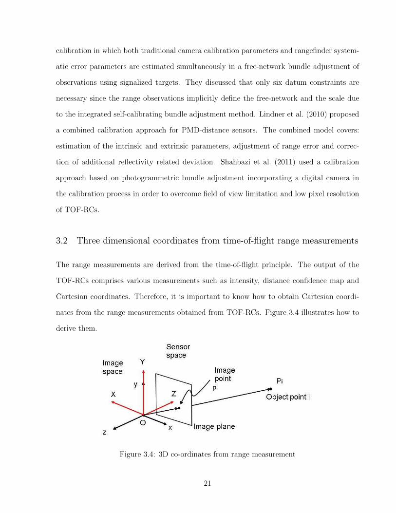
3.2 Three dimensional coordinates from time-of-flight range measurements

The range measurements are derived from the time-of-flight principle. The output of the

TOF-RCs comprises various measurements such as intensity, distance confidence map and

Cartesian coordinates. Therefore, it is important to know how to obtain Cartesian coordi-

nates from the range measurements obtained from TOF-RCs. Figure 3.4 illustrates how to

derive them.

Figure 3.4: 3D co-ordinates from range measurement

21

An important output of TOF-RCs is range measurements which are measured indepen-

dently at every pixel in the sensor frame. The image space coordinate system and the sensor

space coordinate system have the same origin O. The 3D coordinates of the image point pi

in the image space coordinate system are (xi − xp, yi − yp,−pd), where (xp, yp) is principal

point offset and pd is principal distance. The 3D coordinates of object point Pi in the sensor

space coordinate system are (Xi, Yi, Zi). The measurement range ρi is the distance from the

origin O to the object point in 3D object space. Based on the pinhole camera model and

similar triangles, the 3D coordinates of the object point Pi are calculated by using the known

image coordinates in accordance with Equation 3.10.

−→Opi−−→OPi

=

√(xi − xp)2 + (yi − yp)2 + pd2

ρi(3.9)

Xi

Yi

Zi

=ρi√

(xi − xp)2 + (yi − yp)2 + pd2

−(xi − xp)

yi − yp

pd

(3.10)

3.3 Light coded range camera technology

Most commercial LC-RCs are based on PrimeSense chips. Generally, a LC-RC consists of an

RGB-camera, an IR projector and an IR depth camera illustrated in Figure 3.5. The IR light

coded pattern emitted from the IR projector is projected onto the scene in order to obtain a

matrix implementation of active triangulation principle for estimating depth measurements

and 3D geometry. This section discusses active triangulation for LC-RCs and error sources

of Kinect LC-RCs.

3.3.1 Triangulation algorithm

A LC-RC is essentially a stereo vision system based on triangulation. A stereo vision system

consists of two standard (typically identical) cameras whose fields of view partially overlap.

22

Figure 3.5: A Kinect

Additionally, two cameras of a stereo vision system are coplanar and have aligned imaging

sensors and parallel optical axes. The two cameras of a stereo vision system are illustrated

in Figure 3.6. The left camera L is called the reference camera with coordinate system (xL,

yL, zL) and the right camera is called the target camera with coordinate system (xR, yR,

zR).

Figure 3.6: Stereo vision system

In the stereo vision system, an object point P with 3D coordinates (x, y, z) in the reference

camera coordinate system is projected into the stereo cameras whose corresponding 2D image

coordinates are pL = (upL , vpL), pR = (upR , vpR) respectively as shown in Figure 3.7. pL

and pR (Mutto et al., 2010) have the same vertical coordinates. According to the stereo

vision system principle, there are upR = upL − d and vpR = vpL , where d is the difference

between the horizontal coordinates of pL and pR, which is called the disparity. In addition,

23

by triangular similarity the disparity is inversely proportional to the depth value z as in

Equation (3.11,(Klette et al., 1998)).

z =b|f |d

(3.11)

where b is the baseline which is the distance between the two camera perspective centers and

f is the common focal length of the two cameras.

Figure 3.7: Triangulation with a pair of stereo cameras

From the 2D image coordinates of pL and its corresponding depth z obtained from Equa-

tion 3.11, the 3D coordinates of the object point P can be derived by following Equation 3.12

(Mutto et al., 2010). x

y

z

= K−1L

upL

vpL

1

z (3.12)

where K (Equation 3.13, (Mutto et al., 2010)) is the matrix of intrinsic parameters of the

stereo cameras.

K =

f 0 xp

0 f yp

0 0 1

(3.13)

24

A light coded camera system is basically a stereo vision system with one of two cameras

replaced by a projector. The stereo vision system of a LC-RC is comprised of a camera C

and a projector A as shown in Figure 3.8. The camera C has a camera coordinate system

(xC , yC , zC). This camera coordinate system is also called the reference coordinate system.

The projector A has a projector coordinate system (xA, yA, zA). The camera C is an IR

depth camera and a projector is used to emit an IR light pattern.

Figure 3.8: Light coded system

3.3.2 Light code-word technologies

Each pixel of a projector should have an associated code-word, which can simplify conjugate

point identification. Namely, each pixel has a specific local configuration in the projected

pattern. The specific pattern is projected onto the scene by the projector. Then, the

pattern is reflected by the scene and captured by the camera. The main purpose of using

the projected pattern is to obtain conjugate points between the camera image and projector

image by analyzing received code-words in the images of the cameras. Therefore, the goal

of the pattern design is to design a set of code-words which can be effectively decoded even

if the pattern projection or acquisition process is not perfect.

A pixel pA = (uA, vA) of the pattern, its corresponding object point P and its correspond-

ing image point pC = (uC , vC) are illustrated in Figure ??. The projection or acquisition

procedure introduces a horizontal shift d which is proportional to the inverse of the depth z

25

of P as the Equation 3.11. The disparity shift d is the most critical quantity and should be

measured accurately in an active triangulation process, since it is used to measure the 3D

coordinates of the object point P by using Equation 3.12.

There are three code-word methods discussed in Mutto et al. (2010) for LC-RCs as

follows:

1. Direct coding as shown in Figure 3.9 is a code strategy in which a code-word is

associated to pA represented by the pattern value at pA. The gray-level or RGB value of the

pattern at pA is used. It is the easiest code-word method to perform. This code-word allows

for dynamic scene capture because it just requires a single pattern projection. However

the disadvantage of the direct coding method is that it is extremely sensitive to color or

gray-level distortion because of scene color distribution, reflectivity properties and external

illumination.

Figure 3.9: Direct coding

2. Time-multiplexing coding shown in Figure 3.10: a sequence of T patterns is projected

onto a surface to be measured at a subsequent time t. The code-word associated to each

pixel pA is a sequence of the T pattern values (i.e., of gray-level or color values) at pA.

26

Time-multiplexing coding uses a very small set of binary patterns for creating arbitrarily

different code-words for each pixel. Its major disadvantage is that it requires the projection

of a time sequence of T patterns for every single depth measurement, hence it is not suited

in dynamic scenes.

Figure 3.10: Time-multiplexing coding

3. Spatial-multiplexing coding illustrated in Figure 3.11: the code-word associated to

each pixel pA is a spatial pattern distribution in a window of nW pixels centered around pA.

For example, for a window with 9 rows and 9 columns so nW is equal to 81.

27

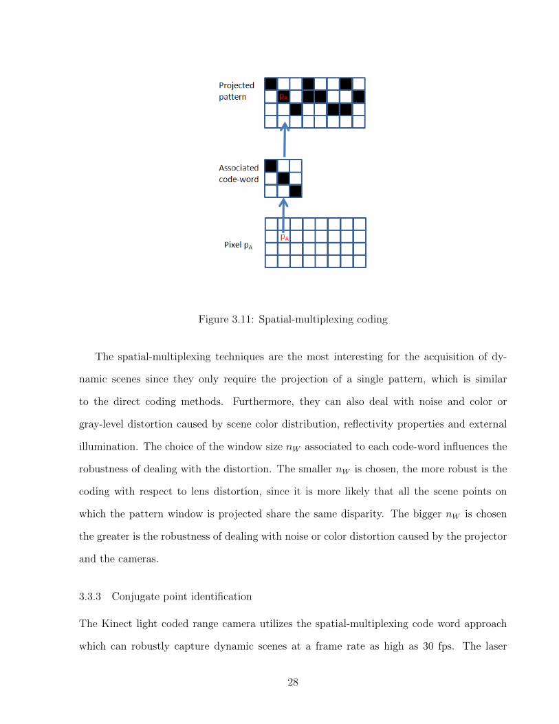
Figure 3.11: Spatial-multiplexing coding

The spatial-multiplexing techniques are the most interesting for the acquisition of dy-

namic scenes since they only require the projection of a single pattern, which is similar

to the direct coding methods. Furthermore, they can also deal with noise and color or

gray-level distortion caused by scene color distribution, reflectivity properties and external

illumination. The choice of the window size nW associated to each code-word influences the

robustness of dealing with the distortion. The smaller nW is chosen, the more robust is the

coding with respect to lens distortion, since it is more likely that all the scene points on

which the pattern window is projected share the same disparity. The bigger nW is chosen

the greater is the robustness of dealing with noise or color distortion caused by the projector

and the cameras.

3.3.3 Conjugate point identification

The Kinect light coded range camera utilizes the spatial-multiplexing code word approach

which can robustly capture dynamic scenes at a frame rate as high as 30 fps. The laser

28

projector of a Kinect emits a single beam which is split into multiple beams by a diffraction

grating to create a spatial-multiplexing pattern of speckles (Freedman et al., 2012). The

spatial-multiplexing pattern is projected onto the scene. This pattern is captured by the

infrared depth camera. By calculating the covariance (Equation 3.14) (Mutto et al., 2010)

between the spatial-multiplexing window centered at a given pattern point piA and the pro-

jected pattern captured by the IR camera, the conjugate points of the projector and the IR

depth camera are identified, which is called local algorithm.

C(ui, uj, vj) =∑

(u,v)∈W (uA,vA)

[s(u−uiA, v−viA)−s(uiA, viA)]·[s(u−ujC , v−viC)−s(ujC , v

iA)] (3.14)

s(uiA, viA) =

∑(u,v)∈W

s(u− uA, v − vA) (3.15)

where s(uiA, viA) is the average of the spatial multiplexing window centered at (uiA, v

iA)T and

C(ui, uj, vj) is the horizontal covariance of the projected pattern between piA and pjC .

Therefore, for a given pixel pjC and all the pixels piA in the same row as pjC in the projected

pattern, the covariance presents a unique peak in correspondence with the actual couple of

conjugate points.

The local algorithm considers a measurement of the local similarity between all pairs

of possible conjugate points. However, this method requires a great number of complex

computations, which is time-consuming computations. Therefore, detection of the conjugate

points to meet the high frame video rate is necessary. However it is not possible to meet

the high frame video rate requirement by using a local algorithm to identify the conjugate

points .

Freedman et al. (2012) discussed using a reference image. The reference image can be

obtained by capturing a plane at a known distance from the camera. The reference is stored

in the memory of the camera. When the speckles from the IR light are projected onto an

object, there is a distance between the object and the sensor. If the distance is smaller

or larger than the known distance, the position of the speckle in the infrared image will

29

be shifted towards the baseline between the IR projector and the IR depth camera. The

shifts of all speckles can be determined by a simple image correlation procedure, which yields

conjugate points and a disparity matrix. The distance of each pixel to the sensor can then be

retrieved from the corresponding disparity and conjugate points by using the triangulation

algorithm.

3.3.4 Light coded range camera error sources

For the LC-RCs, different error sources such as the sensor, the measurement setup and the

environment of the scene impacts the depth measurements.

The sensor errors are caused by inadequate calibration and inaccurate measurement of

disparities.

The systematic errors should be considered first. Since there are three different sensors

of Kinect LC-RCs, the three sensors also have common systematic errors of three sensors

including lens distortions (radial and decentring ) and range errors. In addition, the relative

orientation between the RGB camera and the IR depth camera is not estimated or modelled

properly which can cause the errors. Inadequate calibration or errors in estimation of cal-

ibration parameters results in systematic errors. Such systematic errors can be eliminated

by a proper calibration procedure. Herrera et al. (2011) discussed Kinect camera calibra-

tion using a planar check-board pattern. Chow et al. (2012) investigated a new calibration

model for simultaneously determining exterior orientation parameters, interior orientation

parameters and object space feature parameters.

Inaccurate measurements of disparities within the correlation algorithm during normal-

ization also results in errors.

Errors are also caused by environment of the scene, which are also called scene depen-

dent errors. The scene dependent errors are related to the system environment, e.s. am-

bient imaging conditions, and object scene structure, e.s. external experiment environment

temperature and sensor internal temperature. First, the light conditions impact the corre-

30

lation and computation of disparities. Under strong light, the laser speckles appear with

low contrast in the infrared image, which can lead to outliers or gaps in the output depth

measurements. Second, some other aspects influence the depth measurement accuracy. For

example, low reflectivity and background illumination impact the measurement of points. In

case of low reflectivity and excessive background illumination, the camera can not acquire

any information about the reflected pattern. The corresponding estimation algorithm does

not produce any results. Hence in these situations, there is generally no depth information

available.

Another error is caused by camera operating conditions. Chow et al. (2012) discussed

that at least 60 minutes warm-up is necessary to obtain stable depth measurement from

LC-RCs.

3.4 Three dimensional coordinates from light coded range measurements

The LC-RCs provide depth measurements and RGB measurements due to their measurement

principle. However, it is critical to derive 3D coordinates from the depth measurements of

LC-RCs shown in Equation 3.16((Khoshelham and Elberink, 2012))

Xk = −depthkf

(xk − xp + ∆x)

Yk = −depthkf

(yk − yp + ∆y)

Zk = depthk

(3.16)

(xk, yk) are image coordinates of the image point k;

(xp, yp) are coordinates of the perspective centre;

(∆x,∆y) are additional calibration parameters;

(Xk, Yk, Zk) are 3D coordinates of the object point k;

f is focal length of the IR depth sensor;

depthk is the depth measurement from the IR depth sensor.

31

3.5 Summary

First, this chapter reported on the range camera technologies of TOF-RCs. TOF-RCs use the

time-of-flight measurement principle and four discrete measurement samples to derive range

measurements. Additionally, error sources in the TOF-RCs were described such as noise,

systematic artifacts, scene-independent systematic artefacts, scene-independent instrumental

systematic effects and motion artefacts. Finally, derivation of 3D coordinates was discussed

using range measurement from TOF-RCs.

Second, this chapter discussed the LC-RCs as well. It is a new type of 3D LC-RCs. They

are designed on the basis of stereo vision technologies and coded light. They use a reference

image to estimate disparities and derive the depth using the disparities, baseline and focal

length of IR depth camera. In addition, error sources of LC-RCs were also presented such

as sensors, measurement setup and environment of the scene. Based on the studies for RCs,

the concrete beam experiment is going to be discussed in the next chapter.

32

Chapter 4

Structure deflection measurement experiment

description

In this chapter, Section 4.1 discusses the experiment design and setup for measuring dynamic

concrete beam deflection. Section 4.2 describes the sensors for the data capture during the

fatigue loading tests. Four different types of optical sensors are used to measure the beam

deflection. Their specifications are described in this section. Section 4.3 reports the data

capture procedure. Section4.4 reports the raw data of the beam deflection from the different

sensors. The raw data discussed in this chapter is the basis for the range camera data

processing in Chapter 5. The experimental details are presented first to help readers more

clearly understand the methodology that is presented in Chapter 5.

4.1 Experiment design and setup

Figure 4.1 and Figure 4.2 show the experimental arrangement for measuring the concrete

beam deflection subjected to periodic loads, which are called fatigue loading tests. The

fatigue loading test experiment was conducted by Dr. Mamdouh El-Badry in the Department

of Civil Engineering MikeWard Structural Laboratory at the University of Calgary. As can

be seen in Figure 4.2, a 3 m long, reinforced concrete beam having a 150 mm × 300 mm

rectangular cross section was supported at its two ends and was painted white. A hydraulic

actuator was used to apply the periodically-varying loads to the concrete beam through a

spreader beam in contact with the top surface of the concrete beam.

33

Figure 4.1: Schematic view of the experiment setup

Figure 4.2: Photographic image of actual experiment setup

34

The experimental setup for measuring dynamic concrete beam deflection comprised three

TOF-RCs, one LC-RC (LC-RC 1), five LDSs and a target system. Three different SR4000

TOF-RCs were used to capture data during the experiment. They are two ethernet cable

SR4000-00400011 (TOF-RC 3 and TOF-RC 4) and one USB cable SR4000-0040001 (TOF-

RC 1). In this thesis, LC-RC 1, TOF-RC 1, TOF-RC 3 and TOF-RC 4 are called Cam 1,

Cam 2, Cam 3 and Cam 4 respectively. The target system compirsed thirteen thin plates

and a concrete beam. The surface of interest for the range cameras was the top surface of

the concrete beam. Since the spreader beam occluded almost half of the concrete beam,

an alternative method was used to measure the target system. Thirteen white-washed thin

aluminum plates (220 mm × 50 mm) were bonded to the side of the concrete beam at

intervals of 250 mm along its length.

4.2 Sensors

4.2.1 SR4000 time-of-flight range camera

SR4000 TOF-RCs were positioned on the steel frame of each side of the hydraulic actuator

with nadir-looking orientation and 1.9 m standoff distance from the camera to the top

surface of the concrete beam for complete coverage of the concrete beam. Table 4.1 gives the

specifications of the TOF-RCs. As can be seen, the absolute accuracy of SR4000 TOF-RC

is 10 mm provided by the manufacturer. The maximum frame rate is 54 fps.

Since the deflection measurement of the concrete beam has to be made in the direction of

the gravity vector, the Z-axis for the range camera has to be aligned as close to the gravity

vector as possible (Jamtsho, 2010). Moreover, the TOF-RCs do not have a leveling system

so a small external level was required to align the Z-axis of the camera coordinate system

with the gravity vector.

35

Table 4.1: Specifications of SR4000 TOF-RC

Camera Type SR4000-0040001 SR4000-00400011

Pixel array (pixel2) 176× 144 176× 144Field of view 43.6◦ × 34.6◦ 69◦ × 56◦

Focal length (mm) 10 5.8Illumination wavelength (nm) 850 850Modulation frequency (MHz) 29/30/31 29/30/31

Detection range (m) 0.1-5 0.1-5Calibrated range (m) 0.8-5 0.8-5

Maximum frame rate (fps) 54 54Absolute accuracy (mm) ±10 ±10

4.2.2 Kinect light coded range cameras

One Kinect (Cam 1) was utilized for data capture. It was positioned on the steel frame

next to one of the SR4000 ethernet cameras. It is difficult to see the Kinect location in

Figure 4.2 since it was hidden behind the TOF-RCs. Table 4.2 gives specifications of the

Kinect LC-RC.

Table 4.2: Specifications of Kinect LC-RC

Camera name Kinect

Field of view 57◦ × 43◦

Frame rate (Hz) 30Camera resolution 640× 480

Nominal depth resolution (mm)-at 2m distance 3Nominal depth range (m) 0.8-3.5Absolute accuracy (mm) ±10

Device connection USB

4.2.3 Laser displacement sensors

The deflection measurements were also recorded by five vertically-oriented KEYENCE LKG407

CCD LDSs positioned directly under the centroid of five of the thin plates. These devices

measure displacement by active laser triangulation. The manufacturer stated linearity and

precision for this sensor is 0.05% of the 100 mm measurement range and 2 µm, respectively.

36

Therefore, the LDSs were used as a benchmark to assess the absolute accuracy of the beam

deflection measurement. The LDS data were provided by Dr. Mamdouh El-Badry.

4.3 The experiment data capture

4.3.1 Data capture procedure

Designed by Dr. Mamdouh El-Badry, Experiment I was comprised of two static loading

and fatigue loading cycles. The periodic loading cycles with 4 mm maximum amplitude

based on the load control were applied to the concrete beam. In general, fatigue loading

tests are commonly conducted at 3 Hz (Papakonstantinou et al., 2001; Heffernan and Erki,

2004). However, in order to meet the sampling frequency requirement of the low-cost digital

camera system (Detchev et al., 2012), the 1 Hz loading frequency fatigue loading testing

was conducted as well. Two TOF-RCs were used to capture 3D image data. The cameras

were used to capture the fatigue loading cycles and record the dynamic deflections fo the

concrete beam. Initially, 7,200 load cycles were applied from 24 kN to 96 kN at 1 Hz loading

frequency. Subsequently, 3 Hz periodic loads were applied. It took two days until the beam

failed.

Designed by Dr. Mamdouh El-Badry, Experiment II also includes static loading and

fatigue loading tests. The periodic loads based on force control were applied to the concrete

beam at different loading frequencies. It took eleven days to apply the periodic loads to the

concrete beam. Measurement data were recorded at 1 Hz for six days and at 3 Hz for 10

days.

4.3.2 Operation conditions of SR4000

During the dynamic data capture, several quality assurance measures were taken to obtain

stable measurement data for the TOF-RCs.

First, the SR4000 TOF-RCs had been warmed up for one hour to obtain stable measure-

37

ment data.

Second, the light of multiple TOF-RCs would interfere with each other if they were

operated with the same MF. Therefore, different modulation frequencies were used to prevent

light interference. In Experiment I, Cam 3 was set at 29 MHz MF and Cam 4 was set at 31

MHz MF. During Experiment II, Cam 3 was set at 30 MHz and Cam 4 was set at 31 MHz.

In addition, the SR4000 USB cable range camera (Cam 2) was mounted on the steel frame

for data capture. It was located next to one of internet cable TOF-RCs. The MF of Cam 2

was set at 29 MHz.

Third, an appropriate integration time should be chosen for TOF-RCs to capture the

data. The frame rate is inversely proportional to the integration time. In addition, the

range measurement precision is related to the integration time. When the integration time

is longer, the range measurement precision is higher. When the integration time is short,

the range measurement precision is lower. In our case, the nominal motion frequencies were

1 Hz and 3 Hz respectively. The SFs should be 2 Hz and 6 Hz when the Nyquist critical

frequencies are 1 Hz and 3 Hz respectively.

The integration times for both TOF-RCs were set at different values: 21 ms, 8.5 ms,

4.4 ms and 2.2 ms for which the corresponding SFs were 10 Hz, 20 Hz, 30 Hz and 40

Hz respectively during Experiment I. However, according to the results and analysis of

Experiment I, the best SF was 20 Hz to keep measurement error under half-millimetre level

accuracy. Therefore, in Experiment II the 20 Hz SF was adopted for data capture. As a

result, all of the SFs meet the requirement.

Fourth, it is also important to note that range measurements of the thin plates were

biased by range scattering error (Jamtsho and Lichti, 2010). Lichti et al. (2012) mentioned

that the scattering error can be largely removed by the differencing operation if the scene

structure does not change significantly from the zero-load state to the loaded state. This is

a fundamental assumption that allows accurate deflection measurements to be made using

38

TOF-RC. In our case, since only the relative periodic motion is desired, the range bias due

to scattering at each target location is of no consequence.

Fifth, systematic errors of the time-of-flight range camera impact the range measure-

ment accuracy. Generally speaking, the systematic errors should be corrected by camera

calibration. However, since only the relative, periodic motion is desired, the range bias due

to systematic errors at each target location is of no consequence. Only very small changes

in position were measured and the differential operation removed unmodelled systematic

errors. In addition, the output of the SR4000 time-of-flight range camera is pre-calibrated

by the manufacturer. Therefore, in our application, additional camera calibration was not

considered.

4.3.3 Operation conditions of Kinect

During data capture, several factors should be considered as well. First, the Kinect LC-RC

had been warmed up for one hour to obtain stable measurement data. Second, the depth

resolution is a function of distance between the cameras and the object. The depth resolution

gets worse with increasing distance. The Kinect LC-RC was mounted in the scaffold assembly

about 1.9 m where the absolute accuracy is ±10 mm according to the Table 4.2. After 2 m,

the absolute accuracy decreases significantly. In our experiment, the maximum deflection of

the concrete beam based on loading control is 4 mm. The very small changes in position were

measured within ±10 mm. In addition, the differential operation can remove unmodelled

systematic errors, which is similar with SR 4000 TOF-RC (Lichti et al., 2012). Therefore,

the calibration of the Kinect LC-RC did not need to be considered.

4.4 The output images of range cameras

A potential advantage of the TOF-RCs is that intensity images and depth images are pro-

vided simultaneously and they are co-located to each other. An advantage of LC-RCs is

39

that RGB images and depth images are offered. Figure 4.3 illustrates the depth image from

a time-of-flight based range camera from top view. Figure 4.4 shows the amplitude image

captured by a TOF-RC from top view.

Figure 4.3: Range image of the Experiment scene (SR4000)

Figure 4.4: Amplitude image of the Experiment scene (SR4000)

However, a LC-RC exports a depth image and a RGB image, which come from two

different types of cameras. Their field of view are not same. The two images are not co-

located with each other. Figure 4.5 shows the depth image of the experiment scene captured

by Kinect. Figure 4.6 gives a RGB image of the experiment scene captured by Kinect.

40

Figure 4.5: Range image of the Experiment scene (Kinect)

Figure 4.6: RGB image of the Experiment scene (Kinect)

4.5 Summary

This chapter presented the experimental design and practical experiment setup for the con-

crete beam deflection measurement. Then, different optical sensors were introduced such

as SR4000 TOF-RCs, Kinect LC-RCs, LDSs and TLS. Many factors impacting the range

measurement accuracy during data capture were presented such as warming up time, light

41

interference, choosing appropriate integration time for dynamic loading data capture and so

on. The output of the two types of range cameras was also discussed. The key to using these

cameras lies in the extraction of the target system from these images. That is treated in the

next chapter.

42

Chapter 5

Range camera data processing

This chapter discusses the data preparation and image processing techniques needed to

extract target objects from 3D point cloud of the RCs. Figure 5.1 shows the corresponding

3D point cloud of the dynamic deflection measurement experiment scene from one of the

SR4000 TOF-RCs. Since a TOF-RC simultaneously provides co-located range and intensity

images, both radiometric and depth information can be used to segment target objects.

Therefore, by using 2D and 3D image processing technologies, the thin plates and the top

beam surface of interest were extracted automatically.

−3000 −2000 −1000 0 1000 2000 3000−2000

0

2000

40000

1000

2000

3000

4000

X (mm)

Y (mm)

Z (

mm

)

Floor

Thin platesBeam topsurface

Figure 5.1: A SR4000 3D point cloud of the deflection measurement scene

Figure 5.2 shows a Kinect 3D point cloud of the deflection measurement scene. How-

ever, the RGB image and the depth image from the Kinect LC-RC are not co-located with

each other. Therefore, another thin plate automatic extraction method is presented in this

chapter.

43

Figure 5.2: A Kinect 3D point cloud of the deflection measurement scene

In addition, a power spectral density (PSD) analysis method is described for unevenly

sampled data. The loading frequency is recovered by PSD analysis. Linear and non-linear

least squares are used to estimate the motion trajectory of the thin plates and to calculate

the dynamic deflection of the concrete beam. Finally, the effects of the motion artefacts of

a TOF-RC are described as well.

5.1 Thin plate point cloud extraction for SR4000

In this section, extracting the thin plate from 3D point cloud derived from a TOF-RC is

discussed. Since the main objects of interest are the thin plates, their automatic extraction

from the TOF-RC data requires specialized image processing techniques.

5.1.1 Depth-based classification

Depth-based classification is used to remove the floor and anything higher than the thin

plates such as the hydraulic actuator, the spreader beam and the top surface of the concrete

beam in the depth image because different objects are at different heights, which is critical to

44

determine depth thresholds to remove non-thin plate regions roughly in the intensity images.

Several techniques are used to estimate two thresholds. First, image edge detection, ellipse

detection and ellipse fitting are used to extract and measure circular targets on the floor.

Then bilinear interpolation is used to determine the depth of the ellipse center that is called

the first depth threshold. The first depth threshold is used to remove floor. The top surface

of the concrete beam is a rectangular shape which is easy to segment. The depth between the

TOF-RC and the top surface of the concrete beam is determined based on the top surface

of the concrete beam segmentation. This depth is the second depth threshold. The second

depth threshold is utilized to remove the hydraulic actuator, the spreader beam and the top

surface of the concrete beam.

5.1.1.1 Image edge detection for intensity images

Since high contrast white circular targets on black paper are used to calculate the first depth

threshold, a circular target centre measurement algorithm is necessary. The first step of

the target centre measurement is to perform edge detection in order to isolate the circular

targets. The Canny edge algorithm has three basic objectives (Gonzalez and Woods, 2008):

the detected edges have to be as close as possible to true edges; the edges should be well

localized, the distance between a point marked by Canny edge detection and the center of

the true edges is as small as possible; and the detector should return a single edge for each

true edge. Those three objectives are all essential for precision and accuracy of the target

measurement. Therefore, the Canny algorithm is used for isolating the circular targets in

this thesis and it consists of the following four steps (Gonzalez and Woods, 2008):

• Smoothing the input amplitude image with a Gaussian filter;

• Finding the gradient magnitude images from input amplitude images;

• Applying the gradient magnitude images for maxima suppression;

• Using double thresholds and connectivity analysis to link edges.

45

Figure 5.3 shows the edge image for a dynamic experiment scene.

Figure 5.3: The edge image of the experiment scene with SR4000

5.1.1.2 Ellipse detection

After edge detection, the circular targets need to be detected. However, a circular target

is projected onto the image plane approximately as an ellipse in the case that the target

and the image planes are not parallel. Thus, ellipse detection with fake eccentricity of each

connected region in the edge image (Rohs, 2004) is used in this thesis.

First of all, the connected regions cluster algorithm (Blackledge, 2005) is applied to the

edge image for segmenting each connected region for further examination. For clustering

one connected region, this algorithm first chooses a white pixel as a seed point. Starting

from this seed point, each pixel of the rest of the connected region is tracked recursively by

analyzing the pixels of the eight-neighborhood. Then, the fake eccentricity is defined as the

ratio of the semi-minor axis Aellipse and the semi-major axis Bellipse. If the fake eccentricity

is close to one, the corresponding connected region has an ellipse-like shape (Rohs, 2004).

Therefore, by estimating the fake eccentricities of all the connected regions, the ellipse target

can be detected from the image. The fake eccentricities are derived from the second-order

46

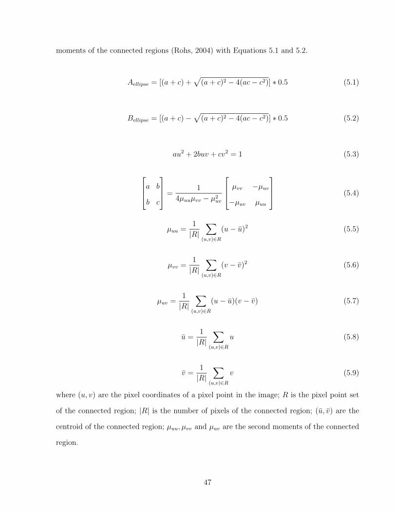
moments of the connected regions (Rohs, 2004) with Equations 5.1 and 5.2.

Aellipse = [(a+ c) +√

(a+ c)2 − 4(ac− c2)] ∗ 0.5 (5.1)

Bellipse = [(a+ c)−√

(a+ c)2 − 4(ac− c2)] ∗ 0.5 (5.2)

au2 + 2buv + cv2 = 1 (5.3)

a b

b c

=1

4µuuµvv − µ2uv

µvv −µuv

−µuv µuu

(5.4)

µuu =1

|R|∑

(u,v)∈R

(u− u)2 (5.5)

µvv =1

|R|∑

(u,v)∈R

(v − v)2 (5.6)

µuv =1

|R|∑

(u,v)∈R

(u− u)(v − v) (5.7)

u =1

|R|∑

(u,v)∈R

u (5.8)

v =1

|R|∑

(u,v)∈R

v (5.9)

where (u, v) are the pixel coordinates of a pixel point in the image; R is the pixel point set

of the connected region; |R| is the number of pixels of the connected region; (u, v) are the

centroid of the connected region; µuu, µvv and µuv are the second moments of the connected

region.

47

5.1.1.3 Target centre estimation

In this section, the centres of target ellipses are estimated by using the algorithm proposed

in Fitzgibbon et al. (1999).

An ellipse is a special conic under certain conditions. It is well known that the general

equation of a conic can be represented as

F (~U, ~X) = ~U · ~X = au2 + buv + cv2 + du+ ev + f = 0 (5.10)

where ~U = [a, b, c, d, e, f ]T is the coefficient (parameter) vector and ~X = [u2, uv, v2, u, v, 1]T .

If a constraint inequality (Equation (5.11)) is imposed on the above general conic equation

b2 − 4ac < 0, (5.11)

then we obtain an ellipse equation. Thus the following system represents an ellipse:F (~U, ~X) = au2 + buv + cv2 + du+ ev + f = 0,

b2 − 4ac < 0.

(5.12)

For a pixel point (ui, vi), F (~U, ~Xi) can be treated as an ”algebraic distance” between

(ui, vi) and ellipse (5.12), where ~Xi = [u2i , uivi, v2i , ui, vi, 1]T .

As Fitzgibbon et al. (1999) mentioned, in general, the constraint inequality (5.11) is

difficult to impose in the estimation procedure. It is realized that when ~U in (5.10) is

replaced by any multiple non-zero scale k~U , F (k~U, ~X) represents the same conic as F (~U, ~X)

does. Thus we are free to scale arbitrarily the coefficients of (5.10) by the same multiple. It

is enough to consider a special case of (5.12) with 4ac − b2 = 1. Therefore the inequality

constraint has been changed into an equality constraint by using scaling.

F (~U, ~X) = au2 + buv + cv2 + du+ ev + f = 0,

4ac− b2 = 1.

(5.13)

Therefore, the centre of each connected region can be estimated by least-squares ellipse

fitting technique (Fitzgibbon et al., 1999) using Equations (5.13). In order to understand the

48

least-squares fitting technique to estimate coefficients of each of the ellipse, it is important

to introduce the following matrix language.

Let D = [ ~X1, ~X2, · · · , ~Xn]T , where ~Xi = [u2i , uivi, v2i , ui, vi, 1]T , that is

D =

u12 u1v1 v1

2 u1 v1 1

......

......

......

ui2 uivi vi

2 ui vi 1

......

......

......

un2 unvn vn

2 un vn 1

. (5.14)

Since 4ac − b2 is a homogeneous quadratic form, we can express the equality constraint

4ac− b2 = 1 in matrix form as follows:

4ac− b2 = ~UTC~U = 1 (5.15)

where ~U = [a, b, c, d, e, f ]T and

C =

0 0 2 0 0 0

0 −1 0 0 0 0

2 0 0 0 0 0

0 0 0 0 0 0

0 0 0 0 0 0

0 0 0 0 0 0

. (5.16)

The sum of squared algebraic distances can be formulated in matrix form as

E =n∑

i=1

F (~U, ~Xi)2 = (D~U)T (D~U) = ||D~U ||2. (5.17)

Thus the ellipse fitting problem reduces to a constrained minimization problem Fitzgib-

bon et al. (1999)

minimize E = ||D~U ||2 = (D~U)T (D~U)

subject to the constraint ~UTC~U = 1,

(5.18)

49

where D is an n×6 matrix, which is called design matrix, and C is a 6×6 matrix as defined

above.

The classical Lagrange multiplier method can be used to obtain the minimum value of

E. The Lagrange function is defined by

H(~U, λ) = (D~U)T (D~U)− λ(~UTC~U − 1) (5.19)

Differentiating H(~U, λ) with respect to ~U and λ, gives2DTD~U − 2λC~U = 0

~UTC~U = 1

(5.20)

The may be rewritten as an equation systemS~U = λC~U

~UTC~U = 1

(5.21)

where S = DTD is the scatter matrix. This system is readily solved by considering the

generalized eigenvectors of the first equation in (5.21).

The linear algebra algorithms were used to determine the eigenvalues-eigenvector pairs of

the matrix S and the vector ~U is derived using the eigenvalues-eigenvector pairs (Fitzgibbon

et al., 1999). The 2D coordinates of ellipse centres are determined based on the vector ~U .

The 3D coordinates of each ellipse centre can be determined by the 2D coordinates of each

ellipse centre using the bilinear interpolation algorithm. The average value of the depth

measurements (Z-coordinates) of each ellipse centre is seen as the first threshold.

5.1.1.4 Top surface of the concrete beam extraction

The top surface of the concrete beam is rectangular on shape which is easy to segment by

the fake eccentricity algorithm since the fake eccentricity of the top surface is close to zero.

The depth between the TOF-RC and the top surface of the concrete beam is determined

based on the depth values of the top surface.

50

In depth images, if the depth value of each pixel is bigger than or equal to the first

threshold, its intensity value of the corresponding pixel is set at zero. Moreover, if the

depth value of each pixel is less than or equal to the second threshold, the intensity value of

the corresponding pixel is set at zero. Therefore, the intensity image contrast is improved,

which is useful for thin plate extraction. Using the first threshold and the second threshold,

preliminary segmentation is done. Figure 5.4 shows the intensity image after the depth-based

classification.

Figure 5.4: The result with depth-based classification (SR4000)

5.1.2 Otsu method for thin plate segmentation

A binary image can be obtained from an intensity image with image threshold estimated by

the Otsu method (Otsu, 1979). The Otsu algorithm is discussed briefly in this thesis because

it is used for segmenting the background and foreground in the intensity image.

By estimating a threshold using maximum between class variance, the weighted intra-

class variance, defined as a weighted sum of variances of two classes (Equation 5.23) is

minimized. Assume, there are L gray levels [1, 2, 3, . . . , i, . . . , L− 2, L− 1, L] for an intensity

image from TOF-RC. The number of pixels at level i is noted by ni and the total number

of pixels by N = n1 + n2 + . . . ,+nL. Therefore, the gray level histogram is normalized as

51

follows.

pi =ni

N(5.22)

An intensity image is divided into two classes C0 = [1, . . . , k] and C1 = [k + 1, . . . , L] by

a threshold k. The within class variance σ2w(k) is given by Equation (5.23).

σ2w(k) = ω0σ

20 + ω1σ

21 (5.23)

where, weights ω0 =∑

ki=1pi and ω1 =

∑Li=k+1pi are probabilities of the two classes separated

by a threshold k; σ20 and σ2

0 are the variances of the two classes.

However, Otsu (1979) reported that minimizing the within-class variance is equal to

maximizing between-class variance σ2b (k).

σ2b (k) =

[µTω(k)− µ(k)]2

ω(k)[1− µ(k)](5.24)

where µT is the expected value of the intensity image; ω(k) is equal to ω0 and µ(k) is the

first class expected value.

Therefore, the optimal threshold ko can be determined by maximizing the between-class

variance σ2b (k). Figure 5.5 shows the binary image of Figure 5.4.

Figure 5.5: The binary image based on Otsu threshold method (SR4000)

52

5.1.3 Fake eccentricity for thin plate classification

There are some non-thin plate connected regions in the binary image shown in Figure 5.6.

It is necessary to remove the regions.

Since each thin plate region has a similar shape and size, the fake eccentricities of those

desired regions should have almost similar values within close proximity. Therefore, fake

eccentricity calculated by second moments is used to classify thin plates from unwanted

regions (Rohs, 2004). Figure 5.6 illustrates the result after removing non-thin plate regions

of Figure 5.6 with the fake eccentricity algorithm.

Figure 5.6: The result after thin plate segmentation (SR4000)

5.1.4 Image erosion algorithm for mixed pixel removing

The boundaries of the thin plates were removed with the image erosion algorithm because

mixed pixels (Dorrington et al., 2011) occur frequently at edges of the thin plates. They are

caused by the superposition of the foreground and background reflected signals. The image

erosion algorithm (Gonzalez and Woods, 2008) can be used to remove the edges of the thin

plates. The method removes unwanted noisy points from edges of the thin plates. Figure

5.7 illustrates the final result after removing edges of the thin plates. The centroid of each

thin plate can be calculated by averaging all point cloud belonging to each thin plate.

53

Figure 5.7: The result after image erosion (SR4000)

5.1.5 3D point cloud of the thin plates from SR4000

Figure 5.8 shows the 3D point cloud of the thin plates by using the thin plate extraction

techniques mentioned previously.

−1500 −1000 −500 0 500 1000−200

−120−4020

19001950

X (mm)

Y (mm)

Z (

mm

)

Figure 5.8: 3D point cloud of the thin plate

The range camera can provide three dimensional measurements: the lateral direction (i.e.

Y-coordinate), the longitudinal direction (i.e. X-coordinate) and the vertical direction (i.e.

Z-coordinate). Based on direction of the periodic force, the thin plates move toward vertical,

longitudinal and lateral directions during the fatigue test experiment. However, even though

the thin plates do move towards lateral direction (Y-coordinate), Y-coordinate can be still

used to judge robustness of the thin plate point extraction techniques.

54

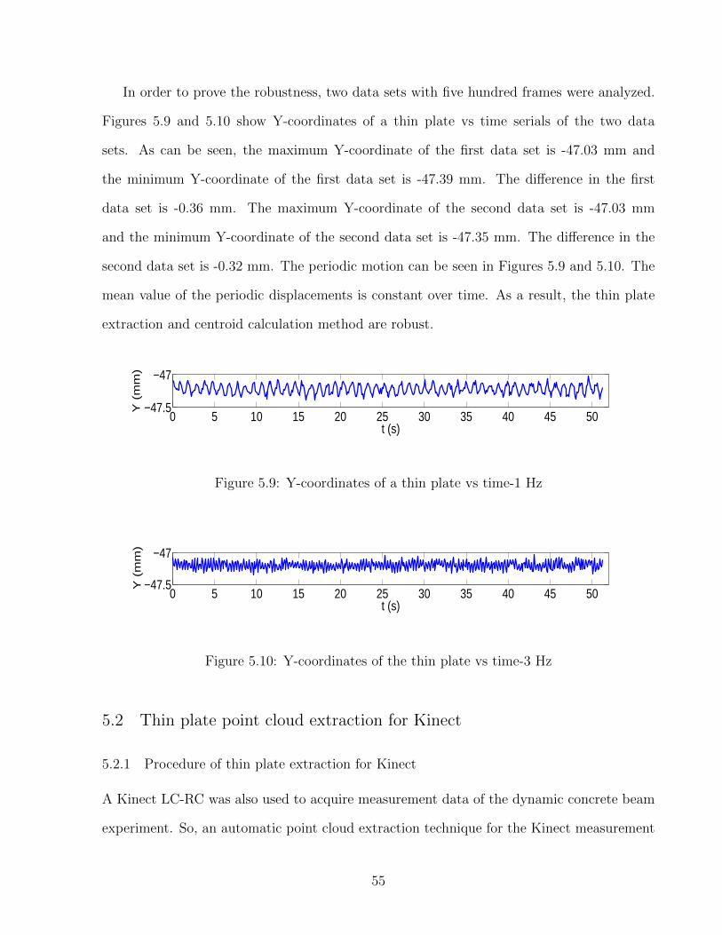
In order to prove the robustness, two data sets with five hundred frames were analyzed.

Figures 5.9 and 5.10 show Y-coordinates of a thin plate vs time serials of the two data

sets. As can be seen, the maximum Y-coordinate of the first data set is -47.03 mm and

the minimum Y-coordinate of the first data set is -47.39 mm. The difference in the first

data set is -0.36 mm. The maximum Y-coordinate of the second data set is -47.03 mm

and the minimum Y-coordinate of the second data set is -47.35 mm. The difference in the

second data set is -0.32 mm. The periodic motion can be seen in Figures 5.9 and 5.10. The

mean value of the periodic displacements is constant over time. As a result, the thin plate

extraction and centroid calculation method are robust.

0 5 10 15 20 25 30 35 40 45 50−47.5

−47

t (s)

Y (

mm

)

Figure 5.9: Y-coordinates of a thin plate vs time-1 Hz

0 5 10 15 20 25 30 35 40 45 50−47.5

−47

t (s)

Y (

mm

)

Figure 5.10: Y-coordinates of the thin plate vs time-3 Hz

5.2 Thin plate point cloud extraction for Kinect

5.2.1 Procedure of thin plate extraction for Kinect

A Kinect LC-RC was also used to acquire measurement data of the dynamic concrete beam

experiment. So, an automatic point cloud extraction technique for the Kinect measurement

55

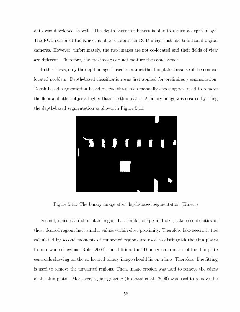
data was developed as well. The depth sensor of Kinect is able to return a depth image.

The RGB sensor of the Kinect is able to return an RGB image just like traditional digital

cameras. However, unfortunately, the two images are not co-located and their fields of view

are different. Therefore, the two images do not capture the same scenes.

In this thesis, only the depth image is used to extract the thin plates because of the non-co-

located problem. Depth-based classification was first applied for preliminary segmentation.

Depth-based segmentation based on two thresholds manually choosing was used to remove

the floor and other objects higher than the thin plates. A binary image was created by using

the depth-based segmentation as shown in Figure 5.11.

Figure 5.11: The binary image after depth-based segmentation (Kinect)

Second, since each thin plate region has similar shape and size, fake eccentricities of

those desired regions have similar values within close proximity. Therefore fake eccentricities

calculated by second moments of connected regions are used to distinguish the thin plates

from unwanted regions (Rohs, 2004). In addition, the 2D image coordinates of the thin plate

centroids showing on the co-located binary image should lie on a line. Therefore, line fitting

is used to remove the unwanted regions. Then, image erosion was used to remove the edges

of the thin plates. Moreover, region growing (Rabbani et al., 2006) was used to remove the

56

3D point cloud that do not belong to any thin plate. Figure 5.12 shows the final result of

the thin plate extraction as a binary image. The centroid of each thin plate was calculated

by averaging all 3D point cloud belonging to each thin plate. Bearing plate on top of the

cylinder is the problem so the extracted thin plate is not rectangular. However, this thin

plate was not used to analyze the deflection of the concrete beam. Therefore the deflection

results were not impacted by this thin plate.

Figure 5.12: Final result of the thin plate extraction (Kinect)

5.2.2 3D point cloud of the thin plates with Kinect

The 3D point cloud derivation was discussed in Section 3.4. Figure 5.13 shows 3D point

cloud of the thin plates from Kinect LC-RCs by using the thin plate extraction procedure

described above.

In order to validate the robustness of the thin plate point cloud extraction procedure for

Kinect LC-RCs, the two data sets with around four hundred frames were analyzed as well.

Y-coordinate vs time series are plotted in Figure 5.14 and Figure 5.15. As can be seen, the

maximum Y-coordinate of the first data set is -227.01 mm and the minimum Y-coordinate of

the first data set is -232.46 mm. The difference in the first data set is -5.45 mm. The mean

value of the first data set is -229.81 mm. The STD is 0.92 mm. The maximum Y-coordinate

57

−1000 −800 −600 −400 −200 0 200 400 600 800 1000

−400

−350

−300

−250

−200

−150

−100

1800

1850

1900

1950

X (mm)

Y (mm)

Z (mm

)

Figure 5.13: The 3D point cloud (Kinect)

of the second data set is -230.28 mm and the minimum Y-coordinate of the second data set

is -236.60 mm. The difference in the second data set is -6.32 mm. The mean value of the

second data set is -233.62 mm. The STD is 0.94 mm. Andersen et al. (2012) presented that

the absolute accuracy is roughly 40 mm at 2 m distance. The standoff distance between the

cameras and the concrete beam is around 2 m. The maximum distance difference of each

data set is less than the measurement precision mentioned in (Andersen et al., 2012), as a

result, the thin plate extraction and centroid calculation method is robust.

0 2 4 6 8 10 12−235−230−225

t (s)

Y (

mm

)

Figure 5.14: Y-coordinates of a thin plate vs time serials-1 Hz (Kinect)

0 5 10 15−240−235−230

t (s)

Y (

mm

)

Figure 5.15: Y-coordinates of a thin plate vs time serials-3 Hz (Kinect)

58

5.3 Displacement measurement from range camera data

5.3.1 Power spectral density analysis

In the beam deflection experiment, the motion of the thin plate centroid is ideally a sinusoidal

waveform. The sinusoidal waveform can be analyzed easily in the frequency domain from

which the approximate signal frequency and amplitude can be derived. Therefore, spectral

analysis methods were used to analyze the thin plate centroid data. Although the range

camera time series were uniformly sampled, some random drop-outs occurred frequently,

which is called the missing data problem.

There are a few ways to deal with the uneven sampling or the missing data problem.

Interpolation is one method. A grid of an even time interval for the observation data is

specified and the missing values are interpolated from the original measurement data on

the grid. Sometimes the missing data are set at zeros or set at fixed values based on the

time series data. The interpolated observation data are analyzed by using the Fast Fourier

Transform method. However, if a lot of consecutive points are missing, in general, such

techniques perform poorly to analyze the measurement data in the frequency domain.

A totally different method of spectral analysis for unevenly sampled data is used in this

thesis that can mitigate these kind of problems caused by the missing data problem. Lomb’s

method (Press et al., 1992) considers data only at time ti that are actually sampled, which

means the spectral density analysis of Lomb method is based on discrete sample points.

Suppose that there are N samples hi = h(ti), i = 0, . . . , N − 1 and their mean and variance

are shown in Equations 5.25 and 5.26 respectively.

h =1

N

N−1∑i=0

hi (5.25)

σ2 =1

N − 1

N−1∑i=0

(hi − h)2 (5.26)

The Lomb normalized periodogram (spectral power density as a function of angular frequency

59

ω = 2πf0 > 0) is defined as follows

PN(ω) =1

2σ2[[∑

j(hj − h) cosω(ti − τ)]2∑j cos2 ω(ti − τ)

+[∑

j(hj − h) sinω(ti − τ)]2∑j sin2 ω(ti − τ)

] (5.27)

tan(2ωτ) =

∑j sin 2ωtj∑j cos 2ωtj

(5.28)

where τ is defined by Equation 5.28 and it is a kind of offset.

Lomb (Press et al., 1992) investigated that the coefficients of the harmonic equation can

be estimated by an observation data set at a given frequency ω by linear least-square fitting

to the harmonic model 5.29. The angular frequency ω can be determined by Equation 5.27.

h(t) = C cosωt+D sinωt+ E (5.29)

The measurements of the thin plates are the sum of a periodic signal and white Gaussian

noise. Thus, spectral analysis of the unevenly sampled data was conducted with the Lomb

method (Press et al., 1992). The approximate loading frequency can be estimated by using

the power spectral density (PSD) analysis of depth measurements. Figure 5.16 shows the

power spectral density as a function of the frequency of the thin plate centroid measurements

with the Lomb method. α = [0.001, 0.005, 0.01, 0.05, 0.1, 0.5] are the statistical significance

levels. In order to see the significance levels clearly, only two levels are shown in Figure5.16.

As can be seen, there is one dominant peak in the power spectrum above α = 0.001, which

shows that there is sinusoidal component in the signal (Press et al., 1992). If there is

no dominant peak above α = 0.5 statistical significance level, which means that there is

noise component in the signal. By searching for a peak of the power spectrum density, the

corresponding frequency is determined, which means the approximate loading frequency is

derived.

With the recovered approximate loading frequency, the approximate coefficients C,D,E

of the harmonic model (Equation 5.29) of the thin plate trajectory can be estimated by using

60

0 1 2 3 4 5 6 7 8 90

20

40

60

80

100

120

140

160

180

200

α =0.001α =0.5

f (Hz)

P(f

)

Figure 5.16: An example of PSD of thin plate centroid observations based on Lomb method

linear least-squares. Then the coefficients C,D,E, ω of the harmonic can be estimated with

non-linear least-squares by using approximate coefficients C,D,E, ω as initial values. The

amplitude A and the load frequency f0 were calculated by using Equations 5.30 and 5.31

respectively.

A =√C2 +D2 (5.30)

f0 = 2πω (5.31)

5.3.2 Linear least-squares estimation

Linear least-squares is described briefly in this thesis. The general observation model can

be expressed as Equation 5.32. If the observation model is linear, Equation 5.32 can be

described using Equation 5.33.

z = g(x) + v (5.32)

z = Gx + v (5.33)

61

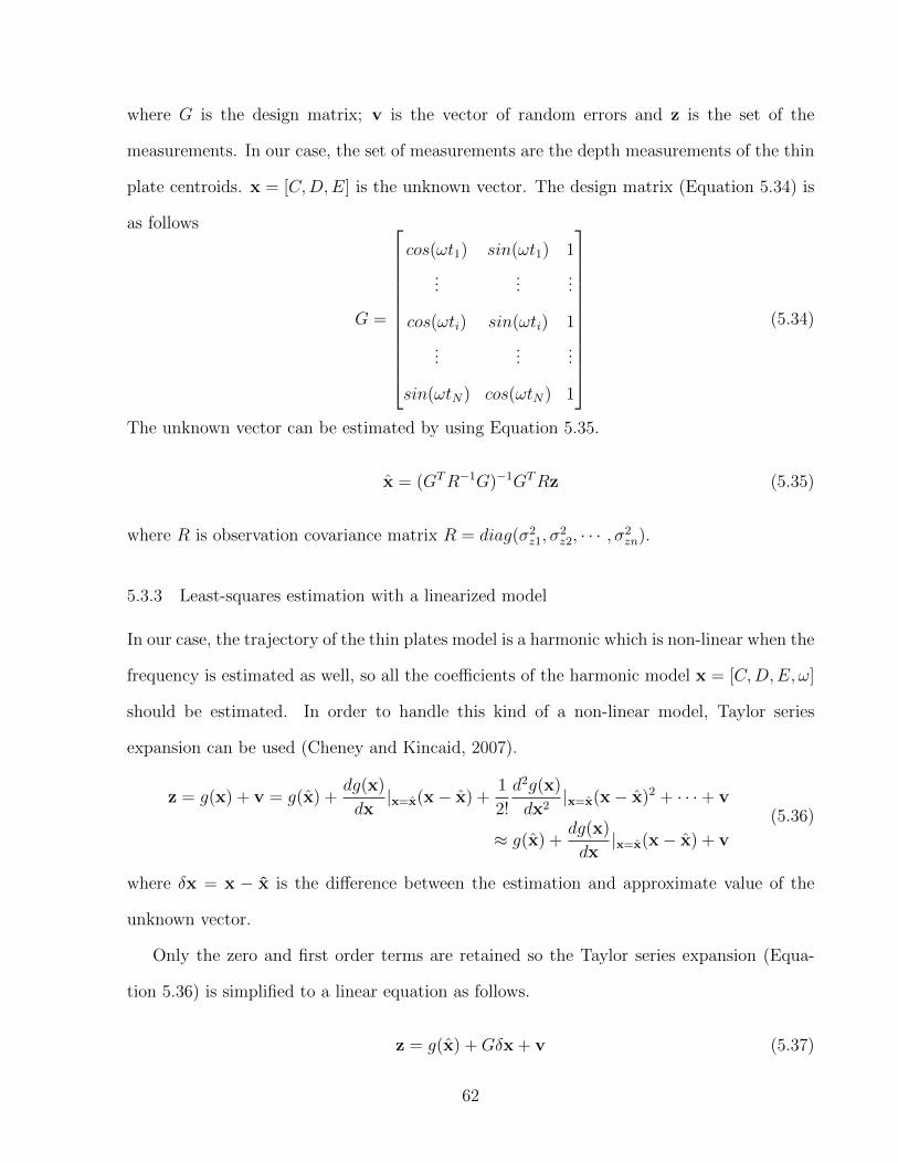
where G is the design matrix; v is the vector of random errors and z is the set of the

measurements. In our case, the set of measurements are the depth measurements of the thin

plate centroids. x = [C,D,E] is the unknown vector. The design matrix (Equation 5.34) is

as follows

G =

cos(ωt1) sin(ωt1) 1

......

...

cos(ωti) sin(ωti) 1

......

...

sin(ωtN) cos(ωtN) 1

(5.34)

The unknown vector can be estimated by using Equation 5.35.

x = (GTR−1G)−1GTRz (5.35)

where R is observation covariance matrix R = diag(σ2z1, σ

2z2, · · · , σ2

zn).

5.3.3 Least-squares estimation with a linearized model

In our case, the trajectory of the thin plates model is a harmonic which is non-linear when the

frequency is estimated as well, so all the coefficients of the harmonic model x = [C,D,E, ω]

should be estimated. In order to handle this kind of a non-linear model, Taylor series

expansion can be used (Cheney and Kincaid, 2007).

z = g(x) + v = g(x) +dg(x)

dx|x=x(x− x) +

1

2!

d2g(x)

dx2|x=x(x− x)2 + · · ·+ v

≈ g(x) +dg(x)

dx|x=x(x− x) + v

(5.36)

where δx = x − x is the difference between the estimation and approximate value of the

unknown vector.

Only the zero and first order terms are retained so the Taylor series expansion (Equa-

tion 5.36) is simplified to a linear equation as follows.

z = g(x) +Gδx + v (5.37)

62

δz = z− g(x) = Gδx + v (5.38)

where δz is called the measurement misclosure vector; z is the observation measurement

of the thin plate centroid from different range cameras; x is the coefficients of the model

[C,D,E, ω] which are called unknowns and g(x) is the predicted observations.

By calculating the correction δx in Equation 5.39, the difference between the approxi-

mated and true values of the unknown vector is derived.

δx = (GTR−1G)−1GTR−1δz (5.39)

where R is the observation covariance matrix R = diag(σ2z1, σ

2z2, · · · , σ2

zn) and G is the design

matrix that is the partial derivatives of the functional model with respect to the unknowns.

G =

cos(ωt1) sin(ωt1) 1 −Ct1 sin(ωt1) +Dt1 cos(ωt1)

......

......

cos(ωti) sin(ωti) 1 −Ct1 sin(ωti) +Dt1 cos(ωti)

......

......

cos(ωtN) sin(ωtN) 1 −Ct1 sin(ωtN) +Dt1 cos(ωtN)

(5.40)

The difference between the approximate and estimated values of the unknown vector

are applied to the current estimates of the unknowns by using iteration to estimate the

best coefficients of the model. For the iteration, the initial values of the unknowns are

denoted x0 and the estimated corrections are denoted δx0. The new estimates are stated as

x1 = x0 + δx0. In general, non-linear least squares are shown as follows.

xk+1 = xk + δxk (5.41)

The iteration process is continued until convergence is declared or a predefined number

of iterations have occurred. Convergence is usually declared when the correction vector, δxk,

has elements that are sufficiently small such that the effect on the final solution is negligible.

63

5.3.4 Statistical testing

After calculating the concrete beam displacements from the measurement data of the range

cameras, it is critical to evaluate the displacement measurement precision using statistical

methods. There are several quantities of interest such as the covariance matrix of parameters,

STDs of estimated parameters to assess the displacement measurement precision and the

STDs of estimated residuals.

The correlation between coefficients of the model can be acquired from the covariance ma-

trix of the estimated parameters x. Before calculating the covariance matrix, the estimated

variance factor σ20 should be derived by using the estimated residuals and the observation

variance matrix .

σ20 =

rTR−1r

n− 4(5.42)

where, R is the observation covariance matrix; r is the estimated residuals; n is the number

of samples and n − 4 is degrees of freedom. The estimated residuals are calculated by

r = Gδx + δz.

Then, the covariance matrix of the estimated parameters is calculated by using Equation

5.43.

Cx = σ20(G

TR−1G)−1 (5.43)

Using the covariance matrix of the estimated parameters, the STDs of the estimated pa-

rameters can be calculated. However, the deflection measurement is calculated by Equation

A =√C2 +D2. The derivation of STD of the deflection measurement is discussed in this

thesis. Given the expectations E(C) and E(D), the variance of the estimated deflections

can be derived by Equation 5.44.

V ar(A) = αTCov(C,D)α (5.44)

64

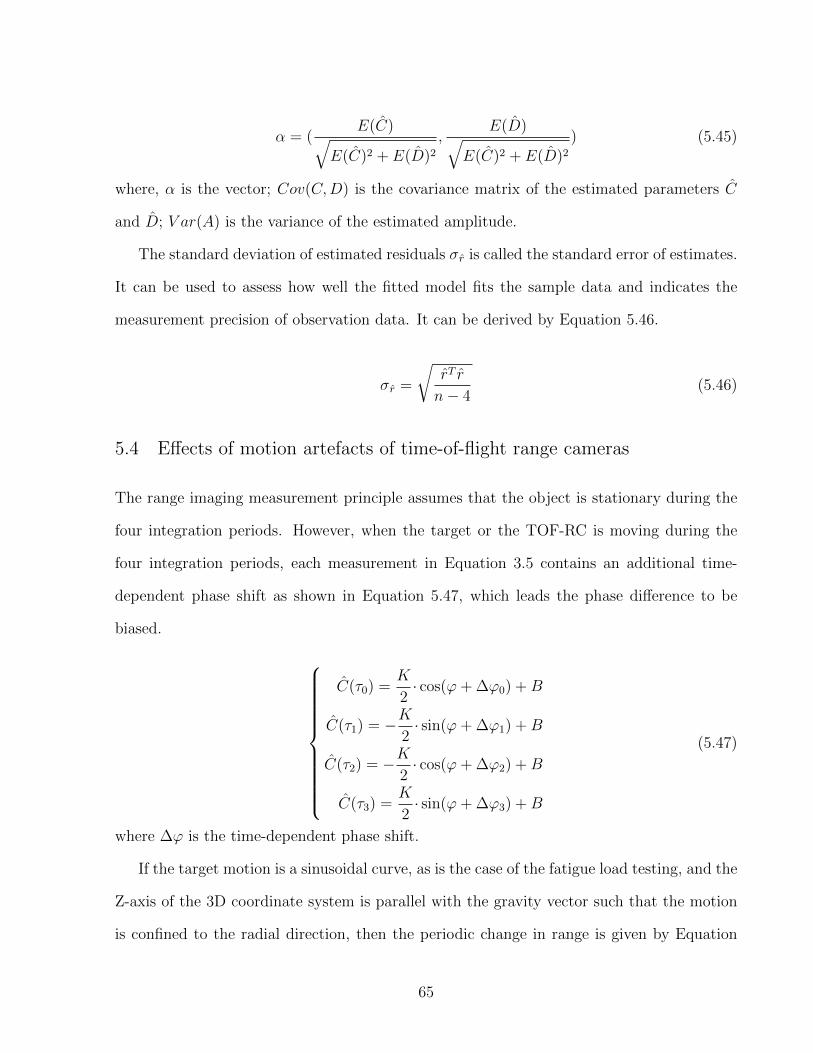
α = (E(C)√

E(C)2 + E(D)2,

E(D)√E(C)2 + E(D)2

) (5.45)

where, α is the vector; Cov(C,D) is the covariance matrix of the estimated parameters C

and D; V ar(A) is the variance of the estimated amplitude.

The standard deviation of estimated residuals σr is called the standard error of estimates.

It can be used to assess how well the fitted model fits the sample data and indicates the

measurement precision of observation data. It can be derived by Equation 5.46.

σr =

√rT r

n− 4(5.46)

5.4 Effects of motion artefacts of time-of-flight range cameras

The range imaging measurement principle assumes that the object is stationary during the

four integration periods. However, when the target or the TOF-RC is moving during the

four integration periods, each measurement in Equation 3.5 contains an additional time-

dependent phase shift as shown in Equation 5.47, which leads the phase difference to be

biased.

C(τ0) =K

2· cos(ϕ+ ∆ϕ0) +B

C(τ1) = −K2· sin(ϕ+ ∆ϕ1) +B

C(τ2) = −K2· cos(ϕ+ ∆ϕ2) +B

C(τ3) =K

2· sin(ϕ+ ∆ϕ3) +B

(5.47)

where ∆ϕ is the time-dependent phase shift.

If the target motion is a sinusoidal curve, as is the case of the fatigue load testing, and the

Z-axis of the 3D coordinate system is parallel with the gravity vector such that the motion

is confined to the radial direction, then the periodic change in range is given by Equation

65

5.48. Therefore, the additional phase shift is shown in Equation 5.49:

∆ρ(t) = k· sin(2πf0t) (5.48)

∆ϕ(t) =4πfmc

∆ρ(t) (5.49)

where k is the amplitude of the target motion; f0 is the frequency of the target motion and

c is speed of light.

Using Equations 5.48 and 5.49, the sampling measurement is thus given by Equation

5.50.

Ci =K

2· cos(ϕ+

πi

2+

4πfmc

ksin(2πf0t)) +B (5.50)

With the four biased sampling measurements, the biased phase difference (Equation 5.51)

is derived. Since the phase difference is biased, the range measurement is biased (Equation

5.52 ) as well. The impact of the target motion on the range measurements is assessed in

Chapter 6 by simulation.

ϕ = tan−1(C3 − C1

C0 − C2

) (5.51)

ρ =ϕc

4πfm(5.52)

5.5 Summary

This chapter presented range camera data processing. Extraction of the thin plates from

the 3D point cloud of the object scene is essential for accurate measurement of the beam

deflection. Therefore, different automatic extraction methods of the thin plates for different

optical sensors were presented.

Depth-based classification was the basis for the thin plate extraction. Traditional 2D

image processing algorithms were very useful to the automatic extraction of the thin plates.

66

The refined point cloud of the thin plates were used to compute the centroid of the thin plates.

The centroid was used as the reference point of interest for measuring the displacement of

the concrete beam.

Power spectral density analysis with the Lomb method on the raw measurement data

of the thin plate centroid overcomes the missing data problem. Linear and non-linear least

squares were used to estimate the loading frequency and the deflection amplitude with time

series measurement data. Statistical methods were used to analyze the displacement mea-

surement precision of the concrete beam.

Motion artefacts of TOF-RCs affect the dynamic deflection measurement accuracy. This

chapter discussed the influence of motion artefacts when target motion is a sinusoidal wave.

Based on the methodology mentioned in this chapter, the results for the concrete beam are

derived. In the next chapter, the results and analysis of the concrete beam deflection are

presented.

67

Chapter 6

Results and analysis

This chapter presents the results and analysis of the deflection measurement for a concrete

beam subjected to dynamic loading observed by two different optical sensors: TOF-RCs

and LC-RCs. First, the simulation results for the concrete beam motion are described in

Section 6.1. Second, the analysis of Experiment I and Experiment II is conducted. Section 6.2

presents the data analysis for the measurements derived from the SR4000 range cameras

set at different SFs during Experiment I. Section 6.3 describes the analysis of dynamic

concrete beam from a SR4000 TOF-RC and a Kinect LC-RC during Experiment II. In

Section 6.3, the vertical deflection, longitudinal, and lateral displacements of the concrete

beam are presented. The ability of Kinect LC-RCs to measure the dynamic deflection is also

investigated. The results derived from LDS are used as a benchmark to evaluate absolute

accuracy of the different sensors.

6.1 Simulation analysis of motion artefacts

The measurement principle of TOF-RCs assumes that the sensor and the target object are

stationary during the four integration times. Motion artefacts occur as a result of the object

target or the sensor motion during data capture. Ideally the trajectory of the thin plate

motion is a sinusoidal curve. Therefore, during the dynamic beam experiment, the impact of

the motion artefacts should be analyzed since the concrete beam was subjected to periodic

loads with 1 Hz or 3 Hz loading frequency and a 4 mm amplitude. So, in this section, a target

experiencing sinusoidal motion with the 1 Hz or 3 Hz frequency and the 4 mm amplitude

was numerically simulated.

Figures 6.1, 6.2, 6.3 and 6.4 illustrate the simulated true and biased ranges ρ for de-

68

flection along with their time stamps using the four different SFs when the target motion

frequency is 1 Hz. The true range represents the range derivation using the time-of-flight

measurement principle without considering the motion artefacts. The biased range denotes

the range derivation using the time-of-flight measurement principle by considering the mo-

tion artefacts. As can be seen, the amplitude difference between them is small but there

is a significant temporal phase difference between the true and biased signals. The biggest

temporal phase difference by calculating the true and biased signal phase is −13.2◦ with 1

Hz motion frequency and 10 Hz SF, but it is of no consequence since it does not impact the

amplitude measurement accuracy which is of prime importance (Qi and Lichti, 2012a,b).

0 0.5 1 1.5 2 2.5 3 3.5 4 4.5 5−5

0

5

t (s)

ρ (m

m)

True rangeBiased range

Figure 6.1: Simulated true and biased ranges vs time (f0 = 1 Hz and fs = 10 Hz)

0 0.5 1 1.5 2 2.5 3 3.5 4 4.5 5−5

0

5

t (s)

ρ (m

m)

True rangeBiased range

Figure 6.2: Simulated true and biased ranges vs time (f0 = 1 Hz and fs = 20 Hz)

69

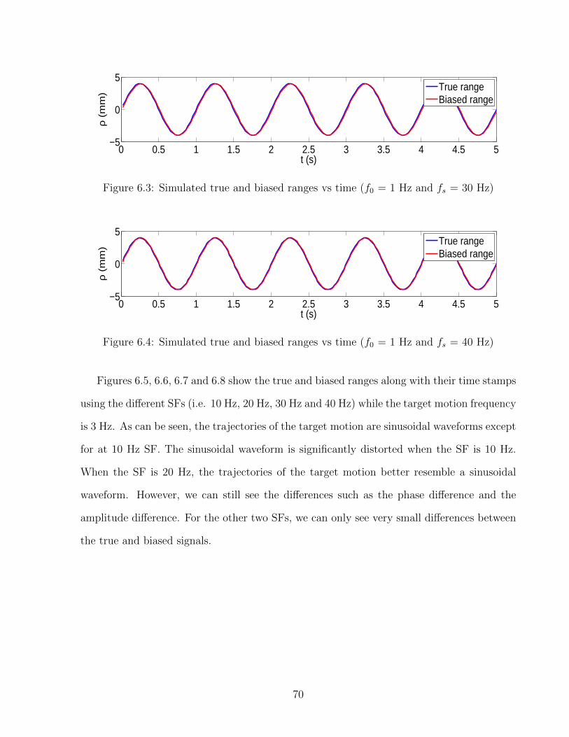
0 0.5 1 1.5 2 2.5 3 3.5 4 4.5 5−5

0

5

t (s)

ρ (m

m)

True rangeBiased range

Figure 6.3: Simulated true and biased ranges vs time (f0 = 1 Hz and fs = 30 Hz)

0 0.5 1 1.5 2 2.5 3 3.5 4 4.5 5−5

0

5

t (s)

ρ (m

m)

True rangeBiased range

Figure 6.4: Simulated true and biased ranges vs time (f0 = 1 Hz and fs = 40 Hz)

Figures 6.5, 6.6, 6.7 and 6.8 show the true and biased ranges along with their time stamps

using the different SFs (i.e. 10 Hz, 20 Hz, 30 Hz and 40 Hz) while the target motion frequency

is 3 Hz. As can be seen, the trajectories of the target motion are sinusoidal waveforms except

for at 10 Hz SF. The sinusoidal waveform is significantly distorted when the SF is 10 Hz.

When the SF is 20 Hz, the trajectories of the target motion better resemble a sinusoidal

waveform. However, we can still see the differences such as the phase difference and the

amplitude difference. For the other two SFs, we can only see very small differences between

the true and biased signals.

70

0 0.5 1 1.5 2 2.5 3 3.5 4 4.5 5−5

0

5

t (s)

ρ (m

m)

True rangeBiased range

Figure 6.5: Simulated true and biased ranges vs time (f0 = 3 Hz and fs = 40 Hz)

0 0.5 1 1.5 2 2.5 3 3.5 4 4.5 5−5

0

5

t (s)

ρ (

mm

)

True rangeBiased range

Figure 6.6: Simulated true and biased ranges vs time (f0 = 3 Hz and fs = 20 Hz)

0 0.5 1 1.5 2 2.5 3 3.5 4 4.5 5−5

0

5

t (s)

ρ (m

m)

True rangeBiased range

Figure 6.7: Simulated true and biased ranges vs time (f0 = 3 Hz and fs = 30 Hz)

0 0.5 1 1.5 2 2.5 3 3.5 4 4.5 5−5

0

5

t (s)

ρ (m

m)

True rangeBiased range

Figure 6.8: Simulated true and biased ranges vs time (f0 = 3 Hz and fs = 40 Hz)

71

Figure 6.9 shows the amplitude differences between the ideal 4 mm amplitude of the target

motion and the estimated amplitude of the target motion by considering motion artefacts

as a function of SF fs.

10 15 20 25 30 35 40−0.7

−0.6

−0.5

−0.4

−0.3

−0.2

−0.1

0

fs (Hz)

A−

diffe

renc

e (m

m)

3 Hz1 Hz

Figure 6.9: The differences between the ideal 4 mm and the biased deflections

As shown by Figure 6.9, when the SF is increased, the amplitude error is reduced. When

the motion frequency is 1 Hz and the SF is 10 Hz, the greatest amplitude difference between

the ideal 4 mm and the biased deflections is only -0.061 mm, which is 1.5% of 4 mm amplitude.

Therefore, it is expected that the motion artefacts do not significantly affect the deflection

measurement accuracy when the amplitude of the periodic sinusoidal loads is 4 mm and the

motion frequency is 1 Hz.

The maximum difference is -0.53 mm, which is 13.6% of 4 mm amplitude when the motion

frequency is 3 Hz and the SF is 10 Hz. The motion artefactes at 3 Hz loading frequency have

more influences than at 1 Hz loading frequency since the higher loading frequency causes the

higher phase shift mentioned in Chapter 5, which leads to higher motion artefacts. However,

when the SF is 20 Hz, the amplitude difference is -0.14 mm. So, in order to reduce the

72

influence of motion artefacts and to keep the deflection measurement error under the half-

millimetre level, the SF of TOF-RCs has to be at least 20 Hz when time-of-flight range

cameras are used for data capture of the periodic motion with 4 mm amplitude and the 3

Hz motion frequency.

As a result, in the beam deflection measurement experiment, if the motion frequency is 1

Hz, the TOF-RCs set at 10 Hz, 20 Hz, 30 Hz and 40 Hz SFs can be used to do data capture,

which can keep the error under half-millimetre as shown in the simulation data analysis.

If the motion frequency is 3 Hz, the TOF-RCs set at 20 Hz, 30 Hz and 40 Hz SFs can be

used to perform data capture, which can keep the measurement error under half-millimetre

according to the simulation data analysis.

6.2 Experiment I: results and analysis

This section mainly focuses on the results and analysis of the deflection of the dynamic con-

crete beam with two SR4000 TOF-RCs set at different SFs during Experiment I. First, the

range measurement precision of TOF-RCs is analyzed. Then, the 3D deflection measure-

ments of the concrete are reported including vertical direction, longitudinal direction and

lateral direction. Furthermore, statistical methods are used to analyze the deflection mea-

surement precision. Finally, the best SF is chosen to monitor the deflection of the dynamic

concrete beam.

6.2.1 The range measurement precision analysis of time-of-flight range cameras

Before the experiment, Cam 3 was used to capture zero-load data with two different MFs:

29 MHz and 31 MHz. Although the objects of main interest to measure the beam deflection

were the thin plates attached to the bottom side of the concrete beam, the top surface of

the beam was still useful to analyze the range measurement precision of the TOF-RC. The

STD of the concrete beam top surface measurements can be used to evaluate the range

73

measurement precision of TOF-RCs. The range measurement precision of the TOF-RC was

analyzed at different MFs and different SFs.

Figure 6.10 shows the STD of the beam top surface measurements as a function of SF and

MF. As can be demonstrated in Figure 6.10, the range measurement precision of the concrete

beam is improved by decreasing SF. In addition, by comparing the measurement precision

between 29 MHz and 31 MHz MFs at the same SF, there are the significant improvements

by using 31 MHz MF.

10 15 20 25 30 35 401.5

2

2.5

3

3.5

4

4.5

5

5.5

fs (Hz)

ST

D (

mm

)

29 MHz31 MHz

Figure 6.10: Precision analysis of the TOF-RCs

Table 6.1 lists the STDs of the beam top surface measurements. The improvement in

range measurement precision is at least 11.3% by comparing the range measurement precision

of these two different modulation frequencies. By comparing the two SFs, 40 Hz and 10 Hz,

the range measurement precision improvement is over 55.4%.

Table 6.1: STDs of the beam top surface measurement

SF (Hz) 10 20 30 40

STD (mm)-29 MHz 2.38 2.56 3.14 5.34STD (mm)-31 MHz 1.61 1.95 2.53 3.94

% improvement 14.5 11.5 11.3 26.3

74

6.2.2 Raw data derived from a SR4000 time-of-flight range camera

This sub-section discusses the deflection measurements of the concrete beam with two

SR4000 TOF-RCs. Cam 3 captured seven thin plates using 29 MHz MF and Cam 4 captured

another seven thin plates using 31 MHz MF. There was a common plate (Plate 7), which

was captured by the two cameras. It is used as an example to analyze the motion trajectory

and the deflection of the concrete beam.

Figure 6.11 illustrates the raw data trajectory of Plate 7’s centroid in vertical direction.

As can be seen, even though there is random noise in the raw trajectory, the trend of the

thin plate centroid is still a harmonic waveform.

0 1 2 3 4 5 6 7 81930

1940

1950

1960

t (s)

Z (

mm

)

Figure 6.11: Raw data trajectory of one thin plate centroid

6.2.3 Data analysis of SR4000 time-of-flight range cameras: 1 Hz

6.2.3.1 Vertical displacement analysis

Absolute evaluation of the motion trajectory and the deflection of the concrete beam with

SR4000 TOF-RCs was performed by comparing the motion trajectory and deflection esti-

mated from the SR4000 TOF-RCs and the independent measurements from LDSs at the

same time. In total 500 frames of measurement data were used to perform data analysis of

the concrete beam deflection in vertical direction.

The motion frequencies (i.e. loading frequencies) and defections of the concrete beam can

be derived based on the range data processing procedure mentioned in Chapter 5. Figure 6.12

shows an example of the so-obtained PSD of the thin plate centroid measured with one of

75

the TOF-RCs. As revealed from Figure 6.12, there is one dominant peak in the spectrum at

the loading frequency. The estimated loading frequency is 1.0286 Hz.

0 1 2 3 4 5 6 7 8 90

20

40

60

80

100

120

140

160

180

200

f (Hz)

P(f

)

Figure 6.12: PSD of a thin plate motion with TOF-RC (f0 = 1 Hz and fs = 20 Hz)

The deflection measurement of the concrete beam from LDSs were analyzed using the

same procedure as from TOF-RCs. The SF of the LDSs is 300 Hz. Figure 6.13 shows the so-

obtained PSD of the same thin plate measured with one of the LDSs. There is one dominant

peak in Figure 6.13 at the loading frequency. The estimated loading frequency is 1.0296 Hz.

With the recovered loading frequency, the other coefficients of the harmonic model Equa-

tion 5.29 can be estimated by using linear least-squares. Then, the approximate values of

the loading frequency and the other coefficients were used as initial values for parameter

estimates of the harmonic model. Non-linear least squares was used to derive the optimal

values of the coefficients that can be used to calculate frequency and amplitude of the con-

crete beam motion. Figures 6.14, 6.15, 6.16 and 6.17 show the thin plate centroid trajectories

when Cam 4 using 31 MHz MF was set at four different SFs. The black curve is the recon-

structed thin plate trajectory. The blue curve is the raw thin plate trajectory. As can be

seen, the motion trajectories are the sinusoidal waveforms at the four different SFs. When

SFs were 10 Hz and 20 Hz, the raw measurements of the thin plate motion have less noise.

76

0 1 2 3 4 5 6 7 8 9 100

500

1000

1500

2000

2500

3000

f (Hz)

P(f

)

Figure 6.13: PSD of a thin plate motion with LDS

While for 30 Hz and 40 Hz SFs, the raw measurements of thin plate motion have much more

noise. The derived trajectories from Cam 3 are similar to those from Cam 4.

0 0.5 1 1.5 2 2.5 3 3.5 4 4.5 5−10

0

10

t (s)

A (

mm

)

Figure 6.14: Thin plate centroid trajectories (f0 = 1 Hz and fs = 10 Hz)

0 0.5 1 1.5 2 2.5 3 3.5 4 4.5 5−10

0

10

t (s)

A (

mm

)

Figure 6.15: Thin plate centroid trajectories (f0 = 1 Hz and fs = 20 Hz)

77

0 0.5 1 1.5 2 2.5 3 3.5 4 4.5 5−10

0

10

t (s)

A (

mm

)

Figure 6.16: Thin plate centroid trajectories (f0 = 1 Hz and fs = 30 Hz)

0 0.5 1 1.5 2 2.5 3 3.5 4 4.5 5−20

0

20

t (s)

A (

mm

)

Figure 6.17: Thin plate centroid trajectories (f0 = 1 Hz and fs = 40 Hz)

Table 6.2 shows the STDs of estimated residuals derived from Cam 3 and Cam 4. As

can be seen from Table 6.2, the STDs assess how well the fitted model fits the observation

measurement data and the observation measurement precision. With increasing SF, the

measurement precision is decreased. Overall, the measurement precision of Cam 4 is higher

than Cam 3 because Cam 4 was set at 31 MHz MF which is higher than Cam 3’s MF.

Table 6.2: Experiment I: STDs of residuals (f0 = 1 Hz)

fs (Hz) 10 20 30 40

σr(Cam3) (mm) 2.37 3.32 6.05 13.08σr(Cam4) (mm) 1.18 1.78 2.73 4.83

Figure 6.18 illustrates an example of the trajectories of the chosen thin plate recovered

from the TOF-RC and the LDS measurements. As can be seen, the recovered trajectories

match very well. The estimated loading frequency is 1.0280 Hz obtained from the LDS mea-

surements using non-linear least-squares. Its STD is 4.53e-006 Hz. The estimated deflection

derived from LDS measurement is 3.93 mm and its corresponding STD is 5.50e-004 mm.

78

0 0.5 1 1.5 2 2.5 3 3.5 4 4.5 5−5

0

5

t (s)

A (

mm

)

TOF−RCsLDSs

Figure 6.18: The estimated trajectories of the same thin plate with TOF-RC and LDS (f0

= 1 Hz and fs = 30 Hz)

The recovered loading frequencies derived from the range measurements of the two TOF-

RCs are reported in Table 6.3 at different SFs. The loading frequency difference ∆f0 is the

difference between the TOF-RC and LDS determined loading frequencies. ∆f0 is listed in

Table 6.3. Moreover, the STDs of the estimated loading frequency σf0 are also reported

in Table 6.3. As revealed from Table 6.3 the loading frequency can be recovered at four

different SFs with high absolute accuracy based on ∆f0. The measurement precision of the

loading frequency is decreased with increasing SF.

Table 6.3: Experiment I: Estimated loading frequency (f0 = 1 Hz)

fs(Hz) 10 20 30 40

f0(Cam3) (Hz) 1.0281 1.0291 1.0266 1.0247f0(Cam4) (Hz) 1.0280 1.0280 1.0276 1.0270∆f0(Cam3) (Hz) 0.0001 0.0011 -0.0014 -0.0033∆f0(Cam4) (Hz) 0 0 -0.0004 -0.0019σf0(Cam3) (Hz) 4.9e-004 0.0012 0.0033 0.0064σf0(Cam4) (Hz) 2.2e-004 5.7e-004 0.0015 0.0031

The maximum deflections estimated for the concrete beam are calculated from the two

TOF-RCs with different SFs and their differences (∆A) with respect to the maximum de-

flections derived from the LDSs. They are reported in Table 6.4. In addition, Table 6.4

reports the differences of the estimated maximum deflection between TOF-RCs and LDSs.

When the ideal loading frequency was 1 Hz, in order to keep the measurement error under

half-millimetre accuracy, Cam 3 cannot be set at 10 Hz and 40 Hz SFs. For Cam 4, the

79

four different SFs can be used to obtain half-millimetre level accuracy. Since the MF of

TOF-RCs impacts the deflection measurement accuracy, the absolute deflection accuracy of

Cam 4 is higher than the absolute deflection accuracy of Cam 3. Meanwhile, when the SF

is higher, the range measurement noise is larger. Motion artefacts cause lower absolute de-

flection accuracy for Cam 3 and Cam 4 set at 10 Hz SF. The absolute accuracy of the beam

deflection with the TOF-RC is much smaller than the 10 mm absolute accuracy reported by

the manufacturer. As shown in Table 6.4, STDs of amplitude σA are all less than 1 mm.

Table 6.4: Experiment I: Deflection of Plate 7 (f0 = 1 Hz)

fs (Hz) 10 20 30 40

A (Cam3) (mm) 3.31 3.55 3.56 4.90A (Cam4) (mm) 3.61 4.05 3.61 3.56∆A (Cam3) (mm) -0.62 -0.38 -0.37 0.97∆A (Cam4) (mm) -0.32 0.12 -0.32 -0.37σA (Cam3) (mm) 0.15 0.21 0.38 0.83σA (Cam4) (mm) 0.08 0.11 0.17 0.31

Moreover, even though, by analyzing Plate 7, the maximum deflection of the concrete

beam was obtained, other thin plate data analysis should be considered as well, which

demonstrates the wide coverage advantage of TOF-RCs. Based on Table 6.4 analysis, the

best sampling frequency is 20 Hz. Therefore, Table 6.5 shows the deflections of the all thin

plate motion except Plate 12 at 20 Hz SFs. There is too much light around Plate 12, which

lead to overexposure so Plate 12 could not be extracted automatically. The deflections of

Plate 1 to Plate 7 are calculated from Cam 4. The deflections of Plate 8 to Plate 13 are

estimated from Cam 3.

Figure 6.19 illustrates the beam deflection at 20 Hz SF derived from the TOF-RCs and

also shows the beam deflection derived the five LDSs. As can be seen, the deflection of the

thin plates along the length of the concrete beam increases towards the centre plate (i.e.

Plate 7). Figure 6.19 illustrates well one of the advantages of the SR4000 TOF-RC: the

wide coverage spanned by two cameras is greater than that of the five LDSs. As shown in

80

Table 6.5: Experiment I: Deflection of the thin plate motion

Plates A (mm)-20 Hz

Plate 1 0.31Plate 2 1.34Plate 3 1.98Plate 4 2.75Plate 5 3.45Plate 6 3.98Plate 7 4.05Plate 8 3.78Plate 9 3.34Plate10 2.59Plate11 1.89Plate13 0.32

Figure 6.19, the LDS located under the Plate 9 was unable to accurately determine the beam

deflection. As shown in Figure 6.20, its raw trajectory is not sinusoidal, suggesting some

sort of defect. The other four plate trajectories derived from LDS are sinusoidal.

0 2 4 6 8 10 12 140

0.5

1

1.5

2

2.5

3

3.5

4

4.5

Plate number

A (

mm

)

TOF−RCLDS

Figure 6.19: Experiment I: Beam deflection (f0 = 1 Hz and fs = 20 Hz)

81

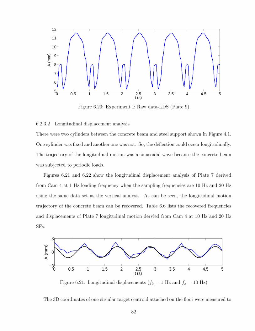
0 0.5 1 1.5 2 2.5 3 3.5 4 4.5 55

6

7

8

9

10

11

12

t (s)

A (

mm

)

Figure 6.20: Experiment I: Raw data-LDS (Plate 9)

6.2.3.2 Longitudinal displacement analysis

There were two cylinders between the concrete beam and steel support shown in Figure 4.1.

One cylinder was fixed and another one was not. So, the deflection could occur longitudinally.

The trajectory of the longitudinal motion was a sinusoidal wave because the concrete beam

was subjected to periodic loads.

Figures 6.21 and 6.22 show the longitudinal displacement analysis of Plate 7 derived

from Cam 4 at 1 Hz loading frequency when the sampling frequencies are 10 Hz and 20 Hz

using the same data set as the vertical analysis. As can be seen, the longitudinal motion

trajectory of the concrete beam can be recovered. Table 6.6 lists the recovered frequencies

and displacements of Plate 7 longitudinal motion dervied from Cam 4 at 10 Hz and 20 Hz

SFs.

0 0.5 1 1.5 2 2.5 3 3.5 4 4.5 5−3

0

3

t (s)

A (

mm

)

Figure 6.21: Longitudinal displacements (f0 = 1 Hz and fs = 10 Hz)

The 3D coordinates of one circular target centroid attached on the floor were measured to

82

0 0.5 1 1.5 2 2.5 3 3.5 4 4.5 5−3

0

3

t (s)

A (

mm

)

Figure 6.22: Longitudinal displacements (f0 = 1 Hz and fs = 20 Hz)

Table 6.6: Experiment I: Longitudinal displacement-Cam4 (f0 = 1 Hz)

fs(Hz) 10 20

f0 (Hz) 1.0276 1.0262A (mm) 1.2 1.4σf0 (Hz) 2.2e-004 5.9e-004σA (Hz) 0.03 0.04

determine the accuracy of the longitudinal displacements. The X-coordinate of the circular

target centroid is as a function of time shown in Figure 6.23. As can be seen, the trajectory

of the X-coordinate as a function of time is not a sinusoidal curve but noise. In order to

prove it is indeed noise, the PSD of the time series can be calculate and analyzed. Figure

6.24 shows the PSD of one circular target centroid trajectory. As can be seen, there is no

dominant peak above the statistical significance level (α = 0.5) in Figure 6.24, which means

that the trajectory is noise (Press et al., 1992). Therefore, it can be conclude that the floor

and the cameras mounted on the steel frames were not moving during the fatigue loading

test. So, the longitudinal displacements of the circular target were not caused by the periodic

loads.

0 1 2 3 4 5 6345

350

355

t (s)

X−c

oord

inat

e (m

m)

Figure 6.23: X-coordinate of an circular target centroid (f0 = 1 Hz and fs = 10 Hz)

83

0 0.5 1 1.5 2 2.5 3 3.5 4 4.50

2

4

6

8

10

12

α =0.001

α =0.005

α =0.01

α =0.05

α =0.1

α =0.5

f (Hz)

P(f

)

Figure 6.24: PSD of longitudinal direction (f0 = 1 Hz)

6.2.3.3 Lateral displacement analysis

The presence of the lateral displacement suggests that the load was applied eccentrically. If

it is not, the lateral displacement will be happened. Figures 6.25 shows the lateral displace-

ment analysis of Plate 7 derived from Cam 4 at 1 Hz loading frequency when the sampling

frequency is 10 Hz. As can be seen, the lateral motion trajectory of the concrete beam can

be recovered.

0 0.5 1 1.5 2 2.5 3 3.5 4 4.5 5−0.2

0

0.2

t (s)

A (

mm

)

Figure 6.25: Lateral displacements (f0 = 1 Hz and fs = 10 Hz)

Figure 6.26 show the Y-coordinate of the circular target centroid is as a function of time.

As can be seen, the trajectory of the Y-coordinate as a function of time is not a sinusoidal

curve. Figure 6.27 show the PSD of the circular target centroid trajectory in lateral direction.

84

As can be seen, there is no dominant peak above α = 0.5 statistical significance level in Figure

6.27 as well. Therefore, it can be concluded that the cameras mounted on the steel frames

were stable during the fatigue loading test. So, the lateral displacements of the circular

target were not caused by the periodic loads.

0 1 2 3 4 5 6994

996

998

1000

1002

1004

1006

t (s)

Y−

coor

dina

te (

mm

)

Figure 6.26: Y-coordinate of an circular target centroid (f0 = 1 Hz and fs = 10 Hz)

0 0.5 1 1.5 2 2.5 3 3.5 4 4.50

2

4

6

8

10

12

α =0.001

α =0.005α =0.01

α =0.05α =0.1

α =0.5

f (Hz)

P(f

)

Figure 6.27: PSD of lateral direction(f0 = 1 Hz)

85

6.2.4 Data analysis of SR4000 time-of-flight range cameras: 3 Hz

In this sub-section, the absolute accuracy of deflections of the concrete beam is assessed when

the loading frequency was 3 Hz. The data processing procedure is similar with Sub-section

6.2.3. The evaluation was performed comparing measurements from two TOF-RCs set at

SFs of 10 Hz, 20 Hz, 30 Hz and 40 Hz and five LDSs using 300 Hz SF. Five hundred frames

of the measurement data were used to perform data analysis of the concrete beam deflection.

6.2.4.1 Vertical displacement analysis

Figure 6.28 shows PSD P (f) of Plate 7 motion at 30 Hz SF in vertical direction. Just like

Figure 6.12, there is one dominant peak in Figure 6.28 at 3 Hz loading frequency. So, the

estimated frequency of the concrete beam motion is 3.0914 Hz.

0 1 2 3 4 5 6 7 80

50

100

150

f (Hz)

P(f

)

Figure 6.28: PSD of thin plate centroid trajectory-3 Hz (TOF-RC)

The same process described in Sub-section 6.2.3 was performed to calculate the vertical

deflections and frequency of the concrete beam motion when the loading frequency was 3

Hz. Figures 6.29, 6.30, 6.31 and 6.32 show the motion trajectories of the thin plate centroid

86

at the four SFs recovered from Cam 4 with 31 MHz MF. The motion trajectories of the thin

plate centriod derived from Cam 3 are similar to those of Cam 4.

0 0.5 1 1.5 2 2.5 3−10

0

10

t (s)

A (

mm

)

Figure 6.29: Thin plate centroid trajectories (f0 = 3 Hz and fs = 10 Hz)

0 0.5 1 1.5 2 2.5 3−10

0

10

t (s)

A (

mm

)

Figure 6.30: Thin plate centroid trajectories (f0 = 3 Hz and fs = 20 Hz)

0 0.5 1 1.5 2 2.5 3−10

0

10

t (s)

A (

mm

)

Figure 6.31: Thin plate centroid trajectories (f0 = 3 Hz and fs = 30 Hz)

0 0.5 1 1.5 2 2.5 3−20

0

20

t (s)

A (

mm

)

Figure 6.32: Thin plate centroid trajectories (f0 = 3 Hz and fs = 40 Hz)

87

Table 6.7 lists the STDs of the estimated residuals. As has been seen from Table 6.7, the

measurement precision of the observation data have a decreasing trend with increasing SF.

Table 6.7: Experiment I: STDs of estimated residuals (f0 = 3 Hz)

fs (Hz) 10 20 30 40

σr(Cam3) (mm) 2.51 3.72 5.34 12.09σr(Cam4) (mm) 1.24 1.71 2.67 4.52

The recovered loading frequencies from the different optical sensors are reported in Ta-

ble 6.8. The differences in recovered loading frequencies between the TOF-RC and the LDS

are presented as well. Meanwhile, the STDs of the estimated loading frequency are illus-

trated at different SFs. The estimated maximum deflection and loading frequency derived

from the LDS measurements were 4.00 mm and 3.0843 Hz with the same solution as the

TOF-RC. Their corresponding STDs were 9.59e-004 mm and 8.21e-006 Hz respectively.

Table 6.8: Experiment I: Estimated loading frequency (f0 = 3 Hz)

fs(Hz) 10 20 30 40

f0(Cam3) (Hz) 3.0842 3.0851 3.0826 3.0801f0(Cam4) (Hz) 3.0846 3.0843 3.0853 3.0904∆f0(Cam3) (Hz) -0.0002 0.0008 -0.0017 -0.0042∆f0(Cam4) (Hz) 0.0003 0 0.0010 0.0061σf0(Cam3) 4.79e-004 0.0012 0.0022 0.0060σf0(Cam4) 2.49e-004 5.94e-004 0.0013 0.2883

Table 6.9 presents the deflection measurements of the concrete beam motion calculated

from the two TOF-RC measurements with different SFs. In addition, the differences of

the estimated maximum deflection derived between the TOF-RC and the LDS results are

presented. The STDs of the deflection estimates are illustrated at different SFs as well.

As revealed in Table 6.8, the loading frequencies can be accurately recovered at all SFs

based on the absolute accuracies reported in Table6.8. Additionally, the differences in the

loading frequency for the two TOF-RCs are very small. Moreover, the STDs of the loading

frequency suggests that a higher SF results in a higher STD.

88

Table 6.9: Experiment I: Deflection of Plate 7 (f0 = 3 Hz)

fs (Hz) 10 20 30 40

A(Cam3) (mm) 3.57 3.71 4.72 5.10A(Cam4) (mm) 3.42 3.80 3.86 4.07∆A(Cam3) (mm) -0.43 -0.29 0.72 1.10∆A(Cam4) (mm) -0.58 -0.2 -0.14 0.07σA(Cam3) (mm) 0.16 0.21 0.34 0.76σA(Cam4) (mm) 0.08 0.11 0.17 0.29

As can be seen in Table 6.9, the largest deflection difference derived from Cam 3 is 1.10

mm at 40 Hz SF. The absolute accuracy of the beam deflection with the TOF-RC is much

greater than the 10 mm absolute accuracy reported by the manufacturer. Motion artefacts

impact the absolute accuracies for both cameras at 10 Hz SF. STDs of the loading frequencies

and deflections are low, which means the deflection is measured with high measurement

precision at all four SFs. However it degrades with increasing SF, and when the SF was 40

Hz, the absolute accuracies for both cameras are low.

According to previous absolute accuracy and precision analysis, the best SF is 20 Hz. So,

Table 6.10 reports the deflections of all thin plates. Figure 6.33 shows the concrete beam

deflection at 20 Hz SF derived from TOF-RC and the beam deflection derived from the five

LDSs. As can be seen, the deflection of all thin plate motion (except Plate 12) along the

length of the concrete beam illustrate the increases towards the mid-span of the concrete

beam. However, the LDS located under the Plate 9 was unable to accurately determine the

beam deflection because of the same reason mentioned in Sub-section 6.2.3.

89

Table 6.10: Experiment I: Deflections of the thin plates (f0 = 3 Hz)

Plates A (mm)-20 Hz

Plate 1 0.33Plate 2 1.22Plate 3 1.84Plate 4 2.57Plate 5 3.43Plate 6 3.52Plate 7 3.80Plate 8 3.52Plate 9 3.22Plate10 2.59Plate11 1.79Plate13 0.21

0 2 4 6 8 10 12 140

0.5

1

1.5

2

2.5

3

3.5

4

Plate number

A (

mm

)

TOF−RCLDS

Figure 6.33: Experiment I: Beam deflection (f0 = 3 Hz and fs = 20 Hz)

6.2.4.2 Longitudinal displacement analysis

Figures 6.34 shows the longitudinal displacement analysis of Plate 7 derived from Cam

4 at 3 Hz loading frequency when the sampling frequency was 20 Hz. As can be seen, the

longitudinal motion trajectory of the concrete beam can be recovered. The recovered loading

90

frequency and recovered deflection on longitudinal are 3.0832 Hz and 1.2 mm respectively.

Their corresponding STDs are 6.4e-004 Hz and 0.04 mm.

0 0.5 1 1.5 2 2.5 3−3

0

3

t (s)

A (

mm

)

Figure 6.34: Longitudinal displacements (f0 = 3 Hz and fs = 20 Hz)

Figure 6.35 shows the X-coordinate of the circular target centroid is as a function of time.

As can be seen, the trajectory of the X-coordinate as a function of time is not a sinusoidal

curve. Figure 6.36 shows the PSD of the one circular target centroid trajectory in longitudinal

direction. As can be seen, there is no dominant peak above α = 0.5 statistical significance

level in Figure 6.36. Therefore, it can be concluded that the cameras mounted on the steel

frames were stable during the fatigue loading test. So, the longitudinal displacements of the

circular target were not caused by the periodic loads when the loading frequency was 3 Hz.

0 1 2 3 4 5 6118

118.5

119

119.5

120

120.5

121

t (s)

X−

coor

dina

te (

mm

)

Figure 6.35: X-coordinate of an circular target centroid (f0 = 3 Hz)

91

0 1 2 3 4 5 6 7 8 90

2

4

6

8

10

12α =0.001

α =0.005

α =0.01

α =0.05

α =0.1

α =0.5

f (Hz)

P(f

)

Figure 6.36: PSD of longitudinal direction(f0 = 3 Hz)

6.2.4.3 Lateral displacement analysis

The loading frequency and deflection on the lateral direction cannot be recovered because

of the effects of the measurement noise significantly. Figure 6.37 show the Y-coordinate

of a circular target centroid is as a function of time. As can be seen, the trajectory of the

Y-coordinate as a function of time is not a sinusoidal curve. However by calculating the PSD

of one circular target centroid trajectory on lateral direction, the PSD can still be used to

analyze whether and the steel frame were moving. Figure 6.38 shows the PSD of the circular

target centroid trajectory on lateral direction. As can be seen, there is no dominant peak

above α = 0.5 in Figure 6.38. Therefore, it can be concluded that the cameras mounted on

the steel frames were stable during the fatigue loading test when the loading frequency was

3 Hz.

92

0 1 2 3 4 5 6644

646

648

650

652

654

656

t (s)

Y−

coor

dina

te (

mm

)

Figure 6.37: Y-coordinate of an circular target centroid (f0 = 3 Hz)

0 1 2 3 4 5 6 7 8 90

2

4

6

8

10

12α =0.001

α =0.005

α =0.01

α =0.05

α =0.1

α =0.5

f (Hz)

P(f

)

Figure 6.38: PSD of lateral direction(f0 = 3 Hz)

93

6.3 Experiment II: results and analysis

During Experiment II, two SR4000 ethernet cable TOF-RCs (Cam 3 and Cam 4), one SR

4000 USB cable TOF-RC camera (Cam 2) and one Kinect LC-RC (Cam 1) were used to

perform data capture for the dynamic deflection experiment (i.e. fatigue loading test). It

took eleven days to do the fatigue loading test. The results of the SR4000 USB cable TOF-

RC are presented. The camera was used to record concrete beam motion in real time, which

was useful to analyze fatigue properties of the concrete beam. Cam 2 was set at 29 MHz.

Based on the results and analysis of Experiment I, it could be concluded that higher dynamic

measurement accuracy could be obtained if the SF was set at 20 Hz. Therefore, the SF of

SR4000 TOF-RCs was set at 20 Hz during Experiment II. In addition, preliminary results

are reported in this section for Kinect LC-RC. The SF of Kinect was set at 30 Hz during

Experiment II.

6.3.1 Repeatability test of SR4000 time-of-flight range cameras

The zero-load test was conducted to assess the beam deflection measurement repeatability

of SR4000 TOF-RCs. Plate 7 was used to evaluate measurement consistency of the SR4000

TOF-RCs. Three data sets (i.e. Case 1, Case 2 and Case 3) derived from different time were

used to analyze the repeatability of the SR4000 TOF-RC. Each data set had over 1500 frames

and the duration was more than 75 s. Figures 6.39, 6.40 and 6.41 show the Z-coordinate of

the thin plate centroid at zero-load state.

0 10 20 30 40 50 60 70 80 901870

1875

1880

1885

t (s)

Z (m

m)

Figure 6.39: Case 1: repeatability test of SR4000

94

0 10 20 30 40 50 60 70 80 901870

1875

1880

1885

t (s)

Z (m

m)

Figure 6.40: Case 2: repeatability test of SR4000

0 10 20 30 40 50 60 70 801870

1875

1880

1885

t (s)

Z (m

m)

Figure 6.41: Case 3: repeatability test of SR4000

Table 6.11 shows the mean values and the STDs of the three cases. As has been demon-

strated in Table 6.11, the maximum difference of Z-coordinates mean among three cases is

0.1 mm. The STDs of the three cases are less than 1.2 mm. The mean values show that

range measurements of SR4000 TOF-RCs are stable over a short period of time, which is

sufficient to meet the absolute accuracy requirements for the deflection measurement.

Table 6.11: Repeatability test of SR4000

Z-Mean (mm) STD (mm)

Case 1 1877.1 0.79Case 2 1877.2 0.79Case 3 1877.1 1.11

6.3.2 Data analysis SR4000 time-of-flight range cameras: 1 Hz

For the SR4000 USB cable TOF-RC, the real-time thin plate extraction method mentioned

in Chapter 5 was used. In order to analyze the tendency of the concrete beam deflection as

a function of time, a random hour of deflection measurement data was extracted for each

day when 1 Hz periodic loads were implemented.

95

6.3.2.1 Vertical displacement analysis

First, several data sets were used to perform vertical displacement analysis when the load-

ing frequency was 1 Hz. Figures 6.42, 6.43 and 6.44 show the raw and estimated motion

trajectories of the concrete beam for three data sets.

0 1 2 3 4 5 6 7 8 9 10−5

0

5

t (s)

A (

mm

)

Figure 6.42: Case 1: thin plate raw and reconstructed trajectories (f0 = 1 Hz)

0 1 2 3 4 5 6 7 8 9 10−5

0

5

t (s)

A (

mm

)

Figure 6.43: Case 2: thin plate raw and reconstructed trajectories (f0 = 1 Hz)

0 1 2 3 4 5 6 7 8 9 10−5

0

5

t (s)

A (

mm

)

Figure 6.44: Case 3: thin plate raw and reconstructed trajectories (f0 = 1 Hz)

Table 6.12 shows the analysis of six day data sets of the dynamic deflection measurement

derived from Cam 2 when the loading frequency was 1 Hz based on the number of cycles

(TNC). The recovered frequencies and deflections of the concrete beam motion are reported

in Table 6.12. The absolute accuracies of the frequencies and deflections of the concrete beam

motion are illustrated as well. Moreover, the STDs of the estimates and their residuals are

96

listed. As can be seen, the motion frequencies and deflections can be accurately recovered for

all cases by calculating the absolute accuracies (∆f0 and ∆A) in Table 6.12. Additionally,

the deflectons of the concrete beam motion changed slightly by comparing Day 1 (4500)

with Day 9 (395500). The deflection difference between Day 1 (4500) and Day 9 (395500) is

0.2 mm based on SR4000 measurement data and it is 0.43 mm based on LDS measurement

data. The absolute accuracy of the deflection is half-millimetre for each day. The STDs of

the motion frequencies and the deflections are very small. The STDs of the loading frequency

are less than 0.1 mHz and the STDs of the deflections are less than 0.015 mm. As a result,

the SR4000 TOF-RCs have the capability to measure dynamic structural behavior with small

deflection.

Table 6.12: Experiment II: Estimated frequency and deflections (f0 = 1 Hz)

Dates Day 1 Day 2 Day 3 Day 6 Day 8 Day 9

TNC 4500 42950 49850 231900 337000 395500f0(Hz)-Cam 2 1.0219 1.0221 1.0221 1.0223 1.0224 1.0221A (mm)-Cam 2 2.35 2.45 2.49 2.54 2.55 2.55f0(Hz)-LDS 1.0219 1.0222 1.0222 1.0222 1.0224 1.0222A (mm)-LDS 2.18 2.32 2.55 2.58 2.59 2.61

∆f0 (Hz) 0 -0.0001 -0.0001 0 -0.0001 -0.0001∆A (mm) 0.17 0.13 0.06 0 -0.04 -0.06

σf0 (Hz)-Cam 2 3.39e-006 6.17e-006 6.91e-006 4.74e-006 1.06e-005 3.34e-006σA (mm)-Cam 2 0.0094 0.0053 0.0127 0.0104 0.0146 0.0098σr (mm)-Cam 2 0.75 0.74 0.80 0.71 0.79 0.77σf0 (Hz)-LDS 1.69e-005 2.28e-005 5.39e-006 1.58e-007 1.76e-007 2.07e-007σA (mm)-LDS 0.0018 0.0026 6.69e-004 2.22e-004 2.47e-004 2.94e-004

6.3.2.2 Longitudinal displacement analysis

Figures 6.45, 6.46 and 6.47 show the longitudinal displacements of several data sets when

the concrete beam was subjected to periodic loads at 1 Hz loading frequency. As can be

seen, the longitudinal motion trajectory of the concrete beam can be recovered for all cases.

97

0 0.5 1 1.5 2 2.5 3 3.5 4 4.5 5−1

0

1

t (s)

A (

mm

)

Figure 6.45: Case 1: longitudinal displacements (f0 = 1 Hz)

0 0.5 1 1.5 2 2.5 3 3.5 4 4.5 5−1

0

1

t (s)

A (

mm

)

Figure 6.46: Case 2: longitudinal displacements (f0 = 1 Hz)

0 0.5 1 1.5 2 2.5 3 3.5 4 4.5 5−1

0

1

t (s)

A (

mm

)

Figure 6.47: Case 3: longitudinal displacements (f0 = 1 Hz)

Table 6.13 shows the recovered frequencies and deflections of the thin plate longitudi-

nal motion based on the SR4000 TOF-RC measurements. Furthermore, Table 6.13 reports

STDs of the estimates of the longitudinal displacements and the motion frequencies. The

measurement precisions of the loading frequencies are very high. Low STDs of the lon-

gitudinal displacement estimates show that the measurement precision of the longitudinal

displacements are very promising. The longitudinal displacements of Plate 7 for each data

set are all around a half millimetre. In addition, the LDSs were not used to obtained the

longitudinal displacements so that the absolute accuracies cannot be obtained.

98

Table 6.13: Experiment II: Longitudinal displacement analysis-Cam 2 (f0 = 1 Hz)

Dates TNC f0(Hz) A (mm) σf0 (Hz) σA (mm) σr (mm)

Day 1 4500 1.0219 0.50 3.39e-006 0.0020 0.16Day 2 42950 1.0221 0.52 6.17e-007 0.0011 0.15Day 3 49850 1.0221 0.53 6.91e-006 0.0027 0.17Day 6 231900 1.0223 0.51 6.76e-006 0.0030 0.20Day 8 337000 1.0224 0.51 1.29e-005 0.0036 0.19Day 9 395500 1.0222 0.52 3.87e-006 0.0023 0.18

Table 6.14 provides comparisons of the recovered loading frequencies from the vertical

displacement and the longitudinal displacement. The loading frequency differences between

them are almost equivalent except that there are tiny differences of Day 8 and Day 9.

Table 6.14: Experiment II: Comparisons of recovered loading frequencies (f0 = 1 Hz)

Dates TNC f0 (Hz)-V f0 (Hz)-L δf0 (Hz)

Day 1 4500 1.0219 1.0219 0Day 2 42950 1.0221 1.0221 0Day 3 49850 1.0221 1.0221 0Day 6 231900 1.0223 1.0223 0Day 8 337000 1.0223 1.0224 -0.0001Day 9 395500 1.0221 1.0222 -0.0001

6.3.2.3 Lateral displacement analysis

Figures 6.48, 6.49 and 6.50 shows the lateral displacements of the concrete beam when the

loading frequency was 1 Hz. The lateral motion trajectories with 1 Hz loading frequency

were sinusoidal curves.

0 0.5 1 1.5 2 2.5 3 3.5 4 4.5 5−0.1

0

0.1

t (s)

A (

mm

)

Figure 6.48: Case 1: lateral displacements (f0 = 1 Hz)

99

0 0.5 1 1.5 2 2.5 3 3.5 4 4.5 5−0.1

0

0.1

t (s)

A (

mm

)

Figure 6.49: Case 2: lateral displacements (f0 = 1 Hz)

0 0.5 1 1.5 2 2.5 3 3.5 4 4.5 5−0.1

0

0.1

t (s)

A (

mm

)

Figure 6.50: Case 3: lateral displacements (f0 = 1 Hz)

Table 6.15 reports the estimated results of the lateral motion of the concrete beam. The

estimated deflections and frequencies of the lateral motion of the concrete beam are reported.

The STDs of the estimated parameters are given as well. As can be illustrated, the loading

frequencies estimated from lateral, vertical and longitudinal motions are identical on Day

1. The loading frequency difference among three motions is only 0.0010 Hz on Day 2. The

loading frequency difference among three motions is only 0.0001 Hz on Day 3. The lateral

displacement measurements are reliable since the floor and steel frame were stable based on

the previous analysis.

Table 6.15: Experiment II: Lateral displacement analysis-Cam 2 (f0 = 1 Hz)

Dates TNC f0(Hz) A (mm) σf0 (Hz) σA (mm) σr (mm)

Day 1 4500 1.0219 0.048 4.22e-005 4.81e-004 0.017Day 2 42950 1.0211 0.049 7.32e-005 5.71e-004 0.017Day 3 49850 1.0220 0.051 2.53e-004 8.29e-004 0.015

But sometimes the raw trajectories of Plate 7 centroid are not sinusoidal curve just like

Figure 6.51. It shows an example of the raw measurement of the lateral motion. Based

on those raw measurements, the deflections and frequencies of the lateral motion cannot be

100

estimated because of the effects of the measurement noise significantly.

0 1 2 3 4 5 6 7 8 9 10

37.4

37.6

37.8

38

38.2

t (s)

Y (m

m)

Figure 6.51: Raw data of the lateral displacements (f0 = 1 Hz)

6.3.3 Data analysis of SR4000 time-of-flight range cameras: 3 Hz

6.3.3.1 Vertical displacement analysis

During the dynamic concrete beam experiment, the vertical motion of the concrete beam

with 3 Hz loading frequency was tested on ten days. Figures 6.52, 6.53 and 6.54 illustrate

the raw and recovered trajectories of the vertical motion of a thin plate.

0 0.5 1 1.5 2 2.5 3 3.5 4 4.5 5−5

0

5

t (s)

A (

mm

)

Figure 6.52: Case 1: thin plate raw and estimated trajectories (f0 = 3 Hz)

0 0.5 1 1.5 2 2.5 3 3.5 4 4.5 5−5

0

5

t (s)

A (

mm

)

Figure 6.53: Case 2: thin plate raw and estimated trajectories (f0 = 3 Hz)

101

0 0.5 1 1.5 2 2.5 3 3.5 4 4.5 5−5

0

5

t (s)

A (

mm

)

Figure 6.54: Case 3: thin plate raw and estimated trajectories (f0 = 3 Hz)

As can be seen, the estimated vertical trajectories of the thin plate motion can be recov-

ered from the raw measurements obtained from SR4000 TOF-RCs. All the figures illustrate

5 s of the vertical motion trajectories. Each data set for vertical analysis was captured at

the same time of each day. The time difference of each data set was 24 hours except that

there was no data set on Day 6. The concrete beam was only subjected to periodic loads at

1 Hz on Day 6.

Table 6.16 shows the recovered loading frequencies and the deflections of the concrete

beam motion derived from TOF-RC (Cam 2) and LDS. Their differences are also given in

Table 6.16. As can be seen, the absolute accuracy on each day is half-millimetre level. In

all the cases, the deflections of the concrete beam increase slightly in time. The maximum

deflection difference between Day 1 (32400) and Day 11 (880286) is just 0.31 mm based on

the LDS measurement. The maximum deflection difference between Day 1 (32400) and Day

11 (880286) is 0.18 mm based on the SR4000 measurement. The recovered loading frequency

differences have high absolute accuracy by comparing the loading frequencies derived from

the TOF-RC and the LDS (i.e. ∆f0).

Table 6.17 gives the STDs of the deflections and loading frequencies derived from Cam

2 and the LDS. The number of raw measurement samples from Cam 2 is much more than

the number of raw measurement samples from the LDS. For example, the number of sample

of Day 1 data set is 35083 which is more than 10 times of the number of sample of Day 1

data set from LDS. Most of the STDs of the deflections derived from the LDS are less than

the STDs derived from TOF-RCs. All STDs of the amplitude estimates on each day are less

102

than 0.02 mm based on the TOF-RC and LDS raw data measurements. All the STDs of the

loading frequencies for each day are less than 0.1 mHz. STDs of Table 6.17 illustrate that

estimates of the deflections and the loading frequencies have high precision. Moreover, Table

6.17 reports the STDs of the estimated residuals. They are less than 1 mm. As a result, the

TOF-RC has an ability to record the dynamic deflection in real time.

Table 6.16: Experiment II: Estimated frequency and maximum deflection of Plate 7 (f0 = 3Hz)

Dates TNC f0 (Hz) A (mm) f0 (Hz)-LDS A (mm)-LDS ∆f0 (Hz) ∆A(mm)

Day 1 32400 3.0672 2.37 3.0680 2.32 -0.0008 0.05Day 2 60050 3.0677 2.42 3.0678 2.42 -0.0001 0.00Day 3 92450 3.0678 2.43 3.0679 2.58 0.0001 -0.15Day 4 154200 3.0677 2.44 3.0678 2.58 0.0001 -0.14Day 5 226400 3.0680 2.46 3.0681 2.58 -0.0001 -0.12Day 7 332900 3.0683 2.47 3.0684 2.60 -0.0001 -0.13Day 8 391000 3.0686 2.48 3.0687 2.61 -0.0001 -0.13Day 9 486400 3.0678 2.48 3.0679 2.63 -0.0001 -0.15Day 10 677400 3.0673 2.54 3.0674 2.64 -0.0001 -0.10Day 11 880286 3.0672 2.55 3.0673 2.63 -0.0001 -0.09

Table 6.17: Experiment II: Standard deviations with Cam 2 and LDS (f0 = 3 Hz)

Dates TNC σf0 (Hz) σA (mm) σr (mm) σf0 (Hz)-LDS σA (mm)-LDS

Day 1 32400 7.43e-007 0.0057 0.76 5.58e-004 0.0061Day 2 60050 2.78e-006 0.0092 0.79 1.02e-005 0.0021Day 3 92450 9.56e-007 0.0060 0.71 4.25e-006 8.29e-004Day 4 154200 5.64e-007 0.0046 0.62 4.68e-006 9.14e-004Day 5 226400 7.81e-007 0.0062 0.82 2.14e-007 3.00e-004Day 7 332900 8.34e-007 0.0059 0.73 1.42e-007 2.01e-004Day 8 391000 1.62e-006 0.0076 0.77 1.48e-007 2.10e-004Day 9 486400 1.52e-006 0.0075 0.77 1.97e-007 2.82e-004Day 10 677400 1.57e-006 0.0062 0.57 1.96e-007 2.82e-004Day 11 880286 5.17e-007 0.0043 0.56 1.93e-007 2.77e-004

The fatigue loading test can be used to determine the behaviour of the concrete beam.

Figure 6.55 shows the fatigue loading results derived from the SR4000 TOF-RC and the

LDS. The deflections of the concrete beam subjected to periodic loads are increased as a

103

function of the number of loading cycles. The maximum deflection difference between the

TOF-RC and the LDS is 0.15 mm.

0 1 2 3 4 5 6 7 8 9x 10

5

2.3

2.35

2.4

2.45

2.5

2.55

2.6

2.65

2.7

The number of cycles

A (

mm

)

SR4000LDS

Figure 6.55: The fatigue loading results with SR4000 and LDS

6.3.3.2 Longitudinal displacement analysis

Figures 6.56, 6.57 and 6.58 show the longitudinal motion of the concrete beam when the

loading frequency was 3 Hz. The motion trajectories with 3 Hz loading frequency have the

same trend as the motion trajectories with 1 Hz loading frequency.

0 0.5 1 1.5 2 2.5 3 3.5 4 4.5 5−1

0

1

t (s)

A (m

m)

Figure 6.56: Case 1: longitudinal displacements (f0 = 3 Hz)

104

0 0.5 1 1.5 2 2.5 3 3.5 4 4.5 5−1

0

1

t (s)

A (m

m)

Figure 6.57: Case 2: longitudinal displacements (f0 = 3 Hz)

0 0.5 1 1.5 2 2.5 3 3.5 4 4.5 5−1

0

1

t (s)

A (m

m)

Figure 6.58: Case 3: longitudinal displacements (f0 = 3 Hz)

Table 6.18 reports the longitudinal displacement analysis with 3 Hz loading frequency.

First, the deflections of the longitudinal motion of the concrete beam are reported. Second,

the estimated loading frequencies of each day are reported as well. Third, the STDs of the

estimated deflections and frequencies of longitudinal motion are given in Table 6.18. As can

be seen, during the fatigue load test, the longitudinal displacement did change significantly

by comparing the deflections of Day 1 (32400) and Day 11 (880286) and the STDs of Day

1 and Day 11. The maximum difference of the deflections is 0.04 mm which is much larger

than STD difference of deflections -0.0002 mm between Day 1 and Day 11 . In addition, the

loading frequency can also be recovered with longitudinal displacement analysis. The low

STDs of the longitudinal displacement estimates indicate that the measurement precisions

the longitudinal displacements are very high when the loading frequency was 3 Hz.

Table 6.19 provides comparisons of the recovered frequencies derived from the vertical

displacement and the longitudinal displacement derived from Cam 2. The loading frequencies

obtained from the vertical and longitudinal displacements of the same data set were identical

for each day.

105

Table 6.18: Experiment II: Longitudinal displacement analysis (f0 = 3 Hz)

Dates TNC f0 (Hz) A (mm) σf0 (Hz) σA (mm) σr (mm)

Day 1 32400 3.0672 0.50 7.44e-007 0.0012 0.16Day 2 60050 3.0677 0.51 2.78-006 0.0019 0.17Day 3 92450 3.0678 0.51 1.17e-006 0.0015 0.18Day 4 154200 3.0677 0.51 6.07e-007 0.0010 0.19Day 5 226400 3.0680 0.51 9.19e-007 0.0015 0.18Day 7 332900 3.0683 0.51 9.79e-007 0.0014 0.18Day 8 391000 3.0686 0.52 1.68e-006 0.0017 0.17Day 9 486400 3.0678 0.52 1.52e-006 0.0016 0.16Day 10 677400 3.0673 0.54 1.57e-006 0.0013 0.12Day 11 880286 3.0672 0.54 5.17e-007 0.0010 0.12

Table 6.19: Experiment II: Comparison of the loading frequencies (f0 = 3 Hz)

Dates TNC f0 (Hz)-V f0 (Hz)-L ∆f0 (Hz)

Day1 32400 3.0672 3.0672 0Day2 60050 3.0677 3.0677 0Day3 92450 3.0678 3.0678 0Day4 154200 3.0677 3.0677 0Day5 226400 3.0680 3.0680 0Day7 332900 3.0683 3.0683 0Day8 391000 3.0686 3.0686 0Day9 486400 3.0678 3.0678 0Day10 677400 3.0673 3.0673 0Day11 880286 3.0672 3.0672 0

6.3.3.3 Lateral displacement analysis

Figures 6.59, 6.60 and 6.61 shows the lateral displacements of the concrete beam when the

loading frequency was 3 Hz. The lateral motion trajectories with 3 Hz loading frequency

were sinusoidal curve.

0 0.5 1 1.5 2 2.5 3 3.5 4 4.5 5−0.1

0

0.1

t (s)

A (

mm

)

Figure 6.59: Case 1: lateral displacements (f0 = 3 Hz)

106

0 0.5 1 1.5 2 2.5 3 3.5 4 4.5 5−0.1

0

0.1

t (s)

A (

mm

)

Figure 6.60: Case 2: lateral displacements (f0 = 3 Hz)

0 0.5 1 1.5 2 2.5 3 3.5 4 4.5 5−0.1

0

0.1

t (s)

A (

mm

)

Figure 6.61: Case 3: lateral displacements (f0 = 3 Hz)

Table 6.20 reports the estimated results of the lateral motion of the concrete beam when

the loading frequency was 3 Hz. The estimated deflections and frequencies of the lateral

motion of the concrete beam are reported. The STDs of the estimated parameters are given

as well. By comparing the frequency difference from Tables 6.19 and 6.20, the maximum

difference of the loading frequency is 0.0004.

Table 6.20: Experiment II: lateral displacement analysis (f0 = 3 Hz)

Dates TNC f0 (Hz) A (mm) σf0 (Hz) σA (mm) σr (mm)

Day 1 32400 3.0668 0.049 3.28e-004 9.12e-004 0.016Day 2 60050 3.0678 0.049 7.28e-005 5.87e-004 0.017Day 9 486400 3.0677 0.049 1.50e-004 7.76e-004 0.019Day 10 677400 3.0673 0.050 6.55e-005 4.67e-004 0.013Day 11 880286 3.0672 0.050 3.03e-005 3.50e-004 0.012

Overall, the TOF-RCs can measure three dimensional displacements including lateral,

longitudinal and vertical components. In this section, the vertical, longitudinal and lateral

displacements as a function of time were analyzed. So, TOF-RCs can be used to track the

107

3D direction motions at small deflections. But if the small deflections is less than 0.1 mm,

the TOF-RCs are not sensitive to estimated the deflections and frequencies.

6.3.4 Repeatability test for Kinect range camera

In Experiment II, a Kinect (Cam 1) was used for data capture as well. The purpose of using

the Kinect was to investigate its performance for deflection measurement. A repeatability

test was conducted to evaluate the precision of the Kinect camera. The only SF of the Kinect

LC-RC is 30 Hz.

First, 3D point cloud of the thin plate centroid at zero-load were used to assess the

repeatability of the Kinect. Although thirteen thin plates were used to describe the beam

deflection status, only one thin plate’s deflection was analyzed for the Kinect LC-RC for sim-

plicity. Three data sets captured at zero load state were chosen randomly. Figures 6.62, 6.63

and 6.64 show the Z-coordinate of the Plate 7 centroid from 330 frames from the Kinect.

0 1 2 3 4 5 6 7 81900

1905

1910

t (s)

Z (

mm

)

Figure 6.62: Case 1: repeatability test

0 2 4 6 8 10 121915

1920

1925

t (s)

Z (

mm

)

Figure 6.63: Case 2: repeatability test

108

0 2 4 6 8 10 121915

1920

1925

t (s)

Z (

mm

)

Figure 6.64: Case 3: repeatability test

Table 6.21 reports the mean values and STDs of the Z-coordinate of the thin plate cen-

troid. Since the concrete beam was at zero-load, the mean value difference of Z-coordinates

between Case 1 and Case 2 should be zero ideally. However, the mean value difference be-

tween Case 1 and Case 2 is 17.6 mm from Table 6.21. The depth values of the thin plate

were fluctuated for Case 3. For example, in Figure 6.64, there a discontinuity at about 10

s which is called instability problem. The repeatability of the Kinect LC-RCs is not stable.

The results have the similar trend as found by Andersen et al. (2012) who reported that

even if the Kinect LC-RCs are setup in static mode, the depth value of a given object point

fluctuates.

Table 6.21: Repeatability test

Z-Mean (mm) STD (mm)

Case 1 1903.6 0.59Case 2 1920.7 0.52Case 3 1919.8 0.92

6.3.5 Displacement analysis

6.3.5.1 Raw data captured by a Kinect range camera

Figures 6.65, 6.66 and 6.67 show the raw data captured during periodic loading derived

from the Kinect. As can be seen, the raw measurement data are unstable. The depth

measurements of the same surface have different levels. It shows the presence of an instability

problem.

109

0 5 10 151850

1855

1860

1865

1870

1875

1880

1885

1890

t (s)

Z (

mm

)

Figure 6.65: Case 1: thin plate raw trajectory with Kinect

0 2 4 6 8 10 121865

1870

1875

1880

1885

1890

t (s)

Z (

mm

)

Figure 6.66: Case 2: thin plate raw trajectory with Kinect

0 2 4 6 8 10 121855

1860

1865

1870

1875

1880

t (s)

Z (

mm

)

Figure 6.67: Case 3: thin plate raw trajectory with Kinect

110

6.3.5.2 Data analysis of a Kinect range camera: 1 Hz

The dynamic data analysis for the same thin plate (Plate 7) was conducted to assess the

Kinect’s performance for the concrete beam deflection measurements. If raw trajectories

derived from Kinect are not stable, which is similar with Figures 6.65, 6.66 and 6.67, we

cannot use these to estimate the frequencies and deflections of the concrete beam motion.

However, there were several data sets which were stable which can show that the Kinect

LC-RCs have a potential ability to measure the dynamic deflections of the concrete beam.

So, the frequency and the deflection estimates were conducted using stable data sets with

330 samples. Figures 6.68 and 6.69 show the recovered and raw trajectory with 1 Hz loading

frequency.

0 0.5 1 1.5 2 2.5 3 3.5 4 4.5 5−5

0

5

t (s)

A (

mm

)

Figure 6.68: Case 1 : Thin plate raw and estimated trajectories with Kinect (f0 = 1 Hz)

0 0.5 1 1.5 2 2.5 3 3.5 4 4.5 5−5

0

5

t (s)

A (

mm

)

Figure 6.69: Case 2: Thin plate raw and estimated trajectories with Kinect (f0 = 1 Hz)

Table 6.22 reports the estimated frequency and the deflection of the Plate 7’s motion

derived from the Kinect. Their absolute accuracies are also reported by calculating the

111

deflection and loading frequency differences between the LDS and the Kinect LC-RC. The

absolute accuracies are at half-millimetre level. Table 6.23 shows the STDs of the estimated

deflection and loading frequencies. The Kinect LC-RCs have an ability to obtain high mea-

surement accuracy and precision for measuring small dynamic deflection when the loading

frequency is 1 Hz but subject to the instability problem.

Table 6.22: Experiment II: Estimated frequency and deflection with Cam 1 (f0 = 1 Hz)

Dates TNC f0 (Hz) A (mm) f0 (Hz)-LDS A (mm)-LDS ∆f0 (Hz) ∆A(mm)

Day 8 337000 1.0213 2.63 1.0224 2.59 -0.0009 0.04Day 9 395500 1.0207 2.36 1.0211 2.61 -0.0004 -0.25

Table 6.23: Experiment II: Standard deviations with Cam 1 (f0 =1 Hz)

Dates TNC σf0 (Hz) σA (mm)

Day 8 337000 0.0015 0.0768Day 9 395500 0.0013 0.0607

6.3.5.3 Data analysis of a Kinect range camera: 3 Hz

The Kinect was used to capture when the concrete beam was subjected to periodic loads

with 3 Hz motion frequency as well. Therefore, the data analysis of Kinect was conducted

too in this thesis. Figures 6.70, 6.71 and 6.72 show the raw and estimated trajectories with

3 Hz loading frequency.

0 0.5 1 1.5 2 2.5 3 3.5 4 4.5 5−10

0

10

t (s)

A (

mm

)

Figure 6.70: Case 1: Thin plate raw and estimated trajectories with Kinect (f0 =3 Hz)

112

0 0.5 1 1.5 2 2.5 3 3.5 4 4.5 5−10

0

10

t (s)

A (

mm

)

Figure 6.71: Case 2: Thin plate raw and estimated trajectories with Kinect (f0 =3 Hz)

0 0.5 1 1.5 2 2.5 3 3.5 4 4.5 5−5

0

5

t (s)

A (

mm

)

Figure 6.72: Case 3: Thin plate raw and estimated trajectories with Kinect (f0 =3 Hz)

Table 6.24 shows the estimated frequencies and maximum deflection with the Kinect.

Even though the raw data derived from Kinect are stable in this case, the absolute accu-

racies of the concrete deflection deflections are sensitive. Table 6.25 reports the STDs of

the deflection and recovered frequencies of the dynamic concrete beam. The STDs of the

estimated deflection are less than 0.2 mm. However, high estimated deflection precision does

not imply high absolute accuracy. The STDs of the recovered frequencies are less than 0.01

mHz. The Kinect LC-RCs did not meet the requirements of measuring the small deflection

of the dynamic concrete beam.

Table 6.24: Experiment II: Estimated frequencies and deflection with Cam 1 (f0 =3 Hz)

Dates TNC f0 (Hz) A (mm) f0 (Hz) A (mm)-LDS ∆f0 (Hz) ∆A (mm)

Day 7 332900 3.0682 3.92 3.0684 2.59 -0.0002 1.33Day 8 391000 3.0669 3.52 3.0687 2.62 -0.0018 -0.90Day 10 677400 3.0681 2.49 3.0675 2.64 0.0006 -0.15

Based on the results and analysis above, the fluctuating measurement is seemingly un-

predictable and this indicated low sensitivity of Kinect LC-RCs. As a result, Kinect LC-RCs

113

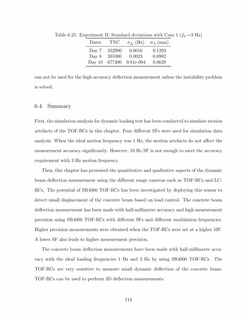
Table 6.25: Experiment II: Standard deviations with Cam 1 (f0 =3 Hz)

Dates TNC σf0 (Hz) σA (mm)

Day 7 332900 0.0016 0.1293Day 8 391000 0.0023 0.0982Day 10 677400 9.81e-004 0.0629

can not be used for the high accuracy deflection measurement unless the instability problem

is solved.

6.4 Summary

First, the simulation analysis for dynamic loading test has been conducted to simulate motion

artefacts of the TOF-RCs in this chapter. Four different SFs were used for simulation data

analysis. When the ideal motion frequency was 1 Hz, the motion artefacts do not affect the

measurement accuracy significantly. However, 10 Hz SF is not enough to meet the accuracy

requirement with 3 Hz motion frequency.

Then, this chapter has presented the quantitative and qualitative aspects of the dynamic

beam deflection measurement using the different range cameras such as TOF-RCs and LC-

RCs. The potential of SR4000 TOF-RCs has been investigated by deploying this sensor to

detect small displacement of the concrete beam based on load control. The concrete beam

deflection measurement has been made with half-millimetre accuracy and high measurement

precision using SR4000 TOF-RCs with different SFs and different modulation frequencies.

Higher precision measurements were obtained when the TOF-RCs were set at a higher MF.

A lower SF also leads to higher measurement precision.

The concrete beam deflection measurements have been made with half-millimetre accu-

racy with the ideal loading frequencies 1 Hz and 3 Hz by using SR4000 TOF-RCs. The

TOF-RCs are very sensitive to measure small dynamic deflection of the concrete beam.

TOF-RCs can be used to perform 3D deflection measurements.

114

A Kinect LC-RC was also used for the dynamic deflection measurement in this section

as well. Half-millimetre accuracy could be achieved sometimes. The range measurements of

Kinect LC-RCs are unstable.

115

Chapter 7

Conclusions and recommendations

7.1 Conclusions

The thesis mainly focused on the development of new algorithms to measure the deflection of

a concrete beam when it was subjected to periodic loads, which is called a fatigue load test.

Three types of optical sensors were used to measure the concrete beam deflection during the

fatigue loading test: SR4000 TOF-RCs, Kinect LC-RCs and LDSs. LDSs were used as the

benchmark to evaluate accuracy of the RCs.

Different automatic methods to extract the thin plates for the SR4000 TOF-RCs and

the Microsoft LC-RCs have been investigated in this thesis. First, the thin plate 3D point

cloud was extracted automatically from the 3D point cloud of the experiment scene based

on 2D and 3D image processing techniques, which was applied for the SR4000 TOF-RCs.

Second, a real-time thin plate extraction system for SR4000 TOF-RCs has been developed

in this work. The system was utilized to record the concrete beam dynamic deflection in real

time. It paves a road for analyzing the concrete beam behaviour in real time. Third, this

thesis proposed a new method with 2D and 3D image processing algorithms to automatically

extract the 3D point cloud of the thin plates for the Kinect LC-RCs.

According to the concrete beam motion analysis by using the simulation data derived

based on the TOF-RC measurement principle and the real data derived from the SR4000

TOF-RCs, It can be concluded that the motion artefacts do not influence the measurement

accuracy significantly when loading frequency is 1 Hz and SF is 10 Hz, 20 Hz, 30 Hz or

40 Hz. However, when the loading frequency is 3 Hz, the absolute accuracies of simulated

motion deflection under SFs of 20 Hz, 30 Hz and 40 Hz are of half-millimetre level which is

sufficient for deflection measurements. The motion artefacts have been reduced by setting a

116

higher SF.

The range measurement precision of a SR4000 TOF-RC has been assessed by analyzing

range measurement of the top surface of the concrete beam at zero-load state. It can be

concluded that the higher modulation frequency is set, the higher range measurement pre-

cision will be obtained; the lower SF is set, the higher range measurement precision will be

achieved.

The results from the real data from Experiment I have indicated that the amplitudes of

the periodic motion can be recovered with half-millimetre accuracy when the 3 Hz target

motion is sampled at 20 Hz, 30 Hz and 40 Hz with 31 MHz modulation frequency. However,

When the 1 Hz target motion is sampled at 10, 20, 30 and 40 Hz with 31 MHz modula-

tion frequency, the concrete beam deflection can be recovered with half-millimetre accuracy.

When the modulation frequency is 29 MHz, the best SF is 20 Hz to keep the error under

half-millimetre for 3 Hz loading frequency. However, for 1Hz loading frequency, the SFs

should be 20 Hz to keep the measurement error under the half-millimetre. In conclusion,

the use of TOF-RC in dynamic vertical deflection measurements in this thesis has shown

that even though the coarse absolute accuracy range camera with ±10 mm, can achieve

half-millimetre accuracy for dynamic deflection measurement.

By analyzing the vertical deflection of the concrete beam during Experiment I, the best

SF is 20 Hz, in order to keep the absolute accuracy under the half-millimetre. Therefore,

in Experiment II, 3D motion trajectories of the concrete beam subjected to 1 Hz and 3 Hz

periodic loads have been measured using the TOF-RC when the SF was set at 20 Hz. Based

on the results and analysis from Experiment II, first, the TOF-RC can be used to track

the properties of the concrete beam over time. Second, the TOF-RCs have the ability to

track the 3D motion trajectories. The deflections and frequencies of the 3D motion of the

concrete beam can be recovered at a high level accuracy. The TOF-RCs in the vertical and

longitudinal displacement analysis have a better performance than the lateral displacement

117

analysis. So, the use of TOF-RC in dynamic vertical, longitudinal and lateral displacements

has shown that the TOF-RC has the capability of measurement 3D deflections. The TOF-

RCs have the capability to estimate the amplitudes of the target motion with small deflection.

Third, by analyzing the dynamic motion amplitudes of the concrete beam for all thin plates

along the length of the concrete beam has shown that wide coverage is a selling feature of

TOF-RCs.

The vertical deflection was also measured using a Kinect light coded range camera. Ac-

cording to the results and analysis from Experiment II, the raw data derived from the Kinect

LC-RCs were unstable. The instability problem of the Kinect LC-RCs was unpredictable.

Therefore, It can be concluded that the depth measurements of Kinect are not stable, which

is not sufficient to meet the half-millimetre accuracy for the deflection measurement. Addi-

tionally, the unstable and unpredictable problem of the raw measurement derived from the

Kinect LC-RCs indicates that the Kinect LC-RCs have low measurement precision. As a

result, the Kinect LC-RCs can not be used for high accuracy deflection measurement unless

the instability problem is solved.

7.2 Recommendations

In this thesis, most of the analysis focuses on the thin plates since the top surface of the

concrete beam were occluded by the spread beam. However, the top surface of the concrete

beam is still very useful to analyze the beam deflection through reconstructing the whole top

surface of the concrete beam. However, due to the limited field of view of the range cameras,

multiple range cameras should be used to cover the complete top surface of the concrete

beam. Therefore, the registration of multi-camera data is a promising for future work and

then the use of the concrete beam itself for analyzing the deflection is another future work.

The TOF-RC is capable of the surface reconstruction with acquired 3D point cloud. The

acquired 3D point cloud can provide highly accurate surface models of the deflection objects.

118

In addition, the top surface of the concrete beam can be recovered by using the mathematical

model of the beam deflection derived in Gordon and Lichti (2007).

In Experiment II, real time extraction of the thin plates allowed detection of the concrete

beam deflection behaviour in real time. During the experiment, the centroids of the thin

plates were recorded in real time. However this is not real time monitoring of concrete beam

deflection. The Kalman filter extends the concept of least-squares to contain the knowledge

of how the state vector behaves in time. In order to monitor the concrete beam deflection

in real time, implementation of a Kalman filter is necessary in future work.

In Experiment II, a Kinect LC-RC was also used to capture the dynamic concrete beam

data which were processed after the experiment. The Kinect LC-RCs include RGB images

and depth images. However, since the relative orientation of the RGB image and depth image

was not estimated, the depth image was just used to isolate the thin plates. Therefore, the

relative orientation of the RGB and depth images is a bridge of two cameras, which is useful

to segment the thin plate with 2D and 3D image process algorithm. Calculating the relative

orientation of the two cameras is necessary in future work. In addition, the instability

problem of the raw measurement of the Kinect LCs should be solved.

119

References

Andersen, M., T. Jensen, P. Lisouski, A. Mortensen, M. Hansen, T. Gregersen, and

P. Ahrendt (2012, February). Kinect depth sensor evaluation for computer vision ap-

plications. Technical Report ECE-TR-6, Aarhus University.

Blackledge, J. (2005). Digital image processing mathematical and computational methods.

Chichester, West Sussex: Horwood.

Bostelman, R. and J. Albus (2007). A multipurpose robotic wheelchair and rehabilitation

device for the home. In Proceedings of the IEEE International Conference on Intelligent

Robots and Systems, San Diego, California, USA, pp. 3348–3353.

Bostelman, R., T. Hong, R. Madhavan, and B. Weiss (2005). 3D range imaging for urban

search and rescue robotics research. In IEEE International Conference On System Safety,

Security and Rescue Robotics, Gaithersburg, MD, USA, pp. 164–169.

Cheney, W. and D. Kincaid (2007). Numerical Mathematics and Computing. Belmont:

Thomson Brooks/Cole.

Chiabrando, F., R. Chiabrando, D. Piatti, and F. Rinaudo (2009). Sensors for 3d imaging:

metric evaluation and calibration of a ccd/cmos time-of-flight camera. Sensors 9 (12),

10080–10096.

Chow, J., K. D. Ang, D. D. Lichti, and W. F. Teskey (2012). Performance analysis of a low-

cost triangulation-based 3D camera: Microsoft kinect system. In International Archieves

of the Photogrammetry, Remote Sensing and Spatial Information Science, XXII ISPRS

Congress, 2012, Volume XXXIX-B5, Melbourne, Australia, pp. 239–244.

Detchev, I., A. Habib, and M. El-Badry (2012). Image-based deformation monitoring of stat-

ically and dynamically loaded beams. In International Archieves of the Photogrammetry,

120

Remote Sensing and Spatial Information Science, XXII ISPRS Congress, 2012, Volume

XXXIX-B5, Melbourne, Australia, pp. 6.

Dorrington, A., J. Godbaz, M. Cree, A. Payne, and L. Streeter (2011). Separating true range

measurements from multi-path and scattering interference in commercial range cameras.

In Proc. of SPIE-IS & T Electronic Imaging, Volume 7864, California, USA, pp. 1–10.

Fitzgibbon, A., M. Pilu, and B. Fisher (1999). Direct least square fitting of ellipses. IEEE

transactions on pattern analysis and machine intelligence 21 (5), 476–480.

Foix, S., G. Alenya, and C. Torras (2011). Lock-in time-of-flight (tof) cameraaas: a survey.

IEEE Sensors Journal 11 (3), 1–11.

Fraser, C. and B. Riedel (2000). Monitoring the thermal deformation of steel beams via

vision metrology. ISPRS Journal of Photogrammetry & Remote Sensing 55 (4), 1–10.

Freedman, B., A. Shpunt, M. Machline, and Y. Arieli (2012, 04). Depth mapping using

projected patterns.

Fuchs, S. and G. Hirzinger (2008). Extrinsic and depth calibration of ToF-cameras. In

Computer Vision and Pattern Recognition, 2008, Anchorage, USA, pp. 1–6.

Gonsalves, R. and J. Teizer (2009). Human motion analysis using 3d range imaging tech-

nology. In 26th Internation Symposium on Automation and Robotics in Construction,

Giorgia, USA, pp. 76–85.

Gonzalez, R. and R. Woods (2008). Digital image processing. Upper Saddle River, NJ, USA:

Prentice Hall.

Gordon, S. and D. Lichti (2007). Modeling terrestrial laser scanner data for precise structural

deformation measurement. ASCE Journal of Surveying Engineering 133 (2), 72–80.

121

Heffernan, P. J. and M. A. Erki (2004). Fatigue behavior of reinforced concrete beams

strengthened with carbon fiber reinforced plastic laminates. Journal of Composites for

Construction 8 (2), 132–140.

Herrera, C., J. Kannala, and J. Heikkila (2011). Accurate and practical calibration of a

depth and color camera pair. In 14th International Conference on Computer Analysis of

Images and Patterns, Seville, Spain, pp. 437–445.

Jamtsho, S. (2010). Geometric modelling of 3D range cameras and their application for

structural deformation measurement. Master’s thesis, University of Calgary, Calgary,

Canada.

Jamtsho, S. and D. Lichti (2010). Modeling scattering distortion of 3d range camera. In

International Archives of the Photogrammetry, Remote Sensing and Spatial Information

Sciences, Volume XXXVIII, Newcastle, UK, pp. 299–304.

Jia, W., W. Yi, J. Saniie, and E. Oruklu (2012). 3d image reconstruction and human body

tracking using stereo vision and Kinect technology. In Electro/Information Technology

(EIT), 2012, Chicago, USA, pp. 1–4.

Kahlmann, T., H. Remondino, and H. Ingensand (2006). Calibration for increased accu-

racy of the range imaging camera swissranger. Remote Sensing and Spatial Information

Sciences 36 (5), 136–141.

Khoshelham, K. and S. Elberink (2012). Accuracy and resolution of kinect depth data for

indoor mapping applications. Sensors 12 (2), 1437–1454.

Klette, R., K. Schluns, and A. Koschan (1998). Computer vision there-dimensional data

from images. Singapore: Springer.

Lahamy, H. and D. Lichti (2010). Real-time hand gesture recognition using range cameras.

122

In Internation Archives of Photogrammetry, Remote Sensing and Spatial Information Sci-

ences, Volume XXXVII, pp. 54–59.

Lahamy, H. and D. Lichti (2012). Towards real-time and rotation-invariant american sign

language alphabet recongnition using a range camera. Sensors 12 (11), 14416–14441.

Lange, R. (2000). 3D time-of-flight distance measurement with solid-state image sensors in

CMOS/CCD-technology. Ph. D. thesis, University of Siegen, Germany.

Lange, R. and P. Seitz (2001). Solid-state time-of-flight range camera. IEEE Journal of

Quantum Electronics 37 (3), 390–397.

Lange, R., P. Seitz, A. Biber, and S. Lauxtermann (2000). Demodulation pixels in ccd

and cmos technologies for time-of-flight ranging. In Sensors, Cameras and Systems for

Scientific/Industrial Applications II, Proc. SPIE, Volume 3965, San Jose, USA, pp. 1–12.

Li, Y. (2012). Hand gesture recognition using Kinect. In Software Engineering and Service

Science (ICSESS), 2012, Beijing, China, pp. 196–199.

Li, Z. and R. Jarvis (2009). Real time hand gesture recognition using a range camera. In

Australian Conferenec on Robotics and Automation (ACRA), Sydney, Australia, pp. 1–7.

Lichti, D., S. Jamtsho, S. El-Halawany, H. Lahamy, J. Chow, T. Chang, and M. El-Badry

(2012). Structural deflection measurement with a range camera. Journal of Surveying

Engineering 183 (2), 66–76.

Lichti, D. and C. Kim (2011). A comparsion of three geometric self-calibration methods for

range cameras. Remote Sensing 3 (5), 1014–1028.

Lichti, D., C. Kim, and S. Jamtsho (2010). An integrated bundle adjustment approach to

range camera geometric self-calibration. ISPRS Journal of Photogrammetry & Remote

Sensing 65 (4), 360–368.

123

Lichti, D., X. Qi, and T. Ahmed (2012). Range camera self-calibration with scattering

compensation. ISPRS Journal of Photogrammetry & Remote Sensing 74 (0), 101–109.

Lindner, M. and A. Kolb (2006). Calibration of the intensity-related distance error of the

pmd tof camera. In Proceedings of the SPIE on Intelligent Robots and Computer Vision,

Volume XXV, Boston, USA.

Lindner, M. and A. Kolb (2009). Compensation of motion artifacts for time-of-flight cameras.

In Proc, Dynamic 3D Vision Workshop, Volume 5742, pp. 16–27.

Lindner, M., I. Schiller, A. Kolb, and R. Koch (2010). Time-of-flight sensor calibration for

accurate range sensing. Computer Vision and Image Understanding 114 (12), 1318–1328.

Lottner, O., A. Sluiter, K. Hartmann, and W. Weihs (2007). Movement artefacts in range

images of time-of-flight cameras. In Signals, Circuits and Systems, 2007. ISSCS 2007.

International Symposium on, Volume 1, pp. 1 –4.

Maas, H. and U. Hampel (2006). Photogrammetric techniques in civil engineering mate-

rial testing and structure monitoring. Photogrammetric Engineering and Remote Sens-

ing 72 (1), 39–45.

MESA-Imaging (2012). Sr 4000 user manual. www.mesa-imaging.ch/dlm.php?fname...

CD/SR4000_Manual.pdf. [Online; accessed 06-June-2012].

Mutto, C., P. Zanuttigh, and G. Cortelazzo (2010). Time-of-flight cameras and Microsoft

Kinect. New York, Heidelberg, Dordrecht and London: Springer.

Otsu, N. (1979). A threshold selection method from gray-level histograms. IEEE Transac-

tions on Systems, Man, and Cybernetics 9 (1), 62–66.

Papakonstantinou, C. G., M. F. Petrou, and K. A. Harries (2001). Fatigue behavior of RC

beams strengthened with GFRP sheets. Journal of Composites for Construction 74 (5),

246–253.

124

Park, H. and H. Lee (2007). A new approach for health monitoring of structures-terrestrial

laser scanning. Computer-Aided Civil and Infrastructure Engineering 22 (1), 19–30.

Piatti, D. and F. Rinaudo (2012). SR-4000 and CamCube3.0 time of flight (ToF) cameras:

tests and comparison. Remote Sensing 4 (4), 1069–1089.

Press, H., A. Teukolsky, T. Vetterling, and P. Flannery (1992). Numerical Recipes in C.

New York: Cambridge University.

Primesense (2012). Primesense, Ltd. http://www.primesensr.com. [Online; accessed 06-

Oct-2012].

Qi, X. and D. Lichti (2012a). Dynamic concrete beam deformation measurement with

3d range cameras. In International Archieves of the Photogrammetry, Remote Sensing

and Spatial Information Science, XXII ISPRS Congress, 2012, Volume XXXIX-B5, Mel-

bourne, Australia, pp. 239–244.

Qi, X. and D. Lichti (2012b). Monitoring dynamic concrete beam deformation with range

cameras. In FIG Working Week 2012, Knowing to Manage the Territory, Protect the

Environment, Evaluate the Cultural Heritage, Rome, Italy, pp. 1–13.

Rabbani, T., F. van den Heuvel, and G. Vosselman (2006). Segmentation of point clouds

using smoothness constraint. In ISPRS Commission V Synposium ’Image Engineering

and Vision Metrology, Volume XXXVI, Dresden, Germany.

Ray, S. and J. Teizer (2012). Real time construction worker posture analysis for ergonomics

training. Advanced Engineering Informatics 26 (2), 493–455.

Rohs, M. (2004). Real-world interaction with camera phones. Lecture Notes in Computer

Science, 74–89.

125

Ronnholm, P., M. Nuikka, A. Suominen, P. Salo, H. Hyypp, P. Pntinen, H. Haggrn, M. Ver-

meer, J. Puttonen, H. Hirsi, A. Kukko, H. Kaartinen, J. Hyypp, and A. Jaakkola (2009).

Comparsion of measurement techniques and static theory applied to concrete beam defor-

mation. Photogrammetric Record 24 (128), 351–371.

Shahbazi, M., S. homayouni, M. Saadatseresht, and M. Sattari (2011). Range camera self-

calibration based on integrated bundle adjustment via joint setup with a 2d digital camera.

Sensors 11 (9), 8721–8740.

Whiteman, T., D. Lichti, and I. Chandler (2002). Measurement of deflections in concrete

beams by close-range digital photogrammetry. In Proceedings of Joint International Sym-

posium on Geospatial Theory, Processing and Applications, Ottawa, Canada. CD-ROM.

Xia, L., C. C. Chen, and J. Aggarwal (2011). Human detection using depth information by

Kinect. In International Workshop on Human Activity Understanding from 3D Data in

conjunction with CVPR, Colorado, USA, pp. 15–22.

Ye, J., G. Fu, and U. Poudel (2011). Edge-based close-range digital photogrammetry struc-

tural deformation measurement. Journal of Engineering Mechanics 137 (7), 475–483.

126