Autocamera Calibration for traffic surveillancecameras with wide angle lenses.Aman Jain

Department of Mechanical EngineeringVisvesvaraya National Institute of Technology

Nagpur, Indiaamanjain@students.vnit.ac.in

Nicolas SaunierDepartment of Civil, Geological and Mining Engineering

Polytechnique MontrealMontreal, Canada

nicolas.saunier@polymtl.ca

Abstract—We propose a method for automatic calibrationof a traffic surveillance camera with wide-angle lenses. Videofootage of a few minutes is sufficient for the entire calibrationprocess to take place. This method takes in the height ofthe camera from the ground plane as the only user input toovercome the scale ambiguity. The calibration is performed intwo stages, 1. Intrinsic Calibration 2. Extrinsic Calibration.Intrinsic calibration is achieved by assuming an equidistant fish-eye distortion and an ideal camera model. Extrinsic calibrationis accomplished by estimating the two vanishing points, on theground plane, from the motion of vehicles at perpendicularintersections. The first stage of intrinsic calibration is alsovalid for thermal cameras. Experiments have been conductedto demonstrate the effectiveness of this approach on visible aswell as thermal cameras.

Index Terms—fish-eye, calibration, thermal camera, intelligenttransportation systems, vanishing points

I. INTRODUCTION

Camera calibration is of immense importance in the extrac-tion of information from video surveillance data. It could eitherbe used to deal with the perspective distortion of the object inthe image plane or it can be used for photogrammetric mea-surements like distances, velocities, trajectories, etc. It is alsofundamental for performing the multiview 3D reconstruction.Besides, with the aid of 3D information, it could also be usedfor vehicle tracking or object detection, robust to occlusion.

Owing to its importance, a significant portion of literature incomputer vision addresses the problem of camera calibration.Almost all the methods of calibration could be categorizedinto two major approaches:-

• Finding image-world correspondences [1]–[4].• Vanishing Point-based methods [5]–[9].

The first method tries to exploits the properties of the 3Dscene structure to find correspondences between the real-worldand its 2D image captured by the camera. With the aid ofthese correspondences, intrinsic as well as extrinsic estimationcould be made. Further, the accuracy can be improved withincreasing such correspondences. The vanishing point methodsare majorly based on estimating the orthogonal vanishingpoints in the scene and requires no a priori knowledge forrecovering the extrinsic and intrinsics matrices.

If the camera is already pre-calibrated using 3D rigs orchecker-board, this data could be used directly in the second

stage. However, in most cases, this data is not always availableand hence there is a need for automatic intrinsic calibrationalso. Most of the literature in traffic surveillance considers anideal camera model which assumes that the pixels are perfectlysquare with zero skew and the optical center of the cameracoincides exactly with the image center. The last assumptionis not necessarily true and in such cases, the optical center iscalculated in a slightly different fashion.

For extrinsic calibration in the context of traffic surveillance,the correspondences approach may require annotation of lanemarking with its lane-width [10] [11] or presence of groundcontrol points, or using regional heuristics such as averagevehicle dimensions [12] or speed. However, the majority of theabove methods involve a human intervention or are location-dependent and are unsuitable for generalized auto-calibration.Thus for such applications, we make use of vanishing points.The vanishing points may be generated from the static scenestructures or lane markings, or motion of vehicles and pedes-trians [13]. For robust auto camera calibration, it is alwaysadvisable that the calibration process is independent of thescene in general and hence our approach will use only themoving objects in the scene. This paper especially deals withthe wide-angle lenses cameras, that are ideal for most of thephotogrammetry applications. However, they are always ac-companied by various distortion effects, among which fisheyeeffects are dominating. It is essential to remove such effectsbefore vanishing points estimation. The remaining paper isorganized into the following sections: Section II defines theCamera Model, Section III and IV describes the process ofIntrinsic as well as Extrinsic Calibration, Section V presentsthe results of our approach and Section VI explains theConclusion and Future Scope of the algorithm.

II. CAMERA MODEL

We have assumed our camera to obey the pin-hole cameramodel. In this model, perspective projection of a 3D point intothe 2D image point can be represented as follows :

λ

uv1

=

fx s cx0 fy cy0 0 1

r11 r12 r13 txr21 r22 r23 tyr31 r32 r33 tz

XYZ1

(1)

arX

iv:2

001.

0724

3v1

[cs

.CV

] 2

0 Ja

n 20

20

(a) (b)

(c) (d)

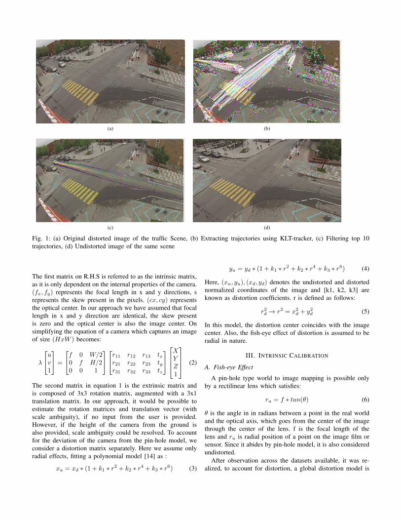
Fig. 1: (a) Original distorted image of the traffic Scene, (b) Extracting trajectories using KLT-tracker, (c) Filtering top 10trajectories, (d) Undistorted image of the same scene

The first matrix on R.H.S is referred to as the intrinsic matrix,as it is only dependent on the internal properties of the camera.(fx, fy) represents the focal length in x and y directions, srepresents the skew present in the pixels. (cx, cy) representsthe optical center. In our approach we have assumed that focallength in x and y direction are identical, the skew presentis zero and the optical center is also the image center. Onsimplifying the equation of a camera which captures an imageof size (HxW ) becomes:

λ

uv1

=

f 0 W/20 f H/20 0 1

r11 r12 r13 txr21 r22 r23 tyr31 r32 r33 tz

XYZ1

(2)

The second matrix in equation 1 is the extrinsic matrix andis composed of 3x3 rotation matrix, augmented with a 3x1translation matrix. In our approach, it would be possible toestimate the rotation matrices and translation vector (withscale ambiguity), if no input from the user is provided.However, if the height of the camera from the ground isalso provided, scale ambiguity could be resolved. To accountfor the deviation of the camera from the pin-hole model, weconsider a distortion matrix separately. Here we assume onlyradial effects, fitting a polynomial model [14] as :

xu = xd ∗ (1 + k1 ∗ r2 + k2 ∗ r4 + k3 ∗ r6) (3)

yu = yd ∗ (1 + k1 ∗ r2 + k2 ∗ r4 + k3 ∗ r6) (4)

Here, (xu, yu), (xd, yd) denotes the undistorted and distortednormalized coordinates of the image and [k1, k2, k3] areknown as distortion coefficients. r is defined as follows:

r2d −→ r2 = x2d + y2d (5)

In this model, the distortion center coincides with the imagecenter. Also, the fish-eye effect of distortion is assumed to beradial in nature.

III. INTRINSIC CALIBRATION

A. Fish-eye Effect

A pin-hole type world to image mapping is possible onlyby a rectilinear lens which satisfies:

ru = f ∗ tan(θ) (6)

θ is the angle in in radians between a point in the real worldand the optical axis, which goes from the center of the imagethrough the center of the lens. f is the focal length of thelens and ru is radial position of a point on the image film orsensor. Since it abides by pin-hole model, it is also consideredundistorted.

After observation across the datasets available, it was re-alized, to account for distortion, a global distortion model is

to be used. The most common and simple among which wasequidistant fish-eye. It is defined as follows :

rd = f ∗ θ (7)

rd is radial position of a point on the image film or sensor.Since it do not abides by pin-hole model, it is also considereddistorted. The equations (6) and (7) can be used for computingforward mapping i.e. from distorted cordinates to undisortedcordinates and inverse mapping i.e. from undistorted cordi-nates to distorted cordinates respectively as follows :

(xu, yu) −→ (xd ∗tan( rdf )

rdf

, yd ∗tan( rdf )

rdf

) (8)

(xd, yd) −→ (xu ∗atan( ruf )

rdf

, yd ∗atan( ruf )

rdf

) (9)

r2u = x2u + y2u (10)

Thus if we have enough correspondences between (xd, yd) and(xu, yu), it would be possible to estimate the focal length aswell as distortion coefficients using a least square approach.

B. Calibration

To make the calibration independent of the scene, onlymoving objects were used. It is done because it is not alwayspossible to have a similar geometric arrangement of staticstructures in every scene on which calibration is performed.However, moving objects could comprise of pedestrians andvehicles, either of which is very easily present in every trafficscene.

There is only one unknown in the intrinsic matrix and equa-tions 8 and 9, i.e. the focal length f. Thus if we can determinef, the intrinsic matrix, and distortion coefficients could becomputed. In general, on a road, it is assumed that vehiclesmove along a straight line. However, due to distortion(fish-eyeeffect), these straight lines become curved in the image. Therelation between the undistorted image and distorted imageis only dependent on the focal length. Thus, by adjusting thevalue of f to undistort the straight line, focal length can becomputed. The calibration process starts with extraction ofmoving object trajectories from video footage as shown inthe image. In a video it is assumed that, there are sufficientnumber of vehicles moving in orthogonal directions. To extractthe distorted straight lines, moving pedestrians or vehicles aretracked in a video footage for a few seconds initially. Trackingis achieved by optical flow with sift keypoints. Multiple tracksare extracted and filtered as follows:

• If the key point is not tracked for more than 80 % of thevideo interval, it is rejected.

• If the total distance in pixels of a keypoints is greater than1.2 times of its displacement, the keypoints is rejected.

Once the trajectories are filtered, top ten longest trajectoriesare selected. These trajectories are fitted with straight linesusing least square method. The sum of least square errors of allthe trajectories gives us the estimate of the straightness of thelines. Now the distorted points on trajectories are undistorted

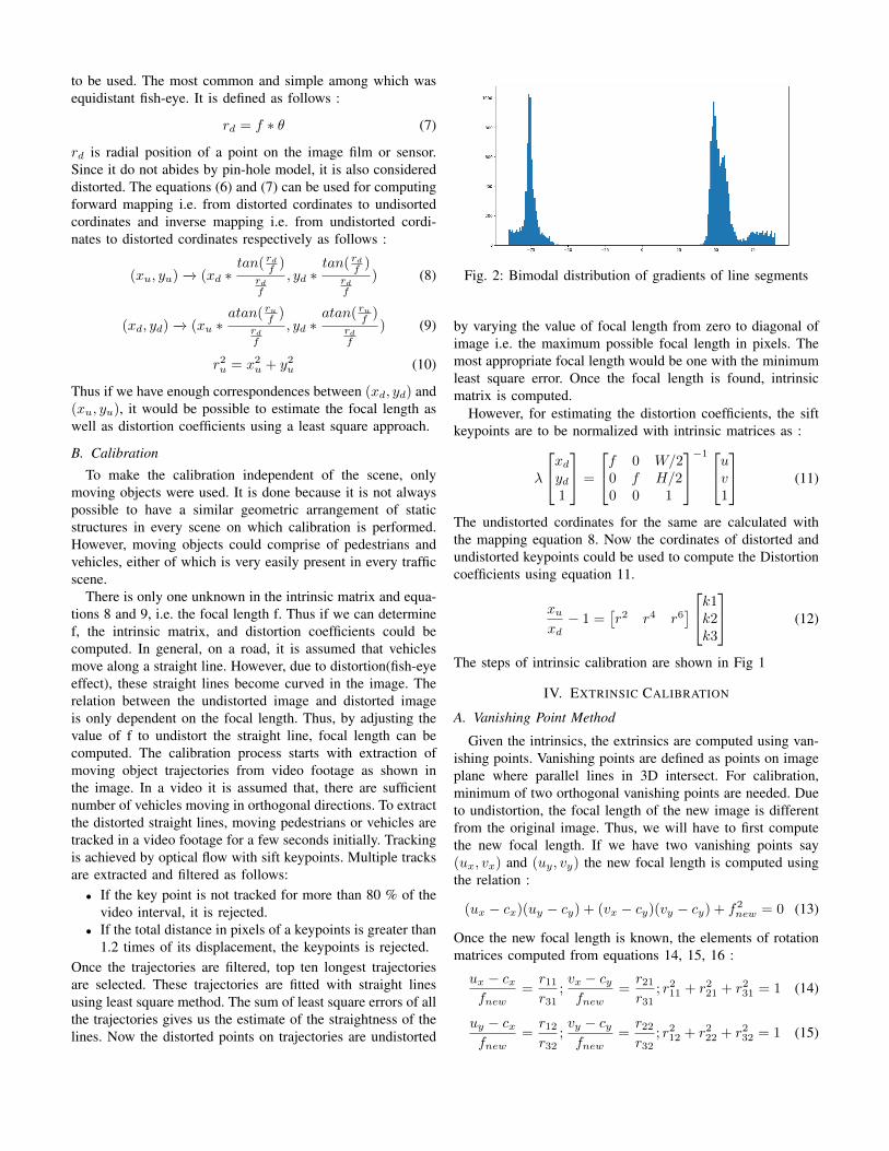
Fig. 2: Bimodal distribution of gradients of line segments

by varying the value of focal length from zero to diagonal ofimage i.e. the maximum possible focal length in pixels. Themost appropriate focal length would be one with the minimumleast square error. Once the focal length is found, intrinsicmatrix is computed.

However, for estimating the distortion coefficients, the siftkeypoints are to be normalized with intrinsic matrices as :

λ

xdyd1

=

f 0 W/20 f H/20 0 1

−1 uv1

(11)

The undistorted cordinates for the same are calculated withthe mapping equation 8. Now the cordinates of distorted andundistorted keypoints could be used to compute the Distortioncoefficients using equation 11.

xuxd− 1 =

[r2 r4 r6

] k1k2k3

(12)

The steps of intrinsic calibration are shown in Fig 1

IV. EXTRINSIC CALIBRATION

A. Vanishing Point Method

Given the intrinsics, the extrinsics are computed using van-ishing points. Vanishing points are defined as points on imageplane where parallel lines in 3D intersect. For calibration,minimum of two orthogonal vanishing points are needed. Dueto undistortion, the focal length of the new image is differentfrom the original image. Thus, we will have to first computethe new focal length. If we have two vanishing points say(ux, vx) and (uy, vy) the new focal length is computed usingthe relation :

(ux − cx)(uy − cy) + (vx − cy)(vy − cy) + f2new = 0 (13)

Once the new focal length is known, the elements of rotationmatrices computed from equations 14, 15, 16 :

ux − cxfnew

=r11r31

;vx − cyfnew

=r21r31

; r211 + r221 + r231 = 1 (14)

uy − cxfnew

=r12r32

;vy − cyfnew

=r22r32

; r212 + r222 + r232 = 1 (15)

(a) (b)

Fig. 3: (a) Vanishing Point in x-direction, (b) Vanishing Point in y-direction

r13r23r33

=

r11r21r31

×r12r22r32

(16)

Assuming the road surface to be planar and constitutes a Z= 0 plane, the equation 2 is transformed to :

λ

uv1

=

f 0 W/20 f H/20 0 1

r11 r12 txr21 r22 tyr31 r32 tz

XY1

(17)

If we assume the origin of World Cordinate System cor-responds with the center of image and height of the camerafrom ground is He then:

tx = 0; ty = 0; tz = −He/r33 (18)

B. Calibration

As mentioned above, extrinsic calibration is also done usingmoving objects only. The motion of pedestrians is highlyerratic thus, only the motion of vehicles is used for vanishingpoint estimation. Vehicles in most of the cases follow eachother along a straight line. If there are multiple key-points ona single vehicle, it can be seen to originate or converge to apoint in image plane, as vehicle moves closer to or fartheraway from the camera. If there are multiple vehicles movingalong two orthogonal directions, orthogonal vanishing pointscan easily be detected.

The algorithm mentioned below is computationally expen-sive, and requires significant movement of vehicles in pixels,thus it is performed in one out of every six frames. The firststep of calibration is to undistort the image with the help ofdistortion coefficients, as it is not easy to detect vanishingpoints from curves. It is followed by YOLO-v3 [15] baseddetection of vehicles. This generates the regions that consistsof vehicles with high probability. A mask of such regions iscomputed for every image on which processing is done. SIFT[16] key points are generated in the masked images and ismatched with the keypoints in the consecutive masked images.The positions of these matched keypoints for any two framesproduces multiple line segments. All the line-segments arestored for future processing.

Once, the whole short video-footage is processed, a list ofline segments are generated. Every line segment is convertedinto polar form i.e (orientation, magnitude, and distance fromorigin). A histogram of orientation is computed from all thesegments as shown in Fig 2. It is observed that it shows a bi-modal distribution. The bimodal distribution implies that thereare two major directions in which vehicles move. This bimodaldistribution helps in generating clusters of line segments ineach orthogonal direction. Most appropriate line segments areselectively picked using the distribution peaks with a thresholdof 5 degree in either direction.

The detection of vanishing point is achieved by voting basedsystem. For each cluster, every line segment is extended toa line. The size of accumulator is equal to one pixel and itsvalue is initially set to zero. Through whichever pixels any linepasses, is incremented by one. Thus the pixels with maximumvotes are considered most likely positions of vanishing points.The votes in the two directions are shown in the Fig 3.

However, the point with maximum votes is not necessarilythe vanishing point, and there can be more than one vanishingpoint because, we do not achieve a perfect undistortion. Ifmore than one vanishing point exists, it may imply that thepoint with maximum votes lie some where in between the twoor more vanishing points. In order, to account for this, we takethe top 20 % of the pixels with maximum votes and computethe mean and standard deviation. The estimates of vanishingpoints is made equal to the sum of mean and two or threetimes of standard deviation. The columns of rotation matricesdoes not vary much with the value of constant multiplied withstandard deviation.

Once the vanishing points are computed, the equations 13,14, 15, 16 and 18, could be used for extrinsic calibration. Toimprove the rotation matrix and enforce constraints on it, SVDis performed on the matrix. The new matrix is defined as:

R = USV T (19)

where S is an identity matrix. With the height of camera fromthe ground, translation vector is computed from equation 18.

Fig. 4: Top-view transformed Image

Datasets Proposed Checker Board1. 1064.20 1012.212. 619.66 584.953. 638.52 584.954. 937.41 1012.215. 933.43 1012.21

TABLE I: Comparison of focal length with the proposedmethod and checkerboard method

V. RESULTS

A. Accuracy of Estimated Focal Length

To estimate the accuracy of the computed focal length fromthe proposed algorithm, camera is calibrated from checker-board pattern. When using checkerboard pattern the focallength in x and y direction may not be same, to get the estimateits geometric mean is considered.

In the table I, Proposed column is one which uses theproposed algorithm for estimation of focal length and Checker-board column uses checkerboard calibration. The results from5 very different video-footages are used to account for gener-ality of results. The accuracy is around 6.35% of truth value(assumming checkerboard to be ground trruth).

B. Accuracy of Estimated Distortion Coefficients

To estimate the accuracy of distortion coefficients, meanleast square error in trajectories is computed with the predicteddistortion coefficients and checkerboard calibrated coefficients.The results are tabulated in Table II

In Table II, the second column represents the mean errorof distortion in trajectory in original image. The third columnrepresents the mean error of distortion in rectified image withproposed algorithm. the last column represents the mean errorin distortion in rectified image with checker-board calibrationcoefficients. It can be seen, in most cases proposed methodperforms better undistortion then the checkerboard calibrationscoefficients.

DatasetsMean LSEbefore calibrationfor a trajectory

Mean LSEafter calibrationfor a trajectory

Mean LSE aftercheckerboardcalibrationfor a trajectory

1. 0.572 0.103 0.1492. 0.923 0.251 0.4563. 0.528 0.069 0.1114. 0.166 0.004 0.0615. 0.052 0.006 0.007

TABLE II: Comparison of undistortion of trajectories beforeand after the Intrinsic Calibration with the proposed methodand Checkerboard Method

C. Accuracy of Rotation Matrices

It was not possible to assess the accuracy of rotation matri-ces because, the rotation data was not computed when camerawas originally set-up, only its video-footage was accessible.However, it is possible to visually estimate its accuracy. Itis done by converting the image of a scene to a top-viewplane transformed image as shown in Fig 4. In such images,the crosswalks will appear rectangular and not trapezium-like, man-holes will appear circular rather than ellipse, roadmarkings will appear parallel instead of intersecting. There areenough visual cues in such images to test the accuracy of thedata visually.

VI. CONCLUSION AND FUTURE SCOPE

The proposed algorithm can perform calibration automat-ically from a video-footage. The intrinsic calibration workswell also for the thermal cameras, since calibration procedureis dependent on only moving objects. However, there arecertain limitations associated with the proposed method :

• Tracking done using KLT tracker is not robust againstocclusion.

• Assumptions of vehicles move along a straight line maybe violated in certain scenarios.

• There should be sufficient number of vehicles moving ineither directions to estimate vanishing points robust tonoise.Once, the calibration is performed it could be usedin multiple applications concerning to photogrammetry,speed-monitoring, 3D-reconstruction, etc. This algorithmin future could also be made independent of the require-ment of perpendicular intersections.

REFERENCES

[1] O. Faugeras, Three dimensional computer vision: A geometric viewpoint.MIT Press, 1993.

[2] R. Hartley and A. Zisserman, Multiple View Geometry in ComputerVision, 2nd ed. New York, NY, USA: Cambridge University Press,2003.

[3] R. Tsai, “An efficient and accurate camera calibration technique for3d machine vision,” in Proceedings of IEEE Conference on ComputerVision and Pattern Recognition, 1986.

[4] Z.Zhang, “A flexible new technique for camera calibration,” in Proceed-ings of 7th International Conference on Computer Vision, 1999.

[5] B. Caprile and V. Torre, “Using vanishing points for camera calibration,”International Journal of Computer Vision, vol. 4, no. 2, pp. 127–139,Mar 1990. [Online]. Available: https://doi.org/10.1007/BF00127813

[6] J. Deutscher, M. Isard, and J. MacCormick, “Automatic camera cali-bration from a single manhattan image,” in Computer Vision — ECCV2002, A. Heyden, G. Sparr, M. Nielsen, and P. Johansen, Eds. Berlin,Heidelberg: Springer Berlin Heidelberg, 2002, pp. 175–188.

[7] A. C. D. Liebowitz and A. Zisserman, “Creating architecural modelsfrom images,” in Proceedings of EuroGraphics, 1999.

[8] Fengjun Lv, Tao Zhao, and R. Nevatia, “Camera calibration from videoof a walking human,” IEEE Transactions on Pattern Analysis andMachine Intelligence, vol. 28, no. 9, pp. 1513–1518, Sep. 2006.

[9] Zhaoxiang Zhang, Min Li, Kaigi Huang, and Tieniu Tan, “Practicalcamera auto-calibration based on object appearance and motion fortraffic scene visual surveillance,” in 2008 IEEE Conference on ComputerVision and Pattern Recognition, June 2008, pp. 1–8.

[10] K. Ismail, M. A Sc, T. Sayed, E. , P. , N. Saunier, and P. Assistant,“Camera calibration for urban traffic scenes: Practical issues and a robustapproach,” 01 2010.

[11] K. Ismail, T. Sayed, and N. Saunier, “A methodology for precise cameracalibration for data collection applications in urban traffic scenes,”Canadian Journal of Civil Engineering, vol. 40, no. 1, pp. 57–67,2013. [Online]. Available: https://doi.org/10.1139/cjce-2011-0456

[12] R. Bhardwaj, G. K. Tummala, G. Ramalingam, R. Ramjee,and P. Sinha, “Autocalib: Automatic traic camera calibration atscale,” in ACM BuildSys 2017. ACM, November 2017, [BestPaper Award Winner and Best Demo Award Winner]. [On-line]. Available: https://www.microsoft.com/en-us/research/publication/autocalib-automatic-tra%ef%ac%80ic-camera-calibration-scale/

[13] I. Junejo and H. Foroosh, “Robust auto-calibration from pedestrians,”in 2006 IEEE International Conference on Video and Signal BasedSurveillance, Nov 2006, pp. 92–92.

[14] J. I. Ronda and A. Valdes, “Geometrical analysis of polynomiallens distortion models,” Journal of Mathematical Imaging andVision, vol. 61, no. 3, pp. 252–268, Mar 2019. [Online]. Available:https://doi.org/10.1007/s10851-018-0833-x

[15] J. Redmon and A. Farhadi, “Yolov3: An incremental improvement,”CoRR, vol. abs/1804.02767, 2018. [Online]. Available: http://arxiv.org/abs/1804.02767

[16] D. G. Lowe, “Distinctive image features from scale-invariant keypoints,”Int. J. Comput. Vision, vol. 60, no. 2, pp. 91–110, Nov. 2004. [Online].Available: https://doi.org/10.1023/B:VISI.0000029664.99615.94