U and Th content in the Central Apennines continental crust: a contribution to the determination of...

Available online at www.sciencedirect.com

www.elsevier.com/locate/gca

Geochimica et Cosmochimica Acta 75 (2011) 2271–2294

U and Th content in the Central Apennines continental crust:A contribution to the determination of the geo-neutrinos

flux at LNGS

M. Coltorti a,⇑, R. Boraso a, F. Mantovani b,e, M. Morsilli a, G. Fiorentini b,e, A. Riva a,G. Rusciadelli c, R. Tassinari a, C. Tomei d, G. Di Carlo d, V. Chubakov b,e

a Dipartimento di Scienze della Terra, Universita di Ferrara, Italyb Dipartimento di Fisica, Universita di Ferrara, Italy

c Dipartimento di Scienze della Terra, Universita di Chieti, Italyd INFN, Laboratorio Nazionale Gran Sasso, Italy

e INFN, Sezione di Ferrara, Italy

Received 16 June 2010; accepted in revised form 18 January 2011; available online 23 January 2011

Abstract

The regional contribution to the geo-neutrino signal at Gran Sasso National Laboratory (LNGS) was determined based ona detailed geological, geochemical and geophysical study of the region. U and Th abundances of more than 50 samples rep-resentative of the main lithotypes belonging to the Mesozoic and Cenozoic sedimentary cover were analyzed. Sedimentaryrocks were grouped into four main “reservoirs” based on similar depositional settings and mineralogy. The initial assumptionthat similar chemico-physical depositional conditions would lead to comparable U and Th contents, was then confirmed bychemical analyses. Basement rocks do not outcrop in the area. Thus U and Th in the upper and lower crust of Valsugana andIvrea–Verbano areas were analyzed. Irrespective of magmatic or metamorphic origin lithotypes were subdivided into a maficand an acid reservoir, with comparable U and Th abundances.

Based on geological and geophysical properties, relative abundances of the various reservoirs were calculated and used to obtainthe weighted U and Th abundances for each of the three geological layers (sedimentary cover, upper and lower crust). Using theavailable seismic profile as well as the stratigraphic records from a number of exploration wells, a 3D modeling was developed overan area of 2� � 2� down to the Moho depth, for a total volume of about 1.2 � 106 km3. This model allowed us to determine thevolume of the various geological layers and eventually integrate the Th and U contents of the whole crust beneath LNGS.

On this base the local contribution to the geo-neutrino flux (S) was calculated and added to the contribution given by therest of the world, yielding a refined reference model prediction for the geo-neutrino signal in the Borexino detector at LNGS:S(U) = (28.7 ± 3.9) TNU and S(Th) = (7.5 ± 1.0) TNU. An excess over the total flux of about 4 TNU was previouslyobtained by Mantovani et al. (2004) who calculated, based on general worldwide assumptions, a signal of 40.5 TNU. Theconsiderable thickness of the sedimentary rocks, almost predominantly represented by U- and Th-poor carbonatic rocks inthe area near LNGS, is responsible for this difference. Thus the need for detailed integrated geological study is underlinedby this work, if the usefulness of the geo-neutrino flux for characterizing the global U and Th distribution within the Earth’scrust, mantle and core is to be realized.� 2011 Elsevier Ltd. All rights reserved.

0016-7037/$ - see front matter � 2011 Elsevier Ltd. All rights reserved.

doi:10.1016/j.gca.2011.01.024

⇑ Corresponding author. Address: Dipartimento di Scienze dellaTerra, Via Saragat 1, 44100 Ferrara, Italy. Tel.: +39 0532 974721;fax: +39 0532 974767.

E-mail address: [email protected] (M. Coltorti).

1. INTRODUCTION

Geo-neutrinos—the antineutrinos from the decay of U,Th and 40K in the Earth—can provide information on the

http://dx.doi.org/10.1016/j.gca.2011.01.024

mailto:[email protected]

http://dx.doi.org/016/j.gca.2011.01.024

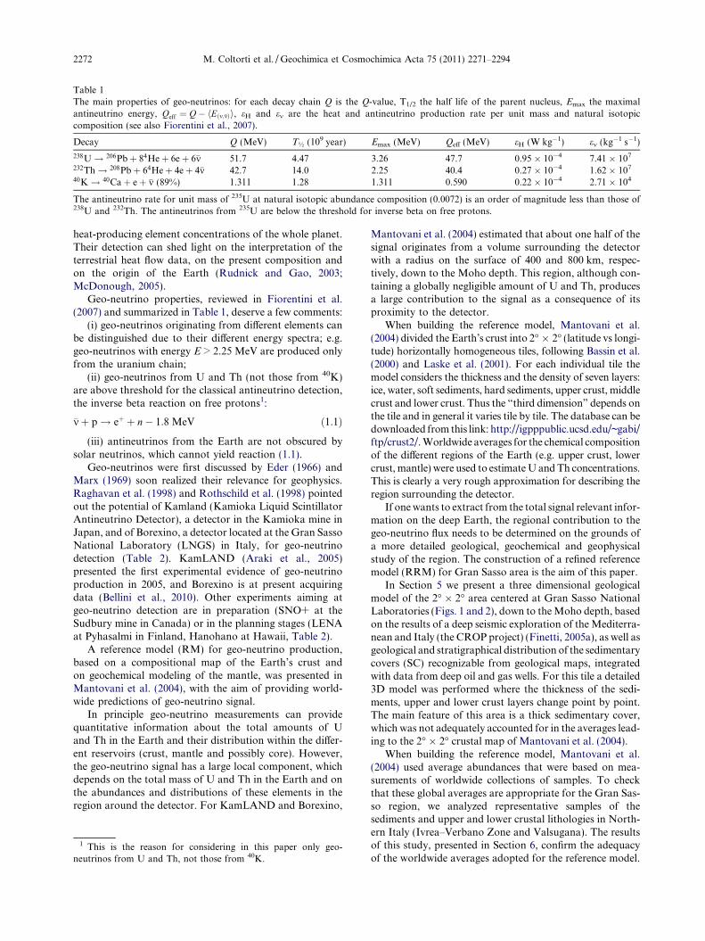
Table 1The main properties of geo-neutrinos: for each decay chain Q is the Q-value, T1/2 the half life of the parent nucleus, Emax the maximalantineutrino energy, Qeff ¼ Q� hEðm;�mÞi, eH and em are the heat and antineutrino production rate per unit mass and natural isotopiccomposition (see also Fiorentini et al., 2007).

Decay Q (MeV) T½ (109 year) Emax (MeV) Qeff (MeV) eH (W kg�1) em (kg�1 s�1)

238U! 206Pbþ 84Heþ 6eþ 6�m 51.7 4.47 3.26 47.7 0.95 � 10�4 7.41 � 107

232Th! 208Pbþ 64Heþ 4eþ 4�m 42.7 14.0 2.25 40.4 0.27 � 10�4 1.62 � 107

40K! 40Caþ eþ �m (89%) 1.311 1.28 1.311 0.590 0.22 � 10�4 2.71 � 104

The antineutrino rate for unit mass of 235U at natural isotopic abundance composition (0.0072) is an order of magnitude less than those of238U and 232Th. The antineutrinos from 235U are below the threshold for inverse beta on free protons.

2272 M. Coltorti et al. / Geochimica et Cosmochimica Acta 75 (2011) 2271–2294

heat-producing element concentrations of the whole planet.Their detection can shed light on the interpretation of theterrestrial heat flow data, on the present composition andon the origin of the Earth (Rudnick and Gao, 2003;McDonough, 2005).

Geo-neutrino properties, reviewed in Fiorentini et al.(2007) and summarized in Table 1, deserve a few comments:

(i) geo-neutrinos originating from different elements canbe distinguished due to their different energy spectra; e.g.geo-neutrinos with energy E > 2.25 MeV are produced onlyfrom the uranium chain;

(ii) geo-neutrinos from U and Th (not those from 40K)are above threshold for the classical antineutrino detection,the inverse beta reaction on free protons1:

�mþ p! eþ þ n� 1:8 MeV ð1:1Þ

(iii) antineutrinos from the Earth are not obscured bysolar neutrinos, which cannot yield reaction (1.1).

Geo-neutrinos were first discussed by Eder (1966) andMarx (1969) soon realized their relevance for geophysics.Raghavan et al. (1998) and Rothschild et al. (1998) pointedout the potential of Kamland (Kamioka Liquid ScintillatorAntineutrino Detector), a detector in the Kamioka mine inJapan, and of Borexino, a detector located at the Gran SassoNational Laboratory (LNGS) in Italy, for geo-neutrinodetection (Table 2). KamLAND (Araki et al., 2005)presented the first experimental evidence of geo-neutrinoproduction in 2005, and Borexino is at present acquiringdata (Bellini et al., 2010). Other experiments aiming atgeo-neutrino detection are in preparation (SNO+ at theSudbury mine in Canada) or in the planning stages (LENAat Pyhasalmi in Finland, Hanohano at Hawaii, Table 2).

A reference model (RM) for geo-neutrino production,based on a compositional map of the Earth’s crust andon geochemical modeling of the mantle, was presented inMantovani et al. (2004), with the aim of providing world-wide predictions of geo-neutrino signal.

In principle geo-neutrino measurements can providequantitative information about the total amounts of Uand Th in the Earth and their distribution within the differ-ent reservoirs (crust, mantle and possibly core). However,the geo-neutrino signal has a large local component, whichdepends on the total mass of U and Th in the Earth and onthe abundances and distributions of these elements in theregion around the detector. For KamLAND and Borexino,

1 This is the reason for considering in this paper only geo-neutrinos from U and Th, not those from 40K.

Mantovani et al. (2004) estimated that about one half of thesignal originates from a volume surrounding the detectorwith a radius on the surface of 400 and 800 km, respec-tively, down to the Moho depth. This region, although con-taining a globally negligible amount of U and Th, producesa large contribution to the signal as a consequence of itsproximity to the detector.

When building the reference model, Mantovani et al.(2004) divided the Earth’s crust into 2� � 2� (latitude vs longi-tude) horizontally homogeneous tiles, following Bassin et al.(2000) and Laske et al. (2001). For each individual tile themodel considers the thickness and the density of seven layers:ice, water, soft sediments, hard sediments, upper crust, middlecrust and lower crust. Thus the “third dimension” depends onthe tile and in general it varies tile by tile. The database can bedownloaded from this link: http://igpppublic.ucsd.edu/~gabi/ftp/crust2/. Worldwide averages for the chemical compositionof the different regions of the Earth (e.g. upper crust, lowercrust, mantle) were used to estimate U and Th concentrations.This is clearly a very rough approximation for describing theregion surrounding the detector.

If one wants to extract from the total signal relevant infor-mation on the deep Earth, the regional contribution to thegeo-neutrino flux needs to be determined on the grounds ofa more detailed geological, geochemical and geophysicalstudy of the region. The construction of a refined referencemodel (RRM) for Gran Sasso area is the aim of this paper.

In Section 5 we present a three dimensional geologicalmodel of the 2� � 2� area centered at Gran Sasso NationalLaboratories (Figs. 1 and 2), down to the Moho depth, basedon the results of a deep seismic exploration of the Mediterra-nean and Italy (the CROP project) (Finetti, 2005a), as well asgeological and stratigraphical distribution of the sedimentarycovers (SC) recognizable from geological maps, integratedwith data from deep oil and gas wells. For this tile a detailed3D model was performed where the thickness of the sedi-ments, upper and lower crust layers change point by point.The main feature of this area is a thick sedimentary cover,which was not adequately accounted for in the averages lead-ing to the 2� � 2� crustal map of Mantovani et al. (2004).

When building the reference model, Mantovani et al.(2004) used average abundances that were based on mea-surements of worldwide collections of samples. To checkthat these global averages are appropriate for the Gran Sas-so region, we analyzed representative samples of thesediments and upper and lower crustal lithologies in North-ern Italy (Ivrea–Verbano Zone and Valsugana). The resultsof this study, presented in Section 6, confirm the adequacyof the worldwide averages adopted for the reference model.

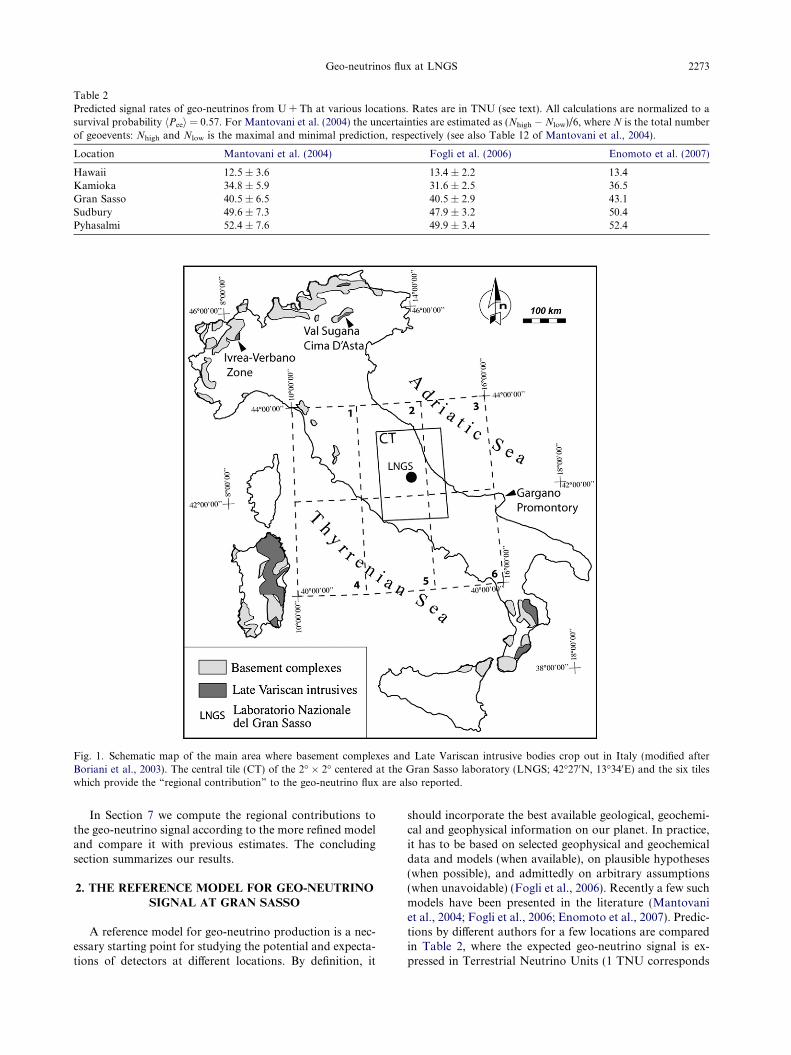
http://igpppublic.ucsd.edu/~gabi/ftp/crust2/

http://igpppublic.ucsd.edu/~gabi/ftp/crust2/

Table 2Predicted signal rates of geo-neutrinos from U + Th at various locations. Rates are in TNU (see text). All calculations are normalized to asurvival probability hPeei = 0.57. For Mantovani et al. (2004) the uncertainties are estimated as (Nhigh � Nlow)/6, where N is the total numberof geoevents: Nhigh and Nlow is the maximal and minimal prediction, respectively (see also Table 12 of Mantovani et al., 2004).

Location Mantovani et al. (2004) Fogli et al. (2006) Enomoto et al. (2007)

Hawaii 12.5 ± 3.6 13.4 ± 2.2 13.4Kamioka 34.8 ± 5.9 31.6 ± 2.5 36.5Gran Sasso 40.5 ± 6.5 40.5 ± 2.9 43.1Sudbury 49.6 ± 7.3 47.9 ± 3.2 50.4Pyhasalmi 52.4 ± 7.6 49.9 ± 3.4 52.4

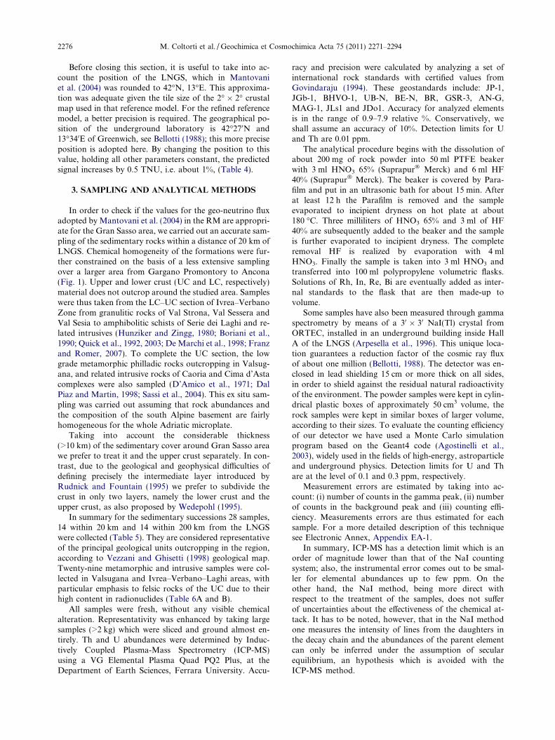
Fig. 1. Schematic map of the main area where basement complexes and Late Variscan intrusive bodies crop out in Italy (modified afterBoriani et al., 2003). The central tile (CT) of the 2� � 2� centered at the Gran Sasso laboratory (LNGS; 42�270N, 13�340E) and the six tileswhich provide the “regional contribution” to the geo-neutrino flux are also reported.

Geo-neutrinos flux at LNGS 2273

In Section 7 we compute the regional contributions tothe geo-neutrino signal according to the more refined modeland compare it with previous estimates. The concludingsection summarizes our results.

2. THE REFERENCE MODEL FOR GEO-NEUTRINO

SIGNAL AT GRAN SASSO

A reference model for geo-neutrino production is a nec-essary starting point for studying the potential and expecta-tions of detectors at different locations. By definition, it

should incorporate the best available geological, geochemi-cal and geophysical information on our planet. In practice,it has to be based on selected geophysical and geochemicaldata and models (when available), on plausible hypotheses(when possible), and admittedly on arbitrary assumptions(when unavoidable) (Fogli et al., 2006). Recently a few suchmodels have been presented in the literature (Mantovaniet al., 2004; Fogli et al., 2006; Enomoto et al., 2007). Predic-tions by different authors for a few locations are comparedin Table 2, where the expected geo-neutrino signal is ex-pressed in Terrestrial Neutrino Units (1 TNU corresponds

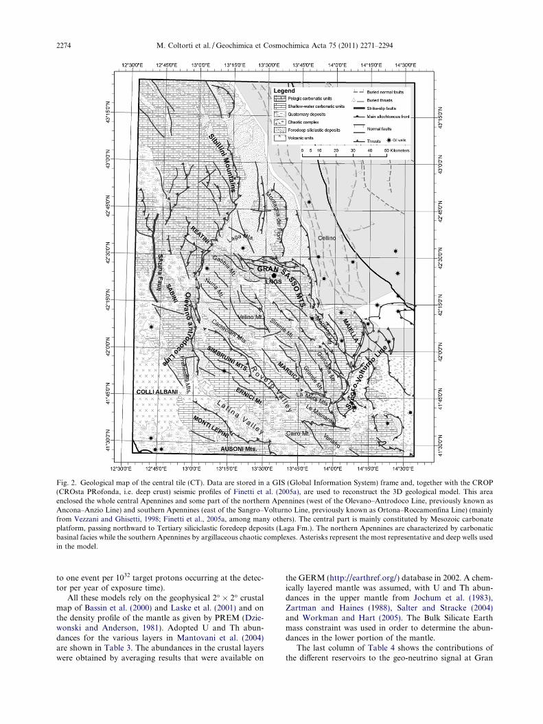
Fig. 2. Geological map of the central tile (CT). Data are stored in a GIS (Global Information System) frame and, together with the CROP(CROsta PRofonda, i.e. deep crust) seismic profiles of Finetti et al. (2005a), are used to reconstruct the 3D geological model. This areaenclosed the whole central Apennines and some part of the northern Apennines (west of the Olevano–Antrodoco Line, previously known asAncona–Anzio Line) and southern Apennines (east of the Sangro–Volturno Line, previously known as Ortona–Roccamonfina Line) (mainlyfrom Vezzani and Ghisetti, 1998; Finetti et al., 2005a, among many others). The central part is mainly constituted by Mesozoic carbonateplatform, passing northward to Tertiary siliciclastic foredeep deposits (Laga Fm.). The northern Apennines are characterized by carbonaticbasinal facies while the southern Apennines by argillaceous chaotic complexes. Asterisks represent the most representative and deep wells usedin the model.


to one event per 1032 target protons occurring at the detec-tor per year of exposure time).

All these models rely on the geophysical 2� � 2� crustalmap of Bassin et al. (2000) and Laske et al. (2001) and onthe density profile of the mantle as given by PREM (Dzie-wonski and Anderson, 1981). Adopted U and Th abun-dances for the various layers in Mantovani et al. (2004)are shown in Table 3. The abundances in the crustal layerswere obtained by averaging results that were available on

the GERM (http://earthref.org/) database in 2002. A chem-ically layered mantle was assumed, with U and Th abun-dances in the upper mantle from Jochum et al. (1983),Zartman and Haines (1988), Salter and Stracke (2004)and Workman and Hart (2005). The Bulk Silicate Earthmass constraint was used in order to determine the abun-dances in the lower portion of the mantle.

The last column of Table 4 shows the contributions ofthe different reservoirs to the geo-neutrino signal at Gran

http://earthref.org/

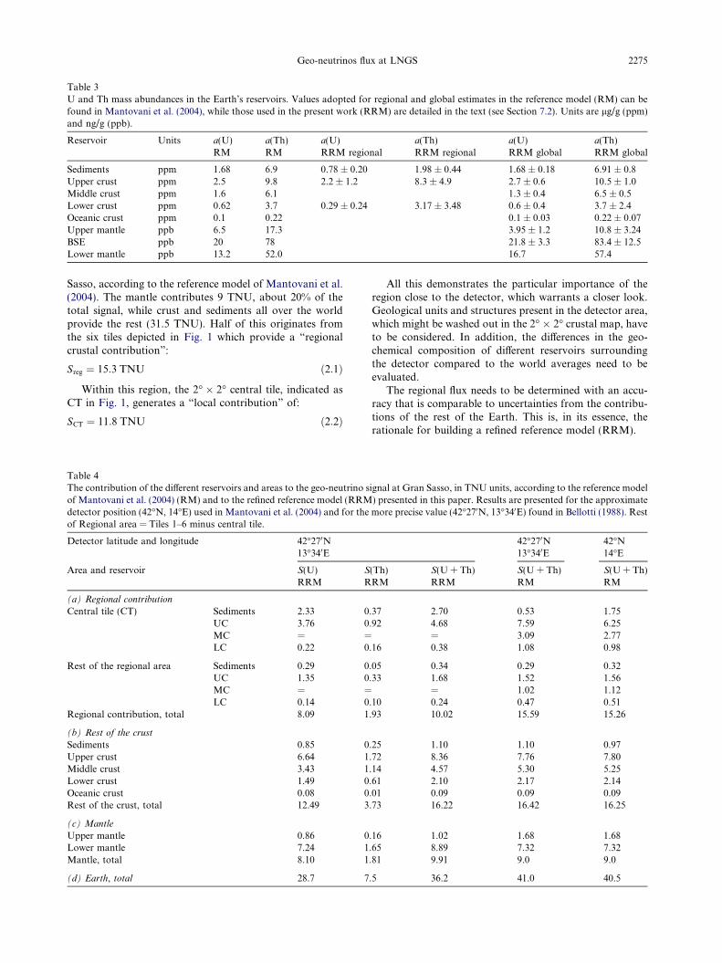
Table 3U and Th mass abundances in the Earth’s reservoirs. Values adopted for regional and global estimates in the reference model (RM) can befound in Mantovani et al. (2004), while those used in the present work (RRM) are detailed in the text (see Section 7.2). Units are lg/g (ppm)and ng/g (ppb).

Reservoir Units a(U)RM

a(Th)RM

a(U)RRM regional

a(Th)RRM regional

a(U)RRM global

a(Th)RRM global

Sediments ppm 1.68 6.9 0.78 ± 0.20 1.98 ± 0.44 1.68 ± 0.18 6.91 ± 0.8Upper crust ppm 2.5 9.8 2.2 ± 1.2 8.3 ± 4.9 2.7 ± 0.6 10.5 ± 1.0Middle crust ppm 1.6 6.1 1.3 ± 0.4 6.5 ± 0.5Lower crust ppm 0.62 3.7 0.29 ± 0.24 3.17 ± 3.48 0.6 ± 0.4 3.7 ± 2.4Oceanic crust ppm 0.1 0.22 0.1 ± 0.03 0.22 ± 0.07Upper mantle ppb 6.5 17.3 3.95 ± 1.2 10.8 ± 3.24BSE ppb 20 78 21.8 ± 3.3 83.4 ± 12.5Lower mantle ppb 13.2 52.0 16.7 57.4


Sasso, according to the reference model of Mantovani et al.(2004). The mantle contributes 9 TNU, about 20% of thetotal signal, while crust and sediments all over the worldprovide the rest (31.5 TNU). Half of this originates fromthe six tiles depicted in Fig. 1 which provide a “regionalcrustal contribution”:

Sreg ¼ 15:3 TNU ð2:1Þ

Within this region, the 2� � 2� central tile, indicated asCT in Fig. 1, generates a “local contribution” of:

SCT ¼ 11:8 TNU ð2:2Þ

Table 4The contribution of the different reservoirs and areas to the geo-neutrino sof Mantovani et al. (2004) (RM) and to the refined reference model (RRMdetector position (42�N, 14�E) used in Mantovani et al. (2004) and for theof Regional area = Tiles 1–6 minus central tile.

Detector latitude and longitude 42�270N13�340E

Area and reservoir S(U)RRM

S

R

(a) Regional contribution

Central tile (CT) Sediments 2.33 0UC 3.76 0MC = =LC 0.22 0

Rest of the regional area Sediments 0.29 0UC 1.35 0MC = =LC 0.14 0

Regional contribution, total 8.09 1

(b) Rest of the crust

Sediments 0.85 0Upper crust 6.64 1Middle crust 3.43 1Lower crust 1.49 0Oceanic crust 0.08 0Rest of the crust, total 12.49 3

(c) Mantle

Upper mantle 0.86 0Lower mantle 7.24 1Mantle, total 8.10 1

(d) Earth, total 28.7 7

All this demonstrates the particular importance of theregion close to the detector, which warrants a closer look.Geological units and structures present in the detector area,which might be washed out in the 2� � 2� crustal map, haveto be considered. In addition, the differences in the geo-chemical composition of different reservoirs surroundingthe detector compared to the world averages need to beevaluated.

The regional flux needs to be determined with an accu-racy that is comparable to uncertainties from the contribu-tions of the rest of the Earth. This is, in its essence, therationale for building a refined reference model (RRM).

ignal at Gran Sasso, in TNU units, according to the reference model) presented in this paper. Results are presented for the approximatemore precise value (42�270N, 13�340E) found in Bellotti (1988). Rest

42�270N13�340E

42�N14�E

(Th)RM

S(U + Th)RRM

S(U + Th)RM

S(U + Th)RM

.37 2.70 0.53 1.75

.92 4.68 7.59 6.25= 3.09 2.77

.16 0.38 1.08 0.98

.05 0.34 0.29 0.32

.33 1.68 1.52 1.56= 1.02 1.12

.10 0.24 0.47 0.51

.93 10.02 15.59 15.26

.25 1.10 1.10 0.97

.72 8.36 7.76 7.80

.14 4.57 5.30 5.25

.61 2.10 2.17 2.14

.01 0.09 0.09 0.09

.73 16.22 16.42 16.25

.16 1.02 1.68 1.68

.65 8.89 7.32 7.32

.81 9.91 9.0 9.0

.5 36.2 41.0 40.5


Before closing this section, it is useful to take into ac-count the position of the LNGS, which in Mantovaniet al. (2004) was rounded to 42�N, 13�E. This approxima-tion was adequate given the tile size of the 2� � 2� crustalmap used in that reference model. For the refined referencemodel, a better precision is required. The geographical po-sition of the underground laboratory is 42�270N and13�340E of Greenwich, see Bellotti (1988); this more preciseposition is adopted here. By changing the position to thisvalue, holding all other parameters constant, the predictedsignal increases by 0.5 TNU, i.e. about 1%, (Table 4).

3. SAMPLING AND ANALYTICAL METHODS

In order to check if the values for the geo-neutrino fluxadopted by Mantovani et al. (2004) in the RM are appropri-ate for the Gran Sasso area, we carried out an accurate sam-pling of the sedimentary rocks within a distance of 20 km ofLNGS. Chemical homogeneity of the formations were fur-ther constrained on the basis of a less extensive samplingover a larger area from Gargano Promontory to Ancona(Fig. 1). Upper and lower crust (UC and LC, respectively)material does not outcrop around the studied area. Sampleswere thus taken from the LC–UC section of Ivrea–VerbanoZone from granulitic rocks of Val Strona, Val Sessera andVal Sesia to amphibolitic schists of Serie dei Laghi and re-lated intrusives (Hunziker and Zingg, 1980; Boriani et al.,1990; Quick et al., 1992, 2003; De Marchi et al., 1998; Franzand Romer, 2007). To complete the UC section, the lowgrade metamorphic philladic rocks outcropping in Valsug-ana, and related intrusive rocks of Caoria and Cima d’Astacomplexes were also sampled (D’Amico et al., 1971; DalPiaz and Martin, 1998; Sassi et al., 2004). This ex situ sam-pling was carried out assuming that rock abundances andthe composition of the south Alpine basement are fairlyhomogeneous for the whole Adriatic microplate.

Taking into account the considerable thickness(>10 km) of the sedimentary cover around Gran Sasso areawe prefer to treat it and the upper crust separately. In con-trast, due to the geological and geophysical difficulties ofdefining precisely the intermediate layer introduced byRudnick and Fountain (1995) we prefer to subdivide thecrust in only two layers, namely the lower crust and theupper crust, as also proposed by Wedepohl (1995).

In summary for the sedimentary successions 28 samples,14 within 20 km and 14 within 200 km from the LNGSwere collected (Table 5). They are considered representativeof the principal geological units outcropping in the region,according to Vezzani and Ghisetti (1998) geological map.Twenty-nine metamorphic and intrusive samples were col-lected in Valsugana and Ivrea–Verbano–Laghi areas, withparticular emphasis to felsic rocks of the UC due to theirhigh content in radionuclides (Table 6A and B).

All samples were fresh, without any visible chemicalalteration. Representativity was enhanced by taking largesamples (>2 kg) which were sliced and ground almost en-tirely. Th and U abundances were determined by Induc-tively Coupled Plasma-Mass Spectrometry (ICP-MS)using a VG Elemental Plasma Quad PQ2 Plus, at theDepartment of Earth Sciences, Ferrara University. Accu-

racy and precision were calculated by analyzing a set ofinternational rock standards with certified values fromGovindaraju (1994). These geostandards include: JP-1,JGb-1, BHVO-1, UB-N, BE-N, BR, GSR-3, AN-G,MAG-1, JLs1 and JDo1. Accuracy for analyzed elementsis in the range of 0.9–7.9 relative %. Conservatively, weshall assume an accuracy of 10%. Detection limits for Uand Th are 0.01 ppm.

The analytical procedure begins with the dissolution ofabout 200 mg of rock powder into 50 ml PTFE beakerwith 3 ml HNO3 65% (Suprapur� Merck) and 6 ml HF40% (Suprapur� Merck). The beaker is covered by Para-film and put in an ultrasonic bath for about 15 min. Afterat least 12 h the Parafilm is removed and the sampleevaporated to incipient dryness on hot plate at about180 �C. Three milliliters of HNO3 65% and 3 ml of HF40% are subsequently added to the beaker and the sampleis further evaporated to incipient dryness. The completeremoval HF is realized by evaporation with 4 mlHNO3. Finally the sample is taken into 3 ml HNO3 andtransferred into 100 ml polypropylene volumetric flasks.Solutions of Rh, In, Re, Bi are eventually added as inter-nal standards to the flask that are then made-up tovolume.

Some samples have also been measured through gammaspectrometry by means of a 30 � 30 NaI(Tl) crystal fromORTEC, installed in an underground building inside HallA of the LNGS (Arpesella et al., 1996). This unique loca-tion guarantees a reduction factor of the cosmic ray fluxof about one million (Bellotti, 1988). The detector was en-closed in lead shielding 15 cm or more thick on all sides,in order to shield against the residual natural radioactivityof the environment. The powder samples were kept in cylin-drical plastic boxes of approximately 50 cm3 volume, therock samples were kept in similar boxes of larger volume,according to their sizes. To evaluate the counting efficiencyof our detector we have used a Monte Carlo simulationprogram based on the Geant4 code (Agostinelli et al.,2003), widely used in the fields of high-energy, astroparticleand underground physics. Detection limits for U and Thare at the level of 0.1 and 0.3 ppm, respectively.

Measurement errors are estimated by taking into ac-count: (i) number of counts in the gamma peak, (ii) numberof counts in the background peak and (iii) counting effi-ciency. Measurements errors are thus estimated for eachsample. For a more detailed description of this techniquesee Electronic Annex, Appendix EA-1.

In summary, ICP-MS has a detection limit which is anorder of magnitude lower than that of the NaI countingsystem; also, the instrumental error comes out to be smal-ler for elemental abundances up to few ppm. On theother hand, the NaI method, being more direct withrespect to the treatment of the samples, does not sufferof uncertainties about the effectiveness of the chemical at-tack. It has to be noted, however, that in the NaI methodone measures the intensity of lines from the daughters inthe decay chain and the abundances of the parent elementcan only be inferred under the assumption of secularequilibrium, an hypothesis which is avoided with theICP-MS method.

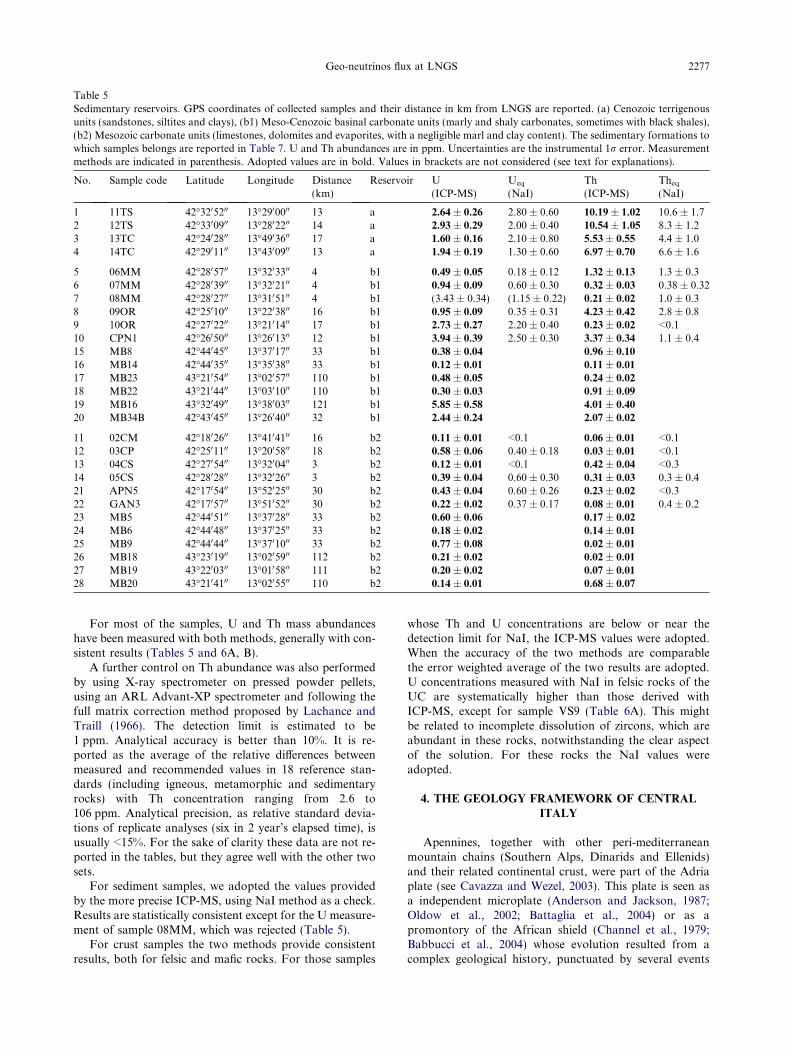
Table 5Sedimentary reservoirs. GPS coordinates of collected samples and their distance in km from LNGS are reported. (a) Cenozoic terrigenousunits (sandstones, siltites and clays), (b1) Meso-Cenozoic basinal carbonate units (marly and shaly carbonates, sometimes with black shales),(b2) Mesozoic carbonate units (limestones, dolomites and evaporites, with a negligible marl and clay content). The sedimentary formations towhich samples belongs are reported in Table 7. U and Th abundances are in ppm. Uncertainties are the instrumental 1r error. Measurementmethods are indicated in parenthesis. Adopted values are in bold. Values in brackets are not considered (see text for explanations).

No. Sample code Latitude Longitude Distance Reservoir U Ueq Th Theq

(km) (ICP-MS) (NaI) (ICP-MS) (NaI)

1 11TS 42�3205200 13�2900000 13 a 2.64 ± 0.26 2.80 ± 0.60 10.19 ± 1.02 10.6 ± 1.72 12TS 42�3300900 13�2802200 14 a 2.93 ± 0.29 2.00 ± 0.40 10.54 ± 1.05 8.3 ± 1.23 13TC 42�2402800 13�4903600 17 a 1.60 ± 0.16 2.10 ± 0.80 5.53 ± 0.55 4.4 ± 1.04 14TC 42�2901100 13�4300900 13 a 1.94 ± 0.19 1.30 ± 0.60 6.97 ± 0.70 6.6 ± 1.6

5 06MM 42�2805700 13�3203300 4 b1 0.49 ± 0.05 0.18 ± 0.12 1.32 ± 0.13 1.3 ± 0.36 07MM 42�2803900 13�3202100 4 b1 0.94 ± 0.09 0.60 ± 0.30 0.32 ± 0.03 0.38 ± 0.327 08MM 42�2802700 13�3105100 4 b1 (3.43 ± 0.34) (1.15 ± 0.22) 0.21 ± 0.02 1.0 ± 0.38 09OR 42�2501000 13�2203800 16 b1 0.95 ± 0.09 0.35 ± 0.31 4.23 ± 0.42 2.8 ± 0.89 10OR 42�2702200 13�2101400 17 b1 2.73 ± 0.27 2.20 ± 0.40 0.23 ± 0.02 <0.110 CPN1 42�2605000 13�2601300 12 b1 3.94 ± 0.39 2.50 ± 0.30 3.37 ± 0.34 1.1 ± 0.415 MB8 42�4404500 13�3701700 33 b1 0.38 ± 0.04 0.96 ± 0.10

16 MB14 42�4403500 13�3503800 33 b1 0.12 ± 0.01 0.11 ± 0.01

17 MB23 43�2105400 13�0205700 110 b1 0.48 ± 0.05 0.24 ± 0.02

18 MB22 43�2104400 13�0301000 110 b1 0.30 ± 0.03 0.91 ± 0.09

19 MB16 43�3204900 13�3800300 121 b1 5.85 ± 0.58 4.01 ± 0.40

20 MB34B 42�4304500 13�2604000 32 b1 2.44 ± 0.24 2.07 ± 0.02

11 02CM 42�1802600 13�4104100 16 b2 0.11 ± 0.01 <0.1 0.06 ± 0.01 <0.112 03CP 42�2501100 13�2005800 18 b2 0.58 ± 0.06 0.40 ± 0.18 0.03 ± 0.01 <0.113 04CS 42�2705400 13�3200400 3 b2 0.12 ± 0.01 <0.1 0.42 ± 0.04 <0.314 05CS 42�2802800 13�3202600 3 b2 0.39 ± 0.04 0.60 ± 0.30 0.31 ± 0.03 0.3 ± 0.421 APN5 42�1705400 13�5202500 30 b2 0.43 ± 0.04 0.60 ± 0.26 0.23 ± 0.02 <0.322 GAN3 42�1705700 13�5105200 30 b2 0.22 ± 0.02 0.37 ± 0.17 0.08 ± 0.01 0.4 ± 0.223 MB5 42�4405100 13�3702800 33 b2 0.60 ± 0.06 0.17 ± 0.02

24 MB6 42�4404800 13�3702500 33 b2 0.18 ± 0.02 0.14 ± 0.01

25 MB9 42�4404400 13�3701000 33 b2 0.77 ± 0.08 0.02 ± 0.01

26 MB18 43�2301900 13�0205900 112 b2 0.21 ± 0.02 0.02 ± 0.01

27 MB19 43�2200300 13�0105800 111 b2 0.20 ± 0.02 0.07 ± 0.01

28 MB20 43�2104100 13�0205500 110 b2 0.14 ± 0.01 0.68 ± 0.07


For most of the samples, U and Th mass abundanceshave been measured with both methods, generally with con-sistent results (Tables 5 and 6A, B).

A further control on Th abundance was also performedby using X-ray spectrometer on pressed powder pellets,using an ARL Advant-XP spectrometer and following thefull matrix correction method proposed by Lachance andTraill (1966). The detection limit is estimated to be1 ppm. Analytical accuracy is better than 10%. It is re-ported as the average of the relative differences betweenmeasured and recommended values in 18 reference stan-dards (including igneous, metamorphic and sedimentaryrocks) with Th concentration ranging from 2.6 to106 ppm. Analytical precision, as relative standard devia-tions of replicate analyses (six in 2 year’s elapsed time), isusually <15%. For the sake of clarity these data are not re-ported in the tables, but they agree well with the other twosets.

For sediment samples, we adopted the values providedby the more precise ICP-MS, using NaI method as a check.Results are statistically consistent except for the U measure-ment of sample 08MM, which was rejected (Table 5).

For crust samples the two methods provide consistentresults, both for felsic and mafic rocks. For those samples

whose Th and U concentrations are below or near thedetection limit for NaI, the ICP-MS values were adopted.When the accuracy of the two methods are comparablethe error weighted average of the two results are adopted.U concentrations measured with NaI in felsic rocks of theUC are systematically higher than those derived withICP-MS, except for sample VS9 (Table 6A). This mightbe related to incomplete dissolution of zircons, which areabundant in these rocks, notwithstanding the clear aspectof the solution. For these rocks the NaI values wereadopted.

4. THE GEOLOGY FRAMEWORK OF CENTRAL

ITALY

Apennines, together with other peri-mediterraneanmountain chains (Southern Alps, Dinarids and Ellenids)and their related continental crust, were part of the Adriaplate (see Cavazza and Wezel, 2003). This plate is seen asa independent microplate (Anderson and Jackson, 1987;Oldow et al., 2002; Battaglia et al., 2004) or as apromontory of the African shield (Channel et al., 1979;Babbucci et al., 2004) whose evolution resulted from acomplex geological history, punctuated by several events

Table 6UC samples are taken from Val Strona, Serie dei Laghi (label VS), Valsugana and Cima d’Asta-Caoria (numbered samples and label CA). LC samples are taken from Ivrea–Verbano Zone (ValStrona, Val Sessera and Val Sesia). U and Th abundances are in ppm. Uncertainties are the instrumental 1r error. Measurement methods are indicated in parenthesis. Adopted values are in bold.Values in brackets are not considered (see text for explanations).

No. Sample code Composition Lithology U U U Th Th Th(ICP-MS) (NaI) (adopted) (ICP-MS) (NaI) (adopted)

(A) Upper crust reservoirs

1 VS11 Mafic Anfibolite 0.59 ± 0.06 0.4 ± 0.3 0.59 ± 0.06 0.43 ± 0.04 <0.3 0.43 ± 0.04

2 VS15 Mafic Anfibolite 0.13 ± 0.01 <0.10 0.13 ± 0.01 0.08 ± 0.01 <0.3 0.08 ± 0.01

3 VS7 Felsic Migmatitic kinzigite 1.92 ± 0.19 / 1.92 ± 0.2 11.7 ± 1.17 / 11.7 ± 1.2

4 VS9 Felsic Kinzigite 3.62 ± 0.36 3.1 ± 0.4 3.1 ± 0.4 18.0 ± 1.80 13.7 ± 1.20 15.0 ± 1.0



7 VS19 Felsic Aplite 1.68 ± 0.17 2.4 ± 0.5 2.4 ± 0.5 15.3 ± 1.53 13.5 ± 1.20 14.2 ± 0.9

8 VS20 Felsic Granit 3.05 ± 0.30 5.9 ± 0.7 5.9 ± 0.7 14.4 ± 1.44 15.6 ± 1.60 14.9 ± 1.1

9 VS21 Felsic Granit 3.24 ± 0.32 3.5 ± 0.6 3.5 ± 0.6 12.8 ± 1.28 13.8 ± 1.30 13.3 ± 0.9

10 VS22 Felsic Schist 1.82 ± 0.18 2.2 ± 0.5 2.2 ± 0.5 10.8 ± 1.08 10.0 ± 1.20 10.4 ± 0.8

11 VS23 Felsic Micascisto 2.03 ± 0.20 2.8 ± 0.6 2.8 ± 0.6 11.9 ± 1.19 9.4 ± 1.10 10.6 ± 0.8

12 14 Felsic Diorite 1.44 ± 0.14 1.7 ± 0.3 1.7 ± 0.3 9.35 ± 0.94 7.6 ± 0.80 8.3 ± 0.6

13 16 Felsic Monzogranite 2.05 ± 0.21 3.1 ± 0.5 3.1 ± 0.5 9.77 ± 0.98 9.1 ± 0.98 9.4 ± 0.7

14 26 Felsic Phyllades-schists 1.30 ± 0.13 2.4 ± 0.4 2.4 ± 0.4 5.01 ± 0.50 5.4 ± 0.70 5.1 ± 0.4

15 27 Felsic Phyllades-schists 1.78 ± 0.18 2.2 ± 0.5 2.2 ± 0.5 11.6 ± 1.16 11.0 ± 1.25 11.3 ± 0.9

16 CA58 Felsic Phyllades-schists 2.34 ± 0.23 2.6 ± 0.5 2.6 ± 0.5 12.5 ± 1.25 12.6 ± 1.20 12.6 ± 0.9

17 CA63 Felsic Phyllades-schists 1.77 ± 0.18 3.3 ± 0.6 3.3 ± 0.6 9.65 ± 0.97 12.8 ± 1.40 10.7 ± 0.8

18 CA65 Felsic Phyllades-schists 1.61 ± 0.16 3.2 ± 0.5 3.2 ± 0.5 7.19 ± 0.72 14.4 ± 1.30 (8.88 ± 0.63)19 CA69 Felsic Phyllades-schists 1.45 ± 0.15 2.2 ± 0.4 2.2 ± 0.4 12.3 ± 1.23 16.2 ± 1.40 14.0 ± 0.9

20 CA74 Felsic Tonalite 1.57 ± 0.16 2.4 ± 0.5 2.4 ± 0.5 6.71 ± 0.67 5.4 ± 0.70 6.1 ± 0.5

(B) Lower crust reservoirs

1 VS1 Mafic Amph-gabbro 0.02 ± 0.01 / 0.02 ± 0.01 <0.01 / 0.005 ± 0.005

2 VS6 Mafic Diorite 0.35 ± 0.03 1.04 ± 0.23 0.35 ± 0.03 0.84 ± 0.08 0.9 ± 0.33 0.84 ± 0.08

3 VS8 Mafic Gabbro 0.05 ± 0.01 <0.1 0.05 ± 0.01 0.03 ± 0.01 <0.3 0.03 ± 0.01

4 VS13 Mafic Granulite <0.01 <0.1 0.01 ± 0.01 0.09 ± 0.01 <0.3 0.09 ± 0.01

5 VS2 Felsic Stronalite 0.42 ± 0.04 0.9 ± 0.35 0.42 ± 0.04 5.46 ± 0.55 12.9 ± 1.3 (6.59 ± 0.51)6 VS3 Felsic Charnockite 0.01 ± 0.01 <0.1 0.01 ± 0.01 0.01 ± 0.01 <0.3 0.01 ± 0.01

7 VS5 Felsic Stronalite 0.10 ± 0.01 / 0.10 ± 0.01 0.17 ± 0.02 <0.3 0.17 ± 0.02

8 VS12 Felsic Stronalite 1.14 ± 0.11 1.3 ± 0.4 1.14 ± 0.11 11.50 ± 1.15 12.6 ± 1.30 12.0 ± 0.9

9 VS14 Felsic Stronalite 0.70 ± 0.07 0.7 ± 0.3 0.70 ± 0.07 15.40 ± 1.54 10.7 ± 1.10 12.3 ± 0.9

/, not measured.

2278M

.C

olto

rtiet

al./G

eoch

imica

etC

osm

och

imica

Acta

75(2011)

2271–2294


related to the evolution from divergent to collisionalcontinental margins occurred in the Mediterranean re-gion, starting from the early Mesozoic (Dewey et al.,1973; Jolivet and Faccenna, 2000; Wortel and Spakman,2000; Carminati et al., 2005; Lucente et al., 2006; Panzaet al., 2007; Mantovani et al., 2009; Viti et al., 2009).With time geodynamical processes have produced thegeological structure of the Central Apennines where theLNGS is located (Fig. 2) (Ghisetti and Vezzani, 1999;Bigi and Costa Pisani, 2005; Finetti et al., 2005a;Scisciani and Calamita, 2009).

The Apennines developed through the deformation oftwo major paleogeographic domains: the Liguria–PiedmontOcean and the Adria–Apulia passive margin (Bernoulli,2001; Elter et al., 2003; Bosellini, 2004; Parotto and Pratur-lon, 2004) which were progressively subducted below theEuropean plate or incorporated into the chain during thegeodynamic events lasting from Late Cretaceous to Plio-Pleistocene (Scisciani and Calamita, 2009 and referencestherein). Actually, the northern and central Apennines arean arc shaped fold-and-thrust belt, with north-eastwardconvexity and vergence that plunges north-westward(Barchi et al., 2001).

We have modeled an area of 2� � 2� of latitude and lon-gitude, centered on the LNGS (Fig. 2). This area includesthe following main geological domains of central Italy:

(1) The northern Apennines, bounded southward by theOlevano–Antrodoco Line.

(2) The central Apennines, bounded southward by theSangro–Volturno Line.

(3) The external Apennine foredeep developed at thefront of the two main structural arcs.

(4) The peri-Adriatic foreland, developing externally tothe main thrusts fronts and in the Adriatic offshore.

Gran Sasso Range (GSR), where the LNGS is located,represents the northernmost front of the Abruzzi Apen-nines (Scisciani et al., 2002; Sani et al., 2004; Scroccaet al., 2005; Billi and Tiberti, 2009). Structural elementsare represented by a complex system of overturnedanticlines and related thrusts (Vezzani and Ghisetti, 1998;Ghisetti and Vezzani, 1999; Speranza et al., 2003; Calamitaet al., 2006). The result of these movements is a juxtaposi-tion of the northern margin of the Lazio–Abruzzi carbon-ate platform and its related pelagic Umbria–MarcheBasin onto the external Apenninic foredeep (Bernoulli,2001; Bosellini, 2004; Parotto and Praturlon, 2004; Finettiet al., 2005a).

Based on the geodynamic and structural evolution ofthis area, the sedimentary pile of the GSR has been subdi-vided into three main sequences. The first two sequences arerelated to the syn- and post-rift evolution of the Adriapaleomargin, and range from Late Triassic to Late Paleo-gene (Bernoulli, 2001; Bosellini, 2004; Parotto and Pratur-lon, 2004; Finetti et al., 2005a). The third sequence relatesto the progressive deformation of the Adria paleomargin,connected with the building process of the Apenninic chain(foreland to thrust-top basins) during the Late Paleogene toPleistocene (Mostardini and Merlini, 1986; Argnani and

Frugoni, 1997; Cipollari et al., 1999; Patacca andScandone, 2001, 2007).

The lithostratigraphic framework is defined by differenttypes of sedimentary successions reflecting various deposi-tional environments (Parotto and Praturlon, 1975, 2004).Carbonate systems develop during the Mesozoic and earlyTertiary with two main depositional systems: carbonateplatforms characterize the Early Triassic to Late Creta-ceous syn- to post-rift evolution, whereas carbonate rampsdominate the transition from the post-rift to the early stagesof the foreland evolution (Eberli et al., 1993; Bernoulli,2001; Bosellini, 2004; Parotto and Praturlon, 2004). Silico-clastic depositional systems, mainly characterize foredeepevolution of the central Apennines, with terrigenous depos-its progressively overlying the previous carbonate deposi-tional systems, from west to east, starting from the lateMiocene onward (Cipollari et al., 1999).

4.1. Sedimentary cover

A geological map of the area (Fig. 2) clearly shows abroad division in four main lithofacies: shallow-water car-bonate, relatively deep-water carbonate, siliciclastic depos-its related to the foredeep, chaotic complexes. They arecomposed by numerous sedimentary units whose thickness,age and depositional environment are reported in Table 7,together with reservoir classification (introduced at Chapter6) and label of the samples taken for this study (Table 5).

In the lower left-hand corner of the map the volcanicproducts of the Roman Magmatic Province also outcrop(Conticelli et al., 2009). Taking into account the distancefrom the detector and the volumetric abundance of theserocks with respect to the huge pile of sediments withinthe sedimentary cover the influence of these rocks on thegeo-neutrino flux has been neglected.

Permian–Early Triassic—The sedimentary successionstarts with a continental clastic deposits (Verrucano Auct.)(Bernoulli, 2001; Vai, 2001) mainly composed by conglom-erate and sandstones (Reservoir b3). In some area aPermian shallow-marine carbonate succession also occurs(see Gargano 1 and Puglia 1 wells in Apulia).

Late Triassic–Early Jurassic—During this time an evap-oritic basin develops, with the deposition of the “Anidriti diBurano” (Martinis and Pieri, 1964), a widespread forma-tion found in the northern Apennines and in the southernItaly (Zappaterra, 1994; Ciarapica and Passeri, 2002)(Reservoir b2). In the Abruzzi and Latium regions coevaldeposits are represented by shallow-water carbonate knownas “Dolomia Principale” (Norian to Rhaetian).

Early Jurassic (Lias)—Shallow water carbonate sedi-mentation persists in all the sectors with the deposition ofthe “Calcare Massiccio” Fm. until the Hettangian–Sinemu-rian when the rifting phase of the future Alpine Tethysstarts (Parotto and Praturlon, 1975) (Reservoir b2). Thisphase starts with the time-transgressive drowning of theUmbria–Marche paleogeographical domain (Montanariet al., 1989; Santantonio, 1993) and the developments ofareas with condensed (seamounts) and normal pelagic se-quences (Coltorti and Bosellini, 1980) (“Rosso Ammoniti-co”, “Corniola”, “Bugarone”, “Maiolica”, “Scisti a

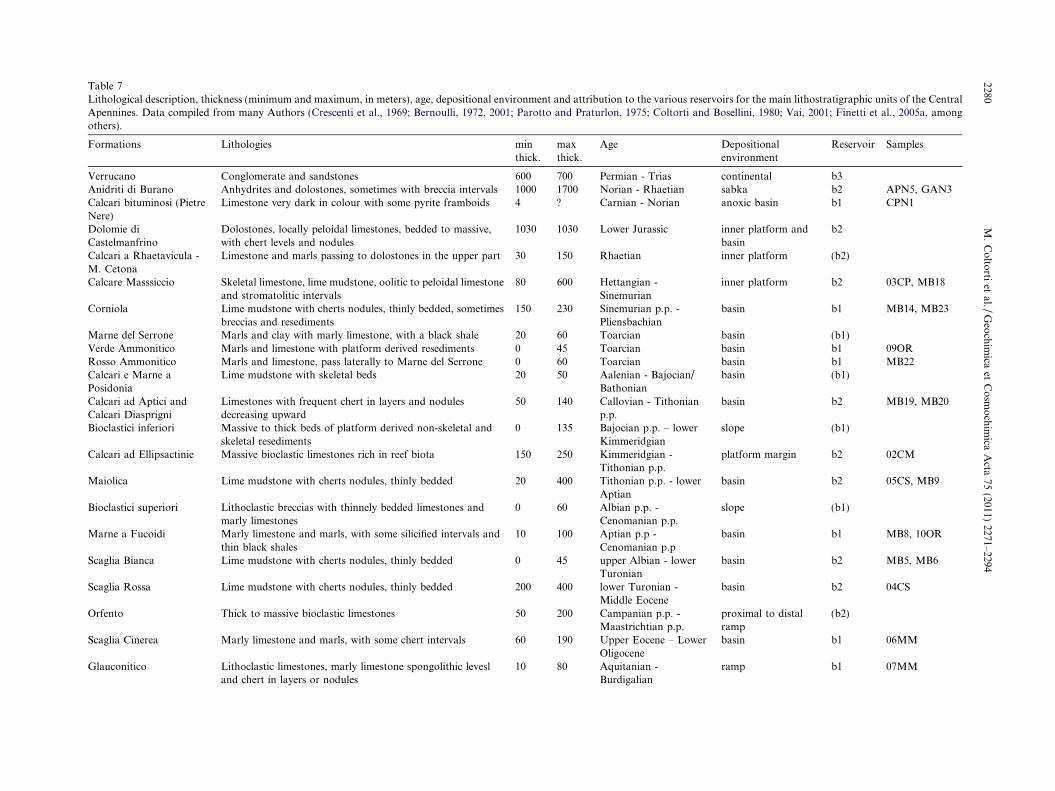
Table 7Lithological description, thickness (minimum and maximum, in meters), age, depositional environment and attribution to the various reservoirs for the main lithostratigraphic units of the CentralApennines. Data compiled from many Authors (Crescenti et al., 1969; Bernoulli, 1972, 2001; Parotto and Praturlon, 1975; Coltorti and Bosellini, 1980; Vai, 2001; Finetti et al., 2005a, amongothers).

Formations Lithologies minthick.

maxthick.

Age Depositionalenvironment

Reservoir Samples

Verrucano Conglomerate and sandstones 600 700 Permian - Trias continental b3Anidriti di Burano Anhydrites and dolostones, sometimes with breccia intervals 1000 1700 Norian - Rhaetian sabka b2 APN5, GAN3Calcari bituminosi (PietreNere)

Limestone very dark in colour with some pyrite framboids 4 ? Carnian - Norian anoxic basin b1 CPN1

Dolomie diCastelmanfrino

Dolostones, locally peloidal limestones, bedded to massive,with chert levels and nodules

1030 1030 Lower Jurassic inner platform andbasin

b2

Calcari a Rhaetavicula -M. Cetona

Limestone and marls passing to dolostones in the upper part 30 150 Rhaetian inner platform (b2)

Calcare Masssiccio Skeletal limestone, lime mudstone, oolitic to peloidal limestoneand stromatolitic intervals

80 600 Hettangian -Sinemurian

inner platform b2 03CP, MB18

Corniola Lime mudstone with cherts nodules, thinly bedded, sometimesbreccias and resediments

150 230 Sinemurian p.p. -Pliensbachian

basin b1 MB14, MB23

Marne del Serrone Marls and clay with marly limestone, with a black shale 20 60 Toarcian basin (b1)Verde Ammonitico Marls and limestone with platform derived resediments 0 45 Toarcian basin b1 09ORRosso Ammonitico Marls and limestone, pass laterally to Marne del Serrone 0 60 Toarcian basin b1 MB22Calcari e Marne aPosidonia

Lime mudstone with skeletal beds 20 50 Aalenian - Bajocian/Bathonian

basin (b1)

Calcari ad Aptici andCalcari Diasprigni

Limestones with frequent chert in layers and nodulesdecreasing upward

50 140 Callovian - Tithonianp.p.

basin b2 MB19, MB20

Bioclastici inferiori Massive to thick beds of platform derived non-skeletal andskeletal resediments

0 135 Bajocian p.p. – lowerKimmeridgian

slope (b1)

Calcari ad Ellipsactinie Massive bioclastic limestones rich in reef biota 150 250 Kimmeridgian -Tithonian p.p.

platform margin b2 02CM

Maiolica Lime mudstone with cherts nodules, thinly bedded 20 400 Tithonian p.p. - lowerAptian

basin b2 05CS, MB9

Bioclastici superiori Lithoclastic breccias with thinnely bedded limestones andmarly limestones

0 60 Albian p.p. -Cenomanian p.p.

slope (b1)

Marne a Fucoidi Marly limestone and marls, with some silicified intervals andthin black shales

10 100 Aptian p.p -Cenomanian p.p

basin b1 MB8, 10OR

Scaglia Bianca Lime mudstone with cherts nodules, thinly bedded 0 45 upper Albian - lowerTuronian

basin b2 MB5, MB6

Scaglia Rossa Lime mudstone with cherts nodules, thinly bedded 200 400 lower Turonian -Middle Eocene

basin b2 04CS

Orfento Thick to massive bioclastic limestones 50 200 Campanian p.p. -Maastrichtian p.p.

proximal to distalramp

(b2)

Scaglia Cinerea Marly limestone and marls, with some chert intervals 60 190 Upper Eocene – LowerOligocene

basin b1 06MM

Glauconitico Lithoclastic limestones, marly limestone spongolithic levesland chert in layers or nodules

10 80 Aquitanian -Burdigalian

ramp b1 07MM

2280M

.C

olto

rtiet

al./G

eoch

imica

etC

osm

och

imica

Acta

75(2011)

2271–2294

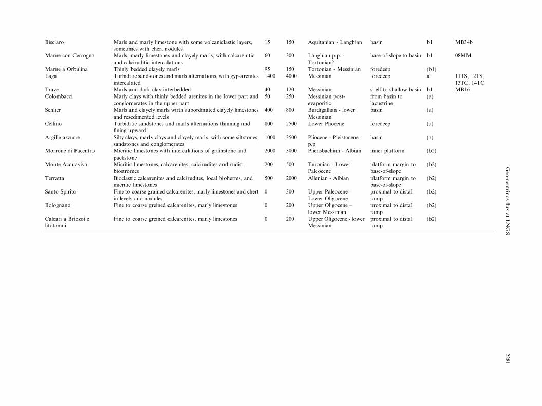
Bisciaro Marls and marly limestone with some volcaniclastic layers,sometimes with chert nodules

15 150 Aquitanian - Langhian basin b1 MB34b

Marne con Cerrogna Marls, marly limestones and clayely marls, with calcareniticand calciruditic intercalations

60 300 Langhian p.p. -Tortonian?

base-of-slope to basin b1 08MM

Marne a Orbulina Thinly bedded clayely marls 95 150 Tortonian - Messinian foredeep (b1)Laga Turbiditic sandstones and marls alternations, with gypsarenites

intercalated1400 4000 Messinian foredeep a 11TS, 12TS,

13TC, 14TCTrave Marls and dark clay interbedded 40 120 Messinian shelf to shallow basin b1 MB16Colombacci Marly clays with thinly bedded arenites in the lower part and

conglomerates in the upper part50 250 Messinian post-

evaporiticfrom basin tolacustrine

(a)

Schlier Marls and clayely marls wirth subordinated clayely limestonesand resedimented levels

400 800 Burdigallian - lowerMessinian

basin (a)

Cellino Turbiditic sandstones and marls alternations thinning andfining upward

800 2500 Lower Pliocene foredeep (a)

Argille azzurre Silty clays, marly clays and clayely marls, with some siltstones,sandstones and conglomerates

1000 3500 Pliocene - Pleistocenep.p.

basin (a)

Morrone di Pacentro Micritic limestones with intercalations of grainstone andpackstone

2000 3000 Pliensbachian - Albian inner platform (b2)

Monte Acquaviva Micritic limestones, calcarenites, calcirudites and rudistbiostromes

200 500 Turonian - LowerPaleocene

platform margin tobase-of-slope

(b2)

Terratta Bioclastic calcarenites and calcirudites, local bioherms, andmicritic limestones

500 2000 Allenian - Albian platform margin tobase-of-slope

(b2)

Santo Spirito Fine to coarse grained calcarenites, marly limestones and chertin levels and nodules

0 300 Upper Paleocene –Lower Oligocene


(b2)

Bolognano Fine to coarse greined calcarenites, marly limestones 0 200 Upper Oligocene –lower Messinian


(b2)

Calcari a Briozoi elitotamni

Fine to coarse greined calcarenites, marly limestones 0 200 Upper Oligocene - lowerMessinian


(b2)

Geo

-neu

trino

sfl

ux

atL

NG

S2281


Fucoidi”, “Scaglia Bianca”, “Scaglia Rossa”, “ScagliaCinerea”) (Reservoir b1).

Middle–Late Lias—In some areas shallow-water car-bonate deposits persists with the deposition of Calcari aPalaeodasycladus Fm., while in some others slope sedi-ments developed (megabreccias and calciturbidites).

Dogger–Malm—In the areas occupied by carbonateplatforms oolitic and micritic limestone are abundant(“Morrone di Pacentro” Fm., “Monte Acquaviva” Fm.).In the basinal areas there are the typical facies with wide-spread formation as “Calcari a Filaments”, “Diaspri”,“Marne ad Aptici” and the lower part of the “Maiolica”

Fm.Early Cretaceous—Carbonate sedimentation continuous

with small hiatus until late Albian to middle Cenomanian.In the whole basinal areas the deposition of typical pelagicfacies take place with the “Maiolica” and “Marne a Fuco-idi” Fms.: in this latter formation some black-shales layersoccur related to the oceanic anoxic events (Jenkyns, 2003)(Reservoirs b1 and b2).

Late Cretaceous—In this period there is the develop-ment of the carbonate platforms dominated by large bi-valve (“Calcari a Rudiste”, “Orfento” Fms.) whereaspelagic lithotypes accumulate in basinal area with the “Sca-glia” Fm. (“Scaglia Bianca” and “Scaglia Rossa”) (Eberliet al., 1993) (Reservoir b2).

Paleogene—The sedimentation become discontinuouswith various lacuna in different platform areas. In the basi-nal area there are the pelagic successions with the ScagliaCinerea Fm. (Reservoir b1).

Miocene—After the widespread lacuna of Paleogene anew marine transgression develop a carbonate ramp (“Cal-cari a Briozoi e Litotamni” Fm.) successively covered byterrigenous deposits of the Apennine foredeep (Laga Fm.,Reservoir a; Cipollari et al., 1999).

Pliocene and Pleistocene—In the Adriatic sector the mid-dle-Pliocene transgression cover unconformably the Mes-sinian or lower Pliocene sediments, with basalconglomerate, clays and sands (Laga Fm., Reservoir a).The marine Pleistocene follows these deposits withclayey–sandy sediments with thickness reaching up to1000 m (“Cellino” Fm.; Carruba et al., 2006).

4.2. Upper crust

The upper crust (UC) can be defined as the portion ofcontinental crust ranging from the bottom of the sedimen-tary cover to the Conrad discontinuity, which marks thetop of the lower crust. This approach, which is mainlybased on geophysical data, shows some problems when try-ing to define the position of the medium-grade, amphibolitefacies rocks. Indeed, Rudnick and Fountain (1995) intro-duced a middle crust mainly composed by migmatitic rocks,whereas Wedepohl (1995) includes the amphibolites withinthe UC. The geophysical profiles beneath Central Italy donot support the existence of a well defined intermediate le-vel, while the limited thickness of the LC induce us to insertthe amphibolitic rocks within the UC.

Two classical outcrops of the Southern Alps were sam-pled as representative of the UC: the Serie dei Laghi near

Lago Maggiore, and the philladic basement of Valsugana,near Trento (Table 6A). The Serie dei Laghi outcrop inthe SE portion of the Ivrea–Verbano Zone. It correspondsto intermediate to upper crust lithologies. The deepest partis made up of Ordovician meta-sandstones to metapelites(paragneiss with calc-silicate inclusions and biotite- andmuscovite-bearing gneiss) in amphibolitic facies intrudedby dioritico-granitic orthogneiss with calc-alkaline affinity(Borghi, 1991). In the upper part micaschists and parag-neiss predominates with two micas, garnet, staurolite andkyanite sometime retrograded to green-schist facies.

In the Valsugana area the pre-Hercynian sediments areslightly metamorphosed. It consists of two phillitic unitsseparated by a complex volcano-sedimentary series withmeta-carbonates and metarhyolites. These metamorphicterrains are intruded by calc-alkaline plutons varying incomposition from diorite to granodiorites and granites(prevalent) (Cima d’Asta and Caoria plutons; D’Amicoet al., 1971).

4.3. Lower crust

LC rocks are available only thanks to tectonic processeswhich denudate the deepest portion of the crust or to basal-tic magmatism scavenging small pieces of LC (xenoliths)during their uprising from the mantle to the Earth’ surface.The two geological evidences however lead to contrastingresults as far as relative proportions of mafic and felsicrocks are concerned. As reviewed by Rudnick and Fountain(1995), mafic rocks are more represented in xenoliths, thanusually are in tectonically emplaced LC terrains where, onthe contrary, felsic rocks are equally encountered if not pre-dominant. Horizontal heterogeneity within LC is of courseexpected, but the simplest explanation for this contrast maylie on the tool we are using for sampling. Where basalts arepresent, underplating process may have been working evenfor a long while, thus mafic rocks in this settings—wherexenoliths are taken—may be more extensively represented.An example of this situation may be seen in the Ivrea Zonewhich, as already remarked, represents the LC outcropnearest to the investigated area. In Val Sessera and Val Se-sia in fact gabbroic rocks predominate as a result of variousintrusions, several km in thickness, while in Val Strona fel-sic rocks are more abundant.

Due to the lack of LC outcrops in the area close to GranSasso, representative LC samples were taken from the Iv-rea–Verbano Zone which represents the most classic andextensive deep crustal section of the Alps. It can be distin-guished in two main lithological units: (a) the layered com-plex Permian in age (278–280 Ma) in contact with theCanavese Line with thickness up to 10 km in Val Sesiaand Val Sessera (Quick et al., 1992, 2003 and referencetherein) and (b) the Kinzigitic Fm. The former unit is madeup of layered gabbros intruded in the deep crust and re-equilibrated in granulite facies (Table 6B). Magmatic litho-types varies from cumulitic peridotites, pyroxenites, gab-bros, anorthosites and diorites (Rivalenti et al., 1980).The intrusion of this body occurs within the older KinzigiticComplex in a general extensive regime which allow the cre-ation of progressive enlarging magma chamber/s. The heat

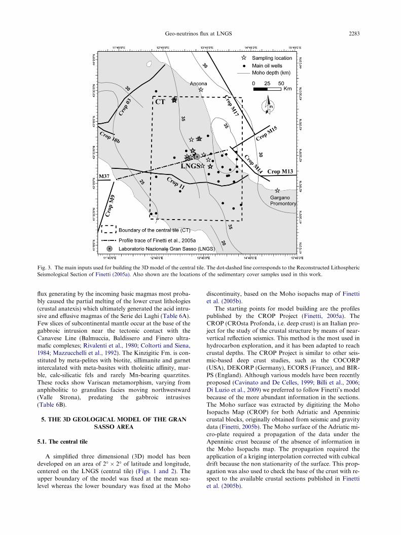
Fig. 3. The main inputs used for building the 3D model of the central tile. The dot-dashed line corresponds to the Reconstructed LithosphericSeismological Section of Finetti (2005a). Also shown are the locations of the sedimentary cover samples used in this work.


flux generating by the incoming basic magmas most proba-bly caused the partial melting of the lower crust lithologies(crustal anatexis) which ultimately generated the acid intru-sive and effusive magmas of the Serie dei Laghi (Table 6A).Few slices of subcontinental mantle occur at the base of thegabbroic intrusion near the tectonic contact with theCanavese Line (Balmuccia, Baldissero and Finero ultra-mafic complexes; Rivalenti et al., 1980; Coltorti and Siena,1984; Mazzucchelli et al., 1992). The Kinzigitic Fm. is con-stituted by meta-pelites with biotite, sillimanite and garnetintercalated with meta-basites with tholeiitic affinity, mar-ble, calc-silicatic fels and rarely Mn-bearing quarztites.These rocks show Variscan metamorphism, varying fromanphibolitic to granulites facies moving northwestward(Valle Strona), predating the gabbroic intrusives(Table 6B).

5. THE 3D GEOLOGICAL MODEL OF THE GRAN

SASSO AREA

5.1. The central tile

A simplified three dimensional (3D) model has beendeveloped on an area of 2� � 2� of latitude and longitude,centered on the LNGS (central tile) (Figs. 1 and 2). Theupper boundary of the model was fixed at the mean sea-level whereas the lower boundary was fixed at the Moho

discontinuity, based on the Moho isopachs map of Finettiet al. (2005b).

The starting points for model building are the profilespublished by the CROP Project (Finetti, 2005a). TheCROP (CROsta Profonda, i.e. deep crust) is an Italian pro-ject for the study of the crustal structure by means of near-vertical reflection seismics. This method is the most used inhydrocarbon exploration, and it has been adapted to reachcrustal depths. The CROP Project is similar to other seis-mic-based deep crust studies, such as the COCORP(USA), DEKORP (Germany), ECORS (France), and BIR-PS (England). Although various models have been recentlyproposed (Cavinato and De Celles, 1999; Billi et al., 2006;Di Luzio et al., 2009) we preferred to follow Finetti’s modelbecause of the more abundant information in the sections.The Moho surface was extracted by digitizing the MohoIsopachs Map (CROP) for both Adriatic and Apenniniccrustal blocks, originally obtained from seismic and gravitydata (Finetti, 2005b). The Moho surface of the Adriatic mi-cro-plate required a propagation of the data under theApenninic crust because of the absence of information inthe Moho Isopachs map. The propagation required theapplication of a kriging interpolation corrected with cubicaldrift because the non stationarity of the surface. This prop-agation was also used to check the base of the crust with re-spect to the available crustal sections published in Finettiet al. (2005b).

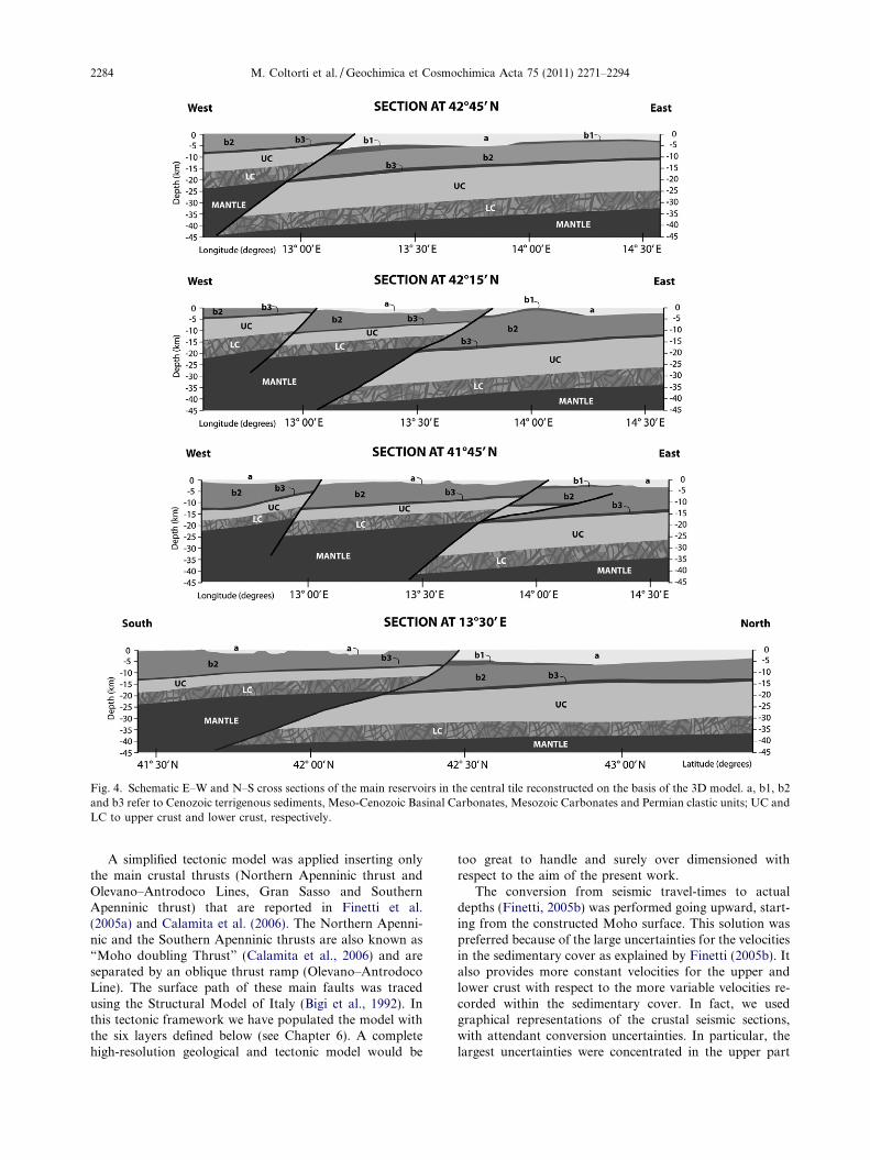
Fig. 4. Schematic E–W and N–S cross sections of the main reservoirs in the central tile reconstructed on the basis of the 3D model. a, b1, b2and b3 refer to Cenozoic terrigenous sediments, Meso-Cenozoic Basinal Carbonates, Mesozoic Carbonates and Permian clastic units; UC andLC to upper crust and lower crust, respectively.


A simplified tectonic model was applied inserting onlythe main crustal thrusts (Northern Apenninic thrust andOlevano–Antrodoco Lines, Gran Sasso and SouthernApenninic thrust) that are reported in Finetti et al.(2005a) and Calamita et al. (2006). The Northern Apenni-nic and the Southern Apenninic thrusts are also known as“Moho doubling Thrust” (Calamita et al., 2006) and areseparated by an oblique thrust ramp (Olevano–AntrodocoLine). The surface path of these main faults was tracedusing the Structural Model of Italy (Bigi et al., 1992). Inthis tectonic framework we have populated the model withthe six layers defined below (see Chapter 6). A completehigh-resolution geological and tectonic model would be

too great to handle and surely over dimensioned withrespect to the aim of the present work.

The conversion from seismic travel-times to actualdepths (Finetti, 2005b) was performed going upward, start-ing from the constructed Moho surface. This solution waspreferred because of the large uncertainties for the velocitiesin the sedimentary cover as explained by Finetti (2005b). Italso provides more constant velocities for the upper andlower crust with respect to the more variable velocities re-corded within the sedimentary cover. In fact, we usedgraphical representations of the crustal seismic sections,with attendant conversion uncertainties. In particular, thelargest uncertainties were concentrated in the upper part

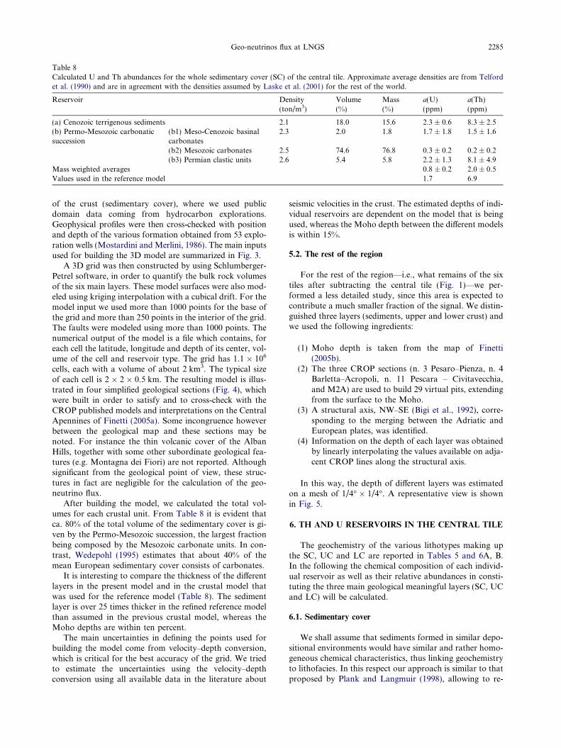
Table 8Calculated U and Th abundances for the whole sedimentary cover (SC) of the central tile. Approximate average densities are from Telfordet al. (1990) and are in agreement with the densities assumed by Laske et al. (2001) for the rest of the world.

Reservoir Density(ton/m3)

Volume(%)

Mass(%)

a(U)(ppm)

a(Th)(ppm)

(a) Cenozoic terrigenous sediments 2.1 18.0 15.6 2.3 ± 0.6 8.3 ± 2.5(b) Permo-Mesozoic carbonaticsuccession

(b1) Meso-Cenozoic basinalcarbonates

2.3 2.0 1.8 1.7 ± 1.8 1.5 ± 1.6

(b2) Mesozoic carbonates 2.5 74.6 76.8 0.3 ± 0.2 0.2 ± 0.2(b3) Permian clastic units 2.6 5.4 5.8 2.2 ± 1.3 8.1 ± 4.9

Mass weighted averages 0.8 ± 0.2 2.0 ± 0.5Values used in the reference model 1.7 6.9


of the crust (sedimentary cover), where we used publicdomain data coming from hydrocarbon explorations.Geophysical profiles were then cross-checked with positionand depth of the various formation obtained from 53 explo-ration wells (Mostardini and Merlini, 1986). The main inputsused for building the 3D model are summarized in Fig. 3.

A 3D grid was then constructed by using Schlumberger-Petrel software, in order to quantify the bulk rock volumesof the six main layers. These model surfaces were also mod-eled using kriging interpolation with a cubical drift. For themodel input we used more than 1000 points for the base ofthe grid and more than 250 points in the interior of the grid.The faults were modeled using more than 1000 points. Thenumerical output of the model is a file which contains, foreach cell the latitude, longitude and depth of its center, vol-ume of the cell and reservoir type. The grid has 1.1 � 106

cells, each with a volume of about 2 km3. The typical sizeof each cell is 2 � 2 � 0.5 km. The resulting model is illus-trated in four simplified geological sections (Fig. 4), whichwere built in order to satisfy and to cross-check with theCROP published models and interpretations on the CentralApennines of Finetti (2005a). Some incongruence howeverbetween the geological map and these sections may benoted. For instance the thin volcanic cover of the AlbanHills, together with some other subordinate geological fea-tures (e.g. Montagna dei Fiori) are not reported. Althoughsignificant from the geological point of view, these struc-tures in fact are negligible for the calculation of the geo-neutrino flux.

After building the model, we calculated the total vol-umes for each crustal unit. From Table 8 it is evident thatca. 80% of the total volume of the sedimentary cover is gi-ven by the Permo-Mesozoic succession, the largest fractionbeing composed by the Mesozoic carbonate units. In con-trast, Wedepohl (1995) estimates that about 40% of themean European sedimentary cover consists of carbonates.

It is interesting to compare the thickness of the differentlayers in the present model and in the crustal model thatwas used for the reference model (Table 8). The sedimentlayer is over 25 times thicker in the refined reference modelthan assumed in the previous crustal model, whereas theMoho depths are within ten percent.

The main uncertainties in defining the points used forbuilding the model come from velocity–depth conversion,which is critical for the best accuracy of the grid. We triedto estimate the uncertainties using the velocity–depthconversion using all available data in the literature about

seismic velocities in the crust. The estimated depths of indi-vidual reservoirs are dependent on the model that is beingused, whereas the Moho depth between the different modelsis within 15%.

5.2. The rest of the region

For the rest of the region—i.e., what remains of the sixtiles after subtracting the central tile (Fig. 1)—we per-formed a less detailed study, since this area is expected tocontribute a much smaller fraction of the signal. We distin-guished three layers (sediments, upper and lower crust) andwe used the following ingredients:

(1) Moho depth is taken from the map of Finetti(2005b).

(2) The three CROP sections (n. 3 Pesaro–Pienza, n. 4Barletta–Acropoli, n. 11 Pescara – Civitavecchia,and M2A) are used to build 29 virtual pits, extendingfrom the surface to the Moho.

(3) A structural axis, NW–SE (Bigi et al., 1992), corre-sponding to the merging between the Adriatic andEuropean plates, was identified.

(4) Information on the depth of each layer was obtainedby linearly interpolating the values available on adja-cent CROP lines along the structural axis.

In this way, the depth of different layers was estimatedon a mesh of 1/4� � 1/4�. A representative view is shownin Fig. 5.

6. TH AND U RESERVOIRS IN THE CENTRAL TILE

The geochemistry of the various lithotypes making upthe SC, UC and LC are reported in Tables 5 and 6A, B.In the following the chemical composition of each individ-ual reservoir as well as their relative abundances in consti-tuting the three main geological meaningful layers (SC, UCand LC) will be calculated.

6.1. Sedimentary cover

We shall assume that sediments formed in similar depo-sitional environments would have similar and rather homo-geneous chemical characteristics, thus linking geochemistryto lithofacies. In this respect our approach is similar to thatproposed by Plank and Langmuir (1998), allowing to re-

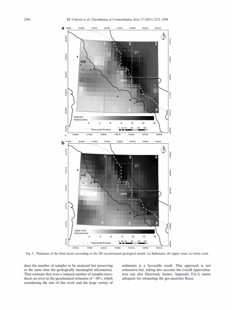
Fig. 5. Thickness of the three layers according to the 3D reconstructed geological model. (a) Sediments, (b) upper crust, (c) lower crust.


duce the number of samples to be analyzed but preservingat the same time the geologically meaningful information.They estimate that even a reduced number of samples intro-duces an error in the geochemical estimates of <30%, whichconsidering the aim of this work and the large variety of

sediments is a favorable result. This approach is notexhaustive but, taking into account the overall approxima-tion (see also Electronic Annex, Appendix EA-2) seemsadequate for estimating the geo-neutrino fluxes.

Fig 5. (continued)

Table 9Volume (in km3 and %) and thickness (in km) of the four sedimentary reservoirs and of the UC and LC. Thicknesses are reported according tothe present model (RRM) and the reference model (RM, Mantovani et al., 2004).

Volume (km3) Volume (%) Thickness (km)

RM RRM

(a) Cenozoic terrigenous sediments 83,589 6.8 0.5 13(b1) Meso-Cenozoic basinal carbonates 9,028 0.7(b2) Mesozoic carbonates 345,684 28.1(b3) Permian clastic units 25,163 2.0Upper crust 468,772 38.0 10 13Middle crust / / 10 /Lower crust 300,566 24.4 10.5 9

Total 1,232,802 100 31 35


For the purpose of this work the Cenozoic terrigenousand the terrigenous/carbonatic Permo-Mesozoic successionhas been divided in four reservoirs (Table 7):

(a) Cenozoic terrigenous units (sandstones, siltites andclays).

(b1) Meso-Cenozoic basinal carbonate units (marly andshaly carbonates, sometimes with black shales).

(b2) Mesozoic carbonate units (limestones, dolomitesand evaporites, with a negligible marl and clay content).

(b3) Permian clastic units (sandstones andconglomerates).

U and Th mass abundances in the three reservoirs areobtained by averaging arithmetically data for the samplesanalyzed (Table 8). Lithotypes belonging to the last reser-

voir (b3) outcrop rarely within the entire Italian Peninsulaand due to their conglomeratic nature, sampling is quitedifficult. For these reasons and taking into account thatthe Permian clastic units (“Verrucano” Fm.) result fromthe dismantling and erosion of the Paleozoic basementrocks, we assume U and Th contents of Reservoir b3 aresimilar to those of the UC.

In each reservoir, the dispersion of the measured abun-dances is much larger than the analytical uncertainty andalso the uncertainties of the mass of the reservoirs arenegligible with respect to them. The uncertainty quoted inTable 5 is the standard deviation among the different sam-ples weighted with the mass of the reservoirs. Taking intoaccount the relative volume (Table 9) of the four reservoirs

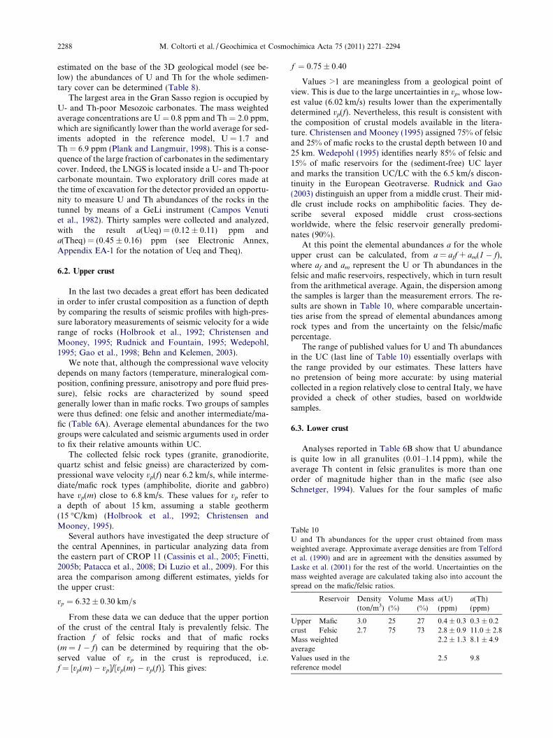
Table 10U and Th abundances for the upper crust obtained from massweighted average. Approximate average densities are from Telfordet al. (1990) and are in agreement with the densities assumed byLaske et al. (2001) for the rest of the world. Uncertainties on themass weighted average are calculated taking also into account thespread on the mafic/felsic ratios.

Reservoir Density(ton/m3)

Volume(%)

Mass(%)

a(U)(ppm)

a(Th)(ppm)

Uppercrust

Mafic 3.0 25 27 0.4 ± 0.3 0.3 ± 0.2Felsic 2.7 75 73 2.8 ± 0.9 11.0 ± 2.8

Mass weightedaverage

2.2 ± 1.3 8.1 ± 4.9

Values used in thereference model

2.5 9.8


estimated on the base of the 3D geological model (see be-low) the abundances of U and Th for the whole sedimen-tary cover can be determined (Table 8).

The largest area in the Gran Sasso region is occupied byU- and Th-poor Mesozoic carbonates. The mass weightedaverage concentrations are U = 0.8 ppm and Th = 2.0 ppm,which are significantly lower than the world average for sed-iments adopted in the reference model, U = 1.7 andTh = 6.9 ppm (Plank and Langmuir, 1998). This is a conse-quence of the large fraction of carbonates in the sedimentarycover. Indeed, the LNGS is located inside a U- and Th-poorcarbonate mountain. Two exploratory drill cores made atthe time of excavation for the detector provided an opportu-nity to measure U and Th abundances of the rocks in thetunnel by means of a GeLi instrument (Campos Venutiet al., 1982). Thirty samples were collected and analyzed,with the result a(Ueq) = (0.12 ± 0.11) ppm anda(Theq) = (0.45 ± 0.16) ppm (see Electronic Annex,Appendix EA-1 for the notation of Ueq and Theq).

6.2. Upper crust

In the last two decades a great effort has been dedicatedin order to infer crustal composition as a function of depthby comparing the results of seismic profiles with high-pres-sure laboratory measurements of seismic velocity for a widerange of rocks (Holbrook et al., 1992; Christensen andMooney, 1995; Rudnick and Fountain, 1995; Wedepohl,1995; Gao et al., 1998; Behn and Kelemen, 2003).

We note that, although the compressional wave velocitydepends on many factors (temperature, mineralogical com-position, confining pressure, anisotropy and pore fluid pres-sure), felsic rocks are characterized by sound speedgenerally lower than in mafic rocks. Two groups of sampleswere thus defined: one felsic and another intermediate/ma-fic (Table 6A). Average elemental abundances for the twogroups were calculated and seismic arguments used in orderto fix their relative amounts within UC.

The collected felsic rock types (granite, granodiorite,quartz schist and felsic gneiss) are characterized by com-pressional wave velocity vp(f) near 6.2 km/s, while interme-diate/mafic rock types (amphibolite, diorite and gabbro)have vp(m) close to 6.8 km/s. These values for vp refer toa depth of about 15 km, assuming a stable geotherm(15 �C/km) (Holbrook et al., 1992; Christensen andMooney, 1995).

Several authors have investigated the deep structure ofthe central Apennines, in particular analyzing data fromthe eastern part of CROP 11 (Cassinis et al., 2005; Finetti,2005b; Patacca et al., 2008; Di Luzio et al., 2009). For thisarea the comparison among different estimates, yields forthe upper crust:

vp ¼ 6:32� 0:30 km=s

From these data we can deduce that the upper portionof the crust of the central Italy is prevalently felsic. Thefraction f of felsic rocks and that of mafic rocks(m = 1 � f) can be determined by requiring that the ob-served value of vp in the crust is reproduced, i.e.f = [vp(m) � vp]/[vp(m) � vp(f)]. This gives:

f ¼ 0:75� 0:40

Values >1 are meaningless from a geological point ofview. This is due to the large uncertainties in vp, whose low-est value (6.02 km/s) results lower than the experimentallydetermined vp(f). Nevertheless, this result is consistent withthe composition of crustal models available in the litera-ture. Christensen and Mooney (1995) assigned 75% of felsicand 25% of mafic rocks to the crustal depth between 10 and25 km. Wedepohl (1995) identifies nearly 85% of felsic and15% of mafic reservoirs for the (sediment-free) UC layerand marks the transition UC/LC with the 6.5 km/s discon-tinuity in the European Geotraverse. Rudnick and Gao(2003) distinguish an upper from a middle crust. Their mid-dle crust include rocks on amphibolitic facies. They de-scribe several exposed middle crust cross-sectionsworldwide, where the felsic reservoir generally predomi-nates (90%).

At this point the elemental abundances a for the wholeupper crust can be calculated, from a = aff + am(1 � f),where af and am represent the U or Th abundances in thefelsic and mafic reservoirs, respectively, which in turn resultfrom the arithmetical average. Again, the dispersion amongthe samples is larger than the measurement errors. The re-sults are shown in Table 10, where comparable uncertain-ties arise from the spread of elemental abundances amongrock types and from the uncertainty on the felsic/maficpercentage.

The range of published values for U and Th abundancesin the UC (last line of Table 10) essentially overlaps withthe range provided by our estimates. These latters haveno pretension of being more accurate: by using materialcollected in a region relatively close to central Italy, we haveprovided a check of other studies, based on worldwidesamples.

6.3. Lower crust

Analyses reported in Table 6B show that U abundanceis quite low in all granulites (0.01–1.14 ppm), while theaverage Th content in felsic granulites is more than oneorder of magnitude higher than in the mafic (see alsoSchnetger, 1994). Values for the four samples of mafic

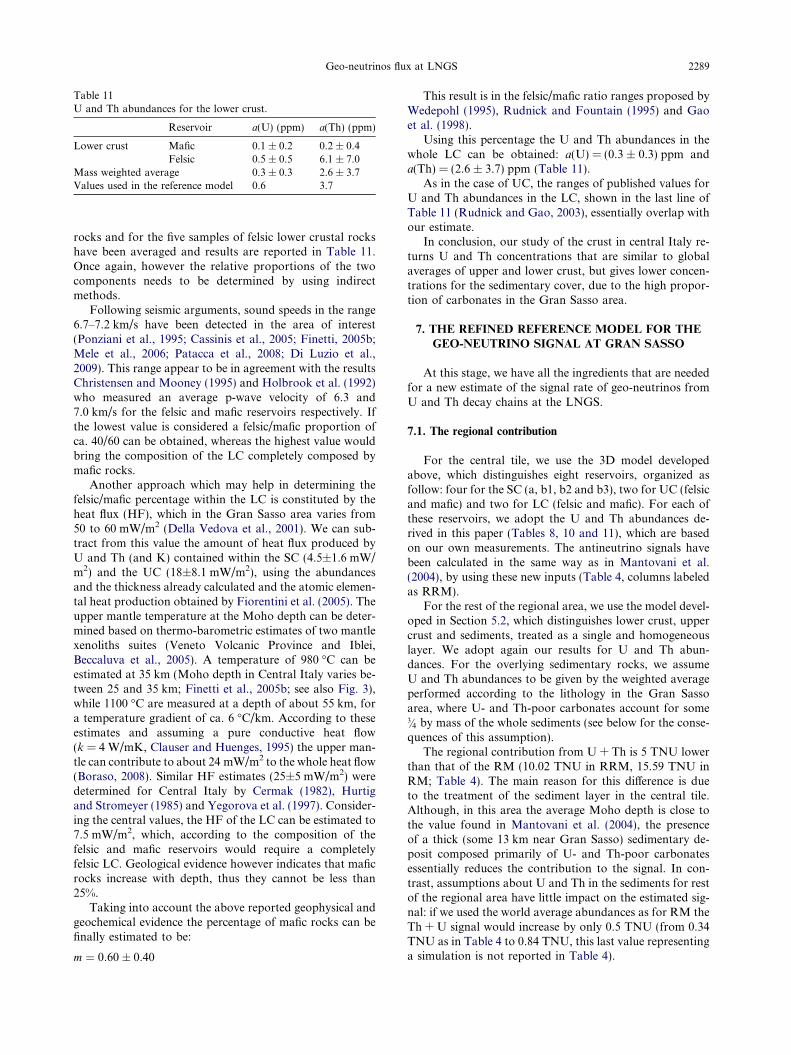
Table 11U and Th abundances for the lower crust.

Reservoir a(U) (ppm) a(Th) (ppm)

Lower crust Mafic 0.1 ± 0.2 0.2 ± 0.4Felsic 0.5 ± 0.5 6.1 ± 7.0

Mass weighted average 0.3 ± 0.3 2.6 ± 3.7Values used in the reference model 0.6 3.7


rocks and for the five samples of felsic lower crustal rockshave been averaged and results are reported in Table 11.Once again, however the relative proportions of the twocomponents needs to be determined by using indirectmethods.

Following seismic arguments, sound speeds in the range6.7–7.2 km/s have been detected in the area of interest(Ponziani et al., 1995; Cassinis et al., 2005; Finetti, 2005b;Mele et al., 2006; Patacca et al., 2008; Di Luzio et al.,2009). This range appear to be in agreement with the resultsChristensen and Mooney (1995) and Holbrook et al. (1992)who measured an average p-wave velocity of 6.3 and7.0 km/s for the felsic and mafic reservoirs respectively. Ifthe lowest value is considered a felsic/mafic proportion ofca. 40/60 can be obtained, whereas the highest value wouldbring the composition of the LC completely composed bymafic rocks.

Another approach which may help in determining thefelsic/mafic percentage within the LC is constituted by theheat flux (HF), which in the Gran Sasso area varies from50 to 60 mW/m2 (Della Vedova et al., 2001). We can sub-tract from this value the amount of heat flux produced byU and Th (and K) contained within the SC (4.5±1.6 mW/m2) and the UC (18±8.1 mW/m2), using the abundancesand the thickness already calculated and the atomic elemen-tal heat production obtained by Fiorentini et al. (2005). Theupper mantle temperature at the Moho depth can be deter-mined based on thermo-barometric estimates of two mantlexenoliths suites (Veneto Volcanic Province and Iblei,Beccaluva et al., 2005). A temperature of 980 �C can beestimated at 35 km (Moho depth in Central Italy varies be-tween 25 and 35 km; Finetti et al., 2005b; see also Fig. 3),while 1100 �C are measured at a depth of about 55 km, fora temperature gradient of ca. 6 �C/km. According to theseestimates and assuming a pure conductive heat flow(k = 4 W/mK, Clauser and Huenges, 1995) the upper man-tle can contribute to about 24 mW/m2 to the whole heat flow(Boraso, 2008). Similar HF estimates (25±5 mW/m2) weredetermined for Central Italy by Cermak (1982), Hurtigand Stromeyer (1985) and Yegorova et al. (1997). Consider-ing the central values, the HF of the LC can be estimated to7.5 mW/m2, which, according to the composition of thefelsic and mafic reservoirs would require a completelyfelsic LC. Geological evidence however indicates that maficrocks increase with depth, thus they cannot be less than25%.

Taking into account the above reported geophysical andgeochemical evidence the percentage of mafic rocks can befinally estimated to be:

m ¼ 0:60� 0:40

This result is in the felsic/mafic ratio ranges proposed byWedepohl (1995), Rudnick and Fountain (1995) and Gaoet al. (1998).

Using this percentage the U and Th abundances in thewhole LC can be obtained: a(U) = (0.3 ± 0.3) ppm anda(Th) = (2.6 ± 3.7) ppm (Table 11).

As in the case of UC, the ranges of published values forU and Th abundances in the LC, shown in the last line ofTable 11 (Rudnick and Gao, 2003), essentially overlap withour estimate.

In conclusion, our study of the crust in central Italy re-turns U and Th concentrations that are similar to globalaverages of upper and lower crust, but gives lower concen-trations for the sedimentary cover, due to the high propor-tion of carbonates in the Gran Sasso area.

7. THE REFINED REFERENCE MODEL FOR THE

GEO-NEUTRINO SIGNAL AT GRAN SASSO

At this stage, we have all the ingredients that are neededfor a new estimate of the signal rate of geo-neutrinos fromU and Th decay chains at the LNGS.

7.1. The regional contribution

For the central tile, we use the 3D model developedabove, which distinguishes eight reservoirs, organized asfollow: four for the SC (a, b1, b2 and b3), two for UC (felsicand mafic) and two for LC (felsic and mafic). For each ofthese reservoirs, we adopt the U and Th abundances de-rived in this paper (Tables 8, 10 and 11), which are basedon our own measurements. The antineutrino signals havebeen calculated in the same way as in Mantovani et al.(2004), by using these new inputs (Table 4, columns labeledas RRM).

For the rest of the regional area, we use the model devel-oped in Section 5.2, which distinguishes lower crust, uppercrust and sediments, treated as a single and homogeneouslayer. We adopt again our results for U and Th abun-dances. For the overlying sedimentary rocks, we assumeU and Th abundances to be given by the weighted averageperformed according to the lithology in the Gran Sassoarea, where U- and Th-poor carbonates account for some3=4 by mass of the whole sediments (see below for the conse-quences of this assumption).

The regional contribution from U + Th is 5 TNU lowerthan that of the RM (10.02 TNU in RRM, 15.59 TNU inRM; Table 4). The main reason for this difference is dueto the treatment of the sediment layer in the central tile.Although, in this area the average Moho depth is close tothe value found in Mantovani et al. (2004), the presenceof a thick (some 13 km near Gran Sasso) sedimentary de-posit composed primarily of U- and Th-poor carbonatesessentially reduces the contribution to the signal. In con-trast, assumptions about U and Th in the sediments for restof the regional area have little impact on the estimated sig-nal: if we used the world average abundances as for RM theTh + U signal would increase by only 0.5 TNU (from 0.34TNU as in Table 4 to 0.84 TNU, this last value representinga simulation is not reported in Table 4).

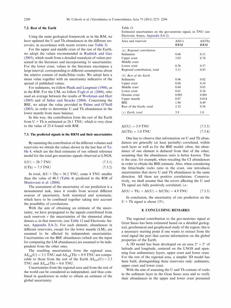
Table 12Estimated uncertainties on the geo-neutrino signal, in TNU (seeElectronic Annex, Appendix EA-2).

Area and reservoir DS(U)RRM

DS(Th)RRM

(a) Regional contribution

Sediments 0.66 0.11Upper crust 3.02 0.76Middle crustLower crust 0.36 0.37Regional contribution, total 3.11 0.85

(b) Rest of the Earth

Sediments 0.06 0.02Upper crust 0.86 0.10Middle crust 0.64 0.05Lower crust 0.61 0.24Oceanic crust 0.003 0.001Upper mantle 0.07 0.014BSE 1.96 0.49Rest of the Earth, total 2.32 0.56

(c) Earth, total 3.9 1.0


7.2. Rest of the Earth

Using the same geological framework as in the RM, wehave updated the U and Th abundances in the different res-ervoirs, in accordance with recent reviews (see Table 3).

For the upper and middle crust of the rest of the Earth,we adopt the values recommended in Rudnick and Gao(2003), which result from a detailed reanalysis of values pre-sented in the literature and incorporating 1r uncertainties.For the lower crust, values in the literature encompass alarge interval, corresponding to different assumptions aboutthe relative content of mafic/felsic rocks. We adopt here amean value together with an uncertainty indicative of thespread of published values.

For sediments, we follow Plank and Langmuir (1998), asin the RM. For the UM, we follow Fogli et al. (2006), whoused an average between the results of Workman and Hart(2005) and of Salter and Stracke (2004). Concerning theBSE, we adopt the value provided in Palme and O’Neill(2003), in order to determine U and Th abundances in thelower mantle from mass balance.

In this way, the contribution form the rest of the Earthfrom U + Th is estimated as 26.1 TNU, which is very closeto the value of 25.4 found with RM.

7.3. The predicted signals in the RRM and their uncertainties

By summing the contribution of the different volumes andreservoirs we obtain the values shown in the last line of Ta-ble 4, which are the final estimates of our refined referencemodel for the total geo-neutrino signals observed at LNGS,

SðUÞ ¼ 28:7 TNU ð7:3:1ÞSðThÞ ¼ 7:5 TNU ð7:3:2Þ

In total, S(U + Th) = 36.2 TNU, some 4 TNU smallerthan the value of 40.5 (Table 4) predicted in the RM ofMantovani et al. (2004).

The assessment of the uncertainty of our prediction is amonumental task, since it results from several differentsources of uncertainty, both statistical and systematic,which have to be combined together taking into accountthe possibility of correlations.

With the aim of obtaining an estimate of the uncer-tainty, we have propagated to the signals contributed fromeach reservoir r the uncertainties of the elemental abun-dances ar in that reservoir, (see Table 12 and Electronic An-nex, Appendix EA-2). For each element, abundances indifferent reservoirs, except for the lower mantle (LM), areassumed to be affected by independent uncertainties.Uncertainties on the BSE abundances (which are the inputfor computing the LM abundances) are assumed to be inde-pendent from the other ones.

The resulting uncertainties form the regional area,DSreg(U) = 3.1 TNU and DSreg(Th) = 0.9 TNU are compa-rable to those from the rest of the Earth DSrest(U) = 2.3TNU and DSrest(Th) = 0.6 TNU.

Uncertainties from the regional area and from the rest ofthe world can be considered as independent, and thus com-bined in quadrature in order to obtain an estimate of theglobal uncertainty:

DSðUÞ ¼ 3:9 TNU ð7:3:3ÞDSðThÞ ¼ 1:0 TNU ð7:3:4Þ

One has to observe that information on U and Th abun-dances are generally (at least partially) correlated, withineach layer as well as for the BSE model: often, the abun-dance of one element is deduced from that of the other,assuming that the abundances ratio is better known. Thisis the case, for example, when rescaling the CI abundancesin order to obtain the BSE estimate. Also, when consideringthe felsic/mafic rocks ratio in the crust, one introducesuncertainties that move U and Th abundances in the samedirection. All these are positive correlations. Conserva-tively, we shall assume that the errors affecting the U andTh signal are fully positively correlated, i.e.:

DSðUþ ThÞ ¼ DSðUÞ þ DSðThÞ ¼ 4:9 TNU ð7:3:5Þ

In conclusion, the uncertainty of our prediction on theU + Th signal is about 13%.

8. CONCLUDING REMARKS

The regional contribution to the geo-neutrino signal atGran Sasso has been estimated based on a detailed geolog-ical, geochemical and geophysical study of the region; this isa necessary starting point if one wants to extract from thetotal signal the part that carries information on the globalproperties of the Earth.

A 3D model has been developed on an area 2� � 2� oflatitude and longitude, centered on the LNGS and span-ning four sedimentary layers, upper crust and lower crust.For the rest of the regional area, a simpler 3D model hasbeen built, distinguishing three reservoirs only: sediments,upper crust and lower crust.

With the aim of assessing the U and Th content of rocksin the sediment layer in the Gran Sasso area and to verifytheir abundances in the upper and lower crust presented


in the literature, we have collected several samples from thesedimentary cover around Gran Sasso and from the crystal-line basement in Northern Italy. We have measured U andTh abundances in these samples by using ICP-MS as well asscintillation (NaI) methods. The results were used to obtainour own estimates of abundances in the different layers ofthe region.

We have thus determined the contribution to the geo-neutrino signal originating from the region. When summedwith the calculations for the rest of the world based onMantovani et al. (2004) and using updated global abun-dances, we obtain the predictions of the refined referencemodel (RRM, Table 4). The results,

SðUÞ ¼ ð28:7� 3:9Þ TNU ð8:1ÞSðThÞ ¼ ð7:5� 1:0Þ TNU ð8:2Þ

confirms, within errors, the values of the previous referencemodel (RM) developed in Mantovani et al. (2004).

With respect to the RM which calculated a total(Th + U) geo-neutrino signal of 40.5 (Table 4), the reduc-tion is essentially due to the reduced content of U and Thin the thick sedimentary layer in the region where the detec-tor is located (see Section 5.1).

The interpretation of geo-neutrino results requires de-tailed geological and geochemical study of the area aroundthe detector. Such studies will be needed as the new geo-neutrino detectors at SNO+, (Sudbury, Canada), LENA(Pyhasalmi, Finland) and Hanohano (Hawaii, USA) beginto acquire data. With appropriate modeling of the datafrom these detectors, the geo-neutrino signal attributableto the U and Th distribution in the Earth’s mantle and evenbeyond can be identified. Further applications of geo-neu-trinos and their implication for Earth Sciences have beenrecently discussed at the 4th Neutrino Geoscience (October6–7, 2010, LNGS. http://geoscience.lngs.infn.it/).

ACKNOWLEDGMENTS

We are grateful to L. Beccaluva, E. Bellotti, C. Bonadiman,B. Della Vedova, L. Carmignani, A. Ianni, J. Majorowicz, W.F.McDonough, R. Rudnick and F. Siena for constructive discussionsand useful comments. An earlier version of the manuscript wasgreatly improved thanks to the work of G. Herzog, M. Chen, A.Montanari and an anonymous referee. We wish to acknowledgethe contribution which Nicola Ferrari gave to this work with hisusual dedication, passion and intelligence. Sadly, an accident oc-curred on a mountain has taken his life, and has taken away fromus an excellent colleague and a splendid friend. This workwas partially supported by MIUR (Ministero dell’Istruzione,dell’Universita e della Ricerca) under MIUR-PRIN-2006 project“Astroparticle physics” and by University of Ferrara underFAR2006 project “I geoneutrini come strumento di indaginegeochimica del mantello terrestre”.

APPENDIX A. SUPPLEMENTARY DATA

Supplementary data associated with this article can befound, in the online version, at doi:10.1016/j.gca.2011.01.024.

REFERENCES

Agostinelli S. et al. (2003) GEANT4—a simulation toolkit. Nucl.

Instrum. Methods A506, 250–303.

Anderson H. and Jackson J. J. (1987) Active tectonics of theAdriatic region. Geophys. J. R. Astron. Soc. 91, 937–983.

Araki T. et al. (2005) Experimental investigation of geologicallyproduced antineutrinos with KamLAND. Nature 436, 499–503.

Argnani A. and Frugoni F. (1997) Foreland deformation in theCentral Adriatic and its bearing on the evolution of theNorthern Apennines. Ann. Geofis. 40, 771–780.

Arpesella C. et al. (1996) A low background counting facility atLaboratori Nazionali del Gran Sasso. Appl. Radiat. Isot. 47,

991–996.

Babbucci D., Tamburelli C., Viti M., Mantovani E., Albarello D.,D’Onza F., Cenni N. and Mugnaioli E. (2004) Relative motionof the Adriatic with respect to the confining plates: seismolog-ical and geodetic constraints. Geophys. J. Int. 159, 765–775.

Barchi M., Landuzzi A., Minelli G. and Pialli G. (2001) OuterNorthern Apennines. In Anatomy of an Orogen: The Apennines

and Adjacent Mediterranean Basins (eds. G. B. Vai and I. P.Martini). Kluwer Academic Publishers, pp. 215–254.

Bassin C., Laske G. and Masters G. (2000) The current limits ofresolution for surface wave tomography in North America.EOS Trans. AGU 81, F897.

Battaglia M., Murray M. H., Serpelloni E. and Burgmann R.(2004) The Adriatic region: an independent microplate withinthe Africa–Eurasia collision zone. Geophys. Res. Lett. 31,

L09605–L09608.

Beccaluva L., Bianchini G., Bonadiman C., Coltorti M., MacciottaG., Siena F. and Vaccaro C. (2005) Within-plate Cenozoicvolcanism and lithospheric mantle evolution in the Western-Central Mediterranean area. In CROP Project: Deep Seismic

Exploration of the Central Mediterranean and Italy Atlases in

Geoscience, vol. 1 (ed. I. R. Finetti). Elsevier, The Netherlands,

pp. 641–664.

Behn M. D. and Kelemen P. B. (2003) The relationship betweenseismic P-wave velocity and the composition of anhydrousigneous and meta-igneous rocks. Geochem. Geophys. Geosyst. 4,

1041–1098.

Bellini G. et al. (2010) Observation of geo-neutrinos. Phys. Lett. B

687, 299–304.

Bellotti E. (1988) The Gran Sasso underground laboratory. Nucl.

Instrum. Methods A264, 274–277.

Bernoulli D. (1972) North Atlantic and Mediterranean Mesozoicfacies: a comparison. In Initial Reports of the Deep Sea Drilling

Project, vol. 11 (eds. C. D. Hollister and J. I. Ewing). U.S.

Government Printing Office, Washington, DC, pp. 801–871.

Bernoulli D. (2001) Mesozoic–Tertiary carbonate platforms, slopesand basins of the external Apennines and Sicily. In Anatomy of

an Orogen: The Apennines and Adjacent Mediterranean Basins

(eds. G. B. Vai and I. P. Martini). Kluwer Academic Publishers,

pp. 307–326.

Bigi G., Cosentino D., Parotto M., Sartori R. and Scandone P.(1992) Structural Model of Italy, Scale 1:500,000: Sheets 1, 2, 3,4, 5 and 6. Progetto Finalizzato Geodinamica, C.N.R., Rome.

Bigi S. and Costa Pisani P. (2005) From a deformed Peri-Tethyancarbonate platform to a fold-and-thrust-belt: an example fromthe Central Apennines (Italy). J. Struct. Geol. 27, 523–539.

Billi A. and Tiberti M. M. (2009) Possible causes of arc develop-ment in the Apennines, central Italy. Geol. Soc. Am. Bull. 121,

1409–1420.

Billi A., Tiberti M. M., Cavinato G. P., Cosentino D., Di Luzio E.,Keller J. V. A., Kluth C., Orlando L., Parotto M., Praturlon A.,Romanelli M., Storti F. and Wardell N. (2006) First resultsfrom the CROP-11 deep seismic profile, central Apennines,

http://geoscience.lngs.infn.it/




Italy: Evidence of mid-crustal folding. J. Geol. Soc. London 163,

583–586.

Boraso R. (2008) Un approccio geochimico-geologico-geofisico perla stima delle abbondanze di Th e U nella crosta dell’Appenn-ino Centrale, per testare i geoneutrini come strumento d’inda-gine per l’interno della Terra. Ph.D. thesis, University ofFerrara.

Borghi A. (1991) Structural evolution of the Northeastern sector ofthe Serie dei Laghi (Southern Alps). Boll. Soc. Geol. Ital. 110,

639–647.

Boriani A., Origoni Giobbi E., Borghi A. and Caironi V. (1990)The evolution of the “Serie dei Laghi” (Strona–Ceneri andSchisti dei Laghi): the upper component of the Ivrea–Verbanocrustal section, Southern Alps, North Italy and Ticino, Swit-zerland. Tectonophysics 182, 103–118.

Boriani A., Sassi F. P. and Sassi R. (2003) The basement complexesin Italy, with special regards to those exposed in the Alps: areview. Episodes 26(3), 186–192.

Bosellini A. (2004) The western passive margin of Adria and itscarbonate platforms. In Geology of Italy (eds. U. Crescenti, S.D’Offizi, S. Merlino, L. Sacchi). Florence, pp. 79–92.

Calamita F., Paltrinieri W., Esestime P. and Viandante M. G.(2006) Assetto strutturale crostale dell’Appennino centro-meridionale. Rend. Soc. Geol. Ital. Nuova Serie 2, 103–107.

Campos Venuti G., Esposito A., Grisanti A., Grisanti G.,Pelliccioni M. and Risica S. (1982) Internal report of INFN,LNF 82/78(R).

Carminati E., Negredo A. M., Valera J. L. and Doglioni C. (2005)Subduction-related intermediate-depth and deep seismicity inItaly: insights from thermal and rheological modelling. Phys.

Earth Planet. In. 149, 65–79.

Carruba S., Casnedi R., Perotti C. R., Tornaghi M. and Bolis G.(2006) Tectonic and sedimentary evolution of the LowerPliocene Periadriatic foredeep in Central Italy. Int. J. Earth

Sci. (Geol. Rundsch.) 95, 665–683.

Cassinis R., Scarascia S. and Lozej A. (2005) Review of seismicwide-angle reflection–refraction (WARR) results in the Italianregion (1956–1987). In CROP PROJECT: Deep Seismic

Exploration of the Central Mediterranean and Italy (ed. I. R.Finetti). Elsevier, Amsterdam, pp. 31–56.

Cavazza W. and Wezel F. C. (2003) The Mediterranean region. Ageological primer. Episodes 26, 160–168.

Cavinato G. P. and De Celles P. G. (1999) Extensional basins in thetectonically bimodal central Apennines fold–thrust belt, Italy:response to corner flow above a subducting slab in retrogrademotion. Geology 27(10), 955–958.

Cermak V. (1982) Crustal temperature and mantle heat in Europe.Tectonophysics 83, 123–142.

Channel J. E. T., D’Argenio B. and Horvath F. (1979) Adria, theAfrican Promontory, in Mesozoic Mediterranean paleogeogra-phy. Earth Sci. Rev. 15, 213–292.

Christensen N. I. and Mooney W. D. (1995) Seismic velocitystructure and composition of the continental crust: a globalview. J. Geophys. Res. 100, 9761–9788.

Ciarapica G. and Passeri L. (2002) The palaeogeographic duplicityof the Apennines. Boll. Soc. Geol. Ital. 1, 67–75.

Cipollari P., Cosentino D. and Gliozzi E. (1999) Extension- andcompression-related basins in central Italy during the MessinianLago-Mare event. Tectonophysics 315, 163–185.

Clauser C. and Huenges E. (1995) Thermal conductivity of rocksand minerals. In Rock Physics and Phase Relations. A Hand-

book of Physical Constants, vol. 3. AGU Reference Shelf, pp.105–126.

Coltorti M. and Bosellini A. (1980) Sedimentazione e tettonica nelGiurassico della Dorsale Marchigiana. Stud. Geol. Camerti 6,

13–21.

Coltorti M. and Siena F. (1984) Mantle tectonite and fractionateperidotite at Finero (Italian Western Alps). Neues Jb. Mineral.

Abh. 149, 225–244.

Conticelli S., Guarnirei L., Farinelli A., Mattei M., Avanzinelli R.,Bianchini G., Boari E., Tommasini S., Tiepolo M., Prelevic D.and Venturelli G. (2009) Trace elements and Sr–Nd–Pbisotopes of K-rich, shoshonitic, and calc-alkaline magmatismof the Western Mediterranean Region: genesis of ultrapotassicto calc-alkaline magmatic associations in a post-collisionalgeodynamic setting. Lithos 107, 68–92.

Crescenti U., Crostella A., Donzelli G. and Raffi G. (1969)Stratigrafia della serie calcarea dal Lias al Miocene nellaregione marchigiano-abruzzese. Mem. Soc. Geol. Ital. 8, 343–

420.

D’Amico C., Del Monte M. and Gandolfi G. (1971) Multipleintusions in the Cima d’Asta pluton (Northern Italy). Contrib.

Mineral. Petrol. 31, 13–27.

Dal Piaz G. V. and Martin S. (1998) Evoluzione litosferica emagmatismo nel dominio austoalpino dall’orogenesi varisica alrifting permo-mesozoico. Mem. Soc. Geol. Ital. 53, 43–62.

De Marchi G., Quick J. E., Sinigoi S. and Mayer A. (1998) Pressuregradient and original orientation of a lower-crustal intrusion inthe Ivrea–Verbano Zone, Northern Italy. J. Geol. 106, 605–609.

Della Vedova B., Bellani S., Pellis G. and Squarci P. (2001) Deeptemperatures and surface heat flow distribution. In Anatomy of

an Orogen: The Apennines and Adjacent Mediterranean Basins

(eds. G. B. Vai and I. P. Martini). Kluwer Academic Publishers,

Amsterdam, pp. 65–76.

Dewey J. F., Pitman W. C., Ryan W. B. F. and Bonnin J. (1973)Plate tectonics and the evolution of the Alpine System. Geol.

Soc. Am. Bull. 84, 3137–3180.

Di Luzio E., Mele G., Tiberti M. M., Cavinato G. P. and ParottoM. (2009) Moho deepening and shallow upper crustal delam-ination beneath the central Apennines. Earth Planet. Sci. Lett.

280, 1–12.

Dziewonski A. M. and Anderson D. L. (1981) Preliminaryreference earth model. Phys. Earth Planet. In. 25, 297–356.

Eberli G. P., Bernoulli D., Sanders D. and Vecsei A. (1993) Fromaggradation to progradation: the Maiella Platform, Abruzzi,Italy. In Cretaceous Carbonate Platforms, vol. 56 (eds. J. A.Simo, R. W. Scott and J. P. Masse). Am. Ass. Petrol. Geol.Memoir, pp. 213–232.

Eder G. (1966) Terrestrial neutrinos. Nucl. Phys. 78, 657–662.

Elter P., Grasso M., Parotto M. and Vezzani L. (2003) Structuralsetting of the Apennine–Maghrebian thrust belt. Episodes 26(3),

205–211.

Enomoto S., Ohtani E., Inoue K. and Suzuki A. (2007) Neutrinogeophysics with KamLAND and future prospects. Earth

Planet. Sci. Lett. 258, 147–159.

Finetti I. R. (2005a) Crop Project: Deep Seismic Exploration of the

Central Mediterranean and Italy. Elsevier, Amsterdam, 779p.Finetti I. R. (2005b) Depth contour map of the Moho discontinuity

in the Central Mediterranean region from new CROP seismicdata. In CROP Project: Deep Seismic Exploration of the Central

Mediterranean and Italy, Atlases in Geoscience, vol. 1 (ed. I. R.Finetti). Elsevier, The Netherlands, pp. 597–606.

Finetti I. R., Calamita F., Crescenti U., Del Ben A., Forlin E.,Pipan M., Rusciadelli G. and Scisciani V. (2005a) Crustalgeological section across Central Italy from the Corsica Basinto the Adriatic Sea based on geological and CROP seismic data.In CROP PROJECT: Deep Seismic Exploration of the Central

Mediterranean and Italy (ed. I. R. Finetti). Elsevier, Amster-

dam, pp. 159–195.

Finetti I. R., Lentini F., Carbone S., Del Ben A., Di Stefano A.,Guarnieri P., Pipan M. and Prizzon A. (2005b) Crustal tectono-stratigraphy and geodynamics of the Southern Apennines from


CROP and other integrated geophysical–geological data. InCROP PROJECT: Deep Seismic Exploration of the Central

Mediterranean and Italy (ed. I. R. Finetti). Elsevier, Amster-

dam, pp. 225–262.

Fiorentini G., Lissia M. and Mantovani F. (2007) Geo-neutrinosand Earth’s interior. Phys. Rep. 453, 117–172.

Fiorentini G., Lissia M., Mantovani F. and Vannucci R. (2005)How much uranium is in the Earth? Predictions for geo-neutrinos at KamLAND. Phys. Rev. D 72, 1–11.

Fogli G. L., Lisi E., Palazzo A. and Rotunno A. M. (2006) Geo-neutrinos: a systematic approach to uncertainties and correla-tions. Earth Moon Planets 99, 111–130.

Franz L. and Romer R. L. (2007) Caledonian high-pressuremetamorphism in the Strona–Ceneri Zone (southern Alps ofsouthern Switzerland and northern Italy). Swiss J. Geosci. 100,

457–467.

Gao S., Luo T., Zhang B., Zhang H. Y. W., Zhao Z. and Hu Y.(1998) Chemical composition of the continental crust asrevealed by studies in east China. Geochim. Cosmochim. Acta

62, 1959–1975.

Ghisetti F. and Vezzani L. (1999) Depths and modes of Pliocene–Pleistocene crustal extension of the Apennines (Italy). Terra

Nova 11, 67–72.

Govindaraju K. (1994) Compilation of working values and sampledescription for 383 geostandards. Geostand. Newsl. Spec. Issue

18, 1–158.

Holbrook W. S., Mooney W. D. and Christensen N. I. (1992) Theseismic velocity structure of the deep continental crust. InContinental Lower Crust: Developments in Geotectonics, vol. 23(eds. D. M. Fountain, R. Arculus and R. Kay). Elsevier,

Amsterdam, pp. 1–43.

Hunziker J. C. and Zingg A. (1980) Lower Palaeozoic amphiboliteto granulite facies metamorphism in the Ivrea Zone (SouthernAlps, Northern Italy). Schweiz. Mineral. Petrogr. Mitt. 60, 181–

213.

Hurtig E. and Stromeyer D. (1985) Three-dimensional modeling ofcrustal temperature and Moho heat flow density in centralEurope and adjacent areas. J. Geodyn. 4, 63–73.

Jenkyns H. (2003) Evidence for rapid climate change in theMesozoic–Palaeogene greenhouse world. Philos. Trans. R. Soc.

Lond. A 361, 1885–1916.

Jochum K. P., Hofmann A. W., Ito E., Seufert H. M. and WhiteW. M. (1983) U and Th in mid-ocean ridge basalt glasses andheat production, K/U and K/Rb in the mantle. Nature 306,

431–436.

Jolivet L. and Faccenna C. (2000) Mediterranean extension and theAfrica–Eurasia collision. Tectonics 19(6), 1095–1106.

Lachance G. R. and Traill R. J. (1966) Practical solution to thematrix problem in X-ray analysis. Can. Spectrosc. 11, 43–48.

Laske G., Masters G. and Reif C. (2001) Crust 2.0 a new globalcrustal model at 2 � 2 degrees. Available from: <http://igpp-web.ucsd.edu/~gabi/rem.dir/crust/crust2.html/>.

Lucente F. P., Margheriti L., Piromallo C. and Barruol G. (2006)Seismic anisotropy reveals the long route of the slab throughthe western-central Mediterranean mantle. Earth Planet. Sci.

Lett. 241, 517–529.

Mantovani E., Babbucci D., Tamburelli C. and Viti M. (2009) Areview on the driving mechanism of the Tyrrhenian–Apenninessystem: implications for the present seismotectonic setting in theCentral-Northern Apennines. Tectonophysics 476, 22–40.

Mantovani F., Carmignani L., Fiorentini G. and Lissia M. (2004)Antineutrinos from Earth: a reference model and its uncertain-ties. Phys. Rev. D 69, 1–12.

Martinis B. and Pieri P. (1964) Alcune notizie sulla formazioneevaporitica del Triasssico superiore nell’Italia centrale e merid-ionale. Mem. Soc. Geol. Ital. 4(1963), 649–678.

Marx G. (1969) Geophysics by neutrinos. Czech. J. Phys. B19,

1471–1479.

Mazzucchelli M., Marchesi S., Bottazzi P., Ottolini L. andVannucci R. (1992) Il corpo peridotitico di Premosello Chiov-enda in Val d’Ossola (Zona Ivrea–Verbano). Atti Ticinensi di

Scienze della Terra 35, 75–81.

McDonough W. F. (2005) Earth sciences: ghosts from within.Nature 436, 467–468.

Mele G., Sandvol E. and Cavinato G. P. (2006) Evidence of crustalthickening beneath the central Apennines (Italy) from teleseis-mic receiver functions. Earth Planet. Sci. Lett. 249, 425–435.

Montanari A., Chan L. S. and Alvarez W. (1989) Synsedimen-tary tectonics in the late Cretaceous–early Tertiary pelagicbasin of the Northern Apennines. In Controls on Carbonate

Platforms and Basin Development, vol. 44 (eds. J. Crevello, J.L. Wilson, R. Sarg and J. F. Read). S.E.P.M. Spec. Publ.,pp. 379–399.

Mostardini F. and Merlini S. (1986) Appennino centro-meridio-nale: sezioni geologiche e proposta di modello strutturale.AGIP Mineraria, Atti 73� Congresso Soc. Geol. Ital., pp. 1–59.

Oldow J. S., Ferranti L., Lewis D. S., Campbell K. J., D’Argenio B.,Catalano R., Pappone G., Carmignani L., Conti P. and Aiken C.L. V. (2002) Active fragmentation of Adria, the north Africanpromontory, central Mediterranean Orogen. Geology 30, 779–

782.

Palme H. and O’Neill H. S. C. (2003) Cosmochemical estimates ofmantle composition. Treatise Geochem. 2, 1–38.

Panza G. F., Peccerillo A., Aoudia A. and Farina B. (2007)Geophysical and petrological modelling of the structure andcomposition of the crust and upper mantle in complexgeodynamic settings: the Tyrrhenian Sea and surroundings.Earth Sci. Rev. 80, 1–46.

Parotto M. and Praturlon A. (1975) Geological summary of theCentral Apennines. In Structural Model of Italy, vol. 90 (eds. L.Ogniben, M. Parotto and A. Praturlon). Quaderni de “La

Ricerca Scientifica” C.N.R. Rome, pp. 257–331.Parotto M. and Praturlon A. (2004) The southern Apennine arc. In

Geology of Italy, Societa Geologica Italiana: Crescenti (eds. S.D’Offizi, S. Merlino and L. Sacchi). Special Volume for the 32�IGC, Florence, pp. 33–58.

Patacca E., Scandone P., Di Luzio E., Cavinato G. P. and ParottoM. (2008) Structural architecture of the central Apennines:interpretation of the CROP 11 seismic profile from the Adriaticcoast to the orographic divide. Tectonics 27, 1–36, TC3006.

Patacca E. and Scandone P. (2001) Late thrust propagation andsedimentary response in the thrust belt–foredeep system of theSouthern Apennines (Pliocene–Pleistocene). In Anatomy of an

Orogen: The Apennines and Adjacent Mediterranean Basins (eds.G. B. Vai and I. P. Martini). Kluwer Academic Publishers, pp.

401–440.

Patacca E. and Scandone P. (2007) Geology of the SouthernApennines. Boll. Soc. Geol. Ital. Spec. Issue 7, 75–119.

Plank T. and Langmuir C. (1998) The chemical composition ofsubducting sediment and its consequences for the crust andmantle. Chem. Geol. 145, 325–394.

Ponziani F., De Franco R., Minelli G., Biella G., Federico C. andPialli G. (1995) Crustal shortening and duplication of the Mohoin the Northern Appennines: a view from seismic refractiondata. Tectonophysics 252, 391–418.

Quick J., Sinigoi S., Negrini L., Demarchi G. and Mayer A. (1992)Synmagmatic deformation in the underplated intrusive complexof the Ivrea–Verbano Zone: evidence and implications. Geology

20, 613–616.

Quick J. E., Sinigoi S., Snoke A. W., Kalakay T. J., Mayer A. andPeressini G. (2003) Geologic Map of the Southern Ivrea–Verbano

Zone, Northwestern Italy. U.S. Geological Survey I-Map, 2776.

http://igppweb.ucsd.edu/~gabi/rem.dir/crust/crust2.html

http://igppweb.ucsd.edu/~gabi/rem.dir/crust/crust2.html


Raghavan R. S., Schoenert S., Enomoto S., Shirai J., Suekane F.and Suzuki A. (1998) Measuring the global radioactivity in theEarth by multidetector antineutrino spectroscopy. Phys. Rev.

Lett. 80, 635–638.

Rivalenti G., Garuti G., Rossi A., Siena F. and Sinigoi S. (1980)Existence of different peridotite types and of a layered igneouscomplex in the Ivrea Zone of the Western Alps. J. Petrol. 22,

127–153.

Rothschild C. G., Chen M. C. and Calaprice F. P. (1998)Antineutrino geophysics with liquid scintillator detectors.Geophys. Res. Lett. 25, 1083–1086.

Rudnick R. L. and Fountain D. M. (1995) Nature and compositionof the continental crust: a lower crustal perspective. Rev.

Geophys. 33, 267–309.

Rudnick R. L. and Gao S. (2003) The crust. In Treatise on

Geochemistry, vol. 3 (ed. R. L. Rudnick). Elsevier–Pergamon,

Oxford, pp. 1–64.

Salter V. J. M. and Stracke A. (2004) The composition of thedepleted mantle. Geochem. Geophys. Geosyst. 5, Q05004.

Sani F., Del Ventisette C., Montanari D., Coli M., Nafissi P. andPiazzini A. (2004) Tectonic evolution of the internal sector ofthe Central Apennines, Italy. Mar. Petrol. Geol. 20,

1–20.

Santantonio M. (1993) Facies associations and evolution of pelagiccarbonate platform/basin systems: examples from the ItalianJurassic. Sedimentology 40, 1039–1067.

Sassi F. P., Cesare B., Mazzoli C., Peruzzo L., Sassi R. and SpiessR. (2004) The crystalline basement of the Italian eastern Alps: areview of the metamorphic features. Per. Miner. 73, 23–42.

Schnetger B. (1994) Partial melting during the evolution of theamphibolite- to granulite-facies gneisses of the Ivrea Zone,northern Italy. Chem. Geol. 113, 71–101.

Scisciani V. and Calamita F. (2009) Active intraplate deformationwithin Adria: examples from the Adriatic region. Tectonophys-

ics 476, 57–72.

Scisciani V., Tavarnelli E. and Calamita F. (2002) The intercationof extensional and contractional deformations in the outerzones of the Central Apennines, Italy. J. Struct. Geol. 10, 1647–

1658.

Scrocca D., Carminati E. and Doglioni C. (2005) Deep structure ofthe southern Apennines, Italy: thin-skinned or thick-skinned?Tectonics 24, TC3005.

Speranza F., Adamoli L., Maniscalco R. and Florindo F. (2003)Genesis and evolution of a curved mountain front: paleomag-netic and geological evidence from the Gran Sasso range(central Apennines, Italy). Tectonophysics 362, 183–197.

Telford W. M., Geldart L. P. and Sheriff R. E. (1990) Applied

Geophysics. Cambridge University Press, 771p.Vai G. B. (2001) Basement and early (pre-Alpine) history. In

Anatomy of an Orogen: The Apennines and Adjacent Mediter-

ranean Basins (eds. G. B. Vai and I. P. Martini). Kluwer

Academic Publishers, pp. 121–150.

Vezzani L. and Ghisetti F. (1998) Carta Geologica dell’Abruzzo.Scale 1: 100,000, Sheets 1 and 2. S.EL.CA, Firenze.

Viti M., Mantovani E., Babbucci D. and Tamburelli C. (2009)Generation of Trench-Arc–Back Arc Systems in The WesternMediterranean Region driven by plate convergence. Ital. J.

Geosci. 128, 89–106.

Wedepohl K. H. (1995) The composition of the continental crust.Geochim. Cosmochim. Acta 59, 1217–1232.

Workman R. K. and Hart S. R. (2005) Major and trace elementcomposition of the depleted MORB mantle (DMM). Earth

Planet. Sci. Lett. 231, 53–72.

Wortel M. J. R. and Spakman W. (2000) Subduction and slabdetachment in the Mediterranean–Carpathian region. Science

290, 1910–1917.

Yegorova T. P., Starostenko V. I., Kozlenkol V. G. and Pavlenk-ova N. I. (1997) Three-dimensional gravity modelling of theEuropean Mediterranean lithosphere. Geophys. J. Int. 129, 355–

367.

Zappaterra E. (1994) Source-rock distribution model of thePeriadriatic region. Am. Ass. Petrol. Geol. Bull. 78(3), 333–354.

Zartman R. E. and Haines S. (1988) The plumbotectonic model forPb isotopic systematics among major terrestrial reservoirs—acase for bi-directional transport. Geochim. Cosmochim. Acta 52,

1327–1339.

Associate editor: Gregory F. Herzog

U and Th content in the Central Apennines continental crust: a contribution to the determination of...

Documents

Transcript of U and Th content in the Central Apennines continental crust: a contribution to the determination of...