Earth and Planetary Science Letters xxx (2011) xxx–xxx

EPSL-10644; No of Pages 12

Contents lists available at ScienceDirect

Earth and Planetary Science Letters

j ourna l homepage: www.e lsev ie r.com/ locate /eps l

Fluid migration in continental subduction: The Northern Apennines case study

Nicola Piana Agostinetti ⁎, Irene Bianchi, Alessandro Amato, Claudio ChiarabbaIstituto Nazionale di Geofisisca e Vulcanologia, Centro Nazionale Terremoti, Via Vigna Murata 605, 00143, Rome, Italy

⁎ Corresponding author.E-mail addresses: nicola.piana@ingv.it (N.P. Agostine

(I. Bianchi), alessandro.amato@ingv.it (A. Amato), claud(C. Chiarabba).

0012-821X/$ – see front matter © 2010 Elsevier B.V. Adoi:10.1016/j.epsl.2010.10.039

Please cite this article as: Agostinetti, N.P., eSci. Lett. (2011), doi:10.1016/j.epsl.2010.10

a b s t r a c t

a r t i c l e i n f o

Article history:Received 26 May 2010Received in revised form 20 October 2010Accepted 31 October 2010Available online xxxx

Editor: L. Stixrude

Keywords:fluid migrationseismic anisotropyNorthern Apenninesreceiver function

Subduction zones are the place in the world where fluids are transported from the foredeep to the mantle andback-to-the-surface in the back-arc. The subduction of an oceanic plate implies the transportation of theoceanic crust to depth and its methamorphization. Oceanic sediments release water in the (relatively)shallower part of the subduction zone, while dehydration of the subducted basaltic crust allows fluidcirculation at larger depths. While the water budget in oceanic subduction has been deeply investigated, lessattention has been given to the fluids implied in the subduction of a continental margin (i.e. in continentalsubduction). In this study, we use teleseismic receiver function (RF) analysis to image the process of watermigration at depth, from the subducting plate to the mantle wedge, under the Northern Apennines (NAP,Italy). Harmonic decomposition of the RF data-set is used to constrain both isotropic and anisotropicstructures. Isotropic structures highlight the subduction of the Adriatic lower crust under the NAP orogens,from 35–40 km to 65 km depth, as a dipping low S-velocity layer. Anisotropic structures indicate the presenceof a broad anisotropic zone (anisotropy as high as 7%). This zone develops in the subducted Adriatic lowercrust and mantle wedge, between 45 and 65 km depth, directly beneath the orogens and the more recentback-arc extensional basin. The anisotropy is related to the metamorphism of the Adriatic lower crust (gabbroto blueschists) and its consequent eclogitization (blueschists to eclogite). The second metamorphic phasereleases water directly in themantle wedge, hydrating the back-arc upper mantle. The fluidmigration processimaged in this study below the northern Apennines could be a proxy for understanding other regions ofongoing continental subduction.

tti), irene.bianchi@ingv.itio.chiarabba@ingv.it

ll rights reserved.

t al., Fluid migration in continental subduction.039

© 2010 Elsevier B.V. All rights reserved.

1. Introduction

Water and hydrous minerals are key components of manygeodynamic processes in subduction zones, from the genesis ofearthquakes and episodic tremors at shallow depth (Abers et al.,2009) to the generation of melts and upwelling diapirs under themagmatic arcs (Stern, 2002).At greater depth, topographyof themantletransition zone has been linked to the water flow induced by thesubduction of oceanic crust (Tonegawa et al., 2008). A widely acceptedmodel forwater transportation into themantle, due to the subduction ofoceanic lithosphere, considers: (1) fluids released from sediments, atshallow depth; and (2) the dehydration of subducting oceanic crust at70–100 km depth (Hacker et al., 2003). Deeper water transportationimplies the presence of a supra-slab serpentinized mantle draggeddown within the descending slab (Iwamori, 1998). Continentalsubduction is likely to show a different behaviour, due to the intrinsicdifferences in the subductedmaterials and their response to subductionprocess. Due to its buoyancy, the continental lithosphere does not easily

sink in theuppermantle, generating gravitational instabilitywhichdoesnot evolve as inoceanic subduction.Moreover, slices of continental crustcan be dragged down coupled to the continental lithosphere inducingpeculiar metamorphism (Whitney et al., 2010).

Manyseismological observationshavebeenused tocatch thepresenceof water and hydrous minerals at depth, as well as the process ofdehydration and water release. Anomalous high Vp/Vs ratio has beenassociated to water confined in the subducted, overpressured oceaniccrust where the interface between the two plates is sealed at shallowdepth (Audet et al., 2009). A seismological signature of water transpor-tation in the fore-arc mantle is the presence of low S-wave velocityanomalies at depth, sub-parallel to the descending oceanic lithosphere,indicating the serpentinization of the supra-slab mantle (Kawakatsu andWatada, 2007) and water released from the dehydration of the oceanicmantle lithosphere. The upper planes of double Benioff Zones have beenassociated to dehydration reactions within the subducting oceanic crust(Brudzinski et al., 2007). Tomographic studies image rock mineraltransformation into the descending crust as a variation of its seismicvelocities with depth (Reyners et al., 2006). Seismic anisotropy is a lessused marker for the presence of hydrated materials and fluids atdepth, even if anisotropic materials are likely in a subduction zone.Serpentinization of the mantle wedge produces a zone of negativeanisotropy (i.e. where the seismic velocity along the symmetry axis islower than along the normal plane) on top of the slab (Park et al., 2004).

: The Northern Apennines case study, Earth Planet.

2 N.P. Agostinetti et al. / Earth and Planetary Science Letters xxx (2011) xxx–xxx

Water released from the slab can induce partial melting of the mantlewedgeperidotite,whichdisplays strong anisotropic pattern (Takei, 2010).Finally, high pressure, hydrous metamorphic faces are intrinsicanisotropic, i.e. amphiboles (Christensen and Mooney, 1995).

1.1. Tectonic setting

Geodynamics of the Mediterranean area is mainly driven by theconvergence between the Nubia and Eurasia plates, occurred in the last100 million years (Faccenna et al., 2001). Due to this ongoing process,from the Upper Cretaceous the centralMediterraneanwas re-organisedas micro-plates which accommodate the convergence in peculiar ways.One example is represented by the Apennines orogen, which strikesalmost parallel to the convergence direction between the main Africaand Eurasia plates (Dewey et al., 1989). Furthermore, tomographicimages of the upper mantle beneath the Apennines reveal the presenceof a cold dipping body and its clear segmentation (Lucente et al., 1999),pointing out the complexity of this re-organisation process. A widelyaccepted hypothesis suggests that the oceanic domain which separatedthe two continents was progressively subducted under the Iberian–European margin due to slab pull, inducing trench retreat (Faccennaet al., 2001). Trench retreat has been observed elsewhere in the centralMediterranean region, and indicate a “path” of counterclockwiserotation of the subduction zone (Carminati et al., 1998). The processof slab retreat has been also invoked to explain the synchronouspresence of coupled extension and compression along the subductionzone (Malinverno and Ryan, 1986; Mariucci et al., 1999), which is along-standing observation in central Mediterranean (Frepoli andAmato, 1997). In the Apennines, starting 30 My ago, continentalmaterials were incorporated in the orogenic wedge, following the

Fig. 1. Tectonic sketch of the study area. The curved black lines toward the Adraitic Sea are thnormal faults. Circles are epicenters of ZN35 km seismicity. The rectangle depicts the area

Please cite this article as: Agostinetti, N.P., et al., Fluid migration in continSci. Lett. (2011), doi:10.1016/j.epsl.2010.10.039

entrance of the continentalmargin of theAdriamicroplate at the trench,and leading to subduction of the continental lithosphere (Di Stefanoet al., 2009; Faccenna et al., 2001). According to some authors (e.g.Channell and Mareschall, 1989) the Apennines continental subductionhas evolved to a stage of “delamination” in which the continentallithosphere is detached by (part of) the crust and sinks in the uppermantle dragged by the oceanic lithosphere negative buoyancy (alsocalled “post-subduction” delamination).

The Northern Apennines (NAP) is the portion of the belt comprisedbetween 43∘ and 45∘ latitude (Fig. 1). In this region the strike of thechain rotate from WNW–ESE to N–S, giving to the orogens its arcuateshape. The NAP separates the Tuscan (West) from the Adriatic (East)regions. The two regions display very different characteristics: localseismicity (De Luca et al., 2009), rheology (Pauselli et al., 2010),crustal structure (Finetti, 2005), heat flux (Pauselli and Federico,2002), geothermal fluids (Minissale et al., 2000) and stress field(Montone et al., 2004; Pondrelli et al., 2006). Tomographic studieshighlighted the presence of a cold dipping body beneath the NAPchain and the Tuscan domain (Lucente et al., 1999). Such body hasbeen interpreted as the cold oceanic lithosphere subducted under theEurasia plate. Subcrustal seismicity is present beneath the Tuscan sideof the orogens (De Luca et al., 2009), revealing the presence of adehydrating body sinking into the upper mantle (Chiarabba et al.,2009) and confirming the subduction hypothesis.

1.2. Previous RF studies across Northern Apennines

Receiver functions (RF) are time-series which emphasise the P-to-s(Ps) converted waves in the P coda of teleseismic records. RF arecomputed through the deconvolution of the vertical from the horizontal

e traces of the more external thrust fronts. The thin black lines in the Apennines are theof the next figure.

ental subduction: The Northern Apennines case study, Earth Planet.

3N.P. Agostinetti et al. / Earth and Planetary Science Letters xxx (2011) xxx–xxx

seismograms. The amplitudes and time-delays of the arrivals recorded inthe RF contain information about the buried seismic discontinuitiesbeneath the receiver seismic station (Langston, 1979). Isotropic andanisotropic structures can be retrieved from the analysis of the RF as afunction of the back-azimuth (Baz) of the incoming teleseismic wave(Savage, 1998). Simple 3D structures, like dipping interfaces and layerscontaining hexagonally anisotropic materials, generate periodic patternsin the RF data-set, as a function of Baz (Levin and Park, 1998). The analysisof such periodicity has beenused to infer the presence of anisotropy in thesubsurface (e.g. Bianchi et al., 2008) or dipping interfaces (e.g. Lucenteet al., 2005). In a recent paper, Bianchi et al. (2010) applied an harmonicdecomposition technique,which is suited to extract the informationaboutthe periodicity of the RF signal, to a linear deployment of seismic stations,producing images of the harmonic components at depth.

RF have been used to infer the bulk seismic velocity structuresacross many subduction zones (e.g. Abers et al., 2009; Bannister et al.,2004; Kawakatsu andWatada, 2007). However, few studies report theanalysis of the off-plane energy (i.e. the Transverse component of theRF data-set) to better define such structures (e.g. Mercier et al., 2008;Savage et al., 2007; Tibi et al., 2008; Tonegawa et al., 2008). More, theanalysis of the periodicity of the RF data-set for stations deployedacross subduction zones is limited to Japan (Shiomi and Park, 2008)and Southern Italy (Piana Agostinetti et al., 2008b). In those cases, thelocal dip angle of the top of the subduction plate and the anisotropicbehaviour of the mantle wedge have been studied, respectively.

The crustal structure across the NAP orogen has been investigatedusing RF in a number of studies (Piana Agostinetti and Amato, 2009,and references therein). Previous works were targeted only to the

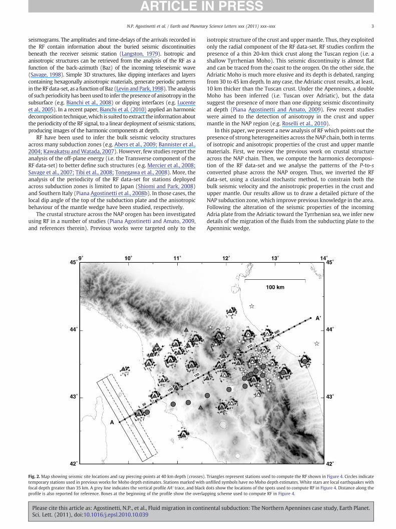
Fig. 2. Map showing seismic site locations and ray piercing-points at 40 km depth (crosses).temporary stations used in previous works for Moho depth estimates. Stations marked withfocal depth greater than 35 km. A grey line indicates the vertical profile AA′ trace, and blackprofile is also reported for reference. Boxes at the beginning of the profile show the overlap

Please cite this article as: Agostinetti, N.P., et al., Fluid migration in continSci. Lett. (2011), doi:10.1016/j.epsl.2010.10.039

isotropic structure of the crust and upper mantle. Thus, they exploitedonly the radial component of the RF data-set. RF studies confirm thepresence of a thin 20-km thick crust along the Tuscan region (i.e. ashallow Tyrrhenian Moho). This seismic discontinuity is almost flatand can be traced from the coast to the orogen. On the other side, theAdriatic Moho is much more elusive and its depth is debated, rangingfrom 30 to 45 km depth. In any case, the Adriatic crust results, at least,10 km thicker than the Tuscan crust. Under the Apennines, a doubleMoho has been inferred (i.e. Tuscan over Adriatic), but the datasuggest the presence of more than one dipping seismic discontinuityat depth (Piana Agostinetti and Amato, 2009). Few recent studieswere aimed to the detection of anisotropy in the crust and uppermantle in the NAP region (e.g. Roselli et al., 2010).

In this paper, we present a new analysis of RF which points out thepresence of strong heterogeneities across the NAP chain, both in termsof isotropic and anisotropic properties of the crust and upper mantlematerials. First, we review the previous work on crustal structureacross the NAP chain. Then, we compute the harmonics decomposi-tion of the RF data-set and we analyse the patterns of the P-to-sconverted phase across the NAP orogen. Thus, we inverted the RFdata-set, using a classical stochastic method, to constrain both thebulk seismic velocity and the anisotropic properties in the crust andupper mantle. Our results allow us to draw a detailed picture of theNAP subduction zone, which improve previous knowledge in the area.Following the alteration of the seismic properties of the incomingAdria plate from the Adriatic toward the Tyrrhenian sea, we infer newdetails of the migration of the fluids from the subducting plate to theApenninic wedge.

Triangles represent stations used to compute the RF shown in Figure 4. Circles indicateunfilled symbols have no Moho depth estimates. White stars are local earthquakes withdots show the locations of the spots used to compute RF in Figure 4. Distance along theping scheme used to compute RF in Figure 4.

ental subduction: The Northern Apennines case study, Earth Planet.

4 N.P. Agostinetti et al. / Earth and Planetary Science Letters xxx (2011) xxx–xxx

2. Data and methods

2.1. Data processing for RF harmonic decomposition

In this study, we analyse teleseismic records from both temporaryand permanent broadband seismic stations (Fig. 2) deployed acrossthe northern part of the Italian peninsula, from the Tyrrhenian to theAdriatic coast. Here, we briefly review the data selection and analysis.

Teleseisms are selected based on their magnitude (MwN=5.5) andepicentral distance (Δ, 30bΔb100). After a first visual inspection,throughwhichwe exclude seismic waveformswith a low s/n ratio, weobtain a data-set of about 15,000 3-component records, with aminimum of 120 and a maximum of 670 records for each station. Werotate teleseismic records in the LQT system, where L is the theoreticaldirection of the incoming P-wave-field, Q is computed along the greatcircle path from the source to the station and normal to Q, and T is thenormal to the QL plane, positive 90∘ CW from L. Then, we computedthe RF data-set using the multitaper correlation code developed byPark and Levin (2000), with a cut-off frequency of 0.5 Hz. To highlightthe main variation of the seismic structure under the NAP chain, theRF data-set is projected along a N60∘ profile which is locally normal tothe strike of the orogen. We filter our RF data-set using a box-shapedmoving window of 10 km half-width, 50% overlapping scheme andwe obtain an ensemble of evenly spaced “spots” of RF. For each spot,both radial (Q) and transverse (T) components, are analysed in termsof their periodicity as a function of the incoming P-wave back-azimuth(Baz). This analysis consists of a decomposition of the P-to-sconverted wave-field in five terms. A first term represents the P-to-sconverted energy from isotropic velocity jumps, which is independentfrom the back-azimuth of the incomingwave-field. Two terms containthe converted energywhich displays a 2π periodicity with Baz, for twonormal directions (i.e. N–S and E–W), while the last two terms displaythe variability of the RF with a π periodicity along two normaldirections. We refer to Bianchi et al. (2010) for a detailed descriptionof the decomposition method. Here, we summarise the importance ofsuch decomposition. For a horizontal seismic discontinuity betweentwo isotropic media, the P-to-s converted energy will be displayedonly on the first term, while the other four terms should be zero. For adipping discontinuity, or for a horizontal discontinuity betweenanisotropic media with plunging symmetry axis, the energy will bemainly distributed between the first three terms. Finally, for ahorizontal discontinuity between anisotropic media with horizontalsymmetry axis, the energy will be found in the first term and in thelast two (see Bianchi et al. (2010, Fig. S1) for detailed examples). Asclearly reported in Bianchi et al. (2010), the analysis of thedecomposition of the RF data-set allows to separate effects due todifferent heterogeneities, giving a fundamental support to theinterpretation of a RF data-set in complex geodynamic settings likethe Northern Apennines. Here we follow Bianchi et al. (2010) and wefocus our data-set on the 20–70 km depth range, where we expectthat the Apennines wedge develops. This depth range fills a gapbetween local earthquakes and teleseismic tomography, unravellingpeculiar details of the seismic structures which could elude otherkinds of seismic investigations.

2.2. RF inversion

To extract precise information on the seismic properties at depth,we apply a classical stochastic method to invert our decomposed RFdata-set. We follow the approach developed in Sambridge (1999) andwe implemented a global search in the parameter space, from whichwe obtain an ensemble of good data-fitting models. (R1.6) Here, webriefly outline the main steps of this method. Our parametrisationcomprises both dipping planar interfaces and anisotropic layers.Forward modeling is achieved using the method presented inFrederiksen and Bostock (2000). (R2.4) For each spot, forward

Please cite this article as: Agostinetti, N.P., et al., Fluid migration in continSci. Lett. (2011), doi:10.1016/j.epsl.2010.10.039

modelling is computed using the back-azimuth and the slowness ofthe RF in the observed data-set. Following Bianchi et al. (2010), wedivide the profile in three areas, adopting a peculiar parametrisationfor each region. Then, we follow a two step approach. First, theclassical Neighbourhood Algorithm inversion is applied (as in Bianchiet al., 2008) to retrieve the bulk properties for each single spot of ourdata-set. Both isotropic and anisotropic (if present) properties areinvestigated at the same time and a single best-fit model isindividuated for each spot. (R1.6) Second, for each different region,the seismic velocities of the different subsurface structures (i.e. thecrust, the mantle wedge the subducted Adriatic crust and the uppermantle) retrieved in best-fit models are averaged. At this point, weperform a second run of the Neighbouhood Algorithm inversion usingthe mean seismic values obtained from the first inversion andsearching for the depth of the interfaces and the anisotropicparameters of the buried body. (R1.6) Formal errors on the invertedparameters are estimated from the best-fit family of sampled models.Best-fit family comprises models which obtained a fit less than 1.2times the best-fit model fit. For the elastic parameters, we computederrors from the best-fit families obtained during the first step of theinversion, while for the depths of the interfaces and the anisotropyparameters, errors are evaluated from the best-fit families of thesecond inversion step. For each parameter, minimum and maximumvalues are extracted from the best-fit family and the half-width oftheir difference is used as error estimate. For the depth parameters,we find that a conservative value for the uncertainty is ±5 km, even ifwe observe an increase of the uncertainties for the deeper interfaces.We associate a ±0.2 km/s uncertainty to the S-velocity parameters.The error on VP/VS ratio is estimated as large as ±0.03. Anisotropicpercentage and the axis direction angles are estimated with errors aslarge as ±2% and ±5∘, respectively.

3. Results

3.1. Review of previous RF studies and local seismicity

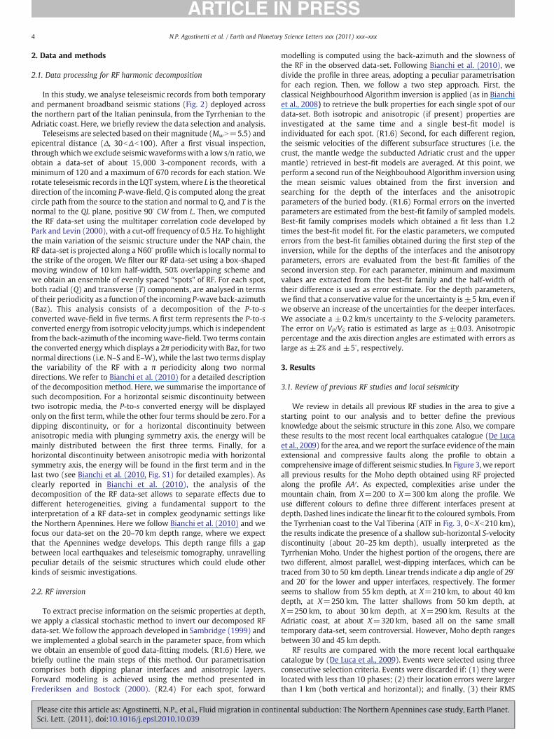
We review in details all previous RF studies in the area to give astarting point to our analysis and to better define the previousknowledge about the seismic structure in this zone. Also, we comparethese results to the most recent local earthquakes catalogue (De Lucaet al., 2009) for the area, andwe report the surface evidence of themainextensional and compressive faults along the profile to obtain acomprehensive image of different seismic studies. In Figure 3, we reportall previous results for the Moho depth obtained using RF projectedalong the profile AA′. As expected, complexities arise under themountain chain, from X=200 to X=300 km along the profile. Weuse different colours to define three different interfaces present atdepth. Dashed lines indicate the linear fit to the coloured symbols. Fromthe Tyrrhenian coast to the Val Tiberina (ATF in Fig. 3, 0bXb210 km),the results indicate the presence of a shallow sub-horizontal S-velocitydiscontinuity (about 20–25 km depth), usually interpreted as theTyrrhenian Moho. Under the highest portion of the orogens, there aretwo different, almost parallel, west-dipping interfaces, which can betraced from 30 to 50 km depth. Linear trends indicate a dip angle of 29∘

and 20∘ for the lower and upper interfaces, respectively. The formerseems to shallow from 55 km depth, at X=210 km, to about 40 kmdepth, at X=250 km. The latter shallows from 50 km depth, atX=250 km, to about 30 km depth, at X=290 km. Results at theAdriatic coast, at about X=320 km, based all on the same smalltemporary data-set, seem controversial. However, Moho depth rangesbetween 30 and 45 km depth.

RF results are compared with the more recent local earthquakecatalogue by (De Luca et al., 2009). Events were selected using threeconsecutive selection criteria. Events were discarded if: (1) they werelocated with less than 10 phases; (2) their location errors were largerthan 1 km (both vertical and horizontal); and finally, (3) their RMS

ental subduction: The Northern Apennines case study, Earth Planet.

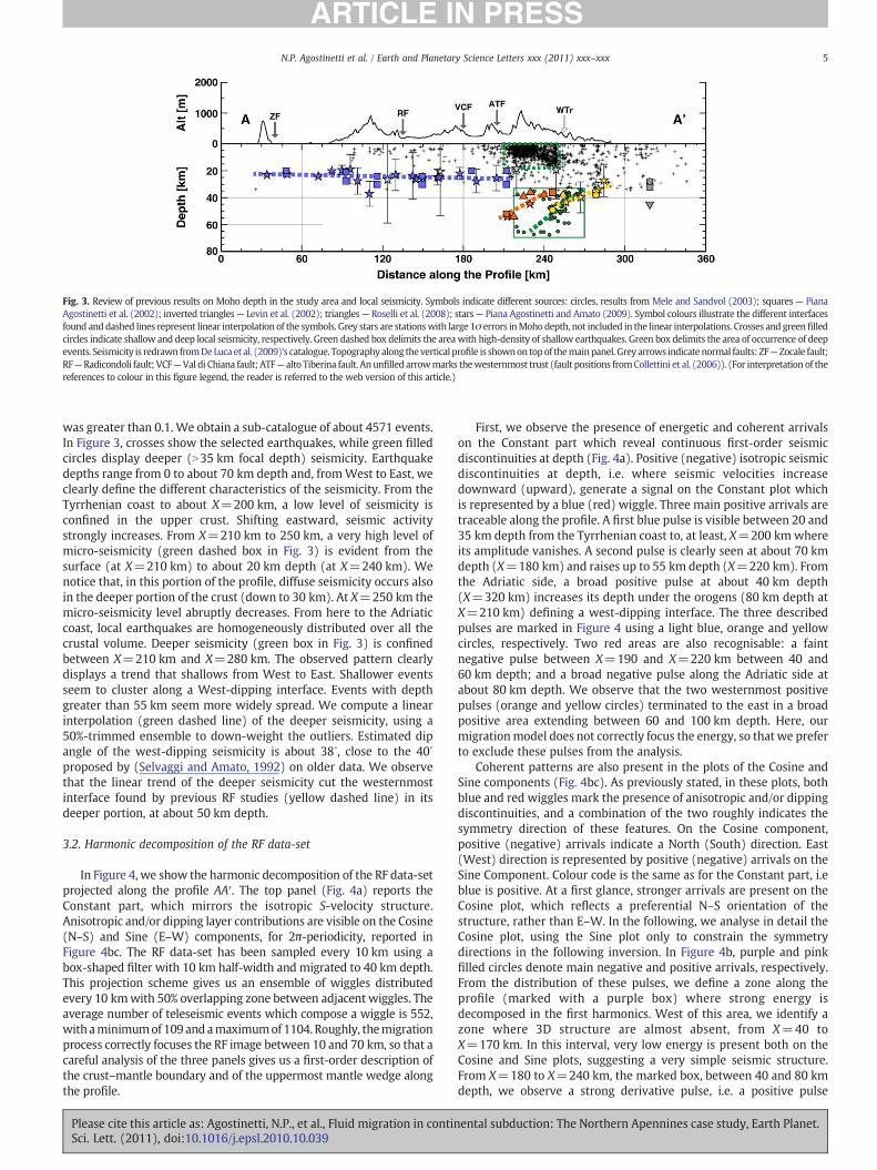
Fig. 3. Review of previous results on Moho depth in the study area and local seismicity. Symbols indicate different sources: circles, results from Mele and Sandvol (2003); squares — PianaAgostinetti et al. (2002); inverted triangles— Levin et al. (2002); triangles— Roselli et al. (2008); stars— Piana Agostinetti and Amato (2009). Symbol colours illustrate the different interfacesfound anddashed lines represent linear interpolation of the symbols. Grey stars are stationswith large 1σ errors inMohodepth, not included in the linear interpolations. Crosses and greenfilledcircles indicate shallow and deep local seismicity, respectively. Green dashed box delimits the areawith high-density of shallow earthquakes. Green box delimits the area of occurrence of deepevents. Seismicity is redrawn fromDeLuca et al. (2009)'s catalogue. Topographyalong thevertical profile is shownon topof themainpanel.Greyarrows indicate normal faults: ZF—Zocale fault;RF—Radicondoli fault; VCF—Val di Chiana fault; ATF— alto Tiberina fault. Anunfilled arrowmarks thewesternmost trust (fault positions fromCollettini et al. (2006)). (For interpretation of thereferences to colour in this figure legend, the reader is referred to the web version of this article.)

5N.P. Agostinetti et al. / Earth and Planetary Science Letters xxx (2011) xxx–xxx

was greater than 0.1. We obtain a sub-catalogue of about 4571 events.In Figure 3, crosses show the selected earthquakes, while green filledcircles display deeper (N35 km focal depth) seismicity. Earthquakedepths range from 0 to about 70 km depth and, fromWest to East, weclearly define the different characteristics of the seismicity. From theTyrrhenian coast to about X=200 km, a low level of seismicity isconfined in the upper crust. Shifting eastward, seismic activitystrongly increases. From X=210 km to 250 km, a very high level ofmicro-seismicity (green dashed box in Fig. 3) is evident from thesurface (at X=210 km) to about 20 km depth (at X=240 km). Wenotice that, in this portion of the profile, diffuse seismicity occurs alsoin the deeper portion of the crust (down to 30 km). At X=250 km themicro-seismicity level abruptly decreases. From here to the Adriaticcoast, local earthquakes are homogeneously distributed over all thecrustal volume. Deeper seismicity (green box in Fig. 3) is confinedbetween X=210 km and X=280 km. The observed pattern clearlydisplays a trend that shallows from West to East. Shallower eventsseem to cluster along a West-dipping interface. Events with depthgreater than 55 km seem more widely spread. We compute a linearinterpolation (green dashed line) of the deeper seismicity, using a50%-trimmed ensemble to down-weight the outliers. Estimated dipangle of the west-dipping seismicity is about 38∘, close to the 40∘

proposed by (Selvaggi and Amato, 1992) on older data. We observethat the linear trend of the deeper seismicity cut the westernmostinterface found by previous RF studies (yellow dashed line) in itsdeeper portion, at about 50 km depth.

3.2. Harmonic decomposition of the RF data-set

In Figure 4, we show the harmonic decomposition of the RF data-setprojected along the profile AA′. The top panel (Fig. 4a) reports theConstant part, which mirrors the isotropic S-velocity structure.Anisotropic and/or dipping layer contributions are visible on the Cosine(N–S) and Sine (E–W) components, for 2π-periodicity, reported inFigure 4bc. The RF data-set has been sampled every 10 km using abox-shaped filter with 10 km half-width and migrated to 40 km depth.This projection scheme gives us an ensemble of wiggles distributedevery 10 kmwith 50% overlapping zone between adjacent wiggles. Theaverage number of teleseismic events which compose a wiggle is 552,with aminimumof 109 and amaximumof 1104. Roughly, themigrationprocess correctly focuses the RF image between 10 and 70 km, so that acareful analysis of the three panels gives us a first-order description ofthe crust–mantle boundary and of the uppermost mantle wedge alongthe profile.

Please cite this article as: Agostinetti, N.P., et al., Fluid migration in continSci. Lett. (2011), doi:10.1016/j.epsl.2010.10.039

First, we observe the presence of energetic and coherent arrivalson the Constant part which reveal continuous first-order seismicdiscontinuities at depth (Fig. 4a). Positive (negative) isotropic seismicdiscontinuities at depth, i.e. where seismic velocities increasedownward (upward), generate a signal on the Constant plot whichis represented by a blue (red) wiggle. Three main positive arrivals aretraceable along the profile. A first blue pulse is visible between 20 and35 km depth from the Tyrrhenian coast to, at least, X=200 kmwhereits amplitude vanishes. A second pulse is clearly seen at about 70 kmdepth (X=180 km) and raises up to 55 km depth (X=220 km). Fromthe Adriatic side, a broad positive pulse at about 40 km depth(X=320 km) increases its depth under the orogens (80 km depth atX=210 km) defining a west-dipping interface. The three describedpulses are marked in Figure 4 using a light blue, orange and yellowcircles, respectively. Two red areas are also recognisable: a faintnegative pulse between X=190 and X=220 km between 40 and60 km depth; and a broad negative pulse along the Adriatic side atabout 80 km depth. We observe that the two westernmost positivepulses (orange and yellow circles) terminated to the east in a broadpositive area extending between 60 and 100 km depth. Here, ourmigrationmodel does not correctly focus the energy, so that we preferto exclude these pulses from the analysis.

Coherent patterns are also present in the plots of the Cosine andSine components (Fig. 4bc). As previously stated, in these plots, bothblue and red wiggles mark the presence of anisotropic and/or dippingdiscontinuities, and a combination of the two roughly indicates thesymmetry direction of these features. On the Cosine component,positive (negative) arrivals indicate a North (South) direction. East(West) direction is represented by positive (negative) arrivals on theSine Component. Colour code is the same as for the Constant part, i.eblue is positive. At a first glance, stronger arrivals are present on theCosine plot, which reflects a preferential N–S orientation of thestructure, rather than E–W. In the following, we analyse in detail theCosine plot, using the Sine plot only to constrain the symmetrydirections in the following inversion. In Figure 4b, purple and pinkfilled circles denote main negative and positive arrivals, respectively.From the distribution of these pulses, we define a zone along theprofile (marked with a purple box) where strong energy isdecomposed in the first harmonics. West of this area, we identify azone where 3D structure are almost absent, from X=40 toX=170 km. In this interval, very low energy is present both on theCosine and Sine plots, suggesting a very simple seismic structure.From X=180 to X=240 km, the marked box, between 40 and 80 kmdepth, we observe a strong derivative pulse, i.e. a positive pulse

ental subduction: The Northern Apennines case study, Earth Planet.

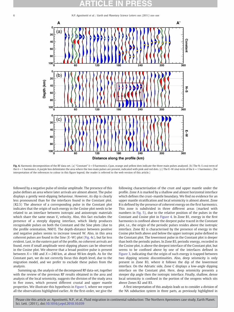
Fig. 4. Harmonic decomposition of the RF data-set. (a) “Constant” k=0 harmonics. Cyan, orange and yellow dots indicate the three main pulses analysed. (b) The N–S cosϕ term ofthe k=1 harmonics. A purple box delimitates the area where the two main pulses are present, indicated with pink and red dots. (c) The E–W sinϕ term of the k=1 harmonics. (Forinterpretation of the references to colour in this figure legend, the reader is referred to the web version of this article.)

6 N.P. Agostinetti et al. / Earth and Planetary Science Letters xxx (2011) xxx–xxx

followed by a negative pulse of similar amplitude. The presence of thispulse defines an area where later arrivals are almost absent. The pulsedisplays a gently west-dipping behaviour. However, its dip is clearlyless pronounced than for the interfaces found in the Constant plot.(R2.5) The absence of a corresponding pulse in the Constant plotindicates that the origin of such energy in the Cosine plot needs to berelated to an interface between isotropic and anisotropic materialswhich share the same mean Vs velocity. Also, this fact excludes thepresence of a steeply dipping interface, which likely producesrecognisable pulses on both the Constant and the Sine plots (due tothe profile orientation, N60∘E. The depth-distance between positiveand negative pulses seems to increase toward W. Also, in this areacoherent pulses are found in the Sine (E–W) plot (Fig. 4c), but far lessevident. Last, in the eastern part of the profile, no coherent arrivals arefound, even if small amplitude west-dipping phases can be observedin the Cosine plot. We observe that a broad positive pulse is presentbetween X=180 and X=240 km, at about 90 km depth. As for theConstant part, we do not correctly focus this depth level, due to themigration model, and we prefer to exclude these pulses from theanalysis.

Summing up, the analysis of the decomposed RF data-set, togetherwith the review of the previous RF results obtained in the area andanalysis of the local seismicity, suggests the division of the study areain five zones, which present different crustal and upper mantleproperties. We illustrate this hypothesis in Figure 5, where we reportall the observations highlighted earlier. At the first-order, we give the

Please cite this article as: Agostinetti, N.P., et al., Fluid migration in continSci. Lett. (2011), doi:10.1016/j.epsl.2010.10.039

following characterisation of the crust and upper mantle under theprofile. Zone A is marked by a shallow and almost horizontal interfacewhich defines the crust–mantle boundary. We find no evidence for anupper mantle stratification and local seismicity is almost absent. ZoneB is defined by the presence of coherent energy on the first harmonics.This zone is subdivided in three different areas (marked withnumbers in Fig. 5), due to the relative position of the pulses in theConstant and Cosine plot in Figure 4. In Zone B1, energy in the firstharmonics is confined above the deepest pulse traced in the Constantplot, i.e., the origin of the periodic pulses resides above the isotropicinterface. Zone B2 is characterised by the presence of energy in theCosine plot both above and below the upper isotropic pulse defined inthe Constant plot. The lowermost pulse in the Constant plot is deeperthan both the periodic pulses. In Zone B3, periodic energy, recorded inthe Cosine plot, is above the deepest interface of the Constant plot, butseems to be confined above by one of the interfaces defined inFigure 3, indicating that the origin of such energy is trapped betweentwo dipping seismic discontinuities. Also, deep seismicity is onlypresent in Zone B3, where it follows the dip of the lowermostinterface. On the Adriatic side, Zone C displays a low-angle dippinginterface on the Constant plot. Here, deep seismicity presents asteeper dip angle then the isotropic interface. Finally, shallow, denselocal seismicity is confined in the portion of the orogens which sitsabove Zones B2 and B3.

A first interpretation of this analysis leads us to consider a division ofthe NA subduction system in three parts, as previously highlighted in

ental subduction: The Northern Apennines case study, Earth Planet.

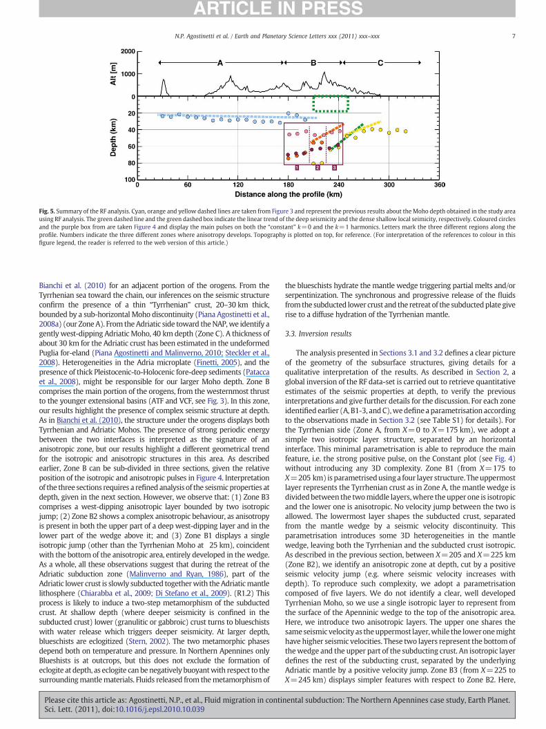
Fig. 5. Summary of the RF analysis. Cyan, orange and yellow dashed lines are taken from Figure 3 and represent the previous results about the Moho depth obtained in the study areausing RF analysis. The green dashed line and the green dashed box indicate the linear trend of the deep seismicity and the dense shallow local seimicity, respectively. Coloured circlesand the purple box from are taken Figure 4 and display the main pulses on both the “constant” k=0 and the k=1 harmonics. Letters mark the three different regions along theprofile. Numbers indicate the three different zones where anisotropy develops. Topography is plotted on top, for reference. (For interpretation of the references to colour in thisfigure legend, the reader is referred to the web version of this article.)

7N.P. Agostinetti et al. / Earth and Planetary Science Letters xxx (2011) xxx–xxx

Bianchi et al. (2010) for an adjacent portion of the orogens. From theTyrrhenian sea toward the chain, our inferences on the seismic structureconfirm the presence of a thin “Tyrrhenian” crust, 20–30 km thick,bounded by a sub-horizontal Moho discontinuity (Piana Agostinetti et al.,2008a) (our ZoneA). From theAdriatic side toward theNAP,we identify agently west-dipping Adriatic Moho, 40 km depth (Zone C). A thickness ofabout 30 km for the Adriatic crust has been estimated in the undeformedPuglia for-eland (Piana Agostinetti and Malinverno, 2010; Steckler et al.,2008). Heterogeneities in the Adria microplate (Finetti, 2005), and thepresence of thick Pleistocenic-to-Holocenic fore-deep sediments (Pataccaet al., 2008), might be responsible for our larger Moho depth. Zone Bcomprises the main portion of the orogens, from the westernmost thrustto the younger extensional basins (ATF and VCF, see Fig. 3). In this zone,our results highlight the presence of complex seismic structure at depth.As in Bianchi et al. (2010), the structure under the orogens displays bothTyrrhenian and Adriatic Mohos. The presence of strong periodic energybetween the two interfaces is interpreted as the signature of ananisotropic zone, but our results highlight a different geometrical trendfor the isotropic and anisotropic structures in this area. As describedearlier, Zone B can be sub-divided in three sections, given the relativeposition of the isotropic and anisotropic pulses in Figure 4. Interpretationof the three sections requires a refinedanalysis of the seismicproperties atdepth, given in the next section. However, we observe that: (1) Zone B3comprises a west-dipping anisotropic layer bounded by two isotropicjump; (2) Zone B2 shows a complex anisotropic behaviour, as anisotropyis present in both the upper part of a deep west-dipping layer and in thelower part of the wedge above it; and (3) Zone B1 displays a singleisotropic jump (other than the Tyrrhenian Moho at 25 km), coincidentwith the bottom of the anisotropic area, entirely developed in the wedge.As a whole, all these observations suggest that during the retreat of theAdriatic subduction zone (Malinverno and Ryan, 1986), part of theAdriatic lower crust is slowly subducted togetherwith theAdriaticmantlelithosphere (Chiarabba et al., 2009; Di Stefano et al., 2009). (R1.2) Thisprocess is likely to induce a two-step metamorphism of the subductedcrust. At shallow depth (where deeper seismicity is confined in thesubducted crust) lower (granulitic or gabbroic) crust turns to blueschistswith water release which triggers deeper seismicity. At larger depth,blueschists are eclogitized (Stern, 2002). The two metamorphic phasesdepend both on temperature and pressure. In Northern Apennines onlyBlueshists is at outcrops, but this does not exclude the formation ofeclogite at depth, as eclogite canbenegatively buoyantwith respect to thesurroundingmantlematerials. Fluids released from themetamorphism of

Please cite this article as: Agostinetti, N.P., et al., Fluid migration in continSci. Lett. (2011), doi:10.1016/j.epsl.2010.10.039

the blueschists hydrate the mantle wedge triggering partial melts and/orserpentinization. The synchronous and progressive release of the fluidsfromthe subducted lower crust and the retreat of the subductedplate giverise to a diffuse hydration of the Tyrrhenian mantle.

3.3. Inversion results

The analysis presented in Sections 3.1 and 3.2 defines a clear pictureof the geometry of the subsurface structures, giving details for aqualitative interpretation of the results. As described in Section 2, aglobal inversion of the RF data-set is carried out to retrieve quantitativeestimates of the seismic properties at depth, to verify the previousinterpretations and give further details for the discussion. For each zoneidentified earlier (A, B1-3, andC),wedefineaparametrisation accordingto the observations made in Section 3.2 (see Table S1) for details). Forthe Tyrrhenian side (Zone A, from X=0 to X=175 km), we adopt asimple two isotropic layer structure, separated by an horizontalinterface. This minimal parametrisation is able to reproduce the mainfeature, i.e. the strong positive pulse, on the Constant plot (see Fig. 4)without introducing any 3D complexity. Zone B1 (from X=175 toX=205 km) is parametrisedusinga four layer structure. Theuppermostlayer represents the Tyrrhenian crust as in Zone A, the mantle wedge isdividedbetween the twomiddle layers,where theupper one is isotropicand the lower one is anisotropic. No velocity jump between the two isallowed. The lowermost layer shapes the subducted crust, separatedfrom the mantle wedge by a seismic velocity discontinuity. Thisparametrisation introduces some 3D heterogeneities in the mantlewedge, leaving both the Tyrrhenian and the subducted crust isotropic.As described in the previous section, between X=205 and X=225 km(Zone B2), we identify an anisotropic zone at depth, cut by a positiveseismic velocity jump (e.g. where seismic velocity increases withdepth). To reproduce such complexity, we adopt a parametrisationcomposed of five layers. We do not identify a clear, well developedTyrrhenian Moho, so we use a single isotropic layer to represent fromthe surface of the Apenninic wedge to the top of the anisotropic area.Here, we introduce two anisotropic layers. The upper one shares thesameseismic velocity as theuppermost layer,while the loweronemighthave higher seismic velocities. These two layers represent the bottomofthewedge and the upper part of the subducting crust. An isotropic layerdefines the rest of the subducting crust, separated by the underlyingAdriatic mantle by a positive velocity jump. Zone B3 (from X=225 toX=245 km) displays simpler features with respect to Zone B2. Here,

ental subduction: The Northern Apennines case study, Earth Planet.

8 N.P. Agostinetti et al. / Earth and Planetary Science Letters xxx (2011) xxx–xxx

anisotropy is confined in the entire subducting crust. A three layerparametrisation is adopted. The uppermost layer represents theApenninic wedge; a second anisotropic layer is introduced at its bottomwithout a seismic velocity jump between the two layers. Finally ahalf-space represents the subducting Adriaticmantle. From X=245 kmto the Adriatic sea (Zone C), we identify a single seismic discontinuity,andwe adopt here the same parametrisation as for the Tyrrhenian side.

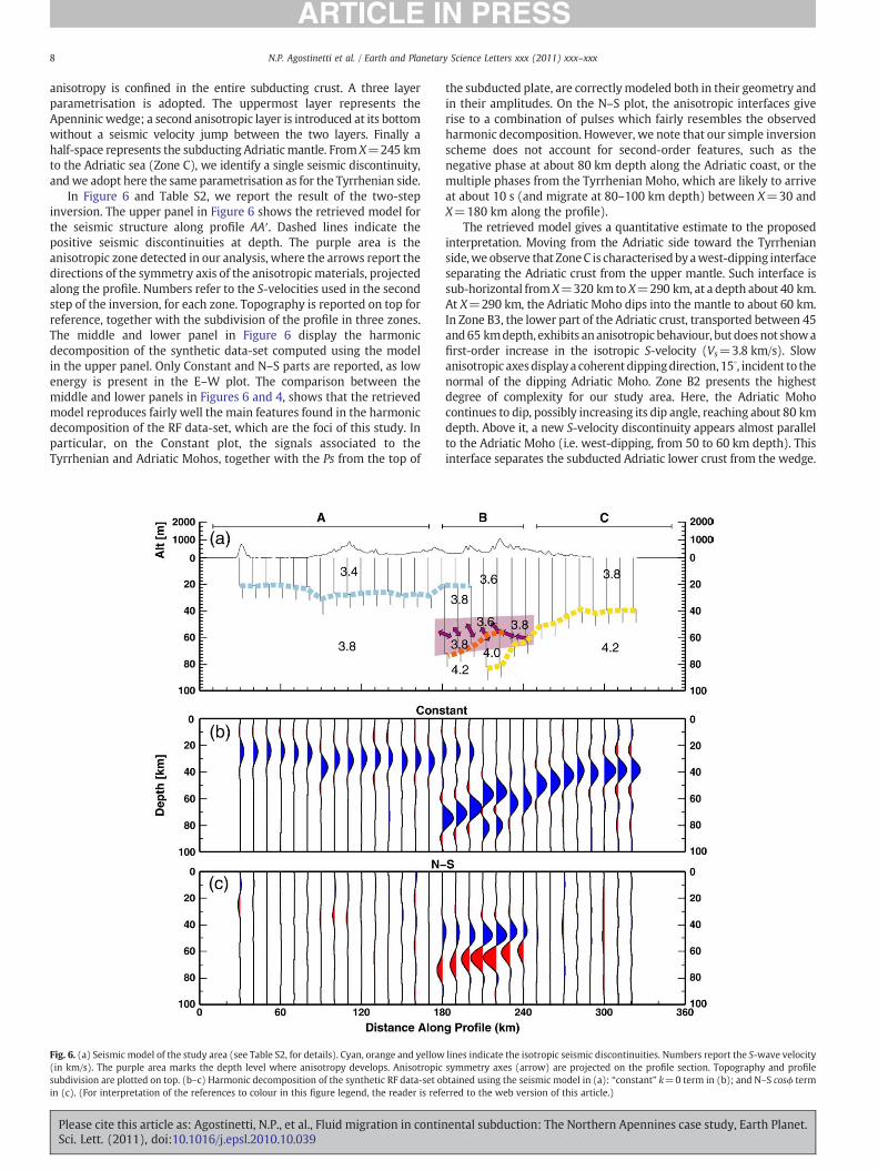
In Figure 6 and Table S2, we report the result of the two-stepinversion. The upper panel in Figure 6 shows the retrieved model forthe seismic structure along profile AA′. Dashed lines indicate thepositive seismic discontinuities at depth. The purple area is theanisotropic zone detected in our analysis, where the arrows report thedirections of the symmetry axis of the anisotropic materials, projectedalong the profile. Numbers refer to the S-velocities used in the secondstep of the inversion, for each zone. Topography is reported on top forreference, together with the subdivision of the profile in three zones.The middle and lower panel in Figure 6 display the harmonicdecomposition of the synthetic data-set computed using the modelin the upper panel. Only Constant and N–S parts are reported, as lowenergy is present in the E–W plot. The comparison between themiddle and lower panels in Figures 6 and 4, shows that the retrievedmodel reproduces fairly well the main features found in the harmonicdecomposition of the RF data-set, which are the foci of this study. Inparticular, on the Constant plot, the signals associated to theTyrrhenian and Adriatic Mohos, together with the Ps from the top of

Fig. 6. (a) Seismic model of the study area (see Table S2, for details). Cyan, orange and yellow(in km/s). The purple area marks the depth level where anisotropy develops. Anisotropicsubdivision are plotted on top. (b–c) Harmonic decomposition of the synthetic RF data-set oin (c). (For interpretation of the references to colour in this figure legend, the reader is refe

Please cite this article as: Agostinetti, N.P., et al., Fluid migration in continSci. Lett. (2011), doi:10.1016/j.epsl.2010.10.039

the subducted plate, are correctlymodeled both in their geometry andin their amplitudes. On the N–S plot, the anisotropic interfaces giverise to a combination of pulses which fairly resembles the observedharmonic decomposition. However, we note that our simple inversionscheme does not account for second-order features, such as thenegative phase at about 80 km depth along the Adriatic coast, or themultiple phases from the Tyrrhenian Moho, which are likely to arriveat about 10 s (and migrate at 80–100 km depth) between X=30 andX=180 km along the profile).

The retrieved model gives a quantitative estimate to the proposedinterpretation. Moving from the Adriatic side toward the Tyrrhenianside,we observe that ZoneC is characterisedby awest-dipping interfaceseparating the Adriatic crust from the upper mantle. Such interface issub-horizontal from X=320 km to X=290 km, at a depth about 40 km.At X=290 km, the Adriatic Moho dips into the mantle to about 60 km.In Zone B3, the lower part of the Adriatic crust, transported between 45and65 kmdepth, exhibits ananisotropic behaviour, but does not showafirst-order increase in the isotropic S-velocity (Vs=3.8 km/s). Slowanisotropic axesdisplaya coherent dippingdirection, 15∘, incident to thenormal of the dipping Adriatic Moho. Zone B2 presents the highestdegree of complexity for our study area. Here, the Adriatic Mohocontinues to dip, possibly increasing its dip angle, reaching about 80 kmdepth. Above it, a new S-velocity discontinuity appears almost parallelto the Adriatic Moho (i.e. west-dipping, from 50 to 60 km depth). Thisinterface separates the subducted Adriatic lower crust from the wedge.

lines indicate the isotropic seismic discontinuities. Numbers report the S-wave velocitysymmetry axes (arrow) are projected on the profile section. Topography and profilebtained using the seismic model in (a): “constant” k=0 term in (b); and N–S cosϕ termrred to the web version of this article.)

ental subduction: The Northern Apennines case study, Earth Planet.

9N.P. Agostinetti et al. / Earth and Planetary Science Letters xxx (2011) xxx–xxx

S-velocity increases, with respect to Zone B1, in the subducted lower-crust to4.0 km/s,while thewedgealmostmaintains themean S-velocityof the Adriatic crust. Anisotropy is still confined between 45 and 65 kmdepth, but now it developsbetween thewedge and the subducted lowercrust. Anisotropic axes are almost normal to the isotropic dippinginterfaces. In Zone B1, the Tyrrhenian Moho appears as a shallowinterface at about 20 km depth. The wedge is composed of an isotropicupper zone (20–25 km thick) and an anisotropic lower zone (25–30 kmthick), above the subducted Adriatic lower crust. The upper interface ofthe subducted lower crust dips towardW, from 65 to 75 km depth. TheTyrrhenian crust is characterised by a low S-velocity (3.4 km/s).S-velocity increases in the wedge to 3.8 km/s. The subducted Adriaticlower crust displays a seismic S-velocitywhich equals the velocity in theAdriatic lithospheric mantle (about 4.2 km/s), so that its lowerboundary results undefined. Anisotropy develops between 40 and70 km depth, a slightly wider depth interval than in Zones B2 and B3.Anisotropic axes shift their directions, from almost normal to thesubducted Adriatic crust (at about X=220 km) to a more horizontaltrend (at about X=180 km). Finally, for Zone A (the Tyrrhenian side),the inversion confirms the presence of a sub-horizontal interface,separating a thin crust (20–30 km thick), characterised by low value ofthe mean S-velocity (3.4 km/s), from a low S-velocity upper mantle(3.8 km/s).

3.4. Interpretation

The inversion result gives a quantitative basis to our interpretation,both in term of interface depth and seismic velocity at depth. Here, wepoint out three key aspects of our results: the wedge, the subductedlower crust and the anisotropy. Focusing on the wedge, which developsin Zones B2 and B3, we observe that the S-velocity increases from E(3.6 km/s in Zone B2) toward W (3.8 km/s in Zone B1). At shallowdepth, the wedge is composed of sediments and crustal slicesoff-scraped from the subducting plate (called crustal wedge orApenninic wedge), while at larger depth sublithospheric upper mantlematerialsmight be involved (indicated aswedge nose ormantlewedge,(Scrocca et al., 2007)). We do not identify a clear jump in the seismicproperties of the wedge at depth, which might be a candidate for suchtransition (from crustal wedge to mantle wedge). This fact suggests agradual transition between the two. Shifting our attention to thesubducted lower crust, its seismic properties change following the samescheme as in the wedge (i.e. S-velocity increases from E toward W).However, S-velocity reaches higher values at relatively shallow depth(70–80 km depth). Considering a mean dip angle of about 30∘, thethickness of the subducted lower crust ranges from 15 to 20 km.

A well defined anisotropic depth level is found under the orogen.Anisotropy starts to develop at about X=240 km and persists at leastat about X=180 km. The minimum and maximum depths of the

Fig. 7. Sketch for the prop

Please cite this article as: Agostinetti, N.P., et al., Fluid migration in continSci. Lett. (2011), doi:10.1016/j.epsl.2010.10.039

anisotropy are almost constant along the profile, at about 45 and65 km depth, respectively. The depth of the lower boundary slightlyincreases in its western termination, where the upper boundaryseems to shallow. Anisotropic axes display an almost trench-normalorientation with coherent patterns in the different parts of theanisotropic zone. Anisotropy percentage is as high as about 7%, whichreflects the presence of highly anisotropic materials (Hacker et al.,2003). Clearly, the anisotropy does not follow the isotropic structurespreviously illustrated (i.e. it is not trapped in the subducted lowercrust nor develops exclusively in the mantle wedge). While theS-velocity evolution gives insights into the metamorphism of thesubducted crustal materials, the evolution of the anisotropy seems toilluminate a different process related to the transformation of suchmaterials, (R1.3) such as lattice preferred orientation (LPO) of olivine,or alignment of melt inclusions.

4. Discussion

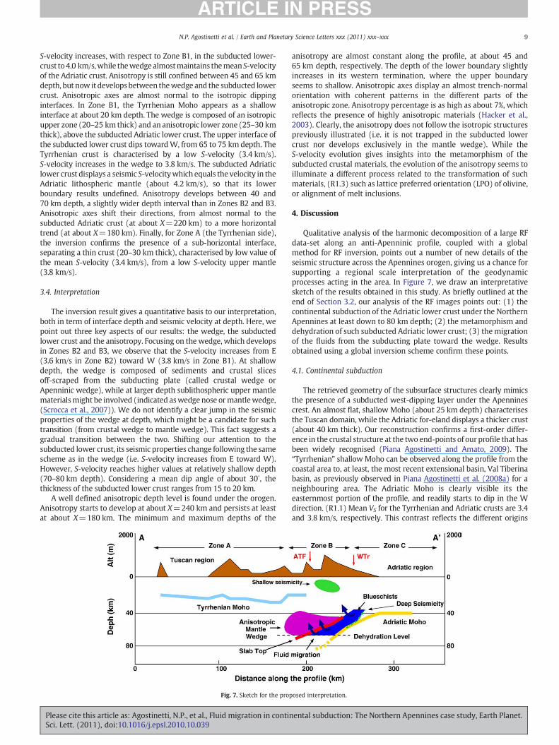
Qualitative analysis of the harmonic decomposition of a large RFdata-set along an anti-Apenninic profile, coupled with a globalmethod for RF inversion, points out a number of new details of theseismic structure across the Apennines orogen, giving us a chance forsupporting a regional scale interpretation of the geodynamicprocesses acting in the area. In Figure 7, we draw an interpretativesketch of the results obtained in this study. As briefly outlined at theend of Section 3.2, our analysis of the RF images points out: (1) thecontinental subduction of the Adriatic lower crust under the NorthernApennines at least down to 80 km depth; (2) the metamorphism anddehydration of such subducted Adriatic lower crust; (3) the migrationof the fluids from the subducting plate toward the wedge. Resultsobtained using a global inversion scheme confirm these points.

4.1. Continental subduction

The retrieved geometry of the subsurface structures clearly mimicsthe presence of a subducted west-dipping layer under the Apenninescrest. An almost flat, shallow Moho (about 25 km depth) characterisesthe Tuscan domain, while the Adriatic for-eland displays a thicker crust(about 40 km thick). Our reconstruction confirms a first-order differ-ence in the crustal structure at the two end-points of our profile that hasbeen widely recognised (Piana Agostinetti and Amato, 2009). The“Tyrrhenian” shallow Moho can be observed along the profile from thecoastal area to, at least, the most recent extensional basin, Val Tiberinabasin, as previously observed in Piana Agostinetti et al. (2008a) for aneighbouring area. The Adriatic Moho is clearly visible its theeasternmost portion of the profile, and readily starts to dip in the Wdirection. (R1.1) Mean VS for the Tyrrhenian and Adriatic crusts are 3.4and 3.8 km/s, respectively. This contrast reflects the different origins

osed interpretation.

ental subduction: The Northern Apennines case study, Earth Planet.

10 N.P. Agostinetti et al. / Earth and Planetary Science Letters xxx (2011) xxx–xxx

and compositions of the two crusts (Pauselli et al., 2010). Beneath theorogen, a new seismic interface develops parallel to the dipping AdriaticMoho, defininga low-velocity layerwhichplunges into themantle. Suchfeature can be observed down to 80 km depth. From the continuity ofthe Adriatic Moho, we interpret it as a part of the Adriatic lower crustthat is dragged downward with the Adriatic mantle lithosphere. Dipangle of such layer (about 30∘) is consistent with worldwide observa-tions of the dipping angle in the shallow part of subduction zones(Lallemand et al., 2005) and with the dip angle of the Wadati–Benioffplane (about 38∘). The thickness of the subducted Adriatic lower crust iscomprised between 15 and 20 km. This value is slightly larger than boththe thickness found in Chiarabba et al. (2009) and the thickness whichcan cause subduction failure (Stern, 2002), as hypothesised in Faccennaet al. (2001). More, the evidence of widespread high pressure materialsin the Tuscan domain (Brun and Faccenna, 2008) confirms that a largeportion of Adriatic crust is dragged downward during the retreat of thesubductionzone, possibly comprising slices of theupper crust (Wuet al.,2009). The amount of Adriatic crust impiled in the orogenic wedge is astill debated issue in the studies of the Apennines chain (e.g. Scroccaet al., 2005). Here, we find a thickness for the impiledmaterials of about20–25 km, which implies that part of the basement is involved in theorogen. Such interpretation is in agreement with the hypothesis of thepartial involvement of themagnetic basement in the orogenicwedge, asseen by magnetic data (Speranza and Chiappini, 2002). Also, this factdoes agree with the evidence of basement rocks found in a 5-km deepwell in the area (S. Donato), consistentwith a complete incorporation ofthe Adriatic upper crust in the orogenic wedge (Barchi et al., 1998).

4.2. Metamorphism and dehydration

Retrieved values of the seismic velocityVs in the different parts of thelow-velocity, dipping layer are consistent with the metamorphism ofthe subducted crust. The increase of the Vs in the subducted lower crustwith depth reflects its progressive transformation (Kawakatsu andWatada, 2007). (R1.2) In this study, we suggest twomainmetamorphicphases. The first occurs at shallow depth (between 40 and 60 km), theother at about 65 km depth. Possible candidate materials for the phasetransformations are: gabbro (or granulite) (VP∼3.9 km/s at 1 GPa,Christensen (1996)) to blueschists (VS∼4.0 km/s at 0.8 GPa, Fujimotoet al. (2007)), and blueschists to eclogite VSN4.4 km/s, Christensen(1996)). Granulite, more than gabbro, can explain the low-levelwidespread seismicity which has been observed in the Adriatic lowercrust (Piccinini et al., 2009). However, gabbro is likely to bear a largeramount ofwater (up to 5%H2O, (Stern, 2002)) todepth, than agranulite.Eclogite is our preferred end-member for the lower crust metamor-phism because it matches our observation due to its elevated seismicvelocity and absence of anisotropy (Christensen andMooney, 1995). Atshallow depth, the subducted lower crustal rocks are changed toblueschists, which, in turn, are transformed in eclogite at larger depths(Stern, 2002). Blueschists display a strong anisotropic behaviour, withpercentage as high as 5–10% (Fujimoto et al., 2007) and its transforma-tion to eclogite release up to 2% H2 (Hacker and Abers, 2004). Theobservation of anisotropy in the subducted crust suggests the formationof blueschists. Blueschists are awidely accepted candidatemetamorphicfaces for subductionmetamorphismand has been postulated elsewhere(Helffrich, 2000).More, high pressure continental blueschists have beenfound in the Tuscan area, after the exhumation process active in the last10–15 My (Jolivet et al., 1998).

4.3. Fluid migration in the mantle wedge

Fluidmigration in themantlewedge is testifiedby the development ofanisotropy directly above the metamorphosed, subducted lower crust(Zones B1–B2). Water which enters the mantle wedge can induce eitherpartial melting or serpentinization of peridotite. Serpentinization is oftenassociated to mantle wedge materials where low seismic velocity,

Please cite this article as: Agostinetti, N.P., et al., Fluid migration in continSci. Lett. (2011), doi:10.1016/j.epsl.2010.10.039

high-VP/VS ratio are observed (e.g Tibi et al., 2008). Serpentinizedperidotite displays an anisotropic behaviour (Dewandel et al., 2003).Partial melting of the mantle wedge can produce diffuse microlensingwhich turns out to be highly anisotropic (Takei, 2010). The anisotropiczone of the mantle wedge found in this study can indicate a strongconcentration of serpentine or partial melts. The absence of anisotropyunder the Tuscan domain can reflect both the decrease of theconcentration of the anisotropic materials and/or the breakup of theanisotropic pattern due to the asthenospheric mantle flow. The abrupttermination of the anisotropy at about 65 km depth beneath theApennines, in coincidence with the disappearance of the low-velocitylayer, defines a “dehydration level”. The low-velocity layer terminationhas been widely observed and associated to the complete transformationof the subducted lower crust to eclogite (Rondenay et al., 2008). Also,eclogite turns out to be almost isotropic (Christensen andMooney, 1995).In our case, as suggested from the clear delimitation of the anisotropy atdepth, the combination between the pressure–temperature conditionsand the slow rate of subduction generates a clear level where all theblueschists are converted to eclogite and the water is released to themantle wedge. The presence of such “dehydration level” has beenhypothesised for the breakdown of amphiboles peridotite in oceanicsubduction (Tatsumi and Eggins, 1995). The depicted scenario of fluidmigration fromthe subducted crust to themantlewedgecanbecombinedwith the long-standing observation of the retreat of the subducted plate(MalinvernoandRyan, 1986). If the “dehydration level”hasbeen constantduring the last ∼10 My, the fluids escaped from the Adriatic crust did notconcentrate in a single point of our profile (i.e. generating the classical“arc” magmatisms) but more likely hydrated all the Tyrrhenianuppermost mantle forming an hydrate mantle layer. This hypothesis isconfirmed by the presence of diffuse attenuation in the upper portion ofthe Tyrrhenianmantle (Piccinini et al., 2010),widespreadmantle layeringfound in the Tyrrhenian sea (Levin and Park, 2009) and the absence ofclear arc magmatisms associated to the Northern Apennines subductionzone (Serri, 1997). The orientations of the anisotropic axes, which weretrieve in the different parts of the profile, are consistent with ourhypothesis. Blueschists in the subducted lower crust display axes incidentwith the normal of the dipping interfaces. We argue that the stress field(i.e. simple shear) inside the subducted layer can induce allineation in theblueschist minerals (Fujimoto et al., 2007). In the hypothesis of partialmelting, anisotropic axes in themantle wedge can be aligned by the flowof themantlematerialswhichfill the gap due to the retreat of the plate. Inthis case,westernmost axeswouldbemorehorizontal, asobserved(Takei,2010).

Our interpretation of the fluid migration beneath the Apennines islikely to leave some evidence in the nature of the geochemical fluidsreaching the surface in the orogen and the Tuscan region. Tuscanydisplays two main geothermal areas, Larderello and Mt. Amiata, and avariety of geothermal springs. Isotopic ratio He3/He4 contained in thespringwater is a widely usedmarker to check its origin. A high He3/He4

ratio indicates that the fluids come from amantle source and do not restin the crust for a long time. On the contrary, a low value of the He3/He4

ratio would imply that the fluids come from a crustal source or theyreside in the crust for a long time. Across the Northern Apennines,Minissale et al. (2000) found an increase of the He3/He4 ratio, from theorogen toward the Tuscan coast. This observation is in agreement withour interpretation, where the fluids, which do not transit through themantle wedge, are released under the compressional front of theorogens, and (possibly) driven by the local fault system to the morerecent extensional basin. Moving westward, fluids cross an increasingamount of mantle materials and the isotopic ratio increases. Near theTuscan coast the ratio reaches itsmaximumvalue. Future investigationsare needed to understand the diffusivity of such fluids through theupper Tuscan mantle.

It is worth to notice that the deeper seismicity is likely to be linkedto the dehydration of the subducted Adriatic plate. Its linear trenddisplays a dip angle which is larger than the local dip of the subducted

ental subduction: The Northern Apennines case study, Earth Planet.

11N.P. Agostinetti et al. / Earth and Planetary Science Letters xxx (2011) xxx–xxx

crust. This phenomenon has been observed in other continentalsubductions (Ferris et al., 2003) and is related to the progressivedehydration of the subducted crust starting from its upper interface(Kirby et al., 2000). In its upper portion (between 35 and 50 kmdepth) the deeper seismicity shows a more concentrated behaviourand is confined to the subducted lower crust. Beneath 50 km depththe seismicity appears to be more diffuse around the subductedAdriatic Moho. This part of the seismicity might be related to thedehydration of the Adriatic mantle. Partial serpentinization of themargins of the Adria continental plate has been observed elsewhere(e.g. Beltrando et al. (2010)). In our setting, the subduction of themargins of the Adriatic plate can induce the release of water fromserpentine in the uppermost part of the subducted lid, which in turn,can trigger earthquakes near the subductedMoho (Abers et al., 2009).

Finally, we observe that the main cluster of shallow seismicity isconfined between the westernmost thrust and the easternmostextensional basin. This area sits directly above Zones B2 and B3,where we find evidence of the first metamorphic phase (gabbro toblueschists), where a large amount of water is released.We argue thatthese fluids are involved in the activation of the upper crust faultsystem. The importance of the uprising fluids for the local seismicityhas been widely recognised (Chiarabba et al., 2009; Chiodini et al.,2004; Collettini et al., 2006). Here, we hypothesise that these fluidscome from a deep crustal source related to the subduction of a slice ofAdriatic crust.

5. Conclusion

In this study, we compute a large RF data-set from teleseismicwaveforms recorded across the NAP orogen. The RF analysis andinversion highlight the details in the seismic structures buried underthe chain and give new insight into the subduction process active inthe area.

1. A first clear picture of the west-subducted Adriatic lower crust isdepicted as it plunges in the upper mantle under this portion of theNorthern Apennines (as a 15–20 km thick low S-velocity layer).

2. (R1.5) The S-velocity of the subducted Adriatic lower crustincreases with depth, from 3.8 to 4.2 km/s. Seismic anisotropydevelops in the 40–60 km depth range within the subducted crust.We suggest that such slice of lower crustal materials undergoestwo main stage of metamorphism, during its dehydration process,from mafic granulite/gabbro to blueschists to eclogite;

3. Fluid migration from the subducted lower crust to the Apenninicwedge is recognised as the formation of a broad seismic anisotropiczone in the mantle wedge. As the subduction zone retreat, fluidsdiffusely hydrate the upper mantle beneath the Tuscan region.

More investigations are needed to understand how the depictedgeodynamic scenario interacts with the intrinsic 3D morphology ofthe NAP orogen.

Supplementarymaterials related to this article can be found onlineat doi:10.1016/j.epsl.2010.10.039.

Acknowledgements

We thank Giovanni Chiodini for a fruitful discussion aboutgeochemical fluids. We thank Claudio Faccenna and an anonymousreviewer for their constructive comments. Daniele Melini helped us inthe computation on the INGV cluster. NPA thanks the OsservatorioXimeniano di Firenze for logistical support. IB is supported by DPC-S1UR02.02. NPA is supported by project Airplane (funded by the ItalianMinistry of Research, Project RBPR05B2ZJ 003). Part of the data wererecorded during RETREAT project (NSF grants EAR-0208652 and

Please cite this article as: Agostinetti, N.P., et al., Fluid migration in continSci. Lett. (2011), doi:10.1016/j.epsl.2010.10.039

EAR-0242291). Figures were drawn using GMT (Wessel and Smith,1998).

References

Abers, G., MacKenzie, L.S., Rondenay, S., Zhang, Z., Wech, A.G., Creager, K.C., 2009.Imaging the source region of Cascadia tremor and intermediate-depth earthquakes.Geology 37, 1119–1122. doi:10.1130/G30143A.1.

Audet, P., Bostock, M.G., Christensen, N.I., Peacock, S.M., 2009. Seismic evidence foroverpressured subducted oceanic crust and megathrust fault sealing. Nature 457,76–78. doi:10.1038/nature07650.

Bannister, S., Yu, J., Leitner, B., Kennett, B.L.N., 2004. Variations in crustal structureacross the transition from West to East Antarctica, Southern Victoria Land.Geophys. J. Int. 155, 870–880.

Barchi, M., Feyter, A.D., Magnani, M., Minelli, G., Pialli, G., Sotera,M., 1998. The structural styleof the Umbria–Marche fold and thrust-belt. Mem. Soc. Geol. It. 52, 557–578.

Beltrando,M., Rubatto, D., Manatschal, G., 2010. From passivemargins to orogens: the linkbetween ocean–continent transition zones and (ultra)high-pressure metamorphism.Geology 559–562. doi:10.1130/G30768.1.

Bianchi, I., Piana Agostinetti, N., De Gori, P., Chiarabba, C., 2008. Deep structure of theColli Albani volcanic district (central Italy) from receiver functions analysis. J.Geophys. Res. 113, B09313. doi:10.1029/2007JB005548.

Bianchi, I., Park, J., Piana Agostinetti, N., Levin, V., 2010. Mapping seismic anisotropyusing harmonic decomposition of receiver functions: An application to NorthernApennines, Italy. J. Geophys. Res. 115, B12317 doi:10.1029/2009JB007061.

Brudzinski, M.R., Thurber, C.H., Hacker, B.R., Engdahl, R., 2007. Global prevalence ofdouble Benioff zones. Science 316, 1472–1474. doi:10.1126/science.1139204.

Brun, J.P., Faccenna, C., 2008. Exhumation of high-pressure rocks driven by slabrollback. Earth Planet. Sci. Lett. 272, 1–7.

Carminati, E., Wortel, M., Meijer, P., Sabadini, R., 1998. The two-stage opening of thewestern central Mediterranean basins: a forward modeling test to a newevolutionary model. Earth Planet. Sci. Lett. 160, 667–679.

Channell, J.E.T., Mareschall, J.C., 1989. Alpine tectonics. Delamination and asymmetriclithospheric thickening in the development of the Tyrrhenian rift: GeologicalSociety special Publication, 45, pp. 285–302.

Chiarabba, C., De Gori, P., Speranza, F., 2009. Deep geometry and rheology of anorogenic wedge developing above a continental subduction zone: seismologicalevidence from the northern-central Apennines (Italy). Lithosphere 1, 95–104.

Chiodini, G., Cardellini, C., Amato, A., Boschi, E., Caliro, S., Frondini, F., Ventura, G., 2004.Carbon dioxide Earth degassing and seismogenesis in central and southern Italy.Geophys. Res. Lett. 31. doi:10.1029/2004GL019480.

Christensen, N.I., 1996. Poisson's ratio and crustal seismology. J. Geophys. Res. 101,3139–3156.

Christensen, N.I., Mooney, W.D., 1995. Seismic velocity structure and composition ofthe continental crust: a global view. J. Geophys. Res. 100, 9761–9788.

Collettini, C., De Paola, N., Holdsworth, R.E., Barchi, M., 2006. The development andbehaviour of low-angle normal faults during Cenozoic asymmetric extension in theNorthern Apennines, Italy. J. Struct. Geol. 28, 333–352.

De Luca, G., Cattaneo, M., Monachesi, G., Amato, A., 2009. Seismicity in central andnorthern Apennines integrating the Italian national and regional networks.Tectonophysics. doi:10.1016/j.tecto.2008.11.032.

Dewandel, B., Boudier, F., Kern, H., Warsi, W., Mainprice, D., 2003. Seismic wave velocityand anisotropy of serpentinized peridotite in the Oman ophiolite. Tectonophysics370, 77–94.

Dewey, J.K., Helman, M.L., Hutton, D.H.W., Knot, S.D., 1989. Kinematics of the westernMediterranean. Geol. Soc. Spec. Publ. 45, 265–283.

Di Stefano, R., Kissling, E., Chiarabba, C., Amato, A., Giardini, D., 2009. Shallow subductionbeneath Italy: three-dimensional images of the Adriatic–European–Tyrrhenianlithosphere system based on high-quality P wave arrival times. J. Geophys. Res.doi:10.1029/2008JB005641.

Faccenna, C., Becker, T.W., Lucente, F.P., Jolivet, L., Rossetti, F., 2001. History ofsubduction and back-arc extension in the Central Mediterranean. Geophys. J. Int.145, 809–820.

Ferris, A., Abers, G.A., Christensen, D.H., Veenstra, E., 2003. High resolution image of thesubducted Pacific (?) plate beneath central Alaska. Earth Planet. Sci. Lett. 214, 575–588.

Finetti, I. (Ed.), 2005. CROP Project: deep seismic exploration of the CentralMediterranean and Italy. Atlases in Geoscience, volume 1. Elsevier.

Frederiksen, A.W., Bostock, M.G., 2000. Modeling teleseismic waves in dippinganisotropic structures. Geophys. J. Int. 141, 401–412.

Frepoli, A., Amato, A., 1997. Contemporaneous extension and compression in thenorthern Apennines from earthquake fault-plane solutions. Geophys. J. Int. 129.

Fujimoto, Y., Kono, Y., Ishikawa, M., Hirajima, T., Arima, M., 2007. Vp and Vsmeasurements of blueschists: implications for the origin of high-Poisson's ratioanomalies in the subducting slab. Japan Geoscience Union.

Hacker, B., Abers, G., 2004. Subduction factory 3: an excel worksheet and macro forcalculating the densities, seismic wave speeds, and HO contents of minerals androcks at pressure and temperature. Geochem. Geophys. Geosyst. 5. doi:10.1029/2003GC000614.

Hacker, B.R., Abers, G., Peacock, S., 2003. Subduction factory 1. Theoretical mineralogy,densities, seismic wave speeds, and H2O contents. J. Geophys. Res. 108.doi:10.1029/2001JB001127.

Helffrich, G., 2000. Subduction: top to bottom. American Geophysical Union. ChapterSubducted lithospheric slab velocity structure: observations and mineralogicalinferences. Number 96 in Geophysical monograph, pp. 215–222.

ental subduction: The Northern Apennines case study, Earth Planet.

12 N.P. Agostinetti et al. / Earth and Planetary Science Letters xxx (2011) xxx–xxx

Iwamori, H., 1998. Transportation ofH2O andmelting in subduction zones. Earth Planet.Sci. Lett. 160, 65–80.

Jolivet, L., Faccenna, C., Rossetti, F., Storti, F., 1998. Midcrustal shear zones inpostorogenic extension: example from the northern Tyrrhenian sea. J. Geophys.Res. 103, 12123–12161.

Kawakatsu, H., Watada, S., 2007. Seismic evidence for deep-water transportation in themantle. Science 306, 1468.

Kirby, S., England, R.E., Denlinger, R., 2000. Subduction: top to bottom. AmericanGeophysical Union. Chapter Intermediate- depth intraslab earthquakes and arcvolcanism as physical expression of crustal and upper mantle metamorphism insubducting slab. Number 96 in Geophysical monograph, pp. 195–214.

Lallemand, S., Heuret, A., Boutelier, D., 2005. On the relationships between slab dip,back-arc stress, upper plate absolute motion, and crustal nature in subductionzones. Geochem. Geophys. Geosyst. 6. doi:10.1029/2005GC000917.

Langston, C.A., 1979. Structure under Mount Rainier, Washington, inferred fromteleseismic body waves. J. Geophys. Res. 84, 4749–4762.

Levin, V., Park, J., 1998. P–SH conversions in layered media with hexagonally symmetricanisotropy: a cookbook. Pure Appl. Geophys. 151, 669–697.

Levin, V., Park, J., 2009. New constraints on the crustal structure beneath northernTyrrhenian sea. Eos Trans. AGU. Fall Meet. Suppl., Abstract, T44A-05.

Levin, V., Margheriti, L., Park, J., Amato, A., 2002. Anisotropic seismic structure of thelithosphere beneath the Adriatic coast of Italy constrained with mode-convertedbody waves. Geophys. Res. Lett. doi:10.1029/2002GL015438.

Lucente, F.P., Chiarabba, C., Cimini, G.B., Giardini, D., 1999. Tomographic constraints onthe geodynamic evolution of the Italian region. J. Geophys. Res. 104, 20307–20327.

Lucente, F.P., Piana Agostinetti, N., Moro, M., Selvaggi, G., Di Bona, M., 2005. Possiblefault plane in a seismic gap area of the Southern Apennines (Italy) revealed byreceiver functions analysis. J. Geophys. Res. 110. doi:10.1029/2004JB003187.

Malinverno, A., Ryan, W.B.F., 1986. Extension in the Tyrrhenian sea and shortening inthe Apennines as results of arc migration driven by sinking of the lithosphere.Tectonics 5, 227–245.

Mariucci, M.T., Amato, A., Montone, P., 1999. Recent tectonic evolution and presentstress in the Northern Apennines (Italy). Tectonics 18, 108–118.

Mele, G., Sandvol, E., 2003. Deep crustal roots beneath the Northern Apennines inferredfrom teleseismic receiver functions. Earth Planet. Sci. Lett. 211, 69–78.

Mercier, J.P., Bostock, M.G., Audet, P., Gaherty, J.B., Garnero, E.J., Revenaugh, J., 2008. Theteleseismic signature of fossil subduction: Northwestern Canada. J. Geophys. Res.113. doi:10.1029/2007JB005127.

Minissale, A., Magro, G., Martinelli, G., Vaselli, O., Tassi, G.F., 2000. Fluid geochemicaltransect in the Northern Apennines (central-northern Italy): fluid genesis andmigration and tectonic implications. Tectonophysics 319, 199–222.

Montone, P., Mariucci, M.T., Pondrelli, S., Amato, A., 2004. An improved stress map forItaly and surrounding regions (central Mediterranean). J. Geophys. Res. 109.doi:10.1029/2003JB00270.

Park, J.J., Levin, V., 2000. Receiver functions from multiple-taper spectral correlationestimates. Bull. Seismol. Soc. Am. 90, 1507–1520.

Park, J.J., Yuan, H., Levin, V., 2004. Subduction zone anisotropy beneath Corvallis,Oregon: a serpentinite skid mark of trench-parallel terrane migration? J. Geophys.Res. 109. doi:10.1029/2003JB002718.

Patacca, E., Scandone, P.,Di Luzio, E., Cavinato,G.P., Parotto,M., 2008. Structural architectureofthe central Apennines: interpretation of the CROP 11 seismic profile from the Adriaticcoast to the orographic divide. Tectonics 27, TC3006. doi:10.1029/2005TC001917.

Pauselli, C., Federico, C., 2002. The brittle/ductile transition along the crop03 seismicprofile: relationship with the geological feature. Boll. Soc. Geol. It. Spec. 1, 25–35.

Pauselli, C., Ranalli, G., Federico, C., 2010. Rheology of the Northern Apennines: Lateralvariations of lithospheric strength. Tectonophysics 484, 27–35. doi:10.1016/j.tecto.2009.08.029.

Piana Agostinetti, N., Amato, A., 2009. Moho depth and vp/vs ratio in peninsular Italyfrom teleseismic receiver functions. J. Geophys. Res. 114, B06303. doi:10.1029/2008JB005899.

Piana Agostinetti, N., Malinverno, A., 2010. Receiver function inversion by trans-dimensionalMonte Carlo sampling. Geophys. J. Int. doi:10.1111/j.1365-246X.2010.04530.x.

Piana Agostinetti, N., Lucente, F.P., Selvaggi, G., Di Bona, M., 2002. Crustal structure andMoho geometry beneath the Northern Apennines (Italy). Geophys. Res. Lett. 29.doi:10.1029/2002GL015109.

Piana Agostinetti, N., Levin, V., Park, J., 2008a. Crustal structure above a retreatingtrench: receiver function study of the northern Apennines orogen. Earth Planet. Sci.Lett. 275, 211–220. doi:10.1016/j.epsl.2008.06.022.

Please cite this article as: Agostinetti, N.P., et al., Fluid migration in continSci. Lett. (2011), doi:10.1016/j.epsl.2010.10.039

Piana Agostinetti, N., Park, J.J., Lucente, F.P., 2008b. Mantle wedge anisotropy inSouthern Tyrrhenian subduction zone (Italy), from receiver function analysis.Tectonophysics 462, 35–48. doi:10.1016/j.tecto.2008.03.020.

Piccinini, D., Piana Agostinetti, N., Roselli, P., Ibs-von Seht, M., Braun, T., 2009. Analysisof small magnitude seismic sequences along the Northern Apennines (Italy).Tectonophysics 476, 136–144. doi:10.1016/j.tecto.2009.04.005.

Piccinini, D., Di Bona, M., Lucente, F.P., Levin, V., Park, J., 2010. Seismic attenuation andmantle wedge temperature in the northern Apennines subduction zone (Italy)from teleseismic body wave spectra. J. Geophys. Res. 115, B09309. doi:10.1029/2009JB007180.

Pondrelli, S., Salimbeni, S., Ekstrom, G., Morelli, A., Gasperini, P., Vannucci, G., 2006. TheItalian CMT dataset from 1977 to the present. Physics of The Earth and PlanetaryInteriors 159 (3–4), 286–303. doi:10.1016/j.pepi.2006.07.008.

Reyners, M., Eberhart-Phillips, D., Stuart, G., Nishimura, Y., 2006. Imaging subductionfrom the trench to 300 km depth beneath the central North Island, New Zealand,with Vp and Vp/Vs. Geophys. J. Int. 165, 565–583.

Rondenay, S., Abers, G.A., van Keken, P.E., 2008. Seismic imaging of subduction zonemetamorphism. Geology 36, 275–278. doi:10.1130/G24112A.1.

Roselli, P., Lucente, F.P., Piana Agostinetti, N., 2008. Crustal structure at colliding platesboundary from receiver functions analysis: a close look beneath the northernApennines (Italy). Geophys. Res. Lett. 35. doi:10.1029/2008GL034055.

Roselli, P., Piana Agostinetti, N., Braun, T., 2010. Shear-velocity and anisotropy structureof a retreating extensional forearc (Tuscany, Italy) from receiver functionsinversion. Geophysical Journal International 181, 545–556. doi:10.1111/j.1365-246X.2010.04520.x.

Sambridge,M., 1999. Geophysical inversionwith a neighbourhood algorithm— I. Searching aparameter space. Geophys. J. Int. 138, 479–494.

Savage, M., 1998. Lower crustal anisotropy or dipping boundaries? Effects on receiverfunctions and a case of study in New Zealand. J. Geophys. Res. 103, 69–87.

Savage, M., Park, J., Todd, H., 2007. Velocity and anisotropy structure at the Hikurangisubduction margin, New Zealand from receiver functions. Geophys. J. Int. 168,1034–1050.

Scrocca, D., Carminati, E., Doglioni, C., 2005. Deep structure of the Southern Apennines(Italy): thin-skinned or thick-skinned? Tectonics 24, TC3005. doi:10.1029/2004TC001634.

Scrocca, D., Carminati, E., Doglioni, C., Marcantoni, D., 2007. Slab retreat and activeshortening along the central-northern Apennines. In: Lacombe, O., Lave’, J., Roure,F., Verges, J. (Eds.), Thrust Belt and Foreland Basins. Springer. chapter 25.

Selvaggi, G., Amato, A., 1992. Subcrustal earthquakes in the Northern Apennines (Italy):evidence for a still active subduction? Geophys. Res. Lett. 19, 2127–2130.

Serri, G., 1997. Neogene–Quaternary magmatic activity and its geodynamic implicationin the Central Mediterranean region. Annals of Geophysics XL, pp. 681–703.

Shiomi, K., Park, J., 2008. Structural features of the subducting slab beneath the KiiPeninsula, central Japan: seismic evidence of slab segmentation, dehydration, andanisotropy. J. Geophys. Res. 113. doi:10.1029/2007JB005535.

Speranza, F., Chiappini, M., 2002. Thick-skinned tectonics in the external Apennines,Italy: new evidence from magnetic anomaly analysis. J. Geophys. Res. 107, 2290.doi:10.1029/2000JB000027.

Steckler, M.S., Piana Agostinetti, N., Wilson, C.K., Roselli, P., Seeber, L., Amato, A., LernerLam, A., 2008. Crustal structure in the southern Apennines from teleseismicreceiver functions. Geology 36, 155–158.

Stern, R.J., 2002. Subduction zones. Rev. Geophys. 40. doi:10.1029/2001RG000108.Takei, Y., 2010. Stress-induced anisotropy of partially molten rock analogue

deformed under quasi-static loading test. J. Geophys. Res. 115. doi:10.1029/2009JB006568.

Tatsumi, Y., Eggins, S., 1995. Subduction Zone Magmatism. Blackwell, Boston, MS.Tibi, R., Wiens, D.A., Yuan, X., 2008. Seismic evidence for widespread serpentinized

forearc mantle along the Mariana convergence margin. Geophys. Res. Lett. 35.doi:10.1029/2008GL034163.

Tonegawa, T., Hirahara, K., Shibutani, T., Iwamori, H., Kanamori, H., Shiomi, K., 2008.Water flow to the mantle transition zone inferred from a receiver function image ofthe Pacific slab. Earth Planet. Sci. Lett. 274, 346–354.

Wessel, P., Smith, W.H.F., 1998. New, improved version of the generic mapping toolsreleased. EOS Trans. Am. Geophys. Union 79, 579.

Whitney, D.L., Teyssier, C., Rey, P.F., 2010. The consequences of crustal melting incontinental subduction. Lithosphere 1, 323–327. doi:10.1130/L62.1.

Wu, Y., Fei, Y., Jin, Z., Liu, X., 2009. The fate of subducted upper continental crust: anexperimental study. Earth Planet. Sci. Lett. 282, 275–284.

ental subduction: The Northern Apennines case study, Earth Planet.