Type IIA orientifolds and orbifolds on non-factorizable tori
43
arXiv:0712.2281v2 [hep-th] 14 Mar 2008 KUNS-2100 YITP-07-82 December 2007 Type IIA orientifolds and orbifolds on non-factorizable tori Tetsuji Kimura 1∗ , Mitsuhisa Ohta 1† and Kei-Jiro Takahashi 2‡ 1 Yukawa Institute for Theoretical Physics, Kyoto University, Kyoto 606-8502, Japan 2 Department of Physics, Kyoto University, Kyoto 606-8502, Japan ∗ [email protected] † [email protected] ‡ [email protected] Abstract We investigate Type II orientifolds on non-factorizable torus with and without its oribifolding. We explicitly calculate the Ramond-Ramond tadpole from string one-loop amplitudes, and confirm that the consistent number of orientifold planes is directly derived from the Lefschetz fixed point theorem. We furthermore classify orientifolds on non-factorizable Z N × Z M orbifolds, and construct new supersymmetric Type IIA orientifold models on them.
Transcript of Type IIA orientifolds and orbifolds on non-factorizable tori

arX
iv:0
712.
2281
v2 [
hep-
th]
14
Mar
200
8
KUNS-2100
YITP-07-82
December 2007
Type IIA orientifolds and orbifoldson non-factorizable tori
Tetsuji Kimura1∗, Mitsuhisa Ohta1† and Kei-Jiro Takahashi2‡
1Yukawa Institute for Theoretical Physics, Kyoto University, Kyoto 606-8502, Japan
2Department of Physics, Kyoto University, Kyoto 606-8502, Japan
∗[email protected]†[email protected]
Abstract
We investigate Type II orientifolds on non-factorizable torus with and without its
oribifolding. We explicitly calculate the Ramond-Ramond tadpole from string one-loop
amplitudes, and confirm that the consistent number of orientifold planes is directly
derived from the Lefschetz fixed point theorem. We furthermore classify orientifolds
on non-factorizable ZN × ZM orbifolds, and construct new supersymmetric Type IIA
orientifold models on them.
1 Introduction
Many attempts have been made for constructing string vacua using D-branes in order to
realize the Standard Model. In Type IIA orientifolds, intersecting D-brane models provide
chiral spectra [1–13], which feature some of the properties of the supersymmetric or non-
supersymmetric Standard Model (see [14–16] and references therein). We know now vast
number of perturbative vacua in the landscape of string theory, and it is of great importance
to further investigate possible vacua in string theory construction [18–21].
Most of Type IIA models compactified on six-dimensional spaces have been constructed
by orbifold tori given by ZN [7, 8], Z2 × Z2 [9, 10, 17] and Z4 × Z2 [12, 13], whose point group
is defined by the Coxeter elements. In the case of ZN orbifold, some models compactified on
non-factorizable tori are constructed by Coxeter elements [22], while, in the case of ZN × ZM
Coxeter orbifolds [23], the compact spaces are factorized to T 2× T 2× T 2. Recently, however,
non-factorizable Z2 × Z2 orbifolds were constructed in heterotic string [24–26], and in Type
IIA string [21]. One of the authors in this paper recently classified ZN × ZM orbifold models
on non-factorizable tori [27, 28]. Non-factorizable orbifolds possess different geometries from
factorizable ones because the number of fixed tori, and the Euler numbers, in six-dimensional
spaces can be less than those of the factorizable ones. Such non-factorizable orbifolds can be
applied to Type IIA string models, which give rise to rather richer structure by inclusion of
D-branes.
For the consistency of theory the tadpole cancellation is required (see [3, 30–34], and for
review, [35–37]). We explicitly calculate string one-loop amplitudes on the Klein bottle, the
annulus and the Mobius strip on non-factorizable tori and orbifolds, and confirm that the
consistent number of orientifold planes (O-planes) is directly derived from the Lefschetz fixed
point theorem via the cancellations of Ramond-Ramond (RR) tadpole. We give a systematic
way to construct various models on non-factorizable orbifolds. Interestingly, we further find
new feature of non-factorizable Z2 × Z2 orbifolds, in which the numbers of O-planes depend
on three-cycles.
This paper is organized as follows: In section 2 we describe the tadpole cancellation condi-
tion on generic non-factorizable tori. In this analysis the Lefschetz fixed point theorem makes
the cancellation condition simplified and provides an intuitive picture. We apply this formula
to orientifold models which have been already well-investigated. In section 3 we explicitly
construct Type IIA orientifolds on Z4 × Z2 and Z2 × Z2 orbifolds on the D6 Lie root lattice.
Because the contributions of untwisted sector in orbifolds are given by the same forms of
those in tori, the formula, which is derived from the Lefschetz fixed point theorem, provides a
necessary condition on non-factorizable orbifolds. We describe general features of orientifold
1

constructions on non-factorizable orbifolds. Section 4 is devoted to the conclusion. In ap-
pendix A we explain details of the classification of orientifolds and orbifolds on the Lie root
lattices. In appendix B we summarize a set of useful conventions to describe non-factorizable
tori in terms of the lattice space and its dual. In appendix C we briefly review the string
one-loop amplitudes which are given by the Klein bottle, the annulus and the Mobius strip as
the worldsheet topologies.
2 Orientifold on non-factorizable torus
In this section we will evaluate RR-tadpole cancellation conditions of torus compactification
in Type IIA string theory in the presence of D6-branes and orientifold planes (O6-planes). We
will show a method to analyze the orientifold models on non-factorizable tori, which can be
applied to any kind of torus compactifications. We introduce a set of general formula for the
tadpole amplitudes in RR-sector on non-factorizable tori, which are defined by the Lie root
lattices. Utilizing the Lefschetz fixed point theorem, we can check the tadpole cancellation
condition not only on the usual factorizable tori but also on the non-factorizable ones in a
quite simple way. We will further apply this method to orbifold models in section 3.
2.1 RR-tadpole and the Lefschetz fixed point theorem
We consider the Type IIA models compactified on a six-torus T 6. A six-torus could be regarded
as a six-dimensional Euclidean space R6 divided by a lattice Λ, i.e., T 6 = R
6/Λ. As we will
see, the structure of the lattice Λ plays a central role in the analysis of this paper. Here let
us consider orientifolds in Type IIA given in the following way:
Type IIA on T 6
ΩR , (2.1)
where Ω is the worldsheet parity operator, and R is the orientifold involution which indicates
the reflection of three directions in T 6. Usually the action R can be given as
R : zi → zi. (2.2)
In order to construct consistent effective theories in four-dimensional spacetime, we study the
tadpole cancellation condition in the presence of orientifolds. The tadpole amplitude is derived
from the string one-loop graphs whose topologies are the Klein bottle, the annulus, and the
Mobius strip. These amplitudes are represented as K, A and M, respectively. Here let us
explicitly describe their amplitudes in terms of a modulus t in the loop channel as follows:
K = 4c
∫ ∞
0
dt
t3Trclosed
(
ΩR2
(
1 + (−1)F
2
)
(−1)se−2πt(L0+L0)
)
, (2.3a)
2
A = c
∫ ∞
0
dt
t3Tropen
(
1
2
(
1 + (−1)F
2
)
(−1)se−2πtL0
)
, (2.3b)
M = c
∫ ∞
0
dt
t3Tropen
(
ΩR2
(
1 + (−1)F
2
)
(−1)se−2πtL0
)
, (2.3c)
where F and s denote the fermion numbers in the worldsheet and in the spacetime, respec-
tively; the overall coefficient c is given by c ≡ V4/(8π2α′)2, where V4 is from the integration
over momenta in non-compact directions. Since the divergence from the RR-tadpole should
be evaluated in the tree channel, which is described by the l-modulus, we should rewrite them
via the modular transformation, even though the computations of the amplitudes are easier
in the loop channel given by t-modulus. The RR-sectors in the tree channel which we should
evaluate in order to see the tadpole cancellation in the presence of orientifold planes and
D-branes, correspond to the states with the following insertions in the loop channel [29]:
Klein bottle : closed string, NS-NS sector, (−1)F
annulus : open string, R sector (2.4)
Mobius strip : open string, NS sector, (−1)F
In this paper we calculate these amplitudes for the case cases that D-branes are parallel on
O-planes. Then the amplitudes can be written in the form as follows:
K = c(1RR − 1NSNS)
∫ ∞
0
dt
t3
ϑ[
01/2
]4
η12LK, (2.5a)
A =c
4(1RR − 1NSNS)(tr(γ1))
2∫ ∞
0
dt
t3
ϑ[
01/2
]4
η12LA, (2.5b)
M = −c
4(1RR − 1NSNS)tr(γ−1
ΩRγTΩR)
∫ ∞
0
dt
t3
ϑ[
1/20
]4
η12LM, (2.5c)
where the string oscillation modes are represented with respect to the ϑ-function and the
Dedekind η-function, while the zero modes are given by LK, LA and LM. The γ matrices are
orientifold actions on the Chan-Paton factors in the notation of [34]. Due to the spacetime
supersymmetry, the total amplitudes from RR- and NSNS-sectors should be cancelled to each
other, as seen the factor (1RR− 1NSNS) on each amplitude in (2.5). The mapping between the
two different moduli t and l in these channels is also given as
Klein bottle : t =l
4, annulus : t =
l
2, Mobius strip : t =
l
8. (2.6)
To evaluate the RR-tadpole generated by the orientifold, we extract only the contributions
from RR-sector in the tree channel. In the IR limit l →∞ the divergence from the RR-tadpole
3
should be cancelled,
KRR + ARR + MRR → 0, (2.7)
where KRR, ARR and MRR are RR-tadpole contributions in the tree channel mapped from K,
A andM in the loop channel under the modular transformation, respectively.
Now let us evaluate the zero mode contributions LK,A,M in (2.5) given by the momentum
modes and the winding modes. p and winding modes w can be written in terms of a set of
certain basis vectors pi and wi, respectively:
p =∑
i
nipi, w =∑
i
miwi, mi, ni ∈ Z. (2.8)
The zero mode contribution to the loop channel amplitudes is
L ≡∑
ni
exp(
− δπtniMijnj
)
·∑
mi
exp(
− δπtmiWijmj
)
, (2.9)
where ni, mi ∈ Z, Mij = pi · pj , Wij = wi ·wj and δ = 1 for Klein bottle, δ = 2 for annulus
and Mobius strip. Using the generalized Poisson resummation formula, we can rewrite
∑
ni
exp(
− πtniAijnj
)
=1
tdim(A)
2 (det A)12
∑
ni
exp(
− π
tniA
−1ij nj
)
. (2.10)
When we move to the tree channel by using (2.6), the zero mode contribution L is
L =∑
ni
(
αlδ
)3
√det M det W
exp(
− παl
δtniM
−1ij nj
)
·∑
mi
exp(
− παl
δmiW
−1ij mj
)
, (2.11)
which goes to(αl
δ)3√
det M det Win the IR limit l →∞.
We consider a six-torus T 6 on a lattice Λ. Then different two points in T 6 are identified
in terms of the lattice shift vector rαi ∈ Λ as
Tαi: x→ x + rαi, (2.12)
where r is a radius of T 6. For simplicity we set r = 1 in the following in this paper . Translation
operator acting on the momentum states |p 〉 is given by
Tαi|p 〉 = exp(2πip · αi)|p 〉. (2.13)
Then the momentum modes are expressed by dual vector α∗i ∈ Λ∗,
αi · α∗j = δij . (2.14)
4

In the Klein bottle amplitude, the momentum modes should be invariant under the action of
ΩR. Thus the vector α∗i consists of the R invariant sublattice in the dual lattice Λ∗, and we
have [21]1 √det MK = Vol(Λ∗
R,inv). (2.15)
In the same way, the winding modes wi are given by the lattice vector αi invariant under the
action −R on the lattice space Λ (with the constant α′ = 1). Then we obtain
√det WK = Vol(Λ−R,inv). (2.16)
One of the simplest way to cancel the RR-tadpole of the O6-plane is to add D6-branes parallel
to the O6-planes. Since the O6-planes lie on theR fixed locus, the basis vectors which describe
three-cycles of the O6-plane are generated from R-invariant sublattice ΛR,inv. Then, in the
case of the annulus amplitude, the momentum modes are described by the vector in the dual
lattice (ΛR,inv)∗. The winding modes are related to the distances between these D6-branes, and
they are the sublattice projected by −R, i.e., Λ−R,⊥ ≡ 1−R2
Λ. In the Mobius strip amplitude
the momentum modes are same as the ones of the annulus amplitude. On the other hand, the
winding modes should be in the invariant sublattice under −ΩR, and it is given by Λ−R,inv.
Summarizing the above, we obtain the following descriptions:
√det MK = Vol(Λ∗
R,inv), (2.17a)√det MA =
√det MM = Vol(Λ∗
R,⊥), (2.17b)√det WK =
√det WM = Vol(Λ−R,inv), (2.17c)√det WA = Vol(Λ−R,⊥), (2.17d)
where we used the following relations:
Λ∗R,⊥ = (ΛR,inv)
∗, Vol(Λ) = Vol(ΛR,inv) · Vol(Λ−R,⊥). (2.18)
For the contributions to Chan-Paton factors, we have γ1 = 11 so that tr(γ1) = N is the
number of D6-branes. Furthermore we require γ−1ΩRγT
ΩR = 11 in order to cancel the RR-tadpole.
Now we are ready to obtain the RR-tadpole cancellation condition. The sum of RR-tadpole
contributions for large l is asymptotically
KRR + ARR + MRR (2.19)
= c
∫ ∞dl
(
64√det MK det WK
+N2
16√
det MA det WA− 4N√
det MM det WM
)
= c
∫ ∞dl
1
16Vol(Λ∗R,⊥)Vol(Λ−R,⊥)
(N − 4NO6)2 , (2.20)
1See appendix B for the definition of ΛR,inv and ΛR,⊥.
5

where NO6 is the number of the O6-planes according to the Lefschetz fixed point theorem:
NO6 ≡Vol((1−R)Λ)
Vol(Λ−R,inv)= 23 · Vol(Λ−R,⊥)
Vol(Λ−R,inv). (2.21)
The equation (2.20) indicates that the RR-tadpole is cancelled by D6-branes whose number
is four times as many as that of O6-planes. Therefore we find that it is enough to count the
number of O6-planes in (2.21) instead of calculating individual amplitudes. For factorizable
models, we have Vol(Λ−R,⊥)/Vol(Λ−R,inv) = 1. The condition (2.20) is also expressed as
NΠ− 4ΠO6 = 0, (2.22)
where Π and ΠO6 denote three-cycles in D6-branes and O6-planes, respectively.
This is the case for O6-planes in Type IIA theory. We can generalize this tadpole cancel-
lation condition to an Oq-plane in type IIA/IIB theory in such a way as
(
N − 2q−4NOq
)2= 0, (2.23)
where the number of Oq-planes is given by
NOq ≡Vol((1−R)Λ)
Vol(Λ−R,inv)= 29−q · Vol(Λ−R,⊥)
Vol(Λ−R,inv). (2.24)
In the case of an O9-plane,the orientifold action is given by Ω, i.e., R = 11, and the above
equation is ill-defined, however we can calculate it in a same way. Then it is appropriate to
set Vol(Λ−R,⊥)/Vol(Λ−R,inv) = 1 for O9-plane.
2.2 Orientifold models on the Lie root lattices
Here let us first review the Type IIA orientifold on a factorizable torus T 2 × T 2 × T 2 to fix
our notation. There are two ways to implement ΩR of (2.2) in each T 2. The lattice Λi which
defines the boundary condition of i-th T 2 is given by
Λi =
n2i−1α2i−1 + n2iα2i
∣
∣
∣n2i−1, n2i ∈ Z
, i = 1, 2, 3, (2.25)
where, for simplicity, we set r = 1 in (2.12); αj is a simple root of the lattice. Without loss
of generality we can define α2i along the x2i-direction for the orientifold action ΩR in (2.2),
which acts crystallographically on the lattice Λi. Therefore the complex structure Ui on the
i-th torus T 2 should satisfy RUi = Ui modulo the shift given by Λi. Then there are only two
solutions
Ui = ia or1
2+ ia , a ∈ R, (2.26)
6
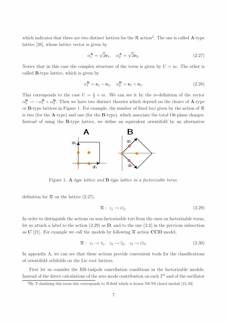
which indicates that there are two distinct lattices for the R action2. The one is called A-type
lattice [38], whose lattice vector is given by
αA1 =√
2e1, αA2 =√
2e2. (2.27)
Notice that in this case the complex structure of the torus is given by U = ia. The other is
called B-type lattice, which is given by
αB1 = e1 − e2, αB
2 = e1 + e2. (2.28)
This corresponds to the case U = 12
+ ia. We can see it by the re-definition of the vector
αB2 → −αB
1 + αB2 . Then we have two distinct theories which depend on the choice of A-type
or B-type lattices in Figure 1. For example, the number of fixed loci given by the action of Ris two (for the A-type) and one (for the B-type), which associate the total O6-plane charges.
Instead of using the B-type lattice, we define an equivalent orientifold by an alternative
Figure 1: A-type lattice and B-type lattice in a factorizable torus.
definition for R on the lattice (2.27),
R : zj → izj . (2.29)
In order to distinguish the actions on non-factorizable tori from the ones on factorizable torus,
let us attach a label to the action (2.29) as D, and to the one (2.2) in the previous subsection
as C [21]. For example we call the models by following R action CCD model,
R : z1 → z1, z2 → z2, z3 → iz3. (2.30)
In appendix A, we can see that these actions provide convenient tools for the classifications
of orientifold orbifolds on the Lie root lattices.
First let us consider the RR-tadpole cancellation conditions in the factorizable models.
Instead of the direct calculations of the zero mode contribution on each T 2 and of the oscillator
2By T-dualizing this torus this corresponds to B-field which is frozen NS-NS closed moduli [15, 33].
7

modes in the Klein bottle, the annulus and the Mobius strip amplitudes, it is enough to count
the number of O6-planes from (2.20): The numbers of O6-planes are NO6 = 8 (for AAA), 4
(for AAB), 2 (for ABB) and 1 (for BBB). The types of the actions in the T 2× T 2× T 2 are
illustrated in Figure 2. Here we obtain the RR-tadpole cancellation conditions3
Figure 2: AAA and AAB models on a factorizable torus. The orientifold planes lie on the
dashed blue lines. In this Figure we used a label B as the D-action on the A-lattice.
AAA : (N − 32)2 = 0,
AAB : (N − 16)2 = 0,
ABB : (N − 8)2 = 0,
BBB : (N − 4)2 = 0.
(2.31)
These are trivial results which have already been known. We emphasize that for the classi-
fication of orientifold models on non-factorizable tori and orbifolds it is convenient to fix the
lattices and distinguish the models with respect to the definitions of R.
Next we analyze some typical models on a non-factorizable4 tori T 6, which cannot be
expressed as the direct product T 2×T 2×T 2. As an example we consider an orientifold model
on a non-factorizable torus given by the Lie root lattice D6. In this model the lattice D6 can
be given by the simple roots
αi = ei − ei+1, α6 = e5 + e6, i = 1, . . . , 5, (2.32)
3Because these are the models on factorizable tori, and the C- and D-actions lead to the A- and B-models,
respectively.4 In this work a compactified space which cannot be represented as the direct products of two-torus T 2 is
called non-factorizable. For example, six-tori on D6, A3×A3 and A3×A2×A1, while six-tori on A2×A2×A2,
A2 ×D2 × (A1)2 and (A1)
6 are factorizable.
8
where ei’s are basis of Cartesian coordinates whose normalization is given as ei ·ej = δij . The
orientifold action R of the CCC-model is
R : e2i−1 → e2i−1, e2i → −e2i, i = 1, 2, 3. (2.33)
The number of O6-planes is obtained by means of (2.21). In order to evaluate the Lefschetz
fixed point theorem, we should fix the sublattice spaces Λ−R,⊥ and Λ−R,inv. Λ−R,⊥ is a lattice
space projected out by −R, and given by
Λ−R,⊥ =
3∑
i=1
n⊥,iα⊥,i
∣
∣
∣n⊥,i ∈ Z
, (2.34)
whose basis vectors are given by
α⊥,1 = e2, α⊥,2 = e4, α⊥,3 = e6. (2.35)
On the other hand, the sublattice Λ−R,inv, which is invariant under −R, is given by
Λ−R,inv =
3∑
i=1
ninv,iαinv,i
∣
∣
∣ninv,i ∈ Z
,
αinv,1 = e2 − e4, αinv,2 = e4 − e6, αinv,3 = e4 + e6.
(2.36)
Then we can easily evaluate the number of the O6-planes for the CCC model as
NO6 = 23 · Vol(Λ−R,⊥)
Vol(Λ−R,inv)= 4 . (2.37)
In the same way, we consider the CCD model. The lattices Λ−R,⊥ is given by
Λ−R,⊥ =
3∑
i=1
n⊥,iα⊥,i
∣
∣
∣n⊥,i ∈ Z
,
α⊥,1 = e2, α⊥,2 = e4, α⊥,3 =1
2(e5 − e6),
(2.38)
and Λ−R,inv is given by
Λ−R,inv =
3∑
i=1
ninv,iαinv,i
∣
∣
∣ninv,i ∈ Z
,
αinv,1 = e2 − e4, αinv,2 = e2 + e4, αinv,3 = e5 − e6.
(2.39)
Then we obtain NO6 = 2. Substituting these numbers into the RR-tadpole cancellation
condition (2.20), we easily obtain the number of D-branes. Here we summarize the data of
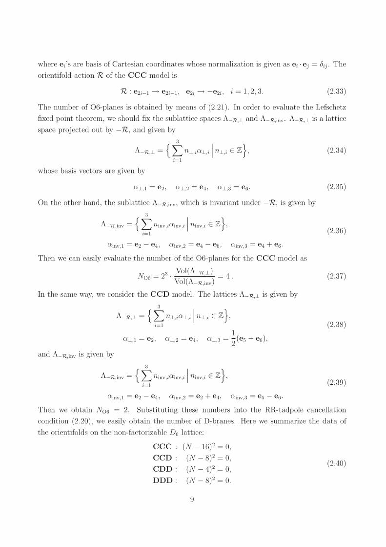
the orientifolds on the non-factorizable D6 lattice:
CCC : (N − 16)2 = 0,
CCD : (N − 8)2 = 0,
CDD : (N − 4)2 = 0,
DDD : (N − 8)2 = 0.
(2.40)
9
These results completely agree with the ones in [21]. The gauge group of these models are
SO(16), SO(8), SO(4) and SO(8), respectively. For models on non-factorizable tori, the
closed string spectra are the same as that of factorizable models.
We evaluated the the number of O6-planes NO6 according to the Lefschetz fixed point
theorem, and from (2.21) this give the necessary and sufficient condition for the RR-tadpole
condition. This analysis is generic and provides quite a simple rule to calculate the number of
O-planes and D-branes in orientifold models on non-factorizable tori in Type II string theory.
3 Supersymmetric ZN × ZM orientifold models
In this section let us consider Type IIA supersymmetric orientifold models on orbifolds and
describe the way to deal with orientifolds on non-factorizable lattices. Since the contributions
of the RR-tadpole from untwisted states are calculated in the same way as the ones of the
orientifolds on tori, we can easily count the numbers of D-branes via the Lefschetz fixed point
theorem (2.21). We also provide detail calculations of the RR-tadpole cancellation condition
on Z4 × Z2 and Z2 × Z2 orbifolds.
3.1 Orbifolds and orientifolds
In the previous section we showed general expressions for orientifolds on non-factorizable tori
(2.1). Here let us consider orientifold models on orbifolds given by
Type IIA on T 6
ΩR× ZN × ZM
. (3.1)
An orbifold is defined as a quotient of torus over a discrete set of isometries of the torus [39],
called the point group P , i.e.,
O = T 6/P = R6/S. (3.2)
Here S is called the space group, and is the semi-direct product of the point group P and the
translation group T . ZN orbifolds on the Lie root lattices have been classified in terms of the
Coxeter elements or the generalized Coxeter elements. In the case of ZN × ZM orbifolds, the
(generalized) Coxeter elements yield only orbifolds on factorizable lattices. Recently, however,
ZN ×ZM orbifolds on non-factorizable lattices were investigated in heterotic strings [27]. We
apply their analyses to Type IIA orientifold models.
Since the point group P of orbifold must act crystallographically on the lattice, we choose
these elements from the group generated by the Weyl reflection (A.4) and the outer auto-
morphisms Gout. In the case of the ZN × ZM orbifold on a Lie root lattice, the point group
10
elements of the orbifold can be defined by two commutative elements in the group generated
from Weyl group and the outer automorphisms, i.e,
[θ, φ] = 0, θ, φ ∈ W, Gout. (3.3)
On the complex coordinates of the torus T 6, the point group elements of the orbifold act in
such a way as
θ : (z1, z2, z3) → (e2πiv1z1, e2πiv2z2, e2πiv3z3),
φ : (z1, z2, z3) → (e2πiw1z1, e2πiw2z2, e2πiw3z3),(3.4)
where (v1, v2, v3) and (w1, w2, w3) are twists of an orbifold. We consider orientifold models
with N = 1 supersymmetry as follows: The requirement of SU(3) holonomy can be phrased
as invariance of the (3, 0)-form Ω = dz1 ∧ dz2 ∧ dz3, and leads to
v1 + v2 + v3 = w1 + w2 + w3 = 0. (3.5)
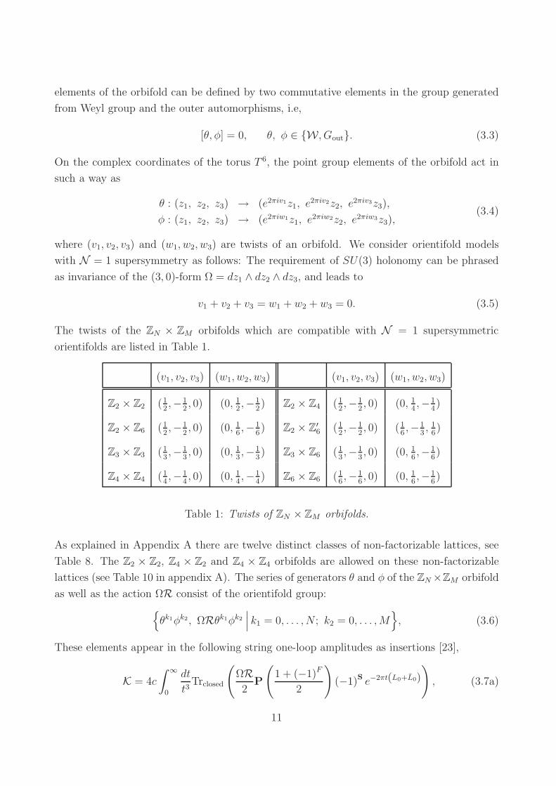
The twists of the ZN × ZM orbifolds which are compatible with N = 1 supersymmetric
orientifolds are listed in Table 1.
(v1, v2, v3) (w1, w2, w3) (v1, v2, v3) (w1, w2, w3)
Z2 × Z2 (12,−1
2, 0) (0, 1
2,−1
2) Z2 × Z4 (1
2,−1
2, 0) (0, 1
4,−1
4)
Z2 × Z6 (12,−1
2, 0) (0, 1
6,−1
6) Z2 × Z
′6 (1
2,−1
2, 0) (1
6,−1
3, 1
6)
Z3 × Z3 (13,−1
3, 0) (0, 1
3,−1
3) Z3 × Z6 (1
3,−1
3, 0) (0, 1
6,−1
6)
Z4 × Z4 (14,−1
4, 0) (0, 1
4,−1
4) Z6 × Z6 (1
6,−1
6, 0) (0, 1
6,−1
6)
Table 1: Twists of ZN × ZM orbifolds.
As explained in Appendix A there are twelve distinct classes of non-factorizable lattices, see
Table 8. The Z2 × Z2, Z4 × Z2 and Z4 × Z4 orbifolds are allowed on these non-factorizable
lattices (see Table 10 in appendix A). The series of generators θ and φ of the ZN×ZM orbifold
as well as the action ΩR consist of the orientifold group:
θk1φk2, ΩRθk1φk2
∣
∣
∣k1 = 0, . . . , N ; k2 = 0, . . . , M
, (3.6)
These elements appear in the following string one-loop amplitudes as insertions [23],
K = 4c
∫ ∞
0
dt
t3Trclosed
(
ΩR2
P
(
1 + (−1)F
2
)
(−1)S e−2πt(L0+L0)
)
, (3.7a)
11

A = c
∫ ∞
0
dt
t3Tropen
(
1
2P
(
1 + (−1)F
2
)
(−1)S e−2πtL0
)
, (3.7b)
M = c
∫ ∞
0
dt
t3Tropen
(
ΩR2
P
(
1 + (−1)F
2
)
(−1)S e−2πtL0
)
. (3.7c)
Here
P =
(
1 + θ + · · ·+ θN−1
N
)(
1 + φ + · · ·+ φM−1
M
)
. (3.8)
After extracting the RR-tadpoles, the insertion of ΩRθk1φk2 in the Klein bottle amplitude
corresponds to the contribution from O-planes fixed by Rθk1φk2 . Since in the ΩRθk1φk2
insertion the contributions from untwisted sectors are calculated in the same way as the cases
of tori in section 2, we obtain the necessary condition (2.20) for the RR-tadpole cancellation by
D-branes parallel to the O-planes. From this necessary condition, we obtain all the numbers
of O-planes and D-branes on the orbifold. In the next subsection we will demonstrate a few
examples of Z4 × Z2 orientifold models, and evaluate the RR-tadpole cancellation condition.
3.2 Z4 × Z2 model
Here we discuss the Z4×Z2 orientifold model on the Lie root lattice D6 (2.32) in detail because
in this case all possible subtleties show up.
There exists only one distinct Z4 × Z2 orbifold on D6, whose point group elements θ and
φ are given by
θ :
e1 → e2 → −e1
e3 → −e4 → −e3
e5 → e5
e6 → e6
φ :
e1 → e1
e2 → e2
ei → −ei i = 3, 4, 5, 6
(3.9a)
or, in matrix representation, by
θ :
0 −1 0 0 0 0
1 0 0 0 0 0
0 0 0 1 0 0
0 0 −1 0 0 0
0 0 0 0 1 0
0 0 0 0 0 1
, φ :
1 0 0 0 0 0
0 1 0 0 0 0
0 0 −1 0 0 0
0 0 0 −1 0 0
0 0 0 0 −1 0
0 0 0 0 0 −1
. (3.9b)
By using the above elements we can show all the orientifold actions which preserve N = 1
supersymmetry by means of C and D actions. For example, the reflection R on the DDC
12

model is given by
R :
0 1 0 0 0 0
1 0 0 0 0 0
0 0 0 1 0 0
0 0 1 0 0 0
0 0 0 0 1 0
0 0 0 0 0 −1
≡ (b,b, a), (3.10)
where we used an abbreviation defined by
(m1,m2,m3) ≡
m1 0 0
0 m2 0
0 0 m3
with mi ∈ ±a,±b,±1
¯ (3.11)
and
a ≡(
1 0
0 −1
)
, b ≡(
0 1
1 0
)
, 1 ≡(
1 0
0 1
)
, 0 ≡(
0 0
0 0
)
. (3.12)
From the Lefschetz fixed point theorem (2.21), the number of O6-plane fixed by R is given
as NO6 = 1. If we put four D-branes parallel to this R-fixed O6-plane, the RR-tadpole of
this model will be cancelled. Similarly, the element Rθ = (a,−a, a) gives NO6 = 4, whose
tadpole is cancelled by sixteen D-branes parallel to this four Rθ-fixed O6-planes. We similarly
evaluate the cases for the other elements of the orientifold group. The relations between the
orientifold group elements and the numbers of O-planes are summarized in Table 2.
Orientifold elements of R # of O6-planes
(±a,±a,±a), (1¯,−1
¯,±a) 4
(±a,±a,±b), (1¯,−1
¯,±b)
2(±b,±b,±b)
(±a,±b,±b) 1
Table 2: Orientifold group elements and the numbers of O6-planes on the D6 lattice. The
underline indicates a symmetry under the cyclic permutation.
Since the Z4 action changes the directions of the O-planes by angle of θ1/2 in the following
way:
Rθ = θ−1/2Rθ1/2. (3.13)
13

This action generates the exchange between the action C and D each other. Then we can see
that CCC and DDC, CCD and DDD, CDD and DCD models are equivalent with each
other, respectively. In the case of the CCC model, for example, two different numbers of
O6-planes appear since the orientifold group elements in R, Rθ2, Rφ and Rθ2φ are given by
(±a,±a,±a), whereas the elements in Rθ, Rθ3, Rθφ and Rθ3φ are given by (±b,±b,±a).
Analyzing such actions, we obtain all the models for Z4 × Z2 orientifolds on D6 lattice, listed
in Table 3.
Lattice Label reps. of R# of O6-planes
R, Rθ2, Rφ, Rθ2φ Rθ, Rθ3, Rθφ, Rθ3φ
D6
CCC (a, a, a) 4 1
CCD (a, a,b) 2 2
CDD (a,b,b) 2 2
DCC (b, a, a) 2 2
Table 3: All the Z4 × Z2 orientifold models on the D6 lattice.
We estimated the RR-tadpole cancellation by counting the O-planes from the equation
(2.20), which is the necessary condition in the case of the orbifold model. However it is
expected that the RR-tadpoles are cancelled even in the orbifold model. These countings also
give correct results for well-investigated non-factorizable models on ZN orbifolds in [22] and
Z2×Z2 orbifolds in [21]. We give the explicit results of the RR-tadpole cancellation for a few
models in the following.
3.2.1 Klein bottle amplitude
First let us evaluate the Klein bottle amplitude of Z4×Z2 orientifold model on the D6 lattice
(2.32) with the orientifold action
R = (b, a, a), (3.14)
which gives the DCC model. The contribution of the oscillator modes are equal in any
insertions of the orientifold group because they act as the unit operator in (3.7a). In the
θn1φn2-twisted sector, the oscillator contribution is given by K(n1,n2) ≡ K(n1,k1)(n2,k2) (see, for
the notation, [23]). We also need the multiplicities χ(n1,k1)(n2,k2)K of the θn1φn2-twisted fixed
sectors, which are invariant under the insertion ΩRθn1φn2 , which can be seen in Table 4.
14

multiplicities χ(n1,k1)(n2,k2)K CCC CCD CDD DCC
(0, k1)(0, k2) 1 1 1 1
(2n1 + 1, k1)(0, k2) 2 2 2 2
(2n1, 2k1 + 1)(0, k2) 4 4 4 4
(2n1, 2k1)(0, k2) 8 8 4 4
(0, 2k1 + 1)(1, k2) 4 4 4 4
(0, 2k1)(1, k2) 8 4 4 4
(2n1 + 1, k1)(1, k2) 8 8 4 8
(2n1, 2k1 + 1)(1, k2) 4 4 4 4
(2n1, 2k1)(1, k2) 8 4 4 4
Table 4: Multiplicities of the fixed points for the DCC and CCC models.
When an action θn1φn2 does not fix certain directions in the compact space, the Kaluza-
Klein momentum modes and the winding modes appear as the zero modes in the θn1φn2-fixed
sector. Let us evaluate such zero modes in the θ-twisted sector. The θ invariant sublattice Λθ
is expanded in terms of the basis
e5 + e6, e5 − e6
. (3.15)
We can see that theR invariant dual sublattice (Λθ)∗R,inv, whose basis is given by 2e5, and the
−R invariant sublattice (Λθ)−R,inv, with its basis 2e6, yield the momentum modes and the
winding modes in this sector, respectively. However there are two subtleties in this evaluation,
one of which is caused by the momentum doubling, and the other from the appearance of the
half winding states [22].
The former subtlety is caused by the shifts associated to the ΩRθk1φk2 insertions. In the
θ-twisted sector we have two fixed tori given by
xe5,1
2(e1 + e2 + e3 + e4) + xe5, (3.16)
where x ∈ R is a coordinate on the fixed tori. Note that the invariance of fixed points or
fixed tori under ΩRθk1φk2 is defined modulo the translation generated by the lattice Λ. The
R insertion acts on the two fixed tori in such a way as
R :
xe5 → xe5,
12(e1 + e2 + e3 + e4) + xe5 →
12(e1 + e2 + e3 − e4) + xe5
= 12(e1 + e2 + e3 + e4) + (−1 + x)e5.
(3.17)
15
In the latter case, the translation of a lattice shift α4 = e4 − e5 is accompanied. Because a
momentum mode |p 〉 picks up a phase factor e2πp·l under the translation by l, we generally
need phase factors in the amplitudes. In the case of (3.17), the phase factor is p·l = 2e5·e5 = 2,
and does not affect the amplitudes. If the phase factor is given as −1, the momentum modes
are effectively doubled by interference between modes with and without shifts:
∑
n
(−1)n exp(−πtn2p2) +∑
n
exp(−πtn2p2) = 2∑
n
exp(−4πtn2p2). (3.18)
The latter subtlety occurs in the winding modes. There are special points with the following
property:
θ :1
2(e1 + e2)→
1
2(−e1 + e2) =
1
2(e1 + e2) + e6, (3.19)
where we used a lattice shift given by e1 + e6. The point does not lie on the θ-fixed tori,
whereas this shift does generate the winding modes:
X(σ, τ) =1
2(e1 + e2) +
σ
2πe6 + (τ dependence), (3.20)
There are two points 12(e1 ± e2) which are invariant under the action R, and the multiplicity
is equal to that of the θ-fixed tori which are also invariant under R.
Therefore we conclude that the zero modes in the θ-twisted sector with R insertion are
given by the following vectors:
p = 2ne5, w = me6, (3.21)
where n, m ∈ Z. In the notation of (C.4), the zero mode contributions in the Klein bottle
amplitude is L2, 12. In a similar way we can evaluate the other twisted sectors in the orbifold
model. Note that for non-factorizable orbifolds the zero mode contributions depend on the
insertion ΩRθk1φk2. In the φ-twisted sector we have L2, 12
for the ΩRθ2k1φk2 insertions, and
L4,1 for the ΩRθ2k1+1φk2 insertions.
Next we evaluate the zero mode contribution from the untwisted sector given in (2.17a).
The basis of dual lattice α∗ ∈ Λ∗, which is defined by α∗i · αj = δij , is given as
α∗1 = e1,
α∗2 = e1 + e2,
α∗3 = e1 + e2 + e3,
α∗4 = e1 + e2 + e3 + e4,
α∗5 = 1
2(e1 + e2 + e3 + e4 + e5 − e6),
α∗6 = 1
2(e1 + e2 + e3 + e4 + e5 + e6).
(3.22)
16
Then the R invariant dual sublattice Λ∗R,inv in (2.17a), which yields the momentum modes in
the Kaluza-Klein states, is expanded by the basis
e1 + e2, e3, e5
. (3.23)
In the same way, the −R invariant lattice Λ−R,inv in (2.17c) yielding the winding states is
expanded by
e1 − e2, 2e4, 2e6
. (3.24)
Substituting these elements into (2.9), we obtain the zero mode contribution L(0,0)K . Its mod-
ular transformation is given by the factors
√det MK = Vol(Λ∗
R,inv) =√
2, (3.25)√det WK = Vol(Λ−R,inv) = 4
√2.
We also need the zero mode contributions with the other insertions ΩRθk1φk2. Since these
elements are given by Rθk1φk2 = (±a,±b,±b) for the DCC model, we have the same results
as that of the R insertion.
We obtained all the ingredients to write down the Klein bottle amplitude for the DCC
model, which are summarized as
K = c(1RR − 1NSNS)
∫ ∞
0
dt
t3
(
L(0,0)K K(0,0) + 2L2, 1
2K(1,0) + 4L2, 1
2K(2,0) + 2L2 1
2K(3,0)
+1
2
(
8L4,1 + 4L2, 12
)
K(0,1) + 8K(1,1)
+1
2
(
8L4,1 + 4L2, 12
)
K(2,1) + 8K(3,1))
. (3.26)
Its modular transformation to the tree channel is
K = 16c(1RR − 1NSNS)
∫ ∞
0
dl(
L(0,0)K K(0,0) − 2L2,8K(1,0) − 4L2,8K(2,0) − 2L2,8K(3,0)
− 2(L1,4 + L2,8)K(0,1) + 4K(1,1)
− 2(L1,4 + L2,8)K(2,1) − 4K(3,1))
. (3.27)
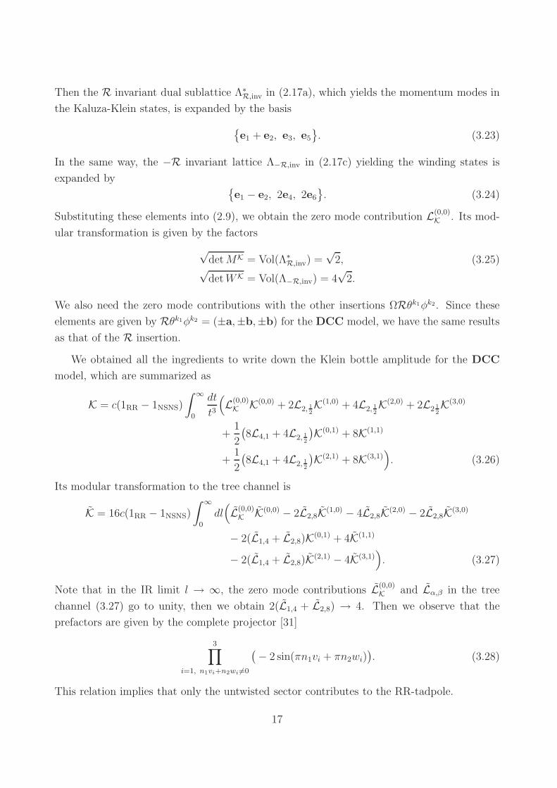
Note that in the IR limit l → ∞, the zero mode contributions L(0,0)K and Lα,β in the tree
channel (3.27) go to unity, then we obtain 2(L1,4 + L2,8) → 4. Then we observe that the
prefactors are given by the complete projector [31]
3∏
i=1, n1vi+n2wi 6=0
(
− 2 sin(πn1vi + πn2wi))
. (3.28)
This relation implies that only the untwisted sector contributes to the RR-tadpole.
17
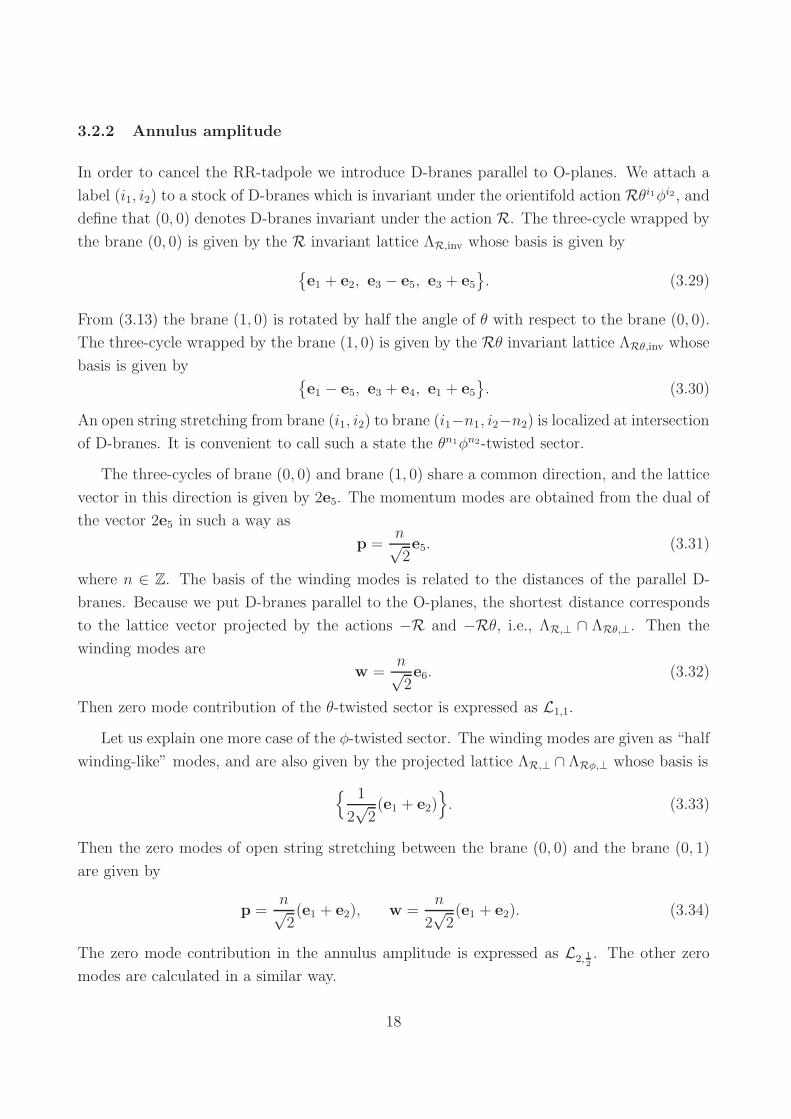
3.2.2 Annulus amplitude
In order to cancel the RR-tadpole we introduce D-branes parallel to O-planes. We attach a
label (i1, i2) to a stock of D-branes which is invariant under the orientifold action Rθi1φi2, and
define that (0, 0) denotes D-branes invariant under the action R. The three-cycle wrapped by
the brane (0, 0) is given by the R invariant lattice ΛR,inv whose basis is given by
e1 + e2, e3 − e5, e3 + e5
. (3.29)
From (3.13) the brane (1, 0) is rotated by half the angle of θ with respect to the brane (0, 0).
The three-cycle wrapped by the brane (1, 0) is given by the Rθ invariant lattice ΛRθ,inv whose
basis is given by
e1 − e5, e3 + e4, e1 + e5
. (3.30)
An open string stretching from brane (i1, i2) to brane (i1−n1, i2−n2) is localized at intersection
of D-branes. It is convenient to call such a state the θn1φn2-twisted sector.
The three-cycles of brane (0, 0) and brane (1, 0) share a common direction, and the lattice
vector in this direction is given by 2e5. The momentum modes are obtained from the dual of
the vector 2e5 in such a way as
p =n√2e5. (3.31)
where n ∈ Z. The basis of the winding modes is related to the distances of the parallel D-
branes. Because we put D-branes parallel to the O-planes, the shortest distance corresponds
to the lattice vector projected by the actions −R and −Rθ, i.e., ΛR,⊥ ∩ ΛRθ,⊥. Then the
winding modes are
w =n√2e6. (3.32)
Then zero mode contribution of the θ-twisted sector is expressed as L1,1.
Let us explain one more case of the φ-twisted sector. The winding modes are given as “half
winding-like” modes, and are also given by the projected lattice ΛR,⊥ ∩ ΛRφ,⊥ whose basis is
1
2√
2(e1 + e2)
. (3.33)
Then the zero modes of open string stretching between the brane (0, 0) and the brane (0, 1)
are given by
p =n√2(e1 + e2), w =
n
2√
2(e1 + e2). (3.34)
The zero mode contribution in the annulus amplitude is expressed as L2, 12. The other zero
modes are calculated in a similar way.
18

Since in the θn1φn2-twisted sector the contributions from the oscillator modes do not depend
on branes (i1, i2), they are given as A(n1,k1)(n2,k2). The insertions of 11, θ2, φ and θ2φ leave
D-branes invariant, and perform non-trivial actions on the Chan-Paton factors described as
γ(i1,i2)k1,k2
, which appear in the amplitude as
tr(
γ(i1−n1,i2−n2)k1,k2
)
tr(
γ(i1,i2)k1,k2
)−1
(3.35)
in the θn1φn2-twisted sector. Sectors of k1 6= 0 or k2 6= 0 cannot be cancelled by the other
diagrams. Therefore the Z2 twisted tadpole cancellation condition is required [23, 34]:
tr(
γ(i1,i2)2,0
)
= tr(
γ(i1,i2)0,1
)
= tr(
γ(i1,i2)2,1
)
= 0. (3.36)
We should also evaluate the multiplicities χM of the open string states, which are given by
the intersection number of D-branes. The intersection numbers of two branes can be obtained
by the determinant of vectors vi and v′i giving the three-cycles in respective D-branes [22].
These vectors can be expanded in terms of the lattice basis as vi =∑
vijαj. Then the
intersection number is
I = det
v11 v12 · · · v16
v21 v22 · · · v26
......
v′31 v′
32 · · · v′36
. (3.37)
Owing to the above Z2 twisted tadpole condition, it is sufficient to consider the intersection
number χM for k1 = k2 = 0, which are given in Table 5.
The contribution from the zero modes of the untwisted sector is obtained from (2.17b) and
(2.17d). For the brane (0, 0), which is paralell to the R-fixed O6-plane ,it is
√det MA = Vol(Λ∗
R,⊥) = 4, (3.38)√det WA = Vol(Λ−R,⊥) = 4.
The contributions from the other branes (i1, i2) give the same values. These values appear in
prefactors of the amplitude after the modular transformation.
Summarizing the above, we obtain the annulus amplitude for the DCC model
A =N2c
4(1RR − 1NSNS)
∫ ∞
0
dt
t3
(
L(0,0)A A(0,0) + L1,1A(1,0) + 2L1,1A(2,0) + L1,1A(3,0)
+ (L2, 12
+ L1,1)K(0,1) + 2A(1,1)
+ (L1,1 + L2, 12)A(2,1) + 2A(3,1)
)
. (3.39)
19
χA CCC CCD CDD DCC
(i1,i2)–(i1,i2) 1 1 1 1
(i1,i2)–(i1+1,i2) 1 1 2 1
(2i1+1,i2)–(2i1+3,i2) 4 2 4 2
(2i1,i2)–(2i1+2,i2) 1 2 4 2
(2i1+1,i2)–(2i1+1,i2+1) 4 2 4 2
(2i1,i2)–(2i1,i2+1) 1 2 4 2
(i1,i2)–(i1+1,i2+1) 2 2 4 2
(2i1+1,i2)–(2i1+3,i2+1) 4 2 4 2
(2i1,i2)–(2i1+2,i2+1) 1 2 4 2
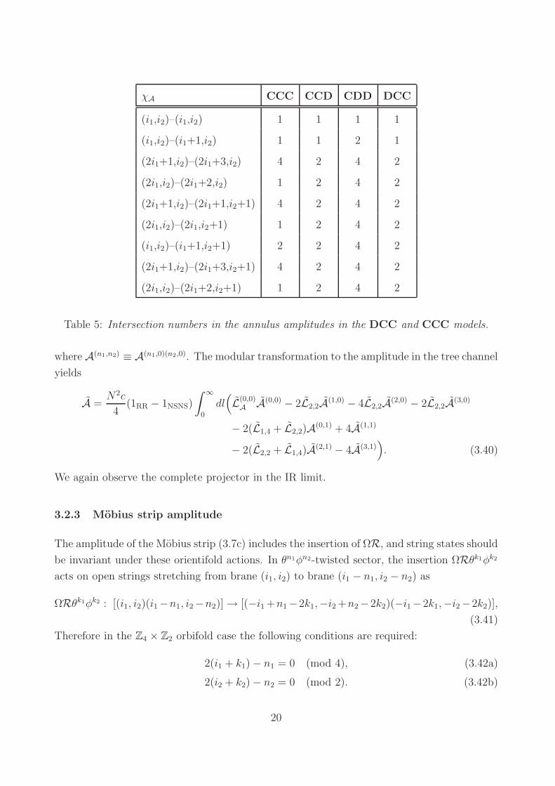
Table 5: Intersection numbers in the annulus amplitudes in the DCC and CCC models.
where A(n1,n2) ≡ A(n1,0)(n2,0). The modular transformation to the amplitude in the tree channel
yields
A =N2c
4(1RR − 1NSNS)
∫ ∞
0
dl(
L(0,0)A A(0,0) − 2L2,2A(1,0) − 4L2,2A(2,0) − 2L2,2A(3,0)
− 2(L1,4 + L2,2)A(0,1) + 4A(1,1)
− 2(L2,2 + L1,4)A(2,1) − 4A(3,1))
. (3.40)
We again observe the complete projector in the IR limit.
3.2.3 Mobius strip amplitude
The amplitude of the Mobius strip (3.7c) includes the insertion of ΩR, and string states should
be invariant under these orientifold actions. In θn1φn2-twisted sector, the insertion ΩRθk1φk2
acts on open strings stretching from brane (i1, i2) to brane (i1 − n1, i2 − n2) as
ΩRθk1φk2 : [(i1, i2)(i1−n1, i2−n2)]→ [(−i1 +n1−2k1,−i2 +n2−2k2)(−i1−2k1,−i2−2k2)],
(3.41)
Therefore in the Z4 × Z2 orbifold case the following conditions are required:
2(i1 + k1)− n1 = 0 (mod 4), (3.42a)
2(i2 + k2)− n2 = 0 (mod 2). (3.42b)
20

Then the sectors with n1 = 0, 2 and n2 = 0 contribute to the amplitude. The intersection
number is obtained in the same way as in the case of annulus. In Table 5, we can see that
χM = 1 for untwisted sectors and χM = 2 for θ2-twisted sectors.
The momentum modes are evaluated in a similar way of subsection 3.2.1, however the
winding modes are changed due to the insertions. In the untwisted sector with the ΩRθ inser-
tion, from the condition (3.42) the open string states [(1, 0)(3, 0)], [(1, 1)(3, 1)], [(1, 1)(3, 1)],
[(1, 1)(3, 1)], [(3, 0)(1, 0)], [(1, 0)(3, 0)] and [(1, 0)(3, 0)] contribute to the amplitude. For in-
stance, in the open string state [(1, 0)(3, 0)], the momentum modes, which are generated by
the dual lattice ΛRθ,inv ∩ ΛRθ3,inv with its basis 2e5, are given as
p =n√2e5. (3.43)
The winding modes invariant under −ΩRθ are given by
w =2n√
2e6. (3.44)
This can also read from Λ−Rθ,inv ∩ Λ−Rθ3,inv. The zero mode contribution for this state is
represented as L1,4.
We should take it account of the orientifold actions to the Chan-Paton factors. For the
open strings [(i1, i2)(i1 − n1, i2 − n2)], the ΩRθk1φk2-insertion contributes in the amplitude as
tr[
(γ(i1,i2)ΩRk1k2
)−1(γ(i1−n1,i2−n2)ΩRk1k2
)T]
. (3.45)
Since only the sectors with n1 = 0, 2 and n2 = 0 contribute to the amplitude, we abbreviate
a(n1)k1k2
≡ tr[
(γ(2i1+1,i2)ΩRk1k2
)−1(γ(2i1+1+n1,i2)ΩRk1k2
)T]
, (3.46)
b(n1)k1k2
≡ tr[
(γ(2i1,i2)ΩRk1k2
)−1(γ(2i1+n1,i2)ΩRk1k2
)T]
. (3.47)
These assignments correspond to two different classes of the D-brane configurations in this
model, and are sufficient to evaluate the tadpole cancellation conditons for Z4 × Z2 models.
However we will need more independent variables for Z2 × Z2 models.
For the contributions from untwisted sector, we can use the results from the (3.26) and
(3.39) owing to the relations (2.17a)-(2.17d).
To summarize, we obtain the Mobius strip amplitude in the loop channel as
M = −Nc
4(1RR − 1NSNS)
∫ ∞
0
dt
t3
(a(0)0,0 + b
(0)0,0
2L(0,0)
M M(0,0)(0,0) + 2a
(2)3,0 + b
(2)3,0
2L1,4M(2,3)(0,0)
+a
(0)2,0 + b
(0)2,0
2L1,4M(0,2)(0,0) + 2
a(2)1,0 + b
(2)1,0
2L1,4M(2,1)(0,0)
21

+a
(0)0,1L2,2 + b
(0)0,1L1,4
2M(0,0)(0,1) + 2
a(2)3,1 + b
(2)3,1
2M(2,3)(0,1)
+a
(0)2,1L1,4 + b
(0)2,1L2,2
2M(0,2)(0,1) + 2
a(2)1,1 + b
(2)1,1
2M(2,1)(0,1)
)
.
(3.48)
The modular transformation to the tree channel yields
M = −4c(1RR − 1NSNS)
∫ ∞
0
dl(a
(0)0,0 + b
(0)0,0
2L(0,0)
M M(0,0) − (a(2)3,0 + b
(2)3,0)L8,2M(1,0)
+ 2(a(0)2,0 + b
(0)2,0)L8,2M(2,0) − (a
(2)1,0 + b
(2)1,0)L8,2M(3,0)
+ 2(a(0)0,1L4,4 + b
(0)0,1L8,2)M(0,1) + 2(a
(2)3,1 + b
(2)3,1)M(1,1)
+ 2(a(0)2,1L8,2 + b
(0)2,1L4,4)M(2,1) + 2(a
(2)1,1 + b
(2)1,1)M(3,1)
)
. (3.49)
To obtain the complete projector and to cancel the tadpole [23], we set
a(0)0,0 = a
(2)1,0 = −a
(0)2,0 = a
(2)3,0 = −a
(0)0,1 = −a
(2)1,1 = −a
(0)2,1 = a
(2)3,1 = N, (3.50)
b(0)0,0 = b
(2)1,0 = −b
(0)2,0 = b
(2)3,0 = −b
(0)0,1 = −b
(2)1,1 = −b
(0)2,1 = b
(2)3,1 = N. (3.51)
Let us focus on the coefficients on the zero mode contributions in the Klein bottle amplitude
(3.27), the annulus amplitude (3.40) and the Mobius strip amplitude (3.49). The RR-tadpole
cancellation condition (2.7) leads to
0 = 16 +N2
4− 4N =
1
4(N − 8)2. (3.52)
The number of one stack of the D-branes is N = 8 to cancel the RR-tadpole. Taking account
of (3.36) and (3.51), the gauge groups are determined as (Sp(2))4 for the DCC model.
For the CCC model, one of whose orientifold actions is given by
R = (a, a, a). (3.53)
On the other hand, the element Rθ in the orientifold group is given by
Rθ = (−b,b, a). (3.54)
As seen in Table 2, these two elements yield different numbers of O-planes. To show this, we
evaluate the RR-tadpole amplitude in the following way: In the tree channel the Klein bottle
amplitude is
K = c(1RR − 1NSNS)
∫ ∞
0
dl(
20L(0,0)K K(0,0) − 32L2,8K(1,0)
22

− 80L2,8K(2,0) − 32L2,8K(3,0)
− 40(L2,8 + L1,4)K(0,1) + 64K(1,1)
− 40(L2,8 + L1,4)K(2,1) − 64K(3,1))
. (3.55)
The prefactors do not correspond to that from the complete projector. The annulus and the
Mobius strip amplitudes are also described as
A =c
16(1RR − 1NSNS)
∫ ∞
0
dl(
(M2 + 4N2)L(0,0)A A(0,0) − 8MNL2,2A(1,0)
− 4(M2 + 4N2)L2,2A(2,0) − 8MNL2,2A(3,0)
− 4(M2L2,2 + 4N2L1,4)A(0,1) + 16MNA(1,1)
− 4(M2L2,2 + 4N2L1,4)A(2,1) − 16MNA(3,1))
, (3.56a)
M = −c(1RR − 1NSNS)
∫ ∞
0
dl(
2(M + N)L(0,0)M M(0,0) − 2(M + 4N)L8,2M(1,0)
− 8(M + N)L8,2M(2,0) − 2(M + 4N)L8,2M(3,0)
− 8(ML8,2 + NL4,4)M(0,1) + 4(M + 4N)M(1,1)
− 8(ML8,2 + NL4,4)M(2,1) − 4(M + 4N)M(3,1))
, (3.56b)
where M and N are the numbers of D-branes which are invariant under the set of orien-
tifold actions R,Rθ2,Rφ,Rθ2φ, and under the other set of actions Rθ,Rθ3,Rθφ,Rθ3φ,respectively. In the Mobius strip amplitude we have set
a(0)0,0 = a
(2)1,0 = −a
(0)2,0 = a
(2)3,0 = −a
(0)0,1 = −a
(2)1,1 = −a
(0)2,1 = a
(2)3,1 = M, (3.57)
b(0)0,0 = b
(2)1,0 = −b
(0)2,0 = b
(2)3,0 = −b
(0)0,1 = −b
(2)1,1 = −b
(0)2,1 = b
(2)3,1 = N. (3.58)
Focus on the coefficient in (3.55), (3.56a) and (3.56b), we obtain the RR-tadpole cancel-
lation conditions (2.7),
0 = 20 +1
16(M2 + 4N2)− 2(M + N) =
1
16
(
(M − 16)2 + (N − 4)2)
, (3.59a)
0 = −32− MN
2+ 2(M + 4N) = −1
2(M − 16)(N − 4), (3.59b)
and find M = 16 and N = 4. This indicates that we should insert sets of different numbers
of D-branes in an appropriate way in several kinds of non-factorizable tori.
The open string massless spectrum is given in Table 6. The multiplicities of twisted states
spectra depend on the intersection numbers [23] (see Table 5). We see that the CCD and
DCC models are distinct from the CDD model despite the same numbers of O-planes, and
actually these four models have different spectra. For the closed string the numbers of massless
states are considerably reduced due to their Hodge numbers in [26, 27].
23

sectors CCC CCD CDD DCC representations
untwisted
1V Sp[M/4]2 × Sp[N/4]2
3C( , 1; 1, 1)⊕ (1, ; 1, 1)
⊕(1, 1; , 1)⊕ (1, 1; 1, )
θ + θ3 2C 2C 4C 2C ( , ; 1, 1)⊕ (1, 1; , )
θ24C 2C 4C 2C ( , 1; 1, 1)⊕ (1, ; 1, 1)
1C 2C 4C 2C (1, 1; , 1)⊕ (1, 1; 1, )
φ4C 2C 4C 2C ( , 1; , 1)
1C 2C 4C 2C (1, ; 1, )
θφ + θ3φ 2C 2C 4C 2C ( , 1; 1, )⊕ (1, ; , 1)
θ2φ4C 2C 4C 2C ( , 1; , 1)
1C 2C 4C 2C (1, ; 1, )
Table 6: Open string massless spectra of Z4×Z2 orbifold on the D6 lattice. The symbols “V ”
and “C” denote the vector and chiral multiplets, respectively.
3.3 Z2 × Z2 model
Since Z2 × Z2 is a subgroup of Z4 × Z2, the calculation is similar to the examples in the
previous subsection. The new feature in Z2 × Z2 is that we have more freedom to choose
orbifold actions in comparison with the case of Z4 × Z2.
For Z2 × Z2 orbifolds on the D6 lattice (2.32), all the point group elements can be given
by the use of a and b in (3.12), see Appendix A. In the case of the CCC orientifold with
R = (a, a, a), the point group elements θ and φ are
θ : (−1¯,−1
¯, 1¯), φ : (1
¯,−1
¯,−1
¯). (3.60)
The orientifold group elements including ΩR are
ΩR, ΩRθ, ΩRφ, ΩRθφ, (3.61)
and these elements generate O6-planes respectively. From Table 3 the numbers of O6-planes
are read two for each elements.
In the CCD orientifold with R = (a, a,b), we have two distinct pairs of the point group
24

elements:
θ: (1¯,−1
¯,−1
¯)
φ: (−1¯,−1
¯, 1¯)
θ: (1¯,−1
¯,−1
¯)
φ: (−1¯,−a,b)
(3.62)
The numbers of O-planes generated by the former orbifold actions are also two. In the latter
case, the ΩR and ΩRθ (ΩRφ and ΩRθφ) generate two (four) O6-planes, respectively. We
can classify the distinct orientifold models on the Lie root lattices, and the other possible
elements on the D6 lattice are listed in Table 7. We should notice that even though the
numbers of O6-planes are the same in any three-cycles in Z2×Z2 orientifold models, those of
non-factorizable models can be different.
Lattice Label reps. of ROrbifold # of O6-planes
rep. of θ rep. of φ R Rθ Rφ Rθφ
D6
CCC (a, a, a) (1,−1,−1) (−1,−1, 1) 4 4 4 4
CCD (a, a,b)(1,−1,−1) (−1,−1, 1) 2 2 2 2
(1,−1,−1) (−1,−a,b) 2 2 4 4
CDD (a,b,b)
(1,−1,−1) (−1,−1, 1) 1 1 1 1
(1,−1,−1) (−1,b,−b) 1 1 4 4
(−1, 1,−1) (a,−1,−b) 1 1 2 2
(a,−1,−b) (−a,b,−1) 1 2 2 4
DDD (b,b,b)
(−1,−1, 1) (1,−1,−1) 2 2 2 2
(1,−1,−1) (−1,−b,b) 2 2 2 2
(−1,−b,b) (b,−1,−b) 2 2 2 2
Table 7: Z2 × Z2 orbifold models on the D6 Lie root lattice.
Finally we check the RR-tadpole cancellation in the Z2×Z2 CCC model on the D6 lattice.
The contribution from φ- and θφ-twisted sectors are the same as θ-sector for the CCC model
on the D6 lattice. The RR-tadpole cancellation is satisfied with N = 4 as we can see the
following amplitudes in the tree channel. The Klein bottle amplitude is given as
K = 32c(1RR − 1NSNS)
∫ ∞
0
dl(
L(0,0)K K(0,0) − 4L2,8K(1,0) − 4L2,8K(0,1) − 4L2,8K(1,1)
)
. (3.63)
25
The annulus and the Mobius amplitudes are also given as
A =N2c
8(1RR − 1NSNS)
∫ ∞
0
dl(
L(0,0)A A(0,0) − 4L2,2A(1,0) − 4L2,2A(0,1) − 4L2,2A(1,1)
)
,
(3.64a)
M = −4Nc(1RR − 1NSNS)
∫ ∞
0
dl(
L(0,0)M M(0,0) − 4L8,2M(1,0) − 4L8,2M(0,1) − 4L8,2M(1,1)
)
.
(3.64b)
We observe that in any amplitudes the prefactors are given by the complete projector (3.28).
4 Conclusion
In this paper we studied the RR-tadpole cancellation condition in Type II string models
compactified on six-tori given by general Lie root lattices. We obtained a simple derivation to
count the orientifold planes lying on the lattice by the use of the Lefschetz fixed point theorem.
As expected the RR-tadpole contributions are cancelled by adding an appropriate number of
D-branes parallel to the O-planes. The Lefschetz fixed point theorem provides an intuitive
picture to non-factorizable models, and we easily showed a way to construct orientifold models
on tori and orbifolds.
In D = 4, N = 1 ZN × ZM orientifolds, mainly the factorizable models on T 2 × T 2 × T 2
have been constructed and investigated. We gave the classifications in Type IIA orientifold
models with O6-planes, and obtained many new models. As explained in detail, the Lefschetz
fixed point theorem provide intuitive and convenient tools in model construction. Since the
condition derived in (2.20) is the necessary condition for orbifolds, we performed explicit cal-
culations for Z4×Z2 and Z2×Z2 orbifold models, and confirmed the RR-tadpole calculations.
It is expected that even in other non-factorizable orbifold models the RR-tadpole cancellation
should be checked in the same calculation. We further found many non-factorizable Z2 × Z2
orbifolds in which the numbers of O-planes depend on the three-cycles left invariant under
the orbifold projections in Table 7 and in Table 11. These features are not seen in factoriz-
able models, and will provide new possibilities for model constructions. On the other hand,
since the metric of non-factorizable tori is changed to B-field via T-duality, our consideration
should be related to compactification with such backgrounds. Actually in heterotic orbifolds
there are some coincidences between non-factorizable models and factorizable models with
generalized discrete torsion [41]. Our results indicate that there would be a possibility to
construct various class of D = 4, N = 1 models with different set of chiral spectra from other
well-known (non-)factorizable models.
26

Acknowledgements
K.T. is supported by the Grand-in-Aid for Scientific Research #172131. T.K. is supported
by the Grant-in-Aid for the 21st Century COE “Center for Diversity and Universal-
ity in Physics” from the Ministry of Education, Culture, Sports, Science and Technology
(MEXT) of Japan.
Appendix
A Six-dimensional Lie root lattice
In this appendix we study basic aspects of the Lie root lattice given by the simple Lie algebra
and its application to non-factorizable six-tori. First we review the simple root on the Lie al-
gebra. In terms of Lie root lattices, we find that there are only twelve distinct non-factorizable
six-tori and four factorizable ones. By the use of the Weyl reflection and the outer automor-
phisms, we can classify all the point groups of orbifolds and orientifold actions R on the tori,
which crystallographically act on the Lie root lattices. We give explicit representations of
point group elements generated by the Weyl reflections and the outer automorphisms of the
Lie root lattices. Some of the point groups can be given by the Coxeter elements from the
Cater diagrams or the generalized Coxeter elements as explained later. Beside these elements,
we see that point groups which are not included in the (generalized) Coxeter elements are also
obtained by the classification.
We utilize these elements for the point groups of our orientifold models, and these elements
lead to many new orientifold models as explained in section 3 and in this appendix. Here we
give the systematic way to construct orbifolds and orientifolds on the Lie root lattices.
A.1 Lie root lattices
We use the words of the Lie algebra in order to define the shape of tori defined in (2.12). The
Lie algebras whose orders are within six are AN , BN , CN , DN , E6, F4 and G2. The simple
27
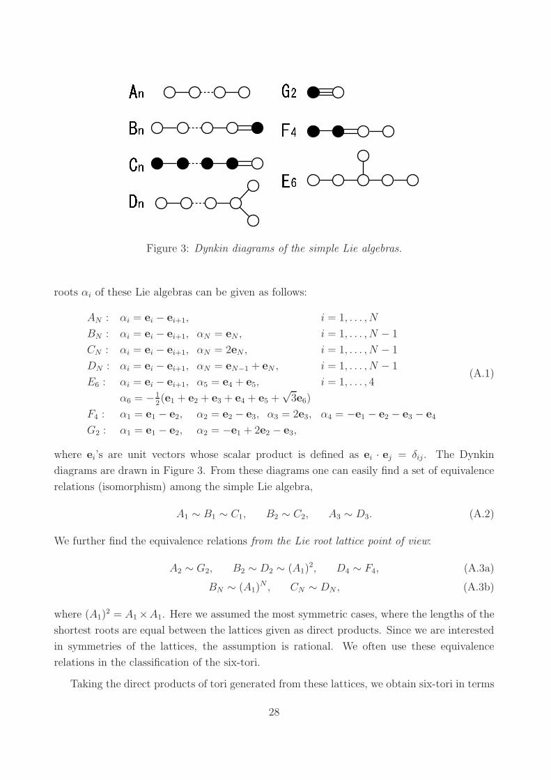
Figure 3: Dynkin diagrams of the simple Lie algebras.
roots αi of these Lie algebras can be given as follows:
AN : αi = ei − ei+1, i = 1, . . . , N
BN : αi = ei − ei+1, αN = eN , i = 1, . . . , N − 1
CN : αi = ei − ei+1, αN = 2eN , i = 1, . . . , N − 1
DN : αi = ei − ei+1, αN = eN−1 + eN , i = 1, . . . , N − 1
E6 : αi = ei − ei+1, α5 = e4 + e5, i = 1, . . . , 4
α6 = −12(e1 + e2 + e3 + e4 + e5 +
√3e6)
F4 : α1 = e1 − e2, α2 = e2 − e3, α3 = 2e3, α4 = −e1 − e2 − e3 − e4
G2 : α1 = e1 − e2, α2 = −e1 + 2e2 − e3,
(A.1)
where ei’s are unit vectors whose scalar product is defined as ei · ej = δij . The Dynkin
diagrams are drawn in Figure 3. From these diagrams one can easily find a set of equivalence
relations (isomorphism) among the simple Lie algebra,
A1 ∼ B1 ∼ C1, B2 ∼ C2, A3 ∼ D3. (A.2)
We further find the equivalence relations from the Lie root lattice point of view:
A2 ∼ G2, B2 ∼ D2 ∼ (A1)2, D4 ∼ F4, (A.3a)
BN ∼ (A1)N , CN ∼ DN , (A.3b)
where (A1)2 = A1×A1. Here we assumed the most symmetric cases, where the lengths of the
shortest roots are equal between the lattices given as direct products. Since we are interested
in symmetries of the lattices, the assumption is rational. We often use these equivalence
relations in the classification of the six-tori.
Taking the direct products of tori generated from these lattices, we obtain six-tori in terms
28

of the Lie root lattices. We conclude that there are only twelve inequivalent non-factorizable
six-tori and four factorizable ones5 in such a way as in Table 8.
[non-factorizable tori]
A6 D6 E6
A5 ×A1 A4 ×A2 A4 × (A1)2
D5 ×A1 D4 ×A2 D4 × (A1)2
A3 ×A3 A3 ×A2 × A1 A3 × (A1)3
[factorizable tori]
(A2)3 (A2)
2 × (A1)2 A2 × (A1)
4 (A1)6
Table 8: All the Lie root lattices in six dimensions.
A.2 Weyl reflection and graph automorphism
Next we investigate the automorphisms of the above lattices. Both orbifold and orientifold
groups should crystallographically act on the lattices. These groups can be classified in terms
of the Weyl reflection and the graph automorphism acting on the simple roots of the Lie root
lattice. The Weyl group W is generated by the following Weyl reflections rαkwhich associate
the simple root αk:
rαk: λ → λ− 2
αk · λ|αk|2
αk. (A.4)
In the case of the DN Lie root lattice, for instance, the Weyl reflection rαkfor k = 1, . . . , N−1
is given as
rαk:
αk−1 → αk−1 + αk
αk → −αk
αk+1 → αk+1 + αk
(A.5a)
and αm for m 6= k − 1, k, k + 1 are unchanged. For k = N it is
rαN:
αN−2 → αN−2 + αN
αN → −αN
(A.5b)
and the other αm’s are unchanged. For the classification of the automorphisms, it would be
convenient to rewrite them in the basis of orthogonal unit vectors ei as
rαk: ek ↔ ek+1 k = 1, . . . , N − 1, (A.6a)
5Most of other six-tori would be obtained by the continuous deformation of moduli of these tori [26].
29
rαN: eN ↔ −eN−1. (A.6b)
On the other hand, the outer automorphism g of the Cartan diagram is represented as
g : αN−1 ↔ αN , (A.7)
and the other simple roots are left unchanged. In the unit vector basis, it is
g : eN → −eN . (A.8)
In terms of ei, we can easily construct any elements generated from rαkand g. For example a
product of two Weyl reflections which do not commute with each other makes up Z3 element
as
rαkrαk+1
: ek → ek+1 → ek+2 → ek, (k < N − 1). (A.9)
This is the permutation group S3. Similarly the Weyl reflections rαkfor k = 1, . . . , N −1 gen-
erate a permutation group SN . Adding the other elements rαNand g to SN , the representation
of the group is given by permutations with signs
ei → ±ej → ±ek → · · · → ±ei. (A.10)
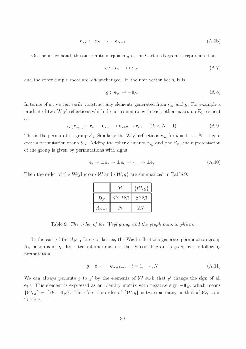
Then the order of the Weyl group W and W, g are summarized in Table 9:
W W, g
DN 2N−1N ! 2NN !
AN−1 N ! 2N !
Table 9: The order of the Weyl group and the graph automorphism.
In the case of the AN−1 Lie root lattice, the Weyl reflections generate permutation group
SN in terms of ei. Its outer automorphism of the Dynkin diagram is given by the following
permutation
g : ei ↔ −eN+1−i, i = 1, · · · , N (A.11)
We can always permute g to g′ by the elements of W such that g′ change the sign of all
ei’s, This element is expressed as an identity matrix with negative sign −11N , which means
W, g = W,−11N. Therefore the order of W, g is twice as many as that of W, as in
Table 9.
30
Then it is straightforward to obtain all Z2 elements of the DN lattice, and they are given
by the following sub-elements
ei ↔ ej ,
ek ↔ −el,
em → −em,
(A.12a)
except for D4. The ZN elements are constructed similarly. For example Z3 elements are
constructed by the following sub-elements,
ei → ±ej → ±ek → ±ei, (# of terms with − sign is even) (A.13)
and their permutations. Z4 elements includes the following sub-elements,
ei → −ej → −ei, i 6= j, (A.14a)
ei → ±ej → ±ek → ±el → ±ei, (# of terms with − sign is even). (A.14b)
We can similarly deal with the AN lattices. Note that the roots of the AN and DN can be
given by
AN : ei − ej , (A.15a)
DN : ±ei ± ej, i, j = 1, . . . , N. (A.15b)
They are symmetric under the permutations of i and j. Now it is apparent that on the D6
lattice, (3.9b) is the only inequivalent Z4 × Z2 elements, and Z2 × Z2 elements can be given
by a, b and 1 in (3.12). From Table 8, we have all the point group elements which can be
expressed by the Weyl reflections and the outer automorphism (except for the E6 lattice).
However there are a few exceptions owing to additional outer automorphisms as follows.
We shortly explain the Coxeter elements and the generalized Coxeter elements6. The
Coxeter element of the Lie root lattice is defined by product of all the Weyl reflections which
associate with simple roots,
DN ≡ rα1rα2 · · · rαN. (A.16)
The other Coxeter elements, which are generated by different ordering of product, are conju-
gate to one another, and lead to the same class of orbifolds. There are other elements generated
by the Weyl reflections. These orbifolds can be classified by the Carter diagrams [40]. The
Coxeter elements of D4 from the Carter diagrams are, for example,
D4 = rα1rα2rα3rα4 , (A.17a)
6From the definition of the (generalized) Coxeter elements, we can see that the elements do not left any
directions invariant for corresponding sub-space. Then it is apparent that for ZN × ZM orbifold they lead to
factorizable models on T 2 × T 2 × T 2.
31
D4(a1) = rα1rα2rα3rα2+α3+α4 , (A.17b)
where rα2+α3+α4 is a Weyl reflection associated with the sum of simple roots α2 + α3 + α4.
Then the order of D4 is six, and that of D4(a1) is four. However these elements do not include
the outer automorphisms7. The generalized Coxeter elements are defined by adding outer
automorphisms to the Coxeter elements. For example the DN Lie root lattice has a graph
automorphism g which exchanges the simple root αN−1 and αN . The generalized Coxeter
element is defined by
C [2] ≡ rα1rα2 · · · rαN−2g. (A.18)
For instance the generalized Coxeter element of D4 is
C [2] = rα1rα2rα3g, (A.19)
and the order of this element is eight.
Actually these (generalized) Coxeter elements and elements from the Cater diagrams are
included in the above classification by the use of ei. An exception occurs in the D4 lattice,
which has another outer automorphism g′,
g′ : α1 → α3 → α4 → α1. (A.20)
The generalized Coxeter element of this outer automorphism is defined by
C [3] ≡ rα1rα2g′. (A.21)
This action corresponds to a rotation of (eπi/6, e5πi/6). For this element the classification in
the ei basis is inconvenient (since for example it acts as g′ : e1 → (e1 + e2 + e3 + e4)/2). We
comment that among ZN ×ZM orbifolds this element generates new orbifold only for Z3×Z3,
e.g. (C [3])4 is rotation of (e2πi/3, e2πi/3) and that of rα3g′ is (1, e2πi/3). Then a torus on the
D4 ×A2 lattice allows a Z3 × Z3 orbifold.
In the case that two independent radii of a torus on the A3 ×A3 lattice are equal to each
other, there is an additional outer automorphism g33,
g33 : αi ↔ ±αi+3, (A.22)
where αi is a simple root of the first (second) A3 for i = 1, 2, 3 (i = 4, 5, 6). From the
observation of its eigenvalues, these elements do not generate another ZN × ZM elements.
However the orientifold action R can be generated from g33, which will be explained in the
7There would be complete classifications including the outer automorphisms by mathematicians. However
the authors do not know it. Alternatively our approach provides a complete classification and useful formula
for the six-dimensional Lie root lattices, except for E6.
32
next subsection. Such outer automorphisms also arise in factorizable tori including sublattices
(A2)n and (A1)
m. For example, (A2)2 has an outer automorphism as
g22 : αi → −α′i → −αi, i = 1, 2. (A.23)
where αi is a simple root of the first A2 and α′i is one of the second A2. The eigenvalues of
this element are (eπi/2, eπi/2), and generate Z4 elements. In this case the factorizable tori are
actually non-factorizable as orbifolds.
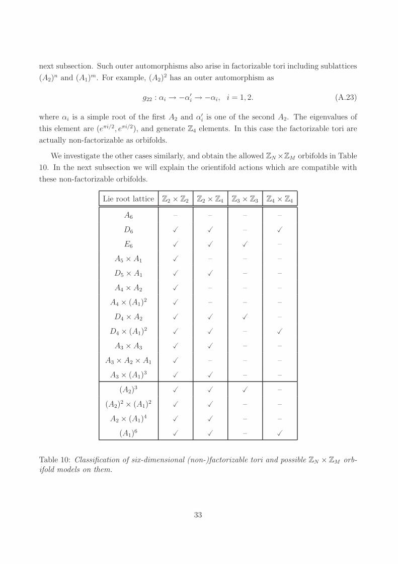
We investigate the other cases similarly, and obtain the allowed ZN×ZM orbifolds in Table
10. In the next subsection we will explain the orientifold actions which are compatible with
these non-factorizable orbifolds.
Lie root lattice Z2 × Z2 Z2 × Z4 Z3 × Z3 Z4 × Z4
A6 – – – –
D6 –
E6 –
A5 × A1 – – –
D5 × A1 – –
A4 × A2 – – –
A4 × (A1)2
– – –
D4 × A2 –
D4 × (A1)2
–
A3 × A3 – –
A3 × A2 × A1 – – –
A3 × (A1)3
– –
(A2)3
–
(A2)2 × (A1)
2 – –
A2 × (A1)4
– –
(A1)6
–
Table 10: Classification of six-dimensional (non-)factorizable tori and possible ZN × ZM orb-ifold models on them.
33
A.3 Orientifolds on non-factorizable orbifolds
In the previous subsection we gave a way to obtain orbifolds on non-factorizable tori. In order
to preserve supersymmetry, the orbifold action θ : (z1, z2, z3) → (e2πiv1z1, e2πiv2z2, e2πiv3z3)
should satisfy the equation v1 + v2 + v3 = 0. Then only a holomorphic (3, 0)-form Ω =
dz1 ∧ dz2 ∧ dz3 and a anti-holomorphic (0, 3)-form Ω are left invariant, and the other three
forms on a six-tori are generally projected out. The orientifold action R of O6-plane, which
preserve N = 1 supersymmetry, should act as
R : (z1, z2, z3)→ (az1, bz2, cz3), (A.24)
where a, b and c are phase factors. Then the every orientifold group element including Rgenerates fixed loci of O6-planes.
For their classification we again use the abbreviations a, b and 1 in (3.12). For the D6
lattice we have Z2 × Z2 elements as θ = (−1,−1, 1) and φ = (1,−1,−1). The orientifold
actions which are compatible with this orbifold are
(±a,±a,±a), (±a,±a,±b), (±a,±b,±b), (±b,±b,±b), (A.25)
where the underlined entries are permuted. For the orbifold elements θ = (−1, a,b), φ =
(1,−1,−1), the compatible orientifold actions are 8
± (a, a,−b), ± (a,−a,b), ± (−b, a,−b), ± (b,−a,b). (A.26)
In other words, the restriction is that the eigenvalues of each orientifold group element R, Rθ,
Rφ and Rθφ should be (−1,−1,−1, 1, 1, 1). Note that there are some equivalent actions due
to the symmetry of the lattice. These considerations lead to Table 7 for the Z2 × Z2 orbifold
models on the D6 lattice.
There exists an exception in this classification for the A3×A3 lattice as mentioned before.
We define the lattice A3 ×A3 by using the simple roots
α1 = e1 − e2,
α2 = e2 − e3,
α3 = e2 + e3,
α4 = e4 − e5,
α5 = e5 − e6,
α6 = e5 + e6.
(A.27)
In this base Z2 × Z2 orbifolds are obtained in a similar manner of the D6 lattice9. Note that
the action R = (∗,b, ∗), where ∗ is b, a or 1, is forbidden due to the lattice structure. The
8Note that for this orbifold elements the basis is different from (A.24).9It may seem that the classification with b,a and 1 elements is missing the action R : αi → −αi with
i = 1, 2, 3, however this action is included in orientifold groups, e.g. the Rθφ action of DCD model on Table
11.
34
outer automorphism between two A3’s generates an exceptional action
R : αi ↔ αi+3, i = 1, 2, 3. (A.28)
If we redefine the base of A3 × A3 as
α1 = e1 − e3,
α2 = e3 − e5,
α3 = e3 + e5,
α4 = e2 − e4,
α5 = e4 − e6,
α6 = e4 + e6,
(A.29)
the exceptional action is expressed by (b,b,b) in the orthogonal ei basis:
R : e1 ↔ e2, e3 ↔ e4, e5 ↔ e6. (A.30)
Actually this element gives only one inequivalent element including the outer automorphism,
and we label it as (DDD)′.
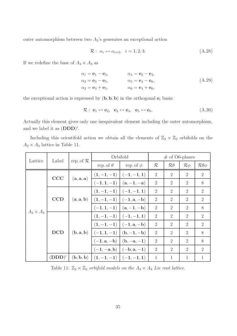
Including this orientifold action we obtain all the elements of Z2 × Z2 orbifolds on the
A3 ×A3 lattice in Table 11.
Lattice Label rep. of ROrbifold # of O6-planes
rep. of θ rep. of φ R Rθ Rφ Rθφ
A3 × A3
CCC (a, a, a)(1,−1,−1) (−1,−1, 1) 2 2 2 2
(−1, 1,−1) (a,−1,−a) 2 2 2 8
CCD (a, a,b)
(1,−1,−1) (−1,−1, 1) 2 2 2 2
(1,−1,−1) (−1, a,−b) 2 2 2 2
(−1, 1,−1) (a,−1,−b) 2 2 2 8
DCD (b, a,b)
(1,−1,−1) (−1,−1, 1) 2 2 2 2
(1,−1,−1) (−1, a,−b) 2 2 2 2
(−1, 1,−1) (b,−1,−b) 2 2 2 8
(−1, a,−b) (b,−a,−1) 2 2 2 8
(−1,−a,b) (−b, a,−1) 2 2 2 2
(DDD)′ (b,b,b) (1,−1,−1) (−1,−1, 1) 1 1 1 1
Table 11: Z2 × Z2 orbifold models on the A3 × A3 Lie root lattice.
35
B Comments on lattices
In this appendix we briefly summarize conventions of the (sub-)lattice and its dual lattice
space for a Z2 action R in the following way:
ΛR,⊥ : lattice projected out by the action R, ΛR,⊥ ≡1 +R
2Λ
ΛR,inv : R invariant sublattice
Λ∗ : dual lattice of Λ, for its base αj · α∗i = δji, αj ∈ Λ, α∗
i ∈ Λ∗
These three lattice spaces are closely related to one another. Introducing a lattice Λ−R,⊥ which
is projected out by the −R action on it, then we find the following non-trivial equations:
Λ∗R,⊥ = (ΛR,inv)
∗, (B.1a)
Vol(Λ) = Vol(ΛR,inv) · Vol(Λ−R,⊥), (B.1b)
Vol(Λ∗) = Vol(Λ)−1. (B.1c)
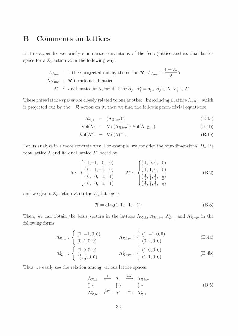
Let us analyze in a more concrete way. For example, we consider the four-dimensional D4 Lie
root lattice Λ and its dual lattice Λ∗ based on
Λ :
( 1,−1, 0, 0)
( 0, 1,−1, 0)
( 0, 0, 1,−1)
( 0, 0, 1, 1)
Λ∗ :
( 1, 0, 0, 0)
( 1, 1, 0, 0)
( 12, 1
2, 1
2,−1
2)
( 12, 1
2, 1
2, 1
2)
(B.2)
and we give a Z2 action R on the D4 lattice as
R = diag(1, 1,−1,−1). (B.3)
Then, we can obtain the basis vectors in the lattices ΛR,⊥, ΛR,inv, Λ∗R,⊥ and Λ∗
R,inv in the
following forms:
ΛR,⊥ :
(1,−1, 0, 0)
(0, 1, 0, 0)ΛR,inv :
(1,−1, 0, 0)
(0, 2, 0, 0)(B.4a)
Λ∗R,⊥ :
(1, 0, 0, 0)
(12, 1
2, 0, 0)
Λ∗R,inv :
(1, 0, 0, 0)
(1, 1, 0, 0)(B.4b)
Thus we easily see the relation among various lattice spaces:
ΛR,⊥⊥←− Λ
inv−→ ΛR,inv
l ∗ l ∗ l ∗Λ∗
R,invinv←− Λ∗ ⊥−→ Λ∗
R,⊥
(B.5)
36
C String one-loop amplitudes
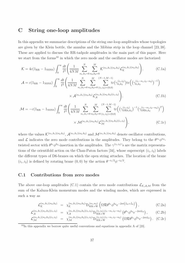
In this appendix we summarize descriptions of the string one-loop amplitudes whose topologies
are given by the Klein bottle, the annulus and the Mobius strip in the loop channel [23, 38].
These are applied to discuss the RR-tadpole amplitudes in the main part of this paper. Here
we start from the forms10 in which the zero mode and the oscillator modes are factorized:
K = 4c(1RR − 1NSNS)
∫ ∞
0
dt
t3
(
1
4NM
N∑
n1,k1=0
M∑
n2,k2=0
K(n1,k1)(n2,k2)L(n1,k1)(n2,k2)K
)
, (C.1a)
A = c(1RR − 1NSNS)
∫ ∞
0
dt
t3
(
1
4NM
N∑
n1,k1=0
M∑
n2,k2=0
(N−1,M−1)∑
(i1,i2)=(0,0)
tr(
γ(i1,i2)k1k2
)
tr(
(
γ(i1−n1,i2−n2)k1k2
)−1)
×A(n1,k1)(n2,k2)L(n1,k1)(n2,k2)(i1,i2)A
)
, (C.1b)
M = −c(1RR − 1NSNS)
∫ ∞
0
dt
t3
(
1
4NM
N∑
n1,k1=0
M∑
n2,k2=0
(N−1,M−1)∑
(i1,i2)=(0,0)
tr(
(
γ(i1,i2)ΩRk1k2
)−1(γ
(i1−n1,i2−n2)ΩRk1k2
)T)
×M(n1,k1)(n2,k2)L(n1,k1)(n2,k2)(i1,i2)M
)
, (C.1c)
where the values K(n1,k1)(n2,k2), A(n1,k1)(n2,k2) andM(n1,k1)(n2,k2) denote oscillator contributions,
and L indicates the zero mode contributions in the amplitudes. They belong to the θn1φn2-
twisted sector with θk1φk2-insertion in the amplitudes. The γ(i1,i2)’s are the matrix representa-
tions of the orientifold action on the Chan-Paton factors [34], whose superscript (i1, i2) labels
the different types of D6-branes on which the open string attaches. The location of the brane
(i1, i2) is defined by rotating brane (0, 0) by the action θ−i1/2φ−i2/2.
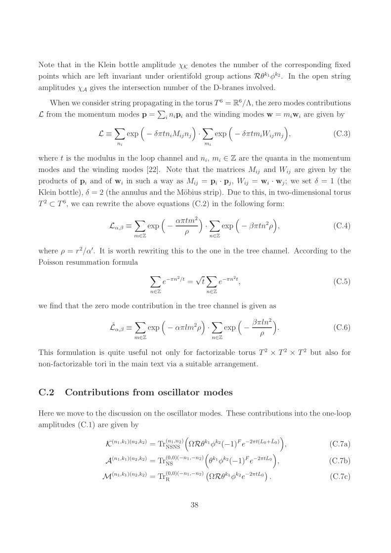
C.1 Contributions from zero modes
The above one-loop amplitudes (C.1) contain the zero mode contributions LK,A,M from the
sum of the Kaluza-Klein momentum modes and the winding modes, which are expressed in
such a way as
L(n1,k1)(n2,k2)K = χ
(n1,k1)(n2,k2)K Tr
(n1,n2)KK+W
(
ΩRθk1φk2e−2πt(L0+L0))
, (C.2a)
L(n1,k1)(n2,k2)(i1,i2)A = χ
(n1,k1)(n2,k2)(i1,i2)A Tr
(i1,i2),(i1−n1,i2−n2)KK+W
(
θk1φk2e−2πtL0)
, (C.2b)
L(n1,k1)(n2,k2)(i1,i2)M = χ
(n1,k1)(n2,k2)(i1,i2)M Tr
(i1,i2),(i1−n1,i2−n2)KK+W
(
ΩRθk1φk2e−2πtL0)
. (C.2c)
10In this appendix we borrow quite useful conventions and equations in appendix A of [23].
37
Note that in the Klein bottle amplitude χK denotes the number of the corresponding fixed
points which are left invariant under orientifold group actions Rθk1φk2. In the open string
amplitudes χA gives the intersection number of the D-branes involved.
When we consider string propagating in the torus T 6 = R6/Λ, the zero modes contributions
L from the momentum modes p =∑
i nipi and the winding modes w = miwi are given by
L ≡∑
ni
exp(
− δπtniMijnj
)
·∑
mi
exp(
− δπtmiWijmj
)
, (C.3)
where t is the modulus in the loop channel and ni, mi ∈ Z are the quanta in the momentum
modes and the winding modes [22]. Note that the matrices Mij and Wij are given by the
products of pi and of wi in such a way as Mij = pi · pj, Wij = wi · wj ; we set δ = 1 (the
Klein bottle), δ = 2 (the annulus and the Mobius strip). Due to this, in two-dimensional torus
T 2 ⊂ T 6, we can rewrite the above equations (C.2) in the following form:
Lα,β ≡∑
m∈Z
exp(
− απtm2
ρ
)
·∑
n∈Z
exp(
− βπtn2ρ)
, (C.4)
where ρ = r2/α′. It is worth rewriting this to the one in the tree channel. According to the
Poisson resummation formula
∑
n∈Z
e−πn2/t =√
t∑
n∈Z
e−πn2t, (C.5)
we find that the zero mode contribution in the tree channel is given as
Lα,β ≡∑
m∈Z
exp(
− απlm2ρ)
·∑
n∈Z
exp(
− βπln2
ρ
)
. (C.6)
This formulation is quite useful not only for factorizable torus T 2 × T 2 × T 2 but also for
non-factorizable tori in the main text via a suitable arrangement.
C.2 Contributions from oscillator modes
Here we move to the discussion on the oscillator modes. These contributions into the one-loop
amplitudes (C.1) are given by
K(n1,k1)(n2,k2) = Tr(n1,n2)NSNS
(
ΩRθk1φk2(−1)F e−2πt(L0+L0))
, (C.7a)
A(n1,k1)(n2,k2) = Tr(0,0)(−n1,−n2)NS
(
θk1φk2(−1)F e−2πtL0
)
, (C.7b)
M(n1,k1)(n2,k2) = Tr(0,0)(−n1,−n2)R
(
ΩRθk1φk2e−2πtL0)
. (C.7c)
38

The superscript (0, 0)(−n1,−n2) on the trace Tr(0,0)(−n1,−n2)NS in (C.7b) indicates open string
states stretching between two distinct branes (0, 0) and (−n1,−n2), or equivalently, between
the brane (i1, i2) and the brane (i1 − n1, i2 − n2). The oscillator contributions (C.7) can be
expressed by the use of Jacobi theta functions ϑ[
αβ
]
(t) and the Dedekind eta function η(t):
ϑ
[
α
β
]
(t) =∑
n∈Z
q(n+α)2
2 e2πi(n+α)β, η (t) = q124
∞∏
n=1
(1− qn) , (C.8)
with q = e−2πt. Then the amplitudes are expressed as
K(n1,n2) =ϑ[
01/2
]
η3
∏
n1vi+n2wi 6∈Z
ϑ[
n1vi+n2wi
1/2
]
ϑ[
1/2+n1vi+n2wi
1/2
]eπi〈n1vi+n2wi〉
×∏
n1vi+n2wi∈Z
ϑ[
01/2
]
η3
, (C.9a)
A(n1,k1)(n2,k2) =ϑ[
01/2
]
η3
∏
(n1vi+n2wi,k1vi+k2wi)6∈Z2
(−2i)δϑ[
n1vi+n2wi
1/2+k1vi+k2wi
]
ϑ[
1/2+n1vi+n2wi
1/2+k1vi+k2wi
] eπi〈n1vi+n2wi〉
×∏
(n1vi+n2wi,k1vi+k2wi)∈Z2
ϑ[
01/2
]
η3
, (C.9b)
M(n1,k1)(n2,k2) =ϑ[
1/20
]
η3
∏
(n1vi+n2wi,k1vi+k2wi)6∈Z2
(−2i)δϑ[
1/2+n1vi+n2wi
k1vi+k2wi
]
ϑ[
1/2+n1vi+n2wi
1/2+k1vi+k2wi
] eπi〈n1vi+n2wi〉
×∏
(n1vi+n2wi,k1vi+k2wi)∈Z2
ϑ[
1/20
]
η3
. (C.9c)
Notice that except for the Z′6 orbifold the values K(n1,k1)(n2,k2) are equal for any insertion of
θk1φk2, even though the lattice contributions differ [38]. Then we omit the label ki in (C.9a).
The arguments in the theta and eta functions are 2t in the Klein bottle, t + i2
in the Mobius
strip, and t in the annulus. Further, we used the notation [38], 〈x〉 ≡ x − [x] − 12, where the
brackets on the rhs denote the integer part and
δ =
1 if (n1vi + n2wi, k1vi + k2wi) ∈ Z× Z + 12
0 otherwise(C.10)
The tree channel expressions K, A and M can be evaluated with the help of the modular
transformation of (C.8).
39

References
[1] G. Aldazabal, S. Franco, L. E. Ibanez, R. Rabadan and A. M. Uranga, “D = 4 chi-
ral string compactifications from intersecting branes,” J. Math. Phys. 42 (2001) 3103
[arXiv:hep-th/0011073].
[2] L. E. Ibanez, F. Marchesano and R. Rabadan, “Getting just the standard model at
intersecting branes,” JHEP 0111 (2001) 002 [arXiv:hep-th/0105155].
[3] R. Blumenhagen, B. Kors, D. Lust and T. Ott, “The standard model from stable inter-
secting brane world orbifolds,” Nucl. Phys. B 616 (2001) 3 [arXiv:hep-th/0107138].
[4] D. Bailin, G. V. Kraniotis and A. Love, “Standard-like models from intersecting D4-
branes,” Phys. Lett. B 530 (2002) 202 [arXiv:hep-th/0108131].
[5] C. Kokorelis, “New standard model vacua from intersecting branes,” JHEP 0209 (2002)
029 [arXiv:hep-th/0205147].
[6] T. Higaki, N. Kitazawa, T. Kobayashi and K. J. Takahashi, “Flavor structure and
coupling selection rule from intersecting D-branes,” Phys. Rev. D 72 (2005) 086003
[arXiv:hep-th/0504019].
[7] R. Blumenhagen, L. Gorlich and T. Ott, “Supersymmetric intersecting branes on the
type IIA T 6/Z4 orientifold,” JHEP 0301 (2003) 021 [arXiv:hep-th/0211059].
[8] R. Blumenhagen, V. Braun, B. Kors and D. Lust, “Orientifolds of K3 and Calabi-Yau
manifolds with intersecting D-branes,” JHEP 0207 (2002) 026 [arXiv:hep-th/0206038].
[9] M. Cvetic, G. Shiu and A. M. Uranga, “Three-family supersymmetric standard
like models from intersecting brane worlds,” Phys. Rev. Lett. 87 (2001) 201801
[arXiv:hep-th/0107143].
[10] M. Cvetic, G. Shiu and A. M. Uranga, “Chiral four-dimensional N = 1 supersym-
metric type IIA orientifolds from intersecting D6-branes,” Nucl. Phys. B 615 (2001)
3 [arXiv:hep-th/0107166].
[11] C. Kokorelis, “Standard model compactifications of IIA Z(3) x Z(3) orientifolds from
intersecting D6-branes,” Nucl. Phys. B 732 (2006) 341 [arXiv:hep-th/0412035].
[12] G. Honecker, “Chiral supersymmetric models on an orientifold of Z4×Z2 with intersecting
D6-branes,” Nucl. Phys. B 666 (2003) 175 [arXiv:hep-th/0303015].
40

[13] M. Cvetic and P. Langacker, “New grand unified models with intersecting D6-branes,
neutrino masses, and flipped SU(5),” arXiv:hep-th/0607238.
[14] R. Blumenhagen, M. Cvetic, P. Langacker and G. Shiu, “Toward realistic intersecting
D-brane models,” Ann. Rev. Nucl. Part. Sci. 55 (2005) 71 [arXiv:hep-th/0502005].
[15] F. G. Marchesano Buznego, “Intersecting D-brane models,” arXiv:hep-th/0307252.
[16] R. Blumenhagen, B. Kors, D. Lust and S. Stieberger, “Four-dimensional string com-
pactifications with D-branes, orientifolds and fluxes,” Phys. Rept. 445 (2007) 1
[arXiv:hep-th/0610327].
[17] M. Berkooz and R. G. Leigh, “A D = 4 N = 1 orbifold of type I strings,” Nucl. Phys. B
483 (1997) 187 [arXiv:hep-th/9605049].
[18] L. Susskind, “The anthropic landscape of string theory,” arXiv:hep-th/0302219.
[19] T. P. T. Dijkstra, L. R. Huiszoon and A. N. Schellekens, “Supersymmetric standard model
spectra from RCFT orientifolds,” Nucl. Phys. B 710 (2005) 3 [arXiv:hep-th/0411129].
[20] O. Lebedev, H. P. Nilles, S. Raby, S. Ramos-Sanchez, M. Ratz, P. K. S. Vaudrevange and
A. Wingerter, “A mini-landscape of exact MSSM spectra in heterotic orbifolds,” Phys.
Lett. B 645 (2007) 88 [arXiv:hep-th/0611095].
[21] S. Forste, C. Timirgaziu and I. Zavala, “Orientifold’s landscape: non-factorisable six-
tori,” JHEP 0710 (2007) 025 [arXiv:0707.0747 [hep-th]].
[22] R. Blumenhagen, J. P. Conlon and K. Suruliz, “Type IIA orientifolds on general super-
symmetric ZN orbifolds,” JHEP 0407 (2004) 022 [arXiv:hep-th/0404254].
[23] S. Forste, G. Honecker and R. Schreyer, “Supersymmetric ZN × ZM orientifolds in 4D
with D-branes at angles,” Nucl. Phys. B 593 (2001) 127 [arXiv:hep-th/0008250].
[24] R. Donagi and A. E. Faraggi, “On the number of chiral generations in Z2×Z2 orbifolds,”
Nucl. Phys. B 694 (2004) 187 [arXiv:hep-th/0403272].
[25] A. E. Faraggi, S. Forste and C. Timirgaziu, “Z2 × Z2 heterotic orbifold mod-
els of non factorisable six dimensional toroidal manifolds,” JHEP 0608 (2006) 057
[arXiv:hep-th/0605117].
[26] S. Forste, T. Kobayashi, H. Ohki and K. J. Takahashi, “Non-factorisable Z2×Z2 heterotic
orbifold models and Yukawa couplings,” JHEP 0703 (2007) 011 [arXiv:hep-th/0612044].
41
[27] K.J. Takahashi, “Heterotic orbifold models on Lie lattice with discrete torsion,” JHEP
0703 (2007) 103 [arXiv:hep-th/0702025].
[28] K. J. Takahashi, “Three-family GUT models from heterotic orbifold on E6 root lattice,”
arXiv:0707.3355 [hep-th].
[29] J. Polchinski and Y. Cai, “Consistency of open superstring theories,” Nucl. Phys. B 296
(1988) 91.
[30] G. Aldazabal, A. Font, L. E. Ibanez and G. Violero, Nucl. Phys. B 536 (1998) 29
[arXiv:hep-th/9804026].
[31] R. Blumenhagen, L. Gorlich and B. Kors, “Supersymmetric orientifolds in 6D with D-
branes at angles,” Nucl. Phys. B 569 (2000) 209 [arXiv:hep-th/9908130].
[32] R. Blumenhagen, L. Gorlich, B. Kors and D. Lust, “Magnetic flux in toroidal type I
compactifications,” Fortsch. Phys. 49 (2001) 591 [arXiv:hep-th/0010198].
[33] R. Blumenhagen, B. Kors and D. Lust, “Type I strings with F- and B-flux,” JHEP 0102
(2001) 030 [arXiv:hep-th/0012156].
[34] E. G. Gimon and J. Polchinski, “Consistency conditions for orientifolds and D-manifolds,”
Phys. Rev. D 54 (1996) 1667 [arXiv:hep-th/9601038].
[35] A. Dabholkar, “Lectures on orientifolds and duality,” arXiv:hep-th/9804208.
[36] C. Angelantonj and A. Sagnotti, “Open strings,” Phys. Rept. 371 (2002) 1 [Erratum-ibid.
376 (2003) 339] [arXiv:hep-th/0204089].
[37] T. Ott, “Aspects of stability and phenomenology in type IIA orientifolds with intersecting
D6-branes,” Fortsch. Phys. 52 (2004) 28 [arXiv:hep-th/0309107].
[38] R. Blumenhagen, L. Gorlich and B. Kors, “Supersymmetric 4D orientifolds of type IIA
with D6-branes at angles,” JHEP 0001 (2000) 040 [arXiv:hep-th/9912204].
[39] L. J. Dixon, J. A. Harvey, C. Vafa and E. Witten, “Strings on orbifolds. 2,” Nucl. Phys.
B 274 (1986) 285.
[40] A. N. Schellekens and N. P. Warner, “Weyl groups, supercurrents and covariant lattices,”
Nucl. Phys. B 308 (1988) 397.
[41] F. Ploger, S. Ramos-Sanchez, M. Ratz and P. K. S. Vaudrevange, “Mirage torsion,” JHEP
0704 (2007) 063 [arXiv:hep-th/0702176].
42