Traveling waves of calcium in pancreatic acinar cells: model construction and bifurcation analysis

Physica D 145 (2000) 158–179

Traveling waves of calcium in pancreatic acinar cells:model construction and bifurcation analysis

James Sneyda,∗, Andrew LeBeaub, David Yulec,1

a Department of Mathematics, University of Michigan, Ann Arbor, MI, USAb Mathematical Research Branch, NIH, 9190 Rockville Pike, Suite 350, Bethesda, MD, USA

c Department of Physiology, University of Michigan, Ann Arbor, MI, USA

Received 23 August 1999; received in revised form 18 April 2000; accepted 21 April 2000Communicated by C.K.R.T. Jones

Abstract

We construct and study a model for intracellular calcium wave propagation, with particular attention to pancreatic acinarcells. The model is based on a model of the inositol trisphosphate (IP3) receptor, which assumes that calcium modulates thebinding affinity of IP3 to the receptor. Two versions of the model, one simpler than the other, are studied numerically. Inboth versions, solitary waves in the excitable regime arise via homoclinic bifurcations in the traveling wave equations. As thebackground concentration of IP3 is increased, the wave speed increases, and for some values of the IP3 concentration, theinitial pulse gives rise to secondary pulses that travel in both directions. This can give rise to irregular spatio-temporal behavior,or to trains of pulses. In the simpler model, these secondary waves are related to the presence of a T-point, a heteroclinic cycle,and an associated spiral of homoclinic orbits, which terminate the branch of homoclinic orbits. © 2000 Elsevier Science B.V.All rights reserved.

Keywords:Calcium waves; Mathematical model; Traveling waves; Bifurcation theory; Inositol trisphosphate receptor; Homoclinicbifurcations; T-point; Pancreatic acinar cells

1. Introduction

Traveling waves of increased cytoplasmic calcium(Ca2+) concentration have been observed in many celltypes, and are widely believed to be one importantmechanism by which a group of cells, or a single largecell, is able to coordinate behavior over a large region

∗ Corresponding author. Present address: Institute of Informationand Mathematical Sciences, Massey University, Albany Campus,Private Bag 102-904, North Shore Mail Centre, Auckland, NewZealand.E-mail address:[email protected] (J. Sneyd).

1 Present address: Department of Pharmacology and Physiol-ogy, University of Rochester, School of Medicine and Dentistry,Rochester, NY, USA.

[36]. Thus, Ca2+ waves, both within a single cell,and between cells, have been studied in detail by bothexperimentalists and theoreticians, and there exists alarge body of work on the mechanisms underlyingsuch wave propagation.

The pancreatic acinus is a particularly interestingsystem to study Ca2+ waves [20,26,29,42]. Firstly,the pancreatic acinar cell is electrically non-excitable,and the Ca2+ wave results (at least in large part)from the release of Ca2+ from the endoplasmic retic-ulum. Secondly, each acinus consists of a number ofcells arranged in a ring around a central duct, andthe Ca2+ wave travels from cell to cell around thisring in a characteristic fashion [42]. The functionof this intercellular Ca2+ wave is not entirely clear,

0167-2789/00/$ – see front matter © 2000 Elsevier Science B.V. All rights reserved.PII: S0167-2789(00)00108-1

J. Sneyd et al. / Physica D 145 (2000) 158–179 159

although it appears to increase the efficiency of en-zyme secretion of the acinus, presumably by coordi-nating the secretion of each individual cell with thatof its neighbors. Thirdly, different agonists cause dif-ferent wave responses [22,37]. This, in turn, resultsfrom the fact that different agonists cause differentoscillatory responses in each individual cell. Applica-tion of intermediate doses of acetylcholine (ACh) orcarbachol (CCh) causes high-frequency oscillationssuperimposed on a raised baseline, while applicationof cholecystokinin (CCK) causes baseline oscillationswith a much larger period [41].

Both types of agonists cause oscillations via theproduction of the intracellular signaling messengerinositol (1,4,5) trisphosphate (IP3). Binding of the ag-onist to the cell surface receptor activates a G-protein,resulting in the activation of phospholipase C (PLC)and the subsequent production of IP3 from phos-phatidylinositol bisphosphate. IP3 diffuses throughthe cell cytoplasm and binds to IP3 receptors locatedon the endoplasmic reticulum (ER). These receptors,which also act as Ca2+ channels, then open, releasingCa2+ from the ER. Subsequent inactivation of the IP3

receptors, and removal of Ca2+ from the cytoplasmby membrane pumps, then returns the Ca2+ concen-tration to its resting value. If the concentration of IP3

is in the correct range, it can initiate a cycle of releaseand uptake of Ca2+ from the ER, resulting in Ca2+

oscillations.Although different agonists cause markedly differ-

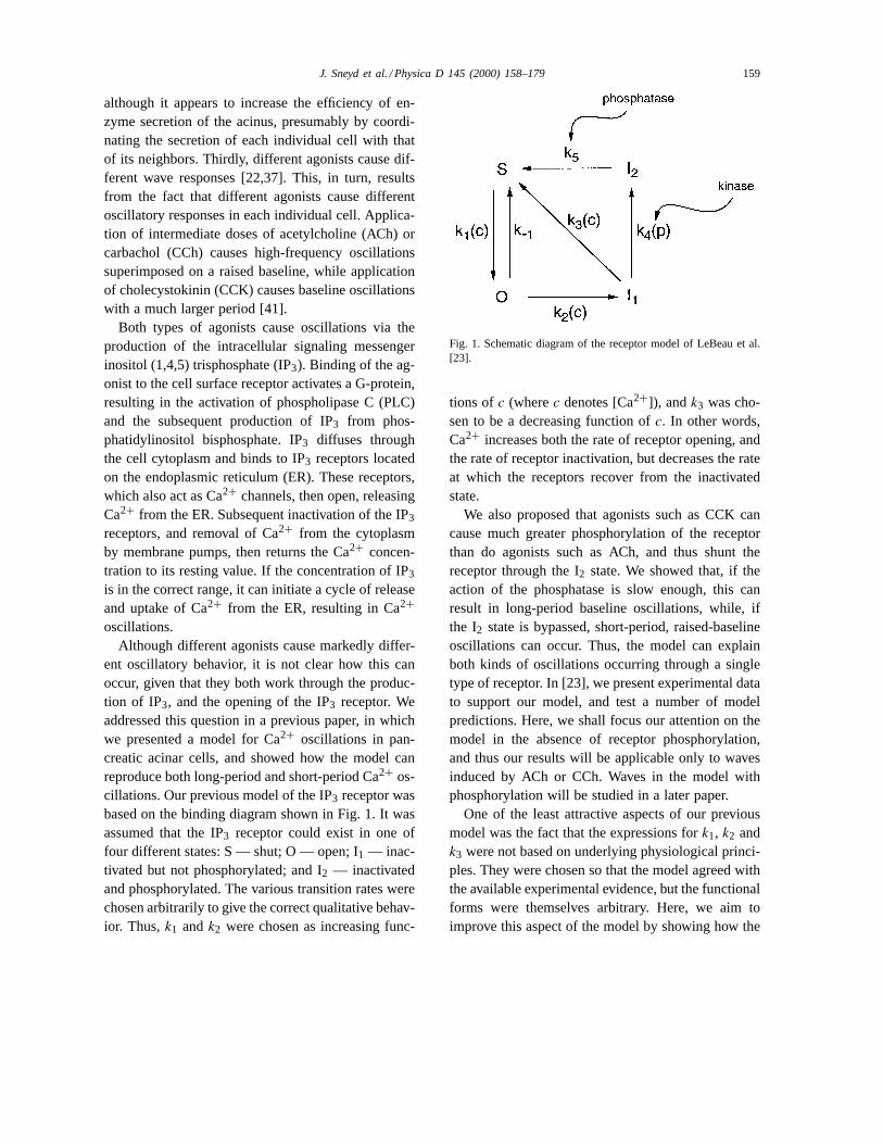
ent oscillatory behavior, it is not clear how this canoccur, given that they both work through the produc-tion of IP3, and the opening of the IP3 receptor. Weaddressed this question in a previous paper, in whichwe presented a model for Ca2+ oscillations in pan-creatic acinar cells, and showed how the model canreproduce both long-period and short-period Ca2+ os-cillations. Our previous model of the IP3 receptor wasbased on the binding diagram shown in Fig. 1. It wasassumed that the IP3 receptor could exist in one offour different states: S — shut; O — open; I1 — inac-tivated but not phosphorylated; and I2 — inactivatedand phosphorylated. The various transition rates werechosen arbitrarily to give the correct qualitative behav-ior. Thus,k1 andk2 were chosen as increasing func-

Fig. 1. Schematic diagram of the receptor model of LeBeau et al.[23].

tions ofc (wherec denotes [Ca2+]), andk3 was cho-sen to be a decreasing function ofc. In other words,Ca2+ increases both the rate of receptor opening, andthe rate of receptor inactivation, but decreases the rateat which the receptors recover from the inactivatedstate.

We also proposed that agonists such as CCK cancause much greater phosphorylation of the receptorthan do agonists such as ACh, and thus shunt thereceptor through the I2 state. We showed that, if theaction of the phosphatase is slow enough, this canresult in long-period baseline oscillations, while, ifthe I2 state is bypassed, short-period, raised-baselineoscillations can occur. Thus, the model can explainboth kinds of oscillations occurring through a singletype of receptor. In [23], we present experimental datato support our model, and test a number of modelpredictions. Here, we shall focus our attention on themodel in the absence of receptor phosphorylation,and thus our results will be applicable only to wavesinduced by ACh or CCh. Waves in the model withphosphorylation will be studied in a later paper.

One of the least attractive aspects of our previousmodel was the fact that the expressions fork1, k2 andk3 were not based on underlying physiological princi-ples. They were chosen so that the model agreed withthe available experimental evidence, but the functionalforms were themselves arbitrary. Here, we aim toimprove this aspect of the model by showing how the

160 J. Sneyd et al. / Physica D 145 (2000) 158–179

same model can be derived from a more detailed andrealistic model of the IP3 receptor. The basis of thenew model is the proposal [6,15] that Ca2+ regulatesthe interconversion of the IP3 receptor between twodifferent states, one of which has a high affinity forIP3, the other a low affinity. Here, we show that ourprevious model can be derived from such an assump-tion, and thus we can provide a mechanistic interpreta-tion of what was, originally, a more phenomenologicalmodel.

Our ultimate goal is the study of intercellular Ca2+

waves in a pancreatic acinus. However, before such agoal can be realized, it is necessary first to understandthe properties of traveling waves in the model in a ho-mogeneous medium. Thus, here we study the behaviorof traveling waves in the model in some detail.

2. The model equations

2.1. The model of the IP3 receptor

Instead of making the ad hoc assumption that therate constants for conversion between the receptorstates are functions of the Ca2+ concentration, we in-stead assume, as described above, that Ca2+ regulatesthe interconversion of the receptor between two dif-ferent shut states. We also make a similar assump-tion for the open and inactivated states. This extendedmodel of the IP3 receptor is shown schematically inFig. 2A. There are two different shut states, S andS,and Ca2+ regulates the interconversion of the recep-tor between these two states. Similarly, there are twoopen, and two inactivated states. Since IP3 can bindto either shut state, and convert it to an open state,the concentration of Ca2+ will determine the rate atwhich receptors are opened by IP3. In a similar fash-ion, [Ca2+] controls the rate of receptor inactivation,and the rate of recovery from inactivation.

We now assume that the interconversion betweenS andS is fast compared to the conversion of S orS to O, and similarly for O and I1. It is a simplematter to express this in terms of a formal perturbationexpansion, but as this adds nothing to the conclusionswe do not do so here. LettingS denote the fraction ofreceptors in state S, and similarly for the other states,

Fig. 2. (A) Schematic diagram of the full receptor model; (B)reduction of the full model by assuming fast calcium binding leadsto this simplified binding diagram, a slightly generalized versionof the one shown in Fig. 1.

we then obtain the relationships

cS= R1S, cO = R3O, cI1 = R5I1, (1)

where c denotes [Ca2+], and Ri = r−i/ri for i =1, 3, 5. Letting

x = S + S, (2)

y = O + O, (3)

z = I1 + I1, (4)

and using the law of mass action, it follows that

dx

dt= O(k−1 + r−2) − k1pS− r2pS

+k3I1 + r6I1, (5)

dy

dt= r2pS + k1pS− (r−2 + k−1)O

−k2O − r4O, (6)


wherep denotes the concentration of IP3. Note that adifferential equation forz is unnecessary, as we havethe conservation lawx + y + z = 1. If we then usethe constraints (1), we get

dx

dt= φ−1(c)y − pφ1(c)x + φ3(c)z, (7)

dy

dt= pφ1(c)x − φ−1(c)y + φ2(c)y, (8)

z = 1 − x − y, (9)

where

φ1(c) = k1R1 + r2c

R1 + c, (10)

φ−1(c) = (k−1 + r−2)R3

c + R3, (11)

φ2(c) = k2R3 + r4c

R3 + c, (12)

φ3(c) = k3R5 + r6c

R5 + c. (13)

We shall call this model, thethree-state model.Clearly, (7)–(9) are equivalent to the binding dia-

gram shown in Fig. 2B, which is itself the same as thebinding diagram of the original model (Fig. 1), withthe exception of the transition from the open state tothe closed state, which is a function ofc in the newversion of the model, but a constant in the old version.

Note that, by appropriate choice of parameters,φ1,φ2 andφ3 can be either increasing or decreasing func-tions of c. For instance, ifk1 < r2 then φ′

1(c) > 0and thus an increase inc increases the rate of receptoropening. The parameters (Table 1) are chosen so thatthe present model agrees with the model of LeBeauet al. [23], and thus has the correct steady-state open

Table 1Parameter values of the model

kf 28 Jleak 0.2Vp 1.2 Kp 0.18k1 0 k2 0.53k3 1 k−1 0.88r2 100 r4 20r6 0 r−2 0R1 6 R3 50R5 1.6 Dc 25

probability, the correct time course for receptor acti-vation and inactivation, and exhibits oscillations withthe correct period and qualitative shape.

2.2. Steady-state open probability

We shall make the simplifying assumption that theIP3 receptor is made up of four independent, identi-cal subunits, and that each subunit obeys the dynam-ics described above. Hence, the open probability,P ,is given byP = y4, with a steady value,Ps, givenby

Ps =(

θ1(c)p

p + θ2(c)

)4

, (14)

where

θ1 = φ3φ1

φ1φ2 + φ1φ3, (15)

θ2 = φ3φ−1 + φ3φ2

φ1φ2 + φ1φ3. (16)

For the parameters used here (see Table 1),Ps isa bell-shaped function ofc, and θ ′

2(c) < 0. Thebell-shaped nature of the steady-state open probabilitycurve is a feature that has been noted experimentallyby a number of groups [5,8,11,27], and the fact thatθ2 is a decreasing function ofc means that the affinityfor IP3 of the receptors increases with increasingc.This has been shown to be the case for Type III IP3

receptors [40], which are the predominant receptortype in pancreatic acinar cells. We thus predict that,for Type III receptors, the peak of the bell-shapedsteady-state open probability curve moves to the leftas p increases. Type I IP3 receptors have an IP3affinity that decreases as Ca2+ increases [40], and wehave shown that, in this case, the model predicts thatthe peak of the steady-state open probability curvewill move to the right asp increases. This is indeedwhat is seen experimentally [19].

2.3. A two-variable receptor model

It will be useful to reduce the three-state model toa simpler version by assuming that opening of the re-ceptor by IP3 binding is a fast process compared toreceptor inactivation and recovery from inactivation.


This is a standard assumption used in many models[1,21,24,33,35] and appears to agree well with exper-imental data. With this assumption we have the con-straint

pφ1x = φ−1y. (17)

Thus, lettingh = x+y, and recalling the conservationlaw which now takes the formh + z = 1, we get

dh

dt= φ3(1 − h) −

(φ1φ2p

φ1p + φ−1

)h. (18)

The open probability of the receptor is now given by

P =(

phφ1

φ1p + φ−1

)4

. (19)

We shall call this model thetwo-state model.

2.4. Incorporation into a whole-cell model

The above models of the IP3 receptor can be in-corporated into models for intracellular Ca2+ dynam-ics by assuming that Ca2+ can enter the cell via twopathways (through the IP3 receptor, fluxJreceptor, orthrough a generic leak from outside the cell or fromthe ER,Jleak), and is removed from the cytoplasm bythe action of Ca2+ ATPase pumps (with flux,Jpump).Thus, conservation of Ca2+ gives

dc

dt= Jreceptor− Jpump+ Jleak. (20)

In choosing functional forms forJpump andJleak wefollow previous models (reviewed in [33]) and assumethat Jleak is just a specified constant, while the Ca2+

ATPases work in a cooperative manner, with a Hillcoefficient of 2, and thus

Jpump = Vpc2

K2p + c2

, (21)

for some constantsVp andKp. The flux through thereceptor is given by the open probability multipliedby some scaling factor, and thus

Jreceptor= kf y4, (22)

for some constantkf . Jleak is assumed to be a constant.Here, we use the same parameter values as previously[23], and these are given in Table 1.

2.5. Summary of the model equations

The three-state model:

dx

dt= φ−1(c)y − pφ1(c)x + φ3(c)(1 − x − y), (23)

dy

dt= pφ1(c)x − φ−1(c)y − φ2(c)y, (24)

dc

dt= kf y4 − Vpc2

K2p + c2

+ Jleak. (25)

The two-state model:

dh

dt= φ3(1 − h) −

(φ1φ2p

φ1p + φ−1

)h, (26)

dc

dt= kf

(phφ1

φ1p + φ−1

)4

− Vpc2

K2p + c2

+ Jleak. (27)

The functionsφ are given by Eqs. (10)–(13).

3. Temporal oscillations

We are interested in the appearance and the be-havior of oscillations asp varies. In general,p willdepend on the concentration of agonist applied tothe cell, and thus, in the physiological situation, isprobably the most important controlling parameter.Oscillatory behavior in the models is most easilysummarized by bifurcation diagrams, usingp as themain bifurcation parameter. All bifurcation figures inthis paper were constructed numerically using AUTO[7], as implemented inxppaut by B. Ermentrout(http://www.pitt.edu/phase).

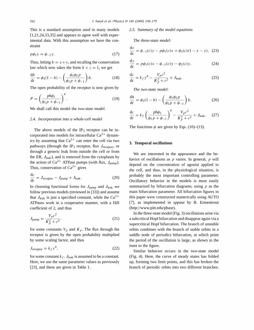
In the three-state model (Fig. 3) oscillations arise viaa subcritical Hopf bifurcation and disappear again via asupercritical Hopf bifurcation. The branch of unstableorbits combines with the branch of stable orbits in asaddle node of periodics bifurcation, at which pointthe period of the oscillation is large, as shown in theinset to the figure.

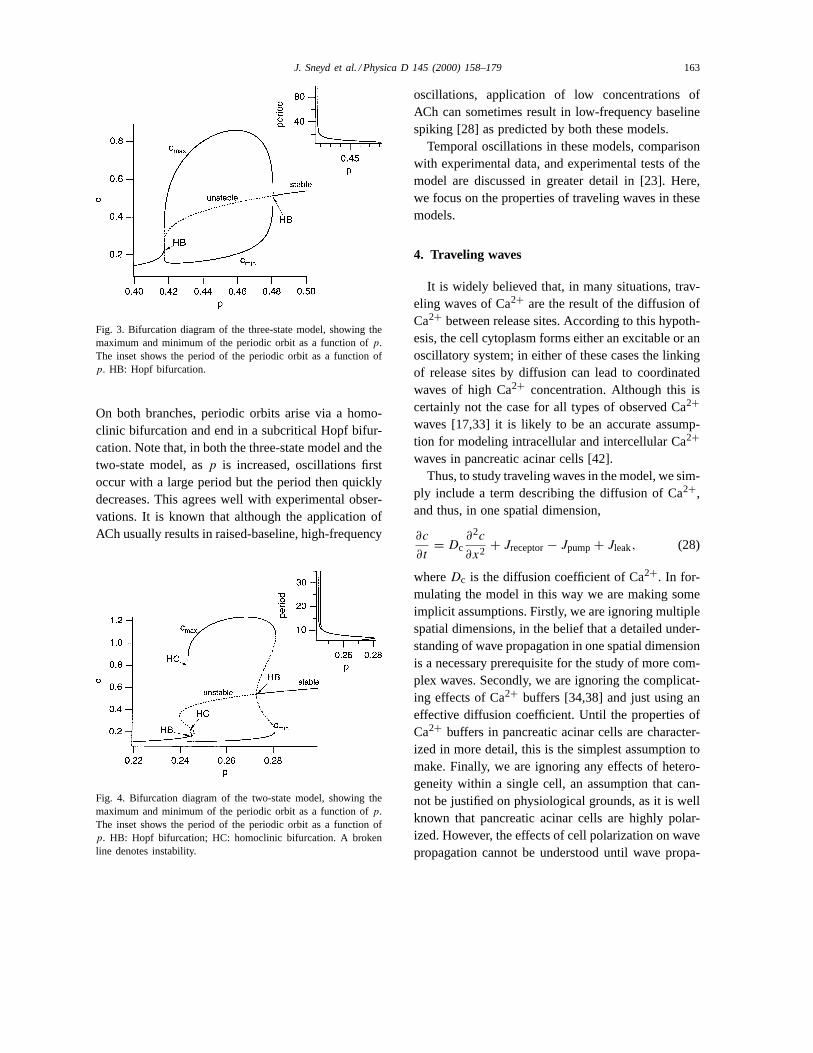
Similar behavior occurs in the two-state model(Fig. 4). Here, the curve of steady states has foldedup, forming two limit points, and this has broken thebranch of periodic orbits into two different branches.


Fig. 3. Bifurcation diagram of the three-state model, showing themaximum and minimum of the periodic orbit as a function ofp.The inset shows the period of the periodic orbit as a function ofp. HB: Hopf bifurcation.

On both branches, periodic orbits arise via a homo-clinic bifurcation and end in a subcritical Hopf bifur-cation. Note that, in both the three-state model and thetwo-state model, asp is increased, oscillations firstoccur with a large period but the period then quicklydecreases. This agrees well with experimental obser-vations. It is known that although the application ofACh usually results in raised-baseline, high-frequency

Fig. 4. Bifurcation diagram of the two-state model, showing themaximum and minimum of the periodic orbit as a function ofp.The inset shows the period of the periodic orbit as a function ofp. HB: Hopf bifurcation; HC: homoclinic bifurcation. A brokenline denotes instability.

oscillations, application of low concentrations ofACh can sometimes result in low-frequency baselinespiking [28] as predicted by both these models.

Temporal oscillations in these models, comparisonwith experimental data, and experimental tests of themodel are discussed in greater detail in [23]. Here,we focus on the properties of traveling waves in thesemodels.

4. Traveling waves

It is widely believed that, in many situations, trav-eling waves of Ca2+ are the result of the diffusion ofCa2+ between release sites. According to this hypoth-esis, the cell cytoplasm forms either an excitable or anoscillatory system; in either of these cases the linkingof release sites by diffusion can lead to coordinatedwaves of high Ca2+ concentration. Although this iscertainly not the case for all types of observed Ca2+

waves [17,33] it is likely to be an accurate assump-tion for modeling intracellular and intercellular Ca2+

waves in pancreatic acinar cells [42].Thus, to study traveling waves in the model, we sim-

ply include a term describing the diffusion of Ca2+,and thus, in one spatial dimension,

∂c

∂t= Dc

∂2c

∂x2+ Jreceptor− Jpump+ Jleak, (28)

whereDc is the diffusion coefficient of Ca2+. In for-mulating the model in this way we are making someimplicit assumptions. Firstly, we are ignoring multiplespatial dimensions, in the belief that a detailed under-standing of wave propagation in one spatial dimensionis a necessary prerequisite for the study of more com-plex waves. Secondly, we are ignoring the complicat-ing effects of Ca2+ buffers [34,38] and just using aneffective diffusion coefficient. Until the properties ofCa2+ buffers in pancreatic acinar cells are character-ized in more detail, this is the simplest assumption tomake. Finally, we are ignoring any effects of hetero-geneity within a single cell, an assumption that can-not be justified on physiological grounds, as it is wellknown that pancreatic acinar cells are highly polar-ized. However, the effects of cell polarization on wavepropagation cannot be understood until wave propa-


gation in a homogeneous medium is understood, andthus the present model should be viewed as a first stepfor the study of more realistic models.

4.1. Waves in the two-state model

We write the model in the traveling wave coordinateξ = x+st, wheres is the wave speed, and then look forhomoclinic orbits of the resulting ordinary differentialequations, as such orbits correspond to isolated trav-eling wave solutions of the original partial differentialequation. (Here, all numerically computed homoclinicorbits are actually just orbits of period 10 000. Com-putation of the branch of periodic orbits of period1000 gives the same result, which implies that the pe-riod 10 000 branch gives a good approximation of theposition of the homoclinic branch. However, it shouldbe noted that at no stage do we actually prove theexistence of the homoclinic branch.) Based on pre-vious work [32], we expect the homoclinic orbits toarise as the limit of periodic orbits as the period tendsto infinity. Hence, we begin by looking for periodicorbits arising from Hopf bifurcations in the travelingwave equations. The traveling wave equations are

c′ = d, (29)

Dcd′ = sd− kf

(phφ1

φ1p + φ−1

)4

+ Vpc2

K2p + c2

− Jleak, (30)

sh′ = φ3(1 − h) −(

φ1φ2p

φ1p + φ−1

)h, (31)

where a prime denotes differentiation with respectto ξ .

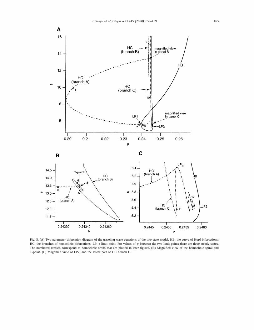
Some of the bifurcations of this three-dimensionalsystem are illustrated in Fig. 5. In panel A, we showa curve of Hopf bifurcations (labeled HB), and threebranches of homoclinic orbits (labeled HC), in thep, s

phase plane. Note that here we are treating the wavespeeds as a secondary bifurcation parameter. PanelsB and C show magnified views of two particular ar-eas of panel A, and we will discuss them later. Thenumbered crosses refer to points for which we plot the

homoclinic orbits in later figures. This lets us deter-mine how the homoclinic orbits change as we movealong the different branches.

4.1.1. Behavior ass → ∞First, we see that the behavior ass → ∞ is ex-

actly that of the model in the absence of diffusion(cf. Fig. 4), as expected from the general theory [25].Thus, for large values ofs there are two Hopf bifurca-tions, and two homoclinic bifurcations. The branch ofperiodic orbits that originates on the rightmost Hopfbifurcation ends in a homoclinic bifurcation on branchB, while the branch of periodic orbits arising from theleftmost Hopf bifurcation extends only a short distanceto the left before ending in a homoclinic bifurcationon branch C, as shown in Fig. 4. These homoclinic or-bits for larges are of little interest as they correspondto waves, which on a finite domain of physiologicalsize, look more like spatially independent responses.

4.1.2. The branch of Hopf bifurcationsFor any fixed value ofs we can find the values ofp

at which the Hopf bifurcations occur, and then thesebifurcation points can be continued in thes, p phasespace to give the curve labeled HB in Fig. 5A. Themost important thing about this curve is the fact thatit forms a loop, and thus has two limit points (labeledLP1 and LP2). These limit points exist only becausethe curve of steady states itself has two limit points(i.e., it is an S-shaped curve) as shown in Fig. 4. Thelimit points of the HB curve must necessarily coincidewith the limit points of the steady-state curve, i.e.,the points LP are when a Hopf bifurcation occurs ata limit point of the steady-state curve. For values ofp between LP1 and LP2, there are three steady-statesolutions.

When the Hopf bifurcation coincides with thelimit point of the steady-state curve we get acodimension-two bifurcation, with eigenvalues0 ± 0.137i and 0 at LP1, and eigenvalues 0± 0.191iand 0 at LP2. Analysis of such codimension-twobifurcations is a standard part of textbooks on dy-namical systems (e.g. [39]). Here, we merely notethat at LP1 there exists a branch of homoclinic or-bits (branch A) which exists on both sides of LP1, a


Fig. 5. (A) Two-parameter bifurcation diagram of the traveling wave equations of the two-state model. HB: the curve of Hopf bifurcations;HC: the branches of homoclinic bifurcations; LP: a limit point. For values ofp between the two limit points there are three steady states.The numbered crosses correspond to homoclinic orbits that are plotted in later figures. (B) Magnified view of the homoclinic spiral andT-point. (C) Magnified view of LP2, and the lower part of HC branch C.


branch of Hopf bifurcations (HB), and a branch ofsaddle-node bifurcations (not shown explicitly in thediagram). The same occurs for LP2, except that nowthe branch of homoclinic orbits (branch C) appears toexist only on one side of LP2, and it has a markedlydifferent character from the homoclinic branch closeto LP1. We shall discuss this in more detail later.

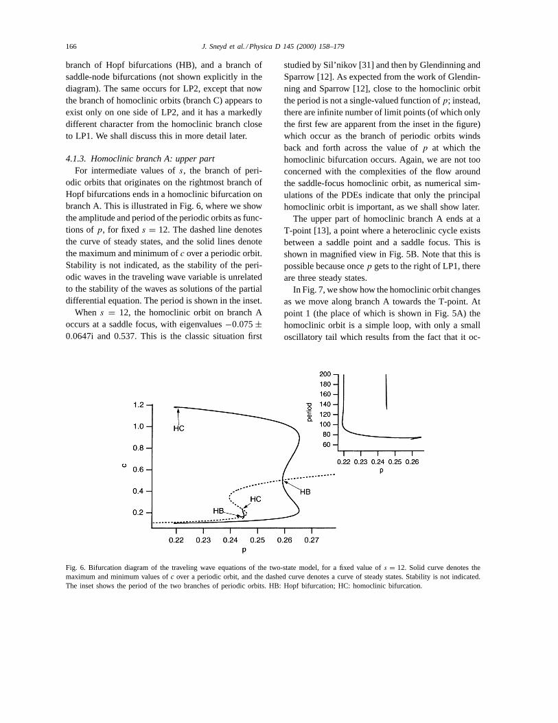
4.1.3. Homoclinic branch A: upper partFor intermediate values ofs, the branch of peri-

odic orbits that originates on the rightmost branch ofHopf bifurcations ends in a homoclinic bifurcation onbranch A. This is illustrated in Fig. 6, where we showthe amplitude and period of the periodic orbits as func-tions ofp, for fixed s = 12. The dashed line denotesthe curve of steady states, and the solid lines denotethe maximum and minimum ofc over a periodic orbit.Stability is not indicated, as the stability of the peri-odic waves in the traveling wave variable is unrelatedto the stability of the waves as solutions of the partialdifferential equation. The period is shown in the inset.

When s = 12, the homoclinic orbit on branch Aoccurs at a saddle focus, with eigenvalues−0.075±0.0647i and 0.537. This is the classic situation first

Fig. 6. Bifurcation diagram of the traveling wave equations of the two-state model, for a fixed value ofs = 12. Solid curve denotes themaximum and minimum values ofc over a periodic orbit, and the dashed curve denotes a curve of steady states. Stability is not indicated.The inset shows the period of the two branches of periodic orbits. HB: Hopf bifurcation; HC: homoclinic bifurcation.

studied by Sil’nikov [31] and then by Glendinning andSparrow [12]. As expected from the work of Glendin-ning and Sparrow [12], close to the homoclinic orbitthe period is not a single-valued function ofp; instead,there are infinite number of limit points (of which onlythe first few are apparent from the inset in the figure)which occur as the branch of periodic orbits windsback and forth across the value ofp at which thehomoclinic bifurcation occurs. Again, we are not tooconcerned with the complexities of the flow aroundthe saddle-focus homoclinic orbit, as numerical sim-ulations of the PDEs indicate that only the principalhomoclinic orbit is important, as we shall show later.

The upper part of homoclinic branch A ends at aT-point [13], a point where a heteroclinic cycle existsbetween a saddle point and a saddle focus. This isshown in magnified view in Fig. 5B. Note that this ispossible because oncep gets to the right of LP1, thereare three steady states.

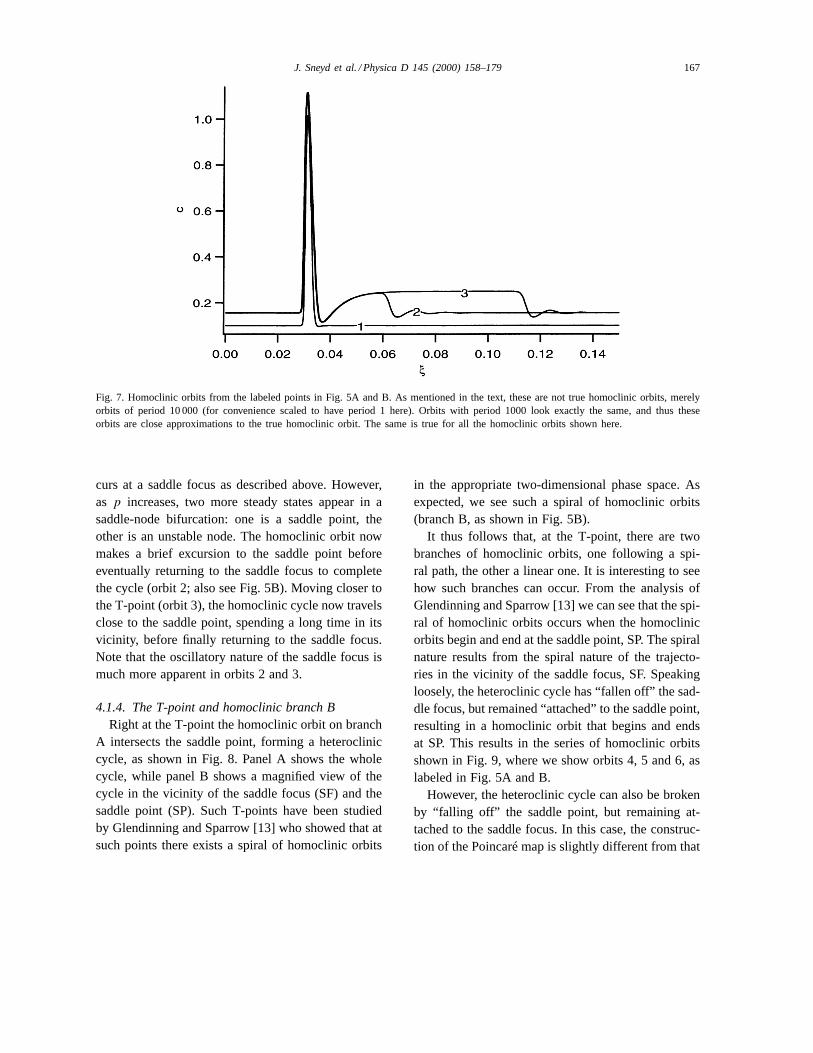
In Fig. 7, we show how the homoclinic orbit changesas we move along branch A towards the T-point. Atpoint 1 (the place of which is shown in Fig. 5A) thehomoclinic orbit is a simple loop, with only a smalloscillatory tail which results from the fact that it oc-


Fig. 7. Homoclinic orbits from the labeled points in Fig. 5A and B. As mentioned in the text, these are not true homoclinic orbits, merelyorbits of period 10 000 (for convenience scaled to have period 1 here). Orbits with period 1000 look exactly the same, and thus theseorbits are close approximations to the true homoclinic orbit. The same is true for all the homoclinic orbits shown here.

curs at a saddle focus as described above. However,as p increases, two more steady states appear in asaddle-node bifurcation: one is a saddle point, theother is an unstable node. The homoclinic orbit nowmakes a brief excursion to the saddle point beforeeventually returning to the saddle focus to completethe cycle (orbit 2; also see Fig. 5B). Moving closer tothe T-point (orbit 3), the homoclinic cycle now travelsclose to the saddle point, spending a long time in itsvicinity, before finally returning to the saddle focus.Note that the oscillatory nature of the saddle focus ismuch more apparent in orbits 2 and 3.

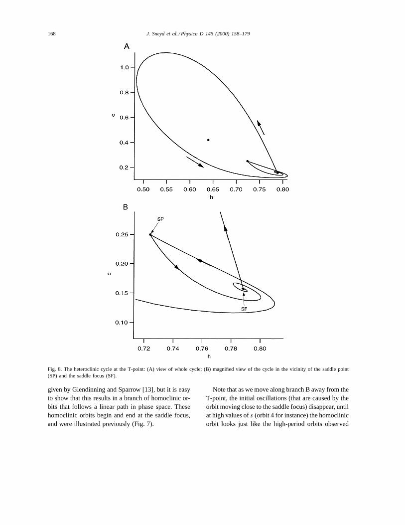
4.1.4. The T-point and homoclinic branch BRight at the T-point the homoclinic orbit on branch

A intersects the saddle point, forming a heterocliniccycle, as shown in Fig. 8. Panel A shows the wholecycle, while panel B shows a magnified view of thecycle in the vicinity of the saddle focus (SF) and thesaddle point (SP). Such T-points have been studiedby Glendinning and Sparrow [13] who showed that atsuch points there exists a spiral of homoclinic orbits

in the appropriate two-dimensional phase space. Asexpected, we see such a spiral of homoclinic orbits(branch B, as shown in Fig. 5B).

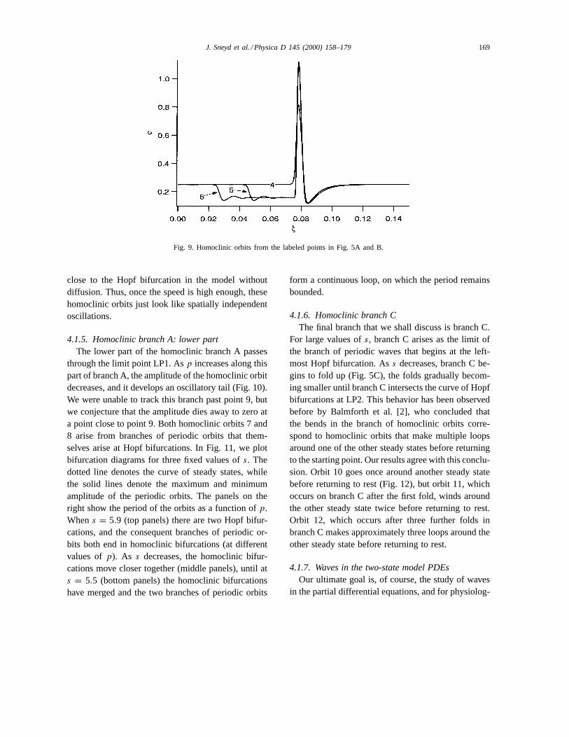
It thus follows that, at the T-point, there are twobranches of homoclinic orbits, one following a spi-ral path, the other a linear one. It is interesting to seehow such branches can occur. From the analysis ofGlendinning and Sparrow [13] we can see that the spi-ral of homoclinic orbits occurs when the homoclinicorbits begin and end at the saddle point, SP. The spiralnature results from the spiral nature of the trajecto-ries in the vicinity of the saddle focus, SF. Speakingloosely, the heteroclinic cycle has “fallen off” the sad-dle focus, but remained “attached” to the saddle point,resulting in a homoclinic orbit that begins and endsat SP. This results in the series of homoclinic orbitsshown in Fig. 9, where we show orbits 4, 5 and 6, aslabeled in Fig. 5A and B.

However, the heteroclinic cycle can also be brokenby “falling off” the saddle point, but remaining at-tached to the saddle focus. In this case, the construc-tion of the Poincaré map is slightly different from that


Fig. 8. The heteroclinic cycle at the T-point: (A) view of whole cycle; (B) magnified view of the cycle in the vicinity of the saddle point(SP) and the saddle focus (SF).

given by Glendinning and Sparrow [13], but it is easyto show that this results in a branch of homoclinic or-bits that follows a linear path in phase space. Thesehomoclinic orbits begin and end at the saddle focus,and were illustrated previously (Fig. 7).

Note that as we move along branch B away from theT-point, the initial oscillations (that are caused by theorbit moving close to the saddle focus) disappear, untilat high values ofs (orbit 4 for instance) the homoclinicorbit looks just like the high-period orbits observed


Fig. 9. Homoclinic orbits from the labeled points in Fig. 5A and B.

close to the Hopf bifurcation in the model withoutdiffusion. Thus, once the speed is high enough, thesehomoclinic orbits just look like spatially independentoscillations.

4.1.5. Homoclinic branch A: lower partThe lower part of the homoclinic branch A passes

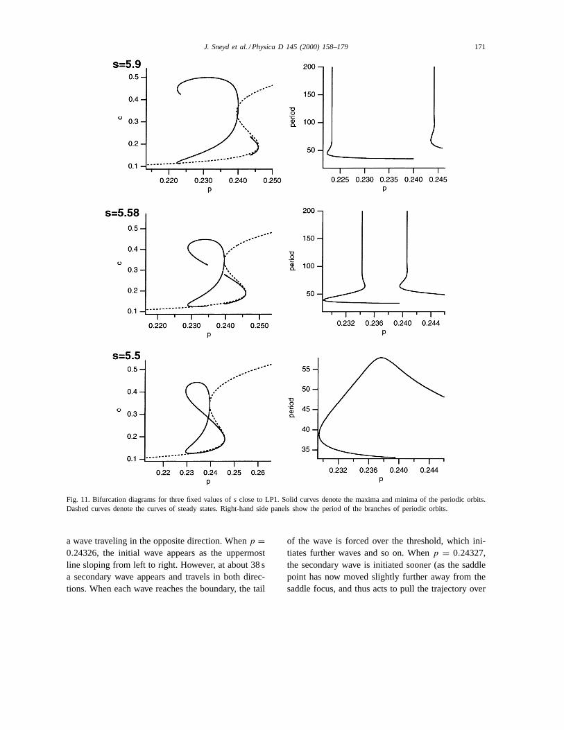
through the limit point LP1. Asp increases along thispart of branch A, the amplitude of the homoclinic orbitdecreases, and it develops an oscillatory tail (Fig. 10).We were unable to track this branch past point 9, butwe conjecture that the amplitude dies away to zero ata point close to point 9. Both homoclinic orbits 7 and8 arise from branches of periodic orbits that them-selves arise at Hopf bifurcations. In Fig. 11, we plotbifurcation diagrams for three fixed values ofs. Thedotted line denotes the curve of steady states, whilethe solid lines denote the maximum and minimumamplitude of the periodic orbits. The panels on theright show the period of the orbits as a function ofp.Whens = 5.9 (top panels) there are two Hopf bifur-cations, and the consequent branches of periodic or-bits both end in homoclinic bifurcations (at differentvalues ofp). As s decreases, the homoclinic bifur-cations move closer together (middle panels), until ats = 5.5 (bottom panels) the homoclinic bifurcationshave merged and the two branches of periodic orbits

form a continuous loop, on which the period remainsbounded.

4.1.6. Homoclinic branch CThe final branch that we shall discuss is branch C.

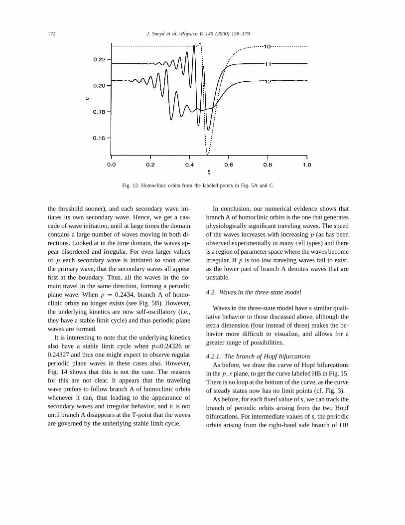
For large values ofs, branch C arises as the limit ofthe branch of periodic waves that begins at the left-most Hopf bifurcation. Ass decreases, branch C be-gins to fold up (Fig. 5C), the folds gradually becom-ing smaller until branch C intersects the curve of Hopfbifurcations at LP2. This behavior has been observedbefore by Balmforth et al. [2], who concluded thatthe bends in the branch of homoclinic orbits corre-spond to homoclinic orbits that make multiple loopsaround one of the other steady states before returningto the starting point. Our results agree with this conclu-sion. Orbit 10 goes once around another steady statebefore returning to rest (Fig. 12), but orbit 11, whichoccurs on branch C after the first fold, winds aroundthe other steady state twice before returning to rest.Orbit 12, which occurs after three further folds inbranch C makes approximately three loops around theother steady state before returning to rest.

4.1.7. Waves in the two-state model PDEsOur ultimate goal is, of course, the study of waves

in the partial differential equations, and for physiolog-


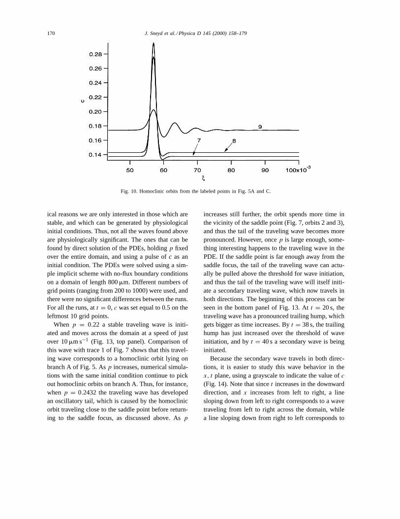
Fig. 10. Homoclinic orbits from the labeled points in Fig. 5A and C.

ical reasons we are only interested in those which arestable, and which can be generated by physiologicalinitial conditions. Thus, not all the waves found aboveare physiologically significant. The ones that can befound by direct solution of the PDEs, holdingp fixedover the entire domain, and using a pulse ofc as aninitial condition. The PDEs were solved using a sim-ple implicit scheme with no-flux boundary conditionson a domain of length 800mm. Different numbers ofgrid points (ranging from 200 to 1000) were used, andthere were no significant differences between the runs.For all the runs, att = 0, c was set equal to 0.5 on theleftmost 10 grid points.

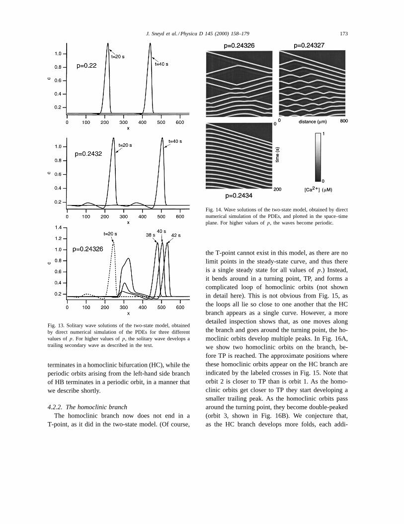
When p = 0.22 a stable traveling wave is initi-ated and moves across the domain at a speed of justover 10mm s−1 (Fig. 13, top panel). Comparison ofthis wave with trace 1 of Fig. 7 shows that this travel-ing wave corresponds to a homoclinic orbit lying onbranch A of Fig. 5. Asp increases, numerical simula-tions with the same initial condition continue to pickout homoclinic orbits on branch A. Thus, for instance,whenp = 0.2432 the traveling wave has developedan oscillatory tail, which is caused by the homoclinicorbit traveling close to the saddle point before return-ing to the saddle focus, as discussed above. Asp

increases still further, the orbit spends more time inthe vicinity of the saddle point (Fig. 7, orbits 2 and 3),and thus the tail of the traveling wave becomes morepronounced. However, oncep is large enough, some-thing interesting happens to the traveling wave in thePDE. If the saddle point is far enough away from thesaddle focus, the tail of the traveling wave can actu-ally be pulled above the threshold for wave initiation,and thus the tail of the traveling wave will itself initi-ate a secondary traveling wave, which now travels inboth directions. The beginning of this process can beseen in the bottom panel of Fig. 13. Att = 20 s, thetraveling wave has a pronounced trailing hump, whichgets bigger as time increases. Byt = 38 s, the trailinghump has just increased over the threshold of waveinitiation, and byt = 40 s a secondary wave is beinginitiated.

Because the secondary wave travels in both direc-tions, it is easier to study this wave behavior in thex, t plane, using a grayscale to indicate the value ofc

(Fig. 14). Note that sincet increases in the downwarddirection, andx increases from left to right, a linesloping down from left to right corresponds to a wavetraveling from left to right across the domain, whilea line sloping down from right to left corresponds to


Fig. 11. Bifurcation diagrams for three fixed values ofs close to LP1. Solid curves denote the maxima and minima of the periodic orbits.Dashed curves denote the curves of steady states. Right-hand side panels show the period of the branches of periodic orbits.

a wave traveling in the opposite direction. Whenp =0.24326, the initial wave appears as the uppermostline sloping from left to right. However, at about 38 sa secondary wave appears and travels in both direc-tions. When each wave reaches the boundary, the tail

of the wave is forced over the threshold, which ini-tiates further waves and so on. Whenp = 0.24327,the secondary wave is initiated sooner (as the saddlepoint has now moved slightly further away from thesaddle focus, and thus acts to pull the trajectory over


Fig. 12. Homoclinic orbits from the labeled points in Fig. 5A and C.

the threshold sooner), and each secondary wave ini-tiates its own secondary wave. Hence, we get a cas-cade of wave initiation, until at large times the domaincontains a large number of waves moving in both di-rections. Looked at in the time domain, the waves ap-pear disordered and irregular. For even larger valuesof p each secondary wave is initiated so soon afterthe primary wave, that the secondary waves all appearfirst at the boundary. Thus, all the waves in the do-main travel in the same direction, forming a periodicplane wave. Whenp = 0.2434, branch A of homo-clinic orbits no longer exists (see Fig. 5B). However,the underlying kinetics are now self-oscillatory (i.e.,they have a stable limit cycle) and thus periodic planewaves are formed.

It is interesting to note that the underlying kineticsalso have a stable limit cycle whenp=0.24326 or0.24327 and thus one might expect to observe regularperiodic plane waves in these cases also. However,Fig. 14 shows that this is not the case. The reasonsfor this are not clear. It appears that the travelingwave prefers to follow branch A of homoclinic orbitswhenever it can, thus leading to the appearance ofsecondary waves and irregular behavior, and it is notuntil branch A disappears at the T-point that the wavesare governed by the underlying stable limit cycle.

In conclusion, our numerical evidence shows thatbranch A of homoclinic orbits is the one that generatesphysiologically significant traveling waves. The speedof the waves increases with increasingp (as has beenobserved experimentally in many cell types) and thereis a region of parameter space where the waves becomeirregular. If p is too low traveling waves fail to exist,as the lower part of branch A denotes waves that areunstable.

4.2. Waves in the three-state model

Waves in the three-state model have a similar quali-tative behavior to those discussed above, although theextra dimension (four instead of three) makes the be-havior more difficult to visualize, and allows for agreater range of possibilities.

4.2.1. The branch of Hopf bifurcationsAs before, we draw the curve of Hopf bifurcations

in thep, s plane, to get the curve labeled HB in Fig. 15.There is no loop at the bottom of the curve, as the curveof steady states now has no limit points (cf. Fig. 3).

As before, for each fixed value ofs, we can track thebranch of periodic orbits arising from the two Hopfbifurcations. For intermediate values ofs, the periodicorbits arising from the right-hand side branch of HB


Fig. 13. Solitary wave solutions of the two-state model, obtainedby direct numerical simulation of the PDEs for three differentvalues ofp. For higher values ofp, the solitary wave develops atrailing secondary wave as described in the text.

terminates in a homoclinic bifurcation (HC), while theperiodic orbits arising from the left-hand side branchof HB terminates in a periodic orbit, in a manner thatwe describe shortly.

4.2.2. The homoclinic branchThe homoclinic branch now does not end in a

T-point, as it did in the two-state model. (Of course,

Fig. 14. Wave solutions of the two-state model, obtained by directnumerical simulation of the PDEs, and plotted in the space–timeplane. For higher values ofp, the waves become periodic.

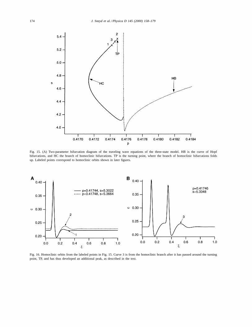
the T-point cannot exist in this model, as there are nolimit points in the steady-state curve, and thus thereis a single steady state for all values ofp.) Instead,it bends around in a turning point, TP, and forms acomplicated loop of homoclinic orbits (not shownin detail here). This is not obvious from Fig. 15, asthe loops all lie so close to one another that the HCbranch appears as a single curve. However, a moredetailed inspection shows that, as one moves alongthe branch and goes around the turning point, the ho-moclinic orbits develop multiple peaks. In Fig. 16A,we show two homoclinic orbits on the branch, be-fore TP is reached. The approximate positions wherethese homoclinic orbits appear on the HC branch areindicated by the labeled crosses in Fig. 15. Note thatorbit 2 is closer to TP than is orbit 1. As the homo-clinic orbits get closer to TP they start developing asmaller trailing peak. As the homoclinic orbits passaround the turning point, they become double-peaked(orbit 3, shown in Fig. 16B). We conjecture that,as the HC branch develops more folds, each addi-


Fig. 15. (A) Two-parameter bifurcation diagram of the traveling wave equations of the three-state model. HB is the curve of Hopfbifurcations, and HC the branch of homoclinic bifurcations. TP is the turning point, where the branch of homoclinic bifurcations foldsup. Labeled points correspond to homoclinic orbits shown in later figures.

Fig. 16. Homoclinic orbits from the labeled points in Fig. 15. Curve 3 is from the homoclinic branch after it has passed around the turningpoint, TP, and has thus developed an additional peak, as described in the text.


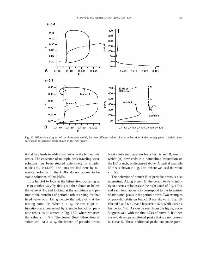
Fig. 17. Bifurcation diagram of the three-state model, for two different values ofs on either side of the turning point. Labeled pointscorrespond to periodic orbits shown in the next figure.

tional fold leads to additional peaks in the homoclinicorbits. The existence of multiple-peak traveling wavesolutions has been studied extensively in simplermodels [9,10,14,16]. The ones we find here by nu-merical solution of the ODEs do not appear to bestable solutions of the PDEs.

It is helpful to look at the bifurcation occurring atTP in another way by fixings either above or belowthe value at TP, and looking at the amplitude and pe-riod of the branches of periodic orbits arising for thatfixed value ofs. Let st denote the value ofs at theturning point, TP. Whens > st, the two Hopf bi-furcations are connected by a single branch of peri-odic orbits, as illustrated in Fig. 17A, where we usedthe values = 5.4. The lower Hopf bifurcation issubcritical. At s = st, the branch of periodic orbits

breaks into two separate branches, A and B, one ofwhich (A) now ends in a homoclinic bifurcation onthe HC branch, as discussed above. A typical exampleof this is shown in Fig. 17B, where we used the values = 5.2.

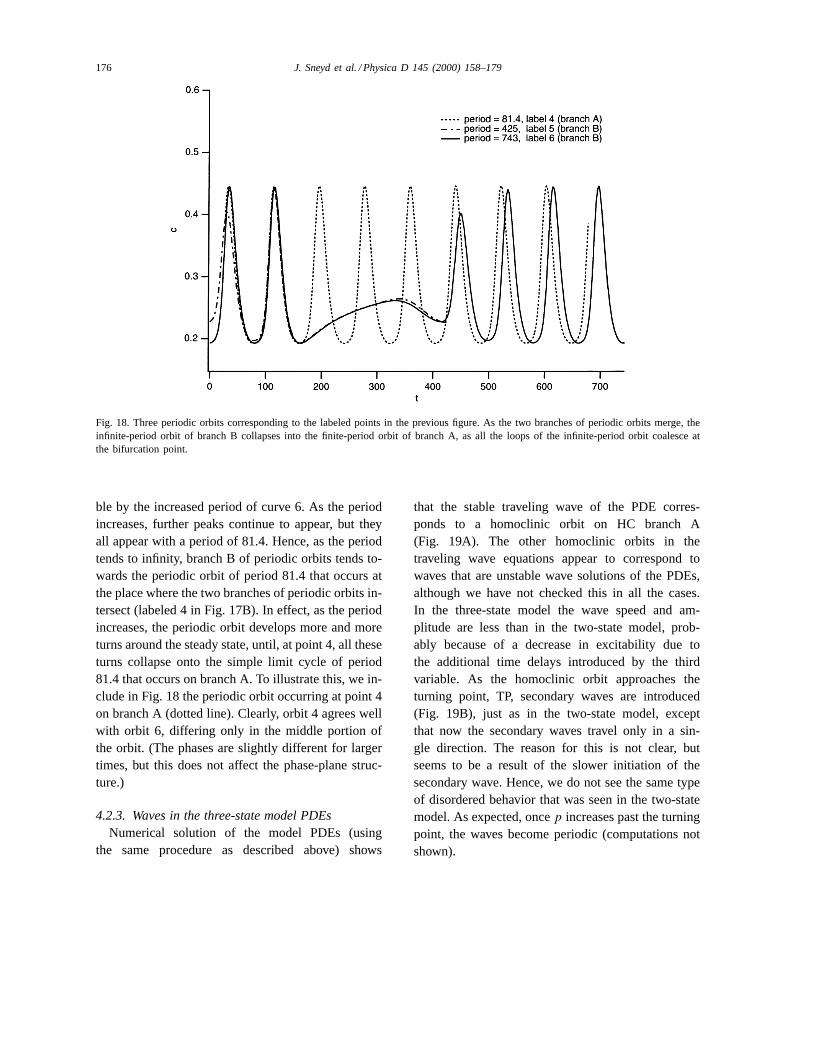
The behavior of branch B of periodic orbits is alsointeresting. Along branch B, the period tends to infin-ity in a series of loops (see the right panel of Fig. 17B),and each loop appears to correspond to the formationof additional peaks in the periodic orbit. Two examplesof periodic orbits on branch B are shown in Fig. 18,labeled 5 and 6. Curve 5 has period 425, while curve 6has period 743. As can be seen from the figure, curve5 agrees well with the first 453 s of curve 6, but thencurve 6 develops additional peaks that are not presentin curve 5. These additional peaks are made possi-


Fig. 18. Three periodic orbits corresponding to the labeled points in the previous figure. As the two branches of periodic orbits merge, theinfinite-period orbit of branch B collapses into the finite-period orbit of branch A, as all the loops of the infinite-period orbit coalesce atthe bifurcation point.

ble by the increased period of curve 6. As the periodincreases, further peaks continue to appear, but theyall appear with a period of 81.4. Hence, as the periodtends to infinity, branch B of periodic orbits tends to-wards the periodic orbit of period 81.4 that occurs atthe place where the two branches of periodic orbits in-tersect (labeled 4 in Fig. 17B). In effect, as the periodincreases, the periodic orbit develops more and moreturns around the steady state, until, at point 4, all theseturns collapse onto the simple limit cycle of period81.4 that occurs on branch A. To illustrate this, we in-clude in Fig. 18 the periodic orbit occurring at point 4on branch A (dotted line). Clearly, orbit 4 agrees wellwith orbit 6, differing only in the middle portion ofthe orbit. (The phases are slightly different for largertimes, but this does not affect the phase-plane struc-ture.)

4.2.3. Waves in the three-state model PDEsNumerical solution of the model PDEs (using

the same procedure as described above) shows

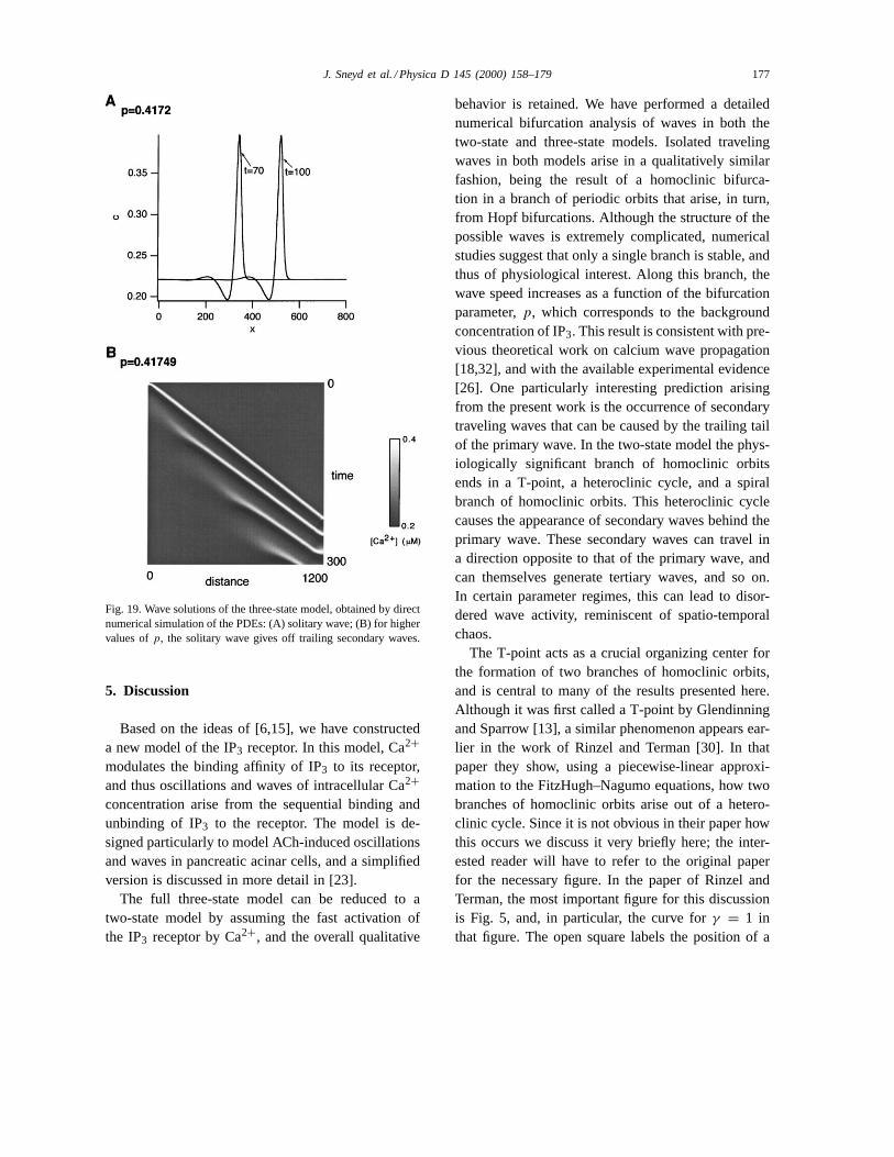
that the stable traveling wave of the PDE corres-ponds to a homoclinic orbit on HC branch A(Fig. 19A). The other homoclinic orbits in thetraveling wave equations appear to correspond towaves that are unstable wave solutions of the PDEs,although we have not checked this in all the cases.In the three-state model the wave speed and am-plitude are less than in the two-state model, prob-ably because of a decrease in excitability due tothe additional time delays introduced by the thirdvariable. As the homoclinic orbit approaches theturning point, TP, secondary waves are introduced(Fig. 19B), just as in the two-state model, exceptthat now the secondary waves travel only in a sin-gle direction. The reason for this is not clear, butseems to be a result of the slower initiation of thesecondary wave. Hence, we do not see the same typeof disordered behavior that was seen in the two-statemodel. As expected, oncep increases past the turningpoint, the waves become periodic (computations notshown).


Fig. 19. Wave solutions of the three-state model, obtained by directnumerical simulation of the PDEs: (A) solitary wave; (B) for highervalues ofp, the solitary wave gives off trailing secondary waves.

5. Discussion

Based on the ideas of [6,15], we have constructeda new model of the IP3 receptor. In this model, Ca2+

modulates the binding affinity of IP3 to its receptor,and thus oscillations and waves of intracellular Ca2+

concentration arise from the sequential binding andunbinding of IP3 to the receptor. The model is de-signed particularly to model ACh-induced oscillationsand waves in pancreatic acinar cells, and a simplifiedversion is discussed in more detail in [23].

The full three-state model can be reduced to atwo-state model by assuming the fast activation ofthe IP3 receptor by Ca2+, and the overall qualitative

behavior is retained. We have performed a detailednumerical bifurcation analysis of waves in both thetwo-state and three-state models. Isolated travelingwaves in both models arise in a qualitatively similarfashion, being the result of a homoclinic bifurca-tion in a branch of periodic orbits that arise, in turn,from Hopf bifurcations. Although the structure of thepossible waves is extremely complicated, numericalstudies suggest that only a single branch is stable, andthus of physiological interest. Along this branch, thewave speed increases as a function of the bifurcationparameter,p, which corresponds to the backgroundconcentration of IP3. This result is consistent with pre-vious theoretical work on calcium wave propagation[18,32], and with the available experimental evidence[26]. One particularly interesting prediction arisingfrom the present work is the occurrence of secondarytraveling waves that can be caused by the trailing tailof the primary wave. In the two-state model the phys-iologically significant branch of homoclinic orbitsends in a T-point, a heteroclinic cycle, and a spiralbranch of homoclinic orbits. This heteroclinic cyclecauses the appearance of secondary waves behind theprimary wave. These secondary waves can travel ina direction opposite to that of the primary wave, andcan themselves generate tertiary waves, and so on.In certain parameter regimes, this can lead to disor-dered wave activity, reminiscent of spatio-temporalchaos.

The T-point acts as a crucial organizing center forthe formation of two branches of homoclinic orbits,and is central to many of the results presented here.Although it was first called a T-point by Glendinningand Sparrow [13], a similar phenomenon appears ear-lier in the work of Rinzel and Terman [30]. In thatpaper they show, using a piecewise-linear approxi-mation to the FitzHugh–Nagumo equations, how twobranches of homoclinic orbits arise out of a hetero-clinic cycle. Since it is not obvious in their paper howthis occurs we discuss it very briefly here; the inter-ested reader will have to refer to the original paperfor the necessary figure. In the paper of Rinzel andTerman, the most important figure for this discussionis Fig. 5, and, in particular, the curve forγ = 1 inthat figure. The open square labels the position of a


T-point there, where there exists a heteroclinic cycleconnecting the two steady states. From this T-pointthere bifurcate two branches of homoclinic orbits; onedenoted by a solid line in that figure (theγ = 1 curve),and the other not shown, but corresponding to whatRinzel and Terman call anE-pulse. The T-point ofRinzel and Terman is slightly different from that ofGlendinning and Tresser, as it occurs at a heterocliniccycle between two saddle points, not between a saddlepoint and a spiral point. Nevertheless, it still resultsin the birth of two branches of homoclinic orbits bythe same generic mechanism as discussed here, i.e.,the heteroclinic cycle can “fall off” either of the twosteady states, thus giving rise to two possible homo-clinic branches.

A heteroclinic cycle between two saddle points, andthe associated two branches of homoclinic orbits, hasalso appeared explicitly in the work of Zimmermannet al. [43]. Furthermore, once one of their parametersbecomes large enough, the eigenvalues around one ofthe steady states become complex, and so their modelprovides an example of both the Rinzel and Termantype of T-point, as well as of the Glendinning andTresser type. Zimmermann et al. present an analysisvery similar to the one presented here, applied to amodel for the propagation of waves of catalytic COoxidation on a Pt(1 1 0) surface. Their numerical sim-ulations show the appearance of “backfiring”, the phe-nomenon we called secondary pulses (Fig. 14), andthey occur by the same mechanism as the ones pre-sented here, i.e., they occur as the homoclinic orbit ap-proaches the T-point, and are caused by the long tailsof the homoclinic orbits going over the threshold forwave initiation. The reason for the similarities betweenthese three different models (FitzHugh–Nagumo, cal-cium dynamics, and catalytic CO oxidation) is thepresence of multiple steady states in some parameterregions. When at least two steady states exist simulta-neously it allows the possibility of the existence of aheteroclinic cycle, with its associated branches of ho-moclinic orbits. There has been a good deal of workdone on the properties of catalytic CO oxidation on aPt(1 1 0) surface, and much of the theory relies on theexistence of multiple simultaneous steady states in themodel. The interested reader is referred to the paper

by Zimmermann et al. [43] and the references therein,as well as to those by Bar et al. [3,4].

Acknowledgements

The authors thank Neil Balmforth for helping themto identify the T-point. They also thank C.K.R.T. Jonesand an anonymous reviewer for telling them of relatedresults in the literature. James Sneyd was supportedby NIGMS grant R01 GM56126, and NSF grant DMS9706565. David Yule was supported by NIDDK grantR01 DK54568.

References

[1] A. Atri, J. Amundson, D. Clapham, J. Sneyd, A single-poolmodel for intracellular calcium oscillations and waves in theXenopus laevisoocyte, Biophys. J. 65 (1993) 1727–1739.

[2] N.J. Balmforth, G.R. Ierley, E.A. Spiegel, Chaotic pulse trains,SIAM J. Appl. Math. 54 (1994) 1291–1334.

[3] M. Bar, S. Nettesheim, H.H. Rotermund, M. Eiswirth, G.Ertl, Transition between fronts and spiral waves in a bistablesurface reaction, Phys. Rev. Lett. 74 (1995) 1246–1249.

[4] M. Bar, N. Gottschalk, M. Hildebrand, M. Eiswirth, Spiralsand chemical turbulence in an excitable surface reaction,Physica A 213 (1995) 173–180.

[5] I. Bezprozvanny, B.E. Ehrlich, The inositol 1,4,5-trisphosphate (InsP3) receptor, J. Membr. Biol. 145 (1995)205–216.

[6] T.J. Cardy, D. Traynor, C.W. Taylor, Differential regulationof types-1 and -3 inositol trisphosphate receptors by cytosolicCa2+, Biochem. J. 328 (1997) 785–793.

[7] E. Doedel, Software for continuation and bifurcation problemsin ordinary differential equations, California Institute ofTechnology, 1986.

[8] J.-F. Dufour, I.M. Arias, T.J. Turner, Inositol 1,4,5-trisphosphate and calcium regulate the calcium channelfunction of the hepatic inositol 1,4,5-trisphosphate receptor,J. Biol. Chem. 272 (1997) 2675–2681.

[9] J.W. Evans, N. Fenichel, J.A. Feroe, Double impulse solutionsin nerve axon equations, SIAM J. Appl. Math. 42 (1982)219–234.

[10] J.A. Feroe, Existence and stability of multiple impulsesolutions of a nerve equation, SIAM J. Appl. Math. 42 (1982)235–246.

[11] E.A. Finch, T.J. Turner, S.M. Goldin, Calcium as acoagonist of inositol 1,4,5-trisphosphate-induced calciumrelease, Science 252 (1991) 443–446.

[12] P. Glendinning, C. Sparrow, Local and global behavior nearhomoclinic orbits, J. Statist. Phys. 35 (1984) 645–696.

[13] P. Glendinning, C. Sparrow, T-points: a codimension twoheteroclinic bifurcation, J. Statist. Phys. 43 (1986) 479–488.


[14] P. Glendinning, Travelling wave solutions near isolatedsoluble-pulse solitary waves of nerve axon equations, Phys.Lett. A 121 (1987) 411–413.

[15] G. Hajnóczky, A.P. Thomas, Minimal requirements forcalcium oscillations driven by the IP3 receptor, EMBO J. 16(1997) 3533–3543.

[16] S.P. Hastings, Single and multiple pulse waves for theFitzHugh–Nagumo equations, SIAM J. Appl. Math. 42 (1982)247–260.

[17] M.S. Jafri, J. Keizer, Diffusion of inositol 1,4,5-trisphosphate,but not Ca2+, is necessary for a class of inositol1,4,5-trisphosphate-induced Ca2+ waves, Proc. Natl. Acad.Sci. USA 91 (1994) 9485–9489.

[18] M.S. Jafri, A theoretical study of cytosolic calcium waves inXenopusoocytes, J. Theor. Biol. 172 (1995) 209–216.

[19] E.J. Kaftan, B.E. Ehrlich, J. Watras, Inositol 1,4,5-trisphosphate (InsP3) and calcium interact to increase thedynamic range of InsP3 receptor-dependent calcium signaling,J. Gen. Physiol. 110 (1997) 529–538.

[20] H. Kasai, Pancreatic calcium waves and secretion, Ciba FoundSymp. 188 (1995) 104–116.

[21] J. Keizer, G. DeYoung, Simplification of a realistic modelof IP3-induced Ca2+ oscillations, J. Theor. Biol. 166 (1994)431–442 .

[22] A.M. Lawrie, E.C. Toescu, D.V. Gallacher, Two differentspatiotemporal patterns for Ca2+ oscillations in pancreaticacinar cells: evidence of a role for protein kinase C inIns(1,4,5)P3-mediated Ca2+ signalling, Cell Calcium 14(1993) 698–710.

[23] A.P. LeBeau, D.I. Yule, G.E. Groblewski, J. Sneyd, Agonist-dependent phosphorylation of the inositol 1,4,5-trisphosphatereceptor: a possible mechanism for agonist-specific calciumoscillations in pancreatic acinar cells, J. Gen. Physiol. 113(1999) 851–871.

[24] Y.-X. Li, J. Rinzel, Equations for InsP3 receptor-mediated[Ca2+] oscillations derived from a detailed kinetic model: aHodgkin–Huxley like formalism, J. Theor. Biol. 166 (1994)461–473.

[25] K. Maginu, Geometrical characteristics associated withstability and bifurcations of periodic travelling waves inreaction–diffusion equations, SIAM J. Appl. Math. 45 (1985)750–774.

[26] M.H. Nathanson, P.J. Padfield, A.J. O’Sullivan, A.D.Burgstahler, J.D. Jamieson, Mechanism of Ca2+ wavepropagation in pancreatic acinar cells, J. Biol. Chem. 267(1992) 18118–18121.

[27] J.B. Parys, S.W. Sernett, S. DeLisle, P.M. Snyder, M.J. Welsh,K.P. Campbell, Isolation, characterization, and localization ofthe inositol 1,4,5-trisphosphate receptor protein inXenopuslaevis oocytes, J. Biol. Chem. 267 (1992) 18776–18782.

[28] C.C.H. Petersen, E.C. Toescu, O.H. Petersen, Differentpatterns of receptor-activated cytoplasmic Ca2+ oscillations

in single pancreatic acinar cells: dependence on receptor type,agonist concentration and intracellular Ca2+ buffering, EMBOJ. 10 (1991) 527–533.

[29] F. Pfeiffer, L. Sternfeld, A. Schmid, I. Schulz, Control ofCa2+ wave propagation in mouse pancreatic acinar cells, Am.J. Physiol. 274 (1998) C663–C672.

[30] J. Rinzel, D. Terman, Propagation phenomena in a bistablereaction–diffusion system, SIAM J. Appl. Math. 42 (1982)1111–1137.

[31] L.P. Sil’nikov, A case of the existence of a denumerableset of periodic motions, Sov. Math. Dokl. 6 (1965) 163–166.

[32] J. Sneyd, S. Girard, D. Clapham, Calcium wave propagationby calcium-induced calcium release: an unusual excitablesystem, Bull. Math. Biol. 55 (1993) 315–344.

[33] J. Sneyd, J. Keizer, M.J. Sanderson, Mechanisms of calciumoscillations and waves: a quantitative analysis, FASEB J. 9(1995) 1463–1472.

[34] J. Sneyd, P. Dale, A. Duffy, Traveling waves in bufferedsystems: applications to calcium waves, SIAM J. Appl. Math.58 (1998) 1178–1192.

[35] Y. Tang, J.L. Stephenson, H.J. Othmer, Simplificationand analysis of models of calcium dynamics based onIP3-sensitive calcium channel kinetics, Biophys. J. 70 (1996)246–263.

[36] A.P. Thomas, G.S.J. Bird, G. Hajnóczky, L.D. Robb-Gaspers,J.W.J. Putney, Spatial and temporal aspects of cellular calciumsignaling, FASEB J. 10 (1996) 1505–1517.

[37] P. Thorn, A.M. Lawrie, P.M. Smith, D.V. Gallacher,O.H. Petersen, Ca2+ oscillations in pancreatic acinar cells:spatiotemporal relationships and functional implications, CellCalcium 14 (1993) 746–757.

[38] J. Wagner, J. Keizer, Effects of rapid buffers on Ca2+ diffusionand Ca2+ oscillations, Biophys. J. 67 (1994) 447–456.

[39] S. Wiggins, Introduction to Applied Nonlinear DynamicalSystems and Chaos, Springer, New York, 1990.

[40] H. Yoneshima, A. Miyawaki, T. Michikawa, T. Furuichi, K.Mikoshiba, Ca2+ differentially regulates the ligand-affinitystates of type 1 and type 3 inositol 1,4,5-trisphosphatereceptors, Biochem. J. 322 (1997) 591–596 .

[41] D.I. Yule, A.M. Lawrie, D.V. Gallacher, Acetylcholineand cholecystokinin induce different patterns of oscillatingcalcium signals in pancreatic acinar cells, Cell Calcium 12(1991) 145–151.

[42] D.I. Yule, E. Stuenkel, J.A. Williams, Intercellular calciumwaves in rat pancreatic acini: mechanism of transmission,Am. J. Phys. Cell Physiol. 271 (1996) C1285–C1294.

[43] M.G. Zimmermann, S.O. Firle, M.A. Natiello, M. Hildebrand,M. Eiswirth, M. Bär, A.K. Bangia, I.G. Kevrekidis, Pulsebifurcation and transition to spatiotemporal chaos in anexcitable reaction–diffusion model, Physica D 110 (1997)92–104.

Traveling waves of calcium in pancreatic acinar cells: model construction and bifurcation analysis

Documents

Transcript of Traveling waves of calcium in pancreatic acinar cells: model construction and bifurcation analysis