,

Transport in Porous Media 15: 183-196,1994. 183 © 1994 Kluwer Academic Publishers. Printed in the Netherlands.

Transport in Ordered and Disordered Porous Media V: Geometrical Results for Two-Dimensional Systems

MICHEL QUINTARD1 and STEPHEN WHITAKER2 1 Laboratoire Energitique et Phenomenes de Transfert, Unite de Recherche Associee au CNRS, URA 873, Esplanade des Arts et Metiers, 33405 Talence Cedex, France 2 Department of Chemical Engineering, University of California, Davis, CA 95616 USA

(Received: 19 July 1993)

Abstract. In this paper we continue the geometrical studies of computer generated two-phase systems that were presented in Part IV. In order to reduce the computational time associated with the previous three-dimensional studies, the calculations presented in this work are restricted to two dimensions. This allows us to explore more thoroughly the influence of the size of the averaging volume and to learn something about the use of a non-representative region in the determination of averaged quantities.

Nomenclature

Roman Letters A,617 interfacial area of the {3-(I interface associated with the local closure

problem, m2 •

ai i = 1, 2, gaussian probability distribution used to locate the position of particles.

m

mv

n,617

unit tensor. characteristic length for the (I-phase particles, m. reference characteristic length for the (I-phase particles, m. characteristic length for the {3-phase, m_ i = 1, 2, 3 lattice vectors, m. convolution product weighting function_ special convolution product weighting function associated with a unit cell. i = 1, 2 integers used to locate the position of particles. unit normal vector pointing from the {3-phase toward the (I-phase. position vector locating the centroid of a particle, m. gaussian probability distribution used to determine the size of a particle, m.

ro characteristic length of an averaging region, m. V averaging volume, m3 .

184 MICHEL QUINTARD AND STEPHEN WHITAKER

V,6 volume of the ,B-phase contained in the averaging volume, V, m3.

x position of the centroid of an averaging area, m. Xo reference position of the centroid of an averaging area, m. Y,6 position vector locating points in the ,B-phase relative to the centroid, m.

Greek Letters E,6 V,6/V, volume average porosity. (Jai standard deviation of ai. (J r standard deviation of r <7.

(1/J,6),6 intrinsic phase average of 1/J,6.

1. Introduction

In Part IV we considered the geometrical quantities (Y,6) and V' (Y,6) for periodic systems, pseudo-periodic systems, and uniformly random systems. For systems generated by the placement of cubes (or spheres in a cubic array), we used a cubic averaging volume to produce the results given by

V' (Y,6) = 0 (1 - E,6), ordered systems,

V' (Y,6) ~ I, disordered systems.

(1.1)

(1.2)

The first of these is an analytic result while the second is based on numerical simulations. For pseudo-periodic systems, which have the appearance of uniformly random systems, we found that V' (Y,6) retains afingerprint of the periodic system of origin.

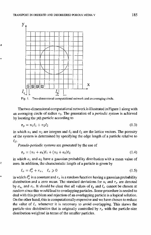
In Part I we suggested that the cellular average should be used with periodic systems and in Part II this idea was made precise in terms of the double convolution product, mv * mv, and the Coo weighting function defined by mg * mv * mv. In Part II we also indicated that the classic volume average, designated by the weighting function mv, should be sufficient for disordered systems as characterized by Equation 1.2. In theory this works quite well, but in practice it may not be obvious that a particular system should be characterized as disordered or ordered, or that a system contains both of these characteristics. Concerning strictly ordered systems, one can easily use a unit cell and the cellular average to produce the desired theoretical dependent variable and this has been illustrated in Figure 4 of Part III. On the other hand, if volume averaged quantities are being determined experimentally in an ordered system, one is likely to be severely restricted in the range of instrument weighting functions (Baveye and Sposito, 1984; Cushman, 1984; Maneval et ai., 1990) that are available. This raises the question: What happens if the averaging volume is not a representative region or an REV? The question can be explored, in part, by the use of a spherical averaging volume for ordered systems or random arrays of uniformly oriented cubes. However, in order to keep computer costs (in 1990) at a reasonable level, we have used a circular averaging area to study the properties of two-dimensional systems.

•

TRANSPORT IN ORDERED AND DISORDERED POROUS MEDIA V 185

y

!I \

\ / v

Fig. I. Two-dimensional computational network and an averaging circle.

The two-dimensional computational network is illustrated in Figure 1 along with an averaging circle of radius ro. The generation of a periodic system is achieved by locating the pth particle according to

(1.3)

in which nl and n2 are integers and fl and f2 are the lattice vectors. The porosity of the system is determined by specifying the edge length of a particle relative to f(3.

Pseudo-periodic systems are generated by the use of

(1.4)

in which al and a2 have a gaussian probability distribution with a mean value of zero. In addition, the characteristic length of a particle is given by

(1.5)

in which f~ is a constant and r a is a random function having a gaussian probability distribution and a zero mean. The standard deviations for ai and r a are denoted by (Jai and (Jr' It should be clear that all values of rp and fa cannot be chosen at random since this would lead to overlapping particles. Some procedure is needed to deal with this problem and rejection of an overlapping particle is a logical solution. On the other hand, this is computationally expensive and we have chosen to reduce the value of fa whenever it is necessary to avoid overlapping. This skews the particle-size distribution that is originally controlled by r a with the particle-size distribution weighted in terms of the smaller particles.

186 MICHEL QUINTARD AND STEPHEN WHITAKER

Uniformly random systems are constructed by choosing r p from a uniformly random spatial distribution while the particle size is determined by Equation 1.5. A particle having a position r p and size £0' is retained in the array if it does not overlap with all previously generated particles. If it does overlap it is discarded as opposed to reducing the value of £0' in order to eliminate overlap as was done with the pseudo-periodic systems. This procedure requires greater computation time and ' it also skews the particle-size distribution in favor of the smaller particles since they more easily fit into the computational network.

For periodic systems the lengths £0' and £(3, shown in Figure 1, are related by

(1.6)

and one begins the calculation by specifying a value of E~ so that £~ can be determined and the periodic array can be constructed. For pseudo-periodic systems one chooses a value of £~ / £ (3 according to

(1.7)

and one uses Equations 1.4 and 1.5 to associate a particle with every cell in the network. When particles overlap the. size is diminished to eliminate the overlap. The calculated porosity for pseudo-periodic systems is always greater than E~ since

the mean particle size is less than £~. For uniformly random systems the value of £~ / £(3 is also determined by Equation 1. 7 and the final value of the porosity is always larger than E~ since rejecting the overlapping particles produces a mean

particle size that is less than £~.

2. Geometrical Properties

In Part IV our objectives were primarily limited to the three-dimensional determi­nation of i . \7 (y (3) . i since this is a key parameter in the development of volume averaged transport equations. In this study, the two-dimensional nature of the cal­culations allows us to explore the geometrical characteristics of our three systems' more broadly and we begin by considering the porosity.

2.1. POROSITY

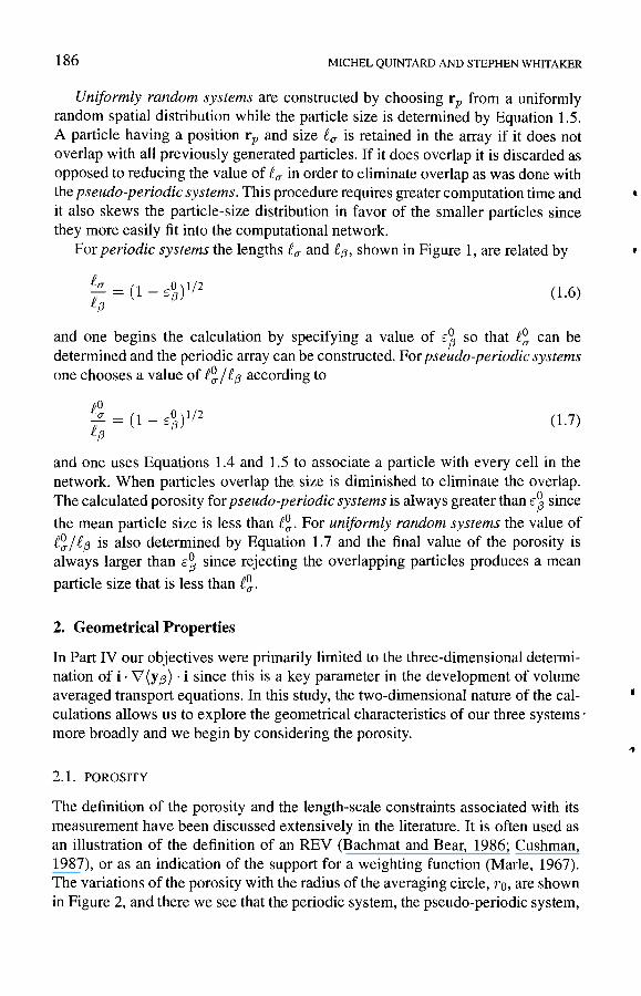
The definition of the porosity and the length-scale constraints associated with its measurement have been discussed extensively in the literature. It is often used as an illustration of the definition of an REV (Bachmat and Bear, 1986; Cushman, 1987), or as an indication of the support for a weighting function (Marle, 1967). The variations of the porosity with the radius of the averaging circle, ro, are shown in Figure 2, and there we see that the periodic system, the pseudo-periodic system,

f

TRANSPORT IN ORDERED AND DISORDERED POROUS MEDIA V 187

0.95

0.9

--periodic

0.85 - - - pseudo·periodic

.-••. _ ••••.• disordered 0.8

0.75

0.7 ... / .... \ .. I ........ ..

0.65 ~~~ 0.6

0.55

0.5

0 2 4 6 12 14 16

Fig. 2. Dependence of the porosity on the size of the averaging circle.

and the uniformly random system all behave in essentially the same manner. When TO f"V 5f.(3 we see that the fluctuations in E(3 are reduced to less than 2%. Maneval (1991) has used magnetic resonance imaging to study porosity variations in packed beds of uniform spheres, and his studies indicate that much larger averaging volumes must be used to reduce the porosity variations to 2%. This is due to the existence of large-scale structures (macro-aggregates) that exist in natural systems of uniform spheres, and these large-scale structures are not present in our computer simulations. In Maneval's studies a value of TO f"V 20f.(3 was necessary to reduce the fluctuations in E(3 to less than 2% and a spectral analysis of the porosity variations clearly identified the existence of large-scale structures having wavelengths in the neighborhood of 5f.(3 to 15£(3. In comparing two-dimensional results with three-dimensional results, it is best to think in terms of numbers of particles. For TO f"V 5f.(3 our two-dimensional averaging area contains about 75 particles while Maneval's (1991) three-dimensional experiments with TO f"V 20f.(3 led to an averaging volume containing about 8000 particles. From this point of view, it would seem that our computer generated systems are much more homogeneous than natural systems-even natural systems that are composed of uniform spheres.

188 MICHEL QUINTARD AND STEPHEN WHITAKER

In Part IV we noted that two of the typical integrals encountered in the method of volume averaging could be expanded according to

......................... ,

~ fvf3 (,1/)(3)(3 dV = E(3(1/J(3)(3 + (Y(3) . V(1/J(3)(3+

+ I (Y(3Y(3): VV(1/J(3)(3

+ ........................ .

(2.1)

(2.2)

The first terms in both these expansions are controlled by the porosity, E(3, which is either a known or measurable parameter. The higher order terms on the right hand side of Equations 2.1 and 2.2 are controlled by (y (3), (y (3 y (3), etc., and the gradients of these spatial moments, and it is these terms that we wish to explore in terms of the system illustrated in Figure 1.

2.2. FIRST ,a-PHASE SPATIAL MOMENT

Here we refer to the vector defined by

(2.3)

and since the two-dimensional systems under consideration are isotropic, we con­sider only the single component, i . (Y(3). When a system is spatially periodic and a unit cell is used as the averaging volume, we have shown in Appendices A and

l

B of Part IV that, ,

i· (Y(3)j£(3 = 0(1 - E(3),

i· V(Y(3)' i = 0(1 - E(3).

(2.4)

(2.5)

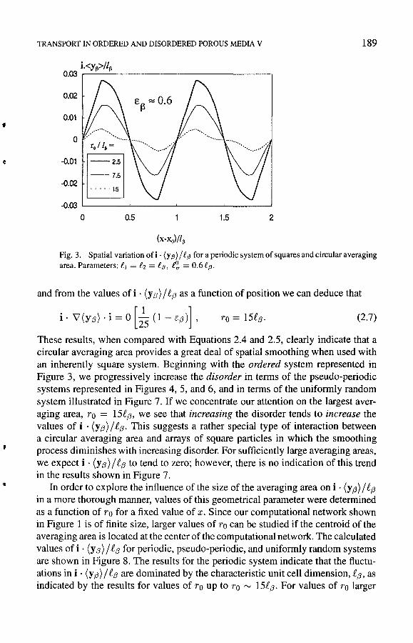
However, the situation is somewhat different when the averaging volume is not a unit cell. For the two-dimensional periodic system and the circular averaging area shown in Figure 1, we obtain the values ofi . (y (3) j £(3 that are illustrated in Figure 3. For the largest averaging area, the computed results for i . (y (3) j £(3 indicate that

(2.6)

f

e

TRANSPORT IN ORDERED AND DISORDERED POROUS MEDIA V 189

i.<y~>/l~ 0.03 r------------------,

0.02

0.01

o r. / l~ =

tj.5

--7.5

- - - -·15

-0.01

-0.02

-0.03 '--___ -'--___ -'--___ -'-___ ---.J

o 0.5 1.5 2

(x-Xo)/l~

Fig. 3. Spatial variation ofi . (y(3) I f(3 for a periodic system of squares and circular averaging area. Parameters: fl = f2 = f(3, ~ = 0.6f(3.

and from the values of i . (y (3) / £(3 as a function of position we can deduce that

i· \l(Y(3) . i = 0 [;5 (1 - [(3)] , TO = 15£(3. (2.7)

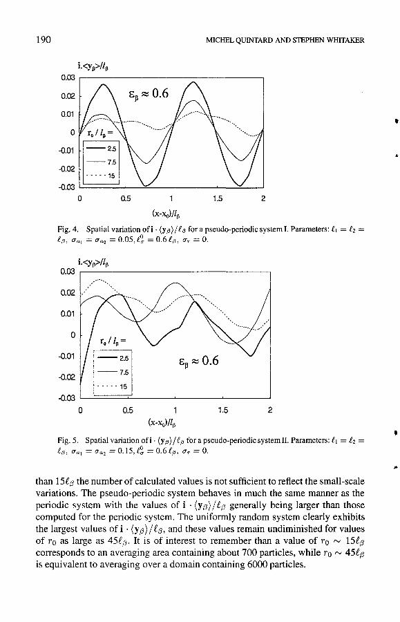
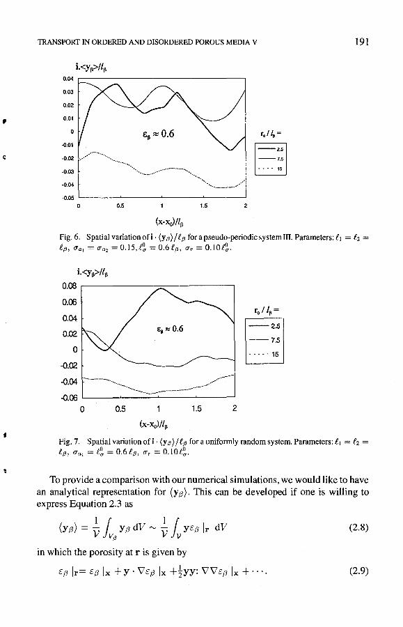
These results, when compared with Equations 2.4 and 2.5, clearly indicate that a circular averaging area provides a great deal of spatial smoothing when used with an inherently square system. Beginning with the ordered system represented in Figure 3, we progressively increase the disorder in terms of the pseudo-periodic systems represented in Figures 4, 5, and 6, and in terms of the uniformly random system illustrated in Figure 7. If we concentrate our attention on the largest aver­aging area, TO = 15£(3, we see that increasing the disorder tends to increase the values of i . (y (3) /£(3. This suggests a rather special type of interaction between a circular averaging area and arrays of square particles in which the smoothing process diminishes with increasing disorder. For sufficiently large averaging areas, we expect i . (y (3) /£(3 to tend to zero; however, there is no indication of this trend in the results shown in Figure 7.

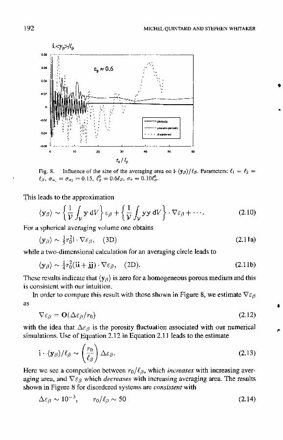
In order to explore the influence of the size of the averaging area on i . (y (3) /£(3 in a more thorough manner, values of this geometrical parameter were determined as a function of TO for a fixed value of x. Since our computational network shown in Figure 1 is of finite size, larger values of TO can be studied if the centroid of the averaging area is located at the center of the computational network. The calculated values of i . (y (3) / £(3 for periodic, pseudo-periodic, and uniformly random systems are shown in Figure 8. The results for the periodic system indicate that the fluctu­ations in i . (y (3) /£(3 are dominated by the characteristic unit cell dimension, £(3, as indicated by the results for values of TO up to TO '" 15£(3. For values of TO larger

190 MICHEL QUINTARD AND STEPHEN WHITAKER

i·<YJl>/IJl 0.03 ,------------------,

0.02 E13~ 0.6

0.01

o ro / Ip =

-0.01

-0.02 El_~:: bJ -0.03 L..-___ "-----=='---_"--___ "-------.::=-----'

o 0.5 1.5 2

(x-Xo)/IJl

Fig. 4. Spatial variation ofi· (Y/3)/£/3 for a pseudo-periodic system!. Parameters: £1 = £2 = £/3, (Tal = (Ta2 = 0.05,e = 0.6£/3, (TT = O.

i·<YJl>IIJl 0.03 ,---------------------,

0.02

0.01

0 ro / I~ =

-0.01

Em -0.02 --7.5

..... 15

-0.03 0 0.5 1.5 2

Fig. 5. Spatial variation ofi . (Y/3) /£/3 for a pseudo-periodic system II. Parameters: £1 = £2 = £/3, (Tal = (Ta2 = 0.15, £~ = 0.6 £/3, (TT = O.

than 15£;3 the number of calculated values is not sufficient to reflect the small-scale variations. The pseudo-periodic system behaves in much the same manner as the periodic system with the values of i . (Y;3) / £;3 generally being larger than those computed for the periodic system. The uniformly random system clearly exhibits the largest values of i . (Y;3) / £;3, and these values remain undiminished for values of ro as large as 45£;3' It is of interest to remember than a value of ro rv 15£;3 corresponds to an averaging area containing about 700 particles, while ro rv 45£;3 is equivalent to averaging over a domain containing 6000 particles.

•

..

•

,

c:

•

TRANSPORT IN ORDERED AND DISORDERED POROUS MEDIA V 191

i.<Yfl>/lfl 0.04 .------------------,

0.03

0.02

0.01

o

·0.01

·0.03

...............................•.......... _----

---------------.-................. _--------------_. a·5

--7.5

•• -. 15

-0.02

-0.04

-0.05 L....-__ -----' ___ --'-___ --'-___ -.l

o 0.5 1.5 2

(X-Xo)/lfl

Fig. 6. Spatial variationofi· (y{3)/£{3 fora pseudo-periodic system III. Parameters: £1 = £2 = £{3, ITal = ITa2 = O.I5,e = O.6£{3, ITr = O.lO£~.

i.<YIl>/lfl 0.08 ,---------=:--------,

0.06

0.04

0.02

o -0.02

-0.04 -0.06 L-____ ~ ____ ~ ___ ~ __ ~

o 1.5 2

ro / lp =

~'5

--7.5

- - . - - 15

Fig. 7. Spatial variation of i . (y (3) / £{3 for a uniformly random system. Parameters: £ 1 = £2 = £{3, ITal = e = O.6£{3, ITr = O.lO£~.

To provide a comparison with our numerical simulations, we would like to have an analytical representation for (y (3). This can be developed if one is willing to express Equation 2.3 as

(Y(3) = ~ fv{3 Y(3 dV rv ~ fv yE(3 Ir dV (2.8)

in which the porosity at r is given by

E(3 Ir= E(3 Ix + y. VE(3 Ix +!yy: VVE(3 Ix + .... (2.9)

192

i,<y~>/l~

0.04

0.02

-0.04

, , I". d:', >:,1. ", ::",: ,:

{ ~

", , . , , " ,

,. r'

MICHEL QUINTARD AND STEPHEN WHITAKER

, ' t ..

" .. " " '

\,

" ,

--periodic

-- pseudo-periodic

•••• disordered

-0.06 '-----'-------'----~----'----'------'

10 20 30 50 60

ro / /~

Fig. 8. Influence of the size of the averaging area on j. (y(3)j£(3. Parameters: £1 = £2 = £(3, O'al = O'a2 = 0.15, £~ = 0.6£(3, O'r = 0.1O~.

This leads to the approximation

(Y(3) rv { ~ fv Y dV} E(3 + { ~ fv YY dV} , \lE(3 + ' ". (2.10)

For a spherical averaging volume one obtains

(Y(3) rv ~r51 . \lE(3, (3D) (2.11a)

while a two-dimensional calculation for an averaging circle leads to

( ) 1 2(" •• ) n Y(3 rv 4rO 11 + JJ . v E(3, (2D). (2.11b)

These results indicate that (y (3) is zero for a homogeneous porous medium and this is consistent with our intuition.

In order to compare this result with those shown in Figure 8, we estimate \lE(3 as

(2.12)

with the idea that ~E (3 is the porosity fluctuation associated with our numerical simulations. Use of Equation 2.12 in Equation 2.11 leads to the estimate

i· (Y(3)j£(3 rv (;~) ~E(3. (2.13)

Here we see a competition between roj £(3, which increases with increasing aver­aging area, and \l E (3 which decreases with increasing averaging area, The results shown in Figure 8 for disordered systems are consistent with

~E(3rvlO-3, roj£(3 rv50 (2.14)

•

,.

•

TRANSPORT IN ORDERED AND DISORDERED POROUS MEDIA V

9.~ ,----------------,

9.4 ~""'" 9.3 -----// ........ " ••••• ......--------•• -

9.2 e~ = 0.6

9.1

8.9

8.8 L-__ -'--__ ~ __ ~ __ --'

0.5 1.5

(x-Xo)/l~

--periodic

-- pseudo-periodic

• • - - disordered

193

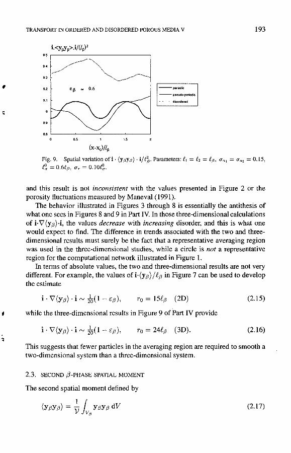
Fig. 9. Spatial variation ofi· (Y!3Y!3)' ilf} Parameters: Ct = C2 = C!3, lTa, = lTa2 = 0.15,

C~ = 0.6C!3, lTr = O.lOC~.

and this result is not inconsistent with the values presented in Figure 2 or the porosity fluctuations measured by Maneval (1991).

The behavior illustrated in Figures 3 through 8 is essentially the antithesis of what one sees in Figures 8 and 9 in Part IV. In those three-dimensional calculations of i·V'(Y;3)·i, the values decrease with increasing disorder, and this is what one would expect to find. The difference in trends associated with the two and three­dimensional results must surely be the fact that a representative averaging region was used in the three-dimensional studies, while a circle is not a representative region for the computational network illustrated in Figure 1.

In terms of absolute values, the two and three-dimensional results are not very different. For example, the values of i· (Y;3) /£;3 in Figure 7 can be used to develop the estimate

TO = 15£;3 (2D) (2.15)

while the three-dimensional results in Figure 9 of Part N provide

TO = 24£;3 (3D). (2.16)

This suggests that fewer particles in the averaging region are required to smooth a two-dimensional system than a three-dimensional system.

2.3. SECOND ,a-PHASE SPATIAL MOMENT

The second spatial moment defined by

(2.17)

194 MICHEL QUINTARD AND STEPHEN WHITAKER

0.15 ,....--------.,.,......-----,

0.1

0.05

·0.05 Ej3 ~ 0.6

-- psoudo-perlodk:

- - - - . disordered

·0.1

................ ---_.............. . ...

-', ..... _..--" ..... ·0.15

.' ... ·02 '-----'-----'-----'-----'

0.5 1.5

(x~)fl~

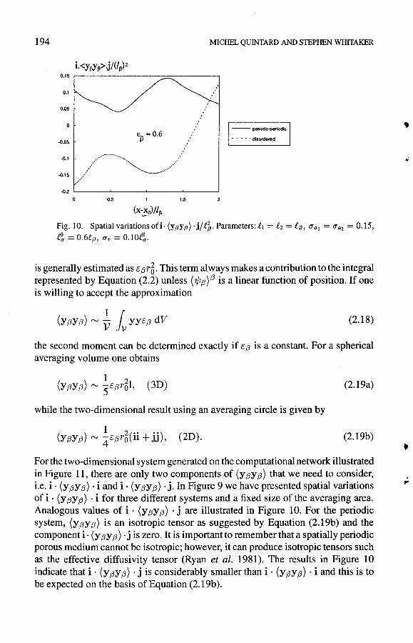
Fig. 10. Spatial variations ofi· (Y,6Y,6)· j/ £1. Parameters: £1 = £2 = £,6, ITa I = ITa2 = 0.15, t~ = 0.6£,6, ITr = 0.1Ot,;..

is generally estimated as E iJr6. This term always makes a contribution to the integral represented by Equation (2.2) unless ('ljJiJ)(3 is a linear function of position. If one is willing to accept the approximation

(2.18)

the second moment can be determined exactly if EiJ is a constant. For a spherical averaging volume one obtains

(2.19a)

while the two-dimensional result using an averaging circle is given by

( ) 1 2(" ") YiJYiJ rv 4EiJrO 11 + JJ , (2D). (2.19b)

For the two-dimensional system generated on the computational network illustrated in Figure 11, there are only two components of (y iJY iJ) that we need to consider, i.e. i· (y iJY iJ) . i and i . (y iJY iJ) . j. In Figure 9 we have presented spatial variations of i . (y iJY iJ) . i for three different systems and a fixed size of the averaging area. Analogous values of i . (y iJY iJ) . j are illustrated in Figure 10. For the periodic system, (y iJY iJ) is an isotropic tensor as suggested by Equation (2.19b) and the component i· (y iJY iJ) . j is zero. It is important to remember that a spatially periodic porous medium cannot be isotropic; however, it can produce isotropic tensors such as the effective diffusivity tensor (Ryan et al. 1981). The results in Figure 10 indicate that i . (y iJY iJ) . j is considerably smaller than i . (y iJY iJ) . i and this is to be expected on the basis of Equation (2.19b).

• " ~

,

TRANSPORT IN ORDERED AND DISORDERED POROUS MEDIA V 195

~r-------------------------------'

35

30

25

15

10 113",o.6 5

10 12 14 16

ro / lp

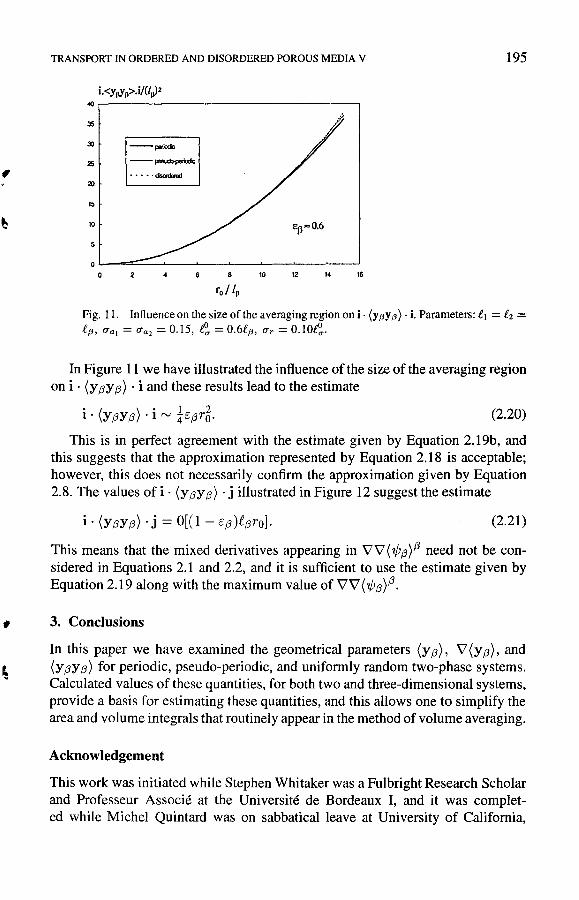
Fig. 11. Influence on the size of the averaging region on i . (y (3y (3) . i. Parameters: £1 = £2 = £{3, O'a, = O'a2 = 0.15, I!;,. = 0.6£{3, O'r = O.IOl!;,..

In Figure 11 we have illustrated the influence of the size of the averaging region on i . (y f3Y (3) . i and these results lead to the estimate

• ( ). I 2 l' Yf3Yf3 . 1 f'V 4cf3rQ. (2.20)

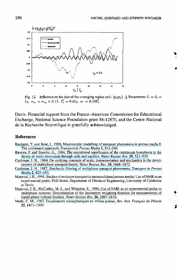
This is in perfect agreement with the estimate given by Equation 2.19b, and this suggests that the approximation represented by Equation 2.18 is acceptable; however, this does not necessarily confirm the approximation given by Equation 2.8. The values of i· (Yf3Yf3) . j illustrated in Figure 12 suggest the estimate

(2.21)

This means that the mixed derivatives appearing in \1\1 (7/Jf3)f3 need not be con­sidered in Equations 2.1 and 2.2, and it is sufficient to use the estimate given by Equation 2.19 along with the maximum value of \1\1 (7/Jf3)f3.

3. Conclusions

In this paper we have examined the geometrical parameters (y (3), \1 (y (3), and (y f3Y (3) for periodic, pseudo-periodic, and uniformly random two-phase systems. Calculated values of these quantities, for both two and three-dimensional systems, provide a basis for estimating these quantities, and this allows one to simplify the area and volume integrals that routinely appear in the method of volume averaging.

Acknowledgement

This work was initiated while Stephen Whitaker was a Fulbright Research Scholar and Professeur Associe at the Universite de Bordeaux I, and it was complet­ed while Michel Quintard was on sabbatical leave at University of California,

196 MICHEL QUINTARD AND STEPHEN WHITAKER

~ r-----------------------------------------,

~ .. --• _. ciIorderad

0.15

0.1

0.05

-0.05

......... . ..., .... " ,', ....., . "p - 0.6

-0.1

.0.15

-02 L-__ ~ ____ ~ ____ ~ __ ~ ____ ~ __ ~ ____ ~ __ ~

10 12 I. 16

ro / lp

Fig. 12. Influence on the size of the averaging region on i· (Y!3Y!3) . j. Parameters: £1 = £2 = £!3, O"at = O"a2 = 0.15, t; = 0.6£!3, O"r = O.lOt;.

Davis. Financial support from the Franco-American Commission for Educational Exchange, National Science Foundation grant 88-12870, and the Centre National de la Recherche Scientifique is gratefully acknowledged.

References

Bachmat, Y. and Bear, J., 1986, Macroscopic modelling of transport phenomena in porous media I: The continuum approach, Transport in Porous Media 1, 2l3-240.

Baveye, P. and Sposito, G., 1984, The operational significance of the continuum hypothesis in the theory of water movement through soils and aquifers, Water Resour. Res. 20,521-530.

Cushman, J. H., 1984, On unifying concepts of scale, instrumentation and stochastics in the devel­opment of multiphase transport theory, Water Resour. Res. 20, 1668-1672.

Cushman, J. H., 1987, Stochastic filtering of multiphase transport phenomena, Transport in Porous Media 2, 425-453.

Maneval, J. E., 1991, Studies of moisture transport in unconsolidated porous media: Use ofNMR as an experimental probe, PhD thesis, Department of Chemical Engineering, University of California at Davis.

Maneval, J. E., McCarthy, M. J., and Whitaker, S., 1990, Use ofNMR as an experimental probe in multi phase systems: Determination of the instrument weighting function for measurements of • liquid-phase volume fraction, Water Resour. Res. 26,2807-2816.

Marie, C. M., 1967, Ecoulements monophasiques en milieu poreux, Rev. [nst. Franr;ais du Petrole 22, 1471-1509. J