- --- . .- - - - . - - -

The GCRC Two-Dimensional Zonally AveragedStatistical Dynamical Climate Model: Development,

Model Performance, and Climate Sensitivity

Robert Malcolm MacKay

B.A., Physics, California State University Chico, 1978

M.S., Physics, Portland State University, 1983

M.S., Atmospheric Physics, Oregon Graduate Institute, 1991

A dissertation presented to the faculty of the

Oregon Graduate Institute of Science & Technology

Department of Environmental Science and Engineering

in partial fulfillment of the requirements for the degree

Doctor of Philosophyin

Attnospheric Physics

January 1994

The Dissertation "The GCRC Two-Dimensional Zonally Averaged Statistical

Dynamical Climate Model: Development, Model Performance, and Climate Sensitivity

Studies" by Robert M. MacKay has been examined and approved by the followingExamination Committee:

..M. A. K. Khalil

Professor, Oregon Graduate Institute of Scince & Technology,Thesis Advisor

James A. Coald

Professor, Oregon S

- (./" ,

Reinhold A. Rasmussen

Professor, Oregon Graduate Institute of Scince & Technology

J. Fred Holmes..,..,.,

Professor, Oregon Grad':lateInstitute of Scince & Technology

11

ACKNOWLEDGMENTS

I would like to express my deep gratitude to my dissertation advisor Dr. Aslam

Khalil, for without his many suggestions, words of encouragement, patience, and support

this work would not have been possible.

I would also like to thank the other members of my dissertation committee, Dr.

James Coakley, Dr. Reinhold Rasmussen, and Dr. Fred Holmes for their time and effort

spent as committee members and reading this manuscript.

I thank the other members of the Global Change Research Center Modeling group

at OGI: Dr. Yu Lu, Mr. Weining Zhao, Mr. Francis Moraes, Mr. Zhongyi Ye, Ms. Edie

Taylor, and Ms. Martha Shearer, for their constructive comments and conversations

throughout the duration of this work. Also I would like to express my appreciation to Dr.

Douglas Kinneson of Lawrence Livermore National Labs for supplying me with his

model's ozone output; Dr. Roy Jenne of NCAR for his help in my acquiring data on

clouds, water vapor, surface elevations, and zonal ocean fraction; and Dr. Ronald Stouffer

for his helpfull discussions during the Aspen Global Change Institute during the summerof 1992.

I would like to thank all of my colleagues at Clark College and the Clark College

administration for their help and support during this work.

I would like to thank all of my family for the patience and encouragement duringthis work.

Finally, I would like to thank my wife Linda for her careful proofreading of this

manuscript, and her never ending patience and love.

This work was partially supported by The U.S. Deparment of Energy grant

number DE-FG06-85ER60313, The Andarz Co., and The Oregon Graduate Institute of

Science & Technology.

III

DEDIC ATION

This dissenation is dedicated to my Uncle, Donald G. MacKay (1917-), who

through his own personal success, kindness, and generous spirit has been, without a

doubt, the most influential individual in my academic career.

iv

TABLE OF CONTENTS

Acknowledgements iii

Dedication IV

Table of Contents V

List of Figures viii

List of Tables xiii

Abstract xiv

CHAPTER 1. INTR0 DUCTI0 N 1

1.1 The Climate System and Climate Modeling 2

1.2 Climate modeling an overview 3

1.3 A Historical Prospective 8

CHAPTER 2. MODEL DESCRIPTION 12

2.1 Model Overview 12

2.1.1 Introduction 12

2.1.2 Model Grid 12

2.1.3 Clouds 13

2.1.4 Solar Energy 152.1.5 Surface Features.. 16

2.2 Model Equations 192.2.1 Numerical Overview 22

v

2.3 Solution of the Basic Equations 242.3.1 Initial Conditions 24

2.3.2 The equation of continuity 25

2.3.3 Zonal Velocity 26

2.3.4 Meridional Velocity 28

2.3.5 The fIrst Law of thermodynamics 29

2.3.5 Hydrostatic Adjustment 32

2.3.6 Atmospheric Moisture 352.4 Other Parameterizations 38

2.4.1 Parameterization of Eddy Momentum Flux u'v' . 382.4.2 Meridional Eddy Flux of Heat Energy v'T 43

2.4.3 Vertical Eddy Flux of Heat Energy w' (}' 44

2.4.4 Latent Heating 452.4.5 Convection 46

2.5 Modifications of the Radiative Convective Model. 47

2.5.1 I-D RCM review 48

2.5.2 ModifIcations of the Radiation Model 48

2.6 Deep Ocean Model 502.7 Sea Ice 52

2.8 Summary of the Model. 53

CHAPTER 3. MODEL PERFORMANCE 57

3.1 Model Overview 57

3.1.1 Introduction 57

3.1.2 General Discussion 57

3.2 The Thermal Structure of the Atmosphere and Energy Balance 60

3.2.1 Temperature Field 60

3.2.2 Energy Balance 73

3.3 Zonal Velocities U and Angular Momentum. 76

3.4 Kinetic Energy and Mass Stream Function 89

3.5 Precipitation and Surface Pressure 92

3.6 Summary of the Model's Performance 97

VI

CHAPTER 4. MODEL SENSITIVITy 103

4.1 Temperature Changes due to 2xCCh 103

4.2 Changes in Zonal Velocity and the Length of Day? 111

4.3 Other Changes for 2xCQz 117

4.4 Summary. 123

CHAPTER S. SUMMARY OF RESULTS 125

REFERENCES 130

APPENDIX A 137

APPENDIX B. CLOUD ANDOZONE DATAUSED IN THE GCRC 2DMODEL 141

B.l. Clouds 141

B.l.l HighClouds 141B.l.2. MiddleClouds 142

B.l.3 LowCloud 143B.2. OzoneProfiles 145

APPENDIX C. SOURCE CODE OF THE GCRC 2-D MODEL 151

VITA 257

Vll

LIST OF FIGURES

Figure 1.1 The graphical description of climate resolution and climate modeling 4

Figure 2.1. The model structure of a 2 layer-4 zone model and geometry of a

typical model grid box. 14

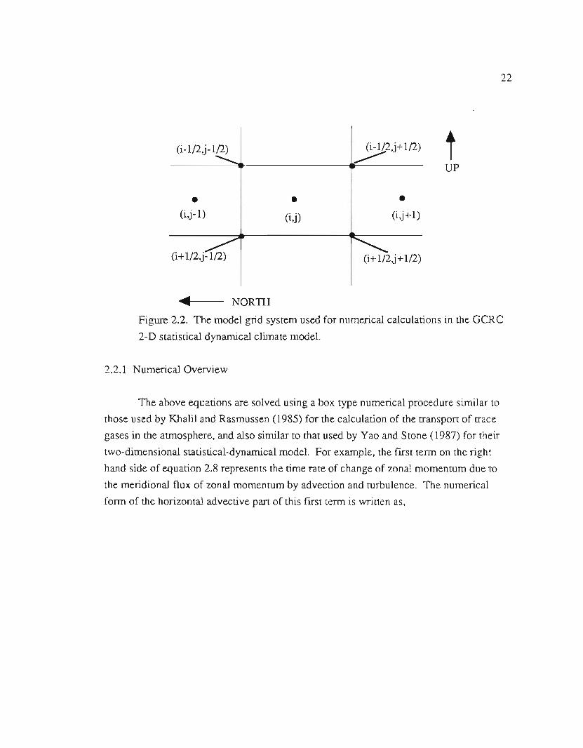
Figure 2.2. The model grid system used for numerical calculations in the aCRC

2-D statistical dynamical climate model. 22

Figure 2.3. The basic flow of the model calculations. 24

Figure 2.4. Surface relative humidity (%) used for the calculation of water vapor

mixing ratio in the aCRC 2D Model. 37

Figure 2.4. The Deep ocean Model used in the aCRC 2D climate model. After

Watts and Morantine (1990) 50

Figure 3.1. Example of grid point fluctuations. 58

Figure 3.2. Surface air temperature annual cycle and approach to equilibrium. 60

Figure 3.3. Annual cycle of surface air temperature. 61

Figure 3.4. Zonal-mean summer (JJA) surface air temperature. 62

Figure 3.5. Zonal-mean winter (DJp) surface air temperature. 63

Vlll

Figure 3.6. Zonal-mean annual average surface air temperature. 64

Figure 3.7. Observed zonal-mean (JJA) average air temperature (top) and

Modeled (bottom). 66

Figure 3.8. Observed zonal-mean (DJF) average air temperature (top) and

Modeled (bottom). 67

Figure 3.9. pbserved zonal-mean annual average air temperature (top) and

Modeled (bottom). 68

Figure 3.10. Model versus Observed flux of sensible heat due to transient eddies. 70

Figure 3.11 The change in mean annual temperature (top) and zonal velocity

(bottom) as the turbulent sensible heat diffusivity parameter CT changes from

0.008 m3f(K3sec) to 0.004 m3f(K3sec). 72

Figure 3.12. Difference between the total absorbed solar energy and the flux of

infrared radiation out of the top of the atmosphere as a function of latitude. 73

Figure 3.13 Global mean difference between the total absorbed solar energy and

the net flux of IR radiation out of the top of the atmosphere. 76

Figure 3.14. Observed zonal-mean (JJA) zonal velocities (top) and Modeled

(bottom). ." 78

Figure 3.15. Observed zonal-mean (DJF) zonal velocities (top) and Modeled

(bottom). 79

Figure 3.16. Observed zonal-mean annual zonal velocities (top) and Modeled

(bottom). 80

IX

Figure 3.17. (Top) Observed (JJA) transient eddy momentum flux u'v' (Bottom)Modeled. 82

Figure 3.18. (Top) Observed (DJF) transient eddy momentum flux u'v' (Bottom)Modeled. 83

Figure 3.19. The vertical mean zonal average value of u'v' 84

Figure 3.20. The zonal velocity for southern winter (JJA) 86

Figure 3.21. The mean 100 m air pressure during southern winter (JJA) for the

control run (modified Stone and Yao u'v') and the unmodified, 87

Figure 3.22. Annual mean belt angular momentum 88

Figure 3.23 Vertical-mean zonal annual kinetic energy per unit mass modelversus observed. 90

Figure 3.24 Total atmospheric kinetic energy per unit area (J/cm2) predicted bythe model. 91

Figure 3.25 (top) DJF mass stream function from observations (bottom) Model. 93

Figure 3.26 (top) Annual mass stream function from Model (bottom) Model. 94

Figure 3.27 Annual latitudinal precipitation profiles 95

Figure 3.28 Annual model surface pressure and pressure at z=l00 m (+40 mb) 96

Figure 4.1. Changes in zonal mean surface air temperature (L\Ts)simulated by

five GCMs for 2xCD2. 104

x

---------...- - -. --. -- -

Figure 4.2. The iatitudinal and seasonal response of the GCRC 2D climate model

to a doubling of CQz. .. 106

Figure 4.3. One year time series of the change in global mean surface air

temperature, dTs , due to a doubling of C02 107

Figure 4.4. The two-dimensional change in the temperature field predicted by theGCRC 2D climate model 109

Figure 4.5. (top) Figure 6 of the review article of Held (1993). His figure has

been reproduced directly from the Bulletin of the American Meteorological

Society with its original caption. (bottom) The two-dimensional change in the

annual average temperature field predicted by the GCRC 2D climate model. 110

Figure 4.6. Differences in total global angular momentum (2xC02-1xC02)

predicted by each model, for JJA and DJF averages 113

Figure 4.7. Differences in zonal velocity resulting from a 2xC02 experiment

predicted by the three GCMs of Rosen and Gutowski's (1992) study for DJF 114

Figure 4.8. Differences in zonal velocity resulting from a 2XC02 experiment

predicted by the three GCMs of Rosen and Gutowski's (1992) study for JJA. 115

Figure 4.9. Differences in zonal velocity resulting from a 2XC02 experiment

predicted by the GCRC 2D model for JJA and DJE 116

Figure 4.10. The yearly cycle of the predicted change in mean global kinetic

energy per unit area. 117

Figure 4.11. The change in Meridional temperature gradient for JJA (top) and

DJF (bottom) due to the 2xCQz experiment. 119

Xl

Figure 4.12. The change in the mass stream function predicted by our model for

JJA (top) and DJF (bottom) averages resulting from the 2xC(h experiment 121

Figure 4.13. The change in the eddy momentum flux predicted by our model for

JJA (top) and DJF (bottom) averages resulting from the 2xCOz experiment 122

Figure B.I. Graphical display of high cloud fraction (%) from sata in Table B.I 142

Figure B.2. Graphical display of middle cloud fraction (%) from sata inTable B.2 143

Figure B.3. Graphical display oflow cloud fraction (%) from sata inTable B.3. 144

Figure BA. Ozone profiles used for our 2D model simulations 150

Xll

LIST OF TABLES

Table 2.1 Horizontal center of model grids with snow free land albedo aL and

percent Ocean fraction ~for each zone. 17

Table 2.2. Surface relative humidity ro (in percent) used for the calculation of

water vapor mixing ratio in the GCRC 2D Model. 36

Table 3.1 Angular momentum in units of 1025 kgm2/s observed versus [model]. 89

Table 3.2 The integrals of atmospheric kinetic energy per unit area in (J/cm2) 91

Table 3.3. Model vs. observed surface air temperatures for JJA, DJF, and Annual

averages. 97

Table 3.4 Summary of zonal velocities (in rn/s) predicted by our 2D model 99

Table 3.5 Summary of latitudinal position of the jets predicted by our 2D model 100

Table B.t. High cloud fraction (%) used in the GCRC 2D model for each season. 141

Table B.2. Middle cloud fraction (%) used in the GCRC 2D Model for each

season. 142

Table B3. Low cloud fraction (%) used in the GCRC 2D Model for each season. 143

XIU

ABSTRACT

The GCRC Two-Dimensional Zonally AveragedStatistical Dynamical Climate Model: Development,

Model Performance, and Climate Sensitivity

Roben M. MacKay, Ph.D.

Supervising Professor: Aslam Khalil

The two-dimensional statistical dynamical climate model that has recently been

developed at the Global Change Research Center and the Oregon Graduate Institute of

Science & Technology (GCRC 2D climate model) is presented and several new results

obtained using the model are discussed. The model solves the 2-D primitive equations in

finite difference form (mass continuity, Newton's second law, and the first law of

thermodynamics) for the prognostic variables zonal mean density, zonal mean zonal

velocity, zonal mean meridional velocity, and zonal mean temperature on a grid that has

18 nodes in latitude and 9 vertical nodes (plus the surface). The equation of state,

p =pRT and an assumed hydrostatic atmosphere, t¥J =-pg&, are used to

diagnostically calculate the zonal mean pressure and vertical velocity for each grid node,

and the moisture balance equation is used to estimate the precipitation rate.

The performance of the model at simulating the two-dimensional temperature,

zonal winds, and mass stream function is explored. The strengths and weaknesses of the

model are highlighted and suggestions for future model improvements are given. The

parameterization of the transient eddy fluxes of heat and momentum developed by Stone

and Yao (1987 and 1990) are used with small modifications. These modifications are

shown to help the performance of the model at simulating the observed climate system as

well as increase the model's computational stability.

XIV

Following earlier work that analyzed the response of the zonal wind fields

predicted by three GCM simulations for a doubling of atmospheric C02, the response of

the GCRC 2D model's zonal wind fields is also explored for the same experiment.

Unlike the GCM simulations, our 2D model results in distinct patterns of change. It is

suggested that the observed changes in zonal winds for the 2xC02 experiment are related

to the increase in the upper level temperature gradients predicted by our model and most

climate models of adequate sophistication and resolution. We thus suggest that the same

mechanism controlling the changes in zonal winds for the 2xC02 experiment in our

model also contributes to the simulated changes in zonal winds of the more complexGCMs.

xv

CHAPTER 1

INTRODUCTION

Understanding Earth's climate has received much attention in the scientific

community over the last 30 years. Today global change scientists are interested in

understanding the complex integrated climate system in order to explain the natural

climatic fluctuations of the past, as well as the potential changes in climate for the future.

Since the mid 1970's the public has become increasingly aware of the possibility that

anthropogenic activities have the potential to alter the global and regional climates of the

Earth (see for example Rasool and Schneider, 1971 and Ramanathan, 1975). Hence

climate change has now grown into a global issue, important not only to scientists but

also to policy makers and the public.

Several methods are used by scientists today to investigate the climate system.

Observations of the recent climate record and paleoclimatic evidence of past climate can

be useful in inferring how the climate system works and how it may work in the future

(see Karl et al., 1989). The use of climate models of varying complexities is also an

attractive method for studying the possible response of the Earth to perturbations in

climate forcing (see Mitchell, 1989). Climate models are especially useful and versatile

since one is free to perform essentially any climate system response study and is not

constrained merely to perturbations that have already happened. Climate models can also

be used to study the intricate interactions and feedbacks between various components of

the climate system.

The goal of this dissertation is to describe the development and use of a 2-

dimensional (2-D) climate model. To achieve this objective, the work is divided into five

distinct topics: 1) An introductory overview of the problem and a review of the state-of-

the-science, including a historical prospective. 2) A description of the model, 3) The

1

2

model's perfonnance, 4) An analysis of model sensitivity to changes in carbon dioxide

concentration, and 5) a summary of the results presented and a discussion of future work.

In this chapter a general overview of the climate system and how scientists have

attempted to model it is presented along with the benefits of using a variety of climate

models of varying complexity. We conceptually describe the range of climate models in

use today and identify where our 2-D model fits into the overall climate modeling

hierarchy. A short outline of the historical development of the present science of climate

modeling is offered at the end of this chapter for perspective.

1.1 The Climate System and Climate Modeling

As pointed out by Peixoto and Oort (1992) the Earth's climate is a result of

complex interactions between the biosphere, B (plants and animals); cryosphere, C

(snow, land ice, and sea ice); geosphere, G (mountains, volcanoes, and soils); the

atmosphere, A (atmospheric gases, aerosols, and clouds); and the hydrosphere, H (oceans,

lakes, atmospheric water vapor, and soil moisture). The primary source of energy driving

the climate system is the sun, S. It is now generally recognized that the large

anthropogenic emissions of trace gases such as carbon dioxide and methane do indeed

have the potential to alter the Earth's climate, see Schneider(1989) or Stone (1992). Thus

the human species, M (economics, politics, culture, and population dynamics) is also a

very important component of the climate system. In the notation of Peixoto and Oort

(1992) the climate system is the union of all of these components, i.e.

Climate System =SUBUCUGUAUHUM

It is impossible to offer a complete description of the climate system without

understanding each component and all interactions between the individual components.

This is a formidable task, 'beyond the present reach of scientists. In an attempt to obtain a

more comprehensive understanding of the climate system, research groups often choose

to pursue a detailed understanding of a single component of the climate system with the

goal of having this understanding ultimately included in a more comprehensive climate

model. Alternately there is a need for researchers to take existing knowledge from the

3

various disciplines and begin the process of creating more integrated models that will

include the essential features of each component and the interactions between them.

In this work we concentrate primarily in the formulation and solution of a 2-

dimensional climate model that primarily models the dynamics and radiative process of

the atmosphere. This dissertation is the completion of a major step in creating a more

comprehensive climate model. In the model presented we have included some

interactions between the atmosphere, hydrosphere, cryosphere, and human activities and

have made the model structure modular for easy modification in the future.

1.2 Climate modeling an overview

The climate of a particular location can be defmed as the long term average

(typically at least five years and more commonly 30 years) atmospheric and surface

conditions of that location. Two important aspects of climate are the length of the time

average of a particular meteorological variable 'P and the extent of the spatial average.

Since the natural climate is not stationary (Le. its average depends on when the average is

taken) reference to the specific time of a given period must also be given for a proper

description of the climate of interest For example, it is hard to discuss the climate of

California without reference to whether the interest is in the present climate, the climate

of the past decade, the past century, or the past millennium. Also, the climate of San

Francisco may be much different than the climate of California, North America, or the

whole globe. The term climate then, can refer to a variety of time average lengths and

spatial average extents as well as to specific eras in time and regions of space. Thus,

when studying climates, particular attention must be given to exactly what features of theclimate are of interest.

Saltzman (1978) gives an excellent presentation of the various climate models in

use today with particular attention to 2-D climate models. Figure 1.1 below is adapted

from Saltzman's (1978) Figure 2 giving the averaging hierarchies for the resolution of

climate. As noted by Saltzman, the climate models in use can be classified in an identical

way and hence Figure 1.1 can also be viewed as the hierarchies of climate models. In the

discussion to follow, the symbol 'P is an arbitrary climate variable of interest

4

(temperature, pressure, precipitation, soil moisture, etc.), ['¥] is a time average of '¥,

('¥) is a vertical average, '¥is latitudinal average, and '¥ is a longitudinal average.

Climate Resolution and Modeling Hierarchies

Figure 1.1 The graphical description of climate resolution and climate modeling

hierarchies given by Saltzman (1978).

5

At the top (box A of Figure 1.1) is the instantaneous resolution of climate, which

at present cannot be modeled. Next (box B) are the explicit-dynamical models with

synoptic resolution in time of 15 to 30 minutes. Present day atmospheric' general

circulation models (AGCMs) fall into this category. The AGCMs are 3-dimensional

models(longitudeA. , latitude l/J,anda verticalcoordinatez) and comewitha varietyof

spatial resolutions. Washington and Parkinson (1986) give a review of the theory and

methods of solution for AGCMs. As with many climate models, the climate parameter of

interest, '1', is obtained by a numerical solution of an initial value problem. The new

value of 'I' after a given time interval (or step) is expressed in terms of its old value at the

beginning of the time step '1'0 plus some average change d'¥ for the time step, estimated

using the laws of physics. AGCMs typically use time steps on the order of 15 to 30

minutes, consistent with the synoptic resolution. After calculating the time series for '1',

hourly, daily, or monthly averages may be taken and then 5 to 10 year averages of these

averages can be calculated to obtain the climate output of interest. For example, the

average of the northern hemisphere night-time temperatures for January over a ten year

period may be of paramount interest.Farther down the hierarchical ladder are the 2-D climate models of which there

are two primary types. Box D of Figure 1 describes the fIrst type of 2-D model which is

a horizontal model with longitude and latitude as the coordinates and 'I' averaged in the

vertical (and time) [('¥(A.,l/J)] (see for example Charney, 1947 and Philips, 1954). In

box E the second type of 2-D model is given with latitude and height (or pressure) as

coordinates and 'I' averaged over longitude (zonal average) ['¥(l/J,z)] (see Held and

Suarez, 1978 and Schneider, 1984). This is the type of model that we have developedand discuss in this dissenation.

Next down the hjerarchy ladder are the I-dimensional models. There are two

types of I-dimensional models that have been used extensively in the past 20 years. The

fIrst, box F, has latitude as a coordinate [('¥(l/J))] (see Budyko, 1969; Sellers, 1973; and

North, 1975). The second type of I-dimensional model, box G, has a vertical coordinateA

such as pressure or height ['¥(z)] (see Manabe and Wetherald, 1967; Ramanathan, 1976;

and MacKay and Khalil, 1991). Finally at the bottom of the ladder, is the O-dimensional

model which gives the global average [('¥)]Goody and Walker (1972).

6

As noted by Saltzman(1978), the highest resolution models require the least

amount of parameterization of sub grid scale physics or sub time step physics, while the

lowest resolution models require the most severe parameterization. Saltzman contends

that climbing the model hierarchy is one way to get a more realistic representation of the

climate system but also points out: "it can be argued that some of the more sophisticated

lower resolution statistical-dynamical models may already contain the maximum amount

of infonnation that is possible to deduce or verify in a very-Iong-tenn integration over

geologic eras and hence may be optimum simulation models for this purpose." Another

point about modeling complexity is worth making. Most AGCMs in use today use time

steps of 15-.30minutes. However the climate variables of interest are often averages over

months, years or even centuries. Little work has been done towards the parameterization

of sub time step processes in an attempt to increase the computational efficiency of these

climate models. As discussed in the historical overview below, the AGCMs of today

evolved from synoptic weather prediction models and hence they may be optimally

designed for this purpose and not for the prediction of climate change.

The model described in this treatise is a 2-D statistical dynamical model with

coordinates of latitude, <p,and vertical height, z. This type of model fits in box E of

Figure 1.1, where the climate variable of interest is taken as the zonal average value of

that variable. There are a variety of models of this type all of varying complexity. Thetwomain typesof 2-D ['¥(<p,z)]modelsare the energybalancemodelsEBM,Wanget

al. (1990b) and Peng et al. (1982); and the momentum models, Held and Suarez (1978),

Ohring and Adler (1978), Yao and Stone (1987), and Stone and Yao (1987, 1990).

Saltzman (1978) discusses both of these types of models and emphasizes that the

momentum models are a much more general type of climate model and hence can be used

for a wider range of climate investigations. Both the 2-D EBMs and the 2-D statistical

dynamical momentum models calculate the temperature structure of the atmosphere, and

sometimes even include implicit or explicit schemes for the calculation of water vapor,

surface processes such as ice or snow growth, or vegetation cover. The 2-D momentum

models have the advantage over the purely 2-D EBMs in that they solve the fundamental

equations of motion and thennodynamics for the zonal, meridional, and vertical

components of zonally averaged momentum while the EBMs ignore explicit reference to

momentum. The computed values of momentum can then be used in model calculations

7

of advection of energy , moisture, aerosols, or momentum to more realistically simulate

the interactions between the different components of the climate system. In addition,

surface momentum is often used in the calculation of surface .fluxes of sensible and latent

heat, as well as frictional drag. Our 2-D model explicitly calculates the atmosphericmomentum.

Previous to this work the OGI data analysis and theory group has developed and

implemented a O-D(box H of Figure 1) climate model for the use as an interactive

learning package for high school and first year college students, MacKay and Khalil

(1993); and a 1-D EBM (box F of Figure 1) into their learning materials package,

MacKay and Khalil (1992). Our group has also created and implemented a research

grade I-D radiative convective model (RCM) of the type shown in box F of Figure 1,

MacKay (1990); have used this model in the simulation of the climate sensitivity to

changes in the atmospheric concentrations of greenhouse gases and volcanic aerosols,

MacKay and Khalil (1991); and have distributed this model world wide for others to use.

The development of the 2-D model described in this paper is thus the next step up the

Climate modeling ladder shown in Figure 1.1.

The rationale for developing a 2-D climate model at the OGI Global Change

Research Center (GCRC) instead of immediately developing a 3-D GCM has several

important facets. From a purely local prospective, since the GCRC climate group is

relatively new, it seems essential that we develop a broad base of model types from which

to grow. This 2-D model is the next component in the climate modeling base at the OGI

Global Change Research Center. As noted by Henderson-Sellers and McGuffie (1987)

two dimensional models have two distinct advantages over 3-D models 1) they are more

computationally efficient and hence can be used for longer time scale integrations than

full AGCMs and 2) 2-D models offers insights into understanding particular interactions

of the climate system more easily and clearly than is possible with 3-D AGCMs. As

pointed out above, Saltzman (1978) suggests that there may be some climate processes

that are optimally described with a sophisticated 2-D model, so using a 3-D model to

simulate some processes might not be justifiable. Joseph Smagorinsky (1983) one of the

pioneers in numerical weather prediction and climate modeling noted, " One must also be

prepared to go backward, hierarchically speaking, in order to isolate essential processes

responsible for results observed from more comprehensive models". Smagorinsky's

8

statement suggests that the 2-D model can be used to obtain insights into the mechanisms

that are important in governing the response of the climate system to various internal and

external climate forcings. We stress the importance of the latter idea more in chapter four

when we investigate the response of our 2-D model to a doubling of atmospheric carbondioxide.

For example, Rosen and Gutowski (1992) recently investigated the change in

zonal velocity u and global angular momentum brought about by doubling the

atmospheric concentration of carbon dioxide as simulated by three different GCMs. As

we point out in Chapter 4 the results from the GCM studies were fairly inconsistent if not

altogether confusing. Since the background noise of our model is low, this is an excellent

example of an experiment that should and can be repeated with our 2-D model.

Analyzing our results and comparing them with those of the GCMs can help add to our

understanding of the physical mechanisms driving the different responses of the models

and hence possibly the actual climate system. We will explore this further in Chapter 4.

The use of 2-D models, or for that matter a variety of models of varying

complexities, truly is an essential ingredient in any complete and comprehensive

exploration of the climate system. Before moving on to a description of our 2-D model,

we briefly outline the history of meteorology and climate modeling below to provide

background for the rest of this dissertation.

1.3 A Historical Prospective

The science of meteorology dates back to the Greeks and Aristotle's book

Meteorologica, written about 340 B.C.( Eagleman, 1985). Edmund Halley in the

seventeenth century, George Hadley in the eighteenth century, and William Ferrel and

G.G. Coriolis both in the nineteenth century all made substantial contributions to our

present understanding of the dynamics of the atmosphere,(Forrester, 1981). However, the

monumental work of Lewis F. Richardson (1922) can be considered as the birth of

present day numerical weather prediction and climate modeling. In Richardson's book

Weather Prediction by Numerical Process he made a heroic attempt to forecast the

changes of such weather variables as temperature, pressure, precipitation, and wind

9

velocity over central Europe using the laws of physics and numerical techniques that are

much more amenable to modern day digital computers. Even though his model forecast

for 6 hours into the future was highly unrealistic, his work paved the way for future

scientists in their attempts to model the weather and climate from the fundamental

principles of physics. Richardson felt that errors in his initial conditions (initial state of

the climate) gave rise to unrealistic results. This is undoubtedly true. However, the fact

that he used a six hour time step for grid sizes of approximately 200 km on a side was

probably more detrimental to his results. We today can gain an appreciation of

Richardson as a true pioneer in the science of weather prediction from his statement,

"Perhaps some day in the dim future it will be possible to advance the computations faster

than the weather advances and at a cost less than the saving to mankind due to the

information gained. But this is a dream."

In 1946 John von Neumann began working at the Institute of Advanced Study

(IAS) in Princeton on an electronic computer ENIAC for the purpose of weather

prediction (Smagorinsky, 1983); and in 1950J.G. Charney used a simplified (filtered)

version of the basic equations governing atmospheric processes to make the first

numerical forecast of geostrophic winds (Holton, 1979). The successful development of

the computer by von Neumann and others in the early 1950s opened the doors to the

study of numerical weather and climate prediction. Because of the early success of the

IAS group, numerical weather prediction had a strong foothold in the scientific

community by 1960 and the decade of the 60's saw a variety of atmospheric circulation

and climate models produced. Sykuro Manabe, who began working with the Princeton

group in 1959, was one of the early pioneers in one dimensional radiative convective

models (Manabe and Strickler, 1964), and general circulation models (Manabe and

Bryan, 1969). Today there are many scientists working with 3-D general circulationmodels worldwide.

The roots of the 2-D zonally averaged statistical dynamical model of the typedeveloped in this dissenation, ['P(<I>,z)], also stem back to the early work of (Charney,

1947; Eady, 1949; and Philips, 1951). Although the original weather prediction models

were considered as 2.5 dimensional models having 2 atmospheric layers and horizontal

resolution in both latitude and longitude, many of the ideas developed for the turbulent

transpon of heat and momentum have been adopted for use in the more recent zonally

10

averaged momentum models. Manabe and Strickler (1964) developed one of the earlier

zonally averaged 2-D models in which they calculated the temperature of the surface and

atmosphere as a function oflatitude and height. Saltzman and Vemekar (1971) were

among the fIrst to introduce the calculation of atmospheric dynamics into a 2-D ['P(ifJ,z)]

climate model. Other noteworthy papers on 2-dimensional zonally averaged.statistical

dynamical models are by Hunt (1973), MacCracken (1972), Temkin and Snell (1976),

Schneider and Lindzen (1977), Held and Suarez (1978), Ohring and Adler (1978),

Vemekar and Chang (1978), Schoeberl and Strobel (1978), and MacCraken (1987).

An important consideration in modeling climate with a 2-D model is a realistic

parameterization of the turbulent eddy flux of heat and momentum at mid-latitudes due to

baroclinic instabilities. Stone (1972,1973, 1978) using ideas originally introduce by

Charney and Eady, made substantial progress towards developing realistic

parameterizations of these turbulent transport processes. Yao and Stone (1987) and Stone

and Yao (1987,1990) have included parameterizations of eddy fluxes of heat and

momentum into one of best 2-D statistical dynamical models in existence today. Many of

the parameterizations they have used stem from Stone's earlier work and from the work

of Branscome (1983). It can be argued that the work of Stone and Yao over the last

several years has inspired new interest in two-dimensional modeling because their

parameterizations of eddy fluxes of heat and momentum have greatly improved our

ability to simulate these sub-gridscale processes.The 2-D ['P(ifJ,z)] model developed and presented in this dissertation includes

some model physics and parameterizations of physical processes that have been

previously used successfully by many other climate modeling researchers as well as some

innovative methods for simulating physical processes of the climate system. The intent

of this work is to develop a two dimensional climate model (base model) that can be used

for a variety of climate studies. The major efforts so far have been spent on

implementing model physics for the transfer of radiation through the atmosphere and the

calculation of the zonally averaged atmospheric motions. Other physical processes have

also been included in the model but as yet are fairly basic. The design of our model is

modular to facilitate future step-wise improvements so that changes of model

performance due to each enhancement in the model physics can be easily understood.

Our ultimate goal is to develop this model into an highly integrated model which will be

able to investigate many of the interactions between the various components of the

climate system. In the next chapter we will offer a complete description of the presentversion of the 2-D climate model. .

11

CHAPTER 2

MODEL DESCRIPTION

2.1 Model Overview

2.1.1 Introduction

We begin with a brief outline of the basic structure of the GCRC 2D statistical

dynamical climate model. The basic equations central to the model's operation are then

presented, followed by a brief discussion of the general numerical procedures used to

solve them. The physics behind each of the equations and the specific details of their

solution are described in enough detail to enable the reader to reproduce the results given

in this and subsequent chapters. Since the ID radiative convective model developed and

described by MacKay (1990) is one of the key components of the 2D model, we will also

briefly describe it and the modifications that have been made. Also, in appendix C, we

have included the source code of the model for those interested in the specific details of

the numerical scheme used for each segment of the model.

2.1.2 Model Grid

Our 2-D statistical-dynamical model is essentially a series of venicallD radiative

convective models aligned next to each other. Fluxes of energy, mass, momentum, and

moisture can be transferred from one neighboring model grid point to the next; or from

the surface to the boundary layer. We solve the model equations for the zonally averaged

values of temperature, pressure, mass density, and wind velocities.

12

13

The horizontal resolution of each grid may be varied, but for this work is taken to

be approximately 9.44 degrees in latitude (170°/18). There are nine atmospheric layers

and one surface layer. The atmospheric layers are at ftxed heights; with a 200 meter

boundary layer and the top of the atmosphere being at 40.0 Ian. The vertical boundaries

(in Ian) of the grid boxes are 40.0, 20.0, 14.0, 10.0,8.0,6.0,4.0,2.0,0.2, and 0.0; while

their horizontal boundaries (in degrees latitude) are 85 (85 N), 75.5 ,66, 85 (85 S).

The polar region between 85 and 90 degrees latitude have been intentional excluded to

enhance computational stability. The center of each grid box is taken to be at its center of

mass. There are thus 9x18=162 atmospheric grid boxes each of which is in the shape of a

thin toroid. For clarity, in ftgure 2.1, we show the model structure for a two layer fourzone model which has the same structure as our 2-D model but with much less resolution.

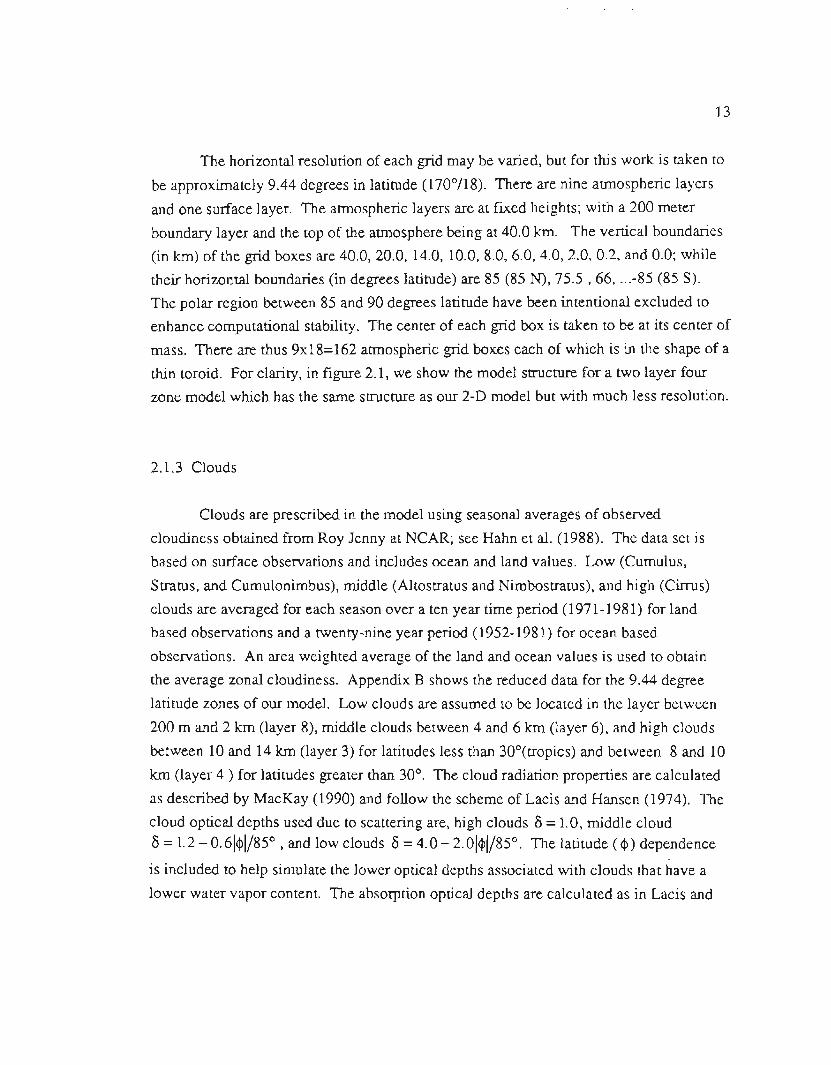
2.1.3 Clouds

Clouds are prescribed in the model using seasonal averages of observed

cloudiness obtained from Roy Jenny at NCAR; see Hahn et al. (1988). The data set is

based on surface observations and includes ocean and land values. Low (Cumulus,

Stratus, and Cumulonimbus), middle (Altostratus and Nimbostratus), and high (Cirrus)

clouds are averaged for each season over a ten year time period (1971-1981) for land

based observations and a twenty-nine year period (1952-1981) for ocean based

observations. An area weighted average of the land and ocean values is used to obtain

the average zonal cloudiness. Appendix B shows the reduced data for the 9.44 degree

latitude zones of our model. Low clouds are assumed to be located in the layer between

200 m and 2 Ian (layer 8), middle clouds between 4 and 6 Ian (layer 6), and high clouds

between 10 and 14 Ian (layer 3) for latitudes less than 300(tropics) and between 8 and 10

Ian (layer 4 ) for latitudes greater than 30°. The cloud radiation properties are calculated

as described by MacKay (1990) and follow the scheme of Lacis and Hansen (1974). The

cloud optical depths used due to scattering are, high clouds 8 =1.0, middle cloud

8 =1.2 - 0.61411/85° , and low clouds 8 = 4.0-:- 2.01411/85°. The latitude ( 41)dependence

is included to help simulate the lower optical depths associated with clouds that have a

lower water vapor content. The absorption optical depths are calculated as in Lacis and

14

Hansen (1974). It should be noted that we have used the scattering optical depths of our

model clouds as adjustable parameters and the values given above were selected to give a

globally averaged absorbed solar energy for the model that is in agreement with

observations. As discussed below, we have not taken the same liberty with surfacealbedos and cloud cover.

dz

y=Rd0 .Figure 2.1. The model structure of a 2 layer-4 zone model and geometry of atypical model grid box.

15

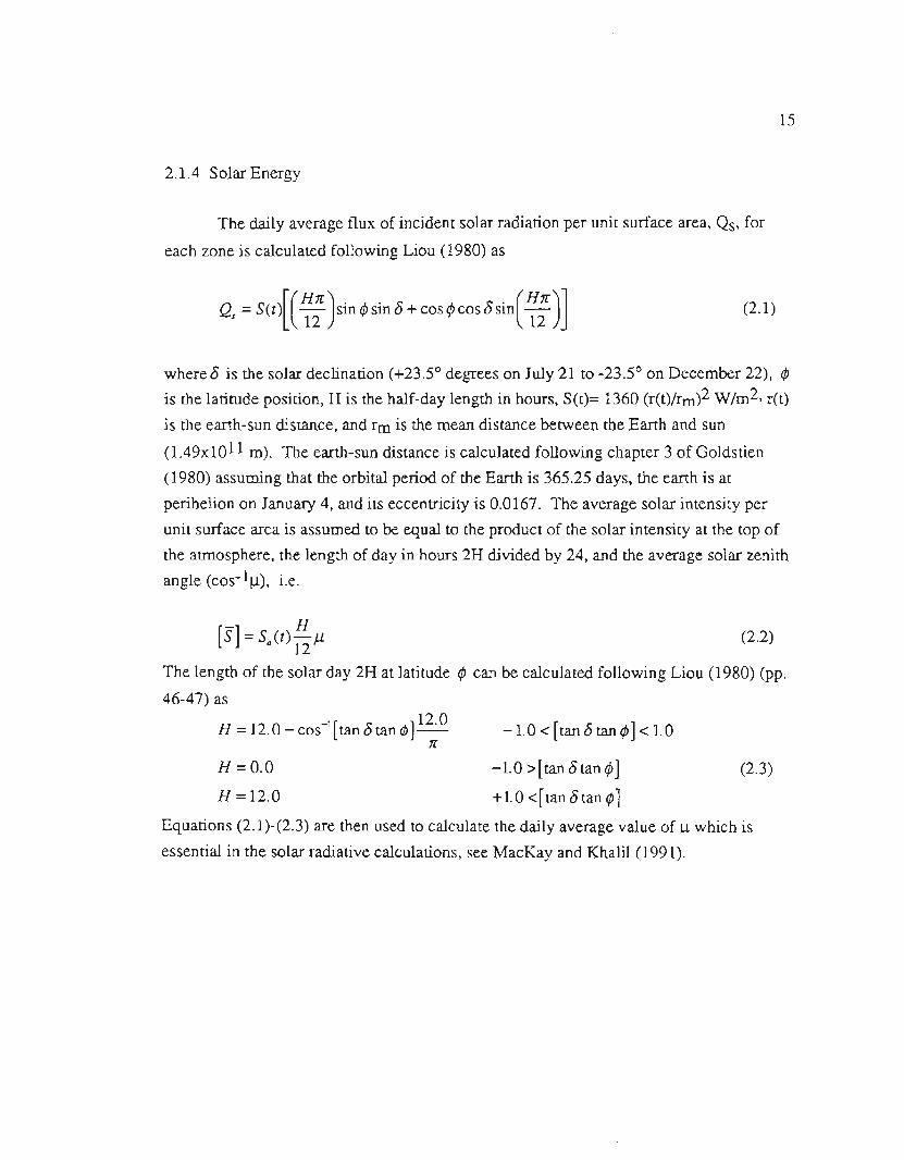
2.1.4 Solar Energy

The daily average flux of incident solar radiation per unit surface area, Qs, for

each zone is calculated following Liou (1980) as

(2.1)

where 8 is the solar declination (+23.50 degrees on July 21 to -23.50 on December 22), iP

is the latitude position, H is the half-day length in hours, S(t)= 1360 (r(t)/rm)2 W/m2, r(t)

is the earth-sun distance, and rm is the mean distance between the Earth and sun

(1.49xlO11 m). The earth-sun distance is calculated following chapter 3 of Goldstien

(1980) assuming that the orbital period of the Earth is 365.25 days, the earth is at

perihelion on January 4, and its eccentricity is 0.0167. The average solar intensity per

unit surface area is assumed to be equal to the product of the solar intensity at the top of

the atmosphere, the length of day in hours 2H divided by 24, and the average solar zenith

angle (cos-1Il), i.e.

[s] =So(t)~ J1. (2.2)

The lengthof the solarday2H at latitude iPcan be calculatedfollowingLiou (1980)(pp.46-47)as

H =12.0 -cos-1[tan8taniP] 12.0 -1.0 < [tan8taniP] < 1.07r

H=O.O -1.0>[tan8taniP] (2.3)

H =12.0 +1.0 <[tan 8 tan iP]

Equations (2.1)-(2.3) are then used to calculate the daily average value of Il which is

essential in the solar radiative calculations, see MacKay and Khalil (1991).

16

2.1.5 Surface Features

For most of the simulations described in this thesis, the Earth's surface is assumed

to consist of land, a mixed layer ocean of depth 50.0 m, and possibly sea ice. The zonal

fraction of ocean and land is taken from the Data Support Section, Scientific Computing

Division, of NCAR, DS750.1 Rand elevation Data. The snow-free land surface albedo

aL for each zone is taken from Hansen et ale(1983) and is assumed to be independent of

time. Table 2.1 gives these values along with the assumed ocean fraction for each model

zone. The two values of 0.7 noted in parentheses for the two southern most grid points

were used by us instead of 0.5 in an attempt to get better agreement between model and

observations.in the Antarctic region

When the land surface temperature TL cools to be below 273 K, the albedo

increases because of assumed snow and ice accumulation, according to.

( (273 - T ))aL=0.6+(aL-0.6)exp 12 L (2.4)

The ocean surface albedo ao is taken from Hansen et al. (1983) and is a function

of ~olar zenith angle J.1and surface wind speed Vs,

ao =0.021 + 0.0421x2 + 0.1283x3 _ 0.04x4 + 3.12xs + 0.074x6 (2.5)5.68 + v,. 1+ 3V..

where x=l-J.1. The portion of the ocean in a particular model zone, that is covered by seaice, is assumed to have an albedo of 0.7+( ao -O.7)exp(-2XI)where XI is the ice thickness

in meters. The dependence of the albedo on ice thickness is intended to simulate the

penetration of solar energy through the ice into the ocean for thin ice.

All earth based surfaces are assumed to have an infrared emissivity of 1.0. The

land area is assumed to have a heat capacity equivalent to 0.5 meters of water and its

temperature is calculated from energy considerations according to the net downward flux

of IR and solar radiation and the net upward flux of IR and solar radiation at the surface,

0.5CwPwa~L = (F J, -<if~ + SJ, -SI)

17

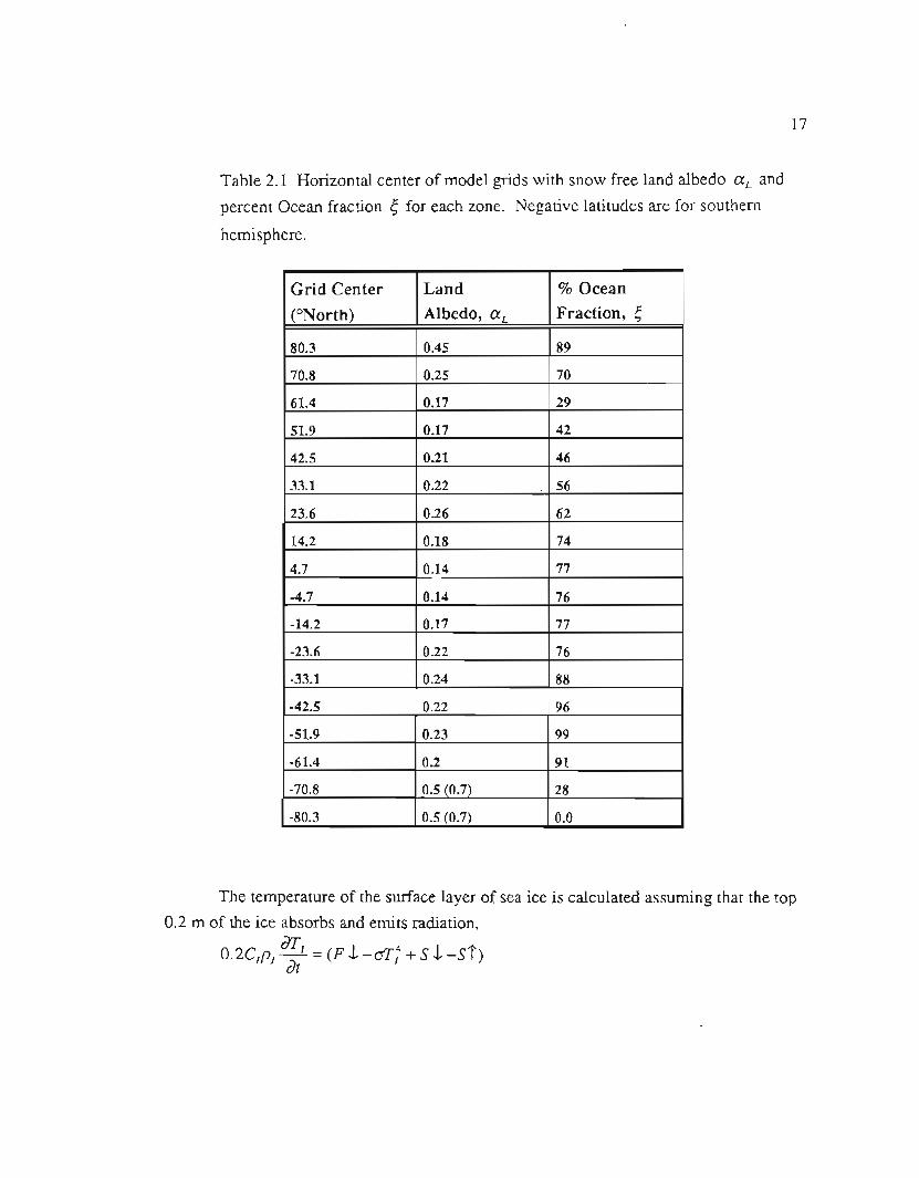
Table 2.1 Horizontal center of model grids with snow free land albedo aL and

percent Ocean fraction ~for each zone. Negative latitudes are for southern

hemisphere.

The temperature of the surface layer of sea ice is calculated assuming that the top0.2 m of the ice absorbs and emits radiation,

0.2C/p/~/ =(FJ, -aT: + S J,-Sf)

Grid Center Land % Ocean

(ONorth) Albedo, aL Fraction,

80.3 0.45 89

70.8 0.25 70

61.4 0.17 29

51.9 0.17 42

42.5 0.21 46

33.1 0.22 . 56

23.6 0.26 62

14.2 0.18 74

4.7 0.14 77

-4.7 0.14 76

-14.2 0.17 77

-23.6 0.22 76

-33.1 0.24 88

-42.5 0.22 96

-51.9 0.23 99

-61.4 0.2 91

-70.8 0.5 (0.7) 28

-80.3 0.5 (0.7) 0.0

--. _. - ... - -. -- --

18

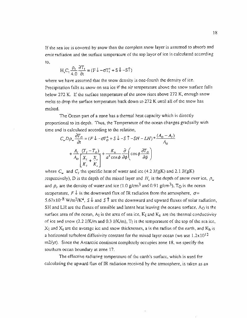
If the sea ice is covered by snow then the complete snow layer is assumed to absorb and

emit radiation and the surface temperature of the top layer of ice is calculated according

to,

H cl.£L aTI =(F J..-crT: + S J..-Sf)5 4.0 at

where we have assumed that the snow density is one-fourth the density of ice.

Precipitation falls as snow on sea ice if the air temperature above the snow surface falls

below 272 K. If the surface temperature of the snow rises above 272 K, enough snow

melts to drop the surface temperature back down to 272 K until all of the snow hasmelted.

The 'Ocean part of a zone has a thermal heat capacity which is directly

proportional to its depth. Thus, the Temperature of the ocean changes gradually with

time and is calculated according to the relation,

C Dp dT° =(F J.. _d['4 + S J..-S f -SH _ LH ) * (.40- AI)w w at ° .40

AI (TI-To) K" a(

iPdTo)+ .40

[XI + Xs

]

+ a2cosiP aiP cos aiP

KI Ks

where Cw and CI the specific heat of water and ice (4.2 J/(gK) and 2.1 J/(gK)

respectively), D is the depth of the mixed layer and Hs is the depth of snow over ice, Pw

and PI are the density of water and ice (1.0 g/cm3 and 0.91 g/cm3), TO is the ocean

temperature, F J.. is the downward flux of IR radiation from the atmosphere, G=

5.67xlO-8 W/m21K4,S J..and sf are the downward and upward fluxes of solar radiation,

SH and LH are the fluxes of sensible and latent heat leaving the oceans surface, AO is the

surface area of the ocean, AI is the area of sea ice, KI and Ks are the thermal conductivity

of ice and snow (2.2 JIK/m and 0.3 JIK/m), TI is the temperature of the top of the sea ice,

XI and Xs are the average ice and snow thicknesses, a is the radius of the earth, and Kh is

a horizontal turbulent diffusivity constant for the mixed layer ocean (we use 1.2xlO12

m2/yr). Since the Antarctic continent completely occupies zone 18, we specify the

southern ocean boundary at zone 17.

The effective radiating temperature of the earth's surface, which is used for

calculating the upward flux of IR radiation received by the atmosphere, is taken as an

19

area weighted average of the temperatures of the land, ocean, and sea ice (TL, To, andTI). Taking the zonal ocean fraction to be ~ and the fraction of it covered by sea ice to

be X , the effective surface radiating temperature is calculate4 from

Ts =[~((1-X)T~+xT:)+(I-~)T1]~ (2.6)

Although the simulations described in this thesis assume a 50 meter deep ocean

mixed layer with no transport to the deep ocean, we have done some preliminary work

with a deep layer ocean model that can be coupled to our model's atmosphere. We

describe this model in a later section of this chapter since the existing treatment of the

ocean is just a simplified version of the more complete ocean model.

We have not explicitly considered orography and we have neglected vegetation

type and soil type in this work.

2.2 Model Equations

The GCRC 2D statistical dynamical climate model uses the primitive equations,

in zonally averaged form, to solve for the climate state of the model planet (i.e. the

temperature, pressure, three dimensional wind velocity, radiative fluxes, and atmospheric

moisture/precipitation). There is extensive discussion of these equations in the literature;

e.g. Lorentz (1967), Saltzman (1978), and Holton (1979). The form of the equations

most closely mimic that used by Yao and Stone (1987) for their statistical-dynamical

model, with the difference being that their equations are written for a sigma vertical

coordinate system instead of a z=ln(p) coordinate system as in our model. The equationsused are:

the equation of continuity,

dp = _ 1 d(pvcosq,) _ dpwdt a cos q, dq, dz

(2.7)

the horizontal equations of motion,

20

apu _at

1 a[p(uv+iJVi)cos4>] _ a[p(uw+H)]acm4> a4> ~

(2.8)

tan 4> -+pfv+ p-(uv + u'v') + pFAa

apv =_.!.;)p _ 1 a[pv2cos4>]_a[p(vw+H)]~ a~ acm4> ~ ~

u2 tan 4>-pfu-p +pF~ (2.9)

the first law of thennodynamics

a[pCpT] = 1 a[pcpcos4>(vT+V'T)] +P(Q+QL)+l.4RT[ap+~ ap

]at acos4> a4> at a a4>(2.10)

+1.4RTw ap _ a[pCp(wT + w'T)]az az

the equation of state,

P = pRT (2.11)

the assumed condition of hydrostatic equilibrium

dP =-pgdz (2.12)

and the moisture balance equation

asp = 1 aspvcos4> aspw +C*-E*at a cos4> a4> az

(2.13)

In the above equations p is the air density (in glm3), t is time, 4>is the latitude

coordinate, u, v, and w are the zonal, meridional, and vertical velocities respectively, f isthe Coriolis parameter, FA and F~ and are the zonal and meridional friction tenns, Cp is

21

the heat capacity of dry air at constant pressure, R is the ideal gas constant for air, Q is

the diabatic heating rate per unit mass of air (Jig) due to the fluxes of solar and terrestrial

radiation, Qr. is the latent heat release (or absorption) per unit mass, g is the acceleration

due to gravity, s is the specific humidity of water vapor, and C* and E* are the rate of

evaporation and condensation respectively (in gHzO/m3/s). The symbols in the above

equations are standard and are also defmed in Appendix A along with all other major

variable symbols used throughout this dissenation in order of their appearance. All

variables are assumed to be zonal averages. The prime indicates deviation from the zonal

average and the overbar is included when a zonal average is emphasized. The above six

equations (2.7 through 2.12) are solved as an initial valued problem using the spatial grid

of 9 vertical atmospheric layers and 18 latitude zones, described previously. The

pressure, density, and temperature (P, p, and T) of a zone are assumed to be the values of

the respective variables at the center of the zone; while the vertical, meridional, and zonal

velocities (w,v, and u) are calculated at the boundary between zones.

We use a grid system that is common in models of this type and in general

circulation models; see Ohan et al. (1982) and Yao and Stone (1987). That is, the center

of a grid point is indicated by an integer, while the boundary is designated as an integer

-1/2 (see Figure 2.2 below). A grid point is designated by two numbers (i,j), where i is

the vertical grid position and j is the horizontal grid position. For example, grid point 1,1

is at the center of the top atmospheric layer directly above 80.3° (85°-4.7°) nonh latitude,

grid 1,9.5 is at the center of the top atmospheric layer directly above the equator, and

grid point 8.5, 18 is at the top of the lowest atmospheric layer directly above 80.3° south

latitude. It should be noted that northward moving meridional velocities(south winds) are

considered positive, as are eastward moving (westerlies) zonal velocities, and upward

moving vertical velocities.

22

(i+ 1/2,j+ 1/2)

4 NORTH

Figure 2.2. The model grid system used for numerical calculations in the aCRC

2-D statistical dynamical climate model.

2.2.1 Numerical Overview

The above equations are solved using a box type numerical procedure similar to

those used by Khalil and Rasmussen (1985) for the calculation of the transport of trace

gases in the atmosphere, and also similar to that used by Yao and Stone (1987) for their

two-dimensional statistical-dynamical model. For example, the fIrst term on the right

hand side of equation 2.8 represents the time rate of change of zonal momentum due to

the meridional flux of zonal momentum by advection and turbulence. The numerical

form of the horizontal advective part of this fIrst term is written as,

(i-l/2,j-l/2) I I (i-1I2,j+1/2) t.UP

.I

. I .(ij-l ) (i,j) I (i,j+1)

23

(2.14)

where

(pj +pj+l

)'"

gj+l/2= 2 Vj+1/2COS'l'j+ll2

In the above; the fIrst index i, corresponding to the vertical level, has been omitted since

it is the same for each term when we consider horizontal transpon only. As another

example we consider vertical advection. The second term on the right hand side of

equation 2.7 is written as,

!J.p . . =~{(

Pi,j + Pi-l.j

)w. . _

(Pi.j + Pi+l.i

)w. .

}I.} tJ.z. 2 l-l/2.} 2 l+l/2.}I

(2.15)

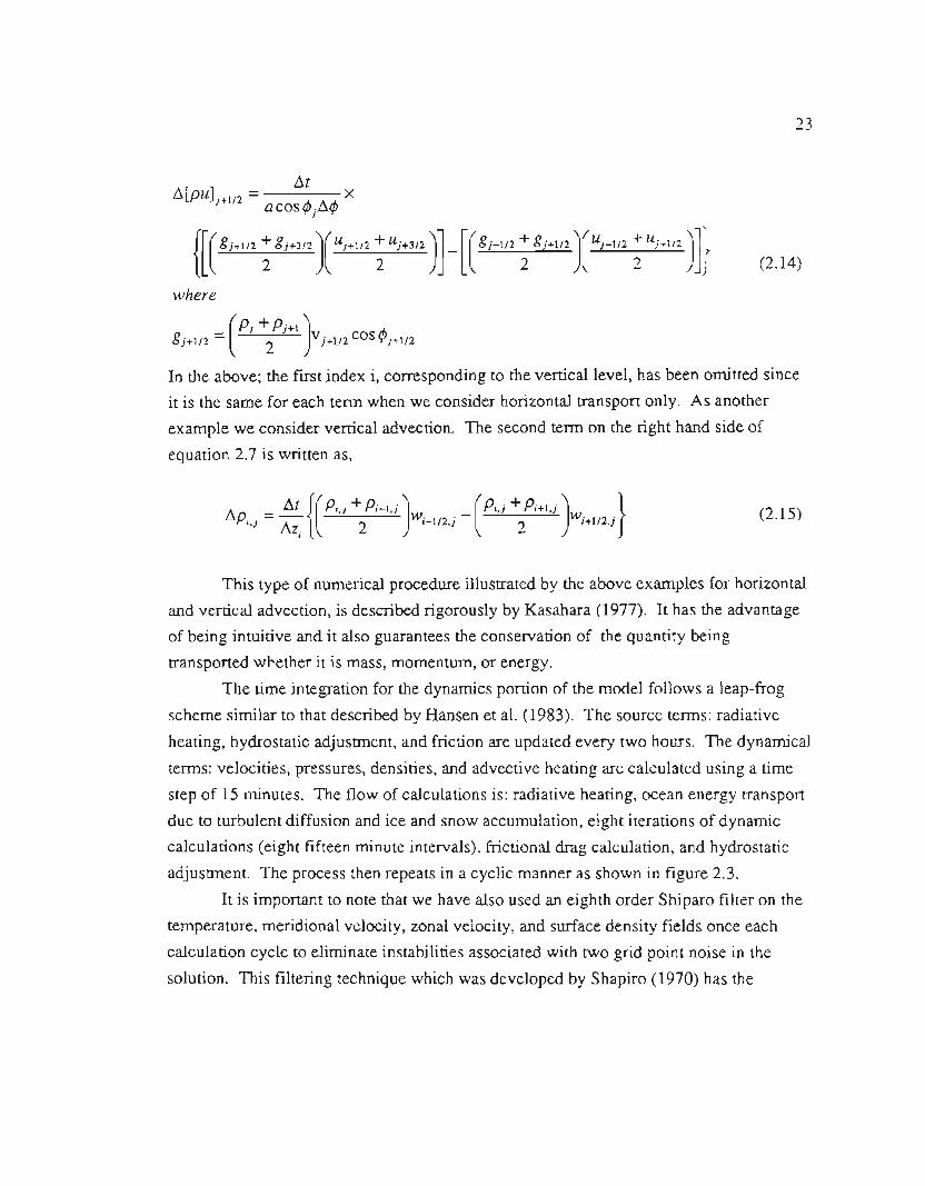
This type of numerical procedure illustrated by the above examples for horizontal

and vertical advection, is described rigorously by Kasahara (1977). It has the advantage

of being intuitive and it also guarantees the conservation of the quantity being

transponed whether it is mass, momentum, or energy.

The time integration for the dynamics portion of the model follows a leap-frog

scheme similar to that described by Hansen et al. (1983). The source terms: radiative

heating, hydrostatic adjustment, and friction are updated every two hours. The dynamical

terms: velocities, pressures, densities, and advective heating are calculated using a time

step of 15 minutes. The flow of calculations is: radiative heating, ocean energy transpon

due to turbulent diffusion and ice and snow accumulation, eight iterations of dynamic

calculations (eight fIfteen minute intervals), frictional drag calculation, and hydrostatic

adjustment The process then repeats in a cyclic manner as shown in fIgure 2.3.

It is imponant to note that we have also used an eighth order Shiparo fIlter on the

temperature, meridional velocity, zonal velocity, and surface density fIelds once each

calculation cycle to eliminate instabilities associated with two grid point noise in the

solution. This fIltering technique which was developed by Shapiro (1970) has the

24

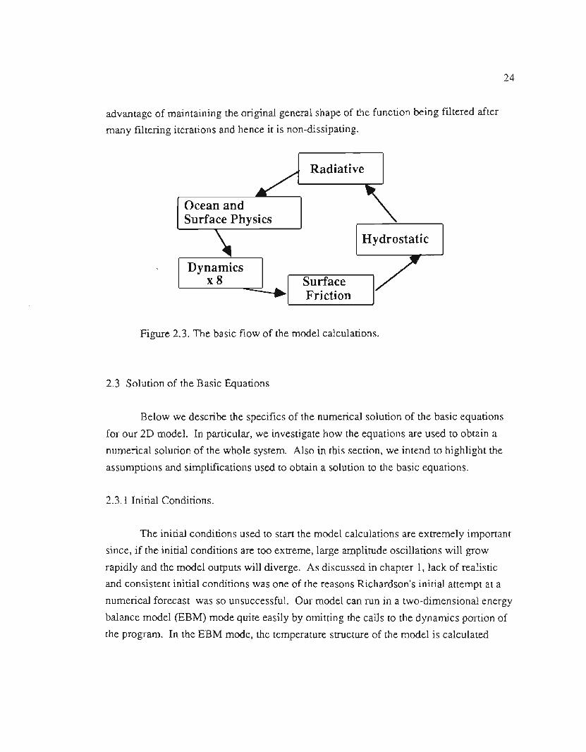
advantage of maintaining the original general shape of the function being fIltered after

many filtering iterations and hence it is non-dissipating.

Radiative

Ocean andSurface Physics

Hydrostatic

Dynamicsx8 Surface

Friction

Figure 2.3. The basic flow of the model calculations.

2.3 Solution of the Basic Equations

Below we describe the specifics of the numerical solution of the basic equations

for our 2D model. In particular, we investigate how the equations are used to obtain a

numerical solution of the whole system. Also in this section, we intend to highlight the

assumptions and simplifications used to obtain a solution to the basic equations.

2.3.1 Initial Conditions.

The initial conditions used to start the model calculations are extremely important

since, if the initial conditions are too extreme, large amplitude oscillations will grow

rapidly and the model outputs will diverge. As discussed in chapter 1, lack of realistic

and consistent initial conditions was one of the reasons Richardson's initial attempt at a

numerical forecast was so unsuccessful. Our model can run in a two-dimensional energy

balance model (EBM) mode quite easily by omitting the calls to the dynamics portion of

the program. In the EBM mode, the temperature structure of the model is calculated

25

using the radiative convective calculations described below coupled with the transfer of

horizontal turbulent energy (driven purely from temperature gradients) and vertical

convective energy. The steady state solution of the EBM model provides a convenient

set of initial conditions for the temperature, density (or pressure), and velocities (which

have been set to zero). Using the steady state EBM atmosphere as an initial state, the

dynamics portion of the program can then be added as a perturbation to this and a new

steady state solution can be obtained which is closer to the real observed atmosphere.

Additional refinements can be made until the mean annual output of the model agrees

closely with the observed mean annual climate. This solution, obtained by bootstrapping,

can then be used as the initial conditions for model climate sensitivity studies due to

perturbations in the model climate system. Our assumption is that if the model's initial

conditions are similar to the observed state of the real Earth, then model perturbation

studies, such as the response of the model to a doubling of C02, will help us estimate and

understand possible changes and interactions of the real climate system due to similar

perturbations of it.

2.3.2 The equation of continuity

The equation of continuity is broken into two parts; horizontal and vertical. The

horizontal transport of mass is calculated by the first term on the right hand side of

equation (2.7). The spatial differencing scheme used is similar to that of equation (2.14)and is written as,

The vertical transport of mass is performed during the hydrostatic adjus~ent.That is, the total mass in a vertical column is redistributed to satisfy the hydrostatic

equation, equation (2.12), and the equation of state, equation (2.11). The hydrostatic

26

adjustment process transfers mass, latent and sensible heat, and zonal and meridional

momentum. The second term on the right hand side of equation (2.7) is used

diagnostically to calculate the vertical velocity, w, from the calculated transfer of mass

during the hydrostatic adjustment process, i.e.&n

_ 1 _

'--.JW - 2

i- 21,j - f1t (P--l -+p --)/2.0r ',J I.)

where f1mis the mass flux in g/m2 across the i-l/2 boundary required to reestablish

hydrostatic equilibrium in one radiative time step f1tt=2.0hr. The process of hydrostatic

adjustment is discussed in more detail in section 2.3.5.

2.3.3 Zonal Velocity

The finite difference form of the fIrst term on the right hand side of equation (2.8)

is written as in equation (2.14). The turbulent transport of zonal momentum, the u'v' part

of this term, is parameterized following Stone and Yao (1987 and 1990). Since this

section is a description of the numerical technique used, we will postpone a discussion of

this parameterization until a section 2.4.1. The fIrStpart of the second term in equation(2.8) is calculated as a flux of zonal momentum during the hydrostatic adjustment

process,

The second part of this term, u' w' is assumed to depend on the vertical shear of zonal

velocity u according to

dpH =~ pK dudz dz'dz(2.16)

27

The values ofKz were originally estimated from those given by Liu et al. (1984) but it

was found that we could not obtain the Ferrel circulations cells in either hemisphere with

these values ofKz which were based on Radon measurements. We have thus used

Kz=lO m2js everywhere except between layers 1 and 2 and layer 2 and 3 at the top of themodel where we have used values of Kz=20 m2js and 4 m2js respectively to inhibit high

zonal winds developing in the stratosphere. Stone and Yao (1987) completely eliminated

the vertical turbulent flux of zonal momentum from their calculations noting that the

output of their model was not significantly affected by whether they included aparameterization for Kz or not. As noted above, we did fmd that our output was

significantly affected by the choice in Kz profile so in this regard our model behaves

differently from the model of Stone and Yao. It is also noteworthy that when we

experimented with setting all values of Kz to zero we obtained tropical easterlies that

were much greater than observed. This result is not surprising since, as will be shown in

chapter 3, our model has a propensity for strong tropical easterlies.

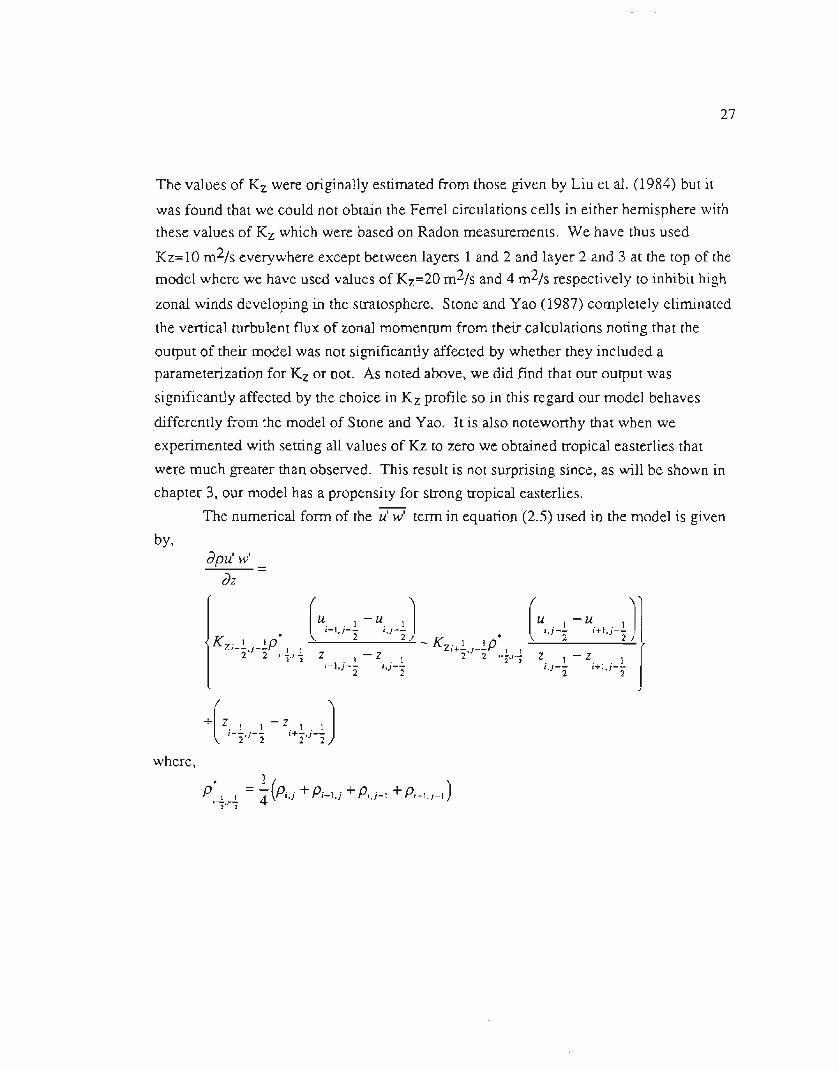
The numerical form of the u' w' term in equation (2.5) used in the model is given

by,dpu'w'

dz

.Kz' IJ'_!P I. I Z I - Z.' J'_!

'-z' 2 '1')"2 i-I,j-z '2

(u - u

J' . I .. I.-I,J-Z ',J-z (

u -uJ

.. I ., I~~ ~J~

z -zi J'_! i+1 J'_!. 2 '2

where,. 1

( )=- ..+ . .+ .. + . .P;...!J...! 4 P',J P'-I,J P..J-I P.-I,J-I2 2

- -.. -..-.

28

The third and fourth tenns in equation (2.8) can be written as

[

f1(PU).. I

] (P+p

) [

u.o Itanq,. I

]

',)-- . 0 . 0 '.)-- )--

2 = '.) ',)-1 V f + 2 2A 2 0 . . 1 o. 1tit . ")-2 ")2 a

Te 3,4

The final tenn in equation (2.8), the frictional drag force, is assumed to be non-zero only

at the Earth's surface. As is standard practice (see for example Washington arid

Parkinson, 1986) we assume that the surface shear stress in the meridional and

longitudinal direction -r, and -r" are given by

-r, = -pCD v.../u2 + v2 and -r" = -pCDU~U2 + v2

where the surface drag coefficient CD is of the order of 0.001 to 0.003 (we use 0.002).

The surface horizontal frictional forces are given by

F =! a-r, and F =.!. a-r", paz " pazThe finite difference fonn for the frictional tenn in equation (2.8) is thus

[

1 a-r,,

]=

[F"]9.j_~= P az 9.j-~

-CDU9)o_.!. /U9 )._.!.2 +V9 )O_.!.2 + ( zs.!.)._.!. -Z9.!. )O_~). 2 V '2 '2 2' 2 2' 2

2.3.4 Meridional Velocity

Except for the first tenn in equation (2.9), the finite difference fonn of each tenn

in equation (2.9) is essentially identical to that used for equation (2.8) and hence will not

be repeated here. The first tenn of equation (2.6) is calculated as

[

apv. . 1

]

1 Po . 1 - P. ° 1

a;;-2 =a ;~+~ _ q,'~)~2re",,_1 )-2 )-2

29

and the v' w' is e~timated by,

dPV'}J =~pK dvdz dz %dz(2.t7)

2.3.5 The fIrst Law of thennodynamics

Since the fonn of the first law of thennodynamics used by us in the numerical

calculation of heat transfer is somewhat unique, we derive it below for clarity and then

explain the numerical procedure used to calculate the change in temperature of a grid

point in the 2-D model atmosphere. The basic fonn of the fIrst law of thennodynamics

(see Lorentz, 1967) is,

CpaT = (Q+QL)dt+ adP (2.18)

where Cp is the heat capacity (J/g/K) of the atmosphere at constant pressure, dT is the

infmitesimal temperature change in time interval dt, Qr the diabatic heating rate per unit

mass (which includes radiative heating and release or absorption of latent heat), a is the

specifIc volume which is the reciprocal of density p, and dP is the infInitesimal pressure

change. We assume the temperature change dT occurs in a two step process; fIrst an

adiabatic temperature change due to the pressure change dP and then adiabatic

temperature change due to the diabatic heating Q. For the adiabatic process it is easy toshow that

aT dP R-= 1(- where 1(=- (2.19)T P Cp

Taking the differential of the equation of state P =pRT and multiplying both sides by a

yieldsad? =adpRT + apRaT

= adpRT + RaTRiff

=adpRT+-dPP

= adpRT + al(dP

or

dP = RTdp = yRTdp = 1.4RTdp(1- 1()

30

since1

(1- lC)=

Thus we write the fIrst law as,tIT dp

Cp - = (Q + QL) + 1.4aRT-. dt dt(2.20)

Sinced a a va a-=-+(u v w).V=-+--+w-dt at " at a aq, az

we can rewrite (2.20) as .

aT vaT aT Pl.4RT[

ap vap ap]

pC -=-pC ---pC w-+P(Q+QL)+ -+--+w-p at p a aq, P az p at a aq, az

At this point we could derive equation (2.10) without the turbulent tenns, by multiplying

the equation of continuity by CpT and adding it to (2.21); instead we proceed in analternate direction to derive our working numerical equations.

We break (2.21) into three parts corresponding to horizontal transpon, venical

transpon, and heating due to radiant heat energy and latent heat (Q),aT v aT

[ap v ap

]pC -=-pC --+l.4RT -+-- ,

P at P a aq, at a aq,aT aT

[ap ap

]pC -=-pC w-+1.4RT-+w- ,pat paz at az

(2.21)

(2.22)

(2.23)

andaT

Cpa; = (Q+QL) (2.24)

where aT and ap in each of equations (2.22) and (2.23) correspond to the changes thatat at

occurduringhorizontalor verticaltranspon separatelyand c::: in (2.24) corresponds to

the temperature change due to radiant heating or heat by latent heat energy (Q+QL). The

radiative heating and energy transpon associated with the convective adjustment, is

calculated in the radiative part of the model and will be discussed below in the overview

of the radiative convective model physics. The parameterization of the heating associatedwith the release of latent heat is discussed in section 2.4.4.

31

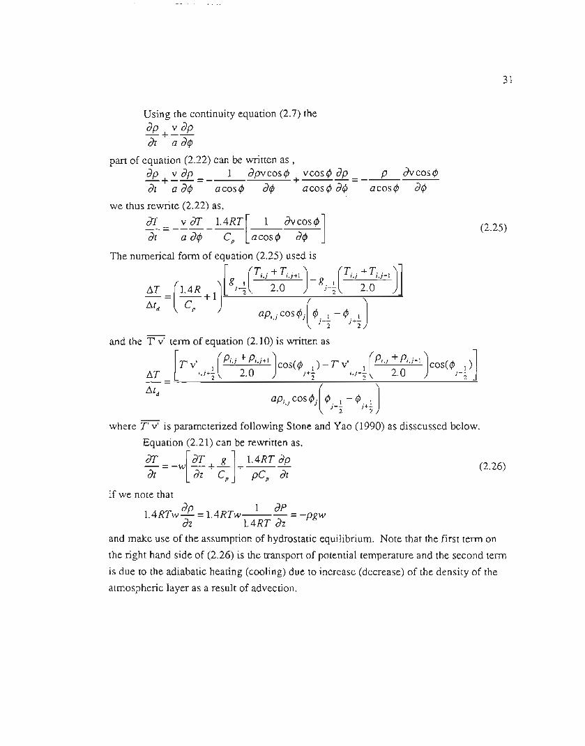
Using the continuity equation (2.7) theap v ap-+--at a aiP

part of equation(2.22)can be writtenas ,ap vap 1 apvcosiP vcosiPap p avcosiP-+--= + =at a aiP a cos iP aiP a cos iPaiP a cos iP aiP

we thus rewrite (2.22) as,

aT =_ vaT _1.4RT[

1 avcosiP

]at a aiP Cp acosiP aiP

The numerical form of equation (2.25) used is

[ (T. . + T. '+1

) (T. . + T. . 1

)]dT =(

1.4R + 1J

gj+~ ',J 2.0',) - gj_~ ',J 2.0',J-

dtd Cp

( JaPi,j cos iPj iP. 1 - iP. 1

J-"2 J+"2

(2.25)

and the T v' term of equation (2.10) is written as

[T v'. . 1 (

Pi,j + Pi,j+1

)COS(iP. I) - T v'. . 1(Pi,j + Pi,j-l

) COS(iP. 1 )]dT _ ',J~ 2.0 J+"2 ',J-"2 2.0 J-"2-- J''''

dtdap. . cos iP.

1iP 1 - iP 1

',J J j__ j+_2 2

where T v'is parameterized following Stone and Yao (1990) as disscussed below.

Equation (2.21) can be rewritten as,

aT =-w[aT+ -L

]+ 1.4RT ap (2.26)

at az Cp pCp atif we note that

ap 1 ap1.4RTw- =1.4RTw =-pgwaz 1.4RTaz

and make use of the assumption of hydrostatic equilibrium. Note that the first term on

the right hand side of (2.26) is the transpon of potential temperature and the second term

is due to the adiabatic heating (cooling) due to increase (decrease) of the density of theatmospheric layer as a result of advection.

32

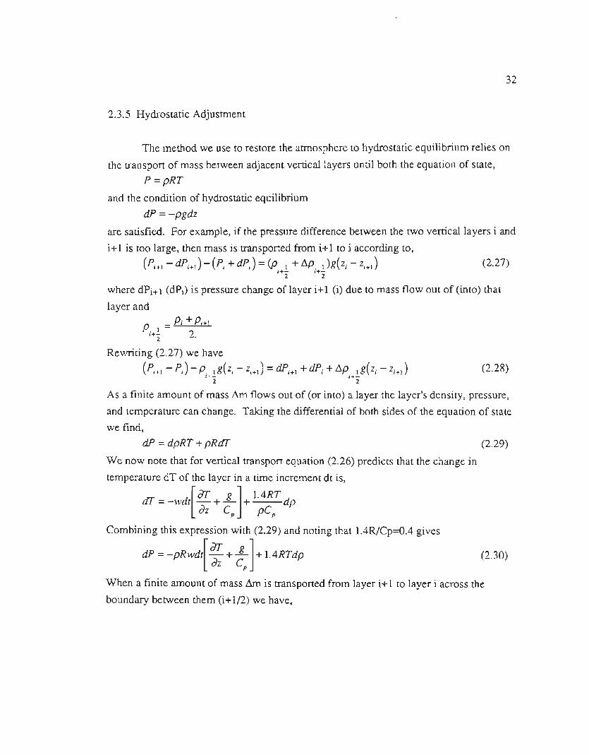
2.3.5 Hydrostatic Adjustment

The method we use to restore the atmosphere to hydrostatic equilibrium relies on

the transport of mass between adjacent vertical layers until both the equation of state,P =pRT

and the condition of hydrostatic equilibrium

dP =-pgdz

are satisfied. For example, if the pressure difference between the two vertical layers i and

i+1 is too large, then mass is transported from i+1 to i according to,

(Pi+l- dPi+1)- (Pi+ dP;)=(p, 1 +~P. 1)g(Zi - Zi+l ) (2.27).+- .+-.22

where dPi+l (dPi) is pressure change of layer i+1 (i) due to mass flow out of (into) that

layer and

P _ Pi + Pi+l1-i+- 22 .

Rewriting (2.27) we have

(Pi+l - Pi) - p, Ig(Zi - Zi+l)= dPi+1+ dPi + ~p, Ig(Zi - Zi+l)1+- 1+-2 2

(2.28)

As a finite amount of mass ~m flows out of (or into) a layer the layer's density, pressure,

and temperature can change. Taking the differential of both sides of the equation of state

we find,

dP =dpRT + pRclF (2.29)

We now note that for vertical transport equation (2.26) predicts that the change in

temperature dT of the layer in a time increment dt is,

[

ar g]

1.4RTclF=-wdt -+- + dp

Jz Cp pCp

Combining this expression with (2.29) and noting that 1.4R1Cp=O.4 gives

dP =-PRWd{~ + ~J + 1.4RTdp (2.30)

When a finite amount of mass &n is transported from layer i+1 to layer i across the

boundary between them (i+1/2) we have,

33

or

(2.31)

where

L(z. - z

))C I .1I+-

P 2

and

~_1 = ( R(

1.4Y. + (Ti-}+ T;) g

( ))1,1 _

)

I - - Z -2 2 C 1 Z.

Z - Z . i-- I

i-1. i+1. P 22 2

The pans of ~Pi associated with mass transport across the i+1 or i boundary can thus

easily be identified. We can rewrite (2.28) as

B. 1 =dPi+1+dPi+~P. 19(Zi-Zi+l)1+- 1+-2 2

where we have defined Bi+l/2 to be identical to the left hand side of (2.28). Combining

this with equation (2.31) and noting that

34

gives

B 1 =-;+'2

O.5g(z;- Z;+1)

I

~. 1g +

J

.-;.;-~(z. 1 - Z.+.!. 2'2 · 2

O.5g(z; -Z;+I)

I

~. 1

J

.+-+ I-g. . 1 + _ 2g..+.!. .+1..~ ( Z

J-

(z 1 Z.3',' 2 Z 1 - . 1 ;+_ .+_

. &+- 2 2'-'2 2

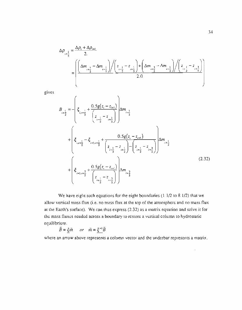
(2.32)

We have eight such equations for the eight boundaries (11/2 to 8 1/2) that we

allow venical mass flux (i.e. no mass flux at the top of the atmosphere and no mass flux

at the Earth's surface). We can thus express (2.32) as a matrix equation and solve it for

the mass fluxes needed across a boundary to restore a vertical column to hydrostatic

equilibrium.

B = fm or m= g-1Bwhere an arrow above represents a column vector and the underbar represents a matrix.

35

2.3.6 Atmospheric Moisture

For moisture, we assume the constant relative humidity profile for each latitude

zone introduced by Manabe and Wetherald (1967) and used by MacKay and Khalil

(1991). The relative humidity r is expressed in terms of the surface relative humidity h'

and the pressure p (in atmospheres) byr = ro(P- 0.02)/ 0.98

We use data from the Data Suppon Section, Scientific Computing Division, of NCAR,

DS205.0, N Hem. Climatological Grid Data (N.H. and S.H.) for the surface relative

humidity of each zone for each season. These data are presented in tabular form in table

2.2 and graphically in figure 2.4. We use a linear interpolation of the seasonal averages

to estimate the surface relative humidity at any give time.

36

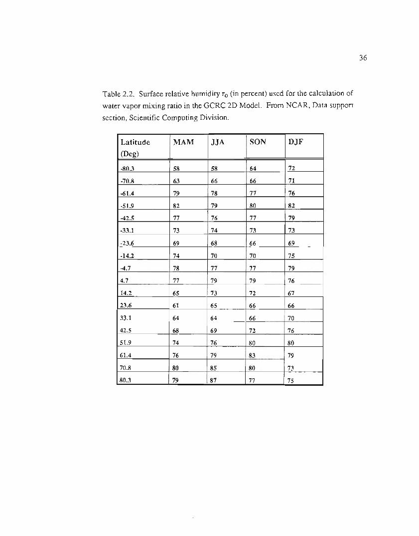
Table 2.2. Surface relative humidity ro (in percent) used for the calculation of

water vapor mixing ratio in the GCRC 2D Model. From NCAR, Data support

section, Scientific Computing Division.

Latitude MAM JJA SON DJF

(Deg)

-80.3 58 58 64 72

-70.8 63 66 66 71

-61.4 79 78 77 76

-51.9 82 79 80 82

-42.5 77 76 77 79

-33.1 73 74 73 73

-23.6 69 68 66 69

-14.2 74 70 70 75

-4.7 78 77 77 79

4.7 77 79 79 76

14.2 65 73 72 67

23.6 61 65 66 66

33.1 64 64 66 70

42.5 68 69 72 76

51.9 74 76 80 80

61.4 76 79 83 79

70.8 80 85 80 73

80.3 79 87 77 75

37

---MAM

--<>--DJF

-90.0 -60.0 -30.0 0.0 30.0 60.0 90.0

Latitude (Deg)

Figure 2.4. Surface relative humidity (%) usedfor the calculation of water vapor

mixing ratio in the aCRC 2D Model. From table 2.2.

The specific humidity, s, is related to the temperatureT and the relative humidity r by

s = rs*(T) s> 3.0 X 10-6gH2.OgAlr

s =3.0 X 10-6 rs*(T) < 3.0 x 10-6 gH2.OgAlr

where s* is the saturation vapor pressure. The saturation vapor pressure is assumed to

depend on the temperature according to the Clausius Clapeyron equation,

s*(T) = s*(273K) exp[O.622L

(~ - 1.)]R 273K T

seefor exampleWashingtonand Parkinson(1986). L is the LatentHeatof vaporization(251O-2.38[T-273]J/g) from Stone and Carlson 1979, R the ideal gas constant (J/[kgKD,

and s*(273)=3.75xlO-3 gH20/gair. Thus as the temperature of a model grid point

changes, the water vapor content also changes.

We use a modified specific heat capacity Cp* identical to that used by Manabe

and Wetherald (1967) to account for the greater thermal inertia of the atmosphere due to

an assumed fixed relative humidity,

38

c. = C[1+ Lv as

]p P C iJTP

We havereplacedCpby Cp*on the left sideof equation(2.10),the fIrstlaw ofthennodynamics. That is, the thennal inertia of the moist layer is assumed to be larger

than a dry layer but the dry sensible heat capacity of the layer is the same for both a dry

and moist layer.

We can use equation 2.13 to diagnostically calculate the difference between the

condensation and evaporation for a model grid point To estimate the precipitation for a

given grid point we rely on the fact that its actual moisture content is in a quasi-steady

state, since it only changes as the temperature changes. We assume that all cooling

processes during a time step results in precipitation. We thus estimate the rate of

precipitation P in mm/day by,

P= as~T; +~T~ Pair ~ziJT ~tR Pw

where ~T; and ~T~ are the magnitudes of the cooling tenn associated with energy loss

during the radiative (including convection) and dynamical (including hydrostatic

adjustment) calculations respectively. This estimate of precipitation works fairly well

considering our present simplifIcation of the moisture budget, see section 3.4 of the next

chapter. Improvements in precipitation estimates are expected following a more

comprehensive treatment of our model hydrodynamics. Future model improvements will

include a prognostic calculation of the moisture budget as well as a prognosticdetennination of clouds.

2.4 Other Parameterizations

2.4.1 Parameterization of Eddy Momentum Flux u' v' .

For the flux of eddy momentum u'v' ,we use the parameterization scheme given

by Yao and Stone (1987) with the slight modifications described by Stone and Yao

(1990) As they describe their parameterization in great detail, we will only outline the

39

essentials of their scheme below. We will attempt to give enough infonnation so the

reader can reproduce our calculations from this dissertation as well as understand the

underlying theory of the work of Yao and Stone. Starting from the equations of motion

(2.7)-(2.9) and the continuity equation, Pedlosky (1979) in chapter 6 of his classic text on

geophysical fluid dynamics, derives the equation for the conservation of potential

vorticity (q) on a beta plane using the quasigeostrophic approximation (his equations

6.5.32 or 6.5.19). In dimensional fonn his equation takes the fonn of,

[q + Poy+~~

(PS2 ~ op

)]=0

Ps dz Ns dz Ps

where (2.33)

dv duq=---

iJx dyis the relative vorticity, Po is the rate of change of the Coriolis parameter f (in the

vicinity of some reference position corresponding to fo) with respect to meridional

coordinate y, Ps is the density of the stationary state, x and z are the longitudinal and

vertical coordinates (both in meters), op is the fIrst order penurbation from the stationary

state of the pressure, and Ns is the Brunt - Viiisiilii frequency of the stationary state,

N2 = .K. dOss Os dz

with Osbeing the potential temperature of the stationary state. Note that (2.33) is a

perturbation equation about some mid latitude position Yo, usually taken to be 45 degrees.

If we note that for geostrophic flow,d'¥ d'¥u=-- and v=-dy iJx

where

'II= opfoPs

and using this defInition for 'II, we can rewrite (2.33) as,

40

dq =-l('¥,q)dtwhere

(2.34)

l(A B)= dA dB _ dA dB, dxdy dydx

is the Jacobian of the functions A and B. Held (1978) starts from (2.34) to show that the

height parameter

h=f2au~o dz f3N2

appearing often in the model of Charney (1947), is related to the vertical structure of the

baroclinic disturbance. Held notes that when h«H "the amplitude of the most unstable

wave decays more or less exponentially above the ground with an e-folding proportional

to h " (H is the atmospheric scale height). If h»H then H takes the role of the vertical

scale for the most unstable wave. Held shows that the parameterd =H / (1+ r)where r=H / h

(2.35)

is a good measure of the vertical structure of the baroclinic disturbance.

It is worth noting that in Chapter 7 of his book, Pedlosky (1979) discusses

instability theory in some detail. In sections 7.6-7.8, he discusses the basic mechanism of

baroclinic instability, the simple baroclinic model of Eady (1949), and Charney's model.

Other texts contain a review of this material, but in my opinion, Pedlosky's text is by far

the most authoritative on baroclinic instability as it penains to the parameterization of

Yao and Stone (1987, 1990).

Yao and Stone (1987) begin the derivation of their parameterization by using the

relationship between the eddy fluxes of zonal.momentum per unit mass u, potential

temperature, and quasi-geostrophic potential vonicity q given by Green (1970)

41

df d fJv' , ,

-uv =. ---qvdy dp (j

dewhere (j =-L

dp

An alternate derivation of this equation, to that of Green, can be obtained by combining

equations 7.2.24 and 7.2.22 of Pedlosky. Green's parameterization also assumes that the

two tenns on the right hand side of (2.36) can be parameterized by a mixing-length

fonnulation as,

e'v'=-K de -K (jvy dy vp

, , K aq K aqqv=- vYdy- vPdp

Stone and Yao (1987) then show that combining these assumptions, using the

thennal wind relation, and an equation equivalent to our (2.34) they obtaind iPs-

- u'v'dpdyo

= rPs{

K(/3_ d2U

)_.!.. de dKvyt.,p

Jo vy dy2 (j dy dp fJfor the gradient of the flux of zonal momentum per unit mass. Thus only Kvyneeds to be

parameterized to calculate the vertical mean eddy momentum flux. They estimate the

vertical profile of u'v'to be the same at each latitude and equal to the average vertical

profile obtained by their 3-D control run obtained using the GISS Model II GCM

described by Hansen et al. (1983). They then experimented with the vertical structure of

u'v' and found that the general circulation was not too strongly dependent on it, and

hence suggested that a fixed vertical structure based on their 3-D control run was valid.

We use the same vertical structure for our 2-D model and have also experimented with

the dependence of the assumed vertical structure of u'v' on the general circulation of ourmodel.

To complete the parameterization scheme, Stone and Yao (1987) used the

parameterization of Kvydeveloped by Branscome (1983) for eddy heat transport

parameterization, with several modifications. In the notation of Stone and Yao (1987)Branscome's Parameterization for K is

vy

(2.36)

(2.37)

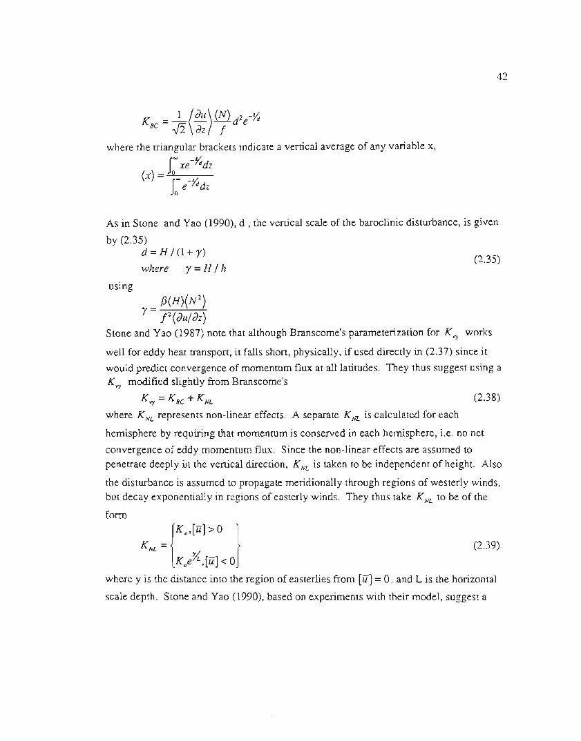
42

K = ~ (dU

)(N) d2e-YriBC .J2 dz J

where the triangular brackets indicate a vertical average of any variable x,

J.- xe -Yridz(x) =

J.0- _z/

e /ddzo

As in Stone and Yao (1990), d , the vertical scale of the baroclinic disturbance, is given

by (2.35)d = H / (1+ r)

where r =H / h(2.35)

using

r = P(H)(N2)J2(dU/dZ)

Stone and Yao (1987) note that although Branscome's parameterization for Kvy works

well for eddy heat transpon, it falls shon, physically, if used directly in (2.37) since it

would predict convergence of momentum flux at all latitudes. They thus suggest using a

Kvy modified slightly from Branscome's

Kvy =KBC + KNL (2.38)where KNLrepresents non-linear effects. A separate KNL is calculatedfor each

hemisphere by requiring that momentum is conserved in each hemisphere, i.e. no net

convergence of eddy momentum flux. Since the non-linear effects are assumed to

penetrate deeply in the vertical direction, KNLis taken to be independent of height. Also

the disturbance is assumed to propagate meridionally through regions of westerly winds,but decay exponentially in regions of easterly winds. They thus take KNLto be of theform

{

K o,[u] > 0

}KNL =

K oeYL:, [u] < 0

where y is the distance into the region of easterlies from [u] = O.and L is the horizontal

scale depth. Stone and Yao (1990), based on experiments with their model, suggest a

(2.39)

43

value ofL=313 km as an appropriate scale depth. To include the effects of moisture

Stone and Yao (1987) modify (2.37) to bed IPs-

- u'v'dpiJyo

= rPS{

K(fJ

- dZUJ

_ (I+M)f de dKvyLJo vy iJyz a« iJy iJp rP

(2.40)

where

M=!:irdS* and a =a+Lv(

po

J

/( ds

Cp (JT «Cp p iJp

In the above, r, s*, and s are the relative humidity, saturation specific humidity, and

specific humidity of the basic state respectively. To summarize, for the parameterization

of the eddy momentum flux, we use (2.40) combined with (2.38) and (2.39). The results

of this parameterization will be shown in the next chapter.

In the next chapter we describe a modification to the above scheme that seems to

improve our results for the zonal velocity. In the modified version of the Stone and Yao

scheme for the calculation of u'v' we have simply set

KBC =0 if 14>1>4>* (2.41)

where 4>* is some prescribed high latitude position. In our modified parameterization

scheme we have set 4>*=650.

As shown in the next chapter this modification seems to improve the agreement

between observed and modeled values of u' v' as well as enhance the stability of the

model in the polar regions. Our justification for this modification is purely based on

empirical evidence at present. However, the realization that the Stone and Yao

parameterization scheme disagrees with observations in the polar regions and that our

modification seems to improve the parameterization there, is a motivating factor forfuture theoretical research.

2.4.2 Meridional Eddy Flux of Heat Energy v'T

For the parameterization of the meridional flux of heat energy we use the

parameterization of Branscome (1983) with the modifications described by Stone and

44

Yao (1990). In terms of the variables discussed above, the final form of their

parameterization is

.- _ gd2(N)((

de)]

2

{

z

}v (J - 0.6 ,-. A a; exp - (H)(1.48r+OA8)

x[1- exp{ A;km} ]

(2.42)

The physical justification of this parameterization is based on the quasigeostrophic

penurbation theory outline above for the u' v' parameterization. For use in (2.10) wemultiply (2.42) by the appropriate conversion factor (P / Ps)" to obtain v'T. Equation

(2.42) alone works well at simulating the general latitudinal dependency of the eddy heat

flux, but we find our implementation of it alone underestimates the total turbulent flux of

heat energy from the tropics to the high latitude regions and hence results in equator to

pole temperature gradients that are too large. We thus add to (2.42) a second term v' (1'2

that depends simply on the square of the latitudinal temperature gradient as,.-(de

)de

[ {

z

}]v (J2 =-Cr dy dy 1- exp ASkm(2.43)

where CTis an adjustable parameter of the model. We found this additional term was

needed in our model primarily for the higher layers of the troposphere where equation

(2.42) fails to simulate the secondary maxima observed in both hemispheres in the

midlatitudes near the tropopause. We also multiply (2.43) by the appropriate conversionfactor (P / PJ" to obtain V'T2.

2.4.3 Vertical Eddy Flux of Heat Energy w' (}'

We again follow Stone and Yao (1990) for an estimation of the vertical flux of

eddy heat energy. We do not go into .thedetails of their parameterization here but only

give it in its basic form. The interested reader is encouraged to consult the original work

of Stone and Yao (1990) for full details. Their parameterization is given by

45

w U=-{).6 ~2d~ 0 (~J~F(r{~ - 4~2}-Yowhere

r = (r.) (i!f;)+(r .)

(rd) (~)+(rd)

1+ r~ .573.fix= /A. and .1,=

1+ A 1- UA.L./r

Although the original fonn of the fIrst law of thennodynamics (2.10) requires a

knowledge of w'T' , we actually use an equation similar to 2.26aT

[

aT g

]

lART dp

dt =-w dz + Cp + pCp dt

for the heating due to the vertical turbulent transport of heat given by

aT =_[

dVlU]dt dz

Note that the[a; +~

]tenn of 2.26 is equivalent to dO .

oZ Cp dz

(2.44)

(2.26)

2.4.4 Latent Heating

Althougl:twe have not as yet included a prognostic equation for specifIc humidity

we have attempted to estimate some of the fluxes of latent heat energy with moisture flux

calculations using our prescribed humidity profIles. Our idea is that whenever water

vapor is added to (or removed from) the air of a layer by advection it is immediately

removed from (or added to) the air of the layer by condensation (or evaporation). This

will keep the absolute humidity of the layer fIxed during moisture transport but will result

in latent heating or cooling of the layer. This model thus assumes a quasi-steady state

moisture budget. The horizontal flux of latent heat QL is calculated according to,

QL= pLy(Iv + s'v')

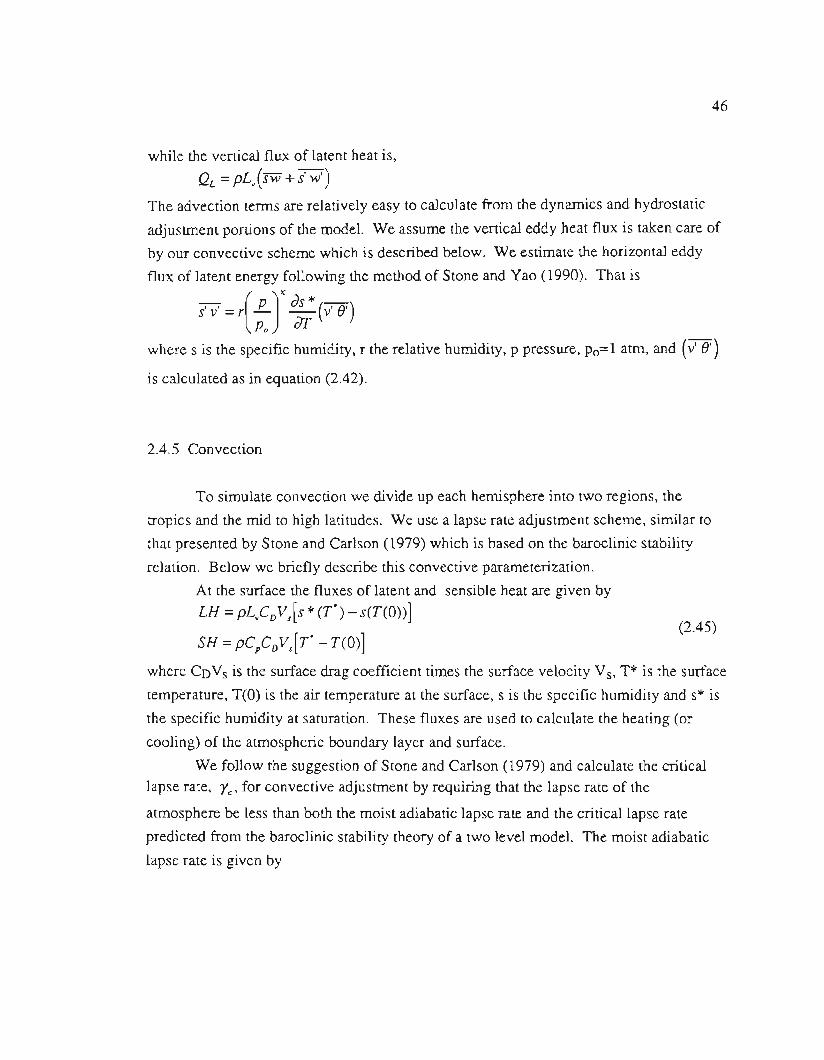
46

while the vertical flux of latent heat is,

QL = pLy(sw + s' w,)

The advection tenns are relatively easy to calculate from the dynamics and hydrostatic

adjustment portions of the model. We assume the vertical eddy heat flux is taken care of

by our convective scheme which is described below. We estimate the horizontal eddy

flux of latent energy following the method of Stone and Yao (1990). That is

S~v' =r(

J!...

]" as*(v'8')

Po aT

wheres is the specifichumidity,r therelativehumidity,p pressure,Po=1 atm, and (v'8' )

is calculatedas in equation(2.42).

2.4.5 Convection

To simulate convection we divide up each hemisphere into two regions, the

tropics and the mid to high latitudes. We use a lapse rate adjustment scheme, similar to

that presented by Stone and Carlson (1979) which is based on the baroclinic stability

relation. Below we briefly describe this convective parameterization.

At the surface the fluxes of latent and sensible heat are given by

LH = pLyCDVs[s*(T*)-s(T(O»] .

SH=pCpCDVs[T* -T(O)](2.45)

where CDVs is the surface drag coefficient times the surface velocity Vs, T* is the surface

temperature, T(O)is the air temperature at the surface, s is the specific humidity and s* is

the specific humidity at saturation. These fluxes are used to calculate the heating (or

cooling) of the atmospheric boundary layer and surface.

We follow the suggestion of Stone and Carlson (1979) and calculate the criticallapse rate, re' for convective adjustment by requiring that the lapse rate of the

atmosphere be less than both the moist adiabatic lapse rate and the critical lapse rate

predicted from the baroclinic stability theory of a two level model. The moist adiabatic

lapse rate is given by

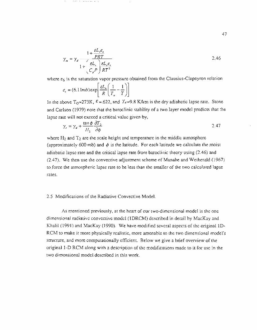
47

1 eLves+-

rlit= rd PRT

1+(

eLv

J

eLves

CpP RT2

where es is the saturation vapor pressure obtained from the Clausius-Clapeyron relation

e. = (6.11nW )exp[ e;G. - n]In the above To=273K, £=.622, and rd=9.8 K/km is the dry adiabatic lapse rate. Stone

and Carlson (1979) note that the baroclinic stability of a two layer model predicts that the

lapse rate will not exceed a critical value given by,tan 4> (J['2

rc = rd +/i; d4>

where H2 and T2 are the scale height and temperature in the middle atmosphere

(approximately 600 mb) and 4>is the latitude. For each latitude we calculate the moist

adiabatic lapse rate and the critical lapse rate from baroclinic theory using (2.46) and

(2.47). We then use the convective adjustment scheme of Manabe and Wetherald (1967)

to force the atmospheric lapse rate to be less than the smaller of the two calculated lapse

2.46

2.47

rates.

2.5 Modifications of the Radiative Convective Model.

As mentioned previously, at the heart of our two-dimensional model is the one

dimensional radiative convective model (1DRCM) described in detail by MacKay and

Khalil (1991) and MacKay (1990). We have modified several aspects of the originallD-

RCM to make it more physically realistic, more amenable to the two dimensional model's

structure, and more computationally efficient. Below we give a brief overview of the

originall-D RCM along with a description of the modifications made to it for use in thetwo dimensional model described in this work.

48

2.5.1 1-D RCM review

The 1D RCM of MacKay and Khalil (1991) has eighteen layers arid calculates the

absorption of solar radiation due to H20, 03, 02, and CO2for both clear and cloudy

conditions following the methods described by Lacis and Hansen (1974) for H20 and 03;

and by Sasamori (1972) for 02 and C02. Infrared fluxes for H20, CO2, 03, N20, Cf4,

F-11, and F-12 are calculated using parameterizations previously published by:

Ramanathan (1976), Roberts et al. (1976), and Kuo (1977) for H20; Kiehl and

Ramanathan (1983) for C02; Kuo (1977) for 03; Donner and Ramanathan (1980) for

N20, Ramanathan et al. (1985) for Cf4; and Ramanathan et al. (1985) and Ramanathan

(1976) for .F-II and F-12. Convection is simulated by performing a convective

adjustment similar to that used by Manabe and Wetherald (1967) using either a constant

critical lapse rate or the moist adiabatic lapse rate. A single cloud is included in one of

the atmospheric layers to simulate the average cloudiness of the atmosphere. This cloud

occupies one complete layer in the vertical direction .and approximately 50% of the layer

in the horizontal direction. The cloud is assumed to be a black body to terrestrial

radiation and its altitude is typically chosen to be between roughly 3 to 4 km. This type

of cloud is similar to that described by Stephens (1984) for I-D models. The surface heat

capacity is an adjustable parameter that has been included to simulate the thermal inertiaof the oceans.

2.5.2 Modifications of the Radiation Model

We have reduced the vertical resolution of the I-D RCM from eighteen layers to

nine layers. This change alone increases the speed of the radiation part of the calculations

by a factor of four. We have changed the parameterization for the calculation of the

infrared absorptivity of C02 to that used by Ramanathan et al. (1983) in the NCAR

general circulation model. Since the parameterization used in the original model was

very computationally intensive, this change also reduced the total computational time for

radiative flux calculations by about 30%. The net affect of these changes on the

sensitivity of the surface temperature to a doubling of C02 was to increase it by about

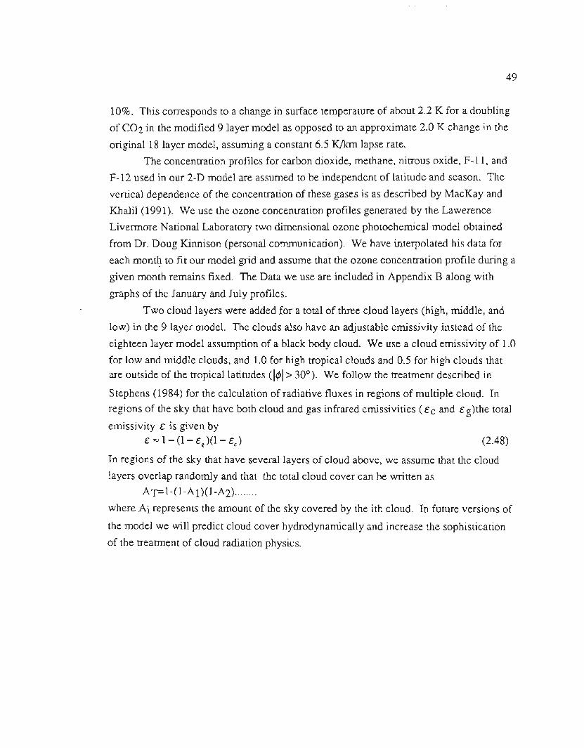
49

10%. This cOITespondsto a change in surface temperature of about 2.2 K for a doubling

of C02 in the modified 9 layer model as opposed to an approximate 2.0 K change in the

original 18 layer model, assuming a constant 6.5 K/km lapse rate.

The concentration profiles for carbon dioxide, methane, nitrous oxide, F-11, and

F-12 used in our 2-D model are assumed to be independent of latitude and season. The

vertical dependence of the concentration of these gases is as described by MacKay and

Khalil (1991). We use the ozone concentration profiles generated by the Lawerence

Livennore National Laboratory two dimensional ozone photochemical model obtained

from Dr. Doug Kinnison (personal communication). We have interpolated his data for

each mond?-to fit our model grid and assume that the ozone concentration profile during a

given month remains fixed. The Data we use are included in Appendix B along with

graphs of the January and July profiles.

Two cloud layers were added for a total of three cloud layers (high, middle, and

low) in the 9 layer model. The clouds also have an adjustable emissivity instead of the

eighteen layer model assumption of a black body cloud. We use a cloud emissivity of 1.0

for low and middle clouds, and 1.0 for high tropical clouds and 0.5 for high clouds thatare outside of the tropical latitudes (/4>/> 30°). We follow the treatment described in

Stephens (1984) for the calculation of radiative fluxes in regions of multiple cloud. In

regions of the sky that have both cloud and gas infrared emissivities (c c and c g)the totalemissivity c is given by

c "" 1- (1- cg)(l- cC> (2.48)

In regions of the sky that have several layers of cloud above, we assume that the cloud

layers overlap randomly and that the total cloud cover can be wrinen asAT=1-(1-AI)(1-A2)........

where Ai represents the amount of the sky covered by the ith cloud. In future versions of

the model we will predict cloud cover hydrodynamically and increase the sophistication

of the treatment of cloud radiation physics.

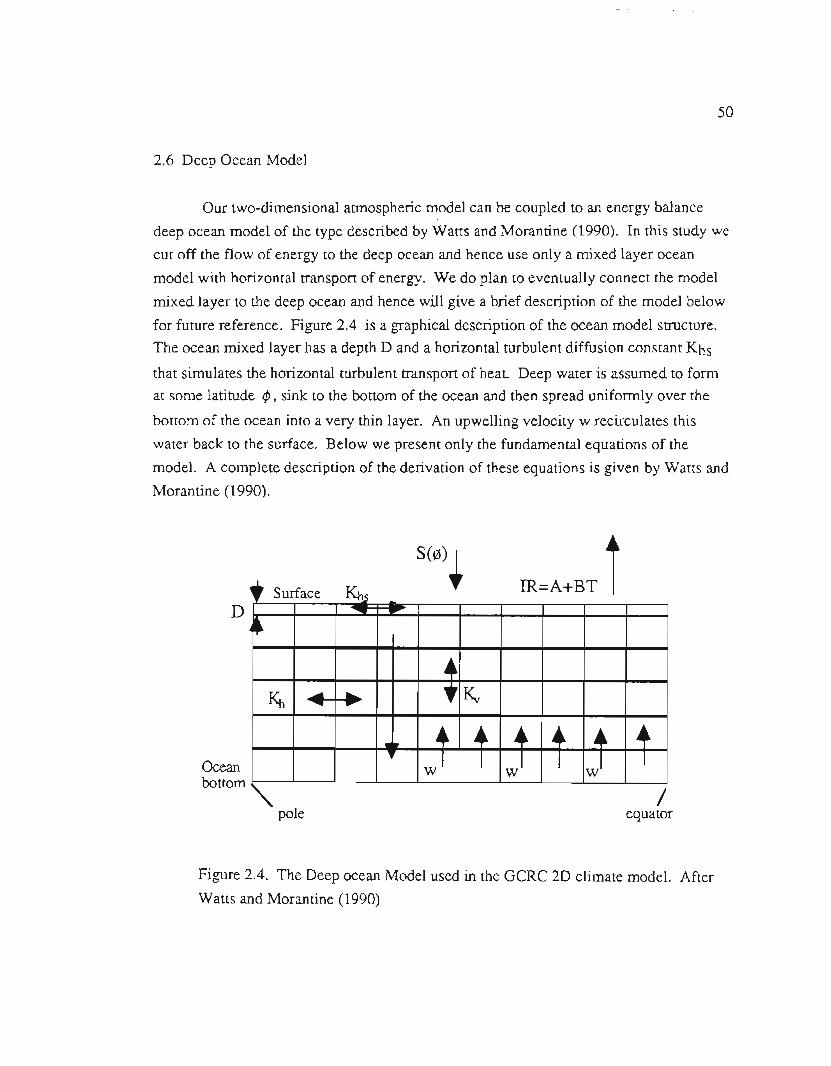
50

2.6 Deep Ocean Model

Our two-dimensional atmospheric model can be coupled to an energy balance

deep ocean model of the type described by Watts and Morantine (1990). In this study we

cut off the flow of energy to the deep ocean and hence use only a mixed layer ocean

model with horizontal transport of energy. We do plan to eventually connect the model

mixed layer to the deep ocean and hence will give a brief description of the model below

for future reference. Figure 2.4 is a graphical description of the ocean model structure.

The ocean mixed layer has a depth D and a horizontal turbulent diffusion constant Khs

that simulates the horizontal turbulent transport of heat. Deep water is assumed to format some latitude if', sink to the bottom of the ocean and then spread uniformly over the

bottom of the ocean into a very thin layer. An upwelling velocity w recirculates this

water back to the surface. Below we present only the fundamental equations of the

model. A complete description of the derivation of these equations is given by Watts and

Morantine (1990).

DS(0). i

Ocean

bottom'\.pole

/equator

Figure 2.4. The Deep ocean Model used in the GCRC 2D climate model. After

Watts and Morantine (1990)

'r SurfaceKtt.s

Ktt .... -. , Kv..... ....

.. . .

w w w

51

The surface of the Watts and Morantine model has no atmospheric model to

couple to so they have to crudely parameterize the net flux of solar radiation as a functionof latitude, 5(0), and the net flux of infrared radiation leaving the surface by A+BT. Our

detailed radiation code allows us to explicitly calculate these fluxes.

The respective energy balance equations for the surface and interior,

dT W dT W dT Kv aT- = tanl/J----at D az D al/J D az

K a[

dT

]

1

+ 2 hs a cosl/J:;- + [(1- a)S(l/J)- (A + BT)]a cos l/J l/J ul/J P DC

W W

(2.49)

and

dT dT a2T Kh a[

dT

]-=-w-+Kv-+ cosl/J-at az a2 z a2 cos l/Jal/J al/J

In the above a is the Earth's radius, D is the depth of the mixed layer (50-100 m).

In their original model Watts and Moratine used w=4.0 m/yr for the upwelling velocity

which was assumed to be independent of latitude up to 60 degrees from the equator

(where the deep water is assumed to form) and zero for latitudes above that region, Kv(=2000 m2jyr) for the vertical diffusivity of heat, Khs for the horizontal diffusivity of

heat at the surface (=1.2xiOI2 m2jyr), and Kh for the diffusivity of heat in the internal

ocean (=2xlOlO m2jyr). The variables T, .l/J,and z are the temperature, latitude, and

vertical depth respectively.

In the present work the above deep ocean model is used as a.simple mixed layer

model since we set both Kv and w equal to zero. We have used this full deep ocean

model in a simple energy balance model as described by Watts and Morantine (1990) and

found, as they suggested, that the mean surface temperature was highly sensitive to

changes in upwelling velocity. Although their original study was of the Younger Dryas

reversal, we believe that this sensitivity of mean surface temperature to upwelling

velocity w is also very important in terms of present and future climate change scenarios

over decades to centuries. Preliminary investigations with the model of Watts and

Moratine suggest that if w decreases as the equator to pole temperature gradient decreases

(2.50)

52

(due to increases in greenhouse gases) then this would constitute a possible negative

feedback mechanism. A decrease in w for a decrease in equator to pole temperature

gradient seems intuitively plausible if we believe that the driving force of ocean

circulations is the atmosphere. More work needs to be done however, before we can

incorporate this full deep ocean model reliably to our climate model and pursue this idea.

2.7 Sea Ice

We have performed some preliminary experiments with the development of a

prognostic thermodynamic sea ice model but have found that it adds too many additional

processes for us to clearly understand the basics of our 2D atmosphere model. That is,

the much longer response time of the integrated sea ice model and atmosphere model andthe additional feedbacks associated with a variable sea ice extent seemed to overshadow

the fundamental aspects of the atmosphere model. Thus in this first presentation of our

2D model, we have prescribed the seasonal sea ice area to agree with the observations

reported by Peixoto and Oort (1992), page 213. Following the work of Parkinson and

Washington (1980) we have used a mean sea ice thickness of 3.0 meters for the Arctic

and 1.5 meters for the Antarctic regions.

2.8 Summary of the Model.

53

The primitive equations (2.7-2.12) in two-dimensional zonally averaged fonn tobe solved are,

the equation of continuity,

dp = 1 d(pvcostfJ) _ dpwdt acostfJ dtfJ dz

the horizontal equations of motion,

dpu =_ 1 d[p(uv + iJVi)costfJ]_ d[P(uw + i7}Vi)]dt acos tfJ dtfJ dz

tan tfJ -+pfv+p-(uv + u'v') +pF~a

dpv = _.!.. dp 1 d[pv2 cos tfJ]_ d[p(vw + H)]dt a dtfJ a cos tfJ dtfJ dz

u2 tan tfJ-pfu-p +pF

a ~

the fIrst law of thennodynamics

d[pCpT] =_ 1 d[pCpcostfJ(vT + V'T)] + P(Q+QL)+ 1.4RT[

dP + v dP]dt acostfJ dtfJ dt a dtfJ

+1.4RTw dp _ d[pCp(wT + W'T)]dz dz

the equation of state,

P =pRT

(2.7)

(2.8)

(2.9)

(2.10)

(2.11 )

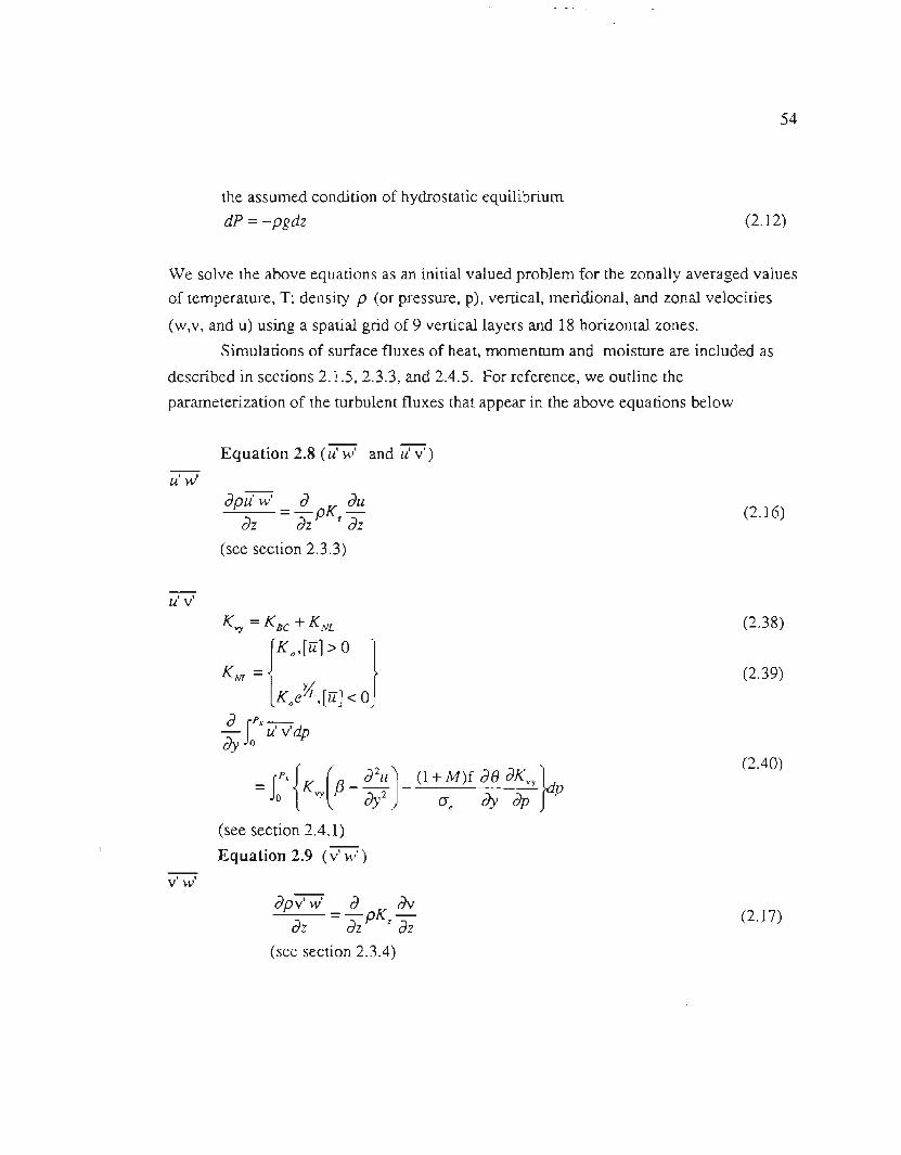
54

the assumed condition of hydrostatic equilibrium

dP =-pgdz (2.12)

We solve the above equations as an initial valued problem for the zonally averaged values

of temperature, T; density p (or pressure, p), vertical, meridional, and zonal velocities

(w,v, and u) using a spatial grid of9 vertical layers and 18 horizontal zones.

Simulations of surface fluxes of heat, momentum and moisture are included as

described in sections 2.1.5, 2.3.3, and 2.4.5. For reference, we outline the

parameterization of the turbulent fluxes that appear in the above equations below

Equation 2.8 (u' w' and u' v' )

u'w'

dp"iJWi=~ pK dUdz dz'dz

(see section2.3.3)

(2.16)

u'v'(2.38)

(2.39)

(2.40)

v'w'

dpH =~pK avdz dz'dz

(see section2.3.4)

(2.17)

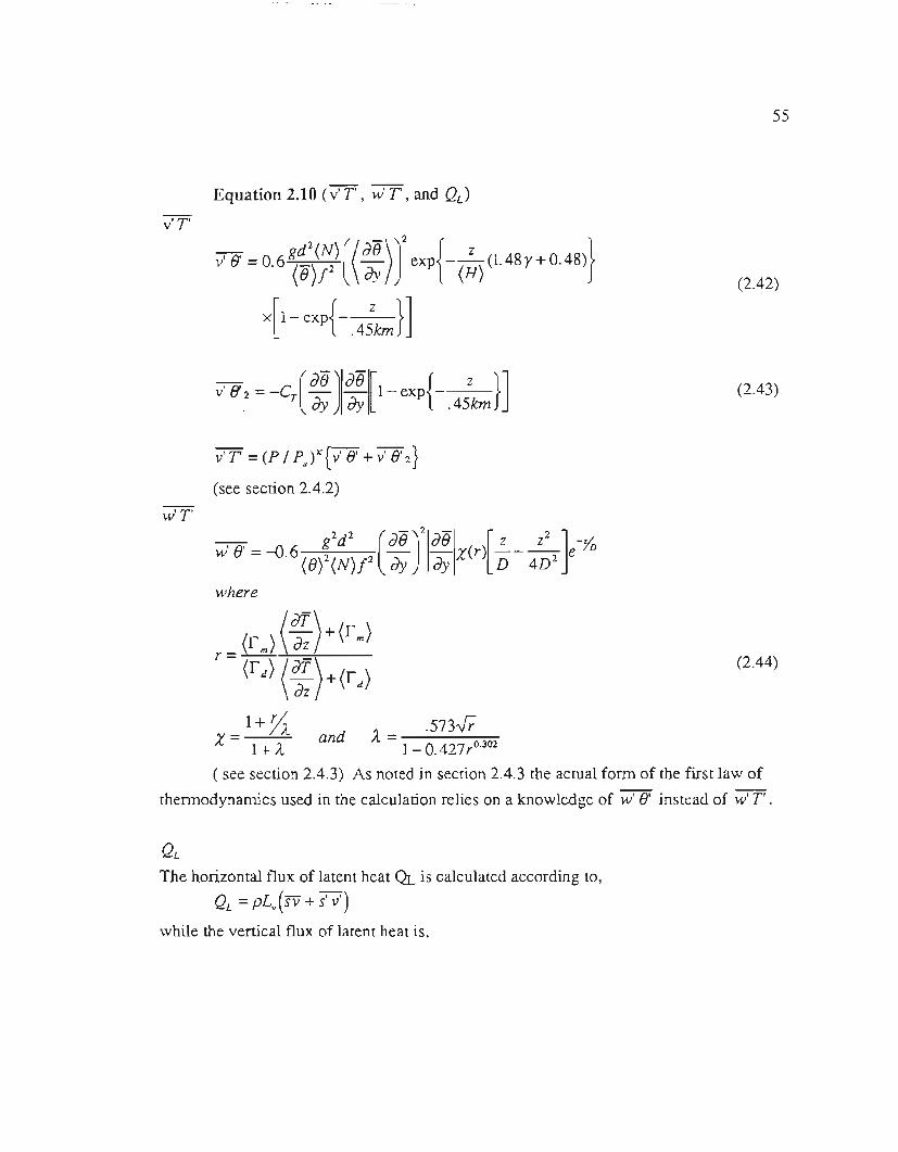
55

Equation 2.10 (v' T , w'T, and QL)

v'T'

v' (J =0.6 g,~.(":) ((~) J exph~) (1.48r + 0.48) }

X[1- exp{ .4;km} ]

(2.42)

v' (J.. =-CT(~) ~[ 1- exp{ .4:km}](2.43)

v'T =(P / p..)K{V' 9' +v' 9'2}

(see section 2.4.2)

w'T2 2

(

_

)

2 -

F [ ]w' 9' =-0 6 g d d9 d9 z Z2 -Yr

. (fJ?(N)/2 dy dy (r) D - 4D2 e Dwhere

_ (r m)(~)+(r m)r--

(rd) (~)+(rd)

X= 1+!A and A= .573*1+ A.. 1 - U.4.L.Ir---

( see section 2.4.3) As noted in section 2.4.3 the actual fonn of the fIrst law of

thennodynamics used in the calculation relies on a knowledge of w' 9' instead of w'T .

(2.44)

QL

The horizontal flux of latent heat QL is calculated according to,

QL =pLy (sv + s' v')

while the vertical flux of latent heat is,

56

QL =pLv(sw + s' W') with (V'8') given by 2.42. Latent heat is also transfered

during the convective adjustment and we assume that this process simulates s' w' .In the next chapter we explore the actual performance of the aCRC 2-D model.

We pay particular attention to the simulation of zonally averaged temperature and zonal

velocity for summer (JJA), winter (DJF), and annual mean conditions.

CHAPTER 3

MODEL PERFORMANCE

3.1 Model Overview

3.1.1 Introduction

In this chapter we present and discuss the perfonnance of the GCRC 2D zonally

averaged statistical dynamical model, beginning with a general overview of its

perfonnance followed by a presentation of the outputs for the model's control climate for

summer (JJA), Winter (DJF), and annual averages compared to observations. Our model

does very well at simulating the observed state of Earth's atmosphere, however below we

will not only focus on the model's strengths but will also pay particular attention to its

weaknesses. We hope that this will identify areas that require improvements and identifyareas of future work for other 2D climate modelers.

The order of our presentation of model outputs will be: section 2, zonal mean

temperatures and energy balance; section 3, zonal mean velocities u and angular

momentum budget; section 4, model kinetic energy and mass stream function; section 5

zonal mean precipitation and surface pressure, and section 6 a summary of the important

results of this chapter.

3.1.2 General Discussion

Our 2D model runs on an IBM RISC 6000 work station taking approximately 2

CPU hours for each simulated year. Stability of the model is an important consideration.

As described in the previous chapter, if the initial conditions (initial state of the model's

atmosphere) are too far away from the steady state solution, large amplitude oscillations

can grow without bound destroying the model output. After getting into a stable run with

57

58

Grid Point Fluctuations

2000 4000

Time (Days)

6000 8000

Figure 3.1. Example of grid point fluctuations.

a particular initial condition, starting as described in chapter 2, care must be taken not to

introduce extraordinarily large perturbations into the initial state. Our technique has been

to use the output from one run as the initial state of the next run (with a perturbation) to

explore the phase space of the model. As shown in the next chapter, the model is stable

to perturbation studies such as doubling of C02 and indeed works well with much larger

perturbations of the initial state. For example, the model runs stablely when the pressure

of the whole system (each grid point) is altered by 4.0% but would most likely "blow up"

if the pressure of an isolated grid point were altered by 4.0%.

Figure 3.1 shows the output of the meridional velocity in cm/s at grid point 3,2

(approx. 200 mb, 75°N) for a 20 year run. For this particular grid point and output

10

8

6-fI)- 4SC.I'-"

2-0'-"

;>-2

-4

-60

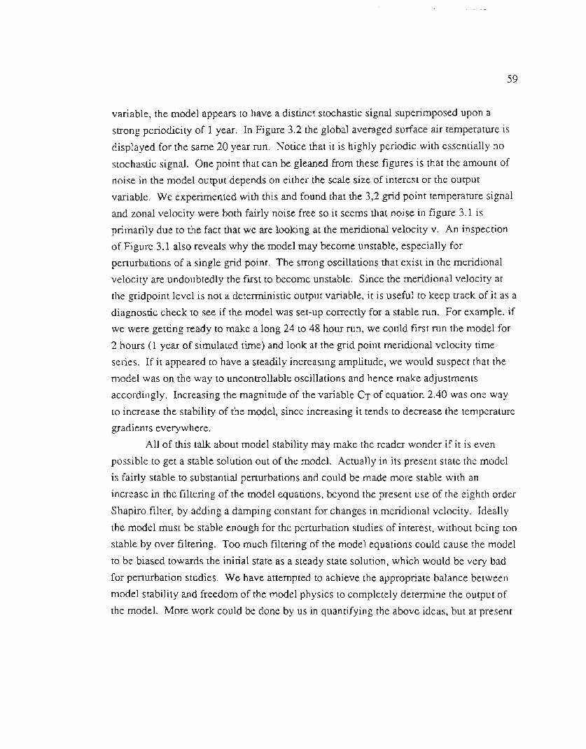
59

variable, the model appears to have a distinct stochastic signal superimposed upon a

strong periodicity of 1 year. In Figure 3.2 the global averaged surface air temperature is

displayed for the same 20 year run. Notice that it is highly periodic with essentially no

stochastic signal. One point that can be gleaned from these figures is that the amount of

noise in the model output depends on either the scale size of interest or the output

variable. We experimented with this and found that the 3,2 grid point temperature signal

and zonal velocity were both fairly noise free so it seems that noise in figure 3.1 is

primarily due to the fact that we are looking at the meridional velocity v. An inspection

of Figure 3.1 also reveals why the model may become unstable, especially for

penurbations of a single grid point. The strong oscillations that exist in the meridional

velocity are undoubtedly the first to become unstable. Since the meridional velocity at

the gridpoint level is not a deterministic output variable, it is useful to keep track of it as a

diagnostic check to see if the model was set-up correctly for a stable run. For example, if

we were getting ready to make a long 24 to 48 hour run, we could first run the model for

2 hours (1 year of simulated time) and look at the grid point meridional velocity time

series. If it appeared to have a steadily increasing amplitude, we would suspect that the

model was on the way to uncontrollable oscillations and hence make adjustments

accordingly. Increasing the magnitude of the variable CT of equation 2.40 was one way

to increase the stability of the model, since increasing it tends to decrease the temperature

gradients everywhere.

All of this talk about model stability may make the reader wonder if it is even

possible to get a stable solution out of the model. Actually in its present state the model

is fairly stable to substantial penurbations and could be made more stable with an

increase in the filtering of the model equations, beyond the present use of the eighth order

Shapiro filter, by adding a damping constant for changes in meridional velocity. Ideally

the model must be stable enough for the penurbation studies of interest, without being too

stable by over filtering. Too much filtering of the model equations could cause the model

to be biased towards the initial state as a steady state solution, which would be very bad

for penurbation studies. We have attempted to achieve the appropriate balance between

model stability and freedom of the model physics to completely determine the output of

the model. More work could be done by us in quantifying the above ideas, but at present

60

Global Mean Surface Air Temperature

288

...-..

~--~ 287a..

=-'"

a..

~ 286e~.!::285<

283o 2000 4000

Time (Days)

6000 8000

Figure 3.2. Smface air temperature annual cycle and approach to equilibrium.

we feel that we have achieved a good balance. The next sections dealing with the

presentation of model output data lend suppon to this claim.

3.2 The Thermal Structure of the Atmosphere and Energy Balance

3.2.1 Temperature Field

Several interesting features of the model can be extracted from a careful

inspection of Figure 3.2. First, it appears that a run length of 20 years is more than

61

Annual Cycle of Surface AirTemperature

283 _o 30 60 90 120 150 180 210 240 270 300 330 360

Time (Days)

Figure 3.3. Annual cycle of surface air temperature. Note that March fIrst

corresponds to time=O.O.

adequate for the model's surface air temperature to reach equilibrium and that even 10

years (3650 days) would be sufficient. Through experimentation we have found that

fairly small differences exist in the overall temperature structure, or dynamical structure

of the atmosphere between year twenty and year two of the model simulation even

though the penurbation from the initial state may have been substantial. The differences

that do exist between years two and twenty are mostly concentrated in the polar regions.

Thus for quick model sensitivity studies, aimed at investigating the effects of changes in

model parameterizations or physics, two year simulations are efficient and seem to work

well. However for penurbation studies involving changes in the physical state of theatmosphere such as a doubling of C02, where the greatest precision possible is desired,

then we have concluded that a twelve year simulation is optimum from the view point of

efficiency and precision. This twelve year simulation takes 24 CPU hours to run. It

should be stressed here that as other physical processes are introduced, such as a

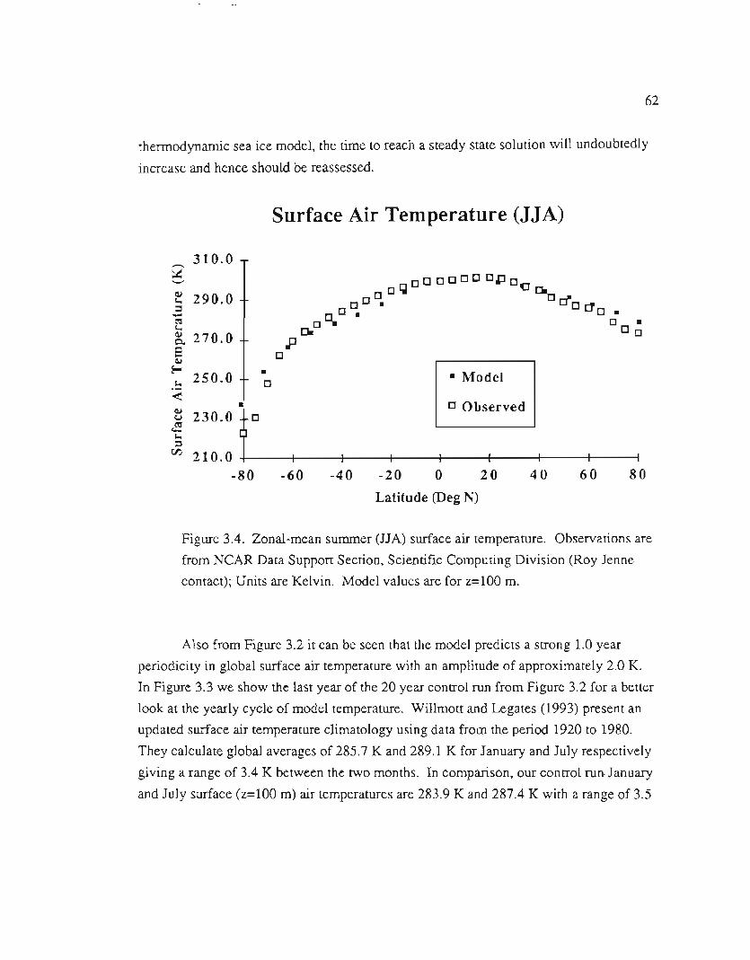
62

thennodynamic sea ice model, the time to reach a steady state solution will undoubtedlyincrease and hence should be reassessed.

__ 310.0~'-"

~ 290.0=....=s..

~ 270.0eQJ~s.. 250.0

:.(QJ~ 230.0

COOis..=

00. 210.0-80

Surface Air Temperature (JJA)

. · Model[J

[J Observed[J

-60 -20 0 20 40

Latitude (Deg N)

60 80-40

Figure 3.4. Zonal-mean summer (JJA) surface air temperature. Observations are

from NCAR Data Support Section, Scientific Computing Division (Roy Jenne

contact); Units are Kelvin. Model values are for z=l00 m.

Also from Figure 3.2 it can be seen that the model predicts a strong 1.0 year

periodicity in global surface air temperature with an amplitude of approximately 2.0 K.

In Figure 3.3 we show the last year of the 20 year control run from Figure 3.2 for a better

look at the yearly cycle of model temperature. Willmott and Legates (1993) present an

updated surface air temperature climatology using data from the period 1920 to 1980.

They calculate global averages of 285.7 K and 289.1 K for January and July respectively

giving a range of 3.4 K between the two months. In comparison, our control run January

and July surface (z=l00 m) air temperatures are 283.9 K and 287.4 K with a range of 3.5

63

K which are in good agreement with their observations. The yearly cycle is dominated

by the asymmetrically larger amount of land mass in northern hemisphere compared to

that in the southern hemisphere.

Surface Air Temperature (DJF)

__ 310.0~'-'"

f 290.0=-"=...~c.S~

Eo-... 250.0

<[]

t 230.0~...=

~ 210.0

-80

[] Observed .

-60 -40 -20 0 20

Latitude (Deg N)

40 60 80

Figure 3.5. Zonal-mean winter (DJF) surface air temperature. Observations are

from NCAR Data Suppon Section, Scientific Computing Division (Roy Jenne

contact);Unitsare Kelvin. Modelvaluesare for z=l00 m. .

In figures 3.4 through 3.6 we compare the latitudinal dependency of the model's

zonal mean surface air temperature (for the last year of the 20 year run) with observed

values obtained from the NCAR Data Suppon Section, Scientific Computing Division for

summer, winter and annual averages respectively. The model agrees with the obser-

vations well for all latitudes except near Antarctica where we have close to a 10 %

64

discrepancy for the DJF and annual averages. For all three figures the Model's surface air

temperature is higher than the observed values over Antarctica. The reason for this is

most likely because our model does not at present simulate the orography of the Antarctic

continent. Consistent with observations the model does predict slightly cooler Antarctic

winters than Arctic winters since no heat energy is allowed to flow from the Southern

Ocean onto the continent. Inspection of these three figure lends credibility to our model's

ability to.simulate the real climate. Uncertainties in actual cloud amounts and cloud

optical properties are probably responsible for the majority of the deviation between

observed and model output; especially around 30 S latitude.

Surface Air Temperature (Annual)

QJt..=-=t..QJQ,

SQJ

Eo-

t..

<QJ(oJ

~t..=

rJ:J 210.0 .-80

· Model

C Observed

-60 -40 -20 0 20 40

Latitude (Deg N)

60 80

Figure 3.6. Zonal-mean annual average surface air temperature. Observations are

from NCAR Data Support Section, Scientific Computing Division (Roy Jennecontact); Units are Kelvin. Model values are for z=l00 m.

310.0

290.0

270.0I .

250.0 J.c

Ic

I230.0

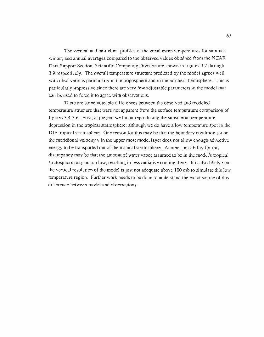
65

The vertical and latitudinal profiles of the zonal mean temperatures for summer,

winter, and annual averages compared to the observed values obtained from the NCAR

Data Support Section, Scientific Computing Division are shown in figures 3.7 through

3.9 respectively. The overall temperature structure predicted by the model agrees well

with observations particularly in the troposphere and in the northern hemisphere. This is

particularly impressive since there are very few adjustable parameters in the model that

can be used to force it to agree with observations.There are some noteable differences between the observed and modeled

temperature structure that were not apparent from the surface temperature comparison of

figures 3.4-3.6. First, at present we fail at reproducing the substantial temperature

depression in the tropical stratosphere; although we do have a low temperature spot in the

DJF tropical stratosphere. One reason for this may be that the boundary condition set on

the meridional velocity v in the upper most model layer does not allow enough advective

energy to be transported out of the tropical stratosphere. Another possibility for this

discrepancy may be that the amount of water vapor assumed to be in the model's tropical

stratosphere may be too low, resulting in less radiative cooling there. It is also likely that

the vertical resolution of the model is just not adequate above 100 mb to simulate this low

temperature region. Further work needs to be done to understand the exact source of thisdifference between model and observations.

Figure 3.7. Observed zonal-mean (JJA) average air temperature (top) and

Modeled (bottom). Observations are from NCAR Data Support Section,

Scientific Computing Division; Units are Kelvin.

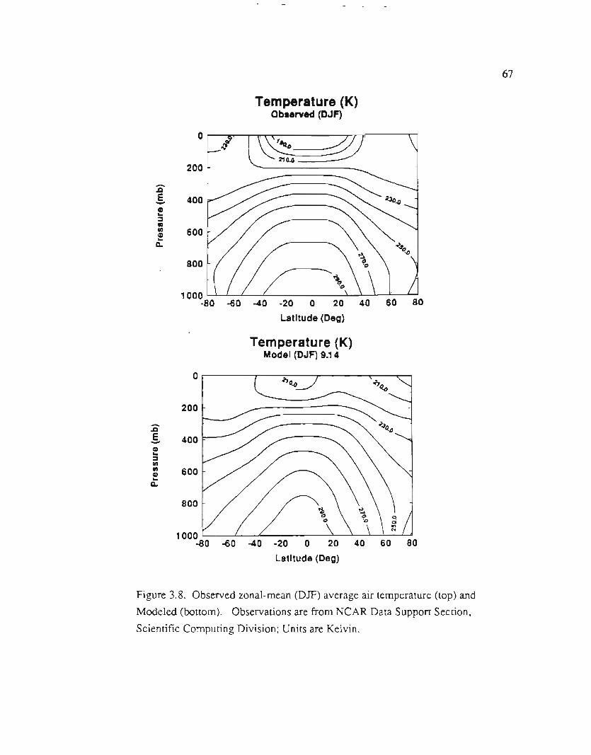
Figure 3.8. Observed zonal-mean (DJF) average air temperature (top) and

Modeled (bottom). Observations are from NCAR Data Support Section,

Scientific Computing Division; Units are Kelvin.

67

Temperature (K)Obl.rveel (DJF)

0

200-J:8.§. 400!.. 600!a.

800

100060 80-80 -60 -40 -20 0 20 40

Latitude (Deg)

Temperature (K)Model (DJF) 9.14

O. t '17

t "----.:200-

.12E 400-!.,., 6000..a.

800

1000-80 -60 -40 -20 0 20 40 60 80

Latitude (Deg)

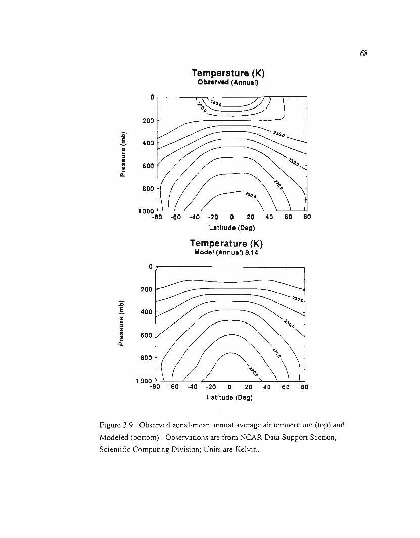
Figure 3.9. Observed zonal-mean annual average air temperature (top) and

Modeled (bottom). Observations are from NCAR Data Support Section;

Scientific Computing Division; Units are Kelvin.

68

Temperature (K)Oblerved (Annual)

0

200-.QE 400-CD..110110 600CD..A.

800

100020 40 60 80-80 -60 -40 .20 0

Latitude (Deg)

Temperature (K)Model (Annual)9.14

0

200-.QE 400-CD..110

110 600CD..G.

800

1000-80 -60 -40 .20 0 20 40 60 80

Latitude (Deg)

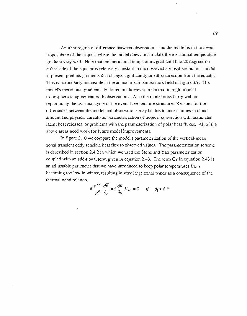
69

Another region of difference between observations and the model is in the lower

troposphere of the tropics, where the model does not simulate the meridional temperature

gradient very well. Note that the meridional temperature gradient 10 to 20 degrees on

either side of the equator is relatively constant in the observed atmosphere but our model

at present predicts gradients that change significantly in either direction from the equator.

This is particularly noticeable in the annual mean temperature field of figure 3.9. The

model's meridional gradients do flatten out however in the mid to high tropical

troposphere in agreement with observations. Also the model does fairly well at

reproducing the seasonal cycle of the overall temperature structure. Reasons for the

differences between the model and observations may be due to uncertainties in cloud

amount and physics, unrealistic parameterization of tropical convection with associated

latent heat releases, or problems with the parameterization of polar heat fluxes. All of the

above areas need work for future model improvements.

In figure 3.10 we compare the model's parameterization of the vertical-mean

zonal transient eddy sensible heat flux to observed values. The parameterization scheme

is described in section 2.4.2 in which we used the Stone and Yao parameterization

coupled with an additional term given in equation 2.43. The term CT in equation 2.43 is

an adjustable parameter that we have introduced to keep polar temperatures from

becoming too low in winter, resulting in very large zonal winds as a consequence of thethermal wind relation,

RPIC-1ae = f au K = 0 if lA./ A.*P: dy dp BC' 'I' > 'I'

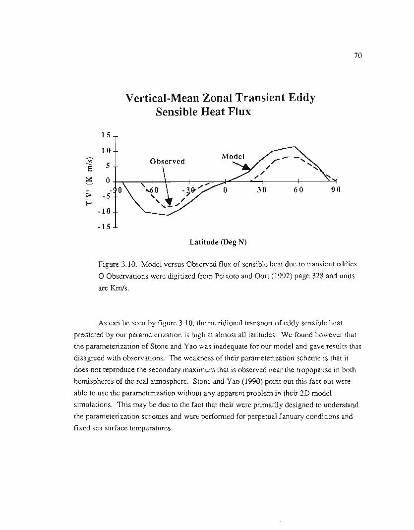
70

Vertical-Mean Zonal Transient EddySensible Heat Flux

Figure 3.10. Model versus Observed flux of sensible heat due to transient eddies.

o Observations were digitized from Peixoto and Oort (1992) page 328 and units

are Krn/s.

As can be seen by figure 3.10, the meridional transport of eddy sensible heat

predicted by our parameterization is high at almost all latitudes. We found however that

the parameterization of Stone and Yao was inadequate for our model and gave results that

disagreed with observations. The weakness of their parameterization scheme is that it

does not reproduce the secondary maximum that is observed near the tropopause in both

hemispheres of the real atmosphere. Stone and Yao (1990) point out this fact but were

able to use the parameterization without any apparent problem in their 2D model

simulations. This may be due to the fact that their were primarily designed to understand

the parameterization schemes and were performed for perpetual January conditions and

fixed sea surface temperatures.

15

10-fI.)

5-E

0---

-5Eo-

-10

-15

Latitude (Deg N)

71

For our control run, we used a value of CT=o.008 m3f(K3sec) and when we

reduced CTto 0.004 m3f(K3-hr) Arctic polar temperatures dropped by about 3 K, the

global kinetic energy increased by about 20 %, and the strength of the subtropical jets

increased by roughly 10 %. Figure 3.11 summarizes some of the essential features of the

model's sensitivity to a change in the parameter CT. The change in temperature resulting

from a decrease in CTfrom 0.004 m3f(K3-hr) to 0.008 m3f(K3-hr) is consistent with

intuition, the tropics become warmer and the poles become cooler as the gradient driven

transport of energy is decreased. The increase in the strength of the subtrocial jets is also

consistent with the thermal wind relation given above. It is also worth noting that as CT

decreases the strength of the Hadley circulation increases by up to 20 % and the

magnitude of the parameterized u'v' flux increases by up to 20 %. Also, when we

attempted to run the model from the same initial conditons that were used for the control

. run (CT=O.008m3f(K3sec)) using a value of CT=O.OOO,the polar temperatures

(particularly in the stratosphere) reached very low values and the model became

numerically unstable after 4 years.

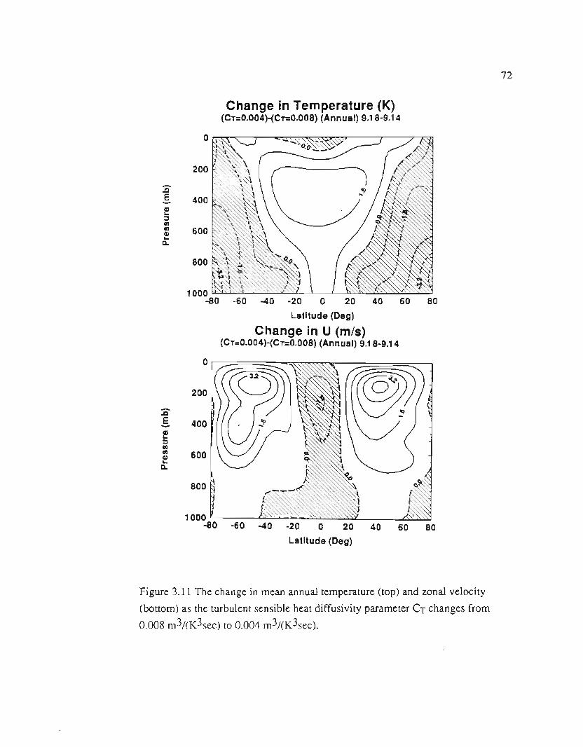
72

Change InTemperature (K)(CT=0.004)-(CT=0.008) (Annual) 9.18-9.14

o

-~E-e::Ienen4)..a.

,.-40 -20 0 20 40 60 80

Latitude (Deg)

Change in U (m/s)(CT=0.004)-(CT=0.008) (Annual) 9.18-9.14

Figure 3.11 The change in mean annual temperature (top) and zonal velocity

(bottom) as the turbulent sensible heat diffusivity parameter CTchanges from

0.008 m3f(K3sec) to 0.004 m3f(K3sec).

0

200-.aE 400-4)..::Ienen 600!a.

800

1000-80 -60 -40 -20 0 20 40 60 80

73

Model Seasonal Energy Balance

Figure 3.12. Difference between the total absorbed solar energy and the flux of

infrared radiation out of the top of the atmosphere as a function of latitude.

Observed values are represented as line and model output are indicated by

symbols. Observations were digitized from Peixoto and Oort (1992) page 128and Units are W1m2.

3.2.2 Energy Balance

In our model, the lack of poleward energy transport in the upper troposphere

results in extremely low polar stratospheric temperatures and unrealistically high pressure

gradients. We thus added the parameter CTand equation 2.43 to reduce this problem.

However in doing so, as is evident by figure 3.10, we have overestimated the transient

eddy sensible heat flux. This over estimate of sensible heat flux is most likely

120I I

[] Ann Mod60

- - - - - - - ------

I ,,{o [1.tJ 9. -',.."" u I 6 JJA Mod- "N

<E o 161 ,. I: 1 '\.1 l 1 \1 I 0 DJF Mod-- .

-60 r. '- 1:1 I -------- Ann Ob

c.=- '--.'"

);_.: LJ,

-\. .[1 [] I -----JJA Ob/A-000 -120 . . a ....._.'-

DJF Ob...._/A I

-180

Latitude (Deg N)

74

compensated in our model from an underestimate of latent heat flux or advective heat

flux since we reproduce the basic temperature structure of the atmosphere fairly well.

However, it is likely that the existing discrepancies between pur model and observations

could be reduced with an improvement of the parameterization of eddy heat (both latent

and sensible) fluxes. Future improvements in the parameterization of eddy sensible heat

flux must try to capture the secondary maxima found in both hemispheres near the

tropopause.

In figure 3.12 the difference between the total absorbed solar energy and the

outward flux of teITestrialradiation at the top of the atmosphere is presented. Since when

the model reaches steady state, the annual mean surface temperature remains in

equilibrium, the curve for the annual average can be interpreted as the net poleward flux

of energy out of a region from all transport mechanisms. Our model agrees well with the

observations, hence we feel that the total energy transport simulated by the model isrealistic.

The agreement between model and observations is good at all latitudes exceptaround 5.0oN where the difference is lower than it should be in the summer months and at

800N where it looks like the surface albedo is too low. There are two possible physical

reasons for the difference between the model and observations around 5.0oN: 1) the

temperatures at this latitude are over estimated causing the teITestrialradiation leaving the

top of the atmosphere to be too large or 2), the amount of solar energy absorbed is

underestimated. From an inspection of figure 3.4 we can rule out the first option and by

an inspection of figure B.2 and B.3 of appendix B we can see that the second explanation

is most likely, in that our cloud data have an unusually high value for this latitude,

especially the middle cloud amount. It is possible that the cloud amount has been simply

overestimated in this region. Alternately, the large middle and low cloud amounts in this

region are probably of the cumulus type which may absorb radiation much differently

than the broad spread out stratus type clouds which we have assumed to be in our model.

Not only do we need to add a prognostic cloud prediction scheme as mentioned

previously, we also need to improve the treatment of the cloud optical properties in our

model and allow for a greater variety of cloud types. In fact it is our plan to improve the

cloud radiation scheme in our model first and then add a scheme for the prognostic

-.- --.-..- -..-.

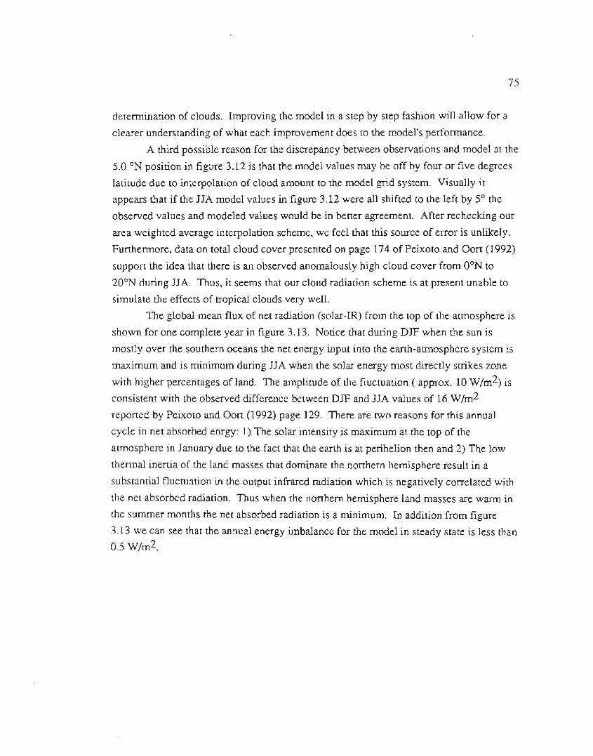
75

detenmnation of clouds. Improving the model in a step by step fashion will allow for a

clearer understanding of what each improvement does to the model's performance.

A third possible reason for the discrepancy between observations and model at the

5.0 oN position in figure 3.12 is that the model values may be off by four or five degrees

latitude due to interpolation of cloud amount to the model grid system. Visually it

appears that if the JJA model values in figure 3.12 were all shifted to the left by 5° the

observed values and modeled values would be in bener agreement. After rechecking our

area weighted average interpolation scheme, we feel that this source of error is unlikely.

Furthermore, data on total cloud cover presented on page 174 of Peixoto and Oon (1992)

suppon the idea that there is an observed anomalously high cloud cover from OONto

200N during JJA. Thus, it seems that our cloud radiation scheme is at present unable to

simulate the effects of tropical clouds very well.

The global mean flux of net radiation (solar-IR) from the top of the atmosphere is

shown for one complete year in figure 3.13. Notice that during DJF when the sun is

mostly over the southern oceans the net energy input into the earth-atmosphere system is

maximum and is minimum during JJA when the solar energy most directly strikes zone

with higher percentages of land. The amplitude of the fluctuation ( approx. 10W/m2) isconsistent with the observed difference between DJF and JJA values of 16 W/m2

reponed by Peixoto and Oon (1992) page 129. There are two reasons for this annual

cycle in net absorbed enrgy: 1) The solar intensity is maximum at the top of the

atmosphere in January due to the fact that the earth is at perihelion then and 2) The low

thermal inertia of the land masses that dominate the northern hemisphere result in a

substantial fluctuation in the output infrared radiation which is negatively correlated with

the net absorbed radiation. Thus when the nonhern hemisphere land masses are warm in

the summer months the net absorbed radiation is a minimum. In addition from figure

3.13 we can see that the annual energy imbalance for the model in steady state is less than0.5 W/m2.

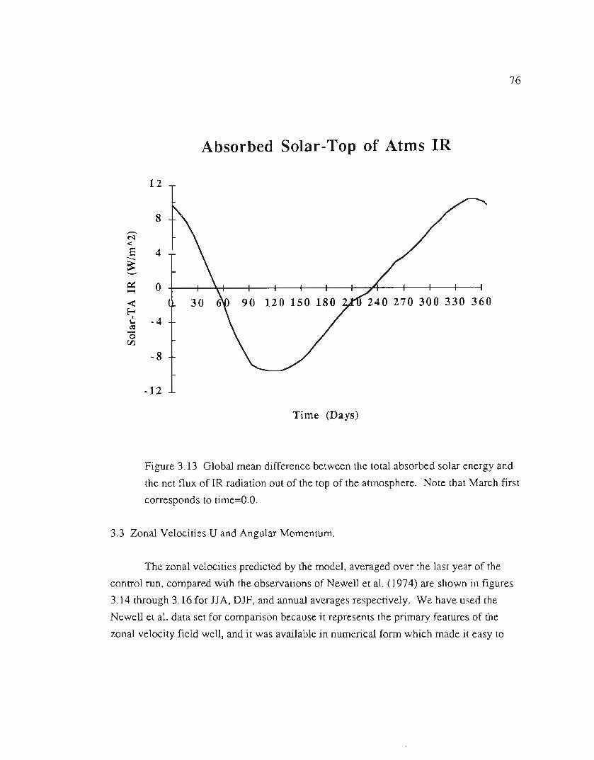
76

Absorbed Solar-Top of Atms IR

Figure 3.13 Global mean difference between the total absorbed solar energy and

the net flux of IR radiation out of the top of the atmosphere. Note that March first

corresponds to time=O.O.

3.3 Zonal Velocities U and Angular Momentum.

The zonal velocities predicted by the model, averaged over the last year of the

control run, compared with the observations of Newell et al. (1974) are shown in figures

3.14 through 3.16 for JJA, DJF, and annual averages respectively. We have used the

Newell et al. data set for comparison because it represents the primary features of the

zonal velocity field well, and it was available in numerical form which made it easy to

12

8,-..N<5 4-'-'

0

< d. 30 00 90 120 150 180.

-4...-0

CIl

-8

-12

Time (Days)

77

reproduce accurately. We have also carefully scrutinized the data set published by

Peixoto and Oort (1992) page 154 in the analysis of our model's performance at

simulating the observed zonal velocities of Earth.

The model predicts weak northern hemisphere jets and strong southern

hemisphere jets in JJA which are both consistent with observations. The magnitude and

position of the model's JJA southern hemisphere jet is much more consistent with the

Peixito and Oort data set in that they show a 35 m/s maximum near 200 mb at around 35°

S. However the strength of our northern hemisphere JJA jet stream (15 m/s) is more

consistent with the Newell et al. data set The vertical position of the model jet streams

for both hemispheres and all seasons are a little high 100-150 mb compare to 200 mb in

both of the observed data sets (except for the Newell data set for the JJA southern

hemisphere). We are also lacking a strong tropical easterly in the stratosphere during JJA

which is present in both observed data sets. Also the tropical easterlies predicted by the

model are generally too high. However, the overall structure and seasonal cycle of the

modeled zonal wind field seems to agree well with the observed structure. The annual

mean zonal wind field appears to match both sets of observations very well.

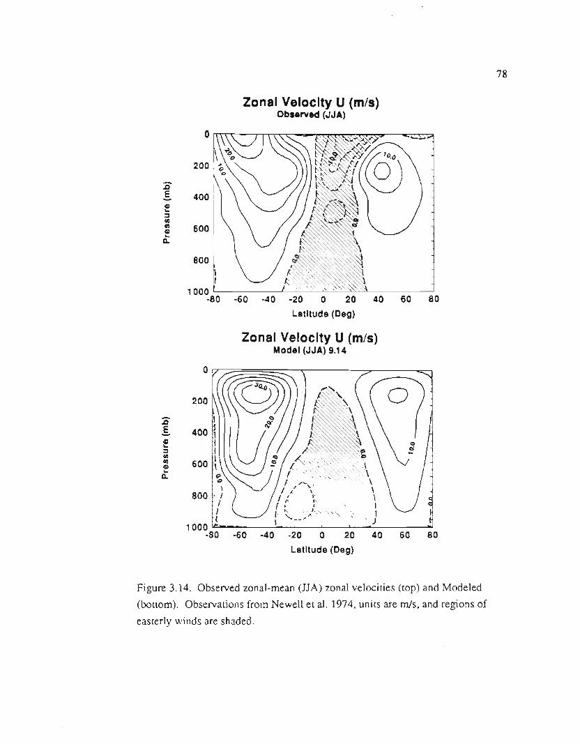
78

Zonal Velocity U (mls)Observed (JJA)

Zonal Velocity U (m/s)Model (JJA) 9.14

o

:aE-!=(I)(I)G)..a.

200

60 80

Figure 3.14. Observed zonal-mean (JJA) zonal velocities (top) and Modeled

(bottom). Observations from Newell et al. 1974, units are mis, and regions of

easterly winds are shaded.

0

200-.QE 400-G)-=(I)(I) 600G)..a.

800h

!1000

-80 -60 -40 -20 0 20 40 60 80

79

Zonal Velocity U (mil)Observed (DJF)

Zonal Velocity U (m/s)Model (DJF) 9.14

1OO~O .60 40 60 80

Figure 3.15. Observed zonal-mean (DJF) zonal velocities (top) and Modeled

(bottom). Observations from Newell et al. 1974, units are mis, and regions of

easterly winds are shaded.

0

200-.DE 400-CD..=ww 600CD..

t\A.00

800 (1000.80 .60 -40 .20 0 20 40 60 80

0

200-.DE 400-!='"'" 600CD..A.

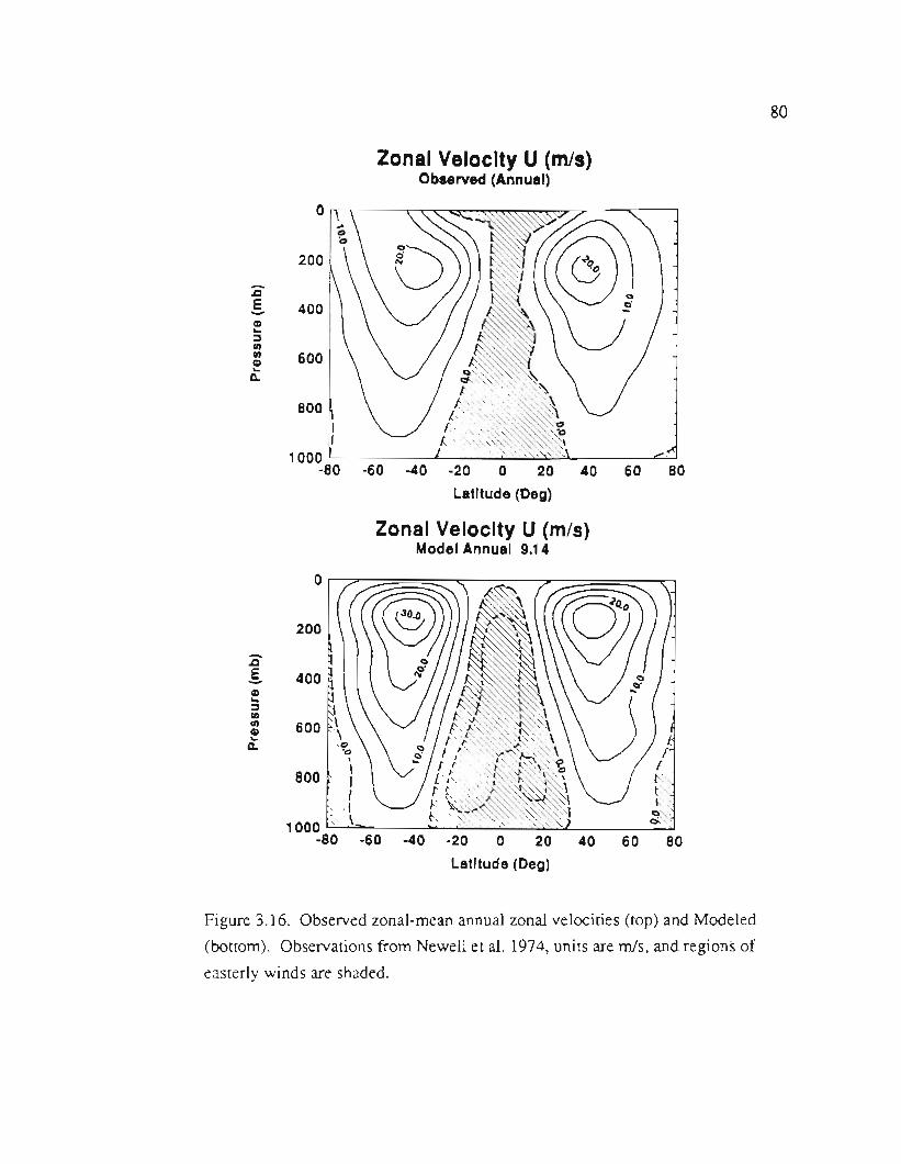
Figure3.16. ObseIVedzonal-meanannualzonalvelocities(top)and Modeled(bottom). ObseIVationsfrom Newell et al. 1974, units are mis, and regions of

easterly winds are shaded.

80

Zonal Velocity U (mlS)Observed (Annual)

0

200-.cE 400-eII)II) 600G)..G.

.8001\I,.

1000-80 -60 -40 -20 0 20 40 60 80

Latitude (Deg)

Zonal Velocity U (m/s)ModelAnnual 9.14

0

200-.cE 400-e(IIII)G)

600 }o..G. ..,,

\800 . ' I

. "':/'<t

1000 ," \-80 -60 -40 -20 0 20 40 60 80

81

The observed ttansient eddy momentum flux u'v' for JJA and DJF are compared

with the model parameterized values in figures 3.17 and 3.18, and in figure 3.19 we show

the vertical mean zonal average u'v' flux compared with observations. The qualitative

agreement between the model and observations is good in that the position of the model's

principle maxima are consistent with the observed values. The values of u'v' are

dependent upon the meridional temperature gradient and hence, as mentioned previously,

increase as the diffusivity parameter CTof equation 2.43 for T'v' decreases. We have

adjusted the value of the parameter CT to CrQ.OO8 m3/(K3sec) to obtain a good model

simulation of the temperature, zonal velocity, and eddy turbulent ttanspon of momentum.

As mentioned in the previous chapter, we have modified the Stone and Yao u'v'

parameterization scheme slightly. The modification not only enhances the model's

stability but also results in better agreement between modeled and observed zonal wind

fields. In the modified Stone and Yao scheme, we assume that KBCof equation (2.38) is

zero for all latitudes poleward of 65°S and 65 oN. This assumption results in the

nonlinear effects KNLgiving u'v' values which have sttonger negative values at high

nonhern latitudes and sttonger positive values at high southern hemisphere latitudes

("reverse" polar fluxes). These "reverse" fluxes at the poles, which do appear in the

observations, result in the jet stteam positions being focused closer to their observed

positions near 35° north and south. This seemed to also help maintain the polar easterlies

and reduces the sensitivity of polar pressures and temperatures to the eddy heat flux

parameterization constant CT. Stone and Yao (1987) did not have these "reverse" fluxes

at the poles in their January simulation. As can be seen from figure 3.19 (top) we still

underestimate the positive u'v' flux in the Antarctic region even with the modifi-cation.

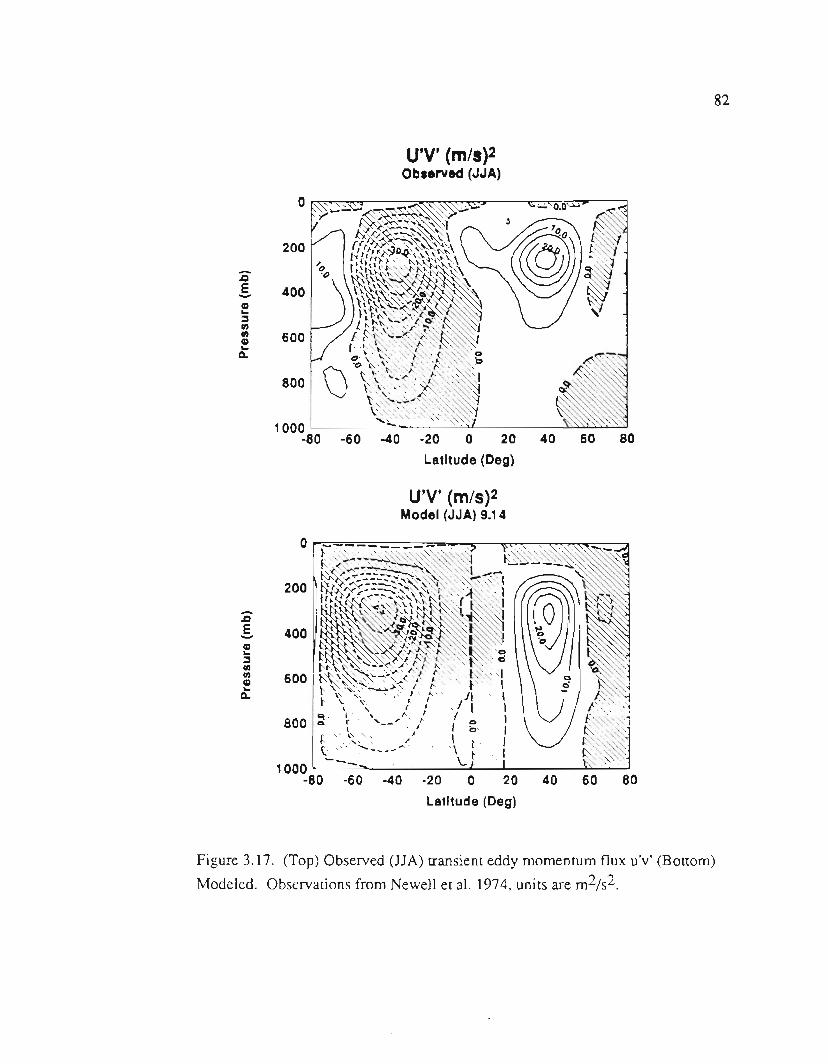
-.CI

.5. 400!~co: 600~a.

U'V' (m/s)2Observed (JJA)

o

200

800

82

40 60 80

Figure 3.17. (Top) Observed (JJA) transient eddy momentum flux u'v' (Bottom)

Modeled. Observations from Newell et al. 1974, units are m2js2.

U'V' (m/s)2Model (JJA) 9.14

0

200-E 400-!coco 600Q)a.

800

1000-80 -60 -40 -20 0 20 40

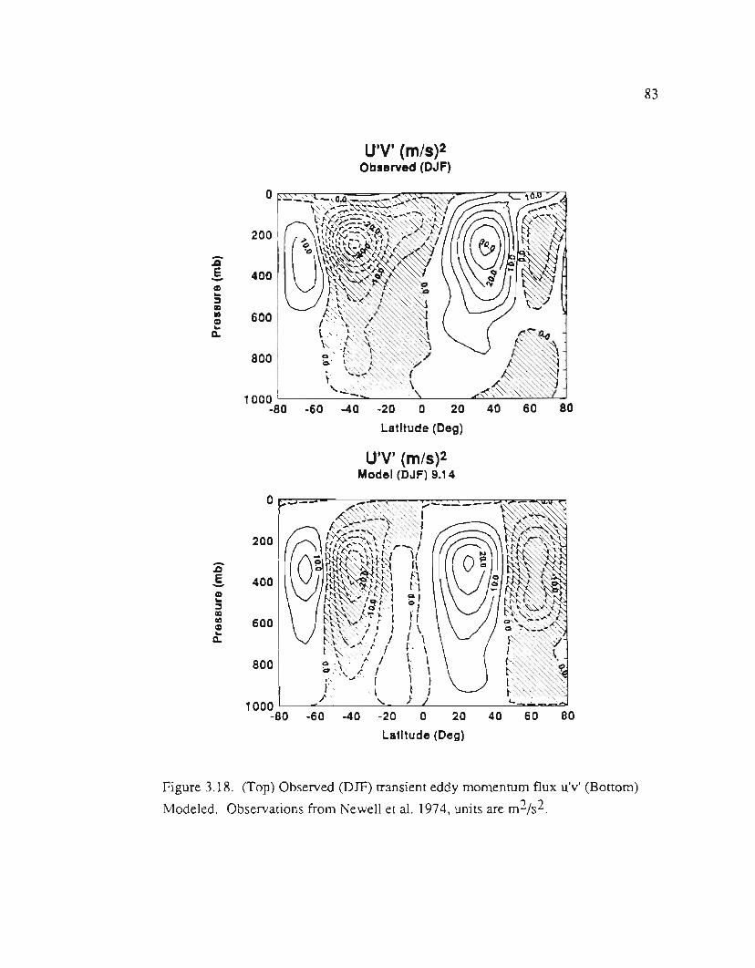
83

Figure 3.18. (Top) Observed (DJF) transient eddy momenrum flux u'v' (Bottom)

Modeled. Observations from Newell et al. 1974, units are m2js2.

U'V' (m/s)2Observed (DJF)

0

200-.aE 400-I»::s.10 600I»

a.

800

1000-80 -60 -40 -20 0 20 40 60 80

U'V' (m/s)2Model (DJF)9.14

0

200-.aE 400-!::s.10 600I»...a.

800

1000.80 .60 -40

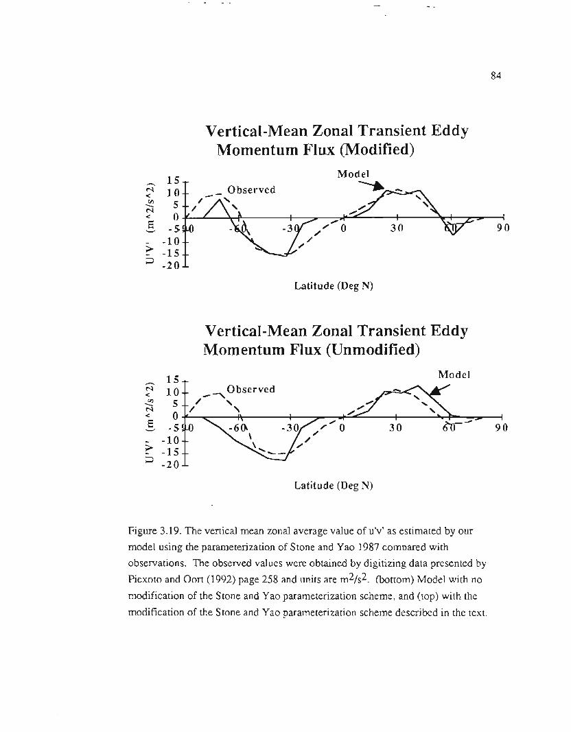
15-N 10~ 5-~ 0E -5--

-10~ -15~ -20

15N 10~ 5-~ 0E -5--- -10~ -15~ -20

84

Vertical-Mean Zonal Transient EddyMomentum Flux (Modified)

_ 0 bserved~-A'~ /'-,

90

Latitude (Deg N)

Vertical-Mean Zonal Transient EddyMomentum Flux (Unmodified)

Model

/_ --"'Observed/ ' ,

30 90

Latitude (Deg N)

Figure 3.19. The vertical mean zonal average value ofu'v' as estimated by our

model using the parameterization of Stone and Yao 1987 compared with

observations. The observed values were obtained by digitizing data presented by

Piexoto and Don (1992) page 258 and units are m2/s2. (bottom) Model with no

modification of the Stone and Yao parameterization scheme, and (top) with the

modification of the Stone and Yao parameterization scheme described in the text.

85

One justifiable reason for setting KBC=O.Ofor latitudes greater than some high

latitude position like 65° is that the parameterization of Stone and Yao (1987) is based on

quasi-geostrophic theory about some mid latitude position making it questionable at high

latitudes. We have found that the significant difference between the modified and

unmodified runs is apparent only in the winter hemisphere. The following discussion

will focus on the southern hemisphere during (JJA) but similar features also exist in the

northern hemisphere for (DJF).

Figure 3.20 compares the two-dimensional (JJA) zonal wind profile from the

control run.(with the modification, labeled 9.14) and an identical run that does not have

the above modification (labeled 9.21). The major difference between the two is that the

southern hemisphere jet stream for the unmodified run is closer to the pole than in the

modified run. A close inspection of 3.20 also shows that the strength of the westerly flow

at a position of 800S and a vertical level of 200 mb is about 14 m/s in the unmodified run

and about 4 m/s in the modified run indicating that the modification tends to reduce the

westerly flow in the high polar atmosphere. The observed values for 800S and 200 mb

are 6 m/s (Newell et al., 1972) and 8 m/s (peixoto and Oort, 1992). A careful inspection

of figure 3.20 also shows that the position of the center of the jet in the unmodified run is

about 9° (one latitude grid) farther south than in the modified run; the modified run,

although an improvement, still predicts a southern hemisphere jet stream position which

is about 10° farther south than the observed position of the jet reported by Piexoto and

Oort (1992). Thus the modification, which gives positve (negative) u'v' fluxes in the high

latitude south (north), tends to keep the jet streams closer to their observed positions and

maintains polar westerly flows with magnitudes closer to those observed.

The poleward shift of the jet in the winter hemisphere in the unmodified run also

seems to make the model less stable than it is in the modified run. These strong

westerlies are related to large pressure gradients at the poles. Figure 3.21 which is a

graph of the 100 m air pressure for the two runs supports this claim. In the unmodified

run, the 100 m pressure is about 15mb lower at 800Sthan in the modified run and about

7 mb lower is at 700S. At all other latitudes the agreement between the two runs is very

Figure 3.20. The zonal velocity for southern winter (JJA) for the control "run

(modified Stone and Yao u'v', 9.14) and the unmodified, 9.21.

86

Zonal Velocity U (m/s)Model(JJA)9.14

0

200-.CIE 400-II)...

enen 600II)..a.

800

1000-40 .20 0 20 40 60 80-80 .60

Latitude (Deg)

Zonal Velocity U (m/S)Model (JJA) 9.21

0

200

:s-A 400I!.

! 600A.

800

1000-80 -60 -40 .20 0 20 40 60 80

Latitude (Deg)

87

close. These extra low pressures at the poles of the winter hemisphere add to the

instability of the 'model and are also inconsistent with observations. The described

modification of the Stone and Yao u'v' parameterization defmately improves the overall

performance of the model.

-8- Modified

D- Unmodified

-40 -20 0 20

Latitude (De g)

40 60 80

Figure 3.21. The mean 100 m air pressure during southern winter (JJA) for the

control run (modified Stone and Yao u'v') and the unmodified, 9.21.

Rosen et al. (1990) performed a careful analysis of NMC (National

Meteorological (:enter) data on global angular momentum for the years 1976 to 1987.

They defined the latitudinal belt angular momentum as the total angular momentum

contained within a 2.50 latitude belt. We have shown their results, with their computed

standard deviations, in figure 3.22 along with the belt angular momentum simulated by

our model for the last year of the 20 year control run. Aside from the larger magnitude of

the tropical easterlies predicted by the model, the agreement is strikingly good.

990--

E 980--

; 970fI:)fI:) 8

Q: 960E= 950=940

-80 -60

Belt Angular Momentum(xl0"24 Kg m"2/s/2.5° )

88

--- Model

-o-RSW

. , ,sig +

. , ,sig -

Figure 3.22. Annual mean belt angular momentum predicted by model compared

with the analysis ofNMC observational data for the years 1976 to 1987. RSW

indicates observational analysis of Rosen, Salstein, and Wood (1991). Units are

1024kgm2/s/2.5°.

In Table 3.1 we compare the observed values of global, northern hemisphere, and

southern hemisphere atmospheric angular momentum with our model predictions (in

square brackets) for JJA, DJF, and annual means. The units are 1025 kgm2/s and the

observed values were from Rosen and Salstein reported by Peixoto and Oort (1992). The

agreement between observed and modeled angular momentum is good in the southern

10

8>.-.= 6

Q

5 4=-=

5 20

I.ec 0:;Cl) -so -60 -40=< -2

-4

Latitude (Deg N)

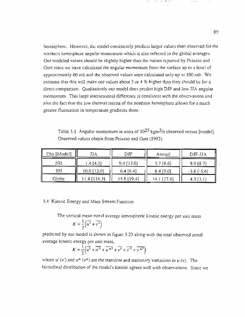
89

hemisphere. However, the model consistently predicts larger values than observed for the

northern hemisphere angular momentum which is also refected in the global averages.

Our modeled values should be slightly higher than the values reported by.Peixoto and

Oort since we have calculated the angular momentum from the surface up to a level of

approximately 60 mb and the observed values were calculated only up to 100 mb. Weestimate that this will make our values about 3 or 4 % higher than they should be for a

direct comparison. Qualitatively our model does predict high DJF and low JJA angular

momentum. This large interseasonal difference is consistent with the observations andalso the fact that the low thermal inertia of the northern hemisphere allows for a much

greater fluctuation in temperature gradients there.

Table 3.1 Angular momentum in units of 1025 kgm2/s observed versus [model].Observed values obtain from Peixoto and Oort (1992).

3.4 Kinetic Energy and Mass Stream Function

The vertical mean zonal average atmospheric kinetic energy per unit mass1(---:... -

)K = 2 u2 +v2

predicted by our model is shown in figure 3.23 along with the total observed zonal

average kinetic energy per unit mass,

K =~ (u2 +U,2 +U*2 +v2 +V,2 +V*2)

where u' (v') and u* (v*) are the transient and stationary variations in u (v). The

latitudinal distribution of the model's kinetic agrees well with observations. Since we

Obs [Model] JJA DJF Annual DJF-JJA

NH 1.4 [4.3] 9.4 [13.0] 5.7 [8.6] 8.0 [8.7]

SH 10.0 [12.0] 6.4 [6.4] 8.4 [9.0] -3.6 [-5.6]

Globe 11.4 [116.3] 15.8 [19.4] 14.1 [17.6] 4.5 [3.1]

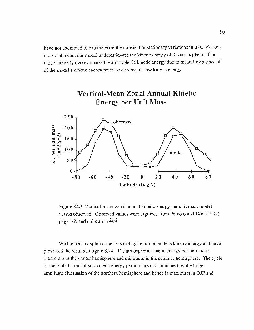
90

have not attempted to parameterize the transient or stationary variations in u (or v) from

the zonal mean, our model underestimates the kinetic energy of the atmosphere. The

model actually overestimates the atmospheric kinetic energy due to mean flows since all

of the model's kinetic energy must exist as mean flow kinetic energy.

Vertical-Mean Zonal Annual KineticEnergy per Unit Mass

2-50c;I)

~ 200e-M

;::< 150= c;I)=-M~e 100--~ 50

o .-80 -60 -40 -20 0 20

Latitude (Deg N)

40 60 80

Figure 3.23 Vertical-mean zonal annual kinetic energy per unit mass model

versus observed. Observed values were digitized from Peixoto and Oort (1992)

page 165 and units are m2Js2.

We have also explored the seasonal cycle of the model's kinetic energy and have

presented the results in figure 3.24. The atmospheric kinetic energy per unit area is

maximum in the winter hemisphere and minimum in the summer hemisphere. The cycle

of the global atmospheric kinetic energy per unit area is dominated by the larger

amplitude fluctuation of the northern hemisphere and hence is maximum in DJF and

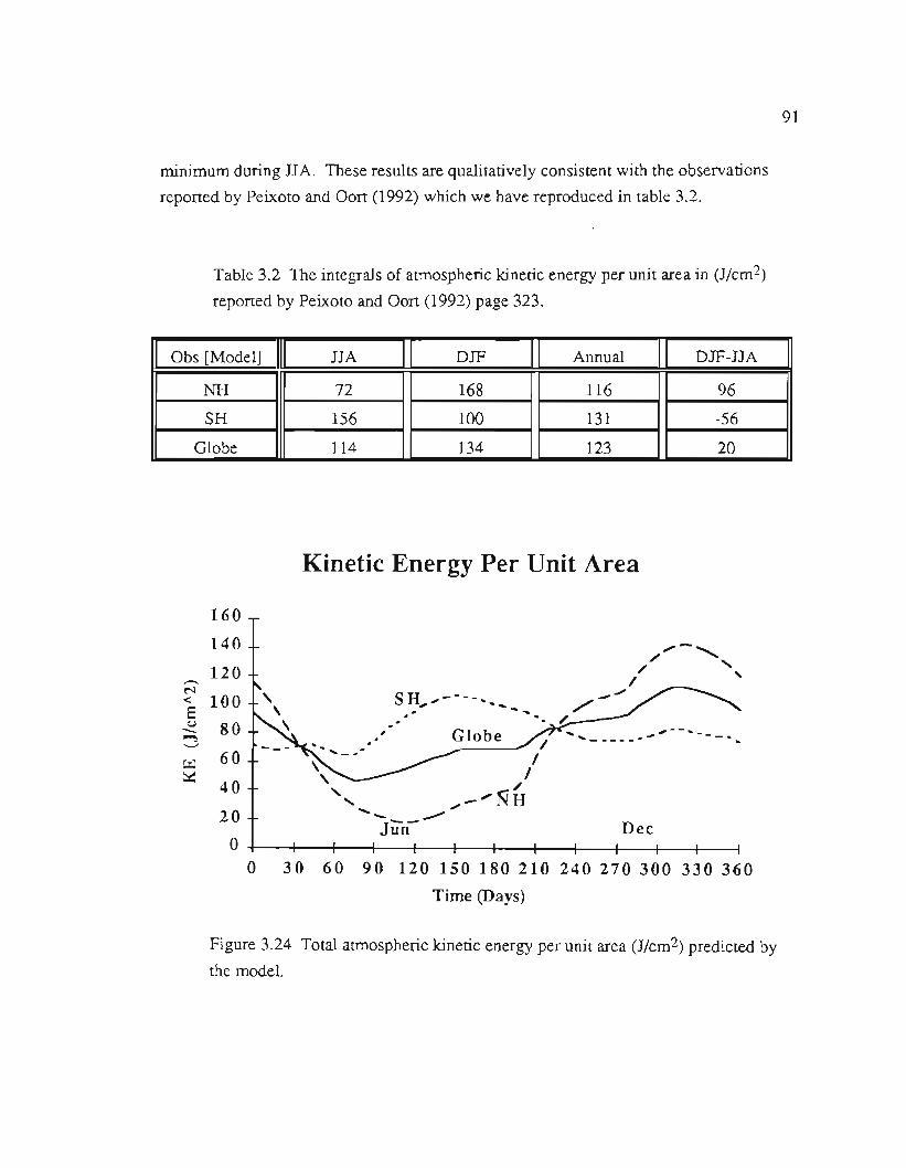
91

minimum during JJA. These results are qualitatively consistent with the observations

reponed by Peixoto and Oon (1992) which we have reproduced in table 3.2.

Table 3.2 The integrals of atmospheric kinetic energy per unit area in (J/cm2)

reponed by Peixoto and Oon (1992) page 323.

Kinetic Energy Per Unit Area

160

140120-

N< 100S

~ 80~'-"

60

40

20

o .o

SH ,~----_...........- '-....

.' /, I, I, /'" -~~H" "

~Jiin-

~-/ "'"

/ '"/ '-~

/"/...

Dee

30 60 90 120 150 180 210 240 270 300 330 360

Time (Days)

Figure 3.24 Total atmospheric kinetic energy per unit area (J/cm2) predicted bythe model.

Obs [Model] JJA DJF Annual DJF-JJA

NH 72 168 116 96

SH 156 100 131 -56

Globe 114 134 123 20

92

In figures 3.25 and 3.26 we compare the model predicted mass stream function. 'II

for JJA and DJF with values computed by from observations of meridional velocities v,21CaIP-

'II(p) =- v cos tfJdpg 0

At present the model underestimates the mass stream function by about 50 %. The

model does predict the seasonal movement of the inter tropical convergence zone (ITCZ)

fairly accurately and simulates a Ferrel cell circulation reasonably well. In addition, themodel is also consistent with observations in that it predicts Hadley circulations that are

much stronger in the winter hemisphere.

3.5 Precipitation and Surface Pressure

To simulate the amount of high latitude snow fall for use in the sea ice model that

we have been developing, we have estimated the precipitation as described in section

2.3.6. The annual precipitation estimated by the model is compared with the observed

values of precipitation in figure 3.27. Despite the fact that we do not have a prognostic

treatment of the water vapor cycle included in our model at present, the model estimates

magnitudes of precipitation that are surprisingly close to the observed values. Our

method for estimating precipitation is to produce precipitation whenever the atmosphere

cools either by radiation or dynamical transport so as to keep the relative humidity of the

atmosphere constant. Since the model reproduces the tropospheric temperature field

well, has a water :vaporprofile close to the observed, and has a cloud amount that is based

on observations; our method for estimating the precipitation gives a.good first

approximation. The model does however fail to reproduce the subtropical dry regions

and the secondary maxima in the mid latitudes. However, the model's estimate of

precipitation in the polar regions is good and the shape of the precipitation profile in the

tropics agrees well with observations. Thus, these precipitation values can be used in

estimating snow cover over sea ice in the development of a prognostic sea ice model.

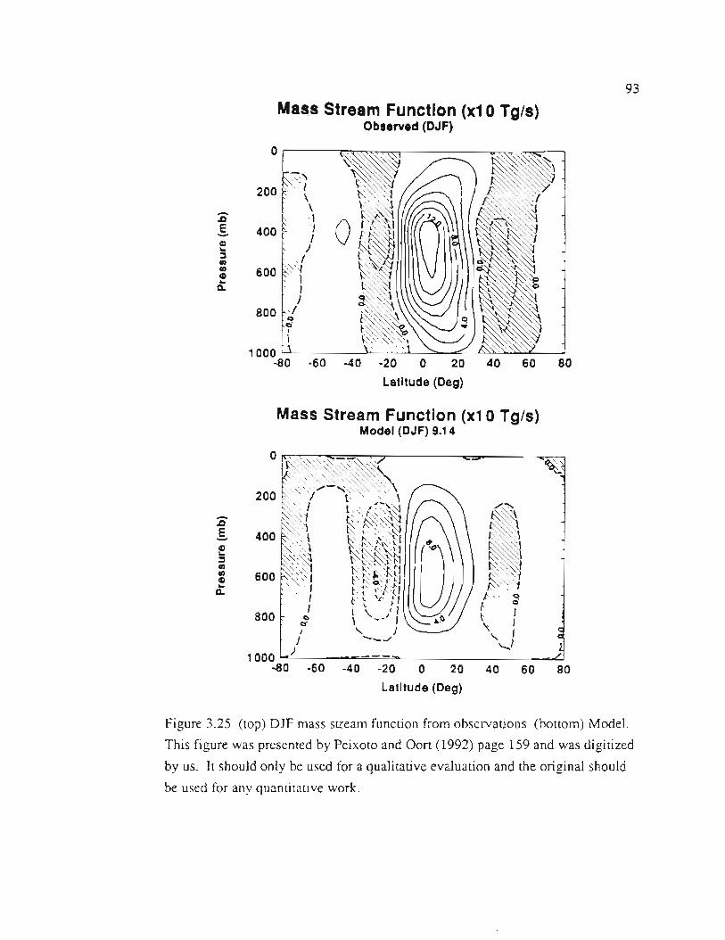
93

Ma.s Stream Function (x10 Tg/s)Observed (DJF)

1000-80 -60 -40 -20 0 20 40 60 80

Latitude(Deg)

o

-.aE-!~.,.,Q)...Q.

Figure 3.25 (top) DJF mass stream function from observations (bottom) Model.

This figure was presented by Peixoto and Oort (1992) page 159 and was digitized

by us. It should only be used for a qualitative evaluation and the original should

be used for any quantitative work.

200

400

600

-.aE-Q)...~.,.,Q)...Q.

'

"":.

I""

S :jt;:;,'-.

f' . 0\- 1\. I" I

'-...'_./1

40 60 80

94

Mas.sStream Function (x10 Tg/s)Observed (Annual)

o

-~S-

200":\'i

400 ~f1D~D

600 ~""\'-,'y:1

800 ~I

80

o..~.,.,o..a.

100~80 .60

Mass Stream Function (x10 Tg/s)Model (Annual) 9.14

:a-S-o..~.,.,o..a.

600 F0JII

800 tl

40 60 80

Figure 3.26 (top) Annual mass stream function from Model (bottom) Model.

This figure was presented by Peixoto and Dort (1992) page 159 and was digitized

by us. It should only be used for a qualitative evaluation and the original should

be used for any quantitative work.

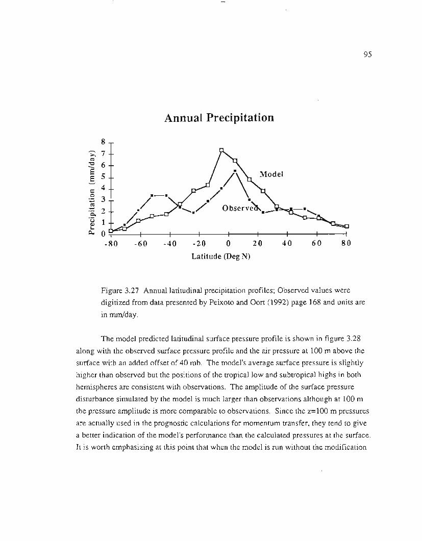
95

Annual Precipitation

8>;7~

~ 6

~ 5--= 4Q

~ 3~

~ 2Q..~ 1'"'

=-- 0-80

f-60

f-40

I I I-20 0 20

Latitude (Deg N)

f40

f60

Figure 3.27 Annual latitudinal precipitation profiles; Observed values were

digitized from data presented by Peixoto and Oort (1992) page 168 and units are

in mm/day.

The model predicted latitudinal surface pressure profile is shown in figure 3.28

along with the observed surface pressure profile and the air pressure at 100 m above the

surface with an added offset of 40 mb. The model's average surface pressure is slightly

higher than observed but the positions of the tropical low and subtropical highs in both

hemispheres are consistent with observations. The amplitude of the surface pressure

disturbance simulated by the model is much larger than observations although at 100 m

the pressure amplitude is more comparable to observations. Since the z=loo m pressures

are actually used in the prognostic calculations for momentum transfer, they tend to give

a better indication of the model's performance than the calculated pressures at the surface.

It is worth emphasizing at this point that when the model is run without the modification

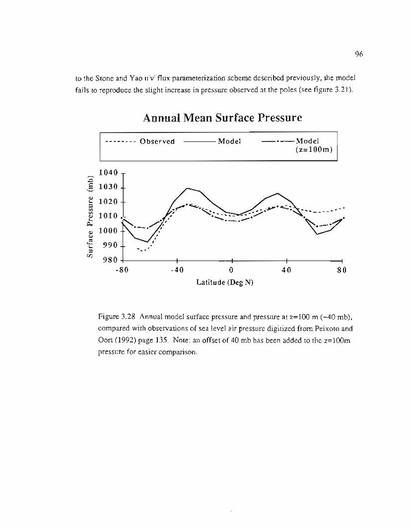
96

to the Stone and Yao u'v' flux parameterization scheme described previously, the model

fails to reproduce the slight increase in pressure observed at the poles (see figure 3.21).

Annual Mean Surface Pressure

nnnn Observed Model -.-Model(z=100m)

.........-------..~.

-40 0

Latitude (DegN)

40 80

Figure 3.28 Annual model surface pressure and pressure at z=100 m (+40 mb),

compared with observations of sea level air pressure digitized from Peixoto and

Oon (1992) page 135. Note: an offset of 40 mb has been added to the z=100m

pressure for easier comparison.

1040-E 1030--

1020=c:lI

1010.a..

Q.1000

(,I

990a..=

r:r.J

980-80

97

3.6 Summary of the Model's Perfonnance

To provide a quick reference to the model's perfonnance, the results of this

chapter are summarized in this section in outline fonn.

Temperature

Global Averages

Table 3.3. Model vs. observed surface air temperatures for JJA, DJF, and Annual

averages. Observations are from NCAR Data Support Section, Scientific

Computing Division; Units are Kelvin. Model values are for z=1oo m.

Latitudinal summary for surface air temperature.

· All model values are within 2% of observations except near the poles where

the discrepancy is a maximum of 8% at 800Sfor DJF mean.

Two-dimensional summary

. Annual mean temperature profile has less than 5 % error at all positions

except for the surface near 800S (8%) and above 100 mb in the tropics where

the model is approximately 10 % too warm.

Temperature (K) Model Obs. NCAR

JJA 288.5 289.1

DJF 284.3 285.6

Annual 286.3 287.4

98

Energy Balance .

· The difference between the net absorbed solar radiation and the outgoing

infrared radiation (Solar-IR) is less than 0.5 W/m2 for the annual mean.

· The difference between observed (Solar-IR) and modeled (Solar-IR) is less

than 15W/m2 at all latitudes and all seasons except:

a) At the poles where the maximum difference is at 800N for JJA average

and is 45 W/m2 difference or about 19 % of the global mean absorbed flux

of solar energy (Sab). At 70° Nor S the values of (Solar-IR) immediately

drop to less than 5 W/m2 for both winter and summer except for the JJA

average at 70 S where it is about 20 W/m2 or about 8 % of Sab.

b) In the tropics during JJA where the maximum difference is 31 W/m2 or

about 13 % of Sab.

Mean Zonal Velocity u

. The latitudinal and vertical profile of zonal velocities predicted by the model

are in good qualitative agreement with observations; see figure 3.22.

The strength of the model's mean tropical easterlies is about twice as strong as

it should be during all seasons;see figure 3.22.

.

Table 3.4 summarizes the comparison between the maximum zonal velocities

(subtropical jets) predicted by the GCRC 2D model and the observations of

Newell et al. (1972) and Peixoto and Oon (1992).

· Our results are in better agreement with the observations of Peixoto and Oon

(1992) being within 25 % during all seasons and in both hemispheres.

· There is considerable disagreement between the two data sets.

- - ----~---- ----

99

Table 3.5 shows the latitudinal position of the jets predicted by our 2D model

compare to the observations of Newell et al. (1972) and Peixoto and Oort (1992).

. Our model tends to predict jet stream positions that are too far poleward,

especially during JJA.

· The vertical position of the center of the jets in both hemispheres predicted byour model is closer to 100 or 150 mb where the observed vertical positions areabout 200 mb.

Table 3.4 Summary of zonal velocities (in m/s) predicted by our 2D model as

compared to the observations of Newell et al. [N. et al.] (1972) and Peixoto and

Oort [P & 0] (1992) for summer (JJA), winter (DJF), and annual averages. Top

three rows are for the southern hemisphere and the bottom three rows are for the

northern hemisphere. The columns headed by d% (N), d% (P&O), and d% (N-

(P&O» are the percent differences between the model and the data from Newell

et al. (1972), the model and the data from Peixoto and Oort (1992), and theNewell et al. data and the Peixoto and Oort Data.

u m/s Model N. et al. P&O d% (N) d% (P&O) d% (N-(P&O»jjA 32 23 35 39 -9 -34

SH DjF 30 20 24 50 25 -17Annual 30 22 25 36 20 -12

jjA 15 15 20 0 -25 -25

NH DjF 40 27 39 48 3 -31Annual 25 22 25 14 0 -12

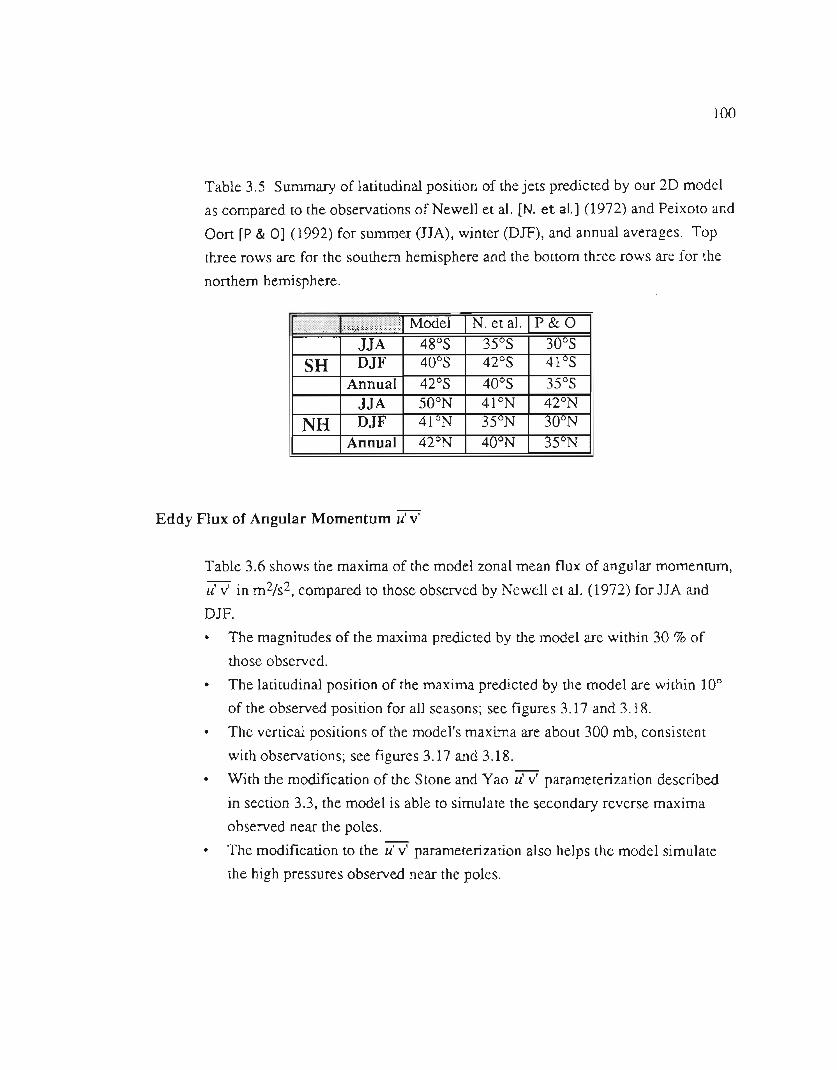
100

Table 3.5 Summary of latitudinal position of the jets predicted by our 2D model

as compared to the observations of Newell et al. [N. et a!.] (1972) and Peixoto and

Oort [P &0] (1992) for summer (JJA), winter (DJF), and annual averages. Top

three rows are for the southern hemisphere and the bottom three rows are for the

northern hemisphere.

'r.'T:r r...' ' ] Mod Ie::~:~:~:~:~:~:}~:~:~:~:}~:~:~:~:~:~:~:~:~

JJA 48 SSO DJF 40 S

Annual 42 SJJA 50 N

NO DJF 41 NAnnual 42 N

Eddy Flux of Angular Momentum u'v'

Table 3.6 shows the maxima of the model zonal mean flux of angular momentum,

u'v' in m2/s2, compared to those observed by Newell et al. (1972) for JJA andDJF.

· The magnitudes of the maxima predicted by the model are within 30 % ofthose observed.

· The latitudinal position of the maxima predicted by the model are within 10°

of the observed position for all seasons; see figures 3.17 and 3.18.

· The vertical positions of the model's maxima are about 300 mb, consistent

with observations; see figures 3.17 and 3.18.

· With the modification of the Stone and Yao u'v' parameterization described

in section 3.3, the model is able to simulate the secondary reverse maxima

observed near the poles.

· The modification to the u'v' parameterization also helps the model simulate

the high pressures observed near the poles.

101

Table 3.6. The hemispherical maxima of the model zonal mean flux of angular

momentum, u'v' in m2fs2, compared to those observed by Newell et al. (1972) forJJA and DJF

Mass Stream Function, Surface Pressure, and Precipitation.

Mass Stream Function

· The seasonal movement and position of the ITCZ is simulated very well bythe model.

· The model does simulate a weak Farrel circulation in both hemispheres.

· The strength of the Hadley circulation (mass stream function) is about 50 %too low.

Precipitation

· The global mean annual precipitation rate estimated by the model is 3.3

mm/day compared to the observed 2.7 mm/day reported by Peixoto and Oort

(1992), which is about 20 % too high.

· The model estimates that the precipitation is maximum in the tropics and

minimum at the poles in agreement with observations.

· The model fails to simulate the subtropical dry regions.

Surface Pressure

· The latitudinal profile of the annual mean surface air pressure agrees very well

with observations in that the model simulates: 1) the surface pressure low of

the tropics, 2) the subtropical highs, and 3) the polar highs.

u'v' m2fs2 Model N. et al. %

JJA -40 -35 14

SH DJF -25 -35 -28

JJA 25 20 25

NH DJF 25 30 -17

102

· The amplitude of the model's surface pressure is much larger (2 to 3 times)

than the observed, but the amplitude of the model's air pressure at a height of100 meters is much more consistent with observations.

.---.-.

CHAPTER 4

MODEL SENSITIVITY

In this chapter we explore the equilibrium response of the model to a doubling of

carbon dioxide (the 2xC02 experiment). Many other groups have performed this same

experiment so this offers a way to compare our model's sensitivity to that of other climate

models. In the first section we will focus on the change in the temperature structure of

the atmosphere for a 2XC02 experiment and in the second section we follow the

investigation of Rosen and Gutowski (1992) and analyze the change in model's zonal

wind field and angular momentum due to a doubling of CO2. In the third section, in the

hope of understanding the model's response more completely, we present the simulated

changes in the mass stream function, meridional temperature gradients, and eddy

momentum flux due to a doubling of atmospheric CO2. Finally, in the last section we

summarize the results obtained throughout this chapter.

4.1 Temperature Changes due to 2XC02

The changes in the annual mean zonally averaged surface temperatures due to a

doubling of C02 predicted by five different general circulation models (GCM) are shown

in figure 4.1. Most all of the models are qualitatively consistent in that they predict

changes in surface temperature which are greater in the high latitudes than in the tropics

for bothhemispheres. In a recentIntergovernmentalPanelon ClimateChangerepon .

(IPCC 1990), this was also one of the features noted as being common to most climate

model predictions. In figure 4.2 we present the latitudinal and seasonal response of our

model's zonal surface air (z=l00 m) temperature and surface temperature (z=O.O)for the

103

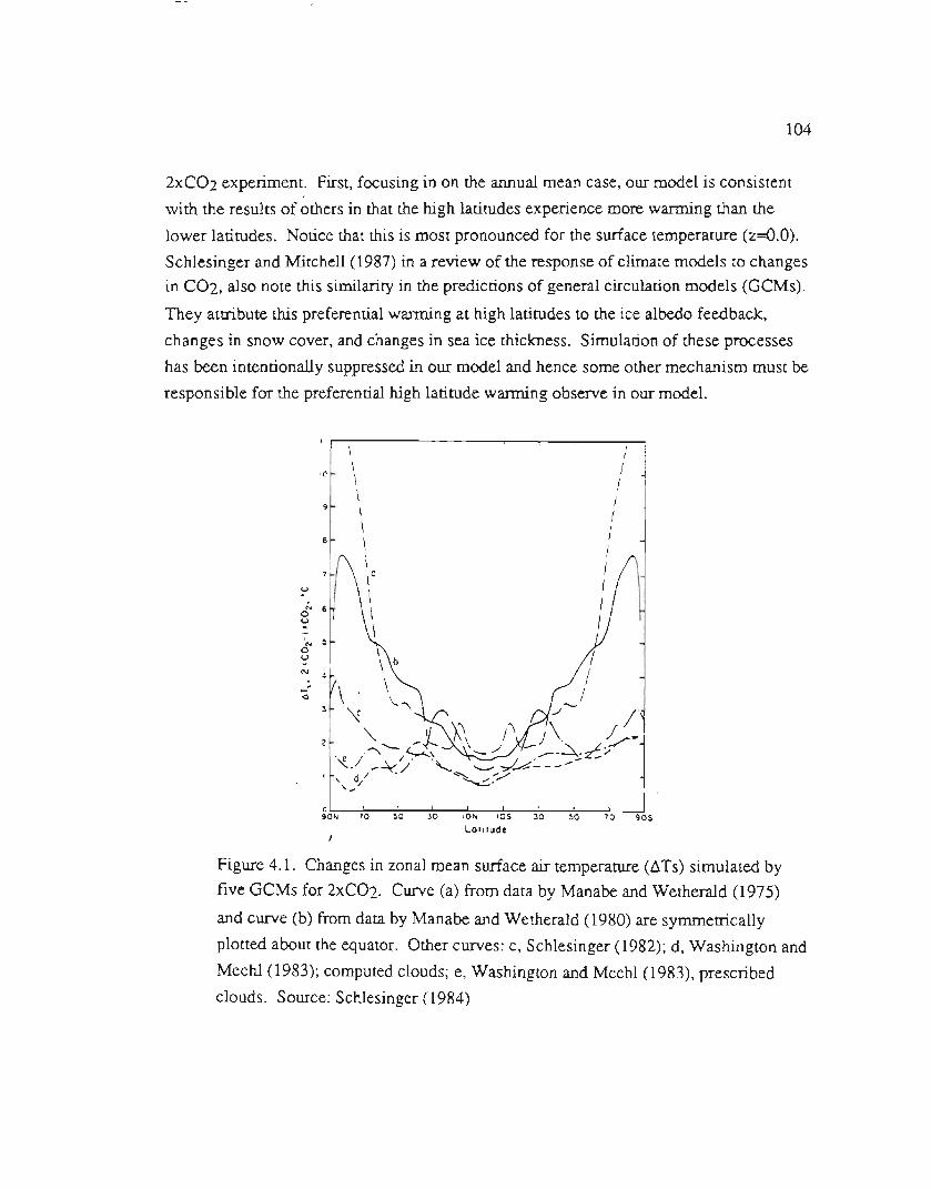
104

2XC02 experiment. First, focusing in on the annual mean case, our model is consistent

with the results of others in that the high latitudes experience more warming than the

lower latitudes. Notice that this is most pronounced for the surface temperature (z=O.O).

Schlesinger and Mitchell (1987) in a review of the response of climate models to changesin C02, also note this similarity in the predictions of general circulation models (GCMs).

They attribute this preferential warming at high latitudes to the ice albedo feedback,

changes in snow cover, and changes in sea ice thickness. Simulation of these processes

has been intentionally suppressed in our model and hence some other mechanism must be

responsible for the preferential high latitude warming observe in our model.

o90" 70 ~o ~o 10" ,OS ~o ~o 70 90S

La"'udeI

Figure 4.1. Changes in zonal mean surface air temperature (.1Ts) simulated by

five GCMs for 2xC02. Curve (a) from data by Manabe and Wetherald (1975)

and curve (b) from data by Manabe and Wetherald (1980) are symmetrically

plotted about the equator. Other curves: c, Schlesinger (1982); d, Washington and

Meehl (1983); computed clouds; e, Washington and Meehl (1983), prescribedclouds. Source: Schlesinger (1984)

"\ I\

.N- \I

\I

9 \I

\I

8 \I

\ I

\0I

1' \\

III

'N0u..N 4

-...<I

- -- -.

105

One possible mechanism for the polar amplification of the climate sensitivity is

that since the absolute humidity at the cool high latitudes is much smaller than it is in the

tropics, C02 may playa much more important role in the greenhouse warming at high

latitudes. We explored this idea using the ID-RCM described by MacKay and Khalil

(1991) and found that its climate sensitivity actually decreased as the model became

cooler (less water vapor). We found that w/:lenthe equilibrium surface temperature for

the ID-RCM control run is 289 K, the increase in surface temperature predicted due to a

doubling of C02 concentration is 1.9 K. The surface temperature increase is 1.6 K when

the control surface temperature is decreased to 272 K by decreasing the solar constant,

and 0.9 K for a 235 K control surface temperature. Thus the mechanism proposed above

for the polar amplification of the climate sensitivity seems unlikely.

Ramanathan (1977) noted the importance of atmospheric static stability in

determing its climate sensitivity. In the tropical regions, where the atmosphere is very

unstable the sensitivity is decreased since surface warming will cause an enhancement of

convection resulting in enhanced surface cooling, a negative feedback. The opposite is

true of a highly stable atmosphere such as the polar atmosphere. Thus, the difference

between the static stability of the polar atmosphere and the tropical atmosphere results in

this preferential warming in the polar regions.

Certainly the other processes discussed by Schlesinger and Mitchell are very

important and should be included in any comprehensive model. However, care must be

taken to model positive feedbacks, such as the ice albedo feedback, correctly. Errors in

the physics of feedbacks can easily result in an overestimation of the true sensitivity of

the climate system to perturbations. For example, in our preliminary work with a

thermodynamic prognostic version of a sea ice model we found a polar warming in

excess of 12 K for a 2xC02 experiment. This may indeed be a realistic response of the

real climate system but this will require closer scrutiny by us.

106

Z=lOO m Temperature Change (K)2xC02-1xC02

--/

//

DJF//""

'"/

/""

..,,'" ------....- - -::---"" ---~ JJA

-40 oLatitude (Deg N)

40 80

Figure 4.2. The latitudinal and seasonal response of the GCRC 2D climate model

to a doubling of C02. (top) z=l00m air temperature change (K) (bottom) Surface

temperature change (K).

2.5

-2--

E=>=>

i1 1.5N

@I

Eo- 1<:]

0.5-80

2.5 .....Surface Temperature Change (K) /

--2xC02-1xC02 I

, /- 2 ,DJF/--

1-/CJ I

1.5 I1.0= I1"1}

_"'.1 .......... JJAEo- 1 .-. ---"-...<:] --- .....-".."L

.0.5

-80 -40 0 40 80

Latitude (DegN)

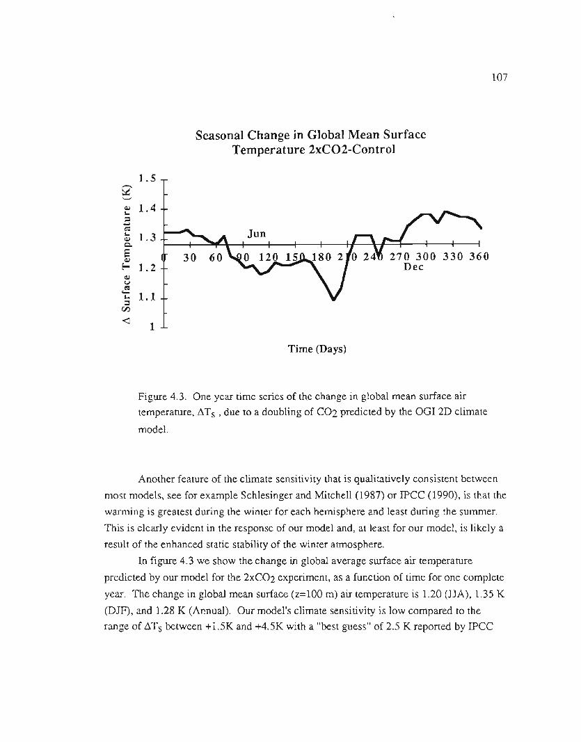
107

Seasonal Change in Global Mean SurfaceTemperature 2xC02-Control

1.5

~ 1.4s..=-cut 1.3c.S~

Eo- 1.2

270 300 330 360Dee

Time (Days)

Figure 4.3. One year time series of the change in global mean surface air

temperature, .1Ts , due to a doubling of C02 predicted by the OGI 2D climate

model.

Another feature of the climate sensitivity that is qualitatively consistent between

most models, see for example Schlesinger and Mitchell (1987) or IPCC (1990), is that the

warming is greatest during the winter for each hemisphere and least during the summer.

This is clearly evident in the response of our model and, at least for our model, is likely a

result of the enhanced static stability ()fthe winter atmosphere.

In figure 4.3 we show the change in global average surface air temperature

predicted by our model for the 2XC02 experiment, as a function of time for one complete

year. The change in global mean surface (z=100 m) air temperature is 1.20 (JJA), 1.35 K

(DJF), and 1.28 K (Annual). Our model's climate sensitivity is low compared to the

range of .1Ts between +1.5K and +4.5K with a "best guess" of 2.5 K reported by IPCC

108

(1990) for the climate sensitivity of most GCMs for a doubling of CO2. This is expected

since we have attempted to suppressed all feedbacks except for the water vapor feedback.

In figure 4.4 we present the changes in the two-dimensional temperature field

predicted by our model for JJA and DJF. Held (1993) gave a review of climate models

which included a brief description of their sensitivity to a doubling of carbon dioxide.

We present his qualitative results in figure 4.5 along with the change in the annual

average temperature field predicted by our model. Our results have several features in

common with Held's qualitative interpretation of what most climate models predict for

the changes in temperature field due to a doubling of CO2. As noted previously, we have

an increase PI magnitude of the surface warming as the latitude increases towards the

poles in both hemispheres. Note also the maximum in temperature change predicted to

occur in the middle to upper tropical troposphere. Held (1993) attributes this maximum

warming in the upper tropical troposphere simulated by most climate models to an

increase in the vertical transport of latent heat energy in the tropics due to surface

warming. Finally, as with most climate models, we have a substantial cooling in the

stratosphere. Our model predicts changes in the two-dimensional temperature fields that

are qualitatively consistent with most climate models of this or greater sophistication.

Although we do have good qualitative agreement between our results and the results of

other climate models, our model is quantitatively less sensitive to changes in carbon

dioxide than the average climate model. As mentioned previously this is primarily due to

the lack of positive feedback processes included in our model.

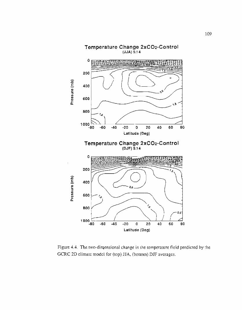
109

Temperature Change 2XC02-Control(JJA) 9.14

Figure 4.4. The two-di~ensional change in the temperature field predict~ by the

GCRC 2D climate model for (top) JJA, (bottom) DJF averages.

0

200-.QE 400-CD..:sfI)fI) 600CD..Co

800

1000-80 -60 -40 -20 0 20 40 60 80

Latitude (Deg)

Temperature Change 2XC02-Control(DJF)9.14

0

200-.QE 400-CD..:sfI)fI) 600CD..Go

800

1000-80 -60 -40 -20 0 20 40 60 80

Latitude (Deg)

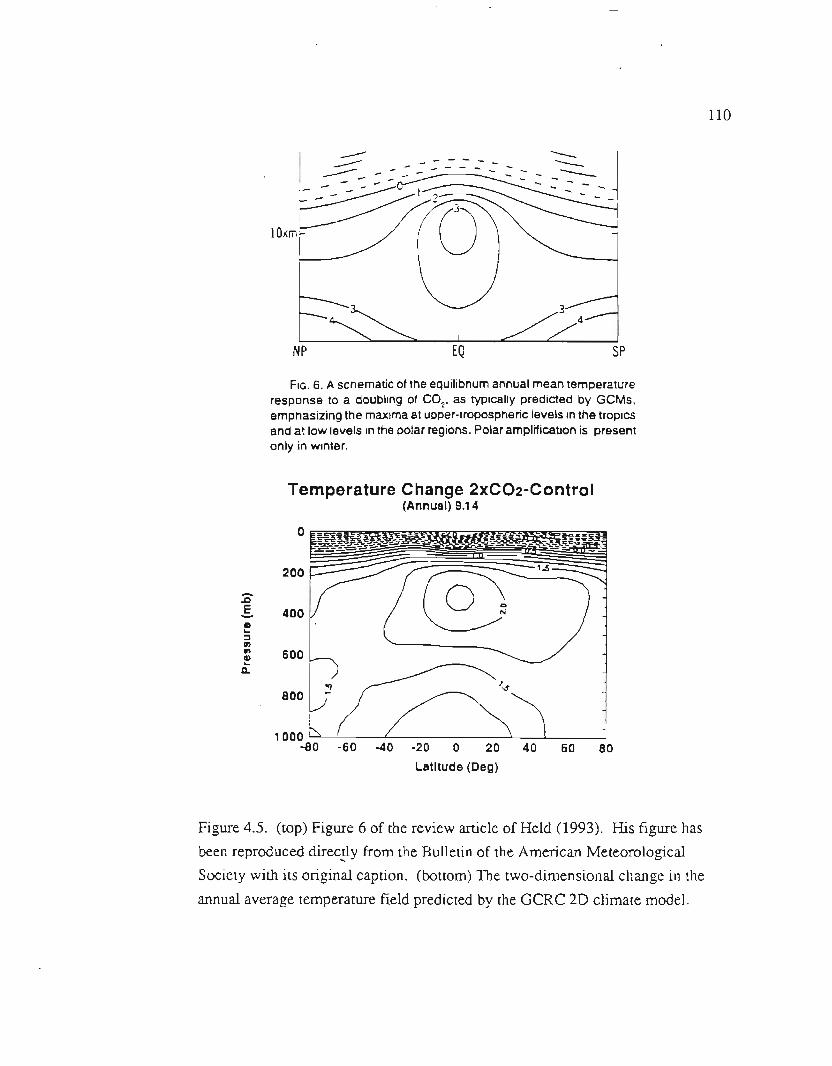
110

FIG.6. A schematic of the equilibriumannual mean temperatureresponse to a doubling of C02' as typically predicted by GCMs.emphasizing the maxima at upper-tropospheric levels inthe tropicsand at low levels in the polar regions. Polar amplification is presentonly in winter.

Temperature Change 2XC02-Control(Annual) 9.14

o

-~E-CD..~8181CD..a.

200

400

600

800

-40 -20 0 20 40 60 80

Latitude (Deg)

Figure 4.5. (top) Figure 6 of the review anicle of Held (1993). His figure has

been reproduced directly from the Bulletin of the American Meteorological....

Society with its original caption. (bottom) The two-dimensional change in the

annual average temperature field predicted by the GCRC 2D climate model.

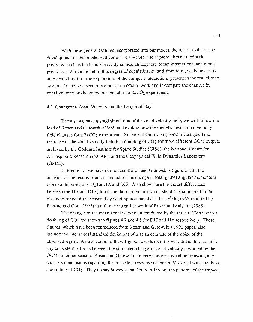
111

With these general features incorporated into our model, the real payoff for the

development of this model will come when we use it to explore climate feedback

processes such as land and sea ice dynamics, atmosphere-ocean interactions, and cloud

processes. With a model of this degree of sophistication and simplicity, we believe it is

an essential tool for the exploration of the complex interactions present in the real climate

system. In the next section we put our model to work and investigate the changes in

zonal velocity predicted by our model for a 2xCOz experiment.

4.2 Changes in Zonal Velocity and the Length of Day?

Because we have a good simulation of the zonal velocity field, we will follow the

lead of Rosen and Gutowski (1992) and explore how the model's mean zonal velocity

field changes for a 2XC02 experiment Rosen and Gutowski (1992) investigated the

response of the zonal velocity field to a doubling of C02 for three different GCM outputs

archived by the Goddard Institute for Space Studies (GISS), the National Center for

Atmospheric Research (NCAR), and the Geophysical Fluid Dynamics Laboratory

(GFDL).

In Figure 4.6 we have reproduced Rosen and Gutowski's figure 2 with the

addition of the results from our model for the change in total global angular momentum

due to a doubling of C02 for JJA and DJE Also shown are the model differences

between the JJA and DJF global angular momentum which should be compared to the

observed range of the seasonal cycle of approximately -4.4 x1025kg m2/s reponed by

Peixoto and Oon (1992) in reference to earlier work of Rosen and Salstein (1983).

The changes in the mean zonal velocity, u, predicted by the three GCMs due to a

doubling of C02 are shown in figures 4.7 and 4.8 for DJF and JJA respectively. These

figures, which have been reproduced from Rosen and Gutowski's 1992 paper, alsoinclude the interannual standard deviations of u as an estimate of the noise of the

observed signal. An inspection of these figures reveals that it is very difficult to identify

any consistent patterns between the simulated change in zonal velocity predicted by the

GCMs in either season. Rosen and Gutowski are very conservative about drawing any

concrete conclusions regarding the consistent response of the GCM's zonal wind fields to

a doubling of C02. They do say however that "only in JJA are the patterns of the tropical

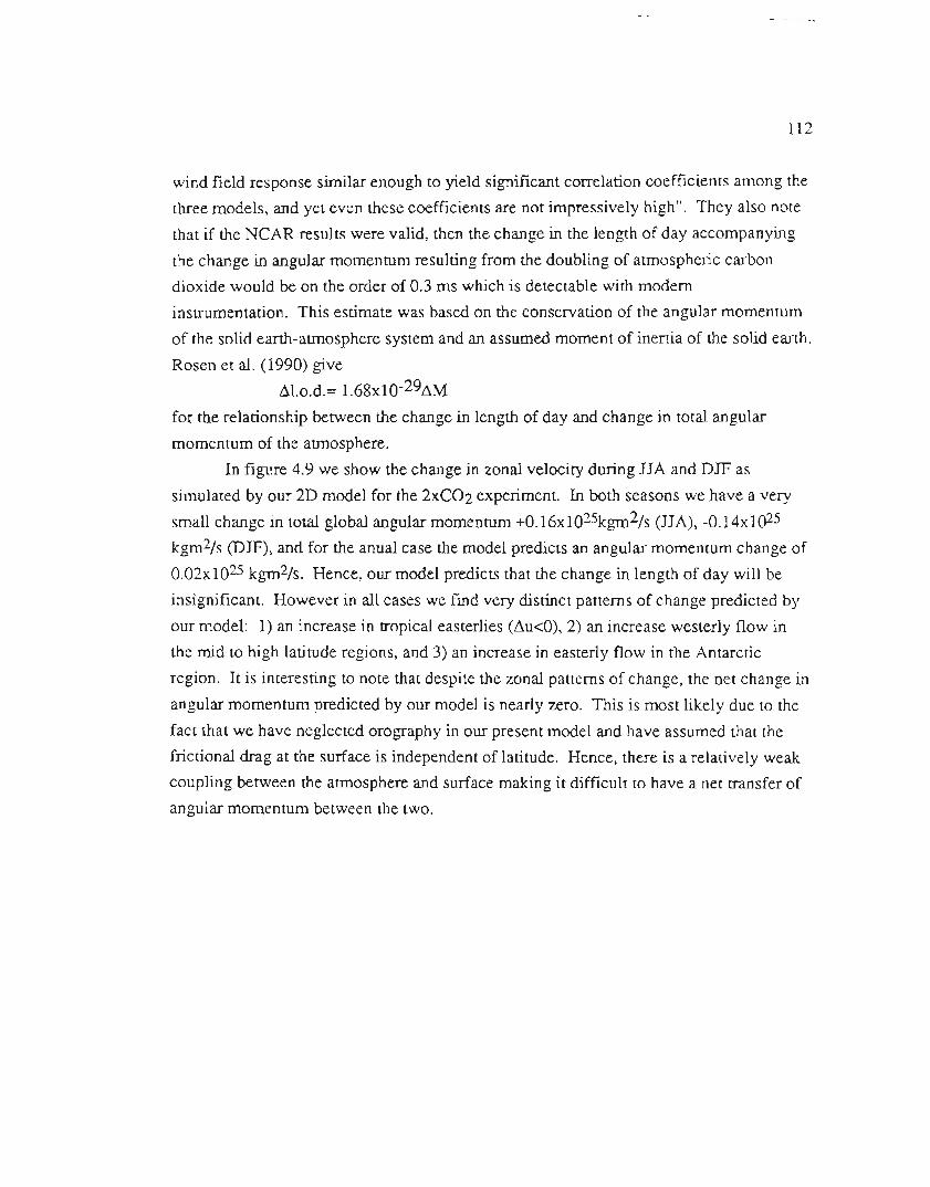
112

wind field response similar enough to yield significant correlation coefficients among the

three models, and yet even these coefficients are not impressively high". They also note

that if the NCAR results were valid, then the change in the length of day accompanying

the change in angular momentum resulting from the doubling of atmospheric carbondioxide would be on the order of 0.3 ms which is detectable with modern

instrumentation. This estimate was based on the conservation of the angular momentum

of the solid earth-atmosphere system and an assumed moment of inertia of the solid earth.

Rosen et al. (1990) give~l.o.d.= 1.68xlO-29~M

for the relationship between the change in length of day and change in total angular

momentum of the atmosphere.

In figure 4.9 we show the change in zonal velocity during JJA and DJF as

simulated by our 2D model for the 2XC02 experiment. In both seasons we have a very

small change in total global angular momentum +O.16x1025kgm2/s(JJA), -0.14xl()25

kgm2/s (DJF), and for the anual case the model predicts an angular momentum change of

0.02x1025 kgm2/s. Hence, our model predicts that the change in length of day will be

insignificant. However in all cases we fmd very distinct patterns of change predicted by

our model: I) an increase in tropical easterlies (~u<O),2) an increase westerly flow in

the mid to high latitude regions, and 3) an increase in easterly flow in the Antarctic

region. It is interesting to note that despite the zonal patterns of change, the net change in

angular momentum predicted by our model is nearly zero. This is most likely due to the

fact that we have neglected orography in our present model and have assumed that the

frictional drag at the surface is independent of latitude. Hence, there is a relatively weak

coupling between the atmosphere and surface making it difficult to have a net transfer of

angular momentum between the two.

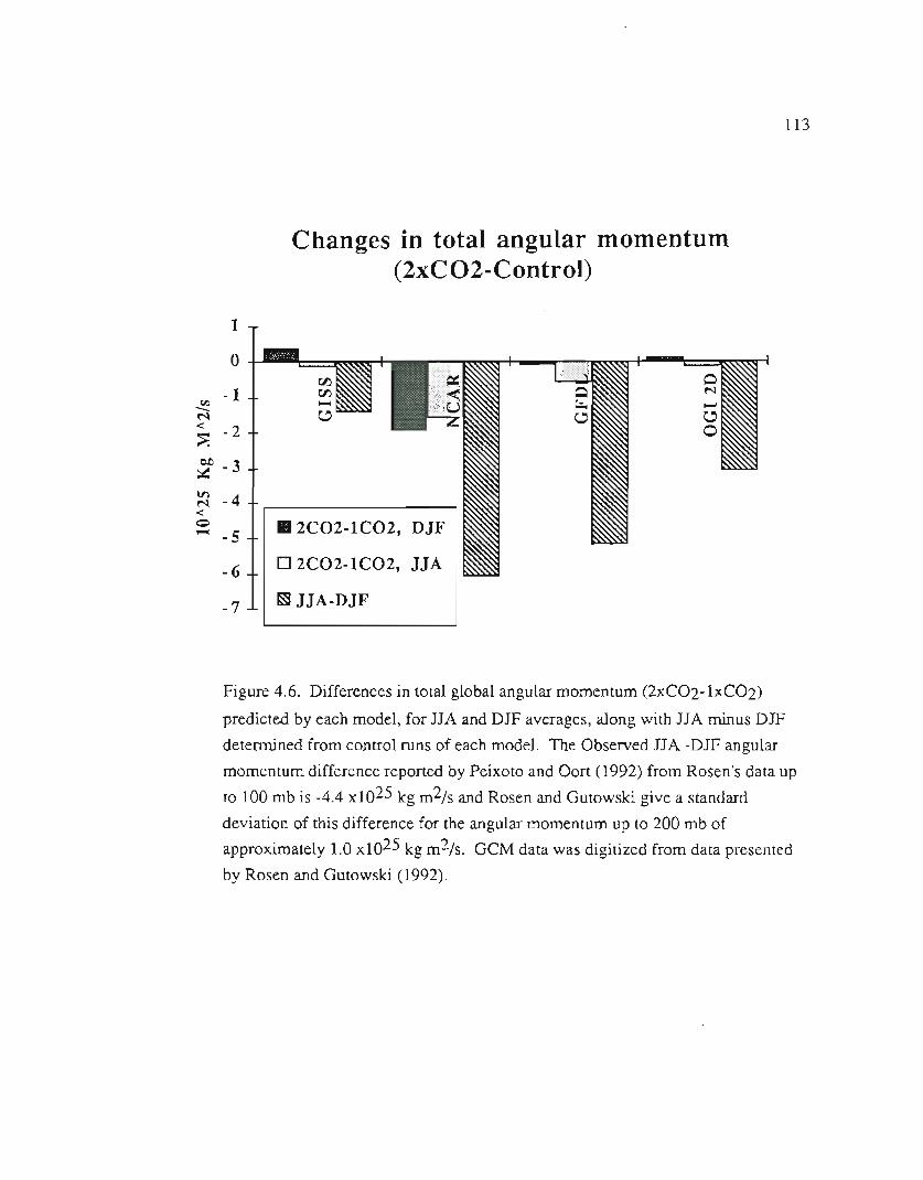
113

Changes in total angular momentum(2xC02-ControI)

1

o

VJ -I-M<:t -2.~~ -3~ -4<

~ _s

j

Il2C02-IC02, DJF

:: :;~::;~02. JJA

Figure 4.6. Differences in total global angular momentum (2xC02-1xC02)

predicted by each model, for JJA and DJF averages, along with JJA minus DJF

determined from control runs of each model. The Observed JJA -DJF angular

momentum difference reponed by Peixoto and Oon (1992) from Rosen's data up

to 100 mb is -4.4 x1025 kg m2/s and Rosen and Gutowski give a standard

deviation of this difference for the angular momentum up to 200 mb of

approximately 1.0 xl025 kg m2/s. GCM data was digitized from data presented

by Rosen and Gutowski (1992).

114

Figure 4.7. Differences in zonal velocity resulting from a 2XC02 experiment

predicted by the three GCMs of Rosen and Gutowski's (1992) study for DJF.

Also shown are the interannual standard deviations of the zonal velocity based on

14 years of NMC data. Units are meters per second and shaded regions represent

decreases in zonal velocity. The ordinate is the vertical pressure in units of

millibars and the abscissa is the latitude in degrees north.

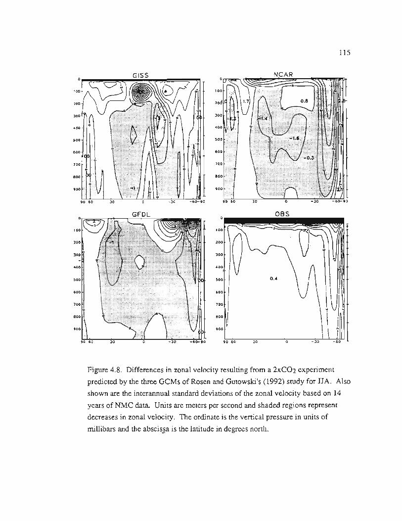
115

Figure 4.8. Differences in zonal velocity resulting from a 2XC02 experiment

predicted by the three GCMs of Rosen and Gutowski's (1992) study for JJA. Also

shown are the interannual standard deviations of the zonal velocity based on 14

years of NMC data. Units are meters per second and shaded regions represent

decreases in zonal velocity. The ordinate is the venical pressure in units of

millibars and the abscis.§ais the latitude in degrees north.

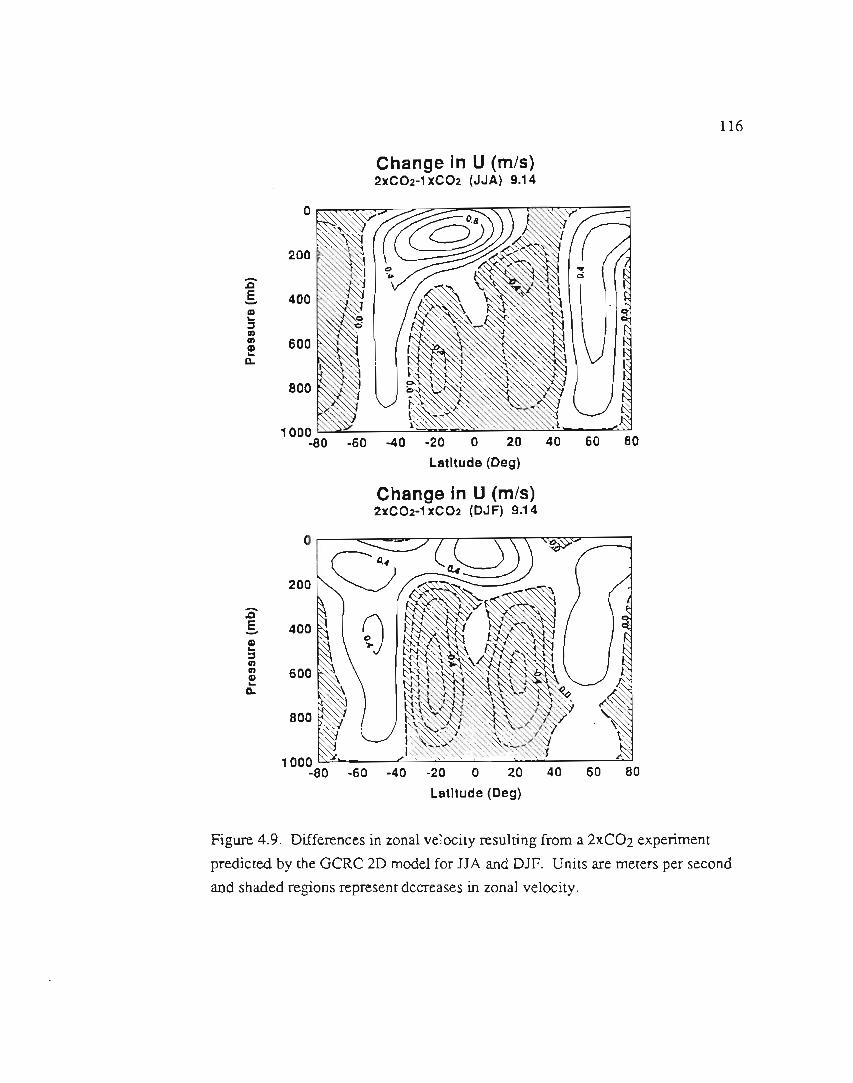
Figure 4.9. Differences in zonal velocity resulting from a 2xC02 experiment

predicted by the GCRC 2D model for JJA and DIE Units are meters per second

and shaded regions represent decreases in zonal velocity.

116

Change In U (m/s)2XC02-1XC02 (JJA) 9.14

0

200-E 400-CD...,., 600CD..A-

800

1000-80 -60 -40 -20 0 20 40 60 80

Latitude (Deg)

Change In U (m/s)2XC02-1XC02 (DJF) 9.14

0

. 200-E 400-CD...,., 600CD..A-

800 .

,1000

-80 -60 -40 -20 0 20 40 60 80

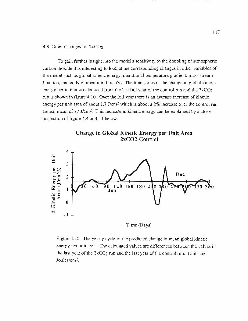
117

4.3 Other Changes for 2XC02

To gain further insight into the model's sensitivity to the doubling of atmospheric

carbon dioxide it is interesting to look at the corresponding changes in other variables of

the model such as global kinetic energy, meridional temperature gradient, mass stream

function, and eddy momentum flux, u'v'. The time series of the change in global kinetic

energy per unit area calculated from the last full year of the control run and the 2XC02

run is shown in figure 4.10. Over the full year there is an average increase of kinetic

energy per unit area of about 1.7 J/cm2 which is about a 2% increase over the control runannual mean of 77 J/cm2. This increase in kinetic energy can be explained by a close

inspection of figure 4.4 or 4.11 below.

Change in Global Kinetic Energy per Unit Area2xC02-Control

Figure 4.10. The yearly cycle of the predicted change in mean global kinetic

energy per unit area. The calculated values are differences between the values in

the last year of the 2XC02 run and the last year of the control run. Units areJoules/cm2.

4;:::=;:J

3I.Q,I.-c.N<>'5 2Ol)1.-Q,I

IVO60 O 120 150 180 2=-

JunQ,I._ I.<

= 0

<J-1

Time (Days)

118

The change in meridional temperature gradient resulting from the 2XC02

experiment is shown in figure 4.11 for JJA and DJF. From this figure we can see that the

magnitude of the meridional temperature gradient decreases in both hemispheres near the

surface. This fact is also evident from figure 4.2. However, at higher altitudes the

magnitude of the meridional temperature gradient typically increases. This same result is

also suggested by figure 4.5, which shows the qualitative change in temperature field

from Held's review article. That is, the maximum in the change of temperature predicted

to occur in the mid to high level tropical troposphere results in an upper level temperature

gradient increase. Since the upper atmosphere is not directly affected by surface drag, the

increase in kinetic energy associated with the upper level temperature gradient increase is

larger in magnitude than the decrease in kinetic energy that would be expected from the

near surface temperature gradient reduction. This results in a net global kinetic energy

increase due to a doubling of atmospheric carbon dioxide.

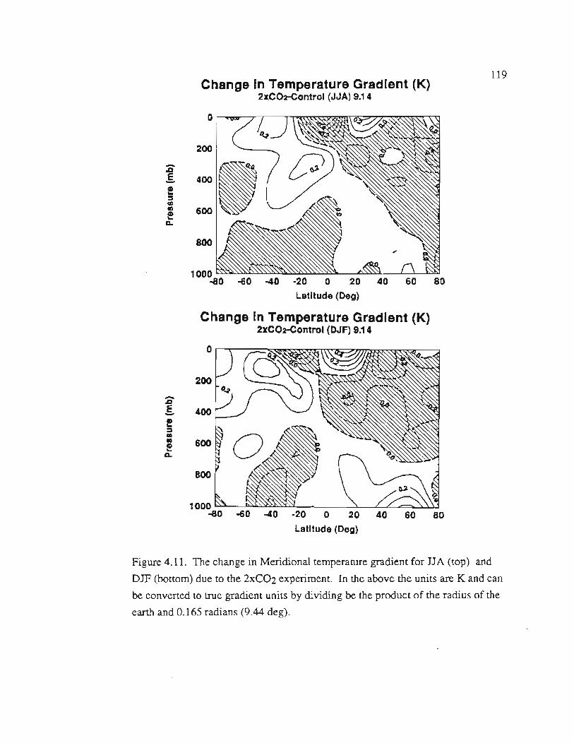
Figure 4.11. The change in Meridional temperature gradient for JJA (top) and

DJF (bottom) due to the 2XC02 experiment. In the above the units are K and can

be convened to true gradient units by dividing be the product of the radius of the

eanh and 0.165 radians (9.44 deg).

119Change In Temperature Gradient (K)

2xC02-Control (JJA)9.14

0

200- ..QA 400!::swto 600!A.

800 ,1000

-ao -60 -40 .20 0 20 40 60 80

Latitude (Deg)

Change In Temperature Gradient (K)2xC02-Control (DJF)9.14

0

200

:s-A 400!::sw! vvv

(\ -A.

800

1000-ao -60 -40 .20 0 20 40 60 80

Latitude (Deg)

120

The changes in the mass stream function for JJA and DJF resulting from the

2XC02 experiment are shown in figure 4.12. Consistent with the increase in global

kinetic energy, the Hadley circulation increases in both hemispheres by up to 3%. This

certainly would have consequences in our model if we had a prognostic determination of

cloud amount. Finally in figure 4.13 we show the 2xC02 changes in the eddy flux of

momentum (u'v') predicted by our model for JJA and DJF. In both hemispheres the

magnitude of the poleward flux of westerly momentum increases in the mid latitude

regions. Since the parameterized eddy momentum flux is highly dependent upon the

temperature gradient, this increase in mid latitude eddy momentum transfer predicted by

our model is a direct consequence of the meridional temperature gradient changes shown

in figure 4.11.

This change in eddy momentum flux is also consistent with the changes in zonal

velocity predicted by our model in figure 4.9. That is, the increase in u'v' flux in the mid

latitude regions will result in more transfer of westerly momentum out of the tropics and

into higher latitudes. This will result in an increase in the tropical easterly flow and a

corresponding increase in high latitude westerly flow. Since in general our model's

results are qualitatively consistent with the results of GCMs, we suspect that this same

basic mechanism is responsible for the changes predicted by them.

Although Rosen and Gutowski (1992) stressed the weakness of the correlations

between the changes in zonal velocity predicted by the GCMs of their study, they did

state "Comparisons among the three models of the difference in zonal-mean zonal winds

between 2XC02 and lxC02 simulations indicate a common tendency when C02 is

doubled for winds to become more easterly in much of the tropics during June-July-

.August." They were reluctant to propose any mechanism for the observed changes

predicted by the GCMs. The mechanism described above is one possible mechanism

driving the response of the GCMs.

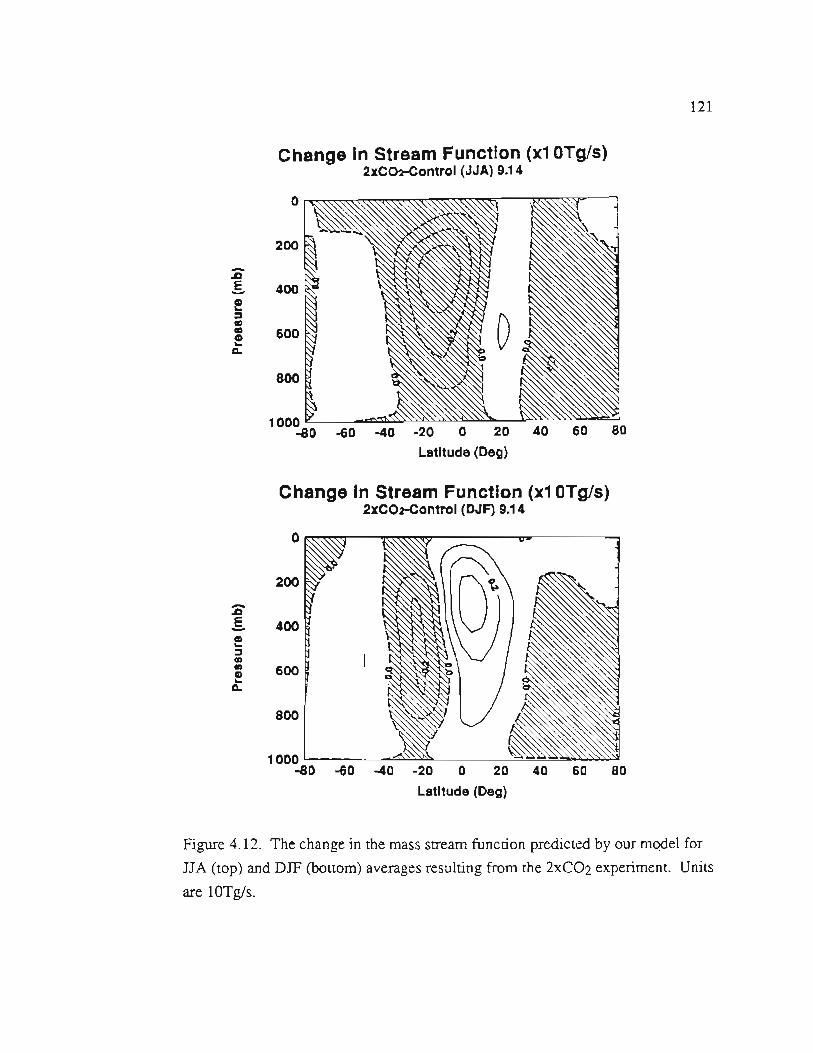
121

Figure 4.12. The change in the mass stream function predicted by our model for

JJA (top) and DJF (bottom) averages resulting from the 2XC02 experiment. Units

are lOTg/s.

Change In Stream Function (xi OTg/s)2xC02-Control(JJA)9.14

0...

200 '(A "",,""""',""""'"i""""

:DoS 400t!::I

, _0.toCD..a.

800

1000-40 .20 0 20 40 60 80-80 -60

Latitude(Deg)

Change In Stream Function (xi OTg/s)2xC02-Control(DJF)9.14

0

200-ZloS 400e::I.to 600CD..a.

800

1000 I_-<'\.,," , .

-80 -60 -40 .20 0 20 40 60 80

Latitude (Deg)

Figure 4.13. The change in the eddy momentum flux predicted by our model for

JJA (top) and DJF (bottom) averages resulting from the 2xC02 experiment. Unitsare m2fs2.

122Change In U'V' (m/s)2

2xC02-Control (JJA) 9.14

0

200-.QoS 400!(I)., 600G)..A.

800

1000-80 -60 -40 .20 0 20 40 60 80

Latitude (Deg)

Change In U'V' (m/s)22xC02-Control(DJF) 9.14

0

200r ,-or

.QE 400-G)..(I)., 600 IIG)..A.

800

1000-80 -60 -40 .20 0 20 40 60 80

Latitude (Deg)

123

4.4 Summary.

The sensitivity of the GCRC 2D statistical dynamical climate model to the

doubling of atmospheric carbon dioxide is investigated and we find that the change in

temperature structure predicted by the model has several features that are also common to

more sophisticated GCMs. In particular:

· The annual mean warming is greatest at the poles and smallest at the equator.

· There is a substantial cooling found in the stratosphere.

· The warming at the poles is greatest during the winter months for the

particular hemisphere.

· There is a maximum in warming predicted to occur in the mid to upper

tropical troposphere.

We suggest that the greater warming at the poles predicted by our model is likely the

result of the enhanced upper level temperature gradients driving more energy from the

equatorial regions towards the poles. The enhanced upper level temperature gradients

are a direct result of the local maximum in temperature change found to occur in the

upper tropical troposphere. This local maximum is believed to be associated with an

increase in the vertical transport of latent heat energy. Since the change in temperature

gradient is greatest in the winter hemisphere, this would also suggest a cause for the

greater warming at the poles predicted for the winter months.

Following the work of Rosen and Gutowski (1992), we investigated the change in

zonal mean zonal velocity predicted by our model for a doubling of C02. We find that

our model predicts:

· An increase in easterly flow from about 35°S to 40oN.

· An increase in westerly flow from 600S to 35°S and 400N to 70oN.

· An increase in easterly flow for latitudes poleward of about 65°S and 75°N.

· The net angular momentum of the atmosphere remains relatively unchanged.

With our model we are able to recognize patterns of change in the zonal velocity

for the 2xC02 experiment that are consistent with the change in temperature structure of

the atmosphere. We suggest that the increase in upper level temperature gradients

124

predicted by our model result in an increase in the simulated eddy flux of zonal

momentum u'v' , and that this causes more westerly momentum to be transferred from

the tropics to the higher latitudes. In addition, we believe that the lack of a significant

change in total atmospheric angular momentum is probably due to the lack of orography

in our model and the relatively weak coupling between the atmosphere and the solid

earth. Hence, our model atmosphere should conserve angular momentum.

We also attribute the 2% increase in global kinetic energy per unit are to the

enhanced upper level temperature gradients as well as the 3% increase in the Hadleycirculation.

CHAPTER 5

SUMMARY OF RESULTS

The GCRC two-dimensional statistical dynamical climate model presented in this

dissertation has been developed using the one-dimensional radiative convective model of

MacKay and Khalil (1991) as its basic core. Although the mid to late 1970s saw anabundance of two-dimensional climate models, their use in the 1980s and 1990s has been

limited with few exceptions (MacCraken, 1987; and Stone and Yao,1990. There are two

possible reasons for the apparent lack of interest in the use of two-dimensional climate

model over the last decade. First, the tremendous advances in computing power and the

increase in the sophistication of GCMs over the last several years has made their use very

attractive for many climate modelers. Second, the difficulties encountered in attempting

to parameterize the fluxes of eddy heat and momentum have been formidable. Recently

however, Stone and Yao (1987) and (1990) following the work of others, have made

substantial progress towards obtaining realistic parameterization schemes for calculating

the eddy fluxes of heat and momentum. We have exploited their success by

incorporating their parameterization scheme into the GCRC 2-D model.

The intent of this work was to develop a 2-D statistical dynamical climate model

(base model) that can be used for a variety of climate simulations. In chapter one we give

several arguments to support the usefulness of a suite of climate models of varyingcomplexities for the study of climate change and the interactions between the various

components of the climate system. It is also noted that the model presented in this

dissertation is the most recent and most sophisticated addition to our climate modeling

package at the Global Change Research Center. In Chapter two we describe our 2-D

model in detail. The model has latitude and height as spatial coordinates and we use a

numerical time stepping procedure to prognostically solve the primitive equations for

zonal-mean temperatures, air density, zonal velocity, and meridional velocity. The

125

126

vertical velocity, pressure, and precipitation are calculated diagnostically. Cloud

amounts, relative humidity profile, surface albedo, and the atmospheric concentrations of

C02, Cf4, N20, 03, CFCI3, and CF2Cl2have all been prescribed.

The model performance is evaluated in chapter 3, where we stress that it

reproduces the two-dimensional seasonal temperature field of the earth to fairly well.

Namely: 1) all surface temperatures predicted by the model are within 2% of observations

except at the poles where there is a maximum discrepancy of 8%,2) the annual mean

two-dimensional temperature profile is within 5% of observations except at 800S (8%

difference) and the stratosphere where the model is about 10 % too warm. The good

agreement 1?etweenthe modeled and observed temperatures at most positions is

impressive considering the limited number of adjustable parameters that we have

included in our model. It was suggested that improved boundary conditions in the model

stratosphere for the meridional velocity or an improved estimate of the relative humidity

of the tropical stratosphere may improve the simulation of the temperature minimum in

the tropical stratosphere. The model's temperature gradient in the lower tropical

troposphere seems to disagree somewhat with the observations there. We suspect that an

over simplified parameterization of the cloud radiation physics and/or an unrealistic

simulation of tropical convection is responsible for this difference between model and

observations. The fact that the agreement between modeled and observed radiation

balance of absorbed solar energy and outgoing long wave radiation is poor in the tropics

for JJA and annual averages, also suggests that improvements in the model's tropicalcloud radiative parameterization are needed. Also, we attribute a lack of model

orography to be the major reason that the near surface temperatures in the Antarctic

region simulated by the model are high in all seasons.

To improve the model's stability and performance, we have added an additional

term to the Stone and Yao (1990) parameterization of the eddy flux of sensible heat, TV,

that depends on the square of the meridional temperature gradient (equation 2.43). We

have found that the inability of their parameterization to simulate the secondary

maximum of TV near the tropopause causes our model's polar winter stratospheric

temperatures to be much lower than observed and the winter polar pressure gradients

much larger than observed. It has been stressed that future improvements can be made in

our parameterization scheme for the eddy flux of sensible heat.

.. ..- ... - ..-'-

127

The agreement between the model's zonal velocity field and observations is good.

The magnitudes of the subtropical jet streams predicted by our model are within 25% of

the observed values reported by Peixoto and Oort (1992) for JJA, DJF, and annual means.

We do however note that the model overestimates the tropical easterlies, the vertical level

of the model's jet stream is about 50 mb too high, and the latitudinal positions of the

model's jet streams are typically a little too far poleward. We have also described a

simple modification in the Stone and Yao (1987) parameterization scheme for the eddy

momentum flux, u' v' ,which enhances the model's stability by reducing polar pressure

gradients, focuses the jets closer to their observed positions at 35 degrees north and south

latitude, and gives a better estimate of the vertical-mean u'v' flux in the polar regions. We

fmd that this modification also reduces the need of the extra term of equation 2.43 for the

T'v' flux. We find that our parameterization of u' v' does a good job at simulating the

general features of the observed u' v' field.

Our model was able to give a good qualitative simulation of the mass stream

function despite the fact that the maximum magnitude of the Hadley circulation wasabout 50 % of that observed. The seasonal movement of the ITCZ and seasonal

variations in Hadley circulation strength also had good qualitative agreement withobservations and we did obtain a weak Ferrel circulation.

Chapter 4 was devoted to exploring the equilibrium response of our 2-D model to

a doubling of atmospheric carbon dioxide and comparing it to that of more sophisticated

GCMs. The change in temperature profile predicted by our model is in excellent

qualitative agreement with that typically simulated by GCMs in that our model simulated:

1) larger than average warming at the poles in winter months and not in the summer, 2) a

maximum in the change in temperature simulated for the mid to upper tropical

troposphere, and 3) stratospheric cooling. The change in mean annual global surface

temperature for the 2XC02 experiment for our model is about half of the IPCC (1990)

best guess value of 2.5 K. We attribute our reduced sensitivity to the lack of positive

feedback processes such as sea ice thickness, ice albedo, and cloud dynamics. Although

we have experimented with coupling a simplified thermodynamic sea ice model to our

atmospheric model and have obtained much greater polar warming than in our base

model, we stress the importance of moving cautiously when adding positive feedback

processes to a climate model. Small errors in assumptions and/or model physics of the

128

positive feedbacks may result in the model greatly over estimating the response of the

real climate system. We plan to couple a sea ice model to the base model.

The good performance of the model at simulating the observed zonal velocity

field has prompted us to follow the work of Rosen and Gutowski (1992) and explore the

equilibrium response our model's zonal velocity field to a 2XC02 experiment. Rosen and

Gutowski (1992) investigated the response of three GCMs (NCAR, GISS, and GFDL) to

the same experiment and found very few patterns that were similar between them.

Because our model has much less inherent noise than GCMs, it is an ideal tool for

investigating the basic mechanism behind the expected response of the real climate

system and the observed response of the GCMs. We find that doubling C02 results in an

increase in tropical easterly flow and an increase in the westerly flow at higher latitudes.

The increase in tropical easterly flow in JJA was the only pattern that Rosen and

Gutowski were willing to acknowledge as being consistent between the GCMs. We show

that the change in zonal velocity predicted by our model for the 2XC02 experiment is

closely related to the change in temperature gradient simulated by our model which in

turn drives the change in calculated u' v' flux. Since the change in the structure of the

two-dimensional temperature gradient predicted by our model is qualitatively consistent

with that simulated by most GCMs and the u' v' flux parameterization was designed by

Stone and Yao (1987) primarily to agree with the u'v' flux of the GISS model, we

conclude that the response of our model is indicative of the basic response expected of

the GCMs and possibly the real earth. Of course there are other factors that complicate

the output of the GCMs, but this is precisely the reason that a model of the sophisticationof our two-dimensional model is so attractive.

In summary the model presented in this dissertation is a g~ solid working two-

dimensional model of the earth-atmosphere climate system. Its has been intentionally

designed modularly to aid in the implementation of future improvements. Although, as

shown here, the present version of the model can be used for legitimate scientific

investigations, the real pay-off for the development of this model will come when we

begin implementing improvements into the model, such as (but not limited to) a deep

ocean model, cloud dynamics and radiative properties, a prognostic sea ice model,

prognostic hydrodynamics, and improvements in the calculation of the eddy fluxes of

129

heat and momentum. With each addition the model's perfonnance should improve and

the affect of each component of the whole can be carefully explored.

REFERENCES

Branscome, L.E., 1983a: A Parameterization of transient Eddy Heat Flux on a Beta-Plane. J. of the Atmospheric Sciences, Vol. 40, 2508-2521.

Branscome, L.E., 1983b: The Charney Baroclinic Stability Problem: ApproximateSolutions and Modal Structures. Journal. of the Atmospheric Sciences, Vol. 40, 1393-1409.

Budyko, M.I., 1969. The Effect of Solar Radiation Variations on the Climate of theEarth. Tellus, 21, 611-619.

Charney, J.G., 1947. The Dynamics of Long Waves in a Baroclinic Westerly Current.Journal of Meteorology, Vol. 4, No.5, 135-163.

Donner, L., and V. Ramanathan, 1980. Methane and Nitrous Oxide: Their effects on theTerrestrial Climate. Journal Of Atmospheric Sciences, Vol. 37, 119-124.

Eady, E.T., 1949. Long Waves and Cyclone Waves. Tellus, Vol. 1, No.3, 33-52.

Eagleman, l.R, 1985. Meteorology: The Atmosphere in Action. Wadsworth Publishing,Belmont California.

Forrester, F. H., 1981. 1001 Questions Answered About the Weather. DoverPublications, New York.

Ghan, S.J., J.W. Lingaas, M.E. Schlesinger, RL. Mobley, and W.L. Gates, 1982. ADocumentation of the OSU Two-Level Atmospheric General Circulation Model.Climatic Research Institute Report No. 35, Oregon State University, Corvallis, Oregon.

Goldstein, H. 1982. Classical Mechanics Second Edition (chapter 3). Addison WesleyPublishers, Reading Mass.

Goody, RM. and J.C.G. Walker, 1972. Atmospheres. Prentice-Hall, Englewood Cliffs,N.J.

Green, J.S.A., 1970. Transfer Properties of the Large-Scale Eddies and the GeneralCirculation of the Atmosphere. Quarterly Journal of the Royal Meteorological Society.Vol. 96, No. 408, 157-185.

130

131

Hahn, c.J., S.G. Warren, J. London, RL. Jenne and RM. Chervin, 1987: ClimatologicalData for Clouds over the Globe from Surface Observations, Report NDP-026, CarbonDioxide Information Center, Oak Ridge, TN 37831-6050

Hansen, J., G. Russell, D. Rind, P. Stone, A. Lacis, S. Lebedeff, R. Ruedy and L. Travis,1983. Efficient Three-Dimensional Global Models for Climate Studies: Models I and II.Monthly Weather Review, Vo1. 111, No.4, 609-662.

Harvey, L.D.D., 1988. Development of a Sea Ice Model for Use in Zonally AveragedEnergy Balance Climate Models. Journal of Climate, Vo1. 1, 1221-1238.

Held, LM., 1978. The Vertical Scale of an Unstable Baroclinic Wave and Its Importancefo Eddy Heat Flux Parameterizations. Journal of the Atmospheric Sciences, Vol 35,572-576.

Held, LM.and M.J. Suarez, 1978. A Two-Level Primitiv Equation Atmospheric ModelDesigned for Climate Sensitivity Experiments. Journal of the Atmospheric Sciences, Vol35, 206-229.

Held, LM., 1993. Large-Scale Dynamics and Global Warming. Bulletin of the AmericanMeteorological Society. V01.74, 228-241.

Henderson-Sellers, A. and K. McGuffie. 1987. A Climate Modeling Primer. John Wiley& Sons, New York.

Holton, J.R, 1979. An Introduction to Dynamic Meteorology, Second Edition.International Geophysics Series Vol. 23. Academic Press, Inc. Harcourt BraceJovanovich, Publishers, New York.

Hunt, B.G., 1973, Zonally Symmetric Global General Circulation Models With andWithout the Hydrologic Cycle. Tellus XXV, 4, 337~354.

IPCC, 1990. Climati Change, The IPCC Scientific Assessment. J.T. Houghton, G.J.Jenkins, and J.J. Ephraums Editors. Cambridge University Press, Cambridge U.K.

Karl, T.R, J.D. Tarpley, RO. Quayle, H.P. Diaz, D.A. Robinson, and RS. Bradley,1989. The Recent Climate Record: What it Can and Cannot Tell Us. Reviews ofGeophysics, 27, 3, 405-430

Kasahara, A., 1977. Computational Aspects of Numerical Models for Weather Predictionand Climate Simulation. In Methods in Computational Physics Volume 17 J. ChangEditor. Academic Press, New York.

Khalil, M.A.K. and RA. Rasmussen, 1985. Modeling Chemical Transport and MassBalances in the Atmosphere. Chapter 2 in Environmental Exposure From ChemicalsVolume II W.B. Neely and G.E. Blau Editors. CRC Press, Inc. Boca Raton, Florida.

132

Kiehl, J.T. and V. Ramanathan, 1983. C02 Radiative Parameterization Used in ClimateModels: Comparison With Narrow Band Models and With Laboratory Data. Journal ofGeophysical Research, Vol 88, No. C9, 5191-5202

Kuo, H.L., 1977. Analytic Infared Transmissivities of the Atmosphere. Beitr. Phys.Atmos., Vol. 50, 331-349.

Lacis, A.A., and J.E. Hansen, 1974. A Parameterization for the absorption of SolarRadiation in the Earth's Atmosphere. Journal Of Atmospheric sciences, Vol. 31, 118-133.

Liu, S.C., J.R McAfee, and RJ. Cicerone, 1984. Radon 222 and Tropospheric VerticalTransport. J. of Geophysical Research, Vol. 89, No. D5, 7291-7297.

Liou, Kuo-Nan. 1980. An Introduction to Atmospheric Radiation.Academic Press.

Lorentz, E.N., 1967. The Nature and Theory of the General Circulation of theAtmosphere. Published by The Wodd Meteorological Organization.

MacCracken, M.C., 1972. Zonal Atmospheric Model ZAM2. Lawrence LivermoreNational Lab. UCRL-74254 UNCLAS

MacCracken, M. C. and S. Ghan. 1987. Design and Use of Zonally-Averaged ClimateModels, UCRL-94338, University of California, Livermore CA, 44pp.\

MacKay, RM., 1990. The Oregon Graduate Institute One-Dimensional Time-DependentRadiative Convective Model: Theory and Application. M.S. Thesis, The OregonGraduate Institute of Science & Technology, Department of Environmental Science andEngineering, Global Change Research Center, Beaverton, Oregon.

MacKay, RM., and M.A.K. Khalil, 1991. Theory and Development of a One-Dimensional Time-Dependent Radiative Convective Climate Model. Chemosphere, Vol.22. No. 3-4318-417.

MacKay, RM. and M.A.K. Khalil, 1992. Global Change Science and Education. Paperpresented at the 1992 Aspen Global Change Institute, Aspen Colorado.

MacKay, RM. and M.A.K. Khalil, 1993. Computer Based Activities for UnderstandingGlobal Change. In the Proceedings of the 1st International Conference on Computer-aided Learning and Distance Learning in Meteorology, Hydrology, and Oceanography(CALMet).

Manabe, S. and RF. Strickler, 1964. Thermal Equilibrium of the Atmosphere with aConvective Adjustment. Journal Of Atmospheric sciences, Vol. 21, 361-385

133

Manabe, S. and R.T. Wetherald, 1967. Thermal Equilibrium of the Atmosphere with agiven Distribution of Relative Humidity. Journal of Atmospheric Sciences, Vol. 24, No.3,241-259

Manabe, S. and K. Bryan. 1969. Climate Calculations with a Combined OceanAtmosphere Model. Journal of the Atmospheric Sciences, Vol. 26, 786-789.

Mitchell, John F.B., 1989. The "Greenhouse" Effect and Climate Change. Reviews ofGeophysics Vol. 27 No.1 115-139.

North, G.R., 1975. Theory of Energy Balance Climate Models. Journal of theAtmospheric Sciences, Vol. 32, 3-15

Newell, R.E., J.W. Kidson, D.G. Vincent, and G.J. Boer, 1972. The General Circulationof the Tropical Atmosphere and Interactions with Extratropical Latitudes Vol.1. MITPress, Cambridge, Mass.

Ohring, G. and S. Adler. 1978. Some Experiments with a Zonally Averaged ClimateModel. Journal of the Atmospheric Sciences, Vol. 35, 186-205

Parkinson, C.L. and W.M. Washington, 1979. A Large-Scale Numerical Model of SeaIce. Journal of Geophysical Research, Vol. 84, No. Cl, 311-337.

Pedlosky, J. 1979. Geophysical Fluid Dynamics. Springer-Verlag Publishers, NewYork.

Peixoto, J. P. and A.H. Oort, 1992. Physics of Climate. American Institue of Physics.

Peng, L., M-D Chou, and A. Arking, 1982. Climate Studies with a Multilayer EnergyBalance Model. Part I: Model Description and Sensitivity to the solar Constant. Journalof the Atmospheric Sciences, Vol. 39, 2639-2656.

Phillips, N. A., 1954. Energy Transformations and Meridional Circulations AssociatedWith Simple Baroclinic Waves in a Two-level, Quasi-geostrophic Model. Tellus Vol. 6,pp 273-286.

Ramanathan, V. 1975. Greenhouse Effect Due to Chlorofluorocarbons: ClimaticImplications. Science Vol. 19050-51.

Ramanathan, V., 1976. Radiative Transfer Within the Earth's Troposphere andStratosphere: A simplified Radiative-Convective Model. Journal of AtmosphericSciences, Vol. 33, 1330-1346.

Ramanathan, V., 1977. Interactions between Ice-Albedo, Lapse-Rate and Cloud-TopFeedbacks: An Analysis of the Nonlinear Response of a GCM Climate model. Journalof Atmospheric Sciences, Vol. 34, 1885-1897.

134

Ramanathan, V., and J.A. Coakley Jr., 1978. Climate Modeling Through RadiativeConvective Models. Rev. of Geophysics and Space Physics, 6, 465-489.

Ramanathan, V., E.J.Pitcher, R.C. Malone, and M.L. Blackmon, 1983. The Response ofa Spectral General Circulation Model to refinements in Radiative Processes.Journal ofAtmospheric sciences, Vol. 40, 605-631.

Ramanathan, V., RJ. Cicerone, H.B. Singh, and J.T. Kiehl, 1985. Trace Gas Trends andTheir Potential Role in Climatic Change. Journal of Geophysical Research, Vol. 90,5547-5566.

Rasool, S.I. and S.H. Schneider, 1971. Atmospheric Carbon Dioxide and Aerosols:Effects of Large Increases on Global Climate. Science, Vol. 173, 138-141

Richardson, L. F., 1922. Weather Prediction by Numerical Process, CambridgeUniversity Press, reprinted Dover, New York, 236 pp.

Robens, R.E., J.E.A. Selby, and L.M. Biberman, 1976. Infared Continuum Absorptionby Atmospheric Water Vapor in the 8-12 Jlm Window. Applied Optics, Vol.15, No.9,2085-2090.

Rosen, R D. and W. J. Gutowski Jr., 1992. Response to Zonal Winds and AtmosphericAngular Momentum to a doubling of C02. Journal of Climate, Vol. 5, No. 12, 1391-1404

Rosen, RD., D.A. Salstein, and T.M. Wood, 1990. Discrepancies in the Eanhe-Atmosphere Angular Momentum Budget, Journal of Geophysical Research, Vol. 95, No.Bl,265-279.

Rosen, RD., D.A. Salstein, and T.M. Wood, 1991. Zonal Conttibutions to GlobalMomentum Variations on Intraseasonal Through Interannual Time Scales, Journal ofGeophysical Research, Vol. 96, No. D3, 5145-5151.

Saltzman, B., 1978. A Survey of Statistical-Dynamical Models of the TerresttialClimate. In Ad~ances in Geophysics Vol. 20 Academic Press, New York.

Sasamori, T., J. London, and D.V. Hoyt, 1972. Radiation Budget of the SouthernHemisphere. Meteorological Monographs, Vo1.13,No.35.9-23

Schlesinger, M.E. and J.F.B. Mitchell, 1985. Model Projections of the EquilibriumClimatic Response to Increased Carbon Dioxide. Chapter 4 of The Potetial ClimaticEffects of Increasing Carbon Dioxide. DOEIER-0237.

Schlesinger, M.E. and J.F.B. Mitchell, 1987. Climate Model Simulations of theEquilibrium Climatic Response to Increased Carbon Dioxide. Reviews of Geophysics,Vol. 25, No.4, 760-798.

135

Schneider, E.K. and RS. Lindzen, 1977. Axially Symmetric Steady-State Models of theBasic State for Instability and Climate Studies. Part I. Linearized Calculations. Journalof the Atmospheric Sciences, Vol. 34, 263-279.

Schneider, E. K., 1984. Response of the Annual and Zonal Mean Winds andTemperatures to Variations in the Heat and Momentum Sources. Journal of theAtmospheric Sciences, Vol. 41, 1093-1115.

Schneider, S. H., 1989. Global Warming: Are We Entering the Greenhouse Century?Sierra Club Books, San Francisco, Calif.

Schoeberl, M. R and D. F. Strobel, 1978. The Zonall Averaged Circulation of theMiddle Atmosphere. Journal of the Atmospheric Sciences, Vol. 35,577-591.

Sellers, W.D., 1973. A New Global Climate Model, Journal of Applied Meteorology,Vol. 12,241-254.

Semtner, A.J. , 1976. A Model for the thermodynamic Growth of Sea Ice in NumericalInvestigations of Climate. Journal of Physical Oceanography, "pp379-389.

Shapiro, R, 1970. Smoothing, Filtering, and Boundary Effects. Reviews of Geophysicsand Space Physics, Vol. 8, No.2, 359-387

Smagorinsky, J., 1983. The Beginnings of Numerical Weather Prediction and GeneralCirculation Modeling: Early Recollections. In B. Saltzmann (ed.) Theory of Climate,Academic Press, New York, pp3-38.

Stephens, G.L., 1984. The Parameterization of Radiation for Numerical WeatherPrediction and Climate Models. Monthly Weather Review, Vol. 112,826-867.

Stone, P. H., 1972. The Effect of Large-Scale Eddies on Clamatic Change. Journal ofthe Atmospheric Sciences, Vol. 30, 521-529

Stone, P. H., 1973. A Simplified Radiative-Dynamical Model for the Static Stability ofRotating Atmospheres. Journal of the Atmospheric Sciences, Vol. 29,405-418.

Stone, P. H., 1978. Baroclinic Adjustment. Journal of the Atmospheric Sciences, Vol.35,561-571.

Stone, P.H., and J.H. Carlson, 1979. Atmospheric Lapse Rate Regimes and TheirParameterization. Journal of Atmospheric Sciences, Vol. 36,415-423.

Stone, P.H., and M.-S. Yao. 1987. Development of a Two-Dimensional ZonallyAveraged Statistical-Dynamical Model. Part II: The Role of Eddy Momentum Fluxes inthe General Circulation and their Parameterization. Journal of the Atmospheric Sciences,Vol. 44, No. 24, 3769-3786.

136

Stone, P.H., and M.-S. Yao. 1990. Development of a Two-Dimensional ZonallyAveraged Statistical-Dynamical Model. Part III: The Parameterization of Eddy Fluxesof Heat and Moisture. Journal of Climate Volume 3, 726-740.

Stone, P.H., 1992. Forecast Cloudy: The Limits of Global Warming Models.Technology Review, Feb/Mar 1992, pp. 32-40.

Temkin, R. L. and EM. Snell, 1976. An Annual Zonally Averaged HemisphericalClimate Model with Diffuse Cloudiness Feedback. Journal of the Atmospheric Sciences,VoL 33, 1671-1685.

Vernekar, A. D. and H. D. Chang, 1978. A Statistical-Dynamical Model for StationaryPerturbations in the Atmosphere. Journal of the Atmospheric Sciences, Vol. 35,433-444.

Wang, W-C, M.P. Dudek, X-Z. Liang, and J.T. Kiehl, 1990a. Inadequacy of EffectiveC02 as a Proxy in Simulating the Greenhouse Effect of Other Radiatively Active Gases.Nature, Vol. 350, pp573-577.

Wang, W.-C., G. Molnar, M.K.W. KO, S. Goldenberg, and N.D. Sze, 1990b.Atmospheric Trace Gases and Global Climate: A Seasonal Model Study. Tellus, 42B, 2,149-161.

Washington, W.M., and c.L. Parkinson, 1986. An Introduction to Three-DimensionalClimate Modeling. University Science Books.

Watts, R.g. and M. Morantine, 1990. Rapid Climatic Change and the Deep Ocean.Climatic Change, Vol. 16,83-97.

Willmott, C. J. and D. R. Legates, 1993. A Comparison of GCM-Simulated andObserved Mean January and Jully Surface Air Temperature. Journal of Climate, Vol. 6,No. 2,274-291

Yao, M.-S., and P.R. Stone, 1987. Development of a Two-Dimensional ZonallyAveraged Statistical-Dynamical Model. Part I: The Parameterization of MoistConvection and its Role in the General Circulation. Journal of the Atmospheric Sciences,Vol. 44, No.1, 65-82.

APPENDIX ALIST OF SYMBOLS

Qs

S(t)H

r(t)

Daily average flux of incident solar radiation per unit surface area,

Tme dependent solar constant at the top of the atmosphere

Half day length in hoursEarth-sun distance at time t

Mean Earth-Sun distance 1.49x1011m

Solar declination

Latitude

Cosine of daily average solar zenith angleSnow-free land surface albedo

Snow-covered land surface albedo

% Ocen fractionOcean surface albedo

(j

SJ.

1-Jl

Surface wind speedMean sea ice thickness

Specific heat of water 4.19 J/K/g

Specific heat of ice 2.0 J/K/g

Depth of the mixed layer (typically 50 m)Snow thickness over sea ice

Density of water (1.0 glcm3)

Density of ice (0.9 glcm3)

Ocean temperature,

Downward flux of IR radiation at the Earth's surface from the atmosphere

5.67xlO-8W/m21K4

Downward flux of solar radiation at the Earth's surface

Vs

XI

Cw

CI

D

Hs

Pw

PI

To

FJ.

137

sfSHLH

AO

AI

KI

Kg

TIa

z

p

PR

T

f

w

u

v

t

.~t

~tr

c*E*

i

i+1/2

J

j+ 1/2

138

Upward flux of solar radiation at the Earth's surface

Flux of sensible heat leaving the Earth's surface

Flux of latent heat leaving the Earth's surfaceSurface area of the ocean

Area of sea ice

Thennal conductivity ice (2.2 J/K/m)

Thennal conductivity snow (.3 J/K/m)

Temperature of the top of the sea iceRadius of the earth

Horizontal turbulent difusivity constant for ocean heat transport

Land surface temperature

Fraction of ocean covered by sea ice

Longitude

vertical height

zonal average pressurezonal average air density

gas constant (287 J/(g K) for dry air

zonal average atmospheric temperature

coriolis parameter

vertical velocity

zonal velocity

meridional velocityTime

time step for dynamical numerical integration (0.25 hr)

time step for radiation numerical integration (2.0 hr)Rate of condensation

Evaporation rate

Vertical center of model grid

Bottom boundary of model grid i

Horizontal center of model grid

Southern boundary of model grid j

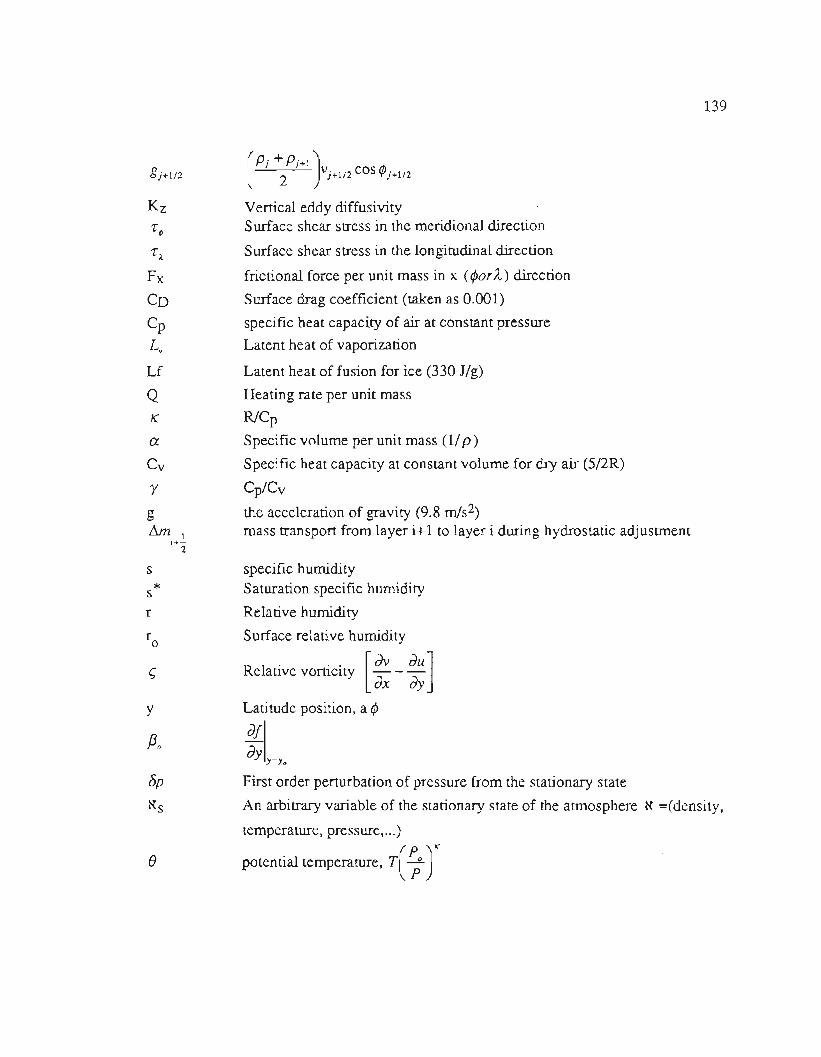
Lf

Q1C

a

Cv

rgt::..m1

i+'2

s*s

r

y

8p

~s

()

139

Vertical eddy diffusivitySurface shear stress in the meridional direction

Surface shear stress in the longitudinal direction

frictional force per unit mass in x (tfJorA) direction

Surface drag coefficient (taken as 0.(01)

specific heat capacity of air at constant pressure

Latent heat of vaporization

Latent heat of fusion for ice (330 JIg)

Heating rate per unit mass

R/CpSpecific volume per unit mass (11p )

Specific heat capacity at constant volume for dry air (5/2R)

Cp/Cv

the acceleration of gravity (9.8 m/s2)mass transport from layer i+1 to layer i during hydrostatic adjustment

specific humiditySaturation specific humidity

Relative humidity

Surface relative humidity

R I. ..

[

av au]e anve vorttCIty ax - iJy

Latitude position, a tfJ

atiJy'Y=Yo

First order perturbation of pressure from the stationary state

An arbitrary variable of the stationary state of the atmosphere ~ =(density,

temperature, pressure,...)

potentialtemperature,T(; )K

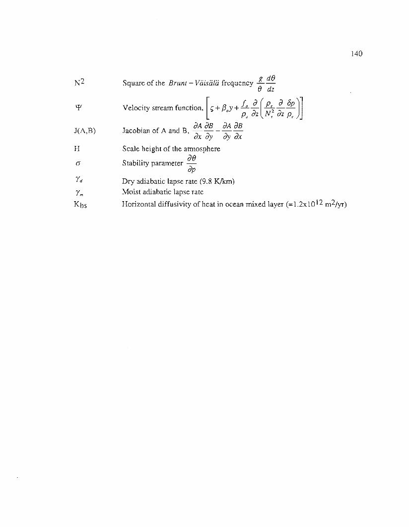
J(A,B)

H

140

S fth B 1r'. " ,..

ft g dequare 0 e runt - "alsa a equency--e dz

Velocity stream function,[,+ {JoY + 10 ~

(Ps2 ~ 8p

)]Ps oZ Ns aZ Ps

, dA dB dA dBJacobIan of A and B -- ---

, dxdy dydxScale height of the atmosphere

S b.l. de

ta I Ity parameter -dp

Dry adiabatic lapse rate (9.8 K/km)Moist adiabatic lapse rate

Horizontal diffusivity of heat in ocean mixed layer (=1.2x1012 m2/yr)

APPENDIX B

CLOUD AND OZONE DATA USED IN THE GCRC 2D MODEL

B.l. Clouds

B.l.l High Clouds

Table B.t. High cloud fraction (%) used in the aCRC 2D model for each season. VaIueswere interpolated from NCAR cloud data set; See Hahn et aI. (1988).

141

Latitude (Deg) Season

MAM JJA SON DJF

-80.3 22.3 20.2 37.2 28.1

-70.8 22.9 20.4 26.6 23.2

-61.4 24.0 23.8 28.1 18.8

-51.9 17.6 14.0 17.5 18.3

-42.5 14.8 13.4 15.7 16.5

-33.1 11.7 10.4 11.6 10.3

-23.6 9.9 7.0 9.3 11.4

-14.2 12.4 6.7 10.0 16.7

-4.7 16.4 12.1 13.6 16.8

4.7 21.6 23.0 20.9 19.5

14.2 15.4 24.1 19.6 12.8

23.6 12.5 16.2 11.3 8.9

33.1 20.6 14.0 14.0 16.8

42.5 20.8 15.5 16.1 18.0

51.9 24.5 20.5 22.5 24.0

61.4 25.7 21.1 24.1 25.2

70.8 21.3 18.8 18.0 17.7

80.3 29.2 26.4 23.0 16.8

142

50 or % Cloud Cover High Cloud

40

30

MAM

[]-;- JJA

_u_+ uO. SON

-.~--DJF

-90 -60 -30 0 30

Latitude (deg)

60 90

Figure B.1. Graphical display of high cloud fraction (%) from sata in Table B.1.

B.1.2. Middle Clouds

Table B.2. Middle cloud fraction (%) used in the GCRC 2D Model for each season.Values were interpolated from NCAR cloud data set obtained from Roy Jenny. See Hahnet al. 1988.

Latitude (Deg) Season

MAM JJA SON DJF

-80.3 19.4 15.1 20.3 30.5

-70.8 38.2 31.0 32.9 38.5

-61.4 47.5 45.4 39.9 49.7

-51.9 40.7 31.8 29.0 46.6

-42.5 28.5 27.7 27.7 32.1

-33.1 25.2 23.3 25.5 23.5

-23.6 20.6 17.9 20.5 22.7

-14.2 21.3 16.5 19.6 28.2

-4.7 28.2 23.5 25.3 32.0

4.7 31.3 39.8 36.7 30.2

14.2 15.3 34.0 26.2 15.6

23.6 22.4 23.4 21.5 21.8

33.1 27.5 22.7 24.6 28.0

143

50 or % Cloud Cover

r;.~

;,. "., 40PI-' '\-t ,\,

d. , tel

7' ·

~' 3 .p

1 ',P/.., -~ ..,: .

10

Middle Cloud

MAM

--D-JJA

uu. _u SON

---<>---DJF

-90 -60 -30 0 30

Latitude (deg)

60 90

Figure B.2. Graphical display of middle cloud fraction (%) from sata inTable B.2

B.I.3 Low Cloud

Table B3. Low cloud fraction (%) used in the GCRC 2D Model for each season. Valueswere interpolated from NCAR cloud data set obtained from Roy Jenny. See Hahn et al.1988.

42.5 31.7 27.7 29.4 33.3

51.9 32.6 33.5 36.4 36.2

61.4 34.3 35.4 42.2 39.7

70.8 32.5 37.4 41.0 33.5

80.3 25.6 36.7 37.5 26.9

Latitude (Deg) Season

Low MAM JJA SON DJF

-80.3 11.0 7.5 9.7 12.6

-70.8 33.2 30.9 28.5 36.0

-61.4 64.9 66.0 67.2 64.7-51.9 68.6 63.6 69.2 70.0

-42.5 58.5 57.0 55.1 57.2-33.1 47.6 47.5 48.2 46.6

-23.6 40.9 40.2 42.8 42.5-14.2 41.6 43.5 45.5 44.2

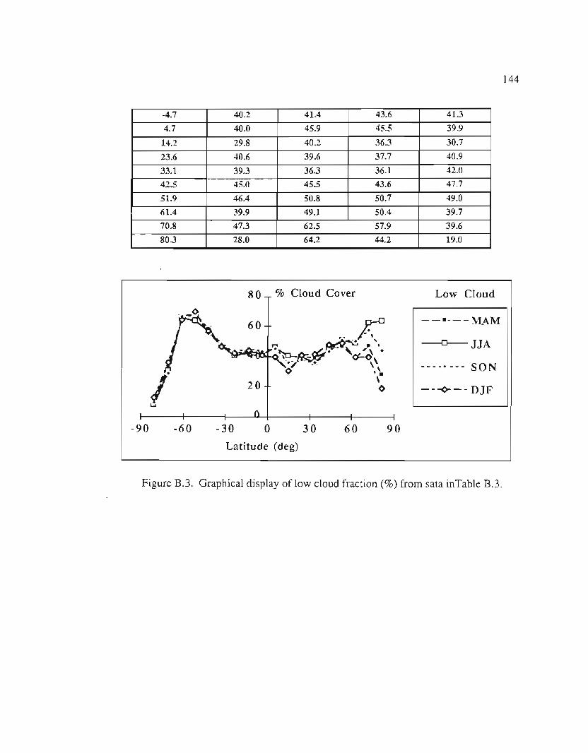
144

Cloud Cover Low Cloud

MAM

---0-- JJA

--- SON

---<>---DJF

-90 -60 -30 o 30 60 90

Latitude (deg)

Figure B.3. Graphical display of low cloud fraction (%) from sata inTable B.3.

-4.7 40.2 41.4 43.6 41.3

4.7 40.0 45.9 45.5 39.9

14.2 29.8 40.2 36.3 30.7

23.6 40.6 39.6 37.7 40.9

33.1 39.3 36.3 36.1 42.0

42.5 45.0 45.5 43.6 47.7

51.9 46.4 50.8 50.7 49.0

61.4 39.9 49.1 50.4 39.7

70.8 47.3 62.5 57.9 39.6

80.3 28.0 64.2 44.2 19.0

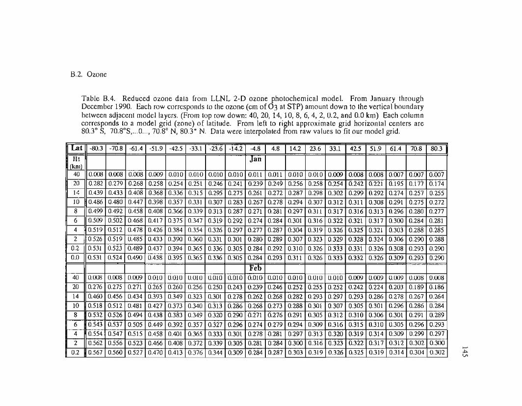
B.2. Ozone

Table 8.4. Reduced ozone data from LLNL 2-D ozone photochemical model. From January throughDecember 1990. Each row corresponds to the ozone (cm of 03 at STP) amount down to the vertical boundarybetween adjacent model layers. (From top row down: 40,20, 14, 10, 8, 6, 4, 2, 0.2, and 0.0 km) Each columncorresponds to a model grid (zone) of latitude. From left to right approximate grid horizontal centers are80.3° 8, 70.8°8,...0..., 70.8° N, 80.3* N. Data were interpolated from raw values to fit our model grid.

-~VI

Lat -80.3 -70.8 -61.4 -51.9 -42.5 -33.1 -23.6 -14.2 -4.8 4.8 14.2 23.6 33.1 42.5 51.9 61.4 70.8 80.3

lit Jan(km)

40 0.008 0.008 0.008 0.009 0.010 0.010 0.010 0.010 0.011 0.011 0.010 0.010 0.009 0.008 0.008 0.007 0.007 0.00720 0.282 0.279 0.268 0.258 0.254 0.251 0.246 0.241 0.239 0.249 0.256 0.258 0.254 0.242 0.221 0.195 0.177 0.17414 0.439 0.433 0.408 0.368 0.336 0.315 0.295 0.275 0.261 0.272 0.287 0.298 0.302 0.299 0.292 0.274 0.257 0.25510 0.486 0.480 0.447 0.398 0.357 0.331 0.307 0.283 0.267 0.278 0.294 0.307 0.312 0.311 0.308 0.291 0.275 0.2728 0.499 0.492 0.458 0.408 0.366 0.339 0.313 0.287 0.271 0.281 .0.297 0.311 0.317 0.316 0.313 0.296 0.280 0.2776 0.509 0.502 0.468 0.417 0.375 0.347 0.319 0.292 0.274 0.284 0.301 0.316 0.322 0.321 0.317 0.300 0.284 0.281

4 0.519 0.512 0.478 0.426 0.384 0.354 0.326 0.297 0.277 0.287 0.304 0.319 0.326 0.325 0.321 0.303 0.288 0.2852 0.526 0.519 0.485 0.433 0.390 0.360 0.331 0.301 0.280 0.289 0.307 0.323 0.329 0.328 0.324 0.306 0.290 0.288

0.2 0.531 0.523 0.489 0.437 0.394 0.365 0.336 0.305 0.284 0.292 0.310 0.326 0.333 0.331 0.326 0.308 0.293 0.2900.0 0.531 0.524 0.490 0.438 0.395 0.365 0.336 0.305 0.284 0.293 0.311 0.326 0.333 0.332 0.326 0.309 0.293 0.290

}t'eb40 0.008 0.008 0.009 0.010 0.010 0.010 0.010 0.010 0.010 0.010 0.010 0.010 0.010 0.009 0.009 0.009 0.008 0.00820 0.276 0.275 0.271 0.265 0.260 0.256 0.250 0.243 0.239 0.246 0.252 0.255 0.252 0.242 0.224 0.203 0.189 0.186

14 0.460 0.456 0.434 0.393 0.349 0.323 0.301 0.278 0.262 0.268 0.282 0.293 0.297 0.293 0.286 0.278 0.267 0.264

10 0.518 0.512 0.481 0.427 0.373 0.340 0.313 0.286 0.268 0.273 0.288 0.301 0.307 0.305 0.301 0.296 0.286 0.284

8 0.532 0.526 0.494 0.438 0.383 0.349 0.320 0.290 0.271 0.276 0.291 0.305 0.312 0.310 0.306 0.301 0.291 0.289

6 0.543 0.537 0.505 0.449 0.392 0.357 0.327 0.296 0.274 0.279 0.294 0.309 0.316 0.315 0.310 0.305 0.296 0.293

4 0.554 0.547 0.515 0.458 0.401 0.365 0.333 0.301 0.278 0.281 0.297 0.313 0.320 0.319 0.314 0.309 0.299 0.2972 0.562 0.556 0.523 0.466 0.408 0.372 0.339 0.305 0.281 0.284 0.300 0.316 0.323 0.322 0.317 0.312 0.302 0.300

0.2 0.567 0.560 0.527 0.470 0.413 0.376 0.344 0.309 0.284 0.287 0.303 0.319 0.326 0.325 0.319 0.314 0.304 0.302

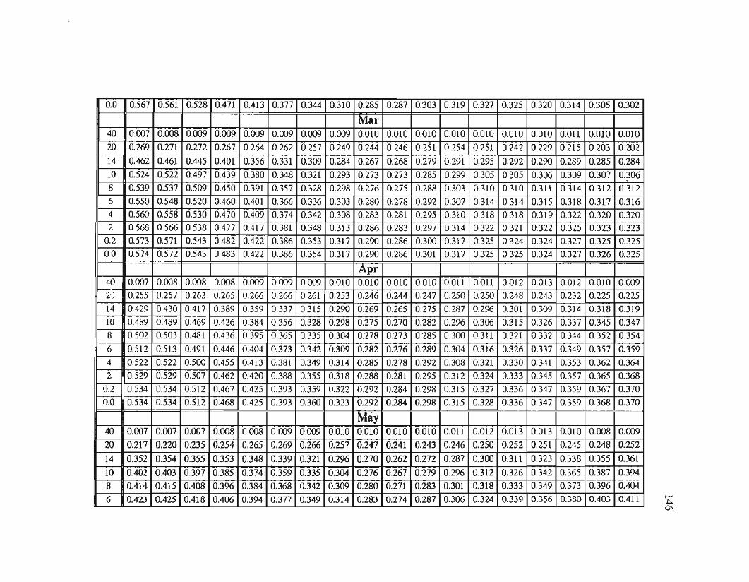
-~0\

0.0 0.567 0.561 0.528 0.471 0.413 0.371 0.344 0.310 0.285 0.287 0.303 0.319 0.327 0.325 0.320 0.314 0.305 0.302

Mar40 0.007 0.008 0.009 0.009 0.009 0.009 0.009 0.009 0.010 0.010 0.010 0.010 0.010 0.010 0.010 0.011 0.010 0.01020 0.269 0.271 0.272 0.267 0.264 0.262 0.257 0.249 0.244 0.246 0.251 0.254 0.251 0.242 0.229 0.215 0.203 0.20214 0.462 0.461 0.445 0.401 0.356 0.331 0.309 0.284 0.267 0.268 0.279 0.291 0.295 0.292 0.290 0.289 0.285 0.28410 0.524 0.522 0.497 0.439 0.380 0.348 0.321 0.293 0.273 0.273 0.285 0.299 0.305 0.305 0.306 0.309 0.307 0.3068 0.539 0.537 0.509 0.450 0.391 0.357 0.328 0.298 0.276 0.275 0.288 0.303 0.310 0.310 0.311 0.314 0.312 0.3126 0.550 0.548 0.520 0.460 0.401 0.366 0.336 0.303 0.280 0.278 0.292 0.307 0.314 0.314 0.315 0.318 0.317 0.3164 0.560 0.558 0.530 0.470 0.409 0.374 0.342 0.308 0.283 0.281 0.295 0.310 0.318 0.318 0.319 0.322 0.320 0.3202 0.568 0.566 0.538 0.471 0.417 0.381 0.348 0.313 0.286 0.283 0.297 0.314 0.322 0.321 0.322 0.325 0.323 0.323

0.2 0.573 0.571 0.543 0.482 0.422 0.386 0.353 0.317 0.290 0.286 0.300 0.317 0.325 0.324 0.324 0.327 0.325 0.3250.0 0.574 0.572 0.543 0.483 0.422 0.386 0.354 0.317 0.290 0.286 0.301 0.317 0.325 0.325 0.324 0.327 0.326 0.325

Apr40 0.007 0.008 0.008 0.008 0.009 0.009 0.009 0.010 0.010 0.010 0.010 0.011 0.011 0.012 0.013 0.012 0.010 0.00920 0.255 0.257 0.263 0.265 0.266 0.266 0.261 0.253 0.246 0.244 0.247 0.250 0.250 0.248 0.243 0.232 0.225 0.22514 0.429 0.430 0.417 0.389 0.359 0.337 0.315 0.290 0.269 0.265 0.275 0.287 0.296 0.301 0.309 0.314 0.318 0.31910 0.489 0.489 0.469 0.426 0.384 0.356 0.328 0.298 0.275 0.270 0.282 0.296 0.306 0.315 0.326 0.337 0.345 0.3478 0.502 0.503 0.481 0.436 0.395 0.365 0.335 0.304 0.278 0.273 0.285 0.300 0.311 0.321 0.332 0.344 0.352 0.3546 0.512 0.513 0.491 0.446 0.404 0.373 0.342 0.309 0.282 0.276 0.289 0.304 0.316 0.326 0.337 0.349 0.357 0.3594 0.522 0.522 0.500 0.455 0.413 0.381 0.349 0.314 0.285 0.278 0.292 0.308 0.321 0.330 0.341 0.353 0.362 0.3642 0.529 0.529 0.507 0.462 0.420 0.388 0.355 0.318 0.288 0.281 0.295 0.312 0.324 0.333 0.345 0.357 0.365 0.368

0.2 0.534 0.534 0.512 0.467 0.425 0.393 0.359 0.322 0.292 0.284 0.298 0.315 0.327 0.336 0.347 0.359 0.367 0.3700.0 0.534 0.534 0.512 0.468 0..425 0.393 0.360 0.323 0.292 0.284 0.298 0.315 0.328 0.336 0.347 0.359 0.368 0.370

Vay40 0.007 0.007 0.007 0.008 0.008 0.009 0.009 0.010 0.010 0.010 0.010 0.011 0.012 0.013 0.013 0.010 0.008 0.00920 0.217 0.220 0.235 0.254 0.265 0.269 0.266 0.257 0.247 0.241 0.243 0.246 0.250 0.252 0.251 0.245 0.248 0.252

14 0.352 0.354 0.355 0.353 0.348 0.339 0.321 0.296 0.270 0.262 0.272 0.287 0.300 0.311 0.323 0.338 0.355 0.36110 0.402 0.403 0.397 0.385 0.374 0.359 0.335 0.304 0.276 0.267 0.279 0.296 0.312 0.326 0.342 0.365 0.387 0.3948 0.414 0.415 0.408 0.396 0.384 0.368 0.342 0.309 0.280 0.271 0.283 0.301 0.318 0.333 0.349 0.373 0.396 0.4046 0.423 0.425 0.418 0.406 0.394 0.371 0.349 0.314 0.283 0.274 0.287 0.306 0.324 0.339 0.356 0.380 0.403 0.411

-~

4 0.432 0.433 0.426 0.414 0.402 0.384 0.356 0.319 0.286 0.277 0.291 0.311 0.329 0.344 0.361 0.386 0.410 0.4172 0.439 0.440 0.433 0.421 0.409 0.391 0.361 0.323 0.289 0.280 0.294 0.315 0.333 0.348 0.365 0.390 0.414 0.422

0.2 0.443 0.445 0.438 0.426 0.414 0.396 0.366 0.326 0.292 0.283 0.298 0.318 0.336 0.351 0.368 0.393 0.417 0.4250.0 0.444 0.445 0.439 0.426 0.415 0.396 0.366 0.327 0.293 0.283 0.298 0.319 0.337 0.351 0.368 0.393 0.418 0.425

Jun40 0.007 0.007 0.007 0.008 0.008 0.009 0.010 0.010 0.011 0.011 0.010 0.011 0.011 0.012 0.011 0.008 0.008 0.00820 0.194 0.197 0.215 0.241 0.259 0.267 0.267 0.260 0.249 0.240 0.241 0.245 0.249 0.252 0.254 0.260 0.271 0.27614 0.282 0.285 0.298 0.319 0.331 0.330 0.319 0.297 0.273 0.263 0.273 0.289 0.304 0.318 0.338 0.366 0.391 0.39810 0.316 0.318 0.328 0.345 0.354 0.348 0.331 0.305 0.278 0.268 0.280 0.300 0.318 0.335 0.360 0.394 0.425 0.4338 0.328 0.330 0.339 0.356 0.364 0.357 0.337 0.309 0.281 0.272 0.285 0.306 0.325 0.343 0.368 0.403 0.436 0.4446 0.338 0.339 0.349 0.366 0.373 0.365 0.344 0.314 0.284 0.275 0.290 0.312 0.332 0.351 0.376 0.412 0.444 0.4534 0.346 0.348 0.357 0.374 0.381 0.372 0.349 0.317 0.287 0.279 0.294 0.318 0.338 0.357 0.383 0.420 0.452 0.4612 0.353 0.355 0.364 0.380 0.388 0.378 0.354 0.321 0.290 0.282 0.299 0.322 0.343 0.362 0.389 0.426 0.459 0.467

0.2 0.358 0.359 0.369 0.385 0.393 0.383 0.359 0.325 0.293 0.285 0.302 0.326 0.347 0.365 0.392 0.429 0.462 0.4710.0 0.358 0.360 0.369 0.386 0.394 0.384 0.359 0.325 0.294 0.285 0.303 0.327 0.347 0.366 0.392 0.430 0.463 0.471

Jul40 0.007 0.007 0.008 0.008 0.009 0.010 0.011 0.011 0.011 0.011 0.010 0.010 0.010 0.010 0.009 0.007 0.007 0.00720 0.188 0.191 0.209 0.235 0.256 0.265 0.267 0.261 0.250 0.242 0.243 0.247 0.249 0.249 0.251 0.262 0.278 0.283

14 0.256 0.259 0.276 0.300 0.317 0.320 0.313 0.296 0.274 0.265 0.277 0.295 0.309 0.324 0.348 0.379 0.408 0.416

10 0.282 0.284 0.299 0.320 0.335 0.335 0.323 0.303 0.279 0.271 0.285 0.306 0.324 0.342 0.370 0.408 0.443 0.452

8 0.292 0.295 0.309 0.330 0.344 0.342 0.329 0.307 0.282 0.275 0.290 0.312 0.332 0.350 0.379 0.418 0.454 0.463

6 0.302 0.304 0.318 0.338 0.352 0.349 0.334 0.311 0.285 0.278 0.295 0.319 0.339 0.359 0.388 0.428 0.464 0.473

4 0.309 0.312 0.325 0.346 0.359 0.355 0.338 0.314 0.288 0.282 0.300 0.325 0.346 0.366 0.396 0.437 0.473 0.483

2 0.316 0.318 0.331 0.352 0.365 0.360 0.343 0.317 0.291 0.286 0.305 0.330 0.351 0.371 0.403 0.444 0.481 0.491

0.2 0.320 0.323 0.336 0.357 0.370 0.365 0.347 0.321 0.294 0.289 0.309 0.334 0.355 0.375 0.407 0.448 0.485 0.495

0.0 0.321 0.323 0.337 0.357 0.371 0.366 0.347 0.321 0.295 0.289 0.309 0.334 0.355 0.375 0.407 0.449 0.486 0.496

Aug40 0.009 0.009 0.009 0.009 0.010 0.010 0.011 0.011 0.011 0.010 0.010 0.010 0.010 0.010 0.009 0.007 0.005 0.005

20 0.195 0.197 0.213 0.234 0.253 0.263 0.264 0.260 0.252 0.246 0.249 0.253 0.255 0.253 0.245 0.247 0.257 0.262

14 0.258 0.260 0.274 0.293 0.308 0.313 0.307 0.292 0.275 0.271 0.285 0.304 0.322 0.335 0.348 0.369 0.391 0.399

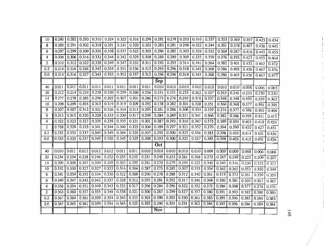
..-~00

10 0.280 0.282 0.293 0.310 0.324 0.325 0.316 0.299 0.281 0.278 0.293 0.316 0.337 0.353 0.369 0.397 0.425 0.4348 0.289 0.291 0.302 0.318 0.331 0.331 0.320 0.302 0.283 0.281 0.298 0.322 0.344 0.361 0.378 0.407 0.436 0.4456 0.297 0.299 0.309 0.326 0.338 0.337 0.325 0.305 0.286 0.285 0.303 0.329 0.352 0.369 0.387 0.416 0.445 0.4554 0.304 0.306 0.316 0.332 0.344 0.342 0.329 0.308 0.289 0.289 0.309 0.335 0.359 0.376 0.395 0.425 0.455 0.4642 0.310 0.312 0.322 0.338 0.349 0.347 0.332 0.311 0.292 0.293 0.314 0.341 0.364 0.382 0.401 0.432 0.462 0.472

0.2 0.314 0.316 0.326 0.342 0.354 0.351 0.336 0.315 0.295 0.296 0.318 0.345 0.368 0.386 0.405 0.436 0.467 0.4760.0 0.314 0.316 0.327 0.343 0.355 0.352 0.337 0.315 0.296 0.296 0.318 0.345 0.368 0.386 0.405 0.436 0.467 0.477

Sep40 0.011 0.011 0.011 0.011 0.011 0.011 0.011 0.011 0.010 0.010 0.010 0.010 0.010 0.010 0.010 0.008 0.006 0.00520 0.212 0.214 0.224 0.238 0.250 0.259 0.260 0.256 0.251 0.251 0.255 0.262 0.267 0.263 0.246 0.233 0.230 0.23014 0.277 0.278 0.285 0.296 0.305 0.307 0.301 0.286 0.273 0.276 0.293 0.316 0.337 0.348 0.348 0.350 0.359 0.36210 0.298 0.299 0.304 0.313 0.319 0.319 0.309 0.292 0.278 0.282 0.301 0.328 0.351 0.366 0.368 0.377 0.391 0.3958 0.307 0.307 0.312 0.321 0.326 0.324 0.313 0.295 0.281 0.286 0.306 0.334 0.359 0.374 0.377 0.386 0.401 0.4066 0.315 0.315 0.320 0.328 0.333 0.330 0.317 0.298 0.284 0.289 0.311 0.341 0.366 0.382 0.386 0.395 0.411 0.4154 0.322 0.323 0.327 0.335 0.339 0.335 0.321 0.301 0.287 0.293 0.316 0.347 0.373 0.389 0.393 0.403 0.419 0.4242 0.328 0.329 0.333 0.341 0.344 0.340 0.325 0.304 0.289 0.297 0.321 0.352 0.379 0.394 0.399 0.410 0.427 0.431

0.2 0.332 0.333 0.337 0.345 0.349 0.344 0.329 0.307 0.292 0.300 0.325 0.356 0.383 0.398 0.403 0.414 0.431 0.4360.0 0.333 0.333 0.337 0.345 0.350 0.345 0.329 0.308 0.293 0.300 0.325 0.357 0.383 0.398 0.403 0.415 0.431 0.436

Oct40 0.010 0.011 0.012 0.012 0.012 0.011 0.011 0.010 0.010 0.010 0.010 0.010 0.009 0.009 0.009 0.008 0.006 0.00620 0.234 0.234 0.238 0.246 0.252 0.255 0.255 0.251 0.248 0.253 0.261 0.268 0.272 0.267 0.249 0.222 0.209 0.20714 0.309 0.308 0.307 0.309 0.309 0.305 0.295 0.281 0.270 0.279 0.299 0.322 0.340 0.349 0.346 0.330 0.323 0.32210 0.332 0.330 0.327 0.327 0.323 0.316 0.304 0.287 0.275 0.285 0.307 0.333 0.354 0.365 0.365 0.353 0.350 0.3498 0.341 0.339 0.335 0.334 0.330 0.322 0.308 0.290 0.278 0.288 0.312 0.340 0.361 0.373 0.373 0.361 0.359 0.3596 0.349 0.347 0.343 0.342 0.337 0.328 0.312 0.293 0.281 0.292 0.317 0.346 0.368 0.380 0.381 0.369 0.367 0.3674 0.356 0.354 0.351 0.349 0.343 0.333 0.317 0.296 0.284 0.296 0.322 0.352 0.375 0.386 0.388 0.377 0.374 0.3742 0.363 0.360 0.357 0.355 0.349 0.338 0.321 0.300 0.287 0.299 0.327 0.357 0.380 0.391 0.393 0.382 0.380 0.380

0.2 0.367 0.364 0.361 0.359 0.354 0.343 0.325 0.303 0.290 0.302 0.330 0.361 0.383 0.395 0.396 0.385 0.384 0.3830.0 0.367 0.365 0.361 0.359 0.354 0.343 0.325 0.303 0.290 0.303 0.331 0.362 0.384 0.395 0.396 0.386 0.384 0.384

Nov

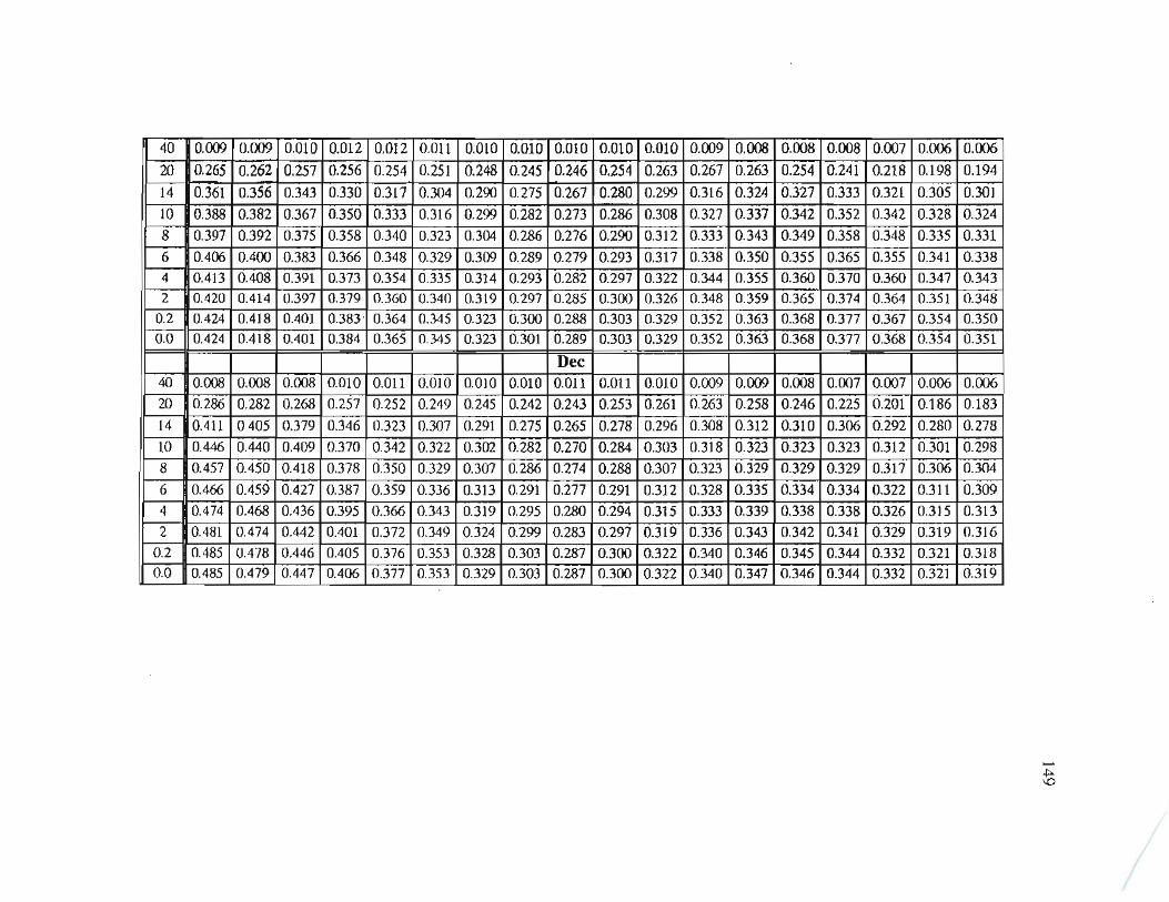
>-".j:::o..\0

40 0.009 0.009 0.010 0.012 0.012 0.011 0.010 0.010 0.010 0.010 0.010 0.009 0.008 0.008 0.008 0.007 0.006 0.00620 0.265 0.262 0.257 0.256 0.254 0.251 0.248 0.245 0.246 0.254 0.263 0.267 0.263 0.254 0.241 0.218 0.198 0.19414 0.361 0.356 0.343 0.330 0.317 0.304 0.290 0.275 0.267 0.280 0.299 0.316 0.324 0.327 0.333 0.321 0.305 0.30110 0.388 0.382 0.367 0.350 0.333 0.316 0.299 0.282 0.273 0.286 0.308 0.327 0,337 0.342 0.352 0.342 0.328 0.3248 0.397 0.392 0.375 0.358 0.340 0.323 0.304 0.286 0.276 0.290 0.312 0.333 0.343 0.349 0.358 0.348 0.335 0.3316 0.406 0.400 0.383 0.366 0.348 0.329 0.309 0.289 0.279 0.293 0.317 0.338 0.350 0.355 0.365 0.355 0.341 0.3384 0.413 0.408 0.391 0.373 0.354 0.335 0.314 0.293 0.282 0.297 0.322 0.344 0.355 0.360 0.370 0.360 0.347 0.3432 0.420 0.414 0.397 0.379 0.360 0.340 0.319 0.297 0.285 0.300 0.326 0.348 0.359 0.365 0.374 0.364 0.351 0.348

0.2 0.424 0.418 0.401 0.383' 0.364 0.345 0.323 0.300 0.288 0.303 0.329 0.352 0.363 0.368 0.377 0.367 0.354 0.3500.0 0.424 0.418 0.401 0.384 0.365 0.345 0.323 0.301 0.289 0.303 0.329 0.352 0.363 0.368 0.377 0.368 0.354 0.351

Dee40 0.008 0.008 0.008 0.010 0.011 0.010 0.010 0.010 0.011 0.011 0.010 0.009 0.009 0.008 0.007 0.007 0.006 0.00620 0.286 0.282 0.2()8 0.257 0.252 0.249 0.245 0.242 0.243 0.253 0.261 0.263 0.258 0.246 0.225 0.201 0.186 0.18314 0.411 0.405 0.379 0.346 0.323 0.307 0.291 0.275 0.265 0.278 0.296 0.308 0.312 0.310 0.306 0.292 0.280 0.27810 0.446 0.440 0.409 0.370 0.342 0.322 0.302 0.282 0.270 0.284 0.303 0.318 0.323 0.323 0.323 0.312 0.301 0.2988 0.457 0.450 0.418 0.378 0.350 0.329 0.307 0.286 0.274 0.288 0.307 0.323 0.329 0.329 0.329 0.317 0.306 0.3046 0.466 0.459 0.427 0.387 0.359 0.336 0.313 0.291 0.277 0.291 0.312 0.328 0.335 0.334 0.334 0.322 0.311 0.3094 0.474 0.468 0.436 0.395 0.366 0.343 0.319 0.295 0.280 0.294 0.315 0.333 0.339 0.338 0.338 0.326 0.315 0.3132 0.481 0.474 0.442 0.401 0.372 0.349 0.324 0.299 0.283 0.297 0.319 0.336 0.343 0.342 0.341 0.329 0.319 0.316

0.2 0.485 0.478 0.446 0.405 0.376 0.353 0.328 0.303 0.287 0.300 0.322 0.340 0.346 0.345 0.344 0.332 0.321 0.3180.0 0.485 0.479 0.447 0.406 0.377 0.353 0.329 0.303 0.287 0.300 0.322 0.340 0.347 0.346 0.344 0.332 0.321 0.319

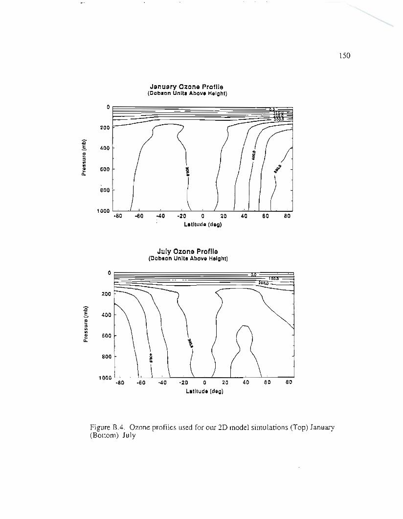
o

200-.a.5. 400e:Ilit

! 600Do

800

150

January Ozone Profile(Dobson Unlt8Above HeIght)

1000.80 -60 -40 .20 0 20

latItude (deg)

40 60 80

July Ozone Profile(Dobson Unlt8 Above HeIght)

Figure B.4. Ozone profiles used for our 2D model simulations (Top) January(Bottom) July

0

200

.5. 400e:Ilitft0 600..Do

800

1000.80 .60 -40 .20 0 20 40 60 80

LatItude (deg)

APPENDIX C

SOURCE CODE OF THE GCRC 2-D MODEL

* Main Body of.Programprogram mamreal t( 1O),z( 1O),p( 1O),sg( 1O),u( 10,20),v( 10,20), w( 10,20)real wt( 10,20),h( 10,20),pr(1 0,20), uvp( 10,20),xr( 10), vt( 10,20)real at( 1O),pa( 1O),za( 1O),cp( 1O),c( 1O),ra( 10,20),rs( 10,20)real t2d( 10,20),p2d(10,20),z2d( 10,20),pa2d(10,20),za2d( 10,20)real ch(1O),ce(10),f(20),sun,fl (20),sab(20),sth(20),cp2d(10,20)real hcld(20,4),mcld(20,4),lcld(20,4),uo2d(10,20),tco2(10,20)real at1(10),ch2d(10,20),ce2d(10,20),asa(20),avb(20),ava(20)real elev(36),ely(20),tp2d( 10,20),xt(10),pha(20),phb(20)real c2d( 10,20),dv( 10;20),du(10,20),rdw(10,20)real dpr( 10,20),dw( 10,20),uav( 10,20),vav(10,20),tvp( 10,20)real ts(20),ocfra(20),ot(20),uo( 10),uco2(1O,20),tv1(10,20)real ti(20),xi(20),al(20),albl(20),vice(20),suavg(20)real pavg( 10,20),tavg( 10,20),avgv(10,20),emp(20)real pav( 10,20),ps(20),gc(20),srg(20),tdeep,vi(20)real stravg(10,20),smtmp,smstr,rhp(4,20),uozon(12,10,20)real smuz,uzavg( 10,20),cwat( 10,20),dcwat(10,20),rain(20)real hsnow(20),twp(10,20),qwp(10,20),smuvp,auvp( 10,20)

************************************************************************

real sO,step,s1,time,day,sout,stm,strs,dstep,dmp.real c20,ch40,n20,abtot,re,ftop,rht,tke,dphireal pout,dwat,xgo,rhO(20),sk(20),tku,ytt,udragreal wo,vk,ho,hk,to(7,20),docean,uvam,year,area,ytrreal stav,surtmpreal vtpz(20),uvpz(20),kza(22),angza(22)integer nt,kap,nset,nturb,nyao,kozoneinteger nb,ndyn,npree,navg

* data z/34.,20.0, 14.0,12.0,10.0,8.0,6.0,4.0,2.0,0.0/* z vertical boundary between layers

data z/34.,20.0, 14.0,10.0,8.0,6.0,4.0,2.0,0.2,0.0/* surface elevations for zones north to south

data elevlO,84,242,222,315,315,21O,262,1000,1000& ,601,599,335,195,140,112,127,111,132,115,151,176,& 163,129,69,31,20,12,2,0,0,283,1200,1892,2000,2640/

151

152

* earth radiusre=6.4e6

* ndyn,navg,stav, nturb are not nonnally usedndyn=Onavg=Ostav=O.nturb=O

* year for cyclic time. print out time =365*year+time* O,time,365.25 for calculations

year=O.O* datm is the only input (data) file

open(unit=1O,file='datm')* oc82 gives the pressure, temp, ulv',v'T', etc at the end of the* full run

open(unit=20,file='oc82' )* open(unit=30,fi1e=loutuv')* seasonal averages of 2-D U'V'are in uvp.pm

open(unit=35,fi1e='uvp.pm')* time series of surfacte temp, radiation balance, kinetic energy* and V(2,3)

open(unit=40,file='ocw')* seasonal averages of 2-D temp are in tmp.pm

open(unit=50,file='tmp.pm ')* seasonal averages of 2-D stream func. are in str.pm

open(unit=52,file='str.pm ')* open(unit=55,file='ice.pm')* open(unit=56,file='snow.pm')* Latitudinal profile of vertically averaged precipitation

open(unit=57 ,file='rain.pm ')* seasonal averages of 2-D zonal velocity are in uz.pm

open(unit=58,file='uz.pm')* Latitudinal profile of vertically averaged v'T'

open(unit=62,file='vtpz.pm ')* Latitudinal profile of vertically averaged U'V'

open(unit=65,file='uvpz.pm')* Latitudinal profile of absorbed solar -emitted IR at top of atmosphere

open(unit=66,file='smf.pm ')* Latitudinal profile of vertically averaged kinetic energy per unit mass

open(unit=67,file='kza.pm ')* Belt angular momentum

open(unit=68,file='angza.pm ')*

* step is the radiation time step, day is the end of run, dwat is not usually used,* time is the start day, pout is the number of iterations between output* c20, ch40, n20, are the initial carbon dioxide, methane, and nitrous oxideconcentrations* trs is the energy transport coefficient when running in an EBM mode using* subroutine tra, nb is the number of latitudinal boxes, npree is a toggle to have print-out

153

* to screen (1) not (0), nyao is not nonnally usedread( 10,*) step,day,dwat,time,pout,c20,ch40,n20,trs,

& nb,npree,nyao* xt are the assumed Kz values at the vertical boundaries between boxes

read(10,*) (xt(i),i=l,1O)* dstep is the dynamical time step, yk and uvam are not nonnally used

read( 10,*) yk,uvam,dstepread(1O,*) (rhO(i),i=1,9)

* nset Number of hydrostic adjustment iterations, dmp is not nonnally usedread( 10,*) nset,dmp

* ocean transpon coefficients strn and strs for nonhero and souther hemispheres* used by subroutine trans. ytr and ytt are usually the same and are* the added tenn to the v'T' flux not given by the Stone and Yao scheme (ytr is for the* subtropics and ytt is for the tropics.(these are the coefficients of the temperaure* gradient driven transpon of heat)

read( 10,*) strn,strs,ytr,ytt* sk is not nonnal1y used

read(10,*)(sk(i),i=1,20) .

* suavg is the annual mean flux of radiation reaching the top of the atmosphere for each* zone (W/m2)

read( 10,*) (suavg(i),i=1,9)do i=1O,18

suavg(i)=suavg(19-i)end do

* initial pressure at the center of the gridbox (mb)do i=l,10

read(1O,*) (pa2d(i,j),j=l,nb+l)doj=l,nb+lif(i.le.2) thenpa2d(i,j)=pa2d(i,j)* (1000.+0.0*abs(9.5-j»elsepa2d(i,j)=pa2d(i,j)*( 1000.+0.0*abs(9.5-j»end ifend do

end do.* initial pressure at the vertical boundary of the gridbox (mb)

do i=l,10read(1O,*) (P2d(i,j),j=1,nb+1)

do j=l,nb+ 1p2d(i,j)=p2d(ij)* 1000.end do

pa2d(i, 19)=pa2d(i,18)end do

* initial meridional velocities (m/s)do i=l,10

read(1O,*) (v(i,j),j=1,nb+1)end do

* initial zonal velocities (m/s)

154

do i=l,l0read(lO,*) (u(i,j),j=l,nb+l)

end do* initial values of (l/cp).1L/.1T for calculating the effective heat capacity of a moist* atmosphere

do i=l,l0read(lO,*) (c2d(i,j),j=1,nb)end do

* initial convective energy transport (K per radiation time step)do i=l,l0read(lO,*) (ch2d(ij),j=l,nb)end do

* initial convective energy transport (K per rad step) (ce2d is the long term* convective transport and ch2d is a fine tuning of ce2d) See subroutines* tpch.f and lapadj.f called from rad.f

do i=l,l0read(lO,*) (ce2d(i,j),j=1,nb)end do

* initial 2-D temperature profIledo i=l,l0read(lO,*) (t2d(i,j),j=l,nb)end do .

* initial sea ice fraction area coverage=all\2read(lO,*) (alG),j=l,nb)

* initial sea ice thickness (m)read( 10,*) (xi(j),j=1,nb)

* initial ocean surface temperature (K)read(l 0,*) (ot(j),j= 1,nb)

* initial surface temperature (K) of land surfacesread(lO,*) (ts(j)j=l,nb)

* initial surface temperature (K) for sea ice regionsread(lO,*) (ti(j)j=l,nb)

* initial snow thickness (decimeters)read(10,*) (hsnow(j),j=1,nb)do j=l,nb

hsnow(j)=hsnow(j)11O.* initial sea ice volume

vi(j)=al(j)*al(j)*xi(j)end do

* initial v'T' fluxes m/sKdo i=l,l0read(lO,*) (tvp(i,j),j=l,nb+ 1)

end do* initial u'v' fluxes m2/s2

do i=l,l0read(lO,*) (uvp(i,j),j=l,nb+ 1)

end do

155

* Zonal frictional drag coefficients, and meridional frictional drag xr(1) and xr(2)* xr(8) is a zonal-drag on the top layer of the atmosphere see subroutine dy3.f

read(1O,*) (xr(i),i=I,1O)* venical boudaries of each layer

read(1O,*) (z(i),i=I,1O)* deep ocean stuff not presently in use except for docean which is the depth of the deep* ocean.

read (10,*) wo,rl,hk,ho,vk,docean,tdeep* initial deep ocean temperature profile

read(1O, *) « to(i,j),j=1 ,9),i= 1,6)

do i=I,6do j=1O,18

to(i,j)=to(i,19-j)end do

end do* high, middle, and low cloud data for spr, summ, aut, win 1,2,3,4

do i=18,1,-1read( 10,*) hc1d(i,1),hc1d(i,2),hc1d(i,3),hc1d(i,4)end dodo i=18,1,-1read( 10,*) mc1d(i,1),mc1d(i,2),mc1d(i,3),mc1d(i,4)end dodo i=18,1,-1read( 10,*) lc1d(i,1),Ic1d(i,2),Ic1d(i,3),Ic1d(i,4)end do

* ocean fraction of each zonedo i=I,18

ot(i)=to(1,i)read( 10,*) ocfra(i)end do

* land albedosdo j=l,nbread(10,*) albl(j)srg(j)=O.90

end do*spring ozone profile

do i=I,10read(10,*) (u02d(i,j),j=I,18)end do

* surface relative humidity profiles 1,18 N to South j= 1,4 sp, su, atum, windo j=18,1,-1read(1O,*) (rhp(i,j),i=I,4)end do

do j=l,nbrhO(j)=rhp(1,j)+(time-O.)*(rhp(2,j)-rhp(1,j))/91.end do

*

156

* do j=I,9* rhO(j)=rh0(19-j)* end do* seasonal ozone profIles 1 Mar, 2 Apr, .. 12 Feb

do k=I,12do i=l,l0read(10,*) (uozon(k,i,j)j=I,18)end do

end do

do j=l,nbuo2d(lj)=O.10

to(1j)=t2d(1 O,j)end do

* No Mountainsdo 10 i=I,36elev(i)=O.O

10 continue*

*

do i=l,l0do j=l,nb+l

* averages of pressure, temp, v,upav(ij)=pa2d(i,j)

twp(i,j)=O.O*

pavg(i,j)=O.Otavg(i,j)=O.Oavgv(i,j)=O.Oend do

t2d(i,nb+ 1)=t2d(i,nb)end do

* set up to calculate density from pressures and temperaturescall box (nb,pha,phb,sth,asa,ava,avb,z,z2d,za2d& ,pa2d,ra,rs,u,v,w,wt,h,t2d,dphi,rhO)

* calc elevation averages( not presently used)call avg(sth,elev,nb,ely)

or=Oarea=O.Odo 45 j=l,nb

* surface are of the eartharea=area+asa(j)

* surface boundaryz2d( 1O,j)=ely(j)/1000.0

45 continuedo i=l,l0do j=l,nb-l

* set hydrostatic adjustment mass flow to 0.0rdw(i,j)=O.O

end doend do

100610021009

format(8(f8.3, Ix»format(9(f6.3, Ix»format(19(f5.1, Ix»

do i=I,10do j=l,nb+l

e=esat(t2d(ij»* e saturation vapor pressure, cwat specific humidity

cwat(i,j)=rwat(pa2d(i,j)/l.O 13e5,e,1,1,rhO(j»end doend do

1008 format(2x,18(el1.4,2x»if(npree.eq.l) then

print*,'Set-up Complete'end if

* Below is main call to 1D model for each zone100 sO=O.* calculates the critical lapse rate from baroclinic theory as given by Stone and* Carlson 1979*gc is the critical lapse rate from baroclinic theory* t2d is the 2D temperature profIle at the grid center* pha is the latitude of the center of the grid* dphi is the latitudinal grid spacing* nb is the number of latitudinal grids

call baroclinic (gc,t2d,pha,dphi,nb)* ozone interpolation parameter to interpolate ozone monthly values

kozone=int(1 +time/30.5)

do 180j=l,nbdo 110 i=I,10

* change 2-D to 1 D data for sending to IDRCM subroutinesat(i)=t2d(i,j)

*ch/ch2d are the convective adjustment terms ID and 2D they should be close* to zero because they are small adjustments where ce/ce2d are the convective* adjustments that are made each time bothe ce & ch have units of (K)

ch(i)=ch2d(i,j)ce(i)=ce2d(i,j)

*uo/u02d are ozone amounts from the top of the atmosphere in cm* uo(i)=u02d(i,j)

uo(i)=uozon(kozone,ij)* cp is the heat capacity of the atmosphere

cp(i)=cp2d(i,j)* c is the correction to cp for a moist atmosphere

c(i)=c2d(i,j)*pa/pa2d are pressures in atms / pascals

157

158

pa(i)=pa2d(i,j)/1.0e5* p is the pressure between venicallayers

p(i)=(p2d(i,j) )/l.0e5*za/z are the heights at the center and boundary of the atms layers

za(i)=za2d(i,j)/l 000.z(i)=z2d(i,j)/I000.

* tp2d is a temperature change calculation variable used for diagnosticstp2d(ij)=t2d(ij)

110 continueif(time.gt900)thench40=1.60end if

if(time.lt.dwat)then* dwat allows for the exploration of water vapor feedback* at! is the temperature used in water vapor cales of radiation code

do 150 i=l,l0at! (i)=at(i)

150 continueend if

* effective surfave drag velocity* u and v are the zonal and meridional velocities

udrag=sqn( « u(9,j)+u(9,j+1))/2.)**2+& «v(9j)+v(9j+l»/2.)**2)

* radiation is the main IDRCM program*sun is the solar constant times the mean zenith angle* sout is the reflected solar energy* f is the flux of ir radiation at each level* abtot is the total absorbed solar energy by the eanh-atms system* ac is the total cloud cover* sl is a diagnostic related to total temperature change of all layers* nt is the layer corresponding to the tropopause when using the cumuls* convection scheme* c20,ch40,n20 are the concentrations of co2, ch4, n20* j is the latitudinal grid number* sth is the sine of latitude boundaries (j+1/2 or j-1I2)* suavg is the average solar intensity for annual mean conditions* rhp are the seasonal profiles of surface relative humidity

call radiation(at,at1,t,p,pa,z,za,ch,ce,sun,sout,f,& c,abtot,ac,s 1,nt,step,c20,ch40,n20,j,sth,cp,rhO(j),& hc1d,mc1d,lc1d,ts(j),ot(j),ocfra(j),uo,gc(j)& ,udrag,al(j),xi(j),ti (j),albl(j),srg(j),suavg(j),time& ,vi(j),rhp,rain(j),hsnow(j»

* rain(j) is the precipatation from radiative cooling* return back to 2D mode

f1(j)=f(1)sab(j)=sun-soutsO=sO+asa(j)*sun/areado 170 i=l,l0

159

tp2d( ij)=t2d(ij)-at(i)t2d(i,j)=at(i)

rs(i,j)=( 1.0+rhO(j)*esat( t2d(i,j»)ch2d(ij)=ch(i)ce2d(ij)=ce(i)cp2d(i,j)=cp(i)c2d(ij)=c(i)p2d(i,j)=p(i)* 1.0e5

pa2d(ij)=+ra(i,j) *287 *t2d(i,j) *rs( ij)za2d(i,j)=za(i)* 1000.z2d(i,j)=z(i)* 1000.

170. continue180 continue

do 183 i=I,9do 182j=l,nb

vt(i,j)=v(i,j) .

tp2d(i,j)=t2d(i,j)rdw(i,j)=O.O

182 continue183 continue* Ocean mixed layer horizontal transport of energy* stm and strs are the turbulent diffusion coefficients for the northern* hemisphere and southern hemisphere oceans* tdeep is the effective temperature of the deep ocean (not used here)

call trans(t2d,sth,nb,cp2d,z2d,step,& trs,stm,strs,c2d,ot,ocfra,tdeep,al)

* tra is EBM transport atm and Ocean* call tra(t2d,sth,nb,cp2d,z2d,step,trs,str,c2d)* if(ndy.lt.O)then* dyn is the main dynamics portion of program (see eqns 2.7 to 2.9 of text)* ra is the 2-D density, rs is and adjustment in ra for a moist atmosphere* step is the radiation time step, and dstep is the dynamics time step* phb is the cosine of the grid box boundaries (j+1/2or j-l/2)* uvp =u'v' tvp=t'v' eddy momentum and sensible heat* qwp =s'w' vertical eddy flux of moisture* twp =t'w' vertical eddy flux of sensible heat* cwat is the specific humidity* yay, uav, pay are the meridional and zonal velocities and pressure averaged over the* dyn subroutine (Le. rad step)* docean is the depth of the mixed layer ocean* sk are not used at present and should be set to zero* asa is the earth radius*(sin(phb(j)-sin(phb(j+ 1»* ava =cos(pha(j) avb=cos(phb(j» time is the time in days & is not used* by dyn subroutine

call dyn(u,v,t2d,pa2d,ra,rs,z2d,za2d,pha,phb,step& ,dstep,uvp,nb,xt,xr,asa,ava,avb,c2d,p2d,time,vav,uav& ,docean,sk,tvp,pav,rhO,twp,qwp,cwat)

160

**

do j=l,nb+lpav(10j)=pa2d(10j)

v(lj)=O.Oend do

* ytt is tropical cr coefficient for t'v' calculation using eqn 2.42 of text* ytr is mid to high latitude cr* tvl is t'v' without the addition of eq 2.42* yao is the stone and Yao (1987,1990) parameterization of eddy fluxes

call yao(pa2d,t2d,uav,p2d,za2d,z2d,phb,uvp,nb,dphi,rhO& ,c2d,tvp,ytr,ytt,twp,cwat,qwp,tv 1)

*

do i=I,9do j=l,nb

* tp2d(ij)=t2d(i,j)-tp2d(i,j)* v(ij)=.5*v(i,j)+.5*vt(i,j)

end doend do

* hydrostatic adjustment* rdw is the transfer of mass across the vertical boundary between two layers* resulting from the hydrostatic adjustment* ps is is not presently in use* dpr is the rate of change of pressure* nset is usually =1

do i=l,nsetcall hys(nb,pa2d,t2d,ra,rs,pr,w,rdw,

& dw,step*86400.,dpr,z2d,za2d,c2d,p2d,v,u,ps,cwat)end do

* end if*

do i=l,9do j=l,nb

tp2d(i,j)=t2d(i,j)-tp2d(i,j)* it rains some more if there is cooling due to dynamic transport of energy

if (tp2d(i,j).1t.0.0)thenel=esat(t2d(i,j)+ 1)e=esat(t2d(i,j))dr=rwat(pa2d(i,j),e l,j, 1,rhOG))

& -rwat(pa2d(i,j),e,j,l,rhOG))rainG)=rainG)-(p2d(i+1,j)-p2d(i,j))*dr*tp2d(i,j)

& /(step*9.8)end ifend doend do

* assume that fresh snow is 10 times less dense than waterdo j=l,nbif(t2d(9,j).le.272) then

161

hsnowG)=hsnow(j)+1O.O*rain(j)*step/1000.end ifend do

do i=l,l0do j=l,nb+ 1

* calc mass stream function vav was mean meridional velocity and is tranformed into* mass stream function (lOTg/sec)

vav(i,j)=(ra(i,j-l )+ra(i,j»*vav(i,j)*3.14 *re*avb(j)& *(z2d(i,j)-z2d(i+l,j»/(lelO)

end doend do

*do i=2,9

do j=l,nbvav(i,j)=vav(i -1,j)+vav(i,j)end doend do

*

do i=I,9do j=l,nbe=esat(t2d(i,j»

* cwat is gH20/gAir)cwat(i,j)=rwat(pa2d(i,j)/1.0 13e5,e,1,1,rhO(j»end doend do

* advection of water. Not in use really at this timecall gasstr(ra,cwat,v,w,dcwat,phb,pha,z2d

& ,nb,emp)*

* seasonal zonal averages of temp, stream function, zonal velocity* u'v' written to tmp.prn, str.prn, uz.prn, uvp.prn

call xavge(tavg,t2d,& time,smtnip,nb,step,pa2d,pha, 'tmp',50)call xavge(stravg,vav,time,smstr,

& nb,step,pa2d,pha,'str',52)call xavge(uzavg,u,time,smuz

& ,nb+1,step,pa2d,phb,'uz',58)call xavge(auvp,uvp,time,smuvp

& ,nb,step,pa2d,pha,'uvp',35)* Shiparo filter this could be written in more compact form* but we were experimenting around with the effects* of filtering different layers

call shfil(t2d,nb,9)call shfil(t2d,nb,l)call shfiJ(t2d,nb,2)

162

*

call shfil(t2d,nb,3)call shfil(t2d,nb,4)call shfil(t2d,nb,5)call shfil(t2d,nb,6)call shfil(t2d,nb,7)call shfil(t2d,nb,8)

* call shfil(t2d,nb,10)*

* call shfil(ra,nb, 1)* call shfil(ra,nb,2)* call shfil(ra,nb,9)

call filtl(pa2d,nb)call shfil(v,nb+1,9)call shfil(v,nb+l,2)call shfil(v,nb+1,3)

* between these lines has been added since 5/17call shfil(v,nb+1,1)call shfil(v,nb+ 1,4)call shfil(v,nb+I,5)call shfil(v,nb+1,6)call shfil(v,nb+1,7)call shfil(v,nb+ 1,8)

call shfil(u,nb+1,5)call shfil(u,nb+l,6)call shfil(u,nb+1,7)

*

***

*

call shfil(u,nb+ 1,1)call shfil(u,nb+1,2)call shfil(u,nb+ 1,3)call shfil(u,nb+1,4)call shfil(u,nb+1,8)call shfil(u,nb+1,9)

do j=l,nbto( 1j)=ot(j)

to( 1,j)=t2d(10j)end do

* call ocean(to,pha,phb,step/365.,vk,bk,ho,wo,docean,-.1,nb)* total kinetic energy per unit area tke & tku

tke=O.Otku=O.O

sul=O.navg=navg+l

ttnax=t2d(1, 1)

*

163

do 187 i=I,10do 186j=l,nb

if(t2d(ij).gt. tmax)thentmax=t2d(i,j)

end if

tke=tke+(z2d(i,j)-z2d(i+ 1,j»*dphi *& cos(phb(j))*vav(i,j)*vav(i,j)*ra(i,j)/40000.

tku=tku+(z2d(i,j)-z2d(i+ 1j) )*dphi*& cos(phb(j))*uav(i,j)*uav(ij)*ra(i,j)/40000.

* t2d(1O,j)=to(1,j)* tp2d(i,j)=t2d(i,j)-tp2d(i,j)* su1=su 1+ra(i,j)*(phb(j)-phb(j+ 1»* suI is a diagnostic check for conservation of energy

su1=su1+ra(i,j)*(z2d(ij)-z2d(i +1,j»& *tp2d(i,j)*(c2d(i,j)+ 1)*1005.*asa(j)/(2.*re**2*step)

186 continue187 continue

8001 fonnat (9(2x,fS.2»if(time.gt.365.25) thentime=time-365.25year=year+ 1end if

*

time=time+step* actual ice volume mA3

do j=l,nbvice(j)=ocfra(j)*2.57 e14*al(j)**2*(asa(j))/6.4e6/1e13end do

* write(*,2002) 365.*year+time,vice(I)+vice(2)+* & vice(3),vice( 18)+vice(17)+vice(16)+vice(15)+vice(14)

* output is belowif(time+365.25*year.gt.9000.and.time+365.25*year.le

& .9000+step)thenc20=640.

write(20,*)'v'do i=I,10write(20,3oo 1) (v(i,j),j=l,n b+1)end dowrite(20,*)'u'do i=I,10write(20,3000) (u(i,j),j=1,nb+1)end dowrite(20,*)'w'do i=1,10

164

***************

write(20,4000) (w(i,j),j=1,nb)end do

write(20,*)'t2d'do i=l,l0write(20,3000) (t2d(i,j),j=l,nb)

end dowrite(20,*)'tocean'do i=1,6

write(20,3000) (to(i,j),j=1,nb)end do

write(20,*) 'fl'write(20,3000) (fl (j),j=1,nb)write(20,*) 'sab'

write(20,*) 'al'write(20,3OO1)(al(j),j=l,nb)

write(20,*) 'area'write(20,3OO1)(al(j)**2j=1,nb)

write(20,*) 'area x10A13m"2'write(20,3OO1)(vice(j),j=l,nb)

write(20,*) 'xice'write(20,3OO1)(xi(j),j=l,nb)

do i=l,l0doj=1,nb+1rdw(i,j)=rdw(ij)*6.28 *re*asa(j)

write(30,5OO1)float(80.75-9.5*(j-1»,& za2d(i,j)/l OOO,(vav(i,j)+vav(i,j+1))l2e9,rdw(i,j)/l e9

end doend dodo i=2,9do j=l,nbvav(i,j)=vav(i-1,j)+vav(i,j)

end doend do

do i=1,9write(35,3000) (vav(i,j)/l e1O,j=1,nb)

end doend if

update printer countabtot=Oftop=O

surtmp=O.Odo 200 j= 1,nb

abtot=abtot+sab(j)*asa(j)/areaftop=ftop+fl (j)*asa(j)/area

surtmp=surtmp+t2d(9 ,j)*asa(j)/areacontinue

prt=prt+ 1.

*

200

165

if (pn.gt.pout.or.time.1t.OO.O+OO*step)thenif(npree.eq.1) then

do i=l,l0write(*,3000) (tp2d(i,j),j=1,nb)end do

end if* file 40 is called ocw time series of temp ...

write(40,800 1) 365.*year+time,100*v(3,2)& ,sunmp,tku,ftop-abtot,ftop,abtot,t2d(2,3), u(2,3)doj=l,nb .

vice(j)=ocfra(j)*2.57 e14*al(j)**2*(asa(j))/6.4e6/1e13end do

* file 55 is ice.pmwrite(55,2002) 365.*year+time,vice(1)+vice(2)+

& vice(3),vice(18)+vice(17)+vice(16)+vice(15)+vice(14),& xi(I),xi(2),xi(3),xi(16),xi(17)& ,vi(1),vi(2),vi(3),vi(16),vi(17)

* & ,vi(1)-al(l)*al(1)*xi(1)* & ,vi(2)-al(2)*al(2)*xi(2),vi(3)-al(3)**2*xi(3)* & ,vi(16)-al(16)**2*xi(16),vi(17)-al(17)**2*xi(17)

write(56,2001) 365.*year+time,(hsnow(j),j=1,nb)write(57,2001) 365.*year+time,(rain(j),j=1,nb)*

* zonal value of vertical1integrated u'v', KE, v'T', ang mom, rain, solar-IRdo j=l,nbvtpz(j)=O.O

uvpz(j)=O.Okza(j)=O.Oangza(j)=O.O

end dodo j=2,nbdo i=2,9vtpz(j)=vtpz(j)+tvp(i,j)*(p2d(i+ 1j)-p2d(i,j»/

& (p2d(1O,j)-p2d(2,j»* KE per unit mass in m1\2/s1\2. kza(j)=kza(j)+.5*(u(i,j)**2+v(i,j)**2)

&*(p2d(i+1,j)-p2d(i,j))/(p2d(10,j)-p2d(2,j»* angular momentum in units of 10A25kg m/s

angza(j)=angza(j)+(6.37**3)*u(i,j)*6.28& *cos(phb(j»*(pha(j)-phb(j+ 1»*& 2.*(p2d(i+ l,j)-p2d(ij»/9.8/1.0e7

uvpz(j)=uvpz(j)+uvp(i,j)*& (p2d(i+1,j)-p2d(i,j))/(p2d(10,j)-p2d(2,j»

end doend doangza(22)=0.0angza(21)=0.0angza(20)=0.0

166

do j=1,nb/2angza(22)=angza(22)+angzaG)end do

angza(22)=angza(22)+ .5*angza(10)doj=l1,nb .

angza(21)=angza(21)+angzaG)end do

angza(21)=angza(21)+.5*angza(10)angza(20)=angza(21 )+angza(22)

* file 66 is smf.pm 1atprofile* file 62 is vtpz.pm v't' vertical average 1atprofile* file 65 is uvpz.pm u'v' vertical average lat profile* file 67 is kza.pm total kinetic energy per unit mass lat profile* file 68 is angza.pm vertical total ang mom for each lat grid lat profile

write(66,3(02) 365.*year+time,(sabG)-f1G),j=1,nb)write(62,3(02) 365.*year+time,(vtpzG),j=1,nb)write(65,3002) 365.*year+time,(uvpzG),j=l,nb)write(67,3002) 365.*year+time,(kzaG),j=1,nb)write(68,3OO3)365.*year+time,(angzaG),j=1,22)*

******** More output file 20 is oc82 gives the results of most thing for the end of therun .

if(time.gt.60000.) thenwrite(20,3000) «pa2d(i,j)/l OOO.,j=1,nb+1),i=1,10)

write(20,*)write(20,3000) «p2d(i,j)/1OOO.,j=l,nb+1),i=l, 10)

write(20,*)do i=l,l0write(20,3001) (v(i,j),j=l,nb+ 1)end dowrite(20,*)do i=l,l0write(20,3000) (u(i,j),j=l,nb+ 1)end dowrite(20,*)do i=l,l0write(20,3001) (c2d(i,j),j=1,nb)end dowrite(20,*)do i=l,l0write(20,3001) (ch2d(i,j),j=1,nb)end dowrite(20,*)do i=l,l0write(20,3001) (ce2d(i,j),j=1,nb)end do

write(20,*)do i=l,l0

167

write(20,3000) (t2d(i,j),j=1,nb)end do .

write(20,*)write(20,3001) (al(j),j=1,nb)write(20,3001) (xi(j),j=1,nb)write(20,3000) (ot(j)j= 1,nb)write(20,3000) (ts(j),j=1,nb)write(20,3000) (ti(j),j=1,nb)

write(20,300 1) (10.*hsnow(j),j= 1,nb)write(20,*)

write(20,3000)( (tvp(i,j)& ,j=1,nb+1),i=1,1O)

write(20,*)write(20,3000) «uvp(i,j),j=1,nb+ 1),i=1,1O)

write(20,*) 'rain in mm/day'write(20,3001) (rain(j),j=1,nb)

write(20,*)'evaporation minus precipitation'write(20,3001) (emp(j),j=1,nb)

write(20,*)'snow depth in em'write(20,3001) (10.*hsnow(j),j=1,nb)

write(20,*) 'al'write(20,3001) (al(j),j=1,nb)

write(20,*) 'area'write(20,3001) (al(j)**2j=1,nb)

write(20,*) 'area x10" 13 mA2'write(20,3001) (viee(j),j=1,nb)

write(20,*) 'xiee'write(20,300 1) (xi(j)j= 1,nb)

write(20,*) 'tocean'write(20,3000) (ot(j),j=1,nb)

write(20,*) 'tland'write(20,3000) (ts(j),j=1,nb)

write(20,*) 'tiee'write(20JOOO)(ti(j),j=1,nb)write(20,*) 'tdeep', tdeep

write(20,*)'tocean'do i=1,6

write(20,3000) (to(i,j),j=1,nb)end do

write(20,*)'w'do i=1,10write(20,3000) (10000.*w(i,j),j=1,nb)

end dowrite(20,*) 'twp'

do i=1,10write(20,3001) «ra(i,j)+ra(i-l ,j))*500.*twp(i,j),j=1,nb)

168

end dowrite(20,*) 'qwp'

do i=l,l0write(20,3000) (1005.*c2d(i,j)*tvp(i,j)*qwp(i,j)

& *(ra(ij)+ra(i-l,j»*.5,j=1,nb)end do

write(20,*) 'qvp'do i=l,l0

write(20,3OOO)(c2d(i,j)*tvp(i,j)& *(ra(i,j)+ra(i,j+1»*.5,j=l,nb)

end do

write(20,*)'tp2d'write(20,3OOO)((10.*tp2d(i,j),j=l,nb+ 1),i=l,lO)

write(20,*) 'fl'write(20,3OOO)(fl G),j=1,nb)write(20,*) 'sab'write(20,3OOO)(sab(j),j=1,nb)

write(20,*)

write(20,*) 'ftop' ,ftopwrite(20,*) 'sab', abtotwrite(20,*) 'time', time+365.25*year

end if********20012002

*****

***

fonnat(f7 .1,lx, 18(f5.2»fonnat(13(1x,f7 ;2»

if(npree.eq.l) thendo i=l,l0

write(*,3OOO)(t2d(i,j),j=l,nb)end dowrite(*,*)'p'

write(* ,3000) (pa2d(9 ,j)/1OO,j=1,nb)write(*,*)'u2,u3'do i=I,9write(*,3000) (u(i,j),j=l,nb)

end dowrite(*,*) 'al/xi'

write(*,3OOO)(a1(j),j=l,nb)write(*,3000) (xi(j),j=1,nb)write(*,*) 'snow (dm)'

write(*,3001) (lO.*hsnow(j),j=l,nb)write(*,*) time,vav(9,8),sul

write(*,*) 's f ketot',abtot,ftop,tke+tkuwrite(*,*) 'land'

write(*,3OOO)(ts(j),j=l,nb)write(*,*) 'tice'

******

3000300130023003

*

*

169

write(*,3000) (tiG),j=l,nb)write(*,*) 'tocean'write(*,3000) (otG),j=l,nb)write(*,*) 'SH sur temp'write(*,3(00) (t2d(9,j),j=1O,nb)

write(*,3000) (ot(j)*ocfra(j)+ts(j)*( l-ocfra(j) ),j=1,nb)write(*,*)' I

end if

prt=O.O

format(19(f5.1 ,Ix))format(19(f5.2,lx))format (19(t7.1,lx))format(t7 .1, lx,22(f5.2,lx))end if

if«tmax.gt.l000.0).or.(tmax.lt.50.)) thentime=1.0e9end if

if (time+365.25*year.gt.day) thengoto 500elsegoto 100end if

500 continuewrite(20,*)'pa2d'

write(20,3000) «pa2d(i,j)/I000.,j=l,nb+ 1),i=I,1O)write(20,*)

write(20,3000) «p2d(i,j)/I000.,j=l,nb+ l),i=l, 10)write(20,*)do i=I,10write(20,3001) (v(i,j),j=l,nb+ 1)end dowrite(20,*)do i=I,10write(20,3000) (u(i,j),j=l,nb+ 1)end dowrite(20,*)do i=I,10write(20,3001) (c2d(i,j),j=l,nb)end dowrite(20,*)do i=I,10write(20,3001) (ch2d(i,j),j=l,nb)end dowrite(20,*)

170

do i=1,10write(20,300 1) (ee2d(i,j),j=1,nb)end do

write(20,*)do i=1,10write(20,3000) (t2d(i,j),j=1,nb)end do

write(20,*)write(20,3001) (alG),j=1,nb)write(20,3001) (xiG)j=1,nb)write(20,3000) (otG),j=1,nb)write(20,3000) (tsG),j=1,nb)write(20,3000) (tiG),j=l,nb)

write(20,300 1) (10.*hsnow(j),j=1,nb)write(20,*)

write(20,3000)( (tvp(i,j)& ,j=1,nb+1),i=1,1O)

write(20,*)write(20,3000) « uvp(i,j),j=1,nb+1),i=1,10)

write(20,*) 'rain in mm/day'write(20,3001) (rainG),j=l,nb)

write(20,*)'evaporation minus precipitation'write(20,3001) (empG),j=l,nb)

write(20,*)'snow depth in em'write(20,300 1) (10.*hsnowG),j=1,nb)

write(20,*) 'al'write(20,3001) (alG),j=l,nb)

write(20,*) 'area'write(20,3001) (alG)**2,j=1,nb)

write(20,*) 'area xl()l'13 mJ\2'write(20,3001) (viceG),j=1,nb)

write(20,*) 'xiee'write(20,3001) (xiG),j=1,nb)

write(20, *) 'tocean'write(20,3000) (otG),j= 1,nb)

write(20, *) 'tland'write(20,3000) (ts(j),j=1,nb)

write(20, *) 'tiee'write(20,3000) (tiG),j=1,nb).

write(20,*) 'tdeep', tdeepwrite(20, *)'tocean'

do i=1,6write(20,3000) (to(i,j),j=1,nb)

end dowrite(20, *)'w'do i=1,10

171

write(20,3000) (10000.*w(i,j),j=1,nb)end do

write(20,*) 'twp'do i=l,l0

write(20,3001) «ra(i,j)+ra(i-l ,j))*500.*twp(i,j),j=1,nb)end do

write(20,*) 'qwp'do i=l,l0

write(20,3000) (1005.*c2d(i,j)*qwp(i,j)& *(ra(ij)+ra(i-1,j»*.5,j=l,nb)

end dowrite(20,*) 'qvp'

do i=l,l0write(20,3000) (c2d(ij)*tvp(i,j)

& *(ra(iJ)+ra(ij+ 1»* .5j= 1,nb)end do

write(20, *)'tp2d'write(20,3000) « 100. *tp2d(ij)j= 1,nb+ 1),i= 1,10)

write(20, *) 'fl'write(20,3000) (fl (j),j= 1,nb)write(20, *) 'sab'write(20,3000) (sab(j),j= 1,nb)

write(20, *)

write(20, *) 'ftop' ,ftopwrite(20,*) 'sab', abtotwrite(20,*) 'time', time+365.25*yearwrite(20, *) 'U'

do i=l,l0do j=l,nb+1write(20, *) 57 .3*phb(j),-pa2d(ij)/l OO.,u(i,j)end doend do

write(20, *)'delta U'do i=l,l0

do j=l,nb+ 1write(20, *) 57 .3*phb(j),-pa2d(i,j)/1 OO.,u(i,j)-uco2(i,j)

end doend do

do i=I,10doj=1,nb+1vav(ij)=(ra(i,j-l )+ra(i,j))*vav(i,j)*3.14*re*avb(j)

& *(z2d(i,j)-z2d(i+ 1j»rdw(i,j)=rdw(i,j)*6.28*re*asa(j)

172

* wrlte(30,5001) float(90-10*(j-l)),* & za2d(ij)I1000,vav(i,j)/le9,rdw(ij)/le9

end doend dodo i=2,9doj=l,nb .

vav(i,j)=vav(i-lj)+vav(ij)end doend do

* wrlte(*,35)'UVP'do i=I,10

do j=1,nb+1* wrlte(35,*) 57.3*phbG),-pa2d(i,j)11OO.,uvp(i,j)

end doend do

* wrlte(35,*) TYP'do i=l,lOdo j=1,nb+1

* wrlte(35,*) 57.3*phb(j),-pa2d(ij)/100.,tvp(i,j)end doend do

fonnat (f6.1,2x,f8.2,2x,f8.3,2x,f8.3)fonnat(10(e8.2,lx))fonnat(lO(f5.1,lx))

goto 1000

lOOO continueif(npree.eq.1) thenprint*, 's f ,abtot,ftopprint*, 'albedo', 1-abtot/(sO)

print*,'total kinetic energy', tke,tku,tku+tkewrlte(20,*) 'tKE',tke,tku,tku+tkewrite(20,*) 'done'

wrlte(20,*) 's', abtot,'f,ftopprint*,'done'

end if*********************************************************************

end******************************************************************

* this fitler is a simple triangular filter and is not presently in usesubroutine filt1(x,nb)real x(10,20),tp(lO,40)integer nbdo i= 1,lOtp(i,1)=x(i,2)tp(i,nb+2)=x(i,nb-l)

500140004001

173

do j=l,nbtp(i,j+1)=x(i,j)

end doend dodo i=l,l0do j=l,nbx(i,j)=(tp(i,j)+2*tp(i,j+1)+tp(i,j+2»/4.0end doend doreturnend

*****************************************************************

* Shiparo filter subroutine see shapiro (1970)subroutine shfil(x,nb,ni)real x(10,20),tp(10,40)integer nb,nido i= ni,nitp(i, 1)=2*x(i,1)-x(i,5)tp(i,2)=2*x(i, 1)-x(i,4)tp(i,3)=2*x(i, 1)-x(i,3)tp(i,4)=2*x(i, 1)-x(i,2)tp(i,nb+8)=2*x(i,nb)-x(i,nb-4)tp(i,nb+7)=2*x(i,nb)-x(i,nb-3)tp(i,nb+6)=2*x(i,nb)-x(i,nb-2)

tp(i,nb+5)=2*x(i,nb)-x(i,nb-l)do j=l,nbtp(i,j+4)=x(i,j)end do

end do*

do i=ni,nido j=l,nbx(ij)=(186. *tp(i,j+4)+56.*(tp(i,j+3)+tp(i,j+5»-

& 28.*(tp(i,j+2)+tp(i,j+6»+8. *(tp(i,j+1)+tp(i,j+7»& -(tp(ij)+tp(i,j+8» )/256.

end doend doreturnend

***** Supporting Subroutines are below ********* this subroutine sets up the model structure it is used only once at the beginning of a run

subroutine box (nb,pha,phb,th,asa,ava,avb,z1,z,za& ,p,r,rs,u,v,w,wt,h,t,dp,rh)

* set up of initial grid boxes and pressures/densitiesreal th(20),pi,dp,asa(20),avb(20),zl (1O),t(10,20)real z(10,20),za( 10,20),p(10,20),r(10,20),rs( 10,20)

174

real phb(20),pha(20),ava(20),rh(20)real u( 10,20),v(10,20),w( 10,20),wt(10,20),h(10,20)pi=3.1415926re=6.4e6dp=(pi-pi/20.)/(float(nb))phb(1)=pi/2.-pi/40.do 10j=2,nb+ 1phbG)=phbG-l )-dp

10 continue*

*

do j=l,nbphaG)=(phbG)+phbG+ 1))/2.end dopha(nb+ 1)=pha(nb)

do 20 j=l,nb+ 1rhG)=.7 5+.1 *cos( 6*phaG))thG)=sin(phbG) )continue

*

20*

30*

do 30 j=l,nbasaG)=re*(thG)-thG+1))

continue

35

do 35 j=l,nbavbG)=cos(PhbG))avaG)=cos(phaG))continue

do i=l,10do j=l,nb+ 1z(i,j)=z 1(i)*1000.end doend do

*

do 42 i=1O,I,-1do 40 j=l,nb+lrs(i,j)=(1+rhG)*esat(t(ij)))rs(i,j)=1.if(Leq.l0)thenza(i,j)=zl (i)elseht=287.*t(ij)I9.8za(i,j)=z(i+ 1j)-ht*log( (exp(-(z(i,j)-z(i+1j) )/ht)+1)/2.)end ifu(i,j)=O.Ov(i,j)=O.O

**

175

*

w(i,j)=O.Owt(i,j)=O.Oh(i,j)=O.Oif(Leq.lO)thenp(i,j)=1.013e5r(ij)=p( i,j)/(287*t(i,j)*rs(i,j))p( 1,j)=p(2,j)*exp((19000-za(i,j))*.034/255)r(1j)=p(ij)/(287*t(ij))elsep(i,j)=p(i+ 1,j)*exp(-(z(i+1,j)-za(i+1,j))*.034/

&(t(i+ 1,j)*rs(i+Ij)))& *exp(-(za(i,j)-z(i+ l,j))*.034/(t(ij)*rs(i,j)))

r(ij)=p(i,j )/(287*t(ij)*rs(i,j))end ifcontinuecontinuedo i=8,1,-1do j=l,nbr(ij)=(p(i+ 1,j)-r(i+l,j)*9.8*(z(i+ Ij)-za(i+ 1,j)))/

& (287*t(ij)+9 .8*(za(i,j)-z(i+1,j)))p(i,j)=r(i,j)*t(ij)*287.

end doend do

**

***

4042*******

*returnend

************************************************************************

subroutine avg(sth,y,nb,ya)real phb(20),y(36),ya(20),sth(20)real a,sum(20),s1(20)integer nbdo 50 j=l,nb+ 1phbG)=180/3.1415926*asin(sthG))sumG)=O.OsIG)=O.O

50 continuedo 200 i=1,36zl=(95-5*(i))*3.1415926/180z2=(95-5*(i+ 1))*3.1415926/180a=sin(zl)-sin(z2)zl=(92.5-5*(i))do 100j=l,nbif(z1.lt.phbG).and.z1.gt.phbG+1))thensumG)=sumG)+asIG)=sIG)+a*y(i)end if

100 continue

176

200 continuedo 300 j=l,nb

ya(j)=s 1(j)/sum(j)300 continue

returnend

*********************************************************************** This is the cumulus convection scheme it is based on that of Lindzen et al. 1982 JAS* V.39 1189-1205 it is not in use right now but could be put to use anytime.

subroutine cumulus (at,t,za,z,pa,ch,jb,step,ce,c,cpt,lh,sh)real at( 1O),t(1 O),z( 1O),za( 1O),pa( 1O),ch( 1O),ce( 10)real zt,tt,cp,rhoO,l,qs,c( 1O),cpt( lO),lh,shreal e,qO,lhf,shf,cdus,mc,lqinteger mjbcdus= 1071cdus=.OO26rhoO= 1294 *(273 ./at(9))cp= 1.005do i=I,9

ch(i)=O.Oce(i)=0.0

end do1=2510-2.38*(at(9)-273)e=esat(at(10))qs=rwat(1.0,e,I,I,1.0)

qs=rwat(I.0,e,I,I)e=esat(at(9))qO=rwat(.998,e,1,1,.77)

qO=rwat(.998,e,1,1)lq=l*qOprint*,lqIhf=rhoO*1*cdus*( qs-qO)shf=rhoO*cdus*cp*(at(10)-at(9))Ihf=lhshf=shprint*,sh,shf,lh,lhfshf=rhoO*cdus*~p*0.8

call trpause (at,t,lq,z,zt,tt,m)mc=(lhf+shf)/lq

sl=O.Odo 8850 i=9,m,-1

rho=1294*(273/at(i) )*pa(i)if(Leq.m) thendt=(lhf+shf-sl )/«z(i)-z(i+ 1))*cp*mc)

*

*

***

**

elsedt=(t(i)-at(i))/(z(i)-za(i))+9.8/cp

177

end ifsl=sl +dt*cp*mc*(z(i)-z(i+ 1»ch(i)=cp*mc*dt*(z(i)-z(i+ 1))*step/cpt(i)

* ch(i)=cp*mc*dt* step*86400/((1+c(i»* 1.005*1ooO*rho)* if(i.eq.9) then* dt=(lhf+shf)/«z(i)-z(i+ 1»)* ch(i)=ch(i)+dt*step*86400/«1 +c(i»* 1Ooo*rho)* end if* print*,i,ch(i)jb,m8850 continue* print*

do i=I,9at(i)=at(i)+ch(i)

end doat( 1O)=at( 1O)-(lhf+shf)*step/cpt( 10)print*,(lhf+shf)*step/cpt(1O),s1,lhf+shfprint*,lhf,shf,lhf+shf,m,qs-qO,at(9),at(1O),ch(m)

returnend

*****************************************************************

***

subroutine trpause(at,t,lq,z,zt,tt,m)real at(10),z(1O),t(1O)real zt,tt,y,x,lqinteger m

cp=1.005do 8860 i=9,1,-1y=lq+cp*t(10)-cp*t(i)x=9.81*z(i)

if (y.ltx) thentt=t(i)zt=z(i)m=lgoto 8870

end if8860 continue

.8870 returnend

***********************************************************************

* This is the main dynamics part of the program**subroutine dyn(u,v,t,p,r,rs,z,za,pha,phb,step

& ,dstep,uvp,nb,xt,xr,asa,ava,avb,c2,pb,tr3,tav ,rav,& doc,sk,tvp,pav,rh,twp,qwp,cwat)real u(10,20),v( 10,20),w(10,20),t(10,20),p(10,20),dr(10,20)real r( 10,20),z(10,20),step,dt(10,20),sum,rereal ra( 10,20),wt(10,20),dw( 10,20),dpr(10,20),za(10,20)real phb(20),yk,xt(1O),pb(10,20),tt(10,20)

real dp( I0,20),pr( 10,20),dv( 10,20),du( 10,20),xr( 1O),pt(10,20)real vt( 10,20),ut(10,20),rs( 10,20),c2(10,20),cwat( 10,20)

178

real gv(10,20),n( 10,20),cp(10,20),tvp( 10,20),twp(10,20)real tx( 10,20),ux(10,20),vx( 10,20),rx(10,20),rh(20)real pha(20),asa(20),ava(20),avb(20),uvp( 10,20)real omega,fc(20),st,dstep,tr3,savegreal tav(10,20),rav( 10,20),pav( 10,20),Sk(20)real dmp,doc,sav( 10,20),qwp( 10,20)integer nhtime=O.Oyk=O.Onh=O

dmp=1.rl=24.*stepst=36oo.*dstepre=6.4e6omega=6.28/864oonx=O

* set up initial conditionsdo 35 j=l,nb+lv(1,j)=O.OfcG)=2.*omega*sin(phbG»pb(lj)=O.Odo i=l,l0cp(i,j)=(1+c2(i,j»* 1005.w(i,j)=O.Odr(ij)=O.dt(ij)=O.Odv(i,j)=O.tav(i,j)=O.Osav(i,j)=O.Orav(i,j)=O.Opav(i,j)=O.O

du(i,j)=O.dw(i,j)=dw(i,j)*dstep/(step*24.)

dw(i,j)=O.Opr(i,j)=O.Oend do

35 continuesaveg=O.Odo i=l,l0cp(i,nb+ 1)=cp(i,nb)

end dodo j=l,nbcp(10j)=doc*le7end do

*

call avdens(r,ra,nb)call vsw(t,r,u,v,tt,n,ut,vt,nb)*

.. - -..

179

***

call uvel(w,u,v,du,pha,phb,avb,re,r,ra,dr,pr,gv,& fC,xt,xr,nb;z,za,uvp)

call vvel(p,w,u,v,dv,pha,phb,avb,re,r,ra,dr,pr,gv&,fc,xt,xr,nb,yk,z,za)

do i=1,9do j=1,nbgv(i,j)=.5*(r(i,j-l )+r(i,j))*v(i,j)*avb(j)if(j.eq.2) thengv(ij)=gv(i,j)/2.end if

end doend docall masst(gv,phb,r,dr,ava,re,nb,z,w)call heattr(r,p,t,w,v,cp,pha,phb,gv,nb,

& re,dt,asa,z,za,xr,xt,u,sk,tvp, twp,rh,qwp,cwat)sum=O.O

call hy(nb,p,t,r ,rs,pr,dt,dr,w,dw,.67*st,dpr,dmp& ,z,za,c2,pb,v,dv)call uvinc(v,u,dv,du,O.67*st,nb,r,dr,t,dt,tt,n,vt,ut)

do i=1,9do j=l,nbpr(i,j)=O.O

dpr(ij)=O.Osum=sum+dr(i,j)*asa(j)p(ij)=287. *t(ij)*r(ij)*rs(ij)if(j.eq.nb) thenp(i,j+ 1)=p(ij)end if

end doend do .call avdens(r,ra,nb)

call uvel(w,u,v,du,pha,phb,avb,re,r,ra,dr,pr,gv,& fC,xt,xr,nb,z,za,uvp)

call vvel(p,w,u,v,dv,pha,phb,avb,re,r,ra,dr,pr,gv&,fc,xt,xr,nb,yk,z,za)

do i=1,9do j=1,nbgv(i,j)=.5*(r(ij-l )+r(ij) )*v(ij)*avb(j)if(j.eq.2) then .

gv(ij)=gv(i,j)/2.end if

end doend docall masst(gv,phb,r,dr,ava,re,nb,z,w)call heattr(r,p,t,w,v,cp,pha,phb,gv,nb,

& re,dt,asa,z,za,xr,xt,u,sk,tvp,twp,rh,qwp,cwat)sum=O.O

call hy(nb,p,t,r,rs,pr,dt,dr,w,dw,st,dpr,dmp

**

*

***

*

180

* & ,z,za,c2,pb, v ,dv)call uvinc( v,u,dv ,du,st,nb,r,dr, t,dt, tt,rt, vt, ut)

do i=I,9do j=l,nbpr(i,j)=O.O

dpr(i,j)=O.Osum=sum+dr(i,j)* asa(j)p(i,j)=287. *t(i,j)*r(i,j)*rs(i,j)if(j.eq.nb) thenp(ij+ 1)=p(i,j)

end ifend doend do

time=time+dstepdo i=1,9do j=l,nb+ltav( i,j )=tav( i,j)+v(i,j)* dsteprave i,j )=rav (i,j)+u (i,j)*dstepsavei,j)=sav(i,j )+t( i,j) *dsteppave i,j )=pav( i,j)+p( i,j) *dstep

end doend dosaveg=saveg+dstep

** calculations**

*

55 continuecall vsw(t,r,u,v,tx,rx,ux,vx,nb)call avdens(r,ra,nb)

call uvel(w,u,v,du,pha,phb,avb,re,r,ra,dr,pr,gv,& fc,xt,xr,nb,z,za,uvp)

call vvel(p,w,U,v,dv,pha,phb,avb,re,r,ra,dr,pr,gv&,fc,xt,xr,nb,yk,z,za)

do i=I,9do j=l,nbgv(i,j)=.5*(r(i,j-l )+r(i,j))*v(i,j)*avb(j)if(j.eq.2) thengv(i,j)=gv(i,j)/2.end if

end doend docall masst(gv ,phb,r,dr,ava,re,nb,z,w)call heattr(r,p,t,w,v,cp,pha,phb,gv,nb,

& re,dt,asa,z,za,xr,xt,u,sk,tvp, twp,rh,qwp,cwat)sum=O.O

call hy(nb,p,t,r,rs,pr,dt,dr,w,dw,2.*st,dpr& ,dmp,z,za,c2,pb,v,dv)

if(time.ge.rV2.0.and.nh.eq.0) then

***

**

181

nh=1call hy(nb,p,t,r,rs,pr,dt,dr,w,dw,2.*st,dpr

& ,dmp,z,za,c2,pb,v,dv)do i=I,9

write(*,2001) (dt(i,j)*st*lO.,j=l,nb+ 1)end do

end if .

2001 fonnat (lO(f7.3,lx»call uvinc(v,u,dv,du,2.*st,nb,r,dr,t,dt,tt,n,vt,ut)call vsw(tx,rx,ux,vx,tt,n,ut, vt,nb)

do i=I,9do j=l,nbpr(i,j)=O.O

dpr(ij)=O.Osum=sum+dr(i,j)*asa(j)p(ij)=287. *t(ij)*r(ij)*rs(ij)

* pb(i+ 1,j)=pb(i,j)+r(i,j)*9.8*(z(i,j)-z(i+1,j))*rs(i,j)pb(i+ 1j)=p(ij)+r(ij)*9 .8*(za(i,j)-z(i+1j) )*rs(i,j)

if(j.eq.nb) thenp(ij+ 1)=p(ij)pb(i+ 1,j+1)=pb(i+1,j)

end ifend doend do

*****

**

do i=1,9do j=l,nb+ 1

tav(ij)=tav(ij )+v(i,j)*dsteprav(ij)=rav(i,j)+u(i,j)*dsteppav(i,j)=pav(i,j)+p(i,j) *dstepend doend dosaveg=saveg+dstep

time=time+dstep

if(time.lt.rl-dstep/l O.)thengoto55

end if

*

do i=1,9doj=l,nb+l

tav(ij)=tav(ij)/savegt(ij)=tav(i,j)

rav(ij)=rav(ij)/savegr(i,j)=rav(ij)

pav(i,j)=pav(i,j)/savegp(i,j)=pav(i,j)

du(i,j)=O.O

*

*

182

***

dv(i,j)=O.Oend doend doprint*,sum,'sum'

call hy(nb,pav,tav,rav& ,rs,pr,dt,dr,w,dw,2.,dpr,z,za,c2,pb)call uvinc(v ,u,dv,du,2.,nb,r,dr,t,dt,t,r,v,u)

do j=l,nbv(l,j)=v(1j)& -xr(7)*tav(1 ,j)*sqrt(tav(1,j)**2+rav(1,j)**2)& -xr(7)*v(1,j)*sqrt(v(1,j)**2+u(l,j)**2)& *step*86400.u(1,j)=u(1,j)& -xr(8)*rav( 1,j)* sqrt( tav( 1,j)**2+rav( 1,j)* *2)

& -xr(8)*u(1,j)*sqrt(v(1,j)**2+u(l,j)**2)& *step*86400.v(2,j)=v(2,j)& -xr(9)*rav(2,j)*sqrt(tav(2,j)**2+rav(2,j)**2)

& -xr(9)*v(2,j)& *step*86400.

****

*

*

*

v(9j)=v(9j)* &-xr(2)*tav(9j)*sqrt(tav(9 ,j)**2+rav(9,j)**2)

&-xr(2)*v(9 ,j)*sqrt(v(9j)**2+u(9 ,j)**2)& *step*86400.*2./(z(9,j-l)+z(9,j»u(9,j)=u(9,j)

* &-xr(1)*rav(9,j)*sqrt(tav(9,j)**2+rav(9,j)**2)&-xr(1)*u(9j)* sqrt(v(9j)**2+u(9 ,j)**2)& *step*86400.*2./(z(9,j-l)+z(9,j»

end dou(9,1)=u(9,2)u(9,nb+ 1)=u(9,nb)

returnend

***********************************************************************

* part of dynamics average density between grid points calculationsubroutine avdens(r,ra,nb)real r(1O,20),ra(1O,20)integer nbdo i=2,9do j=l,nbif(j.gt.l)thenra(i,j)=.25*(r(i,j)+r(i,j-l)+r(i-l ,j)+r(i-l ,j-l»elsera(i,j)=.5*(r(i,j)+r(i-l j»

end if

end do

183

ra(10,i)=.5*(r(10,i-I)+r(10,i»ra(1,i)=.5*(r(1,i)+r(1,i-I»ra(i,nb+ 1)=.5*(r(i,nb)+r(i-l,nb»ra(i,I)=.5*(r(i-I,I)+r(i,I»end doreturnend

******************************************************************

*part of dynamics save old value ofv,u,r,w..subroutine uvset(w,wt,dw,u,v,ut,vt,r,p,rt,pt,dr,dp,du

& ,dv,nb,step,pr,dpr,tt,t)real u( 10,20),v( 10,20),ut(10,20),vt( 10,20),du( 10,20)real dv( 10,20),step,dp(10,20),dr( 10,20),pt(10,20)

real n(10,20),r(1 0,20),p(10,20),wt(10,20),w(10,20),dw( 10,20)real pr(1O,20),dpr(1O,20),tt(1O,20)integer nbdo 96 i=I,9do 94 j=l,nb+ 1vt(i,j)=v(i,j)+O.O*dv(ij)*steputei,j)=u(i,j)+O.O*du(ij)*stepwt(ij)=w(i,j)+O.O*dw(ij)n(i,j)=r(ij)+ .0*(dr(i,j)+pr(ij) )*steptt(i,j)=t(i,j)pt(i,j)=p(i,j)+ .0*(dp(i,j»dv(ij)=O.du(i,j)=O.

94 continue96 continue

returnend

***********************************************************************

* part of dynamics mass transfer eqn of continuitysubroutine masst(gv,phb,r,dr,ava,re,nb,z,w)real gv(10,20),phb(20),r(10,20),dr(10,20),z(10,20)real ava(20),reinteger nbdo 64 i=2,9do 62 j=l,nb

zs=z(ij)-z(i+ 1,j)dr(i,j)=(+gv(ij+ I)-gv(i,j»

& f(re*ava(j)*(phbG)-phb(j+I»)* & +(w(i+ Ij)*(r(i+ Ij)+r(i,j»-w(i,j)*(r(i,j)+r(i-l,j»)f(4. *zs)62 continue64 continue*

returnend

******************************************************************

* part of dynamics increment prognostic variablessubroutine uvinc(v,u,dv,du,step,nb,r,dr,t,dt,tt,rt,vt,ut)real v(10,20),u(IO,20),dv(IO,20),du(IO,20)real r( 10,20),dr( 10,20),t( 10,20),dt( 10,20)real vt( 10,20),ut(IO,20),rt(10,20),tt(10,20)

real stepinteger nbdo 104 i=I,10do 102j=l,nb+lv(i,j)=vt(ij)+dv(i,j)*stepu(i,j)=ut(ij)+du(ij) *stepr(i,j)=rt(i,j)+dr(i,j)*stept(ij)=tt( ij)+dt(i,j)* stepv(i,j)=O.Ou(i,j)=O.Ou(9,j)=u(9,j)/2.continue

v(i,nb+ 1)=0.u(i,nb+ 1)=2.0*u(i,nb)-u(i,nb-l)u(i,nb+1)=u(i,nb)/2.u(i,nb+ 1)=0

r(i,nb+ 1)=r(i,nb)t(i,nb+ 1)=t(i,nb)v(i,I)=O.v(i, 1O)=O.9*v(i,10)u(i, 1)=2.*u(i,2)-u(i,3)u(i,I)=u(i,2)12.

* u(i,I)=O.O104 continue* Antartic land mass* v(8,nb)=0.0* v(9,nb)=O.0* v(9,nb-l)=O.0* u(8,nb)=O.0* u(9,nb)=O.0* u(9,nb-l)=O.0* No meridional flow in the two layers of the stratosphere

do j=l,nbv(2,j)=v(3j)*0.0

v(2j)=O.0*v(3,j)v( 1,j)=v(2,j)*0.5

end doreturnend

******************************************************************

*

**

**

184

***102

*

* part of dynamics zonal velocity equation of motionsubroutine uvel(w,u,v,du,pha,phb,avb,re,r,ra,dr,pr,gv,f

& ,xt,xr,nb,z,za,uvp)

185

**

real u( 10,20),v( 10,20),du(10,20),r(10,20),ra(10,20),w(10,20)real pr(10,20),gv( 10,20),dr(10,20),dru(10,20),dpr( 10,20)real pha(20),phb(20),f(20),xt( 10),avb(20),xr(1O),z(10,20)real za(1O,20),zp,zm,zs,uvp(10,20)real re,dzinteger nbdz=2000.do i=I,9do j=2,nb

zp=«za(i,j-l)-za(i+ 1,j-l»+(za(i,j)-za(i+ l,j»)/2.zm=«za(i-l,j-l)-za(i,j-l»+(za(i-l,j)-za(i,j)))/2.zs=«z(i,j-l)-z(i+ 1,j-l»+(z(i,j)-z(i+ l,j»)/2.0

if(j.eq.2)thendru(ij)=«gv(i,j+ 1)+gv(ij»*(u(ij+ 1)+u(i,j»)/

& (4*re*avb(j)*(pha(j-l)-pha(j))end ifif(j.eq.nb)thendru(i,j)=-(gv(i,j-l )+gv(i,j))*(u(i,j-l )+u(i,j»/

& (4*re*avb(j)*(pha(j-l )-pha(j»)end ifif(j.gt2.and.j.1t.nb )then

dru(i,j)=«gv(i,j+ 1)+gv(i,j»*(u(i,j+ 1)+u(i,j»-& (gv(i,j-l)+gv(i,j»*(u(i,j-l)+u(i,j»)/& (4*re*avb(j)*(pha(j-l)-pha(j»)

end ifdru(i,j)=dru(i,j)

& +«r(i+ Ij)+r(i,j»*w(i+ l,j)*(u(i,j)+u(i+ l,j»-& (r(i,j)+r(i-l j»*w(i,j)*(u(i,j)+u(i-l,j»)/( 4.*zs)

&+v(i,j)*(r(i,j-l )+r(i,j))/2.*(f(j)+u(i,j)*tan(phb(j»)/re)& +(xt(i)*ra(i,j)*(u(i- J,j)-u(i,j»/zm+xt(i+ 1)*ra(i+1,j)*& (u(i+l,j)-u(i,j»/zp)/(zs)

if(i.eq.9)then .

dru(i,j)=dru(i,j)-xr(2)*(r(9 ,j)+r(9,j-l) )/2.*sqrt(v(i,j)**2+&u(i,j)**2)*u(i,j)/zs

end if .if(i.eq.2)thendru(i,j)=dru(ij)- xr(8)

&*sqrt(v(i,j)**2+u(i,j)**2)*u(i,j)*(r(i,j)+r(i,j-l) )/2.end if

********

dru(i,j)=dru(i,j)-(r(i,j-l )*(uvp(i,j)+uvp(ij-l»& *(avb(j)+avb(j-l»& -(uvp(i,j)+uvp(i,j+ 1»*(avb(j)+avb(j+ l»*r(i,j»/& (4.*re*avb(j)*(pha(j-l)-pha(j»)& +uvp(i,j)*(r(i,j-l )+r(i,j))/2.*(tan(phb(j))/re)

dpr(i,j)=(dr(i,j)+dr(i,j-l) )/2.

186

dpr(i,j)=O.Odu(i,j)=2.0* (dru(i,j)-u(ij)*dpr(i,j) )/(r(i,j)+r(i,j-l))end doend doreturn

end******************************************************************

*

***

* part of dynamics meridional velocity equation of motionsubroutine vvel(p,w,u,v,dv,pha,phb,avb,re,

& r,ra,dr,pr,gv,f,xt,xr,nb,yk,z,za)real u( 10,20), v( 10,20),dv( 10,20),r( 10,20),ra( 10,20)

& ,w(10,20),p(10,20),z( 10,20),za( 10,20)real pre10,20),gv( 10,20),dr( 10,20),drv( 10,20),dpr( 10,20)real pha(20),phb(20),f(20),xt( 10),avb(20),xr(10)real re,dz,zp,zm,zsinteger nbdz=2000.do i=1,9

do j=2,nbzp=«za(i,j-l)-za(i+ l,j-l))+(za(i,j)-za(i+ 1,j)))/2.zm=«za(i-l,j-l)-za(i,j-l))+(za(i-l,j)-za(i,j)))/2.zs=«z(i,j-l)-z(i+ l,j-l))+(z(i,j)-z(i+ 1,j)))/2.0

if(j.eq.2) thendrv(i,j)=(gv(i,j+ 1)+gv(i,j))*(v(i,j+1)+v(i,j))/

&(4*re*avb(j)*(pha(j-l)- pha(j)))end ifif (j.eq.nb)thendrv(i,j)=-(gv(ij-l )+gv(i,j))*(v(i,j-l )+v(i,j))/

&(4*re*avb(j)*(pha(j-l)-pha(j)))end ifif (j.gt.2.and.j.lt.nb)then

drv(i,j)=((gv(i,j+1)+gv(i,j))*(v(i,j+1)+v(i,j))-& (gv(i,j-l)+gv(i,j))*(v(i,j-l)+v(i,j)))/&(4*re*avb(j)*(pha(j-l )-pha(j)))

end ifdrv(i,j)=drv(i,j)

* & +«r(i+ 1,j)+r(i,j))*w(i+1,j)*(v(i,j)+v(i+1,j))-* & (r(i,j)+r(i-l,j))*w(i,j)*(v(i,j)+v(i-l,j)))/(4.*zs)

& -u(i,j)*(r(i,j-l )+r(i,j))/2.*(f(j)+u(i,j)*tan(phb(j))/re)& -(p(i,j-l)-p(i,j))/(re*(pha(j-l)-pha(j)))& +(xt(i)*ra(i,j)*(v(i-l ,j)-v(i,j))/zm+xt(i+1)*ra(i+1,j)*& (v(i+l,j)-v(i,j))/zp)/(zs)& -(r(i,j)+r(i,j-l))/2. *& yk*v(i,j)*sqrt(v(i,j)**2.+u(ij)**2.)

if(Leq.9)thendrv(i,j)=drv(i,j)-xr(1)*(r(9,j)+r(9,j-l) )/2.

&*sqrt(v(i,j)**2+u(i,j)**2)*v(i,j)/zs

187

*****

end ifif(Leq.2)then

drv(i,j)=dIv(ij)- xr(8)&*sqn(v(ij)**2+u(i,j)**2)*v(ij)*(r(ij)+r(i,j-l) )/2.

end if

dpr(i,j)=(dr(i,j)+dr(i,j-l) )/2.dpr(i,j)=O.O

dv(i,j)=2.0*(drv(ij)-v(ij)*dpr(i,j) )/(r(i,j)+r(i,j-l»end doend doreturnend

******************************************************************

* part of dynamics first law of thennodynamics for horizontal advectionsubroutine heattr(r,p,t,w,v,cp,pha,phb,gv,nb,

& re,dt,asa,z,za,xr ,xt,u,sk,tvp,twp,rh,qwp,cwat)real r( 1O,20),p(10,20),t(10,20),w(10,20),rh(20)real v( 10,20),cp(10,20),pha(20),phb(20),gv( 10,20)real gt(10,20),vp(10,20),za(10,20),tvp(10,20)real dt( 10,20),asa(20),z( 10,20),dt 1(10,20),cwat( 10,20)

real xt( 1O),xr(1O),u(10,20),sk( 1O),twp( 10,20),qwp(1 0,20)* gt is temporary gv

real kappa,cpa,ta,rav,zt,zs,zr,dn,cps,rq,paqreal e,lvinteger nbkappa=28711005

*

* sum=O.do i=l,l0do j=l,nbdt(i,j)=O.O

if (j.eq.l) thengt(i, 1)=0.0vp(i,I)=O.Ogt(i,nb+ 1)=0.0vp(i,nb+ 1)=0.0elsegt(i,j)=gv(i,j)vp(i,j)=v(i,j)end ifath(ij)=t(i,j)/(p( i,j)/l. 0e5)**kappa

end doend dodo i=I,9doj=l,nb-l

**********

188

*

zt=(z(i,j+ 1)-z(i+ l,j+ 1))zs=(z(i,j)-z(i+ l,j))zr=(zs+zt)/2.ta=(t(i,j)+t(i,j+ 1))/2.paq=(p(i,j)+p(i,j+ 1))/2.0/l.0e5e=esat(ta)

Iv=I000. *(2510-2.38*(ta-273))rq=rwat(paq,e, 1,1,(rh(j)+rh(j + 1))/2.)

rq=(cwat(i,j+ 1)+cwat(i,j))I2.cpa=(cp(i,j)+cp(i,j+ 1))/2.rav=(r(i,j)+r(i,j+ 1))/2.

00=( 1.0*287 + 1005.)& *rav*ta*v(i,j+ 1)*zr*cos(phb(j+ 1))& +(cpa)*rav*tvp(i,j+ 1)*zr*cos(phb(j+ 1))& +lv*rq*v(i,j+ 1)*rav*zr*cos(phb(j+ 1))

dt 1(i,j)=+drt/(zs* asa(j)*r(i,j)*cp(i,j))dtl(i,j+ 1)=-drt/(zt*asa(j+ 1)*r(i,j+ 1)*cp(i,j+ 1))

dt(i,j)=dt(i,j)+dt 1(i,j)dt(i,j+ 1)=dt(i,j+ 1)+dtl(i,j+ 1)

sum=sum+r(i,j)*dt(i,j)*zs*cp(i,j)*(phb(j)-phb(j+ 1))*ava(j)& +r(i,j+ 1)*dt(i,j+ 1)*zt*cp(i,j+ 1)*(phb(j+ 1)-phb(j+2))*ava(j+ 1)

end doend do

do i=3,9do j=l,nb

zm=za(i-l,j)-za(i,j)zs=(z(i-l,j)-z(i,j))zt=(z(ij)-z(i+ l,j))rm=(r(ij)+r(i-l ,j))/2.cpa=(cp(i-l,j)+cp(i,j))/2.0

OO=rm*twp(i,j)* 1005.oo=drt+rm*( cpa-l oo5.)*qwp(i,j)

dtl (ij)=-drt/(zt*r(i,j)*cp(i,j))dtl (i-l ,j)=+drt/(zs*r(i-l ,j)*cp(i-l ,j))dt(i,j)=dt(i,j)+dtl (i,j)dt(i-l ,j)=dt(i-l ,j)+dtl (i-l ,j)

end doend doend if

**

**

* print*,sum1000 format (l0(e7.2,2x))

returnend

****************************************************************

* part of dynamics subroutine vsw(t,r,u,v,tx,rx,ux,vx,nb)real t(1O,20),r(1O,20),u(l0,20),v(1O,20)real tx(10,20),rx(l 0,20),ux( 10,20),vx(10,20)

189

integer nbdo i=l,l0do j=l,nb+ 1tx(i,j)=t(i,j)rx(i,j)=r(ij)vx(i,j)=v(i,j)ux(ij)=u(i,j)end doend do

returnend

**End of dynamics subroutine ****************************************************************************** calculate IR fluxes of radiation

subroutine flux (ern,p,at,kap1,ac1,kap2,ac2,kap3,ac3,c,dc,f,> irel,ire2,ire3)real trt(1O,1O),at(10)real ern( 10, lO),c( 1O),c1(10, lO),tr( 10)real fd( 1O),fu(1O),ftot(1O),dc(lO),f( lO),p( 10)real ac1,ac2,ac3,cf,sig,ire 1,ire2,ire3integer kap 1,kap,kap2,kap3,ntkap=kap 1sig=5.67e-8do 203 i=l,l0

tr(i)=1.0203 continue

tr(kapl)=(1.0-irel *ac1)tr(kap2)=(1.0-ac2*ire2)tr(kap3)=(1.0-ac3*ire3)do 206 i=l,l0

ern(i,i+l)=ern(i,i)do 205 j=i+l,lOc1(i,j)=1.0do 204 k=i,j-lc1(ij)=cl(i,j)*tr(k)

204 continueern(i,j)=ern(i,j)*c1(i,j)+(l-cl(i,j»ern(j,i)=ern(i,j)

205 continueern(i,i)=O.O

206 continue*

trt(10,10)=-1.0do 240 i=1,9

do 239 j=l,l0if(i.eq.j)then

if(Leq.l)thentrt(i,i)=-2.0*ern(i,i+1)

190

elsetrt(i,j)=-2*em(i,i+ 1)

end ifend if

if(i.lt.j .and.j.It.1O)thentrt(i,j)=(em(j+ 1,i+l)-em(j,i+ l»-(em(j+ 1,i)-em(j,i»

end ifif(j.eq.1O)thentrt(i,j)=(em(10,i»-(em(10,i+ 1»end ifif(i.gt.j) thentrt(i,j)=(em(i,j)-em(i+ 1,j»-(em(i,j+ I)-em(i+ 1,j+1»

end if239 continue

trt(IO,i)=(em(i,IO)-em(i+1,10»240 continue

fd( 1)=0.0write(20,4050) «trt(j,i),j=I, 1O),i=1,10)sig=5.67e-8

fu( 1)=( 1.0-em( 10, 1»* sig*at( 10)** 4+sig*em( 1,2)*at( 1)**4fu(4)=( I.O-em( 10,4»* sig* at( 10)**4

do 4043 j=I,1Oftot(j)=O.Odo 4041 i=l,10ftot(j)=ftot(j)+trt(j,i)* sig* at(i) **4

4041 continueif(j.gt.l.and.j.It.10) thenfu(1 )=fu(1 )+sig*( em( 1,j+ 1)-em( 1,j))*at(j)**4end ifif(j.1t.1O)thenfu( 4)=fu( 4)+sig*( em( 4,j+ 1)-em( 4,j) )*at(j)**4end if

4043 continueftot( 1O)=ftot( 1O)+sig*at( 10)**4

do 4046 i=I,9dc(i)=.OO83224*(ftot(i»/(p(i+I)-p(i»

4046 continuefd(10)=ftot(10)f(10)=fd(10)

print*,'1O',fd(1O)print*, 'I' ,fu(1)

f(l)=fu(l)4050 format (1O(f8.5,2x»* write(20,*) 'em '* write(20,4050) «em(j,i),i=I,1O),j=l,1O)* write(20,*) 'hi'* write(20,4050) «trt(j,i),i= 1,1O),j=1,10)* write(20,*) (dc(i),i=I,1O)

*

**

191

* write(20,*) fd(lO)*

returnend

**********************************************************************

* hydrostatic adjustment**subroutine hys(nb,p,t,r,rs,pr,w,rdw,dw,step,dpr,z,za,c,pb,

& v,u,ps,cwat)real p( 10,20),t(1 0,20), w( 10,20),pr( 10,20),rs( 10,20)real r(10,20),dw( 10,20),dpr(10,20),cp(10,20),c( 10,20)real z(10,20),za( 10,20),step,pb(10,20),lv,thp(10,20)real sb( 1O),st(1O),cb(lO),ct(10),cm(8,8),rd(8),rd1(7)real zp(1O),zm(lO),z1(10),ga(10),z2(1O),cwat(10,20)

real v( 10,20),u(10,20),rdw(10,20),dmp,ps(20),cm1(7,7)integer nb

dmp=21600/stepl2.dmp=86400/stepdz=2000.do 50 i=1,9

do 49 j=1,nbthp(i,j)=t(i,j)*(p(9,j)/p(i,j))**(.287)

cp(ij)=( 1.+c(i,j))cp(i,j)=1005.

pr(i,j)=r(i,j)dpr(i,j)=p(ij)dw(i,j)=w(ij)continuecontinue

do j=1,nbps(j)=p( 1O,j)-r(9,j)*9.8*za(9j)

r(9 ,j)=p(9,j)/(287.*t(9,j))end do

*

*

4950

*

*

do 86 j=1,nbpb(1,j)=O.O

do i=1,9zm(i)=za(i,j)-z(i+ 1,j)zp(i)=z(i,j)-za(i,j)z1(i)=z(ij)-z(i+ 1,j)

z2(i)=za(i,j)-za(i+ 1,j)end do

*do 84 i=1,9ct(i)=(0.0*(t(i,j)+t(i-1,j))+

& (t(i-1,j)+t(i,j))/2.+.0098*z2(i-1)/2.)/z1(i)/r(i,j)/* & (thp(i-1,j)+thp(i,j))/2.)/z1(i)/r(i,j)/

& cp(i,j)cb(i)=(O.O*(t(i,j)+t(i+1,j))+

192

& (t(i+l,j)+t(ij»I2.-'()()98*z2(i)I2.)/z 1(i)/r(i,j)/* & (thp(i+l,j)+thp(i,j»I2.)/zl(i)/r(i,j)/

& cp(i,j)st(i)=287.*rs(i,j)*(t(i,j)/zl (i)+r(i,j)*ct(i»sb(i)=287.*rs(i,j)*(t(i,j)/z1(i)+r(i,j)*cb(i»

84 continuedo i=I,8rd(i)=p(i+ Ij)-p(i,j)-(r(i+ l,j)+r(i,j»*z2(i)*4.9end dodo i=2,7cm(i,i+ 1)=-sb(i+1)+9.8*z2(i)/(2.*zl(i+ 1»cm(i,i)=sb(i)+st(i+ 1)+9.8*z2(i)l2.*

& (l/zl(i)-lIzl(i+l»cm(i,i-l)=-st(i)-9.8*z2(i)/(2.0*zl (i»end docm(1,I)=sb(1)+st(2)cm(1,2)=-sb(2)cm(8,7)=-st(7)cm(8,8)=st(9)+sb(8)

* cm(2,2)=sb(2)+st(3)* cm(2,3)=-sb(3)1002 format (3x,4(flOA,3x»* do i=I,7* rdl(i)=rd(i+ 1)* do k=I,7* cml(i,k)=cm(i+l,k+l)* end do* end do**

*****

call sle(cm,rd,8,8,.00OOOI)call sle(cml,rdl,7,7,0.OOOOOlO)do i=2,8

rd(i)=rdl(i-l)end dord(1)=O.O

**********

ifG.eq.nb) thenrd(8)=0.0rd(7)=O.end if

rd(1)=0.rd(2)=0.0rd(1)=0.2*rd(1)rd(2)=0.6*rd(2)rd(8)=rd(8)+2.*(p(9,j)-psG))/st(9)do i=I,8

193

***

rd(i)=rd(i)/dmpta=(t(i,j)+t(ij+ 1))/2.

lv= 1000. *(251O-2.38*(ta-273))t(ij)=t(i,j )+rd(i) *cb( i)t(ij )=t(i,j )+rd(i) *cb( i)+

& lv*(cwat(i,j)+cwat(i+ 1,j))* .5*rd(i)/cp(i,j)/1 005.& /r(i,j)/zl (i)

t(i+ l,j)=t(i+ l,j)-rd(i)*ct(i+ 1)t(i+ l,j)=t(i+ l,j)-rd(i)*ct(i+ 1)-

& lv*( cwat(i,j)+cwat(i+ 1,j))* .5*rd(i)/cp(i+ 1,j)/1005.& /r(i+ l,j)/zl(i+ 1)

r(ij)=r(i,j)+rd(i)/zl (i)r(i+ l,j)=r(i+ l,j)-rd(i)/zl(i+ 1)

ifG.gt.l) thenv(i,j)=v(i,j)+rd(i)* (v(i,j)+v(i + 1,j))/

&(2*zl (i)*r(i,j) )/2.0v(i+ 1,j)=v(i+ 1,j)-rd(i)*(v(i,j)+v(i+ 1,j))/

& (2*zl(i+l)*r(i+l,j))/2.0end if

***

****

ifG.1t.nb) thenv(i,j+ 1)=v(i,j+ 1)+rd(i)*(v(i,j+ 1)+v(i+ l,j+ 1))/

&(2*zl(i)*r(ij+ 1))12.v(i+ l,j+ 1)=v(i+ l,j+ 1)-rd(i)*(v(i,j+ 1)+v(i+ l,j+ 1))/

& (2*zl(i+l)*r(i+l,j+l))/2.end ifif(Leq.8.and.j.eq.8) thenprint* ,rd(i)*(v(i,j)+v(i+ 1,j) )/(2*zl (i)*r(i,j)), v(i,j)

& ,v(i+l,j)end if

ifG.gt.l) thenu(i,j)=u(ij)+rd(i)*( u(i,j)+u(i+ 1,j))/

&(2*zl(i)*r(i,j))/2.u(i+ l,j)=u(i+ l,j)-rd(i)*(u(i,j)+u(i+ l,j))/

& (2*zl(i+l)*r(i+l,j))/2.end if

ifG.1t.nb) thenu(i,j+ 1)=u(i,j+ 1)+rd(i)*( u(i,j+ 1)+u(i+ 1,j+ 1))/

&(2*zl(i)*r(i,j+ 1))12.0u(i+ l,j+ 1)=u(i+ l,j+ 1)-rd(i)*(u(i,j+ 1)+u(i+ l,j+ 1))/

& (2*zl(i+ 1)*r(i+ l,j+ 1))/2.0end if

** dt(i,j)=dt(i,j)+rd(i)/(z1(i)*r(i,j)*cp(i,j))*ga(i)/step

dt(i+ l,j)=dt(i+ l,j)-rd(i)/(zl(i+ 1)*r(i+l,j)*cp(i+ l,j))

194

****

& *ga(i)/stepdr(i,j)=dr(i,j)+rd(i)/zl (i)/stepdr(i+ 1,j)=dr(i+1,j)-rd(i)/zl (i+1)/step

w(i+ 1,j)=rd(i)*2./(pr(i+1j)+pr(i,j»/steprdw(i+ 1,j)=rdw(i+1,j)+rd(i)/step

w(i+1,j)=rdw(i+1,j)*2.0/(r(i+1,j)+r(i,j»end do

*do i=1,9p(i,j)=287.*rs(i,j)*r(i,j)*t(i,j)pb(i+ 1,j)=pb(i,j)+r(i,j)*9.8*zl (i)*rs(i,j)

* pb(i+ 1,j)=p(i,j)+r(i,j)*9.8*zm(i)*rs(i,j)end do

*86 continue*

do i=1,9pb(i,nb+ 1)=pb(i,nb)

p(i,nb+ 1)=p(i,nb)do j=l,nb

pr(i,j)=(r(i,j)-pr(i,j))/stepdpr(i,j)=(p(i,j)-dpr(i,j) )/stepdw( i,j)=( w(i,j )-d w(i,j) )end doend do

do j=l,nb+ 1p( 1O,j)=pb( 1O,j)

end dopb( 1O,nb+ 1)=pb( 1O,nb)

p(10,nb+ 1)=p(10,nb)*returnend

**********************************************************************

* n eqns n unknowns matrix solutionsubroutine sle(a,b,n,n1,zero)real a(n1,n1),b(n1)do 100 i=l,ndiv=a(i,i)if(abs(div)-zero) 99,99,1

1 do 101j=l,na(i,j)=a(i,j)/div

101 continueb(i)=b(i)/divdo 102j=l,nif (i-j) 2,102,2

2 ratio=aG,i)

- - - - - - - - - - - -------..--.--.--..-..........

195

do 103 k=l,naG,k)=aG,k)-ratio*a(i,k)

103 continuebG)=bG)-ratio*b(i)

102 continue100 continue

return*99 print*,'matrix error',' ',i99 end**********************************************************************

* input program not presently usedsubroutine inmain(step,day,dwat,tme,pout,

& c20,c40,n20,trs)real step,low,day,c20,c40,n20,tme,dwat,trsstep=3.0low=.OOOOO 1

day=120.0c20=320.0c40=1.6n20=.3trs=.07tme=O.Odwat=2000pout=17

returnend

**********************************************************

* input called by rad.fsubroutine inp(aoz,boz,coz,sO,theta,albedo,lap,cp)

real aoz,boz,coz,sO,theta,albedo,cp(10),lapaoz=.318boz=23.0coz=5.0s0=680.0theta=60.0albedo=O.O

lap=35.0cp(1O)=50.0returnend

*********************************************************************** cloud calculations* ire!... are infrared emissivities* ac1... are cloud fractions 1 top 3 lowest* dep 1 cloud optical depth* hcld, mcld, lcld are high mid and low cloud amount for each season

subroutine cloud(ac1,kapI,dep1,ire1,ac2,kap2,dep2,ire2,

196

& ac3,kap3,dep3,ire3,rg,depth,time,hc1d,mc1d,lc1dj,rhO,rhp)real ac1,ac2,ac3,dep1,dep2,dep3,ire1,ire2,ire3,rg,depthreal time,hc1d(20,4),mc1d(20,4),Ic1d(20,4),tm(5),tc

real rhO,rhp(4,20)integer kap1,kap2,kap3,j

tc=time-21if(tc.lt.O.O)then

tc=365.25+time-21end if

tm(1)=Otm(2)=91tm(3)=183tm(4)=275tm(5)=365.30do k=1,3if (time.ge.tm(k).and.time.lt.tm(k+1» thenac 1=(hc1dG,k)+(hc1dG ,k+ 1)-hc1dG,k) )*( time-tm(k»

& /(tm(k+ l)-tm(k»)/l00ac2=(mc1dG,k)+(mc1dG,k+1)-mc1dG,k»*(time-tm(k»

& /(tm(k+1)-tm(k»)/100ac3=(Ic1dG,k)+(1cldG,k+ 1)-Ic1dG,k))*(time-tm(k»

& /(tm(k+ l)-tm(k»)/lOOrhO=rhp(k,j)+(rhp(k+1j)-rhp(kj) )*(time-tm(k»

& /(tm(k+ l)-tm(k»end if

end dok=4if (time.ge.tm(k).and.time.lt.tm(k+1» thenac1=(hc1dG,k)+(hcldG,1)-hc1dG,k))*(time-tm(k»

& /(tm(k+ l)-tm(k»)/l00ac2=(mc1dG,k)+(mcldG,1)-mc1dG,k»*(time-tm(k»

& /(tm(k+ l)-tm(k»)/100ac3=(Ic1dG,k)+(Ic1dG,1)-Ic1dG,k»*(time-tm(k»

& /(tm(k+ l)-tm(k»)/l00rhO=rhp(k,j)+(rhp(l ,j)-rhp(k,j»* (time-tm(k»

& /(tm(k+ l)-tm(k»

end ifif(absG-9.5).lt.3) then

kap1=3ire1=1.0dep 1=O.6-abs(0.0*(9.5-j)/9.)

* was 1.0 0.0elsekap1=4ire1=0.5dep 1=0. 6-abs(0.0*(9 .5-j)/9 .0)

* was 1.00.0

197

end ifkap2=6dep2= 1.2-abs(0.6*(9.5-j)/9)

* was 1.5 .5ire2=1.0kap3=8dep3=4.0-abs(2.0*(9.5-j)/9)

* was 5.5 2.0ire3=1.0rg=.lldepth=8.0returnend

**********************************************************************

*

* simpler cloud input not use at presentsubroutine cl1(ac1,kap1,dep1,ire1,ac2,kap2,dep2,ire2,

& ac3,kap3,dep3,ire3,rg,depth)real ac1,ac2,ac3,dep1,dep2,dep3,ire1,ire2,ire3,rg,depthinteger kap1,kap2,kap3ac1=O.lkap1=3dep1=3.0ire1=0.5ac2=.15kap2=5dep2=8.0ire2=1.0ac3=.35kap3=7dep3=8.0ire3=1.0rg=.lldepth=8.0returnend

*********************************************

* seasonal average subroutine called from main portion of programsubroutine xavge(xa,x,time,stav,nb,step,za2d,pha,text,nf)real xa(10,20),x(10,20),time,stavreal tm( 1O),za2d(10,20),step,pha(20)character* 10 textinteger nb

tm(1)=Otm(2)=91tm(3)=183tm(4)=275tm(5)=365.25do k=1,5

198

if(time.ge.tm(k).and.time.lt.tm(k)+step) thenif(stav.gt.2.0) then

write(nf,*) text,'season',k-ldo i=l,l0do j=l,nb

write(nf,*) 57.3*pha(j),-za2d(i,j)/100.,xa(i,j)/stavxa(i,j)=O.O

end doend dostav=O.O

end ifend if

*

if (time.ge.tm(k).and.time.lt.tm(k+l)) thendo i=l,l0do j=l,nb+ 1xa(i,j)=xa(i,j )+x(i,j)end do

end dostav=stav+1.0

end ifend doreturnend

**********************************************************************

* convective lapse rate adjustment gam=gamma is the critical lapse rate for the* convective adjustment of Manabe and Wetherald 1967

subroutine lapadj (at,gam,za,cp,ch,nt,ce)real at(1 O),gam( 1O),za(1 O),cp(1 O),ch(1 O),ce(1 0)real s2,dl,d2,d3,db,dtinteger ntnt=6do 7998 i=l,l0ch(i)=O.O

7998 continue7999 s2=O.0

za( 10)=0.0do 8002 i=8,2,-1dl=at(i+ 1)-at(i)d2=gam(i)*(za(i)-za(i+ 1))if (d1.gt.d2) then

d3=1.0*(dl-d2)db=cp(i)*d3/( cp(i)+cp(i+ 1))dt=cp(i+ 1)*d3/(cp(i)+cp(i+ 1))at(i)=at(i)+dtat(i+ 1)=at(i+ 1)-dbch(i)=eh(i)+dtch(i+1)=eh(i+I)-db

199

s2=s2+d3nt=i

end if8002 continue

if (s2.gt..005)thengoto 7999

endifdo 8005 i=2,8

if (at(1O).1t.(at(9)+.04»thence(i)=ce(i)*.95

end ifce(i)=ce(i)+ch(i)/8.0

if(ch(i).1t..OOO1)thence(i)=ce(i)* .99end if

8005 continuereturnend

*********************************************************************

* set critical1apse rate to a fixed value such as 6.5 K/kmsubroutine lap1 (gam,lap)real gam(lO)real lapdo 8600 i=1,9gam(i)=lap

8600 continuereturnend

**********************************************************************

subroutine lap2 (gam,at,pa,gc)* moist adiabatic lapse rate from Stone & Carlson 1979* gc is the critical baroclinic lapse rate vi stone & carlson* 1979

real gam(1O),at(10),pa(10),gcreall,r,de,er=.287do 8700 i=1,91=2510.-2.38*(at(i)-273)e=esat( at(i) )

de=.622*1*e/(r*at(i)**2)gam(i)=9.8*(1+.622*1*e/(pa(i)*r*at(i»)/1(1+(.622*1*de)/(1.005*pa(i»)if(gam(i).gt.6.0) then

gam(i)=6.0end if

8700 continue* gam(9)=1.0

200

returnend

*********************************************************************** Stone and Carlson 1979

subroutine baroclinic(gc,t,pha,dp,nb)real gc(20),t(10,20),pha(20),dp,h2integer nb

do j=3,nb-2h2=287*t(6j)/9.8gcG)=9.8+1000.*

& tan(pha(j»/h2*(t(6,j-l)-t(6,j+ 1»/(2.*dp)end dogc(2)=gc(3)gc(1)=gc(2)gc(nb-l)=gc(nb-2)gc(nb)=gc(nb-l)returnend

*******************************************************

* chooses between critical lapse rate from baroclink theory or moist adiabatic lapse ratesubroutine lapstone(g,gc,p)real g(10),gc,p(10)

18 sl=O.s2=0.

do i=I,8sl=sl +g(i)*(p(i+1)-p(i»

s2=s2+p(i+ 1)-p(i)end doavg=slls2

if (avg.gt.gc) thendo i=9,1,-1

g(i)=gcend do

end ifreturnend

*********************************

* calculates the average lapse ratefunction avlap(at,za,p)real avlap,at( 1O),za( 1O),p(10)sl=O. .

s2=0.do i=3,8sl=sl +(at(i+ 1)-at(i»*(p(i+ 1)-p(i»/

& (za(i)-za(i+ 1»s2=s2+(p(i+ 1)-p(i»

end doavlap=sl/s2

201

returnend

**********************************************************************

* 2-D ocean model from Watts and Morentine (1990)subroutine ocean(t,pha,phb,st,vk,hk,ho,w,d,rl,nb)real t(7,20),dt(7,20),dz(7,20),tp(7,20)real pha(20),phb(20)

real a,b,q,x,al,st,vk,hk,ho,w,d,rc,rl,y,yp,ymreal xm,xpinteger nbopen(unit=1O,file='inoc1')open(unit=20,flle='out')

open(unit=30,f1le='out.ext')read (10,*) nb,st,w,d,rl,hk,ho,vkread(10, *) «t(ij)j=l,nb),i=I,6)

time=O.rc=4.186e6/3.15e7

do j=l,nbdo i=1,6

if(Leq.l )thendz(ij)=delsedz(ij)= 1000

end ift(ij)=t(i, 1)

if(Leq.6)thendz(ij)=O.t(i,j)=t(1,3)

end ifend doend do

*****

*

a=-283.4b=1.8

30 do i=l,ldo j=l,nbx=sin(pha(j) )y=cos(pha(j»yp=cos(phb(j+ 1»ym=cos(phb(j) )xp=sin(phb(j+ 1»xm=sin(phb(j) )if(x.gt..94)thenal=.4elseal=.75-.18*x**2end ifq=al*345*( 1.25-.7 5*x**2)

202

* dt(ij)=( q-(a+b*t(ij» )/(rc*d)-vk*(t(i,j)-t(i+1,j))*2.dt(ij)=-vk*(t(ij)-t(i+ l,j»*2.

& /((dz(i,j)+dz(i+ 1j) )*d)sum=sum+(q-(a+b*t(i,j» )*y

if(j.eq.l)thendt(ij)=dt(ij)-hk*yp*(t(i,j)-t(i,j+ I))/(y*.1744**2)end if

**

if(j.eq.9)thendt(ij)=dt(ij)-hk*ym*(t(i,j)-t(i,j-I»/(y* .1744**2)

& -xm*w*(t(ij»/(d*.1744*y)& +w*t(i+ Ij)/d

& -xm*w*(t(ij)+t(i,j-I»/(2.*d*.1744*y)& +w*(t(i+1j)*30. +500.*t(ij) )/530./d

& -xm*w*(t(ij»/(d*.1744*y)end if

*

***

if(j.gt.l.and.j.lt.9)thendt(ij)=dt(ij)-hk*ym*(t(i,j)-t(i,j-I»/(y* .1744**2)

& -hk*yp*(t(ij)-t(ij+ I))/(y*.1744**2)

if(j.gt3.and.j .1t.9)thendt(i,j)=dt(i,j)+xp*w*t(ij+ 1)/(d*.1744*y)

& -xm*w*t(ij)/( d*.1744*y)& +w*t(i+I,j)/(d)

dt(i,j)=dt(i,j)+xp*w*( t(ij+ 1)+t(i,j))/(2.*d*.1744*y)& -xm*w*(t(ij)+t(i,j-I»/(2.*d*.1744*y) .

& +w*(30.*t(i+Ij)+500. *t(i,j»/(530. *d)& -xm*w*t(ij)/(d* .1744*y)

end if*

if(j.eq.3)thendt(i,j)=dt(i,j)+xp*w*(t(ij+ 1)-t(ij) )/(d*.1744*y)dt(i,j)=dt(i,j)+xp*w*( t(ij+ 1)-t(i,j))/(2.*d*.1744*y)

wst=xp*w/(.1744*y)end ifend if

*.1744=dphiend doend do

*

do i=2,5do j=l,nb

x=sin(3. 14*(95-1O*j)/180)y=cos(3.14*(95-1O*j)1180)yp=cos(3.14*(90-1O*j)1180)

203

ym=cos(3.14*(90-1O*G-l»/180)

if (i.lt.5.and.i.gt.2)thendt(i,j)=

& +vk*(t(i-l ,j)-t(ij) )*2./«dz(i-l ,j)+dz(i,j»*dz(i,j»& -vk*(t(i,j)-t(i+1,j))*2./((dz(i+1,j)+dz(i,j))*dz(i,j»

ifG.gt.3) thendt(ij)=dt(ij)+w*(t(i+ 1,j)-t(i-l,j»/(2. *dz(ij»

end ifend if

*

if (Leq.5)thendt(ij)=

& +vk*(t(i-l ,j)-t(ij) )*2./((dz(i-l ,j)+dz(i,j))*dz(ij»& -vk*(t(i,j)-t(i+ l,j»*2./«dz(i+ l,j)+dz(i,j»*dz(i,j»

ifG.gt.3) thendt(ij)=dt(ij)+w*( t(i+1,j)-

& (t(i-l,j)+t(ij»/2.)/(dz(ij»end if

end if

if (Leq.2)thendt(ij)=

& +vk*(t(i-l,j)-t(i,j) )*2./«dz(i-l ,j)+dz(i,j»*dz(i,j»& -vk*(t(i,j)-t(i+ Ij»*2./«dz(i+ Ij)+dz(i,j»*dz(i,j»

ifG.gt.3) thendt(i,j)=dt(ij)+w*(t(i+ 1,j)+t(ij) )/(2.*dz(i,j»

& -w*(t(i,j)*30.+500.*t(i-lj»/(530. *dz(i,j»end if

end if

ifG.eq.l )thendt(i,j)=dt(ij)-ho*yp*(t(i,j)-t(i,j+ 1))/(y*.1744**2)end if .

ifG.eq.nb)thendt(i,j)=dt(ij)-ho*ym*(t(i,j)-t(i,j-l»/(y* .1744**2)end if

ifG.gt.l.and.j.lt.9)thendt(ij)=dt(ij)-ho*ym*(t(i,j)-t(i,j-l»/(y* .1744**2)

& -ho*yp*(t(ij)-t(ij+l»/(y*.1744**2)end if

*.1744=dphiend doend do

204

do i=1,5do j=1,nbt(i,j)=t(i,j)+dt(i,j)*st

* sum=sum+t(i,j)*cos(3.14*(10*j-5)/180)*dz(i,j)/10000.end doend do

do j~1,nbt(6,j)=t(1,3)

end do

count=count+stif(time.eq.0.or.count.ge.50)thencount=O.Owrite(20,*) 'time=',timewrite(20,1000) «t(i,j),j=1,nb),i=1,6)

trade=t( 1, 1)t( 1, 1)=time

write(30, 100 1)(t( 1,j)j= 1,nb,2)write(*,1001)(t(1j)j=1,nb,2)write(*, 1(01) t( 1,1),t(1 ,2),t(1 ,3),t( 1,5),t(1 ,7),t( 1,9)write(30, 1(01) t( 1,1),t(1 ,2),t(1 ,3),t( 1,5),t( 1,7),t(1 ,9)

t( 1, 1)=trade

print*,sumend iftime=time+st

if(time.gt2000-1 O.and.time.1t.2(00)thendo j=1,nbtp(1j)=t(1 ,j)

end doend ifif (time.gt2000.and.time.1t.2200+st/2.) then

w=O.Oend ifsum=O.

if (time.1t.rl+.Ol)goto 30format(9(f6.1,1x»format(9(f6.2,1x»write(*,1(00) « t(i,j),j=1,nb),i=1,6)write(30,1001) «t(i,j),j=1,nb ),i=1,6)

write(*,*)write(*,1000) (t(1,j),j=1,nb)write(*,1000) (tp(1,j),j=1,nb)write (*,1000) «t(1,j)-tp(1,j»,j=1,nb)

end**********************************************************************

**

****

*

*

10001001******

205

*************************************************************************

subroutine sol03 (sO,theta,uo,p,ho,fso,abo,ac,rg)* Calculate ozone solar heating according to Lacis and Hansen 1974* Clear Skies

real a(lO),x( lO),xu(lO),au(lO),ab(10)real uo(10), ho(10), fso(1O),p(10)real muO,mbar, m, rg, ra2, ra1, theta, rareal abo,rrm,rrss=sO*(l-ac)muO=cos(theta)mbar=1.9ra2=.l44ra1=.2191(1+.816*muO)ra=ra1+(1-ra1)*(1-ra2)*rg/(1-ra2*rg)m=35./sqrt(1224*muO*muO+1)

do 5000 i=l'l0x(i)=m*uo(i)a(i)=a03(x(i))

5000 continuedo 5010 i=l,l0xu(i)=x( 1O)+mbar*(x(l 0)-x(i))/mau(i)=a03(xu(i))

5010 continuefso(l)=s*muO

abo=O.Odo 5020 i=1,9ab(i)=s*muO*«a(i+ l)-a(i»+ra*(au(i)-au(i+ 1»)ho(i)=.OO83224*ab(i)/(p(i+1)-p(i»fso(i+ l)=(s-s*a(i+ l»*muO

abo=abo+ab(i)5020 continue

rrm=.28/(l +6.43*muO)rrs=.0685fso(l 0)=s*(l-rg)*muO*(.647-rrm-a(lO»/(l-rrs*rg)abo=abo+fso( 10)returnend

*************************************************************************

subroutine sc03 (sO,theta,uo,p,ho,fso,abo,ac,rg,kap,depth)* Calculate ozone solar heating according to lads and hansen 1974* Cloudy Skies

real a(lO),x( lO),xu(lO),au(1O),ab(10)real uo(lO)' ho(lO), fso(1O),p(10)real muO,mbar, m, rg, ra2, ra1, theta, rareal ac,depth,abo,x 1,rrm,rrsimeger kap

206

s=sO*acmuO=cos(theta)xl=.85mbar=1.9ra2=(I-xl )*depth*sqrt(3.0)/(2+(1-xl )*depth*sqrt(3.0»ral=ra2ra=ral +(1-ra1)*( 1-ra2)*rg/(1-ra2*rg)m=35./sqn(l224*muO*muO+1)

do 5000 i=1,lOx(i)=m*uo(i)a(i)=a03(x(i))

5000 continuedo 50lO i=1,lOxu(i)=x(kap+ 1)+mbar*(x(kap+1)-x(i))/mau(i)=a03(xu(i))

50 lO continuefso(1)=s*muO

abo=O.Odo 5020 i=1,9ab(i)=s*muO*«a(i+1)-a(i»+ra*(au(i)-au(i+ 1»)ho(i)=.OO83224*ab(i)/(p(i+1)-p(i»fso(i+1)=(s-s*a(i+1»*muO

abo=abo+ab(i)5020 continue

rrm=.28/(1+6.43*muO)rrs=.0685 .

fso(1O)=s*(I-rg)*(1-ral )*muO*(.647-a(10))/(1-ra2*rg)abo=abo+fso( 10)returnend

***************************************************************

function a03(x)al=.02118*x/(l+.042*x+.000323*x*x)a2=(1.082*x/(l +138.6*x)**.805)+.0658*x/(1+(103.6*x)**3)a03=al +a2returnend

**************************************************************************************************************************************

*Hub of radiation calculations See Mackay (1990)subroutine radiation(at,at1,t,p,pa;z,za,ch,ce,sun,sout,f,

& c,abtot,ac,s 1,nt,step,c20,c40,n20jb,sth,cp,rhO,& hcld,mcld,lcld,ts,ot,of,uo,gc,u,al,xi,ti,albl,rg,suavg& ,time,vi,rhp,rain,hs)real t(10),z(10),p(1O),uo(10),sth(20),suavg

real at(1 O),pa(1O),za(1O),uoa( 1O),cp(1O),c(10)real ta(lO, lO),ut(lO,lO),time,lh,shreal gam(lO),ch(lO),ce(lO),xmu,zave,gc

207

real tr2(1 0, 1O),tco2n2( 10, 1O),tnc4(1 0,1 0),tr5(1O, 10)real tr3(1 0, 1O),tr4(1O, 1O),tr6(1 0,10)real dg(1 O),sho(IO),shw( 10), shoc ( 1O),shco2( 10),sho2( 10)real g( 1O),gw(IO),go( 1O),goc(IO),em(1 0, 1O),c 1(1 0, 10)real xk(10),pk(10),atl(10)real dc(10),dw(10),do(10),d4(10),d5(10),ds(10) .

real df( 1O),f(1O),fw( 1O),fs( 10),ts,ureal hcld(20,4),mcld(20,4),lcld(20,4),rhp(4,20)************************************************************************

real sO,theta,step,albedo,s1,sout,lap,ot,ofreal sun,abw,abo,aboc,abo2,abco2,abtotreal c20,c40,n20,rhO,rain,oalb,ialb,lalbreal ire 1,ire2,ire3real depth,rg,ac,ac 1,ac2,ac3,dep1,dep2,dep3real al,xi,ti,albl,vi,hsinteger kapl,kap2,kap3,nt,kap,jb************************************************************************

data xk(1),xk(2),xk(3),xk(4),xk(5),xk(6),xk(7),xk(8)>1.00004, .002, .035, .377, 1.95,9.40,44.6, 190./data pk(1),pk(2),pk(3),pk(4),pk(5),pk(6),pk(7),pk(8)>1.647, .0698, .1443, .0584, .0335, .0225, .0158, .00871

************************************************************************* time=O.O

call inp(aoz,boz,coz,sO,theta,albedo,lap,cp)* call cloud(ac 1,kap1,depl,ire 1,ac2,kap2,dep2,ire2,* & ac3,kap3,dep3,ire3,rg,depth,21.,hcld,mcld,lcld,jb,rhO,rhp)

call cloud(ac 1,kap1,depl,ire 1,ac2,kap2,dep2,ire2,& ac3,kap3,dep3,ire3,rg,depth,time,hcld,mcld,lcld,jb,rhO,rhp)

* use heat capacity units of J-Day/(m"2 K)kap=kap 1ac=ac1cp(10)=cp(10)*4.186e6/86400nt=6.0sun=sO

call sunstuff(sth,tm,xmu,zave,21.,jb,sO)*

**

call sunstuff(sth,tm,xmu,zave,time,jb,sO)print*,jb,xmu,zave,sO,tm

call sunavg(jb,zave,tm,sO,suavg)sO=sO*tm/24.00

**

sun=sO*cos(zave)print* ,jb,sun,sOwrite(20,*) jb,sun,zave,xmu,tmg(1)=sunprint*,j,sun,tm,zave

theta=zavecall suralbedo«sth(jb )+sth(jb+1))/2.,rg,ti,ts,al

*

208

********

& ,albl,zave,u,of,lalb,ialb,oalb)print*,jb,rgsO=sO*(1.0-albedo)theta=theta*3.1415926/180.0sun=sun*cos(theta)g(1)=sO*cos(theta)

**

set initial pressures,temperature,height, and reference lapserate of each layer.do 9 i=1,10

uo(i)=(aoz+aoz*exp(-boz/coz))/(1+exp«z(i)- boz)/coz))uoa(i)=(aoz+aoz*exp( -boz/coz))/(1+exp((za(i)-boz)/coz))if(i.lt.10) thenuoa(i)=(uo(i)*(za(i)-z(i+ 1))+uo(i+1)*(z(i)-za(i)))

& /(z(i)-z(i+ 1))else

uoa(i)=uo(i)end if

uoa(i)=(aoz+aoz*exp(-boz/coz))/(1+exp((za(i)-boz)/coz))continueif (lap.gt.O)thencall lap1(gam,lap)end if

*9

***10*

main iterative part of the programcalculate pressure weighted average temperature btwn layer i and j

call tempave (at,p,ta)calculate the n20 (1285 cm-1) ch4 overlap

call n2och4 (tnc4,p,pa,at,c40)moist adiabatic lapse rate calculation (used instead of lap1 above)

if(lap.gt.20)thencall1ap2 (gam,at,pa,gc)end if

if(gc.ltA.O) thengc=4.0end ifcall1apstone(gam,gc,pa)if(jb.eq.3) thendo i=l,l0

print*,i,jb,gam(i),gcend do

end ifrecalc temps at top and bottom of each layercall tempset (t,at,p,kap)

*

******

** Calculate h20 IR absortion and transmissions

call water (pa,at,p,t,ta,dw,fw,tr2,ac,kap,tr3,x tr4,tr5,tr6,nt,atl ,em,rhO)

209

** update co2 concentration and calculate IR absorption transmission

call co2 (t,p,ta,tr2,tr3,c20,tc02n2,em,c1)

fonnat(1 0(f7.3, Ix»850** Calculate cloudy & clear sky solar absorption due to water vapor

call solclod (p,pa,at,xk,pk,theta,sO,rg,kap1,ac1,kap2,ac2,kap3x ,ac3,dep1,dep2,dep3,shw,abw,gw,at! ,rhO)

Methane IR absorptioncall ch4cool (ta,p,tr4,c40,em)

N20 (1285 cm-1) IR absorptioncall n205cool (ta,p,pa,t,tr5,tnc4,n20,ut,em)

N20 (590 cm-I) IR absorptioncall n206cool (pa,ta,t,tr6,tc02n2,n20,ut,em)

do 15 i=l,l0ds(i)=O.Ofs(i)=O.O

15 continuecall small (ta,p,t,275.,850.0,1965.0,em)

**

**

**

*

*

* call small (ta,p,t,275.,1075.0,736.0,em)

call small (ta,p,t,468.,912.0,1568.0,em)

call small (ta,p,t,468.,1090.0,1239.0,em)

call small (ta,p,t,468.,1150.0,836.0,em)

call smap (ta,p,t,.OOO28,1150.0,767.0,em)

call small (ta,p,t,.OOO28,1150.0,767.0,em)

*

*

******* Ozone planck function and IR absorption

* call03cool (at,t,pa,uo,tr3,em,ta)ozone clear and cloudy skies solar absorptionac=l-(1-ac 1)*(1-ac2)*(l-ac3)call sol03 (sO,theta,uo,p,sho,go,abo,ac,rg)*

depth=(ac1 *dep1+ac2*dep2+ac3*dep3)/(l-ac)call sc03 (sO,theta,uo,p,shoc,goc,aboc,ac,rg,kap1,depth)*

210

* solar absorption for C02call sco2 (p,pa,shco2,abco2,c20,sO,theta)*

* solar absoprption for molecular oxygencall soxy (p,sho2,abo2,sO,theta)*

* combine IR and Solar heating rates and fluxescall combine(dw,dc,do,d4,d5,ds,shw,shoe

x ,sho2,shco2,sho,dg,dt)call flux (em,p,at,kapl,ac1,kap2,ac2,kap3,ac3,c,df,f,

> irel,ire2,ire3)g( 1O)=goe(lO)+gw(lO)+go(l0)-

x(l-rg)*(abo2+abco2)write(*,*) g(l O),g(1O)/(l-rg),f(10)abtot=abw+abo+aboc+rg*(abo2+abco2)

if(jb.eq.18) thendo i=l,1O

print*,dg(i),shw(i),sho(i),sho2(i),shco2(i)end doend if

sout=albedo*sun+(g( 1)-abtot)change the average temperature of each layer

*

*****

*

call tempchng(pa,p,cp,at,dg,df,g,step,s 1,& f,ch,ce,kap,ft,c,at 1,rhO,ts,ot,of,u,al,xi,ti,vi&,lh,shjb,rain,hs,oalb,ialb,lalb,rg, time)

print* jb,at(1O),ot,ti,tsif(abs(jb-9.5).lt3.) then

call cumulus(at,t,za,z,pa,chjb,step,ce,c,cp,lh,sh)elseif(lap.gt.O)thencalilapadj (at,gam,za,cp,ch,nt,ce)end if

end if* recalculate the height of each layer* call height(z,za,p,pa,at)* perform the lapse rate adjustment1003 format (1O(f7.3,2x»

returnend

******************************************************************************************************************************************

****

*

calculates the specific humidityfunction rwat(p,ej,kap,rhO)real rwat,h,e,p,rhOinteger j,kapif(j.eq.kap) thenh=rhO*(P-.02)/.98

211

elseh=rhO*(P-.02)/.98

end ifrwat=.622*h *e/(p-h*e)

if (rwat.lt.3.0e-6) thenrwat=3.0e-6end ifreturn

end .*****************************************************************

* stauration vapor pressure in attnospheresfunction esat(t)real esat,l,r,t1=2510.-2.38*(t-273)r=.287 .

esat=(6.11/IO 12.34)*exp((.622*Vr)*(t-273)/(t*273))returnend

******************************************************************

* advection for trace gases which is not in use at presentsubroutine gasstr(r,c,v,w,dc,phb,pha,z,nb,emp)real r(I 0,20),c(10,20),v(IO,20),w(IO,20),dc(10,20)real g(10,20),za(10,20),z( 10,20)real phb(20),pha(20),a,step,emp(20)integer nba=6.37e6

do i=2,9doj=I,nb+I

if(Leq.2) thenempG)=O.Oend if

g(i,j)=.25*v(i,j)*(c(i,j)+c(i,j+ 1))*(r(i,j)+r(i,j+1))& *cos(phb(j))

end doend do

* de is in mm of water per day* kg WatlmA3air*(1mA3h20/lOoo kg h20)=m h20/m air*dz(air)

do i=2,9do j=I,nbdc(i,j)=«g(i,j+ I)-g(ij))/(a*(phb(j+ 1)-phb(j)))

& +(w(i+1,j)*.25*(c(i+ 1j)+c(i,j) )*(r(i+1j)+r(i,j))-& w(ij)* .25*(c(i-I ,j)+c(i,j))*(r(i-I ,j)+r(ij)))/& (z(ij)-z(i+ Ij)))*(z(i,j)-z(i+ Ij))*864oo

emp(j)=emp(j)+dc(ij)end do

end dodo i=I,9write(20,6ooI) (dc(i,j),j=I,nb)

**

212

* end do6001 fonnat(19(f7.4,lx»

rewrnend

*************************************************

* slightly different version of Shiparo Filtersubroutine shfi12(x,nb)real x(10,30),tp(10,40)integer nbdo i= 1,10tp(i, 1)=2*x(i, 1)-x(i,5)tp(i,2)=2*x(i, 1)-x(i,4)tp(i,3)=2*x(i, 1)-x(i,3)tp(i,4)=2*x(i, 1)-x(i,2)tp(i,nb+8)=2*x(i,nb)-x(i,nb-4)tp(i,nb+7)=2*x(i,nb)-x(i,nb-3)tp(i,nb+6)=2*x(i,nb)-x(i,nb-2)

tp(i,nb+5)=2*x(i,nb)-x(i,nb-1)do j=l,nbtp(i,j+4)=x(i,j)end do

end do*

do i=l'l0do j=l,nbx(ij)=(186. *tp(i,j+4)+56.*(tp(i,j+3)+tp(i,j+5»-

& 28.*(tp(i,j+2)+tp(i,j+6»+8. *(tp(i,j+l)+tp(i,j+ 7»& -(tp(ij)+tp(i,j+8»)/256.

end doend doreturnend

************************************************************************** Calculates solar heating due to C02 following the paramaterization

given by Sasamori 1972subroutine sc02(p,pa,shc02,abc02,c20,sO,theta)real p( 1O),pa( 10),shc02( 10),a2( 10)real u2,abc02,c20,theta,sO,muO

muO=cos(theta)abc02=O.0u2=O.Oa2(1)=0.0

do 9600 i=1,9u2=u2+c20*.8*(p(i+1)-p(i))*pa(i)a2(i+1)=(2.35e-3)*«u2+.0129)** .26)-7.5e-4

9600 continuedo 9610 i=1,9

if (Lgt.kap-1) then*

213

shc02(i)=(1-ac)*sO*muO*(a2(i+1)-a2(i»else

shc02(i)=sO*muO*(a2(i+1)-a2(i»end if

abc02=abc02+shc02(i)shc02(i)=shc02(i)* .0083224/(p(i+1)-p(i»

9610 continuereturnend

****************************************************************************

**

*

Calculates solar absorbtion due to molecular Oxygen followingSasamori 1972Subroutine soxy(p,sh02,abo2,sO,theta)real p( 10),sh02( 1O),a4(10)real abo2,theta,muO,sOmuO=cos(theta)abo2=O.0a4(1)=0.0do 9700 i=I,9

a4(i+1)=7.5e-3*(p(i+1)/(muO+O.001»**.8759700 continue

do 9710 i=I,9if (i.gt.kap-l) thensh02(i)=(1-ac)*sO*muO*(a4(i+1)-a4(i»else

sh02(i)=sO*muO*(a4(i+1)-a4(i»end if

abo2=abo2+sh02(i)sh02(i)=sh02(i)* .0083224/(p(i+1)-p(i»

9710 continuereturnend

***********************************************************************

* calculates the solar intensity at the top of the atmosphere/ and mean solar-*zenith

subroutine sunstuff(th,tm,xmu,zave,time,node,sO)real th(32),tm,xmu,zave,ts,tmlreal ec,pi,del,time,cs,sO,ss,csz,zareal tl,t2,t3,t4,rl,r2,phsl,sq,htinteger node,nd

nd=node* time=O.

ec=.0167504pi=acos( -1.(0)ts=time-21.

if(ts.lt.O)thents=365.25+ts

***

*

214

end ifpsi=2.00*pi*(ts)/365.25+1.308

if(psLgt2*pi) thenpsi=psi-2*piend if

r 1=atan((ec*sin(psi))/(1.-ec*cos(psi)))r2=rl +asin(-ec**3*sin(psi+rl)*(1 +ec*cos(psi)))

psi=psi+r2cs=(-ec+cos(psi))/(1.0-ec*cos(psi))if(tan(psi).1t.O.O.and.cs.gt.O.)thenif(psLge.O.O.and.psi.le.pi)thenss=sqn(l-cs**2)elsess=-sqn(1-cs**2)end if

if(tan(psi).gt.O.O.and.cs.1t.O.)thenss=-sqn(1-cs**2)elsess=sqn( l-cs**2)end if

del=(23.5*pi/180.00)*(cs*cos(2.911)+ss*sin(2.911))*57.****** solar constant vs Earth's orbital radius (* H. Goldstein Classical Mechanics Addison Wesley 1982 2nd* Chapter 3

sO=1360.0/(1.00-ec*cos(psi))**2.0* sO=1360.0********Calculatetimeof daylighttmand averagezenithanglezave

tl=asin(th(nd))t2=asin(th(nd+ 1))

t3=asin«th(nd)+th(nd+ 1))/2.00)t4=tan(del)*tan(t3)

if(t4.1t.-1.0) thentm=O.OOzave=pi/2.00elseif(t4.gt.1.00) thentm=24.00elsetm=24.00-acos(t4)*24.00/piendif

ht=tm*pi/24* calculate the average daylight zenith angle* This doesn't work* suml=O* dx=ht/40* hl=ht/2-dx/2* do k=I,20* suml=suml +(sin(t3)*sin(del)+

*

*****

215

* & cos(t3)*cos(del)*cos(hl»/20.* hl=hl-dx* end do* This seems to work well for avg cos(zen) Liou p46* z1=sin(t3)*sinedel)+cos(t3)*cos(del)*sin(ht)/ht* end calc of zaverage*The following line is from Liou 1980

sq=(sO/pi)*(sin(t3)*sin(del)*ht> +cos(t3)*cos(del)*sin(ht»

xmu=(1.00/(2.00*pi*(th(nd)-th(nd+ 1»))*(tl-t2+.5*> (sin(2.00*(tl-del»-sin(2.00*(t2-del»»

print*,node,t4,del,pi*1.5,ss,cs,psi,tan(psi)zave=acos(24.0/tm*sq/sO)

tml =(sq*24.0)/(sO*sum1)za=acos(suml )print*, 'zav,za',acos(z1),za,zave,tmzave=acos(24.0/tm*xmu)

endifprint*,tm,sO,del*180./pi,xmureturnend

******************************************************************

***

****

*

* suface albedosubroutine suralbedo(sine,rg,ti,ts,al,albl,zave,u,of,

& lalb,ialb,oalb)real rg, sine,ti,ts,al,albl,zave,x,albo,of,lalb

real ialb,oalbx=l-cos(zave)if (ts.lt.273.) then

lalb=O. 6+( albl-O. (J)*exp( -(273-ts )/12.)elselalb=alblend if

oalb=O.021+0.0421*x*x+O.128*x**3-0.04*x**4& +3.12*x**5/(5.68+u)+0.074*x**6/(l +3*u)rl=of*((l-aI*al)*oalb+al*al* .6)& +(1-of)*lalb

ialb=O.6rg=rl

rg=albo*of+(1-of)*alblrg=.55*sine**6+.08

rg=rlprint*,rg,rl,oalb,lalb,ialb

returnend

**************************************

* solar energy for annual mean conditionssubroutine sunavg(jb,zave,tm,sO,s1)

****

216

real sl,sO,tm,zave,zainteger jbtm=12.oo

* tml=8.48 gives correct sl and za for annual meantml=8.48

zave=acos(s1/680)za=acos( s 1*24/( 1360*tm 1»

print*,zave,zasO=1360.returnend

***************************************************************** Calculate methane transmission in N20 1200-1350 cm-l* region using Green's 1964 method

function tn2c4(w)real dn( 10), we (10)real w,tn2c4dn(1)=35.6dn(2)=12.0dn(3)=18.5dn(4)=13.1dn(5)=72.0we(1)=18.4we(2)=9.08we(3)=2.6Owe(4)=6.47we(5)=14.95tn2c4=O.0do 9400 i=I,5tn2c4=tn2c4+exp(-((w/we(i))**.46))*dn(i)/151.2

9400 continuereturnend

****************************************************************** Calculate N20 CH4 overlap

subroutine n2och4 (tnc,p,pa,at,c40)real tnc(10, 10)real p(1 O),pa(1O),at(10)real f,w,tn2c4,c40

* f is ch4 mixing ratio 1.6 ppmvf=c40do 9360 i=I,9

w=f*(1.29/1.6)*pa(i)*(p(i+ 1)-p(i))*sqrt(300/at(i»tnc(i,i)=tn2c4(w)

do 9359 j=i+l,1Odo 9355 k=i,j-l

w=w+f*( 1.2911.6)*pa(k)*(p(k+1)-p(k))*sqrt(300/at(k»9355 conrinne

.. ... -.. - .. -. . - .. - - - -

tnc(iJ)=tn2c4(w)9359 continue9360 continue

returnend

****************************************************************

* Calculate CH4 cooling via Ramanathan 1980subroutine ch4cool (ta,p,tr4,c40,ew)real p(IO),ew(IO,IO)real tr4(1 0, 1O),a4,ta( 10, 1O),ut(1 0,10)real pe,bet,aO,u,c40,c,a,x,d,bla=3.03x=O.l04d=1.012c=1.66* 185*c40*(1.28/1.6)

* 134 (Goody 1989) is the band strength S 1.28*(c40/1.6) *delta p* is the absorber amount in atm-cm c40 is the concemtration* of CH4 in ppmv

call ucalc(p,ut,3,a,x,d,1.6)do 9005 j=1,9pe=(pG)+pG+1))/2.00bet=pe*.211*(3oo./taGJ+1»

* betO=.17from Ramanathan 1980a0=68.2*(taG,j+1)/300)**.858bl=3.742e-16*(130600.**3)/((exp(1.438*1306./taG,j+1»)-1)

u=(c/aO)*utG,j)a4=2oo.*aO*log(1+(u/(.106+sqn(3.59+u*(1 +1Ibet»»)

ewGJ)=ewGJ)+bl *a4*tr4G,j)/(5.67e-8*taGJ+ 1)**4)do 9004 i=j+1,10pe=(pG)+p(i))/2.0bet=pe*.211*(3oo./taG,i»

bl=3.742e-16*(1306OO.**3)/«exp(1.438*1306./taG,i»)-1)* betO=.17from Ramanathan 1980

aO=68.2*(taG,i)/3OO)**.858u=(c/aO)*utG,i)a4=2oo.*aO*log(1+(u/(.106+sqn(3.59+u*(1 +1Ibet»»)

ewG,i)=ewG,i)+bl*a4*tr4G,i)/(5.67e-8*ta(j,i)**4)9004 continue9005 continue

returnend

*************************************************************************************************************************** C02 emissivities from Ramanathan et al. 1983

subroutine co2 (t,p,ta,tr2,tr3,con2,tco2n2,ew,ac)real ta(lO, 1O),tr2(10, 1O),tco2n2(10,10)real tr3(1O,1O),b1(10)real a1

217

-- -- -. . -.. - - -- - - - - - -

218

real b(10),p(10),t(10)real ew(1O,10),ac(10,1O)real aO,aOl,con2,bl

* if (nr.eq.O.or.nr.gt.O)then* nr=O

call bpl(b,t,667.0)call bpl(b 1,t,1020.0)

do 320 i=I,9aO=(22.18)*sqrt(ta(i,i)/296.0)aO1=( 1.2)* sqrt( ta(i,i)/296.0)c=(26.54)*(1.0-1.5*exp(-960.0/ta(i,i)»/sqrt(ta(i,i)/3oo.0)c=c*sqrt(con2/320.)c2=I.oo+ 3.41*exp(-480.0/ta(i,i»+ 7.05*exp(-960.0/ta(i,i»u=1.66*.8*con2*(p(i+ 1)-p(i»pave=(p(i+ 1)+p(i))/2.00call uco2(qc,dq,ec,vc,sc,ta(i,i),pave,u,aO,ab)ab=2*aO*log(1.O+c*c2*sqrt(abs(p(i+1)**2-p(i)**2»)tco2n2(i,i)=I-ab* 100/30000.00ew(i,i)=ew(i,i)+tr2(i,i)*b(i)*ab* 100./(5.67e-8*ta(i,i)**4)

ac(i,i)=tr2(i,i)*b(i)*ab* 100./(5.67e-8*ta(i,i)**4)u=1.66*.8*con2*abs(p(i+1)-p(i»w=.05*u/aOI

al=2oo*aO1*tr3(i,i)*bl(i)*x log(1+w/(4+w*(1+1/(pave*.1084*(298/ta(i,i»** .56»)** .5)

ew(i,i)=ew(i,i)+a 1/(5.67e-8*ta(i,i)**4)ac(i,i )=ac(i,i )+a 1/(5.67 e-8 *ta(i,i)* *4 )do 319 j=i+l,lOaO=(22.18)*sqrt(ta(ij)/296.0)aO1=(1.2)*sqrt(ta(i,i)/296.0)c=(26.54)*(1.0-1.5*exp( -960.0/ta(ij) »/sqrt(ta(i,j)/300.0)c=c*sqrt(con2/320.)c2=1.00+3.41*exp(-480.0/ta(ij»+ 7.05*exp(-960.0/ta(i,j»u=I.66* .8*con2*(p(j)-p(i»pave=(p(j)+p(i»/2.oocall uco2(qc,dq,ec,vc,sc,ta(ij),pave,u,aO,ab)ab=2*aO*log(1.0+c*c2*sqrt(abs(p(j)**2-p(i)**2»)tco2n2(i,j)= 1-~b*100/30000.00bl=3.742e-16*(64000.**3)/« exp(1.438*640./ta(i,j» )-1)

ew(ij)=ew(ij)+tr2(i,j)*bl *ab*100./(5.67e-8*ta(i,j)**4)ac(i,j)=tr2(i,j)*bl*ab*100./(5.67e-8*ta(ij)**4)bl=3.742e-16*(I00000. **3)/«exp(I.438* 1000./ta(i,j»)-I)u=I.66* .8*con2*abs(p(j)-p(i»w=.05*u/aOI

al=2oo*aO1*tr3(i,j)*bl*x log(1+w/(4+w*(1+1/(pave*.1084*(298/ta(i,j»** .56» )**.5)

ew(i,j)=ew(i,j)+a 1/(5.67e-8*ta(i,j)**4)ac(i,j)=ac(ij)+al/( 5.67e-8*ta(ij)**4)

319 continue

*

*

320*****

219

continueelsedo 330 i=1,9ew(i,i)=ew(i,i)+ac(i,i)do 325 j=i+1,10ew(i,j)=ew(i,j)+ac(ij)

continuecontinueend ifnr=nr+ 1

*325*330***

* write (20,399) «a1(ij)/lOOOOj=1,1O),i=1,1O)399 fonnat (l0(f5.3,2x»*

return .end

Ramanathan et. al. 1983aO=(4400.0)*sqn(ta(j,i)/300.0)c=(26.54)*(1.0-1.5*exp(-960.0/ta(j,i)»/sqn(ta(j,i)/300.0)c=c*sqn(con2/320.)

c2= 1.00+3.41*exp(-480.0/ta(j,i»+ 7.05*exp(-960.0/ta(j ,i»a(i,j)=aO*log(l.0+c*c2*sqn( abs(p(j)**2-p(i)**2»)

***********************************************************************

* Calculate N20 1200-1350 cooling via Donner & Ramanathan 1980 see macKay1990

subroutine n205cool (ta,p,pa,t,tr5,tnc4,n20,ut,ew)real p( 1O),pa(l O),t(1O),ew( 10,10)real tr5(10,1O),a5,ut(10,1O),ta(10,10),tnc4(l 0,10)real pe,bet,aO,u,n20,c,a,x,d,bla=.559x=.2d=.096c=1.66*264*n20*(.2391.30)

* 264 (Goody 1989) is the band strength S .239*(n20/.30) *delta p* is the absorber amount in atm-cm n20 is the concemtration* of n20 in ppmv

call ucalc(p,ut,3,a,x,d,.30)do 9005 j=1,9pe=(p(j)+p(j+ 1»/2bet=pe* 1.12*(300./ta(jj»** .5

bl=3.742e-16*(l28500. **3)/«exp(l.438* 1285./ta(j,j»)-I)* betO=1.12from Ramanathan 1980

aO=20.4*(ta(j,j)/300)**.5u=( c/aO)*ut(j,j)a5=200*aO*log(l+(u/sqn(4+u*(l +1lbet»»ew(jj)=ew(jj)+bl *a5

> *tr5(j,j)*tnc4(jj)/(5.67 e-8*ta(jj)**4)

220

do 9004i=j+1,10pe=(p(j)+p(i) )/2.00bet=pe* 1.12*(300./ta(j,i»** .5

bl=3.742e-16*(128500.**3)/« exp(1.438*1285./ta(j,i» )-.1)* be1O=1.12fromRamanathan1980 .

aO=20.4*(ta(j,i)/300)**.5u=(c/aO)*ut(j,i)a5=200*aO*10g(1+(u/sqrt(4+u*(1+1lbet»»ew(j,i)=ew(j,i)+bl *a5

> *tr5(j,i)*tnc4(j,i)/(5.67e-8*ta(j,i)**4)9004 continue9005 continue

returnend

***************************************************************** Calculate N20 520-660 cooling via Donner & Ramanathan 1980 see MacKay 1990

subroutine n206cool (pa,ta,t, tr6, tc02n2,n20,ut,ew)real pa(lO),t(lO),ut(lO,lO) .real tr6(1 0,1 0),a6,tc02n2(1 0,1O),ta(10,1 O),ew(10,10)real pe,bet,aO,u,n20,c,blc= 1.66*24*020*( .239/.30)

* 24 (Ramanathan 1985) is the band strength S .239*(n20/.30) *delta p* is the absorber amount in atm-cm n20 is the concemtration* of n20 in ppmv

do 9005j=1,9pe=(pa(j))bet=pe* 1.08*(300./ta(j,j))**.5

bl=3.742e-16*(58900. **3)/«exp(1.438*589./ta(j,j»)-1)* betO=1.12from Ramanathan 1980

a0=23.0*(ta(j,j)/300)** .5u=(c/aO)*ut(j,j)a6=200*aO*10g(1+(u/sqrt(4+u*(1+1lbet»»ew(j,j)=ew(jj)+bl

> *a6*tr6(j,j)*tc02n2(jj)/( 5.67e-8*ta(jj)**4)do 9003 i=j+1,10pe=(pa(j)+pa(i-1))/2.00bet=pe* 1.08*(300./ta(j,i-1»**.5

bl=3.742e-16*(58900. **3)/«exp(1.438*589./ta(j,i-1 »)-1)* be1O=1.12from Ramanathan 1980

aO=23.0*(ta(j,i-1)/300)**.5u=(c/aO)*ut(j,i)a6=200*aO*10g(1+(u/sqrt(4+u*(1+1Ibet»»ew(j,i)=ew(j,i)+bl

> *a6*tr6(j,i)*tc02n2(j,i)/(5.67e-8*ta(j,i-1)**4)9003 continue .

9005 continuereturnend

.. --- --- .---

221

****************************************************************

* not in use at present. It was used in the more detailed scheme for C02 emissivities* used by MacKay (1990)

subroutine ucalc (p,ut,nt,a,x,d,cO)real u(IO),c(10),p(lO)real ut( 10,10)integer ntdo 9520 i=I,9

if(i.lt.nt)thenc(i)=(a*«.5*(p(i)+p(i+ 1»)**x)-d)/cO

elsec(i)=1.0

end ifu(i)=c(i)*(p(i+ 1)-p(i»

9520 continuedo 9540 i=I,9

ut(i,i)=u(i)do 9535 j=i+l,10ut(i,j)=O.O

do 9530 k=i,j-lut(ij)=ut(ij)+u(k)

9530 continue9535 continue9540 continue

returnend

************************************************************************* used in ozone calc below

function alpha(u,p)real alpha,u,p,au,al,betaau=(4.1*u)/(1+9.5*u)al=.8467*u*(1.9-u)/(1+2.0*u)if (p.ge..015) thenbeta=sqn( (p-.O15)/.235)end ifif (p.le..OI5) thenalpha=( 1.085-.085*p)*auelseif((p.ge..O15).and.(p.le..25» thenalpha=(au**( I-beta) )*(al**beta)elsealpha=.6667*( 1.75-p)*al

endifendifreturnend

******************************************************* IR Ozone calcs

- - -.-.._--

222

subroutine o3cool (at,t,pa,uo,tr3,ew,ta)dimension tr3(1O,1O),ew(10,1O),ta(1O,1O)dimension b(10), pa(10),uo(50),at(1O)dimension ua(1O),us(1O),a(1O),t(10)real u,el,e2,abs,y,alpha,blcall bpl(b,t,1042.0)

do 605 i=1,9u=(uo(i+ l)-uo(i))

if(u.lt.O.OOOl)thenu=O.OOOlend ifa(i)=alpha(u,pa(i))ua(i)=u* 1.66*pa(i)**a(i)

605 continuedo 610 i=1,9y=.5138*ua(i)/sqrt( 1+3.7145*ua(i))call expon (y,e1)call expon (17.778*y,e2)tm=.3476*(el-e2)abs=13700*(1-tm)*tr3(i,i)ew(i,i)=ew(i,i)+abs*b(i)/(5.67e-8*at(i)**4)do 608j=i+l,1Out=O.Odo 606 k=i,j-lut=ut+ua(k)

606 continuebl=3.742e-16*(100000.**3)/«exp(1.438* lOOO./ta(i,j)))-l)y=.5138*ut/sqrt(1+3.7145*ut)call expon (y,e1)call expon (17.778*y,e2)tm=.3476*(el-e2)abs=13700*(1-tm)*tr3(i,j)ew(ij)=ew(i,j)+abs *bV(5.67e-8*ta(i,j)**4)

608 continue610 continue*

*

returnend

******************************************************************************************************************************

* F-ll and F-12 or other gases of small concentration < 1ppb with linear* absorption/emissivities

subroutine small(ta,p,t,csO,vO,strength,ew)real ta( 10,1O),p(1O),t(1O),asreal ew(1O,1O)real csO,vO,strength,bl

. . - . ...

223

*

c= 1.66*strength*.8*csO/le6do 9808 i=I,9

bl=3.742e-16*((vO*100)**3)/((exp(1.438*vO/ta(i,i)))-1)as=100*c*(ta(i,i)/3OO)*abs(p(i+1)-p(i))ew(i,i)=ew(i,i)+bl *as/(5.67e-8*ta(i,i)**4)do 9807 j=i+ 1,10bl=3.742e-16*((vO*100)**3)/((exp(1.438*vO/ta(i,j)))-1)as=1oo*c*(ta(i,j)/3OO)*abs(p(i)-p(j))ew(ij)=ew(ij)+bl *as/(5.67e-8*ta(i,j)**4)

9807 continue9808 continue

returnend

****************************************************************************************************************************************

*Change of temperature called by subroutine radiationsubroutine tempchng(pa,p,cp,at,dg,df,g,step,s 1,f,ch,ce,

xkap,abt,c,at 1,rhO,ts,ot,of,u,al,xice,ti,vi,lh,sh,jb,& rain,hs,oalb,ialb,lalb,rg,time)real pa(1 O),at(1 O),dg( 1O),df(1 O),f( 1O),g(IO),ch(1 0)real p( 1O),cp( 1O),ce(1 O),c( 1O),atl (1O),hOreal dt,s1,dr,step,e1,e,q,l,rhO,ts,ot,of,dt9,qs,qOreal shf,lhf,vi,al,xice,ti,lh,sh,rain,hs,rcond,rgreal oalb,ialb,lalb,timeinteger kap,jbabt=O.Oet=O.Orain=O.O

* vi=al*al*xicehO=cp(10)*86400/4.186e6

sl=O.Odo 3400 j=I,9el=esat(atl(j)+ 1)e=esat(atl G))

* calculate modified heat capacity Manabe & Wetherald 1967?dr=rwat(paG),el,j ,kap,rhO)-rwat(paG),e,j,kap,rhO)1=2510-2.38*(atl G)-273)cG)=.622*1*1*rwat(paG),ej,kap,rhO)/(l.005* .287*atl G)**2)cPG)=(1.0+cG))*1.038165e7*(pG+1)-pG))/864oodt=step*(dgG)+((ceG))*(1.0+cG))/step)+dfG))

x/(1.0+cG))et=et+cpG)*(ceG))sl=sl +abs(dt+chG))atG)=atG)+dt

if(dfG).lt.O.O)thenrain=rain-l 0330*(pG+1)-pG))*dr*(dfG))/(1.0+cG))

end if

224

if(dgG).1t.O.O) thenrain=rain-l 0330*(p(j+ 1)-p(j))*dr*(dg(j))/( 1.0+c(j))

end ifif(ce(j).1t.O.O) then

rain=rain-10330*(p(j+ 1)-p(j))*dr*(ce(j))/stepend if

if(ch(j).1t.O.O) thenrain=rain-l 0330*(p(j+ 1)-p(j))*dr*(ch(j) )/step

end if*3400 continue*

et=et!stepdt9=O.O

* sea ice subroutine callcall vice(vi,al,xice,ot,ti,hO,at,cp,jb,hs,time)e=esat(ot)qs=rwat(1.0,e, 1,1,1.0)e=esat(at(9))qO=rwat(.998,e,1,1,.77)

1=(2510-2.38*(atl (9)-273))*1000.lhf=l *(qs-qO)*O.OO1O*u*1.29*(273/at(9))

shf=O.OO10*1005.*u*1.29*(273/at(9))*(ts-at(9))

q2=(g(l0)-et+f(1O)-5.67e-8*ts**4-shf)/(21.1 *1.)ts=ts+q2*stepts=«O.*(ts-ot)& +g(1O)*(l.-lalb)/(l-rg)-et+f(10))/5.67e-8)** .25

& +g(1O)-et+f(l0))/5.67e-8)**.25do k=I,3

ts=«O.*(ts-ot)& +g(1O)-et+f(1O)-shf)/5.67e-8)**.25& +g(10)*( 1.0-lalb)/(l.-rg)-et+f( 10)-shf)/5.67e-8)**.25

end dodt9=(I-of)*shf+(1.0-al **2)*0f*lhfsh=(1-of)*shfIh=(1.0-al**2)*0f*lhfif(al.gt.O.Ol) then

ti=tsdt9=dt9+of*al*al*shf .

shf=O.0010*1005.*u*1.29*(273/at(9))*(ot-at(9))rcond=xicel2.2+hs/.31 .

q=(l-al**2)*(g(1O)q=(l-al**2)*(g( 1O)*(l-oalb)/(l-rg)

& +f(1O)-et-shf-Ihf-5.67e-8*ot**4)& - (ot-at(9))*al*aVrcond

if (hs.1t.O.l)then

*********

*

*

225

q 1=(g(10)+f(IO)-5.67e-8*ti**4)* q 1=(g(10)*(1-iabl)/(l-rg)+f( 10)-5.67e-8*ti**4)

& /(21.1*0.2)else

q1=(g(10)+f(10)-5.67e-8*ti**4)* q 1=(g(10)*(I-iabl)/( l-rg)+f(10)-5.67e-8*ti**4)

& /(21.1*hs/4.0)end if

q=q*step/(cp(10)*(l-al*al*xice/hO»ti=ti+ql *stepot=ot+qdt9=dt9+

& of*« 1.0-al*al)*shf+(ot-at(9))*al*al/rcond)sh=sh+(1.0-al*al)*shf*of

elseshf=O.oo10*1005.*u*1.29*(273/at(9»*(ot-at(9»

q=(g( 1O)+f(10)-et-shf-lhf-5.67e-8*ot**4)* q=(g(10)*(1-oabl)/(I-rg)* & +f(10)-et-shf-Ihf-5.67e-8*ot**4)

q=q*step/(cp(10)*( l-al*al*xice/hO»ot=ot+qti=otdt9=dt9+of*(shf)sh=sh+of*shfend if

if(jb.lt.7.or.jb.gt.12) thenat(9)=at(9)+dt9*step/cp(9)

end ifce(10)=-et*step/cp(10)

at(IO)=(of*((l-al*al)*ot**4+al *al*ti**4)& +(1-0f)*ts**4)**.25

o£2=of*(1-al*al)at( 10)=(9*0£2*0t+( l-o£2)*ts )/(8 *0£2+ 1)at(10)=ot

returnend

*******************************************************************

*

*

***

* combine heating and cooling due to all gasessubroutine combine (dw,dc,do,d4,d5,d6,shw,shoc,

x sh02,shc02,sho,dg,df)real dw(1 O),dc(1 O),do( 1O),shw(1 O),sho( 1O),shoc( 10)real dg( 1O),df( 10),d4(1 0),d5( 10),d6( 10),sh02( 10),shc02( 10)do 3500 i=I,9

df(i)=dw(i)+do(i)+dc(i)+d4(i)+d5(i)+d6(i)dg(i)=shw(i)+sho(i)+shoc(i)+shc02(i)+sh02(i)

3500 continuereturn

226

end*********************************************************************

* calculates an average temp between vertical layers Not in use at presentsubroutinetempave(at,p,ta) .

dimension at(10),p(10)dimension ta( 10,10)real s

****

calculate the average temperaure to be used for each pathusing a pressure weighted average Dp=6sigma(1-sigma)

do 600 i=l,lOdo 599 j=i, 10ta(i,j)=O.Os=O.Odo 590 k=i,jta(i,j)=ta(i,j)+(p(k+ 1)-p(k))*at(k)s=s+(p(k+l)-p(k))

590 continueif(s-O.O)595,595,596

595 ta(ij)=at(i)goto 597

596 ta(ij)=ta(ij)/s597 taQ,i)=ta(ij)599 continue600 continue

returnend

************************************************************************************************************************************* Plank function

subroutine bpl(b,t,nu)real b(lO),t(lO)real nudo 5500 i=l,lO

b(i)=3.742e-16*(nu* 100)**3/«exp (1.438*nu/t(i)))-1)5500 continue

returnend

**************************************************************

* Not in use at presentsubroutine tempset (t,at,p,kap)real t( lO),at(lO),p(10)integer kapt( 1O)=at( 10)do 4200 i=2,9

227

t(i)=((p(i+1)-p(i))*at(i)+(p(i)-p(i-l »*at(i-l»/x(p(i+ 1)-p(i-l~)

4200 continuet( 1)=at( 1)+( .002/.007)*( at( 1)- t(2»

returnend

************************************************************

* Not in use at presentsubroutine presset(sg,p,pa)real pa(1O),sg(10),p(1O)sg(2)=1.0/18.0pa(1)= (sg(2)**2)*(3.0-2.0*sg(2»p(1)=O.Op(10)=1.0pa(10)=1.0sg(1)=0.0do 4300 i=2,9

p(i)=p(i-l )+6.0*sg(i)*(I-sg(i) )/9.0sg(i+1)=sg(i)+( 1.00/9.00)pa(i)=(sg(i+ 1)**2)*(3.0-2.0*sg(i+1»

4300 continuereturnend

**********************************************************

* Sea ice subroutine/model at present we have a formula in here that simulates* the observations. i.e. sea ice seasonal cycle remains the same.

subroutine vice(vi,al,xice,to,tice,ho,at,cpjb,hs,& time) .

real vi,al,xice,tice,to,ho,ci,b 1,b2,at(10)real cp(10),hs,timeinteger jb

ifGb.eq.1.or.jb.eq.18) thenci=O.35end ififGb.eq.2.or.jb.eq.17) then

ci=O.35end ififGb.eq.3.or.jb.e,q.16)thenci=O.5end ififGb.gt.3.and.jb.lt.16) thenci=O.5end if

* ci=O.35dvi=4.186*(272.-to)* 1.09*(ho-vi)/(333)if(dvi.gt.O.O)then

228

vi=vi+dvito=272.end if

if(dvi.le.O.O.and.vLgt.O.O)thenvi=vi+dvito=272

end ifif(vi.lt.O.O)then

vi=O.Oend if

*

if(hs.gt.O.O)thenif(tice.gt.272) then

hs=hs+2.1*hs*(272-tice)/333tice=272.

end ifend if

if(hs.lt.O.)thenhs=O.Oend if

*

if(vi.gt.0.2) thenif(tice.gt.272) thenvi=vi+(272-tice)*0.2*2.11333

* 33.3 =L*O.lm* tice=272.

end ifend if

*

if(vi.ge.O)thenvcrit=( 1/1.4)**(1/(1.4-1»if(vLgt.vcrit) thenal=ci*vi**0.7elseal=ci*vi**0.50

end if****

***

ifGb.eq.l) thenal=sqrt(.82+.18*cos(0.0172*time+O.06»xice=2.5+al*alend ifif Gb.eq.2) thenal=sqrt(.74+.36*cos(0.0 172*time+0.06»xice=2.5+al*alend if

ifGb.eq.3) thenal=sqrt(.OO+.04*cos(0.0172*time+0.06»end if

229

ifOb.eq.16) thenal=sqn(.48-.37*cos(0.0172*rlme+O.16))

xice=1.0+al*alend ififOb.eq.17) thenal=sqn(. 79-.21*cos(O.O172*time+O.16»xice=1.0+al*al

end if****

if(al.gt.1.) thenal=1.0end if

elseal=O.O

end ifif(al.gt.O.Ol) then

* xice=vi/(al*al)end if

returnend .

***********************************************************

* EBM subroutine for temp gradient driven transpon of heat in* ocean and atmosphere Not in use at present

subroutine tra(t,th,nb,cp,z2d,step,trs,str,c2)real t(10,20),tk( 10,20),tp(10,20),th(20),t3(20)real trs,t4(20),t5(20),cp( 10,20),c2(10,20)real dp2d(10,20),z2d( 10,20),strinteger nbdo 8 i=I,9do 7 j=l,nh-lif «z2d(ij)-z2d(i+ l,j».lt.(z2d(i,j+ 1)-z2d(i+l,j+ l))thendp2d(i,j+ 1)=(z2d(ij)-z2d(i+ Ij»/lOO.elsedp2d(i,j+ 1)=( z2d(ij+ 1)-z2d(i + 1,j+ 1))/1 00.end if

7 continue8 continue

do 20 i=l,nbdp2d(1,i)=dp2d(1,i)/100

t3(i)=asin«th(i)+th(i+ 1»/2.0)t4(i)=sqn(1-th(i)**2)

t5(i)=th(i)-th(i+ 1)20 . continue

s2=0.do 35 i=I,9do 30 j=l,nbtk(i,j+1)=dp2d(i,j+1)*t40+1)*trs/(t30)-t30+ 1»tp(i,j)=t(i,j)*cp(ij)

. . . - . .. - --..

230

* tp(ij)=t(ij)*cp(i,j)/( 1+c2(ij))continue

continuedo 50 i=I,9do 45 j=l,nb-l

t(ij)=t(ij)-step*tk(i,j+ 1)*(tp(ij)-tp(i,j+ 1))/(cp(i,j)> *t50))

3035

*

t(i,j+ 1)=t(i,j+1)+step*tk(ij+ 1)*(tp(i,j)-tp(i,j+ 1))/(cp(i,j+1)> *t50+1))

45 continue50 continue

returnend

***********************************************************

* Ocean only EBMsubroutine trans(t1,th,nb,cp,z2d,step,trs,stn,sts,c2,ot,of,

& tdeep,al)real t(10,20),tk(10,20),tp(10,20),th(20),t3(20)real trs,t4(20),t5(20),cp(10,20),c2( 10,16),po(20),of(20),al(20)real dp2d( 10,20),z2d( 10,20),stn,sts,dmp,ot(20),t 1(10,20)integer nb

deepk=2.do j=l,nbt(10j)=tl(10,j)

end dodo j=l,nbt( 10,j)=otO)end dodo 4 j=2,nb+ 1

ifO.lt.lO) thendp2d(10j)=stn*( of0-1)+ofO))/2.

dp2d( 10,j)=stnelse

dp2d( 10j)=stsdp2d( 1O,j)=sts *(of 0-1 )+of 0) )f2.

end ifcontinue

dp2d( 10,10)=(stn+sts)/2.dp2d(10,nb+ 1)=0.0dp2d( 1O,nb)=0.0

dp2d( 1O,nb-l )=sts/4.dp2d( 1O,nb-2)=sts/2.

*

*

4

**

do 20 i=l,nbdp2d(1,i)=dp2d(1,i)/100

t3(i)=asin«th(i)+th(i+ 1))/2.0)t4(i)=sqrt(1-th(i)**2)

231

15(i)=th(i)-th(i+1)20 continue

s2=0.

do 30 j=l,nbtk(lOj+1)=1.0*

& dp2d( 1O,j+ 1)*t4G+ 1)*trs/( t3G)-t3G+ 1»tp( 1OJ)=t(1 O,j)*cp( 10,j)

30 continue

do j=l,nbtk( 1OJ+ 1)=dp2d( 1OJ+ 1)*t4G+ 1)/( t3G)-t3G+ 1»

end do

do 45 j=1,nb-2* ifG.eq.1) then* t(1O,j)=t(10j)-0.333*step** & tk(lOj+1)*(tp(1O,j)-tp(1O,j+3»/(cp(10j)*15G»****************

t(10j+ 1)=t(10j+ 1)+O.333*step*tk(10j+ 1)>*(tp( lOj)-tp(10,j+ 3»/( cp(1 O,j+1)> *15G+1»

end if

ifG.eq.nb-2) thent( 1O,j)=t( 10j)-0.333*step*

& tk( lOj+ 1)*(tp(1O,j-2)-tp(1O,j+ 1))/(cp(1 O,j)*15G»

t(10,j+ 1)=t(10j+ 1)+O.333*step*tk(lOj+ 1)>*(tp(10j-2)-tp(lOj+ l»/(cp(lO,j+ 1)> *15G+1»

end if

ifG.gt.1.and.j.lt.nb-2) thent(1O,j)=t(1OJ)-step*tk(1 OJ+ 1)*( tp(1O,j)-tp(1O,j+1))/(cp(1 OJ)

> *15G»

t( lOj+ 1)=t(1 OJ+ 1)+step*tk(1 O,j+1)>*(tp(lOj)-tp(lO,j+ 1»/(cp(10,j+ 1)> *150+1»

* end if45 continue

doj=1,nb-1otO)=otG)+( tdeep-otG) )*deepktdeep=tdeep+( ot(j)-tdeep )*(deepk/60.)*15G)/2.0end do

do j=l,nbot(j)=t(lO,j)

*

*

232

end doreturn

end****************************************************************************************************************************** See Roberts et al. 1976* Calculates the transmission of water vapor continuum in 8-12* micro meter region for C02 overlap

subroutine trc2 (u4,t,e,trc)real trc,t,e,k,u4

k=(4.2+5588*exp(-7.87))*exp(18oo*(296-t)/(296*t))*etrc=(exp(-k*1.66*u4»

returnend

*********************************************************************

See Mackay (1990)Calculates the transmission of water vapor continuum in 1042 cm-lregion for ozone overlapsubroutine trc3 (u4,t,e,trc)real trc,t,e,k,u4

k=(4.2+5588*exp(-8.20))*exp(1800*(296-t)/(296*t))*etrc=(exp(-k*1.66*u4»

returnend

**

******************************************************************* Roberts et al. 1976* water vapor Continuum overlap between wavenumbers nu1 and nu2

subroutinetrcont(nul,nu2,u4,t,e,trch) .

real trch,nu 1,nu2,nu,t,e,kinteger nl,02nl=int(nul)n2=int(nu2)trch=O.O

do 3000 i=nl,n2-20,20nu=i+ 10k=(4.2+5588*exp(-.OO787*nu»*exp(18oo*(296-t)/(296*t»

x*etrch=trch+(exp(-k*1.66*u4»*20/(nu2-nu 1)

3000 continuereturnend

***********************************************************************************************************************

subroutine trrl(t,p,u4,tr)transmission of rotation band from 660-800 cm-l usingstatistical model Goody 1964, Rodgers & Walshaw 1966

233

real kd,kpa,a,al,b,bl,phi,t,psi,phb,m,mbm=1.66*u4kd=.911kpa=15.84a=.0204al=.0209b=-4.8ge-5bl=-6.87e-5phi=exp( a*(t-26O)+b* (t-260)**2)psi=exp(al *(t-26O)+b1*(t-26O)**2)mb=phi*mphb=psi *p*m/mbtr=exp(-(kd*mb)/sqrt(1+kpa*mb/phb»returnend

****************************************************************

* used by subroutine bcalcsubroutine expon (y,e1)real gamma, el,ygamma=.5772157el=O

if (y.1t.1.)thene1=-log(y)-gammael =e1+.9999919*y-.2499106*y*y+.0551997*y**3-.00976oo*y**4

x +.OO10786*y**5elseel=(y**4)+8.5733287*y**3+ 18.0590170*y*y+8.6347609*y+.26777373el=el/(y**4+9.5733223*y**3+25.6329561 *y*y+21.0996531*y

x +3.9584969)el=(el *exp(-y»/yendifreturnend

******************************************************************

* used by subroutine overlap belowsubroutine bcalc (t,btl,bt2,bt6,vl,v2)subroutine for co2 overlap calculation using Kuo 1977real btl,bt2,bt6,t,ts,ts2,vl,v2ts=t/l00.-2.6ts2=15*tsbtl=O.bt2=O.bt6=O.bt=O.bt=bt+1.6*.8457*(1-.2569*ts+.1191 *ts2)bt=bt+.60*.4643*(I-.6739*ts+.36*ts2)bt=bt+.60*1.464*(1-.2605*ts+.1307*ts2)btl=bt+(.9+vl-5.)*.927*(1-.1641 *ts+.0255*ts2)

*

234

bt6=(v2-v1)*.927*(1-.1641*ts+.0255*ts2)bt2=bt1+bt6returnend

**********************************************subroutine overlap (t,p,u4,tch,tr,trx)real e1,e2,btl,bt2,bt6,mreal t,p,u4,tr,tr1,tr2,tch,trxm=1.66*u4*p

call bcalc (t,btl,bt2,bt6,5.0,8.0)y1=51.8845*sqn(m)y5=y 1*exp(-btl)y6=y5*exp(-bt6)call expon (y5,e1)call expon (y6,e2)tch=(e2-e1)/bt6call trr1(t,p,u4,tr1)tr=tr 1call bcalc (t,btl,bt2,bt6,4.8,8.0)y1=51.8845*sqn(m)y5=y1*exp(-btl)y6=y5*exp(-bt6)call expon (y5,e1)call expon (y6,e2)trx=( e2-e 1)/bt6returnend

**********************************************************************************************************************************

Calculate H2O overlap in methane region1200-1650 vibrotation & 950-1200 continuumsubroutine ch40vl (pa,u4,at,th4,e)real pa,u4,th4,e,tr1,tr2,at

call trr4 (pa,u4,tr1)call trcont(920.,12oo.,u4,at,e,tr2)th4=(280*tr2+450*tr 1)n 50

returnend

****************************************************************** C~culates Vib-rot H2Oin CH4 overlap 1200-1650

Rodgers & Walshaw 1966subroutine trr4(p,u4,tr)real p,u4,tr,m,kd,kpam=1.66*u4kd=248kpa=1276tr=exp(-kd*m/sqn(1+kpa*m/p))return

end**************************************************************************************************************************************

Calculates Vib-rot H2Oin CH4 overlap 1200-1350Rodgers & Walshaw 1966subroutine trrn(p,u4,tr)real p,u4,tr,m,kd,kpam=1.66*u4kd=12.65kpa=142.13tr=exp(-kd*m/sqn( 1+kpa*m/p»returnend

****************************************************************

subroutine trr6(t,p,u4,tr)* transmission of rotation band from 660-800 cm-l using* statistical model Goody 1964, Rodgers & Walshaw 1966

real kd,kpa,a,al,b,bl,phi,t,psi,phb,m,mbm=1.66*u4kd=9.706kpa=162.6a=.0168al=.0172b=-3.63e-5bl=-4.86e-5phi=exp( a *( t-26O)+b*( t-260)**2)psi=exp(al *(t-260)+bl *(t-260)**2)mb=phi*mphb=psi*p*m/mbtr=exp(-(kd*mb)/sqn( 1+kpa*mb/phb»returnend

****************************************************************

* water vapor emissivity calculations see MacKay (1990)subroutine water (pa,at,p,t,ta,dw,fw,tr2,ac,kap,tr3,tr4,

x tr5,tr6,nt,atl,ew,rhO)dimension pa(lO), p(lO), dw(10), t(lO), fw(lO),at(lO)dimension ta( 10,10), tr2(10,10)dimension fu( lO),fd(lO),ftot(1O),b(lO),drl(1O),fr(10),tr3(10,10)real tr4( 10, 10),tr5( 10,1 0),tr6( 10, 1O),at 1(I O),ew( I 0, I 0)real sig,cf, eml,ul,e,ac,pe,rhOinteger kap,ntsig=5.67e-8call h20trans (pa,at,p,tr2,tr3,tr4,tr5,tr6,kap,atl ,ew,ta,rhO)*

do 740 j=1,9e=esat(atl (j»pe=.5*(p(j)+p(j+ 1»

235

236

r=rwat(pe,e,j,kap,rhO)u2=pe*sqrt(273/atl G))*r*1033*(p(j+1)-p(j))

eml=(1-.5*«(1/(1 +19*sqrt(u2)))+(1/(1+3.5*sqrt(u2)))))eml=eml *.59*«273/atl(j))**.25)

aml=.847*(u2** .022)*emlew(j,j)=.5*(eml +aml)do 738 i=j+l,tOu2=O.0do 736 k=j,i-le=esat(atl(k))pe=(p(k)+p(k+ 1))/2.0r=rwat(pe,e,k,kap,rhO)

u2=u2+(pe)*sqrt(273/atl (k))> *r*t033*(p(k+ 1)-p(k))

736 continue. eml=(1-.5*«(1/(1+19*sqrt(u2)))+(1/(1+3.5*sqrt(u2)))))eml=eml *.59*«273/atl(k))**.25)

aml=.847*(u2** .022)*emleml=.5*(eml +aml)ew(j,i)=ew(j,i)+eml

738 continue740 continue

returnend

************************************************************************

subroutine h20trans (pa,at,p,tr2,tr3,tr4,tr5,x tr6,kap,at 1,ew,ta,rhO)calculate h20 transmissiontr 1 is trans for 660 - 800 cm-l h20tr2isco2h2ooverlaptr3 is ozone overlaptr4 is ch4 h20 overlaptr5 is 1200-1350 n20 h20 overlaptr6 is 520-660 n20 h20 overlaptrc is the emissivity of the 800-1200 cm-l h20 cont.try is the emissivity of h20 cont 400-660 x tr rot

real pa(1 O),at(1O),p(1O),atl (10),r3(1 O),ew(10,10)real tr2( to, 10),tr4( to, to),tr5(tO, 10),tr6( to, to)real tr3( 10, 1O),rc(1O),ry(10),r2( to),ta(1 0, 1O),pereal th4,tr,tch,sig,trx,u5,rhO .

integer kapsig=5.67e-8

do 839 i=I,9e=esat(atl(i))pave=(p(i)+p(i+ 1))/2.0r=rwat(pave,e,i,kap,rhO)

e=esat(atl (i))*. 77 *(pave-.02)/.98

*********

*

836

237

if(e.le.O.OO)thene=.OOOO 1

end ifu5=r* lO33*(p(i+1)-p(i))

call trcont (800.,1200.,u5,atl (i),e,rc(i))call trcont(480.,800.,u5,atl (i),e,ry(i))

call trcont(580.,740.,u5,atl(i),e,r2(i))call overlap (at1(i),pave,u5,tch,tr,trx)

bl=3.742e-I6*(73000. **3)/«exp(I.438*730./atI(i)))-I)ew(i,i)=14000. *bl*(l-tr)/(sig*atl (i)**4)bl=3.742e-I6*(64000. **3)/«exp(I.438*640./atl (i)))-I)

ew(i,i)=ew(i,i)+32000.*bl*trx*(I-ry(i))/(sig*atI (i)**4)bl=3.742e-I6*(l 00000.**3)/« exp(1.438*1OOO./atl(i)))-1)

ew(i,i)=ew(i,i)+40000. *bl*(I-rc(i) )/(sig*atl (i)**4)

tr2(i,i)=r2(i)call trc3(u5,atl(i),e,tr)tr3(i,i)=trcall ch40vl(pave,u5,atl (i),th4,e)tr4(i,i)=th4call trrn (pave,u5,tr)tr5(i,i)=trcall trr6 (at1(i),pave,u5,tr)

tr6(i,i)=trdo 838 j=i+ I,lO

e=esat(atl (i))r=rwat(pave,e,i,kap,rhO)

e=esat(atl (i))*.77*(pave-.02)/.98if(e.1e.O.OO)thene=.OOOO 1

end ifu5=r* I033*(p(i+ I)-p(i))tave=atI(i)*r*1033*(p(i+ I)-p(i))pave=.5*(p(i)+p(i+ 1))*r* 1033*(p(i+ 1)-p(i))

do 836 k=i+lj-Ie=esat( atl (k))pe=.5*(p(i)+p(i+ 1))r=rwat(pe,e,k,kap,rhO)

e=esat(atl (k))* .77*(pe-.02)/.98if(e.1e.O.OO)thene=.OOOOOIend ifu5=u5+r* lO33*(p(k+ 1)-p(k))pave=pave+pe*r* 1033*(p(k+ 1)-p(k))tave=tave+atl (k)*r* lO33*(p(k+ 1)-p(k))

continuetave=tave/u5pave=pave/u5

238

e=esat(tave)*.77*(pave-.02)/.98if(e.lt.(4.8e-6*pave))then

e=(4.8e-6*pave)end ifcall trcont (800.,12oo.,u5,tave,e,rc(i))call trcont(480.,8oo.,u5,tave,e,ry(i))call trcont(580.,740.,u5,tave,e,r2(i))call overlap (tave,pave,u5,tch,tr,trx)

bl=3.742e-16*(73ooo.**3)/« exp(1.438*730./tave))-1)ew(ij)=14ooo. *bl*(1-tr)/(sig*tave**4)bl=3.742e-16*(64000.**3)/« exp(1.438*640./tave))-1)

ew(ij)=ew(ij)+ 32000.*bl*trx*(l-ry(i))/(sig*tave**4)bl=3.742e-16*(100000.**3)/«exp(1.438*looo./tave))-I)

ew(ij)=ew(ij)+40000. *bl*(I-rc(i) )/(sig*tave**4)

tr2(i,j)=r2(i)call trc3(u5,tave,e,tr)tr3(ij)=trcall ch40vl(pave,u5,tave,th4,e)tr4(i,j)=th4call trrn (pave,u5,tr)tr5(i,j)=trcall trr6 (tave,pave,u5,tr)

tr6(i,j)=tr838 continue*

*

839 continuetr2(1 0, to)= 1.0tr3(1 0, to)= 1.0tr4(10,10)=1.0tr5(tO,10)=1.0tr6(tO, to)= 1.0returnend

*******************************************************************

* Used by subroutine solclod belowsubroutine kdist (tau,omeg,tx,rx)real tau,omeg,g,u,t,tx,rxg=.85if (omeg.lt.l.0) thent=sqrt(3*(1-omeg)*(1-g*omeg) )*tauu=sqrt( (l-g*omeg)/(I-omeg))bot=(u+ 1)**2-exp(-2*t)*(u-l)**2rx=(u+ 1)*(u-l)*(1.0-exp(-2*t))/bottx=4*u*exp(-t)/botelserx=O.O

- --- .--.-.---.---.--------

239

tx=1.0end ifreturnend

************************************************************************ * solar heating for cloudy portion of the sky

via Lacis and Hansen 1974 (revised by Mackay 2/1991)subroutine solclod (p,pa,at,xk,pk,theta,sO,rg,kap1,ac1,kap2,

x ac2,kap3,ac3,dep 1,dep2,dep3,shc,abs,gw,at1,rhO)real gw( 1O),p( 1O),pa( 1O),at( 1O),xk( 1O),pk( 1O),shc( 10)real up (10, 1O),d(10, 1O),ab(10, 1O),clh(10,1O),atl (10)real rl (1O,IO),rls( 10, 10),rI9( 10, 1O),tl (10, 1O),rx(10,10)real tx(1 0,10)real tt,sO,s,abs,u 1,muO,e,r,m,theta,tau,omeg,ref,ts,rsreal ac 1,ac2,ac3,ac,dep 1,dep2,dep3,rhOinteger kap 1,kap2,kap3muO=cos(theta)m=35.0/sqrt( 1224.0*muO**2+ 1)s=sOdo 4500 j=I,10

gwG)=O.OshcG)=O.O

4500 continuegw(1)=s

abs=O.Oref=O.O

do 4700 k=2,8do 4510 j=I,9

rxO,k)=O.Oe=esat(at! 0)) .

r=rwat(paO),e,j,kap,rhO)ul =paO)*sqrt(273/atO»*r* 1033*(P0+ 1)-pO))*mtau=xk(k)*u 1txO,k)=exp( -tau)

4510 continuee=esat( at 1(kap 1»r=rwat(pa(kap 1),e,kap 1,kap 1,rhO)u 1=pa(kap 1)*sqrt(273/at(kap 1))*r* 1033

> *(p(kap1+1)-p(kap1»*5/3

*

tau=dep 1+xk(k)*u 1omeg=dep l/tauts=tx(kap 1,k)call kdist(tau,omeg,tx(kapl,k),rx(kapl,k»

tx(kap 1,k)=ac1 *tx(kap 1,k)+(1-ac 1)*tsrx(kap 1,k)=ac1 *rx(kap 1,k)

do 4520 j=kap 1+ 1,kap2

240

ac=acIe=esat(atl G»r=rwat(paO),e,j,kapI ,rhO)

uI=paO)*sqrt(273/at(j)*r* I033*(P0+ I)-pO))*5/3tau= xk(k)*uIts=txO,k)txO,k)=ac*exp(-tau)+(1-ac)*ts

4520 continuee=esat(atl(kap2»r=rwat(pa(kap2),e,kap2,kap2,rhO)uI=pa(kap2)*sqrt(273/at(kap2))*r*1033

> *(p(kap2+1)-p(kap2»*5/3tau=dep2+xk(k)*u Iomeg=dep2/tauts=tx(kap2,k)rs=rx(kap2,k)

call kdist(tau,omeg,tx(kap2,k),rx(kap2,k»tx(kap2,k)=ac2*tx(kap2,k)+( l-ac2)*tsrx(kap2,k)=( l-ac2)*rs+ac2 *rx(kap2,k)

do 4525 j=kap2+ l,kap3ac= 1-(1-acI)*(1-ac2)e=esat( at I 0) )r=rwat(paO),e,j,kap l,rhO)

u l=paO)*sqrt(273/atG»*r* 1033*(pO+I)-pO))*5/3tau= xk(k)*ults=txO,k)txO,k)=ac*exp(-tau)+(I-ac )*ts

4525 continue

*

*

*

>

e=esat(atl(kap3»r=rwat(pa(kap3),e,kap3,kap3,rhO)uI=pa(kap3)*sqrt(273/at(kap3) )*r*1033*(p(kap3+1)-p(kap3»*5/3tau=dep3+xk(k)*u Iomeg=dep3/tauts=tx(kap3,k)rs=rx(kap3,k)call kdist(tau,omeg,tx(kap3,k),rx(kap3,k»tx(kap3,k)=ac3*tx(kap3,k)+( l-ac3)*tsrx(kap3,k)=(1-ac3)*rs+ac3*rx(kap3,k)

do 4528 j=kap3+ 1,9ac=I-(I-acl)*(1-ac2)*(1-ac3)e=esat( at I 0) )

241

r=rwat(pa(j),e,j,kap 1,rhO)u1=pa(j)*sqrt(273/at(j))*r* 1033*(p(j+1)-p(j))*5/3

tau= xk(k)*ults=tx(j,k)tx(j,k)=ac*exp(-tau)+(I-ac )*ts

4528 continue*

tl(1,k)=tx(I,k)rl(1,k)=O.Orx( 10,k)=rgrI9(10,k)=rgtx(10,k)=O.0rls(l,k)=O.Odo 4530 j=2, 10

tl (j,k)=tl (j-l ,k)*tx(j,k)rl (j,k)=rl (j-l ,k)+rx(j,k)*tl (j-l ,k)**2rl s(j,k)=rx(j,k)+rl s(j-l ,k)*tx(j,k)**2

* tls(j,k) would need to be calculated if there were 2 adjacent* cloud layers4530 continue

do 4540 j=9,1,-1tt=tx(j,k)

rI9(j,k)=rx(j,k)+rI9(j+ 1,k)*tt**2/(1-rx(j,k)*rI9(j+ 1,k))4540 continue

do 4550j=I,9 .

up(j,k)=tl(j,k)*rI9(j+ 1,k)/(1-rls(j,k)*rI9(j+ l,k))d(j,k)=tl (j,k)/(1-rls(j,k)*rI9(j+ l,k))gw(j+1)=gw(j+1)+s*pk(k)*d(j,k)

ab(j,k)=pk(k)*(1-rl (10,k)+up(j,k)-d(j,k))4550 continue

abs=abs+ab(9,k)*s*muOref=ref+rI9( 1,k)*s*muO*pk(k)

clh(1 ,k)=ab(1,k)shc(1 )=shc( 1)+clh( 1,k)*( .OO83224/(p(2)-p( 1)))* s*muO

do 4560 j=2,9clh(j ,k)=ab(j ,k)-ab(j-l,k)shc(j)=shc(j)+clh(j,k)* (.OO83224/(p(j+ 1)-p(j)))* s*muO

4560 continueab(10,k)=tl (9,k)*(I-rg)*pk(k)shc( 1O)=shc(1 O)+ab( 10,k)

4599 format (7(f6.4,3x))4600 format (9(f6.4,3x))4700 continue

gw(10)=shc(10)*muO*sabs=abs+gw(10)

returnend

********************************************************************

... - ..~_.. .---

242

* Calculates u'v'. t'v', t'w'. q'w', q'v' from the algorithims given by Yao and Stone* (1987) and Stone and Yao (1987) and (1990)

subroutine yao(pa,t,u,p,z2,z,phb,uvp,nb,dp,rh,c2,tvp,ytr& ,ytt,twp,cwat,qwp,tv1)

* subroutine to calculate eddie transport of momentum* via method of Yao and Stone 1987

real pa(1 0,20),t(1 0,20),u( 10,20),v( 10,20),xk(1 0,20),p( 10,20)real fc(20),zb( 1O),za( 1O),z(10,20),z2( 10,20),dp,phb(20),pha(20)real a,bt(20),thp( 10,20),kp,h,d1 ,d2,uvs(20),uv(20),ub(20)real uvp( 1O,20),rh(20),c2( 10,20),sig,sg 1,ytt,tv 1(10,20)

real tvp( 10,20),ytr,twp( 10,20),cwat( 10,20),qwp(1 0,20)integer nb

* nb=9kp=287./1oo5.a=6.4e6

pa( 1O,nb+ 1)=pa(1 O,nb)do i=1,10

pa(i,nb+ 1)=pa(i,nb)cwat(i,nb+ 1)=cwat(i,nb)t(i,nb+ 1)=t(i,nb)

do j=1,nb+ 1thp(i,j)=t(i,j)*(pa( 1OJ)/pa(i,j))**kpend doend do

do i=1,nb+1fc(i)=4.0*3.1415926*sin(phb(i) )/86400.bt(i)=4.0*3.1415926*cos(phb(i) )/864oo./aend do

*****

*

uv( 1)=0.0uv(2)=O.0uv(nb)=O.Ouv(nb-1)=0.0

uv(nb-2)=O.uv(nb+1)=O.0uvs(nb+ 1)=0.0uvs(lO)=O.O

do j=2,9call yaoav(xk,j,h,d1 ,d2,z2,z,u,(fc(j)+fc(j+1))/2.

& ,(bt(j)+bt(j+ 1))/2.,t,thp,purz,pa,p,kp,uv(j),ub(j),a,dp& ,rh,c2,tvp,ytr,fc(j),bt(j),ytt,twp,cwat,qwp,tv 1)

end douv(2)=O.0

s1=0.0do j=9,1,-1uvs(j)=uvs(j+ 1)+a*dp*uv(j)

*

*

- .- - ....-.

243

if(ubG).gt.O)thensl=sl +a*dp*(bt(j)+bt(j+ 1»/2.*1.0l3e5

end ifif (ub(j).1e.O.and.(ub(j+l).gt.O.or.ub(j-l).gt.O.» thensl=sl +a*dp*(bt(j)+bt(j+ 1»/2. *1.0l3e5/1 6.end ifend do

xkO=-uvs(2)/s1do j=I,9if(ub(j).gt.O)thenuv(j)=uv(j)+xkO*(bt(j)+bt(j+1))/2.*1.0l3e5end ifif (ub(j).1e.O.and.(ub(j+l).gt.O.or.ub(j-l).gt.O» thenuv6)=uv(j)+xkO*(bt(j)+bt(j+1))/2.*1.0l3e5/16.

end ifend dodo j=9,1,-1uvs(j)=uvs(j+ 1)+a*dp*uv(j)

end do*

**

do j=lO,nbcall yaoav(xk,j,h,dl ,d2,z2,z,u,(fc(j)+fc(j+1))/2.

& ,(bt(j)+bt(j+ 1))/2.,t,thp,purz,pa,p,kp,uv(j),ub(j),a,dp& ,rh,c2,tvp,ytr,fc(j),bt(j),ytt,twp,cwat,qwp,tv 1)

end douv(nb)=O.Ouv(nb-l)=O.O

uv(nb-2)=O.0

uvs(10)=O.0sl=O.Odo j= 1O,nbuvs(j+l)=uvs(j)+a*dp*uv(j)if(ub(j).gt.O)thens1=s I-a*dp*(bt(j)+bt(j+1»/2. *1.0l3e5

end ifif (ub(j).1e.O.and.(ub(j+1).gt.O.or.ub(j-l).gt.O.» thensl=sl-a*dp*(bt(j)+bt(j+ 1»/2.*1.013e5/16.end ifend doxkO=-uvs(nb)/sldo j=lO,nbif(ub(j).gt.O)thenuv(j):=uv(j)-xkO*(bt(j)+bt(j+1))/2.*1.013e5

end ifif (ub(j).1e.O.and.(ub(j+1).gt.O.or.ub(j-l).gt.O»thenuv(j)=uv(j)-xkO*(bt(j)+bt(j+1»/2. *1.013e5/16.

244

****

end ifend dodo j= 1O,nbuvs(j+1)=uvs(j)+a*dp*uv(j)

end dodo i=l,l0tvp(i, 10)=0.0end do

call vertdis(uvp,z2,uvs,p,nb)do i=8,9

tvp(i,18)=O.0twp(i,18)=O.0qwp (i,18)=O.0uvp(i,18)=O.0end do

tvp(9,17)=O.0twp(9,17)=O.0

qwp(9,17)=O.0uvp(9,17)=O.0

goto 59write(*,*)write(*,looo) (1e5*fc(j),j=I,1O)

write(*,looo) (1e5*fc(j)j=nb+l,1O,-I)write(*,looo) (1elO*bt(j)j=l,lO)

write(*,1000) (1elO*bt(j)j= 19,10,-1)write(*,looo) (uvs(j)/1.013e5,j=I,1O)write(*,looo) (uvs(j)/1.013e5j=nb+ 1,10,-1)write(*,looo) (uv(j)j=I,9)write(*, 1000) (uv(j)j=nb, 10,-1)write(*, 1000) (ub(j)j= 1,nb+1)

write(*,*)xkO/le6 .

write(* ,*)* do i=I,10* write(*, 1000) (uvp(i,j),j=l,lO)* write(*,looo) (uvp(i,j),j=nb+l,lO,-I)* write(*,*)* end do* read(* ,*)1000 format (2x,19(f7.2,lx))1001 format(2x,19(e8.1,lx))59 end**********************************

**********

*******

**

subroutine yao(pa,t,u,p,z2,z,phb,uvp,nb,dp,rh,c2,tvp,ytr& ,ytt,twp,cwat,qwp,tv1) .

* subroutine to calculate eddie transport of momentum* via method of Yao and Stone 1987

real pa(10,20),t(10,20),u(10,20),v(10,20),xk(10,20),p( 10,20)

245

real fc(20),zb( 1O),za(1O),z(10,20),z2( 10,20),dp,phb(20),pha(20)real a,bt(10),thp(10,20),kp,h,d 1,d2,uvs(20),uv(20),ub(20)real uvp( 10,20),rh(20),c2( 10,20),sig,sg1,ytt,tv1(10,20)

real tvp(10,20),ytt,twp(10,20),cwat( 10,20),qwp(10,20)real prz(20),zr(20),xr(20)

integer nb* nb=9

kp=287./1oo5.a=6.4e6

pa(1 O,nb+ 1)=pa(1 O,nb)do i=l,lO

pa(i,nb+ 1)=pa(i,nb)cwat(i,nb+ 1)=cwat(i,nb)t(i,nb+ 1)=t(i,nb)

do j=l,nb+lthp(i,j)=t(i,j)* (pa(1O,j)/pa(i,j))**kpend doend do

do i=l,nb+ 1* fc is the coriolis parameter* bt is beta partial of f wrt Y

fc(i)=4.0*3.1415926*sin(phb(i) )/86400.bt(i)=4.0*3.1415926*cos(phb(i) )/864oo./aend do

*****

* uv is the partial of u'v' wrt y the meridional coordinateuv(1)=O.Ouv(2)=O.0uv(nb)=0.0uv(nb-l )=0.0

* uv(nb-2)=O.uv(nb+l)=O.Ouvs(nb+ 1)=0.0

uvs(lO)=O.O

doj=2,lO .call yaoav(xk,j,h,dl,d2,z2,z,u,(fc(j)+fc(j+ 1))/2.

& ,(bt(j)+bt(j+ 1))/2.,t,thp,purz,pa,p,kp,uv(j),ub(j),a,dp& ,rh,c2,tvp,ytt,fc(j),bt(j),ytt,twp,cwat,qwp,tv 1)

* ub is the vertical mean value of uprz(j)=purz

end douv(2)=O.0

* zero cales the latitude where westerlies turn into easterlies i.e. ub=Ocall zero(ub,zr)zr(8)= 1.0*zr(8)**3zr(9)=1.0*zr(9)**3zr(10)=1.0*zr(10)**3

*

- -. -. .. -.. . . . -. -. -

246

call zero(prz,xr)do j=l,l0

uvG)=uv(j)*xr(j)end do

*sl=O.Odo j=9,1,-1uvs(j)=uvs(j+ 1)+a*dp*uv(j)sl=sl +a*dp*zr(j)*(bt(j)+bt(j+ 1»/2.*1.0l3e5

end do

xkO=-uvs(2)/sldo j=I,9uv(j)=uv(j)+xkO*zr(j)*(bt(j)+bt(j+1))/2.*1.013e5

end dodo j=9,1,-1uvs(j)=uvs(j+ 1)+a*dp*uv(j)

end do*

do j=10,nbcall yaoav(xk,j,h,dl,d2,z2,z,u,(fc(j)+fc(j+ 1»/2.

& ,(bt(j)+bt(j+ 1))12.,t,thp,purz,pa,p,kp,uv(j),ub(j),a,dp& ,rh,c2,tvp,ytr,fc(j),bt(j),ytt,twp,cwat,qwp,tv 1)

prz(j)=purzend do

uv(nb)=O.Ouv(nb-l )=0.0call zero(ub,zr)

zr(1O)=1.0*zr(10)**3zr(II)=1.0*zr(11)**3zr(12)=1.0*zr(12)**3do j= 1O,nbuv(j)=uv(j)*xr(j)end do

**

uv(nb-2)=O.0

uvs( 10)=0.0sl=O.Odo j= 1O,nbuvs(j+ 1)=uvs(j)+a*dp*uv(j)sl=sl-zr(j)*a*dp*(bt(j)+bt(j+ 1»/2. * 1.0l3e5

end doxkO=-uvs(nb )/s 1do j= 1O,nbuv(j)=uv(j)-zr(j)*xkO*(bt(j)+bt(j+ 1))/2. *1.0 13e5

end dodo j= 1O,nb

247

uvs(j+1)=uvs(j)+a*dp*uv(j)end do

* do i=l,l0* tvp(i,10)=O.0* end do*

call vertdis(uvp,z2,uvs,p,nb)do i=8,9

tvp(i,18)=O.0twp(i,18)=O.0qwp (i,18)=O.0uvp(i,18)=O.0end do

tvp(9,17)=O.0twp(9,17)=O.0

qwp(9,17)=0.0uvp(9,17)=O.0

goto 59write(*,*)write(*,looo) (1e5*fc(j)j=I,1O)

write(*,1000) (1e5*fc(j)j=nb+ 1,10,-1)write(*,looo) (1elO*btG)j=l,lO)

write(*,I000) (1elO*btG),j=19,1O,-I)write(*,1000) (uvsG)/1.013e5j=I,10)write(*,looo) (uvsG)/1.013e5j=nb+ 1,10,-1)write(*,I000) (uvG)j=I,9)write(*,I000) (uvG)j=nb,10,-I)write(*,1000) (ubG)j= 1,nb+1)

write(*,*) xkO/le6write(*,*)

* do i=l,l0* write(*,looo) (uvp(i,j),j=l,lO)* write(*,I000) (uvp(i,j),j=nb+l,lO,-I)* write(*,*)* end do* read(*,*)1000 format (2x,19(f7.2,lx»1001 format(2x,19(e8.1,lx»59 end**********************************

subroutine yaoav(xk,j,h,d 1,d2,z2,z,u,f,b,t,thp,purz,pa& ,p,kp,uv,ub,a,dp,rh,c2,tvp,ytr,n,b 1,ytt,twp,cwat,qwp,tv1)real s3,sl ,s2,h,yn2,f,dl ,d2,xk(10,20),e,el ,tvp(10,20)real ga,b,purz,t( 10,20),thp( 10,20),z2( 10,20),u(10,20)real p( 10,20),pa( 10,20),kp,a,dp,rh(20),c2( 10,20)real thya2,thza,z( 10,20),yn,ub,ptrz,ytr,n,b 1,ga1real dal,da2,purl ,sal ,sa2,h1,yan2,yan,ca,plr,ytt

real twp( 10,20),thy3,adbm,l,de,ptz,s4,s5,ryao,tv 1(10,20)

**********

*******

**

248

real ylmd,chi,cwat( 10,20),qwp( 10,20),qy ,qz,zd,qeff,qsyinteger ncntncnt=O .

yn2=(9 .8/thp(8,j»* (thp(5,j)-thp(8,j) )/( (z2(5,j)-z2(8,j»* 1.0)purz=( u( 8j)-u( 5,j) )/(z2(5,j)- z2(8 j»yan2=yn2if (abs(fl).lt.1.2e-5) thenfl =1.2e-7end if

h=287 .*t( 4j)/9.8h1=hd1=h/2.d2=h/2.da1=d1da2=d2

ga=1.0if(pur1.gt.O) then

ga1=b1*h1*yn2/(pur1*f1**2.0)end if

if (ga1.gt.l60.) thenga1=160.end if

ga=ga1d1=h/(1.48*ga+.48)d2=h/(1.0+ga)

da1=hll(1.48*ga1 +.48)da2=hll(1.0+ga1)

30 d1=d1-(d1-h/(1.48*ga+.48»/2.5d2=d2-(d2-h/( 1.0+ga))/2.5

da1=da1-(da1-hll(1.48*ga1 +.48»/2.5da2=da2-(da2-h 1/(l.0+ga1) )/2.5if G.eq.13) thenend if

sl=O.Osa 1=0.0

s2=0.0sa2=O.Os3=O.0s4=0.0s5=O.0

do i=3,8sl =sl +O.50*(u(i-1j)+u(i-1 ,j+1)-u(ij+ 1)-u(i,j»

& *exp(-z(i,j)/d 1)sa1=sa1+(u(i-1,j)-u(i,j»

& *exp(-z(i,j)/da1)

- - ----_.

249

s3=s3+D.50*(thp(i-lj)+thp(i-l,j-l)-thp(ij-l)-thp(i,j»& *exp(-z(i,j)/d1)

s5=s5+D.50*(t(i-l,j)+t(i-lj-l)-t(i,j-l)-t(i,j»& *exp(-z(i,j)/d 1)

1=2510.-2.38*(.5*(t(i-l ,j)+t(ij) )-273)e=esat(0.5*(t(i-lj)+t(i,j»)

de=.622*1*e*le5/(.287*(.5*(t(i-l j)+t(i,j» )**2)s4=s4+(9.8*(1+.622*1*e*le5/(p(i,j)*0.287*

& .5*(t(i-lj)+t(i,j»»/(1+(0.622*1*de)& /(I.005*p(ij»»*& (z2(i-lj)-z2(i,j»*exp( -z(i,j)/dl)

sa2=sa2+(z2(i-l j)-z2(i,j) )*exp(-z(i,j)/da1)s2=s2+(z2(i-l ,j)-z2(ij) )*exp(-z(i,j)/dl)end do

purz=sl/s2purl=sal/sa2ptrz=s3/s2ptz=s5/s2adbm=s4/s2

*sl=O.O

sal=O.Odo i=3,8sl=sl +(287.*(t(i-l,j)+t(ij»*.5/9.8)

& *exp(-z(i,j)/dl )*(z2(i-l j)-z2(i,j»sal=sal +(287.*(t(i-lj)+t(i,j)+t(i-lj-l)+t(ij-l»

&*.25/9.8)& *exp(-z(i,j)/dal )*(z2(i-l j)-z2(i,j»

end doh=sl/s2

hl=sal/sa2

sl=O.Osal=O.O

do i=3,8sl=sl +(2.0*9.8/(thp(ij)+thp(i-l,j»)

& *(thp(i-lj)-thp(ij»& *exp(-z(i,j)/d 1)

sal=sal +(2.0*9.8& /(thp(ij)+thp(i-l ,j)+thp(i,j-l )+thp(i-l j-l»)& *(thp(i-lj)+thp(i-lj-l)-thp(i,j-l)-thp(ij»& *exp(-z(i,j)/da 1)

end do

250

*

yn2=sl/s2yan2=sal/sa2

yn=s3/s2yn=sqn(yn2)

yan=sqn(yan2)* parameters from Stone and Yao 1990page 733,734

ryao=(adbm/9 .8)*(ptz+adbm/l OOO.)/(Ptz+O.OO98)& +purz**2/yn2 .

if(ryao.lt.O.l) thenryao=O.1

end ifylmd=O.573*sqn(ryao)/(1-0.427*ryao**.302)chi=(1+ylmdlryao)/(1+ylmd)qeff=+ 1.005/1*(ptz+adbm/l000.)*(I-adbm/9 .8)

*

*

*

sl=O.Odo i=3,8

sl=sl +.25*(thp(i,j-l)+thp(i-l,j)+thp(i-lj-l)+thp(i,j»& *exp(-z(i,j)/dal )*(z2(i-l j)-z2(i,j»

end dothza=s l/sa2sl=O.Os3=O.0

do i=3,8sl=sl +«thp(i,j-l)+thp(i-l,j-l)-thp(i-l ,j)-thp(ij»& /(2.0*a*dp»**2.

& /(2.0*a*dp»& *exp(-z(i,j)/dal)*(z2(i-lj)-z2(i,j»

end dothya2=(sl/sa2)thya2=(s l/sa2) *abs(sl/sa2)thy3=thya2*(sl/sa2)print*,s2,dl

if(purz.gt.0.OOOO1)thenga=b*h*yn2/(purz*f**2.0)

end ifif (ga.gt.40.) thenga=40.end if

*

*

*

if(pur1.gt.0.OOOO1)thengal=bl *hl *yan2/(purl *f1**2.0)

end ifif (ga1.gt.40.) thengal =40.0end if

251

**

ncnt=ncnt+ 1if(ncnt.lt.lO) goto 30

ub=O.Od2=h/(l +ga)

da2=hl/(l +gal)uv=O.Os2=0.0

print*,j,thya2,thza,dalprint*,j,dl,d2

do i=1,9if(i.lt.3.or.abs(9.5-j).lt.3.)thentvp(i,j)=

& +O.O*ytr*«t(ij-l)-t(ij»& /(dp»**2.

elsetvp(i,j)=

tvp(i,j)=-exp(-z2(ij)/h 1)*& ytr*«t(i,j-l)+t(i-l,j-l)-t(i-lj)-t(ij»& /(2.0*dp))*abs(t(ij-l )+t(i-lj-l)-t(i-l ,j)-t(i,j» .

& /(2.0*dp)end if

**

************

* if(purl.gt.O.) thenif(abs(10.-j).lt.3.1) thenif(i.lt.4) thentvp(ij)=-1.0*(1-exp( -z2(ij)/450»*exp( -z2(i,j)/dal)*

tvp(ij)=-1.0*(1-exp( -z2(ij)/450»*& ytt*« t(i,j-l )-t(i,j»& /(1.0*dp»*abs(t(ij-l)-t(ij»& /(1.0*dp)

elsetvp(ij)=-l..o*(1-exp( -z2(ij)/450»*exp( -z2(i,j)/da1)*

tvp(ij)=-l.O* (l-exp( -z2(ij)/450»*& ytr*«t(i,j-l)-t(ij»& /(l.O*dp»*abs(t(ij-l)-t(ij»& /(1.0*dp)

end ifend ifelsetvp(ij)=-1.0*(1-exp( -z2(i,j)/450»*

& ytt*«t(i,j-l)+t(i-l,j-l)-t(i-lj)-t(i,j»& /(2.0*dp»*abs(t(ij-l)+t(i-lj-l)-t(i-l,j)-t(i,j»& /(2.0*dp)

end if& ytt*«t(i,j-l)+t(i-l,j-l)-t(i-l,j)-t(i,j»

**

*

********

- ..- ... --. -- -..

252

** & /(2.0*dp»**2.

end ifif(pur1.gt.O.O.and.j.ne.lO)then

tvp(i,j)=(pa(i,j)/pa( 1OJ))**kp*ca=(c2(i,j)+c2(i,j-1))/2.

p 1r=(pa(ij)+pa(ij-1) )/(pa(1O,j)+pa(1OJ-I))tv1(i,j)=-1.0*(p1r)**kp*

& (1+ca)*.60*9.8*da2**2.*yan*thya2/(thza*f1**2)& *exp(-z2(i,j)/da1)*(1-exp(-z2(i,j)/450.»

tvp(ij)=tvp(ij)+tv 1(i,j)end ifif(purz.gt.0.0.and.j.ne.10) thentwp(ij)=chi *0.6*9.8*9.8*d2**2*thy3*

& (z(i,j)/d1-(z(i,j)/(2*d1»**2)*exp( -z(i,j)/d1)& /(yn*f**2*thza**2) .

e=esat«t(i-1,j-1)+t(i,j-1»* .5)*.622*1.013e5/& (pa(i-1j-1)+pa(ij-1»I2.

e1=esat«t(i-1,j+ l)+t(ij+ 1»*.5)*.622* 1.013e5/& (pa(i-1j+1)+pa(i,j+1»/2.

qz=(cwat(i-1,j)-cwat(ij) )/(z2(i-1,j)-z(ij»qy=(cwat(i-1j-1 )+cwat(ij-1 )-cwat(i-1j+ 1)-cwat(ij+ 1»

& /(2*a*dp)qsy=(e-e1)/(2*a*dp)zd=z(ij)/d1if(abs(qy).gt.O.OO)then

if(Lgt.3.and.j.gt.1.and.j.1t.nb)thenif(Lgt.3) then

qwp(ij)=tv 1(i,j)*(1./(1.+ylmd))*f*purz*zd/(yn2)*& (1.0& +zd*f*purz*q7/qy/yn2/4.& +(ylmd/ryao)*(1+zd/4.*f*purzlryao/yn2*qeff/qsy»

elseqwp(ij)=O.Oend if

end ifend if

ifG.eq.6) thenprint*,i,ptz,adbrn/1OOO.,qeff,qsy,qz,qy

end if

*

*

***

* if(purz.gt.O.) thenxk(ij)=.707 *purz*yn*d2**2*exp(-z2(i,j)/d1)/felsexk(i,j)=O.O

end ifend do

print*,j,thya2,yan,pur1if G.gt.9) then

***

**

253

***********

do i=I,9tvp(i,j)=-tvp(i,j)end doend if

if (j.gt 7.and.j.lt.12) thenprint*,j,purl,purzend ifif(purz.le.O.) thenuv=o.Ogoto 60end if

sl=O.********************************************************************

do i=3,9sig=(thp(i,j)-thp(i-l ,j))/((pa(i,j)-pa(i-1,j»)*

e=esat(t(6,j»el=esat(t(5,j»sg1=(lfus(t(i,j))/1005.)*((pa(1O,j)/pa(ij))**kp)

&*(rwat(pa(6,j)/1.0 13e5,ej, l,rhG»& -rwat(pa(5j)/1.013e5,el,j,l,rh(j»)& /«pa(6j)-pa(5,j»)*

* print*,sig,sgl,isg=sig+sg 1

sg=sigif(sg.eq.O.) thensg=-4./(2.0*(p(i+ l,j)-p(i,j»)end if

xd=(thp(i,j-l )-thp(i,j+1))*f& *(xk(i,j)-xk(i-lj»/(a*2.*dp)

uv=uv+xk(ij)*(pa(i,j)-pa(i-l ,j))*(b&-.5*(u(i,j-l)- u(i,j)-u(i,j+ 1)+u(i,j+2))/(a*dp)**2.)& -(1.0+c2(ij»*xdlsg

uv=uv+1.0*xk(i,j)*(p(i+1j)-p(i,j»*(b& -(u(ij-l )+u(i,j+1)-2.*u(i,j))/(a*dp)**2.)& -1.0*(1.0+c2(i,j»*xdlsg

end ifsl=sl+xd

print*,thya2,thza,yn2,d2**2.end do

print*j,uvprint*,j,(u(4j-l )-u(4j)-u( 4j+ 1)+u(4,j+2»do i=2,8

ub=ub+.5*(u(i,j)+u(ij+ 1»*(P(i+ l,j)-p(i,j»s2=s2+(p(i+ Ij)-p(ij»

*

*****

*

**60

... . ..----

254

*

end doub=ub/s2

print*,j,uv,purz,sg1,sig

returnend

**************************

subroutine vertdis(uvp,z2,uv,p,nb)real uv(20),uvp( 10,20),p( 10,20),z2(10,20)integer nbdo j=2,nbsl=O.Odo i=2,9

if (z2(ij).le.l0000.) thensl=sl +(p(i+l,j)-p(i,j»*exp( -(z2(i,j)/I000.-10.)**2./45.)elsesl=sl +(P(i+l,j)-p(i,j»*exp( -(z2(i,j)/lOOO.-1O.)**2./15.)end if

end dodo i=2,9

if (z2(ij).le.l0000.) thenuvp(i,j)=uv(j)*exp( -(z2(i,j)/I000.-1 0.)**2./45.)/(s 1*1.0)

elseuvp(i,j)=uv(j)*exp( -(z2(i,j)/l OOO.-10.)**2./15.)/(sl*1.0)

end ifend doend do

returnend

*****************

function lfus(t)real tIfus=I000. *(2510.-2.38*(t-273»returnend

**************************************

* locates where the zero"crossing of ub issubroutine zero( ub,zr)

real al,ub(20),zr(20)do j=I,18zr(j)=o.O

if(ub(j).gt.O) thenif(j.eq.18) then

zr(j)=zr(j)+O.5end if

if(j.lt.18) thenif(ub(j+ 1).gtO) then

255

zr(j)=zrG)+.5end if .

if(ub(j+ 1).1t.0)thena1=1.0+ub(j+ 1)/(ub(j)-ub(j+1»+ 1/16if(a1.gt.0.5) then

zr(j)=zr(j)+O.5else

zr(j)=zr(j)+alend if

end ifend if

if(j.eq.1) thenzr(j)=zr(j)+.5end ifif(j.gt.1) then

if(ub(j-1).gt.0) thenzr(j)=zr(j)+ .5end ifif(ub(j-1).1t.0) thena1=1.0+ub(j-1)/(ub(j)-ub(j-1»+ 1/16if(a1.gt.0.5) thenzr(j)=zr(j)+.5elsezr(j)=zr(j)+a1end if

end ifend if

end if***

if(ub(j).1t.O)thenif(j.1t.18)then

if(ub(j+1).gt.0) thena1=.5+ub(j)/(-ub(j)+ub(j+1»+ 1116

if(al.gt.O.O)thenzr(j)=zr(j)+al

end ifend if

end ifif(j.gt.1) then

if(ub(j-1).gt.0) thena1=.5+ub(j)/(-ub(j)+ub(j-1»+ 1/16

if(a1.gt.O.O)thenzr(j)=zr(j)+alend if

end ifend if

256

end ifend doreturnend

VITA

Robert MacKay was born on 21 September 1956 in Oroville, California. He has earned a

Bachelors of Art Degree in Physics and Mathematics from The California State

University at Chico in 1978, a Masters of Science in Physics from Portland State

University in 1983, and a Masters in Atmospheric Physics from The Oregon Graduate

Institute of Science & Technology in 1991. In 1983 he accepted his present position as a

tenured track faculty member at Clark College in Vancouver, and was awarded tenure in

1986. He has coupled his experience in the atmospheric sciences and teaching by

developing interactive computer aided learning activities for enhancing student

understanding of science concepts. Example of these learning packages have been

presented recently at The Aspen Global Change Institute (1992) and 1st International

Conference on Computer-aided Learning and Distance Learning in meteorology,

Hydrology, and Oceanography (1993). After the completion of his Ph.D. he plans to

continue his research activities in Global Change Science and Continue his career as ateacher.

Publications and Presentations

Khalil, M.A.K., Zhao W., and RM. MacKay, 1990. The Relationship between Temperature andPrecipitation. Encyclopedia of Earth System Science. Academic Press, San Diego California.

MacKay, RM. and M.A.K. Khalil, 1990. Free Oscillations of the Earth Climate System: A Theory of the100 kyr Climate Cycle. Annals of Glaciology 14. International Glaciological Society. (Extended Abstract)

MacKay, RM. and M.A.K. Khalil, 1991. Theory and Development of a One Dimensional Time DependentRadiative Convective Climate Model. Chemosphere, Vol. 22 #3-4 pp. 383-417.

Khalil, M.A.K.Khalil and RM. MacKay, 1991. Global Warming by Trace Gases in a One DimensionalClimate Model. World Resource Review, Vol. 3 # 2.

257

258

MacKay, RM. and M.A.K. Khalil, 8 July 1993. "Computer Based Activities for Understanding GlobalChange". Presented at the 1st International Conference on Computer-aided Learning and DistanceLearning in meteorology, Hydrology, and Oceanography held at COMET in Boulder Colo.

MacKay, RM. and M.A.K. Khalil, 13 August 1992. "Global Change Science and Education" Presented atthe Aspen Global Change Instiblte, Aspen Colorado.

MacKay, RM., 21 March 1992. "Global Warming: What we Know and What we Can 00" Presented inSalem Oregon at the Oregon state section of NATO spring 1992 meeting on the Rio Earth Summit.Sponsored by the America Association of University Women.