TRANSIENT BASED EARTH FAULT LOCATION IN 110 KV ...
223
TKK Dissertations 42 Espoo 2006 TRANSIENT BASED EARTH FAULT LOCATION IN 110 KV SUBTRANSMISSION NETWORKS Doctoral Dissertation Helsinki University of Technology Department of Electrical and Communications Engineering Power Systems and High Voltage Engineering Peter Imriš
-
Upload
khangminh22 -
Category
Documents
-
view
7 -
download
0
Transcript of TRANSIENT BASED EARTH FAULT LOCATION IN 110 KV ...

TKK Dissertations 42Espoo 2006
TRANSIENT BASED EARTH FAULT LOCATION IN 110 KV SUBTRANSMISSION NETWORKSDoctoral Dissertation
Helsinki University of TechnologyDepartment of Electrical and Communications EngineeringPower Systems and High Voltage Engineering
Peter Imriš

TKK Dissertations 42Espoo 2006
TRANSIENT BASED EARTH FAULT LOCATION IN 110 KV SUBTRANSMISSION NETWORKSDoctoral Dissertation
Peter Imriš
Dissertation for the degree of Doctor of Science in Technology to be presented with due permission of the Department of Electrical and Communications Engineering for public examination and debate in Auditorium S5 at Helsinki University of Technology (Espoo, Finland) on the 5th of October, 2006, at 12 noon.
Helsinki University of TechnologyDepartment of Electrical and Communications EngineeringPower Systems and High Voltage Engineering
Teknillinen korkeakouluSähkö- ja tietoliikennetekniikan osastoSähköverkot ja suurjännitetekniikka

Distribution:Helsinki University of TechnologyDepartment of Electrical and Communications EngineeringPower Systems and High Voltage EngineeringP.O. Box 3000FI - 02015 TKKFINLANDURL: http://powersystems.tkk.fi/eng/Tel. +358-9-4511Fax +358-9-451 5012E-mail: [email protected]
© 2006 Peter Imriš
ISBN 951-22-8370-0ISBN 951-22-8371-9 (PDF)ISSN 1795-2239ISSN 1795-4584 (PDF) URL: http://lib.tkk.fi/Diss/2006/isbn9512283719/
TKK-DISS-2173
Edita Prima OyHelsinki 2006

AB
HELSINKI UNIVERSITY OF TECHNOLOGY
P. O. BOX 1000, FI-02015 TKK
http://www.tkk.fi
ABSTRACT OF DOCTORAL DISSERTATION
Author Peter Imriš
Name of the dissertation
Transient based earth fault location in 110 kV subtransmission networks
Date of manuscript August 2006 Date of the dissertation 5th October 2006
Monograph Article dissertation (summary + original articles)
Department Department of Electrical and Communications Engineering
Laboratory Power Systems and High Voltage Engineering
Field of research Pover systems
Opponent(s) Professor, Linas Markevičius, Dr. Seppo Hänninen
Supervisor Professor Matti Lehtonen
Abstract
This thesis deals with ground fault location in subtransmission networks. The main subject of the thesis is transient
based ground fault location using low frequency fault generated transients. However, the thesis also considers the con-
ventional fault location methods and reviews the various other methods. Low frequency transient based methods, in
general, are more precise and more reliable than the conventional methods based on fundamental frequency. They also
avoid the need for further investment in existing systems that would be required, for example, for the implementation of
travelling wave fault location, as existing transient recorders can be used.
As a byproduct of the thorough investigation of conventional fault location and the presentation of its properties and
limitations, a new error estimation technique is proposed.
Fault generated transients are presented and tested, and their potential to aid fault location using the phase or neutral
current is studied. The thesis also tries to solve some of the problems related to fault transient generation and propaga-
tion, as well as measurements and signal processing. The network configuration and transformer neutral grounding type
receive special attention. The thesis shows the network conditions under which the method works reliably and accu-
rately, and for critical conditions it proposes appropriate correction factors. The studies are performed for the 110 kV
overhead lines under the jurisdiction of Fingrid (the Finnish electricity transmission system operator) for all kinds of
neutral configurations. The EMTP/ATP software package is used as the network simulator. The results of the simula-
tions as well as real ground fault recordings are analysed and processed in a fault locator developed by the author and
implemented in Matlab.
Keywords Fault location, Single-phase to ground faults, Fault transients, Subtransmission network, Wavelets
ISBN (printed) 951-22-8370-0 ISSN (printed) 1795-2239
ISBN (pdf) 951-22-8371-9 ISSN (pdf) 1795-4584
ISBN (others) Number of pages 156 p.+ app. 45 p.
Publisher Helsinki University of Technology, Power Systems and High Voltage Engineering
Print distribution Helsinki University of Technology, Power Systems and High Voltage Engineering
The dissertation can be read at http://lib.tkk.fi/Diss/2006/isbn9512283719/

ii
--St. Mother Teresa of Calcutta

i
Acknowledgements
This thesis was prepared at the Helsinki University of Technology (HUT) during the
years 2003-2006. The research project was sponsored by the Finnish electricity trans-
mission system operator (Fingrid Oyj).
In the first place I would like to express my thanks to Prof. Matti Lehtonen, the head of
the Power Systems and High Voltage Engineering laboratory at HUT, for his guidance
and help as supervisor of this work. Personally, I also thank the leading expert for tech-
nology and development, Jarmo Elovaara, MSc., and also Simo Välimaa, MSc., and
Patrik Lindblad, MSc., the protection experts in Fingrid, for their valuable comments on
this work. Thanks also for the pre-examination and comments on this thesis, namely, to
Dr. Seppo Hänninen, Senior Research Scientist at VTT (Technical research centre of
Finland), and to Ülo Treufeldt, associate professor, PhD., at the Department of Electri-
cal Power Engineering of the Tallinn University of Technology. I am also thankful to
John Millar, who helped me to correct the language errors in the original document,
since English is not my mother tongue. Many thanks also to Prof. Tapani Jokinen, who
helped me during my first stay in Finland in 2001.
I am very grateful to all the financial supporters of this research. In particular, I am very
thankful for the financial support of Fingrid over three years and for the technical data.
The support of the Power Systems and High Voltage Engineering laboratory over the
final period of this work is very much appreciated. Many thanks also to the Fortum
company for supporting the writing of this thesis by awarding me with the stipendium
“Fortumin säätiö - B3”, in the year 2006. Thanks also to the Graduate School of Electri-
cal and Communications Engineering for their scholarships.
My stay in the Power Systems and High Voltage Engineering laboratory would not be so
pleasant without its staff. I would like to thank to all members of the Power system and
High Voltage Engineering laboratory for their friendship and support over the past
years.
At last but most significantly, thanks to my parents and grandparents for everything.
In Otaniemi, October 5th 2006, A.D.+
Peter Imriš

ii

Author’s contribution
iii
Author’s contribution
Conventional methods
The conventional method for fault location in radially operated solidly earthed network
is based on estimation of the fault loop impedance. This method has limitations, mainly
imposed by the load current and fault resistance. The error is linearly dependent with
fault resistance. This sensitivity to the fault resistance can be reduced by the improved
conventional method. This approach takes into account only the reactance of the fault
loop and this way the fault resistance effect is reduced (supposing the fault is purely
resistive). The reduction in the influence of the fault resistance is significant, but it also
means that the fault location will have more limited usage under certain conditions,
namely if the relation between the load and fault current is unfavourable. This area is
theoretically described and tested with simulated data, and an error estimation algorithm
is developed. The new error estimation algorithm is based on the measured load/fault
current ratio and the line parameters.
Signal processing
So far the wavelet algorithm has only been tested with the wavelet transform. However,
fault transients can be filtered out of fault signals by either the wavelet transform or the
wavelet filter. The wavelet transform is very good for visualisation of the signal in dif-
ferent frequency bands, but its application for fault location purposes may be rather
risky in some cases. The wavelet transform might in practice fail in cases where the
transient appears close to the scale border. In such cases the scale borders should be
changed. Therefore, for practical applications, it is more convenient to use the wavelet
filter instead. In this thesis, both techniques are used in the wavelet algorithm. The utili-
sation of the wavelet filter with the wavelet algorithm is a new approach in this area and
makes fault distance calculation more accurate in subtransmission networks.
Modelling of the voltage transformer
A new model of 110 kV voltage transformers is developed for use with transients. The
modelling is based on open and short circuit measurements at 50 Hz to calculate the
lumped resistances and inductances. In order to make the model frequency response
similar to a real transformer, capacitances are added. These capacitances are achieved
from an impulse measurement on the real transformer and are recalculated by a new
method for the model. The developed model of the instrument transformer can be used
for correction of the measured signals in real fault recording.

Author’s contribution
iv
Transient propagation through the network
A typical subtransmission network is modelled and shows that the fault transient returns
via the ground wires rather than via the ground. This makes the transient less dependent
on the unstable ground resistivity.
Correction factors
The transient based fault location method can be used in networks with solidly grounded
neutrals. Use of the method in a network with some grounding impedance (Petersen
coil, low-reactance, or isolated) depends on the existence of a return path to the substa-
tion. The zero-sequence current in the measurement point is increased by the connected
lines or by compensation capacitors placed on the busbar (with grounded neutral). The
longer the connected lines and shorter the line section behind the fault, the more precise
the fault location will be. However, this phenomenon is mathematically described and
the critical area can be corrected by the method proposed.

Table of contents
v
Table of contents
1 Introduction .............................................................................................................1
2 Finnish transmission networks...............................................................................4
2.1 Network description ..........................................................................................4
2.2 Fingrid’s fault policy .........................................................................................7
3 Fault locators............................................................................................................9
3.1 Division of fault locators ...................................................................................9
3.1.1 Fault locators using fault generated signals...............................................9
3.1.2 Fault locators using external signal sources ............................................11
3.2 Low frequency transient based fault location ..................................................12
3.2.1 Wavelet algorithm ...................................................................................13
3.2.2 Differential equation algorithm ...............................................................13
3.3 Literature review..............................................................................................14
4 Conventional fault location...................................................................................15
4.1 Conventional method.......................................................................................15
4.1.1 Method error ............................................................................................17
4.1.2 EMTP/ATP simulations ..........................................................................19
4.2 Improved conventional fault location..............................................................22
4.2.1 Method error ............................................................................................22
4.2.2 Example of zero-crossing calculation......................................................25
4.2.3 EMTP/ATP Simulations..........................................................................27
4.2.4 Principle of error estimation ....................................................................29
4.3 Conventional methods vs. neutral grounding ..................................................30
4.4 Conventional methods vs. real ground faults ..................................................32
4.5 Utilising the zero-sequence current in conventional fault location .................33
4.5.1 EMTP/ATP Simulations..........................................................................33
4.5.2 Real faults from the Pyhäkoski – Rautaruukki line .................................35
4.6 Discussion........................................................................................................36
5 General study of fault transients..........................................................................38
5.1 Charge transient ...............................................................................................39
5.2 Discharge transient ..........................................................................................42
5.3 Suppression coil current transient....................................................................44
Table of contents
vi
6 Signal processing methods ....................................................................................47
6.1 Pre-processing of the signal.............................................................................47
6.2 Spectrum analysis ............................................................................................49
6.3 Time-frequency representation of the signal ...................................................50
6.3.1 Windowed Fourier transform ..................................................................51
6.3.2 Wavelet transform ...................................................................................53
6.4 Wavelet filter ...................................................................................................55
7 Obtaining the fault distance from fault transients .............................................56
7.1 Fault transients.................................................................................................56
7.2 Frequency identification of fault transients .....................................................57
7.3 Fault location algorithms .................................................................................60
7.3.1 Wavelet algorithm with the wavelet transform .......................................60
7.3.2 Wavelet algorithm with the wavelet filter ...............................................62
7.3.3 Differential equation algorithm ...............................................................64
7.4 Automatic fault distance detection ..................................................................65
7.5 Discussion........................................................................................................66
8 EMTP/ATP fault transient simulation ................................................................68
8.1 Description of the simulated network in EMTP/ATP .....................................68
8.2 Fault transients versus fault location ...............................................................68
8.2.1 Charge transient .......................................................................................70
8.2.2 Discharge transients.................................................................................71
8.3 Fault transients versus fault conditions ...........................................................72
8.3.1 Fault resistance ........................................................................................72
8.3.2 Fault voltage inception angle...................................................................75
8.4 Fault transients versus neutral grounding type ................................................76
8.5 Double-ended method......................................................................................78
8.6 Discussion........................................................................................................79
9 Modelling of the 110 kV instrument transformers for transients.....................81
9.1 Voltage transformer .........................................................................................82
9.1.1 The model’s backbone.............................................................................82
9.1.2 Calculation of the equivalent model capacitances...................................84
9.1.3 Model analysis with EMTP/ATP ............................................................88
9.1.4 Analysis of the impact of the model components on the frequency
response 92
9.2 Burden of the voltage transformer ...................................................................94
9.3 Current transformer .........................................................................................95
10 Line reactances at transient frequencies .........................................................98
10.1 Zero-sequence impedance of the line ............................................................100

Table of contents
vii
10.2 Self and mutual inductance of a conductor....................................................101
10.3 Reduction factor ............................................................................................102
10.4 Matrix method ...............................................................................................105
10.4.1 The effect of counterpoises....................................................................112
10.5 Line parameter calculation by the Carson formula........................................115
10.6 Discussion......................................................................................................119
11 Correction factors............................................................................................120
11.1 Ground fault studies using symmetrical components and line models..........120
11.1.1 EMTP/ATP modelling of the network ..................................................120
11.1.2 Correction factor definition ...................................................................123
11.1.3 Comparison of the Clark network model with the symmetrical
component model ..................................................................................................123
11.2 Evaluation of a correction factor for transient based fault location...............125
11.2.1 Data acquisition .....................................................................................126
11.2.2 EMTP-ATP model.................................................................................126
11.2.3 Error source ...........................................................................................126
11.2.4 Comparison of designed correction factor with simulations .................130
11.3 Impact of the neutral grounding on fault location accuracy ..........................133
11.4 Error estimation for the transient based ground fault location ......................135
11.5 Discussion......................................................................................................136
12 Transients in real networks ............................................................................137
12.1 Faults in the 110 kV Pyhäkoski – Rautaruukki line ......................................138
12.2 Faults in the 400 kV Alapitkä – Huutokoski line ..........................................140
12.3 Faults in MV networks ..................................................................................141
12.4 Discussion......................................................................................................143
13 Fault location program ...................................................................................144
14 Conclusions ......................................................................................................151
References.....................................................................................................................153
Appendices ...................................................................................................................157
A Fault simulations.....................................................................................................158
A.1 Parameters of the simulated network..................................................................158
A.2 Simulation results ...............................................................................................159
A.2.1 Transient fault location ................................................................................159
A.2.2 Conventional fault location..........................................................................162
A.3 Pyhäkoski – Rautaruukki faults ..........................................................................165
A.3.1 Real faults ....................................................................................................165

Table of contents
viii
A.3.2 Simulated faults ...........................................................................................166
A.4 Developing of the equation for improved conventional fault location ...............167
A.5 Correction factor .................................................................................................168
B Modelling of instrument transformers..................................................................170
B.1 Parameters of the measured transformers ...........................................................170
B.2 Lists of performed measurements .......................................................................178
B.3 Capacitance measurements of PT1 .....................................................................179
Capacitance P-S1...................................................................................................180
Capacitance P-S2...................................................................................................181
Capacitance S1-S2.................................................................................................182
Capacitance P-B ....................................................................................................183
Capacitance S1-B ..................................................................................................184
Capacitance S2-B ..................................................................................................185
B.4 Detailed calculation of the PT’s capacitances.....................................................186
B.5 Measurement of the cable capacitance................................................................187
C Transient propagation in HV OH lines ................................................................189
C.1 Description of the overhead line .........................................................................189
C.2 Detailed calculations of reduction factor ............................................................190
C.3 Detailed calculations for the matrix method .......................................................194
C.4 Carson’s formula.................................................................................................195
C.4.1 Definition .....................................................................................................195
C.4.2 Terms and definitions ..................................................................................196
C.5 Line impedance transformation...........................................................................200

Terms and Abbreviations
ix
Terms and Abbreviations
AC Alternating current
CFL Conventional fault location
CT Current transformer at 110 kV level (also CT1, CT2, CT3 and CT4)
DEA Differential equation algorithm
DC Direct current
DEM Double-ended method
Den Denominator of the fault location equation
DFT Discrete Fourier transform
DWF Discrete wavelet filter
DWT Discrete wavelet transform
EMTP/ATP Electromagnetic Transients Program-Alternative Transient Program
FEM Finite element method
Fingrid Finnish electricity transmission system operator
FIR Finite impulse response
FL Fault locator
Fortum Energy company in the Nordic countries
FT Fourier transform
GMD Geometric mean distance
GMR Geometric mean radius
HUT Helsinki University of Technology, Finland
HV High voltage
ICFL Improved conventional fault location
MEM Multi-ended method
MRA Multi-resolution analysis
MV Medium voltage
OH Overhead (lines)
P Primary of the transformer
PSS/E Power system simulator for engineering
PT Potential (voltage) transformer at 110 kV level (also PT1, PT2 and PT3)
S Secondary of the transformer (also S1, S2)
SEM Single-ended method
VTT Technical research centre of Finland
WA Wavelet algorithm
WDFT Window discrete Fourier transform
WF Wavelet filter

Terms and Abbreviations
x
WFT Window Fourier transform
WT Wavelet transform
a Scale
b Translation
ib Carson’s coefficient
c The speed of light
C Capacitance
'0C Zero-sequence capacitance of the line per km
'1C Positive-sequence capacitance of the line per km
'2C Negative-sequence capacitance of the line per km
12C Measured capacitance between the primary (P) and secondary (S1) of the
transformer
13C Measured capacitance between the primary (P) and secondary (S2) of the
transformer
14C Measured capacitance between the primary (P) and body (b) of the trans-
former
24C Measured capacitance between the secondary (S1) and body (b) of the
transformer
34C Measured capacitance between the secondary (S2) and body (b) of the
transformer
23C Measured capacitance between the secondary (S1) and secondary (S2) of
the transformer
BC Busbar capacitance
EC Phase to earth capacitance of the line
'EC Phase to earth capacitance of the connected line
eqC Equivalent capacitance of the line
'eqC Equivalent capacitance of the connected line
fC Correction factor
iC Carson’s coefficient
pbC Capacitance between the primary winding (P) and body (b) of the trans-
former
ppC Phase to phase capacitance of the line
'ppC Phase to phase capacitance of the connected line
1psC Capacitance between the primary winding (P) and secondary (S1) of the
transformer

Terms and Abbreviations
xi
2psC Capacitance between the primary winding (P) and secondary (S2) of the
transformer
bsC 1 Capacitance between the secondary (S1) and body (b) of the transformer
bsC 2 Capacitance between the secondary (S2) and body (b) of the transformer
21ssC Capacitance between the secondary (S1) and secondary (S2) of the trans-
former
)(ωC Frequency dependent capacitance
D Distance between the conductors
123D Equivalent distance between the phase conductors
aaD Self GMD of the composite line conductor
agD GMD between line conductors and ground wires
eD Depth of equivalent ground conductor
DFT(v) Spectrum of the voltage
DFT(i) Spectrum of the current
ggD Self GMD of the composite ground wire
hD Height of the phase conductor over ground
id Carson’s coefficient
ijD Distance between conductor i and image of conductor j
ijd Distance between conductors i and j
kkD GMR of a conductor
''kkD GMR of a fictional ground conductor
kk'D Depth of equivalent ground conductor
xD Height of overhead ground conductors above phase conductors
yD Horizontal spacing of the conductors
zD Horizontal spacing of the conductors
f Frequency
0F Magnetic flux of the transformer
cf Frequency of charge transient
1cf Lower cutoff frequency of band-pass FIR filter
2cf Higher cutoff frequency of band-pass FIR filter
df Frequency of discharge transient
][nf Original signal - discrete function of the samples
sf Sampling frequency
][ng New signal - discrete function of the samples
)(kh Filter coefficients

Terms and Abbreviations
xii
ih Average height above ground of conductor i
i Current
I Current
0I Zero-sequence current
aI Phase current
ci Initial amplitude of the charge transient in an undamped case
ci Current of charge transient
di Current of discharge transient
ei Uncompensated steady state fault current peak value with zero fault resis-
tance
fI Fault current
grI Ground current
LI Load current
nI Nominal current
ogwI Overhead ground wire current
OMI Current through magnetizing branch of the transformer
k Integer variable parameter
ek Earth fault factor
mk Variable
uk Reduction factor
l Length
'l Calculated fault distance
L Inductance
'0L Zero-sequence inductance of the line per km
'1L Positive-sequence inductance of the line per km
'2L Negative-sequence inductance of the line per km
aL Inductance per km of a phase conductor
aaL Inductance of phase conductor-ground loop
bL Inductance per km of a phase conductor
cL Inductance per km of a phase conductor
eqL Equivalent inductance
cll Length of the connected line
fl Fault distance
fL Fault path inductance
ggL Inductance of overhead ground conductor-ground loop

Terms and Abbreviations
xiii
intL Internal inductance of the conductor
Lm Magnetizing inductance of the transformer
1nL Inductance per km of an overhead ground conductor
2nL Inductance per km of an overhead ground conductor
Lp Inductance of transformer primary
Lps1 Short circuit inductance of the transformer, primary (P) to secondary (S1)
sL Inductance of transformer secondary winding
L’s1 Inductance of the transformer secondary (S1) recalculated to the primary
L’s2 Inductance of transformer secondary (S2) recalculated to the primary
scL Sum of the inductances of the suppression coil, coupling transformer
winding, faulty line length and fault
TL Substation transformer inductance
m Integer variable parameter
M Mutual inductance
agM Mutual inductance between the “phase conductor-ground loop” and the
“overhead ground conductor-ground loop”
n Integer variable parameter
0n Number of overhead ground wires
N Number of samples
50N Number of samples related to 20 ms (if system frequency is 50 Hz)
grwn Nunber of wires representing ground
R Resistance
'0R Zero-sequence resistance of the line per km
'1R Positive-sequence resistance of the line per km
'2R Negative-sequence resistance of the line per km
r Radius
ar Radius of phase conductor
'ar Equivalent radius of phase conductor
aR Resistance per km of the phase conductor
bR Resistance per km of the phase conductor
cR Resistance per km of the phase conductor
fR Fault resistance
FR Fault path resistance
gR Carson’s correction term for self resistance due to the earth
gmR Carson’s correction term for mutual resistance due to the earth
grR Resistance of the ground return circuit

Terms and Abbreviations
xiv
ir Radius of conductor i
intR AC resistance of the conductor
kkR Resistance of the conductor
''kkR Resistance of the ground return circuit
Rm Resistance in magnetizing branch
1nR Resistance per km of the overhead ground conductor
2nR Resistance per km of the overhead ground conductor
ogwr Radius of overhead ground wire
'ogwr Equivalent radius of ground wire
ogwR Resistance per km of the overhead ground wire
Rp Resistance of the transformer primary
Rps1 Short circuit resistance of the transformer, primary (P) to secondary (S1)
Rs Resistance of the transformer secondary
R’s1 Resistance of the transformer secondary (S1) recalculated to the primary
R’s2 Resistance of the transformer secondary (S2) recalculated to the primary
scR Sum of the resistances of the suppression coil, coupling transformer wind-
ing, faulty line length and fault
t Time
T Period
ft Time when the fault happened
v Voltage
0V Zero-sequence voltage
1V Primary voltage of the transformer
2V Secondary voltage of the transformer
AaV Voltage drop
aeV Voltage drop
''eaV Voltage drop
cv Voltage of charge transient
dv Voltage of discharge transient
ev Instantaneous phase to earth voltage at the fault moment
fV Fault phase voltage
geV Voltage drop
''egV Voltage drop
nNV Voltage drop
rpV Rated voltage in primary winding of the transformer

Terms and Abbreviations
xv
rsV Rated voltage in secondary winding of the transformer
w Window function
'0X Zero-sequence reactance of the line per km
'1X Positive-sequence reactance of the line per km
'2X Negative-sequence reactance of the line per km
x Length of line section
[ ]nx Discrete function of the samples
)(tx Continuous function of time
gX Carson’s correction term for self reactance due to the earth
gmX Carson’s correction term for mutual reactance due to the earth
y Length of line section
Y Admittance
z Length of line section
Z Impedance
0Z Zero-sequence impedance of the line
'0Z Zero-sequence impedance of the line per km
'1Z Positive-sequence impedance of the line per km
'2Z Negative-sequence impedance of the line per km
aaZ Self-impedance of phase conductor-ground loop
agZ Mutual impedance between the “phase conductor-ground loop” and the
“overhead ground conductor-ground loop”
CZ Characteristic impedance of the line
extZ External impedance of the wire
fZ Fault impedance
gZ∆ Carson’s correction term for earth self impedance
ggZ Self-impedance of overhead ground conductor-ground loop
gmZ∆ Carson’s correction term for earth mutual impedance
intZ Internal impedance of the wire
'ijZ Mutual impedance of the two conductors i and j
LZ Load impedance
Zp Open circuit impedance of the transformer from primary side
Zps1 Short circuit impedance of the transformer, primary (P) to secondary (S1)
TZ Terminal impedance of the line
α Constant
δ Standard deviation

Terms and Abbreviations
xvi
fδ Error of fault distance computation (also 1δ , 2δ and 3δ )
0ε Permittivity of free space
0µ Permeability of free space
rµ Relative permeability
ν Velocity of the traveling wave
θ Angle
ρ Ground resistivity
Alρ Resistivity of aluminium
Feρ Resistivity of steel
iρ Reflection coefficient for current
vρ Reflection coefficient for voltage
τ Translation
ϕ Initial phase angle
0ϕ Zero-crossing angle
∞ϕ Border angle
crϕ Critical angle
fϕ Inception angle of fault voltage (from zero crossing) in fault phase
Fϕ Fault current angle
Lϕ Load current angle
1zϕ Angle of positive-sequence impedance of the line
ψ Mother wavelet
1ψ flux linkage
ω Angular frequency
0ω Normalised angular frequency of the wavelet
cω Angular frequency of charge transient
dω Angular frequency of discharge transient
fω Fundamental angular frequency

1. Introduction
1
1 Introduction
Fault location in power systems is not a new task. From the very beginning of power
system transmission many techniques have already been applied. One of the first ap-
proaches, most probably because of its easy implementation, was based on 50 Hz meas-
urements. This so-called conventional fault location method is still applied in many op-
erating power systems because of its simplicity. Both the accuracy and reliability, how-
ever, very much depend on the conditions and behaviour of both the fault and the net-
work. This is the main reason why new fault location methods have been, and still are
being, developed in power systems. Nevertheless, not all approaches lead to practical
implementation. Many methods based on post fault circuit analysis with outside signal
sources, such as the bridge and travelling wave radar methods, are in many cases not
applicable. This is most probably because they are slow, require human control and can
not detect non-permanent faults. Therefore, the usage of fault generated signals in fault
location is highly reasonable.
Due to high fault currents, the location of two- or three- phase short circuits is not a
problem. However, the majority of all faults in the 110 kV overhead lines in Finland are
of the single-phase to ground type. Their share of all fault types has been in the range of
73-81% during the past 20 years, [27], [10]. Therefore, only this kind of fault is investi-
gated in this thesis. Fault behaviour and hence fault signals (power frequency compo-
nent and transients) can vary with the neutral grounding type of the network. Therefore,
the different kinds of neutral grounding impedances must be taken into account in any
general study of fault location. In the network of Fingrid, the Finnish electricity trans-
mission system operator, compensated, reactance grounded and ungrounded neutrals
predominate. Most of the 400 and 220 kV transmission networks throughout Finland are
effectively grounded. The 110 kV subtransmission networks are for the most part par-
tially grounded via grounding coils. A small part of the 110 kV network is grounded via
Petersen coils, mainly in northern Finland. Conventional fault location methods can
therefore be effectively used on all 400 kV and 220 kV lines and some of the 110 kV
lines, due to the low earthing impedance of the network neutral. However, in the case of
a compensated network neutral with Petersen coils, they cannot be used due to the low
fault currents. For this part of the network, transient based fault location can be the solu-
tion.
Nowadays the trend is to locate faults quickly, reliably and, if possible, without human
intervention. This is made directly possible by utilising fault generated signals. A fault

1. Introduction
2
produces a wide spectrum of signals that contains information about the fault distance.
These signals are the power frequency component and the transients. The transients can
be used in fault location for both repair and protection purposes instead of the power
frequency. This is possible because the fault transients develop much faster and are less
dependent on network configuration than the power frequency component. Travelling
wave fault locators have already been applied in power systems with success. The trav-
elling waves are of short duration and a high sampling frequency is needed [3] along
with a special transducer. Another group of fault locators is based on lower frequency
transients, which result from the charging or discharging of the network capacitances.
Previous studies of this matter in MV networks are in [1], [2], but their accuracy and
reliability are still unknown in HV systems. However, there is the potential to use these
transients for fault location, because they do not depend on parameters such as the load
as much as conventional fault location based on 50 Hz, and do not need as high an addi-
tional investment to the existing system as is required for travelling wave fault location.
These methods will be discussed in this thesis, especially the low frequency transient
method. Low frequency transient in this work means the charge transient or the suppres-
sion coil current transient. The high frequency transients are the discharge transient and
travelling waves and are mentioned as well.
Because the fault transients are of different frequencies (higher) than the fundamental
frequency, the following aspects must be investigated: 1) The conditions under which
the fault transients will be of sufficient amplitude and frequency for fault location. 2)
The transients are affected by the network itself during their propagation in fault loop.
The line parameters are not constant for different transient frequencies and ground im-
pedances. Also, the way by which the transient returns to the substation might be influ-
ential. The return path of the fault current will depend on the overhead ground wires, the
network configuration (mainly the connected lines) and also the neutral grounding type.
3) The measurements of the transients are usually performed by instrument transform-
ers, which are designed for 50 Hz. Using these devices for fault transients might not be
as accurate as for 50 Hz. The fault transients can be obtained from the measurement of
voltages and current at the substation. In practice, the phase voltages and current sum
are usually recorded and in some substations the phase voltages and phase currents are
recorded. 4) Fault signals are of the special “non-stationary signal” type. In practice
these signals also contain a lot of noise and transients other than the needed component.
The transient might also be of small amplitude and length. Therefore, for good fault
estimation, a suitable signal processing must be chosen.
The objective of the thesis is to develop earth fault distance computation methods for
110 kV subtransmission systems, especially for Petersen coil earthed systems.

1. Introduction
3
The above mentioned issues are considered in this thesis as follows: The Finnish trans-
mission network and the fault policy in networks of different voltage levels is described
in Chapter 2. Chapter 3 reviews “Fault locators”, which in general use the fault gener-
ated signals. Special attention is paid to those that use the transients. The conventional
method of fault location based on 50 Hz is studied in Chapter 4. Chapter 5, “General
study of fault transients”, introduces some theoretical background relevant to fault tran-
sient phenomena. “Signal processing methods”, needed for fault location signal process-
ing, are described in Chapter 6. Chapter 7, “Obtaining the fault distance from fault tran-
sients”, attempts to explain the principle of fault location implementation in fault sig-
nals. “EMTP/ATP fault transient simulation” is presented in Chapter 8. The study of
measurement transformer behaviour at transient frequencies is described in Chapter 9,
“Modelling of the 110 kV instrument transformers for transients”. Chapter 10, “ Line
reactances at transient frequencies”, shows line parameter calculation according to the
Carson theory and also deals with fault transient penetration into overhead ground wires
or the ground, respectively. Chapter 11, “ Correction factors”, shows the application
area of transient fault location from the network configuration point of view, proposes
the necessary corrections and estimates the total error in the transient based method. “
Transients in real networks” are studied in Chapter 12. Chapter 13 describes the fault
location program developed as a practical implementation of the algorithms studied in
this work. The thesis also contains 3 appendicies, A, B and C.

2 Finnish transmission networks
4
2 Finnish transmission networks
The Finnish transmission system consists of 3 voltage levels, 400 kV, 220 kV and 110
kV. The networks consist of overhead lines only. Most of the network is effectively
grounded or grounded via low impedance reactors and some of the 110 kV network is
compensated by Petersen coils. Some of the network operates radially and some in a
loop. Accurate fault location systems for single-phase to ground faults cover most of the
transmission network. The exception is the compensated part of the 110 kV network.
Section 2.1 describes the Finnish network in detail. Section 2.2 describes Fingrid’s fault
policy.
2.1 Network description
The 400 kV transmission network throughout the whole of Finland is effectively
grounded (earth fault factor ek ≤1.4). Each transformer’s 400 kV neutral is earthed at
every substation, usually via a low-reactance earthing coil of about 100 Ω size, in order
to decrease the earth fault currents to a reasonable level. That is, only some transformer
neutrals are directly earthed.
The 220 kV transmission network is also effectively grounded, but the need for limiting
earthing coils is restricted to some substations, i.e. the transformer 220 kV neutrals are
usually directly earthed.
The 110 kV (sub)transmission network is mostly of the partially grounded ( ek ≤1.7)
type, i.e. only a portion of the transformer 110 kV neutrals are earthed at all. Trans-
former earthing is made in some larger 400/110 kV substations or power plants. This is
almost always done via an earthing coil because of the need to limit the earth fault cur-
rent in the network to a maximum of about 3,5 kA. The earthing of transformer neutrals
without earthing coils generally only concerns some of the smallest types of 110/20 kV
subtransmission transformers. The 110 kV partially grounded network is mostly
meshed, but some parts of it are constructed or used radially. These mostly belong to the
regional networks. Fingrid's network is a meshed system.
Only a smallish part of the Finnish 110 kV network is earthed via Petersen coils. This is
the network in Northern Finland, mainly Lapland, Fig. 1. This network is naturally iso-
lated from the partially grounded 110 kV Finnish network, as these two cannot be inter-
2 Finnish transmission networks
5
connected due to their different grounding methods. The Petersen coil grounding con-
cerns only about 15 substations (approximately 10 %) out of all the 110 kV substations
if we do not take into account the additional 110/20 kV branch substations, which are
for regional feeding of the 20 kV networks only. Also, in the Petersen coil grounded
network, Petersen grounding coils have only been constructed at about one third of the
substations; all the other substations are not earthed. In total, the Petersen coil grounded
network consists of about 1000 km of lines; 200 km belongs to Fingrid and 800 km to
regional network owners. One reason for the Petersen coil grounding in that part of the
network is the relatively high number of hydro power plants that do not have to be dis-
connected due to non-permanent faults in the nearby network. In addition, the 110 kV
network in Northern Finland is widespread and scattered, so the effect of an outage
would always be extremely significant to a few customers in the region. According to
experience, about 90 % of the faults are cleared without any line outages at all.

2 Finnish transmission networks
6
Fig. 1 Transmission grid in Finland on 1.1 2003 , [28]. Fingrid’s lines are marked in
blue, red and green. The lines of other companies are marked in black.
100 km

2 Finnish transmission networks
7
2.2 Fingrid’s fault policy
The Finnish electricity transmission system operator (Fingrid) carries out grid operator
services not only in its own network but also in part of the regional 110 kV networks
that are interconnected with Fingrid's network. Thus, Fingrid also performs fault clear-
ance and fault location for a major part of the Finnish 110 kV network.
Disturbance recorders
Fingrid today uses disturbance recorders at substations geographically distributed over
the whole network, so that fault location can be calculated from the recorded waveforms
with sufficient accuracy over most of the network. There are recorders on practically all
400 kV substations but only on some of the 220 kV and 110 kV substations. In some
cases protection relays are used for disturbance recording, too. The normal sample fre-
quency is 1 kHz. In some special cases and for this research project, the sampling fre-
quency of some individual recorders was changed to 2.5 kHz. Where the need for a
higher sampling frequency is necessary for fault location, e.g. in the Petersen coil
grounded parts of the network, Fingrid will consider increasing the sampling frequency
to a higher level in all required recorders at the corresponding substations as a conse-
quence of this research project. A new recorder with a sampling rate of 5 kHz has also
been installed at one special location.
All three phase voltages are recorded at all substations. About 73-81 % of all network
faults are single-phase to ground, [10], [27]. Therefore, the focus has been on recording
the earth-fault current ( 03I ) and not the phase currents. This has led to cost saving in
disturbance recorders and their measuring circuits, as only one analogue channel is
needed per bay instead of three or four. Only in some special cases and when distur-
bance recordings are read from protection relays are three phase currents included in the
study. This is the main motivation for developing a fault location software application
based on earth-fault currents ( 03I ) instead of phase currents.
Fault location methods
At the 400 kV voltage level travelling wave fault location is the main method. Five de-
vices are installed permanently at substations, suitably distributed over the network to
cover as much as possible of the grid.
In the 220 and 110 kV networks, fault location is based on a fault location software ap-
plication that calculates the fault position using the Power System Simulator for Engi-
neering (PSS/E) software package. The fault voltages and the zero sequence current of
the fault are read from the disturbance recordings and fed into this software application,

2 Finnish transmission networks
8
which then uses a two-step method to calculate the probable fault location. This soft-
ware application is the reserve system also for 400 kV faults. The accuracy of this
method is very high, as the PSS/E simulation is based on an exact electrical model of
the Finnish grid taking into account, for example, the prevailing switching situation as
well as all parts of the lines or other components that have discontinuations or irregulari-
ties in their electrical values. Even the fault resistance is modelled, the dependence of
which is built from the measured currents and voltages. Accuracy is also increased if
several fault voltages and currents from different substation recordings are used in the
calculation instead of only from one substation. Therefore, it is possible to calculate the
fault location with a certain degree of accuracy also on branch lines.
The above mentioned fault location software application can be used for normal
grounded networks, but not with Petersen coil grounded systems, in which the earth-
fault currents are very low because the 50 Hz component is effectively suppressed.
Therefore, Fingrid has so far had no effective method for calculating the fault location in
Petersen grounded networks; a major motivation for this research project!
Fault types
Faults in the northern Finnish 110 kV network often concern icing on conductors and
line poles, which are remote or otherwise difficult to reach due to a harsh environment
consisting of a snowy and cold climate. When shield wires are covered with a lot of ice,
this has to be manually removed. In the worst cases the shield wire is sometimes broken.
Together with some wind, ice-covered heavy shield wires may cause a lot of temporary
earth-faults when they touch or move too close to the phase conductors. A fault location
system for the Petersen coil grounded network in Northern Finland would be very useful
when seeking and removing ice from wires to hinder continuing temporary earth-faults
on the same line and also to remove similar permanent faults.
Most earth-faults are initiated at the moment of phase voltage maximum, except for
surges, which arise from, for example, lightning strokes.

3. Fault locators
9
3 Fault locators
There are several methods for fault location. They use either the fault generated signals
themselves or separate signal sources to measure the fault distance. According to fault
statistics, the majority (73-81%) of all faults in 110 kV lines are single-phase to ground,
[10], [27]. Therefore, fault locators for these faults are most needed. Other faults such as
phase to phase, double-phase to ground, etc., are not studied, because their appearance
in 110 kV networks is low compared to the single-phase to ground faults. Moreover
their location is not so difficult due to the high fault currents.
The aim of Section 3.1 is to provide an overview and comparison of existing fault loca-
tors for ground faults (especially single-phase to ground faults). Section 3.2 then reviews
the algorithms for ground fault location, which are based on the analysis of low fre-
quency fault transients.
3.1 Division of fault locators
3.1.1 Fault locators using fault generated signals
Fault locators (FL) based on the fault generated signals can be divided, according to Fig.
2, into:
• Conventional fault locators (50Hz)
• Transient fault locators
• Travelling wave fault locators

3. Fault locators
10
Fig. 2. Fault generated signals and fault locators.
Conventional methods
The conventional fault locators determine the fault position by measuring the post fault
impedance from the relay end to the fault point. This is based on the rms voltage and
current of the power frequency component. This method is one of the oldest and is still
widely used in power systems. The method is analysed in Chapter 4.
Transient based methods
The transient methods are based on the transient signals generated during the fault as a
result of the charging or discharging of the network capacitances. More can be found in
Chapter 5.
Travelling wave based methods
Travelling wave fault locators are based on travelling waves. They usually work on the
detection of a fault generated high frequency transient signal. They require new trans-
ducers with a wider frequency band and sophisticated electronic devices. Based on the
type of measurement, they can be divided into so-called single-ended (SEM), double-
(DEM) or multi-ended (MEM) methods. SEM uses the direct and reflected travelling
wave from the fault location. Their typical problem is that the reflected wave might not
be properly detected at the measurement point (due to the damping in the network, fault
impedance, etc.) or might be confused with the wave reflections from the other ends of
the network, for example, in the case of a network consisting of 3 ends (a T-branch).
Another case is a simple two-ended line, when the fault is behind half of the line from
Fault
Conventional
fault locator
Travelling wave
fault locator
Transient
fault locator
Freq. [Hz] 10
5 10
3 10
1 102 10
4
Spectrum of the fault current
Subtransmission network

3. Fault locators
11
the measurement point of view. When MEM is applied to the network instead of the
single-ended approach, the above mentioned reflections have no influence. MEM uses
only the first arrival of the wave at each substation. MEM is more accurate, but requires
synchronised measurements at all ends of the network. However, travelling wave meth-
ods are more accurate than both the conventional and other transient fault location
methods. More about the topic can be found in [3], [4], [5].
3.1.2 Fault locators using external signal sources
These fault locators use their own signal sources, i.e. not fault-generated signals. These
consist of, for example, an external pulse generator (travelling wave method based on
the radar principle) or the bridge methods. They are not in widespread use, however,
because they are very slow, require human control, cannot detect non-permanent faults,
and the measurements cannot be easily performed in operating networks.

3. Fault locators
12
3.2 Low frequency transient based fault location
This type of fault location is based on the detection of the fault path inductance using
the ground fault transients. The benefit of using ground fault transients is that they are
easily distinguished from the fundamental frequency load currents. The fault distance
calculated in this way is largely independent from the fault resistance, too. The inde-
pendence from the fault resistance and load current makes this method better and more
reliable than the conventional method for fault location presented in Chapter 4.
In practice, there are two significant transient components that can be used, the charge
and discharge transients. The charge transient is fortunately of high amplitude and rela-
tively low frequency, which makes the method suitable for practical implementation.
The discharge transient is of higher frequency and lower amplitude than the charge tran-
sient.
In the case of a single-phase to ground fault, the fault loop can be represented by a series
connection of the line’s symmetrical component impedances, [2]. The fault path induc-
tance fL is proportional to the fault distance according to the following equation.
ff lLLLL ⋅++= )'''(3
1210
(1)
where: fl is the fault distance and 0'L , 1'L and 2'L are the zero-, positive- and negative-
sequence inductances of the line per km at the frequency concerned.
In practice, the series connection of the line sequence inductances is affected by the
transformer neutral grounding, its phase inductances and also the network configuration
(for example, connected lines). The transient method accuracy also depends on the line
model. Eq. (1) represents the simplest model (consisting of network series impedances),
and does not take into account the network capacitances. This model is also tested in
this thesis. The existence of capacitances in the network is the reason for applying a
correction factor to the previous model or for using a more complicated model. The
model with capacitances included is more complicated, but can be more accurate, [1].
The accuracy also depends on the fault location techniques. There are several methods,
such as the Fourier algorithm used by Igel [12] and the differential equation methods
used by Schegner [11] and tested for MV networks in [1]. In this thesis the wavelet al-
gorithm is tested, similar to the work in [2] by Hänninen, and comparison is made with
a differential equation algorithm.

3. Fault locators
13
3.2.1 Wavelet algorithm
The wavelet algorithm (WA) uses the wavelet transform or wavelet filter for the fault
path inductance calculation, according to Eq. (2):
=
),(
),(Im
1
cc
cc
cf ti
tvL
ω
ω
ω
(2)
where cω , cv and ci are the angular frequency, voltage and current of the charge tran-
sient (i.e. wavelet coefficients).
The fault path inductance can then be converted by Eq. (1) into the fault distance. The
time-frequency representation of the signal using wavelets is described in more detail in
Chapter 6.
3.2.2 Differential equation algorithm
The differential equation algorithm (DEA) computes the fault path inductance by nu-
merically solving the differential equation that desribes the fault circuit. In terms of first
order modelling the fault circuit can be represented by a simple R-L circuit, Eq. (3).
dt
tdiLiRtv fF
)()( +=
(3)
where: v and i are the voltage and current of the transient in the faulty phase, FR and
fL are the resistance and inductance of the fault path, and t is time.
The equation can then be solved by numerical integration because it is easier to solve
than the derivatives, as shown in [25]:
∫ ∫ −+=1
0
1
0
)]()([)()( 01
t
t
t
t
fF titiLdttiRdttv (4)
∫ ∫ −+=2
1
2
1
)]()([)()( 12
t
t
t
t
fF titiLdttiRdttv
(5)
The integrations of the functions in Eq. (4) and (5) for equally spaced samples can be
done by the trapezoidal rule:

3. Fault locators
14
∫ −∆
=1
0
)]()([2
)( 01
t
t
tvtvt
dttv (6)
Then the fault path inductance can be computed as a solution of Eqs. (4) and (5) for
three samples of voltage and current:
−+−−+
++−++∆=
++++++
++++++
))(())((
))(())((
2 112121
112121
kkkkkkkk
kkkkkkkkf iiiiiiii
vviivviitL
(7)
where t∆ is the sampling time, and v and i are samples of the transient of the faulty
phase voltage and current. k is an integer variable. The fault path inductance can then be
converted by Eq. (1) into the fault distance.
The differential equation algorithm is not as sensitive to the transient frequency estima-
tion as the wavelet algorithm. The wavelet algorithm includes the transient frequency in
its fault location equation, Eq. (2), but it is not seen directly in Eq. (7). Therefore, this
algorithm may be more accurate and reliable than the wavelet algorithm. This question
arises in cases where the transient is represented by only a few samples. Hence, it is dif-
ficult to estimate the transient frequency accurately.
3.3 Literature review
Fault transients have been an object of interest for many years. The charge transient is
theoretically studied, for example, in [13], [14]. Fault location based on the charge tran-
sient in MV networks (20 kV) has been studied in Finland [1], [2]. However, the
method has not yet been applied in the subtransmission networks.
The fault location algorithm requires filtering. There are many filters which might be
used for this purpose. The use of the different transformations (Fourier, windowed Fou-
rier and wavelet transform) on the fault transient is thoroughly studied in [15]. All of
these techniques have already been applied to fault location based on transients. Fault
location algorithms that have already been developed include the Fourier algorithm,
[12], and the wavelet algorithm, [2]. A somewhat different approach is provided by the
differential equation methods, [11], which are based on solving the differential equation
of a model of the line by using the fault transients.
Conventional fault location based on 50 Hz is still very much in use and many research-
ers continue to investigate new algorithms, for example, [37].
4 Conventional fault location
15
4 Conventional fault location
The conventional fault location method is studied in this chapter. The main purpose is to
show the limitations of this technique in typical 110 kV Finnish networks. Conventional
fault location is easily applied to radially operated systems with low impedance
grounded neutrals, but may be used in networks with isolated neutrals or Petersen coil
grounding under some circumstances.
In this chapter the so-called “conventional method” is theoretically analysed with simu-
lated examples in a network with a solidly grounded neutral, Section 4.1. The influence
of the fault resistance is then eliminated in the so called “improved conventional
method”, Section 4.2. Section 4.3 studies the influence of the type of neutral grounding
on the conventional methods. In Sections 4.4 and 4.5 the phase current and zero-
sequence currents are used for fault location in real 110 kV networks. The chapter con-
cludes with a discussion, in Section 4.6.
4.1 Conventional method
Conventional fault location (CFL) is based on the measurement of a short circuit loop at
fundamental frequency, in solidly grounded networks. The faults are most commonly
analysed by symmetrical components, Fig. 3. The model in Fig. 3 is a simplification of a
more general symmetrical component model for solidly grounded networks, found for
instance in [29]. This model is also valid for non-solidly grounded networks (for exam-
ple, Petersen coil grounded or isolated neutral), but only under some special circum-
stances. In subtransmission networks such as the 110 kV system studied in this thesis,
the load is expected to be more or less symmetrical, therefore the load impedance is
modelled as a positive sequence impedance at the terminal, Fig. 3. This assumption will
simplify the derivation of the final equations.
In this study, only single-phase to ground faults in radially operated systems where the
neutral is grounded with zero impedance will be analysed.

4 Conventional fault location
16
Fig. 3 The symmetrical component model of a radially operated network for the conven-
tional fault location method. This diagram is for single-phase to ground fault analysis.
The load is represented by the positive sequence impedance only.
Based on the model shown in Fig. 3, the faulted phase voltage can be estimated from the
zero-, positive- and negative- sequence impedances according to Eq. (8), when the fault
current fI is flowing through the above mentioned impedances and fault resistance
fR3 , and the load current LI (which stays symmetrical after the fault) is flowing only
through the positive-sequence impedance of the model.
3'
3'
33)
3(' 201
ff
ff
ff
fLff
IZl
IZl
IR
IIZlV ++++= (8)
Simplified:
fLfffff lZIIRIlZZZV 1210 ')'''(3
1++++= (9)
Lf II +3/ 1Z LI
3/fI
LZ fV
2Z
0Z fR3
Load
Source
LV

4 Conventional fault location
17
Based on the measured currents fI and LI , and the voltage fV in the substation, the
fault distance can be calculated from the following equation, Eq. (10).
1210 ')'''(3
1Z
I
IZZZ
RI
V
l
f
L
ff
f
f
+++
−
= (10)
where:
fV is the fault phase voltage
fI is the fault current
LI is the load current
210 ' and ',' ZZZ are the zero-, positive- and negative- sequence impedances of the line
per km
fR is the fault resistance
fl is the fault distance
4.1.1 Method error
The fault location accuracy mainly depends on the fault resistance and load/fault current
ratio as can be seen from Eq. (10).
Fault resistance
The uncertainty in the fault resistance is one of the biggest disadvantages of this method
and causes problems if the fault resistance is not close to zero. Nevertheless, low resis-
tance faults (of a few ohms) can sometimes be identified with acceptable error.
The error term due to the fault resistance can be expressed as:
1210 ')'''(3
1Z
I
IZZZ
R
f
L
ff
+++
−=δ
(11)
The error is linearly dependent on the fault resistance. This is an advantage, because in
cases where we can estimate the fault resistance, the necessary correction can be made
easily. The fault resistance (resistance of the power arc) can be calculated as shown in
[2].

4 Conventional fault location
18
Load and fault current
Other circumstances also lead to very innaccurate fault location, such as when the volt-
age drop caused by the fault current fI in the line impedances is fully or partially com-
pensated by the voltage drop caused by the load current LI . In this case the denominator
of the fault location equation becomes zero, which increases the inaccuracy. Because the
line parameters are given, this will depend only on the load and fault current ratio.
The critical ratio of load current to fault current, derived from the denominator of Eq.
(10), is:
1
210
'
)'''(3
1
Z
ZZZ
I
I
f
L++
−=
(12)
Eq. (12) defines the case where the denominator of Eq. (10) or Eq. (11) is equal to zero.
For the studied network (the data is in Appendix A), the critical ratio is
174.5882º1.1371/ ∠=fL II . The dependence of Eq. (11) for Ω= 1fR is shown graphi-
cally in 3D in Fig. 4. This phenomenon is also shown in the simulated examples in the
following sub-section, 4.1.2.
Fig. 4 Error term of the fault location equation with the ratio and the angle of fL II / .
The fault resistance is Ω= 1fR . Plotted for the studied network.
174.5882º1.1371∠=f
L
I
I

4 Conventional fault location
19
At the same time, the numerator of Eq. (10) (i.e. the ratio ff IV / ) is at its minimum;
therefore, the fault location equation Eq. (10) starts to become more sensitive to the fault
resistance. The calculation varies with the line parameters, but the example calculation
for the studied network (the network data is shown in Appendix A) can be seen in Fig.
5. The minimum of the curve is defined by the symmetrical components of the line.
0 50 100 150 200 250 300 3500
0.1
0.2
0.3
0.4
0.5
0.6
0.7
0.8
Angle(IL/I
f) [º]
abs(
Vf/I f)
[Ω/k
m]
Fig. 5 The variation of ff IV / per km in the studied network, when Lf II = and the
phase angle between the fault current and load current is changed. Ω= 0fR .
4.1.2 EMTP/ATP simulations
The fault location accuracy of this conventional fault location method was tested with
ground faults in a 110 kV solidly grounded radially operated network using the Elec-
tromagnetic Transients Program - Alternative Transient Program (EMTP/ATP). The
network details and the simulated data can be found in Appendix A. The simulated net-
work is as in Fig. 101 but without the connected line 3.
For analysis of the fault signals generated by the EMTP/ATP model, a fault locator in
Matlab was developed, Chapter 13. This program automatically processes the output of
the EMTP/ATP simulation (*.pl4-file) and plots the results using Eq. (10). The refer-
ence signal for the vector angle identification was the phase to phase voltage (between
4 Conventional fault location
20
non-faulted phases). The sampling rate in the test was 100 kHz in EMTP/ATP and the
signals were subsampled into 2.5 kHz for fault location. It is noteworthy that the load
current is measured here as the pre-fault current. Then a (synchronized) measurement of
the current is not required on the load side. (This assumption is correct if the load does
not change during the fault.)
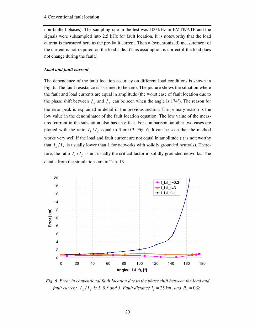
Load and fault current
The dependence of the fault location accuracy on different load conditions is shown in
Fig. 6. The fault resistance is assumed to be zero. The picture shows the situation where
the fault and load currents are equal in amplitude (the worst case of fault location due to
the phase shift between LI and fI can be seen when the angle is 174º). The reason for
the error peak is explained in detail in the previous section. The primary reason is the
low value in the denominator of the fault location equation. The low value of the meas-
ured current in the substation also has an effect. For comparison, another two cases are
plotted with the ratio fL II / equal to 3 or 0.3, Fig. 6. It can be seen that the method
works very well if the load and fault current are not equal in amplitude (it is noteworthy
that fL II / is usually lower than 1 for networks with solidly grounded neutrals). There-
fore, the ratio fL II / is not usually the critical factor in solidly grounded networks. The
details from the simulations are in Tab. 13.
0
2
4
6
8
10
12
14
16
18
20
0 20 40 60 80 100 120 140 160 180
Angle(I_L/I_f), [º]
Err
or
[km
]
I_L/I_f=0.3I_L/I_f=3I_L/I_f=1
Fig. 6 Error in conventional fault location due to the phase shift between the load and
fault current. fL II / is 1, 0.3 and 3. Fault distance kml f 25= , and Ω= 0fR .

4 Conventional fault location
21
Fault resistance
The fault impedance was simulated with a range of fault resistances, 0 -100 Ω. The error
in the fault location for the studied case is shown in Fig. 7. Even though the selected
range of fR might not be as high as in a real case, it indicates the influence of increas-
ing fault resistance. Therefore the potential for using this type of conventional fault loca-
tion method for the ”higher impedance” faults that occur in Fingrid’s 110 kV networks
is very small. The details of the simulations are in Tab. 14.
0
20
40
60
80
100
120
0 10 20 30 40 50 60 70 80 90 100
Rf [Ω]
Err
or,
[km
]
Fig. 7 Error in conventional fault location due to fault resistance; for 3/ =fL II and
fault distance kml f 25= .

4 Conventional fault location
22
4.2 Improved conventional fault location
The improved conventional fault location (ICFL) is a reactance based fault location
method. The influence of unknown fault resistance on single-phase to ground fault loca-
tion can be reduced by taking into account only the imaginary parts of the numerator and
denominator in Eq. (10):
)'()'''(3
1
)(
)')'''(3
1(
)(
12101210 ZI
IimagXXX
I
Vimag
ZI
IZZZimag
RI
Vimag
l
f
L
f
f
f
L
ff
f
f
+++
=
+++
−
= (13)
where the symbols are as in Eq. (10). 0'X , 1'X and 2'X are the zero-, positive- and
negative-sequence reactances of the line per km.
4.2.1 Method error
As can be seen from Eq. (13), the method is less dependent on the fault resistance than
Eq. (10). (It is assumed that the fault impedance can be substituted by the fault resis-
tance, otherwise the numerator will consist of two imaginary components.) Anyhow, the
reduction of the denominator of Eq. (10) into the imaginary part only, Eq.(13), makes
the method more sensitive to the angle between the fault and load currents, fI and LI .
The above mentioned denominator has a zero crossing in the area of interest (for normal
R-L load types in series), which means that Eq.(13) is very unstable around this point:
0)'()'''(3
11210 =+++ Z
I
IimagXXX
f
L
(14)
The denominator of Eq. (13) can be plotted with the parameters of the studied network,
Fig. 8 ( 0'X , 1'X , 2'X and 1'Z can be calculated from the parameters given in Appendix
A). As can be seen, the behavior of the equation and its zero crossing depend on the
ratio fL II / . This dependence is shown in Fig. 8 for different angles and amplitudes of
fL II / . (Note that the curves are valid for any kind of neutral grounding. They depend
only on the line parameters and the load-fault current relation.)
For practical application, the range of the “R-L” load phase angle 0-90º and also the “R-
C” load angles 0-90º are shown for one case, 3/ =fL II . This range of load does not
hold for all cases. In general, the zero-crossing area can be reached with a normal R-L

4 Conventional fault location
23
load, because the fault current magnitude and phase depend on the network configura-
tion, neutral grounding, fault resistance, etc. It just so happens that in the particular case
under study the load is capacitive. In general, the angle of fL II / lies within 360 de-
grees. Therefore, the zero-crossing can be on the both the left and right side of the fig-
ure.
0 50 100 150 200 250 300 350-4
-3
-2
-1
0
1
2
3
4Imaginary part of denominator
Angle(IL/If) [º]
Imag
inar
y pa
rt of
den
omin
ator
[ Ω]
Fig. 8 The imaginary part of the denominator of Eq.(13) for the study network. The dif-
ferent ratios of load to fault current, fL II / , are from 1 to 10.
The phase angle “ =0ϕ angle( fL II / )= FL ϕϕ − ” for the zero crossing can be evaluated
by solving Eq. (14). Eq. (15) presents the angle 0ϕ between the fault and load currents,
fI and LI , where fault location would not be possible because of the denominator zero
crossing. The development of Eq. (15) from Eq. (14) is shown in Appendix A:
))'
)'''(3
1
(asin( 1
1
210
0 z
f
LFL
ZI
I
XXXϕϕϕϕ +
++−=−=
(15)
where Lϕ and Fϕ are the load and the fault current angle where the denominator zero
crossing takes place. 1zϕ is the angle of the positive-sequence impedance of the line.
2
3
4 5 6
7
8
fL II /
1
2 10 ∞
°÷° 275.79185.79
9
10
Zero crossing area
1.1155
Load types for 3/ =fL II
L-R 90˚-0˚
2 10 ∞
°÷° 185.7962.117
Zero crossing area
R-C 0˚-90˚

4 Conventional fault location
24
The zero crossing of Eq. (14) moves between two border values, depending only on the
ratio fL II / and the network parameters.
Moreover, not only cases where the angle FL ϕϕϕ −=0 , calculated in Eq. (15), will be
affected by a denominator zero crossing but also cases where the angle is around this
value. From Fig. 8 it can be seen that the affected area is larger for lower rates of fL II /
than higher ones, because of the lower growth of the denominator curve of Eq. (13)
when crossing the zero point. This can be clearly seen in Fig. 9. In real situations the
maximum error (and error distribution) in fault location caused by the zero crossing can
be estimated using the measured data.
Fig. 9 The absolute value of the imaginary part of the denominator of Eq.(13) for the
studied network. The different ratios of load to fault current, fL II / , are from 1 to 10.
The practical influence of the denominator on fault location can be seen from the simu-
lations in Fig. 10 for 3/ =fL II , and in Fig. 13 for 9/ =fL II . The ratio fL II / seems to
have a strong influence on the affected area. The affected area is much smaller in Fig. 13
than in Fig. 10.

4 Conventional fault location
25
4.2.2 Example of zero-crossing calculation
This calculation example is shown in order to illustrate how to define the border values
for the zero crossing region of the denominator in Eq. (13). The parameters of the stud-
ied network are given in Appendix A.
Critical value of fL II /
The necessary condition for the possible zero crossing of Eq. (14) can be found when
the term under the “asin” in Eq.(15) is equal to 1. This happens at the critical angle,
crϕ , when ))1(asin( 10 zcr ϕϕϕ +−== . For the studied network, this is
°=+°−= 174.21- )90( 1zcr ϕϕ (i.e. °=185.79crϕ ). This value is also shown in Fig. 8
(1.1155). The ratio of fL II / that relates to this zero-crossing is when the argument of
“asin” becomes one, 1210 '/)'''(3
1/ ZXXXII fL ++= . For the network under study, this
is when 1.1155/ =fL II . If the ratio is below this value there is no zero-crossing caused
by any load and there is no significant influence of the phase angle on the fault location
itself. In other cases there does exist a zero crossing and hence an increased error area.
Therefore, this number is named the critical value and is a constant for a given net-
work.
Borders values of 0ϕ
If fL II / is greater than the critical value there is always a zero-crosing for at least one
angle between the load and fault current 0ϕ . The maximum value of FL ϕϕϕ −=0 oc-
curs when the argument of the “asin” of Eq. (15) is equal to zero. This happens at the
border angle ∞ϕ when the load is very big and Eq. (15) can be solved as:
110 180))0(asin()(lim zzI kL
ϕϕϕϕ −°⋅=+−== ∞→∞ , (where k = 0,1,2,3…). This is actu-
ally the negative of the angle of the positive-sequence impedance of the line per km,
1'Z , for k = 0. For the studied network, the roots for k = 0 and k = 1 are:
°=−=∞ -84.211zϕϕ (i.e. °=∞ 275.79ϕ ) and °=°=−=∞ 95.786184.21-180180 1zϕϕ .
The position of these limits can be seen in Fig. 8, marked for an infinitely high load cur-
rent (∞). This range defines the zero-crossing area.
Increased error area
When the ratio fL II / becomes greater than the critical value (1.1155), the zero crossing
occurs within the interval of °=−=∞ 95.7861180 1zϕϕ and °=− 275.791zϕ . For in-

4 Conventional fault location
26
stance, it can be seen in Fig. 8 that the function for 1/ =fL II does not have a zero-
crossing, but the zero crossing has already come into existence when this ratio is 2.
In other words, the existence of a zero crossing does not always mean that the method
will work incorrectly. This happens only under some unfavorable conditions. An inaccu-
rate fault location occurs if the ratio of the amplitudes of the load and fault currents are
greater than the critical value (1.1155 in this studied case) and the angle between them is
specific to this ratio, in accordance with Fig. 8. In other cases the method might work
with small errors even though the above mentioned ratio is greater than the critical
value.
It can be seen that Eq. (15), dependent on fL II / , converges very quickly to the limit
values of °=∞ 275.79ϕ or °=∞ 95.7861ϕ . For higher rates of fL II / the zero-crossing
is more or less constant with the angle of fL II / and equal to the border values of ∞ϕ ,
and the error area is smaller. This is generally the case for networks with isolated or
compensated network neutrals.
For lower rates of fL II / , the zero-crossing changes with the angle of fL II / even more
and the error area is wider. This is usually the case for networks with solidly grounded
neutrals.
These effects are seen in both Fig. 8 and Fig. 9 and in the simulated cases shown in Fig.
10 and Fig. 13.
The minimum of the set of curves in Fig. 8, is at the same value of 0ϕ equal to the criti-
cal angle crϕ . This is because the derivation of Eq. (14) depends only on the positive
sequence impedance, not on the ratio of the fault to load current. When the derivation is
calculated, it comes to °−=+− 901zFL ϕϕϕ and hence, for the studied case,
°=−°−= 185.7990 1zcr ϕϕ .

4 Conventional fault location
27
4.2.3 EMTP/ATP Simulations
Example of zero-crossing simulation
The fault location accuracy of the improved conventional fault location method was
tested with ground faults in a 110 kV solidly grounded radially operated network using
EMTP/ATP. The network details and the simulated data can be found in Appendix A.
The same network as in Fig. 101 was simulated but without the connected line 3. The
reference signal for the vector angle identification was the phase to phase voltage (be-
tween non-faulted phases). The sampling frequency of the test was 100 kHz in
EMTP/ATP and the signals were subsampled into 2.5 kHz for fault location. It should
be noted that the load current is measured here as the pre-fault current. This means that a
(synchronized) measurement of the load current is not required on the load side. This
assumption should be valid if the load does not change during the fault. The results can
be seen in Fig. 10.
0.1
1
10
100
1000
0 20 40 60 80 100 120 140 160 180
Angle(I_L/I_f), [º]
Err
or,
[k
m]
Fig. 10 Error of improved conventional fault location due to phase shift between the
load and fault current. For 3/ =fL II , and fault distance kml f 25= .
In Fig. 10 the output of the developed fault locator is shown. (The fault locator is basi-
cally the same as in Section 4.1, but calculates the imaginary parts of the numerator and
denominator for the fault location equation. The fault locator is presented in Chapter
13). Fig. 10 shows the the situation when 3/ ≅fL II . Simulations clearly show an in-
creased error in fault location under some conditions. Eq. (15) in this case indicates that
the highest error occurs at the same place, where °=117.61490ϕ , which can also be
seen from the simulated case in Fig. 10. The angle 0ϕ represents the capacitive load of
Eq. (14), zero-crossing for 3/ =fL II
°= 117.6160ϕ
L-R Load angle
range 90˚-0˚
R-C Load angle
range 0˚-90˚

4 Conventional fault location
28
approximately )(50 capL °=ϕ , i.e. 0.6428)cos( =Lϕ . The other possible zero-crossing
angle, °= 106.0426- 0ϕ (i.e °= 253.9574 0ϕ ), is not reachable, because the passive load
angle can only change within 180 degrees. The details are shown in Tab. 15 in Appen-
dix A. 3/ ≅fL II is a rather unrealistic case for systems with solidly grounded neutrals.
In a real system where 1/ <fL II , the zero-crossing might not appear at all.
In cases where the load and fault currents do cause a zero-crossing in the fault location
equation of the improved conventional fault location method, the conventional method
can be used more accurately; compare Fig. 10 and Fig. 6 for 3/ =fL II .
Nonetheless, fault location is not possible in cases where the fault and load currents
cancel each other’s voltage drop, as was shown in the previous chapter. In other cases,
the fault location accuracy is affected by the denominator of Eq. (13).
Fault resistance
By defininition, there should not be any influence from the fault resistance on fault loca-
tion. However, higher fault resistance causes lower fault currents. The dependence of
the error in fault location on fault resistance is shown in Fig. 11.
Nevertheless, the influence is much smaller when compared to the conventional fault
location in Fig. 7, which analysed the same data as presented here. The detailed data are
shown in Tab. 14.
0
1
2
3
4
5
6
7
8
0 10 20 30 40 50 60 70 80 90 100
Rf [Ω]
Err
or,
[km
]
Fig. 11 Error in improved conventional fault location due to fault resistance, for
3/ =fL II and fault distance kml f 25= .
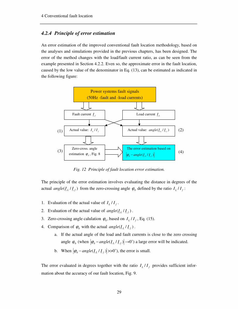
4 Conventional fault location
29
4.2.4 Principle of error estimation
An error estimation of the improved conventional fault location methodology, based on
the analyses and simulations provided in the previous chapters, has been designed. The
error of the method changes with the load/fault current ratio, as can be seen from the
example presented in Section 4.2.2. Even so, the approximate error in the fault location,
caused by the low value of the denominator in Eq. (13), can be estimated as indicated in
the following figure:
Fig. 12 Principle of fault location error estimation.
The principle of the error estimation involves evaluating the distance in degrees of the
actual )/( fL IIangle from the zero-crossing angle 0ϕ defined by the ratio fL II / :
1. Evaluation of the actual value of fL II / .
2. Evaluation of the actual value of )/( fL IIangle .
3. Zero-crossing angle calulation 0ϕ , based on fL II / , Eq. (15).
4. Comparison of 0ϕ with the actual )/( fL IIangle .
a. If the actual angle of the load and fault currents is close to the zero crossing
angle 0ϕ (when )/(0 fL IIangle−ϕ →0˚) a large error will be indicated.
b. When )/(0 fL IIangle−ϕ >>0˚), the error is small.
The error evaluated in degrees together with the ratio fL II / provides sufficient infor-
mation about the accuracy of our fault location, Fig. 9.
Fault current fI Load current LI
Power systems fault signals
(50Hz -fault and -load currents)
Actual value: fL II / Actual value: )/( fL IIangle
Zero-cross. angle
estimation 0ϕ , Fig. 8
The error estimation based on
)/(0 fL IIangle−ϕ
(1) (2)
(4) (3)

4 Conventional fault location
30
It should be noted that in practice there are two zero-crossing angles and therefore two
error angles. The closer one is more influential.
4.3 Conventional methods vs. neutral grounding
The conventional fault location methods for the solidly grounded network described in
the previous sections, 4.1 and 4.2, can work in networks with all the neutral grounding
types (isolated neutral, Petersen coil grounded…), but only for some specific network
configurations. The key element in network configuration is to have a good return path
for the zero-sequence current to the substation. In cases where the network neutral is not
solidly grounded the lines connected to the same substation might help.
The same network is simulated here as in the previous sections. However, one outgoing
line (Line 3) of length 55 km is connected to the substation, Fig. 101 in Appendix A.
The results are shown in Fig. 13. fL II / was choosen to be 9, because in the case of
isolated neutrals or Petersen coil grounded networks the fault current is small. The de-
tailed data are given in Tab. 16.
0.01
0.1
1
10
100
1000
10000
0 50 100 150 200 250 300 350
Angle(IL/If)
Err
or [k
m]
Low-reactance (254.7 mH)Compensated (5050 mH)Isolated
Fig. 13 Error in improved conventional fault location due to phase shift between the
load and fault current, for 9/ =fL II and fault distance kml f 25= . Result for different
neutral grounding types are shown: low impedance, Petersen coil and isolated. The
load conditions are marked as R-resistive, L- inductive and C-capacitive.
The simulation of the studied case for different neutral grounding gave the following
results. If the network neutral is grounded with the low impedance reactors (at 50 Hz, 80
L R C L R C
L R C

4 Conventional fault location
31
Ω), the whole 360 degrees range of FL ϕϕ − can be reached with the passive load, Fig.
13. This is possible because the phase of the fault current changes as well. In the case of
a Petersen coil grounded or isolated neutral network, the fault current angle is almost
stable and therefore only a range of 180 degrees is covered, Fig. 13. The conventional
methods work similarly for all kinds of neutral arrangements, under the above men-
tioned conditions.

4 Conventional fault location
32
4.4 Conventional methods vs. real ground faults
The conventional algorithms presented in the previous sections were tested using real
ground fault recordings from the Finnish 110 kV network. The recordings are from the
Pyhäkoski – Rautaruukki line. This line is radially operated with low reactance ground-
ing. The detailed network data can be found in Appendix A (a diagram of the network is
given in Fig. 102 and the network data is in Tab. 17). The phase voltage and current of
all three phases were measured along with the zero-sequence current in the Pyhäkoski
substation. The sampling frequency was 1 kHz. The exact fault location was measured
with a parallel connected travelling wave recorder.
The error of both the conventional and improved conventional algorithms is similar, as
shown in Fig. 14. More precise data can be found in Tab. 18 in Appendix A.
-15
-10
-5
0
5
10
15
20
0 10 20 30 40 50 60 70 80
Fault distance [km]
Err
or [k
m]
CFLICFL
Fig. 14 The error in the conventional (CFL) and improved conventional (ICFL) algo-
rithms. The test data is from the Pyhäkoski – Rautaruukki line.
The fault location was estimated relatively accurately, ±2 km for the conventional and
±1 km for the improved conventional fault location methods, for the first 50 km of the
line. The fault distance in the last 30 km of the line to the Rautaruukki substation was
calculated with much less accuracy. One possible reason is that the line inductances
were changed due to a second line that runs parallel to the tested line for 29,358 km,
Fig. 102.

4 Conventional fault location
33
4.5 Utilising the zero-sequence current in conventional fault
location
The currents of all three phases are not usually measured in the disturbance recorders of
Fingrid’s 110 kV substations for economic reasons, Chapter 2. The challenge is to use
the zero-sequence current instead of the phase currents. The study covered in this sec-
tion is based on both EMTP/ATP simulations and real fault events.
During the single-phase to ground fault in networks with a solidly grounded neutral, the
positive-, negative- and zero- sequence currents are equal to 1/3 of the phase current,
Fig. 3. Therefore, it is possible to utilise the zero-sequence current in fault location, at
least in theory. The zero-sequence current can be measured in the network as a sum of
the phase currents or as a neutral current. The neutral current can only be measured in
networks with a neutral grounded via some impedance. Using of this methods it is pos-
sible to measure the zero-sequence current under some circumstances. If there are other
lines connected to the substation or if the neutral is grounded via a relatively high im-
pedance, the zero-sequence current will not fully return via the measurement point. In
such cases only a part of the zero-sequence current is measured and therefore some cor-
rection will be needed, [21]. The correction will be based on the lines’ total ground ca-
pacitance and the grounding coil inductance. If the grounding impedance is a low reac-
tance coil and there are no other outgoing lines from the substation, the circumstances
are almost the same as in a solidly grounded network.
Even if all the circumstances mentioned above are ideal for fault location, there will
always be some error. The reason is that it is virtually impossible to detect the load con-
ditions (pre-fault current) by measuring only the zero-sequence current. Therefore, such
fault location methods are only expected to work if the load current is smaller than the
fault current. Otherwise, the load current can be estimated from the power measurement
of the line.
4.5.1 EMTP/ATP Simulations
The simulations were performed with the EMTP/ATP software on a radially operated
network with a reactance grounded neutral. The size of the reactor was tuned to obtain
similar results to those obtained from real faults (500 mH was choosen). The phase volt-
ages and currents were measured in the feeding substation with the neutral current. The
sampling frequency of the test was 100 kHz in EMTP/ATP and the signals were sub-
sampled into 2.5 kHz for fault location. The parameters of the line match Fingrid’s Py-
häkoski – Rautaruukki line. For more details see Appendix A (a schematic representa-
tion of the line is given in Fig. 103).

4 Conventional fault location
34
The so-called “improved conventional fault location method” was tested using both
phase and zero-sequence currents. The fault distance was 25 km in a network of total
line length 81.5 km. The fault resistance was 0 ohms. The simulations were processed
by the fault locator detailed in Chapter 13. The fault data was de-noised by a wavelet
filter. The influence of the load, known/unknown (unknown when the zero-sequence
current is used, known if the phase current is used), is represented by the ratio of load to
fault current. The load and fault currents were in phase in the modelled cases. A com-
parison of the method error is shown in Fig. 15 for both cases. More details and results
can be seen in Tab. 20 in Appendix A.
-45
-35
-25
-15
-5
5
0.01 0.1 1 10
IL/If, [p.u]
Err
or [k
m]
I_phase3I_0
Fig. 15 Error in fault location by the improved conventional method. Utilisation of the
phase (I_phase) and zero-sequence (3I_0) currents are compared. The load ( LI ) and
fault ( fI ) currents are in phase.
From the simulation results, it is clear that fault location using the zero-sequence current
will only work when the load current is much lower than the fault current. More pre-
cisely, the limit for the load current was identified to be 50% of the fault current in this
case. This conclusion might be a bit different if the fault and load currents are not in
phase as they were in this case. However, the trend of the curves would probably remain
the same.
5.0/ =fL II
e.g 50%

4 Conventional fault location
35
4.5.2 Real faults from the Pyhäkoski – Rautaruukki line
Similar results can be obtained for real fault cases from the Pyhäkoski – Rautaruukki
line. Here only 4 cases are presented out of six available, Section 4.4 (fault distances: 1,
25.8, 51.5 and 51.5 km). The other two yielded such a high degree of error that it would
not be illustrative to include them. The error in the so called “improved conventional
fault location” is shown in Fig. 16. This figure shows the error for both the phase current
and zero-sequence current based methods. The detailed data are in Tab. 18 of Appendix
A.
-1
-0.5
0
0.5
1
1.5
2
2.5
3
0 0.05 0.1 0.15 0.2 0.25 0.3 0.35 0.4
IL/If, [p.u]
Err
or [k
m]
I_phase3I_0
Fig. 16 The error in the improved conventional method. Utilisation of the phase
(I_phase) and zero-sequence (3I_0) currents are compared. Data from the Pyhäkoski –
Rautaruukki line.
The figures show similar results to the simulated cases. The fault location error in-
creases with the load/fault current ratio.
1 km
25.8 km
51.5 km

4 Conventional fault location
36
4.6 Discussion
Solidly grounded vs. isolated systems
The conventional fault location methodology was examined in this chapter, defined for
solidly grounded radially operated systems (or low-reactance grounded networks). The
investigation of an isolated neutral network showed that the method can also be applied
to this type of network with similar accuracy. The key element is to have enough zero-
sequence current flow via the measurement point in the substation. In the case of a sol-
idly grounded network, all three components, the positive, negative and zero sequence
components, are equally present and can be measured. However, if the neutral of the
transformer is not grounded solidly, the zero-sequence current will return fully or par-
tially via the power lines. The return path for the zero-sequence current would be im-
proved if there are some other outgoing lines or compensation capacitors with grounded
neutrals connected to the same busbar as the line under consideration (however, they are
not grounded in Finland). In the case of long lines connected to the same busbar, the
accuracy of the method would, in the best case, be the same as for a solidly grounded
network. In our particular case, the length of the line connected to the same busbar was
chosen to improve this path so that the fault location could be made with satisfactory
accuracy. The exact correction factor is of a general nature, however, and will be shown
for the transient method in Chapter 11.
Correction for improved conventional fault location
The improved conventional fault location method calculated the fault distance more
accurately than the conventional fault location method. It has the ability to reduce the
influence of the unknown fault resistance. The improvement is remarkable and the
method can be considered to be more accurate. However, there is also some weakness in
this solution. The fault location equation becomes at some point unreliable, due to the
fault location equation denominator’s small value. In this chapter the problematic cases
have been specified and it is possible to say how accurate our estimation will be directly
from the measured signal (from the method’s point of view).
Zero-sequence current used for fault location
The zero-sequence current can be measured as a sum of the 3 phase currents or as a cur-
rent in the neutral of the transformer. These two cases are quite different. In both cases
the location would be better if the grounding impedance is lower (the lower the better -
the best would be zero) and if the load current is considerably lower than the fault cur-
rent (the best results would be obtained if the network is unloaded).
The length of the connected line would be an advantage in the first case, where the cur-
rent sum is measured. But, it would be disadvantageous to measure the neutral current,

4 Conventional fault location
37
because the neutral current is only part of the total zero-sequence current in the system.
The correction will depend on the total network ground capacitance and the reactor size,
[21].

5. General study of fault transients
38
5 General study of fault transients
In general, a power transmission system consists of resistances, inductances and capaci-
tances, which exist as lumped parameters but are also distributed over the line, trans-
formers, etc. Such a system will generate transients, which are of a wide spectrum, dur-
ing every change such as a switching operation or fault.
Fault transients, which can be used for fault location purposes, are studied in this chap-
ter. The spectrum of fault signals can be categorised and the dominant transient compo-
nents can be identified as in [1]. The typical transients of a fault current are:
Low frequency transients
• Suppression coil current transient (if coil is in use)
• Charge transient
High frequency transients
• Travelling waves
• Discharge transient
The first two transients are of relatively low frequency, which means a maximum level
of a few kilohertz. They are described in detail in Sections 5.1 and 5.3 and the discharge
transient is covered in Section 5.2. Travelling waves travel in the network at approxi-
matelly the speed of light in the case of overhead lines. Even if the network is relatively
long, a quite high sampling frequency is needed to catch the travelling waves. For over-
head lines this is in the range of at least a few hundred kilohertz.

5. General study of fault transients
39
5.1 Charge transient
When an earth fault occurs in a power system, the voltages of the two sound phases rap-
idly increase, which creates a transient. This transient flows through the transformer
primary winding. The simplified situation according to [13] and [14], when the induc-
tance and resistance of the line is neglected, is as shown in Fig. 17. The theory of fault
transients covered in this section deals with ungrounded neutral systems. Although other
systems exist in Finnish networks, such as compensated and reactance grounded neu-
trals, the analysis of fault transients in these systems (e.g. Petersen coil systems) is simi-
lar to the ungrounded one, because the coil is of relatively high impedance at fault tran-
sient frequencies.
Fig. 17 The lumped model for fault transient study in unearthed networks.
During a fault in phase 1, the phase to earth capacitance of the faulted phase can be ne-
glected for the purpose of this study (because it is short-circuited by the fault itself). The
phase to phase capacitances ppC of the surrounding phases are in parallel with their
phase to earth capacitances EC , as shown in Fig. 17. The capacitance between the un-
faulted phases (phases 2-3 in the studied case) can be omitted, since the ends are at the
same potential from the transient’s point of view (symmetrical system). TL is the sub-
station transformer inductance.
Cpp
Cpp
CE
CE
Overhead line
LT
Secondary of supply transformer
Fault
Phase 1
Phase 2
Phase 3
LT
LT
Ω= 0fZ

5. General study of fault transients
40
Fig. 18 The circuit for charge transient calculation.
Hence, the frequency of the “charge” transient during undamped conditions is calculated
as follows:
eqeq
cCL
1=ω , Teq LL 5.1= , )(2 Eppeq CCC +=
(16)
where:
cω is the angular frequency of the charge transient
TL is the substation transformer inductance
ppC is the phase to phase capacitance of the line
EC is the phase to earth capacitance of the line
Note: This example relates only to a fault on the busbar and where the transformer’s
inductance is high compared to the line inductance. For a more complex solution the
line inductances must be added in series to the transformer’s inductance. Then TL in Eq.
(16) should be substituted by fT LL + , where fL is the fault path inductance of the line.
The initial amplitude of the charge transient in an undamped case is calculated by Eq.
(17).
eqceeqc
ec Cv
L
vi ω
ω==ˆ
(17)
If the fault happens at the phase voltage maximum, the amplitude of the charge transient
is as in Eq. (18):
2(Cpp+CE)
1.5LT

5. General study of fault transients
41
efE
ceqc i
C
Ci ˆ
3ˆ
ω
ω=
(18)
where:
fω is the fundamental angular frequency
ev is the instantaneous phase to earth voltage at the fault moment
ei is the uncompensated steady state fault current peak value with zero fault resistance
Influence of the connected lines
If another line (or lines) is connected to the same busbar as the faulted line, the con-
nected line will also contribute to the generation of the fault charge transient. The ca-
pacitances of the healthy phases, 'ppC and 'EC (phase to faulty phase and phase to
ground), of the connected lines are connected in parallel with the healthy phase capaci-
tances of the faulty line, EC and ppC , shown in Fig. 17. The total equivalent capaci-
tance of the connected line 'eqC must be added to the faulted line’s equivalent capaci-
tance, i.e. )''(2)(2' ppEppEeqeq CCCCCC +++=+ . This results in lowering the frequency
of the transient and increasing the initial peak value of the fault current transient in rela-
tion to Eqs. (16) and (17).
The practical charge transient frequency for 110 kV lines is in the range of 80 to 600 Hz
and has a dominant amplitude. For comparison, in medium voltage distribution net-
works the transient frequency is in the range 100-800 Hz and the amplitude can be 10-
20 times higher than the uncompensated fundamental frequency fault current, [1]. It is
also easily distinguished from the 50 Hz load current. Therefore, this transient is suit-
able for fault location.

5. General study of fault transients
42
5.2 Discharge transient
The charge stored in the earth capacitance of the faulty phase is removed during a fault
and a “discharge” transient is generated. The discharging of the capacitance takes place
at a frequency dictated by the speed of the travelling wave in the line and the fault dis-
tance. The situation is clearly illustrated in Fig. 19, where the lattice diagram and the
faulted phase voltages are shown for a single-phase to ground fault. The travelling
waves caused by the fault are reflected between the fault place and the substation. The
amount and polarity of the reflected wave depends on the reflection coefficient. The
reflection coefficient is a number between -1 and 1, and for voltage is defined as:
CT
CTv ZZ
ZZ
+
−=ρ
(19)
where CZ is the characteristic impedance of the line and TZ is the terminal impedance
of the line. The reflection coefficient for the current is vi ρρ −= .
The situation in Fig. 19 is idealized; the reflection coefficient for the voltage is 1 at the
substation (supposing that the impedance is infinite compared to the line impedance
CZ ) and -1 in the fault place (the fault impedance is taken to be zero), [26].
Fig. 19 The lattice diagram for ground fault study (left) with the fault phase voltage in
the substation (right).
Measurement
Lattice diagram
Fault
1−t
0t
1t
2t
3t
4t
1−=vρ 1=vρ
Fault phase voltage measured
in the substation
Fault distance
Ω= 0fR
1−t 0t 1t 2t 3t
4t Time
1
-1
V
olta
ge [
p.u]
dfT /1= Fault start

5. General study of fault transients
43
The reflections of the travelling waves, shown in Fig. 19 (left), will cause a voltage at
the discharge frequency at the measurement point, Fig. 19 (right). The frequency of the
discharge transient can be calculated according to [13] as:
fd l
f4
ν=
(20)
where: ν is the velocity of the travelling wave and fl is the fault distance. The dis-
charge frequency calculated according to Eq. (20) exists in a faulted system if there is a
perfect reflection at the fault place ( Ω= 0fZ ); otherwise it might be mixed with reflec-
tions from the other end of the line.
Influence of the connected line
If another line (or lines) is connected to the same busbar as the faulted line, the con-
nected line will also contribute to the discharging of the capacitance of the faulty line.
This means the dominant discharge frequency of the whole system can no longer be
calculated according to Eq. (20). This situation is made clear in Fig. 20, where the lattice
diagram and the fault phase voltages are shown for a single-phase to ground fault. For
simplicity, the reflection coefficient for the voltage is 1 at the substation of the con-
nected line and -1 at the fault location, and the reflection coefficient in the substation
with the measurement is taken to be 0. The situation is shown for the connected line
length equal to the fault distance. This will cause the total discharge frequency of the
network to be half of the value that would occur if there is no connected line.
Based on these facts and experience gained from the EMTP/ATP simulations presented
in Chapters 7 and 8, the following equation for the discharge transient frequency df can
be written:
)(4 clfd ll
f+
=ν
(21)
where ν is the velocity of the travelling wave in the lines, fl is the fault distance and
cll , in this case, represents the length of the connected line.
The example shown is only one of the possible network configurations. There might,
however, be more than one connected line outgoing from the substation and, what is
more, the speed of the travelling waves might differ for the lines. In such cases a more
detailed analysis based on the travelling waves must be provided in order to compute the
frequency of the discharge transient.

5. General study of fault transients
44
Fig. 20 The lattice diagram for ground fault study in a network with connected lines
(left) with the fault phase voltage in the substation (right).
The amplitude of the discharge transient is normally 5-20% of the charge transient. The
practical frequency range is 500-2500 Hz for distribution networks, according to [1]. In
HV networks the range is wider. The speed of light can be used for approximate calcula-
tion of the discharge transient frequencies in HV overhead lines. (More precisely,
CLv /1= with C and L being the capacitance or the inductance of the line per km). In
fact, the frequency of the discharge transient depends only on the fault distance, Eq. (20)
or (21). Therefore, the frequency can be very high for faults close to the busbar, but the
typical range in 110 kV systems is about 300 Hz -5000 Hz. In practice the frequency of
discharge transients is higher than the charge transients.
5.3 Suppression coil current transient
In a compensated neutral network the energising of the compensation coil creates a tran-
sient during an earth fault. The transient consists of the supply frequency and a DC
component. The suppression coil current transients can be analysed using symmetrical
components or using a single phase representation, as shown in Fig. 21. The idea this
analysis is based on is the description of the fault impedance loop.
Lattice diagram Fault phase voltage measured
in the substation
1−t 0t 1t 2t 3t 4t Time
1
-1
Vol
tage
[p.
u]
dfT /1= Fault start
1−t 0t 1t 2t 3t 4t Time
1
-1
V
olta
ge [
p.u]
dfT /1= Fault start
Single line
With connected line
Measurement Fault
1−t
0t
1t
2t
3t
4t
1−=vρ 1=vρ
Fault distance
Ω= 0fR
0=vρ
Connected line

5. General study of fault transients
45
Fig. 21 Transient of the suppression coil current.
The basic solution according to [1] can be obtained from:
)sin(ˆ ϕω +=+ tviRdt
diL fSCSC
(22)
where: fω is the fundamental angular frequency, t is time, v is the voltage peak value,
i is the current, SCL and SCR are the respective sums of the inductances and resistances
of the suppression coil, coupling transformer winding, faulty line section (length) and
fault, and ϕ is the initial phase angle.
The solution of Eq. (22) can be expressed as:
))]arctan(sin())arctan([sin()(
ˆ /
22SC
SCfRL
t
SC
SCff
SCfSCR
Le
R
Lt
LR
vi SCSC
ωϕ
ωϕω
ω−−−+
+=
−
(23)
The transient includes two components, an exponentially decaying DC component and a
fundamental frequency component. The DC component will appear in situations where
the fundamental frequency current is not zero at the fault moment. If this current is equal
to zero at the fault initiation, the DC transient will not appear at all. The other extreme is
if the fault happens at the current maximum; then the DC component will be maximum,
[1]
Overhead line Secondary of primary transformer
Fault
Compensation
coil
5. General study of fault transients
46
In practice this current transient can be highly distorted because of the magnetic core
saturation caused by the high DC current. The saturation of the coil depends very much
on the initial moment at which the fault occurs. Therefore, this transient can be utilised
in fault location if the fault does not appear at a high instantaneous value of the current.
If the coil has an air gap in the the steel core, there is no saturation at all.
The saturation of the coil can also be harmful in cases where the charge or discharge
transients are used for fault location. The reason is that the saturation of the coil core
produces odd numbers of harmonics in the current, which might become mixed up with
the actual transients, such as the charge or discharge transient, [1].
6. Signal processing methods
47
6 Signal processing methods
The fault signals that can be used for fault location cover a wide frequency spectrum.
Usually the fault signal consists of the 50 Hz wave with some higher or lower frequency
components superposed on it. The higher frequency transients typically attenuate
quicker than the lower ones.
There are many techniques that can be used for filtering out the fault transients from the
measured fault signal. In this chapter the most common ones are represented. More
about signal processing can be found in [4], [5], [15], [22], [24] and [30].
For better frequency estimation of the transient, a pre-processing technique can be per-
formed, Section 6.1. Spectrum analysis is presented in Section 6.2. Section 6.3 reviews
some of the mathematical transformations used in the time-frequency signal representa-
tion. Here the most popular techniques are listed, the windowed Fourier transform and
the wavelet transform. Section 6.4 concentrates specifically on wavelet filters.
6.1 Pre-processing of the signal
Sometimes a transient is represented by a limited number of samples and so estimation
of its frequency might be difficult. Filtering can be performed in order to detect the fre-
quency of the transient more accurately. For this reason signal pre-processing is applied.
Removing the 50 Hz component with a simple filter
This can be accomplished very easily by filtering:
][][][ 50Nnfnfng +−=
(24)
where ][nf is the original signal - discrete function of the samples, ][ng is a new signal
- discrete function of the samples and 50N is the number of samples related to 20 ms (if
the system frequency is 50 Hz). The filter’s advantage lies in its simplicity, but at the
price of a bad side effect. It can partly cancel the other frequencies: DC, 100th 150th
200th… k*50th (where k = 0,1,2…etc), as can be seen from the very simple equation.

6. Signal processing methods
48
Removing the 50 Hz with a band pass FIR filter
A digital FIR (finite impulse response) filter is mainly used to remove the 50 Hz signal,
which usually has the dominant amplitude and is very close in the frequency domain to
the transient itself. It can also remove the higher frequency transients or noise. An ex-
ample of the “sinc” filter coefficients and the filtered spectrum are shown in Fig. 22.
The filter’s lower cutoff frequency is set to Hz 1001 =cf and the higher to Hz 4502 =cf .
50 100 150 200-0.3
-0.2
-0.1
0
0.1
0.2
0.3
0.4
0.5
0.6
0.7
Samples [-]
Impu
lse
resp
onse
[p.u
]
0 100 200 300 400
0
0.2
0.4
0.6
0.8
1
1.2
1.4
Frequency [Hz]
Ma
gni
tude
re
spon
se [p
.u]
Fig. 22 Example of filter for pre-processing. The filter’s coefficients are represented by
200 samples (left), and the frequency response of the filter (right).
This filter characteristic can be achieved with the coefficients calculated according to
Eq. (25), given by the “sinc” function, [22] :
)(
))(2sin(
)(
))(2sin()( 12
mk
mkf
mk
mkfkh cc
−
−−
−
−=
π
π
π
π, if k≠m
)(2)( 12 cc ffkh −= , if k=m
(25)
In order to reduce the pass-band and stop-band ripples we used the Hamming window,
Eq. (26), as presented in [22]. The filter coefficients with the Hamming window applied
can be seen in Fig. 22 (left).
))1/(2cos(46.054.0)( −−= Nkkw π
(26)
where k and m are the integer variables and N is the number of coefficients.
The filter gives very good frequency resolution as is seen from the frequency response in
Fig. 22 (right). However, the time resolution of the filtered signal will strongly depend
on the filtered spectrum width. The time resolution will be lower if the filtered fre-
quency band is too narrow.

6. Signal processing methods
49
6.2 Spectrum analysis
For detection of the signal frequency, the Fourier transform (FT) is used. This transform
can give the frequency content of the signal but not the time position of its components.
The definition of the FT according to [15] is:
( ) ∫∞
∞−
−⋅= dtetxfFT ftj π2)(
(27)
where )(tx is a continuous function of time t , f is the frequency and t is time.
And the discrete version, the discrete Fourier transform:
[ ] [ ]∑=
−
⋅=2/
1
22 N
n
N
knj
enxN
kDFTπ
(28)
where: [ ]nx is a discrete function of the samples, kn and are the integer variable pa-
rameters, and N is the number of samples.
The fault signals are non-stationary signals and the spectrum of such signals gives the
correct frequency position of each signal component, but not their amplitude. Because
the signals do not exist over the entire analysed period, the amplitude is the mean value
over the analysed time interval. The right amplitude can only be achieved if the signal
component is so-called stationary. This means that the signal occurs in the analysed
window with a stable frequency and amplitude.

6. Signal processing methods
50
6.3 Time-frequency representation of the signal
Mathematical transformations are applied to signals in order to obtain information that
would not be readily available in the time-domain signal. There are a number of trans-
formations that can be applied, Fourier, wavelet, and Radon and Hilber, of which the
Fourier transform is probably the most popular.
In practice, most of the signals are time-domain signals. This representation is not al-
ways the best representation of the signal for other applications. Information that often
cannot be readily seen in the time-domain can be seen in the frequency-domain. How-
ever, not all information can be seen only in the time-domain or only in the frequency-
domain. Therefore, a combination of the two, the time-frequency representation of the
signal, is very informative.
For applying the transforms in practice (in digital devices), it is necessary to use their
discrete versions. Therefore, these are also presented.
In order to understand which transform is suitable for which signal, all signals can be
divided into two types:
• Stationary signal
Signals whose frequency content does not change during the analysed period.
• Non-stationary signal
Some frequency components exist in a shorter signal time than the analysed pe-
riod.
Commonly used techniques
In the past, the windowed Fourier transform was in common use. This transform is
based on equal windowing for each frequency level. The equal windowing causes dis-
turbance in such signals as the fault transients, mainly because of the existence of fre-
quency components lower than the needed component. This requires a combination of
other techniques to remove the lower frequencies.
Nowadays the wavelet transform is very frequently used for signals such as fault tran-
sients. The wavelet filtering is based on a multi-resolution analysis that uses small time
windows for higher frequencies and wider time windows for lower frequencies. This is
naturally suitable for signals like fault transients, because the high frequencies attenuate
(die) quickly and the lower transient frequencies are of longer duration, as is shown in
[4], [5].

6. Signal processing methods
51
6.3.1 Windowed Fourier transform
The windowed Fourier transform (WFT), also known as the short-term Fourier trans-
form (STFT), gives the time and frequency position of the signal components. The sig-
nal is divided into a sufficiently large number of small segments so that each segment of
the signal can be assumed to be stationary. The WFT thus gives the frequency spectrum
of every window of the signal and so it is possible to locate the time position of shorter
frequency components in the signal. The continuous WFT is defined according to [15]
by the following equation:
∫+∞
∞−
−⋅−⋅= dtetwtxftWFT ftjxw
πτ 2)()(),(
(29)
where: )(tx is a continuous function of time, f is the frequency, )( τ−tw is the win-
dow function, t is the time and τ is the translation.
This transform can be displayed in a spectrogram, such as the one in Fig. 23 (left),
where the time and frequency domains can be clearly seen. The WFT analyses the signal
with the same resolution at both high and low frequencies. In practice, windowing is
performed by a window function. The most popular window functions are the Gaussian,
rectangular, Hamming, Bartlett and Chebyshev. The Gaussian window function is pre-
sented below, [22]. It is defined by:
2
2
2
2
1)( δ
δπ
t
etw−
=
(30)
where δ is the standard deviation. In Fig. 23 (right), an example of the Gaussian win-
dowed sinusoidal signal at different frequencies and different time locations is presented
for 1=δ . For digital implementation the windowed discrete Fourier transform (WDFT)
is used.
To get better resolution in the time or frequency domains we can change the parameters
of the windows. A narrow window gives good time resolution, but poor frequency reso-
lution, Fig. 24c. Wide windows give good frequency resolution, but poor time resolu-
tion, Fig. 24b. If the window is very narrow, a low frequency signal will appear to be
non-periodical in the window and so its spectrum will tend to infinity and disturb the
higher frequency components, as shown in Fig. 24d. The resolution also depends on the
type of window function. For example, the results using Gaussian windowing are sig-
nificantly superior to those achieved using rectangular windowing, [5].

6. Signal processing methods
52
-80 -60 -40 -20 0 20 40 60 80TIME [ms]
f=100 Hz
ττττ=-40 ms
f=200 Hzττττ=0 ms
f=400 Hz
ττττ=40 ms
Fig. 23 The time-frequency plane for the WFT (left) and an example of a Gaussian win-
dowed sinusoidal signal at different frequencies and different locations in time, (right).
12 24 36 48 60 72 84 96 108 120-20
0
20
TIME [ms]
MA
GN
ITU
DE
TIME [ms]
FR
EQ
UE
NC
Y [H
z]
15 45 75 105
250
500
750
1000
1250
TIME [ms]
FR
EQ
UE
NC
Y [H
z]
2 14 26 38 50 62 74 86 98 110
250
500
750
1000
1250
TIME [ms]
FR
EQ
UE
NC
Y [H
z]
1 13 25 37 49 61 73 85 97 109
250
500
750
1000
1250
(a)
(b)
(c)
(d)
Fig. 24 Input signal (50 Hz + 600 Hz) and its WDFT. The input signal (a), WDFT with
ms 12=τ (b), WDFT with ms 4=τ (c), and WDFT with ms 2=τ (d).
FR
EQ
UE
NC
Y [
Hz]
-40 0 40
100
200
400
TIME [ms]

6. Signal processing methods
53
6.3.2 Wavelet transform
The term wavelet means “small wave”. The wavelet transform (WT) was introduced by
Jean Morlet at the beginning of the 1980s and has undergone rapid development since
then in the fields of image processing and acoustic signal analysis. It has the special fea-
ture of variable time-frequency localisation, which can be more advantageous when ana-
lysing non-stationary signals than WFT. Most of the signals that occur in practice have
their most important features in the high frequency range (for example the voice), there-
fore multi-resolution analysis (MRA) is applied. MRA analyses the signal at different
frequencies with different resolutions as it is designed to give good time resolution and
poor frequency resolution at high frequencies, but good frequency resolution and poor
time resolution at low frequencies, as is shown in Fig. 25 (left). In other words, the WT
uses narrow windows at high frequencies and wide windows at low frequencies, which
does not make the disturbance characteristic of the WFT, (compare Fig. 26b and Fig.
24d). The continuous WT is defined, according to [15], as:
∫+∞
∞−
−⋅= dt
a
bttx
abaWT x )()(
1),( ψψ
(31)
The windowing shown in Fig. 25 (left) is performed in practice by scaling and translat-
ing a “mother wavelet”. The mother wavelet ψ(t) is a function of two parameters, a-
scale and b-translation, according to Eq. (32).
)()(, a
bttba
−=ψψ
(32)
b gives the time position of the wavelet, while the parameter a controls its frequency.
The mother wavelet )(tψ must be short and oscillatory, and it must have a zero average
and decay quickly at both ends, [15]. There are many families of wavelets, for example,
Haar, Daubechies, Meyer, Gaussian, Mexican hat, Morlet, Shannon wavelets, and so on.
For example, a Gaussian function used as a Gaussian mother wavelet is defined as:
tjt
et02
2
2
2
1)(
ωδ
δπψ
+−
=
(33)
where δ is the standard deviation, abtt /)( −= , and 0ω is the normalized angular fre-
quency of the wavelet. An example of a Gaussian mother wavelet is shown in Fig. 25
(right) for different scales (frequencies) and time locations, for srad / 20 πω = and
1=δ . For the situation where the wavelet occurs at time equals zero, the time is trans-
lated by setting sb 0= and the frequency of the wavelet, in this case Hz 200 , is

6. Signal processing methods
54
achieved by scaling with the value sa 200/1= , in accordance with Eq.(32). For digital
implementation, the discrete WT (DWT) is used.
-80 -60 -40 -20 0 20 40 60
TIME [ms]
a=1/100 sb=-40 ms
a=1/200 sb=0 ms
a=1/400 sb=40 ms
Fig. 25 The time-frequency plane for WT, (left), and the scaled and translated real part
of a Gaussian mother wavelet for different scales and different locations in time, (right)
12 24 36 48 60 72 84 96 108 120-20
0
20
TIME [ms]
MA
GN
ITU
DE
TIME [ms]
FR
EQ
UE
NC
Y [H
z]
12 24 36 48 60 72 84 96 108 12039.06
78.12
156.2
312.5
625
1250(a)
(b)
Fig. 26 The input signal (50 Hz + 600 Hz),(a) and its DWT scalogram, (b).
FR
EQ
UE
NC
Y [
Hz]
TIME [ms]
-40 0 40
100
200
400

6. Signal processing methods
55
6.4 Wavelet filter
The wavelet transform represents the analysed signal in many frequency scales. How-
ever for fault location, only the scale where the transient appears is of interest. There-
fore, filtering is more convenient. The wavelet filter can be understood as one scale of
the wavelet transform properly designed for the signal.
The wavelet filter’s (WF) central frequency must be set. In order to set the wavelet filter
at the frequency of the needed frequency component (fault transient), the signal should
be pre-processed. Pre-processing can in practice be performed very easily by the DFT.
The discrete wavelet transform (DWT) of a discrete signal, according to [15], is:
[ ] [ ]∑−
⋅=n
x
a
bnnx
akmDWT )(
1, ψψ
(34)
where: [ ]nx is a discrete function of the samples, a is the scale, b is the translation, ψ
is the mother wavelet, and mnk and , , are integer variable parameters, with n in this
case representing discrete time.
The mother wavelet function is equal to the wavelet filter coefficient.
)()(, a
bnnba
−=ψψ
(35)
The discrete wavelet filter (DWF), the FIR filter, with the Gaussian wavelet and ampli-
tude correction can be derived as:
[ ] [ ]∑−+
−−
⋅=n
abnjabn
enxa
nDWF/)(
2
)/)(( 02
2
2
2 ωδ
δπ
(36)
It should be noted that the scaling factor is now calculated from the sampling frequency
sf and the filtered frequency of the charge transient cf as: cs ffa /= .

7. Obtaining the fault distance from fault transients
56
7 Obtaining the fault distance from fault transients
The main issue in this chapter is to show how the fault distance of a single-phase to
ground fault can be calculated from the fault generated low frequency transient signals,
measured by the voltage and current in the faulted phase. The basic methods of the fault
transient’s signal processing are described, and possible automatisation of the fault dis-
tance computation is presented as well. There are many mathematical solutions avail-
able for the signal processing, as was shown in Chapter 6. In this basic study the spec-
trum of the fault transients is analysed by the Fourier transform and the wavelet algo-
rithm (wavelet transformation and wavelet filter), and the differential equation algo-
rithm will be applied to the fault transients in order to calculate the fault distance, for
comparison.
The study is conducted using the simulation program EMTP/ATP. The frequency in the
EMTP/ATP simulations was 100 kHz and then 2.5 kHz subsampled data was used for
the fault location. The studied case is a single-phase to ground fault in a 110 kV un-
earthed radially operated network, with fault distance kml f 25= , fault resistance
Ω= 0fR and inception angle of the fault voltage (from the zero crossing) in the faulted
phase was °= 90fϕ . The fault happened at time st f 0= . More details are given in Ap-
pendix A.
7.1 Fault transients
Typical single-phase to ground fault transients in the voltage and current of the faulted
phase can be seen in Fig. 27. The signals were achieved by ground fault simulation in
EMTP/ATP. As was described in Chapter 5, the charge and discharge transients with
the travelling waves are generated when a fault appears in the network. All of the above
mentioned transient signals plus the 50 Hz component (and possibly the other compo-
nents) are present in the figure below. In addition to the real transients mentioned above,
the EMTP/ATP program can cause some numerical oscillations, especially at the begin-
ning of the simulations, and hence generate signals that never appear in reality.
.

7. Obtaining the fault distance from fault transients
57
0 10 20 30 40 50 60 70 80 90 100
-10
0
10
20
30
40P
HA
SE
VO
LTA
GE
[kV
]
Time [ms]
0 10 20 30 40 50 60 70 80 90 100
-200
-150
-100
-50
0
50
100
150
200
PH
AS
E C
UR
RE
NT
[A]
Time [ms]
Fig. 27 Typical shapes of the fault current and voltage in the faulted phase. (Study
case: Ω= 0fR , kml f 25= , °= 90fϕ and st f 0= .)
7.2 Frequency identification of fault transients
The fault current and voltage consist of many frequency components of different time
duration. The fault transients are therefore non-stationary signals, such as can be seen in
Fig. 27. The spectrum can be calculated by the Fourier transform. The usage of the DFT
for spectrum analysis of the non-stationarry signals was described in Chapter 6. In Fig.
28, the spectrum of the fault current and voltage is shown (from Fig. 27), as measured in
the faulted phase in the studied case. The spectrum was calculated according to Eq. (28).

7. Obtaining the fault distance from fault transients
58
125 250 375 500 625 750 875 1000 1125 12500
10
20
30
40
50
FAULT CURRENT SPECTRUM
FREQUENCY [Hz]
MA
GN
ITU
DE
[A]
125 250 375 500 625 750 875 1000 1125 12500
500
1000
1500
FAULT VOLTAGE SPECTRUM
FREQUENCY [Hz]
MA
GN
ITU
DE
[V]
Fig. 28 A typical spectrum of fault current and voltage. (Study case: Ω= 0fR ,
kml f 25= , °= 90fϕ , and st f 0= ).
The spectrum consists of many components but nevertheless, the charge and discharge
transients can clearly be seen. In the studied case the charge transient is 260 Hz and the
discharge transient is 1020 Hz. (Note: both frequencies are also affected by connected
lines, Sections 5.1 and 5.2.) In general, the situation is much clearer in the fault current
spectrum than in the fault voltage spectrum. In the current spectrum one can see the 50
Hz fault current, because the frequency components in the studied time window of 100
ms are of comparable amplitude and time duration. This is not true in the voltage spec-
trum, because the transients are of higher amplitude than the 50 Hz component itself
(the fundamental frequency phase voltage collapses). It can also be seen that the fault
voltage transients at higher frequencies are amplified compared to those in the fault cur-
rent spectrum. This phenomenon is caused by the fault loop inductance (the voltage of
an inductor grows linearly with the frequency of its current). The other frequency com-
ponents, such as the 500 Hz and 600 Hz components, are most probably caused by the
connection of the other connected line.
As can be seen from Fig. 27, the charge and discharge transients only exist in the ana-
lysed interval, therefore the use of a longer time period does not bring a better frequency
resolution, only more bars to the graph (in this case it is 10 Hz/bar). If a longer time pe-
50 Hz Charge transient
260 Hz Discharge transient
1020 Hz

7. Obtaining the fault distance from fault transients
59
riod is used, the accuracy of the fault location is not affected. This problem will only
arise if the window is too small.

7. Obtaining the fault distance from fault transients
60
7.3 Fault location algorithms
A fault signal consists of many frequency components, and so the required transient has
to be filtered out. There are many methods available, for example WDFT, DWT, etc, but
a satisfactory analysis can be achieved by the wavelet transform or the wavelet filter.
The principle differences between the wavelet transform and the wavelet filter are de-
scribed in Chapter 6. In this chapter the application of both techniques is shown.
The principle of fault location is based on the detection of the fault path inductance us-
ing the charge transients. In this chapter the fault path inductance is calculated using the
so-called wavelet algorithm, Eq. (2), and the differential equation algorithm, Eq. (7),
and is then converted into the fault distance, Eq. (1). The parameters of the zero-, posi-
tive- and negative-sequence inductances per km of the studied line are shown in Tab. 9.
7.3.1 Wavelet algorithm with the wavelet transform
Filtering
Fig. 29 shows typical examples of fault current and voltage with their wavelet decompo-
sitions (calculated for the studied case). The calculation is according to Eq. (34) with the
Morlet wavelet, with the parameters 2/3=δ and rad/s 336.50 =ω given by Eq. (33).
The real part of the DWT, which is actually a complex vector, is presented. (Note: the
Gaussian wavelet with the setting rad/s 336.50 =ω is the Morlet wavelet, [24].)
The frequency components of the charge transient (260 Hz) and discharge transient
(1020 Hz), the 50 Hz fault signals and the others, detected by the DFT (Fig. 28), are
clearly separated in Fig. 29. According to the wavelet transform setting and the sam-
pling frequency of 2.5 kHz, each scale of the wavelet decomposition has a different fre-
quency band, as shown in the second column of Tab. 1. The signals will appear in dif-
ferent scales, as is shown in the right side of Tab. 1. The frequency band of scale 1 is
<1250-625 Hz> and therefore the discharge transient, which is of frequency 1020 Hz,
occurs in that section. The charge transient in this case has a frequency of 260 Hz, so it
has to be in scale 4, where the frequency band is <312.5- 156.25 Hz>. The 50 Hz signal
will of course occur in scale 16, <78.125- 39.0625 Hz>, as shown in Fig. 29. The origi-
nal signal for both the voltage and the current can be reconstructed from the wavelet
coefficients of all scales 1 to 64. (Note: at the beginning and end of the time window of
each scale, there is an error due to the end of the window. However, in the middle of the
window the filtering is not affected.)

7. Obtaining the fault distance from fault transients
61
0 10 20 30 40 50 60 70 80 90 100
0
20
40
Voltage and its DWT
Vol
tage
[kV
]
0 10 20 30 40 50 60 70 80 90 100
-20
0
20
SC
ALE
1
0 10 20 30 40 50 60 70 80 90 100
-20
0
20
SC
ALE
2
0 10 20 30 40 50 60 70 80 90 100
-20
0
20
SC
ALE
4
0 10 20 30 40 50 60 70 80 90 100
-20
0
20
SC
ALE
8
0 10 20 30 40 50 60 70 80 90 100
-20
0
20
SC
ALE
16
0 10 20 30 40 50 60 70 80 90 100
-20
0
20
SC
ALE
32
0 10 20 30 40 50 60 70 80 90 100
-20
0
20
SC
ALE
64
Time [ms]
0 10 20 30 40 50 60 70 80 90 100-200
0
200
Current and its DWT
Cur
rent
[A
]
0 10 20 30 40 50 60 70 80 90 100-200
0
200
SC
ALE
1
0 10 20 30 40 50 60 70 80 90 100-200
0
200
SC
ALE
2
0 10 20 30 40 50 60 70 80 90 100-200
0
200
SC
ALE
4
0 10 20 30 40 50 60 70 80 90 100-200
0
200
SC
ALE
8
0 10 20 30 40 50 60 70 80 90 100-200
0
200
SC
ALE
16
0 10 20 30 40 50 60 70 80 90 100-200
0
200
SC
ALE
32
0 10 20 30 40 50 60 70 80 90 100-200
0
200
SC
ALE
64
Time [ms] Fig. 29 Fault current and voltage with their wavelet decompositions. (Study case:
Ω= 0fR , kml f 25= , °= 90fϕ and st f 0= ).
Tab. 1 The wavelet transform settings and fault transients for the study case. The sam-
pling frequency is 2.5 kHz.
Wavelet transform properties Identified signals
Scale Filtered freq.
band [Hz] Filtered freq. band
[Bar-graph]
Frequency
[Hz] Name
1 1250-625 1020 Discharge transient
2 625- 312.5
4 312.5- 156.25 260 Charge transient
8 156.25-78.125
16 78.125- 39.0625 50 50 Hz component
32 39.0625-19.5313
64 19.5313-9.7656
Fault
signals
Discharge
transients
Charge
transients
50 Hz -
signals

7. Obtaining the fault distance from fault transients
62
Fault location
The fault path inductance is calculated from the transient components of the voltage and
current (for the charge transient case under study, it is scale 4 of the signal’s DWT, Fig.
29) and the transient frequency itself (in the case of the charge transient, it is 260 Hz,
calculated by the DFT, Fig. 28), in accordance with Eq. (2). The inductance can then be
converted into a distance using Eq. (1), supposing we know the sequence inductances of
the line, and the result can be seen in Fig. 30 (left). For comparison, the fault distance
calculated using the discharge transient is shown in Fig. 30 (right).
0 10 20 30 40 50 60 70 80 90 1000
5
10
15
20
25
30
DISTANCE VERSUS TIME
DIS
TA
NC
E [k
m]
Time [ms]
STABLE PART OF THE CURVE: 23.73 km
0 10 20 30 40 50 60 70 80 90 1000
10
20
30
40
50DISTANCE VERSUS TIME
DIS
TA
NC
E [k
m]
STABLE PART OF THE CURVE: 26.95 km
Time [ms]
Fig. 30 Estimation of the fault distance by the wavelet algorithm with the wavelet
transform, using the charge (left) or discharge (right) transient. (Study case: Ω= 0fR ,
kml f 25= , °= 90fϕ and st f 0= .)
7.3.2 Wavelet algorithm with the wavelet filter
Filtering
Use of the wavelet filter for fault location is described here. According to the spectrum
analysis the charge transient’s frequency is 260 Hz. The wavelet filter is then specifi-
cally designed for this frequency, Fig. 31 (top left and right) using the Gaussian wavelet,
Eq.(36). The filtered frequency band can also be changed, depending on the neighbour-
ing frequencies. In this case, the closest frequency is the 50 Hz component, which is
relatively far from the transient in the frequency domain. (The narrower the frequency
band chosen, the worse the time resolution will be; therefore, a compromise must al-
ways be chosen.) In this case the frequency bandwidth is δ=1 [p.u], expressed as the
standard deviation of the filter response, Fig. 31 (top right).
The original fault current and the filtered fault current are shown in Fig. 31 (bottom
left).

7. Obtaining the fault distance from fault transients
63
50 100 150 200 250 300-0.08
-0.06
-0.04
-0.02
0
0.02
0.04
0.06
0.08
0.1Wavelet coefficients
Time [Samples]
Mag
nitu
de [p
.u]
0 200 400 600 800 1000 12000
0.2
0.4
0.6
0.8
1Spectrum of the wavelet
Frequency [Hz]
Mag
nitu
de [p
.u]
50 100 150 200 250-300
-200
-100
0
100
200
300Fault current and filtered component
Time [Samples]
Cur
rent
[A]
50 100 150 200 250
0
5
10
15
20
25
30
35
40
45
Time [Samples]
Dis
tanc
e [k
m]
Wavelet algorithm - Distance versus time
Fig. 31 Wavelet filtering and estimation of fault distance by the wavelet algorithm with
the wavelet filter, using the charge transient. (Study case: Ω= 0fR , kml f 25= ,
°= 90fϕ and st f 0= ). 1 sample=0.4 ms.
Fault location
The fault path inductance is calculated from the filtered fault current and voltage charge
transient according to Eq. (2) and is then converted into a fault distance using Eq. (1).
The fault distance calculated here is about the same as that calculated by the wavelet
transform; compare Fig. 31 (lower right) and Fig. 30 (left).
260 Hz
δ=1 p.u
23.73 km

7. Obtaining the fault distance from fault transients
64
7.3.3 Differential equation algorithm
Here the fault path inductance is calculated according to Eq.(7). The input signal’s volt-
age and current needed for solving the fault location equation are the charge transient
voltage and current filtered by the wavelet filter, Section 7.3.2. Then the fault distance
can be calculated using Eq. (1), and plotted as in Fig. 32 (left). The detail of the curve is
shown in Fig. 32 (right). Results are comparable to those achieved with the wavelet al-
gorithm.
50 100 150 2000
50
100
150
200
Time [Samples]
Dis
tanc
e [k
m]
Differential Eq. Algorithm - Distance versus time
50 100 150 2000
5
10
15
20
25
30
Time [Samples]
Dis
tanc
e [k
m]
Differential Eq. Algorithm - Distance versus time
Fig. 32 Estimation of the fault distance by the differential equation algorithm using the
charge transient. Presented for the entire time period (left) and in detail (right). (Study
case: Ω= 0fR , kml f 25= , °= 90fϕ and st f 0= ). 1 sample=0.4 ms.
22.84 km
22.84 km

7. Obtaining the fault distance from fault transients
65
7.4 Automatic fault distance detection
The fault distance calculated by the fault location algorithms is not a single number, but
is a time dependent function, Section 7.3. The correct position of the fault can be de-
tected from the stable part of the distance curve, as presented in [2]. A visual estimation
of the fault location might be good enough for repair purposes, but if the method is used
for protection, a detection algorithm should be designed, because the information about
the fault place should be available within a few milliseconds. The detection algorithm is
described in the following three steps:
• Numerical derivation
The analysed interval can be divided into sub-intervals, where the dispersion of
the values over each interval is evaluated.
• Transient “lifetime” estimation
The transient “lifetime” can be evaluated as the time in which the current tran-
sient is damped by x-dB of its peak value.
• Decision making
The fault distance is detected as the mean value of the interval with the smallest
dispersion within the current transient lifetime.
Note: The estimated fault distance also depends on the number of intervals used in the
detection of the stable part of the distance curve and also on size of the analysed time
window, following the occurence of the fault.

7. Obtaining the fault distance from fault transients
66
7.5 Discussion
Line modelling
In this study case a simple first order line model has been used. The practical implemen-
tation of this model is Eq. (1) in Section 3.2. Normally, the method would not work for
isolated network neutral systems, but due to the fact that there is a connected line it was
possible to use this model quite accurately, as shown by the simulation results. This is-
sue is studied further in Chapter 11.
Wavelet algorithm versus differential equation algorithm
The simulation results prove that results by both methods are comparable. However,
there might be some difference in accuracy for some specific conditions. In a case where
the transient is represented by only a few samples, for example, where the sampling fre-
quency is too low or the transient is very much damped, the estimation of the transient
frequency might be inaccurate and therefore the wavelet algorithm would fail. This is
because the wavelet algorithm uses the transient frequency but the differential equation
algorithm does not. In these cases the differential equation algorithm is more reliable,
see Section 3.2.
Wavelet filter versus wavelet transform
The fault transients can be filtered out of the fault signals by either the wavelet trans-
form or the wavelet filter. The wavelet transform is very good for visualisation of the
signal in different frequency bands, but its application for fault location purposes might
be a bit risky in some cases. In practice, the wavelet transform may fail in cases where
the transient appears close to the scale border. In a such a case the scale borders should
be changed. Therefore, for practical purposes it is more convenient to use the wavelet
filter instead. However, the study presented in this thesis has in part been analysed by
the wavelet transform, Chapter 8, and by the wavelet filter presented in Chapters 11 and
12, since both techniques are likely to be used in a real application. In addition, this
technique is very sensitive to the wavelet type. For fault transient analysis the required
accuracy can be achieved with the Gaussian or Morlet wavelets, which were used in this
chapter. Using other types might also be advantageous. The Daubechies wavelets are
very popular, for example, and they have a very good frequency response over a wide
spectrum. A good reference dealing with the application of wavelets to power system
transient analysis is [15]. Because both the wavelet transform and the wavelet filter with
the two different mother wavelets (Morlet and Gaussian) result in the same fault dis-
tance estimation, it can be concluded that the applied signal processing techniques do
not contribute to the error in the final fault location.

7. Obtaining the fault distance from fault transients
67
Sampling frequency
The simulated data were subsampled into 2.5 kHz for the fault location. This frequency
is not randomly chosen; it relates to the practice in Finland. The disturbance recorders
on the lines where the fault location method can be applied usually operate at a fre-
quency of 2.5 or 5 kHz, Section 2.2.

8. EMTP/ATP fault transient simulation
68
8 EMTP/ATP fault transient simulation
This chapter investigates the sensitivity of ground fault transients on parameters such as
the fault distance, fault impedance and the voltage inception angle, and also the impact
of the neutral grounding. The same network is studied as in Chapter 7, using the
EMTP/ATP program. All simulations presented in this section are processed automati-
cally by the wavelet algorithm with the wavelet transform using the Morlet wavelet (as
described in Section 7.3.1). Some results of this study can also be found in [31].
8.1 Description of the simulated network in EMTP/ATP
The simulation of the faults presented in this section was carried out using EMTP/ATP.
The network is shown in Fig. 33. The network is radially operated and consists of a 220
kV supply network and two connected outgoing 110 kV lines. The 110 kV part of the
network is unearthed. The network also consists of the transformers and the terminal
loads, which are modelled as resistances. A single-phase to ground fault was simulated
in phase A of line 2. The detailed parameters of the network and the fault conditions are
shown in Appendix A with the results. The simulations were performed at a frequency
of 100 kHz and the data were analysed after subsampling into 2.5 kHz.
Fig. 33 Schematic diagram of the analysed network.
8.2 Fault transients versus fault location
In this section, the fault location algorithm accuracy based on the charge and discharge
transients is investigated when the fault distance is varied.
lf

8. EMTP/ATP fault transient simulation
69
The results of the simulations of the single-phase to ground faults can be seen in Fig. 34.
The same fault was simulated over the entire length of the line in steps of 5 km. The
fault conditions were: fault resistance Ω= 0fR , fault voltage inception angle °= 90fϕ
and the fault occurred at time st f 0= . More detailed results are given in Tab. 10, Ap-
pendix A.
-30
-25
-20
-15
-10
-5
0
5
10
15
0 10 20 30 40 50
Fault distance [km]
Err
or [k
m]
ChargeDischarge
0
200
400
600
800
1000
1200
1400
0 10 20 30 40 50Fault distance [km]
Tra
nsie
nt fr
eque
ncy
[Hz]
ChargeDischarge
Fig. 34 Transient fault location using charge and discharge transients versus fault dis-
tance: (a) the error in the methods, (b) the frequency of the transients. For the studied
case: Ω= 0fR , °= 90fϕ and st f 0= .
(a)
(b)

8. EMTP/ATP fault transient simulation
70
8.2.1 Charge transient
The charge transient is very strong in amplitude (see Fig. 29), which makes it suitable
for fault location. The average absolute value of the error in this test was 1.239 km, as
can be seen in Fig. 34a. The frequency of the charge transient for a short distance fault
(at the beginning of the line) was 270 Hz and for a long distance fault 250 Hz (at the end
of the studied line), Fig. 34b. This small variation of frequency in the studied case was
caused by the fact that the line inductance was small in comparison to the secondary
transformer inductance. Therefore, the accuracy of fault location is mainly determined
by the estimation accuracy of the amplitude of the fault transients. The sampling fre-
quency of 2.5 kHz used in this test would be high enough for fault location using charge
transients.
In Fig. 35, fault distance estimations are shown for two fault distances, 25 and 35 km.
125 250 375 500 625 750 875 1000 1125 12500
20
40
FAULT CURRENT SPECTRUM
FREQUENCY [Hz]
MA
GN
ITU
DE
[A]
125 250 375 500 625 750 875 1000 1125 12500
500
1000
1500
FAULT VOLTAGE SPECTRUM
FREQUENCY [Hz]
MA
GN
ITU
DE
[V]
0 10 20 30 40 50 60 70 80 90 1000
5
10
15
20
25
30
DISTANCE VERSUS TIME
DIS
TA
NC
E [k
m]
Time [ms]
STABLE PART OF THE CURVE: 23.73 km
125 250 375 500 625 750 875 1000 1125 12500
20
40
FAULT CURRENT SPECTRUM
FREQUENCY [Hz]
MA
GN
ITU
DE
[A]
125 250 375 500 625 750 875 1000 1125 12500
1000
2000
FAULT VOLTAGE SPECTRUM
FREQUENCY [Hz]
MA
GN
ITU
DE
[V]
0 10 20 30 40 50 60 70 80 90 1000
5
10
15
20
25
30
35
40
DISTANCE VERSUS TIME
DIS
TA
NC
E [k
m]
Time [ms]
STABLE PART OF THE CURVE: 34.07 km
Fig. 35 Fault location sensitivity to the other frequency components. Fault distance
estimation using the charge transient for 25=fl km (upper) and 35 km (lower) with
their respective frequency spectrums. For the study case: Ω= 0fR , °= 90fϕ and
st f 0= .

8. EMTP/ATP fault transient simulation
71
As can be seen in the figure above, it is sometimes hard to find a stable part of the dis-
tance curve for fault detection during the lifetime of the signal. Fortunately, in most of
the studied cases such oscillations are near the actual fault distance value, therefore if
the mean values are calculated in the intervals (discussed in Section 7.4) this problem is
partially eliminated. In this case it is the phase voltage which is causing the oscillation
in the fault distance curve; compare the spectrums in Fig. 35. However, this kind of os-
cillation can be eliminated by a narrower filter frequency band. Note that in this case a
wavelet transform with a Morlet mother wavelet was used.
8.2.2 Discharge transients
The discharge transient is not very strong in amplitude and is of shorter duration, which
can be seen in Fig. 29. Therefore, it is hardly detectable, but can still be tested for fault
location. The simulation results are shown in Fig. 34.
Based on theory, the discharge transient frequency of a single line can be calculated us-
ing Eq. (20), which for a fault where kml f 25= and the speed of light skmc / 103 5⋅=
comes to approximately: Hzkmlcf fd 3000)254/(103)4/( 5 =⋅⋅== . This is a relatively
high value that would not be detected by the sampling frequency of 2.5 kHz used in this
test. However, the case in question is rather complicated. One more outgoing line is
connected to the same substation (Line 3), with length kmlcl 55= as in Fig. 33. There-
fore, this line is also discharging, and the dominant discharge frequency will be lower,
as described in Section 5.2. For a fault where kml f 25= , the network discharge fre-
quency is approximately Hzllcf clfd 937))2555(4/(103))(4/( 5 =+⋅⋅=+= .
The average absolute error in the fault estimation was 10.75431 km in this test. The fre-
quency range of the discharge transient for different fault locations varied from 820 Hz
for long distance faults (at the end of the line) to more than 1250 Hz for short distance
faults (at the beginning of the line). This frequency range of more than 430 Hz is wider
than for charge transients (only about 20 Hz), Fig. 34b. The discharging of the faulty
line capacitance of the whole network takes place at the frequency given by Eqs. (20) or
(21). Because of the low amplitude of the discharge transient the error is high. Note that
because the frequency of the discharge transients varies a lot with fault distance, it might
be possible to get an approximate value of the fault distance based only on the frequency
of the transient, in accordance with Eq. (20) or (21).
In cases where the fault was close to the substation (measurement point), the discharge
transients were higher than 1250 Hz, which is half the sampling frequency, and were
therefore not detected. It is therefore possible that in some cases a sampling frequency of

8. EMTP/ATP fault transient simulation
72
2.5 kHz will not be high enough, for example, where the faults are very close to the sub-
station, if the discharge transient is used for fault location.
An example of discharge transient based fault location was shown in Fig. 30. The com-
pared fault distances were calculated using the charge or discharge transient for 25 km,
Chapter 7. On the right side of this figure is the distance curve, calculated using the dis-
charge transient. There was much more noise in this curve than occurred with the charge
transient, possibly because of the low amplitude of the discharge transient and also be-
cause its frequency was close to half the sampling frequency. This noise can be elimi-
nated by using an improved wavelet transform setting. Better results would be expected
with a higher sampling frequency. In practice, the sampling frequency must be 4-8 times
higher than the processed signal, which in this case would be about 5 kHz.
8.3 Fault transients versus fault conditions
Successful fault distance calculation depends very much on the amplitude of the tran-
sient generated during the ground-fault. There are two key factors, the fault resistance
and the voltage inception angle of the faulted phase at the beginning of the fault, affect-
ing the transient’s amplitude and duration. Detailed data from the simulations are in
Tab. 11 and Tab. 12 of Appendix A.
8.3.1 Fault resistance
The fault resistance was a key factor in the conventional fault location method based on
the fundamental frequency presented in Chapter 4. In this method, the detection algo-
rithm does not directly include the fault resistance, as can be seen from Eq.(2), but the
influence of fault resistance has to be understood from a different point of view. It is
important for transient generation. If a fault resistance exists, it attenuates the transient,
which causes problems in the detection of the stable part of the inductance if the tran-
sient is too short in time and too small in amplitude. This effect can be seen in Fig. 36
where: fault distance kml f 25= , fault voltage inception angle °= 90fϕ and the fault
occurred at time st f 0= .
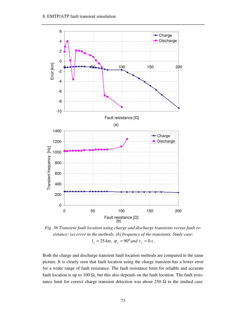
8. EMTP/ATP fault transient simulation
73
-10
-8
-6
-4
-2
0
2
4
6
0 50 100 150 200
Fault resistance [Ω]
Err
or [k
m]
ChargeDischarge
0
200
400
600
800
1000
1200
1400
0 50 100 150 200
Fault resistance [Ω]
Tra
nsie
nt fr
eque
ncy
[Hz]
ChargeDischarge
Fig. 36 Transient fault location using charge and discharge transients versus fault re-
sistance: (a) error in the methods, (b) frequency of the transients. Study case:
kml f 25= , °= 90fϕ and st f 0= .
Both the charge and discharge transient fault location methods are compared in the same
picture. It is clearly seen that fault location using the charge transient has a lower error
for a wider range of fault resistance. The fault resistance limit for reliable and accurate
fault location is up to 100 Ω, but this also depends on the fault location. The fault resis-
tance limit for correct charge transient detection was about 250 Ω in the studied case.
(a)
(b)

8. EMTP/ATP fault transient simulation
74
The damping of fault current transients can be seen when comparing the spectrum dia-
grams in Fig. 37 for different fault resistances, 0, 20, 50 and 200 Ω.
Fault location using the discharge transient works correctly up to 65 Ω, after which the
error starts to increase. When the fault resistance is higher than 110 Ω, the discharge
transient is damped so much that it is not detected at all.
Under the conditions for this study, the limit for the charge transient seems to be about
100 Ω. It must be pointed out that this conclusion is not final, and must be understood in
the scope of this study. Theoretically, fault location should be possible if the charge
transients are detected, in this case up to about 250 Ω. This would be possible with an
increased sampling frequency (to keep the same number of samples describing the tran-
sient). However, in reality the installed recorders have a fixed sampling frequency, and
so from this point of view this study is more realistic, even if the presented values might
not be so representative for general use.
125 250 375 500 625 750 875 1000 1125 12500
20
40
FAULT CURRENT SPECTRUM
FREQUENCY [Hz]
MA
GN
ITU
DE
[A]
125 250 375 500 625 750 875 1000 1125 12500
500
1000
1500
FAULT VOLTAGE SPECTRUM
FREQUENCY [Hz]
MA
GN
ITU
DE
[V]
125 250 375 500 625 750 875 1000 1125 12500
20
40
FAULT CURRENT SPECTRUM
FREQUENCY [Hz]
MA
GN
ITU
DE
[A]
125 250 375 500 625 750 875 1000 1125 12500
200
400
600
800
FAULT VOLTAGE SPECTRUM
FREQUENCY [Hz]
MA
GN
ITU
DE
[V]
125 250 375 500 625 750 875 1000 1125 12500
20
40
FAULT CURRENT SPECTRUM
FREQUENCY [Hz]
MA
GN
ITU
DE
[A]
125 250 375 500 625 750 875 1000 1125 12500
1000
2000
FAULT VOLTAGE SPECTRUM
FREQUENCY [Hz]
MA
GN
ITU
DE
[V]
125 250 375 500 625 750 875 1000 1125 12500
20
40
FAULT CURRENT SPECTRUM
FREQUENCY [Hz]
MA
GN
ITU
DE
[A]
125 250 375 500 625 750 875 1000 1125 12500
2000
4000
6000
8000FAULT VOLTAGE SPECTRUM
FREQUENCY [Hz]
MA
GN
ITU
DE
[V]
Fig. 37 Spectrum of the fault current and voltage for the study case: kml f 25= ,
°= 90fϕ and st f 0= for fR = a) 0 Ω, b) 20 Ω, c) 50 Ω and d) 200 Ω
(a)
(d)
(b)
(c)

8. EMTP/ATP fault transient simulation
75
8.3.2 Fault voltage inception angle
The amount of fault produced transients can also depend very much on the instantane-
ous value of the phase voltage at the fault initiation instant. This can be numerically
estimated by the inception angle of the voltage in the faulted phase. The simulation re-
sults are presented in Fig. 38.
-1.5
-1.0
-0.5
0.0
0.5
1.0
1.5
2.0
2.5
3.0
0 10 20 30 40 50 60 70 80 90
Voltage inception angle [º]
Err
or [k
m]
ChargeDischarge
Fig. 38 Transient fault location using the charge and discharge transients versus volt-
age inception angle. For study case: Ω= 0fR , kml f 25= and st f 0= .
Fault location depends only slightly on the instantaneous voltage level at the fault in-
stant initiation, when the charge transient is used. This is because the charge transient is
generated by the voltage rise in the sound phases. Using the discharge transients there
are larger errors (due to the discharge transient not being detected) if the inception angle
is lower than 3°. The simulation was performed for the studied case, with fault distance
kml f 25= , fault resistance Ω= 0fR and time of fault occurrence st f 0= . The simu-
lation results are more fully presented in Tab. 12 in Appendix A.

8. EMTP/ATP fault transient simulation
76
8.4 Fault transients versus neutral grounding type
Fault transients and hence fault location can also be affected by the type of network neu-
tral grounding used. It is wise to investigate how the generation of transients in the net-
works varies with different grounding. For subtransmission networks, isolated, com-
pensation coil or low-reactance grounded neutral systems are usually employed. In this
case the same network was tested, but with a changed grounding impedance. The stud-
ied case had the following parameters: Ω= 0fR , kml f 25= , °= 90fϕ and st f 0= .
The results appear in the following figures.
125 250 375 500 625 750 875 1000 1125 12500
20
40
FAULT CURRENT SPECTRUM
FREQUENCY [Hz]
MA
GN
ITU
DE
[A]
125 250 375 500 625 750 875 1000 1125 12500
500
1000
1500
FAULT VOLTAGE SPECTRUM
FREQUENCY [Hz]
MA
GN
ITU
DE
[V]
0 10 20 30 40 50 60 70 80 90 1000
5
10
15
20
25
30
DISTANCE VERSUS TIME
DIS
TA
NC
E [k
m]
Time [ms]
STABLE PART OF THE CURVE: 23.73 km
Fig. 39 The fault transient spectrums (left) and fault distance estimation using the
charge transient (right) in an isolated neutral network. For the studied case: Ω= 0fR ,
kml f 25= , °= 90fϕ and st f 0= .
125 250 375 500 625 750 875 1000 1125 12500
10
20
30FAULT CURRENT SPECTRUM
FREQUENCY [Hz]
MA
GN
ITU
DE
[A]
125 250 375 500 625 750 875 1000 1125 12500
500
1000
1500
FAULT VOLTAGE SPECTRUM
FREQUENCY [Hz]
MA
GN
ITU
DE
[V]
0 10 20 30 40 50 60 70 80 90 1000
5
10
15
20
25
30
DISTANCE VERSUS TIME
DIS
TA
NC
E [k
m]
Time [ms]
STABLE PART OF THE CURVE: 23.95 km
Fig. 40 The fault transient spectrums (left), and fault distance estimation using the
charge transient (right) in a compensated network, where: Ω= 0fR , kml f 25= ,
°= 90fϕ and st f 0= . Petersen coil inductance: 5050 mH.

8. EMTP/ATP fault transient simulation
77
As shown in Fig. 39 and Fig. 40 , the fault transient shape does not depend too much on
the impedance of the coils in the neutral grounding. The spectrum of the transients in a
compensated neutral network is almost the same as in an isolated neutral network. The
similarity of the part of the spectrum that contains the transients can be explained by the
coil’s higher impedance for transient frequencies. It was also found that there is no sig-
nificant influence on the fault location itself.
The situation is different in a low-reactance grounded network, where the spectrum of
the transients is slightly shifted. Nevertheless, this does not cause significant problems
in fault location, as can be clearly seen in Fig. 41. Similar results can be achieved in
solidly grounded networks.
125 250 375 500 625 750 875 1000 1125 12500
100
200
FAULT CURRENT SPECTRUM
FREQUENCY [Hz]
MA
GN
ITU
DE
[A]
125 250 375 500 625 750 875 1000 1125 12500
1000
2000
FAULT VOLTAGE SPECTRUM
FREQUENCY [Hz]
MA
GN
ITU
DE
[V]
0 10 20 30 40 50 60 70 80 90 1000
5
10
15
20
25
30
DISTANCE VERSUS TIME
DIS
TA
NC
E [k
m]
Time [ms]
STABLE PART OF THE CURVE: 23.52 km
Fig. 41 The fault transient spectrums (left), and fault distance estimation using the
charge transient (right) in a low-reactance network, where: Ω= 0fR , kml f 25= ,
°= 90fϕ and st f 0= . Low-reactance coil inductance: 600 mH.
Considering all the studied grounding methods, it can be concluded that there is no sig-
nificant difference in fault transient generation and hence fault location caused by the
grounding impedance.

8. EMTP/ATP fault transient simulation
78
8.5 Double-ended method
A simple double-ended method has been tested. A network 100 km long with an iso-
lated neutral was tested in EMTP/ATP. This method requires measurement from both
ends of the line but synchronisation is not required. The method is, in fact, based on two
single-ended methods. The fault distance was measured from each end and the average
of these two, referred to one line end, was calculated.
This method proved to be relatively accurate, Fig. 42. The problematic areas were the
ends of the line. However, in the middle the accuracy was good. The inaccurate regions
increase with the fault resistance, as shown in Fig. 42. For very high fault impedances
the accurate region was confined to just the middle of the line, rendering the algorithm
useless for such faults. However, the simplicity of the algorithm is an advantage.
Fig. 42 The double ended method. The fault resistance was 0 or 2 Ohms.
The inaccurate area covered the beginning and end of the line, where the fault location
error was higher than in the middle of the line. However, the relative error per km was
acceptable along the line for low fault resistances.
-5
-4
-3
-2
-1
0
1
2
3
4
5
0 20 40 60 80 100
Fault distance [km]
Err
or [k
m]
0 Ohms
2 Ohms
Accurate area
Inaccurate
area
Inaccurate
area

8. EMTP/ATP fault transient simulation
79
8.6 Discussion
Charge transient versus discharge transient
In principle it is possible to use both transients, the charge and discharge transients, for
fault location. However, the charge transient is more suitable, mainly because of its
higher amplitude and lower frequency compared to the discharge transient.
Connected line influence
First, the connected lines make the necessary return path for the fault transient current in
the case of the studied network, which has an isolated neutral. This issue will be studied
more fully in Chapter 11. Then Eq. (1) for the first order line model is valid. Secondly,
both charge and discharge transient frequencies are greatly affected by the existence of
connected lines. The connected lines lower both of the frequencies that would occur in a
single line, Chapter 5.
Fault conditions
Finally, there seems to be a problem with fault location when the fault resistance ex-
ceeds a few hundred ohms. The exact limit for general use would be difficult to estimate
from any study. However, the results in this chapter indicate that the method can be used
for faults with higher impedance than the conventional methods, Chapter 4. Under the
studied conditions, the limit when using the charge transient seems to be about 110 Ω.
However, the accurate area can be increased, mainly by a higher sampling rate, but only
up to the limit where the transient is totally damped. This value in our study then be-
comes about 250 Ω for the charge transient. For a realistic estimation, real fault cases
must be processed.
The inception angle of the voltage does not significantly affect the generation of the
charge transient, because it is generated by the voltage rise of the healthy phases.
Fault transients versus neutral grounding type
Although the transients may only be slightly affected by the impedance of the neutral
grounding, as seen in the simulated cases, the fault location will only be accurate where
we have a low impedance return path for the zero-sequence current; for example, a line
connected to the same substation (the studied case). The situation would be very differ-
ent in the case of a single line (no other lines connected to the same busbar). Then the
impedance of the neutral grounding will play a key role in fault location accuracy (the
lower the better), because it is the only way for the zero-sequence current to close via
the measurement point in the substation. These issues will be explored further in Chap-
ter 11.

8. EMTP/ATP fault transient simulation
80
Sampling frequency
The entire study in this chapter was performed with a 2.5 kHz sampling frequency,
mainly to enable practical application of the results in the real Finnish subtransmission
system. The study showed that this value would be high enough for fault location pur-
poses. Increasing the sampling frequency would primarily enable an increase in the al-
lowable fault resistance to the possible maximum. However, because in reality the tran-
sients do not always last as long as those generated in the simulations, it would also be
wise to utilise a higher sampling frequency. Further, as there are other error sources af-
fecting the method accuracy that cannot be reduced, it would be prudent to reduce the
influence of the sampling frequency to the minimum. A sampling rate of 10 kHz would
be relatively safe for this kind of fault location application.

9. Modelling of the 110 kV instrument transformers for transients
81
9 Modelling of the 110 kV instrument transform-
ers for transients
Instrument transformers have a guaranteed ratio at 50 Hz, but it is necessary to investi-
gate how they transmit signals at transient frequencies and in transient situations for the
purpose of fault location. This can be performed by measurement of the transformer
ratio. The modelling is important for the fault simulations and for the analysis of real
fault signals as well. When developing a fault locator using a simulation program, it is
wise to pass the fault signal through the instrument transformer model in order to in-
clude the error of the measurement. The output is then more realistic, and can be used
for fault distance computation with the measurement error included. In real cases, when
we process real fault signals, it is then possible to make corrections based on the model
frequency (transient) response.
In general, the modelling of a voltage transformer for transients is more complicated
than the modelling of a current transformer. The voltage transformer may have a reso-
nance point in the frequency range of the low frequency transients, which can cause in-
accurate measurement at these frequencies. Current transformers on the other hand do
not usually have any non-linearities in transmission in the transient frequency range. In
the context of this study, i.e. in this chapter, the term low frequency transients means the
frequency range of ground fault signals, where the maximum is limited to 5 kHz.
There are many modelling methods used for instrument transformers. Basically, they
can be divided into lumped and distributed parameter models. Some approaches are
based on a mathematical analysis of the measurements performed on the transformer or
on the physical construction of the transformer as well. It is difficult to make a model
that is valid over the entire frequency spectrum, especially with low degrees of freedom
in the model. Only the most complicated models, based on distributed parameters,
which also take into account the geometry of the transformer, can fully satisfy this re-
quirement. In any case, the construction details of the transformer are not always avail-
able to the end user. It is also much easier to build a model for the specific frequency
range we are interested in. In this case very good results can be achieved with lumped
models. There are many methods for constructing such models, but the most common
method is based on the classical model calculated from open and short circuit measure-
ments at 50 Hz (to estimate the lumped resistances and inductances). Capacitances are
usually added to these standard models in order to generate the resonance points and

9. Modelling of the 110 kV instrument transformers for transients
82
there are various methods covering how to estimate them, [1], [6], [7]. In this thesis a
new approach is developed, also published in [32]. All the model element parameters
are calculated from measurements performed on real instrument transformers. Simula-
tions of this model were performed in EMTP/ATP and the necessary signal processing
was conducted in Matlab.
9.1 Voltage transformer
In this section a lumped model of a voltage transformer is constructed. There were three
voltage transformers measured (with internal names PT1, PT2 and PT3), the basic pa-
rameters of which are given in Appendix B. The transformers behaved similarly in the
range of low frequency transients, and therefore only one of them, PT1, was modelled.
The model accuracy was tested in EMTP/ATP and then compared with the real trans-
former.
9.1.1 The model’s backbone
For the modelling of instrument transformers up to 10 kHz it is clear that we can use a
lumped model. PT1 consists of two secondary windings. The simplest lumped parame-
ter model of a voltage transformer with two secondary windings is shown in Fig. 43. For
this model we need the results from open and short circuit measurements on a real volt-
age transformer. The parameters of this model were calculated from measurements pro-
vided by Fortum (an energy company in the Nordic countries) with a network analyser.
Fig. 43 The linear 50 Hz model of a 110 kV voltage transformer.

9. Modelling of the 110 kV instrument transformers for transients
83
Recalculated data from the network analyzer (at 50 Hz) are shown in Tab. 2. It can be
seen that there was no big difference between the short circuit and open circuit meas-
urement performed from the primary side of the investigated voltage transformer (PT1).
Tab. 2 Short and open circuit impedances of the voltage transformer (PT1), cal-
culated from Fortum’s measurements.
Measurement f
[Hz] Impedance Values Unit
Short circuit, P-S1 50 Zps1 1.9259 + 0.98281j kΩ
Open circuit, P 50 Zp 30.950 + 25.167j kΩ
The ratio between the absolute values of the impedances shown in Tab. 2 is only about
18, which means that the primary windings of the transformer form the dominant part of
the short circuit impedance. The model response is similar to the real transformer when
the short circuit impedance is divided between the primary and secondary with a ratio of
90 % on the primary to 10 % on secondary side, as shown in Tab. 3.
Tab. 3 Division of the short-circuit impedance of PT1 to the model’s primary and sec-
ondary.
From Tab. 2 Ratio Primary Secondary S1
Lps1= 3.13 H Lp= 2.8170 H Ls1’= 0.313 H
Rps1= 1.9259 kΩ 90% to 10%
Rp= 1.7333 kΩ Rs1’= 192.59 Ω
for sradf / 314=ω
The transformer model’s vertical branch can be easily calculated from the open circuit
impedance, as shown in Tab. 4.
Tab. 4 The open circuit recalculation for PT1.
Measured values From Tab. 2 Calculated
Imag.part 25.167j kΩ Lm= 80.1497 H
Real part 30.950 kΩ Rm= 30.950 kΩ
for sradf / 314=ω
The second secondary winding S2 has similar parameters to the winding S1. Because of
the symmetry of the transformer model, the coil S2 can be assumed to have the same
parameters as S1.
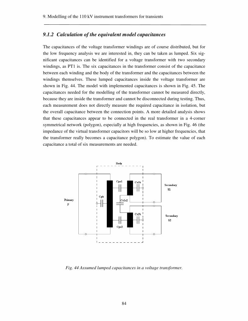
9. Modelling of the 110 kV instrument transformers for transients
84
9.1.2 Calculation of the equivalent model capacitances
The capacitances of the voltage transformer windings are of course distributed, but for
the low frequency analysis we are interested in, they can be taken as lumped. Six sig-
nificant capacitances can be identified for a voltage transformer with two secondary
windings, as PT1 is. The six capacitances in the transformer consist of the capacitance
between each winding and the body of the transformer and the capacitances between the
windings themselves. These lumped capacitances inside the voltage transformer are
shown in Fig. 44. The model with implemented capacitances is shown in Fig. 45. The
capacitances needed for the modelling of the transformer cannot be measured directly,
because they are inside the transformer and cannot be disconnected during testing. Thus,
each measurement does not directly measure the required capacitance in isolation, but
the overall capacitance between the connection points. A more detailed analysis shows
that these capacitances appear to be connected in the real transformer in a 4-corner
symmetrical network (polygon), especially at high frequencies, as shown in Fig. 46 (the
impedance of the virtual transformer capacitors will be so low at higher frequencies, that
the transformer really becomes a capacitance polygon). To estimate the value of each
capacitance a total of six measurements are needed.
Fig. 44 Assumed lumped capacitances in a voltage transformer.

9. Modelling of the 110 kV instrument transformers for transients
85
Fig. 45 Capacitances in the model.
Fig. 46 Connections of the capacitances in the transformer at higher frequencies.
1 2
3
4

9. Modelling of the 110 kV instrument transformers for transients
86
9.1.2.1 Capacitance measurement description
During the six required capacitance measurements, all windings of the transformer were
short-circuited as shown in Fig. 44. An impulse of shape µs 1,2/50 and a voltage level
of a few hundreds volts were applied to the transformer. During the tests the impedance
(or voltage and current) was measured. The connections were between the windings and
between each winding and the body of the transformer (note: in these measurements the
primary was disconnected from the body). The measurement circuits and results are
shown in Appendix B.
When analysing the measurements, the spectrum of the measured voltage and current
was first calculated, using Eq. (28). The frequency dependent capacitance was then cal-
culated from the measured voltage and current spectrum as follows:
))(DFT
)(DFT(
1)(
v
iimagC
ωω =
(37)
where ω is the angular frequency, DFT(v) is the spectrum of the voltage and DFT(i) is
the spectrum of the current.
9.1.2.2 Recalculation of the capacitance network
The basic idea behind the calculation of all six capacitances inside the capacitance net-
work shown in Fig. 46 was to use all possible combinations of measurements (6) be-
tween the corners of the polygon (1, 2, 3, 4) or, in practice, between the windings of the
transformer, primary (P), secondary (S1), secondary (S2) and the body of the trans-
former, as shown in Fig. 44.
For example, the capacitance 1psC between the primary and secondary can be calculated
using the measured capacitance between points 1-2 in Fig. 46 and all known capacitan-
ces from inside the capacitance network, as presented in Eq. (38). The detailed devel-
opment of this equation can be found in Appendix B.
)(
))((
21
212212
21
1221
21
22
21
1121
bsbspb
bspbbsbsssps
bsbspb
bsbsss
bsbspb
bspbps
bsbspb
bspbps
CCC
CCCCCC
CCC
CCC
CCC
CCC
CCC
CCCC
++
+++
+++
+++
−++
−=
(38)

9. Modelling of the 110 kV instrument transformers for transients
87
where:
pbC is the capacitance between primary winding (P) and body (b) of transformer
bsC 1 is the capacitance between secondary (S1) and body (b) of transformer
bsC 2 is the capacitance between secondary (S2) and body (b) of transformer
21ssC is the capacitance between secondary (S1) and secondary (S2) of transformer
1psC is the capacitance between primary winding (P) and secondary (S1) of transformer
2psC is the capacitance between primary winding (P) and secondary (S2) of transformer
12C is the measured capacitance between primary (P) and secondary (S1) of transformer
and other measured capacitances
13C is the measured capacitance between primary (P) and secondary (S2) of transformer
14C is the measured capacitance between primary (P) and body (b) of transformer
24C is the measured capacitance between secondary (S1) and body (b) of transformer
34C is the measured capacitance between secondary (S2) and body (b) of transformer
23C is the measured capacitance between secondary (S1) and secondary (S2) of trans-
former
The capacitances inside the polygon are unknown (only the measured capacitances, 12C ,
13C , 14C , 24C , 34C , and 23C , are known). Nevertheless, a solution similar to Eq. (38)
can be written for each internal capacitance shown in Fig. 46. Hence the systems of six
equations can be solved using a suitable numerical method (in this case the “Gauss-
Seidel iteration method” was used, [8]). The solution of this system of equations with
measured capacitances for the measured voltage transformer (PT1) can be seen in Tab.
5.
Tab. 5 Measured and calculated values of the capacitances in the voltage transformer
(PT1).
Measured capacitances
of voltage transformer PT1
Calculated capacitances
with Gauss-Seidel iteration method
Name Value Unit Name Value Unit
C12 1.1 nF Cps1 0.5371 nF
C13 1.1 nF Cps2 0.5371 nF
C23 2.8 nF Cs1s2 2.4754 nF
C14 0.6 nF Cpb 0.4144 nF
C24 0.5 nF Cs1b 0.1121 nF
C34 0.5 nF Cs2b 0.1121 nF

9. Modelling of the 110 kV instrument transformers for transients
88
9.1.3 Model analysis with EMTP/ATP
The model of the voltage transformer shown in Fig. 45, with the parameters calculated
for PT1 as shown in the previous sections, was simulated in EMTP/ATP. The simulated
model diagram can be seen in Fig. 47.
Fig. 47 The EMTP/ATP model of the voltage transformer with impulse generator and
measurement voltage probes on the primary (P) and secondary (S1).
The frequency response of transformer PT1 was first measured. The transfer function of
the primary (P) to secondary (S1) of the real transformer (PT1) is shown in Fig. 48. It is,
in fact, the response of the transformer to an impulse of a few hundreds volts with shape
1,2/50 µs. The results are shown in the four curves in Fig. 48. Starting from the top,
there is an applied impulse to the primary winding (P) with the response measured on
the secondary (S1) after multiplying by 1000 (so that both impulse and response can be
seen in one picture). Below, the spectrum of both the impulse and the response is
shown. Finally, the last two curves are the rated ratio of the transformer with the phase
angle of the transformer as a function of frequency. The first resonance point of the
transformer was detected at 2600 Hz.
The model of Fig. 47 was actually tested in the same way as the real transformer (using
the connection indicated in Fig. 47, with the same impulse shape 1,2/50 µs and ampli-
tude that were applied to the real transformer). By applying the same measurement to
the model, we obtained the results shown in Fig. 49. The figure consists of the same set
of curves as Fig. 48. The main resonance frequency of the model was 2600 Hz.
In Fig. 50, the measured transfer function of PT1 is compared with its model. The figure
structure is slightly different. In every curve the simulated and measured transformers
are compared; starting from the top: applied impulses, responses, ratios, and phase an-
gles. As is clearly seen, the responses of the model and the transformer are quite similar

9. Modelling of the 110 kV instrument transformers for transients
89
and oscillate at the same main frequency of 2600 Hz with the same attenuation (they
cover each other). The model fits with the real transformer quite well up to 5 kHz. How-
ever, the error in the model was a little higher around the nonlinear point at 2600 Hz.
2 4 6 8 10 12 14 16 18 20
-200
0
200
400
600
IMPULSE AND RESPONSEV
olta
ges
V1,
V2
[V,
10-3
V]
Time [ms]
0 1000 2000 3000 4000 5000 6000 7000 8000 9000 100000
5
10
15 SPECTRUM OF IMPULSE AND RESPONSE
Vol
tage
s V
1, V
2 [V
, 10
-3V
]
Frequnecy [Hz]
0 1000 2000 3000 4000 5000 6000 7000 8000 9000 100000
1
2
3
4RATED TRANSFORMER RATIO V2/V1
1100
*Rat
io [
-]
Frequnecy [Hz]
0 1000 2000 3000 4000 5000 6000 7000 8000 9000 10000-150
-100
-50
0
50PHASE ANGLE
Ang
le [
°]
Frequnecy [Hz]
Fig. 48 The measured ratio of the voltage transformer, (PT1). Measured connection:
primary (P) to secondary (S1). Applied impulse 1,2/50 µs. (V2 – green color)
Frequency [Hz]
Frequency [Hz]
Frequency [Hz]

9. Modelling of the 110 kV instrument transformers for transients
90
2 4 6 8 10 12 14 16 18 20
0
200
400
600
800
1000
IMPULSE AND RESPONSE
Vol
tage
s V
1, V
2 [V
, 10
0 V]
Time [ms]
0 1000 2000 3000 4000 5000 6000 7000 8000 9000 100000
5
10
15
20 SPECTRUM OF IMPULSE AND RESPONSE
Vol
tage
s V
1, V
2 [V
, 10
0 V]
Frequnecy [Hz]
0 1000 2000 3000 4000 5000 6000 7000 8000 9000 100000
1
2
3
4RATED TRANSFORMER RATIO V2/V1
1*R
atio
[-]
Frequnecy [Hz]
0 1000 2000 3000 4000 5000 6000 7000 8000 9000 10000-150
-100
-50
0
50PHASE ANGLE
Ang
le [
°]
Frequnecy [Hz]
Fig. 49 The simulated ratio of the PT1 voltage transformer model. Measured
connection: primary (P) to secondary (S1). Applied impulse 1,2/50 µs. (V2 –
green color)
Frequency [Hz]
Frequency [Hz]
Frequency [Hz]

9. Modelling of the 110 kV instrument transformers for transients
91
2 4 6 8 10 12 14 16 18 200
200
400
600
800
1000
IMPULSE SIGNALS
Prim
ary
volta
ge V
1 [V
]
Time [ms]
2 4 6 8 10 12 14 16 18 20
-0.2
0
0.2
0.4
0.6
0.8RESPONSE SIGNALS
Sec
onda
ry v
olta
ge V
2 [V
]
Time [ms]
0 1000 2000 3000 4000 5000 6000 7000 8000 9000 100000
1
2
3
4RATED TRANSFORMER RATIOS V2/V1
1100
*Rat
io [
-]
Frequnecy [Hz]
0 1000 2000 3000 4000 5000 6000 7000 8000 9000 10000-150
-100
-50
0
50PHASE ANGLES
Ang
le [
°]
Frequnecy [Hz]
Fig. 50 Comparison of the measured ratio of the voltage transformer (PT1) and its
model. Measured connection: primary (P) to secondary (S1). Applied impulse 1,2/50
µs. (Measured signals – green color, simulated signals – blue color)
Frequency [Hz]
Frequency [Hz]

9. Modelling of the 110 kV instrument transformers for transients
92
9.1.4 Analysis of the impact of the model components on the frequency
response
Each element of the model has an impact on its final frequency response and so it is
very important to study the properties of the model. The “back-bone” of the model was
built according to the classical lumped model for 50 Hz. The non-linearity of the core
was not considered in the model. To get the frequency response of the model similar to
the original response of the transformer, the capacitances were added. Therefore, their
impact on the model frequency response is investigated. It is important to know the con-
nection between each capacitance and resonance or shape change in the model, i.e.
which capacitance causes which resonance or shape change in the model.
The model without the capacitances gave the correct ratio at 50 Hz, as expected. The
capacitances added between the windings themselves, and between the windings and the
ground (which are of “nF” size) are of a high impedance at 50 Hz, as an approximate
calculation shows:
Ω=⋅== − M 3.1847)10314/(1/1 9CZ fω . Thus, these capacitances do not influence the
model at 50 Hz, which should be the case. This was proved by the EMTP/ATP simula-
tions, as well.
The capacitance on the primary side, nFC pb 4144.0= , does not have any impact on the
model frequency response. When varying this capacitance, or even if we do not include
this capacitance at all, the model responses will not be changed.
The capacitance between the primary and the secondary, for example, nFC ps 5371.01 = ,
is connected directly across the whole short circuit impedance. This capacitance together
with the short circuit impedance generates the frequency response:
kHz 3.8817)105371.013.32/(12/(1 911 =⋅⋅== −ππ psps CLf . When adding the ca-
pacitance of the secondary to ground, nFC bs 0.11211 = , this resonance point will
change to kHz 3,55=f . When the model is completed with the capacitances of the
second secondary winding 2psC and bsC 2 , the system will have a resonance frequency at
2600 Hz.
The value of the capacitance, nF 2.475421 =ssC , did not make any difference to the fre-
quency response. Only extremely high capacitance values (> 0.1 F, which is not realis-
tic) can change the transformer model response.

9. Modelling of the 110 kV instrument transformers for transients
93
In conclusion, the main impact on the final response is given by the capacitances be-
tween the primary and secondary windings, and between the secondary windings and the
ground.

9. Modelling of the 110 kV instrument transformers for transients
94
9.2 Burden of the voltage transformer
The frequency response of the voltage transformer shows that a PT is suitable for the
transmission of fault signals without any significant influence. This is only true, how-
ever, when the transformer, or the transformer model presented in Section 9.1, is not
loaded. Therefore, to investigate the effect of loading on the transformer, a burden rep-
resenting the cable connection between the secondary of the PT and the substation
building was connected to the model. The typical capacitance of a secondary cable is
nF 20 . This capacitance value was obtained from a measurement in a real substation,
where cables for measurement and protection, 75 m long, are connected to the PT sec-
ondary; the relevant data are presented in Appendix B. To be used in the model, the ca-
pacitance must be referred to the primary side of the transformer. The influence on the
frequency response of the PT1 model can be seen in Fig. 51.
Time [ms]
0 1000 2000 3000 4000 5000 6000 7000 8000 9000 100000
1
2
3
4RATED TRANSFORMER RATIOS V2/V1
1100
*Rat
io [
-]
Frequnecy [Hz]
0 1000 2000 3000 4000 5000 6000 7000 8000 9000 10000-150
-100
-50
0
50PHASE ANGLES
Ang
le [
°]
Frequnecy [Hz]
Fig. 51 The simulated and measured frequency response of PT1. The secondary of the
model was loaded with a cable of capacitance nF20 . The real PT1 was unloaded.
Measured connection: primary (P) to secondary (S1). Applied impulse: 1,2/50 µs.
As can be seen, the loaded model of the voltage transformer with the secondary cable
connected has almost the same frequency response as the unloaded real voltage trans-
former PT1. Therefore, it can be concluded that the secondary burden of the transformer
(mainly the capacitance of the cable) does not significantly influence the frequency re-
Model (Loaded)
Real PT1 (Unloaded)
Real PT1 (Unloaded)
Model (Loaded)
Frequency [Hz]
Frequency [Hz]

9. Modelling of the 110 kV instrument transformers for transients
95
sponse of the voltage transformer model. Hence, it can be assumed that a real trans-
former will behave similarly, and so no correction is needed for fault transients.
9.3 Current transformer
A current transformer’s transfer function was measured. The measured transformer is
CT4 (ratio 80/2=40, 0.5%, 60VA, 5A; the detailed parameters are in appendix B). The
measurement comprised two different approaches, an impulse test and an AC measure-
ment. The impulse test was used to measure the resonance of the transformer, Fig. 52,
and the AC measurement was used to precisely measure the frequency range of interest.
The results are shown in Fig. 53 and Fig. 54. It is clear that the transformer ratio error is
less than about 3.5% up to 1 kHz. The main resonance point of CT4 was at 320 kHz.
Fig. 52 Impulse measurement of CT4 in the HV laboratory, HUT, Finland.

9. Modelling of the 110 kV instrument transformers for transients
96
Fig. 53 The transfer function of CT4 measured with an impulse generator.
Measured connection: primary (P) to secondary (S1).

9. Modelling of the 110 kV instrument transformers for transients
97
Fig. 54 The transfer function of CT4 measured with an AC generator. The measured
frequency range was from 50 Hz to 1 kHz. (The 50-600 Hz range was measured in steps
of 10 Hz, and the 600-1000 Hz frequency range in steps of 100 Hz).

10. Line reactances at transient frequencies
98
10 Line reactances at transient frequencies
Ground fault transients propagate through the network. After passing through the net-
work they can be measured in the substation and used for fault location purposes. On
their way to the substations these transients are affected by the network itself. Moreover,
the line parameters might vary.
Line parameters such as the resistances, inductances and capacitances per km of all the
sequence components are not constants. For the transient based method only the se-
quence inductances are important. The zero- positive- and negative- sequence induct-
ances of the line vary with many of the parameters. The dependence on frequency is
very important, because in practice the fault transient frequency can be as high as 1000
Hz. Moreover, the zero-sequence impedance of the line can also change due to the in-
fluence of the ground, if the current returns via the ground. The study conducted in this
chapter uses the Carson method.
HV subtransmission lines usually have overhead ground wires situated above the phase
conductors and they are grounded at each tower in order to protect the line from light-
ning. The existence of these overhead ground wires has a significant influence on both
the fault generated transient propagation along the network and the line parameters.
Therefore, all fault signals returning to the source can actually propagate through both
the ground and the overhead ground wires, depending on the tower dimensions, wire
parameters, ground parameters and fault signal parameters. The overhead ground wires
are considered to be conductors with more stable electrical parameters than the ground.
The exact division of the returning current between the two can be obtained by studying
the zero-sequence impedance of the line. The study related in this chapter was con-
ducted with various methods derived from the Carson formula.
The standard method proposed by Carson, [19], is probably the most commonly used
method for the calculation of the frequency-dependent line parameters considering an
earth return. However, Carson’s formula does not provide a closed-form solution. It
expresses the impedance by means of an improper integral that has to be expanded into
an infinite series for computation. The complicated impedance solution has several
times been simplified by reducing the infinite series to a finite number. A similar solu-
tion was simultaneusly proposed by Pollaczek [35], [36]. There are also completely dif-
ferent approaches based, for example, on a layer model of the ground or on FEM (the
finite element method). A study in [20] compares the different methods used for calcula-

10. Line reactances at transient frequencies
99
tion of the frequency-dependent impedance of overhead transmission lines. The methods
studied were Carson’s, Gary’s and FEM. From their analysis it can be seen that the re-
sults obtained from the various methods are only slightly different.
Sections 10.1 and 10.2 present the theoretical background relevant to the following sec-
tions. In Sections 10.3 and 10.4, the propagation of a transient is investigated using both
a reduction factor and a matrix based model. Both are based on Carson’s ground simpli-
fication, presented in [17] and [18]. Sub-section 10.4.1 investigates the effect of
counterpoises on zero-sequence current propagation. These sections primarily study the
rate of penetration of the zero-sequence current into the ground. The sections subse-
quently study the impact of the overhead ground wire material on zero-sequence current
propagation and line parameter calculation accuracy. The line parameters for various
frequencies, ground resistivities and different overhead ground wire materials are also
calculated using the original Carson formula in Section 10.5. A typical 110 kV line
structure (3-phase network with two return overhead ground wires) is studied.

10. Line reactances at transient frequencies
100
10.1 Zero-sequence impedance of the line
The transmission system becomes unbalanced when a ground fault occurs. If the phase
currents are not balanced (as during the fault), there will be a return current in the ove-
head grounded neutral wires and in the ground. The ground return current will spread
out under the line, seeking the lowest impedance return path, [17]. An unbalanced
power system can be described in terms of symmetrical components, proposed by
Fortescue [16]. The ratio of how the return fault currents are divided between the ground
and the overhead ground wire will affect the zero-sequence impedance of the line.
In Fig. 55, a network model for zero-sequence impedance estimation is shown. If the
supply zero-sequence voltage 0V is sinusoidal, then the phases will have equal “zero-
sequence” currents 0I . Part of this current returns via the overhead ground wires ogwI
and the rest via the ground, grI . The ground wires are grounded at every tower. They are
connected to the ground through the tower footing resistance. The large number of such
parallel connections to ground per km (in 110 kV lines the number is about 5) allows us
to assume that the ground wires and the ground are electrically in parallel and are con-
nected at the ends of the section of the circuit being considered, [18]. Therefore, the
same voltage nNV can be assumed over both of them, as indicated in Fig. 55. The zero-
sequence impedance can be calculated as: 000 / IVZ = .
Fig. 55 The model of an overhead line used for estimation of the zero-
sequence impedance.
Phase A
Overhead ground wire
Phase B
Phase C
Ground
A a
n N
nNV
0V
03I
0I
0I
0I
03I
grI
ogwI
03I
Return
circuit
Phase
conductors
AaV

10. Line reactances at transient frequencies
101
10.2 Self and mutual inductance of a conductor
Let us consider the situation of a conductor in a group of conductors where the sum of
the currents in all the conductors is zero. Such a group of conductors is shown in Fig.
56. Conductors 1, 2, 3,…n carry the currents 1I , 2I , 3I ,… nI . The distances of the
other conductors from conductor 1 are 12D , 13D ,… nD1 . By solving this problem as in
[18] we get an equation, Eq. (39), for all the flux linkages 1ψ of conductor 1 in a group
of conductors, provided the sum of all the currents is zero.
nn
n
n IMIMIMILD
ID
ID
Ir
I 131321211
113
3
12
2
1
10
1...)
1ln(...)
1ln()
1ln()
'
1ln(
2+++=
+++=
π
µψ
(39)
Hence the equation can be extended and the components nMMML 113121 ... , , , can be
understood as the self and mutual inductances of conductor 1 with the others, as shown
in Eq. (39). The currents are instantaneous values or complex rms values. 4/111 ' −= err is
the equivalent radius of conductor 1 (of radius 1r ) for non bundled conductors (note: the
internal inductance of the conductor is taken into account by the term 4/1−e ). 0µ is the
permeability of free space.
Fig. 56 Cross-sectional view of a group of n-conductors carrying currents whose
sum is zero.
1I
2I
3I
nI
.
.
.
.
1r
nD1
13D
12D
Conductor 1 Conductor 2
Conductor 3
Conductor n
.
.
.
. .
.
.
.

10. Line reactances at transient frequencies
102
10.3 Reduction factor
A section of a transmission line is shown in Fig. 57 on the right. It consists of three sin-
gle-phase conductors, two return overhead ground conductors and the ground as well,
represented by a fictional ground conductor placed at Carson’s distance,
fDe ρ5.685= (the 1st term approximation of the Carson series), [19], and with a
resistance 80 lRgr ωµ= , where 0µ is the permeability of free space, ω is the angular
frequency, l is the length of the analysed line section, ρ is the ground resistivity and f
is the frequency.
The picture assumes that the zero-sequence current 0I flows equally in each phase (as
in Fig. 55). Three times the zero-sequence current returns via both the overhead ground
wires ogwI and the fictional ground wire ogwgr III −= 03 . The method for solving the
zero sequence impedance of such a network is presented in [18]. It is based on the trans-
formation of the three-phase system (Fig. 57 right) into a single phase system (Fig. 57
left) in order to simplify the solution. The three-phase system of wires can be reduced to
a single “composite phase wire – a” and the two overhead ground wires to a single
“composite overhead ground wire – g”. The ground is represented by a “fictional ground
conductor”. A more detailed solution of this problem is given in Appendix C.
Fig. 57 Transformation between the single- and three-phase systems with ground con-
ductors.
ogwI
ogwagr III −=
2/ogwI
2/ogwI
0I
0I
0I 03I
ogwgr III −= 03
03II a =
grR
eD
grR
Composite phase wire
g
a
e
Compositeoverhead ground wire

10. Line reactances at transient frequencies
103
The basic equation describing the zero-sequence impedance of 3-phase overhead lines
with two overhead ground return wires and the ground represented as a single conductor
according to [18] is:
)(32
0
gg
ag
aa Z
ZZZ −=
(40)
where:
aaZ is the self-impedance of the phase conductor-ground loop
ggZ is the self -impedance of the overhead ground conductor-ground loop
agZ is the mutual impedance between the “phase conductor-ground loop” and the
“overhead ground conductor-ground loop”
Detailed calculations of the impedances aaZ , ggZ and agZ can be found in Appendix
C.
The division of 03I , the tripled zero-sequence current, into the ground wires ogwI and
ground grI is expressed by means of the reduction factor uk , which shows the amount
of 03I flowing in the ground grI :
gggrogw
ggagogw
gg
ggaggru LjRnR
LMjnR
Z
ZZ
I
Ik
ω
ω
++
−+=
−==
0
0
0 /
)(/
3
(41)
where:
ogwR is the resistance per km of the overhead ground wire
0n is the number of the overhead ground wires
agM is the mutual inductance between the “phase conductor-ground loop” and the
“overhead ground conductor-ground loop”
ggL is the inductance of the overhead ground conductor-ground loop
The behaviour of the reduction factor and the zero-sequence inductance per km for a
typical Fingrid 110 kV tower is graphically represented in Fig. 58 (a) and (b) (the pa-
rameters of the studied network are given in Appendix C), which shows the situation
when the phase wires and overhead ground wires are made of aluminum and their rela-

10. Line reactances at transient frequencies
104
tive permeability is 1=rµ . Although in practice there is some steel for reinforcement,
the difference in the calculated result will not be significant. In the case of overhead
ground wires completely made of steel, the relative permeability would be 50=rµ and
the resistivity much higher, and then the result will change a lot, Fig. 58 (c) and (d).
0 200 400 600 800 100030
40
50
60
70
80
90
100
k u [%]
Frequency [Hz]
0 200 400 600 800 10002
2.5
3
3.5
4
L 0 [mH
]
Frequency [Hz]
0 200 400 600 800 100098.4
98.6
98.8
99
99.2
99.4
99.6
99.8
100
k u [%]
Frequency [Hz]
0 200 400 600 800 10002
3
4
5
6
7L 0 [m
H]
Frequency [Hz]
Fig. 58 The frequency dependence of the reduction factor and zero-sequence induc-
tance for typical 110 kV overhead lines with two overhead ground wires made of alu-
minium, (a) and (b), and steel, (c) and (d). The calculation is made for
Ωmandρ432 10 10 ,10 ,10= . The arrows indicate an increase in the ground resistance.
The penetration of the zero-sequence current into the ground at transient frequencies is
very much dependent on the ground resistivity and also on the material the overhead
ground wires are made of. The zero-sequence current tends to flow via the overhead
ground wire rather than the ground when aluminum is used. If steel is used, the majority
of the zero-sequence current tends to flow in the ground. This is partly because the
overhead ground wires are of high impedance due to their higher resistance, but is
mainly due to the higher inductance caused by the higher conductor permeability.
(a)
(c)
(b)
(d)
ρ ρ
ρ ρ

10. Line reactances at transient frequencies
105
10.4 Matrix method
The reduction factor was calculated in the previous section using a simplification of the
ground but in this section a different approach is presented. The method of modelling
the zero-sequence impedance of a line section is based on the assumption that the
ground can be substituted by a system of equivalent wires, with the appropriate resis-
tances and inductances, at Carson’s distance 'kkD from the overhead wires (instead of in
the ground). This type of analysis method can be found for instance in [17].
The model can be seen in Fig. 59. The overhead conductors of phases a, b and c, also
numbered 1, 2 and 3, and the return overhead ground wires n1 and n2, also numbered 4
and 5, are situated on a tower. This system of wires has corresponding ground represen-
tatives (which are also shown in Fig. 59) to substitute the influence of the ground itself.
This is a rather complicated approach. In practice, one wire placed in the ground would
be enough.
Fig. 59 Three-phase transmission line with two overhead ground conductors and the
ground replaced by ground return conductors.
Each of the ground conductors a', b', c', n1' and n2' has a GMR (geometric mean radius)
kkkk DD ='' ( 'r for non-bundled conductors) the same as the original conductors, and all
conductors in the ground have the same resistance )8( 0'' lnR grwkk ωµ= , where 0µ is the
permeability of free space, ω is the angular frequency and l is the length of the ana-
lysed line section. grwn is the number of the wires representing the ground (5 in this
model). All the ground return conductors are the same distance 'kkD from their respec-
a(1) b(2) c(3)
n1(4) n2(5)
Overhead
conductors
Ground surface
a'(6) c'(8)
n1'(9) n2'(10) Fictional ground
conductors
b'(7)
'kkD

10. Line reactances at transient frequencies
106
tive overhead conductors [17]. According to Carson´s theory, the distance is
fDkk ρ5.685' = (approximated by using only the 1st term of the Carson series),
where ρ is the ground resistivity and f is the frequency.
Note: the original method described in [17] gives the expression 80'' lR kk ωµ= for each
wire in the ground. However, this causes the total zero-sequence resistance to be too
low. Therefore the total ground resistance of all wires in the ground should be equal to
80 lωµ . This is corrected by grwn , such that )8( 0'' lnR grwkk ωµ= .
The circuit model for the zero-sequence impedance estimation of the line section with,
for example, a length of 1 km is shown in Fig. 60. The model includes the resistance and
inductance of each wire and, moreover, all mutual inductances between all wires. The
tripled zero-sequence current flowing in the phases, 03I , returns through the ground grI
and overhead ground wire ogwI , as shown in the model.

10. Line reactances at transient frequencies
107
Fig. 60 Circuit for estimating the zero-sequence impedance and current of a three-
phase transmision line with two overhead ground conductors.
To describe the voltage drops AaV over the phase conductors and nNV over the ground
wires, and the ground in the circuit shown in Fig. 60, we can write the following matrix
equation:
aR aL aI
A a
bR bL bI
B b
cR cL cI
C c
1nR 1nL 1nI
2nR 2nL 2nI
grR 'aL 'aI
grR 'bL 'bI
grR 'cL 'cI
grR '1nL '1nI
grR '2nL '2nI
N n
Ground surface
Phase
conductors
Overhead ground
conductors
Fictional ground
conductors
03I
nNV
ogwI
grI
03I
a A
03I
AaV

10. Line reactances at transient frequencies
108
The matrix solution:
+
+
+
+
+
+
+
+
+
+
=
'2
'1
'
'
'
2
1
'2
n2'
n1'n2'v'n2'b'n2'a'n2'n2n2'n1n2'cn2'bn2''2
n2'n1''1
n1'
v'n1'b'n1'a'n1'n2n1'n1n1'cn1'bn1''1
n2'c'n1'c''
c'
b'c'a'c'n2c'n1c'cc'bc''
n2'b'n1'b'c'b''
b'
a'b'n2b'n1b'cb'bb''
n2'a'n1'a'c'a'b'a''
a'
n2a'n1a'ca'ba''
n2n2'n2n1'n2c'n2b'n2a'2
n2
n2n1n2cn2b2
n1n2'n1n1'n1c'n1b'n1a'n1n21
n1
n1cn1b1
cn2'cn1'cc'cb'ca'cn2cn1
c
cb
bn2'bn1'bc'bb'ba'bn2bn1bc
b
an2'an1'ac'ab'aa'an2an1acab
*
R
M M M M M M M- M- -
M R
M M M M M M- M- -
M M R
M M M M M- M- -
M M M R
M M M M- M - -
M M M M R
M M M- M- -
M M M M M R
M M- M- -
M M M M M M R
M- M- -
M- M- M- M- M- M- M- R
M
M- M- M- M- M- M- M- M R
M- M- M- M- M- M- M- M M R
n
n
c
b
a
n
n
c
b
a
nan
nan
cac
bab
aaa
nan
nan
cca
bba
a
a
nN
nN
nN
nN
nN
nN
nN
Aa
Aa
Aa
I
I
I
I
I
I
I
I
I
I
Lj
M
Lj
M
Lj
M
Lj
M
Lj
M
Lj
M
Lj
M
Lj
M
Lj
M
Lj
j
V
V
V
V
V
V
V
V
V
V
ω
ω
ω
ω
ω
ω
ω
ω
ω
ω
ω
(42)
where kmM are the mutual inductances between two conductors and ω is the angular
frequency. All matrix elements are calculated in Appendix C.
The matrices in Eq. (42) can be rewritten as:
[ ] [ ] [ ]IZV ⋅=
(43)
where [ ] [ ]TnNnNnNnNnNnNnNAaAaAa VVVVVVVVVVV = is the matrix of the
voltage drops, [ ] [ ]Tnncbanncba IIIIIIIIIII '2'1'''21 = is the matrix of the currents
in each wire and [ ]Z is the impedance matrix according to Eq. (42). The solution for the
unknown currents is:
[ ] [ ] [ ]VYI ⋅=
(44)
where [ ] [ ] 1−= ZY is an admittance matrix. The currents in the 4th and 5th rows of the
matrix equation, Eq. (44), are the currents in the overhead ground wires, 1)4( nII = and
2 )5( nII = , shown in Eq. (45), and the summation of the currents in both the ground and
the ground wires caused by the voltage nNV is 3 times the zero-sequence current itself,
Eq. (46).
[ ] [ ] [ ]VYYIII ogw ⋅+=+= )5()4()5()4(
(45)

10. Line reactances at transient frequencies
109
[ ]
[ ] [ ]VYYYYYYY
IIIIIIII
⋅++++++=
++++++=
)10()9()8()7()6()5()4(
)10()9()8()7()6()5()4(3 0
(46)
Finally, the voltage drop, which is equal over the ground wires and the ground, can be
eliminated. Thus we can now estimate the return current in the overhead ground wire as:
[ ][ ])10()9()8()7()6()5()4(
)5()4(
3 0 YYYYYYY
YY
I
I ogw
++++++
+=
(47)
and the return current in the ground as:
[ ][ ])10()9()8()7()6()5()4(
)10()9()8()7()6(
3 0 YYYYYYY
YYYYY
I
I gr
++++++
++++=
(48)
The return current in the ground for a typical 110 kV Finnish line, according to Eq. (48),
can be plotted as in Fig. 61a. (The parameters of the line appear in Appendix C.)
0 200 400 600 800 10000
10
20
30
40
50
60
70
80
90
I gr/3
I 0 [%]
Frequency [Hz]0 200 400 600 800 1000
86
88
90
92
94
96
98
100
I gr/3
I 0 [%]
Frequency [Hz]
Fig. 61 The frequency dependence of the current penetrating into the ground for typical
110 kV overhead lines with two overhead ground wires made of aluminium (a) and steel
(b). The calculation is made for Ωmandρ432 10 10 ,10 ,10= . The arrows indicate in-
creasing ground resistance.
In Fig. 61a, approximately 15% of the fault transients return via ground, which in other
words means that 85% of the fault transients return via the overhead ground wire. This
result is a bit different from that shown in Fig. 58a, where the reduction factor was used.
When the overhead ground wires are made of steel the zero-sequence currents tend to
return via the ground, Fig. 61b, consistent with the calculation by the reduction factor,
Fig. 58c. Steel wires on the top of the line can cause significant changes in the fault
transient return path. If they are made of steel (the steel wire is modelled as a conductor
ρ
ρ
(a) (b)

10. Line reactances at transient frequencies
110
with a higher relative permeability, 50=rµ , and higher resistance than aluminium) they
have a higher inductance at transient frequencies, as indicated in Fig. 61b. Around 90%
of the zero-sequence current penetrates into the ground for all shown frequencies.
This result basically highlights the practical limitation of the transient based ground
fault location method described in this thesis. When the overhead ground wires are con-
structed from steel, their inductance will be higher (in comparison to the aluminium
wires) and the dominant part of the zero-sequence current will flow through the ground.
The ground is an unstable conductor with continuously changing impedance, strongly
dependent on frequency and soil resistivity, which tends to decrease the reliability of the
method.
The line parameter calculations
The symmetrical components of the line can be easily calculated with this approach as
well. The impedance matrix in Eq. (42) can be used if the designated polarity of the im-
pedances is removed. The matrix accounts for the different current directions in the
phase wires and the ground.
The number of equations, ten for a 10×10 matrix, can be reduced to 3 (a 3×3 matrix) if
it is supposed that the voltage drop over the ground and the ground wires, nNV , is the
same. Then the last equation (row 10) can be subtracted from the other equations. The
details of this matrix manipulation are shown in Appendix C.
The line parameters are calculated for typical 110 kV lines (parameters in Appendix C).
The accuracy is almost as good as when using the original method proposed by Carson,
which can be seen by comparison with Section 10.5.

10. Line reactances at transient frequencies
111
0 200 400 600 800 10002.4
2.6
2.8
3
3.2
L 0 [
mH
/km
]
Frequency [Hz]0 200 400 600 800 1000
1.2815
1.282
1.2825
1.283
1.2835
1.284
L 1 [
mH
/km
]
Frequency [Hz]
0 200 400 600 800 10000.1
0.2
0.3
0.4
0.5
R0 [
Ω/k
m]
Frequency [Hz]0 200 400 600 800 1000
0.0844
0.0846
0.0848
0.085
0.0852
R1 [
Ω/k
m]
Frequency [Hz]
Fig. 62 The symmetrical components of typical 110 kV overhead lines with two ground
wires made of aluminium . The calculation is made for Ωmandρ432 10 10 ,10 ,10= . The
arrows indicate ground resistance growth.
0 200 400 600 800 10004
6
8
10
12
14
L 0 [
mH
/km
]
Frequency [Hz]0 200 400 600 800 1000
1.2868
1.2868
1.2868
1.2868
1.2868
1.2869
L 1 [
mH
/km
]
Frequency [Hz]
0 200 400 600 800 10000
0.5
1
1.5
2
2.5
3
R0 [
Ω/k
m]
Frequency [Hz]0 200 400 600 800 1000
0.0845
0.0845
0.0845
0.0845
0.0845
0.0845
0.0845
R1 [
Ω/k
m]
Frequency [Hz]
Fig. 63 The symmetrical components of typical 110 kV overhead lines with two ground
wires made of steel . The calculation is made for Ωmandρ432 10 10 ,10 ,10= . The ar-
rows indicate an increase in ground resistance.
ρ ρ
ρ
ρ
ρ ρ
ρ
ρ
(a)
(c) (d)
(b)
(a)
(c) (d)
(b)

10. Line reactances at transient frequencies
112
10.4.1 The effect of counterpoises
The ground resistivity in Finland is very high. Therefore, in order to increase the ground
conductivity counterpoises are installed in some line sections. The counterpoises are
situated along the line under the ground surface and are also connected to each tower
and its overhead ground wires. This situation is symbolically illustrated in Fig. 64b.
Modelling principle
The model presented in Fig. 59 is rather complicated but it can be simplified without
any serious impact on the accuracy of the calculation. Because the distance between the
images (situated in the ground) is very small in comparison to their depth (in the fre-
quency range used), all ground images can be represented by one wire, without causing
significant error, Fig. 64a.
Fig. 64 Three-phase transmission line with two overhead ground conductros and with
ground replaced by one ground return conductor for (a) a normal line, (b) a line with
counterpoises.
If all ground conductors are replaced with only one wire, rows 6, 7, 8, 9 and 10 in the
impedance matrix, Eq. (42) will be replaced with only one row, the 6th one. (Note: the
matrix size will become 66× instead of 1010 × ). Hence the current in the ground can
be estimated using Eq. (49).
)6()5()4(
)6(
3 0 YYY
Y
I
I gr
++=
(49)
The meaning of the symbols in Eq. (49) is the same as in Section 10.4.
Over head
conductors
Ground surface
Fictional ground
conductor
a(1) b(2) c(3)
n1(4) n2(5)
(6)
'kkD -Carson’s distance
a(1) b(2) c(3)
n1(4) n2(5)
(6)
'kkD -Carson’s distance
Counterpoises
(7) (8)
(a) (b)
Counterpoises

10. Line reactances at transient frequencies
113
An example calculation was made for a typical 110 kV line and various ground
resistivities, Ωm10 and 10 ,10 ,10 432=ρ , and frequencies up to 1 kHz. All the necessary
parameters for the calculations are given in Appendix C. The counterpoises are placed
one meter below the surface along the line. For easy calculation the counterpoises,
which are made of aluminium of the same radius as the top wires, are situated directly
below the phase conductors a(1) and c(3), one meter below the surface, Fig. 64b. How-
ever, in practice the counterpoises are made of copper. The wires are not bundled.
The impact of the counterpoises is huge. The counterpoises reduce the current in the
ground so much that even if the overhead ground wires are made of steel only a small
fraction of the current will penetrate into the ground. Compare Fig. 65, where the over-
head ground wires are made of aluminium, with Fig. 66, where they are made of steel.
0 200 400 600 800 10000
10
20
30
40
50
60
70
80
90
I gr/3
I 0 [%]
Frequency [Hz]
0 200 400 600 800 10000
10
20
30
40
50
60
70
I gr/3
I 0 [%]
Frequency [Hz]
Fig. 65 The frequency dependent ground current. Overhead ground wires made of alu-
minium: (a) with no counterpoises, (b) with counterpoises. The calculation is made for
Ωm10 and 10 ,10 ,10 432=ρ ; the arrows show the ground resistance growth.
0 200 400 600 800 100085
90
95
100
I gr/3
I 0 [%]
Frequency [Hz] 0 200 400 600 800 1000
0
10
20
30
40
50
60
70
80
90
I gr/3
I 0 [%]
Frequency [Hz]
Fig. 66 The frequency dependent ground current. Overhead ground wires made of
steel: (a) with no counterpoises, (b) with counterpoises. The calculation is made for
Ωm10 and 10 ,10 ,10 432=ρ ; the arrows show the ground resistance growth.
(a) (b)
ρ
ρ
(a) (b)
ρ
ρ

10. Line reactances at transient frequencies
114
The counterpoises cause the current in the ground to be reduced even though the top
wires are made of steel. The existence of counterpoises improves the reliability of the
transient based fault location method, particularly when steel top wires are used. The
effect of the counterpoises can be used in networks where they are already installed.
Otherwise it would be more economical to change the overhead ground wires than to
bury the counterpoises.

10. Line reactances at transient frequencies
115
10.5 Line parameter calculation by the Carson formula
One of the most precise methods for line parameter calculation is based on Carson’s
formula, [19]. The impedance matrix’s series and mutual impedances (of the line) can
be calculated as:
gextii ZZZZ ∆++= int
(50)
gmijij ZZZ ∆+=
(51)
where: intZ is the internal impedance of the conductor, extZ is the external impedance
(reactance) of the conductor, and gZ∆ and gmZ∆ are the earth correction terms in Car-
son’s formula, [19]. A detailed description of how to build the series impedance matrix
is given in Appendix C.4.
Once the impedance matrix has been built for all the conductors (a 55× matrix), the
ground conductors in the impedance matrix are eliminated, resulting in a 33× matrix,
which is then symmetrically transformed. The reduction of the overhead ground wires is
possible because their electrical potential is zero. Details of this transformation are
given in Appendix C. If the symmetrical impedances are calculated, the resistances and
inductances can be plotted as a function of frequency and ground resistivity, Fig. 67.
These components were calculated for a typical 110 kV Finnish line (for a tower con-
struction, the dimensions are given in Appendix C.). The calculation was made for the
frequency range 1-1000 Hz and ground resistances Ωm10 and 10 ,10 ,10 432=ρ . How-
ever, this calculation does not take into account the skin effect of the conductors. The
calculation used the first 100 terms of the infinite Carson series.

10. Line reactances at transient frequencies
116
0 200 400 600 800 1000
2.2
2.4
2.6
2.8
3
L 0 [
mH
/km
]
Frequency [Hz]0 200 400 600 800 1000
1.281
1.2815
1.282
1.2825
1.283
1.2835
1.284
L 1 [
mH
/km
]
Frequency [Hz]
0 200 400 600 800 10000
0.2
0.4
0.6
0.8
R0 [
Ω/k
m]
Frequency [Hz]0 200 400 600 800 1000
0.084
0.085
0.086
0.087
0.088
0.089
R1 [
Ω/k
m]
Frequency [Hz]
Fig. 67 The symmetrical components of typical 110 kV overhead lines with two ground
wires made of aluminium . The calculation was made for Ωmandρ432 10 10 ,10 ,10= ;
the arrows show the direction of ground resistance growth
Zero-sequence resistances have a tendency to grow with the frequency, Fig. 67c. This is
natural behavior because of the ground. If the skin effect is included in the conductors
this value will be higher. However, for frequencies under 1000 Hz the difference will
not be seen. The zero-sequence resistance increases with ground resistivity up to ap-
proximately 100 Hz and decreases with higher ground resistivity for higher frequencies.
A more important conclusion from this analysis concerns the behaviour of the line in-
ductances. Both components, the zero- and the positive-sequence inductances, decrease
with frequency. The zero sequence inductance changes more than the positive, as Fig.
67a shows. This stronger relationship is caused by the ground inductance. With higher
frequencies the returning ground current penetrates less into the ground. Therefore, the
total area occupied by the “flowing current” becomes smaller, hence the mutual and self
inductances of the ground are also reduced.
The positive- and negative- sequence inductance of the line should not be affected by
the ground resistivity. However, some small variation can be seen in the presented fig-
ures.
ρ ρ
ρ
ρ
(a)
(c) (d)
(b)

10. Line reactances at transient frequencies
117
For comparison, the overhead ground wires were substituted by steel wires. Naturally,
the zero-sequence components increase. The positive sequence components stay about
the same.
0 200 400 600 800 10003
4
5
6
7L 0
[m
H/k
m]
Frequency [Hz]0 200 400 600 800 1000
1.2865
1.2866
1.2867
1.2868
1.2869
L 1 [
mH
/km
]
Frequency [Hz]
0 200 400 600 800 10000
0.5
1
1.5
2
2.5
3
R0 [
Ω/k
m]
Frequency [Hz]0 200 400 600 800 1000
0.0845
0.085
0.0855
0.086
0.0865
0.087
R1 [
Ω/k
m]
Frequency [Hz]
Fig. 68 The symmetrical components of typical 110 kV overhead lines with two ground
wires made of steel . The calculation was made for Ωmandρ432 10 10 ,10 ,10= ; the
arrows indicate an increase in the ground resistance.
A comparison of the Carson method with the simplified approaches presented in the
previous sections, 10.3 and 10.4, (compare Fig. 58b and Fig. 58d for the reduction fac-
tor, and Fig. 62 and Fig. 63 for the matrix method) shows that the symmetrical compo-
nents of the line can be calculated accurately for frequencies up to 1 kHz with either
method.
ρ
ρ
ρ
ρ
(a)
(c) (d)
(b)

10. Line reactances at transient frequencies
118
However, for fault location purposes the sum of all the sequence inductances and their
frequency dependence is important. This is shown in Fig. 69. Because the positive and
negative sequence inductances do not vary much with frequency, the zero-sequence in-
ductance has the most influence.
0 200 400 600 800 10001.55
1.6
1.65
1.7
1.75
1.8
1.85
1.9
1.95
2
(L0+
L 1+L 2)/
3 [m
H/k
m]
Frequency [Hz]
0 200 400 600 800 10001.8
2
2.2
2.4
2.6
2.8
3
3.2
(L0+
L 1+L 2)/
3 [m
H/k
m]
Frequency [Hz]
Fig. 69 The fault path inductance of the line per km of typical 110 kV overhead lines
with two ground wires made of aluminium (a) and steel (b) . The calculation is made
for Ωmρ432 10 and 10 ,10 ,10= ; the arrows indicate growth in the ground resistance.
The variation of the fault path inductance at the transient frequency is about 2.5%/700
Hz = 0.0036%/Hz. Because the transients are usually higher than 100 Hz it is not so
important to deal with inductances below 100 Hz. In reality, the range of the transient
frequency does not change very much in a given network configuration. The range is
about 100-300 Hz, which can cause a maximum inductance error of 1%, according to
the results shown in Fig. 69 for an overhead ground wire made of aluminium (with 5%
steel). The influence of ground resistivity on line parameters is much stronger. The
variation of the line parameters with ground resistivity is about 5% at transient frequen-
cies if the overhead ground wires are made of aluminium. In cases where the top wires
are made of steel, the variation is greater, 25%.
2.5%
700 Hz range
(a) (b)
ρ ρ

10. Line reactances at transient frequencies
119
10.6 Discussion
Zero-sequence current return path
The ground is an unstable conductor with parameters that change with the soil resistivity
and frequency. Therefore, it would be best from the fault location point of view that the
transients return via the ground wire. The various methods in this chapter have shown
that the zero-sequence current at transient frequencies tends to return to the source via
the overhead ground wire rather than via the ground. This is true in a normal line, where
the overhead ground wires are made of aluminium. In cases where the overhead ground
wires are made of steel the zero-sequence current mostly returns via the ground. This
can be improved by installing counterpoises along the line. This solution is very effec-
tive but impractical, because of the high cost of installation. The replacement of the
overhead ground wires is therefore more reasonable.
Conductor material
Normally, the conductors used for the phase and ground wires in Finland are made of
aluminium reinforced with a steel wire in the middle (FerAl). Due to the skin effect, the
current flows in the aluminium part and so the relative permeability can be considered to
be 1. The analysis performed for aluminium conductors in this chapter is therefore valid
for FerAl cables as well. In some special cases the ground wires might also be made of
steel. In steel wires both the resistivity and the relative permeability are much higher
than for aluminium.
Line parameter variation
The line parameters are relatively stable with frequency in the range of the transient fre-
quencies. The maximum error caused by the line parameters due to variations in the
transient frequencies was identified to be around 1 % for a line where the overhead
ground conductors are made of aluminium and 5% in the case of steel. However, the
dependence with ground resistivity is much greater, approximately 5% if the overhead
ground wires are made of aluminium and 25% for steel. Due to the fact that the ground
resistivity in Finland is in the range Ωm 1010 50 − and varies along the line, the variation
of line parameters in a typical line is highly significant.
Model comparison
The reduction factor seems to be in good agreement with the original Carson method,
but the matrix model gives a higher error when calculating the line parameters. The dif-
ference is in the ground modelling. The current in the ground estimated by the matrix
model is smaller than it is in reality.

11 Correction factors
120
11 Correction factors
The fault location algorithms are based on the assumption that the fault loop can be rep-
resented by a series connection of the zero-, positive- and negative-sequence induct-
ances and resistances of the faulted line. This assumption has been made in both the
conventional fault location method, Chapter 4, and the transient based fault location
presented in Chapter 3. However, in practice this is only correct in networks with solidly
grounded neutrals (or low impedance grounding). In the case of networks with isolated
neutral or Petersen coil grounding, some correction that takes into account the line and
phase capacitances is required.
Section 11.1 closely focuses on the comparison of the two different line models and also
studies the influence of the other lines connected to a substation where the network neu-
tral is isolated. A correction factor for fault location in a network with an isolated neu-
tral is computed in Section 11.2. In Section 11.3 the impact of network neutral ground-
ing is studied. Section 11.4 summarises the most influential error sources in the fault
location method.
11.1 Ground fault studies using symmetrical components and
line models
Modelling by means of symmetrical components is the most commonly used method for
studying ground faults. In this section the model of a ground fault is designed and com-
pared to a line model. The aim of this simulation was to compare the fault calculation
using the line model, Fig. 71, with its symmetrical component model, Fig. 70. The line
model is the distributed transposed Clark line model. Both were studied in EMTP/ATP
and were then analysed in the fault locator presented in Chapter 13. The results are
given in Tab. 21, Tab. 22 and Tab. 23 in Appendix A.
11.1.1 EMTP/ATP modelling of the network
The faults were simulated in a 110 kV unearthed radially operated network. The line
parameters are the same as for Fingrid’s Pyhäkoski – Rautaruukki line, Tab. 17. The
fault distance varies between 10 and 100 km in a 100 km long line. The model also in-
cludes a connected line, i.e. a line connected to the substation. The length of this con-
nected line is 0, 70 and 300 km. The Clark line model of the network can be seen in Fig.

11 Correction factors
121
71, and the symmetrical component model in Fig. 70. The position of the generator,
which operates at power frequency, can be located in the positive sequence network or,
as is shown here, at the fault location. Note that in the simulations the circuit in Fig. 70
is modelled so that each 10 km of the faulty line represents one pi-section. The faulty
line then consists of ten connected pi-sections. The connected lines are modelled as one
pi-section for the 70 km line and three for the 300 km line, each segment having 100
km.
The symmetrical component model, Fig. 70, generates charge transients similar to those
for the Clark line model, Fig. 71. The results can then be compared.

11 Correction factors
122
Fig. 70 Model of the network with single-phase to ground fault, using symmetrical
components.
Fig. 71 Schematic diagram of the network; modelled with the distributed transposed
Clark line model.
Faulty line Connected line Substation: 1.Transformer 2. Measurement
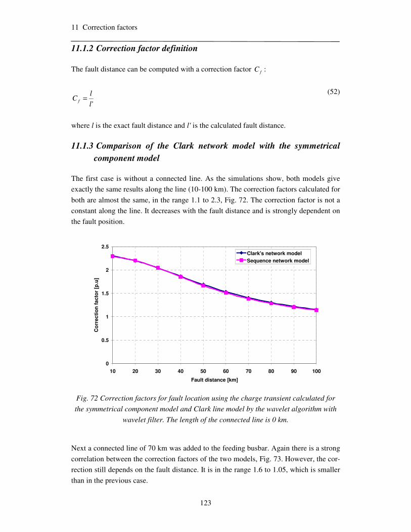
11 Correction factors
123
11.1.2 Correction factor definition
The fault distance can be computed with a correction factor fC :
'l
lC f =
(52)
where l is the exact fault distance and l' is the calculated fault distance.
11.1.3 Comparison of the Clark network model with the symmetrical
component model
The first case is without a connected line. As the simulations show, both models give
exactly the same results along the line (10-100 km). The correction factors calculated for
both are almost the same, in the range 1.1 to 2.3, Fig. 72. The correction factor is not a
constant along the line. It decreases with the fault distance and is strongly dependent on
the fault position.
0
0.5
1
1.5
2
2.5
10 20 30 40 50 60 70 80 90 100
Fault distance [km]
Co
rrec
tio
n f
acto
r [p
.u]
Clark's network model
Sequence network model
Fig. 72 Correction factors for fault location using the charge transient calculated for
the symmetrical component model and Clark line model by the wavelet algorithm with
wavelet filter. The length of the connected line is 0 km.
Next a connected line of 70 km was added to the feeding busbar. Again there is a strong
correlation between the correction factors of the two models, Fig. 73. However, the cor-
rection still depends on the fault distance. It is in the range 1.6 to 1.05, which is smaller
than in the previous case.

11 Correction factors
124
1
1.1
1.2
1.3
1.4
1.5
1.6
1.7
10 20 30 40 50 60 70 80 90 100
Fault distance [km]
Co
rreti
on
fc
tor,
[p
.u]
Clark's network model
Sequence network model
Fig. 73 Correction factors for fault location using the charge transient calculated for
both the symmetrical component and Clark line models by the wavelet algorithm with
wavelet filter. The length of the connected line is 70 km.
Finally, a connected line of length 300 km was added. Both models gave very close re-
sults. Surprisingly, the correction factor is almost equal to one and does not depend
much on fault position. This is different to the previous cases. So, for long connected
lines the correction is not needed for any place in the network because it is almost equal
to one.
0.95
0.97
0.99
1.01
1.03
1.05
10 20 30 40 50 60 70 80 90 100
Fault distance [km]
Co
rre
tio
n f
acto
r [p
.u]
Clark's network model
Sequence network model
Fig. 74 Correction factors for fault location using the charge transient calculated for
the symmetrical component and Clark line models by the wavelet algorithm with wave-
let filter. The length of the connected line is 300 km.

11 Correction factors
125
11.2 Evaluation of a correction factor for transient based fault
location
The accuracy of transient based fault location in a network with an isolated neutral var-
ies due to several factors. Some influential parameters are defined by the line, power
transformer, measurement, load condition, etc. The network configuration and fault po-
sition are investigated in this section. The aim is to show under which circumstances the
method works accurately and under which conditions inaccurately. The critical area
where the correction factor is needed is shown and its calculation is proposed. The study
was made over a large number of faults. Altogether 1100 faults were simulated.
What follows is an example of how fault location in a network with an isolated neutral
can vary with fault distance and the length of the connected line. The example is taken
from the previous section. The calculated correction factors are plotted in Fig. 75. It is
clear that the correction factor decreases with the length of the connected line. For a
long line it will reach 1. In practice this is achieved by a connected line of 300 km, as
seen from the example. However, for shorter lines the correction factor is higher than 1
and varies with the fault position. It is essentially this phenomenon that is analysed in
this section.
0
0.5
1
1.5
2
2.5
10 20 30 40 50 60 70 80 90 100
Fault distance [km]
Co
rreti
on
fac
tor
[p.u
]
Connected line 300 km
Connected line 70 km
Connected line 0 km
Fig. 75 Correction factors for fault location using the charge transient calculated for
both models, the symmetrical component model and the Clark line model, by the wavelet
algorithm with wavelet filter. The length of the connected line is 0, 70 and 300 km.

11 Correction factors
126
11.2.1 Data acquisition
The ground faults were simulated in EMTP/ATP and then processed by the fault locator
developed in Chapter 13. Both of them are controlled automatically by Matlab without
any human intervention. Therefore, it was possible to perform a large number of simula-
tions.
11.2.2 EMTP-ATP model
The faults were simulated in a 110 kV network, Fig. 71. The line parameters match
those of Fingrid’s Pyhäkoski – Rautaruukki line, Tab. 17. Several cases were simulated.
The length of lines x, y and z were changed by the program and the fault distances calcu-
lated.
11.2.3 Error source
The error source in a network can be understood from its symmetrical component
model, Fig. 70. The most influential parts are:
1. Fault distance 2. Line behind the fault 3. Connected lines
The correction idea is based on the symmetrical component model. If the network pa-
rameters do not change over the line, the division of the current between the two line
sections will be a function of their lengths only. Therefore, a correction factor might also
be based on this principle.
Fault distance
The faults were simulated at the end of the line, which means the fault distances were
also the length of the line. This distance was varied from 0 to 200 km. There were no
connected lines. The distances y and z were equal to zero, Fig. 71. The error in the fault
location in such cases grows linearly with the fault distance (line length), Fig. 76. The
approximate analytical solution for the error is:
85.11
x+=δ [km]
(53)
where x is the fault distance. In this particular case there is no path for the zero-sequence
current to be closed via the transformer since the network has an isolated neutral. There-
fore, the fault distance must be corrected by 3/2. Eq. (53) already includes this term.

11 Correction factors
127
0 20 40 60 80 100 120 140 160 180 2000
2
4
6
8
10
12
14
16
Fault distance [km]
Err
or[k
m]
Fig. 76 Error in the fault location using the charge transient versus fault distance. The
computation was made by the wavelet algorithm with the wavelet filter. The fault was
simulated at the end of the line. There were no connected lines.
Line behind the fault
It was recognised from experiences with simulations that the length of the line behind
the fault (from the fault point to the other end of the line) has an important impact on
fault location. Therefore, this phenomenon is now treated independently. The fault
simulations were performed for a network similar to that in Fig. 71, where z=0 km.
The main impact on fault location is given by the zero-sequence part of the line behind
the fault. This is obvious from the symmetrical component model in Fig. 70, because it
is an isolated network. (The positive and negative sequence inductances of the lines are
connected via the low impedances of the transformer, but the zero sequence inductance
of the line is not connected if there are neither connected lines nor low grounding im-
pedance. Moreover, some zero-sequence current will flow to the part of the line behind
the fault instead of the fault section). The longer the line connected behind the fault, the
less the zero-sequence current that will flow to the faulted line section and the greater
the error in the fault location, Fig. 77(solid lines).

11 Correction factors
128
0 50 100 150 200 250 3000
10
20
30
40
50
60
Line length behind the fault [km]
Err
or [
km]
Fault dist. 1 kmFault dist. 10 kmFault dist. 20 kmFault dist. 40 kmFault dist. 60 kmFault dist. 100 km
Fig. 77 Error in the fault location using the charge transient with the line length behind
the fault. The computation was made by the wavelet algorithm with the wavelet filter.
There were no connected lines. Error from simulations (solid lines), the correction
(dashed lines).
A fault transient will divide into two parts at the fault point: one goes to the supply sub-
station via the faulted line section and the other goes to the line section behind the fault,
Fig. 70. The error in the fault location is a parallel combination of the two parts of the
line, x and y, together with the error 1δ , caused by the fault distance:
22
2212 yx
yx
+
+= δδ , [km] (54)
where x is the fault distance and y is the line length behind the fault, according to Fig.
71. The accuracy of this estimation is relatively high. A comparison of the simulated and
calculated error is in Fig. 77 (compare the solid and dashed lines).

11 Correction factors
129
Connected lines
There is a lack of zero-sequence current measurement in the case of an isolated network,
as mentioned earlier. The calculated fault distance can be corrected by a correction fac-
tor equal to 3/2. However, in a case where there are connected lines, there exists a path
for the zero-sequence current to return via the measurement point and be measured as
well, Fig. 71. So, the correction can no longer be 3/2. In order to simulate only the influ-
ence of the connected line, the fault was placed at the end of the line. The error in the
fault location decreases with the length of the connected line, Fig. 78 (solid lines).
0 10 20 30 40 50 60 70 80 90 1000
2
4
6
8
10
12
14
Length of connected line [km]
Err
or [
km]
Fault 1 kmFault 5 kmFault 10 kmFault 20 kmFault 30 kmFault 40 kmFault 50 kmFault 60 kmFault 70 kmFault 80 kmFault 90 kmFault 100 km
Fig. 78 Error in the fault location using the charge transient versus the length of con-
nected line. The computation was performed using the wavelet algorithm with the wave-
let filter. The fault was simulated at the end of the line. Error from simulations (solid
lines), the correction (dashed lines).
The error term in the case of connected lines is:
2
23 x
z
x
+
=δ [p.u] (55)
where x is the fault distance and z is the length of the connected lines. A comparison
between the error from the simulations and the calculated errors is shown in Fig. 78

11 Correction factors
130
(compare the solid and dashed lines). In this particular case the fault distance was also
the length of the faulty line. In a real case there is always some part of the line behind
the fault point. Therefore, instead of x, the fault distance, the length of the entire fault
line must be considered in Eq. (55), i.e. yxx +→ .
11.2.4 Comparison of designed correction factor with simulations
The fault location accuracy was studied for a large number of fault cases. Altogether
some 1100 faults were simulated in EMTP/ATP and then processed by the fault locator.
The error in this fault location method is now compared to the error calculated by the
correction factors proposed in the previous section.
The ground faults were studied in a network of length 100 km, Fig. 71. The part of the
line behind the fault is always 100 - x, where x is the fault distance. The fault distance
was varied from 5 to 95 km in steps of 5 km in the simulations. A connected line of
length 5-300 km (with steps of 5 km) was added to the line. The impact of the connected
lines is similar to the previous section – the error exponentially decreases, Fig. 79. The
error dependence on fault distance is somewhat different from the previous case, how-
ever. This phenomenon is due to the fixed line length. There is increased noise in fault
location for very long connected lines caused by the low frequency resolution in that
area. The transient frequency changes less for long connected lines. Therefore, in order
to reduce this noise a higher sampling frequency would be required (in this case it was
2.5 kHz).

11 Correction factors
131
Fig. 79 Error in the fault location with length of connected line and fault distance. The
graph contains 1080 simulated faults.
The estimation of the error is:
32δδδ =f [km] (56)
The difference between the estimated error according to Eq. (56) and the error of the
simulated cases is very small; compare Fig. 80 to Fig. 79. The increased inaccuracy is
only for the shorter connected lines, see Fig. 81.

11 Correction factors
132
Fig. 80 Error correction term in Eq. (56) versus length of connected line and fault dis-
tance.
Fig. 81 The remaining fault location error after the application of Eq. (56) versus
length of connected line and fault distance.
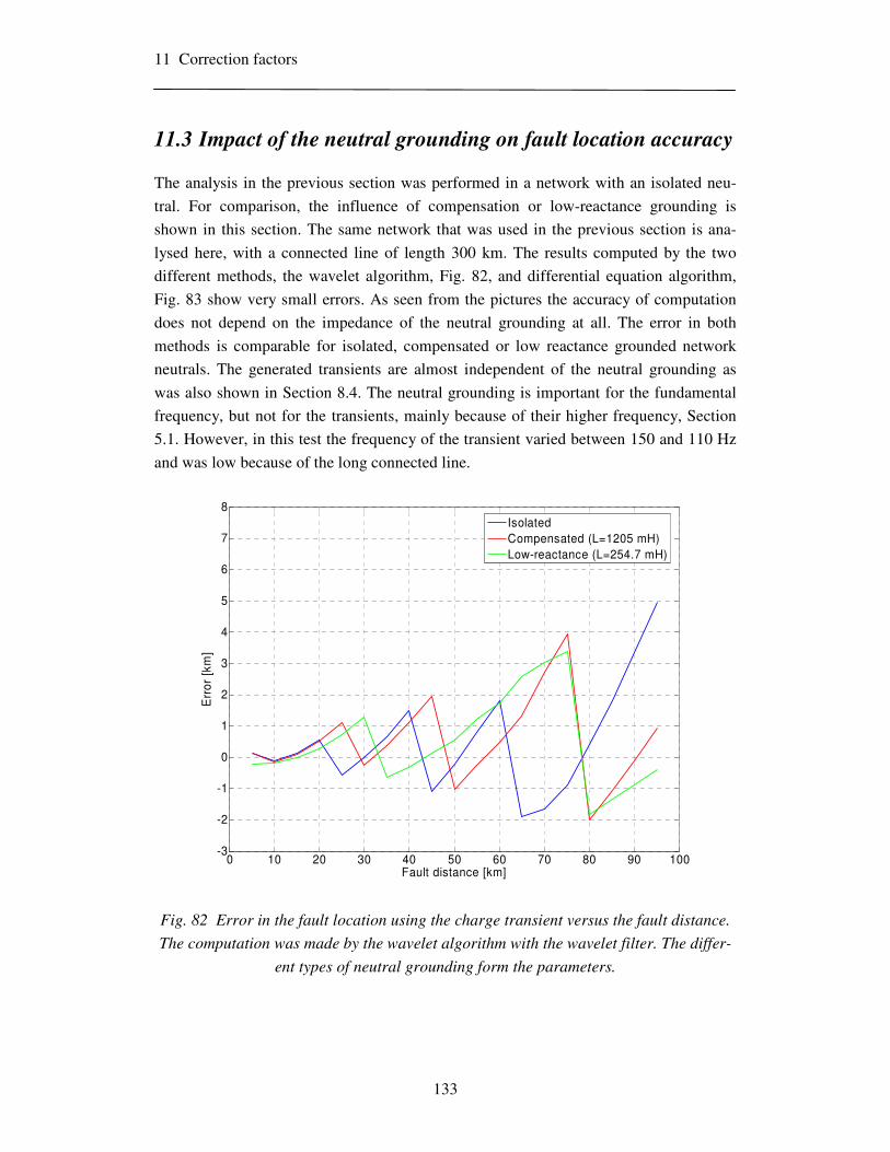
11 Correction factors
133
11.3 Impact of the neutral grounding on fault location accuracy
The analysis in the previous section was performed in a network with an isolated neu-
tral. For comparison, the influence of compensation or low-reactance grounding is
shown in this section. The same network that was used in the previous section is ana-
lysed here, with a connected line of length 300 km. The results computed by the two
different methods, the wavelet algorithm, Fig. 82, and differential equation algorithm,
Fig. 83 show very small errors. As seen from the pictures the accuracy of computation
does not depend on the impedance of the neutral grounding at all. The error in both
methods is comparable for isolated, compensated or low reactance grounded network
neutrals. The generated transients are almost independent of the neutral grounding as
was also shown in Section 8.4. The neutral grounding is important for the fundamental
frequency, but not for the transients, mainly because of their higher frequency, Section
5.1. However, in this test the frequency of the transient varied between 150 and 110 Hz
and was low because of the long connected line.
0 10 20 30 40 50 60 70 80 90 100-3
-2
-1
0
1
2
3
4
5
6
7
8
Fault distance [km]
Err
or [
km]
IsolatedCompensated (L=1205 mH)Low-reactance (L=254.7 mH)
Fig. 82 Error in the fault location using the charge transient versus the fault distance.
The computation was made by the wavelet algorithm with the wavelet filter. The differ-
ent types of neutral grounding form the parameters.

11 Correction factors
134
0 10 20 30 40 50 60 70 80 90 100-0.5
0
0.5
1
1.5
2
2.5
3
Fault distance [km]
Err
or [
km]
IsolatedCompensated (L=1205 mH)low-reactance (L=254.7 mH)
Fig. 83 Error in the fault location using the charge transient versus the fault distance.
The computation utilised the differential equation algorithm. The different types of neu-
tral grounding form the parameters.
By comparing the two figures it can be seen that the wavelet algorithm is more sensitive
to the transient frequency estimation than the differential equation algorithm. However,
the oscillation of the error is around zero, and its variation can be radically decreased by
a higher sampling rate.

11 Correction factors
135
11.4 Error estimation for the transient based ground fault loca-
tion
There are many factors influencing fault location accuracy based on transients. Estima-
tion of the error of the most influential factors is shown in Tab. 6.
Tab. 6 Error estimation for transient based ground fault location.
Source of error Estimated maximum error Comment
Measurement
Current transformer 3.5% Fig. 54 up to 1 kHz
Voltage transformer 4% Fig. 48 up to 1 kHz
Sampling frequency *) 5% Fig. 82 for 2.5 kHz for WA
Signal processing 0% Discussion, Section 7.5
Fault conditions
Fault resistance***) 0% Fig. 36 up to 100 Ω
Connected lines and
line sections behind
the fault
4.5% Fig. 81 for shorter con-
nected lines
Line model inductance**)
with frequency 1% Fig. 69a for 100-300 Hz
with ground resistivity 5% Fig. 69a at 200 Hz
Sum 23%
Geometric mean value 10%
Note:
*) The presented value of 5% is for the wavelet algorithm. A slightly lower value of 2% applies to the
differential equation algorithm, Fig. 83
**) The values are presented for the most typical line construction in Finland (e.g. overhead ground con-
ductors made of aluminium).
***) The fault resistance is not a primary source of error. It simply damps the signal. In the studied case
the error in fault location was the same for fault resistances in the range 0 to 100 Ω. In this range the error
was determined by other factors.
In the worst scenario the error arises from the maximum error of each contributor, and
would be as much as 23%. However, this is highly unlikely, because each element does
not always have the maximum error and the error sources may cancel each other to some
extent. Therefore, the geometric mean value is more informative. This value is around
10 %. It must be stressed that even this value is overestimated. Most likely, better results
would be achieved with a higher sampling frequency (see the discussion in Section 8.6).
Connected lines, which almost always exist in Finnish 110 kV networks, also improve
the results.

11 Correction factors
136
11.5 Discussion
Comparison of models
In this chapter the two different models for ground faults were compared, the line model
(distributed transposed Clark line model) in EMTP/ATP and the symmetrical compo-
nent model. The two models gave very close results for different fault conditions. The
error in both models has probably the same reason. Therefore, it is possible to base the
correction factor on the symmetrical component analysis, which then should also apply
to the line model.
Correction factor
A ground fault in a network with an isolated neutral was simulated. In a single line a
correction will always be needed because of the lack of a zero-sequence measurement in
the substation. The existence of connected lines makes the necessary path for the zero-
sequence current in the substation, which improves the fault location. The same applies
for all signals including the 50 Hz component; refer to the discussion in Chapter 4.
The study of a large number of ground faults has been performed in this chapter. The
area that can be accurately estimated by the fault location algorithms without any correc-
tion has been identified. This applies in networks with long connected lines (more than
100 km if the faulted line is 100 km) and shorter line sections behind the fault. Sec-
ondly, a correction factor based on a symmetrical component representation of the net-
work has been proposed, the accuracy of which is satisfactory.
There are several outgoing lines from most of the substations at the 110 kV level in
Finland. Therefore, the faulty line would probably have enough length of connected
lines and hence the correction factors will be low for Finnish conditions.
Different neutral treatment
The network neutral mainly affects the fundamental frequency component. The charge
transient generation, theoretically described in Section 5.1 for an isolated network, can
also be generated in networks with other neutral configurations. The charge transient
seems to be the same and hence the fault location accuracy is about the same for low-
reactance and compensated network neutrals as in an isolated network.
Error in the transient based fault location method
The error in transient based ground fault location for Finnish 110 kV lines using the
charge transient is about 10 %.
12 Transients in real networks
137
12 Transients in real networks
The ground fault charge transients from a real network are presented in this chapter. The
fault location methods were applied to fault transients recorded in 400 kV, 110 kV and
20 kV lines.
The signal processing is performed in two steps as described in Chapter 7. First the pre-
processing is done in order to detect the transient frequency more accurately and then
the wavelet filter is applied.
1. Digital band-pass FIR filter
2. Charge transient frequency detection
3. Wavelet filter
Then the two methods of fault location are applied.
1. Wavelet algorithm
2. Differential equation algorithm
All signal processing and fault distance estimation were performed by the fault location
program that will be presented in Chapter 13.

12 Transients in real networks
138
12.1 Faults in the 110 kV Pyhäkoski – Rautaruukki line
All data used were recorded in Fingrid’s 110 kV network with the neutral grounded via
low reactance reactors. The sampling frequency was 1 kHz. Altogether, 6 cases were
processed. Not all the faults were permanent; therefore the exact positions of the faults
were calculated by a travelling wave fault locator connected in parallel with the transient
recorder. The faults occurred in the Pyhäkoski - Rautaruukki branch, Fig. 102 in Appen-
dix A. Some results from this analysis have also been presented in [33].
A case from 1.9 2002, where the fault distance was 25.8 km, is shown in the following
figures as an example. Fig. 84, shows the recorded phase voltages and currents. As can
be clearly seen the fault current was of high magnitude. There was a charge transient of
very short duration starting from 200 ms and lasting about 20 ms.
180 190 200 210 220 230-1.5
-1
-0.5
0
0.5
1
1.5
2x 10⁵ Voltages
Time [Samples]
Pha
se v
olta
ge [k
V]
180 190 200 210 220 230-2000
-1500
-1000
-500
0
500
1000
1500Currents
Time [Samples]
Pha
se c
urre
nt [A
]
Fig. 84 The recorded single-phase to ground fault: phase voltages (left) and currents
(right). Case: 1.9 2002.
The frequency of the charge transient was 166.6 Hz. The wavelet algorithm gave the
result shown in Fig. 85. The exact fault distance was taken from the stable part of the
fault distance curve where the transient exists. The results of the differential equation
algorithm applied to the example signals are also shown in Fig. 85. As can be seen, the
stable part of the curve indicates the fault distance. Detailed data can be found in Ap-
pendix A.

12 Transients in real networks
139
195 200 205 210 215 2200
10
20
30
40
50
Time [Samples]
Dis
tanc
e [k
m]
Wavelet algorithm - Distance versus time
195 200 205 210 215 2200
10
20
30
40
50
Time [Samples]
Dis
tanc
e [k
m]
Differential Eq. Algorithm - Distance versus time
Fig. 85 Fault distance curve for the wavelet algorithm (left), and differential equation
algorithm (right). Case: 1.9 2002.
A comparison of both methods can be better seen in Fig. 86. Both methods work very
well up to 50 km of the line length. Similar behavior can be seen in Fig. 14 in Chapter 4,
where the same recording was analyzed by the conventional methods. The sudden
change in accuracy might therefore be caused by the parallel line, which runs parallel to
the faulty line for approximately 30 km, see the schematic diagram of the network in
Fig. 102 in Appendix A.
-15
-10
-5
0
5
10
15
0 10 20 30 40 50 60 70 80
Fault loc a tion [km]
Erro
r [k
m]
WA
DEA
Fig. 86 Transient based fault location using the charge transient. Wavelet algorithm
(WA), Differential equation algorithm (DEA).
Fault distance
Fault distance Fault begin-

12 Transients in real networks
140
12.2 Faults in the 400 kV Alapitkä – Huutokoski line
Single-phase to ground faults were recorded in the 400 kV Fingrid network. The fault
distance in study case 270703 was 28.1 km. This network is solidly grounded with nu-
merous connected lines. The sampling frequency was 12.8 kHz. The phase voltages and
currents, and neutral current were measured in the Alapitkä substation.
2500 2550 2600 2650 2700-4
-3
-2
-1
0
1
2
3
4
5x 10⁵ Voltages
Time [Samples]
Pha
se v
olta
ge [k
V]
2500 2550 2600 2650 2700-5000
-4000
-3000
-2000
-1000
0
1000
2000
3000Currents
Time [Samples]
Pha
se c
urre
nt [A
]
Fig. 87 The fault voltage (left) and current (right). The frequency of the fault transient
was 512 Hz. The exact fault distance was 28.1 km
The fault distances calculated using the charge transient with the wavelet algorithm
using the phase and neutral currents are in following figures.
2620 2640 2660 2680 2700 2720 27400
10
20
30
40
50
60
Time [Samples]
Dis
tanc
e [k
m]
Wavelet algorithm - Distance versus time
2450 2500 2550 26000
5
10
15
20
25
30
35
Time [Samples]
Dis
tanc
e [k
m]
Wavelet algorithm - Distance versus time
Fig. 88 The fault distance calculated using the phase current (left) and the neutral cur-
rent (right). The fault distances were calculated by the wavelet algorithm. The exact
fault distance was 28.1 km.
For comparison, the conventional method in this case located the fault as follows:
1. Phase current: 28.09 km
2. Neutral current: 29.9 km
29.2 km
28.2 km

12 Transients in real networks
141
12.3 Faults in MV networks
MV network faults are presented in this section. Faults artificially made for study pur-
poses were recorded in Vaasan Sahko Oy (VSOY) and Lounais-Suomen Sahko Oy
(LSS) on 11 and 12 December and 19 and 20 June, 1990 by Matti Lehtonen. The 20 kV
networks consist of overhead lines and have isolated, compensated or partially compen-
sated network neutrals. The sampling frequency of the recordings was 20 kHz.
As an example, one single-phase to ground fault from an isolated neutral network, with
fault distance 14.2 km (RTN45), will be presented. The fault voltage and current are
shown in Fig. 89 and the results are given in Fig. 90.
0 500 1000 1500 2000-2
-1.5
-1
-0.5
0
0.5
1
1.5
2x 10⁴ Voltages
Time [Samples]
Pha
se v
olta
ge [k
V]
0 500 1000 1500 2000-40
-20
0
20
40
60
80Currents
Time [Samples]
Pha
se c
urre
nt [A
]
Fig. 89 The fault voltage (left) and fault phase current (right). Case RTN45, fault dis-
tance 14.2 km, Rf=0 Ω. Isolated neutral network
700 750 800 850 900 950 10000
5
10
15
20
25
Time [Samples]
Dis
tanc
e [k
m]
W avelet algorithm - Distance versus time
700 750 800 850 900 950 10000
5
10
15
20
25
Time [Samples]
Dis
tanc
e [k
m]
Differential Eq. Algorithm - Distance versus time
Fig. 90 The fault distance calculated using the charge transient with the wavelet algo-
rithm and the differential equation algorithm. Case RTN45, fault distance 14.2 km, Rf=0
Ω. Isolated neutral network
15.15 km 15.26 km
Fault start
Fault start
Transient appearance Transient appearance

12 Transients in real networks
142
The charge transient of 371 Hz is of strong amplitude. The network has many connected
lines, so there is a sufficient path for the zero-sequence current to be closed via the
measurement point (even if the network neutral is isolated). The calculated fault dis-
tance is relatively accurate. More statistics from similar networks are presented in the
following figures. The processing was made with the fault location program that will be
shown in Chapter 13.
LSS
-2.9
0.2
1.3
-5
0.2
0.9
0.40
-3
0
-0.6
-2.2
-4.6
-0.1
-0.8
-2.1-1.8
-2.8
-6
-5
-4
-3
-2
-1
0
1
2
25.4 25.4 25.4 25.4 25.4 25.4 36 36 36
Fault location [km]
Err
or
[km
]
WA
DEA
RTN
-1.2
-2.3 -2.3
-2.1-2.2
0.11
-1.4
0.36
-1.4
0.16
-1.4
0.35
-2.5
-2
-1.5
-1
-0.5
0
0.5
0.76 0.76 10.4 10.4 14.2 14.2
Fault distance [km]
Err
or
[km
]
WA
DEA
Fig. 91 Fault statistics from the MV network, showing the errors in the wavelet and
differential equation algorithms. The LSS faults are from a partially compensated net-
work. The RTN faults at 0.76 and 10.4 km occurred in a compensated network. The fault
at 14.2 km was in an isolated network

12 Transients in real networks
143
12.4 Discussion
The location of ground faults at different voltage levels has been analysed in this chap-
ter.
Faults on 110 kV and 400 kV lines
The single-phase to ground faults from the 110 kV and 400 kV networks are from net-
works with reactor grounding and solidly grounded neutrals, respectively. Therefore,
these two can be compared quite reasonably. In these networks the accuracy is relatively
high. In the case of a 400 kV line there are also many connected lines, which is favour-
able for fault location.
Ground faults in MV networks
The real “ground faults” were recorded in MV networks with an isolated, compensated
or partially compensated neutral. The network has a lot of connected lines. The tran-
sients in an MV network are of relatively high amplitude. Therefore, fault location is
easier. The reason is that the zero- and positive- sequence capacitances of the lines per
km are much greater in MV networks than in HV networks.
Using the neutral current
In the case of a 400 kV fault, using the neutral current for fault location is almost as ac-
curate as using the phase current.
Conventional method
In addition to the wavelet algorithm, the conventional methods were used for the 400
kV faults and some of 110 kV ground faults were calculated in Chapter 4. The accuracy
is comparable, mainly because of the high ground fault currents due to the neutral
grounding type.
13. Fault location program
144
13 Fault location program
A practical output of this research has been the development of a fault location program
with a graphical user interface. The program was written in Matlab 7 and can also work
outside matlab using the Matlab runtime version. A block diagram of the program with
the basic data flow is shown in Fig. 92.
Data reading
The program can process both the EMTP/ATP simulations and the real fault recordings
from Fingrid’s recorders and can cope with various sampling frequencies, time lengths
and data structures.
Transient methods
The frequency estimation of the fault transients was made with the Fourier transform
following completion of the pre-processsing. The pre-processing was performed with
the sinc filter presented in Section 6.1. The transient based methods with the wavelet
and differential equation algorithms based on the wavelet filter were implemented as
described in sub-sections 7.3.2 and 7.3.3. The automatic detection of the fault distance
works on the principle proposed in Section 7.4. The program preprocessing window can
be seen in Fig. 95, the wavelet filter in Fig. 96 and the fault distance window in Fig. 97.
Conventional methods
The conventional and improved conventional methods, according to the descriptions in
Sections 4.1 and 4.2 and the error estimation in Chapter 4.2.4, are programmed into the
fault locator. The conventional algorithm window is shown in Fig. 98, with the de-
noising wavelet based filter presented in Fig. 99.
Program settings
The line parameter calculations were made by a developed line constant program that
uses the Carson formula presented in Chapter 10.5. The settings for the data reading and
line paramters can be made for both the EMTP/ATP simulation and the real recorders.
A recorder organizer allows the user to save the program settings for future use. The
above mentioned settings can be seen in Fig. 100.

13. Fault location program
145
Fig. 92 Block diagram of the fault location program and basic data flow.

13. Fault location program
146
Main window
Fig. 93 The main window of the fault locator.
Fig. 94 Menu bar of the main window

13. Fault location program
147
Transient fault location
Fig. 95 The pre-processing.
Fig. 96 The wavelet filter.

13. Fault location program
148
Fig. 97 Transient based fault location algorithms.

13. Fault location program
149
Conventional fault location
Fig. 98 Conventional algorithm.
Fig. 99 Wavelet de-noising filter for conventional fault location.
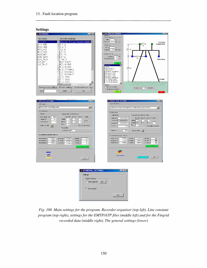
13. Fault location program
150
Settings
Fig. 100 Main settings for the program. Recorder organiser (top left). Line constant
program (top right), settings for the EMTP/ATP files (middle left) and for the Fingrid
recorded data (middle right). The general settings (lower)

14. Conclusions
151
14 Conclusions
This thesis deals with transient based ground fault location and conventional fault loca-
tion methods in subtransmission networks. Based on the analysis and study of the dif-
ferent issues, the following conclusions can be made:
Conventional methods
• The conventional fault location method has limitations, mainly due to the load
current and fault resistance. Reducing the influence of the fault resistance means
that the fault location method will have a more limited usage under certain con-
ditions, caused by the unfavourable relation between the load and fault current.
This area was identified and an error estimation algorithm has been developed.
• The use of the current sum instead of the fault phase current is only reasonable if
the load current is much smaller than the fault current.
• If the network neutral is not grounded solidly, a connected line(s) can improve
the accuracy by increasing the zero-sequence current flow via the measurement
point.
Transient methods
• A sampling frequency of 2.5 kHz would be high enough for fault location based
on charge transients. However, the higher sampling frequency, the more reliable
the fault location. Discharge transient fault location would require a sampling
rate of approximately 5 kHz.
• Fault location based on charge transients works for a wider range of different
fault conditions than discharge transient fault location and conventional fault lo-
cation.
• The wavelet filter is suitable for fault transient filtering. The wavelet transform
and windowed Fourier transform can be used but they are not so convenient.

14. Conclusions
152
• Fault transient signals can be measured by conventional CTs and PTs almost as
accurately as the 50 Hz signals. The capacitance of added secondary cables con-
nected to the substation building does not move the resonance point of PTs into
the fault transient’s spectrum. A new method of PT model parameter estimation
was developed and the model can be used for the correction of measured signals
from both simulations and real fault recordings.
• The line parameters in transient frequencies are almost constant with frequency;
the dependency with ground resistivity is much stronger. Analysis of the propa-
gation of fault transients showed that the fault transients return via the overhead
ground wire rather than the ground. This makes the transient less dependent on
the unstable ground resistivity. In the case of steel overhead ground wires, coun-
terpoises must be used to reduce the portion of the transient that returns via the
ground.
• The transient based fault location method can be used in networks with solidly
grounded neutrals. Application of the method in a network with some grounding
impedance (Petersen coil, low-reactance or isolated) depends on the existence of
a return path to the substation. The zero-sequence current in the measurement
point is increased by connected lines or by compensation capacitors placed on
the busbar (with a grounded neutral). The longer the connected lines and the
shorter the line section behind the fault, the more precise the fault location will
be. However, this phenomenon was mathematically described and the critical
area can be corrected by the method proposed.
• The transient based method inherently works with the phase current; however,
the current sum can be used instead.
• The main conclusion of this work is that transient based fault location can be ap-
plied to Fingrid’s 110 kV subtransmission networks. The developed fault loca-
tion application was tested and verified using both simulated and real power sys-
tem fault data. Since there is no big difference in the charge transients between
the various types of high impedance grounded networks, the transient based
method works similarly in ungrounded, Petersen grounded and low-reactance
coil grounded systems. The main limitations of the method are related to the
fault resistance, overhead ground wires made of steel, low sampling frequency
and network configuration.

References
153
References
[1] Lehtonen, Matti. Transient analysis for ground fault distance estimation in
electrical distribution networks, Espoo 1992, Technical Research Centre of
Finland, VTT Publications 115. 182p+app. 92p
[2] Hänninen, Seppo. Single phase earth faults in high impedance grounded
networks. Characteristic, indication and location. Espoo 2001. Technical
Research centre of Finland, VTT Publication 453. 78p.+app.61p.
[3] Imris, Peter; Lehtonen, Matti; Fault location in underground distribution
networks using travelling waves, The 44th International Scientific Confer-
ence of Riga Technical University, Riga, Latvia, October 9-11, 2003, pp.
227-232.
[4] Imris, Peter; Lehtonen, Matti; A comparison of different signal processing
techniques for travelling wave fault location, The 44th International Scien-
tific Conference of Riga Techni-cal University, Riga, Latvia, October 9-
11, 2003, pp. 220-226.
[5] Imris P. Fault location in underground distribution networks using travel-
ling waves, Univeristy of Zilina, Master’s thesis, Zilina, Slovakia 2002,
91p.
[6] Samesima, M.I.; de Oliveira, J.C.; Dias, E.M.; Frequency response analy-
sis and modeling of measurement transformers under distorted current and
voltage supply, Power Delivery, IEEE Transactions on , Volume: 6 , Issue:
4 , Oct. 1991, Pages:1762 – 1768
[7] Bak-Jensen, B.; Ostergaard, L.; Estimation of the model parameters in
equivalent circuit models of potential transformers, Power Engineering
Society 1999 Winter Meeting, IEEE , Volume: 2 , 31 Jan-4 Feb 1999,
Pages:1053 - 1058 vol.2
[8] Erwin Kreyszig, “Advanced Engineering Mathematics”, 8th edition, John
Wiley & Sons, Inc., 1999.

References
154
[9] J. Lewis Blackburn, ”Symmetrical components for power systems engi-
neering”, Marcel Dekker, Inc., 1993.
[10] Jarmo Elovaara, Yrjö Laiho, “Sähkölaitostekniikan Perusteet”, Otatieto
Oy, 1988.
[11] Schegner, P.: Digitaler Erdschlußuniversalschutz. Konzept und erste Real-
isierung. Dissertation, Universität des Saarlandes, Saarbrücken, 1989, 186
pp.
[12] Igel, M.: Neuartige Verfahren für den Erdschlußdistanzschutz in isoliert
und kompensiert betriebenen Netzen. Signale und Algoritmen im Fre-
quenzbereich. Dissertation, Universität des Saarlandes, Saarbrücken, 1990,
181 pp.
[13] Pundt, H.: Untersuchungen der Ausgleichsvorgänge bei Erdschluß in
Hochspannungsnetzen mit isoliertem Sternpunkt und induktiver Stern-
punkterdung als Grundlage zur selektiven Erdschlußerfassung. Disserta-
tion, TU Dresden, 1963, 167 pp. + app.
[14] Willheim, R., Waters, M.: Neutral earthing in high-voltage transmission.
Elsevier Publishing Co., New York, 1956, 669 pp.
[15] Robertson, D.C.; Camps, O.I.; Mayer, J.S.; Gish, W.B.; Wavelets and
electromagnetic power system transients, Power Delivery, IEEE Transac-
tions on, Volume: 11 , Issue: 2 , April 1996, Pages:1050 – 1058.
[16] C. L. Fortescue; “Method of Symmetrical Coordinates Applied to the So-
lution of Polyphase Networks” AIEE Transactions, Vol. 37, 1918, pp.
1027-1140.
[17] Glover J. D., Sarma M., “Power system analysis and design”, PWS pub-
lishers, Boston, 1987.
[18] Stevenson W., D., JR., ”Elements of power system analysis”, McGRAW-
HILL publishing company LTD., London 1955.
[19] Carson, J.R., Wave propagation in overhead wires with ground return. Bell
System Technical Journal, Vol. 5, 1926. pp. 539-54.

References
155
[20] Yaw-Juen Wang, Shi-Jie LIU. A review of methods for calculation of fre-
quency-dependent impedance of overhead power transmission lines. Proc.
Natl. Sci. Counc. ROC(A),Vol.25, No.6, 2001, p. 329-338.
[21] Lakervi, E; Holmes E,J; Electricity distribution network design. Short Run
Press Ltd., Exeter. 1998, second edition, IEE power engineering series 21.
[22] Stearns Samuel D., Digital Signal Processing with examples in Matlab,
CRC Press LLC, 2000 N.W. Corporate Blvd., Boca Raton, Florida 33431.,
pp. 112-124
[23] Imris, Peter, and Lehtonen, Matti, ”Transient based earth fault location in
110 kV subtransmission networks”, 15th Power Systems Computation
Conference, PSCC 2005, Liege, Belgium, August 22-26, 2005, 4 p.
[24] G.Strang and T.Nguyen, "Wavelets and Filter Banks", Wellesley-
Cambridge Press,1996.
[25] A. G. Phadke and J. S. Thorp, Computer Relaying for Power Systems, Re-
search Studies Press Ltd., 1988.
[26] Grainger, John, J., Stevenson, William D, jr., ”Power system analysis”,
McGraw-Hill, 1994
[27] ”Fault statistic 2004”, http://www.nordel.org/, link available on 20.6 2006:
http://195.18.187.215/2/LIPOBGPBIHCMFOIADNJDKHFFPDB19DBK
CN9DW3571KM/docs/DLS/2005-00486-01-E.pdf
[28] ”Living adjacent to a transmission line”, Fingrid publication. Link avail-
able on 20.6 2006:
http://www.fingrid.fi/attachments/english/publications/LivingAdjacent.pdf
[29] Lehtonen, Matti; Hakola, Tapio: Neutral Earthing and Power System Pro-tection. Earthing Solutions and Protective Relaying in Medium Voltage Distribution Networks. Kirjapaino FRAM Oy. 1996. 118 p.

References
156
[30] Ingrid Daubechies, ”Ten Lectures on Wavelets”, CBMS-NSF Regional
Conference Series in Applied Mathematics Vol. 61 (SIAM, Philadelphia,
1992).
[31] Imriš, P.; Lehtonen, M.; ”Transient based Ground Fault Location using
Wavelets”, The 4th IASTED International Conference on POWER AND
ENERGY SYSTEMS, Rhodes, Greece, June 28-30, 2004, pp. 507-511
[32] Imris, Peter and Lehtonen, Matti, ”Modelling of a voltage transformer for
transients”, 2005 IEEE PowerTech'2005, St. Petersburg, Russia, June, 27-
30, 2005, Paper 201, 5 p.
[33] Imris, Peter, and Lehtonen, Matti, ”Transient based earth fault location in
110 kV subtransmission networks”, 15th Power Systems Computation
Conference, PSCC 2005, Liege, Belgium, August 22-26, 2005, 4 p.
[34] H. W. Dommel, “ EMTP Theory Book” , BPA, Portland, August 1986.
[35] Pollaczek, F. (1926) Uber das feld einer unendlich langen wechselstrom-
durchflossenen Einfachleitung. Elektrische Nachrichlen Technik, 3(9),
339-359.
[36] Pollaczek, F. (1931) Sur le champ produit par un conducteur simple in-
finiment long parcouru par un courant alternatif. Revue Générale
d’Électricité, 29(22), 851-867.
[37] Izykowski, J.; Molag, R.; Rosolowski, E.; Saha, M.M.; “Accurate location
of faults on power transmission lines with use of two-end unsynchronized
measurements” IEEE Transactions on Power Delivery, Volume 21, Issue
2, April 2006 Page(s):627 - 633

Appendices
157
Appendices

A Fault simulations
158
A Fault simulations
A.1 Parameters of the simulated network
Fig. 101 The analysed network: (a) schematic diagram and (b) EMTP/ATP
model
Tab. 7 Parameters of the network.
Network Three phase load Busbar Type of the network
Voltage [kV] Frequency [Hz] R [Ω] CB [µF]
Three phase, ungrounded, radial 220 and 110 50 300 0
(a)
(b)
lf

A Fault simulations
159
Tab. 8 Parameters of the transformers.
Transformer I0M
[A]
F0
[WB-turn]
Rm
[MΩ]
Vrp
[kV]
Rp
[Ω]
Lp
[mH]
Vrs
[kV]
Rs
[Ω]
Ls
[mH]
Cou-
pling
A 3.55 50 10 234 0.966 310 117 0.216 54 Yy
B,C 1 50 1 117 0.216 50 23 0.0216 10 Yy
Tab. 9 Parameters of the lines.
Symmetrical components
LINE In
[A]
Volt-
age
Level
[kV]
Length
[km] R0’
[Ω/km]
R1’
[Ω/km]
L0’
[mH/km]
L1’
[mH/km]
C0’
[µF/km]
C1’
[µF/km]
L [mH]
1 900 220 - - - - - - - 40
2 775 110 50 0.16 0.035 1.5 1.1 0.0063 0.0095 -
3 775 110 55 0.16 0.035 1.5 1.1 0.0063 0.0095 -
A.2 Simulation results
A.2.1 Transient fault location
Tab. 10 Transient fault location versus fault distance.
Rf =0 Ω, ϕf =90°, tf =0 s Time window=100 ms, Maximum transient damping -30 dB, fS=100kHz/2.5 kHz
Charge transient Discharge transient Fault
distance
[km] lf
[km]
Frequency
[Hz]
Freq. Shift
[Hz]
Error, δf
[km]
lf
[km]
Frequency
[Hz]
Freq. Shift
[Hz]
Error, δf
[km]
5 4.752658 270 0 -0.247342 not detected
10 9.404958 270 0 -0.595042 11.34887 1250 0 1.34887
15 13.967120 270 0 -1.032880 18.83920 1150 -100 3.83920
20 18.969280 260 -10 -1.030720 21.37917 1080 -170 1.37917
25 23.728880 260 -10 -1.271120 26.94968 1020 -230 1.94968
30 28.225210 260 -10 -1.774790 22.21482 970 -280 -7.78518
35 34.072750 250 -20 -0.927250 45.79534 930 -320 10.79534
40 38.518660 250 -20 -1.481340 18.34387 890 -360 -21.65613
45 43.008390 250 -20 -1.991610 18.82752 850 -400 -26.17248
50 47.962000 250 -20 -2.038000 28.13722 820 -430 -21.86278
Absolute error 1.239009 10.75431

A Fault simulations
160
Tab. 11 Transient fault location versus fault resistance
lf=25 km, ϕf =90°, tf =0 s, Time window=100 ms, Maximum transient damping –30 dB, fS=100kHz/2.5 kHz
Charge transient Discharge transient Fault
resistance
[Ω] lf
[km]
Frequency
[Hz]
Freq. Shift
[Hz]
Error, δf
[km]
lf
[km]
Frequency
[Hz]
Freq. Shift
[Hz]
Error, δf
[km]
0 23.72888 260 0 -1.27112 26.94968 1020 0 1.94968
1 23.74518 260 0 -1.25482 27.93547 1020 0 2.93547
5 23.80399 260 0 -1.19601 29.02801 1020 0 4.02801
10 23.86447 260 0 -1.13553 25.20060 1030 10 0.20060
15 23.90951 260 0 -1.09049 21.39500 1030 10 -3.60500
20 23.93964 260 0 -1.06036 27.13825 1030 10 2.13825
25 23.95509 260 0 -1.04491 27.09390 1030 10 2.09390
30 23.95590 260 0 -1.04410 27.01637 1030 10 2.01637
35 23.94055 260 0 -1.05945 26.63512 1040 20 1.63512
45 23.86685 260 0 -1.13315 26.22083 1040 20 1.22083
50 23.80677 260 0 -1.19323 25.88271 1040 20 0.88271
55 23.73026 260 0 -1.26974 25.18722 1050 30 0.18722
60 23.64296 260 0 -1.35704 24.59035 1050 30 -0.40965
65 23.53812 260 0 -1.46188 23.81772 1050 30 -1.18228
70 23.41726 260 0 -1.58274 18.19077 1050 30 -6.80923
75 23.28218 260 0 -1.71782 17.93536 1050 30 -7.06464
100 23.26866 250 -10 -1.73134 15.84724 1110 90 -9.15276
110 22.77035 250 -10 -2.22965 13.69684 1250 230 -11.30316
120 22.21048 250 -10 -2.78952
130 21.58071 250 -10 -3.41929
140 20.89017 250 -10 -4.10983 Not detected discharge transient
150 20.10456 250 -10 -4.89544
160 19.27679 250 -10 -5.72321
170 18.30567 250 -10 -6.69433
200 15.64059 240 -20 -9.35941

A Fault simulations
161
Tab. 12 Transient fault location versus voltage inception angle.
lf=25 km, Rf=0 Ω, tf =0 s, Time window 100 ms, Maximum transient damping -30 dB, fS=100kHz/2.5 kHz
Charge transient Discharge transient Voltage
inception
Angle
ϕf [°]
lf
[km]
Frequency
[Hz]
Error, δf
[km]
lf
[km]
Frequency
[Hz]
Error, δf
[km]
0 23.72870 260 -1.27130
1 23.72883 260 -1.27117 Not detected discharge transient
2 23.72908 260 -1.27092
3 23.72909 260 -1.27091 26.91696 1020 1.91696
4 23.72973 260 -1.27027 27.20588 1020 2.20588
5 23.72903 260 -1.27097 26.84813 1020 1.84813
10 23.72868 260 -1.27132 26.82296 1020 1.82296
20 23.72892 260 -1.27108 26.86102 1020 1.86102
30 23.72900 260 -1.27100 26.89302 1020 1.89302
40 23.72888 260 -1.27112 26.91203 1020 1.91203
50 23.72884 260 -1.27116 26.92250 1020 1.92250
60 23.72876 260 -1.27124 26.92978 1020 1.92978
70 23.72895 260 -1.27105 26.93600 1020 1.93600
80 23.72883 260 -1.27117 26.94446 1020 1.94446
90 23.72888 260 -1.27112 26.94968 1020 1.94968

A Fault simulations
162
A.2.2 Conventional fault location
Tab. 13 Conventional fault location in solidly grounded network. Influence of
fL II / .
kml f 25= , Ω= 0fR , simulated time 1 s, st f 45.0= , fS=100kHz/2.5 kHz
Parameters Conventional fault location
I_L/I_f Angle Re Im Re Im Fault Abs
[p.u] (I_L/I_f) (VF/IF) (VF/IF) (Denomin) (Denomin) distance (Error)
[º] [Ω] [Ω] [Ω] [Ω] [km] [km]
I_L/I_f=1
1 6.421 2.276 18.943 0.073 0.734 25.86 0.857
1.012 23.513 -0.434 18.733 -0.03 0.722 25.93 0.932
1.044 40.897 -3.123 17.875 -0.132 0.684 26.05 1.053
1.096 58.848 -5.694 16.263 -0.227 0.616 26.25 1.247
0.983 99.914 -7.156 9.815 -0.264 0.363 27.09 2.088
1.036 121.11 -7.164 6.45 -0.249 0.233 28.27 3.273
1.079 143.45 -5.764 2.962 -0.176 0.11 31.25 6.251
1.095 166.41 -2.745 0.07 -0.049 0.029 48.05 23.047
1.095 172.13 -1.748 -0.443 -0.013 0.018 81.16 56.162
1.094 175.54 -1.122 -0.698 0.009 0.014 80.74 55.743
1.093 176.67 -0.944 -0.807 0.016 0.012 60.01 35.008
I_L/I_f=0.3
0.296 7.378 2.003 12.468 0.074 0.49 25.49 0.486
0.34 -2.081 2.532 12.818 0.093 0.504 25.49 0.486
0.304 46.635 0.199 11.958 0.008 0.467 25.61 0.607
0.31 66.372 -0.513 11.285 -0.017 0.44 25.65 0.646
0.303 106.53 -0.916 9.36 -0.027 0.368 25.51 0.513
0.31 126.66 -0.699 8.375 -0.016 0.332 25.28 0.278
0.314 146.91 -0.123 7.508 0.008 0.302 24.83 0.169
0.317 167.27 0.752 6.894 0.042 0.283 24.26 0.739
0.318 172.36 1.006 6.796 0.051 0.28 24.14 0.863
0.318 175.42 1.162 6.746 0.057 0.279 24.06 0.938
0.318 176.44 1.215 6.732 0.059 0.278 24.04 0.963
I_L/I_f=3
2.959 4.585 3.411 36.486 0.098 1.414 25.85 0.848
3.182 -0.492 5.976 38.253 0.197 1.485 25.84 0.838
3.194 26.198 -6.971 37.018 -0.31 1.426 25.81 0.806
3.518 37.248 -13.3 37.254 -0.561 1.429 25.77 0.767
2.956 81.26 -22.86 18.016 -0.917 0.645 25.97 0.968
2.906 106.5 -23.35 7.301 -0.915 0.2 26.13 1.131
3.075 133.46 -20.74 -3.373 -0.768 -0.27 25.85 0.846
2.94 167.6 -12.89 -10.02 -0.242 -0.58 25.89 0.892
2.972 171.85 -12.59 -10.6 -0.172 -0.61 25.82 0.816

A Fault simulations
163
Tab. 14 Conventional and improved conventional fault location in solidly
grounded network. Influence of the fault resistance. Studied case 3/ =fL II .
3/ =fL II , kml f 25= , simulated time 1 s, st f 45.0= , fS=100kHz/2.5 kHz
Parameters Conventional FL Improved Conventional FL
Rf
I_L/I_f Angle Re Im Re Im Fault Abs Angle Angle Fault Abs
[p.u] (I_L/I_f) (VF/IF) (VF/IF) (Denomin) (Denomin) distance (Error) Accuracy1 Accuracy2 distance (Error)
[Ω] [º] [Ω] [Ω] [Ω] [Ω] [km] [km] [º] [º] [km] [km]
0 2.959 4.585 3.411 36.486 0.098 1.414 25.85 0.848 110.95 113.3 25.798 0.798
1 2.967 2.556 6.284 36.545 0.135 1.416 26.07 1.073 108.85 115.3 25.812 0.812
5 3.046 -5.32 17.765 36.972 0.28 1.425 28.24 3.244 100.38 122.6 25.946 0.946
10 3.066 -14.09 31.386 36.383 0.439 1.388 33 8.002 91.456 131.2 26.206 1.206
15 3.042 -21.4 43.482 35.072 0.559 1.327 38.8 13.799 84.326 138.7 26.434 1.434
20 3.051 -27.46 54.657 34.003 0.657 1.273 44.92 19.924 78.197 144.7 26.707 1.707
30 3.004 -36.46 73.944 31.636 0.778 1.159 57.61 32.605 69.549 154 27.287 2.287
40 3.003 -42.92 91.42 29.833 0.86 1.075 69.84 44.84 63.103 160.5 27.742 2.742
50 2.988 -47.4 106.86 28.755 0.907 1.009 81.56 56.562 58.739 165.1 28.499 3.499
60 3.075 -51 122.78 28.371 0.97 0.972 91.78 66.776 54.479 168.1 29.188 4.188
70 2.969 -53.48 134.95 27.392 0.963 0.914 103.7 78.737 52.8 171.3 29.971 4.971
80 2.96 -55.67 148.03 26.904 0.979 0.878 114.4 89.372 50.687 173.6 30.63 5.63
90 2.95 -57.48 160.64 26.484 0.991 0.848 124.8 99.799 48.951 175.5 31.232 6.232
100 2.94 -59.02 173.21 26.163 1 0.822 135.3 110.329 47.492 177.1 31.839 6.839
Tab. 15 Conventional and improved conventional fault location in solidly
grounded network. Influence of the angle ( fL II / ). Studied case 3/ =fL II .
3/ =fL II , kml f 25= , Ω= 0fR , simulated time 1 s, st f 45.0= , fS=100kHz/2.5 kHz
Parameters Conventional
fault location Improved Conventional fault location
I_L/I_f Angle Re Im Re Im Fault Abs Angle Angle Fault Abs
[p.u] (I_L/I_f) (VF/IF) (VF/IF) (Denomin) (Denomin) distance (Error) Accuracy1 Accuracy2 distance (Error)
[º] [Ω] [Ω] [Ω] [Ω] [km] [km] [º] [º] [km] [km]
2.959 4.585 3.411 36.486 0.098 1.414 25.85 0.848 110.95 113.3 25.798 0.798
2.942 15.699 -1.637 36.057 -0.099 1.393 25.84 0.836 122.19 102.4 25.875 0.875
3.033 27.376 -7.027 35.496 -0.311 1.366 25.83 0.826 133.17 89.99 25.982 0.982
3.083 41.302 -13.02 32.942 -0.545 1.258 25.83 0.832 146.73 75.7 26.179 1.179
3.38 50.809 -18.28 32.054 -0.753 1.217 25.79 0.785 154.29 64.25 26.345 1.345
3.047 54.052 -17.36 28.884 -0.713 1.092 25.85 0.85 159.74 63.21 26.462 1.462
3.102 68.742 -21.79 23.706 -0.883 0.877 25.88 0.877 174.03 48.12 27.031 2.031
3.054 80.345 -23.54 18.658 -0.945 0.67 25.92 0.924 174.02 36.86 27.864 2.864
2.978 105.82 -23.97 7.513 -0.942 0.207 26.05 1.053 147.97 11.96 36.272 11.272
3.031 116.26 -23.47 3.11 -0.909 0.019 26.04 1.037 137.94 1.121 161.78 136.78
2.928 119.9 -22.22 1.949 -0.851 -0.03 26.2 1.195 133.49 1.725 -69.29 94.29
3.006 133.85 -20.23 -3.21 -0.745 -0.26 26 1.002 120.15 16.28 12.532 12.468
3.11 166.94 -13.32 -10.32 -0.272 -0.63 24.41 0.595 87.829 50.13 16.258 8.742

A Fault simulations
164
Not
e:
CA
- c
onve
ntio
nal
faul
t loc
atio
n al
goru
thm
ICA
- i
mpr
oved
con
vent
iona
l fa
ult l
ocat
ion
algo
ruth
m
Tab. 16 Conventional and improved conventional fault location with different
network neutral arrangements. Influence of the angle( fL II / ). Studied case
9/ ≅fL II .

A Fault simulations
165
A.3 Pyhäkoski – Rautaruukki faults
A.3.1 Real faults
Fig. 102 Schematic layout of the Pyhäkoski – Rautaruukki line.
Tab. 17 Parameters of the Pyhäkoski – Rautaruukki line
Symmetrical components of the line Other parameters
'0R
[Ω/km]
'1R
[Ω/km]
'2R
[Ω/km]
'0L
[H/km]
'1L
[H/km]
'2L
[H/km]
Length [km]
Voltage level [kV]
Neutral
0.34 0.0585 0.0585 4.67E-3 9.37E-4 9.37E-4 8.15E+1 110 Low-
reactance
Tab. 18 The conventional and improved conventional fault location methods
for real faults from the Pyhäkoski – Rautaruukki line. fS=1 kHz.
Phase currents (I_phase) Zero-sequence current (3I_0)
CFL ICFL CFL ICFL I_L/I_f
[p.u]
lf
[km] Distance
[km]
Distance
[km]
Error
[km]
Distance
[km]
Distance
[km]
Error
[km]
0.07 1 3.76 1.96 -0.96 3.7 1.8 -0.8
0.267 25.8 26.137 24.95 0.85 25.662 24.54 1.26
0.375 51.5 50.778 50.47 1.03 47.86 48.9 2.6
0.38 51.5 50.107 50.166 1.334 48.08 49.12 2.38
0.382 59 56.38 41.185 17.815 55.16 56.195 2.805
0.49 73.3 85.6 83 -9.7 66.9 66.94 6.36
Note: CFL- Conventional fault location algorithm Eq. (10) ICFL improved conventional fault location algorithm Eq. (13)

A Fault simulations
166
Tab. 19 Transient based methods using the charge transient. Calculated fault
distances of single-phase to ground faults. fS=1 kHz.
Wavelet algorithm Differential equation algorithm
Date of fault Exact Fault
distance [km] Fault distance
[km]
Error
[km]
Fault distance
[km]
Error
[km]
30.06.2002 59 45,65 13,35 61 -2
27.07.2002 1 0,21 0,79 0,45 0,55
01.09.2002 25,8 25,92 -0,120 26,1 0,3
04.10.2002 73,3 82,73 -9,43 85 -11,7
19.05.2003 51,5 51,79 -0,29 52 -0,5
22.05.2003 51,5 50,48 1,02 50 1,5
A.3.2 Simulated faults
Fig. 103 Schematic representation of the simulated network. The line parameters are
the same as in Tab. 17.
Tab. 20 Conventional and improved conventional fault location on the simu-
lated Pyhäkoski – Rautaruukki line.
kml f 25= , Ω= 0fR , fS=100kHz/2.5 kHz
Phase currents I_0 current (3I_0)
CFL ICFL CFL ICFL I_L/I_f, [p.u]
angl(I_L/I_f)=0
Load,
X, [mH] Distance
[km] Distance, [km] Error [km]
Distance
[km] Distance, [km] Error, [km]
0.065 6000 25.87 25.87 -0.87 24.79 24.79 0.21
0.11 4000 25.97 25.98 -0.98 25.303 25.304 -0.304
0.17 3000 26.068 26.086 -1.086 25.811 25.814 -0.814
0.68 1000 26.623 26.685 -1.685 29.772 29.741 -4.741
1.4 500 27.042 27.131 -2.131 35.114 35.174 -10.174
6.23 100 27.178 27.125 -2.125 64.63 65.23 -40.23
Note: CFL- Conventional fault location algorithm Eq. (10) ICFL improved conventional fault location algorithm Eq. (13)

A Fault simulations
167
A.4 Developing of the equation for improved conventional fault
location
Eq. (14) can be developed into Eq. (15) as follows:
0)'()'''(3
11210 =+++ Z
I
IimagXXX
f
L (57)
)'()'''(3
11210 Z
I
IimagXXX
f
L=++− (58)
)'()'''(3
1 )(1210
1zFLj
f
L eZI
IimagXXX ϕϕϕ +−⋅=++− (59)
)sin(')'''(3
111210 zFL
f
L ZI
IXXX ϕϕϕ +−⋅=++− (60)
1
1
210
0 )'
)'''(3
1
(asin z
f
LFL
ZI
I
XXXϕϕϕϕ −
++−=−= (61)
And finally the zero-crossing angle of term fL II / can be calculated as:
))'
)'''(3
1
(asin( 1
1
210
0 z
f
LFL
ZI
I
XXXϕϕϕϕ +
++−=−= (62)
All symbols are as in Section 4.2.

A Fault simulations
168
A.5 Correction factor
Tab. 21 Correction factors for fault location using the charge transient calcu-
lated for both models, the symmetrical component model and Clark line model,
by the wavelet algorithm with wavelet filter. No parallel line connected.
Parallel line length 0 km
Ω= 0fR , fS=100kHz/2.5 kHz
Network model Symmetrical component model
WA
DEA
WA
DEA
fault dist.[km
]
Freq. [Hz]
Dist. [km]
CF [p.u] Dist. [km]
CF [p.u]
Freq. [Hz]
Dist. [km]
CF [p.u] Dist. [km]
CF [p.u]
10 460 4.37 2.28 4.35 2.298 360 4.37 2.28 4.36 2.29
20 470 9.21 2.17 9.1 2.19 372 9.15 2.18 9.08 2.20
30 470 14.9 2.013 14.68 2.04 379 14.7 2.04 14.66 2.04
40 460 21.77 1.83 21.46 1.86 372 21.5 1.86 21.58 1.85
50 440 30 1.66 29.6 1.68 352 29.95 1.66 29.99 1.66
60 420 39.1 1.53 39.1 1.53 326 39.98 1.50 39.76 1.50
70 390 49.85 1.40 49.78 1.40 299 51.18 1.36 50.62 1.38
80 360 61.86 1.29 61.4 1.30 279 62.26 1.28 62.35 1.28
90 340 73.1 1.23 73.77 1.22 259 74.28 1.21 74.78 1.20
100 310 87.8 1.138 86.78 1.15 239 87.57 1.14 87.8 1.138
Tab. 22 Correction factors for fault location using the charge transient calcu-
lated for both models, the symmetrical component model and Clark line model,
by the wavelet algorithm with wavelet filter. Parallel line length 70 km.
Parallel line length 70 km
Ω= 0fR , fS=100kHz/2.5 kHz
Network model Symmetrical component model
WA
DEA
WA
DEA
fault dist.[km
]
Freq. [Hz]
Dist. [km]
CF [p.u] Dist. [km]
CF [p.u]
Freq. [Hz]
Dist. [km]
CF [p.u]
Dist. [km]
CF [p.u]
10 430 6.62 1.51 6.51 1.53 352 6.1 1.63 6 1.66
20 400 15.77 1.26 15.03 1.33 326 15.68 1.27 15.58 1.28
30 360 24.3 1.23 24 1.25 292 24.62 1.22 24.76 1.21
40 330 33.45 1.19 33.37 1.19 259 34.23 1.16 34.69 1.15
50 300 43.38 1.15 43.02 1.16 233 44.29 1.128 43.7 1.14
60 280 52.77 1.13 52.97 1.13 213 54.38 1.10 53.62 1.11
70 260 62.97 1.11 63.23 1.11 199 63.72 1.09 63.844 1.09
80 240 74.31 1.07 73.78 1.08 186 73.9 1.08 74.36 1.07
90 230 83.45 1.07 84.61 1.06 173 85.2 1.05 85.16 1.05
100 210 97.44 1.02 95.7 1.04 159 98.02 1.02 96.25 1.03

A Fault simulations
169
Tab. 23 Correction factors for the fault location using the charge transient
calculated for both the symmetrical component and Clark line models by the
wavelet algorithm with wavelet filter. Parallel line length 300 km.
Parallel line 300 km
Ω= 0fR , fS=100kHz/2.5 kHz
Network model Symmetrical component model
WA
DEA
WA
DEA
fault dist. [km]
Freq. [Hz]
Dist. [km]
CF [p.u]
Dist. [km] CF
[p.u]
Freq. [Hz]
Dist. [km]
CF [p.u]
Dist. [km]
CF [p.u]
10 140 10.19 0.981 9.8 1.020 108 9.992 1.0008 9.992 1.0008
20 140 19.4 1.03 19.65 1.017 104 20 1 19.7 1.015
30 130 30.1 0.99 29.4 1.020 100 29.4 1.020 29.6 1.013
40 130 38.44 1.040 39.22 1.019 96 39.2 1.020 39.4 1.015
50 120 50.37 0.99 49.07 1.018 92 49.23 1.015 49.25 1.015
60 120 58.32 1.028 58.96 1.017 88 59.6 1.006 59.13 1.014
70 110 71.96 0.97 68.9 1.015 84 70.4 0.994 69.1 1.013
80 110 79.7 1.003 78.9 1.013 80 81.87 0.977 79.16 1.010
90 100 93.08 0.966 89.1 1.010 80 89.3 1.007 89.2 1.008
100 100 102 0.980 99.29 1.007 76 101 0.990 99.17 1.008

B Modelling of instrument transformers
170
B Modelling of instrument transformers
B.1 Parameters of the measured transformers

B Modelling of instrument transformers
171
Nameplate of transformer
Name: PT1
Voltage level:
110 kV
ASEA
Made in Sweden Voltage transformer
A Fabrique en Svedo
1a
Type EMFC 145 No. 7150192
Rules IEC 186
145 kV 50 Hz
1n Rated insul. Level 275- 650 kV
Mass incl. Oil 570 kg
Year 1979 Vf 1.9
Mass of oil 90 kg
2a
A-N 1a-1n 2a-2n
2n
3/110000 3/100 3/100
V
V
Output 300 400 100 VA
Class 0.5 1 3P
N

B Modelling of instrument transformers
172
Nameplate of transformer
Name: PT2
Voltage level:
110 kV
GEC ALHSTOM
Berlin T&D Made in Germany
JÄNNITEMUUNTAJA
Type UET 123 V 3/110000 A-N
No. 97/768187
3/100 3/100
123/230/550
V
VA 300 120
kV 1.9 nU 30s
Cl. 0.2/3P
3P
50Hz IEC 186 Ith 25 25 8 h
ULOS ASENNETTAVA a-n d-n
KULJETUS PYSTYASENNOSAA Oil Technol US-3000P 50kg
Weight 325 kg

B Modelling of instrument transformers
173
Nameplate of transformer
Name: PT3
Voltage level:
110 kV
ASEA
Made in Sweden Voltage transformer
A Fabrique en Svedo
1a
Type EMFC 145 No. 6504 073 50 Hz
Rated insul. Level 275- 650 kV Rules IEC 186
1n
Nimel lisjänni tekerroin 1.9/30 S
A-N 1a-1n 2a-2n
2a
3/110000 3/100 3/100 V
V
V
Output 300 300 150 VA
Class 0.5 3P 3P
N
2n

B Modelling of instrument transformers
174
Nameplate of transformer
Name: CT1
Voltage level:
110 kV
Virtamuuntaja
ASEA IMBD 145 A3 N. 7715 677
Made in Sweden Fabrique en Svedo
Rated insul. Level 275- 650 kV 145 kV 50 Hz
Standard SFS 2874 Kuormituskerroin 1,2
P1-P2 1
S1-S2 1
S1-S3 2.3
S1-S2
Ith kA/s
Idyn kA
400 200/5 400/5 400/5 A 32/1 80
800 400/5 800/5 800/5 A 35/1 90
Output 60 60 60 VA
Class 0.2 Fs5 0.2Fs5 10P20
R 75Ω 0.2 1.0 0.35 Sisätaakka
P1 P2
Core 1 S1 S2 S3
Core 2 S1 S2
Core 3 S1 S2
Core
Core

B Modelling of instrument transformers
175
Nameplate of transformer
Name: CT2
Voltage level:
110 kV
ARTECHE Current transformer
Type CTE-123 Voltage kV 123
No. 1992/924038-1 Freq. Hz 50
Standard SFS-2874 Ins.lev. kV 230/550
Oil type
SHELL DIALA G Ith kA 31.5
Oil weight kg 30 Idyn kA 80
Prim. Current A 200-400
Cont.load % 120
Core No. 1 2 3 Weigh kg 330
Sec. current A 1 1 1
Output VA 10 10 10
Class 0.2 10P20 10P20
Coeff.
5
Int. load Ω
Time constant ms
Water resistant, Do not Open, Transport in vertical position.
No. 924038-1
1S1 1S2 2S1 2S2 3S1 3S2
B-ST 1S1-1S2 2S1-2S2 3S1-3S2
A 1 1 1
VA 10 10 10
CL-KL 0.2 10P20 10P20
Fs 5

B Modelling of instrument transformers
176
Nameplate of transformer
Name: CT3
Voltage level:
110 kV
ARTECHE Current transformer
Type CTE-123 Voltage kV 123
No. 1992/924037-1 Freq. Hz 50
Standard SFS-2874 Ins.lev. kV 230/550
Oil type
SHELL DIALA G Ith kA 31.5
Oil weight kg 30 Idyn kA 80
Prim. Current A 150-300
Cont.load % 120
Core No. 1 2 3 Weith kg 330
Sec. current A 1 1 1
Output VA 10 10 10
Class 0.2 10P20 10P20
Coeff.
5
Int. load Ω
Time constant ms
Water resistant, Do not Open, Transport in vertical position.
No. 924037-1
1S1 1S2 2S1 2S2 3S1 3S2
B-ST 1S1-1S2 2S1-2S2 3S1-3S2
A 1 1 1
VA 10 10 10
CL-KL 0.2 10P20 10P20
Fs 5

B Modelling of instrument transformers
177
Nameplate of transformer
Name: CT4
Voltage level:
110 kV
Laji-typ
Strömberg KOTU 110 J2
N.o 593861
1 2 3 110/260 kV
A 4*100 4*100 4*100
50 Hz
A 5 5 5 I term
kA I dyn kA
VA 60 60 60
Ik
4*10 4*25
kI 0.5 0.5 1
n <3 <3 >10

B Modelling of instrument transformers
178
B.2 Lists of performed measurements
Tab. 24 List of the measurements performed on the voltage transformers.
List of measurements- Voltage transformers
Impulse tests LCR-meter Network analyser Signal generator
-Ratio, (P-S1, P-S2)
-Open circuit, (P, S1, S2)
-Short circuit, (P-S1, P-S2,)
-Capacitance, (P-B, S1-B, S2-
B, P-S1, P-S2, S1-S2)
-Capacitance meas-
urements
-Impedances (all com-
binations of open and
short circuit measure-
ments, plus capacitance
measurement)
-Ratio
-Open circuit meas-
urements
Wave shape: –
all tests
-1,2/50
some tests:
-250/2500
-20/2500
Tab. 25 List of the measurements performed on the current transformers.
List of measurements- Current transformers
Impulse tests Network analyser Signal generator
-Ratio, (P-S1, P-S2, P-S3)
-Open circuit, (P, S1,S2)
-Short circuit, (P-S1S2S3, S1-P, S2-P,
S3-P )
-Capacitance, (P-S1, P-S2, P-S3, S1-
S2, S1-S3, S2-S3, P-B, S1-B, S2-B,
S3-B)
-Test of voltage divider
-Impedances (All combina-
tions of open and short cir-
cuit measurements, plus
capacitance measurement)
-Ratio
-Open circuit measurements
Wave shape:
all tests
-1,2/50
some tests:
-250/2500
-20/2500

B Modelling of instrument transformers
179
B.3 Capacitance measurements of PT1
In this measurement a voltage wave was applied to the transformer in order to measure
the impedances and hence the capacitance. The capacitances were calculated from the
imaginary part of the measured impedances. The values were estimated from the most
stable part of the capacitance curve (in each measurement there is a stable part between
approximately 10 kHz and 1 MHz).
Estimated capacitances and the main resonance points for each connection:
Tab. 26 Capacitance measurement, overview.
Connection Estimated capacitance [nF] Main resonance [MHz]
P-S1 1.1 1,600
P-S2 1.1 1,700
S1-S2 2,8 0.950
P-b 0.6 2,200
S1-b 0.5 1,820
S2-b 0.5 1,885

B Modelling of instrument transformers
180
Capacitance P-S1
Fig. 104. Schematic diagram of the measurement setup
Tab. 27 Oscilloscope
Measurement parameters Probes Input of Osc.
Channel 1 V 100:1 100:1, DC
Channel 2 I 1:1 1:1, DC
Tab. 28 Shunt.
T&M RESEARCH PRODUCTS, INC., 129 RHODE ISLAND NE, ALBUQUERQUE, NEW MXICO
87108
W-1T-5-1STUD 0,4905 Ω, 8532
Tab. 29. Measurement record
Sampling Frequency Name of shown file Comments
50 MHz 002 9.07 2003
Comments: The capacitance was estimated from the stable part of the capacitance curve to be:
nFC 1.1=
The main resonance point is: MHzf 6.11 =
0 1 2 3 4 5 6 7 8 9 10
x 106
0
5
10
15
20
25CAPACITANCE
Cap
acita
nce
[10-9
F]
Frequency [Hz]
Fig. 105 The capacitance of the connection. PT002A, 50 MHz, 9.07 2003

B Modelling of instrument transformers
181
Capacitance P-S2
Fig. 106. Schematic diagram of the measurement setup
Tab. 30 Oscilloscope
Measurement parameters Probes Input of Osc.
Channel 1 V 100:1 100:1, DC
Channel 2 I 1:1 1:1, DC
Tab. 31 Shunt
T&M RESEARCH PRODUCTS, INC., 129 RHODE ISLAND NE, ALBUQUERQUE, NEW MXICO
87108
W-1T-5-1STUD 0,4905 Ω, 8532
Tab. 32. Measurement record
Sampling Frequency Name of shown file Comments
1 MHz 003 9.07 2003
Comments: The capacitance was estimated from the stable part of the capacitance curve to be:
nFC 1.1=
The main resonance point is: MHzf 7.11 =
0 1 2 3 4 5 6 7 8 9 10
x 106
0
5
10
15
20CAPACITANCE
Cap
acita
nce
[10-9
F]
Frequency [Hz]
Fig. 107 The capacitance of the connection. PT003A, 1MHz, 9.07 2003

B Modelling of instrument transformers
182
Capacitance S1-S2
Fig. 108. Schematic diagram of the measurement setup
Tab. 33 Oscilloscope
Measurement parameters Probes Input of Osc.
Channel 1 V 100:1 100:1, DC
Channel 2 I 1:1 1:1, DC
Tab. 34 Shunt.
T&M RESEARCH PRODUCTS, INC., 129 RHODE ISLAND NE, ALBUQUERQUE, NEW MXICO
87108
W-1T-5-1STUD 0,4905 Ω, 8532
Tab. 35. Measurement record
Sampling Frequency Name of shown file Comments
5 MHz 037 17.07 2003
Comments: The capacitance was estimated from stable part of the capacitance curve to be:
nFC 8.2=
The main resonance point is: MHzf 95.01 =
0 0.5 1 1.5 2 2.5
x 106
0
50
100
150
200
250CAPACITANCE
Cap
acita
nce
[10-9
F]
Frequency [Hz]
Fig. 109 The capacitance of the connection. 037A, 5 MHz, 17.07 2003

B Modelling of instrument transformers
183
Capacitance P-B
Fig. 110. Schematic diagram of the measurement setup
Tab. 36 Oscilloscope
Measurement parameters Probes Input of Osc.
Channel 1 V 100:1 100:1, DC
Channel 2 I 1:1 1:1, DC
Tab. 37 Shunt
T&M RESEARCH PRODUCTS, INC., 129 RHODE ISLAND NE, ALBUQUERQUE, NEW MXICO
87108
W-1T-5-1STUD 0,4905 Ω, 8532
Tab. 38. Record from measurement
Sampling Frequency Name of the file Comments
10 MHz 002 9.07 2003
Comments: The capacitance was estimated from stable part of capacitance curve to be: nFC 6.0=
The main resonance point is: MHzf 2.21 = x 10
0.5 1 1.5 2 2.5 3 3.5 4 4.5 5
x 106
0
0.002
0.004
0.006
0.008
0.01
0.012CAPACITANCE
Cap
acita
nce
[10-6
F]
Frequency [Hz]PHASE ANGLE
Fig. 111 The capacitance of the connection. 002A, 10 MHz, 9.07 2003

B Modelling of instrument transformers
184
Capacitance S1-B
Fig. 112. Schematic diagram of the measurement setup
Tab. 39 Oscilloscope
Measurement parameters Probes Input of Osc.
Channel 1 V 100:1 100:1, DC
Channel 2 I 1:1 1:1, DC
Tab. 40 Shunt
T&M RESEARCH PRODUCTS, INC., 129 RHODE ISLAND NE, ALBUQUERQUE, NEW MXICO
87108
W-1T-5-1STUD 0,4905 Ω, 8532
Tab. 41 Measurement record
Sampling Frequency Name of shown file Comments
10 MHz 003 9.7 2003
Comments: The capacitance was estimated from the stable part of capacitance curve to be:
nFC 5.0=
The main resonance point is: MHzf 82.11 = x 10
0.5 1 1.5 2 2.5 3 3.5 4 4.5 5
x 106
0
1
2
3
4
5x 10
-3 CAPACITANCE
Cap
acita
nce
[10-6
F]
Frequency [Hz]PHASE ANGLE
Fig. 113 The capacitance of the connection. 003, 10 MHz, 9.07 2003
Frequency [Hz ]

B Modelling of instrument transformers
185
Capacitance S2-B
Fig. 114. The Schematic diagram of the measurement setup
Tab. 42 Oscilloscope
Measurement parameters Probes Input of Osc.
Channel 1 V 100:1 100:1, DC
Channel 2 I 1:1 1:1, DC
Tab. 43 Shunt
T&M RESEARCH PRODUCTS, INC., 129 RHODE ISLAND NE, ALBUQUERQUE, NEW MXICO
87108
W-1T-5-1STUD 0,4905 Ω, 8532
Tab. 44. Record from measurement.
Sampling Frequency Name of the file Comments
10 MHz 002 9.7 2003
Comments: The capacitance was estimated from stable part of capacitance curve to be: nFC 5.0=
The main resonance point is: MHzf 885,1= x 10
0.5 1 1.5 2 2.5 3 3.5 4 4.5 5
x 106
0
1
2
3
4
5
6x 10
-3 CAPACITANCE
Cap
acita
nce
[10-6
F]
Frequency [Hz]PHASE ANGLE
Fig. 115 The capacitance of the connection. 002A, 10 MHz, 9.07 2003
Frequency [Hz ]
B Modelling of instrument transformers
186
B.4 Detailed calculation of the PT’s capacitances
The calculation of the capacitance 1psC , shown in Fig. 46, uses the capacitance 12C ,
measured between the points 1-2, and the other capacitances shown in the same figure.
The calculation starts with a Wye-Delta network transformation. The Wye capacitance
network (Y: 1-4, 2-4, 3-4) from Fig. 46 must be transformed to a Delta network (which
is in parallel with a Delta, : 1-2, 2-3, 3-1). If the Wye-Delta transformation, shown in
[9], is developed for capacitances, it can be written as:
pbbsbs CCCSUM ++= 12 (63)
SUMCCC bspbps /' 11 =
SUMCCC bspbps /' 22 =
SUMCCC bsbsss /' 1221 =
(64)
Now both the Deltas are in parallel, therefore for the parallel capacitances we can write:
'22 pspsy CCC +=
'2121 ssssx CCC += (65)
For the capacitances in series:
)/( yxyxp CCCCC += (66)
The final measured capacitance between the corners 1-2 is:
ppsps CCCC ++= '1112 (67)
In general, the capacitance 1psC can be expressed as a function of the measured capaci-
tance 12C and all the capacitances from inside the capacitance network as:
),,,,,( 21212121 bsbssspbpsps CCCCCCfC = (68)
Or, if Eq. (67) is rewritten using Eqs. (63)-(66), we get:
)(
))((
21
212212
21
1221
21
22
21
1121
bsbspb
bspbbsbsssps
bsbspb
bsbsss
bsbspb
bspbps
bsbspb
bspbps
CCC
CCCCCC
CCC
CCC
CCC
CCC
CCC
CCCC
++
+++
+++
+++
−++
−=
(69)
Eq. (69) is the final equation for the PT model capacitance estimation based on meas-
urements. The symbol explanations are the same as appear below Eq. (38).

B Modelling of instrument transformers
187
B.5 Measurement of the cable capacitance
The capacitance of the cable connected to the secondary of the voltage transformer was
measured in Fingrid’s 110 kV substation at Ruotsinkylä, Tuusula, Finland. In the substa-
tion, two cables are connected to the voltage transformer, one for measurement and one
for protection purposes. The shields of both cables are grounded. The cable consists of 4
conductors, 3 for the phases and one return conductor, which is normally grounded.
During the measurement the ground was disconnected from the return wire to reduce the
possible influence of the ground on the measurement. The cables were open-ended dur-
ing the test.
Fig. 116 Cable configuration.
Tab. 45 The capacitance of both the measurement and protecion cables
Protection and measurement cable connceted. Cable types: MLJM 4*10 and MLJM 4*4, App.length=75 m. Return wires are
connected. Shield grounded.
Between conductors: Measured, [nF] Error of meter on
200nF scale, [nF] Capacitance, [nF]
1-2 20.1 1.1 19
1-3 22.9 1.1 21.8
2-3 23 1.1 21.9
1-return 22.9 1.1 21.8
2-return 22.8 1.1 21.7
3-return 20 1.1 18.9
Average: 21.95 1.1 20.85
Tab. 46 The capacitance of the measurement cable
Measurement cable, Cable type: MLJM 4*10, Shield grounded. App.length=75 m
Between conductors: Measurements, [nF] Error of meter on
20nF scale, [nF] Capacitance, [nF]
1-2 9.35 0.12 9.23
1-3 10.97 0.12 10.85
2-3 10.91 0.12 10.79
1-return 10.91 0.12 10.79
2-return 10.75 0.12 10.63
3-return 9.35 0.12 9.23
Average: 10.37 0.12 10.25
1 3
2
4
Conductor 3
Ground
Return conductor
Conductor 2
Conductor 1
Shield

B Modelling of instrument transformers
188
Tab. 47 The capacitance of the protecion cable
Protection cable. Cable type: MLJM 4*4, App.length=75 m, Shield grounded.
Between conductors: Measurements [nF] Error of meter on
20nF scale, [nF] Capacitance, [nF]
1-2 9.84 0.12 9.72
1-3 11.13 0.12 11.01
2-3 11.29 0.12 11.17
1-return 11.16 0.12 11.04
2-return 11.25 0.12 11.13
3-return 9.84 0.12 9.72
Average: 10.75 0.12 10.63

C Transient propagation in HV OH lines
189
C Transient propagation in HV OH lines
C.1 Description of the overhead line
The high voltage overhead lines at the 110 kV level usually consist of three phase wires
and two return overhead ground wires. A typical example of a Finnish pole is shown in
Fig. 117.
Fig. 117 Typical construction of 110 kV poles in Finland.
Tab. 48 Dimensions of 110 kV poles.
Dimensions
xD yD zD 12D 13D 45D hD
Distances
[m] 3.6 1.85 2 3.85 2*3.85 4 16.1
Note: All overhead ground conductors are connected in parallel and are grounded at regular intervals (each
pole) along the line. The phase conductors are insulated from each other and from the ground.
ar =1 cm, Aluminium ( Alρ =2.655e-8 Ωm, rµ =1),
ogwr =1 cm, Aluminium ( Alρ =2.655e-8 Ωm, rµ =1), Steel ( Feρ =7.2e-7Ωm, rµ =50)
Overhead ground wires
Phase wires
Ground
xD
yD
zD
12D
13D
45D
hD
2 3
4 5 ogwr
ar 1

C Transient propagation in HV OH lines
190
C.2 Detailed calculations of reduction factor
In order to simplify the derivation of the reduction factor, the three phase system of
wires can be reduced to a single “composite phase wire -a” and the two overhead
ground wires to a single “composite overhead ground wire -g”. The ground is repre-
sented by the “fictional ground conductor”, Fig. 118.
Fig. 118 Overhead conductor “a” with return circuit through the ground wire “g” in
parallel with the ground represented by conductor “e”.
The voltage drop per kilometer of circuit ae, including the conductor a and the ground
return in Eq. (70), and the voltage drop per kilometer of circuit ge, including the con-
ductor g and the ground return in Eq. (71) and which is equal to zero, are:
agogwaaeaae ZIZIVV −=− 0'' 3 (70)
ggogwagegge ZIZIVV −=−= 0'' 30 (71)
where:
aaZ is the self-impedance of the phase conductor-ground loop
ggZ is the self-impedance of the overhead ground conductor-ground loop
agZ is the mutual impedance between the “phase conductor-ground loop” and the
“overhead ground conductor-ground loop”
Solving Eqs. (70) and (71) we obtain the impedance of the single-phase circuit model.
03I
ogwI
Fictional ground conductor
a
g
e
ogwagr III −=
aeV
geV
''eaV
''egV
km 1
Composite phase wire
Composite overhead ground

C Transient propagation in HV OH lines
191
3/)( 0
2
ZZ
ZZ
gg
ag
aa =− (72)
The zero-sequence impedance 0Z of the original 3-phase system is therefore three-times
greater than this impedance. i.e.,
)(32
0
gg
ag
aa Z
ZZZ −= (73)
Developing Eqs. (70), (71) and (73) in relation to Fig. 118, we can write the following
equations for the return current in the overhead ground wire, Eq. (74), or the ground, Eq.
(75), respectively. If 03I is the sum of the zero-sequence currents in the phases, then:
ag
gg
gg
ag
ogw
Z
Z
Z
Z
I
I
+
+
=
1
1
3 0
(74)
ag
gg
ag
gg
gg
ag
gr
Z
Z
Z
Z
Z
Z
I
I
+
−
=
13 0
(75)
Equation (75) can be further simplified (this is known as the reduction factor):
gg
ggag
ggagaggg
agggagggag
ag
ggag
aggg
ggag
ag
gg
ag
gg
gg
ag
gru Z
ZZ
ZZZZ
ZZZZZ
Z
ZZ
ZZ
ZZ
Z
Z
Z
Z
Z
Z
I
Ik
−=
+
+−=
+
−
=
+
−
==)(
))((
13
22
0
(76)
where 03I is the zero sequence current which consists of the current in each phase. The
other indices are introduced in the next page.
When Eq. (76) is fitted with the variables agZ and ggZ presented on the next page, we
obtain the reduction coefficient:
gggrogw
ggagogw
gggrogw
gggrogwaggrgru LjRR
LMjR
LjRR
LjRRMjR
I
Ik
ω
ω
ω
ωω
++
−+−=
++
++−+==
2/
)(2/(
2/
)2/(
3 0
(77)

C Transient propagation in HV OH lines
192
Symbol explanations
Fig. 119 Impedances and geometric distances in the model.
Impedances
aagraaa LjRRZ ω++= 3/ Self-impedance of the phase conductor-ground loop
gggrogwgg LjRRZ ω++= 2/ Self-impedance of overhead ground conductor-ground loop
aggrag MjRZ ω+= Mutual impedance between the “phase conductor-ground
loop” and the “overhead ground conductor-ground loop”
Inductances
aa
eaa D
DlL ln
20
π
µ= Inductance of the phase conductor-ground loop
gg
egg D
DlL ln
20
π
µ= Inductance of overhead ground conductor-ground loop
ag
eag D
DlM ln
20
π
µ= Mutual inductance between the “phase conductor-ground
loop” and the “overhead-ground conductor-ground loop”
gggrogwgg LjRRZ ω++= 2/
aagragg LjRRZ ω++= 3/
aggrag MjRZ ω+=
ggogw LR ,
aaa LR ,
grR
agM
ar
ogwr
eD
g
a
e
Compositeoverhead ground wire
Composite phase wire

C Transient propagation in HV OH lines
193
GMD-Geometric mean distances
3 2
123' DrD aaa = Self GMD of the composite line conductor
245'DrD ogwgg = Self GMD of the composite ground wire
6 2
15
4
14 DDDag = GMD between line conductors and ground wires
3231312123 DDDD = Equivalent distance between the phase conductors
Geometric distances according to Fig. 117.
Radii 4/1' −= err aa Equivalent radius of phase conductor
4/1' −= err ogwogw Equivalent radius of overhead ground wire
Ground calculations
fDe
ρ5,658= Depth of the equivalent ground conductor
8/0lRgr ωµ= Resistance of the ground return circuit
aR Resistance per km of the phase conductors

C Transient propagation in HV OH lines
194
C.3 Detailed calculations for the matrix method
The impedance matrix components
≠+
<>><≠−
=+
elsewhere m,kfor )1
ln(2
4)m and 3(kor 3)m and 4(kfor m,kfor )1
ln(2
mkfor )1
ln(2
0
0
0
km
km
kkkk
km
Dj
Dj
DjR
Z
π
µω
π
µω
π
µω
The distance matrix calculations
Diagonal elements - GMR 4/1
332211−==== erDDDD aa GMR of phase wires
4/1887766
−==== erDDDD aa GMR of phase wires in the gorund
4/15544
−=== erDDD ogwg GMR of ground wires
4/1101099
−=== erDDD ogwg GMR of ground wires in the ground
Geometric distances between wires, ½ of the matrix
78672312 DDDD === , 6813 DD = , 91045 DD = , xD , yD , zD , ),(' ρffDkk = ,
22
810693514 xy DDDDDD +==== ; 22'3618 )22()( zykk DDDDD ++== ,
22896103415 )2( xzy DDDDDDD ++==== ;
22'39110 )2()( zyxkk DDDDDD ++−== ,
22'26372817 )()( zykk DDDDDDD ++==== , 22
'31019 )()( yxkk DDDDD +−== ,
'51049382716 kkDDDDDD =====
22710792524 )()( xz DDDDDD +==== , 22
'21029 )()( zxkk DDDDD +−== ,
22'5846 )()( yxkk DDDDD ++== , 22
'5747 )()( zxkk DDDDD ++== ,
22'5648 )2()( yzxkk DDDDDD +++== , 22
'59410 )2()( zkk DDDD +== ,
The second half of the matrix is symmetrical
kmmk DD = , for k, m = <1 to10>
Case parameters, (according to Fig. 59 and Fig. 117)

C Transient propagation in HV OH lines
195
C.4 Carson’s formula
C.4.1 Definition
Carson’s formula is based on the following assumptions (more details can be found in
[19],[20], [34]):
a. The conductors are perfectly horizontal above ground, and long enough so that three-dimensional end effects can be neglected (this makes the field problem two-dimensional). The sag is taken into account indirectly by using the average height above ground.
b. The aerial space is homogeneous without loss, with permeability 0µ and
permittivity 0ε .
c. The earth is homogeneous with uniform resistivity ρ , permeability 0µ and
permittivity 0ε , and it is bounded by a flat plane with infinite extent, to
which the conductors are parallel. The earth behaves as a conductor. d. The spacing between conductors is at least an order of magnitude larger than
the radius of the conductors.
The elements of the series impedance matrix can be calculated from the geometry of the
tower configuration, Fig. 117, and from the characteristics of the conductors.
For self impedances:
gextii ZZZZ ∆++= int
(78)
And for mutual impedances
gmijij ZZZ ∆+= '
(79)
where:
intZ is the internal impedance of the wire, [Ω/m],
extZ is the external impedance of the wire, [Ω/m],
gZ∆ is Carson’s correction term for earth self impedance, [Ω/km],
'ijZ is the mutual impedance of the two conductors i and j, [Ω/km],
gmZ∆ is Carson’s correction term for earth mutual impedance, [Ω/km],
The symbols used in Eqs. (78) and (79) are explained in the following, Appendix C.4.2.

C Transient propagation in HV OH lines
196
C.4.2 Terms and definitions
C.4.2.1 Terms in Eqs. (78) and (79)
Fig. 120 Allocation of conductors i and j and their images.
The mutual impedance of conductors i and j, Fig. 120
)ln2
(' 0
ij
ijij
d
DjZ
π
µω=
(80)
Internal and external impedance of a conductor
Internal impedance of conductor i
)4
1(
20
intintintintπ
µωω jRLjRZ +=+=
(81)
External impedance of conductor i, Fig. 120
)2
(ln2
0
i
iiiext
r
hjLjZ
π
µωω ==
(82)
Carson’s correction terms for earth return effects
The ground self impedance
ggg jXRZ +=∆ (83)
ih2
i
'i
jh2
j ijd
ijD θ
ijX
Images
ir2

C Transient propagation in HV OH lines
197
The ground mutual impedance
gmgmgm jXRZ +=∆
(84)
The symbols used in Eqs. (80) to (84) are explained in the following:
C.4.2.2 Terms in Eqs. (80) to (84)
Carson’s correction terms for earth return effects
For self resistance
−−+−+−×= − ...])ln[(8
104 44
33
222
11
7 kdkbkkCbkbRg
πω
(85)
For self reactance
+−−+−+−×= − ...])ln[()ln6159315.0(2
1104 4
443
32
21
17 kkCbkbkdkbkX g ω
(86)
For mutual resistance
−−+
+−+−×= −
...4cos3cos
]2sin2cos)ln[(cos8104
4
4
3
3
2222
117
θθ
θθθθπ
ω
mm
mmmm
gm
kdkb
kkkCbkbR
(87)
For mutual reactance
++−−
+−+−×= −
...]4cos4cos)ln[(
3cos2coscos)ln6159315.0(2
1
10444
44
3
3
2
2
1
17
θθθ
θθθω
mmm
mmmm
gm
kkkCb
kbkdkbkX
(88)
The symbols used in Eqs. (85) to(88) are explained in the following:
C.4.2.3 Terms of Eq. (85) to(88)
The coefficients ib , iC and id are constants which can be calculated as follows:

C Transient propagation in HV OH lines
198
Coefficients b
6
21 =b
(89)
16
12 =b
(90)
)2(2
+= − ii
signbb ii , ... ,5 ,4 ,3=i
(91)
Note sign=±1 and changes after each successive term (sign=1 for i=1,2,3,4 and sign=-1
for i=5,6,7,8 etc.)
Coefficients C
3659315.12 =C
(92)
and
2
112
+++= − ii
CC ii , ... ,8 ,6 ,4=i
(93)
Coefficients d
ii bd4
π= , ... ,5 ,4 ,3=i
(94)
Variables k and mk are frequency related and are given by:
ρπ /)2(1054 4 fhk i−×=
(95)
and
ρπ /)(1054 4 fDk ijm−×=
(96)
The angle is indicated in Fig. 120
)/sin( ijij Dxa=θ
(97)

C Transient propagation in HV OH lines
199
Other symbols
ih is the average height above ground of conductor i, [m],
ijD is the distance between conductor i and the image of conductor j, [m],
ijd is the distance between conductors i and j, [m],
ir is the radius of conductor i, [m],
ω is the angular frequency, [rad],
intR is the ac resistance of the conductor, [Ω/km],
intL is the internal inductance of the conductor, [H/km],
gR Carson’s correction term for self resistance due to the earth, [Ω/km],
gmR Carson’s correction term for mutual resistance due to the earth, [Ω/km],
gX Carson’s correction term for self reactance due to the earth, [Ω/km],
gmX Carson’s correction term for mutual reactance due to the earth, [Ω/km].

C Transient propagation in HV OH lines
200
C.5 Line impedance transformation
The series impedance of the line is in a general matrix of n×n elements. After reducing
the voltage drop over the ground and ground wires it can be written as follows:
=
][
][
][ ][
][ ][
]0[
][
n
p
DC
BAp
I
I
ZZ
ZZV
(98)
where ][ pV is the matrix of the voltage drops over the phase conductors, ]0[ is the ma-
trix of the voltages over the ground and overhead ground wires, equal to zero, ][ pI is
the matrix of phase currents and ][ nI is the matrix of the currents in the ground or over-
head ground wires. [ ]AZ is the series impedance of the phase wires, always with dimen-
sios 3×3. [ ]BZ , [ ]CZ and [ ]DZ form the rest of the impedance matrix.
The transformation of the n×n series impedance matrix of the line into a 3×3 series-
phase impedance is as follows:
][][][][][ 1
CDBAPZZZZZ −−=
(99)
Transposition of the line
Normally the line is not transposed, therefore the transposition can be performed nu-
merically by:
+
+
=
2,21,23,2
2,11,13,1
2,31,33,3
1,13,12,1
1,33,32,3
1,23,22,2
3,32,31,3
3,22,21,2
3,12,11,1
3
1][
ppp
ppp
ppp
ppp
ppp
ppp
ppp
ppp
ppp
s
ZZZ
ZZZ
ZZZ
ZZZ
ZZZ
ZZZ
ZZZ
ZZZ
ZZZ
Z
(100)
The sequence impedances are then the diagonal elements of the matrix:
][][][][ 1 AZAZ ssym−=
(101)
where:
The zero-sequence impedance 1,10 symZZ =
The positive-sequence impedance 2,21 symZZ =
The negative-sequence impedance 3,32 symZZ =
and

C Transient propagation in HV OH lines
201
=2
2
a a 1
a a 1
1 1 1
][A
(102)
where 3/2 jea π=

ISBN 951-22-8370-0ISBN 951-22-8371-9 (PDF)ISSN 1795-2239ISSN 1795-4584 (PDF)