AAS 13-414

TRAJECTORY EXPLORATION WITHIN BINARY SYSTEMSCOMPRISED OF SMALL IRREGULAR BODIES

Loic Chappaz∗ and Kathleen Howell†

In an initial investigation into the behavior of a spacecraft near a pair of irregularbodies, consider three bodies (one massless). Two massive bodies form the pri-mary system that is comprised of an ellipsoidal primary (P1) and a second spher-ical primary (P2). Two primary configurations are addressed: ‘synchronous’and‘non-synchronous’. Concepts and tools similar to those applied in the CircularRestricted Three-Body Problem (CR3BP) are exploited to construct periodic tra-jectories for a third body in synchronous systems. In non-synchronous systems,however, the search for third body periodic orbits is complicated by several fac-tors. The mathematical model for the third-body motion is now time-variant, themotion ofP2 is not trivial and also requires the distinction betweenP1- andP2-fixed rotating frames.

INTRODUCTION

While most of the more massive bodies in the solar system, e.g., the planets and the Sun, arereasonably spherically-shaped, there are many smaller objects with very irregular shapes that or-bit the Sun or even a planet. These irregular bodies are the focus of increasing scientific interestand their study, through various types of observations, offers insight into the early development ofthe solar system, as well as the formation and origin of more massive bodies such as the planets.However, ground-based observations possess limited capabilities and closer observations, availableduring in situ missions that involve close encounters or sample-return scenarios, supply higher vol-ume and higher quality data for analysis. Yet, to successfully design trajectories to reach such smallarbitrarily-shaped bodies and explore the nearby regions,a thorough understanding of the dynamicalenvironment in the vicinity of such systems is required.

In recent years, several spacecraft have been delivered to the vicinity of small irregular bodies andmore complex missions are under development. In 2001, aftera series of orbital revolutions to bringthe NEAR spacecraft closer to the asteroid 433 Eros and to gather more scientific observations, thevehicle landed on the asteroid surface.1 Launched in 2007, the current Dawn project is anothermission to irregular bodies, with a spacecraft that orbitedVesta for over a year and is now enrouteto the dwarf planet Ceres.2 The Russian Phobos-Graunt spacecraft, launched in November 2011,originally planned to land a probe on Phobos and return a soilsample to Earth; unfortunately, thespacecraft never left Earth orbit.3 In 2016, the NASA mission OSIRIS-REX is scheduled to delivera spacecraft to the asteroid 1999 RQ36 to collect soil samples and to investigate this potentially

∗Ph.D Student, School of Aeronautics and Astronautics, Purdue University, 701 W Stadium Ave., West Lafayette, IN47906; Member AAS, AIAA.

†Hsu Lo Professor, School of Aeronautics and Astronautics, Purdue University, 701 W Stadium Ave., West Lafayette, IN47906; Fellow AAS, AIAA.

1

hazardous object.4 The number of proposals involving such spacecraft destinations is increasing.Current estimates indicate that approximately sixteen percent of the known near-Earth asteroid pop-ulation may be binaries5 and a few new mission concepts are emerging to visit binary systemscomprised of irregular bodies. Thus, the dynamical behavior in such an environment requires fur-ther investigation. To highlight a longer-term goal, a mission selected for the Assessment StudyPhase of the ESA program Cosmic Vision and proposed for a launch between 2020 and 2024, theESA-led MarcoPolo-R spacecraft is expected to visit a near-Earth binary asteroid.6 In support ofsuch future endeavors, other authors have investigated thedynamical environment in the vicinity ofa pair of irregularly-shaped bodies with a similar ellipsoid-sphere model,7,8 and some investigationshave been completed with alternative approaches that are based on modeling of the primary bodiesas a geometric polyhedron.9,10

The focus of this investigation is the exploration of trajectories in the vicinity of a system com-prised of two bodies, one modeled as a massive ellipsoid and asecond massive spherical body.One objective of this analysis is the design of third-body trajectories that exhibit some desired char-acteristics within the context of exploring the primary bodies or the nearby region. Two primaryconfigurations are addressed: ‘synchronous’ and ‘non-synchronous’. The synchronous configura-tion is a time-invariant problem, analogous to the CircularRestricted Three Body Problem (CR3BP)regime, that is, the relative positions of the two primariesare straightforward and known over anyspecified time interval. Thus, concepts and tools similar tothose applied in the CR3BP are avail-able to design the third-body trajectories. In non-synchronous systems, however, the motion of theprimary system is not trivial and a Full Two-Body Problem (F2BP) is formulated to describe themotion of the sphereP2 with respect to the ellipsoidP1. Then, the dynamical model that describesthe behavior of a test particle is time-variant and the same tools are not directly applicable. To mo-tivate the introduction of these models, the familiar circular restricted three-body problem appliedto systems of small bodies is also discussed.

DYNAMICAL MODELS DEVELOPMENT

Within the context of trajectory exploration of nearby systems comprised of small irregular bod-ies, a first step in the analysis is to develop a dynamical model that describes the motion of theprimary system. Then, to incorporate the motion of a third body, additional dynamical models thatdescribe the third-body behavior for different levels of complexity in the primary system model areconstructed.

Full Two-Body Problem (F2BP)

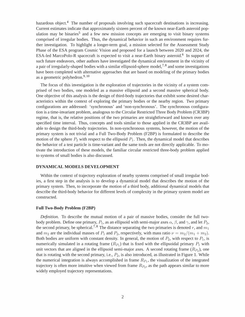
Definition. To describe the mutual motion of a pair of massive bodies, consider the full two-body problem. Define one primary,P1, as an ellipsoid with semi-major axesα, β, andγ, and letP2,the second primary, be spherical.7,8 The distance separating the two primaries is denotedr, andm1

andm2 are the individual masses ofP1 andP2, respectively, with mass ratioν = m2/(m1 +m2).Both bodies are uniform with constant density. In general, the motion ofP2, with respect toP1, isnumerically simulated in a rotating frame (RP1

) that is fixed with the ellipsoidal primaryP1 withunit vectors that are aligned in the ellipsoid semi-major axes. A second rotating frame (RP2

), onethat is rotating with the second primary, i.e.,P2, is also introduced, as illustrated in Figure1. Whilethe numerical integration is always accomplished in frameRP1

, the visualization of the integratedtrajectory is often more intuitive when viewed from frameRP2

, as the path appears similar to morewidely employed trajectory representations.

2

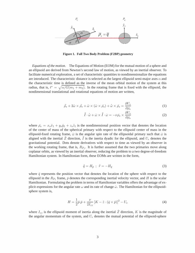
Figure 1. Full Two Body Problem (F2BP) geometry

Equations of the motion.The Equations of Motion (EOM) for the mutual motion of a sphere andan ellipsoid are derived from Newton’s second law of motion,as viewed by an inertial observer. Tofacilitate numerical exploration, a set of characteristicquantities to nondimensionalize the equationsare introduced. The characteristic distance is selected asthe largest ellipsoid semi-major axesα andthe characteristic time is defined as the inverse of the mean orbital motion of the system at thisradius, that is,t∗ =

√

α/G(m1 +m2). In the rotating frame that is fixed with the ellipsoid, thenondimensional translational and rotational equations ofmotion are written,

¨ρs + 2ω × ˙ρs + ω × (ω × ρs) + ˙ω × ρs =∂Ue

∂ρs(1)

¯I · ˙ω + ω ׯI · ω = −νρs ×

∂Ue

∂ρs(2)

whereρs = xsx1 + ysy1 + zsz1 is the nondimensional position vector that denotes the locationof the center of mass of the spherical primary with respect tothe ellipsoid center of mass in theellipsoid-fixed rotating frame,ω is the angular spin rate of the ellipsoidal primary such thatω isaligned with the inertialZ direction, ¯I is the inertia dyadic for the ellipsoid, andUe denotes thegravitational potential. Dots denote derivatives with respect to time as viewed by an observer inthe working rotating frame, that is,RP1

. It is further assumed that the two primaries move alongcoplanar orbits, as viewed by an inertial observer, reducing the problem to a two degree-of-freedomHamiltonian system. In Hamiltonian form, these EOMs are written in the form,

˙q = Hp ; ˙r = −Hq (3)

where q represents the position vector that denotes the location ofthe sphere with respect to theellipsoid in theRP1

frame,p denotes the corresponding inertial velocity vector, andH is the scalarHamiltonian. Formulating the problem in terms of Hamiltonian variables offers the advantage of ex-plicit expressions for the angular rateω and its rate of changeω. The Hamiltonian for the ellipsoid-sphere system is,

H =1

2p.p+

ν

2Izz[K − z · (q × p)]2 − Ue (4)

whereIzz is the ellipsoid moment of inertia along the inertialZ direction,K is the magnitude ofthe angular momentum of the system, andUe denotes the mutual potential of the ellipsoid-sphere

3

system, that is, computed as an elliptical integral. These equations of the motion are numericallyintegrated to simulate the behavior of any given ellipsoid-sphere system.

Synchronous and non-synchronous systems.From the general formulation, two equilibrium pri-mary configurations are identified: the long-axis equilibrium and the short-axis equilibrium con-figurations. Initially, consider the long-axis configuration, that is, a primary orientation such thatthe ellipsoid largest semi-major axis direction,α, is aligned with the ellipsoid-sphere directionx2.For this configuration to be maintained, both rotating frames coincide and the primariesP1 andP2 appear to be fixed in the rotating frame. This configuration islabeled ‘synchronous’. Theprimaries may also move in a configuration that is not fixed relative to an inertial observer. For‘non-synchronous’ systems, the spin rate ofP1 and the orbital rate ofP2 differ as viewed from theinertial frame.

Three-body Dynamical Models

General formulation: non-synchronous systems.The motion of a massless third-body is mod-eled assuming that the primary system is comprised of the twomassive bodies,P1 andP2, as illus-trated in Figure2. Note in the figure that the third particle is located relative to the ellipsoid centerof mass, as viewed in the ellipsoid-fixed frame, by the position vectorρe = xex1 + yey1 + zez1.Similar to the full two-body problem, the equations of the motion that describe the behavior of amassless particle near a primary system are derived from Newton’s second law, that is, the accel-eration of a particle in the gravity field is derived from the gradient of the gravitational potentialfunction. The EOMs are,

¨ρe + 2ω × ˙ρe + ω × (ω × ρe) + ˙ω × ρe =∂U

∂ρe+

∂Ue

∂q(5)

where q represents the location of the sphere center of mass andω is the orbital angular rate ofthe ellipsoidal primaryP1. The symbolU then denotes the gravitational potential defined asU =νUs + (1 − ν)Ue whereUs andUe represent the potential that is associated with the sphere andthe ellipsoid, respectively. Since no analytical solutionto the EOMs exists, the set of differentialequations is numerically integrated along with the F2BP EOMs to simulate the motion of a masslessthird particle.

Figure 2. Three-body problem geometry under periodic F2BP

Synchronous sphere-ellipsoid systems.The complex dynamical model is initially assumed to bebased on a synchronous system, i.e., the behavior of a third body is sought in the vicinity of a syn-chronous sphere-ellipsoid binary system. Thus, a three-body problem is constructed assuming that

4

the position of both primaries remains fixed with respect to theRP1 rotating frame. For this sim-plified problem, both rotating frames, labeledRP1

andRP2, coincide through any time evolution;

thus, for clarity, a unique rotating frame is centered at thesystem barycenter, as illustrated in Figure3. Note that the directions of the unit vectors forRP1

andRP2, as well as the barycentered system

in Figure3, all coincide. Such a system is a reduction of the more general problem as formulatedfor non-synchronous systems, and the vector EOM is similar but distinguished by the disappear-ance of the term∂Ue

∂q. Also true in synchronous systems, the angular velocityω is constant in both

magnitude and direction and the EOM reduces to the scalar form,

x− 2ωy = U∗x ; y + 2ωx = U∗

y ; z = U∗z (6)

whereρ = xx + yy + zz now represents the location of the third body with respect tothe systembarycenter,ω is the orbital angular velocity of the system andU∗

i are the first partial derivatives ofthe pseudo-potential with respect to the position vector, defined asU∗ = U + 1

2ω2(x2 + y2). Note

that this set of scalar equations is time-invariant; however, no analytical solution to the EOMs existsand the set of differential equations is numerically integrated to simulate the motion of the masslessparticle.

Figure 3. Three-body problem geometry under synchronous F2BP

Point mass systems.A further reduction in the complexity of the model is a primary system thatis comprised of two spherical bodies rather than ellipsoidal and spherical primaries, that is, the cir-cular restricted three-body problem. In the CR3BP, the motion of a massless third body is modeledassuming that the primary system is comprised of two point mass bodies. It is further assumed thatthe two primaries move along coplanar circular orbits, as viewed by an inertial observer. Becausethe CR3BP is employed in a variety of different problems, including the modeling of planetary sys-tems, the characteristic distance is generally selected asthe separation between the primaries andthe characteristic time now corresponds to the period of theprimary system. Thus, the equations ofmotion are similar to the synchronous sphere-ellipsoid systems, that is,

x− 2ny = U∗x ; y + 2nx = U∗

y ; z = U∗z (7)

whereU∗i are the first derivatives of the pseudo-potential defined asU∗ = U + 1

2n2(x2 + y2)

andn = 1 is the nondimensional mean motion of the primary system. Similar to the differentialequations governing the behavior in synchronous systems, although the scalar relationships in Eq.(7) are time-invariant, the set of differential equations does not admit any analytical solution andnumerical exploration is required to simulate the motion ofa massless particle.

5

CIRCULAR RESTRICTED THREE-BODY PROBLEM (CR3BP): BINARY SYSTEM

Before focusing on trajectory exploration within systems with added complexity in the dynamicalmodels that describe the motion of the binary (primary) system of interest, first consider the morefamiliar CR3BP. The focus of this investigation is on systems of small bodies, with application tobinary asteroid systems; thus, systems with large value of the mass ratioν, e.g., 0.1 to 0.3, are ofparticular interest.

Equilibrium Solutions, Jacobi Constant, and Zero Velocity Curves (ZVC)

In general, the equations of the motion, as formulated in therotating frame, admit five equilibriumsolutions that manifest as five equilibrium locations wherethe motion of a test particle remainsstationary over any time evolution. The equilibrium locations for a sample system with mass ratioν = 0.3 in the CR3BP are illustrated in Figure4. Note that there are three collinear points, labeled

−40 −20 0 20 40 60

−40

−30

−20

−10

0

10

20

30

40

L1 L2L3

L4

L5

x, km

y,km

Figure 4. Lagrange points in the CR3BP - ν = 0.3

L1, L2, L3 and two equilateral pointsL4 andL5. The equations of motion expressed in terms of thepseudo-potential function, with respect to the rotating frame, also allow the existence of a uniqueintegral of the motion, i.e., the Jacobi integral, i.e.,

C = 2U∗−

1

2(x2 + y2 + z2) (8)

The equilibrium solutions and the Jacobi constant are the basis of another important concept. Whileno analytical solution exists to describe the motion of a particle within this dynamical environment,the motion is bounded under certain conditions. In this dynamical regime, the boundedness of themotion for a specific energy level, or Jacobi constant, is represented by the Zero Velocity Curves(ZVC) that decompose the space in the vicinity of the two primaries into regions where the motionis possible and regions where the motion is not physically allowable. In Figure5, ZVCs for rep-resentative Jacobi constant values are plotted for a systemwith mass ratio equal to 0.3. The colorscale in Figure5 represents the nondimensional Jacobi constant value that is associated with eachcurve. For decreasing Jacobi values, or increasing energy levels, ZVCs that originally encompassboth primaries evolve: the curves merge at the collinear points, first, to open up gateways in thex−y plane for the motion of a third body. Eventually, any constraint on the motion of a test particleis cleared.

6

−100 −50 0 50 100

−80

−60

−40

−20

0

20

40

60

80

L1 L2L3

L4

L5

x, km

y,km

3.2

3.4

3.6

3.8

4

4.2

Figure 5. ZVCs in the CR3BP for representative Jacobi constant values - ν = 0.3

Periodic Orbits in the CR3BP

To explore the dynamical behavior of a third body in the vicinity of two spherical primaries,periodic orbits are of special interest. A differential-corrector based technique is employed to com-pute a trajectory that is periodic in the nonlinear regime given some initial guess. Most commonfamilies of periodic orbits within this regime are labeled libration point orbits and the first-ordervariational equations of the motion are employed to generate an initial guess in the vicinity ofa given equilibrium point. Planar Lyapunov families of periodic orbits associated with differentcollinear equilibrium points appear in Figure6; other families of three-dimensional orbits can alsobe computed.11

−80 −60 −40 −20 0 20 40 60 80

−60

−40

−20

0

20

40

60

x, km

y,km

Figure 6. L1, L2, andL3 Lyapunov families in the CR3BP for mass ratio ν = 0.3

7

THREE-BODY PROBLEM: SYNCHRONOUS FULL TWO-BODY PROBLEM

Within the context of exploring third-body trajectories inthe vicinity of two small irregular bod-ies, that is, a problem where investigating the motion in close proximity of the primaries is neces-sary, two spherical primaries may not, in general, be a reasonable assumption. This more specificproblem motivates the introduction of a dynamical model that incorporates more complexity in theprimary system model. As a first step, consider the Synchronous Sphere-Ellipsoid Three-BodyProblem (SSETBP). With similar equations of motion, the SSETBP possesses attributes similar tothose in the CR3BP. In particular, while no analytical solution for the motion of the particle is avail-able, other concepts, such as equilibrium solutions, integrals of the motion and zero velocity curves,are insightful.

Equivalent Lagrange Points

Similar to the CR3BP, the EOMs admit, in general, five equilibrium solutions that satisfy thevector equation∂U/∂ρ = 0. Because of the symmetry properties of the primaries, note that theequilibrium solutions occur in locations that mimic the general equilibrium positions in the CR3BP:3 collinear points and 2 equilateral points, labeled as equivalent Lagrange points. The correlationbetween the CR3BP and the new problem is highlighted by computing the equilibrium solutions foran array of sphere-ellipsoid systems. From a system that is equivalent to the CR3BP regime, that is,an ellipsoid primary with semi-major axesα = β = γ = 1, continuing semi-major axes parametersβ andγ from 1 to 0.5, that is, from the initial sphere-sphere systemtoward an ellipsoid-spheresystem with a very elongated primary, the corresponding equilibrium locations for each system arestraightforwardly constructed. In Figure7, the locations of the equilibrium positions are illustrated

0.86 0.88 0.9−0.02

0

0.02

x, non-dimensional

y,non-d

imen

sional L

1

3.74 3.76

−0.01

0

0.01

x, non-dimensional

y,non-d

imen

sional L2

−3.38 −3.37

−5

0

5

x 10−3

x, non-dimensional

y,non-d

imen

sional L

3

0.55 0.6

−2.6

−2.58

−2.56

x, non-dimensional

y,non-d

imen

sional L

5

Figure 7. Continuation of equivalent Lagrange points from β = γ = 1 to β = γ = 0.5- ν = 0.3 - r = 3

for systems with mass ratioν = 0.3 for the pointsL1, L2, L3, andL4 ( L5 is the mirror ofL4 acrossthex axis); the color scale, from blue to red, represents a decreasing value of the ellipsoid semi-

8

major axesβ andγ from 1 to 0.5 such thatα = 1 andβ = γ. Note that as the ellipsoid primarybecomes more elongated, from the initial sphere-sphere system, the locations of the equilibriumsolutions migrate accordingly. The pointsL1 andL3 tend to shift towardP1 while L2 is migratingaway from both primaries. Also,L4 andL5 move laterally toward the primaries, that is, along they-axis direction, and migrate axially, that is, along thex-axis direction, towardP2.

Zero velocity Curves for a Synchronous Ellipsoid - Sphere System.

Similar to the CR3BP, the EOMs relative to the ellipsoid-fixed rotating frame admits one integralof the motion with an expression that is equivalent to the expression for the Jacobi constant inthe CR3BP as given in Eq. (8). Thus, when considering an ellipsoidal primary, the motion of athird body remains bounded depending on the energy level, that is, for a given value of the Jacobiconstant, and for certain specified conditions. The evolution of the ZVCs is generally similar to theCR3BP for any given ellipsoid-sphere system; the curves are, however, shaped differently to reflectthe non-spherical shape ofP1.

STRATEGY TO COMPUTE PERIODIC ORBITS IN SYNCHRONOUS SYSTEMS

Libration Point Periodic Orbits

Families of periodic orbits are computed for a sphere-ellipsoid system that are similar to thewell-known CR3BP families of libration point periodic orbits, that is, families of trajectories thatoriginate in the vicinity of a particular equilibrium point. Recall that the motion of the sphere relativeto the fixed ellipsoid is consistent with the full two-body problem, that is, for synchronous systemsthe two primaries are fixed as viewed in the rotating frame. First, the planar Lyapunov familiescorresponding to the equivalent collinear Lagrange pointsare computed for a sample ellipsoid-sphere system with an elongated primary. Employing a continuation strategy, additional families ofmore complex orbits that include three-dimensional trajectories are also computed, as illustrated inFigure8. In this plot are displayed Lyapunov, halo, and axial families of periodic orbits associatedwith each of the collinear points. Although not illustratedin this figure, similar families of orbits canalso be constructed in the vicinity of the equilateral points. Although these families of orbits mayor may not offer options for any direct application in designor analysis scenarios, these trajectoriesare most useful in constructing even more complex orbits.

Heteroclinic and Homoclinic Cycles

Exploiting the tools available from the analysis in the CR3BP, trajectories for a third body in closeproximity to the primaries in synchronous systems are designed. Within the context of trajectoryexploration for application to binary systems of asteroids, the focus in this investigation is on theconstruction of trajectories that exhibit a specific behavior, that is, periodic trajectories that shiftback and forth between the regions dominated by each of the equivalent collinear libration points, asviewed in the rotating frame, offering repeated close passages of both primaries. A strategy similarto the computation of homoclinic and heteroclinic connections in the CR3BP is employed.12,13 Thesteps in a process to compute periodic trajectories include: (i) computation of a suite of familiesof periodic libration point orbits for a given system; (ii) determination and computation of theassociated manifolds corresponding to one libration pointfamily at a desired energy level, i.e., afixed Jacobi constant value; (iii) selection of specific manifold arcs and subsequent construction ofan initial guess for a periodic path linking arcs in the vicinity of one or several libration points;

9

L2 Axial

L1 Halo

L2 Halo

L3 HaloL

1 Axial L

1 Lyapunov

L3

Lyapunov

L2

Lyapunov

Figure 8. Libration point Periodic Orbits (LPO): ellipsoid axes ratios β = γ = 0.5 -primary mass ratio ν = 0.3 - primary distance r = 3

and, (iv) insertion of the initial guess into a prediction-correction algorithm to produce one or moreperiodic trajectories that retain the desired characteristics.

Homoclinic cycles. Within the framework of the CR3BP, a closed trajectory that connects a pe-riodic orbit with itself, that is, an arc that departs and returns to the same periodic orbit, is labeleda homoclinic connection. The construction of such a trajectory is often achieved by exploiting theunstable and stable manifold arcs that are associated with the periodic orbit of interest to producean initial guess. Within the context of trajectory exploration within binary systems of small bodies,consider a scenario that involves periodic trajectories that shift back and forth between the libra-tion pointsL1, L2 andL3, as viewed in the rotating frame. An initial guess for such a trajectoryis constructed from a double homoclinic connection for a periodic L1 libration point orbit, that is,assembling two independent connections from theL1 orbit, one that extends toward theL3 pointand the second that visits the vicinity of theL2 point. This process is realized by selecting unsta-ble and stable manifolds arcs that are associated with aL1 Lyapunov periodic orbit. In Figure9are illustrated the unstable and stable manifold tubes for aL1 Lyapunov orbit in a sphere-ellipsoidsystem with mass ratioν = 0.3, primary separationr = 3 and semi-major axesβ = γ = 0.5.The corresponding manifold tubes extend toward bothP1 andP2, visiting the vicinity of two otherlibration points, that is,L3 andL2, respectively. To facilitate the selection of suitable manifoldsarcs, a Poincare section is employed. In this planar analysis, each manifold tube is numericallypropagated until the first intersection with a specified hyperplane, specifically,y = 0, as definedin the rotating frame. The end result is a trajectory that is continuous both in position and velocityat the originating periodic orbit and at the hyperplane intersection. Considering planar trajectories,the hyperplane reduces the dimensionality of the problem tothree variables. In addition, recall theexistence of one integral the motion, the Jacobi constant, that further reduces the problem to twodimensions. One possible representation for the selectionof a suitable set of manifold arcs is aPoincare mapx − x of the first crossings of the manifold tube with the hyperplane. The mani-folds associated with anL1 Lyapunov orbit at a specified energy level are plotted in Figure 9 inconfiguration space. The Poincare map that corresponds to the crossings of the manifolds with thehyperplaney = 0 are illustrated in Figure10. The upper plot represents the crossings with negativex coordinates that correspond to crossings with the hyperplane to the left ofP1; the bottom plot

10

−5 −4 −3 −2 −1 0 1 2 3 4 5

−4

−3

−2

−1

0

1

2

3

4

x, non-dimensional

y,non-d

imen

sional

Figure 9. Unstable and stable manifold arcs for L1 Lyapunov orbit for β = γ =0.5− ν = 0.3− r = 3

depicts the crossings that occur on the right side ofP2. Red and magenta dots denote crossings ofthe unstable manifold arcs, blue and purple dots correspondto stable manifold arc crossings. Aninitial guess for a periodic orbit is constructed from the selection of two manifold arcs, one stableand one unstable, that pass through the vicinity of theL3 point and two arcs that extend towardL2. On the Poincare map representation, the objective is the selection of two points on each map(both the top and the bottom plot), one that corresponds to a stable manifold arc and the second toan unstable arc, that intersect both in position and velocity, that is, in terms of the coordinatesxand x. If no intersection is apparent, points with the smallest separation on the map are the mostsuitable candidates to produce a reasonable initial guess.Because of the symmetry properties of theproblem, manifold arcs that cross the hyperplane with the smallest transversal velocityx often yielda satisfactory initial guess. A differential corrections algorithm is employed to produce a periodictrajectory that retains the desired characteristics present in the initial guess. Further, a continuationmethod allows the generation of a family of similar trajectories. A set of trajectories that resultfrom this design process appears in Figure11. The family of planar periodic trajectories includesmembers that all shift back and forth between the libration pointsL1, L2 andL3, as displayed inthe rotating frame.

Heteroclinic cycles.Another useful concept in the design of trajectories that exhibit behaviorsimilar to the periodic orbits produced exploiting homoclinic connections, that is, trajectories thatshift back and forth between the libration pointsL1, L2 andL3 is often labeled a heteroclinic con-nection, that is, a trajectory arc that naturally links two periodic orbits with no position or velocitydiscontinuity. The process to construct an initial guess for such a heteroclinic connection is similarto the strategy to produce homoclinic connections but involves two distinct periodic orbits. Often,manifold arcs that are associated with both periodic orbits, stable and unstable, are computed andexploited to determine an initial guess for the desired connection. To design a periodic trajectory

11

−4 −3.5 −3 −2.5 −2 −1.5−0.4

−0.2

0

0.2

0.4

x, non-dimensional

x,non-d

imen

sional

2.5 3 3.5 4 4.5 5−0.4

−0.2

0

0.2

0.4

x, non-dimensional

x,non-d

imen

sional

Figure 10. Unstable and stable manifold arc crossings for L1 Lyapunov orbit forβ = γ = 0.5− ν = 0.3− r = 3

−3 −2 −1 0 1 2

−2

−1.5

−1

−0.5

0

0.5

1

1.5

2

2.5

x, non-dimensional

y,non-d

imen

sional

Figure 11. Family of double homoclinic periodic cycles for β = γ = 0.5− ν = 0.3− r = 3

12

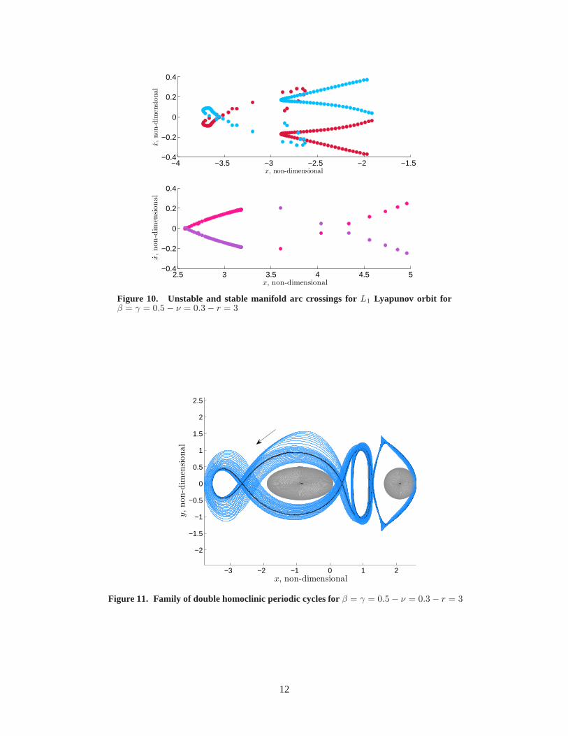
that visits the vicinity of all three collinear libration points, consider an initial guess that is con-structed from a double heteroclinic cycle, that is, an initially discontinuous path that is formed fromtwo independent heteroclinic connections. Consider threelibration point periodic orbits with sim-ilar Jacobi constant values that are centered aroundL1, L2, andL3, respectively. Then, a doublecycle is then constructed from two heteroclinic connections, one between theL1 andL3 orbits andthe second between theL1 andL2 orbits. The initial guess process is initiated via unstableandstable manifold arcs that are associated with aL1 andL3 Lyapunov orbits at the same energy level,i.e., same value of Jacobi constant, respectively. A secondarc is comprised of stable and unsta-ble manifold arcs from the sameL1 trajectory and anL2 Lyapunov orbit, as illustrated in Figure12. Similar to a homoclinic cycle, a Poincare section approach is developed to aid the selection of

−4 −2 0 2 4−4

−3

−2

−1

0

1

2

3

4

x, non-dimensional

y,non-d

imen

sional

Figure 12. Unstable and stable manifold arcs for L1, L2, and L3 Lyapunov orbit forβ = γ = 0.5− ν = 0.3− r = 3

suitable manifold arcs. Consider two hyperplanes, one defined asx = 1/2(xL1+ xL3

) wherexL1

andxL3denote the locations of theL1 andL3 libration points, and a second hyperplane such that

x = 1/2(xL1+ xL2

). The process to generate the initial guess is illustrated inFigure12. Unstableand stable manifold arcs computed for the selectedL1, L2, andL3 Lyapunov orbits are displayedin the figure until the first intersection with the corresponding hyperplane. Also, similar to the ap-proach for homoclinic connections, the crossings of the manifold arcs with the hyperplane for bothunstable and stable manifolds are represented on ay − y Poincare map. From this representation,the selection process for the manifold arcs that are used to construct the initial guess is guided bythe same principles, that is, unstable and stable points on the map that intersect or nearly intersectare employed to create a reasonable, possibly discontinuous, trajectory. The complete initial guessis corrected to produce a periodic orbit that retains the desired characteristics. The orbit obtainedfrom the correction process is subsequently exploited to initialize a continuation method to generatea family of similar periodic trajectories, as illustrated in Figure13.

13

−4 −3 −2 −1 0 1 2 3 4

−3

−2

−1

0

1

2

3

x, non-dimensional

y,non-d

imen

sional

Figure 13. Family of double heteroclinic periodic cycles for β = γ = 0.5− ν = 0.3− r = 3

THREE-BODY PROBLEM: NON-SYNCHRONOUS FULL TWO-BODY PROBLEM

Non-Synchronous Systems

While synchronous systems, or close-to-synchronous systems, are available in the known asteroidpopulation, systems also exist where the primaries move in aconfiguration that is not fixed relativeto the rotating frame. For ‘non-synchronous’ systems, the spin rate of ellipsoidal bodyP1 andthe orbital rate ofP2 are different as viewed from the inertial frame. The initialchallenge thenis the motion of the two-body system. Given various possibleapproaches to this problem, initiallyconsider an analogy with a simple problem, the simple pendulum. The motion of a simple pendulumis described by a simple scalar equation in terms of one time-dependent angular coordinate,θ,that is measured relative to the stable equilibrium orientation. The geometry of the problem isillustrated in Figure14(a)and the EOM is writtenθ + g

lsinθ = 0, whereg is the constant gravity

acceleration andl is the length of the pendulum. Depending on the initial conditions, i.e.,θ0 andθ0, different behavior for the motion of the pendulum is observed and a classic representation thatclearly highlights the various types of behavior is a phase space portrait, that is, aθ-θ plot, asillustrated in Figure14(b). In the figure, are labelled different behaviors that correspond to differentcharacteristic curves in the phase portrait. The fixed points correspond to the equilibrium positions,both stable and unstable. Then, the libration-type behavior is depicted by a set of closed curvescentered on a stable equilibrium position. For an alternative set of initial conditions that correspondto increasing total energy, a critical curve exists that divides the phase space into libration (blue)and circulation (red) regions. The boundary is representedby the magenta curve (separatrix) inthe phase portrait. This analysis is extended to the problemof interest, that is, the motion of asphere moving relative to a fixed ellipsoidal body. To exploit the pendulum analogy, define thecoordinateθ as the angle between theP1-P2 line that corresponds to the equilibrium system, orsynchronous system, that is, thex-axis, and the time-dependent location ofP2. A sample pathfor P2 is represented, along with the geometry of the problem, in Figure15 where the trajectory

14

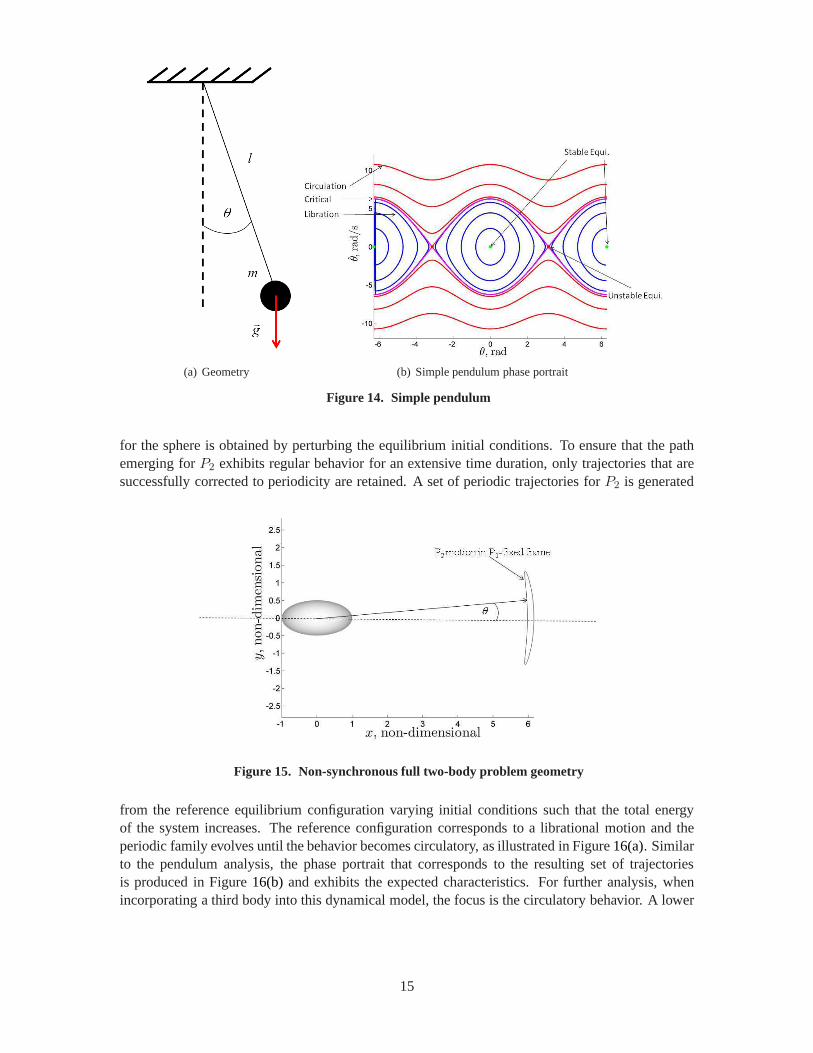
(a) Geometry (b) Simple pendulum phase portrait

Figure 14. Simple pendulum

for the sphere is obtained by perturbing the equilibrium initial conditions. To ensure that the pathemerging forP2 exhibits regular behavior for an extensive time duration, only trajectories that aresuccessfully corrected to periodicity are retained. A set of periodic trajectories forP2 is generated

Figure 15. Non-synchronous full two-body problem geometry

from the reference equilibrium configuration varying initial conditions such that the total energyof the system increases. The reference configuration corresponds to a librational motion and theperiodic family evolves until the behavior becomes circulatory, as illustrated in Figure16(a). Similarto the pendulum analysis, the phase portrait that corresponds to the resulting set of trajectoriesis produced in Figure16(b) and exhibits the expected characteristics. For further analysis, whenincorporating a third body into this dynamical model, the focus is the circulatory behavior. A lower

15

−6 −4 −2 0 2 4 6 8−6

−4

−2

0

2

4

6

x, non-dimensional

y,non-d

imen

sional

(a) SampleP2 periodic paths

−4 −3 −2 −1 0 1 2 3 4−0.2

−0.15

−0.1

−0.05

0

0.05

0.1

0.15

θ, rad

θ,ra

d/s

(b) Phase portrait

Figure 16. Non-synchronous full two-body problem

bound is selected for the ratio of the inertial angular velocity rates betweenP1 andP2, that is, theratio is always greater than two. For the circulation-type motion, the periodic path forP2 resemblesa pseudo-circular orbit, as viewed in the ellipsoid-fixed frame.

Dynamical Substitutes

With a time-dependent solution for the motion ofP2 with respect toP1, equilibrium solutions tothe 3BP EOMs, in the form of fixed stationary points, no longerexist. However, as the path ofP2 isconstrained to be periodic, dynamical substitutes that form closed periodic path replace the equiv-alent Lagrange points from the synchronous case.14,15,16 For any given non-synchronous system,the equivalent Lagrange points for the corresponding synchronous system are employed as initialguesses to compute the dynamical substitutes for the non-synchronous system of interest. In Figure17, a set of non-synchronous systems that correspond to libration and circulation motions forP2 arerepresented as well as the corresponding dynamical substitutes for the equivalent collinear Lagrangepoints. The upper left view corresponds to the periodic substitutes as viewed in the ellipsoid-fixedframeRP1

and the three collinear dynamical substitutes as viewed in the sphere-fixed frameRP2

are individually illustrated in the three other views. Notethat for the computation of the dynamicalsubstitutes, the initial guess for each point is transformed from theRP2

frame to theRP1frame

before the periodic path is computed with a differential corrections algorithm.

Trajectory Exploration in Non-Synchronous Systems

Strategy. A strategy is proposed to construct trajectories that exhibit some set of desired charac-teristics within the context of the non-synchronous 3BP. The strategy relies on exploiting the insightgained from analysis in the synchronous problem. A first stepis the generation of orbits that areperiodic in the non-synchronous problem; periodic libration point orbits previously computed froman equivalent synchronous problem are employed as an initial guess. Recall that, in this analysis,the trajectory forP2 is periodic, thus, for aP3 periodic trajectory to exist, the period of the desiredP3 orbit must be commensurate with the period ofP2. Consequently, while there exists an infiniteset of periodic orbits in the vicinity of a known orbit or a family of orbits in the synchronous case,periodic orbits in the non-synchronous problem are isolated based upon the possible integer ratios

16

−10 −5 0 5 10

−5

0

5

RP1frame

x, non-dimensional

y,non-d

imen

sional

3.2 3.4 3.6 3.8 4

−0.2

0

0.2

x, non-dimensional

y,non-d

imen

sional

L1 - RP2frame

9.4 9.6 9.8 10

−0.2

0

0.2

x, non-dimensional

y,non-d

imen

sional

L2 - RP2frame

−5.3 −5.2 −5.1 −5

−0.1

0

0.1

x, non-dimensional

y,non-d

imen

sional

L3 - RP2frame

Figure 17. Dynamical substitutes for the equivalent collinear Lagrange points

between the periods ofP3 andP2. In summary, for any given non-synchronous system, a discreteset of periodic orbits that are equivalent to Lyapunov, halo, axial and vertical synchronous orbitscan be computed using the equivalent families of trajectories in the synchronous problem as initialguesses. Note that an initial guess from the synchronous problem is more closely related to a tra-jectory in theRP2

frame, that is, a frame where the location of the primaries remains almost fixed,that is, only the relative orientation of the primaries significantly changes over time. This initialguess is transformed from theRP2

frame into theRP1frame prior to any corrections process in

the non-synchronous regime. Similar to the analysis in the synchronous problem, a discrete set ofisolated libration point orbits is likely not directly relevant for any practical application. However,these types of paths serve as a basis for the construction of more complex trajectories that retainsome desired characteristics. In fact, the same procedure that is developed within the context ofthe synchronous problem is adjusted to construct trajectories that visit the regions of the dynamicalsubstitutes for the equivalent collinear Lagrange points as viewed in theP2-fixed frame. Becausethe problem is now time-variant, time continuity must also be maintained between trajectory arcsthat are employed to construct a fully continuous orbit. Twodifferent procedures for trajectory de-sign are available for application in the synchronous case,one based on a double homoclinic cycleand an alternative strategy that relies on a double heteroclinic cycle. Both approaches are directlytranslated to the non-synchronous problem analysis.

Application. Consider a sample non-synchronous system with a primary non-dimenional sep-arationr = 6 such that theP2 motion corresponds to circulation-type behavior, that is,in theellipsoid-fixed frame the trajectory ofP2 resembles a pseudo-circular orbit andP2 remains almoststationary in the sphere-fixed frame. In Figure18(a), represented in black, a non-synchronousperiodic orbit is plotted, as viewed in the sphere-fixed frame; this orbit is computed from anL1

Lyapunov orbit for the equivalent synchronous system. The stable and unstable manifolds that cor-respond to this periodic orbit are also computed. In Figure18(a), the sample unstable arcs also ap-

17

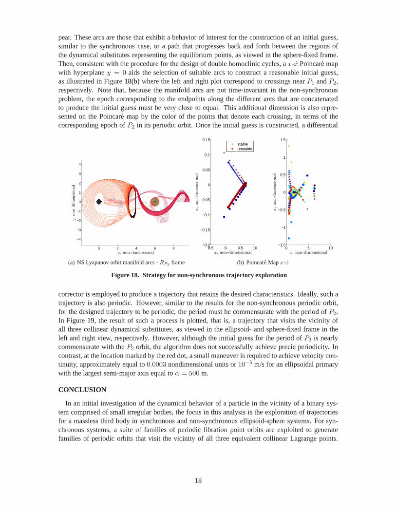
pear. These arcs are those that exhibit a behavior of interest for the construction of an initial guess,similar to the synchronous case, to a path that progresses back and forth between the regions ofthe dynamical substitutes representing the equilibrium points, as viewed in the sphere-fixed frame.Then, consistent with the procedure for the design of doublehomoclinic cycles, ax-x Poincare mapwith hyperplaney = 0 aids the selection of suitable arcs to construct a reasonable initial guess,as illustrated in Figure18(b)where the left and right plot correspond to crossings nearP1 andP2,respectively. Note that, because the manifold arcs are not time-invariant in the non-synchronousproblem, the epoch corresponding to the endpoints along thedifferent arcs that are concatenatedto produce the initial guess must be very close to equal. Thisadditional dimension is also repre-sented on the Poincare map by the color of the points that denote each crossing, in terms of thecorresponding epoch ofP2 in its periodic orbit. Once the initial guess is constructed, a differential

0 2 4 6 8

−4

−3

−2

−1

0

1

2

3

4

x, non dimensional

y,non

dim

ensional

(a) NS Lyapunov orbit manifold arcs -RP2frame

8.5 9 9.5 10−0.2

−0.15

−0.1

−0.05

0

0.05

0.1

0.15

x, non-dimensional

x,non

-dim

ensi

onal

stableunstable

0 5 10−1.5

−1

−0.5

0

0.5

1

1.5

x, non-dimensional

x,non

-dim

ensi

onal

(b) Poincare Mapx-x

Figure 18. Strategy for non-synchronous trajectory exploration

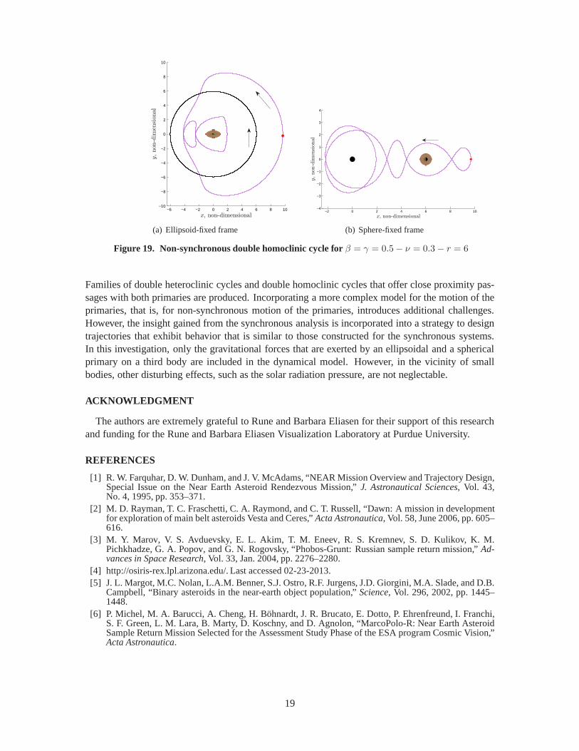
corrector is employed to produce a trajectory that retains the desired characteristics. Ideally, such atrajectory is also periodic. However, similar to the results for the non-synchronous periodic orbit,for the designed trajectory to be periodic, the period must be commensurate with the period ofP2.In Figure19, the result of such a process is plotted, that is, a trajectory that visits the vicinity ofall three collinear dynamical substitutes, as viewed in theellipsoid- and sphere-fixed frame in theleft and right view, respectively. However, although the initial guess for the period ofP3 is nearlycommensurate with theP2 orbit, the algorithm does not successfully achieve precie periodicity. Incontrast, at the location marked by the red dot, a small maneuver is required to achieve velocity con-tinuity, approximately equal to0.0003 nondimensional units or10−5 m/s for an ellipsoidal primarywith the largest semi-major axis equal toα = 500 m.

CONCLUSION

In an initial investigation of the dynamical behavior of a particle in the vicinity of a binary sys-tem comprised of small irregular bodies, the focus in this analysis is the exploration of trajectoriesfor a massless third body in synchronous and non-synchronous ellipsoid-sphere systems. For syn-chronous systems, a suite of families of periodic librationpoint orbits are exploited to generatefamilies of periodic orbits that visit the vicinity of all three equivalent collinear Lagrange points.

18

−6 −4 −2 0 2 4 6 8 10−10

−8

−6

−4

−2

0

2

4

6

8

10

x, non-dimensional

y,non

-dim

ensi

onal

(a) Ellipsoid-fixed frame

−2 0 2 4 6 8 10−4

−3

−2

−1

0

1

2

3

4

x, non-dimensional

y,non

-dim

ensi

onal

(b) Sphere-fixed frame

Figure 19. Non-synchronous double homoclinic cycle for β = γ = 0.5− ν = 0.3− r = 6

Families of double heteroclinic cycles and double homoclinic cycles that offer close proximity pas-sages with both primaries are produced. Incorporating a more complex model for the motion of theprimaries, that is, for non-synchronous motion of the primaries, introduces additional challenges.However, the insight gained from the synchronous analysis is incorporated into a strategy to designtrajectories that exhibit behavior that is similar to thoseconstructed for the synchronous systems.In this investigation, only the gravitational forces that are exerted by an ellipsoidal and a sphericalprimary on a third body are included in the dynamical model. However, in the vicinity of smallbodies, other disturbing effects, such as the solar radiation pressure, are not neglectable.

ACKNOWLEDGMENT

The authors are extremely grateful to Rune and Barbara Eliasen for their support of this researchand funding for the Rune and Barbara Eliasen Visualization Laboratory at Purdue University.

REFERENCES

[1] R. W. Farquhar, D. W. Dunham, and J. V. McAdams, “NEAR Mission Overview and Trajectory Design,Special Issue on the Near Earth Asteroid Rendezvous Mission,” J. Astronautical Sciences, Vol. 43,No. 4, 1995, pp. 353–371.

[2] M. D. Rayman, T. C. Fraschetti, C. A. Raymond, and C. T. Russell, “Dawn: A mission in developmentfor exploration of main belt asteroids Vesta and Ceres,”Acta Astronautica, Vol. 58, June 2006, pp. 605–616.

[3] M. Y. Marov, V. S. Avduevsky, E. L. Akim, T. M. Eneev, R. S. Kremnev, S. D. Kulikov, K. M.Pichkhadze, G. A. Popov, and G. N. Rogovsky, “Phobos-Grunt:Russian sample return mission,”Ad-vances in Space Research, Vol. 33, Jan. 2004, pp. 2276–2280.

[4] http://osiris-rex.lpl.arizona.edu/. Last accessed 02-23-2013.[5] J. L. Margot, M.C. Nolan, L.A.M. Benner, S.J. Ostro, R.F.Jurgens, J.D. Giorgini, M.A. Slade, and D.B.

Campbell, “Binary asteroids in the near-earth object population,” Science, Vol. 296, 2002, pp. 1445–1448.

[6] P. Michel, M. A. Barucci, A. Cheng, H. Bohnardt, J. R. Brucato, E. Dotto, P. Ehrenfreund, I. Franchi,S. F. Green, L. M. Lara, B. Marty, D. Koschny, and D. Agnolon, “MarcoPolo-R: Near Earth AsteroidSample Return Mission Selected for the Assessment Study Phase of the ESA program Cosmic Vision,”Acta Astronautica.

19

[7] J. Bellerose and D. J. Scheeres, “Periodic orbits in the vicinity of the equilateral points of the restrictedfull three-body problem,”AAS/AIAA Astrodynamics Specialist Conference, August 7-11 2005.

[8] J. Bellerose and D. J. Scheeres, “The restricted full three-body problem: Application to binary system1999 kw4,”Journal of Guidance, Control, and Dynamics, Vol. 31, No. 1, 2008, pp. 162–171.

[9] E. G. Fahnestock and D. J. Scheeres, “Simulation and analysis of the dynamics of binary near-EarthAsteroid (66391) 1999 KW4,”Icarus, Vol. 194, 2008, pp. 410–435.

[10] E. G. Fahnestock and D. J. Scheeres, “Characterizationof Spacecraft and Debris Trajectory Stabilitywithin Binary Asteroid Systems,”AIAA/AAS Astrodynamics Specialist Conference and Exhibit, Hon-olulu, Hawaii, August 18-21, 2000.

[11] D. J. Grebow, “Generating Periodic Orbits in the Circular Restricted Three Body Problem with Appli-cations to Lunar South Pole Coverage,” M.S. Thesis, School of Aeronautics and Astronautics, PurdueUniversity, West Lafayette, Indiana, May 2010.

[12] W. S. Koon, M. W. Lo, J. E. Mardsen, and S. D. Ross, “Heteroclinic connections between periodicorbits and resonance transitions in celestial mechanics,”Chaos, Vol. 10, 2000, pp. 427–469.

[13] A. Haapala and K. Howell, “Trajectory Design Using Periapse Poincare Maps and Invariant Manifolds,”21st AAS/AIAA Space Flight Mechanics Meeting, New Orleans, Louisiana, February 2011.

[14] G. Gomez, J. Masdemont, and J. Mondelo, “Dynamical Substitutes of the Libration Points for Simpli-fied Solar System Models,”Libration Point Orbits and Applications: Proceedings of the Conference,Aiguablava, Spain, 10-14 June 2002, 2003, p. 373.

[15] X. Hou and L. Liu, “On quasi-periodic motions around thetriangular libration points of the real Earth–Moon system,”Celestial Mechanics and Dynamical Astronomy, Vol. 108, No. 3, 2010, pp. 301–313.

[16] X. Hou and L. Liu, “On quasi-periodic motions around thecollinear libration points in the real Earth–Moon system,”Celestial Mechanics and Dynamical Astronomy, Vol. 110, No. 1, 2011, pp. 71–98.

20