Joint Source-Channel Decoding of Variable-Length Codes for Convolutional Codes and Turbo Codes
Upload
independentCategory
view
0download
0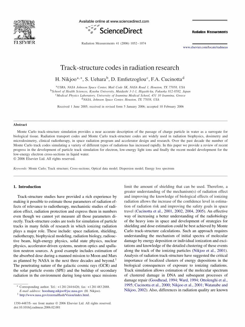
Radiation Measurements 41 (2006) 1052–1074www.elsevier.com/locate/radmeas
Track-structure codes in radiation research
H. Nikjooa,∗, S. Ueharab, D. Emfietzoglouc, F.A. Cucinottad
aUSRA, NASA Johnson Space Center, Mail Code SK, NASA Road 1, Houston, TX 77058, USAbSchool of Health Sciences, Kyushu University, Maidashi 3-1-1, Higashi-ku, Fukuoka 812-8582, Japan
cMedical Physics Laboratory, University of Ioannina Medical School, 451 10 Ioannina, GreecedNASA, Johnson Space Center, Houston, TX 77058, USA
Received 1 June 2005; received in revised form 5 January 2006; accepted 10 February 2006
Abstract
Monte Carlo track-structure simulation provides a near accurate description of the passage of charge particle in water as a surrogate forbiological tissue. Radiation transport codes and Monte Carlo track-structure codes are widely used in radiation biophysics, dosimetry andmicrodosimetry, clinical radiotherapy, in space radiation program and accelerator design and research. Over the past decade the number ofMonte Carlo track codes simulating a variety of different types of radiations has increased rapidly. In this paper we provide a review of recentprogress in the development of particle track simulation for electron, low-energy light ions and finally the recent model development for thelow-energy electron cross-sections in liquid water.© 2006 Elsevier Ltd. All rights reserved.
Keywords: Monte Carlo; Track structure; Cross-sections; Optical data model; Dispersion model; Energy loss spectrum
1. Introduction
Track-structure studies have provided a rich experience bymaking it possible to estimate those parameters of radiation ef-fects of relevance to radiotherapy, mechanistic studies of radi-ation effect, radiation protection and express them in numberseven though we cannot yet measure all those parameters di-rectly. Track-structure codes are tools for simulation of particletracks in many fields of research in which ionizing radiationplays a major role. These include: space radiation, shielding,radiotherapy, biophysical modeling, radiation biology, radioac-tive beam, high-energy physics, solid state physics, nuclearphysics, accelerator-driven systems, neutron optics and spalla-tion neutron sources. A good example includes estimation ofthe absorbed dose during a manned mission to Moon and Marsas planned by NASA in the next three decades and beyond.1
The penetrating nature of the galactic cosmic rays (GCR) andthe solar particle events (SPE) and the buildup of secondaryradiation in the environment during long-term space missions
∗ Corresponding author. Tel.: +1 281 244 6426; fax: +1 281 483 2888.E-mail address: [email protected] (H. Nikjoo).
1 http://www.nasa.gov/externalflash/Vision/index.html.
1350-4487/$ - see front matter © 2006 Elsevier Ltd. All rights reserved.doi:10.1016/j.radmeas.2006.02.001
limit the amount of shielding that can be used. Therefore, agreater understanding of the mechanism(s) of radiation effectand improving the knowledge of biological effects of ionizingradiation allows the increase of the confidence level in estima-tion of radiation risk and improving the safety goals in spacetravel (Cucinotta et al., 2001, 2002, 2004, 2005). An effectiveway of increasing a better understanding of the radiobiologyof the heavy ions in space and development of strategies forshielding and dose estimation could be best achieved by MonteCarlo track-structure calculations. Such an approach requiresunderstanding the mechanism of initial spectra of moleculardamage by energy deposition or individual ionization and exci-tations and knowledge of the detailed clustering of these eventsalong the track of the ionizing particles (Nikjoo et al., 2001).Analysis of radiation track-structure have suggested the criticalimportance of localized clusters of energy depositions in thebiological consequences of exposure to ionizing radiations.Track simulation allows estimation of the molecular spectrumof clustered damage in DNA and subsequent processes ofdamage repair (Goodhead, 1994; Ward, 1994; Ottolenghi et al.,1995; Cucinotta et al., 2000; Nikjoo et al., 2001; Watanabe andNikjoo, 2002). Also, differences in radiation quality are known
H. Nikjoo et al. / Radiation Measurements 41 (2006) 1052–1074 1053
to cause large differences in biological effects of radiation, notonly in magnitude but also in the way physiological and phys-ical conditions can modify the outcome. Some modifiers, forexample, oxygenation, sensitizers and protectors, suggest ra-diation quality-dependent differences in the initial spectra ofmolecular damage, while others, for example, dose, dose rate,delayed plating and genetic deficiencies, suggest differences inreparability. Since insults from all ionizing radiations are es-sentially in the form of ionized and excited molecules alongthe paths of the tracks of charged particles, the structure of thetrack must in some way be involved in determining the biolog-ical effectiveness of the radiation. Therefore, understanding therole of track-structure has important practical implications fortherapy and protection.
There are many different ways of describing a track from asimple one-parameter track to sophisticated 4D Monte Carlotrack-structure codes. Track-structure methods are either basedon solution of analytical equations describing the transport ofcharged particles in the medium (Butts and Katz, 1967; Katzet al., 1993) or using a numerical solution by sampling themodel of the particle interactions with the atoms or moleculesof the medium (Nahum, 1999).
Over the past half century major progress has been madein simulation of charged particle tracks: photons, electrons,ions and neutrons (Kling et al., 2000). This has come aboutmainly due to availability of better theoretical models and cross-sections and more powerful computers. Among the earliest ap-plications of Monte Carlo methods in simulation of particletrack dates back to the work of Wilson (1952) on cosmic rayelectron–photon shower studies, and the use of Monte Carlomethod to study the dependence of gamma-ray backscatteringon the angle of incidence and Z (McCracken, 1955). The ma-jor breakthrough in simulation of photon and electron trans-port came about with the pioneering work of Berger (1963) onthe code ETRAN (Berger and Seltzer (1973)) which laid theground work for what is now known as the condensed-historymethod and subsequently the development of full interaction-by-interaction Monte Carlo track-structure codes giving de-tailed distribution of ionizations and excitations in the medium(Turner et al., 1983; Turner, 1995; Paretzke, 1987).
2. Radiation transport and track-structure codes
High-energy nuclei undergo nuclear reactions in passagethrough matter. For space radiation applications, it is useful tocombine description of ion transport in bulk media with de-tailed models of track-structure defining energy depositions inmicroscopic targets of interest. There are numerous ways ofdescribing radiation transport and track-structure. The 1D de-terministic description of ion transport based on the solution ofBoltzmann transport equation have been developed at NASALangley Research Center (Wilson et al., 1991). Approaches todescription of track-structure include: (1) 1D description oftrack, or target-related track methods, based on a single param-eter of track such as an average quantity of the radiation field(LET—linear energy transfer and LET�—restricted linear en-ergy transfer, single or clusters of ionization, microdosimetric
parameters such as yD—dose average lineal energy andzD—frequency-averaged-specific energy) (ICRU, 1983) andassociated parameters of radiation quality (RBE—relative bi-ological effectiveness, Q—quality factor) (Howard-Flanders,1958; Burch, 1957; Lea, 1946; Kellerer and Chemelevsky,1975; ICRU, 1983); (2) amorphous description of track basedon average radial dose profiles around the charged particletrajectories but ignoring the stochastic structures of the tracks(Cucinotta et al., 1999); (3) condensed-history-method codesproviding averages over discrete particle histories; (4) the full3D Monte Carlo track-structure codes simulating the individ-ual interactions of each particle at the atomic and molecularlevel providing detailed distributions of all elastic and inelasticinteractions (Nikjoo and Uehara, 2003) and (5) Monte Carlosimulation of charged particle track in condensed media andthe evolution of the radical species generated in the mediumwith time (4D codes) (Ballarini et al., 2000). In the followingsections we provide only a brief description of deterministic1D model of radiation transport, the amorphous track de-scription and the condensed-history track models. There arenumerous detailed published reviews of these codes. In thispaper we present a detailed description of Monte Carlo track-structure codes using the code KURBUC as a prime example.As almost all Monte Carlo track-structure codes use the samedatabase for cross-sections and other input data we do notdeem necessary to make a separate description of each pub-lished code as space is limited. However, where necessaryreferences are provided to various publications where compar-isons and bench markings have been made. The URL addressesalso provide access to more detailed information and access tothe codes.
2.1. Deterministic 1D models of ion transport
These are computer codes based on the solution of Boltz-mann transport equation. Ideally, this is the situation in whichone is able to provide an exact mathematical or analytical de-scription of the particle interactions in the medium. However,exact mathematical solutions of Boltzmann transport equationare very difficult to obtain and such solutions needs to be bench-marked and verified by comparison to averages over discreteparticle histories obtained by measurements or other indepen-dent methods, for example, by Monte Carlo ion transport codes.In fact, there is no exact analytical solution to be found tothe radiation transport equation as soon as one deviates fromphotons and homogenous medium. For a mini review of thesetypes of Monte Carlo codes see the paper by Niita et al. (2006)in this volume. The development of these codes dates back topre-NASA history and the work on medical problems of high-altitude travel by pilots (Wilson et al., 1991). Many decadeslater and a greater concern and awareness of the radiation prob-lems and risk in manned space flights led to the developmentof a code system at the Langley Research Center (Wilson et al.,1991). The suite of codes HZETRN (Wilson et al., 1995) andBRYNTRN (Wilson et al., 1989) are used to predict the propa-gation and interactions of charged particles including the trans-port of high-energy ions up to iron or higher charged ions.
1054 H. Nikjoo et al. / Radiation Measurements 41 (2006) 1052–1074
y, keV/µm
0.1 1 10 100 1000
F(>
y), (
cm2
sr d
ay)-1
10-3
10-2
10-1
100
101
102
103
104
Data of Badhwar et al.Direct EventsDirect+ δ -ray EventsLET spectra
Fig. 1. Comparison of calculations of LET and lineal energy spectra to TEPClineal energy spectra measurements from the GCR and secondaries on STS-56shuttle mission.
In general, the space radiation include GCR includinglow-level background radiations composed mainly of protons(85%), helium (14%) and a small component but highly impor-tant heavy energetic ions (HZE particles 1%). The HZETRNcode currently is used by NASA community for transport ofcharged particles in shielding calculations and design, targetfragmentation and radiation protection problems. A compre-hensive detailed description of this code is given by Wilsonet al. (1991). The advantage of a code such as HZETRN overall other codes is that it is fast and most suitable when so-lutions are needed for space engineering problems. The codeHZETRN uses a straight-ahead approximation for the solutionof the Boltzmann transport equation. The code has been op-erated in the energy range 0.01 MeV/u to 50 GeV/u for ionsup to Z = 28 in media composed of elemental H, C, Al, Si,Ca, Cu and molecular targets composed of up to five of theseelements. The NASA radiation codes can be used on-line atLangley Research Center.2
Fig. 1 provides an example of model calculations in com-parison with measured LET spectra for GCR component. Themeasured data were obtained on the International Space Stationusing tissue equivalent proportional counter (TEPC) detectors.The figure shows the integral fluence of GCR as a functionof lineal energy on the space shuttle station (Badhwar et al.,1994). Data are compared with and without the delta-ray com-ponent models of the y-spectra. The resulting fluence spectraof GCR ions can be combined as the input to the Monte Carlotrack-structure codes for applications in microscopic energydepositions.
2 http://SIREST.larc.nasa.gov/.
2.2. Amorphous track codes
The Katz track-structure model and theory of RBE was firstpublished by Butts and Katz (1967). The theory and model hasbeen reviewed extensively including some recent publications(Katz, 2003; Katz et al., 1993), extended versions of the model(Cucinotta et al., 1999; Wilson et al., 1993) and a modifiedversion of the model (Scholz and Kraft, 2004, 1992). The lattermodel has been used in carbon ion therapy planning at GSI(Kraft et al., 1999).
The Katz model of cell survival, a phenomenological model,is perhaps the most successful of all biophysical models in pre-dicting cell survival of mammalian cells exposed to ionizingradiations of different quality. The model of Katz was the firstto introduce the concept of the lateral extension or radial dis-tribution of dose around the track of ionizing radiation. Themodel does not consider the track-structure of individual par-ticles but the radial dose profile represented as a homogenousdose distribution in the irradiated sample. The radial dose pro-file is determined by the ratio of charge to the velocity of theparticle.
The model defines inactivation of the cells in terms of the‘ion-kill’ due to the delta rays by single heavy particles and the‘�-kill’ by delta rays from two or more ion tracks. The modelconsiders four biological parameters for fitting or predicting thecell survival curve. Once the physical parameters describing thecharged particle track are defined (atomic number (Z), velocity(�) or LET and F the fluence (or D the dose)), the biologicalparameters (D0—dose at which there is at least one effective hitper sensitive target, m—the number of sensitive targets whichmust be hit to lead to cell inactivation; �—a dimensionless pa-rameter given byD0a
20/(2 × 10−11 Gy cm2) where a0 is the ra-
dius of the target cylinder, and �0—the saturation cross-sectionwhere an inflection occurs) can be used to describe the proba-bility of biological response. In summary, although the modelis a good phenomenological description of radiation tracks itdoes not provide a description of the underlying mechanism ofradiation action.
2.3. Condensed-history Monte Carlo (CHMC) codes
There are a number of very good reviews of CHMC codes(Berger, 1963; Jenkins et al., 1987; Salvat et al., 1999; Klinget al., 2000; MC, 2005). Demand for high-level accuracy indosimetry, for example, absolute dose distribution in patients inradiotherapy and shielding problems, has led to the generationof general purpose Monte Carlo transport codes for energeticelectrons and photons, and more recently for stripped ions, forarbitrary geometries. To date, there are a number of these gen-eral purpose codes, based on CHMC or other methods, listedin Table 1, available to professionals and researchers. As theinternal structure of these codes are very complex, it is a dif-ficult and complicated task to obtain detailed information onthe input data to these codes. In almost all these codes a mixedprocedure has been adapted for the simulation of hard and softinteractions. The most widely used among these codes whichare in public domain and available commercially include: EGS4
H. Nikjoo et al. / Radiation Measurements 41 (2006) 1052–1074 1055
Table 1A list of Monte Carlo radiation transport codes
Code Particle Medium Energy rangea Reference
ETRAN e− and photon All 10 keV–1 GeV Berger and Seltzer (1973)EGS4 e− and photon All 10 keV–1 GeV Nelson et al. (1985)FLUKA p,n, meson All 1 keV–GeV Fasso et al. (2005)GEANT4 p,n, meson All 250 eV–GeV Agostinelli et al. (2003)MCEP e− photon All 1 keV–30 MeV Uehara (1986)MCNP5 n, photon, e− All See ref. Goorley et al. (2003)MCNPX n, light ions All See ref. Hendricks et al. (2005)PENELOPE e− and e+ All 100 eV–1 GeV Salvat et al. (2003)PHITS HZE All MeV–GeV Iwase et al. (2002)PEREGRINE e− and photon All Therapy beams Hartmann Siantar and Moses (1998)PTRAN Protons Water <250 MeV Berger (1993)SRIM All ions All keV–2 GeV/u Ziegler et al. (2003)SHIELD-HIT 1 < Z < 10 All 1 MeV/u–1 TeV/u Gudowska et al. (2004)
aThese parameters may change as the codes are in continuous state of evolution and improvement. Readers should see the URL for the codes listed in thereference list.
(Jenkins et al., 1987; Kawrakow, 2000) for the simulation ofphotons and electron. The code has been available in public do-main for some time and is well documented, the codes MCNP(Goorley et al., 2003) and MCNPX (Hendricks et al., 2005)are for simulation of neutrons and light ions and PEREGRINE(Hartmann Siantar and Moses, 1998) for simulation of radio-therapy beam treatment and calculations. The codes EGS4,MCNP and MCNPX are well documented including and acces-sible to all researchers through the individual codes web sites.
Interaction of energetic electrons and photons usually leads togeneration of a large number of events. Processing time of theseevents is usually very high and impractical. In CHMC simu-lation technique, a large number of scatterings along the pathof the particle are grouped together, using multiple-scatteringtheories, to calculate the energy losses and angular changes inthe direction of the particle. There are different procedures forgrouping of interactions or selection of the step length as sum-marized by Berger (1963) and Nahum (1985), or the use ofvariance reduction technique (Niita et al., 2006, this volume).
The Monte Carlo track-structure code PENELOPE (Salvatet al., 2003) performs simulation of coupled electron–photontransport in arbitrary materials and complex quadric geometriesin the range of 100 eV–1 GeV. A mixed procedure is used for thesimulation of electron and positron interactions (elastic scatter-ing, inelastic scattering and bremsstrahlung emission), in which‘hard’ events (i.e. those with deflection angle and/or energy losslarger than pre-selected cutoffs) are simulated in a detailed way,while ‘soft’ interactions are calculated from multiple-scatteringapproaches. Photon interactions (Rayleigh scattering, Comp-ton scattering, photoelectric effect and electron–positron pairproduction) and positron annihilation are simulated in a de-tailed way. The code has implemented the Dingfelder-GSF liq-uid model (Dingfelder et al., 1998) as described by Tilly et al.(2002)
The Monte Carlo code PEREGRINE (Hartmann Siantar andMoses, 1998) has been specifically designed for radiother-apy planning. Unlike current dose calculation methods, whichapproximate dose distributions in the patient based on water
phantom measurements, PEREGRINE determines the dose inthe patient by simulating the actual treatment particle interac-tions. PEREGRINE is designed to calculate dose distributionsfor photon, electron, fast-neutron and proton therapies.
The Monte Carlo code GEANT4 (Agostinelli et al., 2003) isa toolkit for the simulation of the passage of particles throughmatter. Its application areas include high-energy physics andnuclear experiments, medical, accelerator and space physicsstudies. The code provides a complete set of tools for all thedomains of detector simulation including geometry, tracking,detector response, visualization
2.4. The 3D (physical-track) and 4D (chemical-track) MonteCarlo track-structure codes (MCTS)
The full Monte Carlo track-structure codes provide the distri-bution of coordinates of all interactions of the charged particlein space (3D codes) and with time (4D codes). The 3D codesprovide the distribution of physical events (ionization, excita-tions and elastic scatterings). This is usually called the physicaltrack. In a biological medium, physical events lead to genera-tion of radicals. The 4D track or the chemical track describesthe distribution of chemical events in the medium with time.The time frame for the physical track is fixed from the time ofthe first interaction at 10−15 s –10−13 s.
Charged particles passing through matter lose energy by col-lisions. The collision losses are through the ionization and theexcitation processes of the target atoms or molecules. Depend-ing on the type and energy of the projectile and the targetmedium interactions ultimately lead to the ejection of secondaryelectrons. These secondary electrons, subsequently, if of suffi-cient energy become a primary independent projectile, usuallydenoted as delta electrons, in the subsequent collisions. Formore detailed discussion of these molecular processes see ref-erences (ICRU, 1995; Mozumder and Hatano, 2004, Chapters1 and 3 and references therein; IAEA, 1995; Mozumder, 1989).
The importance and magnitude of the interactions of ion-izing particles with atoms and molecules are described by
1056 H. Nikjoo et al. / Radiation Measurements 41 (2006) 1052–1074
Table 2A list of Monte Carlo track-structure codes suitable for biophysical modeling at molecular level
Code Particle Energy range Cross-section databasea Reference
CPA100b,c e− �10 eV–100 eV e− Wat. (l) Terrissol and Beaudre, 1990DELTAc e− �10 eV–10 keV e− Wat. (v) Zaider et al. (1983)ETRACKc e−, p,� �10 eV–10 keV e− Wat. (v) Ito (1987)KURBUCc e− �10 eV–10 MeV e− Wat. (v) Uehara et al. (1993)LEEPS e−, e+ 0.1–100 keV Many materials Fernandez-Varea et al. (1996)LEPHISTc p �1 keV–1 MeV Wat. (v) Uehara et al. (1993)LEAHISTc � �1 keV/u–2 MeV/u Wat. (v) Uehara and Nikjoo (2002a)MC4 e−, ions �10 eV e−, ions�0.3 MeV/u Wat. (v,l) Emfietzoglou et al. (2003)NOTRE DAMEc e−, ions �10 eV e−, ions�0.3 MeV/u Wat. (v,l) Pimblott et al. (1990)ORECc e−, ions �10 eV e−, ions�0.3 MeV/u Wat. (v,l) Turner et al. (1983)PARTRACb,c e−, ions �10 eV e−, ions�0.3 MeV/u Wat. (v,l) Friedland et al. (2003)PITS04b e−, ions �10 eV e−, ions�0.3 MeV/u Wat. (l) Wilson et al. (2004)PITS99c e−, ions �10 eV e−, ions�0.3 MeV/u Wat. (v) Wilson and Nikjoo (1999)SHERBROOKEc e−, ions �10 eV e−, ions�0.3 MeV/u Wat. (v,l) Cobut et al. (2004)STBRGENc e−, ions �10 eV e−, ions�0.3 MeV/u Wat. (v,l) Chatterjee and Holley (1993)TRION e−, ions �10 eV e−, ions�0.3 MeV/u Wat. (v,l) Lappa et al. (1993)TRACELc e−, ions �10 eV e−, ions�0.3 MeV/u Wat. (v,l) Tomita et al. (1997)
aNomenclatures ‘l’ and ‘v’ have been used for liquid and vapor. In reality it is not easy to distinguish between these modes as experimental cross-sectionsfor water have been measured only in water vapor or ice phase (see Section 7).
bThese codes have implemented the theoretical model of liquid water by Dingfelder et al. (1998).cThese codes have extension for generating distribution of radicals at 10−12 s and later times.
cross-sections providing the mean free path to the next inter-action, type of interaction, energy loss and the angle of emis-sion of the particle. Over the years, considerable efforts havebeen made to measure and compile these cross-sections suit-able for use in computer codes. Most of the cross-sections usedin MCTS codes are derived by a combination of experimentaldata and model calculations as at present no model has yet beendeveloped capable of generating cross-sections over the en-tire energy loss spectrum and momentum transfer starting fromfundamental principles. Table 2 provides a list of some cur-rently published track-structure codes and used at various cen-ters around the world. The Monte Carlo track-structure codeslisted in Table 2 can be divided into two groups for water va-por and liquid water. In the codes for liquid water a mixtureof data for liquid and vapor have been employed as currentlythere are no direct experimental data for excitation and ioniza-tion cross-sections for liquid water. At present the codes arethe propriety of the authors or have become available to othersthrough research collaboration. As of yet none of these codesare sufficiently developed to become commercially viable fordistribution, as is the practice for the condensed-history codesused in radiotherapy or other large codes in other disciplines,such as Amber (Pearlman et al., 1995) used in computationalchemistry.
For a pure liquid water medium, energy deposition in themedium leads to ionization (H2O+) and excitation (H2O∗)of water molecules. Chemical modules, which simulate pre-chemical and chemical stages of charged particle interactions ina pure liquid water medium, based on the physical track, havebeen developed by many authors. Almost all codes listed inTable 2 contain modules for pre-chemical and chemical stagesof pure water radiolysis as indicated by the letter c. The phys-ical track, defined by the coordinates of energy losses in the
medium, provide the initial spatial distribution of H2O+, H2O∗and sub-excitation electrons at ∼ 10−15 s. A combination ofthe physical track and dissociation scheme for water in the pre-chemical stage (up to 10−12 s) and various chemical parametersare used to construct the initial distribution of water radicals (at10−12 s). A more detailed description of the simulation of pre-chemical and chemical stages following passage of the chargedparticle is given in Section 6.
3. Energetic electrons
3.1. Ionization
As energetic electrons pass through matter they lose energyprimarily through collisions with bound electrons. Ionizationcross-sections at all primary and secondary electrons are neededto follow the history of an incident particle and its products,covering all ranges of energy transferred in individual colli-sions. Cross-section data for liquid water are scarce, as mea-surements are either impractical or very difficult. In this paperwe describe the KURBUC code system which uses water va-por cross-sections, total and partial cross-sections for ionizationand excitation.
3.1.1. Secondary electronsThe calculation of the secondary electron spectrum was car-
ried out using the method of Seltzer (1988). For the j th orbitalof a molecule, the cross-section differential in kinetic energy �of the ejected electron is written as the sum of contributions bythe close collision and the distant collision:
d�(j)
d�= d�(j)
c
d�+ d�(j)
d
d�. (3.1)
H. Nikjoo et al. / Radiation Measurements 41 (2006) 1052–1074 1057
The first term is described in terms of a collision between twoelectrons:
d�(j)c
d�= 2�r2
e m0c2nj
�2
T
T +Bj+Uj
{1
E2 + 1
(T −�)2
+ 1
T 2
(
+1
)2
− 1
E(T −�)
2+1
(+1)2 +Gj
}, (3.2)
Gj=8Uj
3�
[1
E3 + 1
(T −�)3
] [tan−1√y+
√y(y−1)
(y+1)2
], (3.3)
in which � is the kinetic energy of the ejected secondary elec-tron, re the classical electron radius, the kinetic energy ofthe incident electron in units of the electron rest energy ( =T/m0c
2), � the ratio of the velocity of the incident electronto the velocity of light, nj the number of electrons in the or-bital, Bj the orbital binding energy, Uj the mean kinetic en-ergy of the target electron in the orbital, E the energy transfer(=� + Bj ) and y = �/Uj . For the collisions with large impactparameters, Seltzer used the method of virtual quanta (Seltzer,1988). The perturbing fields of the incident electron are re-placed by an equivalent pulse of radiation which is analyzedinto a frequency spectrum of virtual quanta. The cross-sectionfor ionization is calculated for the virtual-photon spectrum.The distant collision cross-section for each orbital is describedas
d�(j)d
d�= nj I (E)�(j)
PE (E), (3.4)
where �(j)PE is the photoelectric cross-section for the j th orbital
(per orbital electron), for an incident photon of energy E, I (E)
is the virtual-photon spectrum whose explicit formula has beengiven in a previous publication (Uehara et al., 1993).
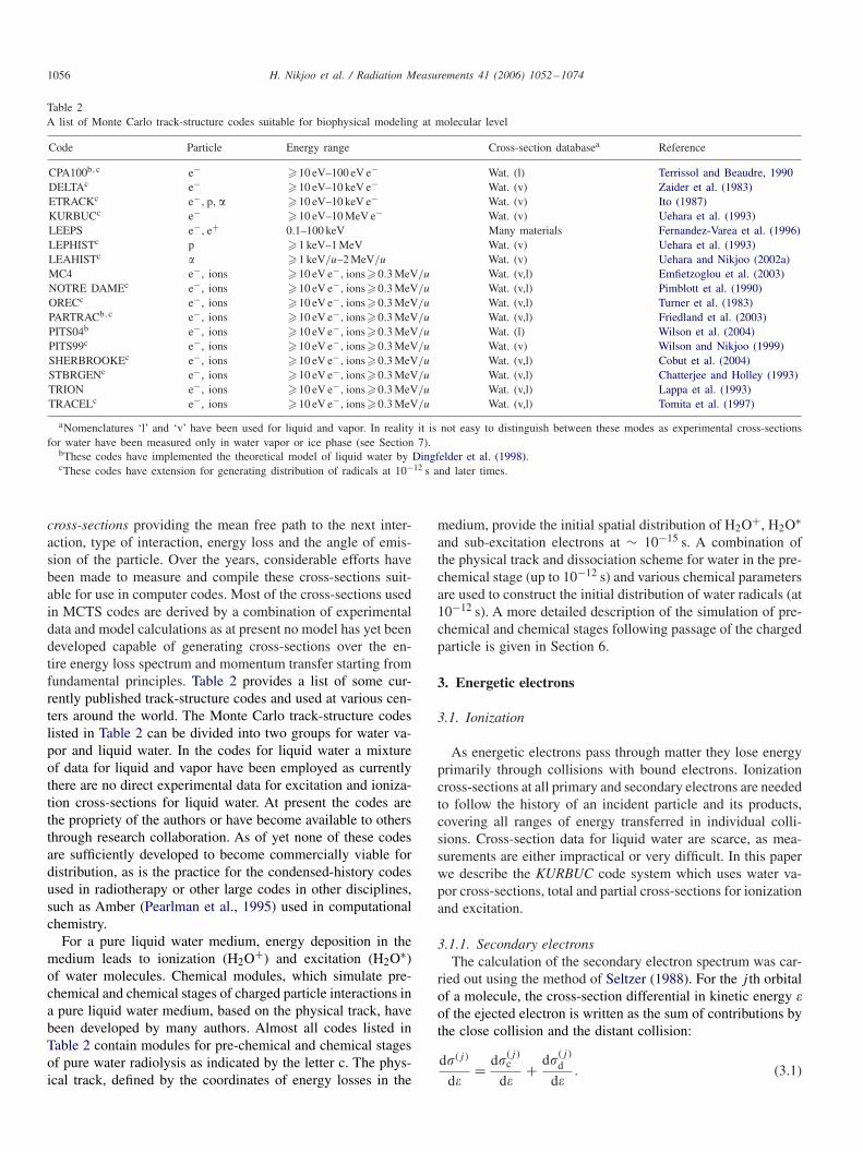
Fig. 2 shows the calculated single differential cross-sections(SDCSs) of secondary electrons for various primary electronenergies. For T = 1 and 10 keV, the present data are in goodagreement with the calculated data of Paretzke (1988) and theexperimental data of Vroom and Palmer (1977) and Bolorizadehand Rudd (1986a).
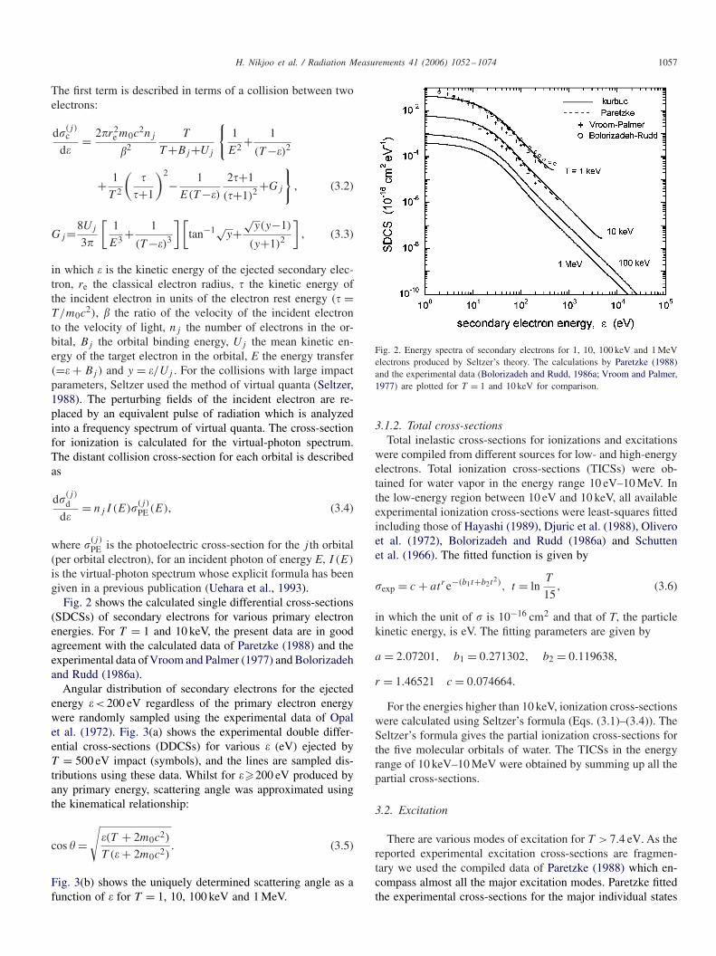
Angular distribution of secondary electrons for the ejectedenergy � < 200 eV regardless of the primary electron energywere randomly sampled using the experimental data of Opalet al. (1972). Fig. 3(a) shows the experimental double differ-ential cross-sections (DDCSs) for various � (eV) ejected byT = 500 eV impact (symbols), and the lines are sampled dis-tributions using these data. Whilst for ��200 eV produced byany primary energy, scattering angle was approximated usingthe kinematical relationship:
cos =√
�(T + 2m0c2)
T (� + 2m0c2). (3.5)
Fig. 3(b) shows the uniquely determined scattering angle as afunction of � for T = 1, 10, 100 keV and 1 MeV.
Fig. 2. Energy spectra of secondary electrons for 1, 10, 100 keV and 1 MeVelectrons produced by Seltzer’s theory. The calculations by Paretzke (1988)and the experimental data (Bolorizadeh and Rudd, 1986a; Vroom and Palmer,1977) are plotted for T = 1 and 10 keV for comparison.
3.1.2. Total cross-sectionsTotal inelastic cross-sections for ionizations and excitations
were compiled from different sources for low- and high-energyelectrons. Total ionization cross-sections (TICSs) were ob-tained for water vapor in the energy range 10 eV–10 MeV. Inthe low-energy region between 10 eV and 10 keV, all availableexperimental ionization cross-sections were least-squares fittedincluding those of Hayashi (1989), Djuric et al. (1988), Oliveroet al. (1972), Bolorizadeh and Rudd (1986a) and Schuttenet al. (1966). The fitted function is given by
�exp = c + atre−(b1t+b2t2), t = ln
T
15, (3.6)
in which the unit of � is 10−16 cm2 and that of T, the particlekinetic energy, is eV. The fitting parameters are given by
a = 2.07201, b1 = 0.271302, b2 = 0.119638,
r = 1.46521 c = 0.074664.
For the energies higher than 10 keV, ionization cross-sectionswere calculated using Seltzer’s formula (Eqs. (3.1)–(3.4)). TheSeltzer’s formula gives the partial ionization cross-sections forthe five molecular orbitals of water. The TICSs in the energyrange of 10 keV–10 MeV were obtained by summing up all thepartial cross-sections.
3.2. Excitation
There are various modes of excitation for T > 7.4 eV. As thereported experimental excitation cross-sections are fragmen-tary we used the compiled data of Paretzke (1988) which en-compass almost all the major excitation modes. Paretzke fittedthe experimental cross-sections for the major individual states
1058 H. Nikjoo et al. / Radiation Measurements 41 (2006) 1052–1074
Fig. 3. (a) Angular distributions of secondary electrons. The symbols are experimental data (Opal et al., 1972) for various secondary electron energies � (eV)for T = 500 eV electrons. The solid lines are the results obtained from sampling 104 times from these data. (b) Scattering angles calculated by Eq. (3.5) as afunction of � for T = 1, 10, 100 keV and 1 MeV.
Table 3Parameters for seven major excitation states from Paretzke (1988)
Excitation state Ea (eV) M2a cs
A1B1 7.4 0.099 1.25B1A1 9.7 0.098 1.25Diffuse band 13.3 0.363 1.25Rydberg (A + B) 10.0 0.041 1.25Rydberg (C + D) 11.0 0.072 1.25H* Lyman � 21.0 0.088 115.00H* Balmer � 21.0 0.0206 32
using the model function:
�exc = �3(T )4��2
0R
TM2
a ln4csT
R(3.7a)
in which �3(T ) is an empirical correction factor,
�3(T ) = 1 − e−0.25(T /Ea−1), (3.7b)
where �0 is the Bohr radius, 5.29 × 10⁻⁹ cm, and R is theRydberg constant equal to 13.6 eV. Table 3 lists the parametersM2
a , Ea and cs for each level considered in KURBUC.An additional OH∗ level was fitted by the analytical model
given by Green and Stolarski (1972).
�exc = 4��20R
2
E2a
f0c0
(Ea
T
)�{
1 −(
Ea
T
)�}v
(3.8)
in which the parameters given by Paretzke (1988) are Ea =9.0 eV, f0c0 = 0.033, � = 1, � = 2, and v = 1.
The total excitation cross-sections in the energy range 10 eVto 10 keV were obtained by summing up the individual cross-sections for the eight major levels listed above. The total ex-citation cross-section for the high-energy region up to 10 MeV
is given by an empirical formula derived from the so-calledFano plot, with the fitting parameters determined by Berger andWang (1988):
�exc = 4�
(�0
137�
)2[
12.30+1.26
{ln
�2
1−�2 −�2
}]. (3.9)
3.3. Elastic scattering
Elastic scattering cross-sections were calculated using theRutherford formula taking into account the screening param-eter given by Moliere (1948). The differential cross-section(d�/d�)el and total cross-sections �el for each molecule arerepresented by(
d�
d�
)el
= Z(Z + 1)r2e
1 − �2
�4
1
(1 − cos + 2 )2 , (3.10)
�el = �Z(Z + 1)r2e
1 − �2
�4
1
( + 1). (3.11)
The screening parameter is given by
= c × 1.7 × 10⁻⁵Z2/3 1
( + 2), (3.12)
where the effective atomic number of the water molecule, Z,was assumed to be 7.42, re = 2.8179 × 10⁻¹³ cm, = T/m0c
2
and
c = 1.198 for T < 50 keV, (3.13a)
=1.13 + 3.76
(Z
137�
)2
for T �50 keV. (3.13b)
The parameter c was determined by the least-square fitting tothe published experimental data (Shyn and Cho, 1987; Katase
H. Nikjoo et al. / Radiation Measurements 41 (2006) 1052–1074 1059
Fig. 4. Total cross-sections for ionization, excitation and elastic scattering ofelectrons in water vapor in the energy range of 10 eV–1 MeV. The experimentalTICS data of various groups (symbols) were used for fitting.
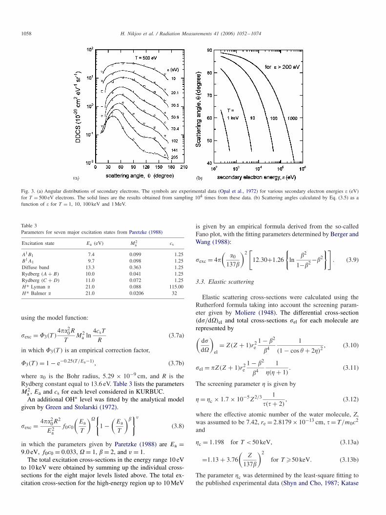
et al., 1986; Nishimura, 1979; Danjo and Nishimura, 1985). An-gular distributions for elastic scattering below 1 keV were ob-tained by direct sampling of various experimental data (Kataseet al., 1986; Nishimura, 1979; Trajmar et al., 1973) in placeof Eq. (3.10). Fig. 4 shows the total cross-sections for ion-ization, excitation and elastic scattering in the energy range10 eV–1 MeV, in which the experimental TICS data used forfitting are plotted in the low-energy regions below 20 keV.
4. Low-energy light ions
4.1. Charge transfers
Here, we use the term ‘light ions’ limited to protons andalpha particles. For fast ions, the majority of energy is trans-ferred in ionizing collisions, resulting in energetic free electronsand the potential energy of residual ions. When fast ions (ionswith energy in the MeV region) slow down around the Braggpeak (∼ 0.3 MeV/u), interactions involving electron captureand loss by the moving ions become an increasingly impor-tant component of the energy loss process. To develop track-structure models, cross-sections are needed for charge transferprocesses. Charge transfer cross-sections were compiled basedon available experimental data for H+ and H0 (Toburen et al.,1968; Dagnac et al., 1970), He2+ (Rudd et al., 1985b), He+(Rudd et al., 1985c; Sataka et al., 1990) and He0 (Sataka et al.,1990; Allison, 1958). Charge transfer cross-sections are gen-erally designated as �if where i is the initial and f the finalcharge state of the moving particle. There is a probability oftwo-electron transfer for helium atom, such as �20 and �02. To-tal cross-sections for electron capture �10 for H+ and electronloss �01 for H0 were evaluated using the analytical functionsdeveloped by Miller and Green (1973). Cross-sections for Heions were least-square fitted by a simple polynomial function
of the form
� =∑j
cj (log T )j−1 (4.1)
in which log is to the base 10, and T in keV/u. Smooth ex-trapolation was carried out where the experimental data werelacking. A detailed description can be found elsewhere (Ueharaand Nikjoo, 2002a).
4.2. Ionization
4.2.1. Secondary electronsEnergy spectra of secondary electrons ejected by proton im-
pact were calculated using the empirical model given by Rudd(1988):
d�i(�)
d�= S
B
F1 + F2w
(1 + w)3{1 + exp[�(w − wc)/v]} , (4.2)
where S = 4��20Nz2(R/B)2, � = electron energy, B =
binding energy for each orbital, �0 = 0.529 × 10⁻⁸ cm, N =electron number in orbital, z=charge of the projectile nucleus,R = 13.6 eV, T = kinetic energy of protons in eV/u units,� = mp/me = 1836, w = �/B, � = (T /�B)1/2, and wc = 4v2 −2v −R/4B. The F1, F2 and � are adjustable fitting parameters.
F1(v) = L1 + H1,
L1 = C1vD1/(1 + E1v
D1+4),
H1 = A1 ln(1 + v2)/(v2 + B1/v2), (4.3a)
F2(v) = L2H2/(L2 + H2),
L2 = C2vD2 ,
H2 = A2/v2 + B2/v
4. (4.3b)
The fitting parameters for water vapor are given by Rudd et al.(1992):
A1 = 0.97, B1 = 82, C1 = 0.40, D1 = −0.30, E1 = 0.38,
A2 = 1.04, B2 = 17.3, C2 = 0.76, D2 = 0.04, � = 0.64.
The Rudd model was applied to the calculations of averageenergy and energy spectra for the secondary electrons ejectedby alpha particle impact (Uehara and Nikjoo (2002a)). Appli-cability of the Rudd model to alpha particles was verified bycomparing the calculations with the experimental spectra. TheSDCS for He2+ was obtained by z2 scaling of proton data.
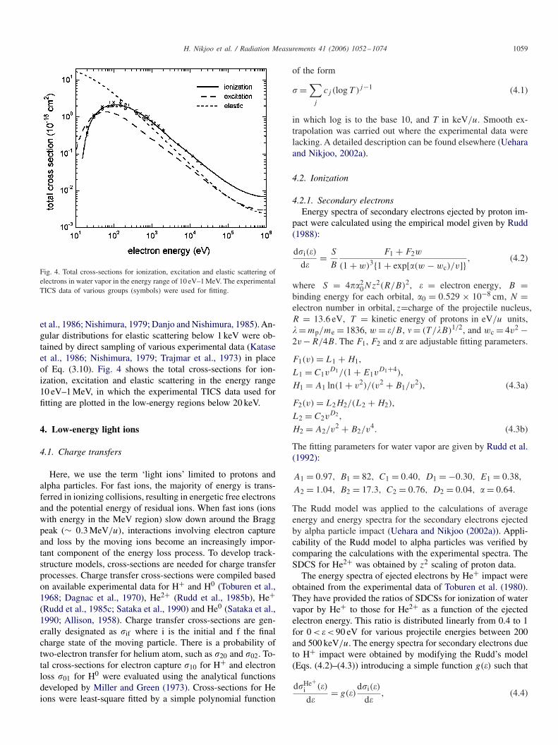
The energy spectra of ejected electrons by He+ impact wereobtained from the experimental data of Toburen et al. (1980).They have provided the ratios of SDCSs for ionization of watervapor by He+ to those for He2+ as a function of the ejectedelectron energy. This ratio is distributed linearly from 0.4 to 1for 0 < � < 90 eV for various projectile energies between 200and 500 keV/u. The energy spectra for secondary electrons dueto H+ impact were obtained by modifying the Rudd’s model(Eqs. (4.2)–(4.3)) introducing a simple function g(�) such that
d�He+i (�)
d�= g(�)
d�i(�)
d�, (4.4)

1060 H. Nikjoo et al. / Radiation Measurements 41 (2006) 1052–1074
Fig. 5. Calculated energy spectra for secondary electrons ejected by ion impact with energies 10, 50, 100, 500 keV/u and 1 MeV/u of He2+ (left), He2+(center) and He+ (right).
in which
g(�) = 0.4 + �/150 for � < 90 eV, (4.5a)
= 1 for ��90 eV. (4.5b)
Fig. 5 shows the calculated SDCS of ejected electrons for var-ious energy of H+ (left), He2+ (center) and He+ (right). It wasassumed that the spectra of electrons ejected from the targetmolecule by neutral hydrogen (H0) and neutral helium (He0)
impact were equal to that of H+ and He+, respectively. Theboundary energy for energetic secondary electrons generatedby ionization was set as 1 eV.
Experimental DDCS of electrons ejected from water by H+impact are given by Bolorizadeh and Rudd (1986b) and byToburen and Wilson (1977) in the energy range between 15 keVand 1 MeV. Available experimental angular distributions forHe2+ and He+ are limited (Toburen et al., 1980). To coverthe broad ion energy range used in these calculations, H+ datawere used assuming that differences of angular distributions be-tween different ions are not very large. Interpolation was madefor the intermediate energies of ejected electrons and incidention. Again, we assumed the angular distributions of electronsejected from the target molecule by H0 and He0 impact to beequal to that of H+ and He+, respectively.
4.2.2. Total cross-sectionsTICSs for bare ions (H+ and He2+) and He+ were obtained
by fitting polynomial functions (Eq. (4.1)) to the experimentaldata given by Rudd et al. (1985a) for protons, Rudd et al.(1985b) and Toburen et al. (1980) for alpha particles, and Ruddet al. (1985c) and Toburen et al. (1980) for He+. Where datawere lacking, the existing data were fitted and extrapolated.
Extrapolation was made by taking into account the repro-ducibility of stopping powers.
The TICS for neutral hydrogen impact was calculated by ananalytical function developed by Green and McNeal (1971):
�i = �0(Za)�(T − B)�
J�+� + T �+�, (4.6)
where �0 = 10−16 cm2, Z = 10, B is the ionization thresholdand the parameters a, J, � and � for H2 and O2 are given inTable 3 of Green and McNeal (1971). Cross-sections for H2Owere obtained from the additivity relationship �(H2)+�(O2)/2using the calculated values for H2 and O2. The TICSs forHe0 are unavailable, therefore those at energies lower than100 keV/u were adjusted to fit the electronic stopping pow-ers tabulated in ICRU Report 49 (1993). In the region below30 keV/u the stopping powers for He0 are the main contribu-tor. At energies above 100 keV/u, the total cross-sections wereassumed to be the same as those of He+.
4.3. Excitation
There are no experiments on excitation cross-sectionsfor proton and alpha-particle impact for water. The protoncross-sections obtained by scaling of the electron excitationcross-sections are plausible for high-energy protons > 500 keV(Dingfelder et al., 2000). To cover the lower energy regions, thesemi-empirical model developed by Miller and Green (1973)was adopted, which is based on the electron impact excitation.The analytical form is the same as Eq. (4.6) but replacing Bby energy of excited states, W, and the values of parameters.The parameters for 28 excited states are given in Table 3 of
H. Nikjoo et al. / Radiation Measurements 41 (2006) 1052–1074 1061
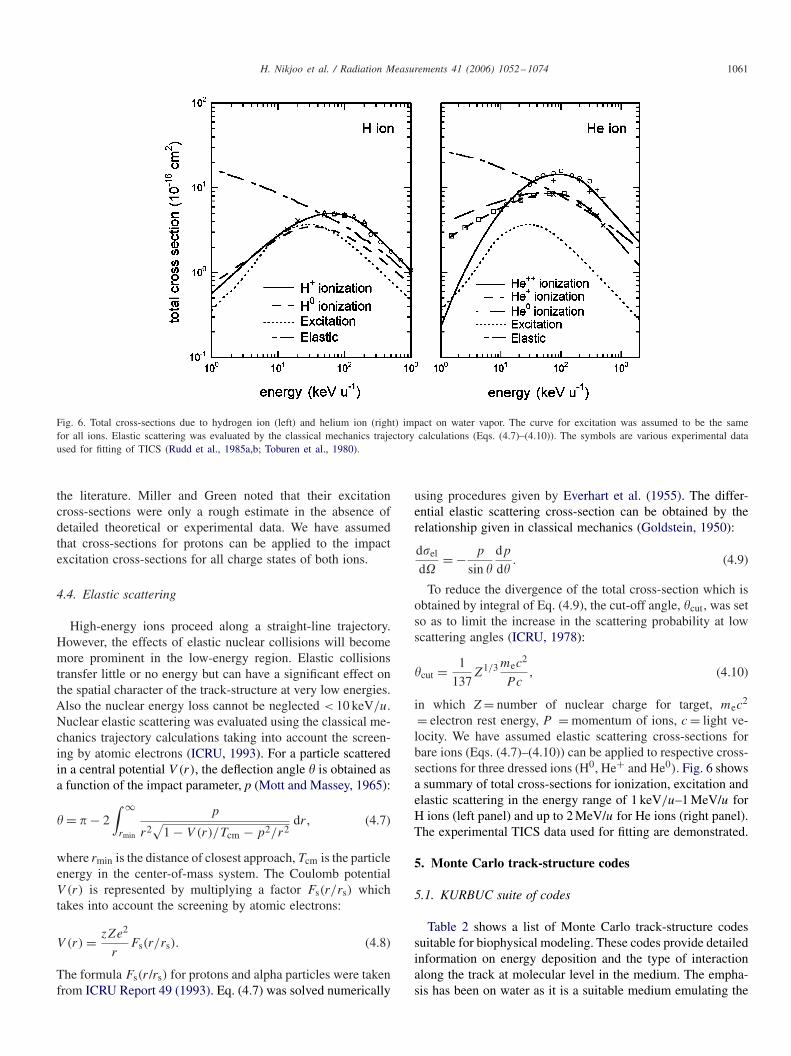
Fig. 6. Total cross-sections due to hydrogen ion (left) and helium ion (right) impact on water vapor. The curve for excitation was assumed to be the samefor all ions. Elastic scattering was evaluated by the classical mechanics trajectory calculations (Eqs. (4.7)–(4.10)). The symbols are various experimental dataused for fitting of TICS (Rudd et al., 1985a,b; Toburen et al., 1980).
the literature. Miller and Green noted that their excitationcross-sections were only a rough estimate in the absence ofdetailed theoretical or experimental data. We have assumedthat cross-sections for protons can be applied to the impactexcitation cross-sections for all charge states of both ions.
4.4. Elastic scattering
High-energy ions proceed along a straight-line trajectory.However, the effects of elastic nuclear collisions will becomemore prominent in the low-energy region. Elastic collisionstransfer little or no energy but can have a significant effect onthe spatial character of the track-structure at very low energies.Also the nuclear energy loss cannot be neglected < 10 keV/u.Nuclear elastic scattering was evaluated using the classical me-chanics trajectory calculations taking into account the screen-ing by atomic electrons (ICRU, 1993). For a particle scatteredin a central potential V (r), the deflection angle is obtained asa function of the impact parameter, p (Mott and Massey, 1965):
= � − 2∫ ∞
rmin
p
r2√
1 − V (r)/Tcm − p2/r2dr , (4.7)
where rmin is the distance of closest approach, Tcm is the particleenergy in the center-of-mass system. The Coulomb potentialV (r) is represented by multiplying a factor Fs(r/rs) whichtakes into account the screening by atomic electrons:
V (r) = zZe2
rFs(r/rs). (4.8)
The formula Fs(r/rs) for protons and alpha particles were takenfrom ICRU Report 49 (1993). Eq. (4.7) was solved numerically
using procedures given by Everhart et al. (1955). The differ-ential elastic scattering cross-section can be obtained by therelationship given in classical mechanics (Goldstein, 1950):
d�el
d�= − p
sin
dp
d. (4.9)
To reduce the divergence of the total cross-section which isobtained by integral of Eq. (4.9), the cut-off angle, cut, was setso as to limit the increase in the scattering probability at lowscattering angles (ICRU, 1978):
cut = 1
137Z1/3 mec
2
Pc, (4.10)
in which Z = number of nuclear charge for target, mec2
= electron rest energy, P = momentum of ions, c = light ve-locity. We have assumed elastic scattering cross-sections forbare ions (Eqs. (4.7)–(4.10)) can be applied to respective cross-sections for three dressed ions (H0, He+ and He0). Fig. 6 showsa summary of total cross-sections for ionization, excitation andelastic scattering in the energy range of 1 keV/u–1 MeV/u forH ions (left panel) and up to 2 MeV/u for He ions (right panel).The experimental TICS data used for fitting are demonstrated.
5. Monte Carlo track-structure codes
5.1. KURBUC suite of codes
Table 2 shows a list of Monte Carlo track-structure codessuitable for biophysical modeling. These codes provide detailedinformation on energy deposition and the type of interactionalong the track at molecular level in the medium. The empha-sis has been on water as it is a suitable medium emulating the
1062 H. Nikjoo et al. / Radiation Measurements 41 (2006) 1052–1074
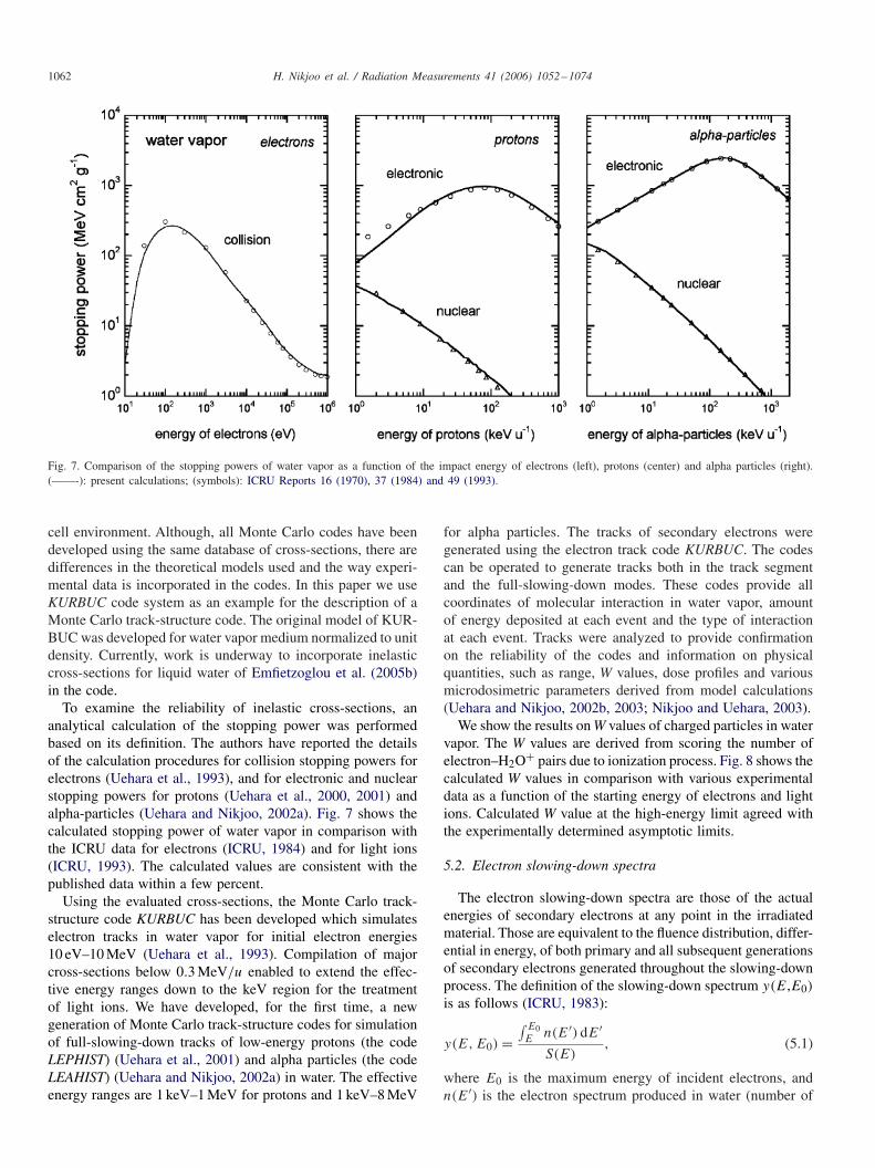
Fig. 7. Comparison of the stopping powers of water vapor as a function of the impact energy of electrons (left), protons (center) and alpha particles (right).(——-): present calculations; (symbols): ICRU Reports 16 (1970), 37 (1984) and 49 (1993).
cell environment. Although, all Monte Carlo codes have beendeveloped using the same database of cross-sections, there aredifferences in the theoretical models used and the way experi-mental data is incorporated in the codes. In this paper we useKURBUC code system as an example for the description of aMonte Carlo track-structure code. The original model of KUR-BUC was developed for water vapor medium normalized to unitdensity. Currently, work is underway to incorporate inelasticcross-sections for liquid water of Emfietzoglou et al. (2005b)in the code.
To examine the reliability of inelastic cross-sections, ananalytical calculation of the stopping power was performedbased on its definition. The authors have reported the detailsof the calculation procedures for collision stopping powers forelectrons (Uehara et al., 1993), and for electronic and nuclearstopping powers for protons (Uehara et al., 2000, 2001) andalpha-particles (Uehara and Nikjoo, 2002a). Fig. 7 shows thecalculated stopping power of water vapor in comparison withthe ICRU data for electrons (ICRU, 1984) and for light ions(ICRU, 1993). The calculated values are consistent with thepublished data within a few percent.
Using the evaluated cross-sections, the Monte Carlo track-structure code KURBUC has been developed which simulateselectron tracks in water vapor for initial electron energies10 eV–10 MeV (Uehara et al., 1993). Compilation of majorcross-sections below 0.3 MeV/u enabled to extend the effec-tive energy ranges down to the keV region for the treatmentof light ions. We have developed, for the first time, a newgeneration of Monte Carlo track-structure codes for simulationof full-slowing-down tracks of low-energy protons (the codeLEPHIST) (Uehara et al., 2001) and alpha particles (the codeLEAHIST) (Uehara and Nikjoo, 2002a) in water. The effectiveenergy ranges are 1 keV–1 MeV for protons and 1 keV–8 MeV
for alpha particles. The tracks of secondary electrons weregenerated using the electron track code KURBUC. The codescan be operated to generate tracks both in the track segmentand the full-slowing-down modes. These codes provide allcoordinates of molecular interaction in water vapor, amountof energy deposited at each event and the type of interactionat each event. Tracks were analyzed to provide confirmationon the reliability of the codes and information on physicalquantities, such as range, W values, dose profiles and variousmicrodosimetric parameters derived from model calculations(Uehara and Nikjoo, 2002b, 2003; Nikjoo and Uehara, 2003).
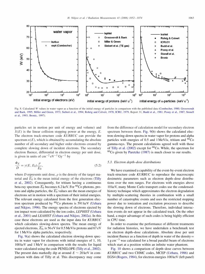
We show the results on W values of charged particles in watervapor. The W values are derived from scoring the number ofelectron–H2O+ pairs due to ionization process. Fig. 8 shows thecalculated W values in comparison with various experimentaldata as a function of the starting energy of electrons and lightions. Calculated W value at the high-energy limit agreed withthe experimentally determined asymptotic limits.
5.2. Electron slowing-down spectra
The electron slowing-down spectra are those of the actualenergies of secondary electrons at any point in the irradiatedmaterial. Those are equivalent to the fluence distribution, differ-ential in energy, of both primary and all subsequent generationsof secondary electrons generated throughout the slowing-downprocess. The definition of the slowing-down spectrum y(E,E0)
is as follows (ICRU, 1983):
y(E, E0) =∫ E0E
n(E′) dE′
S(E), (5.1)
where E0 is the maximum energy of incident electrons, andn(E′) is the electron spectrum produced in water (number of
H. Nikjoo et al. / Radiation Measurements 41 (2006) 1052–1074 1063
Fig. 8. Calculated W values in water vapor as a function of the initial energy of particles in comparison with the published data (Combecher, 1980; Grosswendtand Baek, 1995; Miller and Green, 1973; Siebert et al., 1994; Rohrig and Colvert, 1978; ICRU, 1979, Report 31; Budd et al., 1981; Posny et al., 1987; Stonellet al., 1993; Bronic, 1997).
particles set in motion per unit of energy and volume) andS(E) is the linear collision stopping power at the energy, E.The electron track-structure code KURBUC can provide thespectrum n(E), which is obtained by accumulating the absolutenumber of all secondary and higher order electrons created bycomplete slowing down of incident electrons. The secondaryelectron fluence, differential in electron energy per unit dose,is given in units of cm−2 eV−1 Gy−1 by
�E
D= y(E, E0)
�
E0, (5.2)
where D represents unit dose, � is the density of the target ma-terial and E0 is the mean initial energy of the electrons (Tillyet al., 2002). Consequently, for tritium having a continuousbeta-ray spectrum E0 becomes 6.2 keV. For 60Co photons, pro-tons and alpha particles, the E0 values are the mean energies ofelectrons set in motion with a spectrum of their initial energies.The relevant energy calculated from the first generation elec-tron spectrum produced by 60Co photons is 591 keV (Ueharaand Nikjoo, 1996). The energy spectra of electrons ejected byion impact were calculated by the ion codes, LEPHIST (Ueharaet al., 2001) and LEAHIST (Uehara and Nikjoo, 2002a). In thiscase these electrons are used as the input data for KURBUCwhich calculates slowing-down spectra. The mean energy ofejected electrons, E0, is 56 eV for 0.5 MeV/u protons and 67 eVfor 1 MeV/u alpha particles, respectively.
Fig. 9(a) shows the calculated electron slowing-down spec-tra in water vapor for electrons with initial energies of 1, 10,100 keV and 1 MeV in comparison with the results for liquidwater calculated using the code PENELOPE (Tilly et al., 2002).The present data markedly dip at around E ∼ 20 keV in com-parison with data of Tilly et al. This discrepancy may come
from the difference of calculation model for secondary electronspectrum between them. Fig. 9(b) shows the calculated elec-tron slowing-down spectra in water vapor for protons and alphaparticles with energies of 0.5 and 1 MeV/u, tritium and 60Cogamma-rays. The present calculations agreed well with thoseof Tilly et al. (2002) except for 60Co. While, the spectrum for60Co given by Paretzke (1987) is much closer to our results.
5.3. Electron depth–dose distributions
We have examined a capability of the event-by-event electrontrack-structure code KURBUC to reproduce the macroscopicdosimetric parameters such as electron depth–dose distribu-tions over the mm ranges. For electrons with energies above10 keV, many Monte Carlo transport codes use the condensed-history technique which approximates the electron degradationby multiple-scattering theories in combination with a smallnumber of catastrophic events and uses the restricted stoppingpower due to ionization and excitation processes to describethe slowing down of electrons. Therefore, individual interac-tion events do not appear in the calculated track. On the otherhand, a major advantage of such codes is being highly efficientin CPU time.
In order to examine the performance of different treatmentsfor radiation histories, we have undertaken a benchmark teston electron depth–dose calculations. Absolute dose per unitincident fluence as a function of depth in water of the density=1 g cm−3 was calculated for a broad parallel beam of electronswhich start at a position within an infinite water phantom.
Fig. 10 shows a comparison of depth–dose curves betweenKURBUC and two CHMC codes, MCEP (Uehara, 1986) andEGS4 (Rogers, 1984), for electron energies 100 keV (left panel)

1064 H. Nikjoo et al. / Radiation Measurements 41 (2006) 1052–1074
Fig. 9. Slowing-down spectra in water vapor for (a) electrons with initial energies of 1, 10, 100 keV and 1 MeV and (b) protons and alpha particles withenergies of 0.5 and 1 MeV/u, tritium and 60Co gamma-rays. The spectra of Tilly et al. (2002) for liquid water, Paretzke’s (1987) data for 60Co gamma-raysis for water vapor.
Fig. 10. Comparison of various calculations of the depth–dose curve for a broad parallel beam of electrons with 100 keV (left) and 300 keV (right). Thestarting position of the beam is at the origin of depth within an infinite water phantom.
and 300 keV (right panel). The distributions obtained by thecode KURBUC are in good agreement with EGS4 and MCEPincluding the critical characteristics of backscattering contribu-tions.
It is concluded that consistent results can be obtained fromboth the microscopic and the macroscopic codes for depth–doseof electrons with energies up to several hundred keV. Suchintercomparisons and also with other physical quantities havebeen useful means for checking the reliability of the codes.
6. Monte Carlo simulation codes for description ofpre-chemical and chemical stages of water radiolysis
The KURBUC code provides the initial yields of the forma-tion of the species H2O+, H2O∗ and sub-excitation electrone−
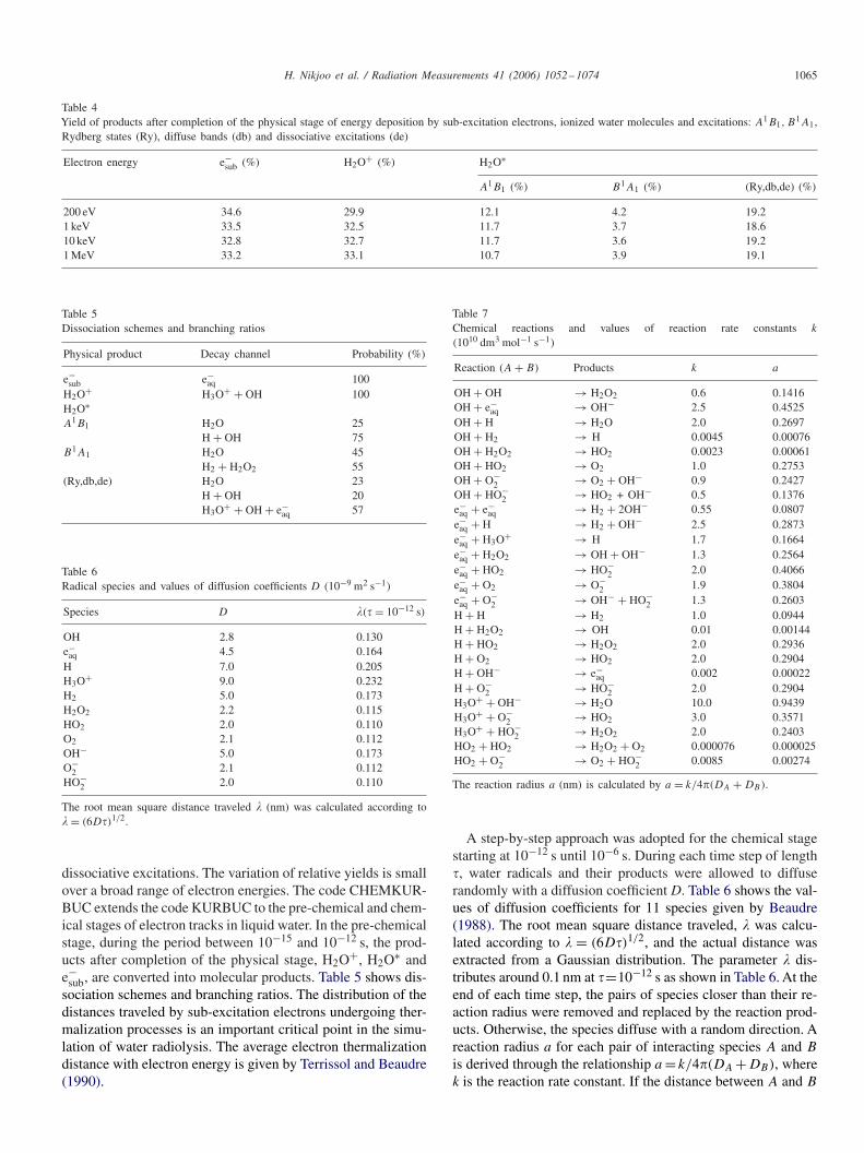
sub (E < 7.4 eV) at ∼ 10−15 s. Table 4 shows the products aftercompletion of the physical stage for various electron energiesin which excited water molecule, H2O∗, are divided into threegroups: A1B1, B1A1 and Rydberg states, diffuse bands and
H. Nikjoo et al. / Radiation Measurements 41 (2006) 1052–1074 1065
Table 4Yield of products after completion of the physical stage of energy deposition by sub-excitation electrons, ionized water molecules and excitations: A1B1, B
1A1,Rydberg states (Ry), diffuse bands (db) and dissociative excitations (de)
Electron energy e−sub (%) H2O+ (%) H2O∗
A1B1 (%) B1A1 (%) (Ry,db,de) (%)
200 eV 34.6 29.9 12.1 4.2 19.21 keV 33.5 32.5 11.7 3.7 18.610 keV 32.8 32.7 11.7 3.6 19.21 MeV 33.2 33.1 10.7 3.9 19.1
Table 5Dissociation schemes and branching ratios
Physical product Decay channel Probability (%)
e−sub e−
aq 100H2O+ H3O+ + OH 100H2O∗A1B1 H2O 25
H + OH 75B1A1 H2O 45
H2 + H2O2 55(Ry,db,de) H2O 23
H + OH 20H3O+ + OH + e−
aq 57
Table 6Radical species and values of diffusion coefficients D (10−9 m2 s−1)
Species D �( = 10−12 s)
OH 2.8 0.130e−
aq 4.5 0.164H 7.0 0.205H3O+ 9.0 0.232H2 5.0 0.173H2O2 2.2 0.115HO2 2.0 0.110O2 2.1 0.112OH− 5.0 0.173O−
2 2.1 0.112HO−
2 2.0 0.110
The root mean square distance traveled � (nm) was calculated according to� = (6D)1/2.
dissociative excitations. The variation of relative yields is smallover a broad range of electron energies. The code CHEMKUR-BUC extends the code KURBUC to the pre-chemical and chem-ical stages of electron tracks in liquid water. In the pre-chemicalstage, during the period between 10−15 and 10−12 s, the prod-ucts after completion of the physical stage, H2O+, H2O∗ ande−
sub, are converted into molecular products. Table 5 shows dis-sociation schemes and branching ratios. The distribution of thedistances traveled by sub-excitation electrons undergoing ther-malization processes is an important critical point in the simu-lation of water radiolysis. The average electron thermalizationdistance with electron energy is given by Terrissol and Beaudre(1990).
Table 7Chemical reactions and values of reaction rate constants k
(1010 dm3 mol−1 s−1)
Reaction (A + B) Products k a
OH + OH → H2O2 0.6 0.1416OH + e−
aq → OH− 2.5 0.4525OH + H → H2O 2.0 0.2697OH + H2 → H 0.0045 0.00076OH + H2O2 → HO2 0.0023 0.00061OH + HO2 → O2 1.0 0.2753OH + O−
2 → O2 + OH− 0.9 0.2427OH + HO−
2 → HO2 + OH− 0.5 0.1376e−
aq + e−aq → H2 + 2OH− 0.55 0.0807
e−aq + H → H2 + OH− 2.5 0.2873
e−aq + H3O+ → H 1.7 0.1664
e−aq + H2O2 → OH + OH− 1.3 0.2564
e−aq + HO2 → HO−
2 2.0 0.4066e−
aq + O2 → O−2 1.9 0.3804
e−aq + O−
2 → OH− + HO−2 1.3 0.2603
H + H → H2 1.0 0.0944H + H2O2 → OH 0.01 0.00144H + HO2 → H2O2 2.0 0.2936H + O2 → HO2 2.0 0.2904H + OH− → e−
aq 0.002 0.00022H + O−
2 → HO−2 2.0 0.2904
H3O+ + OH− → H2O 10.0 0.9439H3O+ + O−
2 → HO2 3.0 0.3571H3O+ + HO−
2 → H2O2 2.0 0.2403HO2 + HO2 → H2O2 + O2 0.000076 0.000025HO2 + O−
2 → O2 + HO−2 0.0085 0.00274
The reaction radius a (nm) is calculated by a = k/4�(DA + DB).
A step-by-step approach was adopted for the chemical stagestarting at 10−12 s until 10−6 s. During each time step of length, water radicals and their products were allowed to diffuserandomly with a diffusion coefficient D. Table 6 shows the val-ues of diffusion coefficients for 11 species given by Beaudre(1988). The root mean square distance traveled, � was calcu-lated according to � = (6D)1/2, and the actual distance wasextracted from a Gaussian distribution. The parameter � dis-tributes around 0.1 nm at =10−12 s as shown in Table 6. At theend of each time step, the pairs of species closer than their re-action radius were removed and replaced by the reaction prod-ucts. Otherwise, the species diffuse with a random direction. Areaction radius a for each pair of interacting species A and B
is derived through the relationship a = k/4�(DA +DB), wherek is the reaction rate constant. If the distance between A and B
1066 H. Nikjoo et al. / Radiation Measurements 41 (2006) 1052–1074
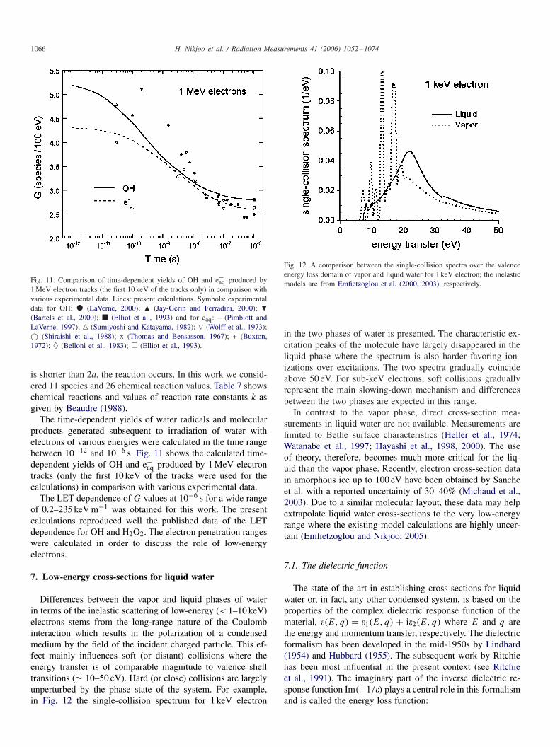
Fig. 11. Comparison of time-dependent yields of OH and e−aq produced by
1 MeV electron tracks (the first 10 keV of the tracks only) in comparison withvarious experimental data. Lines: present calculations. Symbols: experimentaldata for OH: � (LaVerne, 2000); � (Jay-Gerin and Ferradini, 2000); �(Bartels et al., 2000); � (Elliot et al., 1993) and for e−
aq: – (Pimblott andLaVerne, 1997); � (Sumiyoshi and Katayama, 1982); � (Wolff et al., 1973);© (Shiraishi et al., 1988); x (Thomas and Bensasson, 1967); + (Buxton,1972); ♦ (Belloni et al., 1983); � (Elliot et al., 1993).
is shorter than 2a, the reaction occurs. In this work we consid-ered 11 species and 26 chemical reaction values. Table 7 showschemical reactions and values of reaction rate constants k asgiven by Beaudre (1988).
The time-dependent yields of water radicals and molecularproducts generated subsequent to irradiation of water withelectrons of various energies were calculated in the time rangebetween 10−12 and 10−6 s. Fig. 11 shows the calculated time-dependent yields of OH and e−
aq produced by 1 MeV electrontracks (only the first 10 keV of the tracks were used for thecalculations) in comparison with various experimental data.
The LET dependence of G values at 10−6 s for a wide rangeof 0.2–235 keV m−1 was obtained for this work. The presentcalculations reproduced well the published data of the LETdependence for OH and H2O2. The electron penetration rangeswere calculated in order to discuss the role of low-energyelectrons.
7. Low-energy cross-sections for liquid water
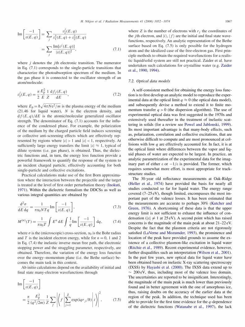
Differences between the vapor and liquid phases of waterin terms of the inelastic scattering of low-energy (< 1–10 keV)electrons stems from the long-range nature of the Coulombinteraction which results in the polarization of a condensedmedium by the field of the incident charged particle. This ef-fect mainly influences soft (or distant) collisions where theenergy transfer is of comparable magnitude to valence shelltransitions (∼ 10–50 eV). Hard (or close) collisions are largelyunperturbed by the phase state of the system. For example,in Fig. 12 the single-collision spectrum for 1 keV electron
Fig. 12. A comparison between the single-collision spectra over the valenceenergy loss domain of vapor and liquid water for 1 keV electron; the inelasticmodels are from Emfietzoglou et al. (2000, 2003), respectively.
in the two phases of water is presented. The characteristic ex-citation peaks of the molecule have largely disappeared in theliquid phase where the spectrum is also harder favoring ion-izations over excitations. The two spectra gradually coincideabove 50 eV. For sub-keV electrons, soft collisions graduallyrepresent the main slowing-down mechanism and differencesbetween the two phases are expected in this range.
In contrast to the vapor phase, direct cross-section mea-surements in liquid water are not available. Measurements arelimited to Bethe surface characteristics (Heller et al., 1974;Watanabe et al., 1997; Hayashi et al., 1998, 2000). The useof theory, therefore, becomes much more critical for the liq-uid than the vapor phase. Recently, electron cross-section datain amorphous ice up to 100 eV have been obtained by Sancheet al. with a reported uncertainty of 30–40% (Michaud et al.,2003). Due to a similar molecular layout, these data may helpextrapolate liquid water cross-sections to the very low-energyrange where the existing model calculations are highly uncer-tain (Emfietzoglou and Nikjoo, 2005).
7.1. The dielectric function
The state of the art in establishing cross-sections for liquidwater or, in fact, any other condensed system, is based on theproperties of the complex dielectric response function of thematerial, �(E, q) = �1(E, q) + i�2(E, q) where E and q arethe energy and momentum transfer, respectively. The dielectricformalism has been developed in the mid-1950s by Lindhard(1954) and Hubbard (1955). The subsequent work by Ritchiehas been most influential in the present context (see Ritchieet al., 1991). The imaginary part of the inverse dielectric re-sponse function Im(−1/�) plays a central role in this formalismand is called the energy loss function:
H. Nikjoo et al. / Radiation Measurements 41 (2006) 1052–1074 1067
Im
[ −1
�(E, q)
]=
∑j
�j2(E, q)
�21(E, q) + �2
2(E, q)
=∑j
Im[�j (E, q)]|�(E, q)|2 , (7.1)
where j denotes the j th electronic transition. The numeratorin Eq. (7.1) corresponds to the single-particle transitions thatcharacterize the photoabsorption spectrum of the medium. Inthe gas phase it is connected to the oscillator strength of anatom/molecule:
�j2(E, q) = �
2
E2p
E
1
Z
dfj (E, q)
dE, (7.2)
where Ep = h̄√
4�Ne2/m is the plasma energy of the medium(21.46 for liquid water), N is the electron density, anddf (E, q)/dE is the atomic/molecular generalized oscillatorstrength. The denominator of Eq. (7.1) accounts for the influ-ence of the condensed phase. For example, the polarizationof the medium by the charged particle field induces screeningor collective anti-screening effects which are effectively rep-resented by regions where |�| > 1 and |�| < 1, respectively. Atsufficiently large energy transfers the limit |�| ≈ 1, typical ofdilute systems (i.e. gas phase), is obtained. Thus, the dielec-tric functions and, in turn, the energy loss function provide apowerful framework to quantify the response of the system toan incident charged particle, effectively accounting for bothsingle-particle and collective excitations.
Practical calculations make use of the first Born approxima-tion where the interaction between the projectile and the targetis treated at the level of first order perturbation theory (Inokuti,1971). Within the dielectric formalism the DDCSs as well asvarious integral quantities are obtained by
d2�
dE dq= 1
��0NT qIm
[ −1
�(E, q)
], (7.3)
M(n)(T ) = 1
��0T
∫En dE
∫1
qIm
[ −1
�(E, q)
]dq, (7.4)
where � is the (microscopic) cross-section, �0 is the Bohr radiusand T is the incident electron energy, while for n = 0, 1 and 2in Eq. (7.4) the inelastic inverse mean free path, the electronicstopping power and the straggling parameter, respectively, areobtained. Therefore, the variation of the energy loss functionover the energy–momentum plane (i.e. the Bethe surface) be-comes the main task in this context.
Ab initio calculations depend on the availability of initial andfinal state many-electron wavefunctions through
Im
[ −1
�(E, q)
]
= �
2
E2p
(q2/2m)
1
Z
∑f
∣∣∣∣∣∣⟨f
∣∣∣∣∣∣Z∑
j=1
exp(iqrj /h̄)
∣∣∣∣∣∣ i⟩∣∣∣∣∣∣
2
, (7.5)
where Z is the number of electrons with rj the coordinates ofthe j th electron, and |i〉, |f 〉 are the initial and final state wave-functions, respectively. An analytic representation of the Bethesurface based on Eq. (7.5) is only possible for the hydrogenatom and the idealized case of the free-electron gas. First prin-ciple methods to obtain the required wavefunctions for a realis-tic liquid/solid system are still not practical. Zaider et al. haveundertaken such calculations for crystalline water (e.g. Zaideret al., 1990, 1994).
7.2. Optical data models
A self-consistent method for obtaining the energy loss func-tion is to first develop an analytic model to reproduce the exper-imental data at the optical limit q ≈ 0 (the optical data model),and subsequently devise a method to extend it to finite mo-mentum transfer q > 0 (the dispersion algorithm). The use ofexperimental optical data was first suggested in the 1970s andextensively used thereafter in the treatment of inelastic scat-tering in solids (for a review see Powel and Jablonski, 1999).Its most important advantage is that many-body effects, suchas, polarization, correlation and collective excitations, that areotherwise difficult to compute and are most pronounced at col-lisions with low q are effectively accounted for. In fact, it is atthe optical limit where differences between the vapor and liq-uid phases of water are expected to be largest. In practice, ananalytic parametrization of the experimental data for the imag-inary part of either � or −1/� is provided. The former, whichrequires somewhat more effort, is most appropriate for track-structure studies.
The 30-year old reflectance measurements at Oak-Ridge(Heller et al., 1974) have provided the basis for nearly allstudies conducted so far for liquid water. The energy rangecovered (7–25 eV), though limited, encompasses the most im-portant part of the valence losses. It has been estimated thatthe measurements are accurate to perhaps 30% (Kutcher andGreen, 1976). A shortcoming of these data is that the upperenergy limit is not sufficient to exhaust the influence of con-densation (|�| �= 1 at 25 eV). A second point which has raisedconcerns is the magnitude of the main peak at about 21–22 eV.Despite the fact that the plasmon criteria are not rigorouslysatisfied (LaVerne and Mozumder, 1993), the prominence andlocation of the peak have provided grounds to assume the ex-istence of a collective plasmon-like excitation in liquid water(Ritchie et al., 1989). Recent experimental evidence, however,further disqualifies such an interpretation (Wilson et al., 2001).In the past few years, new optical data for liquid water havebeen obtained based on inelastic X-ray scattering spectroscopy(IXSS) by Hayashi et al. (2000). The IXSS data extend up to∼ 200 eV, thus, including most of the valence loss domain.The uncertainties are reported to be insignificant. Interestingly,the magnitude of the main peak is much lower than previouslyfound and in better agreement with the one of amorphous ice,thus, raising doubts on the accuracy of the earlier data at theregion of the peak. In addition, the technique used has beenable to provide for the first time evidence for the q-dependenceof the dielectric functions (Watanabe et al., 1997), the lack
1068 H. Nikjoo et al. / Radiation Measurements 41 (2006) 1052–1074
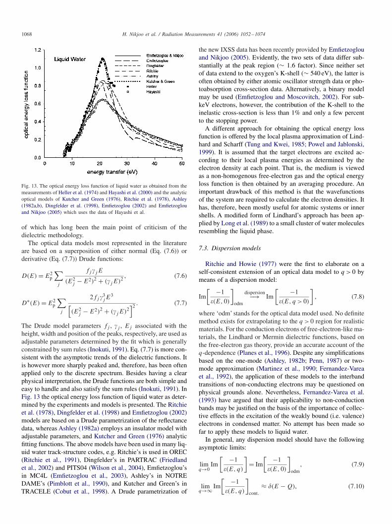
Fig. 13. The optical energy loss function of liquid water as obtained from themeasurements of Heller et al. (1974) and Hayashi et al. (2000) and the analyticoptical models of Kutcher and Green (1976), Ritchie et al. (1978), Ashley(1982a,b), Dingfelder et al. (1998), Emfietzoglou (2002) and Emfietzoglouand Nikjoo (2005) which uses the data of Hayashi et al.
of which has long been the main point of criticism of thedielectric methodology.
The optical data models most represented in the literatureare based on a superposition of either normal (Eq. (7.6)) orderivative (Eq. (7.7)) Drude functions:
D(E) = E2p
∑j
fj �jE
(E2j − E2)2 + (�jE)2 , (7.6)
D∗(E) = E2p
∑j
2fj �3jE
3[(E2
j − E2)2 + (�jE)2]2 . (7.7)
The Drude model parameters fj , �j , Ej associated with theheight, width and position of the peaks, respectively, are used asadjustable parameters determined by the fit which is generallyconstrained by sum rules (Inokuti, 1991). Eq. (7.7) is more con-sistent with the asymptotic trends of the dielectric functions. Itis however more sharply peaked and, therefore, has been oftenapplied only to the discrete spectrum. Besides having a clearphysical interpretation, the Drude functions are both simple andeasy to handle and also satisfy the sum rules (Inokuti, 1991). InFig. 13 the optical energy loss function of liquid water as deter-mined by the experiments and models is presented. The Ritchieet al. (1978), Dingfelder et al. (1998) and Emfietzoglou (2002)models are based on a Drude parametrization of the reflectancedata, whereas Ashley (1982a) employs an insulator model withadjustable parameters, and Kutcher and Green (1976) analyticfitting functions. The above models have been used in many liq-uid water track-structure codes, e.g. Ritchie’s is used in OREC(Ritchie et al., 1991), Dingfelder’s in PARTRAC (Friedlandet al., 2002) and PITS04 (Wilson et al., 2004), Emfietzoglou’sin MC4L (Emfietzoglou et al., 2003), Ashley’s in NOTREDAME’s (Pimblott et al., 1990), and Kutcher and Green’s inTRACELE (Cobut et al., 1998). A Drude parametrization of
the new IXSS data has been recently provided by Emfietzoglouand Nikjoo (2005). Evidently, the two sets of data differ sub-stantially at the peak region (∼ 1.6 factor). Since neither setof data extend to the oxygen’s K-shell (∼ 540 eV), the latter isoften obtained by either atomic oscillator strength data or pho-toabsorption cross-section data. Alternatively, a binary modelmay be used (Emfietzoglou and Moscovitch, 2002). For sub-keV electrons, however, the contribution of the K-shell to theinelastic cross-section is less than 1% and only a few percentto the stopping power.
A different approach for obtaining the optical energy lossfunction is offered by the local plasma approximation of Lind-hard and Scharff (Tung and Kwei, 1985; Powel and Jablonski,1999). It is assumed that the target electrons are excited ac-cording to their local plasma energies as determined by theelectron density at each point. That is, the medium is viewedas a non-homogenous free-electron gas and the optical energyloss function is then obtained by an averaging procedure. Animportant drawback of this method is that the wavefunctionsof the system are required to calculate the electron densities. Ithas, therefore, been mostly useful for atomic systems or innershells. A modified form of Lindhard’s approach has been ap-plied by Long et al. (1989) to a small cluster of water moleculesresembling the liquid phase.
7.3. Dispersion models
Ritchie and Howie (1977) were the first to elaborate on aself-consistent extension of an optical data model to q > 0 bymeans of a dispersion model:
Im
[ −1
�(E, 0)
]odm
dispersion−→ Im
[ −1
�(E, q > 0)
], (7.8)
where ‘odm’ stands for the optical data model used. No definitemethod exists for extrapolating to the q > 0 region for realisticmaterials. For the conduction electrons of free-electron-like ma-terials, the Lindhard or Mermin dielectric functions, based onthe free-electron gas theory, provide an accurate account of theq-dependence (Planes et al., 1996). Despite any simplificationsbased on the one-mode (Ashley, 1982b; Penn, 1987) or two-mode approximation (Martinez et al., 1990; Fernandez-Vareaet al., 1992), the application of these models to the interbandtransitions of non-conducting electrons may be questioned onphysical grounds alone. Nevertheless, Fernandez-Varea et al.(1993) have argued that their applicability to non-conductionbands may be justified on the basis of the importance of collec-tive effects in the excitation of the weakly bound (i.e. valence)electrons in condensed matter. No attempt has been made sofar to apply these models to liquid water.
In general, any dispersion model should have the followingasymptotic limits:
limq→0
Im
[ −1
�(E, q)
]= Im
[ −1
�(E, 0)
]odm
, (7.9)
limq→∞ Im
[ −1
�(E, q)
]cont.
≈ �(E − Q), (7.10)
H. Nikjoo et al. / Radiation Measurements 41 (2006) 1052–1074 1069
where Q = q2/2m is the free-electron recoil energy. Eq. (7.9)is self-evident while Eq. (7.10) simply ensures that the free-electron limit is approached at sufficiently high momentumtransfer. The so-called extended-Drude and �-oscillator modelshave been extensively applied to the dispersion of interbandtransitions of semiconducting and insulating materials.
The extended-Drude model was first suggested by Ritchieand Howie (1977). It amounts to the incorporation ofthe q-dependence directly into the Drude model parame-ters by substituting the triad of values {fj , �j , Ej } with{fj (q), �j (q), Ej (q)}. For calculation of integral quantities(Akkerman and Akkerman, 1999; Emfietzoglou and Moscov-itch, 2002) it is sufficient to merely use a one-parameterDrude dispersion {fj , �j , Ej (q)} in the form of the impulseapproximation:
Ej(q) = Ej + q2
2m. (7.11)
Eq. (7.11) ensures the correct asymptotic behavior dic-tated by Eqs. (7.9) and (7.10). A two-parameter dispersion{fj (q), �j , Ej (q)}, however, is necessary to properly accountfor the discrete spectrum. Then, Eq. (7.11) is applied to thecontinuum only, and the following relationship is also used:
f(j)excit.(q) = f
(j)excit.
∑n
a(j)n qn exp(−b
(j)n q), (7.12)
where an, bn are empirical parameters determined from molec-ular data. The corresponding f
(j)ioniz(q) may be found from the
Bethe sum rule. The two-parameter Drude dispersion have beenused in many liquid water track-structure codes such as theOREC (Turner et al., 1983), PARTRAC (Friedland et al., 2002),PITS04 (Wilson et al., 2004), and MC4L (Emfietzoglou et al.,2003).
The origin of the �-oscillator dispersion models is a �-function representation of the optical oscillator strength of anatom (Fernandez-Varea et al., 1992):
df (E)
dE=
∑j
fj�(E − Ej). (7.13)
By means of a dispersion function Gj(q), such as Gj(0) ≡ Ej ,Eq. (7.13) may be used to extend the optical oscillator strengthto q > 0. After generalization to condensed matter:
Im
[ −1
�(E, q)
]
=∫ ∞
0
E′
EIm
[ −1
�(E′, 0)
]�(E − G(E′; q)) dE′. (7.14)
The �-function in Eq. (7.14) is called the �-oscillator. Eq. (7.14)indicates that the q > 0 region of the Bethe surface may bederived from its optical limit (q = 0) by using �-oscillatorsalong the curves defined by the dispersion function G(E′; q).
Liljequist (1983) has suggested a dispersion scheme basedon Bohr’s early distinction between resonant-like and binary-like collisions:
G(E′; q) = E′ for Q�E′,G(E′; q) = Q for Q > E′. (7.15)
The second condition in Eq. (7.15) corresponds to the Betheridge. The energy loss function takes the following form:
Im
[ −1
�(E, q)
]
=∫ ∞
0E′Im
[ −1
� (E′, 0)
]�(E − E′)
E�(E′ − Q) dE′
+∫ ∞
0E′Im
[ −1
�(E′, 0)
]�(E − Q)
E
× �(Q − E′) dE′, (7.16)
which may be simplified to
Im
[ −1
�(E, q)
]= Im
[ −1
�(E, 0)
]�(E − Q)
+ E2p�
2
Zeff(q)
Z
�(E − Q)
E, (7.17)
where Zeff(q) is the effective number of target electrons whichparticipate in collisions with energy transfer up to Q as obtainedfrom the Bethe sum rule.
An alternative scheme based on a simple quadratic dispersionhas been suggested by Ashley (1988):
G(E′; q) = E′ + Q. (7.18)
The above form resembles the plasmon dispersion of the free-electron gas at low q, while asymptotically leading to Eq. (7.10)at high q. By inserting Eq. (7.18) into Eq. (7.17) the followingenergy loss function formula is obtained:
Im
[ −1
�(E, q)
]=
∫ ∞
0
E′
EIm
[ −1
�(E′, 0)
]× �(E − (E′ + Q)) dE′, (7.19)
which may be simplified to
Im
[ −1
�(E, q)
]=E−Q
EIm
[ −1
�(E − Q, 0)
]�(E−Q). (7.20)
Note that within this model no distinction is made betweendiscrete and continuum transitions leading to an unrealisticdispersion for the former. It also results in doubling the ioniza-tion threshold. Both shortcomings may be important in track-structure studies. Tan et al. (2004) have shown that Ashley’smodel is equivalent to Penn’s algorithm using a single-poleapproximation to Lindhard’s function (Penn, 1987) and theequivalent quadratic dispersion of Eq. (7.18).
Dingfelder and Inokuti (1999) were first to show that theextended-Drude model provides a reasonable representation ofthe global characteristics of the experimental Bethe surface.Significant deviations were found mostly in the Bethe ridge.A comparison between various dielectric models against theIXSS data is presented in Emfietzoglou et al. (2005a), whilein Emfietzoglou et al. (2005b) a complete model consistentwith the IXSS data over the entire energy–momentum plane isprovided.
In Fig. 14 the differential cross-section in units of 1/lengthfor 1 keV incident electron in liquid water is calculated on thebasis of various optical data models (panel (a)) and dispersion
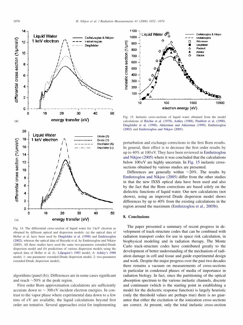
1070 H. Nikjoo et al. / Radiation Measurements 41 (2006) 1052–1074
Fig. 14. The differential cross-section of liquid water for 1 keV electron asobtained by different optical and dispersion models: (a) the optical data ofHeller et al. have been used by Dingfelder et al. (1998) and Emfietzoglou(2002), whereas the optical data of Hayashi et al. by Emfietzoglou and Nikjoo(2005). All three studies have used the same two-parameter extended-Drudedispersion model and (b) predictions of various dispersion models using theoptical data of Heller et al. (L: Liljequist’s 1983 model, A: Ashley’s 1988model, 1: one-parameter extended-Drude dispersion model, 2: two-parameterextended-Drude dispersion model).
algorithms (panel (b)). Differences are in some cases significantand reach ∼50% at the peak region.
First order Born approximation calculations are sufficientlyaccurate down to ∼ 300 eV incident electron energies. In con-trast to the vapor phase where experimental data down to a fewtens of eV are available, the liquid calculations beyond firstorder are tentative. Several approaches exist for implementing
Fig. 15. Inelastic cross-sections of liquid water obtained from the modelcalculations of Ritchie et al. (1978), Ashley (1988), Pimblott et al. (1990),Dingfelder et al. (1998), Akkerman and Akkerman (1999), Emfietzoglou(2002) and Emfietzoglou and Nikjoo (2005).
perturbation and exchange corrections to the first Born results.In general, their effect is to decrease the first order results byup to 40% at 100 eV. They have been reviewed in Emfietzoglouand Nikjoo (2005) where it was concluded that the calculationsbelow 100 eV are highly uncertain. In Fig. 15 inelastic cross-sections obtained by various studies are presented.
Differences are generally within ∼20%. The results byEmfietzoglou and Nikjoo (2005) differ from the other studiesin that the new IXSS optical data have been used and alsoby the fact that the Born corrections are based solely on thedielectric functions of liquid water. Our new calculations (notshown), using an improved Drude dispersion model showsdifferences by up to 40% from the existing calculations in theregion around the maximum (Emfietzoglou et al., 2005b).
8. Conclusions
The paper presented a summary of recent progress in de-velopment of track-structure codes that can be combined withradiation transport codes for use in space risk calculation, inbiophysical modeling and in radiation therapy. The MonteCarlo track-structure codes have contributed greatly to thedevelopment of better understanding of the mechanism of radi-ation damage in cell and tissue and guide experimental designand work. Despite the major progress over the past two decadesthere remains a vacuum on measurements of cross-sectionsin particular in condensed phases of media of importance inradiation biology. In fact, since the partitioning of the opticalabsorption spectrum to the various inelastic channels, discreteand continuum (which is the starting point in establishing amodel for the dielectric response function) is largely heuristic(only the threshold values are perhaps true) there is no guar-antee that either the excitation or the ionization cross-sectionsare correct. At present, only the total inelastic cross-section
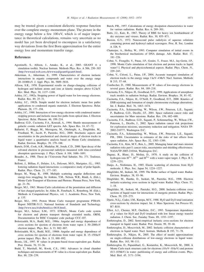
H. Nikjoo et al. / Radiation Measurements 41 (2006) 1052–1074 1071
may be trusted given a consistent dielectric response functionover the complete energy–momentum plane. The picture in theenergy range below a few 100 eV, which is of major impor-tance in theoretical calculations, remains very uncertain as nomodel has yet been developed to encompass in a satisfactoryway deviations from the first Born approximation for the entireenergy loss and momentum transfer range.
References
Agostinelli, S., Allison, J., Amako, K., et al., 2003. GEANT 4: asimulation toolkit. Nuclear Instrum. Methods Phys. Res. A 506, 250–303〈http://wwwasd.web.cern.ch/wwwasd/geant4/geant4.html〉.
Akkerman, A., Akkerman, E., 1999. Characteristics of electron inelasticinteractions in organic compounds and water over the energy range20–10 000 eV. J. Appl. Phys. 86, 5809–5816.
Allison, S.K., 1958. Experimental results on charge-changing collisions ofhydrogen and helium atoms and ions at kinetic energies above 0.2 keV.Rev. Mod. Phys. 30, 1137–1168.
Ashley, J.C., 1982a. Stopping power of liquid water for low-energy electrons.Radiat. Res. 89, 25–31.
Ashley, J.C., 1982b. Simple model for electron inelastic mean free paths:applications to condensed organic materials. J. Electron Spectrosc. Relat.Phenom. 28, 177–194.
Ashley, J.C., 1988. Interaction of low-energy electrons with condensed matter:stopping powers and inelastic mean free paths from optical data. J. ElectronSpectrosc. Relat. Phenom. 46, 199–214.
Badhwar, G.D., Cucinotta, F.A., Konradi, A., 1994. Shuttle measurements ofgalactic cosmic radiation LET spectra. Adv. Space Res. 14, 67–72.
Ballarini, F., Biaggi, M., Merzagora, M., Ottolenghi, A., Dingfelder, M.,Friedland, W., Jacob, P., Paretzke, H.G., 2000. Stochastic aspects anduncertainties in the prechemical and chemical stages of electron tracks inliquid water: a quantitative analysis based on Monte Carlo simulations.Radiat. Environ. Biophys. 39, 179–188.
Bartels, D.M., Cook, A.R., Mudaliar, M., Jonah, C.D., 2000. Spur decay of thesolvated electron in picosecond radiolysis measured with time-correlatedabsorption spectroscopy. J. Phys. Chem. A 104, 1686–1691.
Beaudre, A., 1988. These de l’Universite Paul Sabatier, No. 371. Toulouse,France.
Belloni, J., Billiau, F., Delaire, J.A., Delcourt, M.O., Marignier, J.L., 1983.Ionizing radiation–liquid interactions: a comparative study of polar liquids.Radiat. Phys. Chem. 21, 177–183.
Berger, M., Wang, R., 1988. Multiple scattering angular deflections andenergy-loss straggling. In: Jenkins, T.M., Nelson, W.R., Rindi, A. (Eds.),Monte Carlo Transport of Electrons and Photons. Plenum Press, New York,pp. 21–56.
Berger, M.J., 1963. Monte-Carlo calculations of the penetration and diffusionof fast charged particles. In: Alder, B., Fenebach, S., Rotenberg, M. (Eds.),Methods in Computational Physics, vol. 1. Academic Press, New York,p. 135.
Berger, M.J., 1993. Proton Monte Carlo transport programme PTRAN.Report NISTIR-5113. National Institute of Standards and Technology.〈http://www.nea.fr/abs/html/ccc-0618.html〉.
Berger, M.J., Seltzer, S.M., 1973. ETRAN, Monte Carlo code systemfor electron and photon transport through extended media. ORNLDocumentation for RISC Computer code package CCC-107.
Bolorizadeh, M.A., Rudd, M.E., 1986a. Angular and energy dependence ofcross sections for ejection of electrons from water vapor. I. 50–2000 eVelectron impact. Phys. Rev. A 33, 882–887.
Bolorizadeh, M.A., Rudd, M.E., 1986b. Angular and energy dependence ofcross sections for ejection of electrons from water vapor. II. 15–150 keVproton impact. Phys. Rev. A 33, 888–892.
Bronic, I.K., 1997. W values in propane-based tissue-equivalent gas. Radiat.Prot. Dosim. 70, 33–36.
Budd, T., Marshall, M., Kwok, C.S., 1981. Advances in cloud chambertechniques and measurements of W -value in a tissue equivalent gas. Radiat.Res. 88, 228–239.
Burch, P.R., 1957. Calculations of energy dissipation characteristics in waterfor various radiations. Radiat. Res. 6, 289–301.
Butts, J.J., Katz, R., 1967. Theory of RBE for heavy ion bombardment ofdry enzymes and viruses. Radiat. Res. 30, 855–871.
Buxton, G.V., 1972. Nanosecond pulse radiolysis of aqueous solutionscontaining proton and hydroxyl radical scavengers. Proc. R. Soc. LondonA 328, 9.
Chatterjee, A., Holley, W., 1993. Computer simulation of initial events inthe biochemical mechanisms of DNA damage. Adv. Radiat. Biol. 17,181–226.
Cobut, V., Frongillo, Y., Patau, J.P., Goulet, T., Fraser, M.J., Jay-Gerin, J.P.,1998. Monte Carlo simulation of fast electron and proton tracks in liquidwater? I. Physical and physicochemical aspects. Radiat. Phys. Chem. 51,229–243.
Cobut, V., Cirioni, L., Patau, J.P., 2004. Accurate transport simulation ofelectron tracks in the energy range 1 keV–4 MeV. Nucl. Instrum. MethodsB 215, 57–68.
Combecher, D., 1980. Measurements of W values of low-energy electrons inseveral gases. Radiat. Res. 84, 189–218.
Cucinotta, F.A., Nikjoo, H., Goodhead, D.T., 1999. Applications of amorphoustrack models in radiation biology. Radiat. Environ. Biophys. 38, 81–92.
Cucinotta, F.A., Nikjoo, H., O’Neill, P., Goodhead, D.T., 2000. Kinetics ofDSB rejoining and formation of simple chromosome exchange aberrations.Int. J. Radiat. Biol. 76, 1463–1474.
Cucinotta, F.A., Schimmerling, W., Wilson, J.W., Peterson, L.E., Saganti,P., Badhwar, G.D., Dicello, J.F., 2001. Space radiation cancer risks anduncertainties for Mars missions. Radiat. Res. 156, 682–688.
Cucinotta, F.A., Badhwar, G.D., Saganti, P., Schimmerling, W., Wilson J.W.,Peterson, L., Dicello, J., 2002. Space radiation cancer risk projectionsfor exploration missions, uncertainty reduction and mitigation. NASA TP-2002-210777, Washington D.C.
Cucinotta, F.A., Schimmerling, W., Wilson, J.W., Peterson, L.E., Saganti,P.B., 2004. Uncertainties in estimates of the risks of late effects fromspace radiation. Adv. Space Res. 32, 1383–1389.
Cucinotta, F.A., Kim, M.Y., Ren, L., 2005. Managing lunar and mars missionradiation risks part I: cancer risks, uncertainties and shielding effectiveness.NASA/TP-2005-210164, Washington D.C.
Dagnac, R., Blanc, D., Molina, D., 1970. A study on the collision ofhydrogen ions H1+, H2+ and H3+ with a water-vapor target. J. Phys. B 3,1239–1251.
Danjo, A., Nishimura, H., 1985. Elastic scattering of electrons from H2Omolecule. J. Phys. Soc. Japan 54, 1224–1227.
Dingfelder, M., Inokuti, M., 1999. The Bethe surface of liquid water. Radiat.Environ. Biophys. 38, 93–96.
Dingfelder, M., Hantke, D., Inokuti, M., Paretzke, H.G., 1998. Electroninelastic-scattering cross sections in liquid water. Radiat. Phys. Chem. 53,1–18.
Dingfelder, M., Inokuti, M., Paretzke, H.G., 2000. Inelastic-collision crosssections of liquid water for interactions of energetic protons. Radiat. Phys.Chem. 59, 255–275.
Djuric, N.Lj., Cadez, I.M., Kurepa, M.V., 1988. H2O and D2O total ionisationcross-sections by electron impact. Int. J. Mass Spectrom. Ion Process 83,R7–R10.
Elliot, A.J., Chenier, M.P., Ouellette, D.C., 1993. Temperature dependenceof g values for H2O and D2O irradiated with low linear energy transferradiation. J. Chem. Soc. Faraday Trans. 89, 1193–1197.
Emfietzoglou, D., 2002. Semi-empirical inelastic cross-sections for electrontransport in liquid water. Radiat. Prot. Dosim. 99, 39–46.
Emfietzoglou, D., Moscovitch, M., 2002. Inelastic collision characteristics ofelectrons in liquid water. Nucl. Instrum. Methods B 193, 71–78.
Emfietzoglou, D., Nikjoo, H., 2005. The effect of model approximationson single-collision distributions of low-energy electrons in liquid water.Radiat. Res. 163, 98–111.
Emfietzoglou, D., Papamihael, G., Kostarelos, K., Moscovitch, M., 2000. AMonte Carlo track structure code for electrons (10 eV–10 keV) and protons(0.3–10 MeV) in water: partitioning of energy and collision events. Phys.Med. Biol. 45, 3171–3194.

1072 H. Nikjoo et al. / Radiation Measurements 41 (2006) 1052–1074
Emfietzoglou, D., Karava, K., Papamichael, G., Moscovitch, M., 2003. MonteCarlo simulation of the energy loss of low-energy electrons in liquid water.Phys. Med. Biol. 48, 2355–2371.
Emfietzoglou, D., Pathak, A., Moscovitch, M., 2005a. Modeling the energyand momentum dependent loss function of the valence shells of liquidwater. Nucl. Instrum. Methods B 230, 77–84.
Emfietzoglou, D., Cucinotta, F.A., Nikjoo, H., 2005b. A complete dielectricresponse model for liquid water: a solution of the Bethe ridge problem.Radiat. Res. 164, 202–211.
Everhart, E., Stone, G., Carbone, R.J., 1955. Classical calculation ofdifferential cross section for scattering from a Coulomb potential withexponential screening. Phys. Rev. 99, 1287–1290.
Fasso, A., Ferrari, A., Ranft, J., Sala, P., 2005. Current version of FLUKA2005.6. 〈http://www.fluka.org/〉.
Fernandez-Varea, J.M., Mayol, R., Salvat, F., Liljequist, D., 1992. Acomparison of inelastic scattering models based on a �-functionrepresentation of the Bethe surface. J. Phys. Condens. Matter 4,2879–2890.
Fernandez-Varea, J.M., Mayol, R., Liljequist, D., Salvat, F., 1993. Inelasticscattering of electrons in solids from a generalized oscillator strengthmodel using optical and photoelectric data. J. Phys. Condens. Matter 5,3593–3610.
Fernandez-Varea, J.M., Liljequist, D., Csillag, S., Rdty, R., Salvat, F., 1996.Monte Carlo simulation of 0.1–100 keV electron and positron transport insolids using optical data and partial wave methods. Nucl. Instrum. MethodsB 108, 35–50.
Friedland, W., Bernhard, P., Jacob, P., Paretzke, H.G., Dingfelder, M., 2002.Simulation of DNA damage after proton and low LET irradiation. Radiat.Prot. Dosim. 99, 99–102.
Friedland, W., Jacob, P., Bernhardt, P., Paretzke, H.G., Dingfelder, M., 2003.Simulation of DNA damage after proton irradiation. Radiat Res. 159,401–410.
Goldstein, H., 1950. Classical Mechanics. Addison-Wesley, Reading, MA,USA.
Goodhead, D.T., 1994. Initial events in the cellular effects of ionisingradiations; clustered damage in DNA. Int. J. Radiat. Biol. 65, 7–17.
Goorley, T., Brown, F., Cox, L.J., MCNP5TM, 2003. Improvements forWindows PCs. In: Proceedings of the M&C 2003: Nuclear Mathematicaland Computational Sciences: a Century in Review, A Century Anew,Gatlinburg, TN, April 6–10, 〈http://laws.lanl.gov/x5/MCNP/index.html〉.
Green, A.E.S., McNeal, R.J., 1971. Analytic cross sections for inelasticcollisions of protons and hydrogen atoms with atomic and molecular gases.J. Geophys. Res. 76, 133–144.
Green, A.E.S., Stolarski, R.S., 1972. Analytic models of electron impactexcitation cross sections. J. Atm. Terr. Phys. 34, 1703–1717.
Grosswendt, B., Baek, W.Y., 1995. The energy dependence of W values forprotons of energies up to 10 MeV. Radiat. Prot. Dosim. 61, 267–274.
Gudowska, I., Sobolevsky, N., Andreo, P., Belkic, D., Brahme, A., 2004. Ionbeam transport in tissue like media using the Monte Carlo code SHIELD-HIT. Phys. Med. Biol. 49, 1933–1958.
Hartmann Siantar, C.L., Moses, E.I., 1998. The PEREGRINeTM programmer:using physics and computer simulation to improve radiation therapyfor cancer. Eur. J. Phys. 19, 513–521 〈http://www.llnl.gov/peregrine/techpubs.html〉.
Hayashi, H., Watanabe, N., Udagawa, Y., 1998. Optical spectra of liquid waterin vacuum uv region by means of inelastic X-ray scattering spectroscopy.J. Chem. Phys. 108, 823–825.
Hayashi, H., Watanabe, N., Udagawa, Y., Kao, C.C., 2000. The completeoptical spectrum of liquid water measured by inelastic x-ray scattering.Proc. Natl. Acad. Sci. 97, 6264–6266.
Hayashi, M., 1989. Electron collision cross-sections for atoms and moleculesdetermined from beam and swarm data. IAEA-TECDOC-506, pp. 194–200.
Heller, J.M., Hamm, R.N., Birkhoff, R.D., Painter, L.R., 1974. Collectiveoscillation in liquid water. J. Chem. Phys. 60, 3483–3486.
Hendricks, J.S., McKinney, G.W., Trellue, H.R., et al., 2005. MCNPX, Version2.6.A. Los Alamos National Laboratory. 〈http://mcnpx.lanl.gov/main.html〉.
Howard-Flanders, P., 1958. Physical and chemical mechanisms in the injuryof cells by ionizing radiations. Adv. Biol. Med. Phys. 6, 553–603.
Hubbard, J., 1955. The dielectric theory of electronic interactions in solids.Proc. Phys. Soc. (London) A 68, 976–986.
IAEA, 1995. Atomic and molecular data for radiotherapy and radiationresearch. IAEA-TECDOC-799, IAEA, Vienna.
ICRU, 1970. Linear energy transfer. Report 16, International Commission ofRadiation Units and Measurements, Bethesda, MD.
ICRU, 1978. Basic aspects of high energy particle interactions and radiationdosimetry. Report 28, International Commission of Radiation Units andMeasurements, Bethesda, MD. 〈http://www.icru.org〉.
ICRU, 1979. Average energy required to produce an ion pair. Report31, International Commission of Radiation Units and Measurements,Washington, DC. 〈http://www.icru.org〉.
ICRU, 1983. Microdosimetry. Report 36, International Commission ofRadiation Units and Measurements, Bethesda, MD. 〈http://www.icru.org〉.
ICRU, 1984. Stopping powers for electrons and positrons. Report 37,International Commission of Radiation Units and Measurements, Bethesda,MD. 〈http://www.icru.org〉.
ICRU, 1993. Stopping powers and ranges for protons and alphaparticles. Report 49, International Commission of Radiation Units andMeasurements, Bethesda, MD. 〈http://www.icru.org〉.
ICRU, 1995. Secondary electron spectra from charged particle interactions.Report 55, International Commission of Radiation Units andMeasurements, Bethesda, MA 〈http://www.icru.org〉.
Inokuti, M., 1971. Inelastic collisions of fast charged particles with atomsand molecules—the Bethe theory revisited. Rev. Mod. Phys. 43, 297–347.
Inokuti, M., 1991. How is radiation energy absorption different between thecondensed phase and the gas phase? Radiat. Eff. Defects Solids 117,143–162.
Ito, A., 1987. Calculation of double strand break probability of DNA for lowLET radiations based on track structure analysis. Nuclear and atomic datafor radiotherapy and related radiobiology. International Atomic EnergyAgency, IAEA, Vienna.
Iwase, H., Niita, K., Nakamura, T., 2002. Development of general-purposeparticle and heavy ion transport Monte Carlo code. J. Nucl. Sci. 39,1142–1151.
Jay-Gerin, J.P., Ferradini, C., 2000. A new estimate of the OH radical yieldat early times in the radiolysis of liquid water. Chem. Phys. Lett. 317,388–391.
Jenkins, T.M., Nelson, W.R., Rindi, A., (Eds.) 1987. Monte Carlo Transportof Electrons and Photons. Plenum Press, New York.
Katase, A., Ishibashi, K., Matsumoto, Y., Sakae, T., Maezono, S., Murakami,E., Watanabe, K., Maki, H., 1986. Elastic scattering of electrons by watermolecules over the range 100–1000 eV. J. Phys. B 19, 2715–2734.
Katz, R., 2003. The parameter-free track structure model of Scholz and Kraftfor heavy-ion cross sections. Radiat. Res. 160, 724–728.
Katz, R., Cucinotta, F.A., Wilson, J.W., Shinn, J.L., Ngo, D.M., 1993. Amodel of cell damage in space flight. In: Swenberg, C.E., Horneck, G.,Stassinopoulos, E.G. (Eds.), Biological Effects and Physics of Solar andGalactic Cosmic Radiation, Part A. Plenum Press, New York, pp. 235–268.
Kawrakow, I., 2000. Accurate condensed history Monte Carlo simulation ofelectron transport. I. EGSnrc, the new EGS4 version. Med. Phys. 27 (3),485–498.
Kellerer, A.M., Chemelevsky, D., 1975. Criteria for the applicability of LET.Radiat. Res. 63, 226–234.
Kling, A., Barao, F., Nakagawa, M., Tavora, L., Vaz, P., (Eds.) (2000).MC2000 Advanced Monte Carlo for Radiation Physics, Particle TransportSimulation and Applications. Springer, Berlin.
Kraft, G., Scholz, M., Bechthold, U., 1999. Tumour therapy and trackstructure. Radiat. Environ. Biophys. 38, 229–237.
Kutcher, G.J., Green, A.E.S., 1976. A model for energy deposition in liquidwater. Radiat. Res. 67, 408–425.
Lappa, A.V., Bigildeev, E.A., Burmistrov, D.S., Vasilyev, O.N., 1993. Trioncode for radiation action calculations and its application in microdosimetryand radiobiology. Radiat. Environ. Biophys. 32, 1–19.
LaVerne, J.A., 2000. OH radicals and oxidizing products in the gammaradiolysis of water. Radiat. Res. 153, 196–200.
LaVerne, J.A., Mozumder, A., 1993. Concerning plasmon excitations in liquidwater. Radiat. Res. 133, 282.
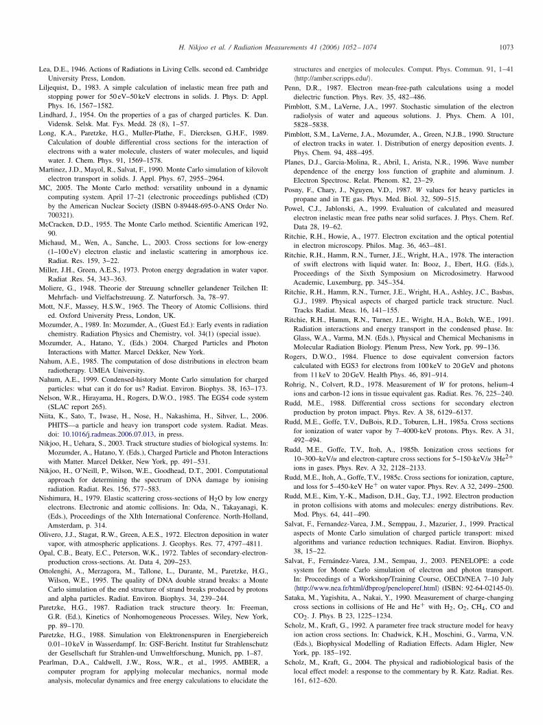
H. Nikjoo et al. / Radiation Measurements 41 (2006) 1052–1074 1073
Lea, D.E., 1946. Actions of Radiations in Living Cells. second ed. CambridgeUniversity Press, London.
Liljequist, D., 1983. A simple calculation of inelastic mean free path andstopping power for 50 eV–50 keV electrons in solids. J. Phys. D: Appl.Phys. 16, 1567–1582.
Lindhard, J., 1954. On the properties of a gas of charged particles. K. Dan.Vidensk. Selsk. Mat. Fys. Medd. 28 (8), 1–57.
Long, K.A., Paretzke, H.G., Muller-Plathe, F., Diercksen, G.H.F., 1989.Calculation of double differential cross sections for the interaction ofelectrons with a water molecule, clusters of water molecules, and liquidwater. J. Chem. Phys. 91, 1569–1578.
Martinez, J.D., Mayol, R., Salvat, F., 1990. Monte Carlo simulation of kilovoltelectron transport in solids. J. Appl. Phys. 67, 2955–2964.
MC, 2005. The Monte Carlo method: versatility unbound in a dynamiccomputing system. April 17–21 (electronic proceedings published (CD)by the American Nuclear Society (ISBN 0-89448-695-0-ANS Order No.700321).
McCracken, D.D., 1955. The Monte Carlo method. Scientific American 192,90.
Michaud, M., Wen, A., Sanche, L., 2003. Cross sections for low-energy(1–100 eV) electron elastic and inelastic scattering in amorphous ice.Radiat. Res. 159, 3–22.
Miller, J.H., Green, A.E.S., 1973. Proton energy degradation in water vapor.Radiat .Res. 54, 343–363.
Moliere, G., 1948. Theorie der Streuung schneller gelandener Teilchen II:Mehrfach- und Vielfachstreuung. Z. Naturforsch. 3a, 78–97.
Mott, N.F., Massey, H.S.W., 1965. The Theory of Atomic Collisions. thirded. Oxford University Press, London, UK.
Mozumder, A., 1989. In: Mozumder, A., (Guest Ed.): Early events in radiationchemistry. Radiation Physics and Chemistry, vol. 34(1) (special issue).
Mozumder, A., Hatano, Y., (Eds.) 2004. Charged Particles and PhotonInteractions with Matter. Marcel Dekker, New York.
Nahum, A.E., 1985. The computation of dose distributions in electron beamradiotherapy. UMEA University.
Nahum, A.E., 1999. Condensed-history Monte Carlo simulation for chargedparticles: what can it do for us? Radiat. Environ. Biophys. 38, 163–173.
Nelson, W.R., Hirayama, H., Rogers, D.W.O., 1985. The EGS4 code system(SLAC report 265).
Niita, K., Sato, T., Iwase, H., Nose, H., Nakashima, H., Sihver, L., 2006.PHITS—a particle and heavy ion transport code system. Radiat. Meas.doi: 10.1016/j.radmeas.2006.07.013, in press.
Nikjoo, H., Uehara, S., 2003. Track structure studies of biological systems. In:Mozumder, A., Hatano, Y. (Eds.), Charged Particle and Photon Interactionswith Matter. Marcel Dekker, New York, pp. 491–531.
Nikjoo, H., O’Neill, P., Wilson, W.E., Goodhead, D.T., 2001. Computationalapproach for determining the spectrum of DNA damage by ionisingradiation. Radiat. Res. 156, 577–583.
Nishimura, H., 1979. Elastic scattering cross-sections of H2O by low energyelectrons. Electronic and atomic collisions. In: Oda, N., Takayanagi, K.(Eds.), Proceedings of the XIth International Conference. North-Holland,Amsterdam, p. 314.
Olivero, J.J., Stagat, R.W., Green, A.E.S., 1972. Electron deposition in watervapor, with atmospheric applications. J. Geophys. Res. 77, 4797–4811.
Opal, C.B., Beaty, E.C., Peterson, W.K., 1972. Tables of secondary-electron-production cross-sections. At. Data 4, 209–253.
Ottolenghi, A., Merzagora, M., Tallone, L., Durante, M., Paretzke, H.G.,Wilson, W.E., 1995. The quality of DNA double strand breaks: a MonteCarlo simulation of the end structure of strand breaks produced by protonsand alpha particles. Radiat. Environ. Biophys. 34, 239–244.
Paretzke, H.G., 1987. Radiation track structure theory. In: Freeman,G.R. (Ed.), Kinetics of Nonhomogeneous Processes. Wiley, New York,pp. 89–170.
Paretzke, H.G., 1988. Simulation von Elektronenspuren in Energiebereich0.01–10 keV in Wasserdampf. In: GSF-Bericht. Institut fur Strahlenschutzder Gesellschaft fur Strahlen-und Umweltforschung, Munich, pp. 1–87.
Pearlman, D.A., Caldwell, J.W., Ross, W.R., et al., 1995. AMBER, acomputer program for applying molecular mechanics, normal modeanalysis, molecular dynamics and free energy calculations to elucidate the
structures and energies of molecules. Comput. Phys. Commun. 91, 1–41〈http://amber.scripps.edu/〉.
Penn, D.R., 1987. Electron mean-free-path calculations using a modeldielectric function. Phys. Rev. 35, 482–486.
Pimblott, S.M., LaVerne, J.A., 1997. Stochastic simulation of the electronradiolysis of water and aqueous solutions. J. Phys. Chem. A 101,5828–5838.
Pimblott, S.M., LaVerne, J.A., Mozumder, A., Green, N.J.B., 1990. Structureof electron tracks in water. 1. Distribution of energy deposition events. J.Phys. Chem. 94, 488–495.
Planes, D.J., Garcia-Molina, R., Abril, I., Arista, N.R., 1996. Wave numberdependence of the energy loss function of graphite and aluminum. J.Electron Spectrosc. Relat. Phenom. 82, 23–29.
Posny, F., Chary, J., Nguyen, V.D., 1987. W values for heavy particles inpropane and in TE gas. Phys. Med. Biol. 32, 509–515.
Powel, C.J., Jablonski, A., 1999. Evaluation of calculated and measuredelectron inelastic mean free paths near solid surfaces. J. Phys. Chem. Ref.Data 28, 19–62.
Ritchie, R.H., Howie, A., 1977. Electron excitation and the optical potentialin electron microscopy. Philos. Mag. 36, 463–481.
Ritchie, R.H., Hamm, R.N., Turner, J.E., Wright, H.A., 1978. The interactionof swift electrons with liquid water. In: Booz, J., Ebert, H.G. (Eds.),Proceedings of the Sixth Symposium on Microdosimetry. HarwoodAcademic, Luxemburg, pp. 345–354.
Ritchie, R.H., Hamm, R.N., Turner, J.E., Wright, H.A., Ashley, J.C., Basbas,G.J., 1989. Physical aspects of charged particle track structure. Nucl.Tracks Radiat. Meas. 16, 141–155.
Ritchie, R.H., Hamm, R.N., Turner, J.E., Wright, H.A., Bolch, W.E., 1991.Radiation interactions and energy transport in the condensed phase. In:Glass, W.A., Varma, M.N. (Eds.), Physical and Chemical Mechanisms inMolecular Radiation Biology. Plenum Press, New York, pp. 99–136.
Rogers, D.W.O., 1984. Fluence to dose equivalent conversion factorscalculated with EGS3 for electrons from 100 keV to 20 GeV and photonsfrom 11 keV to 20 GeV. Health Phys. 46, 891–914.
Rohrig, N., Colvert, R.D., 1978. Measurement of W for protons, helium-4ions and carbon-12 ions in tissue equivalent gas. Radiat. Res. 76, 225–240.
Rudd, M.E., 1988. Differential cross sections for secondary electronproduction by proton impact. Phys. Rev. A 38, 6129–6137.
Rudd, M.E., Goffe, T.V., DuBois, R.D., Toburen, L.H., 1985a. Cross sectionsfor ionization of water vapor by 7–4000-keV protons. Phys. Rev. A 31,492–494.
Rudd, M.E., Goffe, T.V., Itoh, A., 1985b. Ionization cross sections for10–300–keV/u and electron-capture cross sections for 5–150-keV/u 3He2+ions in gases. Phys. Rev. A 32, 2128–2133.
Rudd, M.E., Itoh, A., Goffe, T.V., 1985c. Cross sections for ionization, capture,and loss for 5–450-keV He+ on water vapor. Phys. Rev. A 32, 2499–2500.
Rudd, M.E., Kim, Y.-K., Madison, D.H., Gay, T.J., 1992. Electron productionin proton collisions with atoms and molecules: energy distributions. Rev.Mod. Phys. 64, 441–490.
Salvat, F., Fernandez-Varea, J.M., Semppau, J., Mazurier, J., 1999. Practicalaspects of Monte Carlo simulation of charged particle transport: mixedalgorithms and variance reduction techniques. Radiat. Environ. Biophys.38, 15–22.
Salvat, F., Fernández-Varea, J.M., Sempau, J., 2003. PENELOPE: a codesystem for Monte Carlo simulation of electron and photon transport.In: Proceedings of a Workshop/Training Course, OECD/NEA 7–10 July〈http://www.nea.fr/html/dbprog/peneloperef.html〉 (ISBN: 92-64-02145-0).
Sataka, M., Yagishita, A., Nakai, Y., 1990. Measurement of charge-changingcross sections in collisions of He and He+ with H2, O2, CH4, CO andCO2. J. Phys. B 23, 1225–1234.
Scholz, M., Kraft, G., 1992. A parameter free track structure model for heavyion action cross sections. In: Chadwick, K.H., Moschini, G., Varma, V.N.(Eds.), Biophysical Modelling of Radiation Effects. Adam Higler, NewYork, pp. 185–192.
Scholz, M., Kraft, G., 2004. The physical and radiobiological basis of thelocal effect model: a response to the commentary by R. Katz. Radiat. Res.161, 612–620.
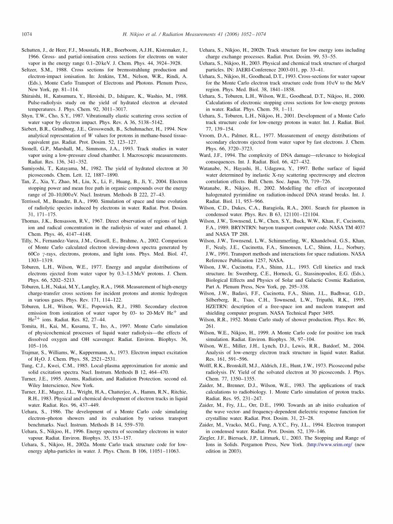
1074 H. Nikjoo et al. / Radiation Measurements 41 (2006) 1052–1074
Schutten, J., de Heer, F.J., Moustafa, H.R., Boerboom, A.J.H., Kistemaker, J.,1966. Gross- and partial-ionisation cross sections for electrons on watervapor in the energy range 0.1–20 keV. J. Chem. Phys. 44, 3924–3928.
Seltzer, S.M., 1988. Cross sections for bremsstrahlung production andelectron-impact ionisation. In: Jenkins, T.M., Nelson, W.R., Rindi, A.(Eds.), Monte Carlo Transport of Electrons and Photons. Plenum Press,New York, pp. 81–114.
Shiraishi, H., Katsumura, Y., Hiroishi, D., Ishigure, K., Washio, M., 1988.Pulse-radiolysis study on the yield of hydrated electron at elevatedtemperatures. J. Phys. Chem. 92, 3011–3017.
Shyn, T.W., Cho, S.Y., 1987. Vibrationally elastic scattering cross section ofwater vapor by electron impact. Phys. Rev. A 36, 5138–5142.
Siebert, B.R., Grindborg, J.E., Grosswendt, B., Schuhmacher, H., 1994. Newanalytical representation of W values for protons in methane-based tissue-equivalent gas. Radiat. Prot. Dosim. 52, 123–127.
Stonell, G.P., Marshall, M., Simmons, J.A., 1993. Track studies in watervapor using a low-pressure cloud chamber. I. Macroscopic measurements.Radiat. Res. 136, 341–352.
Sumiyoshi, T., Katayama, M., 1982. The yield of hydrated electron at 30picoseconds. Chem. Lett. 12, 1887–1890.
Tan, Z., Xia, Y., Zhao, M., Liu, X., Li, F., Huang, B., Ji, Y., 2004. Electronstopping power and mean free path in organic compounds over the energyrange of 20–10,000 eV. Nucl. Instrum. Methods B 222, 27–43.
Terrissol, M., Beaudre, B.A., 1990. Simulation of space and time evolutionof radiolytic species induced by electrons in water. Radiat. Prot. Dosim.31, 171–175.
Thomas, J.K., Bensasson, R.V., 1967. Direct observation of regions of highion and radical concentration in the radiolysis of water and ethanol. J.Chem. Phys. 46, 4147–4148.
Tilly, N., Fernandez-Varea, J.M., Grusell, E., Brahme, A., 2002. Comparisonof Monte Carlo calculated electron slowing-down spectra generated by60Co �-rays, electrons, protons, and light ions. Phys. Med. Biol. 47,1303–1319.
Toburen, L.H., Wilson, W.E., 1977. Energy and angular distributions ofelectrons ejected from water vapor by 0.3–1.5 MeV protons. J. Chem.Phys. 66, 5202–5213.
Toburen, L.H., Nakai, M.Y., Langley, R.A., 1968. Measurement of high-energycharge-transfer cross sections for incident protons and atomic hydrogenin various gases. Phys. Rev. 171, 114–122.
Toburen, L.H., Wilson, W.E., Popowich, R.J., 1980. Secondary electronemission from ionization of water vapor by 03- to 20-MeV He+ andHe2+ ions. Radiat. Res. 82, 27–44.
Tomita, H., Kai, M., Kusama, T., Ito, A., 1997. Monte Carlo simulationof physicochemical processes of liquid water radiolysis—the effects ofdissolved oxygen and OH scavenger. Radiat. Environ. Biophys. 36,105–116.
Trajmar, S., Williams, W., Kuppermann, A., 1973. Electron impact excitationof H2O. J. Chem. Phys. 58, 2521–2531.
Tung, C.J., Kwei, C.M., 1985. Local-plasma approximation for atomic andsolid excitation spectra. Nucl. Instrum. Methods B 12, 464–470.
Turner, J.E., 1995. Atoms, Radiation, and Radiation Protection. second ed.Wiley Interscience, New York.
Turner, J.E., Magee, J.L., Wright, H.A., Chatterjee, A., Hamm, R.N., Ritchie,R.H., 1983. Physical and chemical development of electron tracks in liquidwater. Radiat. Res. 96, 437–449.
Uehara, S., 1986. The development of a Monte Carlo code simulatingelectron–photon showers and its evaluation by various transportbenchmarks. Nucl. Instrum. Methods B 14, 559–570.
Uehara, S., Nikjoo, H., 1996. Energy spectra of secondary electrons in watervapour. Radiat. Environ. Biophys. 35, 153–157.
Uehara, S., Nikjoo, H., 2002a. Monte Carlo track structure code for low-energy alpha-particles in water. J. Phys. Chem. B 106, 11051–11063.
Uehara, S., Nikjoo, H., 2002b. Track structure for low energy ions includingcharge exchange processes. Radiat. Prot. Dosim. 99, 53–55.
Uehara, S., Nikjoo, H., 2003. Physical and chemical track structure of chargedparticles. IN: JAERI-Conference 2003-011, pp. 33–41.
Uehara, S., Nikjoo, H., Goodhead, D.T., 1993. Cross-sections for water vapourfor the Monte Carlo electron track structure code from 10 eV to the MeVregion. Phys. Med. Biol. 38, 1841–1858.
Uehara, S., Toburen, L.H., Wilson, W.E., Goodhead, D.T., Nikjoo, H., 2000.Calculations of electronic stopping cross sections for low-energy protonsin water. Radiat. Phys. Chem. 59, 1–11.
Uehara, S., Toburen, L.H., Nikjoo, H., 2001. Development of a Monte Carlotrack structure code for low-energy protons in water. Int. J. Radiat. Biol.77, 139–154.
Vroom, D.A., Palmer, R.L., 1977. Measurement of energy distributions ofsecondary electrons ejected from water vapor by fast electrons. J. Chem.Phys. 66, 3720–3723.
Ward, J.F., 1994. The complexity of DNA damage—relevance to biologicalconsequences. Int. J. Radiat. Biol. 66, 427–432.
Watanabe, N., Hayashi, H., Udagawa, Y., 1997. Bethe surface of liquidwater determined by inelastic X-ray scattering spectroscopy and electroncorrelation effects. Bull. Chem. Soc. Japan. 70, 719–726.
Watanabe, R., Nikjoo, H., 2002. Modelling the effect of incorporatedhalogenated pyrimidine on radiation-induced DNA strand breaks. Int. J.Radiat. Biol. 11, 953–966.
Wilson, C.D., Dukes, C.A., Baragiola, R.A., 2001. Search for plasmon incondensed water. Phys. Rev. B 63, 121101–121104.
Wilson, J.W., Townsend, L.W., Chen, S.Y., Buck, W.W., Khan, F., Cucinotta,F.A., 1989. BRYNTRN: baryon transport computer code. NASA TM 4037and NASA TP 288.
Wilson, J.W., Townsend, L.W., Schimmerling, W., Khandelwal, G.S., Khan,F., Nealy, J.E., Cucinotta, F.A., Simonsen, L.C., Shinn, J.L., Norbury,J.W., 1991. Transport methods and interactions for space radiations. NASAReference Publication 1257, NASA.
Wilson, J.W., Cucinotta, F.A., Shinn, J.L., 1993. Cell kinetics and trackstructure. In: Swenberg, C.E., Horneck, G., Stassinopoulos, E.G. (Eds.),Biological Effects and Physics of Solar and Galactic Cosmic Radiation,Part A. Plenum Press, New York, pp. 295–338.
Wilson, J.W., Badavi, F.F., Cucinotta, F.A., Shinn, J.L., Badhwar, G.D.,Silberberg, R., Tsao, C.H., Townsend, L.W., Tripathi, R.K., 1995.HZETRN: description of a free-space ion and nucleon transport andshielding computer program. NASA Technical Paper 3495.
Wilson, R.R., 1952. Monte Carlo study of shower production. Phys. Rev. 86,261.
Wilson, W.E., Nikjoo, H., 1999. A Monte Carlo code for positive ion tracksimulation. Radiat. Environ. Biophys. 38, 97–104.
Wilson, W.E., Miller, J.H., Lynch, D.J., Lewis, R.R., Batdorf, M., 2004.Analysis of low-energy electron track structure in liquid water. Radiat.Res. 161, 591–596.
Wolff, R.K., Bronskill, M.J., Aldrich, J.E., Hunt, J.W., 1973. Picosecond pulseradiolysis. IV. Yield of the solvated electron at 30 picoseconds. J. Phys.Chem. 77, 1350–1355.
Zaider, M., Brenner, D.J., Wilson, W.E., 1983. The applications of trackcalculations to radiobiology. 1. Monte Carlo simulation of proton tracks.Radiat. Res. 95, 231–247.
Zaider, M., Fry, J.L., Orr, D.E., 1990. Towards an ab initio evaluation ofthe wave vector- and frequency-dependent dielectric response function forcrystalline water. Radiat. Prot. Dosim. 31, 23–28.
Zaider, M., Vracko, M.G., Fung, A.Y.C., Fry, J.L., 1994. Electron transportin condensed water. Radiat. Prot. Dosim. 52, 139–146.
Ziegler, J.F., Biersack, J.P., Littmark, U., 2003. The Stopping and Range ofIons in Solids. Pergamon Press, New York. 〈http://www.srim.org/ (newedition in 2003).
Copyright © 2022 FDOKUMEN