Towards the automated evaluation of crystallization trials

Acta Cryst. (2002). D58, 1907±1914 Wilson � Automatic evaluation of crystallization trials 1907

research papers

Acta Crystallographica Section D

BiologicalCrystallography

ISSN 0907-4449

Towards the automated evaluation of crystallizationtrials

Julie Wilson

York Structural Biology Laboratory, Chemistry

Department, University of York, Heslington,

York YO10 5DD, England

Correspondence e-mail: [email protected]

# 2002 International Union of Crystallography

Printed in Denmark ± all rights reserved

A method to evaluate images from crystallization experiments

is described. Image discontinuities are used to determine

boundaries of artifacts in the images and these are then

considered as individual objects. This allows the edge of the

drop to be identi®ed and any objects outside this ignored.

Each object is evaluated in terms of a number of attributes

related to its size and shape, the curvature of the boundary

and the variance in intensity, as well as obvious crystal-like

characteristics such as straight sections of the boundary and

straight lines of constant intensity within the object. With each

object in the image assigned to one of a number of different

classes, an overall report can be given. The objects to be

considered have no prede®ned shape or size and, although one

may expect to see straight edges and angles in a crystal, this is

not a prerequisite for diffraction. This means there is much

overlap in the values of the variables expected for the

different classes. However, each attribute gives some informa-

tion about the object in question and, although no single

attribute can be expected to correctly classify an image, it has

been found that a combination of classi®ers gives very good

results.

Received 5 February 2002

Accepted 12 September 2002

1. Introduction

The number of putative protein sequences determined by

worldwide DNA-sequencing efforts in recent years now vastly

exceeds the rate at which protein structures can be analyzed

experimentally. Although methods are being developed to

predict protein structure from the sequence alone, accurate

experimentally determined molecular structures are necessary

for structure-based functional studies and effective drug

design. Crystallography can reliably provide the answer to

many such questions when suitable crystals are obtained.

Improvements to beamline optics and the intense highly

focused X-rays available at synchrotron sources now allow the

use of ¯ash-frozen micrometre-sized crystals. Along with

advances in protein expression and puri®cation, the auto-

mation of microcrystallization is an essential tool for high-

throughput protein crystallography. Robotic systems capable

of performing thousands of crystallization experiments a day

have been developed and are already in use in a number of

laboratories (Stevens, 2000). The results from each of these

experiments must be recorded and assessed routinely and

automatically. So far, the available detection software can only

indicate the presence or absence of crystal-like objects and

results must be veri®ed by manual inspection (Rupp, 2000).

The dif®culty is intrinsic to the problem: the size and

morphology of crystals can vary greatly and it is vital to

research papers

1908 Wilson � Automatic evaluation of crystallization trials Acta Cryst. (2002). D58, 1907±1914

develop software that can also identify other phenomena in

the drop. Microcrystals and aggregates, thin plates, clusters of

needles and crystalline precipitates all indicate conditions that

could be optimized and must be recognized as well as large

single crystals. Cracks and other irregularities in crystals also

have to be dealt with.

2. Image analysis

The edges of a structure are often the most important features

in pattern recognition, as demonstrated by our ability to

recognize an object from a rough line drawing, and the nature

of crystal growth makes edge detection an obvious choice for

identifying the presence of crystals. Traditionally, edges are

de®ned as pixel-intensity discontinuities within an image and

most edge-detection methods identify edge points from the

extrema of the ®rst- or second-order derivatives of the image

(see, for example, Marr & Hildreth, 1980).

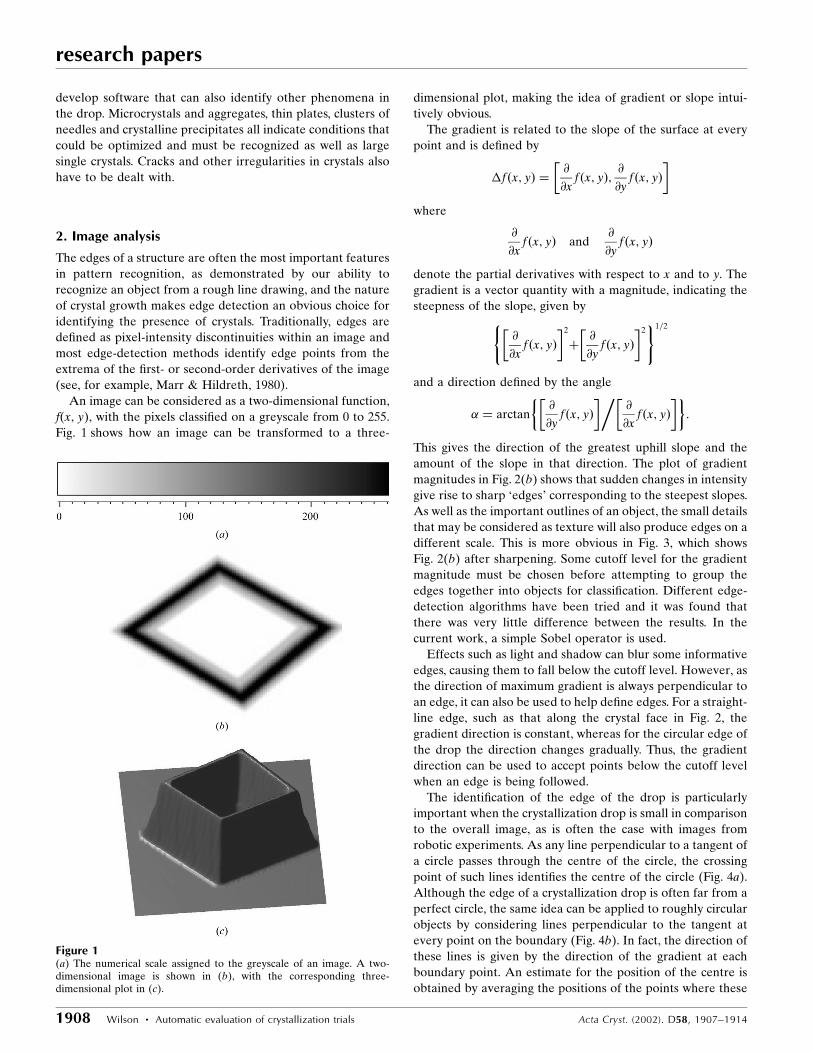
An image can be considered as a two-dimensional function,

f(x, y), with the pixels classi®ed on a greyscale from 0 to 255.

Fig. 1 shows how an image can be transformed to a three-

dimensional plot, making the idea of gradient or slope intui-

tively obvious.

The gradient is related to the slope of the surface at every

point and is de®ned by

�f �x; y� � @

@xf �x; y�; @

@yf �x; y�

� �where

@

@xf �x; y� and

@

@yf �x; y�

denote the partial derivatives with respect to x and to y. The

gradient is a vector quantity with a magnitude, indicating the

steepness of the slope, given by

@

@xf �x; y�

� �2

� @

@yf �x; y�

� �2( )1=2

and a direction de®ned by the angle

� � arctan@

@yf �x; y�

� ��@

@xf �x; y�

� �� :

This gives the direction of the greatest uphill slope and the

amount of the slope in that direction. The plot of gradient

magnitudes in Fig. 2(b) shows that sudden changes in intensity

give rise to sharp `edges' corresponding to the steepest slopes.

As well as the important outlines of an object, the small details

that may be considered as texture will also produce edges on a

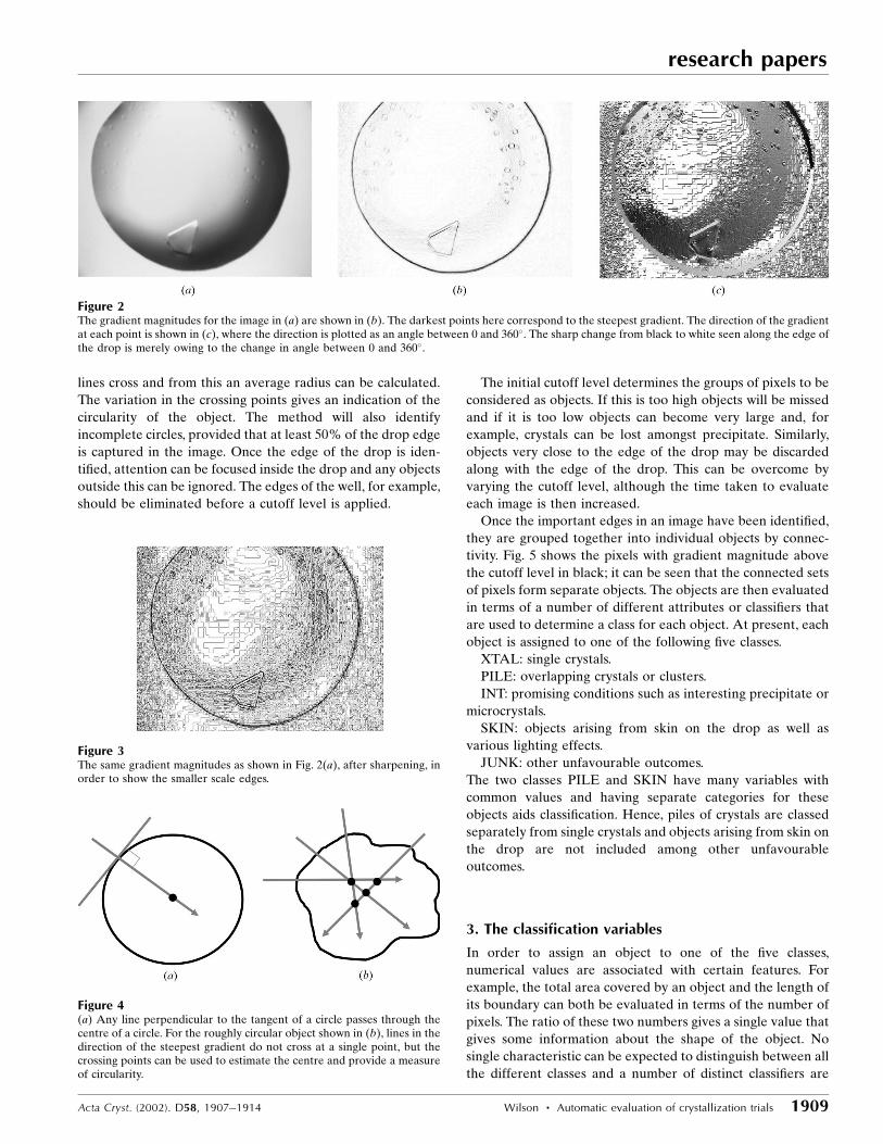
different scale. This is more obvious in Fig. 3, which shows

Fig. 2(b) after sharpening. Some cutoff level for the gradient

magnitude must be chosen before attempting to group the

edges together into objects for classi®cation. Different edge-

detection algorithms have been tried and it was found that

there was very little difference between the results. In the

current work, a simple Sobel operator is used.

Effects such as light and shadow can blur some informative

edges, causing them to fall below the cutoff level. However, as

the direction of maximum gradient is always perpendicular to

an edge, it can also be used to help de®ne edges. For a straight-

line edge, such as that along the crystal face in Fig. 2, the

gradient direction is constant, whereas for the circular edge of

the drop the direction changes gradually. Thus, the gradient

direction can be used to accept points below the cutoff level

when an edge is being followed.

The identi®cation of the edge of the drop is particularly

important when the crystallization drop is small in comparison

to the overall image, as is often the case with images from

robotic experiments. As any line perpendicular to a tangent of

a circle passes through the centre of the circle, the crossing

point of such lines identi®es the centre of the circle (Fig. 4a).

Although the edge of a crystallization drop is often far from a

perfect circle, the same idea can be applied to roughly circular

objects by considering lines perpendicular to the tangent at

every point on the boundary (Fig. 4b). In fact, the direction of

these lines is given by the direction of the gradient at each

boundary point. An estimate for the position of the centre is

obtained by averaging the positions of the points where these

Figure 1(a) The numerical scale assigned to the greyscale of an image. A two-dimensional image is shown in (b), with the corresponding three-dimensional plot in (c).

lines cross and from this an average radius can be calculated.

The variation in the crossing points gives an indication of the

circularity of the object. The method will also identify

incomplete circles, provided that at least 50% of the drop edge

is captured in the image. Once the edge of the drop is iden-

ti®ed, attention can be focused inside the drop and any objects

outside this can be ignored. The edges of the well, for example,

should be eliminated before a cutoff level is applied.

The initial cutoff level determines the groups of pixels to be

considered as objects. If this is too high objects will be missed

and if it is too low objects can become very large and, for

example, crystals can be lost amongst precipitate. Similarly,

objects very close to the edge of the drop may be discarded

along with the edge of the drop. This can be overcome by

varying the cutoff level, although the time taken to evaluate

each image is then increased.

Once the important edges in an image have been identi®ed,

they are grouped together into individual objects by connec-

tivity. Fig. 5 shows the pixels with gradient magnitude above

the cutoff level in black; it can be seen that the connected sets

of pixels form separate objects. The objects are then evaluated

in terms of a number of different attributes or classi®ers that

are used to determine a class for each object. At present, each

object is assigned to one of the following ®ve classes.

XTAL: single crystals.

PILE: overlapping crystals or clusters.

INT: promising conditions such as interesting precipitate or

microcrystals.

SKIN: objects arising from skin on the drop as well as

various lighting effects.

JUNK: other unfavourable outcomes.

The two classes PILE and SKIN have many variables with

common values and having separate categories for these

objects aids classi®cation. Hence, piles of crystals are classed

separately from single crystals and objects arising from skin on

the drop are not included among other unfavourable

outcomes.

3. The classification variables

In order to assign an object to one of the ®ve classes,

numerical values are associated with certain features. For

example, the total area covered by an object and the length of

its boundary can both be evaluated in terms of the number of

pixels. The ratio of these two numbers gives a single value that

gives some information about the shape of the object. No

single characteristic can be expected to distinguish between all

the different classes and a number of distinct classi®ers are


research papers

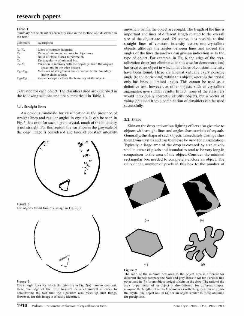
Figure 3The same gradient magnitudes as shown in Fig. 2(a), after sharpening, inorder to show the smaller scale edges.

Figure 4(a) Any line perpendicular to the tangent of a circle passes through thecentre of a circle. For the roughly circular object shown in (b), lines in thedirection of the steepest gradient do not cross at a single point, but thecrossing points can be used to estimate the centre and provide a measureof circularity.

Figure 2The gradient magnitudes for the image in (a) are shown in (b). The darkest points here correspond to the steepest gradient. The direction of the gradientat each point is shown in (c), where the direction is plotted as an angle between 0 and 360�. The sharp change from black to white seen along the edge ofthe drop is merely owing to the change in angle between 0 and 360�.

research papers


evaluated for each object. The classi®ers used are described in

the following sections and are summarized in Table 1.

3.1. Straight lines

An obvious candidate for classi®cation is the presence of

straight lines and regular angles in crystals. It can be seen in

Fig. 5 that even for such a good crystal, much of the boundary

is not straight. For this reason, the variation in the greyscale of

the edge image is considered and lines of constant intensity

anywhere within the object are sought. The length of the line is

important and lines of different length related to the overall

size of the object are used. Of course, it is possible to ®nd

straight lines of constant intensity across non-crystalline

objects, although the angles between lines and indeed the

angles of the lines themselves can give an indication as to the

type of object. For example, in Fig. 6, the edge of the crys-

tallization drop (not eliminated in this case for demonstration)

has created an object in which many lines of constant intensity

have been found. There are lines at virtually every possible

angle (to the horizontal) within this object, whereas the crystal

only has lines at limited angles. This cannot be used as a

de®nitive test, however, as other objects, such as crystalline

aggregates, give similar results. In fact, none of the classi®ers

would individually correctly identify objects, but a vector of

values obtained from a combination of classi®ers can be used

successfully.

3.2. Shape

Skin on the drop and various lighting effects also give rise to

objects with straight lines and angles characteristic of crystals.

Generally, the shape of such objects immediately distinguishes

them from crystals and can therefore be used for classi®cation.

Typically, a large area of the drop is covered by a relatively

small number of pixels and boundaries tend to be very long in

comparison to the area of the object. Consider the minimal

rectangular box needed to completely enclose an object. The

ratio of the number of pixels in this box to the number of

Table 1Summary of the classi®ers currently used in the method and described inthe text.

Classi®ers Description

X1±X4 Lines of constant intensity.X5 Ratio of minimum box area to object area.X6 Ratio of object's area to perimeter.X7 Rectangularity of minimal box.X8±X9 Variation in intensity with the object (in both the original

image and in the edge image).X10±X11 Measures of straightness and curvature of the boundary

(using chain codes).X12±X13 Shape descriptors from the boundary of the object.

Figure 6The straight lines for which the intensity in Fig. 2(b) remains constant.Here, the edge of the drop has not been eliminated in order todemonstrate the fact that the algorithm also picks up such things.However, for this image it is easily identi®ed.

Figure 7The ratio of the minimal box area to the object area is different fordifferent shapes: compare the back and grey areas in (a) for a crystal-likeobject and in (b) for an object typical of skin on the drop. The ratio of thearea to perimeter of an object is also different for different shapes:compare the length of the black boundaries with the grey areas in (c) forthe crystal-like object and in (d) for an object similar to those obtainedfor precipitate.

Figure 5The objects found from the image in Fig. 2(a).

pixels in the object will have a different value for different

shapes (see Fig. 7a). Furthermore, we can say something about

the shape of the minimal box, i.e. how rectangular it is. The

quantity

max�x; y��x� y� ;

where x and y are the lengths of the sides of the rectangle, will

give a value of 0.5 when x = y, i.e. when the minimal box is

square. However, if x is very small in comparison to y and we

have a very long thin rectangle, then we obtain a value close to

1.0. Fig. 7(b) shows a shape typical of precipitate that has been

grouped together as a single object. Here, there are a large

number of pixels on the boundary in comparison to the overall

size of the object, whereas the crystal-like object in the ®gure

has a smaller perimeter-to-area ratio.

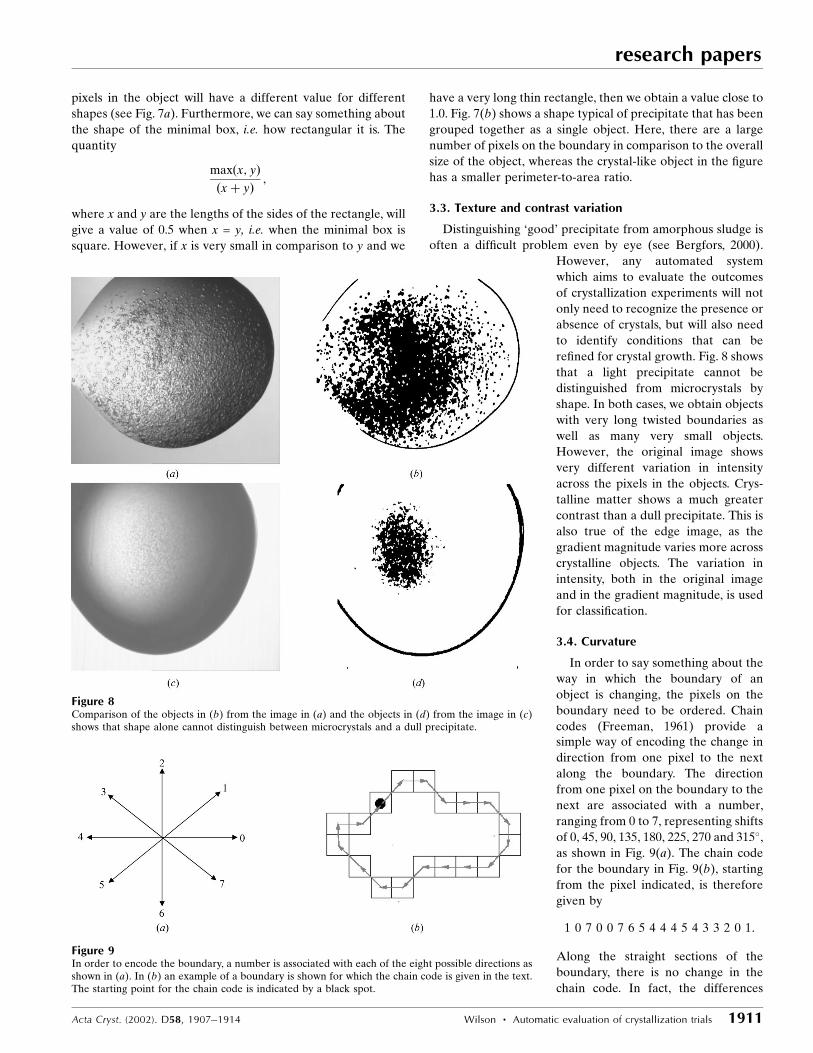
3.3. Texture and contrast variation

Distinguishing `good' precipitate from amorphous sludge is

often a dif®cult problem even by eye (see Bergfors, 2000).

However, any automated system

which aims to evaluate the outcomes

of crystallization experiments will not

only need to recognize the presence or

absence of crystals, but will also need

to identify conditions that can be

re®ned for crystal growth. Fig. 8 shows

that a light precipitate cannot be

distinguished from microcrystals by

shape. In both cases, we obtain objects

with very long twisted boundaries as

well as many very small objects.

However, the original image shows

very different variation in intensity

across the pixels in the objects. Crys-

talline matter shows a much greater

contrast than a dull precipitate. This is

also true of the edge image, as the

gradient magnitude varies more across

crystalline objects. The variation in

intensity, both in the original image

and in the gradient magnitude, is used

for classi®cation.

3.4. Curvature

In order to say something about the

way in which the boundary of an

object is changing, the pixels on the

boundary need to be ordered. Chain

codes (Freeman, 1961) provide asimple way of encoding the change in

direction from one pixel to the next

along the boundary. The direction

from one pixel on the boundary to the

next are associated with a number,

ranging from 0 to 7, representing shifts

of 0, 45, 90, 135, 180, 225, 270 and 315�,as shown in Fig. 9(a). The chain code

for the boundary in Fig. 9(b), starting

from the pixel indicated, is therefore

given by

1 0 7 0 0 7 6 5 4 4 4 5 4 3 3 2 0 1:

Along the straight sections of the

boundary, there is no change in the

chain code. In fact, the differences


research papers

Figure 8Comparison of the objects in (b) from the image in (a) and the objects in (d) from the image in (c)shows that shape alone cannot distinguish between microcrystals and a dull precipitate.

Figure 9In order to encode the boundary, a number is associated with each of the eight possible directions asshown in (a). In (b) an example of a boundary is shown for which the chain code is given in the text.The starting point for the chain code is indicated by a black spot.

research papers


between adjacent chain codes show how the boundary is

changing. An estimate for the curvature at each point on the

boundary is obtained by taking the chain code for this point

and subtracting the chain code for the preceding point. Thus,

the curvature for this boundary in is given by

ÿ1 ÿ1 1 0 ÿ1 ÿ1 ÿ1 ÿ1 0 0 1 ÿ1 ÿ1 0 ÿ1 ÿ2 1 0

[using 7 � ÿ1 (mod 8)]. The zeros correspond to the straight

sections of the boundary, with the number of consecutive zeros

indicating the length of that section. The parity is unimportant

here, as it merely shows a convex or concave corner and it is

the absolute value that matters. For example, the value of 2

towards the end of the boundary arises from the more acute

corner here. The sum of these absolute values provides a value

associated with the curvature and a measure of straightness is

obtained by considering the consecutive zeros.

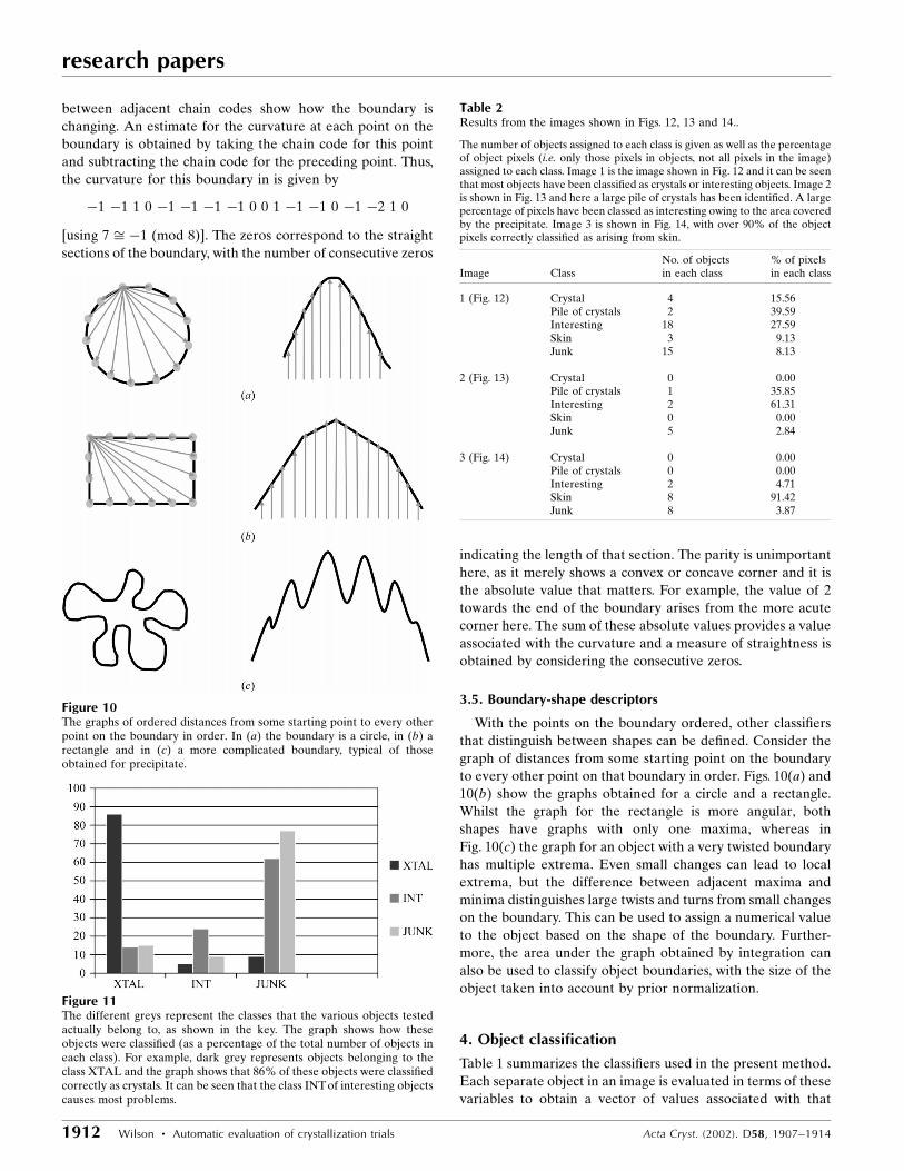
3.5. Boundary-shape descriptors

With the points on the boundary ordered, other classi®ers

that distinguish between shapes can be de®ned. Consider the

graph of distances from some starting point on the boundary

to every other point on that boundary in order. Figs. 10(a) and

10(b) show the graphs obtained for a circle and a rectangle.

Whilst the graph for the rectangle is more angular, both

shapes have graphs with only one maxima, whereas in

Fig. 10(c) the graph for an object with a very twisted boundary

has multiple extrema. Even small changes can lead to local

extrema, but the difference between adjacent maxima and

minima distinguishes large twists and turns from small changes

on the boundary. This can be used to assign a numerical value

to the object based on the shape of the boundary. Further-

more, the area under the graph obtained by integration can

also be used to classify object boundaries, with the size of the

object taken into account by prior normalization.

4. Object classification

Table 1 summarizes the classi®ers used in the present method.

Each separate object in an image is evaluated in terms of these

variables to obtain a vector of values associated with that

Figure 10The graphs of ordered distances from some starting point to every otherpoint on the boundary in order. In (a) the boundary is a circle, in (b) arectangle and in (c) a more complicated boundary, typical of thoseobtained for precipitate.

Figure 11The different greys represent the classes that the various objects testedactually belong to, as shown in the key. The graph shows how theseobjects were classi®ed (as a percentage of the total number of objects ineach class). For example, dark grey represents objects belonging to theclass XTAL and the graph shows that 86% of these objects were classi®edcorrectly as crystals. It can be seen that the class INT of interesting objectscauses most problems.

Table 2Results from the images shown in Figs. 12, 13 and 14..

The number of objects assigned to each class is given as well as the percentageof object pixels (i.e. only those pixels in objects, not all pixels in the image)assigned to each class. Image 1 is the image shown in Fig. 12 and it can be seenthat most objects have been classi®ed as crystals or interesting objects. Image 2is shown in Fig. 13 and here a large pile of crystals has been identi®ed. A largepercentage of pixels have been classed as interesting owing to the area coveredby the precipitate. Image 3 is shown in Fig. 14, with over 90% of the objectpixels correctly classi®ed as arising from skin.

Image ClassNo. of objectsin each class

% of pixelsin each class

1 (Fig. 12) Crystal 4 15.56Pile of crystals 2 39.59Interesting 18 27.59Skin 3 9.13Junk 15 8.13



object. These vectors are then used to assign

each object to a particular class.

A training data set consisting of�200 objects

from each class was used to provide probability

distributions for the classi®ers. The objects

were then classi®ed by eye and evaluated in

terms of the classi®ers that have been

described. Thus, for each classi®er, say Xi, a

probability distribution can be obtained from

the values of this variable for all the objects in

the class XTAL, say. In other words, we have

the conditional probability distribution

P�Xi=XTAL� for each i:

Labelling the ®ve classes Ck, for k = 1, . . . , 5,

gives

P�Xi=Ck� for k � 1; . . . ; 5

for each i. Also, since the number of objects in

each class is known, P(Ck) is known and so

Bayes theorem (see Bayes, 1763) can be used to

®nd the probability of an object being in any

class given that it has a particular value of Xi.

That is,

P�Ck=Xi� �P�Xi=Ck�P�Ck�P

j�1;5

P�Xi=Cj�P�Cj�:

Thus, each classi®er gives the probability of an

object being in a particular class. These prob-

abilities are combined by assuming indepen-

dence and simply multiplying them together to

obtain

P�Ck=fX1;X2; . . . ;X13g� �Q

i�1;13

WiP�Ck=Xi�;

where the Wi indicate weights. In the results of

the next section, all the classi®ers were given

equal weights, although some may well prove to

be more reliable than others and weighting

schemes are now being tried. Weights would be

accounted for automatically in a suitable neural

network combination of the classi®ers and such

a system is also being considered.

5. Results

With the probability distributions obtained

from a training data set, the algorithm was tested on new

images. Initially, each object is assigned to a particular class

based on the values obtained for the classi®er variables. Fig. 11

shows the results of this classi®cation on test images. Here, the

classes Xtal and PILE are combined as Xtal, as both classes

indicate the presence of crystals. Also, objects from the class

SKIN are shown in the class JUNK as all are unfavourable.

The graph shows that 86% of crystals are identi®ed correctly

and that 77% of unfavourable objects are also classi®ed

correctly. However, objects belonging to the class INT, indi-

cating promising conditions, are often classi®ed incorrectly. In

particular, some objects that could be of interest are classi®ed

as unfavourable. This re¯ects the dif®cult and subjective

judgements made in the usual classi®cation. Encouragingly,

however, crystalline precipitate is usually identi®ed correctly.

Furthermore, the results presented are for individual objects

and many of the wrongly classi®ed objects are insigni®cant.

The results are better when considered over an entire image.

Currently, the number of objects assigned to each class is

output as a percentage of pixels. These are percentages of the


research papers

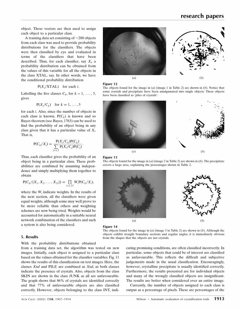
Figure 12The objects found for the image in (a) (image 1 in Table 2) are shown in (b). Notice thatsome crystals and precipitate have been amalgamated into single objects. These objectshave been classi®ed as `piles of crystals'.

Figure 13The objects found for the image in (a) (image 2 in Table 2) are shown in (b). The precipitatecovers a large area, explaining the percentages shown in Table 2.

Figure 14The objects found for the image in (a) (image 3 in Table 2) are shown in (b). Although theobjects exhibit straight boundary sections and regular angles, it is immediately obviousfrom the shapes that the objects are not crystals.

research papers


pixels in objects and not of the total number of pixels in the

image. For example, if there is only one small crystal in the

image, it will be classi®ed as `100% crystals'. On the other

hand, for a small crystal and lots of precipitate, a possible

classi®cation would be `10% crystals, 90% interesting'. A

suitable scoring system still needs to be devised. The aim is to

assign single scores to images indicating their signi®cance.

Images from various sources have been tested. This does

not present a problem, except that the initial parameters need

to be adjusted to the expected resolution. In the images shown

here, the crystallization drop approximately ®lls the image.

Although this sometimes makes identi®cation of the drop

edge dif®cult, it is not important for these cases. However, for

images in which the drop is very small in comparison to the

overall image, it is much more important to identify the

crystallization drop and eliminate everything outside it. In

practice, the type and resolution of images for a particular

setup would be suf®ciently consistent.

The following three examples are cases in which the entire

image is considered. Therefore, objects arising from the edge

of the drop or the well will also be present and should be

classi®ed appropriately. Table 2 shows the results as the

number of objects from each class and the percentage of pixels

in each class. Image 1 the table is shown in Fig. 12(a). In this

case, a large percentage of the pixels have been identi®ed as

belonging to objects classi®ed as piles of crystals. This is owing

to crystals and precipitate being grouped together and

considered as single objects (see Fig. 12b).

The percentage of pixels in each class also indicates the size

of the objects found. Image 2 from the table (Fig. 13) shows a

large percentage of pixels classi®ed as interesting. This is

because the precipitate covers a large area in comparison to

the pile of crystals. Fig. 14 shows image 3 from Table 2, a less

desirable effect owing to skin forming on the crystallization

drop. Although a quanti®cation scheme for the results still

needs to be formulated, it can easily be seen from the graphs

in Fig. 15 the sort of outcomes the three images exhibit.

Further classi®ers and weighting schemes are being inves-

tigated as well as different classi®cation methods such as

neural networks and cluster analysis. No automated image-

recognition system can be expected to identify objects with

complete accuracy, but one that errs on the side of caution and

produces few false negatives would dramatically reduce the

amount of human intervention necessary. With robots capable

of performing tens of thousands of crystallization experiments

a day, effective automated image classi®cation is essential.

The author would like to thank Victor Lamzin, EMBL

Hamburg for useful discussion and for supplying the ®rst

images used in this research. The author is a Royal Society

University Research Fellow and would like to acknowledge

the support of the Royal Society.

References

Bayes, Rev. T. (1763). Philos. Trans. R. Soc. London, 53, 370±418.Reprinted in Biometrika, 45, 293±315 (1958).

Bergfors, T. (2000). Pictorial Library of CrystallizationDrop Phenomena, http://alpha2.bmc.uu.se/terese/crystallization/library.html

Freeman, H. (1961). Trans. Electron. Comput. EC10, 260±268.Marr, D. C. & Hildreth, E. (1980). Proc. R. Soc. London Ser. B, 207,

187±212.Rupp, B. (2000). High-Throughput Protein Crystallization. EMBL

Practical Course on Protein Expression, Puri®cation and Crystal-lization. EMBL Outstation Hamburg, Germany.

Stevens, R. C. (2000). Curr. Opin. Struct. Biol. 10, 558±563.

Figure 15(a), (b) and (c) show the graphs of results associated with Figs. 12, 13 and14, respectively. The results are also given in Table 2. It can be seen thatthe ®rst two images have been classi®ed as having crystals, whereas thethird image is mostly rubbish.

Towards the automated evaluation of crystallization trials

Documents

Transcript of Towards the automated evaluation of crystallization trials