
Towards KriCatch, A Slip Catching Practice System for the ...
52
A. (Ajinkya) Bhole C e Dr. R. Carloni Towards KriCatch, A Slip Catching Practice System for the game of Cricket MSc Report C Prof.dr.ir. G.J.M. Krijnen Dr.ir. D. Dresscher Dr. A.H. Mader Dr. S. Vanapalli September 2018 038RAM2018 Robotics and Mechatronics EE-Math-CS University of Twente P.O. Box 217 7500 AE Enschede The Netherlands
-
Upload
khangminh22 -
Category
Documents
-
view
3 -
download
0
Transcript of Towards KriCatch, A Slip Catching Practice System for the ...

Control of a Variable Stiffness Joint for
Catching a Moving Object
A. (Ajinkya) Bhole
Individual Assignment Report
C e
Dr. R. Carloni
E. Barrett, MSc
M. Reiling, MSc
May 2017
008RAM2017
Robotics and Mechatronics
EE-Math-CS
University of Twente
P.O. Box 217
7500 AE Enschede
The Netherlands
Towards KriCatch, A Slip Catching Practice System for the game of Cricket
MSc Report
C
Prof.dr.ir. G.J.M. KrijnenDr.ir. D. Dresscher
Dr. A.H. MaderDr. S. Vanapalli
September 2018
038RAM2018Robotics and Mechatronics
EE-Math-CSUniversity of Twente
P.O. Box 2177500 AE Enschede
The Netherlands

2 Towards KriCatch, A Slip Catching Practice System for the game of Cricket
Ajinkya A. Bhole University of Twente

Towards
A Slip Catching Practice System for the game of Cricket
By
Ajinkya Arun Bhole
in partial fulfillment of the requirements for the degree of
Master of Science in Systems and Control
Faculty of Electircal Engineering, Mathematics and Computer ScienceUniversity of Twente, The Netherlands
Assessment Committee:
prof.dr.ir. Stefano Stramigioliprof.dr.ir. Gijs Krijnendr.ir. Douwe Dresscher
dr. Angelika Maderdr. Srinivas Vanapalli
September 6, 2018

2 Towards KriCatch, A Slip Catching Practice System for the game of Cricket
Ajinkya A. Bhole University of Twente

i
Abstract
This work presents KriCatch 1.0, output of the first design iteration for KriCatch, a slip catchingpractice system for the game of Cricket.
Present slip catching practice systems for the game of Cricket comprise of a thrower throwinga ball towards a coach or a passive equipment, which then swerve the ball for a user’s catch-ing practice. These methods cannot provide a catching practice with good efficacy, versatilityand a degree of realism, pointing towards the need for one. In this respect, KriCatch is beingdesigned.
KriCatch 1.0 comprises of a thrower who throws a ball towards a robotic manipulator whichcan swerve the ball to a desired point. To achieve this, four subsystems are designed.
The first subsystem senses the position of the thrown ball, estimates and predicts the trajectoryof the ball and finally provides an interception point for the robotic manipulator.
The second subsystem decides the spot where the thrown ball should be sent to.
The third subsystem decides the strategy for how the ball needs to be sent to, to the spot de-cided by the second subsystem, by the robotic manipulator.
The fourth subsystem finally plans and executes the trajectory for the robotic manipulator, tointercept the ball.
To evaluate the designed system, a prototype of the designed system is setup and experimentedupon. It is observed that the ball is successfully intercepted by the robotic manipulator whenthe interception point lies in the manipulators achievable workspace. However, the ball cannotbe sent accurately to the desired spots. This is mainly because the robotic manipulator is notable to perfectly track the commanded trajectory to intercept the ball, on account of its jointvelocity, acceleration and jerk limits.
Robotics and Mechatronics Ajinkya A. Bhole

ii Towards KriCatch, A Slip Catching Practice System for the game of Cricket
To Vasant Shankar Bhole
Dear Ajoba,
I can’t thank you enough for introducing me to the wonderful game of Cricket,For showing me and Aaji those interesting Cricket matches,And, for mostly saying yes to play Cricket with me. It was always fun for me to makeyou run around in the front yard to collect the ball.Someday soon, KriCatch will be realized. I hope this will bring some more RahulDravids to the game!
Tumcha bhaari naatu,Ajju
Ajinkya A. Bhole University of Twente

iii
Acknowledgements
This report marks my final step as a Systems and Controls student at the University of Twenteand the first step in my journey towards the development of KriCatch. It cannot express thelong days spent in the lab, the tiredness debugging the codes, the joy for each successfully builtand working code, the hope for good results and the sadness with each failed attempt.
The environment created at the Robotics and Mechatronics Lab at the University of Twente isprobably the best a student interested in robotics could ever hope for.
I would like to take this opportunity to thank Stefano Stramigioli, head of the RAM lab, forbelieving in me, my idea and letting me work on it with the RAM group. You are one of the mostenergetic personalities I have ever met. I can never understand where you get all your energyfrom (maybe you have some magical energy tank hidden somewhere).
Thanks Douwe Dresscher. Inspite of your busy schedule, you agreed to mentor me on thisproject, which does not come in your research domain. When asked for an advise or presentedwith a problem, you can process it, think critically and suggest great ideas at a brisk. You gaveme the total control of the steering wheel for my thesis, which was a great learning experiencefor me.
Marcel Schwirtz, thanks a tonne for taking my constant bugging, for always having five minutesfor me and being my ‘instant problem solver’. Someday I will beat your cycling records. Alfredde Vries, thanks for all your efforts in finding time-slots for me to work in the Smart-XP Lab.Someday, I will build a robot which will perform all your crazy ideas.
Sahib Dhanjal (aka Chopa), it is because of you, that I never had to use roswtf. Ishan Kanade,thanks for being my Ubuntu repair guy. Keep solving my computer related problems, you guys.
Kaul (aka Judgeet Singh), I cannot thank you enough for grooming my English writing skillsduring the four wonderful years we spent in Pilani.
Thesis work can become really stressful sometimes. Florentine, I had a great time sharing andlistening to thesis miseries over lunch in Waaier. Also, thanks for bringing in adventures in mydull mainstream life during thesis. Peshwe Amit, bhau, thanks for all your endless hilariousyapping in our Haveli. If KriCatch becomes a success someday, all business plans of yours areon tap.
Maushi, Aaji, I would have gotten nowhere without your blessings. Rashu, thanks for yourregular ‘cool.. good luck dude’ wishes.
Mummi, Pappa and Appu, I can dream big and follow my heart only because of your uncondi-tional support. It is so easy for me to find my motivation to work hard and give in my best atanything and everything that comes my way, just by looking at you three.
Picture abhi baaki hai,
Ajinkya Bhole
Robotics and Mechatronics Ajinkya A. Bhole

iv Towards KriCatch, A Slip Catching Practice System for the game of Cricket
Preface
This tour de force in experimental robotics marks the embarkation towards the journey of de-sign and development of ‘KriCatch’, a slip catching practice system for the game of Cricket.
It is identified that the current catching practice equipment for Cricket, available in the mar-ket, cannot provide a catching practice with good efficacy, versatility and a degree of realism,pointing towards the need for one.
Iterative design is a process of designing a product in which the product is tested and eval-uated repeatedly at different stages of design to eliminate usability flaws before the product isdesigned and launched. In other words, iterative design is a process of improving and polishingthe design over time.
The iterative design methodology is used to develop KriCatch and this work describes the firstiteration of this design process leading to KriCatch 1.0.
Ajinkya A. Bhole University of Twente

v
Contents
1 Introduction 1
1.1 Context . . . . . . . . . . . . . . . . . . . . . . . . . . . . . . . . . . . . . . . . . . . . 1
1.2 Identifying the Problem . . . . . . . . . . . . . . . . . . . . . . . . . . . . . . . . . . 1
1.3 Defining the Problem: . . . . . . . . . . . . . . . . . . . . . . . . . . . . . . . . . . . 5
1.4 Content . . . . . . . . . . . . . . . . . . . . . . . . . . . . . . . . . . . . . . . . . . . . 5
2 Analysis 6
2.1 How does an event of slip catch occur? . . . . . . . . . . . . . . . . . . . . . . . . . 6
2.2 How can a slip catch be taken successfully? . . . . . . . . . . . . . . . . . . . . . . . 6
2.3 Feinting Motions by the Batsmen . . . . . . . . . . . . . . . . . . . . . . . . . . . . . 6
2.4 Functional Requirements . . . . . . . . . . . . . . . . . . . . . . . . . . . . . . . . . 6
2.5 Functional Analysis . . . . . . . . . . . . . . . . . . . . . . . . . . . . . . . . . . . . . 7
3 System Architecture 9
3.1 Subsystem1: Sensing the thrown ball . . . . . . . . . . . . . . . . . . . . . . . . . . 10
3.2 Subsystem 2: Decide where to send the ball to . . . . . . . . . . . . . . . . . . . . . 19
3.3 Subsystem 3: Strategy for how to send the ball to a desired spot . . . . . . . . . . . 20
3.4 Subsystem 4: Trajectory Planning and Execution on BIM . . . . . . . . . . . . . . . 23
3.5 KriCatch 1.0: System Overview . . . . . . . . . . . . . . . . . . . . . . . . . . . . . . 26
4 Experiments on KriCatch 1.0 27
4.1 Ball Interception Results . . . . . . . . . . . . . . . . . . . . . . . . . . . . . . . . . . 29
4.2 Catching Point Results . . . . . . . . . . . . . . . . . . . . . . . . . . . . . . . . . . . 30
4.3 Discussion on the results . . . . . . . . . . . . . . . . . . . . . . . . . . . . . . . . . 31
5 Conclusions and Recommendations 33
A Appendix 1 35
A.1 Optimal Online Estimation of Linear Gaussian Systems: The Kalman Filter . . . . 35
A.2 Sub-Optimal Solution for Online Estimation of Non-Linear Systems: The Ex-tended Kalman Filter . . . . . . . . . . . . . . . . . . . . . . . . . . . . . . . . . . . . 36
A.3 Constrained Extended Kalman Filter . . . . . . . . . . . . . . . . . . . . . . . . . . . 37
A.4 Adaptive adjustment of Noise Covariance (Cv and Cw ) in Kalman Filter . . . . . . 38
B Appendix 2 40
B.1 Calculation of co-efficient of restitution of ball . . . . . . . . . . . . . . . . . . . . . 40
Bibliography 41
Robotics and Mechatronics Ajinkya A. Bhole

vi Towards KriCatch, A Slip Catching Practice System for the game of Cricket
Ajinkya A. Bhole University of Twente

1
1 Introduction
1.1 Context
“..Sports is actually a chance for us to have other human beings push us to excel."
-John Keating, (Robin William’s character in Dead Poet’s Society)
And to keep up the gradient of this spirit, the expertise of a sports player and thus a sport overallmust keep advancing. Application of technology to sports equipment has a great impact on theperformance of players and has a potential to revolutionize the entire sporting culture throughvariegated approaches, such as improvement in training methods, development of new equip-ment, improvement of existing equipment, strategy planning and tactical analysis.
Practice makes perfect, and practicing using training equipment is a tremendously effectivemethod to achieve desired skill sets in a sport. Now-a-days many are moving to automatedtraining equipment, which offer increased efficiency of practice and great versatility (Sato et al.,2017; Miyazaki et al., 2006; Li et al., 2012; ProBatter Sports, 2011). Moreover, in many sports,automation eliminates the needs of any accompanying personage to provide practice.
Leg-side
Off-side
Figure 1.1: The basics of the game of Cricket. Image Source: http://www.chicagotribune.com/
1.2 Identifying the Problem
Cricket is a widely popular bat-and-ball sport (Wikipedia, 2018b). ‘Catches win matches’ isprobably the oldest adage in the game of Cricket. Catching in Cricket requires great concentra-tion, agility, hand-eye coordination and sure-handedness. Knowledge of good catching tech-niques alone does not suffice, ample practice is required to master the art of catching and build-ing up confidence.
Before discerning the problem, some basic facts about Cricket and the terminologies used inthe game are introduced ahead. Cricket is played with two teams of 11 players each. Each
Robotics and Mechatronics Ajinkya A. Bhole

2 Towards KriCatch, A Slip Catching Practice System for the game of Cricket
team takes turns batting and playing the field, as is done in the game of Baseball. In Cricket,the batter is called the batsman and the pitcher is called the bowler. The bowler tries to knockdown the bail of the wicket (refer Figure 1.1). A batsman tries to prevent the bowler from hittingthe wicket, by hitting the ball. Two batsmen are on the pitch at the same time. The batsmencan run, after the ball is hit. A run is scored each time the two batsmen change their places onthe pitch.
The Cricket field can be divided in two ways:
1. When the batsman is facing the bowler, the side to the right hand side of the batsman iscalled the off-side and the one on the left hand side is called the leg-side (Figure 1.1).
2. As is shown in Figure 1.2 the ground can be divided into four sections, outfield, infield,close-infield and the pitch.
Outfield
Infield
Close-Infield
Pitch
Cricket Field
Figure 1.2: A standard Cricket ground showing the Pitch, Close-Infield, Infield and the Outfield.
Based on the second way of division, the catches taken in Cricket are differentiated as outfield,infield and close-infield catches.
A slip fielder (collectively, a slip cordon or the slips) is placed in the close-infield, behind thebatsman on the off side field (Figure 1.3). The catches coming in this region are called slipcatches. These catches are the most difficult to make, as the players have a very less reflex timeand need to be extremely attentive. Naturally, these are the most practiced catches in game.
Ajinkya A. Bhole University of Twente

1. INTRODUCTION 3
Bowler
Batsman
Slip Cordon
Wicket-Keeper
Figure 1.3: A Slip Catch scenario in the game of Cricket
There are numerous ways and equipment to practice slip catching which go as follows:
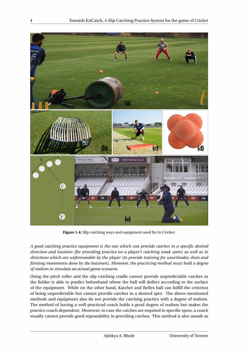
1. A traditional way of practicing slip catches is by shooting a ball on a pitch roller. The ballhits the curved surface of the roller and gets swerved towards the fielders. (Figure 1.4 (a))
2. The slip catching cradle (Figure 1.4 (b)) is similar to using a pitch roller and consists oflong, thin ash lathes over a bowed metal frame.
3. Katchet (Figure 1.4 (c)) is a portable equipment with an uneven surface which can pro-vide unpredictable catches.
4. Using Reflex ball (Figure 1.4 (d)) is another technique to practice for slip catches. Thisball is made up of uneven surface and bounces in unpredictable direction when it hitsthe ground.
5. Finally, the most realistic way to practice slip catching requires a well-practiced coach tomake it worthwhile. As shown in Figure 1.4 (e), the feeder (F) throws the ball such that itreaches the coach (C) at chest height, wide to the off side and the coach deflects the ballwith a bat into the slip cordon (S) for practicing catches.
Robotics and Mechatronics Ajinkya A. Bhole
4 Towards KriCatch, A Slip Catching Practice System for the game of Cricket
F
C
S
(a)
(e)
(b) (c) (d)
Figure 1.4: Slip catching ways and equipment used for in Cricket.
A good catching practice equipment is the one which can provide catches in a specific desireddirection and location (for providing practice on a player’s catching weak spots) as well as indirections which are unforeseeable by the player (to provide training for unorthodox shots andfeinting movements done by the batsmen), Moreover, the practicing method must hold a degreeof realism to simulate an actual game scenario.
Using the pitch roller and the slip catching cradle cannot provide unpredictable catches asthe fielder is able to predict beforehand where the ball will deflect according to the surfaceof the equipment. While on the other hand, Katchet and Reflex ball can fulfill the criterionof being unpredictable but cannot provide catches in a desired spot. The above-mentionedmethods and equipment also do not provide the catching practice with a degree of realism.The method of having a well-practiced coach holds a good degree of realism but makes thepractice coach dependent. Moreover, in case the catches are required in specific spots, a coachusually cannot provide good repeatability in providing catches. This method is also unsafe as
Ajinkya A. Bhole University of Twente

1. INTRODUCTION 5
there are chances of the ball hitting the coach in case he/she accidentally misses it or does notduck at the appropriate moment in case required.
1.3 Defining the Problem:
Based on the identified problem in the previous section, following problem is evident:
There is a requirement for an equipment / system for slip catching practice which can provideunpredictable catches as well as catches in desired spots with a good degree of realism.
The main goal of this work is to design KriCatch, a slip catching practice system which solvesthe above-mentioned problem. An iterative design methodology (Wikipedia, 2018c) is used todevelop KriCatch and this work focuses on the first iteration of this design process leading toKriCatch 1.0.
KriCatch 1.0 KriCatch
Figure 1.5: Iterative design process for the design of KriCatch.
1.4 Content
Chapter 2 discerns in detail, the functional requirements for KriCatch. Chapter 3 describes thesystem architecture of KriCatch 1.0. The experimental results performed on KriCatch 1.0 arepresented in Chapter 4. Finally, conclusions and recommendations are described in Chapter 5.
Robotics and Mechatronics Ajinkya A. Bhole

6 Towards KriCatch, A Slip Catching Practice System for the game of Cricket
2 Analysis
Before starting the prototyping phase of KriCatch 1.0, it is important to understand its func-tional requirements. This chapter describes some easily discernable functional requirementsfor KriCatch. Thereafter, a functional analysis is performed. Necessary subsystems are identi-fied and their function allocation is done to meet the overall system’s functional requirements.
The simplest way to provide slip catching practice is by having a machine which can shoot aball in desired spots for the player. But, this kind of equipment does not provide a catchingpractice with a good degree of realism.
To understand how an apt catching practice system should look like, it is important to firstlyanalyze how an event of slip catch occurs, how can a slip catch be taken successfully and whatare some of the challenges the players in Cricket face while using the present catching practiceequipment in the market.
2.1 How does an event of slip catch occur?
The goal of a batsman in the game of Cricket is to hit the ball by finding gaps amongst thefielders so as to make runs. It is therefore never the intent of a batsman to hit the ball straighttowards a player. An event of a catch usually occurs when, the ball hits a spot on the bat whichwas not desired by the batsman (possibly due to a swing in the ball trajectory or an error madeby the batsman).
2.2 How can a slip catch be taken successfully?
Based on the discussion in the previous section on how an event of slip catch occurs in thegame of Cricket, the coaches always advice the fielders to keep an eye on the swing and the faceof the bat. The fielders are also advised to observe and predict the trajectory and swing of thethrown ball. This is because if the ball is swinging, there are high chances that the batsmanmakes an error and the ball hits an undesired spot on the bat.
2.3 Feinting Motions by the Batsmen
Now-a-days batsmen play many unorthodox shots and also feint the motion of their body andbat to trick the fielders. As can be seen from the Figure 2.1, that the batsman initially feintedhis motion by moving to his leg-side and the wicket-keeper followed his motion. The batsmanthen swerved the ball in the direction opposite to that of the wicket-keeper’s direction of travel.It is therefore also necessary for the fielders to get used to such tactics used by the batsmen.
Figure 2.1: An example of unorthodox batting method: The Late Cut Shot played by Eoin Morgan.
2.4 Functional Requirements
Based on the above discussion, it is clear that an apt catching practice system should:
• Imitate the bowler, so that the fielder needs to keep an eye on the direction and swing ofthe ball
Ajinkya A. Bhole University of Twente
2. ANALYSIS 7
• Imitate the batsman, so that he/she can observe the swing and face of the bat
• Imitate feinting motions done by the batsmen
2.5 Functional Analysis
Two of the functional requirements identified in the previous section are imitating the bowlerand the batsman.
2.5.1 Imitation of Bowler:
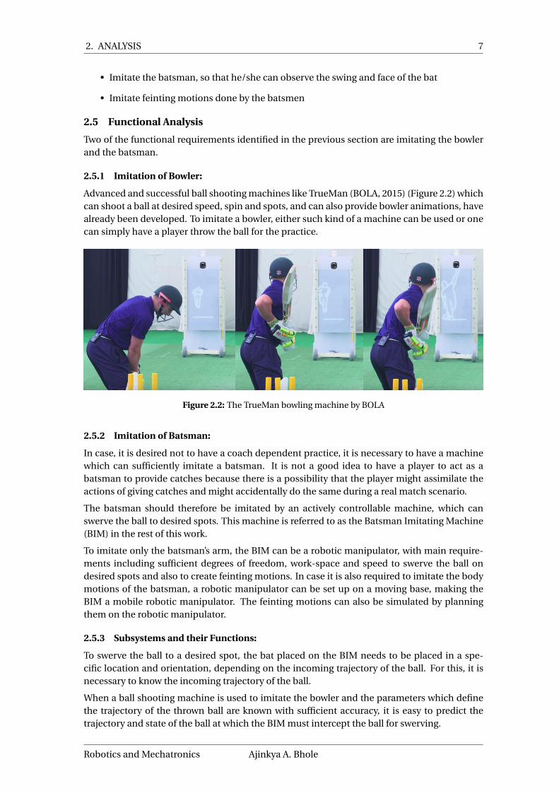
Advanced and successful ball shooting machines like TrueMan (BOLA, 2015) (Figure 2.2) whichcan shoot a ball at desired speed, spin and spots, and can also provide bowler animations, havealready been developed. To imitate a bowler, either such kind of a machine can be used or onecan simply have a player throw the ball for the practice.
Figure 2.2: The TrueMan bowling machine by BOLA
2.5.2 Imitation of Batsman:
In case, it is desired not to have a coach dependent practice, it is necessary to have a machinewhich can sufficiently imitate a batsman. It is not a good idea to have a player to act as abatsman to provide catches because there is a possibility that the player might assimilate theactions of giving catches and might accidentally do the same during a real match scenario.
The batsman should therefore be imitated by an actively controllable machine, which canswerve the ball to desired spots. This machine is referred to as the Batsman Imitating Machine(BIM) in the rest of this work.
To imitate only the batsman’s arm, the BIM can be a robotic manipulator, with main require-ments including sufficient degrees of freedom, work-space and speed to swerve the ball ondesired spots and also to create feinting motions. In case it is also required to imitate the bodymotions of the batsman, a robotic manipulator can be set up on a moving base, making theBIM a mobile robotic manipulator. The feinting motions can also be simulated by planningthem on the robotic manipulator.
2.5.3 Subsystems and their Functions:
To swerve the ball to a desired spot, the bat placed on the BIM needs to be placed in a spe-cific location and orientation, depending on the incoming trajectory of the ball. For this, it isnecessary to know the incoming trajectory of the ball.
When a ball shooting machine is used to imitate the bowler and the parameters which definethe trajectory of the thrown ball are known with sufficient accuracy, it is easy to predict thetrajectory and state of the ball at which the BIM must intercept the ball for swerving.
Robotics and Mechatronics Ajinkya A. Bhole

8 Towards KriCatch, A Slip Catching Practice System for the game of Cricket
But, in case a person is throwing the ball, to imitate the bowler, it is necessary to have a sensingsubsystem for estimating and predicting the trajectory of the thrown ball.
In this work, it is assumed that we have a person throwing the ball for the practice. Based onthis, following subsystems and their functions are proposed:
• Subsystem 1: Senses the position of the thrown ball, estimates and predicts the trajectoryof the ball and finally provides an interception point for the BIM.
• Subsystem 2: Decides where the thrown ball should be deviated to.
• Subsystem 3: Decides the strategy for the BIM, for how to send the ball to the spot de-cided by Subsystem 2, by providing the orientation of the normal vector to the surface ofthe bat used on the BIM.
• Subsystem 4: Plans and executes the trajectory of the bat used on the BIM.
Figure 2.3 shows a rough overview of the connections of the subsystems used for KriCatch 1.0.
Ball Thrown Subsystem 1 Interceptionpoint details Subsystem 3
Subsystem 2 Desired spot tosend the ball to
TrajectoryPlanningParameters
Subsystem 4 BIM
Figure 2.3: A rough idea of the connections of the subsystems used for KriCatch 1.0
Ajinkya A. Bhole University of Twente
9
3 System Architecture
This chapter firstly discusses the general workflow of KriCatch 1.0 and finally describes everysubsystem involved in detail.
Interception Plane
BIMx
yz
Figure 3.1: A general workflow of KriCatch 1.0
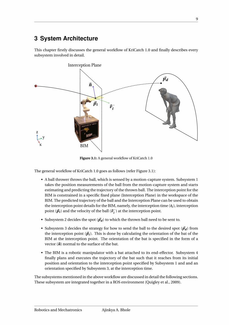
The general workflow of KriCatch 1.0 goes as follows (refer Figure 3.1):
• A ball thrower throws the ball, which is sensed by a motion-capture system. Subsystem 1takes the position measurements of the ball from the motion-capture system and startsestimating and predicting the trajectory of the thrown ball. The interception point for theBIM is constrained in a specific fixed plane (Interception Plane) in the workspace of theBIM. The predicted trajectory of the ball and the Interception Plane can be used to obtainthe interception point details for the BIM, namely, the interception time (ti ), interceptionpoint (~pi ) and the velocity of the ball (~v−
i ) at the interception point.
• Subsystem 2 decides the spot ( ~pd ) to which the thrown ball need to be sent to.
• Subsystem 3 decides the strategy for how to send the ball to the desired spot ( ~pd ) fromthe interception point (~pi ). This is done by calculating the orientation of the bat of theBIM at the interception point. The orientation of the bat is specified in the form of avector (~n) normal to the surface of the bat.
• The BIM is a robotic manipulator with a bat attached to its end-effector. Subsystem 4finally plans and executes the trajectory of the bat such that it reaches from its initialposition and orientation to the interception point specified by Subsystem 1 and and anorientation specified by Subsystem 3, at the interception time.
The subsystems mentioned in the above workflow are discussed in detail the following sections.These subsystem are integrated together in a ROS environment (Quigley et al., 2009).
Robotics and Mechatronics Ajinkya A. Bhole

10 Towards KriCatch, A Slip Catching Practice System for the game of Cricket
3.1 Subsystem1: Sensing the thrown ball
It is necessary to predict the motion of the ball in advance as this provides the system withsome time to plan and execute the the trajectory for the BIM. For this it is necessary to firstlysense the motion of the ball. Based on the measurements from a sensing system, estimationand prediction of the trajectory of the thrown ball can be done. Using the predicted trajectory,the interception point for the BIM can be calculated. This subsystem outputs the interceptionpoint details namely, the interception time (ti ), interception point (~pi ) and the velocity of theball (~v−
i ) at the interception point. The methodology used to obtain these outputs are explainedin the following subsections.
3.1.1 Sensing Ball Position:
This subsection briefly discusses OptiTrack (Point, 2011), a marker-based motion capture sys-tem used to procure the position of the thrown ball.
OptiTrack has been used in several works wherein robotic manipulators are made to catchthrown objects ((Brescianini and D’Andrea, 2018; Cigliano et al., 2015; Kim et al., 2014)). TheOptiTrack system used in this work provides position measurements with a position accuracyof about 0.01 mm and measurements at the rate of 250 Hz.
The data from OptiTrack can be streamed over a network using the OptiTrack Streaming En-gine. The mocap_optitrack package (Kathrin Gräve, 2018) developed for ROS can be usedto provide 6D poses of rigid bodies defined by a set of markers placed onto it. This packagewas modified to provide the position data of individual markers present in the OptiTrack en-vironment. Any ball covered with retro-reflective tape can then be tracked using the modifiedpackage. Figure 3.2 shows the ball covered with a retro-reflective tape used in this work.
Figure 3.2: Ball covered with retro-reflective tape used in OptiTrack environment
It is necessary to predict the motion of the ball in advance as this provides the system with sometime to plan and execute the the trajectory for the BIM. For this it is necessary to estimate andpredict the trajectory of the thrown ball and calculate the interception point for the BIM. Themethodology used to perform these tasks are explained in following subsections.
3.1.2 Estimation of the state of ball:
To predict the trajectory of a thrown ball, it is required to estimate its current state of motion.
The Bayesian state estimation approach is widely used for state estimation, as it provides a sys-tematic and general approach to handle the effect of various random uncertainties on the pro-cess states and measurements. Bayesian state algorithms use a first-principles based dynamicmodel and the statistical properties of random disturbances and measurements to obtain theposterior distribution of the state estimates.
Ajinkya A. Bhole University of Twente
3. SYSTEM ARCHITECTURE 11
The Kalman Filter (KF) introduced by Rudolf E. Kalman (Kalman, 1960) is a widely usedBayesian estimation technique. This technique works best in-case the system under consid-eration is linear. In case of a non-linear system, which is generally the case, there is anotherapproach with almost the same computational complexity, but with better performance. Thatapproach is the Extended Kalman filter (EKF) (Anderson and Moore, 1979). In EKF the statedistribution is approximated by a Gaussian Random Variable (GRV), which is then propogatedthrough the first order linearization of the non-linear system.
EKF has been successfully implemented in many previous works involving prediction of balltrajectories under the effect of gravity and drag (Koç et al., 2018; Brescianini and D’Andrea,2018; Zhang et al., 2014). An EKF algorithm implemented in C++ language, is used in this work.The general framework for KF and EKF is described in the Appendix A.1-A.2.
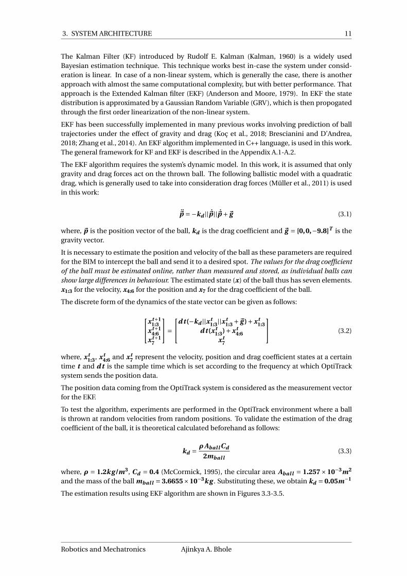
The EKF algorithm requires the system’s dynamic model. In this work, it is assumed that onlygravity and drag forces act on the thrown ball. The following ballistic model with a quadraticdrag, which is generally used to take into consideration drag forces (Müller et al., 2011) is usedin this work:
~p =−kd ||~p||~p +~g (3.1)
where, ~p is the position vector of the ball, kd is the drag coefficient and ~g = [0, 0,−9.8]T is thegravity vector.
It is necessary to estimate the position and velocity of the ball as these parameters are requiredfor the BIM to intercept the ball and send it to a desired spot. The values for the drag coefficientof the ball must be estimated online, rather than measured and stored, as individual balls canshow large differences in behaviour. The estimated state (x) of the ball thus has seven elements.x1:3 for the velocity, x4:6 for the position and x7 for the drag coefficient of the ball.
The discrete form of the dynamics of the state vector can be given as follows:
x t+11:3
x t+14:6
x t+17
=d t (−kd ||x t
1:3||x t1:3 +~g )+x t
1:3d t (x t
1:3)+x t4:6
x t7
(3.2)
where, x t1:3, x t
4:6 and x t7 represent the velocity, position and drag coefficient states at a certain
time t and d t is the sample time which is set according to the frequency at which OptiTracksystem sends the position data.
The position data coming from the OptiTrack system is considered as the measurement vectorfor the EKF.
To test the algorithm, experiments are performed in the OptiTrack environment where a ballis thrown at random velocities from random positions. To validate the estimation of the dragcoefficient of the ball, it is theoretical calculated beforehand as follows:
kd = ρAbal l Cd
2mbal l(3.3)
where, ρ = 1.2k g /m3, Cd = 0.4 (McCormick, 1995), the circular area Abal l = 1.257×10⁻³m2
and the mass of the ball mbal l = 3.6655×10⁻³k g . Substituting these, we obtain kd = 0.05m−1
The estimation results using EKF algorithm are shown in Figures 3.3-3.5.
Robotics and Mechatronics Ajinkya A. Bhole

12 Towards KriCatch, A Slip Catching Practice System for the game of Cricket
0 0.2 0.4 0.6
time (s)
-1.15
-1.1
-1.05
-1
-0.95
-0.9
-0.85
Positio
n X
(m
)
X Position
Measured
Estimated
0 0.2 0.4 0.6
time (s)
-1
0
1
2
3
4
5
Positio
n Y
(m
)
Y Position
Measured
Estimated
0 0.2 0.4 0.6
time (s)
1.4
1.6
1.8
2
2.2
2.4
Positio
n Z
(m
)
Z Position
Measured
Estimated
0 0.2 0.4 0.6
time (s)
-2
-1.5
-1
-0.5
0
0.5
1
1.5
2
Estim
ation E
rror
X (
m)
10-4Estimation Error X
0 0.2 0.4 0.6
time (s)
-2
-1
0
1
2
3
Estim
ation E
rror
Y (
m)
10-4Estimation Error Y
0 0.2 0.4 0.6
time (s)
-0.5
0
0.5
1
1.5
2
2.5
Estim
ation E
rror
Z (
m)
10-4Estimation Error Z
Figure 3.3: Position Estimates and their Estimation errors after application of the EKF algorithm
Ajinkya A. Bhole University of Twente

3. SYSTEM ARCHITECTURE 13
0 0.2 0.4 0.6
time (s)
-0.5
-0.49
-0.48
-0.47
-0.46
-0.45
-0.44
-0.43
-0.42
-0.41
-0.4
Ve
locity X
(m
/s)
X Velocity
0 0.2 0.4 0.6
time (s)
7.5
8
8.5
9
9.5
10
Ve
locity Y
(m
/s)
Y Velocity
0 0.2 0.4 0.6
time (s)
-4
-3
-2
-1
0
1
2
Ve
locity Z
(m
/s)
Z Velocity
Figure 3.4: Velocity estimates of the ball after application of the EKF algorithm
0 0.1 0.2 0.3 0.4 0.5 0.6 0.7
time (s)
-0.1
0
0.1
0.2
0.3
0.4
0.5
Dra
g (
1/m
)
Drag
Estimated
Calculated
Figure 3.5: Estimate of the drag coefficient of the ball after application of the EKF algorithm
From the estimation results shown in Figure 3.3-3.5 it can be seen that the estimate of the po-sition of the ball is quite accurate and the estimation errors lie in the range of -0.3 mm to 0.3mm. It can be also seen that the estimate of the drag coefficient of the ball converges to thetheoretically calculated value in about 0.05 secs.
Although it can be seen that the estimation of drag coefficient has spikes and goes to negativevalues at some points, which is unrealistic. To avoid negative values of the drag coefficientestimates, the EKF algorithm is modified to add a constraint on its estimated state, leading to aConstrained-EKF (CAEKF) algorithm. The framework for adding constraints on the estimatedstate is explained in Appendix A.3.
A constraint which keeps the estimated drag coefficient above the value of zero is used in theCEKF algorithm. The estimation results using CEKF algorithm are shown in Figures 3.6-3.8.
Robotics and Mechatronics Ajinkya A. Bhole

14 Towards KriCatch, A Slip Catching Practice System for the game of Cricket
0 0.2 0.4 0.6 0.8
time (s)
-0.98
-0.96
-0.94
-0.92
-0.9
-0.88
-0.86
-0.84
Po
sitio
n X
(m
)X Position
Measured
Estimated
0 0.2 0.4 0.6 0.8
time (s)
-1
0
1
2
3
4
5
Po
sitio
n Y
(m
)
Y Position
Measured
Estimated
0 0.2 0.4 0.6 0.8
time (s)
1.4
1.6
1.8
2
2.2
2.4
Po
sitio
n Z
(m
)
Z Position
Measured
Estimated
0 0.2 0.4 0.6 0.8
time (s)
-1.5
-1
-0.5
0
0.5
1
1.5
Estim
ation E
rror
X (
m)
10 -4Estimation Error X
0 0.2 0.4 0.6 0.8
time (s)
-3
-2
-1
0
1
2
3
Estim
ation E
rror
Y (
m)
10 -4Estimation Error Y
0 0.2 0.4 0.6 0.8
time (s)
-1
-0.5
0
0.5
1
1.5
2
2.5
Estim
ation E
rror
Z (
m)
10 -4Estimation Error Z
Figure 3.6: Position Estimates and their Estimation errors after application of the CEKF algorithm
Ajinkya A. Bhole University of Twente

3. SYSTEM ARCHITECTURE 15
0 0.2 0.4 0.6 0.8
time (s)
-0.185
-0.18
-0.175
-0.17
-0.165
-0.16
-0.155
-0.15
-0.145
-0.14
Ve
locity X
(m
/s)
X Velocity
0 0.2 0.4 0.6 0.8
time (s)
7
7.5
8
8.5
9
9.5
10
Ve
locity Y
(m
/s)
Y Velocity
0 0.2 0.4 0.6 0.8
time (s)
-4
-3
-2
-1
0
1
2
3
Ve
locity Z
(m
/s)
Z Velocity
Figure 3.7: Velocity estimates of the ball after application of the CEKF algorithm
0 0.1 0.2 0.3 0.4 0.5 0.6 0.7
time (s)
-0.1
0
0.1
0.2
0.3
0.4
0.5
0.6
Dra
g (
1/m
)
Drag
Estimated
Calculated
Figure 3.8: Estimate of the drag coefficient of the ball after application of the CEKF algorithm
It can be seen that the drag coefficient is now constrained to non-negative values and con-verges to the theoretically calculated value in about 0.05 secs. Also, the estimation error in theposition of the ball are in a similar range to that of the EKF algorithm. The estimation of thedrag estimate still remains spiky.
It is well known that the co-variance matrices of process noise (Cw ) and measurement noise(Cv ) have a significant impact on the Kalman filter’s (KF) gain in estimating dynamic states(Almagbile et al., 2010). A high Kalman Gain can spike the estimates even for a very small in-novation (difference between current measurement and its corresponding predicted measure-ment). The spiking can be mitigated by modifying the EKF’s Kalman gain to be adaptive, lead-ing to an Adaptive Extended Kalman Filter (AEKF). The adaptive part of the algorithm can makesure that the Kalman filter becomes less aggressive once convergence is achieved reducing thespikes. This can also mitigate the problems in tuning the filter by trial and error methods, whichcan be a tedious task. Moreover, the noise levels may change for changing environment makingthe chosen tuning parameters of the KF ineffective. The AEKF algorithm can adapt the Kalmangain making it more robust against noise. The AEKF algorithm used in this work is described inAppendix A.4.
The estimation results using the AEKF algorithm are shown in Figures 3.9-3.11.
Robotics and Mechatronics Ajinkya A. Bhole

16 Towards KriCatch, A Slip Catching Practice System for the game of Cricket
0 0.2 0.4 0.6 0.8
time (s)
-0.77
-0.768
-0.766
-0.764
-0.762
-0.76
-0.758
-0.756
Po
sitio
n X
(m
)X Position
Measured
Estimated
0 0.2 0.4 0.6 0.8
time (s)
-1
0
1
2
3
4
5
Po
sitio
n Y
(m
)
Y Position
Measured
Estimated
0 0.2 0.4 0.6 0.8
time (s)
2.2
2.3
2.4
2.5
2.6
2.7
2.8
2.9
Po
sitio
n Z
(m
)
Z Position
Measured
Estimated
0 0.2 0.4 0.6 0.8
time (s)
0
5
10
15
Estim
ation E
rror
X (
m)
10 -3Estimation Error X
0 0.2 0.4 0.6 0.8
time (s)
-1
0
1
2
3
4
5
Estim
ation E
rror
Y (
m)
10 -3Estimation Error Y
0 0.2 0.4 0.6 0.8
time (s)
0
5
10
15
20
Estim
ation E
rror
Z (
m)
10 -3Estimation Error Z
Figure 3.9: Position Estimates and their Estimation errors after application of the CEKF algorithm
Ajinkya A. Bhole University of Twente

3. SYSTEM ARCHITECTURE 17
0 0.2 0.4 0.6 0.8
time (s)
-0.08
-0.07
-0.06
-0.05
-0.04
-0.03
-0.02
-0.01
0
Ve
locity X
(m
/s)
X Velocity
0 0.2 0.4 0.6 0.8
time (s)
6
6.5
7
7.5
8
8.5
Ve
locity Y
(m
/s)
Y Velocity
0 0.2 0.4 0.6 0.8
time (s)
-4
-3
-2
-1
0
1
2
3
4
Ve
locity Z
(m
/s)
Z Velocity
Figure 3.10: Velocity estimates of the ball after application of the CEKF algorithm
0 0.1 0.2 0.3 0.4 0.5 0.6 0.7 0.8
time (s)
0
0.05
0.1
0.15
0.2
0.25
0.3
0.35
0.4
0.45
0.5
Dra
g (
1/m
)
Drag
Estimated
Calculated
Figure 3.11: Estimate of the drag coefficient of the ball after application of the CEKF algorithm
It can be seen that the drag coefficient now has no spikes. But, its value converges to the the-oretically calculated value in about 0.2 secs, which is much more than that of EKF and CEKF.Also, the estimation error in the position of the ball are quite large as compared to the resultsfrom EKF and CEKF. The AEKF algorithm is thus chucked out.
The EKF and CEKF algorithms provide almost similar results for the estimation of position andvelocity of the ball. The drag estimate obtained from CEKF is constrained to be non-zero, mak-ing it more realistic. Although the CEKF algorithm is computationally more expensive thanEKF, this is of no concern because, each iteration of the EKF and CEKF is finished well beforethe minimum possible sampling time d t of the algorithms, which is set according to the fre-quency at which the OptiTrack provides position measurements. It is therefore decided to makeuse of the CEKF algorithm for estimating the ball trajectory.
3.1.3 Prediction of the ball trajectory:
As seen from the CEKF estimation results (Figures 3.6-3.8) in the previous section, the estima-tion algorithm converges in about 0.05 secs. Once the estimation has converged, the predictionof the ball trajectory can be started. The trajectory of the ball can be predicted by numericallyintegrating the discrete dynamic model (Equation 3.2), by setting its initial value to the cur-rently estimated state of the ball. The estimation and prediction of the ball trajectory take placecontinuously till the ball is intercepted.
Robotics and Mechatronics Ajinkya A. Bhole

18 Towards KriCatch, A Slip Catching Practice System for the game of Cricket
3.1.4 Calculation of the interception point details:
The trajectory (i.e. the state) of the ball is predicted till it intersects an Interception Plane (Fig-ure 3.1). This provides the interception point details, namely, the interception time (ti ), inter-ception point (~pi ) and the velocity of the ball (~v−
i ) at the interception point. As the state of theball is continuously estimated, the predicted interception point details keep bettering. Figure3.12 shows the development in the x and z co-ordinates of the predicted interception point. They co-ordinate of the interception point remains constant as the interception plane is parallel tothe XZ plane ((Figure 3.1)).
0 50 100
Prediction Iteration
-0.965
-0.96
-0.955
-0.95
-0.945
X (
m)
Predicted
Measured
0 50 100
Prediction Iteration
1.2
1.3
1.4
1.5
Z (
m)
Predicted
Measured
Figure 3.12: Development of x and z co-ordinates of the predicted interception point with each predic-tion iteration.
The result for the interception position of the ball is acceptable, as the size of the bat used inthis work is 20 cm× 40 cm ,which is quite large compared to the distance error in the measuredand predicted interception point, which is usually around 0.5 cm.
Interception Plane
BIM
x
yz
t=0s t=0.05s t=ti
Ballthrown
CEKFinitialized
Estimationof state of ball
Estimation& Prediction
of state of ball
Interceptiontime
Figure 3.13: Work-flow of Subsystem 1
Ajinkya A. Bhole University of Twente

3. SYSTEM ARCHITECTURE 19
3.1.5 Subsystem Overview
Figure 3.13 shows an overall work-flow of Subsystem 1 and Figure 3.14 shows an overview ofthe inputs and outputs Subsystem 1.
Ball Thrown Interception Time
Interception coordinates of ball
Interceptionvelocity of ball
Subsystem 1
Sensing
Initialization ofCEKF
Estimate andPredict state of theball at Interception
Plane
Figure 3.14: Subsystem 1 Overview
3.2 Subsystem 2: Decide where to send the ball to
This susbsystem decides the spot for sending the thrown ball to, by the BIM. This spot is called‘catching point’ in the discussion ahead.
S
C
C
r
f
i
p
Figure 3.15: Selection of catching points
To decide the catching point, firstly a semi-circular catching region ‘S’ is defined around theplayer as is shown in Figure 3.15. For every throw of the ball, a random point (c f ) is then se-lected in this circular region for providing catches.
It is assumed that the thrown ball has enough speed so that it can reach any point in the catchingregion after it is swerved from the BIM. This is a fitting assumption as players usually have a goodidea of what speed should the ball be thrown, so that it can reach the fielder taking catches.
To provide a feinting motion, the catch is set up as follows: A random point (c f ) is selected inthe catching region S and another random point (ci ) is selected such that it lies in the region S,but outside a circle of a pre-defined radius rp having its center at c f (See Figure 3.15). Duringthe interception of the thrown ball the bat of the BIM is firstly made to orient itself to show as ifit is trying to provide a catch at the point ci , but the bat finally orients itself to provide a catchat the point c f at the interception point, thus in all, feinting its motion. The decision to feintthe motion of the ball is made randomly by the subsystem.
3.2.1 Subsystem Overview
Figure 3.16 shows an overview of Subsystem 2.
Robotics and Mechatronics Ajinkya A. Bhole
20 Towards KriCatch, A Slip Catching Practice System for the game of Cricket
Cf , Ci FeintingMotion
Cf
Subsystem 2 Yes
No
Catching Points
Figure 3.16: Subsystem 2 Overview
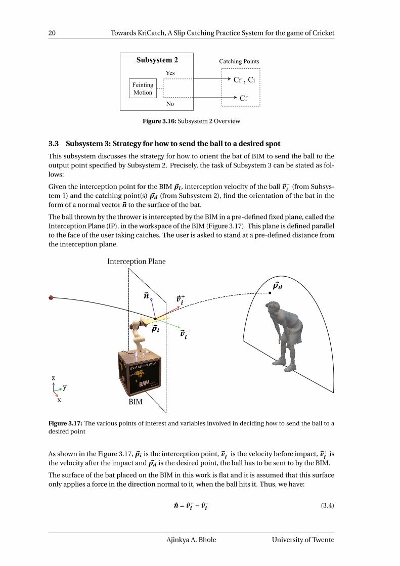
3.3 Subsystem 3: Strategy for how to send the ball to a desired spot
This subsystem discusses the strategy for how to orient the bat of BIM to send the ball to theoutput point specified by Subsystem 2. Precisely, the task of Subsystem 3 can be stated as fol-lows:
Given the interception point for the BIM ~pi , interception velocity of the ball ~v−i (from Subsys-
tem 1) and the catching point(s) ~pd (from Subsystem 2), find the orientation of the bat in theform of a normal vector ~n to the surface of the bat.
The ball thrown by the thrower is intercepted by the BIM in a pre-defined fixed plane, called theInterception Plane (IP), in the workspace of the BIM (Figure 3.17). This plane is defined parallelto the face of the user taking catches. The user is asked to stand at a pre-defined distance fromthe interception plane.
Interception Plane
BIMx
yz
Figure 3.17: The various points of interest and variables involved in deciding how to send the ball to adesired point
As shown in the Figure 3.17, ~pi is the interception point, ~v−i is the velocity before impact, ~v+
i isthe velocity after the impact and ~pd is the desired point, the ball has to be sent to by the BIM.
The surface of the bat placed on the BIM in this work is flat and it is assumed that this surfaceonly applies a force in the direction normal to it, when the ball hits it. Thus, we have:
~n = v+i − v−
i (3.4)
Ajinkya A. Bhole University of Twente
3. SYSTEM ARCHITECTURE 21
where, ~n is the normal vector to the surface of the bat, v+i and v−
i are unit vectors in the direc-tion of ~v+
i and ~v−i respectively.
Also, the bat of the BIM is made to have a zero velocity at the time of impact, giving the folowingequation:
||~v+i || =β||~v−
i || (3.5)
where, β = 0.6 is the coefficient of restitution, which is calculated experimentally. The proce-dure to calculate the co-efficient of restitution is explained in Appendix B.
As can be seen in Equation 3.4, to calculate ~n is it required to calculate ~v+i . The problem of
Subsystem 3 can thus be recast as follows:
Given ~pi , ~v−i , β and ~pd , it is required to calculate ~v+
i .
This problem comes under the class of Two-point boundary value problem (TPBVP) (Wikipedia,2018a). A detailed analysis of the problem and its solution methodology is described in thefollowing subsections.
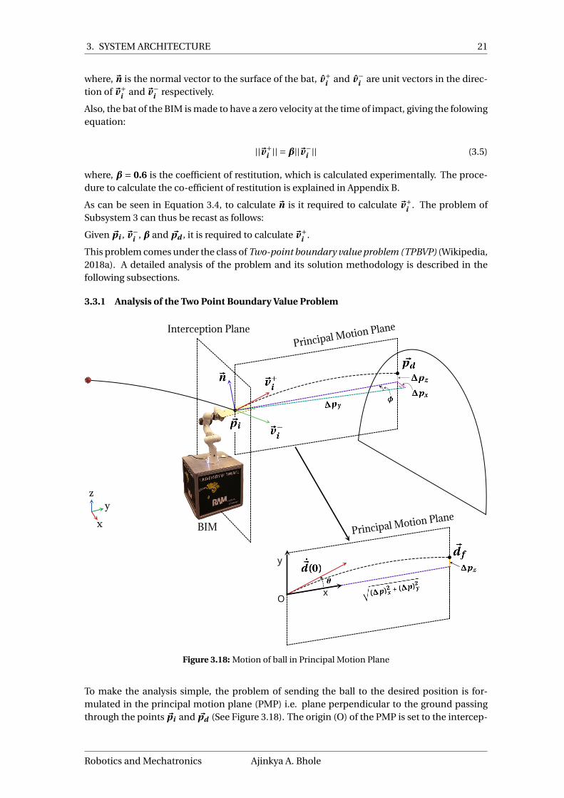
3.3.1 Analysis of the Two Point Boundary Value Problem
Interception PlanePrincipal Motion Plane
Principal Motion PlaneBIMx
yz
Ox
y
Figure 3.18: Motion of ball in Principal Motion Plane
To make the analysis simple, the problem of sending the ball to the desired position is for-mulated in the principal motion plane (PMP) i.e. plane perpendicular to the ground passingthrough the points ~pi and ~pd (See Figure 3.18). The origin (O) of the PMP is set to the intercep-
Robotics and Mechatronics Ajinkya A. Bhole

22 Towards KriCatch, A Slip Catching Practice System for the game of Cricket
tion point ~pi and the desired point ~pd in the PMP can now be given as follows :
~d f =[√
(∆p)2x + (∆p)2
y
∆pz
](3.6)
where,∆p = ~pd − ~pi and∆px ,∆p y and∆pz are the x,y and z components of∆p .
Let ~d (t ) represent a position of the ball in the PMP at a specific time instant t . We have thefollowing differential equation and initial conditions involved in the problem:
~d (t ) =−kd || ~d (t )|| ~d (t )+~g (3.7)
~d (0) =[
00
](3.8)
~d (0) =[||~v+
i ||cos(θ)||~v+
i ||si n(θ)
](3.9)
~d (t f ) = ~d f (3.10)
where, kd is the drag coefficient of the ball, ~g = [0,−9.8]T is the gravity vector, θ is the launchangle and t f is the time at which the ball reaches the point ~pd .
Equation 3.7 is the dynamic model of the thrown ball. Equations 3.8-3.10 are the boundaryconstraints of the problem.
As can be seen in Equation 3.7 there are four integration constants involved. From equations3.8-3.10 we have six boundary conditions and two free parameters i.e. θ and t f . A TPBVP iswell defined if the number of integration constants and free parameters add to the number ofboundary conditions, which is the case here. The formulated TPBVP is thus well-defined.
3.3.2 Existence and Uniqueness of the TPBVP solution
For a given ||~v+i ||, there exists an envelope in which all the possible trajectories of the ball lie
(Chudinov, 2005). In case the catching point ~pd lies:
• inside this envelope, the TPBVP has two set of solutions for θ and t f .
• on this envelope, the TPBVP has a unique solution for θ and t f .
• outside this envelope, the TPBVP has no solution.
As described in Subsystem 2, it is assumed that the ball is thrown with a velocity such thatit is able to reach the desired point when swerved by the BIM. The TPBVP thus always has asolution. In case the TPBVP has two set of solutions for θ and t f , the solution with a lowervalue of θ is chosen. This is because the trajectory of the ball in a slip catch is usually almostflat.
3.3.3 Solution Methodology for the TPBVP
The TPBVP formulated in the previous section does not have an analytic solution. Hence, itneeds to be solved using appropriate numerical methods (Ascher et al., 1994).
The scikits.bvp_solver, a python package (John Salvatier, 2012) which can solve a gen-eral TPBVP is used to solve the formuated problem in the subsection 3.3.1. The package takes
Ajinkya A. Bhole University of Twente

3. SYSTEM ARCHITECTURE 23
around 10 ms to solve the formulated problem and is computationally fast enough to guaranteethat it can suitably be implemented in the task at hand wherein time is a cardinal resource.
The parameter θ obtained from solving the TPBVP is then used to obtain the velocity of the ballpost impact i.e. ~v+
i . This is done as follows (refer Figure 3.18):
~v+i =
||~v+i ||cos(θ)si n(φ)
||~v+i ||cos(θ)cos(φ)||~v+
i ||si n(θ)
(3.11)
where, ||~v+i || is calculated from Equation 3.5 and φ= t an−1(∆px
∆p y).
The unit vectors v+i and v−
i can then be calculated and substituted in equation 3.4 to obtainthe required normal vector (~n) for the surface of the bat.
3.3.4 Choice of BIM
Based on the above analysis, it can be seen that the BIM needs to have atleast 4 degrees offreedom (DOFs). Two for translating in the interception plane and two to set the normal vectorof the surface of the bat. Based on the availability of resources, it was decided to make use of a7 DOF robotic manipulator, ‘Panda’ (Franka Emika GmbH, 2018b) as the BIM.
3.3.5 Subsystem Overview
Figure 3.19 shows an overview of Subsystem 3 .
Interception coordinates of ball
Interceptionvelocity of ball Subsystem 3
TPBVPSolver
Vector normalto bat surface
Figure 3.19: Subsystem 3 Overview
3.4 Subsystem 4: Trajectory Planning and Execution on BIM
This subsystem discusses the trajectory planning and its execution on the BIM.
3.4.1 Trajectory Planning
To plan the trajectory for the bat of the BIM, the interception time, interception point and therequired orientation of the bat at the interception point are required. The interception time andpoint are provided by Subsystem 1 while the orientation of the bat is provided by the Subsystem3.
Assume that, at a certain time to , the interception time ti , the interception point ~p(ti ), the vec-tor normal to the surface of the bat~n(ti ) required to send the ball to desired point are available.A trajectory planner is then evoked to plan a trajectory for the bat of the BIM starting from itscurrent configuration to the interception point configuration.
The trajectory for ~p(t ) (hitting point of the bat) and ~n(t ) (normal vector to the surface of thebat) is planned separately and is explained in the following subsections.
Robotics and Mechatronics Ajinkya A. Bhole

24 Towards KriCatch, A Slip Catching Practice System for the game of Cricket
Trajectory Planning for ~p(t ):
To achieve the desired translation of the hitting point of the bat ~p(t ), a third order polynomialtrajectory is used:
~p(t ) = ~a0 + ~a1(ti − to)+ ~a2(ti − to)2 + ~a3(ti − to)3 (3.12)
We have the following boundary conditions on this trajectory:
• ~p(to) is the position of the hitting point of the bat when the trajectory planner is evoked.
• ~p(to) is the velocity of the hitting point of the bat when the trajectory planner is evoked.
• ~p(ti ) is the interception point received from Subsystem 1.
• ~p(ti ) is zero.
Based on these boundary conditions we have,
~a0 = ~p(to) (3.13)
~a1 = ~p(to) (3.14)
~a2 = −3(~p(to)−~p(ti ))−2~p(to)(ti − to))
(ti − to)2 (3.15)
~a3 = 2(~p(to)−~p(ti ))+ ~p(to)(ti − to))
(ti − to)3 (3.16)
Trajectory Planning for~n(t ):
The trajectory for ~n(t ) i.e. the unit normal vector to the surface of the bat is planned by plan-ning the trajectory of a rotation vector~r (t ), such that following equation holds:
~n(t ) = e[~r (t )]~n(to) (3.17)
where, [~r (t )] is the skew-symmetric cross-product matrix representation of~r (t ).
Following holds from Equation 3.17:
~n(t ) = ~r (t )×~n(t ) (3.18)
It is clear from Equation 3.17 that~r (to) =~0. Thus, the following third order polynomial trajec-tory is used for~r (t ):
~r (t ) = ~b1(ti − to)+ ~b2(ti − to)2 + ~b3(ti − to)3 (3.19)
We have the following boundary conditions on this trajectory:
• ~n(to) is the unit vector normal to the surface of the bat when the trajectory planner isevoked.
• ~n(to) is the rate of change of the unit vector normal to the surface of the bat when thetrajectory planner is evoked.
• ~n(ti ) is the unit vector normal to the surface of the bat at interception point obtainedfrom Subsystem 3.
Ajinkya A. Bhole University of Twente

3. SYSTEM ARCHITECTURE 25
• ~n(ti ) is zero.
Based on the above boundary conditions we have,
~b1 = ~r (to) (3.20)
~b2 = 3(~r (ti )−2~r (to)(ti − to)
(ti − to)2 (3.21)
~b3 = (−2~r (ti )+~r (to)(ti − to))
(ti − to)3 (3.22)
As discussed in Subsystem 2, in case the subsystem decides to feint the motion of the bat, theSubsystem 2 provides two normal vectors for the surface of bat~ni (for the catching point ci ) and~n f (for the catching point c f ). The trajectory to set these normal vectors is done in two phases.Let ts be the time at which subsystem 4 is evoked to start planning the trajectory for BIM. Inthe first phase, a fraction k = 0.5 of the time ti − ts is allocated to set the normal vector to thesurface of the bat from~n(ts ) to~ni and in the second phase, the remaining time (1−k)(ti −ts ) isallocated to set the normal from ~ni to ~n f . Both the phases are applied a third order trajectoryprofile as mentioned in Equation 3.19.
3.4.2 Motion Execution
The planned trajectory from the previous section is executed on the BIM i.e. the Panda arm byproviding it with the twist command T (t ) given as follows:
T (t ) =[~p(t )~r (t )
](3.23)
where, ~p(t ) and ~r (t ) are the velocity profiles defined in the previous section and r is the axis ofrotation for the normal vector to the surface of the bat.
The Panda arm is controlled in the ROS environment using the franka_ros package (FrankaEmika GmbH, 2018a). The twist commands are sent at a frequency of 1000 Hz to the manipu-lator. A new trajectory is planned at a frequency of 250 Hz, based on the updated interceptionpoint details obtained from Subsystem 1 and Subsystem 3.
3.4.3 Subsystem Overview
Figure 3.20 shows an overview of Subsystem 4.
Interception Time
Interception coordinates of ball
Vector normalto bat surface
Subsystem 4
Trajectory Planingand Motion
Execution on BIM
Figure 3.20: Subsystem 4 Overview
Robotics and Mechatronics Ajinkya A. Bhole

26 Towards KriCatch, A Slip Catching Practice System for the game of Cricket
3.5 KriCatch 1.0: System Overview
A complete system overview of KriCatch 1.0 is shown in Figure 3.21. Once the ball is thrown,Subsystem 1 starts the sensing, estimation and prediction of the ball’s trajectory and outputsthe interception point details. Based on the catching points obtained from Subsystem 2 andthe interception point details from Subsystem 1, Subsystem 3 decides the strategy for how thesend the ball to the desired catching points by providing the normal vector to the surface of thebat. Subsystem 4 now has all its required inputs to plan the trajectory of the bat towards theinterception point and finally execute it on the BIM.
Ball Thrown
Interception Time
Interception coordinates of ball
Interceptionvelocity of ball
Subsystem 1
Sensing
Initialization ofCEKF
Estimate andPredict state of theball at Interception
PlaneSubsystem 3
TPBVPSolver
Vector normalto bat surface
Subsystem 4
Trajectory Planingand Motion
Execution on BIM
Cf , Ci FeintingMotion
Cf
Subsystem 2 Yes
No
Catching Points
Figure 3.21: A complete system overview of KriCatch 1.0.
Ajinkya A. Bhole University of Twente

27
4 Experiments on KriCatch 1.0
The experimental setup of KriCatch 1.0 is shown in Figure 4.1. The distance between thethrower and the BIM, D , shown in the figure, available in the OptiTrack environment is around4.5 m. This is slightly less than the usual distance (5-6 m) set between a thrower and a coachproviding catching practice as shown in Figure 1.4 (e). Also, the ball is usually thrown towardsthe coach at speeds which require the coach to intercept the ball in about 0.3-0.4 secs.
D
BIM
Bat
Thrower
Ball
OptiTrack Cameras
Figure 4.1: Experimental setup of KriCatch 1.0.
The robotic manipulator used in this work, i.e. the Panda Arm has limits on its joint velocity,acceleration and jerk, which are violated in case it is asked to traverse outside a radius of 5 cmfrom its initial position, within a time period of 0.3-0.4 secs.
To avoid facing the joint limits, following steps need to be taken:
• the ball needs to be thrown at lower speeds so that the interception time reaches around0.6-0.7 secs
• the ball needs to be thrown in a radius of 10 cm from the starting position of the hittingpoint on the bat and the tip-tilt rotation of the bat is restricted within 20 degrees of theinitial orientation. This is the achievable work-space of Panda arm for the task at hand.
Robotics and Mechatronics Ajinkya A. Bhole

28 Towards KriCatch, A Slip Catching Practice System for the game of Cricket
• the feinting motion is disabled
• a low pass filter has to be applied to the sent twist commands to the manipulator to avoidjoint velocity and acceleration command discontinuity errors given by the manipulator.
0.645 0.65 0 .655 0.66 0 .665 0.67 0 .675 0.68 0 .685 0.690
0.002
0.004
0.006
0.008
0.01
0.012
0.014
0.016
0 0.2 0.4 0.6time (s)
0
0.002
0.004
0.006
0.008
0.01
0.012
0.014
0.016
0.018
Erro
rin
X(m
)
0 0.2 0.4 0.6time (s)
-1
0
1
2
3
4
5
6
7
Erro
rin
Y(m
)
10 -9
0 0.2 0.4 0.6time (s)
-0.018
-0.016
-0.014
-0.012
-0.01
-0.008
-0.006
-0.004
-0.002
0
Erro
rin
Z(m
)
Figure 4.2: Error in position tracking of the bat of BIM for an example trajectory.
The effect of applying the low pass filter, on the position tracking of the hitting point of the batfor an example trajectory is shown in Figure 4.2. The plot show errors between the commandedposition and the actual tracked position of the hitting point on the bat. At the red dotted lines,the trajectory is re-planned on the basis of the new interception point details. It can be seen
Ajinkya A. Bhole University of Twente

4. EXPERIMENTS ON KRICATCH 1.0 29
that the errors in the x and z positions at the end of the trajectory went to 1.6 cms and -1.6 cmsrespectively. Through experiments, it has been observed that the magnitude of this error cango up to 3 cms for each co-ordinate in case the trajectory needs to be completed in a minimumof 0.5 seconds.
4.1 Ball Interception Results
Figure 4.3 shows different episodes wherein the BIM successfully intercepts and swerves theball.
Figure 4.3: Different scenarios wherein the BIM intercepts and swerves the ball.
Robotics and Mechatronics Ajinkya A. Bhole

30 Towards KriCatch, A Slip Catching Practice System for the game of Cricket
4.2 Catching Point Results
To examine the working of KriCatch 1.0, it is also important to check if the ball indeed getsswerved to the desired catching points. Two of the episodes of providing a catch are shown inFigure 4.4 and 4.5. It can be seen that the ball indeed gets swerved towards the catching points,although not with a good accuracy (within a radius of 10 cms from the desired catching point).
5
4
Y(m)
3
20
1
0.5
1
-0.2
1.5
X(m)
0
2
0
Z(m)
0.2
2.5
1
1.2
1.4
1.6
1.8
2
2.2
-0.2
2.4
2.6
Z(m)
2.8
X(m)
00.2
Y(m)5.25.154.94.84.74.64.54.44.3
1
1.2
1.4
-0.2
1.6
1.8
X(m)
0
2
5.2
Z(m)
Y(m)
5
2.2
4.8
2.4
0.2 4.6
2.6
4.4
2.8Desired Catching Point
Attained Catching Point
Start
End
View 1 View 2
Desired Interception Point
Attained Interception Point
Direction of travel of hitting point
Changing orientationof bat
Desired Bat Orientation
Figure 4.4: Scenario 1 showing the details of a catch given by the BIM.
Ajinkya A. Bhole University of Twente

4. EXPERIMENTS ON KRICATCH 1.0 31
5
4
Y(m)
3
20
0.5
1
1
-0.2
1.5
X(m)
0
2
Z(m)
00.2
2.5
1
1.2
1.4
1.6
1.8
2
2.2
-0.2
2.4
2.6
Z(m)
2.8
X(m)
0
Y(m)
5.50.2 54.5
4.9Y(m) 5.44.5 4.6 4.7 4.8 5 5.1 5.2 5.3 5.5
Z(m)
2.8
2.6
2.4
2.2
2
1.8
1.6
1.4
1.2
1
View 1 View 2
Desired Catching Point
Attained Catching Point
Desired Interception Point
Attained Interception Point
Direction of travel of hitting point
Changing orientationof bat
Desired Bat Orientation
Start
End
Figure 4.5: Scenario 2 showing the details of a catch given by the BIM.
4.3 Discussion on the results
The main reason for the ball not getting accurately sent to desired catching point can be ac-counted to the the low-pass filter applied for tracking the planned trajectory of the bat. FromFigures 4.4 and 4.5 it can be seen that, the position and orientation of the hitting point of thebat try to follow the desired position and orientation at the interception point. Although thedesired position and orientation at the interception point is not accurately reached due to theapplication of the low pass filter. This results in, the ball hitting the bat at points different than
Robotics and Mechatronics Ajinkya A. Bhole

32 Towards KriCatch, A Slip Catching Practice System for the game of Cricket
that of the hitting point. Moreover, due to the application of the low pass filter, the velocity ofthe hitting point is not exactly zero when the ball hits the bat, which is an assumption takeninto consideration for Subsystem 3 to calculate the orientation of the bat. This non-zero ve-locity of the bat at the interception point provides and extra velocity to the ball resulting in anerror for the attained catching point.
Another reason can be accounted to the assumption in the Subsystem 3 that the surface of thebat applies only a force normal to the surface of the bat, when the ball hits it. In reality, thereare forces which act tangential to the surface of the bat, which result in more loss of energyfrom the ball. Moreover, this tangential impulse at the surface can make the ball spin resultingto forces acting on the ball due to magnus effect. This conclusion can be verified by looking atthe Figure 4.5. It can be seen that although the hitting point almost reaches the interceptionpoint, the ball gets sent to a lesser vertical height than that of the expected point i.e. the desiredcatching point.
Ajinkya A. Bhole University of Twente

33
5 Conclusions and Recommendations
Following conclusions are made based on the experiments described in the previous chapter:
• The EKF algorithm converges in about 0.05 seconds. This is around 10% of the availableinterception time for the BIM. A better estimation algorithm or system model can helpgetting additional convergence speed.
• Based on the observation and opinions from experienced Cricket players, setting the ve-locity of the bat to zero at the interception point does not provide a good degree of real-ism for the system. In reality, during an event of slip catch, the bat usually possesses anon-zero velocity at the time it intercepts the ball.
• The interception point is constrained in a fixed plane. Although this makes the problemof ‘how to send the ball to the desired spot’ easier and thus computationally inexpensive,it suffers from the fact that it generates restrictive strokes and can result in unnaturalstrategies when compared with human playing
• The contact model of the bat hitting the needs improvement by taking into considerationthe tangential forces which act on the ball during contact.
• The TPBVP formulates for Subsystem 3 is solved using a package written in Python. AC++ implementation of package can be faster in terms of time.
• The Panda manipulator used as the BIM, in terms of speed is too slow to intercept theball thrown at the usual speeds during a slip catching practice session in Cricket.
• It is difficult for the thrower to throw the ball accurately in the limited working space ofthe Panda manipulator.
• The ball thrown in the achievable work space of the Panda arm is not intercepted ac-curately at the calculated interception point as a low pass filter is applied on the twistcommand sent to the manipulator. This leads to the ball hitting the bat around the hit-ting point making it difficult for the ball to be sent to the desired catching point.
Based on the above conclusions and from far-sight, following ideas have been gathered for thenext iteration of KriCatch:
• The trajectory estimation of the ball can be improved by considering other non-linearestimation algorithms (example Unscented Kalman Filter/ Particle Filter) along with abetter ballistic model of the ball, taking into consideration the magnus effect. This needsto be done by taking care of the criterion of computation time and resources.
• Implementation of an Artifical-Intelligence algorithm that tracks the progress and levelof the user and provides catching points and feinting motions accordingly.
• The BIM must be chosen/custom made with appropriate specifications such that it has alarger working space (as compared to the one in this work), in which a thrower can easilythrow the ball.
• The strategy used in Subsystem 3 for how to send the ball to desired points involves theconstraint of setting the velocity of the bat to zero at the interception point. This con-straint must be freed, to make the swerving action of the BIM more realistic. At the sametime, it must be taken care that the new strategy used is not computationally expensiveand is real-time implementable.
Robotics and Mechatronics Ajinkya A. Bhole

34 Towards KriCatch, A Slip Catching Practice System for the game of Cricket
• The constraint of intercepting the ball in a specific fixed plane (Interception Plane) canbe freed and be chosen on a criterion which makes the BIM to intercept the ball with-out breaking its hardware limits. Again, the solution to this problem must be real-timeimplementable.
• Presently, the ball is thrown directly to the BIM without bouncing it on the floor. Usuallyin the game of Cricket, the ball reaches the batsman after bouncing once on the floor.It is then important to integrate this bouncing action in the trajectory estimation andprediction subsystem.
Ajinkya A. Bhole University of Twente

35
A Appendix 1
A.1 Optimal Online Estimation of Linear Gaussian Systems: The Kalman Filter
Online estimation is the estimation of the present state using all the measurements that areavailable, i.e. all measurements up to the present time. This subsection explains the frame-work for the online estimation of the states of time-discrete processes. Most physical processesevolve in the continuous time. Nevertheless, it can be assumed that these systems can be de-scribed adequately by a model where the continuous time is reduced to a sequence of specifictimes.
Figure A.1: An overview of online estimation of Linear Gaussian System Systems (Lei et al., 2017)
Figure A.1 presents an overview of the scheme for the online estimation of the state. The con-notation of the phrase online is that for each time index i an estimate x(i ) of x(i ) is producedbased on Z (i ), i.e. based on all measurements that are available at that time. The crux of op-timal online estimation is to maintain the posterior density p(x(i ) | Z (i )) for running valuesof i . This density captures all the available information of the current state x(i ) after havingobserved the current measurement and all previous ones.
The state model is said to be linear if the transition from one state to the next can be expressedby a so-called linear system equation:
x(i +1) = F (i )x(i )+L(i )u(i )+w (i ) (A.1)
y(i ) = H(i )x(i )+v (i ) (A.2)
F (i ) is the system matrix. The vector u(i ) is the control vector (input vector). L(i ) is the gainmatrix. w (i ) is the process noise, y(i ) is the measurement vector and H(i ) is the measurementmatrix which maps x(i ) to y(i ). The process noise represents the unknown influences on thesystem, for instance, formed by disturbances from the environment. The process noise canalso represent an unknown input/control signal. Sometimes process noise is also used to takecare of modelling errors. The general assumption is that the process noise is a white randomsequence with normal distribution and has the following properties:
E [w (i )] = 0 (A.3)
E [w (i )w T ( j )] =Cw (i )δ(i , j ) (A.4)
Robotics and Mechatronics Ajinkya A. Bhole

36 Towards KriCatch, A Slip Catching Practice System for the game of Cricket
Cw (i ) is the covariance matrix of w (i ). Since w(i) is supposed to have a normal distributionwith zero mean, Cw (i ) defines the density of w (i ) in full.
The update steps, i.e. the determination of p((x(i ) | Z (i )) shown in Figure A.1 are given asfollows:
z(i ) = H(i )x(i | i −1) (A.5)
S(i ) = H(i )C (i | i −1)H T (i )+Cv (i ) (A.6)
K (i ) =C (i | i −1)H T (i )S−1(i ) (A.7)
x(i | i ) = x(i | i −1)+K (i )(z(i )− z(i )) (A.8)
C (i | i ) =C (i | i −1)−K (i )S(i )K T (i ) (A.9)
The interpretation is as follows: z(i ) is the predicted measurement. It is an unbiased estimateof z(i ) using all information from the past. The so-called innovation matrix S(i ) represents theuncertainty of the predicted measurement. The uncertainty is due to two factors: the uncer-tainty of x(i ) as expressed by C (i | i −1), and the uncertainty due to the measurement noisev (i ) as expressed by Cv (i ). The matrix K (i ) is the Kalman gain matrix. This matrix has large,when S(i ) is small and C (i | i −1)H T (i ) is large, that is, when the measurements are relativelyaccurate. When this is the case, the values in the error covariance matrix C (i | i ) will be muchsmaller than C (i | i −1).
The prediction, i.e. the determination of p(x(i +1) | Z (i )) given p(x(i ) | Z (i )), boils down tofinding out how the expectation x(i | i ) and the covariance matrix C (i | i ) propagate to the nextstate. We thus have:
x(i +1 | i ) = F (i )x(i | i )+L(i )u(i ) (A.10)
C (i +1 | i ) = F (i )C (i | i )F T (i )+Cw (i ) (A.11)
The above presented recursive equations are generally referred to as the discrete Kalman filter(DKF).
A.2 Sub-Optimal Solution for Online Estimation of Non-Linear Systems: The Ex-tended Kalman Filter
The general case of nonlinear systems and nonlinear measurement functions can be given asfollows:
x(i +1) = f (x(i ), u(i ), i )+w (i ) (A.12)
y(i ) = h(x(i ), i )+v (i ) (A.13)
The vector f (., ., .) is a nonlinear, time variant function of the state x(i) and the control vectoru(i).
Any Gaussian random vector that undergoes a linear operation retains its Gaussian distribu-tion. A linear operator only affects the expectation and the covariance matrix of that vector.This property is the basis of the Kalman filter. It is applicable to linear-Gaussian systems, and itpermits a solution that is entirely expressed in terms of expectations and covariance matrices.However, the property does not hold for nonlinear operations. In nonlinear systems, the state
Ajinkya A. Bhole University of Twente

APPENDIX A. APPENDIX 1 37
vectors and the measurement vectors are not Gaussian distributed, even though the processnoise and the measurement noise might be. Consequently, the expectation and the covariancematrix do not fully specify the probability density of the state vector. The question is then howto determine this non-Gaussian density, and how to represent it in an economical way. Unfor-tunately, no general answer exists to this question.
assuming that the nonlinearities of the system are smooth enough to allow linear or quadraticapproximations, Kalman-like filters become within reach. These solutions are suboptimalsince there is no guarantee that the approximations are close. An obvious way to get the ap-proximations is by application of a Taylor series expansion of the functions.
f (x +ε) = f (x)+F (x)ε+H .O.T . (A.14)
h(x +ε) = h(x)+H(x)ε+H .O.T . (A.15)
where, H.O.T. represent the higher order terms.
The update steps then become:
z(i ) = H(x(i ))x(i | i −1) (A.16)
S(i ) = H(x(i ))C (i | i −1)H T (x(i ))+Cv (i ) (A.17)
K (i ) =C (i | i −1)H T (x(i ))S−1(i ) (A.18)
x(i | i ) = x(i | i −1)+K (i )(z(i )− z(i )) (A.19)
C (i | i ) =C (i | i −1)−K (i )S(i )K T (i ) (A.20)
And the prediction step can be given as follows:
x(i +1 | i ) = f (x(i ), u(i ), i ) (A.21)
C (i +1 | i ) = F (i )C (i | i )F T (i )+Cw (i ) (A.22)
A.3 Constrained Extended Kalman Filter
In case it is known that the state estimates are bounded in certain range, it can be useful tointegrate these constrains in the EKF algorithm to obtain better convergence.
The structure of the EKF does not include constraints on the states. Dan Simon et. al. (Si-mon and Chia, 2002) have proposed a methodology to integrate inequality constraints for stateestimation which uses the Projection Approach. This methodology is briefly described ahead:
Consider the following linearized model of the plant:
x(i +1) = F (i )x(i )+L(i )u(i )+w (i ) (A.23)
y(i ) = H(i )x(i )+v (i ) (A.24)
Robotics and Mechatronics Ajinkya A. Bhole
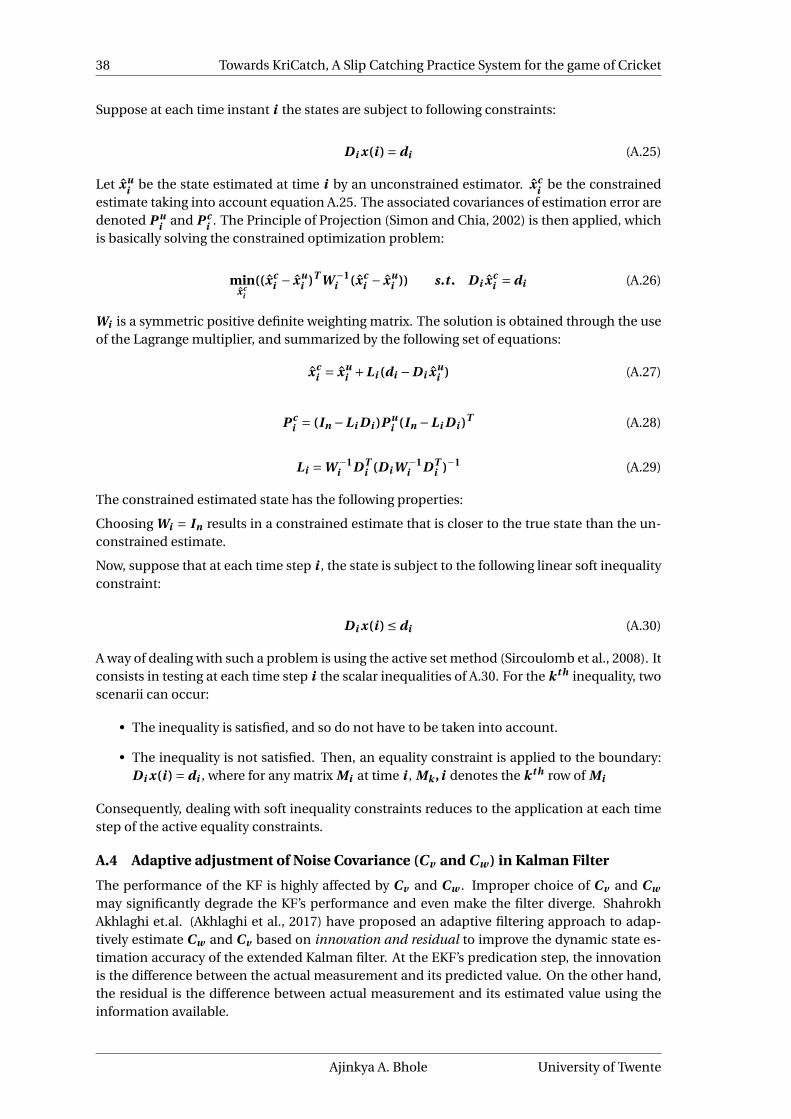
38 Towards KriCatch, A Slip Catching Practice System for the game of Cricket
Suppose at each time instant i the states are subject to following constraints:
Di x(i ) = di (A.25)
Let xui be the state estimated at time i by an unconstrained estimator. xc
i be the constrainedestimate taking into account equation A.25. The associated covariances of estimation error aredenoted P u
i and P ci . The Principle of Projection (Simon and Chia, 2002) is then applied, which
is basically solving the constrained optimization problem:
minxc
i
((xci − xu
i )T W −1i (xc
i − xui )) s.t . Di xc
i = di (A.26)
Wi is a symmetric positive definite weighting matrix. The solution is obtained through the useof the Lagrange multiplier, and summarized by the following set of equations:
xci = xu
i +Li (di −Di xui ) (A.27)
P ci = (In −Li Di )P u
i (In −Li Di )T (A.28)
Li =W −1i DT
i (Di W −1i DT
i )−1 (A.29)
The constrained estimated state has the following properties:
Choosing Wi = In results in a constrained estimate that is closer to the true state than the un-constrained estimate.
Now, suppose that at each time step i , the state is subject to the following linear soft inequalityconstraint:
Di x(i ) ≤ di (A.30)
A way of dealing with such a problem is using the active set method (Sircoulomb et al., 2008). Itconsists in testing at each time step i the scalar inequalities of A.30. For the k t h inequality, twoscenarii can occur:
• The inequality is satisfied, and so do not have to be taken into account.
• The inequality is not satisfied. Then, an equality constraint is applied to the boundary:Di x(i ) = di , where for any matrix Mi at time i , Mk , i denotes the k t h row of Mi
Consequently, dealing with soft inequality constraints reduces to the application at each timestep of the active equality constraints.
A.4 Adaptive adjustment of Noise Covariance (Cv and Cw ) in Kalman Filter
The performance of the KF is highly affected by Cv and Cw . Improper choice of Cv and Cw
may significantly degrade the KF’s performance and even make the filter diverge. ShahrokhAkhlaghi et.al. (Akhlaghi et al., 2017) have proposed an adaptive filtering approach to adap-tively estimate Cw and Cv based on innovation and residual to improve the dynamic state es-timation accuracy of the extended Kalman filter. At the EKF’s predication step, the innovationis the difference between the actual measurement and its predicted value. On the other hand,the residual is the difference between actual measurement and its estimated value using theinformation available.
Ajinkya A. Bhole University of Twente
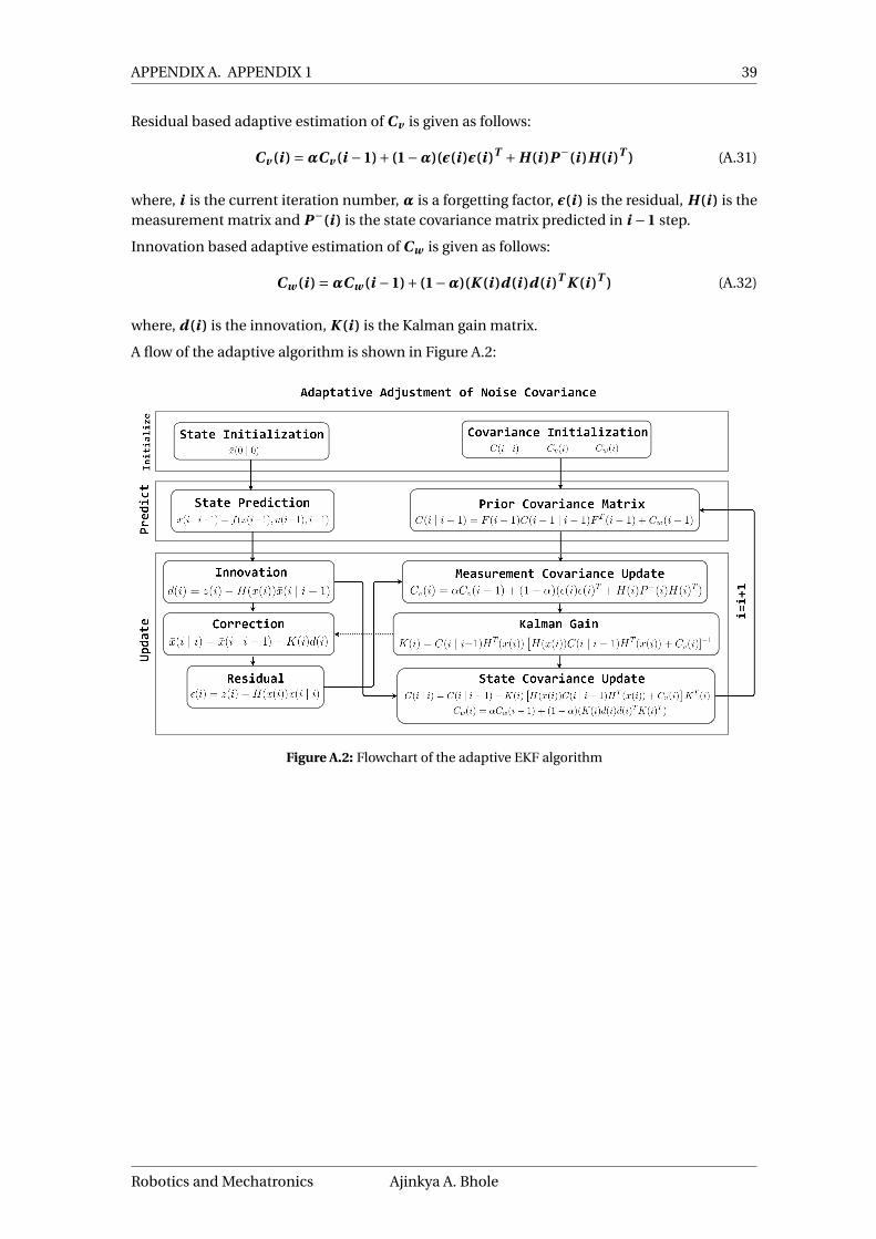
APPENDIX A. APPENDIX 1 39
Residual based adaptive estimation of Cv is given as follows:
Cv (i ) =αCv (i −1)+ (1−α)(ε(i )ε(i )T +H(i )P−(i )H(i )T ) (A.31)
where, i is the current iteration number, α is a forgetting factor, ε(i ) is the residual, H(i ) is themeasurement matrix and P−(i ) is the state covariance matrix predicted in i −1 step.
Innovation based adaptive estimation of Cw is given as follows:
Cw (i ) =αCw (i −1)+ (1−α)(K (i )d (i )d (i )T K (i )T ) (A.32)
where, d (i ) is the innovation, K (i ) is the Kalman gain matrix.
A flow of the adaptive algorithm is shown in Figure A.2:
Figure A.2: Flowchart of the adaptive EKF algorithm
Robotics and Mechatronics Ajinkya A. Bhole

40 Towards KriCatch, A Slip Catching Practice System for the game of Cricket
B Appendix 2
B.1 Calculation of co-efficient of restitution of ball
An experimental method to approximately calculate the co-efficient of restitution as is ex-plained in (Briggs, 1945) is used in this work. During the experiment, the ball is thrown from aspecific height (H) onto the bat of the BIM, and the height of rebound (h) was measured (SeeFigure B.1). The position of the ball during the experimentation is measured using the Opti-Track system.
H
h
Figure B.1: Bouncing experiment to calculate the co-efficient of restitution of the ball.
The co-efficient of restitution β is calculated as follows:
β=
√√√√ e−2kd h
m −1
1−e−2kd H
m
(B.1)
where, kd is the drag co-efficient of the ball calculated through estimation experiments fromSubsystem 1, H is the height from which ball is thrown, h is the rebound height and m is themass of the ball.
Ajinkya A. Bhole University of Twente

41
BibliographyAkhlaghi, S., N. Zhou and Z. Huang (2017), Adaptive adjustment of noise covariance in Kalman
filter for dynamic state estimation, arXiv preprint arXiv:1702.00884.
Almagbile, A., J. Wang and W. Ding (2010), Evaluating the performances of adaptive Kalmanfilter methods in GPS/INS integration, vol. 9, no.1, pp. 33–40.
Anderson, B. D. and J. B. Moore (1979), Optimal filtering, Englewood Cliffs, vol. 21, pp. 22–95.
Ascher, U. M., R. M. Mattheij and R. D. Russell (1994), Numerical solution of boundary valueproblems for ordinary differential equations, volume 13, Siam.
BOLA (2015), TrueMan by BOLA, http://www.bola.co.uk/TrueMan.html, [Online;accessed 12-August-2018].
Brescianini, D. and R. D’Andrea (2018), Computationally Efficient Trajectory Generation forFully Actuated Multirotor Vehicles, IEEE Transactions on Robotics.
Briggs, L. J. (1945), Methods for measuring the coefficient of restitution and the spin of a ball, USDepartment of Commerce, National Bureau of Standards.
Chudinov, P. (2005), The envelope of projectile trajectories in midair, arXiv preprintphysics/0511059.
Cigliano, P., V. Lippiello, F. Ruggiero and B. Siciliano (2015), Robotic ball catching with an eye-in-hand single-camera system, vol. 23, no.5, pp. 1657–1671.
Franka Emika GmbH (2018a), frankar os, , [Online; accessed 12-August-2018].
Franka Emika GmbH (2018b), Panda, https://www.franka.de/, [Online; accessed 12-August-2018].
John Salvatier (2012), Python package for solving two-point boundary value problems.https://pypi.org/project/scikits.bvp_solver/
Kalman, R. E. (1960), A new approach to linear filtering and prediction problems, vol. 82, no.1,pp. 35–45.
Kathrin Gräve, A. B. (2018), mocapo pt i t r ack , , [Online; accessed 30-August-2018].
Kim, S., A. Shukla and A. Billard (2014), Catching objects in flight, vol. 30,no.EPFL-ARTICLE-198748.
Koç, O., G. Maeda and J. Peters (2018), Online optimal trajectory generation for robot tabletennis, Robotics and Autonomous Systems, vol. 105, pp. 121–137.
Lei, B., G. Xu, M. Feng, F. van der Heijden, Y. Zou, D. de Ridder and D. M. Tax (2017),Classification, parameter estimation and state estimation: an engineering approach usingMATLAB, John Wiley & Sons.
Li, H., H. Wu, L. Lou, K. Kühnlenz and O. Ravn (2012), Ping-pong robotics with high-speedvision system, in Control Automation Robotics & Vision (ICARCV), 2012 12th InternationalConference on, IEEE, pp. 106–111.
McCormick, B. W. (1995), Aerodynamics, aeronautics, and flight mechanics, volume 2, WileyNew York.
Miyazaki, F., M. Matsushima and M. Takeuchi (2006), Learning to dynamically manipulate: Atable tennis robot controls a ball and rallies with a human being, in Advances in Robot Control,Springer, pp. 317–341.
Robotics and Mechatronics Ajinkya A. Bhole

42 Towards KriCatch, A Slip Catching Practice System for the game of Cricket
Müller, M., S. Lupashin and R. D’Andrea (2011), Quadrocopter ball juggling, in IntelligentRobots and Systems (IROS), 2011 IEEE/RSJ International Conference on, IEEE, pp. 5113–5120.
Point, N. (2011), Optitrack, Natural Point, Inc.,[Online]. Available: http://www. naturalpoint.com/optitrack/.[Accessed 22 2 2014].
ProBatter Sports (2011), ProBatter PX2 Cricket Video Simulator,http://probatter.com/cricket/, [Online; accessed 08-June-2018].
Quigley, M., K. Conley, B. Gerkey, J. Faust, T. Foote, J. Leibs, R. Wheeler and A. Y. Ng (2009),ROS: an open-source Robot Operating System, in ICRA workshop on open source software,volume 3, Kobe, Japan, p. 5.
Sato, K., K. Watanabe, S. Mizuno, M. Manabe, H. Yano and H. Iwata (2017), Development of ablock machine for volleyball attack training, in Robotics and Automation (ICRA), 2017 IEEEInternational Conference on, IEEE, pp. 1036–1041.
Simon, D. and T. L. Chia (2002), Kalman filtering with state equality constraints, vol. 38, no.1,pp. 128–136.
Sircoulomb, V., G. Hoblos, H. Chafouk and J. Ragot (2008), State estimation under nonlinearstate inequality constraints. A tracking application, in Control and Automation, 2008 16thMediterranean Conference on, IEEE, pp. 1669–1674.
Wikipedia (2018a), Boundary value problem — Wikipedia, The Free Encyclopedia,https://en.wikipedia.org/wiki/Boundary_value_problem, [Online; accessed08-June-2018].
Wikipedia (2018b), Cricket — Wikipedia, The Free Encyclopedia, http://en.wikipedia.org/w/index.php?title=Cricket&oldid=844653304,[Online; accessed 08-June-2018].
Wikipedia (2018c), Iterative design — Wikipedia, The Free Encyclopedia,https://en.wikipedia.org/wiki/Iterative_design, [Online; accessed29-August-2018].
Zhang, Y., Y. Zhao, R. Xiong, Y. Wang, J. Wang and J. Chu (2014), Spin observation andtrajectory prediction of a ping-pong ball, in Robotics and Automation (ICRA), 2014 IEEEInternational Conference on, IEEE, pp. 4108–4114.
Ajinkya A. Bhole University of Twente