Toward a viable, self-reproducing universal computer

ELSEVIER Physica D 97 (1996) 335-352

PHYSICA

Toward a viable, self-reproducing universal computer* Jean-Yves Perrier 1, Moshe Sipper*, Jacques Zahnd 2

Logic Systems Laborato~', Swiss Federal Institute of Technology, lN-Ecublens, CH-IO I 5 Lausanne, Switzerland

Received 26 January 1996; accepted 7 April 1996 Communicated by H. Flaschka

Abstract

Self-reproducing, cellular automata-based systems developed to date broadly fall under two categories; the first consists of machines which are capable of performing elaborate tasks, yet are too complex to simulate, while the second consists of extremely simple machines which can be entirely implemented, yet lack any additional functionality aside from self- reproduction. In this paper we present a self-reproducing system which is completely realizable, while capable of executing any desired program, thereby exhibiting universal computation. Our starting point is a simple self-reproducing loop structure onto which we "attach" an executable program (Turing machine) along with its data. The three parts of our system (loop, program, data) are all reproduced, after which the program is run on the given data. The system reported in this paper has been simulated in its entirety; thus, we attain a viable, self-reproducing machine with programmable capabilities.

1. I n t r o d u c t i o n

The study of artificial self-reproducing structures or "machines" has been taking place for almost half a century.

Much of this work is motivated by the desire to understand the fundamental information-processing principles

and algorithms involved in self-reproduction, independent of their physical realization [20,25]. An understanding of

these principles could prove useful in a number of ways. It may advance our knowledge of biological mechanisms of

reproduction by clarifying the conditions that any self-reproducing system must satisfy and by providing alternative

explanations for empirical ly observed phenomena. Work in this area can shed light on issues regarding origin of

life theories [20]. The fabrication of artificial self-reproducing machines can also have diverse applications, ranging

from nanotechnology [4,5] to space exploration [6]. Ultimately, we wish to produce machines that display an array

of desirable biological characteristics, including self-reproduction, self-repair, growth and evolution [ 15].

* vi.a.ble Vvi--*-b*l \ \-ble-\ aj [E fr. ME ft. vie life, ft. L vita - more at VITAL] 1: capable of living; esp : born alive with such form and development of organs as to be normally capable of living 2: capable of growing or developing {- seeds- eggs} 3: WORKABLE - vi.a.bly av

Webster dictionary * Corresponding author. E-mail: [email protected]. 1 E-mail: [email protected]. 2 E-mail: [email protected].

0167-2789/96/$15.00 Copyright © 1996 Elsevier Science B.V. All rights reserved PH SO 167-2789(96)00091-7

336 J.-Y. Perrier et al./Physica D 97 (1996) 335-352

One of the central models used to study self-reproduction is that of cellular automata (CA). CAs are dynamical

systems in which space and time are discrete. They consist of an array of cells, each of which can be in one of a finite

number of possible states, updated synchronously in discrete time steps according to a local, identical interaction

rule. The state of a cell at the next time step is determined by the previous states of a surrounding neighborhood of

cells; this is usually specified in the form of a rule table (also referred to as the transition function), delineating the

cell's next state for each possible neighborhood configuration [24,27]. The cellular array (grid) is n-dimensional,

where n = 1, 2, 3 is used in practice; in this work we shall concentrate on n = 2, i.e., two-dimensional grids.

The self-reproducing systems developed to date broadly fall under two categories. The first consists of universal

constructor-computers, which are capable of performing elaborate tasks beyond mere self-reproduction, yet are

highly complex machines of prohibitive size, thereby preventing their realization or simulation. The second category

consists of extremely simple machines which are completely realizable, yet lack any additional functionality aside

from self-reproduction.

Our goal in this paper is to present a self-reproducing system which is completely realizable, while capable of

executing any desired program, thereby exhibiting universal computation. Thus, we attain the advantages of both

aforementioned categories. Our starting point is a simple self-reproducing structure (a loop) onto which we "attach"

an executable program along with its data. The three parts of our system (loop, program, data) are all reproduced,

after which the program (Turing machine) is run on the given data. It is important to note that the self-reproducing

system reported in this paper has been simulated in its entirety. Indeed, this is a crucial requirement since our aim

is to attain viable, self-reproducing systems with programmable capabilities.

In Section 2 we provide an account of the study of self-reproduction in cellular automata. In Section 3 we

describe the basic design of our automaton. Section 4 delineates the functioning of our system, including the

self-reproduction process and the execution of the attached program. In Section 5 we describe an example of a

self-reproducing machine whose program consists of a parenthesis checker. A discussion of our results follows in Section 6.3

2. Self-reproduction in cellular automata

In this section we provide a short survey of previous work on self-reproduction in cellular automata, concentrating

mainly on those works that are relevant to our own. Von Neumann is credited with being the first to conduct a formal

investigation of self-reproduction by machines; in particular, he asked whether we can use purely mathematical-

logical considerations to discover the specific features of biological automata that make them self-reproducing. To conduct a formal investigation of this issue, von Neumann used the cellular automaton model, conceived by

Ulam [25]. Von Neumann used two-dimensional CAs with 29 states per cell and a neighborhood consisting of five cells. 4

He showed that a universal computercan be embedded in such cellular space, namely a device whose computational

power is equivalent to that of a universal Turing machine. He also described how a universal constructor may be built, namely a machine capable of constructing, through the use of a "constructing arm", any configuration whose description can be stored on its input tape. This universal constructor is therefore capable, given its own description, of constructing a copy of itself, i.e., self-reproduce (Fig. 1). The terms "machine" and "tape" refer to configurations, i.e., assignments of states to grid cells (for formal definitions see [3]). It has been noted that the basic mechanisms von

3 For those readers who are familiar with previous work on self-reproduction in CAs we suggest a quick tour of the figures, by which a basic comprehension of our system may be gained.

4 The neighborhood consists of the cell itself together with its four immediate non-diagonal neighbors.

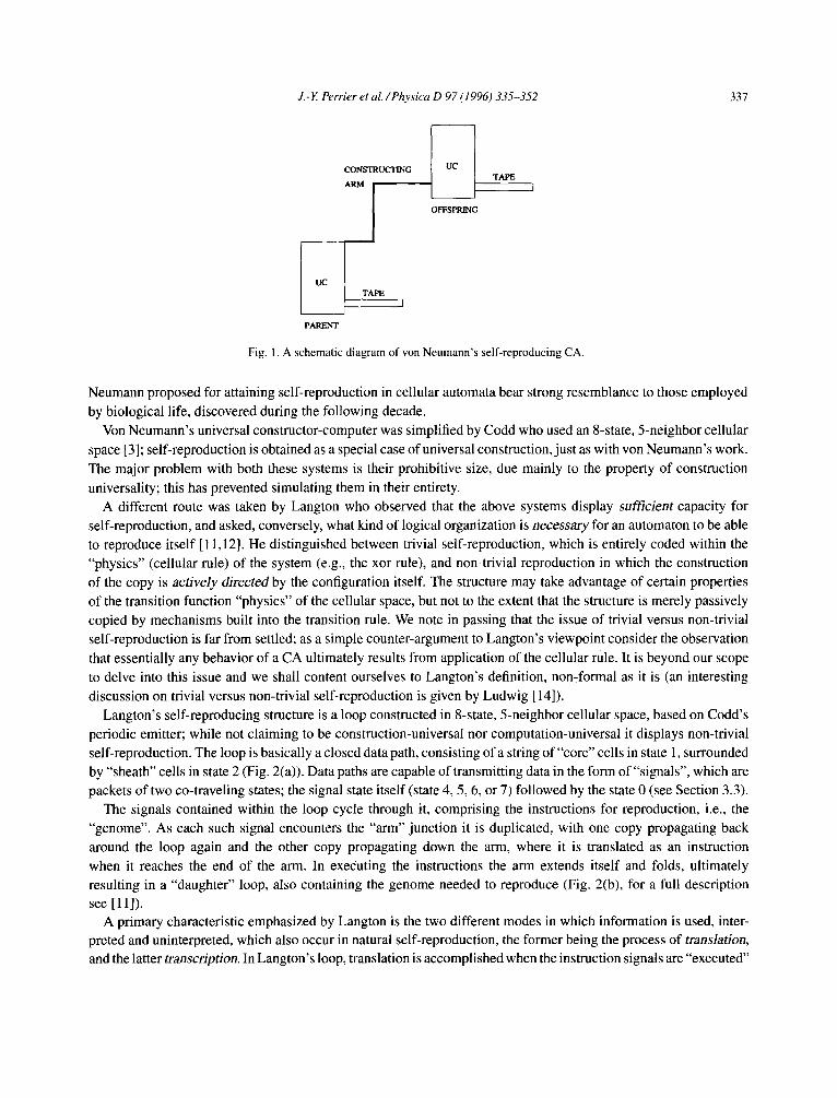
J.-Y. Perrier et al./Physica D 97 (1996) 335-352 337

CONSTRUCTING ARM

UC l TAPE I

PARENT

T~E

OFFSPRING

Fig. 1. A schematic diagram of von Neumann's self-reproducing CA.

Neumann proposed for attaining self-reproduction in cellular automata bear strong resemblance to those employed by biological life, discovered during the following decade.

Von Neumann's universal constructor-computer was simplified by Codd who used an 8-state, 5-neighbor cellular space [3]; self-reproduction is obtained as a special case of universal construction, just as with von Neumann's work. The major problem with both these systems is their prohibitive size, due mainly to the property of construction universality; this has prevented simulating them in their entirety.

A different route was taken by Langton who observed that the above systems display sufticient capacity for self-reproduction, and asked, conversely, what kind of logical organization is necessary for an automaton to be able to reproduce itself [ 11,12]. He distinguished between trivial self-reproduction, which is entirely coded within the "physics" (cellular rule) of the system (e.g., the xor rule), and non-trivial reproduction in which the construction of the copy is actively directed by the configuration itself. The structure may take advantage of certain properties of the transition function "physics" of the cellular space, but not to the extent that the structure is merely passively copied by mechanisms built into the transition rule. We note in passing that the issue of trivial versus non-trivial self-reproduction is far from settled; as a simple counter-argument to Langton's viewpoint consider the observation that essentially any behavior of a CA ultimately results from application of the cellular rule. It is beyond our scope to delve into this issue and we shall content ourselves to Langton's definition, non-formal as it is (an interesting discussion on trivial versus non-trivial self-reproduction is given by Ludwig [ 14]).

Langton's self-reproducing structure is a loop constructed in 8-state, 5-neighbor cellular space, based on Codd's periodic emitter; while not claiming to be construction-universal nor computation-universal it displays non-trivial self-reproduction. The loop is basically a closed data path, consisting of a string of"core" cells in state 1, surrounded by "sheath" cells in state 2 (Fig. 2(a)). Data paths are capable of transmitting data in the form of"signals", which are packets of two co-traveling states; the signal state itself (state 4, 5, 6, or 7) followed by the state 0 (see Section 3.3).

The signals contained within the loop cycle through it, comprising the instructions for reproduction, i.e., the "genome". As each such signal encounters the "arm" junction it is duplicated, with one copy propagating back around the loop again and the other copy propagating down the ann, where it is translated as an instruction when it reaches the end of the arm. In exec~uting the instructions the arm extends itself and folds, ultimately resulting in a "daughter" loop, also containing the genome needed to reproduce (Fig. 2(b), for a full description see [11]).

A primary characteristic emphasized by Langton is the two different modes in which information is used, inter- preted and uninterpreted, which also occur in natural self-reproduction, the former being the process of translation,

and the latter transcription. In Langton's loop, translation is accomplished when the instruction signals are "executed"


1 7 0 1 4 0 1 4

0 . . . . . . 0

7 ° . 1

1 . ° 1

0 . . 1

7 ° • 1

1 . . . . . . 1 o . • o °

0 7 1 0 7 1 0 7 1 1 1 1 1 .

. . . . . . . . . . ~ ° .

7 0 1 7 0 1 7 0

I . . . . . . 1

1 . . 7

1. . 0

1 . . 1

1 . .7

0 . . . . . . 0

4 1 0 4 1 0 7 1

1 4 0 1 4 0 1 1

0 . . . . . . 1

7. . 1

i. . 1

0 . . 7

7 . . 0

1 . . . . . . 1

7 0 6 1 0 7 1 0 7

(a) (b)

Fig. 2. Langton's self-reproducing loop: (a) time step O; (b) time step 125. Sheath cells are denoted by dots. Cells in the quiescent state (zero) are shown as spaces.

as they reach the end of the construction ann, and upon collision of signals with other signals. Transcription is ac-

complished by the duplication of signals at the arm junctions [ 11 ].

Following in Langton's footsteps, smaller (non-trivial) self-reproducing loops, embedded in cellular spaces with

fewer states, were demonstrated by Byl [2] and later by Reggia et al. [20]. The latter constructed several such loops, sheathed as well as unsheathed, also studying the issue of rotational symmetry (see Section 3.3); the smallest demonstrated loop is unsheathed, consisting of five cells, embedded in 6-state cellular space [20].

The loop structures discussed above display only one functionality, namely self-reproduction; while simple enough to simulate in their entirety they represent an extreme opposite of the works of von Neumann and Codd. As put forward by Langton, one can imagine a scale of complexity of self-reproducing entities, with one end repre-

senting simple, marginally non-trivial, self-reproducing structures, and the other end representing highly complex mechanisms such as the universal constructor-computer [ 11]. The above loops occupy an intermediate position,

albeit close to the low complexity end. The systems designed by von Neumann and Codd are highly complex and do not yield themselves easily to

implementation. Taking a different approach we ask whether one can start at the low end of the complexity spectrum,

namely with simple self-reproducing structures, and add functionalities to these entities, ultimately attaining highly complex machines, that are nonetheless completely realizable. A first step in this direction was recently taken by

Tempesti [23]. His self-reproducing system resembles that of Langton's, with the added capability of attaching to the automaton an executable program which is duplicated and executed in each of its copies. The program is stored within the loop, interlaced with the reproduction code and is therefore somewhat limited (see Section 3.2).

Our work takes an additional step forward, by demonstrating a self-reproducing loop that is capable of implementing any program, written in a simple yet universal programming language. The program and its data are reproduced along with the loop, after which program execution takes place.

Before ending this short exposition, we briefly mention a number of recent research themes, which, though not bearing directly on our work, are interesting nonetheless. Ibfinez et al. [7] present a cellular reproduction model based

on self-inspection, in which the description of the object to be reproduced (the "genome") is dynamically constructed concomitantly with its interpretation. 5 This entails a more robust reproduction scheme, which also affords the possibility of inheritance of phenotypical variations in a Lamarckian manner. The embryonics (embryological electronics) project is a CA-based approach in which three principles of natural organization are employed: multi- cellular organization, cellular differentiation and cellular division, cf. Mange and co-workers, [ 15-18]. Their intent is to create an architecture which is complex enough for (quasi) universal computation yet simple enough for physical implementation; among the properties demonstrated by this group is a form of"multi-cellular" reproduction. Finally,

5 Self-inspection based methods were first introduced by Laing [8-10] using a different model than that of the CA.

J.-Y Perrier et al./Physica D 97 (1996) 335-352 339

we mention the work of Sipper [21,22], in which a non-uniform, CA-derived model is presented, and used to

implement various systems, among them a self-reproducing, multi-cellular loop.

3. Des igning a n e w automaton

In this section we describe the overall design of our automaton. Note that we do not wish to attain construction

universality, a property which stood as the main reason for the prohibitive size of the machines designed by yon

Neumann and Codd; our aim is to attain a self-reproducing system exhibiting universal computation, which is

completely realizable.

Our starting point is Langton's self-reproducing loop to which we add the capability of universal computation.

Toward this end we must choose a suitable Turing machine model, decide upon the storage method of program and

data, and realize the capacity for signal transmission. These issues are discussed ahead.

3.1. The Turing machine model

The Turing machine model chosen for our work is the W-machine, introduced by Wang [26] and named for him

by Lee [13], who explored its relation with finite automata (see also [1]). A W-machine is like a Turing machine

with two symbols 0 and 1, save that its operation at each time step is guided not by a Turing quintuple but by an

instruction from the following list [1]:

- PRINT 0: print the symbol 0 on the square under scan.

- PRINT 1: print the symbol 1 on the square under scan.

- MOVE DOWN: move the read-wri te head one square down. 6

- MOVE UP: move the read-wri te head one square up.

- IF i THEN (n) ELSE (next instruction) : conditional jump.

- STOP.

The complete program for a particular machine is a finite ordered list of instructions with position in the program

corresponding to the state of a Turing machine. After execution of an instruction of the first four types, control

is automatically transferred to the next instruction. The conditional jump transfers control to the nth instruction if

the square under scan contains a 1 symbol, otherwise it transfers control to the next instruction. Note that this is a

program jump, not a move on the tape. If control is transferred to the STOP instruction, or to an instruction outside

the program, the computation halts [1 ].

The W-machine is similar to the Turing machine model in that it uses an infinite, cellular tape, however the

program consists of more easily manipulable high level instructions rather than a state transition diagram.

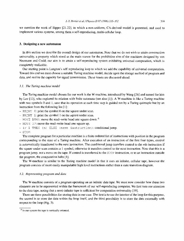
3.2. Representing program and data

The W-machine consists of a program operating on an infinite data tape. We must now consider how these two

elements are to be represented within the framework of our self-reproducing computer. We first turn our attention

to the data tape, noting that a semi-infinite tape is sufficient for computation universality [ 19].

There are three possibilities for storing data in our case. The first is to use the interior of the loop for this purpose,

the second is to store the data within the loop itself, and the third possibili ty is to store the data externally with

respect to the loop (Fig. 3).

6 In our system the tape is vertically oriented.


0 . . . . . . 0

1 1

0 1

? 1

1 . . . . . . 1 . . . . .

0 7 1 0 7 1 0 7 1 1 1 1 1 °

0 . . . . . . 0 .

I °

0 • •

? . ° 1 °

1 1 . . . . .

0 7 1 0 7 1 0 7 1 1 1 1 1 .

1 7 0 1 & 0 1 ~

0 . . . . . . 0

7 • . 1

1 . . 7

0 • . 0

? • , 1

1 . . . . . . 1 . . . . .

0 7 X 0 7 1 0 7 1 1 1 1 1 .

(a) (b) (c)

Fig. 3. Three possibilities for data storage: (a) within the interior of the loop; (b) within the loop itself; (c) externally with respect to the loop.

The first two options lack an essential element necessary for the construction of a universal computer, namely an

infinitely expandable memory. One can obviously "tailor" the loop a priori to any desirable size, however, once the

system begins its operation, memory size is essentially fixed, i.e., finite. Designing such a loop to actually change

its size dynamically during operation would be an arduous task; moreover, this creates another problem since we

end up with a multitude of loops, dynamically growing in all directions, mutually interfering with each other. 7

Our choice for data representation lies therefore in the third possibility, which affords dynamic adaptation of tape

size. As the tape can grow unchecked in one direction (down) we must limit our reproduction to one dimension (the

remaining one). Thus, while previous loops reproduced in two dimensions, ours will be a linear reproduction, the

other dimension being reserved for tape "growth". 8

As opposed to the data tape whose size cannot be limited at the outset, program size is fixed in advance; therefore

any of the above three options can be used for its storage. We have chosen the third option, so that the program is

represented in an identical manner to that of the data tape. This is more convenient in practice; the first option would

entail a novel mechanism for reading and reproducing the enclosed program, while the second option presents some

synchronization problems due to the mobility of the program within the loop. 9 Using the third option, in which the

program is stored externally, eschews these problems; no novel reproduction nor reading mechanism is required,

and synchronization is facilitated since the program is essentially immobile.

3.3. Signals

In Section 2 we noted that the process of reproduction involves signals which are transmitted between the mother

structure and the daughter one. In this section we take a look at some possible signal implementations, choosing

the most appropriate one for our case.

Von Neumann's transition function satisfies weak rotational symmetry; some cell states are directionally oriented

[25]. The oriented cell states are such that they permute among one another consistently under successive 90 °

rotations of the underlying two-dimensional coordinate system [20] (for a formal definition of rotational symmetry in cellular automata see [3]). For example, the cell state designated t is oriented and thus permutes to different cell states --~, $, and ~ under successive 90 ° rotations; it represents one oriented component that can exist in four

7 The loop of Tempesti [23], discussed in Section 2, takes the second approach, i.e., the program and data are stored within the loop itself.

8 Another possibility would be to use a three-dimensional cellular space with reproduction occurring, as before, in two dimensions, and tape growth taking place in the third.

9 These concern the maintaining of the current instruction "pointer", and especially the execution of the I F instruction, which entails a break in sequential execution.


• • ° • ° ° • °

7 0 1 7 0 1 7 0

1 . . . . . . 1

1 . . 7

1 . . 0

I . . 1

1 . ° 7

0 . . . . . . 0 . . . .

4 1 0 4 1 0 7 1 0 7 1 1 .

A ° . . • . . . . . o .

P . D .

P . D .

P . D .

P . D •

P

P

P

Fig. 4. The automaton structure. P denotes a state belonging to the set of program states,/3 denotes a state belonging to the set of data states, and A is a state which indicates the position of the program.

different states or orientations. A major problem with this approach is the large number of states required; for each direction two different states are needed, an active one, denoting the presence of a signal, and an inactive one. This

also entails a highly complicated implementation of signals intersection. Codd's simplified version of von Neumann's self-reproducing universal constructor-computer [3] and the simpler

sheathed loops that followed [2,11,12] are all based on a more stringent criterion called strong rotational symmetry [3]; all cell states are viewed as being unoriented or rotationally symmetric. In this case, the "wire", i.e., signal path,

is bi-directional, and the direction of the signal is indicated by a trailing state. For example, in Codd's model the

two adjoined states {0, 7} represent a value of 7 moving right, while {7, 0} represents the same value moving left.

Langton simplified Codd's construction, making the individual signals more "powerful", by altering the transition function; for example, one signal is sufficient to cause the loop arm to extend, rather than the two used by Codd. He also added a special signal, which travels within the sheath, and upon arriving at the next corner initiates the

construction of a new construction arm. In [20] both types of rotational symmetry are studied. Our choice of signals lies with the latter approach, i.e., that of Codd and Langton, due to their simplified form.

Our system consists of three parts: loop, program, and data, with Codd-type signals used for the first part, and Langton-type signals used for the latter two. Essentially, Codd-type signals are used to store the loop's "genome", i.e., the instructions necessary for its reproduction, while Langton-type signals are used for handling information

pertaining to the program and data.

3.4. The automaton structure

Upon examining the different issues above we arrive at our basic automaton design, shown in Fig. 4. The system consists of a self-reproducing loop onto which we attach the program and data, both of which are reproduced (along with the loop). In Section 4 we describe in detail the functioning of our self-reproducing computer.

4. Description of the automaton's functioning

In this section we delineate the workings of our system, explicating its two main functionalities: reproduction and program execution. The 5-neighbor cellular space consists of 63 states, theoretically entailing a huge rule table of size 635; however, the number of table entries actually used, i.e., those which do not transform a state to itself (identity transformations), is only 8503. This renders our automaton completely realizable. Note that we did not attempt to

342 J-Y Perrier et al./Physica D 97 (1996) 335-352

• ° • o • ° • •

7 0 1 7 0 1 7 0

1 . . . . . . 1

1 . . 7

1 . • 0

1 . . 1

1 • • 7

0 . . . . . . 0

4 1 0 4 1 0 7 1

. . . . ° ° ° °

1 4 0 1 4 0 1 1

0 . . . . . . 1

7 . • 1

1 . • 1

0 . • 7

7 • • 0

1 . . . . . . 1

7 r ~ l o l ~ l o 7 l O 7 A . . . . . . . . . . ] ~ t . ~ . . . . .

P • D .

P • D •

P . D .

P . D .

P

P

P

Fig. 5. Program reproduction: I. Daughter loop has been created. Three signals are generated, a left-moving signal which will initiate program reproduction (boxed 5), a program-top marker (boxed 8), and a right-moving signal which will create the data-top marker (boxed 6).

minimize the number of states, though it is most likely that such a reduction is possible, aided by novel CA design tools (see Section 6). In the figures that follow we denote states by illustrative symbols rather than by their actual values.

4.1. Reproduction

Our system consists of three parts: loop, program, and data, each of which is reproduced (in this order) as described ahead. In what follows we use the terms mother unit and daughter unit to denote the respective systems, consisting of all th~Tee parts.

4.1.1. Reproduction of the loop

The loop reproduces in an identical manner to Langton's loop [11 ], with the exception that specialized signals are incorporated within the sheath for handling information pertaining to the program and data (these are explained in the sections ahead).

4.1.2. Reproduction of the program

Once the loop's reproduction ends, i.e., a daughter loop has been created, three special states are generated; the

first, traveling toward the mother unit, starts the reproduction of the program, the second creates a "marker" for the program position within the daughter unit (signifying the top of the program structure), and the third creates a marker for the data position (signifying the top of the data structure, see Fig. 5). This last signal will also eventually serve to initiate the reproduction of the daughter unit, once the data structure (tape) has been reproduced in its entirety (thereby ending the reproductive process).

The signal transmitted to the mother unit first acts to cut part of the "umbilical cord" connecting both systems. It then generates a special state at the top of the mother data structure, which blocks "undesirable" signals from entering during program reproduction; this state will also serve to eventually initiate data reproduction (Fig. 6).

The signal continues to propagate until arriving at the top of the mother program structure, where it proceeds to travel down the length of the program, acting as a "read" head. For each program state encountered, a corresponding mobile "traveling" state is generated within the sheath, which travels upward (Fig. 7).

These upward-traveling signals propagate to the daughter unit. There, upon encountering the program-top marker, they travel down the length of the daughter structure under construction; once at the bottom, the newly arrived state is inserted into the growing program structure.


• . ° . . . . .

7 0 1 7 0 1 7 0

1 . . . . . . 1

1 • . 7

1 . • 0

1 . . 1

1 . o 7

0 . . . . . . 0

4 1 0 4 1 0 7 1

A . . . . . . [ ]

P . D Z

P . D .

P . D .

P . D .

P

P

P

• • ° . . . . °

4 0 1 1 1 1 1 7

1 . . . . . . 0

0 . . 1

• . . 7

1 . . 0

0 • . 1

7 . . . . . . 7

1 0 7 1 0 6 1 0

0 . . . . . . .

9

Fig. 6. Program reproduction: 2. "Umbilical reproduction, creates the blocker signal at the unit has been completed (states 8,9), and the

cord" is partially severed. The left moving 5 signal, that ultimately initiates program top of the mother data structure (z). Meanwhile, the program-top marker in the daughter 6 signal continues traveling right to create the data-top marker.

7 0 1 7 0 1 7 0

1 . . . . . . 1

1 • . 7

i . . 0

i . . 1

1 . . 7

0 . . . . . . 0

4 1 0 4 1 0 7 1

• • • . . . . .

1 7 0 1 6 0 1 7

0 . . . . . . 0

7 . . 1

1 . . 7

0 . . 0

7 • • 1

I . . . . . . 4

1 1 1 1 0 4 1 O

~ . ~ . . . . . . . 0 . . . . . . 8

P . . D Z 9 9

" ° "

• D .

• D .

P

P o

Fig. 7. Program reproduction: 3. Actual program reproduction has started. As the 5 signal moves down the mother structure it generates for each program state a corresponding upward-traveling state within the sheath (boxed T), which travels to the daughter unit. Note that the data-top marker of the daughter unit has been completed.

When the read head arrives at the bottom of the mother program structure, a signal is generated which erases

the program-top marker within the daughter unit, and also ends the construction of the daughter program structure

(Fig. 8).

4.1.3. Reproduction of the data

The signal that ended program reproduction also serves a second purpose; once arriving at the blocker state, at

the top of the mother data structure, it activates the data reproduction process (Fig. 9).

This process is similar to program reproduction. A read "head" (signal) transforms each data state to a corre-

sponding traveling state that travels to the daughter unit. Each such signal arrives at the (daughter) data-top marker,

travels down the length of the data structure, and is added to it at the bottom.

The signal that had initiated the entire reproductive process, upon arriving at the end of the mother data structure,

generates a signal that signifies the end of reproduction. This will cut the remainder of the umbilical cord, and

complete the construction of the daughter data structure. Once this process ends, the entire daughter unit has been

formed and can commence its own reproduction.


7 0 1 7 0 1 7 0

1 . . . . . . 1

1 . • 7

1 • • 0

I . . 1

1 . • 7

0 . . . . . . 0

• 0 ~ 1 0 7 1

P . D Z

P • D .

P . D •

P . D •

P

P

P

1 7 0 1 6 0 1 7

0 . . . . . . 0

7 . . 1

1 • . 7

0 . • 0

7 • . 1

1 . . . . . . 4

1 1 1 1 0 4 1 0

[] 0 . . . . . . 0

[]P. 9

• P • ~ 9

Fig. 8. Program reproduction: 4. Final steps of program reproduction. The last "traveling" program states are followed by the final $ signal. This signal will complete the construction of the daughter program structure, and activate the data reproduction process.

. . . . , • ° •

7 0 1 7 0 1 7 0

1 . . . . . . 1

1 • • 7

1 • • 0

1 . • 1

1 • , 7

0 . . . . . . 0

4 1 0 4 1 0 7 1 0

A . . . . o o ° ° ~

P . D ~

P • D .

P . D °

P • D ,

P

P

P

1 7 0 1 6 0 1 7

0 . . . . . . 0

7 • . 1

1 • • 7

0 . . 0

7 • • 1

1 . . . . . . 4

1 1 1 1 0 4 1 0

8 . . . . . . $

T P . 9

• P •

T P .

• P .

T 9

Fig. 9. Data reproduction: the $ signal, which ends program reproduction, also activates the data reproduction process by creating a read head (%). This head passes down the length of the mother data structure, generating the corresponding traveling states (as with program reproduction).

4.2. Program execution

We have described above the reproductive process by which a mother unit, composed of loop, program, and data,

creates" an identical daughter unit. Once this process is over, the mother unit can "fulfill" its function by executing the program (Turing machine).

In this section we explicate the manner by which programs are executed. This begins with an initialization

phase which occurs immediately after reproduction has terminated, followed by execution of instructions from the

instruction set of Section 3.1: PRINT, MOVE, IF , and STOP.

4.2.1. Initialization

As described above, after reproduction of the mother data structure (tape), a signal is sent to the daughter unit to

indicate end of reproduction. A second signal is concomitantly generated, that propagates in the opposite direction, toward the (mother) program in order to initiate its execution. On its way this signal creates the data read-write head (henceforth data head) at the sheath's exterior, and upon arriving at the program top, it generates the program read head (henceforth program head. see Fig. 10). These heads are signals that control the execution of the program; once in place, program execution begins.


• ° ° ° • ° ° °

7 0 1 7 0 1 7 0

1 . . . . . . 1

1 . . 7

1 . . 0

1 . . 1

1 . . 7

0 . . . . . . 0

4 1 0 4 1 0 7 1

A . . ° ° ° . . .

PN N - ~ . P • D .

P • D •

P . D .

P

P

P

Fig. 10. Program execution: end of initialization phase. Program head and data head are in place (boxed H).

. . . . . . o °

7 0 1 7 0 1 7 0

1 . . . . . . 1

1 . . 7

1 . • 0

1 . . 1

1 . . 7

0 . . . . . . 0

4 1 0 4 1 0 7 1

A C . C . C . .

P. Z C -

PC .+

P ° . ÷

P .

P .

PH

P.

. . . . o ° ° o

7 0 1 7 0 1 7 0

1 . . . . . . 1

1 . . 7

1 . . 0

1 • . 1

1 . . 7

0 . . . . . . 0

4 1 0 4 1 0 7 1

A . C . C . C .

P C ~ . +

P • . +

P . . +

P .

P .

P K P .

(a) (h)

Fig. 11. Program execution: the PRINT instruction (shown for PRINT 1). Data states are shown as - (0) and + (1). C denotes an instruction (command) on its way to being executed. (a) Before execution: data state at current position of data head is 0 (-). Command (C) at current position of data head is PRINT 1. (b) After execution: data state is 1 (+).

4.2.2. The P R I N T instructions

When the program head encounters an instruction PRINT 0 or PRINT 1, it implements it by generating a

signal which propagates within the sheath toward the data structure. 10 When the signal arrives at the position of

the data head, it is transformed to the appropriate data state (i.e., 0 or 1), and placed in the respective position of the data structure (tape). The process is demonstrated in Fig. 11.

4.2.3. The MOVE instructions

The MOVE DOWN instruction is implemented similar to the PRINT instructions. When the program head en-

counters this command, a signal is propagated to the data tape, which moves the data head one position down (note

that the data itself is left unchanged). The process is demonstrated in Fig. 12. Whereas in theory the data tape is infinite, in practice we cannot simulate an infinite number of cells in a computer.

We therefore start off with a finite-size data tape, assuming all other cells beyond it are in state zero; if the data head

10 Note that the program can continue executing without waiting for such an instruction to end; we must only insure that successive instructions terminate after this one.


7 0 1 7 0 1 7 0

1 . . . . . . 1

I . . 7

1 . . 0

1 . . 1

1 . . 7

0 . . . . . . 0

4 , 1 0 4 1 0 7 1 A C • C . . . . .

P . H . - •

P C . + .

P C

P H

P .

P •

7 0 1 7 0 1 7 0

1 . . . . . . 1

1 • . 7

1 • • 0

1 • • 1

1 • . 7

0 . . . . . . 0

4 1 0 4 1 0 7 1

A. • C • C . .

P • C -

P . H . +

P • . +

P .

P H

P •

P •

(a) (b)

Fig. 12. Program execution - the MOVE DOWN instruction. (a) before execution; (b) after execution. Note that the data head has moved one position down.

7 0 1 7 0 1 7 0

1 . . . . . . 1

1 • • 7

I • . 0

1 • • 1

1 • • 7

0 . . . . . . 0

4 1 0 4 1 0 7 1

A . C C C C ,

P H B -

P . ÷

P . ÷

P S -

P

P H

P .

7 0 1 7 0 1 7 0

1 . . . . . . 1

1 • . 7

1 • • 0

1 • . 1

1 • . 7

0 . . . . . . 0

• 0 4 1 0 7 1 A . C C C C .

P H B -

P • +

P . S

P • +

P

P H

P .

7 0 1 7 0 1 7 0

I . . . . . . 1

I • . 7

i • . 0

1 . • 1

1 • . 7

0 . . . . . . 0

4 1 0 4 1 0 7 1 A . C C C C .

P H , -

p

P • ÷

P • +

p

PH

P.

(a) (b) (c)

Fig. 13. Program execution - increasing the data tape when the data head is at the top and a MOVE UP is executed: (a) increase signal sent to bottom of data tape (S), while instruction execution is blocked by signal B; (b) tape has been increased by one cell. As the extension signal returns upward the data is shifted one cell down. Note that program execution is still halted. (c) End of tape increase. Data head is at the (new) top; tape has been extended by one cell, and all data shifted downwards. The program resumes execution.

arrives at the tape's end, and a HOVE DOWN instruction is executed, the tape is dynamica l ly extended by one cell.

The MOVE UP instruct ion is s imilar to MOVE DOWN, causing a signal to be generated that moves the data head

one posit ion up. However, as the data tape is essentially infinite in both directions, we must consider what happens

when the data head reaches the top posit ion, and a MOVE UP is executed. As noted in Section 3.2, a semi-infinite,

tape is sufficient for computa t ion universality, however, the p rogramming of such a machine is more difficult; we

therefore automatical ly augment the size of the data tape. In order to accomplish this, a signal is sent to the bottom

of the structure, increasing its size by one cell; upon returning upward the data is shifted one posit ion down, and

once this signal arrives at the top the data head can assume its new position.

Note that while the tape increase process takes place, the program must be suspended, i.e., the signals sent by the

program head must be blocked. This is accomplished by a b locking signal, which is essentially transparent to the

program, i.e., it does not "know" that a certain instruction takes longer than usual to execute (Fig. 13).


7 0 1 7 0 1 7 0

1 . . . . . . 1

1 . . 7

1 . . 0

1 . . 1

1 . . 7

0 . . . . . . 0

4 1 0 4 1 0 7 1

A . . . . . . . .

P . ~ II . - . I

P C • ÷ •

P .

J W • + •

J .

P .

P .

• o o ° ° ° ° °

7 0 1 7 0 1 7 0

1 . . . . . . 1

1 . . 7

1 . . 0

1 . . 1

1 . . 7

0 . . . . . . 0

4 1 0 4 1 0 7 1

A . • R . . . . . 4 - -

P . H . - .

P . . + .

P o

J W . + °

J .

P .

P .

(a) (b)

Fig. 14. Program execution: The IF instruction; 1. Testing the condition. (a) A signal is sent to the data head to obtain the current data state. Program head enters a waiting state (W). (b) The current data state, i.e., result of test, is returned (R) to activate the awaiting program head (w). J denotes cells containing the jump address.

. . . . . . o •

7 0 1 7 0 1 7 0

1 . . . . . . 1

1 . . 7

1 . . 0

1 . . 1

1 . . 7

0 . . . . . . 0

4 1 0 4 1 0 7 1

A . . . . . . . .

P . H . - .

P • . ÷ .

P °

J O . + °

.

P •

P •

. . . . . . . o

7 0 1 7 0 1 7 0

1 . . . . . . 1

1 . . 7

1 . . 0

1 . . 1

1 . • 7

0 . . . . . . 0

4 1 0 4 1 0 7 1

A . . . . ~ ° • •

P . H . - .

P o ° ÷ •

P .

J . . ÷ •

P H

P .

(~) (b)

Fig. 15. Program execution: The I F instruction; 2. Condition is false (0). (a) A 0 arrives at the program head, signifying that the condition is false. (b) The program head skips over the cells containing the jump address (denoted by if) and positions itself at the next instruction.

4.2.4. The I F ins t ruc t ion

This instruction is the most complex one; in contrast to the others whose execution is independent of the data

tape contents, the I F instruction must read some data value, and possibly engender a break in sequential program

execution as a function of this value.

Upon encountering an I F, the program head waits for the response of the data head; this consists of one of the two

possible signals, signifying whether the current data cell under scan is in state 0 or 1. The response "retro"-propagates

back through the sheath, and activates the awaiting program head (Fig. 14).

The returned data state (i.e., condition value) may be either 0 or 1. In the former case, the program continues

executing sequentially, i.e., the program head must position itself at the next instruction. It must therefore skip over

the following cells which represent the I F ' s jump address; this is easily accomplished since it must simply ignore

the cells in jump-states 0 or 1 (these are specific states that only appear as jump addresses, see Fig. 15).


7 0 1 7 0 1 7 0

i . . . . . . 1

1 . . 7

1 . . 0

1 . . 1

1 . . 7

0 . . . . . . 0

4 1 0 4 1 0 7 1

A . . ° . . • ° •

P . H . - °

j ~ . + .

j ~ P M . ÷ .

P .

P •

P .

7 0 1 7 0 1 7 0

1 . . . . . . 1

1 , . 7

1 . . 0

1 . . 1

1 . . 7

0 . . . . . . 0

4 1 0 4 1 0 7 1

A • . . . . . . .

P H . - .

J ° ÷ °

J

P . ÷ °

P

P

P H

(a) (b)

Fig. 16. Program execution: The IF instruction; 3. Condition is true (1), forward jump. (a) Generating advancement signals. Program head is in a special 'receiving-advancement-signals' mode (M). (b) Program head reaches jump destination. Note that two J's signify a displacement of three instructions (see text).

If the condition value is 3_, the program head must jump to the appropriate address; this is coded by the following

cells, representing a relat ive positive or negative displacement. The cell immediately following the I F instruction is

the sign bit, with a value of 1 denoting a forward (downward)jump and a value of 0 denoting a backward (upward) jump.

The forward (downward) jump is accomplished by moving x instructions forward, where x is specified by the

number of 1 s immediately following the sign bit. 11 The program head enters a special state, moving along these I s,

generating for each one an "advancement" signal. When the head reaches the next instruction (i.e., finishes reading

the jump address), it enters a state in which it waits for the advancement signals; as each one of these arrives, the

program head advances one instruction forward. When the "flow" of advancement signals ceases, the program head

changes from the waiting state to its normal state, and resumes program execution. Note that the program head and

the advancement signals must be synchronized; if the head is not in the "receiving-advancement-signals" mode, the latter will have no effect. The process is demonstrated in Fig. 16.

For a backward (upward) jump the relative displacement must be read in the following cells (as before), however

the jump is in the opposite direction of normal execution. This is carried out by having the program head "split" into

two; the first head rests in its place, while the second goes on (down) to generate an advancement signal for each of

the displacement bits (J cells), as for the forward jump. This second head will ultimately disappear upon arriving

at the end of the jump address. Meanwhile, the first head, which is in a "backward-move" state, travels upward as it

encounters the upward-moving advancement signals. When these cease to arrive, the program head changes from

the backward-move state to its normal forward state, and resumes program execution.

4.2.5. The STOP ins t ruc t ion

When the program head passes the last instruction or carries out a backward jump beyond the first instruction, it disappears. Thus, the S TO P instruction can easily be implemented by inserting a GOTO instruction (see Section 4.3) whose target lies before the first instruction or after the last one, causing the program head to disappear, and the

11 We assume that x >_ 2 since using an IF for a one-instruction jump is unnecessary; therefore, the number of ls needed to specify the displacement is actually x - 1. Note that x specifies the number of instructions to jump and not the number of cells.


program to terminate. Note that a "terminated" program can easily be detected by the presence of a data head

coupled with the absence of a program head.

4.3. Enhancing the instruction set

In this section we describe one possible addition to the instruction set of Section 3.1, namely a GOTO instruction.

This is not necessary for computation universality, but is convenient in practice for carrying out unconditional jumps.

The instruction GOTO (n) , denoting an unconditional jump n instructions forward, is implemented using the

I F instruction in the following manner:

IF i THEN (n) ELSE (next instruction) { n is the relative displacement to }

PRINT i { instruction j }

IF i THEN (n-3) ELSE (next instruction){n-3istherelativedisplacement

Continuation of program. { to instruction j - 1 }

i :

/ + l :

i + 2 :

i + 3 :

[

j - 2 :

j - l : j :

IF i THEN (2) ELSE (next instruction)

PRINT 0 { restore previous data state to tape } Continuation of program.

where i and j denote instruction numbers, with the relative displacement between them being n. Note that instruction

j - 2 is essentially a simplified jump, that skips the PRINT 0 instruction, used in the GOTO implementation; this is necessary so as not to alter the program's semantics, m We note in passing that in certain cases the GOTO

implementation can be simplified; for example, if we know that the current data state is 1 then we can eliminate

steps i + 1, i + 2, j - 2, and j - 1 (other optimizations are also possible).

5. Example: A parenthesis checker

In this section we demonstrate the operation of our automaton by implementing a program that performs parenthe-

sis checking. This problem is to decide whether a sequence of left and right parentheses is well-#ormed, i.e., whether

they can be paired off from inside to outside so that each left parenthesis has a right-hand mate. The problem was

discussed at length by Minsky [ 19]; note that the computation involved corresponds to recognition of a non-regular

language.

A good procedure for checking parentheses consists of searching to the right for a right parenthesis and then

searching to the left for its mate and removing both. One keeps doing this until no more pairs are found. If any

unmatched symbols remain, the expression is not well-formed, and conversely. The input consists of left and right

parentheses enclosed between the symbol A, e.g., A ( ( ) ( ( ) ) i [19].

To implement this procedure we need four input symbols: ( , ) , A, and x (the removal symbol). As our data tape

consists of two symbols, we use the following two bit code:

00 A

01 X 10 ( 11 )

12 Note that this instruction is reached only if a jump is made to an instruction between i + 3 and j - 3.

350 J.-Y Perrier et al./Physica D 97 (1996) 335-352

The program's output is a data state of 1 or 0 placed in the uppermost data cell, signifying whether the input

string is well-formed or not well-formed, respectively. The program listing is given in Appendix A. Note that the self-reproducing parenthesis checker has been implemented in its entirety.

6. Discussion

In this paper we presented a self-reproducing system, consisting of three parts: a loop, a program and data; the entire system is reproduced, after which the program is executed on the given data. We remark that as the W-machine

used is a Turing-machine equivalent, we can theoretically implement a universal Turing machine, i.e., a machine

which accepts as input the description of any program and its data, and then runs (or simulates) the program on the given data.

One problem which as yet remains unresolved is that of dynamical input; currently, the data tape is precisely reproduced, with each daughter unit containing the same data. One possibility is the use of randomly generated

data, in cases where the program operates on random input sets; another option is to obtain data at grid boundaries or at specific regions of the grid. These are only traces of ideas; in fact, the problem of data acquisition affects many systems, including CA-based ones, and will require continued research in order to arrive at satisfactory solutions.

A number of possible improvements and extensions of our system are possible. The number of CA states currently

used is 63; as noted in Section 4, the actual number of non-identity rule table entries is small, thus rendering our system realizable. Still, it would be interesting to reduce the number of states; indeed, automatic tools for the construction

of CA rule tables have recently made their appearance on the scene, e.g., that developed by Tempesti [23] and used as a basis for our work.

The program language we have used (W-machine) is simple, consisting of a small instruction set, of which we have already seen one possible enhancement in Section 4.3. One can conceive of developing a high level language (or using an existing one), with a compiler for our "machine" language. This could form the basis of a programming environment, allowing high level programming of self-reproducing, computing systems.

Looking further into the future one can imagine a system comprising several interacting self-reproducing machines, each with a (possibly) different functionality (i.e., program and data). These interactions could be of a cooperative or a competitive nature, the end result being a system displaying some global (worthwhile) functioning. An evolutionary component could also be added to such a system, increasing its adaptive capabilities, and allowing us to control or "program" its behavior [28,29].

Self-reproducing, computing systems hold potential, both from an applicative standpoint as well as from a theoretical one. This work has shed light on the possibility of constructing such systems, and demonstrated the feasibility of their practical implementation.

... living organisms are very complicated aggregations of elementary parts, and by any reasonable theory of probability or thermodynamics highly improbable. That they should occur in the world at all is a miracle of

the first magnitude; the only thing which removes, or mitigates, this miracle is that they reproduce themselves. Therefore, if by any peculiar accident there should ever be one of them, from there on the rules of probability do not apply, and there will be many of them, at least if the milieu is reasonable.

John von Neumann Theory o f Self-Reproducing Automata

Acknowledgements

We are grateful to Daniel Mange and Gianluca Tempesti for helpful discussions.

J.-Y Perrier et al./Physica D 97 (1996) 335-352

Appendix A. Program listing of the parenthesis checker

351

The program, written using the instruction set of Section 3.1, is based on Minsky's state transition table detailed in [19, pp. 121-123]

LABEL State_0

0 PRINT 0

1 MOVE DOWN

2 IF 1 THEN 12 (LABEL Case 0 1 ?)

LABEL Case_0_0_?

3 MOVE DOWN

4 IF 1 THEN 1 (LABEL State_0 + i)

LABEL Case 0 0 0

5 MOVE UP

6 MOVE UP

7 MOVE UP

8 MOVE UP


i0 PRINT 1

ii IF 1 THEN 49 (LABEL State 2)

LABEL Case_0_l_?

12 MOVE DOWN

13 IF 1 THEN 16 (LABEL Case 0 i_i)

LABEL Case 0 1 0

14 PRINT 1

15 IF 1 THEN 0 (LABEL State 0)

LABEL Case 0 1 1

16 MOVE UP

17 PRINT 0

18 MOVE UP

19 MOVE UP

20 MOVE UP

21 IF 1 THEN 24 (LABEL State_l + i)

22 PRINT 1

LABEL State_l

23 PRINT 0

24 MOVE DOWN

25 IF 1 THEN 37 (LABEL Case 1 i_?)

26 MOVE DOWN

27 IF 1 THEN 30 (LABEL Case_l_0_l)

LABEL Case 1 0 0

28 PRINT 1

29 IF 1 THEN 63 (LABEL Last)

LABEL Case 1 0 1

30 MOVE UP

31 MOVE UP

32 MOVE UP

33

34

35

36

MOVE UP

IF 1 THEN 24 (LABEL State_l + i)

PRINT 1

IF 1 THEN 23 (LABEL State l)

LABEL Case_l l?

37 MOVE DOWN

38 IF 1 THEN 44 (LABEL Case 1 i_i)

LABEL Case 1 1 0

39 MOVE UP

40 PRINT 0

41 MOVE DOWN

42 PRINT 1


LABEL Case 1 1 1

44 MOVE UP

45 MOVE UP

46 MOVE UP

47 MOVE UP

48 IF 1 THEN 24 (LABEL State_l + i)

LABEL State_2

49 PRINT 0

50 MOVE DOWN

51 IF 1 THEN 63 (LABEL Last)

LABEL Case_2_0 ?

52 MOVE DOWN

53 IF 1 THEN 56 (LABEL Case 2 0 i)

LABEL Case 2 0 0

54 PRINT 1 (Well-formed)

55 IF 1 THEN 64 (LABEL Last + i)

LABEL Case 2 @ i

56 MOVE UP

57 MOVE UP

58 MOVE UP

59 MOVE UP

60 IF ! THEN 50

61 PRINT 1

62

(LABEL State_2 + i)

IF 1 THEN 49 (LABEL State_2)

LABEL Last

63 PRINT 0 (NOT Well-formed)

352

References

J.-Y. Perrier et al./Physica D 97 (1996) 335-352

[1 ] M.A. Arbib, Theories of Abstract Automata (Prentice-Hall, Englewood Cliffs, N J, 1969). [2] J. Byl, Self-reproduction in small cellular automata, Physica D 34 (1989) 295-299. [3] E.E Codd, Cellular Automata (Academic Press, New York, 1968). [4] K.E. Drexler, Biological and nanomechanical systems: Contrasts in evolutionary capacity, in: Artificial Life, ed. C.G. Langton, SFI

Studies in the Sciences of Complexity, Vol. VI (Addison-Wesley, Reading, MA, 1989) pp. 501-519. [5] K.E. Drexler, Nanosystems: Molecular Machinery, Manufacturing and Computation (Wiley, New York, 1992). [6] R.A. Freitas, Jr. and W.E Gilbreath, eds., Advanced Automation for Space Missions: Proc. 1980 NASA/ASEE, Summer Study,

Replicating Systems Concepts: Self-replicating Lunar Factory and Demonstration Ch. 5, NASA, Scientific and Technical Information Branch (available from US GPO) Washington, DC, 1980.

[7] J. Ib~inez, D. Anabitarte, I. Azpeitia, O. Barrera, A. Barrutieta, H. Blanco and E Echarte, Self-inspection based reproduction in cellular automata, in: ECAL'95: Third Eur. Conf. on Artificial Life, eds. E Morfin, A. Moreno, J. J. Merelo and E Chac6n, Lecture Notes in Computer Science, Vol. 929 (Springer, Berlin, 1995) pp. 564-576.

[8] R. Laing, Some alternative reproductive strategies in artificial molecular machines, J. Theoret. Biol. 54 (1975) 63-84. [9] R. Laing, Automaton introspection, J. Comput. System Sci. 13 (1976) 172-183.

[10] R. Laing, Automaton models of reproduction by self-inspection, J. Theoret. Biol. 66 (1977) 437-456. [11 ] C.G. Langton, Self-reproduction in cellular automata, Physica D 10 (1984) 135-144. [12] C.G. Langton, Studying artificial life with cellular automata, Physica D 22 (1986) 120-140. [13] C.Y. Lee, Automata and finite automata, Bell System Tecfi. J. XXXIX (1960) 1267-95. [14] M.A. Ludwig, Computer Viruses, Artificial Life and Evolution (American Eagle Publications, Tucson, Arizona, 1993). [15] D. Mange and A. Stauffer, Introduction to embryonics: Towards new self-repairing and self-reprodncing hardware based on biological-

like properties, in: Artificial Life and Virtual Reality, eds. N.M. Thalmann and D. Thalmann (Wiley, Chicester, UK, 1994) pp. 61-72. [ 16] D. Mange, E. Sanchez, A. Stauffer, G. Tempesti, S. Durand, P. Marchal and C. Piguet, Embryonics: A new methodology for designing

field- programmable gate arrays with self-repair and self-reproducing properties, Technical Report 95/152, Department of Computer Science, Swiss Federal Institute of Technology, Lausanne, Switzerland (1995).

[17] D. Mange, M. Goeke, D, Mandon, A. Stauffer, G. Tempesti and S. Durand, Embryonics: A new family of coarse-grained field- programable gate arrays with self-repair and self-reproducing properties, in: Towards Evolvable Hardware, eds. E. Sanchez and M. Tomassini, Lecture Notes in Computer Science (Springer, Berlin, to appear); also available as: Technical Report 95/154, Department of Computer Science, Swiss Federal Institute of Technology, Lausanne, Switzerland (1995).

[18] E Marchal, C. Piguet, D. Mange, A. Stauffer and S. Durand, Embryological development on silicon, in: Artificial Life IV, eds. R.A. Brooks and E Maes (MIT Press, Cambridge, MA, 1994) pp. 365-370.

[19] M.L. Minsky, Computation: Finite and Infinite Machines (Prentice-Hall, Englewood Cliffis, N J, 1967). [20] J.A. Reggia, S.L. Armetrout, H.-H. Chou and Y. Peng, Simple systems that exhibit self-directed replication, Science 259 (1993)

1282-1287. 121 ] M. Sipper, Non-uniform cellular automata: Evolution in rule space and formation of complex structures, in: Artificial Life IV, eds.

R.A. Brooks and E Maes (MIT Press Cambridge, MA, 1994) pp. 394-399. [22] M. Sipper, Studying artificial life using a simple, general cellular model, Artificial Life J. 2 (1) (1995) 1-35. [23] G. Tempesti, A new self-reproducing cellular automaton capable of construction and computation, in: ECAL'95: Third Eur. Conf,

on Artificial Life, eds. E Morfin, A. Moreno, J. J. Merelo and E Chac6n, Lecture Notes in Computer Science Vol. 929 (Springer, Berlin, 1995) pp. 555-563.

[24] T. Toffoli and N. Margolus, Cellular Automata Machines (MIT Press, Cambridge, MA, 1987). [25] J. von Neumann, Theory of Self-Reproducing Automata (edited and completed by A.W. Burks, University of Illinois Press, Illinois,

1966). [261 H. Wang, A variant to Turing's theory of computing machines, J. ACM IV (1957) 63-92. [27] S. Wolfram, Universality and complexity in cellular automata, Physica D 10 (1984) 1-35. [281 M. Mitchell, J.E Crutchfield and RT. Hraber, Evolving cellular automata to perform computations: mechanisms and impediments,

Physica D 75 (1994) 361-391. [291 M. Sipper, Co-evolving non-uniform cellular automata to perform computations, Physica D 92 (1996) ! 93-208.

Toward a viable, self-reproducing universal computer

Documents

Transcript of Toward a viable, self-reproducing universal computer