exploration of the intensified vibratory mill as viable particle ...
216
KU Leuven Biomedical Sciences Group Faculty of Pharmaceutical Sciences Department of Pharmaceutical and Pharmacological sciences EXPLORATION OF THE INTENSIFIED VIBRATORY MILL AS VIABLE PARTICLE SIZE REDUCTION TECHNOLOGY FOR THE PRODUCTION OF NANO- AND MICROSUSPENSIONS Elene DE CLEYN Dissertation presented in partial fulfilment of the requirements for the degree of Doctor in Pharmaceutical Sciences March 2021 Jury: Promoter: Prof. dr. Guy Van den Mooter Co-promoter: Prof. dr. René Holm Chair: Prof. dr. Jef Rozenski Jury members: Prof. dr. Erwin Adams Prof. dr. Christian Clasen Prof. dr. Brigitte Evrard Dr. Bernard Van Eerdenbrugh
-
Upload
khangminh22 -
Category
Documents
-
view
5 -
download
0
Transcript of exploration of the intensified vibratory mill as viable particle ...
KU Leuven Biomedical Sciences Group Faculty of Pharmaceutical Sciences Department of Pharmaceutical and Pharmacological sciences
EXPLORATION OF THE INTENSIFIED
VIBRATORY MILL AS VIABLE
PARTICLE SIZE REDUCTION
TECHNOLOGY FOR THE PRODUCTION
OF NANO- AND MICROSUSPENSIONS
Elene DE CLEYN
Dissertation presented in
partial fulfilment of the
requirements for the
degree of Doctor in
Pharmaceutical Sciences
March 2021
Jury:
Promoter: Prof. dr. Guy Van den Mooter
Co-promoter: Prof. dr. René Holm
Chair: Prof. dr. Jef Rozenski
Jury members: Prof. dr. Erwin Adams
Prof. dr. Christian Clasen
Prof. dr. Brigitte Evrard
Dr. Bernard Van Eerdenbrugh


“It is not the critic who counts; not the man who points out how the strong man
stumbles, or where the doer of deeds could have done them better.
The credit belongs to the man who is actually in the arena, whose face is marred by
dust and sweat and blood; who strives valiantly; who errs, who comes short again
and again, because there is no effort without error and shortcoming;
but who does actually strive to do the deeds; who knows great enthusiasms, the
great devotions; who spends himself in a worthy cause; who at the best knows in the
end the triumph of high achievement, and who at the worst, if he fails,
at least fails while daring greatly, so that his place shall never be with those cold and
timid souls who neither know victory nor defeat.”
(Theodore Roosevelt)


i
Acknowledgements
At the end of these four years of joy and tears, hopes and fears and overall the
rollercoaster this PhD was – and as you might know, I am not the kind of theme park-
person – I cannot more profoundly state that this booklet, this PhD, this research
project was never started nor finished, if it was not by the endless support of many.
First of all, I want to express my deep appreciation to my promoter Guy Van den Mooter
for granting me the opportunity of joining his team. Based on my not so overwhelming
grades, but supported by the positive feedback from TCD Dublin, I think you might
have made a jump in the dark over there. Therefore, I am more than grateful that you
dared to do so. I am grateful for your keen motivation and passion, how you could
motivate and push me to that next limit and how you taught me to improve my scientific
and time management skills. In this context I would like to convey my deep appreciation
to my co-promoter René Holm as well. In addition to your strong scientific and industrial
input, you taught me how to improve my interpersonal skills, to be loyal to myself and
certainly, to be more resilient. Aside from these soft skills, your scientific interest has
built many bridges at Janssen Pharmaceutica, for which I am more than grateful. In
this regard, I would like to thank Janssen Pharmaceutica for making this research
possible.
I wish to thank all jury members, Professor Jef Rozenski, Professor Erwin Adams,
Professor Christian Clasen, Professor Brigitte Evrard and Doctor Bernard Van
Eerdenbrugh to meticulously assess my thesis and for the constructive feedback,
which enhanced the overall quality of the presented work.
Another radiant spotlight must be shed on my wonderful colleagues. I was not only
blessed by a tremendous team in my laboratory at the KULeuven but by a marvellous
team at JnJ as well. I cannot fully grasp how profoundly grateful I am for the fact that
you all decided to welcome me and to include me in your group, as the whirlwind I can
be. Feeling as if you could be yourself at your workspace is not granted to many, and
hereby, I was blessed twice. Listing all these people would take a while but to give you
a couple; Maarten, Annelies, Timothy, Sien, Melissa end Eline at the KULeuven, and
Jasmine, Famke, Eddy, Marleen, Tom, Sanket and Nathalie at JnJ but also the many
others in my team at the KUL and at JnJ and also the people from the other teams at

ii
JnJ with who I collaborated such as Tanya, Linda, Jasper, Alain, Brecht, Christopher;
I owe you big time! My warmest thanks.
I am not joking when I say that my thesis would literally not exist without the warm,
fuzzy feelings of drinking a well-caffeinated cup of coffee and retrieving focus when
listening to ASMR Weekly on YouTube. A big ‘thank you’ to that!
I would like to express my heartfelt appreciation to my wonderful friends as well. I am
certainly not going to list them all. But really, even though you, my dear friend, were
not fully aware of it, your support, your kindness, all the motivational cards and gifts I
received, I deeply appreciate it! Imagine one moment in your life, you had that special
moment with me… Thank you for that! I love you all!
At the end of this lengthy list there are still seven, important people I would like to refer
to; two women - three men - two women.
First of all, two women, who shaped my life, but could not be here today. My dearest
and sweetest Lauren and oma Luce, I do miss you. This one is for you…
Secondly, I want to thank the three strongest and bravest men of my life. Papa, I am
so grateful for who you are, how you always try to make me laugh, how you believed
in me and how you supported me which led me this far. Alec, I am blessed to have
such a protective though massively proud and supporting brother like you. How you
wanted to be updated, how you believed in me, how you stood by my side… It radiated
in me. Mattias, though you ended up in the middle of this bumpy ride, even at the start
of the rockiest patch, you were at the end the sturdy rock I could hold on to. I cannot
express how grateful I am for who you are. Really, Mattias, this one is also for you!
Last but not least, I wanted to express my warmest feelings, extend my profoundest
gratitude and send my deepest love to the two strongest women in my life: Karin Thijs
(my mother) and Margaretha Jozephina Heylen (my grandmother). I hope you realise
how you were an immense support during my PhD and even broader, in my life.
Though, without your awareness, you did perform a second roll as well. You were and
are an important role model in my life. I would not be this social, this caring, this
assertive, this keen on being independent, this (pro-)active and this strong, as it was
not without your input and overall being. My warmest and most grateful ‘Thank you’ to
my mama and my oma, as they were both an important basis and trigger for this work.

iii
List of Abbreviations
αGMmax: Maximum contact pressure
a: Frequency of particle compressions
AFM: Atomic force microscopy
API: Active pharmaceutical ingredient
BCS: Biopharmaceutics Classification System
CMC: Critical micellar concentration
CV: Coefficient of variation
DCS: Developability Classification System
DoE: Design of experiments
Ekin: Kinetic energy
FDA: Food and Drug Administration
GI: Gastro-intestinal
GM: Grinding media
HPH: High-pressure homogenisation
HPMC: Hydroxypropyl methyl cellulose
IM: Intramuscular
iRI: Imaginary part of the complex refractive index
IV: Intravenous
IVM: Intensified vibratory milling
LAI: Long-acting injectables
LD: Laser diffraction
mDSC: Modulated differential scanning calorimetry
MPS: Mononuclear phagocytic system
iv
NC: Number of contact moments between beads
Obsc: Red light obscuration
Obsc. blue.: Blue light obscuration
OVAT: One-variable-at-a-time
PSD: Particle size distribution
R2: Determination coefficient
Radj2: Adjusted determination coefficient
RAM: Resonant Acoustic® Mixing
REML: Restricted maximum likelihood
Res.: Residuals
Res. weight.: Residuals weighted
RI: Refractive index
RMSE: Root mean square error
rRI: Real part of the complex refractive index
SC: Subcutaneous
SDS: Sodium dodecyl sulphate
SEM: Scanning electron microscopy
SF: Stress frequency
SI: Stress intensity
SN: Stress number
Sodium CMC: Sodium carboxymethylcellulose
SThM: Scanning thermal microscopy
TEM: Transmission electron microscopy
TPGS: d-α-Tocopherol polyethylene glycol succinate

v
UWL: Unstirred water layer
WBM: Wet bead milling
XRPD: X-ray powder diffraction

vi

vii
Table of Contents
Acknowledgements i
List of Abbreviations iii
Table of Contents vii
Graphical abstract 1
Introduction 5
NANO-AND MICROSUSPENSIONS: FROM INTEREST TO NEED 7
THE DISADVANTAGE OF POORLY WATER SOLUBLE COMPOUNDS 9
Hurdles 9
Increasing the solubility and the dissolution rate 11
Nano- and microsuspensions: Small but significant 13
DELIVERY DEPENDENT DELIVERABLES: NANO- AND MICROSUSPENSIONS IN ACTION 15
Oral delivery 15
Parenteral delivery 16
1.3.2.1. Intravenous delivery 16
1.3.2.2. Long-acting injectables: The advantage of poorly water soluble compounds 18
1.3.2.3. Other routes of administration 19
FROM PRODUCTION TO PATIENT: HOW TO PRODUCE, STABILISE AND CHARACTERISE
NANO– AND MICROSUSPENSIONS? 20
Production 20
Stabilisation 21
Characterisation 24
TOP-DOWN PRODUCTION 25
High-pressure homogenisation 25
Wet bead milling 26
Modelling 28
New technologies: Intensified vibratory milling 30
Objectives 35
Size analysis of small particles in wet dispersions by laser diffractometry 39
ABSTRACT 41
INTRODUCTION 42
THEORETICAL BACKGROUND OF LASER DIFFRACTOMETRY 44
MATERIALS AND METHODS 48

viii
Materials 48
Methods 48
3.4.2.1. Retrieving the real part of the complex refractive index 48
3.4.2.2. Production of suspensions 49
3.4.2.3. Size determination by laser diffractometry 50
RESULTS AND DISCUSSION 51
Optical parameters 51
3.5.1.1. The influence of the imaginary part of the complex refractive index on the final
particle size distribution 51
3.5.1.2. Techniques to find the real part of the complex refractive index 52
Background signal 53
Data analysis: Fitting 55
Data analysis: Obscuration 58
Data analysis: Stability of the sample within the hydro-unit 60
Flow chart 61
CONCLUSIONS 64
SUPPLEMENTARY INFORMATION 64
Exploration of the heat generation within the intensified vibratory mill 65
GRAPHICAL ABSTRACT 67
ABSTRACT 67
INTRODUCTION 68
MATERIALS AND METHODS 71
Materials 71
Methods 71
4.4.2.1. Production of suspensions 71
4.4.2.2. Temperature measurement 72
4.4.2.3. Laser diffractometry 73
RESULTS AND DISCUSSION 74
The effect of acceleration, bead-suspension ratio and milling time. 74
The effect of acceleration 78
The effect of API concentration and milling time 80
CONCLUSIONS 86
Picking up good vibrations: Exploration of the intensified vibratory mill via a modern design of
experiments 87
GRAPHICAL ABSTRACT 89
ABSTRACT 89

ix
INTRODUCTION 90
MATERIALS AND METHODS 93
Materials 93
Methods 93
5.4.2.1. Preparation of suspensions 93
5.4.2.2. Experimental design 94
5.4.2.3. Temperature measurement 94
5.4.2.4. Laser diffractometry 94
RESULTS 96
Design of experiments computation 96
Statistical analysis of the dv50 101
Statistical analysis of the temperature after milling 103
Statistical analysis of the particle size distribution (dv90, span) 105
DISCUSSION 108
Application of the stress model 108
The optimal bead size 109
Cooling the system 111
Method optimisation 112
CONCLUSIONS 116
SUPPLEMENTARY INFORMATION 116
Stability trends of micron and submicron suspensions manufactured by the intensified vibratory
mill 117
GRAPHICAL ABSTRACT 119
ABSTRACT 119
INTRODUCTION 120
MATERIALS AND METHODS 122
Materials 122
Methods 122
6.4.2.1. Preparation of suspensions 122
6.4.2.2. Laser diffractometry 122
6.4.2.3. Differential centrifugal sedimentation 123
6.4.2.4. Scanning electron microscopy 123
6.4.2.5. Caking test 123
6.4.2.6. Stability study 124
RESULTS AND DISCUSSION 126
Post-milling stability trends 126

x
Confirmation of the new trend 131
CONCLUSIONS 139
SUPPLEMENTARY INFORMATION 139
General discussion and future outlook 141
QUESTIONS ARISING FROM LASER DIFFRACTION AND INTENSIFIED VIBRATORY MILLING 143
POSITION IN THE LASER DIFFRACTION AND INTENSIFIED VIBRATORY MILLING LANDSCAPE
144
Guidance to quality laser diffraction data 144
Filling the knowledge gaps in the field of intensified vibratory milling 145
The peculiar aftermath of intensified vibratory milling 147
TOWARDS THE FUTURE 148
The challenges and opportunities of the Resodyn® Acoustic Mixers 148
Embarking future research 149
7.3.2.1. Consolidation of the predictive models 149
7.3.2.2. Investigation of the peculiar stability trend 150
Summary - Samenvatting 153
Summary 155
Samenvatting 159
Supplementary information 163
SUPPLEMENTARY INFORMATION TO CHAPTER 3 165
SUPPLEMENTARY INFORMATION TO CHAPTER 5 167
SUPPLEMENTARY INFORMATION TO CHAPTER 6 171
A POEM ON CHAPTER 5 180
References 185
Contributions 199
Curriculum Vitae 201

Graphical abstract


3

4

Introduction


7
NANO-AND MICROSUSPENSIONS: FROM INTEREST TO NEED
Modern advances in drug discovery programs have led to an increasing number of
chemical compounds having a poor water solubility and/or dissolution rate in aqueous
media, which impedes their oral bioavailability. Recent numbers proposed values of
36% to 40% of the marketed drugs and nearly 90% of the developmental pipeline drugs
presenting these hampering conditions.1, 2 These numbers have sparked the scientist’
interest in the search for enabling formulation strategies. Among these enabling
strategies, micronisation and nanonisation have widely present their merit, enhancing
bioavailability, safety and patient compliance.3, 4 In light of particle size reduction, drug
particles were on a first attempt micronised whereby an increase in bioavailability was
observed, but results were overall poor. With the advent of nanonisation, the
formulation of poorly soluble compounds into acceptable orally bioavailable immediate-
release formulations succeeded.5 In addition, these nano- and microsuspensions were
exploited as parenteral formulation, and especially microsuspensions found renewed
virtue as a sustained delivery platform in the form of long-acting injectables (LAIs).
Beside its use as an injectable, these drug particles were further explored for a variety
of other administration routes such as the ocular, brain, topical, buccal, nasal and
transdermal route. Hence, this enabling platform may tackle many formulation and
pharmacokinetic challenges.1, 6; 7 As a result, the microsuspensions, -particles and -
crystals and nanosuspensions, -particles and -crystals have since the sixties and
nineties respectively, been vastly explored and even to this day, the research on both
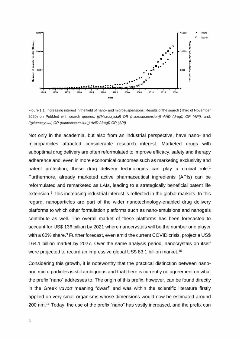
topics is still booming and blooming (Figure 1.1).
8
Figure 1.1. Increasing interest in the field of nano- and microsuspensions. Results of the search (Third of November
2020) on PubMed with search queries; (((Microcrystal) OR (microsuspension)) AND (drug)) OR (API), and,
(((Nanocrystal) OR (nanosuspension)) AND (drug)) OR (API)
Not only in the academia, but also from an industrial perspective, have nano- and
microparticles attracted considerable research interest. Marketed drugs with
suboptimal drug delivery are often reformulated to improve efficacy, safety and therapy
adherence and, even in more economical outcomes such as marketing exclusivity and
patent protection, these drug delivery technologies can play a crucial role.1
Furthermore, already marketed active pharmaceutical ingredients (APIs) can be
reformulated and remarketed as LAIs, leading to a strategically beneficial patent life
extension.8 This increasing industrial interest is reflected in the global markets. In this
regard, nanoparticles are part of the wider nanotechnology-enabled drug delivery
platforms to which other formulation platforms such as nano-emulsions and nanogels
contribute as well. The overall market of these platforms has been forecasted to
account for US$ 136 billion by 2021 where nanocrystals will be the number one player
with a 60% share.9 Further forecast, even amid the current COVID crisis, project a US$
164.1 billion market by 2027. Over the same analysis period, nanocrystals on itself
were projected to record an impressive global US$ 83.1 billion market.10
Considering this growth, it is noteworthy that the practical distinction between nano-
and micro particles is still ambiguous and that there is currently no agreement on what
the prefix “nano” addresses to. The origin of this prefix, however, can be found directly
in the Greek νανοσ meaning “dwarf” and was within the scientific literature firstly
applied on very small organisms whose dimensions would now be estimated around
200 nm.11 Today, the use of the prefix “nano” has vastly increased, and the prefix can

9
be found in diverse scientific disciplines, where a different terminology is commonly
applied.11 In colloid chemistry and material sciences the threshold of nanoparticles has
been placed at 100 nm. As materials at this scale exhibit distinguishable quantum
electronic properties, the photographic and semiconductor field commonly apply this
limit as well.7 The theory that materials smaller than 100 nm can, de facto, exhibit new
or enhanced properties that might be of chemical, optical, mechanical or electrical
nature, even advanced in the ISO-guidelines.12 Such a discontinuity in particle
properties can be merely found in APIs as well, nevertheless, the pharmaceutical field
uses a more metric unit nomenclature and considers nanoparticles and therefore
nanosuspensions as having sizes below 1000 nm.5, 7 Worse still, this aberrant
terminology is in practice only loosely applicable, as suspensions always display a
certain degree of polydispersity, meaning that suspensions with a median particle size
of 1000 nm or below can still include an important number of microparticles and vice
versa. Even more, the question rises what a particle size defines, as it can be
measured via various techniques and dependent upon, will be expressed by various
terms such as the hydrodynamic radius and the volumetric median diameter.13 Within
this dissertation the term nano- and microsuspension will be variably used and
interpreted based on the particle size distribution (PSD). The main particle size
measurement technique was laser diffraction (LD) and therefore the volumetric median
diameter will be standard-wise employed. A volumetric median particle size of 1000
nm could be set as threshold; however, one has to keep in mind that particle size is
only an attribute in defining the desired, final pharmacokinetic profiles and should
always be considered within this context.
THE DISADVANTAGE OF POORLY WATER SOLUBLE COMPOUNDS
Hurdles
In the middle of the twentieth century, drug discovery shifted from its early traditional
and serendipitous discovery in merely mother nature, to the roots of rational drug
design. First steps were found in the exploration of the enzymatic interactions and the
drug-receptor interactions in the 1960s. Twenty years later, the advancements in
molecular biology, gene research and technology directed rational drug design towards
two remarkable discovery platforms: combinatorial chemistry and high-throughput
screening. Within combinatorial chemistry, chemical building blocks are combined and
permuted to create vast compound libraries, which are in a next step high-throughput

10
screened for biological or pharmacological activity, leading to vast arrays of potential
drug leads.14 Despite these platforms proving their high efficacy, they nonetheless did
not result in an increasing number of marketing authorisations.15
While many dosage forms exist, the easy-to-use and less invasive oral formulation is
generally preferred by patients and manufacturers.16 Fundamental parameters
controlling rate and extent of drug exposure after oral administration, are the drug
dissolution and permeability in and through the gastro-intestinal (GI) tract.17 Prior to
permeation the drug must, in most cases, dissolve in the GI fluids (Figure 1.2.).
Solubility is therefore one of the key drivers in the oral bioavailability of APIs.2, 17
Figure 1.2. Fate of soluble drugs passing through the GI tract. Figure adapted from Lipp, 20162.
The highly potent and highly selective drugs derived from the aforementioned
platforms tend to be larger, more lipophilic and less water-soluble than their
predecessors.14 Despite their superb in vitro results, poor absorption, distribution,
metabolism and excretion properties such as dose-limiting solubility will in most cases
eventually lead to a poor oral bioavailability and thus, poor in vivo results.14, 15, 17 Hence
these compounds will likely fail during clinical trials and cause a costly late stage
attrition, which is one of the reasons why the development of a novel treatment can
range to 1.8 billion dollars and can take on an average 13.5 years.2, 14, 15

11
Increasing the solubility and the dissolution rate
To establish a firm grip on these issues, the terminology of poor and good solubility
and permeability should be well defined. In need of this classification and overall
harmonisation, Amidon and co-workers crafted the Biopharmaceutics Classification
System (BCS), which correlates the in vitro drug product dissolution to the in vivo
bioavailability and categorises all APIs in four classes dependent on their solubility and
permeability; The most desired Class I drugs with a high solubility and permeability;
Class II drugs are poorly soluble, but highly permeable; Class III drugs are poorly
permeable, but highly soluble; Class IV drugs combine a poor solubility and poor
permeability.17 A drug is regarded as highly soluble if its highest dose can be
solubilised in one glass (250 mL) or less of an aqueous medium over a specific pH
range at 37 °C.17, 18 Depending if the Food and Drug Administration (FDA), World
Health Organisation or European Medicine Agency guidelines are followed, this pH
range is 1 to 7.5, 1.2 to 6.8 or 1 to 8, respectively. High permeability on other hand, is
demonstrated if at least 85% of the administered dose is absorbed, as compared to an
intravenous (IV) reference bolus or values obtained via mass balance determination.
Permeability determination via in vivo intestinal perfusion in humans is accepted as
well, if suitability of the methodology is demonstrated.18
Yet another determinant in an APIs’ bioavailability is its dissolution rate. If insufficient,
it can leave an API undissolved over its time-window for absorption in the GI tract and
thus limit the APIs’ bioavalability.19 Therefore, an improved classification system arose
from the BCS: the Developability Classification System (DCS) which implements the
dissolution rate, aside from the solubility and permeability. Thus, BCS class II
compounds are, within the DCS, further subdivided in the dissolution-rate limited and
the solubility limited compounds, DCS class IIa and DCS class IIb, respectively.20
Dependent on scientific advancements, the DCS is continuously optimised and
therefore remains highly applicable.21

12
Figure 1.3. Marketed versus pipeline drugs: trend toward low solubility. Figure adapted from Lipp, 20162.
As briefly stated before, 36% to 40% of the marketed drugs and nearly 90% of the
development drugs would nowadays be assorted to BSC class II and IV (Figure 1.3.).1,
2 These percentages reflect the critical need for enabling production and formulation
strategies.
Luckily, the past decades, formulation scientists abided to the request and designed
strategies that may confer new hope for promising drugs that would otherwise be
abandoned. Examples of these newly developed go-to strategies that address the
solubility and dissolution rate challenge are:
Amorphous solid dispersions: Formulations containing a drug molecularly
dispersed within an inert carrier matrix. Drug dissolution is enhanced via several
mechanisms including improved wetting, reduction or even elimination of the impact of
lattice energy and reduction in the effective particle size.19
Inclusion complexation with cyclodextrins: Cyclodextrins are macrocyclic
oligosaccharides enhancing the apparent solubility by inclusion of the poorly water
soluble compounds in their hydrophobic inner cavity, while keeping their hydrophilic
exterior in contact with the aqueous medium.19
Lipid based formulations: These formulations range from simple solutions or
suspensions of drug in lipids to the most complex combinations of different lipids,
13
surfactants and cosolvents. Oral bioavailability is enhanced via increased solubilisation
and dissolution rate, the stimulation of the intestinal lymphatic drug transport and the
inhibition of intestinal efflux and metabolism.19
Nano- and microsuspensions: A flexible formulation approach to parenteral
as well as oral administration, applicable on both bench level and on commercial scale.
Both dissolution rate and saturation solubility are increased via the decreased particle
size, the increased surface area and the decreased diffusional layer.19 The formulation
generally consists of drug particles homogenously dispersed in an aqueous or
nonaqueous medium (e.g. oils or polyethylene glycol) with a suitable mix of stabilisers.
These nano and microparticles can be in crystalline, partially amorphous or amorphous
state.13 Formulations comprising crystalline nano- and microsuspensions are the focus
of this PhD dissertation and will be discussed in more detail in following paragraphs.
Nano- and microsuspensions: Small but significant
Nano- and microsuspensions display distinctive properties as compared to their poorly
soluble bulk counterparts. Via number of ways, their solubility and dissolution rate are
increased leading to an enhanced oral bioavailability.
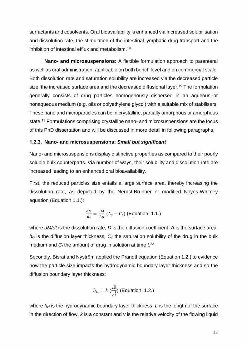
First, the reduced particles size entails a large surface area, thereby increasing the
dissolution rate, as depicted by the Nernst-Brunner or modified Noyes-Whitney
equation (Equation 1.1.):
𝑑𝑀
𝑑𝑡=
𝐷𝐴
ℎ𝐷 (𝐶𝑠 − 𝐶𝑡) (Equation. 1.1.)
where dM/dt is the dissolution rate, D is the diffusion coefficient, A is the surface area,
hD is the diffusion layer thickness, Cs the saturation solubility of the drug in the bulk
medium and Ct the amount of drug in solution at time t.22
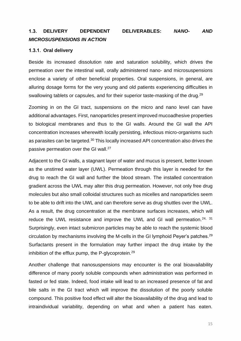
Secondly, Bisrat and Nyström applied the Prandtl equation (Equation 1.2.) to evidence
how the particle size impacts the hydrodynamic boundary layer thickness and so the
diffusion boundary layer thickness:
ℎ𝐻 = 𝑘 (𝐿
12
𝑉 12
) (Equation. 1.2.)
where hH is the hydrodynamic boundary layer thickness, L is the length of the surface
in the direction of flow, k is a constant and v is the relative velocity of the flowing liquid

14
against the surface.23 The fraction of the hydrodynamic boundary layer (hH) where the
diffusion dominates, the diffusion boundary layer (hD), will probably vary between
materials, nonetheless, general trends can be depicted.23 As the particle becomes
smaller and more regularly shaped, the hH becomes smaller and hence hD becomes
smaller, which will eventually lead to an increased dissolution rate (Equation 1.1.). This
phenomenon is especially pronounced for particle sizes below 2 to 5 µm.5, 23, 24
Thirdly, the increased surface curvature of especially particles smaller than 100 nm, is
strongly correlated with a higher saturation solubility as described by the Ostwald-
Freundlich or Kelvin equation (Equation 1.3.):
𝐶𝑠 = 𝐶∞𝑒𝑥𝑝 (2𝜆Μ
𝑟𝜌𝑅𝑇) (Equation 1.3.)
where Cs is the saturation solubility of the API, C∞ is the saturation solubility of an
infinitely large drug crystal, λ is the interfacial tension between crystal and matrix, M is
the drug molecular weight, r is the particle radius, ρ is the particle density, R is the gas
constant and T is the absolute temperature.25 After decades of vast presence in the
scientific literature, the application of the given equation (Equation 1.3.) has
nonetheless been challenged.26 The Ostwald-Freundlich equation and so the Kelvin
equation seemed to contradict the thermodynamics of Gibbs, by an incorrect
application of the Laplace equation. Still, this publication acknowledged the
nanosuspensions’ increased saturation solubility but, the increased surface area, the
size dependence of the interfacial energy and the altered surface energies were
accounted for this trend.6, 26 Irrespective to its origin, this supersaturation will further
drive the dissolution process (Equation 1.1.).27 Last, the stabilisers present in nano-
and microsuspensions often contain surface-wetting capabilities. Improving the
wettability of the drug leads to less drug agglomeration and thus, an increase in the
‘effective’ surface area which, via the Noyes-Whitney equation (Equation 1.1.), further
enhances the dissolution process.24, 28
Even though these advantages already proved the great capabilities of the extremely
small particle size, the next paragraphs will substantiate more how nano- and
microsuspensions may be a large player per administration route.
15
DELIVERY DEPENDENT DELIVERABLES: NANO- AND
MICROSUSPENSIONS IN ACTION
Oral delivery
Beside its increased dissolution rate and saturation solubility, which drives the
permeation over the intestinal wall, orally administered nano- and microsuspensions
enclose a variety of other beneficial properties. Oral suspensions, in general, are
alluring dosage forms for the very young and old patients experiencing difficulties in
swallowing tablets or capsules, and for their superior taste-masking of the drug.29
Zooming in on the GI tract, suspensions on the micro and nano level can have
additional advantages. First, nanoparticles present improved mucoadhesive properties
to biological membranes and thus to the GI walls. Around the GI wall the API
concentration increases wherewith locally persisting, infectious micro-organisms such
as parasites can be targeted.30 This locally increased API concentration also drives the
passive permeation over the GI wall.27
Adjacent to the GI walls, a stagnant layer of water and mucus is present, better known
as the unstirred water layer (UWL). Permeation through this layer is needed for the
drug to reach the GI wall and further the blood stream. The installed concentration
gradient across the UWL may alter this drug permeation. However, not only free drug
molecules but also small colloidal structures such as micelles and nanoparticles seem
to be able to drift into the UWL and can therefore serve as drug shuttles over the UWL.
As a result, the drug concentration at the membrane surfaces increases, which will
reduce the UWL resistance and improve the UWL and GI wall permeation.24, 31
Surprisingly, even intact submicron particles may be able to reach the systemic blood
circulation by mechanisms involving the M-cells in the GI lymphoid Peyer’s patches.29
Surfactants present in the formulation may further impact the drug intake by the
inhibition of the efflux pump, the P-glycoprotein.29
Another challenge that nanosuspensions may encounter is the oral bioavailability
difference of many poorly soluble compounds when administration was performed in
fasted or fed state. Indeed, food intake will lead to an increased presence of fat and
bile salts in the GI tract which will improve the dissolution of the poorly soluble
compound. This positive food effect will alter the bioavailability of the drug and lead to
intraindividual variability, depending on what and when a patient has eaten.
16
Nanosuspensions’ remarkable increase in dissolution rate and their mucoadhesive
properties are not heavily affected by the patient’s nutritional state and as a result, this
positive food effect may be mitigated.24, 27
During toxicological studies, high drug doses are preferably administered via the same
route as the intended clinical use. Hence, formulators are often challenged to orally
administer highly concentrated formulations during the drug development process. To
solubilise these high doses, concentrated surfactant, co-solvent or lipid systems were
previously employed, however these can have vehicle effects in the GI tract. Nano-
and microsuspensions can accommodate these large drug amounts with minimal GI
concerns.24
Parenteral delivery
1.3.2.1. Intravenous delivery
The earlier mentioned solubilisation of poorly soluble compounds via excessive
amounts of surfactants, co-solvents or lipids, did not only facilitate their oral
administration but enabled their IV administration as well. This formulation approach,
however, provoked severe side effects such as anaphylactic reactions and pain upon
injection.29 Nanosuspensions on the other hand were capable to administer larger IV
quantities of drugs at importantly lower toxicity.7
The fate of these injected nanoparticles strongly depends on the particle morphology,
size, dissolution rate, surface morphology and surface modification.32 The dissolution
rate in particular will determine the drugs’ biodistribution since it will discriminate if the
nanoparticles will occur as a solid or if it will mimic a solution.33
To mimic such an injected solution and retrieve a fast onset of action, the nanoparticles
should, as a rule of thumb, be smaller than 100 nm.27 After injection these suspensions
are subject to an instantaneous sink condition and likely have a quick dissolution.32
Nanoparticles up to 150 nm may even extravasate and distribute as such over
surrounding tissues.7
The IV injected nanoparticles larger than 150 nm cannot extravasate and are naturally
targeted by the mononuclear phagocytic system (MPS) cells.7, 30 Recognised as being
foreign, the particles are phagocytosed and accumulate mainly in the Kupffer cells in
the liver and to a lesser extent in the spleen and in the lung macrophages. Due to this

17
process, nanoparticles may directly combat MPS infections. To this end, the particle
surface should be modulated to enhance the macrophages’ clearance.27, 30
Furthermore, these macrophages can act as a depot for sustained drug release.27
To target other organs, surface modulation can help to circumvent the recognition by
the MPS and enable longer recirculation times.27 As a result, nanoparticles will
disperse over the body and will preferentially diffuse into tissues with a leaky
vasculature such as tumours or sites of infection and inflammation.29, 32 A more active
approach to target tumour cells may be possible as well such as surface modification
of nanoparticles with folate via conjugation or coating since its receptor is generally
overexpressed in tumour cells.7
Even though the maximum acceptable particle size for IV nanoparticles is still
ambiguous, first results showed how surprisingly well this formulation platform was
tolerated (Table 1.1.). Consequently, the FDA granted in 2006 for the first time a
marketing authorisation to an IV administered nanoformulation, Abraxane.32
Table 1.1. Outcome of injecting particles. Table reproduced from Wong, J et al, 2008. 32
Protocol, particle dose/kg Particle size (µm) Outcome
Bolus, 6 x 10⁹ 1.3 Pharmacokinetic study
Bolus, 1.6 x10¹² 0.5 – 1.17 Pharmacokinetic study
Rats, bolus, 8 x 10⁶ 0.4, 4, 10 Well tolerated
Dogs, bolus, 1 x10¹⁰ 3.4 Well tolerated
Dogs, repeated bolus, 2.4x 10⁸ 3.7 Well tolerated
Dogs, 2 min bolus, 8.9 x 10⁷ 3.4 Well tolerated
Humans, bolus, 9.9 x 10⁷ 2.0-4.5 Optison, approved product
Dogs, infusion, 1.3 x 10¹² 0.4 Well tolerated
Rats, bolus, 2.5 x 10¹² 0.4 Well tolerated

18
1.3.2.2. Long-acting injectables: The advantage of poorly water soluble
compounds
LAIs are weekly, monthly or less frequently administered formulations enabling a
controlled drug release and thus a prolonged and stable therapeutic exposure.4, 7 They
are mostly administered intramuscularly (IM) or subcutaneously (SC) as oil solutions,
liposomes, implants and micro- or nanosuspensions.34 The ease of self-administration,
the mild discomfort and large injection area, are strong motivators for SC use.
However, for larger injection volumes (2 – 5 mL) and for irritants, the IM route is
preferred.34 As a result, a high drug loading can be delivered via a fairly small injection
volume into a body compartment of limited fluid volume. The blood plasma
concentration profile following this LAI delivery is typically less variable over time which
reduces the number and extent of adverse effects.4, 35 Another clear advantage for the
patient is the prolonged exposure, which importantly enhances the patient compliance
(Figure 1.4.).7 29
For people suffering from dysphagia and in the field of chronic diseases where patient
adherence is detrimental for the treatment’s outcome, LAI can undoubtedly herald a
new era. Since the incidence of chronic diseases and of dysphagia is sharply
increasing in our aging population, it comes as no surprise that the LAIs currently
represent an expanding share of the drug products reaching the market.34, 36
From a strategical and economical perspective, LAIs may offer some other clear
advantages as they might be highly protected by complex regulations on their
intellectual property, comprising multi-layered patent protection.37 Additionally, the
reformulation of already marketed APIs to LAIs can, as previously alluded on, result in
an extended patent protection.8
The hallmark of the LAIs might be situated in the field of the antipsychotics, as it
encompasses some of the most successful LAI formulations. In the 1960s, their oil-
based parenteral depot formulations were introduced on the European, Canadian and
Australian market. However, the greatest breakthrough occured in 2003 when a LAI
suspension of risperidone (Risperdal Consta®, Janssen Pharmaceutica) was
introduced in the market. Before this date, the United States was reluctant to use
parenteral depot formulation of antipsychotics due to concerns regarding adverse
events, tolerability and the sense of disrespect for the patients voice.34, 38 In 2009 this
19
market expanded with a LAI containing paliperidone palmitate (Invega Sustenna®,
Janssen Pharmaceutica) and a LAI containing olanzapine pamoate (Zyprexa®
Relprevv™, Elli Lily).34 Remarkably, all these more recent LAIs are nano- and
microsuspensions. Even though critical research has nowadays put the first
overwhelmingly positive, clinical results in a better, realistic context, and stigma is still
ongoing, clinicians increasingly appraise the platform and warmly welcome advances
herein.38, 39, 40
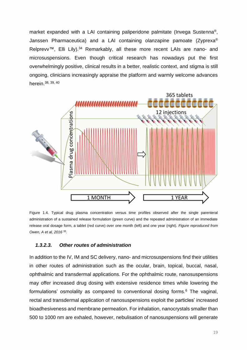
Figure 1.4. Typical drug plasma concentration versus time profiles observed after the single parenteral
administration of a sustained release formulation (green curve) and the repeated administration of an immediate
release oral dosage form, a tablet (red curve) over one month (left) and one year (right). Figure reproduced from
Owen, A et al, 2016 35.
1.3.2.3. Other routes of administration
In addition to the IV, IM and SC delivery, nano- and microsuspensions find their utilities
in other routes of administration such as the ocular, brain, topical, buccal, nasal,
ophthalmic and transdermal applications. For the ophthalmic route, nanosuspensions
may offer increased drug dosing with extensive residence times while lowering the
formulations’ osmolality as compared to conventional dosing forms.6 The vaginal,
rectal and transdermal application of nanosuspensions exploit the particles’ increased
bioadhesiveness and membrane permeation. For inhalation, nanocrystals smaller than
500 to 1000 nm are exhaled, however, nebulisation of nanosuspensions will generate
20
droplets in the size of a few µm, which are suitable for successful pulmonary
administration.27 Even the brain can be targeted via nano- and microsuspensions for
which currently, more invasive ways are adapted, but future work aims to retrieve a
passive or active targeting of the brain via a less invasive route.29
FROM PRODUCTION TO PATIENT: HOW TO PRODUCE, STABILISE AND
CHARACTERISE NANO– AND MICROSUSPENSIONS?
Production
The existing technologies to produce micron and submicron suspensions can be
divided into the so-called top-down technologies and the bottom-up technologies. In
the top-down approach large particles are reduced in size, whereas in the bottom-up
approach molecules are precipitated in a controlled manner. The latter approach
usually involves extensive amounts of organic solvents which are, aside of their
economic and ecological burden, difficult to remove from the final formulation.
Moreover, the precipitation process is hard to control in terms of particle size and
morphology.41, 42 All these elements seem to reduce the success of the bottom-up
approaches, whilst the top-down approach already showed its ease-to-use and
commercial viability, leading to a vast array of commercialised products.3, 42 However,
the top-down approach is prone to flaws as well (Table 1.2.) and thus, is still open for
advancements and future research.

21
Table 1.2. Overview of the general advantages and disadvantages of the top-down approaches, the bottom-up
approaches and the hybrid methods. Modified from Fontana,F. et al. ,2018.42
Methodology Advantages Disadvantages
Top-down approaches Simple
Fast
Avoid organic solvents
High reproducibility
Easy of scale-up
Energy-intensive process
Potential instability induced by high shear and temperature
Product contamination from the grinding media
Bottom-up approaches Small particle size
Monodispersed particles
Difficult to scale-up
Time consuming to find the suitable conditions
Difficult to control the particle growth
Incomplete removal of toxic solvents
Hybrid method Remarkably smaller particle sizes Increase in cost and time for preparation
During the top-down production, the suspension particles are subjected to mechanical
attrition during wet bead milling (WBM) or to high pressure during high-pressure
homogenisation (HPH).42 Recent years hybrid methods have been developed where
different production technologies are combined, which merely consists of a bottom-up
approach to generate crystals that are in a next step reduced in size by a top-down
approach. As an example, these hybrid methods encompass the combination of
solvent/antisolvent precipitation with HPH (NANOEDGE®); spray drying with HPH (H42
technology), freeze drying with HPH (H96 technology) and WBM with HPH
(smartCrystal® technology).13, 42
In a next step, nano- and microsuspensions can be converted to the dried state via
conventional drying operations such as lyophilisation, spray-draying or fluid-bed
coating. To preserve the redispersibility upon reconstitution, redispersants such as
sucrose are commonly added. Reconstitution can happen with either water prior to
patient intake or directly with gastric fluids if the dried powder has been converted to a
conventional formulation such as a capsule or tablet.6, 43
Stabilisation
The long-term stabilisation of micron and submicron suspensions imposes an uphill
battle against the suspensions’ unfavourable thermodynamics.7 The most important
stability issues lead to a change in the suspensions’ PSD and as the particle size is

22
the key contributor to the drug products’ safety and efficacy, the formulator is
challenged to appropriately address these stability issues of which agglomeration,
sedimentation, Ostwald ripening and secondary nucleation will be dealt in more detail
below.44
First, the sharp decrease in particle size entails a large surface area which is, from a
thermodynamic point of view, correlated to an increase in the system’s Gibbs free
energy (Equation 1.4.) and is, thus, inherently unfavourable.29
∆𝐺 = 𝛾𝑠/𝑙 ∆𝐴 (Equation 1.4.)
where ΔG refers to the system’s Gibbs free energy increase, γs/l refers to the solid-
liquid interfacial tension, and ΔA refers to the surface increase of this solid-liquid
interface.29
As a reduction in Gibbs free energy will drive these metastable systems to a
thermodynamically stable state, these systems will spontaneously try to reduce their
interfacial surface area. Accordingly, the system will try to counterbalance the particle
size reduction by agglomeration.44 To impede this natural tendency, the formulator may
add excipients with stabilising properties such as a surfactant(s) and/or polymer(s),
which may stabilise the system by i) the reduction of the interfacial tension via wetting
properties, ii) steric hindrance (steric stabilisation), iii) the electrostatic repulsion of
(surface-)charged individual particles (electrostatic stabilisation), iv) the synergetic
combination of the steric and electrostatic stabilisation (electrosteric stabilisation).7, 29,
44, 45 Besides their impact on short- and long term storage, these stabilisers will also
contribute to the successful formation of submicron particles during production.44
Another natural occurring phenomenon that needs to be tackled is sedimentation. As
long as the resuspendability is adequate, this is not necessarily deleterious, simple
shaking will homogenise the system, but in most cases, the formulator needs to take
this in consideration.7 As indicated in Stokes’ law (Equation 1.5.) the rate of this
process is dependent on the particle size, medium viscosity and difference in medium
and API density.29, 44 Since smaller particles will compensate this sedimentation
process by Brownian motion, particle size reduction forms the most commonly applied
strategy to avoid severe particle settling. The addition of viscosity enhancers such as
carboxymethylcellulose may alleviate this process as well.7

23
𝑣 = 2𝑟2(𝜌𝑝−𝜌𝑚)𝑔
9𝜂 (Equation 1.5.)
where v is the settling rate of the particle, r is the radius of the particle, ρp is the density
of the particle, ρm is the density of the medium, g is the gravitational acceleration and
η is the viscosity of the medium.29
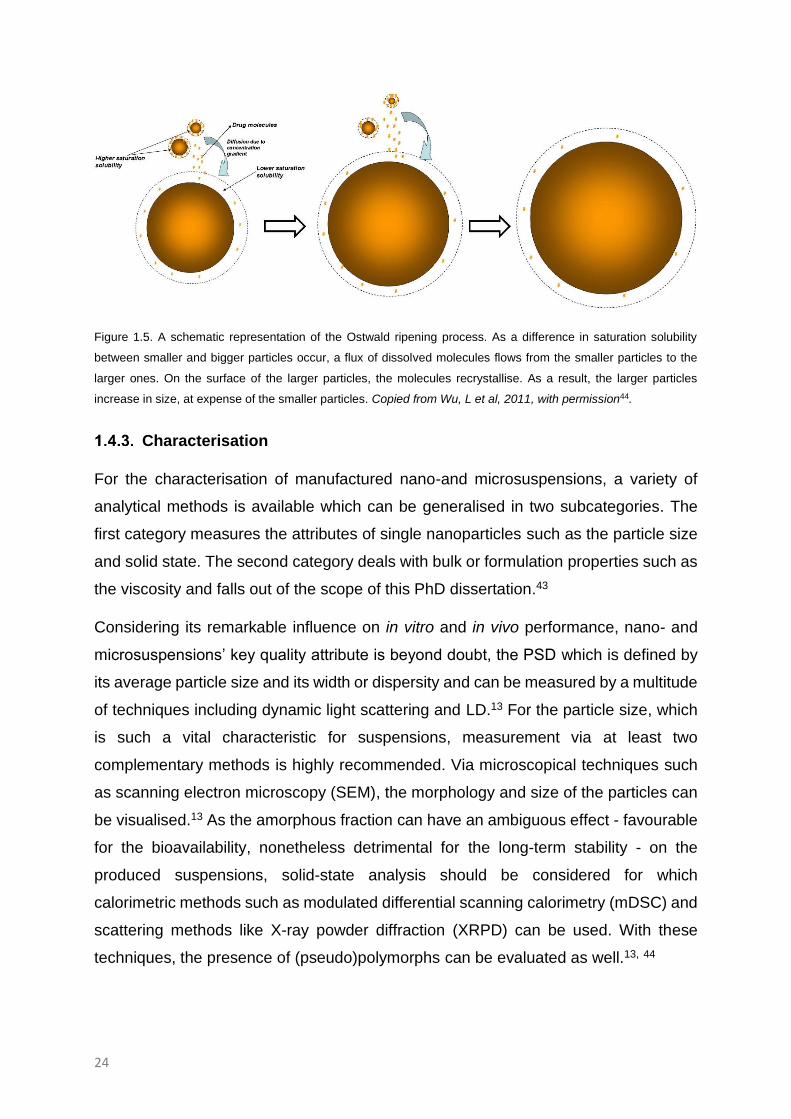
Finally, the shelf life of nano- and microsuspensions can be gravely reduced due to
secondary nucleation and Ostwald ripening (Figure 1.5.). Secondary nucleation is the
natural crystallisation of the supersaturated system where as the temperature
fluctuates drug can dissolve and crystallise from the seeded supersaturated matrix
upon cooling.7 Ostwald ripening, on other hand, is merely present in polydisperse
systems where the large particles will, at expense of the smaller particles, increase in
size. Smaller particles will have, as alluded on in Equation 1.3., a higher saturation
solubility than their larger counterparts, and will more easily dissolve, generating a
local, high API concentration. This local difference in API concentration will drive a flux
of dissolved API molecules to the larger particles where they will crystallise and cause
particle growth.7, 44, 46 A narrow PSD may mitigate the differences in the saturation
solubilities, and thus prevent the Ostwald ripening process. Stabilisers may also
reduce the interfacial tension and hence, tune the Ostwald ripening process as long as
they do not enhance the drug solubility. In this context, many authors suggest that an
excess of stabiliser may promote Ostwald ripening.44, 46 Current literature, however,
presents Ostwald ripening as a multi-step process where, depending on the rate-
controlling step, another optimal surfactant concentration may be adequate.47 Other
nanoparticle growth pathways such as digestive and intraparticle ripening may
occasionally occur in inorganic materials, but are only scarcely discussed in the
pharmaceutical context.48
Nowadays, the selection of a suitable stabiliser and stabiliser concentration is merely
based on trial and error and therefore there is considerable scope of improvement
herein. Few studies have attempted to develop a more rational approach and develop
predictive methods.45 Current studies do not try to resolve the matter but are devoted
to streamline high-throughput methods in order to save time and materials.46
24
Figure 1.5. A schematic representation of the Ostwald ripening process. As a difference in saturation solubility
between smaller and bigger particles occur, a flux of dissolved molecules flows from the smaller particles to the
larger ones. On the surface of the larger particles, the molecules recrystallise. As a result, the larger particles
increase in size, at expense of the smaller particles. Copied from Wu, L et al, 2011, with permission44.
Characterisation
For the characterisation of manufactured nano-and microsuspensions, a variety of
analytical methods is available which can be generalised in two subcategories. The
first category measures the attributes of single nanoparticles such as the particle size
and solid state. The second category deals with bulk or formulation properties such as
the viscosity and falls out of the scope of this PhD dissertation.43
Considering its remarkable influence on in vitro and in vivo performance, nano- and
microsuspensions’ key quality attribute is beyond doubt, the PSD which is defined by
its average particle size and its width or dispersity and can be measured by a multitude
of techniques including dynamic light scattering and LD.13 For the particle size, which
is such a vital characteristic for suspensions, measurement via at least two
complementary methods is highly recommended. Via microscopical techniques such
as scanning electron microscopy (SEM), the morphology and size of the particles can
be visualised.13 As the amorphous fraction can have an ambiguous effect - favourable
for the bioavailability, nonetheless detrimental for the long-term stability - on the
produced suspensions, solid-state analysis should be considered for which
calorimetric methods such as modulated differential scanning calorimetry (mDSC) and
scattering methods like X-ray powder diffraction (XRPD) can be used. With these
techniques, the presence of (pseudo)polymorphs can be evaluated as well.13, 44

25
As the focus of this dissertation is the investigation of the intensified vibratory mill (IVM)
as a viable nanonisation and micronisation technique, the analytical focus is placed on
the key characteristic: the PSD, and consequently, considerable research attention has
been devoted to LD as particle size measurement technique. In a next step, LD and
SEM were employed to evaluate the suspensions’ PSD and aggregation behaviour.
Other techniques such as mDSC and XRPD were only employed in a limited manner.
TOP-DOWN PRODUCTION
High-pressure homogenisation
The second most frequently used top-down production technique is HPH. The two
most common homogenisation principles that subdivide this category are
microfluidisation on the one hand and piston-gap homogenisation on the other hand.42,
49 Within the latter category, particle size reduction merely relies on the forces aroused
when a suspension is forced to pass a very narrow gap, where the extreme reduction
in diameter leads to a sharp increase in dynamic pressure and sharp decrease in static
pressure, which can even drop below the vapour pressure of the liquid, causing boiling
to occur.42, 49 As the suspension leaves the gap, the earlier formed gas pockets will
implode, generating a micro-jet and shock waves which crush on nearby solid
particles.49 This process, better known as cavitation, is mostly present in the
Dissocubes® technology where suspensions in aqueous medium are prepared. In the
Nanopure® technology on the other hand, a lower vapour pressure and temperature
are applied to create non-aqueous suspensions. As a result, the cavitation is reduced
or practically inexistent, but the high turbulence still causes extensive shear forces to
perform a particle size reduction.42, 49
In case of microfluidisation (patented as IDD-P® technology), the suspension is
accelerated through purpose-built homogenisation chambers, which are named after
the path’s geometry. Thus, the suspensions flow changes a few times in the Z
chamber, while in the Y chamber the suspension gets divided in two streams which
eventually frontally collide.42, 49 Particle size reduction occurs due to these frontal
collisions, collisions on impact valves and chamber walls, attrition forces and to a
limited extent, cavitation.41, 42, 49 For the production of drug nanocrystals, the most
common geometry is the Z-shaped chamber, whereas the Y-chamber is more often
applied to prepare liquid-liquid type dispersions.42 Microfluidisation seemed to be more

26
effective as compared to the commonly applied piston-gap method. For the
nanonisation of softer materials, the HPH seems to be preferred over WBM.50
Furthermore, HPH generate suspensions with a more uniform particle size and better
thermal stability as compared to WBM.51 Finally, HPH can cause cell lysis which
lessens the microbiological hurdles within the final drug formulations.50
Despite these various merits, HPH based nanoparticles are underrepresented on the
pharmaceutical market since the production technologies’ success is hampered by
various hurdles. Even though the contamination risk is reduced as compared to WBM,
wearing of the valves and hence product contamination may still occur.42 Particle size
reduction seems to be less effective compared to WBM as well.42, 49 The high number
of passages makes this technology less production friendly. To minimise this number
of passages, prior micronisation is often applied.7, 13, 42 As HPH miniaturisation is less
straightforward and these technologies come at a costly expense, pharmaceutical
companies may have the tendency to stick to the more universally applied WBM.51
Wet bead milling
As WBM forms the most notable top-down production technique, with demonstrated
efficiency, viability and cost-effectiveness on both bench level as production scale, the
technology has been detailed in numerous papers.33, 46 Summarising this large body
of scientific data in a one-pager would be preposterous. For further background
information, the interested reader is, hence, referred to excellent review papers
available in the field.
To stage the results of this dissertation, the following paragraphs will nonetheless
elaborate on the concept of WBM, the technologies’ strengths and flaws, a
summarising overview of how it can be modelled and how as a widely spread
production technology it may form a benchmark for comparison for upcoming milling
technologies.
As mentioned earlier, WBM delivery has been propelled to the forefront by researchers
from both academia and industry to effectively produce nano- and microsuspensions,
which comes as no surprise given the extensive list of merits that this method
encompasses. This technology is widely spread, in both experience and literature, is
commercially established, is simple and highly reproducible. WBM is from a practical

27
point of view easy-to scale up and continuous manufacturing by recirculation of a
mother suspensions boosts the production efficiency.50
As a nanonisation technology, it was patented as the Nanocrystal® technology in 1990
by Elan.30 Its success is reflected in the manifold of marketing authorisations granted
to formulations produced with this technique.6 Within WBM the API, excipients,
dispersant and milling beads, which can compose of various inert materials such as
highly cross-linked polystyrene, glass and yttrium stabilised zirconia, are charged into
the milling chamber.13, 52. Next, the milling beads are accelerated by the movement of
the complete container, or by agitators installed in the chamber.52 The movement of
API particles and beads generate forces such as impact, pressure and shear forces
whereby a particle size reduction of drugs to the nanoscale is achieved.30 However,
these highly energetic forces come at a cost. Inefficiently dissipated energy can pose
three different hurdles. First, it can generate uncontrolled heat. Heat may have
detrimental effects on the chemical and physical stability of the suspension.
Evaporation of the solvent may occur, and the stabilisers’ cloud point may be
surpassed, causing it to dehydrate leading to re-micellisation. Hence, less stabiliser
will be accessible for the newly formed high-energy surfaces. This ineffective
stabilisation may lead to aggregation. With the temperature, the solubility of the API
may rise, leading to a temporarily supersaturated state. As the suspensions cools down
after comminution, second nucleation and crystal growth will thereupon occur. As a
result, WBM technologies should be equipped with adequate water jackets. The
second hurdle is how the uncontrolled energy may cause solid state changes as
amorphisation and polymorphism. 7 Finally, these energetic conditions leave the beads
to wear, eventually contaminating the final drug formulation.46, 49 Despite these
extensive energetic conditions, nanonisation with WBM may still take hours to days.30
Another major disadvantage, not yet touched upon, is the cumbersome drug product
development process, which is merely based on trial and error rather than rationally
approached. It is currently not possible to predict a priori which stabilisers and process
parameters should be applied. Even though high-throughput platforms for WBM are
available, the investigation of all these variables makes an onerous and highly
inefficient process.53 This has led authors such as Kwade, Eskin and Afolabi to predict
milling outcomes, which will be the main topic of the next paragraph. In a further step,
new grinding platforms may be explored to address the WBM challenges.54, 55

28
Modelling
Considering the 44 different parameters that have been identified as affecting the WBM
process, the complexity of WBM cannot be underestimated.56 Nevertheless,
researchers try to predict milling kinetics and milling outcomes by process modelling
where the stress model, as suggested by Kwade54, and the microhydrodynamic model,
as proposed by Afolabi and co-workers55, are the most widely known.
In this respect, Kwade was the first to describe the milling process in a mechanistic
model that linked the process parameters of a stirred media mill to the stress applied
on the suspension’s particles via two central parameters, the stress number (SN) and
the stress intensity of the grinding media (SIGM). This simplification and the direct link
between process parameters and the stress applied on the suspension’s particles
made the model easy to apply.54 However, this simplification resulted in significant
caveats such as the absence of most parameter interactions and the absence of
important terms such as the formulations viscosity. Afolabi and co-workers resolved
these caveats in their advanced microhydrodynamic model, which was firstly
introduced by Eskin and co-workers.55, 57, 58, 59 This microhydrodynamic model was
based on the transformation of turbulent flow into kinetic energy, Hertzian contact angle
mechanics and particle compression probability to estimate the total energy spent on
solids deformation.55, 60 In this regard, the breaking kinetics were defined by the power
dissipation mechanisms which comprises energy dissipation by liquid-bead viscous
friction and lubrication, energy dissipation from inelastic bead collisions and the power
spent on suspension shearing.55
Even though the stress model presented by Kwade54 and the microhydrodynamic
model of Afolabi and co-workers55 were based on different principles, process
optimisation with respect to a certain particle size, could be realised with either models,
leading to the same optimal process parameters for a specific compound fineness.60
De facto, both models contain two central parameters which are remarkably similar
and define the final optimised process variables:
One central parameter describes the frequency of particle stressing, which is
stress frequency (SF) or frequency of particle compressions (a), in the model of
Kwade54 or in the model of Afolabi and co-workers55, respectively.

29
The second central parameter describes the stress on the particle during a
collision, which is SI and maximum contact pressure (αGMmax) , in the model of Kwade54
or in the model of Afolabi and co-workers55, respectively.
Still, due to its complexity and its broader content, the microhydrodynamic model
parameters proved to be more accurate.60 Interested readers are therefore strongly
advised to read through the microhydrodynamic modelling of Afolabi and co-workers.55,
57 As the scope of this thesis dissertation is to give a first mechanistic insight in the
milling by the IVM, the stress model of Kwade54 which links concrete operation
parameters to final particle sizes, was favoured and therefore will be further applied
and will be described in more detail below.
As previously mentioned, the stress model of Kwade contains two central parameters
of which the SIGM can be described by the bead size (dGM, m), the bead density (ρGM,
kg/m3) and the tip speed of the stirred media mill (vt, m/s), which in a broader context
can be interpreted as the speed generated by the driving system of the mill 54 (Equation.
1.6.).
𝑆𝐼𝐺𝑀 = 𝑑𝐺𝑀3𝜌𝐺𝑀 𝑣𝑡
2 (Equation 1.6.)
SN is determined by the number of contacts between the beads (NC), the probability
that a particle is caught between the beads and sufficiently stressed during the media
contact (PS) and by the overall number of API particles inside the mill (NP) (Equation
1.7.). NC can be assumed to be proportional to the number of stirrer revolutions (n, s-
1), which is comparable to the stirrer speed or in a broader context the speed generated
by the driving system of the mill, the grinding time (t, s) and the number of grinding
media (NGM) (Equation 1.8.).54
𝑆𝑁 =𝑁𝐶 𝑃𝑆
𝑁𝑃 (Equation 1.7.)
𝑁𝐶 ∝ 𝑛 𝑡 𝑁𝐺𝑀 ∝ 𝑛 𝑡 𝑉𝐺𝐶 𝜑𝐺𝑀 (1−𝜀)
𝜋
6 𝑑𝐺𝑀
3 (Equation. 1.8.)
where n (s-1) is the number of revolutions of the stirrer per unit time; t (s) is the milling
time, VGC (m3) is the volume of the grinding chamber, φGM is the filling ratio of the
grinding media, ε is the porosity of the bulk of grinding media (GM), dGM (m) is the
diameter of the grinding media.61 The product of SI and SN is proportional to the total
specific energy, which is the total energy input to the total mass of feed material, which

30
can, if under control, guarantee an efficient production of suspension with a certain
particle fineness.61
New technologies: Intensified vibratory milling
The vast interest in nano- and micronisation along with the drawbacks of conventional
WBM have sparked the scientist’ interest in and search for new milling platforms. In
this spirit, Leung and co-workers62 reported for the first time in 2013 on a new drug
sparing technology utilizing low shear acoustic mixing to quickly manufacture nano-
and microsuspensions, which was in a later publication of Li and co-workers referred
to as the IVM process.63 This process applies the Resonant Acoustic® Mixing (RAM)
platform (Figure 1.6.) which was originally commercialised as a dry mixing platform.64
Consequently, several studies have been conducted on RAMs application in dry
mixing, while very little is known about its application in wet milling.62, 63
Figure 1.6. Figure illustrating the LabRAM II equipment. As depicted in the picture right above, the recipient should
be fixed in-between two transducers. The recipient will be forcefully vibrated and as a result, the content of the
recipient will be mixed.
In this respect, there is considerable ambiguity with regard to the IVMs mixing and
milling regime. Previously, the mixing behaviour was introduced as micro-mixing

31
zones, but current knowledge seems to present a more complex mixing and milling
regime with multiple, integrated phenomena dependent on both process parameters
and product properties (manufacturer communication). Since the geometry and the
motion of IVMs recipients significantly differ from conventional mills, one can assume
a different bead motion and consequently composition of comminution forces which
will lead to different comminution output in terms of particle size, generated heat and
eventually stability propensities.50 The internal knowhow presumably falls under patent
restrictions and an early publication on the RAMs software even referred to it as
Resodyn ‘black box’ controller.65 Nonetheless, for the IVM is a fairly new concept, we
want, to the extent possible, shortly elaborate on the equipment, production
mechanism and recent literature.
The IVM (Figure 1.7.) consists of a platform with a vibrating container to which, as in
the case of conventional WBM, milling media, suspension matrix and API are charged.
Due to the vibration, the milling media start to move and collide, resulting in the desired
particle size reduction. This vibrating container could be well-plates or vials, wherefore
the IVM can serve as a drug sparing, high-throughput screening method.62 For the
bench level IVM, as in the case of the LabRAM II (Figure 1.6.), vacuum equipped, inline
temperature controlled and jacketed mixing vessels are commercially available, but
these vessels’ minimal content remains a considerable volume of 500 mL.
As a mechanical vibrating system, the IVM works as a spring-damper system, where
the springs, driven by the driving system, store the potential energy, that is further
transferred to the plate, recipient and mixing/milling content, which will cause the
damping by energy adsorption. The vibration of the mixing recipient could be plotted
in time as a sinusoidal wave with a frequency of around 60 Hertz to keep the system
at its optimal and safe conditions, namely the resonance. This resonance is a
parametric resonance, where the system is driven at twice its natural frequency and
will cause a maximum amplitude while the required power stays minimal. As the period
of oscillation is fixed, the only value that can be altered is the amplitude which differs
based on the milling content and the set acceleration level. As an example, an empty
container can reach in the LabRAM II at the maximal acceleration of 100 g a vertical
displacement of 1.4 cm. A certain level of mixing intensity, given by the software as a
power percentage (0 – 100%) will be needed to substantiate this acceleration for a

32
certain mixing/milling mass. Via an accelerometer on the baseplate and a back-track
system, the acceleration and frequency will be controlled within its installed range. If
an adaptation is needed, it will be tracked as a change in power or phase for the
amplitude or frequency, respectively. Sudden changes in the power and phase often
relate to changes in the mixing/milling regime whereas a more gradual change is linked
to changing material properties.
Figure 1.7. The concept of IVM. At the beginning (left), the recipient is charged with beads (grey spheres), API (dark
polygons), suspension matrix and other excipients. Parameters are installed on the IVM software and the process
is started. During the process, the transducer will make an upwards and downwards movement that may be
depicted as a sinusoidal wave over time. This movement is copied by the installed recipient and thus, the beads
start to accelerate (middle). During their movement, the beads can cause impact, shear forces and pressure, which
causes the particles to break. After the mixing and milling process (right) the recipient and transducer are
motioneless and the API particles are reduced in size.
Over the last decades, the RAM has been widely explored as a powder mixer, yet it
was only in 2013, that the group of Leung and co-workers applied it for the first time as
a milling platform.62 Their first investigation included a miniaturisation of the IVM
process via a high-through put platform for rapid evaluation of APIs millability and the
formulation stabilising propensities; and directly translated these high-throughput
results to scale-up possibilities. IVM was, within this article, marked for its fast
comminution which overcame WBMs extensive milling times. The slight temperature
increase within the IVM was attributed to the more efficient energy use.62 Later

33
publications noted this temperature increase as well, even though limited to a couple
degrees.64 A more considerable heat generation was observed by Hoang and co-
workers with final temperatures of around 30 to 60 degrees.66 Within this article the
impact of a set of process variables on the particle size reduction process of the IVM.
The study results were encouraging and well-found, nonetheless, created via a one-
variable-at-a-time (OVAT) approach and merely translated to guidance maps. Even
though these guidance maps are of great practical value, profound mechanistic
insights in the IVM were not provided.66 In a further investigation on the IVM, Li and
co-workers attempted to control the heat generation via the insertion of pauses where
the recipients were removed from the milling equipment and placed in a refrigerated
bath.63 This approach proved to be effective, but was not suitable to standardise or
scale-up. Furthermore, the influence of this quick cooling step on the aggregation of
particles and recrystallisation of dissolved API was not explored. In contradiction to
early findings, this article disagreed whether the IVM could outperform the conventional
WBM. These contradictory results in terms of milling capability and heat generation
highlight the current knowledge gaps in the intriguing field of IVM.
What we know on this less conventional, but auspicious nanonisation and
micronisation method, is solemnly based on this scarce body of data. Therefore, we
would like to take a new look at the IVM as milling technology and try to extend our
understanding of the underlying principles. Still in its infancy, this milling process can
be more in-depth explored in terms of the impact of process variables on the
suspension’s critical quality attributes. In this scope, the particle size reduction, heat
generation and the effect of the milling regime on the final stability propensities will be
more thoroughly investigated in this thesis project with, not surprisingly, the IVM as key
player.

34

Objectives

37
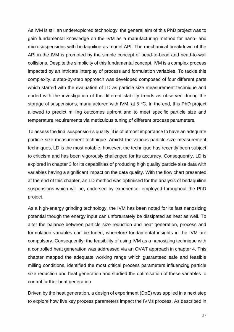
As IVM is still an underexplored technology, the general aim of this PhD project was to
gain fundamental knowledge on the IVM as a manufacturing method for nano- and
microsuspensions with bedaquiline as model API. The mechanical breakdown of the
API in the IVM is promoted by the simple concept of bead-to-bead and bead-to-wall
collisions. Despite the simplicity of this fundamental concept, IVM is a complex process
impacted by an intricate interplay of process and formulation variables. To tackle this
complexity, a step-by-step approach was developed composed of four different parts
which started with the evaluation of LD as particle size measurement technique and
ended with the investigation of the different stability trends as observed during the
storage of suspensions, manufactured with IVM, at 5 °C. In the end, this PhD project
allowed to predict milling outcomes upfront and to meet specific particle size and
temperature requirements via meticulous tuning of different process parameters.
To assess the final suspension’s quality, it is of utmost importance to have an adequate
particle size measurement technique. Amidst the various particle size measurement
techniques, LD is the most notable, however, the technique has recently been subject
to criticism and has been vigorously challenged for its accuracy. Consequently, LD is
explored in chapter 3 for its capabilities of producing high quality particle size data with
variables having a significant impact on the data quality. With the flow chart presented
at the end of this chapter, an LD method was optimised for the analysis of bedaquiline
suspensions which will be, endorsed by experience, employed throughout the PhD
project.
As a high-energy grinding technology, the IVM has been noted for its fast nanosizing
potential though the energy input can unfortunately be dissipated as heat as well. To
alter the balance between particle size reduction and heat generation, process and
formulation variables can be tuned, wherefore fundamental insights in the IVM are
compulsory. Consequently, the feasibility of using IVM as a nanosizing technique with
a controlled heat generation was addressed via an OVAT approach in chapter 4. This
chapter mapped the adequate working range which guaranteed safe and feasible
milling conditions, identified the most critical process parameters influencing particle
size reduction and heat generation and studied the optimisation of these variables to
control further heat generation.
Driven by the heat generation, a design of experiment (DoE) was applied in a next step
to explore how five key process parameters impact the IVMs process. As described in

38
chapter 5, this study generated predictive models that allow to forecast milling
outcomes in terms of particle size and temperature, facilitating the rational selection of
optimal process parameters.
Chapter 6 reported on the stability of the DoE’s suspensions stored at 5 °C. In one
specific condition, an unusual particle size reduction was observed during the cold
storage, which seems to contradict the stability trends described in chapter 1. To study
the repeatability of the given phenomenon, this specific sample was manufactured in
several-fold, kept on cold storage and tracked via LD. In a further step, the particle size
was tracked via an optimised LD system and an orthogonal particle size technique, the
differential centrifugal sedimentation. The physical chemistry behind this observation
still needs to be elucidated, however, we propose several hypotheses in the final
chapter.
In this final chapter 7, the results of chapter 3 to 6 are broadly discussed in light of
recent literature, general conclusions are provided, and future works are identified.
Size analysis of small particles in wet dispersions by
laser diffractometry
Results in this chapter are based on:
De Cleyn, E., Holm, R. & Van den Mooter, G. Size Analysis of Small Particles in Wet
Dispersions by Laser Diffractometry: A Guidance to Quality Data. J. Pharm. Sci. 108,
1905–1914 (2019).


41
ABSTRACT
In the present work, the question how to obtain high quality LD results is discussed by
investigating various hurdles that can be encountered during particle size
measurements in wet dispersions and the associated data interpretation. Following
this an effective troubleshooting is discussed based upon theoretical insight in the LD
measurement. As an important element of the Mie theory, the refractive indices (RIs)
of the model compounds, bedaquiline and cinnarizine, were quantified using the LD
software, the Becke Line technique and the single solvent technique, as described by
Saveyn et al.67 The influence of parameters such as obscuration level, background
quality and fitting of data was investigated, and a summarising flow chart has been
provided. Through this analysis the present work emphasizes the need for a systematic
approach when conducting LD measurements, including standard performance of an
obscuration titration and an extended method optimisation, in order to reach high
quality LD results.
42
INTRODUCTION
Extensive efforts have been made by the pharmaceutical industry with respect to target
identification and lead candidate generation through high-throughput screening and
combinatorial chemistry.33 Although these advanced technologies have offered vast
amounts of new chemical entities, a significant part of these compounds are poorly
water soluble. Given that aqueous solubility is a critical parameter for drug absorption
from conventional dosage forms, it has become a significant hurdle within the
pharmaceutical development process to define formulations that provide sufficient and
constant plasma concentrations of the administered compound.68, 69 New formulation
strategies have been introduced to tackle this hurdle, from which the generation of
nano- and microsuspensions has already demonstrated its value, utility and
commercial viability.33, 70 The stability of these suspensions is judged by critical
attributes such as particle size and PSD.70
Different techniques can be opted to quantify the particle size and PSD, from which
coulter counting, microscopy and dynamic light scattering are well-known, despite
having considerable technical disadvantages such as their narrow measuring range.
44, 68, 71 For suspensions it is important to detect the larger particles as well as the
smaller sized population, given that the long-term stability of suspensions may be
notably decreased by a broad PSD.50 As a result, LD, comprising a measurement
range of 0.01 µm to 3500 µm, is often used alone or in combination with dynamic light
scattering to characterise suspensions and thus forms the preferred method for size
analysis of sub-millimetre particles.44, 72 To be able to analyse particles of such a broad
size range the equipment has to accommodate and implement complementary
techniques. Particles scatter light in every direction and more information can be
gained if sideward and backward scattering are captured as well. Furthermore, diverse
scattering patterns can be obtained from light with different wavelengths.
Consequently, LD equipment manufacturers tend to incorporate multiple laser sources
with different wavelengths, as in the case of the Mastersizer 2000™ and Mastersizer
3000™ from Malvern Instruments®, or polarisation intensity differential scattering,
which is patented by Beckman Coulter Inc. Besides its broad range, LD is popular for
its ease of use and adequate reproducibility. Despite these clear advantages, the
trustworthiness and accuracy of LD data have been questioned by numerous
authors.73, 74, 75
43
Keck and Müller investigated the significant impact on the final PSD of choosing either
the Fraunhofer or Mie theory.73 This included investigations of the differences obtained
when using complex scattering pattern, along with the choice of optical parameters in
the case of the Mie theory. Although the work by Keck and Müller73 discussed some of
the most important parameters influencing the LD results, additional hurdles
concerning LD analysis and data interpretation are still present, both within the case of
dry and wet measurements. Obscuration parameters such as the red (obsc. red) and
blue light obscuration (obsc. blue) and fitting parameters such as residual (res.) and
residual weighted (res. weight.) in the case of the Mastersizer 2000™ or R and Chi-
squared in case of the L-950 of HORIBA76 offer a clear insight in the quality of the
results, however, they are still often overlooked. Understanding these attributes is the
only way to precisely develop and optimise a LD method. To limit the scope of this
work, the focus is placed on wet samples. Dry powders need different set-ups with
different hurdles to tackle, though the overall LD theory and above-mentioned
parameters can still be considered during method development and data interpretation.
The objective of the present work was therefore to provide the reader with a deeper
insight into the LD system and the factors that should be considered during
measurement, analysis and data interpretation to obtain meaningful wet LD
measurements.
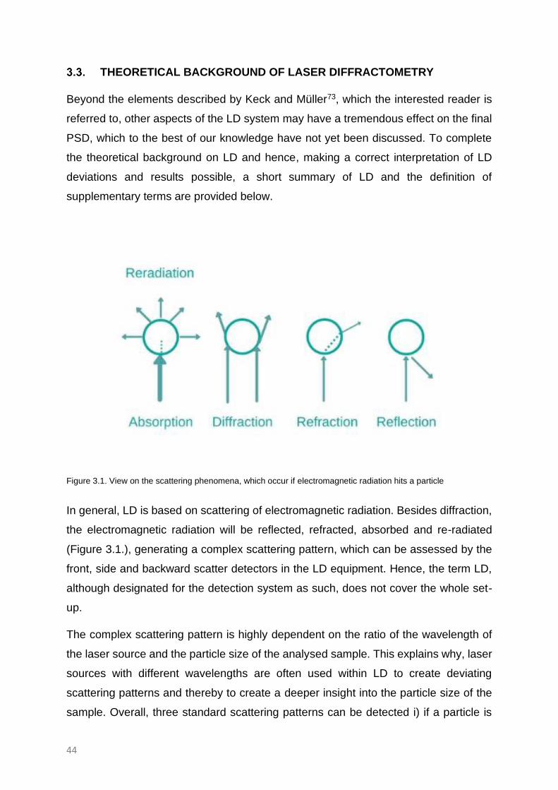
44
THEORETICAL BACKGROUND OF LASER DIFFRACTOMETRY
Beyond the elements described by Keck and Müller73, which the interested reader is
referred to, other aspects of the LD system may have a tremendous effect on the final
PSD, which to the best of our knowledge have not yet been discussed. To complete
the theoretical background on LD and hence, making a correct interpretation of LD
deviations and results possible, a short summary of LD and the definition of
supplementary terms are provided below.
Figure 3.1. View on the scattering phenomena, which occur if electromagnetic radiation hits a particle
In general, LD is based on scattering of electromagnetic radiation. Besides diffraction,
the electromagnetic radiation will be reflected, refracted, absorbed and re-radiated
(Figure 3.1.), generating a complex scattering pattern, which can be assessed by the
front, side and backward scatter detectors in the LD equipment. Hence, the term LD,
although designated for the detection system as such, does not cover the whole set-
up.
The complex scattering pattern is highly dependent on the ratio of the wavelength of
the laser source and the particle size of the analysed sample. This explains why, laser
sources with different wavelengths are often used within LD to create deviating
scattering patterns and thereby to create a deeper insight into the particle size of the
sample. Overall, three standard scattering patterns can be detected i) if a particle is
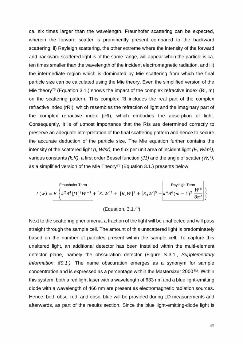
45
ca. six times larger than the wavelength, Fraunhofer scattering can be expected,
wherein the forward scatter is prominently present compared to the backward
scattering, ii) Rayleigh scattering, the other extreme where the intensity of the forward
and backward scattered light is of the same range, will appear when the particle is ca.
ten times smaller than the wavelength of the incident electromagnetic radiation, and iii)
the intermediate region which is dominated by Mie scattering from which the final
particle size can be calculated using the Mie theory. Even the simplified version of the
Mie theory73 (Equation 3.1.) shows the impact of the complex refractive index (RI, m)
on the scattering pattern. This complex RI includes the real part of the complex
refractive index (rRI), which resembles the refraction of light and the imaginary part of
the complex refractive index (iRI), which embodies the absorption of light.
Consequently, it is of utmost importance that the RIs are determined correctly to
preserve an adequate interpretation of the final scattering pattern and hence to secure
the accurate deduction of the particle size. The Mie equation further contains the
intensity of the scattered light (I, W/sr), the flux per unit area of incident light (E, W/m2),
various constants (k,K), a first order Bessel function (J1) and the angle of scatter (W,°),
as a simplified version of the Mie Theory73 (Equation 3.1.) presents below;
𝐼 (𝑤) = 𝐸 {𝑘2𝐴4[𝐽1]2𝑊−1 + [𝐾1𝑊]1 + [𝐾2𝑊]3 + [𝐾3𝑊]5 + 𝑘4𝐴6(𝑚 − 1)2 𝑊6
8𝜋2 }
(Equation. 3.1.73)
Next to the scattering phenomena, a fraction of the light will be unaffected and will pass
straight through the sample cell. The amount of this unscattered light is predominately
based on the number of particles present within the sample cell. To capture this
unaltered light, an additional detector has been installed within the multi-element
detector plane, namely the obscuration detector (Figure S-3.1., Supplementary
Information, §9.1.). The name obscuration emerges as a synonym for sample
concentration and is expressed as a percentage within the Mastersizer 2000™. Within
this system, both a red light laser with a wavelength of 633 nm and a blue light-emitting
diode with a wavelength of 466 nm are present as electromagnetic radiation sources.
Hence, both obsc. red. and obsc. blue will be provided during LD measurements and
afterwards, as part of the results section. Since the blue light-emitting-diode light is
Fraunhofer Term Rayleigh Term

46
more prone to be scattered by smaller particles, the corresponding obscuration will
mostly represent the number of smaller particles present within the sample cell and
hence, within the original sample. Obsc. red is often envisaged as the standard
obscuration level. Within the equipment of HORIBA, multiple light sources are present
as well. The sample concentration is presented as the percentage transmission (%T),
the percentage of incident light not scattered by the particles.77
A part of the LD method development will enclose the search for the optimal
obscuration. Information offered by the manufacturer78 recommends obscuration
ranges based on the particle size of the sample, although this attribute is actually the
output of the LD measurement itself. Besides, the optimal obscuration is a balance
between recording sufficient light intensity and avoiding multiple light scattering. A too
low obscuration will allow background noise to affect the results. Multiple light
scattering on the other hand will lead to a reduction in the detected particle size. As
the term suggests, at excessive obscuration levels, the light will be scattered multiple
times (Figure 3.2.). The diffracted light may hit another particle and thereby be
scattered towards higher angle detectors. Since smaller particles scatter
electromagnetic radiation to these detectors, the presence of these particles will be
overestimated. Hence, finding the optimal obscuration by titration of the obscuration is
a critical step in gaining a precise LD method.79
Figure 3.2. Multiple light scattering.
Another point to consider is the fitting of the raw data. The raw data, as offered by the
LD equipment, enclose both the background signal and the complex scattering pattern

47
which is described by the intensity of the scattered light and the angle of the scattered
light, presented by the detector number. If the intensity of the background, also called
‘blank’, surpasses the measurement signal, so-called negative data are generated,
leading to an underestimation of the scattering signal and so, a deviation in the final
PSD. The raw data will be fitted to acquire the PSD. In the case of the Mastersizers™,
both the raw and the fitted data will be plotted, visualising the accuracy of the given fit.
If deviations are noted between detectors numbers 1 to 50 an inaccurate rRI may be
the cause. Inconsistency around the detectors capturing light extinction80, namely
detector number 51 and 52, can be induced by an inaccurate iRI. All manufacturers of
LD system will present their fit quality in a different way. In the case of Malvern, the fit
quality is indicated in two terms, the res. and res. weight. should be below 2% and in
the same order of magnitude to consolidate a reliable measurement. HORIBA on other
hand will present fit quality based on the Chi-squared, which presents the overall
quality of the experiment and the R parameter, showing the correctness of the chosen
optical parameters, which must be minimised to produce qualitative LD data.76
Deviations of fit can also be linked to poor background quality and poor data quality.

48
MATERIALS AND METHODS
Materials
Bedaquiline and hydroxypropyl methylcellulose (HPMC) were provided by Janssen
Pharmaceutica (Beerse, Belgium). d-α-Tocopherol polyethylene glycol 400 succinate
(TPGS 400) was provided by Eastman Chemical Company Kingsport (TN, USA).
Cinnarizine, polysorbate 20 and polysorbate 80 were obtained from Fagron Belgium
NV (Nazareth, Belgium). Sodium dodecyl sulphate (SDS) was obtained from Sigma
Aldrich Chemie GmbH (Steinheim, Germany). Sodium carboxymethylcellulose
(sodium CMC) and ethyl acetate were obtained from Merck KGaA (Darmstadt,
Germany). Isopropanol, acetone and 1-methyl-2-pyrrolidinone were obtained from
VWR (VWR international, Germany). Deionised water (R≥18 mΩ, Maxima Ultrapure
Water, Elga Ltd., Wycombe, England or Milli-Q® Advantage A10 system, Merck KGaA,
Darmstadt) was used for all the experiments.
Methods
3.4.2.1. Retrieving the real part of the complex refractive index
In the Becke line technique, the compound was consecutively dispersed in a broad set
of rRI matching liquids (Cargille-Sacher Laboratories Inc., NJ, USA) and placed
underneath a microscope (Nikon Eclipse E1000 Microscope with Film Camera System,
Nikon instruments Inc., NY, USA). By lowering the stage of the microscope and
observing in which direction the condensed Becke line moved, the material with the
highest rRI, particle or matrix, could be identified.81
In addition, the single solvent method, as described by Saveyn et al.67, was used. The
density of bedaquiline was measured, using a pycnometer (Beckman Instruments
INC., Fullerton, CA, USA). To simplify the calculations, the rRI of very low concentrated
(0.2, 0.4, 0.6, 0.8 and 1.0%(v/v)) solutions was computed, using an Abbé refractometer
(Atago NAR-1T Liquid, ATAGO U.S.A., Inc., WA, USA). Ultimately, extrapolation up to
100% solute gave the rRI of the analysed compound.67
Finally, the rRI were calculated based on the chemical structure of the compounds,
using the predictive software Chemsketch (Advanced Chemistry Development, Inc.,
Toronto, Canada).
49
The selected rRIs were further optimised within the Mastersizer 2000™ software
(Version 5.61, Malvern Instruments Ltd, Malvern, UK). One set of raw data was
subjected to a range of varying rRIs and iRIs. The tendency of the particle size and the
efficiency of the overlap of the raw and fitted distribution were evaluated. As a result,
the best fitted model and consequently the most appropriate res. and res. weight. were
retrieved. These RIs were used for further LD experiments.
3.4.2.2. Production of suspensions
All suspensions were prepared using wet media milling. 10 mL vials were filled with
bedaquiline (5 wt%), 3 mL of zirconia beads (ø 1mm, Nikkato Corporation, Sakai,
Osaka, Japan) and 8 mL of a stabiliser solution. Both surfactants and hydrophilic
polymers were used as stabilisers in this study.
When a surfactant was used, the concentration was set at 50 times the corresponding
critical micellar concentration (CMC), as obtained from literature. The concentration
TPGS 400 was based on the CMC of TPGS 1000. If needed, average values were
calculated (Table 3.1.). The surfactant solutions were produced one day in advance
and magnetically stirred overnight. To improve dissolution, the SDS and TPGS solution
were stored at approximately 60 °C overnight.
In case of the hydrophilic polymers HPMC and sodium CMC, a concentration of 0.125
%w/v was applied.
Later the vials were placed on an in-house made roller mill. The suspensions were
milled for 28 hours at a speed of ca. 327 rpm.

50
Table 3.1. Surfactants and their corresponding CMC
3.4.2.3. Size determination by laser diffractometry
Conducting laser diffraction experiments
LD measurements were performed on a Mastersizer 2000™ with hydro-unit. In all
experiments, a degassed 0.005 %w/v polysorbate 20 solution was used as dispersant.
As a further preparation of the LD experiments, the hydro-unit was shut down for 90 s
after addition of the dispersant after which a stirrer speed of 600 rpm was set and the
system was left to stabilise. Finally, the system was aligned, and the background was
evaluated.
The general-purpose model for irregularly shaped particles with normal calculation
sensitivity was applied within the Mastersizer 2000™ software. The set optical
parameters were a sample rRI of 1.595 (see below), a sample iRI of 0.001 (see below)
and a dispersant rRI of 1.333. The stirrer speed was set at 600 rpm and no sonication
was applied. An obscuration titration was performed for each sample to elucidate the
optimal obscuration level.
Analysis of Data
Overall, the size range was set at 2000 µm. If gas bubbles emerged as peaks within
the final PSD, the size range was decreased to 96.86 µm to exclude these peaks from
the PSD. Runs that even after size range reduction presented dv-values that were
affected by gas bubbles were removed and averages were recalculated. The
volumetric PSDs with complementary dv-values, residuals, obscuration levels and
volume-based median diameters were interpreted and background stability over time
was assessed.
Stabiliser CMC (%w/v) Applied CMC (%w/v) 50CMC (%w/v)
Polysorbate 20 0.007482 0.0074 0.37
Polysorbate 80 0.001683 0.0016 0.080
SDS 0.2016
as average of 0.1728 - 0.230482, 84
0.2016 10.08
TPGS 0.0285 0.02 1
51
RESULTS AND DISCUSSION
The optimisation of a LD method and further, finding the source of the deviations in LD
data can be complicated since the different aspects of the LD system are often
interconnected. Searching for the correct optical parameters, ensuring background
quality, fitting of raw data, the obscuration titration and ensuring the stability of the
sample within the hydro-unit are key steps in LD method optimisation that will be
discussed in this work. Numerous deviations that occurred during the analysis of fine
suspensions, and the ways how to tackle them, will be discussed as well. Finally, a
flow chart can be found at the end of this article, providing a guideline in LD method
optimisation.
Optical parameters
The implementation of the complex RI within the Mie theory and the associated
calculation model is critical in acquiring correct LD data. Consequently, the question
rises how to measure both the iRI and the rRI. Guidelines offer numerous techniques
to predict or to calculate the rRI, whereas standard methods for the measurement of
the iRI are still lacking. Retrieving the correct optical parameters forms the first step in
achieving qualitative LD results.
3.5.1.1. The influence of the imaginary part of the complex refractive index
on the final particle size distribution
Preliminary experiments showed that the iRI had only limited effect on the fitting of the
Mie model and thus on the final PSDs in the software supplied with the Mastersizer
2000™. Due to hardware and software development such as the increased number of
higher-angle detectors, the Mastersizer 3000™ on other hand implements the iRI more
accurately, which then evidently has a larger effect on the final PSDs.82
Information offered by the manufacturer mentioned two techniques wherewith the iRI
could be estimated.80 The iRI could be predicted based on microscopical images of the
compound or determined based on volume concentration measurements and Lambert-
Beer’s law. Overall, particles with chromophores, low transparency, aspherical habitus
and rough surface structure are prone to have a higher iRI. Within the LD software the
accuracy of this value has to be specified with an order of magnitude, hence making
fit optimisation within the software the most common way of finding an acceptable iRI.80
52
Fit optimisation of the Mie model of an SDS- and TPGS-stabilised suspension, by
comparison of the effect of the different iRIs on the final PSD, residual (res.) and
residuals weighted (res. weight.) with the goal to diminish the latter two, led to an
optimal value of 0.001 which was set within the software for further experiments (Table
S-3.1., Supplementary Information, §9.1.). Fit optimisation could be applied on LD
systems of different manufactures too. When using the LD-950, provided by Horiba,
the minimisation of the residual R-value has to be taken into account to verify the
correct refractive indices, as information offered by the manufacturer suggests.76
3.5.1.2. Techniques to find the real part of the complex refractive index
Numerous approaches to determine the rRI have been described in the literature and
guidelines.67, 86 Empirical methods based on the Clausius-Mossotti equation, the
Gladstone-Dale approximation and RI trend analysis could estimate rRIs, though more
accuracy is preferable.86
Predictive software estimated the rRI based on the compounds chemical structure.
The results were 1.666 ± 0.020 and 1.625 ± 0.020 for bedaquiline and cinnarizine,
respectively (Table 3.2). These outcomes were close to the values found with the
Becke line technique, which were 1.5920 - 1.5960 and 1.6880 - 1.6920 for bedaquiline
and cinnarizine, respectively. However, as these were based on experimental data,
they were presumed to be more accurate. The single solvent technique of Saveyn et
al.67 was applied as well. The density of the compounds must be measured to prepare
volumetric based sample solutions. For this reason, the density of bedaquiline was
experimentally determined to be 1.35 ± 0.00 g/mL and the density of cinnarizine, 1.13
± 0.00 g/mL, was obtained from the literature.87 The single solvent technique of Saveyn
et al. resulted in higher rRIs than the predictive software and the Becke line technique.
For bedaquiline the values ranged from 1.7678 to 1.8342, while values around 1.73
were obtained for cinnarizine. Elements such as the limited precision of the used
refractometer and the lack of a thermostabilising system could explain the deviating
data.

53
Table 3.2. Computed rRI results.
ChemSketch Becke Line Single solvent technique67
Compound Acetone Ethyl acetate 1-methyl-2-pyrrolidinone
Bedaquiline 1.666 ± 0.02 1.5920 - 1.5960
1.8342 1.7678 1.7749
Cinnarizine 1.625 ± 0.02 1.6880 - 1.6920
1.734 1.737
The Becke line data, i.e. values between 1.5920 and 1.5960 for bedaquiline, were used
as input values in the software for further refinement using fit optimisation.
Consequently, the fitting, the PSD and residuals of the SDS- and TPGS-stabilised
suspensions were evaluated while varying the rRI. Based upon this optimisation, a final
rRI of 1.595 for bedaquiline suspensions was found (Table S-3.2., Supplementary
Information, §9.1.).
The predicted value of 1.666, set as rRI during the analysis of the TPGS-stabilised
suspension, would lead to a slight residual increase from 0.501 to 0.532, compared to
the optimal value of 1.595. The dv50-value on the other hand increased to 0.400 µm.
When the same comparison was applied on the SDS-stabilised suspension, both
residual as residual weighted decreased slightly. In this specific case, the predicted
values with fit optimisation could be set instead of the Becke line data. Broadening this
conclusion to other suspensions could be false since the effect on the final fitting and
PSD is unclear. Albeit, predictive software can offer a fast, first idea of the rRI.
Background signal
Besides the correct RIs, a qualitative acceptable background forms one of the primary
steps in retrieving qualitatively and quantitatively correct PSDs. The background or
blank will be subtracted from the measurement signal and thus produces the final
complex scattering pattern from which the PSD will be derived. Hence, when deviations
such as gas bubbles, noise, contamination or misalignment present themselves during
background measurement, they will cause deviations in the final obscuration, fitting
and PSD.
An example of how poor background quality inferred with the LD results was found
during the measurement of an SDS-stabilised suspension (Figure 3.3.). Due to the
presence of background noise and gas bubbles, which were not captured during
background measurement, the baseline of the final PSD was raised and additional
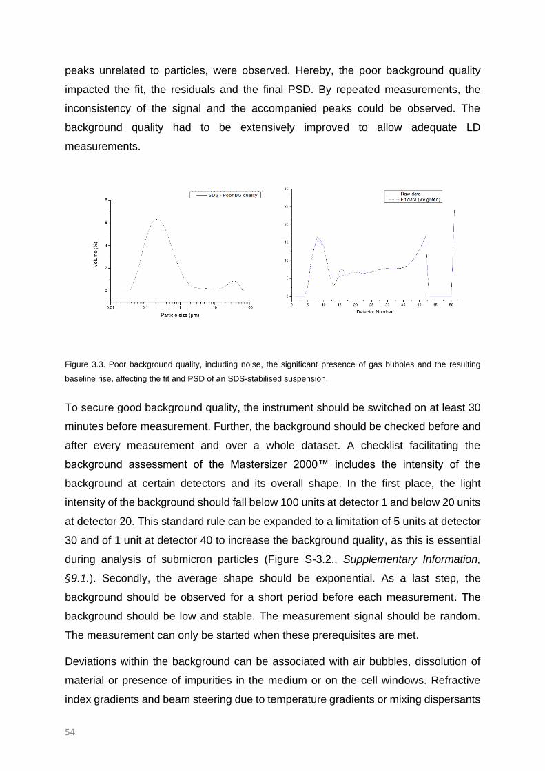
54
peaks unrelated to particles, were observed. Hereby, the poor background quality
impacted the fit, the residuals and the final PSD. By repeated measurements, the
inconsistency of the signal and the accompanied peaks could be observed. The
background quality had to be extensively improved to allow adequate LD
measurements.
Figure 3.3. Poor background quality, including noise, the significant presence of gas bubbles and the resulting
baseline rise, affecting the fit and PSD of an SDS-stabilised suspension.
To secure good background quality, the instrument should be switched on at least 30
minutes before measurement. Further, the background should be checked before and
after every measurement and over a whole dataset. A checklist facilitating the
background assessment of the Mastersizer 2000™ includes the intensity of the
background at certain detectors and its overall shape. In the first place, the light
intensity of the background should fall below 100 units at detector 1 and below 20 units
at detector 20. This standard rule can be expanded to a limitation of 5 units at detector
30 and of 1 unit at detector 40 to increase the background quality, as this is essential
during analysis of submicron particles (Figure S-3.2., Supplementary Information,
§9.1.). Secondly, the average shape should be exponential. As a last step, the
background should be observed for a short period before each measurement. The
background should be low and stable. The measurement signal should be random.
The measurement can only be started when these prerequisites are met.
Deviations within the background can be associated with air bubbles, dissolution of
material or presence of impurities in the medium or on the cell windows. Refractive
index gradients and beam steering due to temperature gradients or mixing dispersants
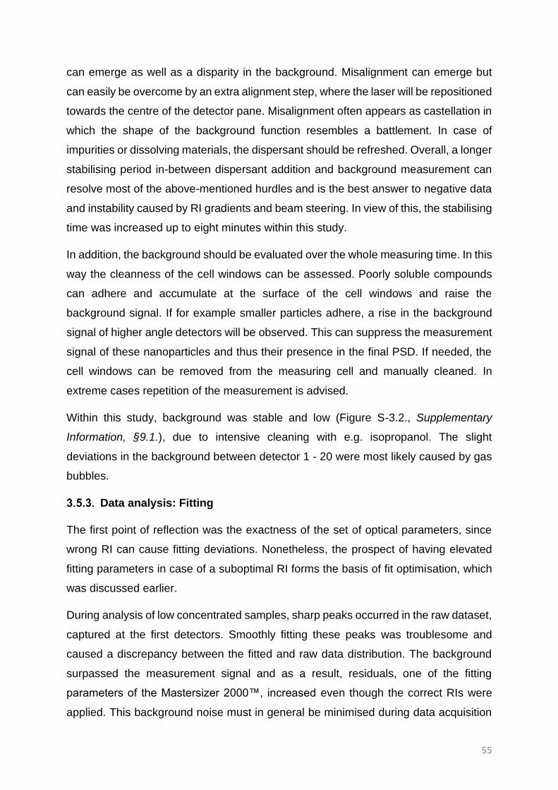
55
can emerge as well as a disparity in the background. Misalignment can emerge but
can easily be overcome by an extra alignment step, where the laser will be repositioned
towards the centre of the detector pane. Misalignment often appears as castellation in
which the shape of the background function resembles a battlement. In case of
impurities or dissolving materials, the dispersant should be refreshed. Overall, a longer
stabilising period in-between dispersant addition and background measurement can
resolve most of the above-mentioned hurdles and is the best answer to negative data
and instability caused by RI gradients and beam steering. In view of this, the stabilising
time was increased up to eight minutes within this study.
In addition, the background should be evaluated over the whole measuring time. In this
way the cleanness of the cell windows can be assessed. Poorly soluble compounds
can adhere and accumulate at the surface of the cell windows and raise the
background signal. If for example smaller particles adhere, a rise in the background
signal of higher angle detectors will be observed. This can suppress the measurement
signal of these nanoparticles and thus their presence in the final PSD. If needed, the
cell windows can be removed from the measuring cell and manually cleaned. In
extreme cases repetition of the measurement is advised.
Within this study, background was stable and low (Figure S-3.2., Supplementary
Information, §9.1.), due to intensive cleaning with e.g. isopropanol. The slight
deviations in the background between detector 1 - 20 were most likely caused by gas
bubbles.
Data analysis: Fitting
The first point of reflection was the exactness of the set of optical parameters, since
wrong RI can cause fitting deviations. Nonetheless, the prospect of having elevated
fitting parameters in case of a suboptimal RI forms the basis of fit optimisation, which
was discussed earlier.
During analysis of low concentrated samples, sharp peaks occurred in the raw dataset,
captured at the first detectors. Smoothly fitting these peaks was troublesome and
caused a discrepancy between the fitted and raw data distribution. The background
surpassed the measurement signal and as a result, residuals, one of the fitting
parameters of the Mastersizer 2000™, increased even though the correct RIs were
applied. This background noise must in general be minimised during data acquisition

56
to preserve their high quality. In extreme cases, these sharp peaks raised the baseline.
A signal at the lower numbered detectors is often linked to the presence of bigger
particles. As a consequence, dv-values increased, in particular the dv90-value. A low
measurement signal and thus a low sample concentration within the measuring cell
provoked these sharp peaks. These peaks emphasise the need for a background of
utmost quality. The inconvenience can be overcome by increasing the sample
concentration, though multiple light scattering, which will be touched upon below,
should be taken into consideration as well.
A second element that needed consideration was the inconsistent presence of an extra
peak around detector 10, which caused the overall fit to deviate (Figure 3.4. and 3.5.).
This peak sharply affected the final dv-values (Figure 3.4.) and randomly reoccurred
in the PSD over consecutive runs, though it was not linked to the original sample.
These peaks were often present with a size of ca. 100 to 300 µm (Figure 3.5.). The
light intensity of the peaks was high and highly variable. To obtain a stable, dispersed
system, a surfactant was added to the dispersant in low concentration, which, however,
induced the risk of foaming. The inconsistency in the presence and the size of the peak
during consecutive runs and observation of foam strongly suggested that the peaks
originated from gas bubbles that would influence the final data.
Practical steps could be implemented to avoid gas bubbles and their influence on both
the fit and PSD. Dispersant was degassed and after its addition to the hydro-unit, the
unit was shut down for a few minutes, so the air bubbles could evacuate. Further, the
rotation speed of the stirrer was reduced to 600 rpm and stabilisation time was
enhanced up to eight minutes. If not sufficient, extra stabilisation time or short, sharp
surges in the stirrer speed may drive the bubbles to the surface. However, gas bubbles
could not always be completely avoided. If they appeared as additional peaks within
the PSD, the size measurement range was retrospectively limited to 96.86 µm, which
improved the dv-values (Figure 3.5.). Certainly, when lower obscuration levels were
analysed, gas bubbles had less resistance to appear in the volumetric distribution. If
size range reduction was not sufficient, the runs containing these gas bubbles were
excluded from the average calculation, leading to a better fitting quality. However, by
this latter step, the background noise impacted the distribution even more, envisaged
in the previously mentioned sharp peaks in the raw data (Figure 3.4.).
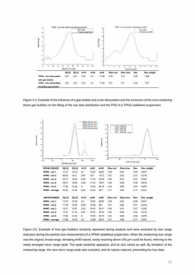
57
Figure 3.4. Example of the influence of a gas bubble and a low obscuration and the exclusion of the runs containing
these gas bubbles on the fitting of the raw data distribution and the PSD of a TPGS-stabilised suspension.
Figure 3.5. Example of how gas bubbles randomly appeared during analysis and were excluded by size range
reduction during the particle size measurement of a HPMC-stabilised suspension. When the measuring size range
was the original, broad range, deviating dv90-values, easily reaching above 150 µm could be found, referring to the
newly emerged micro range peak. The peak randomly appeared, and its size varied as well. By limitation of the
measuring range, the new micro range peak was excluded, and dv-values reduced, presenting the true data.
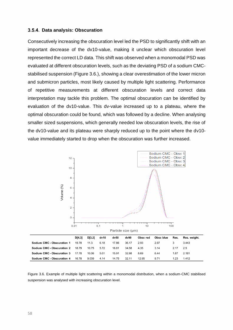
58
Data analysis: Obscuration
Consecutively increasing the obscuration level led the PSD to significantly shift with an
important decrease of the dv10-value, making it unclear which obscuration level
represented the correct LD data. This shift was observed when a monomodal PSD was
evaluated at different obscuration levels, such as the deviating PSD of a sodium CMC-
stabilised suspension (Figure 3.6.), showing a clear overestimation of the lower micron
and submicron particles, most likely caused by multiple light scattering. Performance
of repetitive measurements at different obscuration levels and correct data
interpretation may tackle this problem. The optimal obscuration can be identified by
evaluation of the dv10-value. This dv-value increased up to a plateau, where the
optimal obscuration could be found, which was followed by a decline. When analysing
smaller sized suspensions, which generally needed low obscuration levels, the rise of
the dv10-value and its plateau were sharply reduced up to the point where the dv10-
value immediately started to drop when the obscuration was further increased.
Figure 3.6. Example of multiple light scattering within a monomodal distribution, when a sodium-CMC stabilised
suspension was analysed with increasing obscuration level.

59
The obscuration titration of a polysorbate 20-stabilised suspension showed a
monomodal distribution in the micrometre range during the first measurement,
however, increasing obscuration led to the emerge of a submicron peak which
moderately extended during further obscuration enhancement (Figure 3.7.). This led
to a sudden drop of the dv10-value and the dv50-value. The lower obscuration levels
on the other hand showed a poorer fit than those of the higher obscuration levels.
Overall, depending on the obscuration, markedly different PSDs could be obtained,
emphasising the need of an obscuration titration
Figure 3.7. Example of multiple light scattering, occurring within the multimodal PSD of a polysorbate 20 stabilised
suspension.

60
Besides multiple light scattering and the minimum obscuration have to surpass the
background noise, additional factors influenced the effect of the obscuration level on a
multimodal PSD. The intensity of light scattered by nanoparticles was lower than the
intensity of light when scattered by microparticles. Thus, the obscuration has to be
significantly increased to visualize the nanoparticles when present within a multimodal
system. This phenomenon was enhanced by the volumetric display of the PSD, leading
to the dilemma of the need to measure nanocrystals while increasing the risk of multiple
light scattering. Generally, the lowest obscuration level, which was not affected by
noise, was selected as the optimal obscuration level. The low obscuration level will
offer the researcher the worst-case scenario where no or only limited multiple light
scattering can be expected. Also, the quality of the background related to the optimal
obscuration level was an important factor, as the measurement signal must be larger
than the background signal to give a meaningful read-out. For finer suspensions, the
lower obscuration limit was defined by the noise level in the system, i.e. requiring a
high background quality for the measurement.
Data analysis: Stability of the sample within the hydro-unit
Another hurdle that may be encountered is a gradual shift of the PSD during
consecutive runs of a measurement, making it hard to decide at which point
representative data are obtained. Overall, three different, time dependent phenomena
can take place within the LD system that reduce the representability of the sample
within the LD system, namely i) dissolution of the compound, ii) agglomeration of the
compound particles, or iii) an inhomogeneous dispersion of the sample.
Dissolution will appear as a gradual decrease of the median particle size when
microparticles are analysed. During the analysis of nanosuspensions, dissolution may
make these particles undetectable, leading to an increasing dv10-value. Dissolution
will always be accompanied by a decreasing obscuration. In case of agglomeration,
both red and blue light obscuration can increase due to the presence of bigger particles
that scatter the light more intensively. Alternatively, the red light obscuration can
increase, as a consequence of disappearance of smaller particles, leading to a
diminishing blue light obscuration. If not properly dispersed, the dv-values and
obscuration levels will change depending on the fraction of particles passing the laser.
To obtain representative data, the rotation speed of the stirrer and the time between
sample addition and sample measurement must be optimised. This speed should be
61
high enough for homogenisation, without promoting dissolution and foaming. Enough
time was required to secure an adequate sample dispersion in the measuring cell
before analysis. Although these phenomena were more difficult to identify, they can
co-occur as well.
The influence of these phenomena can be restricted through the use of a limited
number of runs in the calculation of the average, as has been done within this study. If
dissolution or agglomeration took place, the first three reliable runs were selected.
While in the case of an inadequate dispersion, the measurement was repeated or only
the last runs were accepted. When the measurement was repeated, the time in-
between sample addition and analysis was increased to secure a homogenously
dispersed sample. The variability in-between the particle sizes of the consecutive runs
should comply to the ISO 13320 guidelines.88 These guidelines state that the
coefficient of variation (CV) should be below 5% in case of dv10- and dv90-value, while
the dv50-value should stay below the limit of 3%. These values are doubled in the case
of a value below 10 µm and can be applied to assess the precision of the data and
hence the stability of the dispersed system within the LD system In the case of
dissolution, the dispersant could be replaced with one where the particles are less
soluble in.
Flow chart
To summarise all the information that has been provided in this work, a flow chart has
been offered, based on the Mastersizer 2000™ software but which can be extrapolated
to other LD systems as well. Although such a summarising chart cannot fully cover the
complexity of LD and its broad range of samples, it can form a basic guideline during
LD method optimisation and data analysis. Overall, due to the possible lower accuracy
and precision of the LD method, even after method optimisation, additional analysis
with an orthogonal technique or multiple sampling is advised.
When optimising a LD method (Figure 3.8.), the RIs must be set first. Different
techniques, as has been previously mentioned can be opted to find both the iRI and
the rRI. For the estimation of the rRI, the Becke line technique and further fit
optimisation in the software is advised. Additionally, the number of runs during one
analysis, the measurement time of one run and the delay in-between the different runs
have to be set, which is e.g. dependent on the stability of the sample within the hydro-

62
unit. Afterwards, the accessory parameters must be installed. Dispersant has to be
added to the hydro-unit. The choice of this dispersant is dependent on the solubility
and the stability of the sample in the dispersant during measurement. To mimic the
compounds matrix and to stabilise the sample during analysis, surfactant can be added
to the dispersant or the dispersant can be saturated with the compound. After addition,
the stirrer speed and sonication level will be set. Stirrer speed should be high enough
to homogenise the sample but should be reduced in case of foaming or sample fragility.
Sonication can be introduced to break agglomerates. After installation of the accessory
parameters, a background stabilisation time can be introduced before alignment and
background/blank measurement take place. The background signal and the random
measurement signal should be briefly checked and secured. The background must
accomplish the previously mentioned prerequisites. If not, additional cleaning steps or
background stabilisation time can usually omit the issue. Misalignment can present
itself as castellation and can be overcome by cleaning or replacement of the cell
windows. Alignment can be set manually as well but is not preferred. After the
background check, sample will be added. Depending on the state of the sample within
the hydro-unit, additional dispersion time can be introduced before the measurement
is started. After the measurement, the data should be first qualitatively checked before
conclusions based on the dv-values can be made. First the measuring range should
be expanded or rather reduced, though this is only the final resort in case of gas
bubbles, to cover the full PSD of the sample. ‘Data’ should be checked for the presence
of negative data. Further ‘Fit’ is reviewed to check fitting parameters such as res., res.
weight, R parameter or Chi-squared. and where possible discrepancy between the raw
data and the fitted data takes place. Only then, the ‘Records’ can be examined. Not
only the dv-values on itself are important but also trends during analysis, can indicate
instability of the sample during analysis or issues regarding impurities or gas bubbles
which should be taken into consideration during further result analysis. When runs are
excluded due to discrepancies, averages have to be recalculated. After cleaning, the
background must be shortly assessed and also over the whole experiment.
Accumulating impurities can be found and resolved by additional cleaning. Finally, the
overall quality of the method can be evaluated and if needed, further optimised by
variation of the different software parameters, accessory parameters and stabilisation
periods. Thus, the flow chart should be executed algorithmically to obtain a final
optimised method. When an optimised method is found, it is still important to execute

63
an obscuration titration every time samples are analysed. Overall, relying on standard
LD methods will not guarantee LD quality and so the quantity of the LD results could
be inaccurate.
Figure 3.8. Flowchart wherewith LD method optimisation can be conducted, starting with the installation of the
correct software parameters, leading to accessory parameters selection, sample measurement, analysis of results
and cleaning of system. Intermediate steps are presented in the diamond shaped boxes.
64
CONCLUSIONS
Over the last decades, nano- and microsuspensions have been well received within
the pharmaceutical community. For the analysis of one of their most critical quality
attributes, the particle size and PSD, different techniques have been described within
the literature. Of these LD is the most widely used technique, due to its broad
measuring range, its reproducibility, and its ease to use. However, the accuracy of LD
has been questioned by multiple authors.73, 74, 75 The present work showed that not
only the set of optical parameters, but also parameters such as the fit, obscuration,
stability of the dispersion within the LD system and background quality can have a
significant impact on the final PSD. An extensive insight in the LD system and effective
troubleshooting, such as suggested in the present work are needed during LD
measurements, if high quality LD data should be generated.
SUPPLEMENTARY INFORMATION
All supplementary material as denoted in the manuscript is provided in Chapter 9:
Supplementary Information, §9.1

Exploration of the heat generation within the intensified
vibratory mill
Results in this chapter are based on:
De Cleyn, E., Holm, R. & Van den Mooter, G. Exploration of the heat generation within
the intensified vibratory mill. Int. J. Pharm. 119644 (2020).
doi:10.1016/j.ijpharm.2020.119644

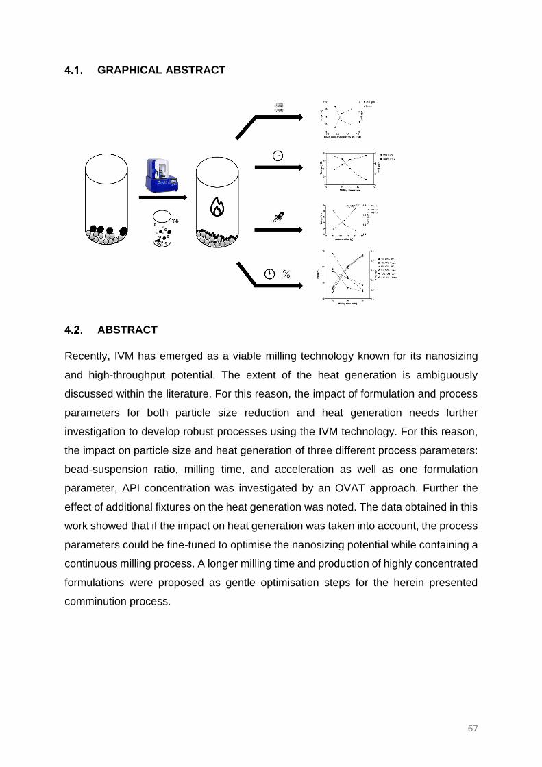
67
GRAPHICAL ABSTRACT
ABSTRACT
Recently, IVM has emerged as a viable milling technology known for its nanosizing
and high-throughput potential. The extent of the heat generation is ambiguously
discussed within the literature. For this reason, the impact of formulation and process
parameters for both particle size reduction and heat generation needs further
investigation to develop robust processes using the IVM technology. For this reason,
the impact on particle size and heat generation of three different process parameters:
bead-suspension ratio, milling time, and acceleration as well as one formulation
parameter, API concentration was investigated by an OVAT approach. Further the
effect of additional fixtures on the heat generation was noted. The data obtained in this
work showed that if the impact on heat generation was taken into account, the process
parameters could be fine-tuned to optimise the nanosizing potential while containing a
continuous milling process. A longer milling time and production of highly concentrated
formulations were proposed as gentle optimisation steps for the herein presented
comminution process.

68
INTRODUCTION
Over the past decades, the number of drug molecules in the pharmaceutical
development pipelines with poor aqueous solubility has steadily increased, leading to
low and variable oral bioavailability if administered in a conventional dosage form. To
address this challenge, both industry and academia have put significant effort into
finding enabling formulation and processing technologies that can facilitate the usage
of these molecules.33, 42 Among these, the production of micron and submicron
suspensions is a viable and cost-effective strategy, resulting in marketed drugs such
as Rapamune® (Pfizer (Wyeth), NY, USA), Emend® (Merck, NJ, USA) and Megace
ES® (Par Pharmaceutical, NY, USA). 3, 42
Micro- and certainly nanoparticle suspensions exhibit distinctive performance
properties when compared to their poorly soluble bulk counterparts, leading to
enhanced bioavailability after oral uptake, which have been described by numerous
authors.33, 42 Their large specific surface area enhances the dissolution rate, as
described by the Nernst- and Brunner equation (Equation 1.1.).22 In addition, the
diffusion layer thickness decreases with increasing curvature, as described by the
Prandtl equation (Equation 1.2.), further increasing the dissolution performance.5 The
greater surface curvature of particles <100 nm is strongly correlated with a higher
saturation solubility, as described by the Ostwald-Freundlich equation (Equation 1.3.).5
As a formulation system, nano- and microsuspensions can also be used to create LAIs,
a formulation route of utmost interest to combat chronic diseases where patient
compliance is essential for the treatment response.35
Nano- and microsuspensions can be produced in two ways overall; either by particle
size reduction of larger particles, the so-called top-down approach, or via the controlled
precipitation of dissolved molecules, the so-called bottom-up approach. The bottom-
up process usually demands significant volumes of organic solvents and is generally
hard to control with respect to particle size. With the top-down approach, no harsh
solvents are used, but the energy generated is often inefficiently dissipated, leading to
heat generation and potential mechanochemical activation. This may alter the
physicochemical state of the compound and cause instability of the produced drug
product.41, 42, 89 Currently, manufacturers are able to control the overall temperature
rise of the WBM process by the implementation of a cooled water jacket. Two other
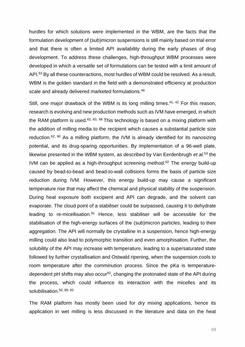
69
hurdles for which solutions were implemented in the WBM, are the facts that the
formulation development of (sub)micron suspensions is still mainly based on trial error
and that there is often a limited API availability during the early phases of drug
development. To address these challenges, high-throughput WBM processes were
developed in which a versatile set of formulations can be tested with a limit amount of
API.53 By all these counteractions, most hurdles of WBM could be resolved. As a result,
WBM is the golden standard in the field with a demonstrated efficiency at production
scale and already delivered marketed formulations.46
Still, one major drawback of the WBM is its long milling times.41, 42 For this reason,
research is evolving and new production methods such as IVM have emerged, in which
the RAM platform is used.62, 63, 66 This technology is based on a mixing platform with
the addition of milling media to the recipient which causes a substantial particle size
reduction.62, 90 As a milling platform, the IVM is already identified for its nanosizing
potential, and its drug-sparing opportunities. By implementation of a 96-well plate,
likewise presented in the WBM system, as described by Van Eerdenbrugh et al.53 the
IVM can be applied as a high-throughput screening method.62 The energy build-up
caused by bead-to-bead and bead-to-wall collisions forms the basis of particle size
reduction during IVM. However, this energy build-up may cause a significant
temperature rise that may affect the chemical and physical stability of the suspension.
During heat exposure both excipient and API can degrade, and the solvent can
evaporate. The cloud point of a stabiliser could be surpassed, causing it to dehydrate
leading to re-micellisation.91 Hence, less stabiliser will be accessible for the
stabilisation of the high-energy surfaces of the (sub)micron particles, leading to their
aggregation. The API will normally be crystalline in a suspension, hence high-energy
milling could also lead to polymorphic transition and even amorphisation. Further, the
solubility of the API may increase with temperature, leading to a supersaturated state
followed by further crystallisation and Ostwald ripening, when the suspension cools to
room temperature after the comminution process. Since the pKa is temperature-
dependent pH shifts may also occur92, changing the protonated state of the API during
the process, which could influence its interaction with the micelles and its
solubilisation.50, 89, 93
The RAM platform has mostly been used for dry mixing applications, hence its
application in wet milling is less discussed in the literature and data on the heat

70
generation is underrepresented and ambiguous.62, 63, 66 The heat generation within the
IVM has been previously mentioned by Li and co-workers, but the publication did not
explore this phenomenon further. Li et al. interrupted the milling process every eight
minutes, when the samples were dipped in a refrigerated bath.63 Even though this
method was presented to be effective in small scale, it will be hard to standardise
according to good manufacturing practices or scale-up for clinical or commercial
production. Further, it is known that the final PSD of a milling process is based on the
counteracting trends of comminution and agglomeration.94 The effect of these
implemented breaks and sharp temperature fluctuations on the agglomeration and
thereby the final particle size hence the effective comminution of the milling process
was not explored. To strengthen our knowledge on the heat generation within the IVM
while keeping a continuous manufacturing process, the impact of different formulation
and process parameters on the final temperature should be explored. In this scope,
this article elaborates further on the limited temperature mapping within the IVM
presented by the group of Lu et al.66 Herein, we demonstrate the important heat
generation within the IVM, we report the impact of additional IVM fixtures on the final
temperature and we present the impact of different process and formulation
parameters on both particle size reduction and temperature rise using an OVAT
approach.

71
MATERIALS AND METHODS
Materials
Bedaquiline, a poorly soluble model drug (BSC class II), was provided by Janssen
Pharmaceutica (Beerse, Belgium). The particle size of this starting material was 7.5
µm, 48.5 µm and 328 µm for dv10, dv50 and dv90, respectively. Polysorbate 20 was
obtained from Croda (Trappes, France). Deionised water (R≥18.2 mΩ, Milli-Q®
Advantage A10, Merck, Darmstadt, Germany) was used for all experiments.
Methods
4.4.2.1. Production of suspensions
All suspensions were prepared using IVM. Glass vials were filled with bedaquiline,
zirconia beads (Nikkato Corporation, Sakai, Osaka, Japan) and a polysorbate 20
solution. A specific bead-suspension ratio (mL/mL) was set and a bead size of 1000
µm was used. Polysorbate 20 was used in concentrations corresponding to 50, 250 or
500 times its CMC, respectively 0.37 %w/v, 1.85 %w/v and 3.70 %w/v.82 The vials were
placed on an in-house made platform within the LabRAM II (Resodyn Acoustic Mixers,
Butte, USA) and milled for a certain period of time (min), at a defined acceleration (g).
Within the IVM, the vials are shaken vigorously and must therefore be properly
secured. For this reason, a polyoxymethylene derivative-based in-house platform was
constructed (Figure 4.1.).
Figure 4.1. The in-house made platform for holding vials during IVM. An additional hole had to be made at the
bottom of the plate to reduce the mass of this additional feature.
An overview of the different processes and formulation parameters used is shown in
Table 4.1.

72
Table 4.1. Overview of the experiments and their varying formulation and process parameters
Formulation Beads Mill
Sample API conc (%)
Stabiliser conc (*CMC)
Bead size (µm)
Bead-suspension ratio (mL/mL)
Acceleration (g)
Milling time (min)
1 5 50 1000 1.125 75 5
2 5 50 1000 1.125 75 10
3 5 50 1000 1.125 75 15
4 5 50 1000 1.125 75 20
5 5 50 1000 1.125 75 25
6 5 50 1000 1.2 50 15
7 5 50 1000 1.2 75 15
8 5 50 1000 1.2 100 15
9 5 50 1000 0.692 100 15
10 5 50 1000 0.375 100 15
11 5 50 1000 0.774 50 20
12 5 50 1000 0.774 65 20
13 5 50 1000 0.774 80 20
14 1 50 1000 0.774 65 10
15 1 50 1000 0.774 65 20
16 1 50 1000 0.774 65 30
17 5 250 1000 0.774 65 10
18 5 250 1000 0.774 65 20
19 5 250 1000 0.774 65 30
20 10 500 1000 0.774 65 10
21 10 500 1000 0.774 65 20
22 10 500 1000 0.774 65 30
4.4.2.2. Temperature measurement
The temperature of the suspension was initially determined using a manual
thermometer (Sample 1 – 5, Table 4.2.) by measuring the suspensions temperature
over the period of 1min 10 s – 1 min 25 s after milling, as an indication of the final
suspension temperature. In later experiments (Sample 6 – 22, Table 4.2.), the
temperature was measured with an infrared thermometer (VWR® Traceable® Infrared
Thermometer, Radnor, PA, US) for which an emissivity of 0.69 was set. Temperature
was measured at fixed time points after milling. Extrapolation to zero could give an
estimate of the suspension’s temperature immediately after milling, as more deeply
discussed in ‘§4.5. Results and Discussion’.

73
4.4.2.3. Laser diffractometry
LD measurements were performed on a Mastersizer 2000™ (Malvern Instruments,
Worcestershire, UK) with a hydro-unit, using deionised water as dispersant. Stirring
speed was set to 600 rpm and the system was left to stabilise for five minutes. Finally,
the system was aligned, and the background was evaluated. The general-purpose
model for irregularly shaped particles with normal calculation sensitivity was applied.
The set optical parameters were a sample rRI of 1.595, a sample iRI of 0.001 and a
dispersant rRI of 1.333. A limited obscuration titration was performed for each sample
to determine the optimal obsc. and obsc. blue. The quality of the LD data was based
on the fitting, res. and res. weight., as described in chapter 3.95 The particle size was
described by the volumetric median, the dv50-value. Additionally, the PSD was
described by a volumetric distribution with the dv10-, dv50- and dv90-values.
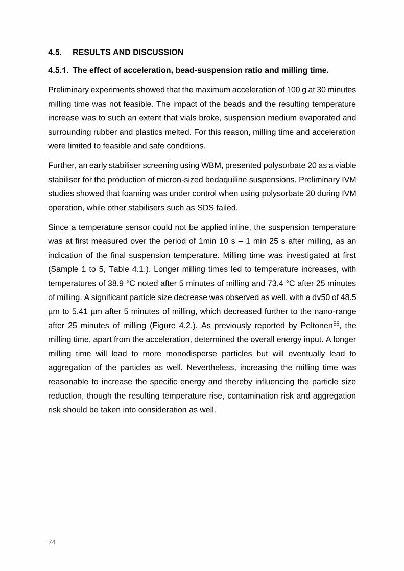
74
RESULTS AND DISCUSSION
The effect of acceleration, bead-suspension ratio and milling time.
Preliminary experiments showed that the maximum acceleration of 100 g at 30 minutes
milling time was not feasible. The impact of the beads and the resulting temperature
increase was to such an extent that vials broke, suspension medium evaporated and
surrounding rubber and plastics melted. For this reason, milling time and acceleration
were limited to feasible and safe conditions.
Further, an early stabiliser screening using WBM, presented polysorbate 20 as a viable
stabiliser for the production of micron-sized bedaquiline suspensions. Preliminary IVM
studies showed that foaming was under control when using polysorbate 20 during IVM
operation, while other stabilisers such as SDS failed.
Since a temperature sensor could not be applied inline, the suspension temperature
was at first measured over the period of 1min 10 s – 1 min 25 s after milling, as an
indication of the final suspension temperature. Milling time was investigated at first
(Sample 1 to 5, Table 4.1.). Longer milling times led to temperature increases, with
temperatures of 38.9 °C noted after 5 minutes of milling and 73.4 °C after 25 minutes
of milling. A significant particle size decrease was observed as well, with a dv50 of 48.5
µm to 5.41 µm after 5 minutes of milling, which decreased further to the nano-range
after 25 minutes of milling (Figure 4.2.). As previously reported by Peltonen56, the
milling time, apart from the acceleration, determined the overall energy input. A longer
milling time will lead to more monodisperse particles but will eventually lead to
aggregation of the particles as well. Nevertheless, increasing the milling time was
reasonable to increase the specific energy and thereby influencing the particle size
reduction, though the resulting temperature rise, contamination risk and aggregation
risk should be taken into consideration as well.
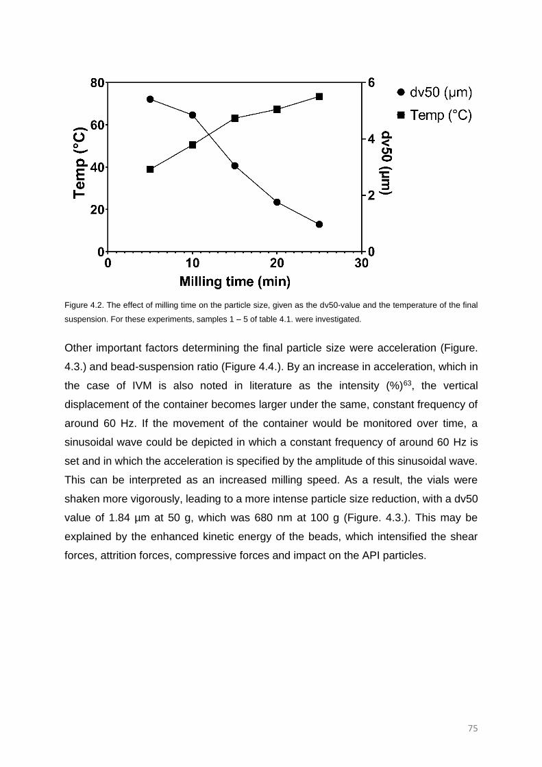
75
Figure 4.2. The effect of milling time on the particle size, given as the dv50-value and the temperature of the final
suspension. For these experiments, samples 1 – 5 of table 4.1. were investigated.
Other important factors determining the final particle size were acceleration (Figure.
4.3.) and bead-suspension ratio (Figure 4.4.). By an increase in acceleration, which in
the case of IVM is also noted in literature as the intensity (%)63, the vertical
displacement of the container becomes larger under the same, constant frequency of
around 60 Hz. If the movement of the container would be monitored over time, a
sinusoidal wave could be depicted in which a constant frequency of around 60 Hz is
set and in which the acceleration is specified by the amplitude of this sinusoidal wave.
This can be interpreted as an increased milling speed. As a result, the vials were
shaken more vigorously, leading to a more intense particle size reduction, with a dv50
value of 1.84 µm at 50 g, which was 680 nm at 100 g (Figure. 4.3.). This may be
explained by the enhanced kinetic energy of the beads, which intensified the shear
forces, attrition forces, compressive forces and impact on the API particles.

76
Figure 4.3. The influence of acceleration, given by sample 6 to 8 of Table 4.1., on both temperature and particle
size after milling.
Figure 4.4. The influence of bead-suspension ratio, given by sample 8 to 10 of Table 4.1., on particle size and
temperature of the suspension after milling.

77
Higher bead-suspension ratio means that more beads per API particle are present in
the vial. As a result, the probability for the particle to undergo collision will increase and
so a higher specific energy input will go in the system. As expected, final dv50 values
of about 2.5 µm were found, which further decreased to 680 nm, when increasing the
bead-suspension ratio from 0.375 mL/ mL to 1.2 mL/mL (Figure. 4.4.).
As presented above, the specific energy of the milling process increases when the
acceleration or the bead-suspension ratio are enhanced. On the other hand, this
increased specific energy is reflected in a sharp heat generation as well. To obtain a
more accurate estimation of the suspension’s final temperature, the temperature was
measured at fixed time points after milling, using an infrared thermometer. The
temperature values were fitted to Newton’s law of cooling (Equation. 4.1.) for which a
high determination coefficient could be reached, as presented in the case of sample 7
in Table 4.1. (Figure 4.5.). Extrapolation to zero could give an estimate of the
suspension’s temperature immediately after milling. In this way, heating was identified
when a high acceleration (Figure 4.3.) or bead-suspension ratio (Figure 4.4.) was set.
In the most extreme settings, 90 °C could be reached. This value approached the cloud
point of the stabiliser used (polysorbate 20), which is about 92-97 °C.91, 96 Parameters
such as acceleration and bead-suspension ratio should thus be taken into
consideration when controlling the temperature of the milling process.
(𝑇𝑡 − 𝑇𝑎) = (𝑇0 − 𝑇𝑎) 𝑒𝑥𝑝 (−𝑡
𝑦) (Equation 4.1)
where Tt is the temperature of the object at time t, Ta is the surrounding, ambient
temperature, T0 is the initial temperature of the object and y is a time constant.97
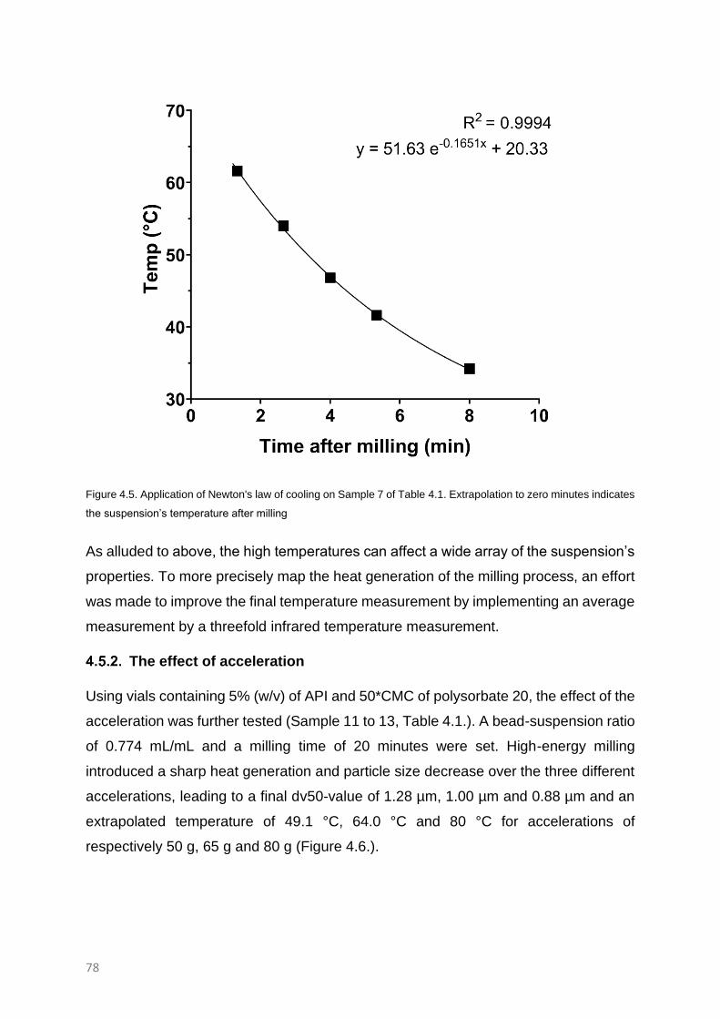
78
Figure 4.5. Application of Newton's law of cooling on Sample 7 of Table 4.1. Extrapolation to zero minutes indicates
the suspension’s temperature after milling
As alluded to above, the high temperatures can affect a wide array of the suspension’s
properties. To more precisely map the heat generation of the milling process, an effort
was made to improve the final temperature measurement by implementing an average
measurement by a threefold infrared temperature measurement.
The effect of acceleration
Using vials containing 5% (w/v) of API and 50*CMC of polysorbate 20, the effect of the
acceleration was further tested (Sample 11 to 13, Table 4.1.). A bead-suspension ratio
of 0.774 mL/mL and a milling time of 20 minutes were set. High-energy milling
introduced a sharp heat generation and particle size decrease over the three different
accelerations, leading to a final dv50-value of 1.28 µm, 1.00 µm and 0.88 µm and an
extrapolated temperature of 49.1 °C, 64.0 °C and 80 °C for accelerations of
respectively 50 g, 65 g and 80 g (Figure 4.6.).

79
Figure 4.6. The effect of acceleration on the particle size reduction and heat generation, as presented by samples
11 to 13 of Table 4.1. The computed end-of-milling temperatures were fitted as a function of acceleration (g). An
exponential trend with a determination coefficient of 1.000 could be noted.
Mathematical fitting of the extrapolated temperatures to the set acceleration suggested
an exponential trend (Figure 4.6.). By extrapolation of this function, the temperature
after milling can be estimated for other accelerations. It is worth mentioning that if an
acceleration of 100 g would be applied under these process conditions, an estimated
temperature of over 120 °C is computed.
Heat transfer from the vial to the polyoxymethylene platform was expected to be
limited, but the platform became hot, nonetheless. Temperatures of 30-40 °C were
often measured and depending on the process parameters, the resultant temperature
could be 60 °C or even 70 °C, leaving the platform as a cooking plate. Therefore, users
of the IVM should be aware that additional fixtures such as platforms will not only lead
to possible motor deterioration but could also cause heating of the samples. In this
study, the influence of the platform on the final temperature was further considered.
Based on first the short milling time and brief exposure to the platform and secondly
the poor thermal conductivity of the platform, the heat transfer was expected to be

80
limited within the earlier mentioned dataset. In this sense, the effect of acceleration on
temperature cannot be proven to be exponential but can still be assumed to be non-
linear.
The effect of API concentration and milling time
In a next set of experiments (Sample 14 to 22, Table 4.1.), the effect of a cooled
platform, API concentration and milling time were analysed. The stabiliser
concentration was increased to 50, 250 and 500 times the CMC for the 1%(w/v),
5%(w/v) and 10%(w/v) API suspensions, respectively. Platforms were cooled between
experiments. To investigate the influence of this adaptation, the 5%(w/v) API
suspension were milled within a cooled and a non-cooled platform. Variation on the
temperature measurement was considerably lower in the case of the cooled platform
and in the end, the final, extrapolated temperature was reduced (Figure 4.7.). Cooling
fixtures in-between milling experiments seemed to be a necessity to avoid additional
heating and to keep the variability on the final temperature under control.
Figure 4.7. The cooling profile of the 1%, 5% and 10% suspensions milled for 20 minutes at 65 g. in which the 1%
and 10% suspensions were milled on a cooled platform. In the case of the 5% suspension, the suspension was
milled on a platform that was not cooled (left) and that was cooled (right). Cooling the platform will lead to a decrease
in both the variability of the temperature measurement and the temperature measurement on itself.
In scope of the particle size reduction, the same trends were observed for the IVM as
discussed within the WBM system. Overall, a longer milling time and lower API
concentration will lead to smaller particles. Nonetheless, an interaction between milling
time and API concentration was found in the WBM, in which a higher API concentration
will lead to additional shear forces and so a more effective comminution process.55
This interaction could be extrapolated to IVM as well, if the dv90-value is taken into
consideration (Table 4.2.). Since the dv10-value and dv50-value of the 1%-suspension
nearly reached the detection limit of the Mastersizer 2000™, focus was placed on the
81
dv90-value as a more precise descriptor of this trend. Nonetheless, further research
would be interesting to underscore this trend and to investigate the extent of this
additional shear, as in comparison to its presence in WBM. A reduced presence could
be the reasoning why the WBM led to faster particle breakage as compared to IVM.63
Overall, this phenomenon was to the best of our knowledge never addressed in the
scope of the resultant temperature rise. Surprisingly, while the temperature increased
as a function of milling time, it appeared to be independent of the API concentration
(Figure 4.8., Table 4.2.). This was, to the best of our knowledge, not mentioned in
literature before and in this way, the usage of more concentrated formulations should
be even more favoured. Thus, the additional shear of the API particles has a limited
effect on heat generation during IVM. The movement of the beads could be
represented as cloud milling, as alluded on by Hagedorn et al.98. Their team found that
within the dual centrifugation system virtually all beads accelerate as one cloud and
clash at once to the bottom or top of the vial, which is one of the main movement paths
that can be found within the IVM as well. This in comparison to WBM, where an
important part of the beads is distributed to the wall of the chamber and is not active
within the milling process. By the cloud movement, a set of bead-wall collisions could
be prevented, whereby high temperatures could be prevented. Even though a solid
scientific background is still needed, this movement and the origin of the temperature
rise being the bead-wall collisions, could explain why the additional API particles did
not have a significant effect on the final temperatures measured.98 Since the trends in
particle size reduction found in WBM seem to be extrapolatable to IVM, it can be
anticipated that the same trend is also applicable for WBM. If not, the hypothesis of
cloud milling is more substantiated, but further research is for this reason needed.
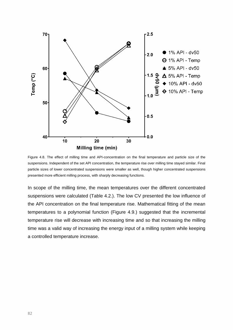
82
Figure 4.8. The effect of milling time and API-concentration on the final temperature and particle size of the
suspensions. Independent of the set API concentration, the temperature rise over milling time stayed similar. Final
particle sizes of lower concentrated suspensions were smaller as well, though higher concentrated suspensions
presented more efficient milling process, with sharply decreasing functions.
In scope of the milling time, the mean temperatures over the different concentrated
suspensions were calculated (Table 4.2.). The low CV presented the low influence of
the API concentration on the final temperature rise. Mathematical fitting of the mean
temperatures to a polynomial function (Figure 4.9.) suggested that the incremental
temperature rise will decrease with increasing time and so that increasing the milling
time was a valid way of increasing the energy input of a milling system while keeping
a controlled temperature increase.

83
Figure 4.9. Fitting the temperature rise as a function of the milling time, using the average temperatures of the
different concentrated formulations on the different time points, as given in Table 4.2.
In this scope, initial steps for method optimisation can be suggested. Similar particle
sizes were found for the set-up with 20 min milling time and an acceleration of 80 g
and the set-up with 30 min and 65 g, but with a lower temperature in the latter case.
Thus, using a longer milling time seems to be advantageous if important to limit
temperature increase while keeping a continuous milling process. These outcomes are
in agreement with the suggested exponential increase in temperature versus
acceleration and the polynomial fit between temperature and milling time.
Further, the optimisation of the bead size can be assumed to be a valid step in the
optimisation of a milling process, but this parameter fell out of the scope of this study.
Thus, temperature increase as well as particle size reduction should be considered
when choosing a suitable nanosizing technology and corresponding process
parameters. Depending on the API and formulation properties, IVM might still be the
method of choice due to its efficient and rapid nanosizing, but this technology should
be avoided for thermolabile compounds if cooling cannot be guaranteed during
processing. On the other hand, the milling process can be modified by choosing

84
process parameters that limit temperature rise while substantiating the nanosizing
potential. Since Newton’s law of cooling describes an exponential relationship, short
pauses during milling can produce a temperature decrease to limit temperature
increase and is the focus of current investigation, albeit these breaks should be
standardised and upscalable. A more complex experimental design could offer the
insight in the complexity of this milling platform for which this study could already offer
a strong methodological basis.

85
Table 4.2. Final PSDs and computed temperatures, when the milling time and API concentration of the suspensions were varied.
Milling time
API conc.
Stabiliser conc. 10 min 20 min 30 min
dv10 (µm)
dv50 (µm)
dv90 (µm)
Temperature (°C)
dv10 (µm)
dv50 (µm)
dv90 (µm)
Temperature (°C)
dv10 (µm)
dv50 (µm)
dv90 (µm)
Temperature (°C)
1%(w/v)
50*CMC 0.126 1.545 4.576 47.5 0.098 0.586 4.091 60.4 0.092 0.379 2.901 67.3
5%(w/v)
250*CMC 0.149 1.423 3.626 46.2 0.12 1.083 3.58 59.5 0.098 0.47 2.451 66.7
10%(w/v)
500*CMC 1.052 2.353 5.279 44.4 0.137 1.137 3.242 59.9 0.111 0.7 2.685 67.3
Average 46.1 60.2 67.1
Standard deviation
1.6 0.3 0.4
CV (%) 3.4 0.6 0.5

86
CONCLUSIONS
Within the IVM, we found that similar formulation and process parameters as in WBM
will influence the particle size reduction, higher bead-suspension ratio, higher
acceleration, lower API concentration and longer milling time leading to a faster
comminution process. Nevertheless, these key formulation and process parameters
significantly impacted the heat generation as well, leading to temperatures of 100 °C
and above. Heat can gravely affect the (physico)chemical properties of the suspension,
hence, its generation should be under control. Due to the counteracting effect of the
different formulation and process parameters on particle size and generated heat, the
IVM seems to be as complex as the WBM process. Nevertheless, some first efforts
were made to optimise a continuous milling process while limiting heat generation.
Thus, to increase the specific energy of an IVM process an increased milling time is
favoured over acceleration. Only a modest temperature increase was found during
these optimisation steps. Furthermore, the production of more concentrated
formulations is favoured. During their production, additional shear by the API particles
boost the efficiency of the milling process but do not affect the generated heat. We
anticipate that this additional advantage of highly concentrated formulations, is
extrapolatable to WBM as well. Further, fixtures used to secure the vials within IVM,
can gravely impact the heat generated as well and should be cooled in-between
experiments. Since controlled heat generation is of utmost importance within the
milling process, these first steps can help in the optimisation of an IVM continuous
milling process and can open further research on its complex interplay with particle
size reduction.

Picking up good vibrations: Exploration of the intensified
vibratory mill via a modern design of experiments
Results in this chapter are based on:
De Cleyn, E., Holm, R., Khamiakova, T. & Van den Mooter, G. Picking up good
vibrations: Exploration of the intensified vibratory mill via a modern Design of
Experiments. Int. J. Pharm. 120367 (2021). doi:10.1016/j.ijpharm.2021.120367
With exception of: Supplementary information regarding the explanation of Kwades
stress model has been removed, as the Introduction (Introduction, §1.5.3.) broadly
describes the subject. The necessary references were provided instead.


89
GRAPHICAL ABSTRACT
ABSTRACT
The aim of this work was to strengthen the understanding of the IVM by unravelling the
milling process in terms of the particle size reduction and heat generation via a modern
DoE approach. Hence, the influence of five process parameters (acceleration, breaks
during milling, bead size, milling time and bead-suspension ratio) was investigated via
an I-optimal design. Particle size was measured via laser diffraction and the
temperature of the sample after milling was computed. To advance our understanding,
a mechanistic model for the set-up of wet-stirred media milling processes was applied
on the observed milling trends. A generic approach for the optimisation of the milling
process was retrieved and included the optimisation of the bead size and intermittent
pausing for effective cooling. To finetune the remaining process parameters, the
present work provides contour plots and strong predictive models. With these models,
the particle size and the temperature after milling of suspensions manufactured with
the IVM could be forecasted for the first time.

90
INTRODUCTION
Micronisation and nanonisation are commonly applied approaches to enable the
bioavailability of poorly water soluble compounds by enhancing their solubility and/or
dissolution rate.46 Formulated as a nano- or microsuspension, these poorly soluble
compounds may be delivered via a variety of administration routes including the oral,
ocular, brain, topical, buccal, nasal and transdermal routes.6 By virtue of their ease of
use, suspensions can be orally administered in wet state or after incorporation into
conventional dosage forms such as tablets or capsules.99 Injectable nano- and
microsuspensions have drawn increasing attention due to their potential use as
LAIs.100 This formulation type can offer great utility for chronic diseases, where lack of
medication compliance may be detrimental for the pharmacological response.35
Overall, advancements in the production and formulation of these suspensions can
solve numerous pharmacokinetic challenges and these topics are therefore still heavily
studied.6
Among all the usable production technologies, WBM is most widely applied with
demonstrated efficiency, viability and cost-effectiveness at production scale.33, 46
Milling media, dispersant, stabiliser, other excipients and the API are charged into the
milling chamber and by the movement of the milling media, shear forces, pressure and
impact are generated, leading to a particle size reduction. Either the milling beads are
accelerated by the movement of the complete container, or by agitators installed in the
chamber.52 Extensive ball milling to the nanorange was patented as the Nanocrystal®
Technology by Elan, in 199030, a technology that led to many (sub)micronised drug
products of poorly soluble APIs on the market.6 Opportunities for milling on bench-level
are numerous, such as the high-throughput platforms, streamlining formulation
screening and optimisation.53 The technologies’ major drawback is the heat generated
by inefficiently dissipated energy wherefore a water jacket is more often installed. Yet,
WBM is considered as the golden standard for nanonisation and micronisation.
However, this enabling platform still encounters some unresolved issues. These
include erosion of the milling media which may contaminate the final formulation46 and
extensive milling times from several hours to days30.
Consequently, new milling technologies such as the IVM in which the RAM platform is
used, are introduced in the field. Originally commercialised as a mixing platform, the
RAM platform has been mostly employed as a dry mixing process, whereas its

91
application in wet milling is less studied.62, 63 As a milling platform, it consists of a
closed vibrating container to which milling media are charged. The vibrating container
could be of various types of vessels, vials or well-plates. In this way, the IVM could
serve as a drug sparing, high-throughput screening method.62 The vibration can be
described as a sinusoidal wave with a frequency of around 60 Hz, as to keep the
system at its optimal and safe conditions, the parametric resonance. The amplitude of
the sinusoidal wave on the other hand differs, based on the milling content and the set
acceleration. Previously, the mixing behaviour was introduced as micro-mixing zones,
but current knowledge seems to present a more complex mixing and milling regime.101
Insights in milling regimes and the motion of grinding bodies in conventional mills have
already been broadly discussed in the literature.102, 103 Concerning later mill types,
Hagedorn and co-workers have discussed how virtually all beads accelerate as ‘one
cloud’ (cloud milling) in the dual centrifuge.98 Since the geometry and the motion of
IVMs milling chamber significantly differ from conventional and later mill types, one can
assume a different bead motion. Consequently, the extent and distribution of milling
forces will differ, leading to a different milling process in terms of particle size reduction
and heat generation.
In this viewpoint, IVM has been marked for its fast particle size reduction which may
overcome the extensive milling times, encountered in classical WBM. Yet
unacceptable high temperatures have been observed.104 First attempts to control this
temperature included the installation of milling breaks in which the containers were
removed from the milling equipment and placed in a refrigerated bath.63 This method
proved to be effective, but difficult to standardise or scale-up. Further, the influence of
this quick cooling step on the aggregation of particles and recrystallisation of dissolved
API was not explored. Consequently, the purpose of this study was to obtain a
comprehensive insight in the process of particle size reduction and heat generation as
it applies to IVM, with the usage of a DoE.
To the best of our knowledge, publications on the usage of DoE methodologies within
pharmaceutical milling are limited to classical designs such as the central composite
or (fractional) factorial designs.56 In order to reach predictive models of similar quality
and precision, modern DoE methodologies allow to simultaneously study many factors
in an irregular experimental domain in an economic fashion.105, 106 Surprisingly, the
application of modern DoE methodologies on pharmaceutical milling is so far

92
unexplored. Moreover, no previous study on the investigation of IVM via a DoE,
classical or modern, has, to the best of our knowledge, been published.
In this work, a novel DoE methodology was applied to generate deep insights in the
heat generation and nanosizing potential of the IVM. The selected I-optimal design and
consecutive statistical analysis ranked the investigated process parameters (bead
size, breaks during milling, acceleration, milling time and bead-suspension ratio),
elucidated interactions between these parameters and provided a predictive model for
important suspension attributes such as the dv50-value, dv90-value, span and
temperature after milling. To gain more mechanistic insight in the milling kinetics, the
stress model54 was applied on the milling trends and questions regarding the impact
of pausing on heat generation and particle size, were addressed.

93
MATERIALS AND METHODS
Materials
Bedaquiline was provided by Janssen Pharmaceutica (Beerse, Belgium). Polysorbate
20 was obtained from Croda (Trappes, France). Deionised water (R≥18.2 mΩ, Mili-Q®
Advantage A10, Merck, Darmstadt, Germany) was used for all the experiments.
Methods
5.4.2.1. Preparation of suspensions
Glass vials were filled with bedaquiline (5%w/v), zirconia beads (Nikkato Corporation,
Sakai, Osaka, Japan) and polysorbate 20 solution (1.85%w/v). The vials were
thoroughly shaken on an in-house manufactured platform within the LabRAM II
(Resodyn Acoustic Mixers, Butte, USA). The investigated process parameters - the
acceleration, the bead size, the bead-suspension ratio, the milling time and the breaks
during milling - were varied as proposed in the DoE (Figure. 5.1.).
Figure 5.1. Experimental space of the custom designed DoE, including the investigated parameters; breaks during
milling (y-axis, left), milling time (y-axis, right), acceleration (x-axis below), bead-suspensions ratio (x-axis above) and
bead size (dot size). Every dot represents an experimental run of the DoE. The experimental design space seemed
widely covered by the installed experimental runs.

94
5.4.2.2. Experimental design
The acceleration, the bead size, the bead-suspension ratio and the milling time were,
as earlier demonstrated104, explorable parameters that could impact the output of the
milling process in terms of the suspension’s final particle size and temperature. In
attempt to control the temperature, an additional parameter, named ‘Breaks during
milling’, was included. This parameter encompassed the duration of the installed break
(0 minutes, 2.5 minutes or 5 minutes), implemented every 7.5 minutes of the milling
process.
Within the Jump software package (JMP® 13.0.0, SAS Institute Inc.), a custom DoE
was built in which the five process parameters were set as quantitative, continuous
parameters with an upper and lower limit based on historical data. To enhance the
predictive power and the robustness of the model, two centre points and four replicates
were included. Blocking was applied and experiments were randomised. Chosen
responses were the median particle size (dv50), the PSD (dv90, span) and the final
temperature of the suspension (Temp.). In order to broadly explore the complexity of
the milling process, 22 model parameters were selected for investigation. These
parameters included the intercept, all main effects, all two-way interactions, all
quadratic effects, and one three-way interaction (acceleration/bead-suspension
ratio/bead size). For a classical DoE with five factors, high-resolution designs would
be required to resolve such three-factor interaction. Nonetheless, the final
experimental design, generated with the JMP® software, was a three level I-optimal
design with 30 experimental runs, which covered the whole experimental domain
(Figure 5.1.).
5.4.2.3. Temperature measurement
After production, the temperature decline of the suspension was tracked with a
temperature gun (VWR® Traceable® Infrared Thermometer, Radnor, PA, US), as
presented previously104. The temperature directly after milling was obtained by
extrapolation of this tracked temperature trend.
5.4.2.4. Laser diffractometry
LD measurements were performed on a Mastersizer™ 2000 (Malvern Instruments,
Worcestershire, UK) with hydro-unit, using miliQ water as the dispersant. Stirring
95
speed of 600 rpm was set, no sonication was applied, and the system was left to
stabilise for five minutes. Finally, the system was aligned, and the background was
evaluated. The general-purpose model for irregularly shaped particles with normal
calculation sensitivity was applied. The set optical parameters were a sample rRI of
1.595, a sample iRI of 0.001 and a dispersant rRI of 1.333. A limited obscuration
titration was performed for each sample to elucidate the optimal set of obsc. and obsc.
blue. Quality of data was given in terms of res. and res weight., as described in chapter
3.95 The final PSD was presented by the dv50-value, the dv90-value and the span
(Equation 5.1.).
𝑆𝑝𝑎𝑛 =𝑑𝑣90 − 𝑑𝑣10
𝑑𝑣50 (Equation 5.1.)

96
RESULTS
Design of experiments computation
To deconvolute the individual effects of, and the interactions between the various
parameters, the raw data (Table 5.1.) were analysed with the JMP® software. The data
were modelled by predictive models with restricted maximum likelihood (REML) to
account for the blocking nature of the experiment. REML with unbounded variance
components was used for the dv50-value, span and temperature after milling. As the
block variance was negligible, REML with bounded variance components was applied
on the dv90-value. To get valid statistical estimates, a Bayesian hierarchical model
was performed to compute the block variance for the dv90-value (Figure 5.2.) and to
test the significance of the different model parameters (Figure 5.3.). The block
variability approached zero and the same model parameters were significant for the
dv90-value, rationalizing the statistical adaptation to bounded variance components.
Predictive models are generally expressed as:
Y = β0 + β1X1 + β2X2 + β3X3 + … + β12X1X2 + β23X2X3 + β13X1X3 + … + β123X1X2X3 +
β11X12 + β22X2
2… + ε (Equation. 5.2.)
where Y is the dependent variable or response such as the temperature after milling;
X1, X2, X3… are the independent variables or factors such as milling time; β0 is the
intercept; β1, β2, β12, β23, β123, … are empirically estimated coefficients, better known
as the model parameters, which relate the main factors (if the parameters subscript is
one digit), interactions (if the parameters subscript is two or more digits) and quadratic
effects (if the parameters subscript is two times the same digit) to the forecasted
response Y; ε is the total error.
During the interpretation of the significance of the model parameters, the power of the
DoE for these model parameters (Table 5.2.) should be taken into consideration. The
power for a certain model parameter is the probability of the DoE to detect its
significance. The DoE was designed to have an optimal power in the evaluation of all
main effects and most two-way interactions. Since the DoE was restricted to 30
experiments, which was still an elaborated number, the power of the five quadratic
effects and of the intercept was rather modest (Table 5.2.). Notwithstanding this
modest power, the corresponding model estimates may still have an important effect
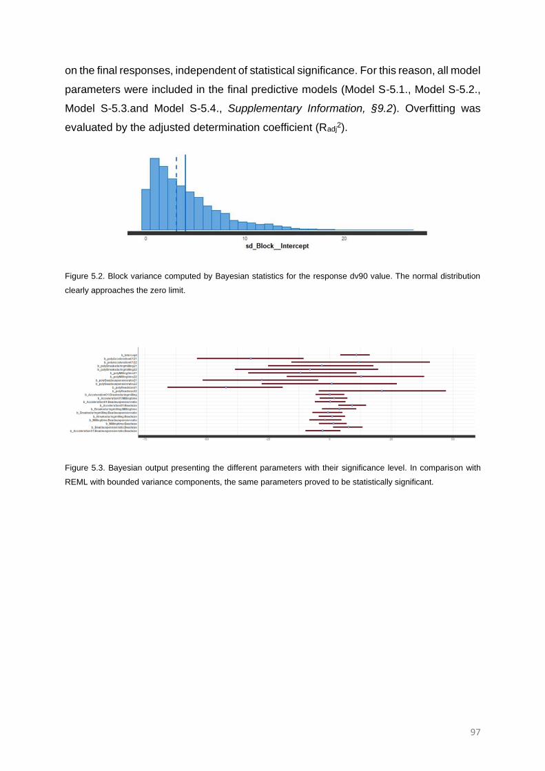
97
on the final responses, independent of statistical significance. For this reason, all model
parameters were included in the final predictive models (Model S-5.1., Model S-5.2.,
Model S-5.3.and Model S-5.4., Supplementary Information, §9.2). Overfitting was
evaluated by the adjusted determination coefficient (Radj2).
Figure 5.2. Block variance computed by Bayesian statistics for the response dv90 value. The normal distribution
clearly approaches the zero limit.
Figure 5.3. Bayesian output presenting the different parameters with their significance level. In comparison with
REML with bounded variance components, the same parameters proved to be statistically significant.

98
Table 5.1. Process parameters and raw data concerning PSD and temperature after milling, as have been input in the JMP® software
Sample Process Parameters
Results PSD
Quality of LD data
Bead size (µm)
Bead-suspension ratio (mL/mL)
Acceleration (g)
Total milling time (min)
Breaks during milling (min)
Temperature (°C)
Dv50 (µm)
Dv90 (µm) Span Obsc
Obsc blue Res.
Res. weight.
Block 1
Sample 1 200 0.375 50 10 2.5 22.5 21.125 64.279 2.879 9.72 7.63 0.366 0.378
Sample 2 200 1.200 50 10 0 29.5 3.97 40.469 10.109 8.22 9.96 0.442 0.527
Sample 3 1000 0.375 65 20 5 40.1 1.657 4.27 2.484 6.45 7.87 0.589 0.355
Sample 4 200 0.375 80 30 5 39.6 0.637 22.695 35.443 5.59 8.63 0.577 0.419
Sample 5 1000 0.774 80 30 2.5 89.6 0.376 1.746 4.388 5.20 8.21 1.878 1.066
Sample 6 1750 0.375 80 20 0 66.2 1.918 4.924 2.490 4.41 5.43 0.483 0.388
Block 2
Sample 1 1000 1.200 50 20 2.5 50.2 0.658 2.65 3.871 5.99 6.9 0.403 0.298
Sample 2 1750 0.774 65 10 2.5 50.1 2.046 4.929 2.330 4.64 6.17 0.499 0.386
Sample 3 1750 1.200 80 10 5 78.6 1.34 4.025 2.910 4.89 6.49 0.534 0.349
Sample 4 1750 1.200 80 10 5 78.8 1.283 3.807 2.866 4.64 5.56 0.516 0.485
Sample 5 1750 0.774 65 10 2.5 52.1 1.768 4.152 2.262 4.23 5.9 0.754 0.393
Sample 6 1000 1.200 50 20 2.5 51.9 0.855 2.885 3.240 6.09 8.84 0.703 0.573
Block 3
Sample 1 200 1.200 80 30 2.5 77.6 0.158 0.433 2.291 2.89 6.79 1.312 1.418
Sample 2 1000 1.200 80 10 0 85.0 0.897 3.088 3.315 4.02 5.66 0.543 0.372
Sample 3 1750 0.774 50 10 5 39.3 1.946 4.509 2.231 4.13 4.91 0.612 0.536
Sample 4 1750 0.375 50 30 2.5 43.8 1.736 4.13 2.300 3.45 4.21 0.69 0.438
Sample 5 1000 0.774 65 20 2.5 60.9 0.682 2.585 3.632 3.13 4.48 0.625 0.74

99
Sample 6 1750 0.375 50 10 0 32.9 2.077 4.378 1.699 5.41 6.15 0.491 0.342
Block 4
Sample 1 1750 1.200 80 30 0 134.7 1.241 2.881 2.227 5.87 7.56 0.635 0.526
Sample 2 1000 0.774 65 20 2.5 58.5 0.568 2.271 3.819 4.97 7.09 0.567 1.032
Sample 3 1750 1.200 50 30 0 71.0 0.516 2.287 4.229 2.33 3.54 0.768 0.87
Sample 4 1750 0.375 80 10 5 47.9 1.958 4.437 2.187 5.22 6.04 0.526 0.41
Sample 5 200 1.200 65 20 0 52.0 0.213 0.898 3.836 5.98 11.58 2.486 1.93
Sample 6 1000 0.375 65 30 0 55.0 1.184 3.286 2.662 4.00 5.42 0.849 0.943
Block 5
Sample 1 200 0.774 50 30 0 28.1 4.855 48.012 9.751 4.60 5.62 0.455 0.536
Sample 2 1750 0.774 65 30 5 72.7 0.908 3.225 3.426 4.00 5.68 0.487 0.402
Sample 3 200 0.774 50 30 0 31.2 2.651 18.444 6.781 3.08 3.79 0.439 0.455
Sample 4 200 0.774 80 10 5 41.6 0.414 4.081 9.614 4.87 7.85 0.565 0.645
Sample 5 200 1.200 50 30 5 31.4 1.777 18.073 10.075 6.17 8.12 0.601 0.622
Sample 6 200 0.375 80 10 0 33.2 3.099 25.094 7.781. 3.20 3.71 0.661 0.548

100
Table 5.2.: Power analysis of the investigated model parameters.
Parameter Power
Intercept 0.193
Acceleration (g) 0.932
Breaks during milling (min) 0.897
Milling time (min) 0.869
Bead-suspension ratio 0.776
Bead size (µm) 0.751
Acceleration (g)*Breaks during milling (min) 0.773
Acceleration (g)*Milling time (min) 0.692
Acceleration (g)*Bead-suspension ratio 0.639
Acceleration (g)*Bead size (µm) 0.721
Breaks during milling (min)*Milling time (min) 0.528
Breaks during milling (min)*Bead-suspension ratio 0.721
Breaks during milling (min)*Bead size (µm) 0.818
Milling time (min)*Bead-suspension ratio 0.567
Milling time (min)*Bead size (µm) 0.752
Bead-suspension ratio*Bead size (µm) 0.711
Acceleration (g)*Acceleration (g) 0.247
Breaks during milling (min)*Breaks during milling (min) 0.23
Milling time (min)*Milling time (min) 0.272
Bead-suspension ratio*Bead-suspension ratio 0.24
Bead size (µm)*Bead size (µm) 0.312
Acceleration (g)*Bead-suspension ratio*Bead size (µm) 0.601
A high power was installed for all main effects and for most two-way
interactions. The power to identify the significance of most quadratic effects
and of the intercept, was rather modest.

101
Statistical analysis of the dv50
Table 5.3. Investigated model parameters with their estimated parameter effects, their corresponding standard error
and borders of the 95%-confidence interval and computed p-values for the response dv50-value.
Term Estimate Std Error
Lower 95%
Upper 95% Prob>|t|
Intercept 0.41 0.49 -0.74 1.55 0.4349
Acceleration (g) (50,80) -1.97 0.24 -2.54 -1.40 <.0001
Breaks during milling (min) (0,5) 0.46 0.28 -0.18 1.11 0.1357
Milling time (min) (10,30) -1.16 0.23 -1.69 -0.64 0.0009
Bead-suspension ratio (0.375,1.2) -1.77 0.28 -2.50 -1.04 0.0014
Bead size (µm) (200,1750) -1.51 0.23 -2.05 -0.97 0.0003
Acceleration (g)*Breaks during milling (min) -0.48 0.31 -1.21 0.25 0.1622
Acceleration (g)*Milling time (min) 0.64 0.33 -0.43 1.70 0.1512
Acceleration (g)*Bead-suspension ratio 1.44 0.40 -0.09 2.98 0.0566
Acceleration (g)*Bead size (µm) 2.23 0.37 0.55 3.91 0.0301
Breaks during milling (min)*Milling time (min) 0.59 0.48 -0.78 1.96 0.2918
Breaks during milling (min)*Bead-suspension ratio 0.11 0.37 -0.75 0.97 0.7783
Breaks during milling (min)*Bead size (µm) -0.11 0.29 -0.80 0.57 0.7034
Milling time (min)*Bead-suspension ratio -0.02 0.42 -1.13 1.09 0.9566
Milling time (min)*Bead size (µm) 0.86 0.26 0.27 1.46 0.0102
Bead-suspension ratio*Bead size (µm) 1.92 0.39 0.98 2.85 0.0021
Acceleration (g)*Acceleration (g) 0.37 0.74 -2.21 2.96 0.6548
Breaks during milling (min)*Breaks during milling (min) -1.35 0.51 -2.66 -0.04 0.0455
Milling time (min)*Milling time (min) 1.21 0.63 -0.29 2.72 0.0978
Bead-suspension ratio*Bead-suspension ratio 1.45 0.53 -0.17 3.06 0.0660
Bead size (µm)*Bead size (µm) 1.69 0.61 0.24 3.13 0.0278
Acceleration (g)*Bead-suspension ratio*Bead size (µm) -2.11 0.38 -3.00 -1.21 0.0007
Statistically significant output is coloured in orange (|t| < 0.05) and red (|t| < 0.01).
In short, a broad set of parameters was statistically significant for the final median
particle size, the dv50-value (p-value < 0.05) (Table 5.3.). Milling time, acceleration,
bead-suspension ratio and bead size were critical factors, both as main factor as in
most of their two-way interactions (acceleration/bead size, milling time/bead size and
bead-suspension ratio/bead size), as illustrated in the broad set of crossing functions
in the interaction profiler (Figure 5.4.). Even with their modest power, some quadratic
interactions (breaks during milling and bead size) had a statistically significant
outcome. Also, the three-way interaction (acceleration/bead-suspension ratio/bead
size) had a statistically significant effect on the final dv50-value.

102
Acceleration was the most important factor governing the milling process, with a
statistically significant parameter estimate of -1.97 (± 0.24). Milling time showed a
statistically significant inverse dependence on the dv50-value with a parameter
estimate of -1.16 (± 0.23). Bead-suspension ratio and the bead size were other key
variables in the milling process with parameter estimates of -1.77 (± 0.28) and -1.51 (±
0.23), respectively. Surprisingly, the breaks during milling did not have in the provided
dataset a statistically significant effect on the final dv50-value.
Even with a modest power of 0.321 and 0.23, the quadratic effects of bead size and
breaks during milling were statistically significant with parameter estimates of 1.69 (±
0.61) and -1.35 (± 0.53), respectively. The quadratic term of milling time on the other
hand, did not show a statistically significant outcome. Albeit some factors were not
considered to be statistically significant, all model terms were included in the predictive
model (Model S-5.1., Supplementary Information, §9.2), as alluded to above. The
accuracy of the generated prediction model was described by the determination
coefficient (R2) and Radj2. As the final R2of 0.982 only decreased to a Radj
2 of 0.934, the
inclusion of all parameters was well-founded.
Figure 5.4. Interaction profiler depicting two-way interactions for dv50-value

103
Statistical analysis of the temperature after milling
Table 5.4. Investigated model parameters with their estimated parameter effects, their standard errors, the limits of
their 95%-confidence interval and computed p-values for the response temperature after milling.
Term Estimate Std Error
Lower 95%
Upper 95% Prob>|t|
Intercept 58.71 1.14 55.89 61.53 <.0001
Acceleration (g) (50,80) 16.06 0.45 14.96 17.16 <.0001
Breaks during milling (min) (0,5) -3.33 0.48 -4.48 -2.18 0.0003
Milling time (min) (10,30) 8.56 0.46 7.48 9.64 <.0001
Bead-suspension ratio (0.375,1.2) 12.29 0.61 10.87 13.71 <.0001
Bead size (µm)(200,1750) 13.15 0.53 11.82 14.49 <.0001
Acceleration (g)*Breaks during milling (min) -1.68 0.57 -3.09 -0.28 0.0263
Acceleration (g)*Milling time (min) 4.55 0.72 2.87 6.22 0.0003
Acceleration (g)*Bead-suspension ratio 5.04 0.79 3.22 6.86 0.0002
Acceleration (g)*Bead size (µm) 3.34 0.72 1.69 4.99 0.0016
Breaks during milling (min)*Milling time (min) -0.89 0.84 -2.82 1.05 0.3214
Breaks during milling (min)*Bead-suspension ratio -1.66 0.64 -3.18 -0.13 0.0372
Breaks during milling (min)*Bead size (µm) -0.70 0.53 -2.01 0.61 0.2338
Milling time (min)*Bead-suspension ratio 2.70 0.77 0.91 4.49 0.0083
Milling time (min)*Bead size (µm) 4.26 0.56 2.95 5.57 <.0001
Bead-suspension ratio*Bead size (µm) 2.33 0.66 0.78 3.88 0.0092
Acceleration (g)*Acceleration (g) 2.72 1.41 -0.52 5.97 0.0889
Breaks during milling (min)*Breaks during milling (min) 0.14 1.18 -2.98 3.25 0.9139
Milling time (min)*Milling time (min) 0.46 1.12 -2.35 3.27 0.6954
Bead-suspension ratio*Bead-suspension ratio -2.07 1.22 -5.25 1.11 0.1522
Bead size (µm)*Bead size (µm) -7.56 1.05 -10.17 -4.95 0.0005
Acceleration (g)*Bead-suspension ratio*Bead size (µm) 0.93 0.71 -0.80 2.67 0.2357
Statistically significant output is coloured in orange (|t| < 0.05) and red (|t| < 0.01).
Nearly all parameters demonstrated a significant effect on the temperature after milling
and thus on the heat generation during IVM (Table 5.4.). This high level of significance
is substantiated by the broad operational ranges and the high precision of the
temperature measurements. Albeit, it may also indicate the high complexity of the IVM
process.
Acceleration was a key contributor to the heat generation with a remarkable parameter
estimate of 16.06 (± 0.45). The milling time on the other hand only encompassed a
parameter estimate of 8.56 (± 0.46). Other significant key variables were bead size

104
and bead-suspension ratio, with parameter estimates of 13.15 (± 0.53) and 12.29 (±
0.61), respectively. Even in this case, bead size’ quadratic effect of -7.56 (± 1.05) was
statistically significant. As presumed, breaks during milling had a statistically significant
effect on the suspension’s final temperature. Albeit, the parameter estimate was only
-3.33 (± 0.48) implying that despite its significance, the model estimate on itself was
rather modest as compared to the model estimates of the remaining process
parameters. Thus, a temperature rise stayed, even with the inclusion of a periodical
five-minute break during milling, inevitable. Hence finetuning of all process parameters
remained important.
Almost all two-way interactions had a statistically significant outcome with parameter
estimates ranging from circa |2| to |5|. All parameters were included in the predictive
model (Model S-5.2., Supplementary Information, §9.2). With a R2 of 0.999 and a Radj2
of 0.996 (Figure 5.5.), temperature may be accurately forecasted.
Figure 5.5. Strong linear relationship (R2 of 0.999 and Radj2 of 0.996) between the predicted temperatures and the
actual temperatures of the suspensions after production.

105
Statistical analysis of the particle size distribution (dv90, span)
Table 5.5. Investigated model parameters with their estimated parameter effects, their corresponding standard error
and borders of their 95%-confidence intervals including the computed p-value for the response dv90-value.
Term Estimate Std Error
Lower 95%
Upper 95% Prob>|t|
Intercept -0.24 4.20 -9.93 9.44 0.9554
Acceleration (g) (50,80) -6.88 1.91 -11.28 -2.48 0.0069
Breaks during milling (min) (0,5) -0.85 1.98 -5.41 3.72 0.6804
Milling time (min) (10,30) -2.32 1.84 -6.58 1.93 0.2427
Bead-suspension ratio (0.375,1.2) -6.43 1.99 -11.01 -1.85 0.0120
Bead size (µm) (200,1750) -9.13 1.94 -13.60 -4.66 0.0015
Acceleration (g)*Breaks during milling (min) -0.10 2.44 -5.72 5.53 0.9697
Acceleration (g)*Milling time (min) 1.84 2.11 -3.03 6.71 0.4095
Acceleration (g)*Bead-suspension ratio 0.54 2.33 -4.83 5.91 0.8231
Acceleration (g)*Bead size (µm) 8.86 2.08 4.06 13.66 0.0028
Breaks during milling (min)*Milling time (min) 4.03 2.77 -2.36 10.42 0.1839
Breaks during milling (min)*Bead-suspension ratio -0.99 2.44 -6.62 4.63 0.6948
Breaks during milling (min)*Bead size (µm) 0.93 2.34 -4.46 6.33 0.7001
Milling time (min)*Bead-suspension ratio -1.98 2.62 -8.01 4.06 0.4717
Milling time (min)*Bead size (µm) 1.40 2.10 -3.45 6.25 0.5242
Bead-suspension ratio*Bead size (µm) 7.32 2.41 1.75 12.88 0.0163
Acceleration (g)*Acceleration (g) 5.20 4.30 -4.72 15.11 0.2612
Breaks during milling (min)*Breaks during milling (min) -2.91 4.00 -12.13 6.30 0.4866
Milling time (min)*Milling time (min) 5.33 5.02 -6.26 16.91 0.3199
Bead-suspension ratio*Bead-suspension ratio 0.28 3.80 -8.47 9.03 0.9435
Bead size (µm)*Bead size (µm) 8.52 4.58 -2.05 19.08 0.1001
Acceleration (g)*Bead-suspension ratio*Bead size (µm) -3.05 2.95 -9.86 3.76 0.3323
Statistically significant output is coloured in orange (|t| < 0.05) and red (|t| < 0.01).
In the analysis of the dv90-value, relatively high standard errors were observed and
only a handful of factors were statistically significant (Table 5.5). Due to this high
variation unaccounted by the model terms, the dv90 was only shortly described, though
the final predictive model (Model S-5.3., Supplementary Information, §9.2) was still
computed. As expected, the resulting R2 and Radj2 were the lowest so far with final
values of 0.928 and 0.739, respectively.
Acceleration had, as in the case of dv50, an important impact on the dv90, with a
parameter estimate of -6.88 (± 1.91). Other main effects such as bead-suspension ratio

106
and bead size and the two-way interactions acceleration/bead size and bead-
suspension ratio/bead size were also statistically significant. The effect of breaks
during milling on the other hand was limited.
Table 5.6. Investigated model parameters with their estimated parameter effects, their corresponding standard error
and the borders of their 95%-confidence interval including the computed p-value for the response span.
Term Estimate Std Error
Lower 95%
Upper 95% Prob>|t|
Intercept 2.10 1.11 -0.95 5.15 0.1291
Acceleration (g) (50,80) 0.65 0.26 -0.02 1.32 0.0541
Breaks during milling (min) (0,5) 1.16 0.30 0.44 1.88 0.0063
Milling time (min) (10,30) 1.26 0.41 0.24 2.28 0.0233
Bead-suspension ratio (0.375,1.2) -1.87 0.44 -2.88 -0.85 0.0030
Bead size (µm) (200,1750) -3.15 0.54 -4.59 -1.72 0.0030
Acceleration (g)*Breaks during milling (min) 1.14 0.34 0.29 1.99 0.0175
Acceleration (g)*Milling time (min) 1.13 0.47 0.05 2.22 0.0423
Acceleration (g)*Bead-suspension ratio -3.12 0.45 -4.21 -2.03 0.0003
Acceleration (g)*Bead size (µm) 0.39 0.42 -0.61 1.39 0.3885
Breaks during milling (min)*Milling time (min) 2.74 0.54 1.49 3.99 0.0010
Breaks during milling (min)*Bead-suspension ratio -1.82 0.38 -2.75 -0.89 0.0027
Breaks during milling (min)*Bead size (µm) -2.38 0.32 -3.18 -1.59 0.0004
Milling time (min)*Bead-suspension ratio -3.91 0.54 -5.17 -2.66 0.0001
Milling time (min)*Bead size (µm) -1.98 0.48 -3.17 -0.79 0.0068
Bead-suspension ratio*Bead size (µm) 3.57 0.40 2.63 4.51 <.0001
Acceleration (g)*Acceleration (g) 2.82 0.85 0.83 4.81 0.0118
Breaks during milling (min)*Breaks during milling (min) 0.16 1.20 -3.12 3.44 0.8996
Milling time (min)*Milling time (min) -1.32 0.67 -3.01 0.37 0.1032
Bead-suspension ratio*Bead-suspension ratio -1.44 1.15 -4.50 1.62 0.2726
Bead size (µm)*Bead size (µm) 4.81 0.61 3.24 6.37 0.0005
Acceleration (g)*Bead-suspension ratio*Bead size (µm) 1.03 0.42 -0.02 2.08 0.0533
Statistically significant output is coloured in orange (|t| < 0.05) and red (|t| < 0.01).
In contrast to dv90s limited set of statistically significant parameters, span produced
an extensive list of variables approaching and surpassing the statistical significance of
0.05 (Table 5.6.). Bead size critically impacted the span, indicated by the statistically
significant main effect, quadratic effect and two-way interaction with bead-suspension
ratio. For a limited set of model parameters, statistical significance could not be proven.

107
The resultant predictive model (Model S-5.4., Supplementary Information, §9.2.) had
a high R2 and Radj2 of 0.995 and 0.983, respectively.
108
DISCUSSION
Application of the stress model
Researchers attempt to predict WBM kinetics and WBM outcomes by process
modelling where the stress model suggested by Kwade54 and the microhydrodynamic
model proposed by Afolabi and co-workers55 are the most widely known. A brief
recapitulation of the stress model is provided below. A more detailed elaboration on
Kwades stress model, has been provided in the Introduction (Introduction, §1.5.3.)
Nonetheless, interested readers are referred to the original articles presenting these
pioneering mechanistic models54, 55.
In the stress model54 the process parameters of a stirred media mill are directly linked
to the stress applied on the suspension’s particles via two central parameters, SN
(Equation 1.7.) and SIGM (Equation 1.6.). The SN is a measure for the number of stress
events, and SIGM is the specific energy consumed by a single stress event. This
simplification resulted in important caveats. However, it made the model easy to apply
and offered easy to understand insights in the milling process.61 Accordingly, the
question rises if these principles, build upon a stirred media mill, are applicable on the
trends observed in the IVM.
Regarding the DoE, acceleration was the most important factor impacting the particle
size reduction in the IVM. As explained by the stress model (Introduction, §1.5.3), the
increased acceleration will lead to both an increased intensity of the stress during a
milling moment - an increased SI - and an increased number of stress moments overall
- an increased SN. Bead-suspension ratio was another key operation parameter.
Increasing the bead-suspension ratio, led to a higher NGM and thus a higher SN. This
increased number of collisions will naturally lead to a more intense particle size
reduction. In a similar manner, the milling time (t) led, via an increased NC, to an
increased SN. Thus, smaller particles were retrieved, when milling for a longer time.
To be more accurate, milling curves are within the literature described by a fast non-
linear decrease which eventually stabilise towards the (apparent) grinding limit where
the particle size will fluctuate based on the balancing phenomena of grinding,
aggregation and crystal growth.50, 94 In this study, the quadratic term of milling time,
which would indicate non-linearity, did not show a statistically significant outcome.
Nonetheless, the power of the quadratic term was low and may indicate that in the

109
case of a larger sample size, statistical significance would be evoked. This example
explains why power analysis is an important element to consider during DoE analysis.
Aside of its effect on the final particle size, milling time importantly impacted the span.
During the milling process the PSD evolves from a multimodal to a monomodal
distribution based on the interplay between particle size reduction, (re)aggregation and
recrystallisation94 and as a result, the span will differ in function of the grinding time.
The optimal bead size
The common rule, “the smaller the bead size, the smaller the final particle size”, has
already been variously challenged in the field of WBM.57, 56, 107 Depending on the
process parameters and the suspension properties, the impact of the bead size will
differ.56 The literature suggests that an optimal bead size exists within the IVM. This
bead size is dependent on the power density and hence dependent on the installed
acceleration and bead-suspension ratio.63 Nonetheless, this conclusion was based on
an OVAT approach which cannot capture interaction effects and hence present
conclusive results.
Within this DoE however the existence of the optimal bead size was confirmed. Aside
of the main effect, a wide array of two-way interactions proved to be statistically
significant. Furthermore, the quadratic effect was, even with a modest power of 0.312,
statistically significant indicating the non-linear impact of this process parameter on the
final dv50-value.
These previously mentioned two-way interactions could be mechanistically explained.
The statistically significant two-way interaction acceleration/bead size could be
rationalised by its similar effect on the kinetic energy (Ekin) (Equation 5.3.) of the
grinding media:
𝐸𝑘𝑖𝑛 = 𝑚 𝑣2
2 (Equation 5.3.)
where Ekin (J) is kinetic energy, m (kg) is the mass of the moving bead and v (m/s) is
the speed of the moving bead. If the acceleration increased, the velocity of the beads
rose, and more kinetic energy was created (Equation 5.3.). Since the velocity of the
beads is squared in Ekin’s equation as opposed to the mass, the acceleration could be
increased to such extent that the added value of the mass of the grinding media - and
so the bead size - to the final Ekin becomes negligible.

110
The statistically significant interaction bead-suspension ratio/bead size can be
depicted in the crossing functions in the interaction profiler (Figure 5.4.). The bead size
will influence the number of beads present in a fixed bead-suspension ratio. As the
bead size decreases, a higher number of beads may be present in the same bead-
suspension ratio but the generated kinetic energy per bead may be lower. This will
directly impact the NGM, SN and SI. As follows, the NGM and SN will increase whereas
the SI will most probably decrease (Introduction, §1.5.3). At a low bead-suspension
ratio and thus, low input energy, the bigger beads yielded the smallest particles, whilst
at a higher bead-suspension ratio, the smallest beads were more favourable (Figure
5.6.).The reason for this counteracting effect may be recognised in the voids in-
between the beads. At a larger bead size, the voids in-between the beads tend to be
larger. By settling herein, bigger API particles could avoid the milling process, leading
to an overall larger median particle size.
Figure 5.6. dv50-values (y-axis) in function of the bead size (x-axis) for an acceleration of 50 g (left) and 80 g (right)
at a bead-suspension ratio of 1.2.
Lastly, the optimal bead size was substantiated by the statistically significant effect of
the three-way interaction (bead-suspension ratio/acceleration/bead size). Normally
these more complex multiple-way-interactions are, based on the hierarchy-principle
and the sparsity-of-effects-principle omitted out of a DoE. Nonetheless, the
significance of this three-way interaction profoundly substantiated the literature
suggesting that the optimal bead size was highly correlated to the installed acceleration
and bead-suspension ratio.63 As visualised in Figure 5.6., at high specific energies
such as the acceleration of 80 g, smaller beads yielded smaller API particles. The fitting
111
of the function describing the impact of the bead size at low acceleration was
suboptimal. Nonetheless, it cannot be mistaken that at this lower specific energy, larger
beads were more advantageous.
Similarly, the dv90 was remarkably influenced by the acceleration as main effect and
the two-way interactions acceleration/bead size and bead-suspension ratio/bead size.
This could be explained by the interplay between the kinetic energy of the beads, the
number of beads and the size of the voids in-between the beads and their dependence
on the bead size.
These voids did not only impact the dv50 and dv90 but had an important influence on
the span as well. Within these voids, a fairly monodisperse PSD could evade further
milling. Consequently, the bead size as both main factor and quadratic effect produced
statistically significant parameter estimates of -3.15 (± 0.54) and 4.81 (± 0.61),
respectively.
Aside of its effect on the particle size reduction, the bead size critically determined the
heat generation in the IVM. Aside of the statistically significant main effect, the
statistically significant quadratic effect had a strong presence in the predictive model,
with a parameter estimate of -7.56 (± 1.05). Considering its important effect on both
particle size and generated heat, the optimisation of the bead size should be a standard
step during IVMs process optimisation.
Cooling the system
The breaks during milling had an important effect on the final temperature of the
suspension. Surprisingly, this main effect did not have in the provided dataset a
statistically significant effect on the final dv50 and dv90. Hence, every 7.5 minutes, a
break of five minutes may be included without constraining the milling process.
Intermittent pausing to cool the system was therefore an attractive option to control the
temperature during IVM, which would be easy to standardise and scale-up.
Nonetheless the model estimate of -3.33 (± 0.48) was quite modest as compared to
the model estimate of the other process parameters. Elevated temperatures may have
deteriorating effects on the (physico)chemical properties of the compound, the
stabiliser and other excipients. Besides, an increased temperature indicate that energy
was lost and thus indicate a suboptimal power consumption. To further limit the
generated heat, expected temperature may be computed, based on the set process

112
parameters, via the predictive model (Model S-5.2., Supplementary Information, §9.2).
Optimisation of the process parameters to limit this heat generation afterwards is
feasible and highly recommended. Another possibility is to lengthen the break.
However, this fell beyond the operational ranges studied in this DoE.
Method optimisation
Table 5.7. Parameter estimates of all main effects on the different process parameters and calculation of the ratio
of the estimated parameter effect on the temperature versus the estimated parameter effect on the dv50-value.
Model estimates
Acceleration (g) (50,80)
Breaks during milling (min) (0,5)
Milling time (min) (10,30)
Bead-suspension ratio (mL/mL) (0.375,1.2)
Bead size (µm) (200,1750)
dv50 -1.97 (± 0.24) 0.46 (± 0.28) -1.16 (± 0.23) -1.77 (± 0.28) -1.51 (± 0.23)
dv90 -6.88 (± 1.91) -0.85 (± 1.98) -2.32 (± 1.84) -6.43 (± 1.99) -9.13 (± 1.94)
Temp 16.06 (± 0.45) -3.33 (± 0.48) 8.56 (± 0.46) 12.29 (± 0.61) 13.15 (± 0.53)
Span 0.65 (± 0.26) 1.16 (± 0.30) 1.26 (± 0.41) -1.87 (± 0.44) -3.15 (± 0.54)
Temp / dv50 -8.15 -7.24 -7.38 -6.94 -8.71
In the present study, an imposing array of 22 model parameters and four responses
was extensively investigated. In general, all 22 investigated model parameters showed
a statistically significant effect on at least one of the four responses, with an exception
of the quadratic effects for milling time and bead-suspension ratio. Albeit, the power of
these factors was rather modest. Accordingly, they may still play a fair part in one of
the responses. All these statistically significant main effects, two-way interactions,
quadratic interactions and even three-way interaction marked the complexity of the
IVM process.
Nonetheless, the valuable and fast nanosizing potential of IVM and its potential high-
throughput screening was illustrated. After ten minutes of grinding, final dv50-values
in the lower micron range (Sample 4, block 2, Table 5.1.) and even submicron range
(Sample 2, block 3 and sample 4, block 5, Table 5.1.) could be detected. This particle
size reduction as presented by a decrease in dv50, dv90 and span, was strongly
associated with a temperature increase (Figure 5.7.). The large variability depicted at
the lowest dv50, dv90 and span, however, indicated that particle size reduction with a
controlled heat generation might be attainable.

113
In the provided datasets, nanonisation seemed to be the most attainable at the highest
acceleration, highest bead-suspension ratio and lowest bead size, which is
comprehendible as the high acceleration and bead-suspension ratio would install high
energy milling for which a smaller bead size is optimal. Even though these settings
would maximise the particle size reduction, they would enhance the heat generation
as well. In these cases, it might be advantageous to mill for a longer time than to
increase the acceleration. Even though they both lead to a temperature increase, their
trend towards this heat generation was different (Figure 5.8.). As suggested in chapter
4104, the temperature increase in function of acceleration seemed to be more
pronounced than the increase in function of milling time. The ratios of the parameter
estimate of temperature on dv50-value were calculated and seem to portray a similar
picture (Table 5.7.). While the ratio for acceleration presented a value of -8.15, this
change would only be limited to -7.38 in case of the milling time. In a similar manner,
an increase in bead-suspension ratio seemed to be a gentler approach for process
intensification than acceleration. At high bead-suspension ratios, even mild
acceleration led to appropriate particle size reduction, where dv50-values might reach
nanolevels and dv90-value lower microlevels (Sample 1 and 6, block 2, Table 5.1. and
sample 3, block 4, Table 5.1.). A further increase in grinding time would be interesting
to explore, but more experimentation is therefore required. Finally, an optimal bead
size may be chosen based on the installed acceleration and bead-suspension ratio.
In this regard, method optimisation may be supported by the determination of the
designs sweet spot via contour plots. The contour plot of the smaller bead size
displayed extreme values. At low acceleration and low bead-suspension ratio, the
small beads did not have the capability to compensate for the low kinetic energy and
a limited particle size reduction occurred. Whilst, at high accelerations and bead-
suspension ratios, the high number of small beads and the smaller voids in-between
the beads will enhance the particle size reduction (Figure 5.9., left). Independent of the
set bead size, the temperature showed the same trend. As the acceleration or bead-
suspension ratio rose, a higher temperature was attained. (Figure 5.9., right). In finding
a sweet spot, the two figures may be overlaid. Thus, to attain an extreme particle size
reduction with an acceptable temperature increase, a combination of for example a
relatively high bead-suspension-ratio, a relatively high acceleration and a relatively
small bead size would be advised.

114
Finally, for a more adequate optimisation, the herein described strong predictive
models may be utilised. With these models, JMP® may directly simulate data over the
full experimental domain. With flexible desirability functions, best possible conditions
may be obtained. Nonetheless, the model is currently further explored and validated
for other APIs and process parameters.
Figure 5.7. Measured temperatures in function of the dv90 (left), dv50 (middle) and span (right). Similar trends could
be noted where a decrease in particle size or PSD was importantly related to an increase in temperature. Nonetheless,
an important variability on the temperature could be detected by the bootstrap confidentiality intervals (coloured zone).

115
Figure 5.8. The temperature trend during continuous milling (breaks during milling = 0 min) when the milling time (left)
or the acceleration (right) were investigated. Even though the bootstrap confidence intervals (coloured zone) presented
a certain level of variability, the curve fitting acceleration seemed to be steeper than the curve fitting bead-suspension
ratio
Figure 5.9. Contour plots for the dv50 (left) and temperature after milling (right) with as independent variables: bead-
suspension ratio (x-axis, below), acceleration (y-axis, left) and bead size (x-axis, above). The settings of the other
parameters were variable. The response, dv50 and temperature after milling, was log-transformed and depicted by
colour. High values were coloured in red, whereas low values were coloured in blue. Generally, opposite trends were
observed.
116
CONCLUSIONS
In this work, an I-optimal design was applied to investigate how five critical process
parameters, namely bead size, bead-suspension ratio, milling time, breaks during
milling and acceleration, govern IVM in terms of heat generation and particle size
reduction. As a result, our understanding of the IVM was improved, which was further
strengthened by the application of Kwades stress model54. The complexity of the IVM
was demonstrated in the wide extent of statistically significant main effects, two-way
interactions, quadratic effects and even three-way interaction. The DoE confirmed the
existence of an optimal bead size. Intermitting pausing of 7.5 minutes proved to cool
down the system without constraining the particle size reduction. However, to keep
temperature under control, the remaining process parameters should be optimised as
well. In this regard, contour plots and accurate predictive models might be of value,
which were generated for the investigated API and process parameter ranges. With
these, both particle size and temperature may be for the first time accurately
forecasted. For other APIs and process parameters, the model may currently serve as
a rule of thumb. Further research is nonetheless required to substantiate these
extrapolations.
SUPPLEMENTARY INFORMATION
All supplementary material as denoted in the manuscript is provided in Chapter 9:
Supplementary Information, §9.2.

Stability trends of micron and submicron suspensions
manufactured by the intensified vibratory mill


119
GRAPHICAL ABSTRACT
ABSTRACT
IVM is a nanonisation and micronisation technology which can be used to enable the
oral bioavailability of poorly soluble compounds. The generated nano- and
microsuspensions entail a large surface area which enhances the compounds
solubility and dissolution rate, yet it may cause unfavourable effects and hence
spontaneous destabilisation as well. Stability studies on suspensions manufactured via
IVM have, to the best of our knowledge, not been reported in the literature before. An
extended stability study was, therefore, executed with 30 bedaquiline suspensions
milled with the intensified vibratory mill under various process settings. The PSD was
measured after production, after four weeks of storage at 5 °C and after eleven weeks
of storage at 5 °C with LD and SEM. In addition, a caking test was applied to scrutinise
the redispersibility of the prevailing sediments. One sample whose sediment proved to
be redisperible, demonstrated a peculiar trend during storage where a narrowing of the
PSD and a general particle size reduction was detected, which opposed the
conventional stability tendencies such as Ostwald ripening. This enigmatic trend was
further explored via a repetitive analysis with LD and in a further phase, with an
orthogonal particle sizing technique. Still, no matter the frequency nor technique, a
narrowing PSD was observed. To the best of our knowledge, this article reports for the
first time in the pharmaceutical literature on a narrowing PSD of a micronised
suspension. Inevitably, this trend might shed a fundamental new light on the stability
trends, exposed by suspensions post-micronisation.

120
INTRODUCTION
During the technological and scientific advances of the 1980s, two discovery platforms,
were generated that led to a wide range of potential drug leads: combinatorial
chemistry and high-throughput screening. Despite their high potential, most of these
potential drug leads exhibited a poor aqueous solubility and as a consequence, a poor
oral bioavailability.14 Nano- and microsuspensions have presented a strong
marketable value in the formulation of these poorly soluble compounds, as their
entailed large surface area enhances the compounds solubility and dissolution rate.
Nevertheless, these systems are, de facto, thermodynamically unfavourable.42, 44 The
stability of nano- and microsuspensions is therefore continuously challenged by a
multitude of destabilising phenomena, comprising sedimentation, Ostwald ripening,
secondary nucleation and aggregation.44 Sedimentation is the most abundant among
particles larger than 5 µm. Provided that the sediment can be homogeneously
redispersed, the settling process is not necessarily detrimental for the suspension’s
storage life. In this light, suspensions are often categorised in flocculated and
deflocculated systems, where flocculated systems contain loose aggregates.7 Their
sediment is easy to redisperse, but settles fast which restrains the time-window for
accurate sampling or accurate patient-dosing. Deflocculated systems gradually settle
but their particles create a sturdy, non-dispersible, solid cake. Formulation scientists
consequently aim for the midpoint of these two extremes, the partial or controlled
flocculation, where the loose aggregates are still resuspendable and settle at an
acceptable rate.108
By virtue of Brownian motion, particles smaller than 5 µm may evade the sedimentation
process but are, especially in the case of polydisperse systems, more prone to undergo
Ostwald ripening; a process wherein large particles grow at the expense of smaller
particles. A large body of literature suggests that an excess of stabiliser might promote
Ostwald ripening, however, a more recent study of Verma and co-workers identified
Ostwald ripening as a multi-step process whose rate controlling step will determine the
optimal stabiliser concentration.47, 109 Other nanoparticle growth pathways such as
digestive ripening and intraparticle ripening may occasionally occur in inorganic
materials but are only scarcely discussed in pharmaceutical literature.48 There are, to
the best of our knowledge, only two publications in the pharmaceutical literature
reporting a particle size reduction of an API during storage. Even though the API

121
appeared in the dry state in both publications, different reasons were provided for the
observed trend. In their seminal paper of 1985, Nyqvist and co-workers demonstrated
how the water molecules in the crystal lattice of zimeldine dihydrochloride, raclopride
and amiflamine would rearrange and cause crystal cracking and subsequent crystal
fracture.110 Such an anomalous decrease in particle size was also observed by Joshi
and co-workers during the storage of micronised budesonide. After air-jet milling, the
budesonide powder increased in specific surface area, increased in surface roughness
and in total pore volume. Stress relief by intraparticle crack formation, crack
propagation and particle fracture was suggested as the primary mechanism.108
It has been hypothesised that the manufacturing technology can impact the stability of
the manufactured suspension, nonetheless, in-depth research on the topic is lacking.50
In order to contribute to this neglected area, the samples prepared for the DoE
proposed in chapter 5 were stored at 5 °C and the particle size was assessed after
production, after four and after eleven weeks of storage. Anticipated stability trends
encompass Ostwald ripening and a stable suspension. Surprisingly, a peculiar particle
size reduction was observed for one sample which appeared to contradict these
conventional stability trends. This peculiar trend was further explored for its
reproducibility and its accuracy as it would shed a fundamental new light on post-milling
behaviour of suspensions.
122
MATERIALS AND METHODS
Materials
Bedaquiline was provided by Janssen Pharmaceutica (Beerse, Belgium). Polysorbate
20 was obtained from Croda (Trappes, France). Poloxamer 338 was obtained from
BASF (Kolliphor® P338, BASF, USA). Deionised water (R≥18.2 MΩ, Mili-Q® Advantage
A10, Merck, Darmstadt, Germany) was used for all the experiments.
Methods
6.4.2.1. Preparation of suspensions
Glass vials were filled with bedaquiline (5%w/v), zirconia beads (Nikkato Corporation,
Sakai, Osaka, Japan) and polysorbate 20 solution (1.85%w/v). The vials were
thoroughly shaken on an in-house manufactured platform within the LabRAM II
(Resodyn™ Acoustic Mixers, Butte, USA). The process parameters - the acceleration,
the bead size, the bead-suspension ratio, the milling time and the breaks during milling
- were varied as proposed in the DoE (Chapter 5, §5.3.).
6.4.2.2. Laser diffractometry
Mastersizer 2000™
In the Mastersizer 2000™ (Malvern Instruments, Worcestershire, UK) with hydro-unit,
miliQ water was used as the dispersant. A stirring speed of 600 rpm was set, no
sonication was applied, and the system was left to stabilise. The general-purpose
model for irregularly shaped particles with normal calculation sensitivity was applied.
The set optical parameters were a rRI of 1.595 for the sample, iRI of 0.001 for the
sample and a dispersant rRI of 1.333. A limited obscuration titration was performed for
each sample to elucidate the optimal set of obsc. and obsc. blue. Quality of data was
given in terms of res. and res weight., as described in chapter 3.95 The final PSD was
described by the dv10-value, dv50-value and the dv90-value.
Mastersizer 3000™
In the Mastersizer 3000™ (Malvern Instruments, Worcestershire, UK) with hydro-unit,
a 1% dilution of poloxamer 338 in miliQ water was used as the dispersant. A stirring
speed of 2000 rpm was set, and no sonication was applied. The general-purpose
model for irregularly shaped particles with normal calculation sensitivity was applied.
123
The set optical parameters were rRI of 1.61, a sample iRI of 0.01 and a dispersant rRI
of 1.333. As sample preparation, 0.1 mL of the suspension was diluted in 10 mL of
miliQ water. The final PSD was described by the dv10-value, the dv50-value and the
dv90-value.
6.4.2.3. Differential centrifugal sedimentation
The differential centrifugal sedimentation was performed on a CPS Instruments Disk
Centrifuge (CPS Instruments, Inc. Prairieville, LA, USA), model DC24000 equipped
with a normal density disc and detector at the wavelength of 405 nm, to obtain a weight-
average PSD, described by the dw10-value, the dw50-value and the dw90-value. The
disk centrifuge was operated at 20 000 rpm, and the spin fluid contained a sucrose
density gradient (4% to 12%) which was refreshed every four hours. A calibration and
a system suitability test with polyvinylchloride standards were executed prior to sample
analysis. For the sample analysis, the particle density was set at 1.31 g/mL and the
particle refractive index and particle absorption were set at 1.61 and 0.01, respectively.
The sample was diluted prior to analysis, by the dispersion of 70 drops of the
suspension, generated with a 23G needle, in 50 mL of miliQ water.
6.4.2.4. Scanning electron microscopy
Suspensions were diluted with miliQ water and consecutively dried on an Isopore filter
(ø 0.100 µm). The filters were adhered to the SEM stubs using double-sided carbon
tape. All samples were gold coated with a Quorum Q150 R S gold sputter (Quorum
Technologies Ltd, Laughton, East Sussex, England) and placed within the Phenom
Pro-X (ThermoFisher Scientific, MA, USA) to acquire the SEM images.
6.4.2.5. Caking test
For the caking test, the vials containing the samples were vigorously shaken to
homogeneously disperse the suspension and to redisperse possible sediment. If a
headspace was present, the vial was held upside down to control if a solid cake was
even after agitation, still attached at the bottom of the vial. If this in-situ control was not
attainable, the suspension was sacrificed and poured out to enable the solid cake
identification in the vial.

124
6.4.2.6. Stability study
Post-milling stability trends
All samples from the DoE, described in chapter 5, were stored after production at 5 °C.
To investigate their particle size and morphology, SEM was executed after production
and after four weeks of storage. Further, a Mastersizer 2000™ particle size
measurement was performed after production, after four weeks and after eleven weeks
of storage at 5 °C with exception of the samples of block 4 which were, due to practical
constraints, analysed after fifteen weeks instead of eleven weeks. The PSDs of each
sample were superimposed within the Mastersizer 2000™ software to identify the
stability trend of the sample, which subcategorised the samples in the following, four
categories: The category ‘Stable’ referred to the stable suspensions whose PSDs
minimally changed over time; the category ‘Ostwald’ referred to the suspensions
whose particle size clearly increased over time; for the suspensions of the category
‘Unclear’, the variability of the LD data did not permit a clear identification of the stability
trend; the suspensions of the category ‘New trend’ demonstrated a peculiar particle
size reduction during storage. The caking test was performed at the end of the stability
study, hence after 21 to 11 weeks of storage at 5 °C, for block 1 to block 5, respectively.
If caking was observed in a sample of block 1 to 3, inadequate sampling during particle
size measurements might have occurred which would have resulted in invalid data.
Thus, the results of the particle size measurement of the second stability point might
be invalid and were therefore highlighted in bold, red and italic. If a solid cake was
detected in a sample of block 4 or block 5, the second stability measurement was not
performed.

125
Confirmation of the new trend
In a second study, the reproducibility of the previously mentioned ‘New trend’ was
tested. The ‘New trend’ sample where no caking prevailed (Sample 2, Block 3, Table
6.2.), was, therefore, remanufactured in fourfold at two different time points, leading to
two different sample sets. These sample sets were investigated with LD, SEM and the
caking test on at least two different timepoints, as presented in Table 6.1.
Table 6.1. Overview of the timing and the analysis techniques applied to confirm the reproducibility of the new trend
observed in sample 2 of block 3 of the DoE
Sample set 1 Sample set 2
After production Caking, SEM LD, SEM
Timepoint 1 4 weeks: LD, Caking, SEM 3 weeks: LD, caking, SEM
Timepoint 2: 7 weeks: LD, Caking, SEM /
In order to verify this new trend, the ‘New trend’ sample (Sample 2, Block 3, Table 6.2.)
was remanufactured in sixfold and divided in sets of three where one set was studied
with the Mastersizer 2000™ and the other set was investigated with the Mastersizer
3000™ and differential centrifugal sedimentation with as analysis time points; after
production, after four weeks of storage at 5 °C and after ten weeks of storage at 5 °C.

126
RESULTS AND DISCUSSION
Post-milling stability trends
Table 6.2. Overview of the stability trends of all the DoE samples. In the case of caking, the data of the data of the second stability measurement were highlighted in bold, red
and italic to signal its possible inaccuracy (Block 1, block 2 and block 3) or the data of the second stability measurement was not collected at all. (Block 4 and block 5).
Stability 0 After production
Stability 1 After 4 weeks
Stability 2 After 11 weeks
Sample Particle size
Particle size
Particle size
Stability trend
Block 1 dv10 (µm) dv50 (µm) dv90 (µm) dv10 (µm) dv50 (µm) dv90 (µm) dv10 (µm) dv50 (µm) dv90 (µm) Overlap PSD
Caking test
Sample 1 3.469 21.125 64.279 3.553 21.194 55.701 4.147 26.549 75.073 Stable No caking
Sample 2 0.335 3.97 40.469 0.849 3.699 37.467 1.137 4.332 43.17 Ostwald No caking
Sample 3 0.154 1.657 4.27 0.165 1.346 3.306 0.195 1.43 3.426 Stable No caking
Sample 4 0.118 0.637 22.695 0.128 0.808 8.733 0.148 1.05 24.646 Stable No caking
Sample 5 0.096 0.376 1.746 0.101 0.316 0.932 0.096 0.333 1.512 Stable No caking
Sample 6 0.148 1.918 4.924 0.105 0.374 1.288 0.117 0.388 1.17 New trend Caking
Block 2 dv10 (µm) dv50 (µm) dv90 (µm) dv10 (µm) dv50 (µm) dv90 (µm) dv10 (µm) dv50 (µm) dv90 (µm) Overlap PSD
Caking test
Sample 1 0.103 0.658 2.65 0.109 0.562 2.234 0.134 0.944 2.89 Ostwald No caking
Sample 2 0.161 2.046 4.929 0.106 0.828 2.528 0.191 1.445 3.86 Unclear Caking
Sample 3 0.126 1.34 4.025 0.102 0.515 2.341 0.143 1.198 3.736 Unclear Caking
Sample 4 0.13 1.283 3.807 0.102 0.513 2.344 0.108 0.504 2.056 Unclear No caking
Sample 5 0.153 1.768 4.152 0.11 0.798 2.529 0.134 1.146 2.999 Unclear Caking
Sample 6 0.115 0.855 2.885 0.105 0.531 2.239 0.143 1.044 3.138 Unclear No caking
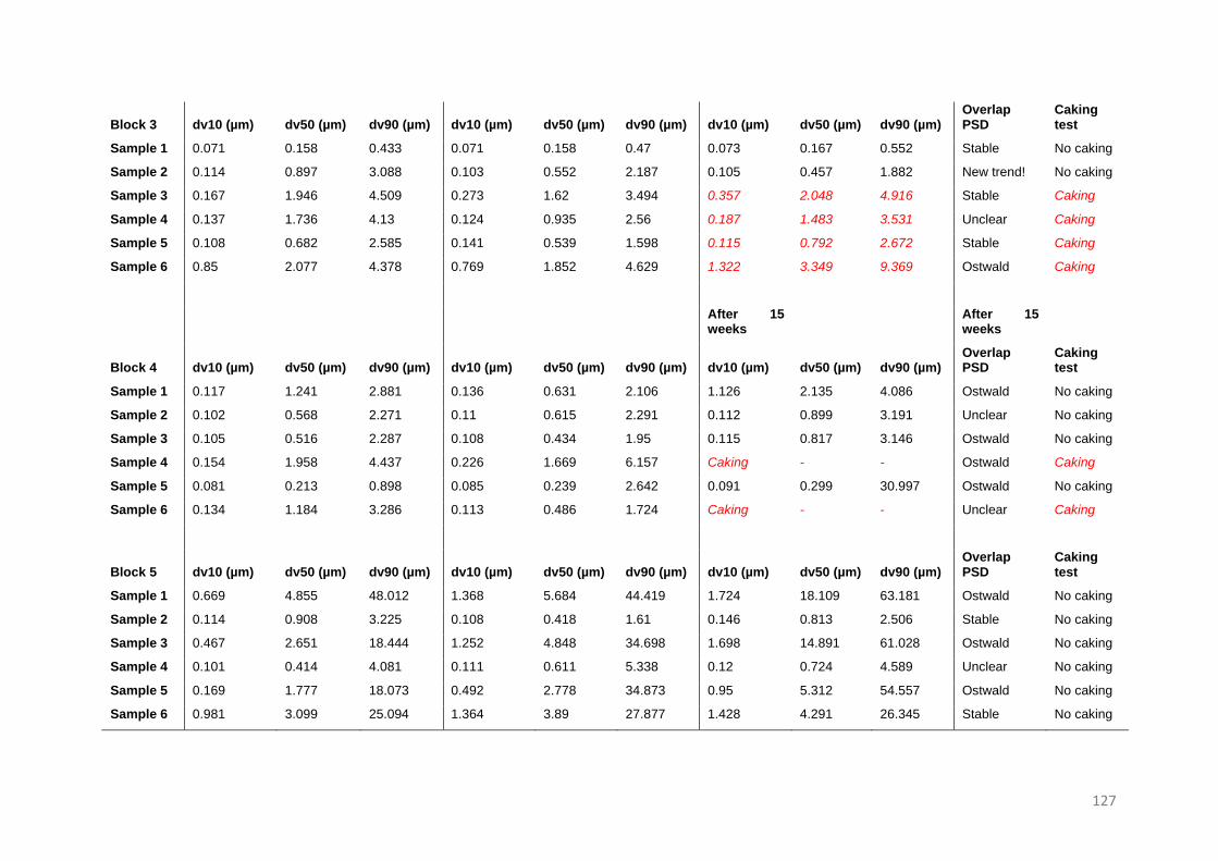
127
Block 3 dv10 (µm) dv50 (µm) dv90 (µm) dv10 (µm) dv50 (µm) dv90 (µm) dv10 (µm) dv50 (µm) dv90 (µm) Overlap PSD
Caking test
Sample 1 0.071 0.158 0.433 0.071 0.158 0.47 0.073 0.167 0.552 Stable No caking
Sample 2 0.114 0.897 3.088 0.103 0.552 2.187 0.105 0.457 1.882 New trend! No caking
Sample 3 0.167 1.946 4.509 0.273 1.62 3.494 0.357 2.048 4.916 Stable Caking
Sample 4 0.137 1.736 4.13 0.124 0.935 2.56 0.187 1.483 3.531 Unclear Caking
Sample 5 0.108 0.682 2.585 0.141 0.539 1.598 0.115 0.792 2.672 Stable Caking
Sample 6 0.85 2.077 4.378 0.769 1.852 4.629 1.322 3.349 9.369 Ostwald Caking
After 15 weeks
After 15 weeks
Block 4 dv10 (µm) dv50 (µm) dv90 (µm) dv10 (µm) dv50 (µm) dv90 (µm) dv10 (µm) dv50 (µm) dv90 (µm) Overlap PSD
Caking test
Sample 1 0.117 1.241 2.881 0.136 0.631 2.106 1.126 2.135 4.086 Ostwald No caking
Sample 2 0.102 0.568 2.271 0.11 0.615 2.291 0.112 0.899 3.191 Unclear No caking
Sample 3 0.105 0.516 2.287 0.108 0.434 1.95 0.115 0.817 3.146 Ostwald No caking
Sample 4 0.154 1.958 4.437 0.226 1.669 6.157 Caking - - Ostwald Caking
Sample 5 0.081 0.213 0.898 0.085 0.239 2.642 0.091 0.299 30.997 Ostwald No caking
Sample 6 0.134 1.184 3.286 0.113 0.486 1.724 Caking - - Unclear Caking
Block 5 dv10 (µm) dv50 (µm) dv90 (µm) dv10 (µm) dv50 (µm) dv90 (µm) dv10 (µm) dv50 (µm) dv90 (µm) Overlap PSD
Caking test
Sample 1 0.669 4.855 48.012 1.368 5.684 44.419 1.724 18.109 63.181 Ostwald No caking
Sample 2 0.114 0.908 3.225 0.108 0.418 1.61 0.146 0.813 2.506 Stable No caking
Sample 3 0.467 2.651 18.444 1.252 4.848 34.698 1.698 14.891 61.028 Ostwald No caking
Sample 4 0.101 0.414 4.081 0.111 0.611 5.338 0.12 0.724 4.589 Unclear No caking
Sample 5 0.169 1.777 18.073 0.492 2.778 34.873 0.95 5.312 54.557 Ostwald No caking
Sample 6 0.981 3.099 25.094 1.364 3.89 27.877 1.428 4.291 26.345 Stable No caking
128
The 30 samples did not only present different PSDs after production but demonstrated
different stability trends (Figure S-6.1., Figure S-6.2., Figure S-6.3., Figure S-6.4.,
Figure S-6.5, Supplementary Information, §9.3.) as well, leading to their categorisation
in four stability trends (Table 6.2.). Even though these PSDs and thus stability trends
were confirmed by SEM, they were merely defined by LD data and their accuracy was
therefore challenged by a caking test. The large volume of data extracted from this
stability study (Table 6.2.) impeded a broad, yet accurate discussion of each sample.
Nonetheless, some peculiar trends were noted which will be detailed below.
Despite their identical formulation, suspensions with comparable PSDs after
production could still demonstrate different stability trends, as displayed in sample 3
and sample 6 of block 1 of Table 6.2. They presented similar PSDs after production
with a dv10-, dv50- and dv90-value of 0.154 µm, 1.657 µm, 4.27 µm, and, 0.148 µm,
1.918 µm, 4.29 µm, respectively. Nonetheless, the PSDs evolved differently during
storage where sample 3 remained stable throughout the whole study whereas an
indispersible cake materialised in sample 6. The temperature after production,
retrieved as explained in chapter 5104 was distinct with a value of 40.1 °C and 66.2 °C
for sample 3 and sample 6, respectively. As an increased temperature might lead to
the (partial) desolvation of the hydrophilic part of the applied surfactant, it might have
impacted its stabilisation efficacy. As a result, the attraction energy between two
particles will prevail, and the particles will tend to aggregate. The higher temperature
that sample 6 faced could therefore explain the poor stability outcome as compared to
sample 3. From a stability point of view, these data suggested a preferred use of a
moderate acceleration, a smaller and thus, in this case, more performant bead size
and even intermittent pausing, as occurred during the production of sample 3, over
milling at a higher acceleration without intermittent pausing as occurred during the
manufacturing of sample 6. As proposed by Wang and co-workers50, these findings
suggest that the applied particle size reduction technology and even more, the applied
process parameters, might impact the stability of the manufactured suspension.
Furthermore, as formulation screenings are merely executed with fixed process
settings, these findings highlight how formulation scientists should take the production
technology and parameters in consideration when examining the results of such
formulation screenings.

129
The most striking result to emerge from this dataset was the anomalous trend of a
particle size reduction during storage, observed in a few samples of the stability study
(‘New trend’, Table 6.2.). This new trend was, as a first investigation, challenged via a
caking test. As described by Stokes’ law (Equation 1.5.), larger particles of a
multidisperse system will settle faster than their smaller counterparts.29, 44 To produce
an indispersible cake, smaller particles need to settle in-between these sedimented
larger particles, however, the smallest particles (mostly nanometer-range) will, by
virtue of the Brownian motion, hardly settle, if at all. The undispersible sediment will
therefore merely comprise of the larger particles of a multidisperse system. The
supernatans will as a consequence increasingly contain smaller particles. As sampling
occurs in the supernatans, the measured PSD will become less and less representative
for the suspensions aggregation behaviour and will falsly represent a particle size
reduction. Via the caking test, samples containing a solid, indispersible sediment and
thus, reflecting a false particle size reduction, were traced down (Table 6.2.). The last
stability data of the samples of block 1 to 3, were, as caking occurred, highlighted in
bold, italic and red to indicate their possible inaccuracy. In the case of the samples of
block 4 and 5, the particle size measurement was not executed if caking occured
(Sample 4 and sample 6, Block 4, Table 6.2.).
Suprisingly, sample 2 of block 3 did not demonstrate an indispersible cake, even after
17 weeks of storage. However, it did present the new trend during storage (Figure
6.1.). The change in the PSD was confirmed via SEM, where the size distribution of
the rather multidisperse particulate system seemed to narrow down as a function of
time (Figure 6.2.). The operating parameters to manufacture this suspension were an
acceleration of 80 g, a milling time of 10 min, a bead-suspension ratio of 1.2 mL/mL
and a bead size of 1000 µm. The installed bead-suspension ratio and acceleration
were rather extreme, though the milling time was limited to 10 minutes. With a final
suspension temperature of 85 °C, heat was generated to a high extent and the system
did approach the cloud point of the stabiliser polysorbate 20 (ca. 97 °C)91. Partial
dehydration could occur but aggregation was not observed in the SEM images. As this
unexpected behaviour would shed a new light on the behaviour of suspensions after
micronisation, an investigation of this particular trend was pursued.
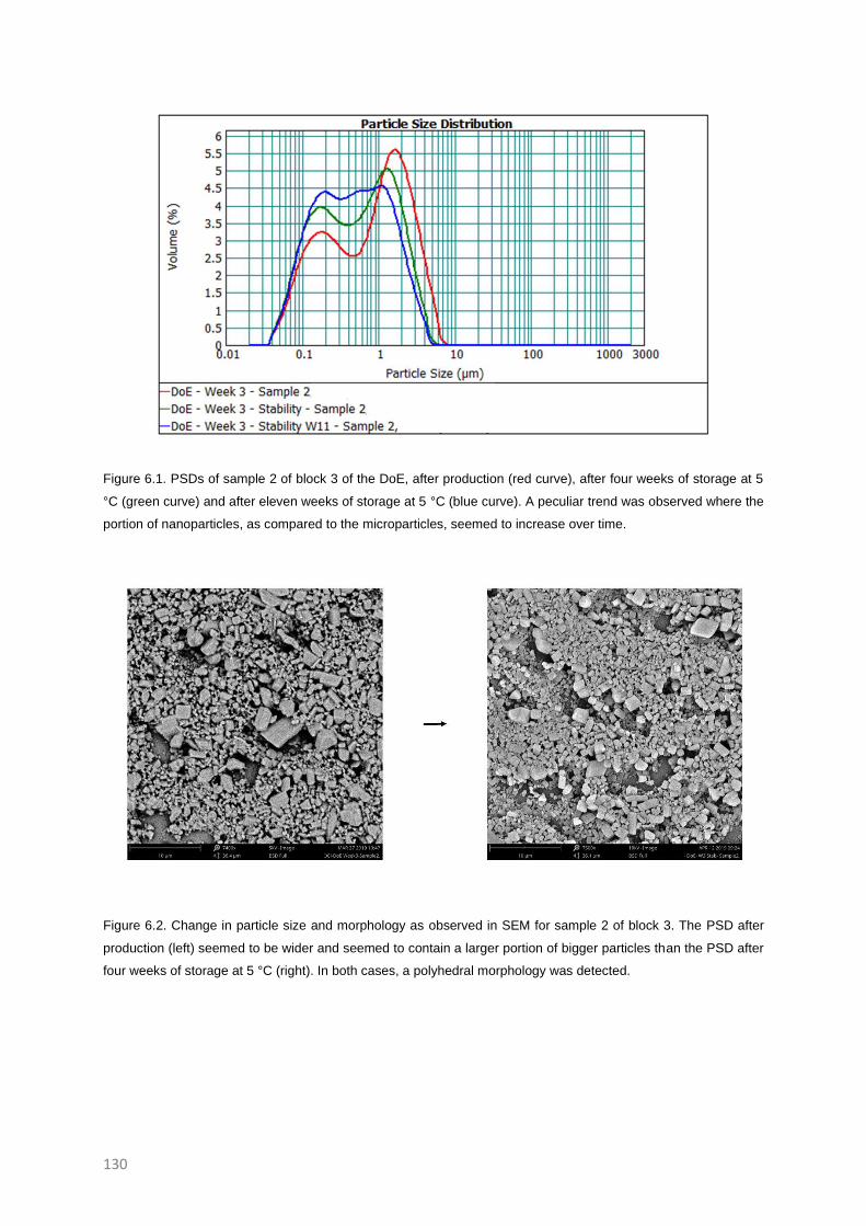
130
Figure 6.1. PSDs of sample 2 of block 3 of the DoE, after production (red curve), after four weeks of storage at 5
°C (green curve) and after eleven weeks of storage at 5 °C (blue curve). A peculiar trend was observed where the
portion of nanoparticles, as compared to the microparticles, seemed to increase over time.
Figure 6.2. Change in particle size and morphology as observed in SEM for sample 2 of block 3. The PSD after
production (left) seemed to be wider and seemed to contain a larger portion of bigger particles than the PSD after
four weeks of storage at 5 °C (right). In both cases, a polyhedral morphology was detected.

131
Confirmation of the new trend
Table 6.3. Investigation of the reproducibility of the particle size reduction during storage observed in sample 2 of
block 3 of the DoE.
Sample set Stability point dv10 (µm) dv50 (µm) dv90 (µm)
2 0 0.109 0.939 3.568
2 1 0.122 0.541 1.99
1 1 0.13 0.573 2.175
1 2 0.118 0.796 3.095
The particle sizes presented in this summarising table are the average values,
measured with the Mastersizer 2000™. Sample set 2 was measured after
production and after three weeks of storage at 5 °C and sample set 1 was
measured after four weeks and after seven weeks of storage at 5 °C.
As a confirmation of the reproducibility of this newly found stability trend, the
investigated suspension (Sample 2, Block 3, Table 6.2.) was remanufactured in
manifold and tracked over time. The caking test remained negative throughout the
stability study, indicating that the suspension could be completely redispersed. The
summarising results (Table 6.3) of the raw data (Table S-6.1., Table S-6.2, Table S-
6.3, Table S-6.4., Supplementary Information, §9.3.), endorse the reproducibility of this
enigmatic behaviour. The dv50-value declined from a value of 0.939 µm to a value of
0.541 and 0.573 µm during the first three to four weeks of storage (Table 6.3.). This
particle size reduction was even more apparent in the dv90-value which sharply
reduced to approximately half its original value. The particle size change from week
four to week seven was opposite to what was observed during the previous stability
study. In the previous stability study the particle size continued to decrease over time,
whereas the PSDs in this stability study presented a mild particle growth. Despite this
difference in the second phase of the stability study, the net result remained the same.
In both stability studies the PSDs at the end of the storage time were still narrower and
had an importantly lower dv50-value than the PSDs after production. In order to
exclude that the trend was a reproducible flaw of the analysis technique, the
Mastersizer 2000™, the trend was further studied using the Mastersizer 3000™ and
an orthogonal particle size measurement technique namely differential centrifugal
sedimentation.
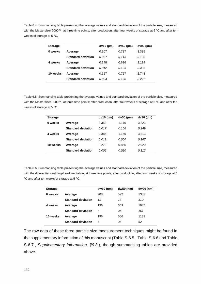
132
Table 6.4. Summarising table presenting the average values and standard deviation of the particle size, measured
with the Mastersizer 2000™, at three time points; after production, after four weeks of storage at 5 °C and after ten
weeks of storage at 5 °C.
Storage
dv10 (µm) dv50 (µm) dv90 (µm)
0 weeks Average 0.107 0.787 3.385
Standard deviation 0.007 0.113 0.103
4 weeks Average 0.148 0.626 2.194
Standard deviation 0.012 0.103 0.435
10 weeks Average 0.157 0.757 2.748
Standard deviation 0.024 0.128 0.227
Table 6.5. Summarising table presenting the average values and standard deviation of the particle size, measured
with the Mastersizer 3000™, at three time points; after production, after four weeks of storage at 5 °C and after ten
weeks of storage at 5 °C.
Storage
dv10 (µm) dv50 (µm) dv90 (µm)
0 weeks Average 0.353 1.170 3.223
Standard deviation 0.017 0.106 0.249
4 weeks Average 0.385 1.150 3.213
Standard deviation 0.019 0.050 0.167
10 weeks Average 0.279 0.866 2.920
Standard deviation 0.006 0.020 0.113
Table 6.6. Summarising table presenting the average values and standard deviation of the particle size, measured
with the differential centrifugal sedimentation, at three time points; after production, after four weeks of storage at 5
°C and after ten weeks of storage at 5 °C.
Storage dw10 (nm) dw50 (nm) dw90 (nm)
0 weeks Average 208 592 1332
Standard deviation 11 17 110
4 weeks Average 196 509 1045
Standard deviation 7 36 161
10 weeks Average 196 506 1139
Standard deviation 6 35 62
The raw data of these three particle size measurement techniques might be found in
the supplementary information of this manuscript (Table S-6.5., Table S-6.6 and Table
S-6.7., Supplementary Information, §9.3.), though summarising tables are provided
above.

133
The PSDs observed with the Mastersizer 2000™ (Table 6.4.) were comparable to the
previously retrieved data. The Mastersizer 3000™ data (Figure 6.3. and Table 6.5.)
confirmed the particle size reduction from week zero to week four. However, in the
second phase of the stability study a particle size decrease was detected by the
Mastersizer 3000™ whereas a mild particle size increase was detected by the
Mastersizer 2000™. This difference may be attributed to the increased sensitivity of
the Mastersizer 3000™ to nanoparticles, hence the Mastersizer 3000™ data were
presumably more accurate. Still, the dv50-value in both the Mastersizer 2000™ and
the Mastersizer 3000™ reduced during the entire stability study. This trend was further
substantiated by the data acquired by differential centrifugal sedimentation (Figure 6.4.
and Table 6.6.). However, the particle sizes generated by differential centrifugal
sedimentation were considerably smaller than their counterparts measured with LD.
As the focus of the study was an early investigation of the observed new trend, an
extensive method optimisation of the differential centrifugal sedimentation method was
not pursued, resulting in the methods inferior accuracy. Yet, the dataset confirmed, the
peculiar narrowing of the PSD over time. Moreover, similar stability trends were
observed in other APIs as well (data non-disclosed). Even though this peculiar trend
seemed very contraindicative towards the widely known and accepted stability trends,
it was repeatedly observed and confirmed by an orthogonal particle sizing technique.
However, more particle size data with optimised (orthogonal) particle sizing techniques
are strongly required to fully confirm the perceived trend. Future studies might address
the explanation of the peculiar trend as well. Based on physicochemical principles, a
non-exhaustive list of plausible hypotheses is provided below, comprising digestive
ripening or reversed Ostwald ripening, the crystallisation of the amorphous (regions on
the) surface of the API particle, (surface) degradation and the Rehbinder effect.
Discarded hypotheses included intraparticle ripening and a stabiliser enabled
disaggregation.
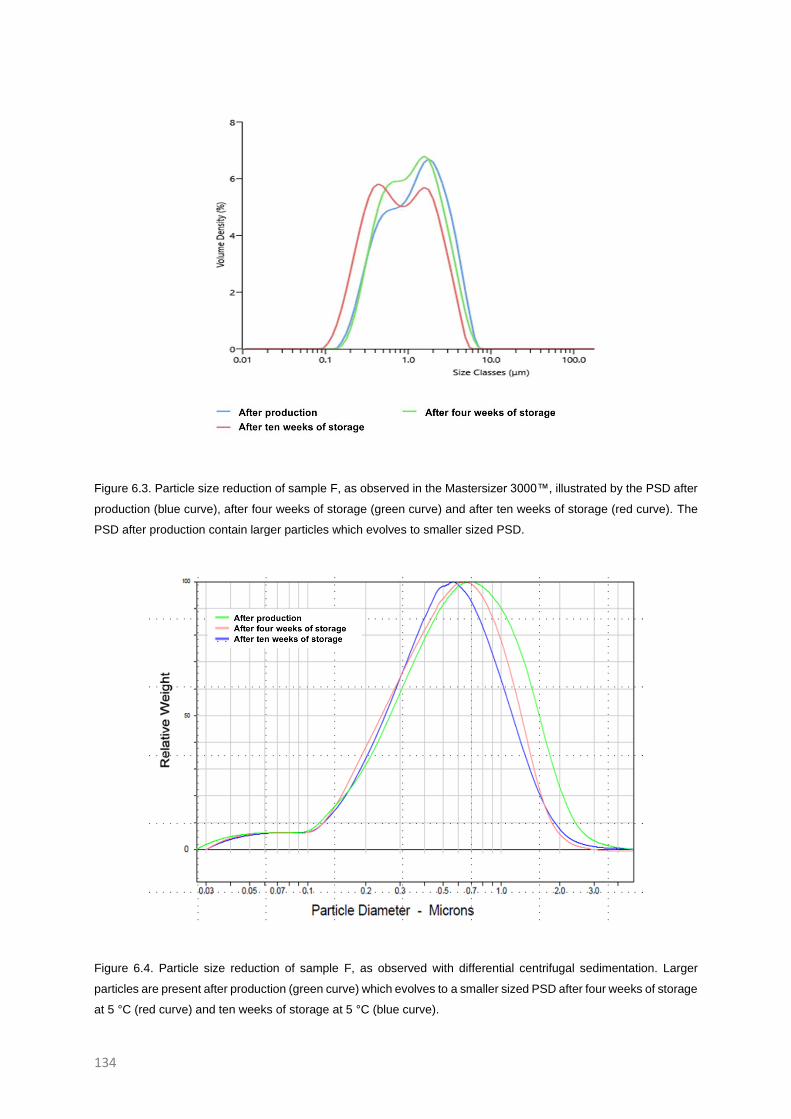
134
Figure 6.3. Particle size reduction of sample F, as observed in the Mastersizer 3000™, illustrated by the PSD after
production (blue curve), after four weeks of storage (green curve) and after ten weeks of storage (red curve). The
PSD after production contain larger particles which evolves to smaller sized PSD.
Figure 6.4. Particle size reduction of sample F, as observed with differential centrifugal sedimentation. Larger
particles are present after production (green curve) which evolves to a smaller sized PSD after four weeks of storage
at 5 °C (red curve) and ten weeks of storage at 5 °C (blue curve).
135
Within inorganic chemistry, the process in which smaller particles grow at the expense
of larger particles is denoted as the process of digestive ripening or reversed Ostwald
ripening and has been the subject of extensive research.48, 111 How the size
modification during reversed Ostwald ripening precisely occurs still remains to be
elucidated and mainly descriptive insights are provided within inorganic chemistry.111
A current working hypothesis is the existence of a region in the parameter space of
component concentrations and interaction energies where smaller particles are more
stable than their larger counterparts. By the addition of a surface energy lowering
excipient, e.g. the wetting agent polysorbate 20, the effective surface energy of the
small particles might become negative. Mass would transfer from the larger particles
to these smaller particles and subsequently the PSD narrows to mono-sized
particles.48, 112, 113 Even though this theory appears particularly appealing to the
investigated system consisting of an API and the stabiliser polysorbate 20, extreme
caution must be paid in the direct translation of the given theorem. Contrary to the
research carried out in the field, the rate of the phenomenon presented itself over
weeks, whereas digestive ripening merely appears as a rapid process of maximum a
few hours. Another disagreement is the particle size range in which the phenomenon
takes place. While in the field of inorganic chemistry digestive ripening applies to a few
dozen of nanometres to quantum dots, the trend observed in our study was only
present at the higher nano- and lower microscale.48, 114 Albeit, the most intriguing
analogy of the surface energy lowering excipient, resuscitates digestive ripening as
potential hypothesis.112
Other interpretations for this intriguing trend, are related to the surface of the API
particle (Figure 6.5.). As the IVM is a high intensity milling process, it might
mechanically activate regions at the surface of the API and consequently reduce the
crystallinity of the milled compound.50

136
Figure 6.5. Surface phenomena that might occur during milling, illustrated by the circumstances before milling (left),
immediately after milling (middle) and the stabilised conditions after milling (right). Due to the high intensity milling,
surface domains might amorphisize which might crystallise during storage causing a volume reduction (green
arrows). Due to the high intensity milling, surface degradation may occur. The degradation product might have a
higher solubility than its poorly soluble parent compound and might consequently dissolve in the suspension matrix
(yellow arrows). Bedaquiline submicron suspensions are more prone to degradation than their macro-counterparts.
As a result, degradation in the suspension matrix might shift equilibria to an extent that particles start to dissolve
over time (yellow and blue arrows).
As a result, the crystal surface becomes disordered, which results in a highly defective
crystal phase that may spontaneously convert to localised amorphous regions.50, 115
As the amorphous compound is characterised by an enhanced solubility and a higher
free energy, reordering of these crystal defects and crystallisation of the amorphous
regions might spontaneously occur during storage. The high water content of the
suspension matrix will act as a plasticiser, which undoubtedly will trigger this
crystallisation process.50, 115 causing a reduction of the particle volume and hence, an
overall size reduction (Figure 6.5.).116 However, previous findings in our group
suggested that in the case of naproxen and cinnarizine amorphisation due to media
milling is highly unlikely in the suspended state and that the occasionally detected
amorphous fraction presumably originates form the drying process, required for solid-
state analysis. These findings were more specifically prevalent for APIs that had an
increased solubility in the stabiliser, which complies to the herein studied system of
bedaquiline and polysorbate 20.117
Further, these amorphous regions show a higher reactivity which in the presence of an
aqueous medium, may lead to chemical degradation, as observed for naproxen by
other authors.118 Furthermore, research in our group distinguished how cryomilling
might trigger polymer and subsequentially API degradation.119 Considering mechanical
activation might occur in the highly energetic IVM as well, surface API may degrade,
generating degradation products that might be more soluble than their poorly soluble

137
parent compound. In these circumstances, the degradation product might dissolve in
the aqueous environment, which drives particle size reduction (Figure 6.5.).
Despite the stability of bedaquiline in solid or in dispersed state, the submicron
suspension demonstrated an increased photodegradation (data non-disclosed).
Provided that the degradants are more soluble than to the parent compound
bedaquiline, photodegradation might shift the mass equilibria and drive a particle size
reduction (Figure 6.5.).
Another hypothesis is the propagation of the Rehbinder effect post-micronisation.
During nano- and micronisation, the stabiliser plays a major role in the mechanical
breakdown of the API via three different phenomena comprising the wetting and
stabilisation of the newly formed surfaces, its contribution to the microhydrodynamics
of the mixing and milling regime, and in the particle strength as described by the
Rehbinder effect.120 This Rehbinder effect explains how the stabiliser reduces the
compound hardness which eventually leads to crack propagation.3, 120, 121 The addition
of a stabiliser enhances the wet breakage rate via both the Rehbinder effect and the
wetting and stabilisation mechanism. However, as they coincidently occur, there is no
consensus on which mechanism is more dominant. Attempts of Biligili and co-workers
to address the question, led to two publications with contradictory findings.3, 120 The
increasing surface area of dry budesonide post-micronisation, was nonetheless
clarified by the theories of stress relief and crack propagation.108 Taken together, there
is still considerable controversy on the applicability of the Rehbinder effect in
pharmaceutical wet milling kinetics. Bearing in mind that the crack propagation would,
within the presented study, occur during storage, the hypothesis seemed highly
doubtful as compared to other well-reasoned hypotheses. Albeit, Monteiro and co-
workers described how the stabiliser sodium lauryl sulphate enabled the penetration
of the suspension medium into the aggregate pores. The aggregates consequently
disaggregated resulting in an apparent particle size reduction.120 This theory could be
transposed to our investigated system, but was discarded as the acquired SEM images
did not display any (dis)aggregation behaviour.
Another interesting hypothesis, which was eventually discarded by the SEM
observations and the orthogonal particle sizing technique, included intraparticle
ripening; a process where monomers diffuse along the surface of nanoparticles to
modify the particles habitus with time (Figure 6.6.). The working hypothesis of
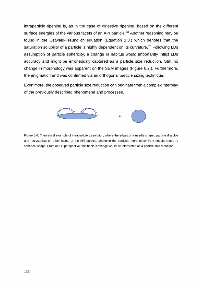
138
intraparticle ripening is, as in the case of digestive ripening, based on the different
surface energies of the various facets of an API particle.48 Another reasoning may be
found in the Ostwald-Freundlich equation (Equation 1.3.) which denotes that the
saturation solubility of a particle is highly dependent on its curvature.25 Following LDs
assumption of particle sphericity, a change in habitus would importantly inflict LDs
accuracy and might be erroneously captured as a particle size reduction. Still, no
change in morphology was apparent on the SEM images (Figure 6.2.). Furthermore,
the enigmatic trend was confirmed via an orthogonal particle sizing technique.
Even more, the observed particle size reduction can originate from a complex interplay
of the previously described phenomena and processes.
Figure 6.6. Theoretical example of intraparticle dissolution, where the edges of a needle shaped particle dissolve
and recrystallise on other facets of the API particle, changing the particles morphology from needle shape to
spherical shape. From an LD perspective, this habitus change would be interpreted as a particle size reduction.

139
CONCLUSIONS
The herein provided stability study contributed to the observation that the selected
production technology and process parameters considerably affect the stability of the
produced suspensions. As a result, the applied process technology and process
parameters should be taken into consideration during a formulation screening as it is
conventionally executed with fixed process settings. Furthermore, one manufactured
suspension presented an unconventional narrowing of its PSD over time which was to
the best of our knowledge not reported in the pharmaceutical literature before. This
peculiar trend was further explored via a caking test, via repetitive measurements with
LD and via an orthogonal particle sizing technique which all confirmed this enigmatic
trend. More confirmatory experiments are, however, required. Due to time constraints,
this enigmatic behaviour was not further assessed. A non-exhaustive list of
hypothesises based on physicochemical principles provide the needed framework for
further exploration.
SUPPLEMENTARY INFORMATION
All supplementary material as denoted in the manuscript is provided in Chapter 9:
Supplementary Information, §9.3.


General discussion and future outlook


143
QUESTIONS ARISING FROM LASER DIFFRACTION AND INTENSIFIED
VIBRATORY MILLING
This PhD project revolved around the particle size analysis via LD, the nanonisation
and micronisation via IVM and the stability trends of the herewith manufactured micron
and submicron suspensions. Despite the simplicity of the LD and IVM set-up,
numerous questions arose from the ambiguous nature of the preliminary LD data and
from the intricate interplay of IVMs critical process parameters as which parameters
have an impact on the quality of LD data and how to treat them with care? How can
nano- and microsuspensions be manufactured with IVM and how can this
manufacturing process be finetuned? How do the manufactured (sub)micron
suspensions behave during storage?
Reviewing literature, these questions related to LD quality were nefariously all too often
ignored, whereas the questions concerning IVM are commonly addressed via the
cumbersome trial-and error approach. In adverse to these toilsome trends, this PhD
research project employed a step-by-step approach, as explained in chapter 2, which
followed the rational that before exploration of nanosizing technologies such as IVM, a
reliable particle size measurement method should be obtained. Consequently, one of
the most eminent particle sizing methods, LD, was studied for its capabilities of
producing high quality data. With the usage of the flow design provided at the end of
the first research project, an LD method was optimised for the analysis of (sub)micron
suspensions containing bedaquiline, the model compound throughout this PhD
dissertation. Furthermore, various polymers and surfactants were applied during this
first research project in order to stabilise the manufactured (sub)micron suspensions.
In the case of polysorbate 20, there were no aggregates detected on the SEM images,
the LD results indicated a short-term stability and the foam generated during milling
appeared negligible. Polysorbate 20 was therefore selected as a model stabiliser to be
considered for the subsequent research projects on IVM.
Endorsed by experience, this optimised LD method was transferred to the second
research project, which addressed the feasibility of IVM as nanosizing technique with
controlled heat generation via an assessment of various process parameters via an
OVAT approach. However, as temperature may have detrimental effects on the drug
product, a more thorough research was required. As a result, the early OVAT approach
paved the way for a profound DoE approach where the complex interplay of five

144
process variables was eventually unravelled. The fourth and last project of this PhD
dissertation studied the stability of the suspensions manufactured in the DoE (Chapter
5) during storage at 5 °C. Interestingly, few suspensions with similar PSD’s post-
manufacturing, did not show similar trends in particle size evolution during storage.
Moreover, a peculiar particle size reduction of a suspension post-micronisation was
observed, which to the best of our knowledge has not been reported in the
pharmaceutical literature before.
POSITION IN THE LASER DIFFRACTION AND INTENSIFIED VIBRATORY
MILLING LANDSCAPE
Guidance to quality laser diffraction data
Through its simplicity of use and its brief measurement time, LD has expeditiously been
incorporated in a manifold of projects in numerous academical and industrial
laboratories. In contrast to its wide application and the numerous papers emerging
hereof, 90% of the reported data has been stated to be false.73 As the reliability of LD
data is of utmost importance considering the harming impact of a false PSD on
conclusions with respect to the suspensions’ stability, suspensions’ syringeability and
more importantly the suspensions’ behaviour in the human body, a profound method
optimisation felt indispensable. During this method optimisation, issues concerning the
fit of the data, the obscuration, the samples stability within the LD system and the
background quality had to be tackled, before an optimised method could be installed.
When looking into the literature on LD accuracy, it shows that the critical impact of the
applied calculation model (Fraunhofer or Mie) and the applied refractive indices have
been repeatedly conveyed.73, 74, 75 A more recent investigation on this matter listed,
aside of the optical parameters, other important, yet questionable LD parameters such
as the technologies’ assumptions on the volume based results and on the spherical
equivalent diameter.74 Despite this prominent list of disputable parameters, these
articles failed to include the hurdles observed during our first research project. Even
more, as these articles highlighted the pitfalls of the LD platform, they did not seem to
propose solutions to resolve these hurdles and to advance in quality LD data.
Therefore, to aid formulation scientists in their search for an optimal LD method, the
previously identified critical variables were described and more importantly addressed
in a peer-reviewed publication.
145
Although the quality of LD results can be first-hand evaluated with the residuals and
residuals weighted, these parameters seemed to be rarely reported in scientific
literature. Even though the accuracy of this particle size technique was not proven in
this study and additional particle sizing with an orthogonal technique remained
recommended, peer reviewers are, nonetheless, advised to request these values as a
first assessment of one’s published LD data.
Filling the knowledge gaps in the field of intensified vibratory milling
As the first investigations on IVM were only conducted in 2013, it comes as no surprise
that only scant information is currently available on the topic.66 Even though these
former research efforts were undertaken to profoundly introduce IVM into the field of
pharmaceutical milling, most of them lacked (some) ingenuity to enable a thorough
understanding of this complex milling platform and consequently, there is still ample
room for investigation. This limited body of research considered IVMs critical process
parameters63, 66 or compared this novel milling technology with the golden standard
WBM62, 63, albeit contradictory conclusions were drawn on the latter subject. Various
authors confirmed the potential of IVM as drug-sparing nanonisation technique62, 63, 66,
122,, although there is still some critical disagreement to the extent (observable66, 63 to
barely or non62, 64) of IVMs heat build-up. Overall, current literature is dominated by
reports that do not consider heat generation as a fundamental determinant in IVMs
applicability.
As our preliminary data suggested, a critical portion of the power of this high-energy
grinding technology dissipated as heat, a second project was enrolled to investigate
the impact of five parameters, four process parameters and one formulation parameter,
on both the size reduction and the heat generation. Still, papers have been published
engaging the latter topic wherein Lu and co-workers have reported the highest
temperatures so far. In their study, temperatures of maximal 60 °C were reported.
Pursuant to the importantly higher temperatures observed in our study, which could
expand to 100 °C or above, this problematic heat generation felt underestimated. Even
more, Lu and co-workers continued milling for at least two hours without major issues
regarding heating or particle reaggregation. Even though our research suggested that
milling time presented a polynomial term towards its heat-build up, two hours of IVM
milling strongly feels, endorsed by our broader experience, as an excessive milling
time. However, the remark can be made that milling occurred in maximal 8 mL vials in

146
the study by Lu and co-workers, whereas 20 mL vials were used in our study, and as
pointed out by Lu et al., this could importantly influence the generated heat.66
Furthermore, the extreme temperatures detected during this second research project
did not appear to correlate with the observations of Leung and co-workers, who
outlined in their pioneering paper from 2013 how the mild temperature increases of the
IVM were enabled by a homogenous energy dissipation and effective energy
utilisation.66
Valuable conclusions were drawn in this second project, however, to tip the energy
balance further from heat generation to size reduction, an expert knowledge on IVM is
imperative. In order to unravel the complex interplay between IVMs process
parameters, a modern DoE was conducted in the third research project that deep dived
in the impact of five process parameters on the mechanical API breakdown and heat
generation. Through the complexity of the milling process and scarce publications on
the subject, direct comparison of results might be interesting, nonetheless
cumbersome and should therefore be interpreted with care. Our data seemed to merely
reinforce the recommendations towards process optimisation as described by Lu and
co-workers66 and by Li and co-workers63 which would in their case have been more
persuasive, if they were not solemnly drawn from an OVAT-perspective.63, 66 In this
respect, the considerable impact of acceleration and bead-suspension ratio on both
size reduction and heat generation was confirmed.
Regarding the bead size, our findings refute previous results of Lu and co-workers,
which stated that for nanonisation the smallest bead size is preferred, which was earlier
disproved by Li and co-workers.63, 66 The evidence in the third research project
highlighted the existence of an optimum bead size towards size reduction and heat
generation. Thus the selected media had an important impact on the heat generation
which was in contrast to the findings of Lu and co-workers who stated that the media
had only small effects on the operation temperature.66 Interestingly, this optimal value
was power dependent, as suggested by the group of Li and co-workers63, and therefore
related to the acceleration and bead-suspension ratio. However, the OVAT approach
used by Li and co-workers did not have the power to properly identify such multiple
way interactions, for which our DoE now provide sufficient credential. However, in
contrast to the performed optimisation steps of Li and co-workers63, our findings advise
to maximise the bead-suspensions ratio instead of acceleration in order to obtain high
147
power milling. Furthermore, the third research project confirmed how “breaks during
milling” contribute to an effective heat control without constraining the grinding process.
This scalable and standard parameter might be preferable to the effective, yet
laboursome milling interruption, described by Li and co-workers.63
The references made in these previous sections66, 63, 62, 122, pointed out that IVM is
undoubtfully an interesting and fast nanonisation and micronisation technology which
was captured in the findings of this third research project as well. Effective mechanical
breakdown to micron and submicron level persisted in a time frame of 10 to 30 minutes.
Within this DoE, multiple statistically significant interactions were identified which
displayed the complexity of IVM. This complexity translated in the major constraint of
this project; no generic recommendations could be determined. However, for the size
reduction the mechanistic model of Kwade54 was for the first time applied to gain some
mechanistic insights. Furthermore, the given project did provide predictive models that
may accurately predict milling outcomes based on the inserted process parameters.
The peculiar aftermath of intensified vibratory milling
Considering the overall dearth of information in the field of IVM, it came as no surprise
that no stability study on IVM was published so far. Therefore, post-production stability
was evaluated in the fourth research study (Chapter 6), utilising the samples of the
third research study (Chapter 5). During this stability study, samples with similar
particle sizes yet counteracting stability trends were detected; one suspension could
remain stable whereas the other underwent Ostwald ripening. In a formulation
screening, the first suspension would be accepted whereas the latter one would be
rejected. These findings sound a note of caution with the interpretation of a formulation
screening. As formulation screenings merely include a fixed set of process parameters,
they do not consider the impact of the process parameters on the stability of the
suspension.
The single most conspicuous observation to emerge from this dataset was undoubtely
the puzzling phenomenon of particle size reduction postmicronisation for which scarce
information is available in the pharmaceutical literature. There are, to the best of our
knowledge, only two published articles that discuss an API in crystalline state that
reduces in size during storage, however the API was in these both cases in the dry
148
state.108, 110 Unlike these two studies, we were surprised to confirm a similar trend in a
suspended, wet state. As these data were gathered in a preliminary, very exploratory
phase, the evidence seems highly valuable for future investigation.
TOWARDS THE FUTURE
The challenges and opportunities of the Resodyn® Acoustic Mixers
Today, IVM is facing key challenges making this technology unattractive for
commercialisation which consecutively hampered their industrial success. First, the
low production output is a major drawback, and IVM would indisputably be impossible
to use in such conditions in the pharmaceutical industry. For mixing purposes, the
LabRAM II might be upscaled to the commercially available versions with higher
production capacity such as the RAM 5 with a payload capacity of 35 kg and the RAM
55 with a payload capacity of 420 kg.90 An early investigation in milling upscaling by
Lu and co-workers, showed that the vessel size must be restrained to prevent
excessive heat build-up, so the upscaling may be more troublesome for aqueous
suspensions. As presented in chapter 4, highly concentrated formulations are
advantageous to mill as well.66 It is, nonetheless, highly doubtful if an increase in API
concentration and in vessel number per run could proceed to such an extent that a full-
scale industrial production would be realised.
This leads to the second major drawback, the extensive heat generation. Since the
RAM has mostly been used in mixing procedures, RAMs manufacturing company
appeared to merely invest their developments in this area. IVM could on the other hand
be an appealing, drug sparing, high-throughput screening platform to scope an APIs’
millability or to screen variable formulations. In these circumstances, the previous
recommended multivessel production might be employed, however a suiting water
jacket would be highly recommended. Therefore, RAMs manufacturing company
should enable the commercialisation of these additional IVM water jackets.
As the potential of the IVM is currently jeopardised by its rather low output and major
temperature build-up, the costly acquirement of the RAM is for milling purposes still
questionable. Interest could, nonetheless, be sparked by RAMs multitude of
applications, which encompass, in comparison to WBM, other formulation platforms as
well. Recent studies have shown that the RAM is highly applicable for nano-silica dry
coating of microcrystalline cellulose, where this technology outperformed two more

149
conventional technologies.123 Recently, the RAM presented great potential for the
development and scale-up of co-crystals in a practical and environmentally friendly
approach.124 In the more traditional approach, RAM is employed as a highly effective
mixing device, albeit, temperature increases were hereby detected as well.90
Embarking future research
7.3.2.1. Consolidation of the predictive models
A first approach for future research would be the consolidation of the predictive models
that were generated in the third research project (Chapter 5). Within the JMP®
software, experiments can randomly be generated with a forecasted dv50-value and
temperature after milling, which should comply to prior set specification limits. In order
to display the chance that the milling process would not comply to these prior set specs,
due to the process’ variability and natural occurring variability, an upper limit defect
rate, lower limit defect rate and total defect rate were calculated by the JMP® software.
Consequently, a formulation scientist may identify which dv50-value and temperature
after milling would be acceptable for a given formulation which can be input as specs
in the JMP® software to compute the required process parameters. These process
parameters are a well-founded starting point and thus, might highly accelerate the
production process development. In order to validate this application, confirmatory
experiments with bedaquiline have to be executed.
With respect to the stress model of Kwade54, as outlined in chapter 5, a milling process
is described by two important variables, the SE and the SN. Dependent on the process
parameters, a certain SN will be created wherein each collision will create a certain SE
on the particle, leading to particle fatigue or fracture. As observed throughout this PhD
project, the IVM may be categorised as a high-energy mill and therefore the
assumption can be made that the SE, accumulated in the samples of the DoE, is of a
rather high magnitude. This SE, developed in the DoEs working ranges, might be
capable to exceed the millability differences between different poorly soluble APIs. In
this context, the predictive model could be extrapolated to other APIs; without the
implementation of a millability factor, although with the assumption of a properly
stabilising formulation. Even if the model would be solemnly applied as a rule of thumb
where actual outputs slightly differ from the computed output, an extensive trial-and-
error research would still be eliminated.

150
7.3.2.2. Investigation of the peculiar stability trend
A second path for future research is to deep dive in the peculiar trend that was noted
in the stability study, provided in chapter 6, which may be scrutinised in twofold. First,
more information concerning this trend should be gathered as it may indicate which
hypothesis is worth further exploration. First of all, the employed differential centrifugal
sedimentation should be optimised for the investigated bedaquiline suspensions and
other orthogonal particle size measurement techniques which have measuring ranges
encompassing the suspensions PSD such as transmission electron microscopy (TEM)
or SEM, should be included.125, Since a multimodal PSD is involved, it is preferable to
employ TEM as literature indicates TEMs ability to distinguish smaller from larger
particles.125 In order to more precisely denote this enigmatic trend, the measurement
frequency may be increased and the study might be prolonged in time. As the caking
test in chapter 5 was executed a few weeks after the second stability measurement for
samples of block 1 to 3 and to have a benchmark for comparison, DoE samples with
similar particle sizes to the investigated sample (Table 6.2., Chapter 6) such as
samples 6 and 5 from block 2 and 3, respectively, might be included in future
assessment.
Secondly, hypotheses as provided at the end of chapter 6, may be evaluated in order
to rationalise this enigmatic trend. Revision of these hypotheses reduced the likelihood
of phenomena such as the Rehbinder effect, disaggregation or intraparticle dissolution
whilst phenomena, such as surface amorphisation and subsequent crystallisation,
surface degradation or reversed Ostwald ripening, are more likely to occur. As these
trends are mainly explained by surface changes such as altering surface energies or
transitions in solid-state, alternative techniques that can cope with nano- and
microparticle surface characteristics come into the picture.
In their seminal paper from 2014, Chen and co-workers have drawn our attention to
the use of synchrotron-based high-resolution total scattering pair distribution function
coupled with nanoindentation measurement as a valuable and effective tool for
investigation of subtle structural disorders in API crystals, a tool worth trying on this
peculiar sample as well.126 One year later, Maughan and co-workers achieved to
expand this nanoindentation method to (sub)micron crystals. In contrast to the
described production via crystallisation, it might be possible to apply nanoindentation
on the dried crystals to investigate if the peculiar sample concerns a distinct Young

151
modulus or a distinct hardness.127 For further surface assessment, inverse gas
chromatography may detect and localise surface amorphicity.128 In the more traditional
approach, inverse gas chromatography is employed for surface energy analysis, an
interesting output for our research as well since a change in surface energy is
correlated to inverse Ostwald ripening. These attachment energies might be ex-situ
computed by software packages as Materials studio, as well.126, 129 In quantitative
advanced imaging mode, atomic force microscopy (AFM) simultaneously provides the
surface topography and quantitative mechanical information such as stiffness,
adhesion and dissipation.128 At the end of the previous century, AFM was for the first
time linked to thermal analysis on a µm/nm scale. The resulting scanning thermal
microscopy (SThM) was able to provide simultaneous topographical and thermal
properties of a surface and near surface region. SThM might therefore serve as a
technique to discriminate between amorphous and crystalline regions on a sub-micron
scale and as highlighted by Bond and co-workers, the acquired data may be highly
comparable to the conventional differential scanning calorimetry data.130, 131 As a
result, the concept of local amorphous regions at the APIs surface, may be evaluated.
To investigate surface degradation, time-of-flight mass spectrometry would be advised,
as it might identify the surface chemistry.132
Even though these nano-and micro surface analysis techniques are still in their infancy,
it is not inconceivable that one of these techniques might be applied in our future work
to discover more on this peculiar trend, however, one should be aware that each
analysis technique has its own set of assumptions and limitations that fell out of the
scope of this discussion. Furthermore, these techniques are often limited by a poor
reproducibility and resolution, hence ideal background and matrix conditions are
merely required. Finally, sample preparation including drying seemed frequently
required, which may modify the surface characteristics of the sample. This PhD
dissertation was limited in time to test all hypotheses. Nonetheless, this discussion
provides a springboard for further exploration as results so far have been very
promising.
Overall, the findings presented in this thesis dissertation are substantial to the general
understanding of IVM, where the prospect of the prediction of IVMs milling outcomes,
serve as a spur to future research. This PhD dissertation led to the conclusion that IVM
is a feasible option to obtain nano- and microsuspensions in small scale for drug-

152
sparing high-throughput screening, despite all remaining challenges. Furthermore, the
subject of the detected particle size reduction post-micronisation is undoubtedly
reserved for future work.

Summary - Samenvatting


155
Summary
This thesis revolves around intensified vibratory milling (IVM) as a manufacturing
method for micron- and submicron suspensions, with the overall aim to profoundly
understand the main tenets governing the grinding process. A general introduction to
establish the framework for the subsequent research chapters is provided in the first
chapter. This introduction provides the prognosis why the interest in nano- and
microsuspensions is currently rapidly growing. In this context, the tendency towards
the manufacturing of poorly soluble compounds is placed in its historical context.
Subsequently, various enabling strategies that address this solubility hurdle are further
discussed. Two of these strategies, nanonisation and micronisation, were brought at
the foreground with an elaboration on their specific advantages per administration
route. Furthermore, the production, stabilisation and characterisation of these fine
particles are discussed whereupon a deep-dive in the top-down production of the nano-
and microsuspensions was provided, highlighting the commercial viability of one of the
top-down approaches, wet bead milling (WBM). As a consequence of the different
challenges still faced in WBM research, an alternative top-down production technology
was introduced in the form of the IVM. In regard to the frequent comparison of this
novel methodology with the golden standard WBM, not only the fundamentals of the
WBM are mentioned, but also the impact of its process parameters on the grinding
process as well as the attempts to mechanistically model this grinding process. The
introduction is concluded with a section on IVM and the scant information currently
available on the topic.
The second chapter defined the objectives and thus the framework of the presented
PhD dissertation.
In the third chapter, laser diffraction (LD) was assessed as a widely adopted particle
sizing technique to identify the critical parameters that infringe the data quality. Various
parameters attributing to poor data quality including poor background quality, instability
of the sample in the equipment, presence of gas bubbles and substandard obscuration
were addressed and tackled. Diverse techniques to retrieve a compound’s real part of
the refractive index were compared where a combination of the Becke line technique
and fit optimisation seemed to be most favourable. With the flow chart provided at the
end of this chapter, an optimal LD method was generated for the particle sizing of

156
(sub)micron suspensions composed of bedaquiline, the model active pharmaceutical
ingredient (API) throughout this PhD. This method was, endorsed by experience,
transposed to the subsequent research work on IVM.
The first work on IVM was provided in chapter four, where the impact of three process
parameters (bead-suspension ratio, milling time and acceleration) and one formulation
variable (API concentration) on size reduction and heat generation was explored via
an one-variable-at-a-time (OVAT) approach. While the nanosizing potential of IVM has
been investigated by previous authors62, not much was known regarding the heat
generation of this novel milling technique. It was observed that an increasing
acceleration restricted the process via its excessive heat build-up, whereas the milling
time presented a more acceptable heating. High drug loadings did not affect the final
temperature, whereas they create highly effective grinding processes, ergo, the
combination of concentrated formulations with prolonged milling times formed the most
favourable approach for process optimisation. Furthermore, these observations
facilitated a more rational selection of critical process parameters and feasible working
windows for the subsequent research project.
As particle size reduction seemed to go hand in hand with heat generation, the
feasibility to manufacture a (sub)micronised suspension with acceptable heat
generation with IVM had to be more profoundly explored. Via a Design of Experiments
(DoE) the impact of five process variables (bead-suspension ratio, milling time,
acceleration, bead size and breaks during milling) on the characteristics of the grinded
suspensions was therefore assessed, which led to the following conclusions: IVM is a
complex process defined by a wide extent of statistically significant main effects, two-
way interactions, quadratic effects and even a three-way interaction; the existence of
the optimal bead size, which is both acceleration and bead-suspension ratio
dependent; a generic approach for process optimisation constitutes the optimisation of
the bead size and intermittent breaks during the milling process. During this project,
an attempt was undertaken to tackle the excessive heat generation in a standard and
scalable fashion by the inclusion of a cooling parameter denoted as ‘break during
milling’, which proved to provide a substantial yet standardised cooling of the
suspension, without restraining the APIs mechanical breakdown. To advance our
understanding of the IVMs process, the stress model of Kwade54 was applied on the
observed grinding trends. In order to control the heat generation in the IVM, fine-tuning

157
of IVMs process parameters in a more confined manner appeared indispensable.
Therefore, the generated predictive models were applied to project the suspensions’
particle size distribution (PSD) and temperature, based on the installed process
parameters. From a statistical point of view, our data highlighted how modern DoEs
such as the I-optimal design can be successfully applied to elucidate the interplay of
process variables in complex milling platforms in a fast and economic fashion. In our
view these results constitute an excellent initial step towards a rational installation of
process parameters when grinding via IVM is required.
After the assessment of the nanonisation and micronisation potential via a DoE in
chapter five, the impact of these process parameters on stability prospects was studied
in the subsequent chapter six. Accordingly, the PSD of the manufactured suspensions
of described in chapter five were tracked during storage at 5 °C post nano- and
micronisation. Generally, the samples remained stable or experienced Ostwald
ripening, except for one sample, which presented the peculiar trend of PSD narrowing.
Concerning the stable suspensions and suspensions experiencing Ostwald ripening,
even suspensions with similar PSDs after production could follow opposite trends
during storage, a very important finding illustrating that the feasibility to produce a
stable microsuspension depends both on the formulation parameters as well as the
process parameters. Hence, these findings underline the importance to consider the
process technology and applied process parameters when examining the results of a
formulation screening. The peculiar trend of PSD narrowing, perceived in one
particular sample, requires a combination of surface and bulk characterisation to
elaborate on the samples’ solid-state, chemical and PSD behaviour. In a first attempt,
the trend was further explored for its reproducibility with the Mastersizer 2000™ and
explored with the Mastersizer 3000™ and an orthogonal particle sizing technology,
differential centrifugal sedimentation. Still, no matter the frequency nor technique, a
narrowing PSD was detected. Our observations are encouraging and should be further
validated by optimised orthogonal particle sizing techniques. Future studies on the
current topic are also required to verify which physicochemical principle might explain
this enigmatic trend.
In the final chapter, an overall discussion on all these results and conclusions is
presented, challenges ascribed to the heat generation and upscaling are discussed
and a prospective framework for future research is provided.

158
159
Samenvatting
Deze thesis behandelt intensief vibratorisch malen (IVM) als een productietechniek
voor micron en submicron suspensies, met als overkoepelend doel een grondig inzicht
te bekomen in de belangrijkste principes die dit maalproces beïnvloeden. Een
algemene introductie in het eerste hoofdstuk dient als kader voor de daaropvolgende
onderzoekshoofdstukken. Deze introductie biedt een inzicht in de snel groeiende
interesse in nano- en microsuspensies. Het stijgende aandeel van slecht oplosbare
geneesmiddelen wordt binnen zijn historische context geplaatst. Daarenboven wordt
de impact van deze slechte oplosbaarheid op de formulatie van orale
toediengingsvormen beschreven. Vervolgens worden de verschillende technieken
besproken die een slechte oplosbaarheid en lage oplossnelheid aanpakken. Een van
deze strategieën, nanonisering en micronisering, wordt naar de voorgrond gebracht
met een verdere analyse over de specifieke voordelen per toedieningsweg. Daarna
worden de productie, stabilisatie en eigenschappen van deze fijne partikels besproken
waarbij er dieper ingaan wordt op de top-down productie. De commerciële
haalbaarheid van een van deze top-down benaderingen wordt uitgelicht, namelijk het
natte kogelmalen (NKM). Aangezien het onderzoek op NKM nog steeds verschillende
uitdagingen met zich meebrengt wordt een alternatieve top-down productietechnologie
geïntroduceerd in de vorm van IVM. Omdat deze nieuwe methodologie vaak
vergeleken wordt met de gouden standaard die NKM bekracht, worden niet enkel de
basisprincipes van NKM vermeld maar ook de mechanistische modellen die NKM
omschrijven. De introductie wordt afgesloten met een sectie over IVM en de schaarse
informatie die momenteel beschikbaar is over deze techniek.
In het tweede hoofdstuk worden de objectieven van de vier experimentele
hoofdstukken en daardoor de omkadering van deze doctoraatsthesis omschreven.
In het derde hoofdstuk werd LD als deeltjesgrootte meettechniek geëvalueerd en
werden de kritische parameters geïdentificeerd die de datakwaliteit negatief
beïnvloedden. Verschillende parameters die leiden tot slechte datakwaliteit,
waaronder een inadequate achtergrond, labiliteit van het staal in het meettoestel, de
aanwezigheid van gasbubbels tijdens de meting en inadequate obscuratie werden
besproken en aangepakt. Diverse technieken waarmee het reeël gedeelte van de
complexe, refractieve index gegenereerd kon worden, werden vergeleken, waarbij een

160
combinatie van de Becke lijn-techniek en fit optimalisatie het meest wenselijke leek.
Met behulp van de flowchart, die aan het einde van dit hoofdstuk terug te vinden is,
vonden we een optimale LD methode voor de deeltjesgroottemeting van micron en
submicron suspensies die bedaquiline bevatten, het model actieve farmaceutische
ingredient (API) doorheen deze PhD. Deze methode werd verder toegepast in de
volgende onderzoekshoofdstukken.
Het eerste onderzoekswerk op IVM werd aangereikt in hoofdstuk vier, waarin de
impact van drie procesparameters (de kogelsuspensie ratio, productietijd en
acceleratie) en één formulatievariabele (de API concentratie) op de
deeltjesgroottereductie en warmteopwekking verkend werd door één parameter per
keer te wijzigen. Hoewel het nanonisatiepotentieel van IVM onderzocht werd door
eerdere auteurs62, was er weinig geweten omtrent de warmteopbouw van deze nieuwe
maaltechniek. In dit onderzoek bleek een stijgende acceleratie het process te
beperken door de exponentiële warmteopbouw, terwijl de productietijd een
aanvaardbaardere warmteopbouw veroorzaakte. Hoge API-concentraties hadden
geen invloed op de uiteindelijke temperatuur, terwijl ze wel uiterst efficiënte
maalprocessen genereren. Bijgevolg vormde de combinatie van sterk
geconcentreerde suspensies met verlengde productietijd de meest wenselijke
benadering voor procesoptimalisatie. Verder maakten deze observaties een rationele
selectie van de kritische processparameters voor het volgende researchproject
mogelijk.
Aangezien de deeltjesverkleining sterk leek te correleren met warmteopbouw, moest
verder nagegaan worden of het mogelijk was om met IVM een gemicroniseerde
suspensie met acceptabele warmteopwekking te bekomen. Via een statisisch
onderzoeksplanning werd de impact van vijf procesvariabelen (kogelsuspensieratio,
productietijd, acceleratie, kogelgrootte en periodieke onderbrekingen tijdens het
malen) op de eigenschappen van de gemaalde suspensies onderzocht, wat leidde tot
de volgende conclusies: IVM is een complex proces dat grotendeels gedefinieerd
wordt door statistisch significante hoofdeffecten, statistisch significante interacties
tussen twee factoren, statistisch significante quadratische effecten en zelfs een
statistisch significante interactie tussen drie factoren; het bestaan van de optimale
kogelgrootte, die afhankelijk is van zowel de acceleratie en kogelsuspensieratio; een
algemene benadering voor procesoptimalisatie omvat de optimalisatie van de
161
kogelgrootte en periodieke onderbrekingen tijdens het malen. Tijdens dit project werd
een poging ondernomen om de buitensporige warmteopwekking tegen te gaan door
een gestandaardiseerde en opschaalbare parameter omschreven als ‘periodieke
onderbreking tijdens het malen’ te implementeren, wat zorgt voor een substantiële
doch gestandaardiseerde afkoeling van de suspensie, zonder de deeltjesverkleining
te beperken. Om ons begrip van het IVM-proces te verbeteren werd het stress model
van Kwade54 toegepast op de geobserveerde maaltrends. Om de warmteopwekking
verder te beheersen, moesten de overige procesparameters van de IVM ook worden
afgesteld. Daarvoor werden de gegenereerde predictieve modellen toegepast om de
partikelgrootte en de temperatuur van de suspensie na het malen te voorspellen.
Vanuit een statistisch standpunt benadrukten onze data hoe een moderne statistische
onderzoeksplanning zoals het I-optimale design gehanteerd kan worden om op een
snelle en economische manier de interacties tussen procesvariabelen in complexe
maalplatformen te ontrafelen. Volgens ons bieden deze resultaten een uitstekende
eerste stap richting een rationele implementatie van procesparameters wanneer malen
via IVM vereist is.
Na het beoordelen van het nanonisatie- en micronisatiepotentieel via de statistische
onderzoekstplanning in hoofdstuk vijf werd de impact van deze procesparameters op
de stabiliteitsverwachtingen bestudeerd in hoofdstuk zes. Overeenkomstig met
hoofdstuk vijf werd de partikelgroottedistributie (PGD) van de gemaakte suspensies
gemeten na het malen en nadat zij vier en elf weken bewaard waren bij een
temperatuur van 5 °C. De stalen bleven grotendeels stabiel of ondergingen Ostwald
rijping, met uitzondering van één staal waarbij een bijzondere versmalling van de PGD
optrad. Wat betreft de stabiele suspensies en suspensies die Ostwald rijping
ondergingen konden suspensies met gelijkaardige PGD na de productie
tegenovergestelde stabiliteitstrends volgen, wat een zeer belangrijke vaststelling was
die illustreerde dat de slaagkans om stabiele microsuspensies te produceren
afhankelijk is van zowel de gebruikte formulatie als de gebruikte procesvariabelen. Bij
het bestuderen van formulatiescreeningen is het dan ook van belang om de gebruikte
procestechnologie en ingestelde procesparameters mee in consideratie te nemen.
De opmerkelijke trend van PGD-versmalling die ontdekt werd in één staal in hoofdstuk
zes vereist bij verder onderzoek een combinatie van oppervlakte- en
bulkkarakterisatietechnieken om inzicht te krijgen in het staal zijn kristalliniteit, zijn

162
PGD, zijn gehalte en zijn afbraakproducten. Bij een eerste poging werd de trend verder
onderzocht op vlak van reproduceerbaarheid met de Mastersizer 2000™. Om de trend
te verifiëren werd de partikelgrootte verder onderzocht met de Mastersizer 3000™ en
de differentieel centrifugale sedimentatie. Ongeacht de frequentie of gehanteerde
techniek werd een vernauwde PGD gedetecteerd. Onze observaties zijn bemoedigend
en zouden verder gevalideerd moeten worden met geoptimaliseerde
deeltjesgroottemetingen. Verdere studies op dit onderwerp zijn ook vereist om te
verifiëren welke fysicochemische principes deze merkwaardige trend kunnen
verklaren.
Het laatste hoofdstuk omvat een algemene discussie van al deze resultaten. Tot slot
worden de uitdagingen aangaande warmteopwekking en opschaling besproken en
wordt een kader voor toekomstig onderzoek voorgesteld.

Supplementary information


165
SUPPLEMENTARY INFORMATION TO CHAPTER 3
Tables
Table S-3.1. Fit optimisation of the iRI within the Mastersizer2000™ software, using a TPGS- and an SDS-stabilised
suspension.
Table S-3.2. Fit optimisation of the rRI within the Mastersizer 2000™ software, using an SDS-stabilised suspension
and a TPGS-stabilised suspension.
rRI iRI D[4,3] D[3,2] dv10
(µm) dv50 (µm)
dv90 (µm)
Obsc red
Obsc blue
Res. Res. weight.
SDS 1.595 0 0.72 0.43 0.25 0.47 1.135 4.2 7.4 1.47 2.291
SDS 1.595 0.001 0.73 0.43 0.24 0.46 1.149 4.2 7.4 1.41 2.259
SDS 1.595 0.1 1.7 0.44 0.24 0.48 1.672 4.2 7.4 3.49 5.186
TPGS 1.595 0 4.54 0.44 0.12 3.87 10.32 2.1 3.16 0.51 0.522
TPGS 1.595 0.001 4.85 0.48 0.13 4.07 10.39 2.1 3.16 0.5 0.471
TPGS 1.595 0.1 5.51 2.59 1.03 4.98 10.41 2.1 3.16 1.2 1.216
rRI iRI Res. Res. weight.
SDS 1.55 0.001 1.38 2.663
SDS 1.592 0.001 1.41 2.284
SDS 1.595 0.001 1.41 2.259
SDS 1.596 0.001 1.4 2.25
SDS 1.6 0.001 1.42 2.212
TPGS 1.55 0.001 0.39 0.468
TPGS 1.592 0.001 0.5 0.472
TPGS 1.595 0.001 0.5 0.471
TPGS 1.596 0.001 0.5 0.47
TPGS 1.6 0.001 0.51 0.467
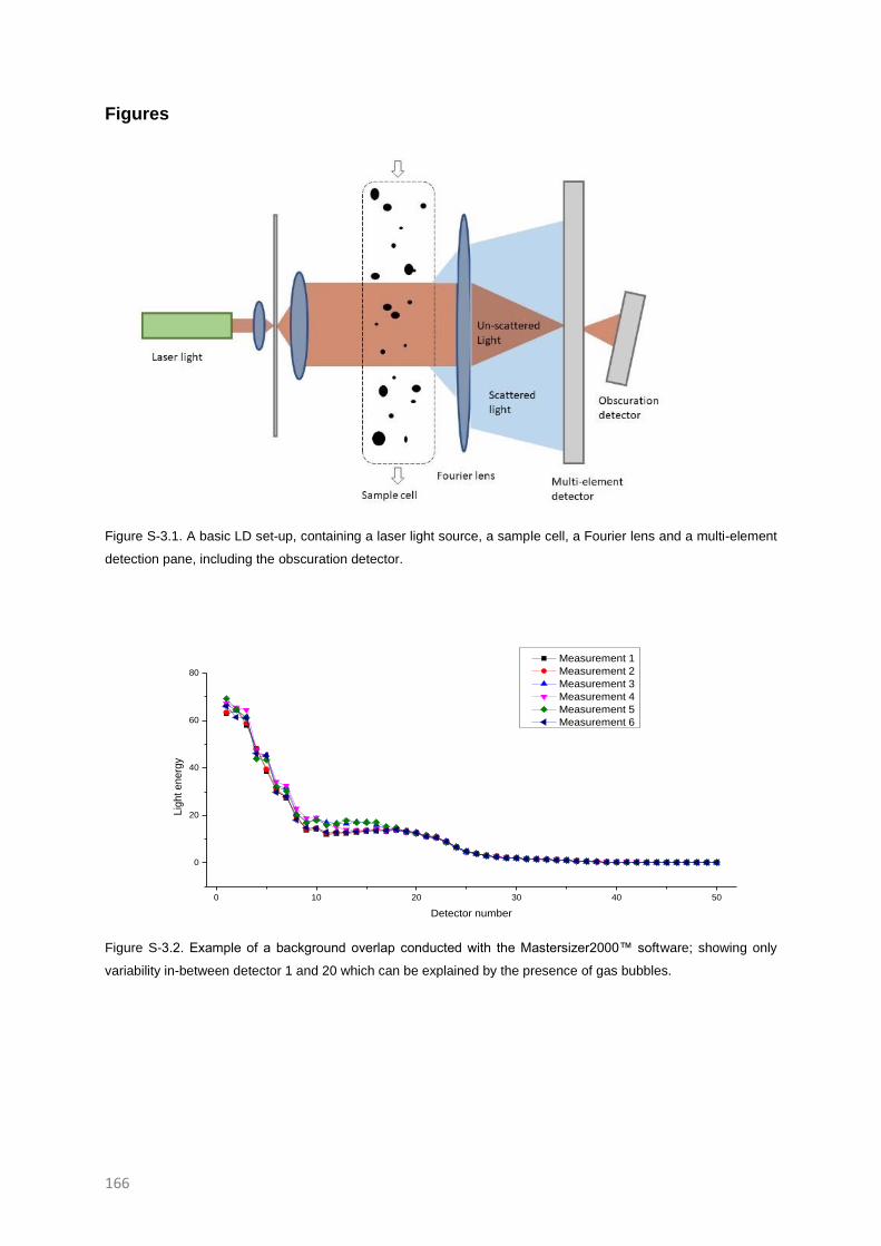
166
Figures
Figure S-3.1. A basic LD set-up, containing a laser light source, a sample cell, a Fourier lens and a multi-element
detection pane, including the obscuration detector.
0 10 20 30 40 50
0
20
40
60
80
Lig
ht e
ne
rgy
Detector number
Measurement 1
Measurement 2
Measurement 3
Measurement 4
Measurement 5
Measurement 6
Figure S-3.2. Example of a background overlap conducted with the Mastersizer2000™ software; showing only
variability in-between detector 1 and 20 which can be explained by the presence of gas bubbles.

167
SUPPLEMENTARY INFORMATION TO CHAPTER 5
Predictive models
Model S-5.1. Predictive model for dv50-value
.

168
Model S-5.2. Predictive model for temperature after milling

169
Model S-5.3. Predictive model for dv90-value

170
Model S-5.4. Predictive model for span
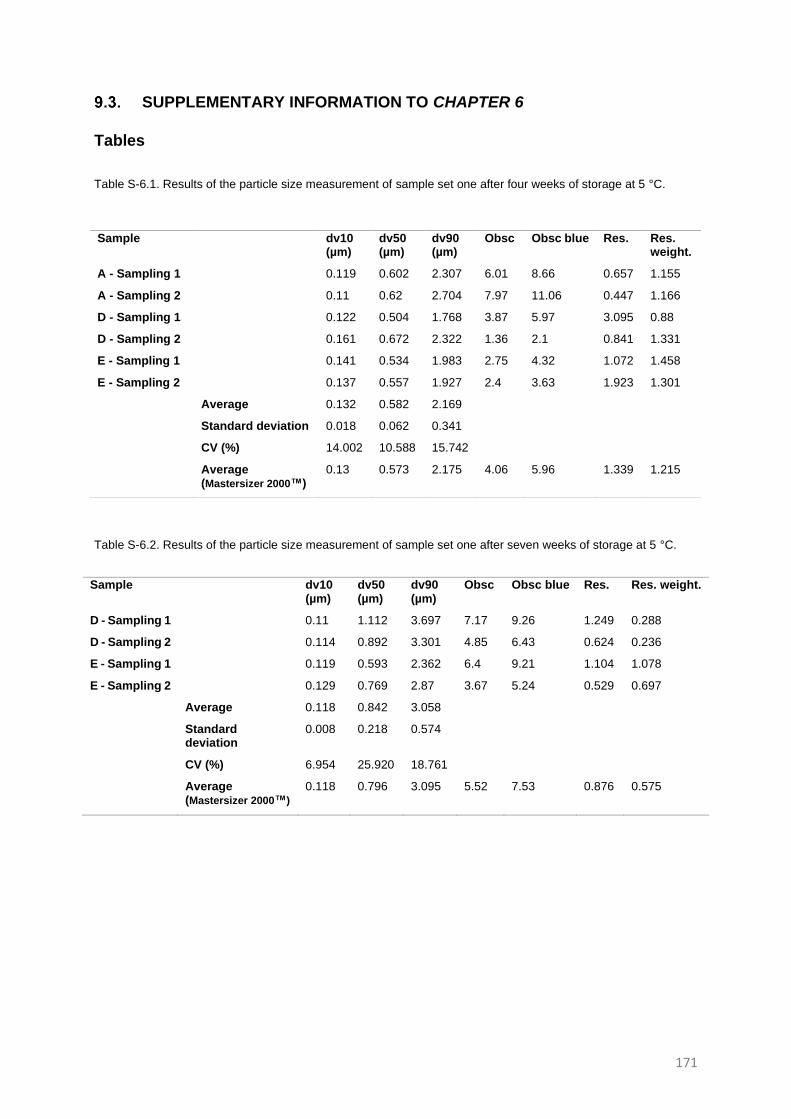
171
SUPPLEMENTARY INFORMATION TO CHAPTER 6
Tables
Table S-6.1. Results of the particle size measurement of sample set one after four weeks of storage at 5 °C.
Table S-6.2. Results of the particle size measurement of sample set one after seven weeks of storage at 5 °C.
Sample
dv10 (µm)
dv50 (µm)
dv90 (µm)
Obsc Obsc blue Res. Res. weight.
D - Sampling 1
0.11 1.112 3.697 7.17 9.26 1.249 0.288
D - Sampling 2
0.114 0.892 3.301 4.85 6.43 0.624 0.236
E - Sampling 1
0.119 0.593 2.362 6.4 9.21 1.104 1.078
E - Sampling 2
0.129 0.769 2.87 3.67 5.24 0.529 0.697
Average 0.118 0.842 3.058
Standard deviation
0.008 0.218 0.574
CV (%) 6.954 25.920 18.761
Average (Mastersizer 2000™)
0.118 0.796 3.095 5.52 7.53 0.876 0.575
Sample
dv10 (µm)
dv50 (µm)
dv90 (µm)
Obsc Obsc blue Res. Res. weight.
A - Sampling 1
0.119 0.602 2.307 6.01 8.66 0.657 1.155
A - Sampling 2
0.11 0.62 2.704 7.97 11.06 0.447 1.166
D - Sampling 1
0.122 0.504 1.768 3.87 5.97 3.095 0.88
D - Sampling 2
0.161 0.672 2.322 1.36 2.1 0.841 1.331
E - Sampling 1
0.141 0.534 1.983 2.75 4.32 1.072 1.458
E - Sampling 2
0.137 0.557 1.927 2.4 3.63 1.923 1.301
Average 0.132 0.582 2.169
Standard deviation 0.018 0.062 0.341
CV (%) 14.002 10.588 15.742
Average (Mastersizer 2000™)
0.13 0.573 2.175 4.06 5.96 1.339 1.215

172
Table S-6.3. Results of the particle size measurement of sample set two after production.
Sample
dv10 (µm)
dv50 (µm)
dv90 (µm)
Obsc Obsc blue Res. Res. weight.
A - Sampling 1
0.107 1.1 3.899 5.19 6.92 1.675 0.291
A - Sampling 2
0.111 1.326 4.256 3.79 4.98 0.692 0.326
B - Sampling 1
0.106 0.767 3.185 5.04 6.97 0.912 0.299
B - Sampling 2
0.109 0.884 3.342 4.04 5.51 3.256 0.272
C - Sampling 1
0.116 0.735 3.07 3.21 4.65 0.449 0.562
C - Sampling 2
0.109 0.91 3.54 4.37 5.85 1.341 0.249
Average 0.110 0.954 3.549
Standard deviation 0.003 0.204 0.414
CV (%) 2.963 21.381 11.660
Average (Mastersizer 2000™)
0.109 0.939 3.568 4.27 5.81 1.388 0.333
Table S-6.4. Results of the particle size measurement of sample set two after three weeks of storage at 5 °C.
Sample
dv10 (µm)
dv50 (µm)
dv90 (µm)
Obsc Obsc blue Res. Res. weight.
A
0.143 0.72 2.471 2.56 3.82 0.559 0.992
B
0.109 0.439 1.612 7.68 12.04 1.699 1.749
C
0.123 0.522 1.779 5.26 8.15 2.789 1.218
Average 0.125 0.560 1.954
Standard deviation 0.017 0.144 0.455
CV (%) 13.670 25.765 23.309
Average (Mastersizer 2000™)
0.122 0.541 1.99 5.17 8 1.682 1.319
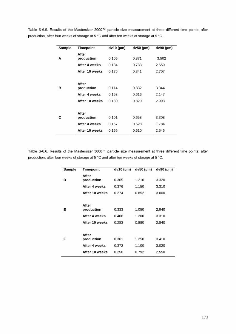
173
Table S-6.5. Results of the Mastersizer 2000™ particle size measurement at three different time points; after
production, after four weeks of storage at 5 °C and after ten weeks of storage at 5 °C.
Sample Timepoint dv10 (µm) dv50 (µm) dv90 (µm)
A After production 0.105 0.871 3.502
After 4 weeks 0.134 0.733 2.650
After 10 weeks 0.175 0.841 2.707
B After production 0.114 0.832 3.344
After 4 weeks 0.153 0.616 2.147
After 10 weeks 0.130 0.820 2.993
C After production 0.101 0.658 3.308
After 4 weeks 0.157 0.528 1.784
After 10 weeks 0.166 0.610 2.545
Table S-6.6. Results of the Mastersizer 3000™ particle size measurement at three different time points: after
production, after four weeks of storage at 5 °C and after ten weeks of storage at 5 °C.
Sample Timepoint dv10 (µm) dv50 (µm) dv90 (µm)
D After production 0.365 1.210 3.320
After 4 weeks 0.376 1.150 3.310
After 10 weeks 0.274 0.852 3.000
E After production 0.333 1.050 2.940
After 4 weeks 0.406 1.200 3.310
After 10 weeks 0.283 0.880 2.840
F After production 0.361 1.250 3.410
After 4 weeks 0.372 1.100 3.020
After 10 weeks 0.250 0.792 2.550
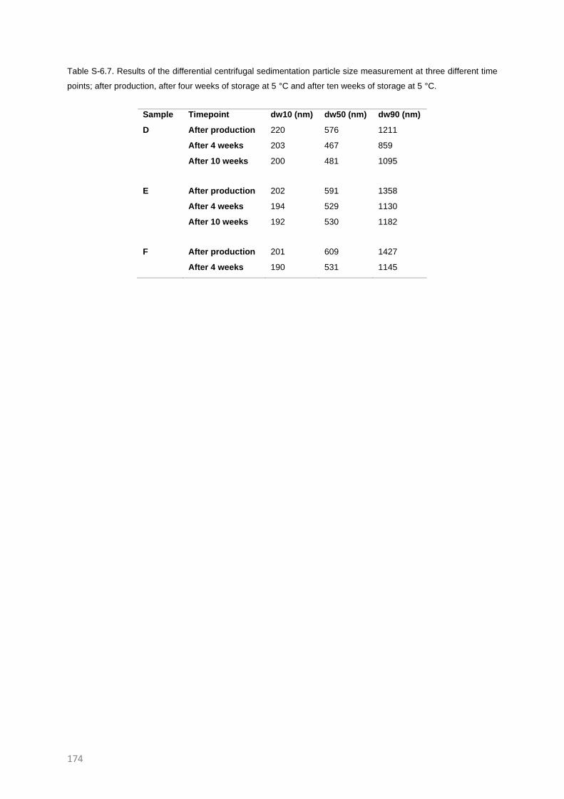
174
Table S-6.7. Results of the differential centrifugal sedimentation particle size measurement at three different time
points; after production, after four weeks of storage at 5 °C and after ten weeks of storage at 5 °C.
Sample Timepoint dw10 (nm) dw50 (nm) dw90 (nm)
D After production 220 576 1211
After 4 weeks 203 467 859
After 10 weeks 200 481 1095
E After production 202 591 1358
After 4 weeks 194 529 1130
After 10 weeks 192 530 1182
F After production 201 609 1427
After 4 weeks 190 531 1145
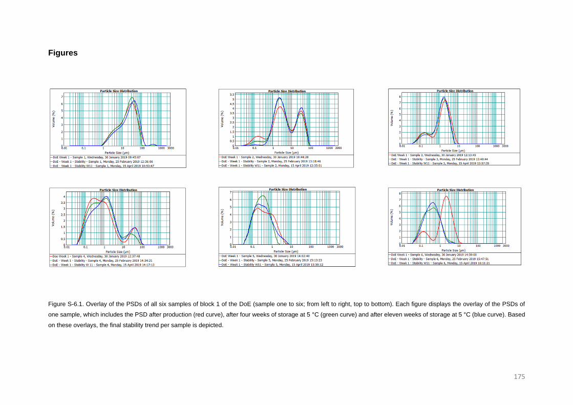
175
Figures
Figure S-6.1. Overlay of the PSDs of all six samples of block 1 of the DoE (sample one to six; from left to right, top to bottom). Each figure displays the overlay of the PSDs of
one sample, which includes the PSD after production (red curve), after four weeks of storage at 5 °C (green curve) and after eleven weeks of storage at 5 °C (blue curve). Based
on these overlays, the final stability trend per sample is depicted.
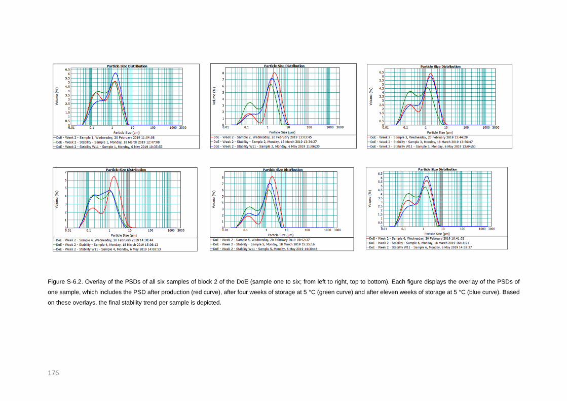
176
Figure S-6.2. Overlay of the PSDs of all six samples of block 2 of the DoE (sample one to six; from left to right, top to bottom). Each figure displays the overlay of the PSDs of
one sample, which includes the PSD after production (red curve), after four weeks of storage at 5 °C (green curve) and after eleven weeks of storage at 5 °C (blue curve). Based
on these overlays, the final stability trend per sample is depicted.

177
Figure S-6.3. Overlay of the PSDs of all six samples of block 3 of the DoE (sample one to six; from left to right, top to bottom). Each figure displays the overlay of the PSDs of
one sample, which includes the PSD after production (red curve), after four weeks of storage at 5 °C (green curve) and after eleven weeks of storage at 5 °C (blue curve). Based
on these overlays, the final stability trend per sample is depicted.
.

178
Figure S-6.4. Overlay of the PSDs of all six samples of block 4 of the DoE (sample one to six: from left to right, top to bottom). Each figure displays the overlay of the PSDs of
one sample, which includes the PSD after production (red curve), after four weeks of storage at 5 °C (green curve) and after eleven weeks of storage at 5 °C (blue curve). Based
on these overlays, the final stability trend per sample is depicted.
.
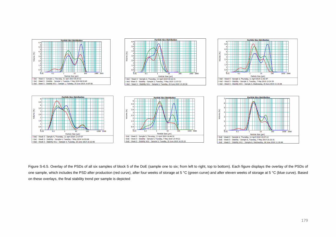
179
Figure S-6.5. Overlay of the PSDs of all six samples of block 5 of the DoE (sample one to six; from left to right, top to bottom). Each figure displays the overlay of the PSDs of
one sample, which includes the PSD after production (red curve), after four weeks of storage at 5 °C (green curve) and after eleven weeks of storage at 5 °C (blue curve). Based
on these overlays, the final stability trend per sample is depicted

180
A POEM ON CHAPTER 5
As science shines in a PhD, we thought that
research should be well communicated
The data of the fifth chapter
were therefore in a poem captivated
Within this poem,
We present a rather new technique
The intensified vibratory mill
A mixing platform in milling streak
By addition of beads in the recipient,
and vertical displacement, labelled as acceleration,
mixing and milling can be achieved,
with as basis: the acoustic vibration
Since earlier research showed its nanosizing potential
though immense heat was generated
We decided to explore
and a design of experiments (DoE) was therefore created
Since heat generation can lead quite quick
to thousand and one physicochemical changes,
and might lead to chemical degradation

181
we start our search for the optimal process parameter ranges
And so were milling time,
bead-suspension ratio, acceleration,
bead size and breaks during milling
the parameters under investigation
As a result, a complex DoE was created,
With which two-way interactions, one three-way interaction
and quadratic effects were going to be rated
Power had to be diminished for some terms.
Nonetheless, we expect
To optimally find the parameters with a significant effect
One finding was the existence of the optimal bead size,
not only for particle size reduction and for contamination,
but also, for the aforementioned,
heat generation
Another conclusion was the next:
To have the API gently reduced,
Increasing milling time is preferred,
as increasing acceleration granted a heat boost

182
Another conclusion is the complexity of the system
which is clearly a fact,
With almost all parameters having
A statistically significant impact
In the prediction expression, is where
All the parameters went,
But, in the end,
a complex mathematical function was generated
with a high (adjusted) determination coefficient
With these prediction expressions,
A new possibility rose: the simulation,
Reducing time, energy and money
are clear advantages in this occasion
Simulated results as a rule of thumb,
will avoid unnecessary experimentation
And can challenge the models’ prediction capacity
as an important evaluation
Finally, visuals extracted out of the DoE
might be handy

183
to find the designs’ sweet spot
Within this rhyme,
no lucky shot,
but only stating that with this DoE,
The possibilities are a lot
Overall, the explosivity of the intensified vibratory mill can so,
Be further explored though not underrated,
But capitulated:
Opportunities such as optimisation and simulation are shown
Even though research is needed for the further unknown

184
185
References
1. Kalepu, S. & Nekkanti, V. Insoluble drug delivery strategies: Review of recent
advances and business prospects. Acta Pharmaceutica Sinica B 5, 442–453
(2015).
2. Lipp, R. The innovator pipeline: Bioavailability challenges and advanced oral
drug delivery opportunities. Am. Pharm. Rev. 16, (2013).
3. Bhakay, A., Merwade, M., Bilgili, E. & Dave, R. N. Novel aspects of wet milling
for the production of microsuspensions and nanosuspensions of poorly water-
soluble drugs. Drug Dev. Ind. Pharm. 37, 963–976 (2011).
4. Burgess, D. J. & Wright, J. C. An Introduction to Long Acting Injections and
Implants. in Long Acting Injections and Implants 1–9 (Springer US, 2012).
doi:10.1007/978-1-4614-0554-2_1
5. Morales, J. O., Watts, A. B. & McConville, J. T. Mechanical Particle-Size
Reduction Techniques. in 133–170 (Springer, New York, NY, 2012).
doi:10.1007/978-1-4614-1144-4_4
6. Jacob, S., Nair, A. B. & Shah, J. Emerging role of nanosuspensions in drug
delivery systems. Biomaterials Research 24, (2020).
7. Kipp, J. E. E. The role of solid nanoparticle technology in the parenteral
delivery of poorly water-soluble drugs. Int. J. Pharm. 284, 109–122 (2004).
8. Remenar, J. F. Making the leap from daily oral dosing to long-acting
injectables: Lessons from the antipsychotics. Mol. Pharm. 11, 1739–1749
(2014).
9. Nanotechnology for Drug Delivery: Global Market for Nanocrystals. Available
at:
https://www.researchandmarkets.com/reports/2124025/nanotechnology_for_dr
ug_delivery_global_market. (Accessed: 27th October 2020)
10. Nanotechnology in Drug Delivery - Global Market Trajectory & Analytics.
Available at:
https://www.researchandmarkets.com/reports/2769238/nanotechnology_in_dru

186
g_delivery_global_market. (Accessed: 27th October 2020)
11. Joachim, C. To be nano or not to be nano? Nature Materials 4, 107–109
(2005).
12. ISO/TR 18401:2017(en), Nanotechnologies — Plain language explanation of
selected terms from the ISO/IEC 80004 series. Available at:
https://www.iso.org/obp/ui/#iso:std:iso:tr:18401:ed-1:v1:en. (Accessed: 4th
November 2020)
13. Shah, S., Date, A. & Holm, R. Strategies for the Formulation Development of
Poorly Soluble Drugs via Oral Route. in 49–89 (John Wiley & Sons, Ltd, 2019).
doi:10.1002/9783527812172.ch2
14. Van Hijfte, L., Marciniak, G. & Froloff, N. Combinatorial chemistry, automation
and molecular diversity: New trends in the pharmaceutical industry. Journal of
Chromatography B: Biomedical Sciences and Applications 725, 3–15 (1999).
15. Bleicher, K. H., Böhm, H.-J., Müller, K. & Alanine, A. I. A guide to drug
discovery: Hit and lead generation: beyond high-throughput screening. Nat.
Rev. Drug Discov. 2, 369–378 (2003).
16. Stewart, K. D. et al. Preference for pharmaceutical formulation and treatment
process attributes. Patient Preference and Adherence 10, 1385–1399 (2016).
17. Amidon, G. L., Lennernäs, H., Shah, V. P. & Crison, J. R. A Theoretical Basis
for a Biopharmaceutic Drug Classification: The Correlation of in Vitro Drug
Product Dissolution and in Vivo Bioavailability. Pharm. Res. An Off. J. Am.
Assoc. Pharm. Sci. 12, 413–420 (1995).
18. Chavda, H. V., Patel, C. N. & Anand, I. S. Biopharmaceutics classification
system. Systematic Reviews in Pharmacy 1, 62–69 (2010).
19. Williams, H. D. et al. Strategies to address low drug solubility in discovery and
development. Pharmacological Reviews 65, 315–499 (2013).
20. Butler, J. M. & Dressman, J. B. The developability classification system:
Application of biopharmaceutics concepts to formulation development. J.
Pharm. Sci. 99, 4940–4954 (2010).

187
21. Rosenberger, J., Butler, J., Muenster, U. & Dressman, J. Application of a
Refined Developability Classification System. J. Pharm. Sci. 108, 1090–1100
(2019).
22. Bosselmann, S. & Williams, R. O. Route-Specific Challenges in the Delivery of
Poorly Water-Soluble Drugs. in 1–26 (Springer, New York, NY, 2012).
doi:10.1007/978-1-4614-1144-4_1
23. Bisrat, M. & Nyström, C. Physicochemical aspects of drug release. VIII. The
relation between particle size and surface specific dissolution rate in agitated
suspensions. International Journal of Pharmaceutics 47, (1988).
24. Kesisoglou, F. & Mitra, A. Crystalline nanosuspensions as potential toxicology
and clinical oral formulations for BCS II/IV Compounds. AAPS J. 14, 677–687
(2012).
25. Sandri, G., Bonferoni, M. C., Rossi, S., Caramella, C. M. & Ferrari, F. Effects of
particle size, surface nature and crystal type on dissolution rate. in AAPS
Advances in the Pharmaceutical Sciences Series 29, 303–328 (Springer
Verlag, 2018).
26. Kaptay, G. On the size and shape dependence of the solubility of nano-
particles in solutions. Int. J. Pharm. 430, 253–257 (2012).
27. Shegokar, R. & Müller, R. H. Nanocrystals: Industrially feasible multifunctional
formulation technology for poorly soluble actives. International Journal of
Pharmaceutics 399, 129–139 (2010).
28. Lippold, B. C. & Ohm, A. Correlation between wettability and dissolution rate of
pharmaceutical powders. Int. J. Pharm. 28, 67–74 (1986).
29. Rabinow, B. E. Nanosuspensions in drug delivery. Nature Reviews Drug
Discovery 3, 785–796 (2004).
30. Müller, R. H., Jacobs, C. & Kayser, O. Nanosuspensions as particulate drug
formulations in therapy: Rationale for development and what we can expect for
the future. Adv. Drug Deliv. Rev. 47, 3–19 (2001).
31. Imono, M. et al. The elucidation of key factors for oral absorption enhancement
of nanocrystal formulations: In vitro–in vivo correlation of nanocrystals. Eur. J.
188
Pharm. Biopharm. 146, 84–92 (2020).
32. Wong, J. et al. Suspensions for intravenous (IV) injection: A review of
development, preclinical and clinical aspects. Advanced Drug Delivery Reviews
60, 939–954 (2008).
33. Merisko-Liversidge, E. & Liversidge, G. G. Nanosizing for oral and parenteral
drug delivery: A perspective on formulating poorly-water soluble compounds
using wet media milling technology. Adv. Drug Deliv. Rev. 63, 427–440 (2011).
34. DeLuca, P.P.; Mansour, H.M.; Rhee, Y.S.; Park, C. W. Sustained-Release
Injectable Drug Delivery. Pharm. Technol. 2010, (2010).
35. Owen, A. & Rannard, S. Strengths, weaknesses, opportunities and challenges
for long acting injectable therapies: Insights for applications in HIV therapy.
Advanced Drug Delivery Reviews 103, 144–156 (2016).
36. Maresova, P. et al. Consequences of chronic diseases and other limitations
associated with old age - A scoping review. BMC Public Health 19, 1431
(2019).
37. Marmora, L. & Gore, C. Intelectual Property Report on Long Acting
Technologies - November 2018. (2018).
38. Brissos, S., Veguilla, M. R., Taylor, D. & Balanzá-Martinez, V. The role of long-
acting injectable antipsychotics in schizophrenia: A critical appraisal.
Therapeutic Advances in Psychopharmacology 4, 198–219 (2014).
39. Rubio, J. M. et al. Psychosis relapse during treatment with long-acting
injectable antipsychotics in individuals with schizophrenia-spectrum disorders:
an individual participant data meta-analysis. The Lancet Psychiatry 7, 749–761
(2020).
40. Morris, M. T. & Tarpada, S. P. Long-acting injectable paliperidone palmitate: A
review of efficacy and safety. Psychopharmacol. Bull. 47, 42–52 (2017).
41. Verma, S., Gokhale, R. & Burgess, D. J. A comparative study of top-down and
bottom-up approaches for the preparation of micro/nanosuspensions. Int. J.
Pharm. 380, 216–222 (2009).
189
42. Fontana, F. et al. Production of pure drug nanocrystals and nano co-crystals by
confinement methods. Adv. Drug Deliv. Rev. 131, 3–21 (2018).
43. Kesisoglou, F., Panmai, S. & Wu, Y. Nanosizing — Oral formulation
development and biopharmaceutical evaluation. Adv. Drug Deliv. Rev. 59,
631–644 (2007).
44. Wu, L., Zhang, J. & Watanabe, W. Physical and chemical stability of drug
nanoparticles. Adv. Drug Deliv. Rev. 63, 456–469 (2011).
45. Malamatari, M., Taylor, K. M. G., Malamataris, S., Douroumis, D. &
Kachrimanis, K. Pharmaceutical nanocrystals: production by wet milling and
applications. Drug Discov. Today 23, 534–547 (2018).
46. Li, M., Azad, M., Davé, R. & Bilgili, E. Nanomilling of Drugs for Bioavailability
Enhancement: A Holistic Formulation-Process Perspective. Pharmaceutics 8,
17 (2016).
47. Verma, S., Kumar, S., Gokhale, R. & Burgess, D. J. Physical stability of
nanosuspensions: Investigation of the role of stabilizers on Ostwald ripening.
Int. J. Pharm. 406, 145–152 (2011).
48. Thanh, N. T. K., Maclean, N. & Mahiddine, S. Mechanisms of Nucleation and
Growth of Nanoparticles in Solution. Chem. Rev. 114, 7610–7630 (2014).
49. Keck, C. M. & Müller, R. H. Drug nanocrystals of poorly soluble drugs produced
by high pressure homogenisation. Eur. J. Pharm. Biopharm. 62, 3–16 (2006).
50. Wang, Y., Zheng, Y., Zhang, L., Wang, Q. & Zhang, D. Stability of
nanosuspensions in drug delivery. J. Control. Release 172, 1126–1141 (2013).
51. Nakach, M., Authelin, J.-R. R., Perrin, M.-A. A. & Lakkireddy, H. R. Comparison
of high pressure homogenization and stirred bead milling for the production of
nano-crystalline suspensions. Int. J. Pharm. 547, 61–71 (2018).
52. Müller, R. & Junghanns. Nanocrystal technology, drug delivery and clinical
applications. Int. J. Nanomedicine 3, 295 (2008).
53. Van Eerdenbrugh, B. et al. Downscaling drug nanosuspension production:
processing aspects and physicochemical characterization. AAPS

190
PharmSciTech 10, 44–53 (2009).
54. Kwade, A. Wet Comminution In Stirred Media Mills - research and its practical
application. Powder Technol. 105, 14–20 (1992).
55. Afolabi, A., Akinlabi, O. & Bilgili, E. Impact of process parameters on the
breakage kinetics of poorly water-soluble drugs during wet stirred media
milling: A microhydrodynamic view. Eur. J. Pharm. Sci. 51, 75–86 (2014).
56. Peltonen, L. Design space and QbD approach for production of drug
nanocrystals by wet media milling techniques. Pharmaceutics 10, 104 (2018).
57. Li, M., Alvarez, P. & Bilgili, E. A microhydrodynamic rationale for selection of
bead size in preparation of drug nanosuspensions via wet stirred media milling.
Int. J. Pharm. 524, 178–192 (2017).
58. Eskin, D., Zhupanska, O., Hamey, R., Moudgil, B. & Scarlett, B.
Microhydrodynamic analysis of nanogrinding in stirred media mills. AIChE J.
51, 1346–1358 (2005).
59. Eskin, D., Zhupanska, O., Hamey, R., Moudgil, B. & Scarlett, B.
Microhydrodynamics of stirred media milling. in Powder Technology 156, 95–
102 (2005).
60. Flach, F., Breitung-Faes, S. & Kwade, A. Model based process optimization of
nanosuspension preparation via wet stirred media milling. Powder Technol.
331, 146–154 (2018).
61. Kwade, A. & Schwedes, J. Breaking characteristics of different materials and
their effect on stress intensity and stress number in stirred media mills. Powder
Technol. 122, (2002).
62. Leung, D. H. et al. A new and improved method for the preparation of drug
nanosuspension formulations using acoustic mixing technology. Int. J. Pharm.
473, 10–19 (2014).
63. Li, M., Zhang, L., Davé, R. N. & Bilgili, E. An Intensified Vibratory Milling
Process for Enhancing the Breakage Kinetics during the Preparation of Drug
Nanosuspensions. AAPS PharmSciTech 17, 389–399 (2016).

191
64. Kotter, L. N. & Groven, L. J. Milling of Energetic Crystals with the LabRAM.
Propellants, Explos. Pyrotech. 44, 908–914 (2019).
65. Rexroth Corporation, B. Bosch Rexroth Resodyn RAM 5 success story.
66. Lu, H. D., D Aquino, J. A., Caruso, J., Ghosh, A. & Lohani, S. Application of
Acoustic- Vibratory Milling For Screening and Scale-Up of Micro/
Nanosuspensions in Early Drug Discovery and Development. J. Pharm. Drug
Deliv. Res. 07, (2018).
67. Saveyn, H., Mermuys, D., Thas, O. & van der Meeren, P. Determination of the
Refractive Index of Water-dispersible Granules for Use in Laser Diffraction
Experiments. Part. Part. Syst. Charact. 19, 426–432 (2002).
68. Zhang, X., Li, L. C. & Mao, S. Nanosuspensions of Poorly Water Soluble Drugs
Prepared by Top-down Technologies. Curr. Pharm. Des. 20, 388–407 (2014).
69. Lakshmi, P. & Kumar, G. A. Nano-suspension technology: A review. Int. J.
Pharm. Pharm. Sci. 2, 35–40 (2010).
70. Lestari, M. L. A. D., Müller, R. H. & Möschwitzer, J. P. Systematic Screening of
Different Surface Modifiers for the Production of Physically Stable
Nanosuspensions. J. Pharm. Sci. 104, 1128–1140 (2015).
71. Rawle, A. Basic principles of particle size analysis. Available at:
http://www.rci.rutgers.edu/~moghe/PSD Basics.pdf. (Accessed: 21st January
2018)
72. Erdoǧan, S. T. et al. Shape and size of microfine aggregates: X-ray
microcomputed tomography vs. laser diffraction. Powder Technol. 177, 53–63
(2007).
73. Keck, C. M. & Müller, R. H. Size analysis of submicron particles by laser
diffractometry—90% of the published measurements are false. Int. J. Pharm.
355, 150–163 (2008).
74. Kelly, R. N. & Etzler, F. M. What is wrong with laser diffraction? A Critical
Review of Current Laser Diffraction Methods for Particle Size Analysis.
Available at: http://www.donner-tech.com/whats_wrong_with_ld.pdf.
(Accessed: 22nd January 2018)

192
75. Beekman, A. et al. Micrometer-Scale Particle Sizing by Laser Diffraction:
Critical Impact of the Imaginary Component of Refractive Index. Pharm. Res.
22, 518–522 (2005).
76. Horiba. Technical Note: LA-950 Series Particle Size Distribution Analyzer
Understanding the Chi Square and R Parameter Calculations in the LA-950
Software.
http://www.horiba.com/fileadmin/uploads/Scientific/Documents/PSA/TN153.pdf
Available at:
http://www.horiba.com/fileadmin/uploads/Scientific/Documents/PSA/TN153.pdf.
(Accessed: 27th November 2018)
77. Horiba. Technical note: Effect of concentration on laser diffraction
measurements. (2010). Available at: www.horibalab.com. (Accessed: 27th
November 2018)
78. Malvern Instruments Ltd. Wet or liquid dispersion method development for
laser diffrraction particle size measurements. Available at:
https://warwick.ac.uk/fac/cross_fac/sciencecity/programmes/internal/themes/a
m2/booking/particlesize/wet_dispersion_application_note.pdf. (Accessed: 23rd
January 2018)
79. Malvern Instruments Ltd. Transferring methods from the Mastersizer 2000 to
the Mastersizer 3000 laser diffraction particle size analyzer. Available at:
https://www.malvern.com/en/support/resource-center/technical-
notes/TN130912TransferingMethodsMastersizer.html. (Accessed: 23rd
January 2018)
80. Malvern Instruments Ltd. Technical note: Selecting an appropiate particle
absorption for laser diffraction particle size calculations. Available at:
https://www.malvern.com/en/support/resource-center/technical-
notes/TN101104SelectingParticleAbsorbtionLaserDiffractio.html. (Accessed:
23rd January 2018)
81. Storey, R. A. & Ymen, I. Solid state characterization of pharmaceuticals. in
Solid state characterization of pharmaceuticals: 9.4.5 Measuring the Refractive
Indices of Solids (New Jersey; John Wiley & Sons, 2011).
193
82. Evans, M., Han, L., Ratcliffe, I. & Williams, P. A. Synthesis, characterisation
and properties of novel biosurfactants based on hydrophobically-modified
inulins. in Gums and Stabilisers for the Food Industry 18: Hydrocolloid
Functionality for Affordable and Sustainable Global Food Solutions (eds. A.
Williams, P. & O. Phillip, G.) 129 (2016).
83. Singh, M. S. & Lamprecht, A. P-glycoprotein inhibition of drug resistant cell
lines by nanoparticles. Drug Dev. Ind. Pharm. 42, 325–331 (2016).
84. Thermo Fisher Scientific. Sodium Dodecyl Sulfate (SDS), Lauryl - Safety data
sheet. Available at: https://www.thermofisher.com/order/catalog/product/28364.
(Accessed: 23rd January 2018)
85. Guo, Y., Luo, J., Tan, S., Otieno, B. O. & Zhang, Z. The applications of Vitamin
E TPGS in drug delivery. Eur. J. Pharm. Sci. 49, 175–186 (2013).
86. Malvern Instruments Ltd. Technical notes: Empirical methods for selecting an
appropiate refractive index for laser diffraction particle size calculations. (2007).
Available at: https://www.malvern.com/en/support/resource-center/technical-
notes/in-progress/TN101104SelectingRefractiveIndexParticleSize.html.
(Accessed: 30th January 2018)
87. Van Eerdenbrugh, B. et al. Drying of crystalline drug nanosuspensions—The
importance of surface hydrophobicity on dissolution behavior upon
redispersion. Eur. J. Pharm. Sci. 35, 127–135 (2008).
88. Virden, A. Method Development for Laser-Diffraction Particle-Size Analysis.
PharmTech 34, 100–106 (2010).
89. Michalchuk, A. A. L., Tumanov, I. A. & Boldyreva, E. V. The effect of ball mass
on the mechanochemical transformation of a single-component organic
system: anhydrous caffeine. J. Mater. Sci. 53, 13380–13389 (2018).
90. Osorio, J. G. & Muzzio, F. J. Evaluation of resonant acoustic mixing
performance. Powder Technol. 278, 46–56 (2015).
91. Na, G. C. et al. Cloud point of nonionic surfactants: modulation with
pharmaceutical excipients. Pharm. Res. 16, 562–568 (1999).
92. Reijenga, J., van Hoof, A., van Loon, A. & Teunissen, B. Development of

194
methods for the determination of pKa values. Analytical Chemistry Insights 8,
53–71 (2013).
93. Colombo, M., Minussi, C., Orthmann, S., Staufenbiel, S. & Bodmeier, R.
Preparation of amorphous indomethacin nanoparticles by aqueous wet bead
milling and in situ measurement of their increased saturation solubility. Eur. J.
Pharm. Biopharm. 125, 159–168 (2018).
94. Sommer, M., Stenger, F., Peukert, W. & Wagner, N. J. Agglomeration and
breakage of nanoparticles in stirred media mills-a comparison of different
methods and models. Chem. Eng. Sci. 61, 135–148 (2006).
95. De Cleyn, E., Holm, R. & Van den Mooter, G. Size Analysis of Small Particles
in Wet Dispersions by Laser Diffractometry: A Guidance to Quality Data. J.
Pharm. Sci. 108, 1905–1914 (2019).
96. Durga Maheswari, P., Rambhau, D. & Narasu, M. L. Micellar Solubilization in
the Formulation Development of Poorly Soluble Naproxen. Pharm. Regul. Aff.
Open Access 02, 1–12 (2013).
97. Besson, U. The History of the Cooling Law: When the Search for Simplicity can
be an Obstacle. Sci. Educ. 21, 1085–1110 (2012).
98. Hagedorn, M., Bögershausen, A., Rischer, M., Schubert, R. & Massing, U. Dual
centrifugation – A new technique for nanomilling of poorly soluble drugs and
formulation screening by an DoE-approach. Int. J. Pharm. 530, 79–88 (2017).
99. Malamatari, M., Somavarapu, S., Taylor, K. M. G. & Buckton, G. Solidification
of nanosuspensions for the production of solid oral dosage forms and inhalable
dry powders. Expert Opinion on Drug Delivery 13, 435–450 (2016).
100. Sigfridsson, K., Rydberg, H. & Strimfors, M. Nano- and microcrystals of
griseofulvin subcutaneously administered to rats resulted in improved
bioavailability and sustained release. Drug Dev. Ind. Pharm. 45, 1477–1486
(2019).
101. Resodyn acoustic mixers. No Title. in Technical InterChange 2018 (2018).
102. Raasch, J. Trajectories and impact velocities of grinding bodies in planetary
ball mills. Chem. Eng. Technol. 15, 245–253 (1992).
195
103. Blecher, L., Kwade, A. & Schwedes, J. Motion and stress intensity of grinding
beads in a stirred media mill. Part 1 : Energy density distribution and motion of
single grinding beads. Powder Technol. 86, 59–68 (1996).
104. De Cleyn, E., Holm, R. & Van den Mooter, G. Exploration of the heat
generation within the intensified vibratory mill. Int. J. Pharm. 587, 119644
(2020).
105. de Aguiar, P. F., Bourguignon, B., Khots, M. S., Massart, D. L. & Phan-Than-
Luu, R. D-optimal designs. Chemom. Intell. Lab. Syst. 30, 199–210 (1995).
106. Jensen, W. A. Open problems and issues in optimal design. Qual. Eng. 30,
583–593 (2018).
107. Ghosh, I., Bose, S., Vippagunta, R. & Harmon, F. Nanosuspension for
improving the bioavailability of a poorly soluble drug and screening of
stabilizing agents to inhibit crystal growth. Int. J. Pharm. 409, 260–268 (2011).
108. Joshi, V., Dwivedi, S. & Ward, G. H. Increase in the specific surface area of
budesonide during storage postmicronization. Pharm. Res. 19, 7–12 (2002).
109. Ariyaprakai, S. & Dungan, S. R. Influence of surfactant structure on the
contribution of micelles to Ostwald ripening in oil-in-water emulsions. J. Colloid
Interface Sci. 343, 102–108 (2009).
110. Nyqvist, H. & Wadsten, T. Can ageing effects in drugs be measured and
interpreted by ta-techniques? Thermochim. Acta 93, 125–127 (1985).
111. Shimpi, J. R., Sidhaye, D. S. & Prasad, B. L. V. Digestive Ripening: A Fine
Chemical Machining Process on the Nanoscale. Langmuir 33, 9491–9507
(2017).
112. Burlakov, V. M. et al. Reversing Ostwald Ripening. arxiv.org (2014).
113. Burlakov, V. M. & Goriely, A. Reverse coarsening and the control of particle
size distribution through surfactant. Appl. Sci. 10, 5359 (2020).
114. Lee, D. K., Park, S. Il, Lee, J. K. & Hwang, N. M. A theoretical model for
digestive ripening. Acta Mater. 55, 5281–5288 (2007).
115. Shah, U. V. et al. Effect of milling temperatures on surface area, surface
196
energy and cohesion of pharmaceutical powders. Int. J. Pharm. 495, 234–240
(2015).
116. Chu, J. J. & Steeves, C. A. Thermal expansion and recrystallization of
amorphous Al and Ti: A molecular dynamics study. J. Non. Cryst. Solids 357,
3765–3773 (2011).
117. Kayaert, P. & Van Den Mooter, G. Is the amorphous fraction of a dried
nanosuspension caused by milling or by drying? A case study with Naproxen
and Cinnarizine. Eur. J. Pharm. Biopharm. 81, 650–656 (2012).
118. Kumar, S. & Burgess, D. J. Wet milling induced physical and chemical
instabilities of naproxen nano-crystalline suspensions. Int. J. Pharm. 466, 223–
232 (2014).
119. Pas, T. et al. Mechanodegradation of Polymers: A Limiting Factor of
Mechanochemical Activation in the Production of Amorphous Solid Dispersions
by Cryomilling. Mol. Pharm. 17, 2987–2999 (2020).
120. Monteiro, A., Afolabi, A. & Bilgili, E. Continuous production of drug nanoparticle
suspensions via wet stirred media milling: A fresh look at the Rehbinder effect.
Drug Dev. Ind. Pharm. 39, 266–283 (2013).
121. Erik Kissa. 7.I.C. Effect of dispersant on communition. in Dispersions:
Characterization, Testing, and Measurement - (ed. Kissa, E.) (1999).
122. Higgins, J. D. & Leung, D. A New and Versatile Method for Preparing Drug
Nanoparticle Formulations for Enhancing Bioperformance. TechConnect Briefs
3. Biotech, 68–70 (2015).
123. Chen, L. et al. Fine grade engineered microcrystalline cellulose excipients for
direct compaction: Assessing suitability of different dry coating processes. Eur.
J. Pharm. Sci. 151, 105408 (2020).
124. Am Ende, D. J., Anderson, S. R. & Salan, J. S. Development and Scale-Up of
Cocrystals Using Resonant Acoustic Mixing. Org. Process Res. Dev. 18, 331–
341 (2014).
125. Hennart, S. L. A. et al. Particle Size Characterization of an Extra Fine Milled
Product. Part. Part. Syst. Charact. 29, 285–303 (2012).

197
126. Chen, S., Sheikh, A. Y. & Ho, R. Evaluation of effects of pharmaceutical
processing on structural disorders of active pharmaceutical ingredient crystals
using nanoindentation and high-resolution total scattering pair distribution
function analysis. J. Pharm. Sci. 103, 3879–3890 (2014).
127. Maughan, M. R., Carvajal, M. T. & Bahr, D. F. Nanomechanical testing
technique for millimeter-sized and smaller molecular crystals. Int. J. Pharm.
486, 324–330 (2015).
128. Aleandri, S., Schönenberger, M., Niederquell, A. & Kuentz, M. Temperature-
Induced Surface Effects on Drug Nanosuspensions. Pharm. Res. 35, (2018).
129. Cares-Pacheco, M. G., Calvet, R., Vaca-Medina, G., Rouilly, A. & Espitalier, F.
Inverse gas chromatography a tool to follow physicochemical modifications of
pharmaceutical solids: Crystal habit and particles size surface effects. Int. J.
Pharm. 494, 113–126 (2015).
130. Bond, L. et al. Differential scanning calorimetry and scanning thermal
microscopy analysis of pharmaceutical materials. Int. J. Pharm. 243, 71–82
(2002).
131. Harding, L., King, W. P., Dai, X., Craig, D. Q. M. & Reading, M. Nanoscale
characterisation and imaging of partially amorphous materials using local
thermomechanical analysis and heated tip AFM. Pharm. Res. 24, 2048–2054
(2007).
132. Barnes, T. J., Kempson, I. M. & Prestidge, C. A. Surface analysis for
compositional, chemical and structural imaging in pharmaceutics with mass
spectrometry: A ToF-SIMS perspective. Int. J. Pharm. 417, 61–69 (2011).

Contributions
Scientific acknowledgements
Within the own KU Leuven department, Bernard Appeltans is acknowledged for the
technical support in the laboratory. Elene De Cleyn acknowledges Janssen
Pharmaceutica for the usage of their facilities; mainly within the laboratory “Parenterals
and Liquids”. Within Janssen Pharmaceutica, the following persona are acknowledged
for the provided trainings and follow-up guidance: Jasmine Bogaerts (Technical
support in the laboratory), Maxim Verstraeten (Proofreading), Christopher De
Dobbelaere (mDSC), Jasper Jammaer and Linda Lauwerysen (LD), Alain Collas,
Brecht De Fre and Steve De Cort (SEM) and Tatsiana Khamiakova (DoE and
statistics).
Personal contributions
Elene De Cleyn conceptualised, scheduled, executed and written all experiments, data
and texts included in this thesis, with following exceptions:
• For Chapter 5, Tatsiana Khamiakova gave advice on the set-up of the Design
of Experiments, the statistical analysis and data interpretation. She applied
Bayesian statistics and provided the figures concerning Bayesian statistics in
chapter 5. She reviewed the related article, prior to publication.
• For Chapter 6, LD measurements with the Mastersizer 3000™ were performed
by Divya Bahadur and particle size measurements with differential centrifugal
sedimentation by Linda Lauwerysen.
Guy Van den Mooter and René Holm were the promotors of this PhD project and
helped to develop a research strategy and design the experiments. They reviewed and
edited the text of the given dissertation and the articles generated during this PhD
project.
Conflicts of interest statement
The authors would like to acknowledge Janssen Pharmaceutica for their financial
support. Apart from this acknowledgement, the authors declare no conflict of interest.


Curriculum Vitae
Education
2017 – present: Doctoral Training in Pharmaceutical Sciences (KU Leuven, BE,
Janssen Pharmaceutica, BE)
2016 - 2017: Advanced master’s in industrial pharmacy (KU Leuven, U Antwerpen, U
Gent, VU Brussel, BE)
Research topic (TCD Dublin, IE): “Establishing and using USP apparatus 4,
dissolution simulation and shadowgraph imaging to interpret dissolution profiles
of ibuprofen particles with varying sizes and morphologies”
2015 - 2016: Management: Preparatory programme (VU Brussel, BE)
2013 - 2015: Master of Science in Drug Development, specialisation in pharmacy (KU
Leuven, BE)
Research topic (U Liège, BE): “Development of an analytical method for the
determination of human insulin in medicinal products by micellar electrokinetic
chromatography”
2010 - 2013: Bachelor of Pharmaceutical Sciences (KU Leuven, BE)
Scientific Publications
• De Cleyn, E., Holm, R., Khamiakova, T. & Van den Mooter, G. Picking up good
vibrations: Exploration of the intensified vibratory mill via a modern Design of
Experiments. Int. J. Pharm. 120367 (2021). doi: 10.1016/j.ijpharm.2021.120367
• De Cleyn, E., Holm, R. & Van den Mooter, G. Exploration of the heat generation
within the intensified vibratory mill. Int. J. Pharm. 119644 (2020).
doi:10.1016/j.ijpharm.2020.119644
• De Cleyn, E., Holm, R. & Van den Mooter, G. Size Analysis of Small Particles
in Wet Dispersions by Laser Diffractometry: A Guidance to Quality Data. J.
Pharm. Sci. (2019). doi: 10.1016/j.xphs.2018.12.010

Presentations at (inter)national meetings
Poster presentations
• “Size analysis of small particles in wet dispersion by laser diffractometry: A
guidance to quality data”, ULLA Summer School, Helsinki, 04 Jul 2019
• “Size analysis of small particles in wet dispersion by laser diffractometry: A
guidance to quality data”, 4th Spring Symposium, Leuven, 03 May 2019
Oral presentations
• “Picking up good vibrations: The intensified vibratory mill via a modern design
of experiments approach”, PSSRC Annual Meeting Online, 23 June 2020
• “Size analysis of small particles in wet dispersion by laser diffractometry: A
guidance to quality data”, 20th forum of BSPS (Belgian Society of
Pharmaceutical Sciences), 20 May 2019