Tobin2014.pdf - New Mexico Tech
93
Dedicated to my parents for their unending support in all capacities, and for not rubbing it in too hard when I finally proved that our family really is made up entirely of engineers. You’ve been on my side since the beginning and I can’t thank you enough for it. J. D. Tobin New Mexico Institute of Mining and Technology August, 2014
-
Upload
khangminh22 -
Category
Documents
-
view
2 -
download
0
Transcript of Tobin2014.pdf - New Mexico Tech

Dedicated to my parents for their unending support in all capacities, and for notrubbing it in too hard when I finally proved that our family really is made upentirely of engineers. You’ve been on my side since the beginning and I can’t
thank you enough for it.
J. D. TobinNew Mexico Institute of Mining and Technology
August, 2014

QUANTITATIVE SCHLIEREN MEASUREMENT OFEXPLOSIVELY-DRIVEN SHOCK WAVE DENSITY,
TEMPERATURE, AND PRESSURE PROFILES.
by
J. D. Tobin
Submitted in Partial Fulfillmentof the Requirements for the Degree of
Master of Science in Mechanical Engineeringwith Specialization in Explosives Engineering
New Mexico Institute of Mining and TechnologySocorro, New Mexico
August, 2014

ABSTRACT
Shock waves produced from the detonation of small explosives are char-acterized using the high-speed schlieren imaging technique. Results are used todetermine quantitative and qualitative information about the shocks characteris-tics. The refractive index gradient field is extracted from successive images andconverted to a density field using the Abel deconvolution method. The densityfield was used to determine shock overpressure and overpressure duration be-hind the shock wave. This analysis used a weak lens, which provided a knowncalibration to convert the images pixel intensities into refractive index gradientvalues. The tests performed used three types of explosive compounds: shotgunshell primers, NONEL shock tube, and Detasheet. The analysis only consideredtime periods where the shock was clearly separated from the detonation gasesand free of any explosively-propelled fragments. Several different temperatureprofiles were used to determine the pressure field using the ideal gas law. Thehydrocode CTH, developed by Sandia National Laboratories, was used to deter-mine a temperature profile, which was also used to calculate the pressure field.Results showed the ability to accurately measure the pressure profile of a shockwave optically using a quantitative schlieren technique. The use of a temperaturedecay profile as predicted from CTH was observed to yield the most accurate op-tical pressure data compared to piezoelectric pressure gage data.
Keywords: EXPLOSIVES; SHOCK WAVES; SCHLIEREN IMAGING; PRESSUREPROFILE; TEMPERATURE PROFILE; DENSITY PROFILE; ABEL INVERSIONMETHOD
CONTENTS
LIST OF FIGURES iv
1. INTRODUCTION 11.1 Motivation . . . . . . . . . . . . . . . . . . . . . . . . . . . . . . . . . 11.2 Literature Review . . . . . . . . . . . . . . . . . . . . . . . . . . . . . 1
1.2.1 Shock Waves . . . . . . . . . . . . . . . . . . . . . . . . . . . 11.2.2 Traditional Pressure Measurement Techniques . . . . . . . . 21.2.3 Optical Techniques . . . . . . . . . . . . . . . . . . . . . . . . 41.2.4 Objectives . . . . . . . . . . . . . . . . . . . . . . . . . . . . . 5
2. EXPERIMENTAL METHODS 62.1 High-Speed Imaging . . . . . . . . . . . . . . . . . . . . . . . . . . . 62.2 Schlieren Imaging Technique . . . . . . . . . . . . . . . . . . . . . . 7
2.2.1 Dual-Field-Lens Schlieren Setup . . . . . . . . . . . . . . . . 72.3 Quantitative Schlieren Imaging . . . . . . . . . . . . . . . . . . . . . 9
2.3.1 General Principles of Light Refraction . . . . . . . . . . . . . 92.3.2 General Process for Determining the Density Field . . . . . . 12
2.4 Explosive Material . . . . . . . . . . . . . . . . . . . . . . . . . . . . 142.5 Pressure Gage Measurements . . . . . . . . . . . . . . . . . . . . . . 142.6 Shock Wave Imaging . . . . . . . . . . . . . . . . . . . . . . . . . . . 17
2.6.1 Digital Image Processing for Pressure Measurement . . . . . 182.6.2 Abel Deconvolution Process . . . . . . . . . . . . . . . . . . . 20
3. FLAT PLATE ANALYSIS 24
4. CTH MODELING 27
ii

5. EXPERIMENTAL RESULTS 385.1 Temperature Calculations from Optical Measurements . . . . . . . 38
5.1.1 Shot Shell Primers . . . . . . . . . . . . . . . . . . . . . . . . 385.1.2 NONEL Shock Tube . . . . . . . . . . . . . . . . . . . . . . . 485.1.3 Detasheet . . . . . . . . . . . . . . . . . . . . . . . . . . . . . 57
5.2 Pressure Calculations from Optical Measurements . . . . . . . . . . 665.2.1 Shot Shell Primers . . . . . . . . . . . . . . . . . . . . . . . . 665.2.2 NONEL Shock Tube . . . . . . . . . . . . . . . . . . . . . . . 695.2.3 Detasheet . . . . . . . . . . . . . . . . . . . . . . . . . . . . . 725.2.4 Intensity Corrections . . . . . . . . . . . . . . . . . . . . . . . 74
6. CONCLUSIONS AND RECOMMENDATIONS FOR FUTURE RESEARCH 786.1 Future Work . . . . . . . . . . . . . . . . . . . . . . . . . . . . . . . . 79
BIBLIOGRAPHY 80
iii

LIST OF FIGURES
1.1 Idealized pressure profile denoting peak overpressure and pres-sure duration, including negative pulse. . . . . . . . . . . . . . . . . 2
1.2 Schematic of dual-field-lens arrangement. . . . . . . . . . . . . . . . 4
2.1 Schematic of dual-field-lens arrangement with area highlighted de-noting placement of explosives (shotshell primers, NONEL shocktube, or Detasheet). . . . . . . . . . . . . . . . . . . . . . . . . . . . . 8
2.2 Diagram of light refraction through some schlieren object centeredin the dual-field-lens schlieren setup. . . . . . . . . . . . . . . . . . . 9
2.3 A) shows a diagram of light refraction through positive lens inthe dual-field-lens schlieren setup; b) shows gradients across twolenses of 10m (on the left) and 4m focal lengths; c) shows an aver-age of three horizontal rows of pixels taken from the center of thetwo lens. . . . . . . . . . . . . . . . . . . . . . . . . . . . . . . . . . . 11
2.4 Calibration lens intensity and specific physical location with 5th-order polynomial fit. . . . . . . . . . . . . . . . . . . . . . . . . . . . 13
2.5 Piezoelectric gage location within dual-field-lens schlieren setup.The gage is secured within an aluminum plate. The edge of theplate is diagonally cut to allow shock to travel over top surfacewithout reflecting off plate surface. In this orientation, the shockwill be coming from the right. . . . . . . . . . . . . . . . . . . . . . . 16
2.6 Standard pressure trace from the detonation of Detasheet using 50psi piezoelectric gage for data collection. . . . . . . . . . . . . . . . . 17
2.7 Example of shock track routine using a non-sequential series of im-ages from the detonation of NONEL. Time step between sequen-tial images is 8.3µs. The white line is generated by the trackingprogram; the black line is the shock imaged by the dual-field-lensschlieren setup, though it is mostly obscured by the tracking pro-gram. The program tracks backwards in time towards the detona-tion center. Note the subsequent misalignment of the shock track-ing line and the shock profile; this is caused by purposefully incor-rect placement of the charge center. Images are not sequential. . . . 19
2.8 Row of pixel intensities across a shock from the detonation of NONEL. 21
3.1 Setup of heated flat plate. . . . . . . . . . . . . . . . . . . . . . . . . 25
iv

3.2 Comparison of flat plate temperature profiles of theoretical and ex-perimental measurements. Uncertainty of experimental tempera-ture is ± 2K, denoted by the size of the data points (blue). . . . . . . 26
4.1 Schematic of CTH model. PETN is in gray, tracers in yellow. Totalregion modeled extends to 2m. . . . . . . . . . . . . . . . . . . . . . 27
4.2 CTH pressure output of 1g PETN detonation, 10cm, 44cm, and 90cmfrom charge center. . . . . . . . . . . . . . . . . . . . . . . . . . . . . 29
4.3 Logarithmic scale of CTH pressure output of 1g PETN detonation,10cm, 44cm, and 90cm from charge center. . . . . . . . . . . . . . . . 30
4.4 CTH temperature output of 1g PETN detonation, 10cm, 44cm, and90cm from charge center. . . . . . . . . . . . . . . . . . . . . . . . . . 31
4.5 Logarithmic scale of CTH temperature output of 1g PETN detona-tion, 10cm, 44cm, and 90cm from charge center. . . . . . . . . . . . . 32
4.6 Normalized CTH output of 1g PETN detonation, 10cm from chargecenter. . . . . . . . . . . . . . . . . . . . . . . . . . . . . . . . . . . . . 33
4.7 Normalized CTH output of 1g PETN detonation, 44cm from chargecenter. . . . . . . . . . . . . . . . . . . . . . . . . . . . . . . . . . . . . 34
4.8 Normalized CTH output of 1g PETN detonation, 90cm from chargecenter. . . . . . . . . . . . . . . . . . . . . . . . . . . . . . . . . . . . . 35
4.9 Scaled CTH output of 1g PETN detonation, 44cm from charge center. 36
5.1 Detonation of shotshell primer. Distance across field-of-view (lightgray circle) in lens is 0.1524m. . . . . . . . . . . . . . . . . . . . . . . 39
5.2 Oblique shocks forming from fragmentation before shock. . . . . . 395.3 Shock Mach number from the detonation of shot shell primer. . . . 405.4 Streak image and single image of shot shell primer fired at a 45
degree angle. Vertical time step in streak image is 8.33µs, distanceacross field of view (gray background) is 0.0254m. . . . . . . . . . . 41
5.5 Pixel intensity across shock front. . . . . . . . . . . . . . . . . . . . . 415.6 Gage pressure profile. Highlighted portion (red) used to determine
temperature. Distance from primer face to gage is 0.165m. . . . . . 435.7 Optical density profile created using Abel deconvolution. High-
lighted portion (red) used to determine temperature. . . . . . . . . 445.8 Compilation of temperature profiles from detonation of shot shell
primers. . . . . . . . . . . . . . . . . . . . . . . . . . . . . . . . . . . 455.9 Linear approximation (red) of CTH temperature profile. . . . . . . . 465.10 Peak and atmospheric points used to create linear temperature fit
from density profile. . . . . . . . . . . . . . . . . . . . . . . . . . . . 475.11 Comparison of linear approximations of temperature profile. . . . . 48
v
5.12 Detonation of NONEL shock tube. Distance across field-of-viewis 0.1524m. First image at t=104.86µs from shock exiting NONELtube, time between sequential images 104.8µs. . . . . . . . . . . . . 49
5.13 Mach number of shock generated by detonation of NONEL shocktube. Mach number past 0.3m remains constant at 1.03. . . . . . . . 50
5.14 Example of pixel intensities across shock from NONEL shock tube.Distance from NONEL to gage is 0.127m. . . . . . . . . . . . . . . . 51
5.15 Gage pressure profile. Highlighted portion red used to determinetemperature. Distance from NONEL to gage is 0.127m. . . . . . . . 52
5.16 Optical density profile. Entire signal used to determine tempera-ture. Distance from NONEL to gage is 0.127m. . . . . . . . . . . . . 53
5.17 Temperature profile directly calculated from optical density andgage pressure. Mach 1.03. . . . . . . . . . . . . . . . . . . . . . . . . 54
5.18 Time of peak and low points highlighted. . . . . . . . . . . . . . . . 555.19 Linear fit of experimental temperature profile. . . . . . . . . . . . . 565.20 Temperature profile and linear fit directly calculated from opti-
cal density and gage pressure. Distance from NONEL to gage is0.102m. Mach 1.06. . . . . . . . . . . . . . . . . . . . . . . . . . . . . 57
5.21 Typical shock from the detonation of Detasheet. . . . . . . . . . . . 595.22 Shock Mach numbers from detonation of Detasheet. . . . . . . . . . 605.23 Example of pixel intensity across shock from detonation of De-
tasheet, distance from charge to gage 0.9017m. Mach 1.08. . . . . . . 615.24 Gage pressure profile. Highlighted portion red used to determine
temperature. Distance from Detasheet to gage is 0.902m. . . . . . . 625.25 Optical density profile. Location of leading edge of shock high-
lighted. Linear fit of entire selection used to determine temperature. 635.26 Compilation of temperature profiles from detonation of Detasheet. 645.27 Linear fit to CTH profile and calculated temperature profile. . . . . 655.28 Linear fit to temperature profile. Distance from gage to charge is
0.456m. . . . . . . . . . . . . . . . . . . . . . . . . . . . . . . . . . . . 665.29 Compilation of pressure profiles used with shot shell primers. Mach
1.12, theoretical pressure 185kPa ±7kPa. . . . . . . . . . . . . . . . . 675.30 Zoomed in example of raw background intensity. . . . . . . . . . . 685.31 Comparison of theoretical, gage, and optical peak pressures at three
distances using NONEL shock tube. . . . . . . . . . . . . . . . . . . 695.32 Pressure fields derived from linear temperature trends compared
to gage pressure. Distance to gage 0.127m. . . . . . . . . . . . . . . . 705.33 Pressure fields derived from linear temperature trends compared
to gage pressure. Distance to gage 0.102m. . . . . . . . . . . . . . . . 71
vi
5.34 Comparison of theoretical, gage, and optical peak pressures at threedistances using rolled 1g balls of Detasheet. . . . . . . . . . . . . . . 72
5.35 Comparison of calculated pressure field to gage and CTH pressureprofiles. Distance charge to gage 0.9017m. Mach 1.08. . . . . . . . . 73
5.36 Comparison of calculated pressure field to gage and CTH pressureprofiles. Distance charge to gage 0.457m. Mach 1.09. . . . . . . . . . 74
5.37 Background and shock intensities for detonation of Detasheet. . . . 755.38 Deviated background and shock intensities for detonation of De-
tasheet. Correction also shown. . . . . . . . . . . . . . . . . . . . . . 76
vii

This thesis is accepted on behalf of the faculty of the Institute by the followingcommittee:
Michael Hargather, Advisor
I release this document to the New Mexico Institute of Mining and Technology.
J. D. Tobin Date
CHAPTER 1
INTRODUCTION
1.1 Motivation
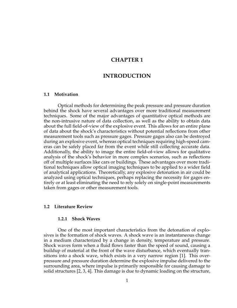
Optical methods for determining the peak pressure and pressure durationbehind the shock have several advantages over more traditional measurementtechniques. Some of the major advantages of quantitative optical methods arethe non-intrusive nature of data collection, as well as the ability to obtain dataabout the full field-of-view of the explosive event. This allows for an entire planeof data about the shock’s characteristics without potential reflections from othermeasurement tools such as pressure gages. Pressure gages also can be destroyedduring an explosive event, whereas optical techniques requiring high-speed cam-eras can be safely placed far from the event while still collecting accurate data.Additionally, the ability to image the entire field-of-view allows for qualitativeanalysis of the shock’s behavior in more complex scenarios, such as reflectionsoff of multiple surfaces like cars or buildings. These advantages over more tradi-tional techniques allow optical imaging techniques to be applied to a wider fieldof analytical applications. Theoretically, any explosive detonation in air could beanalyzed using optical techniques, perhaps replacing the necessity for gages en-tirely or at least eliminating the need to rely solely on single-point measurementstaken from gages or other measurement tools.
1.2 Literature Review
1.2.1 Shock Waves
One of the most important characteristics from the detonation of explo-sives is the formation of shock waves. A shock wave is an instantaneous changein a medium characterized by a change in density, temperature and pressure.Shock waves form when a fluid flows faster than the speed of sound, causing abuildup of material at the front of the wave disturbance, which eventually tran-sitions into a shock wave, which exists in a very narrow region [1]. This over-pressure and pressure duration determine the explosive impulse delivered to thesurrounding area, where impulse is primarily responsible for causing damage tosolid structures [2, 3, 4]. This damage is due to dynamic loading on the structure,
1
imparting kinetic energy leading to structural deformation [5]. The shock waveis oftentimes the first thing to interact with a structure (exempting shrapnel). Itis important to understand the characteristics of the shock wave and its propaga-tion through air, particularly in scenarios where can reflect off multiple surfaces,such as in urban environments. In these scenarios, it can be difficult to predictthe impulse delivered by a shock wave, or extrapolate a full-field understandingfrom singular data collection points as is the case with the use of more traditionaldiagnostic methods, such as piezoelectric gages [4]. Developing a diagnostic toolthat can be applied to scenarios where these interactions occur will improve therange of choices available for shock analysis.
1.2.2 Traditional Pressure Measurement Techniques
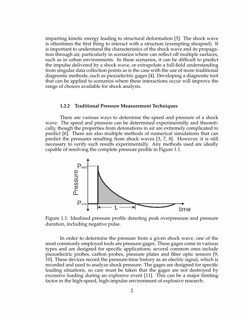
There are various ways to determine the speed and pressure of a shockwave. The speed and pressure can be determined experimentally and theoreti-cally, though the properties from detonations in air are extremely complicated topredict [6]. There are also multiple methods of numerical simulations that canpredict the pressures resulting from shock waves [3, 7, 8]. However, it is stillnecessary to verify such results experimentally. Any methods used are ideallycapable of resolving the complete pressure profile in Figure 1.1.
Figure 1.1: Idealized pressure profile denoting peak overpressure and pressureduration, including negative pulse.
In order to determine the pressure from a given shock wave, one of themost commonly employed tools are pressure gages. These gages come in varioustypes and are designed for specific applications; several common ones includepiezoelectric probes, carbon probes, pressure plates and fiber optic sensors [9,10]. These devices record the pressure-time history as an electric signal, which isrecorded and used to analyze shock pressure. The gages are designed for specificloading situations, so care must be taken that the gages are not destroyed byexcessive loading during an explosive event [11]. This can be a major limitingfactor in the high-speed, high-impulse environment of explosive research.
2
Both Sayapin [9] and MacPherson [10] noted the challenges associatedwith pressure sensors, particularly in the gages response time when comparedto the fast loading and unloading of shock wave pressure. The gages record aplane wave when the shock wave hits the sensor and ideally have a responsetime fast enough that the noise from the gage would not distort the shocks peaksignal [9]. In addition, the gages must be rugged and well designed to withstandthe heat and debris from explosions [10].
Alternative methods for determining shock pressure and pressure dura-tion include using a ballistic pendulum or performing plate dent test [12, 13].The ballistic pendulum method uses two long suspended metal bars placed endto end, with an explosive compound located near the end of the one bar. Theexplosive is detonated, creating a shock that will travel through the first bar intothe second. Ideally, the interface between the two bars is cut and faced suchthat a wave will be transmitted without reflection. Additionally, the explosivecompound is placed far enough away from the metal bars that there will be nodeformation from the blast [12]. The wave traveling through the two bars reflectsoff of the end, creating a tension wave traveling backwards. This tension waveinteracts with the remainder of the pressure wave, which can lead to separationof the two bars. The ideal scenario has the second bar sufficiently long enoughfor the front of the tension wave and the tail of the pressure wave reach the in-terface at the same moment; the bars will not separate under these conditions.This case demonstrates the length of the pressure wave, as this is true only whenthe second bar is half the length of the pressure wave [12]. The ballistic pendu-lum test is fairly complex, requiring multiple tests both to determine the correctlength of the second bar, and to account for potential damage done to the firstrod by the detonation of high explosives. While this technique can be applied ina laboratory setting, piezoelectric gages are far simpler to operate and produceimmediate results after a single test.
The plate dent test, the lead block test, the cylinder expansion test, and theunderwater expansion test are used to determine the blast potential of a particu-lar explosive compound [13]. In the first two tests, the known yield strength ofthe metal is used to determine the output strength, but the initial confinementof the explosive, followed by the fracturing and release of detonation gases pre-vents exact characterization, as both the shock and the detonation gases act on thematerial. The third test has the advantage of being completely confined by thewater, and the shock can be visualized using high-speed cameras, while the det-onation gases oscillate between expansion and implosion. While this techniquemay yield reasonable information about the shock, the overall technique is morecomplicated than simply detonating in air. The plate dent test consists of deto-nating an unconfined charge against a witness plate of known properties. Thedepth of the dent produced from the detonation can be linearly correlated to thedetonation pressure for many explosives. However, a single value for detonationpressure is insufficient data to make any conclusions about the shock overpres-sure and pressure duration.
3
1.2.3 Optical Techniques
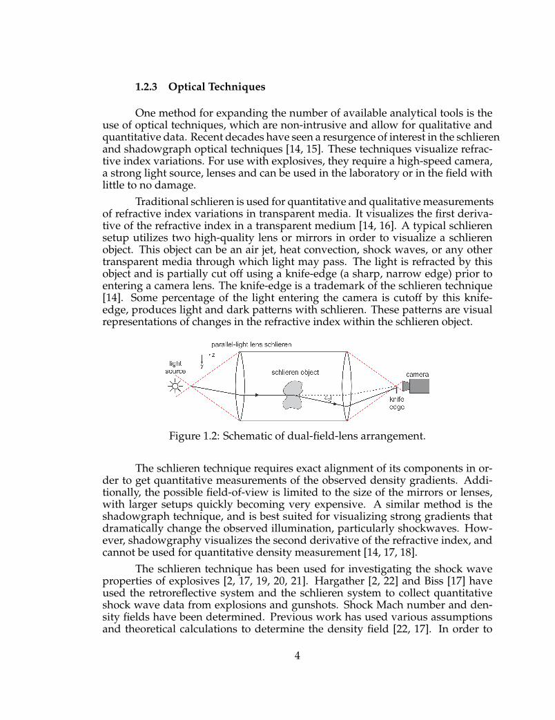
One method for expanding the number of available analytical tools is theuse of optical techniques, which are non-intrusive and allow for qualitative andquantitative data. Recent decades have seen a resurgence of interest in the schlierenand shadowgraph optical techniques [14, 15]. These techniques visualize refrac-tive index variations. For use with explosives, they require a high-speed camera,a strong light source, lenses and can be used in the laboratory or in the field withlittle to no damage.
Traditional schlieren is used for quantitative and qualitative measurementsof refractive index variations in transparent media. It visualizes the first deriva-tive of the refractive index in a transparent medium [14, 16]. A typical schlierensetup utilizes two high-quality lens or mirrors in order to visualize a schlierenobject. This object can be an air jet, heat convection, shock waves, or any othertransparent media through which light may pass. The light is refracted by thisobject and is partially cut off using a knife-edge (a sharp, narrow edge) prior toentering a camera lens. The knife-edge is a trademark of the schlieren technique[14]. Some percentage of the light entering the camera is cutoff by this knife-edge, produces light and dark patterns with schlieren. These patterns are visualrepresentations of changes in the refractive index within the schlieren object.
Figure 1.2: Schematic of dual-field-lens arrangement.
The schlieren technique requires exact alignment of its components in or-der to get quantitative measurements of the observed density gradients. Addi-tionally, the possible field-of-view is limited to the size of the mirrors or lenses,with larger setups quickly becoming very expensive. A similar method is theshadowgraph technique, and is best suited for visualizing strong gradients thatdramatically change the observed illumination, particularly shockwaves. How-ever, shadowgraphy visualizes the second derivative of the refractive index, andcannot be used for quantitative density measurement [14, 17, 18].
The schlieren technique has been used for investigating the shock waveproperties of explosives [2, 17, 19, 20, 21]. Hargather [2, 22] and Biss [17] haveused the retroreflective system and the schlieren system to collect quantitativeshock wave data from explosions and gunshots. Shock Mach number and den-sity fields have been determined. Previous work has used various assumptionsand theoretical calculations to determine the density field [22, 17]. In order to
4
determine the pressure field from the density field, the temperature behind theshock was assumed constant [17]. The equations used to determine the theoreti-cal pressure and temperature from Mach number are shown in Equations 1.1 and1.2.
PPatm
= (1 +γ− 1
2M2)
−γγ−1 (1.1)
TTatm
= (1 +γ− 1
2M2)−1 (1.2)
1.2.4 Objectives
The schlieren technique will be evaluated for use in measuring the pres-sure profile. This work will investigate new approaches to determining the tem-perature field. Computational and experimental methods of determining thetemperature field will be analyzed and the effect on the derived pressure fieldwill be quantified.
5

CHAPTER 2
EXPERIMENTAL METHODS
2.1 High-Speed Imaging
Digital high-speed photography has become commonplace in recent years,with several different manufacturers supplying a wide range of options for sci-entific analysis. Here, the Photron FASTCAM SA-X2 was used for the majority ofexperimental testing. This camera allows for a maximum resolution of 1024x1024images and is capable of recording up to 1 million frames per second (fps) at areduced resolution of 128x8. It records in grayscale, allowing for increased lightsensitivity over color camera options. The camera has a 16 GB internal memoryand can record up to 11.18 seconds at the maximum frame rate. The shutter hasa standard minimum speed of 1ms with a digital option of 293ns. The camerahas a c-mount lens attachment with an optional Nikon F-mount attachment andNikon lenses were used during all testing. The camera interfaces with ”PhotronFASTCAM Viewer” software. This allows for digital images to be saved in a vari-ety of formats for later viewing in the software or processing in other programs.Imaging with this camera utilized resolutions ranging from 1024x1024 for generalcharacteristics to 1024x48 for quantitative analysis. Multiple experiments demon-strated the repeatability of the events, allowing for slower frame rates and widerresolutions to be used. In general, frame rates ranging between 64,800 to 100,000fps is sufficient for accurate analysis. In all cases, the exposure was kept at 0.293µsin order to prevent smearing of the shock. A Nikon 80-200 mm zoom lens set withmaximum aperture (f-stop 2.8) and variable zoom was used during testing. Theimaging technique requires maximum aperture as closing the aperture truncatesthe light hitting the camera sensor.
Phantom v711 high-speed camera developed by Vision Research, was usedto record data for one day of testing. This camera has a maximum HD resolutionof 1280x800 and is capable of recording at frame rates up to 1.4 million fps at areduced resolution of 128x8. The camera has a 16 GB internal memory and canrecord gray-scale images up to 2.97 seconds at the maximum frame rate. Theshutter has a standard minimum speed 1ms, with a digital option of 300ns. Thecamera has a standard Nikon F-mount and Nikon lenses were used during alltesting. The camera interfaces with a laptop installed with Vision Research PCCsoftware using a GB Ethernet for control and data. Post-processing is done us-ing PCC and multiple file formats may be exported using this software. Imagingwith this camera utilized resolutions ranging from 800x600 to 800x32, with frame
6

rates ranging from 13001 to 230508, respectively. A larger resolution allows for acomplete visualization of flow characteristics in the field-of-view allowed by thesize of the lenses used in the schlieren system. The smallest resolution used al-lowed for a faster fps, resolving the shocks motion at more locations as it crossedthe field-of-view. At this frame rate, the shock wave observed to jump 15 pix-els between frames. During testing, an exposure time of 0.294µs was selected toprevent smearing of the shock wave over multiple pixels. Neutral density filterswere used to filter light entering the camera to prevent overexposure of the im-age. The strength of the filter was chosen based on the lens used and the intensityof the light source. The camera lens specifications used with the Photron wherealso used with the Phantom.
2.2 Schlieren Imaging Technique
There are multiple techniques available to image shock waves, the keylimiting factor being the size of the explosive event and the available equipment.The schlieren technique is the primary investigative tool, as it permits the directcalculation of the density field from the first-derivative of the refractive index gra-dient [14]. From the derived density field, it is possible to determine the pressurefield behind the shock.
2.2.1 Dual-Field-Lens Schlieren Setup
Figure 2.1 shows the setup used throughout testing; the specific orienta-tion of lenses, light and camera is called the dual-field-lens setup. The two largelenses have a focal length of 70cm. The distance between the two field lensesis approximately 1m. The Nikon 80-200mm lens has a minimum focal distanceof roughly 1m, so the center of the test section is at least 1m . Additionally, thelenses cannot be too close together in order to prevent the shock from reflectingoff the lenses during testing.
7
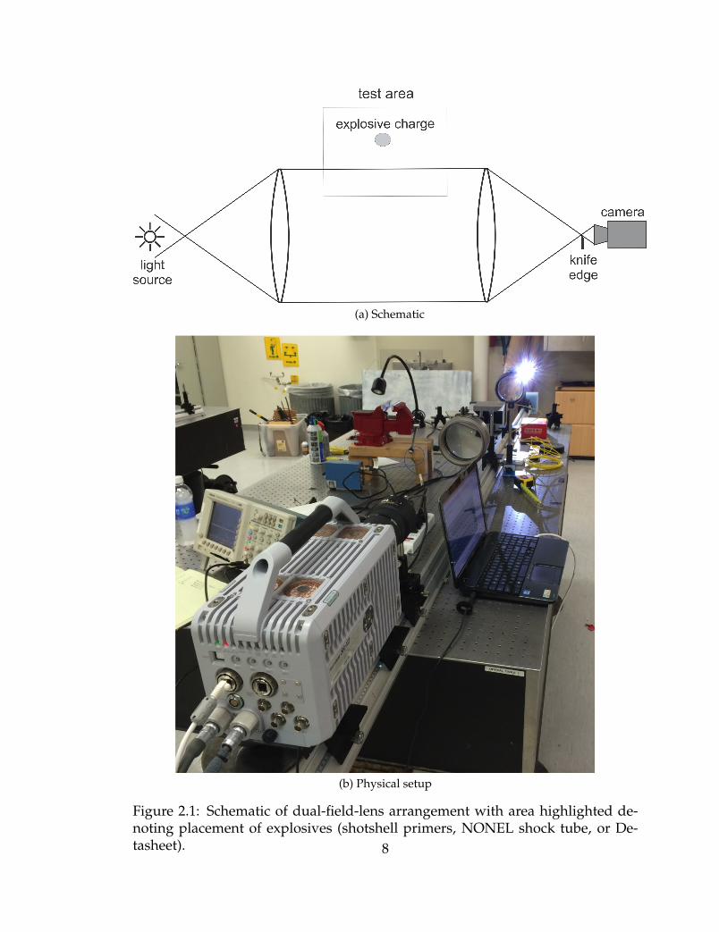
(a) Schematic
(b) Physical setup
Figure 2.1: Schematic of dual-field-lens arrangement with area highlighted de-noting placement of explosives (shotshell primers, NONEL shock tube, or De-tasheet). 8
The light source must be a point light source, requiring either an LED orarc lamp, with extraneous light blocked from illuminating the lenses, test areaand camera. The knife edge is placed at the focal point of the second lens, withthe camera placed as close as possible to the knife edge in order to prevent addi-tional cutoff from the camera lens itself. When the arc lamp was used, a neutraldensity filter was placed before the knife-edge in order to prevent overexposureof the image. Typical tests using this system are small in scale, making it idealfor laboratory use. It is possible to use this system in the field, though there issome inherent difficulty in using highly sensitive equipment in an unregulatedenvironment. This system was used in all stages of testing described below, bothin the laboratory and in the field.
2.3 Quantitative Schlieren Imaging
2.3.1 General Principles of Light Refraction
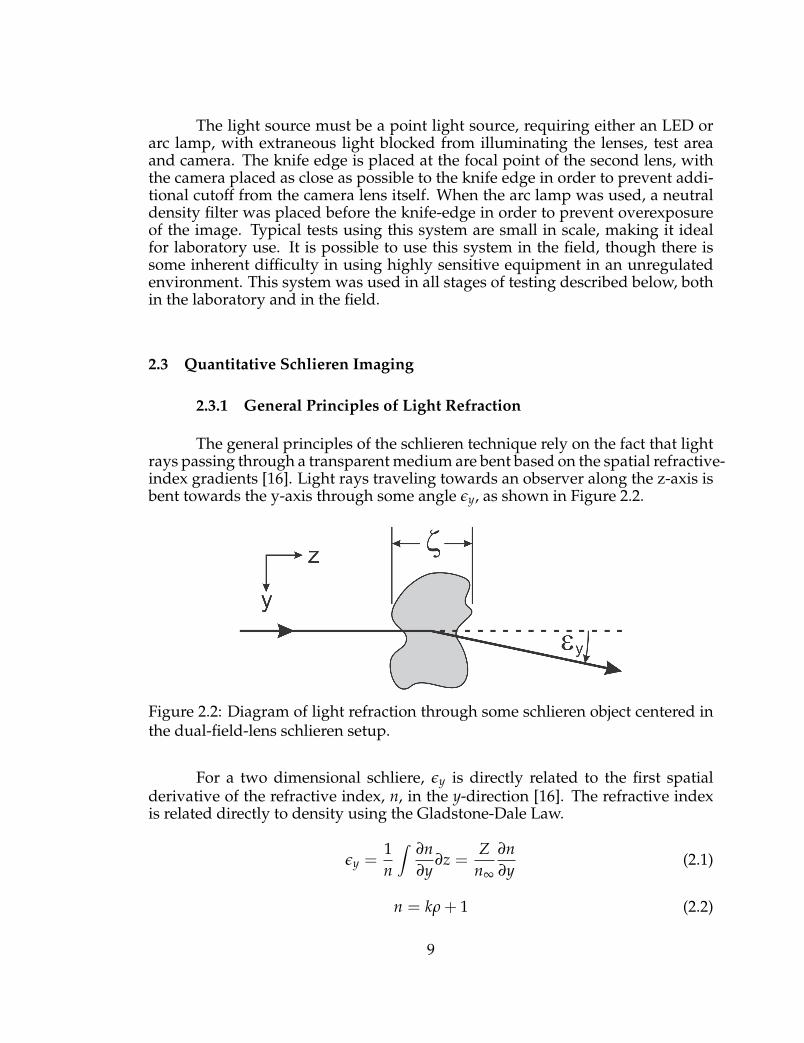
The general principles of the schlieren technique rely on the fact that lightrays passing through a transparent medium are bent based on the spatial refractive-index gradients [16]. Light rays traveling towards an observer along the z-axis isbent towards the y-axis through some angle εy, as shown in Figure 2.2.
Figure 2.2: Diagram of light refraction through some schlieren object centered inthe dual-field-lens schlieren setup.
For a two dimensional schliere, εy is directly related to the first spatialderivative of the refractive index, n, in the y-direction [16]. The refractive indexis related directly to density using the Gladstone-Dale Law.
εy =1n
∫∂n∂y
∂z =Z
n∞
∂n∂y
(2.1)
n = kρ + 1 (2.2)
9

Equation 2.2 shows the direct correlation between refractive index anddensity, using the Gladstone-Dale constant for air, k=0.000226m3/kg. The physicsof refractivity lead to some small variability in k, which increases with increasinglight wavelength [14]. However, the variability in k for most gaseous species arevery weakly dispersive at different wavelengths in the visible range [23]. There-fore, variability in k is insignificant for experiments using visible light. The vari-able Z refers to the physical distance that light must travel through the schlierenobject. This value can be constant or variable depending on the event being ana-lyzed.
One of the key elements to analyzing the density-gradient field is beingable to calibrate it to a known value. Here, a simple, weak, positive lens (longfocal length) is used. The diameter of the lens is 0.0254m and the focal length is10m for all primers and NONEL testing, and 4m for Detasheet testing. Incom-ing light traveling through the lens will focus all light to a point. Light passingthrough the lens will be refracted through a maximum angle at the radius of thelens, with the angle decreasing to zero at the center of the lens, as seen in Fig-ure 2.3. Note in Figure 2.3 that the background intensity is delineated in green,the 10m focal length positive lens is in red, and the 4m lens is in blue. As thefocal length of the weak lens increases, the overall sensitivity of the weak lens in-creases. This fact is best described by Equation 2.3, which shows the relation be-tween radius and focal length. As the focal length increases, the refraction angleε becomes smaller, meaning that the lens will be capable of resolving smaller re-fraction angles within the schlieren image. However, there is a trade off betweensensitivity and the overall intensity range within the lens. Greater sensitivity willhave a smaller range of maximum observed values, so care must be taken thatthe calibration lens’ range will encompass the observed intensity values from theschlieren object.
10
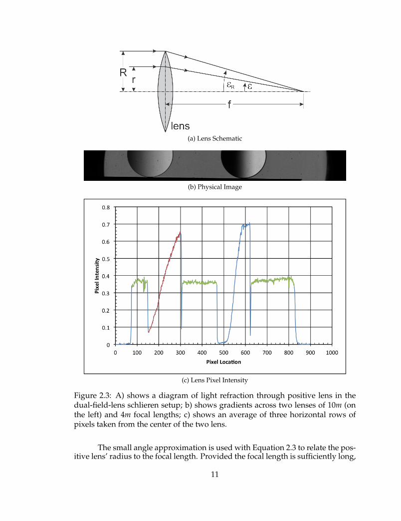
(a) Lens Schematic
(b) Physical Image
(c) Lens Pixel Intensity
Figure 2.3: A) shows a diagram of light refraction through positive lens in thedual-field-lens schlieren setup; b) shows gradients across two lenses of 10m (onthe left) and 4m focal lengths; c) shows an average of three horizontal rows ofpixels taken from the center of the two lens.
The small angle approximation is used with Equation 2.3 to relate the pos-itive lens’ radius to the focal length. Provided the focal length is sufficiently long,
11
this approximation is justified, which simplifies the overall calculations.
rf= tan ε ≈ ε (2.3)
A key point in this analysis is that the camera must be sharply focused onthe plane on which measurements are made. This translates to the center axis ofthe explosive being used during testing. Therefore, the lens must be placed onthe same focal plane. The overall range of intensity values observed in the lensis determined by the degree of cutoff. Too much cutoff will lower the image’soverall grayscale. In some cases, using too much cutoff can lead to the schlierenobject’s intensity values zeroing out. Therefore, sufficient cutoff should be chosenbased on test parameters. Sufficient cutoff implies that the range of intensity val-ues observed within the lens utilizes a significant portion of the cameras useabledynamic range [21].
2.3.2 General Process for Determining the Density Field
The process for determining the density field from a schlieren object isrelatively simple with the use of the calibration lens described above. First, theschlieren setup was optimized by placing the light source and knife edge at thefocal points of the two field lenses. This will create the parallel light in the testsection, and will result in uniform background illumination. This uniformity iskey to analyzing deviations from the average background intensity. Next, a rowof pixels is taken from images showing the calibration lens or the schlieren object.Some analyses have the calibration lens within the field-of-view during testing,though this is not necessary, provided the background intensity does not shift,multiple successive images can be compared to the calibration image.
In order to determine the density field around the schlieren object, the in-tensity values associated with the calibration lens must be analyzed. The averagebackground intensity in the image is identified, along with the correspondingintensity in the calibration lens. This intensity’s distance from the physical lenscenter is defined as r0, which refracts through an angle ε0 as defined by Equa-tion 2.3. The r0 is determined by fitting a 5th-order polynomial to a plot of pixelintensity versus pixel location (see Figure 2.4). This polynomial is used with theaverage background intensity to determine r0.
12
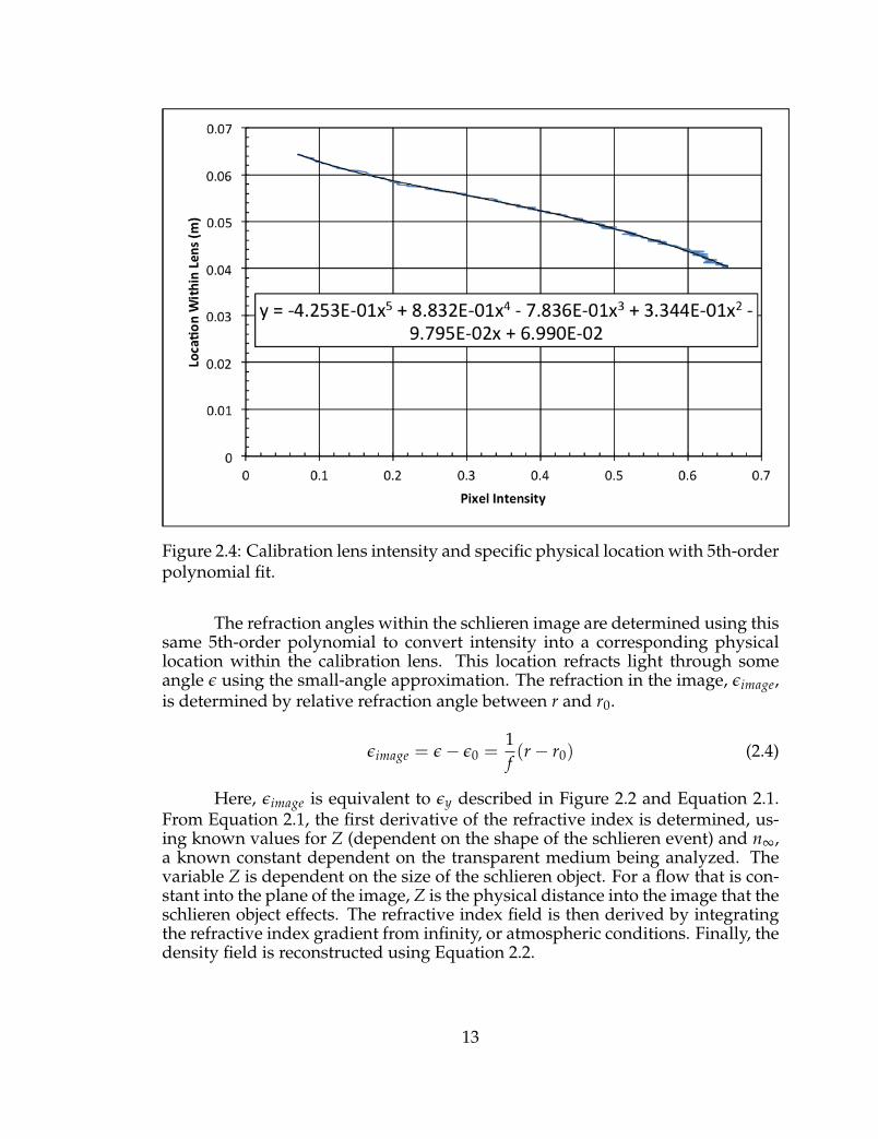
Figure 2.4: Calibration lens intensity and specific physical location with 5th-orderpolynomial fit.
The refraction angles within the schlieren image are determined using thissame 5th-order polynomial to convert intensity into a corresponding physicallocation within the calibration lens. This location refracts light through someangle ε using the small-angle approximation. The refraction in the image, εimage,is determined by relative refraction angle between r and r0.
εimage = ε− ε0 =1f(r− r0) (2.4)
Here, εimage is equivalent to εy described in Figure 2.2 and Equation 2.1.From Equation 2.1, the first derivative of the refractive index is determined, us-ing known values for Z (dependent on the shape of the schlieren event) and n∞,a known constant dependent on the transparent medium being analyzed. Thevariable Z is dependent on the size of the schlieren object. For a flow that is con-stant into the plane of the image, Z is the physical distance into the image that theschlieren object effects. The refractive index field is then derived by integratingthe refractive index gradient from infinity, or atmospheric conditions. Finally, thedensity field is reconstructed using Equation 2.2.
13

2.4 Explosive Material
Lab testing was done using Remington 209 Premier STS primers and cutlengths of NONEL Lead Line shock tube, and field testing was done using De-tasheet. During testing, efforts were made to ensure that the environment was ascontrolled as possible. In the lab, the air was kept at a constant temperature andall vents were shut off to prevent air currents. In the field, testing was conductedin a large bunker and doors were kept closed during testing; the air temperaturewas measured for each test. The explosive compound in the Remington primersis primarily lead styphnate along with other metal fuels. The lead styphnate com-poses 1-26% of the primer’s explosive compound, with copper, zinc, antimony,arsenic, iron, barium, and tetrazene as additional compounds . The primers werefired using a pin mechanism which crushed the compound, igniting the materialand generating a shock. The NONEL shock tube is composed of a mixture ofcyclotetramethylene-tetranitramine (HMX) and aluminum (Al) powder inside asmall diameter, three-layer plastic tube. A small amount of the explosive materialcoats the innermost tube. Shock tube is primarily used as a nonelectric detona-tor, which initiates an explosive by transmitting a shock down the length of thetube. It is a safe material with a wide variety of initiation applications. HMX,or octagen, is a powerful primary explosive and is used primarily in militaryapplications. Some common applications include use as a detonator, the maincompound in shaped charges, and as rocket propellant. Overall, the compoundis relatively insensitive. Detasheet, which contains approximately 80% pentaery-thritol tetranitrate (PETN), was cut and rolled into balls roughly 1g in weight.Preparation of the charges took place on-site. PETN is a common military ex-plosive frequently used in blasting caps. The compound is well documented,with a known TNT equivalence [24]. PETN is a secondary explosive, requiring ashock impulse in order to detonate. An exploding bridge-wire detonator (EBW)was used to detonate the charges. The charges were secured to the EBW using asmall amount of tape. An attempt was made to prevent the tape from facing theschlieren setup, thereby minimizing fragments passing through the field-of-viewahead of the explosive shock wave.
For all testing, the charge was suspended in air in order to prevent reflec-tions from the table surface or the ground from interfering with the initial shockwave reaching the schlieren system (Figure 2.1). In the case of the NONEL, theend of the tube was secured in order to prevent movement during firing. In orderto ensure accurate imaging of the shock passed through the schlieren test area, thecharge was placed roughly center between the two field lenses. The charge wasoffset some distance to the side of the schlieren apparatus but was kept along thesame center axis.
2.5 Pressure Gage Measurements
The gages are a small metal housing holding small crystal discs. Thesecrystals respond to compressive loading and generate an electrical signal that
14
can be directly converted to pressure [11]. The gages are capable of resolving thepressure duration, recording both positive and negative impulses relative to theatmospheric pressure. However, these gages often fail to resolve the initial peakpressure accurately, particularly as the shock’s Mach number increases [11].
An important aspect of this research is the ability to verify the accuracy ofthe deconvolution technique in reproducing the pressure signal across the shock[6]. A 50 psi PCB Piezotronics model 102 A07 SN 19907 pressure gage and a Tex-tronix Digital Oscilloscope model TDS 3034B were used to measure the pressuresignals. A single pressure gage was placed at a set position within the field-of-view to allow close comparison between the gage signal and the pressure signalderived from the deconvolution. Side-on pressures were collected by insertingthe gage into an aluminum plate. The plate was cut at an angle on the lead-ing edge to allow the shock to travel over the gage without interference fromreflections (see Figure 2.5). A typical pressure trace is shown in Figure 2.6. Thepressure trace shows the arrival of the initial shock, followed by a slight negativepressure. The additional noise following the complete shock signal is due to bothvibrations within the plate and the detonation gases.
15

Figure 2.5: Piezoelectric gage location within dual-field-lens schlieren setup. Thegage is secured within an aluminum plate. The edge of the plate is diagonally cutto allow shock to travel over top surface without reflecting off plate surface. Inthis orientation, the shock will be coming from the right.
16
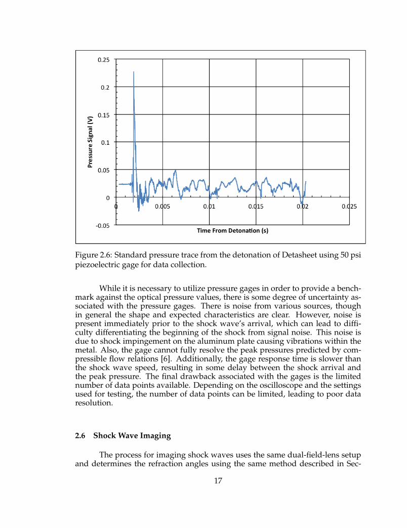
Figure 2.6: Standard pressure trace from the detonation of Detasheet using 50 psipiezoelectric gage for data collection.
While it is necessary to utilize pressure gages in order to provide a bench-mark against the optical pressure values, there is some degree of uncertainty as-sociated with the pressure gages. There is noise from various sources, thoughin general the shape and expected characteristics are clear. However, noise ispresent immediately prior to the shock wave’s arrival, which can lead to diffi-culty differentiating the beginning of the shock from signal noise. This noise isdue to shock impingement on the aluminum plate causing vibrations within themetal. Also, the gage cannot fully resolve the peak pressures predicted by com-pressible flow relations [6]. Additionally, the gage response time is slower thanthe shock wave speed, resulting in some delay between the shock arrival andthe peak pressure. The final drawback associated with the gages is the limitednumber of data points available. Depending on the oscilloscope and the settingsused for testing, the number of data points can be limited, leading to poor dataresolution.
2.6 Shock Wave Imaging
The process for imaging shock waves uses the same dual-field-lens setupand determines the refraction angles using the same method described in Sec-
17
tion 2.3.2. As a shock causes a rapid increase in pressure, temperature and den-sity, the assumption of a constant temperature cannot be used. Previous studiesshow that both pressure and temperature decay exponentially, but assume thatthe temperature decays sufficiently slowly so as to be considered constant com-pared to the pressure decay [21, 25]. Compressible flow relations were used todetermine the temperature at the shock wave and this temperature was assumedconstant behind the shock for initial analysis, but other temperature profiles werealso investigated. Additionally, while the same process of determining the re-fraction angle, εy, is used, an additional deconvolution of the data is necessary inorder to account for the spherical nature of the event.
2.6.1 Digital Image Processing for Pressure Measurement
Initial processing of the experimental data requires the determination ofthe Mach number of the shock. Knowing the Mach number allows for the deter-mination of the theoretical pressure and temperature at the shock wave. This in-formation is necessary for later processing and allows for the experimental pres-sure field to be compared against some known theoretical value. The Mach num-ber is determined by relating the pixel size to some known physical length usinga calibration object. For this, the calibration object used was the calibration lens,either by itself or secured within a frame of known diameter. Inspection of thecalibration lens provides the length of the object in pixels, which determines thelength/pixel ratio.
The physical distance the shock moves between frames is then dividedby the time between frames, which is a constant value based on the frames perseconds (fps) setting chosen for the high-speed camera. For the majority of theexperiments conducted, the explosive event occurred at distances great enoughthat the shock travelled fairly constantly through the field-of-view, close to Mach1.
Initial analysis of an explosive event utilizes a Matlab program to trackspherical shocks. The program takes a sequential series of gray-scale schlierenimages from the camera and user-variables to track the shocks position and deter-mine the Mach number between images. Below, a typical shock tracking routineis shown. The initial image designates the location of the explosive center, withsequential images highlighting the position of the shock. The analysis focusedon a shock wave, so imaging the detonation of the explosive was not necessary.Therefore, the explosive center is chosen as the edge of the field-of-view in theimage immediately prior to the shock entering the field-of-view. This does notaffect the programs ability to track the shock and will generate accurate velocitydata everywhere except between the first and second images. However, distancesfrom the charge center reported by the program will not be accurate with the ar-tificial explosive center. Therefore, the distance from the charge center to someestablished point in the field-of-view must be known for later processing. Note
18
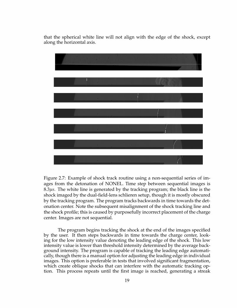
that the spherical white line will not align with the edge of the shock, exceptalong the horizontal axis.
Figure 2.7: Example of shock track routine using a non-sequential series of im-ages from the detonation of NONEL. Time step between sequential images is8.3µs. The white line is generated by the tracking program; the black line is theshock imaged by the dual-field-lens schlieren setup, though it is mostly obscuredby the tracking program. The program tracks backwards in time towards the det-onation center. Note the subsequent misalignment of the shock tracking line andthe shock profile; this is caused by purposefully incorrect placement of the chargecenter. Images are not sequential.
The program begins tracking the shock at the end of the images specifiedby the user. It then steps backwards in time towards the charge center, look-ing for the low intensity value denoting the leading edge of the shock. This lowintensity value is lower than threshold intensity determined by the average back-ground intensity. The program is capable of tracking the leading edge automati-cally, though there is a manual option for adjusting the leading edge in individualimages. This option is preferable in tests that involved significant fragmentation,which create oblique shocks that can interfere with the automatic tracking op-tion. This process repeats until the first image is reached, generating a streak
19
image and plots of the Mach number. An output file is also generated, whichincludes shock position, Mach number, the speed of sound in air, other suppliedatmospheric constants, as well as uncertainties for the generated values.
Once the Mach number is known for all images of interest, rows of pixel in-tensities along the horizontal plane of the shock were extracted and, in some casesaveraged, in order to determine the refractive index described in Section 2.3.2.
2.6.2 Abel Deconvolution Process
The intensity values across the shock are used to determine the deflectionangle, εy, by comparing it to the calibration lens. An example of the pixel intensi-ties across a shock is shown below in Figure 5.14. However, due to the schlierensystems parallel light passing through the spherical shock, the refractive-indexgradient field defined in Equation 2.1 are path-integrated quantities. Therefore,a deconvolution of the deflection data, εy, is necessary in order to reproduce thelocal density field from the integrated quantities seen in the image plane of thecamera[21, 26]. For an axisymmetric object such as spherical shock, the Abel in-version method is sufficient to reproduce the field from its 1D representation inthe schlieren image.
20

(a) Shock
(b) Pixel Intensity
Figure 2.8: Row of pixel intensities across a shock from the detonation of NONEL.
Several different Abel inversion methods exist, each with varying degreesof accuracy and uncertainty. These methods are the 1/3rd rule, the 1-point for-mula, the 2-point formula and the least-squares approximation. Among these,the 2-point formula described in Equation 2.5, 2.6, and 2.7 is preferable, as ithas the best inversion accuracy with the least amount of error [26]. The deflec-tion data is calculated as outlined in the flat plate analysis and is input into theAbel inversion method. The Abel inversion method considers a range of datafrom the center outwards of a spherically symmetric object. Therefore, intensitydata points outside of the visible range were artificially filled with backgroundintensity values [21]. This results in zero deflection for non-visible data points.Adding these artificial points is necessary in order for the inversion method towork properly.
The indices i and j correspond to data points between 1 and N+1, whereN represents the total number of data points. Dij contains the independent data-spacing linear operator coefficients specific to the 2-point method [26]. A simpleMatlab code was written to perform the mathematical operation outlined below.The code takes the deflection data in vector form and runs it through the code.The output δ will be plotted against the radius, with the distance between datapoints determined by the pixel calibration constant for an individual test.
21
δ(ri) =N+1
∑j=i
Dij · εj (2.5)
Dij =1π· (Ai,j − Ai,(j-1) − j · Bi,j + (j− 2) · Bi,(j-1))
i f j > i and j 6= 2,
=1π· (Ai,j − j · Bi,j − 1)
i f j > i and j = 2,
=1π· (Ai,j − j · Bi,j)
i f j = i and i 6= 1,
= 0
i f j = i = 1 or j < i
(2.6)
where Ai,j and Bi,j are
Ai,j =√
j2 − (i− 1)2 −√(j− 1)2 − (i− 1)2,
Bi,j = ln (j +
√j2 − (i− 1)2
(j− 1) +√(j− 1)2 − (i− 1)2
)
(2.7)
The refractive index n is reproduced from the 2-point output δ using Equa-tion 2.8. Equation 2.2 is used to reproduce the density field. Once the density fieldhas been reconstructed, the ideal gas law can be used to calculate the pressurefield from Equation 2.9.
δ =nn0− 1 (2.8)
P = ρRairT (2.9)
For the Abel inversion method to be successful, the shock must be trav-eling at speeds that allow the ideal gas assumption to hold. At speeds aboveMach 5, ionization and molecular dissociation begin to occur in the gas species.The ideal gas law cannot be used when interactions between molecules becomessignificant. During testing, Mach numbers were all under Mach 2, making thisassumption valid. Additionally, the shock must be clearly separated from thedetonation gases in order to allow an accurate deconvolution. A wide separation
22

will also permit the complete pressure profile to be calculated. In addition, oneof the major disadvantages of the Abel technique is the assumption that all de-flection is solely caused by a purely spherical schlieren object. Any deflectionscaused by oblique shocks formed by fragments will remain in the deconvolutionresults, despite the fact that the fragments may not be traveling in the plane ofinterest. Therefore, the shock must not only be cleanly separated from the det-onation gases, but it also must not have any oblique shocks interfering with theregion of interest.
23

CHAPTER 3
FLAT PLATE ANALYSIS
A simple flat plate analysis was used to test the method of deriving thedensity field. A comparison of experimental and theoretical results was usedto verify the accuracy of the technique. A vertical flat plate placed in the field-of-view was heated to achieve steady, laminar flow and imaged using a digitalNikon SLR camera (see Figure 3.1). For this test, the light source in the dual-field-lens setup was an LED. As this is not a high-speed object, only a single image isneeded for data analysis. The resolution was chosen to image the entire field-of-view in the schlieren system. The temperature of the plate was measured multi-ple times during heating to find the steady temperature. The temperature of theplate was deemed steady once the temperature did not vary over a time periodof 10 minutes. The temperature was tested at several locations across the plate.Once a steady temperature of 325 ± 1K was achieved, the flat plate was imagedfor processing in Matlab. The density-gradient field around the flat plate was adirect result from the change in air temperature. Therefore, applying the idealgas law (see Equation 2.9) was a simple matter of determining density from therefractive-index gradient using the method described above to determine density,then using atmospheric pressure to calculate the temperature field. The theoret-ical profile was derived using the method described by Ostrach [27]. The theo-retical temperature profile is compared to the experimental temperature profile(Figure 3.2). The good agreement between the experimental measurement andthe theoretical calculations demonstrates that the technique used to reconstructthe density field is accurate.
24

Figure 3.1: Setup of heated flat plate.
25
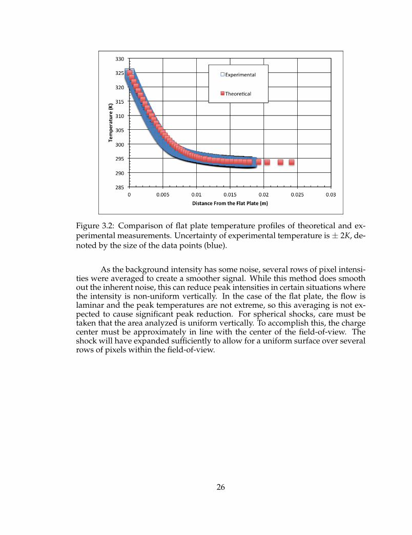
Figure 3.2: Comparison of flat plate temperature profiles of theoretical and ex-perimental measurements. Uncertainty of experimental temperature is ± 2K, de-noted by the size of the data points (blue).
As the background intensity has some noise, several rows of pixel intensi-ties were averaged to create a smoother signal. While this method does smoothout the inherent noise, this can reduce peak intensities in certain situations wherethe intensity is non-uniform vertically. In the case of the flat plate, the flow islaminar and the peak temperatures are not extreme, so this averaging is not ex-pected to cause significant peak reduction. For spherical shocks, care must betaken that the area analyzed is uniform vertically. To accomplish this, the chargecenter must be approximately in line with the center of the field-of-view. Theshock will have expanded sufficiently to allow for a uniform surface over severalrows of pixels within the field-of-view.
26
CHAPTER 4
CTH MODELING
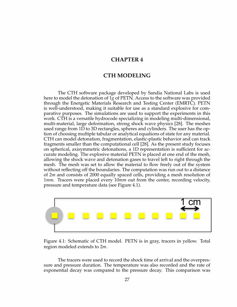
The CTH software package developed by Sandia National Labs is usedhere to model the detonation of 1g of PETN. Access to the software was providedthrough the Energetic Materials Research and Testing Center (EMRTC). PETNis well-understood, making it suitable for use as a standard explosive for com-parative purposes. The simulations are used to support the experiments in thiswork. CTH is a versatile hydrocode specializing in modeling multi-dimensional,multi-material, large deformation, strong shock wave physics [28]. The meshesused range from 1D to 3D rectangles, spheres and cylinders. The user has the op-tion of choosing multiple tabular or analytical equations of state for any material.CTH can model detonation, fragmentation, elastic-plastic behavior and can trackfragments smaller than the computational cell [28]. As the present study focuseson spherical, axisymmetric detonations, a 1D representation is sufficient for ac-curate modeling. The explosive material PETN is placed at one end of the mesh,allowing the shock wave and detonation gases to travel left to right through themesh. The mesh was set to allow the material to flow freely out of the systemwithout reflecting off the boundaries. The computation was run out to a distanceof 2m and consists of 2000 equally spaced cells, providing a mesh resolution of1mm. Tracers were placed every 10mm out from the center, recording velocity,pressure and temperature data (see Figure 4.1).
Figure 4.1: Schematic of CTH model. PETN is in gray, tracers in yellow. Totalregion modeled extends to 2m.
The tracers were used to record the shock time of arrival and the overpres-sure and pressure duration. The temperature was also recorded and the rate ofexponential decay was compared to the pressure decay. This comparison was
27
used to analyze the applicability of the assumption of constant temperature be-hind the shock. The air surrounding the PETN was modeled as an ideal gas andthe PETN was modeled using Jones-Wilkins-Lee equation of state for high explo-sives.
One of the primary goals of the CTH analysis was obtaining an accuratetemperature profile to use when determining the shock overpressure and pres-sure duration from the density field. Previous research has made the assumptionthat the temperature profile’s relative rate of decay is slow enough to be con-sidered constant when compared with the rate of decay of the pressure profile[21]. This assumption may hold true close to the center of the explosive, how-ever, CTH modeling indicates that after a certain point, the relative rates of decayof pressure, temperature, and density are roughly equivalent.
While CTH has been known to inaccurately calculate temperature, the rel-atively slow Mach numbers being analyzed here allow the assumption that thetemperature profiles are appropriate. The goal of the CTH analysis is to guide theshape of the temperature profiles and to serve as a benchmark for experimentalcomparison. The peak temperatures are accurate, as they are calculated usingRankine-Hugoniot jump conditions across the shock wave. The temperature de-cay profile is expected to be reasonably accurate. This assumption is shown to beaccurate by comparison to experimental results.
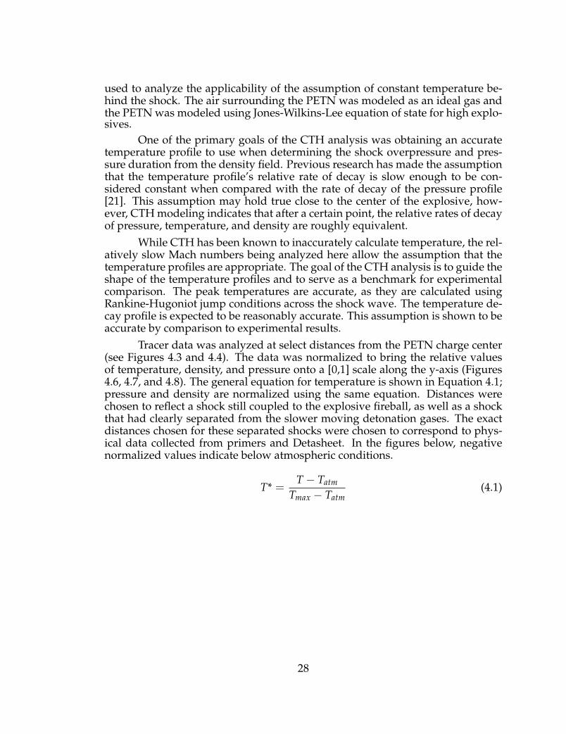
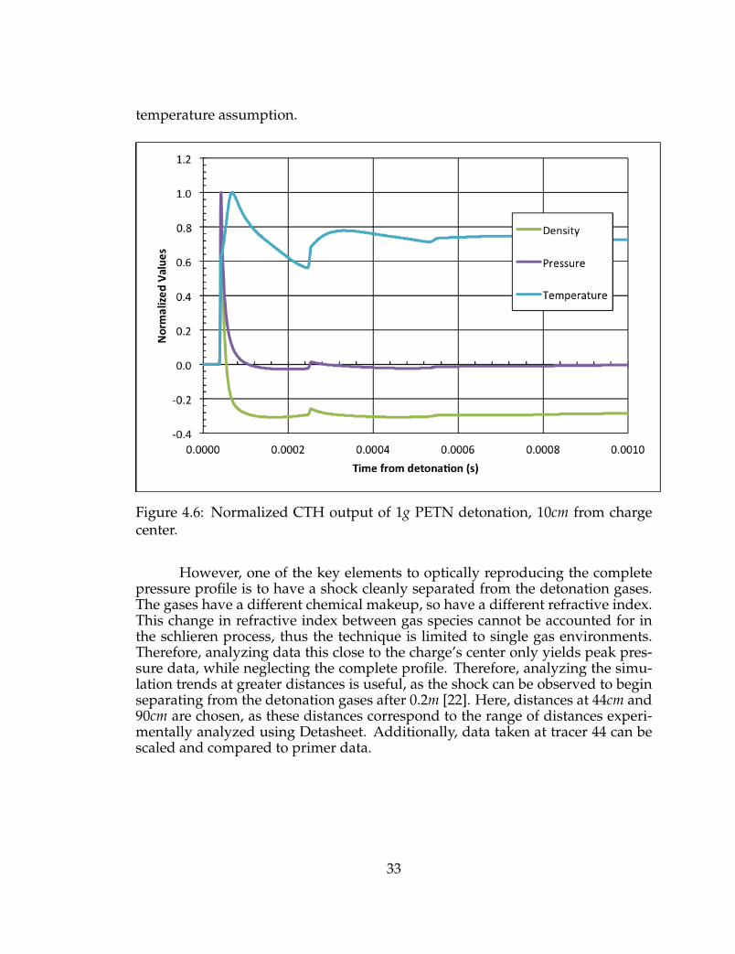
Tracer data was analyzed at select distances from the PETN charge center(see Figures 4.3 and 4.4). The data was normalized to bring the relative valuesof temperature, density, and pressure onto a [0,1] scale along the y-axis (Figures4.6, 4.7, and 4.8). The general equation for temperature is shown in Equation 4.1;pressure and density are normalized using the same equation. Distances werechosen to reflect a shock still coupled to the explosive fireball, as well as a shockthat had clearly separated from the slower moving detonation gases. The exactdistances chosen for these separated shocks were chosen to correspond to phys-ical data collected from primers and Detasheet. In the figures below, negativenormalized values indicate below atmospheric conditions.
T* =T − Tatm
Tmax − Tatm(4.1)
28
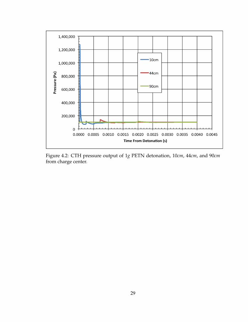
Figure 4.2: CTH pressure output of 1g PETN detonation, 10cm, 44cm, and 90cmfrom charge center.
29
Figure 4.3: Logarithmic scale of CTH pressure output of 1g PETN detonation,10cm, 44cm, and 90cm from charge center.
30
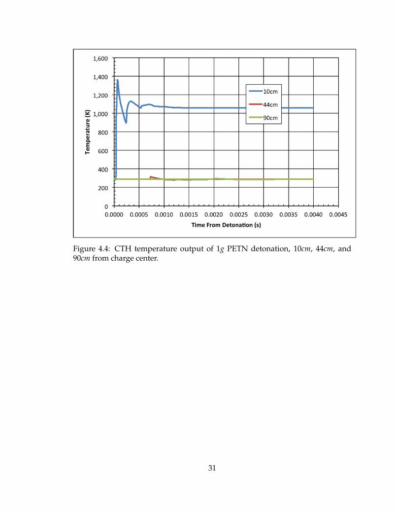
Figure 4.4: CTH temperature output of 1g PETN detonation, 10cm, 44cm, and90cm from charge center.
31
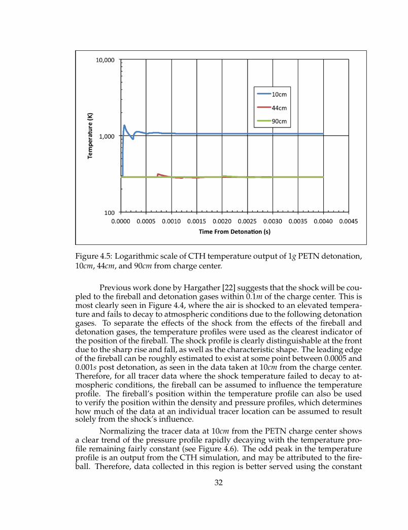
Figure 4.5: Logarithmic scale of CTH temperature output of 1g PETN detonation,10cm, 44cm, and 90cm from charge center.
Previous work done by Hargather [22] suggests that the shock will be cou-pled to the fireball and detonation gases within 0.1m of the charge center. This ismost clearly seen in Figure 4.4, where the air is shocked to an elevated tempera-ture and fails to decay to atmospheric conditions due to the following detonationgases. To separate the effects of the shock from the effects of the fireball anddetonation gases, the temperature profiles were used as the clearest indicator ofthe position of the fireball. The shock profile is clearly distinguishable at the frontdue to the sharp rise and fall, as well as the characteristic shape. The leading edgeof the fireball can be roughly estimated to exist at some point between 0.0005 and0.001s post detonation, as seen in the data taken at 10cm from the charge center.Therefore, for all tracer data where the shock temperature failed to decay to at-mospheric conditions, the fireball can be assumed to influence the temperatureprofile. The fireball’s position within the temperature profile can also be usedto verify the position within the density and pressure profiles, which determineshow much of the data at an individual tracer location can be assumed to resultsolely from the shock’s influence.
Normalizing the tracer data at 10cm from the PETN charge center showsa clear trend of the pressure profile rapidly decaying with the temperature pro-file remaining fairly constant (see Figure 4.6). The odd peak in the temperatureprofile is an output from the CTH simulation, and may be attributed to the fire-ball. Therefore, data collected in this region is better served using the constant
32
temperature assumption.
Figure 4.6: Normalized CTH output of 1g PETN detonation, 10cm from chargecenter.
However, one of the key elements to optically reproducing the completepressure profile is to have a shock cleanly separated from the detonation gases.The gases have a different chemical makeup, so have a different refractive index.This change in refractive index between gas species cannot be accounted for inthe schlieren process, thus the technique is limited to single gas environments.Therefore, analyzing data this close to the charge’s center only yields peak pres-sure data, while neglecting the complete profile. Therefore, analyzing the simu-lation trends at greater distances is useful, as the shock can be observed to beginseparating from the detonation gases after 0.2m [22]. Here, distances at 44cm and90cm are chosen, as these distances correspond to the range of distances experi-mentally analyzed using Detasheet. Additionally, data taken at tracer 44 can bescaled and compared to primer data.
33
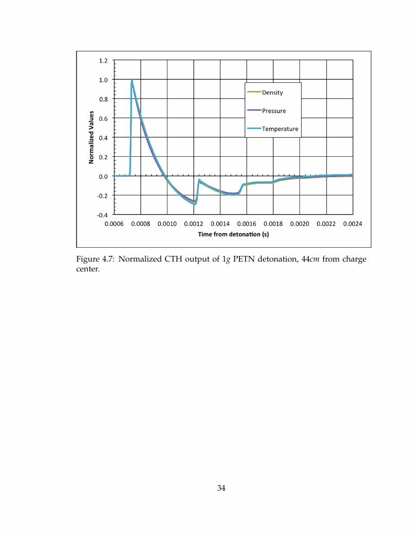
Figure 4.7: Normalized CTH output of 1g PETN detonation, 44cm from chargecenter.
34
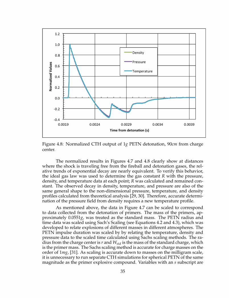
Figure 4.8: Normalized CTH output of 1g PETN detonation, 90cm from chargecenter.
The normalized results in Figures 4.7 and 4.8 clearly show at distanceswhere the shock is traveling free from the fireball and detonation gases, the rel-ative trends of exponential decay are nearly equivalent. To verify this behavior,the ideal gas law was used to determine the gas constant R with the pressure,density, and temperature data at each point; R was calculated and remained con-stant. The observed decay in density, temperature, and pressure are also of thesame general shape to the non-dimensional pressure, temperature, and densityprofiles calculated from theoretical analysis [29, 30]. Therefore, accurate determi-nation of the pressure field from density requires a new temperature profile.
As mentioned above, the data in Figure 4.7 can be scaled to correspondto data collected from the detonation of primers. The mass of the primers, ap-proximately 0.0551g, was treated as the standard mass. The PETN radius andtime data was scaled using Sach’s Scaling (see Equations 4.2 and 4.3), which wasdeveloped to relate explosions of different masses in different atmospheres. ThePETN impulse duration was scaled by by relating the temperature, density andpressure data to the scaled time calculated using Sachs scaling methods. The ra-dius from the charge center is r and Wstd is the mass of the standard charge, whichis the primer mass. The Sachs scaling method is accurate for charge masses on theorder of 1mg, [31]. As scaling is accurate down to masses on the milligram scale,it is unnecessary to run separate CTH simulations for spherical PETN of the samemagnitude as the primer explosive compound. Variables with an s subscript are
35
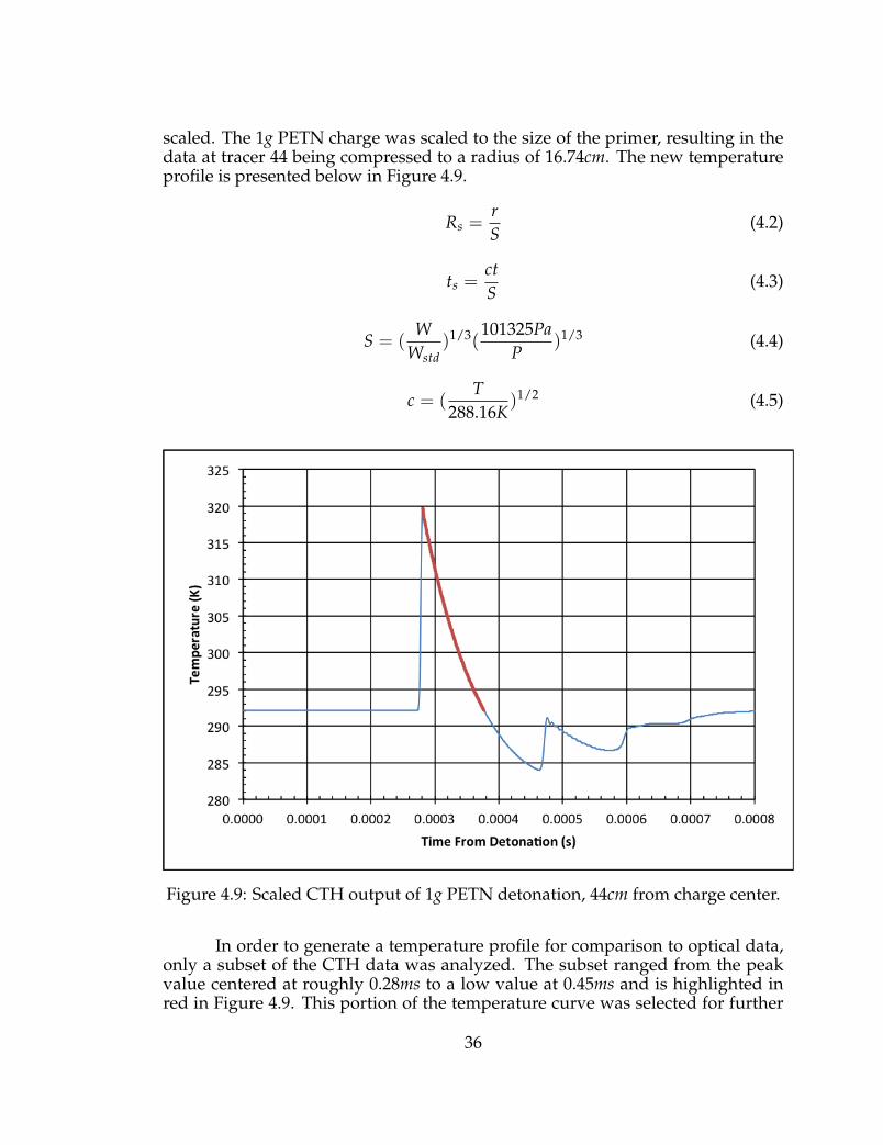
scaled. The 1g PETN charge was scaled to the size of the primer, resulting in thedata at tracer 44 being compressed to a radius of 16.74cm. The new temperatureprofile is presented below in Figure 4.9.
Rs =rS
(4.2)
ts =ctS
(4.3)
S = (W
Wstd)1/3(
101325PaP
)1/3 (4.4)
c = (T
288.16K)1/2 (4.5)
Figure 4.9: Scaled CTH output of 1g PETN detonation, 44cm from charge center.
In order to generate a temperature profile for comparison to optical data,only a subset of the CTH data was analyzed. The subset ranged from the peakvalue centered at roughly 0.28ms to a low value at 0.45ms and is highlighted inred in Figure 4.9. This portion of the temperature curve was selected for further
36

pressure calculations using experimental density values because it only takes theprimary shock into account, while ignoring the secondary shock. The secondaryshock is not observed in the primer tests due to the asymmetric explosion ofthe shot shells. This temperature curve will be compared to other temperatureprofiles in the next chapter.
37
CHAPTER 5
EXPERIMENTAL RESULTS
Several different types of explosives were analyzed for the ability to accu-rately determine temperature and pressure profiles peak pressure and pressureduration behind the shock. The density field was derived using the methodsdescribed in Section 2.6.1. Initial analysis of the temperature profiles was doneusing data from firing shot-shell primers. Results from temperature analysis areapplied to testing of shot shell primers, NONEL shock tube, and Detasheet.
5.1 Temperature Calculations from Optical Measurements
5.1.1 Shot Shell Primers
Initial analysis utilized primers in order to establish general shock prop-agation trends and analysis techniques within a laboratory setting. As seen inFigures 5.1 and 5.2, there is a great deal of light flare and fragmentation follow-ing the detonation of shotshell primers. The fragmentation is both unburned ex-plosive composition, as well as pieces of the paper used to hold the pellet withinthe primer. The light interferes with data collection as it distorts the uniformity ofthe background. The fragments present can create oblique shocks both before andafter the spherical shock, preventing accurate reconstruction using the Abel de-convolution technique, as this technique assumes a uniform spherical shock [26].Figure 5.3 shows the shock Mach number from the detonation of the primers. Theshock decays to a near constant speed after 0.17m from the primer face. Whiletesting the Abel deconvolution technique on a variety of shock Mach numbersis preferable, accurate deconvolution requires that the shock be relatively free ofinterference from oblique shocks coming off of high-velocity fragments. Addi-tionally, the shock must be clearly separated from detonation gases. An idealsituation has the entire shock completely exit the field of view prior to the deto-nation gases entering the field-of-view. This will allow the pressure profile to bereconstructed by stitching together data from sequential images. If the detona-tion gases follow the shock too closely, only a small portion of the shock could beused to reconstruct the pressure profile.
38
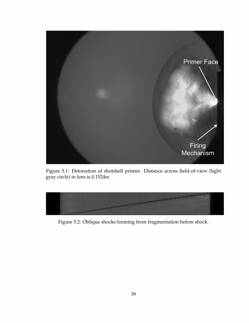
Figure 5.1: Detonation of shotshell primer. Distance across field-of-view (lightgray circle) in lens is 0.1524m.
Figure 5.2: Oblique shocks forming from fragmentation before shock.
39
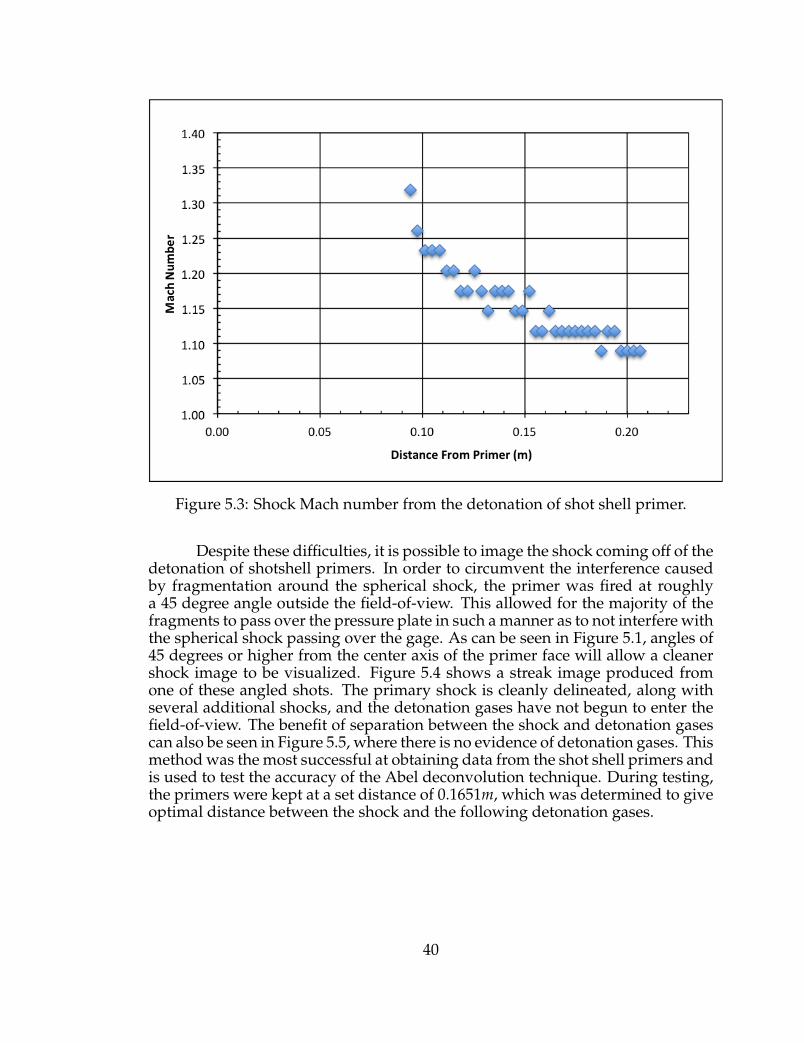
Figure 5.3: Shock Mach number from the detonation of shot shell primer.
Despite these difficulties, it is possible to image the shock coming off of thedetonation of shotshell primers. In order to circumvent the interference causedby fragmentation around the spherical shock, the primer was fired at roughlya 45 degree angle outside the field-of-view. This allowed for the majority of thefragments to pass over the pressure plate in such a manner as to not interfere withthe spherical shock passing over the gage. As can be seen in Figure 5.1, angles of45 degrees or higher from the center axis of the primer face will allow a cleanershock image to be visualized. Figure 5.4 shows a streak image produced fromone of these angled shots. The primary shock is cleanly delineated, along withseveral additional shocks, and the detonation gases have not begun to enter thefield-of-view. The benefit of separation between the shock and detonation gasescan also be seen in Figure 5.5, where there is no evidence of detonation gases. Thismethod was the most successful at obtaining data from the shot shell primers andis used to test the accuracy of the Abel deconvolution technique. During testing,the primers were kept at a set distance of 0.1651m, which was determined to giveoptimal distance between the shock and the following detonation gases.
40

(a) Streak Image
(b) Shock at Gage Location
Figure 5.4: Streak image and single image of shot shell primer fired at a 45 degreeangle. Vertical time step in streak image is 8.33µs, distance across field of view(gray background) is 0.0254m.
Figure 5.5: Pixel intensity across shock front.
In addition to testing the accuracy of the Abel deconvolution technique,one of the primary goals of this analysis is to test previous assumptions that the
41

temperature can be assumed constant behind the shock. As seen in Section 4, therelative rate of decay of temperature and pressure becomes roughly equivalent asdistance from the charge increases. At distances where the shock is cleanly sep-arated from the detonation gases, it is no longer feasible to assume that the tem-perature profile is constant. Additionally, while CTH is useful as a comparativetool, it is also beneficial to develop temperature profiles based on experimentaldata. Comparing different explosives can lead to erroneous conclusions, particu-larly in situations where a highly idealized scenario of the detonation of PETN iscompared to the highly non ideal detonation/deflagration of shot shell primers.Developing a temperature profile based on observed experimental shock behav-ior will yield more accurate results.
Three different methods for reproducing the temperature, and subsequentlypressure, field from the detonation of primers are considered. The first methodis the constant temperature assumption and uses a temperature calculated fromthe Mach number of the shock wave and compressible flow relations (Equations1.1 and 1.2). The second method is the CTH idealized temperature profile. Thelast method uses the ideal gas law and calculates temperature directly from thepiezoelectric pressure signal and the optical density field. For the gage’s pressuredata, only the signal corresponding to the peak pressure and pressure durationare considered; the atmospheric signal and the noise after the shock are neglected.Figures 5.6 and 5.7 show the respective portions of the experimental pressure anddensity fields under consideration. A second-order polynomial fit is applied tothe highlighted sections of the pressure and density profiles to account for oscil-lation and is used in the subsequent analysis.
42

Figure 5.6: Gage pressure profile. Highlighted portion (red) used to determinetemperature. Distance from primer face to gage is 0.165m.
43
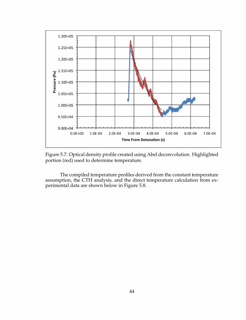
Figure 5.7: Optical density profile created using Abel deconvolution. Highlightedportion (red) used to determine temperature.
The compiled temperature profiles derived from the constant temperatureassumption, the CTH analysis, and the direct temperature calculation from ex-perimental data are shown below in Figure 5.8.
44

Figure 5.8: Compilation of temperature profiles from detonation of shot shellprimers.
Figure 5.8 shows a clear decay in the temperature profile for the calcu-lated temperature scenario. The constant temperature profile is not appropriatefor resolving the complete pressure field. Agreement between the calculated andCTH temperature profiles is also good, though the calculated profile shows adecay that does not drop below atmospheric temperature to the extent that theCTH profile shows. The CTH profile is highly idealized and uses PETN, as op-posed to the explosive mixture in the primers. Additionally, the primer mixtureis confined in a metal cup, whereas the PETN is detonated in air, which mayalso be a source of the differing behaviors. The confinement is designed to sendmost of the energy forward from the primer face, whereas the shock was ana-lyzed at an angle away from the primer face. This confinement led to a slightlynon-spherical shock, but as all testing with the primers was relatively far awayfrom the face, the analyzed shock can be assumed spherical. These differencesin the compound and methods used to calculate the profile could be the causeof the discrepancy between the primer and PETN data. Compared to the calcu-lated temperature profile, CTH would be a poor model for resolving the entirepressure profile. In situations where gage data is not available, a more accuratemethod of generating a temperature profile would be to use the CTH profile togenerate a linear temperature profile as seen in Figure 5.9. As the experimentaldata does not show a significant negative pulse as is seen in the CTH profile, oncethe experimental data has decayed to atmospheric levels, constant atmospheric
45
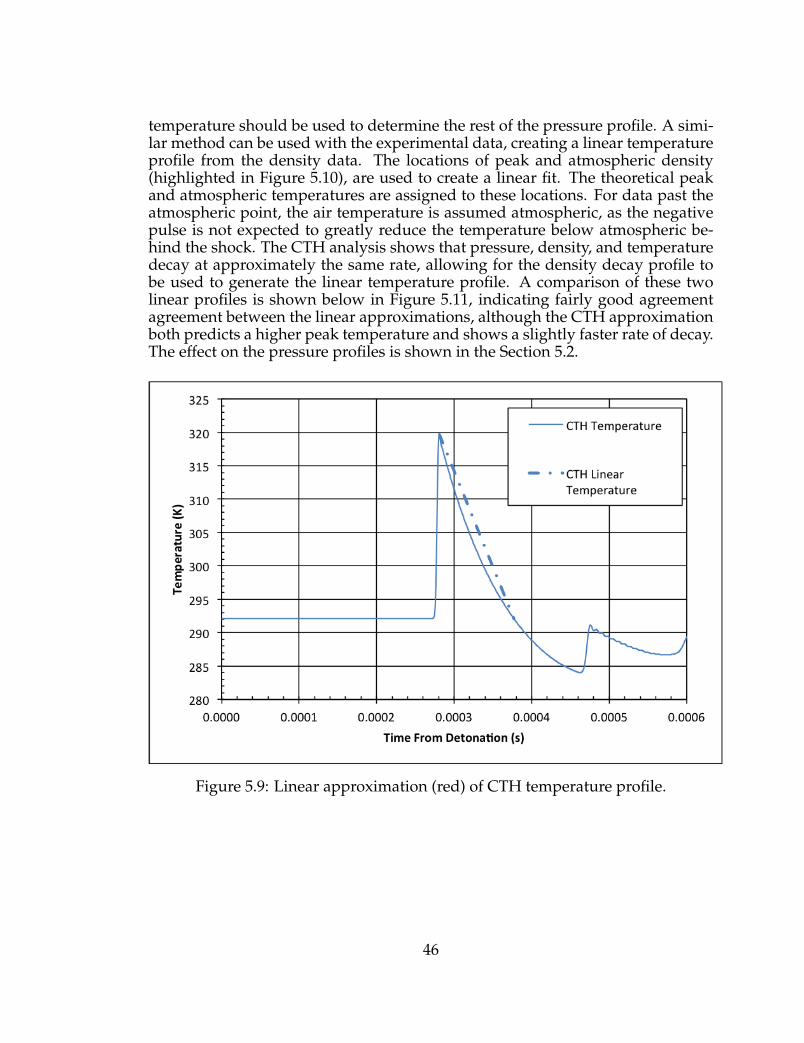
temperature should be used to determine the rest of the pressure profile. A simi-lar method can be used with the experimental data, creating a linear temperatureprofile from the density data. The locations of peak and atmospheric density(highlighted in Figure 5.10), are used to create a linear fit. The theoretical peakand atmospheric temperatures are assigned to these locations. For data past theatmospheric point, the air temperature is assumed atmospheric, as the negativepulse is not expected to greatly reduce the temperature below atmospheric be-hind the shock. The CTH analysis shows that pressure, density, and temperaturedecay at approximately the same rate, allowing for the density decay profile tobe used to generate the linear temperature profile. A comparison of these twolinear profiles is shown below in Figure 5.11, indicating fairly good agreementagreement between the linear approximations, although the CTH approximationboth predicts a higher peak temperature and shows a slightly faster rate of decay.The effect on the pressure profiles is shown in the Section 5.2.
Figure 5.9: Linear approximation (red) of CTH temperature profile.
46
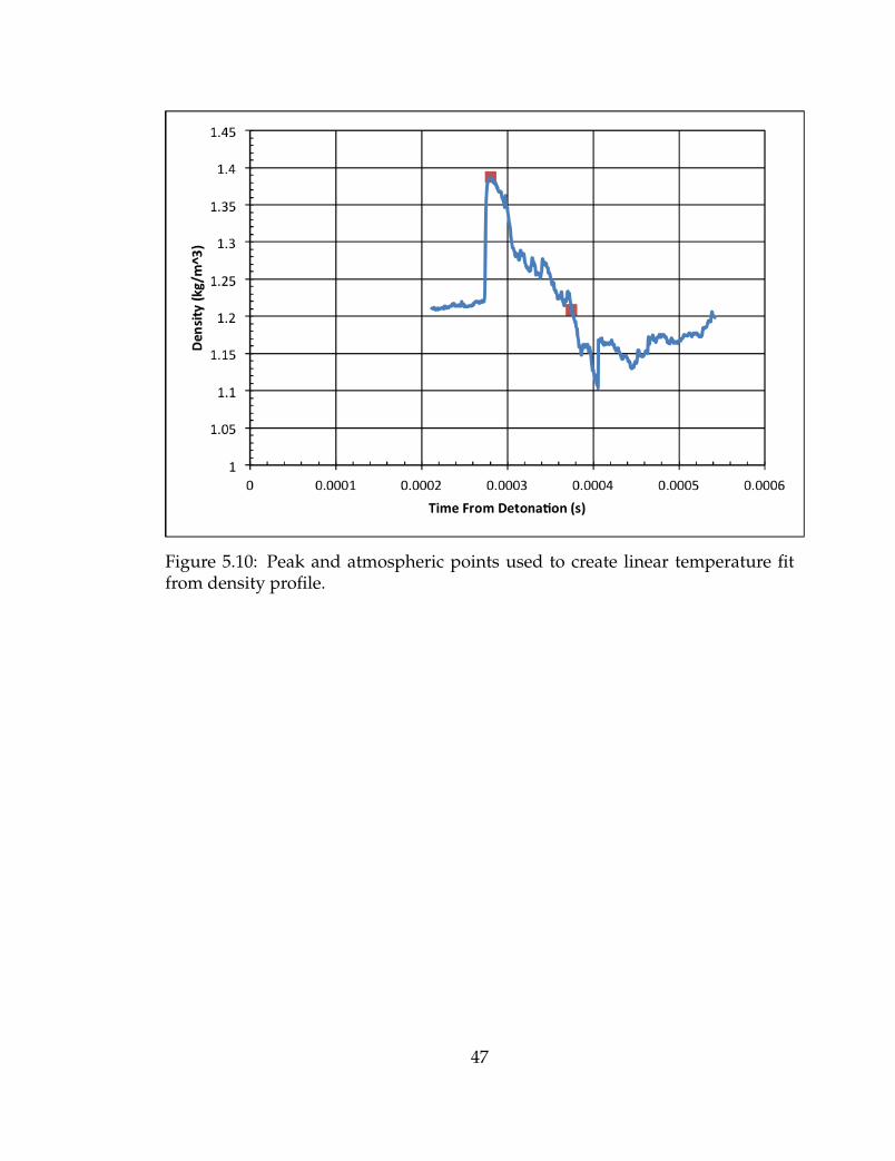
Figure 5.10: Peak and atmospheric points used to create linear temperature fitfrom density profile.
47
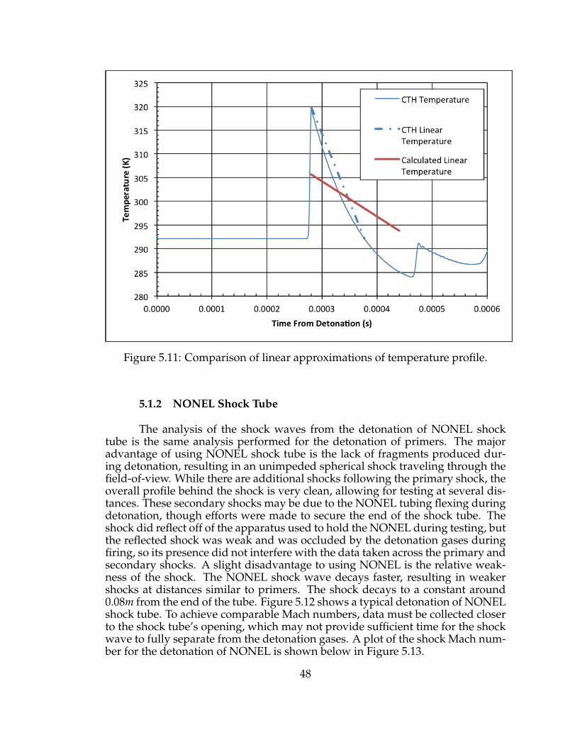
Figure 5.11: Comparison of linear approximations of temperature profile.
5.1.2 NONEL Shock Tube
The analysis of the shock waves from the detonation of NONEL shocktube is the same analysis performed for the detonation of primers. The majoradvantage of using NONEL shock tube is the lack of fragments produced dur-ing detonation, resulting in an unimpeded spherical shock traveling through thefield-of-view. While there are additional shocks following the primary shock, theoverall profile behind the shock is very clean, allowing for testing at several dis-tances. These secondary shocks may be due to the NONEL tubing flexing duringdetonation, though efforts were made to secure the end of the shock tube. Theshock did reflect off of the apparatus used to hold the NONEL during testing, butthe reflected shock was weak and was occluded by the detonation gases duringfiring, so its presence did not interfere with the data taken across the primary andsecondary shocks. A slight disadvantage to using NONEL is the relative weak-ness of the shock. The NONEL shock wave decays faster, resulting in weakershocks at distances similar to primers. The shock decays to a constant around0.08m from the end of the tube. Figure 5.12 shows a typical detonation of NONELshock tube. To achieve comparable Mach numbers, data must be collected closerto the shock tube’s opening, which may not provide sufficient time for the shockwave to fully separate from the detonation gases. A plot of the shock Mach num-ber for the detonation of NONEL is shown below in Figure 5.13.
48

Figure 5.12: Detonation of NONEL shock tube. Distance across field-of-view is0.1524m. First image at t=104.86µs from shock exiting NONEL tube, time betweensequential images 104.8µs.
49
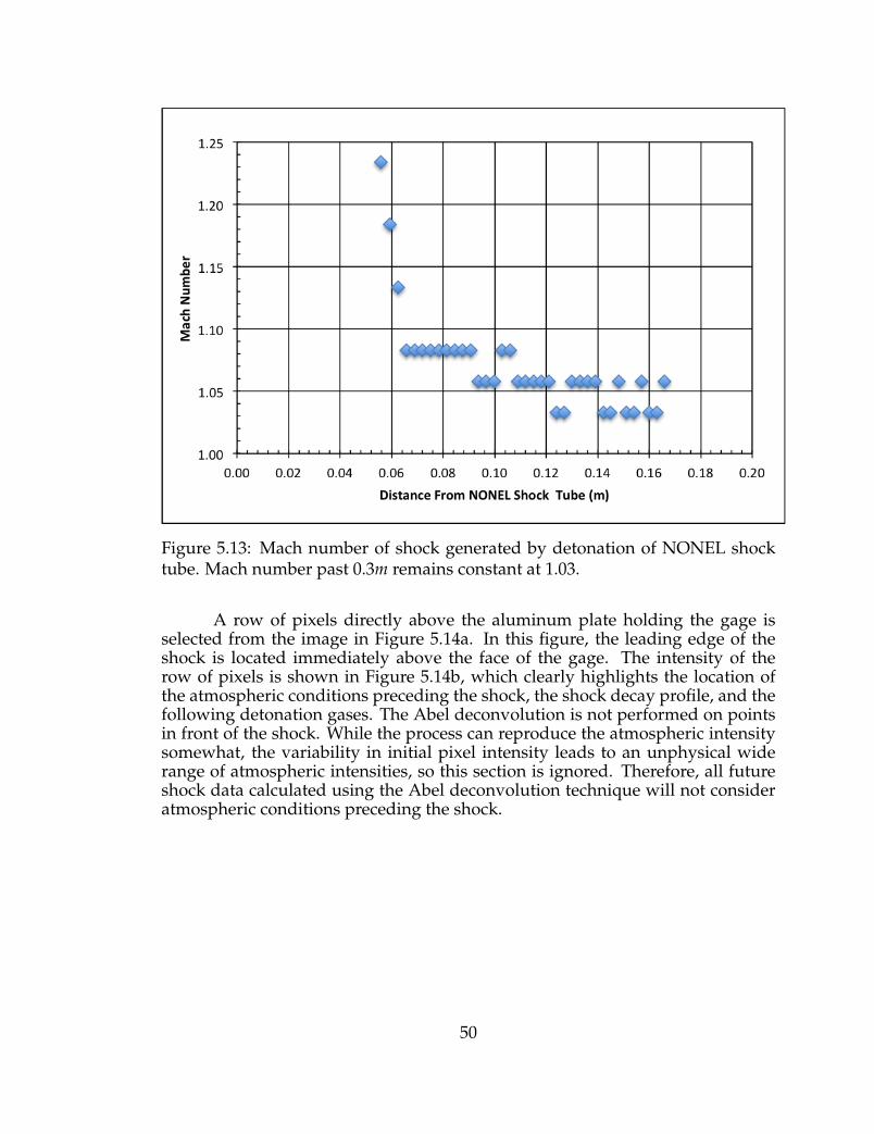
Figure 5.13: Mach number of shock generated by detonation of NONEL shocktube. Mach number past 0.3m remains constant at 1.03.
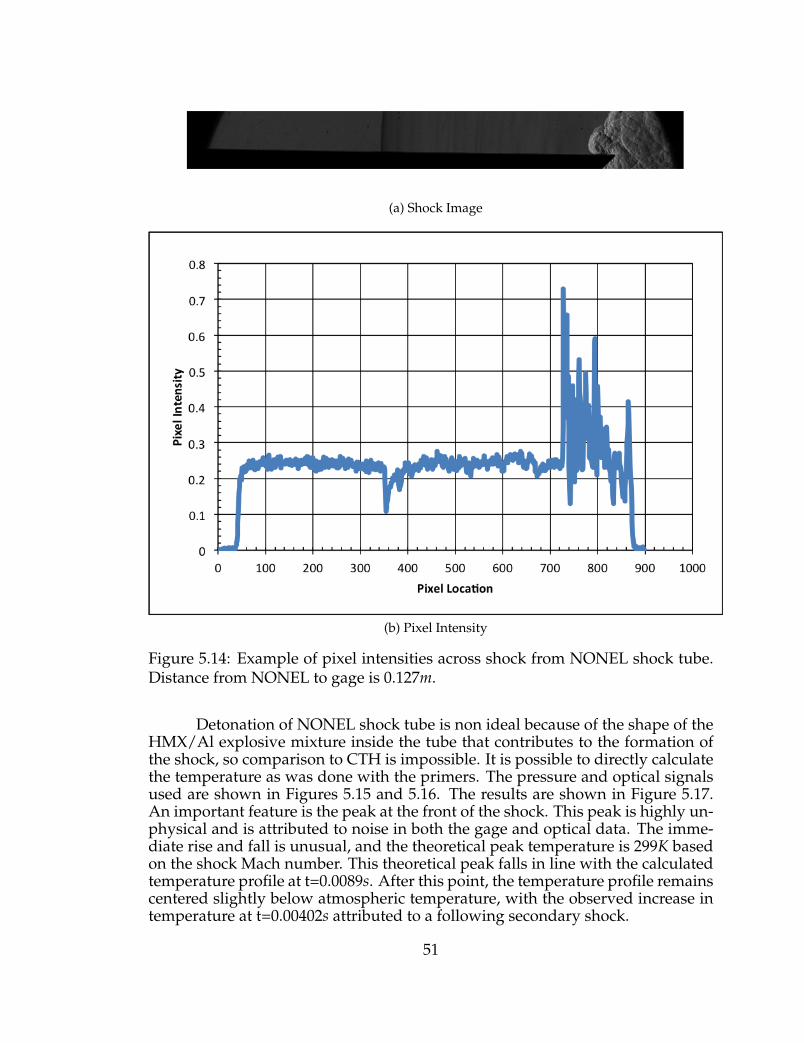
A row of pixels directly above the aluminum plate holding the gage isselected from the image in Figure 5.14a. In this figure, the leading edge of theshock is located immediately above the face of the gage. The intensity of therow of pixels is shown in Figure 5.14b, which clearly highlights the location ofthe atmospheric conditions preceding the shock, the shock decay profile, and thefollowing detonation gases. The Abel deconvolution is not performed on pointsin front of the shock. While the process can reproduce the atmospheric intensitysomewhat, the variability in initial pixel intensity leads to an unphysical widerange of atmospheric intensities, so this section is ignored. Therefore, all futureshock data calculated using the Abel deconvolution technique will not consideratmospheric conditions preceding the shock.
50
(a) Shock Image
(b) Pixel Intensity
Figure 5.14: Example of pixel intensities across shock from NONEL shock tube.Distance from NONEL to gage is 0.127m.
Detonation of NONEL shock tube is non ideal because of the shape of theHMX/Al explosive mixture inside the tube that contributes to the formation ofthe shock, so comparison to CTH is impossible. It is possible to directly calculatethe temperature as was done with the primers. The pressure and optical signalsused are shown in Figures 5.15 and 5.16. The results are shown in Figure 5.17.An important feature is the peak at the front of the shock. This peak is highly un-physical and is attributed to noise in both the gage and optical data. The imme-diate rise and fall is unusual, and the theoretical peak temperature is 299K basedon the shock Mach number. This theoretical peak falls in line with the calculatedtemperature profile at t=0.0089s. After this point, the temperature profile remainscentered slightly below atmospheric temperature, with the observed increase intemperature at t=0.00402s attributed to a following secondary shock.
51

Figure 5.15: Gage pressure profile. Highlighted portion red used to determinetemperature. Distance from NONEL to gage is 0.127m.
52

Figure 5.16: Optical density profile. Entire signal used to determine temperature.Distance from NONEL to gage is 0.127m.
53

Figure 5.17: Temperature profile directly calculated from optical density and gagepressure. Mach 1.03.
The existence of this secondary shock is seen in all tests using the NONELshock tube, and its existence makes it difficult to attribute a single linear temper-ature profile to the data. Additionally, there is no CTH profile to compare to thecalculated temperature profile. To calculate a linear temperature profile, the factthat the relative rates of temperature, density, and pressure decay are equivalentis used to generate a linear profile. Using the density profile, the time locations ofthe peak and atmospheric density after the secondary shock are chosen (see Fig-ure 5.18). A linear fit is created from these two points using the theoretical peaktemperature and the atmospheric temperature and compared to the calculatedtemperature profile in Figure 5.19.
54

Figure 5.18: Time of peak and low points highlighted.
55
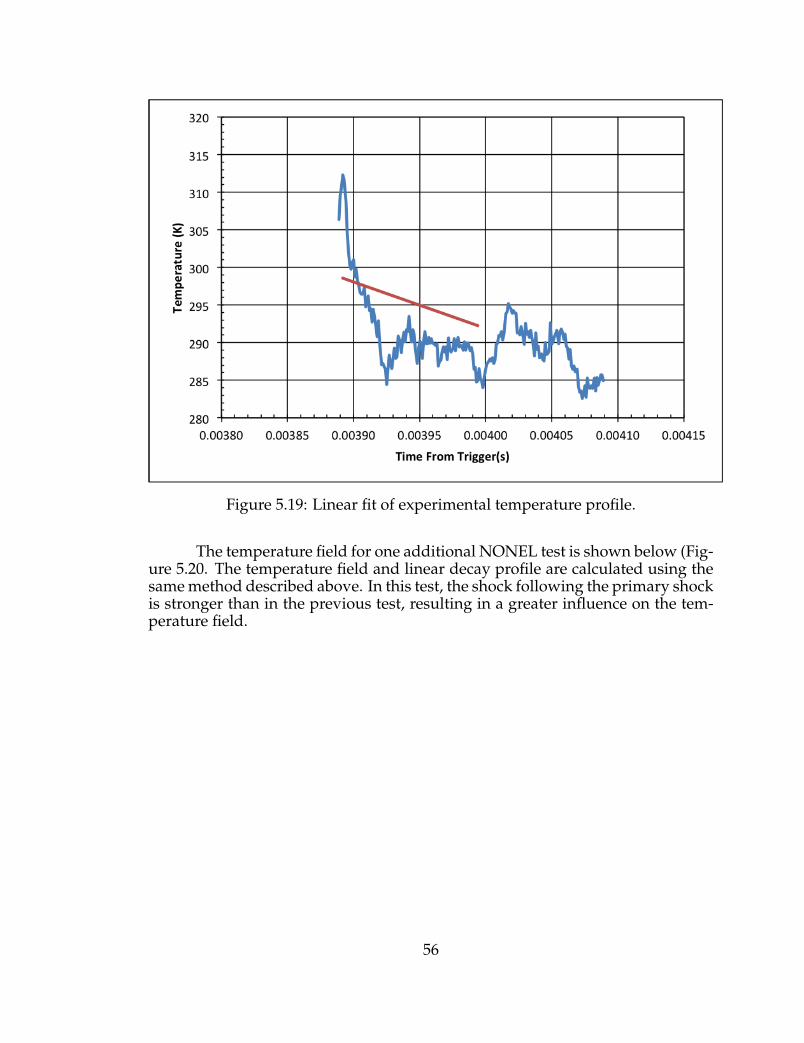
Figure 5.19: Linear fit of experimental temperature profile.
The temperature field for one additional NONEL test is shown below (Fig-ure 5.20. The temperature field and linear decay profile are calculated using thesame method described above. In this test, the shock following the primary shockis stronger than in the previous test, resulting in a greater influence on the tem-perature field.
56

(a) Shock Image
(b) Calculated Temperature
Figure 5.20: Temperature profile and linear fit directly calculated from opticaldensity and gage pressure. Distance from NONEL to gage is 0.102m. Mach 1.06.
5.1.3 Detasheet
The last set of explosive compounds testing were 1g rolled balls of De-tasheet, consisting of 80% PETN. Again, the same analysis done to the primersand NONEL shock tube is done here. In this series, all testing was done in thefield, so the setup used with the schlieren system is slightly different. Addition-ally, during testing the background intensity shutting, requiring a correction tothe intensity be applied. This is described in further detail in Section 5.2.4. Themajor differences are the use of an arc lamp in place of a single-die LED, and thepresence of the calibration lens within the field-of-view during all detonations.The presence of the calibration lens is unfortunate as the shock impinged on itssurface causing a backwards reflection into the oncoming shock. This occurrence
57

prevented the analysis of the complete pressure profile as done with primers andNONEL. The Detasheet was fired at least 0.45m outside the field-of-view, pre-venting collection of the entire Mach profile; the shocks were observed to be trav-eling at a fairly constant rate through the field-of-view. Figure 5.22 shows theshock Mach numbers from the firing of the Detasheet at two locations. A com-plete Mach profile could not be collected due to the limited field-of-view and thelocation of the charge. The limited field-of-view and the camera’s frame rate alsoresulted in the small number of data points available. One last major differenceis the focal length of the calibration lens; here it is 4m, which was later discov-ered to give less accurate results than using the 10m focal length calibration lens.However, the comparison between the gage and optical data still shows goodagreement for the portion of the shock being analyzed. Figure 5.21 shows the fullview of the shock impinging on the calibration lens during propagation. Alsonote that for this analysis, the row of pixels analyzed goes through the center ofthe calibration lens, not directly over the gage as has been done in the previoussections. For these tests, the gage was not in the field-of-view. This may also ac-count for some of the discrepancy between the gage and optical measurements.The shock and corresponding pixel intensities from the detonation of Detasheetare shown in Figure 5.23. The charge is 0.902m from the face of the gage.
58
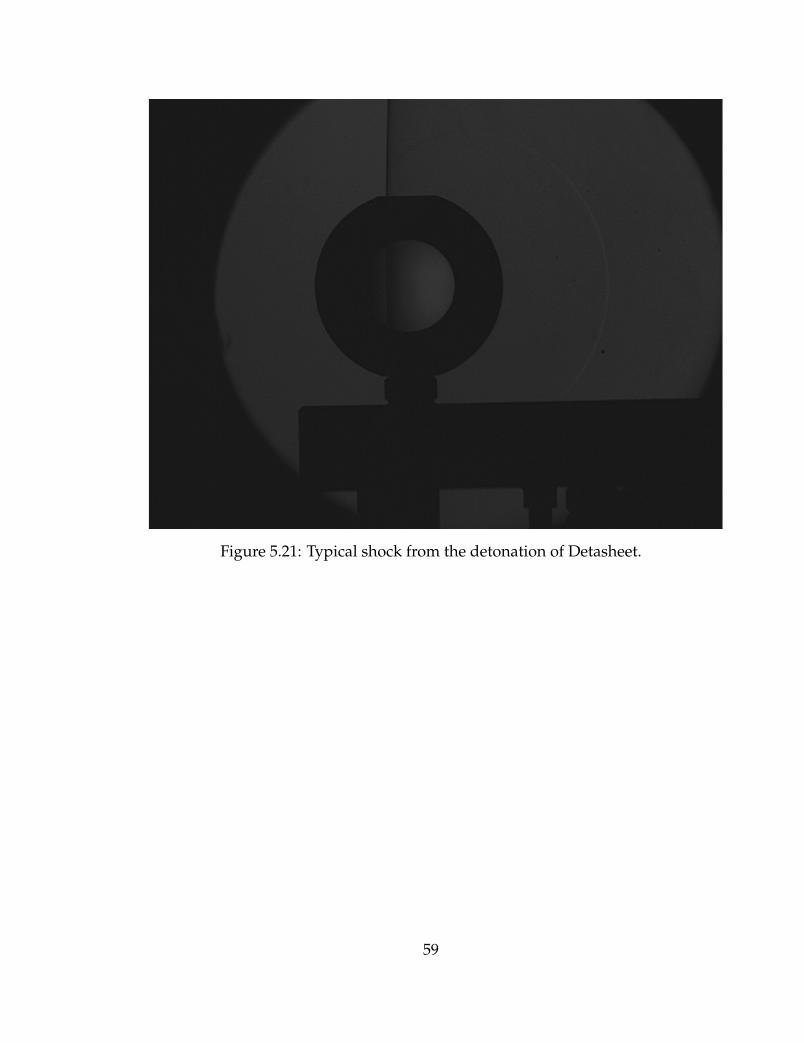
Figure 5.21: Typical shock from the detonation of Detasheet.
59
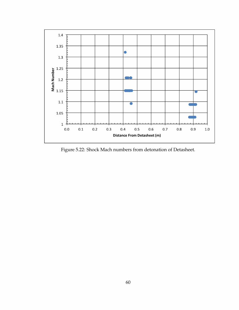
Figure 5.22: Shock Mach numbers from detonation of Detasheet.
60

(a) Shock Image
(b) Pixel Intensity
Figure 5.23: Example of pixel intensity across shock from detonation of Detasheet,distance from charge to gage 0.9017m. Mach 1.08.
The temperature profile is recreated using sections of the gage pressureand optical density profiles (Figures 5.24 and 5.25). The optical density had a lin-ear fit applied to the data for this calculation. The gage pressure and the densitycalculated by the linear fit were used to determine the temperature field. Thisallowed the temperature field to be expanded past the data available in the opti-cal signal. The additional small peaks behind the leading edge of the shock arecaused by additional shocks visible in Figure 5.23a. The calculated temperatureprofile is compared to the constant temperature profile and the CTH temperatureprofile in Figure 5.26. As with the primers, the temperature at the leading edgeof the shock is higher than expected, most likely due to noise in either the gage oroptical signals. This temperature signal also decays faster than the CTH profilewould predict, indicating that the CTH profile may predict higher temperatures
61
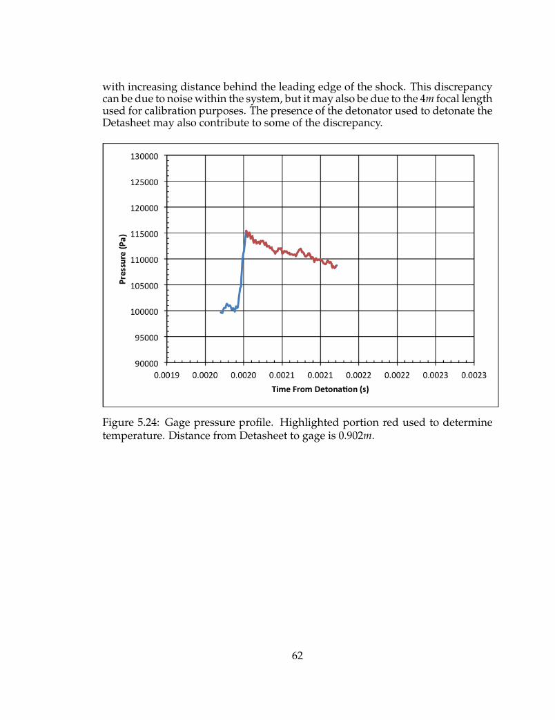
with increasing distance behind the leading edge of the shock. This discrepancycan be due to noise within the system, but it may also be due to the 4m focal lengthused for calibration purposes. The presence of the detonator used to detonate theDetasheet may also contribute to some of the discrepancy.
Figure 5.24: Gage pressure profile. Highlighted portion red used to determinetemperature. Distance from Detasheet to gage is 0.902m.
62

Figure 5.25: Optical density profile. Location of leading edge of shock high-lighted. Linear fit of entire selection used to determine temperature.
63
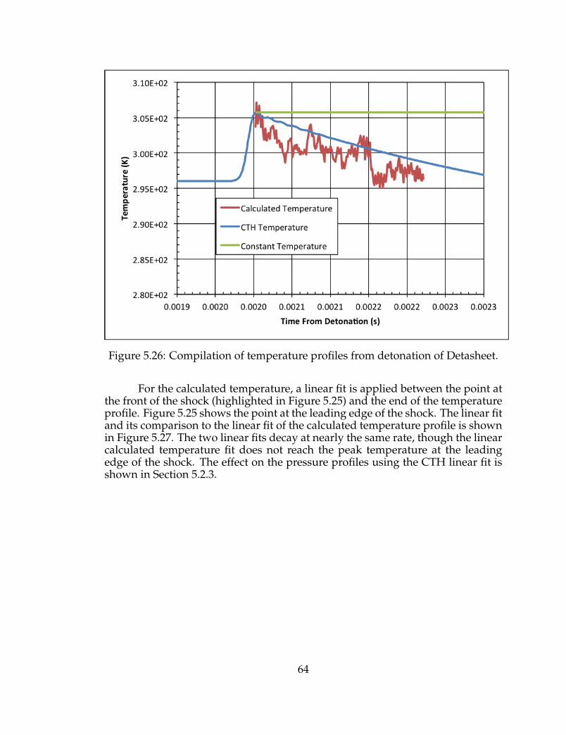
Figure 5.26: Compilation of temperature profiles from detonation of Detasheet.
For the calculated temperature, a linear fit is applied between the point atthe front of the shock (highlighted in Figure 5.25) and the end of the temperatureprofile. Figure 5.25 shows the point at the leading edge of the shock. The linear fitand its comparison to the linear fit of the calculated temperature profile is shownin Figure 5.27. The two linear fits decay at nearly the same rate, though the linearcalculated temperature fit does not reach the peak temperature at the leadingedge of the shock. The effect on the pressure profiles using the CTH linear fit isshown in Section 5.2.3.
64
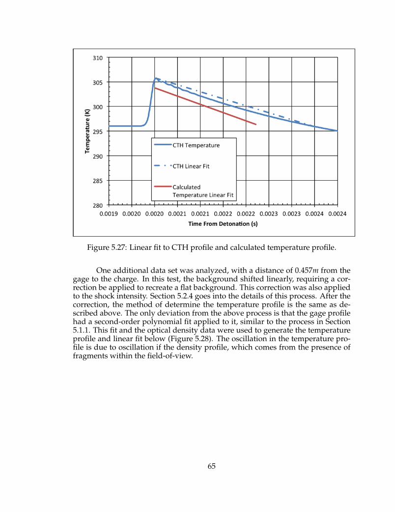
Figure 5.27: Linear fit to CTH profile and calculated temperature profile.
One additional data set was analyzed, with a distance of 0.457m from thegage to the charge. In this test, the background shifted linearly, requiring a cor-rection be applied to recreate a flat background. This correction was also appliedto the shock intensity. Section 5.2.4 goes into the details of this process. After thecorrection, the method of determine the temperature profile is the same as de-scribed above. The only deviation from the above process is that the gage profilehad a second-order polynomial fit applied to it, similar to the process in Section5.1.1. This fit and the optical density data were used to generate the temperatureprofile and linear fit below (Figure 5.28). The oscillation in the temperature pro-file is due to oscillation if the density profile, which comes from the presence offragments within the field-of-view.
65
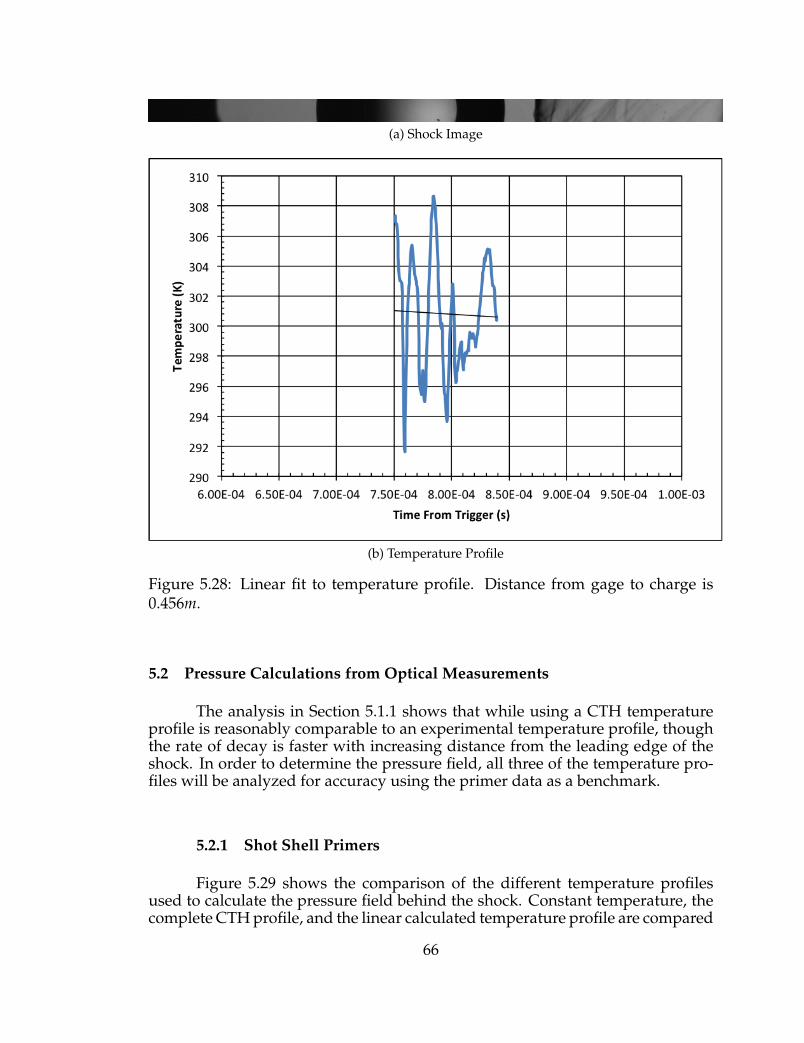
(a) Shock Image
(b) Temperature Profile
Figure 5.28: Linear fit to temperature profile. Distance from gage to charge is0.456m.
5.2 Pressure Calculations from Optical Measurements
The analysis in Section 5.1.1 shows that while using a CTH temperatureprofile is reasonably comparable to an experimental temperature profile, thoughthe rate of decay is faster with increasing distance from the leading edge of theshock. In order to determine the pressure field, all three of the temperature pro-files will be analyzed for accuracy using the primer data as a benchmark.
5.2.1 Shot Shell Primers
Figure 5.29 shows the comparison of the different temperature profilesused to calculate the pressure field behind the shock. Constant temperature, thecomplete CTH profile, and the linear calculated temperature profile are compared
66

to the gage pressure. The CTH profile is included as a comparison to an idealizeddetonation, but clearly shows very poor agreement between the other profilesand the gage data It neither resolves the experimental peak pressure, and it pre-dicts a larger negative pulse than is backed up experimentally. Therefore, careshould be taken if the CTH profile is to be used to generate temperature or pres-sure decay trends for experimental data.. The good agreement between the gageand linear profile throughout indicates that using an experimentally derived tem-perature decay field provides the best reproduction of the pressure field behindthe shock. Additionally, using a constant temperature profile clearly shows verypoor agreement with the gage pressure and the linear temperature pressure pro-file. Therefore, using a constant temperature profile is a poor choice and all otherwork will exclude analysis of the constant temperature profile.
Figure 5.29: Compilation of pressure profiles used with shot shell primers. Mach1.12, theoretical pressure 185kPa ±7kPa.
An analysis of the relative uncertainty in the optical pressure signals candetermine how well these various temperature and pressure profiles compare.However, one drawback to the high-speed imaging is high levels of uncertaintydue to noise. An example of the oscillation in the background intensity is shownbelow (Figure 5.30).
67

Figure 5.30: Zoomed in example of raw background intensity.
In this test, there was an average oscillation of ±114 values in the rawpixel intensity data. This becomes a variation of ±57 pixels in in the backgroundintensity from the average, which lead to an uncertainty of ±4000Pa. This highlevel of uncertainty is attributed to noise from the camera sensor. A more appro-priate estimate of the uncertainty is calculated by determining the atmosphericpressure across the field-of-view in one image using the Abel transform on a sec-tion of the field-of-view unaffected by the shock. Using this method, the averageatmospheric pressure was 101292Pa, with a standard deviation of 507Pa. This isstill a large degree of uncertainty, and an accurate uncertainty would more likelybe ±200Pa. The gage pressure is within the linear temperature pressure’s uncer-tainty, while the constant temperature and CTH pressures are not. There is alsosome degree of uncertainty of the theoretical pressure based on the Mach num-ber. The Mach number calculated by the shock tracking program is dependent onthe uncertainty in pixel location, temperature, and the size of the calibration ob-ject. The program outputs an uncertainty based on these parameters. The Machnumber in this primer test was 1.14 ±0.022. With this uncertainty, the range intheoretical pressure becomes 130 to 144kPa. All but the CTH pressure profile areoutside of the range of possible theoretical pressures. However, the wide rangein the theoretical pressure indicates that the theoretical peak pressure should be
68
treated as a benchmark figure. Another possible reason for the optical or gagemeasurements to fail at resolving the theoretical pressure is the relative pixel sizeand gage response time, respectively. As the Mach number increases, the cameraand gage may not be able to resolve the small area where the peak intensity ofthe shock exists.
5.2.2 NONEL Shock Tube
A compilation of the theoretical, gage, and optical peak pressures fromthree different distances of NONEL shock tube are shown below in Figure 5.31.The uncertainty of the theoretical pressure is±4300Pa. The two data sets furthestfrom the shock tube were chosen for analysis, as more of the pressure field couldbe analyzed before the detonation gases interfered. The pressure field for thedetonation of NONEL shock is calculated at 0.127m in Figure 5.32 and 0.102min Figure 5.33 from the end of the shock tube. The uncertainty is calculated inthe same manner as with the primers. Here, the average background pressure is101591Pa, with a standard deviation of ±407Pa.
Figure 5.31: Comparison of theoretical, gage, and optical peak pressures at threedistances using NONEL shock tube.
69

Figure 5.32: Pressure fields derived from linear temperature trends compared togage pressure. Distance to gage 0.127m.
70
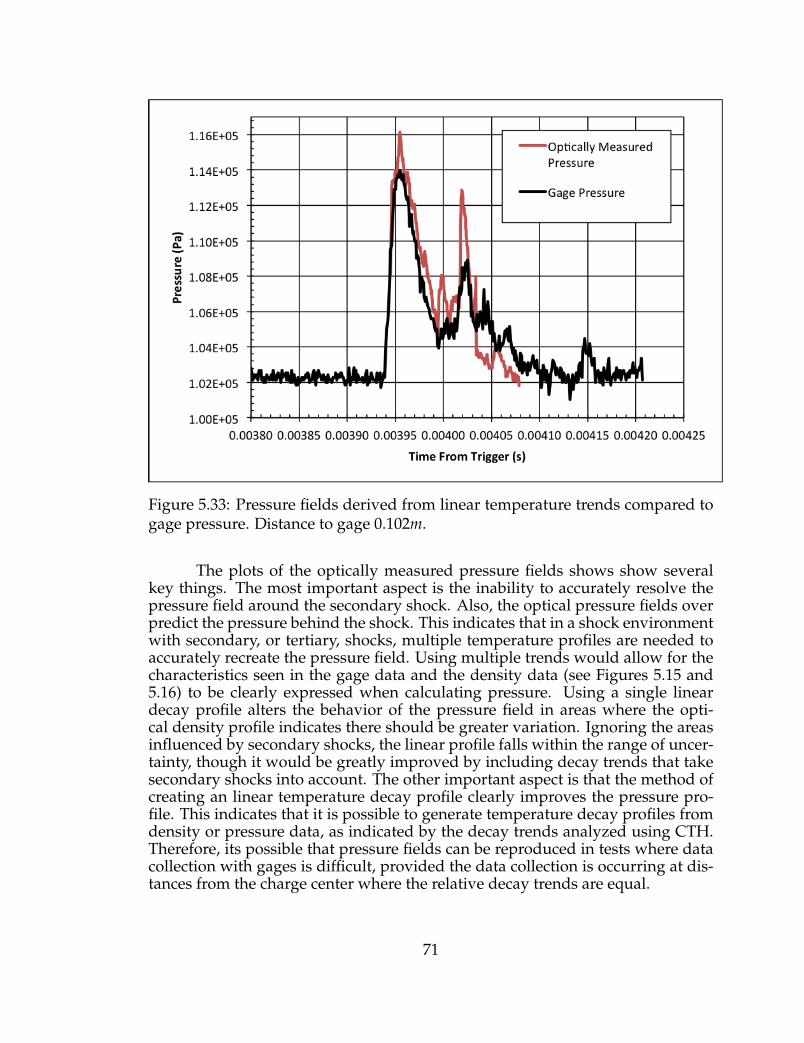
Figure 5.33: Pressure fields derived from linear temperature trends compared togage pressure. Distance to gage 0.102m.
The plots of the optically measured pressure fields shows show severalkey things. The most important aspect is the inability to accurately resolve thepressure field around the secondary shock. Also, the optical pressure fields overpredict the pressure behind the shock. This indicates that in a shock environmentwith secondary, or tertiary, shocks, multiple temperature profiles are needed toaccurately recreate the pressure field. Using multiple trends would allow for thecharacteristics seen in the gage data and the density data (see Figures 5.15 and5.16) to be clearly expressed when calculating pressure. Using a single lineardecay profile alters the behavior of the pressure field in areas where the opti-cal density profile indicates there should be greater variation. Ignoring the areasinfluenced by secondary shocks, the linear profile falls within the range of uncer-tainty, though it would be greatly improved by including decay trends that takesecondary shocks into account. The other important aspect is that the method ofcreating an linear temperature decay profile clearly improves the pressure pro-file. This indicates that it is possible to generate temperature decay profiles fromdensity or pressure data, as indicated by the decay trends analyzed using CTH.Therefore, its possible that pressure fields can be reproduced in tests where datacollection with gages is difficult, provided the data collection is occurring at dis-tances from the charge center where the relative decay trends are equal.
71
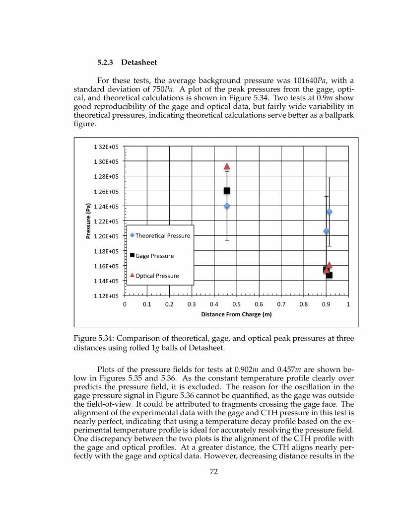
5.2.3 Detasheet
For these tests, the average background pressure was 101640Pa, with astandard deviation of 750Pa. A plot of the peak pressures from the gage, opti-cal, and theoretical calculations is shown in Figure 5.34. Two tests at 0.9m showgood reproducibility of the gage and optical data, but fairly wide variability intheoretical pressures, indicating theoretical calculations serve better as a ballparkfigure.
Figure 5.34: Comparison of theoretical, gage, and optical peak pressures at threedistances using rolled 1g balls of Detasheet.
Plots of the pressure fields for tests at 0.902m and 0.457m are shown be-low in Figures 5.35 and 5.36. As the constant temperature profile clearly overpredicts the pressure field, it is excluded. The reason for the oscillation in thegage pressure signal in Figure 5.36 cannot be quantified, as the gage was outsidethe field-of-view. It could be attributed to fragments crossing the gage face. Thealignment of the experimental data with the gage and CTH pressure in this test isnearly perfect, indicating that using a temperature decay profile based on the ex-perimental temperature profile is ideal for accurately resolving the pressure field.One discrepancy between the two plots is the alignment of the CTH profile withthe gage and optical profiles. At a greater distance, the CTH aligns nearly per-fectly with the gage and optical data. However, decreasing distance results in the
72
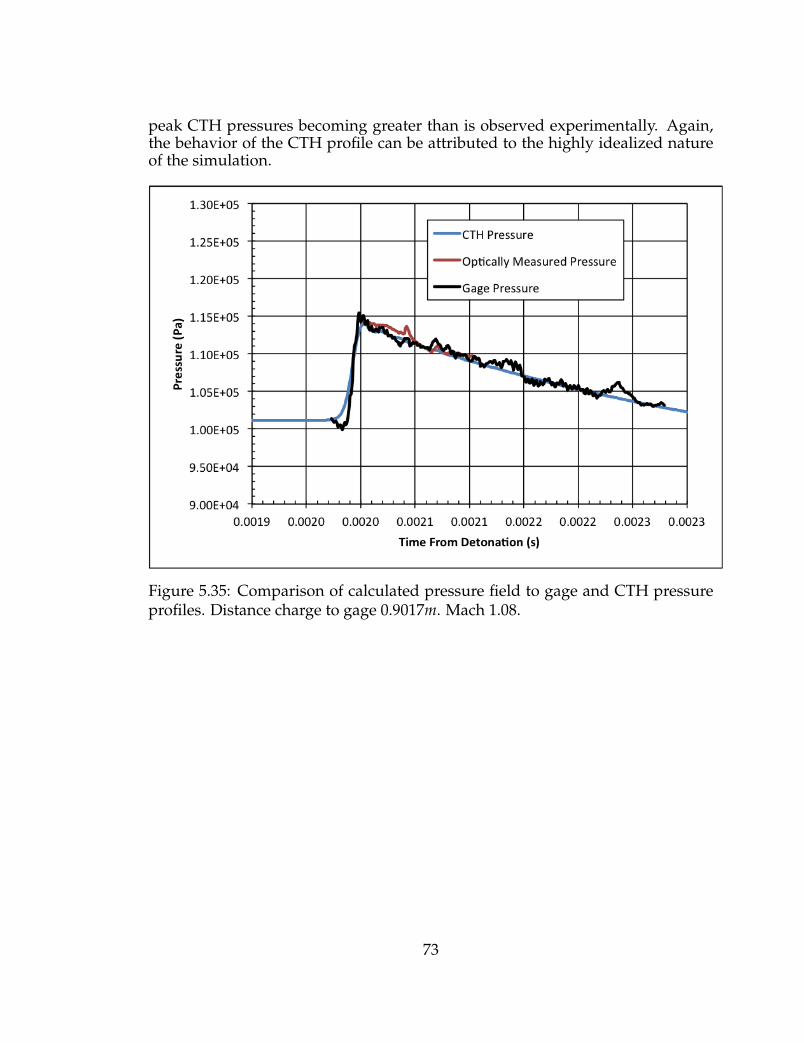
peak CTH pressures becoming greater than is observed experimentally. Again,the behavior of the CTH profile can be attributed to the highly idealized natureof the simulation.
Figure 5.35: Comparison of calculated pressure field to gage and CTH pressureprofiles. Distance charge to gage 0.9017m. Mach 1.08.
73

Figure 5.36: Comparison of calculated pressure field to gage and CTH pressureprofiles. Distance charge to gage 0.457m. Mach 1.09.
5.2.4 Intensity Corrections
When the schlieren setup is correct, the intensity across the entire field-of-view should be uniform. However, should this intensity deviate linearly, it ispossible to apply a correction to generate a flat background intensity. Adding orsubtracting a constant value from the intensity creates this new background ateach pixel location. The correction must be applied to all images being analyzed,including the intensities observed in the calibration images. For the analysis ofthe Detasheet, it was necessary to apply the correction to several of the later tests.An example of a typical flat background intensity and shock versus a deviatedbackground intensity and shock is shown below in Figures 5.37 and 5.38.
74

(a) Background
(b) Shock
Figure 5.37: Background and shock intensities for detonation of Detasheet.
75
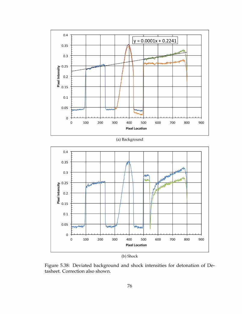
(a) Background
(b) Shock
Figure 5.38: Deviated background and shock intensities for detonation of De-tasheet. Correction also shown.
76

This method of correction was used to create the pressure profiles in theprevious section. As there is good agreement between the experimental gage andoptical results, this technique is a valid tool for future use. Situations where auniform background is difficult to achieve can be made to yield accurate results.
77

CHAPTER 6
CONCLUSIONS AND RECOMMENDATIONS FOR FUTURERESEARCH
The schlieren technique has been shown to be capable of successfully cap-turing images of explosively-driven shocks, and for the shock overpressure andpressure duration to be reproduced. The images used must meet certain criteriato be successfully analyzed. The most important consideration is that the back-ground intensity in the calibration and shock images is uniform, which allows fordeviations from the background to be quantified with little error. In cases wherethe background deviates linearly, it is possible to apply a correction and accu-rately process images. Ideally, the shock should be clearly separated from thefollowing detonation gases, as the observed changes in refractive index are quan-tifiable for one gas species. Additionally, the shock should be purely spherical,without fragments within the field-of-view. Oblique shocks form from the frag-ments, creating interference with shock processing. Finally, the schlieren setupmust have sufficient light that applying a cutoff will not cause the shock intensityto zero out. The light entering the camera should take up most of the sensor’srange.
The Abel two-point deconvolution technique is effective at reproducingthe density, and subsequently the pressure, field. The method used has a highdegree of accuracy with little computational noise. However, a disadvantageto the technique is the assumption on spherical geometry. When fragments arepresent, the deflection angles due to both the spherical shock and the fragments’oblique shocks are carried through the calculations. Some discrepancies betweenthe gage and optical pressure fields is due to this.
For all three explosives, creating an optically-derived temperature fieldyielded better results than using the constant temperature assumption. The tem-perature field for the shot shell primers was created using second-order polyno-mial fits of the experimental density data and gage pressure. A linear decay pro-file was fit to the derived temperature field and used to determine the pressurefield. The calculated pressure field showed the best agreement with the pressuregage data. The constant temperature profile resulted in a pressure field that wastoo high everywhere, so it is inappropriate to use this assumption. The CTH dataover-predicted the peak pressures and under predicted the negative pulse fol-lowing the shock. In the case of non ideal explosives such as shot shell primers, itis inappropriate to use the highly idealized temperature profiles determined by
78
CTH to calculate the experimental pressure.The temperature profile of NONEL shock tube was created by directly ap-
plying the ideal gas law to corresponding optical density and gage pressure datapoints. A linear fit was applied to this profile and used to determine the opticalpressure field. The use of NONEL was complicated by the presence of large sec-ondary shocks. As the Mach number increased, the influence of secondary shockson the pressure profile increased. Applying trends to the data was complicatedby this secondary shock, as the current research focused on using a single fit fordata set being analyzed. Despite this difficulty, the NONEL pressure signal wascalculated with reasonable accuracy. The accuracy was best for data immediatelybehind the primary shock and preceding the secondary shock.
The tests using Detasheet were the closest experimental comparison to theCTH simulation. Only subsections corresponding to available optical data wereanalyzed to determine the temperature field. A linear fit was applied to thistemperature field and used to determine the optical pressure field. These testsshowed the best agreement between the gage, optically calculated pressure, andthe CTH pressure data. The good alignment between the optically calculatedpressure, the gage, and CTH pressures indicates that the method of deriving thetemperature field is accurate, as well as the use of a linear temperature decayprofile to calculate pressure.
6.1 Future Work
Future extensions to this work will be the application of the schlieren tech-niques and computational processes to the background-oriented schlieren (BOS)technique. The BOS technique visualizes the first-derivative of the refractive in-dex and can be used to determine the same information. This technique is capableof visualizing large-scale events, using a simplified setup of the high-speed cam-era and a natural landscape. Other issues to be addressed include improving theaccuracy of the technique and reducing the uncertainty. Different light sourcesand cameras should be tested in order to quantify the source of the noise in thebackground seen throughout the images analyzed. Additionally, the degree towhich a background can vary and still produce accurate data should be quan-tified. Extreme setup accuracy is not always possible, particularly during fieldtesting. Acceptable parameters for background deviation should be established.Finally, developing a method to measure across the detonation gases would behighly beneficial. Current methods cannot image through the gases, and theirpresence interferes with the collection of the compete pressure profile. Develop-ing a method to image through these gases at the same time as air would allowthe shock properties to be quantified very close to the explosive.
79

BIBLIOGRAPHY
[1] R. E. Duff and E. Houston. Measurement of the chapman jouguet pressureand reaction zone length in a detonating high explosive. Journal of ChemicalPhysics, 23:1268–1273, jul 1955.
[2] Michael J Hargather and Gary S Settles. Optical measurement and scaling ofblasts from gram-range explosive charges. Shock waves, 17(4):215–223, 2007.
[3] A. M. Bagabir. Cylindrical blast wave propagation in an enclosure. SHOCKWAVES, 22(6):547–556, NOV 2012.
[4] K. Spranghers, I. Vasilakos, D. Lecompte, H. Sol, and J. Vantomme. Nu-merical simulation and experimental validation of the dynamic response ofaluminum plates under free air explosions. INTERNATIONAL JOURNALOF IMPACT ENGINEERING, 54:83–95, APR 2013.
[5] Geoffrey Mays and Peter D Smith. Blast effects on buildings: design of buildingsto optimize resistance to blast loading. Thomas Telford, 1995.
[6] Gilbert Ford Kinney and Kenneth Judson Graham. Explosive shocks in air.Berlin and New York, Springer-Verlag, 1985, 282 p., 1, 1985.
[7] Zhang Qi, Qin Bin, and Lin Da-Chao. Estimation of pressure distribution forshock wave through the bend of bend laneway. Safety Science, 48(10):1263 –1268, 2010.
[8] Qi Zhang, Bin Qin, and Da-Chao Lin. Estimation of pressure distribution forshock wave through the junction of branch gallery. Safety Science, 57(0):214– 222, 2013.
[9] A Sayapin, A Grinenko, S Efimov, and YE Krasik. Comparison of differentmethods of measurement of pressure of underwater shock waves generatedby electrical discharge. SHOCK WAVES, 15(2):73–80, JUN 2006.
[10] WN MacPherson, MJ Gander, JS Barton, JDC Jones, CL Owen, AJ Watson,and RM Allen. Blast-pressure measurement with a high-bandwidth fibre op-tic pressure Sensor. MEASUREMENT SCIENCE & TECHNOLOGY, 11(2):95–102, FEB 2000.
[11] AJ Hoffman and SM Mills Jr. Air blast measurements about explosivecharges at side-on and normal incidence. Technical report, DTIC Document,1956.
80
[12] Bertram Hopkinson. A method of measuring the pressure produced in thedetonation of high explosives or by the impact of bullets. Proceedings of theRoyal Society of London. Series A, 89(612):411–413, 1914.
[13] Per-Anders Persson, Roger Holmberg, and Jaimin Lee. Rock blasting andexplosives engineering. CRC press, 1993.
[14] G. S. Settles. Schlieren and Shadowgraph Techniques. Springer, 2001.
[15] L Venkatakrishnan and GEA Meier. Density measurements using theBackground Oriented Schlieren technique. EXPERIMENTS IN FLUIDS,37(2):237–247, AUG 2004.
[16] Michael J. Hargather and Gary S. Settles. A comparison of three quantitativeschlieren techniques. OPTICS AND LASERS IN ENGINEERING, 50(1, SI):8–17, JAN 2012.
[17] MM Biss, GS Settles, MJ Hargather, LJ Dodson, and JD Miller. High-speeddigital shadowgraphy of shock waves from explosions and gunshots. InShock Waves, pages 91–96. Springer, 2009.
[18] Michael J. Hargather and Gary S. Settles. Retroreflective shadowgraph tech-nique for large-scale flow visualization. APPLIED OPTICS, 48(22):4449–4457, AUG 1 2009.
[19] O. K. Sommersel, D. Bjerketvedt, S. O. Christensen, O. Krest, andK. Vaagsaether. Application of background oriented schlieren for quan-titative measurements of shock waves from explosions. SHOCK WAVES,18(4):291–297, SEP 2008. 21st International Colloquium on the Dynamics ofExplosions and Reactive Systems, Poitiers, FRANCE, JUL 23-28, 2007.
[20] M. J. Hargather. Background-oriented schlieren diagnostics for large-scaleexplosive testing. SHOCK WAVES, 23(5):529–536, SEP 2013.
[21] Matthew Biss. Laboratory-scale technique to optically measure explosiveimpulse for energetic-material air-blast characterization. Technical ReportARL-TR-6185, Army Research Laboratory, 2012.
[22] Michael J Hargather. Scaling, Characterization, and Application of Gram-rangeExplosive Charges to Blast Testing of Materials. PhD thesis, Pennsylvania StateUniversity, 2008.
[23] Wolgang Merzkirch. Flow visualization. Elsevier, 1987.
[24] Paul W Cooper. Explosives engineering. VCH New York, 1996.
[25] Harold L Brode. Numerical solutions of spherical blast waves. Journal ofApplied physics, 26(6):766–775, 2004.
81

[26] Pankaj S Kolhe and Ajay K Agrawal. Abel inversion of deflectometric data:comparison of accuracy and noise propagation of existing techniques. Ap-plied optics, 48(20):3894–3902, 2009.
[27] Simon Ostrach. An analysis of laminar free-convection flow and heat trans-fer about a flat plate parallel to the direction of the generating body force.NACA, 1953.
[28] J.M. McGlaun, S.L. Thompson, and M.G. Elrick. Cth: A three-dimensionalshock wave physics code. International Journal of Impact Engineering, 10(1–4):351 – 360, 1990.
[29] Geoffrey Taylor. The formation of a blast wave by a very intense explosion.i. theoretical discussion. Proceedings of the Royal Society of London. Series A.Mathematical and Physical Sciences, 201(1065):159–174, 1950.
[30] Geoffrey Taylor. The formation of a blast wave by a very intense explosion.ii. the atomic explosion of 1945. Proceedings of the Royal Society of London.Series A. Mathematical and Physical Sciences, 201(1065):175–186, 1950.
[31] H Kleine, JM Dewey, K Ohashi, T Mizukaki, and K Takayama. Studies of thetnt equivalence of silver azide charges. Shock Waves, 13(2):123–138, 2003.
82

QUANTITATIVE SCHLIEREN MEASUREMENT OF EXPLOSIVELY-DRIVENSHOCK WAVE DENSITY, TEMPERATURE, AND PRESSURE PROFILES.
by
J. D. Tobin
Permission to make digital or hard copies of all or part of this workfor personal or classroom use is granted without fee provided thatcopies are not made or distributed for profit or commercial advantageand that copies bear this notice and the full citation on the last page.To copy otherwise, to republish, to post on servers or to redistributeto lists, requires prior specific permission and may require a fee.
83