To Migrate or to Forage?

The Where, When and Why Behind Grevy’s Zebra Movement

Nika Levikov

September 2014

A thesis submitted in partial fulfilment of the requirement for the degree of Master of Science and the Diploma of Imperial College London

1

DECLARATION OF OWN WORK

I declare that this thesis, “To Migrate or to Forage? The Where, When and Why Behind

Grevy’s Zebra Movement,” is entirely my own work and that where material could be

construed as the work of others, it is fully cited and referenced and/or with appropriate

knowledge given.

Signature

Name of student: Nika Levikov

Names of Supervisors: Dr. Marcus Rowcliffe Belinda Low Dr. Sarah Robinson

Contents

Abstract ................................................................................................................................................... 5

Acknowledgements ................................................................................................................................. 6

1. Introduction ........................................................................................................................................ 8

1.1 Problem Statement ....................................................................................................................... 8

1.2 Aim and Objectives ..................................................................................................................... 10

1.3 Hypotheses ................................................................................................................................. 11

2. Background ....................................................................................................................................... 11

2.1 Grevy’s Zebra .............................................................................................................................. 11

2.1.1 Background and Ecology ...................................................................................................... 11

2.1.2 Threats and Legal Status ...................................................................................................... 12

2.2 Methods Approach ..................................................................................................................... 14

2.2.1 Normalized Differential Vegetation Index ........................................................................... 14

2.2.2 Dynamic Brownian Bridge Movement Model...................................................................... 15

2.3 Animal Movement ...................................................................................................................... 17

2.3.1 Understanding Movement and Utilization Distribution ...................................................... 17

2.3.2 Movement Research for Conservation Planning ................................................................. 17

2.4 Study Area ................................................................................................................................... 19

3. Methods ............................................................................................................................................ 20

3.1 Methodological Framework ........................................................................................................ 20

3.2 Data Collection ............................................................................................................................ 20

3.3 Data Analysis ............................................................................................................................... 22

3.3.1 Movement Modelling .......................................................................................................... 22

3.3.2 Core Foraging Areas and Priority Corridors ......................................................................... 25

3.3.3 Generalized Additive Model ................................................................................................ 26

4. Results ............................................................................................................................................... 28

4.1 Vegetation Driver ........................................................................................................................ 28

4.2 Utilization Distribution, Core Foraging Areas and Corridors ...................................................... 30

4.3 Generalized Additive Model ....................................................................................................... 31

5. Discussion .......................................................................................................................................... 36

5.1 Significance of Core Foraging Areas and Priority Movement Corridors ..................................... 36

5.2 Effects From Movement Drivers ................................................................................................. 39

5.2.1 NDVI Value Associations Between Foraging and Migratory Behaviour ............................... 39

3

5.2.2 Presence/Absence Response to NDVI .................................................................................. 40

5.2.3 Presence/Absence Response to Water Points and Human Settlements ............................. 40

5.3 Application to Future Threats ..................................................................................................... 42

5.3.1 Increased Human Wildlife Conflicts ..................................................................................... 42

5.3.2 Infrastructure Planning and Oil Pipelines ............................................................................ 43

5.4 Future Research Recommendations ........................................................................................... 44

References ............................................................................................................................................ 47

Appendix I ............................................................................................................................................. 52

Appendix II ............................................................................................................................................ 53

Appendix III ........................................................................................................................................... 54

Appendix IV ........................................................................................................................................... 56

Appendix V ............................................................................................................................................ 59

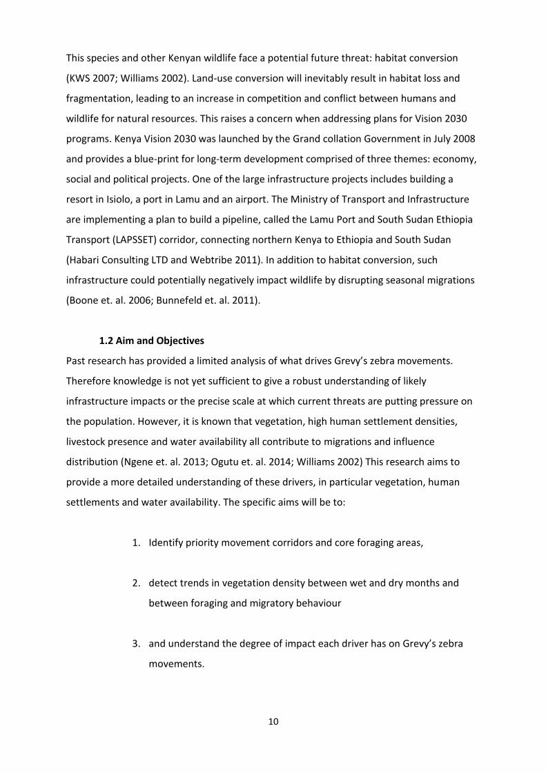
Acronyms AIC Akaike’s Information Criteria BBMM Brownian Bridge Movement Model CA Core Area(s) CITES Convention on International Trade in Endangered Species of Wild Fauna and

Flora dBBMM dynamic Brownian Bridge Movement Model GAM Generalized Additive Model GE Google Earth GIS Geographic Information System GLEWS Global Livestock Early Warning System GPS Global Positioning System GZT Grevy’s Zebra Trust IUCN International Union for the Conservation of Nature LAPSSET Lamu Port and South Sudan Ethiopia Transport MODIS Moderate Resolution Imaging Spectroradiometer MV Motion Variance NDVI Normalized Difference Vegetation Index PA Protected Area(s) UD Utilization Distribution

5

Abstract

Biodiversity loss from habitat fragmentation and degradation continues to threaten much of

Eastern Africa. Migratory ungulates face added pressure from fragmentation and land-use

conversion due to increased agricultural expansion and infrastructure development, which

may disrupt important movement corridors and migration pathways. For the endangered

Grevy’s zebra (Equus grevyi), additional threats from limited natural resources make the

future of this species uncertain.

To develop appropriate conservation initiatives in light of present and future threats, it is

vital to understand how and where Grevy’s zebra move. This study analyses three previously

identified drivers of movement: vegetation, water availability and human settlements, to

understand which of them has a greater effect by running a generalized additive model.

Additionally, through the incorporation of the dynamic Brownian bridge movement model

that estimates utilization distribution, core foraging areas and priority movement corridors

are identified. This approach has not been used before and results indicate that it is more

accurate in analysing space use than previous methods such as kernel densities.

Results also found that vegetation explains little of Grevy’s zebra movements, but distance

to settlements and water points have a greater effect. The probability of zebra presence

according to core areas increases closer to water and away from settlements, suggesting a

minimum distance threshold of 20km to water. In addition, it is suggested that Grevy’s zebra

will migrate long distances only when natural resources become limiting and will keep

further from water sources to avoid livestock and settlements.

This study concludes that all identified core foraging areas occur outside of protected areas

and mainly within conservancies that are managed by communities. Recommendations are

made for management and monitoring of this species as well as for surrounding wildlife,

livestock and pastoralist communities. Future research recommendations are also

discussed.

Word Count: 14,383

6

Acknowledgements

I would like to thank the Grevy’s Zebra Trust for allowing me to conduct this research and

their partners, specifically Marwell Wildlife and the Northern Rangelands Trust, for

providing data. An immense thank you goes to Belinda Low, my external supervisor, for her

support and advice and facilitating the field work component of this project including

applying for and being awarded funding. I am also thankful for all other members of the

Grevy’s Zebra Trust staff that took part in the field work: Francis Lemoile, Julius Lekenit and

Ropi Lekwale. Without their participation in data collection, I would not have been able to

carry through with my research.

I would like to thank Dr. Siva Sundaresan, Morgan Pecora-Saipe, Dr. Zeke Davidson and Dr.

Guy Parker for their additional support and advice in developing the methodology and

analysis for this research. Zeke Davidson provided useful insight into the different

partnerships between NGOs in northern Kenya that helped me develop ideas for future

research. I thank Dr. Henrik Rasmussen for his aid in using software to download GPS

telemetry data and for providing information on zebra collars.

I am extremely grateful for my internal supervisors, Dr. Marcus Rowcliffe and Dr. Sarah

Robinson, for their continual support, especially during analysis and my thesis write-up.

Sarah Robinson gave vital advice for the remote sensing side of my work. Marcus Rowcliffe

provided invaluable encouragement, consultation and input throughout the entirety of my

project, especially in guiding me through a seemingly impossible animal movement model.

Additionally, I thank Dr. Igor Lysenko for his patience and support through the process of

navigating ArcGIS. I am also grateful for his tolerance of my sustained habitation inside his

office. Dr. Bart Kranstauber must also be thanked for addressing my questions regarding

movement modelling.

I am grateful to my course director, Professor EJ Milner-Gulland, for her support during

unexpected changes in research planning and Dr. Aidan Keane for his advice on statistical

analysis. I thank Simone Cutajar for her additional input and motivational speeches.

7

Finally, I would like to thank all my friends and family who have supported my endeavour to

enter this Masters course and continue in the field of conservation. I sincerely hope that the

work presented here will reflect my decision to pursue future conservation work and make

a positive impact on Grevy’s zebra and their surrounding landscape.

8

1. Introduction

1.1 Problem Statement

Understanding the way an animal species uses its habitat and movement patterns

associated with migration provide vital linkages to threats, including the degree of impact

threats have on population dynamics and viability (Pettorelli et. al. 2005). Habitat

fragmentation remains one of the greatest threats to biodiversity, therefore identifying the

consequences of it through methods such as movement modelling using telemetry data is

necessary for conservation planning and management. Global Positioning System (GPS)

tracking has become an essential tool in not only defining which areas should be protected,

but also helps find a balance between animals and humans that are utilizing the same

natural resources. For example, by identifying home ranges and connectivity corridors

between them, wildlife managers can determine important areas for forage that allow

mitigation of human wildlife conflicts (Rubenstein 2004). Telemetry is a primary approach to

acquiring movement data for modelling and has revolutionized ecological and conservation

studies (Schofield et. al. 2007). Models on spatial ecology and movement that use GPS

telemetry help direct conservation initiatives by showing large-scale and long-term effects

of habitat fragmentation (Augustine and Mcnaughton 2004). More specifically, migration

models are able to identify and important seasonal ranges by distinguishing migrations from

other movement types, which leads to influencing policy and management decisions to

secure important areas. This plays a large role in mitigating negative impacts due to

increasing habitat fragmentation and loss from anthropogenic activities (Bunnefeld et. al.

2011).

There are many drivers of movement that may be identified through modelling and include

environmental conditions, changes along temporal and spatial scales, predator presence

and infrastructure development (McDermid et. al. 2005; Pettorelli et. al. 2005). Movement

is most commonly connected with resource availability in which home ranges are defined by

an area that provides necessary resources for reproduction and foraging. Foraging is the

primary behaviour associated with home ranges while migratory behaviour is correlated

with movement outside of these ranges (Mutanga and Skidmore 2010).

9

Understanding migrations and threats linked to this behaviour could remove unnecessary

barriers within or along movement corridors, promote ecotourism, mitigate inappropriate

land-use and preserve different value sets ranging from economic to aesthetic (McDermid

et. al. 2005). Various models have been used in the past to understand migratory behaviour,

including nonlinear modelling, dynamic linear modelling, evolutionary programming and

space use models along with incorporation of rainfall patterns and vegetation indexes using

satellite imagery (Boone et. al. 2006; Gillespie et. al. 2001).

Africa serves as the continent with the most extinct and extant populations of migratory

ungulates. Whilst some large migrations persist, such as the wildebeest migration in the

Serengeti, threats to this behaviour still exist. Unsustainable hunting, restricted access to

food and water, infrastructure development, agricultural expansion and livestock grazing

and fencing all contribute to habitat loss and disruption of migratory pathways (Mose et. al.

2013).

Much of Kenya’s wildlife faces a myriad of threats aside from reduced migration areas

ranging from competition with humans for natural resources and habitat loss and

degradation (Bennett 2003; Hanski 1998). One species in particular has faced the most

significant decrease in population size in comparison to other megafuana: the Grevy’s zebra

(Equus grevyi), which is listed as endangered under the IUCN Red List (Moehlman et. al.

2013). Up until recently, the species neared extinction. Overall population size has

decreased by approximately 80% since the 1970s (KWS 2007; Low et. al. 2009; Ngene et. al.

2013; Williams 1998). Its present range has been reduced to northern Kenya and a small

portion of southern Ethiopia with a total population of less than 3,000 individuals (Ngene et.

al. 2013; Williams 2002).

The current major threats to Grevy’s zebra within northern Kenya are habitat loss due to

overgrazing by livestock and patchy resource distribution, especially during the dry season

(Low et. al. 2009; Williams 2002; Wheeler 2013). The dry season also increases susceptibility

to disease and competition for water between zebras and livestock. The Grevy’s zebra

population is additionally threatened by urban area expansion, hunting/poaching and

predation (KWS 2007; Williams 2002).

10

This species and other Kenyan wildlife face a potential future threat: habitat conversion

(KWS 2007; Williams 2002). Land-use conversion will inevitably result in habitat loss and

fragmentation, leading to an increase in competition and conflict between humans and

wildlife for natural resources. This raises a concern when addressing plans for Vision 2030

programs. Kenya Vision 2030 was launched by the Grand collation Government in July 2008

and provides a blue-print for long-term development comprised of three themes: economy,

social and political projects. One of the large infrastructure projects includes building a

resort in Isiolo, a port in Lamu and an airport. The Ministry of Transport and Infrastructure

are implementing a plan to build a pipeline, called the Lamu Port and South Sudan Ethiopia

Transport (LAPSSET) corridor, connecting northern Kenya to Ethiopia and South Sudan

(Habari Consulting LTD and Webtribe 2011). In addition to habitat conversion, such

infrastructure could potentially negatively impact wildlife by disrupting seasonal migrations

(Boone et. al. 2006; Bunnefeld et. al. 2011).

1.2 Aim and Objectives

Past research has provided a limited analysis of what drives Grevy’s zebra movements.

Therefore knowledge is not yet sufficient to give a robust understanding of likely

infrastructure impacts or the precise scale at which current threats are putting pressure on

the population. However, it is known that vegetation, high human settlement densities,

livestock presence and water availability all contribute to migrations and influence

distribution (Ngene et. al. 2013; Ogutu et. al. 2014; Williams 2002) This research aims to

provide a more detailed understanding of these drivers, in particular vegetation, human

settlements and water availability. The specific aims will be to:

1. Identify priority movement corridors and core foraging areas,

2. detect trends in vegetation density between wet and dry months and

between foraging and migratory behaviour

3. and understand the degree of impact each driver has on Grevy’s zebra

movements.

11

1.3 Hypotheses

Under the umbrella of understanding drivers behind Grevy’s zebra movement, I have

developed the following hypotheses:

1. When foraging, zebras will select for areas of low vegetation density in

comparison to migrations, in which zebra associations with vegetation

density will be random.

2. Core foraging areas will have a lower vegetation density in comparison to

non-core areas.

3. Core foraging areas will be closer to water points and farther from human

settlements.

2. Background

2.1 Grevy’s Zebra

2.1.1 Background and Ecology

The Grevy’s zebra is a large-bodied grazing ungulate that uses hindgut fermentation to

process forage, which requires feeding throughout the day (Rubenstein 2010; Sundaresan

et. al. 2007; Sundaresan et. al. 2008). They live in arid to semi-arid open grass and shrubland

where food and water sources may be sparsely distributed (Rubenstein 2010; Williams

2002). This is preferred over areas with high bush density since it is more difficult to spot

potential predators (Sundaresan et. al. 2008).

Short green grass, which contains the most nutrients compared to tall mature grass, is

generally preferred (Ogutu et. al. 2014). However, feeding behaviour varies depending on

reproductive class. Whilst lactating females and bachelors are more selective towards

higher quality grasses, nonlactating females and territorial males prefer low-quality grasses

with greater biomass (Sundaresan et. al. 2008). Additionally, due to high rates of

consumption, zebras become restricted to areas with highest biomass regardless of quality

when vegetation is a limiting factor (Williams 1998). Forage is a limiting factor only when

12

livestock are present, therefore this impact is greater on spatial distribution than human

settlements and predators. Williams (1998) found a forage availability threshold below

which zebras will disperse once this threshold is met.

Like vegetation selection, herding behaviour and relationship with distance to water vary

based on reproductive class, which in turns influences movement since individuals will

decide to stay or leave a herd depending on forage availability. Grevy’s zebra belong in open

membership groups that can either be all female, all male or a mixture of both. Males

unable to mate with females may form bachelor groups or wander. Herd formation is more

influenced by vegetation abundance than by quality or diversity of grasses (Rubenstein

2010). A recent study found (through the use of local pastoralists as citizen scientists) that

herd size decreases as dry seasons intensify (Rubenstein 2010).

The presence/absence of livestock and pastoralists affect how far zebra move to and from

sources of water. This trend has been found for other herbivores in savannahs and is likely

due to depleted vegetation rather than settlements and predators. Livestock may be largely

responsible for depleting available forage and their presence results in wildlife displacement

and interference with temporal patterns of coming to water points (Ogutu et. al. 2014). High

settlement densities force zebras to move large distances and drink at night (resulting in

increased risk of predation) rather than during the day to avoid livestock (Wheeler 2013;

Williams 1998; Williams 2002). Lactating females and young foals, however, will stay closer

to water points since they are required to drink everyday versus every few to five days for

zebras from other reproductive classes (Sundaresan et. al. 2008). In contrast, nonlactating

females avoid livestock more than any other age or reproductive class (Rubenstein 2004).

Breeding is indirectly influenced by the above factors, but also greatly depends on stochastic

climate patterns and environmental conditions. Therefore, rainfall becomes a primary factor

in reproduction by increasing primary productivity resulting in more available forage for

females in oestrus (Williams 2002).

2.1.2 Threats and Legal Status

Grevy’s zebra are legally protected in Ethiopia, although laws in place are not effective. A

hunting ban was initiated for Kenya in 1977 and the Convention on International Trade in

13

Endangered Species (CITES) listed this species under Appendix I, which bans all trade. These

laws and regulations did not prevent continual decline of the species and currently

Protected Areas (PAs) make up less than .5% of their total range (Williams 2002). Despite

this, conservancies such as Buffalo Springs, Samburu, and Shaba National Reserve have

played a critical role in stabilizing population numbers in recent years. Records have

observed a growing population with zebras moving further south into the Lewa and Laikipia

conservancies (Williams 2002).

Historically, this species occurred in north-east Ethiopia, south Eritrea, north-west Djibouti

(particularly in the Danakil Desert), western Somalia, east of the Rift Valley and south-east

down the Tana River in Kenya. At present there is a population in northern Kenya and a very

small population in southern Ethiopia (Williams 2002). Approximately 93% of the global

population is found in Kenya (Low et. al. 2009; Williams 2002).

Many factors have contributed to the rapid loss of Grevy’s zebra. Historical threats include

hunting for trading of meat and skins and anthrax outbreaks, although cases of anthrax have

been poorly documented over the last 60 years (Lelenguyah et. al. 2011; Lelenguyah et. al.

2012; Muoria et. al. 2007). However, an anthrax outbreak between 2005 and 2006

confirmed by laboratory testing of bacteria resulted in the death of 53 zebras (Muoria et. al.

2007). Reasons for recent declines include intensification of human land use for livestock

production, habitat degradation and poaching (KWS 2007). Habitat degradation results from

heavy grazing that erodes soil and becomes more apparent in pastoral areas (Sundaresan et.

al. 2012). A report by the non-governmental organisation Grevy’s Zebra Trust (Woodfine et.

al. 2005) argues that poaching may become an increasing threat given the prevalence of

guns in local communities. Additionally, cultural taboos in the Samburu and Aarial tribes

against meat consumption are waning. Other tribes sharing land with zebras include the

Boran, Somali, Rendille, Gabbra and Turkana, some of which have used zebras in the past

for consumption as well as their fat for medicines (Low et. al. 2009). The report also found

increased livestock in far northern districts of Kenya from the establishment of permanent

water sources. In these areas, livestock numbers are significantly higher than wildlife.

Although limited natural resources is the overall threat that encompass more specific

threats, it is important to understand other contributing factors. Reduction in available

14

water sources has resulted in two ways: unsustainable extraction of river water for irrigating

land in the highlands of Kenya and exclusion of wildlife from water points used by

pastoralists (Williams 2002). Various studies have questioned whether or not interactions

between Grevy’s zebra and livestock could be considered competition (Low et. al. 2009;

Williams 1998) however, during dry seasons when vegetation and water is increasingly

limited, researchers have concluded in recent years that competition is occurring (KWS

2007; Rubenstein 2010). Pastoralists in northern Kenya are considered semi-nomadic and

move every few years, but the trend is changing (Wheeler 2013). GZT has reported a

relatively new transition from nomadic grazing to permanent grazing areas, which

contributes not only to soil erosion, but decreases favourable habitat for zebras

(Sundaresan et. al. 2012). Tourism is yet another concerning factor since some PAs are

poorly managed. Hunting and trade were considered to be a historical cause of decline, but

given increasing poaching effort, this may become a more serious threat in the near future

(Williams 2002). With the growing possibility of increased infrastructure through projects

like LAPSSET, competition between livestock and wildlife will either develop or increase

where it already exists. Construction resulting in habitat fragmentation will make it difficult

for both pastoralists and animals to gain access to water points and potentially negatively

impact priority movement corridors.

2.2 Methods Approach

2.2.1 Normalized Differential Vegetation Index

Satellite tracking began as early as the 1970s and has played a vital role in the long-term

monitoring of animals movements and distributions (Gillespie et. al. 2001). Remote sensing

methods have been applied for over 50 years and up until recently, these non-invasive

approaches have been used to assess vegetation state without factoring habitat use and

selection by a given species. Being able to correlate animal movement with environmental

factors is becoming more common as technology advances, particularly in the field of

remote sensing. This combination allows for the study of animal movement over a large

spatial and temporal scale. Additionally, satellite imaging increases understanding of habitat

degradation, land use changes overtime, plant primary productivity, natural resource

availability and habitat dynamics in regards to large herbivore forage selection (Pettorelli et.

al. 2005; Pettorelli et. al. 2011). Leyeguien et. al. (2007) argues that remote sensing makes

15

an important contribution to conservation initiatives by providing information about species

distribution and diversity.

The Normalized Differential Vegetation Index (NDVI) is an index that is generated from

satellite imagery to document vegetation primary productivity overtime. This approach to

understanding vegetation growth patterns across different landscapes has been well

documented and established. NDVI acts a strong indicator for climate variation on plant

biomass and phonological patterns of vegetation. Furthermore, its implication in animal

ecological and conservation research help facilitate appropriate wildlife and livestock

management (Pettorelli et. al. 2005). McDermid et. al. (2005) used remote sensing to model

the initiation of migration and speed of travel in plains zebras (Equus bruchelli). NDVI was

found to complement precipitation data, creating a picture of how zebra migrations are

initiated by environmental cues. McDermid et. al. concluded that remote sensing in animal

movement research helps to understand decision rules, orientation and navigation

mechanisms employed in migratory behaviour.

This research uses NDVI to acquire an understanding of primary productivity and changes in

vegetation over time, especially in comparing periods of rain and drought. Analysing the

relationships between vegetation density as measured by NDVI and intensity of space use

along given trajectories established from the utilization distribution (UD) may serve as an

indicator that zebras are not distributed at random with respect to vegetation.

2.2.2 Dynamic Brownian Bridge Movement Model

The dynamic Brownian bridge movement model (dBBMM) used in this research is based off

the original Brownian bridge model (BBMM). The BBMM was developed by Horne et. al.

(2007) as a method to accurately assess and estimate UD along migratory pathways by

creating Brownian bridges (Horne et. al. 2007). Brownian bridges determine movement

between two telemetry locations (thus creating a “bridge”) as opposed to kernel methods

that look at each location independently. However, these bridges assume continuous

movement throughout a trajectory rather than including periods of inactivity such as

sleeping (Yan et. al. 2014). The BBMM quantifies a probability of habitat use and is able to

incorporate distance variability and time lag between locations while applying a random

walk. A random walk is a probability of an individual’s decision to move in any given

16

direction from a spatial position (or GPS location) or continue along the same spatial axis to

the next position. It assumes the likelihood of movement in any direction are all equal

(Kranstauber et. al. 2014; Patterson et. al. 2007). Kernel methods, in contrast, are not able

to incorporate such factors or temporal structure and thus overly simplify space use. Other

methods have also been used in the past to determine home ranges, such as the popular

and simplistic approach of minimum convex polygons. This method may produce

inaccuracies by over estimating space use for several individuals in the same area when the

actual probability of overlap is small (Hostens 2009; Pierce and Garton 1985).

Horne et. al. (2007) took samples of two bird species, Black and Turkey vultures, and

compared BBMM with kernel density estimators and found the former more accurate in

determining home range. The BBMM has also been used to model disease outbreaks and

predict where an animal is likely to cross infrastructure (such as highway) during migration

(Horne et. al. 2007; Kranstauber et. al. 2012).

Since this model was developed, other studies have modified it or incorporated it into

alternative methods of animal movement analyses (Kranstauber et. al. 2014; Wells et. al.

2014; Yan et. al. 2014). One such approach is the dynamic Brownian bridge movement

model (dBBMM) developed by Kranstauber et. al. (2012). The dynamic version of this model

differs from the BBMM in several ways. Motion variance (MV) is a continuous variable that

quantifies the speed of migratory movement in meters by calculating step length, turning

angle and speed between two GPS locations. While the BBMM assumes a fixed MV along a

given path, the dBBMM is able to break a trajectory into segments through the use of a

sliding window and thus calculate MVs along the pathway. The significance of this approach

is the ability to distinguish between different behaviour types rather than assuming

migration along an entire path. Kranstauber et. al. compared the dBBMM with the BBMM in

two sample tracks of bird species (fischer and lesser black-backed gull) and found that this

model performed better, or was at least equally strong, with a constant MV. The dBBMM

performed better when animal telemetry locations were randomly sampled, which proves it

is more useful for tracks that contain missing GPS locations. The model was also better at

describing space use through the calculation of MV by segments.

17

2.3 Animal Movement

2.3.1 Understanding Movement and Utilization Distribution

As previously mentioned, understanding animal movement is an imperative for

conservation planning and management of a given species within a community. To develop

a clear picture of movement and different movement behaviours, various ecological

associations must also be understood including: home ranges, migration pathways, resource

selection and social interactions. In some prior studies, patterns have been found between

direction of movement and resource abundance. For large herbivores, long directional

movements occur in areas with low resource abundance and shorter movements are

associated with areas of high resource abundance. Animals that forage in low resource

patches therefore benefit from rapid movement in straight lines (Fryxell et. al. 2008).

Movement type is also of relevance when studying both fine scale and large scale

movements and may reveal behavioural changes according to landscape dynamics (Morales

et. al. 2005). Different kinds of movement are considered behaviours in which a given

individual can alternate between foraging, resting/sleeping, searching (for forage) and

migrating (Fryxell et. al. 2008; Kranstauber et. al. 2012).

Analysing home range is another common approach to space use and movement analysis. In

the past, home range was defined through boundary estimation by selecting a percentage

of total space use. However, this method ignores intensity of utilization. The concept of core

areas (CAs) was developed in 1962 to further understand animal movement within a

defined home range and describe space use (Pierce and Garton 1985). More recently,

however, UD has become a widely accepted and accurate approach to quantifiably describe

home ranges and CAs. UD is a probability distribution that predicts the way a given animal

uses space within its home range. It is important for understanding habitat selection and

home range overlap between individuals of the same species (Fieberg and Kochanny 2005).

2.3.2 Movement Research for Conservation Planning

For Grevy’s zebra, threats from habitat fragmentation and loss may become a dire reality

once infrastructure expansion begins in northern Kenya. As previously mentioned, another

concern is semi-nomadic pastoralists transitioning to permanent settlements, which not

only threatens to reduce the amount of favourable forage, but also leads to habitat loss

18

from overgrazing, especially around water points (Low et. al. 2009; Ogutu et. al. 2010;

Woodfine et. al. 2005). Understanding where an animal moves establishes habitat links and

corridors, both corridors that animals use naturally and ones that may be created through

conservation efforts and community involvement (Bennett et. al. 1998).

As previously mentioned, tracking movement helps define which areas should be protected

for a given species. Choosing the right movement model to understand space use and

identify CAs is useful in making correlations with priority movement corridors. Identifying

corridor use and migrations, especially between seasons and to facilitate connectivity

between different CAs, helps secure and protect habitats when faced with increasing

threats from habitat fragmentation and other anthropogenic impacts (Bunnefeld et. al.

2011; Hanski 1998).

Studying drivers of movement is also important to understand threats. Many studies have

found that human populations and land-use affect animal distribution. Graham et. al. (2009)

found that elephants are absent from landscapes that contain a human population above a

particular density level. Movement speed was also affected by the presence/absence of

people. A clear pattern between human settlements and elephant abundance led to

predicting the viability of the elephant population. For Grevy’s zebra, previous studies have

already found that distribution is affected by human settlement densities and livestock

(Pierce and Garton 1985; Sundaresan et. al. 2012; Wheeler 2013; Williams 1998).

Pastoralists and their livestock tend to concentrate in areas near and around water points,

which can lead to degraded vegetation and soils. Within northern Kenya specifically,

Cornelius and Shutlka (1990) found increased grazing pressure from livestock in Isiolo and

Samburu districts. Water points are an additional driver of movement and strongly

correlated with human settlements. de Leeuw et. al. (2001) studied 10 herbivores in

northern Kenya and found the frequency distribution for Grevy’s zebra near water points

was equal to that of distance further away from water. For all species observed, the study

found a negative association between livestock and wildlife distribution. Negative impacts

from livestock are possibly due to competition for natural resources (Ogutu et. al. 2010).

Another explanation for the negative association was thought to be distribution of water

points. Sparse distribution forces livestock to cluster and drive wildlife away, but more

19

evenly distributed water sources allows for an even distribution of livestock, thus decreasing

competition with wild herbivores (de Leeuw et. al. 2001).

Understanding the settlement, water and livestock drivers of movement for appropriate

management becomes complicated in considering placement of settlements. Ogutu et. al.

(2010) observed that distance from water and settlements for large herbivores in Kenya

varied depending on whether the animals were inside ranches or reserves. This indicated

that wildlife is restricted by settlements, cultivation and livestock. Additionally, Ogutu et. al.

stressed the importance of establishing PAs where there is minimal livestock and human

activity.

This research focuses on three movement drivers: vegetation, human settlements and

water points to understand which of these drivers have a greater effect on Grevy’s zebra

movements and distribution both across their range and within defined core foraging areas.

By developing a more thorough understanding based on prior research and through

incorporation of movement modelling, a foundational framework will be established to

create clear conservation management goals that facilitate the protection of CAs and

priority corridors as well as considering important areas for pastoralists and livestock.

2.4 Study Area

This research was conducted on Grevy’s zebra occurring in two sub-populations of northern

Kenya: the southern sub-population, located in the Samburu and Laikipia districts and the

northern sub-population, located in the Marsabit district (Sundaresan et. al. 2007;

Sundaresan et. al. 2012). Their total range expands into other districts including Isiolo,

Nyambene and Meru. The region consists of community rangelands, commercial livestock

ranches and conservancies. The dominant tree species come from the genus Acacia (Low et.

al. 2009; Sundaresan et. al. 2007). Northern Kenya normally goes through periods of rainy

and dry seasons with an average rainfall of 375mm, but in recent years, rainfall pattern has

been very unpredictable with occasional droughts (Cordingley et. al. 2009; Low et. al. 2009).

Northern Kenya contains an arid to semi-arid open grassland/savannah ecosystem with

mixed grasses including Indigofera and Cynodon species. Part of the analysis in this study

was conducted only within the Melako conservancy, which encompasses the majority of

zebra distribution for the northern sub-population (Figure 1.1).

20

Figure 1.1: Map of Kenya with different regions as well as all conservancies within northern Kenya provided by

the Northern Rangelands Trust (NRT).

3. Methods

3.1 Methodological Framework

This study focuses on understanding how different movement drivers contribute to Grevy’s

zebra distribution. By using remote sensing to analyse vegetation over a temporal scale and

a complex animal movement model, core foraging areas and priority movement corridors

were established and vegetation density was compared between core and non-core areas

as well as between two distinct behaviour types: foraging and migration. The other two

identified drivers, water points and human settlements, were assessed and analysed along

with NDVI in a multivariate nonlinear model to further determine which variables are

primary influences of Grevy’s zebra movement. Analysis was performed using the following

programs: ArcGIS 10.0 (ESRI 2014), Microsoft Office Excel 2010, Google Earth (GE) and R

version 3.1.1 (R Core Team 2014).

3.2 Data Collection

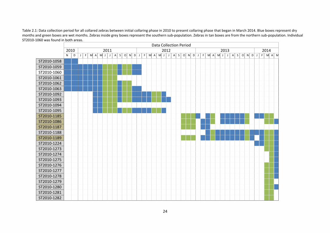
Grevy’s zebras were first collared in November 2010 and some individuals are currently still

being tracked. This study has collected data up until May 2014 (Table 2.1). All collared

zebras are female with a mixture of lactating and nonlactating females at the time of collar

fitting. For collars to be fitted appropriately, zebras were tranquilized and given a health

Legend

<all other values>

ADM1_NAME

Central

Coast

Eastern

Nairobi

North Eastern

Nyanza

Rift Valley

Western

21

check by a veterinarian. They were collared both in the southern sub-population and the

northern sub-population. Data was downloaded using the Savannah Data Management

software. A total of 166,623 GPS data point locations were recorded from 26 individuals.

Human settlement data were collected using GE software and followed the same approach

used by Wheeler (2013). Marked settlements included infrastructure such as buildings,

schools and churches, but mainly referred to manyattas which are semi-permanent houses

that contain a circular outer fence to keep livestock and huts inside the fence. Only

manyattas that showed signs of present use were marked as opposed to abandoned

settlements. Active manyattas were mainly distinguished by darker coloration inside the

settlement, intact fencing and visible huts. However, due to poor resolution in some of the

satellite images, it was difficult to determine whether or not a settlement was in use.

Outside these conservancies, settlements were partially identified within the following

defined coordinates: 36.8, 38.1 latitudes and .1, 2.1 longitudes. These coordinates were

determined by creating a rectangle that included all GPS collar locations with the exclusion

of visible outliers. Due to time constraints, settlements were not identified for the entire

study area and limitations in ground truthing from inability to access at random any area

within or outside conservancies led to the analysis of settlement data within Melako only.

GZT ground truthed areas within Kalama, West Gate, Meibae and Melako conservancies

(Figure 4.6). GPS locations were taken of all permanent and seasonal water points. The

following data were recorded: water point type, accessibility to both livestock and wildlife

and year the water source was built (unless it was a natural source). Since movement

modelling was not split according to season, only permanent water points were used. For

settlements, their status was confirmed as either active or abandoned, and the year that the

settlement was constructed was also recorded (Appendix IV). Ground truthed settlements

were then compared with settlements identified via GE to determine accuracy. The number

of marked settlements that ground truthing confirmed as abandoned were taken into

account.

Rainfall data were acquired from the Global Livestock Early Warning System (GLEWS)

database and GZT season classification data (unpublished) to compare vegetation selection

between years. Accumulated rainfall was broken into wet and dry months with more than

22

60mm of rain within a month labelled as “wet”. Due to high variability in rainfall patterns,

possible trends in vegetation selection were analysed by month type rather than season.

The Moderate Resolution Imaging Spectroradiometer (MODIS) satellite images were

downloaded for the study area to determine NDVI values at each zebra location. NDVI is a

reflectance ratio computed by satellite sensors that capture near-infrared and red light

reflected from plants to produce a value that ranges from -1 to 1. Negative values are

associated with snow and water whilst values between zero and one are correlated with

vegetation density and primary productivity (Pettorelli et. al. 2005). Images came from the

University of Natural Resources and Life Sciences, Vienna. The tiles were smoothed and

filtered with a 250m resolution and taken at 16 day intervals (Vuolo et. al. 2012).

3.3 Data Analysis

3.3.1 Movement Modelling

Before running the model, each zebra location was assigned a particular NDVI value that

matched both spatially and temporally. Data cleaning was performed as part of the

preparation to run the dBBMM. Visible outliers, such as GPS locations in Nairobi, were

removed by setting minimum and maximum latitude and longitude coordinates in the R

program. All collared zebras experienced GPS location failures, which resulted in shorter

time periods of data collection and/or gaps in location fix attempts. Location fixes are

dependent on spatial resolution and a certain degree of error may result from landscape

type as well as the presence of clouds and rain (Frair et. al. 2004). The dBBMM factors in

location error from GPS telemetry by providing an error argument. Consulting with GZT, a

location error of 10m was put into the model. Data cleaning also involved removing

duplicate GPS locations where both the latitude/longitude coordinates and time of

download were exactly the same. Although the number of duplicates was extremely low,

more zebra locations were excluded during the creation of a “move” object to run the

movement model that did not fit within the defined latitude and longitude coordinates.

This research focused on understanding UD and MA over a spatial scale, therefore data

were manipulated to maximize the likelihood of detecting behavioural changes along a

given path. To account for time gaps in individual trajectories due to GPS failures, tracks

were split when there was more than a 12 hour time lapse between two given locations.

23

Locations were normally downloaded once every hour. Breaking the trajectories and

creating “new” individuals/pathways for analysis was done to better predict where

migration and foraging behaviour was occurring. Splitting trajectories at a larger time gap,

for example 24 hours, would have risked detecting migratory behaviour when in actuality a

zebra had a higher probability of foraging. A total of 130 “new” individuals were created in

the program Excel.

The movement model was run in the R program using the Move package version 1.2.475.

Several arguments were used to run the model: window size, margin size, extent and raster.

The window size corresponds with number of locations and moves along a given trajectory

to estimate the MA parameter within defined subsections of the path. This increases the

ability to detect breakpoints where changes in behaviour occur.

According to Kranstauber et. al. (2012), the window size should relate to what kind of

behaviours the model is desired to identify. Since Grevy’s zebra are able to migrate and

forage within the same day, a window size of 19 was used. Therefore, the sliding window

moved every 19 locations or every 19 hours. It was assumed that a smaller window size

would increase probability of detecting behavioural changes within the same day as

opposed to a window size between 21 and 25. A value of 9 was given for margin size based

on the recommendation in Kranstauber et. al. (2012). A raster with a cell size of 250m was

created for the model to match with coordinates used to make the move object and remove

outliers. The raster dictates the grid cell size for the UD to be calculated per grid cell per

individual. The extent argument is incorporated if there are animal locations that border the

edges of the raster. An extent of .5 was put into the model to account for this.

The dBBMM predicts space use between two locations instead of looking at each point

individually. This results in the exclusion of the very start and end of a given track. Since the

window size was small and with the inclusion of “new” individuals, several tracks were too

short to be analysed in the model. Out of the original data set, a total of 154,843 zebra

locations were used for analysis resulting in the exclusion of approximately 7% of unusable

data.

24

Table 2.1: Data collection period for all collared zebras between initial collaring phase in 2010 to present collaring phase that began in March 2014. Blue boxes represent dry months and green boxes are wet months. Zebras inside grey boxes represent the southern sub-population. Zebras in tan boxes are from the northern sub-population. Individual ST2010-1060 was found in both areas.

Data Collection Period

2010 2011 2012 2013 2014 N D J F M A M J J A S O N D J F M A M J J A S O N D J F M A M J J A S O N D J F M A M

ST2010-1058

ST2010-1059

ST2010-1060

ST2010-1061

ST2010-1062

ST2010-1063

ST2010-1092

ST2010-1093

ST2010-1094

ST2010-1095

ST2010-1185

ST2010-1086

ST2010-1187

ST2010-1188

ST2010-1189

ST2010-1224

ST2010-1273

ST2010-1274

ST2010-1275

ST2010-1276

ST2010-1277

ST2010-1278

ST2010-1279

ST2010-1280

ST2010-1281

ST2010-1282

25

Two main functions were used in the Move package to further analyse MA and UD. The

getMotionVariance function was applied to extract information on MA (Kranstauber et. al.

2012) and provided a value in meters for each zebra location point. Although MA is a

continuous variable, a unit per point is calculated by determining speed of movement

between two locations and then calculating the average per point, thus a MA at the start

and end of each track is not possible. The points were plotted in ArcGIS and labelled with

MA values to determine which corresponded with foraging and which with migration. Each

track was assigned a colour scheme that ranged from light to dark according to time. Long,

unidirectional trajectories were then identified and MA values were assessed per point and

compared to values of cluster points where zebras were assumed to be foraging. The

Corridor function was also used to calculate which zebra location points correspond with

corridor use behaviour and migrations. This function looks at the speed and turning angle at

each point along a given trajectory to determine whether or not it is indicative of corridor

use behaviour where speed is above a particular threshold (unless otherwise specified,

within the top 25% of speed range) and turning angle is small (less than 25% variance)

indicating fast, unidirectional movement. Additionally, a circular buffer is created that

identifies the number of neighbouring “corridor” points within it. Two approaches were

used to detect migratory behaviour since the corridor function is more likely to observe

large scale migrations whilst analysis in ArcGIS provides an ability to not only determine

shorter migrations (within core foraging areas for example), but also estimate the speed at

which migratory behaviour is initiated. Let “corridor point” correspond with zebra locations

analysed from the Move package and “migration point” correspond with locations analysed

in ArcGIS for the remainder of this thesis.

3.3.2 Core Foraging Areas and Priority Corridors

The resulting UDs from the movement model are part of the “dbbmm” class, but function as

a raster within the Raster package in R. The rasters were converted to ascii format for

further analysis in ArcGIS. Each raster was normalized so that the probability of space use

contained a minimum value of 0 and a maximum value of 1 and was calculated by dividing

the raster by its largest probability using the Raster Calculator tool. This ensured that each

individual zebra (which includes separate rasters for each “new” individual) provided the

26

same input into the final raster displaying all probabilities of space use. The rasters were

combined into one final raster by adding them all together in the Raster Calculator. The

result was normalized again by dividing by the largest probability. For determining core

foraging areas, any cell that had a probability above zero was considered. Many grid cells

showed concentrated use by more than one individual, but covered a very small area (less

than 1km2). An assumption was made that areas of this size are too small to be considered

CAs for multiple individuals, especially in the context of conservation management planning.

To filter out such cells and smooth adjacent ones, several tools were incorporated. First the

Majority Filter tool was applied to link cells with differing probabilities into one group under

the same value (1). Then the Shrink tool was used to remove all areas that displayed

concentrated use for one to few grid cells by a set value (1). The Expand tool was applied to

connect zones that bordered one another with an expansion value of 1. Finally the resulting

CAs were converted from a raster to shapefile with the Raster to Polygon tool to smooth the

edges of the zones. The identified corridor points were then plotted and using the Editing

Lines tool, lines were manually drawn to connect points that indicated priority movement

corridors between core foraging areas.

3.3.3 Generalized Additive Model

The generalized additive model (GAM) was used to correlate the likelihood of zebra

presence in a given area with the three explanatory variables: vegetation, distance to

settlement and distance to water. As previously mentioned, ground truthing was limited to

several conservancies in northern Kenya. To test all possible drivers of movement, a subset

of the study area was selected that included settlement points, water points and CAs within

Melako conservancy boundaries. The final raster displaying CAs was cropped to fit the data

within Melako and then converted to points. A presence/absence binomial argument was

implemented in GAM by assigning a value of 1 to all points within a CA, thus having a high

probability of zebra presence. All other points were given a value of 0 and considered zebra

absence points. To ensure the best fit model, all possible combinations of explanatory

variables against presence/absence were tested (Table 2.2).

27

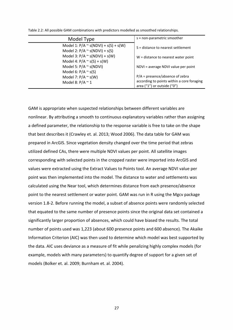
Table 2.2: All possible GAM combinations with predictors modelled as smoothed relationships.

Model Type s = non-parametric smoother S = distance to nearest settlement W = distance to nearest water point NDVI = average NDVI value per point P/A = presence/absence of zebra according to points within a core foraging area (“1”) or outside (“0”)

Model 1: P/A ~ s(NDVI) + s(S) + s(W) Model 2: P/A ~ s(NDVI) + s(S) Model 3: P/A ~ s(NDVI) + s(W) Model 4: P/A ~ s(S) + s(W) Model 5: P/A ~ s(NDVI) Model 6: P/A ~ s(S) Model 7: P/A ~ s(W) Model 8: P/A ~ 1

GAM is appropriate when suspected relationships between different variables are

nonlinear. By attributing a smooth to continuous explanatory variables rather than assigning

a defined parameter, the relationship to the response variable is free to take on the shape

that best describes it (Crawley et. al. 2013; Wood 2006). The data table for GAM was

prepared in ArcGIS. Since vegetation density changed over the time period that zebras

utilized defined CAs, there were multiple NDVI values per point. All satellite images

corresponding with selected points in the cropped raster were imported into ArcGIS and

values were extracted using the Extract Values to Points tool. An average NDVI value per

point was then implemented into the model. The distance to water and settlements was

calculated using the Near tool, which determines distance from each presence/absence

point to the nearest settlement or water point. GAM was run in R using the Mgcv package

version 1.8-2. Before running the model, a subset of absence points were randomly selected

that equated to the same number of presence points since the original data set contained a

significantly larger proportion of absences, which could have biased the results. The total

number of points used was 1,223 (about 600 presence points and 600 absence). The Akaike

Information Criterion (AIC) was then used to determine which model was best supported by

the data. AIC uses deviance as a measure of fit while penalizing highly complex models (for

example, models with many parameters) to quantify degree of support for a given set of

models (Bolker et. al. 2009; Burnham et. al. 2004).

28

4. Results

4.1 Vegetation Driver

Grevy’s zebra were strongly associated with NDVI values between .2 and .3 that relates to

shorter, more nutritious grasses and low vegetation density (Figure 4.2). However, selection

varied from year to year. 2013 was a drought year with only two wet months. NDVI value

was on average lower than in other years as expected since less rain reduces the rate of

primary productivity. For 2014, NDVI at occupied sites was higher on average in comparison

to the other years. As images below indicate, overall distribution of vegetation shows a

range from low to high densities regardless of month type. Additionally, zebra locations

associated with migrations occurred both during wet and dry months. To get rid of pseudo-

replication, aggregates of NDVI values and MA were calculated in R by finding the mean

value per individual per day. From the aggregated data, averages per month type per year

are displayed below (Figure 4.1) and compared between zebra locations that are considered

to be part of foraging behaviour and those associated with migration. Averages did not

greatly differ between the two categories. Zebras were also associated with slightly lower

NDVI values in dry months compared to wet months with the exception of NDVI values for

migratory points in 2012 and values for forage points in 2014. The first hypothesis

comparing NDVI values for migratory zebra locations with those of foraging locations is

rejected given zebra locations estimated to be part of migratory movement are mainly

associated with low vegetation density, which falls in line with foraging.

Kernel density estimation was performed on a subset of the data that was used to run the

GAM, which compared NDVI value ranges between core foraging areas (presence) and non-

core areas (absence) (Figure 4.3). The probability of zebra presence is very high at an NDVI

value of .2 and gradually decreases after .3. The likelihood of zebra absence also increases at

a value of .2, but the probability is not as high as for presence indicating a small degree of

selection. Although zebras are predicted to forage within areas of low vegetation density,

the absence curve also indicates that non-CAs contain a similar level of vegetation biomass.

The second hypothesis, which states that vegetation density will be lower in core foraging

areas compared to non-core areas is therefore rejected.

29

(a) (b)

(c) (d)

Figure 4.1: NDVI images with matching zebra locations for the southern sub-population. Red represents very

low NDVI values, yellow is low to middle and green represents high values that equates to high vegetation

biomass. The first image (a) is between 2 February – 17 February 2011 and the second image (b) is from 18

Feburary – 5 March 2011 and shows migratory movement along an identified priority movement corridor

(Figure 4.6). Both of these images are from a dry period. Image two Image three (c) is from 1 November – 16

November 2011 and image four (d) is from 17 November – 2 December 2011. Both of these images are from a

wet period.

(a) (b)

Figure 4.2: Average NDVI values per month type per year for zebra locations with a MA indicating foraging

behaviour (a) and average values with a MA indicating migratory behaviour (b).

0.1

0.2

0.3

0.4

2010 2011 2012 2013 2014

ND

VI

Year

Average NDVI Values - Forage

Dry

Wet 0.1

0.2

0.3

0.4

2010 2011 2012 2013 2014

ND

VI

Year

Average NDVI Values - Migration

Dry

Wet

30

Figure 4.3: NDVI kernel density estimation for zebra presence and absence within the Melako conservancy.

4.2 Utilization Distribution, Core Foraging Areas and Corridors

After all individual UDs were summed together into one final raster, there were relatively

large areas of high probability of occurrence for multiple individuals. Few areas of overlap

occurred in isolation and the vast majority of pixels with a high intensity of space use were

connected with one another indicating many possible movement corridors. An insignificant

degree of error resulted from normalizing and not all rasters had exact values ranging from

a maximum of 1 and minimum of 0. The resulting final raster had a minimum value that

approached zero enough to consider these areas as zebra absences (Figure 4.5).

The majority of the zebra locations fell under what was considered foraging behaviour.

When plotted in ArcGIS, transition from foraging to migration was detected at 2.5km with

migration behaviour occurring at 3km and above. Therefore, zebras migrate at a speed of

3km per hour and higher. Many migration points occurred within core foraging areas. Out of

over 150,000 zebra locations, 41,650 were estimated to correspond with migratory

behaviour. In contrast, the corridor function applied in the Move package found a total of

2,373 points that attributed to corridor use. Of these points, about 57% had a value within

the estimated range of migratory movement and 6% fell into the estimated range of

transitory movement into migration. Some points that were considered part of corridor use

behaviour exhibited a MA value (less than 50m) that was very close to resting or foraging

— Absence

— Presence

31

indicating a certain degree of error in estimation. Majority of the estimated corridor points

were located in-between CAs revealing strong connectivity between important areas for

forage. However, many of these points when plotted revealed a high amount of scatter

rather than straight lines. Manually developed lines in ArcGIS were created in places where

there were high concentrations of points, thus assuming weak connectivity between CAs

that displayed few points.

There are a total of 26 core foraging areas. All areas are located outside of PAs indicating

zebras within them are not legally protected. However, majority are located within

community conservancies with wildlife management schemes. Out of the six districts that

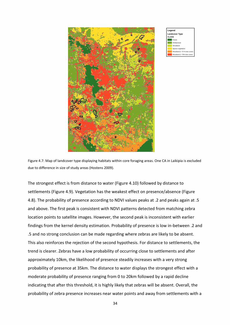
Grevy’s zebra are found in, CAs are contained within: Laikipia, Marsabit, Samburu and Isiolo

counties. Samburu contains the most CAs (12) followed by Marsabit (7) which solely

represents the northern sub-population. The CAs are located within different landcover

types according to a landcover map provided by Hostens (2009) (Figure 4.7). The majority of

CAs are in sparse vegetation and herbaceous habitats. Sparse vegetation habitat dominates

in the northern sub-population. CAs are also in woodland (with less than 70% tree cover)

and a very small amount of shrubland habitat. The majority of priority movement corridors

occur in conservancies. Although prior research has found no evidence that the two sub-

populations mix, one individual (ST2010-1060) did show presence in both areas.

Additionally, plotted corridor points indicated migration occurring between the southern

sub-population and the northern one.

4.3 Generalized Additive Model

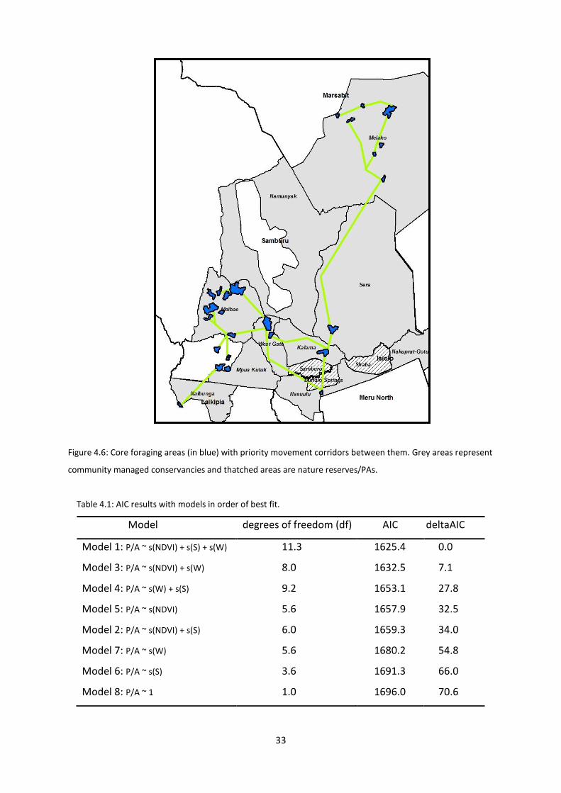
The best fit model from the AIC was model 1, which included all three explanatory variables

for zebra presence/absence: vegetation, distance to settlement and distance to water. All

three variables help explain Grevy’s zebra presence and absence, but to varying degrees.

Despite clear relationships, the model only explained 5.39% of the residual deviance. The

deltaAIC (Table 4.1) visibly indicates that all other models are a very poor fit.

32

(a) (b)

Figure 4.5: UDs for northern sub-population (a) and for the southern sub-population (b). Areas in red have the highest probability of zebra presence and green, blue and

yellows areas correspond with middling probabilities while purple pixels represent the lowest probability of occurrence nearing zero (absence).

Legend

Summed Utilization Distribution

Value1

0.857143

0.714286

0.571429

0.428571

0.285714

0.142857

2.09444e-013

33

Figure 4.6: Core foraging areas (in blue) with priority movement corridors between them. Grey areas represent

community managed conservancies and thatched areas are nature reserves/PAs.

Table 4.1: AIC results with models in order of best fit.

Model degrees of freedom (df) AIC deltaAIC

Model 1: P/A ~ s(NDVI) + s(S) + s(W)

Model 3: P/A ~ s(NDVI) + s(W)

Model 4: P/A ~ s(W) + s(S)

Model 5: P/A ~ s(NDVI)

Model 2: P/A ~ s(NDVI) + s(S)

Model 7: P/A ~ s(W)

Model 6: P/A ~ s(S)

Model 8: P/A ~ 1

11.3

8.0

9.2

5.6

6.0

5.6

3.6

1.0

1625.4

1632.5

1653.1

1657.9

1659.3

1680.2

1691.3

1696.0

0.0

7.1

27.8

32.5

34.0

54.8

66.0

70.6

34

Figure 4.7: Map of landcover type displaying habitats within core foraging areas. One CA in Laikipia is excluded

due to difference in size of study areas (Hostens 2009).

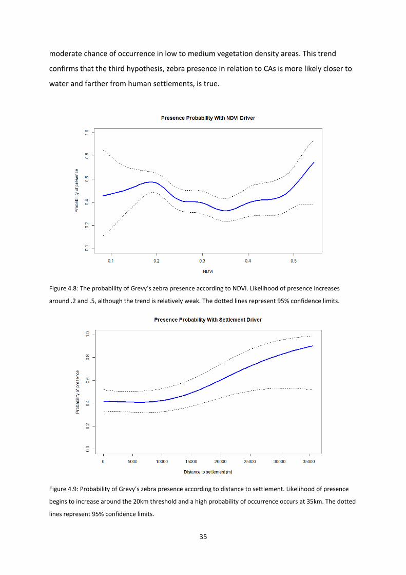
The strongest effect is from distance to water (Figure 4.10) followed by distance to

settlements (Figure 4.9). Vegetation has the weakest effect on presence/absence (Figure

4.8). The probability of presence according to NDVI values peaks at .2 and peaks again at .5

and above. The first peak is consistent with NDVI patterns detected from matching zebra

location points to satellite images. However, the second peak is inconsistent with earlier

findings from the kernel density estimation. Probability of presence is low in-between .2 and

.5 and no strong conclusion can be made regarding where zebras are likely to be absent.

This also reinforces the rejection of the second hypothesis. For distance to settlements, the

trend is clearer. Zebras have a low probability of occurring close to settlements and after

approximately 10km, the likelihood of presence steadily increases with a very strong

probability of presence at 35km. The distance to water displays the strongest effect with a

moderate probability of presence ranging from 0 to 20km followed by a rapid decline

indicating that after this threshold, it is highly likely that zebras will be absent. Overall, the

probability of zebra presence increases near water points and away from settlements with a

Legend

Landcover Type

CLASS

Forest

Herbaceous

Shrubland

Sparse vegetation

Woodland (< 70 % tree cover)

Woodland (> 70% tree cover)

35

moderate chance of occurrence in low to medium vegetation density areas. This trend

confirms that the third hypothesis, zebra presence in relation to CAs is more likely closer to

water and farther from human settlements, is true.

Figure 4.8: The probability of Grevy’s zebra presence according to NDVI. Likelihood of presence increases

around .2 and .5, although the trend is relatively weak. The dotted lines represent 95% confidence limits.

Figure 4.9: Probability of Grevy’s zebra presence according to distance to settlement. Likelihood of presence

begins to increase around the 20km threshold and a high probability of occurrence occurs at 35km. The dotted

lines represent 95% confidence limits.

36

Figure 4.10: Probability of Grevy’s zebra presence according to distance to water. Likelihood of occurrence is

moderate up until 20km, where probability increases followed by a rapid decrease leading to strong

probability of absence between 30km and 40km. The dotted lines represent 95% confidence limits.

5. Discussion

Animal movements across a landscape are affected by environmental changes,

infrastructure and anthropogenic factors. This research has assessed three movement

drivers to help understand which factors are most important and should be considered in

future conservation management planning for Grevy’s zebra and their surrounding habitats.

Along with providing a framework to begin evaluating where and when migrations occur,

core foraging areas and priority corridors have been identified to direct future infrastructure

development and guide community-led wildlife management schemes. This chapter will

discuss the relative importance of each movement driver, including in the context of

potential future threats and provide recommendations for future research to further

develop a robust understanding of Grevy’s zebra movements in the context of climate

change and tribal community and landscape changes.

5.1 Significance of Core Foraging Areas and Priority Movement Corridors

There was a significantly larger proportion of migration points as opposed to corridor points.

The corridor function exhibited some error given the assumption that a MV below 50m is

37

strongly associated with resting and/or foraging. However, majority of estimated corridor

points matched with the migration analysis in ArcGIS according to MV. Additionally, corridor

points occurred mostly between core foraging areas, which indicates strong connectivity

between these areas and also reflects Grevy’s zebra distribution from plotting raw GPS

location data. It is also important to consider that the use of corridors does not necessarily

equate to migration as indicated in comparing the difference in point distributions between

corridor points and migratory points. There is a possibility that zebras are foraging both

within CAs and inside corridors. A large amount of migratory movement was found both

within and outside of CAs, which suggests that zebras migrate not only from one preferred

area of forage to another, but also within these zones. This claim is further explained by the

location of water points within Melako (Appendix V), all of which are not inside of CAs as

well as by the degree of scatter for corridor points (as opposed to long, unidirectional paths)

between CAs.

Although prior research has not documented a mixing of the two sub-populations, individual

ST2010-1060 was recorded in both places. The Corridor function produced points that

connected the two sub-populations as well, creating a large connectivity corridor. However,

no other individual was found to migrate such a long distance and individual ST2010-1060

spent very little time in the northern sub-population, suggesting that the connectivity

between these two areas is weak.

The application of the dBBMM has shown to be an effective approach for understanding

space use and identifying core foraging areas and priority corridors from analysis of UDs for

multiple individuals. Unlike the original BBMM, this model was able to distinguish between

two behaviour types and although MV is unable to recognize periods of inactivity, such as

sleeping, using a small window size increased sensitivity to behavioural changes and

produced MVs close enough to zero that indicated when zebras were stationary. In turn,

this also helps understand at what speed migrations are occurring since MV ranged from as

low as .0001km to more than 10km. The dBBMM also estimated intensity of space use on a

fine scale, which allowed a detailed understanding of which areas are heavily utilized by

multiple individuals. Without having such a small scale to observe probabilities, the size of

CAs could have been easily overestimated. Prior research on Grevy’s zebra used kernel

38

density estimates of population distribution in comparison with livestock distribution

(Ngene et. al. 2013). Although results provide a general picture of movement, Horne et. al.

(2007) found that Brownian bridges are more accurate in determining space use since

kernel densities risk oversimplification, including overestimation of home ranges. It is

proposed that the results from this model have produced a more detailed and robust

depiction of space use for the entire Grevy’s zebra population.

In regards to CA distribution, it is interesting to note that despite much of the literature

suggesting that Grevy’s zebra prefer open shrubland and grassland, there are several

different landcover types present in core foraging areas. Hostens (2009) looked at individual

habitat preferences and found different types of habitat preference for each zebra. Overall,

the most preferred habitat was herbaceous and shrubland and the least preferred was open

woody habitat. The results from this research are slightly inconsistent with these findings,

which is possibly due to analysing different individuals over a different time period. The

biggest discrepancy with Hostens’ findings is CAs in open woodland. Given variance

between individuals, the reason for this once again could be due to analysing data from

different zebras over a different time scale. Further research should be done in CAs within

open woodland habitat to explore alternative reasons for this. In contrast, the results here

are in agreement with Hostens for zebra absences from forest habitat. This makes sense not

only in considering Grevy’s zebra diet which consists of grasses, but also in relation to

predator avoidance.

The most significant finding is that the majority of core foraging areas are within

conservancies, with the exception of six areas in the Laikipia and Isiolo districts.

Conservancies provide protection to some degree since community-led management

schemes incorporate wildlife conservation planning. This includes, for example, the

implementation of a successful citizen science program by GZT in the Samburu district that

uses data gathered by locals to investigate relationships between zebras and livestock to

determine whether or not competition is occurring (Low et. al. 2009). However, aside from

the national hunting ban and CITES listing, there is no legal protection in these places. The

six CAs outside of conservancies are therefore the most vulnerable. Although it should be

noted that human settlement and water point data are poorly understood outside

39

conservancies and PAs and efforts should be made to better understand the degree of

threats that zebras face in this context. Only three reserves provide legal protection for

wildlife in northern Kenya: Buffalo Springs, Shaba and Samburu. Raw data indicates that

Grevy’s zebra are found here, but CAs are not and only two priority corridors pass through

them. This suggests the importance of developing policies that ensure the legal protection

of zebras inside conservancies.

5.2 Effects From Movement Drivers

5.2.1 NDVI Value Associations Between Foraging and Migratory Behaviour

Since migrations from one area of low resource availability are initiated to access other

areas with more resources, mainly forage and water, it was assumed that Grevy’s zebra

would migrate through places that had high vegetation biomass to reach more favourable

grasses in low vegetation density areas. However, the results indicated that regardless of

whether zebras were migrating or foraging, they were mostly found in areas associated with

low vegetation density. There is not enough evidence to strongly support selectivity, rather

understanding that zebras inhabit dry savannah and grassland means regardless of rainy or

dry periods, much of the landscape will contain low vegetation densities. This is further

explained by a significant proportion of “green” areas observed in satellite images

corresponding with forest habitat found in the map of landcover type (Figure 4.7). The

distribution of vegetation densities is also relevant in regards to livestock grazing. Previous

studies have found overgrazing around water points and increases in livestock in some areas

due to increases in the human population (Low et. al. 2010; Ngene et. al. 2013) Heavily

grazed areas as well as long periods of drought contribute to low vegetation densities and

may increase the likelihood that zebras will be associated with similar vegetation densities

regardless of movement type.

Additionally, prior research has found reproductive class influences vegetation selection

(Sundaresan et. al. 2008). At the time of collar fitting, some zebras were lactating and others

were not. There is no documentation of pregnancies and reproductive status over time,

which makes it impossible to correlate NDVI value associations according to this variable. It

is possible that the number of migrations and NDVI values associated with those locations

were influenced by whether or not a female was pregnant, nursing or in oestrus.

40

5.2.2 Presence/Absence Response to NDVI

The presence/absence response to NDVI is observed through a kernel density estimation

and from the GAM. Unlike the associations made between foraging and migratory locations,

the kernel density and GAM reveal marginally more conclusive results. Both the absence

and presence curves peaked at an NDVI value of .2, suggesting that zebras are both likely to

occur and be absent from low vegetation density areas. However, the presence curve peaks

at a much higher probability, allowing for the conclusion that some level of selectivity is

occurring.

The NDVI response plot from the GAM exposes a slightly different trend. There is a small

peak at .2 matching with the kernel density; however the probability of presence at that

peak is only moderate. Likelihood of presence increases more after a value of .5. The kernel

density plot shows a very small rise in the presence curve over the absence curve at .5, but

not enough to indicate presence or selectivity in relation to that value. Additionally, the

confidence interval widens at both ends of the plot, suggesting a higher degree of standard

error, thus weakening of confidence in the effect of NDVI on zebra presence/absence.

Overall, it is safe to conclude that Grevy’s zebra forage in low density areas, but they do not

appear to be very selective, and it is possible they will forage and migrate in areas of

medium vegetation density. Therefore it can also be concluded that vegetation does not

strongly influence distribution, which also helps explain the different habitat types found in

core foraging areas.

5.2.3 Presence/Absence Response to Water Points and Human Settlements

The water and settlement movement drivers show a greater effect on presence/absence

than NDVI. As hypothesized, the probability of zebra presence increases further away from

settlements and closer to water. Although livestock data was not used in this study, it is

assumed that zebras avoid livestock as well given majority of settlement data points

corresponded with manyattas. The association of livestock and settlements has been

documented in several studies (Ngene et. al. 2013; Ogutu et. al. 2014; Williams 1998). The

results are also consistent with previous findings on livestock avoidance (de Leeuw et. al.

2001; Young et. al. 2005.) However, there is a moderate chance that zebras will occur near

settlements. This trend can be seen by looking at settlement points near core foraging areas

41

(Appendix V). Pastoralists need to stay near water because of their livestock, although like

wildlife, they must also migrate to find forage. As previously mentioned, Grevy’s zebra

require water every three to five days unless lactating, in which case they must drink every

day. The moderate chance of occurring closer to settlements could be due to collared zebras

that were lactating at the time and therefore stayed closer to water under the assumption

that water points are also located near the same settlements.

The strongest effect comes from distance to water, suggesting that water point availability

is the most important driver for movement. Only a moderate likelihood of presence occurs

close to water, however, a dramatic decline in probability is observed after 20km,

suggesting that Grevy’s zebra must keep a minimum distance to water and are highly

unlikely to be found further away from this threshold. Prior research has stressed the threat

of poor resource distribution and water becoming a limiting factor during dry periods (Low

et. al. 2009; Moehlman 2013; Rubenstein 2010; Williams 2002). This result emphasizes the

importance of water in predicting where zebras are likely to occur. No strong conclusion can

be made regarding how close zebras keep to water points, which is possibly due to the fact

that zebras are willing to migrate to water sources in exchange for being farther away from

settlements. In other words, rather than staying very close to water, Grevy’s zebra prefer to

find a balance between keeping a certain distance from water points that can be accessed

within a day or over several days through migration to avoid settlements and livestock. This

finding is consistent with previous research concluding that Grevy’s zebras avoid livestock

and settlements (Sundaresan et. al. 2008; Williams 1998; Williams 2002). Furthermore, if

zebras begin migration at a rate of 3km per hour, it would take over 6 hours for that

individual to reach a water point that is 20km away. At the opposing end, at a distance of

40km from water, it would take a given zebra more than half a day to reach this resource.

This would be especially problematic for lactating females not only for their need to drink

daily, but also with the addition of foals that do not have the energy to migrate the same

long distances as adults. It is suggested that whilst zebras will migrate and forage in the

same day, they will not migrate over long distances unless resources become limiting.

It should be noted that the lower confidence limit for settlements at high probabilities and

the upper confidence limit for water at low probabilities widened. Although this weakens

42

the trend, the probabilities are high enough and low enough respectively to confirm the

effects of water and settlements as movement drivers. The results also indicated that a very

low percentage of residual deviance was explained from the modelling. This suggests that

there are other factors in place affecting the probability of zebra presence and underlying

processes not examined in the modelling are likely to explain most of the variation.

This analysis was also limited by a small degree of error from settlement data. Ground

truthing indicated that some settlements believed to be active on the basis of satellite

images were actually abandoned within the last two years. However, during the time of the

zebra location recording, the settlement may have been in use or was recently abandoned,

which is likely to still impact zebra movements. Additionally, not all settlements from

satellite images matched with ground truthed data, but there was enough overlap to

consider this method accurate.

5.3 Application to Future Threats

5.3.1 Increased Human Wildlife Conflicts

GZT has reported increases in livestock numbers and amount of permanent settlements

(Woodfine et. al. 2005). This inevitably raises pressure on wildlife since more domestic

animals will require the same natural resources. Permanent settlements will further

contribute to habitat degradation under the assumption that livestock grazing in a given

area will increase. Additionally, previous studies have highlighted the negative impacts from

heavy grazing by livestock, especially around water points (Ogutu et. al. 2010; Wheeler

2013; Williams 1998; Young et. al. 2005). If livestock numbers increase, this will magnify the

amount of trampled vegetation and degraded soils, thus continue to decrease preferred

foraging habitat for Grevy’s zebra. On a wider scale, this will potentially increase

human/wildlife conflict for other species inhabiting northern Kenya. Grevy’z zebra have

already been found to change their drinking habits when near human settlements by

drinking at night rather than during the day (Wheeler 2013; Williams 1998). This pattern is

likely to grow as human wildlife conflicts increase.

43

To give these potential threats more serious consideration, livestock numbers and

settlement data should be continuously assessed alongside GPS telemetry data from

presently collared zebras. It has been documented that livestock and wildlife both take

advantage of artificially built water sources. The continued use of these sources should be

monitored. If pastoralists are preventing wildlife from accessing water as prior research has

found, this will also contribute to increased competition and conflicts.

5.3.2 Infrastructure Planning and Oil Pipelines

Kenya’s plans to undergo large infrastructure expansion are poorly understood in the public

eye. However, ideas behind Kenya Vision 2030 programs are openly available. The LAPSSET

corridor could have a potentially devastating impact on wildlife if mitigation measures are

not implemented. Oil pipelines, railways and roads all impact wildlife, especially species that

migrate and depend heavily on movement corridors to do so (Horne et. al. 2007; Mose et.

al. 2013). The research here presents important areas for conservation, including priority

movement corridors. Pipelines built near or within these areas would lead to habitat

fragmentation and loss. This could also potentially increase human wildlife conflicts since a

fragmented landscape restricts accessibility to areas containing important natural resources

and preferred habitat types, in turn decreasing the ability to disperse and practice

avoidance of competition with livestock.

If LAPSSET corridor construction takes place, it is recommended that pipelines avoid core

foraging areas and priority movement corridors identified in this research in addition to

water points. Pump locations should also be built away from these areas to minimize

environmental impacts on Grevy’s zebra and other wildlife. It is especially important for

potential below-ground pipelines to be built away from water to avoid contamination if a

leak occurs. Policies and protocols should be developed and implemented in the case of oil

leaks, spills and other contaminations. Policies should also be implemented that legally

protect core foraging areas and priority corridors, thus decreasing the chances of

infrastructure directly negatively impacting these sensitive areas. In addition, it is worth

examining prior environmental impact assessments that factor in the contribution of and

interaction with local communities (Corriol et. al. 2011).

44

5.4 Future Research Recommendations

The results presented here provide a foundational framework from which to improve

conservation management planning for Grevy’s zebra and the wider community that share

habitat and natural resources. Through movement modelling, core foraging areas have been

developed, however, a difference in space use according to seasonal changes and other

environmental factors such as long drought periods, have not been assessed. Future

research should implement the dBBMM with data split according to month type (wet or dry)

to test whether or not there is a significant effect of rainfall on space use. Another benefit

for studying movements over a temporal scale is the ability to include all water point data

given that seasonal water points were excluded in this analysis. The analysis of changes over

time is especially relevant in the context of climate change. Whilst many previous studies

have analysed movements and habitat use according to rainy and dry seasons, the decision

was made in this study to focus on wet and dry months instead because of recent

unpredictable rainfall patterns (Appendix II) that do not fall in line with the usual occurrence

of short and long rainy seasons in Kenya.

Since the GAM was only run on a subset of the study area applied for movement modelling,

it would be beneficial to apply this analysis for the entire Grevy’s zebra population,

especially for the southern sub-population. To proceed with this recommendation, human

settlement and water point data need to be collected outside of conservancies. Determining

settlements through GE presented several limitations, including the bias introduced from

using satellite images from differing years which were not matched with zebra locations

according to date. It is worth exploring other methods including better quality satellite

images with higher resolution.

It is also recommended that the GAM be applied to foraging versus migratory movements.

The response variable implemented in the multivariate analysis focused on zebra

presence/absence based on locations within or outside CAs. It would be beneficial to

compare migration and foraging behaviour as the response variable to develop a deeper

understanding of how identified movement drivers may influence or initiate a migration. In

addition, future research should incorporate modelling that studies how different

45

movement drivers interact with one another since the GAM is limited to analysing

explanatory variables independently.

If GPS telemetry data continues to be recorded for Grevy’s zebra, documenting reproductive

class consistently for each individual (rather than only during initial collar fitting) would

provide useful information to attribute to vegetation selection. This research was not able

to make strong conclusions about the effect of vegetation on movement and detected only

a weak trend for selection of low vegetation density areas. Understanding reproductive

class in addition to NDVI values that have been matched temporally with locations may help

explain the association some zebras have had with medium to high vegetation densities.

The presence of livestock impacting wildlife is well researched (de Leeuw et. al. 2001;

Georgiadis et. al. 2007; Young et. al. 2005). To give the emerging evidence of human wildlife

conflicts with Grevy’s zebra more weight, livestock movements should be studied. Although

prior research and this thesis assume a close association of livestock with settlements,

livestock movements may have another effect on wildlife that has not yet been identified.

Moreover, the degree of impact is difficult to understand without having further

information on how livestock are utilising important areas for wildlife excluding space

around water points.

Finally, it is imperative to understand peoples’ relationship to wildlife. The Grevy’s zebra is

becoming an important symbol for conservation in northern Kenya and is considered a

flagship species by some (Low et. al. 2009). However, attitudes towards them vary according

to tribe and a recent report by GZT (Woodfine et. al. 2005) has found changes in traditional

views. Understanding present attitudes will help shape management initiatives and identify

potential future threats, especially in regards to the rise of gun sales in some areas that may

contribute to increased poaching efforts.

It has been well documented and confirmed in this thesis that vegetation, human

settlements and water points all influence Grevy’s zebra movement and in a wider context,

play a role in movements of other ungulate species. GPS telemetry, remote sensing and

modelling all provide vital tools for understanding these drivers and identifying present

46

threats. Although the Grevy’s zebra population has stabilized in recent years, future threats

must be considered. The results presented here may be applied in conservation

management planning that will not only continue to ensure the fight to take this species of

the endangered list, but also secure habitat that is utilized by many other species. The

results may also be applied to community-led conservation management schemes that

focus on how to share vital resources between livestock, people and wildlife. Finding this

balance will be crucial not only in mitigating human wildlife conflicts, but also to provide a

foundation in the case of possible future threats from climate change and increased

infrastructure developments.

47

References

Augustine, D. J. & Mcnaughton, S. J. (2004) Regulation of shrub dynamics by native browsing ungulates on East African rangeland. Journal of Applied Ecology. 41 (1), 45-58.

Bennett, A. F. (1998) Linkages in the landscape: the role of corridors and connectivity in wildlife conservation, IUCN Gland, Switzerland.

Bolker, B. M., Brooks, M. E., Clark, C. J., Geange, S. W., Poulsen, J. R., Stevens, M. H. H. & White, J. S. (2009) Generalized linear mixed models: a practical guide for ecology and evolution. Trends in Ecology & Evolution. 24 (3), 127-135.

Boone, R. B., Thirgood, S. J. & Hopcraft, J. G. C. (2006) Serengeti wildebeest migratory patterns modeled from rainfall and new vegetation growth. Ecology. 87 (8), 1987-1994.

Bunnefeld, N., Börger, L., van Moorter, B., Rolandsen, C. M., Dettki, H., Solberg, E. J. & Ericsson, G. (2011) A model‐driven approach to quantify migration patterns: individual, regional and yearly differences. Journal of Animal Ecology. 80 (2), 466-476.

Burnham, K. P. & Anderson, D. R. (2004) Multimodel inference understanding AIC and BIC in model selection. Sociological Methods & Research. 33 (2), 261-304.

Cornelius, R. & Schultka, W. (1997) Vegetation structure of a heavily grazed range in northern Kenya: ground vegetation. Journal of Arid Environments. 36 (3), 459-474.

Corriol, A., Poncelet, S., Leroy, F., Jay, G., Massike, M., Anye, D., Hoencamp, T. (2011) Specific Environmental Impact Assessment (SEIA) for the Interaction between the Chad-Cameroon Pipeline Project and the Lom Pangar Dam Project.

Crawley, M. J. (2012) The R book, John Wiley & Sons.

de Leeuw, J., Waweru, M. N., Okello, O. O., Maloba, M., Nguru, P., Said, M. Y., Aligula, H. M., Heitkönig, I. & Reid, R. S. (2001) Distribution and diversity of wildlife in northern Kenya in relation to livestock and permanent water points. Biological Conservation. 100 (3), 297-306.

Douglas-Hamilton, I., Krink, T. & Vollrath, F. (2005) Movements and corridors of African elephants in relation to protected areas. Naturwissenschaften. 92 (4), 158-163.

ESRI 2014. ArcGIS Desktop: Release 10. Redlands, CA: Environmental Systems Research Institute.

Fieberg, J. & Kochanny, C. O. (2005) Quantifying home-range overlap: the importance of the utilization distribution. Journal of Wildlife Management. 69 (4), 1346-1359.

Frair, J. L., Nielsen, S. E., Merrill, E. H., Lele, S. R., Boyce, M. S., Munro, R. H., Stenhouse, G. B. & Beyer, H. L. (2004) Removing GPS collar bias in habitat selection studies. Journal of Applied Ecology. 41 (2), 201-212.

48

Fryxell, J. M., Hazell, M., Borger, L., Dalziel, B. D., Haydon, D. T., Morales, J. M., McIntosh, T. & Rosatte, R. C. (2008) Multiple movement modes by large herbivores at multiple spatiotemporal scales. Proceedings of the National Academy of Sciences of the United States of America. 105 (49), 19114-19119.

Georgiadis, N. J., Ihwagi, F., Olwero, J. G. N. & Romanach, S. S. (2007) Savannah herbivore dynamics in a livestock-dominated landscape. II: Ecological, conservation, and management implications of predator restoration. Biological Conservation. 137 (3), 473-483.

Gillespie, T. W. (2001) Remote sensing of animals. Progress in Physical Geography. 25 (3), 355-362.

Habari Consulting LTD and Webtribe. (2011) Kenya Vision 2030. [Online]. Available from: http://www.vision2030.go.ke/ [Accessed 28th April 2014]

Hanski, I. (1998) Metapopulation dynamics. Nature. 396 (6706), 41-49.

Horne, J. S., Garton, E. O., Krone, S. M. & Lewis, J. S. (2007) Analyzing animal movements using Brownian bridges. Ecology. 88 (9), 2354-2363.

Hostens, E. (2009) Modelling the Migration of Grevy’s Zebra in Function of Habitat Type Using Remote Sensing. MSc Thesis. Ghent University.

Kenya Wildlife Service (KWS). (2007) Conservation and Management Strategy for Grevy’s Zebra (Equus grevyi) in Kenya 2007-2011.

Kranstauber, B., Kays, R., LaPoint, S. D., Wikelski, M. & Safi, K. (2012) A dynamic Brownian bridge movement model to estimate utilization distributions for heterogeneous animal movement. Journal of Animal Ecology. 81 (4), 738-746.

Lelenguyah, G. L. (2012) Drought, diseases and Grevy's zebra (Equus grevyi) mortality–the Samburu people perspective. African Journal of Ecology. 50 (3), 371-376.

Lelenguyah, G. L., Ogol, C. K. & Muoria, P. K. (2011) Historical distribution and threats to Grevy’s zebra (Equus grevyi) in Samburu–an indigenous people perspective. African Journal of Ecology. 49 (2), 258-260.

Leyequien, E., Verrelst, J., Slot, M., Schaepman-Strub, G., Heitkönig, I. & Skidmore, A. (2007) Capturing the fugitive: Applying remote sensing to terrestrial animal distribution and diversity. International Journal of Applied Earth Observation and Geoinformation. 9 (1), 1-20.

Low, B., Davidson, Z., Parker, G., Sundaresan, S., Fischer, M., Lalampaa, P. (2010) Reassessing the status of Grevy’s zebra (Equus grevyi), and other large mammals in the Marsabit region of northern Kenya. (unpublished)

Low, B., Sundaresan, S. R., Fischhoff, I. R. & Rubenstein, D. I. (2009) Partnering with local communities to identify conservation priorities for endangered Grevy’s zebra. Biological Conservation. 142 (7), 1548-1555.

49

Ngene, S., Davidson, Z., Anyona, G., Mukeka J., Gacheru, P., Kathiwa, J. (2013) Total aerial count of elephants, Grevy’s zebra and other large mammals in Laikipia-Samburu-Marsabit Ecosystem in (November 2012) (unpublished).

McDermid, G. J., Franklin, S. E. & LeDrew, E. F. (2005) Remote sensing for large-area habitat mapping. Progress in Physical Geography. 29 (4), 449-474.

Morales, J. M., Fortin, D., Frair, J. L. & Merrill, E. H. (2005) Adaptive models for large herbivore movements in heterogeneous landscapes. Landscape Ecology. 20 (3), 301-316.

Mose, V. N., Nguyen-Huu, T., Western, D., Auger, P. & Nyandwi, C. (2013) Modelling the dynamics of migrations for large herbivore populations in the Amboseli National Park, Kenya. Ecological Modelling. 254, 43-49.

Muoria, P. K., Muruthi, P., Kariuki, W. K., Hassan, B. A., Mijele, D. & Oguge, N. O. (2007) Anthrax outbreak among Grevy's zebra (Equus grevyi) in Samburu, Kenya. African Journal of Ecology. 45 (4), 483-489.

Mutanga, O. and Skidmore, A. K. (2004) Narrow band vegetation indices overcome the saturation problem in biomass estimation. International Journal of Remote Sensing. 25 (19), 3999-4014.

Ogutu, J. O., Piepho, H., Reid, R. S., Rainy, M. E., Kruska, R. L., Worden, J. S., Nyabenge, M. & Hobbs, N. T. (2010) Large herbivore responses to water and settlements in savannas. Ecological Monographs. 80 (2), 241-266.

Ogutu, J. O., Reid, R. S., Piepho, H., Hobbs, N. T., Rainy, M. E., Kruska, R. L., Worden, J. S. & Nyabenge, M. (2014) Large herbivore responses to surface water and land use in an East African savanna: implications for conservation and human-wildlife conflicts. Biodiversity and Conservation. 23 (3), 573-596.

Patterson, T. A., Thomas, L., Wilcox, C., Ovaskainen, O. & Matthiopoulos, J. (2008) State–space models of individual animal movement. Trends in Ecology & Evolution. 23 (2), 87-94.

Pettorelli, N., Ryan, S., Mueller, T., Bunnefeld, N., Jedrzejewska, B., Lima, M. & Kausrud, K. (2011) The Normalized Difference Vegetation Index (NDVI): unforeseen successes in animal ecology. Climate Research. 46 (1), 15-27.

Pettorelli, N., Vik, J. O., Mysterud, A., Gaillard, J., Tucker, C. J. & Stenseth, N. C. (2005) Using the satellite-derived NDVI to assess ecological responses to environmental change. Trends in Ecology & Evolution. 20 (9), 503-510.

Samuel, M. D., Pierce, D. & Garton, E. O. (1985) Identifying areas of concentrated use within the home range. The Journal of Animal Ecology. , 711-719.

50

Schofield, G., Bishop, C. M., MacLean, G., Brown, P., Baker, M., Katselidis, K. A., Dimopoulos, P., Pantis, J. D. & Hays, G. C. (2007) Novel GPS tracking of sea turtles as a tool for conservation management. Journal of Experimental Marine Biology and Ecology. 347 (1), 58-68.

R Core Team, 2014. R: A Language and environment for statistical computing.

Rubenstein, D. I. (2004) Zebra Sociality: Different Stripes for Different Types. Balliol College Record.

Rubenstein, D. I. (2010) Ecology, social behavior, and conservation in zebras. Advances in the Study of Behavior. 42, 231-258.

Sundaresan, S. R., Fischhoff, I. R., Hartung, H. M., Akilong, P. & Rubenstein, D. I. (2008) Habitat choice of Grevy’s zebras (Equus grevyi) in Laikipia, Kenya. African Journal of Ecology. 46 (3), 359-364.

Sundaresan, S. R., Fischhoff, I. R. & Rubenstein, D. (2007) Male harassment influences female movements and associations in Grevy's zebra (Equus grevyi). Behavioral Ecology. 18 (5), 860-865.

Sundaresan, S., Bruyere, B., Parker, G., Low, B., Stafford, N. & Davis, S. (2012) Pastoralists' Perceptions of the Endangered Grevy's Zebra in Kenya. Human Dimensions of Wildlife. 17 (4), 270-281.

Vuolo, F., Mattiuzzi, M., Klisch, C., Atzberger, P. (2012) SPIE Earth Resources and Environmental Remote Sensing/GIS Applications III, 85380A.

Wells, A. G., Blair, C. C., Garton, E. O., Rice, C. G., Horne, J. S., Rachlow, J. L. & Wallin, D. O. (2014) The Brownian bridge synoptic model of habitat selection and space use for animals using GPS telemetry data. Ecological Modelling. 273, 242-250.

Wheeler, L. J. (2013) Using Telemetry Data to Study Behavioural Responses of Grevy’s Zebra in a Pastoral Landscape in Samburu, Kenya. MSc Thesis. Imperial College London.

Williams, S. D. (1998) Grevy’s Zebra: Ecology in a Heterogeneous Environment. PhD Thesis. University College London.

Williams, S. D. (2002) Status and action plan for the Grevy’s zebra (Equus grevyi). Equids: Zebras, Asses, and Horses: Status Survey and Conservation Action Plan. 34, 11.

Wood, S. (2006) Generalized additive models: an introduction with R, CRC press.

Woodfine, T., Chege, G., Langenhorst, T., Lumbasi, J., Low, B. (2005) A Review of the Lesser Known Sub-populations of Grevy’s Zebra Equus grevyi in Northern Kenya. (unpublished)

51

Yan, J., Chen, Y., Lawrence-Apfel, K., Ortega, I. M., Pozdnyakov, V., Williams, S. & Meyer, T. (2014) A moving-resting process with an embedded Brownian motion for animal movements. Population Ecology. 56 (2), 401-415.

Young, T. P., Palmer, T. M. & Gadd, M. E. (2005) Competition and compensation among cattle, zebras, and elephants in a semi-arid savanna in Laikipia, Kenya. Biological Conservation. 122 (2), 351-359.

52

Appendix I

Example of an active manyatta (A) with an intact inner and out fence, dark coloration within inner fencing and visible huts and an abandoned manyatta (B) with eroded fencing and no visible huts.

53

Appendix II

Table of rainfall data for all the years that Grevy’s zebra were collared. Rainfall is shown in millimetres with more than 60mm of rain considered a wet month under the Koppen climate classification for tropical climates. Data was acquired from GZT and GLEWS (unpublished).

Jan Feb March April May June July Aug Sept Oct Nov Dec

2010 29.8 21.3 65.1 125.3 157.4 27.3 34.3 59.5 24.4 15.3 17.2 5.3

Month Type Dry Dry Wet Wet Wet Dry Dry Dry Dry Dry Dry Dry

2011 0 0 10.3 25.5 18.5 69.3 51.7 65.7 35.0 115.0 137.4 45.0

Month Type Dry Dry Dry Dry Dry Wet Wet Wet Dry Wet Wet Dry

2012 0 .9 2.3 120.0 60.3 3.6 4.5 3.1 2.2 90.8 54.7 96.1

Month Type Dry Dry Dry Wet Wet Dry Dry Dry Dry Wet Wet Wet

2013 27.6 1.1 52.2 134.7 .80 10.5 2.3 3.5 8.4 .53 93.1 12.0

Month Type Dry Dry Dry Wet Dry Dry Dry Dry Dry Dry Wet Dry

2014 0 22.1 78.3 77.4 2.6 7.3 — — — — — —

Month Type Dry Dry Wet Wet Dry Dry — — — — — —

54

Appendix III

Table of ground truthed water points within the Melako conservancy. Yes/no response to GZ (Grevy’z zebra), wildlife and livestock correspond to evidence that these species were observed at the site. Lat Long Water Type Year

Built/Natural Description Water

Access Livestock Use Habitat GZ Other

Wildlife Livestock Settlement

within 100m

1.431 37.689 Stagnant/ seepage Natural Permanent Shared Light (10am-2pm) Medium Yes No Yes Yes

1.585 37.806 Seepage/shallow wells Natural Permanent Shared heavy(all day and all night)

Open Yes No Yes No

1.746 37.594 Stagnant 2008 Permanent Shared Light (10am-2pm) Closed Yes Yes Yes No

1.986 37.914 Stagnant Unknown Permanent Shared heavy(all day and all night)

Open No Yes Yes yes

1.918 37.900 Stagnant 2013 Permanent Shared Light (10am-2pm) Open Yes Yes Yes No

1.417 37.792 Stagnant Natural Seasonal Seepage

Shared Light (10am-2pm) Closed Yes Yes Yes No

1.975 38.043 Borehole Unknown Permanent Shared Light (10am-2pm) Medium Yes Yes Yes No

1.975 38.042 Dam Unknown Seasonal Shared None Medium No No No No

1.974 38.028 Dam Unknown Seasonal Shared Light (10am-2pm) Open No No Yes No

1.833 38.065 Borehole Unknown Permanent Shared Light (10am-2pm) Open No No Yes No

1.897 37.950 Dam Unknown Seasonal Shared Light (10am-2pm) Medium No No No No

1.450 37.635 Deep Wells/Pools Natural Seasonal Shared Light (10am-2pm) Medium No Yes Yes No

1.594 37.617 Deep Wells Unknown Permanent Shared Light (10am-2pm) Medium No Yes No No

1.596 37.637 Stagnant pools and shallow wells

Natural Seasonal Shared Light (10am-2pm) Medium No Yes Yes No

1.910 37.613 Pools Natural Seasonal Shared Light (10am-2pm) Medium No No No No

1.431 37.689 pools Natural Seasonal Shared Light (10am-2pm) Medium No N/A Yes No

1.431 37.682 Pools Natural Seasonal Shared Light (10am-2pm) Medium No N/A Yes No

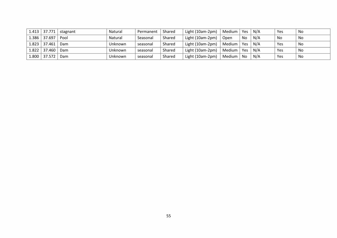
55

1.413 37.771 stagnant Natural Permanent Shared Light (10am-2pm) Medium Yes N/A Yes No

1.386 37.697 Pool Natural Seasonal Shared Light (10am-2pm) Open No N/A No No

1.823 37.461 Dam Unknown seasonal Shared Light (10am-2pm) Medium Yes N/A Yes No

1.822 37.460 Dam Unknown seasonal Shared Light (10am-2pm) Medium Yes N/A Yes No

1.800 37.572 Dam Unknown seasonal Shared Light (10am-2pm) Medium No N/A Yes No

56

Appendix IV

Table of ground truthed data for settlements within the Melako conservancy. Number of houses corresponds to manyattas that are grouped together. The term “boma” is used interchangeably with manyattas. “Fora” is a temporary circular fence used to keep livestock when pastoralists are migrating and are not able to build huts. “Mabati” is a tin roof and “centre” represents small villages.

Latitude Longitude Settlement Type

Number of Houses

Permanent/Temporary Year/Month Built

1.416466366 37.72286092 Centre Unknown Permanent Unknown

1.429139217 37.698728 Boma 33 Temporary 2012

1.429436691 37.6881844 Boma 27 Temporary 2010

1.425016914 37.68376387 Boma 45 Temporary 2013

1.427763328 37.68778081 Boma 1 Temporary 2010

1.433019452 37.68969633 Boma 5 Temporary Uknown

1.433019452 37.68969633 Mabati 3 Permanent 2007

1.426821034 37.70067142 Mabati 5 Permanent 2005

1.603676174 37.67158538 Centre Unknown Permanent Unknown

1.600599512 37.84300402 Boma 74 Temporary 2011

1.598354001 37.8369781 Boma 58 Temporary 2007

1.592591191 37.83457249 Boma 63 Temporary 2013

1.592426822 37.83649631 Boma 16 Temporary 2013

1.597636761 37.8348216 School 1 Permanent 2011

1.596301692 37.83302494 Boma 67 Temporary 2007

1.605998548 37.81800273 Boma 18 Temporary Unknown

1.601829641 37.8156159 Boma 24 Temporary Unknown

1.600591717 37.81573442 Boma 12 Temporary Unknown

1.591302976 37.8033453 Town Unknown Permanent Unknown

1.635933509 37.7809942 Boma 92 Temporary 2011

1.640849747 37.78839567 Boma 60 Temporary 2007

1.634723414 37.78561011 Church 1 Temporary Unknown

1.632815022 37.77930214 Boma 25 Temporary 2012

1.620341996 37.78773241 School 2 Permanent 2013

1.613944257 37.78340651 Boma 31 Temporary 2010

1.614178615 37.7874429 Boma 23 Temporary 2012

1.61568962 37.7898226 Boma 32 Temporary 2012

1.613064157 37.78957718 Church 1 Permanent 2014

1.613765806 37.79135574 School 1 Permanent Unknown

1.612246418 37.79247372 Boma 1 Temporary 2007

1.607055841 37.79982557 Church 2 Permanent 2013

1.608095448 37.79991911 Mabati 1 Permanent 2013

1.606017994 37.79962499 Mabati 2 Permanent Unknown

1.604751572 37.80142735 Boma 5 Temporary 1990

57

1.603351627 37.8020658 Boma 6 Temporary 2007

1.60275341 37.80009328 Boma 12 Temporary 1992

1.601791084 37.79786496 Boma 6 Temporary 1994

1.603909861 37.79641463 Boma 14 Temporary 2006

1.606373889 37.80167772 Boma 9 Temporary 1989

1.606373889 37.80167772 Mabati 1 Permanent 2001

1.608990552 37.80232983 Mabati 8 Permanent Unknown

1.633167313 37.80668959 Boma 65 Temporary 2008

1.63509775 37.80634468 Church 1 Permanent Unknown

1.638144236 37.8070506 Boma 53 Temporary 2007

1.660786858 37.81313351 Boma 87 Temporary 2010

1.658064499 37.8161862 Boma 67 Temporary 2010

1.655525956 37.81717468 Boma 6 Temporary 2010

1.65400221 37.81652927 Boma 39 Temporary 2010

1.646539215 37.82040121 School 1 Permanent 2012

1.616434017 37.80714557 Dispensary 5 Permanent 2013

1.887900978 37.88553095 Fora 4 Temporary 2014

1.893938044 37.8957391 Fora 6 Temporary 2014

1.924041146 37.89541706 Fora Abandoned Abandoned May-14

1.920619402 37.89562762 Fora Abandoned Abandoned May-14

1.919583315 37.89413556 Fora Abandoned Abandoned 14-May

1.918212036 37.89656958 Fora Abandoned Abandoned 2013

1.906676944 37.90647523 Fora Abandoned Abandoned 2013

1.905722162 37.90950964 Fora Abandoned Abandoned 2013

1.901310012 37.90442325 Fora Abandoned Abandoned Jun-14

1.897831354 37.9054834 Fora Abandoned Abandoned Jun-14

1.889557159 37.91168919 Fora Abandoned Abandoned May-14

1.891150139 37.91325895 Fora Abandoned Abandoned May-14

1.89196419 37.91465127 Fora Abandoned Abandoned 2013

1.894204756 37.91588006 Fora Abandoned Abandoned Jun-14

1.893522805 37.91311361 Fora Abandoned Abandoned Jun-14

1.896194201 37.91350815 Fora Abandoned Abandoned Jun-14

1.895634457 37.91334403 Fora Abandoned Abandoned 2013

1.893939469 37.90495408 Fora Abandoned Abandoned Jun-14

1.895610737 37.90163334 Fora Abandoned Abandoned May-14

1.895076809 37.90037446 Fora Abandoned Abandoned 2013

1.892690063 37.8928812 Fora Abandoned Abandoned 2013

1.894278685 37.88950472 Fora Abandoned Abandoned Mar-14

1.892112717 37.8887729 Fora Abandoned Abandoned Feb-14

1.888536662 37.88684322 Fora Abandoned Abandoned 2013

1.888973024 37.88614257 Fora Abandoned Abandoned May-14

1.890144227 37.88264304 Fora Abandoned Abandoned 2013

1.887709871 37.88276634 Fora Abandoned Abandoned May-14

1.720975377 37.83092503 Fora Abandoned Abandoned May-14

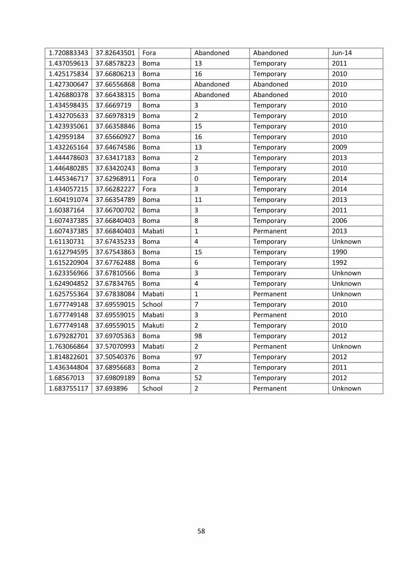
58

1.720883343 37.82643501 Fora Abandoned Abandoned Jun-14

1.437059613 37.68578223 Boma 13 Temporary 2011

1.425175834 37.66806213 Boma 16 Temporary 2010

1.427300647 37.66556868 Boma Abandoned Abandoned 2010

1.426880378 37.66438315 Boma Abandoned Abandoned 2010

1.434598435 37.6669719 Boma 3 Temporary 2010

1.432705633 37.66978319 Boma 2 Temporary 2010

1.423935061 37.66358846 Boma 15 Temporary 2010

1.42959184 37.65660927 Boma 16 Temporary 2010

1.432265164 37.64674586 Boma 13 Temporary 2009

1.444478603 37.63417183 Boma 2 Temporary 2013

1.446480285 37.63420243 Boma 3 Temporary 2010

1.445346717 37.62968911 Fora 0 Temporary 2014

1.434057215 37.66282227 Fora 3 Temporary 2014

1.604191074 37.66354789 Boma 11 Temporary 2013

1.60387164 37.66700702 Boma 3 Temporary 2011

1.607437385 37.66840403 Boma 8 Temporary 2006

1.607437385 37.66840403 Mabati 1 Permanent 2013

1.61130731 37.67435233 Boma 4 Temporary Unknown

1.612794595 37.67543863 Boma 15 Temporary 1990

1.615220904 37.67762488 Boma 6 Temporary 1992

1.623356966 37.67810566 Boma 3 Temporary Unknown

1.624904852 37.67834765 Boma 4 Temporary Unknown

1.625755364 37.67838084 Mabati 1 Permanent Unknown

1.677749148 37.69559015 School 7 Temporary 2010

1.677749148 37.69559015 Mabati 3 Permanent 2010

1.677749148 37.69559015 Makuti 2 Temporary 2010

1.679282701 37.69705363 Boma 98 Temporary 2012

1.763066864 37.57070993 Mabati 2 Permanent Unknown

1.814822601 37.50540376 Boma 97 Temporary 2012

1.436344804 37.68956683 Boma 2 Temporary 2011

1.68567013 37.69809189 Boma 52 Temporary 2012

1.683755117 37.693896 School 2 Permanent Unknown

59

Appendix V

Melako conservancy with core areas (in red) and identified human settlements from GE as well as water points that were used in data analysis. The defined study area for the dBBMM excluded part of Melako (to the right) accounting for the large amount of area with no settlements and water data.