Uncertainty evaluation of displacements measured by ESPI with divergent wavefronts

Optics Communications 241 (2004) 279–292

www.elsevier.com/locate/optcom

Uncertainty evaluation of displacements measuredby electronic speckle-pattern interferometry

Raul R. Cordero a,b,*, Amalia Martınez c, Ramon Rodrıguez-Vera c,Pedro Roth d

a Faculty of Mechanical and Production Sciences Engineering, Escuela Superior Politecnica del Litoral, Km. 30,

5 Via Perimetral, Guayaquil, Ecuadorb Department of Mechanical and Metallurgical Engineering, Pontificia Universidad Catolica de Chile,

Vicuna Mackenna 4860, Santiago, Chilec Centro de Investigaciones en Optica, Apartado Postal 1-948, C.P. 37000, Leon, Gto., Mexico

d Department of Mechanical Engineering, Universidad Tecnica Federico Santa Maria, Ave. Espana 1680, Valparaıso, Chile

Received 31 March 2004; received in revised form 6 July 2004; accepted 16 July 2004

Abstract

We have applied electronic speckle-pattern interferometry (ESPI), a whole-field optical technique, to measure the

displacements induced by applying tensile load on a metallic sheet sample. Because we used a dual-beam ESPI inter-

ferometer with collimated incident beams, our measurements were affected by errors in the collimation and in the align-

ment of the illuminating beams of the optical setup. In this paper, the influences of these errors are characterized and

compared with other systematic effects through an uncertainty analysis. We found that the displacement uncertainty

depends strongly on the incidence angles of the illuminating beams of the interferometer. Moreover, faults in the align-

ment of the incident beams have more influence on the uncertainty than errors in their collimation. The latter errors

change the incident beams from collimated to slightly divergent, modifying in turn the interferometer sensitivity. We

found that this sensitivity change can be generally neglected.

� 2004 Elsevier B.V. All rights reserved.

PACS: 42.30.M; 42.40.K; 07.60.L

Keywords: Speckle interferometry; Displacement measurements; Uncertainty analysis

0030-4018/$ - see front matter � 2004 Elsevier B.V. All rights reserv

doi:10.1016/j.optcom.2004.07.040

* Corresponding author. Tel.: +5632654501; fax:

+5632797656.

E-mail address: [email protected] (R.R. Cordero).

1. Introduction

Electronic speckle-pattern interferometry (ESPI)

[1] and Moire interferometry [2] are used to obtain

ed.

mailto:[email protected]

280 R.R. Cordero et al. / Optics Communications 241 (2004) 279–292

relative displacement fields from fringe patterns

that may be interpreted as contour maps of the

phase difference induced by the specimen deforma-

tion. The automatic extraction of the information

encoded in a pattern, includes several stages: first,phase-shifting technique [3] or Fourier transform

method [4] is used to obtain the wrapped phase

map; second, phase unwrapping is performed to ob-

tain the phase differences induced by the deforma-

tion [5]; third, the relative displacements are

evaluated by using the unwrapped phase difference

values and the adequate sensitivity vector

components.Independently of the phase measuring tech-

nique or the interferometer used, displacement

measurements are affected by several random

and systematic influences. These include: optical

noise, environmental perturbations, characteristics

of the phase measuring technique, misalignments

and collimation faults of the beams, etc.

The measured values of the phase are mainly af-fected by optical noise and environmental perturba-

tions. In order to minimize and to compensate these

problems, efforts have been done in the determina-

tion of the influence of noise under some particular

conditions [6] and in the experimental quantifica-

tion of the effect of the environmental vibration

on Moire interferometry [7]. Moreover, some sys-

tematic errors in the measured phase, introducedby limitations in the phase measuring and unwrap-

ping techniques, have been reported [8–12].

The displacement measurements depend also on

the sensitivity vector of the interferometer. If colli-

mated wavefronts are used, a dual-beam interfer-

ometer can be set up with sensitivity along just

one spatial coordinate; this means that two com-

ponents of the sensitivity vector are nominallyzero. Alternatively, if one uses an interferometer

with divergent illumination, it inevitably has sensi-

tivity along all the spatial coordinates [13–15]. If

the illuminating beams are collimated, sensitivity

vector components are affected by errors in the

collimation and in the alignment of the beams.

The collimation errors produce slightly divergent

beams, hence changing the sensitivity of the inter-ferometer. Although, it has been reported a com-

parison between the components of the

sensitivity vectors of ESPI interferometers that

use either collimated or spherical illumination

[16], the problem of the uncertainty evaluation of

displacement measured by an interferometer with

nominally collimated illumination remains open.

In this work, we use internationally acceptedrecommendations [17] to evaluate the uncertainty

of the relative displacements measured by a sym-

metrical dual-beam ESPI interferometer that uses

collimated wavefronts. The displacements were in-

duced by applying tensile load to an aluminum

sheet sample. In our analysis, special attention

was paid to include the uncertainty sources associ-

ated to the change of the interferometer sensitivitycaused by faults in the collimation.

We found that the uncertainty of the components

of the sensitivity vector depend strongly on the inci-

dence angles, measured with respect to the specimen

normal. Furthermore, we established that the errors

in the alignment had more influence on the uncer-

tainty of the displacements, than the faults in the col-

limation.Although theuncertaintiesof thenominallynull components of the sensitivity vector were not

insignificant, their contributions to the displacement

uncertainty were negligible. Therefore, we conclude

that the changes of the interferometer sensitivity

caused by faults in the collimation can be ignored.

2. Experimental details

Speckle-based methods, such as ESPI, are based

on the digital subtraction of two video frames cap-

tured meanwhile a sample undergoes mechanical

deformation. We used a dual-beam interferometer,

with two mutually coherent collimated beams

impinging from opposite sides upon a rough spec-

imen surface Lx · Ly of 30 mm per side (Fig. 1).The sample was an 1100 aluminum sheet sample,

0.58 mm thick in the ‘‘as received’’ state (i.e., cold

worked) and cut along the rolling direction. A first

scattered speckle pattern was captured by a CCD

camera of 512 · 512 pixels focused on the sample

surface. A second pattern was recorded after the

deformation of the specimen. The deformation

was induced by an Instron machine working intension along x. The digital subtraction of these

patterns yielded the ESPI fringe pattern shown in

Fig. 2(a). Conventional phase-shifting technique

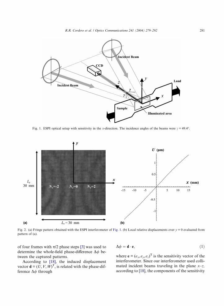
Fig. 1. ESPI optical setup with sensitivity in the x-direction. The incidence angles of the beams were c = 49.4�.

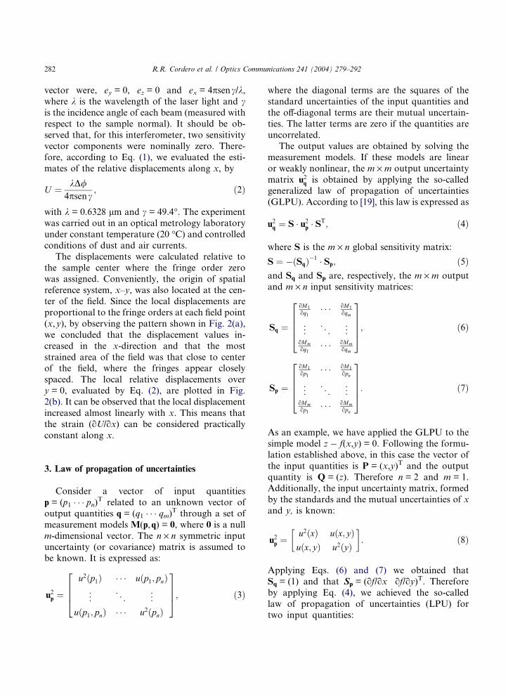
Fig. 2. (a) Fringe pattern obtained with the ESPI interferometer of Fig. 1. (b) Local relative displacements over y = 0 evaluated from

pattern of (a).

R.R. Cordero et al. / Optics Communications 241 (2004) 279–292 281

of four frames with p/2 phase steps [3] was used to

determine the whole-field phase-difference D/ be-

tween the captured patterns.According to [18], the induced displacement

vector d = (U,V,W)T, is related with the phase-dif-

ference D/ through

D/ ¼ d � e; ð1Þ

where e = (ex,ey,ez)T is the sensitivity vector of the

interferometer. Since our interferometer used colli-

mated incident beams traveling in the plane x–z,

according to [18], the components of the sensitivity


vector were, ey = 0, ez = 0 and ex = 4psenc/k,where k is the wavelength of the laser light and cis the incidence angle of each beam (measured with

respect to the sample normal). It should be ob-

served that, for this interferometer, two sensitivityvector components were nominally zero. There-

fore, according to Eq. (1), we evaluated the esti-

mates of the relative displacements along x, by

U ¼ kD/4psenc

; ð2Þ

with k = 0.6328 lm and c = 49.4�. The experiment

was carried out in an optical metrology laboratory

under constant temperature (20 �C) and controlled

conditions of dust and air currents.

The displacements were calculated relative to

the sample center where the fringe order zerowas assigned. Conveniently, the origin of spatial

reference system, x–y, was also located at the cen-

ter of the field. Since the local displacements are

proportional to the fringe orders at each field point

(x,y), by observing the pattern shown in Fig. 2(a),

we concluded that the displacement values in-

creased in the x-direction and that the most

strained area of the field was that close to centerof the field, where the fringes appear closely

spaced. The local relative displacements over

y = 0, evaluated by Eq. (2), are plotted in Fig.

2(b). It can be observed that the local displacement

increased almost linearly with x. This means that

the strain (oU/ox) can be considered practically

constant along x.

3. Law of propagation of uncertainties

Consider a vector of input quantities

p = (p1 � � � pn)T related to an unknown vector of

output quantities q = (q1 � � � qm)T through a set of

measurement models M(p,q) = 0, where 0 is a null

m-dimensional vector. The n · n symmetric inputuncertainty (or covariance) matrix is assumed to

be known. It is expressed as:

u2p ¼

u2ðp1Þ � � � uðp1; pnÞ... . .

. ...

uðp1; pnÞ � � � u2ðpnÞ

2664

3775; ð3Þ

where the diagonal terms are the squares of the

standard uncertainties of the input quantities and

the off-diagonal terms are their mutual uncertain-

ties. The latter terms are zero if the quantities are

uncorrelated.The output values are obtained by solving the

measurement models. If these models are linear

or weakly nonlinear, the m · m output uncertainty

matrix u2q is obtained by applying the so-called

generalized law of propagation of uncertainties

(GLPU). According to [19], this law is expressed as

u2q ¼ S � u2p � ST; ð4Þ

where S is the m · n global sensitivity matrix:

S ¼ �ðSqÞ�1 � Sp; ð5Þand Sq and Sp are, respectively, the m · m outputand m · n input sensitivity matrices:

Sq ¼

oM1

oq1� � � oM1

oqm

..

. . .. ..

.

oMmoq1

� � � oMmoqm

26664

37775; ð6Þ

Sp ¼

oM1

op1� � � oM1

opn

..

. . .. ..

.

oMmop1

� � � oMmopn

26664

37775: ð7Þ

As an example, we have applied the GLPU to the

simple model z � f(x,y) = 0. Following the formu-

lation established above, in this case the vector of

the input quantities is P = (x,y)T and the output

quantity is Q = (z). Therefore n = 2 and m = 1.Additionally, the input uncertainty matrix, formed

by the standards and the mutual uncertainties of x

and y, is known:

u2p ¼u2ðxÞ uðx; yÞuðx; yÞ u2ðyÞ

� �: ð8Þ

Applying Eqs. (6) and (7) we obtained that

Sq = (1) and that Sp = (of/ox of/oy)T. Therefore

by applying Eq. (4), we achieved the so-called

law of propagation of uncertainties (LPU) fortwo input quantities:


u2ðzÞ ¼ ofox

� �2

u2ðxÞ þ ofoy

� �2

u2ðyÞ

þ 2ofox

� �ofoy

� �uðx; yÞ: ð9Þ

The generalization of this law to more than two in-

put quantities is straightforward. The terms (of/

ox)2u2(x) and (of/oy)2u2(y) are the contributions

of the input quantities x and y, to the square of

the uncertainty of the output quantity z.

It should be observed that in the case of a single

output quantity, the GLPU reduces to the LPU,

and the matrix formulation becomes unnecessary.There are two approaches to evaluate the stand-

ard uncertainties of the input quantities (diagonal

elements of the input uncertainty matrix). The type

A evaluation [17] applies only to quantities which

are measured directly several times under repeata-

bility conditions. Uncertainty of input quantities

that are measured only once, those are evaluated

from models that involve further quantities, or thatare imported from other sources, should be evalu-

ated by the type B method of evaluation [17]. In

many cases, this type involves obtaining an uncer-

tainty as the standard deviation of the probability

density function (pdf) that is assumed to apply.

For example, if a quantity X is assumed to vary

uniformly within a given range of width dX, is rec-

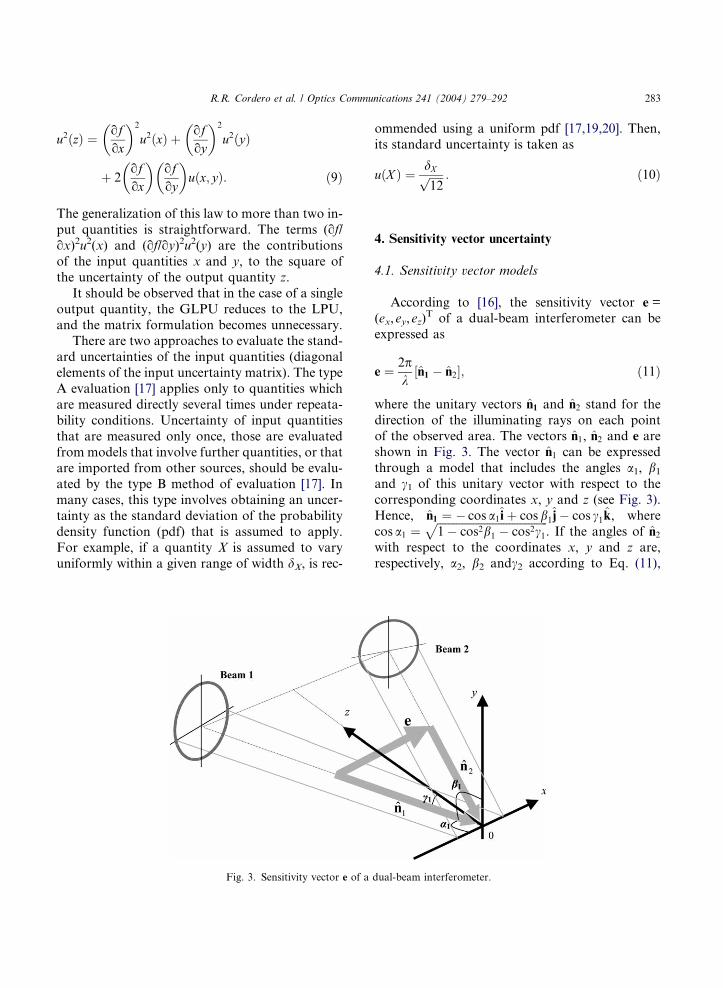
Fig. 3. Sensitivity vector e of a

ommended using a uniform pdf [17,19,20]. Then,

its standard uncertainty is taken as

uðX Þ ¼ dXffiffiffiffiffi12

p : ð10Þ

4. Sensitivity vector uncertainty

4.1. Sensitivity vector models

According to [16], the sensitivity vector e =(ex,ey,ez)

T of a dual-beam interferometer can be

expressed as

e ¼ 2pk

n1 � n2½ �; ð11Þ

where the unitary vectors n1 and n2 stand for the

direction of the illuminating rays on each pointof the observed area. The vectors n1, n2 and e are

shown in Fig. 3. The vector n1 can be expressed

through a model that includes the angles a1, b1and c1 of this unitary vector with respect to the

corresponding coordinates x, y and z (see Fig. 3).

Hence, n1 ¼ � cos a1iþ cos b1j� cos c1k, where

cos a1 ¼ffiffiffiffiffiffiffiffiffiffiffiffiffiffiffiffiffiffiffiffiffiffiffiffiffiffiffiffiffiffiffiffiffiffiffiffiffiffiffiffi1� cos2b1 � cos2c1

p. If the angles of n2

with respect to the coordinates x, y and z are,respectively, a2, b2 andc2 according to Eq. (11),

dual-beam interferometer.


the components of the sensitivity vector e of Fig. 3

can be written as

ex ¼2pk

ffiffiffiffiffiffiffiffiffiffiffiffiffiffiffiffiffiffiffiffiffiffiffiffiffiffiffiffiffiffiffiffiffiffiffiffiffiffiffiffiffiffiffiffiffiffiffiffiffiffiffiffiffiffiffiffiffiffiffiffiffiffiffiffiffiffiffiffiffiffiffiffiffiffi1� cos2 c1 þ Dc1ð Þ � cos2ðb1 þ Db1Þ

ph

þffiffiffiffiffiffiffiffiffiffiffiffiffiffiffiffiffiffiffiffiffiffiffiffiffiffiffiffiffiffiffiffiffiffiffiffiffiffiffiffiffiffiffiffiffiffiffiffiffiffiffiffiffiffiffiffiffiffiffiffiffiffiffiffiffiffiffiffiffiffiffiffiffiffi1� cos2 c2 þ Dc2ð Þ � cos2 b2 þ Db2ð Þ

p i;

ð12aÞ

ey ¼2pk

cos b1 þ Db1ð Þ � cos b2 þ Db2ð Þ½ �; ð12bÞ

ez ¼2pk

� cos c1 þ Dc1ð Þ þ cos c2 þ Dc2ð Þ½ �; ð12cÞ

where we included the quantities Dc1, Dc2 andDb2 to account for eventual errors in the colli-

mation of the incident beams. Although in our

experiment the estimates of Dc1, Dc2, Db1 and

b2 were zero, their corresponding uncertainties

were not. Since we used the symmetrical interfer-

ometer of Fig. 1, with collimated beams traveling

in the x–z plane, we considered that

b1 = b2 = 90� and that c1 = c2. Therefore, byevaluating Eqs. (12a–c) we obtained that the esti-

mates of the components of the sensitivity vector

of this interferometer were ex = 4p senc1/k, ey = 0

and ez = 0.

Estimates of the sensitivity vector components

can be affected by errors in the collimation and er-

rors in the alignment of the wavefronts used to

illuminate the sample. The latter errors can shiftthe values of b1, b2, c1 and c2; and the former er-

rors can affect the values of Dc1, Dc2, Db1 and

Db2. If Dc1, Dc2, Db1 and Db2 are not zero, eyand ez, evaluated by Eqs. (12b–c) are not zero.

This means that the collimation errors produce

slightly divergent beams changing in turn the sen-

sitivity of the interferometer.

4.2. Uncertainty of the input quantities

According to the formulation established in

Section 3, with Eqs. (12a–c) we built up a set of

three measurement models that we represented

compactly as M(p,e) = 0, where the 8-dimensional

vector of input quantities p = (b1, b2, c1, c2, Dc1,Dc2, Db1, Db2)

T is related to the vector of output

quantities e = (ex,ey,ez)T. Since the maximum rea-

sonable error associated to the estimated value of kis just about 0.1 nm, we decided to neglect the con-

tribution of k to the uncertainty of the sensitivity

vector components. Therefore, k was not consid-ered as an element of the input vector p.

Because, we assumed that the input quantities

were uncorrelated, the 8 · 8 input uncertainty ma-

trix u2p was diagonal. Its diagonal terms were the

squares of the standard uncertainties of the input

quantities b1, b2, c1, c2, Dc1, Dc2, Db1 and Db2.c1 is the angle with respect to z of the symmetry

axis of the beam 1 of the interferometer of Fig. 3.Its standard uncertainty was taken as equal to the

standard deviation of the uniform probability den-

sity function (pdf) that we assumed to apply. The

width of the pdf was assigned considering the max-

imum reasonable deviation of c1 with respect to its

estimated value. This deviation is the alignment er-

ror. Thus, according to Eq. (10) and considering

that the maximum reasonable alignment errorwas 1�, we used

uðc1Þ ¼2 1�ð Þffiffiffiffiffi12

p : ð13Þ

Analogous equations to Eq. (13) were utilized to

evaluate the uncertainties of c2, b1 and b2, consid-ering for these input quantities the same maximum

reasonable alignment error.

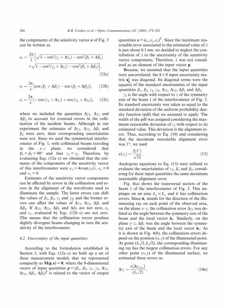
Fig. 4(a) shows the transversal section of the

beam 1 of the interferometer of Fig. 3. This im-pinges on an area Lx · Ly and it has collimation

errors. Since n1 stands for the direction of the illu-

minating ray on each point of the observed area,

on the plane x–z, the collimation error Dc1 was de-fined as the angle between the symmetry axis of the

beam and the local vector n1. Similarly, on the

plane y–z, Db1 was the angle between the symme-

try axis of the beam and the local vector n1. Asit is shown in Fig. 4(b), the collimation errors de-

pend on the position (x,y) of the illuminated point.

At point (Lx/2,Ly/2), the corresponding illuminat-

ing ray has the largest collimation errors. For any

other point (x,y) of the illuminated surface, we

estimated these errors as

Dc1 ¼x Dc1;Lx� �Lx=2ð Þ ; ð14aÞ

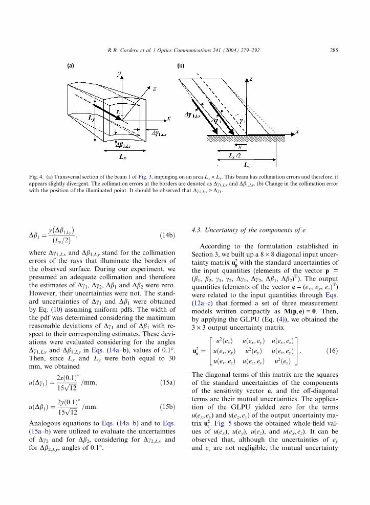
Fig. 4. (a) Transversal section of the beam 1 of Fig. 3, impinging on an area Lx · Ly. This beam has collimation errors and therefore, it

appears slightly divergent. The collimation errors at the borders are denoted as Dc1,Lx and Db1,Ly. (b) Change in the collimation error

with the position of the illuminated point. It should be observed that Dc1,Lx > Dc1.


Db1 ¼y Db1;Ly

� �Ly=2� � ; ð14bÞ

where Dc1,Lx and Db1,Ly stand for the collimation

errors of the rays that illuminate the borders of

the observed surface. During our experiment, wepresumed an adequate collimation and therefore

the estimates of Dc1, Dc2, Db1 and Db2 were zero.

However, their uncertainties were not. The stand-

ard uncertainties of Dc1 and Db1 were obtained

by Eq. (10) assuming uniform pdfs. The width of

the pdf was determined considering the maximum

reasonable deviations of Dc1 and of Db1 with re-

spect to their corresponding estimates. These devi-ations were evaluated considering for the angles

Dc1,Lx and Db1,Ly in Eqs. (14a–b), values of 0.1�.Then, since Lx and Ly were both equal to 30

mm, we obtained

u Dc1ð Þ ¼ 2x 0:1ð Þ15

ffiffiffiffiffi12

p�

=mm; ð15aÞ

u Db1ð Þ ¼ 2y 0:1ð Þ15

ffiffiffiffiffi12

p�

=mm: ð15bÞ

Analogous equations to Eqs. (14a–b) and to Eqs.

(15a–b) were utilized to evaluate the uncertainties

of Dc2 and for Db2, considering for Dc2,Lx and

for Db2,Ly, angles of 0.1�.

4.3. Uncertainty of the components of e

According to the formulation established inSection 3, we built up a 8 · 8 diagonal input uncer-

tainty matrix u2p with the standard uncertainties of

the input quantities (elements of the vector p =

(b1, b2, c1, c2, Dc1, Dc2, Db1, Db2)T). The output

quantities (elements of the vector e = (ex, ey, ez)T)

were related to the input quantities through Eqs.

(12a–c) that formed a set of three measurement

models written compactly as M(p,e) = 0. Then,by applying the GLPU (Eq. (4)), we obtained the

3 · 3 output uncertainty matrix

u2e ¼u2ðexÞ uðex; eyÞ uðex; ezÞuðex; eyÞ u2ðeyÞ uðez; eyÞuðex; ezÞ uðez; eyÞ u2ðezÞ

264

375: ð16Þ

The diagonal terms of this matrix are the squares

of the standard uncertainties of the componentsof the sensitivity vector e, and the off-diagonal

terms are their mutual uncertainties. The applica-

tion of the GLPU yielded zero for the terms

u(ex,ey) and u(ez,ey) of the output uncertainty ma-

trix u2e . Fig. 5 shows the obtained whole-field val-

ues of u(ex), u(ey), u(ez), and u(ex,ez). It can be

observed that, although the uncertainties of eyand ez are not negligible, the mutual uncertainty

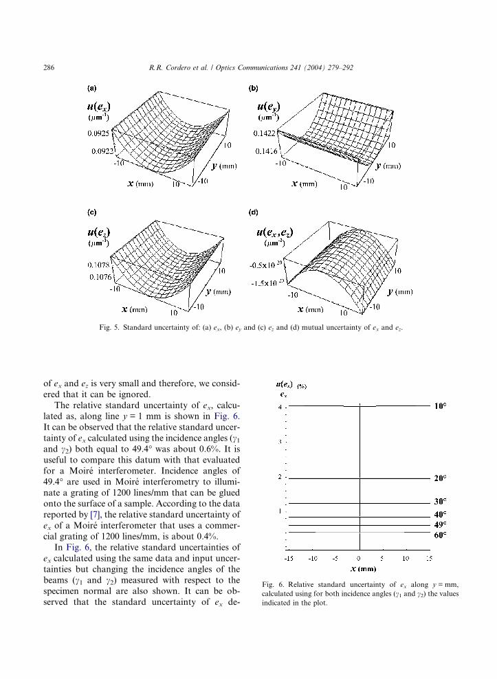
Fig. 5. Standard uncertainty of: (a) ex, (b) ey and (c) ez and (d) mutual uncertainty of ex and ez.

Fig. 6. Relative standard uncertainty of ex along y = mm,

calculated using for both incidence angles (c1 and c2) the valuesindicated in the plot.


of ex and ez is very small and therefore, we consid-

ered that it can be ignored.

The relative standard uncertainty of ex, calcu-lated as, along line y = 1 mm is shown in Fig. 6.

It can be observed that the relative standard uncer-

tainty of ex calculated using the incidence angles (c1and c2) both equal to 49.4� was about 0.6%. It is

useful to compare this datum with that evaluated

for a Moire interferometer. Incidence angles of

49.4� are used in Moire interferometry to illumi-

nate a grating of 1200 lines/mm that can be gluedonto the surface of a sample. According to the data

reported by [7], the relative standard uncertainty of

ex of a Moire interferometer that uses a commer-

cial grating of 1200 lines/mm, is about 0.4%.

In Fig. 6, the relative standard uncertainties of

ex calculated using the same data and input uncer-

tainties but changing the incidence angles of the

beams (c1 and c2) measured with respect to thespecimen normal are also shown. It can be ob-

served that the standard uncertainty of ex de-

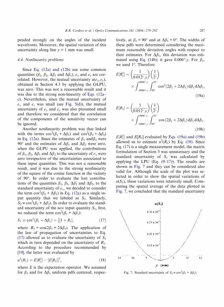
Fig. 7. Standard uncertainty of S1 ” cos2(b1 + Db1).


pended strongly on the angles of the incident

wavefronts. Moreover, the spatial variation of this

uncertainty along line y = 1 mm was small.

4.4. Nonlinearity problems

Since Eq. (12a) and (12b) use some common

quantities (b1, b2, Db1 and Db1), ex and ey are cor-

related. However, the mutual uncertainty u(ex,ey),

obtained in Section 4.3 by applying the GLPU,

was zero. This was not a reasonable result and it

was due to the strong non-linearity of Eqs. (12a–

c). Nevertheless, since the mutual uncertainty ofex and ez was small (see Fig. 5(d)), the mutual

uncertainty of ex and ey was also presumed small

and therefore we considered that the correlation

of the components of the sensitivity vector can

be ignored.

Another nonlinearity problem was that linked

with the terms cos2(b1 + Db1) and cos2(b2 + Db2)in Eq. (12a). Since the estimates of b1 andb2 were90� and the estimates of Db1 and Db2 were zero,

when the GLPU was applied, the contributions

of b1, b2, Db1 and Db2 to the uncertainty of ex were

zero irrespective of the uncertainties associated to

these input quantities. This was not a reasonable

result, and it was due to the strong nonlinearity

of the square of the cosine function in the vicinity

of 90�. In order to evaluate the lost contribu-tions of the quantities b1, b2, Db1 and Db2, to the

standard uncertainty of ex, we decided to consider

the term cos2(b1 + Db1) in Eq. (12a) as a single in-

put quantity that we labeled as S1. Similarly,

S2 ” cos2(b2 + Db2). In order to evaluate the stand-

ard uncertainty of the new input quantity S1, first,

we reduced the term cos2(b1 + Db1):

S1 � cos2 b1 þ Db1ð Þ ¼ 121þ R1½ �; ð17Þ

where R1 = cos(2b1 + 2Db1). The application of

the law of propagation of uncertainties to Eq.(17) allowed us to evaluate the uncertainty of S1

which in turn depended on the uncertainty of R1.

According to the procedure recommended by

[19], the latter was evaluated by

u2ðR1Þ ¼ E½R21� � ½E½R1��2; ð18Þ

where E is the expectation operator. We assumed

for b1 and for Db1 uniform pdfs centered, respec-

tively, at b1 = 90� and at Db1 = 0�. The widths of

these pdfs were determined considering the maxi-

mum reasonable deviation angles with respect to

their estimates. For Db1, this deviation was esti-

mated using Eq. (14b); it gave 0.006�.y. For b1,we used 1�. Therefore

E½R21� ¼

1

0:012�:y

� �1

2�

� �

�Z 0006�:y

�0006�:y

Z 91�

89�cos2 2b1 þ 2Db1ð Þdb1 dDb1;

ð19aÞ

E½R1� ¼1

0:012�:y

� �1

2�

� �

�Z 0006�:y

�0006�:y

Z 91�

89�cos 2b1 þ 2Db1ð Þdb1 dDb1:

ð19bÞ

E½R21� and E[R1] evaluated by Eqs. (19a) and (19b)

allowed us to estimate u2(R1) by Eq. (18). Since

Eq. (17) is a single measurement model, the matrix

formulation of Section 3 was unnecessary and the

standard uncertainty of S1 was calculated by

applying the LPU (Eq. (9–17)). The results are

shown in Fig. 7 and they can be considered alsovalid for. Although the scale of the plot was se-

lected in order to show the spatial variations of

u(S1), these variations were relatively small. Com-

puting the spatial average of the data plotted in

Fig. 7, we concluded that the standard uncertainty


of was just about 9.2 · 10�5. This means that the

combined contribution of the input quantities b1and Db1 to the standard uncertainty of ex should

be very small. The same is valid for the contribu-

tions of b2 and Db2.Therefore, we concluded that the uncertainty

evaluation performed in Section 4.3 was not af-

fected significantly by the application of the

GLPU to the non-linear equations (12a–c). Never-

theless, the values of u(ex) shown in Fig. 5(a) in-

clude the combined contribution of b1, Db1, b2and Db2, calculated through the evaluation of

u(S1) and u(S2) following the procedure describedabove.

4.5. Contributions to the ex uncertainty

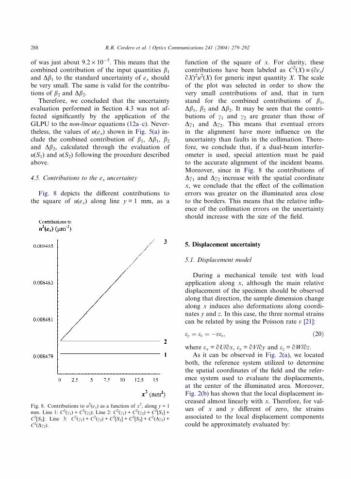
Fig. 8 depicts the different contributions to

the square of u(ex) along line y = 1 mm, as a

Fig. 8. Contributions to u2(ex) as a function of x2, along y = 1

mm. Line 1: C2(c1) + C2(c2); Line 2: C2(c1) + C2(c2) + C2[S1] +

C2[S2]; Line 3: C2(c1) + C2(c2) + C2[S1] + C2[S2] + C2(Dc1) +C2(Dc2).

function of the square of x. For clarity, these

contributions have been labeled as C2(X) ” (oex/

oX)2u2(X) for generic input quantity X. The scale

of the plot was selected in order to show the

very small contributions of and, that in turnstand for the combined contributions of b1,Db1, b2 and Db2. It may be seen that the contri-

butions of c1 and c2 are greater than those of

Dc1 and Dc2. This means that eventual errors

in the alignment have more influence on the

uncertainty than faults in the collimation. There-

fore, we conclude that, if a dual-beam interfer-

ometer is used, special attention must be paidto the accurate alignment of the incident beams.

Moreover, since in Fig. 8 the contributions of

Dc1 and Dc2 increase with the spatial coordinate

x, we conclude that the effect of the collimation

errors was greater on the illuminated area close

to the borders. This means that the relative influ-

ence of the collimation errors on the uncertainty

should increase with the size of the field.

5. Displacement uncertainty

5.1. Displacement model

During a mechanical tensile test with load

application along x, although the main relative

displacement of the specimen should be observed

along that direction, the sample dimension change

along x induces also deformations along coordi-

nates y and z. In this case, the three normal strainscan be related by using the Poisson rate v [21]:

ey ¼ ez ¼ �vex; ð20Þ

where ex = oU/ox, ey = oV/oy and ez = oW/oz.

As it can be observed in Fig. 2(a), we located

both, the reference system utilized to determine

the spatial coordinates of the field and the refer-

ence system used to evaluate the displacements,

at the center of the illuminated area. Moreover,Fig. 2(b) has shown that the local displacement in-

creased almost linearly with x. Therefore, for val-

ues of x and y different of zero, the strains

associated to the local displacement components

could be approximately evaluated by:


ex ¼Ux; ð21aÞ

ey ¼Vy; ð21bÞ

ez ¼W T

Lz; ð21cÞ

where, the total displacement induced along z(WT)

and the sample thick (Lz) were used to evaluate ez.Combining Eqs. (1) and (20) and Eqs. (21a–c), and

solving for U, we obtain

U ¼ D/xexx� veyy � vezLz

: ð22Þ

Since the components of the sensitivity vector of

our ESPI interferometer were ex = 4p senc1/k,ey = 0 and ez = 0, Eq. (22) reduces to Eq. (2). How-

ever, because the uncertainties of ey and ez were

not negligible (see Fig. 5), we considered that Eq.

(2) does not include all the uncertainty sources.

Therefore, we took Eq. (22) as the measurement

model to evaluate the displacement uncertaintyby applying the law of propagation of

uncertainties.

5.2. Uncertainty of the input quantities

According to the formulation established in

Section 3, Eq. (22) is a single measurement model

where U is related to the input quantities D/, ex,ey and ez. Since the estimates of ey and ez were

zero, when the LPU (Eq. (9)) was applied to

Eq. (22), the contributions to the U uncertainty

of the terms v and Lz were zero. Although ithas been recommended several methods to in-

clude these lost contributions [19], independently

of the selected technique, these contributions are

very small compared to those of D/ and ex.

Therefore, we decided ignore the standard uncer-

tainties of v and Lz ; they were not considered as

input quantities.

As pointed out in Section 4.4, although thecomponents of the sensitivity vector are correlated,

in our case, their mutual uncertainties can be ig-

nored. Therefore, we applied the law of propaga-

tion of uncertainties to the model (22) assuming

that the input quantities were uncorrelated.

The standard uncertainty of D/ depends on sys-

tematic effects linked with the used phase-shifting

procedure and on the influence of noise and the

perturbing environment. Assuming that the first

one was compensated adequately, we have consid-ered just the eventual variations in the phase-dif-

ference caused by the optical noise and the

external influence. We estimated a maximum even-

tual error of about 0.5 rad in the measured D/ val-

ues. Therefore, assuming a uniform pdf, we took

u D/ð Þ ¼ 2 0:5ð Þffiffiffiffiffi12

p rad: ð23Þ

The standard uncertainty of D/, estimated by

Eq. (23), was 0.28 rad. This is a standard uncer-tainty considerably greater than that reported for

the D/ values measured under similar experimen-

tal conditions with a Moire interferometer of the

same sensitivity of our ESPI interferometer.

According to [7], for the D/ values measured by

phase-shifting Moire interferometry, u( D/) is justabout 0.13 rad. The difference can be explained by

considering the different signal-to-noise ratios ofESPI and of Moire interferometry. Since ESPI

yields patterns noisier than those obtained by

Moire, we speculate that in the former method,

the influence of optical noise should be greater

than in the case of Moire.

The standard uncertainties of ex,ey and ez were

evaluated in Section 4.3. Fig. 5 shows these stand-

ard uncertainties.

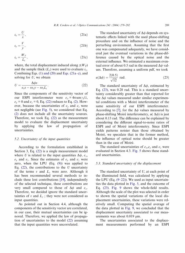
5.3. Standard uncertainty of the displacement

The standard uncertainty of U, at each point of

the illuminated field, was calculated by applying

the LPU (Eq. (9–22)). We used as input uncertain-

ties the data plotted in Fig. 5, and the outcome of

Eq. (23). Fig. 9 shows the whole-field results.Although the scale of the plot was selected in order

to shown the spatial variations of the local dis-

placement uncertainties, these variations were rel-

atively small. Computing the spatial average of

the data plotted in Fig. 9, we concluded that the

displacement uncertainty associated to our meas-

urements was about 0.019 lm.

The uncertainties associated to the displace-ment measurements performed by an ESPI

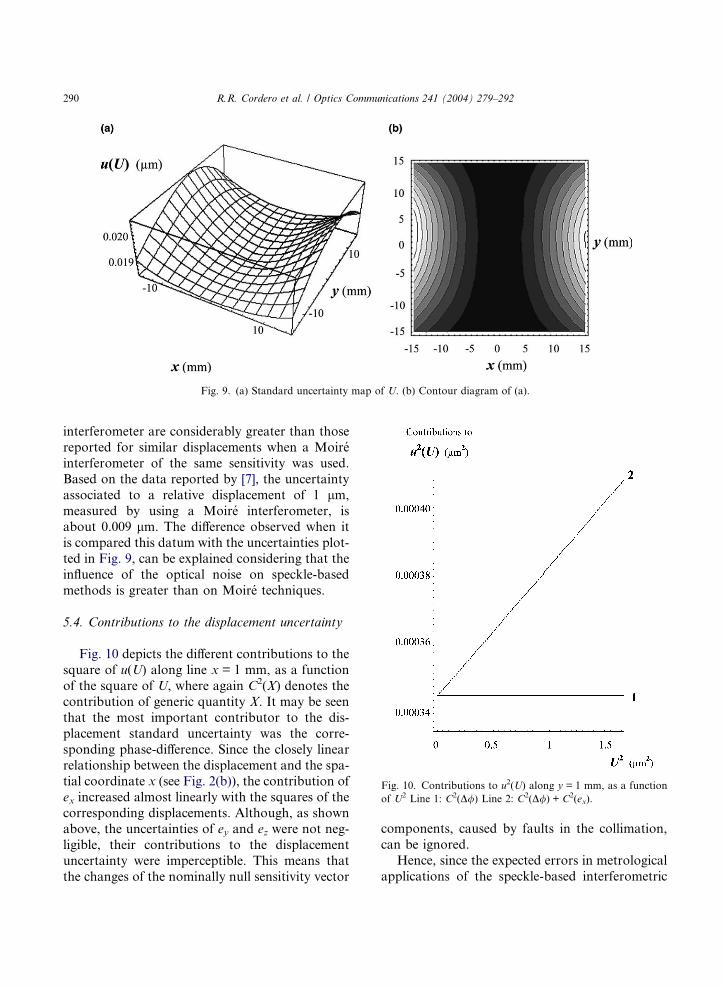
Fig. 9. (a) Standard uncertainty map of U. (b) Contour diagram of (a).

Fig. 10. Contributions to u2(U) along y = 1 mm, as a function

of U2 Line 1: C2(D/) Line 2: C2(D/) + C2(ex).


interferometer are considerably greater than those

reported for similar displacements when a Moire

interferometer of the same sensitivity was used.

Based on the data reported by [7], the uncertainty

associated to a relative displacement of 1 lm,

measured by using a Moire interferometer, isabout 0.009 lm. The difference observed when it

is compared this datum with the uncertainties plot-

ted in Fig. 9, can be explained considering that the

influence of the optical noise on speckle-based

methods is greater than on Moire techniques.

5.4. Contributions to the displacement uncertainty

Fig. 10 depicts the different contributions to the

square of u(U) along line x = 1 mm, as a function

of the square of U, where again C2(X) denotes the

contribution of generic quantity X. It may be seen

that the most important contributor to the dis-

placement standard uncertainty was the corre-

sponding phase-difference. Since the closely linear

relationship between the displacement and the spa-tial coordinate x (see Fig. 2(b)), the contribution of

ex increased almost linearly with the squares of the

corresponding displacements. Although, as shown

above, the uncertainties of ey and ez were not neg-

ligible, their contributions to the displacement

uncertainty were imperceptible. This means that

the changes of the nominally null sensitivity vector

components, caused by faults in the collimation,

can be ignored.

Hence, since the expected errors in metrological

applications of the speckle-based interferometric


techniques are generally smaller than the assumed

maximum reasonable errors in the alignment and

in the collimation, we concluded that reliable

uncertainty evaluations of measurements obtained

by an ESPI interferometer with collimated illumi-nation, can be performed by applying the LPU

to the simple model:

U ¼ kD/2p sen c1 þ Dc1ð Þ þ sen c2 þ Dc2ð Þ½ � : ð24Þ

6. Summary and conclusions

An investigation was carried out to evaluate the

uncertainty of displacements measured by using a

dual-beam ESPI interferometer that used colli-

mated illuminating beams. Displacements were in-

duced by applying tensile load to a metallic sheetsample. The interferometer was sensible just along

the pulling direction. The other two sensitivity vec-

tor components were nominally zero.

Displacement measurements depend on the

interferometer sensitivity that is affected by errors

in the collimation and in the alignment of the illu-

minating beams. Collimation errors produce

slightly divergent beams changing in turn the inter-ferometer sensitivity.

In this work, special attention was paid to eval-

uate the contributions to the displacement uncer-

tainty of eventual changes of the interferometer

sensitivity produced by faults in the collimation

of the beams.

We found that the uncertainty of the sensitivity

vector components depended strongly on the angleof the incident wavefronts, measured with respect

to the specimen normal. We established that the

errors in the alignment had more influence on

the uncertainty evaluation than the faults in the

collimation. Moreover, we found that the effect

of the collimation errors was greater on the illumi-

nated area close to the borders. This means that

the relative influence of the collimation errorson the uncertainty should increase with the size

of the field.

Although the uncertainties of the nominally

null sensitivity vector components were not insig-

nificant, we found that their contributions to the

displacement uncertainty can be neglected if the

maximum reasonable errors in alignment and in

collimation are in the order of those assumed in

this work. Since the expected errors in metrologi-

cal applications of the speckle-based interferomet-ric techniques are generally smaller than the

assumed maximum reasonable errors, we conclude

that the changes of the ESPI interferometer sensi-

tivity, caused by faults in the collimation, can be

generally ignored.

Acknowledgements

R.R. Cordero thanks support of MECESUP

PUC/19903 Project and VLaamse Interuniversi-

taire Road (VLIR IUC, Componente 6). A.

Martınez and R. Rodrıguez-Vera thank Consejo

Nacional de Ciencia y Tecnologıa (CONACYT)

and Consejo de Ciencia y Tecnologıa del Estado

de Guanajuato (CONCYTEG) for their suportto carry out this research. We thank Dr. Gonzalo

Fuster, Dr. Luciano Laroze and the referee, for

helpful suggestions to the final draft of this paper.

References

[1] R. Jones, C. Wykes, Holographic and Speckle Interferom-

etry, first ed., Cambridge University Press, Cambridge,

1983.

[2] D. Post, B. Han, P. Ifju, High Sensitivity Moire: Exper-

imental Analysis for Mechanics and Materials, Springer,

New York, 1994.

[3] J.M. Huntley, in: P.K. Rastogi (Ed.), Digital Speckle

Pattern Interferometry and Related Techniques, Wiley,

Chichester, 2001.

[4] M. Takeda, H. Ina, S. Kobayashi, J. Opt. Soc. Am. 72 (1)

(1982) 156160.

[5] D.W. Robinson, G.T. Reid, Phase Unwrapping Methods.

Interferogram Analysis, Institute of Physics, Bristol, UK,

1993.

[6] M.R. Miller, I. Mohammed, P.S. Ho, Opt. Lasers Eng. 36

(2) (2001) 127.

[7] R.R. Cordero, I. Lira, Opt. Commun. 237 (2004) 25.

[8] J. Schwider, R. Burow, K.E. Elner, J. Grzanna, R.

Spolaczyk, K. Merkel, Appl. Opt. 22 (1983) 3421.

[9] J. Schmit, K. Creath, Appl. Opt. 34 (1995) 3610.

[10] H. Zhang, M. Lalor, D. Burton, Opt. Lasers Eng. 31

(1999) 381.

[11] K. Creath, J. Schmit, Opt. Laser Eng. 24 (1996) 365.

[12] P.J. de Groot, L.L. Deck, Appl. Opt. 35 (1996) 2172.


[13] D. Albrecht, Opt. Lasers Eng. 31 (1) (1999) 6381.

[14] H.J. Puga, R. Rodriguez-Vera, A. Martinez, Opt. Lasers

Technol. 34 (1) (2002) 8192.

[15] A. Martinez, R. Rodriguez-Vera, J.A. Rayas, H.J. Puga,

Opt. Lasers Eng. 39 (2003) 525.

[16] A. Martinez, R. Rodriguez-Vera, J.A. Rayas, H.J. Puga,

Opt. Commun. 223 (2003) 239.

[17] ISO Guide to the Expression of Uncertainty in Measure-

ment, Geneva, 1993.

[18] T. Kreis, Holographic Interferometry Principles and Meth-

ods, first ed., Akademic, Berlin, 1996.

[19] I. Lira, Evaluating the Uncertainty of Measurement:

Fundamentals and Practical Guidance, Institute of Physics

Publishing, Bristol, 2002.

[20] R.R. Cordero, P. Roth, Metrologia 41 (4) (2004) L22.

[21] S.P. Timoshenko, J.N. Goodier, Theory of Elasticity,

third ed., McGraw-Hill International Editions, Singa-

pore, 1970.

Uncertainty evaluation of displacements measured by ESPI with divergent wavefronts

Documents

Transcript of Uncertainty evaluation of displacements measured by ESPI with divergent wavefronts