Segmentation of liver portal veins by global optimization
12
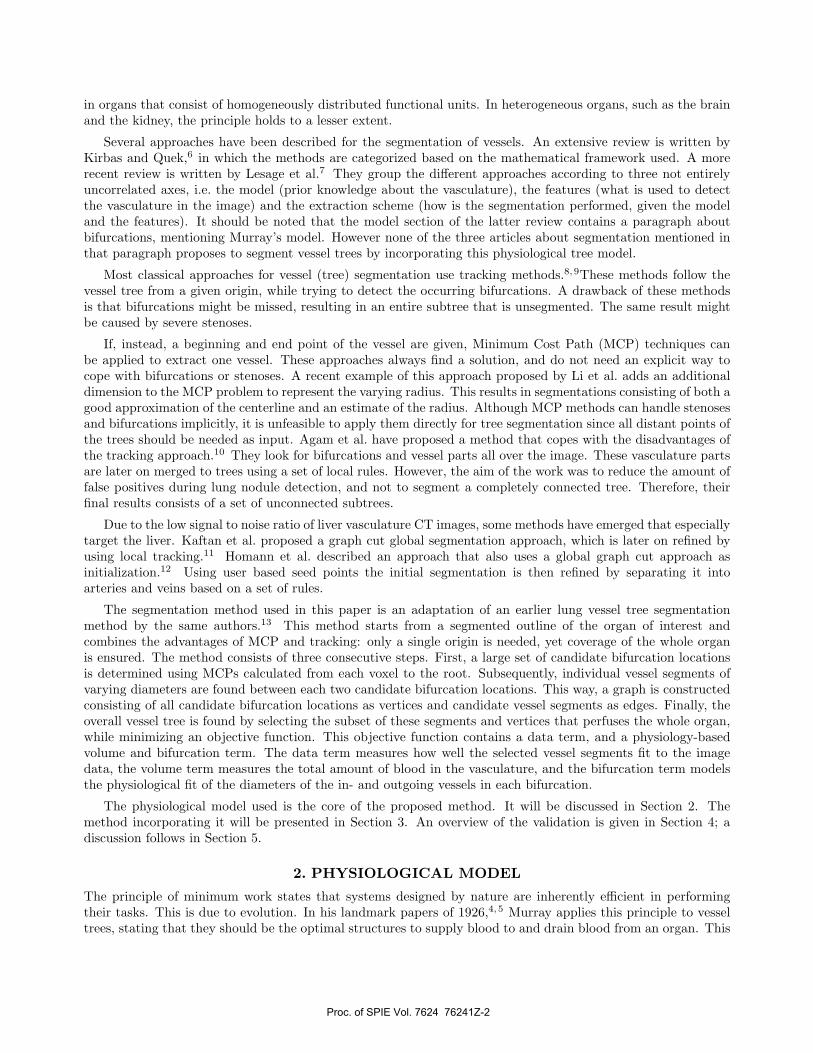
Segmentation of liver portal veins by global optimization Pieter Bruyninckx and Dirk Loeckx and Dirk Vandermeulen and Paul Suetens Medical Image Computing (ESAT/PSI), Faculty of Engineering, Katholieke Universiteit Leuven, University Hospital Gasthuisberg, Herestraat 49 bus 7003, B-3000 Leuven, Belgium ABSTRACT We present an algorithm for the segmentation of the liver portal veins from an arterial phase CT. The developed segmentation algorithm incorporates a physiological model that states that the vasculature pattern is organized such that the whole organ is perfused using minimal mechanical energy. This model is, amongst others, applicable to the lungs, the liver, and the kidneys. The algorithm first locally detects probable candidate vessel segments in the image. The subset of these segments that generates the most probable vessel tree according the image and the physiological model is afterwards sought by a global optimization method. The algorithm has already been applied successfully to segment heavily simplified lung vessel trees from CT images. Now the general feasibility of this approach is evaluated by applying it to the segmentation of the liver portal veins from an arterial phase CT scan. This is more challenging, because the intensity difference between the vessels and the parenchyma is small. To cope with the low contrast a support vector machines approach with a robust feature vector is used to locally detect vessels. This approach has been applied to a set of five images, for which a ground truth segmentation is available. This algorithm is a first step towards an automatic segmentation of all of the liver vasculature. Keywords: Segmentation, liver vasculature, global optimization, physiological model 1. INTRODUCTION The liver has a number of important functions in the body, including amongst others detoxification and glycogen storage. It contains three vessel trees. The portal veins deliver blood to the liver that should be filtered, while the smaller arterial tree delivers oxygen. All blood is drained through the hepatic veins. These vascular structures entail important information. They allow surgeons to orientate themselves in the liver, and to locate tumors and examine their relation to the vasculature. Positions in the liver are often described using the Couinaud segments system. 1 This system divides the liver into parts based upon the vasculature. An example of an application for which knowledge of the vasculature is essential is the living donor transplantation. 2 During such a surgery a part of the liver from a healthy subject is removed, and transplanted to the patient. The part consists of a number of Couinaud segments. Care should be taken that after the surgery both the donor and the patient dispose of a sufficient volume of viable liver. Since vessels may pass the borders of Couinaud segments, knowledge about the vasculature is important to assess whether a subject is a suitable donor. Contrast-enhanced CT is the most common imaging technique for the liver vasculature. Depending on the timing of the scan, either only the arterial tree and the portal veins (arterial phase) or all vasculature (venous phase) is visible. Segmenting the liver vasculature in Computed Tomography (CT) images is challenging, because of the low contrast between the vasculature and the parenchyma, which results in a low signal to noise ratio. Moreover there is a high inter-patient variability. However the liver vessel trees, as well as those in lungs and kidneys, exhibit a similar regularity, which might be exploited for segmentation purposes. Vessel trees enter an organ at the root and recursively bifurcate into a tree-like structure to perfuse the whole organ. Although these trees appear random, they all exhibit a fractal-like pattern, 3 and their bifurcations seem to obey some geometric rules on ingoing and outgoing diameters and relative orientation. Murray offered an explanation for this phenomenon by ascribing it to the principle of minimum work, which states that bodily systems have evolved over time towards a configuration of maximum efficiency. 4, 5 Vessel trees are modeled as the most efficient structure to distribute blood over a homogeneous area. This yields a fractal-like pattern, 3 which can be observed Corresponding author: [email protected] Medical Imaging 2010: Computer-Aided Diagnosis, edited by Nico Karssemeijer, Ronald M. Summers, Proc. of SPIE Vol. 7624, 76241Z · © 2010 SPIE · CCC code: 1605-7422/10/$18 · doi: 10.1117/12.843995 Proc. of SPIE Vol. 7624 76241Z-1
Transcript of Segmentation of liver portal veins by global optimization
Segmentation of liver portal veins by global optimization
Pieter Bruyninckx and Dirk Loeckx and Dirk Vandermeulen and Paul Suetens
Medical Image Computing (ESAT/PSI), Faculty of Engineering, Katholieke UniversiteitLeuven, University Hospital Gasthuisberg, Herestraat 49 bus 7003, B-3000 Leuven, Belgium
ABSTRACT
We present an algorithm for the segmentation of the liver portal veins from an arterial phase CT. The developedsegmentation algorithm incorporates a physiological model that states that the vasculature pattern is organizedsuch that the whole organ is perfused using minimal mechanical energy. This model is, amongst others, applicableto the lungs, the liver, and the kidneys. The algorithm first locally detects probable candidate vessel segments inthe image. The subset of these segments that generates the most probable vessel tree according the image andthe physiological model is afterwards sought by a global optimization method. The algorithm has already beenapplied successfully to segment heavily simplified lung vessel trees from CT images. Now the general feasibilityof this approach is evaluated by applying it to the segmentation of the liver portal veins from an arterial phaseCT scan. This is more challenging, because the intensity difference between the vessels and the parenchymais small. To cope with the low contrast a support vector machines approach with a robust feature vector isused to locally detect vessels. This approach has been applied to a set of five images, for which a ground truthsegmentation is available. This algorithm is a first step towards an automatic segmentation of all of the livervasculature.
Keywords: Segmentation, liver vasculature, global optimization, physiological model
1. INTRODUCTION
The liver has a number of important functions in the body, including amongst others detoxification and glycogenstorage. It contains three vessel trees. The portal veins deliver blood to the liver that should be filtered, while thesmaller arterial tree delivers oxygen. All blood is drained through the hepatic veins. These vascular structuresentail important information. They allow surgeons to orientate themselves in the liver, and to locate tumors andexamine their relation to the vasculature. Positions in the liver are often described using the Couinaud segmentssystem.1 This system divides the liver into parts based upon the vasculature. An example of an application forwhich knowledge of the vasculature is essential is the living donor transplantation.2 During such a surgery a partof the liver from a healthy subject is removed, and transplanted to the patient. The part consists of a numberof Couinaud segments. Care should be taken that after the surgery both the donor and the patient dispose of asufficient volume of viable liver. Since vessels may pass the borders of Couinaud segments, knowledge about thevasculature is important to assess whether a subject is a suitable donor.
Contrast-enhanced CT is the most common imaging technique for the liver vasculature. Depending on thetiming of the scan, either only the arterial tree and the portal veins (arterial phase) or all vasculature (venousphase) is visible. Segmenting the liver vasculature in Computed Tomography (CT) images is challenging, becauseof the low contrast between the vasculature and the parenchyma, which results in a low signal to noise ratio.Moreover there is a high inter-patient variability. However the liver vessel trees, as well as those in lungs andkidneys, exhibit a similar regularity, which might be exploited for segmentation purposes. Vessel trees enteran organ at the root and recursively bifurcate into a tree-like structure to perfuse the whole organ. Althoughthese trees appear random, they all exhibit a fractal-like pattern,3 and their bifurcations seem to obey somegeometric rules on ingoing and outgoing diameters and relative orientation. Murray offered an explanationfor this phenomenon by ascribing it to the principle of minimum work, which states that bodily systems haveevolved over time towards a configuration of maximum efficiency.4,5 Vessel trees are modeled as the most efficientstructure to distribute blood over a homogeneous area. This yields a fractal-like pattern,3 which can be observed
Corresponding author: [email protected]
Medical Imaging 2010: Computer-Aided Diagnosis, edited by Nico Karssemeijer, Ronald M. Summers, Proc. of SPIE Vol. 7624, 76241Z · © 2010 SPIE · CCC code: 1605-7422/10/$18 · doi: 10.1117/12.843995
Proc. of SPIE Vol. 7624 76241Z-1
in organs that consist of homogeneously distributed functional units. In heterogeneous organs, such as the brainand the kidney, the principle holds to a lesser extent.
Several approaches have been described for the segmentation of vessels. An extensive review is written byKirbas and Quek,6 in which the methods are categorized based on the mathematical framework used. A morerecent review is written by Lesage et al.7 They group the different approaches according to three not entirelyuncorrelated axes, i.e. the model (prior knowledge about the vasculature), the features (what is used to detectthe vasculature in the image) and the extraction scheme (how is the segmentation performed, given the modeland the features). It should be noted that the model section of the latter review contains a paragraph aboutbifurcations, mentioning Murray’s model. However none of the three articles about segmentation mentioned inthat paragraph proposes to segment vessel trees by incorporating this physiological tree model.
Most classical approaches for vessel (tree) segmentation use tracking methods.8,9These methods follow thevessel tree from a given origin, while trying to detect the occurring bifurcations. A drawback of these methodsis that bifurcations might be missed, resulting in an entire subtree that is unsegmented. The same result mightbe caused by severe stenoses.
If, instead, a beginning and end point of the vessel are given, Minimum Cost Path (MCP) techniques canbe applied to extract one vessel. These approaches always find a solution, and do not need an explicit way tocope with bifurcations or stenoses. A recent example of this approach proposed by Li et al. adds an additionaldimension to the MCP problem to represent the varying radius. This results in segmentations consisting of both agood approximation of the centerline and an estimate of the radius. Although MCP methods can handle stenosesand bifurcations implicitly, it is unfeasible to apply them directly for tree segmentation since all distant points ofthe trees should be needed as input. Agam et al. have proposed a method that copes with the disadvantages ofthe tracking approach.10 They look for bifurcations and vessel parts all over the image. These vasculature partsare later on merged to trees using a set of local rules. However, the aim of the work was to reduce the amount offalse positives during lung nodule detection, and not to segment a completely connected tree. Therefore, theirfinal results consists of a set of unconnected subtrees.
Due to the low signal to noise ratio of liver vasculature CT images, some methods have emerged that especiallytarget the liver. Kaftan et al. proposed a graph cut global segmentation approach, which is later on refined byusing local tracking.11 Homann et al. described an approach that also uses a global graph cut approach asinitialization.12 Using user based seed points the initial segmentation is then refined by separating it intoarteries and veins based on a set of rules.
The segmentation method used in this paper is an adaptation of an earlier lung vessel tree segmentationmethod by the same authors.13 This method starts from a segmented outline of the organ of interest andcombines the advantages of MCP and tracking: only a single origin is needed, yet coverage of the whole organis ensured. The method consists of three consecutive steps. First, a large set of candidate bifurcation locationsis determined using MCPs calculated from each voxel to the root. Subsequently, individual vessel segments ofvarying diameters are found between each two candidate bifurcation locations. This way, a graph is constructedconsisting of all candidate bifurcation locations as vertices and candidate vessel segments as edges. Finally, theoverall vessel tree is found by selecting the subset of these segments and vertices that perfuses the whole organ,while minimizing an objective function. This objective function contains a data term, and a physiology-basedvolume and bifurcation term. The data term measures how well the selected vessel segments fit to the imagedata, the volume term measures the total amount of blood in the vasculature, and the bifurcation term modelsthe physiological fit of the diameters of the in- and outgoing vessels in each bifurcation.
The physiological model used is the core of the proposed method. It will be discussed in Section 2. Themethod incorporating it will be presented in Section 3. An overview of the validation is given in Section 4; adiscussion follows in Section 5.
2. PHYSIOLOGICAL MODEL
The principle of minimum work states that systems designed by nature are inherently efficient in performingtheir tasks. This is due to evolution. In his landmark papers of 1926,4,5 Murray applies this principle to vesseltrees, stating that they should be the optimal structures to supply blood to and drain blood from an organ. This
Proc. of SPIE Vol. 7624 76241Z-2
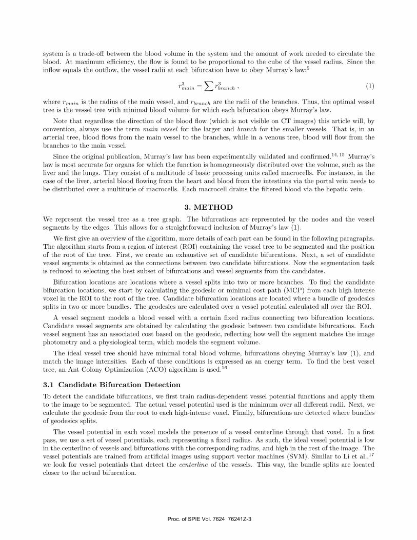
system is a trade-off between the blood volume in the system and the amount of work needed to circulate theblood. At maximum efficiency, the flow is found to be proportional to the cube of the vessel radius. Since theinflow equals the outflow, the vessel radii at each bifurcation have to obey Murray’s law:5
r3main =∑
r3branch , (1)
where rmain is the radius of the main vessel, and rbranch are the radii of the branches. Thus, the optimal vesseltree is the vessel tree with minimal blood volume for which each bifurcation obeys Murray’s law.
Note that regardless the direction of the blood flow (which is not visible on CT images) this article will, byconvention, always use the term main vessel for the larger and branch for the smaller vessels. That is, in anarterial tree, blood flows from the main vessel to the branches, while in a venous tree, blood will flow from thebranches to the main vessel.
Since the original publication, Murray’s law has been experimentally validated and confirmed.14,15 Murray’slaw is most accurate for organs for which the function is homogeneously distributed over the volume, such as theliver and the lungs. They consist of a multitude of basic processing units called macrocells. For instance, in thecase of the liver, arterial blood flowing from the heart and blood from the intestines via the portal vein needs tobe distributed over a multitude of macrocells. Each macrocell drains the filtered blood via the hepatic vein.
3. METHOD
We represent the vessel tree as a tree graph. The bifurcations are represented by the nodes and the vesselsegments by the edges. This allows for a straightforward inclusion of Murray’s law (1).
We first give an overview of the algorithm, more details of each part can be found in the following paragraphs.The algorithm starts from a region of interest (ROI) containing the vessel tree to be segmented and the positionof the root of the tree. First, we create an exhaustive set of candidate bifurcations. Next, a set of candidatevessel segments is obtained as the connections between two candidate bifurcations. Now the segmentation taskis reduced to selecting the best subset of bifurcations and vessel segments from the candidates.
Bifurcation locations are locations where a vessel splits into two or more branches. To find the candidatebifurcation locations, we start by calculating the geodesic or minimal cost path (MCP) from each high-intensevoxel in the ROI to the root of the tree. Candidate bifurcation locations are located where a bundle of geodesicssplits in two or more bundles. The geodesics are calculated over a vessel potential calculated all over the ROI.
A vessel segment models a blood vessel with a certain fixed radius connecting two bifurcation locations.Candidate vessel segments are obtained by calculating the geodesic between two candidate bifurcations. Eachvessel segment has an associated cost based on the geodesic, reflecting how well the segment matches the imagephotometry and a physiological term, which models the segment volume.
The ideal vessel tree should have minimal total blood volume, bifurcations obeying Murray’s law (1), andmatch the image intensities. Each of these conditions is expressed as an energy term. To find the best vesseltree, an Ant Colony Optimization (ACO) algorithm is used.16
3.1 Candidate Bifurcation Detection
To detect the candidate bifurcations, we first train radius-dependent vessel potential functions and apply themto the image to be segmented. The actual vessel potential used is the minimum over all different radii. Next, wecalculate the geodesic from the root to each high-intense voxel. Finally, bifurcations are detected where bundlesof geodesics splits.
The vessel potential in each voxel models the presence of a vessel centerline through that voxel. In a firstpass, we use a set of vessel potentials, each representing a fixed radius. As such, the ideal vessel potential is lowin the centerline of vessels and bifurcations with the corresponding radius, and high in the rest of the image. Thevessel potentials are trained from artificial images using support vector machines (SVM). Similar to Li et al.,17
we look for vessel potentials that detect the centerline of the vessels. This way, the bundle splits are locatedcloser to the actual bifurcation.
Proc. of SPIE Vol. 7624 76241Z-3
Because the correct annotation of real images is infeasible, we use artificial images to train the SVM. Theseartificial images mimic the characteristics of real vessel images. They contain vessel-like structures with intensitiesand noise characteristics similar to the real images. A feature vector based on the octiles of the neighborhood ofeach voxel is used to train and later evaluate the SVM. I.e., the intensities in certain regions centered at the voxelare sorted and the values at relative positions n/8, n = 1, 2, 3, 4 = median, 5, 6, 7 are computed first. The valuesstored in the feature vector are the differences between the octiles and the mean of the largest region for all butthe largest region; for the largest region the octiles themselves are stored. This feature vector is chosen due toits robustness to noise and as it allows to distinguish between vessels of varying caliber. The regions are sphereswith radius r ∈ R. The linearly incrementing values in R span the range of observable vessel radii in the image.To enhance robustness the feature vector for potential prk only contains the relative octiles of regions with aradius up to rk+2, as well as the mean of the largest region. A training potential value is computed for the subsetof features that is used for training the SVM. A training value of 0 is used for voxels at the centerline of a vesselwith the right radius, linearly increasing to 1 outside the vessel centerline or for vessels with a different radius.An example of a resulting potential evaluated on a random tree image (in 2D for demonstration purposes) isshown in Figure 2. Given the trained SVM the feature vectors that have been computed for each voxel x withinthe ROI this yields the vessel potentials pr(x).
Bifurcations are locations where a vessel splits into two or more usually smaller vessels. Given that geodesicsbetween any voxel in the image and the given origin of the vessel tree tend to follow the vessel centerlines, thiscan be used to detect bifurcations. To ensure bifurcation bundles merge close to the real bifurcation locations thegeodesics are computed on p(x) = min
rpr(x). The geodesics are computed from each voxel for which P (x) < .5
to the origin. The candidate bifurcations locations are now located where (at least) two bundels each containingat least 1‰ of the computed geodesics merge or start to travel in parallel.
3.2 Candidate Vessel Segments
A candidate vessel segment models a blood vessel with a certain constant radius connecting two candidatebifurcation locations. A vessel segment s is therefore defined by a starting location p0,s ∈ B, a target locationp1,s ∈ B and a radius rs ∈ R. Each vessel also has an associated local image cost cs and a length ls. The imagecost reflects how well the vessel segment matches the image photometry. It is the cost of the geodesic betweenp0,s and p1,s using potential Prs with fixed radius rs. The length ls is the Euclidean length length of the vesselcenterline along the geodesic.
Some constraints are added to limit the number of vessel segments and thus the size of the solution space.A maximum Euclidean distance (50 mm) between the start location and the target location of a segment isimposed, as well as a maximum mean potential(0.5) for the centerline voxels. Segments that are not connectedthrough other segments to the origin o are removed. The set of candidate vessel segment is further pruned sothe only candidate bifurcation locations a segment contains are its start and target location. E.g. a segmentA−B −C can not exist as such, but can be represented as the union of a segment A−B and a segment B −Cis the latter segments exist. This pruning step ensures that no candidate vessel segment can be described as theunion of other candidate vessel segments. This results in a set of candidate vessel segments S.
3.3 Optimization
The final segmentation should be a tree structure T = {Tb, Ts}. It consists of a set of nodes or bifurcationsTb ⊂ B and segments Ts ⊂ S. T should perfuse the whole organ, reflect the image, and follow the physiologicalmodel discussed in Section 2. We use an energy function combining an image and physiological model termsthat assess the quality of the segmented tree. To make sure the tree delivers blood to the whole organ, artificialterminal nodes that should cover the whole ROI are introduced. These artificial nodes are connected to all realnodes within a range dmax by artificial edges.
Finding the optimal graph tree that connects a subset of the graph’s nodes resembles the Steiner MinimalTree (SMT) problem, which is known to be NP-complete. We adopt an Ant Colony Optimization (ACO) strategyto find the optimal tree.
Proc. of SPIE Vol. 7624 76241Z-4
3.3.1 Energy function
We distinguish 3 energy terms: EV , EB , and EI , representing respectively the volume, bifurcation, and imageenergy. The volume and bifurcation energy measure how well the vessel tree follows the physiological model.They are based on the model discussed in Section 2, which states that vessel trees with minimum volume whileobeying Murray’s law (1) are preferred. The image energy EI models the probability of the whole image ROI(thus also including voxels outside the selected vessel segments) given the segmentation.
The volume term equals the total volume of the vessel tree, i.e. the sum of the volume of all the selectedsegments:
EV (T ) =∑s∈Ts
2πr2s ls. (2)
The bifurcation term models the mismatch between the radius relations expected according to Murray’s law (1)and the actual relations
EB(T ) =∑b∈Tb
⎛⎝rb,main − 3
√∑i
r3b,branch
⎞⎠
2
(3)
for each bifurcation, with rb,main the radius of the main segment and rb,branch the radii of the branches.
The image term expresses the probability of the image given the segmentation P (I|T ). The total imageprobability P (I|T ) =
∏x p(I(x)|T ) is calculated as the product of the probability p(I(x)|T ) that the voxel x
has intensity I(x). The same model as for the artificial images in 3.1 is used, assuming a Gaussian distributionfor vessel and background. To simplify the computation, the partial volume effects are individually computed foreach segment. Initially a voxel is considered to be in a vessel segment s ∈ T if and only if its center lays withina distance rs of the centerline of the segment s. The partial volume effects are computed by twice convolvingthis initial estimate with the PSF h. These per segment partial volume ratios are combined into one ratio forall selected segments by taking the maximum. The probability term is transformed into an energy function bytaking the negative logarithm of it, thus the final image energy is given by
EI(T ) =∑x
− log (p (I (x) |T )) . (4)
The final energy term for a solution T becomes
E(T ) =wV
ΔVEV (T ) +
wB
ΔBEB(T ) +
wI
ΔIEI(T ) (5)
in which wV , wB , and wI are weight terms, while Δx is the difference between the largest and the smallestenergy in an optimization process where wx = 1 and all other weights are set to 0. This allows the weight termsto be more independent in regard to the particular datasets.
3.3.2 Perfusion constraint
Vessel trees deliver blood to the whole organ. To ensure the selected tree reaches the whole organ a perfusionconstraint is added. This is translated in the graph framework by adding artificial terminal nodes that arelocated all over the ROI. The resulting tree has to reach these artificial target nodes, and is thus forced to coverthe whole ROI. For this application the artificial target nodes coincide with the candidate bifurcation locations,since these are supposed to be located in the more interesting areas of the image, while still being limited innumber. These artificial target nodes are connected to all real nodes within a range dmax by artificial edges.The artificial edges are excluded when computing the energy term (5).
Proc. of SPIE Vol. 7624 76241Z-5

(a) All vasculature (b) Portal veins only
Figure 1: Example of an image before and after the removal of the arteries and the hepatic veins.
3.3.3 Optimization
Finding the optimal tree in a graph that connects a subset of the graph’s nodes resembles the Steiner MinimalTree (SMT) problem. In a (weighted) graph G(V, E , w) with vertices V, edges E with weights w, the SMT aimis to find the tree structure T ⊂ G with minimum total weight
∑w that contains at least all vertices of a given
subset L ⊂ V. This problem is known to be NP-complete, which means it is assumed that no algorithm canexist that always finds the optimal solution in polynomial time. So the only feasible way to solve it for largeinstances of the problem graph is by using (meta)heuristics, i.e. methods that return near-optimal results withina reasonable amount of time.
The energy term (5) contains terms that do not fit the SMT framework, i.e. the image term and the bifurcationterm. Therefore the Ant Colony Optimization (ACO) meta-heuristic16 was chosen. ACO was already successfullyapplied for solving SMT problems;18,19 these methods inspired the optimization method used. Furthermore ACOhas the advantage that it allows for a straightforward inclusion of global energy terms.
ACO is a meta-heuristic based on the behavior of ant colonies. There exist multiple flavors of ACO. We havechosen the Ant Colony System (ACS) flavor, because it promises a good exploration of the solution space.20 ACSconstructs multiple random solutions on a graph. Each edge of the graph has an associated pheromone value τand an associated heuristic term η. Both associated terms guide the construction of random solutions, i.e. edgesassociated with a high pheromone and heuristic value are more likely to be contained in a random solution.The heuristic term is based on the cost of the MCP to the origin of the tree, defined by the cost cs of the usedsegments. The pheromone value depends on the quality of previously constructed random solutions. After theconstruction of a random solution, pheromone gets deposited on the edges contained in the best solution thus farfar. Hence the algorithm focuses on the best solution thus far. To encourage exploration it removes pheromonefrom the edges during the solution construction. In the early stage of the algorithm the heuristic terms will bedominant, hence gently guiding the optimization in a good direction. In the final stage the pheromone termshould be dominant, thus exploiting the knowledge about earlier solutions.
4. VALIDATION
The proposed method has been applied to the five images without a tumor of the 3D-IRCADb-01 database.21
This database contains twenty venous phase CT scans of the abdomen, together with a ground truth segmentationof a.o. the liver, the arteries, the hepatic veins, and the portal veins. This allows for a quantitative validationof the results. Since the scans were taken in the venous phase, all liver vessel trees are clearly visible. As theproposed method can only segment a single tree, the voxels belonging to the hepatic veins and the arteries arereplaced by noise with similar characteristics as the parenchyma. This yields images containing exactly onevascular tree, an example slice before and after removing the tree is shown in Figure 1. The algorithm consistsof multiple steps, and each of them influences the final result. Hence each of them will be validated separately,and for each of them an appropriate validation measure based on their role in the whole framework is proposed.
Proc. of SPIE Vol. 7624 76241Z-6
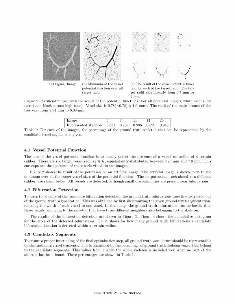
(a) Original Image (b) Minimum of the vesselpotential function over alltarget radii
(c) The result of the vessel potential func-tion for each of the target radii. The tar-get radii vary linearly from 0.7 mm to7 mm.
Figure 2: Artificial image, with the result of the potential functions. For all potential images, white means low(zero) and black means high (one). Voxel size is 0.78(×0.78) × 1.6 mm3. The radii of the main branch of thetree vary from 9.81 mm to 0.88 mm.
Image 5 7 11 14 20Represented skeleton 0.831 0.732 0.906 0.899 0.945
Table 1: For each of the images, the percentage of the ground truth skeleton that can be represented by thecandidate vessel segments is given.
4.1 Vessel Potential Function
The aim of the vessel potential function is to locally detect the presence of a vessel centerline of a certaincaliber. There are six target vessel radii rk ∈ R, equidistantly distributed between 0.75 mm and 7.0 mm. Thisencompasses the spectrum of the vessels visible in the images.
Figure 2 shows the result of the potentials on an artificial image. The artificial image is shown, next to theminimum over all the target vessel sizes of the potential functions. The six potentials, each aimed at a differentcaliber, are shown below. All vessels are detected, although small discontinuities are present near bifurcations.
4.2 Bifurcation Detection
To asses the quality of the candidate bifurcation detection, the ground truth bifurcations were first extracted outof the ground truth segmentation. This was obtained by first skeletonizing the given ground truth segmentation,reducing the width of each vessel to one voxel. In this image the ground truth bifurcations can be localized asthose voxels belonging to the skeleton that have three different neighbors also belonging to the skeleton.
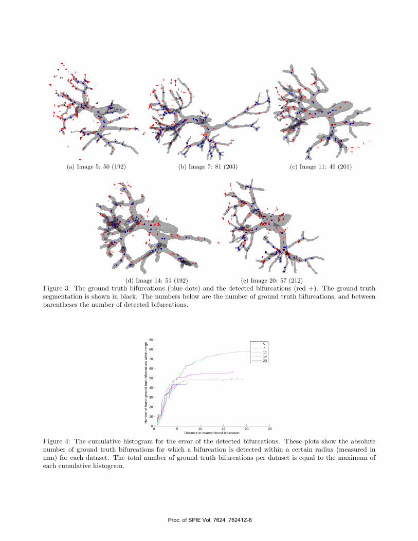
The results of the bifurcation detection are shown in Figure 3. Figure 4 shows the cumulative histogramfor the error of the detected bifurcations. I.e. it shows for how many ground truth bifurcations a candidatebifurcation location is detected within a certain radius.
4.3 Candidate Segments
To ensure a proper functioning of the final optimization step, all ground truth vasculature should be representableby the candidate vessel segments. This is quantified by the percentage of ground truth skeleton voxels that belongto the candidate segments. This values from 1 when the whole skeleton is included to 0 when no part of theskeleton has been found. These percentages are shown in Table 1.
Proc. of SPIE Vol. 7624 76241Z-7
(a) Image 5: 50 (192) (b) Image 7: 81 (203) (c) Image 11: 49 (201)
(d) Image 14: 51 (192) (e) Image 20: 57 (212)
Figure 3: The ground truth bifurcations (blue dots) and the detected bifurcations (red +). The ground truthsegmentation is shown in black. The numbers below are the number of ground truth bifurcations, and betweenparentheses the number of detected bifurcations.
0 5 10 15 20 250
10
20
30
40
50
60
70
80
90
Distance to nearest found bifurcation
Num
ber
of fo
und
grou
nd tr
uth
bifu
rcat
ions
with
in r
ange 5
7111420
Figure 4: The cumulative histogram for the error of the detected bifurcations. These plots show the absolutenumber of ground truth bifurcations for which a bifurcation is detected within a certain radius (measured inmm) for each dataset. The total number of ground truth bifurcations per dataset is equal to the maximum ofeach cumulative histogram.
Proc. of SPIE Vol. 7624 76241Z-8
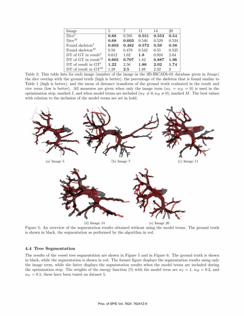
Image 5 7 11 14 20DiceI 0.68 0.595 0.551 0.553 0.54DiceM 0.68 0.603 0.546 0.529 0.534Found skeletonI 0.603 0.482 0.572 0.59 0.58Found skeletonM 0.58 0.479 0.542 0.55 0.525DT of GT in resultI 0.612 1.02 1.8 0.924 2.04DT of GT in resultM 0.605 0.707 1.82 0.887 1.96DT of result in GTI 1.22 2.56 1.86 2.02 1.74DT of result in GTM 1.28 2.5 1.88 2.32 2
Table 2: This table lists for each image (number of the image in the 3D-IRCADb-01 database given in Image)the dice overlap with the ground truth (high is better), the percentage of the skeleton that is found similar toTable 1 (high is better), and the mean of distance transform of the ground truth evaluated in the result andvice versa (low is better). All measures are given when only the image term (wV = wB = 0) is used in theoptimization step, marked I, and when model terms are included (wV �= 0, wB �= 0), marked M . The best valueswith relation to the inclusion of the model terms are set in bold.
(a) Image 5 (b) Image 7 (c) Image 11
(d) Image 14 (e) Image 20
Figure 5: An overview of the segmentation results obtained without using the model terms. The ground truthis shown in black, the segmentation as performed by the algorithm in red.
4.4 Tree Segmentation
The results of the vessel tree segmentation are shown in Figure 5 and in Figure 6. The ground truth is shownin black, while the segmentation is shown in red. The former figure displays the segmentation results using onlythe image term, while the latter displays the segmentation results when the model terms are included duringthe optimization step. The weights of the energy function (5) with the model term are wI = 1, wB = 0.2, andwV = 0.1; these have been tuned on dataset 5.
Proc. of SPIE Vol. 7624 76241Z-9
(a) Image 5 (b) Image 7 (c) Image 11
(d) Image 14 (e) Image 20
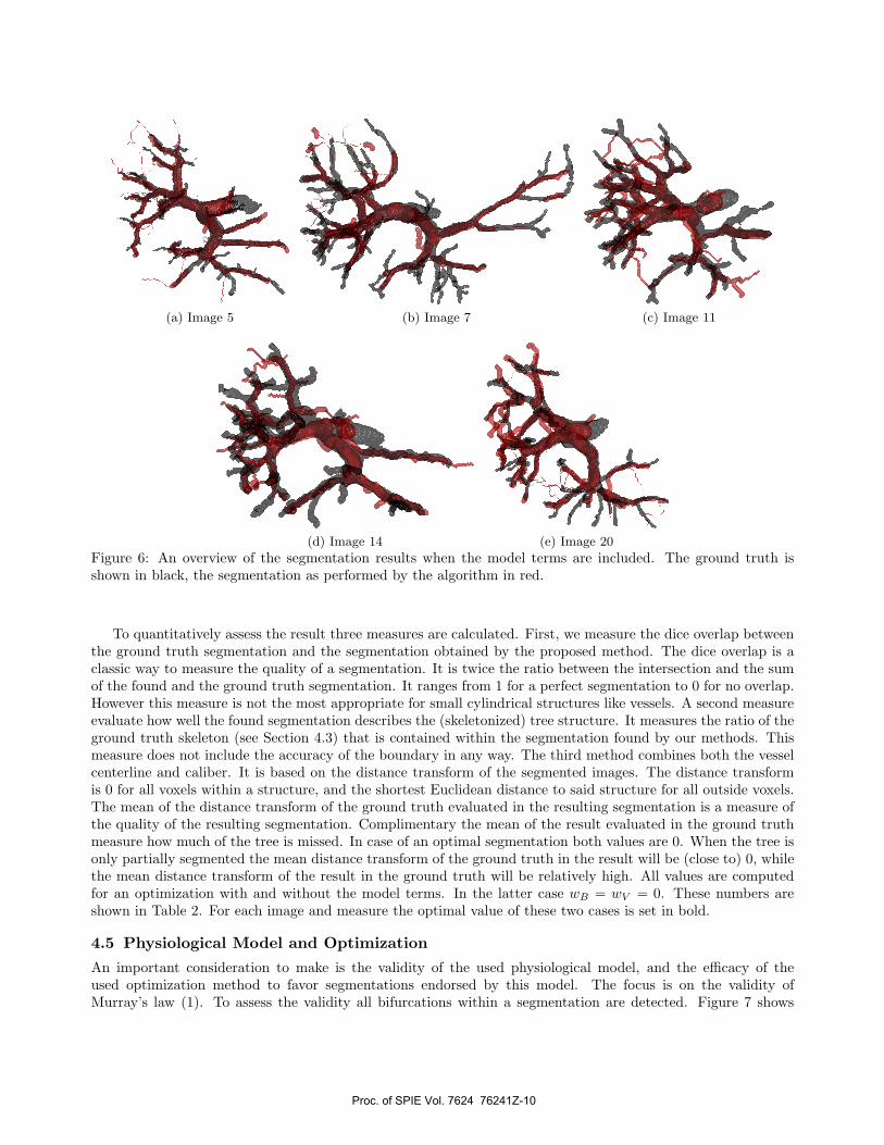
Figure 6: An overview of the segmentation results when the model terms are included. The ground truth isshown in black, the segmentation as performed by the algorithm in red.
To quantitatively assess the result three measures are calculated. First, we measure the dice overlap betweenthe ground truth segmentation and the segmentation obtained by the proposed method. The dice overlap is aclassic way to measure the quality of a segmentation. It is twice the ratio between the intersection and the sumof the found and the ground truth segmentation. It ranges from 1 for a perfect segmentation to 0 for no overlap.However this measure is not the most appropriate for small cylindrical structures like vessels. A second measureevaluate how well the found segmentation describes the (skeletonized) tree structure. It measures the ratio of theground truth skeleton (see Section 4.3) that is contained within the segmentation found by our methods. Thismeasure does not include the accuracy of the boundary in any way. The third method combines both the vesselcenterline and caliber. It is based on the distance transform of the segmented images. The distance transformis 0 for all voxels within a structure, and the shortest Euclidean distance to said structure for all outside voxels.The mean of the distance transform of the ground truth evaluated in the resulting segmentation is a measure ofthe quality of the resulting segmentation. Complimentary the mean of the result evaluated in the ground truthmeasure how much of the tree is missed. In case of an optimal segmentation both values are 0. When the tree isonly partially segmented the mean distance transform of the ground truth in the result will be (close to) 0, whilethe mean distance transform of the result in the ground truth will be relatively high. All values are computedfor an optimization with and without the model terms. In the latter case wB = wV = 0. These numbers areshown in Table 2. For each image and measure the optimal value of these two cases is set in bold.
4.5 Physiological Model and Optimization
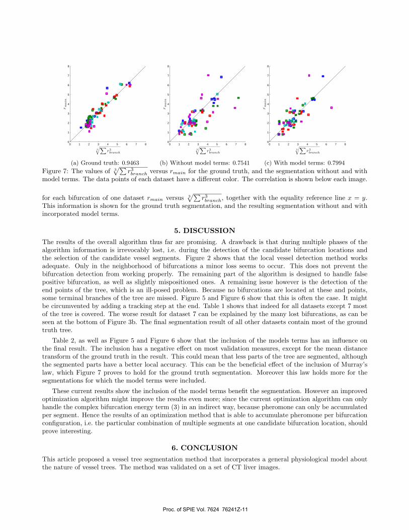
An important consideration to make is the validity of the used physiological model, and the efficacy of theused optimization method to favor segmentations endorsed by this model. The focus is on the validity ofMurray’s law (1). To assess the validity all bifurcations within a segmentation are detected. Figure 7 shows
Proc. of SPIE Vol. 7624 76241Z-10
0 1 2 3 4 5 6 7 80
1
2
3
4
5
6
7
8
3
√∑r3
branch
rm
ain
(a) Ground truth: 0.9463
0 1 2 3 4 5 6 7 80
1
2
3
4
5
6
7
8
3
√∑r3
branch
rm
ain
(b) Without model terms: 0.7541
0 1 2 3 4 5 6 7 80
1
2
3
4
5
6
7
8
3
√∑r3
branch
rm
ain
(c) With model terms: 0.7994
Figure 7: The values of 3√∑
r3branch versus rmain for the ground truth, and the segmentation without and withmodel terms. The data points of each dataset have a different color. The correlation is shown below each image.
for each bifurcation of one dataset rmain versus 3√∑
r3branch, together with the equality reference line x = y.This information is shown for the ground truth segmentation, and the resulting segmentation without and withincorporated model terms.
5. DISCUSSION
The results of the overall algorithm thus far are promising. A drawback is that during multiple phases of thealgorithm information is irrevocably lost, i.e. during the detection of the candidate bifurcation locations andthe selection of the candidate vessel segments. Figure 2 shows that the local vessel detection method worksadequate. Only in the neighborhood of bifurcations a minor loss seems to occur. This does not prevent thebifurcation detection from working properly. The remaining part of the algorithm is designed to handle falsepositive bifurcation, as well as slightly mispositioned ones. A remaining issue however is the detection of theend points of the tree, which is an ill-posed problem. Because no bifurcations are located at these and points,some terminal branches of the tree are missed. Figure 5 and Figure 6 show that this is often the case. It mightbe circumvented by adding a tracking step at the end. Table 1 shows that indeed for all datasets except 7 mostof the tree is covered. The worse result for dataset 7 can be explained by the many lost bifurcations, as can beseen at the bottom of Figure 3b. The final segmentation result of all other datasets contain most of the groundtruth tree.
Table 2, as well as Figure 5 and Figure 6 show that the inclusion of the models terms has an influence onthe final result. The inclusion has a negative effect on most validation measures, except for the mean distancetransform of the ground truth in the result. This could mean that less parts of the tree are segmented, althoughthe segmented parts have a better local accuracy. This can be the beneficial effect of the inclusion of Murray’slaw, which Figure 7 proves to hold for the ground truth segmentation. Moreover this law holds more for thesegmentations for which the model terms were included.
These current results show the inclusion of the model terms benefit the segmentation. However an improvedoptimization algorithm might improve the results even more; since the current optimization algorithm can onlyhandle the complex bifurcation energy term (3) in an indirect way, because pheromone can only be accumulatedper segment. Hence the results of an optimization method that is able to accumulate pheromone per bifurcationconfiguration, i.e. the particular combination of multiple segments at one candidate bifurcation location, shouldprove interesting.
6. CONCLUSION
This article proposed a vessel tree segmentation method that incorporates a general physiological model aboutthe nature of vessel trees. The method was validated on a set of CT liver images.
Proc. of SPIE Vol. 7624 76241Z-11
ACKNOWLEDGMENTS
Dirk Loeckx is Postdoctoral Fellow of the Research Foundation Flanders (FWO).
REFERENCES
1. C. Couinaud, A. Delmas, and J. Patel, Le foie. Etudes anatomiques et chirurgicales., Masson, 1957.
2. M. J. Bassignani, A. S. Fulcher, R. A. Szucs, W. K. Chong, U. R. Prasad, and A. Marcos, “Use of imagingfor living donor liver transplantation.,” Radiographics 21, pp. 39–52, Jan. 2001.
3. M. Zamir, “Arterial Branching within the Confines of Fractal L-System Formalism,” J. Gen. Physiol. 118,pp. 267–276, Sept. 2001.
4. C. D. Murray, “The physiological principle of minimum work: I. The vascular system and the cost of bloodvolume.,” Proc Natl Acad Sci U S A 12, pp. 207–214, Mar. 1926.
5. C. D. Murray, “The physiological principle of minimum work applied to the angle of branching of arteries,”The Journal of General Physiology 9, pp. 835–841, July 1926.
6. C. Kirbas and F. Quek, “A review of vessel extraction techniques and algorithms,” ACM computing sur-veys 36, pp. 81–121, June 2004.
7. D. Lesage, E. D. Angelini, I. Bloch, and G. Funka-Lea, “A review of 3D vessel lumen segmentationtechniques: Models, features and extraction schemes,” Medical Image Analysis In Press, AcceptedManuscript, pp. –, 2009.
8. O. Wink, W. Niessen, and M. Viergever, “Fast delineation and visualization of vessels in 3-D angiographicimages,” IEEE Transactions on Medical Imaging 19, pp. 337–346, 2000.
9. T. Deschamps and L. Cohen, “Fast extraction of tubular and tree 3D surfaces with front propagationmethods,” in 16th International Conference on Pattern Recognition, ICPR’02, (Quebec, Canada), Aug.2002.
10. G. Agam, S. Armato, III, and C. Wu, “Vessel tree reconstruction in thoracic CT scans with application tonodule detection,” Medical Imaging, IEEE Transactions on 24, pp. 486–499, Apr. 2005.
11. J. N. Kaftan, H. Tek, and T. Aach, “A two-stage approach for fully automatic segmentation of venousvascular structures in liver CT images,” in Medical Imaging 2009: Image Processing, J. P. W. Pluim andB. M. Dawant, eds., 7259, pp. 725911–1–12, SPIE, (Orlando, USA), February 7–12 2009.
12. H. Homann, G. Vesom, and J. Noble, “Vasculature segmentation of CT liver images using graph cuts andgraph-based analysis,” in Proc IEEE Int Symp Biomed Imaging, pp. 53–56, May 2008.
13. P. Bruyninckx, D. Loeckx, D. Vandermeulen, and P. Suetens, “Segmentation of lung vessel trees by global op-timization,” in Proceedings of the SPIE - The International Society for Optical Engineering, 7259, p. 725912(12 pp.), SPIE - The International Society for Optical Engineering, (USA), Feb. 2009. Medical Imaging2009: Image Processing, 8 February 2009, Lake Buena Vista, FL, USA.
14. T. F. Sherman, “On connecting large vessels to small: The meaning of Murray’s law,” J Gen Physiol 78,pp. 431–453, Oct. 1981.
15. H. N. Mayrovitz and J. Roy, “Microvascular blood flow: evidence indicating a cubic dependence on arteriolardiameter.,” Am J Physiol 245, pp. H1031–H1038, Dec. 1983.
16. M. Dorigo and L. Gambardella, “Ant colony system: a cooperative learning approach to the travelingsalesman problem,” IEEE Transactions on Evolutionary Computation 1(1), pp. 53–66, 1997.
17. H. Li and A. Yezzi, “Vessels as 4-D curves: Global minimal 4-D paths to extract 3-D tubular surfaces andcenterlines,” Medical Imaging, IEEE Transactions on 26, pp. 1213–1223, Sept. 2007.
18. Y. Hu, T. Jing, Z. Feng, X. L. Hong, X. D. Hu, and G. Y. Yan, “ACO-Steiner: Ant colony optimization basedrectilinear Steiner minimal tree algorithm,” Journal Of Computer Science And Technology 21, pp. 147–152,Jan. 2006.
19. S. Das, S. V. Gosavi, W. H. Hsu, and S. A. Vaze, “An ant colony approach for the Steiner tree problem,”in GECCO ’02: Proceedings of the Genetic and Evolutionary Computation Conference, p. 135, MorganKaufmann Publishers Inc., (San Francisco, CA, USA), 2002.
20. M. Dorigo and T. Stutzle, Ant Colony Optimization, MIT Press, 2004.
21. http://www.ircad.fr/softwares/3Dircadb/3Dircadb1.
Proc. of SPIE Vol. 7624 76241Z-12