Time scale effects in acute association between air-pollution and mortality

Myrto Valari, Lucio Martinelli, Edouard Chatignoux, James Crooks and Val Garcia

Myrto Valari:

NRC Post-doc at the U.S Environmental Protection Agency, Atmospheric Modeling Division

U.S. Environmental Protection Agency

109 T.W. Alexander Drive

Research Triangle Park, NC 27711

Valari.Myrto@epa.gov

Lucio Martinelli:

Laboratoire de Physique de la Matière Condensée

Ecole Polytechnique, 91128 Palaiseau Cedex, France

Edouard Chatignoux:

Obseravatoire Régional de Santé Ile-de-France

21/23, rue Miollis 75732 Paris Cedex 15, France

e.chatignoux@ors-idf.org

James Crooks:

U.S Environmental Protection Agency, Atmospheric Modeling Division

U.S. Environmental Protection Agency

109 T.W. Alexander Drive

Research Triangle Park, NC 27711

1

2

3

4

5

6

7

8

9

10

11

12

13

14

15

16

17

18

19

20

21

22

23

24

25

Crooks.James@epa.gov

Val Garcia:

U.S Environmental Protection Agency, Atmospheric Modeling Division

U.S. Environmental Protection Agency

109 T.W. Alexander Drive

Research Triangle Park, NC 27711

Garcia.Val@epa.gov

26

27

28

29

30

31

32

33

Abstract

We used wavelet analysis and generalized additive models (GAM) to study timescale effects in the

acute association between mortality and air-pollution. Daily averages of measured NO2 concentrations

in the metropolitan Paris area are used as surrogates of human exposure from 2000 to 2004. The NO2

time series was decomposed with wavelet analysis to six independent variables representing different

durations of population exposure. We used these variables as predictors in a mortality regression model

and compared the coefficients estimated for the different timescales. We found a strong dependency of

the exposure-response function on the duration of the air-pollution event. In contrast to previous studies

that showed a monotone increase in the relationship between exposure to air-pollution and mortality

from shorter to longer timescales, our results show a non-linear response suggesting that the overall

acute effect consists of two discrete patterns: a short-term response (2 to 15 days) where mortality

relative risks decrease to near null values with the duration of the air-pollution event; an intermediate

timescale pattern (16 to 55 days) where mortality relative risk climbs back up to positive levels. The

revealed pattern shows that the overall acute effect of air-pollution on mortality does not reflect only a

short-term mortality displacement in a population already at high death risk due to chronic conditions

but also the transition into this pool from the healthy population.

34

35

36

37

38

39

40

41

42

43

44

45

46

47

48

49

50

Introduction

Epidemiological evidence relating air-pollution to mortality at metropolitan areas [Katsouyanni et al.,

2001 and Samet et al., 2000] has been widely interpreted as the response in a population of individuals

with fragile health, such as the elderly and persons with chronic cardiac or respiratory diseases

[Environmental Protection Agency, 1996]. This means that part of the epidemiological association

reflects the shortening of life expectancy by only a few days. This effect, termed as mortality

displacement [Schimmel and Murawski, 1976] has been, in some cases, suggested as the only

interpretation of the acute association between air-pollution and mortality and has led to reluctance to

enhance emission controls [Lipfert and Wyzga, 1995]. Such policy implications, stress the need to

quantify the shortening of life expectancy implied by acute epidemiological studies.

In response to this, the epidemiological research community developed several methods to

estimate air pollution-mortality associations at various timescales. If the statistical association between

exposure and mortality only reflected a few days shortening in the life expectancy at a population

group already at high death risk, the days following the air pollution episode should be marked with

mortality below baseline levels [Zanobetti et al., 2002]. However, previous investigations provided

counter evidence of this short-term mortality displacement hypothesis by showing that associations

between air-pollution and mortality increase with the duration of the exposure [Dominici et al., 2003;

Kelsall et al., 1999; Zeger et al., 1999 and Schwartz, 2000].

Here we extended the methodology of Dominici et al. [2003] to study the mortality displacement

effect on a five-year dataset (2000-2004) in the metropolitan Paris area. Similarly to Dominici et al.,

[2003], we used cutoff frequencies in the power spectrum to isolate the temporal variability of the

exposure variable corresponding to a set of discrete timescales. Each wavelength specific component

was back transformed to the time domain and the complete set of independent variables was used as

co-variates in the regression to mortality. Here, we used an orthogonal wavelet decomposition of the

exposure variable instead of Fourier analysis [Dominici et al., 2003]. Wavelets preserve local features

51

52

53

54

55

56

57

58

59

60

61

62

63

64

65

66

67

68

69

70

71

72

73

74

75

of the time-series [Farge, 1992] and therefore, the decomposed exposure variables contain an

additional layer of information compared to the Fourier decomposition on the moment in time when

specific frequency events occur. This enhancement in locality is bound to help capturing the transition

between a state where short-term mortality displacement is the major component of the

epidemiological association to a timescale where refill from the healthy population overcomes the

depletion rate of the susceptible pool.

Data

Mortality and Health Predictors

We used daily non-accidental mortality (ICD-10 A00-R99) counts for the metropolitan Paris area from

2000 to 2004. Data from August 1st 2003 to August 15th 2003 are excluded from the analysis because

of the exceptionally high temperatures and pollutant levels (heat wave of summer 2003 over Europe).

The approach we followed (see Methods below) relates daily mortality counts to a set of health

predictors. Air-pollution predictors were derived from ambient NO2 measurements at several central

monitors in the area on hourly basis. To assure the quality of NO2 data only monitors with less than

25% of missing hourly values were used. Monitors were selected to represent only background air-

pollution levels. This was achieved by applying two criteria: (i) coherence between data measured at

different monitors (overlap of the interquartiles and differences between mean values lower than

15µg/m3) and (ii) sensitivity to the addition of each individual monitor (variability of the mean value

less than 15% and correlation coefficient higher than 0.8). Data were spatially aggregated across the

selected monitors and temporally averaged over twenty four hours to represent the daily exposure

experienced by the mean metropolitan population (see the study of Host et al., [2008] for more details

on data).

Methods

Epidemiological model

76

77

78

79

80

81

82

83

84

85

86

87

88

89

90

91

92

93

94

95

96

97

98

99

The daily data were analyzed with time-series methods, using generalized additive Poisson regression

models allowing for overdispersion [Wood, 2006]. Possible confounders, including long-term trend,

seasonality, days of the week, holidays, influenza epidemics, minimum temperature of the current day

and maximum temperature of the previous day, were controlled using Air Pollution and Health: A

European Approach 2 (APHEA-2) methodology [Touloumi et al., 2004]. Long-term trend and

seasonality were modeled using a penalised regression spline of time. A large set of basis functions

(equal to 50 per year) was used, and smoothing was used to remove autocorrelation of the model’s

residuals (by minimising the absolute value of the sum of the partial autocorrelation function of the

model’s residuals) [Touloumi et al., 2006]. Dummy variables for days of the week and holidays were

included as other independent variables. Temperature and influenza terms were modeled using

parametric splines with 3 degrees of freedom. Both minimal and maximal temperatures were taken into

account because other than minimum or maximum temperatures acting alone, their combination has

been also associated with health effects [Samet, 1998]. All analyses were performed using the MGCV

package in R software (R 2.11.1).

Spectral analysis and timescale decomposition

Using wavelet analysis, the time series of the exposure variable is decomposed into a set of six

independent variables each representing a different timescale of exposure. All six wavelength

components are used as linear mortality co-predictors in the same Poisson regression following the

model developed by Dominici et al., [2003]:

where k indicates the discrete timescales of wavelet decomposition, t the day index, µt the quasi-

poisson mean of the output mortality distribution at day t, Xk the exposure variable representing

100

101

102

103

104

105

106

107

108

109

110

111

112

113

114

115

116

117

118

119

120

121

temporal variations within the kth wavelength range. S and β are determined by the regression and they

represent a smooth function of calendar time and the linear coefficients reflecting correlation between

mortality and air-pollution respectively.

The wavelet transform of the exposure variable for each pollutant returns a two dimensional set

of coefficients representing the wavelet power spectrum at each point in time. The clear advantage of

this method compared to the Fourier transform is that the power spectrum is computed separately at

each point of the time-series. Its computation depends only on a finite window around that point and

not on the whole time series, therefore accounting for transient features of periodicity instead of pre-

assuming a global pattern [Cazelles et al., 2007]. The time series decomposition consists of two steps:

first, the time series is analyzed following a multi-resolution scheme, providing a set of decomposition

coefficients at different scales [Farge, 1992]. For this study, we performed a five level analysis using

orthogonal Daubechies (order 5) mother functions. In the frequency domain, we discretized the NO2

power spectra into six timescales: <4, 4 to 8, 9 to 15, 15 to 28, 29 to 55, and > 55 days. Then the

coefficients of each discrete time scale are back transformed to the time domain.

Results and discussion

Wavelet power spectra for each timescale are shown in Figure 1. Note that for visualization

reasons the power spectrum shown in Figure 1 has been computed using continuous wavelets (Morlet

mother functions) instead of the orthogonal Daubechies to obtain a smoother pattern. To respect the

Nyquist theorem, and given that the resolution of our data is one day, the highest frequency considered

in the analysis is every two days. For the longest wavelength component (i.e. events of duration longer

than 55 days) the dominant feature is the annual cycle at 365 days that is distributed across the study

period in a near-uniform pattern. At intermediate time scales sporadic weather and air-pollution events

are captured, such as particularly cold months (January 2002 and 2003) or the heat-wave of August

2003. At the shortest timescales weekly or few days long anomalies are represented. We note here that

122

123

124

125

126

127

128

129

130

131

132

133

134

135

136

137

138

139

140

141

142

143

144

145

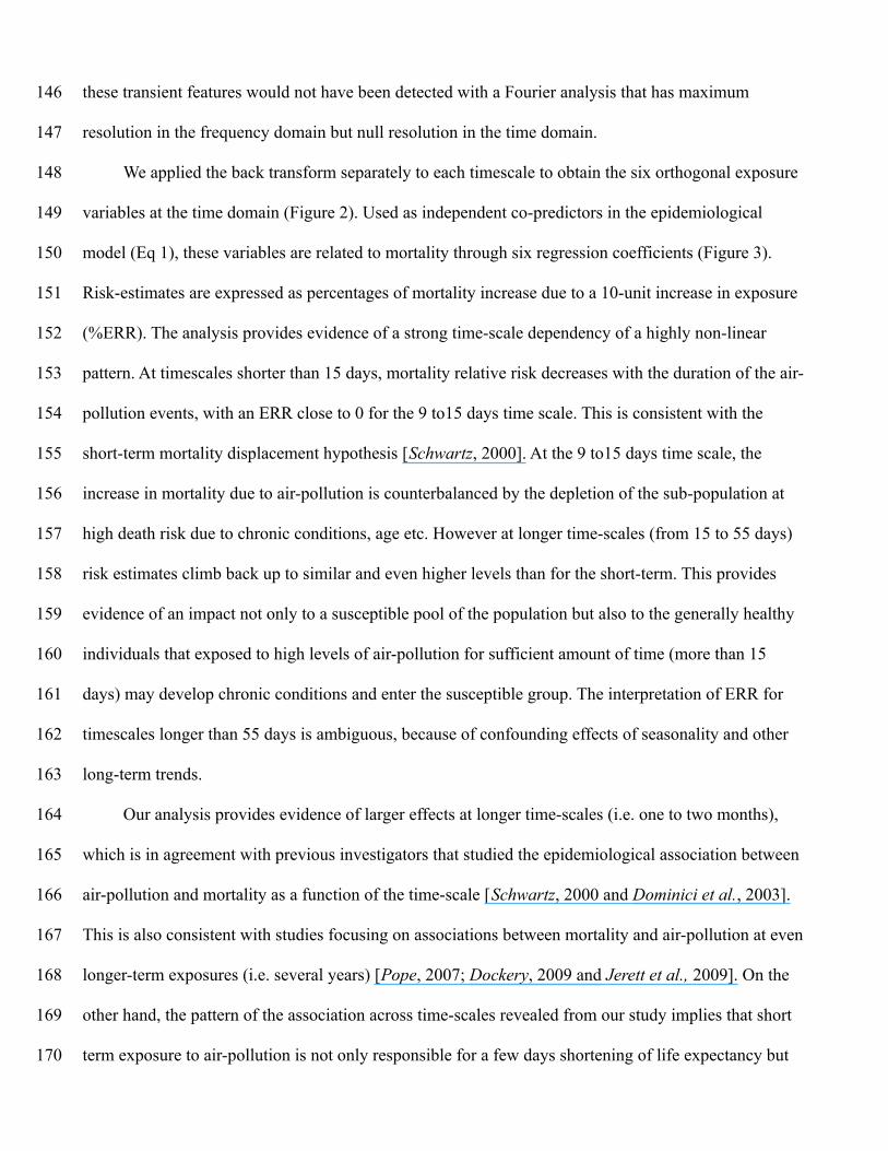
these transient features would not have been detected with a Fourier analysis that has maximum

resolution in the frequency domain but null resolution in the time domain.

We applied the back transform separately to each timescale to obtain the six orthogonal exposure

variables at the time domain (Figure 2). Used as independent co-predictors in the epidemiological

model (Eq 1), these variables are related to mortality through six regression coefficients (Figure 3).

Risk-estimates are expressed as percentages of mortality increase due to a 10-unit increase in exposure

(%ERR). The analysis provides evidence of a strong time-scale dependency of a highly non-linear

pattern. At timescales shorter than 15 days, mortality relative risk decreases with the duration of the air-

pollution events, with an ERR close to 0 for the 9 to15 days time scale. This is consistent with the

short-term mortality displacement hypothesis [Schwartz, 2000]. At the 9 to15 days time scale, the

increase in mortality due to air-pollution is counterbalanced by the depletion of the sub-population at

high death risk due to chronic conditions, age etc. However at longer time-scales (from 15 to 55 days)

risk estimates climb back up to similar and even higher levels than for the short-term. This provides

evidence of an impact not only to a susceptible pool of the population but also to the generally healthy

individuals that exposed to high levels of air-pollution for sufficient amount of time (more than 15

days) may develop chronic conditions and enter the susceptible group. The interpretation of ERR for

timescales longer than 55 days is ambiguous, because of confounding effects of seasonality and other

long-term trends.

Our analysis provides evidence of larger effects at longer time-scales (i.e. one to two months),

which is in agreement with previous investigators that studied the epidemiological association between

air-pollution and mortality as a function of the time-scale [Schwartz, 2000 and Dominici et al., 2003].

This is also consistent with studies focusing on associations between mortality and air-pollution at even

longer-term exposures (i.e. several years) [Pope, 2007; Dockery, 2009 and Jerett et al., 2009]. On the

other hand, the pattern of the association across time-scales revealed from our study implies that short

term exposure to air-pollution is not only responsible for a few days shortening of life expectancy but

146

147

148

149

150

151

152

153

154

155

156

157

158

159

160

161

162

163

164

165

166

167

168

169

170

also for the transition from a healthy population in the susceptible group. This is in agreement with

many studies highlighting adverse effects of exposure to air-pollution on less severe outcomes than

mortality (e.g. hospitalization [Host et al., 2008] or medical visits [Larrieu et al., 2009]), discarding the

hypothesis that air pollution effects are limited to the pool of very frail people. However, our results

provide evidence of some degree of short-term mortality displacement during the first two weeks

following air-pollution events. Similar patterns were observed by [Schwartz, 2000] for acute

pneumonia, but not for all causes mortality.

Conclusion

With the present study we find evidence of strong and highly non-linear time-dependencies in the

association between exposure to air-pollution and mortality. A low degree of short-term mortality

displacement is found for the first couple of weeks after air-pollution events. However, our analysis

strongly suggests that the acute impact of air-pollution on mortality does not reflect only the

precipitation of deaths that would occur shortly afterwards regardless pollution; larger effects are

estimated for longer-term exposures, which is consistent with the hypothesis that air-pollution is

responsible for the development of chronic conditions at healthy individuals.

References

Cazelles, B., M. Chavez, G. Constantin de Magny, J-F Guégan, and S. Hales (2007),

J. R. Soc. Interface, 4, 625-636 doi: 10.1098/rsif.2007.0212

Dockery, D.W. (2009), Health effects of particulate air pollution, Ann Epidemiol, 19, 257-263.

Dominici F, A. McDermott, S.L. Zeger and J.M. Samet (2003), Airborne particulate matter and

mortality: timescale effects in four US cities, Am J Epidemiol, 157,1055-1065.

Environmental Protection Agency (1996), Office of Air Quality Planning and Standards. Review of the

National Ambient Air Quality Standards for Particulate Matter: policy assessment of scientific and

technical information. OAQPS Staff Paper. Research Triangle Park, NC: Environmental Protection

Agency. (Publication no. EPA-452\R-96-013).

171

172

173

174

175

176

177

178

179

180

181

182

183

184

185

186

187

188

189

190

191

192

193

194

195

Farge M. Wavelet Transforms and their Applications to Turbulence (1992), Annual Review of Fluid

Mechanics, 24, 395-458.

Host S, S. Larrieu, L. Pascal, M. Blanchard, C. Declercq, P. Fabre, J-F Jusot, B. Chardon, A. Le Tertre ,

V. Wagner, H. Prouvost and A. Lefranc (2008), Short-term associations between fine and coarse

particles and hospital admissions for cardiorespiratory diseases in six French cities, Occup Environ

Med, 65(8), 544-551, doi:10.1136/oem.2007.036194.

Jerrett M, R.T. Burnett, CA3 Pope, K. Ito, G. Thurston, D. Krewski, Y. Shi, E. Calle and M. Thun

(2009), Long-term ozone exposure and mortality. N Engl J Med, 360, 1085-1095.

Katsouyanni K, G. Touloumi, E. Samoli, A. Gryparis, A. Le Tertre, Y. Monopolis, G. Rossi, D. Zmirou,

F. Ballester, A. Boumghar, H.R. Anderson, B. Wojtyniak, A. Paldy, R. Braunstein, J. Pekkanen, C.

Schindler and J. Schwartz (2001), Confounding and effect modification in the short-term effects of

ambient particles on total mortality: results from 29 European cities within the APHEA2 project,

Epidemiology, 12(5), 521-531.

Kelsall J, S. Zeger and J. Samet (1999), Frequency domain log-linear models: air pollution and

mortality. Appl Stat, 48, 331-344.

Larrieu S, A. Lefranc, G. Gault, E. Chatignoux, F. Couvy, B. Jouves and L. Filleul (2009), Are the

short-term effects of air pollution restricted to cardiorespiratory diseases?, Am J Epidemiol, 169, 1201-

1208.

Lipfert FW and R.E. Wyzga (1995), Air pollution and mortality: issues and uncertainties, J Air Waste

Manage Assoc, 45, 949-966.

Pope, CA3 (2007), Mortality effects of longer term exposures to fine particulate air pollution: review of

recent epidemiological evidence, Inhal Toxicol, 19(1), 33-38.

Samet J, S. Zeger, J. Kelsall, J. Xu and L. Kalkstein (1998), Does weather confound or modify the

association of particulate air pollution with mortality? An analysis of the Philadelphia data, 1973-1980,

Environ Res, 77, 9-19.

196

197

198

199

200

201

202

203

204

205

206

207

208

209

210

211

212

213

214

215

216

217

218

219

220

Samet, J. M., F. Dominici, F. C. Curriero, I. Coursac, and S. L. Zeger (2000), Fine particulate air

pollution and mortality in 20 U.S. cities, 1987-1994, N. Engl. J. Med, 343(24), 1742-1749,

doi:10.1056/NEJM200012143432401.

Schimmel H and T.J. Murawski (1976). Proceedings: the relation of air pollution to mortality, J Occup

Med, 18, 316-333.

Schwartz J. (2000), Harvesting and long term exposure effects in the relationship between air pollution

and mortality, Am J Epidemiol, 151,440-448.

Touloumi, G., R. Atkinson, A. Le Tertre, E. Samoli, J. Schwartz, C. Schindler, J.M. Vonk, G. Rossi, M.

Saez, D. Rabszenko, and K. Katsouyanni (2004), Analysis of health outcome time series data in

epidemiological studies, Environmetrics, 15, 101-117.

Touloumi G, E. Samoli, M. Pipikou, A. Le Tertre, R. Atkinson and K. Katsouyanni (2006), Seasonal

confounding in air pollution and health time-series studies: effect on air pollution effect estimates, Stat

Med, 25, 4164-4178.

Wood S. (2006), Generalized additive models: An Introduction with R. Boca Raton, Chapman &

Hall/CRC.

Zanobetti A, J. Schwartz, E. Samoli, A. Gryparis, G. Touloumi, R. Atkinson, A. Le Tertre, J. Bobros,

M. Celko, A. Goren, B. Forsberg, P. Michelozzi, D. Rabczenko, E. Aranguez Ruiz and K. Katsouyanni

(2002), The temporal pattern of mortality responses to air pollution: a multicity assessment of mortality

displacement, Epidemiology, 13, 87-93.

Zeger SL, F. Dominici and J. Samet (1999), Harvesting-resistant estimates of air pollution effects on

mortality, Epidemiology, 10, 171-175.

Figure captions

Figure 1: Wavelet power spectrum (square modulus of wavelet coefficients) of NO2 daily averaged

concentration time-series measured and spatially aggregated across several central monitors in the city

of Paris from January 1, 2000 to December 31, 2004. Continuous Morlet wavelets are used as mother

221

222

223

224

225

226

227

228

229

230

231

232

233

234

235

236

237

238

239

240

241

242

243

244

245

functions for the decomposition. The spectrum is divided in six sections to isolate variability in the set

of the six discrete timescales (top to bottom) 55 days, 29 to 55, 16 to 28, 9 to 15, 4 to 8, <4. The y-axis

is the Fourier period (scale) in days and the x-axis is the date in the time domain. The colormap

corresponds to the power of the wavelet spectrum. The absolute value of power increases for long

periods due to the corresponding wavelet broadening.

Figure 2: Decomposition into a six-component series of data on NO2 (µg/m3) for Paris, from January 1,

2000 to December 21, 2004. On each plot the overall (i.e. before decomposition) time series is plotted

for reference (black line) and on top of it each wavelength component (colored line). Time series 1 to 6

(top to bottom) are the timescale decompositions from the longer to the shortest time-scales (> 55 days,

29 to 55, 16 to 28, 9 to 15, 4 to 8, <4)

Figure 3: Estimated % of increase in mortality due to increase of the NO2 concentration by 10 µg/m3.

The point at the left extreme of the plot represents the overall effect (i.e. without spectral analysis) and

is added as a reference. Points 1 to 6 (left to right) are the excess relative risks estimated for each

timescale component of the orthogonal wavelet decomposition from the shortest to the longest

wavelengths.

246

247

248

249

250

251

252

253

254

255

256

257

258

259

260

261

262

Figure 1: Wavelet power spectrum (square modulus of wavelet coefficients) of NO2 daily averaged concentration time-series measured and spatially aggregated across several central monitors in the city of Paris from January 1, 2000 to December 31, 2004. Continuous Morlet wavelets are used as mother functions for the decomposition. The spectrum is divided in six sections to isolate variability in the set of the six discrete timescales (top to bottom) 55 days, 29 to 55, 16 to 28, 9 to 15, 4 to 8, <4. The y-axis is the Fourier period (scale) in days and the x-axis is the date in the time domain. The colormap corresponds to the power of the wavelet spectrum. The absolute value of power increases for long periods due to the corresponding wavelet broadening.

264265266267268269270271

Figure 2: Decomposition into a six-component series of data on NO2 (µg/m3) for Paris, from January 1, 2000 to December 21, 2004. On each plot the overall (i.e. before decomposition) time series is plotted for reference (black line) and on top of it each wavelength component (colored line). Time series 1 to 6(top to bottom) are the timescale decompositions from the longer to the shortest time-scales (> 55 days, 29 to 55, 16 to 28, 9 to 15, 4 to 8, <4)

273274275276277

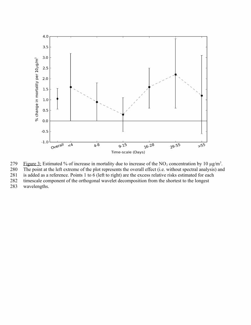
Figure 3: Estimated % of increase in mortality due to increase of the NO2 concentration by 10 µg/m3. The point at the left extreme of the plot represents the overall effect (i.e. without spectral analysis) and is added as a reference. Points 1 to 6 (left to right) are the excess relative risks estimated for each timescale component of the orthogonal wavelet decomposition from the shortest to the longest wavelengths.

279280281282283