arX

iv:c

ond-

mat

/020

7236

v1 [

cond

-mat

.dis

-nn]

9 J

ul 2

002

Time delay as a key to Apoptosis Induction in

the p53 Network

G. Tiana1,2, M. H. Jensen2 and K. Sneppen3

1Department of Physics, Univeristy of Milano,

via Celoria 16, 20133 Milano, Italy2The Niels Bohr Institute

Bledgamsvej 17, 2100 Copenhagen, Denmark3 Department of Physics, Norwegian University of Science and Technology,

N-7491, Trondheim, Norway.

February 1, 2008

Abstract

A feedback mechanism that involves the proteins p53 and mdm2, in-

duces cell death as a controled response to severe DNA damage. A min-

imal model for this mechanism demonstrates that the respone may be

dynamic and connected with the time needed to translate the mdm2 pro-

tein. The response takes place if the dissociation constant k between p53

and mdm2 varies from its normal value. Although it is widely believed

that it is an increase in k that triggers the response, we show that the ex-

perimental behaviour is better described by a decrease in the dissociation

constant. The response is quite robust upon changes in the parameters

of the system, as required by any control mechanism, except for few weak

points, which could be connected with the onset of cancer.

PACS: 87.16.Yc

1

1 Introduction

In healthy cells, a loopback mechanism involving the protein p53 is believed tocause growth arrest and apoptosis as a response to DNA damage [1, 2, 3, 4].Mutations in the sequence of p53 that potentially interfere with this mechanismhave been observed to lead to the upraise of cancer [5, 6].

Under normal conditions the amount of p53 protein in the cell is kept lowby a genetic network built of the mdm2 gene, the mdm2 protein and the p53protein itself. p53 is produced at a essentially constant rate and promotes theexpression of the mdm2 gene [7]. On the other hand, the mdm2 protein bindsto p53 and promotes its degradation [8], decreasing its concentration. WhenDNA is damaged, a cascade of events causes phosphorylation of several serinesin the p53 protein, which modifies its binding properties to mdm2 [9]. As aconsequence, the cell experiences a sudden increase in the concentration of p53,which activates a group of genes (e.g., p21, bax [10]) responsible for cell cyclearrest and apoptosis. This increase in p53 can reach values of the order of 16times the basal concentration [11].

A qualitative study of the time dependence of the concentration of p53 andmdm2 has been carried out in ref. [7]. Approximately one hour after the stressevent (i.e., the DNA damage which causes phosphorylation of p53 serines), apeak in the concentration of p53 is observed, lasting for about one hour. Thispeak partially overlaps with the peak in the concentration of mdm2, lastingfrom ≈ 1.5 to ≈ 2.5 hours after the stress event. Another small peak in theconcentration of p53 is observed after several hours.

The purpose of the present work is to provide the simpest mathematicalmodel which describes all the known aspect of the p53–mdm2 loop, and toinvestigate how the loop is robust to small variations to the ingredients of themodel. The ”weak points” displayed by the system, namely those variationsin some parameters which cause abrupt changes in the overall behaviour ofthe loop, are worth to be investigated experimentally because they can containinformations about how a cell bacomes tumoral.

The model we suggest is described in Fig. 1. The total number of p53molecules, produced at constant rate S, is indicated with p. The amount of thecomplexes built of p53 bound to mdm2 is called pm. These complexes cause thedegradation of p53 (through the ubiquitin pathway), at a rate a, while mdm2re–enters the loop. Furthermore, p53 has a spontaneous decay rate b. The totalnumber of mdm2 proteins is indicated as m. Since p53 activates the expressionof the mdm2 gene, the production rate of mdm2 is proportional (with constantc) to the probability that the complex p53/mdm–gene is built. We assume thatthe complex p53/mdm2–gene is at equilibrium with its components, where kg isthe dissociation constant and only free p53 molecules (whose amount is p−pm)can participate into the complex. The protein mdm2 has a decay rate d. Theconstants b and d describe not only the spontaneous degradation of the proteins,but also their binding to some other part of the cell, not described explicitely bythe model. The free proteins p53 and mdm2 are considered to be at equilibriumwith their bound complex pm, and the equilibrium constant is called k.

2

The dynamics of the system can be described by the equations

∂p

∂t= S − a · pm − b · p (1)

∂m

∂t= c

p(t − τ) − pm(t − τ)

kg + p(t − τ) − pm(t − τ)− d · m

pm =1

2

(

(p + m + k) −√

(p + m + k)2 − 4p · m)

.

In the second equation we allow a delay τ in the production of mdm2, due tothe fact that the transcription and translation of mdm2 lasts for some time afterthat p53 has bound to the gene.

The choice of the numeric parameters is somewhat difficult, due to the lackof reliable experimental data. The degradation rate through ubiquitin pathwayhas been estimated to be a ≈ 3·10−2s−1 [12], while the spontaneous degradationof p53 is ≈ 10−4s−1 [7]. The dissociation constant between p53 and mdm2 isk ≈ 180 [13] (expressed as number of molecules, assuming for the nucleus avolume of 0.6µm3), and the dissociation constant between p53 and the mdm2gene is kg ≈ 28 [14]. In lack of detailed values for the protein production rates,we have used typical values, namely S = 1s−1 and c = 1s−1. The degradationrate of mdm2 protein has been chosen of the order of d = 10−2s−1 to keep thestationary amount of mdm2 of the order of 102.

The behaviour of the above model is independent on the volume in which weassume the reaction takes place. That is, multiplying S, c, kg and k by the sameconstant ω gives exactly the same dynamics of the rescaled quantities ωp andωm. Futhermore, due to the fact that the chosen parameters put the system inthe saturated regime, an increase in the producing rates S and c with respectto kg and k will not affect the response. On the contrary, a decrease of S andc with respect to kg and k can drive the system into a non–saturated regime,inhibiting the response mechanism.

2 Results with no delay

In the case that the production of mdm2 can be regarded as instantaneous (nodelay, τ = 0), the concentration of p53 is rather insensitive to the change of thedissociation constant k. The stationary values of p and m are found as fixedpoints of the equations 1 (see Appendix) and in Table I we list the stationaryvalues p∗ of the amount of p53 molecules for values of k spanning seven ordersof magnitude around the basal value k = 180. Moreover, transient oscillatorybehaviour upon change in the dissociation constant k is not observed. Thisis supported by the fact that the eigenvalues of the stationary points (listedin Table I) have negative real parts, indicating stable fixed points, and rathersmall imaginary pats indicating absence of oscillations.

More precisely, the variation ∆p of the stationary amount of p53 if thedissociation constant undergoes a change ∆k can be estimated, under the ap-

3

proximation that kg ≪ p (cf. the Appendix), to be

∆p =d(S − bp)

ackg(a + b)∆k. (2)

The fact that ∆p is approximately linear with ∆k with a proportionality con-stant which is at most of the order of 10−2 makes this system rather inefficientas response mechanism. Furthermore, it does not agree with the experimentaldata which show a peak of p53 followed, after several minutes, by a peak inmdm2 [7], and not just a shift of the two concentration to higher values.

To check whether the choice of the system parameters affects the observedbehaviour, we have repeated all the calculations varying each parameter of fiveorders of magnitude around the values used above. The results (listed in TableII for S and kg and not shown for the other parameters) indicate the samebehaviour as above (negative real part and no or small imaginary part in theEigenvalues). Consequently, the above results about the dynamics of p53 seemnot to be sensitive to the detailed choice of parameters (on the contrary, theamount of mdm2 is quite sensitive).

3 Results with delay

The dynamics changes qualitatively if we introduce a nonzero delay in Eqs. 1.Keeping that the halflife of an RNA molecule is of the order of 1200 s [16],we repeat the calculations with τ = 1200. The Eqs. 1 are solved numerically,starting from the conditions p(0) = 0 and m(0) = 0 and making use of avariable–step Adams algorithm. After the system has reached its stationarystate under basal condition, a stress is introduced (at time t = 20000 s) bychanging instantaneously the dissociation constant k. In Fig. 2 we display acase in which the stress multiplies k by a factor 15 (a), a case in which it dividesit by a factor 15 (b) and by a factor 5 (c).

When k is increased by any factor, the response is very similar to the responseof the system without delay (cf. e.g. Fig. 2a). On the contrary, when k isdecreased the system displays an oscillatory behaviour. The height ∆p of theresponse peak is plotted in Fig. 3 as a function of the quantity which multipliesk. If the multiplier is larger than 0.1 the response is weak or absent. At thevalue 0.1 the system has a marked response (cf. also Figs. 2b and c). Themaximum of the first peak takes place approximately 1200s after the stress,which is consistent with the lag–time observed in the experiment [7], and thepeaks are separated from ≈ 2300s.

Although it has been suggested that the effect of the stress is to increase thedissociation constant between p53 and mdm2 [6], our results indicate that anefficient response take place if k decreases of a factor ≥ 15 (cf. Fig. 2b). Onehas to notice that the conclusions of ref. [6] have been reached from the analysisin vivo of the overall change in the concentration of p53, not from the directmeasurement of the binding constant after phosphorylation. Our results alsoagree with the finding that p53asp20 (a mutated form of p53 which mimicks

4

phosphorylated p53, due to the negative charge owned by aspartic acid) bindsmdm2 in vitro more tightly than p53ala20 (which mimicks unphosphorylatedp53) [6].

This hypothesis is supported by molecular energy calculations made withclassical force fields. Even if this kind of force fields is not really reliable for thecalculation of binding constants, it gives an estimate of the sign of the change ininteraction among p53 and mdm2 upon phosphorylation. We have performed anenergy minimization of the conformation of the system composed by the bindingsites of p53 and mdm2, starting form the crystallographic positions of ref. [13]and using the force fields mm3 [17] and mmff [18], for both the wild–type systemand for the system where serine 20 of p53 in phosphorylated. Using mm3 wefound that the phosphorylated system has an electrostatic energy 16 kcal/mollower than the wild–type system, while this difference is 26 kcal/mol using themmff force field. Our calculations suggest that phopshprylated p53 is moreattracted by mdm2 due to the enhanced interaction of phosphorylated SER20with LYS60, LYS46 and LYS70 of mdm2, and consequently the dissociationconstant is lowered.

The robustness of the response mechanism with respect to the parametersof the system, which is typical of many biological systems (cf., e.g., [19, 20]),has been checked both to assess the validity of the model and to search forweak points which could be responsible for the upraise of the disease. Eachparameter has been varied of five orders of magnitude around its basal quantity.The results are listed in Table III. One can notice that the response mechanismis quite robust to changes in the parameters a, b and c. For low values of a orc the system no longer oscillates, but displays, in any case, a rapid increase inthe amount of p which can kill the cell. This is true also for large values of d.What is dangerous for the cell is a decrease of d or of kg, which would drop theamount of p53 and let the damaged cell survive. This corresponds either to anincrease of the affinity between p53 and the mdm2 gene, or to an increase ofmdm2 half–life.

To be noted that, unlike the case τ = 0, the system with delay never displaysdamped oscillations as a consequence of the variation of the parameters in therange studied in the present work. This sharp behaviour further testifies to therobustness of the response mechanism. Anyway, one has to keep in mind thatthe oscillating response produces the death of the cell, and consequently thelong–time behaviour is only of theoretical interest.

The minimum value of the delay which gives rise to the oscillatory behaviouris τ ≈ 100s. For values of the delay larger than this threshold, the amplitude ofthe response is linear with τ (cf. Fig. 4), a fact which is compatible with theexplanation of the response mechanism of Section IV.

The lag time before the p53 response is around 3000s (in accordance withthe 1h delay observed experimentally [7] and is independent on all parameters,except c and τ . The dependence of the lag time on τ is approximately linearup to 5000s (the longest delay analyzed). Increasing c the lag time increases to8000s (for c = 104) and 25000s (for c = 105). On the other hand, the period ofoscillation depends only on the delay τ , being approximately linear with it.

5

We have repeated the calculations squaring the variable p in Eqs. 1, to keepinto account the cooperativity induced by the fact that the active form of p53is a dimer of dimers [21]. The results display qualitative differences neither fornon–delayed nor for the delayed system.

4 Discussion

All these facts can be rationalized by analyzing the mechanism which producesthe response. The possibility to trigger a rise in p53 as a dynamic response toan increased binding between p53 and mdm2, relies on the fact that a suddenincrease in p–m binding diminishes the production of mdm2, and therefore(subsequently) diminishes the amount of pm. In other words, while the change ink has no direct effect in the first of Eqs. 1, it directly reduces mdm2 productionby subtracting p53 from the gene which producese mdm2.

Mathematically, the oscillations arise because the saturated nature of thebinding pm imply that pm is approximately equal to the minimum between pand m. Each time the curves associated with p and m cross each other (eitherat a given time or τ instants before), the system has to follow a different setof dynamic equations than before, finding itself in a state far from stationarity.This gives rise to the observed peaks.

To be precise, the starting condition (before the stress) is m > p. The stressreduces the dissociation constant k of, at least, one order of magnitude, causinga drop in p, which falls below m. For small values of k (to be precise, fork ≪ min(|p − m|, p, m)), one can make the simplification pm ≈ min(p, m), andconsequently rewrite Eqs. 1 as

for p < m∂p

∂t= S − (a + b)p (3)

for p(t − τ) < m(t − τ)∂m

∂t= −dm (4)

for p > m∂p

∂t= S − am − bp (5)

for p(t − τ) > m(t − τ)∂m

∂t= c

p(t − τ) − m(t − τ)

kg + p(t − τ) − m(t − τ)− dm. (6)

Each period after the stress can be divided in four phases. In the first onep < m and p(t − τ) < m(t − τ), so that p stays constant at its stationary valueS/(a + b) ≈ p∗, while m decreases with time constant d−1 towards zero (notexactly zero, since the approximated Equations do not hold for m ∼ k). In thesecond phase one has to consider the second (p(t− τ) < m(t− τ)) and the third(p > m) Equations (4 and 5). The new stationary value for p is (S−am)/b ≈ S/bwhich is much larger than p∗ since b ≪ a. This boost takes place in a time ofthe order of b−1, so if b−1 > τ , as in the present case, p has no time to reach thestationary state and ends in a lower value. In the meanwhile, m remains in thelow value given by Eq. 4. At a time τ after the stress Eq. 4 gives way to Eq. 6.The latter is composed by a positive term which is ≈ c if p(t−τ)−m(t−τ) ≫ kg

6

and ≈ 0 under the opposite condition. Since p(t − τ) ≫ m(t − τ) (it refers tothe boost of p), then the new stationary value of m is c/d ≈ m∗. The raise ofm takes place in a time of the order of d−1 and causes the decrease of p, whoseproduction rate is ruled by S−am. The fourth phase begins when p approachesm. Now one has to keep Eqs. 3 and 6, so that p returns to the basal valuep∗, while m stays for a period of τ at the value c/d ≈ m∗ reached in the thirdphase. After such period, Eq. 4 substitutes Eq. 6 and another peak takes place.

The heigth of the p53 peak is given by S/b if p has time to reach its stationarystate of phase two (i.e., if b−1 < τ), or by S/b(1 − exp(−bτ)) if the passage tothe third phase takes place before it can reach the stationary state. The widthof the peak is ≈ τ and the spacing among the peaks ≈ τ , so that the oscillationperiod is ≈ 2τ .

The necessary conditions for the response mechanism to be effective are 1)that s/a ≪ c/d, that is that the stationary value of p just after the stress ismuch lower than the stationary value of m, 2) that b ≪ a, in such a way thatthe stationary state of p in the second phase is much larger than that in thefirst phase, in order to display the boost, 3) that d−1 < τ , otherwise m has notenough time to decrease in phase one and to increase in phase three.

The failure of the response for low values of a (cf. Table 3) is due to the fallof condition 2), the failure for small c is caused by condition 1), the failure atsmall and large values of d is associated with conditions 3) and 1), respectively.At low values of kg the response does not take place because the positive termin Eq. 6 is always ∼ c, and thus m never decreases.

5 Conclusions

In summa, we have shown that the delay is an essential ingredient of the systemto have a ready and robust peak in p53 concentration as response to a damagestress. In order to have a peak which is comparable with those observed experi-mentally, the dissociation constant between p53 and mdm2 has to decrease of afactor 15. Although it is widely believed that phosphorylation of p53 increasesthe dissociation constant, we observe an oscillating behaviour similar to the ex-perimental one only if k decreases. In this case the response is quite robust withrespect to the parameters, except upon increaasing of the half–life of mdm2 andupon decreasing of the dissociation constant between p53 and the mdm2 gene,in which cases there is no response to the stress. Moreover, an increase in theproduction rate of mdm2 can delay the response and this can be dangerous tothe cell as well. We hope that detailed experimental measurements of the phys-ical parameters of the system will be made soon, in order to improve the modeland to be able to make more precise predictions about the weak point of themechanism, weak points which could be intimately connected with the upraiseof cancer.

7

Appendix

The stationary condition for Eqs. 1 without delay can be found by theintersection of the curves

m(p) =c(a + b)p − cs

d(a + b)p − d(S − akg

(7)

mk(p) =(S − bp)((a + b)p + ak − S)

a((a + b)p − S), (8)

which have been obtained by the conditions p = m = 0, explicitating pm fromthe first of Eqs. 1 and substituting it in the second and the third, respectively.To be noted that mk is linear in k.

The variation ∆p of the stationary value of p53 upon change ∆k in thedissociation constant can be found keeping that

dp

dk=

dp

dm

dmk

dk≈

d(S − bp)

ckg(a + b), (9)

where the approximation kg ≪ p has been used. Consequently,

∆p =d(S − bp)

ckg(a + b)∆k, (10)

which assumes the largest value when p is smallest. Using the parameters listedabove, the proportionality constant is, at most, 10−2.

Furthermore, keeping that pm < min(p, m) for any value of p and m, theEigenvalues of the dynamical matrix have negative real part, indicating that thestationary points are always stable.

8

References

[1] B. Vogelstein, D. Lane and A. J. Levine, Nature 408 (2000) 307–310

[2] M. D. Shair, Chemistry and Biology 4 (1997) 791–794

[3] M. L Agarwal, W. R. Taylor, M. V. Chernov, O. B. Chernova and G. R.Stark, J. Biol. Chem. 273 (1998) 1–4

[4] R. L. Bar–Or et al., Proc. Natl. Acad. Sci. USA 97 (2000) 11250

[5] M. S. Greenblatt, W. P. Bennett, M. Hollstein and C. C. Harris, CancerRes. 54 (1994) 4855–4878

[6] T. Gottlieb and M. Oren, Biochim. Biophys. Acta 1287 (1996) 77–102

[7] Y. Haupt, R. Maya, A. Kazaz and M. Oren, Nature 387 (1997) 296–299

[8] M. H. G. Kubbutat, S. N. Jones and K. H. Vousden, Nature 387 (1997)299–393

[9] T. Unger, T. Juven–Gershon, E. Moallem, M. Berger, R. Vogt Sionov, G.Lozano, M. Oren and Y. Haupt, EMBO Journal 18 (1999) 1805–1814

[10] W. El–Deiry, Cancer Biology 8 (1998) 345–357

[11] J. D. Oliner, J. A. Pietenpol, S. Thiagalingam, J. Gyuris, K. W. Kinzlerand B. Vogelstein, Nature 362 (1993) 857–860

[12] K. D. Wilkinson, Cell. Dev. Biol. 11, 141 (2000)

[13] P. H. Kussie et al., Science 274 (1996) 948

[14] P. Balagurumoortitiy et al., Proc. Natl. Acad. Sci. USA 92, 8591 (1995)

[15] B. Alberts et al., Molecular Biology of the Cell, Garland (1994)

[16] F. S. Holstege et al., Cell 95, 717 (1995)

[17] J. H. Lii and N. L. Allinger, J. Comput. Chem. 12 (1991) 186

[18] T. A. Halgren,J. Comput. Chem. 17 (1996) 490

[19] M. A. Savageau, Nature 229, 542 (1971)

[20] U. Alon, M. G. Surette, N. Barkai, S. Leibler, Nature 397, 168 (1999)

[21] M. G. Mateu, M. M. Sanchez Del Pino, A. R. Fersht, Nature Struct. Biol.6, 191 (1999)

9

Table 1: Stationary values p∗ and m∗ for the amount of p53 and mdm2, respec-tively, calculated at τ = 0. In the last column the Eigenvalues of the linearized(around the fixed points p∗, m∗) dynamical matrix are displayed, by real andimaginary part. The real part of the Eigenvalues is always negative and theimaginary part, when different from zero, is lower than the real part, indicatingthat the stationary values are always stable and the dynamics is overdamped.

k p∗ m∗ λ1,2

0.18 47.3 33.6 -0.017± 0.013i1.8 49.5 36.8 -0.012, -0.01418 63.9 52.4 -0.011, -0.008180 154.6 81.3 -0.007±0.001i

1800 858.3 96.7 -0.009, -0.000818000 4287 99.3 -0.009, -0.0002180000 8632 99.6 -0.009, -0.0001

Figure 1: A sketch of the loopback mechanism which control the amount of p53in the cell. The grey crosses indicate that the associated molecule leaves thesystem.

10

Table 2: Same as in Table I, varying some of the parameters which define thesystem of five orders of magnitude. In each cell it is indicated the quantity atk = 18, k = 180 (basal value) and k = 1800.

p∗ m∗ λ1,2

S = 0.01 1.6 4.6 −0.02 ± 0.006i4.6 13.6 -0.007, -0.00515.1 34.6 -0.009, -0.001

S = 0.1 8.3 15.1 −0.01 ± 0.008i20.2 37.8 −0.007 ± 0.001i81.1 73.6 -0.009, -0.001

S = 1 63.9 52.4 −0.01 ± 0.008i154.6 81.3 −0.007 ± 0.001i858 96.7 -0.009, -0.0008

S = 10 70019 99.9 -0.009, -10−4

70088 99.9 -0.009, -10−4

70756 99.9 -0.009, -10−4

S = 100 970000 99.9 -0.01, -10−4

970000 99.9 -0.01, -10−4

970000 99.9 -0.01, -10−4

kg = 0.28 42.5 97.0 -0.02, -0.01121.7 99.6 -0.009, -0.006824.1 99.9 -0.009, -0.006

kg = 2.8 45.5 81.5 −0.01 ± 0.003i125.2 97.0 -0.009, -0.006827.3 99.6 -0.009, -0.008

kg = 28 63.9 52.4 −0.01 ± 0.008i154.6 81.3 −0.007 ± 0.001i858 96.7 -0.009, -0.0008

kg = 280 192.7 36.3 −0.006± 0.0003i331.1 51.6 -0.008, -0.0031104.1 79.3 -0.009, -0.007

kg = 2800 1214 29.0 -0.009, -0.00061380 32.5 -0.009, -0.00062345 45.3 -0.009, -0.0006

11

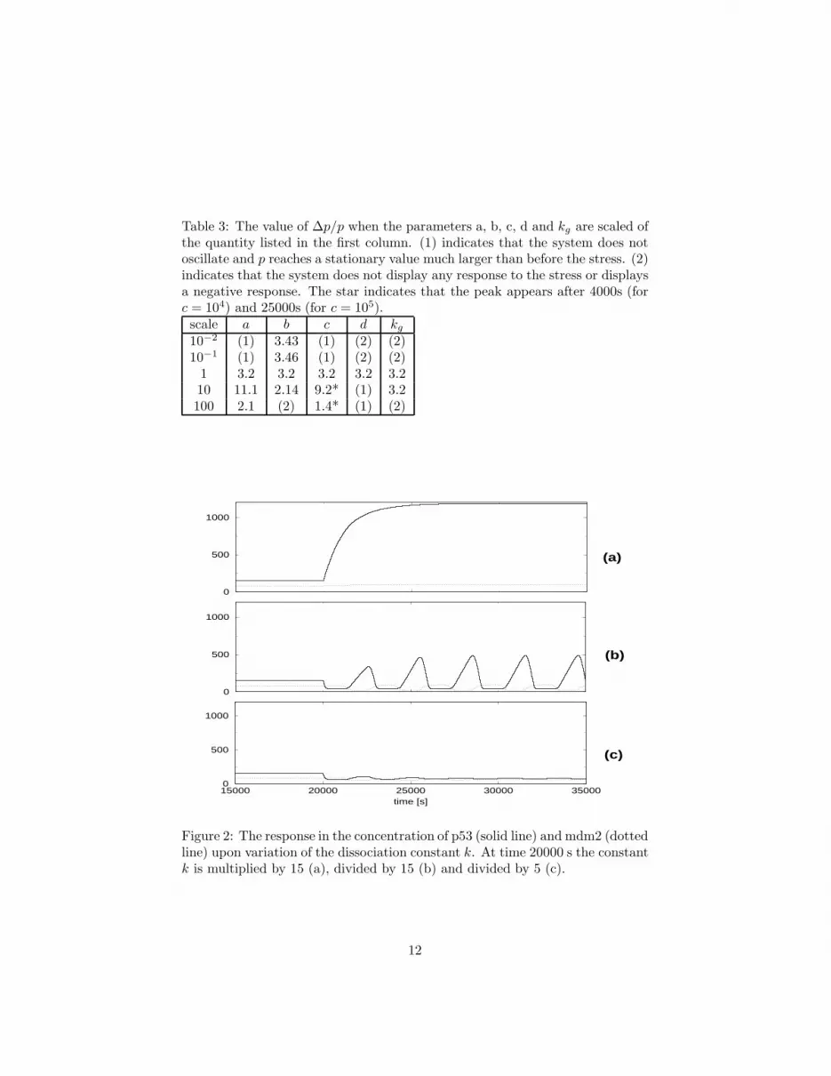
Table 3: The value of ∆p/p when the parameters a, b, c, d and kg are scaled ofthe quantity listed in the first column. (1) indicates that the system does notoscillate and p reaches a stationary value much larger than before the stress. (2)indicates that the system does not display any response to the stress or displaysa negative response. The star indicates that the peak appears after 4000s (forc = 104) and 25000s (for c = 105).scale a b c d kg

10−2 (1) 3.43 (1) (2) (2)10−1 (1) 3.46 (1) (2) (2)

1 3.2 3.2 3.2 3.2 3.210 11.1 2.14 9.2* (1) 3.2100 2.1 (2) 1.4* (1) (2)

0

500

1000

15000 20000 25000 30000 35000time [s]

0

500

1000

0

500

1000

(a)

(b)

(c)

Figure 2: The response in the concentration of p53 (solid line) and mdm2 (dottedline) upon variation of the dissociation constant k. At time 20000 s the constantk is multiplied by 15 (a), divided by 15 (b) and divided by 5 (c).

12

10−4

10−2

100

102

multiplier of k

0

101

∆p/p

Figure 3: The height of the response peak ∆p with respect to the quantity thatmultiplies k, mimicking the stress. The dotted line indicates that the systemdoes not display oscillatory behaviour.

0 1000 2000 3000 4000 5000τ

0

5

10

∆p/p

Figure 4: The dependence of the height of the response peak ∆p on the delayτ .

13