TI-Nspire™ CX Student Software Guidebook
547
TI-Nspire™ CX Student Software Guidebook Learn more about TI Technology through the online help at education.ti.com/eguide .
-
Upload
khangminh22 -
Category
Documents
-
view
0 -
download
0
Transcript of TI-Nspire™ CX Student Software Guidebook

TI-Nspire™ CX Student SoftwareGuidebook
Learn more about TI Technology through the online help at education.ti.com/eguide.
ii
Important InformationExcept as otherwise expressly stated in the License that accompanies a program, TexasInstruments makes no warranty, either express or implied, including but not limited toany implied warranties of merchantability and fitness for a particular purpose,regarding any programs or book materials and makes such materials available solelyon an "as-is" basis. In no event shall Texas Instruments be liable to anyone for special,collateral, incidental, or consequential damages in connection with or arising out of thepurchase or use of these materials, and the sole and exclusive liability of TexasInstruments, regardless of the form of action, shall not exceed the amount set forth inthe license for the program. Moreover, Texas Instruments shall not be liable for anyclaim of any kind whatsoever against the use of these materials by any other party.
Adobe®, Adobe® Flash®, Excel®, Mac®, Microsoft®, PowerPoint®, Vernier DataQuest™,Vernier EasyLink®, Vernier EasyTemp®, Vernier Go!Link®, Vernier Go!Motion®, VernierGo!Temp®, Windows®, and Windows® XP are trademarks of their respective owners.
Actual products may vary slightly from provided images.
© 2006 - 2019 Texas Instruments Incorporated
Contents
Getting Started with TI-Nspire™ CX Student Software 1Selecting the Handheld Type 1Exploring the Documents Workspace 2Changing Language 3Using Software Menu Shortcuts 4Using Handheld Keyboard Shortcuts 7
Using the Documents Workspace 12Exploring the Documents Workspace 12Using the Documents Toolbox 12Exploring Document Tools 13Exploring the Page Sorter 14Exploring the TI-SmartView™ Feature 15Exploring Content Explorer 17Exploring Utilities 19Using the Work Area 20Changing Document Settings 21Changing Graphs & Geometry Settings 23
Working with Connected Handhelds 25Managing Files on a Connected Handheld 25Checking for an OS Update 27Installing an OS Update 28
Working with TI-Nspire™ Documents 32Creating a New TI-Nspire™ Document 32Opening an Existing Document 33Saving TI-Nspire™ Documents 34Deleting Documents 35Closing Documents 35Formatting Text in Documents 36Using Colors in Documents 37Setting Page Size and Document Preview 37Working with Multiple Documents 39Working with Applications 40Selecting and Moving Pages 43Working with Problems and Pages 46Printing Documents 48Viewing Document Properties and Copyright Information 49
iii
iv
Working with PublishView™ Documents 51Creating a New PublishView™ Document 51Saving PublishView™ Documents 55Exploring the Documents Workspace 57Working with PublishView™ Objects 60Working with TI-Nspire™ Applications 67Working with Problems 70Organizing PublishView™ Sheets 73Using Zoom 79Adding Text to a PublishView™ Document 79Using Hyperlinks in PublishView™ Documents 81Working with Images 88Working with Video Files 91Converting Documents 92Printing PublishView™ Documents 94
Working with Lesson Bundles 96Creating a New Lesson Bundle 96Adding Files to a Lesson Bundle 97Opening a Lesson Bundle 99Managing Files in a Lesson Bundle 100Managing Lesson Bundles 102Packaging Lesson Bundles 104Emailing a Lesson Bundle 105Sending Lesson Bundles to Connected Handhelds 106
Capturing Screens 107Accessing Screen Capture 107Using Capture Page 107Using Capture Selected Handheld 108Viewing Captured Screens 109Saving Captured Pages and Screens 110Copying and Pasting a Screen 111Capturing Images in Handheld Mode 112
Working with Images 115Working with Images in the Software 115
Responding to Questions 119Understanding the Question Toolbar 119Types of Questions 119Responding to Quick Poll Questions 120
Submitting Responses 122
Calculator Application 123Entering and Evaluating Math Expressions 124CAS: Working with Measurement Units 131Using the Unit Conversion Assistant 133Working with Variables 135Creating User-defined Functions and Programs 136Editing Calculator Expressions 140Financial Calculations 140Working with the Calculator History 142
Using Variables 145Linking Values on Pages 145Creating Variables 145Using (Linking) Variables 150Naming Variables 152Adjusting Variable Values with a Slider 154Locking and Unlocking Variables 156Removing a Linked Variable 159
Graphs Application 160What You Must Know 161Graphing Functions 163Exploring Graphs with Path Plot 164Manipulating Functions by Dragging 165Specifying a Function with Domain Restrictions 167Finding Points of Interest on a Function Graph 168Graphing a Family of Functions 170Graphing Equations 171Graphing Conic Sections 172Graphing Relations 175Graphing Parametric Equations 178Graphing Polar Equations 178Graphing Scatter Plots 179Plotting Sequences 180Graphing Differential Equations 182Viewing Tables from the Graphs Application 185Editing Relations 186Accessing the Graph History 187Zooming/Rescaling the Graphs Work Area 188Customizing the Graphs Work Area 190
v
vi
Hiding and Showing Items in the Graphs Application 193Conditional Attributes 194Calculating a Bounded Area 195Tracing Graphs or Plots 197Introduction to Geometric Objects 199Creating Points and Lines 200Creating Geometric Shapes 206Creating Shapes Using Gestures (MathDraw) 211Basics of Working with Objects 214Measuring Objects 217Transforming Objects 223Exploring with Geometric Construction Tools 226Animating Points on Objects 230Adjusting Variable Values with a Slider 231Labeling (Identifying) the Coordinates of a Point 234Displaying the Equation of a Geometric Object 234Using the Calculate Tool 235
3D Graphs 237Graphing 3D Functions 237Graphing 3D Parametric Equations 238Rotating the 3D View 239Editing a 3D Graph 240Accessing the Graph History 240Changing the Appearance of a 3D Graph 241Showing and Hiding 3D Graphs 242Customizing the 3D Viewing Environment 242Tracing in the 3D View 244Example: Creating an Animated 3D Graph 245
Geometry Application 247What You Must Know 247Introduction to Geometric Objects 250Creating Points and Lines 252Creating Geometric Shapes 257Creating Shapes Using Gestures (MathDraw) 263Basics of Working with Objects 266Measuring Objects 269Transforming Objects 274Exploring with Geometric Construction Tools 277Using Geometry Trace 282Conditional Attributes 282
Hiding Objects in the Geometry Application 284Customizing the Geometry Work Area 284Animating Points on Objects 285Adjusting Variable Values with a Slider 286Using the Calculate Tool 289
Lists & Spreadsheet Application 291Creating and Sharing Spreadsheet Data as Lists 292Creating Spreadsheet Data 294Navigating in a Spreadsheet 296Working with Cells 297Working with Rows and Columns of Data 301Sorting Data 304Generating Columns of Data 305Graphing Spreadsheet Data 308Exchanging Data with Other Computer Software 312Capturing Data from Graphs & Geometry 314Using Table Data for Statistical Analysis 319Statistics Input Descriptions 320Statistical Calculations 321Distributions 326Confidence Intervals 332Stat Tests 333Working with Function Tables 338
Data & Statistics Application 340Basic Operations in Data & Statistics 341Overview of Raw and Summary Data 345Working with Numeric Plot Types 346Working with Categorical Plot Types 356Exploring Data 365Using Window/Zoom Tools 374Graphing Functions 375Using Graph Trace 381Customizing Your Workspace 381Adjusting Variable Values with a Slider 383Inferential Statistics 385
Notes Application 387Using Templates in Notes 388Formatting Text in Notes 389Using Color in Notes 390
vii
viii
Inserting Images 391Inserting Items on a Notes Page 391Inserting Comments in Notes Text 392Inserting Geometric Shape Symbols 392Entering Math Expressions in Notes Text 393Evaluating and Approximating Math Expressions 394Using Math Actions 396Graphing from Notes and Calculator 398Inserting Chemical Equations in Notes 400Deactivating Math Expression Boxes 401Changing the Attributes of Math Expression Boxes 402Using Calculations in Notes 403Exploring Notes with Examples 404
Data Collection 409What You Must Know 410About Collection Devices 411Connecting Sensors 415Setting Up an Offline Sensor 416Modifying Sensor Settings 417Collecting Data 419Using Data Markers to Annotate Data 422Collecting Data Using a Remote Collection Unit 425Setting Up a Sensor for Automatic Triggering 427Collecting and Managing Data Sets 429Using Sensor Data in Programs 432Collecting Sensor Data using RefreshProbeVars 433Analyzing Collected Data 434Displaying Collected Data in Graph View 440Displaying Collected Data in Table View 441Customizing the Graph of Collected Data 445Striking and Restoring Data 455Replaying the Data Collection 455Adjusting Derivative Settings 457Drawing a Predictive Plot 458Using Motion Match 459Printing Collected Data 459
Widgets 462Creating a Widget 462Adding a Widget 462Saving a Widget 465
Libraries 466Creating Libraries and Library Objects 466Private and Public Library Objects 467Using Library Objects 468Creating Shortcuts to Library Objects 469Included Libraries 469Restoring an Included Library 469
Getting Started with the Program Editor 471Defining a Program or Function 472Viewing a Program or Function 474Opening a Function or Program for Editing 475Importing a Program from a Library 476Creating a Copy of a Function or Program 476Renaming a Program or Function 476Changing the Library Access Level 477Finding Text 477Finding and Replacing Text 477Closing the Current Function or Program 478Running Programs and Evaluating Functions 478Getting Values into a Program 481Displaying Information from a Function or Program 483Using Local Variables 484Differences Between Functions and Programs 485Calling One Program from Another 485Controlling the Flow of a Function or Program 487Using If, Lbl, and Goto to Control Program Flow 487Using Loops to Repeat a Group of Commands 489Changing Mode Settings 493Debugging Programs and Handling Errors 493
Using the TI-SmartView™ Emulator 495Opening the TI-SmartView™ Emulator 495Choosing Display Options 496Working with the Emulated Handheld 497Using the Touchpad 498Using Settings and Status 498Changing TI-SmartView™ Options 499Working with Documents 500Using Screen Capture 500
ix
x
Writing Lua Scripts 502Overview of the Script Editor 502Exploring the Script Editor Interface 502Using the Toolbar 503Inserting New Scripts 505Editing Scripts 506Changing View Options 506Setting Minimum API Level 507Saving Script Applications 507Managing Images 508Setting Script Permissions 509Debugging Scripts 510
Using the Help Menu 511Activating Your Software License 511Registering Your Product 513Downloading the Latest Guidebook 513Exploring TI Resources 513Updating the TI-Nspire™ Software 514Updating the OS on a Connected Handheld 514Viewing Software Version and Legal Information 515Helping Improve the Product 516
Appendix A: Conversion Categories and Units 517
General Information 521Online Help 521Contact TI Support 521Service and Warranty Information 521
Index 522
Getting Started with TI-Nspire™ CX Student SoftwareTI-Nspire™ CX Student Software enables students to use PC and Mac® computers toperform the same functions as on a handheld. This document covers:
• TI-Nspire™ CX Student Software
• TI-Nspire™ CX CAS Student Software
Note: When there are differences between the software, those differences aredescribed.
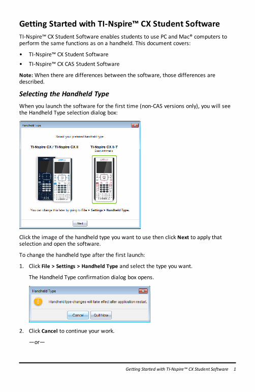
Selecting the Handheld TypeWhen you launch the software for the first time (non-CAS versions only), you will seethe Handheld Type selection dialog box:
Click the image of the handheld type you want to use then click Next to apply thatselection and open the software.
To change the handheld type after the first launch:
1. Click File > Settings > Handheld Type and select the type you want.
The Handheld Type confirmation dialog box opens.
2. Click Cancel to continue your work.
—or—
Getting Started with TI-Nspire™ CX Student Software 1
2 Getting Started with TI-Nspire™ CX Student Software
Click Quit Now to close the software immediately. You will be prompted to saveany open documents. When you restart the software, the new handheld type willbe applied.
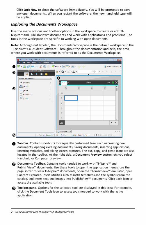
Exploring the Documents WorkspaceUse the menu options and toolbar options in the workspace to create or edit TI-Nspire™ and PublishView™ documents and work with applications and problems. Thetools in the workspace are specific to working with open documents.
Note: Although not labeled, the Documents Workspace is the default workspace in theTI-Nspire™ CX Student Software. Throughout the documentation and help, the areawhere you work with documents is referred to as the Documents Workspace.
À Toolbar. Contains shortcuts to frequently performed tasks such as creating newdocuments, opening existing documents, saving documents, inserting applications,inserting variables, and taking screen captures. The cut, copy, and paste icons are alsolocated in the toolbar. At the right side, a Document Preview button lets you selectHandheld or Computer preview.
Á Documents Toolbox. Contains tools needed to work with TI-Nspire™ andPublishView™ documents. Use these tools to open the application menus, use thepage sorter to view TI-Nspire™ documents, open the TI-SmartView™ emulator, openContent Explorer, insert utilities such as math templates and the symbols from thecatalog, and insert text and images into PublishView™ documents. Click each icon toaccess the available tools.
 Toolbox pane. Options for the selected tool are displayed in this area. For example,click the Document Tools icon to access tools needed to work with the activeapplication.
à Work area. Shows the current page of the active (selected) document. Lets youperform calculations, add applications, and add problems and pages. Only onedocument at a time is active. Multiple documents appear as tabs.
Ä Status bar. Provides information about the active document.
Understanding the Status Bar
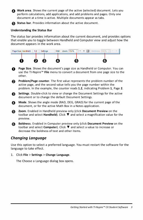
The status bar provides information about the current document, and provides optionsthat enable you to toggle between Handheld and Computer view and adjust how thedocument appears in the work area.
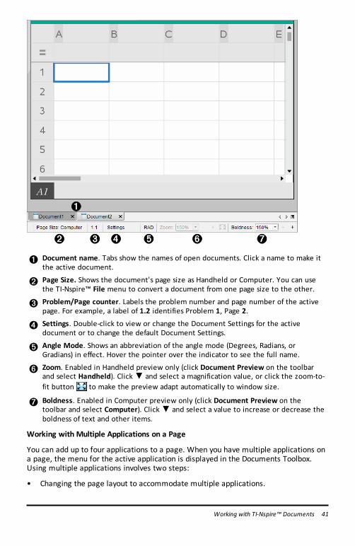
À Page Size. Shows the document's page size as Handheld or Computer. You canuse the TI-Nspire™ File menu to convert a document from one page size to theother.
Á Problem/Page counter. The first value represents the problem number of theactive page, and the second value tells you the page number within theproblem. In the example, the counter reads 1.2, indicating Problem 1, Page 2.
 Settings. Double-click to view or change the Document Settings for the activedocument or to change the default Document Settings.
à Mode. Shows the angle mode (RAD, DEG, GRAD) for the current page of thedocument, or for the active Math Box in a Notes application.
Ä Zoom. Enabled in Handheld preview only (click Document Preview on thetoolbar and select Handheld). Click▼ and select a magnification value for thepreview.
Å Boldness. Enabled in Computer preview only (click Document Preview on thetoolbar and select Computer). Click▼ and select a value to increase ordecrease the boldness of text and other items.
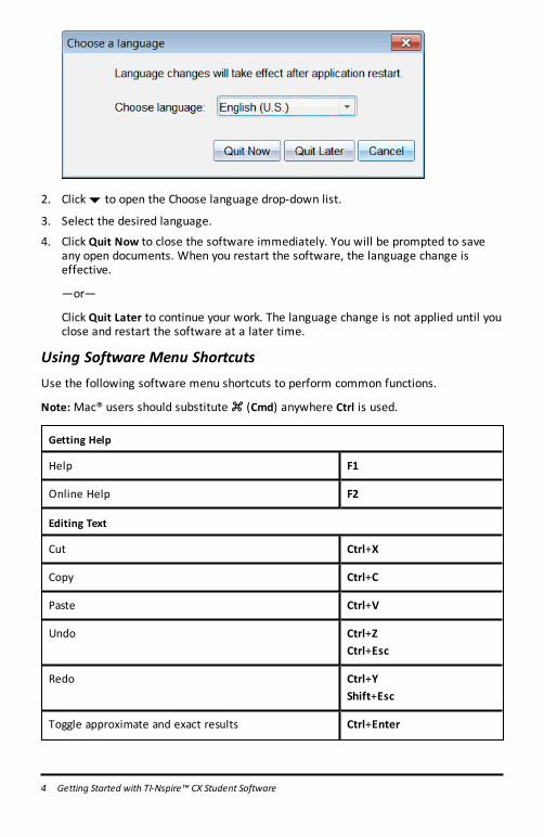
Changing LanguageUse this option to select a preferred language. You must restart the software for thelanguage to take effect.
1. Click File > Settings > Change Language.
The Choose a Language dialog box opens.
Getting Started with TI-Nspire™ CX Student Software 3
4 Getting Started with TI-Nspire™ CX Student Software
2. Click¤ to open the Choose language drop-down list.
3. Select the desired language.
4. Click Quit Now to close the software immediately. You will be prompted to saveany open documents. When you restart the software, the language change iseffective.
—or—
Click Quit Later to continue your work. The language change is not applied until youclose and restart the software at a later time.
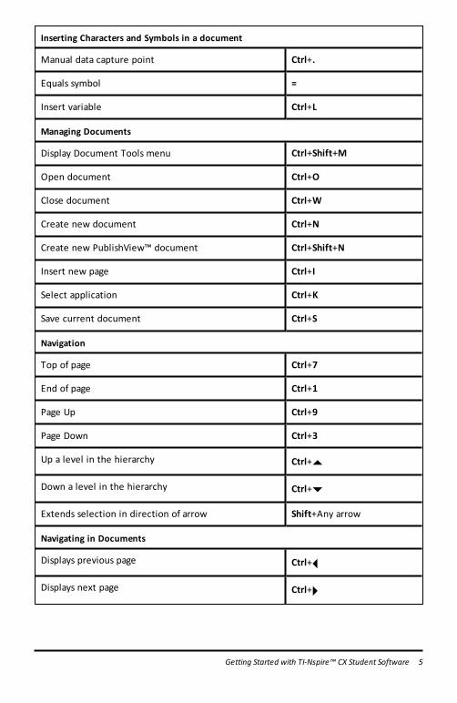
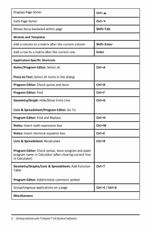
Using Software Menu ShortcutsUse the following software menu shortcuts to perform common functions.
Note: Mac® users should substitute “ (Cmd) anywhere Ctrl is used.
Getting Help
Help F1
Online Help F2
Editing Text
Cut Ctrl+X
Copy Ctrl+C
Paste Ctrl+V
Undo Ctrl+ZCtrl+Esc
Redo Ctrl+YShift+Esc
Toggle approximate and exact results Ctrl+Enter
Inserting Characters and Symbols in a document
Manual data capture point Ctrl+.
Equals symbol =
Insert variable Ctrl+L
Managing Documents
Display Document Tools menu Ctrl+Shift+M
Open document Ctrl+O
Close document Ctrl+W
Create new document Ctrl+N
Create new PublishView™ document Ctrl+Shift+N
Insert new page Ctrl+I
Select application Ctrl+K
Save current document Ctrl+S
Navigation
Top of page Ctrl+7
End of page Ctrl+1
Page Up Ctrl+9
Page Down Ctrl+3
Up a level in the hierarchy Ctrl+£
Down a level in the hierarchy Ctrl+¤
Extends selection in direction of arrow Shift+Any arrow
Navigating in Documents
Displays previous page Ctrl+¡
Displays next page Ctrl+¢
Getting Started with TI-Nspire™ CX Student Software 5
6 Getting Started with TI-Nspire™ CX Student Software
Displays Page Sorter Ctrl+£
Exits Page Sorter Ctrl+6
Moves focus backward within page Shift+Tab
Wizards and Templates
Add a column to a matrix after the current column Shift+Enter
Add a row to a matrix after the current row Enter
Application-Specific Shortcuts
Notes/Program Editor: Select all
Press-to-Test: Select all items in the dialog
Ctrl+A
Program Editor: Check syntax and store Ctrl+B
Program Editor: Find Ctrl+F
Geometry/Graph: Hide/Show Entry Line
Lists & Spreadsheet/Program Editor: Go To
Ctrl+G
Program Editor: Find and Replace Ctrl+H
Notes: Insert math expression box Ctrl+M
Notes: Insert chemical equation box Ctrl+E
Lists & Spreadsheet: Recalculate
Program Editor: Check syntax, store program and pasteprogram name in Calculator (after clearing current linein Calculator)
Ctrl+R
Geometry/Graphs/Lists & Spreadsheet: Add FunctionTable
Program Editor: Add/remove comment symbol
Ctrl+T
Group/Ungroup applications on a page Ctrl+4 / Ctrl+6
Miscellaneous
Handheld Preview Alt+Shift+H
Computer Preview Alt+Shift+C
Capture Page Ctrl+J
Rename (Content Workspace only) F2
Print Ctrl+P
Exit Software Alt+F4
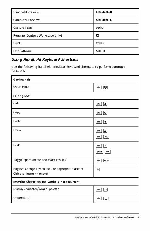
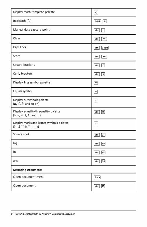
Using Handheld Keyboard ShortcutsUse the following handheld emulator keyboard shortcuts to perform commonfunctions.
Getting Help
Open Hints /µ
Editing Text
Cut /X
Copy /C
Paste /V
Undo /Z
/d
Redo /Y
gd
Toggle approximate and exact results /·
English: Change key to include appropriate accentChinese: Insert character
;
Inserting Characters and Symbols in a document
Display character/symbol palette /k
Underscore /_
Getting Started with TI-Nspire™ CX Student Software 7
8 Getting Started with TI-Nspire™ CX Student Software
Display math template palette t
Backslash ( \ ) gp
Manual data capture point /^
Clear /.
Caps Lock /g
Store /h
Square brackets /(
Curly brackets /)
Display Trig symbol palette µ
Equals symbol =
Display pi symbols palette(p, à, q, and so on)
¹
Display equality/inequality palette(>, <, ≠, ≤, ≥, and | )
/=
Display marks and letter symbols palette(? ! $ ¡ ' % " : ; _ \)
º
Square root /q
log /s
ln /u
ans /v
Managing Documents
Open document menu ~
Open document /O
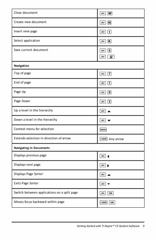
Close document /W
Create new document /N
Insert new page /I
Select application /K
Save current document /S
/»
Navigation
Top of page /7
End of page /1
Page Up /9
Page Down /3
Up a level in the hierarchy /£
Down a level in the hierarchy /¤
Context menu for selection b
Extends selection in direction of arrow g Any arrow
Navigating in Documents
Displays previous page /¡
Displays next page /¢
Displays Page Sorter /£
Exits Page Sorter / 6
Switch between applications on a split page /e
Moves focus backward within page ge
Getting Started with TI-Nspire™ CX Student Software 9
10 Getting Started with TI-Nspire™ CX Student Software
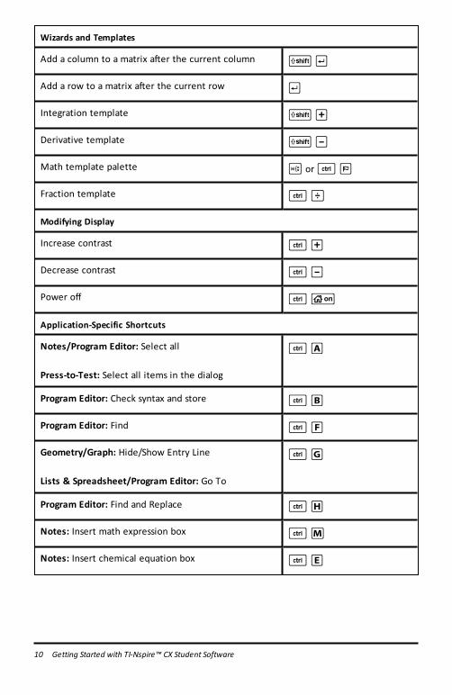
Wizards and Templates
Add a column to a matrix after the current column g@
Add a row to a matrix after the current row @
Integration template g+
Derivative template g-
Math template palette t or/;
Fraction template /p
Modifying Display
Increase contrast /+
Decrease contrast /-
Power off /c
Application-Specific Shortcuts
Notes/Program Editor: Select all
Press-to-Test: Select all items in the dialog
/A
Program Editor: Check syntax and store /B
Program Editor: Find /F
Geometry/Graph: Hide/Show Entry Line
Lists & Spreadsheet/Program Editor: Go To
/G
Program Editor: Find and Replace /H
Notes: Insert math expression box /M
Notes: Insert chemical equation box /E
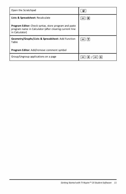
Open the Scratchpad »
Lists & Spreadsheet: Recalculate
Program Editor: Check syntax, store program and pasteprogram name in Calculator (after clearing current linein Calculator)
/R
Geometry/Graphs/Lists & Spreadsheet: Add FunctionTable
Program Editor: Add/remove comment symbol
/T
Group/Ungroup applications on a page /4 //6
Getting Started with TI-Nspire™ CX Student Software 11
12 Using the Documents Workspace
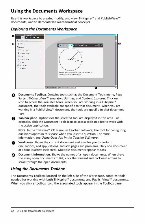
Using the Documents WorkspaceUse this workspace to create, modify, and view TI-Nspire™ and PublishView™documents, and to demonstrate mathematical concepts.
Exploring the Documents Workspace
À Documents Toolbox. Contains tools such as the Document Tools menu, PageSorter, TI-SmartView™ emulator, Utilities, and Content Explorer. Click eachicon to access the available tools. When you are working in a TI-Nspire™document, the tools available are specific to that document. When you areworking in a PublishView™ document, the tools are specific to that documenttype.
Á Toolbox pane. Options for the selected tool are displayed in this area. Forexample, click the Document Tools icon to access tools needed to work withthe active application.Note: In the TI-Nspire™ CX Premium Teacher Software, the tool for configuringquestions opens in this space when you insert a question. For moreinformation, see Using Question in the Teacher Software.
 Work area. Shows the current document and enables you to performcalculations, add applications, and add pages and problems. Only one documentat a time is active (selected). Multiple documents appear as tabs.
à Document information. Shows the names of all open documents. When theretoo many open documents to list, click the forward and backward arrows toscroll through the open documents.
Using the Documents ToolboxThe Documents Toolbox, located on the left side of the workspace, contains toolsneeded for working with both TI-Nspire™ documents and PublishView™ documents.When you click a toolbox icon, the associated tools appear in the Toolbox pane.
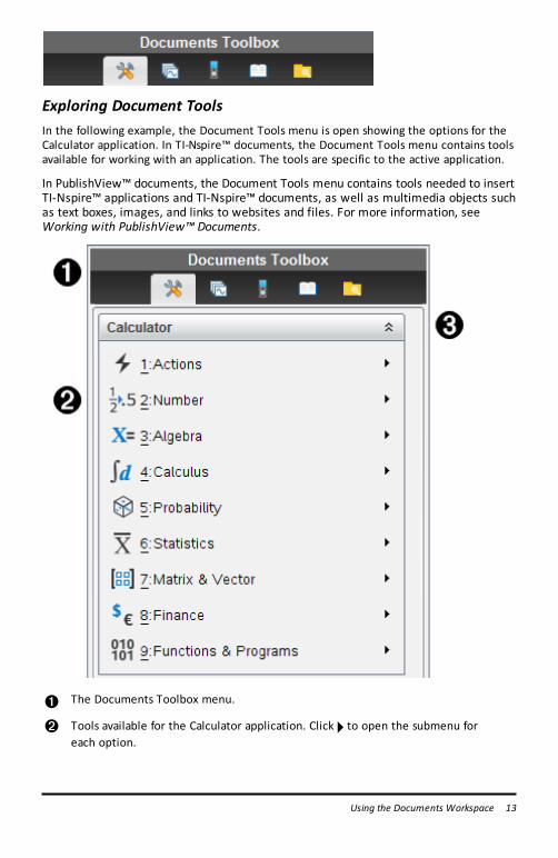
Exploring Document ToolsIn the following example, the Document Tools menu is open showing the options for theCalculator application. In TI-Nspire™ documents, the Document Tools menu contains toolsavailable for working with an application. The tools are specific to the active application.
In PublishView™ documents, the Document Tools menu contains tools needed to insertTI-Nspire™ applications and TI-Nspire™ documents, as well as multimedia objects suchas text boxes, images, and links to websites and files. For more information, seeWorking with PublishView™ Documents.
À The Documents Toolbox menu.
Á Tools available for the Calculator application. Click ¢ to open the submenu foreach option.
Using the Documents Workspace 13
14 Using the Documents Workspace
ÂClick to close and click to open Document Tools.
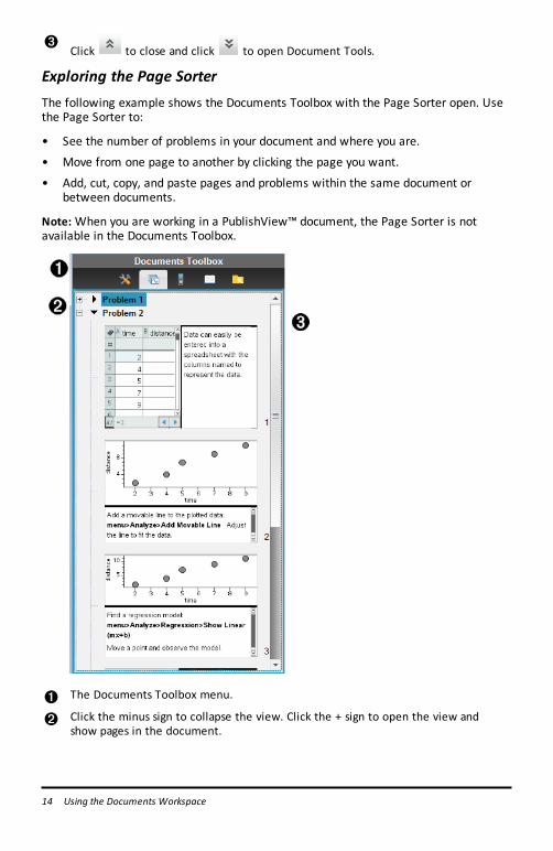
Exploring the Page SorterThe following example shows the Documents Toolbox with the Page Sorter open. Usethe Page Sorter to:
• See the number of problems in your document and where you are.
• Move from one page to another by clicking the page you want.
• Add, cut, copy, and paste pages and problems within the same document orbetween documents.
Note: When you are working in a PublishView™ document, the Page Sorter is notavailable in the Documents Toolbox.
À The Documents Toolbox menu.
Á Click the minus sign to collapse the view. Click the + sign to open the view andshow pages in the document.
 Scroll bar. The scroll bar is only active when there are too many pages to showin the pane.
Exploring the TI-SmartView™ FeatureThe TI-SmartView™ feature emulates how a handheld works. In the teacher software,the emulated handheld facilitates classroom presentations. In the student software,the emulated keypad gives students the ability to drive the software as if using ahandheld.
Note: Content is displayed on the TI-SmartView™ small screen only when thedocument is in Handheld view.
When working in a PublishView™ document, TI-SmartView™ emulator is not available.
Note: The following illustration shows the TI-SmartView™ panel in the teachersoftware. In the Student Software, only the keypad is shown. For more information,see Using the TI-SmartView™ Emulator.
Using the Documents Workspace 15
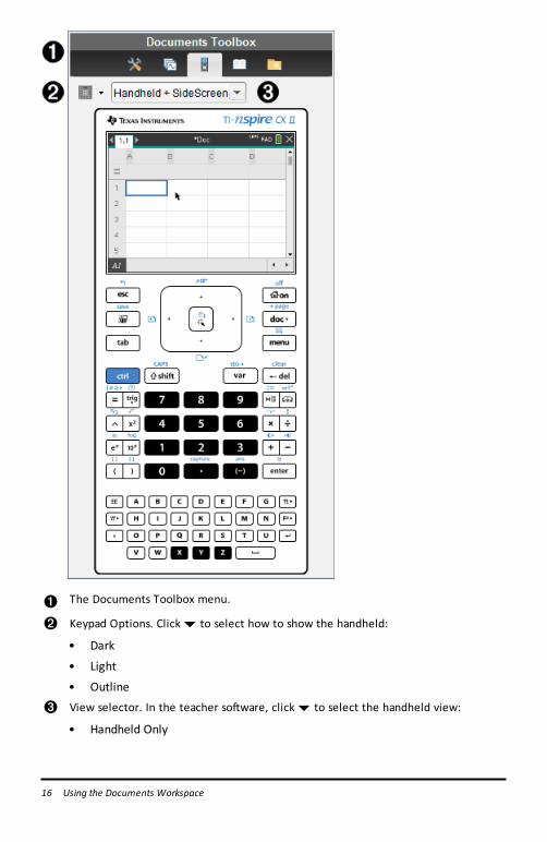
16 Using the Documents Workspace
À The Documents Toolbox menu.
Á Keypad Options. Click¤ to select how to show the handheld:
• Dark
• Light
• Outline View selector. In the teacher software, click¤ to select the handheld view:
• Handheld Only
• Keypad + SideScreen
• Handheld + SideScreen
Note: You can also change these options in the TI-SmartView™ Optionswindow. Click File > Settings > TI-Smartview™ Options to open the window.Note: The view selector is not available in the student software.When the Handheld Only display is active, select Always in Front to keep thedisplay in front of all other open applications. (Teacher software only.)
Exploring Content ExplorerUse Content Explorer to:
• See a list of files on your computer.
• Create and manage lesson bundles.
• If using software that supports connected handhelds, you can:
- See a list of files on any connected handheld.- Update the OS on connected handhelds.- Transfer files between a computer and connected handhelds.
Note: If you are using TI-Nspire™ software that does not support connected handhelds,the Connected Handheld heading is not shown in the Content Explorer pane.
Using the Documents Workspace 17
18 Using the Documents Workspace
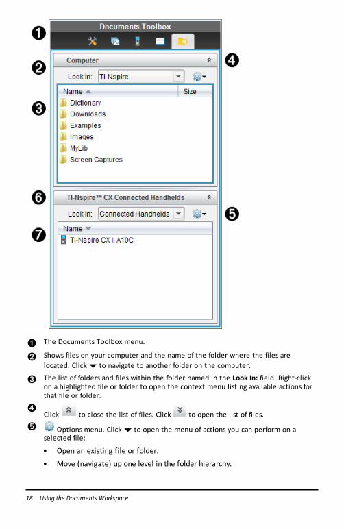
À The Documents Toolbox menu.
Á Shows files on your computer and the name of the folder where the files arelocated. Click¤ to navigate to another folder on the computer.
 The list of folders and files within the folder named in the Look In: field. Right-clickon a highlighted file or folder to open the context menu listing available actions forthat file or folder.
ÃClick to close the list of files. Click to open the list of files.
Ä Options menu. Click¤ to open the menu of actions you can perform on aselected file:
• Open an existing file or folder.
• Move (navigate) up one level in the folder hierarchy.
• Create a new folder.
• Create a new lesson bundle.
• Rename a file or folder.
• Copy selected file or folder.
• Paste file or folder copied to Clipboard.
• Delete selected file or folder.
• Select all files in a folder.
• Package lesson bundles.
• Refresh the view.
• Install OS.Å Connected handhelds. Lists the connected handhelds. Multiple handhelds are listed
if more than one handheld is connected to the computer or when using the TI-Nspire™ Docking Stations.
Æ The name of the connected handheld. To show the folders and files on a handheld,double-click the name.Click¤ to navigate to another folder on the handheld.
Exploring UtilitiesUtilities provides access to the math templates and operators, special symbols, catalogitems, and libraries that you need when working with documents. In the followingexample, the Math templates tab is open.
Using the Documents Workspace 19
20 Using the Documents Workspace
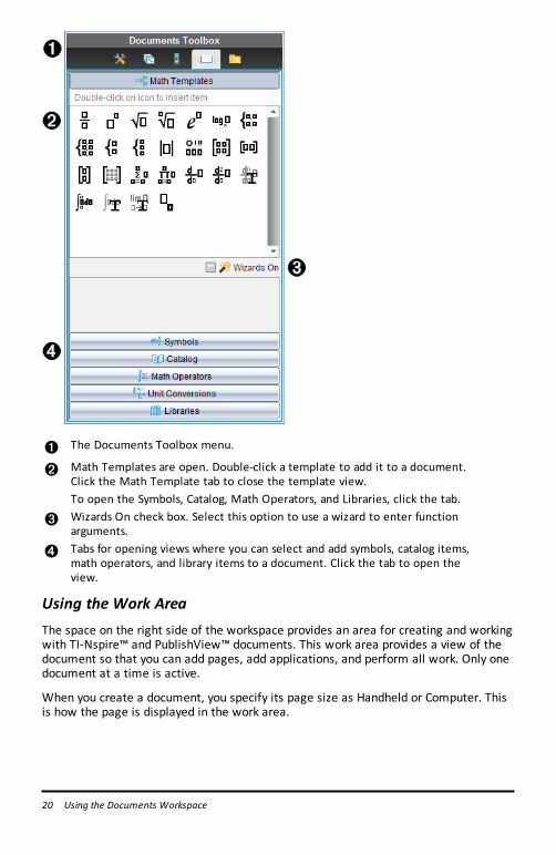
À The Documents Toolbox menu.
Á Math Templates are open. Double-click a template to add it to a document.Click the Math Template tab to close the template view.To open the Symbols, Catalog, Math Operators, and Libraries, click the tab.
 Wizards On check box. Select this option to use a wizard to enter functionarguments.
à Tabs for opening views where you can select and add symbols, catalog items,math operators, and library items to a document. Click the tab to open theview.
Using the Work AreaThe space on the right side of the workspace provides an area for creating and workingwith TI-Nspire™ and PublishView™ documents. This work area provides a view of thedocument so that you can add pages, add applications, and perform all work. Only onedocument at a time is active.
When you create a document, you specify its page size as Handheld or Computer. Thisis how the page is displayed in the work area.
• Handheld page size is optimized for the smaller screen of a handheld. This pagesize can be viewed on handhelds, computer screens, and tablets. The content isscaled when viewed on a larger screen.
• Computer page size takes advantage of the larger space of a computer screen.These documents can show details with less scrolling required. The content is notscaled when viewed on a handheld.
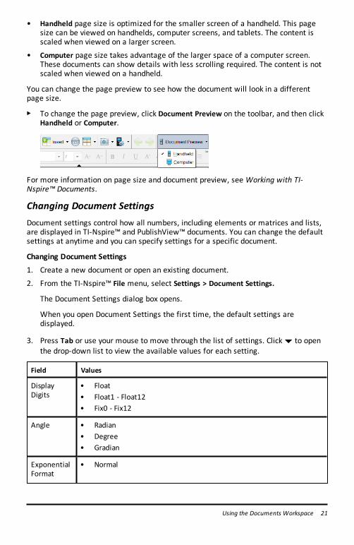
You can change the page preview to see how the document will look in a differentpage size.
▶ To change the page preview, click Document Preview on the toolbar, and then clickHandheld or Computer.
For more information on page size and document preview, see Working with TI-Nspire™ Documents.
Changing Document SettingsDocument settings control how all numbers, including elements or matrices and lists,are displayed in TI-Nspire™ and PublishView™ documents. You can change the defaultsettings at anytime and you can specify settings for a specific document.
Changing Document Settings
1. Create a new document or open an existing document.
2. From the TI-Nspire™ File menu, select Settings > Document Settings.
The Document Settings dialog box opens.
When you open Document Settings the first time, the default settings aredisplayed.
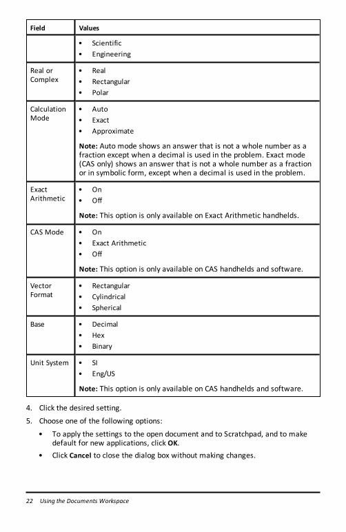
3. Press Tab or use your mouse to move through the list of settings. Click¤ to openthe drop-down list to view the available values for each setting.
Field Values
DisplayDigits
• Float• Float1 - Float12• Fix0 - Fix12
Angle • Radian• Degree• Gradian
ExponentialFormat
• Normal
Using the Documents Workspace 21
22 Using the Documents Workspace
Field Values
• Scientific• Engineering
Real orComplex
• Real• Rectangular• Polar
CalculationMode
• Auto• Exact• Approximate
Note: Auto mode shows an answer that is not a whole number as afraction except when a decimal is used in the problem. Exact mode(CAS only) shows an answer that is not a whole number as a fractionor in symbolic form, except when a decimal is used in the problem.
ExactArithmetic
• On• Off
Note: This option is only available on Exact Arithmetic handhelds.
CAS Mode • On• Exact Arithmetic• Off
Note: This option is only available on CAS handhelds and software.
VectorFormat
• Rectangular• Cylindrical• Spherical
Base • Decimal• Hex• Binary
Unit System • SI• Eng/US
Note: This option is only available on CAS handhelds and software.
4. Click the desired setting.
5. Choose one of the following options:
• To apply the settings to the open document and to Scratchpad, and to makedefault for new applications, click OK.
• Click Cancel to close the dialog box without making changes.
Changing Graphs & Geometry SettingsGraphs & Geometry settings control how information is displayed in open problemsand in subsequent new problems. When you change the Graphs & Geometry settings,the selections become the default settings for all work in these applications.
Complete the following steps to customize the application settings for graphs andgeometry.
1. Create a new graphs and geometry document or open an existing document.
2. In the Documents Toolbox, click to open the Graphs & Geometry applicationmenu.
3. Click Settings > Settings.
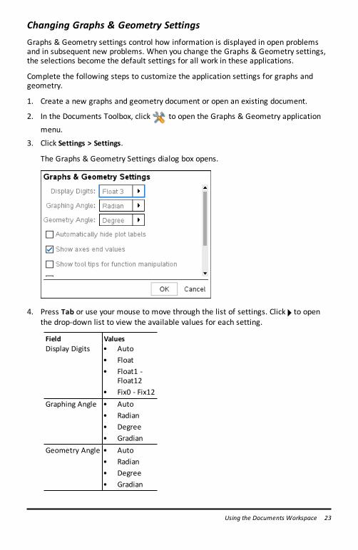
The Graphs & Geometry Settings dialog box opens.
4. Press Tab or use your mouse to move through the list of settings. Click ¢ to openthe drop-down list to view the available values for each setting.
Field ValuesDisplay Digits • Auto
• Float• Float1 -
Float12• Fix0 - Fix12
Graphing Angle • Auto• Radian• Degree• Gradian
Geometry Angle • Auto• Radian• Degree• Gradian
Using the Documents Workspace 23
24 Using the Documents Workspace
5. Select the desired setting.
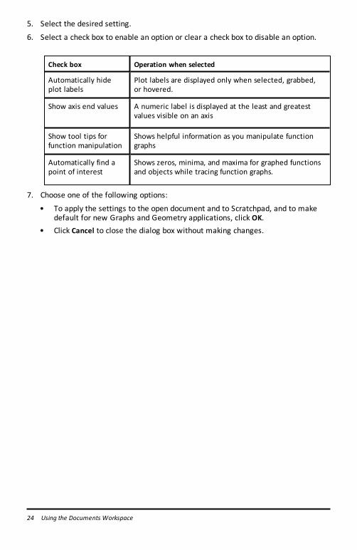
6. Select a check box to enable an option or clear a check box to disable an option.
Check box Operation when selected
Automatically hideplot labels
Plot labels are displayed only when selected, grabbed,or hovered.
Show axis end values A numeric label is displayed at the least and greatestvalues visible on an axis
Show tool tips forfunction manipulation
Shows helpful information as you manipulate functiongraphs
Automatically find apoint of interest
Shows zeros, minima, and maxima for graphed functionsand objects while tracing function graphs.
7. Choose one of the following options:
• To apply the settings to the open document and to Scratchpad, and to makedefault for new Graphs and Geometry applications, click OK.
• Click Cancel to close the dialog box without making changes.
Working with Connected HandheldsThe TI-Nspire™ software enables you to view content, manage files, and installoperating system updates on handhelds connected to the computer.
To use the features described in this chapter, handhelds must be turned on andconnected by one of these means:
• TI-Nspire™ Docking Station or TI-Nspire™ CX Docking Station
• TI-Nspire™ Navigator™ Cradle and access point
• TI-Nspire™ CX Wireless Network Adapter and access point
• TI-Nspire™ CX Wireless Network Adapter - v2 and access point
• A direct connection through a standard USB cable
Note: The tasks in this section can only be performed using TI-Nspire™ handhelds. Inorder to enable wireless connectivity, the TI-Nspire™ Premium Teacher Software andthe OS installed on the TI-Nspire™ CX II handhelds must be version 5.0 or later. For TI-Nspire™ CX handhelds, the OS must be version 4.0 or later.
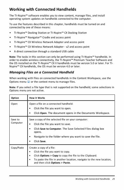
Managing Files on a Connected HandheldWhen working with files on connected handhelds in the Content Workspace, use theOptions menu or the context menu to manage files.
Note: If you select a file type that is not supported on the handheld, some selections inOptions menu are not active.
Option How it Works
Open Open a file on a connected handheld:
• Click the file you want to open.
• Click Open. The document opens in the Documents Workspace.
Save toComputer
Save a copy of the selected file on your computer:
• Click the file you want to save.
• Click Save to Computer. The Save Selected Files dialog boxopens.
• Navigate to the folder where you want to save the file.
• Click Save.
Copy/Paste Create a copy of a file:• Click the file you want to copy.• Click Options > Copy to copy the file to the Clipboard.• To paste the file in another location, navigate to the new location,
and then click Options > Paste.
Working with Connected Handhelds 25
26 Working with Connected Handhelds
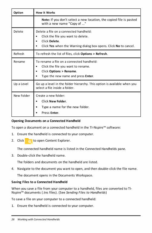
Option How it Works
Note: If you don’t select a new location, the copied file is pastedwith a new name "Copy of ..."
Delete Delete a file on a connected handheld:• Click the file you want to delete.• Click Delete.• Click Yes when the Warning dialog box opens. Click No to cancel.
Refresh To refresh the list of files, click Options > Refresh.
Rename To rename a file on a connected handheld:• Click the file you want to rename.• Click Options > Rename.• Type the new name and press Enter.
Up a Level Go up a level in the folder hierarchy. This option is available when youselect a file inside a folder.
New Folder Create a new folder:
• Click New Folder.
• Type a name for the new folder.
• Press Enter.
Opening Documents on a Connected Handheld
To open a document on a connected handheld in the TI-Nspire™ software:
1. Ensure the handheld is connected to your computer.
2. Click to open Content Explorer.
The connected handheld name is listed in the Connected Handhelds pane.
3. Double-click the handheld name.
The folders and documents on the handheld are listed.
4. Navigate to the document you want to open, and then double-click the file name.
The document opens in the Documents Workspace.
Saving Files to a Connected Handheld
When you save a file from your computer to a handheld, files are converted to TI-Nspire™ documents (.tns files). (See Sending Files to Handhelds)
To save a file on your computer to a connected handheld:
1. Ensure the handheld is connected to your computer.
2. Click to open Content Explorer.
The folders and files on your computer are listed in the Computer pane.
3. Navigate to the folder or file you want to save to the handheld.
4. Click the file to select it.
5. Drag the file to a connected handheld listed in the Connected Handheld pane.
The file is saved to the connected handheld.
Note: To save the file in a folder on the handheld, double-click the handheld nameto list the folders and files, and then drag the file to a folder on the handheld.
If the file already exists on the handheld, a dialog box opens asking if you want toreplace the file. Click Replace to overwrite the existing file. Click No or Cancel toabandon the save.
Checking for an OS UpdateWhen handhelds are connected, you can check for OS updates from the ContentWorkspace or from the Documents Workspace.
Note: Your computer must be connected to the Internet.
1. Show all connected handhelds.
• In the Content Workspace, click Connected Handhelds in the Resources pane.• In the Documents Workspace, open the Content Explorer and click Connected
Handhelds.
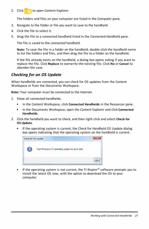
2. Click the handheld you want to check, and then right-click and select Check forOS Update.
• If the operating system is current, the Check for Handheld OS Update dialogbox opens indicating that the operating system on the handheld is current.
• If the operating system is not current, the TI-Nspire™ software prompts you toinstall the latest OS now, with the option to download the OS to yourcomputer.
Working with Connected Handhelds 27
28 Working with Connected Handhelds
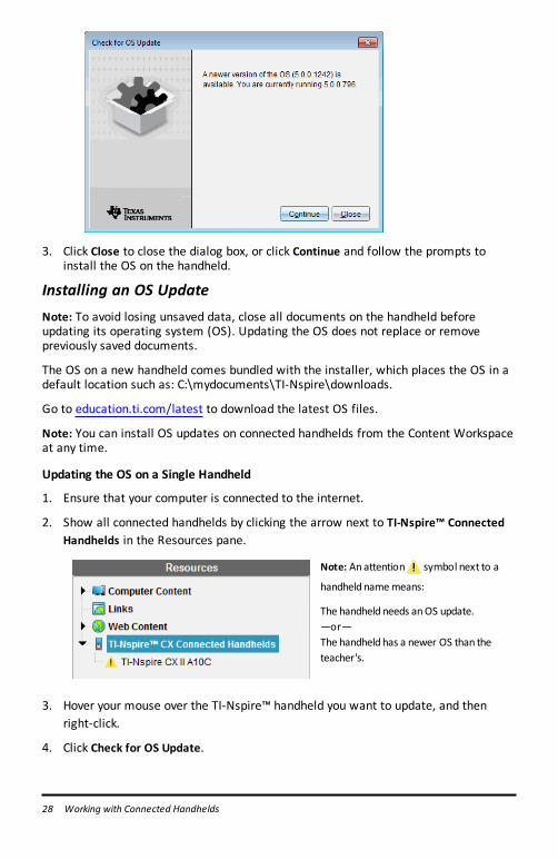
3. Click Close to close the dialog box, or click Continue and follow the prompts toinstall the OS on the handheld.
Installing an OS UpdateNote: To avoid losing unsaved data, close all documents on the handheld beforeupdating its operating system (OS). Updating the OS does not replace or removepreviously saved documents.
The OS on a new handheld comes bundled with the installer, which places the OS in adefault location such as: C:\mydocuments\TI-Nspire\downloads.
Go to education.ti.com/latest to download the latest OS files.
Note: You can install OS updates on connected handhelds from the Content Workspaceat any time.
Updating the OS on a Single Handheld
1. Ensure that your computer is connected to the internet.
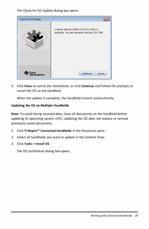
2. Show all connected handhelds by clicking the arrow next to TI-Nspire™ ConnectedHandhelds in the Resources pane.
Note: Anattention symbol next to a
handheldnamemeans:
The handheldneeds anOS update.—or—The handheldhas a newer OS than theteacher's.
3. Hover your mouse over the TI-Nspire™ handheld you want to update, and thenright-click.
4. Click Check for OS Update.
The Check for OS Update dialog box opens.
5. Click Close to cancel the installation, or click Continue and follow the prompts toinstall the OS on the handheld.
When the update is complete, the handheld restarts automatically.
Updating the OS on Multiple Handhelds
Note: To avoid losing unsaved data, close all documents on the handheld beforeupdating its operating system (OS). Updating the OS does not replace or removepreviously saved documents.
1. Click TI-Nspire™ Connected Handhelds in the Resources pane.
2. Select all handhelds you want to update in the Content Pane.
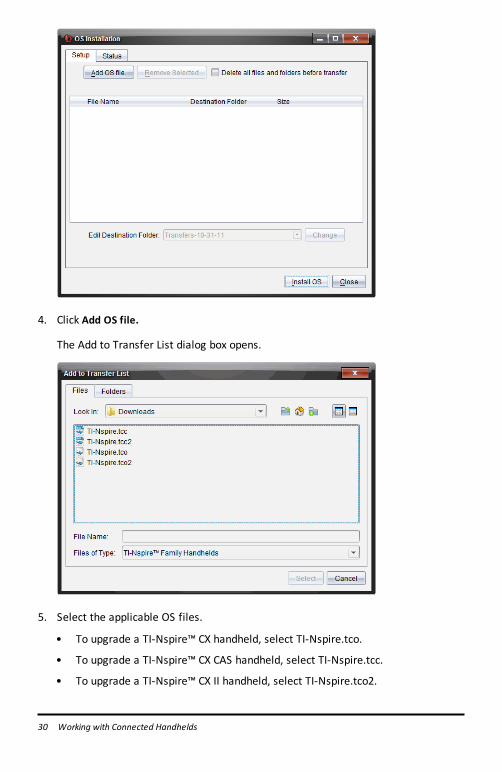
3. Click Tools > Install OS.
The OS Installation dialog box opens.
Working with Connected Handhelds 29
30 Working with Connected Handhelds
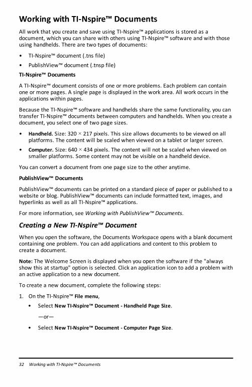
4. Click Add OS file.
The Add to Transfer List dialog box opens.
5. Select the applicable OS files.
• To upgrade a TI-Nspire™ CX handheld, select TI-Nspire.tco.
• To upgrade a TI-Nspire™ CX CAS handheld, select TI-Nspire.tcc.
• To upgrade a TI-Nspire™ CX II handheld, select TI-Nspire.tco2.

• To upgrade a TI-Nspire™ CX II CAS handheld, select TI-Nspire.tcc2.
• To upgrade a TI-Nspire™ CX II-T handheld, select TI-Nspire.tct2.
6. Click Select.
The OS Installation redisplays with your selected OS files.
7. Click Install OS.
The OS version information updates, and the Select OS Handheld File dialogredisplays for further selection.
Working with Connected Handhelds 31
32 Working with TI-Nspire™ Documents
Working with TI-Nspire™ DocumentsAll work that you create and save using TI-Nspire™ applications is stored as adocument, which you can share with others using TI-Nspire™ software and with thoseusing handhelds. There are two types of documents:
• TI-Nspire™ document (.tns file)
• PublishView™ document (.tnsp file)
TI-Nspire™ Documents
A TI-Nspire™ document consists of one or more problems. Each problem can containone or more pages. A single page is displayed in the work area. All work occurs in theapplications within pages.
Because the TI-Nspire™ software and handhelds share the same functionality, you cantransfer TI-Nspire™ documents between computers and handhelds. When you create adocument, you select one of two page sizes.
• Handheld. Size: 320 × 217 pixels. This size allows documents to be viewed on allplatforms. The content will be scaled when viewed on a tablet or larger screen.
• Computer. Size: 640 × 434 pixels. The content will not be scaled when viewed onsmaller platforms. Some content may not be visible on a handheld device.
You can convert a document from one page size to the other anytime.
PublishView™ Documents
PublishView™ documents can be printed on a standard piece of paper or published to awebsite or blog. PublishView™ documents can include formatted text, images, andhyperlinks as well as all TI-Nspire™ applications.
For more information, see Working with PublishView™ Documents.
Creating a New TI-Nspire™ DocumentWhen you open the software, the Documents Workspace opens with a blank documentcontaining one problem. You can add applications and content to this problem tocreate a document.
Note: The Welcome Screen is displayed when you open the software if the "alwaysshow this at startup" option is selected. Click an application icon to add a problem withan active application to a new document.
To create a new document, complete the following steps:
1. On the TI-Nspire™ File menu,
• Select New TI-Nspire™ Document - Handheld Page Size.
—or—
• Select New TI-Nspire™ Document - Computer Page Size.
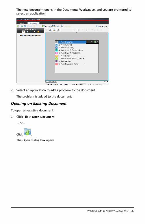
The new document opens in the Documents Workspace, and you are prompted toselect an application.
2. Select an application to add a problem to the document.
The problem is added to the document.
Opening an Existing DocumentTo open an existing document:
1. Click File > Open Document.
—or—
Click .
The Open dialog box opens.
Working with TI-Nspire™ Documents 33
34 Working with TI-Nspire™ Documents
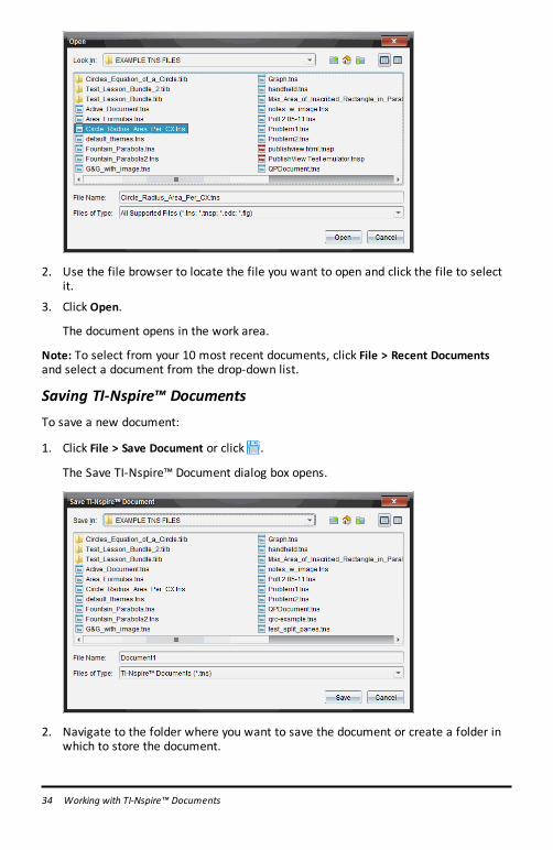
2. Use the file browser to locate the file you want to open and click the file to selectit.
3. Click Open.
The document opens in the work area.
Note: To select from your 10 most recent documents, click File > Recent Documentsand select a document from the drop-down list.
Saving TI-Nspire™ DocumentsTo save a new document:
1. Click File > Save Document or click .
The Save TI-Nspire™ Document dialog box opens.
2. Navigate to the folder where you want to save the document or create a folder inwhich to store the document.
3. Type a name for the new document.
4. Click Save to save the document.
The document closes and is saved with the extension .tns.
Note: When you save a file, the software looks in the same folder the next time youopen a file.
Saving a Document with a New Name
To save a previously saved document in a new folder and/or with a new name:
1. Click File > Save As.
The Save TI-Nspire™ Document dialog box opens.
2. Navigate to the folder where you want to save the document or create a folder inwhich to store the document.
3. Type a new name for the document.
4. Click Save to save the document with a new name.
Deleting DocumentsFile deletions on your computer are sent to the Recycle bin and can be retrieved if theRecycle bin has not been emptied.
Note: File deletions on the handheld are permanent and cannot be undone, so be surethat you want to delete the file that you select.
1. Select the document you want to delete.
2. Click Edit > Delete or press Delete.
The Warning dialog box opens.
3. Click Yes to confirm the delete.
The document is deleted.
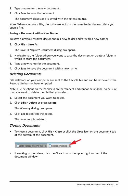
Closing Documents▶ To close a document, click File > Close or click the Close icon on the document tab
at the bottom of the document.
▶ If working in tiled view, click the Close icon in the upper right corner of thedocument window.
Working with TI-Nspire™ Documents 35
36 Working with TI-Nspire™ Documents
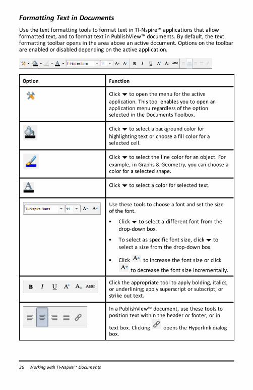
Formatting Text in DocumentsUse the text formatting tools to format text in TI-Nspire™ applications that allowformatted text, and to format text in PublishView™ documents. By default, the textformatting toolbar opens in the area above an active document. Options on the toolbarare enabled or disabled depending on the active application.
Option Function
Click¤ to open the menu for the activeapplication. This tool enables you to open anapplication menu regardless of the optionselected in the Documents Toolbox.
Click¤ to select a background color forhighlighting text or choose a fill color for aselected cell.
Click¤ to select the line color for an object. Forexample, in Graphs & Geometry, you can choose acolor for a selected shape.
Click¤ to select a color for selected text.
Use these tools to choose a font and set the sizeof the font.
• Click¤ to select a different font from thedrop-down box.
• To select as specific font size, click¤ toselect a size from the drop-down box.
• Click to increase the font size or click
to decrease the font size incrementally.
Click the appropriate tool to apply bolding, italics,or underlining; apply superscript or subscript; orstrike out text.
In a PublishView™ document, use these tools toposition text within the header or footer, or in
text box. Clicking opens the Hyperlink dialogbox.
Option Function
For more information, see Working withPublishView™ Documents.
Hiding and Showing the Formatting Toolbar
▶ When the formatting toolbar is visible, click£ (located under the toolbar) to hidethe toolbar.
▶ Click¤ to show the toolbar when the formatting toolbar is hidden.
Using Colors in DocumentsIn the TI-Nspire™ applications that allow formatting, you can use color in filled areas ofan object, or in lines or text, depending on the application you are using and how youhave selected the item. If the icon or menu item that you want to use is not available(dimmed) after you have selected an item, color is not an option for the selected item.
Colors appear in documents opened on your computer and on the TI-Nspire™ CXhandheld. If a document containing color is opened on a TI-Nspire™ handheld, colorsare displayed in shades of gray.
Note: For more information about using color in a TI-Nspire™ application, see thechapter for that application.
Adding Color from a List
To add color to a fill area, line, or text, complete the following steps:
1. Select the item.
2. Click Edit > Color or select where you want to add color (fill, line, or text).
3. Select the color from the list.
Adding Color from a Palette
To add color using the palette, complete the following steps:
1. Select the object.
2. Click the appropriate toolbar icon.
3. Select the color from the palette.
Setting Page Size and Document PreviewWhen you ceate a document, you specify its page size as Handheld or Computer,depending on how you expect the document to be used. Documents of both page sizescan be opened on either platform, and you can convert the page size anytime.
• Handheld. Size: 320 × 217 pixels, fixed. Handheld documents can be viewed on allplatforms. You can magnify (zoom) the content when viewing it on a tablet orlarger screen.
Working with TI-Nspire™ Documents 37
38 Working with TI-Nspire™ Documents
• Computer. Size: 640 × 434 pixels, minimum. Computer documents scale upautomatically to take advantage of higher resolution screens. The minimum size is640 × 434, so some content may be clipped on handheld devices.
Note: You can view documents of either page size using Handheld or Computerpreview.
Converting the Current Document's Page Size
▶ On the main TI-Nspire™ File menu, select Convert to, and then select the page size.
The software saves the current document and creates a copy that uses therequested page size.
Viewing the Document in Handheld Preview
1. On the application toolbar, click Document Preview, and select Handheld.
The preview changes. This does not change the document's underlying page size.
2. (Optional) Adjust the viewing magnification:
- Click the Zoom tool beneath the work area, and select a magnification value.
—or—
- Click the Zoom to Fit button to make the handheld preview adjustautomatically to the window size.
Viewing the Document in Computer Preview
1. On the application toolbar, click Document Preview, and select Computer.
The preview changes. This does not change the document's underlying page size.
2. (Optional) Click the Boldness tool beneath the work area, and select a value toincrease or decrease the boldness of text and other items.
Setting the Default Page Size for New Documents
1. On the main TI-Nspire™ File menu, select Settings > Page Size Settings.
2. Select a default page size, either Handheld or Computer.
The new size applies to documents that you create (Windows®: Ctrl+C, Mac®:Cmd+C) after setting the default, including the blank document createdautomatically each time you open the software. Changing the default setting doesnot convert any currently open documents or other existing documents.
Setting a Default Preview
By default, when you open a document, it is automatically displayed using the previewthat matches its page size. You can override this rule and specify a preview that youprefer.
1. On the main TI-Nspire™ File menu, select Settings > Preview Settings.
2. Select the preview that you want documents to use when you open them.
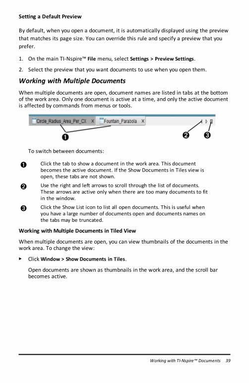
Working with Multiple DocumentsWhen multiple documents are open, document names are listed in tabs at the bottomof the work area. Only one document is active at a time, and only the active documentis affected by commands from menus or tools.
To switch between documents:
À Click the tab to show a document in the work area. This documentbecomes the active document. If the Show Documents in Tiles view isopen, these tabs are not shown.
Á Use the right and left arrows to scroll through the list of documents.These arrows are active only when there are too many documents to fitin the window.
 Click the Show List icon to list all open documents. This is useful whenyou have a large number of documents open and documents names onthe tabs may be truncated.
Working with Multiple Documents in Tiled View
When multiple documents are open, you can view thumbnails of the documents in thework area. To change the view:
▶ ClickWindow > Show Documents in Tiles.
Open documents are shown as thumbnails in the work area, and the scroll barbecomes active.
Working with TI-Nspire™ Documents 39
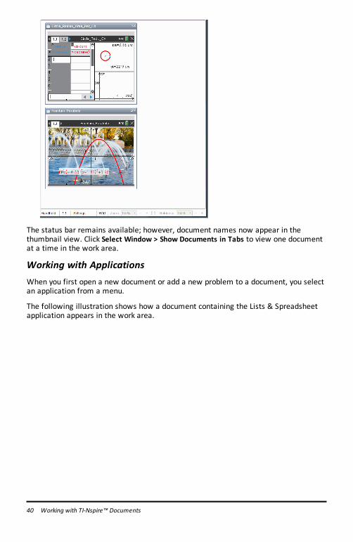
40 Working with TI-Nspire™ Documents
The status bar remains available; however, document names now appear in thethumbnail view. Click Select Window > Show Documents in Tabs to view one documentat a time in the work area.
Working with ApplicationsWhen you first open a new document or add a new problem to a document, you selectan application from a menu.
The following illustration shows how a document containing the Lists & Spreadsheetapplication appears in the work area.
À Document name. Tabs show the names of open documents. Click a name to make itthe active document.
Á Page Size. Shows the document's page size as Handheld or Computer. You can usethe TI-Nspire™ File menu to convert a document from one page size to the other.
 Problem/Page counter. Labels the problem number and page number of the activepage. For example, a label of 1.2 identifies Problem 1, Page 2.
à Settings. Double-click to view or change the Document Settings for the activedocument or to change the default Document Settings.
Ä Angle Mode. Shows an abbreviation of the angle mode (Degrees, Radians, orGradians) in effect. Hover the pointer over the indicator to see the full name.
Å Zoom. Enabled in Handheld preview only (click Document Preview on the toolbarand select Handheld). Click▼ and select a magnification value, or click the zoom-to-fit button to make the preview adapt automatically to window size.
Æ Boldness. Enabled in Computer preview only (click Document Preview on thetoolbar and select Computer). Click▼ and select a value to increase or decrease theboldness of text and other items.
Working with Multiple Applications on a Page
You can add up to four applications to a page. When you have multiple applications ona page, the menu for the active application is displayed in the Documents Toolbox.Using multiple applications involves two steps:
• Changing the page layout to accommodate multiple applications.
Working with TI-Nspire™ Documents 41
42 Working with TI-Nspire™ Documents
• Adding the applications.
You can add multiple applications to a page even if an application is already active.
Adding Multiple Applications to a Page
By default, each page contains space to add one application. To add additionalapplications to the page, complete the following steps.
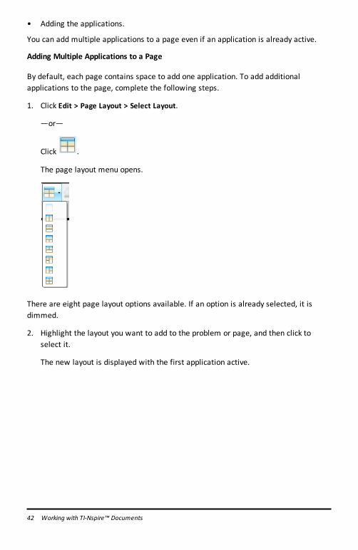
1. Click Edit > Page Layout > Select Layout.
—or—
Click .
The page layout menu opens.
There are eight page layout options available. If an option is already selected, it isdimmed.
2. Highlight the layout you want to add to the problem or page, and then click toselect it.
The new layout is displayed with the first application active.
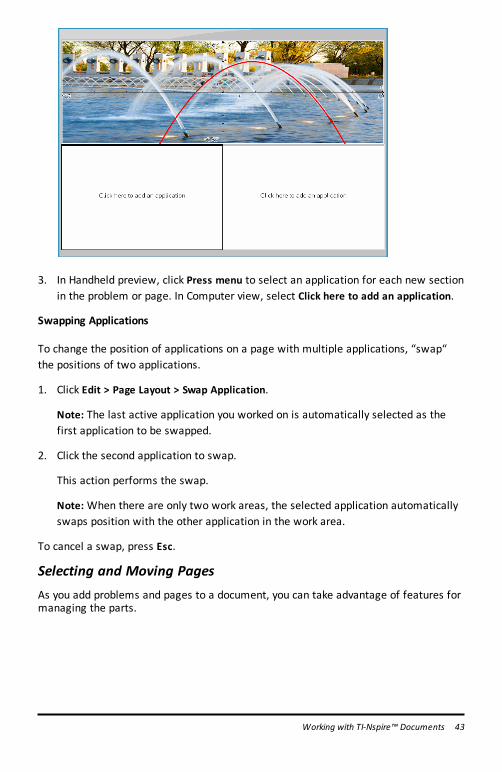
3. In Handheld preview, click Press menu to select an application for each new sectionin the problem or page. In Computer view, select Click here to add an application.
Swapping Applications
To change the position of applications on a page with multiple applications, “swap“ the positions of two applications.
1. Click Edit > Page Layout > Swap Application.
Note: The last active application you worked on is automatically selected as thefirst application to be swapped.
2. Click the second application to swap.
This action performs the swap.
Note: When there are only two work areas, the selected application automaticallyswaps position with the other application in the work area.
To cancel a swap, press Esc.
Selecting and Moving PagesAs you add problems and pages to a document, you can take advantage of features formanaging the parts.
Working with TI-Nspire™ Documents 43
44 Working with TI-Nspire™ Documents
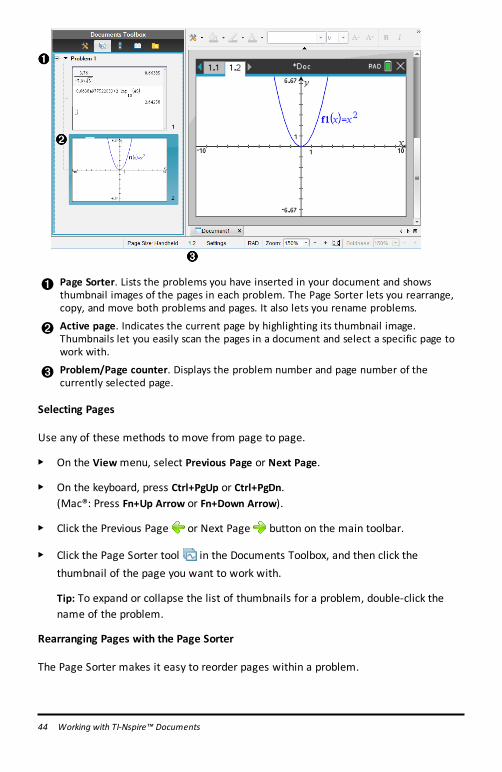
À Page Sorter. Lists the problems you have inserted in your document and showsthumbnail images of the pages in each problem. The Page Sorter lets you rearrange,copy, and move both problems and pages. It also lets you rename problems.
Á Active page. Indicates the current page by highlighting its thumbnail image.Thumbnails let you easily scan the pages in a document and select a specific page towork with.
 Problem/Page counter. Displays the problem number and page number of thecurrently selected page.
Selecting Pages
Use any of these methods to move from page to page.
▶ On the Viewmenu, select Previous Page or Next Page.
▶ On the keyboard, press Ctrl+PgUp or Ctrl+PgDn.(Mac®: Press Fn+Up Arrow or Fn+Down Arrow).
▶ Click the Previous Page or Next Page button on the main toolbar.
▶ Click the Page Sorter tool in the Documents Toolbox, and then click thethumbnail of the page you want to work with.
Tip: To expand or collapse the list of thumbnails for a problem, double-click thename of the problem.
Rearranging Pages with the Page Sorter
The Page Sorter makes it easy to reorder pages within a problem.
1. If necessary, click the Page Sorter tool in the Documents Toolbox.
2. In the Page Sorter, drag the thumbnail image of the page to the desired position.
Copying a Page
You can copy a page within the same problem or copy it to a different problem ordocument.
1. If necessary, click the Page Sorter tool in the Documents Toolbox.
2. Select the thumbnail of the page to be copied.
3. On the Edit menu, click Copy.
4. Click the location at which you want to insert the copy.
5. On the Edit menu, click Paste.
Moving a Page
You can move a page within the same problem or move it to a different problem ordocument.
1. If necessary, click the Page Sorter tool in the Documents Toolbox.
2. Select the thumbnail of the page to be moved.
3. On the Edit menu, click Cut.
4. Click the new location of the page.
5. On the Edit menu, click Paste.
Deleting a Page
1. Select the page in the work area or in the Page Sorter.
2. Click Edit > Delete.
Grouping Applications on a Page
You can combine as many as four consecutive application pages into a single page.
1. Select the first page in the series.
2. Click Edit > Page Layout > Group.
The next page is grouped with the first page. The page layout automatically adjuststo display all the pages in the group.
Working with TI-Nspire™ Documents 45
46 Working with TI-Nspire™ Documents
Ungrouping Applications into Separate Pages
1. Select the grouped page.
2. Click Edit > Page Layout > Ungroup.
The applications are divided into individual pages.
Deleting an Application from a Page
1. Click the application to be deleted.
2. Click Edit > Page Layout > Delete Application.
Tip: To undo the delete, press Ctrl + Z (Mac®: “+ Z).
Working with Problems and PagesWhen you create a new document, it consists of a single problem with a single page.You can insert new problems and add pages to each problem.
Adding a Problem to a Document
A document can contain up to 30 problems. Each problem's variables are unaffected bythe variables in other problems.
▶ On the Insert menu, select Problem.—or—Click the Insert tool on the main toolbar, and select Problem.
A new problem with an empty page is added to your document.
Adding a Page to the Current Problem
Each problem can contain up to 50 pages. Each page has a work area, where you canperform calculations, create graphs, collect and plot data, or add notes andinstructions.
1. Click Insert > Page.—or—Click the Insert tool on the main toolbar, and select Page.
An empty page is added to the current problem, and you are prompted to choosean application for the page.
2. Select an application to add to the page.
Renaming a Problem
New problems are named automatically as Problem 1, Problem 2, and so on. Torename a problem:
1. If necessary, click the Page Sorter tool in the Documents Toolbox.
2. Click the problem name to select it.
3. On the Edit menu, click Rename.
4. Type the new name.
Rearranging Problems with the Page Sorter
The Page Sorter lets you reorder problems within a document. If you move a problemthat you have not renamed, the numeric part of the default name changes to reflectthe new position.
1. If necessary, click the Page Sorter tool in the Documents Toolbox.
2. In the Page Sorter, arrange the problems by dragging each problem name to itsnew position.
Tip: To collapse a problem's list of page thumbnails, double-click the name of theproblem.
Copying a Problem
You can copy a problem within the same document or copy it to a different document.
1. If necessary, click the Page Sorter tool in the Documents Toolbox.
2. Click the problem name to select it.
3. On the Edit menu, click Copy.
4. Click the location at which you want to insert the copy.
5. On the Edit menu, click Paste.
Moving a Problem
You can move a problem within the same document or move it to a differentdocument.
1. If necessary, click the Page Sorter tool in the Documents Toolbox.
2. Click the problem name to select it.
3. On the Edit menu, click Cut.
Working with TI-Nspire™ Documents 47
48 Working with TI-Nspire™ Documents
4. Click the new location of the problem.
5. On the Edit menu, click Paste.
Deleting a Problem
To delete a problem and its pages from the document:
1. If necessary, click the Page Sorter tool in the Documents Toolbox.
2. Click the problem name to select it.
3. On the Edit menu, click Delete.
Printing Documents1. Click File > Print.
The Print dialog box opens.
2. Set options for the print job.
• Printer — Select from your list of available printers• Print What:
- Print All — prints each page on a separate sheet- Viewable Screen — prints selected pages with additional layout options
(see Layout, below)• Print Range — Click All Pages, or click Page range and set the starting and
ending pages.• Layout:
- Orientation (portrait or landscape)- The number of TI-Nspire™ pages (1, 2, 4, or 8) to be printed on each sheet
(available in Viewable Screen option only). The default is 2 pages persheet.
- Whether to allow space below each printed TI-Nspire™ page for comments(available in Viewable Screen option only)
- Margins (from .25 inches to 2 inches). The default margin is .5 inches on alledges.
• Documentation information to include:- Problem name, including the option to group the pages physically by
problem- Page label (such as 1.1 or 1.2) under each page- Page header (up to two lines)- Document name in the footer
3. Click Print, or click Save As PDF.
Note: To restore the Print defaults, click Reset.
Using Print Preview
• Click the Preview check box to toggle the preview pane.
• Click the arrows at the bottom of the preview pane to page through the preview.
Viewing Document Properties and Copyright InformationNote: Most of these instructions apply only to the Teacher Software.
Checking Page Size
1. In the Teacher Software, go to the TI-Nspire™ File menu and select DocumentProperties.
2. Click the Page Size tab.
3. A checkmark indicates the document's current page size.
Viewing Copyright Information
The Teacher Software and Student Software let you view copyright information thathas been added to a document.
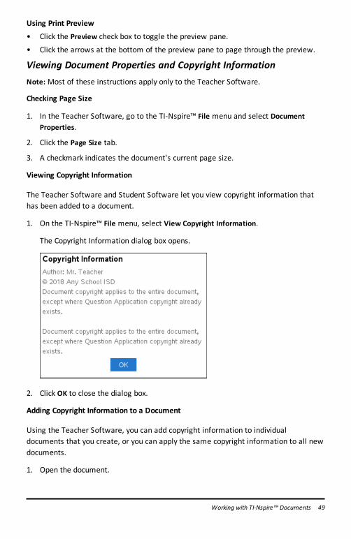
1. On the TI-Nspire™ File menu, select View Copyright Information.
The Copyright Information dialog box opens.
2. Click OK to close the dialog box.
Adding Copyright Information to a Document
Using the Teacher Software, you can add copyright information to individualdocuments that you create, or you can apply the same copyright information to all newdocuments.
1. Open the document.
Working with TI-Nspire™ Documents 49
50 Working with TI-Nspire™ Documents
2. On the TI-Nspire™ File menu, select Document Properties.
3. Click the Copyright tab.
4. Edit the following fields to define the copyright details:
• Author
• Copyright (select Public Domain or Copyright).
• Year (disabled if you selected Public Domain)
• Owner (disabled if you selected Public Domain)
• Comments
5. To add the supplied information to all new documents from this point forward,select Apply this copyright to all new documents.
6. Click OK to apply the copyright information to the document.
Protecting a Document (making a document read-only)
Teachers can protect documents to create a document for distribution to your studentsor for other use. A student who receives a read-only document and makes changes to itwill be prompted to save the document as a new file.
1. Open the document.
2. On the TI-Nspire™ File menu, select Document Properties.
3. Click the Protection tab.
4. Select the Make this document Read Only check box.
5. Click OK.
Working with PublishView™ DocumentsUse the PublishView™ feature to create and share interactive documents with teachersand students. You can create documents that include formatted text, TI-Nspire™applications, images, hyperlinks, links to videos, and embedded videos in a format thatis suitable for printing on a standard piece of paper, publishing to a website or blog, orfor use as an interactive worksheet.
PublishView™ features provide layout and editing features for presenting math andscience concepts in a document where TI-Nspire™ applications can be interactively anddynamically linked with supporting media, enabling you to bring the document to life.Using the PublishView™ feature:
• Teachers can create interactive activities and assessments used on screen.
• Teachers can create printed materials to complement documents used on TI-Nspire™ CX II handhelds.
• When working with lesson plans, teachers can:
- Create lesson plans from existing handheld documents or convert lesson plansto handheld documents.
- Link to related lesson plans or documents.- Embed explanatory text, images, video, and links to web resources.- Build or interact with TI-Nspire™ applications directly from the lesson plan.
• Students can create reports or projects such as lab reports containing dataplayback, curve fits, pictures, and video—all on the same sheet.
• Students can print and turn in assignments on a standard piece of paper.
• Students taking exams can use one tool to create a document that contains: allproblems on the exam, text, images, hyperlinks, or videos, interactive TI-Nspire™applications, screen shots, and layout options needed to print a document.
Note: PublishView™ documents can reside in the Portfolio Workspace, and TI-Nspire™questions within a PublishView™ document can be automatically graded by the TI-Nspire™ Navigator™ system.
Creating a New PublishView™ Document1. From the Documents Workspace, click File > New PublishView™ Document.
—or—
Click , and then click New PublishView™ Document.
• A blank letter-size document opens in the Documents Workspace. Theorientation is portrait, which cannot be changed.
• The default margin settings for the top and bottom margins are one-inch.There are no settings for side margins.
• By default, a problem is added to the document.
Working with PublishView™ Documents 51
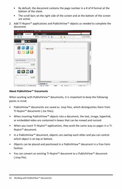
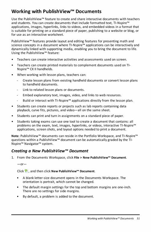
52 Working with PublishView™ Documents
• By default, the document contains the page number in a # of # format at thebottom of the sheet.
• The scroll bars on the right side of the screen and at the bottom of the screenare active.
2. Add TI-Nspire™ applications and PublishView™ objects as needed to complete thedocument.
About PublishView™ Documents
When working with PublishView™ documents, it is important to keep the followingpoints in mind:
• PublishView™ documents are saved as .tnsp files, which distinguishes them fromTI-Nspire™ documents (.tns files).
• When inserting PublishView™ objects into a document, the text, image, hyperlink,or embedded video are contained in boxes that can be moved and resized.
• When you insert TI-Nspire™ applications, they work the same way as pages in a TI-Nspire™ document.
• In a PublishView™ document, objects can overlap each other and you can controlwhich object is on top or bottom.
• Objects can be placed and positioned in a PublishView™ document in a free-formfashion.
• You can convert an existing TI-Nspire™ document to a PublishView™ document(.tnsp file).
• When you convert a PublishView™ document to a TI-Nspire™ document (.tns file),TI-Nspire™ applications are converted. PublishView™ objects containing text,hyperlinks, videos, and images are not converted.
• You cannot create or open a PublishView™ document on a handheld. You mustconvert a PublishView™ document to a TI-Nspire™ document before sending it to ahandheld.
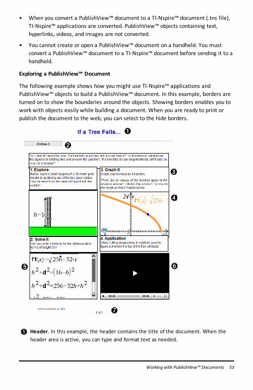
Exploring a PublishView™ Document
The following example shows how you might use TI-Nspire™ applications andPublishView™ objects to build a PublishView™ document. In this example, borders areturned on to show the boundaries around the objects. Showing borders enables you towork with objects easily while building a document. When you are ready to print orpublish the document to the web, you can select to the hide borders.
À Header. In this example, the header contains the title of the document. When theheader area is active, you can type and format text as needed.
Working with PublishView™ Documents 53
54 Working with PublishView™ Documents
Á Problem break and name. In PublishView™ documents, use problem breaks tocontrol the page layout. You can select to hide or show problem breaks. Deleting aproblem removes the contents of the problem and removes the space betweenproblems when there are multiple problems. Problem breaks also enable you to usevariables in PublishView™ documents. Variables that have the same name areindependent of one another if they are used in different problems.
 Text boxes. In this example, the introduction text and the text in boxes 1, 2, 3, and4 is contained in text boxes. You can insert text and hyperlinks into a PublishView™document using a text box. Text boxes can be resized and positioned as needed.PublishView™ text boxes are not retained when you convert a PublishView™document to a TI-Nspire™ document.
à TI-Nspire™ applications. In this example, the author uses Graphs & Geometry toshow the math functions. When a TI-Nspire™ application is active in a PublishView™document, the appropriate application menu opens in the Documents Toolbox. Youcan work in a TI-Nspire™ application just as you would in a TI-Nspire™ document.When you convert a PublishView™ document to a TI-Nspire™ document, applicationsare retained.
Ä Notes application. You can also use the TI-Nspire™ Notes application to add text to aPublishView™ document. Because Notes is a TI-Nspire™ application, it will beretained when you convert the PublishView™ document to a TI-Nspire™ document.Using the Notes application enables you to use an equation editor and can contain TI-Nspire™ math templates and symbols.
Å Video. This is an example of a video that is embedded in a PublishView™ documentwithin a frame. Users can start and stop the video using the controls. Framescontaining videos and images can be resized and positioned in the document asneeded.
Æ Footer. By default, the footer area contains the page number, which cannot beedited. You can add other text above the page number if needed. Like the header,you can format text as needed.
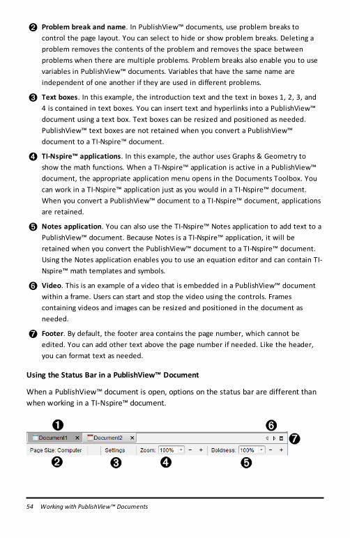
Using the Status Bar in a PublishView™ Document
When a PublishView™ document is open, options on the status bar are different thanwhen working in a TI-Nspire™ document.
À Document names are displayed in tabs. If multiple documents are open, thedocument names are listed. You can have TI-Nspire™ and PublishView™ documentsopen at the same time. In this example, Document 1 is an inactive TI-Nspire™document ( ). Document 2 is the active PublishView™ document ( ). Click the X to
close a document.
Á Page Size. Shows the document's page size as Handheld or Computer. You can usethe TI-Nspire™ File menu to convert a document from one page size to the other.
 Click Settings to change Document Settings. You can specify settings that are specificto an active document or set default settings for all PublishView™ documents. Whenyou convert a TI-Nspire™ document into a PublishView™ document, the settings inthe TI-Nspire™ document convert to the settings defined for PublishView™documents.
à Use the Zoom scale to zoom the active document in or out from 10% to 500%. To seta zoom, type a specific number, use the + and - buttons to increase or decrease byincrements of 10%, or use the drop-down box to choose preset percentages.
Ä In TI-Nspire™ applications, use the Boldness scale to increase or decrease theboldness of text and line thickness within applications. To set the boldness, type aspecific number, use the + and - buttons to increase or decrease by increments of10%, or use the drop-down box to choose preset percentages.
For PublishView™ objects, boldness is used to match text within TI-Nspire™applications to other text on the PublishView™ sheet. It can also be used to increasethe visibility of TI-Nspire™ applications when presenting a document to a class.
Å When there are too many open document names to show in the status bar, click the
forward and backward arrows ( ) to move through the documents.
Æ Click to see a list of all open documents.
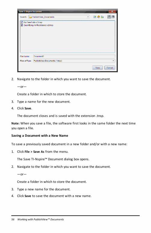
Saving PublishView™ Documents
Saving a New Document
1. Click File > Save Document.
—or—
Click .
The Save TI-Nspire™ Document dialog box opens.
Working with PublishView™ Documents 55
56 Working with PublishView™ Documents
2. Navigate to the folder in which you want to save the document.
—or—
Create a folder in which to store the document.
3. Type a name for the new document.
4. Click Save.
The document closes and is saved with the extension .tnsp.
Note: When you save a file, the software first looks in the same folder the next timeyou open a file.
Saving a Document with a New Name
To save a previously saved document in a new folder and/or with a new name:
1. Click File > Save As from the menu.
The Save TI-Nspire™ Document dialog box opens.
2. Navigate to the folder in which you want to save the document.
—or—
Create a folder in which to store the document.
3. Type a new name for the document.
4. Click Save to save the document with a new name.
Note: You can also use the Save As option to convert documents from TI-Nspire™ filesto PublishView™ files or convert PublishView™ files to TI-Nspire™ files.
Exploring the Documents WorkspaceWhen you create or open a PublishView™ document, it opens in the DocumentsWorkspace. Use the menu options and the toolbar just as you would when workingwith a TI-Nspire™ document to:
• Navigate to existing folders and documents using Content Explorer
• Open existing documents
• Save documents
• Use the copy, paste, undo, and redo options
• Delete documents
• Access TI-Nspire™ application-specific menus
• Open the Variables menu in TI-Nspire™ applications that allow variables
• Access and insert math templates, symbols, catalog items, and library items into aPublishView™ document
Note: For more information, see Using the Documents Workspace.
Exploring the Documents Toolbox
When a PublishView™ document is active, the Documents Toolbox contains toolsneeded for working with PublishView™ documents. You can add TI-Nspire™applications to a problem, insert parts of existing TI-Nspire™ documents into aproblem, and add PublishView™ objects.
The Documents Toolbox opens when you create a new PublishView™ document oropen an existing PublishView™ document. When working in a PublishView™ document,Page Sorter and TI-SmartView™ emulator are not available.
Working with PublishView™ Documents 57
58 Working with PublishView™ Documents
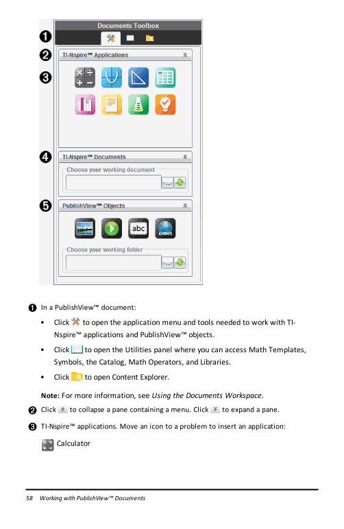
À In a PublishView™ document:
• Click to open the application menu and tools needed to work with TI-Nspire™ applications and PublishView™ objects.
• Click to open the Utilities panel where you can access Math Templates,Symbols, the Catalog, Math Operators, and Libraries.
• Click to open Content Explorer.
Note: For more information, see Using the Documents Workspace.
Á Click to collapse a pane containing a menu. Click to expand a pane.
 TI-Nspire™ applications. Move an icon to a problem to insert an application:
Calculator
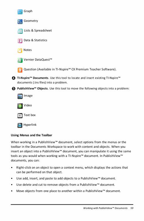
Graph
Geometry
Lists & Spreadsheet
Data & Statistics
Notes
Vernier DataQuest™
Question (Available in TI-Nspire™ CX Premium Teacher Software).
à TI-Nspire™ Documents. Use this tool to locate and insert existing TI-Nspire™documents (.tns files) into a problem.
Ä PublishView™ Objects. Use this tool to move the following objects into a problem:
Image
Video
Text box
Hyperlink
Using Menus and the Toolbar
When working in a PublishView™ document, select options from the menus or thetoolbar in the Documents Workspace to work with content and objects. When youinsert an object into a PublishView™ document, you can manipulate it using the sametools as you would when working with a TI-Nspire™ document. In PublishView™documents, you can:
• Right-click on an object to open a context menu, which displays the actions thatcan be performed on that object.
• Use add, insert, and paste to add objects to a PublishView™ document.
• Use delete and cut to remove objects from a PublishView™ document.
• Move objects from one place to another within a PublishView™ document.
Working with PublishView™ Documents 59
60 Working with PublishView™ Documents
• Copy objects from one document and paste them into another PublishView™document.
• Resize and scale objects such as text boxes and images.
• Change the font face and size and apply formatting such as italics, bold, underline,and color to text.
Note: For more information, see Using the Documents Workspace.
Using Context Menus
In TI-Nspire™ applications and in PublishView™ documents, context menus provide alist of options specific to the task you are working on. For example, when you right-click a cell while working in the TI-Nspire™ Lists & Spreadsheet application, a contextmenu opens providing a list of actions that you can perform on that cell. When youright-click the border of a text box in a PublishView™ document, the context menuprovides actions that can be performed on the text box.
Context Menus in TI-Nspire™ Applications
When you insert a TI-Nspire™ application into a PublishView™ document, theapplication menu and the context menus associated with that application are availableand work the same way they work in a TI-Nspire™ document.
Context Menus in PublishView™ Documents
In PublishView™ documents, context menus provide shortcuts to frequently performedtasks. Context menus are specific to an object or area:
• The Sheet context menu provides options for working with the layout of the sheetand document.
• Object context menus provide options for manipulating the object.
• Content-sensitive context menus provide options for working with the contentinside the object such as text or a video.
Working with PublishView™ ObjectsIn a PublishView™ document, text, hyperlinks, images, and videos are contained inPublishView™ objects. You can move, resize, copy and paste, and delete an objectwithin a PublishView™ document. Objects can also be positioned so that one overlapsthe other.
Within a document, PublishView™ objects can exist in three states: unselected,selected, and interactive.

State Description
Unselected When unselected, an objectdoes not have handles forrepositioning and sizing. Todeselect an object, left-click orright-click outside the object.In this example, bordersaround the object areshowing.
Selected When selected, an object willhave eight square handlesframing the object. To selectan object, click the object’sborder. When selected,objects can be moved andresized.
• To move an object, click aborder and drag theobject to its new location.
• To resize an object, graba handle.
• Right-click the border toopen a context menuwith options formanipulating the object.
Interactive An interactive state isindicated by a blue framearound the object. To enterinteractive state, left-click orright-click anywhere in thebody of the object. When inan interactive state, you canwork with the contents of theobject. For example, you canadd or edit text in a text boxor complete math functions ina TI-Nspire™ application.When in an interactive state,context menus contain optionsspecific to the contents of anobject.
Working with PublishView™ Documents 61
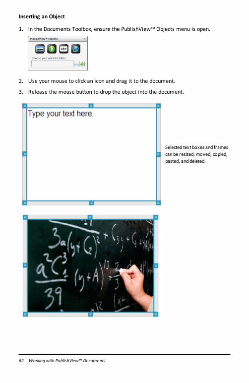
62 Working with PublishView™ Documents
Inserting an Object
1. In the Documents Toolbox, ensure the PublishView™ Objects menu is open.
2. Use your mouse to click an icon and drag it to the document.
3. Release the mouse button to drop the object into the document.
Selected text boxes and framescanbe resized, moved, copied,pasted, anddeleted.
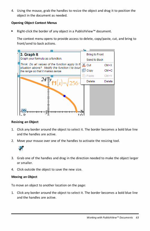
4. Using the mouse, grab the handles to resize the object and drag it to position theobject in the document as needed.
Opening Object Context Menus
▶ Right-click the border of any object in a PublishView™ document.
The context menu opens to provide access to delete, copy/paste, cut, and bring tofront/send to back actions.
Resizing an Object
1. Click any border around the object to select it. The border becomes a bold blue lineand the handles are active.
2. Move your mouse over one of the handles to activate the resizing tool.
3. Grab one of the handles and drag in the direction needed to make the object largeror smaller.
4. Click outside the object to save the new size.
Moving an Object
To move an object to another location on the page:
1. Click any border around the object to select it. The border becomes a bold blue lineand the handles are active.
Working with PublishView™ Documents 63
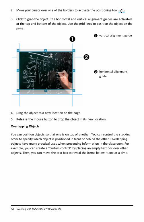
64 Working with PublishView™ Documents
2. Move your cursor over one of the borders to activate the positioning tool .
3. Click to grab the object. The horizontal and vertical alignment guides are activatedat the top and bottom of the object. Use the grid lines to position the object on thepage.
À vertical alignment guide
Á horizontal alignmentguide
4. Drag the object to a new location on the page.
5. Release the mouse button to drop the object in its new location.
Overlapping Objects
You can position objects so that one is on top of another. You can control the stackingorder to specify which object is positioned in front or behind the other. Overlappingobjects have many practical uses when presenting information in the classroom. Forexample, you can create a "curtain control" by placing an empty text box over otherobjects. Then, you can move the text box to reveal the items below it one at a time.
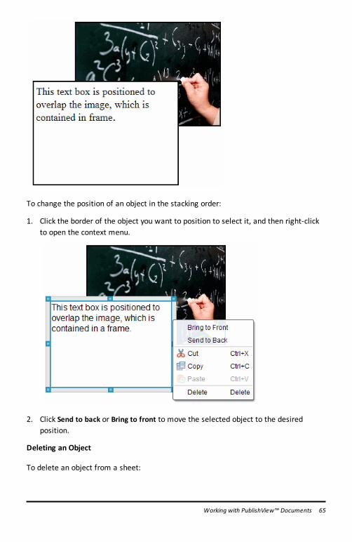
To change the position of an object in the stacking order:
1. Click the border of the object you want to position to select it, and then right-clickto open the context menu.
2. Click Send to back or Bring to front to move the selected object to the desiredposition.
Deleting an Object
To delete an object from a sheet:
Working with PublishView™ Documents 65
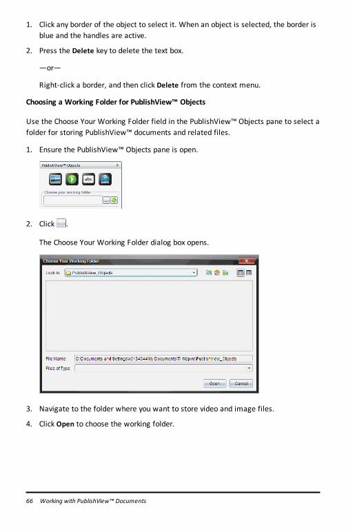
66 Working with PublishView™ Documents
1. Click any border of the object to select it. When an object is selected, the border isblue and the handles are active.
2. Press the Delete key to delete the text box.
—or—
Right-click a border, and then click Delete from the context menu.
Choosing a Working Folder for PublishView™ Objects
Use the Choose Your Working Folder field in the PublishView™ Objects pane to select afolder for storing PublishView™ documents and related files.
1. Ensure the PublishView™ Objects pane is open.
2. Click .
The Choose Your Working Folder dialog box opens.
3. Navigate to the folder where you want to store video and image files.
4. Click Open to choose the working folder.
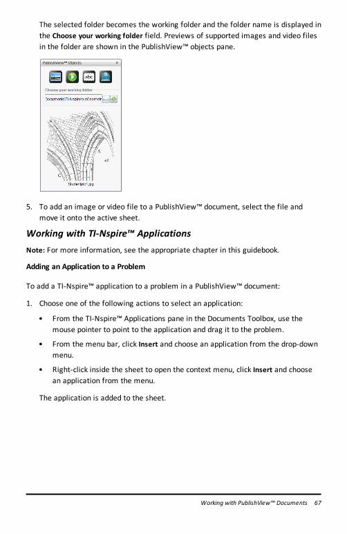
The selected folder becomes the working folder and the folder name is displayed inthe Choose your working folder field. Previews of supported images and video filesin the folder are shown in the PublishView™ objects pane.
5. To add an image or video file to a PublishView™ document, select the file andmove it onto the active sheet.
Working with TI-Nspire™ ApplicationsNote: For more information, see the appropriate chapter in this guidebook.
Adding an Application to a Problem
To add a TI-Nspire™ application to a problem in a PublishView™ document:
1. Choose one of the following actions to select an application:
• From the TI-Nspire™ Applications pane in the Documents Toolbox, use themouse pointer to point to the application and drag it to the problem.
• From the menu bar, click Insert and choose an application from the drop-downmenu.
• Right-click inside the sheet to open the context menu, click Insert and choosean application from the menu.
The application is added to the sheet.
Working with PublishView™ Documents 67
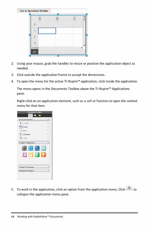
68 Working with PublishView™ Documents
2. Using your mouse, grab the handles to resize or position the application object asneeded.
3. Click outside the application frame to accept the dimensions.
4. To open the menu for the active TI-Nspire™ application, click inside the application.
The menu opens in the Documents Toolbox above the TI-Nspire™ Applicationspane.
Right-click on an application element, such as a cell or function to open the contextmenu for that item.
5. To work in the application, click an option from the application menu. Click tocollapse the application menu pane.
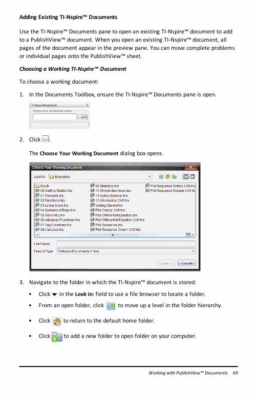
Adding Existing TI-Nspire™ Documents
Use the TI-Nspire™ Documents pane to open an existing TI-Nspire™ document to addto a PublishView™ document. When you open an existing TI-Nspire™ document, allpages of the document appear in the preview pane. You can move complete problemsor individual pages onto the PublishView™ sheet.
Choosing a Working TI-Nspire™ Document
To choose a working document:
1. In the Documents Toolbox, ensure the TI-Nspire™ Documents pane is open.
2. Click .
The Choose Your Working Document dialog box opens.
3. Navigate to the folder in which the TI-Nspire™ document is stored:
• Click¤ in the Look in: field to use a file browser to locate a folder.
• From an open folder, click to move up a level in the folder hierarchy.
• Click to return to the default home folder.
• Click to add a new folder to open folder on your computer.
Working with PublishView™ Documents 69
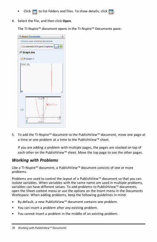
70 Working with PublishView™ Documents
• Click to list folders and files. To show details, click .
4. Select the file, and then click Open.
The TI-Nspire™ document opens in the TI-Nspire™ Documents pane.
5. To add the TI-Nspire™ document to the PublishView™ document, move one page ata time or one problem at a time to the PublishView™ sheet.
If you are adding a problem with multiple pages, the pages are stacked on top ofeach other on the PublishView™ sheet. Move the top page to see the other pages.
Working with ProblemsLike a TI-Nspire™ document, a PublishView™ document consists of one or moreproblems.
Problems are used to control the layout of a PublishView™ document so that you canisolate variables. When variables with the same name are used in multiple problems,variables can have different values. To add problems to PublishView™ documents,open the Sheet context menu or use the options on the Insert menu in the DocumentsWorkspace. When adding problems, keep the following guidelines in mind:
• By default, a new PublishView™ document contains one problem.
• You can insert a problem after any existing problem.
• You cannot insert a problem in the middle of an existing problem.
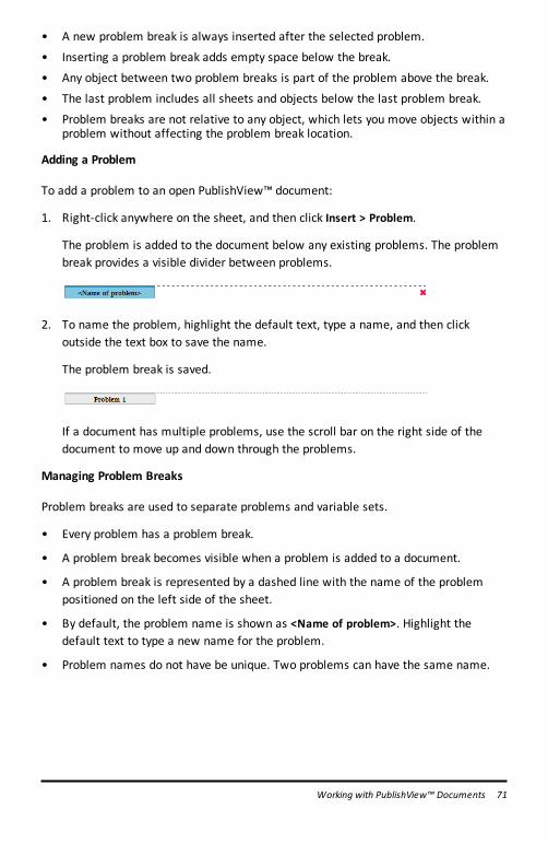
• A new problem break is always inserted after the selected problem.
• Inserting a problem break adds empty space below the break.
• Any object between two problem breaks is part of the problem above the break.
• The last problem includes all sheets and objects below the last problem break.
• Problem breaks are not relative to any object, which lets you move objects within aproblem without affecting the problem break location.
Adding a Problem
To add a problem to an open PublishView™ document:
1. Right-click anywhere on the sheet, and then click Insert > Problem.
The problem is added to the document below any existing problems. The problembreak provides a visible divider between problems.
2. To name the problem, highlight the default text, type a name, and then clickoutside the text box to save the name.
The problem break is saved.
If a document has multiple problems, use the scroll bar on the right side of thedocument to move up and down through the problems.
Managing Problem Breaks
Problem breaks are used to separate problems and variable sets.
• Every problem has a problem break.
• A problem break becomes visible when a problem is added to a document.
• A problem break is represented by a dashed line with the name of the problempositioned on the left side of the sheet.
• By default, the problem name is shown as <Name of problem>. Highlight thedefault text to type a new name for the problem.
• Problem names do not have be unique. Two problems can have the same name.
Working with PublishView™ Documents 71
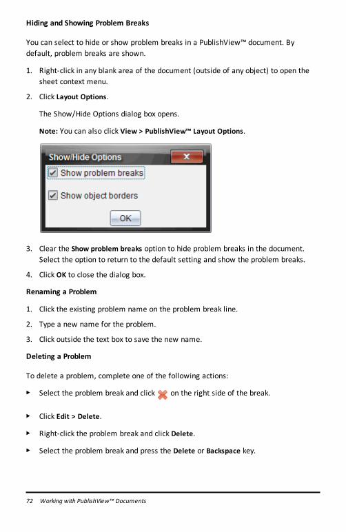
72 Working with PublishView™ Documents
Hiding and Showing Problem Breaks
You can select to hide or show problem breaks in a PublishView™ document. Bydefault, problem breaks are shown.
1. Right-click in any blank area of the document (outside of any object) to open thesheet context menu.
2. Click Layout Options.
The Show/Hide Options dialog box opens.
Note: You can also click View > PublishView™ Layout Options.
3. Clear the Show problem breaks option to hide problem breaks in the document.Select the option to return to the default setting and show the problem breaks.
4. Click OK to close the dialog box.
Renaming a Problem
1. Click the existing problem name on the problem break line.
2. Type a new name for the problem.
3. Click outside the text box to save the new name.
Deleting a Problem
To delete a problem, complete one of the following actions:
▶ Select the problem break and click on the right side of the break.
▶ Click Edit > Delete.
▶ Right-click the problem break and click Delete.
▶ Select the problem break and press the Delete or Backspace key.
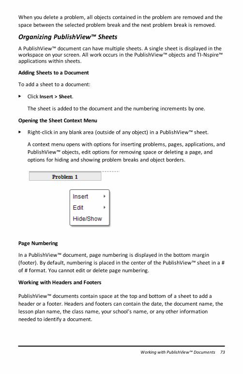
When you delete a problem, all objects contained in the problem are removed and thespace between the selected problem break and the next problem break is removed.
Organizing PublishView™ SheetsA PublishView™ document can have multiple sheets. A single sheet is displayed in theworkspace on your screen. All work occurs in the PublishView™ objects and TI-Nspire™applications within sheets.
Adding Sheets to a Document
To add a sheet to a document:
▶ Click Insert > Sheet.
The sheet is added to the document and the numbering increments by one.
Opening the Sheet Context Menu
▶ Right-click in any blank area (outside of any object) in a PublishView™ sheet.
A context menu opens with options for inserting problems, pages, applications, andPublishView™ objects, edit options for removing space or deleting a page, andoptions for hiding and showing problem breaks and object borders.
Page Numbering
In a PublishView™ document, page numbering is displayed in the bottom margin(footer). By default, numbering is placed in the center of the PublishView™ sheet in a #of # format. You cannot edit or delete page numbering.
Working with Headers and Footers
PublishView™ documents contain space at the top and bottom of a sheet to add aheader or a footer. Headers and footers can contain the date, the document name, thelesson plan name, the class name, your school’s name, or any other informationneeded to identify a document.
Working with PublishView™ Documents 73
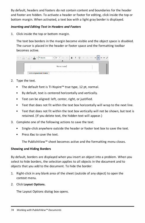
74 Working with PublishView™ Documents
By default, headers and footers do not contain content and boundaries for the headerand footer are hidden. To activate a header or footer for editing, click inside the top orbottom margin. When activated, a text box with a light gray border is displayed.
Inserting and Editing Text in Headers and Footers
1. Click inside the top or bottom margin.
The text box borders in the margin become visible and the object space is disabled.The cursor is placed in the header or footer space and the formatting toolbarbecomes active.
2. Type the text.
• The default font is TI-Nspire™ true type, 12 pt, normal.
• By default, text is centered horizontally and vertically.
• Text can be aligned: left, center, right, or justified.
• Text that does not fit within the text box horizontally will wrap to the next line.
• Text that does not fit within the text box vertically will not be shown, but text isretained. (If you delete text, the hidden text will appear.)
3. Complete one of the following actions to save the text:
• Single-click anywhere outside the header or footer text box to save the text.
• Press Esc to save the text.
The PublishView™ sheet becomes active and the formatting menu closes.
Showing and Hiding Borders
By default, borders are displayed when you insert an object into a problem. When youselect to hide borders, the selection applies to all objects in the document and toobjects that you add to the document. To hide the border:
1. Right-click in any blank area of the sheet (outside of any object) to open thecontext menu.
2. Click Layout Options.
The Layout Options dialog box opens.
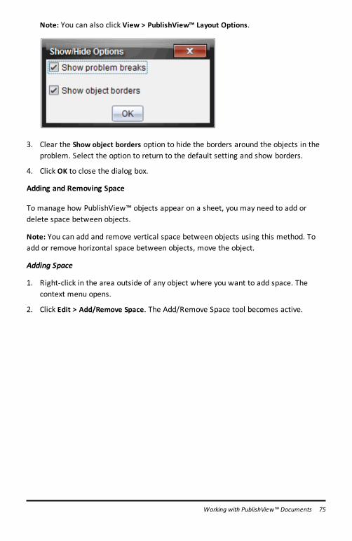
Note: You can also click View > PublishView™ Layout Options.
3. Clear the Show object borders option to hide the borders around the objects in theproblem. Select the option to return to the default setting and show borders.
4. Click OK to close the dialog box.
Adding and Removing Space
To manage how PublishView™ objects appear on a sheet, you may need to add ordelete space between objects.
Note: You can add and remove vertical space between objects using this method. Toadd or remove horizontal space between objects, move the object.
Adding Space
1. Right-click in the area outside of any object where you want to add space. Thecontext menu opens.
2. Click Edit > Add/Remove Space. The Add/Remove Space tool becomes active.
Working with PublishView™ Documents 75
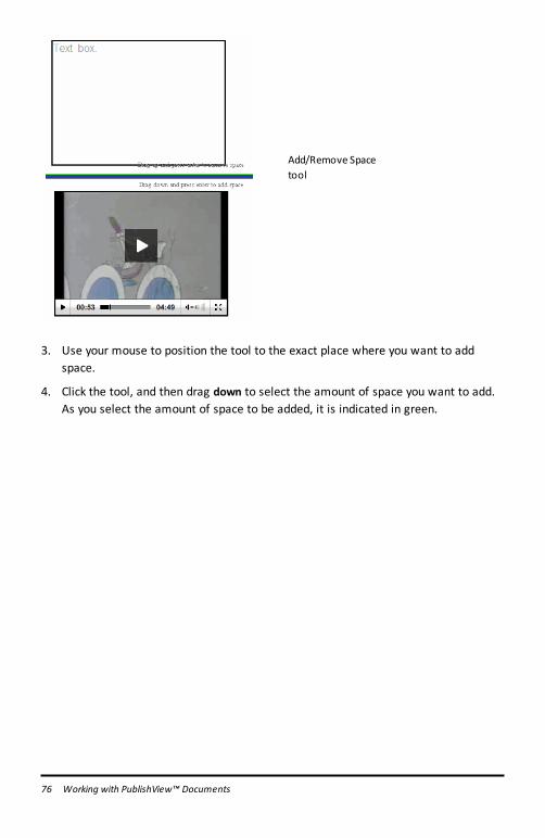
76 Working with PublishView™ Documents
Add/Remove Spacetool
3. Use your mouse to position the tool to the exact place where you want to addspace.
4. Click the tool, and then drag down to select the amount of space you want to add.As you select the amount of space to be added, it is indicated in green.
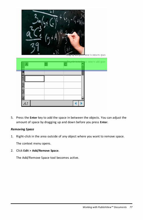
5. Press the Enter key to add the space in between the objects. You can adjust theamount of space by dragging up and down before you press Enter.
Removing Space
1. Right-click in the area outside of any object where you want to remove space.
The context menu opens.
2. Click Edit > Add/Remove Space.
The Add/Remove Space tool becomes active.
Working with PublishView™ Documents 77
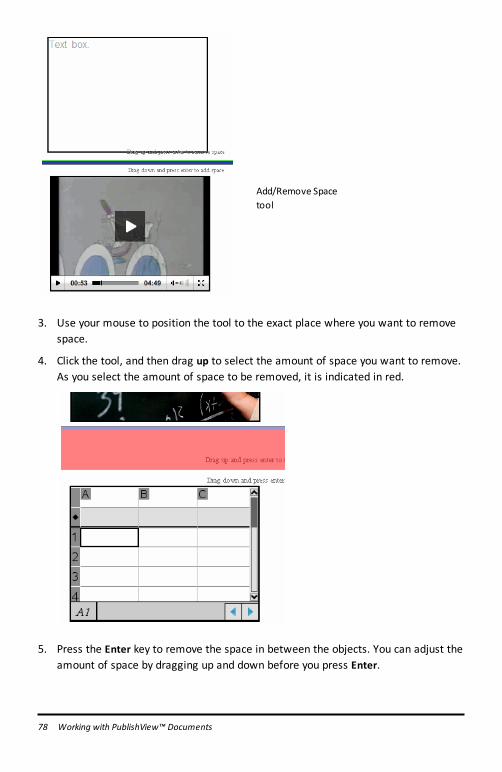
78 Working with PublishView™ Documents
Add/Remove Spacetool
3. Use your mouse to position the tool to the exact place where you want to removespace.
4. Click the tool, and then drag up to select the amount of space you want to remove.As you select the amount of space to be removed, it is indicated in red.
5. Press the Enter key to remove the space in between the objects. You can adjust theamount of space by dragging up and down before you press Enter.
Note: If there is not enough space on the sheet to accommodate the objects, theobjects won’t be moved when space is removed.
Deleting Blank Sheets from Problems
You can delete a sheet that does not contain any TI-Nspire™ applications orPublishView™ objects from a problem. To delete a blank sheet from a problem:
1. Delete any TI-Nspire™ applications, PublishView™ objects, move or delete anyproblem breaks from the sheet.
2. Place your cursor inside the sheet you want to delete.
3. Right-click inside the blank sheet to open the context menu.
4. Click Edit > Delete Sheet.
The blank sheet is removed from the problem.
Using ZoomThe zoom feature lets you zoom in on any object or area on the PublishView™document for discussion, and zoom out to see an overview of the lesson. The zoomuses the center point of the viewable area to zoom in.
The default zoom setting is 100%.
▶ To change the zoom percentage, do one of the following:
• Type the number in the box and press Enter.• Use the - and + buttons to decrease or increase the percentage in 10%
increments.• Use the drop-down arrow to choose a preset percentage.
The zoom settings are retained when you save the document.
Adding Text to a PublishView™ DocumentIn a PublishView™ document, there are three ways to add text:
• Insert a PublishView™ text box to enter free-form text or copy text from othersources into the document. For example, you can place a PublishView™ text boxnext to an image and type a description in a text box. You can also copy and pastetext from .doc, .txt, and .rtf files. Use PublishView™ text boxes when you needoptions for emphasizing and formatting text. PublishView™ text boxes are notconverted when you convert a PublishView™ document to a TI-Nspire™ document.You may want to use a PublishView™ text box to add text that you don’t wanthandheld users to see.
• Use the TI-Nspire™ Notes application. You should use the Notes application whenyou need an advanced equation editor and when you need to use TI-Nspire™ mathtemplates and symbols. Superscript and subscript are also easier to use in the
Working with PublishView™ Documents 79
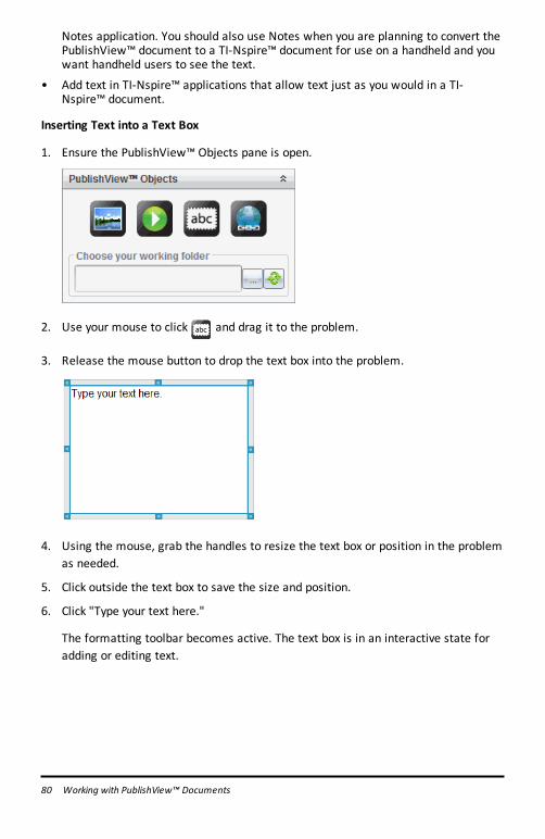
80 Working with PublishView™ Documents
Notes application. You should also use Notes when you are planning to convert thePublishView™ document to a TI-Nspire™ document for use on a handheld and youwant handheld users to see the text.
• Add text in TI-Nspire™ applications that allow text just as you would in a TI-Nspire™ document.
Inserting Text into a Text Box
1. Ensure the PublishView™ Objects pane is open.
2. Use your mouse to click and drag it to the problem.
3. Release the mouse button to drop the text box into the problem.
4. Using the mouse, grab the handles to resize the text box or position in the problemas needed.
5. Click outside the text box to save the size and position.
6. Click "Type your text here."
The formatting toolbar becomes active. The text box is in an interactive state foradding or editing text.
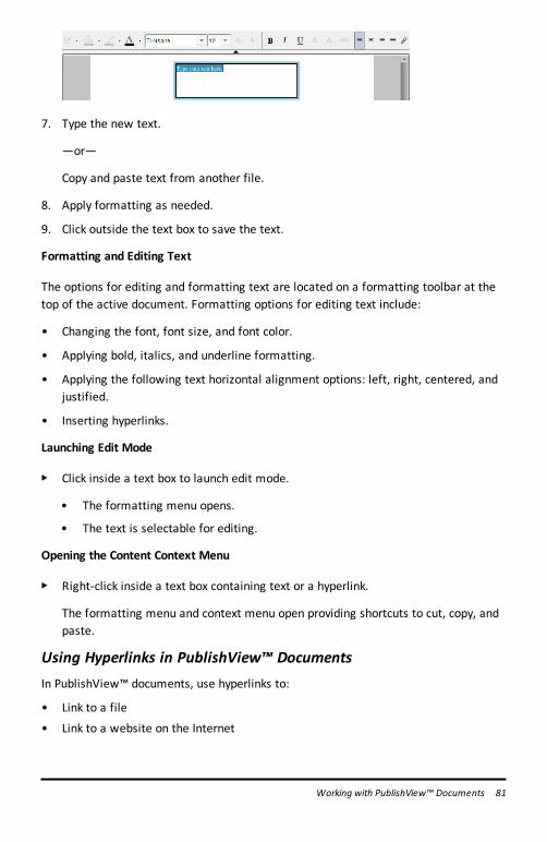
7. Type the new text.
—or—
Copy and paste text from another file.
8. Apply formatting as needed.
9. Click outside the text box to save the text.
Formatting and Editing Text
The options for editing and formatting text are located on a formatting toolbar at thetop of the active document. Formatting options for editing text include:
• Changing the font, font size, and font color.
• Applying bold, italics, and underline formatting.
• Applying the following text horizontal alignment options: left, right, centered, andjustified.
• Inserting hyperlinks.
Launching Edit Mode
▶ Click inside a text box to launch edit mode.
• The formatting menu opens.
• The text is selectable for editing.
Opening the Content Context Menu
▶ Right-click inside a text box containing text or a hyperlink.
The formatting menu and context menu open providing shortcuts to cut, copy, andpaste.
Using Hyperlinks in PublishView™ DocumentsIn PublishView™ documents, use hyperlinks to:
• Link to a file
• Link to a website on the Internet
Working with PublishView™ Documents 81
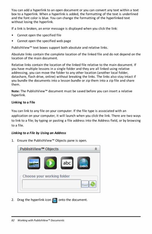
82 Working with PublishView™ Documents
You can add a hyperlink to an open document or you can convert any text within a textbox to a hyperlink. When a hyperlink is added, the formatting of the text is underlinedand the font color is blue. You can change the formatting of the hyperlinked textwithout losing the hyperlink.
If a link is broken, an error message is displayed when you click the link:
• Cannot open the specified file
• Cannot open the specified web page
PublishView™ text boxes support both absolute and relative links.
Absolute links contain the complete location of the linked file and do not depend on thelocation of the main document.
Relative links contain the location of the linked file relative to the main document. Ifyou have multiple lessons in a single folder and they are all linked using relativeaddressing, you can move the folder to any other location (another local folder,datashare, flash drive, online) without breaking the links. The links also stay intact ifyou bundle the documents into a lesson bundle or zip them into a zip file and sharethem.
Note: The PublishView™ document must be saved before you can insert a relativehyperlink.
Linking to a File
You can link to any file on your computer. If the file type is associated with anapplication on your computer, it will launch when you click the link. There are two waysto link to a file; by typing or pasting a file address into the Address field, or by browsingto a file.
Linking to a File by Using an Address
1. Ensure the PublishView™ Objects pane is open.
2. Drag the hyperlink icon onto the document.
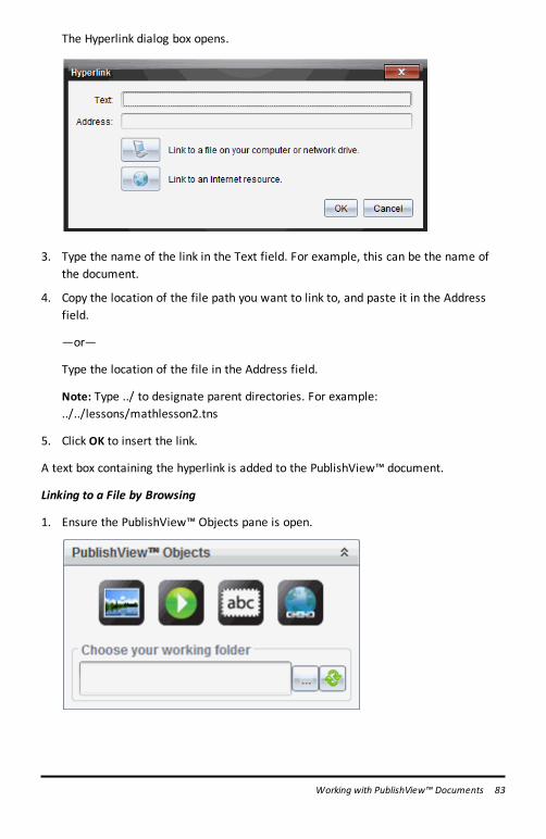
The Hyperlink dialog box opens.
3. Type the name of the link in the Text field. For example, this can be the name ofthe document.
4. Copy the location of the file path you want to link to, and paste it in the Addressfield.
—or—
Type the location of the file in the Address field.
Note: Type ../ to designate parent directories. For example:../../lessons/mathlesson2.tns
5. Click OK to insert the link.
A text box containing the hyperlink is added to the PublishView™ document.
Linking to a File by Browsing
1. Ensure the PublishView™ Objects pane is open.
Working with PublishView™ Documents 83
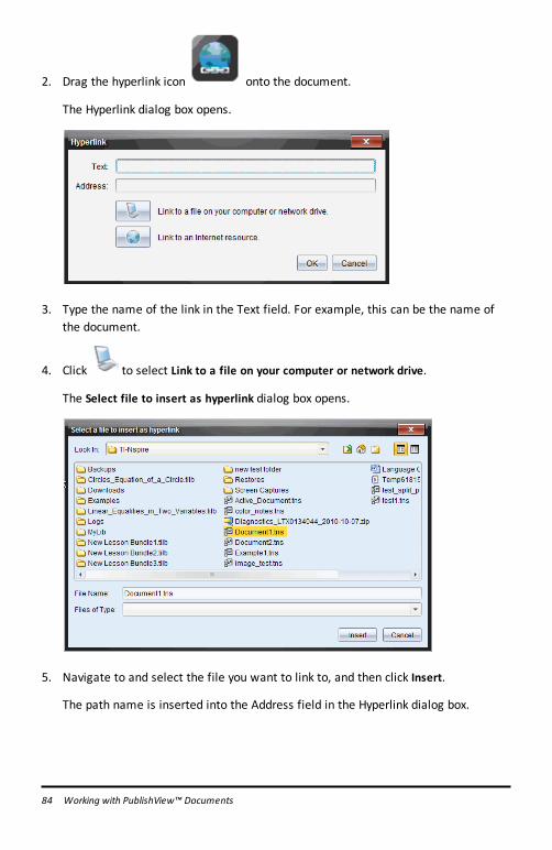
84 Working with PublishView™ Documents
2. Drag the hyperlink icon onto the document.
The Hyperlink dialog box opens.
3. Type the name of the link in the Text field. For example, this can be the name ofthe document.
4. Click to select Link to a file on your computer or network drive.
The Select file to insert as hyperlink dialog box opens.
5. Navigate to and select the file you want to link to, and then click Insert.
The path name is inserted into the Address field in the Hyperlink dialog box.
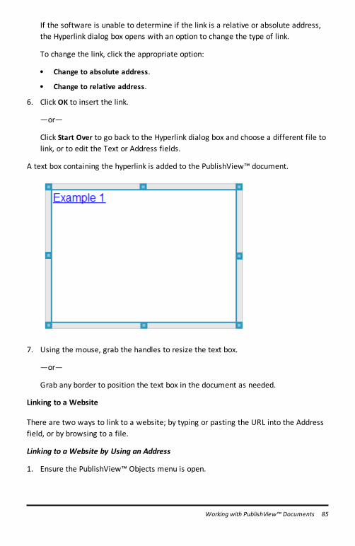
If the software is unable to determine if the link is a relative or absolute address,the Hyperlink dialog box opens with an option to change the type of link.
To change the link, click the appropriate option:
• Change to absolute address.
• Change to relative address.
6. Click OK to insert the link.
—or—
Click Start Over to go back to the Hyperlink dialog box and choose a different file tolink, or to edit the Text or Address fields.
A text box containing the hyperlink is added to the PublishView™ document.
7. Using the mouse, grab the handles to resize the text box.
—or—
Grab any border to position the text box in the document as needed.
Linking to a Website
There are two ways to link to a website; by typing or pasting the URL into the Addressfield, or by browsing to a file.
Linking to a Website by Using an Address
1. Ensure the PublishView™ Objects menu is open.
Working with PublishView™ Documents 85
86 Working with PublishView™ Documents
2. Drag the hyperlink icon onto the document to open the Hyperlink dialogbox.
3. Type or paste the URL you want to link to in the Address field.
4. Click OK.
A text box containing the hyperlink is added to the PublishView™ document.
Linking to a Website by Browsing
1. Ensure the PublishView™ Objects menu is open.
2. Drag the hyperlink icon onto the document to open the Hyperlink dialogbox.
3. Click to select Link to an Internet resource.
The browser opens to your default website.
4. Navigate to the website or file on a website that you want to link to.
5. Copy the URL, and then paste it in the Address field in the Hyperlink dialog box.
—or—
Type the URL in the Address field.
6. Click OK.
A text box containing the hyperlink is added to the PublishView™ document.
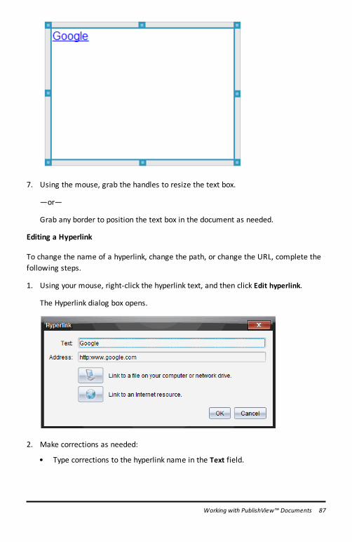
7. Using the mouse, grab the handles to resize the text box.
—or—
Grab any border to position the text box in the document as needed.
Editing a Hyperlink
To change the name of a hyperlink, change the path, or change the URL, complete thefollowing steps.
1. Using your mouse, right-click the hyperlink text, and then click Edit hyperlink.
The Hyperlink dialog box opens.
2. Make corrections as needed:
• Type corrections to the hyperlink name in the Text field.
Working with PublishView™ Documents 87
88 Working with PublishView™ Documents
• Click to open the Select a file to add as a hyperlink dialog box and use the
file browser to navigate to the folder where the file is located.
• Click to open a browser and navigate to a website to copy and paste the
correct the URL in the Address field.
3. Click OK to save the changes.
Converting Existing Text to a Hyperlink
1. Click inside the text box to activate edit mode and open the formatting menu.
2. Select the text you want to convert to a hyperlink.
3. Click .
The Hyperlink dialog box opens with the selected text in the Text field.
4. Click to create a link to a file.
—or—
Click to create a link to page on a website.
Removing a Hyperlink
Use this process to remove a link from text inside a text box. The text remains in thedocument.
1. Using your mouse, right-click the hyperlink text.
2. Click Remove hyperlink.
The hyperlink formatting is removed from the text and the text is no longerclickable.
Note: To remove both the text and hyperlink, delete the text. If a text box contains onlythe linked text, delete the text box.
Working with ImagesImages can be added to PublishView™ documents as PublishView™ objects or can beadded inside TI-Nspire™ applications that support images. Supported files types are.bmp, .jpg, and .png files.
Note: If a TI-Nspire™ application is active in the PublishView™ document, the image isadded to the TI-Nspire™ page if you click Insert > Image from the menu bar or contextmenu. If there is no TI-Nspire™ document active, the image is added as a
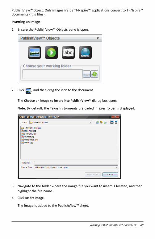
PublishView™ object. Only images inside TI-Nspire™ applications convert to TI-Nspire™documents (.tns files).
Inserting an Image
1. Ensure the PublishView™ Objects pane is open.
2. Click , and then drag the icon to the document.
The Choose an image to insert into PublishView™ dialog box opens.
Note: By default, the Texas Instruments preloaded images folder is displayed.
3. Navigate to the folder where the image file you want to insert is located, and thenhighlight the file name.
4. Click Insert image.
The image is added to the PublishView™ sheet.
Working with PublishView™ Documents 89
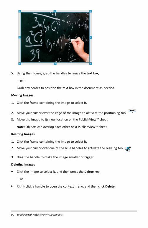
90 Working with PublishView™ Documents
5. Using the mouse, grab the handles to resize the text box,
—or—
Grab any border to position the text box in the document as needed.
Moving Images
1. Click the frame containing the image to select it.
2. Move your cursor over the edge of the image to activate the positioning tool.
3. Move the image to its new location on the PublishView™ sheet.
Note: Objects can overlap each other on a PublishView™ sheet.
Resizing Images
1. Click the frame containing the image to select it.
2. Move your cursor over one of the blue handles to activate the resizing tool.
3. Drag the handle to make the image smaller or bigger.
Deleting Images
▶ Click the image to select it, and then press the Delete key.
—or—
▶ Right-click a handle to open the context menu, and then click Delete.
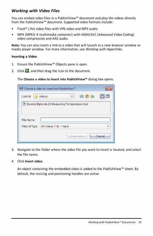
Working with Video FilesYou can embed video files in a PublishView™ document and play the videos directlyfrom the PublishView™ document. Supported video formats include:
• Flash® (.flv) video files with VP6 video and MP3 audio.
• MP4 (MPEG-4 multimedia container) with H264/AVC (Advanced Video Coding)video compression and AAC audio.
Note: You can also insert a link to a video that will launch in a new browser window ormedia player window. For more information, see Working with Hyperlinks.
Inserting a Video
1. Ensure the PublishView™ Objects pane is open.
2. Click , and then drag the icon to the document.
The Choose a video to insert into PublishView™ dialog box opens.
3. Navigate to the folder where the video file you want to insert is located, and selectthe file name.
4. Click Insert video.
An object containing the embedded video is added to the PublishView™ sheet. Bydefault, the resizing and positioning handles are active.
Working with PublishView™ Documents 91

92 Working with PublishView™ Documents
5. Using the mouse, grab the handles to resize the object or grab any border toposition the object in the document as needed. For example, you may want toposition the object containing the video above or below a text box that containstext introducing the video.
6. To play the video, click the forward arrow, or click anywhere in the viewingwindow.
Using the Video Console
The video console lets users control the video.
À Starts or stops the video.
Á Shows the elapsed time as the video plays.
 Mutes or unmutes the audio.
Converting DocumentsYou can convert PublishView™ documents (.tnsp files) to TI-Nspire™ documents (.tnsfiles) for display on handhelds. You can also convert TI-Nspire™ documents toPublishView™ documents.
Converting a document creates a new document—the original document remainsintact and is not linked to the new document. If you make changes to one document,the changes are not reflected in the other document.
Converting PublishView™ Documents to TI-Nspire™ Documents
You cannot open a PublishView™ document (.tnsp file) on a handheld. However, youcan convert the PublishView™ document to a TI-Nspire™ document that can betransferred to and opened on a handheld. When you convert a PublishView™ documentto a TI-Nspire™ document:
• Only the TI-Nspire™ applications become part of the TI-Nspire™ document.
• PublishView™ objects such as text boxes, images, hyperlinks, and videos are notconverted.
• Text contained in PublishView™ text boxes is not converted; however, text in a TI-Nspire™ Notes application is converted.
• If images are contained in a TI-Nspire™ application, they are converted; however,images contained in PublishView™ objects are not converted.
Complete the following steps to convert a PublishView™ document (.tnsp file) to a TI-Nspire™ document (.tns file).
1. Open the PublishView™ document to be converted.
2. Click File > Convert to > TI-Nspire™ Document.
• The new TI-Nspire™ document opens in the Documents Workspace.
• All supported TI-Nspire™ applications are part of the new TI-Nspire™document.
• Starting from top to bottom, and then left to right, the layout of the TI-Nspire™document is based on the order of the TI-Nspire™ applications in thePublishView™ document.
- Every TI-Nspire™ application in a PublishView™ document will appear as apage in the converted TI-Nspire™ document. The order of the pages in theTI-Nspire™ document is based on the layout of the TI-Nspire™ applicationsin the PublishView™ document.
- If two or more problems are at the same level, the order is left to right.
• Problem breaks are maintained.
• The new TI-Nspire™ document is not linked to the PublishView™ document.
3. When work in the document is complete, click to save the document in the
current folder.
—or—
Working with PublishView™ Documents 93
94 Working with PublishView™ Documents
Click File > Save As to save the document in a different folder.
Note: If the document has never been saved, both the Save and Save as optionsallow saving in a different folder.
Note: You can also use the Save as option to convert a PublishView™ document to aTI-Nspire™ document.
Note: If you try to convert a PublishView™ document that does not contain TI-Nspire™pages or applications, an error message is displayed.
Converting TI-Nspire™ Documents to PublishView™ Documents
You can convert existing TI-Nspire™ documents to PublishView™ documents, whichenables you to take advantage of the richer layout and editing features for printing,generating student reports, creating worksheets and assessments, and publishingdocuments to a website or blog.
Complete the following steps to convert a TI-Nspire™ document to a PublishView™document:
1. Open the TI-Nspire™ document you want to convert.
2. Click File > Convert to > PublishView™ Document.
• The new PublishView™ document opens in the Documents Workspace.
• By default, there are six objects per page.
• When converted, each problem from the TI-Nspire™ document will start a newsheet in the PublishView™ document.
• Problem breaks are maintained.
3. When work in the document is complete, click to save the document in the
current folder.
—or—
Click File > Save As to save the document in a different folder.
Note: You can also use the Save as option to save a TI-Nspire™ document as aPublishView™ document.
Printing PublishView™ DocumentsYou can print reports, worksheets, and assessments created using the PublishView™feature. To print a document:
1. Click File > Print.
The Print dialog box opens. A preview of the document is shown on the right sideof the dialog box.
2. Select a printer from the menu.
Note: The Print what field is disabled.
3. Select Paper Size from the menu. Options are:
• Letter (8.5 x 11 inches)• Legal (8.5 x 14 inches)• A4 (210 x 297 mm)
4. Select or type the number of Copies you want to print.
5. In the Print Range area, select to print all sheets in the document, a range ofsheets, or the current sheet only.
Note: By default, top and bottom margins are set to one-inch and are maintainedwhen printing a PublishView™ document. There are no side margins. PublishView™sheets print just as they appear in the workspace.
6. If needed, select or clear the boxes to:
• Print problem breaks and names.• Print headers• Print footers• Print object borders
7. Click Print, or click Save As PDF.
Working with PublishView™ Documents 95
96 Working with Lesson Bundles
Working with Lesson BundlesMany lessons or activities contain multiple files. For example, teachers usually have ateacher version of a file, a student version, assessments, and sometimes supportingfiles. A lesson bundle is a container that enables teachers to group all files needed fora lesson together. Lesson bundles are used to:
• Add any type of file (.tns, .tnsp, .doc, .pdf, .ppt) to a lesson bundle.
• Send lesson bundles to connected handhelds or laptops; however, only the .tns filesare sent to the handheld.
• View all the files in a lesson bundle using the TI-Nspire™ software.
• Group all files associated with one lesson in one place.
• Email one lesson bundle file to teachers or students instead of looking for andattaching multiple files.
Creating a New Lesson BundleTeachers and students can create new lesson bundles in the Documents Workspace.Teachers can also create new lesson bundles in the Content Workspace.
Creating a Lesson Bundle in the Documents Workspace
Complete the following steps to create a new lesson bundle. By default, the newlesson bundle does not contain files.
1. Click in the Documents Toolbox to open the Content Explorer.
2. Navigate to the folder where you want to save the lesson bundle file.
3. Click to open the menu, and then click New Lesson Bundle.
The new lesson bundle file is created with a default name and placed in your list offiles.
4. Type a name for your lesson bundle.
5. Press Enter to save the file.
Creating Lesson Bundles in the Content Workspace
In the Content Workspace, teachers have two options for creating lesson bundles:
• When files needed for a lesson bundle are located in different folders, create anempty lesson bundle, and then add files to the lesson bundle.
• If all needed files are located in the same folder, create a lesson bundle withselected files.
Creating an Empty Lesson Bundle
Complete the following steps to create a lesson bundle that does not contain files.
1. Navigate to the folder on your computer where you want to save the lesson bundle.
Note: If you are using the software for the first time, you may need to create afolder on your computer before creating a lesson bundle.
2. Click or click File > New Lesson Bundle.
The new lesson bundle file is created with a default name and placed in the list offiles.
3. Type a name for the lesson bundle and press Enter.
The lesson bundle is saved with the new name and details are shown in thePreview pane.
Creating a Lesson Bundle Containing Files
You can select multiple files within a folder, and then create the lesson bundle. Youcannot add a folder to a lesson bundle.
1. Navigate to the folder that contains the files you want to bundle.
2. Select the files. To select multiple files, select the first file then hold down Shiftand click the last file in the list. To select random files, select the first file, andthen hold down Ctrl and click the other files to select them.
3. Click , and then click Lesson Bundles > Create New Lesson Bundle from
selected.
A new lesson bundle is created and placed in the open folder. The lesson bundlecontains copies of the selected files.
4. Type a name for the lesson bundle and press Enter.
The lesson bundle is saved in the open folder and the details are shown in thePreview pane.
Adding Files to a Lesson BundleUse any of the following methods to add files to a lesson bundle:
• Drag any file into a selected lesson bundle. This method moves the file to thelesson bundle. If you delete the lesson bundle, the file is deleted from yourcomputer. You can recover the file from the Recycle Bin.
Working with Lesson Bundles 97
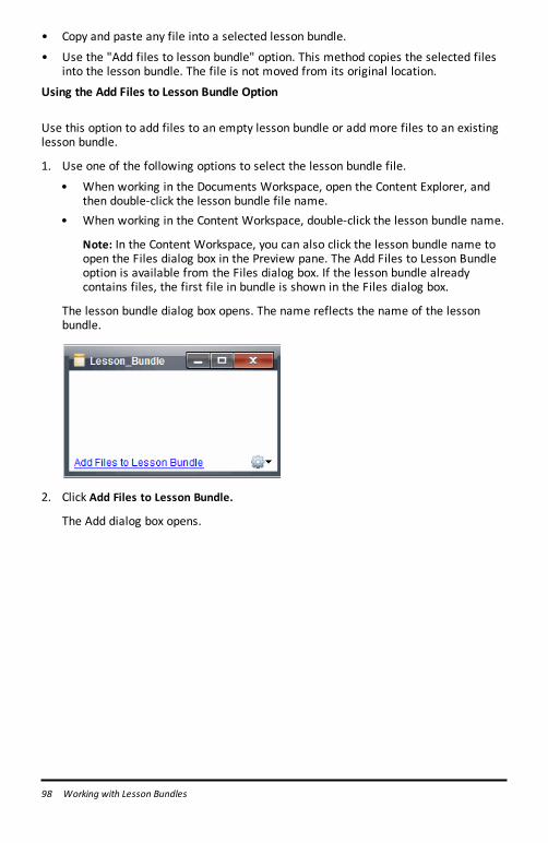
98 Working with Lesson Bundles
• Copy and paste any file into a selected lesson bundle.
• Use the "Add files to lesson bundle" option. This method copies the selected filesinto the lesson bundle. The file is not moved from its original location.
Using the Add Files to Lesson Bundle Option
Use this option to add files to an empty lesson bundle or add more files to an existinglesson bundle.
1. Use one of the following options to select the lesson bundle file.
• When working in the Documents Workspace, open the Content Explorer, andthen double-click the lesson bundle file name.
• When working in the Content Workspace, double-click the lesson bundle name.
Note: In the Content Workspace, you can also click the lesson bundle name toopen the Files dialog box in the Preview pane. The Add Files to Lesson Bundleoption is available from the Files dialog box. If the lesson bundle alreadycontains files, the first file in bundle is shown in the Files dialog box.
The lesson bundle dialog box opens. The name reflects the name of the lessonbundle.
2. Click Add Files to Lesson Bundle.
The Add dialog box opens.
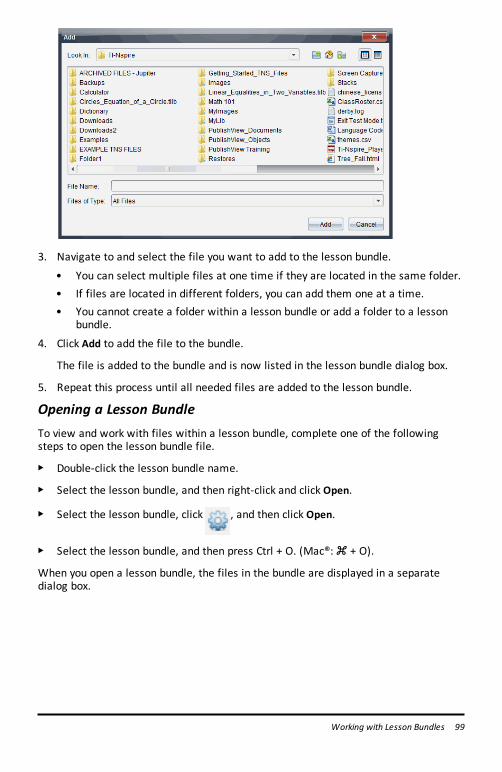
3. Navigate to and select the file you want to add to the lesson bundle.
• You can select multiple files at one time if they are located in the same folder.• If files are located in different folders, you can add them one at a time.• You cannot create a folder within a lesson bundle or add a folder to a lesson
bundle.
4. Click Add to add the file to the bundle.
The file is added to the bundle and is now listed in the lesson bundle dialog box.
5. Repeat this process until all needed files are added to the lesson bundle.
Opening a Lesson BundleTo view and work with files within a lesson bundle, complete one of the followingsteps to open the lesson bundle file.
▶ Double-click the lesson bundle name.
▶ Select the lesson bundle, and then right-click and click Open.
▶ Select the lesson bundle, click , and then click Open.
▶ Select the lesson bundle, and then press Ctrl + O. (Mac®: “ + O).
When you open a lesson bundle, the files in the bundle are displayed in a separatedialog box.
Working with Lesson Bundles 99
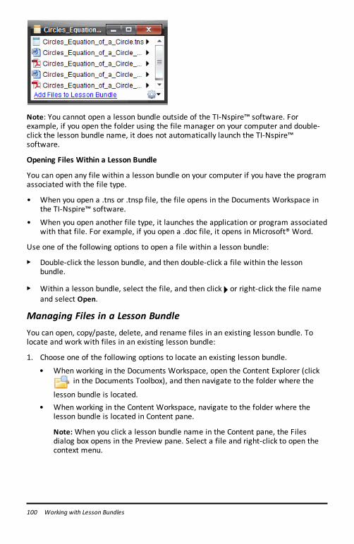
100 Working with Lesson Bundles
Note: You cannot open a lesson bundle outside of the TI-Nspire™ software. Forexample, if you open the folder using the file manager on your computer and double-click the lesson bundle name, it does not automatically launch the TI-Nspire™software.
Opening Files Within a Lesson Bundle
You can open any file within a lesson bundle on your computer if you have the programassociated with the file type.
• When you open a .tns or .tnsp file, the file opens in the Documents Workspace inthe TI-Nspire™ software.
• When you open another file type, it launches the application or program associatedwith that file. For example, if you open a .doc file, it opens in Microsoft® Word.
Use one of the following options to open a file within a lesson bundle:
▶ Double-click the lesson bundle, and then double-click a file within the lessonbundle.
▶ Within a lesson bundle, select the file, and then click ¢ or right-click the file nameand select Open.
Managing Files in a Lesson BundleYou can open, copy/paste, delete, and rename files in an existing lesson bundle. Tolocate and work with files in an existing lesson bundle:
1. Choose one of the following options to locate an existing lesson bundle.
• When working in the Documents Workspace, open the Content Explorer (clickin the Documents Toolbox), and then navigate to the folder where the
lesson bundle is located.• When working in the Content Workspace, navigate to the folder where the
lesson bundle is located in Content pane.
Note: When you click a lesson bundle name in the Content pane, the Filesdialog box opens in the Preview pane. Select a file and right-click to open thecontext menu.
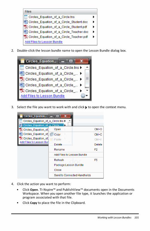
2. Double-click the lesson bundle name to open the Lesson Bundle dialog box.
3. Select the file you want to work with and click ¢ to open the context menu.
4. Click the action you want to perform:
• Click Open. TI-Nspire™ and PublishView™ documents open in the DocumentsWorkspace. When you open another file type, it launches the application orprogram associated with that file.
• Click Copy to place the file in the Clipboard.
Working with Lesson Bundles 101
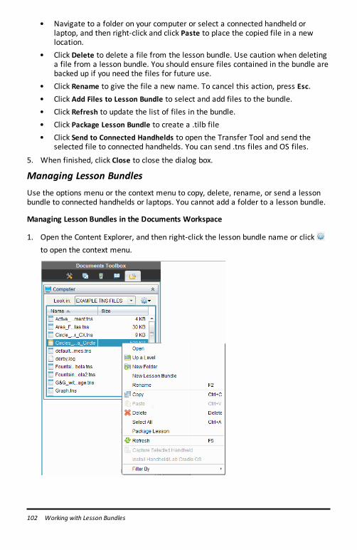
102 Working with Lesson Bundles
• Navigate to a folder on your computer or select a connected handheld orlaptop, and then right-click and click Paste to place the copied file in a newlocation.
• Click Delete to delete a file from the lesson bundle. Use caution when deletinga file from a lesson bundle. You should ensure files contained in the bundle arebacked up if you need the files for future use.
• Click Rename to give the file a new name. To cancel this action, press Esc.• Click Add Files to Lesson Bundle to select and add files to the bundle.• Click Refresh to update the list of files in the bundle.• Click Package Lesson Bundle to create a .tilb file• Click Send to Connected Handhelds to open the Transfer Tool and send the
selected file to connected handhelds. You can send .tns files and OS files.
5. When finished, click Close to close the dialog box.
Managing Lesson BundlesUse the options menu or the context menu to copy, delete, rename, or send a lessonbundle to connected handhelds or laptops. You cannot add a folder to a lesson bundle.
Managing Lesson Bundles in the Documents Workspace
1. Open the Content Explorer, and then right-click the lesson bundle name or clickto open the context menu.
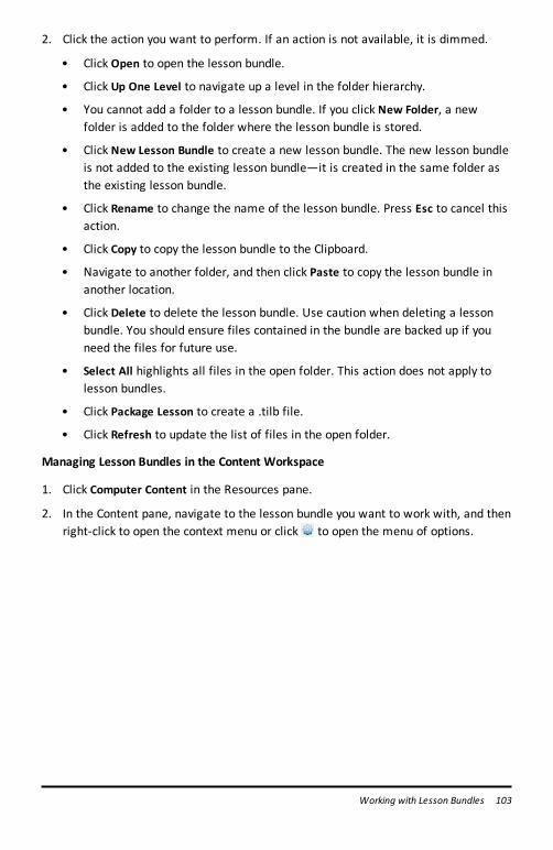
2. Click the action you want to perform. If an action is not available, it is dimmed.
• Click Open to open the lesson bundle.
• Click Up One Level to navigate up a level in the folder hierarchy.
• You cannot add a folder to a lesson bundle. If you click New Folder, a newfolder is added to the folder where the lesson bundle is stored.
• Click New Lesson Bundle to create a new lesson bundle. The new lesson bundleis not added to the existing lesson bundle—it is created in the same folder asthe existing lesson bundle.
• Click Rename to change the name of the lesson bundle. Press Esc to cancel thisaction.
• Click Copy to copy the lesson bundle to the Clipboard.
• Navigate to another folder, and then click Paste to copy the lesson bundle inanother location.
• Click Delete to delete the lesson bundle. Use caution when deleting a lessonbundle. You should ensure files contained in the bundle are backed up if youneed the files for future use.
• Select All highlights all files in the open folder. This action does not apply tolesson bundles.
• Click Package Lesson to create a .tilb file.
• Click Refresh to update the list of files in the open folder.
Managing Lesson Bundles in the Content Workspace
1. Click Computer Content in the Resources pane.
2. In the Content pane, navigate to the lesson bundle you want to work with, and thenright-click to open the context menu or click to open the menu of options.
Working with Lesson Bundles 103
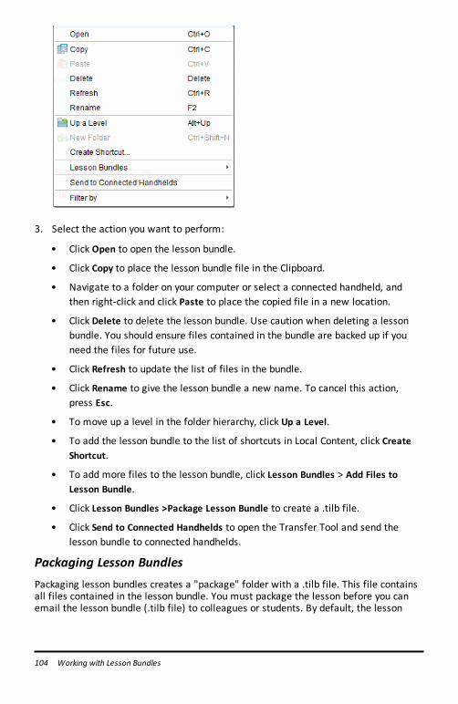
104 Working with Lesson Bundles
3. Select the action you want to perform:
• Click Open to open the lesson bundle.
• Click Copy to place the lesson bundle file in the Clipboard.
• Navigate to a folder on your computer or select a connected handheld, andthen right-click and click Paste to place the copied file in a new location.
• Click Delete to delete the lesson bundle. Use caution when deleting a lessonbundle. You should ensure files contained in the bundle are backed up if youneed the files for future use.
• Click Refresh to update the list of files in the bundle.
• Click Rename to give the lesson bundle a new name. To cancel this action,press Esc.
• To move up a level in the folder hierarchy, click Up a Level.
• To add the lesson bundle to the list of shortcuts in Local Content, click CreateShortcut.
• To add more files to the lesson bundle, click Lesson Bundles > Add Files toLesson Bundle.
• Click Lesson Bundles >Package Lesson Bundle to create a .tilb file.
• Click Send to Connected Handhelds to open the Transfer Tool and send thelesson bundle to connected handhelds.
Packaging Lesson BundlesPackaging lesson bundles creates a "package" folder with a .tilb file. This file containsall files contained in the lesson bundle. You must package the lesson before you canemail the lesson bundle (.tilb file) to colleagues or students. By default, the lesson
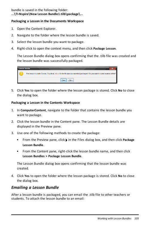
bundle is saved in the following folder:...\TI-Nspire\New Lesson Bundle1.tilb\package\...
Packaging a Lesson in the Documents Workspace
1. Open the Content Explorer.
2. Navigate to the folder where the lesson bundle is saved.
3. Select the lesson bundle you want to package.
4. Right-click to open the context menu, and then click Package Lesson.
The Lesson Bundle dialog box opens confirming that the .tilb file was created andthe lesson bundle was successfully packaged.
5. Click Yes to open the folder where the lesson package is stored. Click No to closethe dialog box.
Packaging a Lesson in the Contents Workspace
1. In ComputerContent, navigate to the folder that contains the lesson bundle youwant to package.
2. Click the lesson bundle in the Content pane. The Lesson Bundle details aredisplayed in the Preview pane.
3. Use one of the following methods to create the package:
• From the Preview pane, click ¢ in the Files dialog box, and then click PackageLesson Bundle.
• From the Content pane, right-click the lesson bundle name, and then clickLesson Bundles > Package Lesson Bundle.
The Lesson Bundle dialog box opens confirming that the lesson bundle wascreated.
4. Click Yes to open the folder where the lesson package is stored. Click No to closethe dialog box.
Emailing a Lesson BundleAfter a lesson bundle is packaged, you can email the .tilb file to other teachers orstudents. To attach the lesson bundle to an email:
Working with Lesson Bundles 105

106 Working with Lesson Bundles
1. In your email client, select the option needed to attach a file, and then navigate tothe .tilb folder.
2. Make sure you open the folder and select the .tilb file to attach to the email. Youcannot email the .tilb folder.
Sending Lesson Bundles to Connected Handhelds1. Complete one of the following actions to select a lesson bundle:
• In the Documents Workspace, open the Content Explorer, and then select thelesson bundle you want to send.
• In the Content Workspace, navigate to the lesson you want to send in theContent pane.
2. Drag the lesson bundle file to a connected handheld. You can also copy the lessonbundle, and then paste it to a connected handheld.
The lesson bundle is transferred to the handheld as a folder with the same name. Only.tns files are transferred to the handheld.
Capturing ScreensScreen Capture enables you to:
• Capture Page
- Capture the active page in a TI-Nspire™ document from the software or fromthe TI-SmartView™ emulator as an image.
- Save captured images as .jpg, .gif, .png, or .tif files, which can be inserted intoTI-Nspire™ applications that allow images.
- Copy and paste images into another application such as Microsoft® Word.
• Capture Selected Handheld
- Capture the current screen on a connected handheld as an image.- Save captured images as .jpg, .gif, .png, or .tif files, which can be inserted into
TI-Nspire™ applications that allow images.- Copy and paste images into another application such as Microsoft® Word.
• Capture Images in Handheld Mode
- In the Documents Workspace, use the DragScreen feature to capture theemulator screen or side screen when the TI-SmartView™ Emulator is active.
- Teachers can use this feature to drag and paste an image to presentation toolssuch as SMART® Notebook, Promethean’s Flipchart, and Microsoft® Officeapplications including Word and PowerPoint®.
Accessing Screen CaptureThe Screen Capture tool is available from all workspaces. To access Screen Capture:
▶ From the menu bar, click Tools > Screen Capture.
▶ From the toolbar, click .
Using Capture PageUse the Capture Page option to capture an image of an active page in a TI-Nspire™document. You can save images in the following file formats: .jpg, .gif, .png, and .tif.Saved images can be inserted into TI-Nspire™ applications that allow images. Theimage is also copied to the Clipboard and can be pasted into other applications such asMicrosoft® Word or PowerPoint®.
Capturing a Page
Complete the following steps to capture an image of an active page.
1. In the Documents Workspace, open a document and navigate to the page you wantto capture to make it active.
2. Click , and then click Capture Page.
Capturing Screens 107
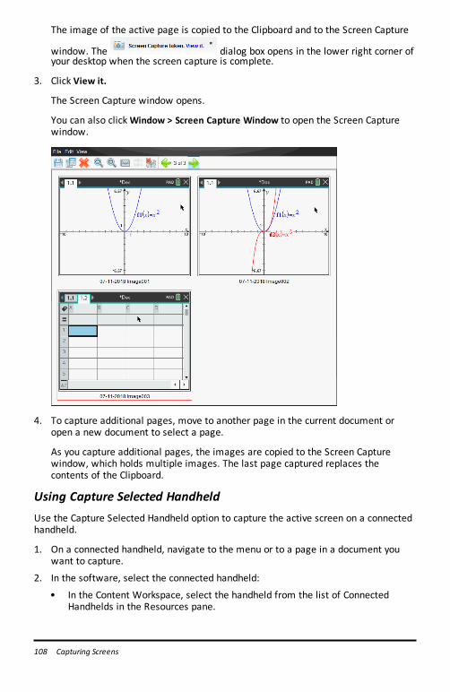
108 Capturing Screens
The image of the active page is copied to the Clipboard and to the Screen Capture
window. The dialog box opens in the lower right corner ofyour desktop when the screen capture is complete.
3. Click View it.
The Screen Capture window opens.
You can also clickWindow > Screen Capture Window to open the Screen Capturewindow.
4. To capture additional pages, move to another page in the current document oropen a new document to select a page.
As you capture additional pages, the images are copied to the Screen Capturewindow, which holds multiple images. The last page captured replaces thecontents of the Clipboard.
Using Capture Selected HandheldUse the Capture Selected Handheld option to capture the active screen on a connectedhandheld.
1. On a connected handheld, navigate to the menu or to a page in a document youwant to capture.
2. In the software, select the connected handheld:
• In the Content Workspace, select the handheld from the list of ConnectedHandhelds in the Resources pane.
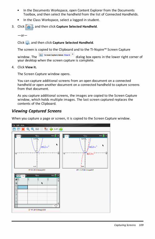
• In the Documents Workspace, open Content Explorer from the DocumentsToolbox, and then select the handheld from the list of Connected Handhelds.
• In the Class Workspace, select a logged in student.
3. Click , and then click Capture Selected Handheld.
—or—
Click , and then click Capture Selected Handheld.
The screen is copied to the Clipboard and to the TI-Nspire™ Screen Capture
window. The dialog box opens in the lower right corner ofyour desktop when the screen capture is complete.
4. Click View it.
The Screen Capture window opens.
You can capture additional screens from an open document on a connectedhandheld or open another document on a connected handheld to capture screensfrom that document.
As you capture additional screens, the images are copied to the Screen Capturewindow, which holds multiple images. The last screen captured replaces thecontents of the Clipboard.
Viewing Captured ScreensWhen you capture a page or screen, it is copied to the Screen Capture window.
Capturing Screens 109
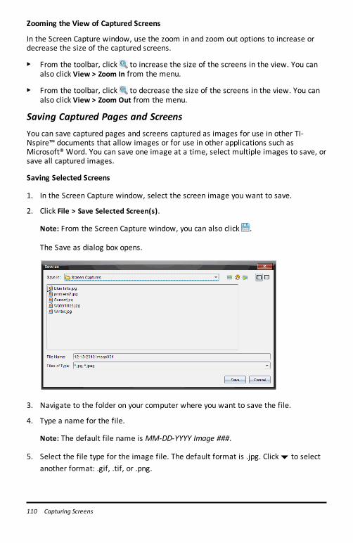
110 Capturing Screens
Zooming the View of Captured Screens
In the Screen Capture window, use the zoom in and zoom out options to increase ordecrease the size of the captured screens.
▶ From the toolbar, click to increase the size of the screens in the view. You canalso click View > Zoom In from the menu.
▶ From the toolbar, click to decrease the size of the screens in the view. You canalso click View > Zoom Out from the menu.
Saving Captured Pages and ScreensYou can save captured pages and screens captured as images for use in other TI-Nspire™ documents that allow images or for use in other applications such asMicrosoft® Word. You can save one image at a time, select multiple images to save, orsave all captured images.
Saving Selected Screens
1. In the Screen Capture window, select the screen image you want to save.
2. Click File > Save Selected Screen(s).
Note: From the Screen Capture window, you can also click .
The Save as dialog box opens.
3. Navigate to the folder on your computer where you want to save the file.
4. Type a name for the file.
Note: The default file name is MM-DD-YYYY Image ###.
5. Select the file type for the image file. The default format is .jpg. Click ¤ to selectanother format: .gif, .tif, or .png.
6. Click Save.
The file is saved in the designated folder.
Saving Multiple Screens
1. In the Screen Capture window, select the screens you want to save.
To select multiple consecutive screens, click the first image, and then hold downthe Shift key and click the additional images. To select screens in random order,press Ctrl (Mac®: “) and click each image you want to save.
2. Click or select File > Save Selected Screen(s). To save all captured screens, selectFile > Save All Screens.
Note: The "Save All Screens" option is not available when using Capture Class.
The Save as dialog box opens.
3. In the Save In field, navigate to the folder where you want to save the images.
4. In the File Name field, type a new folder name. The default folder name is MM-DD-YYYY Image, where MM-DD-YYYY is the current date.
5. Select the file type for the image files. The default format is .jpg. Click ¤ to selectanother format: .gif, .tif, or .png.
6. Click Save.
The images are saved in the specified folder with system-assigned namesreflecting the current date and a sequence number. For example, MM-DD-YYYYImage 001.jpg, MM-DD-YYYY Image 002.jpg and so on.
Copying and Pasting a ScreenYou can select a captured screen and copy it to the Clipboard for inclusion into otherdocuments or applications. You can also print copied screens. Copied screens arecaptured at 100% zoom level, and they are copied in the order of selection.
Copying a Screen
1. Select the screen to copy.
2. Click or Edit > Copy.
The selected screen is copied to the Clipboard.
Pasting a Screen
Depending on the application you are pasting to, click Edit > Paste.
Capturing Screens 111
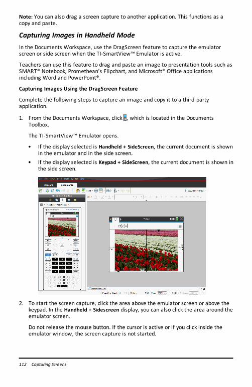
112 Capturing Screens
Note: You can also drag a screen capture to another application. This functions as acopy and paste.
Capturing Images in Handheld ModeIn the Documents Workspace, use the DragScreen feature to capture the emulatorscreen or side screen when the TI-SmartView™ Emulator is active.
Teachers can use this feature to drag and paste an image to presentation tools such asSMART® Notebook, Promethean’s Flipchart, and Microsoft® Office applicationsincluding Word and PowerPoint®.
Capturing Images Using the DragScreen Feature
Complete the following steps to capture an image and copy it to a third-partyapplication.
1. From the Documents Workspace, click , which is located in the DocumentsToolbox.
The TI-SmartView™ Emulator opens.
• If the display selected is Handheld + SideScreen, the current document is shownin the emulator and in the side screen.
• If the display selected is Keypad + SideScreen, the current document is shown inthe side screen.
2. To start the screen capture, click the area above the emulator screen or above thekeypad. In the Handheld + Sidescreen display, you can also click the area around theemulator screen.
Do not release the mouse button. If the cursor is active or if you click inside theemulator window, the screen capture is not started.

InHandheld + SideScreen view, click the areaabove the emulator, click the area around theemulator, or click the border of the emulatorscreen to start the screen capture.
In Keypad+ SideScreen view, click the areaabove the keypad to start the screen capture.
3. Without releasing the mouse, drag the image.
A ghost image of the captured screen opens. The ghost image remains visible untilyou release the mouse button.
The in the corner of the ghost image indicates you cannot paste the image inthat location.
4. Drag the image to an open third-party application. When the image is on top of thethird-party application, the indicates you can drop the image.
5. Release the mouse button to drop the image into the selected application.
The image is also copied to the Clipboard and to the TI-Nspire™ Screen Capturewindow.
To view captured images in the Screen Capture window, clickWindow > ScreenCapture Window.
Capturing Screens 113

114 Capturing Screens
You can capture additional screens as needed. As you capture additional screens,the images are copied to the Screen Capture window, which holds multipleimages. The last screen captured replaces the contents of the Clipboard.
Working with ImagesImages can be used in TI-Nspire™ applications for reference, assessment, andinstructional purposes. You can add images to the following TI-Nspire™ applications:
• Graphs & Geometry
• Data & Statistics
• Notes
• Question, including Quick Poll
In the Graphs & Geometry and Data & Statistics applications, images are set in thebackground behind the axis and other objects. In the Notes and Question applications,the image is set at the cursor location inline with the text (in the foreground).
You can insert the following image file types: .jpg, .png, or .bmp.
Note: The transparency feature of a .png file type is not supported. Transparentbackgrounds are displayed as white.
Working with Images in the SoftwareWhen working in the TI-Nspire™ software, you can insert, copy, move, and deleteimages.
Inserting Images
In the Notes and Question applications, and in Quick Poll, you can insert more than oneimage on a page. You can only insert one image on a page in the Graphs & Geometryand Data & Statistics applications.
1. Open the document where you want to add an image.
2. Click Insert > Image.
The Insert Image dialog box opens.
Working with Images 115
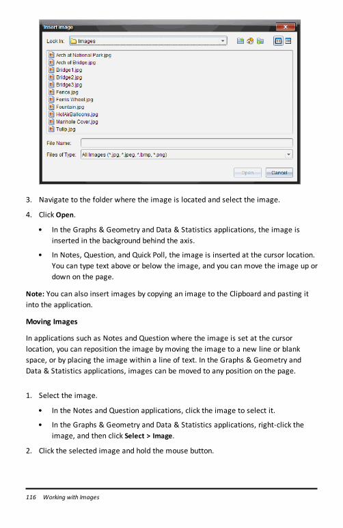
116 Working with Images
3. Navigate to the folder where the image is located and select the image.
4. Click Open.
• In the Graphs & Geometry and Data & Statistics applications, the image isinserted in the background behind the axis.
• In Notes, Question, and Quick Poll, the image is inserted at the cursor location.You can type text above or below the image, and you can move the image up ordown on the page.
Note: You can also insert images by copying an image to the Clipboard and pasting itinto the application.
Moving Images
In applications such as Notes and Question where the image is set at the cursorlocation, you can reposition the image by moving the image to a new line or blankspace, or by placing the image within a line of text. In the Graphs & Geometry andData & Statistics applications, images can be moved to any position on the page.
1. Select the image.
• In the Notes and Question applications, click the image to select it.
• In the Graphs & Geometry and Data & Statistics applications, right-click theimage, and then click Select > Image.
2. Click the selected image and hold the mouse button.
• If an image is in the foreground, the cursor changes to .
• If an image is in the background, the cursor changes to .
3. Drag the image to the new location and release the mouse button to place theimage.
If an image is in the foreground, the cursor changes to when you hover yourmouse pointer over a location where there is a new line or space. Images in thebackground can be moved and placed anywhere on the page.
Resizing Images
To retain the aspect ratio of an image, resize by grabbing the image at one of the fourcorners.
1. Select the image.
• In the Notes and Question applications, click the image to select it.
• In the Graphs & Geometry and Data & Statistics applications, right-click theimage, and then click Select > Image.
2. Move the cursor to one of the corners of the image.
The cursor changes to (a four-sided directional arrow).
Note: If you drag the cursor to an edge of the image, the cursor changes to (atwo-sided directional arrow). If you drag an image from one of its edges to resizeit, the image becomes distorted.
3. Click the corner or edge of the image.
The tool is enabled.
4. Drag in to make the image smaller or drag out to make the image larger.
5. Release the mouse when the image size is correct.
Deleting Images
To delete an image from an open document, complete the following steps.
1. Select the image.
• If an image is in the foreground, click the image to select it.
• If an image is in the background, right-click the image, and then click Select >Image.
Working with Images 117

118 Working with Images
2. Press Delete.
The image is removed.
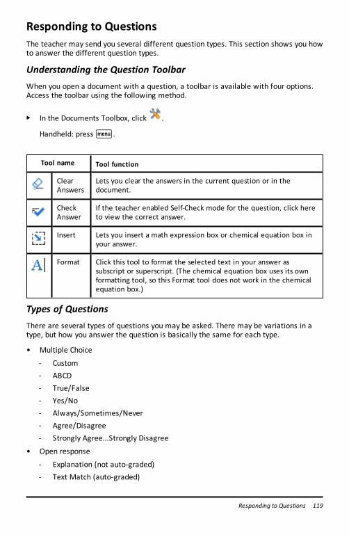
Responding to QuestionsThe teacher may send you several different question types. This section shows you howto answer the different question types.
Understanding the Question ToolbarWhen you open a document with a question, a toolbar is available with four options.Access the toolbar using the following method.
▶ In the Documents Toolbox, click .
Handheld: pressb.
Tool name Tool function
ClearAnswers
Lets you clear the answers in the current question or in thedocument.
CheckAnswer
If the teacher enabled Self-Check mode for the question, click hereto view the correct answer.
Insert Lets you insert a math expression box or chemical equation box inyour answer.
Format Click this tool to format the selected text in your answer assubscript or superscript. (The chemical equation box uses its ownformatting tool, so this Format tool does not work in the chemicalequation box.)
Types of QuestionsThere are several types of questions you may be asked. There may be variations in atype, but how you answer the question is basically the same for each type.
• Multiple Choice
- Custom- ABCD- True/False- Yes/No- Always/Sometimes/Never- Agree/Disagree- Strongly Agree...Strongly Disagree
• Open response
- Explanation (not auto-graded)- Text Match (auto-graded)
Responding to Questions 119
120 Responding to Questions
• Equations and Expressions
- y=- f(x)=- Expression
• Coordinate Points and Lists
- (x,y) numerical input- Drop Point(s)- List(s)
• Image
- Label- Point on
• Chemistry
Responding to Quick Poll QuestionsWhen teachers send quick polls during class, the question opens as a new document ontop of any document you may currently have open. You can access other applications toperform calculations, and check or clear answers before submitting your answer to thequestion or quick poll.
Note: On TI-Nspire™ CX or TI-Nspire™ CX CAS handhelds, questions appear in color ifthe teacher applied color when writing the question. Although you can see color in thequestions you receive, you cannot add color to the responses you submit.
Accessing Other Applications
If the teacher gives permission, the Quick Poll tool allows you to temporarily exit thequestion to perform calculations or access other documents to determine the answerto the question. For example, you can access the Scratchpad to perform a calculation,or you can access the Lists & Spreadsheet application and copy data from there to aList question type. In a List question, you can link to variables from the VernierDataQuest™ or Lists & Spreadsheet applications.
To access other applications while in the Quick Poll screen:
1. Open a new document.
Handheld: Pressc to open the Home screen.
2. Choose an application.
Handheld: To return to the Quick Poll without accessing any documents, chooseC: Quick Poll.
3. When you are finished, click the Quick Poll icon.
When you respond to a poll, your response is immediately sent to the teacher’scomputer and teachers can track student responses in real time.
Showing Your Work
The teacher may request you to show work for your response. If so, the response areahas sections for you to write your starting point, your steps, and the final answer.
Responding to Different Question Types
▶ For Multiple Choice questions, press Tab to navigate to a response. Press Enter tomark a response.
▶ For Open Response questions, type a response.
▶ For Equation questions, type a response. If a graph is included in a question, thegraph updates when you press Enter. Any functions entered show up on the graph,and the cursor remains in the answer box. You cannot manipulate the graph itself.
▶ For Expression questions, type a response. If the response type is Number, yourresponse must be in the form of a number. If the response type is Expression, yourresponse must be in the form of an expression. For example, x+1.
▶ For Coordinate Points: (x,y) questions, type an answer in the x-field box, and pressTab to move to the y-field box. Type an answer.
If a graph is included with the question, the graph is updated when you enter afunction and press Enter.
You can access the Window and Zoom functions while you are working on thegraph.
▶ For Coordinate Points: Drop Points questions, press Tab to move the cursor to apoint on the graph. Press Enter to drop a point at that location.
To delete a point, press Ctrl + Z to undo the action.
▶ For Lists questions, press Tab if necessary to move the cursor to the first cell of thelist. Type an answer, and press Tab to move to the next cell. Type an answer.
To link a column to an existing variable, select the column and then click var. ClickLink To, and then click the variable you want to link to.
The behavior in a Lists question closely matches the behavior of the Lists &Spreadsheet application, with the following exceptions. In a Lists question, youcannot:
• Add, insert, or delete columns.• Change the header row.• Enter formulas.• Switch to Table.• Create plots.
▶ For Chemistry questions, type a response.
▶ For Image: Label questions, press Tab to move the cursor to a label on the image.Type a response in the label field.
Responding to Questions 121
122 Responding to Questions
▶ For Image: Point on questions, press Tab to move the cursor to a point on theimage. Press Enter to mark a response.
Checking Answers
If the teacher enables self-check on the question, the Check Answer option is available.
1. Click .
Handheld: Pressb.
2. Click Check Answer.
Clearing Answers
After you answer a quick poll, you may decide you want to change the answer beforeyou submit it.
▶ ClickMenu > Clear Answers > Current Question or Document.
• Current Question clears answers for the active question.• Document clears answers for all questions contained in the active document.
—or—
If you answered the question, you still have time to clear the answer before you submitit to your teacher.
▶ Click Clear Answer to clear your answer and try again.
Handheld: Press~ and choose Clear Answer.
Submitting ResponsesTo send a final answer to the teacher:
▶ Click Submit Response.
Handheld: Press~ and choose Submit.
The response is sent to the teacher and the last screen you used is displayed.
Your response appears on the teacher’s computer. Your teacher may have set the pollto allow you to submit more than one answer. If so, you can continue to respond to thepoll and submit answers until the teacher stops the poll.
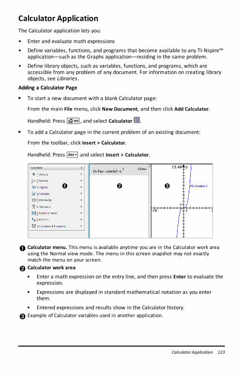
Calculator ApplicationThe Calculator application lets you:
• Enter and evaluate math expressions
• Define variables, functions, and programs that become available to any TI-Nspire™application—such as the Graphs application—residing in the same problem.
• Define library objects, such as variables, functions, and programs, which areaccessible from any problem of any document. For information on creating libraryobjects, see Libraries.
Adding a Calculator Page
▶ To start a new document with a blank Calculator page:
From the main File menu, click New Document, and then click Add Calculator.
Handheld: Pressc, and select Calculator .
▶ To add a Calculator page in the current problem of an existing document:
From the toolbar, click Insert > Calculator.
Handheld: Press~ and select Insert > Calculator.
À Calculator menu. This menu is available anytime you are in the Calculator work areausing the Normal view mode. The menu in this screen snapshot may not exactlymatch the menu on your screen.
Á Calculator work area
• Enter a math expression on the entry line, and then press Enter to evaluate theexpression.
• Expressions are displayed in standard mathematical notation as you enterthem.
• Entered expressions and results show in the Calculator history. Example of Calculator variables used in another application.
Calculator Application 123
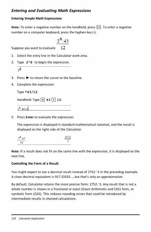
124 Calculator Application
Entering and Evaluating Math Expressions
Entering Simple Math Expressions
Note: To enter a negative number on the handheld, pressv. To enter a negativenumber on a computer keyboard, press the hyphen key (-).
Suppose you want to evaluate
1. Select the entry line in the Calculator work area.
2. Type 2^8 to begin the expression.
3. Press ► to return the cursor to the baseline.
4. Complete the expression:
Type *43/12.
Handheld: Typer 43p 12.
5. Press Enter to evaluate the expression.
The expression is displayed in standard mathematical notation, and the result isdisplayed on the right side of the Calculator.
Note: If a result does not fit on the same line with the expression, it is displayed on thenext line.
Controlling the Form of a Result
You might expect to see a decimal result instead of 2752 ⁄ 3 in the preceding example.A close decimal equivalent is 917.33333..., but that’s only an approximation.
By default, Calculator retains the more precise form: 2752 ⁄ 3. Any result that is not awhole number is shown in a fractional or exact (Exact Arithmetic and CAS) form, orsymbolic form (CAS). This reduces rounding errors that could be introduced byintermediate results in chained calculations.
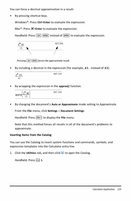
You can force a decimal approximation in a result:
• By pressing shortcut keys.
Windows®: Press Ctrl+Enter to evaluate the expression.
Mac®: Press “+Enter to evaluate the expression.
Handheld: Press/· instead of· to evaluate the expression.
Pressing/· forces the approximate result.
• By including a decimal in the expression (for example, 43. instead of 43).
• By wrapping the expression in the approx() function.
• By changing the document’s Auto or Approximate mode setting to Approximate.
From the File menu, click Settings > Document Settings.
Handheld: Press~ to display the File menu.
Note that this method forces all results in all of the document’s problems toapproximate.
Inserting Items from the Catalog
You can use the Catalog to insert system functions and commands, symbols, andexpression templates into the Calculator entry line.
1. Click the Utilities tab, and then click to open the Catalog.
Handheld: Pressk 1.
Calculator Application 125
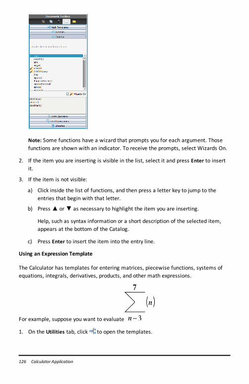
126 Calculator Application
Note: Some functions have a wizard that prompts you for each argument. Thosefunctions are shown with an indicator. To receive the prompts, select Wizards On.
2. If the item you are inserting is visible in the list, select it and press Enter to insertit.
3. If the item is not visible:
a) Click inside the list of functions, and then press a letter key to jump to theentries that begin with that letter.
b) Press ▲ or ▼ as necessary to highlight the item you are inserting.
Help, such as syntax information or a short description of the selected item,appears at the bottom of the Catalog.
c) Press Enter to insert the item into the entry line.
Using an Expression Template
The Calculator has templates for entering matrices, piecewise functions, systems ofequations, integrals, derivatives, products, and other math expressions.
For example, suppose you want to evaluate
1. On the Utilities tab, click to open the templates.
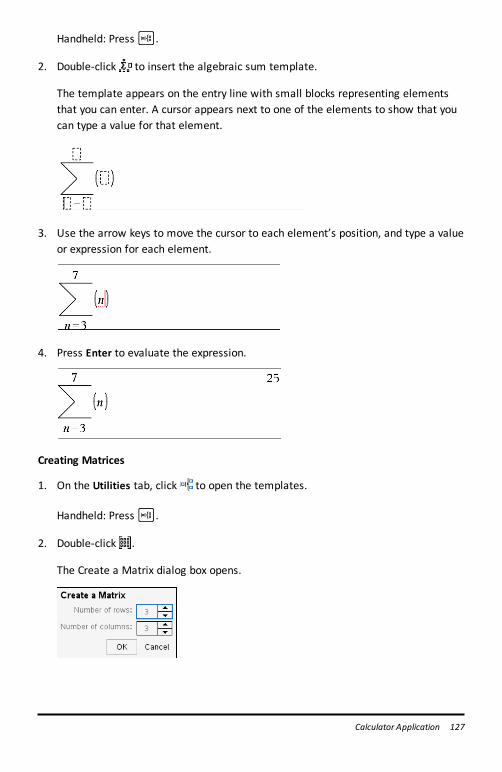
Handheld: Presst.
2. Double-click to insert the algebraic sum template.
The template appears on the entry line with small blocks representing elementsthat you can enter. A cursor appears next to one of the elements to show that youcan type a value for that element.
3. Use the arrow keys to move the cursor to each element’s position, and type a valueor expression for each element.
4. Press Enter to evaluate the expression.
Creating Matrices
1. On the Utilities tab, click to open the templates.
Handheld: Presst.
2. Double-click .
The Create a Matrix dialog box opens.
Calculator Application 127
128 Calculator Application
3. Type the Number of rows.
4. Type the Number of columns, and then click OK.
Calculator opens a template with spaces for the rows and columns.
Note: If you create a matrix with a large number of rows and columns, it may takea few moments to appear.
5. Type the matrix values into the template, and then press Enter to define thematrix.
Inserting a Row or Column into a Matrix
▶ To insert a new row, hold down Alt and press Enter.
▶ To insert a new column, hold down Shift and press Enter.
Handheld:
▶ To insert a new row, press@.
▶ To insert a new column, press Shift+Enter.
Inserting Expressions Using a Wizard
You can use a wizard to simplify entering some expressions. The wizard containslabeled boxes to help you enter the arguments in the expression.
For example, suppose you want to fit a y = mx + b linear regression model to thefollowing two lists:
{1,2,3,4,5}{5,8,11,14,17}
1. On the Utilities tab, click to open the Catalog.
Handheld: Pressk 1.
2. Click an entry in the Catalog, and then press L to jump to the entries that beginwith “L.”
3. Press ▼ as necessary to highlight LinRegMx.
4. Select the Wizards On option, if it is not already selected:
Handheld: Press Tab Tab to highlight Wizards On, press Enter to change the setting,and then press Tab Tab to highlight LinRegMx again.
5. Press Enter.
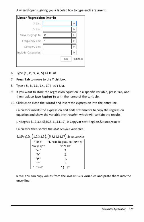
A wizard opens, giving you a labeled box to type each argument.
6. Type {1,2,3,4,5} as X List.
7. Press Tab to move to the Y List box.
8. Type {5,8,11,14,17} as Y List.
9. If you want to store the regression equation in a specific variable, press Tab, andthen replace Save RegEqn To with the name of the variable.
10. Click OK to close the wizard and insert the expression into the entry line.
Calculator inserts the expression and adds statements to copy the regressionequation and show the variable stat.results, which will contain the results.
LinRegMx {1,2,3,4,5},{5,8,11,14,17},1: CopyVar stat.RegEqn,f2: stat.results
Calculator then shows the stat.results variables.
Note: You can copy values from the stat.results variables and paste them into theentry line.
Calculator Application 129
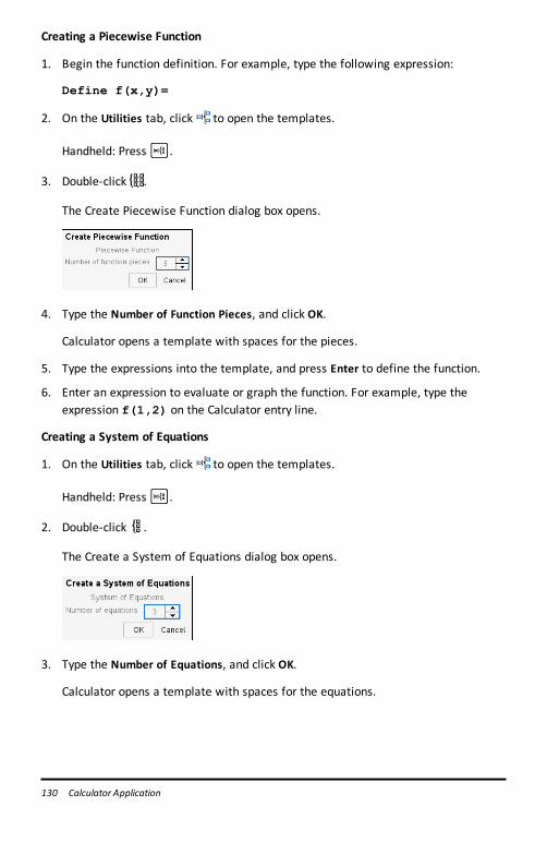
130 Calculator Application
Creating a Piecewise Function
1. Begin the function definition. For example, type the following expression:
Define f(x,y)=
2. On the Utilities tab, click to open the templates.
Handheld: Presst.
3. Double-click .
The Create Piecewise Function dialog box opens.
4. Type the Number of Function Pieces, and click OK.
Calculator opens a template with spaces for the pieces.
5. Type the expressions into the template, and press Enter to define the function.
6. Enter an expression to evaluate or graph the function. For example, type theexpression f(1,2) on the Calculator entry line.
Creating a System of Equations
1. On the Utilities tab, click to open the templates.
Handheld: Presst.
2. Double-click .
The Create a System of Equations dialog box opens.
3. Type the Number of Equations, and click OK.
Calculator opens a template with spaces for the equations.
4. Type the equations into the template, and press Enter to define the system ofequations.
Entering Multiple Statements on the Entry Line
To enter several statements on a single line, separate them with a colon (“:”). Only theresult of the last expression is shown.
CAS: Working with Measurement UnitsA list of pre-defined constants and measurement units is available in the Catalog. Youcan also create your own units.
Note: If you know a unit’s name, you can type the unit directly. For example, you cantype _qt to specify quarts. To type the underscore symbol on the handheld, press/_.
CAS: Converting Between Measurement Units
You can convert a value between any two units within the same category (such aslength).
Example: Using the Catalog, convert 12 meters to feet. The desired expression is 12•_m►_ft.
1. Type 12 on the entry line.
2. On the Utilities tab, click to show the unit conversions.
Handheld: Pressk 3.
Calculator Application 131
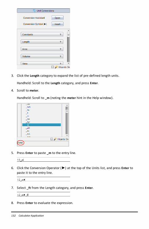
132 Calculator Application
3. Click the Length category to expand the list of pre-defined length units.
Handheld: Scroll to the Length category, and press Enter.
4. Scroll tometer.
Handheld: Scroll to _m (noting the meter hint in the Help window).
5. Press Enter to paste _m to the entry line.
6. Click the Conversion Operator (►) at the top of the Units list, and press Enter topaste it to the entry line.
7. Select _ft from the Length category, and press Enter.
8. Press Enter to evaluate the expression.
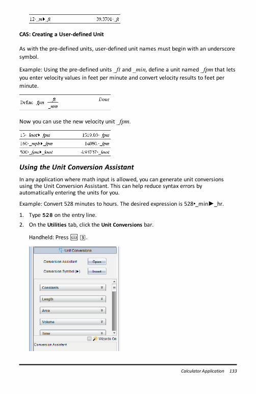
CAS: Creating a User-defined Unit
As with the pre-defined units, user-defined unit names must begin with an underscoresymbol.
Example: Using the pre-defined units _ft and _min, define a unit named _fpm that letsyou enter velocity values in feet per minute and convert velocity results to feet perminute.
Now you can use the new velocity unit _fpm.
Using the Unit Conversion AssistantIn any application where math input is allowed, you can generate unit conversionsusing the Unit Conversion Assistant. This can help reduce syntax errors byautomatically entering the units for you.
Example: Convert 528 minutes to hours. The desired expression is 528•_min►_hr.
1. Type 528 on the entry line.
2. On the Utilities tab, click the Unit Conversions bar.
Handheld: Pressk3.
Calculator Application 133
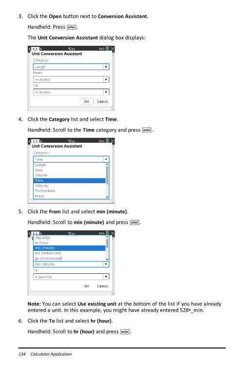
134 Calculator Application
3. Click the Open button next to Conversion Assistant.
Handheld: Press·.
The Unit Conversion Assistant dialog box displays:
4. Click the Category list and select Time.
Handheld: Scroll to the Time category and press·.
5. Click the From list and select min (minute).
Handheld: Scroll tomin (minute) and press·.
Note: You can select Use existing unit at the bottom of the list if you have alreadyentered a unit. In this example, you might have already entered 528•_min.
6. Click the To list and select hr (hour).
Handheld: Scroll to hr (hour) and press·.
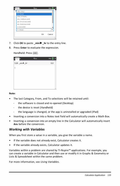
7. Click OK to paste _min►_hr to the entry line.
8. Press Enter to evaluate the expression.
Handheld: Press·.
Note:
• The last Category, From, and To selections will be retained until:
- the software is closed and re-opened (Desktop)- the device is reset (Handheld)- the language is changed, or the app is uninstalled or upgraded (iPad)
• Inserting a conversion into a Notes text field will automatically create a Math Box.
• Inserting a conversion into an empty line in the Calculator will automatically insertAns before the conversion.
Working with VariablesWhen you first store a value in a variable, you give the variable a name.
• If the variable does not already exist, Calculator creates it.
• If the variable already exists, Calculator updates it.
Variables within a problem are shared by TI-Nspire™ applications. For example, youcan create a variable in Calculator and then use or modify it in Graphs & Geometry orLists & Spreadsheet within the same problem.
For more information, see Using Variables.
Calculator Application 135
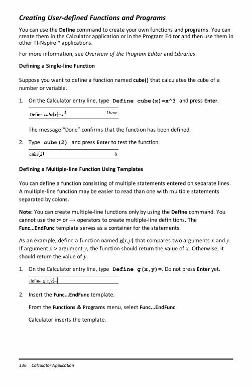
136 Calculator Application
Creating User-defined Functions and ProgramsYou can use the Define command to create your own functions and programs. You cancreate them in the Calculator application or in the Program Editor and then use them inother TI-Nspire™ applications.
For more information, see Overview of the Program Editor and Libraries.
Defining a Single-line Function
Suppose you want to define a function named cube() that calculates the cube of anumber or variable.
1. On the Calculator entry line, type Define cube(x)=x^3 and press Enter.
The message “Done” confirms that the function has been defined.
2. Type cube(2) and press Enter to test the function.
Defining a Multiple-line Function Using Templates
You can define a function consisting of multiple statements entered on separate lines.A multiple-line function may be easier to read than one with multiple statementsseparated by colons.
Note: You can create multiple-line functions only by using the Define command. Youcannot use the := or→ operators to create multiple-line definitions. TheFunc...EndFunc template serves as a container for the statements.
As an example, define a function named g(x,y) that compares two arguments x and y.If argument x > argument y, the function should return the value of x. Otherwise, itshould return the value of y.
1. On the Calculator entry line, type Define g(x,y)=. Do not press Enter yet.
2. Insert the Func...EndFunc template.
From the Functions & Programs menu, select Func...EndFunc.
Calculator inserts the template.
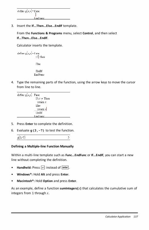
3. Insert the If...Then...Else...EndIf template.
From the Functions & Programs menu, select Control, and then selectIf...Then...Else...EndIf.
Calculator inserts the template.
4. Type the remaining parts of the function, using the arrow keys to move the cursorfrom line to line.
5. Press Enter to complete the definition.
6. Evaluate g(3,-7) to test the function.
Defining a Multiple-line Function Manually
Within a multi-line template such as Func...EndFunc or If...EndIf, you can start a newline without completing the definition.
• Handheld: Press@ instead of·.
• Windows®: Hold Alt and press Enter.
• Macintosh®: Hold Option and press Enter.
As an example, define a function sumIntegers(x) that calculates the cumulative sum ofintegers from 1 through x.
Calculator Application 137
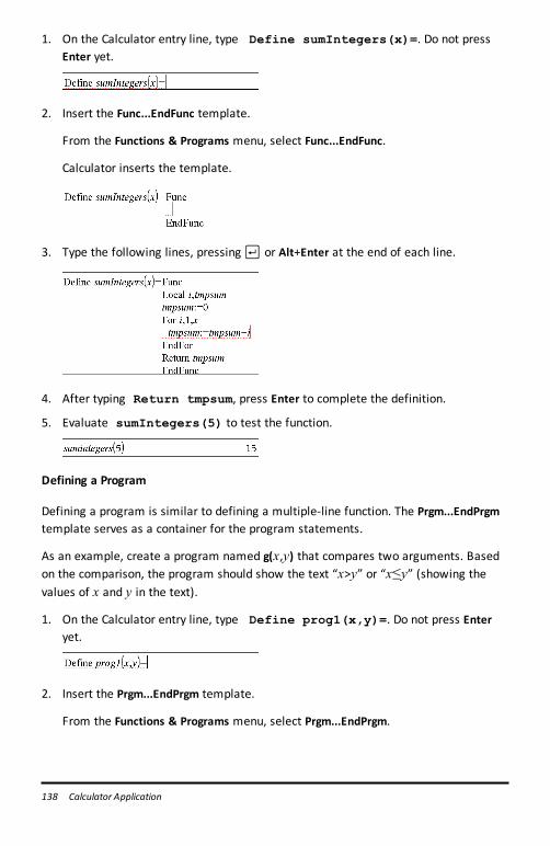
138 Calculator Application
1. On the Calculator entry line, type Define sumIntegers(x)=. Do not pressEnter yet.
2. Insert the Func...EndFunc template.
From the Functions & Programs menu, select Func...EndFunc.
Calculator inserts the template.
3. Type the following lines, pressing@ or Alt+Enter at the end of each line.
4. After typing Return tmpsum, press Enter to complete the definition.
5. Evaluate sumIntegers(5) to test the function.
Defining a Program
Defining a program is similar to defining a multiple-line function. The Prgm...EndPrgmtemplate serves as a container for the program statements.
As an example, create a program named g(x,y) that compares two arguments. Basedon the comparison, the program should show the text “x>y” or “x≤y” (showing thevalues of x and y in the text).
1. On the Calculator entry line, type Define prog1(x,y)=. Do not press Enteryet.
2. Insert the Prgm...EndPrgm template.
From the Functions & Programs menu, select Prgm...EndPrgm.
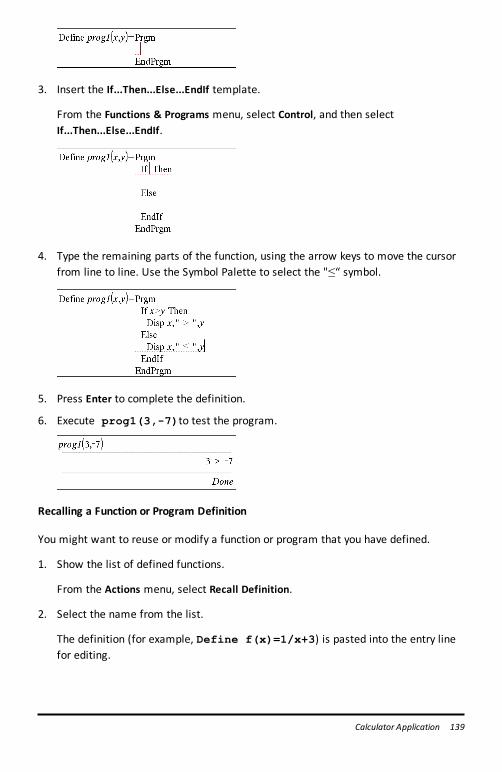
3. Insert the If...Then...Else...EndIf template.
From the Functions & Programs menu, select Control, and then selectIf...Then...Else...EndIf.
4. Type the remaining parts of the function, using the arrow keys to move the cursorfrom line to line. Use the Symbol Palette to select the "≤“ symbol.
5. Press Enter to complete the definition.
6. Execute prog1(3,-7)to test the program.
Recalling a Function or Program Definition
You might want to reuse or modify a function or program that you have defined.
1. Show the list of defined functions.
From the Actions menu, select Recall Definition.
2. Select the name from the list.
The definition (for example, Define f(x)=1/x+3) is pasted into the entry linefor editing.
Calculator Application 139
140 Calculator Application
Editing Calculator ExpressionsAlthough you cannot edit an expression in the Calculator history, you can copy all orpart of an expression from the history and paste it to the entry line. You can then editthe entry line.
Positioning the Cursor in an Expression
▶ Press Tab,◄,►,▲, or▼ to move the cursor through the expression. The cursormoves to the closest valid position in the direction that you press.
Note: An expression template may force the cursor to move through its parameters,even though some parameters may not be exactly in the path of the cursor movement.For example, moving upward from the main argument of an integral always moves thecursor to the top limit.
Inserting into an Expression in the Entry Line
1. Position the cursor at the point where you want to insert additional elements.
2. Type the elements that you want to insert.
Note: When you insert an open parenthesis, Calculator adds a temporary closeparenthesis, displayed in gray. You can override the temporary parenthesis by typingthe same parenthesis manually or by entering something past the temporaryparenthesis (thereby implicitly validating its position in the expression). After youoverride the temporary gray parenthesis, it is replaced with a black parenthesis.
Selecting Part of an Expression
1. Position the cursor at the starting point in the expression.
Handheld: Press ◄,►,▲, or▼ to move the cursor.
2. Press and hold Shift, and then press ◄,►,▲, or▼ to select.
Deleting all or part of an expression on the entry line
1. Select the part of the expression to delete.
2. Press Del.
Financial CalculationsSeveral TI-Nspire™ functions provide financial calculations, such as time value ofmoney, amortization calculations, and return on investment calculations.
The Calculator application also includes a Finance Solver. It lets you dynamically solveseveral types of problems, such as loans and investments.
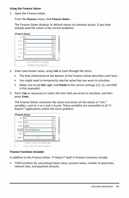
Using the Finance Solver
1. Open the Finance Solver.
From the Finance menu, click Finance Solver.
The Finance Solver displays its default values (or previous values, if you havealready used the solver in the current problem).
2. Enter each known value, using Tab to cycle through the items.
• The help information at the bottom of the Finance Solver describes each item.• You might need to temporarily skip the value that you want to calculate.• Make sure to set PpY, CpY, and PmtAt to the correct settings (12, 12, and END
in this example).
3. Press Tab as necessary to select the item that you want to calculate, and thenpress Enter.
The Finance Solver calculates the value and stores all the values in “tvm.”variables, such as tvm.n and tvm.pmt. These variables are accessible to all TI-Nspire™ applications within the same problem.
Finance Functions Included
In addition to the Finance Solver, TI-Nspire™ built-in finance functions include:
• TVM functions for calculating future value, present value, number of payments,interest rate, and payment amount.
Calculator Application 141
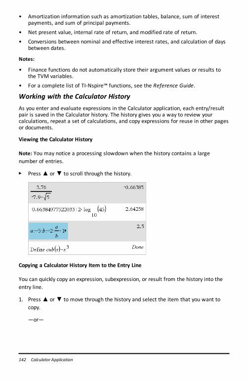
142 Calculator Application
• Amortization information such as amortization tables, balance, sum of interestpayments, and sum of principal payments.
• Net present value, internal rate of return, and modified rate of return.
• Conversions between nominal and effective interest rates, and calculation of daysbetween dates.
Notes:
• Finance functions do not automatically store their argument values or results tothe TVM variables.
• For a complete list of TI-Nspire™ functions, see the Reference Guide.
Working with the Calculator HistoryAs you enter and evaluate expressions in the Calculator application, each entry/resultpair is saved in the Calculator history. The history gives you a way to review yourcalculations, repeat a set of calculations, and copy expressions for reuse in other pagesor documents.
Viewing the Calculator History
Note: You may notice a processing slowdown when the history contains a largenumber of entries.
▶ Press ▲ or▼ to scroll through the history.
Copying a Calculator History Item to the Entry Line
You can quickly copy an expression, subexpression, or result from the history into theentry line.
1. Press ▲ or▼ to move through the history and select the item that you want tocopy.
—or—
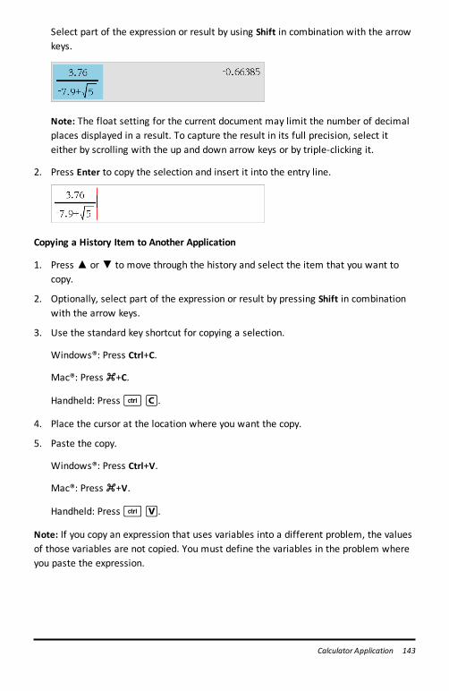
Select part of the expression or result by using Shift in combination with the arrowkeys.
Note: The float setting for the current document may limit the number of decimalplaces displayed in a result. To capture the result in its full precision, select iteither by scrolling with the up and down arrow keys or by triple-clicking it.
2. Press Enter to copy the selection and insert it into the entry line.
Copying a History Item to Another Application
1. Press ▲ or▼ to move through the history and select the item that you want tocopy.
2. Optionally, select part of the expression or result by pressing Shift in combinationwith the arrow keys.
3. Use the standard key shortcut for copying a selection.
Windows®: Press Ctrl+C.
Mac®: Press “+C.
Handheld: Press/C.
4. Place the cursor at the location where you want the copy.
5. Paste the copy.
Windows®: Press Ctrl+V.
Mac®: Press “+V.
Handheld: Press/V.
Note: If you copy an expression that uses variables into a different problem, the valuesof those variables are not copied. You must define the variables in the problem whereyou paste the expression.
Calculator Application 143
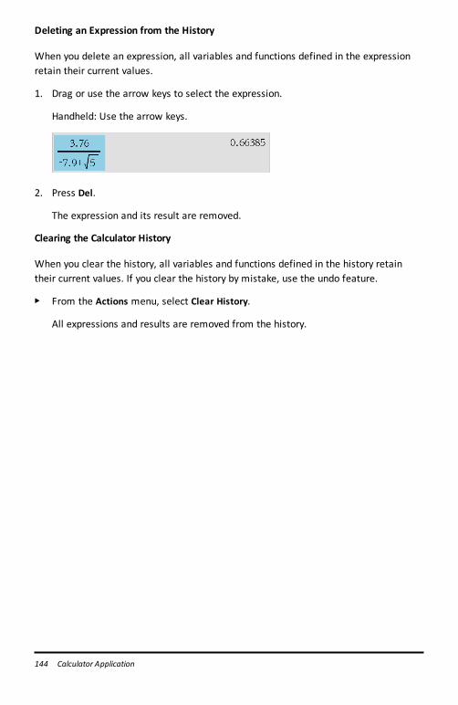
144 Calculator Application
Deleting an Expression from the History
When you delete an expression, all variables and functions defined in the expressionretain their current values.
1. Drag or use the arrow keys to select the expression.
Handheld: Use the arrow keys.
2. Press Del.
The expression and its result are removed.
Clearing the Calculator History
When you clear the history, all variables and functions defined in the history retaintheir current values. If you clear the history by mistake, use the undo feature.
▶ From the Actions menu, select Clear History.
All expressions and results are removed from the history.
Using VariablesA variable is a defined value that can be used multiple times in a problem. You candefine a value or function as a variable within each application. Within a problem,variables are shared by TI-Nspire™ applications. For example, you can create a variablein Calculator, and then use or modify it in Graphs & Geometry or Lists & Spreadsheetwithin the same problem.
Each variable has a name and a definition and the definition can be changed. Whenyou change the definition, all occurrences of the variable in the problem are updated touse the new definition. In the TI-Nspire™ software, a variable has four attributes:
• Name - User-defined name assigned when the variable is created.
• Location - Variables are stored in memory.
• Value - Number, text, mathematical expression, or function.
• Type - Type of data that can be stored as a variable.
Note: Variables created with the Local command within a user-defined function orprogram are not accessible outside that function or program.
Linking Values on PagesValues and functions created or defined in one application can interact with otherapplications (within the same problem) to share data.
When using linked items, keep in mind:
• Values can be linked between applications on one page or between different pagesof the same problem.
• All applications are linked to the same data.
• If the linked value is changed in the original application, the change is reflected inall linked usages.
Defining a variable is the first step in linking values.
Creating VariablesAny portion or attribute of an object or function created within an application can bestored as a variable. Examples of attributes that can become variables are the area ofa rectangle, the radius of a circle, the value contained in a spreadsheet cell or thecontents of a row or column, or a function expression. When you create a variable, it isstored in memory.
Types of Variables
You can store the following data types as variables:
Using Variables 145
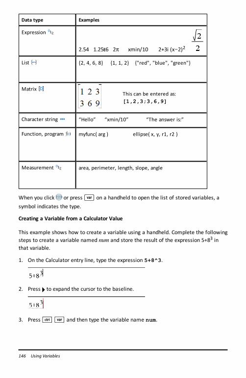
146 Using Variables
Data type Examples
Expression
2.54 1.25E6 2p xmin/10 2+3i (xN2)2
List {2, 4, 6, 8} {1, 1, 2} {"red", "blue", "green"}
MatrixThis can be entered as:[1,2,3;3,6,9]
Character string “Hello” “xmin/10” “The answer is:”
Function, program myfunc( arg ) ellipse( x, y, r1, r2 )
Measurement area, perimeter, length, slope, angle
When you click or pressh on a handheld to open the list of stored variables, asymbol indicates the type.
Creating a Variable from a Calculator Value
This example shows how to create a variable using a handheld. Complete the followingsteps to create a variable named num and store the result of the expression 5+83 inthat variable.
1. On the Calculator entry line, type the expression 5+8^3.
2. Press ¢ to expand the cursor to the baseline.
3. Press/h and then type the variable name num.

This means: Calculate 5+83 and store the result as a variable named num.
4. Press·.
Calculator creates the variable num and stores the result there.
Creating a Variable in the Computer Software
When creating a variable in the computer software, use the following conventions. Asalternatives to using & (store), you can use “:=” or the Define command. All of thefollowing statements are equivalent.
5+83 & numnum := 5+83
Define num=5+83
Checking a Variable’s Value
You can check the value of an existing variable by entering its name on the Calculatorentry line. When you type the name of a stored variable, it appears in bold type.
▶ On the Calculator entry line, type the variable name num and press·.
The value most recently stored in num is displayed as the result.
Automatically Creating Variables in Graphs & Geometry
In the Graphs and Geometry applications, functions defined on the entry line areautomatically stored as variables.
In this example, f1(x)=x3 is a variable definition, which allows it to be displayed inother applications including a table in the Lists & Spreadsheet application.
Using Variables 147
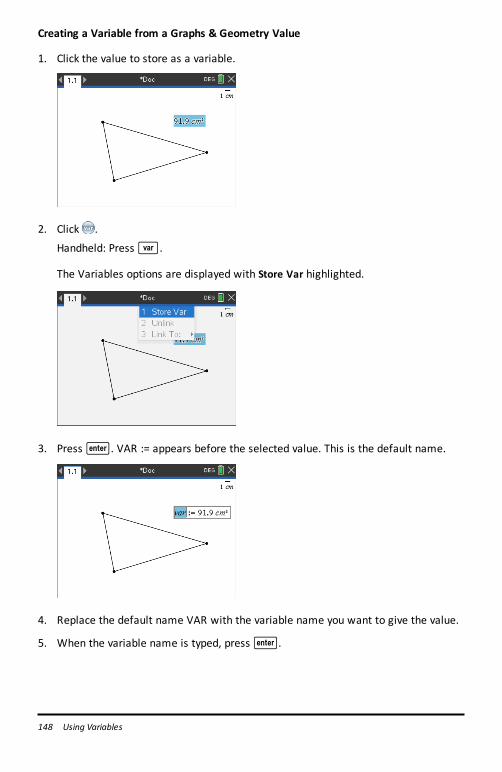
148 Using Variables
Creating a Variable from a Graphs & Geometry Value
1. Click the value to store as a variable.
2. Click .
Handheld: Pressh.
The Variables options are displayed with Store Var highlighted.
3. Press·. VAR := appears before the selected value. This is the default name.
4. Replace the default name VAR with the variable name you want to give the value.
5. When the variable name is typed, press·.
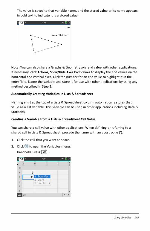
The value is saved to that variable name, and the stored value or its name appearsin bold text to indicate it is a stored value.
Note: You can also share a Graphs & Geometry axis end value with other applications.If necessary, click Actions, Show/Hide Axes End Values to display the end values on thehorizontal and vertical axes. Click the number for an end value to highlight it in theentry field. Name the variable and store it for use with other applications by using anymethod described in Step 2.
Automatically Creating Variables in Lists & Spreadsheet
Naming a list at the top of a Lists & Spreadsheet column automatically stores thatvalue as a list variable. This variable can be used in other applications including Data &Statistics.
Creating a Variable from a Lists & Spreadsheet Cell Value
You can share a cell value with other applications. When defining or referring to ashared cell in Lists & Spreadsheet, precede the name with an apostrophe (‘).
1. Click the cell that you want to share.
2. Click to open the Variables menu.
Handheld: Pressh.
Using Variables 149
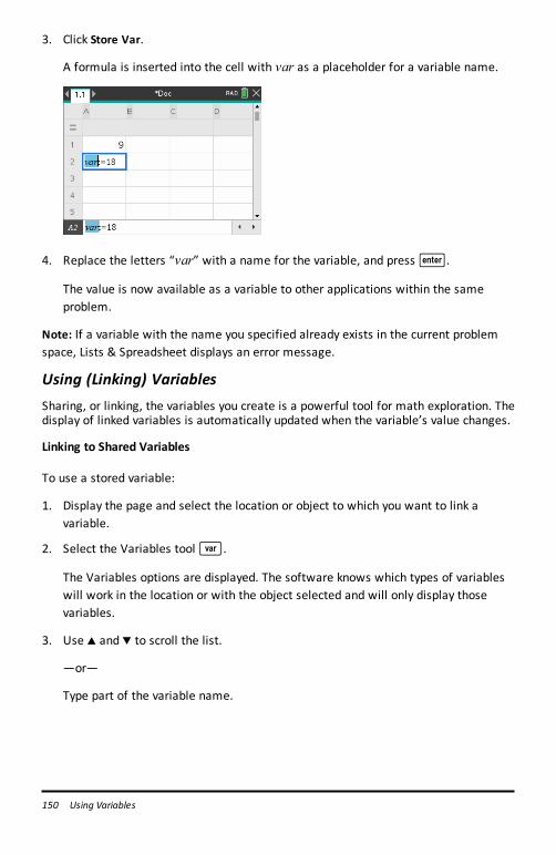
150 Using Variables
3. Click Store Var.
A formula is inserted into the cell with var as a placeholder for a variable name.
4. Replace the letters “var” with a name for the variable, and press·.
The value is now available as a variable to other applications within the sameproblem.
Note: If a variable with the name you specified already exists in the current problemspace, Lists & Spreadsheet displays an error message.
Using (Linking) VariablesSharing, or linking, the variables you create is a powerful tool for math exploration. Thedisplay of linked variables is automatically updated when the variable’s value changes.
Linking to Shared Variables
To use a stored variable:
1. Display the page and select the location or object to which you want to link avariable.
2. Select the Variables toolh.
The Variables options are displayed. The software knows which types of variableswill work in the location or with the object selected and will only display thosevariables.
3. Use 9 and : to scroll the list.
—or—
Type part of the variable name.
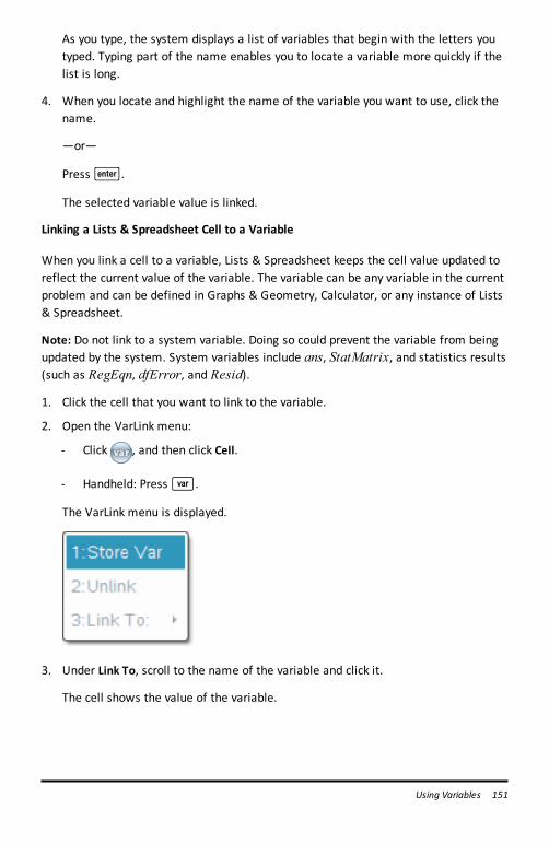
As you type, the system displays a list of variables that begin with the letters youtyped. Typing part of the name enables you to locate a variable more quickly if thelist is long.
4. When you locate and highlight the name of the variable you want to use, click thename.
—or—
Press·.
The selected variable value is linked.
Linking a Lists & Spreadsheet Cell to a Variable
When you link a cell to a variable, Lists & Spreadsheet keeps the cell value updated toreflect the current value of the variable. The variable can be any variable in the currentproblem and can be defined in Graphs & Geometry, Calculator, or any instance of Lists& Spreadsheet.
Note: Do not link to a system variable. Doing so could prevent the variable from beingupdated by the system. System variables include ans, StatMatrix, and statistics results(such as RegEqn, dfError, and Resid).
1. Click the cell that you want to link to the variable.
2. Open the VarLink menu:
- Click , and then click Cell.
- Handheld: Pressh.
The VarLink menu is displayed.
3. Under Link To, scroll to the name of the variable and click it.
The cell shows the value of the variable.
Using Variables 151
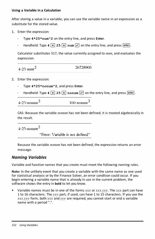
152 Using Variables
Using a Variable in a Calculation
After storing a value in a variable, you can use the variable name in an expression as asubstitute for the stored value.
1. Enter the expression:
- Type 4*25*num^2 on the entry line, and press Enter.
- Handheld: Type 4r 25r numq on the entry line, and press·.
Calculator substitutes 517, the value currently assigned to num, and evaluates theexpression.
2. Enter the expression:
- Type 4*25*nonum^2, and press Enter.
- Handheld: Type 4r 25r nonumq on the entry line, and press·.
CAS: Because the variable nonum has not been defined, it is treated algebraically inthe result.
Because the variable nonum has not been defined, the expression returns an errormessage.
Naming VariablesVariable and function names that you create must meet the following naming rules.
Note: In the unlikely event that you create a variable with the same name as one usedfor statistical analysis or by the Finance Solver, an error condition could occur. If youbegin entering a variable name that is already in use in the current problem, thesoftware shows the entry in bold to let you know.
• Variable names must be in one of the forms xxx or xxx.yyy. The xxx part can have1 to 16 characters. The yyy part, if used, can have 1 to 15 characters. If you use thexxx.yyy form, both xxx and yyy are required; you cannot start or end a variablename with a period “.”.
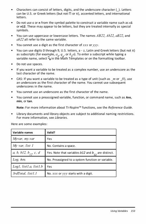
• Characters can consist of letters, digits, and the underscore character (_). Letterscan be U.S. or Greek letters (but not Π or p), accented letters, and internationalletters.
• Do not use c or n from the symbol palette to construct a variable name such as c1or n12. These may appear to be letters, but they are treated internally as specialsymbols.
• You can use uppercase or lowercase letters. The names AB22, Ab22, aB22, andab22 all refer to the same variable.
• You cannot use a digit as the first character of xxx or yyy.• You can use digits 0 through 9, U.S. letters, a - z, Latin and Greek letters (but not p)
as subscripts (for example, a2, q
a, or h
2o). To enter a subscript while typing a
variable name, select in the Math Templates or on the formatting toolbar.
• Do not use spaces.
• If you want a variable to be treated as a complex number, use an underscore as thelast character of the name.
• CAS: If you want a variable to be treated as a type of unit (such as _m or _ft), usean underscore as the first character of the name. You cannot use subsequentunderscores in the name.
• You cannot use an underscore as the first character of the name.
• You cannot use a preassigned variable, function, or command name, such as Ans,min, or tan.
Note: For more information about TI-Nspire™ functions, see the Reference Guide.
• Library documents and library objects are subject to additional naming restrictions.For more information, see Libraries.
Here are some examples:
Variable names Valid?
Myvar, my.var Yes
My var, list 1 No. Contains a space.
a, b, b12, b12, c, d Yes. Note that variables b12 and b12
are distinct.
Log, Ans No. Preassigned to a system function or variable.
Log1, list1.a, list1.b Yes
3rdTotal, list1.1 No. xxx or yyy starts with a digit.
Using Variables 153
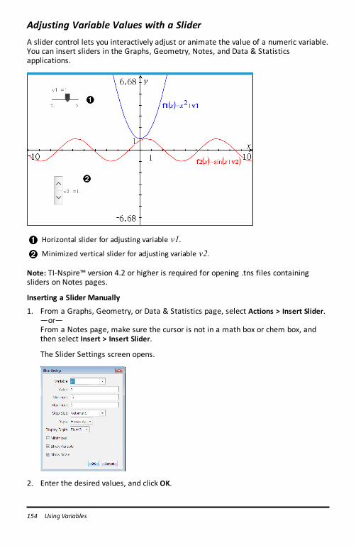
154 Using Variables
Adjusting Variable Values with a SliderA slider control lets you interactively adjust or animate the value of a numeric variable.You can insert sliders in the Graphs, Geometry, Notes, and Data & Statisticsapplications.
Horizontal slider for adjusting variable v1.Minimized vertical slider for adjusting variable v2.
Note: TI-Nspire™ version 4.2 or higher is required for opening .tns files containingsliders on Notes pages.
Inserting a Slider Manually
1. From a Graphs, Geometry, or Data & Statistics page, select Actions > Insert Slider.—or—From a Notes page, make sure the cursor is not in a math box or chem box, andthen select Insert > Insert Slider.
The Slider Settings screen opens.
2. Enter the desired values, and click OK.
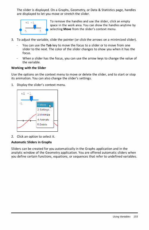
The slider is displayed. On a Graphs, Geometry, or Data & Statistics page, handlesare displayed to let you move or stretch the slider.
To remove the handles and use the slider, click an emptyspace in the work area. You can show the handles anytime byselectingMove from the slider's context menu.
3. To adjust the variable, slide the pointer (or click the arrows on a minimized slider).
- You can use the Tab key to move the focus to a slider or to move from oneslider to the next. The color of the slider changes to show you when it has thefocus.
- When a slider has the focus, you can use the arrow keys to change the value ofthe variable.
Working with the Slider
Use the options on the context menu to move or delete the slider, and to start or stopits animation. You can also change the slider's settings.
1. Display the slider's context menu.
2. Click an option to select it.
Automatic Sliders in Graphs
Sliders can be created for you automatically in the Graphs application and in theanalytic window of the Geometry application. You are offered automatic sliders whenyou define certain functions, equations, or sequences that refer to undefined variables.
Using Variables 155
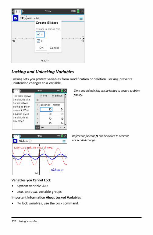
156 Using Variables
Locking and Unlocking VariablesLocking lets you protect variables from modification or deletion. Locking preventsunintended changes to a variable.
Time and altitude lists can be locked to ensure problemfidelity.
Reference function f1 can be locked to preventunintended change.
Variables you Cannot Lock
• System variable Ans• stat. and tvm. variable groups
Important Information About Locked Variables
• To lock variables, use the Lock command.
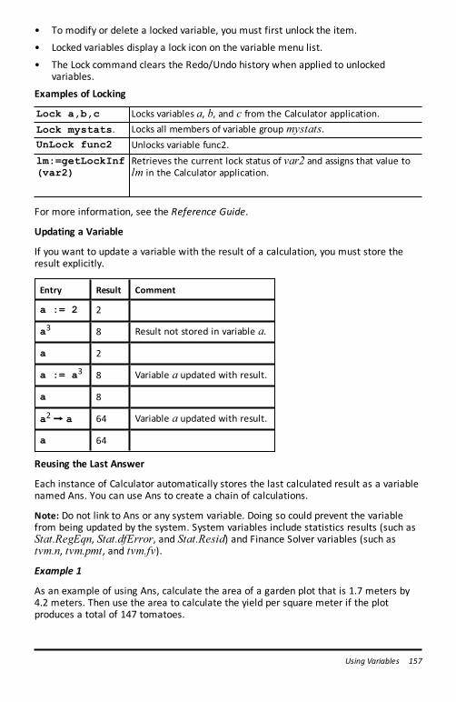
• To modify or delete a locked variable, you must first unlock the item.
• Locked variables display a lock icon on the variable menu list.
• The Lock command clears the Redo/Undo history when applied to unlockedvariables.
Examples of Locking
Lock a,b,c Locks variables a, b, and c from the Calculator application.Lock mystats. Locks all members of variable group mystats.UnLock func2 Unlocks variable func2.lm:=getLockInf (var2)
Retrieves the current lock status of var2 and assigns that value tolm in the Calculator application.
For more information, see the Reference Guide.
Updating a Variable
If you want to update a variable with the result of a calculation, you must store theresult explicitly.
Entry Result Comment
a := 2 2
a3 8 Result not stored in variable a.
a 2
a := a3 8 Variable a updated with result.
a 8
a2 & a 64 Variable a updated with result.
a 64
Reusing the Last Answer
Each instance of Calculator automatically stores the last calculated result as a variablenamed Ans. You can use Ans to create a chain of calculations.
Note: Do not link to Ans or any system variable. Doing so could prevent the variablefrom being updated by the system. System variables include statistics results (such asStat.RegEqn, Stat.dfError, and Stat.Resid) and Finance Solver variables (such astvm.n, tvm.pmt, and tvm.fv).
Example 1
As an example of using Ans, calculate the area of a garden plot that is 1.7 meters by4.2 meters. Then use the area to calculate the yield per square meter if the plotproduces a total of 147 tomatoes.
Using Variables 157
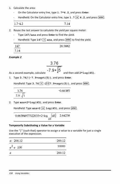
158 Using Variables
1. Calculate the area:
- On the Calculator entry line, type 1.7*4.2, and press Enter.
- Handheld: On the Calculator entry line, type 1.7r 4.2, and press·.
2. Reuse the last answer to calculate the yield per square meter:
- Type 147/ans and press Enter to find the yield.
- Handheld: Type 147p ans, and press· to find the yield.
Example 2
As a second example, calculate and then add 2*log(45).
1. Type 3.76/(-7.9+sqrt(5)), and press Enter.
Handheld: Type 3.76p (v7.9+sqrt(5)), and press·.
2. Type ans+2*log(45), and press Enter.
Handheld: Type ans+2r log(45), and press·.
Temporarily Substituting a Value for a Variable
Use the “|” (such that) operator to assign a value to a variable for just a singleexecution of the expression.

Removing a Linked Variable1. Select the linked variable.
2. Pressh.
The Variables options are displayed.
3. Select Unlink.
The link is removed from the value, and the value is displayed without any boldformatting.
Using Variables 159
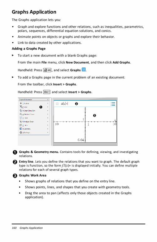
160 Graphs Application
Graphs ApplicationThe Graphs application lets you:
• Graph and explore functions and other relations, such as inequalities, parametrics,polars, sequences, differential equation solutions, and conics.
• Animate points on objects or graphs and explore their behavior.
• Link to data created by other applications.
Adding a Graphs Page
▶ To start a new document with a blank Graphs page:
From the main File menu, click New Document, and then click Add Graphs.
Handheld: Pressc, and select Graphs .
▶ To add a Graphs page in the current problem of an existing document:
From the toolbar, click Insert > Graphs.
Handheld: Press~ and select Insert > Graphs.
Graphs & Geometry menu. Contains tools for defining, viewing, and investigatingrelations.
Entry line. Lets you define the relations that you want to graph. The default graphtype is Function, so the form f1(x)= is displayed initially. You can define multiplerelations for each of several graph types.
Graphs Work Area
• Shows graphs of relations that you define on the entry line.
• Shows points, lines, and shapes that you create with geometry tools.
• Drag the area to pan (affects only those objects created in the Graphsapplication).
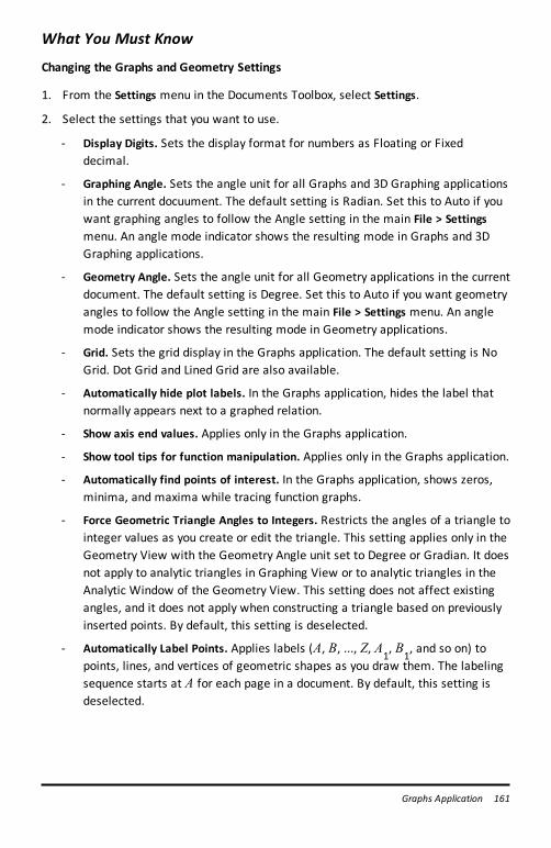
What You Must Know
Changing the Graphs and Geometry Settings
1. From the Settings menu in the Documents Toolbox, select Settings.
2. Select the settings that you want to use.
- Display Digits. Sets the display format for numbers as Floating or Fixeddecimal.
- Graphing Angle. Sets the angle unit for all Graphs and 3D Graphing applicationsin the current docuument. The default setting is Radian. Set this to Auto if youwant graphing angles to follow the Angle setting in the main File > Settingsmenu. An angle mode indicator shows the resulting mode in Graphs and 3DGraphing applications.
- Geometry Angle. Sets the angle unit for all Geometry applications in the currentdocument. The default setting is Degree. Set this to Auto if you want geometryangles to follow the Angle setting in the main File > Settings menu. An anglemode indicator shows the resulting mode in Geometry applications.
- Grid. Sets the grid display in the Graphs application. The default setting is NoGrid. Dot Grid and Lined Grid are also available.
- Automatically hide plot labels. In the Graphs application, hides the label thatnormally appears next to a graphed relation.
- Show axis end values. Applies only in the Graphs application.
- Show tool tips for function manipulation. Applies only in the Graphs application.
- Automatically find points of interest. In the Graphs application, shows zeros,minima, and maxima while tracing function graphs.
- Force Geometric Triangle Angles to Integers. Restricts the angles of a triangle tointeger values as you create or edit the triangle. This setting applies only in theGeometry View with the Geometry Angle unit set to Degree or Gradian. It doesnot apply to analytic triangles in Graphing View or to analytic triangles in theAnalytic Window of the Geometry View. This setting does not affect existingangles, and it does not apply when constructing a triangle based on previouslyinserted points. By default, this setting is deselected.
- Automatically Label Points. Applies labels (A, B, ..., Z, A1, B
1, and so on) to
points, lines, and vertices of geometric shapes as you draw them. The labelingsequence starts at A for each page in a document. By default, this setting isdeselected.
Graphs Application 161
162 Graphs Application
Note: If you create a new object that uses existing unlabeled points, thosepoint are not automatically labeled in the completed object.
- Click Restore to restore all settings to their factory defaults.
- ClickMake Default to apply the current settings to the open document and savethem as the default for new Graphs and Geometry documents.
Using Context Menus
Context menus provide quick access to commonly used commands and tools that applyto a specific object. For example, you can use a context menu to change an object'sline color or to group a set of selected objects.
▶ Display the context menu for an object in one of the following ways.
- Windows®: Right-click the object.
- Mac®: Hold “ and click the object.
- Handheld: Move the pointer to the object, and then press/b.
Finding Hidden Objects in the Graphs or Geometry Application
You can hide and show individual graphs, geometric objects, text, labels,measurements, and axis end-values.
To temporarily view hidden graphs or objects or to restore them as shown objects:
1. From the Actions menu, select Hide/Show.
The Hide/Show tool appears in the work area, and all hidden objects becomevisible in dimmed colors.
2. Click a graph or object to toggle its Hide/Show state.
3. To apply the changes and close the Hide/Show tool, press ESC.
Inserting a Background Image
You can insert an image as a background for a Graphs or Geometry page. The fileformat of the image can be .bmp, .jpg, or .png.
1. From the Insert menu, click Image.
2. Navigate to the image you want to insert, select it, and then click Open.
For information on moving, resizing, and deleting a background image, see Workingwith Images in the Software.
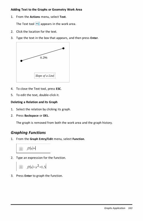
Adding Text to the Graphs or Geometry Work Area
1. From the Actions menu, select Text.
The Text tool appears in the work area.
2. Click the location for the text.
3. Type the text in the box that appears, and then press Enter.
4. To close the Text tool, press ESC.
5. To edit the text, double-click it.
Deleting a Relation and its Graph
1. Select the relation by clicking its graph.
2. Press Backspace or DEL.
The graph is removed from both the work area and the graph history.
Graphing Functions1. From the Graph Entry/Edit menu, select Function.
2. Type an expression for the function.
3. Press Enter to graph the function.
Graphs Application 163
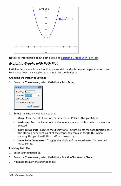
164 Graphs Application
Note: For information about path plots, see Exploring Graphs with Path Plot.
Exploring Graphs with Path PlotPath Plot lets you animate function, parametric, and polar equation plots in real timeto analyze how they are plotted and not just the final plot.
Changing the Path Plot Settings
1. From the Trace menu, select Path Plot > Path Setup.
2. Select the settings you want to use.
- Graph Type: Selects Function, Parametric, or Polar as the graph type.- Path Step: Sets the increment of the independent variable at which values are
plotted.- Show Future Path: Toggles the display of all future points for each function past
the starting or current point of the graph. You can also toggle this whenviewing the graph with the Up/Down arrow keys.
- Show Point Coordinates: Toggles the display of the coordinates for recordedtrace points.
Enabling Path Plot
1. Enter your equation(s).
2. From the Trace menu, select Path Plot > Function/Parametric/Polar.
3. Navigate through the animation by:
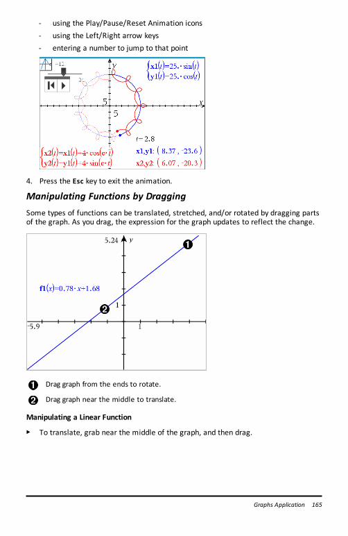
- using the Play/Pause/Reset Animation icons- using the Left/Right arrow keys- entering a number to jump to that point
4. Press the Esc key to exit the animation.
Manipulating Functions by DraggingSome types of functions can be translated, stretched, and/or rotated by dragging partsof the graph. As you drag, the expression for the graph updates to reflect the change.
Drag graph from the ends to rotate.
Drag graph near the middle to translate.
Manipulating a Linear Function
▶ To translate, grab near the middle of the graph, and then drag.
Graphs Application 165
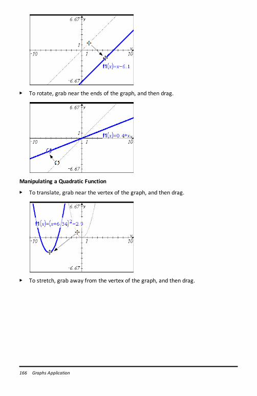
166 Graphs Application
▶ To rotate, grab near the ends of the graph, and then drag.
Manipulating a Quadratic Function
▶ To translate, grab near the vertex of the graph, and then drag.
▶ To stretch, grab away from the vertex of the graph, and then drag.
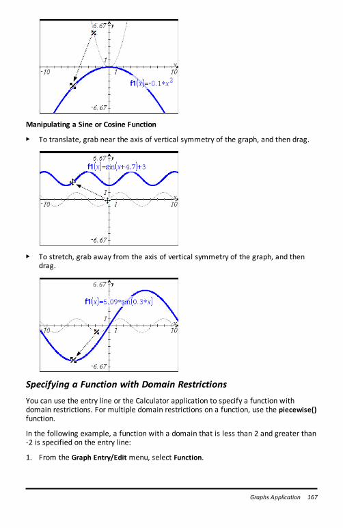
Manipulating a Sine or Cosine Function
▶ To translate, grab near the axis of vertical symmetry of the graph, and then drag.
▶ To stretch, grab away from the axis of vertical symmetry of the graph, and thendrag.
Specifying a Function with Domain RestrictionsYou can use the entry line or the Calculator application to specify a function withdomain restrictions. For multiple domain restrictions on a function, use the piecewise()function.
In the following example, a function with a domain that is less than 2 and greater than-2 is specified on the entry line:
1. From the Graph Entry/Edit menu, select Function.
Graphs Application 167
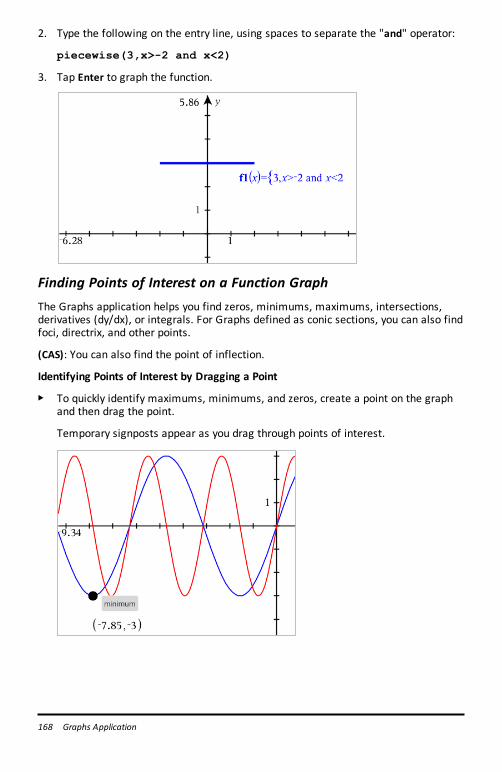
168 Graphs Application
2. Type the following on the entry line, using spaces to separate the "and" operator:
piecewise(3,x>-2 and x<2)
3. Tap Enter to graph the function.
Finding Points of Interest on a Function GraphThe Graphs application helps you find zeros, minimums, maximums, intersections,derivatives (dy/dx), or integrals. For Graphs defined as conic sections, you can also findfoci, directrix, and other points.
(CAS): You can also find the point of inflection.
Identifying Points of Interest by Dragging a Point
▶ To quickly identify maximums, minimums, and zeros, create a point on the graphand then drag the point.
Temporary signposts appear as you drag through points of interest.
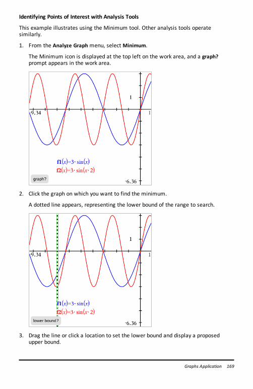
Identifying Points of Interest with Analysis Tools
This example illustrates using the Minimum tool. Other analysis tools operatesimilarly.
1. From the Analyze Graph menu, select Minimum.
The Minimum icon is displayed at the top left on the work area, and a graph?prompt appears in the work area.
2. Click the graph on which you want to find the minimum.
A dotted line appears, representing the lower bound of the range to search.
3. Drag the line or click a location to set the lower bound and display a proposedupper bound.
Graphs Application 169
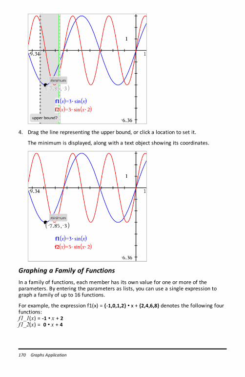
170 Graphs Application
4. Drag the line representing the upper bound, or click a location to set it.
The minimum is displayed, along with a text object showing its coordinates.
Graphing a Family of FunctionsIn a family of functions, each member has its own value for one or more of theparameters. By entering the parameters as lists, you can use a single expression tograph a family of up to 16 functions.
For example, the expression f1(x) = {-1,0,1,2} • x + {2,4,6,8} denotes the following fourfunctions:f1_1(x) = -1 • x + 2f1_2(x) = 0 • x + 4
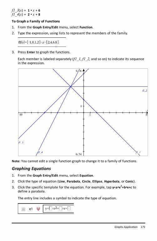
f1_3(x) = 1 • x + 6f1_4(x) = 2 • x + 8
To Graph a Family of Functions
1. From the Graph Entry/Edit menu, select Function.
2. Type the expression, using lists to represent the members of the family.
3. Press Enter to graph the functions.
Each member is labeled separately (f1_1, f1_2, and so on) to indicate its sequencein the expression.
Note: You cannot edit a single function graph to change it to a family of functions.
Graphing Equations1. From the Graph Entry/Edit menu, select Equation.
2. Click the type of equation (Line, Parabola, Circle, Ellipse, Hyperbola, or Conic).
3. Click the specific template for the equation. For example, tap y=a•x2+b•x+c todefine a parabola.
The entry line includes a symbol to indicate the type of equation.
Graphs Application 171
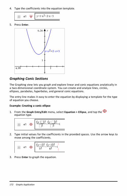
172 Graphs Application
4. Type the coefficients into the equation template.
5. Press Enter.
Graphing Conic SectionsThe Graphing view lets you graph and explore linear and conic equations analytically ina two-dimensional coordinate system. You can create and analyze lines, circles,ellipses, parabolas, hyperbolas, and general conic equations.
The entry line makes it easy to enter the equation by displaying a template for the typeof equation you choose.
Example: Creating a conic ellipse
1. From the Graph Entry/Edit menu, select Equation > Ellipse, and tap theequation type.
2. Type initial values for the coefficients in the provided spaces. Use the arrow keys tomove among the coefficients.
3. Press Enter to graph the equation.
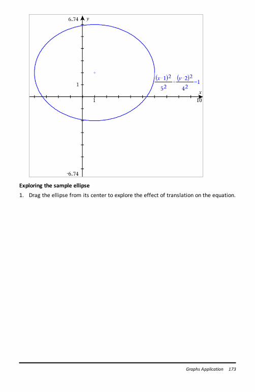
Exploring the sample ellipse
1. Drag the ellipse from its center to explore the effect of translation on the equation.
Graphs Application 173
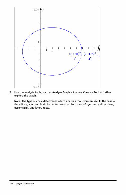
174 Graphs Application
2. Use the analysis tools, such as Analyze Graph > Analyze Conics > Foci to furtherexplore the graph.
Note: The type of conic determines which analysis tools you can use. In the case ofthe ellipse, you can obtain its center, vertices, foci, axes of symmetry, directrices,eccentricity, and latera recta.
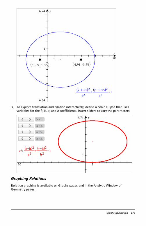
3. To explore translation and dilation interactively, define a conic ellipse that usesvariables for the h, k, a, and b coefficients. Insert sliders to vary the parameters.
Graphing RelationsRelation graphing is available on Graphs pages and in the Analytic Window ofGeometry pages.
Graphs Application 175
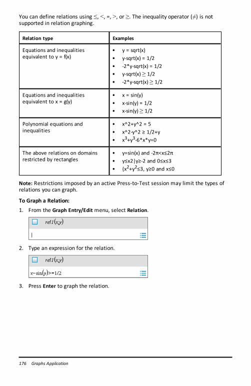
176 Graphs Application
You can define relations using ≤, <, =, >, or ≥. The inequality operator (≠) is notsupported in relation graphing.
Relation type Examples
Equations and inequalitiesequivalent to y = f(x)
• y = sqrt(x)• y-sqrt(x) = 1/2• -2*y-sqrt(x) = 1/2• y-sqrt(x) ≥ 1/2• -2*y-sqrt(x) ≥ 1/2
Equations and inequalitiesequivalent to x = g(y)
• x = sin(y)• x-sin(y) = 1/2• x-sin(y) ≥ 1/2
Polynomial equations andinequalities
• x^2+y^2 = 5• x^2-y^2 ≥ 1/2+y• x3+y3-6*x*y=0
The above relations on domainsrestricted by rectangles
• y=sin(x) and -2π<x≤2π• y≤x2|y≥-2 and 0≤x≤3• {x2+y2≤3, y≥0 and x≤0
Note: Restrictions imposed by an active Press-to-Test session may limit the types ofrelations you can graph.
To Graph a Relation:
1. From the Graph Entry/Edit menu, select Relation.
2. Type an expression for the relation.
3. Press Enter to graph the relation.
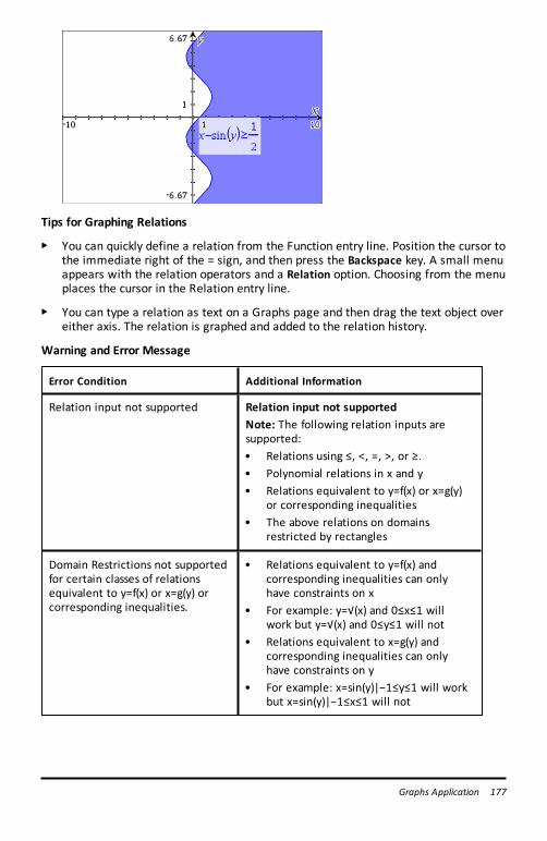
Tips for Graphing Relations
▶ You can quickly define a relation from the Function entry line. Position the cursor tothe immediate right of the = sign, and then press the Backspace key. A small menuappears with the relation operators and a Relation option. Choosing from the menuplaces the cursor in the Relation entry line.
▶ You can type a relation as text on a Graphs page and then drag the text object overeither axis. The relation is graphed and added to the relation history.
Warning and Error Message
Error Condition Additional Information
Relation input not supported Relation input not supportedNote: The following relation inputs aresupported:• Relations using ≤, <, =, >, or ≥.• Polynomial relations in x and y• Relations equivalent to y=f(x) or x=g(y)
or corresponding inequalities• The above relations on domains
restricted by rectangles
Domain Restrictions not supportedfor certain classes of relationsequivalent to y=f(x) or x=g(y) orcorresponding inequalities.
• Relations equivalent to y=f(x) andcorresponding inequalities can onlyhave constraints on x
• For example: y=√(x) and 0≤x≤1 willwork but y=√(x) and 0≤y≤1 will not
• Relations equivalent to x=g(y) andcorresponding inequalities can onlyhave constraints on y
• For example: x=sin(y)|−1≤y≤1 will workbut x=sin(y)|−1≤x≤1 will not
Graphs Application 177
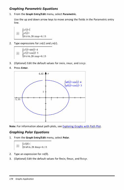
178 Graphs Application
Graphing Parametric Equations1. From the Graph Entry/Edit menu, select Parametric.
Use the up and down arrow keys to move among the fields in the Parametric entryline.
2. Type expressions for xn(t) and yn(t).
3. (Optional) Edit the default values for tmin, tmax, and tstep.4. Press Enter.
Note: For information about path plots, see Exploring Graphs with Path Plot.
Graphing Polar Equations1. From the Graph Entry/Edit menu, select Polar.
2. Type an expression for rn(θ).3. (Optional) Edit the default values for θmin, θmax, and θstep.
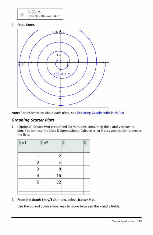
4. Press Enter.
Note: For information about path plots, see Exploring Graphs with Path Plot.
Graphing Scatter Plots1. (Optional) Create two predefined list variables containing the x and y values to
plot. You can use the Lists & Spreadsheet, Calculator, or Notes application to createthe lists.
2. From the Graph Entry/Edit menu, select Scatter Plot.
Use the up and down arrow keys to move between the x and y fields.
Graphs Application 179
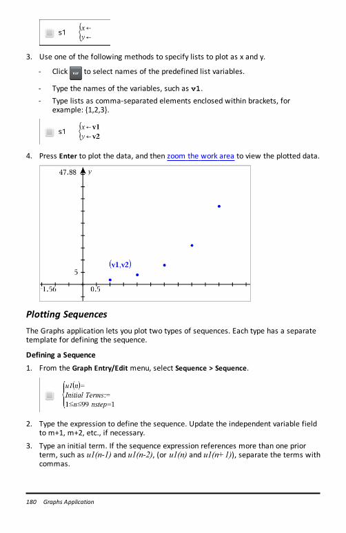
180 Graphs Application
3. Use one of the following methods to specify lists to plot as x and y.
- Click to select names of the predefined list variables.
- Type the names of the variables, such as v1.- Type lists as comma-separated elements enclosed within brackets, for
example: {1,2,3}.
4. Press Enter to plot the data, and then zoom the work area to view the plotted data.
Plotting SequencesThe Graphs application lets you plot two types of sequences. Each type has a separatetemplate for defining the sequence.
Defining a Sequence
1. From the Graph Entry/Edit menu, select Sequence > Sequence.
2. Type the expression to define the sequence. Update the independent variable fieldto m+1, m+2, etc., if necessary.
3. Type an initial term. If the sequence expression references more than one priorterm, such as u1(n-1) and u1(n-2), (or u1(n) and u1(n+1)), separate the terms withcommas.
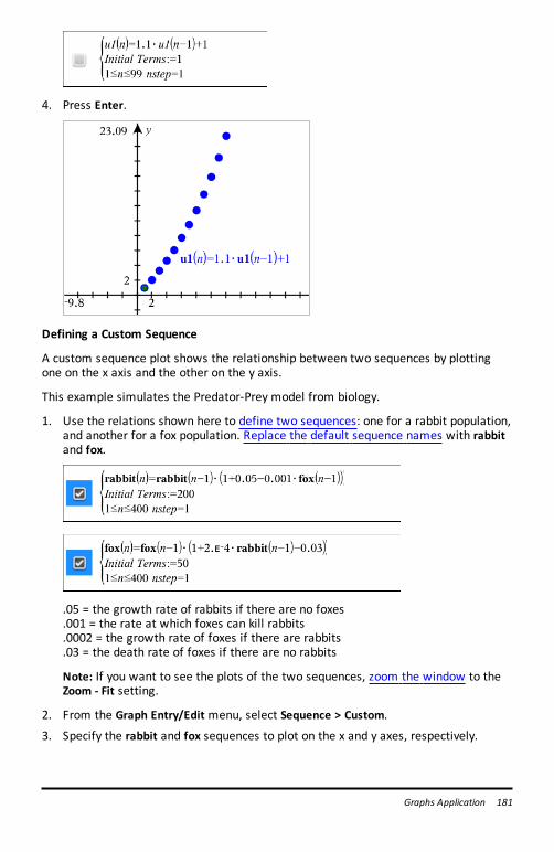
4. Press Enter.
Defining a Custom Sequence
A custom sequence plot shows the relationship between two sequences by plottingone on the x axis and the other on the y axis.
This example simulates the Predator-Prey model from biology.
1. Use the relations shown here to define two sequences: one for a rabbit population,and another for a fox population. Replace the default sequence names with rabbitand fox.
.05 = the growth rate of rabbits if there are no foxes
.001 = the rate at which foxes can kill rabbits
.0002 = the growth rate of foxes if there are rabbits
.03 = the death rate of foxes if there are no rabbits
Note: If you want to see the plots of the two sequences, zoom the window to theZoom - Fit setting.
2. From the Graph Entry/Edit menu, select Sequence > Custom.
3. Specify the rabbit and fox sequences to plot on the x and y axes, respectively.
Graphs Application 181
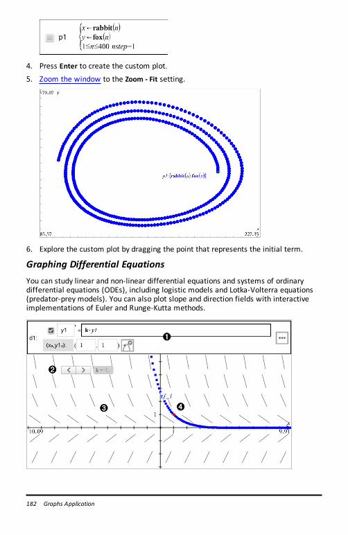
182 Graphs Application
4. Press Enter to create the custom plot.
5. Zoom the window to the Zoom - Fit setting.
6. Explore the custom plot by dragging the point that represents the initial term.
Graphing Differential EquationsYou can study linear and non-linear differential equations and systems of ordinarydifferential equations (ODEs), including logistic models and Lotka-Volterra equations(predator-prey models). You can also plot slope and direction fields with interactiveimplementations of Euler and Runge-Kutta methods.
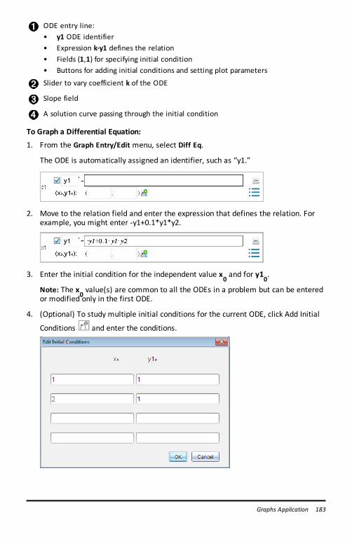
ODE entry line:• y1 ODE identifier• Expression k·y1 defines the relation• Fields (1,1) for specifying initial condition• Buttons for adding initial conditions and setting plot parameters
Slider to vary coefficient k of the ODE
Slope field
A solution curve passing through the initial condition
To Graph a Differential Equation:
1. From the Graph Entry/Edit menu, select Diff Eq.
The ODE is automatically assigned an identifier, such as “y1.”
2. Move to the relation field and enter the expression that defines the relation. Forexample, you might enter -y1+0.1*y1*y2.
3. Enter the initial condition for the independent value x0and for y1
0.
Note: The x0value(s) are common to all the ODEs in a problem but can be entered
or modified only in the first ODE.
4. (Optional) To study multiple initial conditions for the current ODE, click Add Initial
Conditions and enter the conditions.
Graphs Application 183
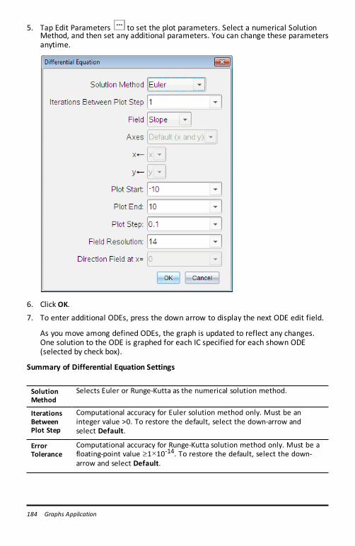
184 Graphs Application
5. Tap Edit Parameters to set the plot parameters. Select a numerical SolutionMethod, and then set any additional parameters. You can change these parametersanytime.
6. Click OK.
7. To enter additional ODEs, press the down arrow to display the next ODE edit field.
As you move among defined ODEs, the graph is updated to reflect any changes.One solution to the ODE is graphed for each IC specified for each shown ODE(selected by check box).
Summary of Differential Equation Settings
SolutionMethod
Selects Euler or Runge-Kutta as the numerical solution method.
IterationsBetweenPlot Step
Computational accuracy for Euler solution method only. Must be aninteger value >0. To restore the default, select the down-arrow andselect Default.
ErrorTolerance
Computational accuracy for Runge-Kutta solution method only. Must be afloating-point value |1×10-14. To restore the default, select the down-arrow and select Default.
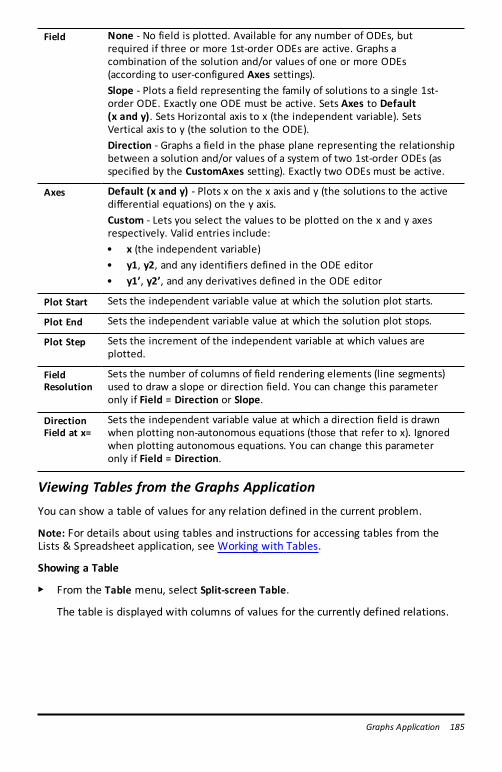
Field None - No field is plotted. Available for any number of ODEs, butrequired if three or more 1st-order ODEs are active. Graphs acombination of the solution and/or values of one or more ODEs(according to user-configured Axes settings).Slope - Plots a field representing the family of solutions to a single 1st-order ODE. Exactly one ODE must be active. Sets Axes to Default (x and y). Sets Horizontal axis to x (the independent variable). SetsVertical axis to y (the solution to the ODE).Direction - Graphs a field in the phase plane representing the relationshipbetween a solution and/or values of a system of two 1st-order ODEs (asspecified by the CustomAxes setting). Exactly two ODEs must be active.
Axes Default (x and y) - Plots x on the x axis and y (the solutions to the activedifferential equations) on the y axis.Custom - Lets you select the values to be plotted on the x and y axesrespectively. Valid entries include:• x (the independent variable)• y1, y2, and any identifiers defined in the ODE editor• y1’, y2’, and any derivatives defined in the ODE editor
Plot Start Sets the independent variable value at which the solution plot starts.
Plot End Sets the independent variable value at which the solution plot stops.
Plot Step Sets the increment of the independent variable at which values areplotted.
FieldResolution
Sets the number of columns of field rendering elements (line segments)used to draw a slope or direction field. You can change this parameteronly if Field = Direction or Slope.
DirectionField at x=
Sets the independent variable value at which a direction field is drawnwhen plotting non-autonomous equations (those that refer to x). Ignoredwhen plotting autonomous equations. You can change this parameteronly if Field = Direction.
Viewing Tables from the Graphs ApplicationYou can show a table of values for any relation defined in the current problem.
Note: For details about using tables and instructions for accessing tables from theLists & Spreadsheet application, see Working with Tables.
Showing a Table
▶ From the Table menu, select Split-screen Table.
The table is displayed with columns of values for the currently defined relations.
Graphs Application 185
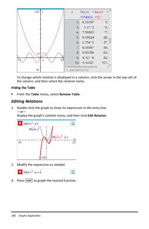
186 Graphs Application
To change which relation is displayed in a column, click the arrow in the top cell ofthe column, and then select the relation name.
Hiding the Table
▶ From the Table menu, select Remove Table.
Editing Relations1. Double-click the graph to show its expression in the entry line.
—or—Display the graph’s context menu, and then click Edit Relation.
2. Modify the expression as needed.
3. Press· to graph the revised function.
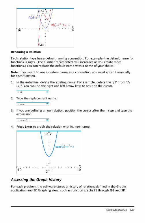
Renaming a Relation
Each relation type has a default naming convention. For example, the default name forfunctions is fn(x). (The number represented by n increases as you create morefunctions.) You can replace the default name with a name of your choice.
Note: If you want to use a custom name as a convention, you must enter it manuallyfor each function.
1. In the entry line, delete the existing name. For example, delete the "f1" from "f1(x)". You can use the right and left arrow keys to position the cursor.
2. Type the replacement name.
3. If you are defining a new relation, position the cursor after the = sign and type theexpression.
4. Press Enter to graph the relation with its new name.
Accessing the Graph HistoryFor each problem, the software stores a history of relations defined in the Graphsapplication and 3D Graphing view, such as function graphs f1 through f99 and 3D
Graphs Application 187
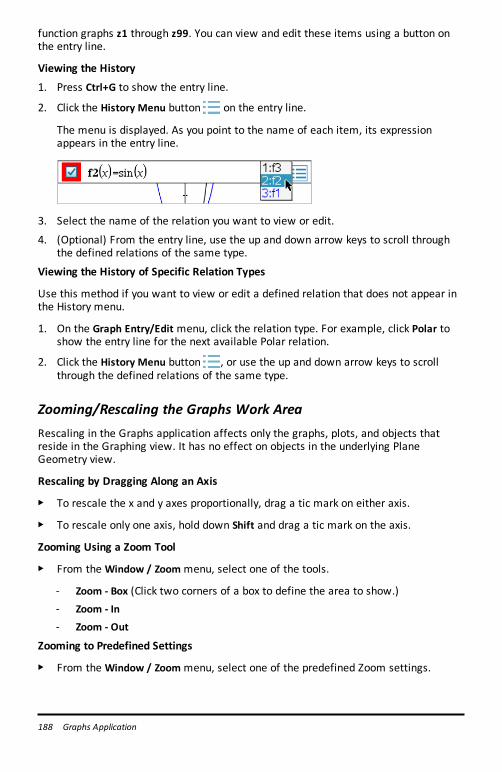
188 Graphs Application
function graphs z1 through z99. You can view and edit these items using a button onthe entry line.
Viewing the History
1. Press Ctrl+G to show the entry line.
2. Click the History Menu button on the entry line.
The menu is displayed. As you point to the name of each item, its expressionappears in the entry line.
3. Select the name of the relation you want to view or edit.
4. (Optional) From the entry line, use the up and down arrow keys to scroll throughthe defined relations of the same type.
Viewing the History of Specific Relation Types
Use this method if you want to view or edit a defined relation that does not appear inthe History menu.
1. On the Graph Entry/Edit menu, click the relation type. For example, click Polar toshow the entry line for the next available Polar relation.
2. Click the History Menu button , or use the up and down arrow keys to scrollthrough the defined relations of the same type.
Zooming/Rescaling the Graphs Work AreaRescaling in the Graphs application affects only the graphs, plots, and objects thatreside in the Graphing view. It has no effect on objects in the underlying PlaneGeometry view.
Rescaling by Dragging Along an Axis
▶ To rescale the x and y axes proportionally, drag a tic mark on either axis.
▶ To rescale only one axis, hold down Shift and drag a tic mark on the axis.
Zooming Using a Zoom Tool
▶ From the Window / Zoommenu, select one of the tools.
- Zoom - Box (Click two corners of a box to define the area to show.)- Zoom - In
- Zoom - Out
Zooming to Predefined Settings
▶ From the Window / Zoommenu, select one of the predefined Zoom settings.
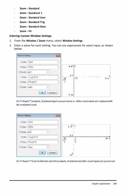
- Zoom - Standard
- Zoom - Quadrant 1
- Zoom - Standard User
- Zoom - Standard Trig
- Zoom - Standard Data
- Zoom - Fit
Entering Custom Window Settings
1. From the Window / Zoommenu, select Window Settings.
2. Enter a value for each setting. You can use expressions for exact input, as shownbelow.
OnTI-Nspire™products, fractional input is preserved as-is. Other exact inputs are replacedwiththe evaluated result.
On TI-Nspire™ ExactArithmetic and CAS products, fractional and other exact inputs are preserved.
Graphs Application 189
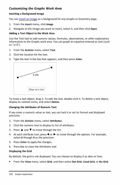
190 Graphs Application
Customizing the Graphs Work AreaInserting a Background Image
You can insert an image as a background for any Graphs or Geometry page.
1. From the Insert menu, click Image.
2. Navigate to the image you want to insert, select it, and then click Open.
Adding a Text Object to the Work Area
Use the Text tool to add numeric values, formulas, observations, or other explanatoryinformation to the Graphs work area. You can graph an equation entered as text (suchas "x=3").
1. From the Actions menu, select Text.
2. Click the location for the text.
3. Type the text in the box that appears, and then press Enter.
To move a text object, drag it. To edit the text, double-click it. To delete a text object,display its context menu, and select Delete.
Changing the Attributes of Numeric Text
If you enter a numeric value as text, you can lock it or set its format and displayedprecision.
1. From the Actions menu, select Attributes.
2. Click the numeric text to display its list of attributes.
3. Press ▲ and ▼ to move through the list.
4. At each attribute icon, press◄ or ► to move through the options. For example,select 0 through 9 as the precision.
5. Press Enter to apply the changes.
6. Press Esc to close the Attributes tool.
Displaying the Grid
By default, the grid is not displayed. You can choose to display it as dots or lines.
▶ From the Viewmenu, select Grid, and then select Dot Grid, Lined Grid, or No Grid.
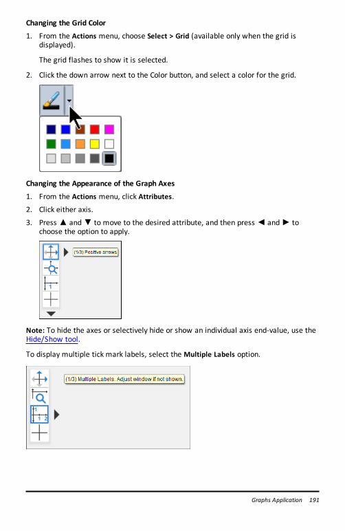
Changing the Grid Color
1. From the Actions menu, choose Select > Grid (available only when the grid isdisplayed).
The grid flashes to show it is selected.
2. Click the down arrow next to the Color button, and select a color for the grid.
Changing the Appearance of the Graph Axes
1. From the Actions menu, click Attributes.
2. Click either axis.
3. Press ▲ and ▼ to move to the desired attribute, and then press ◄ and ► tochoose the option to apply.
Note: To hide the axes or selectively hide or show an individual axis end-value, use theHide/Show tool.
To display multiple tick mark labels, select the Multiple Labels option.
Graphs Application 191
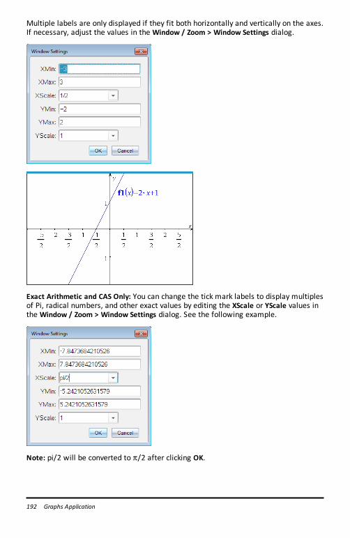
192 Graphs Application
Multiple labels are only displayed if they fit both horizontally and vertically on the axes.If necessary, adjust the values in the Window / Zoom > Window Settings dialog.
Exact Arithmetic and CAS Only: You can change the tick mark labels to display multiplesof Pi, radical numbers, and other exact values by editing the XScale or YScale values inthe Window / Zoom > Window Settings dialog. See the following example.
Note: pi/2 will be converted to p/2 after clicking OK.
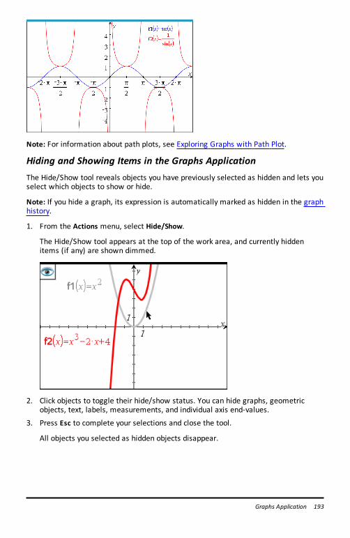
Note: For information about path plots, see Exploring Graphs with Path Plot.
Hiding and Showing Items in the Graphs ApplicationThe Hide/Show tool reveals objects you have previously selected as hidden and lets youselect which objects to show or hide.
Note: If you hide a graph, its expression is automatically marked as hidden in the graphhistory.
1. From the Actions menu, select Hide/Show.
The Hide/Show tool appears at the top of the work area, and currently hiddenitems (if any) are shown dimmed.
2. Click objects to toggle their hide/show status. You can hide graphs, geometricobjects, text, labels, measurements, and individual axis end-values.
3. Press Esc to complete your selections and close the tool.
All objects you selected as hidden objects disappear.
Graphs Application 193
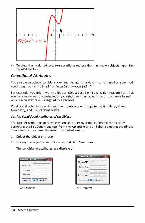
194 Graphs Application
4. To view the hidden objects temporarily or restore them as shown objects, open theHide/Show tool.
Conditional AttributesYou can cause objects to hide, show, and change color dynamically, based on specifiedconditions such as "r1<r2" or "sin(a1)>=cos(a2)."
For example, you might want to hide an object based on a changing measurement thatyou have assigned to a variable, or you might want an object’s color to change basedon a "Calculate" result assigned to a variable.
Conditional behaviors can be assigned to objects or groups in the Graphing, PlaneGeometry, and 3D Graphing views.
Setting Conditional Attributes of an Object
You can set conditions of a selected object either by using its context menu or byactivating the Set Conditions tool from the Actions menu and then selecting the object.These instructions describe using the context menu.
1. Select the object or group.
2. Display the object’s context menu, and click Conditions.
The conditional attributes are displayed.
For 2Dobjects For 3Dobjects
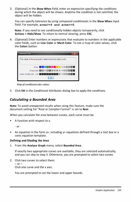
3. (Optional) In the ShowWhen field, enter an expression specifying the conditionsduring which the object will be shown. Anytime the condition is not satisfied, theobject will be hidden.
You can specify tolerance by using compound conditionals in the ShowWhen inputfield. For example, area>=4 and area<=6.
Note: If you need to see conditionally hidden objects temporarily, clickActions > Hide/Show. To return to normal viewing, press ESC.
4. (Optional) Enter numbers or expressions that evaluate to numbers in the applicablecolor fields, such as Line Color orMesh Color. To see a map of color values, clickthe Colors button.
Mapof conditional color values
5. Click OK in the Conditional Attributes dialog box to apply the conditions.
Calculating a Bounded AreaNote: To avoid unexpected results when using this feature, make sure thedocument setting for "Real or Complex Format" is set to Real.
When you calculate the area between curves, each curve must be:
• A function with respect to x.
- or -
• An equation in the form y=, including y= equations defined through a text box or aconic equation template.
Defining and Shading the Area
1. From the Analyze Graph menu, select Bounded Area.
If exactly two appropriate curves are available, they are selected automatically,and you can skip to step 3. Otherwise, you are prompted to select two curves.
2. Click two curves to select them.– or –Click one curve and the x axis.
You are prompted to set the lower and upper bounds.
Graphs Application 195
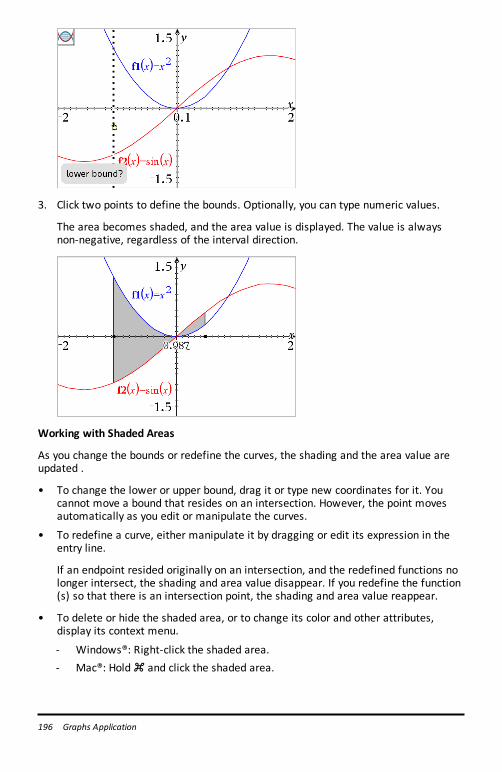
196 Graphs Application
3. Click two points to define the bounds. Optionally, you can type numeric values.
The area becomes shaded, and the area value is displayed. The value is alwaysnon-negative, regardless of the interval direction.
Working with Shaded Areas
As you change the bounds or redefine the curves, the shading and the area value areupdated .
• To change the lower or upper bound, drag it or type new coordinates for it. Youcannot move a bound that resides on an intersection. However, the point movesautomatically as you edit or manipulate the curves.
• To redefine a curve, either manipulate it by dragging or edit its expression in theentry line.
If an endpoint resided originally on an intersection, and the redefined functions nolonger intersect, the shading and area value disappear. If you redefine the function(s) so that there is an intersection point, the shading and area value reappear.
• To delete or hide the shaded area, or to change its color and other attributes,display its context menu.
- Windows®: Right-click the shaded area.- Mac®: Hold “ and click the shaded area.
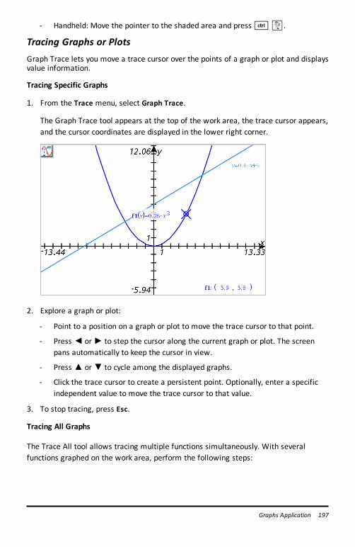
- Handheld: Move the pointer to the shaded area and press/x.
Tracing Graphs or PlotsGraph Trace lets you move a trace cursor over the points of a graph or plot and displaysvalue information.
Tracing Specific Graphs
1. From the Trace menu, select Graph Trace.
The Graph Trace tool appears at the top of the work area, the trace cursor appears,and the cursor coordinates are displayed in the lower right corner.
2. Explore a graph or plot:
- Point to a position on a graph or plot to move the trace cursor to that point.
- Press ◄ or► to step the cursor along the current graph or plot. The screenpans automatically to keep the cursor in view.
- Press ▲ or▼ to cycle among the displayed graphs.
- Click the trace cursor to create a persistent point. Optionally, enter a specificindependent value to move the trace cursor to that value.
3. To stop tracing, press Esc.
Tracing All Graphs
The Trace All tool allows tracing multiple functions simultaneously. With severalfunctions graphed on the work area, perform the following steps:
Graphs Application 197
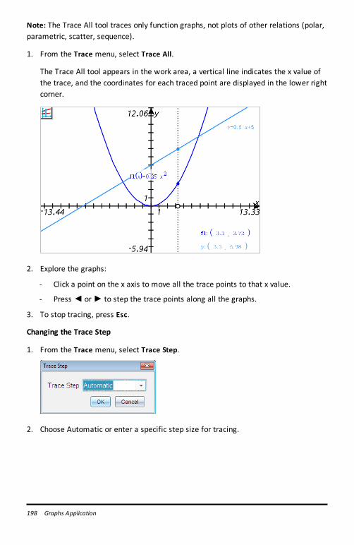
198 Graphs Application
Note: The Trace All tool traces only function graphs, not plots of other relations (polar,parametric, scatter, sequence).
1. From the Trace menu, select Trace All.
The Trace All tool appears in the work area, a vertical line indicates the x value ofthe trace, and the coordinates for each traced point are displayed in the lower rightcorner.
2. Explore the graphs:
- Click a point on the x axis to move all the trace points to that x value.
- Press ◄ or► to step the trace points along all the graphs.
3. To stop tracing, press Esc.
Changing the Trace Step
1. From the Trace menu, select Trace Step.
2. Choose Automatic or enter a specific step size for tracing.
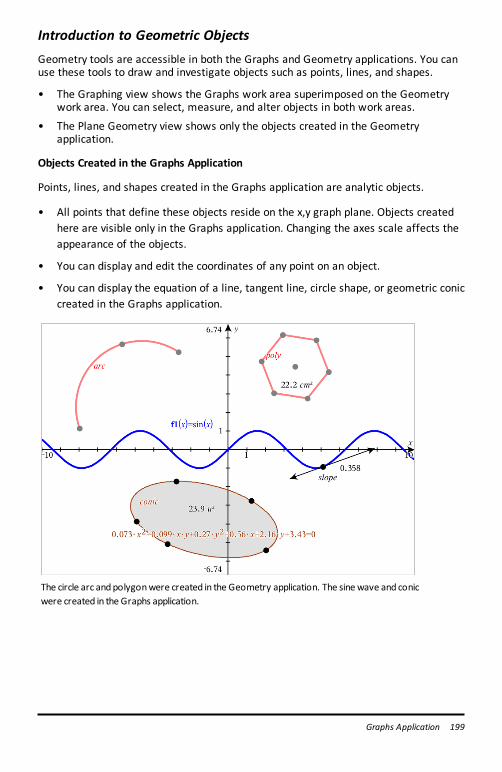
Introduction to Geometric ObjectsGeometry tools are accessible in both the Graphs and Geometry applications. You canuse these tools to draw and investigate objects such as points, lines, and shapes.
• The Graphing view shows the Graphs work area superimposed on the Geometrywork area. You can select, measure, and alter objects in both work areas.
• The Plane Geometry view shows only the objects created in the Geometryapplication.
Objects Created in the Graphs Application
Points, lines, and shapes created in the Graphs application are analytic objects.
• All points that define these objects reside on the x,y graph plane. Objects createdhere are visible only in the Graphs application. Changing the axes scale affects theappearance of the objects.
• You can display and edit the coordinates of any point on an object.
• You can display the equation of a line, tangent line, circle shape, or geometric coniccreated in the Graphs application.
The circle arc andpolygonwere created in the Geometry application. The sinewave and conicwere created in the Graphs application.
Graphs Application 199
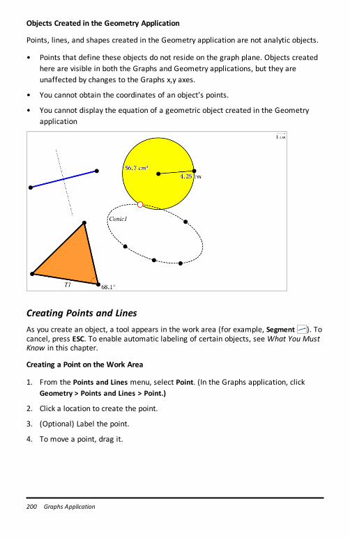
200 Graphs Application
Objects Created in the Geometry Application
Points, lines, and shapes created in the Geometry application are not analytic objects.
• Points that define these objects do not reside on the graph plane. Objects createdhere are visible in both the Graphs and Geometry applications, but they areunaffected by changes to the Graphs x,y axes.
• You cannot obtain the coordinates of an object’s points.
• You cannot display the equation of a geometric object created in the Geometryapplication
Creating Points and LinesAs you create an object, a tool appears in the work area (for example, Segment ). Tocancel, press ESC. To enable automatic labeling of certain objects, see What You MustKnow in this chapter.
Creating a Point on the Work Area
1. From the Points and Lines menu, select Point. (In the Graphs application, clickGeometry > Points and Lines > Point.)
2. Click a location to create the point.
3. (Optional) Label the point.
4. To move a point, drag it.
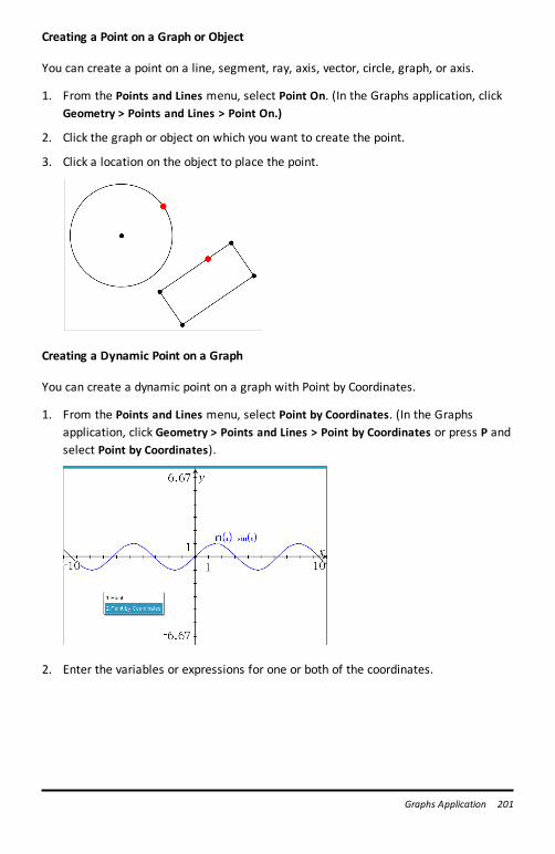
Creating a Point on a Graph or Object
You can create a point on a line, segment, ray, axis, vector, circle, graph, or axis.
1. From the Points and Lines menu, select Point On. (In the Graphs application, clickGeometry > Points and Lines > Point On.)
2. Click the graph or object on which you want to create the point.
3. Click a location on the object to place the point.
Creating a Dynamic Point on a Graph
You can create a dynamic point on a graph with Point by Coordinates.
1. From the Points and Lines menu, select Point by Coordinates. (In the Graphsapplication, click Geometry > Points and Lines > Point by Coordinates or press P andselect Point by Coordinates).
2. Enter the variables or expressions for one or both of the coordinates.
Graphs Application 201
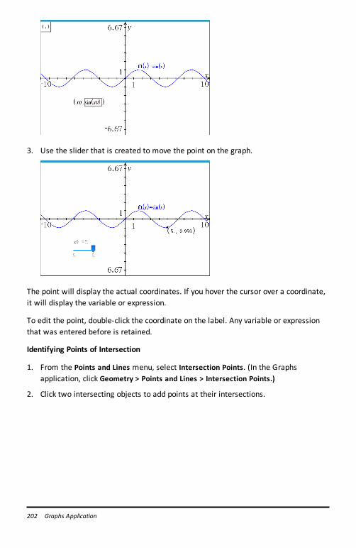
202 Graphs Application
3. Use the slider that is created to move the point on the graph.
The point will display the actual coordinates. If you hover the cursor over a coordinate,it will display the variable or expression.
To edit the point, double-click the coordinate on the label. Any variable or expressionthat was entered before is retained.
Identifying Points of Intersection
1. From the Points and Lines menu, select Intersection Points. (In the Graphsapplication, click Geometry > Points and Lines > Intersection Points.)
2. Click two intersecting objects to add points at their intersections.
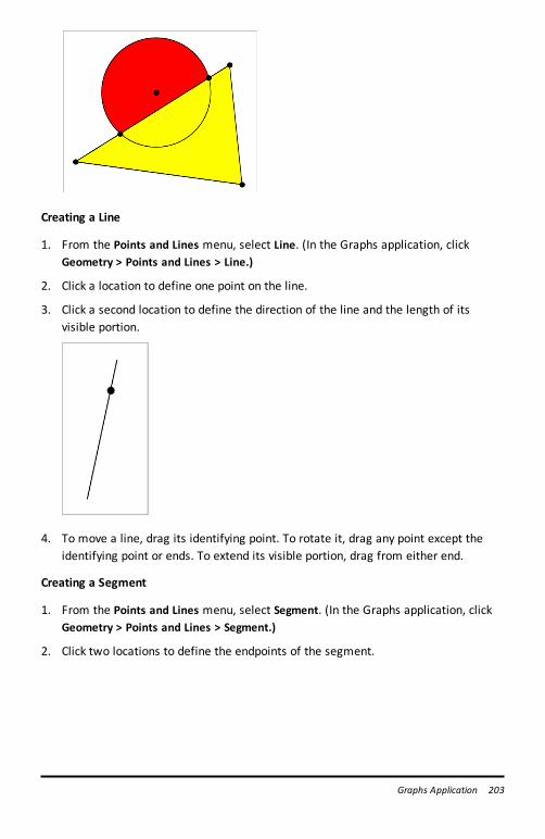
Creating a Line
1. From the Points and Lines menu, select Line. (In the Graphs application, clickGeometry > Points and Lines > Line.)
2. Click a location to define one point on the line.
3. Click a second location to define the direction of the line and the length of itsvisible portion.
4. To move a line, drag its identifying point. To rotate it, drag any point except theidentifying point or ends. To extend its visible portion, drag from either end.
Creating a Segment
1. From the Points and Lines menu, select Segment. (In the Graphs application, clickGeometry > Points and Lines > Segment.)
2. Click two locations to define the endpoints of the segment.
Graphs Application 203
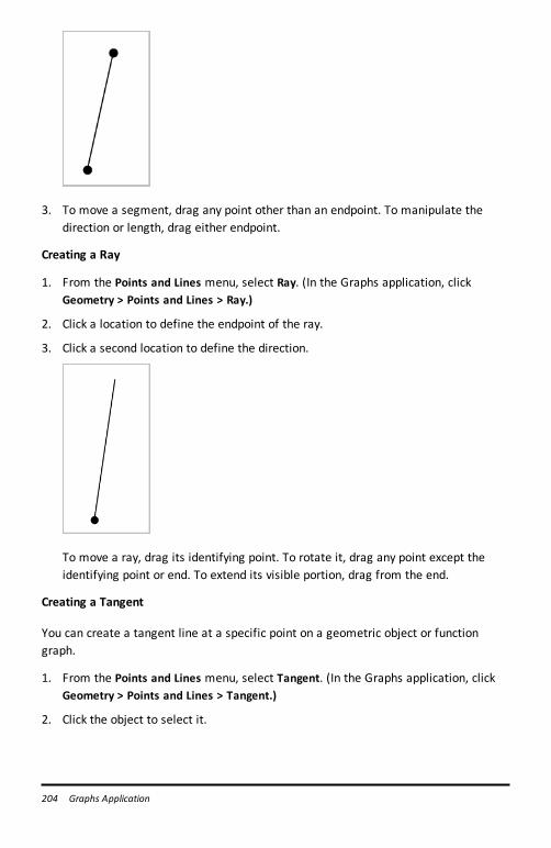
204 Graphs Application
3. To move a segment, drag any point other than an endpoint. To manipulate thedirection or length, drag either endpoint.
Creating a Ray
1. From the Points and Lines menu, select Ray. (In the Graphs application, clickGeometry > Points and Lines > Ray.)
2. Click a location to define the endpoint of the ray.
3. Click a second location to define the direction.
To move a ray, drag its identifying point. To rotate it, drag any point except theidentifying point or end. To extend its visible portion, drag from the end.
Creating a Tangent
You can create a tangent line at a specific point on a geometric object or functiongraph.
1. From the Points and Lines menu, select Tangent. (In the Graphs application, clickGeometry > Points and Lines > Tangent.)
2. Click the object to select it.
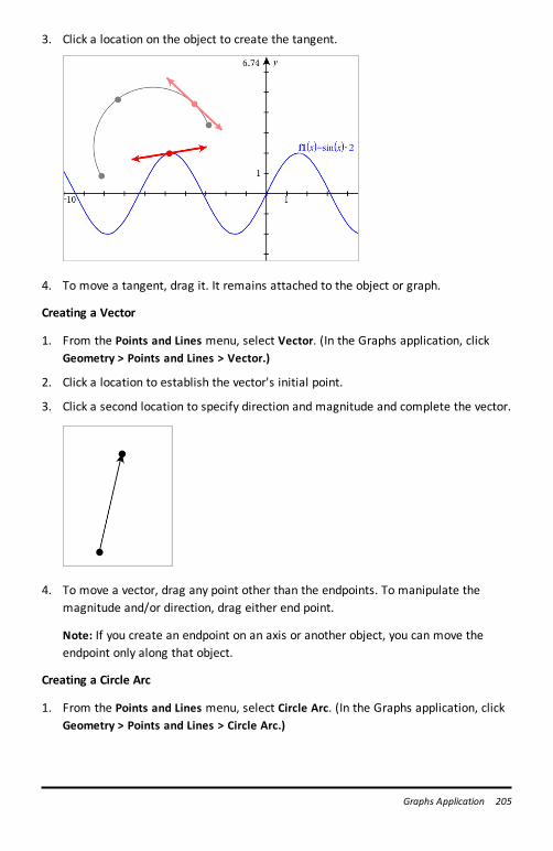
3. Click a location on the object to create the tangent.
4. To move a tangent, drag it. It remains attached to the object or graph.
Creating a Vector
1. From the Points and Lines menu, select Vector. (In the Graphs application, clickGeometry > Points and Lines > Vector.)
2. Click a location to establish the vector's initial point.
3. Click a second location to specify direction and magnitude and complete the vector.
4. To move a vector, drag any point other than the endpoints. To manipulate themagnitude and/or direction, drag either end point.
Note: If you create an endpoint on an axis or another object, you can move theendpoint only along that object.
Creating a Circle Arc
1. From the Points and Lines menu, select Circle Arc. (In the Graphs application, clickGeometry > Points and Lines > Circle Arc.)
Graphs Application 205
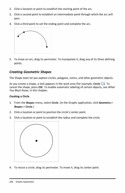
206 Graphs Application
2. Click a location or point to establish the starting point of the arc.
3. Click a second point to establish an intermediate point through which the arc willpass.
4. Click a third point to set the ending point and complete the arc.
5. To move an arc, drag its perimeter. To manipulate it, drag any of its three definingpoints.
Creating Geometric ShapesThe Shape tools let you explore circles, polygons, conics, and other geometric objects.
As you create a shape, a tool appears in the work area (for example, Circle ). Tocancel the shape, press ESC. To enable automatic labeling of certain objects, see WhatYou Must Know, in this chapter.
Creating a Circle
1. From the Shapes menu, select Circle. (In the Graphs application, click Geometry >Shapes > Circle.)
2. Click a location or point to position the circle’s center point.
3. Click a location or point to establish the radius and complete the circle.
4. To resize a circle, drag its perimeter. To move it, drag its center point.
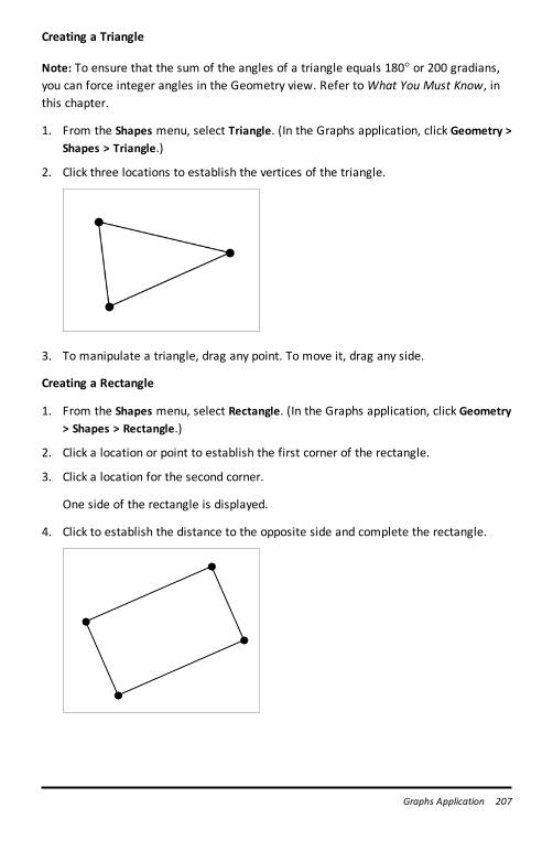
Creating a Triangle
Note: To ensure that the sum of the angles of a triangle equals 180° or 200 gradians,you can force integer angles in the Geometry view. Refer toWhat You Must Know, inthis chapter.
1. From the Shapes menu, select Triangle. (In the Graphs application, click Geometry >Shapes > Triangle.)
2. Click three locations to establish the vertices of the triangle.
3. To manipulate a triangle, drag any point. To move it, drag any side.
Creating a Rectangle
1. From the Shapes menu, select Rectangle. (In the Graphs application, click Geometry> Shapes > Rectangle.)
2. Click a location or point to establish the first corner of the rectangle.
3. Click a location for the second corner.
One side of the rectangle is displayed.
4. Click to establish the distance to the opposite side and complete the rectangle.
Graphs Application 207
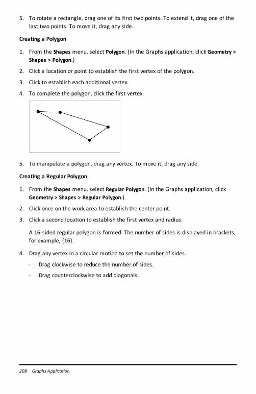
208 Graphs Application
5. To rotate a rectangle, drag one of its first two points. To extend it, drag one of thelast two points. To move it, drag any side.
Creating a Polygon
1. From the Shapes menu, select Polygon. (In the Graphs application, click Geometry >Shapes > Polygon.)
2. Click a location or point to establish the first vertex of the polygon.
3. Click to establish each additional vertex.
4. To complete the polygon, click the first vertex.
5. To manipulate a polygon, drag any vertex. To move it, drag any side.
Creating a Regular Polygon
1. From the Shapes menu, select Regular Polygon. (In the Graphs application, clickGeometry > Shapes > Regular Polygon.)
2. Click once on the work area to establish the center point.
3. Click a second location to establish the first vertex and radius.
A 16-sided regular polygon is formed. The number of sides is displayed in brackets;for example, {16}.
4. Drag any vertex in a circular motion to set the number of sides.
- Drag clockwise to reduce the number of sides.
- Drag counterclockwise to add diagonals.
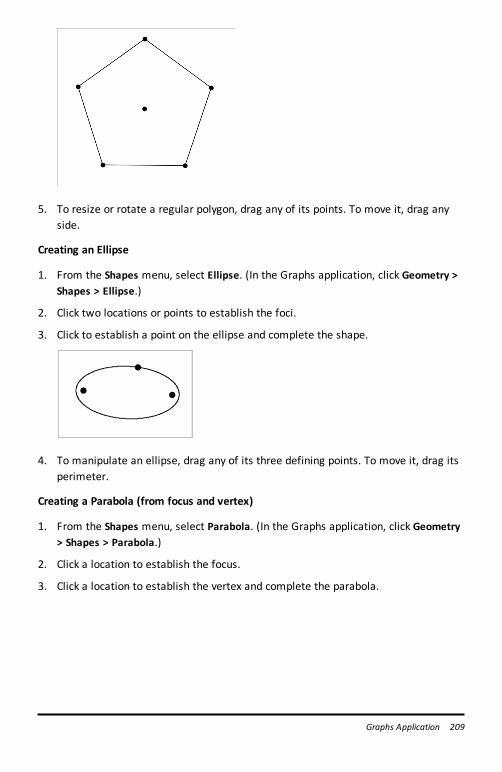
5. To resize or rotate a regular polygon, drag any of its points. To move it, drag anyside.
Creating an Ellipse
1. From the Shapes menu, select Ellipse. (In the Graphs application, click Geometry >Shapes > Ellipse.)
2. Click two locations or points to establish the foci.
3. Click to establish a point on the ellipse and complete the shape.
4. To manipulate an ellipse, drag any of its three defining points. To move it, drag itsperimeter.
Creating a Parabola (from focus and vertex)
1. From the Shapes menu, select Parabola. (In the Graphs application, click Geometry> Shapes > Parabola.)
2. Click a location to establish the focus.
3. Click a location to establish the vertex and complete the parabola.
Graphs Application 209
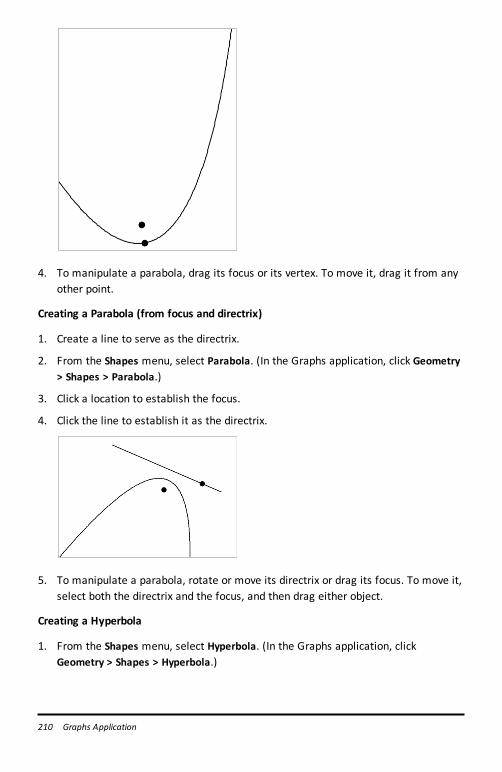
210 Graphs Application
4. To manipulate a parabola, drag its focus or its vertex. To move it, drag it from anyother point.
Creating a Parabola (from focus and directrix)
1. Create a line to serve as the directrix.
2. From the Shapes menu, select Parabola. (In the Graphs application, click Geometry> Shapes > Parabola.)
3. Click a location to establish the focus.
4. Click the line to establish it as the directrix.
5. To manipulate a parabola, rotate or move its directrix or drag its focus. To move it,select both the directrix and the focus, and then drag either object.
Creating a Hyperbola
1. From the Shapes menu, select Hyperbola. (In the Graphs application, clickGeometry > Shapes > Hyperbola.)
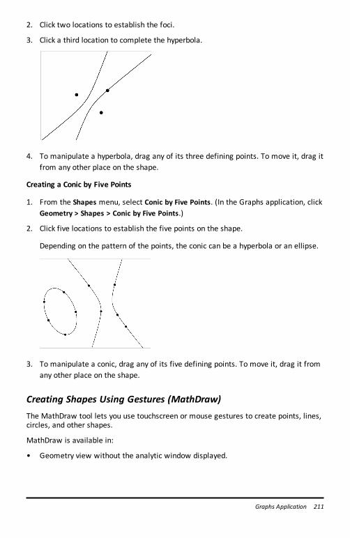
2. Click two locations to establish the foci.
3. Click a third location to complete the hyperbola.
4. To manipulate a hyperbola, drag any of its three defining points. To move it, drag itfrom any other place on the shape.
Creating a Conic by Five Points
1. From the Shapes menu, select Conic by Five Points. (In the Graphs application, clickGeometry > Shapes > Conic by Five Points.)
2. Click five locations to establish the five points on the shape.
Depending on the pattern of the points, the conic can be a hyperbola or an ellipse.
3. To manipulate a conic, drag any of its five defining points. To move it, drag it fromany other place on the shape.
Creating Shapes Using Gestures (MathDraw)The MathDraw tool lets you use touchscreen or mouse gestures to create points, lines,circles, and other shapes.
MathDraw is available in:
• Geometry view without the analytic window displayed.
Graphs Application 211
212 Graphs Application
• Graphing view when the x scale and y scale are identical. This avoids non-circularellipses and non-square rectangles appearing as circles and squares.
MathDraw is not available in the 3D Graphing view or in the Geometry view with theanalytic window displayed.
Activating MathDraw
1. If using the Geometry view with the analytic window visible, use the Viewmenu tohide the window.
2. On the Actions menu, select MathDraw.
The MathDraw icon appears. You can begin using the tool.
Canceling MathDraw
▶ When you have finished using the MathDraw tool, press Esc.
The tool also closes if you select a different tool or change views.
Creating Points
To create a labeled point, tap or click in an open area.
• If the point is close to an existing line, segment, ray, geometric conic (includingcircles), or polygon, the point snaps to that object. You can also place a point on theintersection of any two of those types of objects.
• If the point is close to a visible grid location in a Graphs view or the analyticwindow of a Geometry view, it snaps to the grid.
Drawing Lines and Segments
To create a line or segment, touch or click the initial position, and then drag to the endposition.
• If the drawn line passes near an existing point, the line snaps to the point.
• If the drawn line starts close to an existing point and ends next to another existingpoint , it becomes a segment defined by those points.
• If the drawn line is nearly parallel or perpendicular to an existing line, segment, orside of a polygon, it aligns to that object.
Note: The default tolerance for detecting parallel/perpendicular lines is 12.5degrees. This tolerance can be redefined using a variable named ti_gg_fd.angle_tol.You can change the tolerance in the current problem by setting this variable in thecalculator app to a value in the range 0 through 45 (0=no parallel/perpendiculardetection).
Drawing Circles and Ellipses
To create a circle or ellipse, use the touchscreen or mouse to draw the approximateshape.
• If the drawn shape is sufficiently circular, a circle is created.
• If the shape is elongated, an ellipse is created.
• If the virtual center of the drawn shape is near an existing point, the circle orellipse is centered on that point.
Drawing Triangles
To create a triangle, draw a triangle-like shape.
• If a drawn vertex is close to an existing point, the vertex snaps to the point.
Drawing Rectangles and Squares
To create a rectangle or square, use the touchscreen or mouse to draw the perimeter.
• If the drawn shape is nearly square, a square is created.
• If the drawn shape is elongated, a rectangle is created.
• If the center of a square is close to an existing point, the square snaps to thatpoint.
Drawing Polygons
To create a polygon, tap or click a succession of existing points, ending on the firstpoint you tapped.
Using MathDraw to Create Equations
In the Graphs view, MathDraw attempts to recognize certain gestures as functions foranalytic parabolas.
Note: The default step value for quantization of the parabola coefficients is 1/32. Thedenominator of this fraction can be redefined using a variable named ti_gg_fd.par_quant. You can change the step value in the current problem by setting this variable toa value greater or equal to 2. A value of 2, for example, produces a step value of 0.5.
Using MathDraw to Measure an Angle
To measure the angle between two existing lines, use the touchscreen or mouse todraw a circle arc from one of the lines to the other.
Graphs Application 213
214 Graphs Application
• If the intersection point between the two lines does not exist, it is created andlabeled.
• The angle is not a directed angle.
Using MathDraw to Find a Mid-point
To create a point midway between two points, tap or click point 1, point 2, and thenpoint 1 again.
Using MathDraw to Erase
To erase objects, use the touchscreen or mouse to drag left and right, similar to themotion of erasing a whiteboard.
• The erasure area is the bounding rectangle of the erasure gesture.
• All point objects and their dependents inside the erasure area are removed.
Basics of Working with Objects
Selecting and Deselecting Objects
You can select an individual object or multiple objects. Select multiple objects whenyou want to quickly move, color, or delete them together.
1. Click an object or graph to select it.
The object flashes to indicate selection.
2. Click any additional objects to add them to the selection.
3. Perform the operation (such as moving or setting color).
4. To deselect all objects, click an empty space in the work area.
Grouping and Ungrouping Geometric Objects
Grouping objects gives you a way to reselect them as a set, even after you havedeselected them to work with other objects.
1. Click each object to add it to the current selection.
The selected objects flash.
2. Display a context menu of the selected object or objects.
3. Click Group. You can now select all the items in the group by clicking any of itsmembers.
4. To split a group into individual objects, display a context menu of any of itsmember objects, and click Ungroup.
Deleting Objects
1. Display the context menu of the object or objects.
2. Click Delete.
You cannot delete the origin, the axes, or points representing locked variables, evenif those items are included in the selection.
Moving Objects
You can move an object, group, or combination of selected objects and groups.
Note: If an immovable object (such as the graph axes or a point with lockedcoordinates) is included in a selection or group, you cannot move any of the objects.You must cancel the selection and then select only movable items.
To move this... Drag this
A multiple-objectselection or group
Any of its objects
A point The point
A segment orvector
Any point other than an endpoint
A line or ray The identifying point
A circle The center point
Other geometricshapes
Any position on the object except one of its defining points. Forexample, move a polygon by dragging any of its sides.
Constraining Object Movement
Holding down the SHIFT key before dragging lets you constrain how certain objects aredrawn, moved, or manipulated.
Use the constraint feature to:
• Rescale only a single axis in the Graphs application.
Graphs Application 215
216 Graphs Application
• Pan the work area horizontally or vertically, depending on which direction you draginitially.
• Limit object movement to horizontal or vertical.
• Limit point placement to 15° increments as you draw a triangle, rectangle, orpolygon.
• Limit angle manipulations to 15° increments.
• Limit the radius of a resized circle to integer values.
Pinning Objects
Pinning objects prevents accidental changes as you move or manipulate other objects.
You can pin graphed functions, geometric objects, text objects, the graph axes, and thebackground.
1. Select the object or objects to pin, or click an empty area if you are pinning thebackground.
2. Display the context menu, and select Pin.
A pinned object displays a pin icon when you point to it.
3. To unpin an object, display its context menu, and select Unpin.
Notes:
• Although you cannot drag a pinned point, you can reposition it by editing its x and ycoordinates.
• You cannot pan the work area while the background is pinned.
Changing the Line or Fill Color of an Object
Color changes made in the software are displayed in shades of gray when you work ondocuments using a TI-Nspire™ CX handheld that does not support color. Color ispreserved when you move documents back to the software.
1. Select the object or objects.
2. Display the object’s context menu, click Color, and then click Line Color or Fill Color.
3. Select the color to apply to the objects.
Changing the Appearance of an Object
1. From the Actions menu, select Attributes.
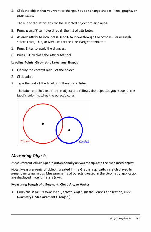
2. Click the object that you want to change. You can change shapes, lines, graphs, orgraph axes.
The list of the attributes for the selected object are displayed.
3. Press 9 and : to move through the list of attributes.
4. At each attribute icon, press 7 or 8 to move through the options. For example,select Thick, Thin, or Medium for the Line Weight attribute.
5. Press Enter to apply the changes.
6. Press ESC to close the Attributes tool.
Labeling Points, Geometric Lines, and Shapes
1. Display the context menu of the object.
2. Click Label.
3. Type the text of the label, and then press Enter.
The label attaches itself to the object and follows the object as you move it. Thelabel's color matches the object's color.
Measuring ObjectsMeasurement values update automatically as you manipulate the measured object.
Note: Measurements of objects created in the Graphs application are displayed ingeneric units named u. Measurements of objects created in the Geometry applicationare displayed in centimeters (cm).
Measuring Length of a Segment, Circle Arc, or Vector
1. From the Measurement menu, select Length. (In the Graphs application, clickGeometry > Measurement > Length.)
Graphs Application 217
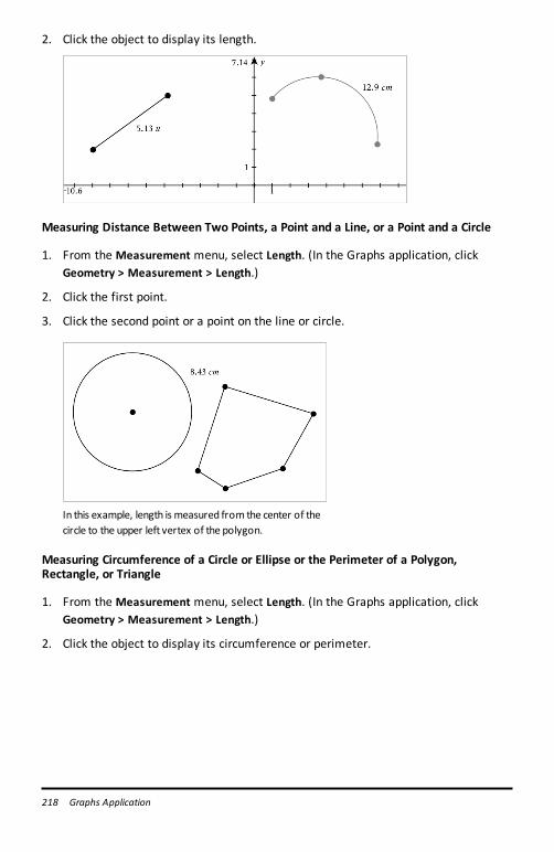
218 Graphs Application
2. Click the object to display its length.
Measuring Distance Between Two Points, a Point and a Line, or a Point and a Circle
1. From the Measurement menu, select Length. (In the Graphs application, clickGeometry > Measurement > Length.)
2. Click the first point.
3. Click the second point or a point on the line or circle.
In this example, length is measured from the center of thecircle to the upper left vertex of the polygon.
Measuring Circumference of a Circle or Ellipse or the Perimeter of a Polygon,Rectangle, or Triangle
1. From the Measurement menu, select Length. (In the Graphs application, clickGeometry > Measurement > Length.)
2. Click the object to display its circumference or perimeter.
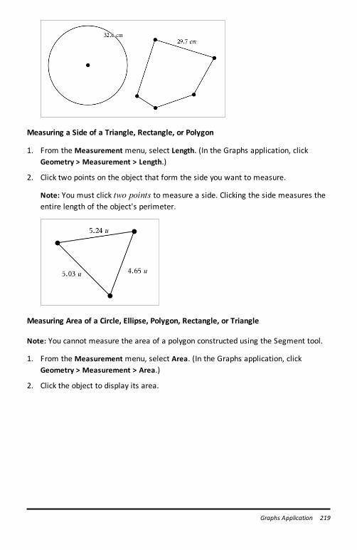
Measuring a Side of a Triangle, Rectangle, or Polygon
1. From the Measurement menu, select Length. (In the Graphs application, clickGeometry > Measurement > Length.)
2. Click two points on the object that form the side you want to measure.
Note: You must click two points to measure a side. Clicking the side measures theentire length of the object's perimeter.
Measuring Area of a Circle, Ellipse, Polygon, Rectangle, or Triangle
Note: You cannot measure the area of a polygon constructed using the Segment tool.
1. From the Measurement menu, select Area. (In the Graphs application, clickGeometry > Measurement > Area.)
2. Click the object to display its area.
Graphs Application 219
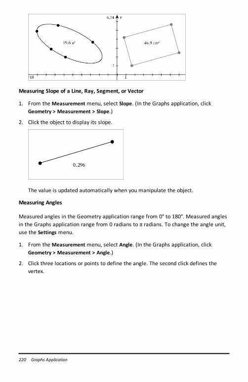
220 Graphs Application
Measuring Slope of a Line, Ray, Segment, or Vector
1. From the Measurement menu, select Slope. (In the Graphs application, clickGeometry > Measurement > Slope.)
2. Click the object to display its slope.
The value is updated automatically when you manipulate the object.
Measuring Angles
Measured angles in the Geometry application range from 0° to 180°. Measured anglesin the Graphs application range from 0 radians to π radians. To change the angle unit,use the Settings menu.
1. From the Measurement menu, select Angle. (In the Graphs application, clickGeometry > Measurement > Angle.)
2. Click three locations or points to define the angle. The second click defines thevertex.
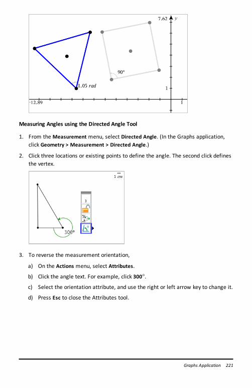
Measuring Angles using the Directed Angle Tool
1. From the Measurement menu, select Directed Angle. (In the Graphs application,click Geometry > Measurement > Directed Angle.)
2. Click three locations or existing points to define the angle. The second click definesthe vertex.
3. To reverse the measurement orientation,
a) On the Actions menu, select Attributes.
b) Click the angle text. For example, click 300°.
c) Select the orientation attribute, and use the right or left arrow key to change it.
d) Press Esc to close the Attributes tool.
Graphs Application 221
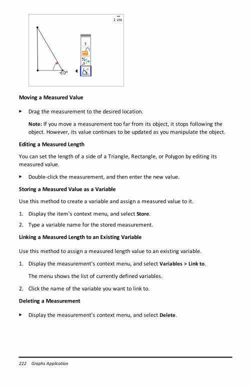
222 Graphs Application
Moving a Measured Value
▶ Drag the measurement to the desired location.
Note: If you move a measurement too far from its object, it stops following theobject. However, its value continues to be updated as you manipulate the object.
Editing a Measured Length
You can set the length of a side of a Triangle, Rectangle, or Polygon by editing itsmeasured value.
▶ Double-click the measurement, and then enter the new value.
Storing a Measured Value as a Variable
Use this method to create a variable and assign a measured value to it.
1. Display the item's context menu, and select Store.
2. Type a variable name for the stored measurement.
Linking a Measured Length to an Existing Variable
Use this method to assign a measured length value to an existing variable.
1. Display the measurement's context menu, and select Variables > Link to.
The menu shows the list of currently defined variables.
2. Click the name of the variable you want to link to.
Deleting a Measurement
▶ Display the measurement's context menu, and select Delete.
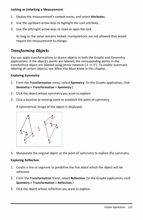
Locking or Unlocking a Measurement
1. Display the measurement's context menu, and select Attributes.
2. Use the up/down arrow keys to highlight the Lock attribute.
3. Use the left/right arrow keys to close or open the lock.
As long as the value remains locked, manipulations are not allowed that wouldrequire the measurement to change.
Transforming ObjectsYou can apply transformations to drawn objects in both the Graphs and Geometryapplications. If the object's points are labeled, the corresponding points in thetransformed object are labeled using prime notation (A → A'). To enable automaticlabeling of certain objects, see What You Must Know in this chapter.
Exploring Symmetry
1. From the Transformation menu, select Symmetry. (In the Graphs application, clickGeometry > Transformation > Symmetry.)
2. Click the object whose symmetry you want to explore.
3. Click a location or existing point to establish the point of symmetry.
A symmetrical image of the object is displayed.
4. Manipulate the original object or the point of symmetry to explore the symmetry.
Exploring Reflection
1. Create a line or segment to predefine the line about which the object will bereflected.
2. From the Transformation menu, select Reflection. (In the Graphs application, clickGeometry > Transformation > Reflection.)
3. Click the object whose reflection you want to explore.
Graphs Application 223
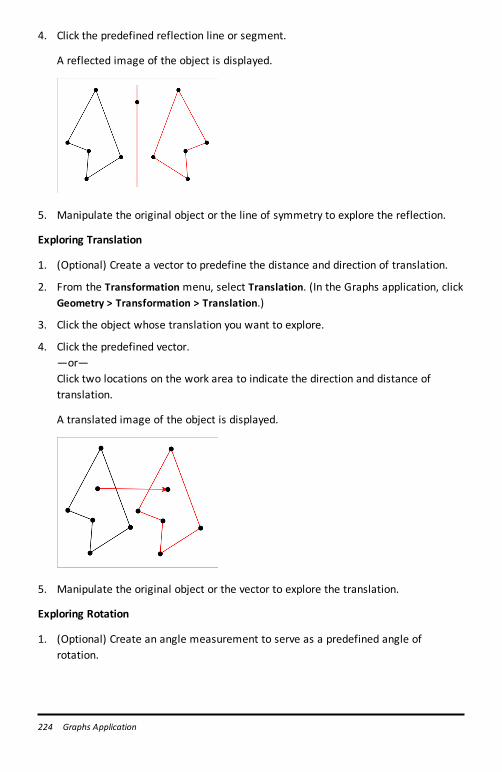
224 Graphs Application
4. Click the predefined reflection line or segment.
A reflected image of the object is displayed.
5. Manipulate the original object or the line of symmetry to explore the reflection.
Exploring Translation
1. (Optional) Create a vector to predefine the distance and direction of translation.
2. From the Transformation menu, select Translation. (In the Graphs application, clickGeometry > Transformation > Translation.)
3. Click the object whose translation you want to explore.
4. Click the predefined vector.—or—Click two locations on the work area to indicate the direction and distance oftranslation.
A translated image of the object is displayed.
5. Manipulate the original object or the vector to explore the translation.
Exploring Rotation
1. (Optional) Create an angle measurement to serve as a predefined angle ofrotation.
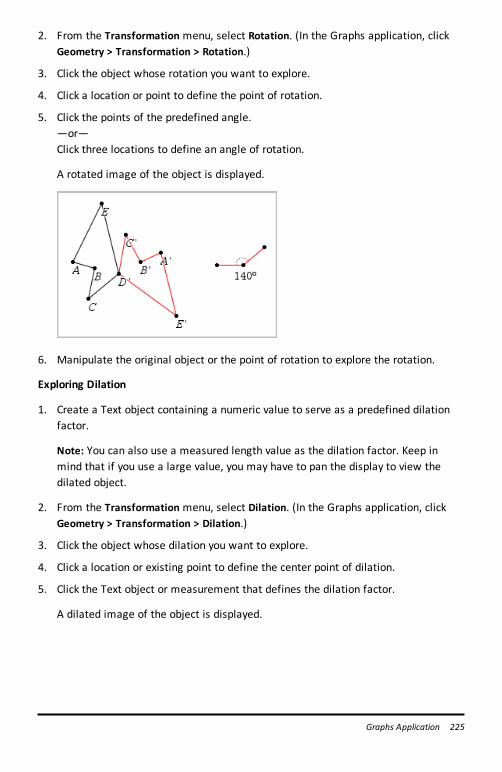
2. From the Transformation menu, select Rotation. (In the Graphs application, clickGeometry > Transformation > Rotation.)
3. Click the object whose rotation you want to explore.
4. Click a location or point to define the point of rotation.
5. Click the points of the predefined angle.—or—Click three locations to define an angle of rotation.
A rotated image of the object is displayed.
6. Manipulate the original object or the point of rotation to explore the rotation.
Exploring Dilation
1. Create a Text object containing a numeric value to serve as a predefined dilationfactor.
Note: You can also use a measured length value as the dilation factor. Keep inmind that if you use a large value, you may have to pan the display to view thedilated object.
2. From the Transformation menu, select Dilation. (In the Graphs application, clickGeometry > Transformation > Dilation.)
3. Click the object whose dilation you want to explore.
4. Click a location or existing point to define the center point of dilation.
5. Click the Text object or measurement that defines the dilation factor.
A dilated image of the object is displayed.
Graphs Application 225
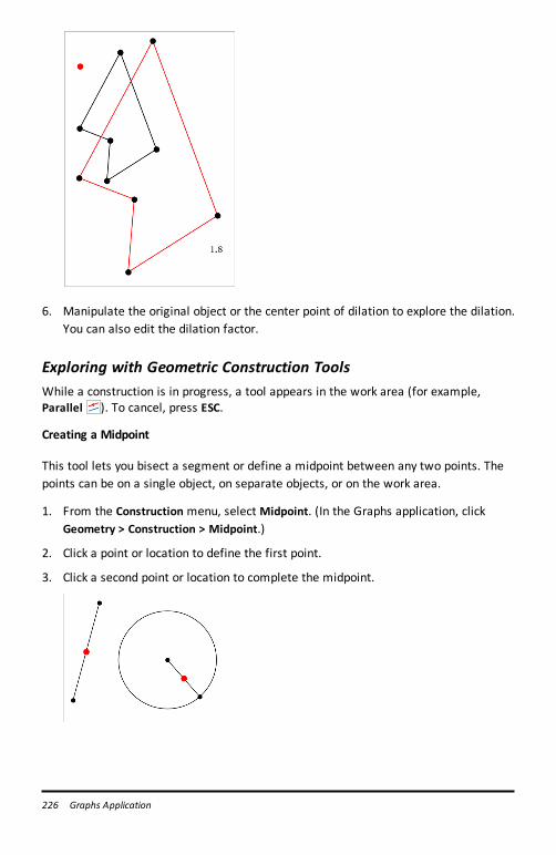
226 Graphs Application
6. Manipulate the original object or the center point of dilation to explore the dilation.You can also edit the dilation factor.
Exploring with Geometric Construction ToolsWhile a construction is in progress, a tool appears in the work area (for example,Parallel ). To cancel, press ESC.
Creating a Midpoint
This tool lets you bisect a segment or define a midpoint between any two points. Thepoints can be on a single object, on separate objects, or on the work area.
1. From the Construction menu, select Midpoint. (In the Graphs application, clickGeometry > Construction > Midpoint.)
2. Click a point or location to define the first point.
3. Click a second point or location to complete the midpoint.
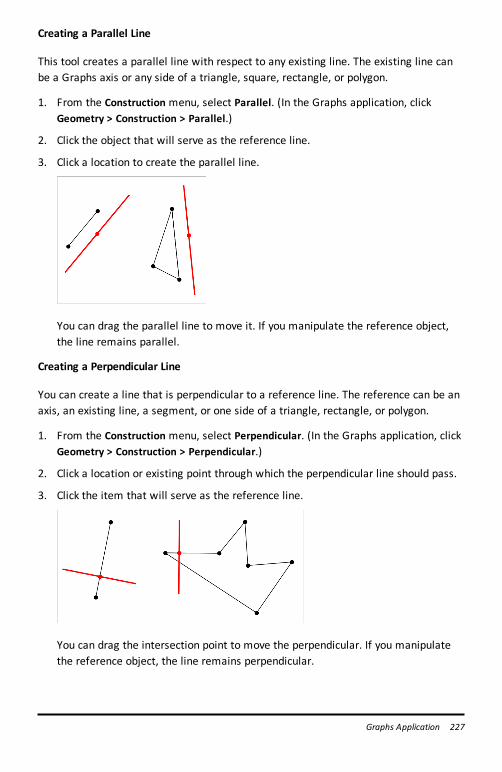
Creating a Parallel Line
This tool creates a parallel line with respect to any existing line. The existing line canbe a Graphs axis or any side of a triangle, square, rectangle, or polygon.
1. From the Construction menu, select Parallel. (In the Graphs application, clickGeometry > Construction > Parallel.)
2. Click the object that will serve as the reference line.
3. Click a location to create the parallel line.
You can drag the parallel line to move it. If you manipulate the reference object,the line remains parallel.
Creating a Perpendicular Line
You can create a line that is perpendicular to a reference line. The reference can be anaxis, an existing line, a segment, or one side of a triangle, rectangle, or polygon.
1. From the Construction menu, select Perpendicular. (In the Graphs application, clickGeometry > Construction > Perpendicular.)
2. Click a location or existing point through which the perpendicular line should pass.
3. Click the item that will serve as the reference line.
You can drag the intersection point to move the perpendicular. If you manipulatethe reference object, the line remains perpendicular.
Graphs Application 227
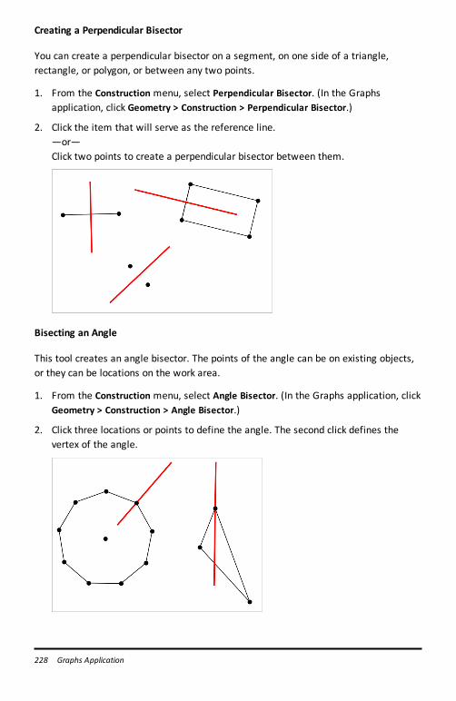
228 Graphs Application
Creating a Perpendicular Bisector
You can create a perpendicular bisector on a segment, on one side of a triangle,rectangle, or polygon, or between any two points.
1. From the Construction menu, select Perpendicular Bisector. (In the Graphsapplication, click Geometry > Construction > Perpendicular Bisector.)
2. Click the item that will serve as the reference line.—or—Click two points to create a perpendicular bisector between them.
Bisecting an Angle
This tool creates an angle bisector. The points of the angle can be on existing objects,or they can be locations on the work area.
1. From the Construction menu, select Angle Bisector. (In the Graphs application, clickGeometry > Construction > Angle Bisector.)
2. Click three locations or points to define the angle. The second click defines thevertex of the angle.
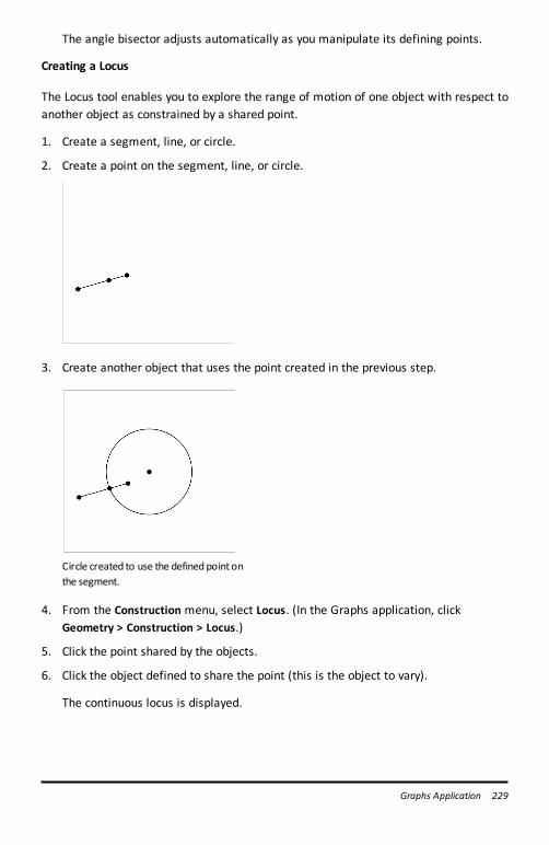
The angle bisector adjusts automatically as you manipulate its defining points.
Creating a Locus
The Locus tool enables you to explore the range of motion of one object with respect toanother object as constrained by a shared point.
1. Create a segment, line, or circle.
2. Create a point on the segment, line, or circle.
3. Create another object that uses the point created in the previous step.
Circle created to use the definedpoint onthe segment.
4. From the Construction menu, select Locus. (In the Graphs application, clickGeometry > Construction > Locus.)
5. Click the point shared by the objects.
6. Click the object defined to share the point (this is the object to vary).
The continuous locus is displayed.
Graphs Application 229
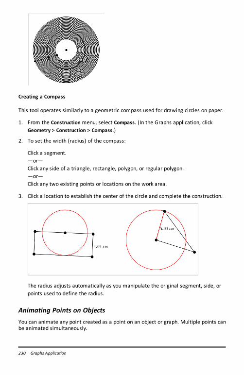
230 Graphs Application
Creating a Compass
This tool operates similarly to a geometric compass used for drawing circles on paper.
1. From the Construction menu, select Compass. (In the Graphs application, clickGeometry > Construction > Compass.)
2. To set the width (radius) of the compass:
Click a segment.—or—Click any side of a triangle, rectangle, polygon, or regular polygon.—or—Click any two existing points or locations on the work area.
3. Click a location to establish the center of the circle and complete the construction.
The radius adjusts automatically as you manipulate the original segment, side, orpoints used to define the radius.
Animating Points on ObjectsYou can animate any point created as a point on an object or graph. Multiple points canbe animated simultaneously.
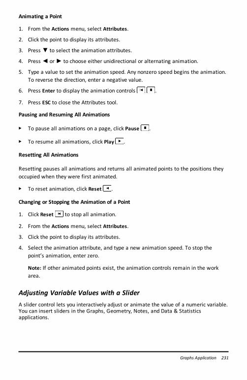
Animating a Point
1. From the Actions menu, select Attributes.
2. Click the point to display its attributes.
3. Press ▼ to select the animation attributes.
4. Press ◄ or ► to choose either unidirectional or alternating animation.
5. Type a value to set the animation speed. Any nonzero speed begins the animation.To reverse the direction, enter a negative value.
6. Press Enter to display the animation controls .
7. Press ESC to close the Attributes tool.
Pausing and Resuming All Animations
▶ To pause all animations on a page, click Pause .
▶ To resume all animations, click Play .
Resetting All Animations
Resetting pauses all animations and returns all animated points to the positions theyoccupied when they were first animated.
▶ To reset animation, click Reset .
Changing or Stopping the Animation of a Point
1. Click Reset to stop all animation.
2. From the Actions menu, select Attributes.
3. Click the point to display its attributes.
4. Select the animation attribute, and type a new animation speed. To stop thepoint’s animation, enter zero.
Note: If other animated points exist, the animation controls remain in the workarea.
Adjusting Variable Values with a SliderA slider control lets you interactively adjust or animate the value of a numeric variable.You can insert sliders in the Graphs, Geometry, Notes, and Data & Statisticsapplications.
Graphs Application 231
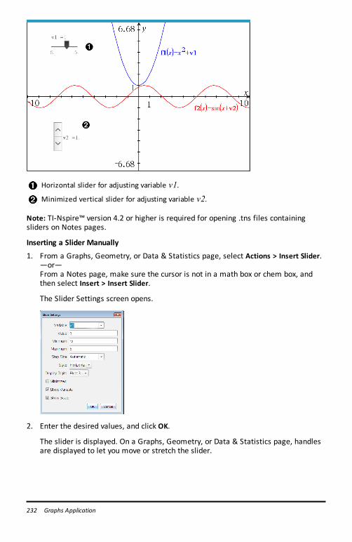
232 Graphs Application
Horizontal slider for adjusting variable v1.Minimized vertical slider for adjusting variable v2.
Note: TI-Nspire™ version 4.2 or higher is required for opening .tns files containingsliders on Notes pages.
Inserting a Slider Manually
1. From a Graphs, Geometry, or Data & Statistics page, select Actions > Insert Slider.—or—From a Notes page, make sure the cursor is not in a math box or chem box, andthen select Insert > Insert Slider.
The Slider Settings screen opens.
2. Enter the desired values, and click OK.
The slider is displayed. On a Graphs, Geometry, or Data & Statistics page, handlesare displayed to let you move or stretch the slider.
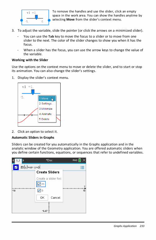
To remove the handles and use the slider, click an emptyspace in the work area. You can show the handles anytime byselectingMove from the slider's context menu.
3. To adjust the variable, slide the pointer (or click the arrows on a minimized slider).
- You can use the Tab key to move the focus to a slider or to move from oneslider to the next. The color of the slider changes to show you when it has thefocus.
- When a slider has the focus, you can use the arrow keys to change the value ofthe variable.
Working with the Slider
Use the options on the context menu to move or delete the slider, and to start or stopits animation. You can also change the slider's settings.
1. Display the slider's context menu.
2. Click an option to select it.
Automatic Sliders in Graphs
Sliders can be created for you automatically in the Graphs application and in theanalytic window of the Geometry application. You are offered automatic sliders whenyou define certain functions, equations, or sequences that refer to undefined variables.
Graphs Application 233
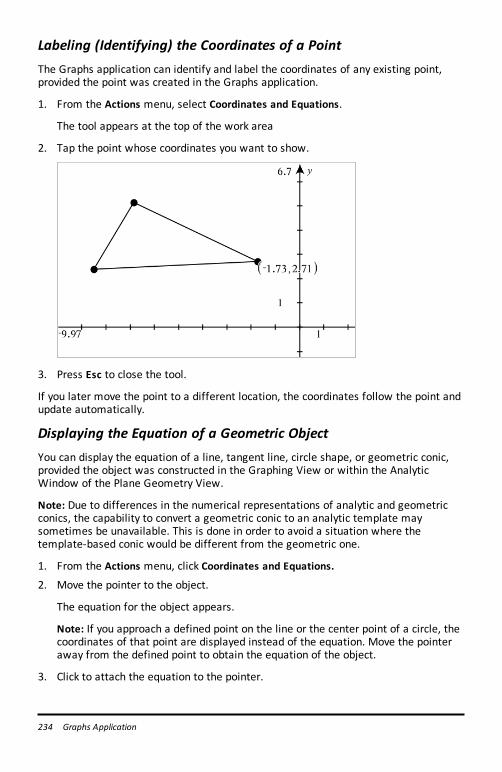
234 Graphs Application
Labeling (Identifying) the Coordinates of a PointThe Graphs application can identify and label the coordinates of any existing point,provided the point was created in the Graphs application.
1. From the Actions menu, select Coordinates and Equations.
The tool appears at the top of the work area
2. Tap the point whose coordinates you want to show.
3. Press Esc to close the tool.
If you later move the point to a different location, the coordinates follow the point andupdate automatically.
Displaying the Equation of a Geometric ObjectYou can display the equation of a line, tangent line, circle shape, or geometric conic,provided the object was constructed in the Graphing View or within the AnalyticWindow of the Plane Geometry View.
Note: Due to differences in the numerical representations of analytic and geometricconics, the capability to convert a geometric conic to an analytic template maysometimes be unavailable. This is done in order to avoid a situation where thetemplate-based conic would be different from the geometric one.
1. From the Actions menu, click Coordinates and Equations.
2. Move the pointer to the object.
The equation for the object appears.
Note: If you approach a defined point on the line or the center point of a circle, thecoordinates of that point are displayed instead of the equation. Move the pointeraway from the defined point to obtain the equation of the object.
3. Click to attach the equation to the pointer.
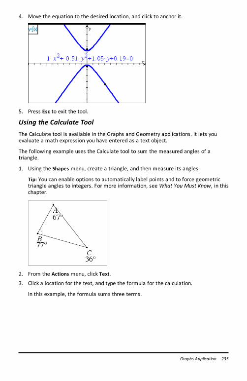
4. Move the equation to the desired location, and click to anchor it.
5. Press Esc to exit the tool.
Using the Calculate ToolThe Calculate tool is available in the Graphs and Geometry applications. It lets youevaluate a math expression you have entered as a text object.
The following example uses the Calculate tool to sum the measured angles of atriangle.
1. Using the Shapes menu, create a triangle, and then measure its angles.
Tip: You can enable options to automatically label points and to force geometrictriangle angles to integers. For more information, see What You Must Know, in thischapter.
2. From the Actions menu, click Text.
3. Click a location for the text, and type the formula for the calculation.
In this example, the formula sums three terms.
Graphs Application 235
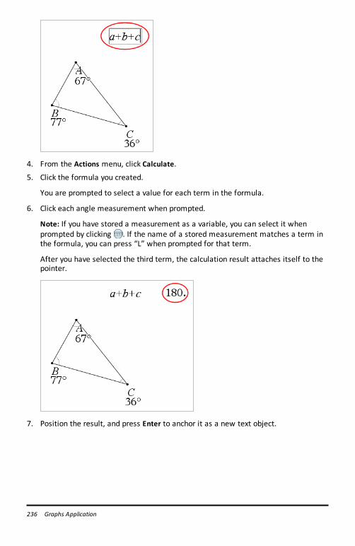
236 Graphs Application
4. From the Actions menu, click Calculate.
5. Click the formula you created.
You are prompted to select a value for each term in the formula.
6. Click each angle measurement when prompted.
Note: If you have stored a measurement as a variable, you can select it whenprompted by clicking . If the name of a stored measurement matches a term inthe formula, you can press “L” when prompted for that term.
After you have selected the third term, the calculation result attaches itself to thepointer.
7. Position the result, and press Enter to anchor it as a new text object.
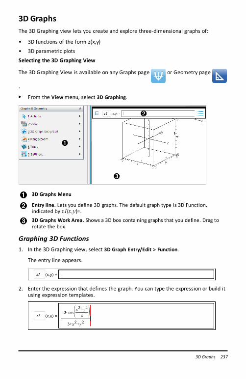
3D GraphsThe 3D Graphing view lets you create and explore three-dimensional graphs of:
• 3D functions of the form z(x,y)
• 3D parametric plots
Selecting the 3D Graphing View
The 3D Graphing View is available on any Graphs page or Geometry page
.
▶ From the Viewmenu, select 3D Graphing.
3D Graphs Menu
Entry line. Lets you define 3D graphs. The default graph type is 3D Function,indicated by z1(x,y)=.3D Graphs Work Area. Shows a 3D box containing graphs that you define. Drag torotate the box.
Graphing 3D Functions1. In the 3D Graphing view, select 3D Graph Entry/Edit > Function.
The entry line appears.
2. Enter the expression that defines the graph. You can type the expression or build itusing expression templates.
3D Graphs 237
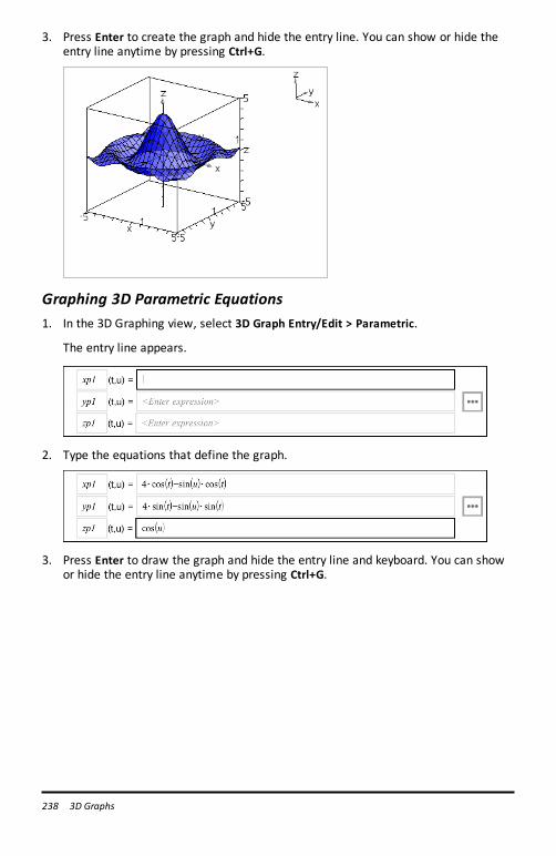
238 3D Graphs
3. Press Enter to create the graph and hide the entry line. You can show or hide theentry line anytime by pressing Ctrl+G.
Graphing 3D Parametric Equations1. In the 3D Graphing view, select 3D Graph Entry/Edit > Parametric.
The entry line appears.
2. Type the equations that define the graph.
3. Press Enter to draw the graph and hide the entry line and keyboard. You can showor hide the entry line anytime by pressing Ctrl+G.
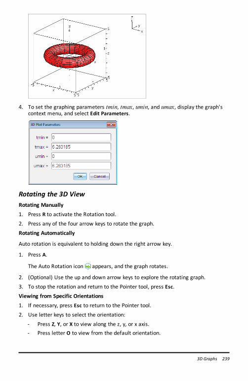
4. To set the graphing parameters tmin, tmax, umin, and umax, display the graph'scontext menu, and select Edit Parameters.
Rotating the 3D ViewRotating Manually
1. Press R to activate the Rotation tool.
2. Press any of the four arrow keys to rotate the graph.
Rotating Automatically
Auto rotation is equivalent to holding down the right arrow key.
1. Press A.
The Auto Rotation icon appears, and the graph rotates.
2. (Optional) Use the up and down arrow keys to explore the rotating graph.
3. To stop the rotation and return to the Pointer tool, press Esc.
Viewing from Specific Orientations
1. If necessary, press Esc to return to the Pointer tool.
2. Use letter keys to select the orientation:
- Press Z, Y, or X to view along the z, y, or x axis.- Press letter O to view from the default orientation.
3D Graphs 239
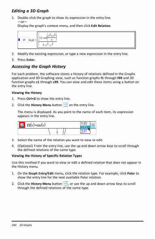
240 3D Graphs
Editing a 3D Graph1. Double-click the graph to show its expression in the entry line.
—or—Display the graph’s context menu, and then click Edit Relation.
2. Modify the existing expression, or type a new expression in the entry line.
3. Press Enter.
Accessing the Graph HistoryFor each problem, the software stores a history of relations defined in the Graphsapplication and 3D Graphing view, such as function graphs f1 through f99 and 3Dfunction graphs z1 through z99. You can view and edit these items using a button onthe entry line.
Viewing the History
1. Press Ctrl+G to show the entry line.
2. Click the History Menu button on the entry line.
The menu is displayed. As you point to the name of each item, its expressionappears in the entry line.
3. Select the name of the relation you want to view or edit.
4. (Optional) From the entry line, use the up and down arrow keys to scroll throughthe defined relations of the same type.
Viewing the History of Specific Relation Types
Use this method if you want to view or edit a defined relation that does not appear inthe History menu.
1. On the Graph Entry/Edit menu, click the relation type. For example, click Polar toshow the entry line for the next available Polar relation.
2. Click the History Menu button , or use the up and down arrow keys to scrollthrough the defined relations of the same type.
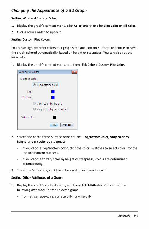
Changing the Appearance of a 3D Graph
Setting Wire and Surface Color:
1. Display the graph’s context menu, click Color, and then click Line Color or Fill Color.
2. Click a color swatch to apply it.
Setting Custom Plot Colors:
You can assign different colors to a graph's top and bottom surfaces or choose to havethe graph colored automatically, based on height or steepness. You can also set thewire color.
1. Display the graph’s context menu, and then click Color > Custom Plot Color.
2. Select one of the three Surface color options: Top/bottom color, Vary color byheight, or Vary color by steepness.
- If you choose Top/bottom color, click the color swatches to select colors for thetop and bottom surfaces.
- If you choose to vary color by height or steepness, colors are determinedautomatically.
3. To set the Wire color, click the color swatch and select a color.
Setting Other Attributes of a Graph:
1. Display the graph’s context menu, and then click Attributes. You can set thefollowing attributes for the selected graph.
- format: surface+wire, surface only, or wire only
3D Graphs 241
242 3D Graphs
- x resolution (enter a value in range 2-200*, default=21)
- y resolution (enter a value in range 2-200*, default=21)
- transparency (enter a value in range 0-100, default=30)
* Handhelds are limited to a maximum display resolution of 21, regardless of thevalue entered.
2. Set the attributes as you like, and then press Enter to accept the changes.
Showing or Hiding a Graph’s Label
▶ Display the graph’s context menu, and then click Hide Label or Show Label.
Showing and Hiding 3D Graphs1. In the 3D Graphing view, select Actions > Hide/Show.
The Hide/Show tool appears, and all hidden items are displayed in gray.
2. Tap a graph to change its hide/show state.
3. To apply the changes and dismiss the tool, press Esc.
Note: If you want to show or hide only the graph's label, see Showing or Hiding aGraph’s Label.
Customizing the 3D Viewing Environment
Setting the Background Color
▶ Display the context menu for the work area, and then click Background Color.
Showing or Hiding Specific View Elements
▶ From the Viewmenu, click the item to show or hide. You can choose items such asthe 3D box, axes, box end values, and legend.
Changing the 3D Projection
▶ From the Viewmenu, click Orthographic Projection or Perspective View.
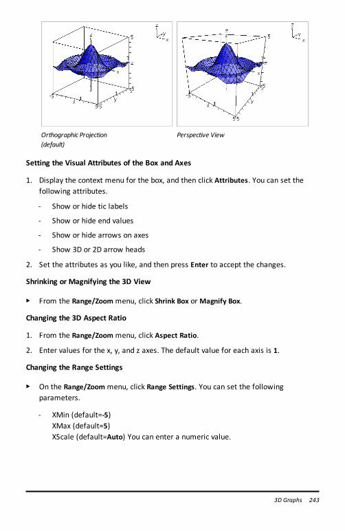
Orthographic Projection(default)
Perspective View
Setting the Visual Attributes of the Box and Axes
1. Display the context menu for the box, and then click Attributes. You can set thefollowing attributes.
- Show or hide tic labels
- Show or hide end values
- Show or hide arrows on axes
- Show 3D or 2D arrow heads
2. Set the attributes as you like, and then press Enter to accept the changes.
Shrinking or Magnifying the 3D View
▶ From the Range/Zoommenu, click Shrink Box orMagnify Box.
Changing the 3D Aspect Ratio
1. From the Range/Zoommenu, click Aspect Ratio.
2. Enter values for the x, y, and z axes. The default value for each axis is 1.
Changing the Range Settings
▶ On the Range/Zoommenu, click Range Settings. You can set the followingparameters.
- XMin (default=-5)XMax (default=5)XScale (default=Auto) You can enter a numeric value.
3D Graphs 243
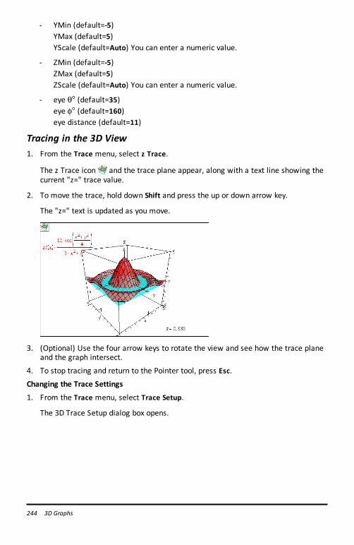
244 3D Graphs
- YMin (default=-5)YMax (default=5)YScale (default=Auto) You can enter a numeric value.
- ZMin (default=-5)ZMax (default=5)ZScale (default=Auto) You can enter a numeric value.
- eye q¡ (default=35)eye f¡ (default=160)eye distance (default=11)
Tracing in the 3D View1. From the Trace menu, select z Trace.
The z Trace icon and the trace plane appear, along with a text line showing thecurrent "z=" trace value.
2. To move the trace, hold down Shift and press the up or down arrow key.
The "z=" text is updated as you move.
3. (Optional) Use the four arrow keys to rotate the view and see how the trace planeand the graph intersect.
4. To stop tracing and return to the Pointer tool, press Esc.
Changing the Trace Settings
1. From the Trace menu, select Trace Setup.
The 3D Trace Setup dialog box opens.
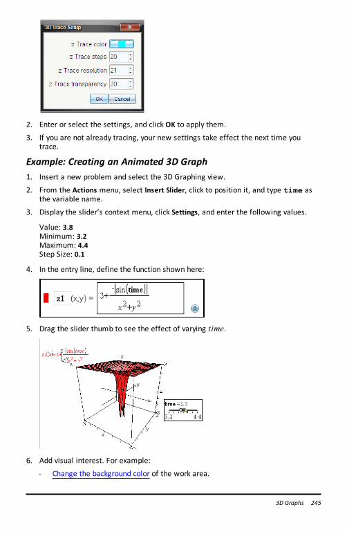
2. Enter or select the settings, and click OK to apply them.
3. If you are not already tracing, your new settings take effect the next time youtrace.
Example: Creating an Animated 3D Graph1. Insert a new problem and select the 3D Graphing view.
2. From the Actions menu, select Insert Slider, click to position it, and type time asthe variable name.
3. Display the slider’s context menu, click Settings, and enter the following values.
Value: 3.8Minimum: 3.2Maximum: 4.4Step Size: 0.1
4. In the entry line, define the function shown here:
5. Drag the slider thumb to see the effect of varying time.
6. Add visual interest. For example:
- Change the background color of the work area.
3D Graphs 245
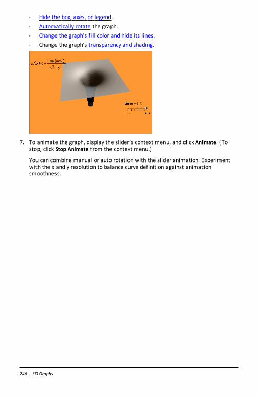
246 3D Graphs
- Hide the box, axes, or legend.- Automatically rotate the graph.- Change the graph's fill color and hide its lines.- Change the graph’s transparency and shading.
7. To animate the graph, display the slider’s context menu, and click Animate. (Tostop, click Stop Animate from the context menu.)
You can combine manual or auto rotation with the slider animation. Experimentwith the x and y resolution to balance curve definition against animationsmoothness.
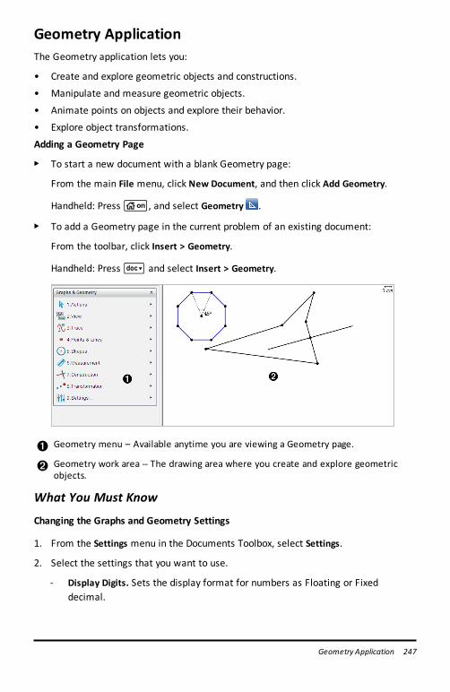
Geometry ApplicationThe Geometry application lets you:
• Create and explore geometric objects and constructions.
• Manipulate and measure geometric objects.
• Animate points on objects and explore their behavior.
• Explore object transformations.
Adding a Geometry Page
▶ To start a new document with a blank Geometry page:
From the main File menu, click New Document, and then click Add Geometry.
Handheld: Pressc, and select Geometry .
▶ To add a Geometry page in the current problem of an existing document:
From the toolbar, click Insert > Geometry.
Handheld: Press~ and select Insert > Geometry.
À Geometry menu – Available anytime you are viewing a Geometry page.
Á Geometry work area -- The drawing area where you create and explore geometricobjects.
What You Must Know
Changing the Graphs and Geometry Settings
1. From the Settings menu in the Documents Toolbox, select Settings.
2. Select the settings that you want to use.
- Display Digits. Sets the display format for numbers as Floating or Fixeddecimal.
Geometry Application 247
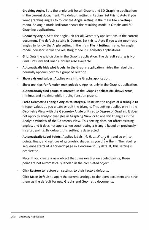
248 Geometry Application
- Graphing Angle. Sets the angle unit for all Graphs and 3D Graphing applicationsin the current docuument. The default setting is Radian. Set this to Auto if youwant graphing angles to follow the Angle setting in the main File > Settingsmenu. An angle mode indicator shows the resulting mode in Graphs and 3DGraphing applications.
- Geometry Angle. Sets the angle unit for all Geometry applications in the currentdocument. The default setting is Degree. Set this to Auto if you want geometryangles to follow the Angle setting in the main File > Settings menu. An anglemode indicator shows the resulting mode in Geometry applications.
- Grid. Sets the grid display in the Graphs application. The default setting is NoGrid. Dot Grid and Lined Grid are also available.
- Automatically hide plot labels. In the Graphs application, hides the label thatnormally appears next to a graphed relation.
- Show axis end values. Applies only in the Graphs application.
- Show tool tips for function manipulation. Applies only in the Graphs application.
- Automatically find points of interest. In the Graphs application, shows zeros,minima, and maxima while tracing function graphs.
- Force Geometric Triangle Angles to Integers. Restricts the angles of a triangle tointeger values as you create or edit the triangle. This setting applies only in theGeometry View with the Geometry Angle unit set to Degree or Gradian. It doesnot apply to analytic triangles in Graphing View or to analytic triangles in theAnalytic Window of the Geometry View. This setting does not affect existingangles, and it does not apply when constructing a triangle based on previouslyinserted points. By default, this setting is deselected.
- Automatically Label Points. Applies labels (A, B, ..., Z, A1, B
1, and so on) to
points, lines, and vertices of geometric shapes as you draw them. The labelingsequence starts at A for each page in a document. By default, this setting isdeselected.
Note: If you create a new object that uses existing unlabeled points, thosepoint are not automatically labeled in the completed object.
- Click Restore to restore all settings to their factory defaults.
- ClickMake Default to apply the current settings to the open document and savethem as the default for new Graphs and Geometry documents.
Using Context Menus
Context menus provide quick access to commonly used commands and tools that applyto a specific object. For example, you can use a context menu to change an object'sline color or to group a set of selected objects.
▶ Display the context menu for an object in one of the following ways.
- Windows®: Right-click the object.
- Mac®: Hold “ and click the object.
- Handheld: Move the pointer to the object, and then press/b.
Finding Hidden Objects in the Graphs or Geometry Application
You can hide and show individual graphs, geometric objects, text, labels,measurements, and axis end-values.
To temporarily view hidden graphs or objects or to restore them as shown objects:
1. From the Actions menu, select Hide/Show.
The Hide/Show tool appears in the work area, and all hidden objects becomevisible in dimmed colors.
2. Click a graph or object to toggle its Hide/Show state.
3. To apply the changes and close the Hide/Show tool, press ESC.
Inserting a Background Image
You can insert an image as a background for a Graphs or Geometry page. The fileformat of the image can be .bmp, .jpg, or .png.
1. From the Insert menu, click Image.
2. Navigate to the image you want to insert, select it, and then click Open.
For information on moving, resizing, and deleting a background image, see Workingwith Images in the Software.
Adding Text to the Graphs or Geometry Work Area
1. From the Actions menu, select Text.
The Text tool appears in the work area.
2. Click the location for the text.
Geometry Application 249
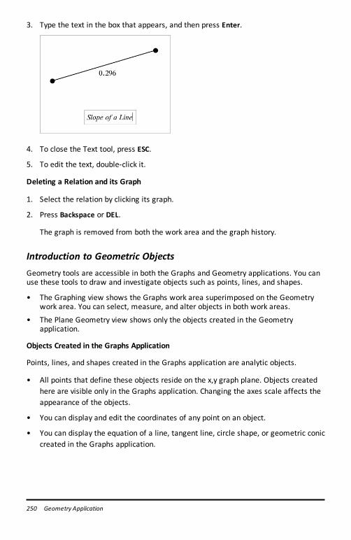
250 Geometry Application
3. Type the text in the box that appears, and then press Enter.
4. To close the Text tool, press ESC.
5. To edit the text, double-click it.
Deleting a Relation and its Graph
1. Select the relation by clicking its graph.
2. Press Backspace or DEL.
The graph is removed from both the work area and the graph history.
Introduction to Geometric ObjectsGeometry tools are accessible in both the Graphs and Geometry applications. You canuse these tools to draw and investigate objects such as points, lines, and shapes.
• The Graphing view shows the Graphs work area superimposed on the Geometrywork area. You can select, measure, and alter objects in both work areas.
• The Plane Geometry view shows only the objects created in the Geometryapplication.
Objects Created in the Graphs Application
Points, lines, and shapes created in the Graphs application are analytic objects.
• All points that define these objects reside on the x,y graph plane. Objects createdhere are visible only in the Graphs application. Changing the axes scale affects theappearance of the objects.
• You can display and edit the coordinates of any point on an object.
• You can display the equation of a line, tangent line, circle shape, or geometric coniccreated in the Graphs application.
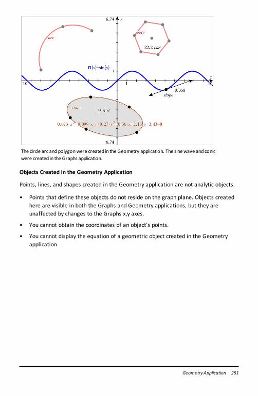
The circle arc andpolygonwere created in the Geometry application. The sinewave and conicwere created in the Graphs application.
Objects Created in the Geometry Application
Points, lines, and shapes created in the Geometry application are not analytic objects.
• Points that define these objects do not reside on the graph plane. Objects createdhere are visible in both the Graphs and Geometry applications, but they areunaffected by changes to the Graphs x,y axes.
• You cannot obtain the coordinates of an object’s points.
• You cannot display the equation of a geometric object created in the Geometryapplication
Geometry Application 251
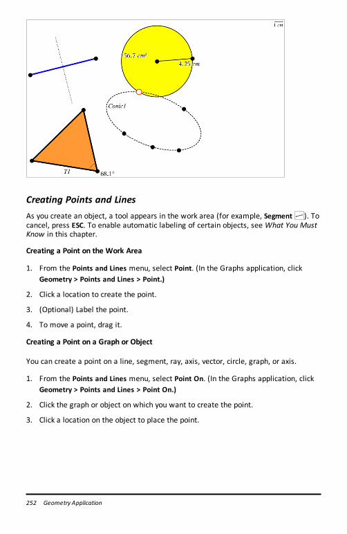
252 Geometry Application
Creating Points and LinesAs you create an object, a tool appears in the work area (for example, Segment ). Tocancel, press ESC. To enable automatic labeling of certain objects, see What You MustKnow in this chapter.
Creating a Point on the Work Area
1. From the Points and Lines menu, select Point. (In the Graphs application, clickGeometry > Points and Lines > Point.)
2. Click a location to create the point.
3. (Optional) Label the point.
4. To move a point, drag it.
Creating a Point on a Graph or Object
You can create a point on a line, segment, ray, axis, vector, circle, graph, or axis.
1. From the Points and Lines menu, select Point On. (In the Graphs application, clickGeometry > Points and Lines > Point On.)
2. Click the graph or object on which you want to create the point.
3. Click a location on the object to place the point.
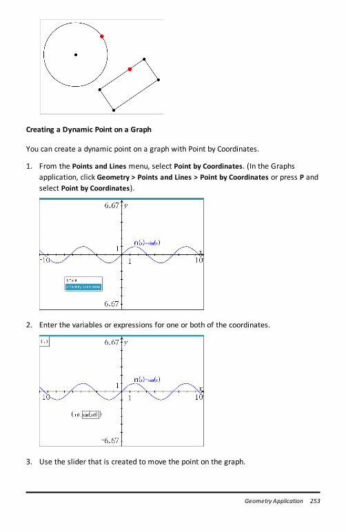
Creating a Dynamic Point on a Graph
You can create a dynamic point on a graph with Point by Coordinates.
1. From the Points and Lines menu, select Point by Coordinates. (In the Graphsapplication, click Geometry > Points and Lines > Point by Coordinates or press P andselect Point by Coordinates).
2. Enter the variables or expressions for one or both of the coordinates.
3. Use the slider that is created to move the point on the graph.
Geometry Application 253
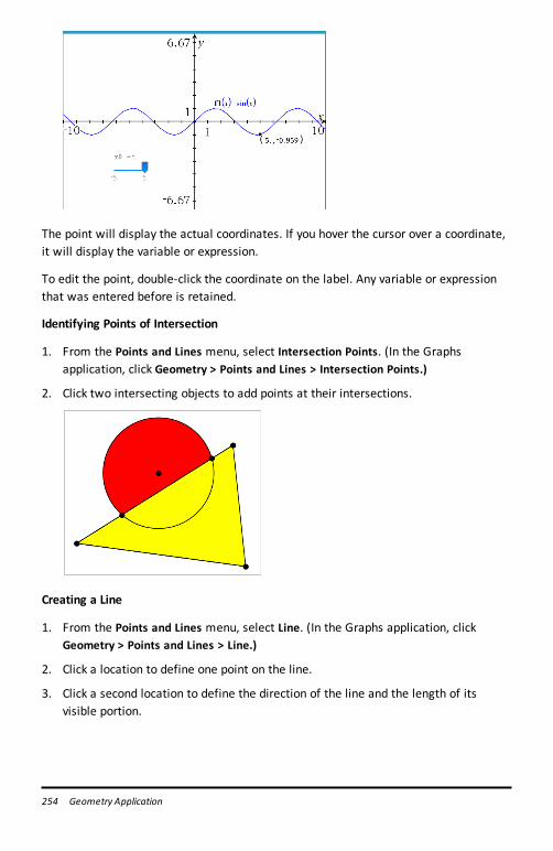
254 Geometry Application
The point will display the actual coordinates. If you hover the cursor over a coordinate,it will display the variable or expression.
To edit the point, double-click the coordinate on the label. Any variable or expressionthat was entered before is retained.
Identifying Points of Intersection
1. From the Points and Lines menu, select Intersection Points. (In the Graphsapplication, click Geometry > Points and Lines > Intersection Points.)
2. Click two intersecting objects to add points at their intersections.
Creating a Line
1. From the Points and Lines menu, select Line. (In the Graphs application, clickGeometry > Points and Lines > Line.)
2. Click a location to define one point on the line.
3. Click a second location to define the direction of the line and the length of itsvisible portion.

4. To move a line, drag its identifying point. To rotate it, drag any point except theidentifying point or ends. To extend its visible portion, drag from either end.
Creating a Segment
1. From the Points and Lines menu, select Segment. (In the Graphs application, clickGeometry > Points and Lines > Segment.)
2. Click two locations to define the endpoints of the segment.
3. To move a segment, drag any point other than an endpoint. To manipulate thedirection or length, drag either endpoint.
Creating a Ray
1. From the Points and Lines menu, select Ray. (In the Graphs application, clickGeometry > Points and Lines > Ray.)
2. Click a location to define the endpoint of the ray.
3. Click a second location to define the direction.
Geometry Application 255
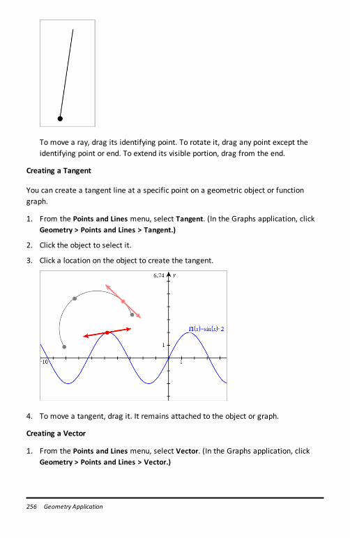
256 Geometry Application
To move a ray, drag its identifying point. To rotate it, drag any point except theidentifying point or end. To extend its visible portion, drag from the end.
Creating a Tangent
You can create a tangent line at a specific point on a geometric object or functiongraph.
1. From the Points and Lines menu, select Tangent. (In the Graphs application, clickGeometry > Points and Lines > Tangent.)
2. Click the object to select it.
3. Click a location on the object to create the tangent.
4. To move a tangent, drag it. It remains attached to the object or graph.
Creating a Vector
1. From the Points and Lines menu, select Vector. (In the Graphs application, clickGeometry > Points and Lines > Vector.)
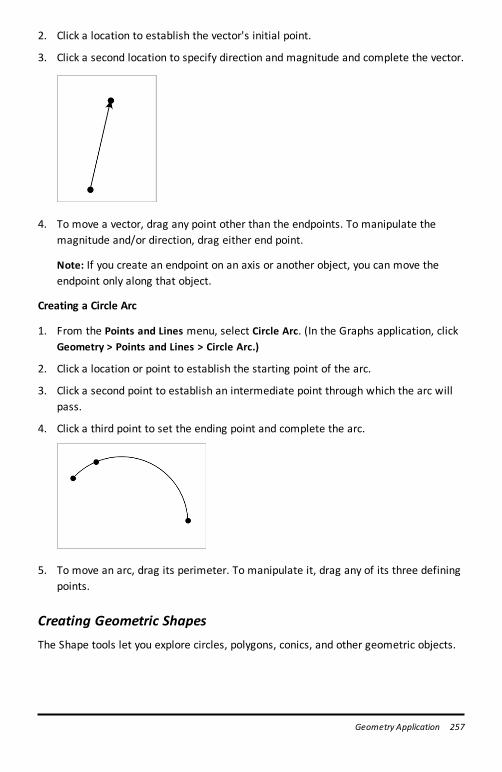
2. Click a location to establish the vector's initial point.
3. Click a second location to specify direction and magnitude and complete the vector.
4. To move a vector, drag any point other than the endpoints. To manipulate themagnitude and/or direction, drag either end point.
Note: If you create an endpoint on an axis or another object, you can move theendpoint only along that object.
Creating a Circle Arc
1. From the Points and Lines menu, select Circle Arc. (In the Graphs application, clickGeometry > Points and Lines > Circle Arc.)
2. Click a location or point to establish the starting point of the arc.
3. Click a second point to establish an intermediate point through which the arc willpass.
4. Click a third point to set the ending point and complete the arc.
5. To move an arc, drag its perimeter. To manipulate it, drag any of its three definingpoints.
Creating Geometric ShapesThe Shape tools let you explore circles, polygons, conics, and other geometric objects.
Geometry Application 257
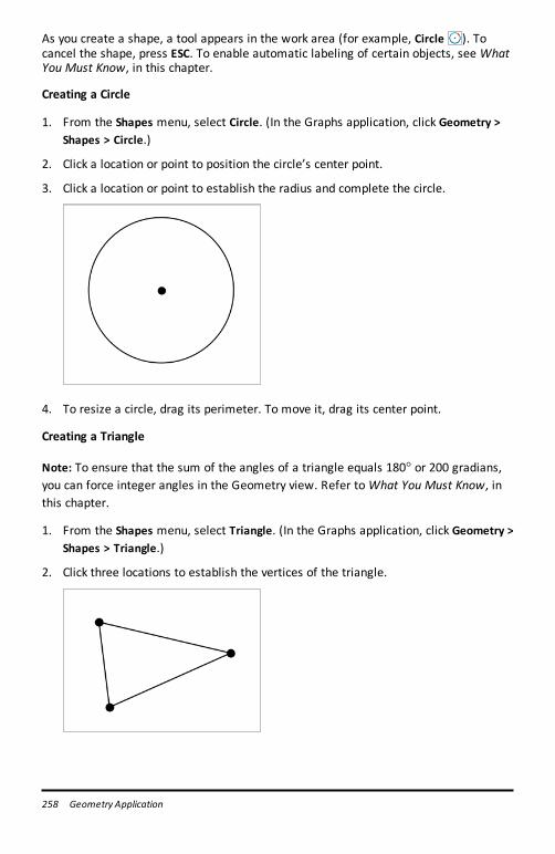
258 Geometry Application
As you create a shape, a tool appears in the work area (for example, Circle ). Tocancel the shape, press ESC. To enable automatic labeling of certain objects, see WhatYou Must Know, in this chapter.
Creating a Circle
1. From the Shapes menu, select Circle. (In the Graphs application, click Geometry >Shapes > Circle.)
2. Click a location or point to position the circle’s center point.
3. Click a location or point to establish the radius and complete the circle.
4. To resize a circle, drag its perimeter. To move it, drag its center point.
Creating a Triangle
Note: To ensure that the sum of the angles of a triangle equals 180° or 200 gradians,you can force integer angles in the Geometry view. Refer toWhat You Must Know, inthis chapter.
1. From the Shapes menu, select Triangle. (In the Graphs application, click Geometry >Shapes > Triangle.)
2. Click three locations to establish the vertices of the triangle.
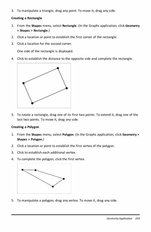
3. To manipulate a triangle, drag any point. To move it, drag any side.
Creating a Rectangle
1. From the Shapes menu, select Rectangle. (In the Graphs application, click Geometry> Shapes > Rectangle.)
2. Click a location or point to establish the first corner of the rectangle.
3. Click a location for the second corner.
One side of the rectangle is displayed.
4. Click to establish the distance to the opposite side and complete the rectangle.
5. To rotate a rectangle, drag one of its first two points. To extend it, drag one of thelast two points. To move it, drag any side.
Creating a Polygon
1. From the Shapes menu, select Polygon. (In the Graphs application, click Geometry >Shapes > Polygon.)
2. Click a location or point to establish the first vertex of the polygon.
3. Click to establish each additional vertex.
4. To complete the polygon, click the first vertex.
5. To manipulate a polygon, drag any vertex. To move it, drag any side.
Geometry Application 259
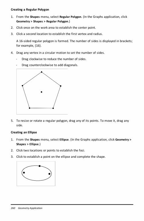
260 Geometry Application
Creating a Regular Polygon
1. From the Shapes menu, select Regular Polygon. (In the Graphs application, clickGeometry > Shapes > Regular Polygon.)
2. Click once on the work area to establish the center point.
3. Click a second location to establish the first vertex and radius.
A 16-sided regular polygon is formed. The number of sides is displayed in brackets;for example, {16}.
4. Drag any vertex in a circular motion to set the number of sides.
- Drag clockwise to reduce the number of sides.
- Drag counterclockwise to add diagonals.
5. To resize or rotate a regular polygon, drag any of its points. To move it, drag anyside.
Creating an Ellipse
1. From the Shapes menu, select Ellipse. (In the Graphs application, click Geometry >Shapes > Ellipse.)
2. Click two locations or points to establish the foci.
3. Click to establish a point on the ellipse and complete the shape.
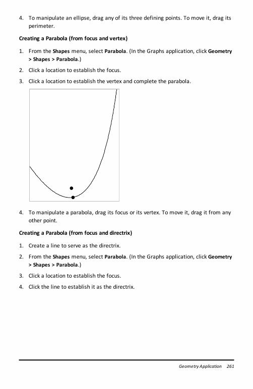
4. To manipulate an ellipse, drag any of its three defining points. To move it, drag itsperimeter.
Creating a Parabola (from focus and vertex)
1. From the Shapes menu, select Parabola. (In the Graphs application, click Geometry> Shapes > Parabola.)
2. Click a location to establish the focus.
3. Click a location to establish the vertex and complete the parabola.
4. To manipulate a parabola, drag its focus or its vertex. To move it, drag it from anyother point.
Creating a Parabola (from focus and directrix)
1. Create a line to serve as the directrix.
2. From the Shapes menu, select Parabola. (In the Graphs application, click Geometry> Shapes > Parabola.)
3. Click a location to establish the focus.
4. Click the line to establish it as the directrix.
Geometry Application 261
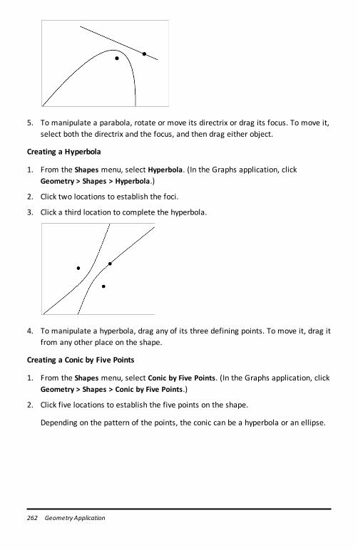
262 Geometry Application
5. To manipulate a parabola, rotate or move its directrix or drag its focus. To move it,select both the directrix and the focus, and then drag either object.
Creating a Hyperbola
1. From the Shapes menu, select Hyperbola. (In the Graphs application, clickGeometry > Shapes > Hyperbola.)
2. Click two locations to establish the foci.
3. Click a third location to complete the hyperbola.
4. To manipulate a hyperbola, drag any of its three defining points. To move it, drag itfrom any other place on the shape.
Creating a Conic by Five Points
1. From the Shapes menu, select Conic by Five Points. (In the Graphs application, clickGeometry > Shapes > Conic by Five Points.)
2. Click five locations to establish the five points on the shape.
Depending on the pattern of the points, the conic can be a hyperbola or an ellipse.
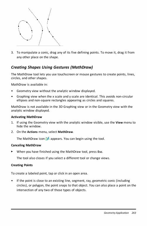
3. To manipulate a conic, drag any of its five defining points. To move it, drag it fromany other place on the shape.
Creating Shapes Using Gestures (MathDraw)The MathDraw tool lets you use touchscreen or mouse gestures to create points, lines,circles, and other shapes.
MathDraw is available in:
• Geometry view without the analytic window displayed.
• Graphing view when the x scale and y scale are identical. This avoids non-circularellipses and non-square rectangles appearing as circles and squares.
MathDraw is not available in the 3D Graphing view or in the Geometry view with theanalytic window displayed.
Activating MathDraw
1. If using the Geometry view with the analytic window visible, use the Viewmenu tohide the window.
2. On the Actions menu, select MathDraw.
The MathDraw icon appears. You can begin using the tool.
Canceling MathDraw
▶ When you have finished using the MathDraw tool, press Esc.
The tool also closes if you select a different tool or change views.
Creating Points
To create a labeled point, tap or click in an open area.
• If the point is close to an existing line, segment, ray, geometric conic (includingcircles), or polygon, the point snaps to that object. You can also place a point on theintersection of any two of those types of objects.
Geometry Application 263
264 Geometry Application
• If the point is close to a visible grid location in a Graphs view or the analyticwindow of a Geometry view, it snaps to the grid.
Drawing Lines and Segments
To create a line or segment, touch or click the initial position, and then drag to the endposition.
• If the drawn line passes near an existing point, the line snaps to the point.
• If the drawn line starts close to an existing point and ends next to another existingpoint , it becomes a segment defined by those points.
• If the drawn line is nearly parallel or perpendicular to an existing line, segment, orside of a polygon, it aligns to that object.
Note: The default tolerance for detecting parallel/perpendicular lines is 12.5degrees. This tolerance can be redefined using a variable named ti_gg_fd.angle_tol.You can change the tolerance in the current problem by setting this variable in thecalculator app to a value in the range 0 through 45 (0=no parallel/perpendiculardetection).
Drawing Circles and Ellipses
To create a circle or ellipse, use the touchscreen or mouse to draw the approximateshape.
• If the drawn shape is sufficiently circular, a circle is created.
• If the shape is elongated, an ellipse is created.
• If the virtual center of the drawn shape is near an existing point, the circle orellipse is centered on that point.
Drawing Triangles
To create a triangle, draw a triangle-like shape.
• If a drawn vertex is close to an existing point, the vertex snaps to the point.
Drawing Rectangles and Squares
To create a rectangle or square, use the touchscreen or mouse to draw the perimeter.
• If the drawn shape is nearly square, a square is created.
• If the drawn shape is elongated, a rectangle is created.
• If the center of a square is close to an existing point, the square snaps to thatpoint.
Drawing Polygons
To create a polygon, tap or click a succession of existing points, ending on the firstpoint you tapped.
Using MathDraw to Create Equations
In the Graphs view, MathDraw attempts to recognize certain gestures as functions foranalytic parabolas.
Note: The default step value for quantization of the parabola coefficients is 1/32. Thedenominator of this fraction can be redefined using a variable named ti_gg_fd.par_quant. You can change the step value in the current problem by setting this variable toa value greater or equal to 2. A value of 2, for example, produces a step value of 0.5.
Using MathDraw to Measure an Angle
To measure the angle between two existing lines, use the touchscreen or mouse todraw a circle arc from one of the lines to the other.
• If the intersection point between the two lines does not exist, it is created andlabeled.
• The angle is not a directed angle.
Using MathDraw to Find a Mid-point
To create a point midway between two points, tap or click point 1, point 2, and thenpoint 1 again.
Using MathDraw to Erase
To erase objects, use the touchscreen or mouse to drag left and right, similar to themotion of erasing a whiteboard.
• The erasure area is the bounding rectangle of the erasure gesture.
• All point objects and their dependents inside the erasure area are removed.
Geometry Application 265
266 Geometry Application
Basics of Working with Objects
Selecting and Deselecting Objects
You can select an individual object or multiple objects. Select multiple objects whenyou want to quickly move, color, or delete them together.
1. Click an object or graph to select it.
The object flashes to indicate selection.
2. Click any additional objects to add them to the selection.
3. Perform the operation (such as moving or setting color).
4. To deselect all objects, click an empty space in the work area.
Grouping and Ungrouping Geometric Objects
Grouping objects gives you a way to reselect them as a set, even after you havedeselected them to work with other objects.
1. Click each object to add it to the current selection.
The selected objects flash.
2. Display a context menu of the selected object or objects.
3. Click Group. You can now select all the items in the group by clicking any of itsmembers.
4. To split a group into individual objects, display a context menu of any of itsmember objects, and click Ungroup.
Deleting Objects
1. Display the context menu of the object or objects.
2. Click Delete.
You cannot delete the origin, the axes, or points representing locked variables, evenif those items are included in the selection.
Moving Objects
You can move an object, group, or combination of selected objects and groups.
Note: If an immovable object (such as the graph axes or a point with lockedcoordinates) is included in a selection or group, you cannot move any of the objects.You must cancel the selection and then select only movable items.
To move this... Drag this
A multiple-objectselection or group
Any of its objects
A point The point
A segment orvector
Any point other than an endpoint
A line or ray The identifying point
A circle The center point
Other geometricshapes
Any position on the object except one of its defining points. Forexample, move a polygon by dragging any of its sides.
Constraining Object Movement
Holding down the SHIFT key before dragging lets you constrain how certain objects aredrawn, moved, or manipulated.
Use the constraint feature to:
• Rescale only a single axis in the Graphs application.
• Pan the work area horizontally or vertically, depending on which direction you draginitially.
• Limit object movement to horizontal or vertical.
• Limit point placement to 15° increments as you draw a triangle, rectangle, orpolygon.
• Limit angle manipulations to 15° increments.
• Limit the radius of a resized circle to integer values.
Geometry Application 267
268 Geometry Application
Pinning Objects
Pinning objects prevents accidental changes as you move or manipulate other objects.
You can pin graphed functions, geometric objects, text objects, the graph axes, and thebackground.
1. Select the object or objects to pin, or click an empty area if you are pinning thebackground.
2. Display the context menu, and select Pin.
A pinned object displays a pin icon when you point to it.
3. To unpin an object, display its context menu, and select Unpin.
Notes:
• Although you cannot drag a pinned point, you can reposition it by editing its x and ycoordinates.
• You cannot pan the work area while the background is pinned.
Changing the Line or Fill Color of an Object
Color changes made in the software are displayed in shades of gray when you work ondocuments using a TI-Nspire™ CX handheld that does not support color. Color ispreserved when you move documents back to the software.
1. Select the object or objects.
2. Display the object’s context menu, click Color, and then click Line Color or Fill Color.
3. Select the color to apply to the objects.
Changing the Appearance of an Object
1. From the Actions menu, select Attributes.
2. Click the object that you want to change. You can change shapes, lines, graphs, orgraph axes.
The list of the attributes for the selected object are displayed.
3. Press 9 and : to move through the list of attributes.
4. At each attribute icon, press 7 or 8 to move through the options. For example,select Thick, Thin, or Medium for the Line Weight attribute.
5. Press Enter to apply the changes.
6. Press ESC to close the Attributes tool.
Labeling Points, Geometric Lines, and Shapes
1. Display the context menu of the object.
2. Click Label.
3. Type the text of the label, and then press Enter.
The label attaches itself to the object and follows the object as you move it. Thelabel's color matches the object's color.
Measuring ObjectsMeasurement values update automatically as you manipulate the measured object.
Note: Measurements of objects created in the Graphs application are displayed ingeneric units named u. Measurements of objects created in the Geometry applicationare displayed in centimeters (cm).
Measuring Length of a Segment, Circle Arc, or Vector
1. From the Measurement menu, select Length. (In the Graphs application, clickGeometry > Measurement > Length.)
2. Click the object to display its length.
Geometry Application 269
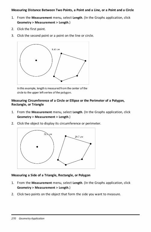
270 Geometry Application
Measuring Distance Between Two Points, a Point and a Line, or a Point and a Circle
1. From the Measurement menu, select Length. (In the Graphs application, clickGeometry > Measurement > Length.)
2. Click the first point.
3. Click the second point or a point on the line or circle.
In this example, length is measured from the center of thecircle to the upper left vertex of the polygon.
Measuring Circumference of a Circle or Ellipse or the Perimeter of a Polygon,Rectangle, or Triangle
1. From the Measurement menu, select Length. (In the Graphs application, clickGeometry > Measurement > Length.)
2. Click the object to display its circumference or perimeter.
Measuring a Side of a Triangle, Rectangle, or Polygon
1. From the Measurement menu, select Length. (In the Graphs application, clickGeometry > Measurement > Length.)
2. Click two points on the object that form the side you want to measure.
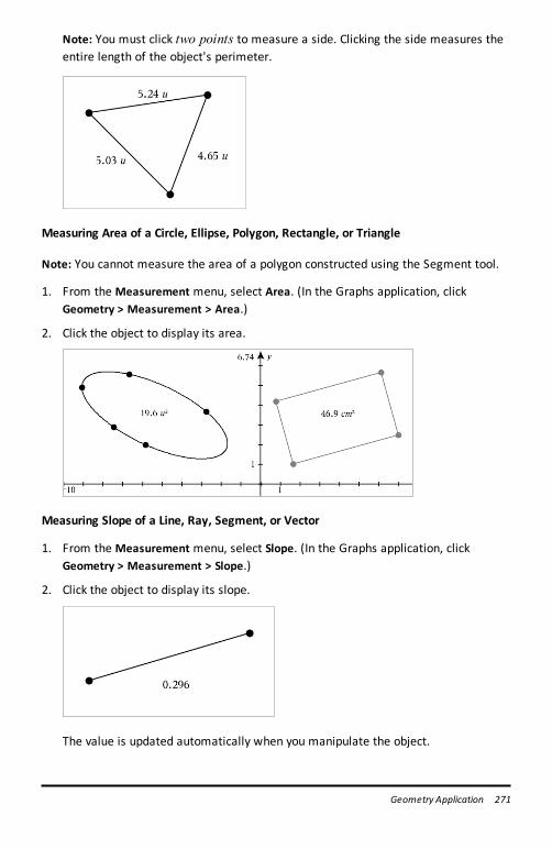
Note: You must click two points to measure a side. Clicking the side measures theentire length of the object's perimeter.
Measuring Area of a Circle, Ellipse, Polygon, Rectangle, or Triangle
Note: You cannot measure the area of a polygon constructed using the Segment tool.
1. From the Measurement menu, select Area. (In the Graphs application, clickGeometry > Measurement > Area.)
2. Click the object to display its area.
Measuring Slope of a Line, Ray, Segment, or Vector
1. From the Measurement menu, select Slope. (In the Graphs application, clickGeometry > Measurement > Slope.)
2. Click the object to display its slope.
The value is updated automatically when you manipulate the object.
Geometry Application 271
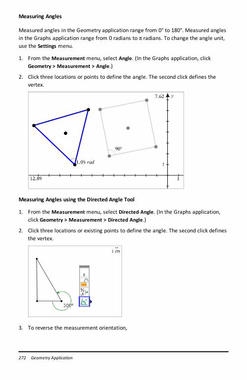
272 Geometry Application
Measuring Angles
Measured angles in the Geometry application range from 0° to 180°. Measured anglesin the Graphs application range from 0 radians to π radians. To change the angle unit,use the Settings menu.
1. From the Measurement menu, select Angle. (In the Graphs application, clickGeometry > Measurement > Angle.)
2. Click three locations or points to define the angle. The second click defines thevertex.
Measuring Angles using the Directed Angle Tool
1. From the Measurement menu, select Directed Angle. (In the Graphs application,click Geometry > Measurement > Directed Angle.)
2. Click three locations or existing points to define the angle. The second click definesthe vertex.
3. To reverse the measurement orientation,
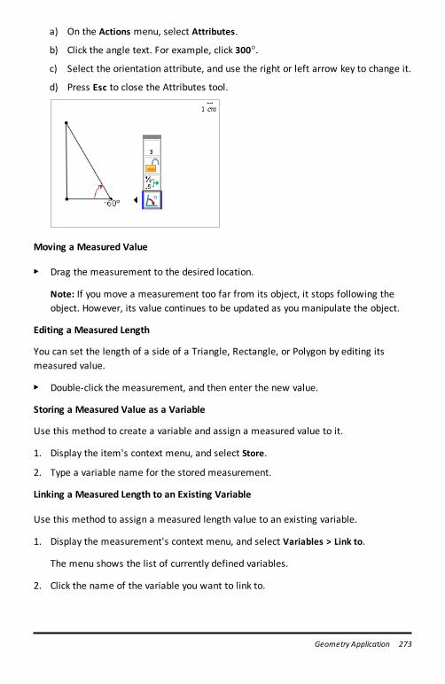
a) On the Actions menu, select Attributes.
b) Click the angle text. For example, click 300°.
c) Select the orientation attribute, and use the right or left arrow key to change it.
d) Press Esc to close the Attributes tool.
Moving a Measured Value
▶ Drag the measurement to the desired location.
Note: If you move a measurement too far from its object, it stops following theobject. However, its value continues to be updated as you manipulate the object.
Editing a Measured Length
You can set the length of a side of a Triangle, Rectangle, or Polygon by editing itsmeasured value.
▶ Double-click the measurement, and then enter the new value.
Storing a Measured Value as a Variable
Use this method to create a variable and assign a measured value to it.
1. Display the item's context menu, and select Store.
2. Type a variable name for the stored measurement.
Linking a Measured Length to an Existing Variable
Use this method to assign a measured length value to an existing variable.
1. Display the measurement's context menu, and select Variables > Link to.
The menu shows the list of currently defined variables.
2. Click the name of the variable you want to link to.
Geometry Application 273
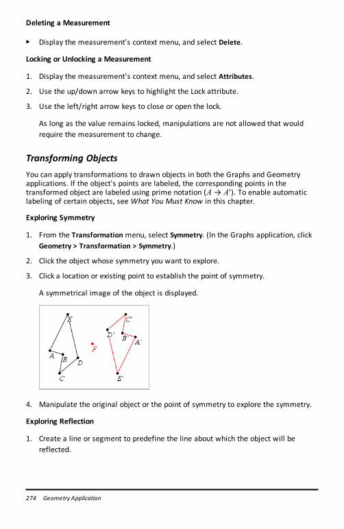
274 Geometry Application
Deleting a Measurement
▶ Display the measurement's context menu, and select Delete.
Locking or Unlocking a Measurement
1. Display the measurement's context menu, and select Attributes.
2. Use the up/down arrow keys to highlight the Lock attribute.
3. Use the left/right arrow keys to close or open the lock.
As long as the value remains locked, manipulations are not allowed that wouldrequire the measurement to change.
Transforming ObjectsYou can apply transformations to drawn objects in both the Graphs and Geometryapplications. If the object's points are labeled, the corresponding points in thetransformed object are labeled using prime notation (A → A'). To enable automaticlabeling of certain objects, see What You Must Know in this chapter.
Exploring Symmetry
1. From the Transformation menu, select Symmetry. (In the Graphs application, clickGeometry > Transformation > Symmetry.)
2. Click the object whose symmetry you want to explore.
3. Click a location or existing point to establish the point of symmetry.
A symmetrical image of the object is displayed.
4. Manipulate the original object or the point of symmetry to explore the symmetry.
Exploring Reflection
1. Create a line or segment to predefine the line about which the object will bereflected.
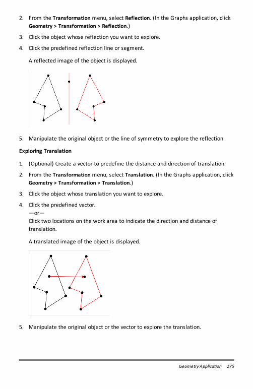
2. From the Transformation menu, select Reflection. (In the Graphs application, clickGeometry > Transformation > Reflection.)
3. Click the object whose reflection you want to explore.
4. Click the predefined reflection line or segment.
A reflected image of the object is displayed.
5. Manipulate the original object or the line of symmetry to explore the reflection.
Exploring Translation
1. (Optional) Create a vector to predefine the distance and direction of translation.
2. From the Transformation menu, select Translation. (In the Graphs application, clickGeometry > Transformation > Translation.)
3. Click the object whose translation you want to explore.
4. Click the predefined vector.—or—Click two locations on the work area to indicate the direction and distance oftranslation.
A translated image of the object is displayed.
5. Manipulate the original object or the vector to explore the translation.
Geometry Application 275
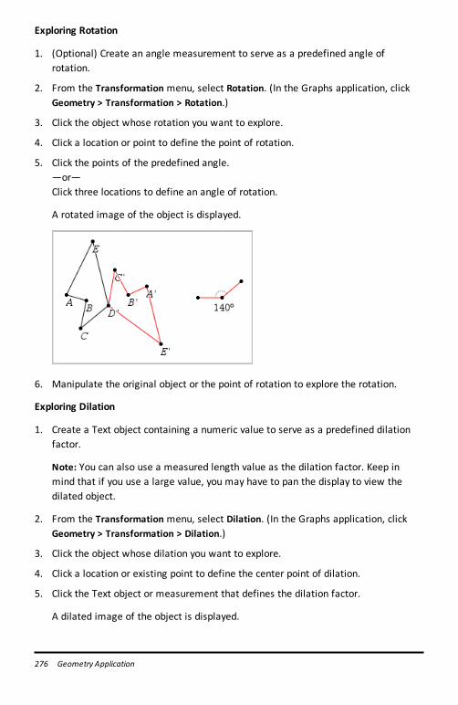
276 Geometry Application
Exploring Rotation
1. (Optional) Create an angle measurement to serve as a predefined angle ofrotation.
2. From the Transformation menu, select Rotation. (In the Graphs application, clickGeometry > Transformation > Rotation.)
3. Click the object whose rotation you want to explore.
4. Click a location or point to define the point of rotation.
5. Click the points of the predefined angle.—or—Click three locations to define an angle of rotation.
A rotated image of the object is displayed.
6. Manipulate the original object or the point of rotation to explore the rotation.
Exploring Dilation
1. Create a Text object containing a numeric value to serve as a predefined dilationfactor.
Note: You can also use a measured length value as the dilation factor. Keep inmind that if you use a large value, you may have to pan the display to view thedilated object.
2. From the Transformation menu, select Dilation. (In the Graphs application, clickGeometry > Transformation > Dilation.)
3. Click the object whose dilation you want to explore.
4. Click a location or existing point to define the center point of dilation.
5. Click the Text object or measurement that defines the dilation factor.
A dilated image of the object is displayed.
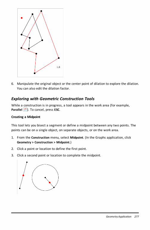
6. Manipulate the original object or the center point of dilation to explore the dilation.You can also edit the dilation factor.
Exploring with Geometric Construction ToolsWhile a construction is in progress, a tool appears in the work area (for example,Parallel ). To cancel, press ESC.
Creating a Midpoint
This tool lets you bisect a segment or define a midpoint between any two points. Thepoints can be on a single object, on separate objects, or on the work area.
1. From the Construction menu, select Midpoint. (In the Graphs application, clickGeometry > Construction > Midpoint.)
2. Click a point or location to define the first point.
3. Click a second point or location to complete the midpoint.
Geometry Application 277
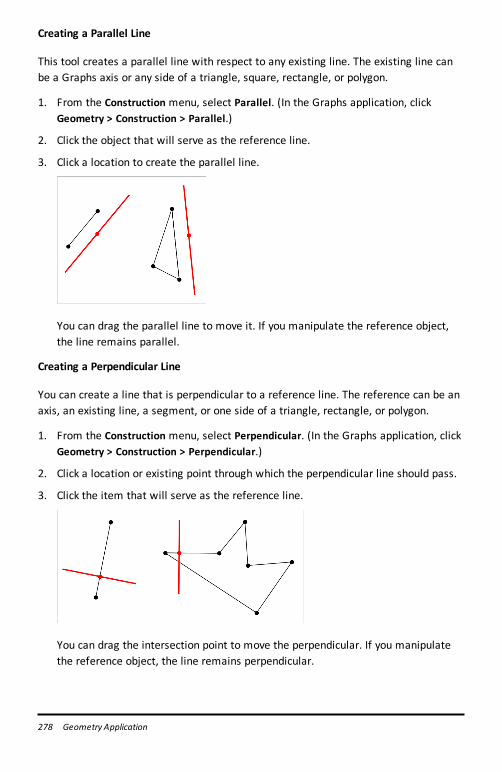
278 Geometry Application
Creating a Parallel Line
This tool creates a parallel line with respect to any existing line. The existing line canbe a Graphs axis or any side of a triangle, square, rectangle, or polygon.
1. From the Construction menu, select Parallel. (In the Graphs application, clickGeometry > Construction > Parallel.)
2. Click the object that will serve as the reference line.
3. Click a location to create the parallel line.
You can drag the parallel line to move it. If you manipulate the reference object,the line remains parallel.
Creating a Perpendicular Line
You can create a line that is perpendicular to a reference line. The reference can be anaxis, an existing line, a segment, or one side of a triangle, rectangle, or polygon.
1. From the Construction menu, select Perpendicular. (In the Graphs application, clickGeometry > Construction > Perpendicular.)
2. Click a location or existing point through which the perpendicular line should pass.
3. Click the item that will serve as the reference line.
You can drag the intersection point to move the perpendicular. If you manipulatethe reference object, the line remains perpendicular.
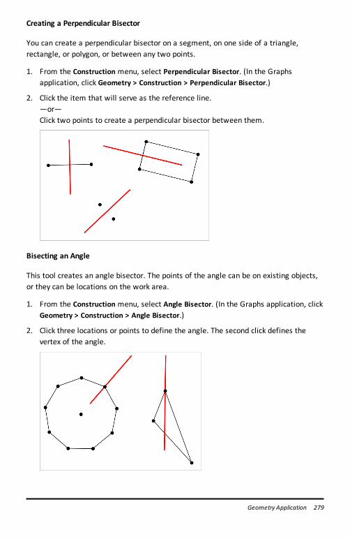
Creating a Perpendicular Bisector
You can create a perpendicular bisector on a segment, on one side of a triangle,rectangle, or polygon, or between any two points.
1. From the Construction menu, select Perpendicular Bisector. (In the Graphsapplication, click Geometry > Construction > Perpendicular Bisector.)
2. Click the item that will serve as the reference line.—or—Click two points to create a perpendicular bisector between them.
Bisecting an Angle
This tool creates an angle bisector. The points of the angle can be on existing objects,or they can be locations on the work area.
1. From the Construction menu, select Angle Bisector. (In the Graphs application, clickGeometry > Construction > Angle Bisector.)
2. Click three locations or points to define the angle. The second click defines thevertex of the angle.
Geometry Application 279
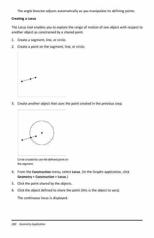
280 Geometry Application
The angle bisector adjusts automatically as you manipulate its defining points.
Creating a Locus
The Locus tool enables you to explore the range of motion of one object with respect toanother object as constrained by a shared point.
1. Create a segment, line, or circle.
2. Create a point on the segment, line, or circle.
3. Create another object that uses the point created in the previous step.
Circle created to use the definedpoint onthe segment.
4. From the Construction menu, select Locus. (In the Graphs application, clickGeometry > Construction > Locus.)
5. Click the point shared by the objects.
6. Click the object defined to share the point (this is the object to vary).
The continuous locus is displayed.
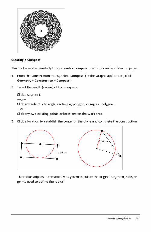
Creating a Compass
This tool operates similarly to a geometric compass used for drawing circles on paper.
1. From the Construction menu, select Compass. (In the Graphs application, clickGeometry > Construction > Compass.)
2. To set the width (radius) of the compass:
Click a segment.—or—Click any side of a triangle, rectangle, polygon, or regular polygon.—or—Click any two existing points or locations on the work area.
3. Click a location to establish the center of the circle and complete the construction.
The radius adjusts automatically as you manipulate the original segment, side, orpoints used to define the radius.
Geometry Application 281
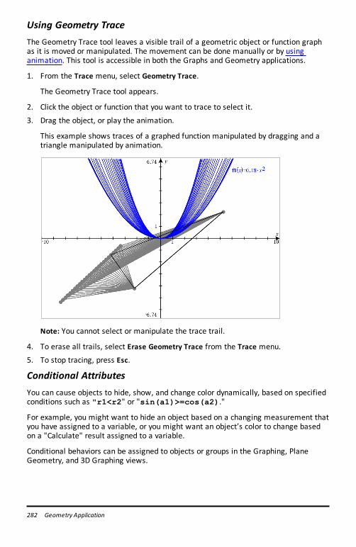
282 Geometry Application
Using Geometry TraceThe Geometry Trace tool leaves a visible trail of a geometric object or function graphas it is moved or manipulated. The movement can be done manually or by usinganimation. This tool is accessible in both the Graphs and Geometry applications.
1. From the Trace menu, select Geometry Trace.
The Geometry Trace tool appears.
2. Click the object or function that you want to trace to select it.
3. Drag the object, or play the animation.
This example shows traces of a graphed function manipulated by dragging and atriangle manipulated by animation.
Note: You cannot select or manipulate the trace trail.
4. To erase all trails, select Erase Geometry Trace from the Trace menu.
5. To stop tracing, press Esc.
Conditional AttributesYou can cause objects to hide, show, and change color dynamically, based on specifiedconditions such as "r1<r2" or "sin(a1)>=cos(a2)."
For example, you might want to hide an object based on a changing measurement thatyou have assigned to a variable, or you might want an object’s color to change basedon a "Calculate" result assigned to a variable.
Conditional behaviors can be assigned to objects or groups in the Graphing, PlaneGeometry, and 3D Graphing views.
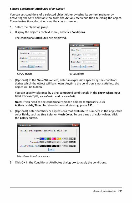
Setting Conditional Attributes of an Object
You can set conditions of a selected object either by using its context menu or byactivating the Set Conditions tool from the Actions menu and then selecting the object.These instructions describe using the context menu.
1. Select the object or group.
2. Display the object’s context menu, and click Conditions.
The conditional attributes are displayed.
For 2Dobjects For 3Dobjects
3. (Optional) In the ShowWhen field, enter an expression specifying the conditionsduring which the object will be shown. Anytime the condition is not satisfied, theobject will be hidden.
You can specify tolerance by using compound conditionals in the ShowWhen inputfield. For example, area>=4 and area<=6.
Note: If you need to see conditionally hidden objects temporarily, clickActions > Hide/Show. To return to normal viewing, press ESC.
4. (Optional) Enter numbers or expressions that evaluate to numbers in the applicablecolor fields, such as Line Color orMesh Color. To see a map of color values, clickthe Colors button.
Mapof conditional color values
5. Click OK in the Conditional Attributes dialog box to apply the conditions.
Geometry Application 283
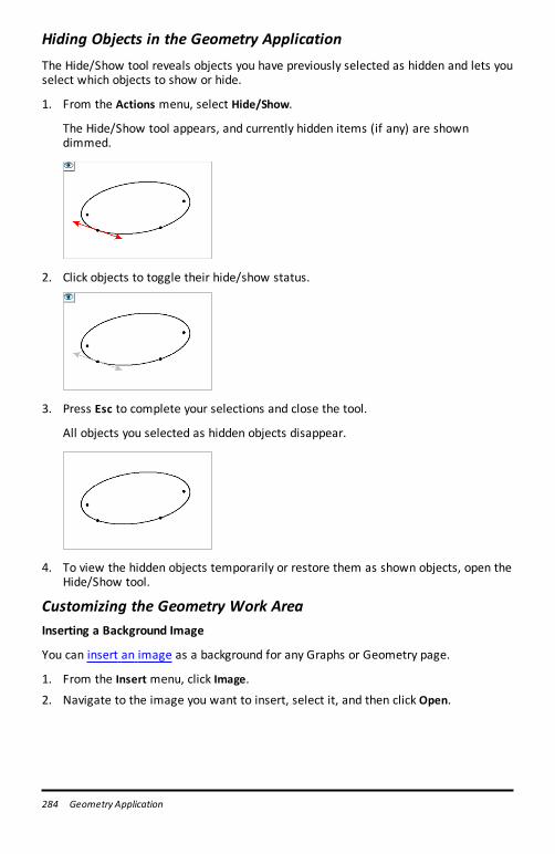
284 Geometry Application
Hiding Objects in the Geometry ApplicationThe Hide/Show tool reveals objects you have previously selected as hidden and lets youselect which objects to show or hide.
1. From the Actions menu, select Hide/Show.
The Hide/Show tool appears, and currently hidden items (if any) are showndimmed.
2. Click objects to toggle their hide/show status.
3. Press Esc to complete your selections and close the tool.
All objects you selected as hidden objects disappear.
4. To view the hidden objects temporarily or restore them as shown objects, open theHide/Show tool.
Customizing the Geometry Work AreaInserting a Background Image
You can insert an image as a background for any Graphs or Geometry page.
1. From the Insert menu, click Image.
2. Navigate to the image you want to insert, select it, and then click Open.
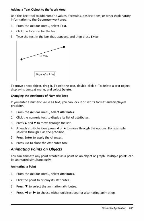
Adding a Text Object to the Work Area
Use the Text tool to add numeric values, formulas, observations, or other explanatoryinformation to the Geometry work area.
1. From the Actions menu, select Text.
2. Click the location for the text.
3. Type the text in the box that appears, and then press Enter.
To move a text object, drag it. To edit the text, double-click it. To delete a text object,display its context menu, and select Delete.
Changing the Attributes of Numeric Text
If you enter a numeric value as text, you can lock it or set its format and displayedprecision.
1. From the Actions menu, select Attributes.
2. Click the numeric text to display its list of attributes.
3. Press 9 and : to move through the list.
4. At each attribute icon, press 7 or 8 to move through the options. For example,select 0 through 9 as the precision.
5. Press Enter to apply the changes.
6. Press Esc to close the Attributes tool.
Animating Points on ObjectsYou can animate any point created as a point on an object or graph. Multiple points canbe animated simultaneously.
Animating a Point
1. From the Actions menu, select Attributes.
2. Click the point to display its attributes.
3. Press ▼ to select the animation attributes.
4. Press ◄ or ► to choose either unidirectional or alternating animation.
Geometry Application 285
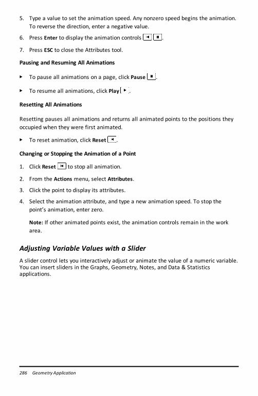
286 Geometry Application
5. Type a value to set the animation speed. Any nonzero speed begins the animation.To reverse the direction, enter a negative value.
6. Press Enter to display the animation controls .
7. Press ESC to close the Attributes tool.
Pausing and Resuming All Animations
▶ To pause all animations on a page, click Pause .
▶ To resume all animations, click Play .
Resetting All Animations
Resetting pauses all animations and returns all animated points to the positions theyoccupied when they were first animated.
▶ To reset animation, click Reset .
Changing or Stopping the Animation of a Point
1. Click Reset to stop all animation.
2. From the Actions menu, select Attributes.
3. Click the point to display its attributes.
4. Select the animation attribute, and type a new animation speed. To stop thepoint’s animation, enter zero.
Note: If other animated points exist, the animation controls remain in the workarea.
Adjusting Variable Values with a SliderA slider control lets you interactively adjust or animate the value of a numeric variable.You can insert sliders in the Graphs, Geometry, Notes, and Data & Statisticsapplications.
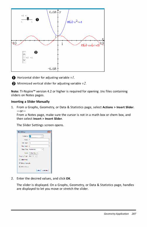
Horizontal slider for adjusting variable v1.Minimized vertical slider for adjusting variable v2.
Note: TI-Nspire™ version 4.2 or higher is required for opening .tns files containingsliders on Notes pages.
Inserting a Slider Manually
1. From a Graphs, Geometry, or Data & Statistics page, select Actions > Insert Slider.—or—From a Notes page, make sure the cursor is not in a math box or chem box, andthen select Insert > Insert Slider.
The Slider Settings screen opens.
2. Enter the desired values, and click OK.
The slider is displayed. On a Graphs, Geometry, or Data & Statistics page, handlesare displayed to let you move or stretch the slider.
Geometry Application 287
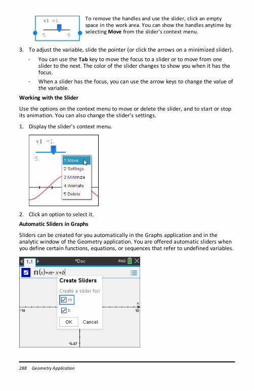
288 Geometry Application
To remove the handles and use the slider, click an emptyspace in the work area. You can show the handles anytime byselectingMove from the slider's context menu.
3. To adjust the variable, slide the pointer (or click the arrows on a minimized slider).
- You can use the Tab key to move the focus to a slider or to move from oneslider to the next. The color of the slider changes to show you when it has thefocus.
- When a slider has the focus, you can use the arrow keys to change the value ofthe variable.
Working with the Slider
Use the options on the context menu to move or delete the slider, and to start or stopits animation. You can also change the slider's settings.
1. Display the slider's context menu.
2. Click an option to select it.
Automatic Sliders in Graphs
Sliders can be created for you automatically in the Graphs application and in theanalytic window of the Geometry application. You are offered automatic sliders whenyou define certain functions, equations, or sequences that refer to undefined variables.
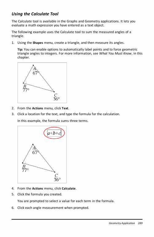
Using the Calculate ToolThe Calculate tool is available in the Graphs and Geometry applications. It lets youevaluate a math expression you have entered as a text object.
The following example uses the Calculate tool to sum the measured angles of atriangle.
1. Using the Shapes menu, create a triangle, and then measure its angles.
Tip: You can enable options to automatically label points and to force geometrictriangle angles to integers. For more information, see What You Must Know, in thischapter.
2. From the Actions menu, click Text.
3. Click a location for the text, and type the formula for the calculation.
In this example, the formula sums three terms.
4. From the Actions menu, click Calculate.
5. Click the formula you created.
You are prompted to select a value for each term in the formula.
6. Click each angle measurement when prompted.
Geometry Application 289
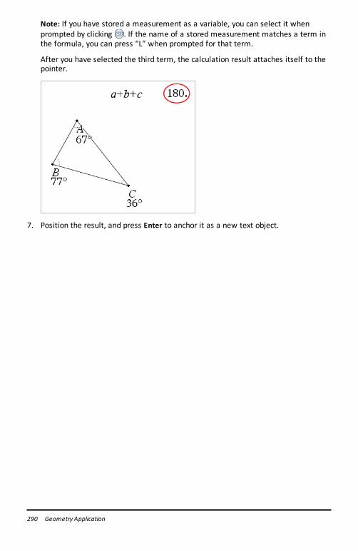
290 Geometry Application
Note: If you have stored a measurement as a variable, you can select it whenprompted by clicking . If the name of a stored measurement matches a term inthe formula, you can press “L” when prompted for that term.
After you have selected the third term, the calculation result attaches itself to thepointer.
7. Position the result, and press Enter to anchor it as a new text object.
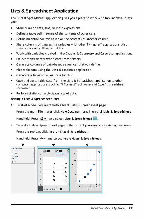
Lists & Spreadsheet ApplicationThe Lists & Spreadsheet application gives you a place to work with tabular data. It letsyou:
• Store numeric data, text, or math expressions.
• Define a table cell in terms of the contents of other cells.
• Define an entire column based on the contents of another column.
• Share columns of data as list variables with other TI-Nspire™ applications. Alsoshare individual cells as variables.
• Work with variables created in the Graphs & Geometry and Calculator applications.
• Collect tables of real-world data from sensors.
• Generate columns of data-based sequences that you define.
• Plot table data using the Data & Statistics application.
• Generate a table of values for a function.
• Copy and paste table data from the Lists & Spreadsheet application to othercomputer applications, such as TI Connect™ software and Excel® spreadsheetsoftware.
• Perform statistical analysis on lists of data.
Adding a Lists & Spreadsheet Page
▶ To start a new document with a blank Lists & Spreadsheet page:
From the main File menu, click New Document, and then click Lists & Spreadsheet.
Handheld: Pressc, and select Lists & Spreadsheet .
▶ To add a Lists & Spreadsheet page in the current problem of an existing document:
From the toolbar, click Insert > Lists & Spreadsheet.
Handheld: Press~ and select Insert >Lists & Spreadsheet.
Lists & Spreadsheet Application 291
292 Lists & Spreadsheet Application
À Lists & Spreadsheet tools (available when a Lists & Spreadsheet work area isactive)
Á Sample Lists & Spreadsheet work area
 Lists & Spreadsheet entry line
à Lists & Spreadsheet data plotted in the Data & Statistics application
Creating and Sharing Spreadsheet Data as ListsYou can define a column as a named list of elements of the same type of data. Afterdefining a list, you can link to it from the Graphs & Geometry, Calculator, orData & Statistics applications, and from other instances of the Lists & Spreadsheetapplication within the current problem.
Note: Lists & Spreadsheet can display a maximum of 2500 elements in a list.
Sharing a Spreadsheet Column as a List Variable
You share a column of data by naming it as a list variable.
Note: Avoid defining variables that use the same names as those used for statisticalanalysis. In some cases, an error condition could occur.
Variable names used for statistical analysis are listed in the TI-Nspire™ ReferenceGuide, under the stat.results entry.
1. Click the cell to move to the column’s name cell (the top cell of the column).
—or—
Press ▲ as necessary.
2. Type a name for the list variable, and press Enter.
The column is now available as a list variable to other TI-Nspire™ applications.
3. Create elements in the list the same as you would create data in spreadsheet cells.For example, you can type the data into each cell or use a formula to generate acolumn of data.
Notes:
• If a variable with the name you specified already exists in the current problem,Lists & Spreadsheet displays an error message.
• When you select the column formula cell of a list, it displays the list name in anexpression similar to width:=.
• Lists can contain empty elements (denoted by “_”) .
• You can refer to a specific element in a named list from the Calculator application.Use the list name and the element’s position within the list. In a list namedHeights, for example, refer to the first element as Heights[1]. The expressionHeights[2] refers to the second element, and so on.
Linking to an Existing List Variable
Linking a column to an existing list variable lets you easily view and edit the values inthe list. The list can be any shared list in the current problem and can be defined inGraphs & Geometry, Calculator, or any instance of Lists & Spreadsheet.
After you link a column to a list, Lists & Spreadsheet automatically shows any changesthat you make to the list with other TI-Nspire™ applications.
1. Click the column formula cell (the second cell from the top) of the column that youwant to link to the variable.
2. Type the name of the list variable you want to link to.
—or—
Click on the toolbar (pressh on the handheld), click Link To, and click thevariable you want to link to.
3. Press Enter.
The column shows the list elements.
Notes:
• You cannot link to the same variable multiple times on the same page.
• Use caution if you link to a system variable. Doing so could prevent the variablefrom being updated by the system. System variables include ans and statisticsresults (such as stat.results, stat.RegEqn, and stat.Resid).
Inserting an Element in a List
When you insert an element in a list, the remaining elements shift downward tocreate space. No other columns are affected.
▶ Click Insert > Insert Cell.
Deleting an Element from a List
When you delete an element, the remaining list elements shift upward to close thegap. The upward shift affects only the selected column.
Lists & Spreadsheet Application 293
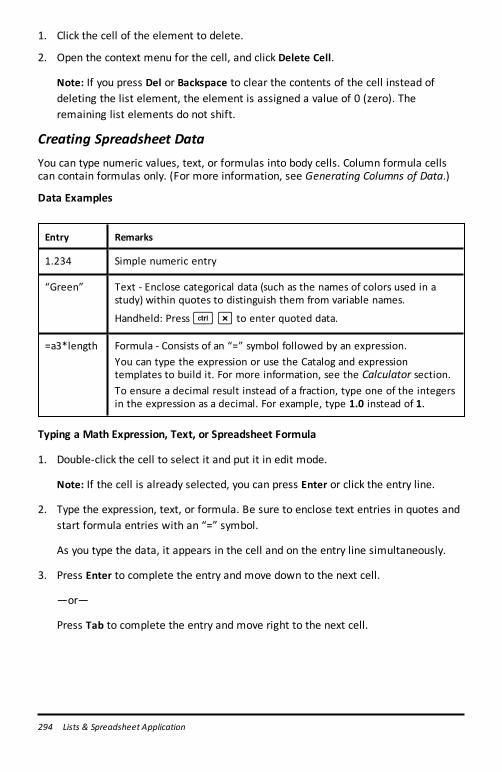
294 Lists & Spreadsheet Application
1. Click the cell of the element to delete.
2. Open the context menu for the cell, and click Delete Cell.
Note: If you press Del or Backspace to clear the contents of the cell instead ofdeleting the list element, the element is assigned a value of 0 (zero). Theremaining list elements do not shift.
Creating Spreadsheet DataYou can type numeric values, text, or formulas into body cells. Column formula cellscan contain formulas only. (For more information, see Generating Columns of Data.)
Data Examples
Entry Remarks
1.234 Simple numeric entry
“Green” Text - Enclose categorical data (such as the names of colors used in astudy) within quotes to distinguish them from variable names.
Handheld: Press/r to enter quoted data.
=a3*length Formula - Consists of an “=” symbol followed by an expression.You can type the expression or use the Catalog and expressiontemplates to build it. For more information, see the Calculator section.To ensure a decimal result instead of a fraction, type one of the integersin the expression as a decimal. For example, type 1.0 instead of 1.
Typing a Math Expression, Text, or Spreadsheet Formula
1. Double-click the cell to select it and put it in edit mode.
Note: If the cell is already selected, you can press Enter or click the entry line.
2. Type the expression, text, or formula. Be sure to enclose text entries in quotes andstart formula entries with an “=” symbol.
As you type the data, it appears in the cell and on the entry line simultaneously.
3. Press Enter to complete the entry and move down to the next cell.
—or—
Press Tab to complete the entry and move right to the next cell.
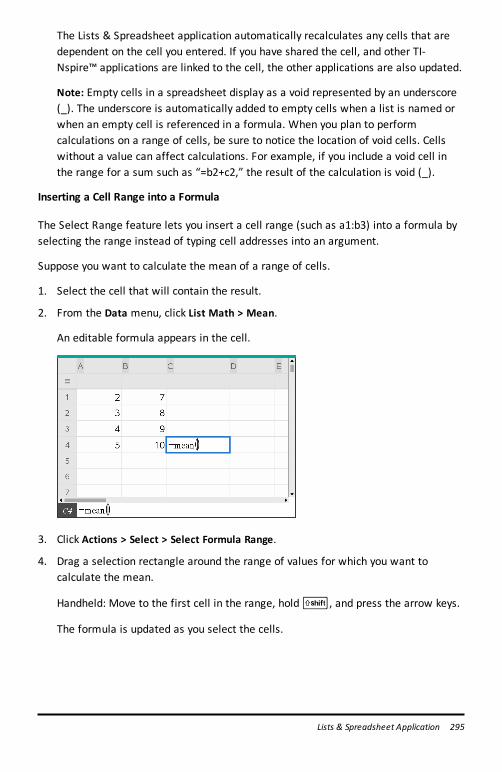
The Lists & Spreadsheet application automatically recalculates any cells that aredependent on the cell you entered. If you have shared the cell, and other TI-Nspire™ applications are linked to the cell, the other applications are also updated.
Note: Empty cells in a spreadsheet display as a void represented by an underscore(_). The underscore is automatically added to empty cells when a list is named orwhen an empty cell is referenced in a formula. When you plan to performcalculations on a range of cells, be sure to notice the location of void cells. Cellswithout a value can affect calculations. For example, if you include a void cell inthe range for a sum such as “=b2+c2,” the result of the calculation is void (_).
Inserting a Cell Range into a Formula
The Select Range feature lets you insert a cell range (such as a1:b3) into a formula byselecting the range instead of typing cell addresses into an argument.
Suppose you want to calculate the mean of a range of cells.
1. Select the cell that will contain the result.
2. From the Data menu, click List Math > Mean.
An editable formula appears in the cell.
3. Click Actions > Select > Select Formula Range.
4. Drag a selection rectangle around the range of values for which you want tocalculate the mean.
Handheld: Move to the first cell in the range, holdg, and press the arrow keys.
The formula is updated as you select the cells.
Lists & Spreadsheet Application 295
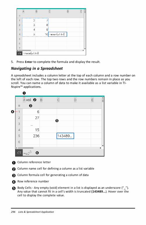
296 Lists & Spreadsheet Application
5. Press Enter to complete the formula and display the result.
Navigating in a SpreadsheetA spreadsheet includes a column letter at the top of each column and a row number onthe left of each row. The top two rows and the row numbers remain in place as youscroll. You can name a column of data to make it available as a list variable in TI-Nspire™ applications.
À Column reference letter
Á Column name cell for defining a column as a list variable
 Column formula cell for generating a column of data
à Row reference number
Ä Body Cells - Any empty (void) element in a list is displayed as an underscore (“_”).Any value that cannot fit in a cell’s width is truncated (143489...). Hover over thecell to display the complete value.
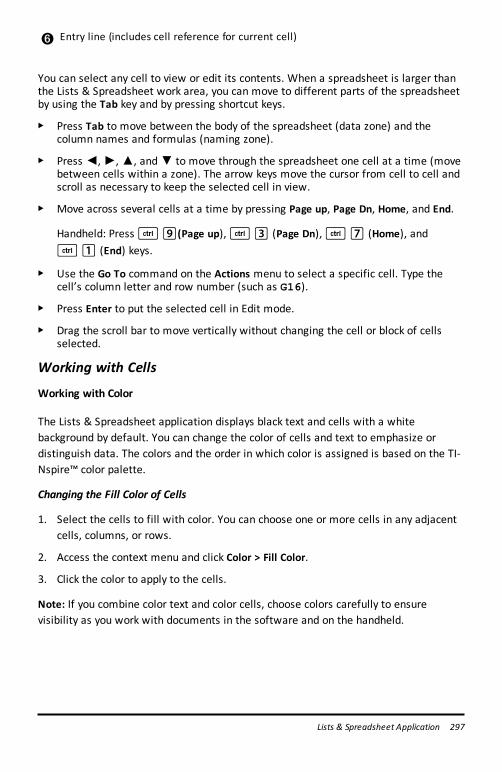
Å Entry line (includes cell reference for current cell)
You can select any cell to view or edit its contents. When a spreadsheet is larger thanthe Lists & Spreadsheet work area, you can move to different parts of the spreadsheetby using the Tab key and by pressing shortcut keys.
▶ Press Tab to move between the body of the spreadsheet (data zone) and thecolumn names and formulas (naming zone).
▶ Press ◄,►,▲, and▼ to move through the spreadsheet one cell at a time (movebetween cells within a zone). The arrow keys move the cursor from cell to cell andscroll as necessary to keep the selected cell in view.
▶ Move across several cells at a time by pressing Page up, Page Dn, Home, and End.
Handheld: Press/9(Page up),/3 (Page Dn),/7 (Home), and/1 (End) keys.
▶ Use the Go To command on the Actions menu to select a specific cell. Type thecell’s column letter and row number (such as G16).
▶ Press Enter to put the selected cell in Edit mode.
▶ Drag the scroll bar to move vertically without changing the cell or block of cellsselected.
Working with Cells
Working with Color
The Lists & Spreadsheet application displays black text and cells with a whitebackground by default. You can change the color of cells and text to emphasize ordistinguish data. The colors and the order in which color is assigned is based on the TI-Nspire™ color palette.
Changing the Fill Color of Cells
1. Select the cells to fill with color. You can choose one or more cells in any adjacentcells, columns, or rows.
2. Access the context menu and click Color > Fill Color.
3. Click the color to apply to the cells.
Note: If you combine color text and color cells, choose colors carefully to ensurevisibility as you work with documents in the software and on the handheld.
Lists & Spreadsheet Application 297
298 Lists & Spreadsheet Application
Changing the Color of Text
1. Select the cells that contain the text to change. You can choose one or more cells inany adjacent cells, columns, or rows.
2. Access the context menu and click Color > Text Color.
3. Click the color to apply to the text. Empty cells in the selection area show the colorchange when text is added.
Understanding Cell References in Formulas
Use a cell reference to use data from a cell or range of cells in a formula. Thecalculation results update automatically when values in cells change.
Relative references include only the cell’s column letter and row number (for example,E7). A relative reference describes where a cell is in relation to other cells of thespreadsheet. The Lists & Spreadsheet application keeps track of relative cell referencesand adjusts the reference automatically when surrounding cells shift (because ofactions you perform, such as column deletions or cell insertions).
Follow these guidelines to specify cell references:
• Include a column letter and row number in a relative reference.
• Include the $ symbol before both the column letter and the row number to specifyan absolute reference.
• Include a colon (:) between a two cell reference to specify a range of cells.
Absolute references include the $ symbol before the column letter and before the rownumber (for example, $B$16). Absolute references always refer to the cell in a specificposition in the spreadsheet. The application does not automatically adjust the cellreference when cell positions change.
Typing a Cell Reference in a Formula
1. Double-click the cell and type the formula. For more information, see theCalculator section.
2. Move to the appropriate position in the formula and type the cell reference. Usethe format for a relative reference (B3), absolute reference ($B$2), or range ofcells (A1:A4).
Note: You can click Recalculate on the Actions menu to update all references andformula results in a spreadsheet.
Deleting the Contents of Cells
1. Click a cell to select it.
—or—
Use the arrow keys to move to the cell.
Note: If you are deleting a range of cells, select a cell at one end or corner of therange, and then use Shift with the arrow keys to select the remaining cells in therange.
2. Press Del.
Note: Any cell that uses a formula with an absolute reference to deleted datashows an error. A cell that uses a formula with a relative reference to deleted datais updated to use the data currently in the referenced position.
Copying Cells
When you copy cells, any formulas in the original cells are copied to the destinationcells.
1. Click the cell to copy.
—or—
Use the arrow keys to move to the cell.
Note: If you are copying a range of cells, select a cell at one end or corner of therange, and then use Shift with the arrow keys to select the remaining cells in therange.
2. Use the standard key shortcut for copying a selection.
Windows®: Press Ctrl+C.
Mac®: Press “+C.
Handheld: Press/C.
3. Click the cell where you want to duplicate the copied cell. If you are copying a blockof data, click the cell that will become the upper left corner of the copied block.
4. Paste the selected cells:
Windows®: Press Ctrl+V.
Mac®: Press “+V.
Lists & Spreadsheet Application 299
300 Lists & Spreadsheet Application
Handheld: Press/V.
Important: Paste copied data into a cell that is in the same mode as the cell fromwhich the data was originally copied. Otherwise, a formula could paste as a stringenclosed in quotes instead of a formula.
Filling Adjacent Cells
You can repeat a cell’s formula or value throughout adjacent cells within the row orcolumn. You can also repeat a range of cells horizontally or vertically. If you fill from arange that contains a simple sequence (such as 2, 4, 6), the sequence continues in thefilled cells.
1. Click the cell that contains the value or formula to repeat.
Note: If you are repeating a range of cells, drag to select the range, or select a cellat one end of the range, and then use Shift with the arrow keys to select theremaining cells.
2. Click Data > Fill.
3. Use the arrow keys, or drag to select the range that will hold the repetitions.
4. Press Enter.
The value, formula, or pattern that you selected for duplication is repeated over theselected range.
Sharing a Cell Value as a Variable
You can share the value of a cell with other TI-Nspire™ applications by storing it as avariable. When you define or refer to a shared cell or variable in Lists & Spreadsheet,the name is preceded with an apostrophe (‘).
1. Click the cell that you want to share.
2. Click on the toolbar, and click Store Var to store the cell’s value.
Handheld: Press/h or pressh and select Store Var).
A formula is inserted into the cell with var as a placeholder for a variable name.
3. Type over the letters “var” with a name for the variable, and press Enter. Use avariable name that does not exist in the current problem.
The value is shown in bold to indicate that it is now available as a variable to otherTI-Nspire™ applications.
Linking a Cell to a Variable
When you link a cell to a variable, Lists & Spreadsheet keeps the cell value updated toreflect the current value of the variable. The variable can be any variable in the currentproblem and can be defined in Graphs & Geometry, Calculator, Data & Statistics, orany instance of Lists & Spreadsheet.
1. Click the cell that you want to link to a variable.
2. Click on the toolbar, and click Link to.
Handheld: Press/h or pressh and select Link to.
The VarLink menu opens.
3. Under Link To, press ▲, and▼ to scroll to the name of the variable.
4. Press Enter.
The cell shows the value of the variable.
Note: Use caution if you link to a system variable. Linking could prevent the variablefrom being updated by the system. System variables include statistics results (such asStat.RegEqn, Stat.dfError, and Stat.Resid) and finance-solver variables (such astvm.n, tvm.pmt, and tvm.fv).
Working with Rows and Columns of Data
Selecting a row or column
▶ To select a column, move to the top of the column and click the column referenceletter. To select a row, move to the leftmost cell of the row and click the rowreference number. Press Esc to cancel the selection.
Handheld: Hold down▲ to move past the top cell, or hold down◄ to move pastthe leftmost cell.
▶ To extend a selection to adjacent rows or columns, hold down Shift and press ◄,►,▲, or▼.
Resizing a Row or Column
1. Click the row or column that you want to resize.
2. From the Actions menu, select Resize, and then select an option.
3. Choose a resizing option for a column or row.
Lists & Spreadsheet Application 301
302 Lists & Spreadsheet Application
- For a column, choose Resize Column Width, Maximize Column Width, orMinimize Column Width.
- For a row, you can choose Resize Row Height.
The tools that minimize and maximize the column width work automatically. Youmust manually adjust the size to use the Resize Column Width and Resize RowHeight tools.
4. To resize manually, use◄ and► to resize the column, or use▲ and▼ to resizethe row, and then press Enter.
Inserting an Empty Row or Column
1. Click a column or row where you want to insert the new data.
2. From the Insert menu, select either Row or Column.
- If you are inserting a row, the remaining rows shift down to create space forthe new row.
- If you are inserting a column, the remaining columns shift right to createspace.
Note: If other cells contain formulas with relative references to a displaced row orcolumn, those references adjust accordingly.
Deleting Entire Rows or Columns
You can delete a row, column, group of rows, or group of columns. When you delete arow or column, the remaining rows or columns move up or left to fill the gap.
1. Click the column or row that you want to delete.
2. (Optional) To select adjacent rows or columns to delete, hold down Shift and press◄,►,▲, or▼.
3. Display the context menu.
- Windows®: Right-click the selected row.
- Mac®: Hold the “ key, and click the selected row.
- Handheld: Press/b.
4. On the context menu, select Delete Row.
The selected rows or columns are deleted.
Note: If other cells contain formulas that refer to the deleted row or column, thosecells show an error. Relative references to cells whose positions have changedbecause of a deletion adjust accordingly.
Copying Rows or Columns
1. Click the row number to copy a row, or click the column letter to copy a column.
2. (Optional) To select adjacent rows or columns to copy, hold down Shift and press◄,►,▲, or▼.
3. Copy the row or column:
Windows®: Press Ctrl+C.
Mac®: Press “+C.
Handheld: Press/C.
4. Move to any cell in the row or column where you want to place the copied items.
5. Paste the row or column:
Windows®: Press Ctrl+V.
Mac®: Press “+V.
Handheld: Press/V.
The copied row or column is pasted in place, replacing the previous contents.
Note: If you copy a named column, it is pasted with the name removed to preventa variable conflict.
Moving a Column
1. Click the column that you want to move.
2. From the Actions menu, select Move Column.
An insertion bar appears.
3. Press ◄ and► to place the insertion bar at the column’s new position, and thenpress Enter.
Note: Relative references to any cell in a position is affected by the move adjustaccordingly.
Lists & Spreadsheet Application 303
304 Lists & Spreadsheet Application
Displaying Results as Exact or Approximate
You can choose to display a column’s calculated results in Exact (fraction) orApproximate (decimal) form. This affects only the values calculated from a formula.
1. Select the column by clicking the reference letter at the top of the column.
Handheld: Hold down▲ to move past the top cell.
2. Display the context menu for the column.
3. On the context menu, click either Data > Exact or Data > Approximate.
Note: To restore the column results to the document’s default setting, select thecolumn and click Data > Restore Document Setting.
Clearing Column Data
The Clear Data command lets you remove the data from selected columns. Clear Datadoes not delete the column, and it does not clear a column’s name or formula.
After clearing the data, Lists & Spreadsheet recalculates column formulas for theselected columns. This makes Clear Data useful for capturing a fresh set of data fromanother application or selectively generating a fresh column of random numbers.
1. Click the column or columns that you want to clear.
2. From the Data menu, select Clear Data.
Note: If a recalculated formula produces the same data as before, it may appearthat the Clear Data command has failed.
Sorting DataYou can sort a selected area of the spreadsheet in ascending or descending order. Youselect which column in the selected area will be used as the key for the sort. When thesort moves data up or down in the key column, the corresponding data in the otherselected columns is also moved up or down. This preserves the integrity of each row.
Note: Sorting is based on numeric values. If you select a key column that contains text,you could get unexpected results.
1. Select the range of cells.
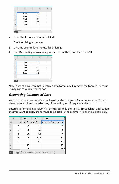
2. From the Actions menu, select Sort.
The Sort dialog box opens.
3. Click the column letter to use for ordering.
4. Click Descending or Ascending as the sort method, and then click OK.
Note: Sorting a column that is defined by a formula will remove the formula, becauseit may not be valid after the sort.
Generating Columns of DataYou can create a column of values based on the contents of another column. You canalso create a column based on any of several types of sequential data.
Entering a formula in a column’s formula cell tells the Lists & Spreadsheet applicationthat you want to apply the formula to all cells in the column, not just to a single cell.
Lists & Spreadsheet Application 305
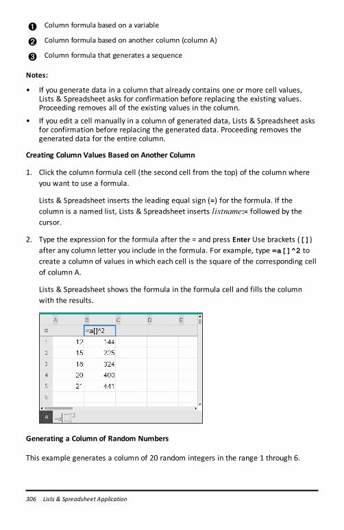
306 Lists & Spreadsheet Application
À Column formula based on a variable
Á Column formula based on another column (column A)
 Column formula that generates a sequence
Notes:
• If you generate data in a column that already contains one or more cell values,Lists & Spreadsheet asks for confirmation before replacing the existing values.Proceeding removes all of the existing values in the column.
• If you edit a cell manually in a column of generated data, Lists & Spreadsheet asksfor confirmation before replacing the generated data. Proceeding removes thegenerated data for the entire column.
Creating Column Values Based on Another Column
1. Click the column formula cell (the second cell from the top) of the column whereyou want to use a formula.
Lists & Spreadsheet inserts the leading equal sign (=) for the formula. If thecolumn is a named list, Lists & Spreadsheet inserts listname:= followed by thecursor.
2. Type the expression for the formula after the = and press Enter Use brackets ([])after any column letter you include in the formula. For example, type =a[]^2 tocreate a column of values in which each cell is the square of the corresponding cellof column A.
Lists & Spreadsheet shows the formula in the formula cell and fills the columnwith the results.
Generating a Column of Random Numbers
This example generates a column of 20 random integers in the range 1 through 6.
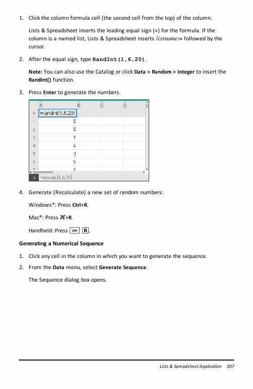
1. Click the column formula cell (the second cell from the top) of the column.
Lists & Spreadsheet inserts the leading equal sign (=) for the formula. If thecolumn is a named list, Lists & Spreadsheet inserts listname:= followed by thecursor.
2. After the equal sign, type RandInt(1,6,20).
Note: You can also use the Catalog or click Data > Random > Integer to insert theRandInt() function.
3. Press Enter to generate the numbers.
4. Generate (Recalculate) a new set of random numbers:
Windows®: Press Ctrl+R.
Mac®: Press “+R.
Handheld: Press/R.
Generating a Numerical Sequence
1. Click any cell in the column in which you want to generate the sequence.
2. From the Data menu, select Generate Sequence.
The Sequence dialog box opens.
Lists & Spreadsheet Application 307
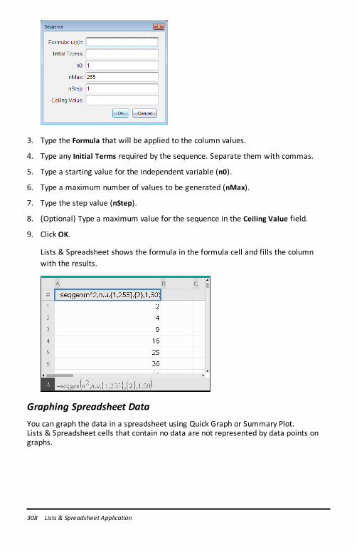
308 Lists & Spreadsheet Application
3. Type the Formula that will be applied to the column values.
4. Type any Initial Terms required by the sequence. Separate them with commas.
5. Type a starting value for the independent variable (n0).
6. Type a maximum number of values to be generated (nMax).
7. Type the step value (nStep).
8. (Optional) Type a maximum value for the sequence in the Ceiling Value field.
9. Click OK.
Lists & Spreadsheet shows the formula in the formula cell and fills the columnwith the results.
Graphing Spreadsheet DataYou can graph the data in a spreadsheet using Quick Graph or Summary Plot.Lists & Spreadsheet cells that contain no data are not represented by data points ongraphs.
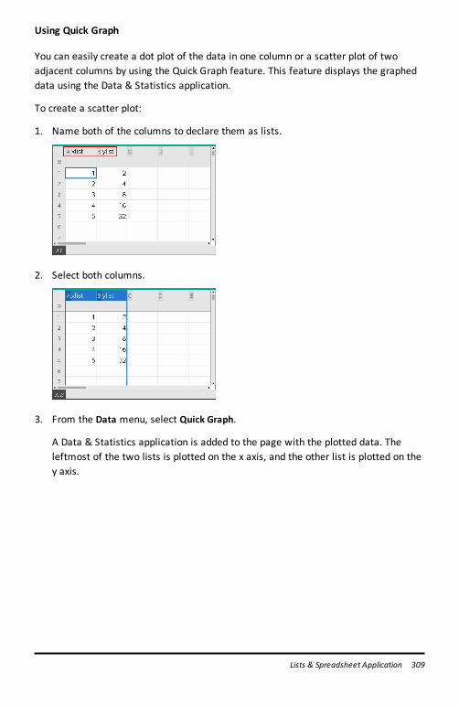
Using Quick Graph
You can easily create a dot plot of the data in one column or a scatter plot of twoadjacent columns by using the Quick Graph feature. This feature displays the grapheddata using the Data & Statistics application.
To create a scatter plot:
1. Name both of the columns to declare them as lists.
2. Select both columns.
3. From the Data menu, select Quick Graph.
A Data & Statistics application is added to the page with the plotted data. Theleftmost of the two lists is plotted on the x axis, and the other list is plotted on they axis.
Lists & Spreadsheet Application 309
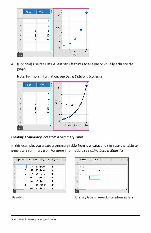
310 Lists & Spreadsheet Application
4. (Optional) Use the Data & Statistics features to analyze or visually enhance thegraph.
Note: For more information, see Using Data and Statistics.
Creating a Summary Plot from a Summary Table
In this example, you create a summary table from raw data, and then use the table togenerate a summary plot. For more information, see Using Data & Statistics.
Rawdata Summary table for eye color basedon rawdata
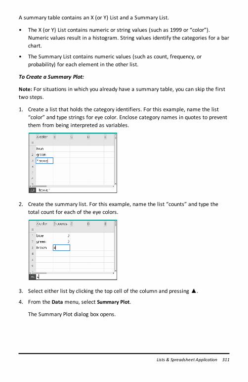
A summary table contains an X (or Y) List and a Summary List.
• The X (or Y) List contains numeric or string values (such as 1999 or “color”).Numeric values result in a histogram. String values identify the categories for a barchart.
• The Summary List contains numeric values (such as count, frequency, orprobability) for each element in the other list.
To Create a Summary Plot:
Note: For situations in which you already have a summary table, you can skip the firsttwo steps.
1. Create a list that holds the category identifiers. For this example, name the list“color” and type strings for eye color. Enclose category names in quotes to preventthem from being interpreted as variables.
2. Create the summary list. For this example, name the list “counts” and type thetotal count for each of the eye colors.
3. Select either list by clicking the top cell of the column and pressing ▲.
4. From the Data menu, select Summary Plot.
The Summary Plot dialog box opens.
Lists & Spreadsheet Application 311
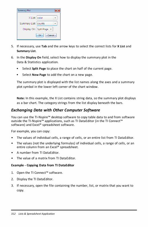
312 Lists & Spreadsheet Application
5. If necessary, use Tab and the arrow keys to select the correct lists for X List andSummary List.
6. In the Display On field, select how to display the summary plot in theData & Statistics application.
• Select Split Page to place the chart on half of the current page.
• Select New Page to add the chart on a new page.
The summary plot is displayed with the list names along the axes and a summaryplot symbol in the lower left corner of the chart window.
Note: In this example, the X List contains string data, so the summary plot displaysas a bar chart. The category strings from the list display beneath the bars.
Exchanging Data with Other Computer SoftwareYou can use the TI-Nspire™ desktop software to copy table data to and from softwareoutside the TI-Nspire™ applications, such as TI DataEditor (in the TI Connect™software) and Excel® spreadsheet software.
For example, you can copy:
• The values of individual cells, a range of cells, or an entire list from TI DataEditor.
• The values (not the underlying formulas) of individual cells, a range of cells, or anentire column from an Excel® spreadsheet.
• A number from TI DataEditor.
• The value of a matrix from TI DataEditor.
Example - Copying Data from TI DataEditor
1. Open the TI Connect™ software.
2. Display the TI DataEditor.
3. If necessary, open the file containing the number, list, or matrix that you want tocopy.
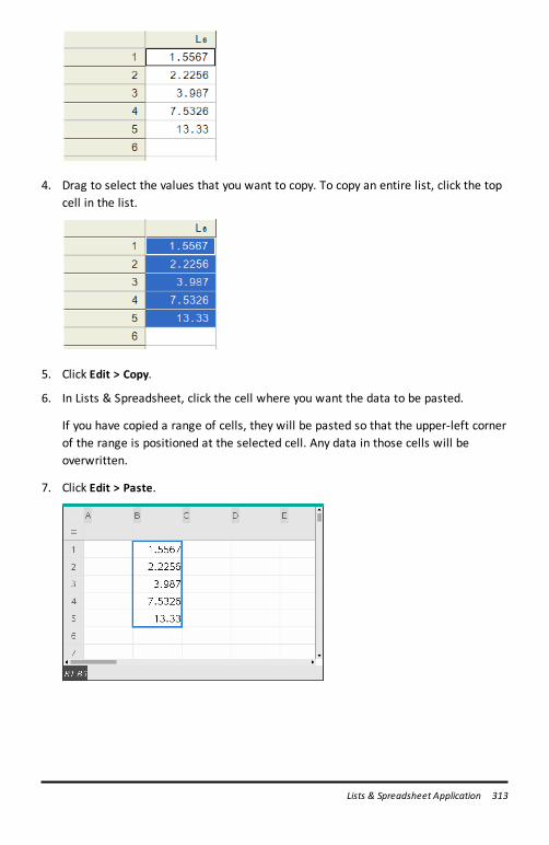
4. Drag to select the values that you want to copy. To copy an entire list, click the topcell in the list.
5. Click Edit > Copy.
6. In Lists & Spreadsheet, click the cell where you want the data to be pasted.
If you have copied a range of cells, they will be pasted so that the upper-left cornerof the range is positioned at the selected cell. Any data in those cells will beoverwritten.
7. Click Edit > Paste.
Lists & Spreadsheet Application 313
314 Lists & Spreadsheet Application
Copying Cells from an Excel® Spreadsheet
You can copy up to 26 columns and 2500 rows from an Excel® spreadsheet to aLists & Spreadsheet application.
1. Drag to select the values that you want to copy from the Excel® spreadsheet. Tocopy an entire column, click the column identifier at the top of the column.
Note: If you select non-contiguous columns in the Excel® spreadsheet, they will bepasted as contiguous columns in Lists & Spreadsheet.
2. Use the standard key shortcut for copying a selection.
Windows®: Press Ctrl+C.
Mac®: Press “+C.
3. In Lists & Spreadsheet, click the cells where you want the data to be pasted.
If you are copying a range of cells, they will be pasted so that the upper-left cornerof the range is positioned at the selected cell. Any data in those cells in will beoverwritten.
4. Paste the data.
Windows®: Press Ctrl+V.
Mac®: Press “+V.
Handheld: Press/V.
Note: Categorical data must be enclosed in quotes (“ “) after the data is pasted.
Capturing Data from Graphs & GeometryYou can use Lists & Spreadsheet application to capture information about objects inthe Graphs & Geometry application. For example, you could track changes in the areaof a triangle as you change the length of a side in the Graphs & Geometry application.
Captured values replace values in the column. If you prefer, you can remove all datafrom a column before starting a new capture by clicking Clear Data on the Data menu.
Capturing Data Manually
1. Make sure the data value that you want to capture is linked to a variable name.
2. Click the column formula cell (the second cell from the top) of the column in whichyou want to capture the values.
Note: Captured values replace values in the column.
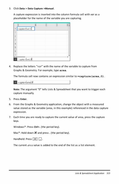
3. Click Data > Data Capture >Manual.
A capture expression is inserted into the column formula cell with var as aplaceholder for the name of the variable you are capturing.
4. Replace the letters “var” with the name of the variable to capture fromGraphs & Geometry. For example, type area.
The formula cell now contains an expression similar to =capture(area,0).
Note: The argument “0” tells Lists & Spreadsheet that you want to trigger eachcapture manually.
5. Press Enter.
6. From the Graphs & Geometry application, change the object with a measuredvalue stored as the variable (area, in this example) referenced in the data captureexpression.
7. Each time you are ready to capture the current value of area, press the capturekeys.
Windows®: Press Ctrl+. (the period key).
Mac®: Hold down “ and press . (the period key).
Handheld: Press/^.
The current area value is added to the end of the list as a list element.
Lists & Spreadsheet Application 315
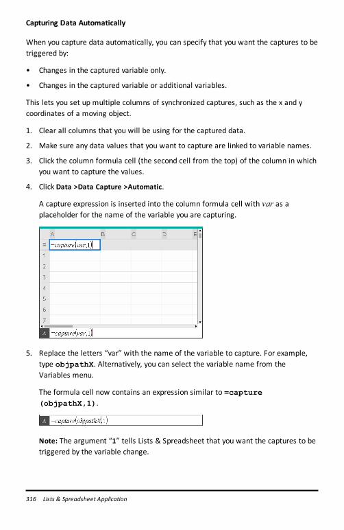
316 Lists & Spreadsheet Application
Capturing Data Automatically
When you capture data automatically, you can specify that you want the captures to betriggered by:
• Changes in the captured variable only.
• Changes in the captured variable or additional variables.
This lets you set up multiple columns of synchronized captures, such as the x and ycoordinates of a moving object.
1. Clear all columns that you will be using for the captured data.
2. Make sure any data values that you want to capture are linked to variable names.
3. Click the column formula cell (the second cell from the top) of the column in whichyou want to capture the values.
4. Click Data >Data Capture >Automatic.
A capture expression is inserted into the column formula cell with var as aplaceholder for the name of the variable you are capturing.
5. Replace the letters “var” with the name of the variable to capture. For example,type objpathX. Alternatively, you can select the variable name from theVariables menu.
The formula cell now contains an expression similar to =capture(objpathX,1).
Note: The argument “1” tells Lists & Spreadsheet that you want the captures to betriggered by the variable change.
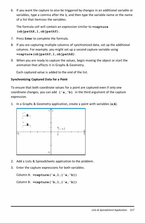
6. If you want the capture to also be triggered by changes in an additional variable orvariables, type a comma after the 1, and then type the variable name or the nameof a list that itemizes the variables.
The formula cell will contain an expression similar to =capture(objpathX,1,objpathY).
7. Press Enter to complete the formula.
8. If you are capturing multiple columns of synchronized data, set up the additionalcolumns. For example, you might set up a second capture variable using=capture(objpathY,1,objpathX).
9. When you are ready to capture the values, begin moving the object or start theanimation that affects it in Graphs & Geometry.
Each captured value is added to the end of the list.
Synchronizing Captured Data for a Point
To ensure that both coordinate values for a point are captured even if only onecoordinate changes, you can add {'a,'b} in the third argument of the captureexpression.
1. In a Graphs & Geometry application, create a point with variables (a,b).
2. Add a Lists & Spreadsheets application to the problem.
3. Enter the capture expressions for both variables.
Column A: =capture('a,1,{'a,'b})
Column B: =capture('b,1,{'a,'b})
Lists & Spreadsheet Application 317
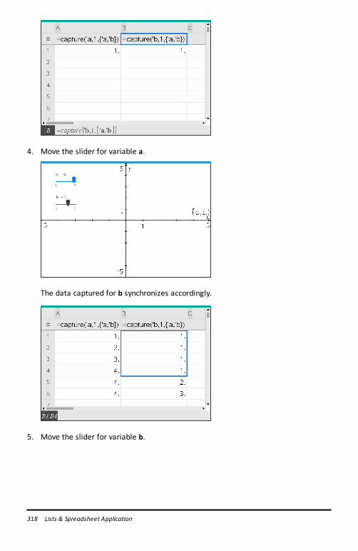
318 Lists & Spreadsheet Application
4. Move the slider for variable a.
The data captured for b synchronizes accordingly.
5. Move the slider for variable b.
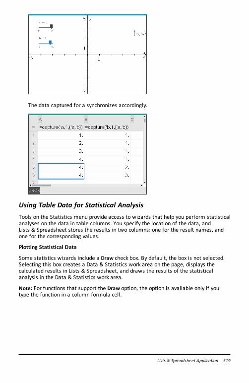
The data captured for a synchronizes accordingly.
Using Table Data for Statistical AnalysisTools on the Statistics menu provide access to wizards that help you perform statisticalanalyses on the data in table columns. You specify the location of the data, andLists & Spreadsheet stores the results in two columns: one for the result names, andone for the corresponding values.
Plotting Statistical Data
Some statistics wizards include a Draw check box. By default, the box is not selected.Selecting this box creates a Data & Statistics work area on the page, displays thecalculated results in Lists & Spreadsheet, and draws the results of the statisticalanalysis in the Data & Statistics work area.
Note: For functions that support the Draw option, the option is available only if youtype the function in a column formula cell.
Lists & Spreadsheet Application 319
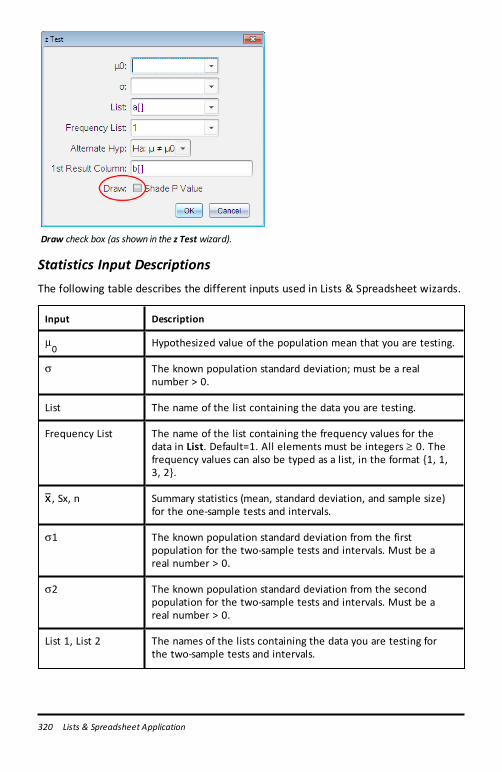
320 Lists & Spreadsheet Application
Draw check box (as shown in the z Test wizard).
Statistics Input DescriptionsThe following table describes the different inputs used in Lists & Spreadsheet wizards.
Input Description
m0 Hypothesized value of the population mean that you are testing.
s The known population standard deviation; must be a realnumber > 0.
List The name of the list containing the data you are testing.
Frequency List The name of the list containing the frequency values for thedata in List. Default=1. All elements must be integers | 0. Thefrequency values can also be typed as a list, in the format {1, 1,3, 2}.
v, Sx, n Summary statistics (mean, standard deviation, and sample size)for the one-sample tests and intervals.
s1 The known population standard deviation from the firstpopulation for the two-sample tests and intervals. Must be areal number > 0.
s2 The known population standard deviation from the secondpopulation for the two-sample tests and intervals. Must be areal number > 0.
List 1, List 2 The names of the lists containing the data you are testing forthe two-sample tests and intervals.
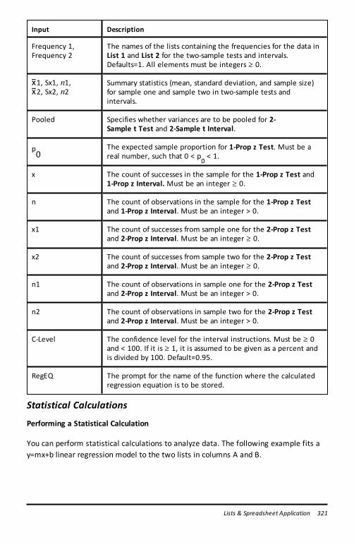
Input Description
Frequency 1,Frequency 2
The names of the lists containing the frequencies for the data inList 1 and List 2 for the two-sample tests and intervals.Defaults=1. All elements must be integers | 0.
v1, Sx1, n1,v2, Sx2, n2
Summary statistics (mean, standard deviation, and sample size)for sample one and sample two in two-sample tests andintervals.
Pooled Specifies whether variances are to be pooled for 2-Sample t Test and 2-Sample t Interval.
p0
The expected sample proportion for 1-Prop z Test. Must be areal number, such that 0 < p
0 < 1.
x The count of successes in the sample for the 1-Prop z Test and1-Prop z Interval. Must be an integer | 0.
n The count of observations in the sample for the 1-Prop z Testand 1-Prop z Interval. Must be an integer > 0.
x1 The count of successes from sample one for the 2-Prop z Testand 2-Prop z Interval. Must be an integer | 0.
x2 The count of successes from sample two for the 2-Prop z Testand 2-Prop z Interval. Must be an integer | 0.
n1 The count of observations in sample one for the 2-Prop z Testand 2-Prop z Interval. Must be an integer > 0.
n2 The count of observations in sample two for the 2-Prop z Testand 2-Prop z Interval. Must be an integer > 0.
C-Level The confidence level for the interval instructions. Must be | 0and < 100. If it is | 1, it is assumed to be given as a percent andis divided by 100. Default=0.95.
RegEQ The prompt for the name of the function where the calculatedregression equation is to be stored.
Statistical Calculations
Performing a Statistical Calculation
You can perform statistical calculations to analyze data. The following example fits ay=mx+b linear regression model to the two lists in columns A and B.
Lists & Spreadsheet Application 321
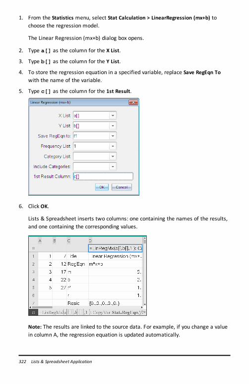
322 Lists & Spreadsheet Application
1. From the Statistics menu, select Stat Calculation > LinearRegression (mx+b) tochoose the regression model.
The Linear Regression (mx+b) dialog box opens.
2. Type a[] as the column for the X List.
3. Type b[] as the column for the Y List.
4. To store the regression equation in a specified variable, replace Save RegEqn Towith the name of the variable.
5. Type c[] as the column for the 1st Result.
6. Click OK.
Lists & Spreadsheet inserts two columns: one containing the names of the results,and one containing the corresponding values.
Note: The results are linked to the source data. For example, if you change a valuein column A, the regression equation is updated automatically.
Storing Statistical Results
Lists & Spreadsheet stores statistical results using a variable-group name with theformat stat.nnn, where nnn is the result name (for example, stat.RegEqn andstat.Resid). The use of standard names for variables makes it easier to identify and usethe statistical variables later. If you want to use a custom variable group instead of thestandard name, you can edit the formula in the column formula cell.
You could use the following formula to store the results in the variable groupMystatsB.
=LinRegMx(a[],b[],1 ): CopyVar Stat., MystatsB.
Later, you could view the results by entering the following expression in the Calculatorapplication or in another column of the Lists & Spreadsheet application:
MystatsB.results
Supported Statistical Calculations
The Stat Calculations menu lets you select from the calculations described below. Formore information, see the TI-Nspire™ Reference Guide.
One-Variable Statistics (OneVar)
Analyzes data with one measured variable. You can specify an optional frequency list.The statistical data returned using this analysis technique are:
• Sample mean, x
• Sum of the data, Gx
• Sum of the squared data, Gx2
• Sample standard deviation, sx
• Population standard deviation, sx
• Sample size, n
• X-min
• First quartile, Q1
• Median
• Third quartile, Q3
• X-max
• Sum of squared deviations, SSx = G(x Nx)2
Lists & Spreadsheet Application 323
324 Lists & Spreadsheet Application
Two-Variable Statistics (TwoVar)
Analyzes paired data. List 1 is the independent variable. List 2 is the dependentvariable. You can specify an optional frequency list. The statistical data returned usingthis analysis technique are:
For each list:
• Sample mean, x or y
• Sum of the data, Gx or Gy
• Sum of the squared data, Gx2 or Gy2
• Sample standard deviation, sx = sn-1
x or sy = sn-1
y
• Population standard deviation, sx = snx or sy = s
ny
• X-min or Y-min
• First quartile, Q1X or Q
1Y
• Median
• Third quartile, Q3X or Q
3Y
• X-max or Y-max
• Sum of squared deviations, SSx = G(x Nx)2 or SSy = G(y Ny)2
Additional data:
• Sample size for each data set, n
• Gxy
• Correlation coefficient, R.
Linear Regression (mx+b) (LinRegMx)
Fits the model equation y=ax+b to the data using a least-squares fit. It displays valuesfor m (slope) and b (y-intercept).
Linear Regression (a+bx) (LinRegBx)
Fits the model equation y=a+bx to the data using a least-squares fit. It displays valuesfor a (y-intercept), b (slope), r2, and r.
Median-Median Line (MedMed)
Fits the model equation y=mx+b to the data using the median-median line (resistantline) technique, calculating the summary points x1, y1, x2, y2, x3, and y3. Median-Median Line displays values for m (slope) and b (y-intercept).
Quadratic Regression (QuadReg)
Fits the second-degree polynomial y=ax2+bx+c to the data. It displays values for a, b, c,and R2. For three data points, the equation is a polynomial fit; for four or more, it is apolynomial regression. At least three data points are required.
Cubic Regression (CubicReg)
Fits the third-degree polynomial y=ax3+bx2+cx+d to the data. It displays values for a, b,c, d, and R2. For four points, the equation is a polynomial fit; for five or more, it is apolynomial regression. At least four points are required.
Quartic Regression (QuartReg)
Fits the fourth-degree polynomial y=ax4+bx3+cx2+dx+e to the data. It displays valuesfor a, b, c, d, e, and R2. For five points, the equation is a polynomial fit; for six or more,it is a polynomial regression. At least five points are required.
Power Regression (PowerReg)
Fits the model equation y=axb to the data using a least-squares fit on transformedvalues ln(x) and ln(y). It displays values for a, b, r2, and r.
Exponential Regression (ExpReg)
Fits the model equation y=abx to the data using a least-squares fit on transformedvalues x and ln(y). It displays values for a, b, r2, and r.
Logarithmic Regression (LogReg)
Fits the model equation y=a+b ln(x) to the data using a least-squares fit ontransformed values ln(x) and y. It displays values for a, b, r2, and r.
Sinusoidal Regression (SinReg)
Fits the model equation y=a sin(bx+c)+d to the data using an iterative least-squares fit.It displays values for a, b, c, and d. At least four data points are required. At least twodata points per cycle are required to avoid aliased frequency estimates.
Note: The output of SinReg is always in radians, regardless of the Radian/Degree modesetting.
Logistic Regression (d=0) (Logistic)
Fits the model equation y=c/(1+a*e⁻bx) to the data using an iterative least-squares fit.It displays values for a, b, and c.
Lists & Spreadsheet Application 325
326 Lists & Spreadsheet Application
Logistic Regression (dƒ0) (LogisticD)
Fits the model equation y=c(1+a*e(⁻bx))+d to the data using an iterative least-squaresfit. It displays values for a, b, c and d.
Multiple Linear Regression (MultReg)
Calculates multiple linear regression of list Y on lists X1, X2, …, X10.
Distributions
Calculating a Distribution
Example: Calculate a distribution to fit the Normal Pdf distribution model.
1. Click the column formula cell (second cell from the top) in column A.
2. Click Statistics > Distributions > Normal Pdf to choose the Distribution model.
The Normal Pdf dialog box opens and displays fields for typing or selecting thearguments for the calculation.
3. Press Tab as necessary to move from field to field and provide each argument. Youcan type values, or select them from the drop down list:
- X Value: Click the drop-down arrow to choose any list in the problem to providethe x values for the calculation.
- Mean: Type a value for the mean or click the drop-down arrow to choose avariable that contains the mean.
- Standard Deviation: Type a value for the standard deviation or choose a variablethat contains the standard deviation.
4. Click the Draw check box to see the distribution plotted in Data & Statistics.
Note: The Draw option is not available for all distributions.
5. Click OK.
Lists & Spreadsheet inserts two columns: one containing the names of the results,and one containing the corresponding values. The results are plotted inData & Statistics.
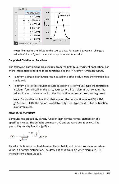
Note: The results are linked to the source data. For example, you can change avalue in Column A, and the equation updates automatically.
Supported Distribution Functions
The following distributions are available from the Lists & Spreadsheet application. Formore information regarding these functions, see the TI-Nspire™ Reference Guide.
• To return a single distribution result based on a single value, type the function in asingle cell.
• To return a list of distribution results based on a list of values, type the function ina column formula cell. In this case, you specify a list (column) that contains thevalues. For each value in the list, the distribution returns a corresponding result.
Note: For distribution functions that support the draw option (normPDF, t PDF,χ² Pdf, and F Pdf), the option is available only if you type the distribution functionin a formula cell.
Normal Pdf (normPdf)
Computes the probability density function (pdf) for the normal distribution at aspecified x value. The defaults are mean μ=0 and standard deviation σ=1. Theprobability density function (pdf) is:
This distribution is used to determine the probability of the occurrence of a certainvalue in a normal distribution. The draw option is available when Normal PDF isinvoked from a formula cell.
Lists & Spreadsheet Application 327
328 Lists & Spreadsheet Application
When you access distributions from the formula cell, you must select a valid list fromthe drop-down list to avoid unexpected results. If accessed from a cell, you mustspecify a number for the x-value. The distribution returns the probability that the valueyou specify will occur.
Normal Cdf (normCdf)
Computes the normal distribution probability between Lower Bound andUpper Bound for the specified mean, μ (default=0) and the standard deviation, s
(default=1). You can click the Draw (Shade area) check box to shade the area betweenthe lower and upper bounds. Changes to the initial Lower Bound andUpper Boundautomatically update the distribution.
This distribution is useful in determining the probability of an occurrence of any valuebetween the lower and upper bounds in the normal distribution. It is equivalent tofinding the area under the specified normal curve between the bounds.
Inverse Normal (invNorm)
Computes the inverse cumulative normal distribution function for a given area underthe normal distribution curve specified by mean, μ, and standard deviation, s.
This distribution is useful in determining the x-value of data in the area from 0 to x<1when the percentile is known.
t Pdf (tPdf)
Computes the probability density function (pdf) for the t-distribution at a specified xvalue. df (degrees of freedom) must be > 0. The probability density function (pdf) is:
This distribution is useful in determining the probability of the occurrence of a valuewhen the population standard deviation is not known and the sample size is small. Thedraw option is available when t Pdf is invoked from a formula cell.
t Cdf (tCdf)
Computes the Student-t distribution probability between Lower Bound andUpper Bound for the specified df (degrees of freedom). You can click the Draw (Shadearea) check box to shade the area between the bounds. Changes to the initialLower Bound andUpper Bound automatically update the distribution.
This distribution is useful in determining the probability of the occurrence of a valuewithin an interval defined by the lower and upper bound for a normally distributedpopulation when the population standard deviation is not known.
Inverse t (invt)
Computes the inverse cumulative t-distribution probability function specified byDegrees of Freedom, df, for a given area under the curve.
This distribution is useful in determining the probability of an occurrence of data in thearea from 0 to x<1. This function is used when the population mean and/or populationstandard deviation is not known.
c2 Pdf (c2 Pdf())
Computes the probability density function (pdf) for the c2 (chi-square) distribution at aspecified x value. df (degrees of freedom) must be an integer > 0. The probabilitydensity function (pdf) is:
This distribution is useful in determining the probability of the occurrence of a givenvalue from a population with a c2 distribution. The draw option is available when c2
Pdf is invoked from a formula cell.
c2 Cdf (c2 Cdf())
Computes the c2 (chi-square) distribution probability between lowBound and upBoundfor the specified df (degrees of freedom). You can click the Draw Shade area check boxto shade the area between the lower and upper bounds. Changes to the initiallowBound and upBound automatically update the distribution.
This distribution is useful in determining the probability of the occurrence of valuewithin given boundaries of a population with a c2 distribution.
F Pdf (F Pdf())
Computes the probability density function (pdf) for the F distribution at a specified xvalue. numerator df (degrees of freedom) and denominator df must be integers > 0.The probability density function (pdf) is:
where n = numerator degrees of freedomd = denominator degrees of freedom
Lists & Spreadsheet Application 329
330 Lists & Spreadsheet Application
This distribution is useful in determining the probability that two samples have thesame variance. The draw option is available when F Pdf is invoked from a formulacell.
F Cdf (F Cdf())
Computes the F distribution probability between lowBound and upBound for thespecified dfnumer (degrees of freedom) and dfDenom. You can click the Draw (Shadearea) check box to shade the area between the lower and upper bounds. Changes tothe initial lowBound and upBound automatically update the distribution.
This distribution is useful in determining the probability that a single observation fallswithin the range between the lower bound and upper bound.
Binomial Pdf (binomPdf())
Computes a probability at x for the discrete binomial distribution with the specifiednumtrials and probability of success (p) on each trial. The x parameter can be aninteger or a list of integers. 0{p{1 must be true. numtrials must be an integer > 0. Ifyou do not specify x, a list of probabilities from 0 to numtrials is returned. Theprobability density function (pdf) is:
where n = numtrials
This distribution is useful in determining the probability of success in a success/failuretrial, at trial n. For example, you could use this distribution to predict the probability ofgetting heads in a coin toss on the fifth toss.
Binomial Cdf (binomCdf())
Computes a cumulative probability for the discrete binomial distribution with n numberof trials and probability p of success on each trial.
This distribution is useful in determining the probability of a success on one trial beforeall trials are completed. For example, if heads is a successful coin toss and you plan totoss the coin 10 times, this distribution would predict the chance of obtaining heads atleast once in the 10 tosses.
Inverse Binomial (invBinom())
• Given the number of trials (NumTrials) and the probability of success of each trial(Prob), this function returns the minimum number of successes, k, such that thecumulative probability of k successes is greater than or equal to the givencumulative probability (CumulativeProb).
Inverse Binomial with respect to N (invBinomN())
Given the probability of success of each trial (Prob), and the number of successes(NumSuccess), this function returns the minimum number of trials, N, such that thecumulative probability of x successes is less than or equal to the given cumulativeprobability (CumulativeProb).
Poisson Pdf (poissPdf())
Computes a probability at x for the discrete Poisson distribution with the specifiedmean, μ, which must be a real number > 0. x can be an integer or a list of integers.The probability density function (pdf) is:
This distribution is useful in determining the probability of obtaining a certain numberof successes before a trial begins. For example, you could use this calculation topredict the number of heads that would occur in eight tosses of a coin.
Poisson Cdf (poissCdf())
Computes a cumulative probability for the discrete Poisson distribution with specifiedmean, x.
This distribution is useful in determining the probability that a certain number ofsuccesses occur between the upper and lower bounds of a trial. For example, you coulduse this calculation to predict the number of heads displayed between coin toss #3 andtoss #8.
Geometric Pdf (geomPdf())
Computes a probability at x, the number of the trial on which the first success occurs,for the discrete geometric distribution with the specified probability of success p. 0{p{1 must be true. x can be an integer or a list of integers. The probability densityfunction (pdf) is:
This distribution is useful in determining the likeliest number of trials before a successis obtained. For example, you could use this calculation to predict the number of cointosses that would be made before a heads resulted.
Geometric Cdf (geomCdf())
Computes a cumulative geometric probability from lowBound to upBound with thespecified probability of success, p.
Lists & Spreadsheet Application 331
332 Lists & Spreadsheet Application
This distribution is useful in determining the probability associated with the firstsuccess occurring during trials 1 through n. For example, you could use this calculationto determine the probability that heads display on toss #1, #2, #3, ..., #n.
Confidence IntervalsSupported Confidence Intervals
The following confidence intervals are available from the Lists & Spreadsheetsapplication. For more information regarding these functions, see the TI-Nspire™Reference Guide.
z Interval (zInterval)
Computes a confidence interval for an unknown population mean, m, when thepopulation standard deviation, s, is known. The computed confidence interval dependson the user-specified confidence level.
This test is useful in determining how far from a population mean a sample mean canget before indicating a significant deviation.
t Interval (tInterval)
Computes a confidence interval for an unknown population mean, m, when thepopulation standard deviation, s, is unknown. The computed confidence intervaldepends on the user-specified confidence level.
This test is useful in examining whether the confidence interval associated with aconfidence level contains the value assumed in the hypothesis. Like the z Interval, thistest helps you determine how far from a population mean a sample mean can getbefore indicating a significant deviation when the population mean is unknown.
2-Sample z Interval (zInterval_2Samp)
Computes a confidence interval for the difference between two population means(m
1Nm
2) when both population standard deviations (s
1and s
2) are known. The
computed confidence interval depends on the user-specified confidence level.
This test is useful in determining if there is statistical significance between the meansof two samples from the same population. For example, this test could determinewhether there is significance between the mean college entrance test score of femalestudents and the mean of college entrance test score of male students at the sameschool.
2-Sample t Interval (tInterval_2Samp)
Computes a confidence interval for the difference between two population means(m
1Nm
2) when both population standard deviations (s
1and s
2) are unknown. The
computed confidence interval depends on the user-specified confidence level.
This test is useful in determining if there is statistical significance between the meansof two samples from the same population. It is used instead of the 2-sample zconfidence interval in situations where the population is too large to measure todetermine the standard deviation.
1-Prop z Interval (zInterval_1Prop)
Computes a confidence interval for an unknown proportion of successes. It takes asinput the count of successes in the sample x and the count of observations in thesample n. The computed confidence interval depends on the user-specified confidencelevel.
This test is useful in determining the probability of a given number of successes thatcan be expected for a given number of trials. For instance, casino examiners would usethis test to determine if observed payouts for one slot machine demonstrate aconsistent pay out rate.
2-Prop z Interval (zInterval_2Prop)
Computes a confidence interval for the difference between the proportion of successesin two populations (p
1-p
2). It takes as input the count of successes in each sample
(x1 and x
2) and the count of observations in each sample (n
1 and n
2). The computed
confidence interval depends on the user-specified confidence level.
This test is useful in determining if two rates of success differ because of somethingother than sampling error and standard deviation. For example, a bettor could use thistest to determine if there is an advantage in the long run by playing one game ormachine versus playing another game or machine.
Linear Reg t Intervals (LinRegtIntervals)
Computes a linear regression t confidence interval for the slope coefficient b. If theconfidence interval contains 0, this is insufficient evidence to indicate that the dataexhibits a linear relationship.
Multiple Reg Intervals (MultRegIntervals)
Computes multiple regression prediction confidence interval for the calculated y and aconfidence for y.
Stat TestsSupported Statistical Tests
Hypothesis tests are available from the Lists & Spreadsheets application. For moreinformation regarding these functions, see the TI-Nspire™ Reference Guide.
Some of the wizards for Stat Tests display a Draw check box. By default, the box is notselected. Selecting the box creates a Data & Statistics work area on the page and plotsthe results in that work area.
z test (zTest)
Performs a hypothesis test for a single unknown population mean, m, when thepopulation standard deviation, s, is known. It tests the null hypothesis H
0: m=m
0against
one of the alternatives below.
• Ha: mƒm
0• H
a: m<m
0• H
a: m>m
0
Lists & Spreadsheet Application 333
334 Lists & Spreadsheet Application
This test is used for large populations that are normally distributed. The standarddeviation must be known.
This test is useful in determining if the difference between a sample mean and apopulation mean is statistically significant when you know the true deviation for apopulation.
t test (tTest)
Performs a hypothesis test for a single unknown population mean, m, when thepopulation standard deviation, s, is unknown. It tests the null hypothesis H
0: m=m
0against one of the alternatives below.
• Ha: mƒm
0• H
a: m<m
0• H
a: m>m
0This test is similar to a z-test, but is used when the population is small and normallydistributed. This test is used more frequently than the z-test because small samplepopulations are more frequently encountered in statistics than are large populations.
This test is useful in determining if two normally distributed populations have equalmeans, or when you need to determine if a sample mean differs from a populationmean significantly and the population standard deviation is unknown.
2-Sample z Test (zTest_2Samp)
Tests the equality of the means of two populations (m1and m
2) based on independent
samples when both population standard deviations (s1and s
2) are known. The null
hypothesis H0: m
1=m
2is tested against one of the alternatives below.
• Ha: m
1ƒm
2• H
a: m
1<m
2• H
a: m
1>m
22-Sample t Test (tTest_2Samp)
Tests the equality of the means of two populations (m1and m
2) based on independent
samples when neither population standard deviation (s1or s
2) is known. The null
hypothesis H0: m
1=m
2is tested against one of the alternatives below.
• Ha: m
1ƒm
2• H
a: m
1<m
2• H
a: m
1>m
21-Prop z Test (zTest_1Prop)
Computes a test for an unknown proportion of successes (prop). It takes as input thecount of successes in the sample x and the count of observations in the sample n. 1-Prop z Test tests the null hypothesis H
0: prop=p
0against one of the alternatives below.
• Ha: propƒp
0
• Ha: prop<p
0• H
a: prop>p
0This test is useful in determining if the probability of the success seen in a sample issignificantly different from the probability of the population or if it is due to samplingerror, deviation, or other factors.
2-Prop z Test (zTest_2Prop)
Computes a test to compare the proportion of successes (p1and p
2) from two
populations. It takes as input the count of successes in each sample (x1and x
2) and the
count of observations in each sample (n1and n
2). 2-Prop z Test tests the null
hypothesis H0: p
1=p
2(using the pooled sample proportionÇ) against one of the
alternatives below.
• Ha: p
1ƒp
2• H
a: p
1<p
2• H
a: p
1>p
2This test is useful in determining if the probability of success seen in two samples isequal.
c2GOF (c2GOF)Performs a test to confirm that sample data is from a population that conforms to aspecified distribution. For example, c2 GOF can confirm that the sample data camefrom a normal distribution.
c2 2-way Test (c22way)
Computes a chi-square test for association on the two-way table of counts in thespecifiedObservedmatrix. The null hypothesis H
0for a two-way table is: no
association exists between row variables and column variables. The alternativehypothesis is: the variables are related.
2-Sample FTest (FTest_2Samp)
Computes an F-test to compare two normal population standard deviations (s1and
s2). The population means and standard deviations are all unknown. 2-Sample FTest,
which uses the ratio of sample variances Sx12/Sx22, tests the null hypothesis H0: s
1=s
2against one of the alternatives below.
• Ha: s
1ƒs
2• H
a: s
1<s
2• H
a: s
1>s
2Below is the definition for the 2-Sample FTest.
Sx1, Sx2 = Sample standard deviations having n1
N1 and n2
N1 degrees offreedom df, respectively.
Lists & Spreadsheet Application 335
336 Lists & Spreadsheet Application
F =F-statistic =
df(x, n1
N1,n2
N1)= Fpdf( ) with degrees of freedom df, n
1N1, and n
2N1
p = reported p value
2-Sample FTest for the alternative hypothesis s1> s
2.
2-Sample FTest for the alternative hypothesis s1< s
2.
2-Sample FTest for the alternative hypothesis s1
ƒs2. Limits must satisfy the following:
where: [Lbnd,Ubnd]=lower and upper limits
The F-statistic is used as the bound producing the smallest integral. The remainingbound is selected to achieve the preceding integral’s equality relationship.
Linear Reg t Test (LinRegtTest)
Computes a linear regression on the given data and a t test on the value of slope b andthe correlation coefficient r for the equation y=a+bx. It tests the null hypothesisH0: b=0 (equivalently, r=0) against one of the alternatives below.
• Ha: bƒ0 and rƒ0
• Ha: b<0 and r<0
• Ha: b>0 and r>0
Multiple Reg Tests (MultRegTest)
Computes a linear regression on the given data, and provides the F test statistic forlinearity.
For more information, see the TI-Nspire™ Reference Guide.
ANOVA (ANOVA)
Computes a one-way analysis of variance for comparing the means of 2 to 20populations. The ANOVA procedure for comparing these means involves analysis of thevariation in the sample data. The null hypothesis H
0: m
1=m
2=...=m
kis tested against the
alternative Ha: not all m
1...m
kare equal.
The ANOVA test is a method of determining if there is a significant differencebetween the groups as compared to the difference occurring within each group.
This test is useful in determining if the variation of data from sample-to-sample showsa statistically significant influence of some factor other than the variation within thedata sets themselves. For example, a box buyer for a shipping firm wants to evaluatethree different box manufacturers. He obtains sample boxes from all three suppliers.ANOVA can help him determine if the differences between each sample group aresignificant as compared to the differences within each sample group.
ANOVA 2-Way (ANOVA2way)
Computes a two-way analysis of variance for comparing the means of two to 20populations. A summary of results is stored in the stat.results variable.
The two-way ANOVA analysis of variance examines the effects of two independentvariables and helps to determine if these interact with respect to the dependentvariable. (In other words, if the two independent variables do interact, their combinedeffect can be greater than or less than the impact of either independent variableadditively.)
This test is useful in evaluating differences similar to the ANOVA analysis but with theaddition of another potential influence. To continue with the ANOVA box example, thetwo-way ANOVA might examine the influence of box material on the differences seen.
Selecting an Alternative Hypothesis (ƒ < >)
Most of the inferential stat editors for the hypothesis tests prompt you to select one ofthree alternative hypotheses.
• The first is a ƒ alternative hypothesis, such as mƒm0 for the z Test.
• The second is a < alternative hypothesis, such as m1<m2 for the 2-Sample t Test.
• The third is a > alternative hypothesis, such as p1>p2 for the 2-Prop z Test.
To select an alternative hypothesis, move the cursor to the appropriate alternative, andthen press Enter.
Selecting the Pooled Option
Pooled (2-Sample t Test and 2-Sample t Interval only) specifies whether the variancesare to be pooled for the calculation.
• Select No if you do not want the variances pooled. Population variances can beunequal.
• Select Yes if you want the variances pooled. Population variances are assumed tobe equal.
To select the Pooled option, select Yes from the drop-down list.
Lists & Spreadsheet Application 337
338 Lists & Spreadsheet Application
Working with Function TablesThe Lists & Spreadsheet application lets you show a table of function values for anyfunction in the current problem. You can change the settings for the table, deletecolumns, add values for multiple functions, and edit the expression that defines afunction without leaving the Lists & Spreadsheet application.
Switching to a Table
1. While working in the Lists & Spreadsheet application:
Windows®: Press Ctrl+T.
Mac®: Press “+T.
Handheld: Press/T.
The Lists & Spreadsheet application disappears and an empty table is displayedwith a list of the functions that are available in the problem.
Note: If you have previously shown a table for a function from theLists & Spreadsheet application, the table includes that function by default.
2. Choose the name of the function for which you want to display values.
Values for the function you selected are displayed in the first column of the table.
3. To move through adjacent cells of the table, press ▲ or▼. Press Tab to movefrom the body of the table (cells) to the top two rows (cells for column names andformulas).
4. To hide the table of values and return to the Lists & Spreadsheet application,repeat Step 1.
Making Changes from a Table
You can change the table of function values using the tools on the Table menu.
▶ To remove a column from the table, click any cell and click Delete Column.
▶ To display the list of functions, click a cell in a column and click Choose. Select acell in an empty column unless you are replacing values already displayed. Click afunction in the list to add its values to the column.
Note: You can also click the drop-down arrow on the top cell of a column to displaythe list of functions in the problem.
▶ To change the expression that defines a function, click Edit Expression. You can alsoedit the expression directly on the entry line beneath the table.
Note: When you edit the expression for a function, that function automaticallychanges in the application used to define the function. For example, if you edit aGraphs & Geometry function in the table, the table values and graph of thefunction are both updated.
▶ To change the default table settings, choose Edit Table Settings.
The Table dialog box opens. Press Tab to move from field to field and type or selectnew values for the default table settings:
- Table Start: Type the value to use as the first value in the table of values.
- Table Step: Type a value for the interval between values.
- Independent and Dependent: Click the drop-down arrow to choose Auto or Askas the method for populating a column with the values of the independent anddependent variables. Auto populates the table starting at the defined tablestart value and displays an independent and dependent value for each step. Asklets you select a cell and press Enter to generate a value for a cell.
Lists & Spreadsheet Application 339
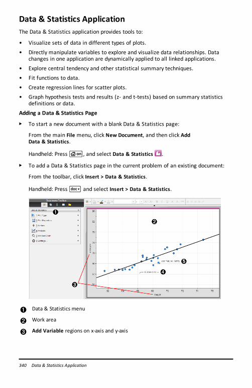
340 Data & Statistics Application
Data & Statistics ApplicationThe Data & Statistics application provides tools to:
• Visualize sets of data in different types of plots.
• Directly manipulate variables to explore and visualize data relationships. Datachanges in one application are dynamically applied to all linked applications.
• Explore central tendency and other statistical summary techniques.
• Fit functions to data.
• Create regression lines for scatter plots.
• Graph hypothesis tests and results (z- and t-tests) based on summary statisticsdefinitions or data.
Adding a Data & Statistics Page
▶ To start a new document with a blank Data & Statistics page:
From the main File menu, click New Document, and then click AddData & Statistics.
Handheld: Pressc, and select Data & Statistics .
▶ To add a Data & Statistics page in the current problem of an existing document:
From the toolbar, click Insert > Data & Statistics.
Handheld: Press~ and select Insert > Data & Statistics.
À Data & Statistics menu
Á Work area
 Add Variable regions on x-axis and y-axis
à Linear Regression Plot with expression
Ä Data point with coordinates
Basic Operations in Data & StatisticsThe Data & Statistics application lets you explore and visualize data and graphinferential statistics. The Lists & Spreadsheet application can work in conjunction withthe Data & Statistics application. The Lists & Spreadsheet Summary Plot and QuickGraph tools automatically add a Data & Statistics application to show plots. A list thatyou create in a problem (using the Lists & Spreadsheet or Calculator applications) canbe accessed as a variable in any TI-Nspire™ application in that problem.
Changing Data & Statistics Settings
1. From the Settings menu, select Settings.
2. Select the settings that you want to use.
• Display Digits. Lets you select the display format for numeric labels in thecurrent document. Select Auto to automatically follow the setting in theDocument Settings dialog box.
• Diagnostics. Displays the value of the r2 or R2 statistic (when available) undercertain regression equations.
- r2 is displayed for Linear (mx+b), Linear (a+bx), Power, Exponential, andLogarithmic regressions.
- R2 is displayed for Quadratic, Cubic, and Quartic regressions.
Using the Default Caseplot
The Data & Statistics application plots numeric and string (categorical) data fromvariables. When you add a Data & Statistics application to a problem that includeslists, a default caseplot displays on the work area.
The caseplot is like having a stack of cards with information on them and scatteringthe cards randomly on a table. You can click a dot to see the information on that“card.” You can drag a dot to “group” the “cards” by the caption variable.
Data & Statistics Application 341
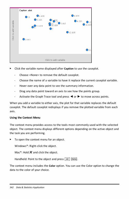
342 Data & Statistics Application
▶ Click the variable name displayed after Caption to use the caseplot.
- Choose <None> to remove the default caseplot.
- Choose the name of a variable to have it replace the current caseplot variable.
- Hover over any data point to see the summary information.
- Drag any data point toward an axis to see how the points group.
- Activate the Graph Trace tool and press ◄ or ► to move across points.
When you add a variable to either axis, the plot for that variable replaces the defaultcaseplot. The default caseplot redisplays if you remove the plotted variable from eachaxis.
Using the Context Menu
The context menu provides access to the tools most commonly used with the selectedobject. The context menu displays different options depending on the active object andthe task you are performing.
▶ To open the context menu for an object.
Windows®: Right-click the object.
Mac®: Hold “ and click the object.
Handheld: Point to the object and press/b.
The context menu includes the Color option. You can use the Color option to change thedata to the color of your choice.
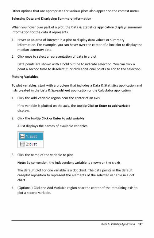
Other options that are appropriate for various plots also appear on the context menu.
Selecting Data and Displaying Summary Information
When you hover over part of a plot, the Data & Statistics application displays summaryinformation for the data it represents.
1. Hover at an area of interest in a plot to display data values or summaryinformation. For example, you can hover over the center of a box plot to display themedian summary data.
2. Click once to select a representation of data in a plot.
Data points are shown with a bold outline to indicate selection. You can click apoint a second time to deselect it, or click additional points to add to the selection.
Plotting Variables
To plot variables, start with a problem that includes a Data & Statistics application andlists created in the Lists & Spreadsheet application or the Calculator application.
1. Click the Add Variable region near the center of an axis.
If no variable is plotted on the axis, the tooltip Click or Enter to add variabledisplays.
2. Click the tooltip Click or Enter to add variable.
A list displays the names of available variables.
3. Click the name of the variable to plot.
Note: By convention, the independent variable is shown on the x-axis.
The default plot for one variable is a dot chart. The data points in the defaultcaseplot reposition to represent the elements of the selected variable in a dotchart.
4. (Optional) Click the Add Variable region near the center of the remaining axis toplot a second variable.
Data & Statistics Application 343
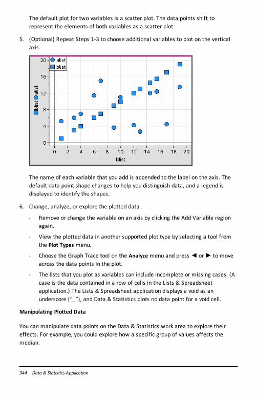
344 Data & Statistics Application
The default plot for two variables is a scatter plot. The data points shift torepresent the elements of both variables as a scatter plot.
5. (Optional) Repeat Steps 1-3 to choose additional variables to plot on the verticalaxis.
The name of each variable that you add is appended to the label on the axis. Thedefault data point shape changes to help you distinguish data, and a legend isdisplayed to identify the shapes.
6. Change, analyze, or explore the plotted data.
- Remove or change the variable on an axis by clicking the Add Variable regionagain.
- View the plotted data in another supported plot type by selecting a tool fromthe Plot Types menu.
- Choose the Graph Trace tool on the Analyze menu and press ◄ or ► to moveacross the data points in the plot.
- The lists that you plot as variables can include incomplete or missing cases. (Acase is the data contained in a row of cells in the Lists & Spreadsheetapplication.) The Lists & Spreadsheet application displays a void as anunderscore (“_”), and Data & Statistics plots no data point for a void cell.
Manipulating Plotted Data
You can manipulate data points on the Data & Statistics work area to explore theireffects. For example, you could explore how a specific group of values affects themedian.
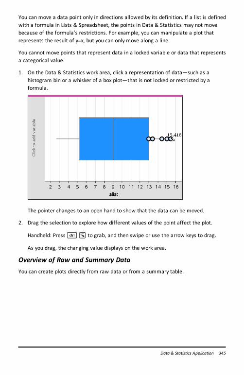
You can move a data point only in directions allowed by its definition. If a list is definedwith a formula in Lists & Spreadsheet, the points in Data & Statistics may not movebecause of the formula’s restrictions. For example, you can manipulate a plot thatrepresents the result of y=x, but you can only move along a line.
You cannot move points that represent data in a locked variable or data that representsa categorical value.
1. On the Data & Statistics work area, click a representation of data—such as ahistogram bin or a whisker of a box plot—that is not locked or restricted by aformula.
The pointer changes to an open hand to show that the data can be moved.
2. Drag the selection to explore how different values of the point affect the plot.
Handheld: Press/a to grab, and then swipe or use the arrow keys to drag.
As you drag, the changing value displays on the work area.
Overview of Raw and Summary DataYou can create plots directly from raw data or from a summary table.
Data & Statistics Application 345
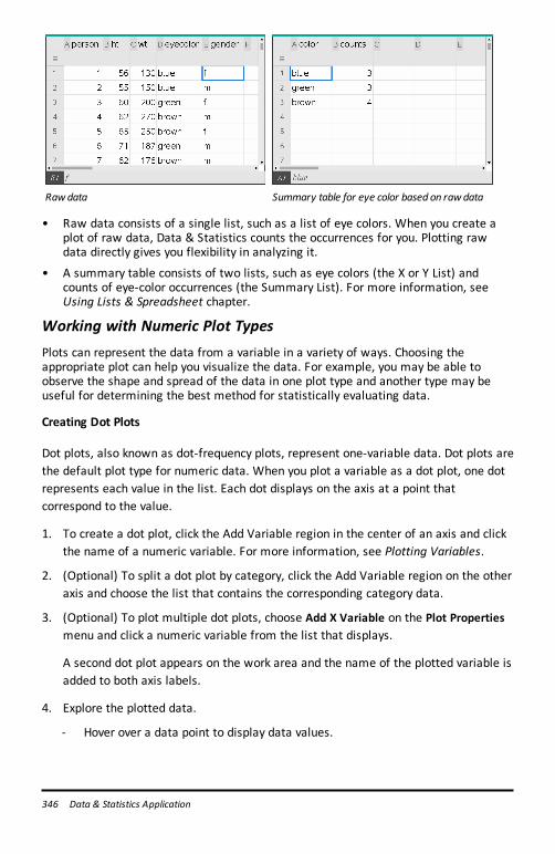
346 Data & Statistics Application
Rawdata Summary table for eye color based on rawdata
• Raw data consists of a single list, such as a list of eye colors. When you create aplot of raw data, Data & Statistics counts the occurrences for you. Plotting rawdata directly gives you flexibility in analyzing it.
• A summary table consists of two lists, such as eye colors (the X or Y List) andcounts of eye-color occurrences (the Summary List). For more information, seeUsing Lists & Spreadsheet chapter.
Working with Numeric Plot TypesPlots can represent the data from a variable in a variety of ways. Choosing theappropriate plot can help you visualize the data. For example, you may be able toobserve the shape and spread of the data in one plot type and another type may beuseful for determining the best method for statistically evaluating data.
Creating Dot Plots
Dot plots, also known as dot-frequency plots, represent one-variable data. Dot plots arethe default plot type for numeric data. When you plot a variable as a dot plot, one dotrepresents each value in the list. Each dot displays on the axis at a point thatcorrespond to the value.
1. To create a dot plot, click the Add Variable region in the center of an axis and clickthe name of a numeric variable. For more information, see Plotting Variables.
2. (Optional) To split a dot plot by category, click the Add Variable region on the otheraxis and choose the list that contains the corresponding category data.
3. (Optional) To plot multiple dot plots, choose Add X Variable on the Plot Propertiesmenu and click a numeric variable from the list that displays.
A second dot plot appears on the work area and the name of the plotted variable isadded to both axis labels.
4. Explore the plotted data.
- Hover over a data point to display data values.
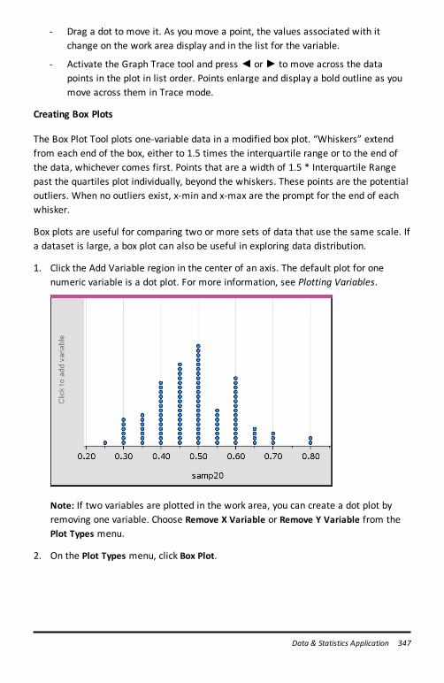
- Drag a dot to move it. As you move a point, the values associated with itchange on the work area display and in the list for the variable.
- Activate the Graph Trace tool and press ◄ or ► to move across the datapoints in the plot in list order. Points enlarge and display a bold outline as youmove across them in Trace mode.
Creating Box Plots
The Box Plot Tool plots one-variable data in a modified box plot. “Whiskers” extendfrom each end of the box, either to 1.5 times the interquartile range or to the end ofthe data, whichever comes first. Points that are a width of 1.5 * Interquartile Rangepast the quartiles plot individually, beyond the whiskers. These points are the potentialoutliers. When no outliers exist, x-min and x-max are the prompt for the end of eachwhisker.
Box plots are useful for comparing two or more sets of data that use the same scale. Ifa dataset is large, a box plot can also be useful in exploring data distribution.
1. Click the Add Variable region in the center of an axis. The default plot for onenumeric variable is a dot plot. For more information, see Plotting Variables.
Note: If two variables are plotted in the work area, you can create a dot plot byremoving one variable. Choose Remove X Variable or Remove Y Variable from thePlot Types menu.
2. On the Plot Types menu, click Box Plot.
Data & Statistics Application 347
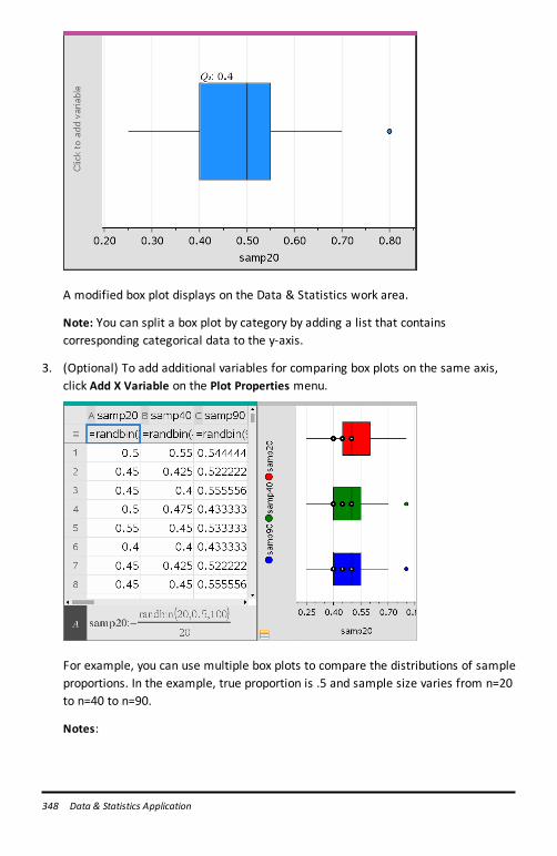
348 Data & Statistics Application
A modified box plot displays on the Data & Statistics work area.
Note: You can split a box plot by category by adding a list that containscorresponding categorical data to the y-axis.
3. (Optional) To add additional variables for comparing box plots on the same axis,click Add X Variable on the Plot Properties menu.
For example, you can use multiple box plots to compare the distributions of sampleproportions. In the example, true proportion is .5 and sample size varies from n=20to n=40 to n=90.
Notes:
- You can create a box plot with frequency by choosing Add X Variable or Add YVariable on the Plot Properties menu.
- You can specify a variable multiple times as you choose variables to plot as boxplots.
- The variable used to provide frequency information is added to the label on thehorizontal axis in the format: x_variablename{frequencylist_name}.
4. Point and click the regions of the box plot to explore and analyze the data itrepresents.
- Hover over a region or over a whisker to display the details for the portion ofthe plot that interests you. The label for the quartile that corresponds to yourselection is displayed.
- Click a region of the box plot to select the data points or whiskers. Click againto remove the selection.
- You can select any box plot that does not include frequency data and chooseDot Plot on the context menu to change the plot type.
- Drag a selection to move it and explore other possibilities for the data.
- Use the arrow keys to move a data point one pixel at a time.
- Activate the Graph Trace tool and press ◄ or ► to move across dots andregions of the plot. As the trace cursor moves, the values for Q1, the median,Q3, and whisker ends/outliers are displayed.
5. Change the plot from a modified box plot to a standard box plot by choosing ExtendBox Plot Whiskers on the Plot Properties menu.
The box plot is redrawn as a standard box plot with extended whiskers.
The standard box plot’s whiskers use the minimum and maximum points in thevariable and outliers are not identified. The whiskers on the plot extend from theminimum data point in the set (x-min) to the first quartile (Q1) and from the thirdquartile (Q3) to the maximum point (x-max). The box is defined by Q1, Med(median), and Q3.
Note: You can click Show Box Plot Outliers on the Plot Properties menu to return tothe modified box plot.
Data & Statistics Application 349
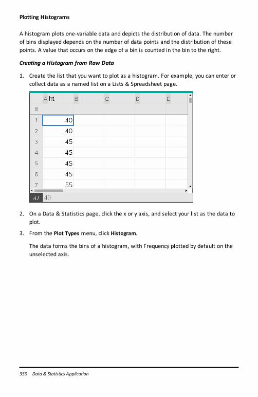
350 Data & Statistics Application
Plotting Histograms
A histogram plots one-variable data and depicts the distribution of data. The numberof bins displayed depends on the number of data points and the distribution of thesepoints. A value that occurs on the edge of a bin is counted in the bin to the right.
Creating a Histogram from Raw Data
1. Create the list that you want to plot as a histogram. For example, you can enter orcollect data as a named list on a Lists & Spreadsheet page.
2. On a Data & Statistics page, click the x or y axis, and select your list as the data toplot.
3. From the Plot Types menu, click Histogram.
The data forms the bins of a histogram, with Frequency plotted by default on theunselected axis.
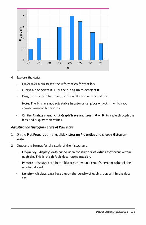
4. Explore the data.
- Hover over a bin to see the information for that bin.
- Click a bin to select it. Click the bin again to deselect it.
- Drag the side of a bin to adjust bin width and number of bins.
Note: The bins are not adjustable in categorical plots or plots in which youchoose variable bin widths.
- On the Analyze menu, click Graph Trace and press ◄ or ► to cycle through thebins and display their values.
Adjusting the Histogram Scale of Raw Data
1. On the Plot Properties menu, click Histogram Properties and choose HistogramScale.
2. Choose the format for the scale of the histogram.
- Frequency - displays data based upon the number of values that occur withineach bin. This is the default data representation.
- Percent - displays data in the histogram by each group’s percent value of thewhole data set.
- Density - displays data based upon the density of each group within the dataset.
Data & Statistics Application 351
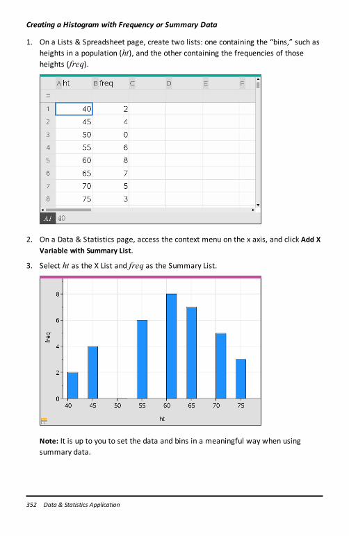
352 Data & Statistics Application
Creating a Histogram with Frequency or Summary Data
1. On a Lists & Spreadsheet page, create two lists: one containing the “bins,” such asheights in a population (ht), and the other containing the frequencies of thoseheights (freq).
2. On a Data & Statistics page, access the context menu on the x axis, and click Add XVariable with Summary List.
3. Select ht as the X List and freq as the Summary List.
Note: It is up to you to set the data and bins in a meaningful way when usingsummary data.
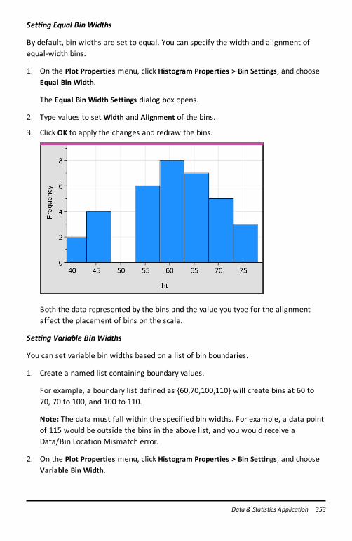
Setting Equal Bin Widths
By default, bin widths are set to equal. You can specify the width and alignment ofequal-width bins.
1. On the Plot Properties menu, click Histogram Properties > Bin Settings, and chooseEqual Bin Width.
The Equal Bin Width Settings dialog box opens.
2. Type values to set Width and Alignment of the bins.
3. Click OK to apply the changes and redraw the bins.
Both the data represented by the bins and the value you type for the alignmentaffect the placement of bins on the scale.
Setting Variable Bin Widths
You can set variable bin widths based on a list of bin boundaries.
1. Create a named list containing boundary values.
For example, a boundary list defined as {60,70,100,110} will create bins at 60 to70, 70 to 100, and 100 to 110.
Note: The data must fall within the specified bin widths. For example, a data pointof 115 would be outside the bins in the above list, and you would receive aData/Bin Location Mismatch error.
2. On the Plot Properties menu, click Histogram Properties > Bin Settings, and chooseVariable Bin Width.
Data & Statistics Application 353
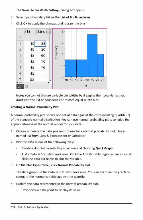
354 Data & Statistics Application
The Variable Bin Width Settings dialog box opens.
3. Select your boundary list as the List of Bin Boundaries.
4. Click OK to apply the changes and redraw the bins.
Note: You cannot change variable bin widths by dragging their boundaries; youmust edit the list of boundaries or restore equal-width bins.
Creating a Normal Probability Plot
A normal probability plot shows one set of data against the corresponding quartile (z)of the standard normal distribution. You can use normal probability plots to judge theappropriateness of the normal model for your data.
1. Choose or create the data you want to use for a normal probability plot. Use anamed list from Lists & Spreadsheet or Calculator.
2. Plot the data in one of the following ways:
- Create a dot plot by selecting a column and choosing Quick Graph.
- Add a Data & Statistics work area. Click the Add Variable region on an axis andclick the data list name to plot the variable.
3. On the Plot Types menu, click Normal Probability Plot.
The data graphs in the Data & Statistics work area. You can examine the graph tocompare the normal variable against the quartile.
4. Explore the data represented in the normal probability plot.
- Hover over a data point to display its value.
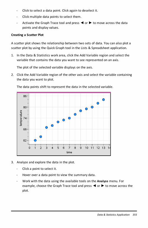
- Click to select a data point. Click again to deselect it.
- Click multiple data points to select them.
- Activate the Graph Trace tool and press ◄ or ► to move across the datapoints and display values.
Creating a Scatter Plot
A scatter plot shows the relationship between two sets of data. You can also plot ascatter plot by using the Quick Graph tool in the Lists & Spreadsheet application.
1. In the Data & Statistics work area, click the Add Variable region and select thevariable that contains the data you want to see represented on an axis.
The plot of the selected variable displays on the axis.
2. Click the Add Variable region of the other axis and select the variable containingthe data you want to plot.
The data points shift to represent the data in the selected variable.
3. Analyze and explore the data in the plot.
- Click a point to select it.
- Hover over a data point to view the summary data.
- Work with the data using the available tools on the Analyze menu. Forexample, choose the Graph Trace tool and press ◄ or ► to move across theplot.
Data & Statistics Application 355
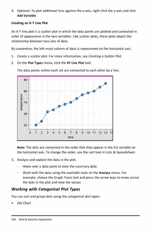
356 Data & Statistics Application
4. Optional: To plot additional lists against the x-axis, right-click the y-axis and clickAdd Variable.
Creating an X-Y Line Plot
An X-Y line plot is a scatter plot in which the data points are plotted and connected inorder of appearance in the two variables. Like scatter plots, these plots depict therelationship between two sets of data.
By convention, the left-most column of data is represented on the horizontal axis.
1. Create a scatter plot. For more information, see Creating a Scatter Plot.
2. On the Plot Types menu, click the XY Line Plot tool.
The data points within each set are connected to each other by a line.
Note: The dots are connected in the order that they appear in the list variable onthe horizontal axis. To change the order, use the sort tool in Lists & Spreadsheet.
3. Analyze and explore the data in the plot.
- Hover over a data point to view the summary data.
- Work with the data using the available tools on the Analyze menu. Forexample, choose the Graph Trace tool and press the arrow keys to move acrossthe dots in the plot and view the values.
Working with Categorical Plot TypesYou can sort and group data using the categorical plot types:
• Dot Chart
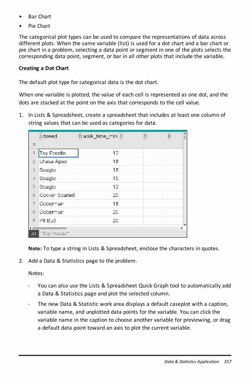
• Bar Chart
• Pie Chart
The categorical plot types can be used to compare the representations of data acrossdifferent plots. When the same variable (list) is used for a dot chart and a bar chart orpie chart in a problem, selecting a data point or segment in one of the plots selects thecorresponding data point, segment, or bar in all other plots that include the variable.
Creating a Dot Chart
The default plot type for categorical data is the dot chart.
When one variable is plotted, the value of each cell is represented as one dot, and thedots are stacked at the point on the axis that corresponds to the cell value.
1. In Lists & Spreadsheet, create a spreadsheet that includes at least one column ofstring values that can be used as categories for data.
Note: To type a string in Lists & Spreadsheet, enclose the characters in quotes.
2. Add a Data & Statistics page to the problem.
Notes:
- You can also use the Lists & Spreadsheet Quick Graph tool to automatically adda Data & Statistics page and plot the selected column.
- The new Data & Statistic work area displays a default caseplot with a caption,variable name, and unplotted data points for the variable. You can click thevariable name in the caption to choose another variable for previewing, or draga default data point toward an axis to plot the current variable.
Data & Statistics Application 357
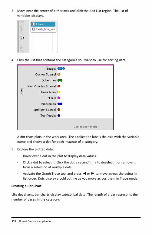
358 Data & Statistics Application
3. Move near the center of either axis and click the Add List region. The list ofvariables displays.
4. Click the list that contains the categories you want to use for sorting data.
A dot chart plots in the work area. The application labels the axis with the variablename and shows a dot for each instance of a category.
5. Explore the plotted data.
- Hover over a dot in the plot to display data values.
- Click a dot to select it. Click the dot a second time to deselect it or remove itfrom a selection of multiple dots.
- Activate the Graph Trace tool and press ◄ or► to move across the points inlist order. Dots display a bold outline as you move across them in Trace mode.
Creating a Bar Chart
Like dot charts, bar charts display categorical data. The length of a bar represents thenumber of cases in the category.
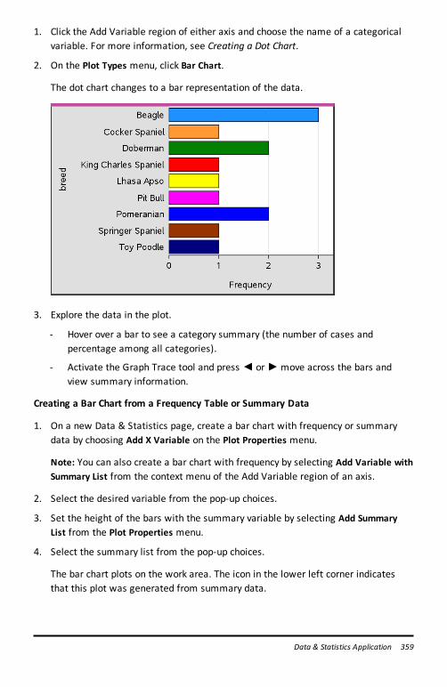
1. Click the Add Variable region of either axis and choose the name of a categoricalvariable. For more information, see Creating a Dot Chart.
2. On the Plot Types menu, click Bar Chart.
The dot chart changes to a bar representation of the data.
3. Explore the data in the plot.
- Hover over a bar to see a category summary (the number of cases andpercentage among all categories).
- Activate the Graph Trace tool and press ◄ or►move across the bars andview summary information.
Creating a Bar Chart from a Frequency Table or Summary Data
1. On a new Data & Statistics page, create a bar chart with frequency or summarydata by choosing Add X Variable on the Plot Properties menu.
Note: You can also create a bar chart with frequency by selecting Add Variable withSummary List from the context menu of the Add Variable region of an axis.
2. Select the desired variable from the pop-up choices.
3. Set the height of the bars with the summary variable by selecting Add SummaryList from the Plot Properties menu.
4. Select the summary list from the pop-up choices.
The bar chart plots on the work area. The icon in the lower left corner indicatesthat this plot was generated from summary data.
Data & Statistics Application 359
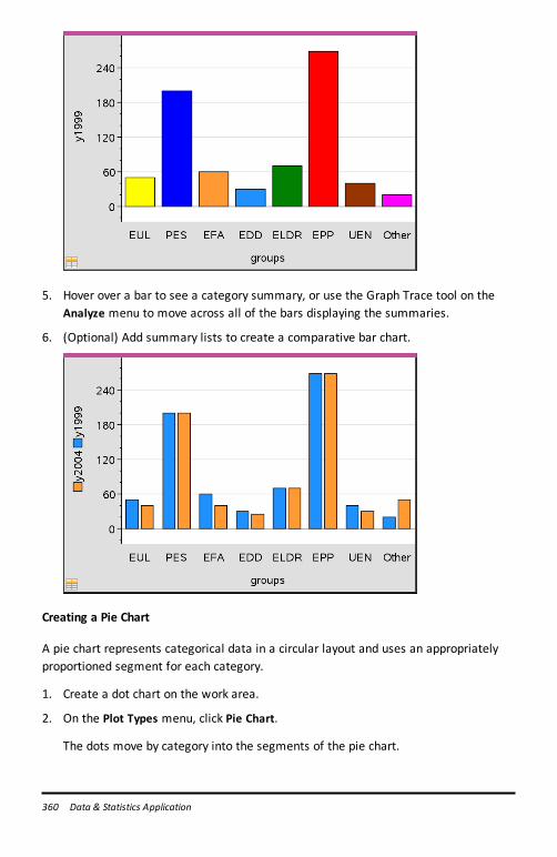
360 Data & Statistics Application
5. Hover over a bar to see a category summary, or use the Graph Trace tool on theAnalyze menu to move across all of the bars displaying the summaries.
6. (Optional) Add summary lists to create a comparative bar chart.
Creating a Pie Chart
A pie chart represents categorical data in a circular layout and uses an appropriatelyproportioned segment for each category.
1. Create a dot chart on the work area.
2. On the Plot Types menu, click Pie Chart.
The dots move by category into the segments of the pie chart.
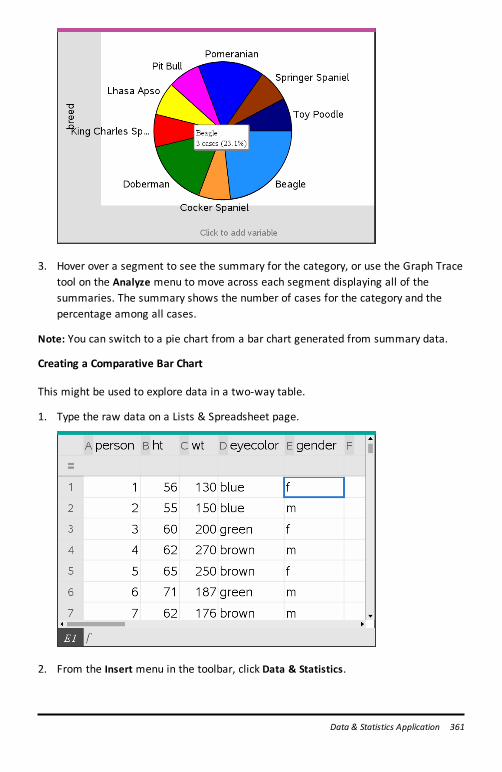
3. Hover over a segment to see the summary for the category, or use the Graph Tracetool on the Analyze menu to move across each segment displaying all of thesummaries. The summary shows the number of cases for the category and thepercentage among all cases.
Note: You can switch to a pie chart from a bar chart generated from summary data.
Creating a Comparative Bar Chart
This might be used to explore data in a two-way table.
1. Type the raw data on a Lists & Spreadsheet page.
2. From the Insert menu in the toolbar, click Data & Statistics.
Data & Statistics Application 361
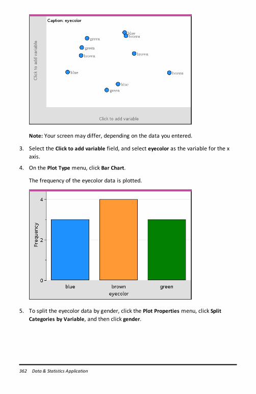
362 Data & Statistics Application
Note: Your screen may differ, depending on the data you entered.
3. Select the Click to add variable field, and select eyecolor as the variable for the xaxis.
4. On the Plot Type menu, click Bar Chart.
The frequency of the eyecolor data is plotted.
5. To split the eyecolor data by gender, click the Plot Properties menu, click SplitCategories by Variable, and then click gender.
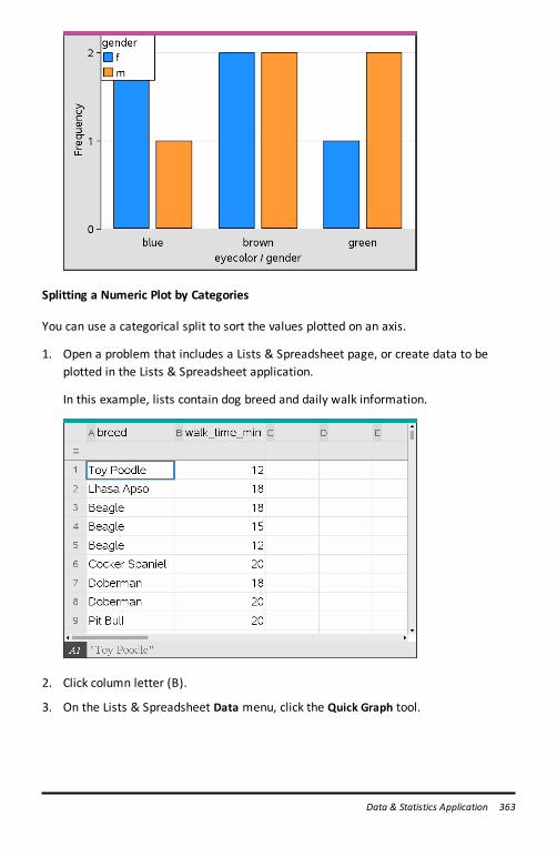
Splitting a Numeric Plot by Categories
You can use a categorical split to sort the values plotted on an axis.
1. Open a problem that includes a Lists & Spreadsheet page, or create data to beplotted in the Lists & Spreadsheet application.
In this example, lists contain dog breed and daily walk information.
2. Click column letter (B).
3. On the Lists & Spreadsheet Data menu, click the Quick Graph tool.
Data & Statistics Application 363
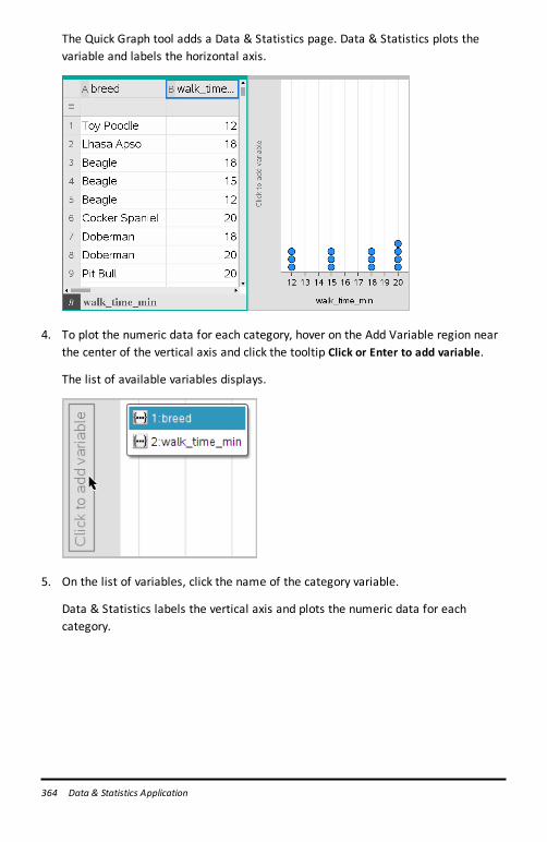
364 Data & Statistics Application
The Quick Graph tool adds a Data & Statistics page. Data & Statistics plots thevariable and labels the horizontal axis.
4. To plot the numeric data for each category, hover on the Add Variable region nearthe center of the vertical axis and click the tooltip Click or Enter to add variable.
The list of available variables displays.
5. On the list of variables, click the name of the category variable.
Data & Statistics labels the vertical axis and plots the numeric data for eachcategory.
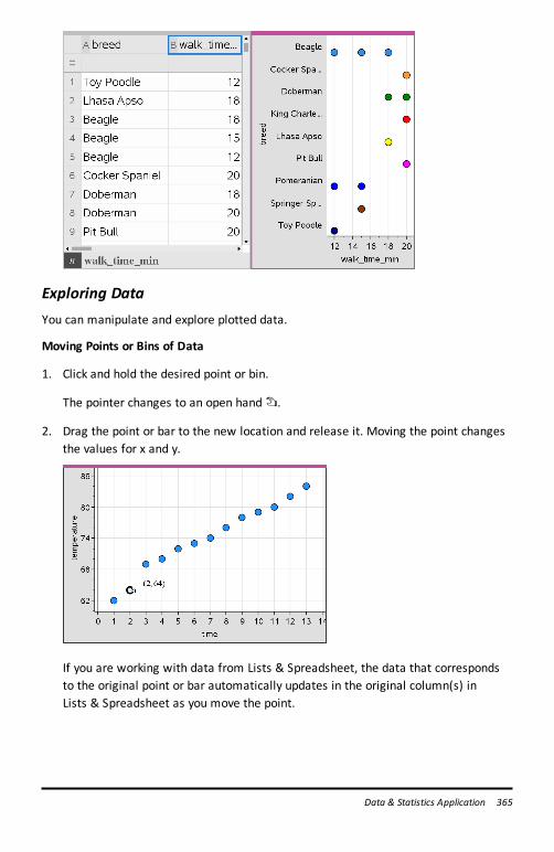
Exploring DataYou can manipulate and explore plotted data.
Moving Points or Bins of Data
1. Click and hold the desired point or bin.
The pointer changes to an open hand÷.
2. Drag the point or bar to the new location and release it. Moving the point changesthe values for x and y.
If you are working with data from Lists & Spreadsheet, the data that correspondsto the original point or bar automatically updates in the original column(s) inLists & Spreadsheet as you move the point.
Data & Statistics Application 365
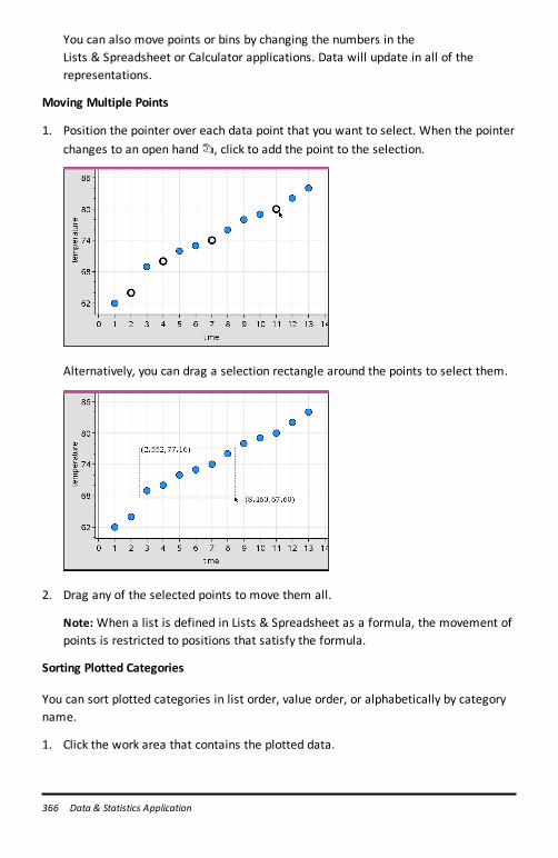
366 Data & Statistics Application
You can also move points or bins by changing the numbers in theLists & Spreadsheet or Calculator applications. Data will update in all of therepresentations.
Moving Multiple Points
1. Position the pointer over each data point that you want to select. When the pointerchanges to an open hand÷, click to add the point to the selection.
Alternatively, you can drag a selection rectangle around the points to select them.
2. Drag any of the selected points to move them all.
Note: When a list is defined in Lists & Spreadsheet as a formula, the movement ofpoints is restricted to positions that satisfy the formula.
Sorting Plotted Categories
You can sort plotted categories in list order, value order, or alphabetically by categoryname.
1. Click the work area that contains the plotted data.
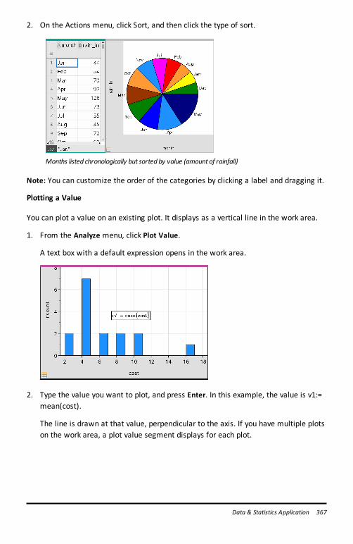
2. On the Actions menu, click Sort, and then click the type of sort.
Months listed chronologically but sorted by value (amount of rainfall)
Note: You can customize the order of the categories by clicking a label and dragging it.
Plotting a Value
You can plot a value on an existing plot. It displays as a vertical line in the work area.
1. From the Analyze menu, click Plot Value.
A text box with a default expression opens in the work area.
2. Type the value you want to plot, and press Enter. In this example, the value is v1:=mean(cost).
The line is drawn at that value, perpendicular to the axis. If you have multiple plotson the work area, a plot value segment displays for each plot.
Data & Statistics Application 367
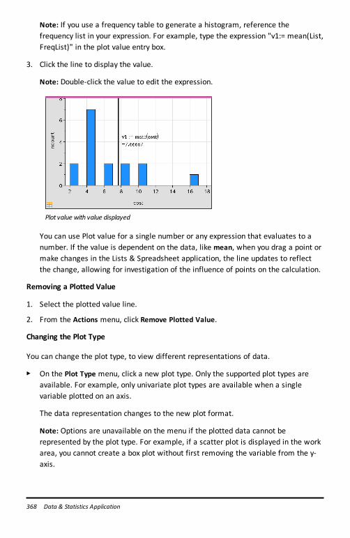
368 Data & Statistics Application
Note: If you use a frequency table to generate a histogram, reference thefrequency list in your expression. For example, type the expression "v1:= mean(List,FreqList)" in the plot value entry box.
3. Click the line to display the value.
Note: Double-click the value to edit the expression.
Plot value with value displayed
You can use Plot value for a single number or any expression that evaluates to anumber. If the value is dependent on the data, like mean, when you drag a point ormake changes in the Lists & Spreadsheet application, the line updates to reflectthe change, allowing for investigation of the influence of points on the calculation.
Removing a Plotted Value
1. Select the plotted value line.
2. From the Actions menu, click Remove Plotted Value.
Changing the Plot Type
You can change the plot type, to view different representations of data.
▶ On the Plot Type menu, click a new plot type. Only the supported plot types areavailable. For example, only univariate plot types are available when a singlevariable plotted on an axis.
The data representation changes to the new plot format.
Note: Options are unavailable on the menu if the plotted data cannot berepresented by the plot type. For example, if a scatter plot is displayed in the workarea, you cannot create a box plot without first removing the variable from the y-axis.
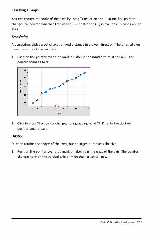
Rescaling a Graph
You can change the scale of the axes by using Translation and Dilation. The pointerchanges to indicate whether Translation (ö) or Dilation (ô) is available in zones on theaxes.
Translation
A translation slides a set of axes a fixed distance in a given direction. The original axeshave the same shape and size.
1. Position the pointer over a tic mark or label in the middle third of the axis. Thepointer changes toö.
2. Click to grab. The pointer changes to a grasping handù. Drag to the desiredposition and release.
Dilation
Dilation retains the shape of the axes, but enlarges or reduces the size.
1. Position the pointer over a tic mark or label near the ends of the axis. The pointerchanges to ó on the vertical axis or ô on the horizontal axis.
Data & Statistics Application 369
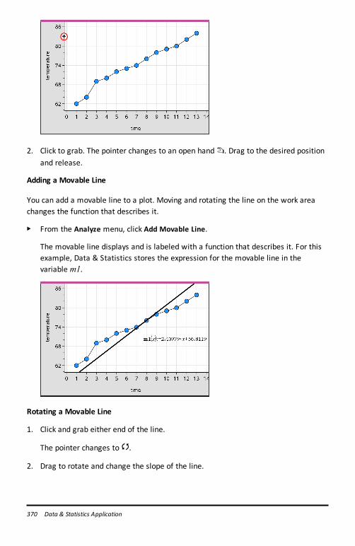
370 Data & Statistics Application
2. Click to grab. The pointer changes to an open hand÷. Drag to the desired positionand release.
Adding a Movable Line
You can add a movable line to a plot. Moving and rotating the line on the work areachanges the function that describes it.
▶ From the Analyze menu, click Add Movable Line.
The movable line displays and is labeled with a function that describes it. For thisexample, Data & Statistics stores the expression for the movable line in thevariable m1.
Rotating a Movable Line
1. Click and grab either end of the line.
The pointer changes toé.
2. Drag to rotate and change the slope of the line.
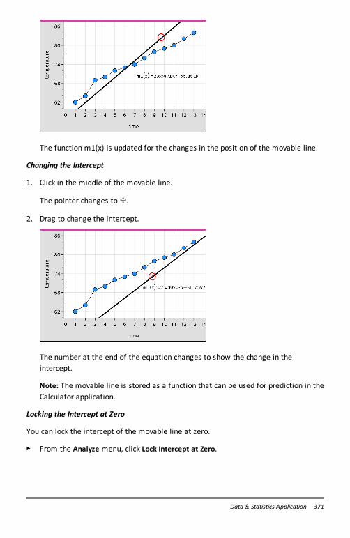
The function m1(x) is updated for the changes in the position of the movable line.
Changing the Intercept
1. Click in the middle of the movable line.
The pointer changes toö.
2. Drag to change the intercept.
The number at the end of the equation changes to show the change in theintercept.
Note: The movable line is stored as a function that can be used for prediction in theCalculator application.
Locking the Intercept at Zero
You can lock the intercept of the movable line at zero.
▶ From the Analyze menu, click Lock Intercept at Zero.
Data & Statistics Application 371
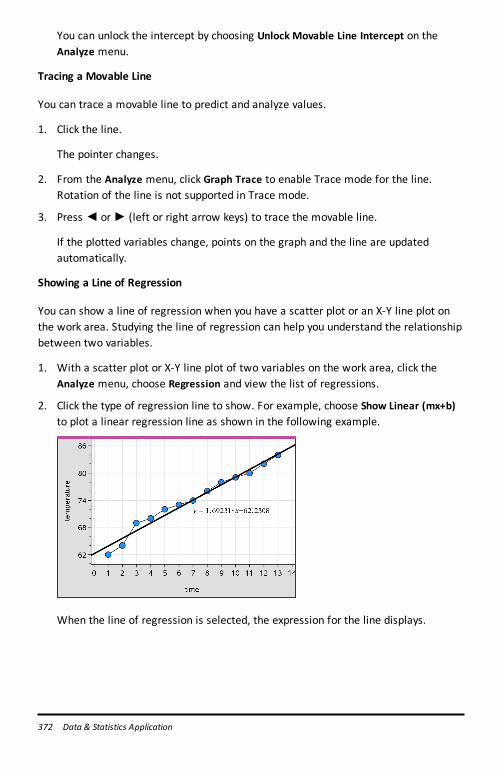
372 Data & Statistics Application
You can unlock the intercept by choosing Unlock Movable Line Intercept on theAnalyze menu.
Tracing a Movable Line
You can trace a movable line to predict and analyze values.
1. Click the line.
The pointer changes.
2. From the Analyze menu, click Graph Trace to enable Trace mode for the line.Rotation of the line is not supported in Trace mode.
3. Press ◄ or ► (left or right arrow keys) to trace the movable line.
If the plotted variables change, points on the graph and the line are updatedautomatically.
Showing a Line of Regression
You can show a line of regression when you have a scatter plot or an X-Y line plot onthe work area. Studying the line of regression can help you understand the relationshipbetween two variables.
1. With a scatter plot or X-Y line plot of two variables on the work area, click theAnalyze menu, choose Regression and view the list of regressions.
2. Click the type of regression line to show. For example, choose Show Linear (mx+b)to plot a linear regression line as shown in the following example.
When the line of regression is selected, the expression for the line displays.
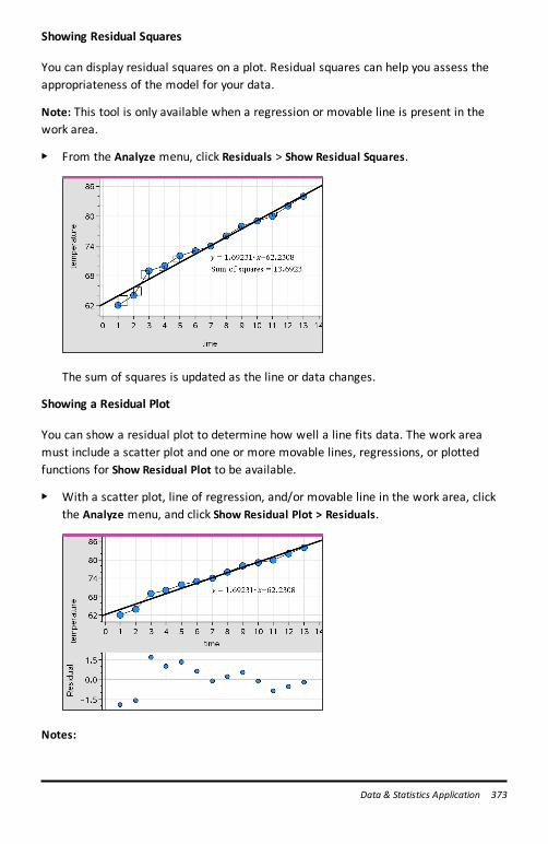
Showing Residual Squares
You can display residual squares on a plot. Residual squares can help you assess theappropriateness of the model for your data.
Note: This tool is only available when a regression or movable line is present in thework area.
▶ From the Analyze menu, click Residuals > Show Residual Squares.
The sum of squares is updated as the line or data changes.
Showing a Residual Plot
You can show a residual plot to determine how well a line fits data. The work areamust include a scatter plot and one or more movable lines, regressions, or plottedfunctions for Show Residual Plot to be available.
▶ With a scatter plot, line of regression, and/or movable line in the work area, clickthe Analyze menu, and click Show Residual Plot > Residuals.
Notes:
Data & Statistics Application 373
374 Data & Statistics Application
• With multiple regressions or functions and movable lines plotted, you can selecteach by clicking the line to show its residual plot.
• Click and hold a dot on the residual plot to see the residual.
• The residual plot for the selected regression or function displays in the work area.
• For consistency in comparing sets of data, residual plots do not rescale when youmove from one function or regression to another.
• Select a function or regression before a showing residual plot. If no function orregression is selected and there are several plotted, Data & Statistics arbitrarilyselects the function or regression for showing the residual plot.
• Axes can be adjusted by clicking and dragging.
Removing a Residual Plot
▶ With a scatter plot, line of regression, and/or movable line in the work area, clickthe Analyze menu, and click Hide Residual Plot.
Using Window/Zoom ToolsUse the Window/Zoom tools to redefine the graph to better view points of interest.The Window/Zoom tools include:
• Window Settings: displays a Window Settings dialog box that lets you type the x-min, x-max, y-min, and y-max values for the axes.
• Zoom - Data: adjusts the zoom factor to display all plotted data.
• Zoom - In: lets you define the center point of the zoom in location. The Zoom Infactor is approximately 2.
• Zoom - Out: lets you define the center point of the zoom out location. The ZoomOut factor is approximately 2.
Using the Window Settings Tool
1. On the Window/Zoommenu, clickWindow Settings.
The Window Settings dialog box opens. The current values for x-min, x-max, y-min,and y-max are displayed in the fields.
Note: Only the appropriate boxes are editable, depending on whether there are oneor two axes in the work area.
2. Type the new values over the old values.
3. Click OK to apply the changes and redraw the plot.
Using the Zoom Data Tool
▶ On the Window/Zoommenu, click Zoom Data.
The work area rescales to display all plotted data.
Using the Zoom In Tool
1. On the Window/Zoommenu, click Zoom In.
2. In the work area, click the center point of the area of interest. This will be thecenter of the zoom in action.
The plot redraws to focus and enlarge the portion of the plot centered about thepoint you selected in the previous step.
Using the Zoom Out Tool
1. On the Window/Zoommenu, click Zoom Out.
2. In the work area, click the center point of the area of interest. This will be thecenter of the zoom out action.
The plot redraws to display a larger portion of the plot, centered about the pointyou selected in the previous step.
Graphing FunctionsYou can graph functions by typing them in Data & Statistics, or you can graph functionsdefined in other applications.
Graphing Functions Using the Plot Function Tool
You can use the Plot Function tool to plot functions in a work area that already includesa plot on the axes. Plot Function lets you specify and graph a function for comparisonto an existing plot.
To use the Plot Function tool:
1. Create or open a problem that includes variables (from Lists & Spreadsheet) thatare plotted on a Data & Statistics work area. Ensure that your work area containsboth a horizontal axis and a vertical axis scale.
2. From the Analyze menu, click Plot Function.
A function entry field displays in the work area.
Data & Statistics Application 375
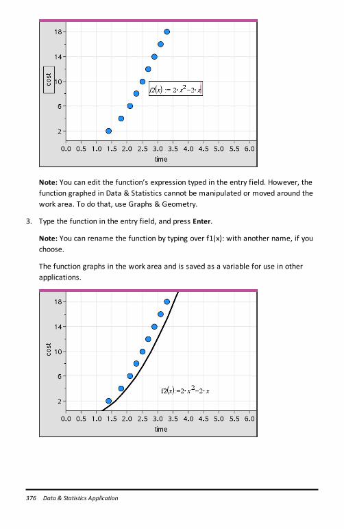
376 Data & Statistics Application
Note: You can edit the function’s expression typed in the entry field. However, thefunction graphed in Data & Statistics cannot be manipulated or moved around thework area. To do that, use Graphs & Geometry.
3. Type the function in the entry field, and press Enter.
Note: You can rename the function by typing over f1(x): with another name, if youchoose.
The function graphs in the work area and is saved as a variable for use in otherapplications.
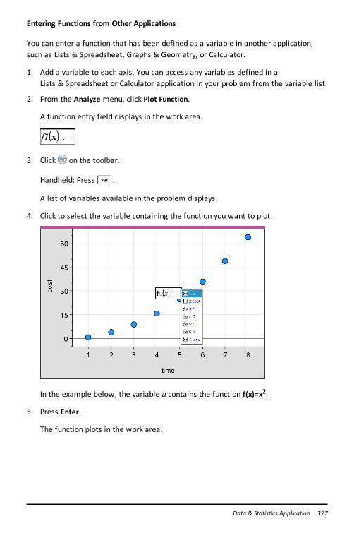
Entering Functions from Other Applications
You can enter a function that has been defined as a variable in another application,such as Lists & Spreadsheet, Graphs & Geometry, or Calculator.
1. Add a variable to each axis. You can access any variables defined in aLists & Spreadsheet or Calculator application in your problem from the variable list.
2. From the Analyze menu, click Plot Function.
A function entry field displays in the work area.
3. Click on the toolbar.
Handheld: Pressh.
A list of variables available in the problem displays.
4. Click to select the variable containing the function you want to plot.
In the example below, the variable a contains the function f(x)=x2.
5. Press Enter.
The function plots in the work area.
Data & Statistics Application 377
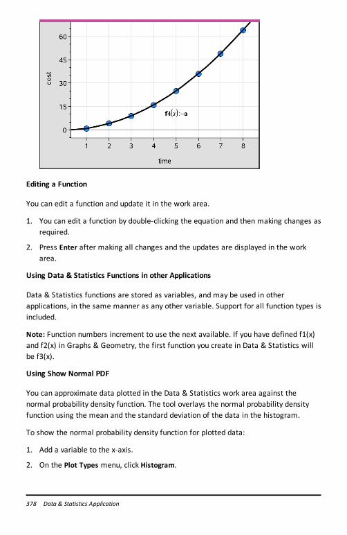
378 Data & Statistics Application
Editing a Function
You can edit a function and update it in the work area.
1. You can edit a function by double-clicking the equation and then making changes asrequired.
2. Press Enter after making all changes and the updates are displayed in the workarea.
Using Data & Statistics Functions in other Applications
Data & Statistics functions are stored as variables, and may be used in otherapplications, in the same manner as any other variable. Support for all function types isincluded.
Note: Function numbers increment to use the next available. If you have defined f1(x)and f2(x) in Graphs & Geometry, the first function you create in Data & Statistics willbe f3(x).
Using Show Normal PDF
You can approximate data plotted in the Data & Statistics work area against thenormal probability density function. The tool overlays the normal probability densityfunction using the mean and the standard deviation of the data in the histogram.
To show the normal probability density function for plotted data:
1. Add a variable to the x-axis.
2. On the Plot Types menu, click Histogram.
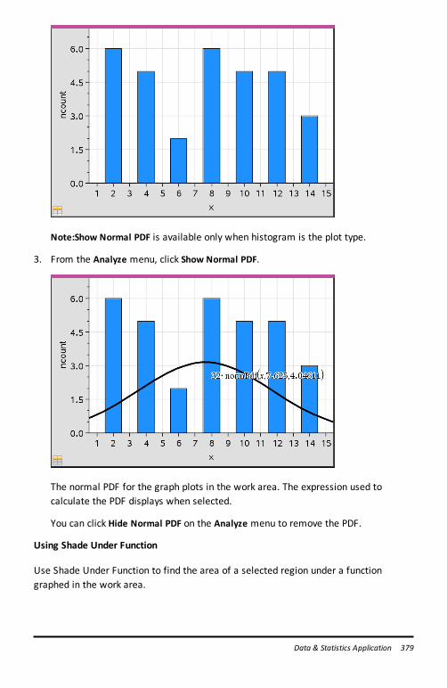
Note:Show Normal PDF is available only when histogram is the plot type.
3. From the Analyze menu, click Show Normal PDF.
The normal PDF for the graph plots in the work area. The expression used tocalculate the PDF displays when selected.
You can click Hide Normal PDF on the Analyze menu to remove the PDF.
Using Shade Under Function
Use Shade Under Function to find the area of a selected region under a functiongraphed in the work area.
Data & Statistics Application 379
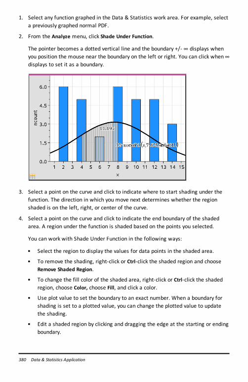
380 Data & Statistics Application
1. Select any function graphed in the Data & Statistics work area. For example, selecta previously graphed normal PDF.
2. From the Analyze menu, click Shade Under Function.
The pointer becomes a dotted vertical line and the boundary +/- ˆ displays whenyou position the mouse near the boundary on the left or right. You can click when ˆ
displays to set it as a boundary.
3. Select a point on the curve and click to indicate where to start shading under thefunction. The direction in which you move next determines whether the regionshaded is on the left, right, or center of the curve.
4. Select a point on the curve and click to indicate the end boundary of the shadedarea. A region under the function is shaded based on the points you selected.
You can work with Shade Under Function in the following ways:
• Select the region to display the values for data points in the shaded area.
• To remove the shading, right-click or Ctrl-click the shaded region and chooseRemove Shaded Region.
• To change the fill color of the shaded area, right-click or Ctrl-click the shadedregion, choose Color, choose Fill, and click a color.
• Use plot value to set the boundary to an exact number. When a boundary forshading is set to a plotted value, you can change the plotted value to updatethe shading.
• Edit a shaded region by clicking and dragging the edge at the starting or endingboundary.
Using Graph TraceGraph Trace lets you move from one point on a graph to another to analyze variationsin the data. You can use Graph Trace mode to explore the data for the followinggraphs.
• Graphs from Plot Function and Show Normal PDF
• Distribution curves (created in the Lists & Spreadsheet application)
• Movable Lines
• Regressions
• Caseplots
• Dot plots
• Scatter plots and X-Y line plots
• Box plots
• Histograms
• Bar charts
• Pie charts
To use Graph Trace
1. From the Analyze menu, click Graph Trace.
2. Press ◄ or ► to move across the plot.
The data representations enlarge and appear with a bold outline as you moveacross them in Trace mode.
Customizing Your Workspace
Working with Color
All data points for a plotted variable display in the same color to distinguish them fromthe data points of other variables. Data plotted by category and split plots areautomatically displayed in different colors to help you distinguish the data.
To emphasize or distinguish certain parts of your work, you can change the defaultcolor for a variable’s data.
• Apply fill colors to objects, such as shading, or change the color for a variable’sdata points.
• Apply color to plotted lines (such as lines of regression) or movable lines.
Inserting a Background Image
Data & Statistics Application 381
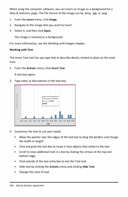
382 Data & Statistics Application
When using the computer software, you can insert an image as a background for aData & Statistics page. The file format of the image can be .bmp, .jpg, or .png.
1. From the Insert menu, click Image.
2. Navigate to the image that you want to insert.
3. Select it, and then click Open.
The image is inserted as a background.
For more information, see the Working with Images chapter.
Working with Text
The Insert Text tool lets you type text to describe details related to plots on the workarea.
1. From the Actions menu, click Insert Text.
A text box opens.
2. Type notes or descriptions in the text box.
3. Customize the text to suit your needs.
• Move the pointer over the edges of the text box to drag the borders and changethe width or height.
• Click and grab the text box to move it near objects that relate to the text.
• Scroll to view additional text in a box by clicking the arrows at the top andbottom edge.
• Click outside of the text entry box to exit the Text tool.
• Hide text by clicking the Actions menu and clicking Hide Text.
• Change the color of text.
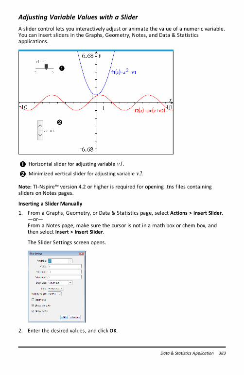
Adjusting Variable Values with a SliderA slider control lets you interactively adjust or animate the value of a numeric variable.You can insert sliders in the Graphs, Geometry, Notes, and Data & Statisticsapplications.
Horizontal slider for adjusting variable v1.Minimized vertical slider for adjusting variable v2.
Note: TI-Nspire™ version 4.2 or higher is required for opening .tns files containingsliders on Notes pages.
Inserting a Slider Manually
1. From a Graphs, Geometry, or Data & Statistics page, select Actions > Insert Slider.—or—From a Notes page, make sure the cursor is not in a math box or chem box, andthen select Insert > Insert Slider.
The Slider Settings screen opens.
2. Enter the desired values, and click OK.
Data & Statistics Application 383
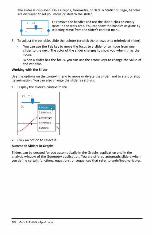
384 Data & Statistics Application
The slider is displayed. On a Graphs, Geometry, or Data & Statistics page, handlesare displayed to let you move or stretch the slider.
To remove the handles and use the slider, click an emptyspace in the work area. You can show the handles anytime byselectingMove from the slider's context menu.
3. To adjust the variable, slide the pointer (or click the arrows on a minimized slider).
- You can use the Tab key to move the focus to a slider or to move from oneslider to the next. The color of the slider changes to show you when it has thefocus.
- When a slider has the focus, you can use the arrow keys to change the value ofthe variable.
Working with the Slider
Use the options on the context menu to move or delete the slider, and to start or stopits animation. You can also change the slider's settings.
1. Display the slider's context menu.
2. Click an option to select it.
Automatic Sliders in Graphs
Sliders can be created for you automatically in the Graphs application and in theanalytic window of the Geometry application. You are offered automatic sliders whenyou define certain functions, equations, or sequences that refer to undefined variables.
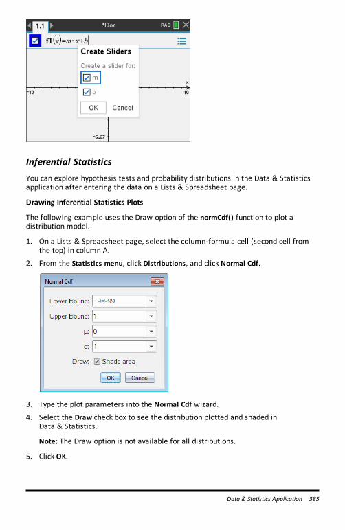
Inferential StatisticsYou can explore hypothesis tests and probability distributions in the Data & Statisticsapplication after entering the data on a Lists & Spreadsheet page.
Drawing Inferential Statistics Plots
The following example uses the Draw option of the normCdf() function to plot adistribution model.
1. On a Lists & Spreadsheet page, select the column-formula cell (second cell fromthe top) in column A.
2. From the Statistics menu, click Distributions, and click Normal Cdf.
3. Type the plot parameters into the Normal Cdf wizard.
4. Select the Draw check box to see the distribution plotted and shaded inData & Statistics.
Note: The Draw option is not available for all distributions.
5. Click OK.
Data & Statistics Application 385
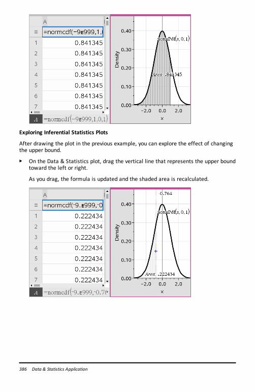
386 Data & Statistics Application
Exploring Inferential Statistics Plots
After drawing the plot in the previous example, you can explore the effect of changingthe upper bound.
▶ On the Data & Statistics plot, drag the vertical line that represents the upper boundtoward the left or right.
As you drag, the formula is updated and the shaded area is recalculated.
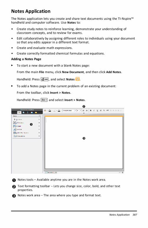
Notes ApplicationThe Notes application lets you create and share text documents using the TI-Nspire™handheld and computer software. Use Notes to:
• Create study notes to reinforce learning, demonstrate your understanding ofclassroom concepts, and to review for exams.
• Edit collaboratively by assigning different roles to individuals using your documentso that any edits appear in a different text format.
• Create and evaluate math expressions.
• Create correctly formatted chemical formulas and equations.
Adding a Notes Page
▶ To start a new document with a blank Notes page:
From the main File menu, click New Document, and then click Add Notes.
Handheld: Pressc, and select Notes .
▶ To add a Notes page in the current problem of an existing document:
From the toolbar, click Insert > Notes.
Handheld: Press~ and select Insert > Notes.
À Notes tools – Available anytime you are in the Notes work area.
Á Text formatting toolbar -- Lets you change size, color, bold, and other textproperties.
 Notes work area -- The area where you type and format text.
Notes Application 387
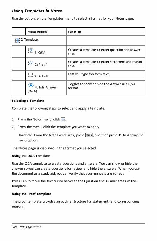
388 Notes Application
Using Templates in NotesUse the options on the Templates menu to select a format for your Notes page.
Menu Option Function
2: Templates
1: Q&ACreates a template to enter question and answertext.
2: ProofCreates a template to enter statement and reasontext.
3: Default Lets you type freeform text.
4:Hide Answer(Q&A)
Toggles to show or hide the Answer in a Q&Aformat.
Selecting a Template
Complete the following steps to select and apply a template:
1. From the Notes menu, click .
2. From the menu, click the template you want to apply.
Handheld: From the Notes work area, pressb, and then press ► to display themenu options.
The Notes page is displayed in the format you selected.
Using the Q&A Template
Use the Q&A template to create questions and answers. You can show or hide theanswer so you can create questions for review and hide the answers. When you usethe document as a study aid, you can verify that your answers are correct.
Press Tab to move the text cursor between the Question and Answer areas of thetemplate.
Using the Proof Template
The proof template provides an outline structure for statements and correspondingreasons.
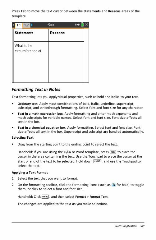
Press Tab to move the text cursor between the Statements and Reasons areas of thetemplate.
Formatting Text in NotesText formatting lets you apply visual properties, such as bold and italic, to your text.
• Ordinary text. Apply most combinations of bold, italic, underline, superscript,subscript, and strikethrough formatting. Select font and font size for any character.
• Text in a math expression box. Apply formatting and enter math exponents andmath subscripts for variable names. Select font and font size. Font size affects alltext in the box.
• Text in a chemical equation box. Apply formatting. Select font and font size. Fontsize affects all text in the box. Superscript and subscript are handled automatically.
Selecting Text
▶ Drag from the starting point to the ending point to select the text.
Handheld: If you are using the Q&A or Proof template, presse to place thecursor in the area containing the text. Use the Touchpad to place the cursor at thestart or end of the text to be selected. Hold downg, and use the Touchpad toselect the text.
Applying a Text Format
1. Select the text that you want to format.
2. On the formatting toolbar, click the formatting icons (such as for bold) to togglethem, or click to select a font and font size.
Handheld: Clickb, and then select Format > Format Text.
The changes are applied to the text as you make selections.
Notes Application 389
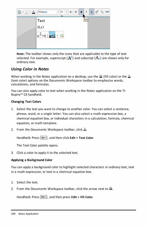
390 Notes Application
Note: The toolbar shows only the icons that are applicable to the type of textselected. For example, superscript ( ) and subscript ( ) are shown only forordinary text.
Using Color in Notes
When working in the Notes application on a desktop, use the (fill color) or the(text color) options on the Documents Workspace toolbar to emphasize words,calculations, and formulas.
You can also apply color to text when working in the Notes application on the TI-Nspire™ CX handheld.
Changing Text Colors
1. Select the text you want to change to another color. You can select a sentence,phrase, word, or a single letter. You can also select a math expression box, achemical equation box, or individual characters in a calculation, formula, chemicalequation, or math template.
2. From the Documents Workspace toolbar, click .
Handheld: Press~, and then click Edit > Text Color.
The Text Color palette opens.
3. Click a color to apply it to the selected text.
Applying a Background Color
You can apply a background color to highlight selected characters in ordinary text, textin a math expression, or text in a chemical equation box.
1. Select the text.
2. From the Documents Workspace toolbar, click the arrow next to .
Handheld: Press~, and then press Edit > Fill Color.
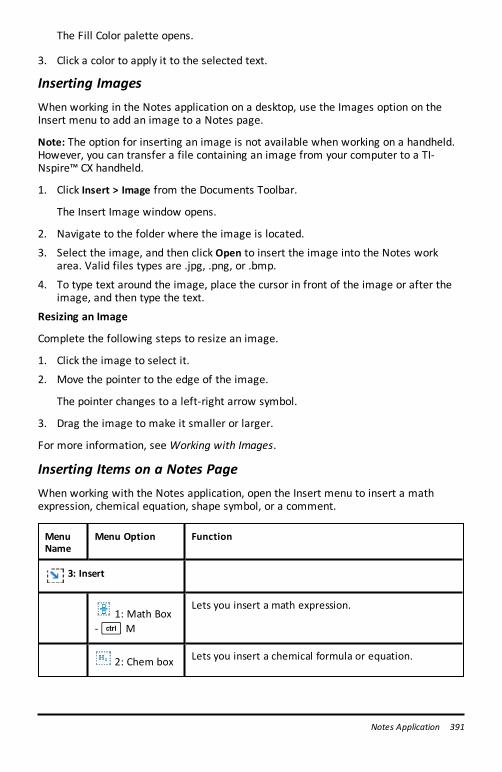
The Fill Color palette opens.
3. Click a color to apply it to the selected text.
Inserting ImagesWhen working in the Notes application on a desktop, use the Images option on theInsert menu to add an image to a Notes page.
Note: The option for inserting an image is not available when working on a handheld.However, you can transfer a file containing an image from your computer to a TI-Nspire™ CX handheld.
1. Click Insert > Image from the Documents Toolbar.
The Insert Image window opens.
2. Navigate to the folder where the image is located.
3. Select the image, and then click Open to insert the image into the Notes workarea. Valid files types are .jpg, .png, or .bmp.
4. To type text around the image, place the cursor in front of the image or after theimage, and then type the text.
Resizing an Image
Complete the following steps to resize an image.
1. Click the image to select it.
2. Move the pointer to the edge of the image.
The pointer changes to a left-right arrow symbol.
3. Drag the image to make it smaller or larger.
For more information, see Working with Images.
Inserting Items on a Notes PageWhen working with the Notes application, open the Insert menu to insert a mathexpression, chemical equation, shape symbol, or a comment.
MenuName
Menu Option Function
3: Insert
1: Math Box-/ M
Lets you insert a math expression.
2: Chem box Lets you insert a chemical formula or equation.
Notes Application 391

392 Notes Application
MenuName
Menu Option Function
-/ E
2: ShapeMarks the selected text as an angle, triangle, circle,line, segment, ray, or vector.
3:Comment
Lets you type text that is italicized and prefaced withTeacher or Reviewer.
Inserting Comments in Notes TextYou can insert Teacher or Reviewer comments into a Notes application. Comments areeasy to distinguish from the original text.
1. Define the type of comments you are inserting (Teacher or Reviewer):
• PC: From the Insert menu, click Comment, and then click Teacher or Reviewer.
• Handheld: While in the Notes work area, pressb to display the Notesmenu. Press Insert > Comment, and then select either Teacher or Reviewer.
2. Type your text.
Text that you type appears in italics.
Inserting Geometric Shape SymbolsYou can use geometric shape symbols to designate selected text as geometric objects,such as an angle, circle, or line segment.
To insert a shape symbol, position the cursor where you want it, and then do thefollowing:
• PC: From the Insert menu, click Shapes, and then select the shape to apply.
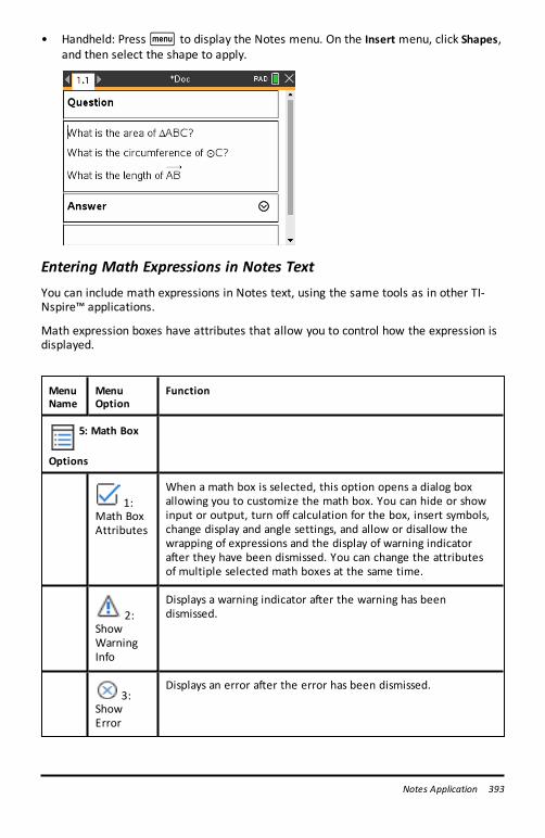
• Handheld: Pressb to display the Notes menu. On the Insert menu, click Shapes,and then select the shape to apply.
Entering Math Expressions in Notes TextYou can include math expressions in Notes text, using the same tools as in other TI-Nspire™ applications.
Math expression boxes have attributes that allow you to control how the expression isdisplayed.
MenuName
MenuOption
Function
5: Math Box
Options
1:Math BoxAttributes
When a math box is selected, this option opens a dialog boxallowing you to customize the math box. You can hide or showinput or output, turn off calculation for the box, insert symbols,change display and angle settings, and allow or disallow thewrapping of expressions and the display of warning indicatorafter they have been dismissed. You can change the attributesof multiple selected math boxes at the same time.
2:ShowWarningInfo
Displays a warning indicator after the warning has beendismissed.
3:ShowError
Displays an error after the error has been dismissed.
Notes Application 393
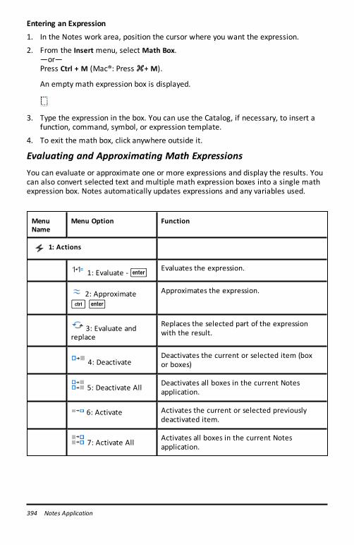
394 Notes Application
Entering an Expression
1. In the Notes work area, position the cursor where you want the expression.
2. From the Insert menu, select Math Box.—or—Press Ctrl + M (Mac®: Press “+ M).
An empty math expression box is displayed.
3. Type the expression in the box. You can use the Catalog, if necessary, to insert afunction, command, symbol, or expression template.
4. To exit the math box, click anywhere outside it.
Evaluating and Approximating Math ExpressionsYou can evaluate or approximate one or more expressions and display the results. Youcan also convert selected text and multiple math expression boxes into a single mathexpression box. Notes automatically updates expressions and any variables used.
MenuName
Menu Option Function
1: Actions
1: Evaluate -· Evaluates the expression.
2: Approximate/·
Approximates the expression.
3: Evaluate andreplace
Replaces the selected part of the expressionwith the result.
4: DeactivateDeactivates the current or selected item (boxor boxes)
5: Deactivate All Deactivates all boxes in the current Notesapplication.
6: Activate Activates the current or selected previouslydeactivated item.
7: Activate All Activates all boxes in the current Notesapplication.
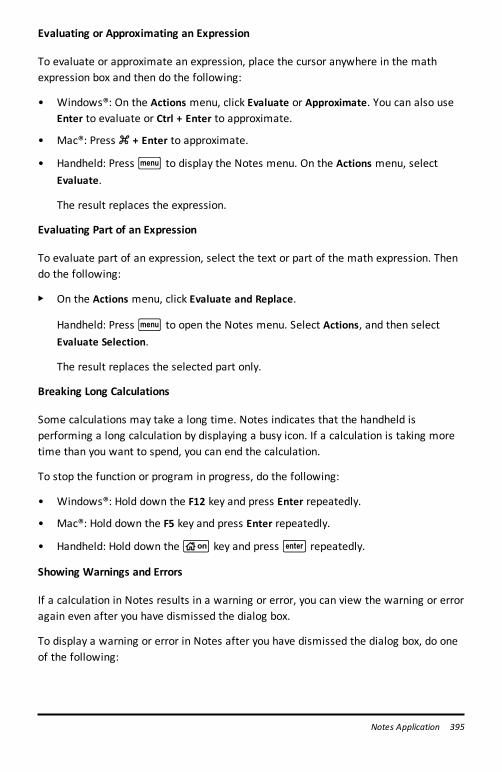
Evaluating or Approximating an Expression
To evaluate or approximate an expression, place the cursor anywhere in the mathexpression box and then do the following:
• Windows®: On the Actions menu, click Evaluate or Approximate. You can also useEnter to evaluate or Ctrl + Enter to approximate.
• Mac®: Press “ + Enter to approximate.
• Handheld: Pressb to display the Notes menu. On the Actions menu, selectEvaluate.
The result replaces the expression.
Evaluating Part of an Expression
To evaluate part of an expression, select the text or part of the math expression. Thendo the following:
▶ On the Actions menu, click Evaluate and Replace.
Handheld: Pressb to open the Notes menu. Select Actions, and then selectEvaluate Selection.
The result replaces the selected part only.
Breaking Long Calculations
Some calculations may take a long time. Notes indicates that the handheld isperforming a long calculation by displaying a busy icon. If a calculation is taking moretime than you want to spend, you can end the calculation.
To stop the function or program in progress, do the following:
• Windows®: Hold down the F12 key and press Enter repeatedly.
• Mac®: Hold down the F5 key and press Enter repeatedly.
• Handheld: Hold down thec key and press· repeatedly.
Showing Warnings and Errors
If a calculation in Notes results in a warning or error, you can view the warning or erroragain even after you have dismissed the dialog box.
To display a warning or error in Notes after you have dismissed the dialog box, do oneof the following:
Notes Application 395
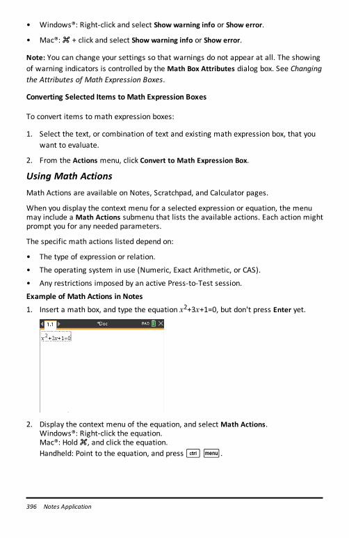
396 Notes Application
• Windows®: Right-click and select Show warning info or Show error.
• Mac®: “ + click and select Show warning info or Show error.
Note: You can change your settings so that warnings do not appear at all. The showingof warning indicators is controlled by the Math Box Attributes dialog box. See Changingthe Attributes of Math Expression Boxes.
Converting Selected Items to Math Expression Boxes
To convert items to math expression boxes:
1. Select the text, or combination of text and existing math expression box, that youwant to evaluate.
2. From the Actions menu, click Convert to Math Expression Box.
Using Math ActionsMath Actions are available on Notes, Scratchpad, and Calculator pages.
When you display the context menu for a selected expression or equation, the menumay include a Math Actions submenu that lists the available actions. Each action mightprompt you for any needed parameters.
The specific math actions listed depend on:
• The type of expression or relation.
• The operating system in use (Numeric, Exact Arithmetic, or CAS).
• Any restrictions imposed by an active Press-to-Test session.
Example of Math Actions in Notes
1. Insert a math box, and type the equation x2+3x+1=0, but don't press Enter yet.
2. Display the context menu of the equation, and select Math Actions.Windows®: Right-click the equation.Mac®: Hold “, and click the equation.Handheld: Point to the equation, and press/b.
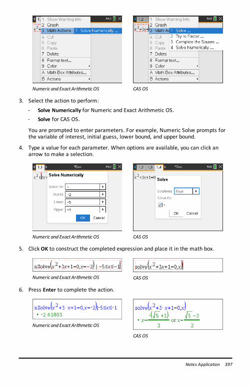
Numeric and ExactArithmetic OS CAS OS
3. Select the action to perform:
- Solve Numerically for Numeric and Exact Arithmetic OS.- Solve for CAS OS.
You are prompted to enter parameters. For example, Numeric Solve prompts forthe variable of interest, initial guess, lower bound, and upper bound.
4. Type a value for each parameter. When options are available, you can click anarrow to make a selection.
Numeric and ExactArithmetic OS CAS OS
5. Click OK to construct the completed expression and place it in the math box.
Numeric and ExactArithmetic OS CAS OS
6. Press Enter to complete the action.
Numeric and ExactArithmetic OS
CAS OS
Notes Application 397
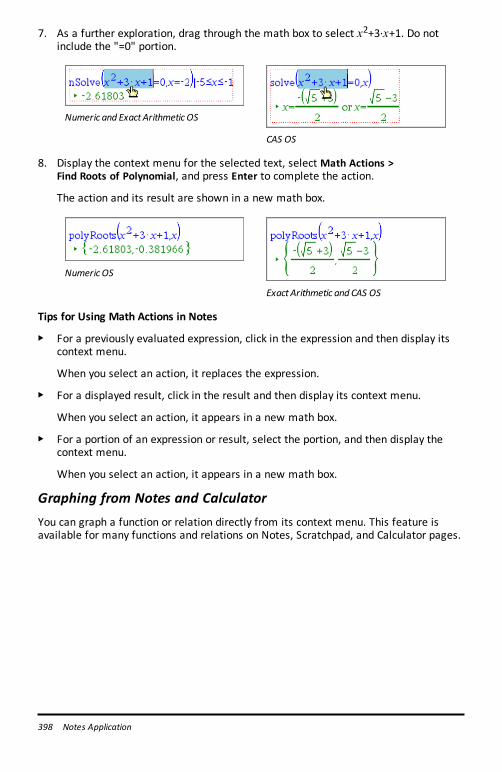
398 Notes Application
7. As a further exploration, drag through the math box to select x2+3·x+1. Do notinclude the "=0" portion.
Numeric and ExactArithmetic OS
CAS OS
8. Display the context menu for the selected text, select Math Actions >Find Roots of Polynomial, and press Enter to complete the action.
The action and its result are shown in a new math box.
Numeric OS
ExactArithmetic and CAS OS
Tips for Using Math Actions in Notes
▶ For a previously evaluated expression, click in the expression and then display itscontext menu.
When you select an action, it replaces the expression.
▶ For a displayed result, click in the result and then display its context menu.
When you select an action, it appears in a new math box.
▶ For a portion of an expression or result, select the portion, and then display thecontext menu.
When you select an action, it appears in a new math box.
Graphing from Notes and Calculator You can graph a function or relation directly from its context menu. This feature isavailable for many functions and relations on Notes, Scratchpad, and Calculator pages.
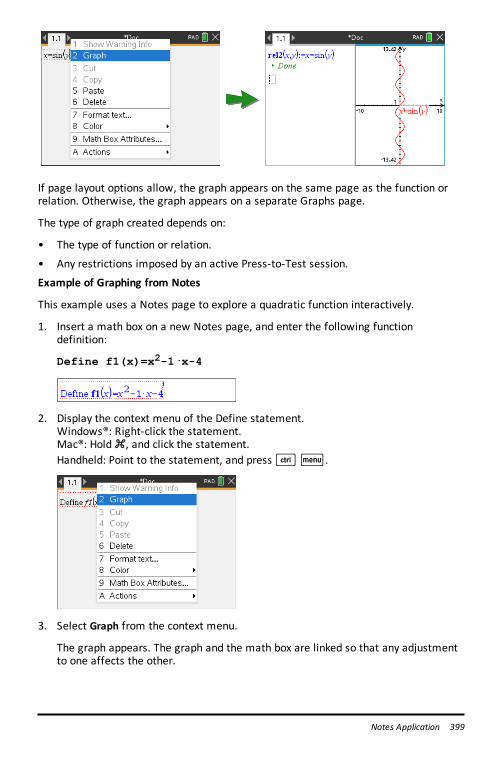
If page layout options allow, the graph appears on the same page as the function orrelation. Otherwise, the graph appears on a separate Graphs page.
The type of graph created depends on:
• The type of function or relation.
• Any restrictions imposed by an active Press-to-Test session.
Example of Graphing from Notes
This example uses a Notes page to explore a quadratic function interactively.
1. Insert a math box on a new Notes page, and enter the following functiondefinition:
Define f1(x)=x2-1·x-4
2. Display the context menu of the Define statement.Windows®: Right-click the statement.Mac®: Hold “, and click the statement.Handheld: Point to the statement, and press/b.
3. Select Graph from the context menu.
The graph appears. The graph and the math box are linked so that any adjustmentto one affects the other.
Notes Application 399
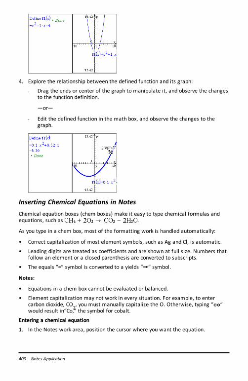
400 Notes Application
4. Explore the relationship between the defined function and its graph:
- Drag the ends or center of the graph to manipulate it, and observe the changesto the function definition.
—or—
- Edit the defined function in the math box, and observe the changes to thegraph.
Inserting Chemical Equations in NotesChemical equation boxes (chem boxes) make it easy to type chemical formulas andequations, such as .
As you type in a chem box, most of the formatting work is handled automatically:
• Correct capitalization of most element symbols, such as Ag and Cl, is automatic.
• Leading digits are treated as coefficients and are shown at full size. Numbers thatfollow an element or a closed parenthesis are converted to subscripts.
• The equals “=” symbol is converted to a yields “&” symbol.
Notes:
• Equations in a chem box cannot be evaluated or balanced.
• Element capitalization may not work in every situation. For example, to entercarbon dioxide, CO
2, you must manually capitalize the O. Otherwise, typing “co”
would result in“Co,” the symbol for cobalt.
Entering a chemical equation
1. In the Notes work area, position the cursor where you want the equation.
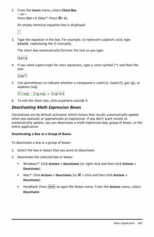
2. From the Insert menu, select Chem Box.—or—Press Ctrl + E (Mac®: Press “+ E).
An empty chemical equation box is displayed.
3. Type the equation in the box. For example, to represent sulphuric acid, typeh2sO4, capitalizing the O manually.
The chem box automatically formats the text as you type:
4. If you need superscripts for ionic equations, type a caret symbol (^) and then thetext.
5. Use parentheses to indicate whether a compound is solid (s), liquid (l), gas (g), oraqueous (aq).
6. To exit the chem box, click anywhere outside it.
Deactivating Math Expression BoxesCalculations are by default activated, which means that results automatically updatewhen you evaluate or approximate an expression. If you don’t want results toautomatically update, you can deactivate a math expression box, group of boxes, or theentire application.
Deactivating a Box or a Group of Boxes
To deactivate a box or a group of boxes:
1. Select the box or boxes that you want to deactivate.
2. Deactivate the selected box or boxes:
• Windows®: Click Actions > Deactivate (or right-click and then click Actions >Deactivate).
• Mac®: Click Actions > Deactivate (or “ + click and then click Actions >Deactivate).
• Handheld: Pressb to open the Notes menu. From the Actions menu, selectDeactivate.
Notes Application 401
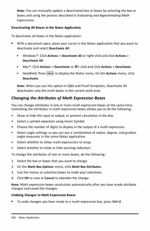
402 Notes Application
Note: You can manually update a deactivated box or boxes by selecting the box orboxes and using the process described in Evaluating and Approximating MathExpressions.
Deactivating All Boxes in the Notes Application
To deactivate all boxes in the Notes application:
▶ With a document open, place your cursor in the Notes application that you want todeactivate and select Deactivate All.
• Windows®: Click Actions > Deactivate All or right-click and click Actions >Deactivate All.
• Mac®: Click Actions > Deactivate or “+ click and click Actions > Deactivate.
• Handheld: Pressb to display the Notes menu. On the Actions menu, clickDeactivate.
Note: When you use this option in Q&A and Proof templates, Deactivate Alldeactivates only the math boxes in the current work area.
Changing the Attributes of Math Expression BoxesYou can change attributes in one or more math expression boxes at the same time.Controlling the attributes in math expression boxes allows you to do the following:
• Show or hide the input or output, or prevent calculation in the box.
• Select a symbol separator using Insert Symbol.
• Choose the number of digits to display in the output of a math expression.
• Select angle settings so you can use a combination of radian, degree, and gradianangle measures in the same Notes application.
• Select whether to allow math expressions to wrap.
• Select whether to show or hide warning indicators.
To change the attributes of one or more boxes, do the following:
1. Select the box or boxes that you want to change.
2. On the Math Box Options menu, clickMath Box Attributes.
3. Use the menus or selection boxes to make your selections.
4. Click OK to save or Cancel to abandon the change.
Note: Math expression boxes recalculate automatically after you have made attributechanges and saved the changes.
Undoing Changes to Math Expression Boxes
▶ To undo changes you have made to a math expression box, press Ctrl+Z.
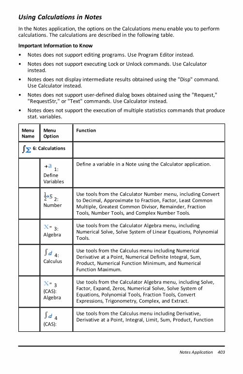
Using Calculations in NotesIn the Notes application, the options on the Calculations menu enable you to performcalculations. The calculations are described in the following table.
Important Information to Know
• Notes does not support editing programs. Use Program Editor instead.
• Notes does not support executing Lock or Unlock commands. Use Calculatorinstead.
• Notes does not display intermediate results obtained using the "Disp" command.Use Calculator instead.
• Notes does not support user-defined dialog boxes obtained using the "Request,""RequestStr," or "Text" commands. Use Calculator instead.
• Notes does not support the execution of multiple statistics commands that producestat. variables.
MenuName
MenuOption
Function
6: Calculations
1:DefineVariables
Define a variable in a Note using the Calculator application.
2:Number
Use tools from the Calculator Number menu, including Convertto Decimal, Approximate to Fraction, Factor, Least CommonMultiple, Greatest Common Divisor, Remainder, FractionTools, Number Tools, and Complex Number Tools.
3:Algebra
Use tools from the Calculator Algebra menu, includingNumerical Solve, Solve System of Linear Equations, PolynomialTools.
4:Calculus
Use tools from the Calculus menu including NumericalDerivative at a Point, Numerical Definite Integral, Sum,Product, Numerical Function Minimum, and NumericalFunction Maximum.
3(CAS):Algebra
Use tools from the Calculator Algebra menu, including Solve,Factor, Expand, Zeros, Numerical Solve, Solve System ofEquations, Polynomial Tools, Fraction Tools, ConvertExpressions, Trigonometry, Complex, and Extract.
4(CAS):
Use tools from the Calculus menu including Derivative,Derivative at a Point, Integral, Limit, Sum, Product, Function
Notes Application 403
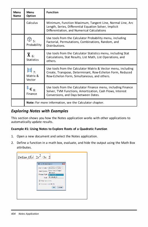
404 Notes Application
MenuName
MenuOption
Function
Calculus Minimum, Function Maximum, Tangent Line, Normal Line, ArcLength, Series, Differential Equation Solver, ImplicitDifferentiation, and Numerical Calculations
5:Probability
Use tools from the Calculator Probability menu, includingFactorial, Permutations, Combinations, Random, andDistributions.
6:Statistics
Use tools from the Calculator Statistics menu, including StatCalculations, Stat Results, List Math, List Operations, andothers.
7:Matrix &Vector
Use tools from the Calculator Matrix & Vector menu, includingCreate, Transpose, Determinant, Row-Echelon Form, ReducedRow-Echelon Form, Simultaneous, and others.
8:Finance
Use tools from the Calculator Finance menu, including FinanceSolver, TVM Functions, Amortization, Cash Flows, InterestConversions, and Days between Dates.
Note: For more information, see the Calculator chapter.
Exploring Notes with ExamplesThis section shows you how the Notes application works with other applications toautomatically update results.
Example #1: Using Notes to Explore Roots of a Quadratic Function
1. Open a new document and select the Notes application.
2. Define a function in a math box, evaluate, and hide the output using the Math Boxattributes.
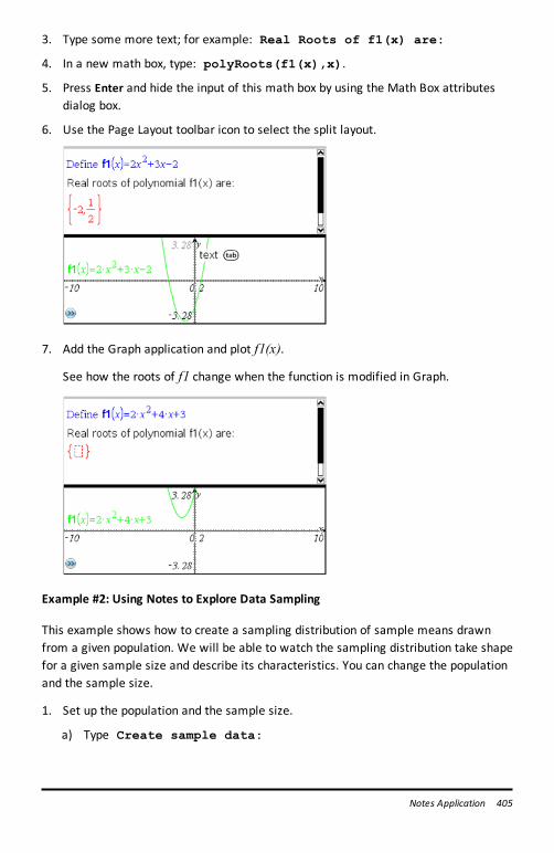
3. Type some more text; for example: Real Roots of f1(x) are:
4. In a new math box, type: polyRoots(f1(x),x).
5. Press Enter and hide the input of this math box by using the Math Box attributesdialog box.
6. Use the Page Layout toolbar icon to select the split layout.
7. Add the Graph application and plot f1(x).
See how the roots of f1 change when the function is modified in Graph.
Example #2: Using Notes to Explore Data Sampling
This example shows how to create a sampling distribution of sample means drawnfrom a given population. We will be able to watch the sampling distribution take shapefor a given sample size and describe its characteristics. You can change the populationand the sample size.
1. Set up the population and the sample size.
a) Type Create sample data:
Notes Application 405
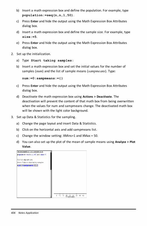
406 Notes Application
b) Insert a math expression box and define the population. For example, typepopulation:=seq(n,n,1,50).
c) Press Enter and hide the output using the Math Expression Box Attributesdialog box.
d) Insert a math expression box and define the sample size. For example, typesize:=5.
e) Press Enter and hide the output using the Math Expression Box Attributesdialog box.
2. Set up the initialization.
a) Type Start taking samples:
b) Insert a math expression box and set the initial values for the number ofsamples (num) and the list of sample means (sampmeans). Type:
num:=0:sampmeans:={}
c) Press Enter and hide the output using the Math Expression Box Attributesdialog box.
d) Deactivate the math expression box using Actions > Deactivate. Thedeactivation will prevent the content of that math box from being overwrittenwhen the values for num and sampmeans change. The deactivated math boxwill be shown with the light color background.
3. Set up Data & Statistics for the sampling.
a) Change the page layout and insert Data & Statistics.
b) Click on the horizontal axis and add sampmeans list.
c) Change the window setting: XMins=1 and XMax = 50.
d) You can also set up the plot of the mean of sample means using Analyze > PlotValue.
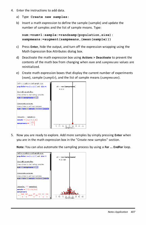
4. Enter the instructions to add data.
a) Type Create new samples:
b) Insert a math expression to define the sample (sample) and update thenumber of samples and the list of sample means. Type:
num:=num+1:sample:=randsamp(population,size):sampmeans:=augment(sampmeans,{mean(sample)})
c) Press Enter, hide the output, and turn off the expression wrapping using theMath Expression Box Attributes dialog box.
d) Deactivate the math expression box using Actions > Deactivate to prevent thecontents of the math box from changing when num and sampmeans values arereinitialized.
e) Create math expression boxes that display the current number of experiments(num), sample (sample), and the list of sample means (sampmeans).
5. Now you are ready to explore. Add more samples by simply pressing Enter whenyou are in the math expression box in the "Create new samples" section.
Note: You can also automate the sampling process by using a For ... EndFor loop.
Notes Application 407
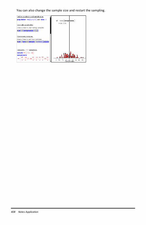
408 Notes Application
You can also change the sample size and restart the sampling.
Data CollectionThe Vernier DataQuest™ application is built into the TI-Nspire™ software and theoperating system (OS) for handhelds. The application lets you:
• Capture, view, and analyze real-world data using a TI-Nspire™ CX II handheld, aWindows® computer, or a Mac® computer.
• Collect data from up to five connected sensors (three analog and two digital) usingthe TI-Nspire™ Lab Cradle.
Important: The TI-Nspire™ CM-C Handheld is not compatible with the Lab Cradleand only supports the use of a single sensor at a time.
• Collect data either in the classroom or at remote locations using collection modessuch as time-based or event-based.
• Collect several data runs for comparison.
• Create a graphical hypothesis using the Draw Prediction feature.
• Play back the data set to compare the outcome to the hypothesis.
• Analyze data using functions such as interpolation, tangential rate, or modeling.
• Send collected data to other TI-Nspire™ applications.
• Access sensor data from all connected sensor probes through your TI-Basicprogram.
Adding a Vernier DataQuest™ Page
Note: The application is launched automatically when you connect a sensor.
Starting a new document or problem for each new experiment ensures that theVernier DataQuest™ application is set to its default values.
▶ To start a new document containing a data collection page:
From the main File menu, click New Document, and then click Add VernierDataQuest™.
Handheld: Pressc, and select Vernier DataQuest™ .
▶ To insert a new problem with a data collection page into an existing document:
From the toolbar, click Insert > Problem>Vernier DataQuest™.
Handheld: Press~ and select Insert > Problem > Vernier DataQuest™.
Data Collection 409
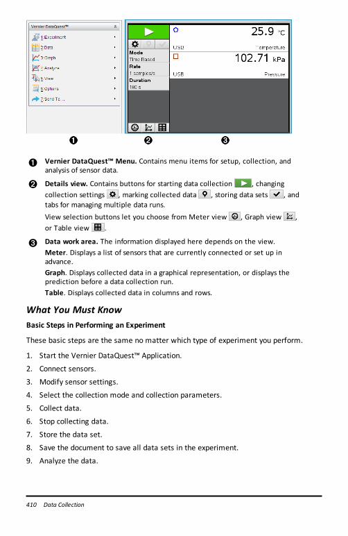
410 Data Collection
À Vernier DataQuest™ Menu. Contains menu items for setup, collection, andanalysis of sensor data.
Á Details view. Contains buttons for starting data collection , changingcollection settings , marking collected data , storing data sets , andtabs for managing multiple data runs.View selection buttons let you choose from Meter view , Graph view ,or Table view .
 Data work area. The information displayed here depends on the view.Meter. Displays a list of sensors that are currently connected or set up inadvance.Graph. Displays collected data in a graphical representation, or displays theprediction before a data collection run.Table. Displays collected data in columns and rows.
What You Must KnowBasic Steps in Performing an Experiment
These basic steps are the same no matter which type of experiment you perform.
1. Start the Vernier DataQuest™ Application.
2. Connect sensors.
3. Modify sensor settings.
4. Select the collection mode and collection parameters.
5. Collect data.
6. Stop collecting data.
7. Store the data set.
8. Save the document to save all data sets in the experiment.
9. Analyze the data.
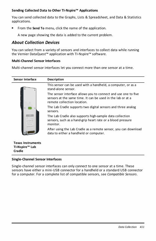
Sending Collected Data to Other TI-Nspire™ Applications
You can send collected data to the Graphs, Lists & Spreadsheet, and Data & Statisticsapplications.
▶ From the Send To menu, click the name of the application.
A new page showing the data is added to the current problem.
About Collection DevicesYou can select from a variety of sensors and interfaces to collect data while runningthe Vernier DataQuest™ application with TI-Nspire™ software.
Multi-Channel Sensor Interfaces
Multi-channel sensor interfaces let you connect more than one sensor at a time.
Sensor Interface Description
Texas InstrumentsTI-Nspire™ LabCradle
This sensor can be used with a handheld, a computer, or as astand-alone sensor.The sensor interface allows you to connect and use one to fivesensors at the same time. It can be used in the lab or at aremote collection location.The Lab Cradle supports two digital sensors and three analogsensors.The Lab Cradle also supports high-sample data collectionsensors, such as a hand-grip heart rate or a blood pressuremonitor.After using the Lab Cradle as a remote sensor, you can downloaddata to either a handheld or computer.
Single-Channel Sensor Interfaces
Single-channel sensor interfaces can only connect to one sensor at a time. Thesesensors have either a mini-USB connector for a handheld or a standard USB connectorfor a computer. For a complete list of compatible sensors, see Compatible Sensors.
Data Collection 411
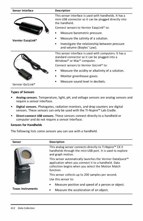
412 Data Collection
Sensor Interface Description
Vernier EasyLink®
This sensor interface is used with handhelds. It has amini-USB connector so it can be plugged directly intothe handheld.Connect sensors to Vernier EasyLink® to:
• Measure barometric pressure.
• Measure the salinity of a solution.
• Investigate the relationship between pressureand volume (Boyles’ Law).
Vernier Go!Link®
This sensor interface is used with computers. It has astandard connector so it can be plugged into aWindows® or Mac® computer.Connect sensors to Vernier GoLink® to:
• Measure the acidity or alkalinity of a solution.
• Monitor greenhouse gases.
• Measure sound level in decibels.
Types of Sensors
• Analog sensors. Temperature, light, pH, and voltage sensors are analog sensors andrequire a sensor interface.
• Digital sensors. Photogates, radiation monitors, and drop counters are digitalsensors. These sensors can only be used with the TI-Nspire™ Lab Cradle.
• Direct-connect USB sensors. These sensors connect directly to a handheld orcomputer and do not require a sensor interface.
Sensors for Handhelds
The following lists some sensors you can use with a handheld.
Sensor Description
Texas Instruments
This analog sensor connects directly to TI-Nspire™ CX IIhandhelds through the mini-USB port. It is used to exploreand graph motion.This sensor automatically launches the Vernier DataQuest™application when you connect it to a handheld. Datacollection begins when you select the Motion Matchfunction.This sensor collects up to 200 samples per second.Use this sensor to:
• Measure position and speed of a person or object.
• Measure the acceleration of an object.
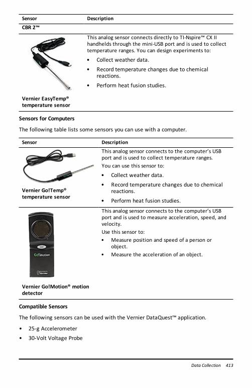
Sensor Description
CBR 2™
Vernier EasyTemp®temperature sensor
This analog sensor connects directly to TI-Nspire™ CX IIhandhelds through the mini-USB port and is used to collecttemperature ranges. You can design experiments to:
• Collect weather data.
• Record temperature changes due to chemicalreactions.
• Perform heat fusion studies.
Sensors for Computers
The following table lists some sensors you can use with a computer.
Sensor Description
Vernier Go!Temp®temperature sensor
This analog sensor connects to the computer’s USBport and is used to collect temperature ranges.You can use this sensor to:
• Collect weather data.
• Record temperature changes due to chemicalreactions.
• Perform heat fusion studies.
Vernier Go!Motion® motiondetector
This analog sensor connects to the computer’s USBport and is used to measure acceleration, speed, andvelocity.Use this sensor to:• Measure position and speed of a person or
object.• Measure the acceleration of an object.
Compatible Sensors
The following sensors can be used with the Vernier DataQuest™ application.
• 25-g Accelerometer
• 30-Volt Voltage Probe
Data Collection 413
414 Data Collection
• 3-Axis Accelerometer
• Low-g Accelerometer
• CBR 2™ - Connects directly to handheld USB port
• Go!Motion® - Connects directly to computer USB port
• Extra Long Temperature Probe
• Stainless Steel Temperature Probe
• Surface Temperature Sensor
• Ammonium Ion-Selective Electrode
• Anemometer
• Barometer
• Blood Pressure Sensor
• C02 Gas Sensor
• Calcium Ion-Selective Electrode
• Charge Sensor
• Chloride Ion-Selective Electrode
• Colorimeter
• Conductivity Probe
• High Current Sensor
• Current Probe
• Differential Voltage Probe
• Digital Radiation Monitor
• Dissolved Oxygen Sensor
• Dual-Range Force Sensor
• EasyTemp® - Connects directly to handheld USB port
• EKG Sensor
• Electrode Amplifier
• Flow Rate Sensor
• Force Plate
• Gas Pressure Sensor
• Go!Temp® - Connects directly to computer USB port
• Hand Dynamometer
• Hand-Grip Heart Rate Monitor
• Instrumentation Amplifier
• Light Sensor
• Magnetic Field Sensor
• Melt Station
• Microphone
• Nitrate Ion-Selective Electrode
• O2 Gas Sensor
• ORP Sensor
• pH Sensor
• Relative Humidity Sensor
• Respiration Monitor Belt (Requires Gas Pressure Sensor)
• Rotary Motion Sensor
• Salinity Sensor
• Soil Moisture Sensor
• Sound Level Meter
• Spirometer
• Thermocouple
• TI-Light - Sold only with the CBL 2™
• TI-Temp - Sold only with the CBL 2™
• TI-Voltage - Sold only with the CBL 2™
• Tris-Compatible Flat pH Sensor
• Turbidity Sensor
• UVA Sensor
• UVB Sensor
• Vernier Constant Current System
• Vernier Drop Counter
• Vernier Infrared Thermometer
• Vernier Motion Detector
• Vernier Photogate
• Voltage Probe
• Wide-Range Temperature Probe
Connecting SensorsDirect-connect USB sensors, such as the Vernier Go!Temp® temperature sensor (forcomputers) or the Vernier EasyLink® temperature sensor (for handhelds), connectdirectly to the computer or handheld and do not need a sensor interface.
Other sensors require a sensor interface such as the TI-Nspire™ Lab Cradle.
Data Collection 415
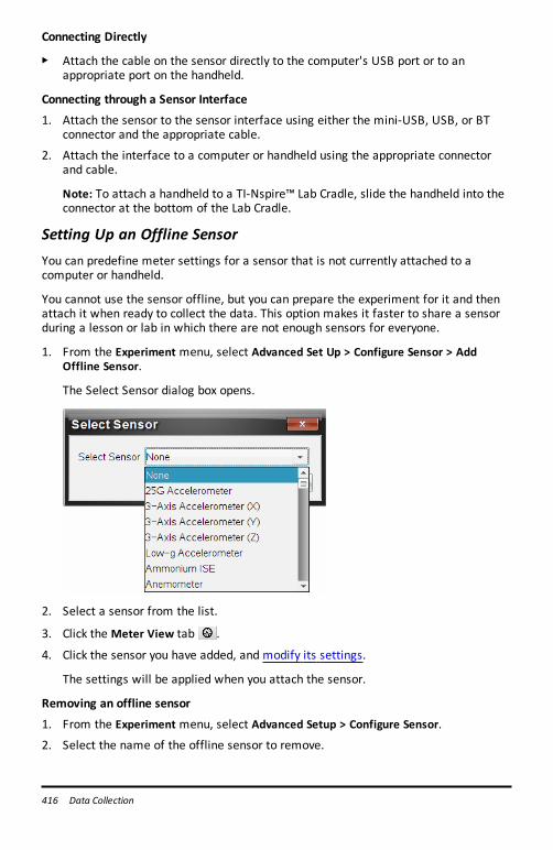
416 Data Collection
Connecting Directly
▶ Attach the cable on the sensor directly to the computer's USB port or to anappropriate port on the handheld.
Connecting through a Sensor Interface
1. Attach the sensor to the sensor interface using either the mini-USB, USB, or BTconnector and the appropriate cable.
2. Attach the interface to a computer or handheld using the appropriate connectorand cable.
Note: To attach a handheld to a TI-Nspire™ Lab Cradle, slide the handheld into theconnector at the bottom of the Lab Cradle.
Setting Up an Offline SensorYou can predefine meter settings for a sensor that is not currently attached to acomputer or handheld.
You cannot use the sensor offline, but you can prepare the experiment for it and thenattach it when ready to collect the data. This option makes it faster to share a sensorduring a lesson or lab in which there are not enough sensors for everyone.
1. From the Experiment menu, select Advanced Set Up > Configure Sensor > AddOffline Sensor.
The Select Sensor dialog box opens.
2. Select a sensor from the list.
3. Click the Meter View tab .
4. Click the sensor you have added, and modify its settings.
The settings will be applied when you attach the sensor.
Removing an offline sensor
1. From the Experiment menu, select Advanced Setup > Configure Sensor.
2. Select the name of the offline sensor to remove.
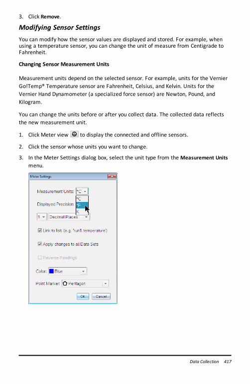
3. Click Remove.
Modifying Sensor SettingsYou can modify how the sensor values are displayed and stored. For example, whenusing a temperature sensor, you can change the unit of measure from Centigrade toFahrenheit.
Changing Sensor Measurement Units
Measurement units depend on the selected sensor. For example, units for the VernierGo!Temp® Temperature sensor are Fahrenheit, Celsius, and Kelvin. Units for theVernier Hand Dynamometer (a specialized force sensor) are Newton, Pound, andKilogram.
You can change the units before or after you collect data. The collected data reflectsthe new measurement unit.
1. Click Meter view to display the connected and offline sensors.
2. Click the sensor whose units you want to change.
3. In the Meter Settings dialog box, select the unit type from the Measurement Unitsmenu.
Data Collection 417
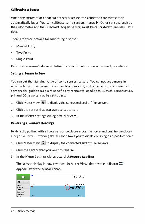
418 Data Collection
Calibrating a Sensor
When the software or handheld detects a sensor, the calibration for that sensorautomatically loads. You can calibrate some sensors manually. Other sensors, such asthe Colorimeter and the Dissolved Oxygen Sensor, must be calibrated to provide usefuldata.
There are three options for calibrating a sensor:
• Manual Entry
• Two Point
• Single Point
Refer to the sensor’s documentation for specific calibration values and procedures.
Setting a Sensor to Zero
You can set the standing value of some sensors to zero. You cannot set sensors inwhich relative measurements such as force, motion, and pressure are common to zero.Sensors designed to measure specific environmental conditions, such as Temperature,pH, and CO
2also cannot be set to zero.
1. Click Meter view to display the connected and offline sensors.
2. Click the sensor that you want to set to zero.
3. In the Meter Settings dialog box, click Zero.
Reversing a Sensor's Readings
By default, pulling with a force sensor produces a positive force and pushing producesa negative force. Reversing the sensor allows you to display pushing as a positive force.
1. Click Meter view to display the connected and offline sensors.
2. Click the sensor that you want to reverse.
3. In the Meter Settings dialog box, click Reverse Readings.
The sensor display is now reversed. In Meter View, the reverse indicatorappears after the sensor name.
Collecting Data
Collecting Time-Based Data
The Time Based collection mode captures sensor data automatically at regular timeintervals.
1. Connect the sensor or sensors.
Sensor names are added to the sensor list automatically.
2. From the Experiment menu, select New Experiment.
This removes all data and restores all meter settings to their defaults.
3. From the Experiment menu, select Collection Mode > Time Based.
a) Select Rate or Interval from the drop-down list, and then type the Rate(samples/second) or Interval (seconds/sample).
b) Type the Duration of the collection.
The Number of points is calculated and displayed, based on rate and duration.Note that collecting too many data points can slow system performance.
c) Select Strip Chart if you want to collect samples continuously, retaining only thelast n samples. (where “n” is the number shown in the Number of points field.)
4. Modify sensor settings as necessary.
5. Click Start Collection .
6. After the data has been collected, click Stop Collection .
The data set run is complete.
Collecting Selected Events
Use the Selected Events collection mode to capture samples manually. In this mode,each sample is automatically assigned an event number.
1. Connect the sensor or sensors.
Sensor names are added to the sensor list automatically.
2. From the Experiment menu, select New Experiment.
This removes all data and restores all meter settings to their defaults.
3. From the Experiment menu, select Collection Mode > Selected Events.
Data Collection 419
420 Data Collection
The Selected Events Setup dialog box opens.
- Name. This text is visible in the Meter View. Its first letter is displayed as theindependent variable in the Graph view.
- Units. This text is displayed in Graph view alongside the Name.
- Average over 10 s. This option averages ten seconds of data for each point.
4. Modify sensor settings as necessary.
5. Click Start Collection .
The Keep Current Reading icon becomes active. The current sensor value
appears in the center of the graph.
6. Click Keep Current Reading to capture each sample.
The data point is plotted, and the current sensor value appears in the center of thegraph.
Note: If you selected the Averaging option, a countdown timer appears. When thecounter reaches zero, the system plots the average.
7. Continue capturing until you collect all of the desired data points.
8. Click Stop Collection .
The data set run is complete.
Collecting Events with Entry
Use the Events with Entry collection mode to capture samples manually. In this mode,you define the independent value for each point you collect.
1. Connect the sensor or sensors.
Sensor names are added to the sensor list automatically.
2. From the Experiment menu, select New Experiment.
This removes all data and restores all meter settings to their defaults.
3. From the Experiment menu, select Collection Mode > Events with Entry.
The Events with Entry Setup dialog box opens.
- Name. This text is visible in the Meter View. Its first letter is displayed as theindependent variable in the Graph view.
- Units. This text is displayed in Graph view alongside the Name.
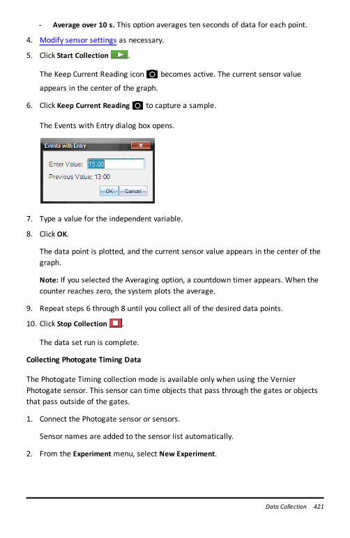
- Average over 10 s. This option averages ten seconds of data for each point.
4. Modify sensor settings as necessary.
5. Click Start Collection .
The Keep Current Reading icon becomes active. The current sensor value
appears in the center of the graph.
6. Click Keep Current Reading to capture a sample.
The Events with Entry dialog box opens.
7. Type a value for the independent variable.
8. Click OK.
The data point is plotted, and the current sensor value appears in the center of thegraph.
Note: If you selected the Averaging option, a countdown timer appears. When thecounter reaches zero, the system plots the average.
9. Repeat steps 6 through 8 until you collect all of the desired data points.
10. Click Stop Collection .
The data set run is complete.
Collecting Photogate Timing Data
The Photogate Timing collection mode is available only when using the VernierPhotogate sensor. This sensor can time objects that pass through the gates or objectsthat pass outside of the gates.
1. Connect the Photogate sensor or sensors.
Sensor names are added to the sensor list automatically.
2. From the Experiment menu, select New Experiment.
Data Collection 421
422 Data Collection
This removes all data and restores all meter settings to their defaults.
3. From the Experiment menu, select Collection Mode > Photogate Timing.
4. Set the collection options.
5. Modify sensor settings as necessary.
6. Click Start Collection .
7. After the data has been collected, click Stop Collection .
The data set run is complete.
Collecting Drop Counter Data
The Drop Counting collection mode is available only when using the Vernier DropCounter optical sensor. This sensor can count the number of drops or record theamount of liquid added during an experiment.
1. Connect the Drop Counter sensor or sensors.
Sensor names are added to the sensor list automatically.
2. From the Experiment menu, select New Experiment.
This removes all data and restores all meter settings to their defaults.
3. From the Experiment menu, select Collection Mode > Drop Counting.
4. Set the collection options.
5. Modify sensor settings as necessary.
6. Click Start Collection .
7. After the data has been collected, click Stop Collection .
The data set run is complete.
Using Data Markers to Annotate DataData markers give you a way to emphasize specific data points, such as when youchange a condition. For example, you might mark a point at which a chemical is addedto a solution or when heat is applied or removed. You can add a marker with orwithout a comment, and you can hide a comment.
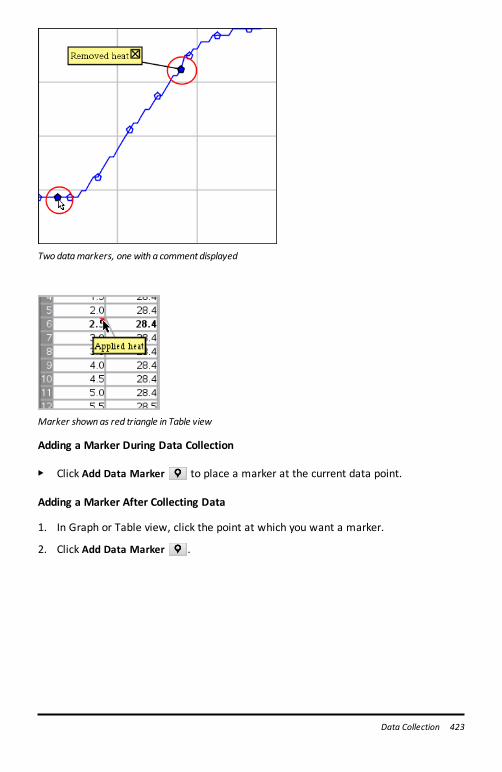
Twodatamarkers, one with a comment displayed
Marker shownas red triangle in Table view
Adding a Marker During Data Collection
▶ Click Add Data Marker to place a marker at the current data point.
Adding a Marker After Collecting Data
1. In Graph or Table view, click the point at which you want a marker.
2. Click Add Data Marker .
Data Collection 423
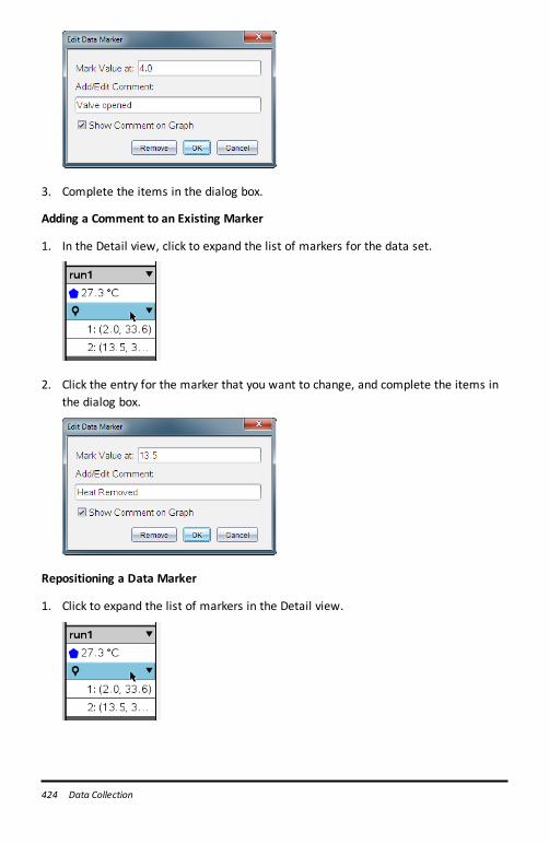
424 Data Collection
3. Complete the items in the dialog box.
Adding a Comment to an Existing Marker
1. In the Detail view, click to expand the list of markers for the data set.
2. Click the entry for the marker that you want to change, and complete the items inthe dialog box.
Repositioning a Data Marker
1. Click to expand the list of markers in the Detail view.
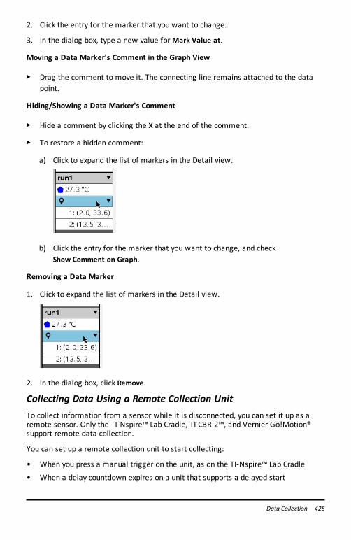
2. Click the entry for the marker that you want to change.
3. In the dialog box, type a new value forMark Value at.
Moving a Data Marker's Comment in the Graph View
▶ Drag the comment to move it. The connecting line remains attached to the datapoint.
Hiding/Showing a Data Marker's Comment
▶ Hide a comment by clicking the X at the end of the comment.
▶ To restore a hidden comment:
a) Click to expand the list of markers in the Detail view.
b) Click the entry for the marker that you want to change, and checkShow Comment on Graph.
Removing a Data Marker
1. Click to expand the list of markers in the Detail view.
2. In the dialog box, click Remove.
Collecting Data Using a Remote Collection UnitTo collect information from a sensor while it is disconnected, you can set it up as aremote sensor. Only the TI-Nspire™ Lab Cradle, TI CBR 2™, and Vernier Go!Motion®support remote data collection.
You can set up a remote collection unit to start collecting:
• When you press a manual trigger on the unit, as on the TI-Nspire™ Lab Cradle
• When a delay countdown expires on a unit that supports a delayed start
Data Collection 425
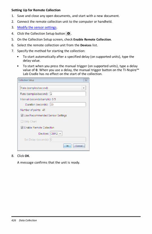
426 Data Collection
Setting Up for Remote Collection
1. Save and close any open documents, and start with a new document.
2. Connect the remote collection unit to the computer or handheld.
3. Modify the sensor settings.
4. Click the Collection Setup button .
5. On the Collection Setup screen, check Enable Remote Collection.
6. Select the remote collection unit from the Devices list.
7. Specify the method for starting the collection:
• To start automatically after a specified delay (on supported units), type thedelay value.
• To start when you press the manual trigger (on supported units), type a delayvalue of 0. When you use a delay, the manual trigger button on the TI-Nspire™Lab Cradle has no effect on the start of the collection.
8. Click OK.
A message confirms that the unit is ready.
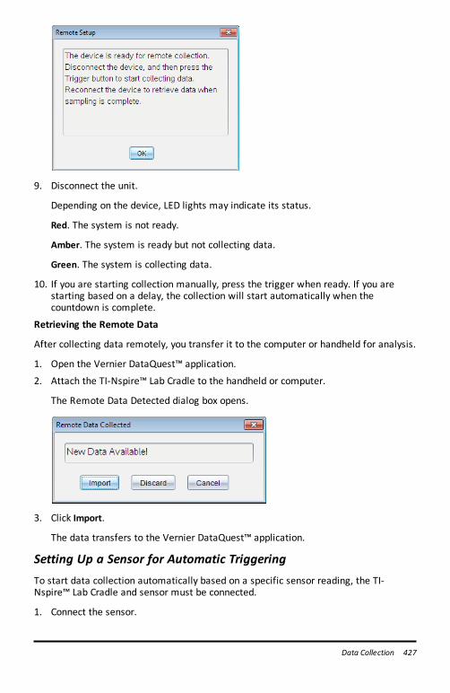
9. Disconnect the unit.
Depending on the device, LED lights may indicate its status.
Red. The system is not ready.
Amber. The system is ready but not collecting data.
Green. The system is collecting data.
10. If you are starting collection manually, press the trigger when ready. If you arestarting based on a delay, the collection will start automatically when thecountdown is complete.
Retrieving the Remote Data
After collecting data remotely, you transfer it to the computer or handheld for analysis.
1. Open the Vernier DataQuest™ application.
2. Attach the TI-Nspire™ Lab Cradle to the handheld or computer.
The Remote Data Detected dialog box opens.
3. Click Import.
The data transfers to the Vernier DataQuest™ application.
Setting Up a Sensor for Automatic TriggeringTo start data collection automatically based on a specific sensor reading, the TI-Nspire™ Lab Cradle and sensor must be connected.
1. Connect the sensor.
Data Collection 427
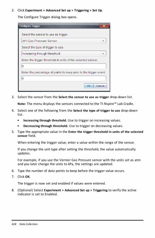
428 Data Collection
2. Click Experiment > Advanced Set up > Triggering > Set Up.
The Configure Trigger dialog box opens.
3. Select the sensor from the Select the sensor to use as trigger drop-down list.
Note: The menu displays the sensors connected to the TI-Nspire™ Lab Cradle.
4. Select one of the following from the Select the type of trigger to use drop-downlist.
• Increasing through threshold. Use to trigger on increasing values.• Decreasing through threshold. Use to trigger on decreasing values.
5. Type the appropriate value in the Enter the trigger threshold in units of the selectedsensor field.
When entering the trigger value, enter a value within the range of the sensor.
If you change the unit type after setting the threshold, the value automaticallyupdates.
For example, if you use the Vernier Gas Pressure sensor with the units set as atmand you later change the units to kPa, the settings are updated.
6. Type the number of data points to keep before the trigger value occurs.
7. Click OK.
The trigger is now set and enabled if values were entered.
8. (Optional) Select Experiment > Advanced Set up > Triggering to verify the activeindicator is set to Enabled.
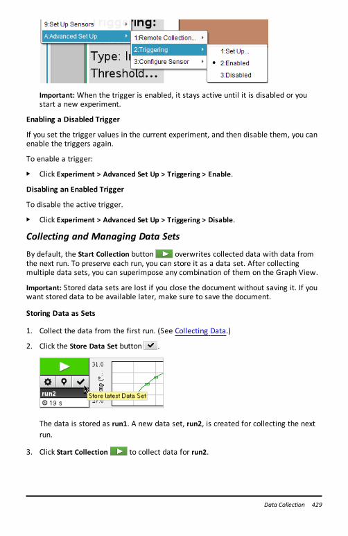
Important: When the trigger is enabled, it stays active until it is disabled or youstart a new experiment.
Enabling a Disabled Trigger
If you set the trigger values in the current experiment, and then disable them, you canenable the triggers again.
To enable a trigger:
▶ Click Experiment > Advanced Set Up > Triggering > Enable.
Disabling an Enabled Trigger
To disable the active trigger.
▶ Click Experiment > Advanced Set Up > Triggering > Disable.
Collecting and Managing Data Sets
By default, the Start Collection button overwrites collected data with data fromthe next run. To preserve each run, you can store it as a data set. After collectingmultiple data sets, you can superimpose any combination of them on the Graph View.
Important: Stored data sets are lost if you close the document without saving it. If youwant stored data to be available later, make sure to save the document.
Storing Data as Sets
1. Collect the data from the first run. (See Collecting Data.)
2. Click the Store Data Set button .
The data is stored as run1. A new data set, run2, is created for collecting the nextrun.
3. Click Start Collection to collect data for run2.
Data Collection 429
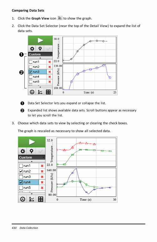
430 Data Collection
Comparing Data Sets
1. Click the Graph View icon to show the graph.
2. Click the Data Set Selector (near the top of the Detail View) to expand the list ofdata sets.
À Data Set Selector lets you expand or collapse the list.
Á Expanded list shows available data sets. Scroll buttons appear as necessaryto let you scroll the list.
3. Choose which data sets to view by selecting or clearing the check boxes.
The graph is rescaled as necessary to show all selected data.
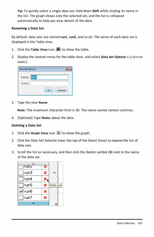
Tip: To quickly select a single data set, hold down Shift while clicking its name inthe list. The graph shows only the selected set, and the list is collapsedautomatically to help you view details of the data.
Renaming a Data Set
By default, data sets are named run1, run2, and so on. The name of each data set isdisplayed in the Table view.
1. Click the Table View icon to show the table.
2. Display the context menu for the table view, and select Data Set Options > [currentname].
3. Type the new Name.
Note: The maximum character limit is 30. The name cannot contain commas.
4. (Optional) Type Notes about the data.
Deleting a Data Set
1. Click the Graph View icon to show the graph.
2. Click the Data Set Selector (near the top of the Detail View) to expand the list ofdata sets.
3. Scroll the list as necessary, and then click the Delete symbol (X) next to the nameof the data set.
Data Collection 431
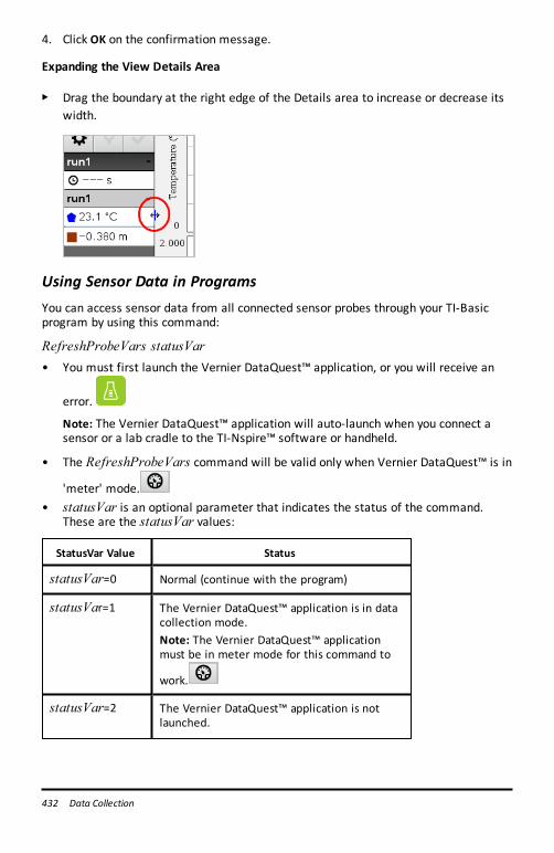
432 Data Collection
4. Click OK on the confirmation message.
Expanding the View Details Area
▶ Drag the boundary at the right edge of the Details area to increase or decrease itswidth.
Using Sensor Data in ProgramsYou can access sensor data from all connected sensor probes through your TI-Basicprogram by using this command:
RefreshProbeVars statusVar• You must first launch the Vernier DataQuest™ application, or you will receive an
error.
Note: The Vernier DataQuest™ application will auto-launch when you connect asensor or a lab cradle to the TI-Nspire™ software or handheld.
• The RefreshProbeVars command will be valid only when Vernier DataQuest™ is in
'meter' mode.• statusVar is an optional parameter that indicates the status of the command.
These are the statusVar values:
StatusVar Value Status
statusVar=0 Normal (continue with the program)
statusVar=1 The Vernier DataQuest™ application is in datacollection mode.Note: The Vernier DataQuest™ applicationmust be in meter mode for this command to
work.
statusVar=2 The Vernier DataQuest™ application is notlaunched.
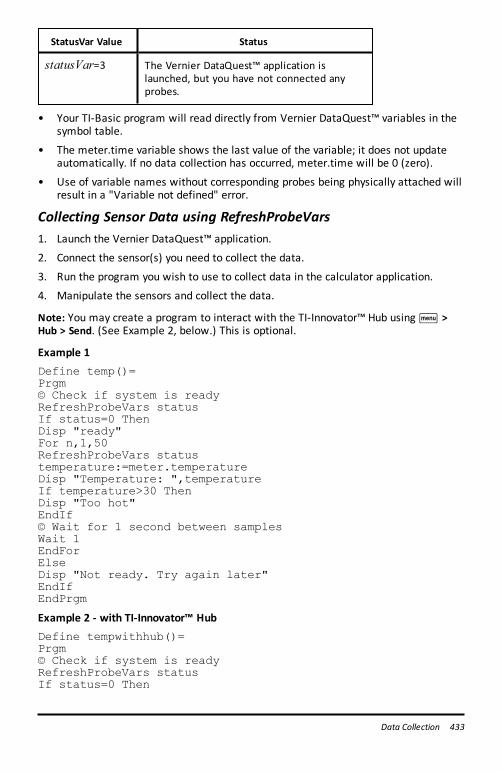
StatusVar Value Status
statusVar=3 The Vernier DataQuest™ application islaunched, but you have not connected anyprobes.
• Your TI-Basic program will read directly from Vernier DataQuest™ variables in thesymbol table.
• The meter.time variable shows the last value of the variable; it does not updateautomatically. If no data collection has occurred, meter.time will be 0 (zero).
• Use of variable names without corresponding probes being physically attached willresult in a "Variable not defined" error.
Collecting Sensor Data using RefreshProbeVars1. Launch the Vernier DataQuest™ application.
2. Connect the sensor(s) you need to collect the data.
3. Run the program you wish to use to collect data in the calculator application.
4. Manipulate the sensors and collect the data.
Note: You may create a program to interact with the TI-Innovator™ Hub usingb >Hub > Send. (See Example 2, below.) This is optional.
Example 1Define temp()=Prgm© Check if system is readyRefreshProbeVars statusIf status=0 ThenDisp "ready"For n,1,50RefreshProbeVars statustemperature:=meter.temperatureDisp "Temperature: ",temperatureIf temperature>30 ThenDisp "Too hot"EndIf© Wait for 1 second between samplesWait 1EndForElseDisp "Not ready. Try again later"EndIfEndPrgm
Example 2 - with TI-Innovator™ HubDefine tempwithhub()=Prgm© Check if system is readyRefreshProbeVars statusIf status=0 Then
Data Collection 433
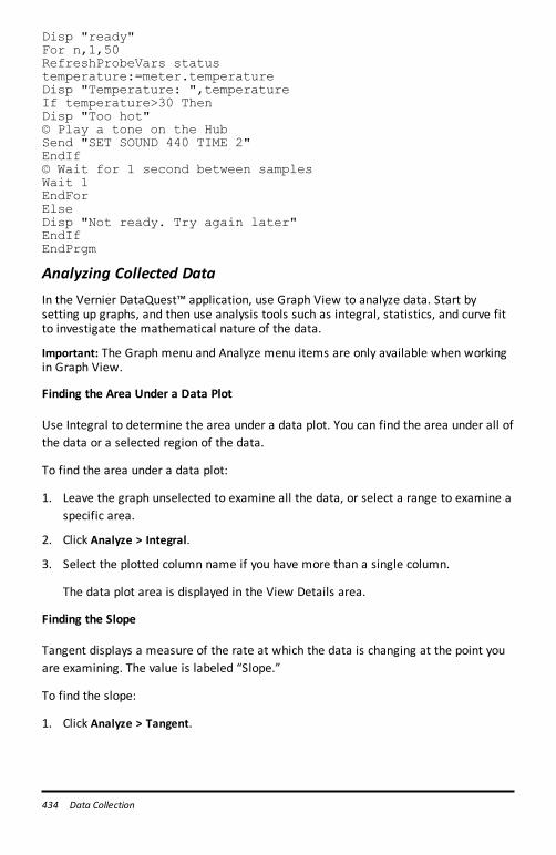
434 Data Collection
Disp "ready"For n,1,50RefreshProbeVars statustemperature:=meter.temperatureDisp "Temperature: ",temperatureIf temperature>30 ThenDisp "Too hot"© Play a tone on the HubSend "SET SOUND 440 TIME 2"EndIf© Wait for 1 second between samplesWait 1EndForElseDisp "Not ready. Try again later"EndIfEndPrgm
Analyzing Collected DataIn the Vernier DataQuest™ application, use Graph View to analyze data. Start bysetting up graphs, and then use analysis tools such as integral, statistics, and curve fitto investigate the mathematical nature of the data.
Important: The Graph menu and Analyze menu items are only available when workingin Graph View.
Finding the Area Under a Data Plot
Use Integral to determine the area under a data plot. You can find the area under all ofthe data or a selected region of the data.
To find the area under a data plot:
1. Leave the graph unselected to examine all the data, or select a range to examine aspecific area.
2. Click Analyze > Integral.
3. Select the plotted column name if you have more than a single column.
The data plot area is displayed in the View Details area.
Finding the Slope
Tangent displays a measure of the rate at which the data is changing at the point youare examining. The value is labeled “Slope.”
To find the slope:
1. Click Analyze > Tangent.
A check mark appears in the menu next to the option.
2. Click the graph.
The examine indicator is drawn to the nearest data point.
The values of the plotted data are shown in the View details area and the AllDetails for Graph dialog box.
You can move the examine line by dragging, clicking another point, or using thearrow keys.
Interpolating the Value Between Two Data Points
Use Interpolate to estimate the value between two data points and to determine thevalue of a Curve Fit between and beyond these data points.
The examine line moves from data point to data point. When Interpolate is on, theexamine line moves between and beyond data points.
To use Interpolate:
1. Click Analyze > Interpolate.
A check mark appears in the menu next to the option.
2. Click the graph.
The examine indicator is drawn to the nearest data point.
The values of the plotted data are shown in the View Details area.
You can shift the examine line by moving the cursor with the arrow keys or byclicking on another data point.
Generating Statistics
You can generate statistics (minimum, maximum, mean, standard deviation, andnumber of samples) for all the collected data or for a selected region. You can alsogenerate a curve fit based on one of several standard models or on a model that youdefine.
1. Leave the graph unselected to examine all the data, or select a range to examine aspecific area.
2. Click Analyze > Statistics.
Data Collection 435
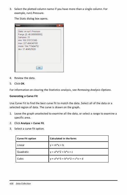
436 Data Collection
3. Select the plotted column name if you have more than a single column. Forexample, run1.Pressure.
The Stats dialog box opens.
4. Review the data.
5. Click OK.
For information on clearing the Statistics analysis, see Removing Analysis Options.
Generating a Curve Fit
Use Curve Fit to find the best curve fit to match the data. Select all of the data or aselected region of data. The curve is drawn on the graph.
1. Leave the graph unselected to examine all the data, or select a range to examine aspecific area.
2. Click Analyze > Curve Fit.
3. Select a curve fit option.
Curve Fit option Calculated in the form:
Linear y = m*x + b
Quadratic y = a*x^2 + b*x + c
Cubic y = a*x^3 + b*x^2 + c*x + d
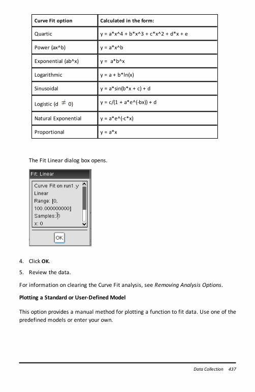
Curve Fit option Calculated in the form:
Quartic y = a*x^4 + b*x^3 + c*x^2 + d*x + e
Power (ax^b) y = a*x^b
Exponential (ab^x) y = a*b^x
Logarithmic y = a + b*ln(x)
Sinusoidal y = a*sin(b*x + c) + d
Logistic (d 0) y = c/(1 + a*e^(-bx)) + d
Natural Exponential y = a*e^(-c*x)
Proportional y = a*x
The Fit Linear dialog box opens.
4. Click OK.
5. Review the data.
For information on clearing the Curve Fit analysis, see Removing Analysis Options.
Plotting a Standard or User-Defined Model
This option provides a manual method for plotting a function to fit data. Use one of thepredefined models or enter your own.
Data Collection 437
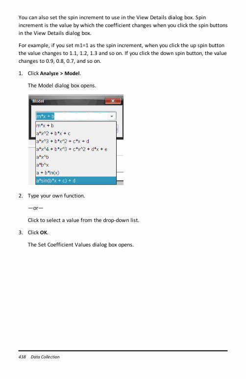
438 Data Collection
You can also set the spin increment to use in the View Details dialog box. Spinincrement is the value by which the coefficient changes when you click the spin buttonsin the View Details dialog box.
For example, if you set m1=1 as the spin increment, when you click the up spin buttonthe value changes to 1.1, 1.2, 1.3 and so on. If you click the down spin button, the valuechanges to 0.9, 0.8, 0.7, and so on.
1. Click Analyze > Model.
The Model dialog box opens.
2. Type your own function.
—or—
Click to select a value from the drop-down list.
3. Click OK.
The Set Coefficient Values dialog box opens.
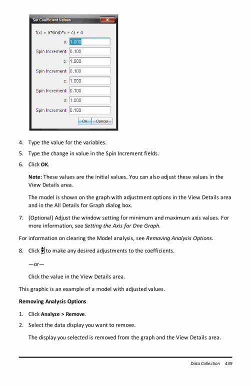
4. Type the value for the variables.
5. Type the change in value in the Spin Increment fields.
6. Click OK.
Note: These values are the initial values. You can also adjust these values in theView Details area.
The model is shown on the graph with adjustment options in the View Details areaand in the All Details for Graph dialog box.
7. (Optional) Adjust the window setting for minimum and maximum axis values. Formore information, see Setting the Axis for One Graph.
For information on clearing the Model analysis, see Removing Analysis Options.
8. Click to make any desired adjustments to the coefficients.
—or—
Click the value in the View Details area.
This graphic is an example of a model with adjusted values.
Removing Analysis Options
1. Click Analyze > Remove.
2. Select the data display you want to remove.
The display you selected is removed from the graph and the View Details area.
Data Collection 439
440 Data Collection
Displaying Collected Data in Graph ViewWhen you collect data, it is written in both the Graph and Table views. Use the Graphview to examine the plotted data.
Important: The Graph menu and Analyze menu items are only active when working inGraph View.
Selecting the Graph View
▶ Click the Graph View tab .
Viewing Multiple Graphs
Use the Show Graph menu to show separate graphs when using:
• A sensor that plots more than one column of data.
• Multiple sensors with different defined units at the same time.
In this example, two sensors (the Gas Pressure sensor and the Hand Dynamometer)were used in the same run. The following image shows the columns Time, Force, andPressure in the Table view to illustrate why two graphs are shown.
Displaying One of Two Graphs
When two graphs are displayed, the top graph is Graph 1 and the bottom graph isGraph 2.
To display only Graph 1:
▶ Select Graph > Show Graph > Graph 1.
Only Graph1 is displayed.
To display only Graph 2:
▶ Select Graph > Show Graph > Graph 2.
Only Graph 2 is displayed.
Displaying Both Graphs
To display both Graph 1 and Graph 2 together:
▶ Select Graph > Show Graph > Both.
Graph1 and Graph 2 are displayed.
Displaying Graphs in the Page Layout View
Use the Page layout view when Show Graph is not the appropriate solution forshowing more than one graph.
The Show Graph option is not applicable for:
• Multiple runs using a single sensor.
• Two or more of the same sensors.
• Multiple sensors that use the same column(s) of data.
To use Page Layout:
1. Open the original data set you want to see in two graph windows.
2. Click Edit > Page Layout > Select Layout.
3. Select the type of page layout you want to use.
4. Click Click here to add an application.
5. Select Add Vernier DataQuest™.
The Vernier DataQuest™ application is added to the second view.
6. To see separate views, click the view you want to change, and then select View >Table.
The new view is displayed.
7. To show the same view, click the view to change.
8. Click View > Graph.
The new view is displayed.
Displaying Collected Data in Table ViewTable view provides another way to sort and view collected data.
Selecting the Table View
▶ Click the Table View tab .
Defining Column Options
You can name columns and define the decimal points and the precision you want touse.
1. from the Data menu, select Column Options.
Data Collection 441
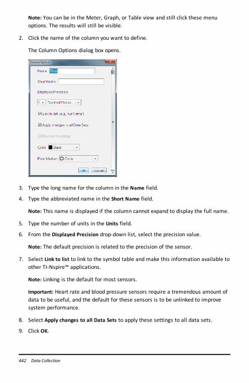
442 Data Collection
Note: You can be in the Meter, Graph, or Table view and still click these menuoptions. The results will still be visible.
2. Click the name of the column you want to define.
The Column Options dialog box opens.
3. Type the long name for the column in the Name field.
4. Type the abbreviated name in the Short Name field.
Note: This name is displayed if the column cannot expand to display the full name.
5. Type the number of units in the Units field.
6. From the Displayed Precision drop-down list, select the precision value.
Note: The default precision is related to the precision of the sensor.
7. Select Link to list to link to the symbol table and make this information available toother TI-Nspire™ applications.
Note: Linking is the default for most sensors.
Important: Heart rate and blood pressure sensors require a tremendous amount ofdata to be useful, and the default for these sensors is to be unlinked to improvesystem performance.
8. Select Apply changes to all Data Sets to apply these settings to all data sets.
9. Click OK.
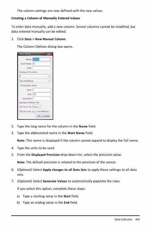
The column settings are now defined with the new values.
Creating a Column of Manually Entered Values
To enter data manually, add a new column. Sensor columns cannot be modified, butdata entered manually can be edited.
1. Click Data > NewManual Column.
The Column Options dialog box opens.
2. Type the long name for the column in the Name field.
3. Type the abbreviated name in the Short Name field.
Note: This name is displayed if the column cannot expand to display the full name.
4. Type the units to be used.
5. From the Displayed Precision drop-down list, select the precision value.
Note: The default precision is related to the precision of the sensor.
6. (Optional) Select Apply changes to all Data Sets to apply these settings to all datasets.
7. (Optional) Select Generate Values to automatically populate the rows.
If you select this option, complete these steps:
a) Type a starting value in the Start field.
b) Type an ending value in the End field.
Data Collection 443
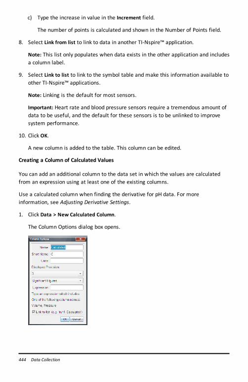
444 Data Collection
c) Type the increase in value in the Increment field.
The number of points is calculated and shown in the Number of Points field.
8. Select Link from list to link to data in another TI-Nspire™ application.
Note: This list only populates when data exists in the other application and includesa column label.
9. Select Link to list to link to the symbol table and make this information available toother TI-Nspire™ applications.
Note: Linking is the default for most sensors.
Important: Heart rate and blood pressure sensors require a tremendous amount ofdata to be useful, and the default for these sensors is to be unlinked to improvesystem performance.
10. Click OK.
A new column is added to the table. This column can be edited.
Creating a Column of Calculated Values
You can add an additional column to the data set in which the values are calculatedfrom an expression using at least one of the existing columns.
Use a calculated column when finding the derivative for pH data. For moreinformation, see Adjusting Derivative Settings.
1. Click Data > New Calculated Column.
The Column Options dialog box opens.
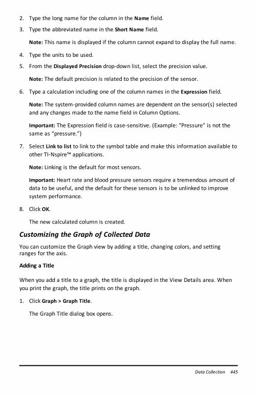
2. Type the long name for the column in the Name field.
3. Type the abbreviated name in the Short Name field.
Note: This name is displayed if the column cannot expand to display the full name.
4. Type the units to be used.
5. From the Displayed Precision drop-down list, select the precision value.
Note: The default precision is related to the precision of the sensor.
6. Type a calculation including one of the column names in the Expression field.
Note: The system-provided column names are dependent on the sensor(s) selectedand any changes made to the name field in Column Options.
Important: The Expression field is case-sensitive. (Example: “Pressure” is not thesame as “pressure.”)
7. Select Link to list to link to the symbol table and make this information available toother TI-Nspire™ applications.
Note: Linking is the default for most sensors.
Important: Heart rate and blood pressure sensors require a tremendous amount ofdata to be useful, and the default for these sensors is to be unlinked to improvesystem performance.
8. Click OK.
The new calculated column is created.
Customizing the Graph of Collected DataYou can customize the Graph view by adding a title, changing colors, and settingranges for the axis.
Adding a Title
When you add a title to a graph, the title is displayed in the View Details area. Whenyou print the graph, the title prints on the graph.
1. Click Graph > Graph Title.
The Graph Title dialog box opens.
Data Collection 445
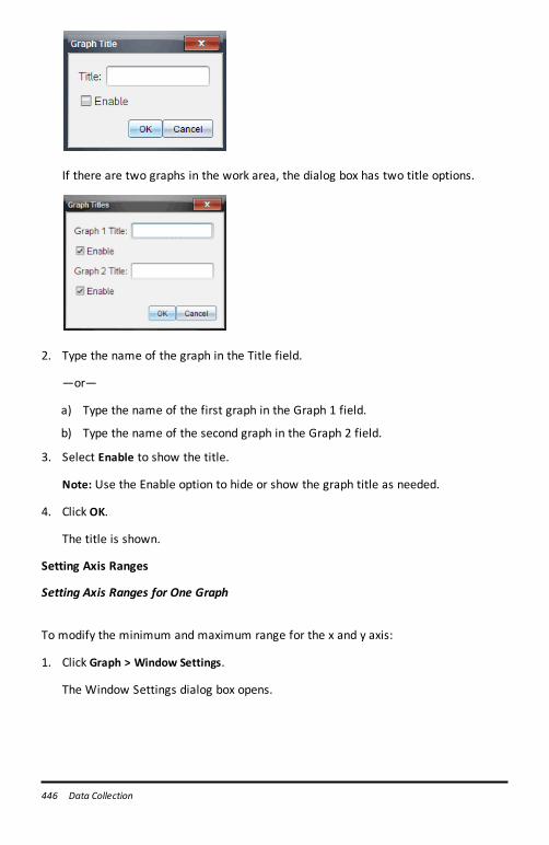
446 Data Collection
If there are two graphs in the work area, the dialog box has two title options.
2. Type the name of the graph in the Title field.
—or—
a) Type the name of the first graph in the Graph 1 field.
b) Type the name of the second graph in the Graph 2 field.
3. Select Enable to show the title.
Note: Use the Enable option to hide or show the graph title as needed.
4. Click OK.
The title is shown.
Setting Axis Ranges
Setting Axis Ranges for One Graph
To modify the minimum and maximum range for the x and y axis:
1. Click Graph > Window Settings.
The Window Settings dialog box opens.
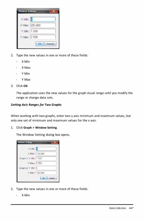
2. Type the new values in one or more of these fields:
- X Min
- X Max
- Y Min
- Y Max
3. Click OK.
The application uses the new values for the graph visual range until you modify therange or change data sets.
Setting Axis Ranges for Two Graphs
When working with two graphs, enter two y axis minimum and maximum values, butonly one set of minimum and maximum values for the x axis.
1. Click Graph > Window Setting.
The Window Setting dialog box opens.
2. Type the new values in one or more of these fields:
- X Min
Data Collection 447
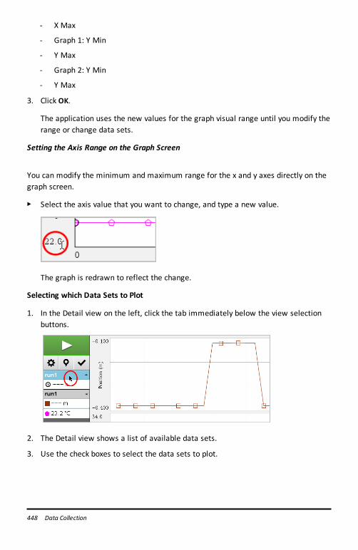
448 Data Collection
- X Max
- Graph 1: Y Min
- Y Max
- Graph 2: Y Min
- Y Max
3. Click OK.
The application uses the new values for the graph visual range until you modify therange or change data sets.
Setting the Axis Range on the Graph Screen
You can modify the minimum and maximum range for the x and y axes directly on thegraph screen.
▶ Select the axis value that you want to change, and type a new value.
The graph is redrawn to reflect the change.
Selecting which Data Sets to Plot
1. In the Detail view on the left, click the tab immediately below the view selectionbuttons.
2. The Detail view shows a list of available data sets.
3. Use the check boxes to select the data sets to plot.
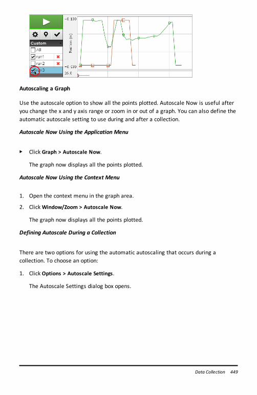
Autoscaling a Graph
Use the autoscale option to show all the points plotted. Autoscale Now is useful afteryou change the x and y axis range or zoom in or out of a graph. You can also define theautomatic autoscale setting to use during and after a collection.
Autoscale Now Using the Application Menu
▶ Click Graph > Autoscale Now.
The graph now displays all the points plotted.
Autoscale Now Using the Context Menu
1. Open the context menu in the graph area.
2. ClickWindow/Zoom > Autoscale Now.
The graph now displays all the points plotted.
Defining Autoscale During a Collection
There are two options for using the automatic autoscaling that occurs during acollection. To choose an option:
1. Click Options > Autoscale Settings.
The Autoscale Settings dialog box opens.
Data Collection 449
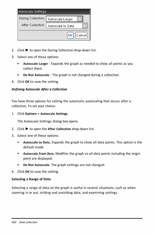
450 Data Collection
2. Click► to open the During Collection drop-down list.
3. Select one of these options:
• Autoscale Larger - Expands the graph as needed to show all points as youcollect them.
• Do Not Autoscale - The graph is not changed during a collection.
4. Click OK to save the setting.
Defining Autoscale After a Collection
You have three options for setting the automatic autoscaling that occurs after acollection. To set your choice:
1. Click Options > Autoscale Settings.
The Autoscale Settings dialog box opens.
2. Click► to open the After Collection drop-down list.
3. Select one of these options:
• Autoscale to Data. Expands the graph to show all data points. This option is thedefault mode.
• Autoscale From Zero. Modifies the graph so all data points including the originpoint are displayed.
• Do Not Autoscale. The graph settings are not changed.
4. Click OK to save the setting.
Selecting a Range of Data
Selecting a range of data on the graph is useful in several situations, such as whenzooming in or out, striking and unstriking data, and examining settings.
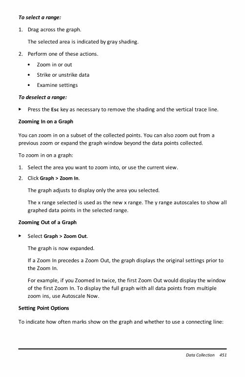
To select a range:
1. Drag across the graph.
The selected area is indicated by gray shading.
2. Perform one of these actions.
• Zoom in or out
• Strike or unstrike data
• Examine settings
To deselect a range:
▶ Press the Esc key as necessary to remove the shading and the vertical trace line.
Zooming In on a Graph
You can zoom in on a subset of the collected points. You can also zoom out from aprevious zoom or expand the graph window beyond the data points collected.
To zoom in on a graph:
1. Select the area you want to zoom into, or use the current view.
2. Click Graph > Zoom In.
The graph adjusts to display only the area you selected.
The x range selected is used as the new x range. The y range autoscales to show allgraphed data points in the selected range.
Zooming Out of a Graph
▶ Select Graph > Zoom Out.
The graph is now expanded.
If a Zoom In precedes a Zoom Out, the graph displays the original settings prior tothe Zoom In.
For example, if you Zoomed In twice, the first Zoom Out would display the windowof the first Zoom In. To display the full graph with all data points from multiplezoom ins, use Autoscale Now.
Setting Point Options
To indicate how often marks show on the graph and whether to use a connecting line:
Data Collection 451
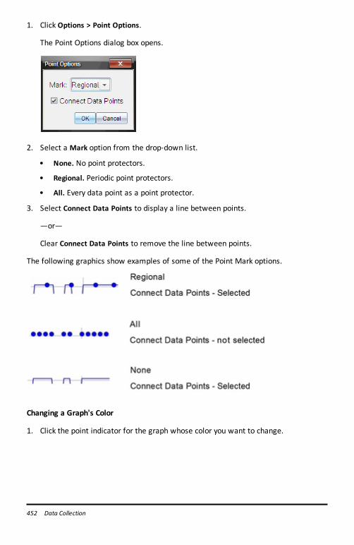
452 Data Collection
1. Click Options > Point Options.
The Point Options dialog box opens.
2. Select a Mark option from the drop-down list.
• None. No point protectors.
• Regional. Periodic point protectors.
• All. Every data point as a point protector.
3. Select Connect Data Points to display a line between points.
—or—
Clear Connect Data Points to remove the line between points.
The following graphics show examples of some of the Point Mark options.
Changing a Graph's Color
1. Click the point indicator for the graph whose color you want to change.
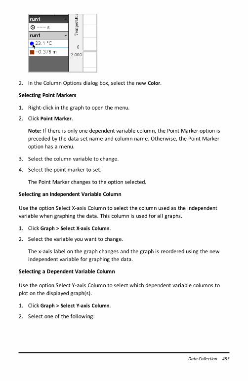
2. In the Column Options dialog box, select the new Color.
Selecting Point Markers
1. Right-click in the graph to open the menu.
2. Click Point Marker.
Note: If there is only one dependent variable column, the Point Marker option ispreceded by the data set name and column name. Otherwise, the Point Markeroption has a menu.
3. Select the column variable to change.
4. Select the point marker to set.
The Point Marker changes to the option selected.
Selecting an Independent Variable Column
Use the option Select X-axis Column to select the column used as the independentvariable when graphing the data. This column is used for all graphs.
1. Click Graph > Select X-axis Column.
2. Select the variable you want to change.
The x-axis label on the graph changes and the graph is reordered using the newindependent variable for graphing the data.
Selecting a Dependent Variable Column
Use the option Select Y-axis Column to select which dependent variable columns toplot on the displayed graph(s).
1. Click Graph > Select Y-axis Column.
2. Select one of the following:
Data Collection 453
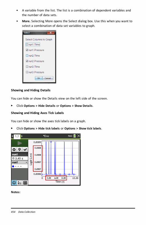
454 Data Collection
• A variable from the list. The list is a combination of dependent variables andthe number of data sets.
• More. Selecting More opens the Select dialog box. Use this when you want toselect a combination of data set variables to graph.
Showing and Hiding Details
You can hide or show the Details view on the left side of the screen.
▶ Click Options > Hide Details or Options > Show Details.
Showing and Hiding Axes Tick Labels
You can hide or show the axes tick labels on a graph.
▶ Click Options > Hide tick labels or Options > Show tick labels.
Notes:
• When a Vernier DataQuest™ application is added to a document, the tick labelswill default to being displayed.
• Tick labels may not be displayed if there is a lack of available space. Minimum andmaximum values will always be displayed.
• Tick labels cannot be edited, but they will recalculate as needed if the minimum ormaximum values are edited or the window settings are changed.
Striking and Restoring DataStriking data omits it temporarily from the Graph view and from the analysis tools.
1. Open the data run that contains the data to be struck.
2. Click Table View .
3. Select the region by dragging from the starting row to the ending point.
The screen scrolls so you can see the selection.
4. Click Data > Strike Data.
5. Select one of the following:
• In Selected Region. Strike the data from the area you selected.• Outside Selected Region. Strike all data except the area you selected.
The selected data is marked as struck in the table and is removed from the graphview.
Restoring Struck Data
1. Select the range of data to restore or if restoring all struck data, start at step two.
2. Click Data > Restore Data.
3. Select one of the following:
• In Selected Region - Restore data in the selected area.• Outside Selected Region - Restore data outside the selected area.• All Data - Restore all data. No data selection necessary.
The data is restored.
Replaying the Data CollectionUse the Replay option to playback the data collection. This option lets you:
• Select the data set you want to replay.
• Pause the playback.
• Advance the playback by one point at a time.
• Adjust the playback rate.
• Repeat the playback.
Data Collection 455
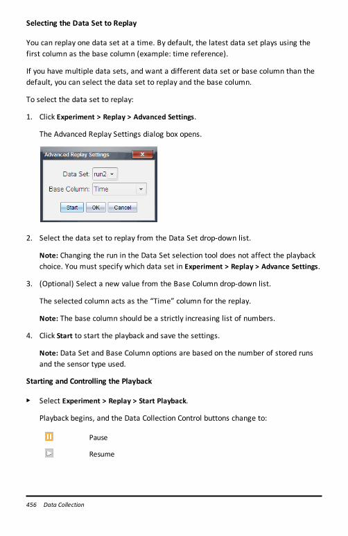
456 Data Collection
Selecting the Data Set to Replay
You can replay one data set at a time. By default, the latest data set plays using thefirst column as the base column (example: time reference).
If you have multiple data sets, and want a different data set or base column than thedefault, you can select the data set to replay and the base column.
To select the data set to replay:
1. Click Experiment > Replay > Advanced Settings.
The Advanced Replay Settings dialog box opens.
2. Select the data set to replay from the Data Set drop-down list.
Note: Changing the run in the Data Set selection tool does not affect the playbackchoice. You must specify which data set in Experiment > Replay > Advance Settings.
3. (Optional) Select a new value from the Base Column drop-down list.
The selected column acts as the “Time” column for the replay.
Note: The base column should be a strictly increasing list of numbers.
4. Click Start to start the playback and save the settings.
Note: Data Set and Base Column options are based on the number of stored runsand the sensor type used.
Starting and Controlling the Playback
▶ Select Experiment > Replay > Start Playback.
Playback begins, and the Data Collection Control buttons change to:
Pause
Resume
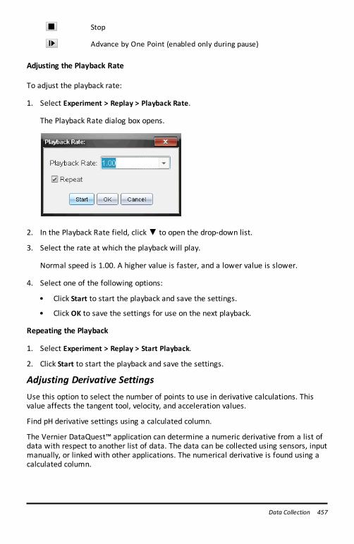
Stop
Advance by One Point (enabled only during pause)
Adjusting the Playback Rate
To adjust the playback rate:
1. Select Experiment > Replay > Playback Rate.
The Playback Rate dialog box opens.
2. In the Playback Rate field, click▼ to open the drop-down list.
3. Select the rate at which the playback will play.
Normal speed is 1.00. A higher value is faster, and a lower value is slower.
4. Select one of the following options:
• Click Start to start the playback and save the settings.
• Click OK to save the settings for use on the next playback.
Repeating the Playback
1. Select Experiment > Replay > Start Playback.
2. Click Start to start the playback and save the settings.
Adjusting Derivative SettingsUse this option to select the number of points to use in derivative calculations. Thisvalue affects the tangent tool, velocity, and acceleration values.
Find pH derivative settings using a calculated column.
The Vernier DataQuest™ application can determine a numeric derivative from a list ofdata with respect to another list of data. The data can be collected using sensors, inputmanually, or linked with other applications. The numerical derivative is found using acalculated column.
Data Collection 457
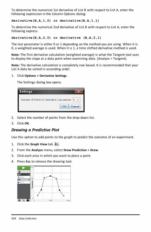
458 Data Collection
To determine the numerical 1st derivative of List B with respect to List A, enter thefollowing expression in the Column Options dialog:
derivative(B,A,1,0) or derivative(B,A,1,1)
To determine the numerical 2nd derivative of List B with respect to List A, enter thefollowing express:
derivative(B,A,2,0) or derivative (B,A,2,1)
The last parameter is either 0 or 1 depending on the method you are using. When it is0, a weighted average is used. When it is 1, a time shifted derivative method is used.
Note: The first derivative calculation (weighted average) is what the Tangent tool usesto display the slope at a data point when examining data. (Analyze > Tangent).
Note: The derivative calculation is completely row based. It is recommended that yourList A data be sorted in ascending order.
1. Click Options > Derivative Settings.
The Settings dialog box opens.
2. Select the number of points from the drop-down list.
3. Click OK.
Drawing a Predictive PlotUse this option to add points to the graph to predict the outcome of an experiment.
1. Click the Graph View tab .
2. From the Analyze menu, select Draw Prediction > Draw.
3. Click each area in which you want to place a point.
4. Press Esc to release the drawing tool.
5. To clear the drawn prediction, click Analyze > Draw Prediction > Clear.
Using Motion MatchUse this option to create a randomly generated plot when creating position-versus-time orvelocity-versus-time graphs.This feature is only available when using a motion detector such as the CBR 2™ sensor orthe Go!Motion® sensor.
Generating a Motion Match Plot
To generate a plot:
1. Attach the motion detector.
2. Click View > Graph.
3. Click Analyze > Motion Match.
4. Select one of the following options:
• New Position Match. Generates a random position plot.• New Velocity Match. Generates a random velocity plot.
Note: Continue selecting a new position or a new velocity match to generate a newrandom plot without removing the existing plot.
Removing a Motion Match Plot
To remove the generated plot:
▶ Click Analyze > Motion Match > Remove Match.
Printing Collected DataYou can only print from the computer. You can print any single displayed active view, orwith the Print All option:
• One data view.
• All of the data views.
• A combination of the data views.
The Print All option has no effect on applications outside of the Vernier DataQuest™application.
Printing Data Views
To print a data view:
1. On the main menu (top of the window), click File > Print.
The Print dialog box opens.
Data Collection 459
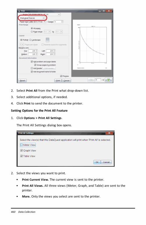
460 Data Collection
2. Select Print All from the Print what drop-down list.
3. Select additional options, if needed.
4. Click Print to send the document to the printer.
Setting Options for the Print All Feature
1. Click Options > Print All Settings.
The Print All Settings dialog box opens.
2. Select the views you want to print.
• Print Current View. The current view is sent to the printer.
• Print All Views. All three views (Meter, Graph, and Table) are sent to theprinter.
• More. Only the views you select are sent to the printer.

3. Click OK.
The Print All Settings are now complete and can be used when printing.
Data Collection 461
462 Widgets
WidgetsAll work that you create and save using TI-Nspire™ applications is stored as adocument, which you can share with others using TI-Nspire™ software, a TI-Nspire™ CXII handheld, or the TI-Nspire™ App for iPad®. You save these TI-Nspire™ documents as.tns files.
A Widget is a .tns document that is stored in your MyWidgets folder.
You can use Widgets to:
• Easily access text files
• Insert and run scripts (such as the pre-loaded widget example: Stopwatch.tns)
• Quickly insert a saved problem into a document
When you add a Widget, TI-Inspire™ CX extracts only the first page of the selected .tnsfile, and inserts it into your open document.
Creating a WidgetA document is regarded as a Widget when it is saved or copied to the designatedMyWidgets folder. The default location is:
• Windows®: My Documents\TI-Nspire\MyWidgets.
• Mac®: Documents/TI-Nspire/MyWidgets.
• Handheld: MyWidgets
• TI-Nspire™ App for iPad® and TI-Nspire™ CAS App for iPad®: MyWidgets
If the MyWidget folder has been inadvertently deleted, you must create it beforeattempting to use a Widget.
Note: When you add a Widget, TI-Inspire™ CX extracts only the first page of theselected .tns file, and inserts it into your open document.
Adding a WidgetAdding a Widget to a New Document
1. Open a new document.
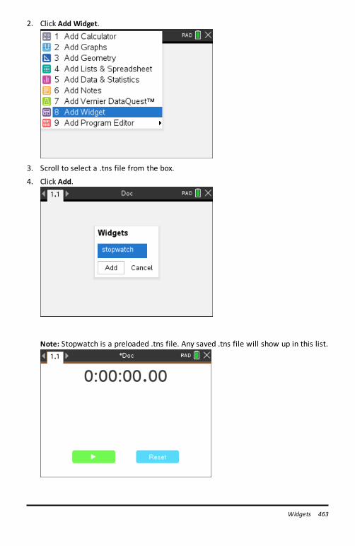
2. Click Add Widget.
3. Scroll to select a .tns file from the box.
4. Click Add.
Note: Stopwatch is a preloaded .tns file. Any saved .tns file will show up in this list.
Widgets 463
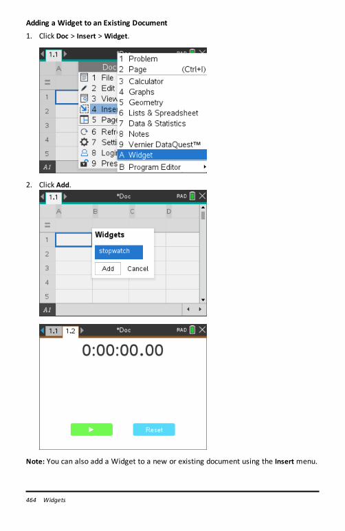
464 Widgets
Adding a Widget to an Existing Document
1. Click Doc > Insert > Widget.
2. Click Add.
Note: You can also add a Widget to a new or existing document using the Insert menu.
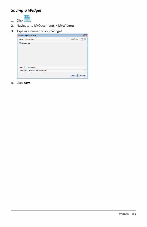
Saving a Widget
1. Click .2. Navigate to MyDocuments > MyWidgets.
3. Type in a name for your Widget.
4. Click Save.
Widgets 465
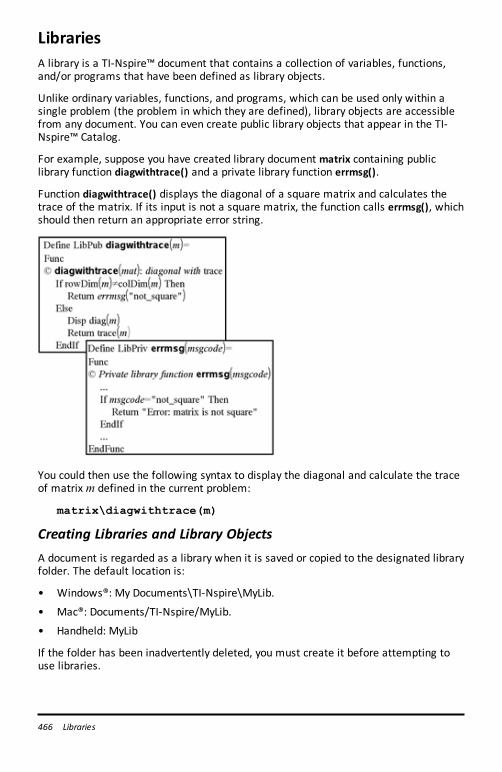
466 Libraries
LibrariesA library is a TI-Nspire™ document that contains a collection of variables, functions,and/or programs that have been defined as library objects.
Unlike ordinary variables, functions, and programs, which can be used only within asingle problem (the problem in which they are defined), library objects are accessiblefrom any document. You can even create public library objects that appear in the TI-Nspire™ Catalog.
For example, suppose you have created library document matrix containing publiclibrary function diagwithtrace() and a private library function errmsg().
Function diagwithtrace() displays the diagonal of a square matrix and calculates thetrace of the matrix. If its input is not a square matrix, the function calls errmsg(), whichshould then return an appropriate error string.
You could then use the following syntax to display the diagonal and calculate the traceof matrix m defined in the current problem:
matrix\diagwithtrace(m)
Creating Libraries and Library ObjectsA document is regarded as a library when it is saved or copied to the designated libraryfolder. The default location is:
• Windows®: My Documents\TI-Nspire\MyLib.
• Mac®: Documents/TI-Nspire/MyLib.
• Handheld: MyLib
If the folder has been inadvertently deleted, you must create it before attempting touse libraries.
You can define library objects using either the Program Editor or the Calculatorapplication. Library objects must be defined with a Define command and must residein the first problem of a library document.
Note: If you use the Program Editor to define a library function or program, you muststore the object and also save the document. Saving the document does notautomatically store the object. For more information, see Programming.
Naming restrictions apply to library documents and library objects.
• A library document name must be a valid variable name between 1 and 16characters long, and it must not contain a period or begin with an underscore.
• A library object name must be a valid variable name between 1 and 15 characterslong. It must not contain a period and must not begin with an underscore.
Private and Public Library ObjectsWhen you define a library object, you designate it as private (LibPriv) or public (LibPub).
Define a=5 a is not a library object.
Define LibPriv b={1,2,3} b is a private library object.
Define LibPub func1(x)=x^2 - 1 func1 is a public library object.
A Private library object does not appear in the Catalog, but you can access it by typingits name. Private objects serve well as building blocks that perform basic, low-leveltasks. Typically, private library objects are called upon by the public functions andprograms.
A Public library object appears in the Catalog’s library tab after you refresh thelibraries. You can access a public library object through the Catalog or by typing itsname.
Mac® only: In version 1.4 of the software, a library document name cannot containextended characters, such as Ö, á, or ñ.
Note: In library programs and functions defined as public, a comment line (©)immediately following the Prgm or Func line is automatically displayed as help in theCatalog. You could, for example, show a syntax reminder there.
Using Short and Long Names
Anytime you are in the same problem where an object is defined, you can access it byentering its short name (the name given in the object’s Define command). This is thecase for all defined objects, including private, public, and non-library objects.
You can access a library object from any document by typing the object’s long name. Along name consists of the name of the object’s library document followed by abackslash “\” followed by the name of the object. For example, the long name of the
Libraries 467
468 Libraries
object defined as func1 in the library document lib1 is lib1\func1. To type the “\”character on the handheld, pressgp.
Note: If you cannot remember the exact name or the order of arguments required for aprivate library object, you can open the library document or use the Program Editor toview the object. You also can use getVarInfo to view a list of objects in a library.
Using Library ObjectsBefore using a library variable, function, or program, make sure that these steps havebeen followed:
• The object has been defined with the Define command, and the commandspecifies either the LibPriv or LibPub attribute.
• The object resides in the first problem of a library document. The document mustreside in the designated library folder and must meet the naming requirements.
• If you defined the object using the Program Editor, it has been stored using CheckSyntax & Store from the Program Editor menu.
• The libraries have been refreshed.
Refreshing the Libraries
▶ Refresh libraries to make the library objects available to your documents.
- From the Tools menu, click Refresh Libraries.
Handheld: Press/b and click Refresh Libraries.
Using a Public Library Object
1. Refresh the libraries.
2. Open the TI-Nspire™ application in which you want to use the variable, function orprogram.
Note: All applications can evaluate functions, but only the Calculator and Notesapplications can run programs.
3. Open the Catalog and use the library tab to find and insert the object.
4. If arguments are required, type them inside the parentheses.
Using a Private Library Object
1. Refresh the libraries.
2. Open the TI-Nspire™ application in which you want to use the variable, function, orprogram.
Note: All applications can evaluate functions, but only the Calculator and Notesapplications can run programs.
3. Type the name of the object, such as lib1\func1().
In case of a function or program, always follow the name with parentheses. Totype the “\” character on the handheld, pressgp.
4. If arguments are required, type them inside the parentheses.
Creating Shortcuts to Library ObjectsYou can make the objects in a library more easily accessible by using libShortcut() tocreate shortcuts to them. This creates a variable group in the current problem thatcontains references to all the objects in the specified library document. You can chooseto include or exclude the private library objects.
For example, suppose the library document linalg contains functions named clearmat,cofactor, gausstep, help, inversestep, kernelbasis, rank, and simultstep. ExecutinglibShortcut(“linalg”,“la”) would create a variable group containing the followingmembers:
la.clearmatla.cofactorla.gausstepla.helpla.inversestepla.kernelbasisla.rankla.simultstep
You can refer to those library objects from within the current problem by typing theirvariable names or by selecting them from the Variables menu.
For more details about using libShortcut(), see the Reference Guide.
Included LibrariesTo help you get started with libraries, the TI-Nspire™ Software installation includes alibrary document with useful Linear Algebra functions. The library is named linalg orlinalgCAS and is installed in the designated library folder.
Note: Updating the handheld’s operating system or reinstalling the computer softwareplaces all included libraries in the default folder. If you have edited an object in anincluded library or replaced an included library with your own document of the samename, updating or reinstalling will overwrite your changes. This could also happenafter batteries are replaced or the handheld system is reset.
Restoring an Included LibraryIf you inadvertently delete or overwrite an included library, you can restore it from theinstallation DVD.
1. Open the DVD, and navigate to the libs folder.
2. Identify the library file to restore, such as linalg.tns or linalgCAS.tns for the linearalgebra library.
3. Copy the file.
- Windows®: Copy the file to your designated library folder. The default locationis My Documents\TI-Nspire\MyLib.
Libraries 469
470 Libraries
- Mac®: Copy the file to your designated library folder. The default location isDocuments/TI-Nspire/MyLib.
- Handheld: Connect the handheld to your computer, open the TI-Nspire™software, and copy the library file to the handheld’s MyLib folder.
4. Activate the new library objects.
- From the TI-Nspire™ Software Tools menu, click Refresh Libraries.
Handheld: Press/b, and click Refresh Libraries.
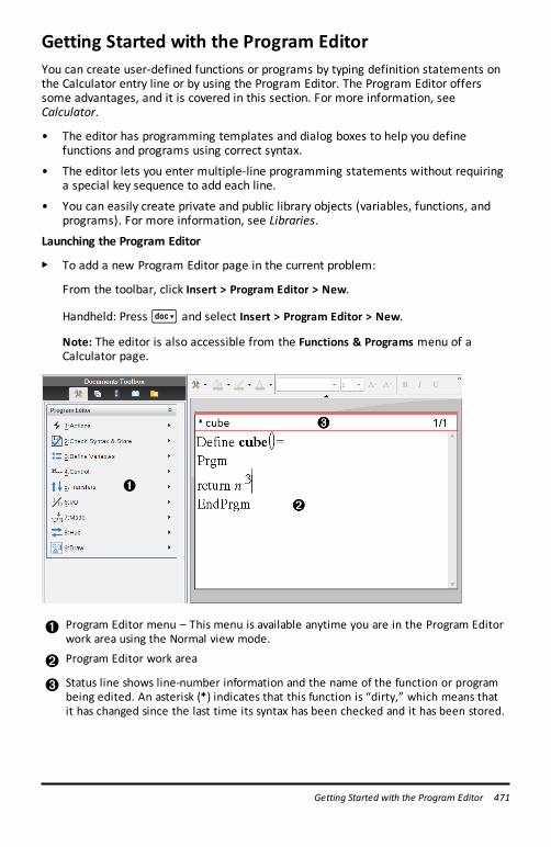
Getting Started with the Program EditorYou can create user-defined functions or programs by typing definition statements onthe Calculator entry line or by using the Program Editor. The Program Editor offerssome advantages, and it is covered in this section. For more information, seeCalculator.
• The editor has programming templates and dialog boxes to help you definefunctions and programs using correct syntax.
• The editor lets you enter multiple-line programming statements without requiringa special key sequence to add each line.
• You can easily create private and public library objects (variables, functions, andprograms). For more information, see Libraries.
Launching the Program Editor
▶ To add a new Program Editor page in the current problem:
From the toolbar, click Insert > Program Editor > New.
Handheld: Press~ and select Insert > Program Editor > New.
Note: The editor is also accessible from the Functions & Programs menu of aCalculator page.
À Program Editor menu – This menu is available anytime you are in the Program Editorwork area using the Normal view mode.
Á Program Editor work area
 Status line shows line-number information and the name of the function or programbeing edited. An asterisk (*) indicates that this function is “dirty,” which means thatit has changed since the last time its syntax has been checked and it has been stored.
Getting Started with the Program Editor 471
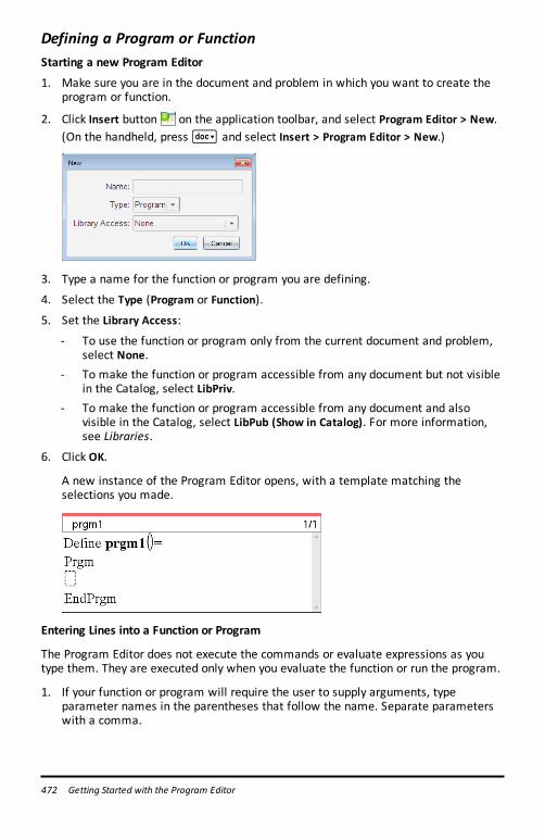
472 Getting Started with the Program Editor
Defining a Program or FunctionStarting a new Program Editor
1. Make sure you are in the document and problem in which you want to create theprogram or function.
2. Click Insert button on the application toolbar, and select Program Editor > New.(On the handheld, press~ and select Insert > Program Editor > New.)
3. Type a name for the function or program you are defining.
4. Select the Type (Program or Function).
5. Set the Library Access:
- To use the function or program only from the current document and problem,select None.
- To make the function or program accessible from any document but not visiblein the Catalog, select LibPriv.
- To make the function or program accessible from any document and alsovisible in the Catalog, select LibPub (Show in Catalog). For more information,see Libraries.
6. Click OK.
A new instance of the Program Editor opens, with a template matching theselections you made.
Entering Lines into a Function or Program
The Program Editor does not execute the commands or evaluate expressions as youtype them. They are executed only when you evaluate the function or run the program.
1. If your function or program will require the user to supply arguments, typeparameter names in the parentheses that follow the name. Separate parameterswith a comma.
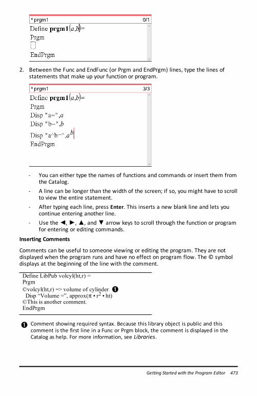
2. Between the Func and EndFunc (or Prgm and EndPrgm) lines, type the lines ofstatements that make up your function or program.
- You can either type the names of functions and commands or insert them fromthe Catalog.
- A line can be longer than the width of the screen; if so, you might have to scrollto view the entire statement.
- After typing each line, press Enter. This inserts a new blank line and lets youcontinue entering another line.
- Use the◄,►,▲, and▼ arrow keys to scroll through the function or programfor entering or editing commands.
Inserting Comments
Comments can be useful to someone viewing or editing the program. They are notdisplayed when the program runs and have no effect on program flow. The © symboldisplays at the beginning of the line with the comment.
Define LibPub volcyl(ht,r) =Prgm©volcyl(ht,r) => volume of cylinder À Disp “Volume =”, approx(p ¦ r2 ¦ ht)©This is another comment.EndPrgm
À Comment showing required syntax. Because this library object is public and thiscomment is the first line in a Func or Prgm block, the comment is displayed in theCatalog as help. For more information, see Libraries.
Getting Started with the Program Editor 473
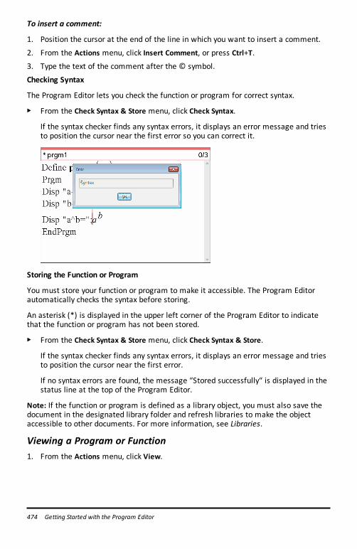
474 Getting Started with the Program Editor
To insert a comment:
1. Position the cursor at the end of the line in which you want to insert a comment.
2. From the Actions menu, click Insert Comment, or press Ctrl+T.
3. Type the text of the comment after the © symbol.
Checking Syntax
The Program Editor lets you check the function or program for correct syntax.
▶ From the Check Syntax & Store menu, click Check Syntax.
If the syntax checker finds any syntax errors, it displays an error message and triesto position the cursor near the first error so you can correct it.
Storing the Function or Program
You must store your function or program to make it accessible. The Program Editorautomatically checks the syntax before storing.
An asterisk (*) is displayed in the upper left corner of the Program Editor to indicatethat the function or program has not been stored.
▶ From the Check Syntax & Store menu, click Check Syntax & Store.
If the syntax checker finds any syntax errors, it displays an error message and triesto position the cursor near the first error.
If no syntax errors are found, the message “Stored successfully“ is displayed in thestatus line at the top of the Program Editor.
Note: If the function or program is defined as a library object, you must also save thedocument in the designated library folder and refresh libraries to make the objectaccessible to other documents. For more information, see Libraries.
Viewing a Program or Function1. From the Actions menu, click View.
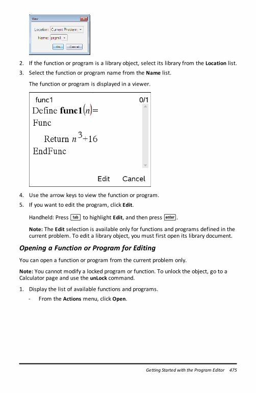
2. If the function or program is a library object, select its library from the Location list.
3. Select the function or program name from the Name list.
The function or program is displayed in a viewer.
4. Use the arrow keys to view the function or program.
5. If you want to edit the program, click Edit.
Handheld: Presse to highlight Edit, and then press·.
Note: The Edit selection is available only for functions and programs defined in thecurrent problem. To edit a library object, you must first open its library document.
Opening a Function or Program for EditingYou can open a function or program from the current problem only.
Note: You cannot modify a locked program or function. To unlock the object, go to aCalculator page and use the unLock command.
1. Display the list of available functions and programs.
- From the Actions menu, click Open.
Getting Started with the Program Editor 475
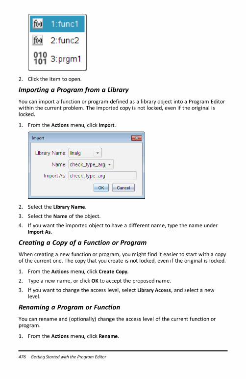
476 Getting Started with the Program Editor
2. Click the item to open.
Importing a Program from a LibraryYou can import a function or program defined as a library object into a Program Editorwithin the current problem. The imported copy is not locked, even if the original islocked.
1. From the Actions menu, click Import.
2. Select the Library Name.
3. Select the Name of the object.
4. If you want the imported object to have a different name, type the name underImport As.
Creating a Copy of a Function or ProgramWhen creating a new function or program, you might find it easier to start with a copyof the current one. The copy that you create is not locked, even if the original is locked.
1. From the Actions menu, click Create Copy.
2. Type a new name, or click OK to accept the proposed name.
3. If you want to change the access level, select Library Access, and select a newlevel.
Renaming a Program or FunctionYou can rename and (optionally) change the access level of the current function orprogram.
1. From the Actions menu, click Rename.
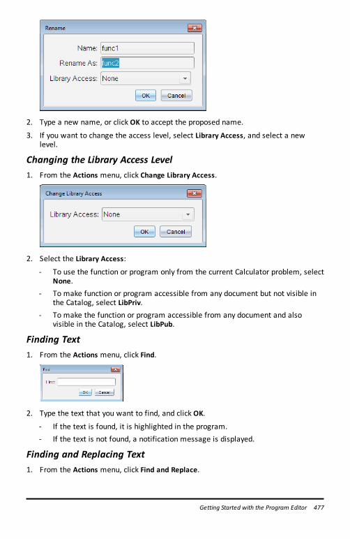
2. Type a new name, or click OK to accept the proposed name.
3. If you want to change the access level, select Library Access, and select a newlevel.
Changing the Library Access Level1. From the Actions menu, click Change Library Access.
2. Select the Library Access:
- To use the function or program only from the current Calculator problem, selectNone.
- To make function or program accessible from any document but not visible inthe Catalog, select LibPriv.
- To make the function or program accessible from any document and alsovisible in the Catalog, select LibPub.
Finding Text1. From the Actions menu, click Find.
2. Type the text that you want to find, and click OK.
- If the text is found, it is highlighted in the program.- If the text is not found, a notification message is displayed.
Finding and Replacing Text1. From the Actions menu, click Find and Replace.
Getting Started with the Program Editor 477
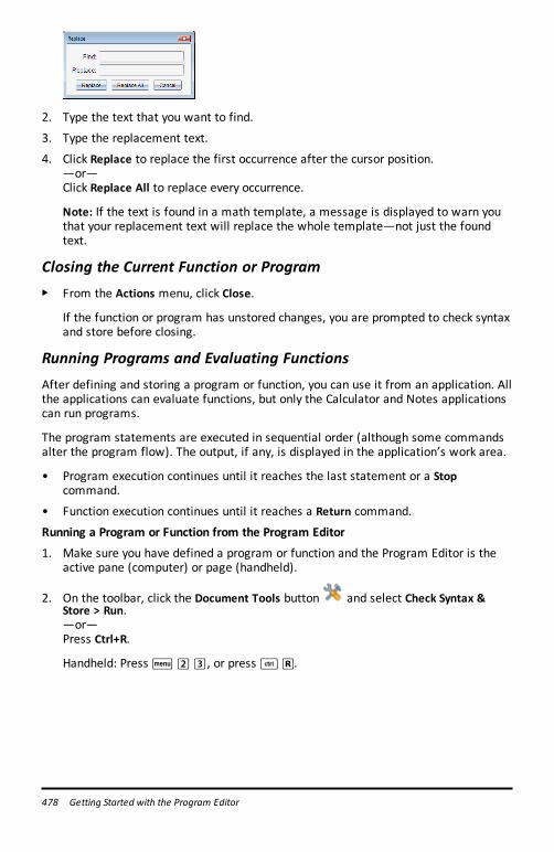
478 Getting Started with the Program Editor
2. Type the text that you want to find.
3. Type the replacement text.
4. Click Replace to replace the first occurrence after the cursor position.—or—Click Replace All to replace every occurrence.
Note: If the text is found in a math template, a message is displayed to warn youthat your replacement text will replace the whole template—not just the foundtext.
Closing the Current Function or Program▶ From the Actions menu, click Close.
If the function or program has unstored changes, you are prompted to check syntaxand store before closing.
Running Programs and Evaluating FunctionsAfter defining and storing a program or function, you can use it from an application. Allthe applications can evaluate functions, but only the Calculator and Notes applicationscan run programs.
The program statements are executed in sequential order (although some commandsalter the program flow). The output, if any, is displayed in the application’s work area.
• Program execution continues until it reaches the last statement or a Stopcommand.
• Function execution continues until it reaches a Return command.
Running a Program or Function from the Program Editor
1. Make sure you have defined a program or function and the Program Editor is theactive pane (computer) or page (handheld).
2. On the toolbar, click the Document Tools button and select Check Syntax &Store > Run.—or—Press Ctrl+R.
Handheld: Pressb23, or press/R.
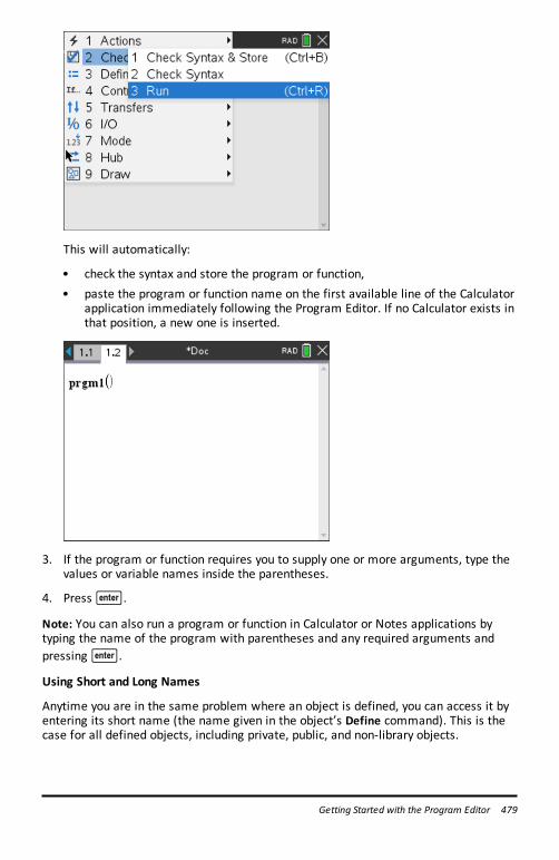
This will automatically:
• check the syntax and store the program or function,• paste the program or function name on the first available line of the Calculator
application immediately following the Program Editor. If no Calculator exists inthat position, a new one is inserted.
3. If the program or function requires you to supply one or more arguments, type thevalues or variable names inside the parentheses.
4. Press·.
Note: You can also run a program or function in Calculator or Notes applications bytyping the name of the program with parentheses and any required arguments andpressing·.
Using Short and Long Names
Anytime you are in the same problem where an object is defined, you can access it byentering its short name (the name given in the object’s Define command). This is thecase for all defined objects, including private, public, and non-library objects.
Getting Started with the Program Editor 479
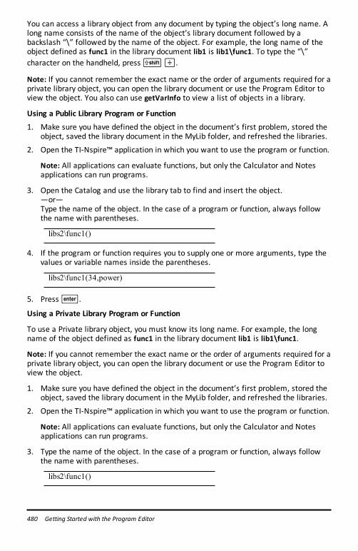
480 Getting Started with the Program Editor
You can access a library object from any document by typing the object’s long name. Along name consists of the name of the object’s library document followed by abackslash “\” followed by the name of the object. For example, the long name of theobject defined as func1 in the library document lib1 is lib1\func1. To type the “\”character on the handheld, pressgp.
Note: If you cannot remember the exact name or the order of arguments required for aprivate library object, you can open the library document or use the Program Editor toview the object. You also can use getVarInfo to view a list of objects in a library.
Using a Public Library Program or Function
1. Make sure you have defined the object in the document’s first problem, stored theobject, saved the library document in the MyLib folder, and refreshed the libraries.
2. Open the TI-Nspire™ application in which you want to use the program or function.
Note: All applications can evaluate functions, but only the Calculator and Notesapplications can run programs.
3. Open the Catalog and use the library tab to find and insert the object.—or—Type the name of the object. In the case of a program or function, always followthe name with parentheses.
libs2\func1()
4. If the program or function requires you to supply one or more arguments, type thevalues or variable names inside the parentheses.
libs2\func1(34,power)
5. Press·.
Using a Private Library Program or Function
To use a Private library object, you must know its long name. For example, the longname of the object defined as func1 in the library document lib1 is lib1\func1.
Note: If you cannot remember the exact name or the order of arguments required for aprivate library object, you can open the library document or use the Program Editor toview the object.
1. Make sure you have defined the object in the document’s first problem, stored theobject, saved the library document in the MyLib folder, and refreshed the libraries.
2. Open the TI-Nspire™ application in which you want to use the program or function.
Note: All applications can evaluate functions, but only the Calculator and Notesapplications can run programs.
3. Type the name of the object. In the case of a program or function, always followthe name with parentheses.
libs2\func1()
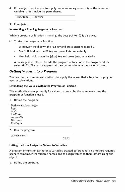
4. If the object requires you to supply one or more arguments, type the values orvariable names inside the parentheses.
libs2\func1(34,power)
5. Press·.
Interrupting a Running Program or Function
While a program or function is running, the busy pointer} is displayed.
▶ To stop the program or function,
- Windows®: Hold down the F12 key and press Enter repeatedly.- Mac®: Hold down the F5 key and press Enter repeatedly.
- Handheld: Hold down thec key and press· repeatedly.
A message is displayed. To edit the program or function in the Program Editor,select Go To. The cursor appears at the command where the break occurred.
Getting Values into a ProgramYou can choose from several methods to supply the values that a function or programuses in calculations.
Embedding the Values Within the Program or Function
This method is useful primarily for values that must be the same each time theprogram or function is used.
1. Define the program.
Define calculatearea()=Prgmw:=3h:=23.64area:=w*hDisp areaEndPrgm
2. Run the program.
calculatearea()70.92
Letting the User Assign the Values to Variables
A program or function can refer to variables created beforehand. This method requiresusers to remember the variable names and to assign values to them before using theobject.
1. Define the program.
Getting Started with the Program Editor 481
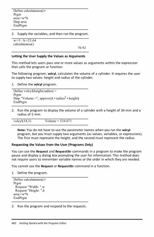
482 Getting Started with the Program Editor
Define calculatearea()=Prgmarea:=w*hDisp areaEndPrgm
2. Supply the variables, and then run the program.
w:=3 : h:=23.64calculatearea()
70.92
Letting the User Supply the Values as Arguments
This method lets users pass one or more values as arguments within the expressionthat calls the program or function.
The following program, volcyl, calculates the volume of a cylinder. It requires the userto supply two values: height and radius of the cylinder.
1. Define the volcyl program.
Define volcyl(height,radius) =PrgmDisp "Volume =", approx(p ¦ radius2 ¦ height)EndPrgm
2. Run the program to display the volume of a cylinder with a height of 34 mm and aradius of 5 mm.
volcyl(34,5) Volume = 534.071
Note: You do not have to use the parameter names when you run the volcylprogram, but you must supply two arguments (as values, variables, or expressions).The first must represent the height, and the second must represent the radius.
Requesting the Values from the User (Programs Only)
You can use the Request and RequestStr commands in a program to make the programpause and display a dialog box prompting the user for information. This method doesnot require users to remember variable names or the order in which they are needed.
You cannot use the Request or RequestStr command in a function.
1. Define the program.
Define calculatearea()=PrgmRequest "Width: ",wRequest "Height: ",harea:=w*hEndPrgm
2. Run the program and respond to the requests.
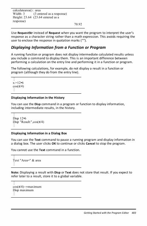
calculatearea() : area Width: 3 (3 entered as a response)Height: 23.64 (23.64 entered as aresponse)
70.92
Use RequestStr instead of Request when you want the program to interpret the user’sresponse as a character string rather than a math expression. This avoids requiring theuser to enclose the response in quotation marks (““).
Displaying Information from a Function or ProgramA running function or program does not display intermediate calculated results unlessyou include a command to display them. This is an important difference betweenperforming a calculation on the entry line and performing it in a function or program.
The following calculations, for example, do not display a result in a function orprogram (although they do from the entry line).
©x:=12•6cos(π/4)©
Displaying Information in the History
You can use the Disp command in a program or function to display information,including intermediate results, in the history.
©Disp 12•6Disp "Result:",cos(π/4)©
Displaying Information in a Dialog Box
You can use the Text command to pause a running program and display information ina dialog box. The user clicks OK to continue or clicks Cancel to stop the program.
You cannot use the Text command in a function.
©Text "Area=" & area©
Note: Displaying a result with Disp or Text does not store that result. If you expect torefer later to a result, store it to a global variable.
©cos(π/4)→maximumDisp maximum©
Getting Started with the Program Editor 483
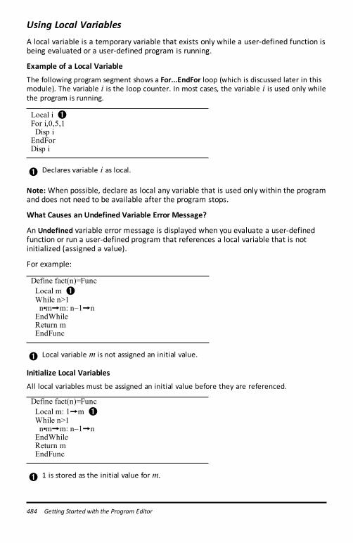
484 Getting Started with the Program Editor
Using Local VariablesA local variable is a temporary variable that exists only while a user-defined function isbeing evaluated or a user-defined program is running.
Example of a Local Variable
The following program segment shows a For...EndFor loop (which is discussed later in thismodule). The variable i is the loop counter. In most cases, the variable i is used only whilethe program is running.
Local i ÀFor i,0,5,1 Disp iEndForDisp i
À Declares variable i as local.
Note: When possible, declare as local any variable that is used only within the programand does not need to be available after the program stops.
What Causes an Undefined Variable Error Message?
An Undefined variable error message is displayed when you evaluate a user-definedfunction or run a user-defined program that references a local variable that is notinitialized (assigned a value).
For example:
Define fact(n)=Func Local m À While n>1 n¦m&m: n–1&n EndWhile Return mEndFunc
À Local variable m is not assigned an initial value.
Initialize Local Variables
All local variables must be assigned an initial value before they are referenced.
Define fact(n)=Func Local m: 1&m À While n>1 n¦m&m: n–1&n EndWhile Return m EndFunc
À 1 is stored as the initial value for m.
Note (CAS): Functions and programs cannot use a local variable to perform symboliccalculations.
CAS: Performing Symbolic Calculations
If you want a function or program to perform symbolic calculations, you must use aglobal variable instead of a local. However, you must be certain that the global variabledoes not already exist outside of the program. The following methods can help.
• Refer to a global variable name, typically with two or more characters, that is notlikely to exist outside of the function or program.
• Include DelVar within a program to delete the global variable, if it exists, beforereferring to it. (DelVar does not delete locked or linked variables.)
Differences Between Functions and ProgramsA function defined in the Program Editor is similar to the functions built into the TI-Nspire™ Software.
• Functions must return a result, which can be graphed or entered in a table.Programs do not return a result.
• You can use a function (but not a program) within an expression. For example: 3 ¦func1(3) is valid, but not 3 ¦ prog1(3).
• You can run programs from Calculator and Notes applications only. However, youcan evaluate functions in Calculator, Notes, Lists & Spreadsheet, Graphs &Geometry, and Data & Statistics.
• A function can refer to any variable; however, it can store a value to a local variableonly. Programs can store to local and global variables.
Note: Arguments used to pass values to a function are treated as local variablesautomatically. If you want to store to any other variables, you must declare themas Local from within the function.
• A function cannot call a program as a subroutine, but it can call another user-defined function.
• You cannot define a program within a function.
• A function cannot define a global function, but it can define a local function.
Calling One Program from AnotherOne program can call another program as a subroutine. The subroutine can be external(a separate program) or internal (included in the main program). Subroutines areuseful when a program needs to repeat the same group of commands at severaldifferent places.
Calling a Separate Program
To call a separate program, use the same syntax that you use to run the program fromthe entry line.
Getting Started with the Program Editor 485
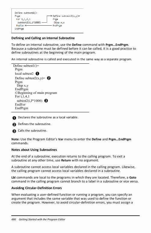
486 Getting Started with the Program Editor
Defining and Calling an Internal Subroutine
To define an internal subroutine, use the Define command with Prgm...EndPrgm.Because a subroutine must be defined before it can be called, it is a good practice todefine subroutines at the beginning of the main program.
An internal subroutine is called and executed in the same way as a separate program.
Define subtest1()= Prgm local subtest2 À Define subtest2(x,y)= Á Prgm Disp x,y EndPrgm ©Beginning of main program For i,1,4,1 subtest2(i,I*1000) Â EndFor EndPrgm
À Declares the subroutine as a local variable.
Á Defines the subroutine.
 Calls the subroutine.
Note: Use the Program Editor’s Var menu to enter the Define and Prgm...EndPrgmcommands.
Notes about Using Subroutines
At the end of a subroutine, execution returns to the calling program. To exit asubroutine at any other time, use Return with no argument.
A subroutine cannot access local variables declared in the calling program. Likewise,the calling program cannot access local variables declared in a subroutine.
Lbl commands are local to the programs in which they are located. Therefore, a Gotocommand in the calling program cannot branch to a label in a subroutine or vice versa.
Avoiding Circular-Definition Errors
When evaluating a user-defined function or running a program, you can specify anargument that includes the same variable that was used to define the function orcreate the program. However, to avoid circular-definition errors, you must assign a
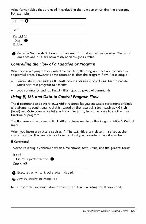
value for variables that are used in evaluating the function or running the program.For example:
x+1&x À
– or –
For i,i,10,1 Disp i ÀEndFor
À Causes a Circular definition error message if x or i does not have a value. The errordoes not occur if x or i has already been assigned a value.
Controlling the Flow of a Function or ProgramWhen you run a program or evaluate a function, the program lines are executed insequential order. However, some commands alter the program flow. For example:
• Control structures such as If...EndIf commands use a conditional test to decidewhich part of a program to execute.
• Loop commands such as For...EndFor repeat a group of commands.
Using If, Lbl, and Goto to Control Program FlowThe If command and several If...EndIf structures let you execute a statement or blockof statements conditionally, that is, based on the result of a test (such as x>5). Lbl(label) and Goto commands let you branch, or jump, from one place to another in afunction or program.
The If command and several If...EndIf structures reside on the Program Editor’s Controlmenu.
When you insert a structure such as If...Then...EndIf, a template is inserted at thecursor location. The cursor is positioned so that you can enter a conditional test.
If Command
To execute a single command when a conditional test is true, use the general form:
If x>5 Disp "x is greater than 5" ÀDisp x Á
À Executed only if x>5; otherwise, skipped.
Á Always displays the value of x.
In this example, you must store a value to x before executing the If command.
Getting Started with the Program Editor 487
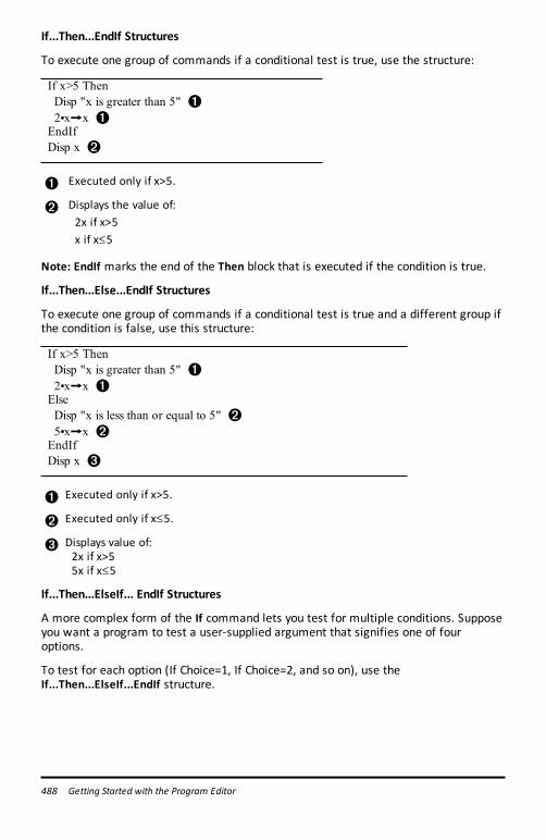
488 Getting Started with the Program Editor
If...Then...EndIf Structures
To execute one group of commands if a conditional test is true, use the structure:
If x>5 Then Disp "x is greater than 5" À 2¦x&x ÀEndIfDisp x Á
À Executed only if x>5.
Á Displays the value of: 2x if x>5 x if x{5
Note: EndIf marks the end of the Then block that is executed if the condition is true.
If...Then...Else...EndIf Structures
To execute one group of commands if a conditional test is true and a different group ifthe condition is false, use this structure:
If x>5 Then Disp "x is greater than 5" À 2¦x&x ÀElse Disp "x is less than or equal to 5" Á 5¦x&x ÁEndIfDisp x Â
À Executed only if x>5.
Á Executed only if x{5.
 Displays value of: 2x if x>5 5x if x{5
If...Then...ElseIf... EndIf Structures
A more complex form of the If command lets you test for multiple conditions. Supposeyou want a program to test a user-supplied argument that signifies one of fouroptions.
To test for each option (If Choice=1, If Choice=2, and so on), use theIf...Then...ElseIf...EndIf structure.
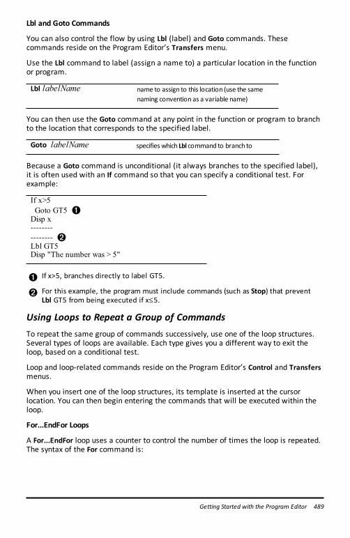
Lbl and Goto Commands
You can also control the flow by using Lbl (label) and Goto commands. Thesecommands reside on the Program Editor’s Transfers menu.
Use the Lbl command to label (assign a name to) a particular location in the functionor program.
Lbl labelName name to assign to this location (use the samenaming convention as a variable name)
You can then use the Goto command at any point in the function or program to branchto the location that corresponds to the specified label.
Goto labelName specifies which Lbl command to branch to
Because a Goto command is unconditional (it always branches to the specified label),it is often used with an If command so that you can specify a conditional test. Forexample:
If x>5 Goto GT5 ÀDisp x---------------- ÁLbl GT5Disp "The number was > 5"
À If x>5, branches directly to label GT5.
Á For this example, the program must include commands (such as Stop) that preventLbl GT5 from being executed if x{5.
Using Loops to Repeat a Group of CommandsTo repeat the same group of commands successively, use one of the loop structures.Several types of loops are available. Each type gives you a different way to exit theloop, based on a conditional test.
Loop and loop-related commands reside on the Program Editor’s Control and Transfersmenus.
When you insert one of the loop structures, its template is inserted at the cursorlocation. You can then begin entering the commands that will be executed within theloop.
For...EndFor Loops
A For...EndFor loop uses a counter to control the number of times the loop is repeated.The syntax of the For command is:
Getting Started with the Program Editor 489
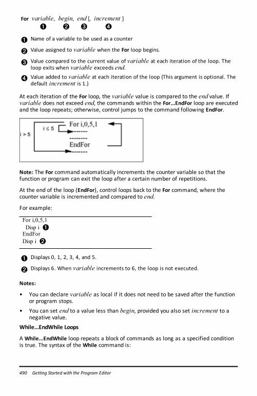
490 Getting Started with the Program Editor
For variable,À
begin,Á
end [,Â
increment ]Ã
À Name of a variable to be used as a counter
Á Value assigned to variable when the For loop begins.
 Value compared to the current value of variable at each iteration of the loop. Theloop exits when variable exceeds end.
à Value added to variable at each iteration of the loop (This argument is optional. Thedefault increment is 1.)
At each iteration of the For loop, the variable value is compared to the end value. Ifvariable does not exceed end, the commands within the For...EndFor loop are executedand the loop repeats; otherwise, control jumps to the command following EndFor.
Note: The For command automatically increments the counter variable so that thefunction or program can exit the loop after a certain number of repetitions.
At the end of the loop (EndFor), control loops back to the For command, where thecounter variable is incremented and compared to end.
For example:
For i,0,5,1 Disp i ÀEndForDisp i Á
À Displays 0, 1, 2, 3, 4, and 5.
Á Displays 6. When variable increments to 6, the loop is not executed.
Notes:
• You can declare variable as local if it does not need to be saved after the functionor program stops.
• You can set end to a value less than begin, provided you also set increment to anegative value.
While...EndWhile Loops
A While...EndWhile loop repeats a block of commands as long as a specified conditionis true. The syntax of the While command is:

While condition
WhenWhile is executed, condition is evaluated. If condition is true, the loop isexecuted; otherwise, control jumps to the command following EndWhile.
Note: The While command does not automatically change the condition. You mustinclude commands that allow the function or program to exit the loop.
At the end of the loop (EndWhile), control jumps back to the While command, wherecondition is re-evaluated.
To execute the loop the first time, the condition must initially be true.
• Any variables referenced in the condition must be set before the While command.(You can build the values into the function or program, or you can prompt the userto enter the values.)
• The loop must contain commands that change the values in the condition,eventually causing it to be false. Otherwise, the condition is always true and thefunction or program cannot exit the loop (called an infinite loop).
For example:
0&x ÀWhile x<5 Disp x Á x+1&x ÂEndWhileDisp x Ã
À Initially sets x.
Á Displays 0, 1, 2, 3, and 4.
 Increments x.
à Displays 5. When x increments to 5, the loop is not executed.
Loop...EndLoop Loops
A Loop...EndLoop creates an infinite loop, which is repeated endlessly. The Loopcommand does not have any arguments.
Getting Started with the Program Editor 491
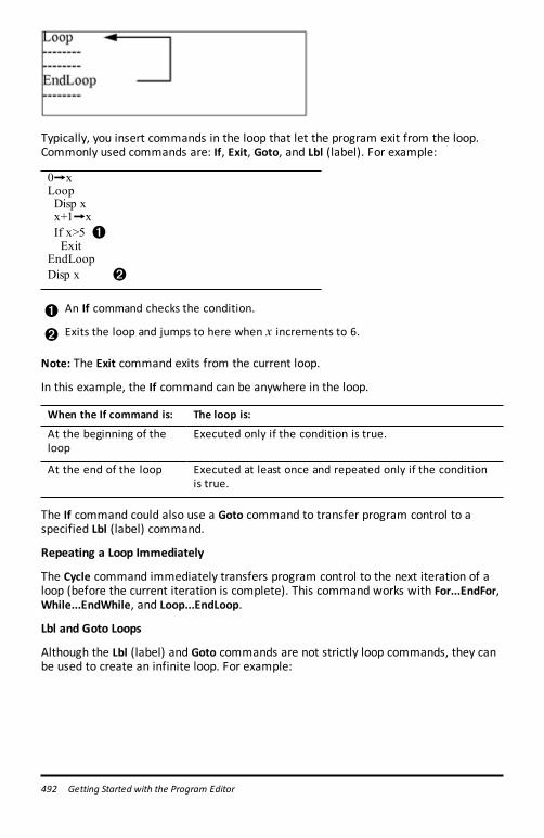
492 Getting Started with the Program Editor
Typically, you insert commands in the loop that let the program exit from the loop.Commonly used commands are: If, Exit, Goto, and Lbl (label). For example:
0&xLoop Disp x x+1&x If x>5 À ExitEndLoopDisp x Á
À An If command checks the condition.
Á Exits the loop and jumps to here when x increments to 6.
Note: The Exit command exits from the current loop.
In this example, the If command can be anywhere in the loop.
When the If command is: The loop is:
At the beginning of theloop
Executed only if the condition is true.
At the end of the loop Executed at least once and repeated only if the conditionis true.
The If command could also use a Goto command to transfer program control to aspecified Lbl (label) command.
Repeating a Loop Immediately
The Cycle command immediately transfers program control to the next iteration of aloop (before the current iteration is complete). This command works with For...EndFor,While...EndWhile, and Loop...EndLoop.
Lbl and Goto Loops
Although the Lbl (label) and Goto commands are not strictly loop commands, they canbe used to create an infinite loop. For example:
As with Loop...EndLoop, the loop should contain commands that let the function orprogram exit from the loop.
Changing Mode SettingsFunctions and programs can use the setMode() function to temporarily set specificcalculation or result modes. The Program Editor’s Mode menu makes it easy to enterthe correct syntax without requiring you to memorize numeric codes.
Note: Mode changes made within a function or program definition do not persistoutside the function or program.
Setting a Mode
1. Position the cursor where you want to insert the setMode function.
2. From the Mode menu, click the mode to change, and click the new setting.
The correct syntax is inserted at the cursor location. For example:
setMode(1,3)
Debugging Programs and Handling ErrorsAfter you write a function or program, you can use several techniques to find andcorrect errors. You can also build an error-handling command into the function orprogram itself.
If your function or program allows the user to select from several options, be sure torun it and test each option.
Techniques for Debugging
Run-time error messages can locate syntax errors but not errors in program logic. Thefollowing techniques may be useful.
• Temporarily insert Disp commands to display the values of critical variables.
• To confirm that a loop is executed the correct number of times, use Disp to displaythe counter variable or the values in the conditional test.
• To confirm that a subroutine is executed, use Disp to display messages such as“Entering subroutine” and “Exiting subroutine” at the beginning and end of thesubroutine.
• To stop a program or function manually,
- Windows®: Hold down the F12 key and press Enter repeatedly.- Mac®: Hold down the F5 key and press Enter repeatedly.
Getting Started with the Program Editor 493
494 Getting Started with the Program Editor
- Handheld: Hold down thec key and press· repeatedly.
Error-handling Commands
Command Description
Try...EndTry Defines a block that lets a function or program execute a commandand, if necessary, recover from an error generated by that command.
ClrErr Clears the error status and sets system variable errCode to zero. For anexample of using errCode, see the Try command in the ReferenceGuide.
PassErr Passes an error to the next level of the Try...EndTry block.
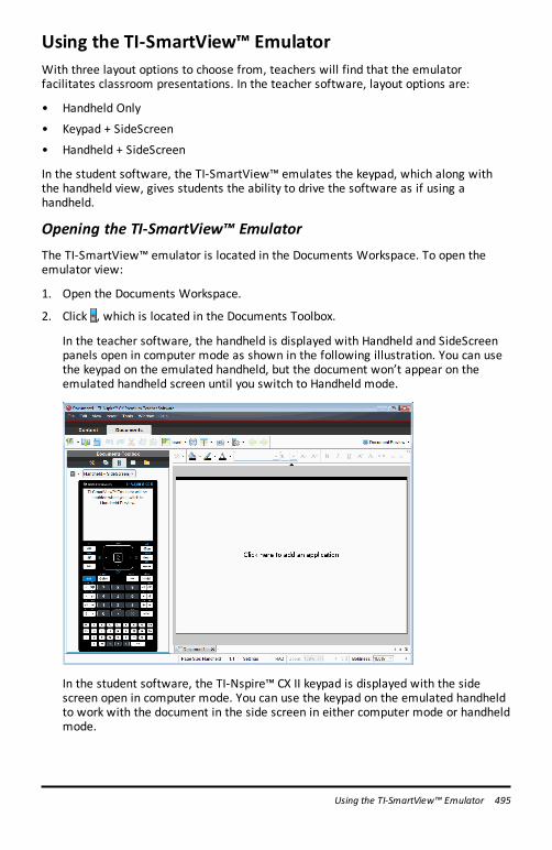
Using the TI-SmartView™ EmulatorWith three layout options to choose from, teachers will find that the emulatorfacilitates classroom presentations. In the teacher software, layout options are:
• Handheld Only
• Keypad + SideScreen
• Handheld + SideScreen
In the student software, the TI-SmartView™ emulates the keypad, which along withthe handheld view, gives students the ability to drive the software as if using ahandheld.
Opening the TI-SmartView™ EmulatorThe TI-SmartView™ emulator is located in the Documents Workspace. To open theemulator view:
1. Open the Documents Workspace.
2. Click , which is located in the Documents Toolbox.
In the teacher software, the handheld is displayed with Handheld and SideScreenpanels open in computer mode as shown in the following illustration. You can usethe keypad on the emulated handheld, but the document won’t appear on theemulated handheld screen until you switch to Handheld mode.
In the student software, the TI-Nspire™ CX II keypad is displayed with the sidescreen open in computer mode. You can use the keypad on the emulated handheldto work with the document in the side screen in either computer mode or handheldmode.
Using the TI-SmartView™ Emulator 495
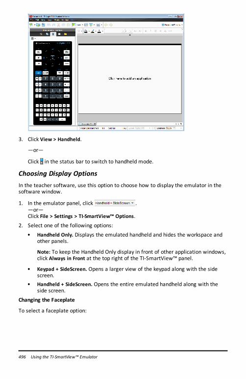
496 Using the TI-SmartView™ Emulator
3. Click View > Handheld.
—or—
Click in the status bar to switch to handheld mode.
Choosing Display OptionsIn the teacher software, use this option to choose how to display the emulator in thesoftware window.
1. In the emulator panel, click .—or—Click File > Settings > TI-SmartView™ Options.
2. Select one of the following options:
• Handheld Only. Displays the emulated handheld and hides the workspace andother panels.
Note: To keep the Handheld Only display in front of other application windows,click Always in Front at the top right of the TI-SmartView™ panel.
• Keypad + SideScreen. Opens a larger view of the keypad along with the sidescreen.
• Handheld + SideScreen. Opens the entire emulated handheld along with theside screen.
Changing the Faceplate
To select a faceplate option:
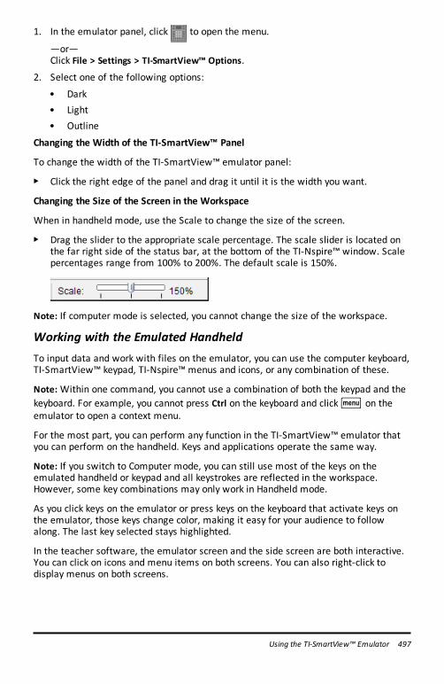
1. In the emulator panel, click to open the menu.
—or—Click File > Settings > TI-SmartView™ Options.
2. Select one of the following options:
• Dark• Light• Outline
Changing the Width of the TI-SmartView™ Panel
To change the width of the TI-SmartView™ emulator panel:
▶ Click the right edge of the panel and drag it until it is the width you want.
Changing the Size of the Screen in the Workspace
When in handheld mode, use the Scale to change the size of the screen.
▶ Drag the slider to the appropriate scale percentage. The scale slider is located onthe far right side of the status bar, at the bottom of the TI-Nspire™ window. Scalepercentages range from 100% to 200%. The default scale is 150%.
Note: If computer mode is selected, you cannot change the size of the workspace.
Working with the Emulated HandheldTo input data and work with files on the emulator, you can use the computer keyboard,TI-SmartView™ keypad, TI-Nspire™ menus and icons, or any combination of these.
Note: Within one command, you cannot use a combination of both the keypad and thekeyboard. For example, you cannot press Ctrl on the keyboard and clickb on theemulator to open a context menu.
For the most part, you can perform any function in the TI-SmartView™ emulator thatyou can perform on the handheld. Keys and applications operate the same way.
Note: If you switch to Computer mode, you can still use most of the keys on theemulated handheld or keypad and all keystrokes are reflected in the workspace.However, some key combinations may only work in Handheld mode.
As you click keys on the emulator or press keys on the keyboard that activate keys onthe emulator, those keys change color, making it easy for your audience to followalong. The last key selected stays highlighted.
In the teacher software, the emulator screen and the side screen are both interactive.You can click on icons and menu items on both screens. You can also right-click todisplay menus on both screens.
Using the TI-SmartView™ Emulator 497
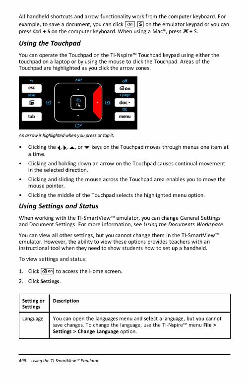
498 Using the TI-SmartView™ Emulator
All handheld shortcuts and arrow functionality work from the computer keyboard. Forexample, to save a document, you can click/S on the emulator keypad or you canpress Ctrl + S on the computer keyboard. When using a Mac®, press “ + S.
Using the TouchpadYou can operate the Touchpad on the TI-Nspire™ Touchpad keypad using either thetouchpad on a laptop or by using the mouse to click the Touchpad. Areas of theTouchpad are highlighted as you click the arrow zones.
Anarrow is highlightedwhen you press or tap it.
• Clicking the ¡, ¢,£, or¤ keys on the Touchpad moves through menus one item ata time.
• Clicking and holding down an arrow on the Touchpad causes continual movementin the selected direction.
• Clicking and sliding the mouse across the Touchpad area enables you to move themouse pointer.
• Clicking the middle of the Touchpad selects the highlighted menu option.
Using Settings and StatusWhen working with the TI-SmartView™ emulator, you can change General Settingsand Document Settings. For more information, see Using the Documents Workspace.
You can view all other settings, but you cannot change them in the TI-SmartView™emulator. However, the ability to view these options provides teachers with aninstructional tool when they need to show students how to set up a handheld.
To view settings and status:
1. Clickc to access the Home screen.
2. Click Settings.
Setting orSettings
Description
Language You can open the languages menu and select a language, but you cannotsave changes. To change the language, use the TI-Nspire™ menu File >Settings > Change Language option.
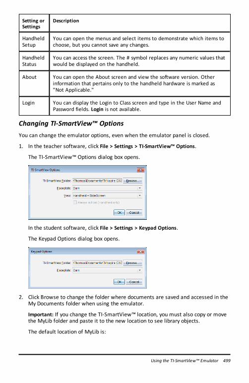
Setting orSettings
Description
HandheldSetup
You can open the menus and select items to demonstrate which items tochoose, but you cannot save any changes.
HandheldStatus
You can access the screen. The # symbol replaces any numeric values thatwould be displayed on the handheld.
About You can open the About screen and view the software version. Otherinformation that pertains only to the handheld hardware is marked as"Not Applicable."
Login You can display the Login to Class screen and type in the User Name andPassword fields. Login is not available.
Changing TI-SmartView™ OptionsYou can change the emulator options, even when the emulator panel is closed.
1. In the teacher software, click File > Settings > TI-SmartView™ Options.
The TI-SmartView™ Options dialog box opens.
In the student software, click File > Settings > Keypad Options.
The Keypad Options dialog box opens.
2. Click Browse to change the folder where documents are saved and accessed in theMy Documents folder when using the emulator.
Important: If you change the TI-SmartView™ location, you must also copy or movethe MyLib folder and paste it to the new location to see library objects.
The default location of MyLib is:
Using the TI-SmartView™ Emulator 499
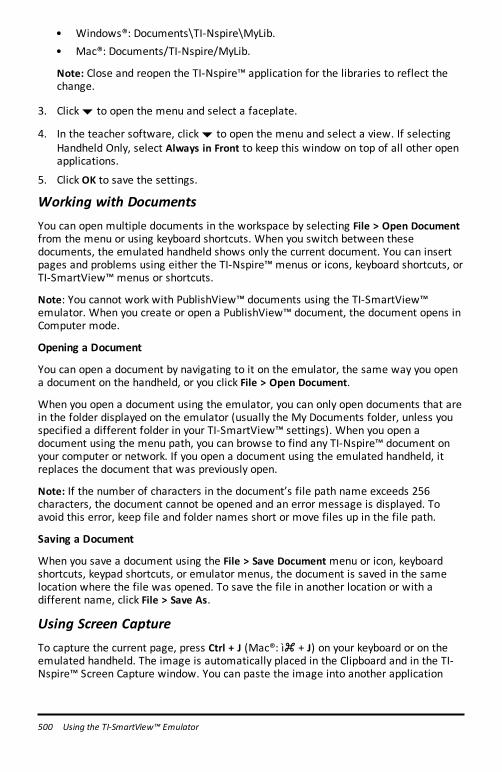
500 Using the TI-SmartView™ Emulator
• Windows®: Documents\TI-Nspire\MyLib.• Mac®: Documents/TI-Nspire/MyLib.
Note: Close and reopen the TI-Nspire™ application for the libraries to reflect thechange.
3. Click¤ to open the menu and select a faceplate.
4. In the teacher software, click¤ to open the menu and select a view. If selectingHandheld Only, select Always in Front to keep this window on top of all other openapplications.
5. Click OK to save the settings.
Working with DocumentsYou can open multiple documents in the workspace by selecting File > Open Documentfrom the menu or using keyboard shortcuts. When you switch between thesedocuments, the emulated handheld shows only the current document. You can insertpages and problems using either the TI-Nspire™ menus or icons, keyboard shortcuts, orTI-SmartView™menus or shortcuts.
Note: You cannot work with PublishView™ documents using the TI-SmartView™emulator. When you create or open a PublishView™ document, the document opens inComputer mode.
Opening a Document
You can open a document by navigating to it on the emulator, the same way you opena document on the handheld, or you click File > Open Document.
When you open a document using the emulator, you can only open documents that arein the folder displayed on the emulator (usually the My Documents folder, unless youspecified a different folder in your TI-SmartView™ settings). When you open adocument using the menu path, you can browse to find any TI-Nspire™ document onyour computer or network. If you open a document using the emulated handheld, itreplaces the document that was previously open.
Note: If the number of characters in the document’s file path name exceeds 256characters, the document cannot be opened and an error message is displayed. Toavoid this error, keep file and folder names short or move files up in the file path.
Saving a Document
When you save a document using the File > Save Document menu or icon, keyboardshortcuts, keypad shortcuts, or emulator menus, the document is saved in the samelocation where the file was opened. To save the file in another location or with adifferent name, click File > Save As.
Using Screen CaptureTo capture the current page, press Ctrl + J (Mac®: ì“ + J) on your keyboard or on theemulated handheld. The image is automatically placed in the Clipboard and in the TI-Nspire™ Screen Capture window. You can paste the image into another application
without having to take additional steps. This feature is only available when the TI-SmartView™ panel is active and the workspace is in Handheld mode.
All other screen capture features work the same way they do in other areas of TI-Nspire™ software. For more information, see Capturing Screens.
Using the TI-SmartView™ Emulator 501
502 Writing Lua Scripts
Writing Lua ScriptsThe Script Editor allows you to create and deliver dynamically linked simulations,powerful and flexible utilities, and other educational content for exploring math andscience concepts. When you open a document containing a script, the script runsautomatically as programmed. To see the running script application, the pagecontaining the script application must be active.
The Script Editor is directed toward teachers and other authors who are comfortableworking in a Lua scripting environment. Lua is a powerful, fast, lightweight scriptinglanguage that is fully supported in TI-Nspire™ and PublishView™ documents.Documents containing script applications can be opened on TI-Nspire™ CX II handhelds.The script application runs on a handheld, but you cannot view or edit the script.
Note these resources for using the Script Editor and creating scripts:
• Press F1 to access the TI-Nspire™ help, which includes the Script Editor help.
• Press F2 for additional TI-Nspire™ resources such as scripting samples and a link tothe TI-Nspire™ Scripting API library. (This information is also available ateducation.ti.com/nspire/scripting.)
• Go to lua.org for more information about Lua.
Overview of the Script EditorWith the Script Editor, you can insert, edit, save, run, and debug script applicationsin TI-Nspire™ (.tns files) and Publishview™ (.tnsp files) documents.
• Script applications function within documents, problems, and pages the same waythat other TI-Nspire™ applications do.
• When you create a new document or open an existing document, you can insert oredit a script application within a page or within a work area of a split page.
• In a split page layout, you can add a script application to each work area of a page.A page can be split into a maximum of four quadrants.
• Images can be added to script applications. See the Inserting Images section.
• All work done in the Script Editor is lost if you close the TI-Nspire™ orPublishView™ document without saving it.
Exploring the Script Editor InterfaceThe Script Editor window opens when you insert a new script application or edit anexisting script application in a TI-Nspire™ or PublishView™ document.
Select options for creating new scripts or editing scripts from the Insert menu in theDocuments Workspace when a document is open.
Note: Although not labeled, the Documents Workspace is the default workspace in theTI-Nspire™ CX Student Software and TI-Nspire™ CX CAS Student Software.
The following figure shows the Script Editor with an existing script.
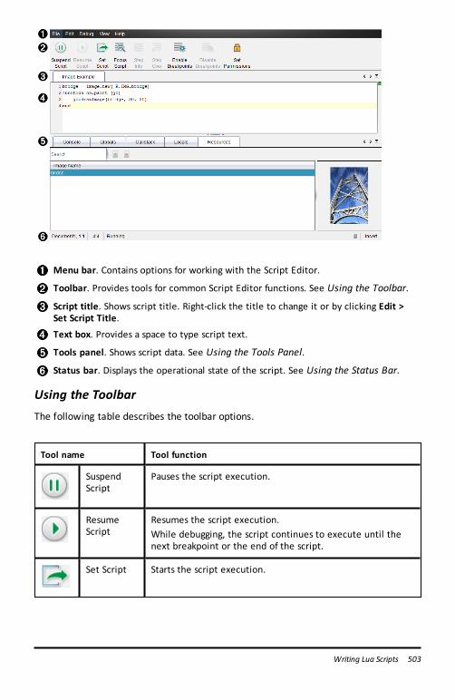
Menu bar. Contains options for working with the Script Editor.
Toolbar. Provides tools for common Script Editor functions. See Using the Toolbar.
Script title. Shows script title. Right-click the title to change it or by clicking Edit >Set Script Title.
Text box. Provides a space to type script text.
Tools panel. Shows script data. See Using the Tools Panel.
Status bar. Displays the operational state of the script. See Using the Status Bar.
Using the ToolbarThe following table describes the toolbar options.
Tool name Tool function
SuspendScript
Pauses the script execution.
ResumeScript
Resumes the script execution.While debugging, the script continues to execute until thenext breakpoint or the end of the script.
Set Script Starts the script execution.
Writing Lua Scripts 503
504 Writing Lua Scripts
Tool name Tool function
FocusScript
Sets the focus to the page in the document where the scriptapplication is attached:
• In a TI-Nspire™ document, sets the focus to the page.
• In a PublishView™ document, sets the focus to theframe on the page.
Step Into While debugging, executes the current statement. If thestatement calls any functions, the debugger stops at the firstline of each function.
Step Over While debugging, executes the current statement.If the statement calls any functions, the debugger does notstop within the function unless the function contains abreakpoint.
EnableBreakpoints
Switches from normal mode to debugging mode.
DisableBreakpoints
Switches back from debugging mode to normal mode andresumes the script.
SetPermissions
Sets permission levels to Protected, View Only, orUnprotected and allows you to set a password for the script.
Using the Tools Panel
At the bottom of the window, the Tools panel shows the scripting data. For moreinformation, see the Debugging Scripts section.
Tab Window Display
Console Script errors are printed here.Print statements embedded in the script also print here.
Globals Selected global variables are displayed.To select a global variable for display, select Click to add new watchvariable at the bottom of the Tools panel.
Call Stack Displays the call tree for the currently executing function.
Locals Local variables in the current function’s scope are displayed.
Resources Upload, insert, and manage images here.
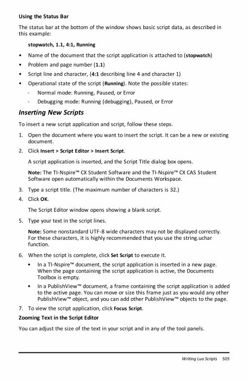
Using the Status Bar
The status bar at the bottom of the window shows basic script data, as described inthis example:
stopwatch, 1.1, 4:1, Running
• Name of the document that the script application is attached to (stopwatch)
• Problem and page number (1.1)
• Script line and character, (4:1 describing line 4 and character 1)
• Operational state of the script (Running). Note the possible states:
- Normal mode: Running, Paused, or Error- Debugging mode: Running (debugging), Paused, or Error
Inserting New ScriptsTo insert a new script application and script, follow these steps.
1. Open the document where you want to insert the script. It can be a new or existingdocument.
2. Click Insert > Script Editor > Insert Script.
A script application is inserted, and the Script Title dialog box opens.
Note: The TI-Nspire™ CX Student Software and the TI-Nspire™ CX CAS StudentSoftware open automatically within the Documents Workspace.
3. Type a script title. (The maximum number of characters is 32.)
4. Click OK.
The Script Editor window opens showing a blank script.
5. Type your text in the script lines.
Note: Some nonstandard UTF-8 wide characters may not be displayed correctly.For these characters, it is highly recommended that you use the string.ucharfunction.
6. When the script is complete, click Set Script to execute it.
• In a TI-Nspire™ document, the script application is inserted in a new page.When the page containing the script application is active, the DocumentsToolbox is empty.
• In a PublishView™ document, a frame containing the script application is addedto the active page. You can move or size this frame just as you would any otherPublishView™ object, and you can add other PublishView™ objects to the page.
7. To view the script application, click Focus Script.
Zooming Text in the Script Editor
You can adjust the size of the text in your script and in any of the tool panels.
Writing Lua Scripts 505
506 Writing Lua Scripts
Menu Method
1. Click in the area of the text to zoom.
2. On the Viewmenu, select Zoom, and then select Zoom In, Zoom Out, or Restore.
Note that the menu also displays keyboard shortcuts for the Zoom commands.
Mouse Method
1. Postion the mouse pointer over the area to zoom.
2. Hold Ctrl, and roll the mouse wheel forward or back.
Editing ScriptsTo edit an existing script, follow these steps.
1. Open the TI-Nspire™ or PublishView™ document that contains the script. The pagecontaining the script must be active.
2. Select the page and the work area that contains the script.
3. Click Insert > Script Editor > Edit Script.
The Script Editor opens showing the script. If the selected work area on the pagedoes not contain a script, Edit Script is dimmed.
If the script is password protected, the Password Protected dialog box opensprompting for a password.
4. Make any desired changes.
• To designate comments, use double hyphens (--) at the start of each commentline.
• To change the title, click Edit > Set Script Title or right-click the title and clickSet Script Title.
Notes:
• Some nonstandard UTF-8 characters may not be displayed correctly. For thesecharacters, it is highly recommended that you use the string.uchar function.
• The print function may yield unexpected results for non–UTF-8 characters.• Some nonprintable characters returned by the on.save function will be
discarded.
5. To execute the script, click Set Script.
Any errors are displayed in the Console area in the Tools panel.
6. To view the script application (running script), click Focus Script.
Changing View OptionsTo change viewing options:
▶ To clear the scripting data in the Tools panel and restore the editor defaults, clickView > Restore Editor to Defaults.
▶ To view the script title in the document and before each print statement in theConsole, click View > Title in Document View.
▶ To hide or show toolbar labels, click View > Toolbar Text Labels.
▶ To show or hide the Tools panel or its areas, click View > Tools Panel and click theappropriate option.
▶ To create tab groups when multiple scripts are open, right-click one of the titlesand click New Horizontal Group or New Vertical Group.
Setting Minimum API LevelEach release of the T-Nspire™ software includes API support for a specific set of Luascripting features. Setting the minimum API level for a script lets you specify aminimum set of features that you require for your script.
If a user tries to run the script on a system that does not meet the script's minimumAPI level, a message notifies the user and prevents the script from running.
To Set the Minimum API Level for a Script:
1. Determine the minimum level that you want your script to require.
- Setting the level too low for the script's feature set can result in a script erroron older software.
- Setting the level too high can result in the script refusing to start on oldersoftware that supports the feature set.
2. On the Script Editor File menu, select Set Minimum API Level.
3. In the dialog box, type the minimum level using the format major.minor. Forexample, you might type 2.3.
This API level or higher will be required for running the script.
Saving Script ApplicationsClicking Set Script resets (updates) a script application in a TI-Nspire™ or PublishView™document. However, the script and script application are not saved until you save thedocument. If you close the document or close the TI-Nspire™ software without saving,work on the script is lost.
To ensure the script application is saved after all work is complete, follow these steps.
1. From the Script Editor window, click Set Script to reset (update) the scriptapplication in the document.
2. From an open document, click File > Save Document to save changes to the TI-Nspire™ or PublishView™ document.
Note: To ensure work is backed up, set the script and save the document frequently.
Writing Lua Scripts 507
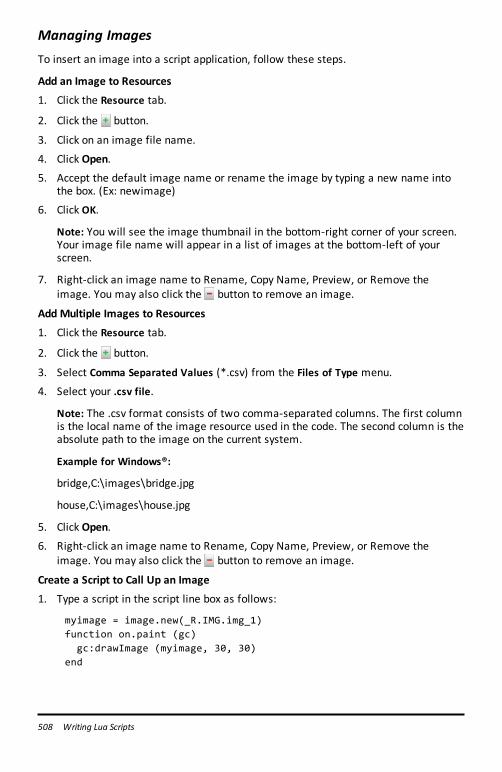
508 Writing Lua Scripts
Managing ImagesTo insert an image into a script application, follow these steps.
Add an Image to Resources
1. Click the Resource tab.
2. Click the button.
3. Click on an image file name.
4. Click Open.
5. Accept the default image name or rename the image by typing a new name intothe box. (Ex: newimage)
6. Click OK.
Note: You will see the image thumbnail in the bottom-right corner of your screen.Your image file name will appear in a list of images at the bottom-left of yourscreen.
7. Right-click an image name to Rename, Copy Name, Preview, or Remove theimage. You may also click the button to remove an image.
AddMultiple Images to Resources
1. Click the Resource tab.
2. Click the button.
3. Select Comma Separated Values (*.csv) from the Files of Type menu.
4. Select your .csv file.
Note: The .csv format consists of two comma-separated columns. The first columnis the local name of the image resource used in the code. The second column is theabsolute path to the image on the current system.
Example for Windows®:
bridge,C:\images\bridge.jpg
house,C:\images\house.jpg
5. Click Open.
6. Right-click an image name to Rename, Copy Name, Preview, or Remove theimage. You may also click the button to remove an image.
Create a Script to Call Up an Image
1. Type a script in the script line box as follows:
myimage = image.new(_R.IMG.img_1)function on.paint (gc) gc:drawImage (myimage, 30, 30)end
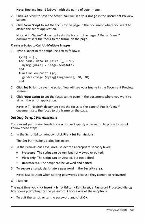
Note: Replace img_1 (above) with the name of your image.
2. Click Set Script to save the script. You will see your image in the Document Previewscreen.
3. Click Focus Script to set the focus to the page in the document where you want toattach the script application.
Note: A TI-Nspire™ document sets the focus to the page; A PublishView™document sets the focus to the frame on the page.
Create a Script to Call Up Multiple Images
1. Type a script in the script line box as follows:
myimg = { }for name, data in pairs (_R.IMG)
myimg [name] = image.new(data)endfunction on.paint (gc)
gc:drawImage (myimg[imagename], 30, 30)end
2. Click Set Script to save the script. You will see your image in the Document Previewscreen.
3. Click Focus Script to set the focus to the page in the document where you want toattach the script application.
Note: A TI-Nspire™ document sets the focus to the page; A PublishView™document sets the focus to the frame on the page.
Setting Script PermissionsYou can set permission levels for a script and specify a password to protect a script.Follow these steps.
1. In the Script Editor window, click File > Set Permissions.
The Set Permissions dialog box opens.
2. In the Permissions Level area, select the appropriate security level:
• Protected. The script can be run, but not viewed or edited.• View only. The script can be viewed, but not edited.• Unprotected. The script can be viewed and edited.
3. To secure a script, designate a password in the Security area.
Note: Use caution when setting passwords because they cannot be recovered.
4. Click OK.
The next time you click Insert > Script Editor > Edit Script, a Password Protected dialogbox opens prompting for the password. Choose one of these options:
• To edit the script, enter the password and click OK.
Writing Lua Scripts 509
510 Writing Lua Scripts
• To view the script only, do not enter the password and click View.
Debugging ScriptsYou can debug your script to investigate runtime errors and trace the execution flow.While debugging, data is displayed in the Tools panel.
▶ To enable debugging mode or disable it and return to normal mode, click Debug >Enable Breakpoints or Disable Breakpoints.
Note: Disabling breakpoints always resumes the script execution.
▶ While debugging, click Step Into and Step Over as appropriate. See the Exploringthe Script Editor Interface section.
▶ To set breakpoints, double-click in the space to the far left of the line number.Breakpoints are disabled until you click EnableBreakpoints.
▶ Note these factors when debugging:
• Breakpoints in coroutines are not supported.• If a breakpoint is set in a function that is a callback, the debugger may not stop
at the breakpoint.• The debugger may not stop at functions such as on.save, on.restore, and
on.destroy.
On the toolbar, Step Into and Step Over are enabled when breakpoints are enabled.
▶ To suspend and resume the script execution, click Suspend Script and ResumeScript. When the script resumes, it runs until the next breakpoint is encountered orto the end of the script. A script can be suspended in normal mode or debuggingmode.
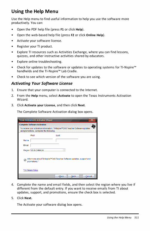
Using the Help MenuUse the Help menu to find useful information to help you use the software moreproductively. You can:
• Open the PDF help file (press F1 or click Help).
• Open the web-based help file (press F2 or click Online Help).
• Activate your software license.
• Register your TI product.
• Explore TI resources such as Activities Exchange, where you can find lessons,quizzes, and other instructive activities shared by educators.
• Explore online troubleshooting.
• Check for updates to the software or updates to operating systems for TI-Nspire™handhelds and the TI-Nspire™ Lab Cradle.
• Check to see which version of the software you are using.
Activating Your Software License1. Ensure that your computer is connected to the Internet.
2. From the Help menu, select Activate to open the Texas Instruments ActivationWizard.
3. Click Activate your License, and then click Next.
The Complete Software Activation dialog box opens.
4. Complete the name and email fields, and then select the region where you live ifdifferent from the default entry. If you want to receive emails from TI aboutupdates, support, and promotions, ensure the check box is selected.
5. Click Next.
The Activate your software dialog box opens.
Using the Help Menu 511
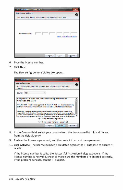
512 Using the Help Menu
6. Type the license number.
7. Click Next.
The License Agreement dialog box opens.
8. In the Country field, select your country from the drop-down list if it is differentfrom the default entry.
9. Review the license agreement, and then select to accept the agreement.
10. Click Activate. The license number is validated against the TI database to ensure itis valid.
If the license number is valid, the Successful Activation dialog box opens. If thelicense number is not valid, check to make sure the numbers are entered correctly.If the problem persists, contact TI Support.
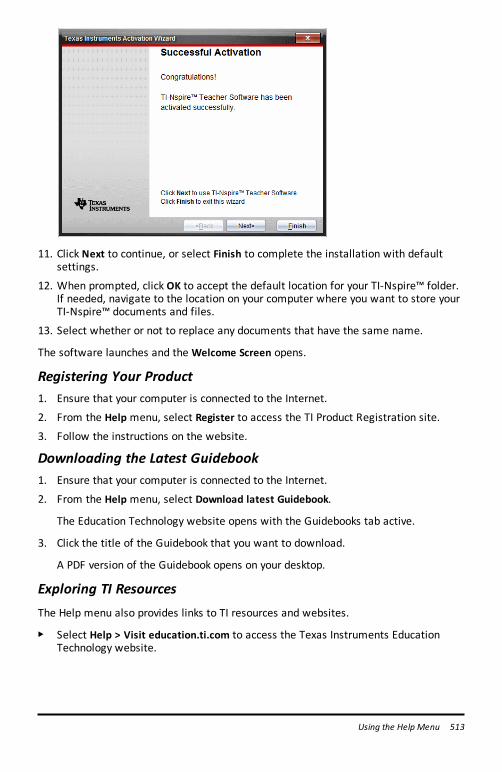
11. Click Next to continue, or select Finish to complete the installation with defaultsettings.
12. When prompted, click OK to accept the default location for your TI-Nspire™ folder.If needed, navigate to the location on your computer where you want to store yourTI-Nspire™ documents and files.
13. Select whether or not to replace any documents that have the same name.
The software launches and the Welcome Screen opens.
Registering Your Product1. Ensure that your computer is connected to the Internet.
2. From the Help menu, select Register to access the TI Product Registration site.
3. Follow the instructions on the website.
Downloading the Latest Guidebook1. Ensure that your computer is connected to the Internet.
2. From the Help menu, select Download latest Guidebook.
The Education Technology website opens with the Guidebooks tab active.
3. Click the title of the Guidebook that you want to download.
A PDF version of the Guidebook opens on your desktop.
Exploring TI ResourcesThe Help menu also provides links to TI resources and websites.
▶ Select Help > Visit education.ti.com to access the Texas Instruments EducationTechnology website.
Using the Help Menu 513
514 Using the Help Menu
▶ Select Help > Visit Activities Exchange to access the Texas Instruments ActivitiesExchange, site, a forum where you can browse by subject to find ready-to-use mathand science learning activities appropriate for middle grades through college.
Note: Activities available for download may vary depending on your geographicalregion.
▶ Select Help > Explore Online Troubleshooting to access the TI Knowledge Basewhere you can find general information, troubleshooting help, product usage tips,and information specific to TI products.
Updating the TI-Nspire™ SoftwareUpdate the Software
1. Ensure that your computer is connected to the Internet.
2. Close any open documents.
3. From the Help menu, select Check for Upgrades and Notifications.
• If your software is current, a confirmation message appears.• If your software is not current, you are prompted to update.
4. Click Update to download and install the update, or click Close to cancel.
A progress indicator shows the download progress. If you receive a connectionerror, check your Internet connection and try again.
Note for users updating TI-Nspire™ Navigator™ Teacher Software: Your portfolio andclass records reside on your computer as a database. Because the new software mighthave features that are not supported in the old database structure, the old data mightneed to be converted. When conversion is necessary, a Database Update tool helps youmake a backup of the old database. The tool appears during the first startup of theupdated software.
Manage Automatic Checking
Automatic checking uses the Internet to check for upgrades each time you open the TI-Nspire™ software. If your system is not up-to-date, you receive a notification. You canturn automatic checking on or off.
1. From the Help menu, select Check for Upgrades and Notifications.
2. Check or clear the Automatically check for updates check box.
3. Click Close.
Updating the OS on a Connected HandheldNote: To avoid losing unsaved data, close all documents on the handheld beforeupdating its operating system.
1. Ensure that your computer is connected to the Internet.
2. In the Documents Toolbox, click the Content Explorer tab to show connectedhandhelds.
3. Select the handheld that you are updating.
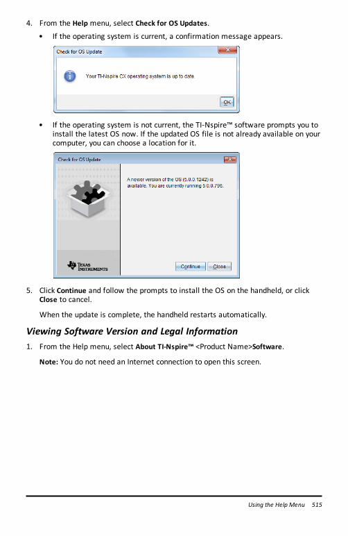
4. From the Help menu, select Check for OS Updates.
• If the operating system is current, a confirmation message appears.
• If the operating system is not current, the TI-Nspire™ software prompts you toinstall the latest OS now. If the updated OS file is not already available on yourcomputer, you can choose a location for it.
5. Click Continue and follow the prompts to install the OS on the handheld, or clickClose to cancel.
When the update is complete, the handheld restarts automatically.
Viewing Software Version and Legal Information1. From the Help menu, select About TI-Nspire™ <Product Name>Software.
Note: You do not need an Internet connection to open this screen.
Using the Help Menu 515
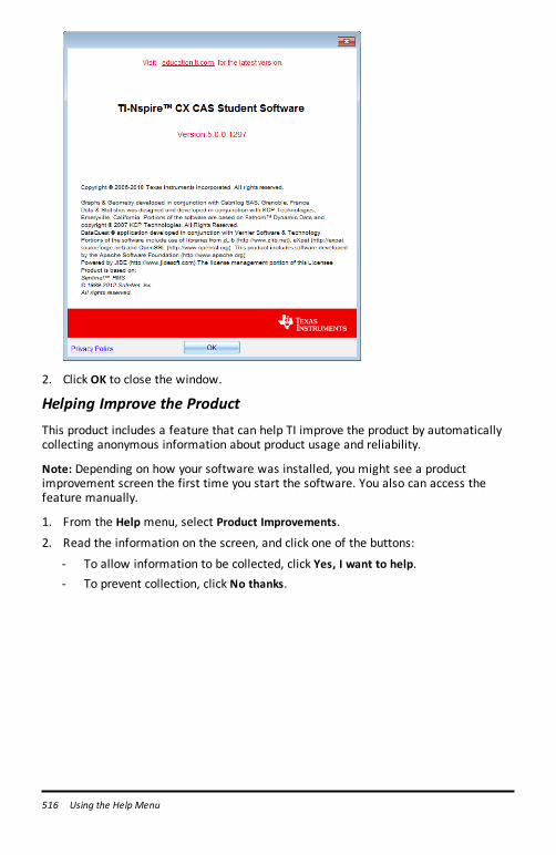
516 Using the Help Menu
2. Click OK to close the window.
Helping Improve the ProductThis product includes a feature that can help TI improve the product by automaticallycollecting anonymous information about product usage and reliability.
Note: Depending on how your software was installed, you might see a productimprovement screen the first time you start the software. You also can access thefeature manually.
1. From the Help menu, select Product Improvements.
2. Read the information on the screen, and click one of the buttons:
- To allow information to be collected, click Yes, I want to help.- To prevent collection, click No thanks.
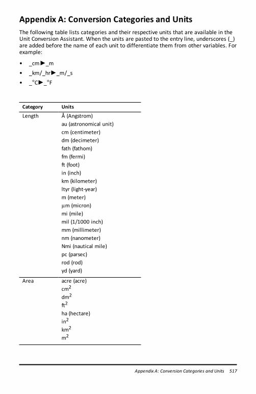
Appendix A: Conversion Categories and UnitsThe following table lists categories and their respective units that are available in theUnit Conversion Assistant. When the units are pasted to the entry line, underscores (_)are added before the name of each unit to differentiate them from other variables. Forexample:
• _cm►_m
• _km/_hr►_m/_s
• _¡C►_¡F
Category Units
Length Å (Angstrom)au (astronomical unit)cm (centimeter)dm (decimeter)fath (fathom)fm (fermi)ft (foot)in (inch)km (kilometer)ltyr (light-year)m (meter)mm (micron)mi (mile)mil (1/1000 inch)mm (millimeter)nm (nanometer)Nmi (nautical mile)pc (parsec)rod (rod)yd (yard)
Area acre (acre)cm2
dm2
ft2
ha (hectare)in2
km2
m2
Appendix A: Conversion Categories and Units 517
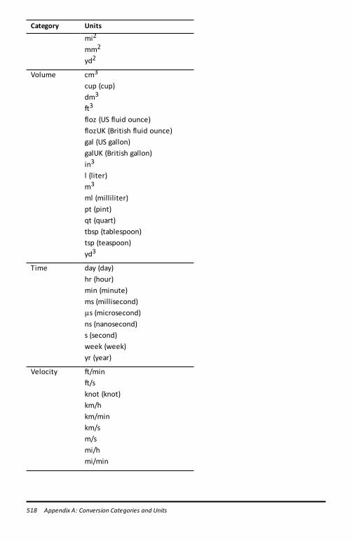
518 Appendix A: Conversion Categories and Units
Category Units
mi2
mm2
yd2
Volume cm3
cup (cup)dm3
ft3
floz (US fluid ounce)flozUK (British fluid ounce)gal (US gallon)galUK (British gallon)in3
l (liter)m3
ml (milliliter)pt (pint)qt (quart)tbsp (tablespoon)tsp (teaspoon)yd3
Time day (day)hr (hour)min (minute)ms (millisecond)ms (microsecond)ns (nanosecond)s (second)week (week)yr (year)
Velocity ft/minft/sknot (knot)km/hkm/minkm/sm/smi/hmi/min
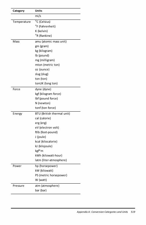
Category Units
mi/s
Temperature ¡C (Celsius)¡F (Fahrenheit)K (kelvin)¡R (Rankine)
Mass amu (atomic mass unit)gm (gram)kg (kilogram)lb (pound)mg (milligram)mton (metric ton)oz (ounce)slug (slug)ton (ton)tonUK (long ton)
Force dyne (dyne)kgf (kilogram force)lbf (pound force)N (newton)tonf (ton force)
Energy BTU (British thermal unit)cal (calorie)erg (erg)eV (electron volt)ftlb (foot-pound)J (joule)kcal (kilocalorie)kJ (kilojoule)kgf*mkWh (kilowatt-hour)latm (liter-atmosphere)
Power hp (horsepower)kW (kilowatt)PS (metric horsepower)W (watt)
Pressure atm (atmosphere)bar (bar)
Appendix A: Conversion Categories and Units 519
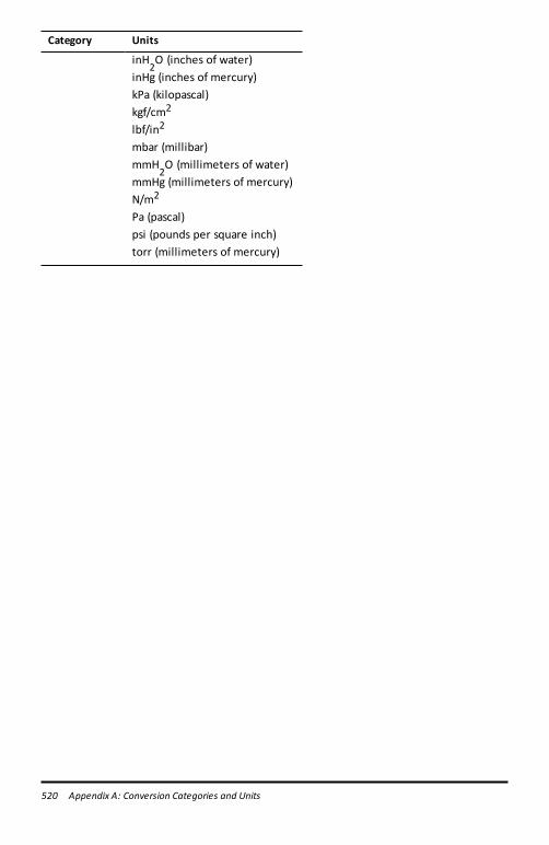
520 Appendix A: Conversion Categories and Units
Category Units
inH2O (inches of water)
inHg (inches of mercury)kPa (kilopascal)kgf/cm2
lbf/in2
mbar (millibar)mmH
2O (millimeters of water)
mmHg (millimeters of mercury)N/m2
Pa (pascal)psi (pounds per square inch)torr (millimeters of mercury)
General InformationOnline Helpeducation.ti.com/eguide
Select your country for more product information.
Contact TI Supporteducation.ti.com/ti-cares
Select your country for technical and other support resources.
Service and Warranty Informationeducation.ti.com/warranty
Select your country for information about the length and terms of the warranty orabout product service.
Limited Warranty. This warranty does not affect your statutory rights.
General Information 521
Index
3
3D aspect ratio, changing 2433D functions
graphing 2373D graph
changing appearance 2413D Graphing view 237, 2393D graphs
animating with sliders 245editing expressions 240plot colors 241range settings 243rotating 239setting background colors 242showing/hiding 242shrinking/magnifying 242
3D parametric equationsgraphing 238
3D projection type 242
A
activating software licenses 511adding
applications 42applications (PublishView™
documents) 67colors 37copyrights to documents (.tns) 49files to lesson bundles 97-98images in Quick Poll 115images to pages 115pages 46problems 46shortcuts to lesson bundles 104text (PublishView™ documents) 80titles to graphs 445
alternative hypothesis 337analysis options
removing 437analyzing data
integral 434
model 437tangent 434
anglesmeasuring 220-221, 272
animatingpoints 231, 285
animationschanging points direction 231, 286pausing 231, 286resetting 231, 286resuming 231, 286
API level, setting for scripts 507appearance
of 3D graph 241application
toolsmenu 2applications
adding 42Calculator 123Data&Statistics 340deleting 46Geometry 247Graphs&Geometry 160grouping 45inserting images 115Lists & Spreadsheet 291Notes 387Program Editor 471swapping 43
approximate or exact results 304arcs, drawing 205, 257area, bounded 195area, measuring 219, 271arguments, user-supplied values 482arithmetic calculations 235, 289aspect ratio, changing in 3D graphing 243attributes
changing for objects 216, 268for variables 145
automaticsliders in Graphs application 153
axesadjusting 374changing attributes in Graphing 191
522 Index
viewdilating 369moving (translation) 369scaling 369setting values (Data &Statistics) 374
axis rangessetting in graphs 446
B
backupof class data 514
bar chartscreating 358-359, 361
borders (PublishView™ documents),hiding/showing 74
bounded area 195box plots 347breaking long calculations 395
C
Calculate output option 319calculating distributions (Lists &
Spreadsheet) 326calculations
arithmetic 235, 289breaking 395derivative settings 457types available 323using variables 152
Calculatormenus 123
Calculator application 123calculated results variables 157
Calculator historycopying 142-143deleting 144reusing 143viewing 142
captions, viewing variable names 341capture pageoption 107Capture Selected Handheld option 108capturing
active pages in documents 107
data (Lists & Spreadsheet) 314handheld current screens 107images in handheld mode 107pages in active documents 107
capturing imagesDragScreen 112
caseplots (default) 341Catalog
convertingmeasurement units 131inserting items from 125, 128, 299, 319
cell referencesabsolute and relative 298using in formulas 298
cellsbody 294copying in tables 299deleting contents 299entering text 294exact or approximate results 304formulas 294inserting ranges in formulas 295linking to variables 301navigating in tables 297repeating formulas 300selecting a block of 299selecting a range 295sharing table cells 300
changingGeneral Settings 21Graphs&Geometry settings 23language 1, 3
changing screen size 497charts
bar 358dot 357pie 360scatter 344
chemical equation boxes 400circle arcs, creating 205, 257circles, drawing 206, 258Circular definition error 486class data
backup 514
Index 523
closingfunctions and programs 478
closing documents (.tns) 35collected data
deleting 431viewing details 432
collecting and managing data sets 429color
setting grid color in Graphs 190colors
3D graph background 242applying to backgrounds 390changing 216, 241, 268,
297-298, 380-381, 390
changing for points 452colors, adding 37columns
based on other columns 306copying 303defining options 441deleting 302deleting data from 304generating data in tables 305inserting 128, 302linking to list variables 293moving 303resizing 301selecting 301, 453sharing table columns as lists 292
commandsIf, Lbl, Goto 487
comments, inserting in Notes 392comparing
data sets 430comparing collected data sets 429confidence intervals available 332conic by five points 211, 262conics, graphing 172constructions
locus 215, 267Content Explorer 17context menu
graphing from 398
context menu in Lists & Spreadsheet 302converting
.tns files to .tnsp files 94
.tnsp files to .tns files 93measurement units 131page size; page size, converting;
preview, settingdocument; setting
document preview 37text to hyperlinks 88
copyingCalculator history 142-143cells from Excel® spreadsheets 314handheld images 107images 107images in handheld mode 107lesson bundles 103screens 111table cells 299table data 312table rows or columns 303
copyrightsadding to documents (.tns) 49
creatingbar charts 358-359, 361copies of functions and
programs 474histograms 351lesson bundles 96, 103lists from table columns 292matrices 127pie charts 360plots 346probability plots 354PublishView™ documents 51scatter plots 355shapeswith MathDraw 211, 263summary plots 311system of equations 130user-defined units 133variables 146-147, 149
creating documents (.tns) 32curve fit options 436curves, bounded area 195
524 Index
customizingGraphswork area 190
D
databackup of class data 514capturing (Lists & Spreadsheet) 314capturing object data (Graphs&
Geometry) 314copying to other applications 312deleting from columns 304displaying values 343, 346exact or approximate results 304generating columns of 305graphing table data 308raw and summary overview 345retrieving remote 427selecting ranges 450sorting in tables 304sorting plotted categories 366
Data&Statisticsgetting started with 340settings 341
data analysisinterpolation 435
data collectionsremote sensors 425scaling graphs 449setting sensor parameters 416thresholds 427
data plotsfinding curve fit 436
data setscomparing 430deleting collected 431renaming 431selecting for replays 456selecting to plot 448storing 429
data sets, collecting and managing 429debugging information 493
displaying in dialog boxes 483displaying values 483
programs 493defined functions, recalling 139defining
functions 130, 136-137settings 1, 3units 133
deletingapplications 46Calculator history 144collected data sets 431contents of table cells 299data from columns 304documents (.tns) 35elements from lists 293global variables 485hyperlinks (PublishView™
documents) 88images 117images (PublishView™
documents) 90lesson bundles 103-104linked variables 159pages 45, 47parts of expressions 140problems 45, 47PublishView™ objects 65table rows and columns 302
derivative settingsadjusting 457
diagnostics, regression 341differential equations, graphing 182dilating axes 369displaying
data values 343, 346Graph 1 440graphs 440graphs in Page Layout view 441grid in Graphs 190TI-SmartView™ emulator in
teacher software 496two graphs simultaneously 440variable values 147
distribution, calculating 326
Index 525
documentscreating .tnsp files 51printing .tnsp files 94saving .tnsp files 55
documents (.tns)changing General Settings 21closing 35creating 32deleting 35opening 26, 33opening with TI-SmartView™
emulator 500printing 48properties 49protecting 50read-only 50saving 26, 34-35saving in emulator 500switching between 39viewing 39
documentsworkspace 2domain restrictions 167dot charts 357DragScreen feature 107, 112drawing
arcs 205, 257rectangles 207, 259statistics plots 385triangles 207, 258
drawing geometric shapes 206, 257drawing shapes
ellipse 209, 260
E
editing 186expressions 140functions 186functions and programs 474table settings 339values in lists 293
elements, deleting from lists 293ellipse
as geometric shape 209, 260
emailing lesson bundles 105embedding
values in functions or programs 481emulator, See TI-SmartView™
emulator 15entry line
multiple statements 131equations
differential 183graphing 171graphing parametric 178graphing polar 178Lotka-Volterra 182of geometric objects 234ordinary differential equations
(ODE) 182errors
circular definitions 486showing (Notes) 395
estimatingvalues between data points 435
evaluating expressions 126exact input, for window settings 188exact or approximate results 304Excel® spreadsheets, copying from 314expanding view details area 432experiments
basic steps 410Exploring theDocumentsworkspace 2expressions 186
changing functions in tables 338copying from Calculator history 142-143deleting parts of 140editing 140, 240entering from templates 125-126entering in tables 294entering with wizards 128, 319evaluating 124, 395selecting (Calculator) 140selecting (Notes) 391
F
filesadding to lesson bundles 97-98, 102
526 Index
copying/pasting from lessonbundles 101
deleting from lesson bundles 102image file types 115opening in lesson bundles 100-101pasting from lesson bundles 102refreshing list in lesson bundles 102-103renaming in lesson bundles 102working with files on connected
handhelds 25finance functions 141Finance Solver 141finding
area under collected data 434slopeof collected data 434software version number 515
Flash (.flv) files 91folders
storing PublishView™ objects 66footers in PublishView™ documents 74formatting
results (Calculator) 124text (PublishView™ documents) 81
formatting text 36formatting toolbar
hiding 37showing 37
frequency plots 310functions
changing expressions in tables 338defining 130, 136-137displaying history 187, 240displaying list of in tables 338domain restrictions 167editing 186evaluating 478finance 141graphing 163, 170, 375hiding table of 186hiding/showing 193recalling definitions 139renaming 187rotating 165showing values in tables 338
stretching 165supported distributions 327translating 165user-defined 485
functions and programschangingmodes 493circular definition errors 486closing 478controlling flow 487creating copies of 474differences between 485editing 474embedding values 481private libraries 480public libraries 480renaming 474settingmodes 493stopping 481storing 474viewing 474
G
generatingcolumns of data 306
geometric objectsequations of 234
geometric shapesconic by five points 211, 262hyperbola 210, 262parabola 209-210, 261
Geometryhiding objects 284
Geometry application 247Geometry application settings 161, 247gestures, to create shapes
(MathDraw) 211, 263global variables 485graph
changing appearance 241graphing
3D functions 2373D parametric equations 2383D view 237
Index 527
conic sections 172equations 171from context menu 398functions 163, 170, 375parametric equations 178path plot 164polar equations 178relations 175scatter plots 179sequences 180table data 308timeplots 180web plots 180
Graphing viewchanging axes attributes 191
graphsadding titles 445displaying 440displaying Graph 1 440displaying in Page Layout view 441displaying two simultaneously 440position versus time 459rescaling 369scaling 449setting axis range 446tracing all 197velocity versus time 459
Graphsrescaling work area 188
Graphs&Geometry application 160Graphs&Geometry settings 23grid
appearance in Graphs 190displaying 190
grouping applications 45guidebooks, downloading 513
H
handheldscapturing current screens 107capturing selected handhelds 108checking for OS updates 27copying images 107
installing OS update 28pasting images 107working with files on connected 25
headers in PublishView™ documents 74Help, accessing 511helping improve the product 516hiding
3D graphs 242functions in work areas 193objects in Geometry 284table of functions 186
hiding format toolbar 37histograms
adjusting scale 351creating 351exploring data in bins 351modifying bins 353scale formats 351
historyrelation 187, 240
history, See Calculator history 142hyperbola
as geometric shape 210, 262hyperlinks (PublishView™
documents)converting text to 88editing 87linking to files 82linking to websites 85
I
If, Lbl, Goto 487images
deleting 117file types 115inserting 115, 391inserting background 162, 249, 284moving 116Quick Poll 115resizing 117saving 107selecting 116TI-Nspire™ applications 115
528 Index
images (PublishView™ documents) 88, 90importing
remote data 427inferential statistics
calculating test results(Calculate) 319
drawing plots 385graphing test results 319input descriptions table 320pooled option 337
initializing variables 484inserting
background images 162, 249, 284cell ranges in formulas 295chemical equations 391comments in Notes 391elements in lists (Lists &
Spreadsheet) 293hyperlinks (PublishView™
documents) 82images 391images (PublishView™
documents) 89images in Quick Poll 115images to pages 115math expressions 391PublishView™ objects 62rows or columns in tables 302rows or columns into matrices 128shape symbols 391text 382text (PublishView™ documents) 80
installingsoftware updates 514
installing a handheld OS update 28intercept, changing 371interfaces
multi-channel sensors 411single-channel sensors 412
intervals 419
L
labelingpoint coordinates 234
languagechanging 1, 3
LED lightssensors 427
lesson bundlesadding files 97-98, 102adding shortcuts to 104copying 104copying/pasting 103-104copying/pasting files 101creating 96-97, 103deleting 103-104deleting files 102emailing 105opening 99-100, 102, 104opening files 100-101packaging 105packaging pages 104pasting 104refreshing list of files 102-104renaming 103-104renaming files 102sending 104, 106
libraries 466changing the access levels 477Linear Algebra functions 469private 480public 480refreshing 468restoring 469
library objectscreating shortcuts 469private 467public 467using 468
Linear Algebra library functions 469lines
addingmovable to plots 370locking intercept at zero 371rotatingmovable 370tracingmovable 372
lines (geometric)creating 203, 254
Index 529
lines and points, creating 200, 252linking
columns to symbol table 441table cells to variables 301table columns to lists 293to files 82to websites 85values between applications 145variables 150-151
list math in Lists & Spreadsheet 295lists
deleting elements in tables 293inserting elements in tables 293sharing table columns as 292viewing and editing 293
Lists & Spreadsheet application 291locating software updates 514locking
intercept ofmovable lines atzero 371
variables 156locus construction 215, 267loops
EndLoop 491For 489using 489While 490
Lotka-Volterra equations 182Lua, scripts 502
M
managing collected data sets 429math actions 396math expression boxes 396, 401-402math expressions, See expressions 124math templates 125MathDraw, creating shapeswith
gestures 211, 263matrices
creating 127inserting rows or columns 128
measurement unitschanging (Vernier DataQuest ™) 417
measurements, converting units 131measuring
angles 220-221, 272circumference or perimeter 218, 270distance between objects 218, 270length 217, 269sides of objects 219, 270slopeof object 220, 271
measuring objects 217, 269menus
Calculator 123minimum API level for scripts 507models, Pdf distribution 326modes
changing in functions andprograms 493
setting in functions andprograms 493
setting in programs 493motion match
options 459removing plots 459
movingimages 116images (PublishView™
documents) 90points (Data &Statistics) 366PublishView™ objects 63rows and columns (Lists &
Spreadsheet) 303multiple-line functions 136-137multiple cells, selecting 299multiple statements on entry line 131
N
namingtable columns 292variables (name conflicts) 301
naming columns 441navigating in tables 296normal probability, creating plots 354Notes
adding shapes 392formatting text 389
530 Index
inserting comments 392selecting text 389using colors 390
numeric plots, splitting by categories 363
O
objects(PublishView™ documents) 60, 67changing attributes 216, 268changing fill colors 216, 268dilating 225, 276duplicating 224, 275enlarging 225, 276finding area 219, 271hiding in Geometry 284measuring 217, 269reflecting 223, 274rotating 224, 276symmetrical images 223, 274tracing geometric 282transformation of 223, 274
openingdocuments (.tns) 26files in lesson bundles 100lesson bundles 99-100, 102, 104
opening documents (.tns) 33options
capture page 107Capture Selected Handheld 108
organizing PublishView™ sheets 73orthogonal 3D view 242orthographic 3D projection 242OS update
installing on a handheld 28overlapping PublishView™ objects 64
P
packaging lesson bundles 105Page Layout view 441pagenumbers (PublishView™
documents) 73Page Sorter 14, 43
pagesadding 46deleting 45, 47grouping 45packaging 104rearranging 44selecting 44ungrouping 46
parabolacreating from focus and
directrix 210, 261creating from focus and vertex 209, 261
parametric equationsgraphing 178
pastinghandheld images 107images 107images in handheld mode 107lesson bundles 103screens 111table data 312
PDFsave document as 48
perspective 3D view 242pie charts, creating 360piecewise functions 130playbacks
adjusting rate 457pausing 456repeating 457starting 456
plotsadding a value on existing plot 367addingmovable lines 370caseplots (default) 341changing type 368colors in 3D graphs 241creating 346customizing 181dot plots 346graphing 179-180path plot 164predictive 458probability 354
Index 531
removingmotion match 459scatter 355sorting categories 366summary 310X-Y line 356
plottingdot charts 357models 437path plot 164statistical data 319table data 308
pointsanimating 231, 285changing colors 452changing direction 231, 286creating 200-201, 252-253identifying intersections 202, 254labeling coordinates 234moving (Data &Statistics) 366of interest 168selecting (Data &Statistics) 366settingmarkers 453setting options 451
points and lines, creating 200, 252polar equations
graphing 178polygons, drawing 208, 259pooled variances 337pre-defined measurement units 131precision of results 124predictive plots
drawing and clearing 458preview, printed document 49print preview 49printing
PublishView™ documents 94printing documents (.tns) 48probability, creating plots 354problems
adding 46deleting 45, 47renaming 48
problems (PublishView™documents) 70, 72
product improvements 516Program Editor application 471programs
calling one from another 485debugging 493defining 136editing 474flows 487running 478
Proof template 388protecting documents (.tns) 50PublishView™ documents 51
applications 67, 70converting 92, 94creating 51hyperlinks 81, 88images 88, 90objects 60, 66printing 94problems 70problemsdeleting
problems (PublishView™ documents)72
saving 55sheets 73, 79text 79, 81video files 91
Q
Q&A template 388questions
responding 120questions (students)
checking answers 122toolbar options 119types of 119
Quick Graph, using 308Quick Poll
images 115Quick Poll questions
clearing answers 122responding 120types 121
532 Index
R
random numbersgenerating in tables 306
rangeof cells, inserting in formulas 295raw data 345raw data, adjusting histogram scale 351rays
creating 204, 255read-only documents (.tns) 50reducing view details area 432RefreshProbeVars 432registering products 513regression diagnostics 341regression lines, showing 372relations
displaying history 187, 240graphing 175showing table of values 185
remote dataretrieving 427
removinghyperlinks from text 88images 117linked variables 159
renamingdata sets 431functions 187functions and programs 474lesson bundles 103-104problems (PublishView™
documents) 72renaming problems 48replays
starting 456repositioning images 116rescaling
graphs (dilation) 369graphs (translation) 369
resizingimages 117images (PublishView™
documents) 90PublishView™ objects 63table rows and columns 301
restoring data 455restoring libraries 469results
copying from Calculator history 142-143setting decimal approximation 124
rotating objects 224, 276rows
copying 303deleting 302inserting 128, 302moving 303resizing 301selecting 301
S
Savedocument as PDF 48
savingcaptured images 107captured pages 110documents (.tns) 26documents (.tns) in emulator 500handheld screens 110images 107PublishView™ documents 55PublishView™ document as PDF 94
saving documents (.tns) 34-35scaling graphs 449scaling PlaneGeometry Analytic
window 188scatter plots 355screen capture tool 107screen captures
copying 111pasting 111
script editorzooming text 505
scriptssetting API level 507
scripts, Lua 502scrolling in tables 296segments
creating 203, 255
Index 533
selectinga block of table cells 299columns 453data ranges 450data sets for replays 456data sets to plot 448expressions in Calculator 140images 116table rows or columns 301templates 388text in Notes 389working folder (PublishView™
objects) 66selecting pages 44sensors
calibrating 418changingmeasurement units 417connecting 415for computers 413for handhelds 412for remote data collections 425interfaces 411-412LED lights 427reversing reading display 418setting to zero 418setting up offline 416triggering 427types 412
sequences, generating in tablecolumns 307
setsrenaming data sets 431
sets of data, comparing 430sets, storing data as 429setting
minimum API level for scripts 507settings
Data&Statistics application 341defining 1, 3in Geometry application 161, 247language 1, 3TI-SmartView™ emulator 498
shapesadding in Notes 392
creating with MathDraw 211, 263drawing geometric 206, 257equations of 234legends 344
shortcutscreating to library objects 469
showing3D graphs 242functions in work areas 193
showing format toolbar 37showing screen details 454sliders
animating 3D graphs 245sliders, adjusting variable values 153slope 434
measuring 220, 271software
checking for updates 514installing updates 514
software licenses, activating 511software version number 515solving simplemath expressions 124sorting
plotted categories 366table data 304
splitting numeric plots by categories 363spreadsheets
navigating 296sharing columns as lists 292
statistical tests, supported 333statistics, drawing plots 385status bar 3storing
data as sets 429striking data 455strip charts 419subroutines, calling 485summary data 345summary information, displaying 343summary plots 308, 310
creating 311symbol table
linking columns to 441
534 Index
syntaxchecking 474using to prevent naming
conflicts 301system of equations 130
T
table datagraphing 308sorting 304using in statistical analysis (Lists
& Spreadsheet) 319table of values 185tables
changing expressions forfunctions 338
copying rows or columns 303deleting contents of cells 299deleting list elements 293deleting rows and columns 302displaying list of functions 338editing settings 339generating column data 305inserting list elements 293inserting rows or columns 302linking columns to lists 293moving rows or columns 303navigating in 296restoring data 455selecting rows or columns 301sharing columns as lists 292showing function values 338striking data 455working with cells 297
tangents, creating 204, 256templates
math 125-126Notes 388Proof 388Q&A 388selecting 388
textadding to work areas 163, 190, 249, 285changing colors 390
entering 294finding in Program Editor 477formatting (Notes) 389selecting in Notes 389zooming in script editor 505
text formatting 36threshold values
increasing/decreasing 427TI-Nspire™ Screen CaptureWindow 109
zooming in/out 110TI-Nspire™ SmartView Emulator
capturing images 112TI-SmartView™
capturing images 107DragScreen feature 107
TI-SmartView™ emulator 15, 497capturing screens 500changing panelwidth 496-497opening 495opening documents (.tns) 500options 499saving documents (.tns) 500settings 498
TI-SmartView™ Emulator 495TI websites 513titles, clicking to see variable names
(Data&Statistics) 341tool palette 2toolbar 2
text formatting 36tools
screen capture 107Touchpad, navigating in emulator 498tracing
all graphs simultaneously 197geometric objects 282
transformation of objects 223, 274triggering
enabling 429troubleshooting information 513
U
undefined variables 484
Index 535
ungroupingapplications 45-46pages 45-46
unitsconvertingmeasurement
symbols 131creating user-defined 133
unlinking variables 159unlocking
variables 156user-defined functions 485
V
valuesassigning to variables 481linking between applications 145requesting for variables 482user-supplied for arguments 482
variables 135adjusting with sliders 153assigning values 481attributes 145calculated results 157creating 147, 149creating from table cells 300deleting 485displaying value 147from calculator values 146in calculations 152in Graphs&Geometry 147in Lists & Spreadsheet 149initializing 484linking 151linking table columns to lists 293linking to 301linking to shared 150locking and unlocking 156naming 152preventing naming conflicts 301removing linked variables 159requesting values 482sharing table columns as lists 292types of 145
undefined 484unlinking 159
variances, pooled 337vectors
creating 205, 256version number, locating 515videos (PublishView™ documents)
inserting files 91video console 92
view3D Graphing 237
viewingcaptured screens 109documents (.tns) 39functions and programming 474values in lists 293
views3D Graphing 239Graph 410Page Layout 441Table 410
W
warnings, showing (Notes) 395websites, locating troubleshooting
information 513window settings
custom 188windows
TI-Nspire™ Screen Capture 109wizards
entering expressions (Calculator) 128entering expressions (Lists &
Spreadsheet) 319statistics 319
work areacustomizing in Graphs and
Geometry 190work areas
adding text to 163, 190, 249, 285workspace
Documents 2
536 Index
X
X-Y line plots 356
Z
zooming 188handheld preview 37in 451in/out 110out 451PublishView™ documents 79text in script editor 505
Index 537