TI-82 STATS GUIDEBOOK - Texas Instruments
442
TI-82 STATS GRAPHING CALCULATOR GUIDEBOOK © 1996, 2000, 2005 Texas Instruments Incorporated. IBM is a registered trademark of International Business Machines Corporation Macintosh is a registered trademark of Apple Computer, Inc.
-
Upload
khangminh22 -
Category
Documents
-
view
0 -
download
0
Transcript of TI-82 STATS GUIDEBOOK - Texas Instruments

82STAT~2.DOC TI-83 Intl English, Title Page Bob Fedorisko Revised: 10/28/05 11:55 AM Printed: 10/28/0511:57 AM Page iii of 8
TI-82 STATSGRAPHING CALCULATOR
GUIDEBOOK
© 1996, 2000, 2005 Texas Instruments Incorporated.
IBM is a registered trademark of International Business Machines CorporationMacintosh is a registered trademark of Apple Computer, Inc.
82STAT~2.DOC TI-83 Intl English, Title Page Bob Fedorisko Revised: 10/28/05 11:55 AM Printed: 10/28/0511:57 AM Page iv of 8
Texas Instruments makes no warranty, either expressed or implied,including but not limited to any implied warranties of merchantabilityand fitness for a particular purpose, regarding any programs or bookmaterials and makes such materials available solely on an “as-is” basis.
In no event shall Texas Instruments be liable to anyone for special,collateral, incidental, or consequential damages in connection with orarising out of the purchase or use of these materials, and the sole andexclusive liability of Texas Instruments, regardless of the form of action,shall not exceed the purchase price of this equipment. Moreover, TexasInstruments shall not be liable for any claim of any kind whatsoeveragainst the use of these materials by any other party.
This equipment has been tested and found to comply with the limits for aClass B digital device, pursuant to Part 15 of the FCC rules. These limitsare designed to provide reasonable protection against harmfulinterference in a residential installation. This equipment generates, uses,and can radiate radio frequency energy and, if not installed and used inaccordance with the instructions, may cause harmful interference withradio communications. However, there is no guarantee that interferencewill not occur in a particular installation.
If this equipment does cause harmful interference to radio or televisionreception, which can be determined by turning the equipment off and on,you can try to correct the interference by one or more of the followingmeasures:
• Reorient or relocate the receiving antenna.
• Increase the separation between the equipment and receiver.
• Connect the equipment into an outlet on a circuit different fromthat to which the receiver is connected.
• Consult the dealer or an experienced radio/television technician forhelp.
Caution: Any changes or modifications to this equipment not expresslyapproved by Texas Instruments may void your authority to operate theequipment.
Important
US FCCInformationConcerningRadio FrequencyInterference
Introduction iii
82STAT~2.DOC TI-83 Intl English, Title Page Bob Fedorisko Revised: 10/28/05 11:55 AM Printed: 10/28/0511:57 AM Page iii of 8
This manual describes how to use the TI-82 STATS Graphing Calculator. GettingStarted is an overview of TI-82 STATS features. Chapter 1 describes how theTI-82 STATS operates. Other chapters describe various interactive features. Chapter17 shows how to combine these features to solve problems.
TI-82 STATS Keyboard..................................................................................... 2TI-82 STATS Menus............................................................................................ 4First Steps .................................................................................................................... 5Entering a Calculation: The Quadratic Formula................................. 6Converting to a Fraction: The Quadratic Formula ............................ 7Displaying Complex Results: The Quadratic Formula................... 8Defining a Function: Box with Lid ............................................................. 9Defining a Table of Values: Box with Lid ............................................. 10Zooming In on the Table: Box with Lid .................................................. 11Setting the Viewing Window: Box with Lid......................................... 12Displaying and Tracing the Graph: Box with Lid ............................. 13Zooming In on the Graph: Box with Lid................................................. 15Finding the Calculated Maximum: Box with Lid .............................. 16Other TI-82 STATS Features.......................................................................... 17
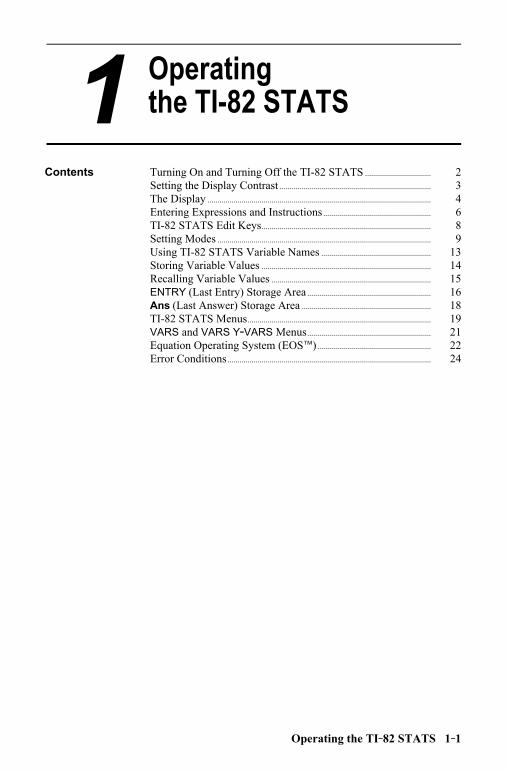
Turning On and Turning Off the TI-82 STATS ................................. 1-2Setting the Display Contrast ............................................................................ 1-3The Display ................................................................................................................ 1-4Entering Expressions and Instructions...................................................... 1-6TI-82 STATS Edit Keys..................................................................................... 1-8Setting Modes ........................................................................................................... 1-9Using TI-82 STATS Variable Names ....................................................... 1-13Storing Variable Values ..................................................................................... 1-14Recalling Variable Values ................................................................................ 1-15ENTRY (Last Entry) Storage Area .............................................................. 1-16Ans (Last Answer) Storage Area.................................................................. 1-18TI-82 STATS Menus............................................................................................ 1-19VARS and VARS Y.VARS Menus.............................................................. 1-21Equation Operating System (EOSé)......................................................... 1-22Error Conditions...................................................................................................... 1-24
Table of Contents
Getting Started:Do This First!
Chapter 1:Operating theTI-82 STATS

iv Introduction
82STAT~2.DOC TI-83 Intl English, Title Page Bob Fedorisko Revised: 10/28/05 11:55 AM Printed: 10/28/0511:57 AM Page iv of 8
Getting Started: Coin Flip ................................................................................. 2-2Keyboard Math Operations .............................................................................. 2-3MATH Operations................................................................................................... 2-5Using the Equation Solver ................................................................................ 2-8MATH NUM (Number) Operations.............................................................. 2-13Entering and Using Complex Numbers.................................................... 2-16MATH CPX (Complex) Operations ............................................................ 2-18MATH PRB (Probability) Operations........................................................ 2-20ANGLE Operations................................................................................................ 2-23TEST (Relational) Operations........................................................................ 2-25TEST LOGIC (Boolean) Operations .......................................................... 2-26
Getting Started: Graphing a Circle .............................................................. 3-2Defining Graphs ...................................................................................................... 3-3Setting the Graph Modes ................................................................................... 3-4Defining Functions ................................................................................................ 3-5Selecting and Deselecting Functions.......................................................... 3-7Setting Graph Styles for Functions.............................................................. 3-9Setting the Viewing Window Variables................................................... 3-11Setting the Graph Format .................................................................................. 3-13Displaying Graphs.................................................................................................. 3-15Exploring Graphs with the Free-Moving Cursor................................ 3-17Exploring Graphs with TRACE..................................................................... 3-18Exploring Graphs with the ZOOM Instructions .................................. 3-20Using ZOOM MEMORY .................................................................................... 3-23Using the CALC (Calculate) Operations.................................................. 3-25
Getting Started: Path of a Ball........................................................................ 4-2Defining and Displaying Parametric Graphs ........................................ 4-4Exploring Parametric Graphs.......................................................................... 4-7
Getting Started: Polar Rose.............................................................................. 5-2Defining and Displaying Polar Graphs..................................................... 5-3Exploring Polar Graphs ...................................................................................... 5-6
Table of Contents (continued)
Chapter 2:Math, Angle, andTest Operations
Chapter 3:FunctionGraphing
Chapter 4:ParametricGraphing
Chapter 5:Polar Graphing

Introduction v
82STAT~2.DOC TI-83 Intl English, Title Page Bob Fedorisko Revised: 10/28/05 11:55 AM Printed: 10/28/0511:57 AM Page v of 8
Getting Started: Forest and Trees................................................................. 6-2Defining and Displaying Sequence Graphs ........................................... 6-3Selecting Axes Combinations......................................................................... 6-8Exploring Sequence Graphs............................................................................. 6-9Graphing Web Plots.............................................................................................. 6-11Using Web Plots to Illustrate Convergence........................................... 6-12Graphing Phase Plots ........................................................................................... 6-13Comparing TI-82 STATS and TI.82 Sequence Variables........... 6-15Keystroke Differences Between TI-82 STATS and TI-82 .......... 6-16
Getting Started: Roots of a Function.......................................................... 7-2Setting Up the Table ............................................................................................. 7-3Defining the Dependent Variables............................................................... 7-4Displaying the Table............................................................................................. 7-5
Getting Started: Drawing a Tangent Line ............................................... 8-2Using the DRAW Menu...................................................................................... 8-3Clearing Drawings ................................................................................................. 8-4Drawing Line Segments ..................................................................................... 8-5Drawing Horizontal and Vertical Lines ................................................... 8-6Drawing Tangent Lines ...................................................................................... 8-8Drawing Functions and Inverses................................................................... 8-9Shading Areas on a Graph ................................................................................ 8-10Drawing Circles....................................................................................................... 8-11Placing Text on a Graph..................................................................................... 8-12Using Pen to Draw on a Graph ...................................................................... 8-13Drawing Points on a Graph .............................................................................. 8-14Drawing Pixels ......................................................................................................... 8-16Storing Graph Pictures (Pic)............................................................................ 8-17Recalling Graph Pictures (Pic)....................................................................... 8-18Storing Graph Databases (GDB)................................................................... 8-19Recalling Graph Databases (GDB).............................................................. 8-20
Getting Started: Exploring the Unit Circle............................................. 9-2Using Split Screen.................................................................................................. 9-3Horiz (Horizontal) Split Screen ..................................................................... 9-4G-T (Graph-Table) Split Screen.................................................................... 9-5TI-82 STATS Pixels in Horiz and G-T Modes .................................... 9-6
Chapter 6:SequenceGraphing
Chapter 7:Tables
Chapter 8:DRAWOperations
Chapter 9:Split Screen
vi Introduction
82STAT~2.DOC TI-83 Intl English, Title Page Bob Fedorisko Revised: 10/28/05 11:55 AM Printed: 10/28/0511:57 AM Page vi of 8
Getting Started: Systems of Linear Equations ..................................... 10-2Defining a Matrix ................................................................................................... 10-3Viewing and Editing Matrix Elements...................................................... 10-4Using Matrices with Expressions ................................................................. 10-7Displaying and Copying Matrices................................................................ 10-8Using Math Functions with Matrices......................................................... 10-9Using the MATRX MATH Operations ....................................................... 10-12
Getting Started: Generating a Sequence .................................................. 11-2Naming Lists.............................................................................................................. 11-3Storing and Displaying Lists ........................................................................... 11-4Entering List Names ............................................................................................. 11-6Attaching Formulas to List Names.............................................................. 11-7Using Lists in Expressions................................................................................ 11-9LIST OPS Menu...................................................................................................... 11-10LIST MATH Menu.................................................................................................. 11-17
Getting Started: Pendulum Lengths and Periods................................ 12-2Setting up Statistical Analyses ....................................................................... 12-10Using the Stat List Editor .................................................................................. 12-11Attaching Formulas to List Names.............................................................. 12-14Detaching Formulas from List Names ...................................................... 12-16Switching Stat List Editor Contexts............................................................ 12-17Stat List Editor Contexts.................................................................................... 12-18STAT EDIT Menu .................................................................................................. 12-20Regression Model Features .............................................................................. 12-22STAT CALC Menu ................................................................................................ 12-24Statistical Variables............................................................................................... 12-29Statistical Analysis in a Program.................................................................. 12-30Statistical Plotting................................................................................................... 12-31Statistical Plotting in a Program.................................................................... 12-37
Getting Started: Mean Height of a Population..................................... 13-2Inferential Stat Editors......................................................................................... 13-6STAT TESTS Menu ............................................................................................. 13-9Inferential Statistics Input Descriptions ................................................... 13-26Test and Interval Output Variables.............................................................. 13-28Distribution Functions ......................................................................................... 13-29Distribution Shading............................................................................................. 13-35
Table of Contents (continued)
Chapter 10:Matrices
Chapter 11:Lists
Chapter 12:Statistics
Chapter 13:InferentialStatistics andDistributions

Introduction vii
82STAT~2.DOC TI-83 Intl English, Title Page Bob Fedorisko Revised: 10/28/05 11:55 AM Printed: 10/28/0511:57 AM Page vii of 8
Getting Started: Financing a Car................................................................... 14-2Getting Started: Computing Compound Interest ................................ 14-3Using the TVM Solver ......................................................................................... 14-4Using the Financial Functions........................................................................ 14-5Calculating Time Value of Money (TVM).............................................. 14-6Calculating Cash Flows...................................................................................... 14-8Calculating Amortization................................................................................... 14-9Calculating Interest Conversion .................................................................... 14-12Finding Days between Dates/Defining Payment Method....................... 14-13Using the TVM Variables................................................................................... 14-14
Browsing the TI-82 STATS CATALOG.................................................. 15-2Entering and Using Strings............................................................................... 15-3Storing Strings to String Variables.............................................................. 15-4String Functions and Instructions in the CATALOG........................ 15-6Hyperbolic Functions in the CATALOG .................................................. 15-10
Getting Started: Volume of a Cylinder ..................................................... 16-2Creating and Deleting Programs................................................................... 16-4Entering Command Lines and Executing Programs ........................ 16-5Editing Programs .................................................................................................... 16-6Copying and Renaming Programs ............................................................... 16-7PRGM CTL (Control) Instructions .............................................................. 16-8PRGM I/O (Input/Output) Instructions..................................................... 16-16Calling Other Programs as Subroutines ................................................... 16-22
Comparing Test Results Using Box Plots............................................... 17-2Graphing Piecewise Functions....................................................................... 17-4Graphing Inequalities........................................................................................... 17-5Solving a System of Nonlinear Equations .............................................. 17-6Using a Program to Create the Sierpinski Triangle .......................... 17-7Graphing Cobweb Attractors .......................................................................... 17-8Using a Program to Guess the Coefficients ........................................... 17-9Graphing the Unit Circle and Trigonometric Curves ...................... 17-10Finding the Area between Curves................................................................ 17-11Using Parametric Equations: Ferris Wheel Problem........................ 17-12Demonstrating the Fundamental Theorem of Calculus.................. 17-14Computing Areas of Regular N-Sided Polygons................................ 17-16Computing and Graphing Mortgage Payments ................................... 17-18
Chapter 14:FinancialFunctions
Chapter 15:CATALOG,Strings,HyperbolicFunctions
Chapter 16:Programming
Chapter 17:Applications
viii Introduction
82STAT~2.DOC TI-83 Intl English, Title Page Bob Fedorisko Revised: 10/28/05 11:55 AM Printed: 10/28/0511:57 AM Page viii of 8
Checking Available Memory.......................................................................... 18-2Deleting Items from Memory ......................................................................... 18-3Clearing Entries and List Elements............................................................. 18-4Resetting the TI-82 STATS ............................................................................. 18-5
Getting Started: Sending Variables............................................................. 19-2TI-82 STATS LINK ............................................................................................... 19-3Selecting Items to Send....................................................................................... 19-4Receiving Items ....................................................................................................... 19-5Transmitting Items................................................................................................. 19-6Transmitting Lists to a TI-82 .......................................................................... 19-8Transmitting from a TI-82 to a TI-82 STATS ..................................... 19-9Backing Up Memory............................................................................................ 19-10
Table of Functions and Instructions............................................................ A-2Menu Map ................................................................................................................... A-39Variables....................................................................................................................... A-49Statistical Formulas ............................................................................................... A-50Financial Formulas ................................................................................................ A-54
Battery Information............................................................................................... B-2In Case of Difficulty ............................................................................................. B-4Error Conditions...................................................................................................... B-5Accuracy Information.......................................................................................... B-10Support and Service Information.................................................................. B-12Warranty Information .......................................................................................... B-13
Table of Contents (continued)
Chapter 18:MemoryManagement
Chapter 19:CommunicationLink
Appendix A:Tables andReferenceInformation
Appendix B:GeneralInformation
Index
Getting Started 1
82STAT~1.DOC TI-83 international English Bob Fedorisko Revised: 10/27/05 1:33 PM Printed: 10/27/05 3:30PM Page 1 of 18
Getting Started:Do This First!
TI-82 STATS Keyboard..................................................................................... 2TI-82 STATS Menus............................................................................................ 4First Steps .................................................................................................................... 5Entering a Calculation: The Quadratic Formula................................. 6Converting to a Fraction: The Quadratic Formula ............................ 7Displaying Complex Results: The Quadratic Formula................... 8Defining a Function: Box with Lid ............................................................. 9Defining a Table of Values: Box with Lid ............................................. 10Zooming In on the Table: Box with Lid .................................................. 11Setting the Viewing Window: Box with Lid......................................... 12Displaying and Tracing the Graph: Box with Lid ............................. 13Zooming In on the Graph: Box with Lid................................................. 15Finding the Calculated Maximum: Box with Lid .............................. 16Other TI-82 STATS Features.......................................................................... 17
Contents

2 Getting Started
82STAT~1.DOC TI-83 international English Bob Fedorisko Revised: 10/27/05 1:33 PM Printed: 10/27/05 3:30PM Page 2 of 18
Generally, the keyboard is divided into these zones: graphing keys, editing keys,advanced function keys, and scientific calculator keys.
Graphing keys access the interactive graphing features.
Editing keys allow you to edit expressions and values.
Advanced function keys display menus that access the advancedfunctions.
Scientific calculator keys access the capabilities of a standardscientific calculator.
TI-82 STATS Keyboard
Keyboard Zones
Editing Keys
AdvancedFunction Keys
ScientificCalculator Keys
Graphing Keys

Getting Started 3
82STAT~1.DOC TI-83 international English Bob Fedorisko Revised: 10/27/05 1:33 PM Printed: 10/27/05 3:30PM Page 3 of 18
The keys on the TI-82 STATS are color-coded to help youeasily locate the key you need.
The gray keys are the number keys. The blue keys along the rightside of the keyboard are the common math functions. The blue keysacross the top set up and display graphs.
The primary function of each key is printed in white on the key.For example, when you press , the MATH menu isdisplayed.
The secondary function of each key is printed in yellow abovethe key. When you press the yellow y key, the character,abbreviation, or word printed in yellow above the other keysbecomes active for the next keystroke. For example, when youpress y and then , the TEST menu is displayed. Thisguidebook describes this keystroke combination as y [TEST].
The alpha function of each key is printed in green above thekey. When you press the green ƒ key, the alpha characterprinted in green above the other keys becomes active for thenext keystroke. For example, when you press ƒ and then, the letter A is entered. This guidebook describes thiskeystroke combination as ƒ [A].
Using theColor.CodedKeyboard
Using the yand ƒ Keys
The y keyaccesses thesecond functionprinted in yellowabove each key.
The ƒ keyaccesses the alphafunction printed ingreen above eachkey.

4 Getting Started
82STAT~1.DOC TI-83 international English Bob Fedorisko Revised: 10/27/05 1:33 PM Printed: 10/27/05 3:30PM Page 4 of 18
Displaying a Menu
While using your TI-82 STATS, you often willneed to access items from its menus.
When you press a key that displays a menu, thatmenu temporarily replaces the screen where youare working. For example, when you press ,the MATH menu is displayed as a full screen.
After you select an item from a menu, the screenwhere you are working usually is displayed again.
Moving from One Menu to Another
Some keys access more than one menu. When youpress such a key, the names of all accessiblemenus are displayed on the top line. When youhighlight a menu name, the items in that menu aredisplayed. Press ~ and | to highlight each menuname.
Selecting an Item from a Menu
The number or letter next to the current menu itemis highlighted. If the menu continues beyond thescreen, a down arrow ( $ ) replaces the colon ( : )in the last displayed item. If you scroll beyond thelast displayed item, an up arrow ( # ) replaces thecolon in the first item displayed.You can select anitem in either of two ways.¦ Press † or } to move the cursor to the number
or letter of the item; press Í.¦ Press the key or key combination for the
number or letter next to the item.
Leaving a Menu without Making a Selection
You can leave a menu without making a selectionin any of three ways.¦ Press ‘ to return to the screen where
you were.¦ Press y [QUIT] to return to the home screen.¦ Press a key for another menu or screen.
TI-82 STATS Menus

Getting Started 5
82STAT~1.DOC TI-83 international English Bob Fedorisko Revised: 10/27/05 1:33 PM Printed: 10/27/05 3:30PM Page 5 of 18
Before starting the sample problems in this chapter, follow the steps on this page toreset the TI-82 STATS to its factory settings and clear all memory. This ensures thatthe keystrokes in this chapter will produce the illustrated results.
To reset the TI-82 STATS, follow these steps.
1. Press É to turn on the calculator.
2. Press and release y, and then press [MEM](above Ã).
When you press y, you access the operationprinted in yellow above the next key that youpress. [MEM] is the y operation of the Ãkey.
The MEMORY menu is displayed.
3. Press 5 to select 5:Reset.
The RESET menu is displayed.
4. Press 1 to select 1:All Memory.
The RESET MEMORY menu is displayed.
5. Press 2 to select 2:Reset.
All memory is cleared, and the calculator isreset to the factory default settings.
When you reset the TI-82 STATS, the displaycontrast is reset.
¦ If the screen is very light or blank, pressand release y, and then press and hold }to darken the screen.
¦ If the screen is very dark, press and releasey, and then press and hold † to lightenthe screen.
First Steps

6 Getting Started
82STAT~1.DOC TI-83 international English Bob Fedorisko Revised: 10/27/05 1:33 PM Printed: 10/27/05 3:30PM Page 6 of 18
Use the quadratic formula to solve the quadratic equations 3X2 + 5X + 2 = 0 and 2X2
N X + 3 = 0. Begin with the equation 3X2 + 5X + 2 = 0.
1. Press 3 ¿ ƒ [A] (above ) tostore the coefficient of the X2 term.
2. Press ƒ [ : ] (above Ë). The colon allowsyou to enter more than one instruction on aline.
3. Press 5 ¿ ƒ [B] (above ) tostore the coefficient of the X term. Pressƒ [ : ] to enter a new instruction on thesame line. Press 2 ¿ƒ [C] (above) to store the constant.
4. Press Í to store the values to the variablesA, B, and C.
The last value you stored is shown on the rightside of the display. The cursor moves to thenext line, ready for your next entry.
5. Press £ Ì ƒ [B] Ãy [‡] ƒ [B]¡ ¹ 4 ƒ [A] ƒ [C] ¤¤¥£ 2ƒ [A] ¤ to enter the expression for oneof the solutions for the quadratic formula,− + −b b ac
a
2 42
6. Press Í to find one solution for theequation 3X2 + 5X + 2 = 0.
The answer is shown on the right side of thedisplay. The cursor moves to the next line,ready for you to enter the next expression.
Entering a Calculation: The Quadratic Formula

Getting Started 7
82STAT~1.DOC TI-83 international English Bob Fedorisko Revised: 10/27/05 1:33 PM Printed: 10/27/05 3:30PM Page 7 of 18
You can show the solution as a fraction.
1. Press to display the MATH menu.
2. Press 1 to select 1:4Frac from the MATH menu.
When you press 1, Ans4Frac is displayed onthe home screen. Ans is a variable thatcontains the last calculated answer.
3. Press Í to convert the result to a fraction.
To save keystrokes, you can recall the last expression you entered, and then edit it fora new calculation.
4. Press y [ENTRY] (above Í) to recall thefraction conversion entry, and then press y[ENTRY] again to recall the quadratic-formulaexpression,− + −b b ac
a
2 42
5. Press } to move the cursor onto the + sign inthe formula. Press ¹ to edit the quadratic-formula expression to become:− − −b b ac
a
2 42
6. Press Í to find the other solution for thequadratic equation 3X2 + 5X + 2 = 0.
Converting to a Fraction: The Quadratic Formula

8 Getting Started
82STAT~1.DOC TI-83 international English Bob Fedorisko Revised: 10/27/05 1:33 PM Printed: 10/27/05 3:30PM Page 8 of 18
Now solve the equation 2X2 N X + 3 = 0. When you set a+bi complex number mode,the TI-82 STATS displays complex results.
1. Press z † † † ††† (6 times), andthen press ~ to position the cursor over a+bi.Press Í to select a+bi complex-numbermode.
2. Press y [QUIT] (above z) to return to thehome screen, and then press ‘ to clear it.
3. Press 2 ¿ ƒ [A] ƒ [ : ] Ì 1¿ƒ [B] ƒ [ : ] 3¿ƒ[C] Í.
The coefficient of the X2 term, the coefficientof the X term, and the constant for the newequation are stored to A, B, and C,respectively.
4. Press y [ENTRY] to recall the storeinstruction, and then press y [ENTRY] againto recall the quadratic-formula expression,− − −b b ac
a
2 42
5. Press Í to find one solution for theequation 2X2 N X + 3 = 0.
6. Press y [ENTRY] repeatedly until thisquadratic-formula expression is displayed:
− + −b b aca
2 42
7. Press Í to find the other solution for thequadratic equation: 2X2 N X + 3 = 0.
Note: An alternative for solving equations for real numbers is to use the built-in EquationSolver (Chapter 2).
Displaying Complex Results: The Quadratic Formula
Getting Started 9
82STAT~1.DOC TI-83 international English Bob Fedorisko Revised: 10/27/05 1:33 PM Printed: 10/27/05 3:30PM Page 9 of 18
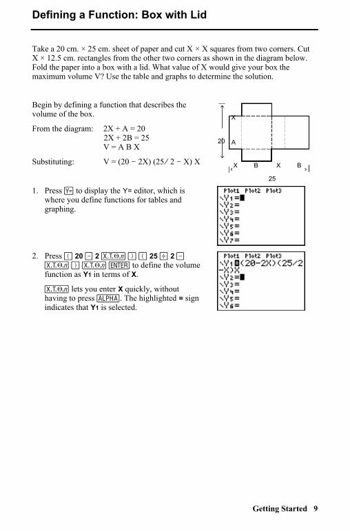
Take a 20 cm. × 25 cm. sheet of paper and cut X × X squares from two corners. CutX × 12.5 cm. rectangles from the other two corners as shown in the diagram below.Fold the paper into a box with a lid. What value of X would give your box themaximum volume V? Use the table and graphs to determine the solution.
Begin by defining a function that describes thevolume of the box.
From the diagram: 2X + A = 20 2X + 2B = 25V = A B X
Substituting: V = (20 N 2X) (25à 2 N X) X
1. Press o to display the Y= editor, which iswhere you define functions for tables andgraphing.
2. Press £ 20 ¹ 2 „¤£ 25¥ 2¹„ ¤ „ Í to define the volumefunction as Y1 in terms of X.
„ lets you enter X quickly, withouthaving to press ƒ. The highlighted = signindicates that Y1 is selected.
Defining a Function: Box with Lid
20 A
X
X B X B
25

10 Getting Started
82STAT~1.DOC TI-83 international English Bob Fedorisko Revised: 10/27/05 1:33 PM Printed: 10/27/05 3:30PM Page 10 of 18
The table feature of the TI-82 STATS displays numeric information about a function.You can use a table of values from the function defined on page 9 to estimate ananswer to the problem.
1. Press y [TBLSET] (above p) to displaythe TABLE SETUP menu.
2. Press Í to accept TblStart=0.
3. Press 1 Í to define the table increment@Tbl=1. Leave Indpnt: Auto andDepend: Auto so that the table will begenerated automatically.
4. Press y [TABLE] (above s) to displaythe table.
Notice that the maximum value for Y1 (box’svolume) occurs when X is about 4, between 3and 5.
5. Press and hold † to scroll the table until anegative result for Y1 is displayed.
Notice that the maximum length of X for thisproblem occurs where the sign of Y1 (box’svolume) changes from positive to negative,between 10 and 11.
6. Press y [TBLSET].
Notice that TblStart has changed to 6 to reflectthe first line of the table as it was lastdisplayed. (In step 5, the first value of Xdisplayed in the table is 6.)
Defining a Table of Values: Box with Lid

Getting Started 11
82STAT~1.DOC TI-83 international English Bob Fedorisko Revised: 10/27/05 1:33 PM Printed: 10/27/05 3:30PM Page 11 of 18
You can adjust the way a table is displayed to get more information about a definedfunction. With smaller values for @Tbl, you can zoom in on the table.
1. Press 3 Í to set TblStart. Press Ë 1Í to set @Tbl.
This adjusts the table setup to get a moreaccurate estimate of X for maximum volumeY1.
2. Press y [TABLE].
3. Press † and } to scroll the table.
Notice that the maximum value for Y1 is410.26, which occurs at X=3.7. Therefore, themaximum occurs where 3.6<X<3.8.
4. Press y [TBLSET]. Press 3 Ë 6Í to setTblStart. Press Ë 01 Í to set @Tbl.
5. Press y [TABLE], and then press † and } toscroll the table.
Four equivalent maximum values are shown,410.60 at X=3.67, 3.68, 3.69, and 3.70.
6. Press † and } to move the cursor to 3.67.Press ~ to move the cursor into the Y1column.
The value of Y1 at X=3.67 is displayed on thebottom line in full precision as 410.261226.
7. Press † to display the other maximums.
The value of Y1 at X=3.68 in full precision is410.264064, at X=3.69 is 410.262318, and atX=3.7 is 410.256.
The maximum volume of the box would occurat 3.68 if you could measure and cut the paper at.01-cm. increments.
Zooming In on the Table: Box with Lid

12 Getting Started
82STAT~1.DOC TI-83 international English Bob Fedorisko Revised: 10/27/05 1:33 PM Printed: 10/27/05 3:30PM Page 12 of 18
You also can use the graphing features of the TI-82 STATS to find the maximumvalue of a previously defined function. When the graph is activated, the viewingwindow defines the displayed portion of the coordinate plane. The values of thewindow variables determine the size of the viewing window.
1. Press p to display the window editor,where you can view and edit the values of thewindow variables.
The standard window variables define theviewing window as shown. Xmin, Xmax,Ymin, and Ymax define the boundaries of thedisplay. Xscl and Yscl define the distancebetween tick marks on the X and Y axes. Xrescontrols resolution.
Xmax
Ymin
Ymax
Xscl
Yscl
Xmin
2. Press 0 Í to define Xmin.
3. Press 20 ¥ 2 to define Xmax using anexpression.
4. Press Í. The expression is evaluated, and10 is stored in Xmax. Press Í to acceptXscl as 1.
5. Press 0 Í 500 Í 100Í 1 Íto define the remaining window variables.
Setting the Viewing Window: Box with Lid

Getting Started 13
82STAT~1.DOC TI-83 international English Bob Fedorisko Revised: 10/27/05 1:33 PM Printed: 10/27/05 3:30PM Page 13 of 18
Now that you have defined the function to be graphed and the window in which tograph it, you can display and explore the graph. You can trace along a function usingthe TRACE feature.
1. Press s to graph the selected function inthe viewing window.
The graph of Y1=(20N2X)(25à2NX)X isdisplayed.
2. Press ~ to activate the free-moving graphcursor.
The X and Y coordinate values for the positionof the graph cursor are displayed on thebottom line.
3. Press |, ~, }, and † to move the free-moving cursor to the apparent maximum of thefunction.
As you move the cursor, the X and Ycoordinate values are updated continually.
Displaying and Tracing the Graph: Box with Lid

14 Getting Started
82STAT~1.DOC TI-83 international English Bob Fedorisko Revised: 10/27/05 1:33 PM Printed: 10/27/05 3:30PM Page 14 of 18
4. Press r. The trace cursor is displayed onthe Y1 function.
The function that you are tracing is displayedin the top-left corner.
5. Press | and ~ to trace along Y1, one X dot ata time, evaluating Y1 at each X.
You also can enter your estimate for themaximum value of X.
6. Press 3 Ë 8. When you press a number keywhile in TRACE, the X= prompt is displayed inthe bottom-left corner.
7. Press Í.
The trace cursor jumps to the point on the Y1function evaluated at X=3.8.
8. Press | and ~ until you are on the maximumY value.
This is the maximum of Y1(X) for the X pixelvalues. The actual, precise maximum may liebetween pixel values.
Displaying and Tracing the Graph: Box with Lid (cont.)

Getting Started 15
82STAT~1.DOC TI-83 international English Bob Fedorisko Revised: 10/27/05 1:33 PM Printed: 10/27/05 3:30PM Page 15 of 18
To help identify maximums, minimums, roots, and intersections of functions, you canmagnify the viewing window at a specific location using the ZOOM instructions.
1. Press q to display the ZOOM menu.
This menu is a typical TI-82 STATS menu. Toselect an item, you can either press the numberor letter next to the item, or you can press †until the item number or letter is highlighted,and then press Í.
2. Press 2 to select 2:Zoom In.
The graph is displayed again. The cursor haschanged to indicate that you are using a ZOOMinstruction.
3. With the cursor near the maximum value ofthe function (as in step 8 on page 14), pressÍ.
The new viewing window is displayed. BothXmaxNXmin and YmaxNYmin have beenadjusted by factors of 4, the default values forthe zoom factors.
4. Press p to display the new windowsettings.
Zooming In on the Graph: Box with Lid

16 Getting Started
82STAT~1.DOC TI-83 international English Bob Fedorisko Revised: 10/27/05 1:33 PM Printed: 10/27/05 3:30PM Page 16 of 18
You can use a CALCULATE menu operation to calculate a local maximum of afunction.
1. Press y [CALC] (above r) to display theCALCULATE menu. Press 4 to select4:maximum.
The graph is displayed again with aLeft Bound? prompt.
2. Press | to trace along the curve to a point tothe left of the maximum, and then pressÍ.
A 4 at the top of the screen indicates theselected bound.
A Right Bound? prompt is displayed.
3. Press ~ to trace along the curve to a point tothe right of the maximum, and then pressÍ.
A 3 at the top of the screen indicates theselected bound.
A Guess? prompt is displayed.
4. Press | to trace to a point near the maximum,and then press Í.
Or, press 3 Ë 8, and then press Í to entera guess for the maximum.
When you press a number key in TRACE, theX= prompt is displayed in the bottom-leftcorner.
Notice how the values for the calculatedmaximum compare with the maximums foundwith the free-moving cursor, the trace cursor,and the table.
Note: In steps 2 and 3 above, you can enter valuesdirectly for Left Bound and Right Bound, in the sameway as described in step 4.
Finding the Calculated Maximum: Box with Lid

Getting Started 17
82STAT~1.DOC TI-83 international English Bob Fedorisko Revised: 10/27/05 1:33 PM Printed: 10/27/05 3:30PM Page 17 of 18
Getting Started has introduced you to basic TI-82 STATS operation. This guidebookdescribes in detail the features you used in Getting Started. It also covers the otherfeatures and capabilities of the TI-82 STATS.
You can store, graph, and analyze up to 10 functions (Chapter3), up to six parametric functions (Chapter 4), up to six polarfunctions (Chapter 5), and up to three sequences (Chapter 6).You can use DRAW operations to annotate graphs (Chapter 8).
You can generate sequences and graph them over time. Or, youcan graph them as web plots or as phase plots (Chapter 6).
You can create function evaluation tables to analyze manyfunctions simultaneously (Chapter 7).
You can split the screen horizontally to display both a graph anda related editor (such as the Y= editor), the table, the stat listeditor, or the home screen. Also, you can split the screenvertically to display a graph and its table simultaneously(Chapter 9).
You can enter and save up to 10 matrices and perform standardmatrix operations on them (Chapter 10).
You can enter and save as many lists as memory allows for usein statistical analyses. You can attach formulas to lists forautomatic computation. You can use lists to evaluateexpressions at multiple values simultaneously and to graph afamily of curves (Chapter 11).
You can perform one- and two-variable, list-based statisticalanalyses, including logistic and sine regression analysis. Youcan plot the data as a histogram, xyLine, scatter plot, modifiedor regular box-and-whisker plot, or normal probability plot. Youcan define and store up to three stat plot definitions (Chapter12).
Other TI-82 STATS Features
Graphing
Sequences
Tables
Split Screen
Matrices
Lists
Statistics
18 Getting Started
82STAT~1.DOC TI-83 international English Bob Fedorisko Revised: 10/27/05 1:33 PM Printed: 10/27/05 3:30PM Page 18 of 18
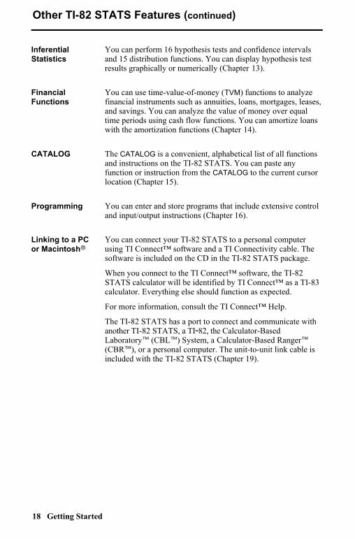
You can perform 16 hypothesis tests and confidence intervalsand 15 distribution functions. You can display hypothesis testresults graphically or numerically (Chapter 13).
You can use time-value-of-money (TVM) functions to analyzefinancial instruments such as annuities, loans, mortgages, leases,and savings. You can analyze the value of money over equaltime periods using cash flow functions. You can amortize loanswith the amortization functions (Chapter 14).
The CATALOG is a convenient, alphabetical list of all functionsand instructions on the TI-82 STATS. You can paste anyfunction or instruction from the CATALOG to the current cursorlocation (Chapter 15).
You can enter and store programs that include extensive controland input/output instructions (Chapter 16).
You can connect your TI-82 STATS to a personal computerusing TI Connect™ software and a TI Connectivity cable. Thesoftware is included on the CD in the TI-82 STATS package.
When you connect to the TI Connect™ software, the TI-82STATS calculator will be identified by TI Connect™ as a TI-83calculator. Everything else should function as expected.
For more information, consult the TI Connect™ Help.
The TI-82 STATS has a port to connect and communicate withanother TI-82 STATS, a TI.82, the Calculator-BasedLaboratoryé (CBLé) System, a Calculator-Based Rangeré(CBRé), or a personal computer. The unit-to-unit link cable isincluded with the TI-82 STATS (Chapter 19).
Other TI-82 STATS Features (continued)
InferentialStatistics
FinancialFunctions
CATALOG
Programming
Linking to a PCor Macintoshë
Operating the TI-82 STATS 1-1
82STAT~3.DOC TI-83 international English Bob Fedorisko Revised: 10/28/05 12:11 PM Printed: 10/28/05 12:11PM Page 1 of 24
1 Operatingthe TI-82 STATS
Turning On and Turning Off the TI-82 STATS ................................. 2Setting the Display Contrast ............................................................................ 3The Display ................................................................................................................ 4Entering Expressions and Instructions...................................................... 6TI-82 STATS Edit Keys..................................................................................... 8Setting Modes ........................................................................................................... 9Using TI-82 STATS Variable Names ....................................................... 13Storing Variable Values ..................................................................................... 14Recalling Variable Values ................................................................................ 15ENTRY (Last Entry) Storage Area .............................................................. 16Ans (Last Answer) Storage Area ................................................................. 18TI-82 STATS Menus............................................................................................ 19VARS and VARS Y.VARS Menus.............................................................. 21Equation Operating System (EOSé)......................................................... 22Error Conditions...................................................................................................... 24
Contents

1-2 Operating the TI-82 STATS
82STAT~3.DOC TI-83 international English Bob Fedorisko Revised: 10/28/05 12:11 PM Printed: 10/28/05 12:11PM Page 2 of 24
To turn on the TI-82 STATS, press É.
• If you previously had turned off the calculator by pressingy [OFF], the TI-82 STATS displays the home screen as itwas when you last used it and clears any error.
• If Automatic Power Down™ (APDé) had previously turnedoff the calculator, the TI-82 STATS will return exactly as youleft it, including the display, cursor, and any error.
To prolong the life of the batteries, APD turns off theTI-82 STATS automatically after about five minutes without anyactivity.
To turn off the TI-82 STATS manually, press y [OFF].
• All settings and memory contents are retained by ConstantMemoryé.
• Any error condition is cleared.
The TI-82 STATS uses four AAA alkaline batteries and has auser-replaceable backup lithium battery (CR1616 or CR1620).To replace batteries without losing any information stored inmemory, follow the steps in Appendix B.
Turning On and Turning Off the TI-82 STATS
Turning On theCalculator
Turning Off theCalculator
Batteries
Operating the TI-82 STATS 1-3
82STAT~3.DOC TI-83 international English Bob Fedorisko Revised: 10/28/05 12:11 PM Printed: 10/28/05 12:11PM Page 3 of 24
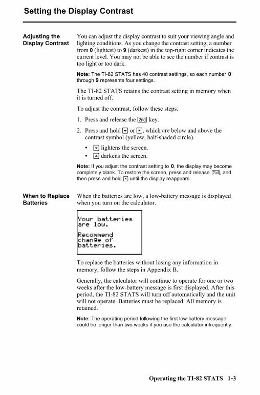
You can adjust the display contrast to suit your viewing angle andlighting conditions. As you change the contrast setting, a numberfrom 0 (lightest) to 9 (darkest) in the top-right corner indicates thecurrent level. You may not be able to see the number if contrast istoo light or too dark.
Note: The TI-82 STATS has 40 contrast settings, so each number 0through 9 represents four settings.
The TI-82 STATS retains the contrast setting in memory whenit is turned off.
To adjust the contrast, follow these steps.
1. Press and release the y key.
2. Press and hold † or }, which are below and above thecontrast symbol (yellow, half-shaded circle).
• † lightens the screen.• } darkens the screen.
Note: If you adjust the contrast setting to 0, the display may becomecompletely blank. To restore the screen, press and release y, andthen press and hold } until the display reappears.
When the batteries are low, a low-battery message is displayedwhen you turn on the calculator.
To replace the batteries without losing any information inmemory, follow the steps in Appendix B.
Generally, the calculator will continue to operate for one or twoweeks after the low-battery message is first displayed. After thisperiod, the TI-82 STATS will turn off automatically and the unitwill not operate. Batteries must be replaced. All memory isretained.
Note: The operating period following the first low-battery messagecould be longer than two weeks if you use the calculator infrequently.
Setting the Display Contrast
Adjusting theDisplay Contrast
When to ReplaceBatteries

1-4 Operating the TI-82 STATS
82STAT~3.DOC TI-83 international English Bob Fedorisko Revised: 10/28/05 12:11 PM Printed: 10/28/05 12:11PM Page 4 of 24
The TI-82 STATS displays both text and graphs. Chapter 3describes graphs. Chapter 9 describes how the TI-82 STATS candisplay a horizontally or vertically split screen to show graphsand text simultaneously.
The home screen is the primary screen of the TI-82 STATS. Onthis screen, enter instructions to execute and expressions toevaluate. The answers are displayed on the same screen.
When text is displayed, the TI-82 STATS screen can display amaximum of eight lines with a maximum of 16 characters perline. If all lines of the display are full, text scrolls off the top ofthe display. If an expression on the home screen, the Y= editor(Chapter 3), or the program editor (Chapter 16) is longer thanone line, it wraps to the beginning of the next line. In numericeditors such as the window screen (Chapter 3), a longexpression scrolls to the right and left.
When an entry is executed on the home screen, the answer isdisplayed on the right side of the next line.
Entry Answer
The mode settings control the way the TI-82 STATS interpretsexpressions and displays answers (page 1.9).
If an answer, such as a list or matrix, is too long to displayentirely on one line, an ellipsis (...) is displayed to the right orleft. Press ~ and | to scroll the answer.
Entry Answer
To return to the home screen from any other screen, press y[QUIT].
When the TI-82 STATS is calculating or graphing, a verticalmoving line is displayed as a busy indicator in the top-rightcorner of the screen. When you pause a graph or a program, thebusy indicator becomes a vertical moving dotted line.
The Display
Types ofDisplays
Home Screen
DisplayingEntries andAnswers
Returning to theHome Screen
Busy Indicator

Operating the TI-82 STATS 1-5
82STAT~3.DOC TI-83 international English Bob Fedorisko Revised: 10/28/05 12:11 PM Printed: 10/28/05 12:11PM Page 5 of 24
In most cases, the appearance of the cursor indicates what willhappen when you press the next key or select the next menuitem to be pasted as a character.
Cursor Appearance Effect of Next KeystrokeEntry Solid rectangle$
A character is entered at the cursor;any existing character is overwritten
Insert Underline__
A character is inserted in front of thecursor location
Second Reverse arrowÞ
A 2nd character (yellow on thekeyboard) is entered or a 2ndoperation is executed
Alpha Reverse AØ
An alpha character (green on thekeyboard) is entered or SOLVE isexecuted
Full Checkerboardrectangle#
No entry; the maximum characters areentered at a prompt or memory is full
If you press ƒ during an insertion, the cursor becomes anunderlined A (A) If you press y during an insertion, theunderline cursor becomes an underlined # ( # ).
Graphs and editors sometimes display additional cursors, whichare described in other chapters.
Display Cursors

1-6 Operating the TI-82 STATS
82STAT~3.DOC TI-83 international English Bob Fedorisko Revised: 10/28/05 12:11 PM Printed: 10/28/05 12:11PM Page 6 of 24
An expression is a group of numbers, variables, functions andtheir arguments, or a combination of these elements. Anexpression evaluates to a single answer. On the TI-82 STATS,you enter an expression in the same order as you would write iton paper. For example, pR2 is an expression.
You can use an expression on the home screen to calculate ananswer. In most places where a value is required, you can use anexpression to enter a value.
To create an expression, you enter numbers, variables, andfunctions from the keyboard and menus. An expression iscompleted when you press Í, regardless of the cursorlocation. The entire expression is evaluated according toEquation Operating System (EOSé) rules (page 1.22), and theanswer is displayed.
Most TI-82 STATS functions and operations are symbolscomprising several characters. You must enter the symbol fromthe keyboard or a menu; do not spell it out. For example, tocalculate the log of 45, you must press « 45. Do not enter theletters L, O, and G. If you enter LOG, the TI-82 STATSinterprets the entry as implied multiplication of the variables L,O, and G.
Calculate 3.76 ÷ (L7.9 + ‡5) + 2 log 45.
3 Ë 76¥£Ì 7Ë 9Ãy [‡] 5¤¤Ã 2 « 45¤Í
To enter two or more expressions or instructions on a line,separate them with colons (ƒ [:]). All instructions arestored together in last entry (ENTRY; page 1.16).
Entering Expressions and Instructions
What Is anExpression?
Entering anExpression
Multiple Entrieson a Line

Operating the TI-82 STATS 1-7
82STAT~3.DOC TI-83 international English Bob Fedorisko Revised: 10/28/05 12:11 PM Printed: 10/28/05 12:11PM Page 7 of 24
To enter a number in scientific notation, follow these steps.
1. Enter the part of the number that precedes the exponent. Thisvalue can be an expression.
2. Press y [EE]. åååå is pasted to the cursor location.
3. If the exponent is negative, press Ì, and then enter theexponent, which can be one or two digits.
When you enter a number in scientific notation, theTI-82 STATS does not automatically display answers inscientific or engineering notation. The mode settings (page 1.9)and the size of the number determine the display format.
A function returns a value. For example, ÷, L, +, ‡(, and log( arethe functions in the example on page 1.6. In general, the first letterof each function is lowercase on the TI-82 STATS. Mostfunctions take at least one argument, as indicated by an openparenthesis ( ( ) following the name. For example, sin( requiresone argument, sin(value).
An instruction initiates an action. For example, ClrDraw is aninstruction that clears any drawn elements from a graph.Instructions cannot be used in expressions. In general, the firstletter of each instruction name is uppercase. Some instructionstake more than one argument, as indicated by an openparenthesis ( ( ) at the end of the name. For example, Circle(requires three arguments, Circle(X,Y,radius).
To interrupt a calculation or graph in progress, which would beindicated by the busy indicator, press É.
When you interrupt a calculation, the menu is displayed.
• To return to the home screen, select 1:Quit.• To go to the location of the interruption, select 2:Goto.
When you interrupt a graph, a partial graph is displayed.
• To return to the home screen, press ‘ or anynongraphing key.
• To restart graphing, press a graphing key or select a graphinginstruction.
Entering aNumber inScientificNotation
Functions
Instructions
Interrupting aCalculation

1-8 Operating the TI-82 STATS
82STAT~3.DOC TI-83 international English Bob Fedorisko Revised: 10/28/05 12:11 PM Printed: 10/28/05 12:11PM Page 8 of 24
Keystrokes Result~ or | Moves the cursor within an expression; these keys repeat.} or † Moves the cursor from line to line within an expression that occupies
more than one line; these keys repeat.On the top line of an expression on the home screen, } moves thecursor to the beginning of the expression.On the bottom line of an expression on the home screen, † moves thecursor to the end of the expression.
y | Moves the cursor to the beginning of an expression.y ~ Moves the cursor to the end of an expression.Í Evaluates an expression or executes an instruction.‘ On a line with text on the home screen, clears the current line.
On a blank line on the home screen, clears everything on the homescreen.In an editor, clears the expression or value where the cursor is located;it does not store a zero.
{ Deletes a character at the cursor; this key repeats.y [INS] Changes the cursor to __ ; inserts characters in front of the underline
cursor; to end insertion, press y [INS] or press |, }, ~, or †.y Changes the cursor to Þ; the next keystroke performs a 2nd operation
(an operation in yellow above a key and to the left); to cancel 2nd,press y again.
ƒ Changes the cursor to Ø; the next keystroke pastes an alpha character(a character in green above a key and to the right) or executes SOLVE(Chapters 10 and 11); to cancel ƒ, press ƒ or press |, },~, or †.
y [A.LOCK] Changes the cursor to Ø; sets alpha-lock; subsequent keystrokes (on analpha key) paste alpha characters; to cancel alpha-lock, press ƒ;name prompts set alpha-lock automatically.
„ Pastes an X in Func mode, a T in Par mode, a q in Pol mode, or an n inSeq mode with one keystroke.
TI-82 STATS Edit Keys

Operating the TI-82 STATS 1-9
82STAT~3.DOC TI-83 international English Bob Fedorisko Revised: 10/28/05 12:11 PM Printed: 10/28/05 12:11PM Page 9 of 24
Mode settings control how the TI-82 STATS displays andinterprets numbers and graphs. Mode settings are retained by theConstant Memory feature when the TI-82 STATS is turned off.All numbers, including elements of matrices and lists, aredisplayed according to the current mode settings.
To display the mode settings, press z. The current settingsare highlighted. Defaults are highlighted below. The followingpages describe the mode settings in detail.
Normal Sci Eng Numeric notationFloat 0123456789 Number of decimal placesRadian Degree Unit of angle measureFunc Par Pol Seq Type of graphingConnected Dot Whether to connect graph pointsSequential Simul Whether to plot simultaneouslyReal a+bi re^qi Real, rectangular cplx, or polar cplxFull Horiz G-T Full screen, two split-screen modes
To change mode settings, follow these steps.
1. Press † or } to move the cursor to the line of the settingthat you want to change.
2. Press ~ or | to move the cursor to the setting you want.
3. Press Í.
You can set a mode from a program by entering the name of themode as an instruction; for example, Func or Float. From ablank command line, select the mode setting from the modescreen; the instruction is pasted to the cursor location.
Setting Modes
Checking ModeSettings
Changing ModeSettings
Setting a Modefrom a Program

1-10 Operating the TI-82 STATS
82STAT~3.DOC TI-83 international English Bob Fedorisko Revised: 10/28/05 12:11 PM Printed: 10/28/05 12:11PM Page 10 of 24
Notation modes only affect the way an answer is displayed onthe home screen. Numeric answers can be displayed with up to10 digits and a two-digit exponent. You can enter a number inany format.
Normal notation mode is the usual way we express numbers,with digits to the left and right of the decimal, as in 12345.67.
Sci (scientific) notation mode expresses numbers in two parts.The significant digits display with one digit to the left of thedecimal. The appropriate power of 10 displays to the right of E,as in 1.234567E4.
Eng (engineering) notation mode is similar to scientificnotation. However, the number can have one, two, or threedigits before the decimal; and the power-of-10 exponent is amultiple of three, as in 12.34567E3.
Note: If you select Normal notation, but the answer cannot display in10 digits (or the absolute value is less than .001), the TI-82 STATSexpresses the answer in scientific notation.
Float (floating) decimal mode displays up to 10 digits, plus thesign and decimal.
0123456789 (fixed) decimal mode specifies the number of digits(0 through 9) to display to the right of the decimal. Place thecursor on the desired number of decimal digits, and then pressÍ.
The decimal setting applies to Normal, Sci, and Eng notationmodes.
The decimal setting applies to these numbers:
• An answer displayed on the home screen• Coordinates on a graph (Chapters 3, 4, 5, and 6)• The Tangent( DRAW instruction equation of the line, x, and
dy/dx values (Chapter 8)• Results of CALCULATE operations (Chapters 3, 4, 5, and 6)• The regression equation stored after the execution of a
regression model (Chapter 12)
Setting Modes (continued)
Normal, Sci, Eng
Float,0123456789

Operating the TI-82 STATS 1-11
82STAT~3.DOC TI-83 international English Bob Fedorisko Revised: 10/28/05 12:11 PM Printed: 10/28/05 12:11PM Page 11 of 24
Angle modes control how the TI-82 STATS interprets anglevalues in trigonometric functions and polar/rectangularconversions.
Radian mode interprets angle values as radians. Answersdisplay in radians.
Degree mode interprets angle values as degrees. Answersdisplay in degrees.
Graphing modes define the graphing parameters. Chapters 3, 4,5, and 6 describe these modes in detail.
Func (function) graphing mode plots functions, where Y is afunction of X (Chapter 3).
Par (parametric) graphing mode plots relations, where X and Yare functions of T (Chapter 4).
Pol (polar) graphing mode plots functions, where r is a functionof q (Chapter 5).
Seq (sequence) graphing mode plots sequences (Chapter 6).
Connected plotting mode draws a line connecting each pointcalculated for the selected functions.
Dot plotting mode plots only the calculated points of theselected functions.
Radian, Degree
Func, Par, Pol,Seq
Connected, Dot
1-12 Operating the TI-82 STATS
82STAT~3.DOC TI-83 international English Bob Fedorisko Revised: 10/28/05 12:11 PM Printed: 10/28/05 12:11PM Page 12 of 24
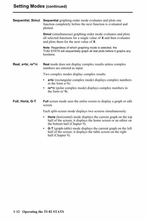
Sequential graphing-order mode evaluates and plots onefunction completely before the next function is evaluated andplotted.
Simul (simultaneous) graphing-order mode evaluates and plotsall selected functions for a single value of X and then evaluatesand plots them for the next value of X.
Note: Regardless of which graphing mode is selected, theTI-82 STATS will sequentially graph all stat plots before it graphs anyfunctions.
Real mode does not display complex results unless complexnumbers are entered as input.
Two complex modes display complex results.
• a+bi (rectangular complex mode) displays complex numbersin the form a+bi.
• re^qi (polar complex mode) displays complex numbers inthe form re^qi.
Full screen mode uses the entire screen to display a graph or editscreen.
Each split-screen mode displays two screens simultaneously.
• Horiz (horizontal) mode displays the current graph on the tophalf of the screen; it displays the home screen or an editor onthe bottom half (Chapter 9).
• G.T (graph-table) mode displays the current graph on the lefthalf of the screen; it displays the table screen on the righthalf (Chapter 9).
Setting Modes (continued)
Sequential, Simul
Real, a+bi, re^qi
Full, Horiz, G.T
Operating the TI-82 STATS 1-13
82STAT~3.DOC TI-83 international English Bob Fedorisko Revised: 10/28/05 12:11 PM Printed: 10/28/05 12:11PM Page 13 of 24
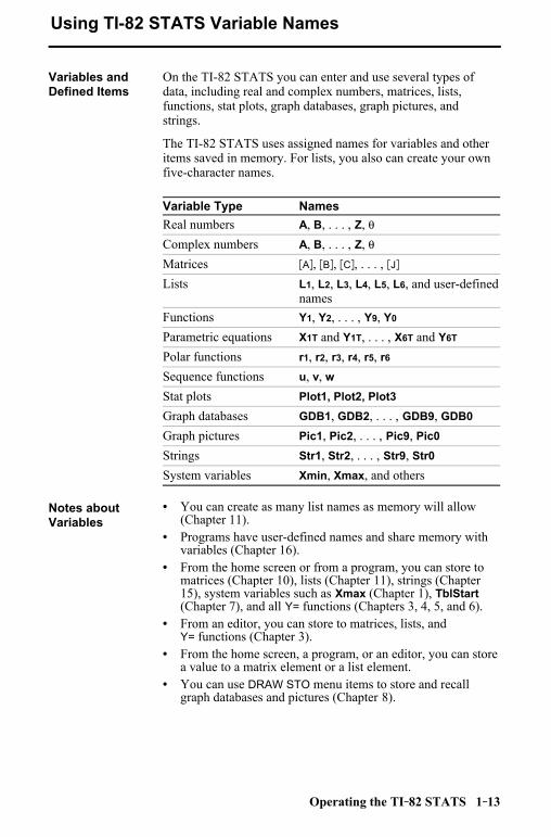
On the TI-82 STATS you can enter and use several types ofdata, including real and complex numbers, matrices, lists,functions, stat plots, graph databases, graph pictures, andstrings.
The TI-82 STATS uses assigned names for variables and otheritems saved in memory. For lists, you also can create your ownfive-character names.
Variable Type NamesReal numbers A, B, . . . , Z, qComplex numbers A, B, . . . , Z, qMatrices ãAä, ãBä, ãCä, . . . , ãJä
Lists L1, L2, L3, L4, L5, L6, and user-definednames
Functions Y1, Y2, . . . , Y9, Y0
Parametric equations X1T and Y1T, . . . , X6T and Y6T
Polar functions r1, r2, r3, r4, r5, r6
Sequence functions u, v, wStat plots Plot1, Plot2, Plot3Graph databases GDB1, GDB2, . . . , GDB9, GDB0Graph pictures Pic1, Pic2, . . . , Pic9, Pic0Strings Str1, Str2, . . . , Str9, Str0System variables Xmin, Xmax, and others
• You can create as many list names as memory will allow(Chapter 11).
• Programs have user-defined names and share memory withvariables (Chapter 16).
• From the home screen or from a program, you can store tomatrices (Chapter 10), lists (Chapter 11), strings (Chapter15), system variables such as Xmax (Chapter 1), TblStart(Chapter 7), and all Y= functions (Chapters 3, 4, 5, and 6).
• From an editor, you can store to matrices, lists, andY= functions (Chapter 3).
• From the home screen, a program, or an editor, you can storea value to a matrix element or a list element.
• You can use DRAW STO menu items to store and recallgraph databases and pictures (Chapter 8).
Using TI-82 STATS Variable Names
Variables andDefined Items
Notes aboutVariables
1-14 Operating the TI-82 STATS
82STAT~3.DOC TI-83 international English Bob Fedorisko Revised: 10/28/05 12:11 PM Printed: 10/28/05 12:11PM Page 14 of 24
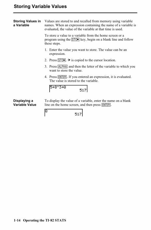
Values are stored to and recalled from memory using variablenames. When an expression containing the name of a variable isevaluated, the value of the variable at that time is used.
To store a value to a variable from the home screen or aprogram using the ¿ key, begin on a blank line and followthese steps.
1. Enter the value you want to store. The value can be anexpression.
2. Press ¿. ! is copied to the cursor location.
3. Press ƒ and then the letter of the variable to which youwant to store the value.
4. Press Í. If you entered an expression, it is evaluated.The value is stored to the variable.
To display the value of a variable, enter the name on a blankline on the home screen, and then press Í.
Storing Variable Values
Storing Values ina Variable
Displaying aVariable Value

Operating the TI-82 STATS 1-15
82STAT~3.DOC TI-83 international English Bob Fedorisko Revised: 10/28/05 12:11 PM Printed: 10/28/05 12:11PM Page 15 of 24
To recall and copy variable contents to the current cursorlocation, follow these steps. To leave RCL, press ‘.
1. Press y ãRCLä. Rcl and the edit cursor are displayed on thebottom line of the screen.
2. Enter the name of the variable in any of five ways.• Press ƒ and then the letter of the variable.• Press y ãLISTä, and then select the name of the list, or
press y [Ln].• Press , and then select the name of the matrix.• Press to display the VARS menu or ~ to
display the VARS Y.VARS menu; then select the type andthen the name of the variable or function.
• Press |, and then select the name of the program(in the program editor only).
The variable name you selected is displayed on the bottomline and the cursor disappears.
3. Press Í. The variable contents are inserted where thecursor was located before you began these steps.
Note: You can edit the characters pasted to the expressionwithout affecting the value in memory.
Recalling Variable Values
Using Recall(RCL)

1-16 Operating the TI-82 STATS
82STAT~3.DOC TI-83 international English Bob Fedorisko Revised: 10/28/05 12:11 PM Printed: 10/28/05 12:11PM Page 16 of 24
When you press Í on the home screen to evaluate anexpression or execute an instruction, the expression orinstruction is placed in a storage area called ENTRY (last entry).When you turn off the TI-82 STATS, ENTRY is retained inmemory.
To recall ENTRY, press y [ENTRY]. The last entry is pasted tothe current cursor location, where you can edit and execute it.On the home screen or in an editor, the current line is clearedand the last entry is pasted to the line.
Because the TI-82 STATS updates ENTRY only when you pressÍ, you can recall the previous entry even if you have begunto enter the next expression.
5 Ã 7Íy [ENTRY]
The TI-82 STATS retains as many previous entries as possiblein ENTRY, up to a capacity of 128 bytes. To scroll those entries,press y [ENTRY] repeatedly. If a single entry is more than 128bytes, it is retained for ENTRY, but it cannot be placed in theENTRY storage area.
1 ¿ƒ AÍ2 ¿ƒ BÍy [ENTRY]
If you press y [ENTRY] after displaying the oldest storedentry, the newest stored entry is displayed again, then the next-newest entry, and so on.
y [ENTRY]
ENTRY (Last Entry) Storage Area
Using ENTRY(Last Entry)
Accessing aPrevious Entry

Operating the TI-82 STATS 1-17
82STAT~3.DOC TI-83 international English Bob Fedorisko Revised: 10/28/05 12:11 PM Printed: 10/28/05 12:11PM Page 17 of 24
After you have pasted the last entry to the home screen andedited it (if you chose to edit it), you can execute the entry. Toexecute the last entry, press Í.
To reexecute the displayed entry, press Í again. Eachreexecution displays an answer on the right side of the next line;the entry itself is not redisplayed.
0 ¿ƒ N̓ Nà 1¿ƒ Nƒ ã:äƒ N¡ÍÍÍ
To store to ENTRY two or more expressions or instructions,separate each expression or instruction with a colon, then pressÍ. All expressions and instructions separated by colons arestored in ENTRY.
When you press y [ENTRY], all the expressions andinstructions separated by colons are pasted to the current cursorlocation. You can edit any of the entries, and then execute all ofthem when you press Í.
For the equation A=pr2, use trial and error to find the radius of acircle that covers 200 square centimeters. Use 8 as your firstguess.
8 ¿ƒ Rƒ[:] y [p] ƒ R¡Íy [ENTRY]
y | 7y [INS] Ë 95ÍContinue until the answer is as accurate as you want.
Clear Entries (Chapter 18) clears all data that the TI-82 STATSis holding in the ENTRY storage area.
Reexecuting thePrevious Entry
Multiple EntryValues on a Line
Clearing ENTRY

1-18 Operating the TI-82 STATS
82STAT~3.DOC TI-83 international English Bob Fedorisko Revised: 10/28/05 12:11 PM Printed: 10/28/05 12:11PM Page 18 of 24
When an expression is evaluated successfully from the homescreen or from a program, the TI-82 STATS stores the answer toa storage area called Ans (last answer). Ans may be a real orcomplex number, a list, a matrix, or a string. When you turn offthe TI-82 STATS, the value in Ans is retained in memory.
You can use the variable Ans to represent the last answer in mostplaces. Press y [ANS] to copy the variable name Ans to thecursor location. When the expression is evaluated, theTI-82 STATS uses the value of Ans in the calculation.
Calculate the area of a garden plot 1.7 meters by 4.2 meters.Then calculate the yield per square meter if the plot produces atotal of 147 tomatoes.
1 Ë 7¯ 4Ë 2Í147 ¥y [ANS]Í
You can use Ans as the first entry in the next expression withoutentering the value again or pressing y [ANS]. On a blank lineon the home screen, enter the function. The TI-82 STATS pastesthe variable name Ans to the screen, then the function.
5 ¥ 2ͯ 9 Ë 9Í
To store an answer, store Ans to a variable before you evaluateanother expression.
Calculate the area of a circle of radius 5 meters. Next, calculatethe volume of a cylinder of radius 5 meters and height 3.3 meters,and then store the result in the variable V.
y [p] 5¡Í¯ 3 Ë 3Í¿ƒ VÍ
Ans (Last Answer) Storage Area
Using Ans in anExpression
Continuing anExpression
Storing Answers
Operating the TI-82 STATS 1-19
82STAT~3.DOC TI-83 international English Bob Fedorisko Revised: 10/28/05 12:11 PM Printed: 10/28/05 12:11PM Page 19 of 24
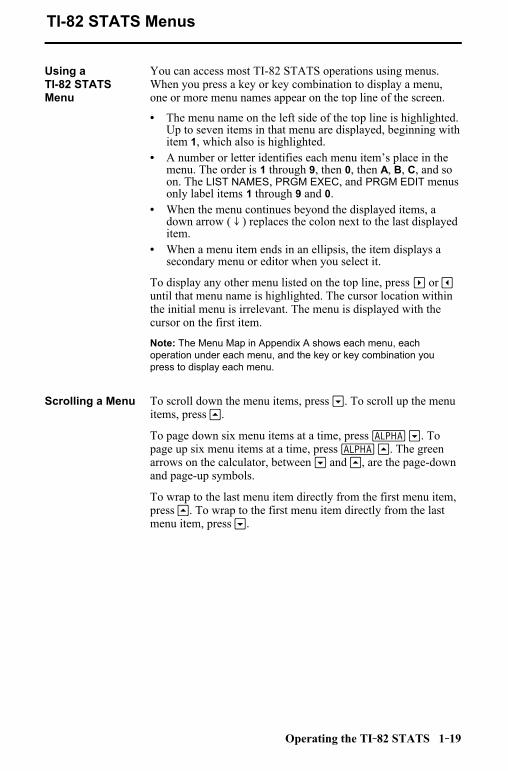
You can access most TI-82 STATS operations using menus.When you press a key or key combination to display a menu,one or more menu names appear on the top line of the screen.
• The menu name on the left side of the top line is highlighted.Up to seven items in that menu are displayed, beginning withitem 1, which also is highlighted.
• A number or letter identifies each menu item’s place in themenu. The order is 1 through 9, then 0, then A, B, C, and soon. The LIST NAMES, PRGM EXEC, and PRGM EDIT menusonly label items 1 through 9 and 0.
• When the menu continues beyond the displayed items, adown arrow ( $ ) replaces the colon next to the last displayeditem.
• When a menu item ends in an ellipsis, the item displays asecondary menu or editor when you select it.
To display any other menu listed on the top line, press ~ or |until that menu name is highlighted. The cursor location withinthe initial menu is irrelevant. The menu is displayed with thecursor on the first item.
Note: The Menu Map in Appendix A shows each menu, eachoperation under each menu, and the key or key combination youpress to display each menu.
To scroll down the menu items, press †. To scroll up the menuitems, press }.
To page down six menu items at a time, press ƒ †. Topage up six menu items at a time, press ƒ }. The greenarrows on the calculator, between † and }, are the page-downand page-up symbols.
To wrap to the last menu item directly from the first menu item,press }. To wrap to the first menu item directly from the lastmenu item, press †.
TI-82 STATS Menus
Using aTI-82 STATSMenu
Scrolling a Menu

1-20 Operating the TI-82 STATS
82STAT~3.DOC TI-83 international English Bob Fedorisko Revised: 10/28/05 12:11 PM Printed: 10/28/05 12:11PM Page 20 of 24
You can select an item from a menu in either of two ways.
• Press the number or letter of the item you want to select. Thecursor can be anywhere on the menu, and the item you selectneed not be displayed on the screen.
• Press † or } to move the cursor to the item you want, andthen press Í.
After you select an item from a menu, the TI-82 STATStypically displays the previous screen.
Note: On the LIST NAMES, PRGM EXEC, and PRGM EDITmenus, only items 1 through 9 and 0 are labeled in such a way thatyou can select them by pressing the appropriate number key. Tomove the cursor to the first item beginning with any alpha character orq, press the key combination for that alpha character or q. If no itemsbegin with that character, then the cursor moves beyond it to the nextitem.
Calculate 3‡27.†††Í27 ¤Í
You can leave a menu without making a selection in any of fourways.
• Press y [QUIT] to return to the home screen.• Press ‘ to return to the previous screen.• Press a key or key combination for a different menu, such as or y [LIST].
• Press a key or key combination for a different screen, suchas o or y [TABLE].
TI-82 STATS Menus (continued)
Selecting an Itemfrom a Menu
Leaving a Menuwithout Making aSelection

Operating the TI-82 STATS 1-21
82STAT~3.DOC TI-83 international English Bob Fedorisko Revised: 10/28/05 12:11 PM Printed: 10/28/05 12:11PM Page 21 of 24
You can enter the names of functions and system variables in anexpression or store to them directly.
To display the VARS menu, press . All VARS menu itemsdisplay secondary menus, which show the names of the systemvariables. 1:Window, 2:Zoom, and 5:Statistics each accessmore than one secondary menu.
VARS Y-VARS1: Window... X/Y, T/q, and U/V/W variables2: Zoom... ZX/ZY, ZT/Zq, and ZU variables3: GDB... Graph database variables4: Picture... Picture variables5: Statistics... XY, G, EQ, TEST, and PTS variables6: Table... TABLE variables7: String... String variables
To display the VARS Y.VARS menu, press ~.1:Function, 2:Parametric, and 3:Polar display secondary menusof the Y= function variables.
VARS Y-VARS1: Function... Yn functions2: Parametric... XnT, YnT functions3: Polar... rn functions4: On/Off... Lets you select/deselect functions
Note: The sequence variables (u, v, w) are located on the keyboardas the second functions of ¬, −, and ®.
To select a variable from the VARS or VARS Y.VARS menu,follow these steps.
1. Display the VARS or VARS Y.VARS menu.• Press to display the VARS menu.• Press ~ to display the VARS Y.VARS menu.
2. Select the type of variable, such as 2:Zoom from the VARSmenu or 3:Polar from the VARS Y.VARS menu. A secondarymenu is displayed.
3. If you selected 1:Window, 2:Zoom, or 5:Statistics from theVARS menu, you can press ~ or | to display othersecondary menus.
4. Select a variable name from the menu. It is pasted to thecursor location.
VARS and VARS Y.VARS Menus
VARS Menu
Selecting aVariable from theVARS Menu orVARS Y.VARSMenu
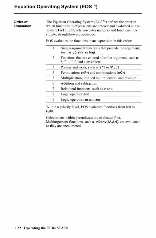
1-22 Operating the TI-82 STATS
82STAT~3.DOC TI-83 international English Bob Fedorisko Revised: 10/28/05 12:11 PM Printed: 10/28/05 12:11PM Page 22 of 24
The Equation Operating System (EOSé) defines the order inwhich functions in expressions are entered and evaluated on theTI-82 STATS. EOS lets you enter numbers and functions in asimple, straightforward sequence.
EOS evaluates the functions in an expression in this order:
1 Single-argument functions that precede the argument,such as ‡(, sin(, or log(
2 Functions that are entered after the argument, such as2, M1, !, ¡, r, and conversions
3 Powers and roots, such as 2^5 or 5x‡324 Permutations (nPr) and combinations (nCr)5 Multiplication, implied multiplication, and division6 Addition and subtraction7 Relational functions, such as > or 8 Logic operator and9 Logic operators or and xor
Within a priority level, EOS evaluates functions from left toright.
Calculations within parentheses are evaluated first.Multiargument functions, such as nDeriv(A2,A,6), are evaluatedas they are encountered.
Equation Operating System (EOSé)
Order ofEvaluation

Operating the TI-82 STATS 1-23
82STAT~3.DOC TI-83 international English Bob Fedorisko Revised: 10/28/05 12:11 PM Printed: 10/28/05 12:11PM Page 23 of 24
The TI-82 STATS recognizes implied multiplication, so youneed not press ¯ to express multiplication in all cases. Forexample, the TI-82 STATS interprets 2p, 4sin(46), 5(1+2), and(2ääää5)7 as implied multiplication.
Note: TI-82 STATS implied multiplication rules differ from those of theTI.82. For example, the TI-82 STATS evaluates 1à2X as (1à2)ääääX,while the TI.82 evaluates 1à2X as 1/(2ääääX) (Chapter 2).
All calculations inside a pair of parentheses are completed first.For example, in the expression 4(1+2), EOS first evaluates theportion inside the parentheses, 1+2, and then multiplies theanswer, 3, by 4.
You can omit the close parenthesis ( ) ) at the end of anexpression. All open parenthetical elements are closedautomatically at the end of an expression. This is also true foropen parenthetical elements that precede the store or display-conversion instructions.
Note: An open parenthesis following a list name, matrix name, or Y=function name does not indicate implied multiplication. It specifieselements in the list (Chapter 11) or matrix (Chapter 10) and specifiesa value for which to solve the Y= function.
To enter a negative number, use the negation key. Press Ì andthen enter the number. On the TI-82 STATS, negation is in thethird level in the EOS hierarchy. Functions in the first level,such as squaring, are evaluated before negation.
For example, MX2, evaluates to a negative number (or 0). Useparentheses to square a negative number.
Note: Use the ¹ key for subtraction and the Ì key for negation. Ifyou press ¹ to enter a negative number, as in 9 ¯ ¹ 7, or if youpress Ì to indicate subtraction, as in 9 Ì 7, an error occurs. If youpress ƒ A Ì ƒ B, it is interpreted as implied multiplication(AääääMB).
ImpliedMultiplication
Parentheses
Negation

1-24 Operating the TI-82 STATS
82STAT~3.DOC TI-83 international English Bob Fedorisko Revised: 10/28/05 12:11 PM Printed: 10/28/05 12:11PM Page 24 of 24
The TI-82 STATS detects errors while performing these tasks.
• Evaluating an expression• Executing an instruction• Plotting a graph• Storing a value
When the TI-82 STATS detects an error, it returns an errormessage as a menu title, such as ERR:SYNTAX orERR:DOMAIN. Appendix B describes each error type andpossible reasons for the error.
• If you select 1:Quit (or press y [QUIT] or ‘), then thehome screen is displayed.
• If you select 2:Goto, then the previous screen is displayedwith the cursor at or near the error location.
Note: If a syntax error occurs in the contents of a Y= function duringprogram execution, then the Goto option returns to the Y= editor, notto the program.
To correct an error, follow these steps.
1. Note the error type (ERR:error type).
2. Select 2:Goto, if it is available. The previous screen isdisplayed with the cursor at or near the error location.
3. Determine the error. If you cannot recognize the error, referto Appendix B.
4. Correct the expression.
Error Conditions
Diagnosing anError
Correcting anError

Math, Angle, and Test Operations 2.1
82STAT~4.DOC TI-83 international English Bob Fedorisko Revised: 10/28/05 12:19 PM Printed: 10/28/05 12:20PM Page 1 of 26
2 Math, Angle, and TestOperations
Getting Started: Coin Flip ................................................................................. 2Keyboard Math Operations .............................................................................. 3MATH Operations................................................................................................... 5Using the Equation Solver ................................................................................ 8MATH NUM (Number) Operations.............................................................. 13Entering and Using Complex Numbers.................................................... 16MATH CPX (Complex) Operations ............................................................ 18MATH PRB (Probability) Operations........................................................ 20ANGLE Operations................................................................................................ 23TEST (Relational) Operations........................................................................ 24TEST LOGIC (Boolean) Operations .......................................................... 26
Contents

2.2 Math, Angle, and Test Operations
82STAT~4.DOC TI-83 international English Bob Fedorisko Revised: 10/28/05 12:19 PM Printed: 10/28/05 12:20PM Page 2 of 2682STAT~4.DOC TI-83 international English Bob Fedorisko Revised: 10/28/05 12:19 PM Printed: 10/28/05 12:20PM Page 2 of 26
Getting Started is a fast-paced introduction. Read the chapter for details.
Suppose you want to model flipping a fair coin 10 times. You want to track howmany of those 10 coin flips result in heads. You want to perform this simulation 40times. With a fair coin, the probability of a coin flip resulting in heads is 0.5 and theprobability of a coin flip resulting in tails is 0.5.
1. Begin on the home screen. Press | todisplay the MATH PRB menu. Press 7 to select7:randBin( (random Binomial). randBin( ispasted to the home screen. Press 10 to enter thenumber of coin flips. Press ¢. Press Ë 5 toenter the probability of heads. Press ¢. Press40 to enter the number of simulations. Press ¤.
2. Press Í to evaluate the expression. A list of40 elements is displayed. The list contains thecount of heads resulting from each set of 10coin flips. The list has 40 elements because thissimulation was performed 40 times. In thisexample, the coin came up heads five times inthe first set of 10 coin flips, five times in thesecond set of 10 coin flips, and so on.
3. Press ¿ y ãL1ä Í to store the data tothe list name L1. You then can use the data foranother activity, such as plotting a histogram(Chapter 12).
4. Press ~ or | to view the additional counts inthe list. Ellipses (...) indicate that the listcontinues beyond the screen.
Note: Since randBin( generates randomnumbers, your list elements may differ from thosein the example.
Getting Started: Coin Flip

Math, Angle, and Test Operations 2.3
82STAT~4.DOC TI-83 international English Bob Fedorisko Revised: 10/28/05 12:19 PM Printed: 10/28/05 12:20PM Page 3 of 26
Math operations that are valid for lists return a list calculatedelement by element. If you use two lists in the same expression,they must be the same length.
You can use + (addition, Ã), N (subtraction, ¹), ääää(multiplication, ¯), and à (division, ¥) with real and complexnumbers, expressions, lists, and matrices. You cannot use à withmatrices.
valueA+valueB valueA N valueBvalueAäääävalueB valueA à valueB
You can use the trigonometric (trig) functions (sine, ˜;cosine, ™; and tangent, š) with real numbers, expressions,and lists. The current angle mode setting affects interpretation.For example, sin(30) in Radian mode returns L.9880316241; inDegree mode it returns .5.
sin(value) cos(value) tan(value)
You can use the inverse trig functions (arcsine, y [SINL1];arccosine, y [COSL1]; and arctangent, y [TANL1]) with realnumbers, expressions, and lists. The current angle mode settingaffects interpretation.
sinL1(value) cosL1(value) tanL1(value)
Note: The trig functions do not operate on complex numbers.
You can use ^ (power, ›), 2 (square, ¡), and ‡( (square root,y [‡]) with real and complex numbers, expressions, lists, andmatrices. You cannot use ‡( with matrices.
value^power value2 ‡(value)
You can use L1 (inverse, —) with real and complex numbers,expressions, lists, and matrices. The multiplicative inverse isequivalent to the reciprocal, 1àx.
valueL1
Keyboard Math Operations
Using Lists withMath Operations
+ (Addition),N (Subtraction),ääää (Multiplication),à (Division)
TrigonometricFunctions
^ (Power),2 (Square),‡( (Square Root)
L1 (Inverse)

2.4 Math, Angle, and Test Operations
82STAT~4.DOC TI-83 international English Bob Fedorisko Revised: 10/28/05 12:19 PM Printed: 10/28/05 12:20PM Page 4 of 2682STAT~4.DOC TI-83 international English Bob Fedorisko Revised: 10/28/05 12:19 PM Printed: 10/28/05 12:20PM Page 4 of 26
You can use log( (logarithm, «), 10^( (power of 10, y[10x]), and ln( (natural log, µ) with real or complex numbers,expressions, and lists.
log(value) 10^(power) ln(value)
e^( (exponential, y ãex]) returns the constant e raised to apower. You can use e^( with real or complex numbers,expressions, and lists.
e^(power)
e (constant, y [e]) is stored as a constant on the TI-82 STATS. Press y [e] to copy e to the cursor location. In calculations,the TI-82 STATS uses 2.718281828459 for e.
M (negation, Ì) returns the negative of value. You can use Mwith real or complex numbers, expressions, lists, and matrices.
Mvalue
EOS rules (Chapter 1) determine when negation is evaluated.For example, LA2 returns a negative number, because squaring isevaluated before negation. Use parentheses to square a negatednumber, as in (LA)2.
Note: On the TI-82 STATS, the negation symbol (M) is shorter andhigher than the subtraction sign (N), which is displayed when youpress ¹.
p (Pi, y [p]) is stored as a constant in the TI-82 STATS. Incalculations, the TI-82 STATS uses 3.1415926535898 for p.
Keyboard Math Operations (continued)
log(,10^(,ln(
e^( (Exponential)
e (Constant)
L (Negation)
p (Pi)

Math, Angle, and Test Operations 2.5
82STAT~4.DOC TI-83 international English Bob Fedorisko Revised: 10/28/05 12:19 PM Printed: 10/28/05 12:20PM Page 5 of 26
To display the MATH menu, press .
MATH
NUM CPX PRB
1: 4Frac Displays the answer as a fraction.2: 4Dec Displays the answer as a decimal.3: 3 Calculates the cube.4: 3‡( Calculates the cube root.5: x‡ Calculates the xth root.6: fMin( Finds the minimum of a function.7: fMax( Finds the maximum of a function.8: nDeriv( Computes the numerical derivative.9: fnInt( Computes the function integral.0: Solver... Displays the equation solver.
4Frac (display as a fraction) displays an answer as its rationalequivalent. You can use 4Frac with real or complex numbers,expressions, lists, and matrices. If the answer cannot besimplified or the resulting denominator is more than three digits,the decimal equivalent is returned. You can only use 4Fracfollowing value.
value 4Frac
4Dec (display as a decimal) displays an answer in decimal form.You can use 4Dec with real or complex numbers, expressions,lists, and matrices. You can only use 4Dec following value.
value 4Dec
MATH Operations
MATH Menu
4Frac,4Dec

2.6 Math, Angle, and Test Operations
82STAT~4.DOC TI-83 international English Bob Fedorisko Revised: 10/28/05 12:19 PM Printed: 10/28/05 12:20PM Page 6 of 2682STAT~4.DOC TI-83 international English Bob Fedorisko Revised: 10/28/05 12:19 PM Printed: 10/28/05 12:20PM Page 6 of 26
3 (cube) returns the cube of value. You can use 3 with real orcomplex numbers, expressions, lists, and square matrices.
value3
3‡( (cube root) returns the cube root of value. You can use 3‡(with real or complex numbers, expressions, and lists.3‡(value)
x‡ (xth root) returns the xth root of value. You can use x‡ withreal or complex numbers, expressions, and lists.
xthrootx‡value
fMin( (function minimum) and fMax( (function maximum) returnthe value at which the local minimum or local maximum valueof expression with respect to variable occurs, between lowerand upper values for variable. fMin( and fMax( are not valid inexpression. The accuracy is controlled by tolerance (if notspecified, the default is 1âL5).
fMin(expression,variable,lower,upper[,tolerance])fMax(expression,variable,lower,upper[,tolerance])
Note: In this guidebook, optional arguments and the commas thataccompany them are enclosed in brackets ([ ]).
MATH Operations (continued)
3(Cube),3‡( (Cube Root)
x‡ (Root)
fMin(,fMax(
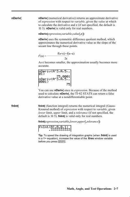
Math, Angle, and Test Operations 2.7
82STAT~4.DOC TI-83 international English Bob Fedorisko Revised: 10/28/05 12:19 PM Printed: 10/28/05 12:20PM Page 7 of 26
nDeriv( (numerical derivative) returns an approximate derivativeof expression with respect to variable, given the value at whichto calculate the derivative and H (if not specified, the default is1âL3). nDeriv( is valid only for real numbers.
nDeriv(expression,variable,value[,H])
nDeriv( uses the symmetric difference quotient method, whichapproximates the numerical derivative value as the slope of thesecant line through these points.
f(x+H)Nf(xNH)f¢(x) =
2HAs H becomes smaller, the approximation usually becomes moreaccurate.
You can use nDeriv( once in expression. Because of the methodused to calculate nDeriv(, the TI-82 STATS can return a falsederivative value at a nondifferentiable point.
fnInt( (function integral) returns the numerical integral (Gauss-Kronrod method) of expression with respect to variable, givenlower limit, upper limit, and a tolerance (if not specified, thedefault is 1âL5). fnInt( is valid only for real numbers.
fnInt(expression,variable,lower,upper[,tolerance])
Tip: To speed the drawing of integration graphs (when fnInt( is usedin a Y= equation), increase the value of the Xres window variablebefore you press s.
nDeriv(
fnInt(

2.8 Math, Angle, and Test Operations
82STAT~4.DOC TI-83 international English Bob Fedorisko Revised: 10/28/05 12:19 PM Printed: 10/28/05 12:20PM Page 8 of 2682STAT~4.DOC TI-83 international English Bob Fedorisko Revised: 10/28/05 12:19 PM Printed: 10/28/05 12:20PM Page 8 of 26
Solver displays the equation solver, in which you can solve forany variable in an equation. The equation is assumed to be equalto zero. Solver is valid only for real numbers.
When you select Solver, one of two screens is displayed.
• The equation editor (see step 1 picture below) is displayedwhen the equation variable eqn is empty.
• The interactive solver editor (see step 3 picture on page 2.9)is displayed when an equation is stored in eqn.
To enter an expression in the equation solver, assuming that thevariable eqn is empty, follow these steps.
1. Select 0:Solver from the MATH menu to display the equationeditor.
2. Enter the expression in any of three ways.
• Enter the expression directly into the equation solver.• Paste a Y= variable name from the VARS Y.VARS menu
to the equation solver.• Press y [RCL], paste a Y= variable name from the
VARS Y.VARS menu, and press Í. The expression ispasted to the equation solver.
The expression is stored to the variable eqn as you enter it.
Using the Equation Solver
Solver
Entering anExpression in theEquation Solver

Math, Angle, and Test Operations 2.9
82STAT~4.DOC TI-83 international English Bob Fedorisko Revised: 10/28/05 12:19 PM Printed: 10/28/05 12:20PM Page 9 of 26
3. Press Í or †. The interactive solver editor is displayed.
• The equation stored in eqn is set equal to zero anddisplayed on the top line.
• Variables in the equation are listed in the order in whichthey appear in the equation. Any values stored to thelisted variables also are displayed.
• The default lower and upper bounds appear in the lastline of the editor (bound={L1åååå99,1åååå99}).
• A $ is displayed in the first column of the bottom line ifthe editor continues beyond the screen.
Tip: To use the solver to solve an equation such as K=.5MV2, entereqn:0=KN.5MV2 in the equation editor.
When you enter or edit a value for a variable in the interactivesolver editor, the new value is stored in memory to that variable.
You can enter an expression for a variable value. It is evaluatedwhen you move to the next variable. Expressions must resolveto real numbers at each step during the iteration.
You can store equations to any VARS Y.VARS variables, such asY1 or r6, and then reference the variables in the equation. Theinteractive solver editor displays all variables of all Y= functionsreferenced in the equation.
Entering anExpression in theEquation Solver(continued)
Entering andEditing VariableValues
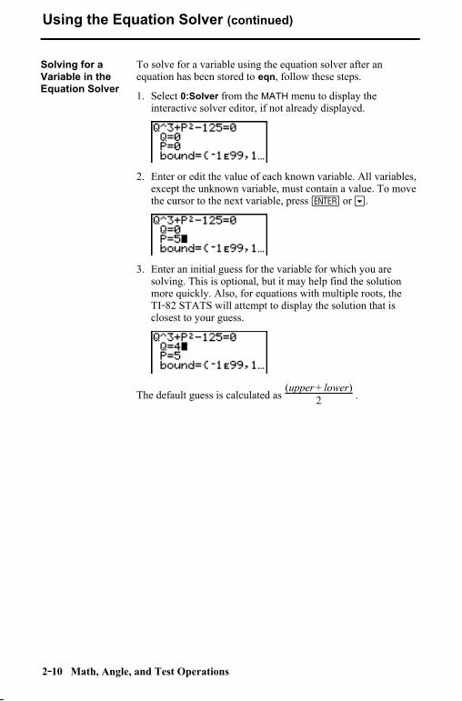
2.10 Math, Angle, and Test Operations
82STAT~4.DOC TI-83 international English Bob Fedorisko Revised: 10/28/05 12:19 PM Printed: 10/28/05 12:20PM Page 10 of 2682STAT~4.DOC TI-83 international English Bob Fedorisko Revised: 10/28/05 12:19 PM Printed: 10/28/05 12:20PM Page 10 of 26
To solve for a variable using the equation solver after anequation has been stored to eqn, follow these steps.
1. Select 0:Solver from the MATH menu to display theinteractive solver editor, if not already displayed.
2. Enter or edit the value of each known variable. All variables,except the unknown variable, must contain a value. To movethe cursor to the next variable, press Í or †.
3. Enter an initial guess for the variable for which you aresolving. This is optional, but it may help find the solutionmore quickly. Also, for equations with multiple roots, theTI-82 STATS will attempt to display the solution that isclosest to your guess.
The default guess is calculated as (upper+lower)
2 .
Using the Equation Solver (continued)
Solving for aVariable in theEquation Solver

Math, Angle, and Test Operations 2.11
82STAT~4.DOC TI-83 international English Bob Fedorisko Revised: 10/28/05 12:19 PM Printed: 10/28/05 12:20PM Page 11 of 26
4. Edit bound={lower,upper}. lower and upper are the boundsbetween which the TI-82 STATS searches for a solution. This isoptional, but it may help find the solution more quickly. Thedefault is bound={L1åååå99,1åååå99}.
5. Move the cursor to the variable for which you want to solveand press ƒ [SOLVE] (above the Í key).
• The solution is displayed next to the variable for whichyou solved. A solid square in the first column marks thevariable for which you solved and indicates that theequation is balanced. An ellipsis shows that the valuecontinues beyond the screen.Note: When a number continues beyond the screen, be sureto press ~ to scroll to the end of the number to see whether itends with a negative or positive exponent. A very smallnumber may appear to be a large number until you scroll rightto see the exponent.
• The values of the variables are updated in memory.• leftNrt=diff is displayed in the last line of the editor. diff is
the difference between the left and right sides of theequation. A solid square in the first column next toleftNrt= indicates that the equation has been evaluated atthe new value of the variable for which you solved.
Solving for aVariable in theEquation Solver(continued)

2.12 Math, Angle, and Test Operations
82STAT~4.DOC TI-83 international English Bob Fedorisko Revised: 10/28/05 12:19 PM Printed: 10/28/05 12:20PM Page 12 of 2682STAT~4.DOC TI-83 international English Bob Fedorisko Revised: 10/28/05 12:19 PM Printed: 10/28/05 12:20PM Page 12 of 26
To edit or replace an equation stored to eqn when the interactiveequation solver is displayed, press } until the equation editor isdisplayed. Then edit the equation.
Some equations have more than one solution. You can enter anew initial guess (page 2.10) or new bounds (page 2.11) to lookfor additional solutions.
After you solve for a variable, you can continue to exploresolutions from the interactive solver editor. Edit the values ofone or more variables. When you edit any variable value, thesolid squares next to the previous solution and leftNrt=diffdisappear. Move the cursor to the variable for which you nowwant to solve and press ƒ [SOLVE].
The TI-82 STATS solves equations through an iterative process.To control that process, enter bounds that are relatively close tothe solution and enter an initial guess within those bounds. Thiswill help to find a solution more quickly. Also, it will definewhich solution you want for equations with multiple solutions.
The function solve( is available only from CATALOG or fromwithin a program. It returns a solution (root) of expression forvariable, given an initial guess, and lower and upper boundswithin which the solution is sought. The default for lower isL1â99. The default for upper is 1â99. solve( is valid only for realnumbers.
solve(expression,variable,guess[,{lower,upper}])
expression is assumed equal to zero. The value of variable willnot be updated in memory. guess may be a value or a list of twovalues. Values must be stored for every variable in expression,except variable, before expression is evaluated. lower and uppermust be entered in list format.
Using the Equation Solver (continued)
Editing anEquation Storedto eqn
Equations withMultiple Roots
Further Solutions
Controlling theSolution forSolver or solve(
Using solve( onthe Home Screenor from aProgram

Math, Angle, and Test Operations 2.13
82STAT~4.DOC TI-83 international English Bob Fedorisko Revised: 10/28/05 12:19 PM Printed: 10/28/05 12:20PM Page 13 of 26
To display the MATH NUM menu, press ~.
MATH NUM
CPX PRB
1: abs( Absolute value2: round( Round3: iPart( Integer part4: fPart( Fractional part5: int( Greatest integer6: min( Minimum value7: max( Maximum value8: lcm( Least common multiple9: gcd( Greatest common divisor
abs( (absolute value) returns the absolute value of real orcomplex (modulus) numbers, expressions, lists, and matrices.
abs(value)
Note: abs( is also available on the MATH CPX menu.
round( returns a number, expression, list, or matrix rounded to#decimals (9). If #decimals is omitted, value is rounded to thedigits that are displayed, up to 10 digits.
round(value[,#decimals])
MATH NUM (Number) Operations
MATH NUM Menu
abs(
round(

2.14 Math, Angle, and Test Operations
82STAT~4.DOC TI-83 international English Bob Fedorisko Revised: 10/28/05 12:19 PM Printed: 10/28/05 12:20PM Page 14 of 2682STAT~4.DOC TI-83 international English Bob Fedorisko Revised: 10/28/05 12:19 PM Printed: 10/28/05 12:20PM Page 14 of 26
iPart( (integer part) returns the integer part or parts of real orcomplex numbers, expressions, lists, and matrices.
iPart(value)
fPart( (fractional part) returns the fractional part or parts of real orcomplex numbers, expressions, lists, and matrices.
fPart(value)
int( (greatest integer) returns the largest integer real orcomplex numbers, expressions, lists, and matrices.
int(value)
Note: For a given value, the result of int( is the same as the result ofiPart( for nonnegative numbers and negative integers, but oneinteger less than the result of iPart( for negative noninteger numbers.
MATH NUM (Number) Operations (continued)
iPart(,fPart(
int(

Math, Angle, and Test Operations 2.15
82STAT~4.DOC TI-83 international English Bob Fedorisko Revised: 10/28/05 12:19 PM Printed: 10/28/05 12:20PM Page 15 of 26
min( (minimum value) returns the smaller of valueA and valueBor the smallest element in list. If listA and listB are compared,min( returns a list of the smaller of each pair of elements. If listand value are compared, min( compares each element in listwith value.
max( (maximum value) returns the larger of valueA and valueBor the largest element in list. If listA and listB are compared,max( returns a list of the larger of each pair of elements. If listand value are compared, max( compares each element in listwith value.
min(valueA,valueB) max(valueA,valueB)min(list) max(list)min(listA,listB) max(listA,listB)min(list,value) max(list,value)
Note: min( and max( also are available on the LIST MATH menu.
lcm( returns the least common multiple of valueA and valueB,both of which must be nonnegative integers. When listA andlistB are specified, lcm( returns a list of the lcm of each pair ofelements. If list and value are specified, lcm( finds the lcm ofeach element in list and value.
gcd( returns the greatest common divisor of valueA and valueB,both of which must be nonnegative integers. When listA andlistB are specified, gcd( returns a list of the gcd of each pair ofelements. If list and value are specified, gcd( finds the gcd ofeach element in list and value.
lcm(valueA,valueB) gcd(valueA,valueB)lcm(listA,listB) gcd(listA,listB)lcm(list,value) gcd(list,value)
min(,max(
lcm(,gcd(

2.16 Math, Angle, and Test Operations
82STAT~4.DOC TI-83 international English Bob Fedorisko Revised: 10/28/05 12:19 PM Printed: 10/28/05 12:20PM Page 16 of 2682STAT~4.DOC TI-83 international English Bob Fedorisko Revised: 10/28/05 12:19 PM Printed: 10/28/05 12:20PM Page 16 of 26
The TI-82 STATS displays complex numbers in rectangularform and polar form. To select a complex-number mode, pressz, and then select either of the two modes.
• a+bi (rectangular-complex mode)• re^qi (polar-complex mode)
On the TI-82 STATS, complex numbers can be stored tovariables. Also, complex numbers are valid list elements.
In Real mode, complex-number results return an error, unlessyou entered a complex number as input. For example, in Realmode ln(L1) returns an error; in a+bi mode ln(L1) returns ananswer.
Real mode a+bi mode
$ $
Complex numbers are stored in rectangular form, but you canenter a complex number in rectangular form or polar form,regardless of the mode setting. The components of complexnumbers can be real numbers or expressions that evaluate to realnumbers; expressions are evaluated when the command isexecuted.
Radian mode is recommended for complex number calculations.Internally, the TI-82 STATS converts all entered trig values toradians, but it does not convert values for exponential,logarithmic, or hyperbolic functions.
In degree mode, complex identities such as e^(iq) = cos(q) + isin(q) are not generally true because the values for cos and sinare converted to radians, while those for e^( ) are not. Forexample, e^(i45) = cos(45) + i sin(45) is treated internally ase^(i45) = cos(p/4) + i sin(p/4). Complex identities are alwaystrue in radian mode.
Entering and Using Complex Numbers
Complex-NumberModes
EnteringComplexNumbers
Note aboutRadian versusDegree Mode

Math, Angle, and Test Operations 2.17
82STAT~4.DOC TI-83 international English Bob Fedorisko Revised: 10/28/05 12:19 PM Printed: 10/28/05 12:20PM Page 17 of 26
Complex numbers in results, including list elements, aredisplayed in either rectangular or polar form, as specified by themode setting or by a display conversion instruction (page 2.19).In the example below, re^qi and Radian modes are set.
Rectangular-complex mode recognizes and displays a complexnumber in the form a+bi, where a is the real component, b is theimaginary component, and i is a constant equal to -1.
To enter a complex number in rectangular form, enter the valueof a (real component), press à or ¹, enter the value of b(imaginary component), and press y [i] (constant).
real component(+ or N)imaginary componenti
Polar-complex mode recognizes and displays a complex number inthe form re^qi, where r is the magnitude, e is the base of the naturallog, q is the angle, and i is a constant equal to -1.
To enter a complex number in polar form, enter the value of r(magnitude), press y [ex] (exponential function), enter thevalue of q (angle), press y [i] (constant), and then press ¤.
magnitudee^(anglei)
InterpretingComplex Results
Rectangular-Complex Mode
Polar-ComplexMode

2.18 Math, Angle, and Test Operations
82STAT~4.DOC TI-83 international English Bob Fedorisko Revised: 10/28/05 12:19 PM Printed: 10/28/05 12:20PM Page 18 of 2682STAT~4.DOC TI-83 international English Bob Fedorisko Revised: 10/28/05 12:19 PM Printed: 10/28/05 12:20PM Page 18 of 26
To display the MATH CPX menu, press ~ ~.
MATH NUM
CPX PRB
1: conj( Returns the complex conjugate.2: real( Returns the real part.3: imag( Returns the imaginary part.4: angle( Returns the polar angle.5: abs( Returns the magnitude (modulus).6: 4Rect Displays the result in rectangular form.7: 4Polar Displays the result in polar form.
conj( (conjugate) returns the complex conjugate of a complexnumber or list of complex numbers.
conj(a+bi) returns aNbi in a+bi mode.conj(re^(qi)) returns re^(Lqi) in re^qi mode.
real( (real part) returns the real part of a complex number or listof complex numbers.
real(a+bi) returns a.real(re^(qi)) returns rääääcos(q).
imag( (imaginary part) returns the imaginary (nonreal) part of acomplex number or list of complex numbers.
imag(a+bi) returns b.imag(re^(qi)) returns rääääsin(q).
MATH CPX (Complex) Operations
MATH CPX Menu
conj(
real(
imag(

Math, Angle, and Test Operations 2.19
82STAT~4.DOC TI-83 international English Bob Fedorisko Revised: 10/28/05 12:19 PM Printed: 10/28/05 12:20PM Page 19 of 26
angle( returns the polar angle of a complex number or list ofcomplex numbers, calculated as tanL1 (b/a), where b is theimaginary part and a is the real part. The calculation is adjustedby +p in the second quadrant or Np in the third quadrant.
angle(a+bi) returns tanL1(b/a).angle(re^(qi)) returns q, where Lp<q<p.
abs( (absolute value) returns the magnitude (modulus),(real2+imag2) , of a complex number or list of complex
numbers.
abs(a+bi) returns (a2+b2) .abs(re^(qi)) returns r (magnitude).
4Rect (display as rectangular) displays a complex result inrectangular form. It is valid only at the end of an expression. Itis not valid if the result is real.
complex result8Rect returns a+bi.
4Polar (display as polar) displays a complex result in polar form.It is valid only at the end of an expression. It is not valid if theresult is real.
complex result8Polar returns re^(qi).
angle(
abs(
4Rect
4Polar

2.20 Math, Angle, and Test Operations
82STAT~4.DOC TI-83 international English Bob Fedorisko Revised: 10/28/05 12:19 PM Printed: 10/28/05 12:20PM Page 20 of 2682STAT~4.DOC TI-83 international English Bob Fedorisko Revised: 10/28/05 12:19 PM Printed: 10/28/05 12:20PM Page 20 of 26
To display the MATH PRB menu, press |.
MATH NUM CPXPRB1: rand Random-number generator2: nPr Number of permutations3: nCr Number of combinations4: ! Factorial5: randInt( Random-integer generator6: randNorm( Random # from Normal distribution7: randBin( Random # from Binomial distribution
rand (random number) generates and returns one or morerandom numbers > 0 and < 1. To generate a list of random-numbers, specify an integer > 1 for numtrials (number of trials).The default for numtrials is 1.
rand[(numtrials)]
Tip: To generate random numbers beyond the range of 0 to 1, youcan include rand in an expression. For example, randääää5 generates arandom number > 0 and < 5.
With each rand execution, the TI-82 STATS generates the samerandom-number sequence for a given seed value. TheTI-82 STATS factory-set seed value for rand is 0. To generate adifferent random-number sequence, store any nonzero seedvalue to rand. To restore the factory-set seed value, store 0 torand or reset the defaults (Chapter 18).
Note: The seed value also affects randInt(, randNorm(, andrandBin( instructions (page 2.22).
MATH PRB (Probability) Operations
MATH PRB Menu
rand

Math, Angle, and Test Operations 2.21
82STAT~4.DOC TI-83 international English Bob Fedorisko Revised: 10/28/05 12:19 PM Printed: 10/28/05 12:20PM Page 21 of 26
nPr (number of permutations) returns the number ofpermutations of items taken number at a time. items and numbermust be nonnegative integers. Both items and number can belists.
items nPr number
nCr (number of combinations) returns the number ofcombinations of items taken number at a time. items and numbermust be nonnegative integers. Both items and number can belists.
items nCr number
! (factorial) returns the factorial of either an integer or a multipleof .5. For a list, it returns factorials for each integer or multipleof .5. value must be ‚L.5 and 69.
value!
Note: The factorial is computed recursively using the relationship(n+1)! = nän!, until n is reduced to either 0 or L1/2. At that point, thedefinition 0!=1 or the definition (L1à2)!=‡p is used to complete thecalculation. Hence:
n!=nä(nN1)ä(nN2)ä ... ä2ä1, if n is an integer ‚0n!= nä(nN1)ä(nN2)ä ... ä1à2ä‡p, if n+1à2 is an integer ‚0n! is an error, if neither n nor n+1à2 is an integer ‚0.
(The variable n equals value in the syntax description above.)
nPr,nCr
! (Factorial)
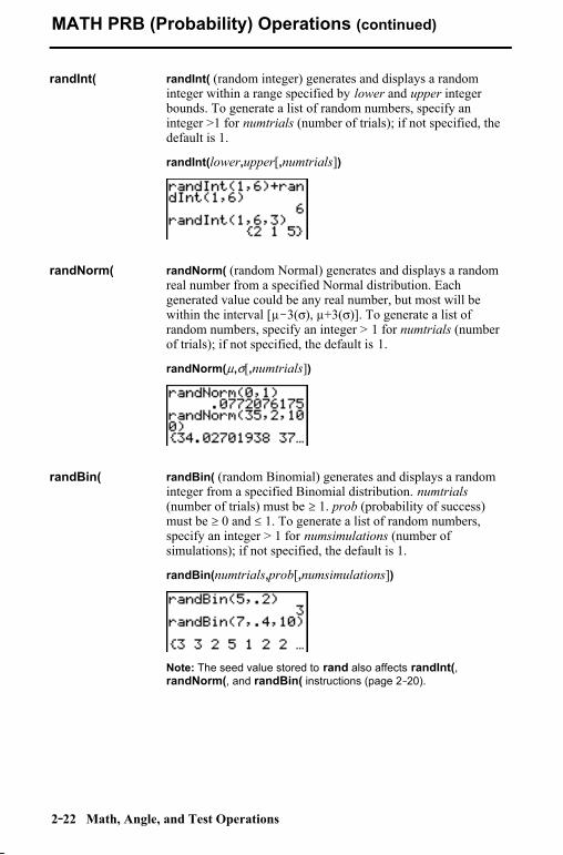
2.22 Math, Angle, and Test Operations
82STAT~4.DOC TI-83 international English Bob Fedorisko Revised: 10/28/05 12:19 PM Printed: 10/28/05 12:20PM Page 22 of 2682STAT~4.DOC TI-83 international English Bob Fedorisko Revised: 10/28/05 12:19 PM Printed: 10/28/05 12:20PM Page 22 of 26
randInt( (random integer) generates and displays a randominteger within a range specified by lower and upper integerbounds. To generate a list of random numbers, specify aninteger >1 for numtrials (number of trials); if not specified, thedefault is 1.
randInt(lower,upper[,numtrials])
randNorm( (random Normal) generates and displays a randomreal number from a specified Normal distribution. Eachgenerated value could be any real number, but most will bewithin the interval [mN3(s), m+3(s)]. To generate a list ofrandom numbers, specify an integer > 1 for numtrials (numberof trials); if not specified, the default is 1.
randNorm(m,s[,numtrials])
randBin( (random Binomial) generates and displays a randominteger from a specified Binomial distribution. numtrials(number of trials) must be ‚ 1. prob (probability of success)must be ‚ 0 and 1. To generate a list of random numbers,specify an integer > 1 for numsimulations (number ofsimulations); if not specified, the default is 1.
randBin(numtrials,prob[,numsimulations])
Note: The seed value stored to rand also affects randInt(,randNorm(, and randBin( instructions (page 2-20).
MATH PRB (Probability) Operations (continued)
randInt(
randNorm(
randBin(

Math, Angle, and Test Operations 2.23
82STAT~4.DOC TI-83 international English Bob Fedorisko Revised: 10/28/05 12:19 PM Printed: 10/28/05 12:20PM Page 23 of 26
To display the ANGLE menu, press y [ANGLE]. The ANGLEmenu displays angle indicators and instructions. TheRadian/Degree mode setting affects the TI-82 STATSinterpretation of ANGLE menu entries.
ANGLE1: ¡ Degree notation2: ' DMS minute notation3: r Radian notation4: 8DMS Displays as degree/minute/second5: R8Pr( Returns r, given X and Y6: R8Pq( Returns q, given X and Y7: P8Rx( Returns x, given R and q8: P8Ry( Returns y, given R and q
DMS (degrees/minutes/seconds) entry notation comprises thedegree symbol (¡), the minute symbol ('), and the second symbol("). degrees must be a real number; minutes and seconds mustbe real numbers ‚ 0.
degrees¡minutes'seconds"
For example, enter for 30 degrees, 1 minute, 23 seconds. If theangle mode is not set to Degree, you must use ¡ so that theTI-82 STATS can interpret the argument as degrees, minutes,and seconds.
Degree mode Radian mode
¡ (degree) designates an angle or list of angles as degrees,regardless of the current angle mode setting. In Radian mode,you can use ¡ to convert degrees to radians.
value¡{value1,value2,value3,value4,...,value n}¡
¡ also designates degrees (D) in DMS format.' (minutes) designates minutes (M) in DMS format." (seconds) designates seconds (S) in DMS format.
Note: " is not on the ANGLE menu. To enter ", press ƒ [ã].
ANGLE Operations
ANGLE Menu
DMS EntryNotation
¡ (Degree)

2.24 Math, Angle, and Test Operations
82STAT~4.DOC TI-83 international English Bob Fedorisko Revised: 10/28/05 12:19 PM Printed: 10/28/05 12:20PM Page 24 of 2682STAT~4.DOC TI-83 international English Bob Fedorisko Revised: 10/28/05 12:19 PM Printed: 10/28/05 12:20PM Page 24 of 26
r (radians) designates an angle or list of angles as radians,regardless of the current angle mode setting. In Degree mode,you can use r to convert radians to degrees.
valuer
Degree mode
8DMS (degree/minute/second) displays answer in DMS format(page 2.23). The mode setting must be Degree for answer to beinterpreted as degrees, minutes, and seconds. 8DMS is validonly at the end of a line.
answer8DMS
R8Pr( converts rectangular coordinates to polar coordinates andreturns r. R8Pq( converts rectangular coordinates to polarcoordinates and returns q. x and y can be lists.
R8Pr(x,y), R8Pq(x,y)
Note: Radian mode is set.
P8Rx( converts polar coordinates to rectangular coordinates andreturns x. P8Ry( converts polar coordinates to rectangularcoordinates and returns y. r and q can be lists.
P8Rx(r,q), P8Ry(r,q)
Note: Radian mode is set.
ANGLE Operations (continued)
r (Radians)
8DMS
R8Pr (,R8Pq ( ,P8Rx(,P8Ry(
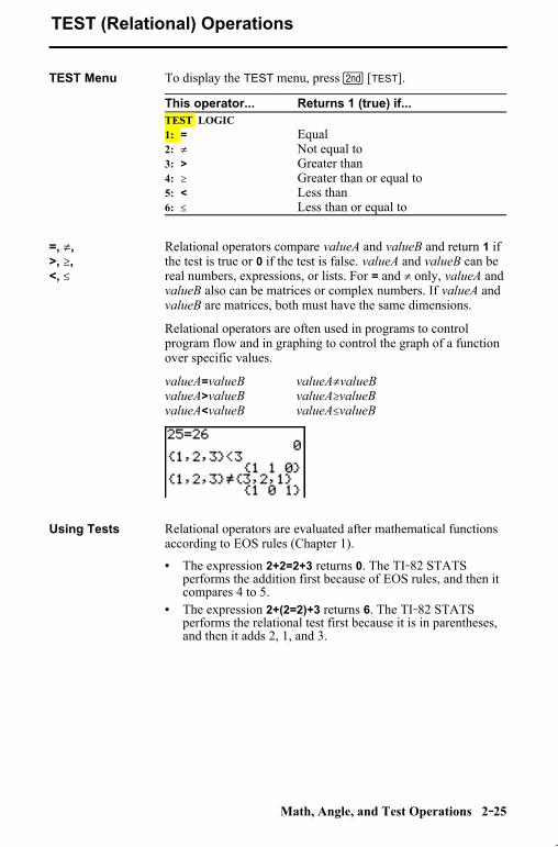
Math, Angle, and Test Operations 2.25
82STAT~4.DOC TI-83 international English Bob Fedorisko Revised: 10/28/05 12:19 PM Printed: 10/28/05 12:20PM Page 25 of 26
To display the TEST menu, press y [TEST].
This operator... Returns 1 (true) if...TEST LOGIC1: = Equal2: ƒ Not equal to3: > Greater than4: ‚ Greater than or equal to5: < Less than6: Less than or equal to
Relational operators compare valueA and valueB and return 1 ifthe test is true or 0 if the test is false. valueA and valueB can bereal numbers, expressions, or lists. For = and ƒ only, valueA andvalueB also can be matrices or complex numbers. If valueA andvalueB are matrices, both must have the same dimensions.
Relational operators are often used in programs to controlprogram flow and in graphing to control the graph of a functionover specific values.
valueA=valueB valueAƒvalueBvalueA>valueB valueA‚valueBvalueA<valueB valueAvalueB
Relational operators are evaluated after mathematical functionsaccording to EOS rules (Chapter 1).
• The expression 2+2=2+3 returns 0. The TI-82 STATSperforms the addition first because of EOS rules, and then itcompares 4 to 5.
• The expression 2+(2=2)+3 returns 6. The TI-82 STATSperforms the relational test first because it is in parentheses,and then it adds 2, 1, and 3.
TEST (Relational) Operations
TEST Menu
=, ƒ,>, ‚,<,
Using Tests
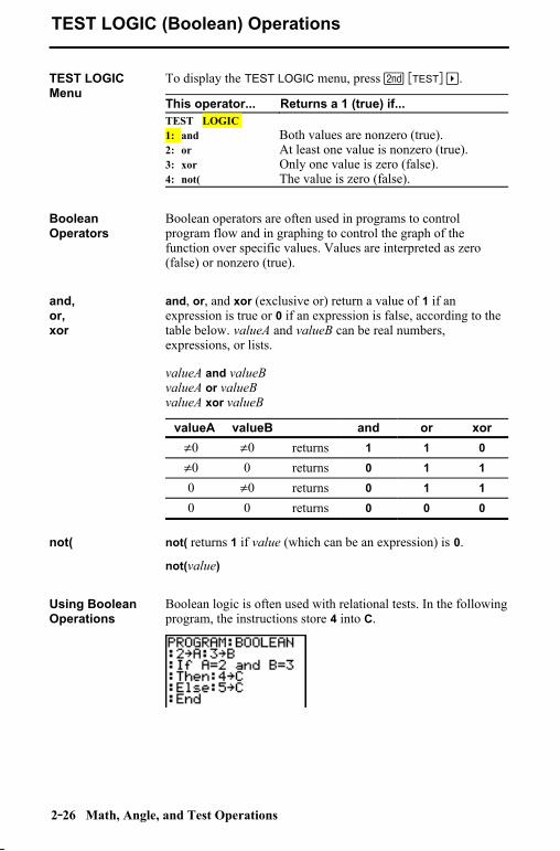
2.26 Math, Angle, and Test Operations
82STAT~4.DOC TI-83 international English Bob Fedorisko Revised: 10/28/05 12:19 PM Printed: 10/28/05 12:20PM Page 26 of 2682STAT~4.DOC TI-83 international English Bob Fedorisko Revised: 10/28/05 12:19 PM Printed: 10/28/05 12:20PM Page 26 of 26
To display the TEST LOGIC menu, press y ãTESTä ~.
This operator... Returns a 1 (true) if...TEST LOGIC1: and Both values are nonzero (true).2: or At least one value is nonzero (true).3: xor Only one value is zero (false).4: not( The value is zero (false).
Boolean operators are often used in programs to controlprogram flow and in graphing to control the graph of thefunction over specific values. Values are interpreted as zero(false) or nonzero (true).
and, or, and xor (exclusive or) return a value of 1 if anexpression is true or 0 if an expression is false, according to thetable below. valueA and valueB can be real numbers,expressions, or lists.
valueA and valueBvalueA or valueBvalueA xor valueB
valueA valueB and or xorƒ0 ƒ0 returns 1 1 0ƒ0 0 returns 0 1 10 ƒ0 returns 0 1 10 0 returns 0 0 0
not( returns 1 if value (which can be an expression) is 0.
not(value)
Boolean logic is often used with relational tests. In the followingprogram, the instructions store 4 into C.
TEST LOGIC (Boolean) Operations
TEST LOGICMenu
BooleanOperators
and,or,xor
not(
Using BooleanOperations
Function Graphing 3.1
82533F~1.DOC TI-83 international English Bob Fedorisko Revised: 10/26/05 1:20 PM Printed: 10/27/05 1:55PM Page 1 of 28
3 FunctionGraphing
Getting Started: Graphing a Circle .............................................................. 2Defining Graphs ...................................................................................................... 3Setting the Graph Modes ................................................................................... 4Defining Functions ................................................................................................ 5Selecting and Deselecting Functions.......................................................... 7Setting Graph Styles for Functions.............................................................. 9Setting the Viewing Window Variables................................................... 11Setting the Graph Format .................................................................................. 13Displaying Graphs.................................................................................................. 15Exploring Graphs with the Free-Moving Cursor................................ 17Exploring Graphs with TRACE..................................................................... 18Exploring Graphs with the ZOOM Instructions .................................. 20Using ZOOM MEMORY .................................................................................... 23Using the CALC (Calculate) Operations.................................................. 25
Contents

3.2 Function Graphing
82533F~1.DOC TI-83 international English Bob Fedorisko Revised: 10/26/05 1:20 PM Printed: 10/27/05 1:55PM Page 2 of 2882533F~1.DOC TI-83 international English Bob Fedorisko Revised: 10/26/05 1:20 PM Printed: 10/27/05 1:55PM Page 2 of 28
Getting Started is a fast-paced introduction. Read the chapter for details.
Graph a circle of radius 10, centered on the origin in the standard viewing window.To graph this circle, you must enter separate formulas for the upper and lowerportions of the circle. Then use ZSquare (zoom square) to adjust the display andmake the functions appear as a circle.
1. In Func mode, press o to display theY= editor. Press y ã‡ä 100¹„¡¤Í to enter the expression Y=‡(100NX2),which defines the top half of the circle.
The expression Y=L‡(100NX2) defines thebottom half of the circle. On the TI-82 STATS,you can define one function in terms of another.To define Y2=LY1, press Ì to enter the negationsign. Press ~ to display theVARS Y.VARS menu. Then press Í toselect 1:Function. The FUNCTION secondarymenu is displayed. Press 1 to select 1:Y1.
2. Press q 6 to select 6:ZStandard. This is aquick way to reset the window variables to thestandard values. It also graphs the functions;you do not need to press s.
Notice that the functions appear as an ellipse inthe standard viewing window.
3. To adjust the display so that each pixelrepresents an equal width and height, pressq 5 to select 5:ZSquare. The functions arereplotted and now appear as a circle on thedisplay.
4. To see the ZSquare window variables, pressp and notice the new values for Xmin,Xmax, Ymin, and Ymax.
Getting Started: Graphing a Circle

Function Graphing 3.3
82533F~1.DOC TI-83 international English Bob Fedorisko Revised: 10/26/05 1:20 PM Printed: 10/27/05 1:55PM Page 3 of 28
Chapter 3 specifically describes function graphing, but the stepsshown here are similar for each TI-82 STATS graphing mode.Chapters 4, 5, and 6 describe aspects that are unique toparametric graphing, polar graphing, and sequence graphing.
To define a graph in any graphing mode, follow these steps.Some steps are not always necessary.
1. Press z and set the appropriate graph mode (page 3.4).
2. Press o and enter, edit, or select one or more functions inthe Y= editor (page 3.5 and 3.7).
3. Deselect stat plots, if necessary (page 3.7).
4. Set the graph style for each function (page 3.9).
5. Press p and define the viewing window variables(page 3.11).
6. Press y [FORMAT] and select the graph format settings(page 3.13).
After you have defined a graph, press s to display it.Explore the behavior of the function or functions using theTI-82 STATS tools described in this chapter.
You can store the elements that define the current graph to anyof 10 graph database variables (GDB1 through GDB9, andGDB0; Chapter 8). To recreate the current graph later, simplyrecall the graph database to which you stored the original graph.
These types of information are stored in a GDB.
• Y= functions• Graph style settings• Window settings• Format settings
You can store a picture of the current graph display to any of 10graph picture variables (Pic1 through Pic9, and Pic0; Chapter8). Then you can superimpose one or more stored pictures ontothe current graph.
Defining Graphs
TI-82 STATS—Graphing ModeSimilarities
Defining a Graph
Displaying andExploring aGraph
Saving a Graphfor Later Use

3.4 Function Graphing
82533F~1.DOC TI-83 international English Bob Fedorisko Revised: 10/26/05 1:20 PM Printed: 10/27/05 1:55PM Page 4 of 2882533F~1.DOC TI-83 international English Bob Fedorisko Revised: 10/26/05 1:20 PM Printed: 10/27/05 1:55PM Page 4 of 28
To display the mode screen, press z. The default settings arehighlighted below. To graph functions, you must select Funcmode before you enter values for the window variables andbefore you enter the functions.
The TI-82 STATS has four graphing modes.• Func (function graphing)• Par (parametric graphing; Chapter 4)• Pol (polar graphing; Chapter 5)• Seq (sequence graphing; Chapter 6)
Other mode settings affect graphing results. Chapter 1 describeseach mode setting.
• Float or 0123456789 (fixed) decimal mode affects displayedgraph coordinates.
• Radian or Degree angle mode affects interpretation of somefunctions.
• Connected or Dot plotting mode affects plotting of selectedfunctions.
• Sequential or Simul graphing-order mode affects functionplotting when more than one function is selected.
To set the graphing mode and other modes from a program,begin on a blank line in the program editor and follow thesesteps.
1. Press z to display the mode settings.
2. Press †, ~, |, and } to place the cursor on the mode thatyou want to select.
3. Press Í to paste the mode name to the cursor location.
The mode is changed when the program is executed.
Setting the Graph Modes
Checking andChanging theGraphing Mode
Setting Modesfrom a Program

Function Graphing 3.5
82533F~1.DOC TI-83 international English Bob Fedorisko Revised: 10/26/05 1:20 PM Printed: 10/27/05 1:55PM Page 5 of 28
To display the Y= editor, press o. You can store up to 10functions to the function variables Y1 through Y9, and Y0. Youcan graph one or more defined functions at once. In thisexample, functions Y1 and Y2 are defined and selected.
To define or edit a function, follow these steps.
1. Press o to display the Y= editor.
2. Press † to move the cursor to the function you want todefine or edit. To erase a function, press ‘.
3. Enter or edit the expression to define the function.
• You may use functions and variables (including matricesand lists) in the expression. When the expressionevaluates to a nonreal number, the value is not plotted; noerror is returned.
• The independent variable in the function is X. Func modedefines „ as X. To enter X, press „ or pressƒ [X].
• When you enter the first character, the = is highlighted,indicating that the function is selected.
As you enter the expression, it is stored to the variable Yn asa user-defined function in the Y= editor.
4. Press Í or † to move the cursor to the next function.
Defining Functions
DisplayingFunctions in theY= Editor
Defining orEditing aFunction
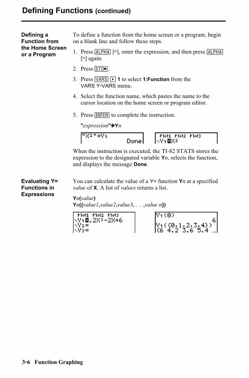
3.6 Function Graphing
82533F~1.DOC TI-83 international English Bob Fedorisko Revised: 10/26/05 1:20 PM Printed: 10/27/05 1:55PM Page 6 of 2882533F~1.DOC TI-83 international English Bob Fedorisko Revised: 10/26/05 1:20 PM Printed: 10/27/05 1:55PM Page 6 of 28
To define a function from the home screen or a program, beginon a blank line and follow these steps.
1. Press ƒ [ã], enter the expression, and then press ƒ[ã] again.
2. Press ¿.
3. Press ~ 1 to select 1:Function from theVARS Y.VARS menu.
4. Select the function name, which pastes the name to thecursor location on the home screen or program editor.
5. Press Í to complete the instruction.
"expression"!!!!Yn
When the instruction is executed, the TI-82 STATS stores theexpression to the designated variable Yn, selects the function,and displays the message Done.
You can calculate the value of a Y= function Yn at a specifiedvalue of X. A list of values returns a list.
Yn(value)Yn({value1,value2,value3, . . .,value n})
Defining Functions (continued)
Defining aFunction fromthe Home Screenor a Program
Evaluating Y=Functions inExpressions

Function Graphing 3.7
82533F~1.DOC TI-83 international English Bob Fedorisko Revised: 10/26/05 1:20 PM Printed: 10/27/05 1:55PM Page 7 of 28
You can select and deselect (turn on and turn off) a function inthe Y= editor. A function is selected when the = sign ishighlighted. The TI-82 STATS graphs only the selectedfunctions. You can select any or all functions Y1 through Y9, andY0.
To select or deselect a function in the Y= editor, follow thesesteps.
1. Press o to display the Y= editor.
2. Move the cursor to the function you want to select ordeselect.
3. Press | to place the cursor on the function’s = sign.
4. Press Í to change the selection status.
When you enter or edit a function, it is selected automatically.When you clear a function, it is deselected.
To view and change the on/off status of a stat plot in theY= editor, use Plot1 Plot2 Plot3 (the top line of the Y= editor).When a plot is on, its name is highlighted on this line.
To change the on/off status of a stat plot from the Y= editor,press } and ~ to place the cursor on Plot1, Plot2, or Plot3, andthen press Í.
Selecting and Deselecting Functions
Selecting andDeselecting aFunction
Turning On orTurning Off a StatPlot in the Y=Editor
Plot1 is turned on.Plot2 and Plot3 are turned off.
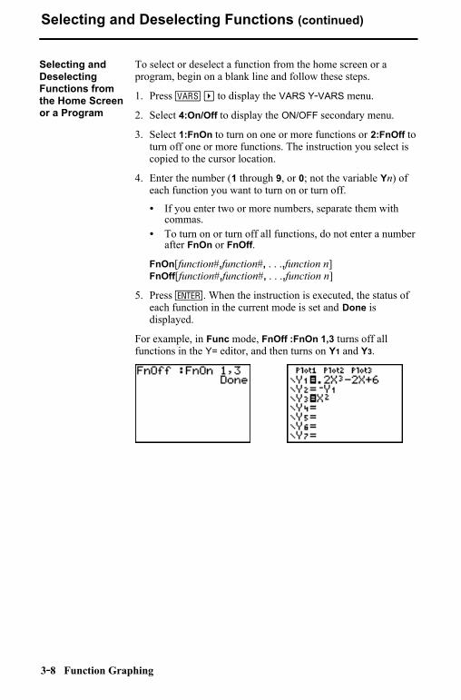
3.8 Function Graphing
82533F~1.DOC TI-83 international English Bob Fedorisko Revised: 10/26/05 1:20 PM Printed: 10/27/05 1:55PM Page 8 of 2882533F~1.DOC TI-83 international English Bob Fedorisko Revised: 10/26/05 1:20 PM Printed: 10/27/05 1:55PM Page 8 of 28
To select or deselect a function from the home screen or aprogram, begin on a blank line and follow these steps.
1. Press ~ to display the VARS Y.VARS menu.
2. Select 4:On/Off to display the ON/OFF secondary menu.
3. Select 1:FnOn to turn on one or more functions or 2:FnOff toturn off one or more functions. The instruction you select iscopied to the cursor location.
4. Enter the number (1 through 9, or 0; not the variable Yn) ofeach function you want to turn on or turn off.
• If you enter two or more numbers, separate them withcommas.
• To turn on or turn off all functions, do not enter a numberafter FnOn or FnOff.
FnOn[function#,function#, . . .,function n]FnOff[function#,function#, . . .,function n]
5. Press Í. When the instruction is executed, the status ofeach function in the current mode is set and Done isdisplayed.
For example, in Func mode, FnOff :FnOn 1,3 turns off allfunctions in the Y= editor, and then turns on Y1 and Y3.
Selecting and Deselecting Functions (continued)
Selecting andDeselectingFunctions fromthe Home Screenor a Program
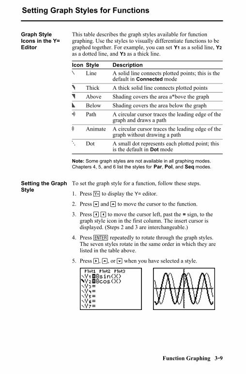
Function Graphing 3.9
82533F~1.DOC TI-83 international English Bob Fedorisko Revised: 10/26/05 1:20 PM Printed: 10/27/05 1:55PM Page 9 of 28
This table describes the graph styles available for functiongraphing. Use the styles to visually differentiate functions to begraphed together. For example, you can set Y1 as a solid line, Y2as a dotted line, and Y3 as a thick line.
Icon Style Descriptionç Line A solid line connects plotted points; this is the
default in Connected modeè Thick A thick solid line connects plotted pointsé Above Shading covers the area a*bove the graphê Below Shading covers the area below the graphë Path A circular cursor traces the leading edge of the
graph and draws a pathì Animate A circular cursor traces the leading edge of the
graph without drawing a pathí Dot A small dot represents each plotted point; this
is the default in Dot mode
Note: Some graph styles are not available in all graphing modes.Chapters 4, 5, and 6 list the styles for Par, Pol, and Seq modes.
To set the graph style for a function, follow these steps.
1. Press o to display the Y= editor.
2. Press † and } to move the cursor to the function.
3. Press | | to move the cursor left, past the = sign, to thegraph style icon in the first column. The insert cursor isdisplayed. (Steps 2 and 3 are interchangeable.)
4. Press Í repeatedly to rotate through the graph styles.The seven styles rotate in the same order in which they arelisted in the table above.
5. Press ~, }, or † when you have selected a style.
Setting Graph Styles for Functions
Graph StyleIcons in the Y=Editor
Setting the GraphStyle

3.10 Function Graphing
82533F~1.DOC TI-83 international English Bob Fedorisko Revised: 10/26/05 1:20 PM Printed: 10/27/05 1:55PM Page 10 of 2882533F~1.DOC TI-83 international English Bob Fedorisko Revised: 10/26/05 1:20 PM Printed: 10/27/05 1:55PM Page 10 of 28
When you select é or ê for two or more functions, theTI-82 STATS rotates through four shading patterns.
• Vertical lines shade the first function with a é or ê graphstyle.
• Horizontal lines shade the second.• Negatively sloping diagonal lines shade the third.• Positively sloping diagonal lines shade the fourth.• The rotation returns to vertical lines for the fifth é or ê
function, repeating the order described above.
When shaded areas intersect, the patterns overlap.
Note: When é or ê is selected for a Y= function that graphs a familyof curves, such as Y1={1,2,3}X, the four shading patterns rotate foreach member of the family of curves.
To set the graph style from a program, select H:GraphStyle(from the PRGM CTL menu. To display this menu, press while in the program editor. function# is the number of the Y=function name in the current graphing mode. graphstyle# is aninteger from 1 to 7 that corresponds to the graph style, as shownbelow.
1 = ç (line) 2 = è (thick) 3 = é (above)4 = ê (below) 5 = ë (path) 6 = ì (animate) 7 = í (dot)
GraphStyle(function#,graphstyle#)
For example, when this program is executed in Func mode,GraphStyle(1,3) sets Y1 to é (above).
Setting Graph Styles for Functions (continued)
Shading Aboveand Below
Setting a GraphStyle from aProgram

Function Graphing 3.11
82533F~1.DOC TI-83 international English Bob Fedorisko Revised: 10/26/05 1:20 PM Printed: 10/27/05 1:55PM Page 11 of 28
The viewing window is the portion of the coordinate planedefined by Xmin, Xmax, Ymin, and Ymax. Xscl (X scale)defines the distance between tick marks on the x-axis. Yscl (Yscale) defines the distance between tick marks on the y-axis. Toturn off tick marks, set Xscl=0 and Yscl=0.
Xmax
Ymin
Ymax
Xscl
Yscl
Xmin
To display the current window variable values, press p.The window editor above and to the right shows the defaultvalues in Func graphing mode and Radian angle mode. Thewindow variables differ from one graphing mode to another.
Xres sets pixel resolution (1 through 8) for function graphs only.The default is 1.
• At Xres=1, functions are evaluated and graphed at each pixelon the x-axis.
• At Xres=8, functions are evaluated and graphed at everyeighth pixel along the x-axis.
Tip: Small Xres values improve graph resolution but may cause theTI-82 STATS to draw graphs more slowly.
To change a window variable value from the window editor,follow these steps.
1. Press † or } to move the cursor to the window variable youwant to change.
2. Edit the value, which can be an expression.
• Enter a new value, which clears the original value.• Move the cursor to a specific digit, and then edit it.
3. Press Í, †, or }. If you entered an expression, theTI-82 STATS evaluates it. The new value is stored.
Note: Xmin<Xmax and Ymin<Ymax must be true in order to graph.
Setting the Viewing Window Variables
The TI-82 STATSViewing Window
Displaying theWindowVariables
Changing aWindow VariableValue

3.12 Function Graphing
82533F~1.DOC TI-83 international English Bob Fedorisko Revised: 10/26/05 1:20 PM Printed: 10/27/05 1:55PM Page 12 of 2882533F~1.DOC TI-83 international English Bob Fedorisko Revised: 10/26/05 1:20 PM Printed: 10/27/05 1:55PM Page 12 of 28
To store a value, which can be an expression, to a windowvariable, begin on a blank line and follow these steps.
1. Enter the value you want to store.
2. Press ¿.
3. Press to display the VARS menu.
4. Select 1:Window to display the Func window variables (X/Ysecondary menu).
• Press ~ to display the Par and Pol window variables (T/qsecondary menu).
• Press ~ ~ to display the Seq window variables (U/V/Wsecondary menu).
5. Select the window variable to which you want to store avalue. The name of the variable is pasted to the currentcursor location.
6. Press Í to complete the instruction.
When the instruction is executed, the TI-82 STATS stores thevalue to the window variable and displays the value.
The variables @X and @Y (items 8 and 9 on the VARS(1:Window) X/Y secondary menu) define the distance from thecenter of one pixel to the center of any adjacent pixel on a graph(graphing accuracy). @X and @Y are calculated from Xmin,Xmax, Ymin, and Ymax when you display a graph.
@X = (Xmax N Xmin)94 @Y = (Ymax N Ymin)
62
You can store values to @X and @Y. If you do, Xmax and Ymaxare calculated from @X, Xmin, @Y, and Ymin.
Setting the Viewing Window Variables (continued)
Storing to aWindow Variablefrom the HomeScreen or aProgram
@X and @Y
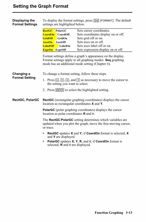
Function Graphing 3.13
82533F~1.DOC TI-83 international English Bob Fedorisko Revised: 10/26/05 1:20 PM Printed: 10/27/05 1:55PM Page 13 of 28
To display the format settings, press y [FORMAT]. The defaultsettings are highlighted below.
RectGC PolarGC Sets cursor coordinates.CoordOn CoordOff Sets coordinates display on or off.GridOff GridOn Sets grid off or on.AxesOn AxesOff Sets axes on or off.LabelOff LabelOn Sets axes label off or on.ExprOn ExprOff Sets expression display on or off.
Format settings define a graph’s appearance on the display.Format settings apply to all graphing modes. Seq graphingmode has an additional mode setting (Chapter 6).
To change a format setting, follow these steps.
1. Press †, ~, }, and | as necessary to move the cursor tothe setting you want to select.
2. Press Í to select the highlighted setting.
RectGC (rectangular graphing coordinates) displays the cursorlocation as rectangular coordinates X and Y.
PolarGC (polar graphing coordinates) displays the cursorlocation as polar coordinates R and q.
The RectGC/PolarGC setting determines which variables areupdated when you plot the graph, move the free-moving cursor,or trace.
• RectGC updates X and Y; if CoordOn format is selected, Xand Y are displayed.
• PolarGC updates X, Y, R, and q; if CoordOn format isselected, R and q are displayed.
Setting the Graph Format
Displaying theFormat Settings
Changing aFormat Setting
RectGC, PolarGC

3.14 Function Graphing
82533F~1.DOC TI-83 international English Bob Fedorisko Revised: 10/26/05 1:20 PM Printed: 10/27/05 1:55PM Page 14 of 2882533F~1.DOC TI-83 international English Bob Fedorisko Revised: 10/26/05 1:20 PM Printed: 10/27/05 1:55PM Page 14 of 28
CoordOn (coordinates on) displays the cursor coordinates at thebottom of the graph. If ExprOff format is selected, the functionnumber is displayed in the top-right corner.
CoordOff (coordinates off) does not display the function numberor coordinates.
Grid points cover the viewing window in rows that correspondto the tick marks (page 3.11) on each axis.
GridOff does not display grid points.
GridOn displays grid points.
AxesOn displays the axes.
AxesOff does not display the axes.
This overrides the LabelOff/LabelOn format setting.
LabelOff and LabelOn determine whether to display labels forthe axes (X and Y), if AxesOn format is also selected.
ExprOn and ExprOff determine whether to display theY= expression when the trace cursor is active. This formatsetting also applies to stat plots.
When ExprOn is selected, the expression is displayed in the top-left corner of the graph screen.
When ExprOff and CoordOn both are selected, the number inthe top-right corner specifies which function is being traced.
Setting the Graph Format (continued)
CoordOn,CoordOff
GridOff, GridOn
AxesOn, AxesOff
LabelOff,LabelOn
ExprOn, ExprOff
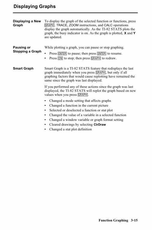
Function Graphing 3.15
82533F~1.DOC TI-83 international English Bob Fedorisko Revised: 10/26/05 1:20 PM Printed: 10/27/05 1:55PM Page 15 of 28
To display the graph of the selected function or functions, presss. TRACE, ZOOM instructions, and CALC operationsdisplay the graph automatically. As the TI-82 STATS plots thegraph, the busy indicator is on. As the graph is plotted, X and Yare updated.
While plotting a graph, you can pause or stop graphing.
• Press Í to pause; then press Í to resume.• Press É to stop; then press s to redraw.
Smart Graph is a TI-82 STATS feature that redisplays the lastgraph immediately when you press s, but only if allgraphing factors that would cause replotting have remained thesame since the graph was last displayed.
If you performed any of these actions since the graph was lastdisplayed, the TI-82 STATS will replot the graph based on newvalues when you press s.
• Changed a mode setting that affects graphs• Changed a function in the current picture• Selected or deselected a function or stat plot• Changed the value of a variable in a selected function• Changed a window variable or graph format setting• Cleared drawings by selecting ClrDraw• Changed a stat plot definition
Displaying Graphs
Displaying a NewGraph
Pausing orStopping a Graph
Smart Graph

3.16 Function Graphing
82533F~1.DOC TI-83 international English Bob Fedorisko Revised: 10/26/05 1:20 PM Printed: 10/27/05 1:55PM Page 16 of 2882533F~1.DOC TI-83 international English Bob Fedorisko Revised: 10/26/05 1:20 PM Printed: 10/27/05 1:55PM Page 16 of 28
On the TI-82 STATS, you can graph one or more new functionswithout replotting existing functions. For example, store sin(X)to Y1 in the Y= editor and press s. Then store cos(X) to Y2and press s again. The function Y2 is graphed on top of Y1,the original function.
If you enter a list (Chapter 11) as an element in an expression,the TI-82 STATS plots the function for each value in the list,thereby graphing a family of curves. In Simul graphing-ordermode, it graphs all functions sequentially for the first element ineach list, and then for the second, and so on.
{2,4,6}sin(X) graphs three functions: 2 sin(X), 4 sin(X), and6 sin(X).
{2,4,6}sin({1,2,3}X) graphs 2 sin(X), 4 sin(2X), and 6 sin(3X).
Note: When using more than one list, the lists must have the samedimensions.
Displaying Graphs (continued)
OverlayingFunctions on aGraph
Graphing aFamily of Curves

Function Graphing 3.17
82533F~1.DOC TI-83 international English Bob Fedorisko Revised: 10/26/05 1:20 PM Printed: 10/27/05 1:55PM Page 17 of 28
When a graph is displayed, press |, ~, }, or † to move thecursor around the graph. When you first display the graph, nocursor is visible. When you press |, ~, }, or †, the cursormoves from the center of the viewing window.
As you move the cursor around the graph, the coordinate valuesof the cursor location are displayed at the bottom of the screen ifCoordOn format is selected. The Float/Fix decimal mode settingdetermines the number of decimal digits displayed for thecoordinate values.
To display the graph with no cursor and no coordinate values,press ‘ or Í. When you press |, ~, }, or †, thecursor moves from the same position.
The free-moving cursor moves from pixel to pixel on the screen.When you move the cursor to a pixel that appears to be on thefunction, the cursor may be near, but not actually on, thefunction. The coordinate value displayed at the bottom of thescreen actually may not be a point on the function. To move thecursor along a function, use r (page 3.18).
The coordinate values displayed as you move the cursorapproximate actual math coordinates, *accurate to within thewidth and height of the pixel. As Xmin, Xmax, Ymin, and Ymaxget closer together (as in a ZoomIn) graphing accuracyincreases, and the coordinate values more closely approximatethe math coordinates.
Exploring Graphs with the Free-Moving Cursor
Free-MovingCursor
GraphingAccuracy
Free-moving cursor “on” the curve

3.18 Function Graphing
82533F~1.DOC TI-83 international English Bob Fedorisko Revised: 10/26/05 1:20 PM Printed: 10/27/05 1:55PM Page 18 of 2882533F~1.DOC TI-83 international English Bob Fedorisko Revised: 10/26/05 1:20 PM Printed: 10/27/05 1:55PM Page 18 of 28
Use TRACE to move the cursor from one plotted point to thenext along a function. To begin a trace, press r. If thegraph is not displayed already, press r to display it. Thetrace cursor is on the first selected function in the Y= editor, atthe middle X value on the screen. The cursor coordinates aredisplayed at the bottom of the screen if CoordOn format isselected. The Y= expression is displayed in the top-left corner ofthe screen, if ExprOn format is selected.
To move the TRACE cursor . . . do this:. . . to the previous or next plotted point, press | or ~.. . . five plotted points on a function (Xresaffects this),
press y| or y~.
. . . to any valid X value on a function, enter a value, andthen press Í.
. . . from one function to another, press } or †.
When the trace cursor moves along a function, the Y value iscalculated from the X value; that is, Y=Yn(X). If the function isundefined at an X value, the Y value is blank.
If you move the trace cursor beyond the top or bottom of thescreen, the coordinate values at the bottom of the screencontinue to change appropriately.
To move the trace cursor from function to function, press † and}. The cursor follows the order of the selected functions in theY= editor. The trace cursor moves to each function at the same Xvalue. If ExprOn format is selected, the expression is updated.
Exploring Graphs with TRACE
Beginning aTrace
Moving the TraceCursor
Moving the TraceCursor fromFunction toFunction
Trace cursor on the curve

Function Graphing 3.19
82533F~1.DOC TI-83 international English Bob Fedorisko Revised: 10/26/05 1:20 PM Printed: 10/27/05 1:55PM Page 19 of 28
To move the trace cursor to any valid X value on the currentfunction, enter the value. When you enter the first digit, an X=prompt and the number you entered are displayed in the bottom-left corner of the screen. You can enter an expression at the X=prompt. The value must be valid for the current viewingwindow. When you have completed the entry, press Í tomove the cursor.
Note: This feature does not apply to stat plots.
If you trace a function beyond the left or right side of the screen,the viewing window automatically pans to the left or right.Xmin and Xmax are updated to correspond to the new viewingwindow.
While tracing, you can press Í to adjust the viewingwindow so that the cursor location becomes the center of thenew viewing window, even if the cursor is above or below thedisplay. This allows panning up and down. After Quick Zoom,the cursor remains in TRACE.
When you leave and return to TRACE, the trace cursor isdisplayed in the same location it was in when you left TRACE,unless Smart Graph has replotted the graph (page 3.15).
On a blank line in the program editor, press r. Theinstruction Trace is pasted to the cursor location. When theinstruction is encountered during program execution, the graphis displayed with the trace cursor on the first selected function.As you trace, the cursor coordinate values are updated. Whenyou finish tracing the functions, press Í to resume programexecution.
Moving the TraceCursor to AnyValid X Value
Panning to theLeft or Right
Quick Zoom
Leaving andReturning toTRACE
Using TRACE ina Program

3.20 Function Graphing
82533F~1.DOC TI-83 international English Bob Fedorisko Revised: 10/26/05 1:20 PM Printed: 10/27/05 1:55PM Page 20 of 2882533F~1.DOC TI-83 international English Bob Fedorisko Revised: 10/26/05 1:20 PM Printed: 10/27/05 1:55PM Page 20 of 28
To display the ZOOM menu, press q. You can adjust theviewing window of the graph quickly in several ways. AllZOOM instructions are accessible from programs.
ZOOM
MEMORY
1: ZBox Draws a box to define the viewing window.2: Zoom In Magnifies the graph around the cursor.3: Zoom Out Views more of a graph around the cursor.4: ZDecimal Sets @X and @Y to 0.1.5: ZSquare Sets equal-size pixels on the X and Y axes.6: ZStandard Sets the standard window variables.7: ZTrig Sets the built-in trig window variables.8: ZInteger Sets integer values on the X and Y axes.9: ZoomStat Sets the values for current stat lists.0: ZoomFit Fits YMin and YMax between XMin and XMax.
When you select 1:ZBox, 2:Zoom In, or 3:Zoom Out, the cursoron the graph becomes the zoom cursor (+), a smaller version ofthe free-moving cursor (+).
To define a new viewing window using ZBox, follow thesesteps.
1. Select 1:ZBox from the ZOOM menu. The zoom cursor isdisplayed at the center of the screen.
2. Move the zoom cursor to any spot you want to define as acorner of the box, and then press Í. When you move thecursor away from the first defined corner, a small, square dotindicates the spot.
3. Press |, }, ~, or †. As you move the cursor, the sides ofthe box lengthen or shorten proportionately on the screen.
Note: To cancel ZBox before you press Í, press ‘.
4. When you have defined the box, press Í to replot thegraph.
To use ZBox to define another box within the new graph, repeatsteps 2 through 4. To cancel ZBox, press ‘.
Exploring Graphs with the ZOOM Instructions
ZOOM Menu
Zoom Cursor
ZBox

Function Graphing 3.21
82533F~1.DOC TI-83 international English Bob Fedorisko Revised: 10/26/05 1:20 PM Printed: 10/27/05 1:55PM Page 21 of 28
Zoom In magnifies the part of the graph that surrounds thecursor location. Zoom Out displays a greater portion of thegraph, centered on the cursor location. The XFact and YFactsettings determine the extent of the zoom.
To zoom in on a graph, follow these steps.
1. Check XFact and YFact (page 3.24); change as needed.
2. Select 2:Zoom In from the ZOOM menu. The zoom cursor isdisplayed.
3. Move the zoom cursor to the point that is to be the center ofthe new viewing window.
4. Press Í. The TI-82 STATS adjusts the viewing windowby XFact and YFact; updates the window variables; andreplots the selected functions, centered on the cursorlocation.
5. Zoom in on the graph again in either of two ways.• To zoom in at the same point, press Í.• To zoom in at a new point, move the cursor to the point
that you want as the center of the new viewing window,and then press Í.
To zoom out on a graph, select 3:Zoom Out and repeat steps 3through 5.
To cancel Zoom In or Zoom Out, press ‘.
ZDecimal replots the functions immediately. It updates thewindow variables to preset values, as shown below. Thesevalues set @X and @Y equal to 0.1 and set the X and Y value ofeach pixel to one decimal place.
Xmin=L4.7 Ymin=L3.1Xmax=4.7 Ymax=3.1Xscl=1 Yscl=1
ZSquare replots the functions immediately. It redefines theviewing window based on the current values of the windowvariables. It adjusts in only one direction so that @X=@Y, whichmakes the graph of a circle look like a circle. Xscl and Ysclremain unchanged. The midpoint of the current graph (not theintersection of the axes) becomes the midpoint of the new graph.
Zoom In,Zoom Out
ZDecimal
ZSquare

3.22 Function Graphing
82533F~1.DOC TI-83 international English Bob Fedorisko Revised: 10/26/05 1:20 PM Printed: 10/27/05 1:55PM Page 22 of 2882533F~1.DOC TI-83 international English Bob Fedorisko Revised: 10/26/05 1:20 PM Printed: 10/27/05 1:55PM Page 22 of 28
ZStandard replots the functions immediately. It updates thewindow variables to the standard values shown below.
Xmin=L10 Ymin=L10 Xres=1Xmax=10 Ymax=10Xscl=1 Yscl=1
ZTrig replots the functions immediately. It updates the windowvariables to preset values that are appropriate for plotting trigfunctions. Those preset values in Radian mode are shownbelow.
Xmin=L(47à24)p Ymin=L4Xmax=(47à24)p Ymax=4Xscl=p/2 Yscl=1
ZInteger redefines the viewing window to the dimensionsshown below. To use ZInteger, move the cursor to the point thatyou want to be the center of the new window, and then pressÍ; ZInteger replots the functions.
@X=1 Xscl=10@Y=1 Yscl=10
ZoomStat redefines the viewing window so that all statisticaldata points are displayed. For regular and modified box plots,only Xmin and Xmax are adjusted.
ZoomFit replots the functions immediately. ZoomFitrecalculates YMin and YMax to include the minimum andmaximum Y values of the selected functions between the currentXMin and XMax. XMin and XMax are not changed.
Exploring Graphs with the ZOOM Instructions (cont.)
ZStandard
ZTrig
ZInteger
ZoomStat
ZoomFit

Function Graphing 3.23
82533F~1.DOC TI-83 international English Bob Fedorisko Revised: 10/26/05 1:20 PM Printed: 10/27/05 1:55PM Page 23 of 28
To display the ZOOM MEMORY menu, press q ~.
ZOOMMEMORY
1: ZPrevious Uses the previous viewing window.2: ZoomSto Stores the user-defined window.3: ZoomRcl Recalls the user-defined window.4: SetFactors... Changes Zoom In and Zoom Out factors.
ZPrevious replots the graph using the window variables of thegraph that was displayed before you executed the last ZOOMinstruction.
ZoomSto immediately stores the current viewing window. Thegraph is displayed, and the values of the current windowvariables are stored in the user-defined ZOOM variables ZXmin,ZXmax, ZXscl, ZYmin, ZYmax, ZYscl, and ZXres.
These variables apply to all graphing modes. For example,changing the value of ZXmin in Func mode also changes it inPar mode.
ZoomRcl graphs the selected functions in a user-definedviewing window. The user-defined viewing window isdetermined by the values stored with the ZoomSto instruction.The window variables are updated with the user-defined values,and the graph is plotted.
Using ZOOM MEMORY
ZOOM MEMORYMenu
ZPrevious
ZoomSto
ZoomRcl

3.24 Function Graphing
82533F~1.DOC TI-83 international English Bob Fedorisko Revised: 10/26/05 1:20 PM Printed: 10/27/05 1:55PM Page 24 of 2882533F~1.DOC TI-83 international English Bob Fedorisko Revised: 10/26/05 1:20 PM Printed: 10/27/05 1:55PM Page 24 of 28
The zoom factors, XFact and YFact, are positive numbers (notnecessarily integers) greater than or equal to 1. They define themagnification or reduction factor used to Zoom In or Zoom Outaround a point.
To display the ZOOM FACTORS screen, where you can reviewthe current values for XFact and YFact, select 4:SetFactorsfrom the ZOOM MEMORY menu. The values shown are thedefaults.
You can change XFact and YFact in either of two ways.
• Enter a new value. The original value is clearedautomatically when you enter the first digit.
• Place the cursor on the digit you want to change, and thenenter a value or press { to delete it.
From the home screen or a program, you can store directly toany of the user-defined ZOOM variables.
From a program, you can select the ZoomSto and ZoomRclinstructions from the ZOOM MEMORY menu.
Using ZOOM MEMORY (continued)
ZOOM FACTORS
Checking XFactand YFact
Changing XFactand YFact
Using ZOOMMEMORY MenuItems from theHome Screen ora Program

Function Graphing 3.25
82533F~1.DOC TI-83 international English Bob Fedorisko Revised: 10/26/05 1:20 PM Printed: 10/27/05 1:55PM Page 25 of 28
To display the CALCULATE menu, press y ãCALCä. Use theitems on this menu to analyze the current graph functions.
CALCULATE1: value Calculates a function Y value for a given X.2: zero Finds a zero (x-intercept) of a function.3: minimum Finds a minimum of a function.4: maximum Finds a maximum of a function.5: intersect Finds an intersection of two functions.6: dy/dx Finds a numeric derivative of a function.7: ‰f(x)dx Finds a numeric integral of a function.
value evaluates one or more currently selected functions for aspecified value of X.
Note: When a value is displayed for X, press ‘ to clear thevalue. When no value is displayed, press ‘ to cancel the valueoperation.
To evaluate a selected function at X, follow these steps.
1. Select 1:value from the CALCULATE menu. The graph isdisplayed with X= in the bottom-left corner.
2. Enter a real value, which can be an expression, for Xbetween Xmin and Xmax.
3. Press Í.
The cursor is on the first selected function in the Y= editor at theX value you entered, and the coordinates are displayed, even ifCoordOff format is selected.
To move the cursor from function to function at the entered Xvalue, press } or †. To restore the free-moving cursor, press| or ~.
Using the CALC (Calculate) Operations
CALCULATEMenu
value

3.26 Function Graphing
82533F~1.DOC TI-83 international English Bob Fedorisko Revised: 10/26/05 1:20 PM Printed: 10/27/05 1:55PM Page 26 of 2882533F~1.DOC TI-83 international English Bob Fedorisko Revised: 10/26/05 1:20 PM Printed: 10/27/05 1:55PM Page 26 of 28
zero finds a zero (x-intercept or root) of a function using solve(.Functions can have more than one x-intercept value; zero findsthe zero closest to your guess.
The time zero spends to find the correct zero value depends onthe accuracy of the values you specify for the left and rightbounds and the accuracy of your guess.
To find a zero of a function, follow these steps.
1. Select 2:zero from the CALCULATE menu. The current graphis displayed with Left Bound? in the bottom-left corner.
2. Press } or † to move the cursor onto the function for whichyou want to find a zero.
3. Press | or ~ (or enter a value) to select the x-value for theleft bound of the interval, and then press Í. A 4indicator on the graph screen shows the left bound. RightBound? is displayed in the bottom-left corner. Press | or ~(or enter a value) to select the x-value for the right bound,and then press Í. A 3 indicator on the graph screenshows the right bound. Guess? is then displayed in thebottom-left corner.
4. Press | or ~ (or enter a value) to select a point near thezero of the function, between the bounds, and then pressÍ.
The cursor is on the solution and the coordinates are displayed,even if CoordOff format is selected. To move to the samex-value for other selected functions, press } or †. To restorethe free-moving cursor, press | or ~.
Using the CALC (Calculate) Operations (continued)
zero

Function Graphing 3.27
82533F~1.DOC TI-83 international English Bob Fedorisko Revised: 10/26/05 1:20 PM Printed: 10/27/05 1:55PM Page 27 of 28
minimum and maximum find a minimum or maximum of afunction within a specified interval to a tolerance of 1âL5.
To find a minimum or maximum, follow these steps.
1. Select 3:minimum or 4:maximum from the CALCULATEmenu. The current graph is displayed.
2. Select the function and set left bound, right bound, and guessas described for zero (steps 2 through 4; page 3.26).
The cursor is on the solution, and the coordinates are displayed,even if you have selected CoordOff format; Minimum orMaximum is displayed in the bottom-left corner.
To move to the same x-value for other selected functions, press} or †. To restore the free-moving cursor, press | or ~.
intersect finds the coordinates of a point at which two or morefunctions intersect using solve(. The intersection must appear onthe display to use intersect.
To find an intersection, follow these steps.
1. Select 5:intersect from the CALCULATE menu. The currentgraph is displayed with First curve? in the bottom-left corner.
2. Press † or }, if necessary, to move the cursor to the firstfunction, and then press Í. Second curve? is displayedin the bottom-left corner.
3. Press † or }, if necessary, to move the cursor to the secondfunction, and then press Í.
4. Press ~ or | to move the cursor to the point that is yourguess as to location of the intersection, and then press Í.
The cursor is on the solution and the coordinates are displayed,even if CoordOff format is selected. Intersection is displayed inthe bottom-left corner. To restore the free-moving cursor, press|, }, ~, or †.
minimum,maximum
intersect

3.28 Function Graphing
82533F~1.DOC TI-83 international English Bob Fedorisko Revised: 10/26/05 1:20 PM Printed: 10/27/05 1:55PM Page 28 of 2882533F~1.DOC TI-83 international English Bob Fedorisko Revised: 10/26/05 1:20 PM Printed: 10/27/05 1:55PM Page 28 of 28
dy/dx (numerical derivative) finds the numerical derivative(slope) of a function at a point, with H=1âL3.
To find a function’s slope at a point, follow these steps.
1. Select 6:dy/dx from the CALCULATE menu. The currentgraph is displayed.
2. Press } or † to select the function for which you want tofind the numerical derivative.
3. Press | or ~ (or enter a value) to select the X value atwhich to calculate the derivative, and then press Í.
The cursor is on the solution and the numerical derivative isdisplayed.
To move to the same x-value for other selected functions, press} or †. To restore the free-moving cursor, press | or ~.
‰f(x)dx (numerical integral) finds the numerical integral of afunction in a specified interval. It uses the fnInt( function, with atolerance of H=1âL3.
To find the numerical derivative of a function, follow thesesteps.
1. Select 7:‰f(x)dx from the CALCULATE menu. The currentgraph is displayed with Lower Limit? in the bottom-leftcorner.
2. Press } or † to move the cursor to the function for whichyou want to calculate the integral.
3. Set lower and upper limits as you would set left and rightbounds for zero (step 3; page 3.26). The integral value isdisplayed, and the integrated area is shaded.
Note: The shaded area is a drawing. Use ClrDraw (Chapter 8) orany action that invokes Smart Graph to clear the shaded area.
Using the CALC (Calculate) Operations (continued)
dy/dx
‰f(x)dx

Parametric Graphing 4-1
82EB1A~1.DOC TI-83 international English Bob Fedorisko Revised: 10/26/05 1:20 PM Printed: 10/27/05 1:58PM Page 1 of 8
4 ParametricGraphing
Getting Started: Path of a Ball........................................................................ 4-2Defining and Displaying Parametric Graphs ........................................ 4-4Exploring Parametric Graphs.......................................................................... 4-7
Contents

4-2 Parametric Graphing
82EB1A~1.DOC TI-83 international English Bob Fedorisko Revised: 10/26/05 1:20 PM Printed: 10/27/05 1:58PM Page 2 of 8
Getting Started is a fast-paced introduction. Read the chapter for details.
Graph the parametric equation that describes the path of a ball hit at an initial speedof 30 meters per second, at an initial angle of 25 degrees with the horizontal fromground level. How far does the ball travel? When does it hit the ground? How highdoes it go? Ignore all forces except gravity.
For initial velocity v0 and angle q, the position of the ball as a function of time hashorizontal and vertical components.
Horizontal: X1(t)=tv0cos(q)Vertical: Y1(t)=tv0sin(q)N 12 gt2
The vertical and horizontal vectors of the ball’s motion also will be graphed.
Vertical vector: X2(t)=0 Y2(t)=Y1(t)Horizontal vector: X3(t)=X1(t) Y3(t)=0Gravity constant: g=9.8 m/sec2
1. Press z. Press † ††~Í to selectPar mode. Press † † ~Í to selectSimul for simultaneous graphing of all threeparametric equations in this example.
2. Press o. Press 30 „™ 25y[ANGLE] 1 (to select ¡) ¤Í to define X1Tin terms of T.
3. Press 30 „ ˜ 25y [ANGLE] 1¤¹9.8 ¥ 2 „ ¡ Í to define Y1T.
The vertical component vector is defined byX2T and Y2T.
4. Press 0 Í to define X2T.
5. Press ~ to display the VARS Y.VARSmenu. Press 2 to display the PARAMETRICsecondary menu. Press 2 Í to define Y2T.
Getting Started: Path of a Ball
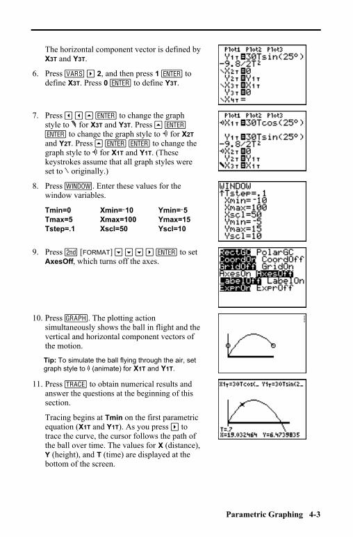
Parametric Graphing 4-3
82EB1A~1.DOC TI-83 international English Bob Fedorisko Revised: 10/26/05 1:20 PM Printed: 10/27/05 1:58PM Page 3 of 8
The horizontal component vector is defined byX3T and Y3T.
6. Press ~ 2, and then press 1Í todefine X3T. Press 0 Í to define Y3T.
7. Press | | } Í to change the graphstyle to è for X3T and Y3T. Press }ÍÍ to change the graph style to ë for X2Tand Y2T. Press } ÍÍ to change thegraph style to ë for X1T and Y1T. (Thesekeystrokes assume that all graph styles wereset to ç originally.)
8. Press p. Enter these values for thewindow variables.
Tmin=0 Xmin=L10 Ymin=L5Tmax=5 Xmax=100 Ymax=15Tstep=.1 Xscl=50 Yscl=10
9. Press y [FORMAT] †††~Í to setAxesOff, which turns off the axes.
10. Press s. The plotting actionsimultaneously shows the ball in flight and thevertical and horizontal component vectors ofthe motion.
Tip: To simulate the ball flying through the air, setgraph style to ì (animate) for X1T and Y1T.
11. Press r to obtain numerical results andanswer the questions at the beginning of thissection.
Tracing begins at Tmin on the first parametricequation (X1T and Y1T). As you press ~ totrace the curve, the cursor follows the path ofthe ball over time. The values for X (distance),Y (height), and T (time) are displayed at thebottom of the screen.

4-4 Parametric Graphing
82EB1A~1.DOC TI-83 international English Bob Fedorisko Revised: 10/26/05 1:20 PM Printed: 10/27/05 1:58PM Page 4 of 8
The steps for defining a parametric graph are similar to the stepsfor defining a function graph. Chapter 4 assumes that you arefamiliar with Chapter 3: Function Graphing. Chapter 4 detailsaspects of parametric graphing that differ from functiongraphing.
To display the mode screen, press z. To graph parametricequations, you must select Par graphing mode before you enterwindow variables and before you enter the components ofparametric equations.
After selecting Par graphing mode, press o to display theparametric Y= editor.
In this editor, you can display and enter both the X and Ycomponents of up to six equations, X1T and Y1T through X6T andY6T. Each is defined in terms of the independent variable T. Acommon application of parametric graphs is graphing equationsover time.
The icons to the left of X1T through X6T represent the graph styleof each parametric equation (Chapter 3). The default in Parmode is ç (line), which connects plotted points. Line, è (thick),ë (path), ì (animate), and í (dot) styles are available forparametric graphing.
Defining and Displaying Parametric Graphs
TI-82 STATSGraphing ModeSimilarities
SettingParametricGraphing Mode
Displaying theParametric Y=Editor
Selecting aGraph Style

Parametric Graphing 4-5
82EB1A~1.DOC TI-83 international English Bob Fedorisko Revised: 10/26/05 1:20 PM Printed: 10/27/05 1:58PM Page 5 of 8
To define or edit a parametric equation, follow the steps inChapter 3 for defining a function or editing a function. Theindependent variable in a parametric equation is T. In Pargraphing mode, you can enter the parametric variable T in eitherof two ways.
• Press „.• Press ƒ ãTä.
Two components, X and Y, define a single parametric equation.You must define both of them.
The TI-82 STATS graphs only the selected parametricequations. In the Y= editor, a parametric equation is selectedwhen the = signs of both the X and Y components arehighlighted. You may select any or all of the equations X1T andY1T through X6T and Y6T.
To change the selection status, move the cursor onto the = signof either the X or Y component and press Í. The status ofboth the X and Y components is changed.
To display the window variable values, press p. Thesevariables define the viewing window. The values below aredefaults for Par graphing in Radian angle mode.
Tmin=0 Smallest T value to evaluateTmax=6.2831853... Largest T value to evaluate (2p)Tstep=.1308996... T value increment (pà24)Xmin=L10 Smallest X value to be displayedXmax=10 Largest X value to be displayedXscl=1 Spacing between the X tick marksYmin=L10 Smallest Y value to be displayedYmax=10 Largest Y value to be displayedYscl=1 Spacing between the Y tick marks
Note: To ensure that sufficient points are plotted, you may want tochange the T window variables.
Defining andEditingParametricEquations
Selecting andDeselectingParametricEquations
Setting WindowVariables
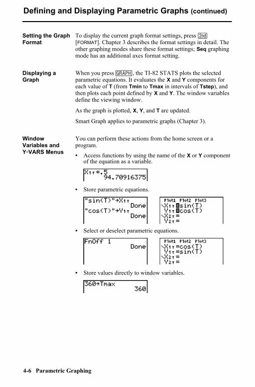
4-6 Parametric Graphing
82EB1A~1.DOC TI-83 international English Bob Fedorisko Revised: 10/26/05 1:20 PM Printed: 10/27/05 1:58PM Page 6 of 8
To display the current graph format settings, press y[FORMAT]. Chapter 3 describes the format settings in detail. Theother graphing modes share these format settings; Seq graphingmode has an additional axes format setting.
When you press s, the TI-82 STATS plots the selectedparametric equations. It evaluates the X and Y components foreach value of T (from Tmin to Tmax in intervals of Tstep), andthen plots each point defined by X and Y. The window variablesdefine the viewing window.
As the graph is plotted, X, Y, and T are updated.
Smart Graph applies to parametric graphs (Chapter 3).
You can perform these actions from the home screen or aprogram.
• Access functions by using the name of the X or Y componentof the equation as a variable.
• Store parametric equations.
• Select or deselect parametric equations.
• Store values directly to window variables.
Defining and Displaying Parametric Graphs (continued)
Setting the GraphFormat
Displaying aGraph
WindowVariables andY.VARS Menus

Parametric Graphing 4-7
82EB1A~1.DOC TI-83 international English Bob Fedorisko Revised: 10/26/05 1:20 PM Printed: 10/27/05 1:58PM Page 7 of 8
The free-moving cursor in Par graphing works the same as inFunc graphing.
In RectGC format, moving the cursor updates the values of Xand Y; if CoordOn format is selected, X and Y are displayed.
In PolarGC format, X, Y, R, and q are updated; if CoordOnformat is selected, R and q are displayed.
To activate TRACE, press r. When TRACE is active, youcan move the trace cursor along the graph of the equation oneTstep at a time. When you begin a trace, the trace cursor is onthe first selected function at Tmin. If ExprOn is selected, thenthe function is displayed.
In RectGC format, TRACE updates and displays the values of X,Y, and T if CoordOn format is on.
In PolarGC format, X, Y, R, q and T are updated; if CoordOnformat is selected, R, q, and T are displayed. The X and Y (or Rand q) values are calculated from T.
To move five plotted points at a time on a function, press y| or y ~. If you move the cursor beyond the top or bottomof the screen, the coordinate values at the bottom of the screencontinue to change appropriately.
Quick Zoom is available in Par graphing; panning is not(Chapter 3).
Exploring Parametric Graphs
Free-MovingCursor
TRACE

4-8 Parametric Graphing
82EB1A~1.DOC TI-83 international English Bob Fedorisko Revised: 10/26/05 1:20 PM Printed: 10/27/05 1:58PM Page 8 of 8
To move the trace cursor to any valid T value on the currentfunction, enter the number. When you enter the first digit, a T=prompt and the number you entered are displayed in the bottom-left corner of the screen. You can enter an expression at the T=prompt. The value must be valid for the current viewingwindow. When you have completed the entry, press Í tomove the cursor.
ZOOM operations in Par graphing work the same as in Funcgraphing. Only the X (Xmin, Xmax, and Xscl) and Y (Ymin,Ymax, and Yscl) window variables are affected.
The T window variables (Tmin, Tmax, and Tstep) are onlyaffected when you select ZStandard. The VARS ZOOMsecondary menu ZT/Zq items 1:ZTmin, 2:ZTmax, and 3:ZTstepare the zoom memory variables for Par graphing.
CALC operations in Par graphing work the same as in Funcgraphing. The CALCULATE menu items available in Pargraphing are 1:value, 2:dy/dx, 3:dy/dt, and 4:dx/dt.
Exploring Parametric Graphs (continued)
Moving the TraceCursor to AnyValid T Value
ZOOM
CALC
Polar Graphing 5–1
825C44~1.DOC TI-83 international English Bob Fedorisko Revised: 10/26/05 1:20 PM Printed: 10/27/05 2:00PM Page 1 of 6
5 PolarGraphing
Getting Started: Polar Rose.............................................................................. 2Defining and Displaying Polar Graphs..................................................... 3Exploring Polar Graphs ...................................................................................... 6
Contents

5–2 Polar Graphing
825C44~1.DOC TI-83 international English Bob Fedorisko Revised: 10/26/05 1:20 PM Printed: 10/27/05 2:00PM Page 2 of 6
Getting Started is a fast-paced introduction. Read the chapter for details.
The polar equation R=Asin(Bq) graphs a rose. Graph the rose for A=8 and B=2.5, andthen explore the appearance of the rose for other values of A and B.
1. Press z to display the mode screen. Press† † † ~ ~ Í to select Pol graphingmode. Select the defaults (the options on theleft) for the other mode settings.
2. Press o to display the polar Y= editor. Press 8˜ 2.5 „ ¤ Í to define r1.
3. Press q 6 to select 6:ZStandard and graphthe equation in the standard viewing window.The graph shows only five petals of the rose,and the rose does not appear to besymmetrical. This is because the standardwindow sets qmax=2p and defines thewindow, rather than the pixels, as square.
4. Press p to display the windowvariables. Press † 4 y [p] to increase thevalue of qmax to 4p.
5. Press q 5 to select 5:ZSquare and plot thegraph.
6. Repeat steps 2 through 5 with new values forthe variables A and B in the polar equationr1=Asin(Bq). Observe how the new valuesaffect the graph.
Getting Started: Polar Rose

Polar Graphing 5–3
825C44~1.DOC TI-83 international English Bob Fedorisko Revised: 10/26/05 1:20 PM Printed: 10/27/05 2:00PM Page 3 of 6
The steps for defining a polar graph are similar to the steps fordefining a function graph. Chapter 5 assumes that you arefamiliar with Chapter 3: Function Graphing. Chapter 5 detailsaspects of polar graphing that differ from function graphing.
To display the mode screen, press z. To graph polarequations, you must select Pol graphing mode before you entervalues for the window variables and before you enter polarequations.
After selecting Pol graphing mode, press o to display the polarY= editor.
In this editor, you can enter and display up to six polarequations, r1 through r6. Each is defined in terms of theindependent variable q (page 5.4).
The icons to the left of r1 through r6 represent the graph style ofeach polar equation (Chapter 3). The default in Pol graphingmode is ç (line), which connects plotted points. Line, è (thick),ë (path), ì (animate), and í (dot) styles are available for polargraphing.
Defining and Displaying Polar Graphs
TI-82 STATSGraphing ModeSimilarities
Setting PolarGraphing Mode
Displaying thePolar Y= Editor
Selecting GraphStyles

5–4 Polar Graphing
825C44~1.DOC TI-83 international English Bob Fedorisko Revised: 10/26/05 1:20 PM Printed: 10/27/05 2:00PM Page 4 of 6
To define or edit a polar equation, follow the steps in Chapter 3for defining a function or editing a function. The independentvariable in a polar equation is q. In Pol graphing mode, you canenter the polar variable q in either of two ways.
• Press „.• Press ƒ ãqä.
The TI-82 STATS graphs only the selected polar equations. Inthe Y= editor, a polar equation is selected when the = sign ishighlighted. You may select any or all of the equations.
To change the selection status, move the cursor onto the = sign,and then press Í.
To display the window variable values, press p. Thesevariables define the viewing window. The values below aredefaults for Pol graphing in Radian angle mode.
qmin=0 Smallest q value to evaluateqmax=6.2831853... Largest q value to evaluate (2p)qstep=.1308996... Increment between q values (pà24)Xmin=L10 Smallest X value to be displayedXmax=10 Largest X value to be displayedXscl=1 Spacing between the X tick marksYmin=L10 Smallest Y value to be displayedYmax=10 Largest Y value to be displayedYscl=1 Spacing between the Y tick marks
Note: To ensure that sufficient points are plotted, you may want tochange the q window variables.
Defining and Displaying Polar Graphs (continued)
Defining andEditing PolarEquations
Selecting andDeselecting PolarEquations
Setting WindowVariables
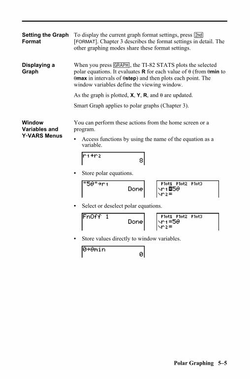
Polar Graphing 5–5
825C44~1.DOC TI-83 international English Bob Fedorisko Revised: 10/26/05 1:20 PM Printed: 10/27/05 2:00PM Page 5 of 6
To display the current graph format settings, press y[FORMAT]. Chapter 3 describes the format settings in detail. Theother graphing modes share these format settings.
When you press s, the TI-82 STATS plots the selectedpolar equations. It evaluates R for each value of q (from qmin toqmax in intervals of qstep) and then plots each point. Thewindow variables define the viewing window.
As the graph is plotted, X, Y, R, and q are updated.
Smart Graph applies to polar graphs (Chapter 3).
You can perform these actions from the home screen or aprogram.
• Access functions by using the name of the equation as avariable.
• Store polar equations.
• Select or deselect polar equations.
• Store values directly to window variables.
Setting the GraphFormat
Displaying aGraph
WindowVariables andY.VARS Menus

5–6 Polar Graphing
825C44~1.DOC TI-83 international English Bob Fedorisko Revised: 10/26/05 1:20 PM Printed: 10/27/05 2:00PM Page 6 of 6
The free-moving cursor in Pol graphing works the same as inFunc graphing. In RectGC format, moving the cursor updatesthe values of X and Y; if CoordOn format is selected, X and Yare displayed. In PolarGC format, X, Y, R, and q are updated; ifCoordOn format is selected, R and q are displayed.
To activate TRACE, press r. When TRACE is active, youcan move the trace cursor along the graph of the equation oneqstep at a time. When you begin a trace, the trace cursor is onthe first selected function at qmin. If ExprOn format is selected,then the equation is displayed.
In RectGC format, TRACE updates the values of X, Y, and q; ifCoordOn format is selected, X, Y, and q are displayed. InPolarGC format, TRACE updates X, Y, R, and q; if CoordOnformat is selected, R and q are displayed.
To move five plotted points at a time on a function, press y| or y ~. If you move the trace cursor beyond the top orbottom of the screen, the coordinate values at the bottom of thescreen continue to change appropriately.
Quick Zoom is available in Pol graphing mode; panning is not(Chapter 3).
To move the trace cursor to any valid q value on the currentfunction, enter the number. When you enter the first digit, a q=prompt and the number you entered are displayed in the bottom-left corner of the screen. You can enter an expression at the q=prompt. The value must be valid for the current viewingwindow. When you complete the entry, press Í to movethe cursor.
ZOOM operations in Pol graphing work the same as in Funcgraphing. Only the X (Xmin, Xmax, and Xscl) and Y (Ymin,Ymax, and Yscl) window variables are affected.
The q window variables (qmin, qmax, and qstep) are not affected,except when you select ZStandard. The VARS ZOOM secondarymenu ZT/Zq items 4:Zqmin, 5:Zqmax, and 6:Zqstep are zoommemory variables for Pol graphing.
CALC operations in Pol graphing work the same as in Funcgraphing. The CALCULATE menu items available in Polgraphing are 1:value, 2:dy/dx, and 3:dr/dq.
Exploring Polar Graphs
Free-MovingCursor
TRACE
Moving the TraceCursor to AnyValid q Value
ZOOM
CALC

Sequence Graphing 6–1
82EAB9~1.DOC TI-83 international English Bob Fedorisko Revised: 10/28/05 9:28 AM Printed: 10/28/05 9:28AM Page 1 of 16
6 SequenceGraphing
Getting Started: Forest and Trees................................................................. 2Defining and Displaying Sequence Graphs ........................................... 3Selecting Axes Combinations......................................................................... 8Exploring Sequence Graphs............................................................................. 9Graphing Web Plots.............................................................................................. 11Using Web Plots to Illustrate Convergence........................................... 12Graphing Phase Plots ........................................................................................... 13Comparing TI-82 STATS and TI.82 Sequence Variables........... 15Keystroke Differences Between TI-82 STATS and TI-82 .......... 16
Contents
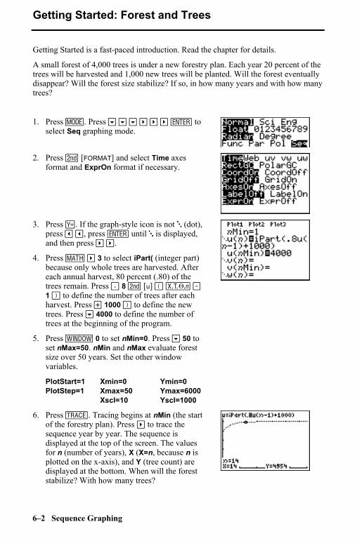
6–2 Sequence Graphing
82EAB9~1.DOC TI-83 international English Bob Fedorisko Revised: 10/28/05 9:28 AM Printed: 10/28/05 9:28AM Page 2 of 16
Getting Started is a fast-paced introduction. Read the chapter for details.
A small forest of 4,000 trees is under a new forestry plan. Each year 20 percent of thetrees will be harvested and 1,000 new trees will be planted. Will the forest eventuallydisappear? Will the forest size stabilize? If so, in how many years and with how manytrees?
1. Press z. Press † ††~~~Í toselect Seq graphing mode.
2. Press y [FORMAT] and select Time axesformat and ExprOn format if necessary.
3. Press o. If the graph-style icon is not íííí (dot),press | |, press Í until íííí is displayed,and then press ~ ~.
4. Press ~ 3 to select iPart( (integer part)because only whole trees are harvested. Aftereach annual harvest, 80 percent (.80) of thetrees remain. Press Ë 8y [u] £„¹1 ¤ to define the number of trees after eachharvest. Press à 1000 ¤ to define the newtrees. Press † 4000 to define the number oftrees at the beginning of the program.
5. Press p 0 to set nMin=0. Press † 50 toset nMax=50. nMin and nMax evaluate forestsize over 50 years. Set the other windowvariables.
PlotStart=1 Xmin=0 Ymin=0PlotStep=1 Xmax=50 Ymax=6000
Xscl=10 Yscl=1000
6. Press r. Tracing begins at nMin (the startof the forestry plan). Press ~ to trace thesequence year by year. The sequence isdisplayed at the top of the screen. The valuesfor n (number of years), X (X=n, because n isplotted on the x-axis), and Y (tree count) aredisplayed at the bottom. When will the foreststabilize? With how many trees?
Getting Started: Forest and Trees

Sequence Graphing 6–3
82EAB9~1.DOC TI-83 international English Bob Fedorisko Revised: 10/28/05 9:28 AM Printed: 10/28/05 9:28AM Page 3 of 16
The steps for defining a sequence graph are similar to the stepsfor defining a function graph. Chapter 6 assumes that you arefamiliar with Chapter 3: Function Graphing. Chapter 6 detailsaspects of sequence graphing that differ from function graphing.
To display the mode screen, press z. To graph sequencefunctions, you must select Seq graphing mode before you enterwindow variables and before you enter sequence functions.
Sequence graphs automatically plot in Simul mode, regardlessof the current plotting-order mode setting.
The TI-82 STATS has three sequence functions that you canenter from the keyboard: u, v, and w. They are above the ¬, −,and ® keys.
You can define sequence functions in terms of:
• The independent variable n• The previous term in the sequence function, such as u(nN1)• The term that precedes the previous term in the sequence
function, such as u(nN2)• The previous term or the term that precedes the previous
term in another sequence function, such as u(nN1) or u(nN2)referenced in the sequence v(n).
Note: Statements in this chapter about u(n) are also true for v(n) andw(n); statements about u(nN1) are also true for v(nN1) and w(nN1);statements about u(nN2) are also true for v(nN2) and w(nN2).
Defining and Displaying Sequence Graphs
TI-82 STATSGraphing ModeSimilarities
Setting SequenceGraphing Mode
TI-82 STATSSequenceFunctions u, v,and w
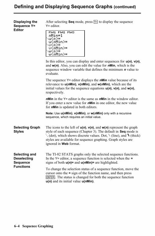
6–4 Sequence Graphing
82EAB9~1.DOC TI-83 international English Bob Fedorisko Revised: 10/28/05 9:28 AM Printed: 10/28/05 9:28AM Page 4 of 16
After selecting Seq mode, press o to display the sequenceY= editor.
In this editor, you can display and enter sequences for u(n), v(n),and w(n). Also, you can edit the value for nMin, which is thesequence window variable that defines the minimum n value toevaluate.
The sequence Y= editor displays the nMin value because of itsrelevance to u(nMin), v(nMin), and w(nMin), which are theinitial values for the sequence equations u(n), v(n), and w(n),respectively.
nMin in the Y= editor is the same as nMin in the window editor.If you enter a new value for nMin in one editor, the new valuefor nMin is updated in both editors.
Note: Use u(nMin), v(nMin), or w(nMin) only with a recursivesequence, which requires an initial value.
The icons to the left of u(n), v(n), and w(n) represent the graphstyle of each sequence (Chapter 3). The default in Seq mode isí (dot), which shows discrete values. Dot, ç (line), and è (thick)styles are available for sequence graphing. Graph styles areignored in Web format.
The TI-82 STATS graphs only the selected sequence functions.In the Y= editor, a sequence function is selected when the =signs of both u(n)= and u(nMin)= are highlighted.
To change the selection status of a sequence function, move thecursor onto the = sign of the function name, and then pressÍ. The status is changed for both the sequence functionu(n) and its initial value u(nMin).
Defining and Displaying Sequence Graphs (continued)
Displaying theSequence Y=Editor
Selecting GraphStyles
Selecting andDeselectingSequenceFunctions

Sequence Graphing 6–5
82EAB9~1.DOC TI-83 international English Bob Fedorisko Revised: 10/28/05 9:28 AM Printed: 10/28/05 9:28AM Page 5 of 16
To define or edit a sequence function, follow the steps inChapter 3 for defining a function. The independent variable in asequence is n.
In Seq graphing mode, you can enter the sequence variable ineither of two ways.
• Press „.• Press y [CATALOG] [N].
You can enter the function name from the keyboard.
• To enter the function name u, press y [u] (above ¬).• To enter the function name v, press y [v] (above −).• To enter the function name w, press y [w] (above ®).
Generally, sequences are either nonrecursive or recursive.Sequences are evaluated only at consecutive integer values. n isalways a series of consecutive integers, starting at zero or anypositive integer.
In a nonrecursive sequence, the nth term is a function of theindependent variable n. Each term is independent of all otherterms.
For example, in the nonrecursive sequence below, you cancalculate u(5) directly, without first calculating u(1) or anyprevious term.
The sequence equation above returns the sequence2, 4, 6, 8, 10, . . . for n = 1, 2, 3, 4, 5, . . . .
Note: You may leave blank the initial value u(nMin) when calculatingnonrecursive sequences.
Defining andEditing aSequenceFunction
NonrecursiveSequences

6–6 Sequence Graphing
82EAB9~1.DOC TI-83 international English Bob Fedorisko Revised: 10/28/05 9:28 AM Printed: 10/28/05 9:28AM Page 6 of 16
In a recursive sequence, the nth term in the sequence is definedin relation to the previous term or the term that precedes theprevious term, represented by u(nN1) and u(nN2). A recursivesequence may also be defined in relation to n, as inu(n)=u(nN1)+n.
For example, in the sequence below you cannot calculate u(5)without first calculating u(1), u(2), u(3), and u(4).
Using an initial value u(nMin) = 1, the sequence above returns1, 2, 4, 8, 16, . . .
Tip: On the TI-82 STATS, you must type each character of the terms.For example, to enter u(nN1), press y [u] £ „ ¹ À ¤.
Recursive sequences require an initial value or values, sincethey reference undefined terms.
• If each term in the sequence is defined in relation to theprevious term, as in u(nN1), you must specify an initial valuefor the first term.
• If each term in the sequence is defined in relation to the termthat precedes the previous term, as in u(nN2), you mustspecify initial values for the first two terms. Enter the initialvalues as a list enclosed in braces ({ }) with commasseparating the values.
The value of the first term is 0 and the value of the second termis 1 for the sequence u(n).
Defining and Displaying Sequence Graphs (continued)
RecursiveSequences
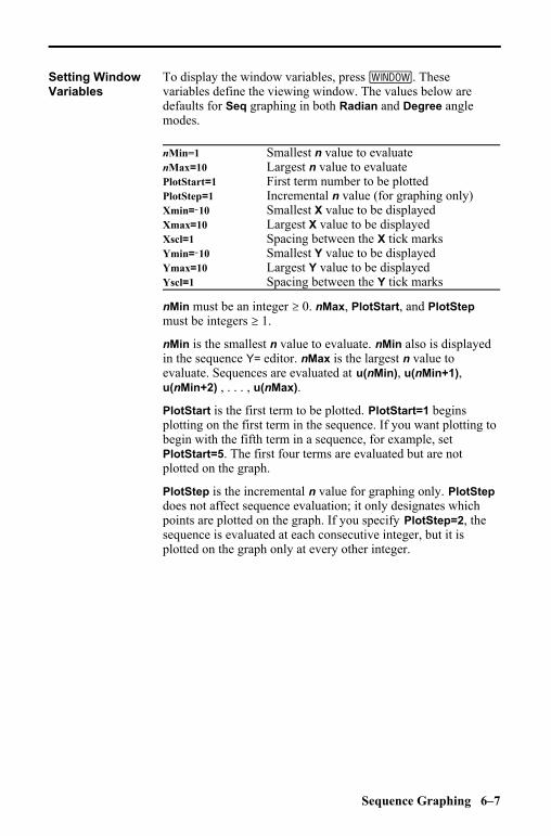
Sequence Graphing 6–7
82EAB9~1.DOC TI-83 international English Bob Fedorisko Revised: 10/28/05 9:28 AM Printed: 10/28/05 9:28AM Page 7 of 16
To display the window variables, press p. Thesevariables define the viewing window. The values below aredefaults for Seq graphing in both Radian and Degree anglemodes.
nMin=1 Smallest n value to evaluatenMax=10 Largest n value to evaluatePlotStart=1 First term number to be plottedPlotStep=1 Incremental n value (for graphing only)Xmin=L10 Smallest X value to be displayedXmax=10 Largest X value to be displayedXscl=1 Spacing between the X tick marksYmin=L10 Smallest Y value to be displayedYmax=10 Largest Y value to be displayedYscl=1 Spacing between the Y tick marks
nMin must be an integer ‚ 0. nMax, PlotStart, and PlotStepmust be integers ‚ 1.
nMin is the smallest n value to evaluate. nMin also is displayedin the sequence Y= editor. nMax is the largest n value toevaluate. Sequences are evaluated at u(nMin), u(nMin+1),u(nMin+2) , . . . , u(nMax).
PlotStart is the first term to be plotted. PlotStart=1 beginsplotting on the first term in the sequence. If you want plotting tobegin with the fifth term in a sequence, for example, setPlotStart=5. The first four terms are evaluated but are notplotted on the graph.
PlotStep is the incremental n value for graphing only. PlotStepdoes not affect sequence evaluation; it only designates whichpoints are plotted on the graph. If you specify PlotStep=2, thesequence is evaluated at each consecutive integer, but it isplotted on the graph only at every other integer.
Setting WindowVariables

6–8 Sequence Graphing
82EAB9~1.DOC TI-83 international English Bob Fedorisko Revised: 10/28/05 9:28 AM Printed: 10/28/05 9:28AM Page 8 of 16
To display the current graph format settings, press y[FORMAT]. Chapter 3 describes the format settings in detail. Theother graphing modes share these format settings. The axessetting on the top line of the screen is available only in Seqmode.
Time Web uv vw uw Type of sequence plot (axes)RectGC PolarGC Rectangular or polar outputCoordOn CoordOff Cursor coordinate display on/offGridOff GridOn Grid display off or onAxesOn AxesOff Axes display on or offLabelOff LabelOn Axes label display off or onExprOn ExprOff Expression display on or off
For sequence graphing, you can select from five axes formats.The table below shows the values that are plotted on the x-axisand y-axis for each axes setting.
Axes Setting x-axis y-axisTime n u(n), v(n), w(n)Web u(nN1), v(nN1), w(nN1) u(n), v(n), w(n)uv u(n) v(n)vw v(n) w(n)uw u(n) w(n)
See pages 6.11 and 6.12 for more information on Web plots.See page 6.13 for more information on phase plots (uv, vw, anduw axes settings).
To plot the selected sequence functions, press s. As agraph is plotted, the TI-82 STATS updates X, Y, and n.
Smart Graph applies to sequence graphs (Chapter 3).
Selecting Axes Combinations
Setting the GraphFormat
Setting AxesFormat
Displaying aSequence Graph
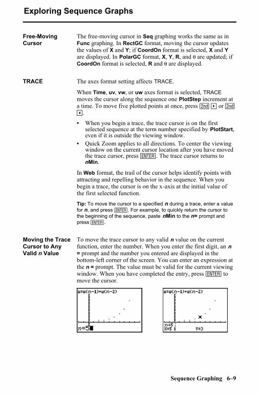
Sequence Graphing 6–9
82EAB9~1.DOC TI-83 international English Bob Fedorisko Revised: 10/28/05 9:28 AM Printed: 10/28/05 9:28AM Page 9 of 16
The free-moving cursor in Seq graphing works the same as inFunc graphing. In RectGC format, moving the cursor updatesthe values of X and Y; if CoordOn format is selected, X and Yare displayed. In PolarGC format, X, Y, R, and q are updated; ifCoordOn format is selected, R and q are displayed.
The axes format setting affects TRACE.
When Time, uv, vw, or uw axes format is selected, TRACEmoves the cursor along the sequence one PlotStep increment ata time. To move five plotted points at once, press y ~ or y|.
• When you begin a trace, the trace cursor is on the firstselected sequence at the term number specified by PlotStart,even if it is outside the viewing window.
• Quick Zoom applies to all directions. To center the viewingwindow on the current cursor location after you have movedthe trace cursor, press Í. The trace cursor returns tonMin.
In Web format, the trail of the cursor helps identify points withattracting and repelling behavior in the sequence. When youbegin a trace, the cursor is on the x-axis at the initial value ofthe first selected function.
Tip: To move the cursor to a specified n during a trace, enter a valuefor n, and press Í. For example, to quickly return the cursor tothe beginning of the sequence, paste nMin to the n= prompt andpress Í.
To move the trace cursor to any valid n value on the currentfunction, enter the number. When you enter the first digit, an n= prompt and the number you entered are displayed in thebottom-left corner of the screen. You can enter an expression atthe n = prompt. The value must be valid for the current viewingwindow. When you have completed the entry, press Í tomove the cursor.
Exploring Sequence Graphs
Free-MovingCursor
TRACE
Moving the TraceCursor to AnyValid n Value
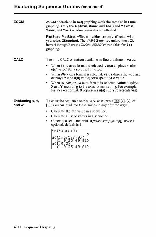
6–10 Sequence Graphing
82EAB9~1.DOC TI-83 international English Bob Fedorisko Revised: 10/28/05 9:28 AM Printed: 10/28/05 9:28AM Page 10 of 16
ZOOM operations in Seq graphing work the same as in Funcgraphing. Only the X (Xmin, Xmax, and Xscl) and Y (Ymin,Ymax, and Yscl) window variables are affected.
PlotStart, PlotStep, nMin, and nMax are only affected whenyou select ZStandard. The VARS Zoom secondary menu ZUitems 1 through 7 are the ZOOM MEMORY variables for Seqgraphing.
The only CALC operation available in Seq graphing is value.
• When Time axes format is selected, value displays Y (theu(n) value) for a specified n value.
• When Web axes format is selected, value draws the web anddisplays Y (the u(n) value) for a specified n value.
• When uv, vw, or uw axes format is selected, value displaysX and Y according to the axes format setting. For example,for uv axes format, X represents u(n) and Y represents v(n).
To enter the sequence names u, v, or w, press y [u], [v], or[w]. You can evaluate these names in any of three ways.
• Calculate the nth value in a sequence.• Calculate a list of values in a sequence.• Generate a sequence with u(nstart,nstop[,nstep]). nstep is
optional; default is 1.
Exploring Sequence Graphs (continued)
ZOOM
CALC
Evaluating u, v,and w
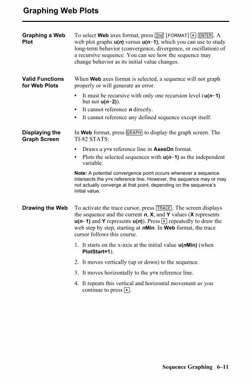
Sequence Graphing 6–11
82EAB9~1.DOC TI-83 international English Bob Fedorisko Revised: 10/28/05 9:28 AM Printed: 10/28/05 9:28AM Page 11 of 16
To select Web axes format, press y [FORMAT] ~ Í. Aweb plot graphs u(n) versus u(nN1), which you can use to studylong-term behavior (convergence, divergence, or oscillation) ofa recursive sequence. You can see how the sequence maychange behavior as its initial value changes.
When Web axes format is selected, a sequence will not graphproperly or will generate an error.
• It must be recursive with only one recursion level (u(nN1)but not u(nN2)).
• It cannot reference n directly.• It cannot reference any defined sequence except itself.
In Web format, press s to display the graph screen. TheTI-82 STATS:
• Draws a y=x reference line in AxesOn format.• Plots the selected sequences with u(nN1) as the independent
variable.
Note: A potential convergence point occurs whenever a sequenceintersects the y=x reference line. However, the sequence may or maynot actually converge at that point, depending on the sequence’sinitial value.
To activate the trace cursor, press r. The screen displaysthe sequence and the current n, X, and Y values (X representsu(nN1) and Y represents u(n)). Press ~ repeatedly to draw theweb step by step, starting at nMin. In Web format, the tracecursor follows this course.
1. It starts on the x-axis at the initial value u(nMin) (whenPlotStart=1).
2. It moves vertically (up or down) to the sequence.
3. It moves horizontally to the y=x reference line.
4. It repeats this vertical and horizontal movement as youcontinue to press ~.
Graphing Web Plots
Graphing a WebPlot
Valid Functionsfor Web Plots
Displaying theGraph Screen
Drawing the Web
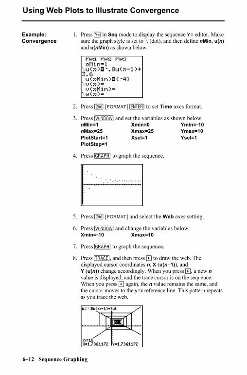
6–12 Sequence Graphing
82EAB9~1.DOC TI-83 international English Bob Fedorisko Revised: 10/28/05 9:28 AM Printed: 10/28/05 9:28AM Page 12 of 16
1. Press o in Seq mode to display the sequence Y= editor. Makesure the graph style is set to í (dot), and then define nMin, u(n)and u(nMin) as shown below.
2. Press y [FORMAT] Í to set Time axes format.
3. Press p and set the variables as shown below.nMin=1 Xmin=0 Ymin=L10nMax=25 Xmax=25 Ymax=10PlotStart=1 Xscl=1 Yscl=1PlotStep=1
4. Press s to graph the sequence.
5. Press y [FORMAT] and select the Web axes setting.
6. Press p and change the variables below.Xmin=L10 Xmax=10
7. Press s to graph the sequence.
8. Press r, and then press ~ to draw the web. Thedisplayed cursor coordinates n, X (u(nN1)), andY (u(n)) change accordingly. When you press ~, a new nvalue is displayed, and the trace cursor is on the sequence.When you press ~ again, the n value remains the same, andthe cursor moves to the y=x reference line. This pattern repeatsas you trace the web.
Using Web Plots to Illustrate Convergence
Example:Convergence

Sequence Graphing 6–13
82EAB9~1.DOC TI-83 international English Bob Fedorisko Revised: 10/28/05 9:28 AM Printed: 10/28/05 9:28AM Page 13 of 16
The phase-plot axes settings uv, vw, and uw show relationshipsbetween two sequences. To select a phase-plot axes setting,press y [FORMAT], press ~ until the cursor is on uv, vw, oruw, and then press Í.
Axes Setting x-axis y-axisuv u(n) v(n)vw v(n) w(n)uw u(n) w(n)
Use the predator-prey model to determine the regionalpopulations of a predator and its prey that would maintainpopulation equilibrium for the two species.
This example uses the model to determine the equilibriumpopulations of wolves and rabbits, with initial populations of200 rabbits (u(nMin)) and 50 wolves (v(nMin)).
These are the variables (given values are in parentheses):
R = number of rabbitsM = rabbit population growth rate without wolves (.05)K = rabbit population death rate with wolves (.001)W = number of wolvesG = wolf population growth rate with rabbits (.0002)D = wolf population death rate without rabbits (.03)n = time (in months)Rn = RnN1(1+MNKWnN1)Wn = WnN1(1+GRnN1ND)
1. Press o in Seq mode to display the sequence Y= editor.Define the sequences and initial values for Rn and Wn asshown below. Enter the sequence Rn as u(n) and enter thesequence Wn as v(n).
Graphing Phase Plots
Graphing with uv,vw, and uw
Example:Predator-PreyModel
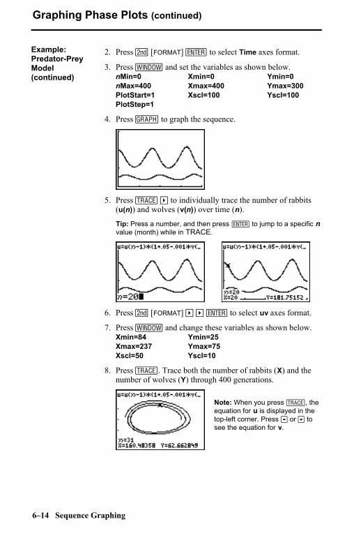
6–14 Sequence Graphing
82EAB9~1.DOC TI-83 international English Bob Fedorisko Revised: 10/28/05 9:28 AM Printed: 10/28/05 9:28AM Page 14 of 16
2. Press y [FORMAT] Í to select Time axes format.
3. Press p and set the variables as shown below.nMin=0 Xmin=0 Ymin=0nMax=400 Xmax=400 Ymax=300PlotStart=1 Xscl=100 Yscl=100PlotStep=1
4. Press s to graph the sequence.
5. Press r ~ to individually trace the number of rabbits(u(n)) and wolves (v(n)) over time (n).
Tip: Press a number, and then press Í to jump to a specific nvalue (month) while in TRACE.
6. Press y [FORMAT] ~ ~ Í to select uv axes format.
7. Press p and change these variables as shown below.Xmin=84 Ymin=25Xmax=237 Ymax=75Xscl=50 Yscl=10
8. Press r. Trace both the number of rabbits (X) and thenumber of wolves (Y) through 400 generations.
Note: When you press r, theequation for u is displayed in thetop-left corner. Press } or † tosee the equation for v.
Graphing Phase Plots (continued)
Example:Predator-PreyModel(continued)

Sequence Graphing 6–15
82EAB9~1.DOC TI-83 international English Bob Fedorisko Revised: 10/28/05 9:28 AM Printed: 10/28/05 9:28AM Page 15 of 16
Refer to the table if you are familiar with the TI-82. It showsTI-82 STATS sequences and sequence window variables, aswell as their TI-82 counterparts.
TI-82 STATS TI.82In the Y= editor:
u(n) Unu(nMin) UnStart (window variable)v(n) Vnv(nMin) VnStart (window variable)w(n) not availablew(nMin) not available
In the window editor:nMin nStartnMax nMaxPlotStart nMinPlotStep not available
Comparing TI-82 STATS and TI-82 Sequence Variables
Sequences andWindowVariables

6–16 Sequence Graphing
82EAB9~1.DOC TI-83 international English Bob Fedorisko Revised: 10/28/05 9:28 AM Printed: 10/28/05 9:28AM Page 16 of 16
Refer to the table if you are familiar with the TI-82. It comparesTI-82 STATS sequence-name syntax and variable syntax withTI.82 sequence-name syntax and variable syntax.
TI-82 STATS /TI.82
On TI-82 STATS,press:
On TI.82, press:
n / n „ y [n]u(n) / Un y [u]
£„¤y [Y.VARS] ¶ À
v(n) / Vn y [v]£„¤
y [Y.VARS] ¶ Á
w(n) y [w]£„¤
not available
u(nN1) / UnN1 y [u]£„¹À¤
y [UnN1]
v(nN1) / VnN1 y [v]£„¹À¤
y [VnN1]
w(nN1) y [w]£„¹À¤
not available
Keystroke Differences Between TI-82 STATS and TI-82
SequenceKeystrokeChanges

Tables 7–1
82533C~1.DOC TI-83 international English Bob Fedorisko Revised: 10/26/05 1:24 PM Printed: 10/27/05 2:20PM Page 1 of 6
7 Tables
Getting Started: Roots of a Function.......................................................... 2Setting Up the Table ............................................................................................. 3Defining the Dependent Variables............................................................... 4Displaying the Table............................................................................................. 5
Contents

7–2 Tables
82533C~1.DOC TI-83 international English Bob Fedorisko Revised: 10/26/05 1:24 PM Printed: 10/27/05 2:20PM Page 2 of 6
Getting Started is a fast-paced introduction. Read the chapter for details.
Evaluate the function Y = X3 N 2X at each integer between L10 and 10. How manysign changes occur, and at what X values?
1. Press z † † † Í to set Funcgraphing mode.
2. Press o. Press „ 3 to select 3.Then press ¹ 2 „ to enter the functionY1=X3N2X.
3. Press y [TBLSET] to display the TABLESETUP screen. Press Ì 10Í to setTblStart=L10. Press 1 Í to set @Tbl=1.
Press Í to select Indpnt: Auto(automatically generated independent values).Press † Í to select Depend: Auto(automatically generated dependent values).
4. Press y [TABLE] to display the table screen.
5. Press † until you see the sign changes in thevalue of Y1. How many sign changes occur,and at what X values?
Getting Started: Roots of a Function

Tables 7–3
82533C~1.DOC TI-83 international English Bob Fedorisko Revised: 10/26/05 1:24 PM Printed: 10/27/05 2:20PM Page 3 of 6
To display the TABLE SETUP screen, press y [TBLSET].
TblStart (table start) defines the initial value for the independentvariable. TblStart applies only when the independent variable isgenerated automatically (when Indpnt: Auto is selected).
@Tbl (table step) defines the increment for the independentvariable.
Note: In Seq mode, both TblStart and @Tbl must be integers.
Selections Table CharacteristicsIndpnt: AutoDepend: Auto
Values are displayed automatically in both theindependent-variable column and in alldependent-variable columns.
Indpnt: AskDepend: Auto
The table is empty; when you enter a value forthe independent variable, all correspondingdependent-variable values are calculated anddisplayed automatically.
Indpnt: AutoDepend: Ask
Values are displayed automatically for theindependent variable; to generate a value for adependent variable, move the cursor to thatcell and press Í.
Indpnt: AskDepend: Ask
The table is empty; enter values for theindependent variable; to generate a value for adependent variable, move the cursor to thatcell and press Í.
To store a value to TblStart, @Tbl, or TblZnput from the homescreen or a program, select the variable name from the VARSTABLE secondary menu. TblZnput is a list of independent-variable values in the current table.
When you press y [TBLSET] in the program editor, you canselect IndpntAuto, IndpntAsk, DependAuto, and DependAsk.
Setting Up the Table
TABLE SETUPScreen
TblStart, @Tbl
Indpnt: Auto,Indpnt: Ask,Depend: Auto,Depend: Ask
Setting Up theTable from theHome Screen ora Program

7–4 Tables
82533C~1.DOC TI-83 international English Bob Fedorisko Revised: 10/26/05 1:24 PM Printed: 10/27/05 2:20PM Page 4 of 6
In the Y= editor, enter the functions that define the dependentvariables. Only functions that are selected in the Y= editor aredisplayed in the table. The current graphing mode is used. InPar mode, you must define both components of each parametricequation (Chapter 4).
To edit a selected Y= function from the table editor, follow thesesteps.
1. Press y [TABLE] to display the table, then press ~ or | tomove the cursor to a dependent-variable column.
2. Press } until the cursor is on the function name at the top ofthe column. The function is displayed on the bottom line.
3. Press Í. The cursor moves to the bottom line. Edit thefunction.
4. Press Í or †. The new values are calculated. The tableand the Y= function are updated automatically.
Note: You also can use this feature to view the function thatdefines a dependent variable without having to leave the table.
Defining the Dependent Variables
DefiningDependentVariables fromthe Y= Editor
EditingDependentVariables fromthe Table Editor

Tables 7–5
82533C~1.DOC TI-83 international English Bob Fedorisko Revised: 10/26/05 1:24 PM Printed: 10/27/05 2:20PM Page 5 of 6
To display the table, press y [TABLE].
Current cell
Independent-variable valuesin the firstcolumn
Dependent-variable values inthe second andthird columns
Current cell’s full valueNote: The table abbreviates the values, if necessary.
The current graphing mode determines which independent anddependent variables are displayed in the table (Chapter 1). In thetable above, for example, the independent variable X and thedependent variables Y1 and Y2 are displayed because Funcgraphing mode is set.
Graphing Mode IndependentVariable
DependentVariable
Func (function) X Y1 through Y9, andY0
Par (parametric) T X1T/Y1T throughX6T/Y6T
Pol (polar) q r1 through r6
Seq (sequence) n u(n), v(n), and w(n)
From the home screen, select the ClrTable instruction from theCATALOG. To clear the table, press Í.
From a program, select 9:ClrTable from the PRGM I/O menu orfrom the CATALOG. The table is cleared upon execution. IfIndpntAsk is selected, all independent and dependent variablevalues on the table are cleared. If DependAsk is selected, alldependent variable values on the table are cleared.
Displaying the Table
The Table
Independent andDependentVariables
Clearing theTable from theHome Screen ora Program

7–6 Tables
82533C~1.DOC TI-83 international English Bob Fedorisko Revised: 10/26/05 1:24 PM Printed: 10/27/05 2:20PM Page 6 of 6
If Indpnt: Auto is selected, you can press } and † in theindependent-variable column to display more values. As youscroll the column, the corresponding dependent-variable valuesalso are displayed. All dependent-variable values may not bedisplayed if Depend: Ask is selected.
Note: You can scroll back from the value entered for TblStart. Asyou scroll, TblStart is updated automatically to the value shown onthe top line of the table. In the example above, TblStart=0 and@Tbl=1 generates and displays values of X=0, . . . , 6; but you canpress } to scroll back and display the table for X=M1, . . ., 5.
If you have defined more than two dependent variables, the firsttwo selected Y= functions are displayed initially. Press ~ or |to display dependent variables defined by other selected Y=functions. The independent variable always remains in the leftcolumn, except during a trace with Par graphing mode and G.Tsplit-screen mode set.
Tip: To simultaneously display on the table two dependent variablesthat are not defined as consecutive Y= functions, go to the Y= editorand deselect the Y= functions between the two you want to display.For example, to simultaneously display Y4 and Y7 on the table, go tothe Y= editor and deselect Y5 and Y6.
Displaying the Table (continued)
ScrollingIndependent-Variable Values
Displaying OtherDependentVariables

DRAW Instructions 8–1
82CA5D~1.DOC TI-83 international English Bob Fedorisko Revised: 10/26/05 1:27 PM Printed: 10/27/05 2:36PM Page 1 of 20
8 DrawInstructions
Getting Started: Drawing a Tangent Line ............................................... 2Using the DRAW Menu...................................................................................... 3Clearing Drawings ................................................................................................. 4Drawing Line Segments ..................................................................................... 5Drawing Horizontal and Vertical Lines ................................................... 6Drawing Tangent Lines ...................................................................................... 8Drawing Functions and Inverses................................................................... 9Shading Areas on a Graph ................................................................................ 10Drawing Circles....................................................................................................... 11Placing Text on a Graph..................................................................................... 12Using Pen to Draw on a Graph ...................................................................... 13Drawing Points on a Graph .............................................................................. 14Drawing Pixels ......................................................................................................... 16Storing Graph Pictures (Pics) ......................................................................... 17Recalling Graph Pictures (Pics) .................................................................... 18Storing Graph Databases (GDBs)................................................................. 19Recalling Graph Databases (GDBs)............................................................ 20
Contents

8–2 DRAW Instructions
82CA5D~1.DOC TI-83 international English Bob Fedorisko Revised: 10/26/05 1:27 PM Printed: 10/27/05 2:36PM Page 2 of 20
Getting Started is a fast-paced introduction. Read the chapter for details.
Suppose you want to find the equation of the tangent line at X = ‡2/2 for the functionY = sinX.
Before you begin, select Radian and Func modefrom the mode screen, if necessary.
1. Press o to display the Y= editor. Press ˜„ ¤ to store sin(X) in Y1.
2. Press q 7 to select 7:ZTrig, which graphsthe equation in the Zoom Trig window.
3. Press y [DRAW] 5 to select 5:Tangent(. Thetangent instruction is initiated.
4. Press y [‡] 2 ¤ ¥ 2.
5. Press Í. The tangent line is drawn; the Xvalue and the tangent-line equation aredisplayed on the graph.
Getting Started: Drawing a Tangent Line

DRAW Instructions 8–3
82CA5D~1.DOC TI-83 international English Bob Fedorisko Revised: 10/26/05 1:27 PM Printed: 10/27/05 2:36PM Page 3 of 20
To display the DRAW menu, press y [DRAW]. TheTI-82 STATS interpretation of these instructions depends onwhether you accessed the menu from the home screen or theprogram editor or directly from a graph.
DRAW
POINTS STO
1: ClrDraw Clears all drawn elements.2: Line( Draws a line segment between 2 points.3: Horizontal Draws a horizontal line.4: Vertical Draws a vertical line.5: Tangent( Draws a line segment tangent to a function.6: DrawF Draws a function.7: Shade( Shades an area between two functions.8: DrawInv Draws the inverse of a function.9: Circle( Draws a circle.0: Text( Draws text on a graph screen.A: Pen Activates the free-form drawing tool.
The DRAW instructions draw on top of graphs. Therefore,before you use the DRAW instructions, consider whether youwant to perform one or more of the following actions.
• Change the mode settings on the mode screen.• Change the format settings on the format screen.• Enter or edit functions in the Y= editor.• Select or deselect functions in the Y= editor.• Change the window variable values.• Turn stat plots on or off.• Clear existing drawings with ClrDraw (page 8.4).
Note: If you draw on a graph and then perform any of the actionslisted above, the graph is replotted without the drawings when youdisplay the graph again.
You can use any DRAW menu instructions except DrawInv todraw on Func, Par, Pol, and Seq graphs. DrawInv is valid onlyin Func graphing. The coordinates for all DRAW instructions arethe display’s x-coordinate and y-coordinate values.
You can use most DRAW menu and DRAW POINTS menuinstructions to draw directly on a graph, using the cursor toidentify the coordinates. You also can execute these instructionsfrom the home screen or from within a program. If a graph is notdisplayed when you select a DRAW menu instruction, the homescreen is displayed.
Using the DRAW Menu
DRAW Menu
Before Drawingon a Graph
Drawing on aGraph
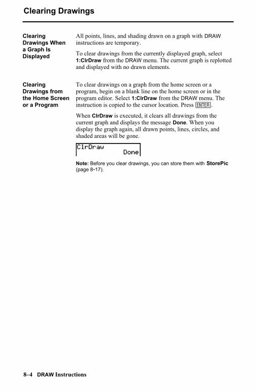
8–4 DRAW Instructions
82CA5D~1.DOC TI-83 international English Bob Fedorisko Revised: 10/26/05 1:27 PM Printed: 10/27/05 2:36PM Page 4 of 20
All points, lines, and shading drawn on a graph with DRAWinstructions are temporary.
To clear drawings from the currently displayed graph, select1:ClrDraw from the DRAW menu. The current graph is replottedand displayed with no drawn elements.
To clear drawings on a graph from the home screen or aprogram, begin on a blank line on the home screen or in theprogram editor. Select 1:ClrDraw from the DRAW menu. Theinstruction is copied to the cursor location. Press Í.
When ClrDraw is executed, it clears all drawings from thecurrent graph and displays the message Done. When youdisplay the graph again, all drawn points, lines, circles, andshaded areas will be gone.
Note: Before you clear drawings, you can store them with StorePic(page 8.17).
Clearing Drawings
ClearingDrawings Whena Graph IsDisplayed
ClearingDrawings fromthe Home Screenor a Program

DRAW Instructions 8–5
82CA5D~1.DOC TI-83 international English Bob Fedorisko Revised: 10/26/05 1:27 PM Printed: 10/27/05 2:36PM Page 5 of 20
To draw a line segment when a graph is displayed, follow thesesteps.
1. Select 2:Line( from the DRAW menu.
2. Place the cursor on the point where you want the linesegment to begin, and then press Í.
3. Move the cursor to the point where you want the linesegment to end. The line is displayed as you move thecursor. Press Í.
To continue drawing line segments, repeat steps 2 and 3. Tocancel Line(, press ‘.
Line( also draws a line segment between the coordinates (X1,Y1)and (X2,Y2). The values may be entered as expressions.
Line(X1,Y1,X2,Y2)
To erase a line segment, enter Line(X1,Y1,X2,Y2,0)
Drawing Line Segments
Drawing a LineSegment Directlyon a Graph
Drawing a LineSegment fromthe Home Screenor a Program

8–6 DRAW Instructions
82CA5D~1.DOC TI-83 international English Bob Fedorisko Revised: 10/26/05 1:27 PM Printed: 10/27/05 2:36PM Page 6 of 20
To draw a horizontal or vertical line when a graph is displayed,follow these steps.
1. Select 3:Horizontal or 4:Vertical from the DRAW menu. Aline is displayed that moves as you move the cursor.
2. Place the cursor on the y-coordinate (for horizontal lines) orx-coordinate (for vertical lines) through which you want thedrawn line to pass.
3. Press Í to draw the line on the graph.
To continue drawing lines, repeat steps 2 and 3.
To cancel Horizontal or Vertical, press ‘.
Drawing Horizontal and Vertical Lines
Drawing a LineDirectly on aGraph
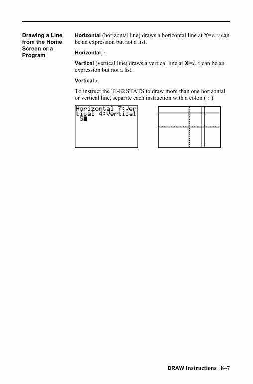
DRAW Instructions 8–7
82CA5D~1.DOC TI-83 international English Bob Fedorisko Revised: 10/26/05 1:27 PM Printed: 10/27/05 2:36PM Page 7 of 20
Horizontal (horizontal line) draws a horizontal line at Y=y. y canbe an expression but not a list.
Horizontal y
Vertical (vertical line) draws a vertical line at X=x. x can be anexpression but not a list.
Vertical x
To instruct the TI-82 STATS to draw more than one horizontalor vertical line, separate each instruction with a colon ( : ).
Drawing a Linefrom the HomeScreen or aProgram

8–8 DRAW Instructions
82CA5D~1.DOC TI-83 international English Bob Fedorisko Revised: 10/26/05 1:27 PM Printed: 10/27/05 2:36PM Page 8 of 20
To draw a tangent line when a graph is displayed, follow thesesteps.
1. Select 5:Tangent( from the DRAW menu.
2. Press † and } to move the cursor to the function for whichyou want to draw the tangent line. The current graph’s Y=function is displayed in the top-left corner, if ExprOn isselected.
3. Press ~ and | or enter a number to select the point on thefunction at which you want to draw the tangent line.
4. Press Í. In Func mode, the X value at which the tangentline was drawn is displayed on the bottom of the screen,along with the equation of the tangent line. In all othermodes, the dy/dx value is displayed.
Tip: Change the fixed decimal setting on the mode screen if you wantto see fewer digits displayed for X and the equation for Y.
Tangent( (tangent line) draws a line tangent to expression interms of X, such as Y1 or X2, at point X=value. X can be anexpression. expression is interpreted as being in Func mode.
Tangent(expression,value)
Drawing Tangent Lines
Drawinga Tangent LineDirectlyon a Graph
Drawinga Tangent Linefrom the HomeScreen ora Program

DRAW Instructions 8–9
82CA5D~1.DOC TI-83 international English Bob Fedorisko Revised: 10/26/05 1:27 PM Printed: 10/27/05 2:36PM Page 9 of 20
DrawF (draw function) draws expression as a function in termsof X on the current graph. When you select 6:DrawF from theDRAW menu, the TI-82 STATS returns to the home screen orthe program editor. DrawF is not interactive.
DrawF expression
Note: You cannot use a list in expression to draw a family of curves.
DrawInv (draw inverse) draws the inverse of expression byplotting X values on the y-axis and Y values on the x-axis. Whenyou select 8:DrawInv from the DRAW menu, the TI-82 STATSreturns to the home screen or the program editor. DrawInv is notinteractive. DrawInv works in Func mode only.
DrawInv expression
Note: You cannot use a list in expression to draw a family of curves.
Drawing Functions and Inverses
Drawing aFunction
Drawing anInverse of aFunction
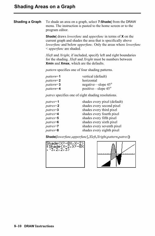
8–10 DRAW Instructions
82CA5D~1.DOC TI-83 international English Bob Fedorisko Revised: 10/26/05 1:27 PM Printed: 10/27/05 2:36PM Page 10 of 20
To shade an area on a graph, select 7:Shade( from the DRAWmenu. The instruction is pasted to the home screen or to theprogram editor.
Shade( draws lowerfunc and upperfunc in terms of X on thecurrent graph and shades the area that is specifically abovelowerfunc and below upperfunc. Only the areas where lowerfunc< upperfunc are shaded.
Xleft and Xright, if included, specify left and right boundariesfor the shading. Xleft and Xright must be numbers betweenXmin and Xmax, which are the defaults.
pattern specifies one of four shading patterns.
pattern=1 vertical (default)pattern=2 horizontalpattern=3 negative—slope 45¡pattern=4 positive—slope 45¡
patres specifies one of eight shading resolutions.
patres=1 shades every pixel (default)patres=2 shades every second pixelpatres=3 shades every third pixelpatres=4 shades every fourth pixelpatres=5 shades every fifth pixelpatres=6 shades every sixth pixelpatres=7 shades every seventh pixelpatres=8 shades every eighth pixel
Shade(lowerfunc,upperfunc[,Xleft,Xright,pattern,patres])
Shading Areas on a Graph
Shading a Graph

DRAW Instructions 8–11
82CA5D~1.DOC TI-83 international English Bob Fedorisko Revised: 10/26/05 1:27 PM Printed: 10/27/05 2:36PM Page 11 of 20
To draw a circle directly on a displayed graph using the cursor,follow these steps.
1. Select 9:Circle( from the DRAW menu.
2. Place the cursor at the center of the circle you want to draw.Press Í.
3. Move the cursor to a point on the circumference. PressÍ to draw the circle on the graph.
Note: This circle is displayed as circular, regardless of the windowvariable values, because you drew it directly on the display. Whenyou use the Circle( instruction from the home screen or aprogram, the current window variables may distort the shape.
To continue drawing circles, repeat steps 2 and 3. To cancelCircle(, press ‘.
Circle( draws a circle with center (X,Y ) and radius. Thesevalues can be expressions.
Circle(X,Y,radius)
Tip: When you use Circle( on the home screen or from a program,the current window values may distort the drawn circle. Use ZSquare(Chapter 3) before drawing the circle to adjust the window variablesand make the circle circular.
Drawing Circles
Drawing a CircleDirectly on aGraph
Drawing a Circlefrom the HomeScreen or aProgram

8–12 DRAW Instructions
82CA5D~1.DOC TI-83 international English Bob Fedorisko Revised: 10/26/05 1:27 PM Printed: 10/27/05 2:36PM Page 12 of 20
To place text on a graph when the graph is displayed, followthese steps.
1. Select 0:Text( from the DRAW menu.
2. Place the cursor where you want the text to begin.
3. Enter the characters. Press ƒ or y [A.LOCK] to enterletters and q. You may enter TI-82 STATS functions,variables, and instructions. The font is proportional, so theexact number of characters you can place on the graphvaries. As you type, the characters are placed on top of thegraph.
To cancel Text(, press ‘.
Text( places on the current graph the characters comprisingvalue, which can include TI-82 STATS functions andinstructions. The top-left corner of the first character is at pixel(row,column), where row is an integer between0 and 57 and column is an integer between 0 and 94. Both rowand column can be expressions.
Text(row,column,value,value . . .)
value can be text enclosed in quotation marks ( " ), or it can bean expression. The TI-82 STATS will evaluate an expressionand display the result with up to 10 characters.
On a Horiz split screen, the maximum value for row is 25. On aG.T split screen, the maximum value for row is 45, and themaximum value for column is 46.
Placing Text on a Graph
Placing TextDirectly on aGraph
Placing Text on aGraph from theHome Screen ora Program
Split Screen

DRAW Instructions 8–13
82CA5D~1.DOC TI-83 international English Bob Fedorisko Revised: 10/26/05 1:27 PM Printed: 10/27/05 2:36PM Page 13 of 20
Pen draws directly on a graph only. You cannot execute Penfrom the home screen or a program.
To draw on a displayed graph, follow these steps.
1. Select A:Pen from the DRAW menu.
2. Place the cursor on the point where you want to begindrawing. Press Í to turn on the pen.
3. Move the cursor. As you move the cursor, you draw on thegraph, shading one pixel at a time.
4. Press Í to turn off the pen.
For example, Pen was used to create the arrow pointing to thelocal minimum of the selected function.
To continue drawing on the graph, move the cursor to a newposition where you want to begin drawing again, and thenrepeat steps 2, 3, and 4. To cancel Pen, press ‘.
Using Pen to Draw on a Graph
Using Pen toDraw on a Graph

8–14 DRAW Instructions
82CA5D~1.DOC TI-83 international English Bob Fedorisko Revised: 10/26/05 1:27 PM Printed: 10/27/05 2:36PM Page 14 of 20
To display the DRAW POINTS menu, press y [DRAW] ~. TheTI-82 STATS interpretation of these instructions depends onwhether you accessed this menu from the home screen or theprogram editor or directly from a graph.
DRAW POINTS STO1: Pt-On( Turns on a point.2: Pt-Off( Turns off a point.3: Pt-Change( Toggles a point on or off.4: Pxl-On( Turns on a pixel.5: Pxl-Off( Turns off a pixel.6: Pxl-Change( Toggles a pixel on or off.7: pxl-Test( Returns 1 if pixel on, 0 if pixel off.
To draw a point on a graph, follow these steps.
1. Select 1:Pt.On( from the DRAW POINTS menu.
2. Move the cursor to the position where you want to draw thepoint.
3. Press Í to draw the point.
To continue drawing points, repeat steps 2 and 3. To cancelPt.On(, press ‘.
Drawing Points on a Graph
DRAW POINTSMenu
Drawing PointsDirectly on aGraph withPt.On(

DRAW Instructions 8–15
82CA5D~1.DOC TI-83 international English Bob Fedorisko Revised: 10/26/05 1:27 PM Printed: 10/27/05 2:36PM Page 15 of 20
To erase (turn off) a drawn point on a graph, follow these steps.
1. Select 2:Pt.Off( (point off) from the DRAW POINTS menu.
2. Move the cursor to the point you want to erase.
3. Press Í to erase the point.
To continue erasing points, repeat steps 2 and 3. To cancelPt.Off(, press ‘.
To change (toggle on or off) a point on a graph, follow thesesteps.
1. Select 3:Pt.Change( (point change) from the DRAW POINTSmenu.
2. Move the cursor to the point you want to change.
3. Press Í to change the point’s on/off status.
To continue changing points, repeat steps 2 and 3. To cancelPt.Change(, press ‘.
Pt.On( (point on) turns on the point at (X=x,Y=y). Pt.Off( turnsthe point off. Pt.Change( toggles the point on or off. mark isoptional; it determines the point’s appearance; specify 1, 2, or 3,where:
1 = ¦ (dot; default) 2 = › (box) 3 = + (cross)
Pt.On(x,y[,mark])Pt.Off(x,y[,mark])Pt.Change(x,y)
Note: If you specified mark to turn on a point with Pt.On(, you mustspecify mark when you turn off the point with Pt.Off(. Pt.Change(does not have the mark option.
Erasing Pointswith Pt.Off(
Changing Pointswith Pt.Change(
Drawing Pointsfrom the HomeScreen or aProgram

8–16 DRAW Instructions
82CA5D~1.DOC TI-83 international English Bob Fedorisko Revised: 10/26/05 1:27 PM Printed: 10/27/05 2:36PM Page 16 of 20
A pixel is a square dot on the TI-82 STATS display. The Pxl.(pixel) instructions let you turn on, turn off, or reverse a pixel(dot) on the graph using the cursor. When you select a pixelinstruction from the DRAW POINTS menu, the TI-82 STATSreturns to the home screen or the program editor. The pixelinstructions are not interactive.
Pxl.On( (pixel on) turns on the pixel at (row,column), whererow is an integer between 0 and 62 and column is an integerbetween 0 and 94.
Pxl.Off( turns the pixel off. Pxl.Change( toggles the pixel onand off.
Pxl.On(row,column)Pxl.Off(row,column)Pxl.Change(row,column)
pxl.Test( (pixel test) returns 1 if the pixel at (row,column) isturned on or 0 if the pixel is turned off on the current graph. rowmust be an integer between 0 and 62. column must be an integerbetween 0 and 94.
pxl.Test(row,column)
On a Horiz split screen, the maximum value for row is 30 forPxl.On(, Pxl.Off(, Pxl.Change(, and pxl.Test(.
On a G.T split screen, the maximum value for row is 50 and themaximum value for column is 46 for Pxl.On(, Pxl.Off(,Pxl.Change(, and pxl.Test(.
Drawing Pixels
TI-82 STATSPixels
Turning On andOff Pixels withPxl.On( andPxl.Off(
Using pxl.Test(
Split Screen
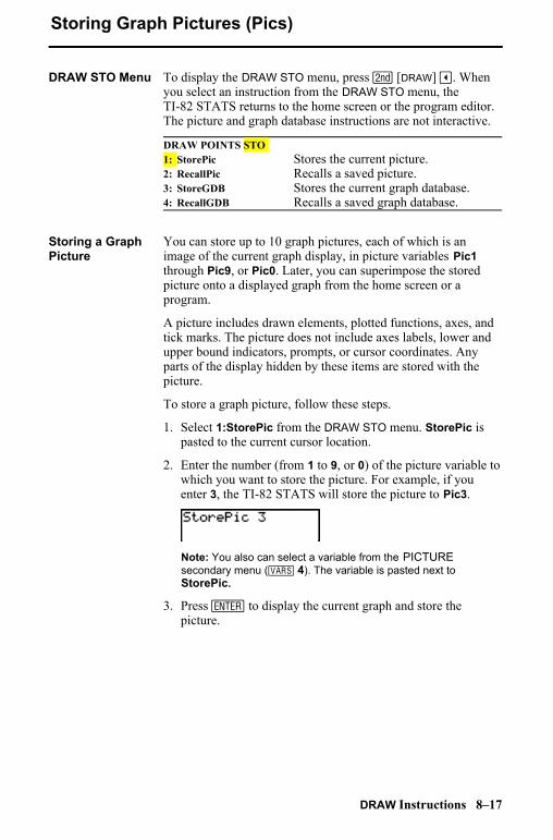
DRAW Instructions 8–17
82CA5D~1.DOC TI-83 international English Bob Fedorisko Revised: 10/26/05 1:27 PM Printed: 10/27/05 2:36PM Page 17 of 20
To display the DRAW STO menu, press y [DRAW] |. Whenyou select an instruction from the DRAW STO menu, theTI-82 STATS returns to the home screen or the program editor.The picture and graph database instructions are not interactive.
DRAW POINTS STO1: StorePic Stores the current picture.2: RecallPic Recalls a saved picture.3: StoreGDB Stores the current graph database.4: RecallGDB Recalls a saved graph database.
You can store up to 10 graph pictures, each of which is animage of the current graph display, in picture variables Pic1through Pic9, or Pic0. Later, you can superimpose the storedpicture onto a displayed graph from the home screen or aprogram.
A picture includes drawn elements, plotted functions, axes, andtick marks. The picture does not include axes labels, lower andupper bound indicators, prompts, or cursor coordinates. Anyparts of the display hidden by these items are stored with thepicture.
To store a graph picture, follow these steps.
1. Select 1:StorePic from the DRAW STO menu. StorePic ispasted to the current cursor location.
2. Enter the number (from 1 to 9, or 0) of the picture variable towhich you want to store the picture. For example, if youenter 3, the TI-82 STATS will store the picture to Pic3.
Note: You also can select a variable from the PICTUREsecondary menu ( 4). The variable is pasted next toStorePic.
3. Press Í to display the current graph and store thepicture.
Storing Graph Pictures (Pics)
DRAW STO Menu
Storing a GraphPicture

8–18 DRAW Instructions
82CA5D~1.DOC TI-83 international English Bob Fedorisko Revised: 10/26/05 1:27 PM Printed: 10/27/05 2:36PM Page 18 of 20
To recall a graph picture, follow these steps.
1. Select 2:RecallPic from the DRAW STO menu. RecallPic ispasted to the current cursor location.
2. Enter the number (from 1 to 9, or 0) of the picture variablefrom which you want to recall a picture. For example, if youenter 3, the TI-82 STATS will recall the picture stored toPic3.
Note: You also can select a variable from the PICTUREsecondary menu ( 4). The variable is pasted next toRecallPic.
3. Press Í to display the current graph with the picturesuperimposed on it.
Note: Pictures are drawings. You cannot trace a curve that is part of apicture.
To delete graph pictures from memory, use theMEMORY DELETE FROM menu (Chapter 18).
Recalling Graph Pictures (Pics)
Recalling aGraph Picture
Deleting a GraphPicture

DRAW Instructions 8–19
82CA5D~1.DOC TI-83 international English Bob Fedorisko Revised: 10/26/05 1:27 PM Printed: 10/27/05 2:36PM Page 19 of 20
A graph database (GDB) contains the set of elements thatdefines a particular graph. You can recreate the graph fromthese elements. You can store up to 10 GDBs in variables GDB1through GDB9, or GDB0 and recall them to recreate graphs.
A GDB stores five elements of a graph.
• Graphing mode• Window variables• Format settings• All functions in the Y= editor and the selection status of each• Graph style for each Y= function
GDBs do not contain drawn items or stat plot definitions.
To store a graph database, follow these steps.
1. Select 3:StoreGDB from the DRAW STO menu. StoreGDB ispasted to the current cursor location.
2. Enter the number (from 1 to 9, or 0) of the GDB variable towhich you want to store the graph database. For example, ifyou enter 7, the TI-82 STATS will store the GDB to GDB7.
Note: You also can select a variable from the GDB secondarymenu ( 3). The variable is pasted next to StoreGDB.
3. Press Í to store the current database to the specifiedGDB variable.
Storing Graph Databases (GDBs)
What Is a GraphDatabase?
Storing a GraphDatabase

8–20 DRAW Instructions
82CA5D~1.DOC TI-83 international English Bob Fedorisko Revised: 10/26/05 1:27 PM Printed: 10/27/05 2:36PM Page 20 of 20
CAUTION: When you recall a GDB, it replaces all existing Y=functions. Consider storing the current Y= functions to anotherdatabase before recalling a stored GDB.
To recall a graph database, follow these steps.
1. Select 4:RecallGDB from the DRAW STO menu. RecallGDBis pasted to the current cursor location.
2. Enter the number (from 1 to 9, or 0) of the GDB variablefrom which you want to recall a GDB. For example, if youenter 7, the TI-82 STATS will recall the GDB stored toGDB7.
Note: You also can select a variable from the GDB secondarymenu ( 3). The variable is pasted next to RecallGDB.
3. Press Í to replace the current GDB with the recalledGDB. The new graph is not plotted. The TI-82 STATSchanges the graphing mode automatically, if necessary.
To delete a GDB from memory, use the MEMORY DELETEFROM menu (Chapter 18).
Recalling Graph Databases (GDBs)
Recalling aGraph Database
Deleting a GraphDatabase
Split Screen 9–1
8253D2~1.DOC TI-83 international English Bob Fedorisko Revised: 10/28/05 9:26 AM Printed: 10/28/05 9:26AM Page 1 of 6
9 SplitScreen
Getting Started: Exploring the Unit Circle............................................. 2Using Split Screen.................................................................................................. 3Horiz (Horizontal) Split Screen..................................................................... 4G.T (Graph-Table) Split Screen.................................................................... 5TI-82 STATS Pixels in Horiz and G.T Mode...................................... 6
Contents

9–2 Split Screen
8253D2~1.DOC TI-83 international English Bob Fedorisko Revised: 10/28/05 9:26 AM Printed: 10/28/05 9:26AM Page 2 of 6
Getting Started is a fast-paced introduction. Read the chapter for details.
Use G.T (graph-table) split-screen mode to explore the unit circle and its relationshipto the numeric values for the commonly used trigonometric angles of 0°, 30°, 45°,60°, 90°, and so on.
1. Press z to display the mode screen. Press† † ~ Í to select Degree mode. Press† ~ Í to select Par (parametric)graphing mode.
Press † † † † ~ ~Í to select G.T(graph-table) split-screen mode.
2. Press y [FORMAT] to display the formatscreen. Press † † † ††~Í toselect ExprOff.
3. Press o to display the Y= editor for Pargraphing mode. Press ™„¤Íto store cos(T) to X1T. Press ˜„¤Í to store sin(T) to Y1T.
4. Press p to display the window editor.Enter these values for the window variables.Tmin=0 Xmin=L2.3 Ymin=L2.5Tmax=360 Xmax=2.3 Ymax=2.5Tstep=15 Xscl=1 Yscl=1
5. Press r. On the left, the unit circle isgraphed parametrically in Degree mode andthe trace cursor is activated. When T=0 (fromthe graph trace coordinates), you can see fromthe table on the right that the value of X1T(cos(T)) is 1 and Y1T (sin(T)) is 0. Press ~ tomove the cursor to the next 15° angleincrement. As you trace around the circle insteps of 15°, an approximation of the standardvalue for each angle is highlighted in thetable.
Getting Started: Exploring the Unit Circle

Split Screen 9–3
8253D2~1.DOC TI-83 international English Bob Fedorisko Revised: 10/28/05 9:26 AM Printed: 10/28/05 9:26AM Page 3 of 6
To set a split-screen mode, press z, and then move thecursor to the bottom line of the mode screen.
• Select Horiz (horizontal) to display the graph screen andanother screen split horizontally.
• Select G.T (graph-table) to display the graph screen andtable screen split vertically.
$ $
The split screen is activated when you press any key that appliesto either half of the split screen.
Some screens are never displayed as split screens. For example,if you press z in Horiz or G.T mode, the mode screen isdisplayed as a full screen. If you then press a key that displayseither half of a split screen, such as r, the split screenreturns.
When you press a key or key combination in either Horiz or G.Tmode, the cursor is placed in the half of the display for whichthat key applies. For example, if you press r, the cursor isplaced in the half in which the graph is displayed. If you pressy [TABLE], the cursor is placed in the half in which the table isdisplayed.
The TI-82 STATS will remain in split-screen mode until youchange back to Full screen mode.
Using Split Screen
Setting a Split-Screen Mode

9–4 Split Screen
8253D2~1.DOC TI-83 international English Bob Fedorisko Revised: 10/28/05 9:26 AM Printed: 10/28/05 9:26AM Page 4 of 6
In Horiz (horizontal) split-screen mode, a horizontal line splitsthe screen into top and bottom halves.
The top half displays the graph.
The bottom half displays any of these editors.
• Home screen (four lines)• Y= editor (four lines)• Stat list editor (two rows)• Window editor (three settings)• Table editor (two rows)
To use the top half of the split screen:
• Press s or r.• Select a ZOOM or CALC operation.
To use the bottom half of the split screen:
• Press any key or key combination that displays the homescreen.
• Press o (Y= editor).• Press … Í (stat list editor).• Press p (window editor).• Press y [TABLE] (table editor).
All other screens are displayed as full screens in Horizsplit-screen mode.
To return to the Horiz split screen from a full screen when inHoriz mode, press any key or key combination that displays thegraph, home screen, Y= editor, stat list editor, window editor, ortable editor.
Horiz (Horizontal) Split Screen
Horiz Mode
Moving from Halfto Half in HorizMode
Full Screens inHoriz Mode

Split Screen 9–5
8253D2~1.DOC TI-83 international English Bob Fedorisko Revised: 10/28/05 9:26 AM Printed: 10/28/05 9:26AM Page 5 of 6
In G.T (graph-table) split-screen mode, a vertical line splits thescreen into left and right halves.
The left half displays the graph.
The right half displays the table.
To use the left half of the split screen:
• Press s or r.• Select a ZOOM or CALC operation.
To use the right half of the split screen, press y [TABLE].
As you move the trace cursor along a graph in the split screen’sleft half in G.T mode, the table on the right half automaticallyscrolls to match the current cursor values.
Note: When you trace in Par graphing mode, both components of anequation (XnT and YnT) are displayed in the two columns of the table.As you trace, the current value of the independent variable T isdisplayed on the graph.
All screens other than the graph and the table are displayed asfull screens in G.T split-screen mode.
To return to the G.T split screen from a full screen when in G.Tmode, press any key or key combination that displays the graphor the table.
G.T (Graph-Table) Split Screen
G.T Mode
Moving from Halfto Half in G.TMode
Using rrrr inG.T Mode
Full Screens inG.T Mode

9–6 Split Screen
8253D2~1.DOC TI-83 international English Bob Fedorisko Revised: 10/28/05 9:26 AM Printed: 10/28/05 9:26AM Page 6 of 6
Note: Each set of numbers in parentheses above represents the rowand column of a corner pixel, which is turned on.
For Pxl.On(, Pxl.Off(, Pxl.Change(, and pxl.Test(:
• In Horiz mode, row must be {30; column must be {94.• In G.T mode, row must be {50; column must be {46.
Pxl.On(row,column)
For the Text( instruction:
• In Horiz mode, row must be {25; column must be {94.• In G.T mode, row must be {45; column must be {46.
Text(row,column,"text")
For the Output( instruction:
• In Horiz mode, row must be {4; column must be {16.• In G.T mode, row must be {8; column must be {16.
Output(row,column,"text")
To set Horiz or G.T from a program, follow these steps.
1. Press z while the cursor is on a blank line in the programeditor.
2. Select Horiz or G.T.
The instruction is pasted to the cursor location. The mode is setwhen the instruction is encountered during program execution.It remains in effect after execution.
Note: You also can paste Horiz or G.T to the home screen orprogram editor from the CATALOG (Chapter 15).
TI-82 STATS Pixels in Horiz and G.T Modes
TI-82 STATSPixels in Horizand G.T Modes
DRAW POINTSMenu PixelInstructions
DRAW MenuText( Instruction
PRGM I/O MenuOutput(Instruction
Setting aSplit-ScreenMode from theHome Screen ora Program
Matrices 10–1
82EA17~1.DOC TI-83 international English Bob Fedorisko Revised: 10/26/05 1:31 PM Printed: 10/27/05 2:47PM Page 1 of 16
10 Matrices
Getting Started: Systems of Linear Equations ..................................... 2Defining a Matrix ................................................................................................... 2Viewing and Editing Matrix Elements...................................................... 4Using Matrices with Expressions ................................................................. 7Displaying and Copying Matrices................................................................ 8Using Math Functions with Matrices......................................................... 9Using the MATRX MATH Operations ....................................................... 12
Contents

10–2 Matrices
82EA17~1.DOC TI-83 international English Bob Fedorisko Revised: 10/26/05 1:31 PM Printed: 10/27/05 2:47PM Page 2 of 16
Getting Started is a fast-paced introduction. Read the chapter for details.
Find the solution of X + 2Y + 3Z = 3 and 2X + 3Y + 4Z = 3. On the TI-82 STATS,you can solve a system of linear equations by entering the coefficients as elements ina matrix, and then using rref( to obtain the reduced row-echelon form.
1. Press . Press ~ ~ to display theMATRX EDIT menu. Press 1 to select 1: [A]¸
2. Press 2 Í 4 Í to define a 2×4 matrix.The rectangular cursor indicates the currentelement. Ellipses (...) indicate additionalcolumns beyond the screen.
3. Press 1 Í to enter the first element. Therectangular cursor moves to the second columnof the first row.
4. Press 2 Í 3 Í 3Í to completethe first row for X + 2Y + 3Z = 3.
5. Press 2 Í 3 Í 4Í 3Í toenter the second row for 2X + 3Y + 4Z = 3.
6. Press y [QUIT] to return to the home screen.If necessary, press ‘ to clear the homescreen. Press ~ to display the MATRXMATH menu. Press } to wrap to the end of themenu. Select B:rref( to copy rref( to the homescreen.
7. Press 1 to select 1: [A] from theMATRX NAMES menu. Press ¤Í. Thereduced row-echelon form of the matrix isdisplayed and stored in Ans.
1X N 1Z = L3 so X = L3 + Z1Y + 2Z = 3 so Y = 3 N 2Z
Getting Started: Systems of Linear Equations
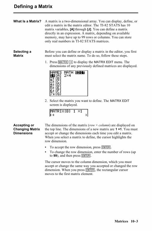
Matrices 10–3
82EA17~1.DOC TI-83 international English Bob Fedorisko Revised: 10/26/05 1:31 PM Printed: 10/27/05 2:47PM Page 3 of 16
A matrix is a two-dimensional array. You can display, define, oredit a matrix in the matrix editor. The TI-82 STATS has 10matrix variables, [A] through [J]. You can define a matrixdirectly in an expression. A matrix, depending on availablememory, may have up to 99 rows or columns. You can storeonly real numbers in TI-82 STATS matrices.
Before you can define or display a matrix in the editor, you firstmust select the matrix name. To do so, follow these steps.
1. Press | to display the MATRX EDIT menu. Thedimensions of any previously defined matrices are displayed.
2. Select the matrix you want to define. The MATRX EDITscreen is displayed.
The dimensions of the matrix (row × column) are displayed onthe top line. The dimensions of a new matrix are 1 ×1. You mustaccept or change the dimensions each time you edit a matrix.When you select a matrix to define, the cursor highlights therow dimension.
• To accept the row dimension, press Í.• To change the row dimension, enter the number of rows (up
to 99), and then press Í.
The cursor moves to the column dimension, which you mustaccept or change the same way you accepted or changed the rowdimension. When you press Í, the rectangular cursormoves to the first matrix element.
Defining a Matrix
What Is a Matrix?
Selecting aMatrix
Accepting orChanging MatrixDimensions

10–4 Matrices
82EA17~1.DOC TI-83 international English Bob Fedorisko Revised: 10/26/05 1:31 PM Printed: 10/27/05 2:47PM Page 4 of 16
After you have set the dimensions of the matrix, you can viewthe matrix and enter values for the matrix elements. In a newmatrix, all values are zero.
Select the matrix from the MATRX EDIT menu and enter oraccept the dimensions. The center portion of the matrix editordisplays up to seven rows and three columns of a matrix,showing the values of the elements in abbreviated form ifnecessary. The full value of the current element, which isindicated by the rectangular cursor, is displayed on the bottomline.
This is an 8 × 4 matrix. Ellipses in the left or right columnindicate additional columns. # or $ in the right column indicateadditional rows.
To delete matrices from memory, use the MEMORY DELETEFROM secondary menu (Chapter 18).
Viewing and Editing Matrix Elements
Displaying MatrixElements
Deleting a Matrix

Matrices 10–5
82EA17~1.DOC TI-83 international English Bob Fedorisko Revised: 10/26/05 1:31 PM Printed: 10/27/05 2:47PM Page 5 of 16
The matrix editor has two contexts, viewing and editing. Inviewing context, you can use the cursor keys to move quicklyfrom one matrix element to the next. The full value of thehighlighted element is displayed on the bottom line.
Select the matrix from the MATRX EDIT menu, and then enter oraccept the dimensions.
Key Function| or ~ Moves the rectangular cursor within the
current row.† or } Moves the rectangular cursor within the
current column; on the top row, } moves thecursor to the column dimension; on the columndimension, } moves the cursor to the rowdimension.
Í Switches to editing context; activates the editcursor on the bottom line.
‘ Switches to editing context; clears the value onthe bottom line.
Any entrycharacter
Switches to editing context; clears the value onthe bottom line; copies the character to thebottom line.
y [INS] Nothing{ Nothing
Viewing a Matrix
Viewing-ContextKeys

10–6 Matrices
82EA17~1.DOC TI-83 international English Bob Fedorisko Revised: 10/26/05 1:31 PM Printed: 10/27/05 2:47PM Page 6 of 16
In editing context, an edit cursor is active on the bottom line. Toedit a matrix element value, follow these steps.
1. Select the matrix from the MATRX EDIT menu, and thenenter or accept the dimensions.
2. Press |, }, ~, and † to move the cursor to the matrixelement you want to change.
3. Switch to editing context by pressing Í, ‘, or anentry key.
4. Change the value of the matrix element using the editing-context keys described below. You may enter an expression,which is evaluated when you leave editing context.
Note: You can press ‘ Í to restore the value at therectangular cursor if you make a mistake.
5. Press Í, }, or † to move to another element.
Key Function| or ~ Moves the edit cursor within the value.† or } Stores the value displayed on the bottom line to
the matrix element; switches to viewingcontext and moves the rectangular cursorwithin the column.
Í Stores the value displayed on the bottom line tothe matrix element; switches to viewingcontext and moves the rectangular cursor to thenext row element.
‘ Clears the value on the bottom line.Any entrycharacter
Copies the character to the location of the editcursor on the bottom line.
y [INS] Activates the insert cursor.{ Deletes the character under the edit cursor on
the bottom line.
Viewing and Editing Matrix Elements (continued)
Editing a MatrixElement
Editing-ContextKeys

Matrices 10–7
82EA17~1.DOC TI-83 international English Bob Fedorisko Revised: 10/26/05 1:31 PM Printed: 10/27/05 2:47PM Page 7 of 16
To use a matrix in an expression, you can do any of thefollowing.
• Copy the name from the MATRX NAMES menu.• Recall the contents of the matrix into the expression withy [RCL] (Chapter 1).
• Enter the matrix directly (see below).
You can enter, edit, and store a matrix in the matrix editor. Youalso can enter a matrix directly in an expression.
To enter a matrix in an expression, follow these steps.
1. Press y [ [ ] to indicate the beginning of the matrix.
2. Press y [ [ ] to indicate the beginning of a row.
3. Enter a value, which can be an expression, for each elementin the row. Separate the values with commas.
4. Press y [ ] ] to indicate the end of a row.
5. Repeat steps 2 through 4 to enter all of the rows.
6. Press y [ ] ] to indicate the end of the matrix.
Note: The closing ]] are not necessary at the end of anexpression or preceding !!!!.
The resulting matrix is displayed in the form:
[[element1,1,...,element1,n],...,[elementm,1,...,elementm,n]]
Any expressions are evaluated when the entry is executed.
Note: The commas that you must enter to separate elements arenot displayed on output.
Using Matrices with Expressions
Using a Matrix inan Expression
Entering a Matrixin an Expression

10–8 Matrices
82EA17~1.DOC TI-83 international English Bob Fedorisko Revised: 10/26/05 1:31 PM Printed: 10/27/05 2:47PM Page 8 of 16
To display the contents of a matrix on the home screen, selectthe matrix from the MATRX NAMES menu, and then pressÍ.
Ellipses in the left or right column indicate additional columns.# or $ in the right column indicate additional rows. Press ~, |,†, and } to scroll the matrix.
To copy a matrix, follow these steps.
1. Press to display the MATRX NAMES menu.
2. Select the name of the matrix you want to copy.
3. Press ¿.
4. Press again and select the name of the new matrix towhich you want to copy the existing matrix.
5. Press Í to copy the matrix to the new matrix name.
On the home screen or from within a program, you can store avalue to, or recall a value from, a matrix element. The elementmust be within the currently defined matrix dimensions. Selectmatrix from the MATRX NAMES menu.
[matrix](row,column)
Displaying and Copying Matrices
Displaying aMatrix
Copying OneMatrix to Another
Accessing aMatrix Element

Matrices 10–9
82EA17~1.DOC TI-83 international English Bob Fedorisko Revised: 10/26/05 1:31 PM Printed: 10/27/05 2:47PM Page 9 of 16
You can use many of the math functions on the TI-82 STATSkeyboard, the MATH menu, the MATH NUM menu, and the MATHTEST menu with matrices. However, the dimensions must beappropriate. Each of the functions below creates a new matrix; theoriginal matrix remains the same.
To add (Ã) or subtract (¹) matrices, the dimensions must bethe same. The answer is a matrix in which the elements are thesum or difference of the individual corresponding elements.
matrixA+matrixBmatrixANmatrixB
To multiply (¯) two matrices together, the column dimensionof matrixA must match the row dimension of matrixB.
matrixAäääämatrixB
Multiplying a matrix by a value or a value by a matrix returns amatrix in which each element of matrix is multiplied by value.
matrixäääävaluevalueäääämatrix
Negating a matrix (Ì) returns a matrix in which the sign ofevery element is changed (reversed).
Lmatrix
Using Math Functions with Matrices
Using MathFunctions withMatrices
+ (Add), –(Subtract), ääää(Multiply)
L (Negation)

10–10 Matrices
82EA17~1.DOC TI-83 international English Bob Fedorisko Revised: 10/26/05 1:31 PM Printed: 10/27/05 2:47PM Page 10 of 16
abs( (absolute value, MATH NUM menu) returns a matrixcontaining the absolute value of each element of matrix.
abs(matrix)
round( (MATH NUM menu) returns a matrix. It rounds everyelement in matrix to #decimals ( 9). If #decimals is omitted,the elements are rounded to 10 digits.
round(matrix[,#decimals])
Use the L1 function (—) to invert a matrix (^L1 is not valid).matrix must be square. The determinant cannot equal zero.
matrixL1
To raise a matrix to a power, matrix must be square. You canuse 2 (¡), 3 (MATH menu), or ^power (›) for integer powerbetween 0 and 255.
matrix2
matrix3
matrix^power
Using Math Functions with Matrices (continued)
abs(
round(
M1 (Inverse)
Powers
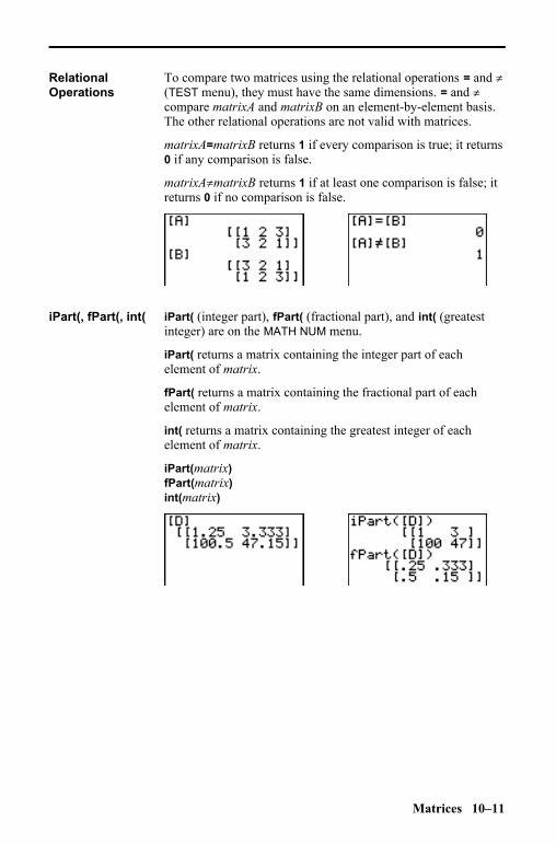
Matrices 10–11
82EA17~1.DOC TI-83 international English Bob Fedorisko Revised: 10/26/05 1:31 PM Printed: 10/27/05 2:47PM Page 11 of 16
To compare two matrices using the relational operations = and ƒ(TEST menu), they must have the same dimensions. = and ƒcompare matrixA and matrixB on an element-by-element basis.The other relational operations are not valid with matrices.
matrixA=matrixB returns 1 if every comparison is true; it returns0 if any comparison is false.
matrixAƒmatrixB returns 1 if at least one comparison is false; itreturns 0 if no comparison is false.
iPart( (integer part), fPart( (fractional part), and int( (greatestinteger) are on the MATH NUM menu.
iPart( returns a matrix containing the integer part of eachelement of matrix.
fPart( returns a matrix containing the fractional part of eachelement of matrix.
int( returns a matrix containing the greatest integer of eachelement of matrix.
iPart(matrix)fPart(matrix)int(matrix)
RelationalOperations
iPart(, fPart(, int(

10–12 Matrices
82EA17~1.DOC TI-83 international English Bob Fedorisko Revised: 10/26/05 1:31 PM Printed: 10/27/05 2:47PM Page 12 of 16
To display the MATRX MATH menu, press ~.
NAMES MATH
EDIT
1: det( Calculates the determinant.2: T Transposes the matrix.3: dim( Returns the matrix dimensions.4: Fill( Fills all elements with a constant.5: identity( Returns the identity matrix.6: randM( Returns a random matrix.7: augment( Appends two matrices.8: Matr4list( Stores a matrix to a list.9: List4matr( Stores a list to a matrix.0: cumSum( Returns the cumulative sums of a matrix.A: ref( Returns the row-echelon form of a matrix.B: rref( Returns the reduced row-echelon form.C: rowSwap( Swaps two rows of a matrix.D: row+( Adds two rows; stores in the second row.E: ärow( Multiplies the row by a number.F: ärow+( Multiplies the row, adds to the second row.
det( (determinant) returns the determinant (a real number) of asquare matrix.
det(matrix)
T (transpose) returns a matrix in which each element (row,column) is swapped with the corresponding element (column,row) of matrix.
matrixT
dim( (dimension) returns a list containing the dimensions({rows columns}) of matrix.
dim(matrix)
Note: dim(matrix)!!!!Ln:Ln(1) returns the number of rows.dim(matrix)!!!!Ln:Ln(2) returns the number of columns.
Using the MATRX MATH Operations
MATRX MATHMenu
det(
T (Transpose)
Accessing MatrixDimensions withdim(
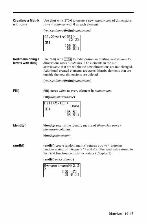
Matrices 10–13
82EA17~1.DOC TI-83 international English Bob Fedorisko Revised: 10/26/05 1:31 PM Printed: 10/27/05 2:47PM Page 13 of 16
Use dim( with ¿ to create a new matrixname of dimensionsrows × columns with 0 as each element.
{rows,columns}!!!!dim(matrixname)
Use dim( with ¿ to redimension an existing matrixname todimensions rows × columns. The elements in the oldmatrixname that are within the new dimensions are not changed.Additional created elements are zeros. Matrix elements that areoutside the new dimensions are deleted.
{rows,columns}!!!!dim(matrixname)
Fill( stores value to every element in matrixname.
Fill(value,matrixname)
identity( returns the identity matrix of dimension rows ×dimension columns.
identity(dimension)
randM( (create random matrix) returns a rows × columnsrandom matrix of integers ‚ L9 and 9. The seed value stored tothe rand function controls the values (Chapter 2).
randM(rows,columns)
Creating a Matrixwith dim(
Redimensioning aMatrix with dim(
Fill(
identity(
randM(

10–14 Matrices
82EA17~1.DOC TI-83 international English Bob Fedorisko Revised: 10/26/05 1:31 PM Printed: 10/27/05 2:47PM Page 14 of 16
augment( appends matrixA to matrixB as new columns. matrixAand matrixB both must have the same number of rows.
augment(matrixA,matrixB)
Matr4list( (matrix stored to list) fills each listname with elementsfrom each column in matrix. Matr4list( ignores extra listnamearguments. Likewise, Matr4list( ignores extra matrix columns.
Matr4list(matrix,listnameA,...,listname n)
&
Matr4list( also fills a listname with elements from a specifiedcolumn# in matrix. To fill a list with a specific column from matrix,you must enter column# after matrix.
Matr4list(matrix,column#,listname)
&
List4matr( (lists stored to matrix) fills matrixname column bycolumn with the elements from each list. If dimensions of all listsare not equal, List4matr( fills each extra matrixname row with 0.Complex lists are not valid.
List4matr(listA,...,list n,matrixname)
&
Using the MATRX MATH Operations (continued)
augment(
Matr4list(
List4matr(
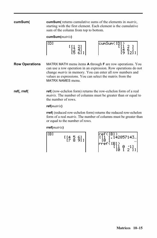
Matrices 10–15
82EA17~1.DOC TI-83 international English Bob Fedorisko Revised: 10/26/05 1:31 PM Printed: 10/27/05 2:47PM Page 15 of 16
cumSum( returns cumulative sums of the elements in matrix,starting with the first element. Each element is the cumulativesum of the column from top to bottom.
cumSum(matrix)
MATRX MATH menu items A through F are row operations. Youcan use a row operation in an expression. Row operations do notchange matrix in memory. You can enter all row numbers andvalues as expressions. You can select the matrix from theMATRX NAMES menu.
ref( (row-echelon form) returns the row-echelon form of a realmatrix. The number of columns must be greater than or equal tothe number of rows.
ref(matrix)
rref( (reduced row-echelon form) returns the reduced row-echelonform of a real matrix. The number of columns must be greater thanor equal to the number of rows.
rref(matrix)
cumSum(
Row Operations
ref(, rref(

10–16 Matrices
82EA17~1.DOC TI-83 international English Bob Fedorisko Revised: 10/26/05 1:31 PM Printed: 10/27/05 2:47PM Page 16 of 16
rowSwap( returns a matrix. It swaps rowA and rowB of matrix.
rowSwap(matrix,rowA,rowB)
row+( (row addition) returns a matrix. It adds rowA and rowB ofmatrix and stores the results in rowB.
row+(matrix,rowA,rowB)
äääärow( (row multiplication) returns a matrix. It multiplies row ofmatrix by value and stores the results in row.
äääärow(value,matrix,row)
äääärow+( (row multiplication and addition) returns a matrix. Itmultiplies rowA of matrix by value, adds it to rowB, and storesthe results in rowB.
äääärow+(value,matrix,rowA,rowB)
Using the MATRX MATH Operations (continued)
rowSwap(
row+(
äääärow(
äääärow+(

Lists 11–1
826886~1.DOC TI-83 international English Bob Fedorisko Revised: 10/26/05 1:33 PM Printed: 10/27/05 2:50PM Page 1 of 18
11 Lists
Getting Started: Generating a Sequence .................................................. 2Naming Lists.............................................................................................................. 3Storing and Displaying Lists ........................................................................... 4Entering List Names ............................................................................................. 6Attaching Formulas to List Names.............................................................. 7Using Lists in Expressions................................................................................ 9LIST OPS Menu...................................................................................................... 10LIST MATH Menu.................................................................................................. 17
Contents
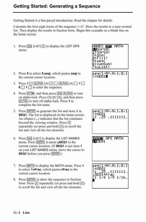
11–2 Lists
826886~1.DOC TI-83 international English Bob Fedorisko Revised: 10/26/05 1:33 PM Printed: 10/27/05 2:50PM Page 2 of 18
Getting Started is a fast-paced introduction. Read the chapter for details.
Calculate the first eight terms of the sequence 1/A2. Store the results to a user-createdlist. Then display the results in fraction form. Begin this example on a blank line onthe home screen.
1. Press y [LIST] ~ to display the LIST OPSmenu.
2. Press 5 to select 5:seq(, which pastes seq( tothe current cursor location.
3. Press 1 ¥ ƒ [A] ¡¢ƒ [A] ¢ 1¢8 ¢ 1 ¤ to enter the sequence.
4. Press ¿, and then press yƒ to turnon alpha-lock. Press [S] [E] [Q], and then pressƒ to turn off alpha-lock. Press 1 tocomplete the list name.
5. Press Í to generate the list and store it inSEQ1. The list is displayed on the home screen.An ellipsis (...) indicates that the list continuesbeyond the viewing window. Press ~repeatedly (or press and hold ~) to scroll thelist and view all the list elements.
6. Press y [LIST] to display the LIST NAMESmenu. Press Í to paste ÙÙÙÙSEQ1 to thecurrent cursor location. (If SEQ1 is not item 1on your LIST NAMES menu, move the cursor toSEQ1 before you press Í.)
7. Press to display the MATH menu. Press 1to select 1:4Frac, which pastes 4Frac to thecurrent cursor location.
8. Press Í to show the sequence in fractionform. Press ~ repeatedly (or press and hold ~)to scroll the list and view all the list elements.
Getting Started: Generating a Sequence
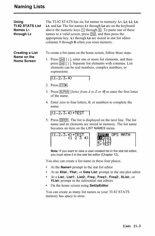
Lists 11–3
826886~1.DOC TI-83 international English Bob Fedorisko Revised: 10/26/05 1:33 PM Printed: 10/27/05 2:50PM Page 3 of 18
The TI-82 STATS has six list names in memory: L1, L2, L3, L4,L5, and L6. The list names L1 through L6 are on the keyboardabove the numeric keys À through ¸. To paste one of thesenames to a valid screen, press y, and then press theappropriate key. L1 through L6 are stored in stat list editorcolumns 1 through 6 when you reset memory.
To create a list name on the home screen, follow these steps.
1. Press y [ { ], enter one or more list elements, and thenpress y [ } ]. Separate list elements with commas. Listelements can be real numbers, complex numbers, orexpressions.
2. Press ¿.
3. Press ƒ [letter from A to Z or q] to enter the first letterof the name.
4. Enter zero to four letters, q, or numbers to complete thename.
5. Press Í. The list is displayed on the next line. The listname and its elements are stored in memory. The list namebecomes an item on the LIST NAMES menu.
Note: If you want to view a user-created list in the stat list editor,you must store it in the stat list editor (Chapter 12).
You also can create a list name in these four places.
• At the Name= prompt in the stat list editor• At an Xlist:, Ylist:, or Data List: prompt in the stat plot editor• At a List:, List1:, List2:, Freq:, Freq1:, Freq2:, XList:, or
YList: prompt in the inferential stat editors• On the home screen using SetUpEditor
You can create as many list names as your TI-82 STATSmemory has space to store.
Naming Lists
UsingTI-82 STATS ListNames L1through L6
Creating a ListName on theHome Screen
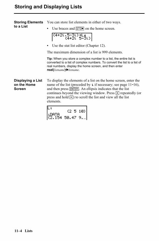
11–4 Lists
826886~1.DOC TI-83 international English Bob Fedorisko Revised: 10/26/05 1:33 PM Printed: 10/27/05 2:50PM Page 4 of 18
You can store list elements in either of two ways.
• Use braces and ¿ on the home screen.
• Use the stat list editor (Chapter 12).
The maximum dimension of a list is 999 elements.
Tip: When you store a complex number to a list, the entire list isconverted to a list of complex numbers. To convert the list to a list ofreal numbers, display the home screen, and then enterreal(listname)!!!!listname.
To display the elements of a list on the home screen, enter thename of the list (preceded by Ù if necessary; see page 11.16),and then press Í. An ellipsis indicates that the listcontinues beyond the viewing window. Press ~ repeatedly (orpress and hold ~) to scroll the list and view all the listelements.
Storing and Displaying Lists
Storing Elementsto a List
Displaying a Liston the HomeScreen

Lists 11–5
826886~1.DOC TI-83 international English Bob Fedorisko Revised: 10/26/05 1:33 PM Printed: 10/27/05 2:50PM Page 5 of 18
To copy a list, store it to another list.
You can store a value to or recall a value from a specific listelement. You can store to any element within the current listdimension or one element beyond.
listname(element)
To delete lists from memory, including L1 through L6, use theMEMORY DELETE FROM secondary menu (Chapter 18).Resetting memory restores L1 through L6. Removing a list fromthe stat list editor does not delete it from memory.
You can use lists to graph a family of curves (Chapter 3).
Copying One Listto Another
Accessing a ListElement
Deleting a Listfrom Memory
Using Lists inGraphing
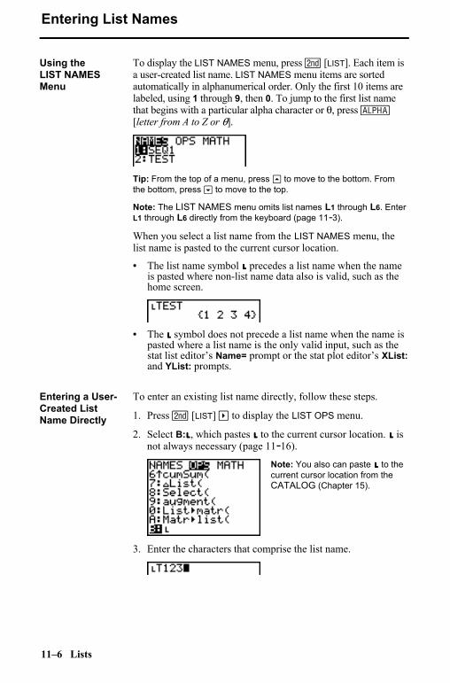
11–6 Lists
826886~1.DOC TI-83 international English Bob Fedorisko Revised: 10/26/05 1:33 PM Printed: 10/27/05 2:50PM Page 6 of 18
To display the LIST NAMES menu, press y [LIST]. Each item isa user-created list name. LIST NAMES menu items are sortedautomatically in alphanumerical order. Only the first 10 items arelabeled, using 1 through 9, then 0. To jump to the first list namethat begins with a particular alpha character or q, press ƒ[letter from A to Z or q].
Tip: From the top of a menu, press } to move to the bottom. Fromthe bottom, press † to move to the top.
Note: The LIST NAMES menu omits list names L1 through L6. EnterL1 through L6 directly from the keyboard (page 11.3).
When you select a list name from the LIST NAMES menu, thelist name is pasted to the current cursor location.
• The list name symbol ÙÙÙÙ precedes a list name when the nameis pasted where non-list name data also is valid, such as thehome screen.
• The ÙÙÙÙ symbol does not precede a list name when the name ispasted where a list name is the only valid input, such as thestat list editor’s Name= prompt or the stat plot editor’s XList:and YList: prompts.
To enter an existing list name directly, follow these steps.
1. Press y [LIST] ~ to display the LIST OPS menu.
2. Select B:ÙÙÙÙ, which pastes ÙÙÙÙ to the current cursor location. ÙÙÙÙ isnot always necessary (page 11.16).
Note: You also can paste ÙÙÙÙ to thecurrent cursor location from theCATALOG (Chapter 15).
3. Enter the characters that comprise the list name.
Entering List Names
Using theLIST NAMESMenu
Entering a User-Created ListName Directly

Lists 11–7
826886~1.DOC TI-83 international English Bob Fedorisko Revised: 10/26/05 1:33 PM Printed: 10/27/05 2:50PM Page 7 of 18
You can attach a formula to a list name so that each list elementis a result of the formula. When executed, the attached formulamust resolve to a list.
When anything in the attached formula changes, the list towhich the formula is attached is updated automatically.
• When you edit an element of a list that is referenced in theformula, the corresponding element in the list to which theformula is attached is updated.
• When you edit the formula itself, all elements in the list towhich the formula is attached are updated.
For example, the first screen below shows that elements arestored to L3, and the formula L3+10 is attached to the list nameÙÙÙÙADD10. The quotation marks designate the formula to beattached to ÙÙÙÙADD10. Each element of ÙÙÙÙADD10 is the sum of anelement in L3 and 10.
The next screen shows another list, L4. The elements of L4 arethe sum of the same formula that is attached to L3. However,quotation marks are not entered, so the formula is not attachedto L4.
On the next line, L6!!!!L3(1):L3 changes the first element in L3 toL6, and then redisplays L3.
The last screen shows that editing L3 updated ÙÙÙÙADD10, but didnot change L4. This is because the formula L3+10 is attached toÙÙÙÙADD10, but it is not attached to L4.
Note: To view a formula that is attached to a list name, use the statlist editor (Chapter 12).
Attaching Formulas to List Names
Attaching aFormula to a ListName
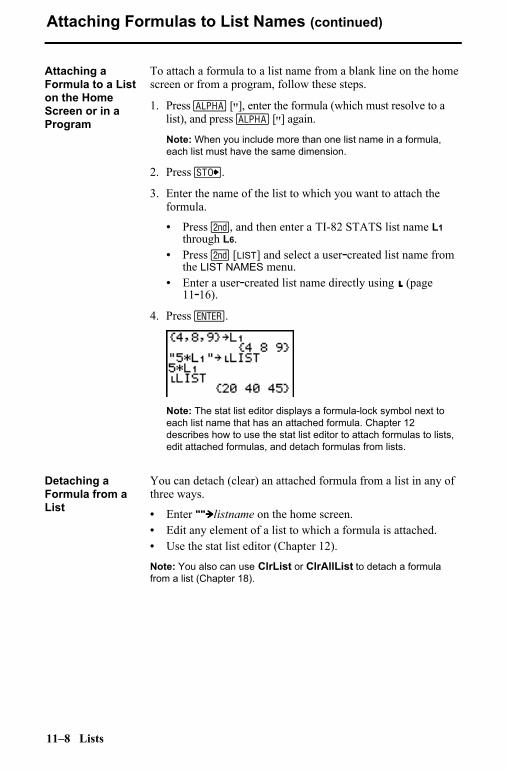
11–8 Lists
826886~1.DOC TI-83 international English Bob Fedorisko Revised: 10/26/05 1:33 PM Printed: 10/27/05 2:50PM Page 8 of 18
To attach a formula to a list name from a blank line on the homescreen or from a program, follow these steps.
1. Press ƒ [ã], enter the formula (which must resolve to alist), and press ƒ [ã] again.
Note: When you include more than one list name in a formula,each list must have the same dimension.
2. Press ¿.
3. Enter the name of the list to which you want to attach theformula.
• Press y, and then enter a TI-82 STATS list name L1through L6.
• Press y [LIST] and select a user.created list name fromthe LIST NAMES menu.
• Enter a user.created list name directly using ÙÙÙÙ (page11.16).
4. Press Í.
Note: The stat list editor displays a formula-lock symbol next toeach list name that has an attached formula. Chapter 12describes how to use the stat list editor to attach formulas to lists,edit attached formulas, and detach formulas from lists.
You can detach (clear) an attached formula from a list in any ofthree ways.
• Enter ""!!!!listname on the home screen.• Edit any element of a list to which a formula is attached.• Use the stat list editor (Chapter 12).
Note: You also can use ClrList or ClrAllList to detach a formulafrom a list (Chapter 18).
Attaching Formulas to List Names (continued)
Attaching aFormula to a Liston the HomeScreen or in aProgram
Detaching aFormula from aList

Lists 11–9
826886~1.DOC TI-83 international English Bob Fedorisko Revised: 10/26/05 1:33 PM Printed: 10/27/05 2:50PM Page 9 of 18
You can use lists in an expression in any of three ways. Whenyou press Í, any expression is evaluated for each listelement, and a list is displayed.
• Use L1–L6 or any user-created list name in an expression.
• Enter the list elements directly (step 1 on page 11.3).
• Use y [RCL] to recall the contents of the list into anexpression at the cursor location (Chapter 1).
&
Note: You must paste user-created list names to the Rcl prompt byselecting them from the LIST NAMES menu. You cannot enter themdirectly using ÙÙÙÙ.
You can use a list to input several values for some mathfunctions. Other chapters and Appendix A specify whether a listis valid. The function is evaluated for each list element, and alist is displayed.
• When you use a list with a function, the function must bevalid for every element in the list. In graphing, an invalidelement, such as L1 in ‡({1,0,L1}), is ignored.
This returns an error.
This graphs Xääää‡(1) and Xääää‡(0),but skips Xääää‡(L1).
• When you use two lists with a two-argument function, thedimension of each list must be the same. The function isevaluated for corresponding elements.
• When you use a list and a value with a two-argumentfunction, the value is used with each element in the list.
Using Lists in Expressions
Using a List in anExpression
Using Lists withMath Functions

11–10 Lists
826886~1.DOC TI-83 international English Bob Fedorisko Revised: 10/26/05 1:33 PM Printed: 10/27/05 2:50PM Page 10 of 18
To display the LIST OPS menu, press y [LIST] ~.
NAMESOPS MATH1: SortA( Sorts lists in ascending order.2: SortD( Sorts lists in descending order.3: dim( Sets the list dimension.4: Fill( Fills all elements with a constant.5: seq( Creates a sequence.6: cumSum( Returns a list of cumulative sums.7: @List( Returns difference of successive elements.8: Select( Selects specific data points.9: augment( Concatenates two lists.0: List4matr( Stores a list to a matrix.A: Matr4list( Stores a matrix to a list.B: ÙÙÙÙ Designates the list-name data type.
SortA( (sort ascending) sorts list elements from low to highvalues. SortD( (sort descending) sorts list elements from high tolow values. Complex lists are sorted based on magnitude(modulus).
With one list, SortA( and SortD( sort the elements of listnameand update the list in memory.
SortA(listname) SortD(listname)
With two or more lists, SortA( and SortD( sort keylistname, andthen sort each dependlist by placing its elements in the sameorder as the corresponding elements in keylistname. All listsmust have the same dimension.
SortA(keylistname,dependlist1[,dependlist2,...,dependlist n])SortD(keylistname,dependlist1[,dependlist2,...,dependlist n])
Note: In the example, 5 is the first element in L4, and 1 is the firstelement in L5. After SortA(L4,L5), 5 becomes the second element ofL4, and likewise, 1 becomes the second element of L5.
Note: SortA( and SortD( are the same as SortA( and SortD( on theSTAT EDIT menu (Chapter 12).
LIST OPS Menu
LIST OPS Menu
SortA(, SortD(

Lists 11–11
826886~1.DOC TI-83 international English Bob Fedorisko Revised: 10/26/05 1:33 PM Printed: 10/27/05 2:50PM Page 11 of 18
dim( (dimension) returns the length (number of elements) of list.
dim(list)
You can use dim( with ¿ to create a new listname withdimension length from 1 to 999. The elements are zeros.
length!!!!dim(listname)
You can use dim with ¿ to redimension an existing listnameto dimension length from 1 to 999.
• The elements in the old listname that are within the newdimension are not changed.
• Extra list elements are filled by 0.• Elements in the old list that are outside the new dimension
are deleted.
length!!!!dim(listname)
Fill( replaces each element in listname with value.
Fill(value,listname)
Note: dim( and Fill( are the same as dim( and Fill( on the MATRXMATH menu (Chapter 10).
Using dim( toFind ListDimensions
Using dim( toCreate a List
Using dim( toRedimension aList
Fill(

11–12 Lists
826886~1.DOC TI-83 international English Bob Fedorisko Revised: 10/26/05 1:33 PM Printed: 10/27/05 2:50PM Page 12 of 18
seq( (sequence) returns a list in which each element is the resultof the evaluation of expression with regard to variable for thevalues ranging from begin to end at steps of increment. variableneed not be defined in memory. increment can be negative; thedefault value for increment is 1. seq( is not valid withinexpression.
seq(expression,variable,begin,end[,increment])
cumSum( (cumulative sum) returns the cumulative sums of theelements in list, starting with the first element. list elements canbe real or complex numbers.
cumSum(list)
@List( returns a list containing the differences betweenconsecutive elements in list. @List subtracts the first element inlist from the second element, subtracts the second element fromthe third, and so on. The list of differences is always oneelement shorter than the original list. list elements can be a realor complex numbers.
@List(list)
Select( selects one or more specific data points from a scatterplot or xyLine plot (only), and then stores the selected datapoints to two new lists, xlistname and ylistname. For example,you can use Select( to select and then analyze a portion ofplotted CBL or CBR data.
Select(xlistname,ylistname)
Note: Before you use Select(, you must have selected (turned on) ascatter plot or xyLine plot. Also, the plot must be displayed in thecurrent viewing window (page 11.13).
LIST OPS Menu (continued)
seq(
cumSum(
@List(
Select(
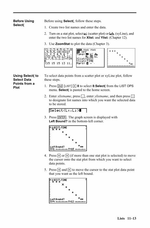
Lists 11–13
826886~1.DOC TI-83 international English Bob Fedorisko Revised: 10/26/05 1:33 PM Printed: 10/27/05 2:50PM Page 13 of 18
Before using Select(, follow these steps.
1. Create two list names and enter the data.
2. Turn on a stat plot, select """" (scatter plot) or ÓÓÓÓ (xyLine), andenter the two list names for Xlist: and Ylist: (Chapter 12).
3. Use ZoomStat to plot the data (Chapter 3).
To select data points from a scatter plot or xyLine plot, followthese steps.
1. Press y [LIST] ~ 8 to select 8:Select( from the LIST OPSmenu. Select( is pasted to the home screen.
2. Enter xlistname, press ¢, enter ylistname, and then press ¤to designate list names into which you want the selected datato be stored.
3. Press Í. The graph screen is displayed withLeft Bound? in the bottom-left corner.
4. Press } or † (if more than one stat plot is selected) to movethe cursor onto the stat plot from which you want to selectdata points.
5. Press | and ~ to move the cursor to the stat plot data pointthat you want as the left bound.
Before UsingSelect(
Using Select( toSelect DataPoints from aPlot

11–14 Lists
826886~1.DOC TI-83 international English Bob Fedorisko Revised: 10/26/05 1:33 PM Printed: 10/27/05 2:50PM Page 14 of 18
6. Press Í. A 4 indicator on the graph screen shows the leftbound. Right Bound? is displayed in the bottom-left corner.
7. Press | or ~ to move the cursor to the stat plot point that youwant for the right bound, and then press Í.
The x-values and y-values of the selected points are stored inxlistname and ylistname. A new stat plot of xlistname andylistname replaces the stat plot from which you selected datapoints. The list names are updated in the stat plot editor.
Note: The two new lists (xlistname and ylistname) will include thepoints you select as left bound and right bound. Also, left-boundx-value right-bound x-value must be true.
LIST OPS Menu (continued)
Using Select( toSelect DataPoints from aPlot (continued)
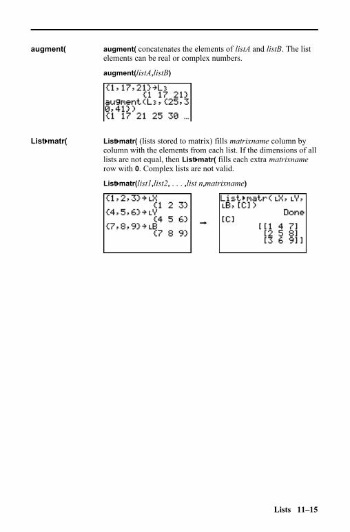
Lists 11–15
826886~1.DOC TI-83 international English Bob Fedorisko Revised: 10/26/05 1:33 PM Printed: 10/27/05 2:50PM Page 15 of 18
augment( concatenates the elements of listA and listB. The listelements can be real or complex numbers.
augment(listA,listB)
List4matr( (lists stored to matrix) fills matrixname column bycolumn with the elements from each list. If the dimensions of alllists are not equal, then List4matr( fills each extra matrixnamerow with 0. Complex lists are not valid.
List4matr(list1,list2, . . . ,list n,matrixname)
&
augment(
List4matr(

11–16 Lists
826886~1.DOC TI-83 international English Bob Fedorisko Revised: 10/26/05 1:33 PM Printed: 10/27/05 2:50PM Page 16 of 18
Matr4list( (matrix stored to lists) fills each listname withelements from each column in matrix. If the number of listnamearguments exceeds the number of columns in matrix, thenMatr4list( ignores extra listname arguments. Likewise, if thenumber of columns in matrix exceeds the number of listnamearguments, then Matr4list( ignores extra matrix columns.
Matr4list(matrix,listname1,listname2, . . . ,listname n)
&
Matr4list( also fills a listname with elements from a specifiedcolumn# in matrix. To fill a list with a specific column frommatrix, you must enter a column# after matrix.
Matr4list(matrix,column#,listname)
&
ÙÙÙÙ preceding one to five characters identifies those characters as auser-created listname. listname may comprise letters, q, andnumbers, but it must begin with a letter from A to Z or q.
ÙÙÙÙlistname
Generally, ÙÙÙÙ must precede a user-created list name when youenter a user-created list name where other input is valid, forexample, on the home screen. Without the ÙÙÙÙ, the TI-82 STATSmay misinterpret a user-created list name as impliedmultiplication of two or more characters.
ÙÙÙÙ need not precede a user-created list name where a list name isthe only valid input, for example, at the Name= prompt in thestat list editor or the Xlist: and Ylist: prompts in the stat ploteditor. If you enter ÙÙÙÙ where it is not necessary, the TI-82 STATSwill ignore the entry.
LIST OPS Menu (continued)
Matr4list(
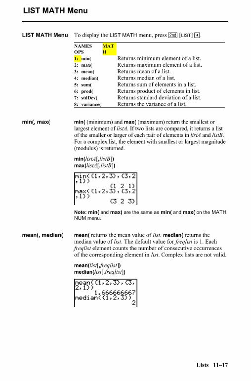
Lists 11–17
826886~1.DOC TI-83 international English Bob Fedorisko Revised: 10/26/05 1:33 PM Printed: 10/27/05 2:50PM Page 17 of 18
To display the LIST MATH menu, press y [LIST] |.
NAMESOPS
MATH
1: min( Returns minimum element of a list.2: max( Returns maximum element of a list.3: mean( Returns mean of a list.4: median( Returns median of a list.5: sum( Returns sum of elements in a list.6: prod( Returns product of elements in list.7: stdDev( Returns standard deviation of a list.8: variance( Returns the variance of a list.
min( (minimum) and max( (maximum) return the smallest orlargest element of listA. If two lists are compared, it returns a listof the smaller or larger of each pair of elements in listA and listB.For a complex list, the element with smallest or largest magnitude(modulus) is returned.
min(listA[,listB])max(listA[,listB])
Note: min( and max( are the same as min( and max( on the MATHNUM menu.
mean( returns the mean value of list. median( returns themedian value of list. The default value for freqlist is 1. Eachfreqlist element counts the number of consecutive occurrencesof the corresponding element in list. Complex lists are not valid.
mean(list[,freqlist])median(list[,freqlist])
LIST MATH Menu
LIST MATH Menu
min(, max(
mean(, median(

11–18 Lists
826886~1.DOC TI-83 international English Bob Fedorisko Revised: 10/26/05 1:33 PM Printed: 10/27/05 2:50PM Page 18 of 18
sum( (summation) returns the sum of the elements in list. startand end are optional; they specify a range of elements. listelements can be real or complex numbers.
prod( returns the product of all elements of list. start and endelements are optional; they specify a range of list elements. listelements can be real or complex numbers.
sum(list[,start,end]) prod(list[,start,end])
You can combine sum( or prod( with seq( to obtain:
upper upper
Gexpression(x) ∏∏∏∏expression(x)x=lower x=lower
To evaluate G 2(N–1) from N=1 to 4:
stdDev( returns the standard deviation of the elements in list. Thedefault value for freqlist is 1. Each freqlist element counts thenumber of consecutive occurrences of the corresponding element inlist. Complex lists are not valid.
variance( returns the variance of the elements in list. The defaultvalue for freqlist is 1. Each freqlist element counts the number ofconsecutive occurrences of the corresponding element in list.Complex lists are not valid.
stdDev(list[,freqlist]) variance(list[,freqlist])
LIST MATH Menu (continued)
sum(, prod(
Sums andProducts ofNumericSequences
stdDev(,variance(

Statistics 12–1
82D315~1.DOC TI-83 international English Bob Fedorisko Revised: 10/26/05 1:36 PM Printed: 10/27/05 2:53PM Page 1 of 38
12 Statistics
Getting Started: Pendulum Lengths and Periods................................ 2Setting Up Statistical Analyses...................................................................... 10Using the Stat List Editor .................................................................................. 11Attaching Formulas to List Names.............................................................. 14Detaching Formulas from List Names ...................................................... 16Switching Stat List Editor Contexts............................................................ 17Stat List Editor Contexts.................................................................................... 18STAT EDIT Menu .................................................................................................. 20Regression Model Features .............................................................................. 22STAT CALC Menu ................................................................................................ 24Statistical Variables............................................................................................... 29Statistical Analysis in a Program.................................................................. 30Statistical Plotting................................................................................................... 31Statistical Plotting in a Program.................................................................... 37
Contents
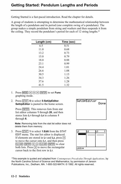
12–2 Statistics
82D315~1.DOC TI-83 international English Bob Fedorisko Revised: 10/26/05 1:36 PM Printed: 10/27/05 2:53PM Page 2 of 38
Getting Started is a fast-paced introduction. Read the chapter for details.
A group of students is attempting to determine the mathematical relationship betweenthe length of a pendulum and its period (one complete swing of a pendulum). Thegroup makes a simple pendulum from string and washers and then suspends it fromthe ceiling. They record the pendulum’s period for each of 12 string lengths.*
Length (cm) Time (sec) 6.5 0.5111.0 0.6813.2 0.7315.0 0.7918.0 0.8823.1 0.9924.4 1.0126.6 1.0830.5 1.1334.3 1.2637.6 1.2841.5 1.32
1. Press z † † † Í to set Funcgraphing mode.
2. Press … 5 to select 5:SetUpEditor.SetUpEditor is pasted to the home screen.
Press Í. This removes lists from statlist editor columns 1 through 20, and thenstores lists L1 through L6 in columns 1through 6.
Note: Removing lists from the stat list editor does notdelete them from memory.
3. Press … 1 to select 1:Edit from the STATEDIT menu. The stat list editor is displayed.If elements are stored in L1 and L2, press }to move the cursor onto L1, and then press‘ Í ~ } ‘Í to clearboth lists. Press | to move the rectangularcursor back to the first row in L1.
*This example is quoted and adapted from Contemporary Precalculus Through Applications, bythe North Carolina School of Science and Mathematics, by permission of JansonPublications, Inc., Dedham, MA. 1-800-322-MATH. © 1992. All rights reserved.
Getting Started: Pendulum Lengths and Periods

Statistics 12–3
82D315~1.DOC TI-83 international English Bob Fedorisko Revised: 10/26/05 1:36 PM Printed: 10/27/05 2:53PM Page 3 of 38
4. Press 6 Ë 5 Í to store the firstpendulum string length (6.5 cm) in L1. Therectangular cursor moves to the next row.Repeat this step to enter each of the 12string length values in the table on page12.2.
5. Press ~ to move the rectangular cursor tothe first row in L2.
Press Ë 51 Í to store the first timemeasurement (.51 sec) in L2. Therectangular cursor moves to the next row.Repeat this step to enter each of the 12 timevalues in the table on page 12.2.
6. Press o to display the Y= editor.
If necessary, press ‘ to clear the functionY1. As necessary, press }, Í, and ~ toturn off Plot1, Plot2, and Plot3 from the topline of the Y= editor (Chapter 3). As necessary,press †, |, and Í to deselect functions.
7. Press y [STAT PLOT] 1 to select 1:Plot1from the STAT PLOTS menu. The stat ploteditor is displayed for plot 1.
8. Press Í to select On, which turns onplot 1. Press † Í to select " (scatterplot). Press † y [L1] to specify Xlist:L1for plot 1. Press † y [L2] to specifyYlist:L2 for plot 1. Press †~Í toselect + as the Mark for each data point onthe scatter plot.
9. Press q 9 to select 9:ZoomStat from theZOOM menu. The window variables areadjusted automatically, and plot 1 isdisplayed. This is a scatter plot of the time-versus-length data.

12–4 Statistics
82D315~1.DOC TI-83 international English Bob Fedorisko Revised: 10/26/05 1:36 PM Printed: 10/27/05 2:53PM Page 4 of 38
Since the scatter plot of time-versus-length data appears to be approximately linear,fit a line to the data.
10. Press … ~ 4 to select 4:LinReg(ax+b)(linear regression model) from the STATCALC menu. LinReg(ax+b) is pasted to thehome screen.
11. Press y [L1] ¢ y [L2] ¢. Press ~ 1 to display the VARS Y.VARSFUNCTION secondary menu, and then press1 to select 1:Y1. L1, L2, and Y1 are pasted tothe home screen as arguments toLinReg(ax+b).
12. Press Í to execute LinReg(ax+b). Thelinear regression for the data in L1 and L2 iscalculated. Values for a and b are displayed onthe home screen. The linear regressionequation is stored in Y1. Residuals arecalculated and stored automatically in the listname RESID, which becomes an item on theLIST NAMES menu.
13. Press s. The regression line and thescatter plot are displayed.
Getting Started: Pendulum Lengths and Periods (cont.)
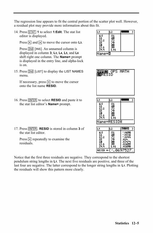
Statistics 12–5
82D315~1.DOC TI-83 international English Bob Fedorisko Revised: 10/26/05 1:36 PM Printed: 10/27/05 2:53PM Page 5 of 38
The regression line appears to fit the central portion of the scatter plot well. However,a residual plot may provide more information about this fit.
14. Press … 1 to select 1:Edit. The stat listeditor is displayed.
Press ~ and } to move the cursor onto L3.
Press y [INS]. An unnamed column isdisplayed in column 3; L3, L4, L5, and L6shift right one column. The Name= promptis displayed in the entry line, and alpha-lockis on.
15. Press y [LIST] to display the LIST NAMESmenu.
If necessary, press † to move the cursoronto the list name RESID.
16. Press Í to select RESID and paste it tothe stat list editor’s Name= prompt.
17. Press Í. RESID is stored in column 3 ofthe stat list editor.
Press † repeatedly to examine theresiduals.
Notice that the first three residuals are negative. They correspond to the shortestpendulum string lengths in L1. The next five residuals are positive, and three of thelast four are negative. The latter correspond to the longer string lengths in L1. Plottingthe residuals will show this pattern more clearly.
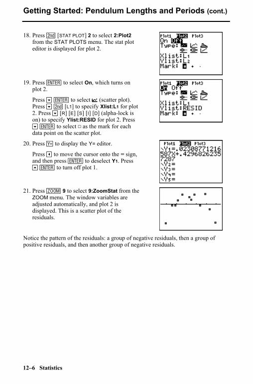
12–6 Statistics
82D315~1.DOC TI-83 international English Bob Fedorisko Revised: 10/26/05 1:36 PM Printed: 10/27/05 2:53PM Page 6 of 38
18. Press y [STAT PLOT] 2 to select 2:Plot2from the STAT PLOTS menu. The stat ploteditor is displayed for plot 2.
19. Press Í to select On, which turns onplot 2.
Press † Í to select """" (scatter plot).Press † y [L1] to specify Xlist:L1 for plot2. Press † [R] [E] [S] [I] [D] (alpha-lock ison) to specify Ylist:RESID for plot 2. Press† Í to select › as the mark for eachdata point on the scatter plot.
20. Press o to display the Y= editor.
Press | to move the cursor onto the = sign,and then press Í to deselect Y1. Press} Í to turn off plot 1.
21. Press q 9 to select 9:ZoomStat from theZOOM menu. The window variables areadjusted automatically, and plot 2 isdisplayed. This is a scatter plot of theresiduals.
Notice the pattern of the residuals: a group of negative residuals, then a group ofpositive residuals, and then another group of negative residuals.
Getting Started: Pendulum Lengths and Periods (cont.)
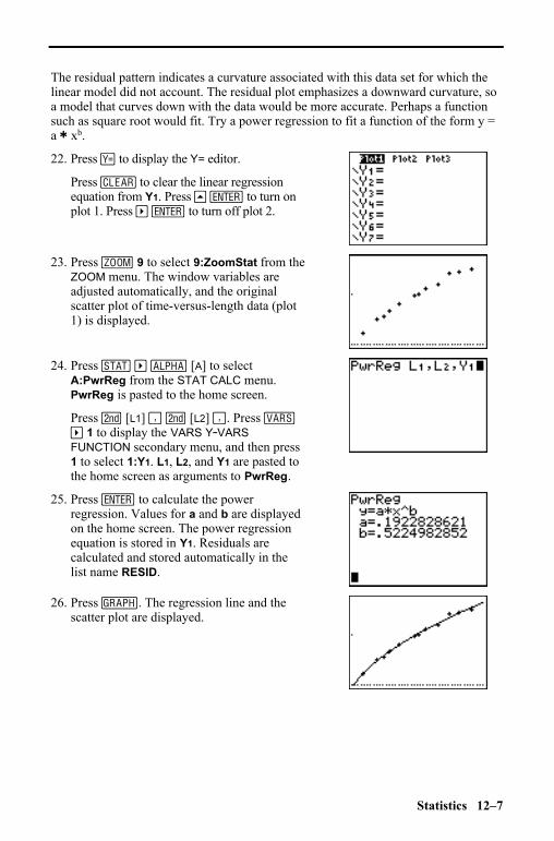
Statistics 12–7
82D315~1.DOC TI-83 international English Bob Fedorisko Revised: 10/26/05 1:36 PM Printed: 10/27/05 2:53PM Page 7 of 38
The residual pattern indicates a curvature associated with this data set for which thelinear model did not account. The residual plot emphasizes a downward curvature, soa model that curves down with the data would be more accurate. Perhaps a functionsuch as square root would fit. Try a power regression to fit a function of the form y =a ä xb.
22. Press o to display the Y= editor.
Press ‘ to clear the linear regressionequation from Y1. Press }Í to turn onplot 1. Press ~ Í to turn off plot 2.
23. Press q 9 to select 9:ZoomStat from theZOOM menu. The window variables areadjusted automatically, and the originalscatter plot of time-versus-length data (plot1) is displayed.
24. Press … ~ ƒ [A] to selectA:PwrReg from the STAT CALC menu.PwrReg is pasted to the home screen.
Press y [L1] ¢ y [L2] ¢. Press ~ 1 to display the VARS Y.VARSFUNCTION secondary menu, and then press1 to select 1:Y1. L1, L2, and Y1 are pasted tothe home screen as arguments to PwrReg.
25. Press Í to calculate the powerregression. Values for a and b are displayedon the home screen. The power regressionequation is stored in Y1. Residuals arecalculated and stored automatically in thelist name RESID.
26. Press s. The regression line and thescatter plot are displayed.

12–8 Statistics
82D315~1.DOC TI-83 international English Bob Fedorisko Revised: 10/26/05 1:36 PM Printed: 10/27/05 2:53PM Page 8 of 38
The new function y=.192x.522 appears to fit the data well. To get more information,examine a residual plot.
27. Press o to display the Y= editor.
Press | Í to deselect Y1.
Press } Í to turn off plot 1. Press ~Í to turn on plot 2.
Note: Step 19 defined plot 2 to plot residuals (RESID)versus string length (L1).
28. Press q 9 to select 9:ZoomStat from theZOOM menu. The window variables areadjusted automatically, and plot 2 isdisplayed. This is a scatter plot of theresiduals.
The new residual plot shows that the residuals are random in sign, with the residualsincreasing in magnitude as the string length increases.
To see the magnitudes of the residuals, continue with these steps.
29. Press r.
Press ~ and | to trace the data. Observethe values for Y at each point.
With this model, the largest positive residualis about 0.041 and the smallest negativeresidual is about L0.027. All other residualsare less than 0.02 in magnitude.
Getting Started: Pendulum Lengths and Periods (cont.)

Statistics 12–9
82D315~1.DOC TI-83 international English Bob Fedorisko Revised: 10/26/05 1:36 PM Printed: 10/27/05 2:53PM Page 9 of 38
Now that you have a good model for the relationship between length and period, youcan use the model to predict the period for a given string length. To predict theperiods for a pendulum with string lengths of 20 cm and 50 cm, continue with thesesteps.
30. Press ~ 1 to display the VARSY.VARS FUNCTION secondary menu, andthen press 1 to select 1:Y1. Y1 is pasted tothe home screen.
31. Press £ 20 ¤ to enter a string length of 20cm.
Press Í to calculate the predicted timeof about 0.92 seconds.
Based on the residual analysis, we wouldexpect the prediction of about 0.92 secondsto be within about 0.02 seconds of the actualvalue.
32. Press y [ENTRY] to recall the Last Entry.
Press | | | 5 to change the string lengthto 50 cm.
33. Press Í to calculate the predicted timeof about 1.48 seconds.
Since a string length of 50 cm exceeds thelengths in the data set, and since residualsappear to be increasing as string lengthincreases, we would expect more error withthis estimate.
Note: You also can make predictions using the tablewith the TABLE SETUP settings Indpnt:Ask andDepend:Auto (Chapter 7).
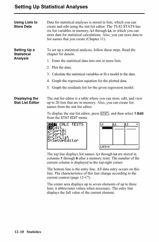
12–10 Statistics
82D315~1.DOC TI-83 international English Bob Fedorisko Revised: 10/26/05 1:36 PM Printed: 10/27/05 2:53PM Page 10 of 38
Data for statistical analyses is stored in lists, which you cancreate and edit using the stat list editor. The TI-82 STATS hassix list variables in memory, L1 through L6, to which you canstore data for statistical calculations. Also, you can store data tolist names that you create (Chapter 11).
To set up a statistical analysis, follow these steps. Read thechapter for details.
1. Enter the statistical data into one or more lists.
2. Plot the data.
3. Calculate the statistical variables or fit a model to the data.
4. Graph the regression equation for the plotted data.
5. Graph the residuals list for the given regression model.
The stat list editor is a table where you can store, edit, and viewup to 20 lists that are in memory. Also, you can create listnames from the stat list editor.
To display the stat list editor, press …, and then select 1:Editfrom the STAT EDIT menu.
The top line displays list names. L1 through L6 are stored incolumns 1 through 6 after a memory reset. The number of thecurrent column is displayed in the top-right corner.
The bottom line is the entry line. All data entry occurs on thisline. The characteristics of this line change according to thecurrent context (page 12.17).
The center area displays up to seven elements of up to threelists; it abbreviates values when necessary. The entry linedisplays the full value of the current element.
Setting Up Statistical Analyses
Using Lists toStore Data
Setting Up aStatisticalAnalysis
Displaying theStat List Editor

Statistics 12–11
82D315~1.DOC TI-83 international English Bob Fedorisko Revised: 10/26/05 1:36 PM Printed: 10/27/05 2:53PM Page 11 of 38
To enter a list name in the stat list editor, follow these steps.
1. Display the Name= prompt in the entry line in either of twoways.• Move the cursor onto the list name in the column where
you want to insert a list, and then press y [INS]. Anunnamed column is displayed and the remaining lists shiftright one column.
• Press } until the cursor is on the top line, and then press~ until you reach the unnamed column.
Note: If list names are stored to all 20 columns, you must removea list name to make room for an unnamed column.
The Name= prompt is displayed and alpha-lock is on.
2. Enter a valid list name in any of four ways.
• Select a name from the LIST NAMES menu (Chapter 11).• Enter L1, L2, L3, L4, L5, or L6 from the keyboard.• Enter an existing user-created list name directly from the
keyboard.• Enter a new user-created list name (page 12.12).
3. Press Í or † to store the list name and its elements, ifany, in the current column of the stat list editor.
To begin entering, scrolling, or editing list elements, press †.The rectangular cursor is displayed.Note: If the list name you entered in step 2 already was stored inanother stat list editor column, then the list and its elements, if any,move to the current column from the previous column. Remaining listnames shift accordingly.
Using the Stat List Editor
Entering a ListName in the StatList Editor

12–12 Statistics
82D315~1.DOC TI-83 international English Bob Fedorisko Revised: 10/26/05 1:36 PM Printed: 10/27/05 2:53PM Page 12 of 38
To create a name in the stat list editor, follow these steps.
1. Follow step 1 on page 12.11 to display the Name= prompt.
2. Press [letter from A to Z or q] to enter the first letter of thename. The first character cannot be a number.
3. Enter zero to four letters, q, or numbers to complete the newuser-created list name. List names can be one to fivecharacters long.
4. Press Í or † to store the list name in the currentcolumn of the stat list editor. The list name becomes an itemon the LIST NAMES menu (Chapter 11).
To remove a list from the stat list editor, move the cursor onto thelist name and then press {. The list is not deleted from memory;it is only removed from the stat list editor.
Note: To delete a list name from memory, use the MEMORYDELETE:List selection screen (Chapter 18).
You can remove all user-created lists from the stat list editor andrestore list names L1 through L6 to columns 1 through 6 in eitherof two ways.
• Use SetUpEditor with no arguments (page 12.21).• Reset all memory (Chapter 18).
You can clear all elements from a list in any of five ways.
• Use ClrList to clear specified lists (page 12.20).• In the stat list editor, press } to move the cursor onto a list
name, and then press ‘ Í.• In the stat list editor, move the cursor onto each element, and
then press { one by one.• On the home screen or in the program editor, enter
0!!!!dim(listname) to set the dimension of listname to 0(Chapter 11).
• Use ClrAllLists to clear all lists in memory (Chapter 18).
Using the Stat List Editor (continued)
Creating a Namein the Stat ListEditor
Removing a Listfrom the Stat ListEditor
Removing AllLists andRestoring L1through L6
Clearing AllElements from aList

Statistics 12–13
82D315~1.DOC TI-83 international English Bob Fedorisko Revised: 10/26/05 1:36 PM Printed: 10/27/05 2:53PM Page 13 of 38
To edit a list element, follow these steps.
1. Move the rectangular cursor onto the element you want toedit.
2. Press Í to move the cursor to the entry line.
Note: If you want to replace the current value, you can enter anew value without first pressing Í. When you enter the firstcharacter, the current value is cleared automatically.
3. Edit the element in the entry line.
• Press one or more keys to enter the new value. When youenter the first character, the current value is clearedautomatically.
• Press ~ to move the cursor to the character before whichyou want to insert, press y [INS], and then enter one ormore characters.
• Press ~ to move the cursor to a character you want todelete, and then press { to delete the character.
To cancel any editing and restore the original element at therectangular cursor, press ‘ Í.
Note: You can enter expressions and variables for elements.
4. Press Í, }, or † to update the list. If you entered anexpression, it is evaluated. If you entered only a variable, thestored value is displayed as a list element.
When you edit a list element in the stat list editor, the list isupdated in memory immediately.
Editing a ListElement

12–14 Statistics
82D315~1.DOC TI-83 international English Bob Fedorisko Revised: 10/26/05 1:36 PM Printed: 10/27/05 2:53PM Page 14 of 38
You can attach a formula to a list name in the stat list editor, andthen display and edit the calculated list elements. Whenexecuted, the attached formula must resolve to a list. Chapter 11describes in detail the concept of attaching formulas to listnames.
To attach a formula to a list name that is stored in the stat listeditor, follow these steps.
1. Press … Í to display the stat list editor.
2. Press } to move the cursor to the top line.
3. Press | or ~, if necessary, to move the cursor onto the listname to which you want to attach the formula.
Note: If a formula in quotation marks is displayed on the entryline, then a formula is already attached to the list name. To editthe formula, press Í, and then edit the formula.
4. Press ƒ [ã], enter the formula, and press ƒ [ã].
Note: If you do not use quotation marks, the TI-82 STATScalculates and displays the same initial list of answers, but doesnot attach the formula for future calculations.
Note: Any user-created list name referenced in a formula must bepreceded by an ÙÙÙÙ symbol (Chapter 11).
5. Press Í. The TI-82 STATS calculates each list elementand stores it to the list name to which the formula is attached.A lock symbol is displayed in the stat list editor, next to thelist name to which the formula is attached.
Attaching Formulas to List Names
Attaching aFormula to a ListName in Stat ListEditor
lock symbol

Statistics 12–15
82D315~1.DOC TI-83 international English Bob Fedorisko Revised: 10/26/05 1:36 PM Printed: 10/27/05 2:53PM Page 15 of 38
When you edit an element of a list referenced in an attachedformula, the TI-82 STATS updates the corresponding element inthe list to which the formula is attached (Chapter 11).
When a list with a formula attached is displayed in the stat listeditor and you edit or enter elements of another displayed list,then the TI-82 STATS takes slightly longer to accept each editor entry than when no lists with formulas attached are in view.
Tip: To speed editing time, scroll horizontally until no lists withformulas are displayed, or rearrange the stat list editor so that no listswith formulas are displayed.
On the home screen, you can attach to a list a formula thatreferences another list with dimension 0 (Chapter 11). However,you cannot display the formula-generated list in the stat listeditor or on the home screen until you enter at least one elementto the list that the formula references.
All elements of a list referenced by an attached formula must bevalid for the attached formula. For example, if Real numbermode is set and the attached formula is log(L1), then eachelement of L1 must be greater than 0, since the logarithm of anegative number returns a complex result.
Tip: If an error menu is returned when you attempt to display aformula-generated list in the stat list editor, you can select 2:Goto,write down the formula that is attached to the list, and then press‘ Í to detach (clear) the formula. You then can use the statlist editor to find the source of the error. After making the appropriatechanges, you can reattach the formula to a list.
If you do not want to clear the formula, you can select 1:Quit, displaythe referenced list on the home screen, and find and edit the sourceof the error. To edit an element of a list on the home screen, store thenew value to listname(element#) (Chapter 11).
Using the StatList Editor WhenFormula-Generated ListsAre Displayed
Handling ErrorsResulting fromAttachedFormulas

12–16 Statistics
82D315~1.DOC TI-83 international English Bob Fedorisko Revised: 10/26/05 1:36 PM Printed: 10/27/05 2:53PM Page 16 of 38
You can detach (clear) a formula from a list name in any of fourways.
• In the stat list editor, move the cursor onto the name of thelist to which a formula is attached. Press Í‘ Í. All list elements remain, but the formula isdetached and the lock symbol disappears.
• In the stat list editor, move the cursor onto an element of thelist to which a formula is attached. Press Í, edit theelement, and then press Í. The element changes, theformula is detached, and the lock symbol disappears. Allother list elements remain.
• Use ClrList (page 12.20). All elements of one or morespecified lists are cleared, each formula is detached, and eachlock symbol disappears. All list names remain.
• Use ClrAllLists (Chapter 18). All elements of all lists inmemory are cleared, all formulas are detached from all listnames, and all lock symbols disappear. All list namesremain.
As described above, one way to detach a formula from a listname is to edit an element of the list to which the formula isattached. The TI-82 STATS protects against inadvertentlydetaching the formula from the list name by editing an elementof the formula-generated list.
Because of the protection feature, you must press Í beforeyou can edit an element of a formula-generated list.
The protection feature does not allow you to delete an elementof a list to which a formula is attached. To delete an element ofa list to which a formula is attached, you must first detach theformula in any of the ways described above.
Detaching Formulas from List Names
Detaching aFormula from aList Name
Editing anElement of aFormula-Generated List

Statistics 12–17
82D315~1.DOC TI-83 international English Bob Fedorisko Revised: 10/26/05 1:36 PM Printed: 10/27/05 2:53PM Page 17 of 38
The stat list editor has four contexts.
• View-elements context • Edit-elements context• View-names context • Enter-name context
The stat list editor is first displayed in view-elements context.To switch through the four contexts, select 1:Edit from theSTAT EDIT menu and follow these steps.
1. Press } to move the cursor onto a list name. You are now inview-names context. Press ~ and | to view list namesstored in other stat list editor columns.
2. Press Í. You are now in edit-elements context. Youmay edit any element in a list. All elements of the current listare displayed in braces ( { } )in the entry line. Press ~ and| to view more list elements.
3. Press Í again. You are now in view-elements context.Press ~, |, †, and } to view other list elements. Thecurrent element’s full value is displayed in the entry line.
4. Press Í again. You are now in edit-elements context.You may edit the current element in the entry line.
5. Press } until the cursor is on a list name, then press y[INS]. You are now in enter-name context.
6. Press ‘. You are now in view-names context.
7. Press †. You are now back in view-elements context.
Switching Stat List Editor Contexts
Stat List EditorContexts

12–18 Statistics
82D315~1.DOC TI-83 international English Bob Fedorisko Revised: 10/26/05 1:36 PM Printed: 10/27/05 2:53PM Page 18 of 38
In view-elements context, the entry line displays the list name,the current element’s place in that list, and the full value of thecurrent element, up to 12 characters at a time. An ellipsis ( ...)indicates that the element continues beyond 12 characters.
To page down the list six elements, press ƒ †. To page upsix elements, press ƒ }. To delete a list element, press{. Remaining elements shift up one row. To insert a newelement, press y [INS]. 0 is the default value for a newelement.
In edit-elements context, the data displayed in the entry linedepends on the previous context.
• When you switch to edit-elements context from view-elements context, the full value of the current element isdisplayed. You can edit the value of this element, and thenpress † and } to edit other list elements.
&
• When you switch to edit-elements context from view-namescontext, the full values of all elements in the list aredisplayed. An ellipsis indicates that list elements continuebeyond the screen. You can press ~ and | to edit anyelement in the list.
&
Note: In edit-elements context, you can attach a formula to a listname only if you switched to it from view-names context.
Stat List Editor Contexts
View-ElementsContext
Edit-ElementsContext

Statistics 12–19
82D315~1.DOC TI-83 international English Bob Fedorisko Revised: 10/26/05 1:36 PM Printed: 10/27/05 2:53PM Page 19 of 38
In view-names context, the entry line displays the list name andthe list elements.
To remove a list from the stat list editor, press {. Remaininglists shift to the left one column. The list is not deleted frommemory.
To insert a name in the current column, press y [INS].Remaining columns shift to the right one column.
In enter-name context, the Name= prompt is displayed in theentry line, and alpha-lock is on.
At the Name= prompt, you can create a new list name, paste alist name from L1 to L6 from the keyboard, or paste an existinglist name from the LIST NAMES menu (Chapter 11). The ÙÙÙÙsymbol is not required at the Name= prompt.
To leave enter-name context without entering a list name, press‘. The stat list editor switches to view-names context.
View-NamesContext
Enter-NameContext

12–20 Statistics
82D315~1.DOC TI-83 international English Bob Fedorisko Revised: 10/26/05 1:36 PM Printed: 10/27/05 2:53PM Page 20 of 38
To display the STAT EDIT menu, press ….
EDIT CALC TESTS1: Edit... Displays the stat list editor.2: SortA( Sorts a list in ascending order.3: SortD( Sorts a list in descending order.4: ClrList Deletes all elements of a list.5: SetUpEditor Stores lists in the stat list editor.
Note: Chapter 13: Inferential Statistics describes the STAT TESTSmenu items.
SortA( (sort ascending) sorts list elements from low to highvalues. SortD( (sort descending) sorts list elements from high tolow values. Complex lists are sorted based on magnitude(modulus). SortA( and SortD( each can sort in either of twoways.
• With one listname, SortA( and SortD( sort the elements inlistname and update the list in memory.
• With two or more lists, SortA( and SortD( sort keylistname,and then sort each dependlist by placing its elements in thesame order as the corresponding elements in keylistname.This lets you sort two-variable data on X and keep the datapairs together. All lists must have the same dimension.
The sorted lists are updated in memory.
SortA(listname)SortD(listname)SortA(keylistname,dependlist1[,dependlist2,...,dependlist n])SortD(keylistname,dependlist1[,dependlist2,...,dependlist n])
Note: SortA( and SortD( are the same as SortA( and SortD( on theLIST OPS menu.
ClrList clears (deletes) from memory the elements of one ormore listnames. ClrList also detaches any formula attached to alistname.
ClrList listname1,listname2,...,listname n
Note: To clear from memory all elements of all list names, useClrAllLists (Chapter 18).
STAT EDIT Menu
STAT EDIT Menu
SortA(, SortD(
ClrList

Statistics 12–21
82D315~1.DOC TI-83 international English Bob Fedorisko Revised: 10/26/05 1:36 PM Printed: 10/27/05 2:53PM Page 21 of 38
With SetUpEditor you can set up the stat list editor to displayone or more listnames in the order that you specify. You canspecify zero to 20 listnames.
SetUpEditor [listname1,listname2,...,listname n]
SetUpEditor with one to 20 listnames removes all list namesfrom the stat list editor and then stores listnames in the stat listeditor columns in the specified order, beginning in column 1.
If you enter a listname that is not stored in memory already,then listname is created and stored in memory; it becomes anitem on the LIST NAMES menu.
SetUpEditor with no listnames removes all list names from thestat list editor and restores list names L1 through L6 in the statlist editor columns 1 through 6.
SetUpEditor
Restoring L1through L6 to theStat List Editor

12–22 Statistics
82D315~1.DOC TI-83 international English Bob Fedorisko Revised: 10/26/05 1:36 PM Printed: 10/27/05 2:53PM Page 22 of 38
STAT CALC menu items 3 through C are regression models(page 12.24). The automatic residual list and automaticregression equation features apply to all regression models.Diagnostics display mode applies to some regression models.
When you execute a regression model, the automatic residuallist feature computes and stores the residuals to the list nameRESID. RESID becomes an item on the LIST NAMES menu(Chapter 11).
The TI-82 STATS uses the formula below to compute RESIDlist elements. The next section describes the variable RegEQ.
RESID = Ylistname N RegEQ(Xlistname)
Each regression model has an optional argument, regequ, forwhich you can specify a Y= variable such as Y1. Upon execution,the regression equation is stored automatically to the specified Y=variable and the Y= function is selected.
Regardless of whether you specify a Y= variable for regequ, theregression equation always is stored to the TI-82 STATSvariable RegEQ, which is item 1 on the VARS Statistics EQsecondary menu.
Note: For the regression equation, you can use the fixed-decimalmode setting to control the number of digits stored after the decimalpoint (Chapter 1). However, limiting the number of digits to a smallnumber could affect the accuracy of the fit.
Regression Model Features
RegressionModel Features
AutomaticResidual List
AutomaticRegressionEquation

Statistics 12–23
82D315~1.DOC TI-83 international English Bob Fedorisko Revised: 10/26/05 1:36 PM Printed: 10/27/05 2:53PM Page 23 of 38
When you execute some regression models, the TI-82 STATScomputes and stores diagnostics values for r (correlationcoefficient) and r2 (coefficient of determination) or for R2
(coefficient of determination).
r and r2 are computed and stored for these regression models.
LinReg(ax+b) LnReg PwrRegLinReg(a+bx) ExpReg
R2 is computed and stored for these regression models.
QuadReg CubicReg QuartReg
The r and r2 that are computed for LnReg, ExpReg, andPwrReg are based on the linearly transformed data. Forexample, for ExpReg (y=ab^x), r and r2 are computed onln y=ln a+x(ln b).
By default, these values are not displayed with the results of aregression model when you execute it. However, you can set thediagnostics display mode by executing the DiagnosticOn orDiagnosticOff instruction. Each instruction is in the CATALOG(Chapter 15).
Note: To set DiagnosticOn or DiagnosticOff from the homescreen, press y [CATALOG], and then select the instruction for themode you want. The instruction is pasted to the home screen. PressÍ to set the mode.
When DiagnosticOn is set, diagnostics are displayed with theresults when you execute a regression model.
When DiagnosticOff is set, diagnostics are not displayed withthe results when you execute a regression model.
DiagnosticsDisplay Mode
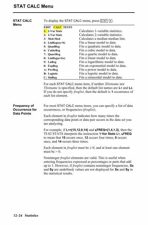
12–24 Statistics
82D315~1.DOC TI-83 international English Bob Fedorisko Revised: 10/26/05 1:36 PM Printed: 10/27/05 2:53PM Page 24 of 38
To display the STAT CALC menu, press … ~.
EDIT CALC TESTS1: 1-Var Stats Calculates 1-variable statistics.2: 2-Var Stats Calculates 2-variable statistics.3: Med-Med Calculates a median-median line.4: LinReg(ax+b) Fits a linear model to data.5: QuadReg Fits a quadratic model to data.6: CubicReg Fits a cubic model to data.7: QuartReg Fits a quartic model to data.8: LinReg(a+bx) Fits a linear model to data.9: LnReg Fits a logarithmic model to data.0: ExpReg Fits an exponential model to data.A: PwrReg Fits a power model to data.B: Logistic Fits a logistic model to data.C: SinReg Fits a sinusoidal model to data.
For each STAT CALC menu item, if neither Xlistname norYlistname is specified, then the default list names are L1 and L2.If you do not specify freqlist, then the default is 1 occurrence ofeach list element.
For most STAT CALC menu items, you can specify a list of dataoccurrences, or frequencies (freqlist).
Each element in freqlist indicates how many times thecorresponding data point or data pair occurs in the data set youare analyzing.
For example, if L1={15,12,9,14} and ÙÙÙÙFREQ={1,4,1,3}, then theTI-82 STATS interprets the instruction 1.Var Stats L1, ÙÙÙÙFREQto mean that 15 occurs once, 12 occurs four times, 9 occursonce, and 14 occurs three times.
Each element in freqlist must be ‚ 0, and at least one elementmust be > 0.
Noninteger freqlist elements are valid. This is useful whenentering frequencies expressed as percentages or parts that addup to 1. However, if freqlist contains noninteger frequencies, Sxand Sy are undefined; values are not displayed for Sx and Sy inthe statistical results.
STAT CALC Menu
STAT CALCMenu
Frequency ofOccurrence forData Points
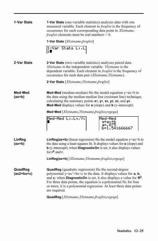
Statistics 12–25
82D315~1.DOC TI-83 international English Bob Fedorisko Revised: 10/26/05 1:36 PM Printed: 10/27/05 2:53PM Page 25 of 38
1.Var Stats (one-variable statistics) analyzes data with onemeasured variable. Each element in freqlist is the frequency ofoccurrence for each corresponding data point in Xlistname.freqlist elements must be real numbers > 0.
1.Var Stats [Xlistname,freqlist]
2.Var Stats (two-variable statistics) analyzes paired data.Xlistname is the independent variable. Ylistname is thedependent variable. Each element in freqlist is the frequency ofoccurrence for each data pair (Xlistname,Ylistname).
2.Var Stats [Xlistname,Ylistname,freqlist]
Med.Med (median-median) fits the model equation y=ax+b tothe data using the median-median line (resistant line) technique,calculating the summary points x1, y1, x2, y2, x3, and y3.Med.Med displays values for a (slope) and b (y-intercept).
Med.Med [Xlistname,Ylistname,freqlist,regequ]
LinReg(ax+b) (linear regression) fits the model equation y=ax+b tothe data using a least-squares fit. It displays values for a (slope) andb (y-intercept); when DiagnosticOn is set, it also displays valuesfor r2 and r.
LinReg(ax+b) [Xlistname,Ylistname,freqlist,regequ]
QuadReg (quadratic regression) fits the second-degreepolynomial y=ax2+bx+c to the data. It displays values for a, b,and c; when DiagnosticOn is set, it also displays a value for R2.For three data points, the equation is a polynomial fit; for fouror more, it is a polynomial regression. At least three data pointsare required.
QuadReg [Xlistname,Ylistname,freqlist,regequ]
1.Var Stats
2.Var Stats
Med.Med(ax+b)
LinReg(ax+b)
QuadReg(ax2+bx+c)

12–26 Statistics
82D315~1.DOC TI-83 international English Bob Fedorisko Revised: 10/26/05 1:36 PM Printed: 10/27/05 2:53PM Page 26 of 38
CubicReg (cubic regression) fits the third-degree polynomialy=ax3+bx2+cx+d to the data. It displays values for a, b, c, andd; when DiagnosticOn is set, it also displays a value for R2. Forfour points, the equation is a polynomial fit; for five or more, itis a polynomial regression. At least four points are required.
CubicReg [Xlistname,Ylistname,freqlist,regequ]
QuartReg (quartic regression) fits the fourth-degree polynomialy=ax4+bx3+cx2+dx+e to the data. It displays values for a, b, c,d, and e; when DiagnosticOn is set, it also displays a value forR2. For five points, the equation is a polynomial fit; for six ormore, it is a polynomial regression. At least five points arerequired.
QuartReg [Xlistname,Ylistname,freqlist,regequ]
LinReg(a+bx) (linear regression) fits the model equation y=a+bxto the data using a least-squares fit. It displays values for a(y-intercept) and b (slope); when DiagnosticOn is set, it alsodisplays values for r2 and r.
LinReg(a+bx) [Xlistname,Ylistname,freqlist,regequ]
LnReg (logarithmic regression) fits the model equationy=a+b ln(x) to the data using a least-squares fit and transformedvalues ln(x) and y. It displays values for a and b; whenDiagnosticOn is set, it also displays values for r2 and r.
LnReg [Xlistname,Ylistname,freqlist,regequ]
ExpReg (exponential regression) fits the model equation y=abx tothe data using a least-squares fit and transformed values x andln(y). It displays values for a and b; when DiagnosticOn is set, italso displays values for r2 and r.
ExpReg [Xlistname,Ylistname,freqlist,regequ]
STAT CALC Menu (continued)
CubicReg(ax3+bx2+cx+d)
QuartReg(ax4+bx3+cx2+dx+e)
LinReg(a+bx)
LnReg(a+b ln(x))
ExpReg(abx)
Statistics 12–27
82D315~1.DOC TI-83 international English Bob Fedorisko Revised: 10/26/05 1:36 PM Printed: 10/27/05 2:53PM Page 27 of 38
PwrReg (power regression) fits the model equation y=axb to thedata using a least-squares fit and transformed values ln(x) andln(y). It displays values for a and b; when DiagnosticOn is set, italso displays values for r2 and r.
PwrReg [Xlistname,Ylistname,freqlist,regequ]
Logistic fits the model equation y=c / (1+aäeLbx) to the data usingan iterative least-squares fit. It displays values for a, b, and c.
Logistic [Xlistname,Ylistname,freqlist,regequ]
SinReg (sinusoidal regression) fits the model equationy=a sin(bx+c)+d to the data using an iterative least-squares fit. Itdisplays values for a, b, c, and d. At least four data points arerequired. At least two data points per cycle are required in orderto avoid aliased frequency estimates.
SinReg [iterations,Xlistname,Ylistname,period,regequ]
iterations is the maximum number of times the algorithm williterate to find a solution. The value for iterations can be aninteger ‚ 1 and 16; if not specified, the default is 3. Thealgorithm may find a solution before iterations is reached.Typically, larger values for iterations result in longer executiontimes and better accuracy for SinReg, and vice versa.
A period guess is optional. If you do not specify period, thedifference between time values in Xlistname must be equal andthe time values must be ordered in ascending sequential order. Ifyou specify period, the algorithm may find a solution morequickly, or it may find a solution when it would not have foundone if you had omitted a value for period. If you specify period,the differences between time values in Xlistname can beunequal.
Note: The output of SinReg is always in radians, regardless of theRadian/Degree mode setting.
A SinReg example is shown on the next page.
PwrReg(axb)
Logisticc / (1+aääääeLbx)
SinRega sin(bx+c)+d
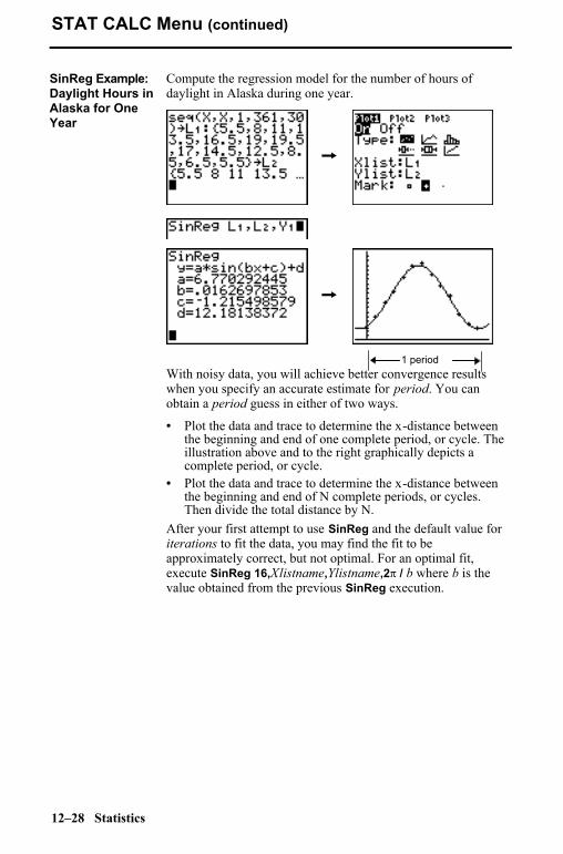
12–28 Statistics
82D315~1.DOC TI-83 international English Bob Fedorisko Revised: 10/26/05 1:36 PM Printed: 10/27/05 2:53PM Page 28 of 38
Compute the regression model for the number of hours ofdaylight in Alaska during one year.
&
&
With noisy data, you will achieve better convergence resultswhen you specify an accurate estimate for period. You canobtain a period guess in either of two ways.
• Plot the data and trace to determine the x-distance betweenthe beginning and end of one complete period, or cycle. Theillustration above and to the right graphically depicts acomplete period, or cycle.
• Plot the data and trace to determine the x-distance betweenthe beginning and end of N complete periods, or cycles.Then divide the total distance by N.
After your first attempt to use SinReg and the default value foriterations to fit the data, you may find the fit to beapproximately correct, but not optimal. For an optimal fit,execute SinReg 16,Xlistname,Ylistname,2p / b where b is thevalue obtained from the previous SinReg execution.
STAT CALC Menu (continued)
SinReg Example:Daylight Hours inAlaska for OneYear
1 period
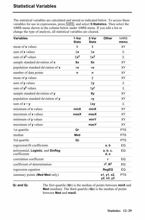
Statistics 12–29
82D315~1.DOC TI-83 international English Bob Fedorisko Revised: 10/26/05 1:36 PM Printed: 10/27/05 2:53PM Page 29 of 38
The statistical variables are calculated and stored as indicated below. To access thesevariables for use in expressions, press , and select 5:Statistics. Then select theVARS menu shown in the column below under VARS menu. If you edit a list orchange the type of analysis, all statistical variables are cleared.
Variables 1.VarStats
2.VarStats
Other VARSmenu
mean of x values v v XY
sum of x values Gx Gx G
sum of x2 values Gx2 Gx2 G
sample standard deviation of x Sx Sx XY
population standard deviation of x sx sx XY
number of data points n n XY
mean of y values w XY
sum of y values Gy G
sum of y2 values Gy2 G
sample standard deviation of y Sy XY
population standard deviation of y sy XY
sum of x … y Gxy G
minimum of x values minX minX XY
maximum of x values maxX maxX XY
minimum of y values minY XY
maximum of y values maxY XY
1st quartile Q1 PTS
median Med PTS
3rd quartile Q3 PTS
regression/fit coefficients a, b EQ
polynomial, Logistic, and SinRegcoefficients
a, b, c,d, e
EQ
correlation coefficient r EQ
coefficient of determination r2, R2 EQ
regression equation RegEQ EQ
summary points (Med.Med only) x1, y1, x2,y2, x3, y3
PTS
The first quartile (Q1) is the median of points between minX andMed (median). The third quartile (Q3) is the median of pointsbetween Med and maxX.
Statistical Variables
Q1 and Q3

12–30 Statistics
82D315~1.DOC TI-83 international English Bob Fedorisko Revised: 10/26/05 1:36 PM Printed: 10/27/05 2:53PM Page 30 of 38
You can enter statistical data, calculate statistical results, and fitmodels to data from a program. You can enter statistical datainto lists directly within the program (Chapter 11).
To perform a statistical calculation from a program, follow thesesteps.
1. On a blank line in the program editor, select the type ofcalculation from the STAT CALC menu.
2. Enter the names of the lists to use in the calculation. Separatethe list names with a comma.
3. Enter a comma and then the name of a Y= variable, if you wantto store the regression equation to a Y= variable.
Statistical Analysis in a Program
Entering StatData
StatisticalCalculations
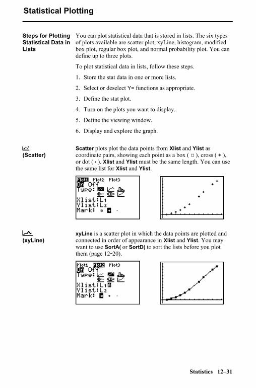
Statistics 12–31
82D315~1.DOC TI-83 international English Bob Fedorisko Revised: 10/26/05 1:36 PM Printed: 10/27/05 2:53PM Page 31 of 38
You can plot statistical data that is stored in lists. The six typesof plots available are scatter plot, xyLine, histogram, modifiedbox plot, regular box plot, and normal probability plot. You candefine up to three plots.
To plot statistical data in lists, follow these steps.
1. Store the stat data in one or more lists.
2. Select or deselect Y= functions as appropriate.
3. Define the stat plot.
4. Turn on the plots you want to display.
5. Define the viewing window.
6. Display and explore the graph.
Scatter plots plot the data points from Xlist and Ylist ascoordinate pairs, showing each point as a box ( › ), cross ( + ),or dot ( ¦ ). Xlist and Ylist must be the same length. You can usethe same list for Xlist and Ylist.
xyLine is a scatter plot in which the data points are plotted andconnected in order of appearance in Xlist and Ylist. You maywant to use SortA( or SortD( to sort the lists before you plotthem (page 12.20).
Statistical Plotting
Steps for PlottingStatistical Data inLists
""""(Scatter)
ÓÓÓÓ(xyLine)

12–32 Statistics
82D315~1.DOC TI-83 international English Bob Fedorisko Revised: 10/26/05 1:36 PM Printed: 10/27/05 2:53PM Page 32 of 38
Histogram plots one-variable data. The Xscl window variablevalue determines the width of each bar, beginning at Xmin.ZoomStat adjusts Xmin, Xmax, Ymin, and Ymax to include allvalues, and also adjusts Xscl. The inequality(Xmax N Xmin) à Xscl 47 must be true. A value that occurs onthe edge of a bar is counted in the bar to the right.
ModBoxplot (modified box plot) plots one-variable data, likethe regular box plot, except points that are 1.5 ääää InterquartileRange beyond the quartiles. (The Interquartile Range is definedas the difference between the third quartile Q3 and the firstquartile Q1.) These points are plotted individually beyond thewhisker, using the Mark (› or + or ¦) you select. You can tracethese points, which are called outliers.
The prompt for outlier points is x=, except when the outlier isthe maximum point (maxX) or the minimum point (minX).When outliers exist, the end of each whisker will display x=.When no outliers exist, minX and maxX are the prompts for theend of each whisker. Q1, Med (median), and Q3 define the box(page 12.29).
Box plots are plotted with respect to Xmin and Xmax, but ignoreYmin and Ymax. When two box plots are plotted, the first oneplots at the top of the screen and the second plots in the middle.When three are plotted, the first one plots at the top, the secondin the middle, and the third at the bottom.
Statistical Plotting (continued)
ÒÒÒÒ(Histogram)
ÕÕÕÕ(ModBoxplot)
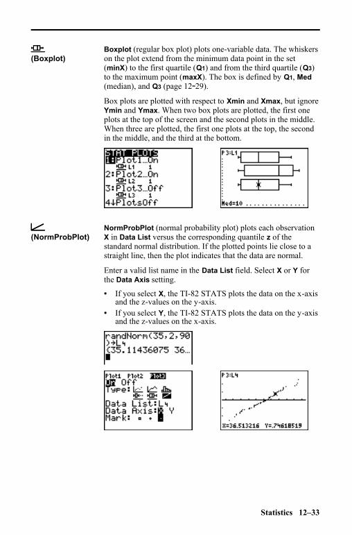
Statistics 12–33
82D315~1.DOC TI-83 international English Bob Fedorisko Revised: 10/26/05 1:36 PM Printed: 10/27/05 2:53PM Page 33 of 38
Boxplot (regular box plot) plots one-variable data. The whiskerson the plot extend from the minimum data point in the set(minX) to the first quartile (Q1) and from the third quartile (Q3)to the maximum point (maxX). The box is defined by Q1, Med(median), and Q3 (page 12.29).
Box plots are plotted with respect to Xmin and Xmax, but ignoreYmin and Ymax. When two box plots are plotted, the first oneplots at the top of the screen and the second plots in the middle.When three are plotted, the first one plots at the top, the secondin the middle, and the third at the bottom.
NormProbPlot (normal probability plot) plots each observationX in Data List versus the corresponding quantile z of thestandard normal distribution. If the plotted points lie close to astraight line, then the plot indicates that the data are normal.
Enter a valid list name in the Data List field. Select X or Y forthe Data Axis setting.
• If you select X, the TI-82 STATS plots the data on the x-axisand the z-values on the y-axis.
• If you select Y, the TI-82 STATS plots the data on the y-axisand the z-values on the x-axis.
ÖÖÖÖ(Boxplot)
ÔÔÔÔ(NormProbPlot)

12–34 Statistics
82D315~1.DOC TI-83 international English Bob Fedorisko Revised: 10/26/05 1:36 PM Printed: 10/27/05 2:53PM Page 34 of 38
To define a plot, follow these steps.
1. Press y [STAT PLOT]. The STAT PLOTS menu is displayedwith the current plot definitions.
2. Select the plot you want to use. The stat plot editor isdisplayed for the plot you selected.
3. Press Í to select On if you want to plot the statisticaldata immediately. The definition is stored whether you selectOn or Off.
4. Select the type of plot. Each type prompts for the optionschecked in this table.
Plot Type XList YList Mark Freq DataList
DataAxis
"""" Scatter œ œ œ
ÓÓÓÓ xyLine œ œ œ
ÒÒÒÒ Histogram œ œ œ œ
ÕÕÕÕ ModBoxplot œ œ œ
ÖÖÖÖ Boxplot œ œ œ œ
ÔÔÔÔ NormProbPlot œ œ œ
5. Enter list names or select options for the plot type.
• Xlist (list name containing independent data)• Ylist (list name containing dependent data)• Mark (› or + or ¦)• Freq (frequency list for Xlist elements; default is 1)• Data List (list name for NormProbPlot)• Data Axis (axis on which to plot Data List)
Statistical Plotting (continued)
Defining thePlots

Statistics 12–35
82D315~1.DOC TI-83 international English Bob Fedorisko Revised: 10/26/05 1:36 PM Printed: 10/27/05 2:53PM Page 35 of 38
Each stat plot has a unique stat plot editor. The name of thecurrent stat plot (Plot1, Plot2, or Plot3) is highlighted in the topline of the stat plot editor. To display the stat plot editor for adifferent plot, press }, ~, and | to move the cursor onto thename in the top line, and then press Í. The stat plot editorfor the selected plot is displayed, and the selected name remainshighlighted.
PlotsOn and PlotsOff allow you to turn on or turn off stat plotsfrom the home screen or a program. With no plot number,PlotsOn turns on all plots and PlotsOff turns off all plots. Withone or more plot numbers (1, 2, and 3), PlotsOn turns onspecified plots, and PlotsOff turns off specified plots.
PlotsOff [1,2,3]PlotsOn [1,2,3]
Note: You also can turn on and turn off stat plots in the top line of theY= editor (Chapter 3).
Displaying OtherStat Plot Editors
Turning On andTurning Off StatPlots

12–36 Statistics
82D315~1.DOC TI-83 international English Bob Fedorisko Revised: 10/26/05 1:36 PM Printed: 10/27/05 2:53PM Page 36 of 38
Stat plots are displayed on the current graph. To define theviewing window, press p and enter values for the windowvariables. ZoomStat redefines the viewing window to displayall statistical data points.
When you trace a scatter plot or xyLine, tracing begins at thefirst element in the lists.
When you trace a histogram, the cursor moves from the topcenter of one column to the top center of the next, starting at thefirst column.
When you trace a box plot, tracing begins at Med (the median).Press | to trace to Q1 and minX. Press ~ to trace to Q3 andmaxX.
When you press } or † to move to another plot or to anotherY= function, tracing moves to the current or beginning point onthat plot (not the nearest pixel).
The ExprOn/ExprOff format setting applies to stat plots(Chapter 3).When ExprOn is selected, the plot number andplotted data lists are displayed in the top-left corner.
Statistical Plotting (continued)
Defining theViewing Window
Tracing a StatPlot

Statistics 12–37
82D315~1.DOC TI-83 international English Bob Fedorisko Revised: 10/26/05 1:36 PM Printed: 10/27/05 2:53PM Page 37 of 38
To display a stat plot from a program, define the plot, and thendisplay the graph.
To define a stat plot from a program, begin on a blank line inthe program editor and enter data into one or more lists; then,follow these steps.
1. Press y [STAT PLOT] to display the STAT PLOTS menu.
2. Select the plot to define, which pastes Plot1(, Plot2(, orPlot3( to the cursor location.
3. Press y [STAT PLOT] ~ to display the STAT TYPE menu.
4. Select the type of plot, which pastes the name of the plottype to the cursor location.
Statistical Plotting in a Program
Defining a StatPlot in a Program
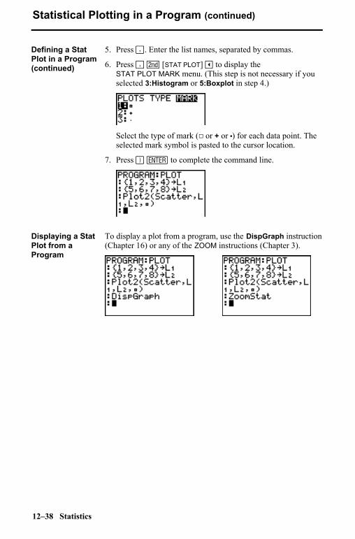
12–38 Statistics
82D315~1.DOC TI-83 international English Bob Fedorisko Revised: 10/26/05 1:36 PM Printed: 10/27/05 2:53PM Page 38 of 38
5. Press ¢. Enter the list names, separated by commas.
6. Press ¢ y [STAT PLOT] | to display theSTAT PLOT MARK menu. (This step is not necessary if youselected 3:Histogram or 5:Boxplot in step 4.)
Select the type of mark (› or + or ¦) for each data point. Theselected mark symbol is pasted to the cursor location.
7. Press ¤ Í to complete the command line.
To display a plot from a program, use the DispGraph instruction(Chapter 16) or any of the ZOOM instructions (Chapter 3).
Statistical Plotting in a Program (continued)
Defining a StatPlot in a Program(continued)
Displaying a StatPlot from aProgram

Inferential Statistics and Distributions 13–1
8250FC~1.DOC TI-83 international English Bob Fedorisko Revised: 10/26/05 1:39 PM Printed: 10/27/05 2:57PM Page 1 of 36
13 Inferential Statisticsand Distributions
Getting Started: Mean Height of a Population..................................... 2Inferential Stat Editors......................................................................................... 6STAT TESTS Menu ............................................................................................. 9Inferential Statistics Input Descriptions ................................................... 26Test and Interval Output Variables.............................................................. 28Distribution Functions ......................................................................................... 29Distribution Shading............................................................................................. 35
Contents

13–2 Inferential Statistics and Distributions
8250FC~1.DOC TI-83 international English Bob Fedorisko Revised: 10/26/05 1:39 PM Printed: 10/27/05 2:57PM Page 2 of 36
Getting Started is a fast-paced introduction. Read the chapter for details.
Suppose you want to estimate the mean height of a population of women given therandom sample below. Because heights among a biological population tend to benormally distributed, a t distribution confidence interval can be used when estimatingthe mean. The 10 height values below are the first 10 of 90 values, randomlygenerated from a normally distributed population with an assumed mean of 165.1 cm.and a standard deviation of 6.35 cm. (randNorm(165.1,6.35,90) with a seed of 789).
Height (in cm.) of Each of 10 Women
169.43 168.33 159.55 169.97 159.79 181.42 171.17 162.04 167.15 159.53
1. Press … Í to display the stat listeditor.
Press } to move the cursor onto L1, and thenpress y [INS]. The Name= prompt isdisplayed on the bottom line. The ØØØØ cursorindicates that alpha-lock is on. The existinglist name columns shift to the right.
Note: Your stat editor may not look like the onepictured here, depending on the lists you havealready stored.
2. Enter [H] [G] [H] [T] at the Name= prompt, andthen press Í. The list to which you willstore the women’s height data is created.
Press † to move the cursor onto the first rowof the list. HGHT(1)= is displayed on the bottomline.
3. Press 169 Ë 43 to enter the first height value.As you enter it, it is displayed on the bottomline.
Press Í. The value is displayed in the firstrow, and the rectangular cursor moves to thenext row.
Enter the other nine height values the sameway.
Getting Started: Mean Height of a Population

Inferential Statistics and Distributions 13–3
8250FC~1.DOC TI-83 international English Bob Fedorisko Revised: 10/26/05 1:39 PM Printed: 10/27/05 2:57PM Page 3 of 36
4. Press … | to display the STAT TESTSmenu, and then press † until 8:TInterval ishighlighted.
5. Press Í to select 8:TInterval. Theinferential stat editor for TInterval isdisplayed. If Data is not selected for Inpt:,press | Í to select Data.
Press † and [H] [G] [H] [T] at the List: prompt(alpha-lock is on).
Press † † Ë 99 to enter a 99 percentconfidence level at the C.Level: prompt.
6. Press † to move the cursor onto Calculate,and then press Í. The confidence intervalis calculated, and the TInterval results aredisplayed on the home screen.
Interpret the results.
The first line, (159.74,173.94), shows that the 99 percent confidence interval for thepopulation mean is between about 159.74 cm. and 173.94 cm. This is about a 14.2cm. spread.
The .99 confidence level indicates that in a very large number of samples, we expect99 percent of the intervals calculated to contain the population mean. The actual meanof the population sampled is 165.1 cm. (introduction; page 13.2), which is in thecalculated interval.
The second line gives the mean height of the sample þþþþ used to compute this interval.The third line gives the sample standard deviation Sx. The bottom line gives thesample size n.

13–4 Inferential Statistics and Distributions
8250FC~1.DOC TI-83 international English Bob Fedorisko Revised: 10/26/05 1:39 PM Printed: 10/27/05 2:57PM Page 4 of 36
To obtain a more precise bound on the population mean m of women’s heights,increase the sample size to 90. Use a sample mean þþþþ of 163.8 and sample standarddeviation Sx of 7.1 calculated from the larger random sample (introduction; page13.2). This time, use the Stats (summary statistics) input option.
7. Press … | 8 to display the inferential stateditor for TInterval.
Press ~ Í to select Inpt:Stats. The editorchanges so that you can enter summarystatistics as input.
8. Press † 163 Ë 8 Í to store 163.8 to þþþþ.
Press 7 Ë 1 Í to store 7.1 to Sx.
Press 90 Í to store 90 to n.
9. Press † to move the cursor onto Calculate,and then press Í to calculate the new 99percent confidence interval. The results aredisplayed on the home screen.
If the height distribution among a population of women is normally distributed with amean m of 165.1 cm. and a standard deviation σσσσ of 6.35 cm., what height is exceededby only 5 percent of the women (the 95th percentile)?
10. Press ‘ to clear the home screen.
Press y [DISTR] to display the DISTR(distributions) menu.
Getting Started: Mean Height of a Population (cont.)

Inferential Statistics and Distributions 13–5
8250FC~1.DOC TI-83 international English Bob Fedorisko Revised: 10/26/05 1:39 PM Printed: 10/27/05 2:57PM Page 5 of 36
11. Press 3 to paste invNorm( to the home screen.
Press Ë 95 ¢ 165 Ë 1 ¢ 6Ë 35 ¤ Í.
.95 is the area, 165.1 is µµµµ, and 6.35 is σσσσ.
The result is displayed on the home screen; it shows that five percent of the womenare taller than 175.5 cm.
Now graph and shade the top 5 percent of the population.
12. Press p and set the window variables tothese values.
Xmin=145 Ymin=L.02 Xres=1Xmax=185 Ymax=.08Xscl=5 Yscl=0
13. Press y [DISTR] ~ to display the DISTRDRAW menu.
14. Press Í to paste ShadeNorm( to the homescreen.
Press y [ANS] ¢ 1 y [EE] 99¢ 165Ë 1¢ 6 Ë 35 ¤.
Ans (175.5448205 from step 11) is the lowerbound. 1å99 is the upper bound. The normalcurve is defined by a mean µµµµ of 165.1 and astandard deviation σσσσ of 6.35.
15. Press Í to plot and shade the normalcurve.
Area is the area above the 95th percentile. lowis the lower bound. up is the upper bound.

13–6 Inferential Statistics and Distributions
8250FC~1.DOC TI-83 international English Bob Fedorisko Revised: 10/26/05 1:39 PM Printed: 10/27/05 2:57PM Page 6 of 36
When you select a hypothesis test or confidence intervalinstruction from the home screen, the appropriate inferentialstatistics editor is displayed. The editors vary according to eachtest or interval’s input requirements. Below is the inferential stateditor for T.Test.
Note: When you select the ANOVA( instruction, it is pasted to thehome screen. ANOVA( does not have an editor screen.
To use an inferential stat editor, follow these steps.
1. Select a hypothesis test or confidence interval from the STATTESTS menu. The appropriate editor is displayed.
2. Select Data or Stats input, if the selection is available. Theappropriate editor is displayed.
3. Enter real numbers, list names, or expressions for eachargument in the editor.
4. Select the alternative hypothesis (ƒ, <, or >) against which totest, if the selection is available.
5. Select No or Yes for the Pooled option, if the selection isavailable.
6. Select Calculate or Draw (when Draw is available) toexecute the instruction.• When you select Calculate, the results are displayed on
the home screen.• When you select Draw, the results are displayed in a
graph.
This chapter describes the selections in the above steps for eachhypothesis test and confidence interval instruction.
Inferential Stat Editors
Displaying theInferential StatEditors
Using anInferential StatEditor

Inferential Statistics and Distributions 13–7
8250FC~1.DOC TI-83 international English Bob Fedorisko Revised: 10/26/05 1:39 PM Printed: 10/27/05 2:57PM Page 7 of 36
Most inferential stat editors prompt you to select one of twotypes of input. (1.PropZInt and 2.PropZTest, 1.PropZInt and2.PropZInt, c2.Test, and LinRegTTest do not.)
• Select Data to enter the data lists as input.• Select Stats to enter summary statistics, such as þþþþ, Sx, and
n, as input.
To select Data or Stats, move the cursor to either Data or Stats,and then press Í.
Inferential stat editors require a value for every argument. If youdo not know what a particular argument symbol represents, seethe tables on pages 13.26 and 13.27.
When you enter values in any inferential stat editor, theTI-82 STATS stores them in memory so that you can run manytests or intervals without having to reenter every value.
Most of the inferential stat editors for the hypothesis testsprompt you to select one of three alternative hypotheses.
• The first is a ƒ alternative hypothesis, such as mƒm0 for theZ.Test.
• The second is a < alternative hypothesis, such as m1<m2 forthe 2.SampTTest.
• The third is a > alternative hypothesis, such as p1>p2 for the2.PropZTest.
To select an alternative hypothesis, move the cursor to theappropriate alternative, and then press Í.
Selecting Data orStats
Entering theValues forArguments
Selecting anAlternativeHypothesis(ƒ < >)
Enter values forarguments
Select an alternativehypothesis
Select Calculateor Draw output
Select Data orStats input

13–8 Inferential Statistics and Distributions
8250FC~1.DOC TI-83 international English Bob Fedorisko Revised: 10/26/05 1:39 PM Printed: 10/27/05 2:57PM Page 8 of 36
Pooled (2.SampTTest and 2.SampTInt only) specifies whetherthe variances are to be pooled for the calculation.
• Select No if you do not want the variances pooled.Population variances can be unequal.
• Select Yes if you want the variances pooled. Populationvariances are assumed to be equal.
To select the Pooled option, move the cursor to Yes, and thenpress Í.
After you have entered all arguments in an inferential stat editorfor a hypothesis test, you must select whether you want to seethe calculated results on the home screen (Calculate) or on thegraph screen (Draw).
• Calculate calculates the test results and displays the outputson the home screen.
• Draw draws a graph of the test results and displays the teststatistic and p-value with the graph. The window variablesare adjusted automatically to fit the graph.
To select Calculate or Draw, move the cursor to eitherCalculate or Draw, and then press Í. The instruction isimmediately executed.
After you have entered all arguments in an inferential stat editorfor a confidence interval, select Calculate to display the results.The Draw option is not available.
When you press Í, Calculate calculates the confidenceinterval results and displays the outputs on the home screen.
To paste a hypothesis test or confidence interval instruction tothe home screen without displaying the correspondinginferential stat editor, select the instruction you want from theCATALOG menu. Appendix A describes the input syntax foreach hypothesis test and confidence interval instruction.
Note: You can paste a hypothesis test or confidence intervalinstruction to a command line in a program. From within the programeditor, select the instruction from either the CATALOG (Chapter 15)or the STAT TESTS menu.
Inferential Stat Editors (continued)
Selecting thePooled Option
SelectingCalculate orDraw for aHypothesis Test
SelectingCalculate for aConfidenceInterval
Bypassing theInferential StatEditors

Inferential Statistics and Distributions 13–9
8250FC~1.DOC TI-83 international English Bob Fedorisko Revised: 10/26/05 1:39 PM Printed: 10/27/05 2:57PM Page 9 of 36
To display the STAT TESTS menu, press … |. When youselect an inferential statistics instruction, the appropriateinferential stat editor is displayed.
Most STAT TESTS instructions store some output variables tomemory. Most of these output variables are in the TESTsecondary menu (VARS menu; 5:Statistics). For a list of thesevariables, see page 13.28.
EDIT CALC TESTS1: Z-Test... Test for 1 m, known s2: T-Test... Test for 1 m, unknown s3: 2-SampZTest... Test comparing 2 m’s, known s’s4: 2-SampTTest... Test comparing 2 m’s, unknown s’s5: 1-PropZTest... Test for 1 proportion6: 2-PropZTest... Test comparing 2 proportions7: ZInterval... Confidence interval for 1 m, known s8: TInterval... Confidence interval for 1 m, unknown s9: 2-SampZInt... Conf. int. for diff. of 2 m’s, known s’s0: 2-SampTInt... Conf. int. for diff. of 2 m’s, unknown s’sA: 1-PropZInt... Confidence int. for 1 proportionB: 2-PropZInt... Confidence int. for diff. of 2 propsC: c2-Test... Chi-square test for 2-way tablesD: 2-SampÛÛÛÛTest... Test comparing 2 s’sE: LinRegTTest... t test for regression slope and rF: ANOVA( One-way analysis of varianceNote: When a new test or interval is computed, all previous outputvariables are invalidated.
In this chapter, the description of each STAT TESTS instructionshows the unique inferential stat editor for that instruction withexample arguments.
• Descriptions of instructions that offer the Data/Stats inputchoice show both types of input screens.
• Descriptions of instructions that do not offer the Data/Statsinput choice show only one input screen.
The description then shows the unique output screen for thatinstruction with the example results.
• Descriptions of instructions that offer the Calculate/Drawoutput choice show both types of screens: calculated andgraphic results.
• Descriptions of instructions that offer only the Calculateoutput choice show the calculated results on the homescreen.
STAT TESTS Menu
STAT TESTSMenu
Inferential StatEditors for theSTAT TESTSInstructions
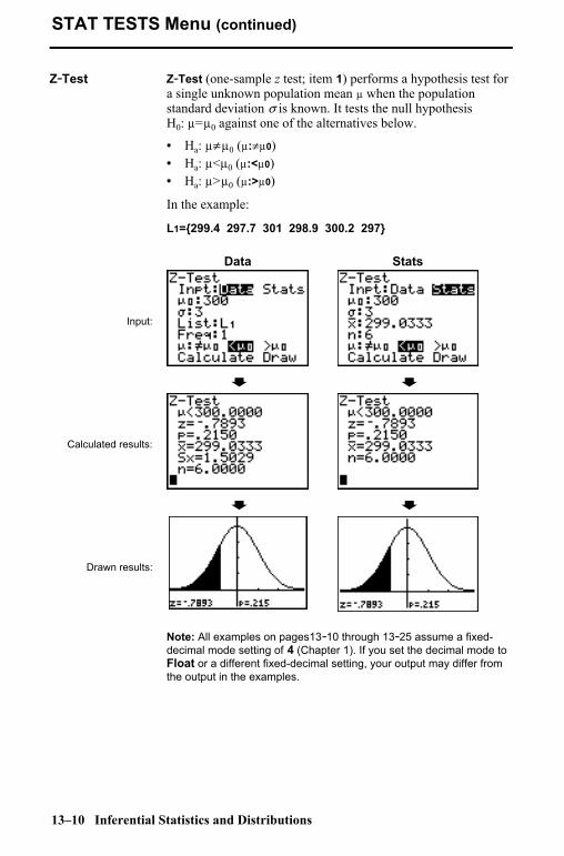
13–10 Inferential Statistics and Distributions
8250FC~1.DOC TI-83 international English Bob Fedorisko Revised: 10/26/05 1:39 PM Printed: 10/27/05 2:57PM Page 10 of 36
Z.Test (one-sample z test; item 1) performs a hypothesis test fora single unknown population mean m when the populationstandard deviation s is known. It tests the null hypothesisH0: m=m0 against one of the alternatives below.
• Ha: mƒm0 (m:ƒm0)• Ha: m<m0 (m:<m0)• Ha: m>m0 (m:>m0)
In the example:
L1={299.4 297.7 301 298.9 300.2 297}
Data Stats
Input:
, ,
Calculated results:
, ,
Drawn results:
Note: All examples on pages13.10 through 13.25 assume a fixed-decimal mode setting of 4 (Chapter 1). If you set the decimal mode toFloat or a different fixed-decimal setting, your output may differ fromthe output in the examples.
STAT TESTS Menu (continued)
Z.Test

Inferential Statistics and Distributions 13–11
8250FC~1.DOC TI-83 international English Bob Fedorisko Revised: 10/26/05 1:39 PM Printed: 10/27/05 2:57PM Page 11 of 36
T.Test (one-sample t test; item 2) performs a hypothesis test fora single unknown population mean m when the populationstandard deviation s is unknown. It tests the null hypothesisH0: m=m0 against one of the alternatives below.
• Ha: mƒm0 (m:ƒm0)• Ha: m<m0 (m:<m0)• Ha: m>m0 (m:>m0)
In the example:
TEST={91.9 97.8 111.4 122.3 105.4 95}
Data Stats
Input:
, ,
Calculated results:
, ,
Drawn results:
T.Test

13–12 Inferential Statistics and Distributions
8250FC~1.DOC TI-83 international English Bob Fedorisko Revised: 10/26/05 1:39 PM Printed: 10/27/05 2:57PM Page 12 of 36
2.SampZTest (two-sample z test; item 3) tests the equality ofthe means of two populations (m1 and m2) based on independentsamples when both population standard deviations (s1 and s2)are known. The null hypothesis H0: m1=m2 is tested against oneof the alternatives below.
• Ha: m1ƒm2 (m1:ƒm2)• Ha: m1<m2 (m1:<m2)• Ha: m1>m2 (m1:>m2)
In the example:
LISTA={154 109 137 115 140}LISTB={108 115 126 92 146}
Data Stats
Input:
, ,
Calculated results:
, ,
Drawn results:
STAT TESTS Menu (continued)
2.SampZTest
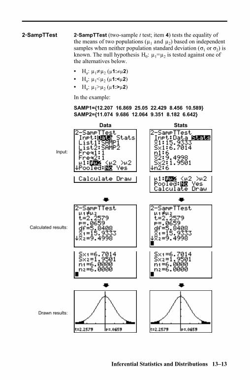
Inferential Statistics and Distributions 13–13
8250FC~1.DOC TI-83 international English Bob Fedorisko Revised: 10/26/05 1:39 PM Printed: 10/27/05 2:57PM Page 13 of 36
2.SampTTest (two-sample t test; item 4) tests the equality ofthe means of two populations (m1 and m2) based on independentsamples when neither population standard deviation (s1 or s2) isknown. The null hypothesis H0: m1=m2 is tested against one ofthe alternatives below.
• Ha: m1ƒm2 (m1:ƒm2)• Ha: m1<m2 (m1:<m2)• Ha: m1>m2 (m1:>m2)
In the example:
SAMP1={12.207 16.869 25.05 22.429 8.456 10.589}SAMP2={11.074 9.686 12.064 9.351 8.182 6.642}
Data Stats
Input:
, ,
Calculated results:
, ,
Drawn results:
2.SampTTest

13–14 Inferential Statistics and Distributions
8250FC~1.DOC TI-83 international English Bob Fedorisko Revised: 10/26/05 1:39 PM Printed: 10/27/05 2:57PM Page 14 of 36
1.PropZTest (one-proportion z test; item 5) computes a test foran unknown proportion of successes (prop). It takes as input thecount of successes in the sample x and the count of observationsin the sample n. 1.PropZTest tests the null hypothesisH0: prop=p0 against one of the alternatives below.
• Ha: propƒp0 (prop:ƒp0)• Ha: prop<p0 (prop:<p0)• Ha: prop>p0 (prop:>p0)
Input:
,
Calculated results:
,
Drawn results:
STAT TESTS Menu (continued)
1.PropZTest

Inferential Statistics and Distributions 13–15
8250FC~1.DOC TI-83 international English Bob Fedorisko Revised: 10/26/05 1:39 PM Printed: 10/27/05 2:57PM Page 15 of 36
2.PropZTest (two-proportion z test; item 6) computes a test tocompare the proportion of successes (p1 and p2) from twopopulations. It takes as input the count of successes in eachsample (x1 and x2) and the count of observations in each sample(n1 and n2). 2.PropZTest tests the null hypothesis H0: p1=p2(using the pooled sample proportion Ç) against one of thealternatives below.
• Ha: p1ƒp2 (p1:ƒp2)• Ha: p1<p2 (p1:<p2)• Ha: p1>p2 (p1:>p2)
Input:
,
Calculated results:
,
Drawn results:
2.PropZTest

13–16 Inferential Statistics and Distributions
8250FC~1.DOC TI-83 international English Bob Fedorisko Revised: 10/26/05 1:39 PM Printed: 10/27/05 2:57PM Page 16 of 36
ZInterval (one-sample z confidence interval; item 7) computes aconfidence interval for an unknown population mean m when thepopulation standard deviation s is known. The computedconfidence interval depends on the user-specified confidencelevel.
In the example:
L1={299.4 297.7 301 298.9 300.2 297}
Data Stats
Input:
, ,
Calculated results:
STAT TESTS Menu (continued)
ZInterval

Inferential Statistics and Distributions 13–17
8250FC~1.DOC TI-83 international English Bob Fedorisko Revised: 10/26/05 1:39 PM Printed: 10/27/05 2:57PM Page 17 of 36
TInterval (one-sample t confidence interval; item 8) computes aconfidence interval for an unknown population mean m when thepopulation standard deviation s is unknown. The computedconfidence interval depends on the user-specified confidencelevel.
In the example:
L6={1.6 1.7 1.8 1.9}
Data Stats
Input:
, ,
Calculated results:
TInterval

13–18 Inferential Statistics and Distributions
8250FC~1.DOC TI-83 international English Bob Fedorisko Revised: 10/26/05 1:39 PM Printed: 10/27/05 2:57PM Page 18 of 36
2.SampZInt (two-sample z confidence interval; item 9)computes a confidence interval for the difference between twopopulation means (m1Nm2) when both population standarddeviations (s1 and s2) are known. The computed confidenceinterval depends on the user-specified confidence level.
In the example:
LISTC={154 109 137 115 140}LISTD={108 115 126 92 146}
Data Stats
Input:
, ,
Calculated results:
STAT TESTS Menu (continued)
2.SampZInt

Inferential Statistics and Distributions 13–19
8250FC~1.DOC TI-83 international English Bob Fedorisko Revised: 10/26/05 1:39 PM Printed: 10/27/05 2:57PM Page 19 of 36
2.SampTInt (two-sample t confidence interval; item 0)computes a confidence interval for the difference between twopopulation means (m1Nm2) when both population standarddeviations (s1 and s2) are unknown. The computed confidenceinterval depends on the user-specified confidence level.
In the example:
SAMP1={12.207 16.869 25.05 22.429 8.456 10.589}SAMP2={11.074 9.686 12.064 9.351 8.182 6.642}
Data Stats
Input:
, ,
Calculated results:
2.SampTInt

13–20 Inferential Statistics and Distributions
8250FC~1.DOC TI-83 international English Bob Fedorisko Revised: 10/26/05 1:39 PM Printed: 10/27/05 2:57PM Page 20 of 36
1.PropZInt (one-proportion z confidence interval; item A)computes a confidence interval for an unknown proportion ofsuccesses. It takes as input the count of successes in the samplex and the count of observations in the sample n. The computedconfidence interval depends on the user-specified confidencelevel.
Input:
,
Calculated results:
STAT TESTS Menu (continued)
1.PropZInt

Inferential Statistics and Distributions 13–21
8250FC~1.DOC TI-83 international English Bob Fedorisko Revised: 10/26/05 1:39 PM Printed: 10/27/05 2:57PM Page 21 of 36
2.PropZInt (two-proportion z confidence interval; item B)computes a confidence interval for the difference between theproportion of successes in two populations (p1Np2). It takes asinput the count of successes in each sample (x1 and x2) and thecount of observations in each sample (n1 and n2). The computedconfidence interval depends on the user-specified confidencelevel.
Input:
,
Calculated results:
2.PropZInt

13–22 Inferential Statistics and Distributions
8250FC~1.DOC TI-83 international English Bob Fedorisko Revised: 10/26/05 1:39 PM Printed: 10/27/05 2:57PM Page 22 of 36
c2.Test (chi-square test; item C) computes a chi-square test forassociation on the two-way table of counts in the specifiedObserved matrix. The null hypothesis H0 for a two-way table is:no association exists between row variables and columnvariables. The alternative hypothesis is: the variables are related.
Before computing a c2.Test, enter the observed counts in amatrix. Enter that matrix variable name at the Observed:prompt in the c2.Test editor; default=[A]. At the Expected:prompt, enter the matrix variable name to which you want thecomputed expected counts to be stored; default=[B].
Matrix editor:
Note: Press ~ ~ 1 toselect 1:[A] from the MATRXEDIT menu.
Input:
, Note: Press [B] Í todisplay matrix [B].
Calculated results:
,
Drawn results:
STAT TESTS Menu (continued)
c2.Test

Inferential Statistics and Distributions 13–23
8250FC~1.DOC TI-83 international English Bob Fedorisko Revised: 10/26/05 1:39 PM Printed: 10/27/05 2:57PM Page 23 of 36
2.SampÜÜÜÜTest (two-sample Û-test; item D) computes an Û-test tocompare two normal population standard deviations (s1 and s2).The population means and standard deviations are all unknown.2.SampÜÜÜÜTest, which uses the ratio of sample variancesSx12/Sx22, tests the null hypothesis H0: s1=s2 against one of thealternatives below.
• Ha: s1ƒs2 (s1:ƒs2)• Ha: s1<s2 (s1:<s2)• Ha: s1>s2 (s1:>s2)
In the example:
SAMP4={ 7 L4 18 17 L3 L5 1 10 11 L2}SAMP5={ L1 12 L1 L3 3 L5 5 2 L11 L1 L3}
Data Stats
Input:
, ,
Calculated results:
, ,
Drawn results:
2.SampÜÜÜÜTest

13–24 Inferential Statistics and Distributions
8250FC~1.DOC TI-83 international English Bob Fedorisko Revised: 10/26/05 1:39 PM Printed: 10/27/05 2:57PM Page 24 of 36
LinRegTTest (linear regression t test; item E) computes a linearregression on the given data and a t test on the value of slope band the correlation coefficient r for the equation y=a+bx. Ittests the null hypothesis H0: b=0 (equivalently, r=0) against oneof the alternatives below.
• Ha: bƒ0 and rƒ0 (b & r:ƒ0)• Ha: b<0 and r<0 (b & r:<0)• Ha: b>0 and r>0 (b & r:>0)
The regression equation is automatically stored to RegEQ(VARS Statistics EQ secondary menu). If you enter a Y= variablename at the RegEQ: prompt, the calculated regression equationis automatically stored to the specified Y= equation. In theexample below, the regression equation is stored to Y1, which isthen selected (turned on).
In the example:
L3={38 56 59 64 74}L4={41 63 70 72 84}
Input:
,
Calculated results:
When LinRegTTest is executed, the list of residuals is createdand stored to the list name RESID automatically. RESID isplaced on the LIST NAMES menu.
Note: For the regression equation, you can use the fix -decimal modesetting to control the number of digits stored after the decimal point(Chapter 1). However, limiting the number of digits to a small numbercould affect the accuracy of the fit.
STAT TESTS Menu (continued)
LinRegTTest
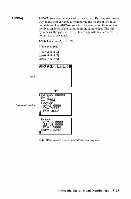
Inferential Statistics and Distributions 13–25
8250FC~1.DOC TI-83 international English Bob Fedorisko Revised: 10/26/05 1:39 PM Printed: 10/27/05 2:57PM Page 25 of 36
ANOVA( (one-way analysis of variance; item F) computes a one-way analysis of variance for comparing the means of two to 20populations. The ANOVA procedure for comparing these meansinvolves analysis of the variation in the sample data. The nullhypothesis H0: m1=m2=...=mk is tested against the alternative Ha:not all m1...mk are equal.
ANOVA(list1,list2[,...,list20])
In the example:
L1={7 4 6 6 5}L2={6 5 5 8 7}L3={4 7 6 7 6}
Input:
,
Calculated results:
Note: SS is sum of squares and MS is mean square.
ANOVA(
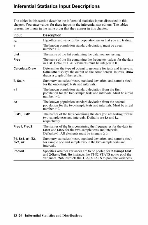
13–26 Inferential Statistics and Distributions
8250FC~1.DOC TI-83 international English Bob Fedorisko Revised: 10/26/05 1:39 PM Printed: 10/27/05 2:57PM Page 26 of 36
The tables in this section describe the inferential statistics inputs discussed in thischapter. You enter values for these inputs in the inferential stat editors. The tablespresent the inputs in the same order that they appear in this chapter.
Input Descriptionm0 Hypothesized value of the population mean that you are testing.s The known population standard deviation; must be a real
number > 0.List The name of the list containing the data you are testing.Freq The name of the list containing the frequency values for the data
in List. Default=1. All elements must be integers | 0.Calculate/Draw Determines the type of output to generate for tests and intervals.
Calculate displays the output on the home screen. In tests, Drawdraws a graph of the results.
v, Sx, n Summary statistics (mean, standard deviation, and sample size)for the one-sample tests and intervals.
s1 The known population standard deviation from the firstpopulation for the two-sample tests and intervals. Must be a realnumber > 0.
s2 The known population standard deviation from the secondpopulation for the two-sample tests and intervals. Must be a realnumber > 0.
List1, List2 The names of the lists containing the data you are testing for thetwo-sample tests and intervals. Defaults are L1 and L2,respectively.
Freq1, Freq2 The names of the lists containing the frequencies for the data inList1 and List2 for the two-sample tests and intervals.Defaults=1. All elements must be integers | 0.
v1, Sx1, n1, v2,Sx2, n2
Summary statistics (mean, standard deviation, and sample size)for sample one and sample two in the two-sample tests andintervals.
Pooled Specifies whether variances are to be pooled for 2.SampTTestand 2.SampTInt. No instructs the TI-82 STATS not to pool thevariances. Yes instructs the TI-82 STATS to pool the variances.
Inferential Statistics Input Descriptions

Inferential Statistics and Distributions 13–27
8250FC~1.DOC TI-83 international English Bob Fedorisko Revised: 10/26/05 1:39 PM Printed: 10/27/05 2:57PM Page 27 of 36
Input Descriptionp0 The expected sample proportion for 1.PropZTest. Must be a
real number, such that 0 < p0 < 1.x The count of successes in the sample for the 1.PropZTest and
1.PropZInt. Must be an integer ‚ 0.n The count of observations in the sample for the 1.PropZTest
and 1.PropZInt. Must be an integer > 0.x1 The count of successes from sample one for the 2.PropZTest
and 2.PropZInt. Must be an integer ‚ 0.x2 The count of successes from sample two for the 2.PropZTest
and 2.PropZInt. Must be an integer ‚ 0.n1 The count of observations in sample one for the 2.PropZTest
and 2.PropZInt. Must be an integer > 0.n2 The count of observations in sample two for the 2.PropZTest
and 2.PropZInt. Must be an integer > 0.C.Level The confidence level for the interval instructions. Must be ‚ 0
and <100. If it is ‚ 1, it is assumed to be given as a percent andis divided by 100. Default=0.95.
Observed (Matrix) The matrix name that represents the columns and rows for theobserved values of a two-way table of counts for the c2.Test.Observed must contain all integers ‚ 0. Matrix dimensions mustbe at least 2×2.
Expected (Matrix) The matrix name that specifies where the expected valuesshould be stored. Expected is created upon successfulcompletion of the c2.Test.
Xlist, Ylist The names of the lists containing the data for LinRegTTest.Defaults are L1 and L2, respectively. The dimensions of Xlistand Ylist must be the same.
RegEQ The prompt for the name of the Y= variable where the calculatedregression equation is to be stored. If a Y= variable is specified,that equation is automatically selected (turned on). The defaultis to store the regression equation to the RegEQ variable only.

13–28 Inferential Statistics and Distributions
8250FC~1.DOC TI-83 international English Bob Fedorisko Revised: 10/26/05 1:39 PM Printed: 10/27/05 2:57PM Page 28 of 36
The inferential statistics variables are calculated as indicated below. To access thesevariables for use in expressions, press , 5 (5:Statistics), and then select theVARS menu listed in the last column below.
Variables Tests IntervalsLinRegTTest,ANOVA
VARSMenu
p-value p p TEST
test statistics z, t, c2, ÜÜÜÜ t, ÜÜÜÜ TEST
degrees of freedom df df df TEST
sample mean of x values for sample1 and sample 2
v1, v2 v1, v2 TEST
sample standard deviation of x forsample 1 and sample 2
Sx1,Sx2
Sx1,Sx2
TEST
number of data points for sample 1and sample 2
n1, n2 n1, n2 TEST
pooled standard deviation SxP SxP SxP TEST
estimated sample proportion ÇÇÇÇ ÇÇÇÇ TEST
estimated sample proportion forpopulation 1
ÇÇÇÇ1 ÇÇÇÇ1 TEST
estimated sample proportion forpopulation 2
ÇÇÇÇ2 ÇÇÇÇ2 TEST
confidence interval pair lower,upper
TEST
mean of x values v v XY
sample standard deviation of x Sx Sx XY
number of data points n n XY
standard error about the line s TEST
regression/fit coefficients a, b EQ
correlation coefficient r EQ
coefficient of determination r2 EQ
regression equation RegEQ EQ
Test and Interval Output Variables

Inferential Statistics and Distributions 13–29
8250FC~1.DOC TI-83 international English Bob Fedorisko Revised: 10/26/05 1:39 PM Printed: 10/27/05 2:57PM Page 29 of 36
To display the DISTR menu, press y [DISTR].
DISTR DRAW1: normalpdf( Normal probability density2: normalcdf( Normal distribution probability3: invNorm( Inverse cumulative normal distribution4: tpdf( Student-t probability density5: tcdf( Student-t distribution probability6: c2pdf( Chi-square probability density7: c2cdf Chi-square distribution probability8: Üpdf( Û probability density9: Ücdf( Û distribution probability0: binompdf( Binomial probabilityA: binomcdf( Binomial cumulative densityB: poissonpdf( Poisson probabilityC: poissoncdf( Poisson cumulative densityD: geometpdf( Geometric probabilityE: geometcdf( Geometric cumulative density
Note: L1å99 and 1å99 specify infinity. If you want to view the area leftof upperbound, for example, specify lowerbound=L1å99.
norwmalpdf( computes the probability density function (pdf) forthe normal distribution at a specified x value. The defaults aremean m=0 and standard deviation s=1. To plot the normaldistribution, paste normalpdf( to the Y= editor. The probabilitydensity function (pdf) is:
f x ex
( ) = >− −1
20
2
22π σ
σµ
σ( )
,
normalpdf(x[,m,s])
Note: For this example,Xmin = 28Xmax = 42Ymin = 0Ymax = .25
Tip: For plotting the normal distribution, you can set window variablesXmin and Xmax so that the mean m falls between them, and thenselect 0:ZoomFit from the ZOOM menu.
Distribution Functions
DISTR menu
normalpdf(

13–30 Inferential Statistics and Distributions
8250FC~1.DOC TI-83 international English Bob Fedorisko Revised: 10/26/05 1:39 PM Printed: 10/27/05 2:57PM Page 30 of 36
normalcdf( computes the normal distribution probabilitybetween lowerbound and upperbound for the specified mean mand standard deviation s. The defaults are m=0and s=1.
normalcdf(lowerbound,upperbound[,m,s])
invNorm( computes the inverse cumulative normal distributionfunction for a given area under the normal distribution curvespecified by mean m and standard deviation s. It calculates the xvalue associated with an area to the left of the x value.0 area 1 must be true. The defaults are m=0 and s=1.
invNorm(area[,m,s])
tpdf( computes the probability density function (pdf) for theStudent-t distribution at a specified x value. df (degrees offreedom) must be >0. To plot the Student-t distribution, pastetpdf( to the Y= editor. The probability density function (pdf) is:
f x dfdf
x dfdf
df( ) [( ) ]
( )( ) ( )
= + + − +ΓΓ
1 22
1 2 1 2//
/ /
π
tpdf(x,df)
Note: For this example,Xmin = L4.5Xmax = 4.5Ymin = 0Ymax = .4
Distribution Functions (continued)
normalcdf(
invNorm(
tpdf(

Inferential Statistics and Distributions 13–31
8250FC~1.DOC TI-83 international English Bob Fedorisko Revised: 10/26/05 1:39 PM Printed: 10/27/05 2:57PM Page 31 of 36
tcdf( computes the Student-t distribution probability betweenlowerbound and upperbound for the specified df (degrees offreedom), which must be > 0.
tcdf(lowerbound,upperbound,df)
c2pdf( computes the probability density function (pdf) for the c2
(chi-square) distribution at a specified x value. df (degrees offreedom) must be an integer > 0. To plot the c2 distribution,paste c2pdf( to the Y= editor. The probability density function(pdf) is:
f xdf
x e xdf df x( )( )
(1/2)= ≥− −12
02 2 1 2Γ /
,/ / /
c2pdf(x,df)
Note: For this example,Xmin = 0Xmax = 30Ymin = L.02Ymax = .132
c2cdf( computes the c2 (chi-square) distribution probabilitybetween lowerbound and upperbound for the specified df(degrees of freedom), which must be an integer > 0.
c2cdf(lowerbound,upperbound,df)
tcdf(
c2pdf(
c2cdf(

13–32 Inferential Statistics and Distributions
8250FC~1.DOC TI-83 international English Bob Fedorisko Revised: 10/26/05 1:39 PM Printed: 10/27/05 2:57PM Page 32 of 36
ÜÜÜÜpdf( computes the probability density function (pdf) for the Ûdistribution at a specified x value. numerator df (degrees offreedom) and denominator df must be integers > 0. To plot the Ûdistribution, paste ÜÜÜÜpdf( to the Y= editor. The probabilitydensity function (pdf) is:
f x n dn d
nd
x nx d xn
n n d( ) [( ) ]( ) ( )
( ) ( )= +
+ ≥− − +ΓΓ Γ
// /
/ ,/
/ /22 2
1 02
2 1 2
where n = numerator degrees of freedomd = denominator degrees of freedom
ÜÜÜÜpdf(x,numerator df,denominator df)
Note: For this example,Xmin = 0Xmax = 5Ymin = 0Ymax = 1
ÜÜÜÜcdf( computes the Û distribution probability betweenlowerbound and upperbound for the specified numerator df(degrees of freedom) and denominator df. numerator df anddenominator df must be integers >0.
ÜÜÜÜcdf(lowerbound,upperbound,numerator df,denominator df)
Distribution Functions (continued)
ÜÜÜÜpdf(
ÜÜÜÜcdf(
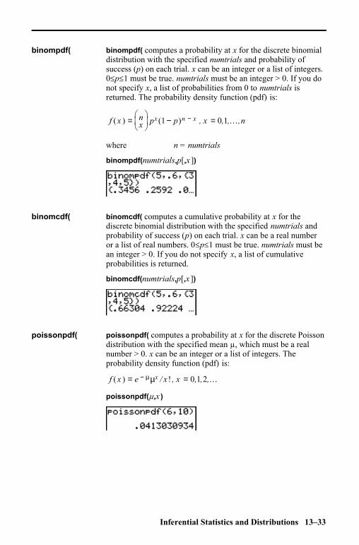
Inferential Statistics and Distributions 13–33
8250FC~1.DOC TI-83 international English Bob Fedorisko Revised: 10/26/05 1:39 PM Printed: 10/27/05 2:57PM Page 33 of 36
binompdf( computes a probability at x for the discrete binomialdistribution with the specified numtrials and probability ofsuccess (p) on each trial. x can be an integer or a list of integers.0p1 must be true. numtrials must be an integer > 0. If you donot specify x, a list of probabilities from 0 to numtrials isreturned. The probability density function (pdf) is:
f x nx p p x nx n x( ) ( )=
− =−1 0 1, , , ,K
where n = numtrials
binompdf(numtrials,p[,x ])
binomcdf( computes a cumulative probability at x for thediscrete binomial distribution with the specified numtrials andprobability of success (p) on each trial. x can be a real numberor a list of real numbers. 0p1 must be true. numtrials must bean integer > 0. If you do not specify x, a list of cumulativeprobabilities is returned.
binomcdf(numtrials,p[,x ])
poissonpdf( computes a probability at x for the discrete Poissondistribution with the specified mean m, which must be a realnumber > 0. x can be an integer or a list of integers. Theprobability density function (pdf) is:
f x e x xx( ) != =− µµ / , , , ,0 1 2 K
poissonpdf(m,x )
binompdf(
binomcdf(
poissonpdf(

13–34 Inferential Statistics and Distributions
8250FC~1.DOC TI-83 international English Bob Fedorisko Revised: 10/26/05 1:39 PM Printed: 10/27/05 2:57PM Page 34 of 36
poissoncdf( computes a cumulative probability at x for thediscrete Poisson distribution with the specified mean m, whichmust be a real number > 0. x can be a real number or a list ofreal numbers.
poissoncdf(m,x )
geometpdf( computes a probability at x, the number of the trialon which the first success occurs, for the discrete geometricdistribution with the specified probability of success p. 0p1must be true. x can be an integer or a list of integers. Theprobability density function (pdf) is:
f x p p xx( ) ( )= − =−1 1 21 , , ,K
geometpdf(p,x )
geometcdf( computes a cumulative probability at x, the numberof the trial on which the first success occurs, for the discretegeometric distribution with the specified probability of successp. 0p1 must be true. x can be a real number or a list of realnumbers.
geometcdf(p,x )
Distribution Functions (continued)
poissoncdf(
geometpdf(
geometcdf(

Inferential Statistics and Distributions 13–35
8250FC~1.DOC TI-83 international English Bob Fedorisko Revised: 10/26/05 1:39 PM Printed: 10/27/05 2:57PM Page 35 of 36
To display the DISTR DRAW menu, press y [DISTR] ~.DISTR DRAW instructions draw various types of densityfunctions, shade the area specified by lowerbound andupperbound, and display the computed area value.
To clear the drawings, select 1:ClrDraw from the DRAW menu(Chapter 8).
Note: Before you execute a DISTR DRAW instruction, you must setthe window variables so that the desired distribution fits the screen.
DISTR DRAW
1: ShadeNorm( Shades normal distribution.2: Shade_t( Shades Student-t distribution.3: Shadec2( Shades c2 distribution.4: ShadeÛÛÛÛ( Shades Û distribution.
Note: L1å99 and 1å99 specify infinity. If you want to view the area leftof upperbound, for example, specify lowerbound=L1å99.
ShadeNorm( draws the normal density function specified bymean m and standard deviation s and shades the area betweenlowerbound and upperbound. The defaults are m=0 and s=1.
ShadeNorm(lowerbound,upperbound[,m,s])
Note: For this example,Xmin = 55Xmax = 72Ymin = L.05Ymax = .2
Distribution Shading
DISTR DRAWMenu
ShadeNorm(

13–36 Inferential Statistics and Distributions
8250FC~1.DOC TI-83 international English Bob Fedorisko Revised: 10/26/05 1:39 PM Printed: 10/27/05 2:57PM Page 36 of 36
Shade_t( draws the density function for the Student-tdistribution specified by df (degrees of freedom) and shades thearea between lowerbound and upperbound.
Shade_t(lowerbound,upperbound,df)
Note: For this example,Xmin = L3Xmax = 3Ymin = L.15Ymax = .5
Shadec2( draws the density function for the c2 (chi-square)distribution specified by df (degrees of freedom) and shades thearea between lowerbound and upperbound.
Shadec2(lowerbound,upperbound,df)
Note: For this example,Xmin = 0Xmax = 35Ymin = L.025Ymax = .1
ShadeÜÜÜÜ( draws the density function for the Û distributionspecified by numerator df (degrees of freedom) anddenominator df and shades the area between lowerbound andupperbound.
ShadeÜÜÜÜ(lowerbound,upperbound,numerator df, denominator df)
Note: For this example,Xmin = 0Xmax = 5Ymin = L.25Ymax = .9
Distribution Shading (continued)
Shade_t(
Shadec2(
ShadeÜÜÜÜ(

Financial Functions 14–1
82D362~1.DOC TI-83 international English Bob Fedorisko Revised: 10/26/05 1:42 PM Printed: 10/27/05 2:59PM Page 1 of 14
14 FinancialFunctions
Getting Started: Financing a Car................................................................... 2Getting Started: Computing Compound Interest ................................ 3Using the TVM Solver ......................................................................................... 4Using the Financial Functions........................................................................ 5Calculating Time Value of Money (TVM).............................................. 6Calculating Cash Flows...................................................................................... 8Calculating Amortization................................................................................... 9Calculating Interest Conversion .................................................................... 12Finding Days between Dates/Defining Payment Method....................... 13Using the TVM Variables................................................................................... 14
Contents
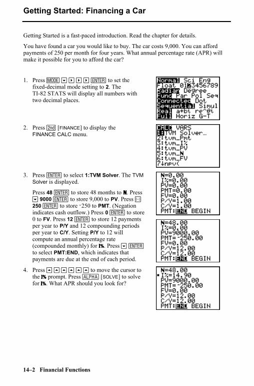
14–2 Financial Functions
82D362~1.DOC TI-83 international English Bob Fedorisko Revised: 10/26/05 1:42 PM Printed: 10/27/05 2:59PM Page 2 of 14
Getting Started is a fast-paced introduction. Read the chapter for details.
You have found a car you would like to buy. The car costs 9,000. You can affordpayments of 250 per month for four years. What annual percentage rate (APR) willmake it possible for you to afford the car?
1. Press z † ~ ~ ~Í to set thefixed-decimal mode setting to 2. TheTI-82 STATS will display all numbers withtwo decimal places.
2. Press y [FINANCE] to display theFINANCE CALC menu.
3. Press Í to select 1:TVM Solver. The TVMSolver is displayed.
Press 48 Í to store 48 months to ÚÚÚÚ. Press† 9000 Í to store 9,000 to PV. Press Ì250 Í to store L250 to PMT. (Negationindicates cash outflow.) Press 0Í to store0 to FV. Press 12 Í to store 12 paymentsper year to P/Y and 12 compounding periodsper year to C/Y. Setting P/Y to 12 willcompute an annual percentage rate(compounded monthly) for ææææ. Press †Íto select PMT:END, which indicates thatpayments are due at the end of each period.
4. Press } } } } } } to move the cursor tothe ææææ prompt. Press ƒ [SOLVE] to solvefor ææææ. What APR should you look for?
Getting Started: Financing a Car
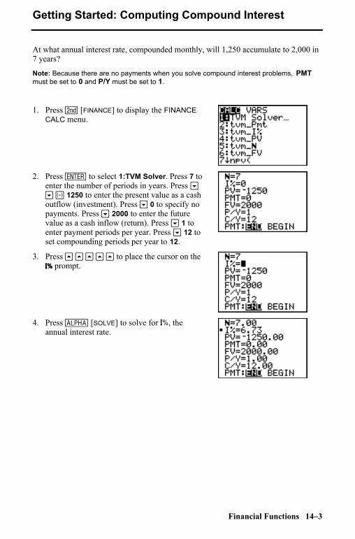
Financial Functions 14–3
82D362~1.DOC TI-83 international English Bob Fedorisko Revised: 10/26/05 1:42 PM Printed: 10/27/05 2:59PM Page 3 of 14
At what annual interest rate, compounded monthly, will 1,250 accumulate to 2,000 in7 years?
Note: Because there are no payments when you solve compound interest problems, PMTmust be set to 0 and P/Y must be set to 1.
1. Press y [FINANCE] to display the FINANCECALC menu.
2. Press Í to select 1:TVM Solver. Press 7 toenter the number of periods in years. Press †† Ì 1250 to enter the present value as a cashoutflow (investment). Press † 0 to specify nopayments. Press † 2000 to enter the futurevalue as a cash inflow (return). Press † 1 toenter payment periods per year. Press † 12 toset compounding periods per year to 12.
3. Press } } } } } to place the cursor on theææææ prompt.
4. Press ƒ [SOLVE] to solve for æ, theannual interest rate.
Getting Started: Computing Compound Interest

14–4 Financial Functions
82D362~1.DOC TI-83 international English Bob Fedorisko Revised: 10/26/05 1:42 PM Printed: 10/27/05 2:59PM Page 4 of 14
The TVM Solver displays the time-value-of-money (TVM)variables. Given four variable values, the TVM Solver solves forthe fifth variable.
The FINANCE VARS menu section (page 14.14) describes thefive TVM variables (ÚÚÚÚ, ææææ, PV, PMT, and FV) and P/Y and C/Y.
PMT: END BEGIN in the TVM Solver corresponds to theFINANCE CALC menu items Pmt_End (payment at the end ofeach period) and Pmt_Bgn (payment at the beginning of eachperiod).
To solve for an unknown TVM variable, follow these steps.
1. Press y [FINANCE] Í to display the TVM Solver. Thescreen below shows the default values with the fixed-decimal mode set to two decimal places.
2. Enter the known values for four TVM variables.
Note: Enter cash inflows as positive numbers and cashoutflows as negative numbers.
3. Enter a value for P/Y, which automatically enters the samevalue for C/Y; if P/Y ƒ C/Y, enter a unique value for C/Y.
4. Select END or BEGIN to specify the payment method.
5. Place the cursor on the TVM variable for which you want tosolve.
6. Press ƒ [SOLVE]. The answer is computed, displayed inthe TVM Solver, and stored to the appropriate TVM variable.An indicator square in the left column designates the solutionvariable.
Using the TVM Solver
Using the TVMSolver

Financial Functions 14–5
82D362~1.DOC TI-83 international English Bob Fedorisko Revised: 10/26/05 1:42 PM Printed: 10/27/05 2:59PM Page 5 of 14
When using the TI-82 STATS financial functions, you mustenter cash inflows (cash received) as positive numbers and cashoutflows (cash paid) as negative numbers. The TI-82 STATSfollows this convention when computing and displayinganswers.
To display the FINANCE CALC menu, press y [FINANCE].
CALC
VARS
1: TVM Solver... Displays the TVM Solver.2: tvm_Pmt Computes the amount of each payment.3: tvm_ææææ Computes the interest rate per year.4: tvm_PV Computes the present value.5: tvm_ÚÚÚÚ Computes the number of payment periods.6: tvm_FV Computes the future value.7: npv( Computes the net present value.8: irr( Computes the internal rate of return.9: bal( Computes the amortization sched. balance.0: GPrn( Computes the amort. sched. principal sum.A: GInt( Computes the amort. sched. interest sum.B: 4Nom( Computes the nominal interest rate.C: 4Eff( Computes the effective interest rate.D: dbd( Calculates the days between two dates.E: Pmt_End Selects ordinary annuity (end of period).F: Pmt_Bgn Selects annuity due (beginning of period).
Use these functions to set up and perform financial calculationson the home screen.
TVM Solver displays the TVM Solver (page 14.4).
Using the Financial Functions
Entering CashInflows and CashOutflows
FINANCE CALCMenu
TVM Solver

14–6 Financial Functions
82D362~1.DOC TI-83 international English Bob Fedorisko Revised: 10/26/05 1:42 PM Printed: 10/27/05 2:59PM Page 6 of 14
Use time-value-of-money (TVM) functions (menu items 2through 6) to analyze financial instruments such as annuities,loans, mortgages, leases, and savings.
Each TVM function takes zero to six arguments, which must bereal numbers. The values that you specify as arguments forthese functions are not stored to the TVM variables (page 14.14).
Note: To store a value to a TVM variable, use the TVM Solver (page14.4) or use ¿ and any TVM variable on the FINANCE VARSmenu (page 14.14).
If you enter less than six arguments, the TI-82 STATSsubstitutes a previously stored TVM variable value for eachunspecified argument.
If you enter any arguments with a TVM function, you must placethe argument or arguments in parentheses.
tvm_Pmt computes the amount of each payment.
tvm_Pmt[(Ú,æ,PV,FV,P/Y,C/Y)]
Note: In the example above, the values are stored to the TVMvariables in the TVM Solver. Then the payment (tvm_Pmt) iscomputed on the home screen using the values in the TVM Solver.Next, the interest rate is changed to 9.5 to illustrate the effect on thepayment amount.
Calculating Time Value of Money (TVM)
Calculating TimeValue of Money
tvm_Pmt
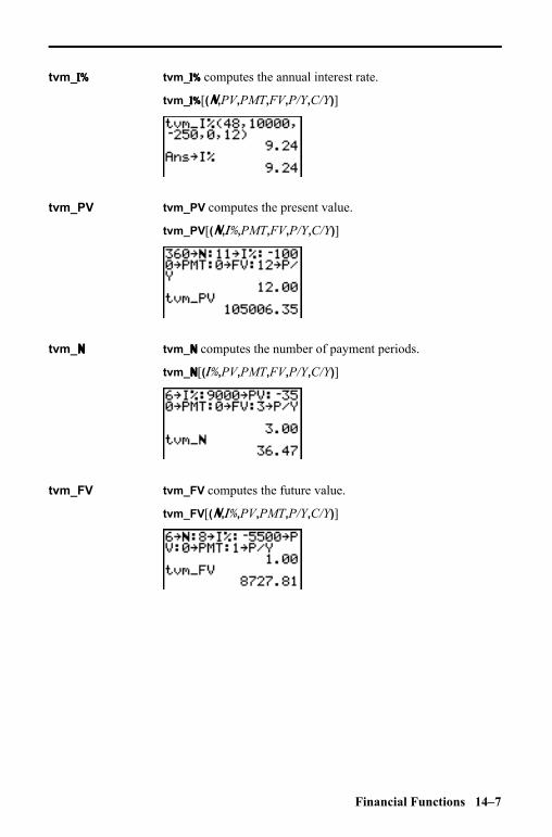
Financial Functions 14–7
82D362~1.DOC TI-83 international English Bob Fedorisko Revised: 10/26/05 1:42 PM Printed: 10/27/05 2:59PM Page 7 of 14
tvm_ææææ computes the annual interest rate.
tvm_ææææ[(Ú,PV,PMT,FV,P/Y,C/Y)]
tvm_PV computes the present value.
tvm_PV[(Ú,æ,PMT,FV,P/Y,C/Y)]
tvm_ÚÚÚÚ computes the number of payment periods.
tvm_ÚÚÚÚ[(æ,PV,PMT,FV,P/Y,C/Y)]
tvm_FV computes the future value.
tvm_FV[(Ú,æ,PV,PMT,P/Y,C/Y)]
tvm_ææææ
tvm_PV
tvm_ÚÚÚÚ
tvm_FV
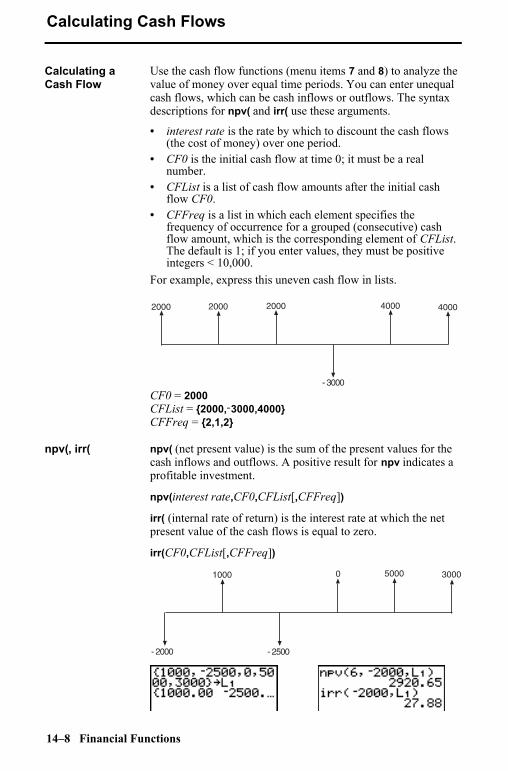
14–8 Financial Functions
82D362~1.DOC TI-83 international English Bob Fedorisko Revised: 10/26/05 1:42 PM Printed: 10/27/05 2:59PM Page 8 of 14
Use the cash flow functions (menu items 7 and 8) to analyze thevalue of money over equal time periods. You can enter unequalcash flows, which can be cash inflows or outflows. The syntaxdescriptions for npv( and irr( use these arguments.
• interest rate is the rate by which to discount the cash flows(the cost of money) over one period.
• CF0 is the initial cash flow at time 0; it must be a realnumber.
• CFList is a list of cash flow amounts after the initial cashflow CF0.
• CFFreq is a list in which each element specifies thefrequency of occurrence for a grouped (consecutive) cashflow amount, which is the corresponding element of CFList.The default is 1; if you enter values, they must be positiveintegers < 10,000.
For example, express this uneven cash flow in lists.
2000 40002000 2000
- 3000
4000
CF0 = 2000CFList = {2000,L3000,4000}CFFreq = {2,1,2}
npv( (net present value) is the sum of the present values for thecash inflows and outflows. A positive result for npv indicates aprofitable investment.
npv(interest rate,CF0,CFList[,CFFreq])
irr( (internal rate of return) is the interest rate at which the netpresent value of the cash flows is equal to zero.
irr(CF0,CFList[,CFFreq])
300050001000
- 2000 - 2500
0
Calculating Cash Flows
Calculating aCash Flow
npv(, irr(

Financial Functions 14–9
82D362~1.DOC TI-83 international English Bob Fedorisko Revised: 10/26/05 1:42 PM Printed: 10/27/05 2:59PM Page 9 of 14
Use the amortization functions (menu items 9, 0, and A) tocalculate balance, sum of principal, and sum of interest for anamortization schedule.
bal( computes the balance for an amortization schedule usingstored values for ææææ, PV, and PMT. npmt is the number of thepayment at which you want to calculate a balance. It must be apositive integer < 10,000. roundvalue specifies the internalprecision the calculator uses to calculate the balance; if you donot specify roundvalue, then the TI-82 STATS uses the currentFloat/Fix decimal-mode setting.
bal(npmt[,roundvalue])
GPrn( computes the sum of the principal during a specified periodfor an amortization schedule using stored values for ææææ, PV, andPMT. pmt1 is the starting payment. pmt2 is the ending payment inthe range. pmt1 and pmt2 must be positive integers < 10,000.roundvalue specifies the internal precision the calculator uses tocalculate the principal; if you do not specify roundvalue, theTI-82 STATS uses the current Float/Fix decimal-mode setting.
Note: You must enter values for ææææ, PV, PMT, and before computingthe principal.
GPrn(pmt1,pmt2[,roundvalue])
GInt( computes the sum of the interest during a specified periodfor an amortization schedule using stored values for ææææ, PV, andPMT. pmt1 is the starting payment. pmt2 is the ending paymentin the range. pmt1 and pmt2 must be positive integers < 10,000.roundvalue specifies the internal precision the calculator uses tocalculate the interest; if you do not specify roundvalue, theTI-82 STATS uses the current Float/Fix decimal-mode setting.
GInt(pmt1,pmt2[,roundvalue])
Calculating Amortization
Calculating anAmortizationSchedule
bal(
GPrn(, GInt(

14–10 Financial Functions
82D362~1.DOC TI-83 international English Bob Fedorisko Revised: 10/26/05 1:42 PM Printed: 10/27/05 2:59PM Page 10 of 14
You want to buy a home with a 30-year mortgage at 8 percentAPR. Monthly payments are 800. Calculate the outstanding loanbalance after each payment and display the results in a graphand in the table.
1. Press z. Press † ~ ~ ~ Í to set the fixed-decimalmode setting to 2. Press † † ~ Í to select Par graphingmode.
2. Press y [FINANCE] Í to display the TVM Solver.
3. Press 360 to enter number of payments. Press † 8 to enterthe interest rate. Press † † Ì 800 to enter the paymentamount. Press † 0 to enter the future value of the mortgage.Press † 12 to enter the payments per year, which also setsthe compounding periods per year to 12. Press † † Íto select PMT:END.
4. Press } } } } } to place the cursor on the PV prompt. Pressƒ [SOLVE] to solve for the present value.
5. Press o to display the parametric Y= editor. Turn off all statplots. Press „ to define X1T as T. Press † y[FINANCE] 9 „¤ to define Y1T as bal(T).
Calculating Amortization (continued)
AmortizationExample:Calculating anOutstandingLoan Balance

Financial Functions 14–11
82D362~1.DOC TI-83 international English Bob Fedorisko Revised: 10/26/05 1:42 PM Printed: 10/27/05 2:59PM Page 11 of 14
6. Press p to display the window variables. Enter thevalues below.Tmin=0 Xmin=0 Ymin=0Tmax=360 Xmax=360 Ymax=125000Tstep=12 Xscl=50 Yscl=10000
7. Press r to draw the graph and activate the trace cursor.Press ~ and | to explore the graph of the outstanding balanceover time. Press a number and then press Í to view thebalance at a specific time T.
8. Press y [TBLSET] and enter the values below.TblStart=0@Tbl=12
9. Press y [TABLE] to display the table of outstandingbalances (Y1T).
10.Press z † † † † † † † ~ ~ Í to select G.Tsplit-screen mode, in which the graph and table are displayedsimultaneously.
Press r to display X1T (time) and Y1T (balance) in thetable.
AmortizationExample:Calculating anOutstandingLoan Balance(continued)
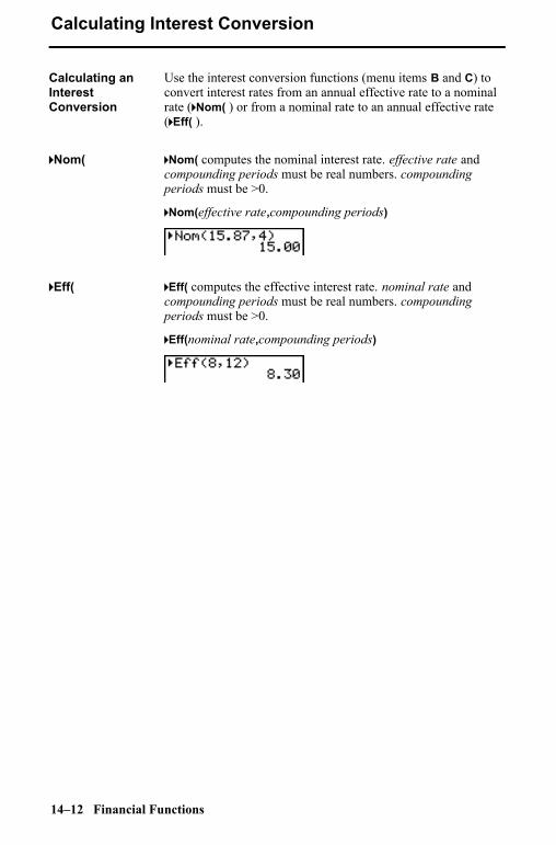
14–12 Financial Functions
82D362~1.DOC TI-83 international English Bob Fedorisko Revised: 10/26/05 1:42 PM Printed: 10/27/05 2:59PM Page 12 of 14
Use the interest conversion functions (menu items B and C) toconvert interest rates from an annual effective rate to a nominalrate (4Nom( ) or from a nominal rate to an annual effective rate(4Eff( ).
4Nom( computes the nominal interest rate. effective rate andcompounding periods must be real numbers. compoundingperiods must be >0.
4Nom(effective rate,compounding periods)
4Eff( computes the effective interest rate. nominal rate andcompounding periods must be real numbers. compoundingperiods must be >0.
4Eff(nominal rate,compounding periods)
Calculating Interest Conversion
Calculating anInterestConversion
4Nom(
4Eff(
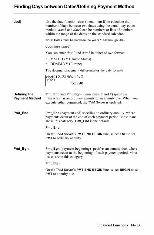
Financial Functions 14–13
82D362~1.DOC TI-83 international English Bob Fedorisko Revised: 10/26/05 1:42 PM Printed: 10/27/05 2:59PM Page 13 of 14
Use the date function dbd( (menu item D) to calculate thenumber of days between two dates using the actual-day-countmethod. date1 and date2 can be numbers or lists of numberswithin the range of the dates on the standard calendar.
Note: Dates must be between the years 1950 through 2049.
dbd(date1,date2)
You can enter date1 and date2 in either of two formats.
• MM.DDYY (United States)• DDMM.YY (Europe)
The decimal placement differentiates the date formats.
Pmt_End and Pmt_Bgn (menu items E and F) specify atransaction as an ordinary annuity or an annuity due. When youexecute either command, the TVM Solver is updated.
Pmt_End (payment end) specifies an ordinary annuity, wherepayments occur at the end of each payment period. Most loansare in this category. Pmt_End is the default.
Pmt_End
On the TVM Solver’s PMT:END BEGIN line, select END to setPMT to ordinary annuity.
Pmt_Bgn (payment beginning) specifies an annuity due, wherepayments occur at the beginning of each payment period. Mostleases are in this category.
Pmt_Bgn
On the TVM Solver’s PMT:END BEGIN line, select BEGIN to setPMT to annuity due.
Finding Days between Dates/Defining Payment Method
dbd(
Defining thePayment Method
Pmt_End
Pmt_Bgn
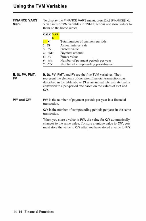
14–14 Financial Functions
82D362~1.DOC TI-83 international English Bob Fedorisko Revised: 10/26/05 1:42 PM Printed: 10/27/05 2:59PM Page 14 of 14
To display the FINANCE VARS menu, press y [FINANCE] ~.You can use TVM variables in TVM functions and store values tothem on the home screen.
CALC VARS
1: Ú Total number of payment periods2: ææææ Annual interest rate3: PV Present value4: PMT Payment amount5: FV Future value6: P/Y Number of payment periods per year7: C/Y Number of compounding periods/year
ÚÚÚÚ, ææææ, PV, PMT, and FV are the five TVM variables. Theyrepresent the elements of common financial transactions, asdescribed in the table above. ææææ is an annual interest rate that isconverted to a per-period rate based on the values of P/Y andC/Y.
P/Y is the number of payment periods per year in a financialtransaction.
C/Y is the number of compounding periods per year in the sametransaction.
When you store a value to P/Y, the value for C/Y automaticallychanges to the same value. To store a unique value to C/Y, youmust store the value to C/Y after you have stored a value to P/Y.
Using the TVM Variables
FINANCE VARSMenu
ÚÚÚÚ, ææææ, PV, PMT,FV
P/Y and C/Y
CATALOG, Strings, Hyperbolic Functions 15–1
82500E~1.DOC TI-83 international English Bob Fedorisko Revised: 10/28/05 9:25 AM Printed: 10/28/05 9:25AM Page 1 of 10
15 CATALOG, Strings,Hyperbolic Functions
Browsing the TI-82 STATS CATALOG.................................................. 2Entering and Using Strings............................................................................... 3Storing Strings to String Variables.............................................................. 4String Functions and Instructions in the CATALOG........................ 6Hyperbolic Functions in the CATALOG .................................................. 10
Contents

15–2 CATALOG, Strings, Hyperbolic Functions
82500E~1.DOC TI-83 international English Bob Fedorisko Revised: 10/28/05 9:25 AM Printed: 10/28/05 9:25AM Page 2 of 10
The CATALOG is an alphabetical list of all functions andinstructions on the TI-82 STATS. You also can access eachCATALOG item from a menu or the keyboard, except:
• The six string functions (page 15.6)• The six hyperbolic functions (page 15.10)• The solve( instruction without the equation solver editor
(Chapter 2)• The inferential stat functions without the inferential stat
editors (Chapter 13)
Note: The only CATALOG programming commands you can executefrom the home screen are GetCalc(, Get(, and Send(.
To select a CATALOG item, follow these steps.
1. Press y ãCATALOGä to display the CATALOG.
The 4 in the first column is the selection cursor.
2. Press † or } to scroll the CATALOG until the selectioncursor points to the item you want.
• To jump to the first item beginning with a particularletter, press that letter; alpha-lock is on.
• Items that begin with a number are in alphabetical orderaccording to the first letter after the number. Forexample, 2.PropZTest( is among the items that beginwith the letter P.
• Functions that appear as symbols, such as +, L1, <, and‡(, follow the last item that begins with Z. To jump to thefirst symbol, !, press [q].
3. Press Í to paste the item to the current screen.
Tip: From the top of the CATALOG menu, press } to move to thebottom. From the bottom, press † to move to the top.
Browsing the TI-82 STATS CATALOG
What Is theCATALOG?
Selecting an Itemfrom theCATALOG

CATALOG, Strings, Hyperbolic Functions 15–3
82500E~1.DOC TI-83 international English Bob Fedorisko Revised: 10/28/05 9:25 AM Printed: 10/28/05 9:25AM Page 3 of 10
A string is a sequence of characters that you enclose withinquotation marks. On the TI-82 STATS, a string has two primaryapplications.
• It defines text to be displayed in a program.• It accepts input from the keyboard in a program.
Characters are the units that you combine to form a string.
• Count each number, letter, and space as one character.• Count each instruction or function name, such as sin( or
cos(, as one character; the TI-82 STATS interprets eachinstruction or function name as one character.
To enter a string on a blank line on the home screen or in aprogram, follow these steps.
1. Press ƒ [ã] to indicate the beginning of the string.
2. Enter the characters that comprise the string.• Use any combination of numbers, letters, function names,
or instruction names to create the string.• To enter a blank space, press ƒ ['].• To enter several alpha characters in a row, press y
[A.LOCK] to activate alpha-lock.
3. Press ƒ [ã] to indicate the end of the string.
"string"
4. Press Í. On the home screen, the string is displayed onthe next line without quotations. An ellipsis (...) indicatesthat the string continues beyond the screen. To scroll theentire string, press ~ and |.
Note: Quotation marks do not count as string characters.
Entering and Using Strings
What Is a String?
Entering a String

15–4 CATALOG, Strings, Hyperbolic Functions
82500E~1.DOC TI-83 international English Bob Fedorisko Revised: 10/28/05 9:25 AM Printed: 10/28/05 9:25AM Page 4 of 10
The TI-82 STATS has 10 variables to which you can storestrings. You can use string variables with string functions andinstructions.
To display the VARS STRING menu, follow these steps.
1. Press to display the VARS menu. Move the cursor to7:String.
2. Press Í to display the STRING secondary menu.
Storing Strings to String Variables
String Variables

CATALOG, Strings, Hyperbolic Functions 15–5
82500E~1.DOC TI-83 international English Bob Fedorisko Revised: 10/28/05 9:25 AM Printed: 10/28/05 9:25AM Page 5 of 10
To store a string to a string variable, follow these steps.
1. Press ƒ [ã], enter the string, and press ƒ [ã].
2. Press ¿.
3. Press 7 to display the VARS STRING menu.
4. Select the string variable (from Str1 to Str9, or Str0) towhich you want to store the string.
The string variable is pasted to the current cursor location,next to the store symbol (!!!!).
5. Press Í to store the string to the string variable. On thehome screen, the stored string is displayed on the next linewithout quotation marks.
To display the contents of a string variable on the home screen,select the string variable from the VARS STRING menu, andthen press Í. The string is displayed.
Storing a Stringto a StringVariable
Displaying theContents of aString Variable

15–6 CATALOG, Strings, Hyperbolic Functions
82500E~1.DOC TI-83 international English Bob Fedorisko Revised: 10/28/05 9:25 AM Printed: 10/28/05 9:25AM Page 6 of 10
String functions and instructions are available only from theCATALOG. The table below lists the string functions andinstructions in the order in which they appear among the otherCATALOG menu items. The ellipses in the table indicate thepresence of additional CATALOG items.
CATALOG...Equ4String( Converts an equation to a string.expr( Converts a string to an expression....inString( Returns a character’s place number....length( Returns a string’s character length....String4Equ( Converts a string to an equation.sub( Returns a string subset as a string....
To concatenate two or more strings, follow these steps.
1. Enter string1, which can be a string or string name.
2. Press Ã.
3. Enter string2, which can be a string or string name. Ifnecessary, press à and enter string3, and so on.
string1+string2+string3. . .
4. Press Í to display the strings as a single string.
To select a string function or instruction and paste it to thecurrent screen, follow the steps on page 15.2.
String Functions and Instructions in the CATALOG
Displaying StringFunctions andInstructions inthe CATALOG
+ (Concatenation)
Selecting a StringFunction fromthe CATALOG
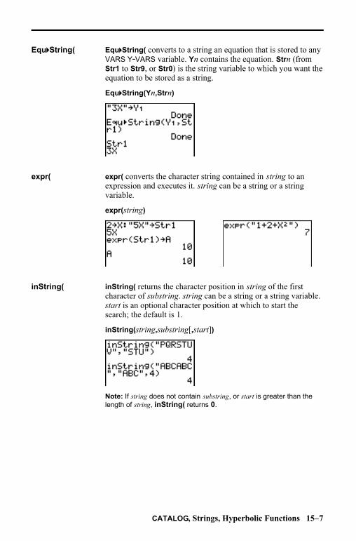
CATALOG, Strings, Hyperbolic Functions 15–7
82500E~1.DOC TI-83 international English Bob Fedorisko Revised: 10/28/05 9:25 AM Printed: 10/28/05 9:25AM Page 7 of 10
Equ4String( converts to a string an equation that is stored to anyVARS Y.VARS variable. Yn contains the equation. Strn (fromStr1 to Str9, or Str0) is the string variable to which you want theequation to be stored as a string.
Equ4String(Yn,Strn)
expr( converts the character string contained in string to anexpression and executes it. string can be a string or a stringvariable.
expr(string)
inString( returns the character position in string of the firstcharacter of substring. string can be a string or a string variable.start is an optional character position at which to start thesearch; the default is 1.
inString(string,substring[,start])
Note: If string does not contain substring, or start is greater than thelength of string, inString( returns 0.
Equ4String(
expr(
inString(

15–8 CATALOG, Strings, Hyperbolic Functions
82500E~1.DOC TI-83 international English Bob Fedorisko Revised: 10/28/05 9:25 AM Printed: 10/28/05 9:25AM Page 8 of 10
length( returns the number of characters in string. string can bea string or string variable.
Note: An instruction or function name, such as sin( or cos(, countsas one character.
length(string)
String4Equ( converts string into an equation and stores theequation to Yn. string can be a string or string variable.String4Equ( is the inverse of Equ4String(.
String4Equ(string,Yn)
String Functions and Instructions in the CATALOG (cont.)
length(
String4Equ(

CATALOG, Strings, Hyperbolic Functions 15–9
82500E~1.DOC TI-83 international English Bob Fedorisko Revised: 10/28/05 9:25 AM Printed: 10/28/05 9:25AM Page 9 of 10
sub( returns a string that is a subset of an existing string. stringcan be a string or a string variable. begin is the position numberof the first character of the subset. length is the number ofcharacters in the subset.
sub(string,begin,length)
In a program, you can enter a function to graph during programexecution using these commands.
Note: When you execute this program, enter a function to store to Y3at the ENTRY= prompt.
sub(
Entering aFunction toGraph duringProgramExecution

15–10 CATALOG, Strings, Hyperbolic Functions
82500E~1.DOC TI-83 international English Bob Fedorisko Revised: 10/28/05 9:25 AM Printed: 10/28/05 9:25AM Page 10 of 10
The hyperbolic functions are available only from the CATALOG.The table below lists the hyperbolic functions in the order inwhich they appear among the other CATALOG menu items. Theellipses in the table indicate the presence of additionalCATALOG items.
CATALOG...cosh( Hyperbolic cosinecoshL1( Hyperbolic arccosine...sinh( Hyperbolic sinesinhL1( Hyperbolic arcsine...tanh( Hyperbolic tangenttanhL1( Hyperbolic arctangent...
sinh(, cosh(, and tanh( are the hyperbolic functions. Each isvalid for real numbers, expressions, and lists.
sinh(value)cosh(value)tanh(value)
sinhL1( is the hyperbolic arcsine function. coshL1( is thehyperbolic arccosine function. tanhL1( is the hyperbolicarctangent function. Each is valid for real numbers, expressions,and lists.
sinhL1(value)coshL1(value)sinhL1(value)
Hyperbolic Functions in the CATALOG
HyperbolicFunctions
sinh(, cosh(,tanh(
sinhL1(, coshL1(,tanhL1(

Programming 16–1
82E978~1.DOC TI-83 international English Bob Fedorisko Revised: 10/26/05 1:47 PM Printed: 10/27/05 3:02PM Page 1 of 22
16 Programming
Getting Started: Volume of a Cylinder ..................................................... 2Creating and Deleting Programs................................................................... 4Entering Command Lines and Executing Programs ........................ 5Editing Programs .................................................................................................... 6Copying and Renaming Programs ............................................................... 7PRGM CTL (Control) Instructions .............................................................. 8PRGM I/O (Input/Output) Instructions..................................................... 16Calling Other Programs as Subroutines ................................................... 22
Contents

16–2 Programming
82E978~1.DOC TI-83 international English Bob Fedorisko Revised: 10/26/05 1:47 PM Printed: 10/27/05 3:02PM Page 2 of 22
Getting Started is a fast-paced introduction. Read the chapter for details.
A program is a set of commands that the TI-82 STATS executes sequentially, as ifyou had entered them from the keyboard. Create a program that prompts for theradius R and the height H of a cylinder and then computes its volume.
1. Press ~ ~ to display the PRGM NEWmenu.
2. Press Í to select 1:Create New. TheName= prompt is displayed, and alpha-lock ison. Press [C] [Y] [L] [I] [N] [D] [E] [R], and thenpress Í to name the program CYLINDER.
You are now in the program editor. The colon( : ) in the first column of the second lineindicates the beginning of a command line.
3. Press ~ 2 to select 2:Prompt from thePRGM I/O menu. Prompt is copied to thecommand line. Press ƒ [R] ¢ƒ [H]to enter the variable names for radius andheight. Press Í.
4. Press y ãpä ƒ [R] ¡ƒ [H] ¿ƒ [V] Í to enter the expression pR2Hand store it to the variable V.
Getting Started: Volume of a Cylinder
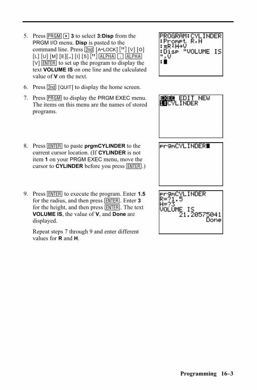
Programming 16–3
82E978~1.DOC TI-83 international English Bob Fedorisko Revised: 10/26/05 1:47 PM Printed: 10/27/05 3:02PM Page 3 of 22
5. Press ~ 3 to select 3:Disp from thePRGM I/O menu. Disp is pasted to thecommand line. Press y [A.LOCK] ããä [V] [O][L] [U] [M] [E]['] [I] [S] ãã䃢ƒ[V] Í to set up the program to display thetext VOLUME IS on one line and the calculatedvalue of V on the next.
6. Press y [QUIT] to display the home screen.
7. Press to display the PRGM EXEC menu.The items on this menu are the names of storedprograms.
8. Press Í to paste prgmCYLINDER to thecurrent cursor location. (If CYLINDER is notitem 1 on your PRGM EXEC menu, move thecursor to CYLINDER before you press Í.)
9. Press Í to execute the program. Enter 1.5for the radius, and then press Í. Enter 3for the height, and then press Í. The textVOLUME IS, the value of V, and Done aredisplayed.
Repeat steps 7 through 9 and enter differentvalues for R and H.

16–4 Programming
82E978~1.DOC TI-83 international English Bob Fedorisko Revised: 10/26/05 1:47 PM Printed: 10/27/05 3:02PM Page 4 of 22
A program is a set of one or more command lines. Each linecontains one or more instructions. When you execute a program,the TI-82 STATS performs each instruction on each commandline in the same order in which you entered them. The numberand size of programs that the TI-82 STATS can store is limitedonly by available memory.
To create a new program, follow these steps.
1. Press | to display the PRGM NEW menu.
2. Press Í to select 1:Create New. The Name= prompt isdisplayed, and alpha-lock is on.
3. Press a letter from A to Z or q to enter the first character ofthe new program name.
Note: A program name can be one to eight characters long. Thefirst character must be a letter from A to Z or q. The secondthrough eighth characters can be letters, numbers, or q.
4. Enter zero to seven letters, numbers, or q to complete thenew program name.
5. Press Í. The program editor is displayed.
6. Enter one or more program commands (page 16.5).
7. Press y [QUIT] to leave the program editor and return tothe home screen.
To check whether adequate memory is available for a programyou want to enter, press y [MEM], and then select1:Check RAM from the MEMORY menu (Chapter 18).
To increase available memory, press y [MEM], and then select2:Delete from the MEMORY menu (Chapter 18).
To delete a specific program, press y [MEM], select 2:Deletefrom the MEMORY menu, and then select 7:Prgm from theDELETE FROM secondary menu (Chapter 18).
Creating and Deleting Programs
What Is aProgram?
Creating a NewProgram
ManagingMemory andDeleting aProgram
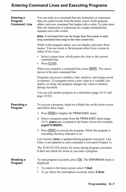
Programming 16–5
82E978~1.DOC TI-83 international English Bob Fedorisko Revised: 10/26/05 1:47 PM Printed: 10/27/05 3:02PM Page 5 of 22
You can enter on a command line any instruction or expressionthat you could execute from the home screen. In the programeditor, each new command line begins with a colon. To enter morethan one instruction or expression on a single command line,separate each with a colon.
Note: A command line can be longer than the screen is wide;long command lines wrap to the next screen line.
While in the program editor, you can display and select frommenus. You can return to the program editor from a menu ineither of two ways.
• Select a menu item, which pastes the item to the currentcommand line.
• Press ‘.
When you complete a command line, press Í. The cursormoves to the next command line.
Programs can access variables, lists, matrices, and strings savedin memory. If a program stores a new value to a variable, list,matrix, or string, the program changes the value in memoryduring execution.
You can call another program as a subroutine (page 16.15 andpage 16.22).
To execute a program, begin on a blank line on the home screenand follow these steps.
1. Press to display the PRGM EXEC menu.
2. Select a program name from the PRGM EXEC menu (page16.7). prgmname is pasted to the home screen (for example,prgmCYLINDER).
3. Press Í to execute the program. While the program isexecuting, the busy indicator is on.
Last Answer (Ans) is updated during program execution. LastEntry is not updated as each command is executed (Chapter 1).
The TI-82 STATS checks for errors during program execution.It does not check for errors as you enter a program.
To stop program execution, press É. The ERR:BREAK menu isdisplayed.
• To return to the home screen, select 1:Quit.• To go where the interruption occurred, select 2:Goto.
Entering Command Lines and Executing Programs
Entering aProgramCommand Line
Executing aProgram
Breaking aProgram

16–6 Programming
82E978~1.DOC TI-83 international English Bob Fedorisko Revised: 10/26/05 1:47 PM Printed: 10/27/05 3:02PM Page 6 of 22
To edit a stored program, follow these steps.
1. Press ~ to display the PRGM EDIT menu.
2. Select a program name from the PRGM EDIT menu (page16.7). Up to the first seven lines of the program aredisplayed.
Note: The program editor does not display a $ to indicate thata program continues beyond the screen.
3. Edit the program command lines.
• Move the cursor to the appropriate location, and thendelete, overwrite, or insert.
• Press ‘ to clear all program commands on thecommand line (the leading colon remains), and then entera new program command.
Tip: To move the cursor to the beginning of a command line, pressy |; to move to the end, press y ~. To scroll the cursor downseven command lines, press ƒ †. To scroll the cursor up sevencommand lines, press ƒ }.
To insert a new command line anywhere in the program, placethe cursor where you want the new line, press y [INS], andthen press Í. A colon indicates a new line.
To delete a command line, place the cursor on the line, press‘ to clear all instructions and expressions on the line, andthen press { to delete the command line, including the colon.
Editing Programs
Editing aProgram
Inserting andDeletingCommand Lines

Programming 16–7
82E978~1.DOC TI-83 international English Bob Fedorisko Revised: 10/26/05 1:47 PM Printed: 10/27/05 3:02PM Page 7 of 22
To copy all command lines from one program into a newprogram, follow steps 1 through 5 for Creating a New Program(page 16.4), and then follow these steps.
1. Press y [RCL]. Rcl is displayed on the bottom line of theprogram editor in the new program (Chapter 1).
2. Press | to display the PRGM EXEC menu.
3. Select a name from the menu. prgmname is pasted to thebottom line of the program editor.
4. Press Í. All command lines from the selected programare copied into the new program.
Copying programs has at least two convenient applications.
• You can create a template for groups of instructions that youuse frequently.
• You can rename a program by copying its contents into anew program.
Note: You also can copy all the command lines from one existingprogram to another existing program using RCL.
The TI-82 STATS sorts PRGM EXEC and PRGM EDIT menuitems automatically into alphanumerical order. Each menu onlylabels the first 10 items using 1 through 9, then 0.
To jump to the first program name that begins with a particularalpha character or q, press ƒ [letter from A to Z or q].
Tip: From the top of either the PRGM EXEC or PRGM EDIT menu,press } to move to the bottom. From the bottom, press † to move tothe top. To scroll the cursor down the menu seven items, press ƒ†. To scroll the cursor up the menu seven items, press ƒ }.
Copying and Renaming Programs
Copying andRenaming aProgram
Scrolling thePRGM EXEC andPRGM EDITMenus

16–8 Programming
82E978~1.DOC TI-83 international English Bob Fedorisko Revised: 10/26/05 1:47 PM Printed: 10/27/05 3:02PM Page 8 of 22
To display the PRGM CTL (program control) menu, press from the program editor only.
CTL I/O EXEC1: If Creates a conditional test.2: Then Executes commands when If is true.3: Else Executes commands when If is false.4: For( Creates an incrementing loop.5: While Creates a conditional loop.6: Repeat Creates a conditional loop.7: End Signifies the end of a block.8: Pause Pauses program execution.9: Lbl Defines a label.0: Goto Goes to a label.A: IS>( Increments and skips if greater than.B: DS<( Decrements and skips if less than.C: Menu( Defines menu items and branches.D: prgm Executes a program as a subroutine.E: Return Returns from a subroutine.F: Stop Stops execution.G: DelVar Deletes a variable from within program.H: GraphStyle( Designates the graph style to be drawn.
These menu items direct the flow of an executing program.They make it easy to repeat or skip a group of commands duringprogram execution. When you select an item from the menu, thename is pasted to the cursor location on a command line in theprogram.
To return to the program editor without selecting an item, press‘.
Program control instructions tell the TI-82 STATS whichcommand to execute next in a program. If, While, and Repeatcheck a defined condition to determine which command toexecute next. Conditions frequently use relational or Booleantests (Chapter 2), as in:
If A<7:A+1!!!!A
or
If N=1 and M=1:Goto Z
PRGM CTL (Control) Instructions
PRGM CTL Menu
ControllingProgram Flow

Programming 16–9
82E978~1.DOC TI-83 international English Bob Fedorisko Revised: 10/26/05 1:47 PM Printed: 10/27/05 3:02PM Page 9 of 22
Use If for testing and branching. If condition is false (zero), thenthe command immediately following If is skipped. If condition istrue (nonzero), then the next command is executed. Ifinstructions can be nested.
:If condition:command (if true):command
Program Output
Then following an If executes a group of commands if conditionis true (nonzero). End identifies the end of the group ofcommands.
:If condition:Then:command (if true):command (if true):End:command
Program Output
If
If.Then
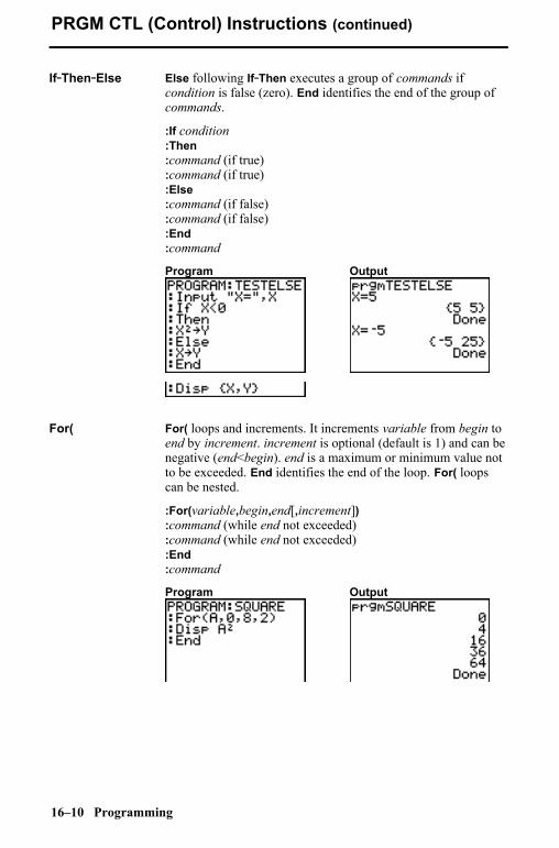
16–10 Programming
82E978~1.DOC TI-83 international English Bob Fedorisko Revised: 10/26/05 1:47 PM Printed: 10/27/05 3:02PM Page 10 of 22
Else following If.Then executes a group of commands ifcondition is false (zero). End identifies the end of the group ofcommands.
:If condition:Then:command (if true):command (if true):Else:command (if false):command (if false):End:command
Program Output
For( loops and increments. It increments variable from begin toend by increment. increment is optional (default is 1) and can benegative (end<begin). end is a maximum or minimum value notto be exceeded. End identifies the end of the loop. For( loopscan be nested.
:For(variable,begin,end[,increment]):command (while end not exceeded):command (while end not exceeded):End:command
Program Output
PRGM CTL (Control) Instructions (continued)
If.Then.Else
For(

Programming 16–11
82E978~1.DOC TI-83 international English Bob Fedorisko Revised: 10/26/05 1:47 PM Printed: 10/27/05 3:02PM Page 11 of 22
While performs a group of commands while condition is true.condition is frequently a relational test (Chapter 2). condition istested when While is encountered. If condition is true (nonzero),the program executes a group of commands. End signifies theend of the group. When condition is false (zero), the programexecutes each command following End. While instructions canbe nested.
:While condition:command (while condition is true):command (while condition is true):End:command
Program Output
Repeat repeats a group of commands until condition is true(nonzero). It is similar to While, but condition is tested whenEnd is encountered; therefore, the group of commands is alwaysexecuted at least once. Repeat instructions can be nested.
:Repeat condition:command (until condition is true):command (until condition is true):End:command
Program Output
While
Repeat

16–12 Programming
82E978~1.DOC TI-83 international English Bob Fedorisko Revised: 10/26/05 1:47 PM Printed: 10/27/05 3:02PM Page 12 of 22
End identifies the end of a group of commands. You mustinclude an End instruction at the end of each For(, While, orRepeat loop. Also, you must paste an End instruction at the endof each If.Then group and each If.Then.Else group.
Pause suspends execution of the program so that you can seeanswers or graphs. During the pause, the pause indicator is on inthe top-right corner. Press Í to resume execution.
• Pause without a value temporarily pauses the program. Ifthe DispGraph or Disp instruction has been executed, theappropriate screen is displayed.
• Pause with value displays value on the current home screen.value can be scrolled.
Pause [value]
Program Output
PRGM CTL (Control) Instructions (continued)
End
Pause
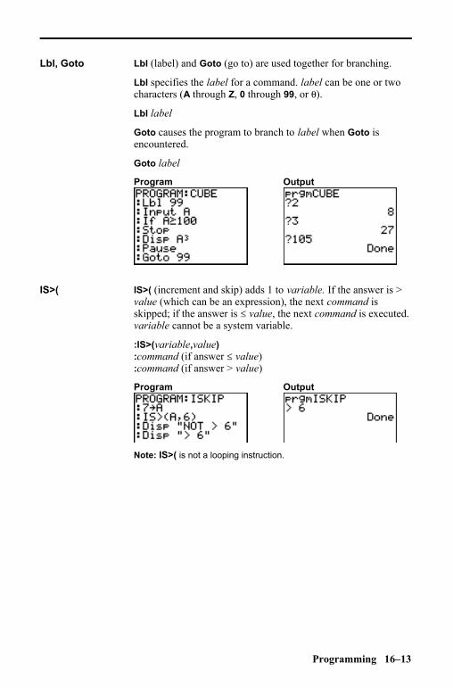
Programming 16–13
82E978~1.DOC TI-83 international English Bob Fedorisko Revised: 10/26/05 1:47 PM Printed: 10/27/05 3:02PM Page 13 of 22
Lbl (label) and Goto (go to) are used together for branching.
Lbl specifies the label for a command. label can be one or twocharacters (A through Z, 0 through 99, or q).
Lbl label
Goto causes the program to branch to label when Goto isencountered.
Goto label
Program Output
IS>( (increment and skip) adds 1 to variable. If the answer is >value (which can be an expression), the next command isskipped; if the answer is { value, the next command is executed.variable cannot be a system variable.
:IS>(variable,value):command (if answer value):command (if answer > value)
Program Output
Note: IS>( is not a looping instruction.
Lbl, Goto
IS>(

16–14 Programming
82E978~1.DOC TI-83 international English Bob Fedorisko Revised: 10/26/05 1:47 PM Printed: 10/27/05 3:02PM Page 14 of 22
DS<( (decrement and skip) subtracts 1 from variable. If theanswer is < value (which can be an expression), the nextcommand is skipped; if the answer is | value, the next commandis executed. variable cannot be a system variable.
:DS<(variable,value):command (if answer ‚ value):command (if answer < value)
Program Output
Note: DS<( is not a looping instruction.
Menu( sets up branching within a program. If Menu( isencountered during program execution, the menu screen isdisplayed with the specified menu items, the pause indicator ison, and execution pauses until you select a menu item.
The menu title is enclosed in quotation marks ( " ). Up to sevenpairs of menu items follow. Each pair comprises a text item(also enclosed in quotation marks) to be displayed as a menuselection, and a label item to which to branch if you select thecorresponding menu selection.
Menu("title","text1",label1,"text2",label2, . . .)
Program Output
The program above pauses until you select 1 or 2. If you select2, for example, the menu disappears and the program continuesexecution at Lbl B.
PRGM CTL (Control) Instructions (continued)
DS<(
Menu(

Programming 16–15
82E978~1.DOC TI-83 international English Bob Fedorisko Revised: 10/26/05 1:47 PM Printed: 10/27/05 3:02PM Page 15 of 22
Use prgm to execute other programs as subroutines (page16.22). When you select prgm, it is pasted to the cursorlocation. Enter characters to spell a program name. Using prgmis equivalent to selecting existing programs from the PRGMEXEC menu; however, it allows you to enter the name of aprogram that you have not yet created.
prgmname
Note: You cannot directly enter the subroutine name when usingRCL. You must paste the name from the PRGM EXEC menu (page16.7).
Return quits the subroutine and returns execution to the callingprogram (page 16.22), even if encountered within nested loops.Any loops are ended. An implied Return exists at the end of anyprogram that is called as a subroutine. Within the main program,Return stops execution and returns to the home screen.
Stop stops execution of a program and returns to the homescreen. Stop is optional at the end of a program.
DelVar deletes from memory the contents of variable.
DelVar variable
GraphStyle( designates the style of the graph to be drawn.function# is the number of the Y= function name in the currentgraphing mode. graphstyle is a number from 1 to 7 thatcorresponds to the graph style, as shown below.
1 = ç (line) 5 = ë (path)2 = è (thick) 6 = ì (animate)3 = é (shade above) 7 = í (dot)4 = ê (shade below)
GraphStyle(function#,graphstyle)
For example, GraphStyle(1,5) in Func mode sets the graph stylefor Y1 to ë (path; 5).
Not all graph styles are available in all graphing modes. For adetailed description of each graph style, see the Graph Stylestable in Chapter 3.
prgm
Return
Stop
DelVar
GraphStyle(

16–16 Programming
82E978~1.DOC TI-83 international English Bob Fedorisko Revised: 10/26/05 1:47 PM Printed: 10/27/05 3:02PM Page 16 of 22
To display the PRGM I/O (program input/output) menu, press ~ from within the program editor only.
CTL I/O EXEC1: Input Enters a value or uses the cursor.2: Prompt Prompts for entry of variable values.3: Disp Displays text, value, or the home screen.4: DispGraph Displays the current graph.5: DispTable Displays the current table.6: Output( Displays text at a specified position.7: getKey Checks the keyboard for a keystroke.8: ClrHome Clears the display.9: ClrTable Clears the current table.0: GetCalc( Gets a variable from another TI-82 STATS.A: Get( Gets a variable from CBL or CBR.B: Send( Sends a variable to CBL or CBR.
These instructions control input to and output from a programduring execution. They allow you to enter values and displayanswers during program execution.
To return to the program editor without selecting an item, press‘.
Input without a variable displays the current graph. You canmove the free-moving cursor, which updates X and Y (and R andq for PolarGC format). The pause indicator is on. Press Íto resume program execution.
Input
Program Output
PRGM I/O (Input/Output) Instructions
PRGM I/O Menu
Displaying aGraph with Input

Programming 16–17
82E978~1.DOC TI-83 international English Bob Fedorisko Revised: 10/26/05 1:47 PM Printed: 10/27/05 3:02PM Page 17 of 22
Input with variable displays a ? (question mark) prompt duringexecution. variable may be a real number, complex number, list,matrix, string, or Y= function. During program execution, entera value, which can be an expression, and then press Í. Thevalue is evaluated and stored to variable, and the programresumes execution.
Input [variable]
You can display text or the contents of Strn (a string variable) ofup to 16 characters as a prompt. During program execution,enter a value after the prompt and then press Í. The valueis stored to variable, and the program resumes execution.
Input ["text",variable]Input [Strn,variable]
Program Output
Note: When a program prompts for input of lists and Yn functionsduring execution, you must include the braces ( { } ) around the listelements and quotation marks ( " ) around the expressions.
Storing aVariable Valuewith Input

16–18 Programming
82E978~1.DOC TI-83 international English Bob Fedorisko Revised: 10/26/05 1:47 PM Printed: 10/27/05 3:02PM Page 18 of 22
During program execution, Prompt displays each variable, oneat a time, followed by =?. At each prompt, enter a value orexpression for each variable, and then press Í. The valuesare stored, and the program resumes execution.
Prompt variableA[,variableB,...,variable n]
Program Output
Note: Y= functions are not valid with Prompt.
Disp (display) without a value displays the home screen. Toview the home screen during program execution, follow theDisp instruction with a Pause instruction.
Disp
Disp with one or more values displays the value of each.
Disp [valueA,valueB,valueC,...,value n]
• If value is a variable, the current value is displayed.• If value is an expression, it is evaluated and the result is
displayed on the right side of the next line.• If value is text within quotation marks, it is displayed on the
left side of the current display line. !!!! is not valid as text.
Program Output
If Pause is encountered after Disp, the program haltstemporarily so you can examine the screen. To resumeexecution, press Í.
Note: If a matrix or list is too large to display in its entirety, ellipses(...) are displayed in the last column, but the matrix or list cannot bescrolled. To scroll, use Pause value (page 16.12).
PRGM I/O (Input/Output) Instructions (continued)
Prompt
Displaying theHome Screen
DisplayingValues andMessages
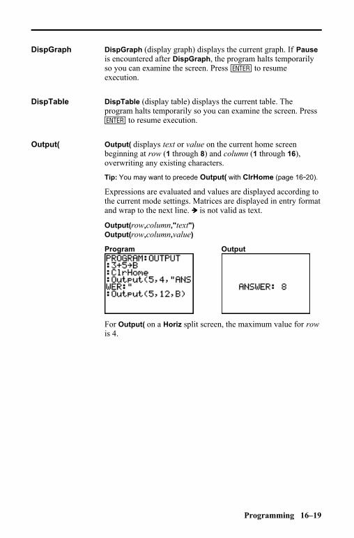
Programming 16–19
82E978~1.DOC TI-83 international English Bob Fedorisko Revised: 10/26/05 1:47 PM Printed: 10/27/05 3:02PM Page 19 of 22
DispGraph (display graph) displays the current graph. If Pauseis encountered after DispGraph, the program halts temporarilyso you can examine the screen. Press Í to resumeexecution.
DispTable (display table) displays the current table. Theprogram halts temporarily so you can examine the screen. PressÍ to resume execution.
Output( displays text or value on the current home screenbeginning at row (1 through 8) and column (1 through 16),overwriting any existing characters.
Tip: You may want to precede Output( with ClrHome (page 16.20).
Expressions are evaluated and values are displayed according tothe current mode settings. Matrices are displayed in entry formatand wrap to the next line. !!!! is not valid as text.
Output(row,column,"text")Output(row,column,value)
Program Output
For Output( on a Horiz split screen, the maximum value for rowis 4.
DispGraph
DispTable
Output(

16–20 Programming
82E978~1.DOC TI-83 international English Bob Fedorisko Revised: 10/26/05 1:47 PM Printed: 10/27/05 3:02PM Page 20 of 22
getKey returns a number corresponding to the last key pressed,according to the key code diagram below. If no key has beenpressed, getKey returns 0. Use getKey inside loops to transfercontrol, for example, when creating video games.
Program Output
Note: , , , andÍ were pressed duringprogram execution.
Note: You can press É at any time during execution to break theprogram (page 16.5).
ClrHome (clear home screen) clears the home screen duringprogram execution.
ClrTable (clear table) clears the values in the table duringprogram execution.
PRGM I/O (Input/Output) Instructions (continued)
getKey
TI-82 STATS KeyCode Diagram
ClrHome,ClrTable

Programming 16–21
82E978~1.DOC TI-83 international English Bob Fedorisko Revised: 10/26/05 1:47 PM Printed: 10/27/05 3:02PM Page 21 of 22
GetCalc( gets the contents of variable on another TI-82 STATSand stores it to variable on the receiving TI-82 STATS. variablecan be a real or complex number, list element, list name, matrixelement, matrix name, string, Y= variable, graph database, orpicture.
GetCalc(variable)
Note: GetCalc( does not work between TI.82 and TI-82 STATS.
Get( gets data from the Calculator-Based Laboratoryé (CBLé)System or Calculator-Based Rangeré (CBRé) and stores it tovariable on the receiving TI-82 STATS. variable can be a realnumber, list element, list name, matrix element, matrix name,string, Y= variable, graph database, or picture.
Get(variable)
Note: If you transfer a program that references the Get( command tothe TI-82 STATS from a TI.82, the TI-82 STATS will interpret it as theGet( described above. Use GetCalc( to get data from anotherTI-82 STATS.
Send( sends the contents of variable to the CBL or CBR. Youcannot use it to send to another TI-82 STATS. variable can be areal number, list element, list name, matrix element, matrixname, string, Y= variable, graph database, or picture. variablecan be a list of elements.
Send(variable)
Note: This program gets sound dataand time in seconds from CBL.
Note: You can access Get(, Send(, and GetCalc( from theCATALOG to execute them from the home screen (Chapter 15).
GetCalc(
Get(, Send(
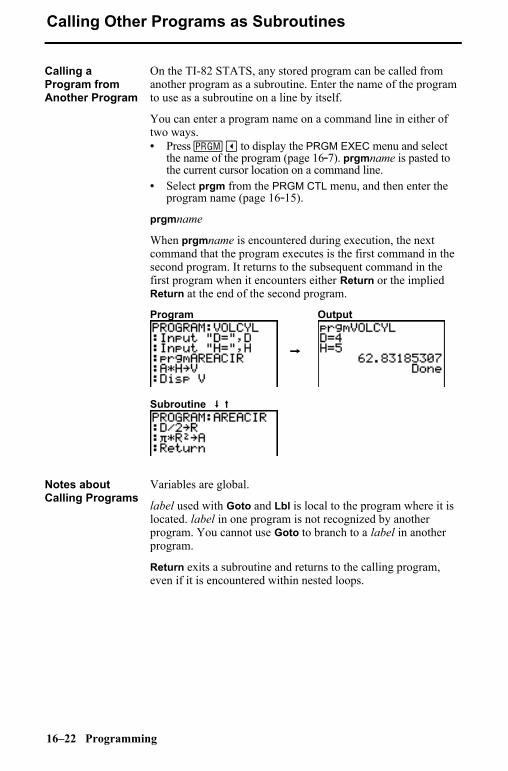
16–22 Programming
82E978~1.DOC TI-83 international English Bob Fedorisko Revised: 10/26/05 1:47 PM Printed: 10/27/05 3:02PM Page 22 of 22
On the TI-82 STATS, any stored program can be called fromanother program as a subroutine. Enter the name of the programto use as a subroutine on a line by itself.
You can enter a program name on a command line in either oftwo ways.• Press | to display the PRGM EXEC menu and select
the name of the program (page 16.7). prgmname is pasted tothe current cursor location on a command line.
• Select prgm from the PRGM CTL menu, and then enter theprogram name (page 16.15).
prgmname
When prgmname is encountered during execution, the nextcommand that the program executes is the first command in thesecond program. It returns to the subsequent command in thefirst program when it encounters either Return or the impliedReturn at the end of the second program.
Program Output
&
Subroutine ( '
Variables are global.
label used with Goto and Lbl is local to the program where it islocated. label in one program is not recognized by anotherprogram. You cannot use Goto to branch to a label in anotherprogram.
Return exits a subroutine and returns to the calling program,even if it is encountered within nested loops.
Calling Other Programs as Subroutines
Calling aProgram fromAnother Program
Notes aboutCalling Programs

Applications 17–1
82501F~1.DOC TI-83 international English Bob Fedorisko Revised: 10/26/05 1:49 PM Printed: 10/27/05 3:04PM Page 1 of 20
17 Applications
Comparing Test Results Using Box Plots............................................... 2Graphing Piecewise Functions....................................................................... 4Graphing Inequalities........................................................................................... 5Solving a System of Nonlinear Equations .............................................. 6Using a Program to Create the Sierpinski Triangle .......................... 7Graphing Cobweb Attractors .......................................................................... 8Using a Program to Guess the Coefficients ........................................... 9Graphing the Unit Circle and Trigonometric Curves ...................... 10Finding the Area between Curves................................................................ 11Using Parametric Equations: Ferris Wheel Problem........................ 12Demonstrating the Fundamental Theorem of Calculus.................. 14Computing Areas of Regular N-Sided Polygons................................ 16Computing and Graphing Mortgage Payments ................................... 18
Contents

17–2 Applications
82501F~1.DOC TI-83 international English Bob Fedorisko Revised: 10/26/05 1:49 PM Printed: 10/27/05 3:04PM Page 2 of 20
An experiment found a significant difference between boys andgirls pertaining to their ability to identify objects held in theirleft hands, which are controlled by the right side of their brains,versus their right hands, which are controlled by the left side oftheir brains. The TI Graphics team conducted a similar test foradult men and women.
The test involved 30 small objects, which participants were notallowed to see. First, they held 15 of the objects one by one intheir left hands and guessed what they were. Then they held theother 15 objects one by one in their right hands and guessed whatthey were. Use box plots to compare visually the correct-guessdata from this table.
Correct Guesses
WomenLeft
WomenRight
MenLeft
MenRight
8 4 7 129 1 8 6
12 8 7 1211 12 5 1210 11 7 78 11 8 11
12 13 11 127 12 4 89 11 10 12
11 12 14 1113 95 9
1. Press … 5 to select 5:SetUpEditor. Enter list namesWLEFT, WRGHT, MLEFT, and MRGHT, separated bycommas. Press Í. The stat list editor now contains onlythese four lists.
2. Press … 1 to select 1:Edit.
3. Enter into WLEFT the number of correct guesses each womanmade using her left hand (Women Left). Press ~ to move toWRGHT and enter the number of correct guesses each womanmade using her right hand (Women Right).
4. Likewise, enter each man’s correct guesses in MLEFT (MenLeft) and MRGHT (Men Right).
5. Press y [STAT PLOT]. Select 1:Plot1. Turn on plot 1; define itas a modified box plot ÕÕÕÕ that uses WLEFT. Move the cursorto the top line and select Plot2. Turn on plot 2; define it as amodified box plot that uses WRGHT.
Comparing Test Results Using Box Plots
Problem
Procedure
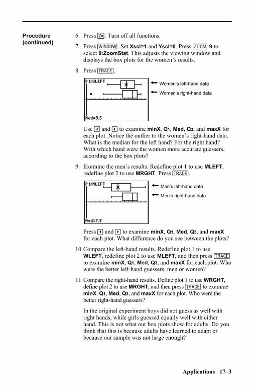
Applications 17–3
82501F~1.DOC TI-83 international English Bob Fedorisko Revised: 10/26/05 1:49 PM Printed: 10/27/05 3:04PM Page 3 of 20
6. Press o. Turn off all functions.
7. Press p. Set Xscl=1 and Yscl=0. Press q 9 toselect 9:ZoomStat. This adjusts the viewing window anddisplays the box plots for the women’s results.
8. Press r.
% Women’s left-hand data
% Women’s right-hand data
Use | and ~ to examine minX, Q1, Med, Q3, and maxX foreach plot. Notice the outlier to the women’s right-hand data.What is the median for the left hand? For the right hand?With which hand were the women more accurate guessers,according to the box plots?
9. Examine the men’s results. Redefine plot 1 to use MLEFT,redefine plot 2 to use MRGHT. Press r.
% Men’s left-hand data
% Men’s right-hand data
Press | and ~ to examine minX, Q1, Med, Q3, and maxXfor each plot. What difference do you see between the plots?
10.Compare the left-hand results. Redefine plot 1 to useWLEFT, redefine plot 2 to use MLEFT, and then press rto examine minX, Q1, Med, Q3, and maxX for each plot. Whowere the better left-hand guessers, men or women?
11.Compare the right-hand results. Define plot 1 to use WRGHT,define plot 2 to use MRGHT, and then press r to examineminX, Q1, Med, Q3, and maxX for each plot. Who were thebetter right-hand guessers?
In the original experiment boys did not guess as well withright hands, while girls guessed equally well with eitherhand. This is not what our box plots show for adults. Do youthink that this is because adults have learned to adapt orbecause our sample was not large enough?
Procedure(continued)
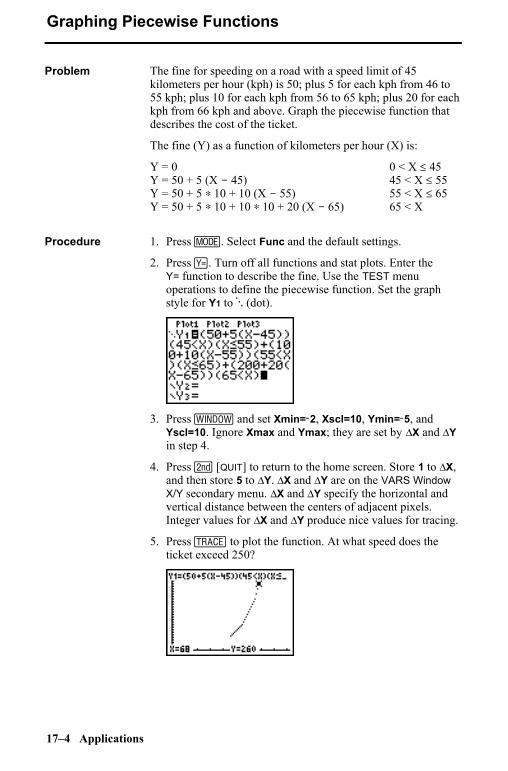
17–4 Applications
82501F~1.DOC TI-83 international English Bob Fedorisko Revised: 10/26/05 1:49 PM Printed: 10/27/05 3:04PM Page 4 of 20
The fine for speeding on a road with a speed limit of 45kilometers per hour (kph) is 50; plus 5 for each kph from 46 to55 kph; plus 10 for each kph from 56 to 65 kph; plus 20 for eachkph from 66 kph and above. Graph the piecewise function thatdescribes the cost of the ticket.
The fine (Y) as a function of kilometers per hour (X) is:
Y = 0 0 < X 45Y = 50 + 5 (X N 45) 45 < X 55Y = 50 + 5 … 10 + 10 (X N 55) 55 < X 65Y = 50 + 5 … 10 + 10 … 10 + 20 (X N 65) 65 < X
1. Press z. Select Func and the default settings.
2. Press o. Turn off all functions and stat plots. Enter theY= function to describe the fine. Use the TEST menuoperations to define the piecewise function. Set the graphstyle for Y1 to í (dot).
3. Press p and set Xmin=L2, Xscl=10, Ymin=L5, andYscl=10. Ignore Xmax and Ymax; they are set by @X and @Yin step 4.
4. Press y [QUIT] to return to the home screen. Store 1 to @X,and then store 5 to @Y. @X and @Y are on the VARS WindowX/Y secondary menu. @X and @Y specify the horizontal andvertical distance between the centers of adjacent pixels.Integer values for @X and @Y produce nice values for tracing.
5. Press r to plot the function. At what speed does theticket exceed 250?
Graphing Piecewise Functions
Problem
Procedure

Applications 17–5
82501F~1.DOC TI-83 international English Bob Fedorisko Revised: 10/26/05 1:49 PM Printed: 10/27/05 3:04PM Page 5 of 20
Graph the inequality 0.4X3 N 3X + 5 < 0.2X + 4. Use the TESTmenu operations to explore the values of X where the inequalityis true and where it is false.
1. Press z. Select Dot, Simul, and the default settings.Setting Dot mode changes all graph style icons to í (dot) inthe Y= editor.
2. Press o. Turn off all functions and stat plots. Enter the leftside of the inequality as Y4 and the right side as Y5.
3. Enter the statement of the inequality as Y6. This functionevaluates to 1 if true or 0 if false.
4. Press q 6 to graph the inequality in the standardwindow.
5. Press r † † to move to Y6. Then press | and ~ totrace the inequality, observing the value of Y.
6. Press o. Turn off Y4, Y5, and Y6. Enter equations to graphonly the inequality.
7. Press r. Notice that the values of Y7 and Y8 are zerowhere the inequality is false.
Graphing Inequalities
Problem
Procedure

17–6 Applications
82501F~1.DOC TI-83 international English Bob Fedorisko Revised: 10/26/05 1:49 PM Printed: 10/27/05 3:04PM Page 6 of 20
Using a graph, solve the equation X3 N 2X = 2cos(X). Statedanother way, solve the system of two equations and twounknowns: Y = X3N2X and Y = 2cos(X). Use ZOOM factors tocontrol the decimal places displayed on the graph.
1. Press z. Select the default mode settings. Press o. Turnoff all functions and stat plots. Enter the functions.
2. Press q 4 to select 4:ZDecimal. The display shows thattwo solutions may exist (points where the two functionsappear to intersect).
3. Press q ~ 4 to select 4:SetFactors from the ZOOMMEMORY menu. Set XFact=10 and YFact=10.
4. Press q 2 to select 2:Zoom In. Use |, ~, }, and † tomove the free-moving cursor onto the apparent intersectionof the functions on the right side of the display. As you movethe cursor, notice that the X and Y values have one decimalplace.
5. Press Í to zoom in. Move the cursor over theintersection. As you move the cursor, notice that now the Xand Y values have two decimal places.
6. Press Í to zoom in again. Move the free-moving cursoronto a point exactly on the intersection. Notice the numberof decimal places.
7. Press y [CALC] 5 to select 5:intersect. Press Í toselect the first curve and Í to select the second curve.To guess, move the trace cursor near the intersection. PressÍ. What are the coordinates of the intersection point?
8. Press q 4 to select 4:ZDecimal to redisplay the originalgraph.
9. Press q. Select 2:Zoom In and repeat steps 4 through 8to explore the apparent function intersection on the left sideof the display.
Solving a System of Nonlinear Equations
Problem
Procedure
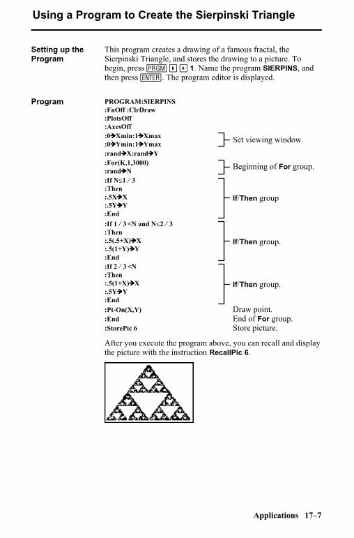
Applications 17–7
82501F~1.DOC TI-83 international English Bob Fedorisko Revised: 10/26/05 1:49 PM Printed: 10/27/05 3:04PM Page 7 of 20
This program creates a drawing of a famous fractal, theSierpinski Triangle, and stores the drawing to a picture. Tobegin, press ~ ~ 1. Name the program SIERPINS, andthen press Í. The program editor is displayed.
PROGRAM:SIERPINS:FnOff :ClrDraw:PlotsOff:AxesOff:0!!!!Xmin:1!!!!Xmax:0!!!!Ymin:1!!!!Ymax Set viewing window.:rand!!!!X:rand!!!!Y:For(K,1,3000):rand!!!!N Beginning of For group.:If N1à3:Then:.5X!!!!X:.5Y!!!!Y:End
If/Then group
:If 1à3 <N and N2à3:Then:.5(.5+X)!!!!X:.5(1+Y)!!!!Y:End
If/Then group.
:If 2à3 <N:Then:.5(1+X)!!!!X:.5Y!!!!Y:End
If/Then group.
:Pt-On(X,Y) Draw point.:End End of For group.:StorePic 6 Store picture.
After you execute the program above, you can recall and displaythe picture with the instruction RecallPic 6.
Using a Program to Create the Sierpinski Triangle
Setting up theProgram
Program
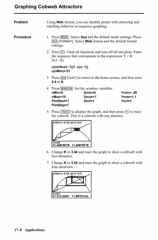
17–8 Applications
82501F~1.DOC TI-83 international English Bob Fedorisko Revised: 10/26/05 1:49 PM Printed: 10/27/05 3:04PM Page 8 of 20
Using Web format, you can identify points with attracting andrepelling behavior in sequence graphing.
1. Press z. Select Seq and the default mode settings. Pressy [FORMAT]. Select Web format and the default formatsettings.
2. Press o. Clear all functions and turn off all stat plots. Enterthe sequence that corresponds to the expression Y = KX(1NX).
u(n)=Ku(nN1)(1Nu(nN1))u(nMin)=.01
3. Press y [QUIT] to return to the home screen, and then store2.9 to K.
4. Press p. Set the window variables.nMin=0 Xmin=0 Ymin=M.26nMax=10 Xmax=1 Ymax=1.1PlotStart=1 Xscl=1 Yscl=1PlotStep=1
5. Press r to display the graph, and then press ~ to tracethe cobweb. This is a cobweb with one attractor.
6. Change K to 3.44 and trace the graph to show a cobweb withtwo attractors.
7. Change K to 3.54 and trace the graph to show a cobweb withfour attractors.
Graphing Cobweb Attractors
Problem
Procedure
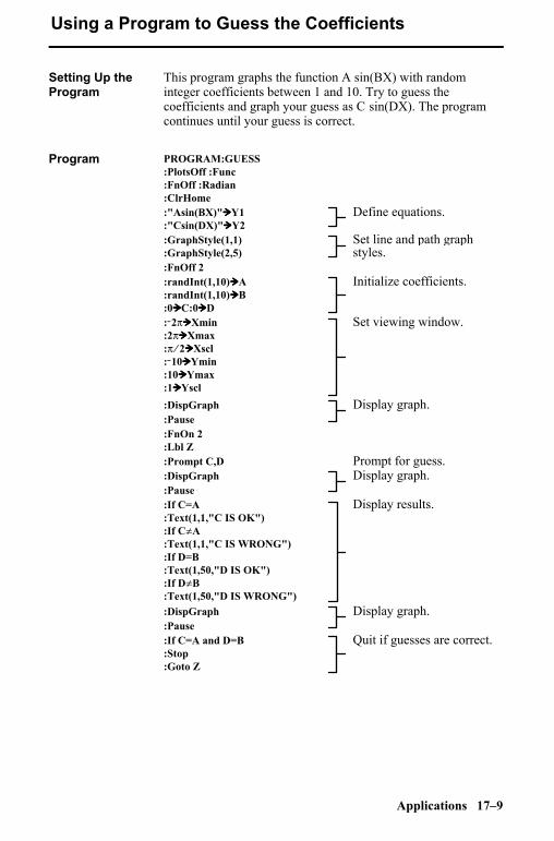
Applications 17–9
82501F~1.DOC TI-83 international English Bob Fedorisko Revised: 10/26/05 1:49 PM Printed: 10/27/05 3:04PM Page 9 of 20
This program graphs the function A sin(BX) with randominteger coefficients between 1 and 10. Try to guess thecoefficients and graph your guess as C sin(DX). The programcontinues until your guess is correct.
PROGRAM:GUESS:PlotsOff :Func:FnOff :Radian:ClrHome:"Asin(BX)"!!!!Y1:"Csin(DX)"!!!!Y2
Define equations.
:GraphStyle(1,1):GraphStyle(2,5)
Set line and path graphstyles.
:FnOff 2:randInt(1,10)!!!!A:randInt(1,10)!!!!B:0!!!!C:0!!!!D
Initialize coefficients.
:L2p!!!!Xmin:2p!!!!Xmax:pà2!!!!Xscl:L10!!!!Ymin:10!!!!Ymax:1!!!!Yscl
Set viewing window.
:DispGraph:Pause
Display graph.
:FnOn 2:Lbl Z:Prompt C,D Prompt for guess.:DispGraph:Pause
Display graph.
:If C=A:Text(1,1,"C IS OK"):If CƒA:Text(1,1,"C IS WRONG"):If D=B:Text(1,50,"D IS OK"):If DƒB:Text(1,50,"D IS WRONG")
Display results.
:DispGraph:Pause
Display graph.
:If C=A and D=B:Stop:Goto Z
Quit if guesses are correct.
Using a Program to Guess the Coefficients
Setting Up theProgram
Program

17–10 Applications
82501F~1.DOC TI-83 international English Bob Fedorisko Revised: 10/26/05 1:49 PM Printed: 10/27/05 3:04PM Page 10 of 20
Using parametric graphing mode, graph the unit circle and thesine curve to show the relationship between them.
Any function that can be plotted in Func mode can be plotted inPar mode by defining the X component as T and the Ycomponent as F(T).
1. Press z. Select Par, Simul, and the default settings.
2. Press p. Set the viewing window.Tmin=0 Xmin=L2 Ymin=L3Tmax=2p Xmax=7.4 Ymax=3Tstep=.1 Xscl=pà2 Yscl=1
3. Press o. Turn off all functions and stat plots. Enter theexpressions to define the unit circle centered on (0,0).
4. Enter the expressions to define the sine curve.
5. Press r. As the graph is plotting, you may press Íto pause and Í again to resume graphing as you watchthe sine function “unwrap” from the unit circle.
Note: You can generalize the unwrapping. Replace sin(T) in Y2T withany other trig function to unwrap that function.
Graphing the Unit Circle and Trigonometric Curves
Problem
Procedure

Applications 17–11
82501F~1.DOC TI-83 international English Bob Fedorisko Revised: 10/26/05 1:49 PM Printed: 10/27/05 3:04PM Page 11 of 20
Find the area of the region bounded by
f(x) = 300x / (x2 + 625)g(x) = 3cos(.1x)x = 75
1. Press z. Select the default mode settings.
2. Press p. Set the viewing window.Xmin=0 Ymin=L5Xmax=100 Ymax=10Xscl=10 Yscl=1
Xres=1
3. Press o. Turn off all functions and stat plots. Enter theupper and lower functions.Y1=300Xà(X2+625)Y2=3cos(.1X)
4. Press y [CALC] 5 to select 5:Intersect. The graph isdisplayed. Select a first curve, second curve, and guess forthe intersection toward the left side of the display. Thesolution is displayed, and the value of X at the intersection,which is the lower limit of the integral, is stored in Ans andX.
5. Press y [QUIT] to go to the home screen. Press y [DRAW]7 and use Shade( to see the area graphically.
Shade(Y2,Y1,Ans,75)
6. Press y [QUIT] to return to the home screen. Enter theexpression to evaluate the integral for the shaded region.
fnInt(Y1–Y2,X,Ans,75)
The area is 325.839962.
Finding the Area between Curves
Problem
Procedure

17–12 Applications
82501F~1.DOC TI-83 international English Bob Fedorisko Revised: 10/26/05 1:49 PM Printed: 10/27/05 3:04PM Page 12 of 20
Using two pairs of parametric equations, determine when twoobjects in motion are closest to each other in the same plane.
A ferris wheel has a diameter (d) of 20 meters and is rotatingcounterclockwise at a rate (s) of one revolution every 12seconds. The parametric equations below describe the locationof a ferris wheel passenger at time T, where a is the angle ofrotation, (0,0) is the bottom center of the ferris wheel, and(10,10) is the passenger’s location at the rightmost point, whenT=0.
X(T) = r cos a where a = 2pTs and r = dà2Y(T) = r + r sin a
A person standing on the ground throws a ball to the ferris wheelpassenger. The thrower’s arm is at the same height as the bottomof the ferris wheel, but 25 meters (b) to the right of the ferriswheel’s lowest point (25,0). The person throws the ball withvelocity (v0) of 22 meters per second at an angle (q) of 66¡ fromthe horizontal. The parametric equations below describe thelocation of the ball at time T.
X(T) = b N Tv0 cosqY(T) = Tv0 sinq N (gà2) T2 where g =9.8 m/sec2
1. Press z. Select Par, Simul, and the default settings.Simul (simultaneous) mode simulates the two objects inmotion over time.
2. Press p. Set the viewing window.Tmin=0 Xmin=L13 Ymin=0Tmax=12 Xmax=34 Ymax=31Tstep=.1 Xscl=10 Yscl=10
3. Press o. Turn off all functions and stat plots. Enter theexpressions to define the path of the ferris wheel and the path ofthe ball. Set the graph style for X2T to ëëëë (path).
Tip: Try setting the graph styles to ëëëë X1T and ìììì X2T, which simulatesa chair on the ferris wheel and the ball flying through the air when youpress s.
Using Parametric Equations: Ferris Wheel Problem
Problem
Procedure

Applications 17–13
82501F~1.DOC TI-83 international English Bob Fedorisko Revised: 10/26/05 1:49 PM Printed: 10/27/05 3:04PM Page 13 of 20
4. Press s to graph the equations. Watch closely as theyare plotted. Notice that the ball and the ferris wheelpassenger appear to be closest where the paths cross in thetop-right quadrant of the ferris wheel.
5. Press p. Change the viewing window to concentrateon this portion of the graph.Tmin=1 Xmin=0 Ymin=10Tmax=3 Xmax=23.5 Ymax=25.5Tstep=.03 Xscl=10 Yscl=10
6. Press r. After the graph is plotted, press ~ to movenear the point on the ferris wheel where the paths cross.Notice the values of X, Y, and T.
7. Press † to move to the path of the ball. Notice the values ofX and Y (T is unchanged). Notice where the cursor is located.This is the position of the ball when the ferris wheelpassenger passes the intersection. Did the ball or thepassenger reach the intersection first?
You can use r to, in effect, take snapshots in time andexplore the relative behavior of two objects in motion.
Procedure(continued)

17–14 Applications
82501F~1.DOC TI-83 international English Bob Fedorisko Revised: 10/26/05 1:49 PM Printed: 10/27/05 3:04PM Page 14 of 20
Using the functions fnInt( and nDeriv( from the MATH menu tograph functions defined by integrals and derivativesdemonstrates graphically that:
F(x) = ‰1
x 1àt dt = ln(x), x > 0 and that
Dx[‰1
x 1àt dt] = 1àx
1. Press z. Select the default settings.
2. Press p. Set the viewing window.Xmin=.01 Ymin=M1.5 Xres=3Xmax=10 Ymax=2.5Xscl=1 Yscl=1
3. Press o. Turn off all functions and stat plots. Enter thenumerical integral of 1àT from 1 to X and the functionln(X). Set the graph style for Y1 to ç (line) and Y2 toë (path).
4. Press r. Press |, }, ~, and † to compare the valuesof Y1 and Y2.
5. Press o. Turn off Y1 and Y2, and then enter the numericalderivative of the integral of 1àX and the function 1àX. Setthe graph style for Y3 to çççç (line) and Y4 to èèèè (thick).
6. Press r. Again, use the cursor keys to compare thevalues of the two graphed functions, Y3 and Y4.
Demonstrating the Fundamental Theorem of Calculus
Problem 1
Procedure 1

Applications 17–15
82501F~1.DOC TI-83 international English Bob Fedorisko Revised: 10/26/05 1:49 PM Printed: 10/27/05 3:04PM Page 15 of 20
Explore the functions defined by
y = ‰M2
x t2 dt, ‰
0
x t2 dt, and ‰
2
x t2 dt
1. Press o. Turn off all functions and stat plots. Use a list todefine these three functions simultaneously. Store thefunction in Y5.
2. Press q 6 to select 6:ZStandard.
3. Press r. Notice that the functions appear identical, onlyshifted vertically by a constant.
4. Press o. Enter the numerical derivative of Y5 in Y6.
5. Press r. Notice that although the three graphs definedby Y5 are different, they share the same derivative.
Problem 2
Procedure 2

17–16 Applications
82501F~1.DOC TI-83 international English Bob Fedorisko Revised: 10/26/05 1:49 PM Printed: 10/27/05 3:04PM Page 16 of 20
Use the equation solver to store a formula for the area of aregular N-sided polygon, and then solve for each variable, giventhe other variables. Explore the fact that the limiting case is thearea of a circle, pr2.
Consider the formula A = NB2 sin(pàN) cos(pàN) for the areaof a regular polygon with N sides of equal length and B distancefrom the center to a vertex.
N = 4 sides N = 8 sides N = 12 sides
1. Press 0 to select 0:Solver from the MATH menu. Eitherthe equation editor or the interactive solver editor isdisplayed. If the interactive solver editor is displayed, press} to display the equation editor.
2. Enter the formula as 0=ANNB2sin(p / N)cos(p / N), and thenpress Í. The interactive solver editor is displayed.
3. Enter N=4 and B=6 to find the area (A) of a square with adistance (B) from center to vertex of 6 centimeters.
4. Press } } to move the cursor onto A, and then press ƒ[SOLVE]. The solution for A is displayed on the interactivesolver editor.
5. Now solve for B for a given area with various number ofsides. Enter A=200 and N=6. To find the distance B, move thecursor onto B, and then press ƒ [SOLVE].
6. Enter N=8. To find the distance B, move the cursor onto B,and then press ƒ [SOLVE]. Find B for N=9, and then forN=10.
Computing Areas of Regular N-Sided Polygons
Problem
Procedure

Applications 17–17
82501F~1.DOC TI-83 international English Bob Fedorisko Revised: 10/26/05 1:49 PM Printed: 10/27/05 3:04PM Page 17 of 20
Find the area given B=6, and N=10, 100, 150, 1000, and 10000.Compare your results with p62 (the area of a circle with radius6), which is approximately 113.097.
7. Enter B=6. To find the area A, move the cursor onto A, andthen press ƒ [SOLVE]. Find A for N=10, then N=100,then N=150, then N=1000, and finally N=10000. Notice thatas N gets large, the area A approaches pB2.
Now graph the equation to see visually how the area changes asthe number of sides gets large.
8. Press z. Select the default mode settings.
9. Press p. Set the viewing window.Xmin=0 Ymin=0 Xres=1Xmax=200 Ymax=150Xscl=10 Yscl=10
10.Press o. Turn off all functions and stat plots. Enter theequation for the area. Use X in place of N. Set the graphstyles as shown.
11.Press r. After the graph is plotted, press 100 Í totrace to X=100. Press 150 Í. Press 188 Í. Noticethat as X increases, the value of Y converges to p62, which isapproximately 113.097. Y2=pB2 (the area of the circle) is ahorizontal asymptote to Y1. The area of an N-sided regularpolygon, with r as the distance from the center to a vertex,approaches the area of a circle with radius r (pr2) as N getslarge.
Procedure(continued)

17–18 Applications
82501F~1.DOC TI-83 international English Bob Fedorisko Revised: 10/26/05 1:49 PM Printed: 10/27/05 3:04PM Page 18 of 20
You are a loan officer at a mortgage company, and you recentlyclosed on a 30-year home mortgage at 8 percent interest withmonthly payments of 800. The new home owners want to knowhow much will be applied to the interest and how much will beapplied to the principal when they make the 240th payment 20years from now.
1. Press z and set the fixed-decimal mode to 2 decimalplaces. Set the other mode settings to the defaults.
2. Press y [FINANCE] 1 to display the TVM Solver. Enter thesevalues.
Note: Enter a positive number (800) to show PMT as a cashinflow. Payment values will be displayed as positive numbers onthe graph. Enter 0 for FV, since the future value of a loan is 0once it is paid in full. Enter PMT: END, since payment is due atthe end of a period.
3. Move the cursor onto the PV= prompt, and then press ƒ[SOLVE]. The present value, or mortgage amount, of thehouse is displayed at the PV= prompt.
Computing and Graphing Mortgage Payments
Problem
Procedure

Applications 17–19
82501F~1.DOC TI-83 international English Bob Fedorisko Revised: 10/26/05 1:49 PM Printed: 10/27/05 3:04PM Page 19 of 20
Now compare the graph of the amount of interest with the graphof the amount of principal for each payment.
4. Press z. Set Par and Simul.
5. Press o. Turn off all functions and stat plots. Enter theseequations and set the graph styles as shown.
Note: GPrn( and GInt( are located on the FINANCE CALCmenu.
6. Press p. Set these window variables.Tmin=1 Xmin=0 Ymin=0Tmax=360 Xmax=360 Ymax=1000Tstep=12 Xscl=10 Yscl=100
Tip: To increase the graph speed, change Tstep to 24.
7. Press r. After the graph is drawn, press 240 Í tomove the trace cursor to T=240, which is equivalent to 20years of payments.
The graph shows that for the 240th payment (X=240), 358.03of the 800 payment is applied to principal (Y=358.03).
Note: The sum of the payments (Y3T=Y1T+Y2T) is always 800.
Procedure(continued)

17–20 Applications
82501F~1.DOC TI-83 international English Bob Fedorisko Revised: 10/26/05 1:49 PM Printed: 10/27/05 3:04PM Page 20 of 20
8. Press † to move the cursor onto the function for interestdefined by X2T and Y2T. Enter 240.
The graph shows that for the 240th payment (X=240), 441.97of the 800 payment is interest (Y=441.97).
9. Press y [QUIT] y [FINANCE] 9 to paste 9:bal( to the homescreen. Check the figures from the graph.
At which monthly payment will the principal allocation surpassthe interest allocation?
Computing and Graphing Mortgage Payments (cont.)
Procedure(continued)

Memory Management 18–1
82D304~1.DOC TI-83 international English Bob Fedorisko Revised: 10/28/05 9:19 AM Printed: 10/28/05 9:21AM Page 1 of 6
18 MemoryManagement
Checking Available Memory.......................................................................... 2Deleting Items from Memory ......................................................................... 3Clearing Entries and List Elements............................................................. 4Resetting the TI-82 STATS ............................................................................. 5
Contents

18–2 Memory Management
82D304~1.DOC TI-83 international English Bob Fedorisko Revised: 10/28/05 9:19 AM Printed: 10/28/05 9:21AM Page 2 of 6
To display the MEMORY menu, press y [MEM].
MEMORY1: Check RAM... Reports memory availability/usage.2: Delete... Displays DELETE FROM menu.3: Clear Entries Clears ENTRY (last-entry storage).4: ClrAllLists Clears all lists in memory.5: Reset... Displays RESET menu (all/defaults).
Check RAM displays the Check RAM screen. The top linereports the total amount of available memory. The remaininglines report the amount of memory each variable type is using.You can check this screen to see whether you need to deletevariables from memory to make room for new data, such asprograms.
To check RAM usage, follow these steps.
1. Press y [MEM] to display the MEMORY menu.
2. Select 1:Check RAM to display the Check RAM screen. TheTI-82 STATS expresses memory quantities in bytes.
Note: The $ in the left column ofthe bottom row indicates that youcan scroll or page down to viewmore variable types.
Note: Real, List, Y.Vars, and Prgm variable types never resetto zero, even after memory is cleared.
To leave the Check RAM screen, press either y [QUIT] or‘. Both options display the home screen.
Checking Available Memory
MEMORY Menu
Displaying theCheck RAMScreen
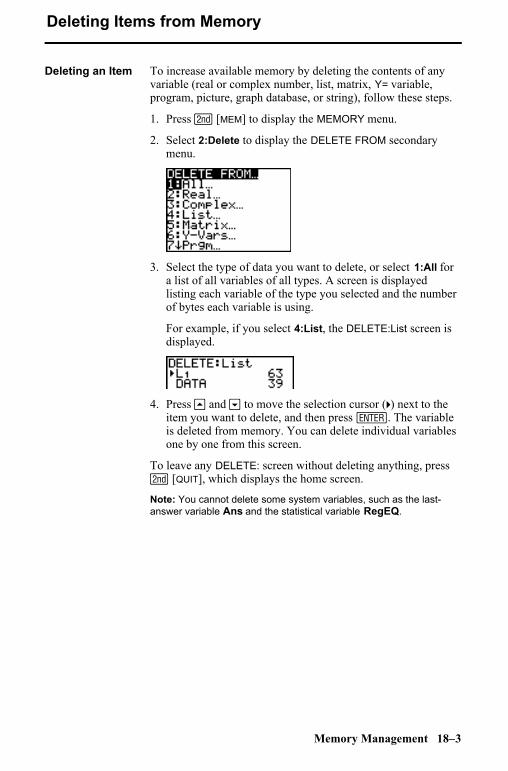
Memory Management 18–3
82D304~1.DOC TI-83 international English Bob Fedorisko Revised: 10/28/05 9:19 AM Printed: 10/28/05 9:21AM Page 3 of 6
To increase available memory by deleting the contents of anyvariable (real or complex number, list, matrix, Y= variable,program, picture, graph database, or string), follow these steps.
1. Press y [MEM] to display the MEMORY menu.
2. Select 2:Delete to display the DELETE FROM secondarymenu.
3. Select the type of data you want to delete, or select 1:All fora list of all variables of all types. A screen is displayedlisting each variable of the type you selected and the numberof bytes each variable is using.
For example, if you select 4:List, the DELETE:List screen isdisplayed.
4. Press } and † to move the selection cursor (4) next to theitem you want to delete, and then press Í. The variableis deleted from memory. You can delete individual variablesone by one from this screen.
To leave any DELETE: screen without deleting anything, pressy [QUIT], which displays the home screen.
Note: You cannot delete some system variables, such as the last-answer variable Ans and the statistical variable RegEQ.
Deleting Items from Memory
Deleting an Item

18–4 Memory Management
82D304~1.DOC TI-83 international English Bob Fedorisko Revised: 10/28/05 9:19 AM Printed: 10/28/05 9:21AM Page 4 of 6
Clear Entries clears the contents of the ENTRY (last entry)storage area (Chapter 1). To clear the ENTRY storage area,follow these steps.
1. Press y [MEM] to display the MEMORY menu.
2. Select 3:Clear Entries to paste the instruction to the homescreen.
3. Press Í to clear the ENTRY storage area.
To cancel Clear Entries, press ‘.
Note: If you select 3:Clear Entries from within a program, the ClearEntries instruction is pasted to the program editor, and the Entry(last entry) is cleared when the program is executed.
ClrAllLists sets to 0 the dimension of each list in memory.
To clear all elements from all lists, follow these steps.
1. Press y [MEM] to display the MEMORY menu.
2. Select 4:ClrAllLists to paste the instruction to the homescreen.
3. Press Í to set to 0 the dimension of each list in memory.
To cancel ClrAllLists, press ‘.
ClrAllLists does not delete list names from memory, from theLIST NAMES menu, or from the stat list editor.
Note: If you select 4:ClrAllLists from within a program, theClrAllLists instruction is pasted to the program editor. The lists arecleared when the program is executed.
Clearing Entries and List Elements
Clear Entries
ClrAllLists

Memory Management 18–5
82D304~1.DOC TI-83 international English Bob Fedorisko Revised: 10/28/05 9:19 AM Printed: 10/28/05 9:21AM Page 5 of 6
The RESET secondary menu gives you the option of resettingall memory (including default settings) or resetting the defaultsettings while preserving other data stored in memory, such asprograms and Y= functions.
Resetting all memory on the TI-82 STATS restores memory tothe factory settings. It deletes all nonsystem variables and allprograms. It resets all system variables to the default settings.
Tip: Before you reset all memory, consider restoring sufficientavailable memory by deleting only selected data (page 18.3).
To reset all memory on the TI-82 STATS, follow these steps.
1. Press y [MEM] to display the MEMORY menu.
2. Select 5:Reset to display the RESET secondary menu.
3. Select 1:All Memory to display the RESET MEMORY tertiarymenu.
4. Read the message below the RESET MEMORY menu.
• To cancel memory reset and return to the home screen,select 1:No.
• To erase from memory all data and programs, select2:Reset. All factory defaults are restored. Mem cleared isdisplayed on the home screen.
Note: When you clear memory, the contrast sometimes changes. Ifthe screen is faded or blank, adjust the contrast (Chapter 1).
Resetting the TI-82 STATS
RESETSecondary Menu
Resetting AllMemory

18–6 Memory Management
82D304~1.DOC TI-83 international English Bob Fedorisko Revised: 10/28/05 9:19 AM Printed: 10/28/05 9:21AM Page 6 of 6
When you reset defaults on the TI-82 STATS, all defaults arerestored to the factory settings. Stored data and programs are notchanged.
These are some examples of TI-82 STATS defaults that arerestored by resetting the defaults.
• Mode settings such as Normal (notation); Func (graphing);Real (numbers); and Full (screen)
• Y= functions off• Window variable values such as Xmin=L10; Xmax=10;
Xscl=1; Yscl=1; and Xres=1• Stat plots off• Format settings such as CoordOn (graphing coordinates on);
AxesOn; and ExprOn (expression on)• rand seed value to 0
To reset all TI-82 STATS factory defaults, follow these steps.
1. Press y [MEM] to display the MEMORY menu.
2. Select 5:Reset to display the RESET secondary menu.
3. Select 2:Defaults to display the RESET DEFAULTS tertiarymenu.
4. Consider the consequences of resetting defaults.
• To cancel reset and return to the home screen, select1:No.
• To restore factory default settings, select 2:Reset.Default settings are restored. Defaults set is displayed onthe home screen.
Resetting the TI-82 STATS (continued)
ResettingDefaults
Communication Link 19–1
825A7D~1.DOC TI-83 Intl English, Chap 19 Bob Fedorisko Revised: 10/27/05 1:26 PM Printed: 10/27/05 3:07PM Page 1 of 10
19 CommunicationLink
Getting Started: Sending Variables............................................................. 2TI-82 STATS LINK ............................................................................................... 3Selecting Items to Send....................................................................................... 4Receiving Items ....................................................................................................... 5Transmitting Items................................................................................................. 6Transmitting Lists to a TI-82 .......................................................................... 8Transmitting from a TI-82 to a TI-82 STATS ..................................... 9Backing Up Memory............................................................................................ 10
Contents

19–2 Communication Link
825A7D~1.DOC TI-83 Intl English, Chap 19 Bob Fedorisko Revised: 10/27/05 1:26 PM Printed: 10/27/05 3:07PM Page 2 of 10
Getting Started is a fast-paced introduction. Read the chapter for details.
Create and store a variable and a matrix, and then transfer them to anotherTI-82 STATS.
1. On the home screen of the sending unit, press5 Ë 5 ¿ ƒ Q. Press Í to store5.5 to Q.
2. Press y [ [ ] y [ [ ] 1¢ 2y [ ] ] y [ [ ]3 ¢ 4 y [ ] ] y [ ] ] ¿ 1. PressÍ to store the matrix to [A].
3. Connect the calculators with the link cable.Push both ends in firmly.
4. On the receiving unit, press y [LINK]~ todisplay the RECEIVE menu. Press 1 to select1:Receive. The message Waiting... isdisplayed and the busy indicator is on.
5. On the sending unit, press y [LINK] todisplay the SEND menu.
6. Press 2 to select 2:AllN. The AllN SELECTscreen is displayed.
7. Press † until the selection cursor ( 4 ) is nextto [A] MATRX. Press Í.
8. Press † until the selection cursor is next toQ REAL. Press Í. A square dot next to[A] and Q indicates that each is selected tosend.
9. On the sending unit, press ~ to display theTRANSMIT menu.
10. On the sending unit, press 1 to select1:Transmit and begin transmission. Thereceiving unit displays the messageReceiving....When the items are transmitted,both units display the name and type of eachtransmitted variable.
Getting Started: Sending Variables
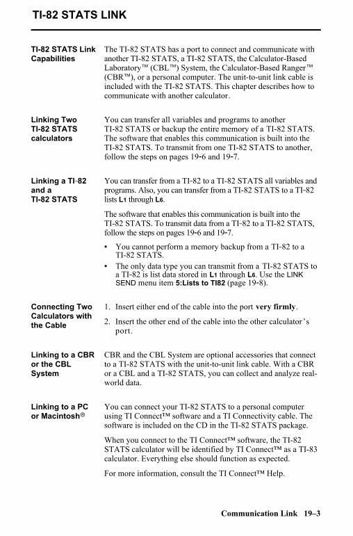
Communication Link 19–3
825A7D~1.DOC TI-83 Intl English, Chap 19 Bob Fedorisko Revised: 10/27/05 1:26 PM Printed: 10/27/05 3:07PM Page 3 of 10
The TI-82 STATS has a port to connect and communicate withanother TI-82 STATS, a TI-82 STATS, the Calculator-BasedLaboratoryé (CBLé) System, the Calculator-Based Rangeré(CBRé), or a personal computer. The unit-to-unit link cable isincluded with the TI-82 STATS. This chapter describes how tocommunicate with another calculator.
You can transfer all variables and programs to anotherTI-82 STATS or backup the entire memory of a TI-82 STATS.The software that enables this communication is built into theTI-82 STATS. To transmit from one TI-82 STATS to another,follow the steps on pages 19.6 and 19.7.
You can transfer from a TI-82 to a TI-82 STATS all variables andprograms. Also, you can transfer from a TI-82 STATS to a TI-82lists L1 through L6.
The software that enables this communication is built into theTI-82 STATS. To transmit data from a TI-82 to a TI-82 STATS,follow the steps on pages 19.6 and 19.7.
• You cannot perform a memory backup from a TI-82 to aTI-82 STATS.
• The only data type you can transmit from a TI-82 STATS toa TI-82 is list data stored in L1 through L6. Use the LINKSEND menu item 5:Lists to TI82 (page 19.8).
1. Insert either end of the cable into the port very firmly.
2. Insert the other end of the cable into the other calculator’sport.
CBR and the CBL System are optional accessories that connectto a TI-82 STATS with the unit-to-unit link cable. With a CBRor a CBL and a TI-82 STATS, you can collect and analyze real-world data.
You can connect your TI-82 STATS to a personal computerusing TI Connect™ software and a TI Connectivity cable. Thesoftware is included on the CD in the TI-82 STATS package.
When you connect to the TI Connect™ software, the TI-82STATS calculator will be identified by TI Connect™ as a TI-83calculator. Everything else should function as expected.
For more information, consult the TI Connect™ Help.
TI-82 STATS LINK
TI-82 STATS LinkCapabilities
Linking TwoTI-82 STATScalculators
Linking a TI-82and aTI-82 STATS
Connecting TwoCalculators withthe Cable
Linking to a CBRor the CBLSystem
Linking to a PCor Macintoshë

19–4 Communication Link
825A7D~1.DOC TI-83 Intl English, Chap 19 Bob Fedorisko Revised: 10/27/05 1:26 PM Printed: 10/27/05 3:07PM Page 4 of 10
To display the LINK SEND menu, press y [LINK].
SEND RECEIVE1: All+... Displays all items selected.2: AllN... Displays all items deselected.3: Prgm... Displays all programs names.4: List... Displays all list names.5: Lists to TI82... Displays list names L1 through L6.6: GDB... Displays all graph databases.7: Pic... Displays all picture data types.8: Matrix... Displays all matrix data types.9: Real... Displays all real variables.0: Complex... Displays all complex variables.A: Y-Vars... Displays all Y= variables.B: String... Displays all string variables.C: Back Up... Selects all for backup to TI-82 STATS.
When you select an item on the LINK SEND menu, thecorresponding SELECT screen is displayed.
Note: Each SELECT screen, except All+ SELECT, is displayedinitially with no data selected.
To select items to send on the sending unit, follow these steps.
1. Press y [LINK] to display the LINK SEND menu.
2. Select the menu item that describes the data type to send.The corresponding SELECT screen is displayed.
3. Press } and † to move the selection cursor ( 4 ) to an itemyou want to select or deselect.
4. Press Í to select or deselect the item. Selected namesare marked with a 0.
5. Repeat steps 3 and 4 to select or deselect additional items.
Selecting Items to Send
LINK SEND Menu
Selecting Itemsto Send

Communication Link 19–5
825A7D~1.DOC TI-83 Intl English, Chap 19 Bob Fedorisko Revised: 10/27/05 1:26 PM Printed: 10/27/05 3:07PM Page 5 of 10
To display the LINK RECEIVE menu, press y [LINK] ~.
SEND RECEIVE1: Receive Sets unit to receive data transmission.
When you select 1:Receive from the LINK RECEIVE menu onthe receiving unit, the message Waiting... and the busy indicatorare displayed. The receiving unit is ready to receive transmitteditems. To exit the receive mode without receiving items, pressÉ, and then select 1:Quit from the Error in Xmit menu.
To transmit, follow the steps on page 19.6.
When transmission is complete, the unit exits the receive mode.You can select 1:Receive again to receive more items. Thereceiving unit then displays a list of items received. Press y[QUIT] to exit the receive mode.
During transmission, if a variable name is duplicated, theDuplicateName menu is displayed on the receiving unit.
DuplicateName1: Rename Prompts to rename receiving variable.2: Overwrite Overwrites data in receiving variable.3: Omit Skips transmission of sending variable.4: Quit Stops transmission at duplicate variable.
When you select 1:Rename, the Name= prompt is displayed,and alpha-lock is on. Enter a new variable name, and then pressÍ. Transmission resumes.
When you select 2:Overwrite, the sending unit’s data overwritesthe existing data stored on the receiving unit. Transmissionresumes.
When you select 3:Omit, the sending unit does not send the datain the duplicated variable name. Transmission resumes with thenext item.
When you select 4:Quit, transmission stops, and the receivingunit exits receive mode.
During transmission, if the receiving unit does not havesufficient memory to receive an item, the Memory Full menu isdisplayed on the receiving unit.
• To skip this item for the current transmission, select 1:Omit.Transmission resumes with the next item.
• To cancel the transmission and exit receive mode, select2:Quit.
Receiving Items
LINK RECEIVEMenu
Receiving Unit
DuplicateNameMenu
InsufficientMemory inReceiving Unit

19–6 Communication Link
825A7D~1.DOC TI-83 Intl English, Chap 19 Bob Fedorisko Revised: 10/27/05 1:26 PM Printed: 10/27/05 3:07PM Page 6 of 10
To transmit selected items after you have selected items to sendon the sending unit (page 19.4) and set the receiving unit toreceive (page 19.5), follow these steps.
1. Press ~ on the sending unit to display the TRANSMIT menu.
2. Confirm that Waiting... is displayed on the receiving unit,which indicates it is set to receive (page 19.5).
3. Press Í to select 1:Transmit. The name and type of eachitem are displayed line by line on the sending unit as the itemis queued for transmission, and then on the receiving unit aseach item is accepted.
After all selected items have been transmitted, the messageDone is displayed on both calculators. Press } and † to scrollthrough the names.
To stop a link transmission, press É. The Error in Xmit menu isdisplayed on both units. To leave the error menu, select 1:Quit.
A transmission error occurs after one or two seconds if:
• A cable is not attached to the sending unit.• A cable is not attached to the receiving unit.
Note: If the cable is attached, push it in firmly and try again.• The receiving unit is not set to receive transmission.• You attempt a backup between a TI-82 and a TI-82 STATS.• You attempt a data transfer from a TI-82 STATS to a TI-82
with data other than lists L1 through L6 or without usingmenu item 5:Lists to TI82.
Although a transmission error does not occur, these twoconditions may prevent successful transmission.
• You try to use Get( with a calculator instead of a CBL orCBR.
• You try to use GetCalc( with a TI-82 instead of aTI-82 STATS.
Transmitting Items
TransmittingItems
Stopping aTransmission
Error Conditions

Communication Link 19–7
825A7D~1.DOC TI-83 Intl English, Chap 19 Bob Fedorisko Revised: 10/27/05 1:26 PM Printed: 10/27/05 3:07PM Page 7 of 10
After sending or receiving data, you can repeat the sametransmission to additional TI-82 STATS units—from either thesending unit or the receiving unit—without having to reselectdata to send. The current items remain selected.
Note: You cannot repeat transmission if you selected All+ or All ..
To transmit to an additional TI-82 STATS, follow these steps.
1. Set the TI-82 STATS to receive (page 19.5).
2. Do not select or deselect any new items to send. If you selector deselect an item, all selections or deselections from theprevious transmission are cleared.
3. Disconnect the link cable from one TI-82 STATS andconnect it to the additional TI-82 STATS.
4. Set the additional TI-82 STATS to receive (page 19.5).
5. Press y [LINK] on the sending TI-82 STATS to display theLINK SEND menu.
6. Select the menu item that you used for the last transmission.The data from your last transmission is still selected.
7. Press ~ to display the LINK TRANSMIT menu.
8. Confirm that the receiving unit is set to receive (page 19.5).
9. Press Í to select 1:Transmit and begin transmitting.
TransmittingItems to anAdditionalTI-82 STATS
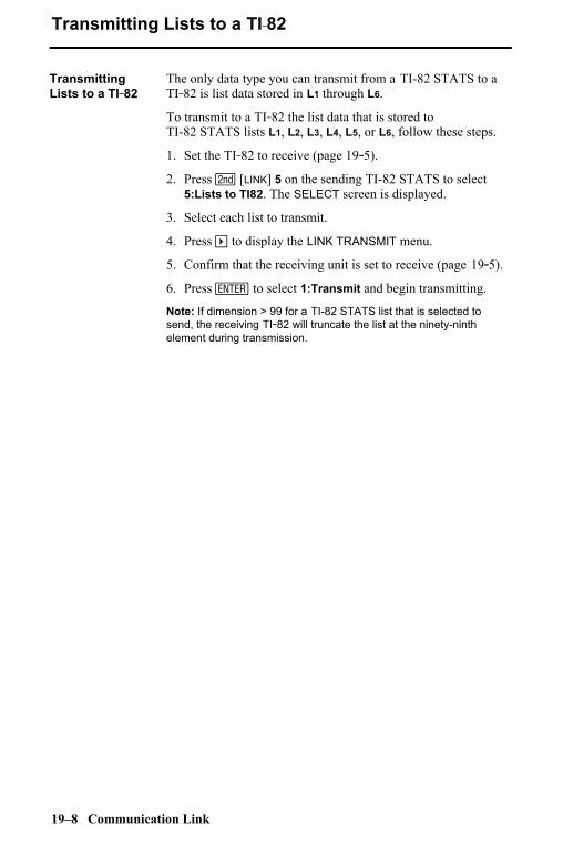
19–8 Communication Link
825A7D~1.DOC TI-83 Intl English, Chap 19 Bob Fedorisko Revised: 10/27/05 1:26 PM Printed: 10/27/05 3:07PM Page 8 of 10
The only data type you can transmit from a TI-82 STATS to aTI-82 is list data stored in L1 through L6.
To transmit to a TI-82 the list data that is stored toTI-82 STATS lists L1, L2, L3, L4, L5, or L6, follow these steps.
1. Set the TI-82 to receive (page 19.5).
2. Press y [LINK] 5 on the sending TI-82 STATS to select5:Lists to TI82. The SELECT screen is displayed.
3. Select each list to transmit.
4. Press ~ to display the LINK TRANSMIT menu.
5. Confirm that the receiving unit is set to receive (page 19.5).
6. Press Í to select 1:Transmit and begin transmitting.
Note: If dimension > 99 for a TI-82 STATS list that is selected tosend, the receiving TI-82 will truncate the list at the ninety-ninthelement during transmission.
Transmitting Lists to a TI-82
TransmittingLists to a TI-82

Communication Link 19–9
825A7D~1.DOC TI-83 Intl English, Chap 19 Bob Fedorisko Revised: 10/27/05 1:26 PM Printed: 10/27/05 3:07PM Page 9 of 10
Generally, you can transmit items to a TI-82 STATS from aTI-82, but differences between the two products may affectsome transmitted data. This table shows differences for whichthe software built into the TI-82 STATS automatically adjustswhen a TI-82 STATS receives TI-82 data.
TI.82 TI-82 STATSnMin PlotStartnStart nMinUn uVn vUnStart u(nMin)VnStart v(nMin)TblMin TblStart
For example, if you transmit from a TI-82 to a TI-82 STATS aprogram that contains nStart on a command line and thendisplay the program on the receiving TI-82 STATS, you will seethat nMin has automatically replaced nStart on the commandline.
The software built into the TI-82 STATS cannot resolve somedifferences between the TI-82 and TI-82 STATS, which aredescribed below. You must edit the data on the TI-82 STATSafter you transmit to account for these differences, or theTI-82 STATS will misinterpret the data.
The TI-82 STATS reinterprets TI-82 STATS prefix functions toinclude open parentheses, which may add extraneousparentheses to transmitted expressions.
For example, if you transmit sin X+5 from a TI-82 to aTI-82 STATS, the TI-82 STATS reinterprets it as sin(X+5.Without a closing parenthesis after X, the TI-82 STATSinterprets this as sin(X+5), not the sum of 5 and sin(X).
If a TI-82 instruction that the TI-82 STATS cannot translate istransmitted, the ERR:INVALID menu is displayed when theTI-82 STATS attempts to execute the instruction. For example,on the TI-82, the character group Un-1 is pasted to the cursorlocation when you press y [UnN1]. The TI-82 STATS cannotdirectly translate Un-1 to the TI-82 STATS syntax u(nN1), so theERR:INVALID menu is displayed.
Note: TI-82 STATS implied multiplication rules differ from those of theTI.82. For example, the TI-82 STATS evaluates 1à2X as (1à2)ääääX,while the TI-82 evaluates 1à2X as 1à(2ääääX) (Chapter 2).
Transmitting from a TI-82 to a TI-82 STATS
ResolvedDifferencesbetween theTI-82 andTI-82 STATS
UnresolvedDifferencesbetween theTI-82 andTI-82 STATS

19–10 Communication Link
825A7D~1.DOC TI-83 Intl English, Chap 19 Bob Fedorisko Revised: 10/27/05 1:26 PM Printed: 10/27/05 3:07PM Page 10 of 10
To copy the exact contents of memory in the sendingTI-82 STATS to the memory of the receiving TI-82 STATS, putthe other unit in receive mode. Then, on the receiving unit,select C:Back Up from the LINK SEND menu.
• Warning: C:Back Up overwrites the memory in thereceiving unit; all information in the memory of thereceiving unit is lost.Note: If you do not want to do a backup, select 2:Quit to return tothe LINK SEND menu.
• Select 1:Transmit to begin transmission.
As a safety check to prevent accidental loss of memory, themessage WARNING . Backup is displayed when the receivingunit receives notice of a backup.
• To continue with the backup process, select 1:Continue. Thebackup transmission begins.
• To prevent the backup, select 2:Quit.
Note: If a transmission error is returned during a backup, thereceiving unit is reset.
When the backup is complete, both the sending calculator andreceiving calculator display a confirmation screen.
Backing Up Memory
Memory Backup
Receiving Unit
Memory BackupComplete
Tables and Reference Information A–1
826DEC~1.DOC TI-83 international English Bob Fedorisko Revised: 10/26/05 2:20 PM Printed: 10/27/05 3:09PM Page 1 of 58
A Tables and ReferenceInformation
Table of Functions and Instructions............................................................ 2TI-82 STATS Menu Map.................................................................................. 39Variables....................................................................................................................... 49Statistics Formulas................................................................................................. 50Financial Formulas ................................................................................................ 54
Contents
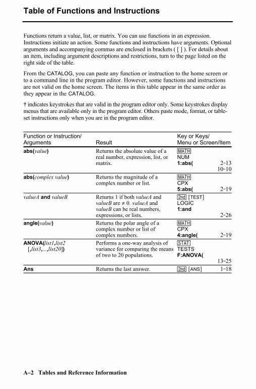
A–2 Tables and Reference Information
826DEC~1.DOC TI-83 international English Bob Fedorisko Revised: 10/26/05 2:20 PM Printed: 10/27/05 3:09PM Page 2 of 58
Functions return a value, list, or matrix. You can use functions in an expression.Instructions initiate an action. Some functions and instructions have arguments. Optionalarguments and accompanying commas are enclosed in brackets ( [ ] ). For details aboutan item, including argument descriptions and restrictions, turn to the page listed on theright side of the table.
From the CATALOG, you can paste any function or instruction to the home screen orto a command line in the program editor. However, some functions and instructionsare not valid on the home screen. The items in this table appear in the same order asthey appear in the CATALOG.
† indicates keystrokes that are valid in the program editor only. Some keystrokes displaymenus that are available only in the program editor. Others paste mode, format, or table-set instructions only when you are in the program editor.
Function or Instruction/Arguments Result
Key or Keys/Menu or Screen/Item
abs(value) Returns the absolute value of areal number, expression, list, ormatrix.
NUM1:abs( 2-13
10-10abs(complex value) Returns the magnitude of a
complex number or list.CPX5:abs( 2-19
valueA and valueB Returns 1 if both valueA andvalueB are ƒ 0. valueA andvalueB can be real numbers,expressions, or lists.
y [TEST]LOGIC1:and
2-26angle(value) Returns the polar angle of a
complex number or list ofcomplex numbers.
CPX4:angle( 2-19
ANOVA(list1,list2 [,list3,...,list20])
Performs a one-way analysis ofvariance for comparing the meansof two to 20 populations.
…TESTSF:ANOVA(
13-25Ans Returns the last answer. y [ANS] 1-18
Table of Functions and Instructions

Tables and Reference Information A–3
826DEC~1.DOC TI-83 international English Bob Fedorisko Revised: 10/26/05 2:20 PM Printed: 10/27/05 3:09PM Page 3 of 58
Function or Instruction/Arguments Result
Key or Keys/Menu or Screen/Item
augment(matrixA,matrixB) Returns a matrix, which is matrixBappended to matrixA as newcolumns.
MATH7:augment( 10-14
augment(listA,listB) Returns a list, which is listBconcatenated to the end of listA.
y [LIST]OPS9:augment( 11-15
AxesOff Turns off the graph axes. † y [FORMAT] AxesOff 3-14
AxesOn Turns on the graph axes. † y [FORMAT] AxesOn 3-14
a+bi Sets the mode to rectangularcomplex number mode (a+bi).
† z a+bi 1-12
bal(npmt[,roundvalue]) Computes the balance at npmt foran amortization schedule usingstored values for PV, ææææ, andPMT and rounds the computationto roundvalue.
y [FINANCE]CALC9:bal(
14-9binomcdf(numtrials,p[,x]) Computes a cumulative
probability at x for the discretebinomial distribution with thespecified numtrials andprobability p of success on eachtrial.
y [DISTR]DISTRA:binomcdf(
13-33binompdf(numtrials,p[,x]) Computes a probability at x for
the discrete binomial distributionwith the specified numtrials andprobability p of success on eachtrial.
y [DISTR]DISTR0:binompdf(
13-33c2cdf(lowerbound, upperbound,df)
Computes the c2 distributionprobability between lowerboundand upperbound for the specifieddegrees of freedom df.
y [DISTR]DISTR7:c2cdf(
13-31
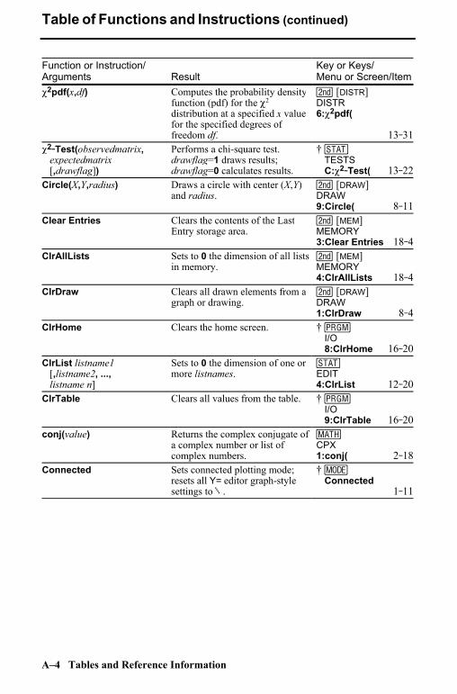
A–4 Tables and Reference Information
826DEC~1.DOC TI-83 international English Bob Fedorisko Revised: 10/26/05 2:20 PM Printed: 10/27/05 3:09PM Page 4 of 58
Function or Instruction/Arguments Result
Key or Keys/Menu or Screen/Item
c2pdf(x,df) Computes the probability densityfunction (pdf) for the c2
distribution at a specified x valuefor the specified degrees offreedom df.
y [DISTR]DISTR6:c2pdf(
13-31c2.Test(observedmatrix, expectedmatrix [,drawflag])
Performs a chi-square test.drawflag=1 draws results;drawflag=0 calculates results.
† … TESTS C:c2.Test( 13-22
Circle(X,Y,radius) Draws a circle with center (X,Y)and radius.
y [DRAW]DRAW9:Circle( 8-11
Clear Entries Clears the contents of the LastEntry storage area.
y [MEM]MEMORY3:Clear Entries 18-4
ClrAllLists Sets to 0 the dimension of all listsin memory.
y [MEM]MEMORY4:ClrAllLists 18-4
ClrDraw Clears all drawn elements from agraph or drawing.
y [DRAW]DRAW1:ClrDraw 8-4
ClrHome Clears the home screen. † I/O 8:ClrHome 16-20
ClrList listname1 [,listname2, ..., listname n]
Sets to 0 the dimension of one ormore listnames.
…EDIT4:ClrList 12-20
ClrTable Clears all values from the table. † I/O 9:ClrTable 16-20
conj(value) Returns the complex conjugate ofa complex number or list ofcomplex numbers.
CPX1:conj( 2-18
Connected Sets connected plotting mode;resets all Y= editor graph-stylesettings to ç .
† z Connected
1-11
Table of Functions and Instructions (continued)

Tables and Reference Information A–5
826DEC~1.DOC TI-83 international English Bob Fedorisko Revised: 10/26/05 2:20 PM Printed: 10/27/05 3:09PM Page 5 of 58
Function or Instruction/Arguments Result
Key or Keys/Menu or Screen/Item
CoordOff Turns off cursor coordinate valuedisplay.
† y [FORMAT] CoordOff 3-14
CoordOn Turns on cursor coordinate valuedisplay.
† y [FORMAT] CoordOn 3-14
cos(value) Returns cosine of areal number, expression, or list.
™
2-3cosL1(value) Returns arccosine of a real
number, expression, or list.y [COSL1]
2-3cosh(value) Returns hyperbolic cosine of a
real number, expression, or list.y [CATALOG]cosh(
15-10coshL1(value) Returns hyperbolic arccosine of a
real number, expression,or list.
y [CATALOG]coshL1(
15-10CubicReg [Xlistname, Ylistname,freqlist, regequ]
Fits a cubic regression model toXlistname and Ylistname withfrequency freqlist, and stores theregression equation to regequ.
…CALC6:CubicReg
12-26cumSum(list) Returns a list of the cumulative
sums of the elements in list,starting with the first element.
y [LIST]OPS6:cumSum( 11-12
cumSum(matrix) Returns a matrix of thecumulative sums of matrixelements. Each element in thereturned matrix is a cumulativesum of a matrix column from topto bottom.
MATH0:cumSum(
10-15dbd(date1,date2) Calculates the number of days
between date1 and date2 using theactual-day-count method.
y [FINANCE]CALCD:dbd( 14-13
value4Dec Displays a real or complexnumber, expression, list, or matrixin decimal format.
MATH2:4Dec 2-5

A–6 Tables and Reference Information
826DEC~1.DOC TI-83 international English Bob Fedorisko Revised: 10/26/05 2:20 PM Printed: 10/27/05 3:09PM Page 6 of 58
Function or Instruction/Arguments Result
Key or Keys/Menu or Screen/Item
Degree Sets degree angle mode. † z Degree 1-11
DelVar variable Deletes from memory thecontents of variable.
† CTL G:DelVar 16-15
DependAsk Sets table to ask for dependent-variable values.
† y [TBLSET] Depend: Ask 7-3
DependAuto Sets table to generate dependent-variable values automatically.
† y [TBLSET] Depend: Auto
7-3det(matrix) Returns determinant of matrix.
MATH1:det( 10-12
DiagnosticOff Sets diagnostics-off mode; r, r2,and R2 are not displayed asregression model results.
y [CATALOG]DiagnosticOff
12-23DiagnosticOn Sets diagnostics-on mode; r, r2,
and R2 are displayed asregression model results.
y [CATALOG]DiagnosticOn
12-23dim(listname) Returns the dimension of
listname.y [LIST]OPS3:dim( 11-11
dim(matrixname) Returns the dimension ofmatrixname as a list.
MATH3:dim( 10-12
length!!!!dim(listname) Assigns a new dimension (length)to a new or existing listname.
y [LIST]OPS3:dim( 11-11
{rows,columns}!!!! dim(matrixname)
Assigns new dimensions to a newor existing matrixname.
MATH3:dim( 10-13
Disp Displays the home screen. † I/O 3:Disp 16-18
Disp [valueA,valueB, valueC,...,value n]
Displays each value. † I/O 3:Disp 16-18
Table of Functions and Instructions (continued)
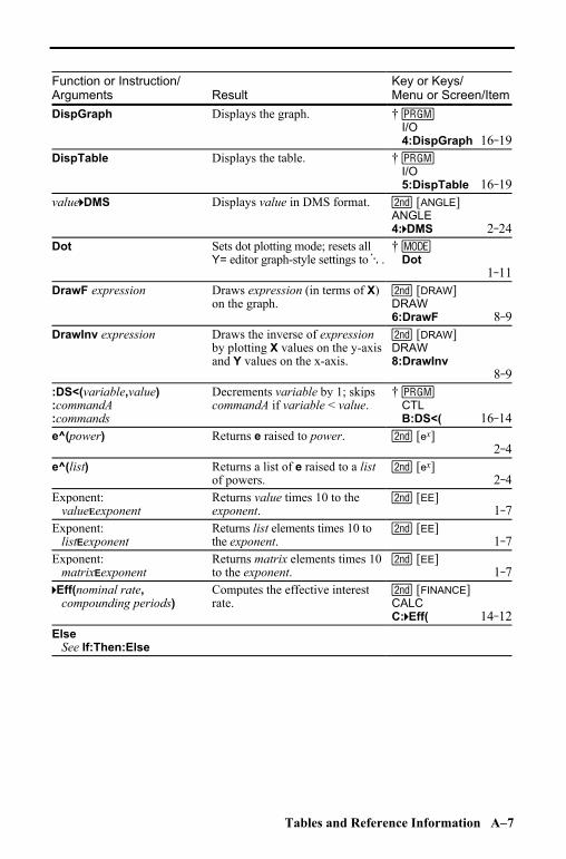
Tables and Reference Information A–7
826DEC~1.DOC TI-83 international English Bob Fedorisko Revised: 10/26/05 2:20 PM Printed: 10/27/05 3:09PM Page 7 of 58
Function or Instruction/Arguments Result
Key or Keys/Menu or Screen/Item
DispGraph Displays the graph. † I/O 4:DispGraph 16-19
DispTable Displays the table. † I/O 5:DispTable 16-19
value4DMS Displays value in DMS format. y [ANGLE]ANGLE4:4DMS 2-24
Dot Sets dot plotting mode; resets allY= editor graph-style settings to í .
† z Dot
1-11DrawF expression Draws expression (in terms of X)
on the graph.y [DRAW]DRAW6:DrawF 8-9
DrawInv expression Draws the inverse of expressionby plotting X values on the y-axisand Y values on the x-axis.
y [DRAW]DRAW8:DrawInv
8-9:DS<(variable,value):commandA:commands
Decrements variable by 1; skipscommandA if variable < value.
† CTL B:DS<( 16-14
e^(power) Returns e raised to power. y [ex]2-4
e^(list) Returns a list of e raised to a listof powers.
y [ex]2-4
Exponent: valueEexponent
Returns value times 10 to theexponent.
y [EE]1-7
Exponent: listEexponent
Returns list elements times 10 tothe exponent.
y [EE]1-7
Exponent: matrixEexponent
Returns matrix elements times 10to the exponent.
y [EE]1-7
4Eff(nominal rate, compounding periods)
Computes the effective interestrate.
y [FINANCE]CALCC:4Eff( 14-12
Else See If:Then:Else

A–8 Tables and Reference Information
826DEC~1.DOC TI-83 international English Bob Fedorisko Revised: 10/26/05 2:20 PM Printed: 10/27/05 3:09PM Page 8 of 58
Function or Instruction/Arguments Result
Key or Keys/Menu or Screen/Item
End Identifies end of For(,If-Then-Else, Repeat, or Whileloop.
† CTL 7:End 16-12
Eng Sets engineering display mode. † z Eng 1-10
Equ4String(Y= var,Strn) Converts the contents of a Y= varto a string and stores it in Strn.
y [CATALOG]Equ4String(
15-7expr(string) Converts string to an expression
and executes it.y [CATALOG]expr( 15-7
ExpReg [Xlistname,Ylistname,freqlist,regequ]
Fits an exponential regressionmodel to Xlistname and Ylistnamewith frequency freqlist, and storesthe regression equation to regequ.
…CALC0:ExpReg
12-26ExprOff Turns off the expression display
during TRACE.† y [FORMAT] ExprOff 3-14
ExprOn Turns on the expression displayduring TRACE.
† y [FORMAT] ExprOn 3-14
ÜÜÜÜcdf(lowerbound, upperbound, numerator df, denominator df)
Computes the Û distributionprobability between lowerboundand upperbound for the specifiednumerator df (degrees offreedom) and denominator df.
y [DISTR]DISTR9:ÛÛÛÛcdf(
13-32Fill(value,matrixname) Stores value to each element in
matrixname.MATH4:Fill( 10-13
Fill(value,listname) Stores value to each element inlistname.
y [LIST]OPS4:Fill( 11-11
Fix # Sets fixed-decimal mode for # ofdecimal places.
† z 0123456789 (select one) 1-10
Float Sets floating decimal mode. † z Float 1-10
Table of Functions and Instructions (continued)

Tables and Reference Information A–9
826DEC~1.DOC TI-83 international English Bob Fedorisko Revised: 10/26/05 2:20 PM Printed: 10/27/05 3:09PM Page 9 of 58
Function or Instruction/Arguments Result
Key or Keys/Menu or Screen/Item
fMax(expression,variable, lower,upper[,tolerance])
Returns the value of variablewhere the local maximum ofexpression occurs, between lowerand upper, with specifiedtolerance.
MATH7:fMax(
2-6fMin(expression,variable, lower,upper[,tolerance])
Returns the value of variablewhere the local minimum ofexpression occurs, between lowerand upper, with specifiedtolerance.
MATH6:fMin(
2-6fnInt(expression,variable, lower,upper[,tolerance])
Returns the function integral ofexpression with respect tovariable, between lower andupper, with specified tolerance.
MATH9:fnInt(
2-7FnOff [function#, function#,...,function n]
Deselects all Y= functions orspecified Y= functions.
Y-VARS On/Off2:FnOff 3-8
FnOn [function#, function#,...,function n]
Selects all Y= functions orspecified Y= functions.
Y-VARS On/Off1:FnOn 3-8
:For(variable,begin,end [,increment]):commands:End:commands
Executes commands throughEnd, incrementing variable frombegin by increment untilvariable>end.
† CTL 4:For(
16-10fPart(value) Returns the fractional part or parts
of a real or complex number,expression, list, or matrix.
NUM4:fPart( 2-14
10-11ÜÜÜÜpdf(x,numerator df, denominator df)
Computes the Û distributionprobability between lowerboundand upperbound for the specifiednumerator df (degrees offreedom) and denominator df.
y [DISTR]DISTR8:ÛÛÛÛpdf(
13-32

A–10 Tables and Reference Information
826DEC~1.DOC TI-83 international English Bob Fedorisko Revised: 10/26/05 2:20 PM Printed: 10/27/05 3:09PM Page 10 of 58
Function or Instruction/Arguments Result
Key or Keys/Menu or Screen/Item
value4Frac Displays a real or complexnumber, expression, list, or matrixas a fraction simplified to itssimplest terms.
MATH1:4Frac
2-5Full Sets full screen mode. † z
Full 1-12Func Sets function graphing mode. † z
Func 1-11gcd(valueA,valueB) Returns the greatest common
divisor of valueA and valueB,which can be real numbers orlists.
NUM9:gcd(
2-15geometcdf(p,x) Computes a cumulative
probability at x, the number of thetrial on which the first successoccurs, for the discrete geometricdistribution with the specifiedprobability of success p.
y [DISTR]DISTRE:geometcdf(
13-34geometpdf(p,x) Computes a probability at x, the
number of the trial on which thefirst success occurs, for the discretegeometric distribution with thespecified probability of success p.
y [DISTR]DISTRD:geometpdf(
13-34Get(variable) Gets data from the CBL System or
CBR and stores it in variable.† I/O A:Get( 16-21
GetCalc(variable) Gets contents of variable onanother TI-82 STATS and stores itto variable on the receivingTI-82 STATS.
† I/O 0:GetCalc( 16-21
getKey Returns the key code for thecurrent keystroke, or 0, if no keyis pressed.
† I/O 7:getKey 16-20
Goto label Transfers control to label. † CTL 0:Goto 16-13
Table of Functions and Instructions (continued)
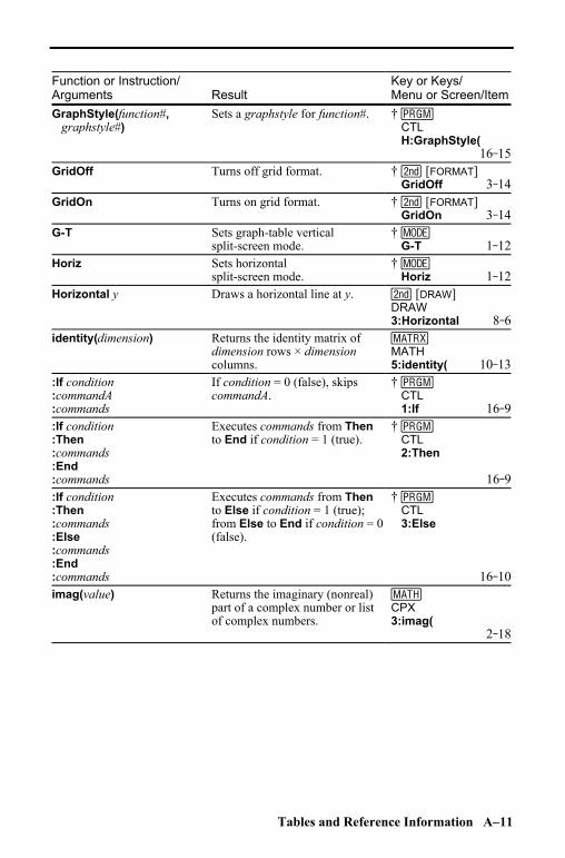
Tables and Reference Information A–11
826DEC~1.DOC TI-83 international English Bob Fedorisko Revised: 10/26/05 2:20 PM Printed: 10/27/05 3:09PM Page 11 of 58
Function or Instruction/Arguments Result
Key or Keys/Menu or Screen/Item
GraphStyle(function#, graphstyle#)
Sets a graphstyle for function#. † CTL H:GraphStyle(
16-15GridOff Turns off grid format. † y [FORMAT]
GridOff 3-14GridOn Turns on grid format. † y [FORMAT]
GridOn 3-14G-T Sets graph-table vertical
split-screen mode.† z G-T 1-12
Horiz Sets horizontalsplit-screen mode.
† z Horiz 1-12
Horizontal y Draws a horizontal line at y. y [DRAW]DRAW3:Horizontal 8-6
identity(dimension) Returns the identity matrix ofdimension rows × dimensioncolumns.
MATH5:identity( 10-13
:If condition:commandA:commands
If condition = 0 (false), skipscommandA.
† CTL 1:If 16-9
:If condition:Then:commands:End:commands
Executes commands from Thento End if condition = 1 (true).
† CTL 2:Then
16-9:If condition:Then:commands:Else:commands:End:commands
Executes commands from Thento Else if condition = 1 (true);from Else to End if condition = 0(false).
† CTL 3:Else
16-10imag(value) Returns the imaginary (nonreal)
part of a complex number or listof complex numbers.
CPX3:imag(
2-18

A–12 Tables and Reference Information
826DEC~1.DOC TI-83 international English Bob Fedorisko Revised: 10/26/05 2:20 PM Printed: 10/27/05 3:09PM Page 12 of 58
Function or Instruction/Arguments Result
Key or Keys/Menu or Screen/Item
IndpntAsk Sets table to ask for independent-variable values.
† y [TBLSET] Indpnt: Ask 7-3
IndpntAuto Sets table to generateindependent-variable valuesautomatically.
† y [TBLSET] Indpnt: Auto
7-3Input Displays graph. †
I/O 1:Input 16-16
Input [variable]Input ["text",variable]
Prompts for value to store tovariable.
† I/O 1:Input 16-17
Input [Strn,variable] Displays Strn and stores enteredvalue to variable.
† I/O 1:Input 16-17
inString(string,substring [,start])
Returns the character position instring of the first character ofsubstring beginning at start.
y [CATALOG]inString(
15-7int(value) Returns the largest integer a real
or complex number, expression,list, or matrix.
NUM5:int( 2-14
10-11GInt(pmt1,pmt2 [,roundvalue])
Computes the sum, rounded toroundvalue, of the interestamount between pmt1 and pmt2for an amortization schedule.
y [FINANCE]CALCA:GInt(
14-9invNorm(area[,m,s]) Computes the inverse cumulative
normal distribution function for agiven area under the normaldistribution curve specified by mand s.
y [DISTR]DISTR3:invNorm(
13-30iPart(value) Returns the integer part of a real
or complex number, expression,list, or matrix.
NUM3:iPart( 2-14
10-11
Table of Functions and Instructions (continued)
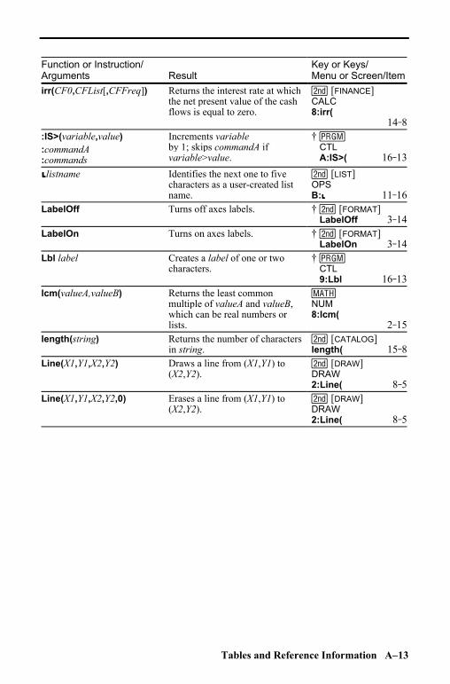
Tables and Reference Information A–13
826DEC~1.DOC TI-83 international English Bob Fedorisko Revised: 10/26/05 2:20 PM Printed: 10/27/05 3:09PM Page 13 of 58
Function or Instruction/Arguments Result
Key or Keys/Menu or Screen/Item
irr(CF0,CFList[,CFFreq]) Returns the interest rate at whichthe net present value of the cashflows is equal to zero.
y [FINANCE]CALC8:irr(
14-8:IS>(variable,value):commandA:commands
Increments variableby 1; skips commandA ifvariable>value.
† CTL A:IS>( 16-13
ÙÙÙÙlistname Identifies the next one to fivecharacters as a user-created listname.
y [LIST]OPSB:ÙÙÙÙ 11-16
LabelOff Turns off axes labels. † y [FORMAT] LabelOff 3-14
LabelOn Turns on axes labels. † y [FORMAT] LabelOn 3-14
Lbl label Creates a label of one or twocharacters.
† CTL 9:Lbl 16-13
lcm(valueA,valueB) Returns the least commonmultiple of valueA and valueB,which can be real numbers orlists.
NUM8:lcm(
2-15length(string) Returns the number of characters
in string.y [CATALOG]length( 15-8
Line(X1,Y1,X2,Y2) Draws a line from (X1,Y1) to(X2,Y2).
y [DRAW]DRAW2:Line( 8-5
Line(X1,Y1,X2,Y2,0) Erases a line from (X1,Y1) to(X2,Y2).
y [DRAW]DRAW2:Line( 8-5
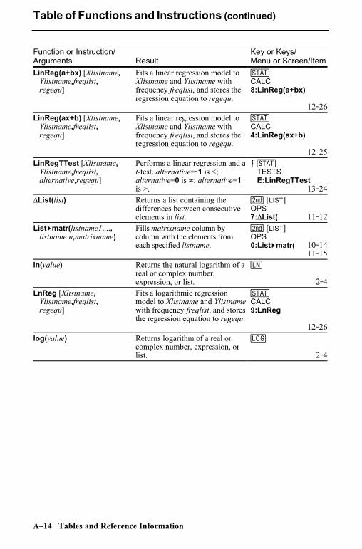
A–14 Tables and Reference Information
826DEC~1.DOC TI-83 international English Bob Fedorisko Revised: 10/26/05 2:20 PM Printed: 10/27/05 3:09PM Page 14 of 58
Function or Instruction/Arguments Result
Key or Keys/Menu or Screen/Item
LinReg(a+bx) [Xlistname, Ylistname,freqlist, regequ]
Fits a linear regression model toXlistname and Ylistname withfrequency freqlist, and stores theregression equation to regequ.
…CALC8:LinReg(a+bx)
12-26LinReg(ax+b) [Xlistname, Ylistname,freqlist, regequ]
Fits a linear regression model toXlistname and Ylistname withfrequency freqlist, and stores theregression equation to regequ.
…CALC4:LinReg(ax+b)
12-25LinRegTTest [Xlistname, Ylistname,freqlist, alternative,regequ]
Performs a linear regression and at-test. alternative=L1 is <;alternative=0 is ƒ; alternative=1is >.
† … TESTS E:LinRegTTest
13-24@List(list) Returns a list containing the
differences between consecutiveelements in list.
y [LIST]OPS7:@List( 11-12
List 4 matr(listname1,..., listname n,matrixname)
Fills matrixname column bycolumn with the elements fromeach specified listname.
y [LIST]OPS0:List 4 matr( 10-14
11-15ln(value) Returns the natural logarithm of a
real or complex number,expression, or list.
µ
2-4LnReg [Xlistname, Ylistname,freqlist, regequ]
Fits a logarithmic regressionmodel to Xlistname and Ylistnamewith frequency freqlist, and storesthe regression equation to regequ.
…CALC9:LnReg
12-26log(value) Returns logarithm of a real or
complex number, expression, orlist.
«
2-4
Table of Functions and Instructions (continued)
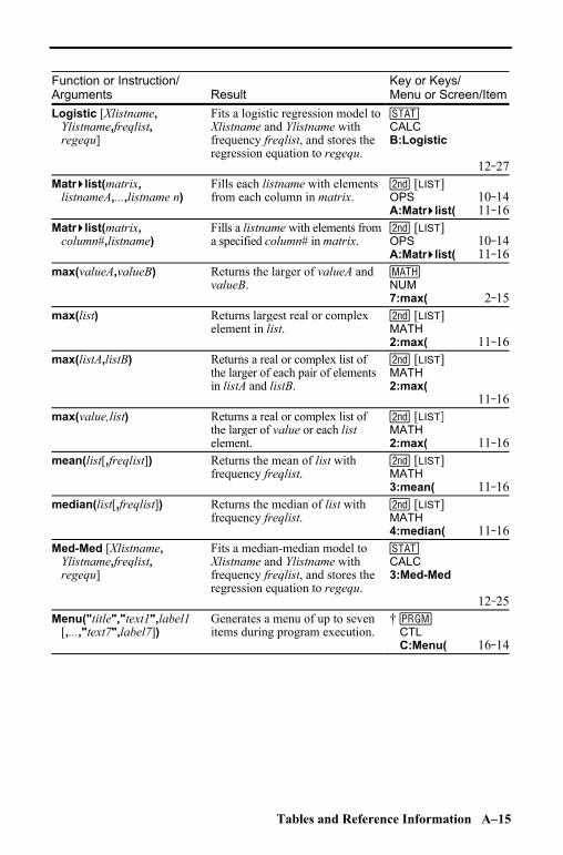
Tables and Reference Information A–15
826DEC~1.DOC TI-83 international English Bob Fedorisko Revised: 10/26/05 2:20 PM Printed: 10/27/05 3:09PM Page 15 of 58
Function or Instruction/Arguments Result
Key or Keys/Menu or Screen/Item
Logistic [Xlistname, Ylistname,freqlist, regequ]
Fits a logistic regression model toXlistname and Ylistname withfrequency freqlist, and stores theregression equation to regequ.
…CALCB:Logistic
12-27Matr 4 list(matrix, listnameA,...,listname n)
Fills each listname with elementsfrom each column in matrix.
y [LIST]OPS 10-14A:Matr 4 list( 11-16
Matr 4 list(matrix, column#,listname)
Fills a listname with elements froma specified column# in matrix.
y [LIST]OPS 10-14A:Matr 4 list( 11-16
max(valueA,valueB) Returns the larger of valueA andvalueB.
NUM7:max( 2-15
max(list) Returns largest real or complexelement in list.
y [LIST]MATH2:max( 11-16
max(listA,listB) Returns a real or complex list ofthe larger of each pair of elementsin listA and listB.
y [LIST]MATH2:max(
11-16max(value,list) Returns a real or complex list of
the larger of value or each listelement.
y [LISTäMATH2:max( 11-16
mean(list[,freqlist]) Returns the mean of list withfrequency freqlist.
y [LIST]MATH3:mean( 11-16
median(list[,freqlist]) Returns the median of list withfrequency freqlist.
y [LIST]MATH4:median( 11-16
Med-Med [Xlistname, Ylistname,freqlist, regequ]
Fits a median-median model toXlistname and Ylistname withfrequency freqlist, and stores theregression equation to regequ.
…CALC3:Med-Med
12-25Menu("title","text1",label1 [,...,"text7",label7])
Generates a menu of up to sevenitems during program execution.
† CTL C:Menu( 16-14

A–16 Tables and Reference Information
826DEC~1.DOC TI-83 international English Bob Fedorisko Revised: 10/26/05 2:20 PM Printed: 10/27/05 3:09PM Page 16 of 58
Function or Instruction/Arguments Result
Key or Keys/Menu or Screen/Item
min(valueA,valueB) Returns smaller of valueA andvalueB.
NUM6:min( 2-15
min(list) Returns smallest real or complexelement in list.
y [LIST]MATH1:min( 11-16
min(listA,listB) Returns real or complex list of thesmaller of each pair of elementsin listA and listB.
y [LIST]MATH1:min( 11-16
min(value,list) Returns a real or complex list ofthe smaller of value or each listelement.
y [LIST]MATH1:min( 11-16
valueA nCr valueB Returns the number ofcombinations of valueA takenvalueB at a time.
PRB3:nCr 2-21
value nCr list Returns a list of the combinationsof value taken each element in listat a time.
PRB3:nCr 2-21
list nCr value Returns a list of the combinationsof each element in list taken valueat a time.
PRB3:nCr 2-21
listA nCr listB Returns a list of the combinationsof each element in listA takeneach element in listB at a time.
PRB3:nCr
2-21nDeriv(expression,variable, value[,H])
Returns approximate numericalderivative of expression withrespect to variable at value, withspecified H.
MATH8:nDeriv(
2-74Nom(effective rate, compounding periods)
Computes the nominal interestrate.
y [FINANCE]CALCB:4Nom( 14-12
Normal Sets normal display mode. † z Normal 1-10
Table of Functions and Instructions (continued)

Tables and Reference Information A–17
826DEC~1.DOC TI-83 international English Bob Fedorisko Revised: 10/26/05 2:20 PM Printed: 10/27/05 3:09PM Page 17 of 58
Function or Instruction/Arguments Result
Key or Keys/Menu or Screen/Item
normalcdf(lowerbound, upperbound[,m,s])
Computes the normal distributionprobability between lowerboundand upperbound for the specifiedm and s.
y [DISTR]DISTR2:normalcdf(
13-27normalpdf(x[,m,s]) Computes the probability density
function for the normaldistribution at a specified x valuefor the specified m and s.
y [DISTR]DISTR1:normalpdf(
13-29not(value) Returns 0 if value is ƒ 0. value
can be a real number, expression,or list.
y [TEST]LOGIC4:not( 2-26
valueA nPr valueB Returns the number ofpermutations of valueA takenvalueB at a time.
PRB2:nPr 2-21
value nPr list Returns a list of the permutationsof value taken each element in listat a time.
PRB2:nPr 2-21
list nPr value Returns a list of the permutationsof each element in list taken valueat a time.
PRB2:nPr 2-21
listA nPr listB Returns a list of the permutationsof each element in listA takeneach element in listB at a time.
PRB2:nPr
2-21npv(interest rate,CF0, CFList[,CFFreq])
Computes the sum of the presentvalues for cash inflows andoutflows.
y [FINANCE]CALC7:npv( 14-8
valueA or valueB Returns 1 if valueA or valueB is ƒ0. valueA and valueB can be realnumbers, expressions, or lists.
y [TEST]LOGIC2:or
2-26
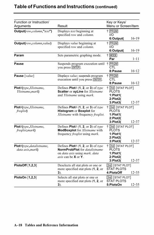
A–18 Tables and Reference Information
826DEC~1.DOC TI-83 international English Bob Fedorisko Revised: 10/26/05 2:20 PM Printed: 10/27/05 3:09PM Page 18 of 58
Function or Instruction/Arguments Result
Key or Keys/Menu or Screen/Item
Output(row,column,"text") Displays text beginning atspecified row and column.
† I/O 6:Output( 16-19
Output(row,column,value) Displays value beginning atspecified row and column.
† I/O 6:Output( 16-19
Param Sets parametric graphing mode. † z Par 1-11
Pause Suspends program execution untilyou press Í.
† CTL 8:Pause 16-12
Pause [value] Displays value; suspends programexecution until you press Í.
† CTL 8:Pause 16-12
Plot#(type,Xlistname, Ylistname,mark)
Defines Plot# (1, 2, or 3) of typeScatter or xyLine for Xlistnameand Ylistname using mark.
† y [STAT PLOT] PLOTS 1:Plot1( 2:Plot2( 3:Plot3( 12-37
Plot#(type,Xlistname, freqlist)
Defines Plot# (1, 2, or 3) of typeHistogram or Boxplot forXlistname with frequency freqlist.
† y [STAT PLOT] PLOTS 1:Plot1( 2:Plot2( 3:Plot3( 12-37
Plot#(type,Xlistname, freqlist,mark)
Defines Plot# (1, 2, or 3) of typeModBoxplot for Xlistname withfrequency freqlist using mark.
† y [STAT PLOT] PLOTS 1:Plot1( 2:Plot2( 3:Plot3( 12-37
Plot#(type,datalistname, data axis,mark)
Defines Plot# (1, 2, or 3) of typeNormProbPlot for datalistnameon data axis using mark. dataaxis can be X or Y.
† y [STAT PLOT] PLOTS 1:Plot1( 2:Plot2( 3:Plot3( 12-37
PlotsOff [1,2,3] Deselects all stat plots or one ormore specified stat plots (1, 2, or3).
y [STAT PLOT]STAT PLOTS4:PlotsOff 12-35
PlotsOn [1,2,3] Selects all stat plots or one ormore specified stat plots (1, 2, or3).
y [STAT PLOT]STAT PLOTS5:PlotsOn 12-35
Table of Functions and Instructions (continued)
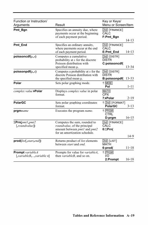
Tables and Reference Information A–19
826DEC~1.DOC TI-83 international English Bob Fedorisko Revised: 10/26/05 2:20 PM Printed: 10/27/05 3:09PM Page 19 of 58
Function or Instruction/Arguments Result
Key or Keys/Menu or Screen/Item
Pmt_Bgn Specifies an annuity due, wherepayments occur at the beginningof each payment period.
y [FINANCE]CALCF:Pmt_Bgn
14-13Pmt_End Specifies an ordinary annuity,
where payments occur at the endof each payment period.
y [FINANCE]CALCE:Pmt_End 14-13
poissoncdf(m,x) Computes a cumulativeprobability at x for the discretePoisson distribution withspecified mean m.
y [DISTR]DISTRC:poissoncdf(
13-34poissonpdf(m,x) Computes a probability at x for the
discrete Poisson distribution withthe specified mean m.
y [DISTR]DISTRB:poissonpdf( 13-33
Polar Sets polar graphing mode. † z Pol 1-11
complex value 4Polar Displays complex value in polarformat.
CPX7:4Polar 2-19
PolarGC Sets polar graphing coordinatesformat.
† y [FORMAT] PolarGC 3-13
prgmname Executes the program name. † CTRL D:prgm 16-15
GPrn(pmt1,pmt2 [,roundvalue])
Computes the sum, rounded toroundvalue, of the principalamount between pmt1 and pmt2for an amortization schedule.
y [FINANCE]CALC0:GPrn(
14-9prod(list[,start,end]) Returns product of list elements
between start and end.y [LIST]MATH6:prod( 11-18
Prompt variableA [,variableB,...,variable n]
Prompts for value for variableA,then variableB, and so on.
† I/O 2:Prompt 16-18

A–20 Tables and Reference Information
826DEC~1.DOC TI-83 international English Bob Fedorisko Revised: 10/26/05 2:20 PM Printed: 10/27/05 3:09PM Page 20 of 58
Function or Instruction/Arguments Result
Key or Keys/Menu or Screen/Item
1.PropZInt(x,n [,confidence level])
Computes a one-proportionz confidence interval.
† … TESTS A:1.PropZInt( 13-20
2.PropZInt(x1,n1,x2,n2 [,confidence level])
Computes a two-proportionz confidence interval.
† … TESTS B:2.PropZInt( 13-21
1.PropZTest(p0,x,n [,alternative,drawflag])
Computes a one-proportion z test.alternative=L1 is <; alternative=0is ƒ; alternative=1 is >.drawflag=1 draws results;drawflag=0 calculates results.
† … TESTS 5:1.PropZTest(
13-142.PropZTest(x1,n1,x2,n2 [,alternative,drawflag])
Computes a two-proportion z test.alternative=L1 is <; alternative=0is ƒ; alternative=1 is >.drawflag=1 draws results;drawflag=0 calculates results.
† … TESTS 6:2.PropZTest(
13-15Pt.Change(x,y) Reverses a point at (x,y). y [DRAW]
POINTS3:Pt.Change( 8-15
Pt.Off(x,y[,mark]) Erases a point at (x,y) using mark. y [DRAW]POINTS2:Pt.Off( 8-15
Pt.On(x,y[,mark]) Draws a point at (x,y) using mark. y [DRAW]POINTS1:Pt.On( 8-14
PwrReg [Xlistname, Ylistname,freqlist, regequ]
Fits a power regression model toXlistname and Ylistname withfrequency freqlist, and stores theregression equation to regequ.
…CALCA:PwrReg
12-27
Table of Functions and Instructions (continued)

Tables and Reference Information A–21
826DEC~1.DOC TI-83 international English Bob Fedorisko Revised: 10/26/05 2:20 PM Printed: 10/27/05 3:09PM Page 21 of 58
Function or Instruction/Arguments Result
Key or Keys/Menu or Screen/Item
Pxl.Change(row,column) Reverses pixel at (row,column);0 row 62 and0 column 94.
y [DRAWäPOINTS6:Pxl.Change( 8-16
Pxl.Off(row,column) Erases pixel at (row,column);0 row 62 and0 column 94.
y [DRAW]POINTS5:Pxl.Off( 8-16
Pxl.On(row,column) Draws pixel at (row,column);0 row 62 and0 column 94.
y [DRAW]POINTS4:Pxl.On( 8-16
pxl.Test(row,column) Returns 1 if pixel (row, column)is on, 0 if it is off; 0 row 62and 0 column 94.
y [DRAW]POINTS7:pxl.Test(
8-16P4Rx(r,q) Returns X, given polar
coordinates r and q or a list ofpolar coordinates.
y [ANGLE]ANGLE7:P4Rx( 2-24
P4Ry(r,q) Returns Y, given polarcoordinates r and q or a list ofpolar coordinates.
y [ANGLE]ANGLE8:P4Ry( 2-24
QuadReg [Xlistname, Ylistname,freqlist, regequ]
Fits a quadratic regression modelto Xlistname and Ylistname withfrequency freqlist, and stores theregression equation to regequ.
…CALC5:QuadReg
12-25QuartReg [Xlistname, Ylistname,freqlist, regequ]
Fits a quartic regression model toXlistname and Ylistname withfrequency freqlist, and stores theregression equation to regequ.
…CALC7:QuartReg
12-26Radian Sets radian angle mode. † z
Radian 1-11rand[(numtrials)] Returns a random number
between 0 and 1 for a specifiednumber of trials numtrials.
PRB1:rand
2-20randBin(numtrials,prob [,numsimulations])
Generates and displays a randomreal number from a specifiedBinomial distribution.
PRB7:randBin( 2-22

A–22 Tables and Reference Information
826DEC~1.DOC TI-83 international English Bob Fedorisko Revised: 10/26/05 2:20 PM Printed: 10/27/05 3:09PM Page 22 of 58
Function or Instruction/Arguments Result
Key or Keys/Menu or Screen/Item
randInt( lower,upper[,numtrials])
Generates and displays a randominteger within a range specifiedby lower and upper integerbounds for a specified number oftrials numtrials.
PRB5:randInt(
2-22randM(rows,columns) Returns a random matrix of rows
(1–99) × columns (1–99).MATH6:randM( 10-13
randNorm(m,s[,numtrials]) Generates and displays a randomreal number from a specifiedNormal distribution specified bym and s for a specified number oftrials numtrials.
PRB6:randNorm(
2-22re^qi Sets the mode to polar complex
number mode (re^qi).† z re^qi 1-12
Real Sets mode to display complexresults only when you entercomplex numbers.
† z Real
1-12real(value) Returns the real part of a complex
number or list of complexnumbers.
CPX2:real( 2-18
RecallGDB n Restores all settings stored in thegraph database variable GDBn.
y [DRAW]STO4:RecallGDB 8-20
RecallPic n Displays the graph and adds thepicture stored in Picn.
y [DRAW]STO2:RecallPic 8-18
complex value 4Rect Displays complex value or list inrectangular format.
CPX6:4Rect 2-19
RectGC Sets rectangular graphingcoordinates format.
† y [FORMAT] RectGC 3-13
ref(matrix) Returns the row-echelon form ofa matrix.
MATHA:ref( 10-15
Table of Functions and Instructions (continued)

Tables and Reference Information A–23
826DEC~1.DOC TI-83 international English Bob Fedorisko Revised: 10/26/05 2:20 PM Printed: 10/27/05 3:09PM Page 23 of 58
Function or Instruction/Arguments Result
Key or Keys/Menu or Screen/Item
:Repeat condition:commands:End:commands
Executes commands untilcondition is true.
† CTL 6:Repeat 16-11
Return Returns to the calling program. † CTL E:Return 16-15
round(value[,#decimals]) Returns a number, expression,list, or matrix rounded to#decimals ( 9).
NUM2:round( 2-13
äääärow(value,matrix,row) Returns a matrix with row ofmatrix multiplied by value andstored in row.
MATHE:äääärow( 10-16
row+(matrix,rowA,rowB) Returns a matrix with rowA ofmatrix added to rowB and storedin rowB.
MATHD:row+( 10-16
äääärow+(value,matrix, rowA,rowB)
Returns a matrix with rowA ofmatrix multiplied by value, addedto rowB, and stored in rowB.
MATHF:äääärow+(
10-16rowSwap(matrix,rowA, rowB)
Returns a matrix with rowA ofmatrix swapped with rowB.
MATHC:rowSwap( 10-16
rref(matrix) Returns the reduced row-echelonform of a matrix.
MATHB:rref( 10-15
R4Pr(x,y) Returns R, given rectangularcoordinates x and y or a list ofrectangular coordinates.
y [ANGLE]ANGLE5:R4Pr( 2-24
R4Pq(x,y) Returns q, given rectangularcoordinates x and y or a list ofrectangular coordinates.
y [ANGLE]ANGLE6:R4Pq( 2-24
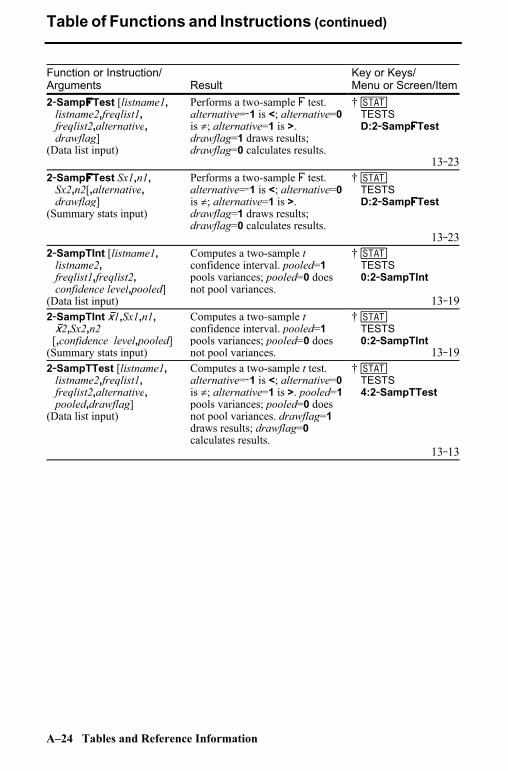
A–24 Tables and Reference Information
826DEC~1.DOC TI-83 international English Bob Fedorisko Revised: 10/26/05 2:20 PM Printed: 10/27/05 3:09PM Page 24 of 58
Function or Instruction/Arguments Result
Key or Keys/Menu or Screen/Item
2.SampÜÜÜÜTest [listname1, listname2,freqlist1, freqlist2,alternative, drawflag](Data list input)
Performs a two-sample Û test.alternative=L1 is <; alternative=0is ƒ; alternative=1 is >.drawflag=1 draws results;drawflag=0 calculates results.
† … TESTS D:2.SampÛÛÛÛTest
13-232.SampÜÜÜÜTest Sx1,n1, Sx2,n2[,alternative, drawflag](Summary stats input)
Performs a two-sample Û test.alternative=L1 is <; alternative=0is ƒ; alternative=1 is >.drawflag=1 draws results;drawflag=0 calculates results.
† … TESTS D:2.SampÛÛÛÛTest
13-232.SampTInt [listname1, listname2, freqlist1,freqlist2, confidence level,pooled](Data list input)
Computes a two-sample tconfidence interval. pooled=1pools variances; pooled=0 doesnot pool variances.
† … TESTS 0:2.SampTInt
13-192.SampTInt v1,Sx1,n1, v2,Sx2,n2 [,confidence level,pooled](Summary stats input)
Computes a two-sample tconfidence interval. pooled=1pools variances; pooled=0 doesnot pool variances.
† … TESTS 0:2.SampTInt
13-192.SampTTest [listname1, listname2,freqlist1, freqlist2,alternative, pooled,drawflag](Data list input)
Computes a two-sample t test.alternative=L1 is <; alternative=0is ƒ; alternative=1 is >. pooled=1pools variances; pooled=0 doesnot pool variances. drawflag=1draws results; drawflag=0calculates results.
† … TESTS 4:2.SampTTest
13-13
Table of Functions and Instructions (continued)

Tables and Reference Information A–25
826DEC~1.DOC TI-83 international English Bob Fedorisko Revised: 10/26/05 2:20 PM Printed: 10/27/05 3:09PM Page 25 of 58
Function or Instruction/Arguments Result
Key or Keys/Menu or Screen/Item
2.SampTTest v1,Sx1,n1, v2,Sx2,n2[,alternative, pooled,drawflag](Summary stats input)
Computes a two-sample t test.alternative=L1 is <; alternative=0is ƒ; alternative=1 is >. pooled=1pools variances; pooled=0 doesnot pool variances. drawflag=1draws results; drawflag=0calculates results.
† … TESTS 4:2.SampTTest
13-132.SampZInt(s1,s2 [,listname1,listname2, freqlist1,freqlist2, confidence level])(Data list input)
Computes a two-sample zconfidence interval.
† … TESTS 9:2.SampZInt(
13-182.SampZInt(s1,s2, v1,n1,v2,n2 [,confidence level])(Summary stats input)
Computes a two-sample zconfidence interval.
† … TESTS 9:2.SampZInt(
13-182.SampZTest(s1,s2 [,listname1,listname2, freqlist1,freqlist2, alternative,drawflag])(Data list input)
Computes a two-sample z test.alternative=L1 is <; alternative=0is ƒ ; alternative=1 is >.drawflag=1 draws results;drawflag=0 calculates results.
† … TESTS 3:2.SampZTest(
13-122.SampZTest(s1,s2, v1,n1,v2,n2 [,alternative,drawflag])(Summary stats input)
Computes a two-sample z test.alternative=L1 is <; alternative=0is ƒ; alternative=1 is >.drawflag=1 draws results;drawflag=0 calculates results.
† … TESTS 3:2.SampZTest(
13-12Sci Sets scientific notation display
mode.† z Sci 1-10
Select(Xlistname, Ylistname)
Selects one or more specific datapoints from a scatter plot orxyLine plot (only), and thenstores the selected data points totwo new lists, Xlistname andYlistname.
y [LIST]OPS8:Select(
11-12

A–26 Tables and Reference Information
826DEC~1.DOC TI-83 international English Bob Fedorisko Revised: 10/26/05 2:20 PM Printed: 10/27/05 3:09PM Page 26 of 58
Function or Instruction/Arguments Result
Key or Keys/Menu or Screen/Item
Send(variable) Sends contents of variable to theCBL System or CBR.
† I/O B:Send( 16-21
seq(expression,variable, begin,end[,increment])
Returns list created by evaluatingexpression with regard tovariable, from begin to end byincrement.
y [LIST]OPS5:seq(
11-11Seq Sets sequence graphing mode. † z
Seq 1-11Sequential Sets mode to graph functions
sequentially.† z Sequential 1-12
SetUpEditor Removes all list names from thestat list editor, and then restoreslist names L1 through L6 tocolumns 1 through 6.
…EDIT5:SetUpEditor
12-21SetUpEditor listname1 [,listname2,..., listname20]
Removes all list names from thestat list editor, then sets it up todisplay one or more listnames inthe specified order, starting withcolumn 1.
…EDIT5:SetUpEditor
12-21Shade(lowerfunc, upperfunc[,Xleft,Xright, pattern,patres])
Draws lowerfunc and upperfuncin terms of X on the current graphand uses pattern and patres toshade the area bounded bylowerfunc, upperfunc, Xleft, andXright.
y [DRAW]DRAW7:Shade(
8-10Shadec2(lowerbound, upperbound,df)
Draws the density function for thec2 distribution specified bydegrees of freedom df and shadesthe area between lowerbound andupperbound.
y [DISTR]DRAW3:Shadec2(
13-36
Table of Functions and Instructions (continued)

Tables and Reference Information A–27
826DEC~1.DOC TI-83 international English Bob Fedorisko Revised: 10/26/05 2:20 PM Printed: 10/27/05 3:09PM Page 27 of 58
Function or Instruction/Arguments Result
Key or Keys/Menu or Screen/Item
ShadeÜÜÜÜ(lowerbound, upperbound, numerator df, denominator df)
Draws the density function for theÛ distribution specified bynumerator df and denominator dfand shades the area betweenlowerbound and upperbound.
y [DISTR]DRAW4:ShadeÜÜÜÜ(
13-36ShadeNorm(lowerbound, upperbound[,m,s])
Draws the normal densityfunction specified by m and s andshades the area betweenlowerbound and upperbound.
y [DISTR]DRAW1:ShadeNorm(
13-35Shade_t(lowerbound, upperbound,df)
Draws the density function for theStudent-t distribution specified bydegrees of freedom df, and shadesthe area between lowerbound andupperbound.
y [DISTR]DRAW2:Shade_t(
13-36Simul Sets mode to graph functions
simultaneously.† z Simul 1-12
sin(value) Returns the sine of a real number,expression, or list.
˜2-3
sinL1(value) Returns the arcsine of a realnumber, expression, or list.
y [SINL1]2-3
sinh(value) Returns the hyperbolic sine of areal number, expression, or list.
y [CATALOG]sinh(
15-10sinhL1(value) Returns the hyperbolic arcsine of
a real number, expression, or list.y [CATALOG]sinhL1(
15-10

A–28 Tables and Reference Information
826DEC~1.DOC TI-83 international English Bob Fedorisko Revised: 10/26/05 2:20 PM Printed: 10/27/05 3:09PM Page 28 of 58
Function or Instruction/Arguments Result
Key or Keys/Menu or Screen/Item
SinReg [iterations, Xlistname,Ylistname, period,regequ]
Attempts iterations times to fit asinusoidal regression model toXlistname and Ylistname using aperiod guess, and stores theregression equation to regequ.
…CALCC:SinReg
12-27solve(expression,variable, guess,{lower,upper})
Solves expression for variable,given an initial guess and lowerand upper bounds within whichthe solution is sought.
† MATH 0:solve(
2-12SortA(listname) Sorts elements of listname in
ascending order.y [LIST]OPS 11-101:SortA( 12-20
SortA(keylistname, dependlist1[,dependlist2, ...,dependlist n])
Sorts elements of keylistname inascending order, then sorts eachdependlist as a dependent list.
y [LIST]OPS1:SortA( 11-10
12-20SortD(listname) Sorts elements of listname in
descending order.y [LIST]OPS 11-102:SortD( 12-20
SortD(keylistname, dependlist1[,dependlist2,..., dependlist n])
Sorts elements of keylistname indescending order, then sorts eachdependlist as a dependent list.
y [LIST]OPS2:SortD( 11-10
12-20stdDev(list[,freqlist]) Returns the standard deviation of
the elements in list withfrequency freqlist.
y [LIST]MATH7:stdDev( 11-18
Stop Ends program execution; returnsto home screen.
† CTL F:Stop 16-15
Store: value!!!!variable Stores value in variable. ¿ 1-14StoreGDB n Stores current graph in database
GDBn.y [DRAW]STO3:StoreGDB 8-19
Table of Functions and Instructions (continued)

Tables and Reference Information A–29
826DEC~1.DOC TI-83 international English Bob Fedorisko Revised: 10/26/05 2:20 PM Printed: 10/27/05 3:09PM Page 29 of 58
Function or Instruction/Arguments Result
Key or Keys/Menu or Screen/Item
StorePic n Stores current picture in picturePicn.
y [DRAW]STO1:StorePic 8-17
String4Equ(string,Y= var) Converts string into an equationand stores it in Y= var.
y [CATALOG]String4Equ(
15-8sub(string,begin,length) Returns a string that is a subset of
another string, from begin tolength.
y [CATALOG]sub(
15-9sum(list[,start,end]) Returns the sum of elements of
list from start to end.y [LIST]MATH5:sum( 11-18
tan(value) Returns the tangent of a realnumber, expression,or list.
š
2-3tanL1(value) Returns the arctangent of a real
number, expression, or list.y [TANL1]
2-3Tangent(expression,value) Draws a line tangent to
expression at X=value.y [DRAWäDRAW5:Tangent( 8-8
tanh(value) Returns hyperbolic tangent of areal number, expression, or list.
y [CATALOG]tanh( 15-10
tanhL1(value) Returns the hyperbolic arctangentof a real number, expression,or list.
y [CATALOG]tanhL1(
15-10tcdf(lowerbound, upperbound,df)
Computes the Student-tdistribution probability betweenlowerbound and upperbound forthe specified degrees of freedomdf.
y [DISTR]DISTR5:tcdf(
13-31Text(row,column,text1, text2,...,text n)
Writes text on graph beginning atpixel (row,column), where0 row 57 and0 column 94.
y [DRAW]DRAW0:Text(
8-12Then See If:Then

A–30 Tables and Reference Information
826DEC~1.DOC TI-83 international English Bob Fedorisko Revised: 10/26/05 2:20 PM Printed: 10/27/05 3:09PM Page 30 of 58
Function or Instruction/Arguments Result
Key or Keys/Menu or Screen/Item
Time Sets sequence graphs to plot withrespect to time.
† y [FORMAT] Time 6-8
TInterval [listname, freqlist,confidence level](Data list input)
Computes a t confidence interval. † … TESTS 8:TInterval 13-17
TInterval v,Sx,n [,confidence level](Summary stats input)
Computes a t confidence interval. † … TESTS 8:TInterval 13-17
tpdf(x,df) Computes the probability densityfunction (pdf) for the Student-tdistribution at a specified x valuewith specified degrees of freedomdf.
y [DISTR]DISTR4:tpdf(
13-30Trace Displays the graph and enters
TRACE mode.r
3-18T-Test m0[,listname, freqlist,alternative, drawflag](Data list input)
Performs a t test with frequencyfreqlist. alternative=L1 is <;alternative=0 is ƒ; alternative=1is >. drawflag=1 draws results;drawflag=0 calculates results.
† … TESTS 2:T-Test
13-11T-Test m0, v,Sx,n [,alternative,drawflag](Summary stats input)
Performs a t test with frequencyfreqlist. alternative=L1 is < ;alternative=0 is ƒ ; alternative=1is >. drawflag=1 draws results;drawflag=0 calculates results.
† … TESTS 2:T-Test
13-11
Table of Functions and Instructions (continued)

Tables and Reference Information A–31
826DEC~1.DOC TI-83 international English Bob Fedorisko Revised: 10/26/05 2:20 PM Printed: 10/27/05 3:09PM Page 31 of 58
Function or Instruction/Arguments Result
Key or Keys/Menu or Screen/Item
tvm_FV[(Ú,æ,PV,PMT, P/Y,C/Y)]
Computes the future value. y [FINANCE]CALC6:tvm_FV 14-7
tvm_ææææ[(Ú,PV,PMT,FV, P/Y,C/Y)]
Computes the annual interest rate. y [FINANCE]CALC3:tvm_ææææ 14-7
tvm_ÚÚÚÚ[(æ,PV,PMT,FV, P/Y,C/Y)]
Computes the number of paymentperiods.
y [FINANCE]CALC5:tvm_ÚÚÚÚ 14-7
tvm_Pmt[(Ú,æ,PV,FV, P/Y,C/Y)]
Computes the amount of eachpayment.
y [FINANCE]CALC2:tvm_Pmt 14-6
tvm_PV[(Ú,æ,PMT,FV, P/Y,C/Y)]
Computes the present value. y [FINANCE]CALC4:tvm_PV 14-7
uvAxes Sets sequence graphs to plot u(n)on the x-axis and v(n) on they-axis.
† y [FORMAT] uv
6-8uwAxes Sets sequence graphs to plot u(n)
on the x-axis and w(n) on the y-axis.
† y [FORMAT] uw
6-81-Var Stats [Xlistname, freqlist]
Performs one-variable analysis onthe data in Xlistname withfrequency freqlist.
…CALC1:1-Var Stats 12-25
2-Var Stats [Xlistname, Ylistname,freqlist]
Performs two-variable analysis onthe data in Xlistname andYlistname with frequency freqlist.
…CALC2:2-Var Stats
12-25variance(list[,freqlist]) Returns the variance of the
elements in list with frequencyfreqlist.
y [LIST]MATH8:variance( 11-18
Vertical x Draws a vertical lineat x.
y [DRAW]DRAW4:Vertical 8-6
vwAxes Sets sequence graphs to plot v(n)on the x-axis and w(n) on the y-axis.
† y [FORMAT] vw
6-8Web Sets sequence graphs to trace as
webs.† y [FORMAT] Web 6-8

A–32 Tables and Reference Information
826DEC~1.DOC TI-83 international English Bob Fedorisko Revised: 10/26/05 2:20 PM Printed: 10/27/05 3:09PM Page 32 of 58
Function or Instruction/Arguments Result
Key or Keys/Menu or Screen/Item
:While condition:commands:End:command
Executes commands whilecondition is true.
† CTL 5:While 16-11
valueA xor valueB Returns 1 if only valueA orvalueB = 0. valueA and valueBcan be real numbers, expressions,or lists.
y [TEST]LOGIC3:xor
2-26ZBox Displays a graph, lets you draw a
box that defines a new viewingwindow, and updates the window.
† q ZOOM 1:ZBox
3-20ZDecimal Adjusts the viewing window so
that @X=0.1 and @Y=0.1, anddisplays the graph screen with theorigin centered on the screen.
† q ZOOM 4:ZDecimal
3-21ZInteger Redefines the viewing window
using these dimensions:@X=1 Xscl=10@Y=1 Yscl=10
† q ZOOM 8:ZInteger
3-22ZInterval s[,listname, freqlist,confidence level](Data list input)
Computes a z confidence interval. † … TESTS 7:ZInterval 13-16
ZInterval s,v,n [,confidence level](Summary stats input)
Computes a z confidence interval. † … TESTS 7:ZInterval 13-16
Zoom In Magnifies the part of the graphthat surrounds the cursor location.
† q ZOOM 2:Zoom In 3-21
Zoom Out Displays a greater portion of thegraph, centered on the cursorlocation.
† q ZOOM 3:Zoom Out 3-21
Table of Functions and Instructions (continued)

Tables and Reference Information A–33
826DEC~1.DOC TI-83 international English Bob Fedorisko Revised: 10/26/05 2:20 PM Printed: 10/27/05 3:09PM Page 33 of 58
Function or Instruction/Arguments Result
Key or Keys/Menu or Screen/Item
ZoomFit Recalculates Ymin and Ymax toinclude the minimum andmaximum Y values, betweenXmin and Xmax, of the selectedfunctions and replots thefunctions.
† q ZOOM 0:ZoomFit
3-22ZoomRcl Graphs the selected functions in a
user-defined viewing window.† q MEMORY 3:ZoomRcl 3-23
ZoomStat Redefines the viewing window sothat all statistical data points aredisplayed.
† q ZOOM 9:ZoomStat 3-22
ZoomSto Immediately stores the currentviewing window.
† q MEMORY 2:ZoomSto 3-23
ZPrevious Replots the graph using thewindow variables of the graphthat was displayed before youexecuted the last ZOOMinstruction.
† q MEMORY 1:ZPrevious
3-23ZSquare Adjusts the X or Y window
settings so that each pixelrepresents an equal width andheight in the coordinate system,and updates the viewing window.
† q ZOOM 5:ZSquare
3-21ZStandard Replots the functions
immediately, updating thewindow variables to the defaultvalues.
† q ZOOM 6:ZStandard
3-22

A–34 Tables and Reference Information
826DEC~1.DOC TI-83 international English Bob Fedorisko Revised: 10/26/05 2:20 PM Printed: 10/27/05 3:09PM Page 34 of 58
Function or Instruction/Arguments Result
Key or Keys/Menu or Screen/Item
ZNTest(m0,s[,listname, freqlist,alternative, drawflag])(Data list input)
Performs a z test with frequencyfreqlist. alternative=L1 is <;alternative=0 is ƒ; alternative=1is >. drawflag=1 draws results;drawflag=0 calculates results.
† … TESTS 1:Z.Test(
13-10ZNTest(m0,s,v,n [,alternative,drawflag])(Summary stats input)
Performs a z test. alternative=L1is <; alternative=0 is ƒ;alternative=1 is >. drawflag=1draws results; drawflag=0calculates results.
† … TESTS 1:Z.Test(
13-10ZTrig Replots the functions
immediately, updating thewindow variables to preset valuesfor plotting trig functions.
† q ZOOM 7:ZTrig
3-22Factorial: value! Returns factorial of value.
PRB4:! 2-21
Factorial: list! Returns factorial of list elements. PRB4:! 2-21
Degrees notation: value¡ Interprets value as degrees;designates degrees in DMSformat.
y [ANGLE]ANGLE1:¡ 2-23
Radian: angler Interprets angle as radians. y [ANGLE]ANGLE3:r 2-24
Transpose: matrixT Returns a matrix in which eachelement (row, column) is swappedwith the corresponding element(column, row) of matrix.
MATH2:T
10-12
Table of Functions and Instructions (continued)
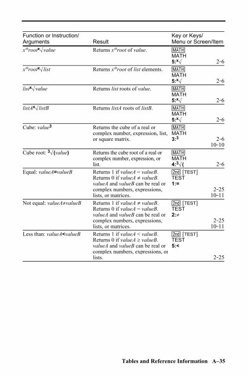
Tables and Reference Information A–35
826DEC~1.DOC TI-83 international English Bob Fedorisko Revised: 10/26/05 2:20 PM Printed: 10/27/05 3:09PM Page 35 of 58
Function or Instruction/Arguments Result
Key or Keys/Menu or Screen/Item
xthrootx‡value Returns xthroot of value. MATH5:x‡ 2-6
xthrootx‡list Returns xthroot of list elements. MATH5:x‡ 2-6
listx‡value Returns list roots of value. MATH5:x‡ 2-6
listAx‡listB Returns listA roots of listB. MATH5:x‡ 2-6
Cube: value3 Returns the cube of a real orcomplex number, expression, list,or square matrix.
MATH3:3 2-6
10-10Cube root: 3‡(value) Returns the cube root of a real or
complex number, expression, orlist.
MATH4:3‡( 2-6
Equal: valueA=valueB Returns 1 if valueA = valueB.Returns 0 if valueA ƒ valueB.valueA and valueB can be real orcomplex numbers, expressions,lists, or matrices.
y [TEST]TEST1:=
2-2510-11
Not equal: valueAƒvalueB Returns 1 if valueA ƒ valueB.Returns 0 if valueA = valueB.valueA and valueB can be real orcomplex numbers, expressions,lists, or matrices.
y [TEST]TEST2:ƒ
2-2510-11
Less than: valueA<valueB Returns 1 if valueA < valueB.Returns 0 if valueA ‚ valueB.valueA and valueB can be real orcomplex numbers, expressions, orlists.
y [TEST]TEST5:<
2-25

A–36 Tables and Reference Information
826DEC~1.DOC TI-83 international English Bob Fedorisko Revised: 10/26/05 2:20 PM Printed: 10/27/05 3:09PM Page 36 of 58
Function or Instruction/Arguments Result
Key or Keys/Menu or Screen/Item
Greater than: valueA>valueB
Returns 1 if valueA > valueB.Returns 0 if valueA valueB.valueA and valueB can be real orcomplex numbers, expressions, orlists.
y [TEST]TEST3:>
2-25Less than or equal: valueAvalueB
Returns 1 if valueA valueB.Returns 0 if valueA > valueB.valueA and valueB can be real orcomplex numbers, expressions, orlists.
y [TEST]TEST6:
2-25Greater than or equal: valueA‚valueB
Returns 1 if valueA ‚ valueB.Returns 0 if valueA < valueB.valueA and valueB can be real orcomplex numbers, expressions, orlists.
y [TEST]TEST4:‚
2-25Inverse: valueL1 Returns 1 divided by a real or
complex number or expression.—
2-3Inverse: listL1 Returns 1 divided by list
elements.—
2-3Inverse: matrixL1 Returns matrix inverted. — 10-10Square: value2 Returns value multiplied by itself.
value can be a real or complexnumber or expression.
¡
2-3Square: list2 Returns list elements squared. ¡
2-3Square: matrix2 Returns matrix multiplied by
itself.¡
10-10Powers: value^power Returns value raised to power.
value can be a real or complexnumber or expression.
›
2-3Powers: list^power Returns list elements raised to
power.›
2-3Powers: value^list Returns value raised to list
elements.›
2-3
Table of Functions and Instructions (continued)
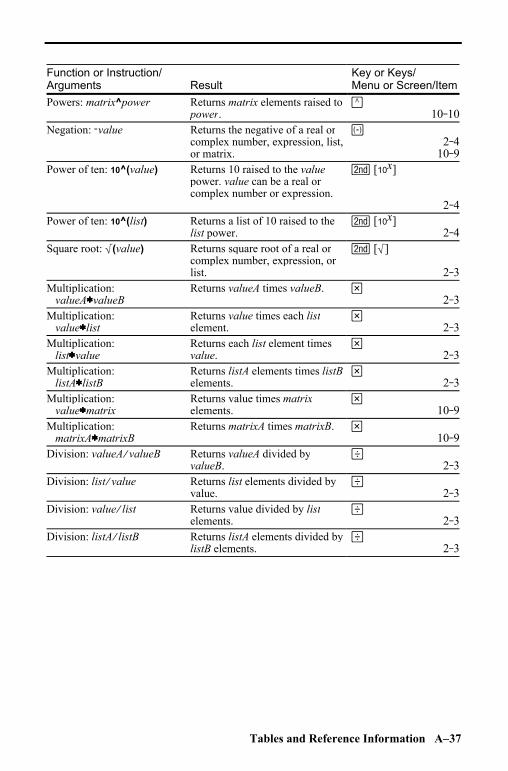
Tables and Reference Information A–37
826DEC~1.DOC TI-83 international English Bob Fedorisko Revised: 10/26/05 2:20 PM Printed: 10/27/05 3:09PM Page 37 of 58
Function or Instruction/Arguments Result
Key or Keys/Menu or Screen/Item
Powers: matrix^power Returns matrix elements raised topower.
›10-10
Negation: Lvalue Returns the negative of a real orcomplex number, expression, list,or matrix.
Ì2-4
10-9Power of ten: 10^(value) Returns 10 raised to the value
power. value can be a real orcomplex number or expression.
y [10x]
2-4Power of ten: 10^(list) Returns a list of 10 raised to the
list power.y [10x]
2-4Square root: ‡(value) Returns square root of a real or
complex number, expression, orlist.
y [‡]
2-3Multiplication: valueAäääävalueB
Returns valueA times valueB. ¯2-3
Multiplication: valueäääälist
Returns value times each listelement.
¯2-3
Multiplication: listäääävalue
Returns each list element timesvalue.
¯2-3
Multiplication: listAäääälistB
Returns listA elements times listBelements.
¯2-3
Multiplication: valueäääämatrix
Returns value times matrixelements.
¯10-9
Multiplication: matrixAäääämatrixB
Returns matrixA times matrixB. ¯10-9
Division: valueAàvalueB Returns valueA divided byvalueB.
¥2-3
Division: listàvalue Returns list elements divided byvalue.
¥2-3
Division: valueàlist Returns value divided by listelements.
¥2-3
Division: listAàlistB Returns listA elements divided bylistB elements.
¥2-3

A–38 Tables and Reference Information
826DEC~1.DOC TI-83 international English Bob Fedorisko Revised: 10/26/05 2:20 PM Printed: 10/27/05 3:09PM Page 38 of 58
Function or Instruction/Arguments Result
Key or Keys/Menu or Screen/Item
Addition: valueA+valueB Returns valueA plus valueB. Ã 2-3Addition: list+value Returns list in which value is
added to each list element.Ã
2-3Addition: listA+listB Returns listA elements plus listB
elements.Ã
2-3Addition: matrixA+matrixB
Returns matrixA elements plusmatrixB elements.
Ã10-9
Concatenation: string1+string2
Concatenates two or more strings. Ã15-6
Subtraction: valueANvalueB
Subtracts valueB from valueA. ¹2-3
Subtraction: valueNlist
Subtracts list elements fromvalue.
¹2-3
Subtraction: listNvalue
Subtracts value from listelements.
¹2-3
Subtraction: listANlistB
Subtracts listB elements fromlistA elements.
¹2-3
Subtraction: matrixANmatrixB
Subtracts matrixB elements frommatrixA elements.
¹10-9
Minutes notation: degrees¡minutes' seconds"
Interprets minutes anglemeasurement as minutes.
y [ANGLE]ANGLE2:' 2-23
Seconds notation: degrees¡minutes' seconds"
Interprets seconds anglemeasurement as seconds.
ƒ [ã]
2-23
Table of Functions and Instructions (continued)
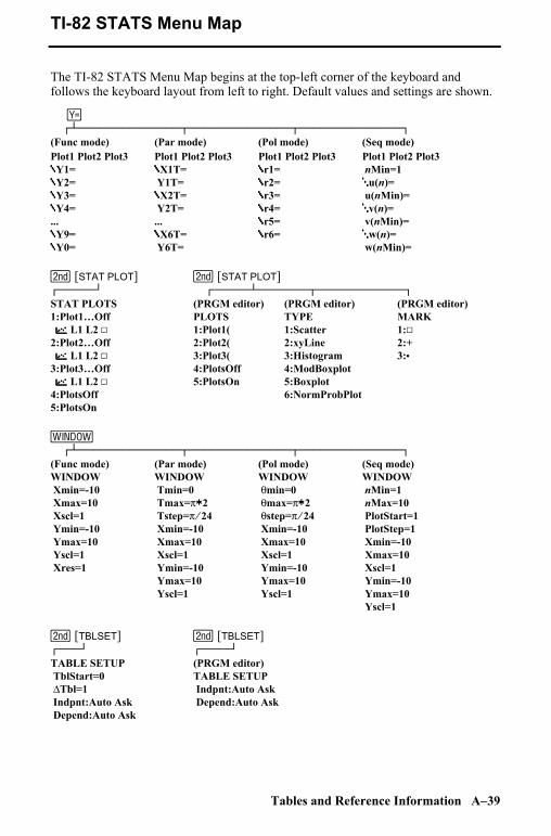
Tables and Reference Information A–39
826DEC~1.DOC TI-83 international English Bob Fedorisko Revised: 10/26/05 2:20 PM Printed: 10/27/05 3:09PM Page 39 of 58
The TI-82 STATS Menu Map begins at the top-left corner of the keyboard andfollows the keyboard layout from left to right. Default values and settings are shown.
o (Func mode)Plot1 Plot2 Plot3ççççY1=ççççY2=ççççY3=ççççY4=...ççççY9=ççççY0=
(Par mode)Plot1 Plot2 Plot3ççççX1T= Y1T=ççççX2T= Y2T=...ççççX6T= Y6T=
(Pol mode)Plot1 Plot2 Plot3ççççr1=ççççr2=ççççr3=ççççr4=ççççr5=ççççr6=
(Seq mode)Plot1 Plot2 Plot3 nMin=1ííííu(n)= u(nMin)=íííív(n)= v(nMin)=ííííw(n)= w(nMin)=
y [STAT PLOT] y [STAT PLOT]
STAT PLOTS1:Plot1…Off """" L1 L2 ›2:Plot2…Off """" L1 L2 ›3:Plot3…Off """" L1 L2 ›4:PlotsOff5:PlotsOn
(PRGM editor)PLOTS1:Plot1(2:Plot2(3:Plot3(4:PlotsOff5:PlotsOn
(PRGM editor)TYPE1:Scatter2:xyLine3:Histogram4:ModBoxplot5:Boxplot6:NormProbPlot
(PRGM editor)MARK1:›2:+3:¦
p (Func mode)WINDOW Xmin=-10 Xmax=10 Xscl=1 Ymin=-10 Ymax=10 Yscl=1 Xres=1
(Par mode)WINDOW Tmin=0 Tmax=pä2 Tstep=pà24 Xmin=-10 Xmax=10 Xscl=1 Ymin=-10 Ymax=10 Yscl=1
(Pol mode)WINDOW qmin=0 qmax=pä2 qstep=pà24 Xmin=-10 Xmax=10 Xscl=1 Ymin=-10 Ymax=10 Yscl=1
(Seq mode)WINDOW nMin=1 nMax=10 PlotStart=1 PlotStep=1 Xmin=-10 Xmax=10 Xscl=1 Ymin=-10 Ymax=10 Yscl=1
y [TBLSET] y [TBLSET]
TABLE SETUP TblStart=0 @Tbl=1 Indpnt:Auto Ask Depend:Auto Ask
(PRGM editor)TABLE SETUP Indpnt:Auto Ask Depend:Auto Ask
TI-82 STATS Menu Map

A–40 Tables and Reference Information
826DEC~1.DOC TI-83 international English Bob Fedorisko Revised: 10/26/05 2:20 PM Printed: 10/27/05 3:09PM Page 40 of 58
q ZOOM1:ZBox2:Zoom In3:Zoom Out4:ZDecimal5:ZSquare6:ZStandard7:ZTrig8:ZInteger9:ZoomStat0:ZoomFit
MEMORY1:ZPrevious2:ZoomSto3:ZoomRcl4:SetFactors…
MEMORY(Set Factors...)ZOOM FACTORS XFact=4 YFact=4
y [FORMAT] (Func/Par/Pol modes)RectGC PolarGCCoordOn CoordOffGridOff GridOnAxesOn AxesOffLabelOff LabelOnExprOn ExprOff
(Seq mode)Time Web uv vw uwRectGC PolarGCCoordOn CoordOffGridOff GridOnAxesOn AxesOffLabelOff LabelOnExprOn ExprOff
y [CALC] (Func mode)CALCULATE1:value2:zero3:minimum4:maximum5:intersect6:dy/dx7:‰f(x)dx
(Par mode)CALCULATE1:value2:dy/dx3:dy/dt4:dx/dt
(Pol mode)CALCULATE1:value2:dy/dx3:dr/dq
(Seq mode)CALCULATE1:value
z
Normal Sci EngFloat 0123456789Radian DegreeFunc Par Pol SeqConnected DotSequential SimulReal a+b×××× re^q××××Full Horiz G-T
TI-82 STATS Menu Map (continued)
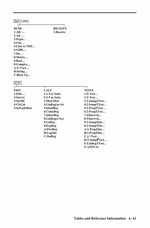
Tables and Reference Information A–41
826DEC~1.DOC TI-83 international English Bob Fedorisko Revised: 10/26/05 2:20 PM Printed: 10/27/05 3:09PM Page 41 of 58
y [LINK] SEND1:All+…2:AllN…3:Prgm…4:List…5:Lists to TI82…6:GDB…7:Pic…8:Matrix…9:Real…0:Complex…A:Y-Vars…B:String…C:Back Up…
RECEIVE1:Receive
…
EDIT1:Edit…2:SortA(3:SortD(4:ClrList5:SetUpEditor
CALC1:1-Var Stats2:2-Var Stats3:Med-Med4:LinReg(ax+b)5:QuadReg6:CubicReg7:QuartReg8:LinReg(a+bx)9:LnReg0:ExpRegA:PwrRegB:LogisticC:SinReg
TESTS1:Z-Test…2:T-Test…3:2-SampZTest…4:2-SampTTest…5:1-PropZTest…6:2-PropZTest…7:ZInterval…8:TInterval…9:2-SampZInt…0:2-SampTInt…A:1-PropZInt…B:2-PropZInt…C:c2-Test…D:2-SampÛÛÛÛTest…E:LinRegTTest…F:ANOVA(

A–42 Tables and Reference Information
826DEC~1.DOC TI-83 international English Bob Fedorisko Revised: 10/26/05 2:20 PM Printed: 10/27/05 3:09PM Page 42 of 58
y [LIST] NAMES1:listname2:listname3:listname...
OPS1:SortA(2:SortD(3:dim(4:Fill(5:seq(6:cumSum(7:@List(8:Select(9:augment(0:List4matr(A:Matr4list(B:ÙÙÙÙ
MATH1:min(2:max(3:mean(4:median(5:sum(6:prod(7:stdDev(8:variance(
MATH1:4Frac2:4Dec3:3
4:3‡(5:x‡
6:fMin(7:fMax(8:nDeriv(9:fnInt(0:Solver…
NUM1:abs(2:round(3:iPart(4:fPart(5:int(6:min(7:max(8:lcm(9:gcd(
CPX1:conj(2:real(3:imag(4:angle(5:abs(6:4Rect7:4Polar
PRB1:rand2:nPr3:nCr4:!5:randInt(6:randNorm(7:randBin(
y [TEST] TEST1:=2:ƒ3:>4:‚5:<6:
LOGIC1:and2:or3:xor4:not(
TI-82 STATS Menu Map (continued)
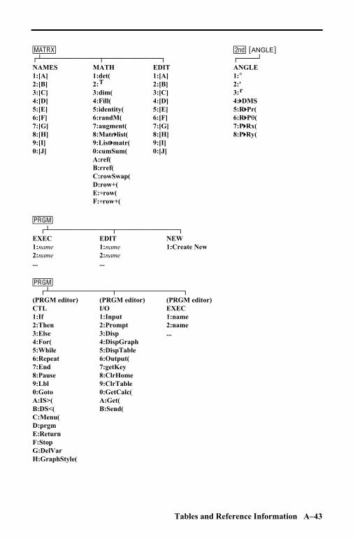
Tables and Reference Information A–43
826DEC~1.DOC TI-83 international English Bob Fedorisko Revised: 10/26/05 2:20 PM Printed: 10/27/05 3:09PM Page 43 of 58
y [ANGLE]
NAMES1:[A]2:[B]3:[C]4:[D]5:[E]6:[F]7:[G]8:[H]9:[I]0:[J]
MATH1:det(2:T
3:dim(4:Fill(5:identity(6:randM(7:augment(8:Matr4list(9:List4matr(0:cumSum(A:ref(B:rref(C:rowSwap(D:row+(E:…row(F:…row+(
EDIT1:[A]2:[B]3:[C]4:[D]5:[E]6:[F]7:[G]8:[H]9:[I]0:[J]
ANGLE1:¡2:'3:r4:4DMS5:R4Pr(6:R4Pq(7:P4Rx(8:P4Ry(
EXEC1:name2:name...
EDIT1:name2:name...
NEW1:Create New
(PRGM editor)CTL1:If2:Then3:Else4:For(5:While6:Repeat7:End8:Pause9:Lbl0:GotoA:IS>(B:DS<(C:Menu(D:prgmE:ReturnF:StopG:DelVarH:GraphStyle(
(PRGM editor)I/O1:Input2:Prompt3:Disp4:DispGraph5:DispTable6:Output(7:getKey8:ClrHome9:ClrTable0:GetCalc(A:Get(B:Send(
(PRGM editor)EXEC1:name2:name...
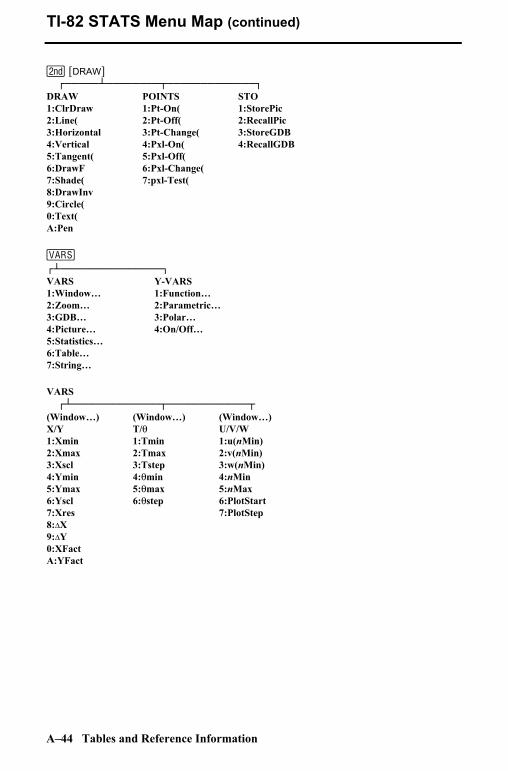
A–44 Tables and Reference Information
826DEC~1.DOC TI-83 international English Bob Fedorisko Revised: 10/26/05 2:20 PM Printed: 10/27/05 3:09PM Page 44 of 58
y [DRAW] DRAW1:ClrDraw2:Line(3:Horizontal4:Vertical5:Tangent(6:DrawF7:Shade(8:DrawInv9:Circle(0:Text(A:Pen
POINTS1:Pt-On(2:Pt-Off(3:Pt-Change(4:Pxl-On(5:Pxl-Off(6:Pxl-Change(7:pxl-Test(
STO1:StorePic2:RecallPic3:StoreGDB4:RecallGDB
VARS1:Window…2:Zoom…3:GDB…4:Picture…5:Statistics…6:Table…7:String…
Y-VARS1:Function…2:Parametric…3:Polar…4:On/Off…
VARS (Window…)X/Y1:Xmin2:Xmax3:Xscl4:Ymin5:Ymax6:Yscl7:Xres8:@X9:@Y0:XFactA:YFact
(Window…)T/q1:Tmin2:Tmax3:Tstep4:qmin5:qmax6:qstep
(Window…)U/V/W1:u(nMin)2:v(nMin)3:w(nMin)4:nMin5:nMax6:PlotStart7:PlotStep
TI-82 STATS Menu Map (continued)
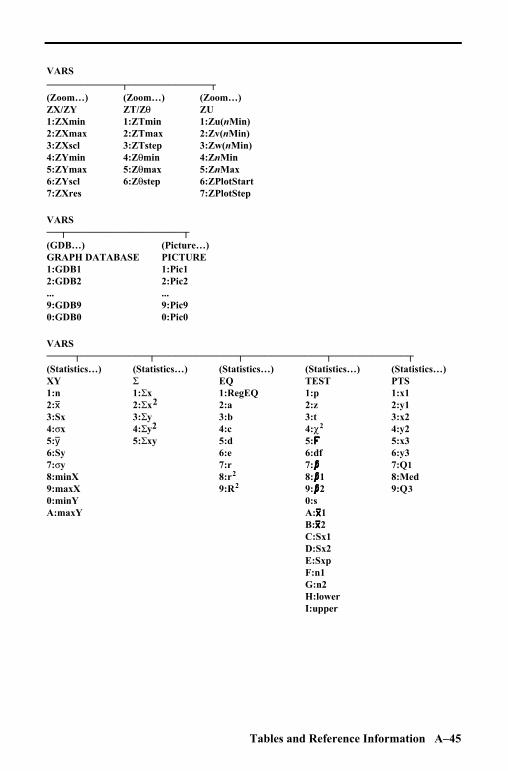
Tables and Reference Information A–45
826DEC~1.DOC TI-83 international English Bob Fedorisko Revised: 10/26/05 2:20 PM Printed: 10/27/05 3:09PM Page 45 of 58
VARS
(Zoom…)ZX/ZY1:ZXmin2:ZXmax3:ZXscl4:ZYmin5:ZYmax6:ZYscl7:ZXres
(Zoom…)ZT/Zq1:ZTmin2:ZTmax3:ZTstep4:Zqmin5:Zqmax6:Zqstep
(Zoom…)ZU1:Zu(nMin)2:Zv(nMin)3:Zw(nMin)4:ZnMin5:ZnMax6:ZPlotStart7:ZPlotStep
VARS
(GDB…)GRAPH DATABASE1:GDB12:GDB2...9:GDB90:GDB0
(Picture…)PICTURE1:Pic12:Pic2...9:Pic90:Pic0
VARS
(Statistics…)XY1:n2:v3:Sx4:sx5:w6:Sy7:sy8:minX9:maxX0:minYA:maxY
(Statistics…)G1:Gx2:Gx2
3:Gy4:Gy2
5:Gxy
(Statistics…)EQ1:RegEQ2:a3:b4:c5:d6:e7:r8:r2
9:R2
(Statistics…)TEST1:p2:z3:t4:c2
5:ÛÛÛÛ6:df7:ÇÇÇÇ8:ÇÇÇÇ19:ÇÇÇÇ20:sA:üüüü1B:üüüü2C:Sx1D:Sx2E:SxpF:n1G:n2H:lowerI:upper
(Statistics…)PTS1:x12:y13:x24:y25:x36:y37:Q18:Med9:Q3

A–46 Tables and Reference Information
826DEC~1.DOC TI-83 international English Bob Fedorisko Revised: 10/26/05 2:20 PM Printed: 10/27/05 3:09PM Page 46 of 58
VARS
(Table…)TABLE1:TblStart2:@Tbl3:TblInput
(String…)STRING1:Str12:Str23:Str34:Str4...9:Str90:Str0
Y-VARS (Function…)FUNCTION1:Y12:Y23:Y34:Y4...9:Y90:Y0
(Parametric…)PARAMETRIC1:X1T2:Y1T3:X2T4:Y2T...A:X6TB:Y6T
(Polar…)POLAR1:r12:r23:r34:r45:r56:r6
(On/Off…)ON/OFF1:FnOn2:FnOff
TI-82 STATS Menu Map (continued)
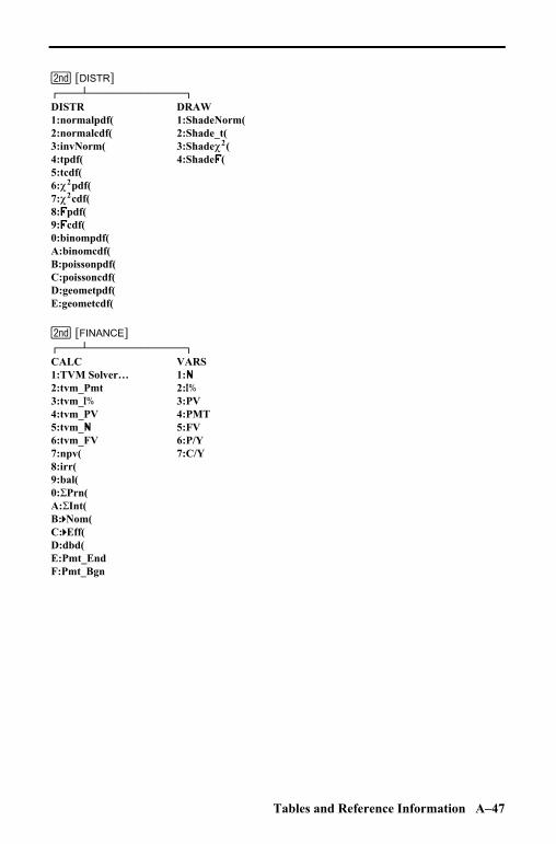
Tables and Reference Information A–47
826DEC~1.DOC TI-83 international English Bob Fedorisko Revised: 10/26/05 2:20 PM Printed: 10/27/05 3:09PM Page 47 of 58
y [DISTR]
DISTR1:normalpdf(2:normalcdf(3:invNorm(4:tpdf(5:tcdf(6:c2pdf(7:c2cdf(8:ÛÛÛÛpdf(9:ÛÛÛÛcdf(0:binompdf(A:binomcdf(B:poissonpdf(C:poissoncdf(D:geometpdf(E:geometcdf(
DRAW1:ShadeNorm(2:Shade_t(3:Shadec2(4:ShadeÛÛÛÛ(
y [FINANCE]
CALC1:TVM Solver…2:tvm_Pmt3:tvm_æ4:tvm_PV5:tvm_Ú6:tvm_FV7:npv(8:irr(9:bal(0:GPrn(A:GInt(B:4Nom(C:4Eff(D:dbd(E:Pmt_EndF:Pmt_Bgn
VARS1:Ú2:æ3:PV4:PMT5:FV6:P/Y7:C/Y

A–48 Tables and Reference Information
826DEC~1.DOC TI-83 international English Bob Fedorisko Revised: 10/26/05 2:20 PM Printed: 10/27/05 3:09PM Page 48 of 58
y [MEM] MEMORY
MEMORY1:Check RAM…2:Delete…3:Clear Entries4:ClrAllLists5:Reset…
(Check RAM…)MEM FREE 27225Real 15Complex 0List 0Matrix 0Y-Vars 240Prgm 14Pic 0GDB 0String 0
(Delete…)DELETE FROM…1:All…2:Real…3:Complex…4:List…5:Matrix…6:Y-Vars…7:Prgm…8:Pic…9:GDB…0:String…
(Reset…)RESET1:All Memory…2:Defaults…
MEMORY (Reset...) y [CATALOG]
(All Memory…)RESET MEMORY1:No2:Reset
Resetting memory erasesall data and programs.
(Defaults…)RESET DEFAULTS1:No2:Reset
CATALOGcosh(coshL1(...Equ4String(expr(...inString(...length(...sinh(sinhL1(...String4Equ(sub(...tanh(tanhL1(
TI-82 STATS Menu Map (continued)
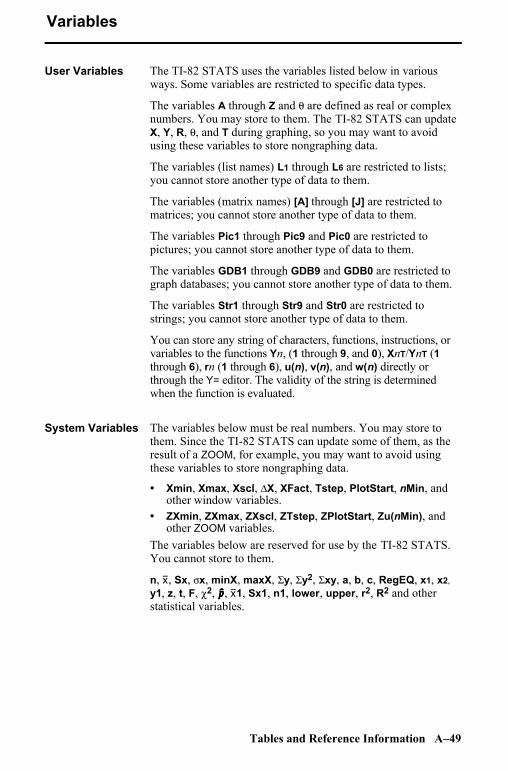
Tables and Reference Information A–49
826DEC~1.DOC TI-83 international English Bob Fedorisko Revised: 10/26/05 2:20 PM Printed: 10/27/05 3:09PM Page 49 of 58
The TI-82 STATS uses the variables listed below in variousways. Some variables are restricted to specific data types.
The variables A through Z and q are defined as real or complexnumbers. You may store to them. The TI-82 STATS can updateX, Y, R, q, and T during graphing, so you may want to avoidusing these variables to store nongraphing data.
The variables (list names) L1 through L6 are restricted to lists;you cannot store another type of data to them.
The variables (matrix names) [A] through [J] are restricted tomatrices; you cannot store another type of data to them.
The variables Pic1 through Pic9 and Pic0 are restricted topictures; you cannot store another type of data to them.
The variables GDB1 through GDB9 and GDB0 are restricted tograph databases; you cannot store another type of data to them.
The variables Str1 through Str9 and Str0 are restricted tostrings; you cannot store another type of data to them.
You can store any string of characters, functions, instructions, orvariables to the functions Yn, (1 through 9, and 0), XnT/YnT (1through 6), rn (1 through 6), u(n), v(n), and w(n) directly orthrough the Y= editor. The validity of the string is determinedwhen the function is evaluated.
The variables below must be real numbers. You may store tothem. Since the TI-82 STATS can update some of them, as theresult of a ZOOM, for example, you may want to avoid usingthese variables to store nongraphing data.
• Xmin, Xmax, Xscl, @X, XFact, Tstep, PlotStart, nMin, andother window variables.
• ZXmin, ZXmax, ZXscl, ZTstep, ZPlotStart, Zu(nMin), andother ZOOM variables.
The variables below are reserved for use by the TI-82 STATS.You cannot store to them.
n, v, Sx, sx, minX, maxX, Gy, Gy2, Gxy, a, b, c, RegEQ, x1, x2,y1, z, t, F, c2, ÇÇÇÇ, v1, Sx1, n1, lower, upper, r2, R2 and otherstatistical variables.
Variables
User Variables
System Variables

A–50 Tables and Reference Information
826DEC~1.DOC TI-83 international English Bob Fedorisko Revised: 10/26/05 2:20 PM Printed: 10/27/05 3:09PM Page 50 of 58
This section contains statistics formulas for the Logistic and SinReg regressions,ANOVA, 2.SampÜÜÜÜTest, and 2.SampTTest.
The logistic regression algorithm applies nonlinear recursiveleast-squares techniques to optimize the following cost function:
J cae
ybx ii
N
i=
+−
−
=∑ 1
2
1
which is the sum of the squares of the residual errors,
where: x = the independent variable listy = the dependent variable listN = the dimension of the lists
This technique attempts to estimate the constants a, b, and crecursively to make J as small as possible.
The sine regression algorithm applies nonlinear recursive least-squares techniques to optimize the following cost function:
[ ]J a bx c d yi ii
N
= + + −=∑ sin ( ) 2
1
which is the sum of the squares of the residual errors,
where: x = the independent variable listy = the dependent variable listN = the dimension of the lists
This technique attempts to recursively estimate the constants a,b, c, and d to make J as small as possible.
Statistics Formulas
Logistic
SinReg
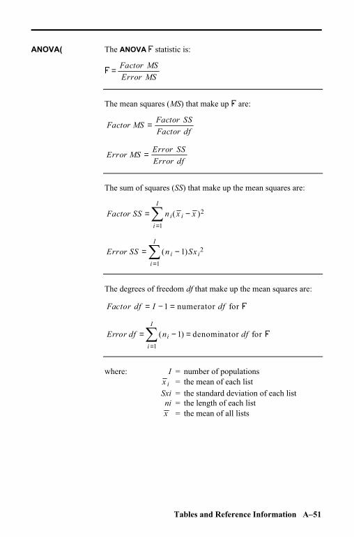
Tables and Reference Information A–51
826DEC~1.DOC TI-83 international English Bob Fedorisko Revised: 10/26/05 2:20 PM Printed: 10/27/05 3:09PM Page 51 of 58
The ANOVA Û statistic is:
Û = Factor MSError MS
The mean squares (MS) that make up Û are:
Factor MS Factor SSFactor df
=
Error MS Error SSError df
=
The sum of squares (SS) that make up the mean squares are:
Factor SS n x xi ii
I
( )= −=∑ 2
1
Error SS n Sxi ii
I
( )= −=∑ 1 2
1
The degrees of freedom df that make up the mean squares are:
Factor df I df= − =1 numerator for Û
Error df n dfii
I
( ) denominator for= − ==∑ 1
1
Û
where: I = number of populationsx i = the mean of each listSxi = the standard deviation of each listni = the length of each listx = the mean of all lists
ANOVA(

A–52 Tables and Reference Information
826DEC~1.DOC TI-83 international English Bob Fedorisko Revised: 10/26/05 2:20 PM Printed: 10/27/05 3:09PM Page 52 of 58
Below is the definition for the 2.SampÜÜÜÜTest.
Sx1, Sx2 = Sample standard deviations having n1-1and n2-1 degrees of freedom df,respectively.
Û = Û-statistic = SxSx
12
2
df(x, n1-1, n2-1) = Ûpdf( ) with degrees of freedomdf, n1-1, and n2-1
p = reported p value
2.SampÜÜÜÜTest for the alternative hypothesis s1 > s2.
p f x n n dxF
= − −∞
∫ ( ), ,1 21 1
2.SampÜÜÜÜTest for the alternative hypothesis s1 < s2.
p f x n n dxF
= − −∫ ( ), ,1 20
1 1
2.SampÜÜÜÜTest for the alternative hypothesis s1 ƒ s2. Limitsmust satisfy the following:
p f x n n dx f x n n dxL
U
bnd
bnd2
1 1 1 11 20
1 2= − − = − −∫ ∫∞
( ) ( ), , , ,
where: [Lbnd,Ubnd] = lower and upper limits
The Û-statistic is used as the bound producing the smallestintegral. The remaining bound is selected to achieve thepreceding integral’s equality relationship.
Statistics Formulas (continued)
2.SampÜÜÜÜTest
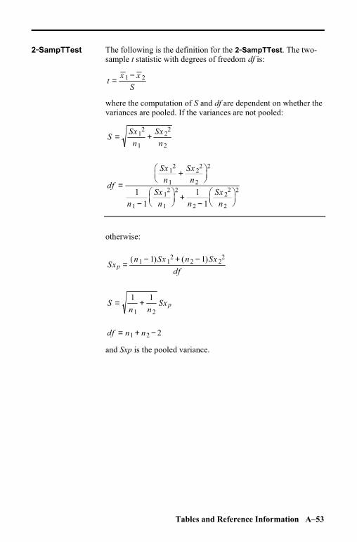
Tables and Reference Information A–53
826DEC~1.DOC TI-83 international English Bob Fedorisko Revised: 10/26/05 2:20 PM Printed: 10/27/05 3:09PM Page 53 of 58
The following is the definition for the 2.SampTTest. The two-sample t statistic with degrees of freedom df is:
t x xS
= −1 2
where the computation of S and df are dependent on whether thevariances are pooled. If the variances are not pooled:
S Sxn
Sxn
= +12
1
22
2
df
Sxn
Sxn
nSxn n
Sxn
=+
−
+−
12
1
22
2
2
1
12
1
2
2
22
2
211
11
otherwise:
Sx n Sx n Sxdfp =
− + −( ) ( )1 12
2 221 1
Sn n
Sxp= +1 1
1 2
df n n= + −1 2 2
and Sxp is the pooled variance.
2.SampTTest

A–54 Tables and Reference Information
826DEC~1.DOC TI-83 international English Bob Fedorisko Revised: 10/26/05 2:20 PM Printed: 10/27/05 3:09PM Page 54 of 58
This section contains financial formulas for computing time value of money,amortization, cash flow, interest-rate conversions, and days between dates.
[ ]i e y x= −× +( ( ))ln 1 1
where: PMT ƒ 0y = C/Y ÷ P/Yx = (.01 × I%) ÷ C/Y
C/Y = compounding periods per yearP/Y = payment periods per yearI% = interest rate per year
i FV PV N= ÷ −− ÷( )( )1 1
where: PMT = 0
The iteration used to compute i:
0 1 1 1= + × − +
+ × +
−−PV PMT G i
iFV ii
NN( ) ( )
[ ]I C Y e y x% /= × × −× +1100 ( ln( ))1 1
where: x = iy = P/Y ÷ C/Y
G i ki = + ×1
where: k = 0 for end-of-period paymentsk = 1 for beginning-of-period payments
N
PMT G FV iPMT G PV i
i
i
i=
× − ×× ×
++
ln
ln ( )1
where: i ƒ 0
N PV FV PMT= + ÷−( )
where: i = 0
Financial Formulas
Time Value ofMoney

Tables and Reference Information A–55
826DEC~1.DOC TI-83 international English Bob Fedorisko Revised: 10/26/05 2:20 PM Printed: 10/27/05 3:09PM Page 55 of 58
PMT iG
PV PV FVii
N= × + ++ −
−
( )1 1
where: i ƒ 0
PMT PV FV N= + ÷−( )
where: i = 0
PV PMT Gi
FVi
PMT Gi
iN
i= × −
×
+− ×1
1( )
where: i ƒ 0
PV FV PMT N= + ×−( )
where: i = 0
FV PMT Gi
i PV PMT Gi
i N i= × − + × + ×
( )1
where: i ƒ 0
FV PV PMT N= + ×−( )
where: i = 0
Time Value ofMoney(Continued)
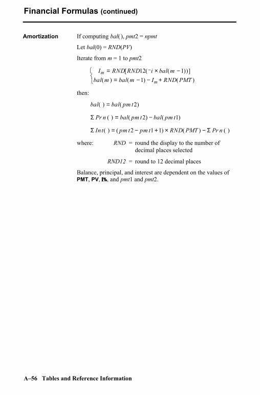
A–56 Tables and Reference Information
826DEC~1.DOC TI-83 international English Bob Fedorisko Revised: 10/26/05 2:20 PM Printed: 10/27/05 3:09PM Page 56 of 58
If computing bal( ), pmt2 = npmt
Let bal(0) = RND(PV)
Iterate from m = 1 to pmt2
II
m
m
= × −= − − +
−RND RND i bal mbal m bal m RND PMT
[ ( ( ))]( ) ( ) ( )
12 11
then:
bal bal pm t( ) ( )= 2
Σ Pr n bal pm t bal pm t( ) ( ) ( )= −2 1
Σ ΣIn t pm t pm t RND PMT n( ) ( ) ( ) ( )= − + × −2 1 1 Pr
where: RND = round the display to the number ofdecimal places selected
RND12 = round to 12 decimal places
Balance, principal, and interest are dependent on the values ofPMT, PV, ææææ, and pmt1 and pmt2.
Financial Formulas (continued)
Amortization
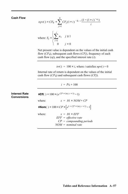
Tables and Reference Information A–57
826DEC~1.DOC TI-83 international English Bob Fedorisko Revised: 10/26/05 2:20 PM Printed: 10/27/05 3:09PM Page 57 of 58
npv CF CF i iij
Sn
j
Nj
j( ) ( ) ( ( ) )= + + − +− −
−
=∑0
1
1 1 11
where: S n j
j
ji
i
j
= ≥
=
=∑
1
1
0 0
Net present value is dependent on the values of the initial cashflow (CF0), subsequent cash flows (CFj), frequency of eachcash flow (nj), and the specified interest rate (i).
irr( ) = 100 × i, where i satisfies npv( ) = 0
Internal rate of return is dependent on the values of the initialcash flow (CF0) and subsequent cash flows (CFj).
i = I% ÷ 100
4Eff( ) ( )( )= × −× +100 11e CP xln
where: x = .01 × NOM ÷ CP
[ ]4Nom( ) ( )= × × −÷ × +100 11 1CP e CP xln
where: x = .01 × EFFEFF = effective rate
CP = compounding periodsNOM = nominal rate
Cash Flow
Interest RateConversions

A–58 Tables and Reference Information
826DEC~1.DOC TI-83 international English Bob Fedorisko Revised: 10/26/05 2:20 PM Printed: 10/27/05 3:09PM Page 58 of 58
With the dbd( function, you can enter or compute a date withinthe range Jan. 1, 1950, through Dec. 31, 2049.
Actual/actual day-count method (assumes actual number ofdays per month and actual number of days per year):
dbd( (days between dates) =Number of Days II - Number of Days I
Number of Days I = (Y1-YB) × 365+ (number of days MB to M1)+ DT1
+ ( )Y YB14−
Number of Days II = (Y2-YB) × 365+ (number of days MB to M2)+ DT2
+ ( )Y YB24−
where: M1 = month of first dateDT1 = day of first date
Y1 = year of first dateM2 = month of second date
DT2 = day of second dateY2 = year of second date
MB = base month (January)DB = base day (1)YB = base year (first year after leap year)
Financial Formulas (continued)
Days betweenDates

General Information B–1
826FEC~1.DOC TI-83 Intl English, Appendix B Bob Fedorisko Revised: 10/27/05 3:16 PM Printed: 10/27/053:16 PM Page 1 of 12
B General Information
Battery Information ................................................................2In Case of Difficulty...............................................................4Error Conditions.....................................................................5Accuracy Information...........................................................10Texas Instruments Support and Service................................12
Contents

B–2 General Information
826FEC~1.DOC TI-83 Intl English, Appendix B Bob Fedorisko Revised: 10/27/05 3:16 PM Printed: 10/27/053:16 PM Page 2 of 12
The TI-82 STATS uses five batteries: four AAA alkalinebatteries and one lithium battery. The lithium battery providesauxiliary power to retain memory while you replace the AAAbatteries.
When the battery voltage level drops below a usable level, theTI-82 STATS displays this message when you turn on the unit.
After this message is first displayed, you can expect thebatteries to function for about one or two weeks, depending onusage. (This one-week to two-week period is based on tests withalkaline batteries; the performance of other kinds of batteriesmay vary.)
The low-battery message continues to be displayed each timeyou turn on the unit until you replace the batteries. If you do notreplace the batteries within about two weeks, the calculator mayturn off by itself or fail to turn on until you install new batteries.
Replace the lithium battery every three or four years.
Do not remove both types of batteries (AAA and lithiumauxiliary) at the same time. Do not allow the batteries to losepower completely. If you follow these guidelines and the stepsfor replacing batteries on page B.3, you can replace either typeof battery without losing any information in memory.
Take these precautions when replacing batteries.
• Do not mix new and used batteries. Do not mix brands (ortypes within brands) of batteries.
• Do not mix rechargeable and nonrechargeable batteries.• Install batteries according to polarity (+ and N) diagrams.• Do not place nonrechargeable batteries in a battery
recharger.• Properly dispose of used batteries immediately. Do not leave
them within the reach of children.• Do not incinerate batteries.
Battery Information
When to Replacethe Batteries
Effects ofReplacing theBatteries
BatteryPrecautions
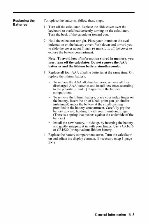
General Information B–3
826FEC~1.DOC TI-83 Intl English, Appendix B Bob Fedorisko Revised: 10/27/05 3:16 PM Printed: 10/27/053:16 PM Page 3 of 12
To replace the batteries, follow these steps.
1. Turn off the calculator. Replace the slide cover over thekeyboard to avoid inadvertently turning on the calculator.Turn the back of the calculator toward you.
2. Hold the calculator upright. Place your thumb on the ovalindentation on the battery cover. Push down and toward youto slide the cover about ¼ inch (6 mm). Lift off the cover toexpose the battery compartment.
Note: To avoid loss of information stored in memory, youmust turn off the calculator. Do not remove the AAAbatteries and the lithium battery simultaneously.
3. Replace all four AAA alkaline batteries at the same time. Or,replace the lithium battery.
• To replace the AAA alkaline batteries, remove all fourdischarged AAA batteries and install new ones accordingto the polarity (+ and N) diagrams in the batterycompartment.
• To remove the lithium battery, place your index finger onthe battery. Insert the tip of a ball-point pen (or similarinstrument) under the battery at the small openingprovided in the battery compartment. Carefully pry thebattery upward, holding it with your thumb and finger.(There is a spring that pushes against the underside of thebattery.)
• Install the new battery, + side up, by inserting the batteryand gently snapping it in with your finger. Use a CR1616or CR1620 (or equivalent) lithium battery.
4. Replace the battery compartment cover. Turn the calculatoron and adjust the display contrast, if necessary (step 1; pageB.4).
Replacing theBatteries

B–4 General Information
826FEC~1.DOC TI-83 Intl English, Appendix B Bob Fedorisko Revised: 10/27/05 3:16 PM Printed: 10/27/053:16 PM Page 4 of 12
To handle a difficulty, follow these steps.
1. If you cannot see anything on the screen, the contrast mayneed to be adjusted.
To darken the screen, press and release y, and then pressand hold } until the display is sufficiently dark.
To lighten the screen, press and release y, and then pressand hold † until the display is sufficiently light.
2. If an error menu is displayed, follow the steps in Chapter 1.Refer to pages B.5 through B.9 for details about specificerrors, if necessary.
3. If a checkerboard cursor ( # ) is displayed, then either youhave entered the maximum number of characters in aprompt, or memory is full. If memory is full, press y[MEM] 2 to select 2:Delete, and then delete some items frommemory (Chapter 18).
4. If the busy indicator (dotted line) is displayed, a graph orprogram has been paused; the TI-82 STATS is waiting forinput. Press Í to continue or press É to break.
5. If the calculator does not seem to work at all, be sure thebatteries are fresh and that they are installed properly. Referto battery information on pages B.2 and B.3.
In Case of Difficulty
Handling aDifficulty
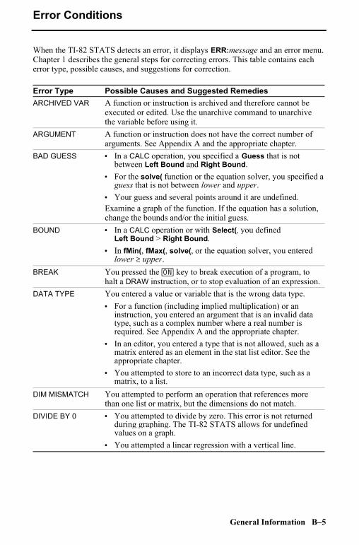
General Information B–5
826FEC~1.DOC TI-83 Intl English, Appendix B Bob Fedorisko Revised: 10/27/05 3:16 PM Printed: 10/27/053:16 PM Page 5 of 12
When the TI-82 STATS detects an error, it displays ERR:message and an error menu.Chapter 1 describes the general steps for correcting errors. This table contains eacherror type, possible causes, and suggestions for correction.
Error Type Possible Causes and Suggested RemediesARCHIVED VAR A function or instruction is archived and therefore cannot be
executed or edited. Use the unarchive command to unarchivethe variable before using it.
ARGUMENT A function or instruction does not have the correct number ofarguments. See Appendix A and the appropriate chapter.
BAD GUESS ¦ In a CALC operation, you specified a Guess that is notbetween Left Bound and Right Bound.
¦ For the solve( function or the equation solver, you specified aguess that is not between lower and upper.
¦ Your guess and several points around it are undefined.Examine a graph of the function. If the equation has a solution,change the bounds and/or the initial guess.
BOUND ¦ In a CALC operation or with Select(, you definedLeft Bound > Right Bound.
¦ In fMin(, fMax(, solve(, or the equation solver, you enteredlower ‚ upper.
BREAK You pressed the É key to break execution of a program, tohalt a DRAW instruction, or to stop evaluation of an expression.
DATA TYPE You entered a value or variable that is the wrong data type.¦ For a function (including implied multiplication) or an
instruction, you entered an argument that is an invalid datatype, such as a complex number where a real number isrequired. See Appendix A and the appropriate chapter.
¦ In an editor, you entered a type that is not allowed, such as amatrix entered as an element in the stat list editor. See theappropriate chapter.
¦ You attempted to store to an incorrect data type, such as amatrix, to a list.
DIM MISMATCH You attempted to perform an operation that references morethan one list or matrix, but the dimensions do not match.
DIVIDE BY 0 ¦ You attempted to divide by zero. This error is not returnedduring graphing. The TI-82 STATS allows for undefinedvalues on a graph.
¦ You attempted a linear regression with a vertical line.
Error Conditions
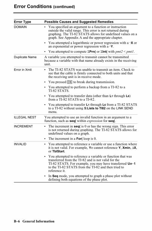
B–6 General Information
826FEC~1.DOC TI-83 Intl English, Appendix B Bob Fedorisko Revised: 10/27/05 3:16 PM Printed: 10/27/053:16 PM Page 6 of 12
Error Type Possible Causes and Suggested RemediesDOMAIN ¦ You specified an argument to a function or instruction
outside the valid range. This error is not returned duringgraphing. The TI-82 STATS allows for undefined values on agraph. See Appendix A and the appropriate chapter.
¦ You attempted a logarithmic or power regression with a LX oran exponential or power regression with a LY.
¦ You attempted to compute GPrn( or GInt( with pmt2 < pmt1.Duplicate Name A variable you attempted to transmit cannot be transmitted
because a variable with that name already exists in the receivingunit.
Error in Xmit ¦ The TI-82 STATS was unable to transmit an item. Check tosee that the cable is firmly connected to both units and thatthe receiving unit is in receive mode.
¦ You pressed É to break during transmission.¦ You attempted to perform a backup from a TI.82 to a
TI-82 STATS.¦ You attempted to transfer data (other than L1 through L6)
from a TI-82 STATS to a TI.82.¦ You attempted to transfer L1 through L6 from a TI-82 STATS
to a TI.82 without using 5:Lists to TI82 on the LINK SENDmenu.
ILLEGAL NEST You attempted to use an invalid function in an argument to afunction, such as seq( within expression for seq(.
INCREMENT ¦ The increment in seq( is 0 or has the wrong sign. This erroris not returned during graphing. The TI-82 STATS allows forundefined values on a graph.
¦ The increment in a For( loop is 0.INVALID ¦ You attempted to reference a variable or use a function where
it is not valid. For example, Yn cannot reference Y, Xmin, @X,or TblStart.
¦ You attempted to reference a variable or function that wastransferred from the TI.82 and is not valid for theTI-82 STATS. For example, you may have transferred UnN1to the TI-82 STATS from the TI.82 and then tried toreference it.
¦ In Seq mode, you attempted to graph a phase plot withoutdefining both equations of the phase plot.
Error Conditions (continued)
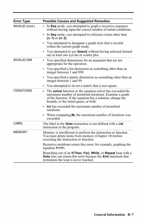
General Information B–7
826FEC~1.DOC TI-83 Intl English, Appendix B Bob Fedorisko Revised: 10/27/05 3:16 PM Printed: 10/27/053:16 PM Page 7 of 12
Error Type Possible Causes and Suggested RemediesINVALID (cont.) ¦ In Seq mode, you attempted to graph a recursive sequence
without having input the correct number of initial conditions.¦ In Seq mode, you attempted to reference terms other than
(nN1) or (nN2).¦ You attempted to designate a graph style that is invalid
within the current graph mode.¦ You attempted to use Select( without having selected (turned
on) at least one xyLine or scatter plot.INVALID DIM ¦ You specified dimensions for an argument that are not
appropriate for the operation.¦ You specified a list dimension as something other than an
integer between 1 and 999.¦ You specified a matrix dimension as something other than an
integer between 1 and 99.¦ You attempted to invert a matrix that is not square.
ITERATIONS ¦ The solve( function or the equation solver has exceeded themaximum number of permitted iterations. Examine a graphof the function. If the equation has a solution, change thebounds, or the initial guess, or both.
¦ irr( has exceeded the maximum number of permittediterations.
¦ When computing ææææ, the maximum number of iterations wasexceeded.
LABEL The label in the Goto instruction is not defined with a Lblinstruction in the program.
MEMORY Memory is insufficient to perform the instruction or function.You must delete items from memory (Chapter 18) beforeexecuting the instruction or function.Recursive problems return this error; for example, graphing theequation Y1=Y1.Branching out of an If/Then, For(, While, or Repeat loop with aGoto also can return this error because the End statement thatterminates the loop is never reached.
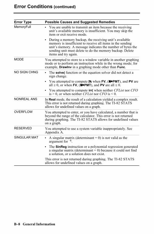
B–8 General Information
826FEC~1.DOC TI-83 Intl English, Appendix B Bob Fedorisko Revised: 10/27/05 3:16 PM Printed: 10/27/053:16 PM Page 8 of 12
Error Type Possible Causes and Suggested RemediesMemoryFull ¦ You are unable to transmit an item because the receiving
unit’s available memory is insufficient. You may skip theitem or exit receive mode.
¦ During a memory backup, the receiving unit’s availablememory is insufficient to receive all items in the sendingunit’s memory. A message indicates the number of bytes thesending unit must delete to do the memory backup. Deleteitems and try again.
MODE You attempted to store to a window variable in another graphingmode or to perform an instruction while in the wrong mode; forexample, DrawInv in a graphing mode other than Func.
NO SIGN CHNG ¦ The solve( function or the equation solver did not detect asign change.
¦ You attempted to compute ææææ when FV, (ÚÚÚÚääääPMT), and PV areall ‚ 0, or when FV, (ÚÚÚÚääääPMT), and PV are all 0.
¦ You attempted to compute irr( when neither CFList nor CFOis > 0, or when neither CFList nor CFO is < 0.
NONREAL ANS In Real mode, the result of a calculation yielded a complex result.This error is not returned during graphing. The TI-82 STATSallows for undefined values on a graph.
OVERFLOW You attempted to enter, or you have calculated, a number that isbeyond the range of the calculator. This error is not returnedduring graphing. The TI-82 STATS allows for undefined valueson a graph.
RESERVED You attempted to use a system variable inappropriately. SeeAppendix A.
SINGULAR MAT ¦ A singular matrix (determinant = 0) is not valid as theargument for L1.
¦ The SinReg instruction or a polynomial regression generateda singular matrix (determinant = 0) because it could not finda solution, or a solution does not exist.
This error is not returned during graphing. The TI-82 STATSallows for undefined values on a graph.
Error Conditions (continued)

General Information B–9
826FEC~1.DOC TI-83 Intl English, Appendix B Bob Fedorisko Revised: 10/27/05 3:16 PM Printed: 10/27/053:16 PM Page 9 of 12
Error Type Possible Causes and Suggested RemediesSINGULARITY expression in the solve( function or the equation solver contains
a singularity (a point at which the function is not defined).Examine a graph of the function. If the equation has a solution,change the bounds or the initial guess or both.
STAT You attempted a stat calculation with lists that are notappropriate.¦ Statistical analyses must have at least two data points.¦ Med.Med must have at least three points in each partition.¦ When you use a frequency list, its elements must be ‚ 0.¦ (Xmax N Xmin) à Xscl must be 47 for a histogram.
STAT PLOT You attempted to display a graph when a stat plot that uses anundefined list is turned on.
SYNTAX The command contains a syntax error. Look for misplacedfunctions, arguments, parentheses, or commas. See Appendix Aand the appropriate chapter.
TOL NOT MET You requested a tolerance to which the algorithm cannot returnan accurate result.
UNDEFINED You referenced a variable that is not currently defined. Forexample, you referenced a stat variable when there is no currentcalculation because a list has been edited, or you referenced avariable when the variable is not valid for the currentcalculation, such as a after Med.Med.
WINDOW RANGE A problem exists with the window variables.¦ You defined Xmax Xmin or Ymax Ymin.¦ You defined qmax qmin and qstep > 0 (or vice versa).¦ You attempted to define Tstep=0.¦ You defined Tmax Tmin and Tstep > 0 (or vice versa).¦ Window variables are too small or too large to graph correctly.
You may have attempted to zoom in or zoom out to a point thatexceeds the TI-82 STATS numerical range.
ZOOM ¦ A point or a line, instead of a box, is defined in ZBox.¦ A ZOOM operation returned a math error.
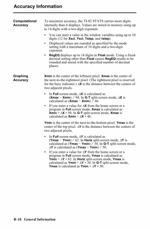
B–10 General Information
826FEC~1.DOC TI-83 Intl English, Appendix B Bob Fedorisko Revised: 10/27/05 3:16 PM Printed: 10/27/053:16 PM Page 10 of 12
To maximize accuracy, the TI-82 STATS carries more digitsinternally than it displays. Values are stored in memory using upto 14 digits with a two-digit exponent.
• You can store a value in the window variables using up to 10digits (12 for Xscl, Yscl, Tstep, and qstep).
• Displayed values are rounded as specified by the modesetting with a maximum of 10 digits and a two-digitexponent.
• RegEQ displays up to 14 digits in Float mode. Using a fixed-decimal setting other than Float causes RegEQ results to berounded and stored with the specified number of decimalplaces.
Xmin is the center of the leftmost pixel, Xmax is the center ofthe next-to-the-rightmost pixel. (The rightmost pixel is reservedfor the busy indicator.) @X is the distance between the centers oftwo adjacent pixels.
• In Full screen mode, @X is calculated as(Xmax N Xmin) à 94. In G.T split-screen mode, @X iscalculated as (Xmax N Xmin) à 46.
• If you enter a value for @X from the home screen or aprogram in Full screen mode, Xmax is calculated asXmin + @X … 94. In G.T split-screen mode, Xmax iscalculated as Xmin + @X … 46.
Ymin is the center of the next-to-the-bottom pixel; Ymax is thecenter of the top pixel. @Y is the distance between the centers oftwo adjacent pixels.
• In Full screen mode, @Y is calculated as(Ymax N Ymin) à 62. In Horiz split-screen mode, @Y iscalculated as (Ymax N Ymin) à 30. In G.T split-screen mode,@Y is calculated as (Ymax N Ymin) à 50.
• If you enter a value for @Y from the home screen or aprogram in Full screen mode, Ymax is calculated asYmin + @Y … 62. In Horiz split-screen mode, Ymax iscalculated as Ymin + @Y … 30. In G.T split-screen mode,Ymax is calculated as Ymin + @Y … 50.
Accuracy Information
ComputationalAccuracy
GraphingAccuracy

General Information B–11
826FEC~1.DOC TI-83 Intl English, Appendix B Bob Fedorisko Revised: 10/27/05 3:16 PM Printed: 10/27/053:16 PM Page 11 of 12
Cursor coordinates are displayed as eight-character numbers(which may include a negative sign, decimal point, andexponent) when Float mode is selected. X and Y are updatedwith a maximum accuracy of eight digits.
minimum and maximum on the CALCULATE menu arecalculated with a tolerance of 1EL5; ‰f(x)dx is calculated at 1EL3.Therefore, the result displayed may not be accurate to all eightdisplayed digits. For most functions, at least five accurate digitsexist. For fMin(, fMax(, and fnInt( on the MATH menu and solve(in the CATALOG, the tolerance can be specified.
Function Range of Input Valuessin x, cos x, tan x 0 |x| < 1012 (radian or degree)sinL1 x, cosL1 x L1 x 1ln x, log x 10L100 < x < 10100
ex L10100 < x 230.2585092994010x L10100 < x < 100sinh x, cosh x |x| 230.25850929940tanh x |x| < 10100
sinhL1 x |x| < 5 × 1099
coshL1 x 1 x < 5 × 1099
tanhL1 x L1 < x < 1‡x (real mode) 0 x < 10100
‡x (complex mode) |x| < 10100
x! L.5 x 69, where x is a multiple of .5
Function Range of ResultsinL1 x, tanL1 x L90¡ to 90¡ or Lpà2 to pà2 (radians)cosL1 x 0¡ to 180¡ or 0 to p (radians)
GraphingAccuracy(continued)
Function Limits
Function Results

B–12 General Information
826FEC~1.DOC TI-83 Intl English, Appendix B Bob Fedorisko Revised: 10/27/05 3:16 PM Printed: 10/27/053:16 PM Page 12 of 12
For more information about TI products and services, contact TIby e-mail or visit the TI Internet address.
E-mail inquiries: [email protected] Page: education.ti.com
For information about the length and terms of the warranty orabout product service, refer to the warranty statement enclosedwith this product or contact your local Texas Instrumentsretailer/distributor.
Texas Instruments Support and Service
For GeneralInformation
Service andwarrantyinformation
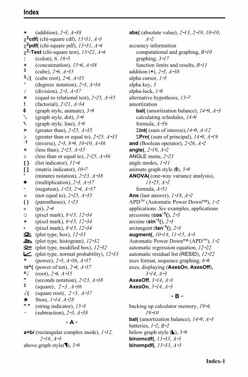
Index-1
Index
825915~1.DOC TI-83 international English Bob Fedorisko Revised: 10/26/05 2:25 PM Printed: 10/27/05 3:22PM Page 1 of 16
+ (addition), 2.3, A.38c2cdf( (chi-square cdf), 13.31, A.3c2pdf( (chi-square pdf), 13.31, A.4c2.Test (chi-square test), 13.22, A.4: (colon), 6, 16.5+ (concatenation), 15.6, A.383 (cube), 2.6, A.353‡( (cube root), 2.6, A.35¡ (degrees notation), 2.3, A.34à (division), 2.3, A.37= (equal-to relational test), 2.25, A.35! (factorial), 2.21, A.34ìììì (graph style, animate), 3.9íííí (graph style, dot), 3.9çççç (graph style, line), 3.9> (greater than), 2.25, A.35‚ (greater than or equal to), 2.25, A.35L1 (inverse), 2.3, 8.9, 10.10, A.36< (less than), 2.25, A.35 (less than or equal to), 2.25, A.36{ } (list indicator), 11.4[ ] (matrix indicator), 10.7' (minutes notation), 2.23, A.38ääää (multiplication), 2.3, A.37M (negation), 1.23, 2.4, A.37ƒ (not equal to), 2.25, A.35( ) (parentheses), 1.23p (pi), 2.4› (pixel mark), 8.15, 12.34+ (pixel mark), 8.15, 12.34¦ (pixel mark), 8.15, 12.34ÖÖÖÖ (plot type, box), 12.33ÒÒÒÒ (plot type, histogram), 12.32ÕÕÕÕ (plot type, modified box), 12.32ÔÔÔÔ (plot type, normal probability), 12.33^ (power), 2.3, A.36, A.3710^( (power of ten), 2.4, A.37x‡ (root), 2.6, A.35" (seconds notation), 2.23, A.382 (square) , 2 .3 , A.36‡( (square root) , 2 .3 , A.37!!!! Store, 1.14, A.28" " (string indicator), 15.3N (subtraction), 2.3, A.38
. A .a+bi (rectangular complex mode), 1.12,
2.16, A.3above graph style(éééé), 3.9
abs( (absolute value), 2.13, 2.19, 10.10,A.2
accuracy informationcomputational and graphing, B.10graphing, 3.17function limits and results, B.11
addition (+), 2.3, A.38alpha cursor, 1.5alpha key, 3alpha-lock, 1.8alternative hypothesis, 13.7amortization
bal( (amortization balance), 14.9, A.3calculating schedules, 14.9formula, A.56GInt( (sum of interest),14.9, A.12GPrn( (sum of principal), 14.9, A.19
and (Boolean operator), 2.26, A.2angle(, 2.19, A.2ANGLE menu, 2.23angle modes, 1.11animate graph style (ìììì), 3.9ANOVA( (one-way variance analysis),
13.25, A.2formula, A.51
Ans (last answer), 1.18, A.2APDé (Automatic Power Down™), 1.2applications. See examples, applicationsarccosine (cosM1(), 2.3arcsine (sinM1(), 2.3arctangent (tanM1(), 2.3augment(, 10.14, 11.15, A.3Automatic Power Down™ (APDé), 1.2automatic regression equation, 12.22automatic residual list (RESID), 12.22axes format, sequence graphing, 6.8axes, displaying (AxesOn, AxesOff),
3.14, A.3AxesOff, 3.14, A.3AxesOn, 3.14, A.3
. B .backing up calculator memory, 19.4,
19.10bal( (amortization balance), 14.9, A.3batteries, 1.2, B.2below graph style (êêêê), 3.9binomcdf(, 13.33, A.3binompdf(, 13.33, A.3

Index-2
Index (continued)
825915~1.DOC TI-83 international English Bob Fedorisko Revised: 10/26/05 2:25 PM Printed: 10/27/05 3:22PM Page 2 of 16
Boolean logic, 2.26box pixel mark (›), 8.15, 12.34Boxplot plot type ( ÖÖÖÖ), 12.33busy indicator, 1.4
. C .CALCULATE menu, 3.25Calculate output option, 13.6, 13.8cash flow
calculating, 14.8formula, A.57irr( (internal rate of return), 14.8, A.13npv( (net present value), 14.8, A.17
CATALOG, 15.2CBLé System, 16.21, 19.3, A.10CBRé, 16.21, 19.3, A.10Check RAM (memory screen), 18.2chi-square cdf (c2cdf(), 13.31, A.3chi-square pdf (c2pdf(), 13.31, A.4chi-square test (c2.Test), 13.22, A.4Circle( (draw circle), 8.11, A.4Clear Entries, 18.4, A.4clearing
entries (Clear Entries), 18.4, A.4all lists (ClrAllLists), 18.4, A.4drawing (ClrDraw), 8.4, A.4home screen (ClrHome), 16.20, A.4list (ClrList), 12.20, A.4table (ClrTable), 16.20, A.4
ClrAllLists (clear all lists), 18.4, A.4ClrDraw (clear drawing), 8.4, A.4ClrHome (clear home screen), 16.20, A.4ClrList (clear list), 12.20, A.4ClrTable (clear table), 16.20, A.4coefficients of determination (r2, R2),
12.23colon separator (:), 6, 16.5combinations (nCr), 2.21, A.16
. C (continued) .complex
modes (a+bi, re^qi), 1.12, 2.16, A.3,A.22
numbers, 1.12, 2.16, 2.18, A.22compounding-periods-per-year variable
(C/Y), 14.4, 14.14concatenation (+), 15.6, A.38confidence intervals, 13.8, 13.16 N 13.21conj( (conjugate), 2.18, A.4
Connected (plotting mode), 1.11, A.4contrast (display), 1.3convergence, sequence graphing, 6.12conversions
4Dec (to decimal), 2.5, A.54DMS (to degrees/minutes/ seconds),
2.24, A.74Eff (to effective interest rate), 14.12,
A.7Equ4String( (equation-to-string
conversion), 15-7, A.84Frac (to fraction conversion), 2.5,
A.10List4matr( (list-to-matrix conversion),
10.14, 11.15, A.14Matr4list( (matrix-to-list conversion),
10.14, 11.16, A.154Nom (to nominal interest rate
conversion), 14.12, A.164Polar (to polar conversion), 2.19,
A.19P4Rx(, P4Ry( (polar-to-rectangular
conversion), 2.24, A.214Rect (to rectangular conversion), 2.19,
A.22R4Pr(, R4Pq( (rectangular-to-polar
conversion), 2.24, A.23String4Equ( (string-to-equation
conversion), 15.8, A.29CoordOff, 3.14, A.5CoordOn, 3.14, A.5correlation coefficient (r), 12.23, 12.25 N
12.27cos( (cosine), 2.3, A.5cosM1( (arccosine), 2.3, A.5cosh( (hyperbolic cosine), 15.10, A.5
. D (continued) .coshM1( (hyperbolic arccosine), 15.10, A.5cosine (cos(), 2.3, A.5cross pixel mark (+), 8.15, 12.34cube ( 3) , 2.6, A.35cube root (3‡(), 2.6, A.35CubicReg (cubic regression), 12.26, A.5cubic regression (CubicReg), 12.26, A.5cumulative sum (cumSum(), 10.15,
11.12, A.5cumSum( (cumulative sum), 10.15,
11.12, A.5

Index-3
825915~1.DOC TI-83 international English Bob Fedorisko Revised: 10/26/05 2:25 PM Printed: 10/27/05 3:22PM Page 3 of 16
cursors, 1.5, 1.8C/Y (compounding-periods-per-year
variable), 14.4, 14.14
. D .Data input option, 13.6, 13.7days between dates (dbd(), 14.13, A.5,
A.58dbd( (days between dates), 14.13, A.5,
A.584Dec (to decimal conversion), 2.5, A.5decimal mode (float or fixed), 1.10decrement and skip (DS<(), 16.14, A.7definite integral, 2.7, 3.28, 4.8, 5.6Degree angle mode, 1.11, 2.23, A.6degrees notation (¡) , 2.3, A.34DELETE FROM menu, 18.3delete variable contents (DelVar), 16.15,
A.6DelVar (delete variable contents), 16.15,
A.6DependAsk, 7.3, 7.5, A.6DependAuto, 7.3, 7.5, A.6derivative. See numerical derivativedet( (determinant), 10.12, A.6determinant (det(), 10.12, A.6DiagnosticOff, 12.23, A.6DiagnosticOn, 12.23, A.6diagnostics display mode(r, r2, R2), 12.23differentiation, 2.8, 3.28, 4.8, 5.6
. D (continued) .dimensioning a list or matrix, 10.12,
10.13, 11.11, A.6dim( (dimension), 10.12, 11.11, A.6!!!!dim( (assign dimension), 10.13, 11.11,
A.6Disp (display), 16.18, A.6DispGraph (display graph), 16.19, A.7display contrast, 1.3display cursors, 1.5DispTable (display table), 16.19, A.7DISTR (distributions menu), 13.29DISTR DRAW (distributions drawing
menu), 13.35distribution functions
binomcdf(, 13.33, A.3binompdf(, 13.33, A.3c2cdf(, 13.31, A.3
c2pdf(, 13.31, A.4ÛÛÛÛcdf(, 13.32, A.8ÛÛÛÛpdf(, 13.32, A.9geometcdf(, 13.34, A.10geometpdf(, 13.34, A.11invNorm(, 13.30, A.12normalcdf(, 13.30, A.17normalpdf(, 13.29, A.17poissoncdf(, 13.34, A.99poissonpdf(, 13.33, A.19tcdf(, 13.31, A.29tpdf(, 13.30, A.29
distribution shading instructionsShadec2(, 13.36, A.26ShadeÛÛÛÛ(, 13.36, A.27ShadeNorm(, 13.35, A.27Shade_t(, 13.36, A.27
division (à) , 2.3, A.37DMS (degrees/minutes/seconds entry
notation), 2.23, A.384DMS (to degrees/minutes/seconds), 2.24,
A.7dot graph style (íííí), 3.9dot pixel mark (¦), 8.15, 12.34Dot (plotting mode), 1.11, A.7DrawF (draw a function), 8.9, A.7

Index-4
Index (continued)
825915~1.DOC TI-83 international English Bob Fedorisko Revised: 10/26/05 2:25 PM Printed: 10/27/05 3:22PM Page 4 of 16
. D (continued) .drawing on a graph
circles (Circle(), 8.11functions and inverses (DrawF,
DrawInv), 8.9lines (Horizontal, Line(, Vertical),
8.6, 8.7line segments (Line(), 8.5pixels (Pxl.Change, Pxl.Off, Pxl.On,
pxl.Test), 8.16points (Pt.Change, Pt.Off, Pt.On),
8.14tangents (Tangent), 8.8text (Text), 8.12using Pen, 8.13
DrawInv (draw inverse), 8.9, A.7DRAW menu, 8.3DRAW instructions, 8.3 N 8.16Draw output option, 13.6 N 13.8DRAW POINTS menu, 8.14DRAW STO (draw store menu), 8.17dr/dq operation on a graph, 5.6DS<( (decrement and skip), 16.14, A.7DuplicateName menu, 19.5dx/dt operation on a graph, 3.28, 4.8dy/dx operation on a graph, 3.28, 4.8, 5.6
. E .e (constant), 2.4e^( (exponential), 2.4, A.7åååå (exponent), 1.7, 1.10, A.7edit keys table, 1.84Eff( (to effective interest rate), 14.12, A.7Else, 16.10End, 16.12, A.8Eng (engineering notation mode), 1.10,
A.8entry cursor, 1.5ENTRY (last entry key), 1.16EOSé (Equation Operating System), 1.22eqn (equation variable), 2.8, 2.12equal-to relational test (=), 2.25, A.35Equation Operating System (EOSé), 1.22Equation Solver, 2.8equations with multiple roots, 2.12
. E (continued) .Equ4String( (equation-to-string
conversion), 15.7, A.8
errorsdiagnosing and correcting, 1.24messages, B.5
examples—applicationsarea between curves, 17.11areas of regular n-sided polygons,
17.16box plots, 17.2cobweb attractors, 17.8fundamental theorem of calculus, 17.14guess the coefficients, 17.9inequalities, 17.5mortgage payments 17.18parametric equations: ferris wheel
problem, 17.12piecewise functions, 17.4Sierpinski triangle, 17.7solving a system of nonlinear equations,
17.6unit circle and trig curves, 17.10
examples—Getting Startedbox with lid 9 – 16
defining a, 9defining a table of values, 10finding calculated maximum, 16setting the viewing window, 12tracing the graph, 13zooming in on the graph, 15zooming in on the table, 11
coin flip, 2.2compound interest, 14.3drawing a tangent line, 8.2financing a car, 14.2forest and trees, 6.2generating a sequence, 11.2graphing a circle, 3.2mean height of a population, 13.2path of a ball, 4.2pendulum lengths and periods, 12.2polar rose, 5.2

Index-5
825915~1.DOC TI-83 international English Bob Fedorisko Revised: 10/26/05 2:25 PM Printed: 10/27/05 3:22PM Page 5 of 16
. E (continued) .examples—Getting Started (continued)
quadratic formulaconverting to a fraction, 7displaying complex results, 8entering a calculation, 6
roots of a, 7.2sending variables, 19.2solving a system of linear equations,
10.2unit circle, 9.2volume of a cylinder, 16.2
examples—miscellaneousconvergence, 6.12daylight hours in Alaska, 12.28calculating outstanding loan balances,
14.10predator-prey model, 6.13
exponential regression (ExpReg), 12.26,A.8
expr( (string-to-expression conversion),15.7, A.8
ExpReg (exponential regression), 12.26,A.8
expression, 1.6converting from string (expr(), 15.7,
A.8turning on and off (ExprOn, ExprOff),
3.14, A.8ExprOff (expression off), 3.14, A.8ExprOn (expression on), 3.14, A.8
. F .‰f(x)dx operation on a graph, 3.28factorial (!), 2.21, A.34family of curves, 3.16ÛÛÛÛcdf(, 13.32, A.8Fill(, 10.13, A.8FINANCE CALC menu, 14.5FINANCE VARS menu, 14.14financial functions
amortization schedules, 14.9cash flows, 14.8days between dates, 14.13interest rate conversions, 14.12payment method, 14.13time value of money (TVM), 14.6
. F (continued) .Fix (fixed-decimal mode), 1.10, A.8fixed-decimal mode (Fix), 1.10, A.8Float (floating-decimal mode), 1.10, A.8floating-decimal mode (Float), 1.10, A.8fMax( (function maximum), 2.6, A.9fMin( (function minimum), 2.6, A.9fnInt( (function integral), 2.7, A.9FnOff (function off), 3.8, A.9FnOn (function on), 3.8, A.9For(, 16.10, A.9format settings, 3.13, 6.8formulas
amortization, A.56ANOVA, A.51cash flow, A.57days between dates, A.58factorial, 2.21interest rate conversions, A.57logistic regression, A.50sine regression, A.50time value of money, A.54two-sample Û-Test, A.52two-sample t test, A.53
fPart( (fractional part), 2.14, 10.11, A.9ÛÛÛÛpdf(, 13.32, A.94Frac (to fraction), 2.5, A.10free-moving cursor, 3.17frequency, 12.24Full (full-screen mode), 1.12, A.10full-screen mode (Full), 1.12, A.10Func (function graphing mode), 1.11,
A.10function, definition of, 1.7function graphing, 3.1 – 3.28
accuracy, 3.17CALC (calculate menu), 3.25defining and displaying, 3.3defining in the Y= editor, 3.5defining on the home screen, in a
program, 3.6deselecting, 3.7displaying, 3.3, 3.11, 3.15evaluating, 3.6family of curves, 3.16format settings, 3.13
. F (continued) .Function graphing (continued)
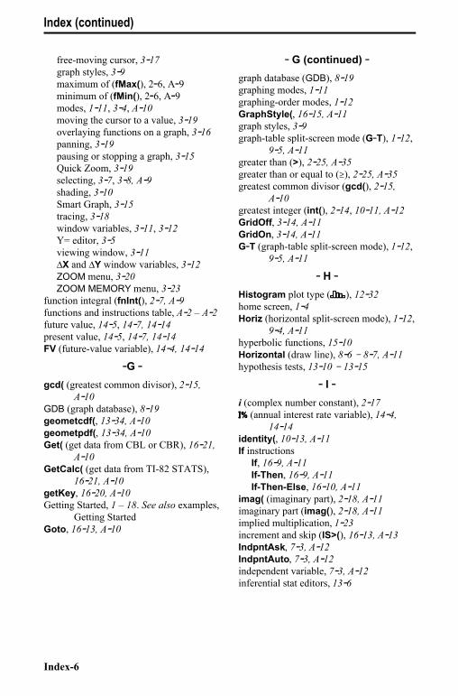
Index-6
Index (continued)
825915~1.DOC TI-83 international English Bob Fedorisko Revised: 10/26/05 2:25 PM Printed: 10/27/05 3:22PM Page 6 of 16
free-moving cursor, 3.17graph styles, 3.9maximum of (fMax(), 2.6, A.9minimum of (fMin(), 2.6, A.9modes, 1.11, 3.4, A.10moving the cursor to a value, 3.19overlaying functions on a graph, 3.16panning, 3.19pausing or stopping a graph, 3.15Quick Zoom, 3.19selecting, 3.7, 3.8, A.9shading, 3.10Smart Graph, 3.15tracing, 3.18window variables, 3.11, 3.12Y= editor, 3.5viewing window, 3.11@X and @Y window variables, 3.12ZOOM menu, 3.20ZOOM MEMORY menu, 3.23
function integral (fnInt(), 2.7, A.9functions and instructions table, A.2 – A.2future value, 14.5, 14.7, 14.14present value, 14.5, 14.7, 14.14FV (future-value variable), 14.4, 14.14
.G .gcd( (greatest common divisor), 2.15,
A.10GDB (graph database), 8.19geometcdf(, 13.34, A.10geometpdf(, 13.34, A.10Get( (get data from CBL or CBR), 16.21,
A.10GetCalc( (get data from TI-82 STATS),
16.21, A.10getKey, 16.20, A.10Getting Started, 1 – 18. See also examples,
Getting StartedGoto, 16.13, A.10
. G (continued) .graph database (GDB), 8.19graphing modes, 1.11graphing-order modes, 1.12GraphStyle(, 16.15, A.11graph styles, 3.9graph-table split-screen mode (G.T), 1.12,
9.5, A.11greater than (>), 2.25, A.35greater than or equal to (‚), 2.25, A.35greatest common divisor (gcd(), 2.15,
A.10greatest integer (int(), 2.14, 10.11, A.12GridOff, 3.14, A.11GridOn, 3.14, A.11G.T (graph-table split-screen mode), 1.12,
9.5, A.11
. H .Histogram plot type (ÒÒÒÒ), 12.32home screen, 1.4Horiz (horizontal split-screen mode), 1.12,
9.4, A.11hyperbolic functions, 15.10Horizontal (draw line), 8.6 N 8.7, A.11hypothesis tests, 13.10 N 13.15
. I .i (complex number constant), 2.17ææææ (annual interest rate variable), 14.4,
14.14identity(, 10.13, A.11If instructions
If, 16.9, A.11If-Then, 16.9, A.11If-Then-Else, 16.10, A.11
imag( (imaginary part), 2.18, A.11imaginary part (imag(), 2.18, A.11implied multiplication, 1.23increment and skip (IS>(), 16.13, A.13IndpntAsk, 7.3, A.12IndpntAuto, 7.3, A.12independent variable, 7.3, A.12inferential stat editors, 13.6

Index-7
825915~1.DOC TI-83 international English Bob Fedorisko Revised: 10/26/05 2:25 PM Printed: 10/27/05 3:22PM Page 7 of 16
. I (continued) .inferential statistics. See also stat tests;
confidence intervalsalternative hypotheses, 13.7bypassing editors, 13.8calculating test results (Calculate),
13.8confidence interval calculations, 13.8,
13.16 N 13.21data input or stats input, 13.7entering argument values, 13.7graphing test results (Draw), 13.8input descriptions table, 13.26pooled option, 13.8STAT TESTS menu, 13.9test and interval output variables, 13.28
Input, 16.16, 16.17, A.12insert cursor, 1.5inString( (in string), 15.7, A.12instruction, definition of, 1.7int( (greatest integer), 2.14, 10.11, A.12GInt( (sum of interest), 14.9, A.12integer part (iPart(), 2.14, 10.11, A.12integral. See numerical integralinterest rate conversions
calculating, 14.124Eff( (compute effective interest rate),
14.12, A.7formula, A.574Nom( (compute nominal interest rate),
14.12, A.16internal rate of return (irr(), 14.8, A.13intersect operation on a graph, 3.27inverse (L1), 2.3, 8.9, 10.10, A.36inverse cumulative normal distribution
(invNorm(), 13.30, A.12inverse trig functions, 2.3invNorm( (inverse cumulative normal
distribution), 13.30, A.12iPart( (integer part), 2.14, 10.11, A.12irr( (internal rate of return), 14.8, A.13IS>( (increment and skip), 16.13, A.13
. K .keyboard
layout, 2, 3math operations, 2.3
key-code diagram, 16.20
. L .L (user-created list name symbol), 11.16,
A.13LabelOff, 3.14, A.13LabelOn, 3.14, A.13labels
graph, 3.14, A.13program, 16.13, A.13
Last Entry, 1.16Lbl (label), 16.13, A.13lcm( (least common multiple), 2.15, A.13least common multiple (lcm(), 2.15, A.13length( of string, 15.8, A.13less than (<), 2.25, A.35less than or equal to (), 2.25, A.36line graph style (çççç), 3.9Line( (draw line), 8.5, A.13line segments, drawing, 8.5lines, drawing, 8.6, 8.7linking
receiving items, 19.5to a CBL System or CBR, 19.3to a PC or Macintosh, 19.3to a TI.82, 19.3, 19.8transmitting items, 19.6two TI-82 STATS units, 19.3
LINK RECEIVE menu, 19.5LINK SEND menu, 19.4LinReg(a+bx) (linear regression), 12.26,
A.14LinReg(ax+b) (linear regression), 12.25,
A.14LinRegTTest (linear regression t test),
13.24, A.14@List(, 11.12, A.14LIST MATH menu, 11.17List4matr( (lists-to-matrix conversion),
10.14, 11.15, A.14LIST NAMES menu, 11.6LIST OPS menu, 11.10
. L (continued) .lists, 11.1 – 11.18

Index-8
Index (continued)
825915~1.DOC TI-83 international English Bob Fedorisko Revised: 10/26/05 2:25 PM Printed: 10/27/05 3:22PM Page 8 of 16
accessing an element, 11.5attaching formulas, 11.7, 12.14clearing all elements, 12.12, 12.20copying, 11.5creating, 11.3, 12.12deleting from memory, 11.5, 18.3detaching formulas, 11.8, 12.16dimension, 11.4, 11.11entering list names, 11.6, 12.11indicator ({ }), 11.4naming lists, 11.3storing and displaying, 11.4transmitting to and from TI.82, 19.4using in expressions, 11.9using to graph a family of curves, 3.16,
11.5using to select data points from a plot,
11.13using with math functions, 11.9using with math operations, 2.3
ln(, 2.4, A.14LnReg (logarithmic regression), 12.26,
A.14log(, 2.4, A.14logic (Boolean) operators, 2.26Logistic (regression), 12.27, A.15logistic regression formula, A.50
. M .MATH CPX (complex menu), 2.18MATH menu, 2.5MATH NUM (number menu), 2.13math operations, keyboard, 2.3MATH PRB (probability menu), 2.20Matr4list( (matrix-to-list conversion),
10.14, 11.16, A.15matrices, 10.1 – 10.16
accessing elements, 10.8copying, 10.8defined, 10.3deleting from memory, 10.4dimensions, 10.3, 10.12, 10.13displaying a matrix, 10.8displaying matrix elements, 10.4editing matrix elements, 10.6
. M (continued) .matrices, (continued)
indicator ([ ]), 10.7
inverse (L1), 10.10math functions, 10.9 – 10.11matrix math functions (det(, T, dim(,
Fill(, identity(, randM(, augment(,Matr4list(, List4matr(, cumSum(),10.12 – 10.16
referencing in expressions, 10.7relational operations, 10.11row operations(ref(, rref(, rowSwap(,
row+(, †row(, †row+( ), 10.15selecting, 10.3viewing, 10.5
MATRX EDIT menu, 10.3MATRX MATH menu, 10.12MATRX NAMES menu, 10.7max( (maximum), 2.15, 11.17, A.15maximum of a function (fMax(), 2.6, A.9maximum operation on a graph, 3.27mean(, 11.17, A.15median(, 11.17, A.15Med.Med (median-median), 12.25, A.15memory
backing up, 19.10checking available, 18.2clearing all list elements from, 18.4clearing entries from, 18.4deleting items from, 18.3insufficient during transmission, 19.5resetting defaults, 18.6resetting memory, 18.5
MEMORY menu, 18.2Menu( (define menu), 16.14, A.15menus, 4, 1.19
defining (Menu(), 16.14, A.15map, A.39scrolling, 1.19
min( (minimum), 2.15, 11.17, A.16minimum operation on a graph, 3.27minimum of a function (fMin(), 2.6, A.9minutes notation ( ') , 2.23, A.38ModBoxplot plot type (ÕÕÕÕ), 12.32
. M (continued) .modified box plot type (ÕÕÕÕ), 12.32mode settings, 1.9
a+bi (complex rectangular), 1.12, 2.16,A.3
re^qi (complex polar), 1.12, 2.16, A.22Connected (plotting), 1.11, A.4

Index-9
825915~1.DOC TI-83 international English Bob Fedorisko Revised: 10/26/05 2:25 PM Printed: 10/27/05 3:22PM Page 9 of 16
Degree (angle), 1.11, 2.24, A.6Dot (plotting), 1.11, A.7Eng (notation), 1.10, A.8Fix (decimal), 1.10, A.8Float (decimal), 1.10, A.8Full (screen), 1.12, A.10Func (graphing), 1.11, A.10G.T (screen), 1.12, A.11Horiz (screen), 1.12, A.11Normal (notation), 1.10, A.16Par/Param (graphing), 1.11, A.18Pol/Polar (graphing), 1.11, A.19Radian (angle), 1.11, 2.24, A.21Real, 1.12, A.22Sci (notation), 1.10, A.25Seq (graphing), 1.11, A.26Sequential (graphing order), 1.12,
A.26Simul (graphing order), 1.12, A.27
modified box plot type (ÕÕÕÕ), 12.32multiple entries on a line, 1.6multiplication (ääää), 2.3, A.37multiplicative inverse, 2.3
. N .ÚÚÚÚ (number of payment periods variable),
14.4, 14.14nCr (number of combinations), 2.21, A.16nDeriv( (numerical derivative), 2.7, A.16negation (M), 1.23, 2.4, A.374Nom( (to nominal interest rate), 14.12,
A.16nonrecursive sequences, 6.5normal distribution probability
(normalcdf(), 13.30, A.17Normal notation mode, 1.10, A.16normal probability plot type (ÔÔÔÔ), 12.33
. N (continued) .normalcdf( (normal distribution
probability), 13.30, A.17normalpdf( (probability density function),
13.29, A.17NormProbPlot plot type (ÔÔÔÔ), 12.33not( (Boolean operator), 2.26, A.17not equal to (ƒ), 2.25, A.35nPr (permutations), 2.21, A.17npv( (net present value), 14.8, A.17numerical derivative, 2.7, 3.28, 4.8, 5.6
numerical integral, 2.7, 3.28
. O .one-proportion z confidence interval
(1.PropZInt), 13.20, A.20one-proportion z test (1.PropZTest),
13.14, A.20one-sample t confidence interval
(TInterval), 13.17, A.30one-variable statistics (1.Var Stats),
12.25, A.31or (Boolean) operator, 2.26, A.17order of evaluating equations, 1.22Output(, 9.6, 16.19, A.18
. P .panning, 3.19Par/Param (parametric graphing mode),
1.9, 1.11, A.18parametric equations, 4.5parametric graphing
CALC (calculate operations on a graph),4.8
defining and editing, 4.4free-moving cursor, 4.7graph format, 4.6graph styles, 4.4moving the cursor to a value, 4.8selecting and deselecting, 4.5setting parametric mode, 4.4tracing, 4.7window variables, 4.5Y= editor, 4.4zoom operations, 4.8
parentheses, 1.23path (ëëëë) graph style, 3.9
. P (continued) .Pause, 16.12, A.18pausing a graph, 3.15Pen, 8.13permutations (nPr), 2.21, A.17phase plots, 6.13Pi (p), 2.4Pic (pictures), 8.17, 8.18pictures (Pic), 8.17, 8.18pixel, 8.16pixels in Horiz/G.T modes, 8.16, 9.6Plot1(, 12.34, A.18
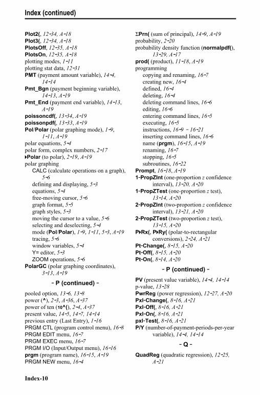
Index-10
Index (continued)
825915~1.DOC TI-83 international English Bob Fedorisko Revised: 10/26/05 2:25 PM Printed: 10/27/05 3:22PM Page 10 of 16
Plot2(, 12.34, A.18Plot3(, 12.34, A.18PlotsOff, 12.35, A.18PlotsOn, 12.35, A.18plotting modes, 1.11plotting stat data, 12.31PMT (payment amount variable), 14.4,
14.14Pmt_Bgn (payment beginning variable),
14.13, A.19Pmt_End (payment end variable), 14.13,
A.19poissoncdf(, 13.34, A.19poissonpdf(, 13.33, A.19Pol/Polar (polar graphing mode), 1.9,
1.11, A.19polar equations, 5.4polar form, complex numbers, 2.174Polar (to polar), 2.19, A.19polar graphing
CALC (calculate operations on a graph),5.6
defining and displaying, 5.3equations, 5.4free-moving cursor, 5.6graph format, 5.5graph styles, 5.3moving the cursor to a value, 5.6selecting and deselecting, 5.4mode (Pol/Polar), 1.9, 1.11, 5.3, A.19tracing, 5.6window variables, 5.4Y= editor, 5.3ZOOM operations, 5.6
PolarGC (polar graphing coordinates),3.13, A.19
. P (continued) .pooled option, 13.6, 13.8power (^), 2.3, A.36, A.37power of ten (10^(), 2.4, A.37present value, 14.5, 14.7, 14.14previous entry (Last Entry), 1.16PRGM CTL (program control menu), 16.8PRGM EDIT menu, 16.7PRGM EXEC menu, 16.7PRGM I/O (Input/Output menu), 16.16prgm (program name), 16.15, A.19PRGM NEW menu, 16.4
GPrn( (sum of principal), 14.9, A.19probability, 2.20probability density function (normalpdf(),
13.29, A.17prod( (product), 11.18, A.19programming
copying and renaming, 16.7creating new, 16.4defined, 16.4deleting, 16.4deleting command lines, 16.6editing, 16.6entering command lines, 16.5executing, 16.5instructions, 16.9 N 16.21inserting command lines, 16.6name (prgm), 16.15, A.19renaming, 16.7stopping, 16.5subroutines, 16.22
Prompt, 16.18, A.191.PropZInt (one-proportion z confidence
interval), 13.20, A.201.PropZTest (one-proportion z test),
13.14, A.202.PropZInt (two-proportion z confidence
interval), 13.21, A.202.PropZTest (two-proportion z test),
13.15, A.20P4Rx(, P4Ry( (polar-to-rectangular
conversions), 2.24, A.21Pt.Change(, 8.15, A.20Pt.Off(, 8.15, A.20Pt.On(, 8.14, A.20
. P (continued) .PV (present value variable), 14.4, 14.14p-value, 13.28PwrReg (power regression), 12.27, A.20Pxl.Change(, 8.16, A.21Pxl.Off(, 8.16, A.21Pxl.On(, 8.16, A.21pxl.Test(, 8.16, A.21P/Y (number-of-payment-periods-per-year
variable), 14.4, 14.14
. Q .QuadReg (quadratic regression), 12.25,
A.21
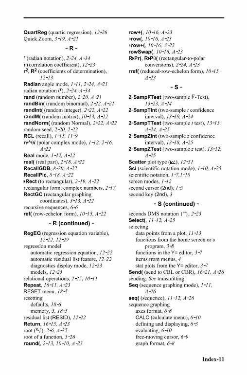
Index-11
825915~1.DOC TI-83 international English Bob Fedorisko Revised: 10/26/05 2:25 PM Printed: 10/27/05 3:22PM Page 11 of 16
QuartReg (quartic regression), 12.26Quick Zoom, 3.19, A.21
. R .r (radian notation), 2.24, A.34r (correlation coefficient), 12.23r2, R2 (coefficients of determination),
12.23Radian angle mode, 1.11, 2.24, A.21radian notation (r), 2.24, A.34rand (random number), 2.20, A.21randBin( (random binomial), 2.22, A.21randInt( (random integer), 2.22, A.22randM( (random matrix), 10.13, A.22randNorm( (random Normal), 2.22, A.22random seed, 2.20, 2.22RCL (recall), 1.15, 11.9re^qi (polar complex mode), 1.12, 2.16,
A.22Real mode, 1.12, A.22real( (real part), 2.18, A.22RecallGDB, 8.20, A.22RecallPic, 8.18, A.224Rect (to rectangular), 2.19, A.22rectangular form, complex numbers, 2.17RectGC (rectangular graphing
coordinates), 3.13, A.22recursive sequences, 6.6ref( (row-echelon form), 10.15, A.22
. R (continued) .RegEQ (regression equation variable),
12.22, 12.29regression model
automatic regression equation, 12.22automatic residual list feature, 12.22diagnostics display mode, 12.23models, 12.25
relational operations, 2.25, 10.11Repeat, 16.11, A.23RESET menu, 18.5resetting
defaults, 18.6memory, 5, 18.5
residual list (RESID), 12.22Return, 16.15, A.23root (x‡), 2.6, A.35root of a function, 3.26round(, 2.13, 10.10, A.23
row+(, 10.16, A.23…row(, 10.16, A.23…row+(, 10.16, A.23rowSwap(, 10.16, A.23R4Pr(, R4Pq( (rectangular-to-polar
conversions), 2.24, A.23rref( (reduced-row-echelon form), 10.15,
A.23
. S .2.SampÛÛÛÛTest (two-sample Û-Test),
13.23, A.242.SampTInt (two-sample t confidence
interval), 13.19, A.242.SampTTest (two-sample t test), 13.13,
A.24, A.252.SampZInt (two-sample z confidence
interval), 13.18, A.252.SampZTest (two-sample z test), 13.12,
A.25Scatter plot type (""""), 12.31Sci (scientific notation mode), 1.10, A.25scientific notation, 1.7,1.10screen modes, 1.12second cursor (2nd), 1.5second key (2nd), 3
. S (continued) .seconds DMS notation (") , 2.23Select(, 11.12, A.25selecting
data points from a plot, 11.13functions from the home screen or a
program, 3.8functions in the Y= editor, 3.7items from menus, 4stat plots from the Y= editor, 3.7
Send( (send to CBL or CBR), 16.21, A.26sending. See transmittingSeq (sequence graphing mode), 1.11,
A.26seq( (sequence), 11.12, A.26sequence graphing
axes format, 6.8CALC (calculate menu), 6.10defining and displaying, 6.3evaluating, 6.10free-moving cursor, 6.9graph format, 6.8

Index-12
Index (continued)
825915~1.DOC TI-83 international English Bob Fedorisko Revised: 10/26/05 2:25 PM Printed: 10/27/05 3:22PM Page 12 of 16
graph styles, 6.4moving the cursor to a value, 6.9nonrecursive sequences, 6.5phase plots, 6.13recursive sequences, 6.6setting sequence mode, 6.3selecting and deselecting, 6.4TI-82 STATS versus TI.82 table, 6.15tracing, 6.9web plots, 6.11window variables, 6.7Y= editor, 6.4ZOOM (zoom menu), 6.10
Sequential (graphing order mode), 1.12,A.26
service information, B.12setting
display contrast, 1.3graph styles, 3.9graph styles from a program, 3.10modes, 1.9modes from a program, 1.9split-screen modes, 9.3split-screen modes from a program, 9.6tables from a program, 7.3
. S (continued) .SetUpEditor, 12.21, A.26shade above (éééé) graph style, 3.9shade below (êêêê) graph style, 3.10Shade(, 8.9, A.26Shadec2(, 13.36, A.26ShadeÛÛÛÛ(, 13.36, A.27ShadeNorm(, 13.35, A.27Shade_t(, 13.36, A.27shading graph areas, 3.10, 8.10Simul (simultaneous graphing order
mode), 1.12, A.27sin( (sine), 2.3, A.27sinM1( (arcsine), 2.3, A.27sine (sin(), 2.3, A.27sine regression formula, A.50sinh( (hyperbolic sine), 15.10, A.27sinhM1( (hyperbolic arcsine), 15.10, A.27SinReg (sinusoidal regression), 12.27,
A.28Smart Graph, 3.15solve(, 2.12, A.28Solver, 2.8
solving for variables in the equation solver,2.10, 2.11
SortA( (sort ascending), 11.10, 12.20,A.28
SortD( (sort descending), 11.10, 12.20,A.28
split-screen modesG.T (graph-table) mode, 9.5Horiz (horizontal) mode, 9.4setting, 9.3, 9.6
split-screen values, 8.12, 8.16, 9.6square ( 2) , 2 .3 , A.36square root (‡() , 2 .3 , A.37STAT CALC menu, 12.24STAT EDIT menu, 12.20stat list editor
attaching formulas to list names, 12.14clearing elements from lists, 12.12creating list names, 12.12detaching formulas from list names,
12.16displaying, 12.10edit-elements context, 12.18
. S (continued) .stat list editor (continued)
editing elements of formula-generatedlists, 12.16
editing list elements, 12.13enter-names context, 12.19entering list names, 12.11formula-generated list names, 12.15removing lists, 12.12restoring list names L1–L6, 12.12,
12.21switching contexts, 12.17view-elements context, 12.18view-names context, 12.19
STAT PLOTS menu, 12.34stat tests and confidence intervals
ANOVA( (one-way analysis ofvariance), 13.25
c².Test (chi-square test), 13.22LinRegTTest (linear regression t test),
13.241.PropZInt (one-proportion
z confidence interval), 13.201.PropZTest (one-proportion z test),
13.14

Index-13
825915~1.DOC TI-83 international English Bob Fedorisko Revised: 10/26/05 2:25 PM Printed: 10/27/05 3:22PM Page 13 of 16
2.PropZInt (two-proportionz confidence interval), 13.21
2.PropZTest (two-proportion z test),13.15
2.SampÛÛÛÛTest (two-sample Û.Test),13.23
2.SampTInt (two-sample t confidenceinterval), 13.19
2.SampTTest (two-sample t test),13.13
2.SampZInt (two-sample z confidenceinterval), 13.18
2.SampZTest (two-sample z test),13.12
TInterval (one-sample t confidenceinterval), 13.17
T.Test (one-sample t test), 13.11ZInterval (one-sample z confidence
interval), 13.16Z.Test (one-sample z test), 13.10
Stats input option, 13.6, 13.7STAT TESTS menu, 13.9statistical distribution functions. See
distribution functions
. S (continued) .statistical plotting, 12.31
Boxplot (regular box plot), 12.33defining, 12.34from a program, 12.37Histogram, 12.32ModBoxplot (modified box plot),
12.32NormProbPlot (normal probability
plot), 12.33Scatter, 12.31tracing, 12.36turning on/off stat plots, 3.7, 12.35viewing window, 12.36xyLine, 12.31
statistical variables table, 12.29stdDev( (standard deviation), 11.18, A.28Stop, 16.15, A.28Store (!!!!), 1.14, A.28StoreGDB, 8.19, A.28StorePic, 8.17, A.29storing
graph databases (GDBs), 8.19graph pictures, 8.17variable values, 1.14
String4Equ( (string-to-equationconversions), 15.8, A.29
strings, 15.3 – 15.9concatenation (+), 15.6, A.38converting, 15.7, 15.8defined, 15.3displaying contents, 15.5entering, 15.3functions in CATALOG, 15.6indicator ("), 15.3length (length(), 15.8, A.13storing, 15.5variables, 15.4
student-t distributionprobability (tcdf(), 13.31, A.29probability density function (tpdf(),
13.30, A.30sub( (substring), 15.9, A.29subroutines, 16.15, 16.22subtraction (N), 2.3, A.38sum( (summation), 11.18, A.29system variables, A.49

Index-14
Index (continued)
825915~1.DOC TI-83 international English Bob Fedorisko Revised: 10/26/05 2:25 PM Printed: 10/27/05 3:22PM Page 14 of 16
. T .TABLE SETUP screen, 7.3tables, 7.1 – 7.6
description, 7.5variables, 7.3 – 7.5
tan( (tangent), 2.3, A.29tanM1( (arctangent), 2.3, A.29tangent (tan(), 2.3, A.29Tangent( (draw line), 8.8, A.29tangent lines, drawing, 8.8tanh( (hyperbolic tangent), 15.10, A.29tanhM1( (hyperbolic arctangent), 15.10,
A.29@Tbl (table step variable), 7.3TblStart (table start variable), 7.3tcdf( (student-t distribution probability),
13.31, A.29technical support, B.12TEST (relational menu), 2.25TEST LOGIC (Boolean menu), 2.26Text(
instruction, 8.12, 9.6, A.29placing on a graph, 8.12
Then, 16.9, A.11thick (èèèè) graph style, 3.9TI.82
link differences, 19.9transmitting to/from, 19.4, 19.8, 19.9
TI-82 STATSfeatures, 17, 18keyboard, 2, 3key code diagram, 16.20Link. See linkingmenu map, A.39
TI.GRAPH LINK, 19.3Time axes format, 6.8, A.30time value of money (TVM)
calculating, 14.6C/Y variable (number of compounding
periods per year), 14.14formulas, A.54FV variable (future value), 14.14ææææ variable (annual interest rate), 14.14
. T (continued) .time value of money (continued)ÚÚÚÚ variable (number of payment
periods), 14.14PMT variable (payment amount), 14.14PV variable (present value), 14.14P/Y variable (number of payment
periods per year), 14.14tvm_FV (future value), 14.7, A.31tvm_I% (interest rate), 14.7, A.31tvm_ÚÚÚÚ (# payment periods), 14.7, A.31tvm_Pmt (payment amount), 14.6,
A.31tvm_PV (present value), 14.7, A.31TVM Solver, 14.4variables, 14.14
TInterval (one-sample t confidenceinterval), 13.17, A.30
tpdf( (student-t distribution probabilitydensity function), 13.30, A.30
TRACEcursor, 3.18entering numbers during, 3.19, 4.8,
5.6, 6.9expression display, 3.14, 3.18Trace instruction in a program, 3.19,
A.30transmitting
error conditions, 19.6from a TI.82 to a TI-82 STATS, 19.9items to another unit, 19.6lists to a TI.82, 19.4, 19.8stopping, 19.6to an additional TI-82 STATS, 19.7
T (transpose matrix), 10.12, A.34transpose matrix (T), 10.12, A.34trigonometric functions, 2.3T.Test (one-sample t test), 13.11, A.30

Index-15
825915~1.DOC TI-83 international English Bob Fedorisko Revised: 10/26/05 2:25 PM Printed: 10/27/05 3:22PM Page 15 of 16
. T (continued) .turning on and off
axes, 3.14calculator, 1.2coordinates, 3.14expressions, 3.14functions, 3.7grid, 3.14labels, 3.14pixels, 8.16points, 8.14stat plots, 3.7, 12.35
tvm_FV (future value), 14.7, A.31tvm_I% (interest rate), 14.7, A.31tvm_ÚÚÚÚ (# payment periods), 14.7, A.31tvm_Pmt (payment amount), 14.6, A.31tvm_PV (present value), 14.7, A.31two-proportion z confidence interval
(2.PropZInt), 13.21, A.20two-proportion z test (2.PropZTest),
13.15, A.20two-sample Û-Test formula, A.52two-sample t test formula, A.53two-variable statistics (2.Var Stats),
12.25, A.31
. U .u sequence function, 6.3user variables, A.49uv/uvAxes (axes format), 6.8, A.31uw/uwAxes (axes format), 6.8, A.31
. V .v sequence function, 6.31.Var Stats (one-variable statistics),
12.25, A.312.Var Stats (two-variable statistics),
12.25, A.31value operation on a graph, 3.25
. V (continued) .variables
complex, 1.13displaying and storing values, 1.14equation solver, 2.10graph databases, 1.13graph pictures, 1.13independent/dependent, 7.5list, 1.13, 11.3matrix, 1.13, 10.3real, 1.13recalling values, 1.15solver editor, 2.9statistical, 12.29string, 15.4, 15.5test and interval output, 13.28types, 1.13user and system, 1.13, A.49VARS and Y.VARS menus, 1.21
variance( (variance of a list), 11.18, A.31variance of a list (variance(), 11.18, A.31VARS menu
GDB, 1.21Picture, 1.21Statistics, 1.21String, 1.21Table, 1.21Window, 1.21Zoom, 1.21
Vertical (draw line), 8.6, A.31viewing window, 3.11vw/uvAxes (axes format), 6.8
. W .w sequence function, 6.3warranty information, B.14Web (axes format), 6.8, A.31web plots, sequence graphing, 6.11While, 16.11, A.32window variables
function graphing, 3.11parametric graphing, 4.5polar graphing, 5.4sequence graphing, 6.7

Index-16
Index (continued)
825915~1.DOC TI-83 international English Bob Fedorisko Revised: 10/26/05 2:25 PM Printed: 10/27/05 3:22PM Page 16 of 16
. X .XFact zoom factor, 3.24x-intercept of a root, 3.26xor (Boolean) exclusive or operator, 2.26,
A.32xth root (x‡), 2.6xyLine (ÓÓÓÓ) plot type, 12.31
@X window variable, 3.12
. Y .YFact zoom factor, 3.24Y= editor
function graphing, 3.5parametric graphing, 4.4polar graphing, 5.3sequence graphing, 6.4
Y.VARS menuFunction, 1.21Parametric, 1.21Polar, 1.21On/Off, 1.21
@Y window variable, 3.12
. Z .ZBox, 3.20, A.32ZDecimal, 3.21, A.32zero operation on a graph, 3.26ZInteger, 3.22, A.32ZInterval (one-sample z confidence
interval), 13.16, A.32zoom, 3.20 – 3.24
cursor, 3.20factors, 3.24function graphing, 3.20parametric graphing, 4.8polar graphing, 5.6sequence graphing, 6.10
ZoomFit (zoom to fit function), 3.22,A.33
Zoom In (zoom in), 3.21, A.32ZOOM menu, 3.20ZOOM MEMORY menu, 3.23Zoom Out (zoom out), 3.21, A.32ZoomRcl (recall stored window), 3.23,
A.33ZoomStat (statistics zoom), 3.22, A.33
. Z (continued) .ZoomSto (store zoom window), 3.23,
A.33ZPrevious (use previous window), 3.23,
A.33ZSquare (set square pixels), 3.21, A.33ZStandard (use standard window), 3.22,
A.33Z.Test (one-sample z test), 13.10, A.34ZTrig (trigonometric window), 3.22, A.34