Three-dimensional coherent structures in a swirling jet undergoing vortex breakdown: Stability...
32
J. Fluid Mech., page 1 of 32 c Cambridge University Press 2011 doi:10.1017/jfm.2011.141 1 Three-dimensional coherent structures in a swirling jet undergoing vortex breakdown: stability analysis and empirical mode construction K. OBERLEITHNER 1 †, M. SIEBER 1 , C. N. NAYERI 1 , C. O. PASCHEREIT 1 , C. PETZ 2 , H.-C. H E G E, 2 B. R. NOACK 3 AND I. WYGNANSKI 4 1 Hermann-F¨ ottinger-Institut, Technische Universit¨ at Berlin, M¨ uller-Breslau Str. 8, D-10623 Berlin, Germany 2 Abteilung Visualisierung und Datenanalyse, Bereich Numerische Mathematik, Zuse-Institut Berlin, Takustr. 7, D-14195 Berlin-Dahlem, Germany 3 D´ epartement Fluides, Thermique, Combustion, CEAT, Institut Pprime, CNRS – Universit´ e de Poitiers – ENSMA, UPR 3346, 43 rue de l’A´ erodrome, F-86036 POITIERS CEDEX, France 4 Department of Aerospace and Mechanical Engineering, The University of Arizona, Tucson, AZ 85721, USA (Received 25 May 2010; revised 14 March 2011; accepted 17 March 2011) The spatio-temporal evolution of a turbulent swirling jet undergoing vortex breakdown has been investigated. Experiments suggest the existence of a self-excited global mode having a single dominant frequency. This oscillatory mode is shown to be absolutely unstable and leads to a rotating counter-winding helical structure that is located at the periphery of the recirculation zone. The resulting time-periodic 3D velocity field is predicted theoretically as being the most unstable mode determined by parabolized stability analysis employing the mean flow data from experiments. The 3D oscillatory flow is constructed from uncorrelated 2D snapshots of particle image velocimetry data, using proper orthogonal decomposition, a phase-averaging technique and an azimuthal symmetry associated with helical structures. Stability- derived modes and empirically derived modes correspond remarkably well, yielding prototypical coherent structures that dominate the investigated flow region. The proposed method of constructing 3D time-periodic velocity fields from uncorrelated 2D data is applicable to a large class of turbulent shear flows. Key words: absolute/convective instability, shear layers, vortex breakdown 1. Introduction Free and confined strongly swirling jets are of great interest due to their unique feature, commonly known as vortex breakdown. This phenomenon occurs when the ratio of the azimuthal to axial momentum exceeds a certain threshold, while both quantities have to be of the same order of magnitude. Breakdown in swirling jets is characterized by a transition of a jet-like axial velocity profile to a wake-like profile † Email address for correspondence: [email protected]
Transcript of Three-dimensional coherent structures in a swirling jet undergoing vortex breakdown: Stability...
J. Fluid Mech., page 1 of 32 c© Cambridge University Press 2011
doi:10.1017/jfm.2011.141
1
Three-dimensional coherent structuresin a swirling jet undergoing vortex breakdown:
stability analysis and empirical modeconstruction
K. OBERLEITHNER1†, M. S IEBER1, C. N. NAYERI1,C. O. PASCHEREIT1, C. PETZ2, H.-C. HEGE,2 B. R. NOACK3
AND I. WYGNANSKI41Hermann-Fottinger-Institut, Technische Universitat Berlin, Muller-Breslau Str. 8,
D-10623 Berlin, Germany2Abteilung Visualisierung und Datenanalyse, Bereich Numerische Mathematik, Zuse-Institut Berlin,
Takustr. 7, D-14195 Berlin-Dahlem, Germany3Departement Fluides, Thermique, Combustion, CEAT, Institut Pprime, CNRS – Universite de Poitiers –
ENSMA, UPR 3346, 43 rue de l’Aerodrome, F-86036 POITIERS CEDEX, France4Department of Aerospace and Mechanical Engineering, The University of Arizona,
Tucson, AZ 85721, USA
(Received 25 May 2010; revised 14 March 2011; accepted 17 March 2011)
The spatio-temporal evolution of a turbulent swirling jet undergoing vortexbreakdown has been investigated. Experiments suggest the existence of a self-excitedglobal mode having a single dominant frequency. This oscillatory mode is shown tobe absolutely unstable and leads to a rotating counter-winding helical structure thatis located at the periphery of the recirculation zone. The resulting time-periodic 3Dvelocity field is predicted theoretically as being the most unstable mode determinedby parabolized stability analysis employing the mean flow data from experiments.The 3D oscillatory flow is constructed from uncorrelated 2D snapshots of particleimage velocimetry data, using proper orthogonal decomposition, a phase-averagingtechnique and an azimuthal symmetry associated with helical structures. Stability-derived modes and empirically derived modes correspond remarkably well, yieldingprototypical coherent structures that dominate the investigated flow region. Theproposed method of constructing 3D time-periodic velocity fields from uncorrelated2D data is applicable to a large class of turbulent shear flows.
Key words: absolute/convective instability, shear layers, vortex breakdown
1. IntroductionFree and confined strongly swirling jets are of great interest due to their unique
feature, commonly known as vortex breakdown. This phenomenon occurs when theratio of the azimuthal to axial momentum exceeds a certain threshold, while bothquantities have to be of the same order of magnitude. Breakdown in swirling jets ischaracterized by a transition of a jet-like axial velocity profile to a wake-like profile
† Email address for correspondence: [email protected]
2 K. Oberleithner and others
with a local minimum on the axis. This leads to a stagnation point to be followed by ahighly turbulent region of reverse flow farther downstream. It can play a crucial role –from desired to detrimental – in a variety of technical applications. For example, vortexbreakdown stabilizes the flame of a gas turbine combustor and enhances mixing, thusleading to a reduction of NOx emissions. On the other hand, bursting of leading-edge vortices adversely affects the lift distribution on delta wings resulting in poorflight performance. Understanding the cause of the vortex breakdown is thereforeof great importance in order to develop appropriate control strategies. Furthermore,the transition of the flow from jet-like to wake-like that generates coexisting innerand outer shear layers and the concomitant axial and azimuthal shear makes thisflow complex and highly three-dimensional and thus poses a formidable challenge tofundamental studies.
In the present work, we investigate coherent structures of a strongly swirling jetundergoing vortex breakdown. This study is based on experiments carried out atthe TU Berlin. 3D time-periodic coherent structures are predicted by stability theoryand are constructed from 2D particle image velocimetry (PIV) data via a proposedidentification method. In the introductory section we describe the main observedphenomena (§ 1.1), highlight the triple decomposition as the corner stone of ourtheoretical and experimental study of coherent structures (§ 1.2) and review currentdefinitions of coherent structures in conjunction with stability analyses (§§ 1.3 and 1.4,respectively). Finally, an outline of the paper is provided (§ 1.5).
1.1. Vortex breakdown studies
Several types of vortex breakdown have experimentally been observed. Lambourne& Bryer (1962) were the first to describe the axisymmetric and spiral type of vortexbreakdown. Swirling jet experiments in pipes conducted by Sarpkaya (1971) and Faler& Leibovich (1978) identified three different types of vortex breakdown, namely thesingle helical, double helical and bubble-shaped vortex breakdown. Billant, Chomaz& Huerre (1998), investigating a swirling jet at a low Reynolds number, observed anadditional conical-shaped breakdown type.
Many researchers found helical disturbances that characterize strongly swirledjets, but their role in the dynamics of vortex breakdown is still a controversialissue. Some experts relate the onset of vortex breakdown to the hydrodynamicinstability of vortical flow. Ludwieg (1961) assumes that the formation of a stagnationpoint results from the sensitivity of the vortex core to helical disturbances. Otherresearchers describe vortex breakdown as a transition of the flow from a supercriticalto a subcritical state similar to a shock wave or a hydraulic jump. According toEscudier & Keller (1985) there is a clear separation of the roles of flow criticalityand flow stability. It was proposed that the criticality of the flow determines thebasic, wake-like character of the flow and that instability waves are a superimposedfine detail. Recent quantitative investigations could significantly contribute to theunderstanding of the dynamics accompanying the onset of vortex breakdown. Time-resolved measurements conducted by Liang & Maxworthy (2005) indicate that arecirculation bubble with nearly axisymmetric shape accompanies the first appearanceof a stagnation point. It was further noticed that in the wake of this dividingstreamline a single helical vortex arises near the jet centre that amplifies until itimposes its frequency onto the entire near field. The authors suggest this to be a self-excited/globally unstable mode, supposably arising from a region of local absoluteinstability in the lee (downstream) of vortex breakdown. Forced experiments usingvortex generators mounted on a rotating nozzle supported the absolute/convective
Three-dimensional coherent structures in a swirling jet 3
nature of the dominating instabilities. Gallaire et al. (2006) performed a linear stabilityanalysis based on numerical simulations of a swirling jet at Re= 200 that wereconducted by Ruith et al. (2003). They found a convective to absolute instabilitytransition in the lee of the recirculation bubble with a single helical mode being mostunstable. Thus, it is likely that the precession of the vortex core and the appearanceof strong oscillations that have been observed in experiments and simulations (Ruithet al. 2003; Liang & Maxworthy 2005; Duwig & Fuchs 2007; Martinelli, Olivani& Coghe 2007) can be attributed to a self-excited global mode initiated by flowinstabilities in the region of vortex breakdown.
1.2. Triple decomposition as a basis for structure extraction and prediction
Large-scale organized structures in turbulent flows were investigated for more than40 years. For a comprehensive summary of earlier work, the reader is referred toLaufer (1975), Roshko (1977), Cantwell (1981) and Ho & Huerre (1984). A varietyof definitions and techniques have been developed to reveal these so-called coherentstructures. These include statistical approaches, pattern recognition methods, stabilitytheory, conditional sampling and averaging and topological methods from dynamicalsystem theory. Some of these methods are based on a triple decomposition introducedby Hussain & Reynolds (1970). Accordingly, turbulent flow may be decomposed intothree constituents: mean (time- or ensemble-averaged), coherent (phase-averaged) andrandom (incoherent turbulent) motion. The triple decomposition method representsa refinement of the classical Reynolds decomposition. It has become a conventionaltool in active flow control (AFC) experiments that distil coherent disturbances bymeans of phase-locked averaging. Its application to experiments is easy when thecoherent structure is tagged by external excitation where a simple synchronizationof the data acquisition with the forcing signals is required. Without such externalphase trigger, proper orthogonal decomposition (POD)-based techniques can provideanother means for phase identification (Depardon et al. 2007).
The triple decomposition method has been implicitly used in a number of theoreticalarticles where the stability analysis was applied for turbulent flows (see, e.g. Crighton& Gaster 1976; Gaster, Kit & Wygnanski 1985). Liu (1989) has developed a localturbulence model for many shear flows utilizing the triple decomposition.
1.3. Empirical identification of coherent structures
Large-scale coherent structures in many turbulent shear flows (see, e.g. Van Dyke 1975)are visually similar to predominant instability modes persisting over a wide rangeof Reynolds numbers. This similarity applies to flows whose mean velocity profilesare inviscidly unstable and whose shape of these profiles does not materially changeduring the transition from laminar to turbulent flow. This observation suggests thatstability considerations can be applied to the mean turbulent flow field, although thereis no theoretical basis for this step. However, weakly nonlinear stability approachesexplicitly assume that instability modes and most energetic (POD) modes are thesame, at least near the onset of a supercritical Hopf bifurcation (Stuart 1958; Noacket al. 2003).
Stability theory approximates the flow as a given mean flow and a superposition ofspace- and time-dependent modes. In similar spirit, turbulent coherent structurescan be conceptualized as an expansion of modes. A corresponding least-orderrepresentation of a flow snapshot ensemble is obtained by the POD. This approachminimizes a time-averaged residual of the POD expansion for a given number ofmodes, and it is equipped with further useful analytical properties (Lumley 1967;Holmes, Lumley & Berkooz 1998). Historically, Lumley (1967) introduced POD as a
4 K. Oberleithner and others
least-biased definition of coherent structures following up on the analytical approachby Townsend (1956) and the well-known Karhunen–Loeve decomposition from the1940s.
Meanwhile, many other empirical expansions of flow snapshots have been proposedserving dynamical systems or control theory goals. For instance, the dynamic modedecomposition (DMD) extracts modes from snapshots that are more related tostability eigenmodes (Rowley et al. 2009; Schmid 2010). Furthermore, the balancedPOD serves as economic expansion for linear input–output relationships (Rowley2005). The present study is restricted to the classical POD since it targets an optimalkinematical representation of the flow.
1.4. Linear stability analysis of swirling jets
Linear stability analysis is presently used to describe the large-scale oscillationsobserved in this experiment. In principle, self-excited oscillations are known to arisefrom a region of absolutely unstable flow. They can be described by an unstable globalmode (Chomaz 2005) or by local spatio-temporal stability analysis with complexfrequency and wavenumber (Huerre & Monkewitz 1990; Monkewitz, Huerre &Chomaz 1993; Pier & Huerre 2001). However, for the underlying flow configuration,we employ a simple local spatial stability analysis to approximate the velocity ofthe global mode. This simplification serves the main purpose of this study, whichis to enhance the understanding of turbulent coherent structures in highly turbulentswirling flows. It is in line with similar studies summarized by Liu (1989), and it isrooted by experimental observations (Oberleithner et al. 2009). Strong oscillations atthe global frequency were found upstream of vortex breakdown, revealing a precessingvortex core that acts as the global wavemaker. In the outer shear layer, downstreamtravelling instabilities were detected that were internally forced by the wavemakerand were synchronized to its frequency. These waves served as amplifiers to externalforcing, which suggests that the signalling problem is valid for the outer flow region.Assuming that the outer shear layer responds to internal forcing in the same way asto external forcing, we may approximate the large-scale fluctuations downstream ofthe wavemaker by convectively unstable modes that oscillate at the global frequency.Hence, the spatial analysis presented here was conducted with an unknown complexstreamwise wavenumber and the known real global frequency.
Computing spatially growing disturbances in shear layers by means of linearstability analysis has a long history. Michalke (1965) calculated the spatial stabilitycharacteristics for the hyperbolic-tangent velocity profile according to inviscid theory.Spatial growth rate and amplitude distribution agreed well with measurementsconducted by Freymuth (1966), but they disagreed in some detail when the flowwas divergent. As refinement, several attempts have been made to account for non-parallel effects (Gaster 1974; Crighton & Gaster 1976; Plaschko 1979; Gaster et al.1985; Cohen, Marasli & Levinski 1994). Gaster et al. (1985) applied the inviscidlinear stability analysis to the periodically forced turbulent and slightly divergentmixing layer. The computed normalized phase and velocity amplitudes agreed withexperimental data but the amplification rates in the direction of streaming werestrongly overpredicted. The robustness of the stability analysis was demonstrated byWeisbrot & Wygnanski (1988), whose computed eigenmodes correctly predicted themeasured phase and amplitude distributions of the excited waves, although the latterwere forced at high amplitudes clearly exceeding the linear regime. It is importantto note that for high Reynolds numbers, the stability analysis is based on the time-averaged turbulent flow which is not a stationary solution of the Navier–Stokes
Three-dimensional coherent structures in a swirling jet 5
equation. It is argued that this infringement of the linear stability theory is possible‘knowing that the random changes in the mean velocity occur on a time scale thatis short in comparison with the period associated with the large coherent structures’(Weisbrot & Wygnanski 1988).
1.5. Overview
The outline of the paper is as follows. The experimental set-up and procedures aredescribed in § 2, while the main features that characterize the strongly swirling jetundergoing vortex breakdown are summarized in § 3. This flow is dominated bystrong oscillations resulting from a self-excited global mode. Two methods to extractthe coherent velocity of this mode are introduced in § 4. The first method employslinear stability analysis and the second, empirical approach, is based on the POD.Stability analysis provides spatially amplified eigenmodes that represent the amplitudedistribution of the phase-averaged velocity. The empirical feature extraction directlyprovides the measured phase-averaged velocity field by applying a proposed method.Finally, the results of both methods are compared in § 5 and a three-dimensionalreconstruction of the global mode is presented. It is based on stability analysis andon PIV data providing a portrait of the dominant coherent structures. The mainobservations are summarized in § 6.
2. Experimental arrangement2.1. The swirling jet facility
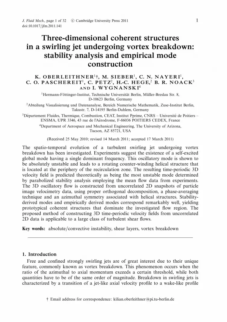
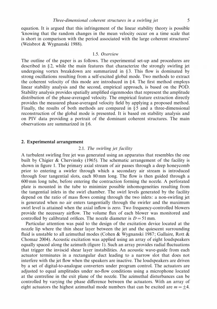
A turbulent swirling free jet was generated using an apparatus that resembles the onebuilt by Chigier & Chervinsky (1965). The schematic arrangement of the facility isshown in figure 1. The primary axial stream of air passes through a deep honeycombprior to entering a swirler through which a secondary air stream is introducedthrough four tangential slots, each 80 mm long. The flow is then guided through a600 mm long tube, before entering the contraction forming the nozzle. A perforatedplate is mounted in the tube to minimize possible inhomogeneities resulting fromthe tangential inlets in the swirl chamber. The swirl levels generated by the facilitydepend on the ratio of mass flows coming through the two inlets: a non-swirling jetis generated when no air enters tangentially through the swirler and the maximumswirl level is attained when the axial inflow is zero. Two frequency-controlled blowersprovide the necessary airflow. The volume flux of each blower was monitored andcontrolled by calibrated orifices. The nozzle diameter is D = 51 mm.
Particular attention was paid to the design of the excitation device located at thenozzle lip where the thin shear layer between the jet and the quiescent surroundingfluid is unstable to all azimuthal modes (Cohen & Wygnanski 1987; Gallaire, Rott &Chomaz 2004). Acoustic excitation was applied using an array of eight loudspeakersequally spaced along the azimuth (figure 1). Such an array provides radial fluctuationsthat trigger the inviscid shear layer instabilities. An acoustic wave-guide from eachactuator terminates in a rectangular duct leading to a narrow slot that does notinterfere with the jet flow when the speakers are inactive. The loudspeakers are drivenby a set of digital-to-analogue converters under program control. The actuators areadjusted to equal amplitudes under no-flow conditions using a microphone locatedat the centreline in the exit plane of the nozzle. The azimuthal disturbances can becontrolled by varying the phase difference between the actuators. With an array ofeight actuators the highest azimuthal mode numbers that can be excited are m = ±4.
6 K. Oberleithner and others
600
51
154
One of eightspeakers
Perforatedplate
Swirler
Swirler
Axial inlet
Honeycomb
One of four swirler inlets
Swirlerinlet
Tangentialinlets
x
zy
rθ
Figure 1. Experimental set-up and coordinate systems (all lengths are expressed in mm).
2.2. Data acquisition
Stereoscopic particle image velocimetry (Stereo-PIV) was used to measure the flowfield. It consists of velocity measurements of particles going through a laser sheetgenerated by a double-pulsed Nd:Yag laser at 532 nm and 25 mJ in 5 ns burst. Two
Three-dimensional coherent structures in a swirling jet 7
CCD cameras with a resolution of 1.3 million pixels were used. Both cameras werepositioned at a 45 angle in order to measure all three velocity components in a 2Dplane. The cameras and the laser were mounted onto a single traversing system. Datawere taken in the crossflow plane as well as in the axial plane. Each ensemble of PIVsnapshots consisted of 800 events captured at approximately 3 Hz.
2.3. Coordinate systems
The orientation of the two coordinate systems used in the present work is shown infigure 1. Cylindrical coordinates are used to describe the flow quantities in thecrossflow plane, whereas Cartesian coordinates are used for data shown in thestreamwise plane. The two coordinate systems are necessary, as the latter does notcause a singularity along the jet axis. On the other hand, in the crossflow plane,cylindrical velocity components are necessary to correctly describe the flow quantitiesof the axisymmetric flow. Furthermore, the normal mode decomposition, necessaryfor the linear stability analysis, is strictly based on an axisymmetric flow given incylindrical coordinates. In order to compare theoretical results with experimentaldata, we will switch between the two coordinate systems.
2.4. Characteristic numbers
Two independent dimensionless numbers characterize the global behaviour of theflow:
ReD =DU
νwith U =
Q
π(D/2)2(2.1)
and
S =Gθ
D/2Gx
=
2π
∫ ∞
0
ρVxVΘr2 dr
Dπ
∫ ∞
0
ρ
(V 2
x − V 2θ
2
)r dr
. (2.2)
The Reynolds number ReD is based on the nozzle diameter D and the average axialvelocity U which is derived from the mean mass flow rate Q. The swirl numberS is the commonly used parameter that quantifies the amount of swirl (Chigier &Chervinsky 1965; Panda & McLaughlin 1994). It is defined as the ratio betweenthe axial flux of angular momentum Gθ and the axial flux of axial momentum Gx .According to the conservation of momentum, the swirl number is conserved in theaxial direction (Rajaratnam 1976).
3. Flow phenomenologyThis paper focuses on the near field of a turbulent jet at a very high rate of swirl.
The basic features of this flow are described in the following section in order toexplain the motivation for investigating the evolution of the coherent structures.
3.1. Mean flow properties
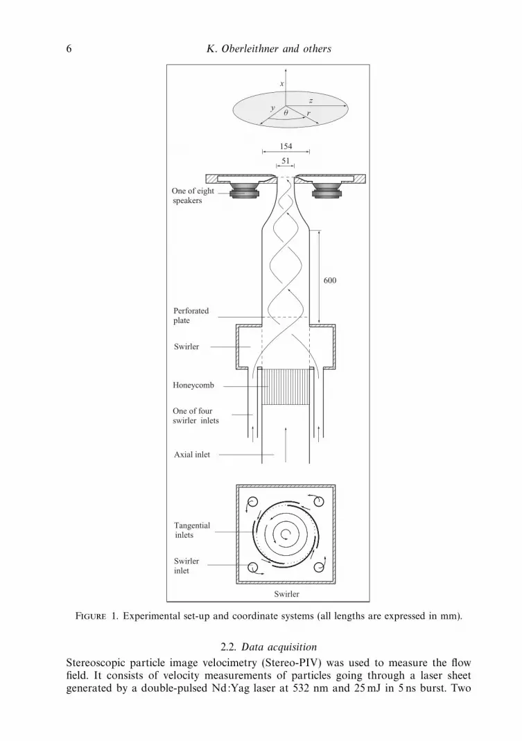
Figure 2 illustrates the streamwise distribution of the time-averaged flow. Due to theoccurrence of vortex breakdown, the maximum axial velocity is displaced from the jetcentre. The axial velocity profiles have a local velocity minimum in the inner region ofthe jet. Thus, a wake with a region of reversed flow on and near the jet axis resembleswith a recirculation bubble that is bound by upstream and downstream stagnationpoints. This reversed flow region is similar to the one created by an obstacle placed onthe jet centre. Hence, the flow emanating from the nozzle is a swirling ring-jet with an
8 K. Oberleithner and others
y/D
y/D
x/D, V/U × 0.40.2 0.6 1.0 1.4 1.8 2.2 2.6 3.0
–0.5
0
0.5
–0.5
0
0.5
Vz /U
Vx /U
Figure 2. Profiles of the time-averaged axial and plane-normal velocity at various axiallocations; velocities are normalized by the bulk velocity U ; streamlines indicate the locationof the recirculation bubble (ReD = 20 000; S = 1.22).
inner and an outer axial and azimuthal shear layer. The streamlines shown in figure 2illustrate how the flow is guided around the recirculation zone causing a rapid increaseof the jet diameter. Downstream the recirculation zone, at approximately x/D > 1.4,the inner shear layers begin to merge and the axial velocity on the jet centre increasesgradually with increasing downstream distance. The azimuthal velocity profiles maybe divided into a vortex core, the region between the jet centre and the maximumazimuthal velocity, and the outer azimuthal shear layer located between the maximumazimuthal velocity and the quiescent surrounding fluid. The axial velocity profile hastwo inflection points, and thus, in terms of inviscid hydrodynamic stability theypossess as many plane instability modes. Since the flow is axisymmetric, these couldcombine with azimuthal modes. The convex streamlines over the frontal part of therecirculation bubble coupled with the decelerating outer flow provide the necessaryconditions for centrifugal instability, as do the concave streamlines in the lee of thebubble coupling with the inner shear layer.
3.2. Self-excited oscillations
Former experimental investigations by Liang & Maxworthy (2005) and numericalsimulations of Ruith et al. (2003) revealed that the onset of vortex breakdown isaccompanied by energetic large-scale fluctuations. In the present investigation, thesestrong oscillations had a distinct frequency (figure 3). By traversing a hot-wire probe in
Three-dimensional coherent structures in a swirling jet 9
Stnat = 0.49
psd
St0.2 0.5 1.0 1.5
100
101
102
103
104
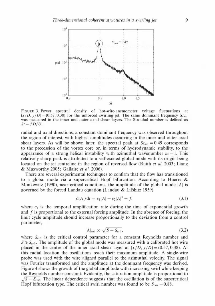
Figure 3. Power spectral density of hot-wire-anemometer voltage fluctuations at(x/D, y/D) = (0.57, 0.38) for the unforced swirling jet. The same dominant frequency Stnat
was measured in the inner and outer axial shear layers. The Strouhal number is defined asSt = f D/U .
radial and axial directions, a constant dominant frequency was observed throughoutthe region of interest, with highest amplitudes occurring in the inner and outer axialshear layers. As will be shown later, the spectral peak at Stnat = 0.49 correspondsto the precession of the vortex core or, in terms of hydrodynamic stability, to theappearance of a strong helical instability with azimuthal wavenumber m =1. Thisrelatively sharp peak is attributed to a self-excited global mode with its origin beinglocated on the jet centreline in the region of reversed flow (Ruith et al. 2003; Liang& Maxworthy 2005; Gallaire et al. 2006).
There are several experimental techniques to confirm that the flow has transitionedto a global mode via a supercritical Hopf bifurcation. According to Huerre &Monkewitz (1990), near critical conditions, the amplitude of the global mode |A| isgoverned by the forced Landau equation (Landau & Lifshitz 1959)
d|A|/dt = c1|A| − c2|A|3 + f, (3.1)
where c1 is the temporal amplification rate during the time of exponential growthand f is proportional to the external forcing amplitude. In the absence of forcing, thelimit cycle amplitude should increase proportionally to the deviation from a controlparameter,
|A|sat ∝√
S − Scrit , (3.2)
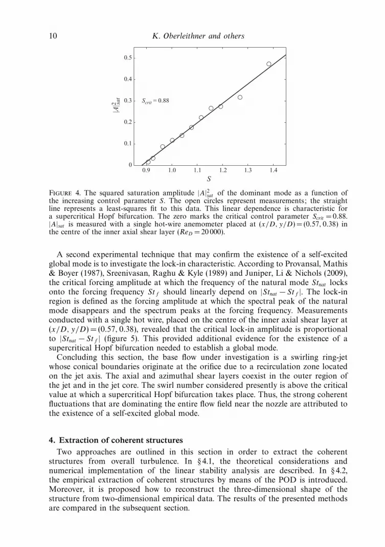
where Scrit is the critical control parameter for a constant Reynolds number andS Scrit . The amplitude of the global mode was measured with a calibrated hot wireplaced in the centre of the inner axial shear layer at (x/D, y/D) = (0.57, 0.38). Atthis radial location the oscillations reach their maximum amplitude. A single-wireprobe was used with the wire aligned parallel to the azimuthal velocity. The signalwas Fourier transformed and the amplitude at the dominant frequency was derived.Figure 4 shows the growth of the global amplitude with increasing swirl while keepingthe Reynolds number constant. Evidently, the saturation amplitude is proportional to√
S − Scrit . The linear dependence suggests that the oscillation is of the supercriticalHopf bifurcation type. The critical swirl number was found to be Scrit = 0.88.
10 K. Oberleithner and others
S
|A|2 sa
t Scrit = 0.88
0.9 1.0 1.1 1.2 1.3 1.40
0.1
0.2
0.3
0.4
0.5
Figure 4. The squared saturation amplitude |A|2sat of the dominant mode as a function ofthe increasing control parameter S. The open circles represent measurements; the straightline represents a least-squares fit to this data. This linear dependence is characteristic fora supercritical Hopf bifurcation. The zero marks the critical control parameter Scrit = 0.88.|A|sat is measured with a single hot-wire anemometer placed at (x/D, y/D) = (0.57, 0.38) inthe centre of the inner axial shear layer (ReD = 20 000).
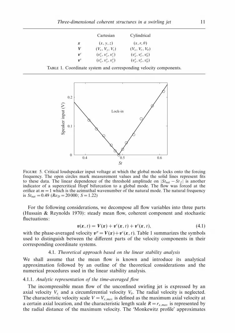
A second experimental technique that may confirm the existence of a self-excitedglobal mode is to investigate the lock-in characteristic. According to Provansal, Mathis& Boyer (1987), Sreenivasan, Raghu & Kyle (1989) and Juniper, Li & Nichols (2009),the critical forcing amplitude at which the frequency of the natural mode Stnat locksonto the forcing frequency Stf should linearly depend on |Stnat − Stf |. The lock-inregion is defined as the forcing amplitude at which the spectral peak of the naturalmode disappears and the spectrum peaks at the forcing frequency. Measurementsconducted with a single hot wire, placed on the centre of the inner axial shear layer at(x/D, y/D) = (0.57, 0.38), revealed that the critical lock-in amplitude is proportionalto |Stnat − Stf | (figure 5). This provided additional evidence for the existence of asupercritical Hopf bifurcation needed to establish a global mode.
Concluding this section, the base flow under investigation is a swirling ring-jetwhose conical boundaries originate at the orifice due to a recirculation zone locatedon the jet axis. The axial and azimuthal shear layers coexist in the outer region ofthe jet and in the jet core. The swirl number considered presently is above the criticalvalue at which a supercritical Hopf bifurcation takes place. Thus, the strong coherentfluctuations that are dominating the entire flow field near the nozzle are attributed tothe existence of a self-excited global mode.
4. Extraction of coherent structuresTwo approaches are outlined in this section in order to extract the coherent
structures from overall turbulence. In § 4.1, the theoretical considerations andnumerical implementation of the linear stability analysis are described. In § 4.2,the empirical extraction of coherent structures by means of the POD is introduced.Moreover, it is proposed how to reconstruct the three-dimensional shape of thestructure from two-dimensional empirical data. The results of the presented methodsare compared in the subsequent section.
Three-dimensional coherent structures in a swirling jet 11
Cartesian Cylindrical
x (x, y, z) (x, r, θ)
V (Vx, Vy, Vz) (Vx, Vr , Vθ )
vc (vcx, v
cy, v
cz ) (vc
x, vcr , v
cθ )
vs (vsx, v
sy, v
sz) (vs
x, vsr , v
sθ )
Table 1. Coordinate system and corresponding velocity components.
St
Spe
aker
inpu
t (V
)
Lock-in
0.4 0.5 0.60
0.1
0.2
Figure 5. Critical loudspeaker input voltage at which the global mode locks onto the forcingfrequency. The open circles mark measurement values and the the solid lines represent fitsto these data. The linear dependence of the threshold amplitude on |Stnat − Stf | is anotherindicator of a supercritical Hopf bifurcation to a global mode. The flow was forced at theorifice at m= 1 which is the azimuthal wavenumber of the natural mode. The natural frequencyis Stnat = 0.49 (ReD = 20 000; S =1.22)
For the following considerations, we decompose all flow variables into three parts(Hussain & Reynolds 1970): steady mean flow, coherent component and stochasticfluctuations:
v(x, t) = V (x) + vc(x, t) + vs(x, t), (4.1)
with the phase-averaged velocity vp = V (x)+vc(x, t). Table 1 summarizes the symbolsused to distinguish between the different parts of the velocity components in theircorresponding coordinate systems.
4.1. Theoretical approach based on the linear stability analysis
We shall assume that the mean flow is known and introduce its analyticalapproximation followed by an outline of the theoretical considerations and thenumerical procedures used in the linear stability analysis.
4.1.1. Analytic representation of the time-averaged flow
The incompressible mean flow of the unconfined swirling jet is expressed by anaxial velocity Vx and a circumferential velocity Vθ . The radial velocity is neglected.The characteristic velocity scale V = Vx,max is defined as the maximum axial velocity ata certain axial location, and the characteristic length scale R = rx,max is represented bythe radial distance of the maximum velocity. The ‘Monkewitz profile’ approximates
12 K. Oberleithner and others
r/R
r/R
0.5 1.0 1.5 2.0 2.5 3.0
2
1
0
1
2
2
1
0
1
2
Vz/V
Vx /V
x/D, V/V × 0.5
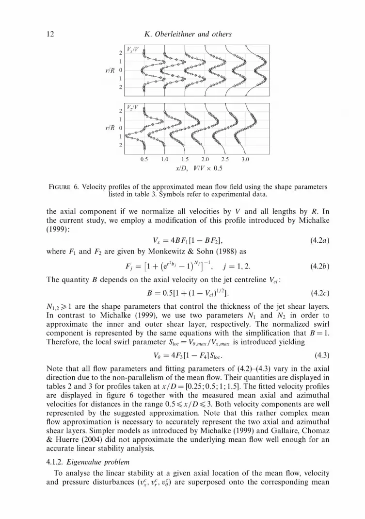
Figure 6. Velocity profiles of the approximated mean flow field using the shape parameterslisted in table 3. Symbols refer to experimental data.
the axial component if we normalize all velocities by V and all lengths by R. Inthe current study, we employ a modification of this profile introduced by Michalke(1999):
Vx = 4BF1[1 − BF2], (4.2a)
where F1 and F2 are given by Monkewitz & Sohn (1988) as
Fj =[1 +
(er2bj − 1
)Nj]−1
, j = 1, 2. (4.2b)
The quantity B depends on the axial velocity on the jet centreline Vcl:
B = 0.5[1 + (1 − Vcl)1/2]. (4.2c)
N1,2 1 are the shape parameters that control the thickness of the jet shear layers.In contrast to Michalke (1999), we use two parameters N1 and N2 in order toapproximate the inner and outer shear layer, respectively. The normalized swirlcomponent is represented by the same equations with the simplification that B =1.Therefore, the local swirl parameter Sloc = Vθ,max/Vx,max is introduced yielding
Vθ = 4F3[1 − F4]Sloc . (4.3)
Note that all flow parameters and fitting parameters of (4.2)–(4.3) vary in the axialdirection due to the non-parallelism of the mean flow. Their quantities are displayed intables 2 and 3 for profiles taken at x/D =[0.25; 0.5; 1; 1.5]. The fitted velocity profilesare displayed in figure 6 together with the measured mean axial and azimuthalvelocities for distances in the range 0.5 x/D 3. Both velocity components are wellrepresented by the suggested approximation. Note that this rather complex meanflow approximation is necessary to accurately represent the two axial and azimuthalshear layers. Simpler models as introduced by Michalke (1999) and Gallaire, Chomaz& Huerre (2004) did not approximate the underlying mean flow well enough for anaccurate linear stability analysis.
4.1.2. Eigenvalue problem
To analyse the linear stability at a given axial location of the mean flow, velocityand pressure disturbances (vc
x, vcr , v
cθ ) are superposed onto the corresponding mean
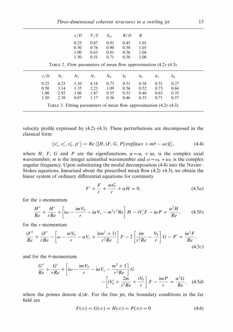
Three-dimensional coherent structures in a swirling jet 13
x/D V/U Sloc R/D B
0.25 0.87 0.91 0.45 1.010.50 0.76 0.90 0.50 1.031.00 0.63 0.81 0.56 1.041.50 0.51 0.71 0.58 1.00
Table 2. Flow parameters of mean flow approximation (4.2)–(4.3).
x/D N1 N2 N3 N4 b1 b2 b3 b4
0.25 4.23 1.10 4.18 0.73 0.51 0.38 0.51 0.270.50 3.14 1.35 2.23 1.09 0.56 0.52 0.73 0.661.00 2.92 1.06 1.87 0.55 0.53 0.46 0.63 0.351.50 2.38 0.87 1.17 0.56 0.46 0.35 0.71 0.57
Table 3. Fitting parameters of mean flow approximation (4.2)–(4.3).
velocity profile expressed by (4.2)–(4.3). These perturbations are decomposed in theclassical form(
vcx, v
cr , v
cθ , p
c)
= Re [H, iF, G, P ] exp[i(αx + mθ − ωt)], (4.4)
where H , F , G and P are the eigenfunctions, α = αr + iαi is the complex axialwavenumber, m is the integer azimuthal wavenumber and ω =ωr +iωi is the complexangular frequency. Upon substituting the modal decomposition (4.4) into the Navier–Stokes equations, linearized about the prescribed mean flow (4.2)–(4.3), we obtain thelinear system of ordinary differential equations for continuity
F ′ +F
r+
mG
r+ αH = 0, (4.5a)
for the x-momentum
H ′′
Re+
H ′
rRe+
[iω − imVθ
r− iαVx − m2r2Re
]H − iV ′
xF − iαP =α2H
Re, (4.5b)
for the r-momentum
iF ′′
Re+
iF ′
rRe−
[ω − mVθ
r− αVx +
i(m2 + 1)
r2Re
]F − 2
[im
r2Re− Vθ
r
]G − P ′ =
iα2F
Re,
(4.5c)
and for the θ-momentum
G′′
Re+
G′
rRe+
[iω − imVθ
r− iαVx − m2 + 1
r2Re
]G
−[iV ′
θ +2m
r2Re+
iVθ
r
]F − imP
r=
α2G
Re, (4.5d)
where the primes denote d/dr . For the free jet, the boundary conditions in the farfield are
F (∞) = G(∞) = H (∞) = P (∞) = 0 (4.6)
14 K. Oberleithner and others
and in the limit along the centreline (r = 0) impose
F (0) = G(0) = H (0) = P (0) = 0 if |m| > 1 (4.7a)
H (0) = P (0) = 0
F (0) + mG(0) = 0
2F ′(0) + mG′(0) = 0
⎫⎪⎬⎪⎭ if |m| = 1 (4.7b)
F (0) = G(0) = 0
H (0) and P (0) finite
if m = 0. (4.7c)
For a given mean velocity profile, the system (4.5)–(4.7) describes an eigenvalueproblem. A non-zero solution of (F, G, H, P ) exists if and only if the complex pair(α, ω) satisfies the dispersion relation D(α, ω, m, Γ, Re) = 0. The symbol Γ representsall control parameters describing the mean velocity profiles.
In the present work, the linear stability analysis is performed to derive the spatialmodes that are retrieved by phase-averaged measurements. Thus, the focus is on theviscous spatial stability analysis where the spatial branches α(ω, Γ ) are obtained bysolving for complex axial wavenumbers when ω and m are real. The non-parallelismof the mean flow requires to solve the eigenvalue problem (4.5)–(4.7) at each axiallocation. The slowly varying amplitudes are expressed by the local eigenmodes. Thefull solution is then constructed by using the eigenfunctions that depend on x andon the global parameters ω and m and a carrier wave exp (
∫ x
0α(x) dx + mθ − ωt).
The Reynolds number in (4.5) is based on the characteristic length and velocity scaleRe= RV/ν and is also varying with x. The flow will be considered as unstable whenthe disturbance grows with x, i.e. when the imaginary part of the eigenvalue αi isnegative. The existence of saddle points in the complex α plane, which serve as anindicator for absolute instability, will not be investigated.
4.1.3. Numerical method
Khorrami, Malik & Ash (1989) demonstrated that the eigenvalue problem canbe efficiently solved by using a Chebyshev spectral collocation method. Followingthis study, the system of ordinary differential equations (4.5) is solved numericallyby discretizing the three velocity components and the three momentum equationsat the Chebyshev collocation points. The continuity equation is enforced at the midgrid points. This approach has been successively applied by Khorrami (1991) to thetemporal problem and recently to the spatial problem by Parras & Fernandez-Feria(2007). For a detailed description of the numerical procedure, the reader is referredto Khorrami et al. (1989); thus, only a brief summary is given here.
The boundary conditions (4.6) are enforced at a large but finite radius rmax 1as was done by Olendraru & Sellier (2002) and Parras & Fernandez-Feria (2007).A coordinate transformation is necessary to map the Chebyshev collocation points,in the interval −1 ξ 1, onto the physical domain of the problem, in the range0 r rmax . Here, the two-parameter transformation proposed by Malik, Zang &Hussaini (1985) is used, which reads
r
rc
=1 + ξ
1 − ξ + 2rc/rmax
. (4.8)
Since the Chebyshev collocation points are known to be distributed in the vicinityof r = 0 and rmax , the parameter rc is necessary to redistribute the collocationpoints. It allows half of the points to be distributed in the region 0 r rc.
Three-dimensional coherent structures in a swirling jet 15
Finally, the eigenvalue problem (4.5) for the case of spatial stability (given realω, complex eigenvalue α) is linearized by introducing a generalized eigenvectorX = [F, G, H, αF, αG, αH, P ]T. Discretizing the system of ordinary differentialequations (4.5) in terms of the variable ξ and enforcing the boundary conditions(4.6)–(4.7), we may write the generalized eigenvalue problem as
DX = αEX . (4.9)
Taking Z as the number of Chebyshev points, both D and E are square matriceswith dimensions of 7Z. Note that the last 14 rows of matrix D contain the boundaryconditions. The eigenvalue problem (4.9) is solved using a standard EIG routineembedded in the software environment MATLABTM. Spurious eigenmodes, causedby the discretization, are discarded by two independent criteria: first, all eigenmodesare discarded that do not diminish at r → ∞, that is to say that we consider onlythose eigenvalues satisfying
Z/10∑i=1
|F (ri)|2
Z∑i=1
|F (ri)|2< ε1 (4.10)
with ri being the radial points and ε1 a given tolerance. Second, spurious eigenvaluesare filtered out by comparing the computed spectra SZ and SZ′ for Z′ >Z. Thelocation of the spurious modes in the complex α-plane is very sensitive to the numberof Chebyshev points Z, in contrast to the few physical eigenvalues of the problem.Thus, the eigenvalues α are considered as spurious if min|α − α′| >ε2.
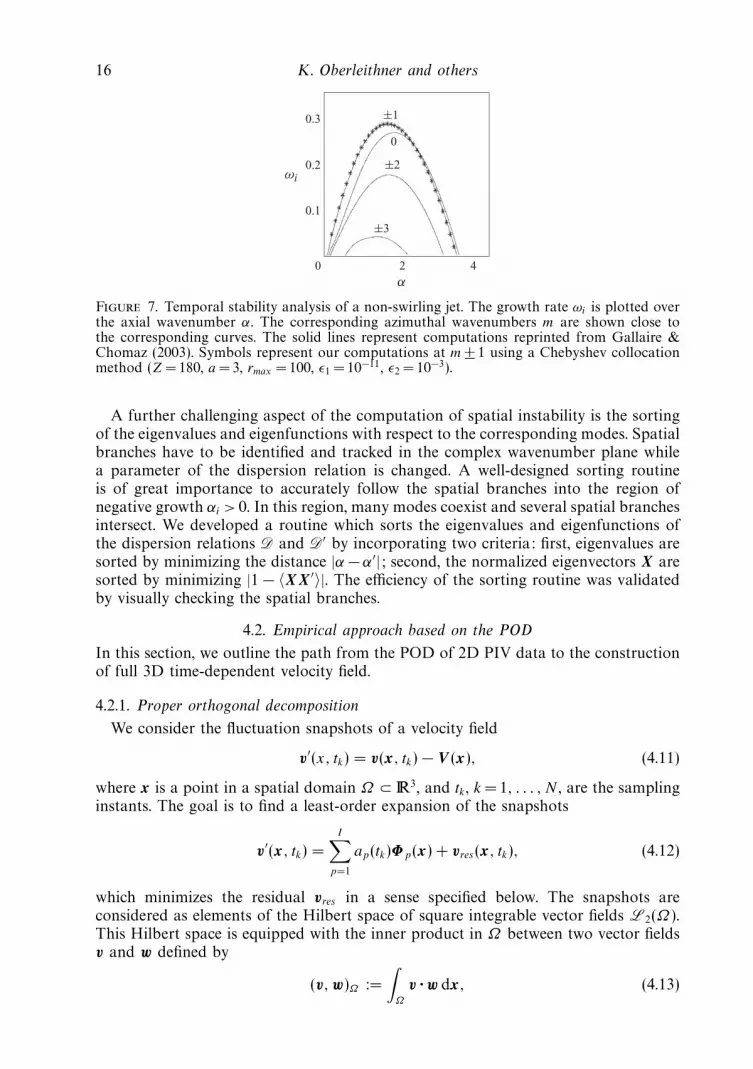
The accuracy of our calculations is first checked by comparing the computedeigenvalues with those calculated by Khorrami et al. (1989) and Parras & Fernandez-Feria (2007). Our computed eigenvalues agree for all shown digits which is notsurprising as these authors use exactly the same numerical method. A comparisonof our computations with the results presented by Gallaire & Chomaz (2003) ismore challenging as their results are retrieved by direct numerical simulations ofthe linear impulse response. Unfortunately, Gallaire & Chomaz do not explicitlypresent computed eigenvalues of their spatio-temporal analysis but only display thecomplex frequency ω of the temporal problem. Hence, for the sake of comparison,we computed the temporal modes using the same base flow as used by Gallaire &Chomaz. Figure 7 clearly shows that for m =1 both numerical methods arrive at thesame solutions. The correctness of the computed eigenvalues makes us confident toapply the computations to our base flow. In comparison to the base flow used byGallaire & Chomaz and Parras & Fernandez-Feria, our mean flow is more complexas it consists of two axial and two azimuthal shear layers. Furthermore, the Reynoldsnumber is in the range of 3000 Re 8000, i.e. one order of magnitude higher thanthat used by Gallaire & Chomaz. Thus, from the numerical point of view the problemis more demanding and the number of collocation points has to be increased. Tosatisfy the filter criterion (4.10) and to successfully discard the spurious eigenvalues, thenumber of Chebyshev points is increased to Z = 300. A convergence study optimizesthe parameters a and rmax of the transformation (4.8) yielding a = 3 and rmax = 100for all computations presented here. It was observed that the calculated eigenvaluesare relatively insensitive to the radial distribution of the collocation points.
16 K. Oberleithner and others
0 2 4
0.1
0.2
0.3
ωi
α
0
±2
±1
±3
Figure 7. Temporal stability analysis of a non-swirling jet. The growth rate ωi is plotted overthe axial wavenumber α. The corresponding azimuthal wavenumbers m are shown close tothe corresponding curves. The solid lines represent computations reprinted from Gallaire &Chomaz (2003). Symbols represent our computations at m ± 1 using a Chebyshev collocationmethod (Z =180, a = 3, rmax = 100, ε1 = 10−11, ε2 = 10−3).
A further challenging aspect of the computation of spatial instability is the sortingof the eigenvalues and eigenfunctions with respect to the corresponding modes. Spatialbranches have to be identified and tracked in the complex wavenumber plane whilea parameter of the dispersion relation is changed. A well-designed sorting routineis of great importance to accurately follow the spatial branches into the region ofnegative growth αi > 0. In this region, many modes coexist and several spatial branchesintersect. We developed a routine which sorts the eigenvalues and eigenfunctions ofthe dispersion relations D and D′ by incorporating two criteria: first, eigenvalues aresorted by minimizing the distance |α − α′|; second, the normalized eigenvectors X aresorted by minimizing |1 − 〈X X ′〉|. The efficiency of the sorting routine was validatedby visually checking the spatial branches.
4.2. Empirical approach based on the POD
In this section, we outline the path from the POD of 2D PIV data to the constructionof full 3D time-dependent velocity field.
4.2.1. Proper orthogonal decomposition
We consider the fluctuation snapshots of a velocity field
v′(x, tk) = v(x, tk) − V (x), (4.11)
where x is a point in a spatial domain Ω ⊂ 3, and tk , k = 1, . . . , N , are the samplinginstants. The goal is to find a least-order expansion of the snapshots
v′(x, tk) =
I∑p=1
ap(tk)Φp(x) + vres (x, tk), (4.12)
which minimizes the residual vres in a sense specified below. The snapshots areconsidered as elements of the Hilbert space of square integrable vector fields L2(Ω).This Hilbert space is equipped with the inner product in Ω between two vector fieldsv and w defined by
(v, w)Ω :=
∫Ω
v · w dx, (4.13)
Three-dimensional coherent structures in a swirling jet 17
and the related norm ‖v‖Ω reads
‖v‖Ω :=√
(v, v)Ω. (4.14)
The velocity fields are provided by PIV snapshots taken at N uncorrelated points atthe times tk , k =1, . . . , N . In addition to the inner product in space, we define theensemble average of a quantity ζ as
ζ :=1
N
N∑k=1
ζ (tk). (4.15)
The quantity ζ may be a scalar, a vector or any other tensor. The norm and ensembleaverage allows one to formulate an optimal property of the Galerkin expansion (4.12).We require that the spatial modes are chosen such that the time-averaged L2 erroris minimal for the number of modes I = 1, . . . , N:
χ2(Φ1, . . . , ΦI ) := ‖vres‖2 = min. (4.16)
Note that the minimized residual vres ≡ 0 for I = N . This optimality property isfulfilled by the snapshot POD modes introduced by Sirovich (1987). The correspondingalgorithm is based on the N × N autocorrelation matrix R =(Rkl) defined by
Rkl :=1
N(v′(x, tk), v
′(x, tl))Ω (4.17)
quantifying the relation between the snapshots. The correlation matrix is symmetricand positive semi-definite, i.e. the eigenvalue problem
Rap = λpap (4.18)
has real and non-negative eigenvalues λp 0. Without loss of generality, we assumethe eigenvalues to be sorted by magnitude:
λ1 λ2 · · · λN = 0. (4.19)
Note that λN = 0 since N linearly independent snapshots cannot span the wholeN-dimensional space. Two points, for instance, define a one-dimensional line. Thecorresponding eigenvectors ap : = [ap(t1), . . . , ap(tN )]T, called temporal modes, areorthogonal by construction. For reasons of convenience, we require
apaq =1
N
N∑k=1
ap(tk)aq(tk) = λpδpq. (4.20)
Now, the spatial POD modes can be calculated as a linear combination of thefluctuation snapshots
Φp(x) =1
Nλp
N∑k=1
ap(tk)v′(x, tk). (4.21)
These spatial POD modes are orthonormal by construction:
(Φp, Φq)Ω = δpq. (4.22)
The eigenvalues λp represent twice the amount of the fluctuating kinetic energy
contained in each POD mode, Kp := (v′, Φp)2Ω/2 = λp/2. The total fluctuation energy
18 K. Oberleithner and others
q
λq
CrosswiseStreamwise
100 101 102
10–1
100
101
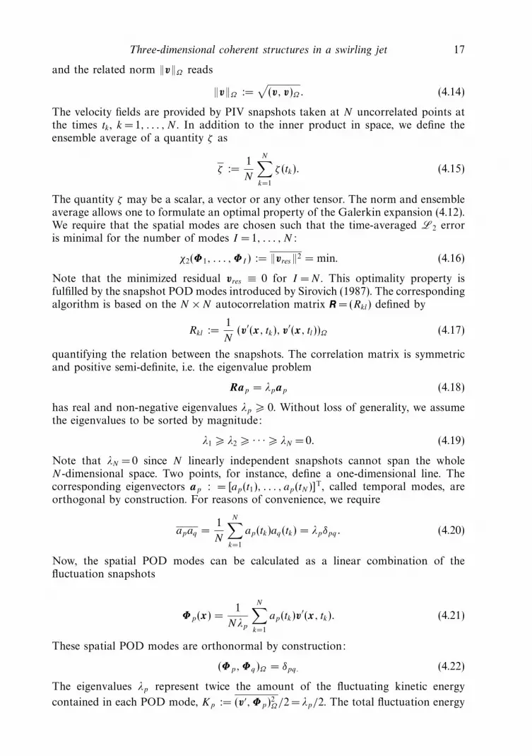
Figure 8. POD spectrum of the velocity modes p for the crossflow and streamwise planes of
measurement. TKE is expressed in per cent of the sum K =∑N
p=1 Kp .
is defined as the sum of the modal contributions owing to orthonormality (4.22):
K :=1
2‖v′‖2
Ω =
N∑p=1
Kp =1
2
N∑p=1
λp. (4.23)
K is generally referred to as turbulent kinetic energy (TKE). Snapshot POD extractsthe most energetic structures representing them as linear combinations of thesnapshots and imposes orthogonality in spatial and temporal modes. Snapshot PODis the time-discrete variant of a general continuous formulation (Holmes et al. 1998).In turbulent flows, the large-scale structures usually contain a major portion of theTKE, so the POD modes with high energy content can hence be expected to spanthe basis for the dominant coherent structures.
4.2.2. Spatial and temporal POD modes
The snapshot POD, as described above, is applied to the data taken in thecrossflow and streamwise planes of measurement. Both sets of measurement consistof 800 snapshots. The observation domains have a spatial extent of −1.1 <y/D < 1.1and −1.1 <z/D < 1.1 at x/D =0.57 for the crossflow plane and 0.25 <x/D < 3 and−1.1 <y/D < 1.1 at z/D = 0 for the streamwise plane. The eigenvalue spectrum ofPOD modes for both measurement planes is shown in figure 8.
For both cases the POD shows that the first two eigenvalues contain substantialamount of energy. In the crossflow plane the first two modes contain already 30 %of TKE, while in the streamwise plane these modes contain more than 14 %. In bothcases, the energy contained in the two leading modes is nearly equal suggesting thatthe two modes span a travelling wave.
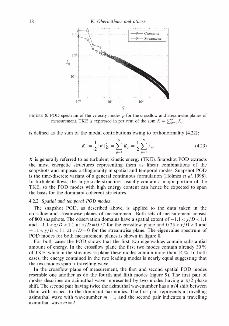
In the crossflow plane of measurement, the first and second spatial POD modesresemble one another as do the fourth and fifth modes (figure 9). The first pair ofmodes describes an azimuthal wave represented by two modes having a π/2 phaseshift. The second pair having twice the azimuthal wavenumber has a π/4 shift betweenthem with respect to the dominant harmonics. The first pair represents a travellingazimuthal wave with wavenumber m =1, and the second pair indicates a travellingazimuthal wave m = 2.
Three-dimensional coherent structures in a swirling jet 19
1
15.0 % TKE
2
14.9 % TKE
3
3.1 % TKE
4
2.9 % TKE
5
2.6 % TKE
Figure 9. First five POD modes of the crossflow plane of measurement; the radial velocitycomponent is shown with contour lines vr/max(vr ) = −0.8, −0.6, −0.4, −0.2, 0.2, 0.4,0.6, 0.8. The POD mode-number p is written in the top-left corner and the percentageof TKE at the bottom. The dashed circle indicates the nozzle diameter.
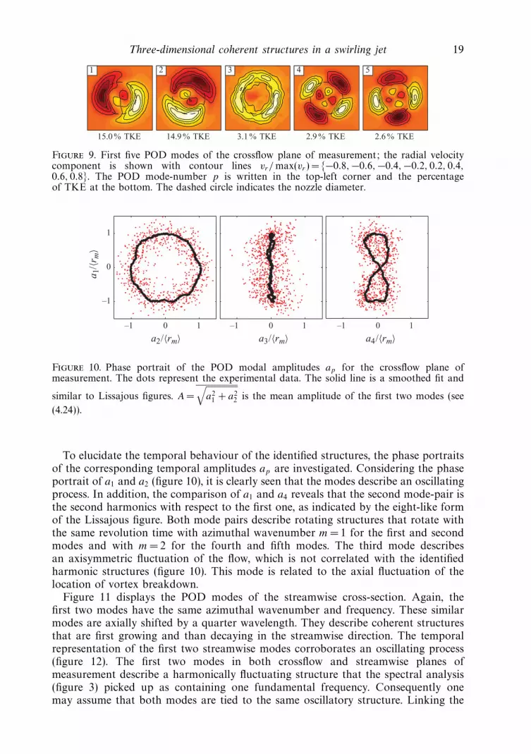
a2/〈rm〉
a 1/〈r
m〉
a3/〈rm〉 a4/〈rm〉–1 0 1 –1 0 1 –1 0 1
–1
0
1
Figure 10. Phase portrait of the POD modal amplitudes ap for the crossflow plane ofmeasurement. The dots represent the experimental data. The solid line is a smoothed fit and
similar to Lissajous figures. A =√
a21 + a2
2 is the mean amplitude of the first two modes (see
(4.24)).
To elucidate the temporal behaviour of the identified structures, the phase portraitsof the corresponding temporal amplitudes ap are investigated. Considering the phaseportrait of a1 and a2 (figure 10), it is clearly seen that the modes describe an oscillatingprocess. In addition, the comparison of a1 and a4 reveals that the second mode-pair isthe second harmonics with respect to the first one, as indicated by the eight-like formof the Lissajous figure. Both mode pairs describe rotating structures that rotate withthe same revolution time with azimuthal wavenumber m =1 for the first and secondmodes and with m =2 for the fourth and fifth modes. The third mode describesan axisymmetric fluctuation of the flow, which is not correlated with the identifiedharmonic structures (figure 10). This mode is related to the axial fluctuation of thelocation of vortex breakdown.
Figure 11 displays the POD modes of the streamwise cross-section. Again, thefirst two modes have the same azimuthal wavenumber and frequency. These similarmodes are axially shifted by a quarter wavelength. They describe coherent structuresthat are first growing and than decaying in the streamwise direction. The temporalrepresentation of the first two streamwise modes corroborates an oscillating process(figure 12). The first two modes in both crossflow and streamwise planes ofmeasurement describe a harmonically fluctuating structure that the spectral analysis(figure 3) picked up as containing one fundamental frequency. Consequently onemay assume that both modes are tied to the same oscillatory structure. Linking the
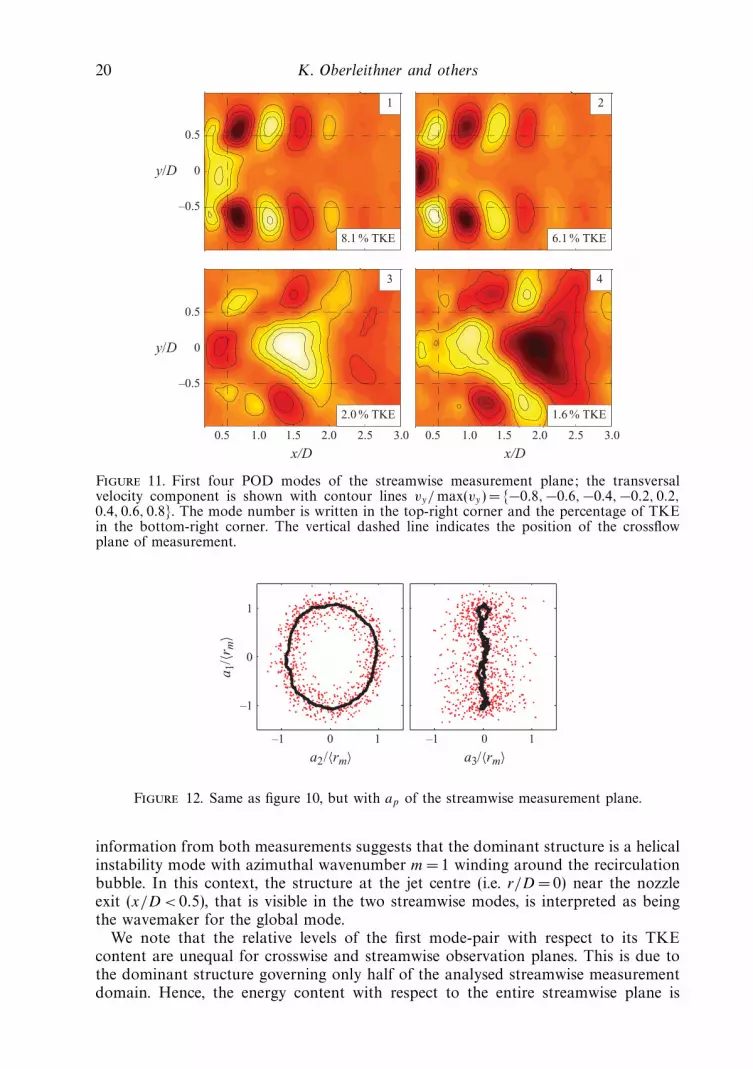
20 K. Oberleithner and others
y/D
y/D
1
8.1 % TKE
2
6.1 % TKE
x/D x/D
3
2.0 % TKE
4
1.6 % TKE
0.5 1.0 1.5 2.0 2.5 3.0 0.5 1.0 1.5 2.0 2.5 3.0
–0.5
0
0.5
–0.5
0
0.5
Figure 11. First four POD modes of the streamwise measurement plane; the transversalvelocity component is shown with contour lines vy/max(vy) = −0.8, −0.6, −0.4, −0.2, 0.2,0.4, 0.6, 0.8. The mode number is written in the top-right corner and the percentage of TKEin the bottom-right corner. The vertical dashed line indicates the position of the crossflowplane of measurement.
–1
0
1
a2/〈rm〉
a 1/〈r
m〉
–1 0 1
a3/〈rm〉–1 0 1
Figure 12. Same as figure 10, but with ap of the streamwise measurement plane.
information from both measurements suggests that the dominant structure is a helicalinstability mode with azimuthal wavenumber m =1 winding around the recirculationbubble. In this context, the structure at the jet centre (i.e. r/D = 0) near the nozzleexit (x/D < 0.5), that is visible in the two streamwise modes, is interpreted as beingthe wavemaker for the global mode.
We note that the relative levels of the first mode-pair with respect to its TKEcontent are unequal for crosswise and streamwise observation planes. This is due tothe dominant structure governing only half of the analysed streamwise measurementdomain. Hence, the energy content with respect to the entire streamwise plane is
Three-dimensional coherent structures in a swirling jet 21
approximately half as high in comparison to the crosswise plane. Using an appropriatesub-domain for streamwise POD analysis can decrease this difference.
The third and forth streamwise modes (figure 11) are coupled and represent themeandering of the recirculation bubble. The phase portrait reveals no relation to thedominant structure. Hence, the meandering is affected by other processes.
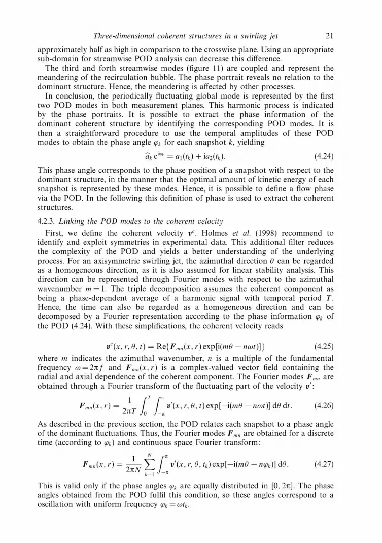
In conclusion, the periodically fluctuating global mode is represented by the firsttwo POD modes in both measurement planes. This harmonic process is indicatedby the phase portraits. It is possible to extract the phase information of thedominant coherent structure by identifying the corresponding POD modes. It isthen a straightforward procedure to use the temporal amplitudes of these PODmodes to obtain the phase angle ϕk for each snapshot k, yielding
ak eiϕk = a1(tk) + ia2(tk). (4.24)
This phase angle corresponds to the phase position of a snapshot with respect to thedominant structure, in the manner that the optimal amount of kinetic energy of eachsnapshot is represented by these modes. Hence, it is possible to define a flow phasevia the POD. In the following this definition of phase is used to extract the coherentstructures.
4.2.3. Linking the POD modes to the coherent velocity
First, we define the coherent velocity vc. Holmes et al. (1998) recommend toidentify and exploit symmetries in experimental data. This additional filter reducesthe complexity of the POD and yields a better understanding of the underlyingprocess. For an axisymmetric swirling jet, the azimuthal direction θ can be regardedas a homogeneous direction, as it is also assumed for linear stability analysis. Thisdirection can be represented through Fourier modes with respect to the azimuthalwavenumber m =1. The triple decomposition assumes the coherent component asbeing a phase-dependent average of a harmonic signal with temporal period T .Hence, the time can also be regarded as a homogeneous direction and can bedecomposed by a Fourier representation according to the phase information ϕk ofthe POD (4.24). With these simplifications, the coherent velocity reads
vc(x, r, θ, t) = ReFmn(x, r) exp[i(mθ − nωt)] (4.25)
where m indicates the azimuthal wavenumber, n is a multiple of the fundamentalfrequency ω =2πf and Fmn(x, r) is a complex-valued vector field containing theradial and axial dependence of the coherent component. The Fourier modes Fmn areobtained through a Fourier transform of the fluctuating part of the velocity v′:
Fmn(x, r) =1
2πT
∫ T
0
∫ π
−π
v′(x, r, θ, t) exp[−i(mθ − nωt)] dθ dt. (4.26)
As described in the previous section, the POD relates each snapshot to a phase angleof the dominant fluctuations. Thus, the Fourier modes Fmn are obtained for a discretetime (according to ϕk) and continuous space Fourier transform:
Fmn(x, r) =1
2πN
N∑k=1
∫ π
−π
v′(x, r, θ, tk) exp[−i(mθ − nϕk)] dθ. (4.27)
This is valid only if the phase angles ϕk are equally distributed in [0, 2π]. The phaseangles obtained from the POD fulfil this condition, so these angles correspond to aoscillation with uniform frequency ϕk =ωtk .
22 K. Oberleithner and others
(a) (b)
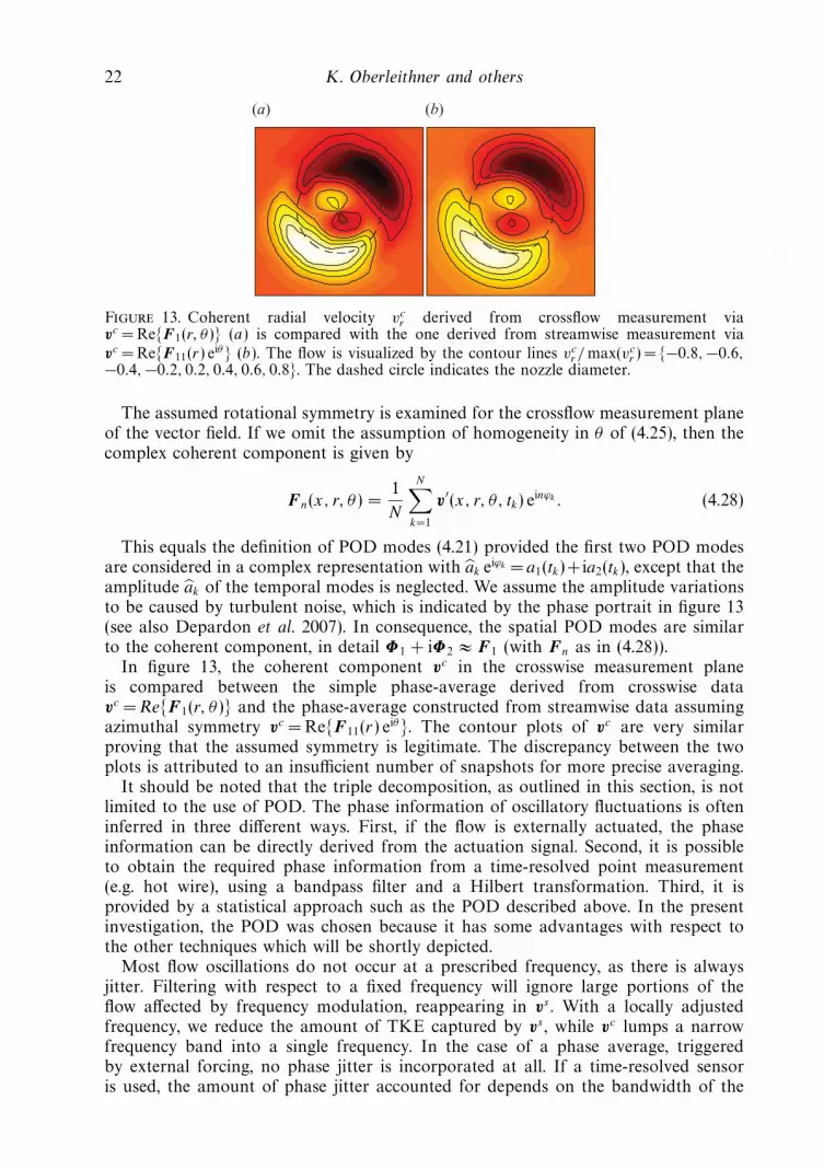
Figure 13. Coherent radial velocity vcr derived from crossflow measurement via
vc = ReF1(r, θ ) (a) is compared with the one derived from streamwise measurement viavc = ReF11(r) eiθ (b). The flow is visualized by the contour lines vc
r /max(vcr ) = −0.8, −0.6,
−0.4, −0.2, 0.2, 0.4, 0.6, 0.8. The dashed circle indicates the nozzle diameter.
The assumed rotational symmetry is examined for the crossflow measurement planeof the vector field. If we omit the assumption of homogeneity in θ of (4.25), then thecomplex coherent component is given by
Fn(x, r, θ) =1
N
N∑k=1
v′(x, r, θ, tk) einϕk . (4.28)
This equals the definition of POD modes (4.21) provided the first two POD modesare considered in a complex representation with ak eiϕk = a1(tk)+ia2(tk), except that theamplitude ak of the temporal modes is neglected. We assume the amplitude variationsto be caused by turbulent noise, which is indicated by the phase portrait in figure 13(see also Depardon et al. 2007). In consequence, the spatial POD modes are similarto the coherent component, in detail Φ1 + iΦ2 ≈ F1 (with Fn as in (4.28)).
In figure 13, the coherent component vc in the crosswise measurement planeis compared between the simple phase-average derived from crosswise datavc =ReF1(r, θ) and the phase-average constructed from streamwise data assumingazimuthal symmetry vc = ReF11(r) eiθ. The contour plots of vc are very similarproving that the assumed symmetry is legitimate. The discrepancy between the twoplots is attributed to an insufficient number of snapshots for more precise averaging.
It should be noted that the triple decomposition, as outlined in this section, is notlimited to the use of POD. The phase information of oscillatory fluctuations is ofteninferred in three different ways. First, if the flow is externally actuated, the phaseinformation can be directly derived from the actuation signal. Second, it is possibleto obtain the required phase information from a time-resolved point measurement(e.g. hot wire), using a bandpass filter and a Hilbert transformation. Third, it isprovided by a statistical approach such as the POD described above. In the presentinvestigation, the POD was chosen because it has some advantages with respect tothe other techniques which will be shortly depicted.
Most flow oscillations do not occur at a prescribed frequency, as there is alwaysjitter. Filtering with respect to a fixed frequency will ignore large portions of theflow affected by frequency modulation, reappearing in vs . With a locally adjustedfrequency, we reduce the amount of TKE captured by vs , while vc lumps a narrowfrequency band into a single frequency. In the case of a phase average, triggeredby external forcing, no phase jitter is incorporated at all. If a time-resolved sensoris used, the amount of phase jitter accounted for depends on the bandwidth of the
Three-dimensional coherent structures in a swirling jet 23
bandpass filter used. When using the POD phase, obtained according to (4.24), nofixed frequency has to be assumed, and the calculated phase is the optimal one interms of energy representation. The optimal phase is related to the optimality ofspatial POD modes, where these modes are understood as a prior guess for coherentstructures providing the phase through projection on the snapshots. Furthermore, incontrast to a time-resolved point measurement, the POD approach predicts the phaseangle from spatial modes and not from one single point in the flow yielding a moreaccurate prediction of the global phase.
4.2.4. Construction of three-dimensional coherent structures
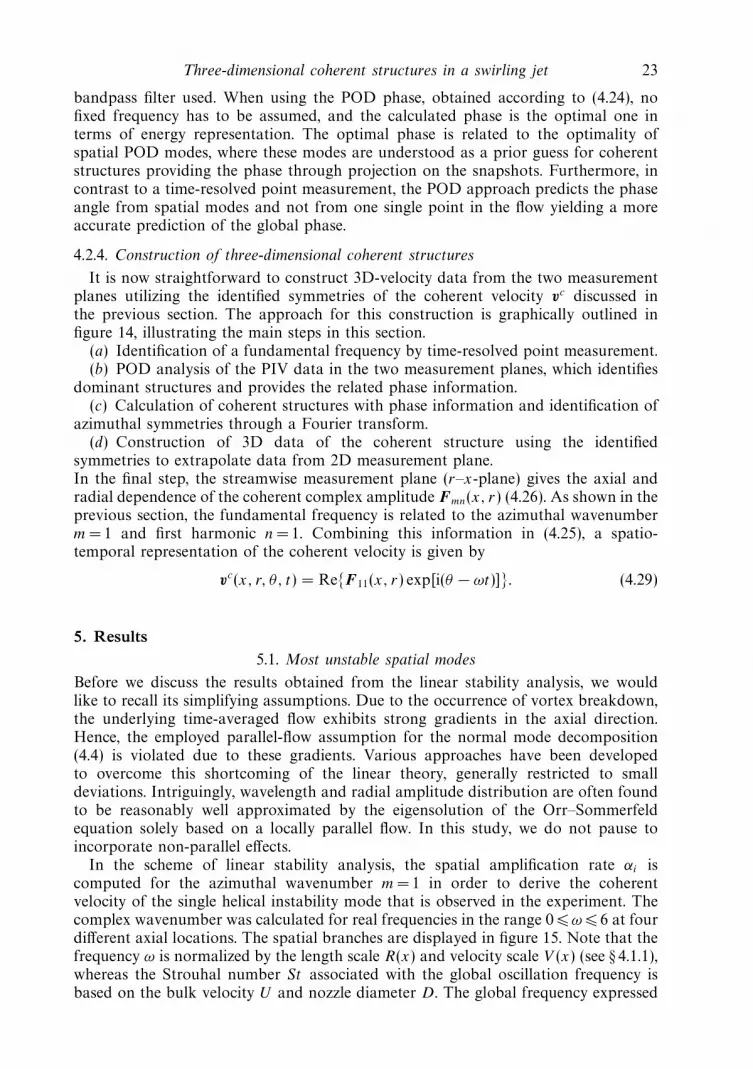
It is now straightforward to construct 3D-velocity data from the two measurementplanes utilizing the identified symmetries of the coherent velocity vc discussed inthe previous section. The approach for this construction is graphically outlined infigure 14, illustrating the main steps in this section.
(a) Identification of a fundamental frequency by time-resolved point measurement.(b) POD analysis of the PIV data in the two measurement planes, which identifies
dominant structures and provides the related phase information.(c) Calculation of coherent structures with phase information and identification of
azimuthal symmetries through a Fourier transform.(d) Construction of 3D data of the coherent structure using the identified
symmetries to extrapolate data from 2D measurement plane.In the final step, the streamwise measurement plane (r–x-plane) gives the axial andradial dependence of the coherent complex amplitude Fmn(x, r) (4.26). As shown in theprevious section, the fundamental frequency is related to the azimuthal wavenumberm = 1 and first harmonic n= 1. Combining this information in (4.25), a spatio-temporal representation of the coherent velocity is given by
vc(x, r, θ, t) = ReF11(x, r) exp[i(θ − ωt)]. (4.29)
5. Results5.1. Most unstable spatial modes
Before we discuss the results obtained from the linear stability analysis, we wouldlike to recall its simplifying assumptions. Due to the occurrence of vortex breakdown,the underlying time-averaged flow exhibits strong gradients in the axial direction.Hence, the employed parallel-flow assumption for the normal mode decomposition(4.4) is violated due to these gradients. Various approaches have been developedto overcome this shortcoming of the linear theory, generally restricted to smalldeviations. Intriguingly, wavelength and radial amplitude distribution are often foundto be reasonably well approximated by the eigensolution of the Orr–Sommerfeldequation solely based on a locally parallel flow. In this study, we do not pause toincorporate non-parallel effects.
In the scheme of linear stability analysis, the spatial amplification rate αi iscomputed for the azimuthal wavenumber m = 1 in order to derive the coherentvelocity of the single helical instability mode that is observed in the experiment. Thecomplex wavenumber was calculated for real frequencies in the range 0 ω 6 at fourdifferent axial locations. The spatial branches are displayed in figure 15. Note that thefrequency ω is normalized by the length scale R(x) and velocity scale V (x) (see § 4.1.1),whereas the Strouhal number St associated with the global oscillation frequency isbased on the bulk velocity U and nozzle diameter D. The global frequency expressed
24 K. Oberleithner and others
3D2D
/Pha
se-a
vera
ge2D
/PO
D0D
/Hot
wir
e
Construction of 3D velocity data
Streamwise data Crosswise data
Hotwire/FFT
PIV/POD PIV/PODPhase information
Phase-average
Spatial rotation + symmetryAzimuthal symmetry3D data
Phase-averageCoherent structures Coherent structures
Phase information
dominant frequency
(a)
(b)
(c)
(d)
Figure 14. Schematic diagram of the 3D flow construction. The illustrated steps are as follows:(a) identification of the fundamental frequency; (b) POD analysis of the PIV data yielding theflow phase; (c) identification of coherent structures and symmetries and (d ) construction of3D data from the 2D measurements.
by ω increases in the downstream direction as the downstream increase of R is morerapid than the decay of U (see the open circles in figure 15). At the axial locationswhere the flow is unstable to the global frequency, only one unstable spatial branchis found and the spatial amplification rate can easily be tracked in the downstreamdirection. Waves forced at the global frequency grow rapidly near the nozzle exitwhere the shear layer is thin relative to the nozzle radius. As the shear layer spreads
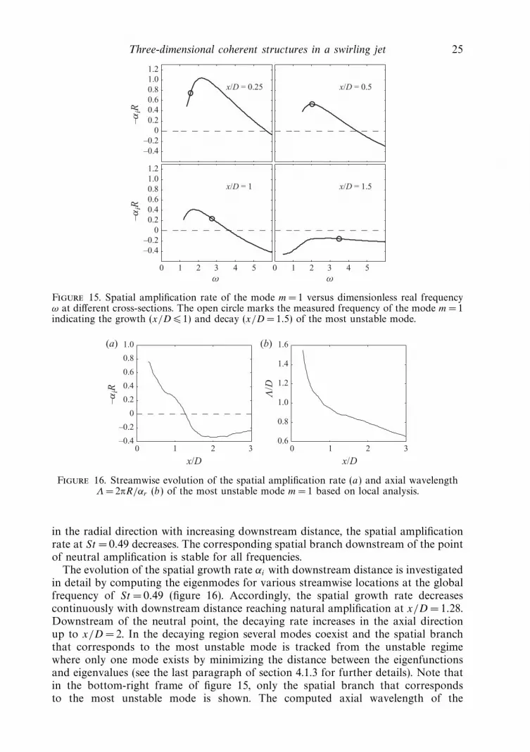
Three-dimensional coherent structures in a swirling jet 25
–αiR
–αiR
x/D = 0.25 x/D = 0.5
ω ω
x/D = 1 x/D = 1.5
0 1 2 3 4 5 0 1 2 3 4 5
–0.4–0.2
00.20.40.60.81.01.2
–0.4–0.2
00.20.40.60.81.01.2
Figure 15. Spatial amplification rate of the mode m= 1 versus dimensionless real frequencyω at different cross-sections. The open circle marks the measured frequency of the mode m= 1indicating the growth (x/D 1) and decay (x/D = 1.5) of the most unstable mode.
x/D x/D0 1 2 3
–0.4
–0.2
0
0.2
0.4
0.6
0.8
1.0
Λ/D
0 1 2 30.6
0.8
1.0
1.2
1.4
1.6
–αiR
(a) (b)
Figure 16. Streamwise evolution of the spatial amplification rate (a) and axial wavelengthΛ= 2πR/αr (b) of the most unstable mode m= 1 based on local analysis.
in the radial direction with increasing downstream distance, the spatial amplificationrate at St = 0.49 decreases. The corresponding spatial branch downstream of the pointof neutral amplification is stable for all frequencies.
The evolution of the spatial growth rate αi with downstream distance is investigatedin detail by computing the eigenmodes for various streamwise locations at the globalfrequency of St = 0.49 (figure 16). Accordingly, the spatial growth rate decreasescontinuously with downstream distance reaching natural amplification at x/D = 1.28.Downstream of the neutral point, the decaying rate increases in the axial directionup to x/D = 2. In the decaying region several modes coexist and the spatial branchthat corresponds to the most unstable mode is tracked from the unstable regimewhere only one mode exists by minimizing the distance between the eigenfunctionsand eigenvalues (see the last paragraph of section 4.1.3 for further details). Note thatin the bottom-right frame of figure 15, only the spatial branch that correspondsto the most unstable mode is shown. The computed axial wavelength of the
26 K. Oberleithner and others
y/D
x/D y/D0.5 –0.5 0.501.0 1.5 2.0 2.5 3.0
–0.5
0
0.5
(a) (b)
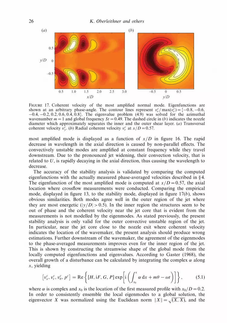
Figure 17. Coherent velocity of the most amplified normal mode. Eigenfunctions areshown at an arbitrary phase-angle. The contour lines represent vc
r /max(vcr ) = −0.8, −0.6,
−0.4, −0.2, 0.2, 0.6, 0.4, 0.8. The eigenvalue problem (4.9) was solved for the azimuthalwavenumber m= 1 and global frequency St =0.49. The dashed circle in (b) indicates the nozzlediameter which approximately separates the inner and the outer shear layer. (a) Transversalcoherent velocity vc
y . (b) Radial coherent velocity vcr at x/D =0.57.
most amplified mode is displayed as a function of x/D in figure 16. The rapiddecrease in wavelength in the axial direction is caused by non-parallel effects. Theconvectively unstable modes are amplified at constant frequency while they traveldownstream. Due to the pronounced jet widening, their convection velocity, that isrelated to U , is rapidly decaying in the axial direction, thus causing the wavelength todecrease.
The accuracy of the stability analysis is validated by comparing the computedeigenfunctions with the actually measured phase-averaged velocities described in § 4.The eigenfunction of the most amplified mode is computed at x/D = 0.57, the axiallocation where crossflow measurements were conducted. Comparing the empiricalmode, displayed in figure 13, to the stability mode, displayed in figure 17(b), showsobvious similarities. Both modes agree well in the outer region of the jet wherethey are most energetic (|y/D| > 0.5). In the inner region the structures seem to beout of phase and the coherent velocity near the jet core that is evident from themeasurements is not modelled by the eigenmodes. As stated previously, the presentstability analysis is only valid for the outer convective unstable region of the jet.In particular, near the jet core close to the nozzle exit where coherent velocityindicates the location of the wavemaker, the present analysis should produce wrongestimations. Further downstream of the wavemaker, the agreement of the eigenmodesto the phase-averaged measurements improves even for the inner region of the jet.This is shown by constructing the streamwise shape of the global mode from thelocally computed eigenfunctions and eigenvalues. According to Gaster (1968), theoverall growth of a disturbance can be calculated by integrating the complex α alongx, yielding
[vc
x, vcr , v
cθ , p
c]
= Re
[H, iF, G, P ] exp
[i
(∫ x
x0
α dx + mθ − ωt
)], (5.1)
where α is complex and x0 is the location of the first measured profile with x0/D = 0.2.In order to consistently ensemble the local eigenmodes to a global solution, theeigenvector X was normalized using the Euclidean norm ‖X‖ =
√(X, X), and the
Three-dimensional coherent structures in a swirling jet 27
(a)
(b)
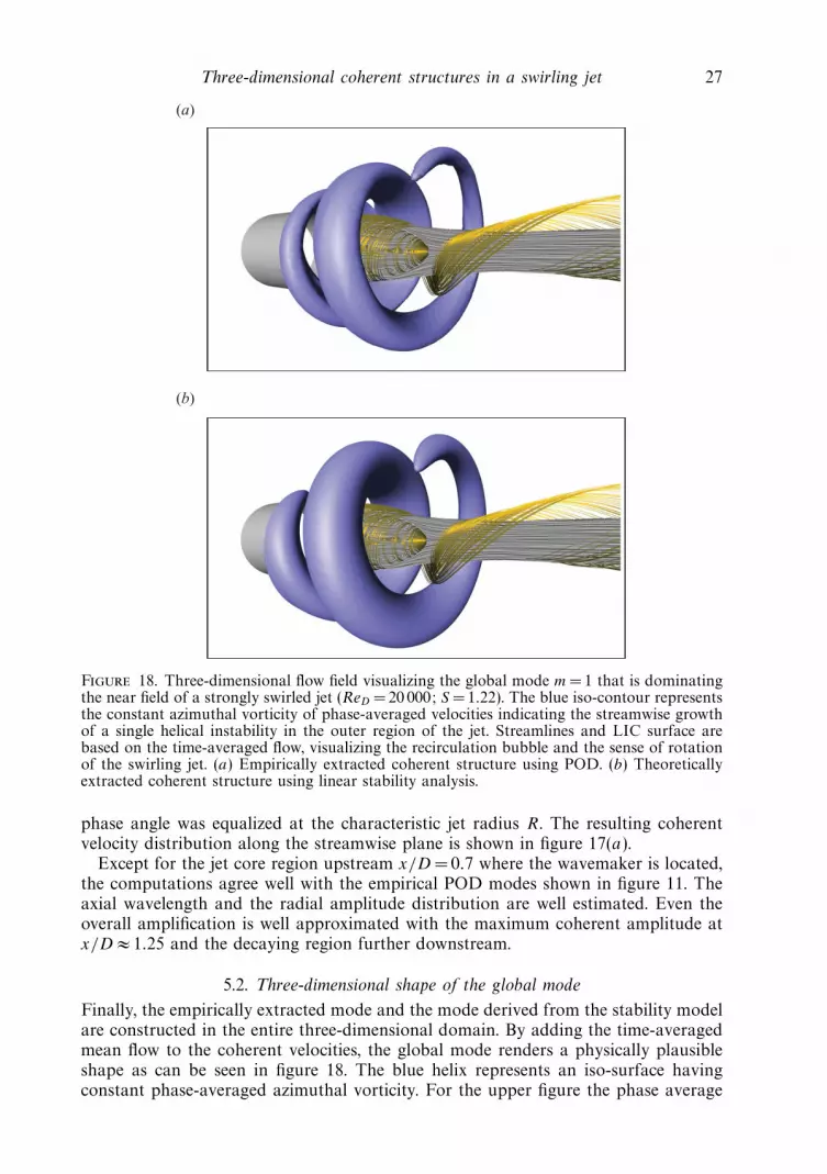
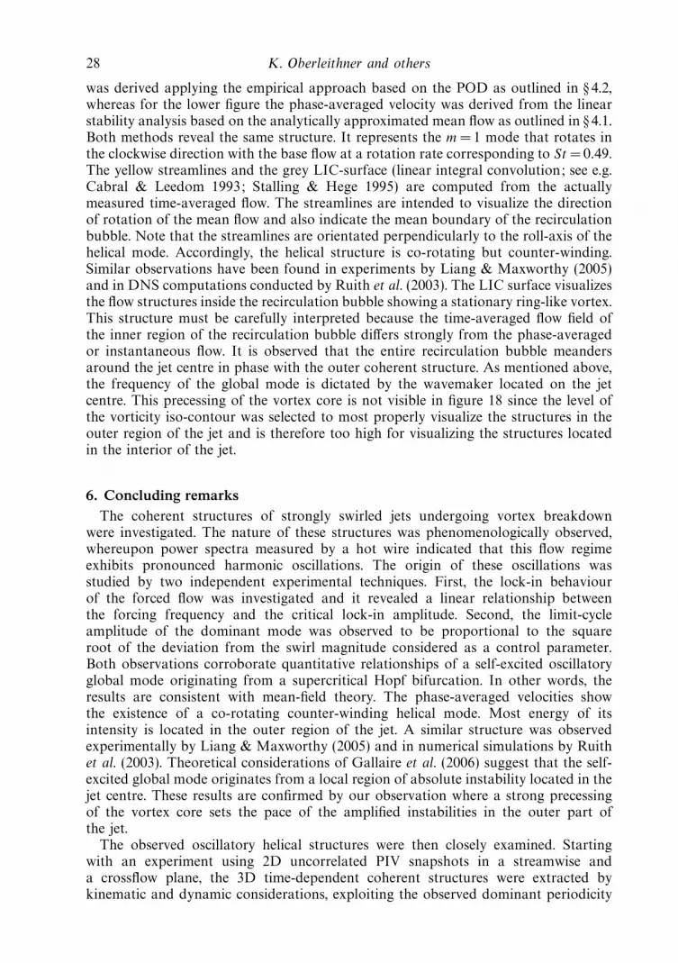
Figure 18. Three-dimensional flow field visualizing the global mode m= 1 that is dominatingthe near field of a strongly swirled jet (ReD = 20 000; S =1.22). The blue iso-contour representsthe constant azimuthal vorticity of phase-averaged velocities indicating the streamwise growthof a single helical instability in the outer region of the jet. Streamlines and LIC surface arebased on the time-averaged flow, visualizing the recirculation bubble and the sense of rotationof the swirling jet. (a) Empirically extracted coherent structure using POD. (b) Theoreticallyextracted coherent structure using linear stability analysis.
phase angle was equalized at the characteristic jet radius R. The resulting coherentvelocity distribution along the streamwise plane is shown in figure 17(a).
Except for the jet core region upstream x/D = 0.7 where the wavemaker is located,the computations agree well with the empirical POD modes shown in figure 11. Theaxial wavelength and the radial amplitude distribution are well estimated. Even theoverall amplification is well approximated with the maximum coherent amplitude atx/D ≈ 1.25 and the decaying region further downstream.
5.2. Three-dimensional shape of the global mode
Finally, the empirically extracted mode and the mode derived from the stability modelare constructed in the entire three-dimensional domain. By adding the time-averagedmean flow to the coherent velocities, the global mode renders a physically plausibleshape as can be seen in figure 18. The blue helix represents an iso-surface havingconstant phase-averaged azimuthal vorticity. For the upper figure the phase average
28 K. Oberleithner and others
was derived applying the empirical approach based on the POD as outlined in § 4.2,whereas for the lower figure the phase-averaged velocity was derived from the linearstability analysis based on the analytically approximated mean flow as outlined in § 4.1.Both methods reveal the same structure. It represents the m =1 mode that rotates inthe clockwise direction with the base flow at a rotation rate corresponding to St =0.49.The yellow streamlines and the grey LIC-surface (linear integral convolution; see e.g.Cabral & Leedom 1993; Stalling & Hege 1995) are computed from the actuallymeasured time-averaged flow. The streamlines are intended to visualize the directionof rotation of the mean flow and also indicate the mean boundary of the recirculationbubble. Note that the streamlines are orientated perpendicularly to the roll-axis of thehelical mode. Accordingly, the helical structure is co-rotating but counter-winding.Similar observations have been found in experiments by Liang & Maxworthy (2005)and in DNS computations conducted by Ruith et al. (2003). The LIC surface visualizesthe flow structures inside the recirculation bubble showing a stationary ring-like vortex.This structure must be carefully interpreted because the time-averaged flow field ofthe inner region of the recirculation bubble differs strongly from the phase-averagedor instantaneous flow. It is observed that the entire recirculation bubble meandersaround the jet centre in phase with the outer coherent structure. As mentioned above,the frequency of the global mode is dictated by the wavemaker located on the jetcentre. This precessing of the vortex core is not visible in figure 18 since the level ofthe vorticity iso-contour was selected to most properly visualize the structures in theouter region of the jet and is therefore too high for visualizing the structures locatedin the interior of the jet.
6. Concluding remarksThe coherent structures of strongly swirled jets undergoing vortex breakdown
were investigated. The nature of these structures was phenomenologically observed,whereupon power spectra measured by a hot wire indicated that this flow regimeexhibits pronounced harmonic oscillations. The origin of these oscillations wasstudied by two independent experimental techniques. First, the lock-in behaviourof the forced flow was investigated and it revealed a linear relationship betweenthe forcing frequency and the critical lock-in amplitude. Second, the limit-cycleamplitude of the dominant mode was observed to be proportional to the squareroot of the deviation from the swirl magnitude considered as a control parameter.Both observations corroborate quantitative relationships of a self-excited oscillatoryglobal mode originating from a supercritical Hopf bifurcation. In other words, theresults are consistent with mean-field theory. The phase-averaged velocities showthe existence of a co-rotating counter-winding helical mode. Most energy of itsintensity is located in the outer region of the jet. A similar structure was observedexperimentally by Liang & Maxworthy (2005) and in numerical simulations by Ruithet al. (2003). Theoretical considerations of Gallaire et al. (2006) suggest that the self-excited global mode originates from a local region of absolute instability located in thejet centre. These results are confirmed by our observation where a strong precessingof the vortex core sets the pace of the amplified instabilities in the outer part ofthe jet.
The observed oscillatory helical structures were then closely examined. Startingwith an experiment using 2D uncorrelated PIV snapshots in a streamwise anda crossflow plane, the 3D time-dependent coherent structures were extracted bykinematic and dynamic considerations, exploiting the observed dominant periodicity
Three-dimensional coherent structures in a swirling jet 29
of the flow. The kinematic velocity field reconstruction started from the uncorrelated2D streamwise velocity fields determined by PIV. The pronounced oscillatory nature ofthe fluctuations was evidenced by two leading POD modes spanning a correspondingconvecting vortex pattern. These two POD modes allowed one to attribute a phaseto each snapshot taken. A continuous time dependence was imposed by assuminga single oscillation frequency, consistent with the experimental measurements. Thisassumption allows for restoration of time dependence provided that small-amplitudevariations of the turbulent flow such as the less-energetic higher harmonics andstochastic small-scale fluctuations are negligible. A 3D flow pattern was reconstructedby exploiting an azimuthal symmetry of the observed helical coherent structures. Theresulting 3D flow pattern corroborates PIV observations in crossflow planes. Thus,the spatio-temporal evolution of the full 3D helical structure was obtained from 2Duncorrelated data sets.
The velocity field of the global mode was also derived by means of a linearstability analysis employing the measured mean flow. A spatial approach was justifiedby previous experiments conducted by the authors, showing that the wavemakergenerating the global oscillations is located inside the jet central core upstreamof the recirculation bubble imposing its frequency on the outer shear layer whereinstabilities are convective. Hence, for a purely spatial analysis, the precessing vortexcore upstream of the vortex breakdown location was considered as a ‘natural oscillator’and the convectively unstable surrounding flow field was modelled as being externallyforced. The spatial approach is corroborated a posteriori by the good agreement ofthe stability eigenmodes, amplification rates and wavelengths with the correspondingquantities of the measured phase-averaged flow, particularly in the periphery of therecirculation bubble. The theoretical prediction was less accurate in the interior ofthe jet near the wavemaker location due to the convective type of the analysis. Thegood agreement in the convective unstable region also gives credibility to the above-mentioned empirical reconstruction of the 3D time-periodic flow, using the samevelocity field ansatz.
Finally, a three-dimensional portrait of the global mode was constructed fromexperimental data and from the theoretical model. Both approaches represent a co-rotating, counter-winding single helical coherent structure that is wrapped aroundthe recirculation zone – in a remarkable agreement. The vortex axis is perpendicularto the mean flow direction which is characteristic for the Kelvin–Helmholtz type ofinstability. The good agreement between instability and POD-based eigenmodes isneither self-evident nor completely unusual in free shear flows. Our study reveals thatthe highly swirled jet has similar dynamics as, e.g. the wake flow with an absolutelyunstable clock-work of vortex shedding in the recirculation zone and convectivelymoving structures in the far wake. Moreover, our study provides simple and effectivekinematic and dynamic tools that complete the coherent-structure extraction from2D PIV data. The proposed approach is expected to be applicable to a large class ofother shear flows.
The authors acknowledge the funding and excellent working conditions of theCollaborative Research Centre (Sfb 557) ‘Control of complex turbulent shear flows’which is supported by the German Research Foundation (DFG) and hosted atthe Berlin Institute of Technology. Anatoli Tumin is gratefully acknowledged for hishelpful suggestions to set up the linear stability solver. The authors appreciate valuablestimulating discussions with Gilead Tadmor, Jonas Moeck and Benoıt Pier. The 3Dflow visualizations have been prepared with Amira software (Zuse Institute, Berlin).
30 K. Oberleithner and others
They also wish to thank the reviewers for their helpful suggestions for improvementof an earlier draft.
REFERENCES
Billant, P., Chomaz, J.-M. & Huerre, P. 1998 Experimental study of vortex breakdown in swirlingjets. J. Fluid Mech. 376, 183–219.
Cabral, B. & Leedom, L. C. 1993 Imaging vector fields using line integral convolution. InProceedings of the 20th Annual Conference on Computer Graphics and Interactive Techniques(SIGGRAPH), Anaheim, CA, pp. 263–270.
Cantwell, B. J. 1981 Organized motion in turbulent flow. Annu. Rev. Fluid Mech. 13, 457–515.
Chigier, N. & Chervinsky, A. 1965 Experimental and theoretical study of turbulent swirling jetsissuing from a round orifice. Isr. J. Technol. 4, 44–54.
Chomaz, J.-M. 2005 Global instabilities in spatially developing flows: non-normality andnonlinearity. Annu. Rev. Fluid Mech. 37, 357–392.
Cohen, J., Marasli, B. & Levinski, V. 1994 Interaction between the mean flow and coherentstructures in turbulent mixing layers. J. Fluid Mech. 260, 81–94.
Cohen, J. & Wygnanski, I. 1987 The evolution of instabilities in the axisymmetric jet. Part I. Thelinear growth of disturbances near the nozzle. Part II. The flow resulting from the interactionbetween two waves. J. Fluid Mech. 176, 191–219.
Crighton, D. G. & Gaster, M. 1976 Stability of slowly diverging jet flow. J. Fluid Mech. 77,397–413.
Depardon, S., Lasserre, J. J., Brizzi, L. E. & Boree, J. 2007 Automated topology classificationmethod for instantaneous velocity fields. Exp. Fluids 42, 697–710.
Duwig, C. & Fuchs, L. 2007 Large eddy simulation of vortex breakdown/flame interaction. Phys.Fluids 19, 5103.
Escudier, M. P. & Keller, J. J. 1985 Recirculation in swirling flow. A manifestation of vortexbreakdown. AIAA J. 23, 111–116.
Faler, J. H. & Leibovich, S. 1978 An experimental map of the internal structure of a vortexbreakdown. J. Fluid Mech. 86, 313–335.
Freymuth, P. 1966 On transition in a separated laminar boundary layer. J. Fluid Mech. 25, 683–704.
Gallaire, F. & Chomaz, J.-M. 2003 Mode selection in swirling jet experiments: a linear stabilityanalysis. J. Fluid Mech. 494, 223–253.
Gallaire, F., Chomaz, J.-M. & Huerre, P. 2004 Closed-loop control of vortex breakdown: a modelstudy. J. Fluid Mech. 511, 67–93.
Gallaire, F., Rott, S. & Chomaz, J.-M. 2004 Experimental study of a free and forced swirling jet.Phys. Fluids 16, 2907–2917.
Gallaire, F., Ruith, M., Meiburg, E., Chomaz, J.-M. & Huerre, P. 2006 Spiral vortex breakdownas a global mode. J. Fluid Mech. 549, 71–80.
Gaster, M. 1968 Growth of disturbances in both space and time. Phys. Fluids 11, 723–727.
Gaster, M. 1974 On the effects of boundary-layer growth on flow stability. J. Fluid Mech. 66,465–480.
Gaster, M., Kit, E. & Wygnanski, I. 1985 Large-scale structures in a forced turbulent mixinglayer. J. Fluid Mech. 150, 23–39.
Ho, C.-M. & Huerre, P. 1984 Perturbed free shear layers. Annu. Rev. Fluid Mech. 16, 365–424.
Holmes, P., Lumley, J. L. & Berkooz, G. 1998 Turbulence, Coherent Structures, Dynamical Systemsand Symmetry . Cambridge University Press.
Huerre, P. & Monkewitz, P. A. 1990 Local and global instabilities in spatially developing flows.Annu. Rev. Fluid Mech. 22, 473–537.
Hussain, A. K. M. F. & Reynolds, W. C. 1970 The mechanics of an organized wave in turbulentshear flow. J. Fluid Mech. 41, 241–258.
Juniper, M. P., Li, L. K. & Nichols, J. W. 2009 Forcing of self-excited round jet diffusion flames.Proc. Combust. Inst. 32 (1), 1191–1198.
Khorrami, M. R. 1991 On the viscous modes of instability of a trailing line vortex. J. Fluid Mech.225, 197–212.
Three-dimensional coherent structures in a swirling jet 31
Khorrami, M. R., Malik, M. R. & Ash, R. L. 1989 Application of spectral collocation techniquesto the stability of swirling flows. J. Comput. Phys. 81 (1), 206–229.
Lambourne, N. C. & Bryer, D. W. 1962 The bursting of leading-edge vortices: some observationsand discussion of the phenomenon, Tech. Rep. Ministry of Aviation, Aeronautical ResearchCouncil, vol. 3282.
Landau, L. D. & Lifshitz, E. M. 1959 Fluid Mechanics . Pergamon.
Laufer, J. 1975 New trends in experimental turbulence research. Annu. Rev. Fluid Mech. 7, 307–326.
Liang, H. & Maxworthy, T. 2005 An experimental investigation of swirling jets. J. Fluid Mech.525, 115–159.
Liu, J. 1989 Coherent structures in transitional and turbulent free shear flows. Annu. Rev. FluidMech. 21, 285–315.
Ludwieg, H. 1961 Erganzung zu der Arbeit: Stabilitat der Stromung in einem zylindrischenRingraum. Z. Flugwiss. 9, 359.
Lumley, J. L. 1967 Atmospheric Turbulence and Radio Wave Propagation . Elsevier.
Malik, M. R., Zang, T. A. & Hussaini, M. Y. 1985 A spectral collocation method for theNavier–Stokes equations. J. Comput. Phys. 61, 64–88.
Martinelli, F., Olivani, A. & Coghe, A. 2007 Experimental analysis of the precessing vortex corein a free swirling jet. Exp. Fluids 42, 841–841.
Michalke, A. 1965 On spatially growing disturbances in an inviscid shear layer. J. Fluid Mech. 23,521–544.
Michalke, A. 1999 Absolute inviscid instability of a ring jet with back-flow and swirl. Eur. J. Mech.18, 3–12.
Monkewitz, P. A., Huerre, P. & Chomaz, J.-M. 1993 Global linear stability analysis of weaklynon-parallel shear flows. J. Fluid Mech. 251, 1–20.
Monkewitz, P. A. & Sohn, K. D. 1988 Absolute instability in hot jets. AIAA J. 26, 911–916.
Noack, B. R., Afanasiev, K., Morzynski, M., Tadmor, G. & Thiele, F. 2003 A hierarchy oflow-dimensional models for the transient and post-transient cylinder wake. J. Fluid Mech.497, 335–363.
Oberleithner, K., Luck, M., Paschereit, C. O. & Wygnanski, I. 2009 Control of vortex breakdownin critical swirl regime using azimuthal forcing. In Minnowbrook VI , Syracuse University.
Olendraru, C. & Sellier, A. 2002 Viscous effects in the absolute convective instability of theBatchelor vortex. J. Fluid Mech. 459, 371–396.
Panda, J. & McLaughlin, D. K. 1994 Experiments on the instabilities of a swirling jet. Phys. Fluids6, 263–276.
Parras, L. & Fernandez-Feria, R. 2007 Spatial stability and the onset of absolute instability ofBatchelor’s vortex for high swirl numbers. J. Fluid Mech. 583, 27.
Pier, B. & Huerre, P. 2001 Nonlinear self-sustained structures and fronts in spatially developingwake flows. J. Fluid Mech. 435, 145–174.
Plaschko, P. 1979 Helical instabilities of slowly divergent jets. J. Fluid Mech. 92, 209–215.
Provansal, M., Mathis, C. & Boyer, L. 1987 Benard-von Karman instability: transient and forcedregimes. J. Fluid Mech. 182, 1–22.
Rajaratnam, N. 1976 Turbulent Jets (Developments in Water Science, vol 5). Elsevier.
Roshko, A. 1977 Errata: structure of turbulent shear flows: a new look. AIAA J. 15, 768–768.
Rowley, C. 2005 Model reduction for fluids using balanced proper orthogonal decomposition. IntlJ. Bifurcation Chaos 15 (3), 997–1013.
Rowley, C. W., Mezic, I., Bagheri, S., Schlatter, P. & Henningson, D. S. 2009 Spectral analysisof nonlinear flows. J. Fluid Mech. 641, 115.
Ruith, M. R., Chen, P., Meiburg, E. & Maxworthy, T. 2003 Three-dimensional vortex breakdownin swirling jets and wakes: direct numerical simulation. J. Fluid Mech. 486, 331–378.
Sarpkaya, T. 1971 On stationary and travelling vortex breakdowns. J. Fluid Mech. 45, 545–559.
Schmid, P. J. 2010 Dynamic mode decomposition of numerical and experimental data. J. FluidMech. 656, 5–28.
Sirovich, L. 1987 Turbulence and the dynamics of coherent structures. Part I. Coherent structures.Q. Appl. Math. XLV, 561–571.
Sreenivasan, K. R., Raghu, S. & Kyle, D. 1989 Absolute instability in variable density round jets.Exp. Fluids 7, 309–317.
32 K. Oberleithner and others
Stalling, D. & Hege, H.-C. 1995 Fast and resolution independent line integral convolution. InProceedings of the 22nd annual conference on Computer graphics and interactive techniques(SIGGRAPH), Los Angeles, CA, pp. 249–256.
Stuart, J. 1958 On the non-linear mechanics of hydrodynamic stability. J. Fluid Mech. 4, 1–21.
Townsend, A. 1956 The Structure of Turbulent Shear Flow . Cambridge University Press.
Van Dyke, M. 1975 Perturbation Methods in Fluid Mechanics , annotated edn. The Parabolic Press.
Weisbrot, I. & Wygnanski, I. 1988 On coherent structures in a highly excited mixing layer. J. FluidMech. 195, 137.