
This electronic thesis or dissertation has been downloaded from the ...
186
This electronic thesis or dissertation has been downloaded from the King’s Research Portal at https://kclpure.kcl.ac.uk/portal/ Take down policy If you believe that this document breaches copyright please contact [email protected] providing details, and we will remove access to the work immediately and investigate your claim. END USER LICENCE AGREEMENT Unless another licence is stated on the immediately following page this work is licensed under a Creative Commons Attribution-NonCommercial-NoDerivatives 4.0 International licence. https://creativecommons.org/licenses/by-nc-nd/4.0/ You are free to copy, distribute and transmit the work Under the following conditions: Attribution: You must attribute the work in the manner specified by the author (but not in any way that suggests that they endorse you or your use of the work). Non Commercial: You may not use this work for commercial purposes. No Derivative Works - You may not alter, transform, or build upon this work. Any of these conditions can be waived if you receive permission from the author. Your fair dealings and other rights are in no way affected by the above. The copyright of this thesis rests with the author and no quotation from it or information derived from it may be published without proper acknowledgement. Aspects of F-Theory and M-Theory Sacco, Damiano Awarding institution: King's College London Download date: 20. May. 2021
-
Upload
khangminh22 -
Category
Documents
-
view
5 -
download
0
Transcript of This electronic thesis or dissertation has been downloaded from the ...

This electronic thesis or dissertation has been
downloaded from the King’s Research Portal at
https://kclpure.kcl.ac.uk/portal/
Take down policy
If you believe that this document breaches copyright please contact [email protected] providing
details, and we will remove access to the work immediately and investigate your claim.
END USER LICENCE AGREEMENT
Unless another licence is stated on the immediately following page this work is licensed
under a Creative Commons Attribution-NonCommercial-NoDerivatives 4.0 International
licence. https://creativecommons.org/licenses/by-nc-nd/4.0/
You are free to copy, distribute and transmit the work
Under the following conditions:
Attribution: You must attribute the work in the manner specified by the author (but not in anyway that suggests that they endorse you or your use of the work).
Non Commercial: You may not use this work for commercial purposes.
No Derivative Works - You may not alter, transform, or build upon this work.
Any of these conditions can be waived if you receive permission from the author. Your fair dealings and
other rights are in no way affected by the above.
The copyright of this thesis rests with the author and no quotation from it or information derived from it
may be published without proper acknowledgement.
Aspects of F-Theory and M-Theory
Sacco, Damiano
Awarding institution:King's College London
Download date: 20. May. 2021

Aspects of F-Theory and M-Theory
Damiano Sacco
Submitted in partial fulfilment
of the requirements of the degree
of Doctor of Philosophy
King’s College London
Department of Mathematics
October 2016

2
Abstract
Non-perturbative phenomena have received much attention in string theory in the
last years. M-Theory and F-Theory are the two main frameworks in which it is possible
to explore such phenomena. This thesis focuses on aspects of both theories.
In the first part of this thesis we study F-Theory compactifications with additional
abelian gauge symmetries. This was motivated by problems affecting usual F-Theory
compactifications and 4-dimensional Grand Unified Theories such as the presence of
proton decay operators, which could in principle be resolved with additional abelian
symmetries. In the F-Theory context, this translated into the novel analysis of elliptic
fibrations with additional (two, in particular) rational sections. A systematic study of
the possible degenerations of such elliptic fibrations through the application of Tate’s
algorithm was carried out and provided new insight into the phenomenology of F-Theory
models with additional U(1) factors.
The second part of this thesis consists of the study of some aspects of membranes
in M-Theory. D-branes in string theory are well understood thanks to a perturbative
definition via open strings. On the contrary, membranes and fivebranes in M-Theory
lack such a description and their effective theories are not as well understood.
In particular the theory on parallel M5-branes, the so-called (2,0) theory, was studied
in some detail. Following a number of results and dualities in lower dimensional field
theories obtained in the last years starting from the (2,0) theory, the latter was compact-
ified on a 2-dimensional sphere to obtain a 4-dimensional sigma model into the moduli
space of monopoles. A supergravity background was turned on in order to preserve su-
persymmetry and an intermediate reduction to 5-dimensional N = 2 Super-Yang-Mills
theory was used by considering the two-sphere as a circle fibration over an interval.
Insight into the theory on parallel M5-branes was also gained by relating it to the
better known dynamics on coincident M2-branes. This followed a recent proposal for
the realization of the (2,0) algebra on a non-abelian tensor multiplet through the use
of 3-algebras. In this thesis we generalize this proposal and find an algebraic structure
which describes two parallel M5-branes or two parallel M2-branes depending on whether
a particular abelian three-form is turned on.

3
Acknowledgements
I would like to thank Sakura Schafer-Nameki for supervision and collaborations
throughout my Phd. I would also like to thank Craig Lawrie, Jenny Wong and Ben-
jamin Assel for collaborations and numerous discussions.
I am particularly grateful to Neil Lambert for letting me work on a great project and
for helping me complete this thesis.
Friends and family have been thanked individually, but I would like to repeat my
gratefulness for their support here. In particular I would like to thank P. Without her
support this work would not have been possible.
The research in this thesis was supported by STFC grant ST/J0028798/1.

Contents
1 Introduction 12
2 Aspects of F-Theory 17
2.1 SL(2,Z) and Type IIB String Theory . . . . . . . . . . . . . . . . . . . . 18
2.2 SL(2,Z) and F-Theory . . . . . . . . . . . . . . . . . . . . . . . . . . . . . 21
2.3 Elliptic Curves . . . . . . . . . . . . . . . . . . . . . . . . . . . . . . . . . 23
2.4 Weierstrass Form for Elliptic Curves . . . . . . . . . . . . . . . . . . . . . 24
2.5 Mordell-Weil Group . . . . . . . . . . . . . . . . . . . . . . . . . . . . . . 28
2.6 Elliptic Fibrations . . . . . . . . . . . . . . . . . . . . . . . . . . . . . . . 29
2.7 Singularities of Elliptic Fibrations . . . . . . . . . . . . . . . . . . . . . . 32
2.8 F-Theory and Dualities . . . . . . . . . . . . . . . . . . . . . . . . . . . . 35
2.9 Abelian Symmetries in F-Theory . . . . . . . . . . . . . . . . . . . . . . . 38
3 Tate’s Algorithm for F-theory GUTs with two U(1)s 41
3.1 Overview and Summary . . . . . . . . . . . . . . . . . . . . . . . . . . . . 43
3.2 Setup . . . . . . . . . . . . . . . . . . . . . . . . . . . . . . . . . . . . . . 49
3.2.1 Embedding . . . . . . . . . . . . . . . . . . . . . . . . . . . . . . . 49
3.2.2 Symmetries and Lops . . . . . . . . . . . . . . . . . . . . . . . . . 49
3.2.3 Resolutions, Intersections, and the Shioda Map . . . . . . . . . . . 53
3.3 Tate’s Algorithm . . . . . . . . . . . . . . . . . . . . . . . . . . . . . . . . 57
3.3.1 Starting Points . . . . . . . . . . . . . . . . . . . . . . . . . . . . . 57
3.3.2 Enhancements from ordz(∆) = 1 . . . . . . . . . . . . . . . . . . . 59
3.3.3 Enhancements from ordz(∆) = 2 . . . . . . . . . . . . . . . . . . . 61
3.3.4 Polynomial enhancement in the z - s3 branch . . . . . . . . . . . . 62
3.3.5 Polynomial enhancement in the z | s3 branch . . . . . . . . . . . . 63
3.3.6 Enhancements from ordz(∆) = 3 . . . . . . . . . . . . . . . . . . . 64
3.3.7 Split/non-split distinction . . . . . . . . . . . . . . . . . . . . . . . 64
3.3.8 Commutative enhancement structure of the algorithm . . . . . . . 65
4

Contents 5
3.3.9 Enhancements from ordz(∆) = 4 . . . . . . . . . . . . . . . . . . . 66
3.3.10 Obstruction from polynomial enhancement . . . . . . . . . . . . . 66
3.3.11 Split/semi-split Distinction . . . . . . . . . . . . . . . . . . . . . . 68
3.3.12 A thrice non-canonical I5 . . . . . . . . . . . . . . . . . . . . . . . 68
3.4 U(1) Charges of SU(5) Fibers . . . . . . . . . . . . . . . . . . . . . . . . . 69
3.4.1 Canonical I5 Models . . . . . . . . . . . . . . . . . . . . . . . . . . 69
3.4.2 Non-canonical I5 Models . . . . . . . . . . . . . . . . . . . . . . . . 71
3.5 Exceptional Singular Fibers . . . . . . . . . . . . . . . . . . . . . . . . . . 76
3.5.1 Canonical Enhancements to Exceptional Singular Fibers . . . . . . 77
3.5.2 Non-canonical Enhancements to Exceptional Singular Fibers . . . 78
4 Aspects of M-Theory 80
4.1 M-Theory and M-Branes . . . . . . . . . . . . . . . . . . . . . . . . . . . . 81
4.2 Degrees of Freedom on Parallel M-Branes . . . . . . . . . . . . . . . . . . 83
4.3 M2-Branes . . . . . . . . . . . . . . . . . . . . . . . . . . . . . . . . . . . . 84
4.4 3-Algebras and the BLG Model . . . . . . . . . . . . . . . . . . . . . . . . 86
4.5 M5-Branes . . . . . . . . . . . . . . . . . . . . . . . . . . . . . . . . . . . . 89
4.6 3-Algebras and M5-branes . . . . . . . . . . . . . . . . . . . . . . . . . . . 92
4.7 M5-Branes and Dualities . . . . . . . . . . . . . . . . . . . . . . . . . . . . 95
5 M2-Branes And The (2,0) Superalgebra 102
5.1 Closure of the Algebra . . . . . . . . . . . . . . . . . . . . . . . . . . . . . 103
5.1.1 Closure on Xi . . . . . . . . . . . . . . . . . . . . . . . . . . . . . 104
5.1.2 Closure on Y µ . . . . . . . . . . . . . . . . . . . . . . . . . . . . . 105
5.1.3 Closure on Aµ . . . . . . . . . . . . . . . . . . . . . . . . . . . . . 106
5.1.4 Closure on Hµνλ . . . . . . . . . . . . . . . . . . . . . . . . . . . . 106
5.1.5 Closure on Ψ . . . . . . . . . . . . . . . . . . . . . . . . . . . . . . 107
5.1.6 Bosonic Equations of Motion . . . . . . . . . . . . . . . . . . . . . 108
5.1.7 Summary . . . . . . . . . . . . . . . . . . . . . . . . . . . . . . . . 108
5.2 Conserved Currents . . . . . . . . . . . . . . . . . . . . . . . . . . . . . . 109
5.3 From (2,0) to 2 M2’s . . . . . . . . . . . . . . . . . . . . . . . . . . . . . . 111
6 M5-branes on S2 115
6.1 Supergravity Backgrounds and Twists . . . . . . . . . . . . . . . . . . . . 116
6.1.1 Twisting on S2 . . . . . . . . . . . . . . . . . . . . . . . . . . . . . 117
6.1.2 Supergravity Background Fields . . . . . . . . . . . . . . . . . . . 118
6.1.3 Killing spinors . . . . . . . . . . . . . . . . . . . . . . . . . . . . . 121

Contents 6
6.2 From 6-dimensional (2, 0) on S2 to 5-dimensional Super-Yang-Mills theory 122
6.2.1 The 6-dimensional (2, 0) Theory . . . . . . . . . . . . . . . . . . . 123
6.2.2 5-dimensional Super-Yang-Mills theory in the Supergravity Back-
ground . . . . . . . . . . . . . . . . . . . . . . . . . . . . . . . . . . 124
6.2.3 Cylinder Limit . . . . . . . . . . . . . . . . . . . . . . . . . . . . . 129
6.2.4 Nahm Equations and Boundary Considerations . . . . . . . . . . . 130
6.3 4-dimensional Sigma-Model and Nahm’s Equations . . . . . . . . . . . . . 132
6.3.1 Poles and Monopoles . . . . . . . . . . . . . . . . . . . . . . . . . . 133
6.3.2 Reduction to the 4-dimensional Sigma-Model . . . . . . . . . . . . 134
6.3.3 Scalars . . . . . . . . . . . . . . . . . . . . . . . . . . . . . . . . . . 136
6.3.4 Fermions . . . . . . . . . . . . . . . . . . . . . . . . . . . . . . . . 137
6.3.5 4-dimensional Sigma-Model Action and Symmetries . . . . . . . . 138
7 Conclusion 139
A Appendices to Chapter 3 141
A.1 Solving Polynomial Equations over UFDs . . . . . . . . . . . . . . . . . . 141
A.1.1 Two Term Polynomial . . . . . . . . . . . . . . . . . . . . . . . . . 142
A.1.2 Perfect Square Polynomial . . . . . . . . . . . . . . . . . . . . . . . 143
A.1.3 Three Term Polynomial . . . . . . . . . . . . . . . . . . . . . . . . 143
A.2 Matter Loci of SU(5) Models . . . . . . . . . . . . . . . . . . . . . . . . . 145
A.3 Resolution of Generic Singular Fibers . . . . . . . . . . . . . . . . . . . . 146
A.3.1 Is(0|n1|m2)2k+1 (n+m ≤ k) . . . . . . . . . . . . . . . . . . . . . . . . . 146
A.3.2 Is(0|n1|m2)2k+1 (k < n+m ≤
⌊23 (2k + 1)
⌋) . . . . . . . . . . . . . . . . . . 147
A.3.3 Is(0|n1|m2)2k (n+m ≤ k, m < k) . . . . . . . . . . . . . . . . . . . . 148
A.3.4 Is(0|n1|m2)2k (n+m ≤
⌊43k⌋) . . . . . . . . . . . . . . . . . . . . . . . 150
A.3.5 Ins(012)2k+1 . . . . . . . . . . . . . . . . . . . . . . . . . . . . . . . . . 150
A.3.6 Ins(012)2k . . . . . . . . . . . . . . . . . . . . . . . . . . . . . . . . . 151
A.3.7 I∗s(0|1||2)2k+1 . . . . . . . . . . . . . . . . . . . . . . . . . . . . . . . . . 151
A.3.8 I∗s(0|1||2)2k . . . . . . . . . . . . . . . . . . . . . . . . . . . . . . . . . 152
A.3.9 I∗s(01||2)2k+1 . . . . . . . . . . . . . . . . . . . . . . . . . . . . . . . . . 153
A.3.10 I∗s(01||2)2k . . . . . . . . . . . . . . . . . . . . . . . . . . . . . . . . . 153
A.3.11 I∗ns(01|2)2k+1 . . . . . . . . . . . . . . . . . . . . . . . . . . . . . . . . . 154
A.3.12 I∗ns(01|2)2k . . . . . . . . . . . . . . . . . . . . . . . . . . . . . . . . . 155
A.4 Determination of the Cubic Equation . . . . . . . . . . . . . . . . . . . . . 155

Contents 7
B Appendices to Chapter 6 158
B.1 Conventions and Spinor Decompositions . . . . . . . . . . . . . . . . . . . 158
B.1.1 Indices . . . . . . . . . . . . . . . . . . . . . . . . . . . . . . . . . . 158
B.1.2 Gamma-matrices and spinors: 6d, 5d and 4d . . . . . . . . . . . . 159
B.1.3 Spinor Decompositions . . . . . . . . . . . . . . . . . . . . . . . . . 161
B.2 Killing spinors for the S2 background . . . . . . . . . . . . . . . . . . . . 163
B.2.1 δψmA = 0 . . . . . . . . . . . . . . . . . . . . . . . . . . . . . . . . . 163
B.2.2 δχmnr = 0 . . . . . . . . . . . . . . . . . . . . . . . . . . . . . . . . 164
B.3 6d to 5d Reduction for bµ = 0 . . . . . . . . . . . . . . . . . . . . . . . . . 165
B.3.1 Equations of Motion for B . . . . . . . . . . . . . . . . . . . . . . . 165
B.3.2 Equation of Motion for the Scalars . . . . . . . . . . . . . . . . . . 166
B.3.3 Equation of Motion for the Spinors . . . . . . . . . . . . . . . . . . 167
B.4 Supersymmetry Variations of the 5-dimensional Action . . . . . . . . . . . 167
B.5 Aspects of the 4-dimensional Sigma-Model . . . . . . . . . . . . . . . . . . 168
B.5.1 Useful Relations . . . . . . . . . . . . . . . . . . . . . . . . . . . . 168
B.5.2 Integrating out Fields . . . . . . . . . . . . . . . . . . . . . . . . . 169
Bibliography 172

List of Figures
2.1 The fundamental domain associated to the torus with complex structure τ . 21
2.2 The elliptic fibration becomes singular at the locus z = z0, where the
7-brane is located. . . . . . . . . . . . . . . . . . . . . . . . . . . . . . . . 22
2.3 A torus as a double sheeted cover of the Riemann sphere P1C branched over
four points. . . . . . . . . . . . . . . . . . . . . . . . . . . . . . . . . . . . 26
2.4 A representation of the group law ⊕ defined on the set of rational points
E(K) of an elliptic curve. If P and Q are rational points it follows by
solving polynomial equations that P ⊕Q is also rational. . . . . . . . . . 28
3.1 The type I2 and type III singular fibers with the possible locations of the
three marked points denoted by the blue nodes. Respectively these are
I(ijk)2 , I
(i|jk)2 , II(ijk) and II(i|jk) fibers. . . . . . . . . . . . . . . . . . . . . 60
3.2 The type I3 singular fibers with the locations of the three marked points
denoted by the blue nodes. Respectively these are I(ijk)3 , I
(ij|k)3 and I
(i|j|k)3
fibers. . . . . . . . . . . . . . . . . . . . . . . . . . . . . . . . . . . . . . . 62
3.3 The I4 singular fibers and the decorations detailing where the rational
sections can intersect. The fibers shown are I(ijk)4 , I
(ij|k)4 , I
(ij||k)4 and I
(i|j|k)4
fibers. . . . . . . . . . . . . . . . . . . . . . . . . . . . . . . . . . . . . . . 64
3.4 The IV fibers. We denote by the blue nodes the components of the fiber
which are intersected by the sections. In the order, the fiber shown are
IV (ijk), IV (i|jk) and IV (i|j|k) fibers. . . . . . . . . . . . . . . . . . . . . . . 65
3.5 The I5 singular fibers. The possible intersections of the sections with the
singular fibers are denoted by the positions of the blue nodes. The fibers
shown in the first row are I(ijk)5 , I
(ij|k)5 and I
(ij||k)5 , whereas the fibers shown
in the second row are, respectively, I(i|j|k)5 and I
(i|j||k)5 . . . . . . . . . . . . 66
8

List of Figures 9
3.6 The type IV ∗s fibers. The sections, which intersect the components of the
IV ∗s fiber represented by the blue nodes, are seen to intersect only the
external, multiplicity one components. Because of the S3 symmetry we
write these as IV ∗s(ijk), IV ∗s(ij|k), and IV ∗s(i|j|k) respectively. . . . . . . . 77
3.7 The type III∗ and II∗ fibers. Shown are the two type III∗(ijk) and
III∗(ij|k) fibers where the sections are distributed over the two multiplicity
one components, and the single type II∗(ijk) fiber, which has all three
sections intersecting the single multiplicity one component. . . . . . . . . 78
4.1 The two compactifications giving rise to the AGT correspondence. Equat-
ing the partition functions allows the non-trivial identification of quantities
in the two different theories. . . . . . . . . . . . . . . . . . . . . . . . . . . 99
4.2 The two compactifications giving rise to the 3d-3d correspondence. In
particular, via 5-dimensional Super-Yang-Mills theory the moduli space of
supersymmetric vacua of T [M3] is identified with the space of complex flat
connections on M3. . . . . . . . . . . . . . . . . . . . . . . . . . . . . . . . 100
4.3 The two compactifications giving rise to the 2d-4d correspondence. The
elliptic genus of the 2d theory can then be identified with the partition
function of the 4-dimensional theory after performing a Vafa-Witten twist. 101

List of Tables
2.1 The classification of singular fibers depending on the vanishing orders of
f, g and the discriminant ∆. Note both the Kodaira denomination of
singular fibers and the corresponding ADE singularity type. . . . . . . . . 35
2.2 Tate’s Algorithm with the vanishing orders of the coefficients ai of the
Tate form. Note in particular the appearance of singular fiber absent from
Kodaira’s Classification arising from the higher dimension of the base. . . 36
3.1 Singular fibers where ordz(∆) ≤ 3. . . . . . . . . . . . . . . . . . . . . . . 46
3.2 Singular fibers where ordz(∆) = 4. . . . . . . . . . . . . . . . . . . . . . . 47
3.3 Singular fibers where ordz(∆) = 5. . . . . . . . . . . . . . . . . . . . . . . 48
3.4 Tate-like Forms for Singular Fibers. We present Tate-like forms for canon-
ical fibers, listing the vanishing orders of the sections and of the discrimi-
nant, the resulting gauge group, and if necessary the conditions of validity
for the forms. In fibers have four Tate forms depending on section separa-
tion and parity of n, while I∗m have six forms again depending on where the
sections intersect the fiber components and on parity of m. Exceptional
singular fibers that could be realized canonically are also included. . . . . 50
3.5 U(1) charges of the canonical I5 models from table 3.3. . . . . . . . . . . . 70
3.6 The lop-equivalent models of the four tops from ([1]). The linear combi-
nation of the U(1) charges gives the charges found in table 3.5, u1 and u2,
in terms of the U(1) charges of the top model, w1 and w2. The reason the
charges of tops 3 and 4 differ is because the lop translation involves the
Z2 symmetry, which exchanges two of the marked points. . . . . . . . . . 71
3.7 The SU(4) tops associated to polygon 5 in appendix B of ([1]) are related
to the canonical I4 models listed in table 3.2 by lop-equivalence. . . . . . 72
3.8 U(1) charges of the once non-canonical I5 models from table 3.3. . . . . . 73
3.9 U(1) charges of the once non-canonical I5 models from table 3.3 (continued). 74
10

List of Tables 11
3.10 U(1) charges of the twice non-canonical I5 models from table 3.3. . . . . . 75
3.11 U(1) charges of the single thrice non-canonical I5 model from table 3.3. . 76
4.1 The D1-D3 system described by Nahm’s equation. . . . . . . . . . . . . . 85
4.2 The M2-M5 system described by the Basu-Harvey equation. . . . . . . . 85
6.1 Bosonic background fields for the 6-dimensional (2,0) conformal supergravity.119
B.1 Spacetime indices in various dimensions. . . . . . . . . . . . . . . . . . . 158
B.2 R-symmetry indices. . . . . . . . . . . . . . . . . . . . . . . . . . . . . . . 158

Chapter 1
Introduction
String theory has been the main attempt in the quantum gravity program to try to
provide a unified description that would include both gravity and the known gauge in-
teractions described by the Standard Model. One of the appeals to string theory was
supposed to be that, through M-Theory, it was to be uniquely defined and therefore
expected to provide a single consistent description of the physics beyond the Standard
Model. As it turned out, this is not the case, since even if the theory in 11 dimensions
is unique, the theories resulting from compactifications down to 4 dimensions are in-
credibly numerous, thus creating an important problem in the extension of our physical
knowledge beyond the Standard Model. On the opposite end of trying to correctly re-
duce the higher dimensional theory to 4 dimensions to reproduce the Standard Model,
lies a yet not complete understanding of M-Theory in its own right. Indeed, the fact
that M-Theory only allows a non-perturbative regime created an obstacle into obtaining
insight into the full dynamics of the theory. Non-perturbative phenomena have therefore
been a very important aspect of research in the string theory program in the last years.
This thesis tries to give a contribution to the two main lines of research just detailed,
that is, the phenomenological reduction to 4 dimensions and the better understanding of
non-perturbative phenomena of string theory.
Before 1994, five 10-dimensional string theories were known, obtained by quantizing
the superstring and applying different projections for the states. The insight provided
by Witten ([2]) was then to understand the strong coupling regime of Type IIA string
theory as an 11-dimensional theory, then called M-Theory, whose circle reduction would
reproduce the perturbative regime of Type IIA. In particular the radius of the circle R
12

Chapter 1. Introduction 13
was related to the string coupling of Type IIA via
R = gsls, (1.0.1)
where ls is the string length. The existence of an 11-dimensional supergravity theory
which could serve as the low energy theory of M-Theory seemed to confirm such pro-
posal, thanks also to the fact that the circle reduction of 11-dimensional supergravity
correctly reproduces Type IIA supergravity. Nevertheless, the absence of a coupling con-
stant presented a major difficulty for the understanding the dynamics of the theory itself.
Such fact was actually signaling the absence of strings themselves as fundamental objects,
and it was soon understood that they were to be replaced by membranes and fivebranes,
the respectively two and five (spatial) dimensional BPS solutions of 11-dimensional su-
pergravity.
Even though the low energy theories describing parallel D-branes can now be under-
stood in detail, and can actually all be derived from 10-dimensional Super-Yang-Mills
theory, a simple generalization did not appear manifest for the case of membranes and
fivebranes. This was of course due to the absence of open strings themselves, which
allowed in the case of D-branes a perturbative definition via string scatterings. This
left an important theoretical gap in the understanding of the full structure of M-Theory
and how it encodes the full set of non-perturbative phenomena of 10-dimensional string
theories. Much work has been dedicated to gaining more insight into the description of
parallel branes in M-Theory, and significant progress has started to be achieved in the
last few years.
The first breakthrough was realized by the BLG model ([3, 4]) which correctly re-
produced the dynamics of two coincident membranes, or M2-branes. Such a theory was
supposed to satisfy a number of requirements, such as preserving N = 8 supersymmetry
(M2-branes being half BPS objects of 11-dimensional supergravity), being a conformal
theory (since there is no characteristic length in M-Theory), correctly reproducing the
particular scaling of the entropy with the number N of parallel membranes (which was
known to be proportional to N3/2) and still allowing a non-trivial interaction between the
degrees of freedom of the theory. The BLG model successfully satisfied all such require-
ments. Surprisingly, it did so through the introduction of a novel gauge symmetry, which
relies on 3-algebras rather than conventional Lie algebras. Such algebraic structures are
characterised by a totally antisymmetric triple bracket which acts as a derivation on a
vector space, thus generalizing the conventional Lie bracket. Successively, a correct de-
scription was found for an arbitrary number of parallel M2-branes through the ABJM
model ([5]), albeit in an orbifold background C4/Zk.

Chapter 1. Introduction 14
The low energy theory describing parallel fivebranes, or M5-branes, has instead pre-
sented more difficulties and a satisfactory description is still lacking. Nevertheless, the
(2,0) theory (the theory on parallel M5-branes), has produced a number of results in lower
dimensional field theories which are independent of the precise formulation of the theory.
In particular, different compactifications of the (2,0) theory have given rise to surprising
dualities between theories in different dimensions, therefore providing insight into such
field theories themselves. For what concerns a formulation of the non-abelian (2,0) theory
itself, progress has been made recently through the realization of a set of equations of
motion for a non-abelian tensor multiplet which is invariant under (2,0) supersymmetry
in 6 dimensions ([6]). As in the case of the BLG model, the gauge symmetry is based on a
3-algebra rather than usual Lie algebras and such proposal aims to correctly describe the
dynamics of two M5-branes. Among the difficulties in providing a Lagrangian description
lies nevertheless the presence of a self-dual three-form field strength, and it is believed
that such description is not actually possible.
Therefore, in the context of M-Theory, one of the main directions of research has
been to gain a full understanding of the dynamics of coincident branes and to shed light
on non-perturbative phenomena arising in string theory.
F-Theory ([7–9]) is a second framework in which non-perturbative phenomena can be
taken into account and which has served a great purpose for the geometric engineering of
4-dimensional theories obtained by compactifications. In 1996 Vafa ([7]) interpreted for
the first time the SL(2,Z) invariance of Type IIB string theory as the modular group of
an auxiliary torus assigned to every point of the internal space-time. In particular, the
axiodilaton field τ of Type IIB string theory was interpreted as the complex structure
of such torus, and compactifications in the presence of 7-branes were studied. At the
locus where the 7-branes are located, the axiodilaton is found to diverge and it therefore
followed that the torus described by such complex structure is not well defined, and is
actually singular. The picture which arises this way is that of a fibration of space-time
by complex tori, an elliptic fibration, which becomes singular at the location of the 7-
branes. This is not actually describing a physical theory in 12 dimensions, for which there
would be no low energy supergravity approximation, but rather a geometric framework
for taking into account the (non) perturbative effects arising in compactifications of type
IIB string theory in the presence of 7-branes. Note that F-Theory also allows definitions
through dualities with M-Theory or with E8 × E8 Heterotic string theory.
Therefore the study of the properties of the resulting compactification is translated
into the study of the geometric properties of the elliptic fibration, which represents the
internal space of the compactification and the two fictitious dimensions of the elliptic

Chapter 1. Introduction 15
fiber. In particular, the gauge group, the matter content and the Yukawa couplings of
the 4-dimensional N = 1 theory, which results from compactifying F-Theory on a Calabi
Yau four-fold, are nicely encoded in the singularity structure of the elliptic fibration in
codimension one, two and three respectively. From a phenomenological perspective, F-
Theory allows to geometrically engineer (that is, to model a theory based on the geometric
properties of the compactification manifold) a whole class of 4-dimensional supersymmet-
ric theories. Such a contribution fits into the study of Grand Unified Theories (GUTs),
a program which, independently from string theory, had tried to unify the known gauge
interactions of the Standard Model into a single gauge group of a supersymmtric theory.
Indeed, contrary to what happens in the Standard Model, in N = 1 supersymmetric the-
ories in 4 dimensions, such as the Minimal Supersymmetric Standard Model, the running
of the coupling constants under the RG flow results in the intersection in a single point
at an energy around 1016 GeV. This can be interpreted as the existence of a single gauge
group at higher energies which then breaks at 1016 GeV to the Standard Model gauge
group SU(3) × SU(2) × U(1). Therefore supersymmetric theories which could embed
the Standard Model gauge group as a maximal subgroup of a single gauge group started
to be proposed as models for the unifications of the known gauge interactions and are
known as GUTs.
Even though supersymmetric theories could solve a number of problems afflicting
the Standard Model and could also provide a surprising way in which the known gauge
interactions could be united, they were also afflicted by their own problems. It was
realized that unwanted operators could result by the embedding of the Standard Model
gauge group in a single group, which could not be reconciled in any way with empirical
observations. The main such case is represented by the proton decay operator which
arises in Grand Unified Theories and which predicts a non-zero half life for the proton.
This is in stark contrast with experiments which have ruled out such eventuality by
asserting that the half life of the proton cannot be smaller than the age of the universe.
Surprisingly F-Theory provides a way to obviate such a problem, again through geo-
metric properties of the compactification manifolds. Indeed, it can be shown that if the
elliptic fibrations admits extra rational sections (that is, extra divisors which are copies of
the base of the fibration), additional abelian gauge factors are introduced in the resulting
theory in 4 dimensions. Such abelian factors are fundamental in getting rid of proton
decay operators, as they can prevent them from being gauge invariant and therefore not
physically realized. Therefore F-Theory can be shown to be a successful framework in
which unwanted phenomena afflicting GUTs can be taken into account.
In this thesis the lines of research just detailed are expanded in more detail and

Chapter 1. Introduction 16
tentative contributions to resolving such questions are presented as follows. In Chapter
2 an extended summary of F-Theory notions is presented, to serve as an introduction to
the results of ([10]). Chapter 3 is then largely based on the work carried out in ([10]),
where the singularity structure of a class of elliptic fibration with two additional rational
sections is studied through the so-called Tate’s algorithm. In the second part of this
thesis, the focus is switched to the study of some aspects of M-Theory. In Chapter 4
we review known facts about M-Theory and its fundamental objects, membranes and
fivebranes. Chapter 5 presents the original results of ([11]), where a novel representation
of the (2,0) algebra in 6 dimensions was realized on a non-abelian tensor multiplet and was
found to be related to the BLG model describing two M2-branes by a natural dimensional
reduction. Finally, Chapter 6 presents some results arising from an early collaboration
toward the work realized in ([12]) and studies the reduction of the (2,0) theory describing
parallel M5-branes on a two-sphere, resulting in a sigma model into the moduli space of
centered SU(2) monopoles.

Chapter 2
Aspects of F-Theory
F-Theory is a geometric framework which takes into account the backreaction of 7-branes
on space-time in type IIB string theory. This will be our starting point in trying to
understand how F-Theory takes into account non-perturbative effects which need to be
considered in type IIB compactifications. Indeed, in ordinary compactifications of type
II string theories in the presence of branes, the backreaction of the latter on spacetime is
usually neglected. This is legitimate as long as the codimension of the brane is different
from two. One of the main reasons why F-Theory is necessary as a framework for studying
configurations of 7-branes can be traced to the different dependence of solutions to the
sourcing Poisson equation for 10-dimensional fields. In the presence of a brane the fields
are sourced by the backreaction of the brane on spacetime. In particular we have
∆Φ(r) ' δ(r) −→ Φ(r) ' 1
r7−p , p-branes
∆Φ(r) ' δ(r) −→ Φ(r) ' log(r), 7-branes, (2.0.1)
where Φ is a generic space-time field and r is the distance from the brane. We see
that branes are sources for space-time fields, and solutions to the corresponding Poisson
equations scale accordingly to the type of brane we are looking at. Such a backreaction of
the branes on the space-time fields can be neglected as long as we are not considering 7-
branes. In that case, the approximation is not valid since the fields scale as Φ(r) ' log(r),
which does not become negligible as we move away from the brane.
Therefore we see that we have a fundamental problem in considering type IIB com-
pactifications in the presence of 7-branes, in as much as the perturbative regime is not
valid and we do not know how to gain full insight into the 4-dimensional theories arising
from such compactifications, which are of phenomenological interest. We gave a heuristic
explanation as to why a framework for taking into account non-perturbative effects of
17

Chapter 2. Aspects of F-Theory 18
type IIB string theory is necessary.
In this chapter we provide a background understanding of F-Theory, including a
presentation of the mathematics behind it. We review concepts in the geometry of elliptic
fibrations and their singularities, in order to understand how F-Theory takes into account
non-perturbative effects of Type IIB string theory. Finally, we address the problem of
developing additional abelian factors in Grand Unified Theories through F-Theoretic
methods. This will turn out to be of relevance for phenomenological reasons.
2.1 SL(2,Z) and Type IIB String Theory
Recall the type IIB field content. We have the metric gµν , the Kalb-Ramond 2-form Bµν ,
the dilaton φ and potentials Cp for p even, denoting coupling to odd dimensional branes.
If we define the axiodilaton as
τ ≡ C0 + ie−φ, (2.1.1)
the action can be written in the Einstein frame, where Gµν = e−φ/2gµν , as ([13])
SIIB =1
2k2
∫d10x√−g
(R− ∂µτ∂
µτ
2 Im(τ)2− |G3|2
2 Im(τ)− |F5|2
4
)
+1
8ik2
∫C4 ∧G3 ∧ G3
Im(τ)(2.1.2)
where
H3 = dBµν Fp+1 = dCp, (2.1.3)
and the following combinations were also defined
F3 = F3 − C0 ∧H3
F5 = F5 −1
2C2 ∧H3 +
1
2F2 ∧ F3
G3 = F3 − τH3. (2.1.4)
We can then define SL(2,Z) transformations represented by matrices
M =
a b
c d
, det(M) = 1, a, b, c, d ∈ Z. (2.1.5)
The action on the axiodilaton is
τ → aτ + b
cτ + d, (2.1.6)

Chapter 2. Aspects of F-Theory 19
while the doublet (C2 ≡ Cµν , Bµν) transforms asCµνBµν
→a b
c d
CµνBµν
. (2.1.7)
The other fields are invariant under such transformations. The action (2.1.2) is then
invariant under the group SL(2,Z), and is actually invariant under the larger group
SL(2,R), but such a symmetry breaks at the quantum level to SL(2,Z). Let us look at
the generators of the group SL(2,Z). They are
SL(2,Z) =⟨T =
1 1
0 1
, S =
0 1
−1 0
⟩. (2.1.8)
It will be relevant to look at how such generators act on the axiodilaton, which can be
re-written in terms of the string coupling as
gs = eφ, τ = C0 +i
gs. (2.1.9)
T transformations do not affect the string couplings and only operate a shift in C0. On
the other hand, we see that under S transformations the axiodilaton transforms as
τ → −1
τ. (2.1.10)
The effect of such a transformation on the string coupling can be analysed in a simple
background with C0 = 0 to see that
gs →1
gs, (2.1.11)
therefore giving rise to a weak-strong duality. We will now see how these dualities come
into play in the presence of 7-branes.
Consider a compactification set up in type IIB string theory where we split space-
time into R1,3 ×M6, where M6 is the internal manifold. Moreover, let a 7-brane wrap
R1,3 ×M4, with M4 a four-cycle inside M6, that isType IIB : R1,3 ×M6
7-brane : R1,3 ×M4
, M4 ⊂M6.
Let the complex coordinate z parametrize the transverse direction to the 7-brane in the
ambient space-time, and let the 7-brane be located at z0. As explained, the brane is a
source for the space-time fields, and in particular ([14]), C8 receives a correction through
the following Poisson equation
d ? F9 ' δ2(z − z0), F9 = dC8. (2.1.12)
Chapter 2. Aspects of F-Theory 20
Let us integrate this equation over the whole complex plane to find∫CdF1 = 1 F1 ≡ ?F9. (2.1.13)
We can then apply Stokes theorem to turn the left-hand side into a contour integral
about the position of the 7-brane ∮S1
dC0 = 1. (2.1.14)
We can find a solution to this equation given by
τ(z) = τ0 +1
2πilog(z − z0) + . . . , (2.1.15)
where the ellipses denotes terms regular in z which do not contribute to the contour
integral. But this raises a problem, as in encircling the 7-brane in the transverse direction,
we see that τ changes as
τ → τ + 1. (2.1.16)
The presence of such a monodromy would turn τ into a multivalued function, therefore
making it quite hard to interpet τ as a space-time field. But as we have seen already,
the situation is saved by the SL(2,Z) invariance of type IIB, so that the value of the
axiodilaton after encircling a 7-brane is the same up to a SL(2,Z) transformation.
We have seen how the SL(2,Z) invariance of type IIB string theory plays an important
role in the presence of 7-branes, guaranteeing that we can make sense of the monodromy
arising from the backreaction of the brane on space-time. We will now see how the
SL(2,Z) group arises in the description of complex tori.

Chapter 2. Aspects of F-Theory 21
Figure 2.1: The fundamental domain associated to the torus with complex structure τ .
2.2 SL(2,Z) and F-Theory
The group SL(2,Z) is better known in the mathematics literature for its relation to
complex tori in the definition of the modular parameter τ . We can always find for a
differentiable torus, that is a Riemann surface of genus one, a complex structure. To get
a more concrete insight into this statement, we can view a torus as the following quotient
of the complex plane
T2 = C/Λ, (2.2.1)
where Λ is an integer lattice, that is Λ ' Z⊕Z = aZ+ bZ ⊂ C. We can always rescale
such a lattice so that the first defining vector can be taken to be the unit vector and the
second defining vector can be taken to be τ , see Figure 2.1.
It is not hard to see that sending
T : τ → τ + 1, (2.2.2)
leaves the lattice unchanged. In a similar fashion, it can be shown that the transforma-
tions
S : τ → −1
τ, (2.2.3)
just flip the sides of the lattice and therefore do not affect the lattice describing the torus.
The modular group is the group generated by such transformations, which are seen to
obey
S2 = 1, (ST )3 = 1. (2.2.4)

Chapter 2. Aspects of F-Theory 22
Figure 2.2: The elliptic fibration becomes singular at the locus z = z0, where the 7-brane
is located.
and which can be represented by matrices
M =
a b
c d
, det(M) = 1, a, b, c, d ∈ Z. (2.2.5)
Therefore we have a one-to-one correspondence between equivalent tori and conjugacy
classes of complex structures modulo the action of the modular group. This defines the
moduli space of complex tori as C/SL(2,Z), which is the usual fundamental region of
the upper complex plane.
What we are interested in here, though, is the fact that each complex number τ
defines the complex structure of a torus up to the action of the SL(2,Z) group. This
is exactly the situation that we found in analysing the axiodilaton τ in type IIB string
theory in the presence of 7-branes. F-theory will take the hint from this appearance
of the modular group as both a symmetry group of type IIB string theory, and as the
mapping class group of complex tori, to give a new interpretation of the axiodilaton field.
Recall the situation described so far. We noted that type IIB string theory possesses
an SL(2,Z) invariance, and we also noted that the axiodilaton undergoes such transfor-
mations in the presence of 7-branes. Or equivalently, 7-branes generates monodromies
for τ which can be reabsorbed by an SL(2,Z) transformation. On the other hand we
saw that the complex number τ describes one and only one torus up to the action of the
SL(2,Z) group, which is a symmetry of type IIB string theory. F-Theory ([7–9]) takes
this hint seriously and interprets the axiodilaton as the complex structure of a torus.
As the axiodilaton varies over space-time, so does the complex struture of the torus.
Effectively, we are associating to each point of space-time a torus, that is, we are fibering

Chapter 2. Aspects of F-Theory 23
space-time with an elliptic fibration. At the location of the 7-brane something particular
happens. Recall that (2.1.15)
∆τ ' 1
2πilog(z − z0). (2.2.6)
We see that at the location z0 of the brane, the complex structure of the torus diverges,
or equivalently, the torus becomes singular, see Figure 2.2. In the next section we will
go in detail into the mathematics of elliptic fibrations and the possible singularities that
may occurr.
Such an elliptic fibration is not to be interpreted as a description of a 12-dimensional
theory, as there is no supergravity which could describe its low energy dynamics. It
should instead be understood as a bookkeeping device to study type IIB string theory
in its different regimes of coupling. Notice that, even though the complex structure
diverges at the location of the brane, the string coupling does not vanish there ([14]).
The ambiguity is due to the casting of the type IIB action in the Einstein frame, but as
usual the coupling of the brane theory is proportional to the volume of the cycle wrapped
by the brane.
2.3 Elliptic Curves
As we saw in the previous section, in order to understand 7-branes configurations, F-
Theory understands the axiodilaton as the varying complex structure of a torus associated
to each point of the internal space. This gives rise to an elliptic fibration, and in this
section we are going in some details into the mathematics describing such constructions.
An elliptic fibration is a fibration such that the generic fiber is an elliptic curve
(nevertheless we will be interested in the non-generic fiber, that is, in singular fibers).
We write this as
E → Y E = Elliptic curvey Y = Total Space
B B = Base of the Fibration (2.3.1)
where E, the fiber, is an elliptic curve, Y is the total space of the fibration, which projects
onto the base B. First it will be necessary to spend some time describing elliptic curves,
their relations to complex tori and their expressions as subsets of projective spaces.
With this background we will then be able to approach elliptic fibrations and study the
conditions for which these are well defined, and their possible degenerations.

Chapter 2. Aspects of F-Theory 24
An elliptic curve is an algebraic curve of genus one with a specified point O which
is non-singular and which is projective, that is, which can be described as a subset of
a projective space ([15]). Since we will be interested in elliptic curves over the complex
numbers, we will also make clear the relation between complex tori, C/Λ, and elliptic
curves over C, E/C. An elliptic curve E/C will turn out to have a standard form, called
the Weierstrass form, in which it is always possible to be cast. To this end recall the
definition of complex projective space Pn as the quotient
Pn = Cn/C∗, (2.3.2)
where the action of C∗ defines the equivalence relation we mod out by as
(x1, . . . , xn) ∼ (y1, . . . , yn)⇔ (x1, . . . , xn) = λ(y1, . . . , yn) λ 6= 0. (2.3.3)
The Weierstrass form allows to cast every elliptic curve into the form
E : y2 = x3 + fx+ g, (2.3.4)
where we work in the affine patch of P2 = [x : y : z] given by z = 1.
In the next section we will find two ways to bring an elliptic curve into the Weierstrass
form. Through one of these we will also show the equivalence of complex tori and
elliptic curves over the complex numbers. Through the second we will introduce algebro-
geometric methods that will be useful in the description of elliptic fibrations.
2.4 Weierstrass Form for Elliptic Curves
In order to cast an elliptic curve into Weierstrass form (2.3.4) we will actually show the
equivalence between complex tori and elliptic curves over the complex numbers, so that
we will effectively get a twofold result. So let us start from a complex torus given by
T2 = C/Λ; we would like to find a function to (an affine patch of) projective space which
is well defined and bijective
Φ : C/Λ ←→ E/C. (2.4.1)
Consider the first direction: we need to find a function which is well defined on the lattice
Λ, that is, a doubly periodic function. The function we will use goes back to Weierstrass
and can be written in the form
℘(z) =1
z2+
∑w∈Λ,w 6=0
(1
(z − w)2− 1
w2
). (2.4.2)

Chapter 2. Aspects of F-Theory 25
Through an expansion in Laurent series of ℘(z) and its derivative ℘′(z) it can be proved
that the following relation holds
℘′(z)2 = ℘(z)3 + f℘(z) + g, (2.4.3)
where we omit the expansion of f and g in terms of Eisenstein series. Therefore we can
define the following map
Φ : C/Λ −→ P2
z −→ [℘(z), ℘′(z), 1] (2.4.4)
which is bijective and well defined between the complex torus and the codimension one
subset of P2[x : y : z] defined by the relation
y2 = x3 + fx+ g. (2.4.5)
Notice that the map Φ is well defined as long as the right hand side of (2.4.3) has different
roots, that is the discriminant of the equation
x3 + fx+ g = 0 (2.4.6)
is non-vanishing. This turns out to be a very important quantity in its own right
∆ = 4f3 + 27g2. (2.4.7)
The subset identified by Φ to be in bijective correspondence with a complex torus is
what we call an elliptic curve. This is indeed an algebraic projective curve of genus one
(since the torus is a Riemann surface of genus one), whose smoothness turns out to be
guaranteed by the non-vanishing of the discriminant, and which has a specified point.
This is the so-called point at infinity and is given by [1 : 1 : 0].
Note that this is the case since the minimal way to homogenize the Weierstrass form
is by understanding it as a subset of the weighted projective space P2[x : y : z] with
weights (2, 3, 1) (which we write as P231). Recall that weighted projective space Pn with
weights (w1, . . . , wn) is the usual projective space where we modify the C∗ action to get
the equivalence relation between two points of Cn given by
(x1, . . . , xn) ∼ (y1, . . . , yn)⇔ (x1, . . . , xn) = (λw1y1, . . . , λwnyn) λ 6= 0. (2.4.8)
Then it is easily seen that the Weierstrass form can be homogenized to y2 = x3+fxz4+gz6
and the point at infinity is indeed a point on the elliptic curve. We have found a bijection
between a complex torus and what we defined as an elliptic curve over the complex

Chapter 2. Aspects of F-Theory 26
Figure 2.3: A torus as a double sheeted cover of the Riemann sphere P1C branched over
four points.
numbers. We saw that in so doing we managed to cast the elliptic curve in the so-called
Weierstrass form. This allows another intuition into the equivalence that we showed.
Indeed we see that following from the rearranging
y = ±√x3 + fx+ g (2.4.9)
we can have a hint of the topology of an elliptic curve over the complex numbers by noting
that the double-sheeted cover of (2.4.9) has branch cuts joining (x1, x2) and (x3, x =∞),
where x1, x2, x3 are the roots of the right-hand side of (2.4.9). Then we can glue two
copies of the Riemann sphere (that is of P1C) along the fattened branch cuts, that is we
glue two spheres with two disks cut out along the cuts. This gives a torus as in Figure
2.3.
As anticipated we are now going to provide a second way to derive the Weierstrsass
form for an elliptic curve using the Riemann-Roch theorem for algebraic curves of genus
one. This will turn out to be useful both to introduce algebro-geometric methods which
play a role in elliptic fibrations and for generalizations to elliptic curves with multiple
points specified that will be studied in Chapter 3.
Let C be an algebraic curve and let L be a line bundle over it. The Riemann-Roch
theorem relates the dimension of the space of global sections of the line bundle L to the
degree of the line bundle L and the genus of the algebraic curve C. In particular recall
that for a divisor
D =∑P∈C
nPP (2.4.10)
on an algebraic curve C, we define the associated line bundle O(D) to be the vector space
of meromorphic functions with poles at worst of order nP at P . Then the Riemann-Roch

Chapter 2. Aspects of F-Theory 27
theorem states that
dimO(D) = deg(D) + 1− g, (2.4.11)
where g is the genus of the curve C and
deg(D) =∑P
nP . (2.4.12)
We see that in particular for an elliptic curve we find
dimO(D) = deg(D). (2.4.13)
Now let us consider the line bundle O(P ), where P is the specified point on the elliptic
curve. As we saw, this is the space of meromorphic functions having at worst a simple
pole at P . By Riemann-Roch such a space is 1-dimensional and is spanned by a single
section, that we call z. Similarly O(2P ) is seen to be generated by z2 and a new section
which we call x. Following this reasoning we see that
O(3P )gen. by−→ z3, zx, y
O(4P )gen. by−→ z4, z2x, zy, y2
O(5P )gen. by−→ z5, z3x, z2y, x2z, xy
O(6P )gen. by−→ z6, z4x, z3y, z2x2, y2, x3, zxy, (2.4.14)
but we immediately see that O(6P ) has naively seven generators, while the Riemann-
Roch theorem states that it should be 6-dimensional. Therefore there must be a relation
between such generators
a1y2 + a2x
3 + a3z6 + a4z
4x+ a5z3y + a6z
2x2 + zxy = 0. (2.4.15)
If the characteristic of the field we are working over is different from 2 or 3, we can then
complete the square in y and the cube in x to turn the last equation into the Weierstrass
form
y2 = x3 + fxz4 + gz6. (2.4.16)
We started from a smooth algebraic curve C of genus one with a specified point, that is
an elliptic curve, and applied the Riemann-Roch theorem on the line bundle O(P ) over
C. This allowed to find three global sections z, x, y which can be considered as maps
z, x, y : C → P2, (2.4.17)
that is they provide an embedding of the elliptic curve into projective space. The projec-
tive equation describing the elliptic curve is found to be the Weierstrass form (2.4.16).

Chapter 2. Aspects of F-Theory 28
Figure 2.4: A representation of the group law ⊕ defined on the set of rational points
E(K) of an elliptic curve. If P and Q are rational points it follows by solving polynomial
equations that P ⊕Q is also rational.
2.5 Mordell-Weil Group
When considering elliptic curves over the complex numbers we saw that we could think
of them as Riemann surfaces of genus one. Therefore, since we have an obvious group
structure on the torus which descends from addition on C under the quotient by Λ,
we might wonder what is the corresponding group structure on the elliptic curve. As it
turns out, elliptic curves admit a group structure not only when defined over the complex
numbers, but over a generic field K. Let us now discuss such group structure in more
detail.
Let E(K) be the set of K-rational points of the elliptic curve E, that is the set of
points in P2K which belong to E. Then the Mordell-Weill theorem states that E(K) is a
group, and in particular it is a finitely generated abelian group ([15]). Every such group
is isomorphic to
E(K) ' Z⊕k ⊕ GT , (2.5.1)
where GT is the torsion part (of finite order). We call E(K) the Mordell-Weil group of E,
so that k, the dimension of the non-torsion part of E(K), is the rank of the t Mordell-Weil
group of the elliptic curve E. The statement that E(K) is a group means that there exist
a binary operation ⊕ on the set E(K) of rational points of an elliptic curve such that the
identity element of the group is the specified point I on the elliptic curve (which can be
taken to be the point at infinity). Then we have that
(i) P ⊕Q = Q⊕ P for all P,Q ∈ E(K);

Chapter 2. Aspects of F-Theory 29
(ii) P ⊕ I = P for all P ∈ E(K);
(iii)(P ⊕Q)⊕R = P ⊕ (Q⊕R) for all P,Q,R ∈ E(K);
(iv) If P ∈ E(K) then there exists Q ∈ E(K) such that P ⊕Q = I.
Even though from an F-Theory perspective we will be interested mainly in the rank
of the Mordell-Weil group, it turns out that there is a graphic description of the group
operation ⊕ on E. For two generic rational points P and Q in E(K) we let R be the
third intersection of the line between P and Q with the elliptic curve. Then we let P ⊕Qbe equal to −R, i.e. the intersection of the line between the point at infinity and R, as
depicted in Figure 2.4. It is a property of polynomial equations that P ⊕ Q is also a
rational point of E (the group law is not well defined if P ⊕Q is taken to be R). Notice
that the group structure on the elliptic curve is well defined because we have a specified
point to begin with, the identity of the group structure.
2.6 Elliptic Fibrations
Recall that we defined an elliptic fibration as
E → Y E = Elliptic curvey Y = Total Space
B B = Base of the Fibration (2.6.1)
Such a variety has as fiber over each point of the base an elliptic curve described by a
Weierstrass form embedded in projective space P123. This is called an E8 fibration for
reasons that will become clear later; there also exist E7 and E6 fibrations represented by
quartic equations in P112 and cubic equations in P2 respectively ( in order to satisfy the
Calabi-Yau condition the homogeneous degree of the equation describing a projective
variety should equal the sum of the weights of the ambient projective space). Such
fibrations will have Mordell-Weil groups of different rank.
Now that we have a clear description of elliptic curves in terms of the Weierstrass
form we can start to understand elliptic fibrations. As to each point of the base of the
fibration B we want to associate an elliptic curve, we let the projective coordinates of
the Weierstrass form and the coefficients f, g depend on the base. Since the base could
be topologically non-trivial, rather than function, we should take f, g to be sections of
line bundles over the base and we define an ambient five-fold which is a projective bundle
over the base B
P(O,K−2B ,K−3
B ). (2.6.2)

Chapter 2. Aspects of F-Theory 30
The notation means that at each point of the base, the projective space associated to it
has, as coordinates, sections of the bundle of constant functions over the base, O, and
sections of powers of the canonical bundle of the base, KB. Then if
x ∈ H0(B,K2) y ∈ H0(B,K3) z ∈ H0, (B,O), (2.6.3)
the Weierstrass form
y2 = x3 + fxz4 + gz6 (2.6.4)
describes an elliptic fibration over the base B. In order for the Weierstrass equation to
have a homogeneous divisor class we require
f ∈ H0(B,K4) g ∈ H0(B,K6). (2.6.5)
We can associate a divisor class to the coordinate hyperplanes
[x] = α+ 2c1 [y] = α+ 3c1 [z] = α (2.6.6)
where α is the hyperplane class of P2 and
π : Y → B c1 = π∗(c1(B)). (2.6.7)
The assignments of the divisor classes follow from the the coordinates being sections of
respective powers of the canonical bundle of the base (2.6.3). The Weierstrass equation
is seen to be a section of OP2(3) and its divisor class is
[Y ] = 3α+ 6c1. (2.6.8)
In order to preserve N = 1 supersymmetry in 4 dimensions, we require the elliptic
fibration to be Calabi-Yau (this will become clear when discussing the F-Theory/M-
Theory duality). A variety is Calabi-Yau if its canonical bundle is trivial, if it is Ricci-
flat or, by the theorem proved by Yau, if its first Chern class vanishes. In order to
determine the Chern class of our elliptically fibered variety, we are going to make use of
the adjunction formula ([16]). Given an algebraic variety Y which is a subset of projective
space Pn we can write down a short exact sequence of bundles, given by
0 −→ TY −→ TPn |Y −→ NPn/Y −→ 0, (2.6.9)
where T(·) is the tangent bundle of a variety and
NPn/Y ≡ TPn |Y/TY (2.6.10)

Chapter 2. Aspects of F-Theory 31
is the normal bundle to Y in Pn. Note that by definition of NPn/Y the sequence (2.6.9) is
exact. Given an exact sequence we can take the determinant line bundles of the bundles
in the sequence to obtain another exact sequence
0 −→ det TY −→ det TPn |Y −→ detNPn/Y −→ 0. (2.6.11)
It follows from such an exact sequence that
det TPn |Y = det TY ⊗ detNPn/Y . (2.6.12)
By definition the determinant line bundle of the tangent bundle to a variety is the canon-
ical bundle to such variety K, while since we are considering hypersurfaces in Pn, the
normal bundle NPn/Y is a line bundle and
detNPn/Y = NPn/Y . (2.6.13)
Therefore we derive the adjunction formula
KY = (KPn ⊗N ∗Pn/Y )|Y . (2.6.14)
Equivalently in terms of divisor classes, this can be written as
[KY ] = ([KPn ] + [Y ])|Y . (2.6.15)
From the properties of Chern classes, it follows from the adjunction formula that the
Chern class of Y can be expressed in terms of the ambient space X as
c(Y ) =c(X)
1 + [Y ]
∣∣∣Y. (2.6.16)
It can be checked that in the case of the Weierstrass fibration c(X) = 1 + 3α+ 6c1 + . . .
and using the class of Y (2.6.8) we see that c1(Y ) indeed vanishes
c(Y ) =1 + 3α+ 6c1 + . . .
1 + 3α+ 6c1
∣∣∣Y
= 1 + c2(Y ) + . . . (2.6.17)
The elliptic fibration becomes singular when the discriminant
∆ = 4f3 + 27g2 (2.6.18)
vanishes, which happens over a divisor in the base. Indeed we saw that an elliptic curve
is defined only when the discriminant is non-vanishing. In the case of elliptic fibrations,
the singularity can occur in the fiber (meaning only the tangent space to the fiber is
degenerate) or in the whole variety. We will spend some time describing singularities of
elliptic fibrations in the next section.

Chapter 2. Aspects of F-Theory 32
2.7 Singularities of Elliptic Fibrations
We saw that elliptic fibrations develop singularities whenever the discriminant ∆ vanishes.
From now on we will take the base of our fibration to be a Kahler three-fold by having in
mind a reduction to 4 dimensions in the F-Theory set up. Therefore the fibration becomes
singular over a codimension one locus in the base, that is over a complex surface. The
correct physical interpretation is that a stack of 7-branes wrap such a divisor in the base:
recall indeed that the complex structure-axiodilaton τ diverges at the location of the
branes, and therefore the fibration degenerates.
Kodaira ([17]) classified all the possible singularities that an elliptic fibration over a
complex 1-dimensional base can develop, and such a classification mostly holds for higher
dimensional bases up to additional monodromies that we will discuss. In order to discuss
the classification of singular elliptic fibrations, we will need to introduce some concepts
in algebraic geometry. In particular, singular elliptic fibrations can be resolved, that is,
a birational map can be found between them and a non-singular variety.
The main such procedure is called blowing up. Let us discuss the simple example
of blowing up affine space An at a point to understand the main characteristics of this
transform. Blowing up An at the origin means considering the variety given by
(x1, . . . , xn), (y1, . . . , yn)|xiyj = xjyi ⊂ An × Pn−1. (2.7.1)
Then we have a natural projection to the original variety given by
π : An × Pn−1 → An, (2.7.2)
which is birational. In particular we see that such a map is not well defined at the point
where we blew up since
π−1(0) ' Pn−1, (2.7.3)
that is we get the whole space of lines through the origin in the affine space An. We call
π−1(An) the total transform of our affine space, while we call the closure of π−1(An/0)the proper transform. The exceptional locus π−1(0) is called the exceptional divisor. We
can see why it can be a sensible thing to blow up a singular variety. Indeed, if a variety
is singular at a point, the tangent space is degenerate at such point, but this does not
have to be the case for the blown up variety, since the blown up point has been replaced
by the exceptional divisor.
Let us look at the easiest hypersurface singularity, whose desingularization will be
the template for more complex singularities. Let the A1 singularity, the so-called simple

Chapter 2. Aspects of F-Theory 33
double point, be described by the equation
P : x21 + x2
2 + x23 = 0 ⊂ A3(x1, x2, x3). (2.7.4)
We immediately see that the hypersurface is singular at the origin since
P |(0,0,0) = 0 dP |(0,0,0) = 0, (2.7.5)
where the first equation implies that the point (x1, x2, x3) = (0, 0, 0) does belong to the
hypersurface, while the second equation implies that the tangent spce at that point is
degenerate, and is equivalent to the condition that ∂iP |(0,0,0) = 0. In order to resolve
such singularity we blow up the origin of the affine space as just explained, to find
x21 + x2
2 + x23 = 0, xiyj = xjyi ⊂ A3 × P2, (2.7.6)
where [y0 : y1 : y2] are homogeneous coordinates on P2. We can then use the C∗ action
of P2 to fix yi ≡ 1 on the patch Ui given by yi 6= 0. Then we just substitute xj = yjxi in
the equation of the singular hypersurface to find, on each patch
U1 : x21(1 + y2
2 + y23) = 0
U2 : x22(y2
1 + 1 + y23) = 0
U3 : x23(y2
1 + y22 + 1) = 0 (2.7.7)
One can indeed check that the proper transform, given by the second branch in each
patch (since setting xi = 0 in Ui gives exactly the origin that we are blowing up), is
not singular any more. One can also check through algebraic techniques that the Euler
characteristic of the exceptional divisor is 2, that is we replaced the singular point on the
hypersurface by a P1 ' S2.
Resolving singularities in elliptic fibrations is for the most part similar to what we
discussed so far. One looks at geometric loci which satisfy simultaneously the equations
Q|x = 0, dQ|x = 0, (2.7.8)
where Q is the equation describing the fibration, and then repeatedly blows up the
singular locus. An important concept is that since we start with a Calabi-Yau variety
one might be worried that the resolved variety is not Calabi-Yau any more. This is a
legitimate concern, which gives rise to the concept of crepant resolution, that is those
resolutions which leave the canonical bundle of the variety unchanged (thus preserving
the Calabi-Yau condition). It can be proved that the proper transform arising from the

Chapter 2. Aspects of F-Theory 34
blowing up procedure preserves the Calabi-Yau condition (and so do small resolutions
([18])).
In order to classify the possible singularities of elliptic fibrations, Kodaira classified
the exceptional divisors obtained by blowing up such singularities and studied how they
intersect. It turns out that the singular locus is replaced by a chain of P1s which intersect
according to an ADE classification. What that means is that the intersection matrices
of the exceptional divisors are the Cartan matrices associated to Dynkin diagrams of
type ADE. For example an A1 singularity once resolved will have as exceptional divisor
a single P1 which is represented in the affine Dynkin diagram by a single node. An A2
singularity, once resolved, will give rise to two P1s that will intersect in two points - which
translates into two nodes connected by a single line. And so on.
Kodaira then classified singularities in complex elliptic surfaces accordingly. Let us
expand the coefficients of the Weierstrass form in a power series in a local coordinate z
of the base, that is
f =∑i
fizi g =
∑i
gizi. (2.7.9)
Then the classification that Kodaira proposed associates ADE singularities to different
vanishing orders of f, g and the discriminant ∆, as reported in Table 2.1.
In a similar spirit, Tate proposed an algorithm ([19]) which allows to determine the
singularity of an elliptic curve/fibration starting from the vanishing orders of the coeffi-
cients ai of the so-called Tate form
y2 + a1xy + a3y = x3 + a2x2 + a4x+ a6, (2.7.10)
which is equivalent to the Weierstrass form. Such analysis, consisting of enhancing the
vanishing order of the discriminant of the fibration by tuning the vanishing order of the
coefficients ai, was repeated for fibrations over higher dimensional bases ([20]) and it
was found that there are some subtle differences compared to complex surfaces, such as
singular fibers dual to F4 and G2 affine Dynkin diagrams, see Table 2.2. Moreover, in
([21]), a more thorough analysis was carried out so as to understand the possible ways
to increase the vanishing order of the discriminant by using the fact that the coefficients
of the Tate form belong to a unique factorization domain. Subtleties related to global
behaviour of the sections might arise, and such an analysis was repeated in ([22]) for the
elliptic fibration P112[4]. In Chapter 3 we will discuss instead Tate’s algorithm applied
to the elliptic fibration realized by a cubic equation embedded in P2.

Chapter 2. Aspects of F-Theory 35
O(f) O(g) O(∆) Fiber Type Singularity Type
≥ 0 ≥ 0 0 smooth none
0 0 n In An−1
≥ 1 1 2 II none
1 ≥ 2 3 III A1
≥ 2 2 4 IV A2
2 ≥ 3 n+ 6 I∗n Dn+4
≥ 2 3 n+ 6 I∗n Dn+4
≥ 3 4 8 IV ∗ E6
3 ≥ 5 9 III∗ E7
≥ 4 5 10 II∗ E8
Table 2.1: The classification of singular fibers depending on the vanishing orders of f, g
and the discriminant ∆. Note both the Kodaira denomination of singular fibers and the
corresponding ADE singularity type.
2.8 F-Theory and Dualities
Now that we discussed elliptic fibrations and their singularities, let us go back to F-
Theory to discuss how the geometric properties of the fibration determine the physics
of the compactifications. So far we discussed F-Theory as a technique to study type
IIB compactificaitons in the presence of 7-branes. In order to understand the physics
underlying such compactifications it will turn out to be useful to relate F-theory to M-
Theory through a chain of dualities. Recall that M-Theory is the non-perturbative uplift
of type IIA string theory where one dimension decompactifies to obtain an 11-dimensional
theory whose low energy dynamics is 11-dimensional supergravity.
Let us consider M-Theory on R1,8×T2, where we take the torus to be T2 = S1A×S1
B
with complex structure τ . Then we follow the next steps:
• We let the radius RA of S1A go to zero, so to regain the perturbative regime of type
IIA.
• We T-dualize using S1B to obtain type IIB string theory on R(1,8) × S1
B, where S1B
has radius proportional to 1/RB.
• We let RB → 0 to decompactify to type IIB string theory. We obtain this way a

Chapter 2. Aspects of F-Theory 36
O(a1) O(a2) O(a3) O(a4) O(a6) O(∆) Fiber Type ADE Group
0 0 0 0 0 0 I0 —
0 0 1 1 1 1 I1 —
0 0 1 1 2 2 I2 SU(2)
0 0 2 2 3 3 Ins3 unconven.
0 1 1 2 3 3 Is3 unconven.
0 0 n n 2n 2n Ins2k Sp(n)
0 1 n n 2n 2n Is2k SU(2n)
0 0 n+ 1 n+ 1 2n+ 1 2n+ 1 Ins2k+1 unconven.
0 1 n n+ 1 2n+ 1 2n+ 1 Is2k+1 SU(2n+ 1)
1 1 1 1 1 2 II —
1 1 1 1 2 3 III SU(2)
1 1 1 2 2 4 IV ns unconven.
1 1 1 2 3 4 IV s SU(3)
1 1 2 2 3 6 I∗ns0 G2
1 1 2 2 4 6 I∗ss0 SO(7)
1 1 2 2 4 6 I∗s0 SO(8)∗
1 1 2 3 4 7 I∗ns1 SO(9)
1 1 2 3 5 7 I∗s1 SO(10)
1 1 3 3 5 8 I∗ns2 SO(11)
1 1 3 3 5 8 I∗s2 SO(12)∗
1 1 n n+ 1 2n 2n+ 3 I∗ns2k−3 SO(4k + 1)
1 1 n n+ 1 2n+ 1 2n+ 3 I∗s2k−3 SO(4k + 2)
1 1 n+ 1 n+ 1 2n+ 1 2n+ 4 I∗ns2k−2 SO(4k + 3)
1 1 n+ 1 n+ 1 2n+ 1 2n+ 4 I∗s2k−2 SO(4k + 4)∗
1 2 2 3 4 8 IV ∗ns F4
1 2 2 3 5 8 IV ∗s E6
1 2 3 3 5 9 III∗ E7
1 2 3 4 5 10 II∗ E8
1 2 3 4 6 12 non-min —
Table 2.2: Tate’s Algorithm with the vanishing orders of the coefficients ai of the
Tate form. Note in particular the appearance of singular fiber absent from Kodaira’s
Classification arising from the higher dimension of the base.

Chapter 2. Aspects of F-Theory 37
duality between M-Theory on a torus of vanishing volume and type IIB which can
be lifted to F-Theory.
Such duality can be extended fiberwise over the base of the fibration, therefore creating
the set up of F-Theory. So we conclude that F-Theory on a Calabi-Yau fourfold is dual
to M-Theory on the fourfold in the limit of vanishing fiber volume.
We can now use this duality to gain insight into the physics of F-Theory. We saw
following Kodaira’s classification that the singular elliptic fibration can be resolved to
obtain a smooth variety, where the singular locus has been replaed by a tree Γi of P1s
intersecting as in the dual affine Dynkin diagram. We can then reduce the C3 form of
M-Theory along these cycles to obtain the abelian gauge degrees of freedom Ai
Ai =
∫Γi
C3. (2.8.1)
These degrees of freedom will form the Cartan subalgebra of our gauge symmetry. The
non-abelian degrees of freedom are instead obtained by letting M2-branes wrap chains of
P1s given by
Sij = Γi ∪ Γi+1 ∪ · · · ∪ Γj , (2.8.2)
provided that Γk and Γk+1 intersect. We obtain the degrees of freedom exactly to realize
the gauge group indicated by the singularity type of the elliptic fibration. Therefore
we see that F-Theory provides a completely geometric framework to study type IIB
compactifications. In particular it lends itself easily to the realization of Grand Unified
Theories since we can engineer 4-dimensional models by studying the singularities of
elliptic fibrations. These are N = 1 supersymmetric theories in 4 dimensions which have
desirable phenomenological properties and that we will discuss in the next section.
We note here, without going into detail, that F-Theory also admits a duality to
Heterotic string theory, although restricted to a smaller class of theories. In particular
the duality states that F-Theory on an elliptically fibered K3 surface is dual to the
Heterotic theory on T 2. We can extend this duality fiberwise to relate
F-Theory on X : K3→ B
&
Heterotic on Y : E→ B, (2.8.3)
but we see that since the K3 surface is itself elliptically fibered
K3 : E→ P1, (2.8.4)

Chapter 2. Aspects of F-Theory 38
we must have on the F-Theory side a base B′ which admits a P1 fibration, thus restricting
the class of theories on which the duality can apply.
Let us now go back to the study of F-Theory compactifications and try to understand
how the matter content and the couplings of the compactifications are encoded in the
geometry of the fibration. So far we saw that the codimension one singularity structure
of the fibration determines the gauge group of the 4-dimensional theory. Nevertheless,
since the base of our fibration is not just one complex dimensional, we see that different
phenomena might happen in higher codimension. In particular for the case of compact-
ifications to 4 dimensions, the base is a complex threefold and we have codimension 2
and codimension 3 singularity at our disposal (that is singularities specified locally by
respectively 2 or 3 equations).
In brane set ups, matter is found at the intersection of (stacks of) branes as open
string excitations stretching between the two branes. In F-Theory context we might have
m 7-branes wrapping a four cycle M4 in the base and n 7-branes wrapping a different
four cycle M ′4. Then since codimensions add, we see that generically the two stacks of
branes intersect over a complex curve Σ in the base, that ism 7-branes on R1,3 ×M4
n 7-branes on R1,3 ×M ′4
∩−→ R1,3 × Σ ⊂ R1,3 ×M6. (2.8.5)
If gauge symmetrise Ga and Gb are associated to the two stacks of 7-branes, and at the
intersection we have an enhanced Gab symmetry we find matter in the representation
(Rx, Ux) under the breaking of the adjoint of Gab → Ga ×Gb ([14])
Gab → Ga ×Gb
adGab → (adGa ,1)⊕ (1, adGb)⊕∑
(Rx, Ux). (2.8.6)
For example enhancements from SU(5) to SO(10) allow matter in the 10 (10) following
the decomposition of the adjoint of SO(10)
45→ 240 + 102 + 10−2 + 10. (2.8.7)
2.9 Abelian Symmetries in F-Theory
It should now be clear that F-Theory is an excellent framework for studying string com-
pactifications and geometrically engineer supersymmetric 4-dimensional theories. This
turned out to be useful in order to realise Grand Unified Theories in which the funda-
mental gauge interactions of the Standard Model are united in a single gauge group,

Chapter 2. Aspects of F-Theory 39
typically SU(5) or SO(10), which then at some energy scale (around 1016 GeV) breaks
to the Standard Model gauge group. Such theories captured a lot of attention in the past
since it was possible to embed the Standard Model gauge group as a maximal subgroup of
a unified group, thus providing the unification of the known interactions which was con-
firmed by the running of the couplings under the RG flow. Even though supersymmetry
potentially allows to solve problems afflicting the Standard Model (Dark Matter, Hier-
archy Problem, etc), Grand Unified Theories suffer themselves from phenomenological
difficulties.
In particular the adjoint of SU(5) under the breaking to the Standard Model gauge
group
SU(5)→ SU(3)× SU(2)× U(1) (2.9.1)
decomposes as follows
24→ (8,1)0 ⊕ (1,3)0 ⊕ (1,1)0 ⊕ (3, 2)−5 ⊕ (3,2)5, (2.9.2)
where the first three terms reproduces correctly the content of the Standard Model, but we
see the appearance of additional gauge bosons. The main threat comes from the fact that
such bosons are able to induce proton decays operators. Protons have experimentally
been shown to possess a half-life which is greater than the life of the universe, so we
see that the presence of proton decay operators in Grand Unified Theories presents a
considerable problem to the unification program.
One way out of this impasse was found to rely on the existence of additional abelian
factors in the unified gauge group. Ideally one would like to find an additional factor
U(1)n such that the U(1) charges would allow operators such as the Top Yukawa coupling
10M10M5H , but prevent the proton decay operator 10M10M5M by deeming it not gauge
invariant.
We saw that in F-Theory we can only engineer theories with a gauge group of ADE
type and there does not seem to be room for additional abelian factors. It turns out
that the correct way to solve this problem is to look at elliptic fibrations which admit
extra rational sections. Recall that the Weierstrass model embedded in P123 = [z : x : y]
admitted one rational point given by
[1 : 1 : 0] ∈ y2 = x3 + fxz4 + gz6, (2.9.3)
and by fibering over the base this implied the existence of a global section of the elliptic
fibration. Consider now the existence of additional rational points on an elliptic curve
and therefore the existence of additional sections of the elliptic fibration. Then such

Chapter 2. Aspects of F-Theory 40
sections are divisors in the Calabi-Yau fourfold and we can consider their Poincare Dual
(1,1)-forms ωi. It is clear that we can use these to reduce the C3 form in the M-Theory
framework to obtain abelian degrees of freedom Ai
C3 = Ai ∧ ωi + . . . . (2.9.4)
We therefore find a gauge field for an abelian U(1) factor for each extra section of the
elliptic fibrations. Now that we know how to engineer additional abelian gauge degrees of
freedom in F-Theory, let us see how we can calculate the U(1) charges of matter arising
from codimension two singularities. We define the Shioda map ([23])
S : Mordell-Weil Group −→ H1,1(Y4), (2.9.5)
which associates to each section generating the Mordell-Weill group a divisor of the
elliptic Calabi-Yau Y4. The U(1) charge of a matter curve Σ associated to a section σi is
found to be the intersection Σ ·Y4 S(σi).
In order to have an elliptic curve with an extra rational point (that will become an
extra section upon fibering over the base) we need to embed it in the weighted projective
space P112[w : x : y] by the equation ([23])
c0w4 + c1w
3x+ c2w2x2 + c3wx
3 = y2 + b0x2y, (2.9.6)
and the two rational points are seen to be
σ1 = [0 : 1 : 0] σ2 = [0 : 1 : −b0]. (2.9.7)
The study of the possible singularities occurring in an elliptic fibration with an extra
rational section was carried out in ([22]). Similarly an elliptic curve with two extra
rational sections can be realized as a cubic equation in projective space P2 ([1, 24–26])
s1w3 + s2w
2x+ s3wx2 + s5w
2y + s6wxy + s7x2y + s8wy
2 + s9xy2 = 0, (2.9.8)
with the three rational points
σ1 = [0 : 0 : 1] σ2 = [0 : 1 : 0] σ3 = [0 : s9 : −s7]. (2.9.9)
In Chapter 3 we will study the possible singularities of such an elliptic fibration through
the application of Tate’s algorithm.

Chapter 3
Tate’s Algorithm for F-theory
GUTs with two U(1)s
As outlined in Chapter 2, the compactification of F-Theory on elliptically fibered Calabi-
Yau manifolds has proven to be a successful framework to realize supersymmetric non-
abelian gauge theories, in particular Grand Unified Theories (GUTs) ([27–29]). Although
GUTs are an appealing framework for supersymmetric model building1, it is well known
that they can suffer from fast proton decay, which, however, can be obviated by having
additional discrete or continuous symmetries. In this chapter we consider F-theory com-
pactifications that give rise to GUTs with two additional U(1)s, which can potentially be
used to suppress certain proton decay operators2. In F-theory abelian gauge factors have
their genesis in geometric properties of the compactification manifold, namely in the ex-
istence of additional rational sections of the elliptic fibration. We carry out a systematic
procedure to constrain which such fibrations can give rise to gauge groups G× U(1)2.
It has been known for many years that abelian gauge symmetries in F-theory are
characterized by the Mordell-Weil group of the elliptically fibered Calabi-Yau compact-
ification space ([8, 9]), which is the group formed by the rational sections of the fibra-
tion. In recent years abelian gauge factors have been much studied in the context of
4-dimensional GUTs arising from F-theory compactifications. In local F-theory models
U(1)s have a realization in terms of factored spectral covers as shown in ([37–44]). Global
models with one U(1) were studied in ([22, 23, 45–52]), however phenomenologically one
U(1) factor is not sufficient to forbid all dangerous couplings ([53]). It is then well moti-
1See ([14,30,31]) for some nice reviews of GUT model building in F-theory.2Discrete symmetries have been studied in local and global F-theory model building in, e.g. ([32–36]).
41

Chapter 3. Tate’s Algorithm for F-theory GUTs with two U(1)s 42
vated to consider elliptic fibrations with multiple U(1) factors, the constuction of which
was initiated in ([1, 24–26, 54–58]), with the realization of the SU(5) × U(1)2 models in
these papers primarily based on constructions from toric tops ([59]).
It is natural to ask whether there is a systematic way to explore the full range of
possible low-energy theories with two additional abelian gauge factors which have an
F-theory realization. One approach to address this question is to apply Tate’s algorithm
([19–21]) to elliptic fibrations with two additional rational sections. This is the approach
that we take in this chapter and indeed we show that there is a large class of new
elliptic fibrations with phenomenologically interesting properties not seen from the top
constructions. While Tate’s algorithm is a comprehensive method to obtain the form
of any elliptic fibration with two rational sections there is a caveat that it is sometimes
difficult in practice to proceed with the algorithm without making simplifications at the
cost of generality.
The starting point for the application of Tate’s algorithm in this context is the re-
alization of the elliptic fiber as a cubic in P2 ([1, 24–26]). Tate’s algorithm involves the
study of the discriminant of this cubic equation, which captures the information about
the singularities of the fiber. The singular fibers of an elliptic surface were classified
by Kodaira ([60, 61]) and Neron ([62]), and they belong to an ADE-type classification;
Tate’s algorithm is a systematic procedure to determine the type of singular fiber. The
ADE type of the singular fiber determines the non-abelian part of the gauge symmetry.
Tate’s algorithm was applied to the Weierstrass form for an elliptic fibration where
there are generically no U(1)s in ([20,21]), and in ([22]) to the quartic equation in P(1,1,2)
which realizes a single U(1) ([23]). The application of the algorithm to the cubic in P2
will constrain the form of the fibrations which realize a G × U(1)2 symmetry, for some
non-abelian gauge group G, which are phenomenologically interesting for model building.
As a result of Tate’s algorithm we find a collection of elliptic fibrations which real-
ize the gauge symmetry SU(5)× U(1)2 where the non-abelian symmetry is the minimal
simple Lie group containing the Standard Model gauge group. The fibrations found en-
compass all of the SU(5) models with two U(1)s in the literature which we are aware
of, and includes previously unknown models which, in many cases, have exciting phe-
nomenological features, such as having multiple, differently charged, 10 matter curves.
We also determine fibrations that lead to E6 and SO(10) gauge groups with two U(1)s.
Our results are not restricted to F-theoretic GUT model building, and we hope that
they are also useful in other areas of F-theory, for example in direct constructions of the
Standard Model ([63, 64]), in the determination of the network of resolutions of elliptic
fibrations ([65–69]), or in the recent relationship drawn between elliptic fibrations with

Chapter 3. Tate’s Algorithm for F-theory GUTs with two U(1)s 43
U(1)s and genus one fibrations with multisections ([70–72]).
In section 3.1 we present a summary where we highlight the fibrations found in the
application of Tate’s algorithm to the cubic equation, up to fibers realizing SU(5). We
also present a table of a particularly nice kind of realizations for Kodaira fibers In and I∗n.
In section 3.2 we recap the embedding of the elliptic fibration as a cubic hypersurface in
a P2 fibration and give details of the resolution and intersection procedures. Section 3.3
contains Tate’s algorithm proper, up to the I5, or SU(5), singular fibers. In section 3.4
the U(1) charges of the various 10 and 5 matter curves that appear in the models from
the SU(5) singular fibers are determined. In section 3.5 Tate’s algorithm is continued
from where it was left off in section 3.3 and we obtain fibrations that have a non-abelian
component corresponding to an exceptional Lie algebra.
3.1 Overview and Summary
For the reader’s convenience, the key results are summarized in this section. For those
interested simply in the new SU(5) models we refer to section 3.4.
An elliptic fibration with two additional rational sections, which gives rise to a gauge
theory with two additional U(1)s, can be realized as a hypersurface in a P2 fibration, as
in ([1, 24–26]), given by the equation
s1w3 + s2w
2x+ s3wx2 + s5w
2y + s6wxy + s7x2y + s8wy
2 + s9xy2 = 0 , (3.1.1)
where [w : x : y] are projective coordinates on the P2. This fibration has three sections
which have projective coordinates
Σ0 : [0 : 0 : 1] , Σ2 : [0 : 1 : 0] , Σ1 : [0 : s9 : −s7] . (3.1.2)
The application of Tate’s algorithm involves enhancing the singularity of this elliptic
fibration, where the particular enhancements are determined by the discriminant. As the
coefficients of the fibration are sections of holomorphic line bundles over the base, one can
look at an open neighbourhood around the singular locus in the base with coordinate z
such that the singular locus is above z = 0, and consider the expansion in the coordinate
z of the si
si =
∞∑j=0
si,jzj . (3.1.3)
Often the pertinent information from the equation (3.1.1) is just the vanishing orders of
the si in z, which we will refer to through
ni = ordz(si) . (3.1.4)

Chapter 3. Tate’s Algorithm for F-theory GUTs with two U(1)s 44
A shorthand for the equation will be the tuple of positive integers (n1, n2, n3, n5, n6, n7, n8, n9)
representing the vanishing orders. It will not always be possible to express a fibration
just through a set of vanishing orders, but there will also be non-trivial relations among
the coefficients of the equation. We will refer to fibrations of this form as non-canonical
models. This will be the result of solving in full generality the polynomials which appear
in the discriminant as a necessary condition for enhancing the singular fiber. In particu-
lar the fact that the coefficients of our fibration belong to a unique factorization domain
([21, 73]) will be used. Schematically we will refer to these fibrations via the shorthand
notation
Inci :
(n1, n2, n3, n5, n6, n7, n8, n9)
[s1,n1 , s2,n2 , s3,n3 , s5,n5 , s6,n6 , s7,n7 , s8,n8 , s9,n9 ]
, (3.1.5)
where the term in square brackets denotes any specialization of the leading non-vanishing
coefficients in the expansion of the si, and the I represents the Kodaira fiber type.
Often, for ease of reading, a dash will be inserted to indicate that a particular coefficient
is unspecialized. The exponent of the index nc will signal how many non-canonical
enhancements of the discriminant were used in order to obtain the singular fiber, that
is, how many times solving a polynomial in the discriminant did not require just setting
some of the expansion coefficients to zero, but also some additional cancellation.
There is a last piece of notation that needs to be explained before the results can be
presented. Since the elliptic fibration has three sections, it will be seen in section 3.3,
where the algorithm is studied in detail, that the discriminant will reflect the fact that
the sections can intersect the components of the resolved fiber in multiple different ways.
Thus, a number of (non-)canonical forms for each Kodaira singular fiber will be obtained
depending on which fiber component each of the sections intersects. To represent this,
denote by I(012)n the case where all the three sections intersect the same fiber component,
and then introduce separation of the sections by means of the notation I(0|n1|m2)n , where
the number of slashes will signal the distance between the fiber components that the
corresponding sections intersect. Consider the two examples:
• Is(01|2)4,nc2
will represent a Kodaira singular fiber I4, obtained through two non-canonical
enhancements of the discriminant. The sections Σ0, Σ2 will intersect one of the fiber
components, while Σ1 will sit on an adjacent fiber component (i.e. one which in-
tersects the previous component). Depicting the P1 components of the singular
fiber as lines, and the sections as nodes, the fiber Is(01|2)4 can be represented by the
diagram

Chapter 3. Tate’s Algorithm for F-theory GUTs with two U(1)s 45
• Is(01||2)5,nc3
will represent an I5 found upon imposing non-canonical conditions on the
coefficients of our equation three times, such that the fiber component intersected
by Σ0 and Σ1 does not intersect the component that Σ2 intersects. This Is(01||2)5 is
represented pictorially as
We refer to section 3.5 for more details about the notation for representing singular fibers
corresponding to other types of Kodaira singular fibers.
All of the fibers found and determined are presented in the following summary ta-
bles, where the fibers are grouped first by the Kodaira type and then by the degree of
canonicality:
• In table 3.1 we list the singular fibers up to vanishing order ordz(∆) = 3. These
include fibers of type I1,I2,I3, II, and III.
• In table 3.2 we list the singular fibers at vanishing order ordz(∆) = 4. These include
both type I4 and type IV Kodaira fibers.
• In table 3.3 we list the I5 singular fibers.
For each of the I5 singular fibers obtained through the algorithm the U(1) charges
are calculated and the results are presented in section 3.4, along with the comparison
with the U(1) charges of the known SU(5) toric tops ([1, 24,51,54,59]).
Tate-like (that is, canonical) forms for generic Kodaira singular fibers were also de-
termined and they are presented in table 3.4. Appendix A.3 includes explicit details of
the resolutions of these forms.

Chapter 3. Tate’s Algorithm for F-theory GUTs with two U(1)s 46
Singular Fiber Vanishing Orders and Non-canonical Data
I(012)1 (1, 1, 0, 1, 0, 0, 0, 0)
I(012)2 (2, 1, 0, 1, 0, 0, 0, 0)
I(01|2)2 (1, 1, 1, 0, 0, 0, 0, 0)
I(1|02)2,nc
(1, 1, 0, 1, 0, 0, 0, 0)
[−,−, σ2σ5,−, σ2σ4 + σ3σ5, σ1σ2, σ3σ4, σ1σ3]
II(012)nc
(1, 1, 0, 1, 0, 0, 0, 0)
[−,−, µσ21,−, 2µσ3σ8,−, µσ2
8,−]
Ins(012)3 (3, 2, 0, 2, 0, 0, 0, 0)
Is(01|2)3 (2, 1, 1, 1, 0, 0, 0, 0)
Is(0|1|2)3 (1, 1, 1, 1, 0, 0, 1, 0)
Is(012)3,nc
(3, 1, 0, 1, 0, 0, 0, 0)
[−, σ1σ2, σ2σ5, σ1σ3, σ2σ4 + σ3σ5,−, σ3σ4,−]
Is(01|2)3,nc
(2, 1, 1, 0, 0, 0, 0, 0)
[−, σ1σ2, σ1σ3, σ2σ5, σ2σ4 + σ3σ5, σ3σ4,−,−]
Is(02|1)3,nc
(2, 1, 0, 1, 0, 0, 0, 0)
[−,−, σ2σ5,−, σ2σ4 + σ3σ5, σ1σ2, σ3σ4, σ1σ3]
Is(0|1|2)3,nc
(1, 1, 1, 0, 0, 0, 0, 0)
[−,−,−, σ2σ5, σ2σ4 + σ3σ5, σ3σ4, σ1σ2, σ1σ3]
III(012)nc
(2, 1, 0, 1, 0, 0, 0, 0)
[−,−, µσ23,−, 2µσ3σ8,−, µσ2
8,−]
III(01|2)nc
(1, 1, 1, 0, 0, 0, 0, 0)
[−,−,−, µσ25, 2µσ5σ7, µσ
27,−,−]
III(02|1)nc2
(1, 1, 0, 1, 0, 0, 0, 0)
[−,−, ξ22ξ4,−, 2ξ2ξ3ξ4, σ1ξ2, ξ
23ξ4, σ1ξ3]
Table 3.1: Singular fibers where ordz(∆) ≤ 3.

Chapter 3. Tate’s Algorithm for F-theory GUTs with two U(1)s 47
Singular Fiber Vanishing Orders and Non-canonical Data
Ins(012)4 (4, 2, 0, 2, 0, 0, 0, 0)
Is(01|2)4 (3, 2, 1, 1, 0, 0, 0, 0)
Ins(01||2)4 (2, 2, 2, 0, 0, 0, 0, 0)
Is(0|1|2)4 (2, 1, 1, 1, 0, 0, 1, 0)
Is(012)4,nc
(4, 2, 0, 2, 0, 0, 0, 0)
[−,−, σ1σ3,−, σ1σ2 + σ3σ4,−, σ2σ4,−]
Is(01|2)4,nc
(2, 1, 1, 1, 0, 0, 0, 0)
[σ3σ4, σ1σ3,−, σ2σ4 + σ3σ5, σ1σ2,−, σ2σ5,−]
Is(02|1)4,nc
(3, 2, 0, 2, 0, 0, 0, 0)
[−,−, σ2σ5,−, σ2σ4 + σ3σ5, σ1σ2, σ3σ4, σ1σ3]
Is(01||2)4,nc
(2, 2, 2, 0, 0, 0, 0, 0)
[−,−,−, σ1σ3, σ1σ2 + σ3σ4, σ2σ4,−,−]
Is(01||2)4,nc
(2, 1, 1, 1, 0, 0, 0, 0)
[−, σ1σ2, σ1σ3,−, σ2σ4, σ3σ4,−,−]
Is(1|0|2)4,nc
(1, 1, 1, 1, 0, 0, 1, 0)
[σ2σ5, σ2σ4 + σ3σ5, σ3σ4,−, σ1σ2, σ1σ3,−,−]
Is(02|1)4,nc2
(3, 2, 0, 2, 0, 0, 0, 0)
[−,−, σ3ξ1ξ2,−, σ2ξ1ξ2 + σ3ξ1ξ3, ξ2ξ4, ξ1ξ3σ2, ξ3ξ4]
Is(0|1|2)4,nc2
(1, 1, 1, 0, 0, 0, 0, 0)
[ξ3ξ4, ξ2ξ4 + ξ3ξ5, ξ2ξ5, ξ3σ5, ξ3σ4 + ξ2σ5, ξ3σ4, σ1ξ3, σ1ξ2]
Is(1|0|2)4,nc2
(1, 1, 1, 0, 0, 0, 0, 0)
[ξ3ξ4, ξ2ξ4 + ξ3ξ5, ξ2ξ5, σ2ξ1ξ3, σ2ξ1ξ3, σ2ξ1ξ2 + σ3ξ1ξ3, σ3ξ1ξ2, σ1σ2, σ1σ3]
IV s(01|2) (2, 1, 1, 1, 1, 0, 0, 0)
IV s(0|1|2) (1, 1, 1, 1, 1, 0, 1, 0)
IVns(012)nc2
(2, 1, 0, 1, 0, 0, 0, 0)
[−, ξ1ξ3, µξ23 , ξ1ξ2, 2µξ2ξ3,−, µξ22 ,−]
IVs(01|2)nc2
(1, 1, 1, 0, 0, 0, 0, 0)
[ξ2ξ5, ξ2ξ4 + ξ3ξ5, ξ3ξ4, µξ22 , 2µξ2ξ3, µξ
23 ,−,−]
IVs(02|1)nc2
(2, 1, 0, 1, 0, 0, 0, 0)
[−,−, ξ4ξ22 ,−, 2ξ2ξ3ξ4, σ1ξ2, ξ4ξ23 , σ1ξ3]
IVs(0|1|2)nc2
(1, 1, 1, 0, 0, 0, 0, 0)
[−,−,−, µξ22 , 2µξ2ξ3, µξ23 , ξ2ξ4, ξ3ξ4]
IVs(012)nc3
(2, 1, 0, 1, 0, 0, 0, 0)
[δ2δ4, ξ3(δ1δ2 + δ3δ4), δ1δ3ξ23 , ξ2(δ1δ2 + δ3δ4), 2δ1δ3ξ2ξ3,−, δ1δ3ξ22 ,−]
Table 3.2: Singular fibers where ordz(∆) = 4.

Chapter 3. Tate’s Algorithm for F-theory GUTs with two U(1)s 48
Singular Fiber Vanishing Orders and Non-canonical Data
Ins(012)5 (5, 3, 0, 3, 0, 0, 0, 0)
Is(01|2)5 (4, 2, 1, 2, 0, 0, 0, 0)
Is(01||2)5 (3, 2, 2, 1, 0, 0, 0, 0)
Is(0|1|2)5 (3, 2, 1, 1, 0, 0, 1, 0)
Is(0|1||2)5 (2, 2, 2, 1, 0, 0, 1, 0)
Is(012)5,nc
(5, 2, 0, 2, 0, 0, 0, 0)
[−, σ1σ2, σ2σ5, σ1σ3, σ2σ4 + σ3σ5,−, σ3σ4,−]
Is(01|2)5,nc
(3, 2, 1, 1, 0, 0, 0, 0)
[σ2σ5, σ2σ4 + σ3σ5, σ3σ4, σ1σ2, σ1σ3,−,−,−]
Is(02|1)5,nc
(4, 2, 0, 2, 0, 0, 0, 0)
[−,−, σ3σ4,−, σ2σ4 + σ3σ5, σ1σ3, σ2σ5, σ1σ2]
Is(0|1|2)5,nc
(2, 1, 1, 1, 0, 0, 1, 0)
[σ1σ3, σ1σ2,−, σ3σ4, σ2σ4,−,−,−]
Is(1|0|2)5,nc
(3, 2, 1, 1, 0, 0, 0, 0)
[−,−,−,−, σ1σ2, σ1σ3, σ2σ4, σ3σ4]
Is(0|1||2)5,nc
(2, 2, 2, 0, 0, 0, 0, 0)
[−,−,−, σ2σ5, σ2σ4 + σ3σ5, σ3σ4, σ1σ2, σ1σ3]
Is(0|1||2)5,nc
(2, 1, 1, 1, 0, 0, 1, 0)
[−, σ1σ2, σ1σ3,−, σ2σ4, σ3σ4,−,−]
Is(02|1)5,nc2
(4, 2, 0, 2, 0, 0, 0, 0)
[−,−, σ3ξ2,−, σ2ξ2 + σ3ξ3, ξ2ξ4, σ2ξ3, ξ3ξ4]
Is(01||2)5,nc2
(2, 1, 1, 1, 0, 0, 0, 0)
[ξ3ξ4, σ2ξ3, σ3ξ3, ξ2ξ4 + ξ3ξ5, σ2ξ2, σ3ξ2, ξ2ξ5,−]
Is(01||2)5,nc2
(2, 2, 2, 0, 0, 0, 0, 0)
[ξ3ξ4, ξ2ξ4 + ξ3ξ5, ξ2ξ5, σ3ξ3, σ2ξ3 + σ3ξ2, σ2ξ2,−,−]
Is(1|0|2)5,nc2
(2, 1, 1, 1, 0, 0, 0, 0)
[σ3σ4, σ3ξ1ξ3,−, σ2σ4 + σ3ξ1ξ2, σ2ξ1ξ3, ξ3ξ4, σ2ξ1ξ2, ξ2ξ4]
Is(0|1||2)5,nc2
(2, 1, 1, 1, 0, 0, 0, 0)
[−, σ1ξ3, σ1ξ2,−, σ4ξ3, σ4ξ2, ξ3ξ4, ξ2ξ4]
Is(0|2||1)5,nc2
(1, 1, 1, 1, 0, 0, 1, 0)
[ξ3ξ4ξ5ξ6, σ4ξ5ξ6 + σ3ξ3ξ4, σ3σ4, ξ3ξ5ξ7 + ξ4ξ6ξ8, ξ1ξ3ξ5ξ6, σ3ξ1ξ3, ξ7ξ8, ξ1ξ6ξ8]
Is(0|1||2)5,nc3
(1, 1, 1, 0, 0, 0, 0, 0)
[ξ3δ3δ4, δ4(δ3ξ2 + δ2ξ3), ξ2δ2δ4, ξ3δ1δ3, δ1(δ2ξ3 + δ3ξ2), δ1δ2ξ2, σ1ξ3, σ1ξ2]
Table 3.3: Singular fibers where ordz(∆) = 5.

Chapter 3. Tate’s Algorithm for F-theory GUTs with two U(1)s 49
3.2 Setup
In this section the general setup for the discussion of singular elliptic fibrations with a
rank two Mordell-Weil group is provided. First it is explained in more detail that such a
fibration can be embedded into a P2 fibration via a cubic hypersurface equation. This is
done in section 3.2.1. In section 3.2.2 the symmetries of this cubic equation are detailed
and it is demonstrated how they lead to a redundancy of singular fiber types. Some
constraints are chosen, listed at the head of section 3.2.2, to eliminate this redundancy.
All the properties of the construction used in the resolution and study of the singular
fibers found are documented in section 3.2.3.
3.2.1 Embedding
By the algebro-geometric construction in ([1, 23–26]), an elliptic fibration with rank two
Mordell-Weil group can be embedded into a P2 fibration by the hypersurface equation
s1w3 + s2w
2x+ s3wx2 + s5w
2y + s6wxy + s7x2y + s8wy
2 + s9xy2 = 0 , (3.2.1)
as seen in the previous section. Some explanation of this construction is given in appendix
A.4. Here [w : x : y] are the projective coordinates of the fibration and the si are elements
of the base coordinate ring, R. It can be seen that this has three marked points, where
w, x, and y take values in the fraction field, K, associated to R. Specifically the three
marked points are
[0 : 0 : 1] , [0 : 1 : 0] , [0 : s9 : −s7] , (3.2.2)
which we label as Σ0, Σ2, and Σ1 respectively.
We will work in an open neighbourhood in the base, around the singular locus, which
has coordinate z such that the singular locus will occur at the origin of this open neigh-
bourhood. In such a local patch we can specify the si as expansions in z,
si =∞∑j=0
si,jzj . (3.2.3)
We also introduce the simplifying notation
si,k =
∞∑j=k
si,jzj−k . (3.2.4)
3.2.2 Symmetries and Lops
In this section note is made of the symmetries inherent in the cubic equation (3.1.1), and
a strategy is devised to remove the redundant multiplicity of fiber types that occurs due

Chapter 3. Tate’s Algorithm for F-theory GUTs with two U(1)s 50
Van
ish
ing
Ord
ers
of
the
Coeffi
cien
ts
Fib
erT
yp
eG
auge
Gro
up
s 1s 2
s 3s 5
s 6s 7
s 8s 9
O(∆
)R
estr
icti
on
s
Is(0|n
1|m
2)
2k+1
SU
(2k
+1)
2k+
1−
(n+m
)k−n
mk
+1−m
00
n0
2k+
1m
+n≤k
Is(0|n
1|m
2)
2k+1
SU
(2k
+1)
2k+
1−
(n+m
)m
mn
00
n0
2k+
1m
+n≤⌊ 2 3
(2k
+1)⌋
Is(0|n
1|m
2)
2k
SU
(2k)
2k−
(n+m
)k−n
mk−m
00
n0
2km
+n≤k,
m<k
Is(0|n
1|m
2)
2k
SU
(2k)
2k−
(n+m
)m
mn
00
n0
2km
+n≤⌊ 4 3k⌋
Ins(0
1|n
2)
2k
kk
k0
00
00
02k
Ins(0
12)
2k+1
−2k
+1
k+
10
k+
10
00
02k
+1
Ins(0
12)
2k
Sp(k
)2k
k0
k0
00
02k
I∗s
(0|1||2
)2k+1
SO
(4k
+10
)k
+2
k+
2k
+1
11
01
02k
+7
I∗s
(0|1||2
)2k
SO
(4k
+8)
k+
2k
+1
k+
11
10
10
2k+
6
I∗s
(01||2
)2k+1
SO
(4k
+10
)k
+3
k+
2k
+2
11
00
02k
+7
I∗s
(01||2
)2k
SO
(4k
+8)
k+
2k
+2
k+
11
10
00
2k+
6
I∗ns(0
1|2)
2k+1
SO
(4k
+10
)2k
+3
k+
21
k+
21
00
02k
+7
I∗ns(0
1|2)
2k
SO
(4k
+8)
2k+
2k
+2
1k
+1
10
00
2k+
6
IV∗(
0|1|2)
E6
22
12
10
10
8
IV∗(
01|2)
E6
32
22
10
00
8
III∗(
01|2)
E7
33
22
10
00
9
Tab
le3.4
:T
ate-
like
Form
sfo
rS
ingu
lar
Fib
ers.
We
pre
sent
Tat
e-li
kefo
rms
for
can
onic
alfi
ber
s,li
stin
gth
eva
nis
hin
gord
ers
ofth
ese
ctio
ns
an
dof
the
dis
crim
inant,
the
resu
ltin
gga
uge
grou
p,
and
ifn
eces
sary
the
con
dit
ion
sof
vali
dit
yfo
rth
efo
rms.I n
fib
ers
hav
efo
ur
Tat
e
form
sd
epen
din
gon
sect
ion
sep
arat
ion
an
dp
ari
tyofn
,w
hil
eI∗ m
hav
esi
xfo
rms
agai
nd
epen
din
gon
wh
ere
the
sect
ion
sin
ters
ect
the
fib
er
com
pon
ents
and
on
pari
tyofm
.E
xce
pti
on
al
sin
gula
rfi
ber
sth
atco
uld
be
real
ized
can
onic
all
yare
als
oin
clu
ded
.

Chapter 3. Tate’s Algorithm for F-theory GUTs with two U(1)s 51
to these symmetries. One finds that the following sets of vanishing orders give rise to
fibrations which have codimension one singular fibers that are related by a relabelling of
the coefficients of (3.1.1)
(n1, n2, n3, n5, n6, n7, n8, n9)↔ (n1, n5, n8, n2, n6, n9, n3, n7)
(n1 + 2, n2 + 1, n3, n5 + 1, n6, n7, n8, n9)↔ (n1, n2, n3, n5, n6, n7 + 1, n8, n9 + 1)
(n1 + 1, n2 + 1, n3 + 1, n5, n6, n7, n8, n9)↔ (n1, n2, n3, n5, n6, n7, n8 + 1, n9 + 1),(3.2.5)
and any composition thereof. In the analysis of Tate’s algorithm for the quartic equation
in P(1,1,2) ([22]) these kind of symmetries were called lops. The first of these relations
will be referred to as the Z2 symmetry, and the second and third relations, respectively,
will be called lop
one and lop two.
These lop relations and the Z2 symmetry generate a family of equivalences by apply-
ing them repeatedly and in different orders. To choose an appropriate element of each
equivalence class the procedure shall be as follows:
• Use the Z2 symmetry to fix n9 ≥ n7.
• Apply lop one to reduce n7 to 0.
• Apply lop two to reduce the least valued of n8 and n9 − n7 to zero.
• Apply the Z2 symmetry.
In this way one can often choose a representative of a particular lop-equivalence class
where n7 = n9 = 0. In the application of Tate’s algorithm enhancements which move a
form out of this lop-equivalence class will not be considered. In this way the redundancies
inherent in the cubic equation (3.1.1) shall be removed. The remainder of this subsection
shall be devoted to showing that these relations hold.
There is a Z2 symmetry that comes from the interchange
(n1, n2, n3, n5, n6, n7, n8, n9)↔ (n1, n5, n8, n2, n6, n9, n3, n7) . (3.2.6)
One can see this by observing that the equations for each form,
s1,n1w3 + s2,n2w
2x+ s3,n3wx2 + s5,n5w
2y+ s6,n6wxy+ s7,n7x2y+ s8,n8wy
2 + s9,n9xy2 = 0 ,
(3.2.7)
and
s1,n1w3 + s2,n5w
2x+ s3,n8wx2 + s5,n2w
2y+ s6,n6wxy+ s7,n9x2y+ s8,n3wy
2 + s9,n7xy2 = 0 ,
(3.2.8)

Chapter 3. Tate’s Algorithm for F-theory GUTs with two U(1)s 52
have identical vanishing orders up to the redefinition x ↔ y. This symmetry can be
removed by only considering forms where, in order of preference,
n7 ≥ n9
n3 ≥ n8
n2 ≥ n5 . (3.2.9)
Furthermore there are symmetries that can occur in the partially resolved forms. One
such, which was referred to as lop one above, is an equivalence between the vanishing
orders
(n1 + 2, n2 + 1, n3, n5 + 1, n6, n7, n8, n9)↔ (n1, n2, n3, n5, n6, n7 + 1, n8, n9 + 1) . (3.2.10)
To see this consider first the geometry of the LHS after resolving the singularity at the
point x = y = z1 = 0 by the blow up (x, y, z1; ζ1)3. It is clear that one can always do such
a blow up as the ni are, by definition, non-negative. The partially resolved geometry is
s1,n1+2w3zn1+2
1 ζn11 + s2,n2+1w
2xzn2+11 ζn2
1 + s3,n3wx2zn3
1 ζn31 + s5,n5+1w
2yzn5+11 ζn5
1
+ s6,n6wxyzn61 ζn6
1 + s7,n7x2yzn7
1 ζn7+11 + s7,n7+1x
2yzn7+11 ζn7+2
1
+ s8,n8wy2zn8
1 + s9,n9xy2zn9
1 ζn9+11 + s9,n9+1xy
2zn9+11 ζn9+2
1 = 0 ,
(3.2.11)
with the Stanley-Reiser ideal
wxy,wζ1, xyz1 . (3.2.12)
Similarly one can consider the RHS geometry after performing the small resolution
(w, z2; ζ2) to separate the reducible divisor z2. The geometry is
s1,n1w3zn1
2 ζn1+22 + s1,n1+1w
3zn1+12 ζn1+3
2 + s1,n1+2w3zn1+2
2 ζn1+42 + s2,n2w
2xzn22 ζn2+1
2
+ s2,n2+1w2xzn2+1
2 ζn2+22 + s3,n3wx
2zn32 ζn3
2 + s5,n5w2yzn5
2 ζn5+12 + s5,n5+1w
2yzn5+12 ζn5+2
2
+ s6,n6wxyzn62 ζn6
2 + s7,n7+1x2yzn7+1
2 ζn72 + s8,n8wy
2zn82 + s9,n9+1xy
2zn9+12 ζn9
2 = 0 ,
(3.2.13)
with Stanley-Reiser ideal
wxy,wz2, xyζ2 . (3.2.14)
Under the identification z1 ↔ ζ2 and ζ1 ↔ z2 it is observed that these equations and
SR ideals are equivalent. Any multiplicity arising from this redundancy in (3.1.1) can
3The notation of ([74]) is used to spectify blow ups throughout this chapter.

Chapter 3. Tate’s Algorithm for F-theory GUTs with two U(1)s 53
be removed by combining it with one of the earlier constraints from the Z2 symmetry
(3.2.9), n7 ≥ n9, so as to choose to consider only forms which have n9 = 0.
There is another relation among the partially resolved geometries, which was referred
to as lop two,
(n1 + 1, n2 + 1, n3 + 1, n5, n6, n7, n8, n9)↔ (n1, n2, n3, n5, n6, n7, n8 + 1, n9 + 1) . (3.2.15)
Again this is seen by studying the partially resolved geometry explicitly. If (n1 +
1, n2 + 1, n3 + 1, n5, n6, n7, n8, n9) is resolved by the small resolution (y, z1; ζ1) the blown
up geometry is given by the equation
s1,n1+1w3zn1+1
1 ζn11 + s1,n1+2w
3zn1+21 ζn1+1
2 + s2,n2+1w2xzn2+1
1 ζn21 + s2,n2+2w
2xzn2+21 ζn2+1
1
+ s3,n3+1wx2zn3+1
1 ζn31 + s3,n3+2wx
2zn3+21 ζn3+1
1 + s5,n5w2yzn5
1 ζn51 + s6,n6wxyz
n61 ζn6
1
+ s7,n7x2yzn7
1 ζn71 + s8,n8wy
2zn81 ζn8+1
1 + s9,n9xy2zn9
1 ζn9+11 = 0 ,
(3.2.16)
with SR-ideal
wxy, yz1, wxζ1 . (3.2.17)
On the other side if (n1, n2, n3, n5, n6, n7, n8 + 1, n9 + 1) is resolved by the resolution
(w, x, z2; ζ2) the geometry is then given as the vanishing of the hypersurface polynomial
s1,n1w3zn1
2 ζn1+12 + s2,n2w
2xzn22 ζn2+1
2 + s3,n3wx2zn3
2 ζn3+12 + s5,n5w
2yzn52 ζn5
2
+ s6,n6wxyzn62 ζn6
2 + s7,n7x2yzn7
2 ζn72 r + s8,n8+1wy
2zn8+12 ζn8
2 + s8,n8+2wy2zn8+2
2 ζn8+12
+ s9,n9+1xy2zn9+1
2 ζn92 + s9,n9+2xy
2zn9+22 ζn9+1
2 = 0 , (3.2.18)
with SR-ideal
wxy,wxz2, ζ2y . (3.2.19)
These two geometries describe the same partially resolved space, and can be related by
the interchange
z1 ↔ ζ2 , ζ1 ↔ z2 . (3.2.20)
3.2.3 Resolutions, Intersections, and the Shioda Map
To determine the Kodaira type, including the distribution of the marked points, of the
codimension one singularity in the fibration specified by (3.1.1) one often explicitly con-
structs the resolved geometry via a sequence of algebraic resolutions. In the context of
elliptic fibrations such resolutions have been constructed in ([18,48,65,68,69,74–78]). In

Chapter 3. Tate’s Algorithm for F-theory GUTs with two U(1)s 54
this section we set up the framework to discuss the resolved geometries and the intersec-
tion computations, for example of U(1) charges of matter curves, that are carried out as
part of the analysis of the singular fibers found. In particular details are given about the
embedding of the fibration as a hypersurface in an ambient fivefold, the details of how
the intersection numbers between curves and fibral divisors are computed, and on the
construction of the U(1) charge generators.
Consider the ambient fivefold X5 = P2(O⊕O(α)⊕O(β)) which is the projectivization
of line bundles over a base space B3. The elliptically fibered Calabi-Yau fourfold will be
realized as the hypersurface in this X5 cut out by the cubic equation (3.1.1). The terms
in the homogeneous polynomial are then sections of the following line bundles
Section Bundle
w O(σ)
x O(σ + α)
y O(σ + β)
z O(SG)
s1,j O(c1 + α+ β − jSG)
s2,j O(c1 + β − jSG)
s3,j O(c1 − α+ β − jSG)
s5,j O(c1 + α− jSG)
s6,j O(c1 − jSG)
s7,j O(c1 − α− jSG)
s8,j O(c1 + α− β − jSG)
s9,j O(c1 − β − jSG)
(3.2.21)
Here c1 is a shorthand notation for π∗c1(B3). In practice, the first step in any explicit
determination of a singular fiber is to blow up the P2 fibration to a dP2 fibration by the
substitution w → l1l2w, x → l1x, and y → l2y and taking the proper transform, as was
also the procedure in ([1, 24–26]).
The geometry is then specified by the equation
s1l21l
22w
3 +s2l21l2w
2x+s3l21wx
2 +s5l1l22w
2y+s6l1l2wxy+s7l1x2y+s8l
22wy
2 +s9l2xy2 = 0 ,
(3.2.22)
in dP2. After these blow ups the fiber coordinates in this equation are sections of the

Chapter 3. Tate’s Algorithm for F-theory GUTs with two U(1)s 55
line bundles
Section Bundle
w O(σ − F1 − F2)
x O(σ + α− F1)
y O(σ + β − F2)
l1 O(F1)
l2 O(F2)
(3.2.23)
As can be seen from the blow ups which mapped P2 to dP2 the marked point [0 : 0 : 1]
has been mapped to the exceptional divisor l1, similarly for [0 : 1 : 0] and l2. As such the
marked points Σ0, Σ1, and Σ2 have been related to the divisors l1, w, and l2 respectively.
As the marked points form sections they are restricted to intersect, in codimension
one, only a single multiplicity one component of the singular fiber ([79]).
The dP2 intersection ring is not freely generated due to the projective relations which
hold in dP2. These relations are, using standard projective coordinate notation,
[wl1l2 : xl1 : yl2] , [w : x] , [w : y] . (3.2.24)
These correspond to the relations in the intersection ring
σ · (σ + α) · (σ + β) = 0
(σ − F1 − F2) · (σ − F1) = 0
(σ − F1 − F2) · (σ − F2) = 0 . (3.2.25)
The strategy, as it was in ([74,77]), will be to choose a basis of the intersection ring and
repeatedly apply these relations, including any that come from exceptional divisor classes
introduced in the resolution. In this way the intersection numbers between curves and
fibral divisors can be computed. In this chapter the resolutions and intersections were
carried out using the Mathematica package Smooth ([80]).
Given an elliptic fibration with multiple rational sections there remains the construc-
tion of the generators of the U(1) symmetries, that is the generators of the Mordell-Weil
group. The Mordell-Weil group is a finitely generated abelian group ([81])
Z⊕ · · · ⊕ Z⊕ G , (3.2.26)
where G is some finite torsion group4. There is a map, known as the Shioda map, which
constructs from rational sections the generators of the Mordell-Weil group. This map is
discussed in detail in ([23,84,85]).
4We shall not concern ourselves with G in this chapter, but some investigations are ([82,83]).

Chapter 3. Tate’s Algorithm for F-theory GUTs with two U(1)s 56
The Shioda map associates to each rational section, σi, a divisor s(σi) such that
s(σi) · Fj = 0
s(σi) ·B = 0 , (3.2.27)
where Fj are the exceptional curves and B is the dual to the class of the base B3.
Reduction on the Fj gives rise to gauge bosons which should be uncharged under the
abelian gauge symmetry. This is ensured by the conditions (3.2.27).
The charge of a particular matter curve C with respect to the U(1) generator as-
sociated to the rational section σi is given by the intersection number s(σi) · C. The
constraints (3.2.27) determine the U(1) charges from s(σi) up to an overall scale. We
shall always consider the zero-section to be the rational section associated with the in-
troduction of the l1 in the blow up to dP2.
As was alluded to in section 3.2.1 it is not always the case that a fibration that
arises from the algorithm can be specified purely in terms of the vanishing orders of
the coefficients. Sometimes it is necessary to also include some specialization of the
coefficients in the z-expansion of the coefficients of the equation. Consider a discriminant
of the form
∆ = (AB − CD)zn +O(zn+1) . (3.2.28)
An enhancement that would enhance this singularity would be where AB − CD = 0.
The solution of this polynomial cannot in general be specified in terms of the vanishing
order of A, B, C, and D. In appendix A.1 we collect the solutions to several polynomials
of this form which come up repeatedly in the application of Tate’s algorithm to (3.1.1).
The solution to this particular polynomial is
A = σ1σ2
B = σ3σ4
C = σ1σ3
D = σ2σ4 , (3.2.29)
where the pairs (σ1, σ4) and (σ2, σ3) are coprime. It is not generally possible to perform
some shift of the coordinates in (3.1.1) to return this solution to an expression involving
just vanishing orders. This is notably different from Tate’s algorithm as carried out on the
Weierstrass equation in ([21]); there the equation includes monic terms unaccompanied by
any coefficient, which often allows one to shift the variables to absorb these non-canonical
like solutions into higher vanishing orders of the model.

Chapter 3. Tate’s Algorithm for F-theory GUTs with two U(1)s 57
3.3 Tate’s Algorithm
In this section we will proceed through the algorithm ([20, 21]), considering the dis-
criminant of the elliptic fibration order by order in the expansion in terms of the base
coordinate z. By enhancing the fiber of our elliptic fibration, we will see under which
conditions on the sections si the order of the discriminant will enhance and then study
the resulting singular fibers. This will be done systematically up to singular I5 fibers for
phenomenological reasons and in section 3.5 we will provide details for some of the ex-
ceptional singular fibers. In a step-by-step application of Tate’s algorithm to the elliptic
fibration (3.1.1) we find the various different types of Kodaira singular fibers decorated
with the information of which sections intersect which components. The discriminant
reflects the different ways in which the sections can intersect the multiplicity one fiber
components (as explained in section 3.2.3), thus giving rise to an increased number of
singular fibers over fibrations with fewer rational sections. The analysis will be carried
out in parallel both for canonical models (determined only by the vanishing orders of the
sections) and for non-canonical models (which require additional specialization arising
from solving polynomials in the discriminant.)
3.3.1 Starting Points
In the following we will assume that the fibration develops a singularity along the locus
z = 0 in the base. A singularity can be characterized by one of the following two criteria:
• The leading order of the discriminant as a series expansion in z must vanish.
• The derivatives of D|z=0 in an affine patch must vanish along the z = 0 locus,
where D is the equation for the fibration.
Since the leading order of the discriminant is a complicated and unenlightening expres-
sion, we will not present it here and instead study the derivatives of the equation of the
fibration. This will turn out to be significantly simpler and we will see that the discrim-
inant will enhance upon substitution of the conditions found by the derivative analysis.
On the other hand, throughout our study of higher order singularities we will look only
at the discriminant ignoring the derivative approach.
Let us then study the equation for the elliptic fibration in the affine patch with
coordinates (x, y), that is, where we can scale such that w = 1. Along the locus z = 0 we
assume that the fiber becomes singular at the point (x0, y0) and require the derivatives

Chapter 3. Tate’s Algorithm for F-theory GUTs with two U(1)s 58
to vanish
D|z=0 =s1,0 + s2,0x0 + s3,0x20 + s5,0y0 + s6,0x0y0 + s7,0x
20y0 + s8,0y
20 + s9,0x0y
20 = 0
∂xD|z=0 =s2.0 + 2s3,0x0 + s6,0y0 + 2s7,0x0y0 + s9,0y20 = 0
∂yD|z=0 =s5,0 + s6,0x0 + s7,0x20 + 2s8,0y0 + 2s9,0x0y0 = 0 .
(3.3.1)
We can solve for s2,0 and s5,0 from the last two equations
s2,0 =− 2s3,0x0 − y0(s6,0 + 2s7,0x0 + s9,0y0)
s5,0 =− x0(s6,0 + s7,0x0)− 2(s8,0 + s9,0x0)y0 .
(3.3.2)
Upon substitution in the first equation we can solve for s1,0
s1,0 = s3,0x20 + y0(s8,0y0 + x0(s6,0 + 2s7,0x0 + 2s9,0y0)) . (3.3.3)
When s1,0, s2,0 and s5,0 satisfy the above requirements the discriminant indeed enhances
to first order. We can bring the equation of the fibration in a canonical form, depending
only on the vanishing orders of the coefficients, by performing the following coordinate
shift x
y
→ x− x0w
y − y0w
. (3.3.4)
We see that the singularity now sits at the origin of the affine patch and has generic
coefficients in addition to s1,0 = s2,0 = s5,0 = 0. This is an I1 singular fiber, which
is the only fiber at vanishing order ordz(∆) = 1 in Kodaira’s classification. That this
is indeed an I1 fiber can also be seen by performing a linear approximation around the
singular point and noting that we obtain two distinct tangent lines, which shows that
this is indeed an ordinary double point. Since there is only one fiber component, all the
three sections will intersect it, and we will denote the singular fiber
I(012)1 : (1, 1, 0, 1, 0, 0, 0, 0) . (3.3.5)
This does not exhaust the possible ways to solve the three equations in (3.3.1). Indeed,
we can look at the affine subspace y = 0 and see that we can find additional solutions.
Note that we will not consider here the case x = 0 as this is related by the Z2 symmetry
discussed in section 3.2.2. The partial derivatives now read
D|z=y=0 =s1,0 + s2,0x0 + s3,0x20 = 0
∂xD|z=y=0 =s2,0 + 2s3,0x0 = 0
∂yD|z=y=0 =s5,0 + s6,0x0 + s7,0x20 = 0 .
(3.3.6)

Chapter 3. Tate’s Algorithm for F-theory GUTs with two U(1)s 59
We see that if we require s1,0 = s2,0 = s3,0 = 0 the three equations are satisfied for
the two solutions of the quadratic equation s5,0 + s6,0x0 + s7,0x20 = 0, which are the
two singular points of an I2 Kodaira fiber as the discriminant enhances to vanishing
order ∆(z2). Indeed, looking at the equation of the fiber, we see that this splits in two
components
D1 : z = y = 0
D2 : z = s5,0w2 + s6,0wx+ s7,0x
2 + (s8,0w + s9,0x)y = 0 .
(3.3.7)
The two components indeed intersect in two different points, thus showing that this is an
I2 singular fiber. One of the sections intersects one component, while the two remaining
sections intersect the other, so we will denote this fiber as
I(01|2)2 : (1, 1, 1, 0, 0, 0, 0, 0) . (3.3.8)
These two fibers represent the starting points for the analysis to be carried out in the
remainder of this section. Given the equation for the fibration, we can ask whether
z divides any of the coefficients si. Then we can conclude, inside our preferred lop-
equivalence class, the following:
• If z - s1 and z - s2 then the fiber over the locus z = 0 is smooth.
• If z | s1, z | s2 and z | s3 then we can carry on the analysis as in the next section
and check whether the singularity is simply I(01|2)2 or some other enhanced kind.
• If z | s1, z | s2 and z | s5 we will instead start our analysis from an I(012)1 singular
fiber. It is important to notice that in this part of the algorithm we will not let
z | s3 as this case is covered in the previous branch.
3.3.2 Enhancements from ordz(∆) = 1
From the previous section we have found exactly one starting point for the algorithm
which has a discriminant linear in z: (1, 1, 0, 1, 0, 0, 0, 0). In this section we shall study
the various ways that this I1 singular fiber can enhance. The discriminant of the
(1, 1, 0, 1, 0, 0, 0, 0) fibration is
∆ = s1,1s3,0s8,0(s26,0 − 4s3,0s8,0)(s2
7,0s8,0 − s6,0s7,0s9,0 + s3,0s29,0)z +O(z2) , (3.3.9)
up to numerical factors. The discriminant factors into five distinct terms which will
enhance the discriminant, and thus the singular fiber, when they vanish. As this set
of vanishing orders is specifying a fibration where z - s3 then we cannot consider the

Chapter 3. Tate’s Algorithm for F-theory GUTs with two U(1)s 60
Figure 3.1: The type I2 and type III singular fibers with the possible locations of the
three marked points denoted by the blue nodes. Respectively these are I(ijk)2 , I
(i|jk)2 ,
II(ijk) and II(i|jk) fibers.
situation where s3,0 = 0. Equivalently, because of the Z2 symmetry explained in section
3.2.2, we cannot consider s8,0 vanishing.
First let us consider the simple case where s1,1 = 0, which is equivalent to stating that
z2 | s1. Then z2 | ∆ and the singular fiber type, determined by resolving the singularity
explicitly as explained in section 3.2.3, is I2. The three rational sections all intersect one
of the two components of the I2 fiber
I(012)2 : (2, 1, 0, 1, 0, 0, 0, 0) , (3.3.10)
listed in table 3.1.
The discriminant can also be enhanced in order by allowing z to divide either of
the two polynomials in (3.3.9). Let us first consider the situation where s26,0 − 4s3,0s8,0
vanishes. The solution to this equation over this unique factorization domain is given in
appendix A.1 and states that
s6,0 = µσ3σ8
s3,0 = µσ23
s8,0 = µσ28 . (3.3.11)
The discriminant then enhances so that z2 | ∆. To determine the type of singular fiber
here let us consider the equation of the single component of the I1 fiber which is being
enhanced
(s3,0x2 + s6,0xy + s8,0y
2) + xy(s7,0x+ s9,0y) = 0 . (3.3.12)
If s26,0− 4s3,0s8,0 = 0 then the quadratic part of the equation factors into a square which
does not divide the cubic terms; this is exactly the form of the equation for a cusp, which

Chapter 3. Tate’s Algorithm for F-theory GUTs with two U(1)s 61
is a type II fiber. Therefore we have observed the fiber
II(012)nc :
(1, 1, 0, 1, 0, 0, 0, 0)
[−,−, µσ23,−, 2µσ3σ8,−, µσ2
8,−]
, (3.3.13)
from table 3.1.
Finally we can consider the singular fiber that occurs when the second polynomial in
∆ vanishes: s27,0s8,0− s6,0s7,0s9,0 + s3,0s
29,0 = 0. Appendix A.1 lists four generic solutions
of this polynomial, three canonical and one non-canonical, which are:
s7,0 = s9,0 = 0
s7,0 = s3,0 = 0
s8,0 = s9,0 = 0
s7,0 = σ1σ2 , s9,0 = σ1σ3 , s8,0 = σ3σ4 , s3,0 = σ2σ5 , s6,0 = σ2σ4 + σ3σ5 .
(3.3.14)
Any of the three canonical solutions will remove us from our preferred lop-equivalence
class and so we do not consider them as they will give rise to a redundancy of singular
fiber types. The only solution to consider therefore is the non-canonical one. The fiber
found at this locus is another I2 fiber, which can be written as
I2,nc :
(1, 1, 0, 1, 0, 0, 0, 0)
[−,−, σ2σ5,−, σ2σ4 + σ3σ5, σ1σ2, σ3σ4, σ1σ3]
, (3.3.15)
Table 3.1 is then complete up to second order, once we also include the I(01|2)2 which was
found in the previous section as one of the alternate starting points in the z | s3 branch.
3.3.3 Enhancements from ordz(∆) = 2
We will now consider the enhancement of the four previously found fibrations which have
a discriminant with vanishing order two in z. In this section we shall include the details
only of those enhancements that have some non-standard behaviour.
The fibrations (2, 1, 0, 1, 0, 0, 0, 0) and (1, 1, 1, 0, 0, 0, 0, 0) can contain, respectively, in
their discriminants polynomials with five and seven terms. These are not polynomials
that are discussed in appendix A.1 as their solutions are not known in full generality. In
lieu of a complete solution we consider non-generic but canonical type solutions which
allow us to obtain singular fibers of a particular type which would be unobtainable
without determining a full, generic solution to these polynomials.

Chapter 3. Tate’s Algorithm for F-theory GUTs with two U(1)s 62
Figure 3.2: The type I3 singular fibers with the locations of the three marked points
denoted by the blue nodes. Respectively these are I(ijk)3 , I
(ij|k)3 and I
(i|j|k)3 fibers.
3.3.4 Polynomial enhancement in the z - s3 branch
The discriminant of the equation for the (2, 1, 0, 1, 0, 0, 0, 0) singular fiber contains the
polynomial
P = s8,0s22,1 − s5,1s6,0s2,1 + s1,2s
26,0 + s3,0
(s2
5,1 − 4s1,2s8,0
). (3.3.16)
As the most general solution for this five-term polynomial is not known we propose here
two specific solutions. The first is a canonical solution obtained by setting s1,2 = s2,1 =
s5,1 = 0. As a consequence z3 | ∆ and we find an Ins(012)3 singular fiber
Ins(012)3 : (3, 2, 0, 2, 0, 0, 0, 0) . (3.3.17)
Recalling the split/non-split monodromy distinction in Tate’s algorithm, we see only
two components in this singular fiber. One of the fiber curves decomposes when the
component of the discriminant, s26,0−4s3,0s8,0 has the form of a perfect, non-zero square.
The second non-general solution to the five-term polynomial we consider here is found
by canonically setting s1,2 = 0, and then the five term polynomial reduces to
P |(s1,2=0) = s22,1s8,0 − s2,1s6,0s5,1 + s2
5,1s3,0 . (3.3.18)
We notice that we cannot set s3,0 to zero because we are in the z - s3 part of the algorithm
(and by Z2 symmetry we cannot set to zero s8,0 either). Moreover we just considered the
canonical solution given by setting s2,1 = s5,1 = 0. We are then left with imposing the
non-canonical solution given in appendix A.1
s2,1 = σ1σ2 , s5,1 = σ1σ3 , s8,0 = σ3σ4 , s3,0 = σ2σ5 , s6,0 = σ2σ4 +σ3σ5 . (3.3.19)
The resulting singular fiber is then an Is(012)3,nc
Is(012)3,nc :
(3, 1, 0, 1, 0, 0, 0, 0)
[−, σ1σ2, σ2σ5, σ1σ3, σ2σ4 + σ3σ5,−, σ3σ4,−]
, (3.3.20)

Chapter 3. Tate’s Algorithm for F-theory GUTs with two U(1)s 63
3.3.5 Polynomial enhancement in the z | s3 branch
The other relevant details we will provide concern enhancements from the singular I(01|2)2
which has vanishing orders (1, 1, 1, 0, 0, 0, 0, 0). The discriminant contains a seven-term
polynomial
P = s23,1s
25,0 + s7,0(s2
2,1s5,0 − s1,1s2,1s6,0 + s21,1s7,0)+
+ s3,1(−s2,1s5,0s6,0 + s1,1(s26,0 − 2s5,0s7,0)) .
(3.3.21)
Since a generic solution is not known for this polynomial, we again take advantage of a
simple canonical solution given by s1,1 = s2,1 = s3,1 = 0. We see that z4 | ∆ and we
observe a singular Ins(01||2)4
Ins(01||2)4 : (2, 2, 2, 0, 0, 0, 0, 0) . (3.3.22)
As in the previous case, we notice that the component of the discriminant s26,0− 4s5,0s7,0
provides the condition for the split/non-split distinction. If this quantity is a perfect,
non-zero square, then applying the solution given in appendix A.1 we have a split Is(01||2)4,nc
Is(01||2)4,nc :
(2, 2, 2, 0, 0, 0, 0, 0)
[−,−,−, σ1σ3, σ1σ2 + σ3σ4, σ2σ4,−,−]
, (3.3.23)
As in the previous subsection, we notice that if we only require s1,1 = 0 the seven
term polynomial reduces to the usual three-term one
P |(s1,2=0) = s5,0(s23,1s5,0 − s3,1s6,0s2,1 + s2
2,1s7,0) . (3.3.24)
The solution involving setting s5,0 to zero in addition to s1,2 would give the fibration
defined by the vanishing orders (2, 1, 1, 1, 0, 0, 0, 0) which is an Is(01|2)3 fiber
Is(01|2)3 : (2, 1, 1, 1, 0, 0, 0, 0) . (3.3.25)
We can also apply the non-canonical solution of appendix A.1 to the three-term compo-
nent
s2,1 = σ1σ2 , s3,1 = σ1σ3 , s7,0 = σ3σ4 , s5,0 = σ2σ5 , s6,0 = σ2σ4 +σ3σ5 . (3.3.26)
Upon substitution we find an Is(01|2)3,nc singular fiber
II(012)nc :
(1, 1, 0, 1, 0, 0, 0, 0)
[−,−, µσ23,−, 2µσ3σ8,−, µσ2
8,−]
, (3.3.27)
Is(01|2)3,nc : (2, 1, 1, 0, 0, 0, 0, 0) , [−, σ1σ2, σ1σ3, σ2σ5, σ2σ4 + σ3σ5, σ3σ4,−,−] . (3.3.28)

Chapter 3. Tate’s Algorithm for F-theory GUTs with two U(1)s 64
Figure 3.3: The I4 singular fibers and the decorations detailing where the rational sections
can intersect. The fibers shown are I(ijk)4 , I
(ij|k)4 , I
(ij||k)4 and I
(i|j|k)4 fibers.
3.3.6 Enhancements from ordz(∆) = 3
We now proceed to consider enhancements of the discriminant starting from the fibers
with ordz(∆) = 3, listed in table 3.1, and we report here the cases that deserve mention
due to some peculiarity. In particular we will consider distinctions between split and
non-split singular fibers and an instance where we will need to consider the structure of
the algorithm in order not to reproduce singular fibers already obtained.
3.3.7 Split/non-split distinction
We recall that in the previous section we found an Ins(012)3 singular fiber and we now
determine the enhancements of this fiber. The discriminant takes the form
∆ = s1,3s3,0s8,0(s26,0 − 4s3,0s8,0)(s2
7,0s8,0 − s6,0s7,0s9,0 + s3,0s29,0)z3 +O(z4) . (3.3.29)
The simple enhancement s1,3 = 0 will produce an Ins(012)4 singular fiber
Ins(012)4 : (4, 2, 0, 2, 0, 0, 0, 0) . (3.3.30)
As already observed, the discriminant component s26,0−4s3,0s8,0 indicates that when this
quantity is a perfect, non-zero square, we obtain the split version of the singular fiber.
Applying the solution in appendix A.1 we then find the singular Is(012)4,nc
Is(012)4,nc : (4, 2, 0, 2, 0, 0, 0, 0) , [−,−, σ1σ3,−, σ1σ2 + σ3σ4,−, σ2σ4,−] . (3.3.31)
Another instance where the split/non-split distinction arises is in the case of type IV
fibers. Consider the singular III(012)nc listed in table 3.1. This has discriminant
∆ = µ6σ3σ8(s5,1σ3 − s2,1σ8)(s9,0σ3 − s7,0σ8)z3 +O(z4) . (3.3.32)
We remark that this was obtained in the algorithm by an application of the non-canonical
solution to s26,0 − 4s3,0s8,0 = 0 and therefore σ3 and σ8 are coprime. Enhancing the

Chapter 3. Tate’s Algorithm for F-theory GUTs with two U(1)s 65
Figure 3.4: The IV fibers. We denote by the blue nodes the components of the fiber
which are intersected by the sections. In the order, the fiber shown are IV (ijk), IV (i|jk)
and IV (i|j|k) fibers.
discriminant by solving non-canonically the first of the two-term polynomials requires
setting
s5,1 = ξ1ξ2, σ3 = ξ3, s2,1 = ξ1ξ3, σ8 = ξ2 . (3.3.33)
Where coprimality of (σ3, σ8) was used in order to set ξ4 = 1. The singular fiber corre-
sponding to this enhancement is a type IVns(012)nc2
IVns(012)nc2
: (2, 1, 0, 1, 0, 0, 0, 0) , [−, ξ1ξ3, µξ23 , ξ1ξ2, 2µξ2ξ3,−, µξ2
2 ,−] . (3.3.34)
Then the discriminant indicates the quantity that needs to be a perfect square in order
for the fiber to become a split type IVs(012)nc3
. This is ξ21−4µs1,2, and applying the solution
in appendix A.1 we find
IVs(012)nc3
: (2, 1, 0, 1, 0, 0, 0, 0) , [δ2δ4, ξ3(δ1δ2+δ3δ4), δ1δ3ξ23 , ξ2(δ1δ2+δ3δ4), 2δ1δ3ξ2ξ3,−, δ1δ3ξ
22 ,−] .
(3.3.35)
3.3.8 Commutative enhancement structure of the algorithm
We consider enhancements from the III(1|02)nc2
fiber type. This was found by applying
twice the solutions in appendix A.1. Schematically
I(012)1 −→ I
(1|02)2,nc −→ III
(1|02)nc2
. (3.3.36)
Noting that in the last step a coprimality condition had to be imposed, the discriminant
of this singular fiber takes the form
∆ = (s31,1ξ
62ξ
63ξ
64)z3 +O(z4) . (3.3.37)
We see that requiring the vanishing of any of the ξi would imply setting to zero two
among s7,0, s9,0, s3,0, s8,0, but we are not allowing the vanishing of any of the those sec-
tions to remain in our lop equivalence class or because we are in the z - s3 branch of

Chapter 3. Tate’s Algorithm for F-theory GUTs with two U(1)s 66
Figure 3.5: The I5 singular fibers. The possible intersections of the sections with the
singular fibers are denoted by the positions of the blue nodes. The fibers shown in the
first row are I(ijk)5 , I
(ij|k)5 and I
(ij||k)5 , whereas the fibers shown in the second row are,
respectively, I(i|j|k)5 and I
(i|j||k)5 .
the algorithm. Moreover, we have considered the case s1,1 = 0 in another part of the
algorithm (specifically in going I(012)1 → I
(012)2 ). We can therefore conclude that all the
enhancements would just reproduce singular fibers found in other parts of the algorithm.
The order in which the enhancements are carried out is of no importance, but it is cru-
cial, in particular with non-canonical fibers, to keep track of which enhancements would
reproduce fiber types already obtained.
3.3.9 Enhancements from ordz(∆) = 4
In this section we will proceed with the algorithm by again mentioning only enhancements
which require comment. In particular we will deal with the structure of obstructions to
full generality due to the complexity of polynomials in the discriminant, we will encounter
the distinction between split and semi-split fibers for I∗0 and we will provide details for
one of the I5,nc3 , obtained by solving non-canonically polynomials in the discriminant
three times.
3.3.10 Obstruction from polynomial enhancement
At vanishing order of the discriminant ordz(∆) = 4 we find again the two obstructions
to full generality encountered at ordz(∆) = 2, i.e. the same five-term and seven-term
polynomials. These come up respectively in the discriminant of the singular fibers Ins(012)4

Chapter 3. Tate’s Algorithm for F-theory GUTs with two U(1)s 67
and Ins(01||2)4 , and will in fact be present at every even vanishing order in the discriminants
of Ins(012)2n and I
ns(01|n2)2n . We therefore review the singular fibers that we obtain from the
enhancements. More details can be found in section 3.3.3.
The discriminant of the singular fiber Ins(012)4 : (4, 2, 0, 2, 0, 0, 0, 0) contains a compo-
nent
∆ ⊃ P = s8,0s22,2 − s5,2s6,0s2,2 + s1,4s
26,0 + s3,0
(s2
5,2 − 4s1,4s8,0
). (3.3.38)
As in section 3.3.3 we consider two specific solutions. The first one consists of setting
s1,4 = s2,2 = s5,2 = 0. This gives the singular fiber Ins(012)5
Ins(012)5 : (5, 3, 0, 3, 0, 0, 0, 0) . (3.3.39)
Upon imposing the perfect square condition s26,0−4s3,0s8,0 = p2 we find the singular fiber
Is(012)5 . Alternatively, we set s1,4 = 0 and we solve non-canonically, as in appendix A.1,
the resulting three-term polynomial polynomial
P |(s1,4=0) = s22,2s8,0 − s2,2s6,0s5,2 + s2
5,2s3,0 . (3.3.40)
This gives the non-canonical singular fiber Is(012)5,nc
Is(012)5,nc : (5, 2, 0, 2, 0, 0, 0, 0) , [−, σ1σ2, σ2σ5, σ1σ3, σ2σ4 + σ3σ5,−, σ3σ4,−] . (3.3.41)
The second obstruction that we encounter is, again, the seven-term polynomial in the
discriminant of the singular Ins(01||2)4
∆ ⊃ P = s23,2s
25,0 + s7,0(s2
2,2s5,0 − s1,2s2,2s6,0 + s21,2s7,0)+
+ s3,2(−s2,2s5,0s6,0 + s1,2(s26,0 − 2s5,0s7,0)) .
(3.3.42)
The canonical solution that we consider requires s1,2 = s2,2 = s3,2 = 0. This gives a
singular Ins(01|||2)6
Ins(01|||2)6 : (3, 3, 3, 0, 0, 0, 0, 0) . (3.3.43)
The split version Is(01|||2)6 is found upon imposing that s2
6,0−4s5,0s7,0 is a perfect, non-zero
square. We can also consider the solution where s1,2 = 0 and the three-term polynomial
component of the resulting polynomial is solved non-canonically. This enhancement now
produces an Is(01||2)5,nc , but this is just a non-generic specialization of one of the I
s(01||2)5,nc2
fibers also found in the algorithm and so we do not consider it further.

Chapter 3. Tate’s Algorithm for F-theory GUTs with two U(1)s 68
3.3.11 Split/semi-split Distinction
The split/semi-split distinction arises for singular fibers of Kodaira type I∗0 . The example
we provide concerns the possible enhancement of the canonical type IV s(01|2), which was
found schematically by
I(01|2)2 −→ I
s(01|2)3 −→ IV s(01|2) . (3.3.44)
The discriminant takes a rather simple form
∆ = s2,1s7,0s8,0z4 +O(z5) . (3.3.45)
The enhancement we will consider here is when s2,1 = 0. As a consequence z2 | s2 and
z6 | ∆. This way we have found the semi-split I∗ss(01|2)0
I∗ss(01|2)0 : (2, 2, 1, 1, 1, 0, 0, 0) . (3.3.46)
In order for one of the curves of the I∗ss(01|2)0 to split into two separate non-intersecting
components, we need to satisfy a perfect square condition for the quantity s25,1−4s1,2s8,0.
Following appendix A.1 we find the split I∗s(01|2)0,nc
I∗s(01|2)0,nc : (2, 2, 1, 1, 1, 0, 0, 0) , [σ1σ3,−,−, σ1σ2 + σ3σ4,−,−, σ2σ4,−] . (3.3.47)
3.3.12 A thrice non-canonical I5
In this section we provide details for an Is(0|1||2)5,nc3
. This singular fiber is observed in the
algorithm by schematically enhancing
I(01|2)2 −→ I
s(0|1|2)3,nc −→ I
s(0|1|2)4,nc2
−→ Is(0|1||2)5,nc3
. (3.3.48)
All the three arrows represent non-canonical enhancements. In particular enhancing from
I(01|2)2 to I
s(0|1|2)3,nc requires solving a three-term polynomial present in the discriminant.
This is ∆ ⊃ (s28,0s7,0 − s8,0s6,0s9,0 + s2
9,0s5,0), which is solved by requiring
s8,0 = σ1σ2, s9,0 = σ1σ3, s7,0 = σ3σ4, s5,0 = σ2σ5, s6,0 = σ2σ4 + σ3σ5 . (3.3.49)
Note that this solution implies that (σ2, σ3) are coprime. This gives an Is(0|1|2)3,nc . Look-
ing at the discriminant of this singular fiber we see that one of the components is
∆ ⊃ (σ23s1,1 − σ2σ3s2,1 + σ2
2s3,1). We apply again the same solution to this three-term
polynomial
σ3 = ξ2, σ2 = ξ3, s1,1 = ξ3ξ4, s3,1 = ξ2ξ5, s2,1 = ξ2ξ4 + ξ3ξ5 . (3.3.50)
Where we used that (σ2, σ3) are coprime to set ξ1 = 1. We have now enhanced the
singular fiber to an Is(0|1|2)4,nc2
. To obtain the thrice non-canonical I5 we now consider the

Chapter 3. Tate’s Algorithm for F-theory GUTs with two U(1)s 69
two-term polynomial contained in the discriminant at fourth order: ∆ ⊃ (σ4ξ4 − σ5ξ5).
Applying the non-canonical solution in appendix A.1
σ4 = δ1δ2, ξ4 = δ3δ4, σ5 = δ1δ3, ξ5 = δ2δ4 . (3.3.51)
We have now reached the singular fiber Is(0|1||2)5,nc3
Is(0|2||1)5,nc3
: (1, 1, 1, 0, 0, 0, 0, 0) ,
[ξ3δ3δ4, δ4(δ3ξ2 + δ2ξ3), ξ2δ2δ4, ξ3δ1δ3, δ1(δ2ξ3 + δ3ξ2), δ1δ2ξ2, σ1ξ3, σ1ξ2] .
(3.3.52)
3.4 U(1) Charges of SU(5) Fibers
In section 3.3 a variety of different, canonical and non-canonical, I5 type singular fibers
were found, and are listed in table 3.3. As elliptic fibrations with SU(5) singular fibers
are phenomenologically interesting in this section the U(1) charges of the matter loci
are determined for the I5 fibers obtained, which lie in the chosen lop-equivalence class.
The U(1) charges are calculated from the intersection number of the matter curve with
the Shioda mapped rational section, as explained in section 3.2.3. For the canonical I5
singular fibers we find, as expected, the same results that were found from the study
of toric tops. Details of the relationship between the canonical models and the SU(5)
top models and their charges as found in ([1]) are given. In the algorithm a number
of non-canonical models which, as far as the authors are aware have not been seen
before, were found, some of which are can realize two or even three distinctly charged 10
matter curves, potentially a desirable feature, also some models realize as many as seven
differently charged 5 matter curves, which are of some interest in light of ([53]).
3.4.1 Canonical I5 Models
The U(1) charges of the canonical models are found in table 3.5. Models with these
particular U(1) charges are well-studied in the literature. In this subsection we pro-
vide a short comparison to the known toric constructions from tops ([59]) , which were
constructed with two extra sections in ([1, 24,51,54]).
The toric tops as extracted from ([1]) are also given by vanishing orders of the coeffi-
cients of the cubic polynomial (3.1.1) and are related to what we called canonical models.
In order to see this we need to perform a series of lop transformations to bring them to
the equivalence class of singular fibers considered in this chapter. Section 3.2.2 contains
the details of the lop transformations. All the tops were found as part of the algorithm
and exhaust the canonical models. The U(1) charges of the matter content matched the
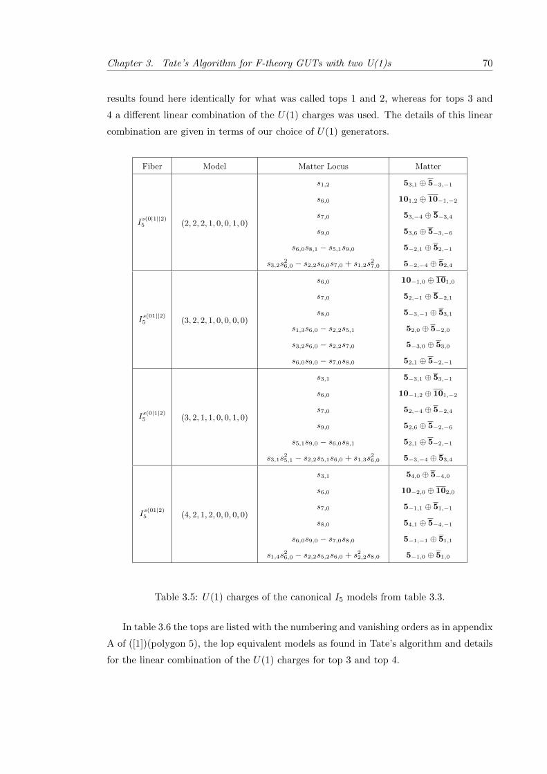
Chapter 3. Tate’s Algorithm for F-theory GUTs with two U(1)s 70
results found here identically for what was called tops 1 and 2, whereas for tops 3 and
4 a different linear combination of the U(1) charges was used. The details of this linear
combination are given in terms of our choice of U(1) generators.
Fiber Model Matter Locus Matter
Is(0|1||2)5 (2, 2, 2, 1, 0, 0, 1, 0)
s1,2
s6,0
s7,0
s9,0
s6,0s8,1 − s5,1s9,0
s3,2s26,0 − s2,2s6,0s7,0 + s1,2s
27,0
53,1 ⊕ 5−3,−1
101,2 ⊕ 10−1,−2
53,−4 ⊕ 5−3,4
53,6 ⊕ 5−3,−6
5−2,1 ⊕ 52,−1
5−2,−4 ⊕ 52,4
Is(01||2)5 (3, 2, 2, 1, 0, 0, 0, 0)
s6,0
s7,0
s8,0
s1,3s6,0 − s2,2s5,1
s3,2s6,0 − s2,2s7,0
s6,0s9,0 − s7,0s8,0
10−1,0 ⊕ 101,0
52,−1 ⊕ 5−2,1
5−3,−1 ⊕ 53,1
52,0 ⊕ 5−2,0
5−3,0 ⊕ 53,0
52,1 ⊕ 5−2,−1
Is(0|1|2)5 (3, 2, 1, 1, 0, 0, 1, 0)
s3,1
s6,0
s7,0
s9,0
s5,1s9,0 − s6,0s8,1
s3,1s25,1 − s2,2s5,1s6,0 + s1,3s
26,0
5−3,1 ⊕ 53,−1
10−1,2 ⊕ 101,−2
52,−4 ⊕ 5−2,4
52,6 ⊕ 5−2,−6
52,1 ⊕ 5−2,−1
5−3,−4 ⊕ 53,4
Is(01|2)5 (4, 2, 1, 2, 0, 0, 0, 0)
s3,1
s6,0
s7,0
s8,0
s6,0s9,0 − s7,0s8,0
s1,4s26,0 − s2,2s5,2s6,0 + s22,2s8,0
54,0 ⊕ 5−4,0
10−2,0 ⊕ 102,0
5−1,1 ⊕ 51,−1
54,1 ⊕ 5−4,−1
5−1,−1 ⊕ 51,1
5−1,0 ⊕ 51,0
Table 3.5: U(1) charges of the canonical I5 models from table 3.3.
In table 3.6 the tops are listed with the numbering and vanishing orders as in appendix
A of ([1])(polygon 5), the lop equivalent models as found in Tate’s algorithm and details
for the linear combination of the U(1) charges for top 3 and top 4.

Chapter 3. Tate’s Algorithm for F-theory GUTs with two U(1)s 71
Top Fiber Vanishing Orders Lop-equivalent model U(1) Linear Combination
Top 1 Is(0|1|2)5 (2, 2, 2, 0, 0, 1, 0, 0) (3, 2, 1, 1, 0, 0, 1, 0) -
Top 2 Is(0|1||2)5 (1, 2, 3, 0, 0, 1, 0, 0) (2, 2, 2, 1, 0, 0, 1, 0) -
Top 3 Is(01||2)5 (1, 1, 2, 0, 0, 2, 0, 0) (3, 2, 2, 1, 0, 0, 0, 0)
u1 = −w1
u2 = 15(w2 − w1)
Top 4 Is(01|2)5 (1, 1, 1, 0, 0, 2, 0, 1) (4, 2, 1, 2, 0, 0, 0, 0)
u1 = −w1
u2 = 15(w2 − w1)
Table 3.6: The lop-equivalent models of the four tops from ([1]). The linear combination
of the U(1) charges gives the charges found in table 3.5, u1 and u2, in terms of the U(1)
charges of the top model, w1 and w2. The reason the charges of tops 3 and 4 differ is
because the lop translation involves the Z2 symmetry, which exchanges two of the marked
points.
3.4.2 Non-canonical I5 Models
Listed in tables 3.9 to 3.11 are the U(1) charges of the, respectively once, twice, and
thrice, non-canonical I5 models found in the algorithm. The U(1) charge generators are
given by the Shioda map, as described in section 3.2.3, where the zero-section of the
fibration corresponds to the divisor l1 = 0 after the P2 fibration ambient space has been
blown up into dP2. As opposed to the canonical models the majority of the models
tabulated in this section were previously unknown. Some of these models appear to have
interesting properties for phenomenology, such as the above noted multiple differently
charged 10 and 5 curves.
While Tate’s algorithm provides a generic procedure there are some caveats that were
introduced in the application of it studied in this chapter. There are situations where
we were not able to solve for the enhancement locus in the discriminant to a reasonable
degree of generality. In these cases we have sometimes, as discussed in section 3.3, used a
less generic solution where it was obtainable in such a way that it did not lead to obvious
irregularities with the model. In cases where no such solution was obtained we have left
that particular subbranch of the Tate tree unexplored.
Throughout the application of Tate’s algorithm the fibrations have remained inside
the chosen lop-equivalence class and so each each model in these tables then represents an
entire lop-orbit of fibrations. The Z2 symmetry which acts inside this orbit interchanges

Chapter 3. Tate’s Algorithm for F-theory GUTs with two U(1)s 72
two of the three marked points of the fibration, which correspond, in the dP2 hypersurface,
to the exchange of l1 and l2. As the U(1) charges are computed from a Shioda map
where the zero-section is taken to be l1 = 0 the U(1) charges are rewritten as a linear
combination under this symmetry in an identical manner to the linear combinations
occurring in the tops in table 3.6.
One may point out the surprising paucity of non-minimal matter loci in these mod-
els with highly specialised coefficients. In the fibrations which are at least twice non-
canonical there can occur polynomial enhancement loci where some of the terms in the
solutions (as given in appendix A.1) are fixed by a coprimality condition coming from a
previously solved polynomial. Were these terms not fixed to unity by the algorithm then
they would contribute non-minimal loci to the fibrations.
In ([1, 51]) there were listed tops corresponding to an SU(4) non-abelian singularity
with two additional rational sections, and it was noted that one expects multiple 10
matter curves where these tops are specialized with some non-generic coefficients of the
defining polynomial, and such a model, which realizes multiple 10 curves, was constructed
there from the SU(4) tops. Included in table 3.7 are the relations (via the lops) between
these SU(4) tops and the SU(4) canonical models which underlie the once non-canonical
SU(5) models obtained in the algorithm.
Top Model Fiber Vanishing Orders Lop-equivalent Model
Top 1 I(0|1|2)4 (1, 1, 2, 0, 0, 1, 0, 0) (2, 1, 1, 1, 0, 0, 1, 0)
Top 2 I(01||2)4 (0, 1, 2, 0, 0, 2, 0, 0) (2, 2, 2, 1, 0, 0, 0, 0)
Top 3 I(01|2)4 (1, 1, 1, 0, 0, 1, 0, 1) (3, 2, 1, 1, 0, 0, 0, 0)
Top 4 I(01||2)4 (0, 1, 2, 0, 0, 1, 0, 1) (2, 2, 2, 1, 0, 0, 0, 0)
Top 5 I(01|2)4 (0, 0, 1, 0, 0, 2, 0, 1) (3, 2, 1, 1, 0, 0, 0, 0)
Table 3.7: The SU(4) tops associated to polygon 5 in appendix B of ([1]) are related to
the canonical I4 models listed in table 3.2 by lop-equivalence.
Note that for SU(4) top 4 is lop equivalent to top 2 and top 5 is lop equivalent top
3, and their U(1) charges, as listed in appendix B of ([1]), can be written as a linear
combination of the lop-equivalent model.

Chapter 3. Tate’s Algorithm for F-theory GUTs with two U(1)s 73
Fiber Model Matter Locus Matter
Is(0|1||2)5
(2, 2, 2, 0, 0, 0, 0, 0)
[−,−,−, σ2σ5, σ2σ4 + σ3σ5, σ3σ4, σ1σ2, σ1σ3]
σ1
σ3
σ4
σ2σ4 − σ3σ5
(A.2.1)
(A.2.2)
(A.2.3)
5−3,−6 ⊕ 53,6
52,−6 ⊕ 5−2,6
5−3,4 ⊕ 53,−4
10−1,−2 ⊕ 101,2
5−3,−1 ⊕ 53,1
52,−1 ⊕ 5−2,1
52,4 ⊕ 5−2,−4
Is(0|1|2)5
(2, 1, 1, 1, 0, 0, 1, 0)
[σ1σ3, σ1σ2,−, σ3σ4, σ2σ4,−,−,−]
σ2
σ4
s7,0
s9,0
σ4s3,1 − σ1s7,0
σ2s8,1 − σ3s9,0
(A.2.4)
101,−2 ⊕ 10−1,2
101,3 ⊕ 10−1,−3
5−2,4 ⊕ 52,−4
5−2,−6 ⊕ 52,6
53,−1 ⊕ 5−3,1
53,4 ⊕ 5−3,−4
5−2,−1 ⊕ 52,1
Is(0|1||2)5
(2, 1, 1, 1, 0, 0, 1, 0)
[−, σ1σ2, σ1σ3,−, σ2σ4, σ3σ4,−,−]
σ2
σ3
σ4
s9,0
σ4s1,2 − σ1s5,1
σ2σ4s8,1 − s5,1s9,0
(A.2.5)
10−1,−2 ⊕ 101,2
5−3,4 ⊕ 53,−4
10−1,3 ⊕ 101,−3
5−3,−6 ⊕ 53,6
5−3,−1 ⊕ 53,1
52,4 ⊕ 5−2,−4
52,−1 ⊕ 5−2,1
Is(1|0|2)5
(3, 2, 1, 1, 0, 0, 0, 0)
[−,−,−,−, σ1σ2, σ1σ3, σ2σ4, σ3σ4]
σ1
σ2
σ3
σ4
s3,1
(A.2.6)
(A.2.7)
10−2,2 ⊕ 102,−2
103,2 ⊕ 10−3,−2
5−1,6 ⊕ 51,−6
54,6 ⊕ 5−4,−6
54,1 ⊕ 5−4,−1
5−1,1 ⊕ 51,−1
5−1,−4 ⊕ 51,4
Table 3.8: U(1) charges of the once non-canonical I5 models from table 3.3.

Chapter 3. Tate’s Algorithm for F-theory GUTs with two U(1)s 74
Fiber Model Matter Locus Matter
Is(01|2)5
(3, 2, 1, 1, 0, 0, 0, 0)
[σ2σ5, σ2σ4 + σ3σ5, σ3σ4, σ1σ2, σ1σ3,−,−,−]
σ1
σ3
σ4
s7,0
s8,0
σ1σ3s9,0 − s7,0s8,0
(A.2.8)
102,0 ⊕ 10−2,0
10−3,0 ⊕ 103,0
5−4,0 ⊕ 54,0
51,−1 ⊕ 5−1,1
5−4,−1 ⊕ 54,1
51,1 ⊕ 5−1,−1
51,0 ⊕ 5−1,0
Is(1|02)5
(4, 2, 0, 2, 0, 0, 0, 0)
[−,−, σ3σ4,−, σ2σ4 + σ3σ5, σ1σ3, σ2σ5, σ1σ2]
σ1
σ2
σ3
σ4
σ5
σ2σ4 − σ3σ5
(A.2.9)
(A.2.10)
50,6 ⊕ 50,−6
51,6 ⊕ 5−1,−6
5−1,1 ⊕ 51,−1
51,1 ⊕ 5−1,−1
5−1,−4 ⊕ 51,4
100,2 ⊕ 100,−2
50,−4 ⊕ 50,4
50,1 ⊕ 50,−1
Is(012)5
(5, 2, 0, 2, 0, 0, 0, 0)
[−, σ1σ2, σ2σ5, σ1σ3, σ2σ4 + σ3σ5,−, σ3σ4,−]
σ2
σ3
σ4
σ5
σ2σ4 − σ3σ5
σ3s7,0 − σ2s9,0
σ4s7,0 − σ5s9,0
(A.2.11)
5−1,0 ⊕ 51,0
51,1 ⊕ 5−1,−1
5−1,−1 ⊕ 51,1
51,0 ⊕ 5−1,0
100,0 ⊕ 100,0
50,−1 ⊕ 50,1
50,1 ⊕ 50,−1
50,0 ⊕ 50,0
Table 3.9: U(1) charges of the once non-canonical I5 models from table 3.3 (continued).

Chapter 3. Tate’s Algorithm for F-theory GUTs with two U(1)s 75
Fiber Model Matter Locus Matter
Is(01||2)5
(2, 2, 2, 0, 0, 0, 0, 0)
[ξ3ξ4, ξ2ξ4 + ξ3ξ5, ξ2ξ5, σ3ξ3, σ2ξ3 + σ3ξ2, σ2ξ2,−,−]
ξ2
σ2
σ2ξ3 − σ3ξ2
σ2ξ4 − σ3ξ5
ξ2s8,0 − ξ3s9,0
σ2s8,0 − σ3s9,0
(A.2.12)
53,−1 ⊕ 5−3,1
5−2,1 ⊕ 52,−1
101,0 ⊕ 10−1,0
53,0 ⊕ 5−3,0
53,1 ⊕ 5−3,−1
5−2,−1 ⊕ 52,1
5−2,0 ⊕ 52,0
Is(0|1||2)5
(2, 1, 1, 1, 0, 0, 0, 0)
[−, σ1ξ3, σ1ξ2,−, σ4ξ3, σ4ξ2, ξ3ξ4, ξ2ξ4]
ξ2
ξ3
ξ4
σ4
(A.2.13)
(A.2.14)
(A.2.15)
52,−6 ⊕ 5−2,6
10−1,−2 ⊕ 101,2
5−3,−6 ⊕ 53,6
10−1,3 ⊕ 101,−3
52,−1 ⊕ 5−2,1
5−3,−1 ⊕ 53,1
52,4 ⊕ 5−2,−4
Is(01||2)5
(2, 1, 1, 1, 0, 0, 0, 0)
[ξ3ξ4, σ2ξ3, σ3ξ3, ξ2ξ4 + ξ3ξ5, σ2ξ2, σ3ξ2, ξ2ξ5,−]
ξ2
ξ5
σ2
σ3
ξ2ξ5σ2 − σ3s9,0
(A.2.16)
(A.2.17)
101,1 ⊕ 10−1,−1
53,1 ⊕ 5−3,−1
5−2,1 ⊕ 52,−1
101,0 ⊕ 10−1,0
5−2,−1 ⊕ 52,1
53,0 ⊕ 5−3,0
5−2,0 ⊕ 52,0
Is(1|0|2)5
(2, 1, 1, 1, 0, 0, 0, 0)
[σ3σ4, σ3ξ1ξ3,−, σ2σ4 + σ3ξ1ξ2, σ2ξ1ξ3, ξ3ξ4, σ2ξ1ξ2, ξ2ξ4]
ξ1
ξ2
ξ3
ξ4
σ2
ξ3ξ4σ3 − σ2s3,1
(A.2.18)
(A.2.19)
103,2 ⊕ 10−3,−2
54,6 ⊕ 5−4,−6
10−2,2 ⊕ 102,−2
5−1,6 ⊕ 51,−6
10−2,−3 ⊕ 102,3
54,1 ⊕ 5−4,−1
5−1,−4 ⊕ 51,4
5−1,1 ⊕ 51,−1
Is(0|2||1)5
(1, 1, 1, 1, 0, 0, 1, 0)
[ξ2ξ3ξ5ξ6, ξ3ξ6σ4 + ξ2ξ5σ3, σ3σ4,
ξ2ξ6ξ7 + ξ3ξ4ξ5, ξ1ξ2ξ3ξ6, ξ1ξ2σ3, ξ4ξ7, ξ1ξ3ξ4]
ξ3
ξ4
ξ5
ξ6
ξ8
σ3
(A.2.20)
(A.2.21)
103,−1 ⊕ 10−3,1
54,2 ⊕ 5−4,−2
103,4 ⊕ 10−3,−4
103,4 ⊕ 10−3,−4
54,7 ⊕ 5−4,−7
54,−3 ⊕ 5−4,3
5−1,−3 ⊕ 51,3
5−1,2 ⊕ 51,−2
Table 3.10: U(1) charges of the twice non-canonical I5 models from table 3.3.

Chapter 3. Tate’s Algorithm for F-theory GUTs with two U(1)s 76
Fiber Model Matter Locus Matter
Is(0|1||2)5
(1, 1, 1, 0, 0, 0, 0, 0)
[ξ3δ3δ4, δ4(δ3ξ2 + δ2ξ3), ξ2δ2δ4,
ξ3δ1δ4, δ1(δ2ξ3 + δ3ξ2), δ1δ2ξ2, σ1ξ3, σ1ξ2]
δ1
δ2
ξ2
σ1
ξ2δ3 − ξ3δ2
(A.2.22)
(A.2.23)
(A.2.24)
101,−3 ⊕ 10−1,3
53,−4 ⊕ 5−3,4
5−2,6 ⊕ 52,−6
53,6 ⊕ 5−3,−6
101,2 ⊕ 10−1,−2
5−2,1 ⊕ 52,−1
53,1 ⊕ 5−3,−1
5−2,−4 ⊕ 52,4
Table 3.11: U(1) charges of the single thrice non-canonical I5 model from table 3.3.
3.5 Exceptional Singular Fibers
In this section the algorithm is continued up to the exceptional singular fibers. In de-
termining the exceptional fibers we recall that the sections can only intersect the fiber
components of multiplicity one, which means that there is a very restricted number of
singular fibers.
For what concerns the type IV ∗ singular fiber there are three different ways in
which the sections can intersect the multiplicity one components. These are the types
IV ∗(012), IV ∗(01|2) and IV ∗(0|1|2). As can be seen from figure 3.6 the three multiplicity one
components of the IV ∗ singular fiber appear symmetrically, and so sections separated by
a slash merely indicates that they do not intersect the same multiplicity one component.
Regarding the singular III∗ fibers, the possible ways the sections can intersect the
components restrict the range of singular fibers to III∗(012) and III∗(01|2). The different
singular fibers can be seen in figure 3.7.
Finally it is clear that the only type II∗ fiber one could find (since there is only one
multiplicity one component) is the II∗(012). This fiber is also shown in figure 3.7.
It was also possible to obtain the singular fibers corresponding to gauge groups G2
and F4 which come from, respectively, the non-split singular fiber types I∗ns(012)0 and
IV ∗ns(012).
Proceeding through these subbranchs of the Tate tree will involve the I∗n fibers corre-
sponding to Dynkin diagrams of D-type in the split case. There fibers are composed of a
chain of multiplicity two nodes with two multiplicity one nodes connected to each end of
the chain. As the rational sections can only intersect the multiplicity one nodes they are

Chapter 3. Tate’s Algorithm for F-theory GUTs with two U(1)s 77
Figure 3.6: The type IV ∗s fibers. The sections, which intersect the components of
the IV ∗s fiber represented by the blue nodes, are seen to intersect only the external,
multiplicity one components. Because of the S3 symmetry we write these as IV ∗s(ijk),
IV ∗s(ij|k), and IV ∗s(i|j|k) respectively.
constrained to lie of these outer legs. The notation of these fibers shall be (01) represents
two sections on the same leg, (0|1) represents two section intersecting two of the outer
legs attached to the same end of the chain, and (0||1) will represent two sections sitting
on multiplicity one component separated by the length of the chain.
3.5.1 Canonical Enhancements to Exceptional Singular Fibers
The starting point for the enhancements to the possible canonical exceptional singular
fibers is the I∗ss(01|2)0 : (2, 2, 1, 1, 1, 0, 0, 0). Recall that one of the fiber components will
split only if the condition s25,1 − 4s1,2s8,0 = p2 is satisfied for some p. The discriminant
at sixth order takes the form
∆ = s27,0s
28,0(s2
5,1 − 4s1,2s8,0)(s1,2s27,0 − s3,1s5,1s7,0 + s2
3,1s8,0)2)z6 +O(z7) . (3.5.1)
First let z | s8 and the resulting fiber is of type Is(0|2||1)1 . The discriminant at seventh
order reads
∆ = s35,1s
37,0(s3,1s5,1 − s1,2s7,0)2s2
9,0z7 +O(z8) . (3.5.2)
Now let z2 | s5 and the first exceptional singular fiber is found; it is of type IV ∗(0|1|2)
IV ∗(0|1|2) : (2, 2, 1, 2, 1, 0, 1, 0) . (3.5.3)
This subbranch of the tree does not continue because the discriminant now takes the
form ∆ = s1,2s7,0s9,0z8 +O(z9) and the only possible enhancement that remains inside

Chapter 3. Tate’s Algorithm for F-theory GUTs with two U(1)s 78
Figure 3.7: The type III∗ and II∗ fibers. Shown are the two type III∗(ijk) and III∗(ij|k)
fibers where the sections are distributed over the two multiplicity one components, and
the single type II∗(ijk) fiber, which has all three sections intersecting the single multi-
plicity one component.
the lop-equivalence class, the vanishing of s1,2, is a non-minimal enhancement.
Looking back at the I∗0 starting point, the discriminant can instead be enhanced by
letting the three-term polynomial vanish, through the canonical solution s1,2 = s3,1 = 0.
This gives an I∗s(01||2)1 singular fiber. The discriminant at seventh order takes the form
∆ = s22,2s
35,1s
57,0s
28,0z
7 +O(z8) . (3.5.4)
The discriminant is enhanced further by letting s5,1 = 0. This gives the second excep-
tional singular fiber, that is a type IV ∗(01|2)
IV ∗(01|2) : (3, 2, 2, 2, 1, 0, 0, 0) . (3.5.5)
Proceeding in this subbranch, the discriminant now reads
∆ = s42,2s
47,0s
48,0z
8 +O(z9) . (3.5.6)
The only enhancement which is possible (as all the others are non-minimal enhancements)
is s2,2 = 0. The canonical excpetional singular fiber that arises from this enhancement
is III∗(01|2)
III∗(01|2) : (3, 3, 2, 2, 1, 0, 0, 0) . (3.5.7)
Every further enhancement in this subbranch is a non-minimal fibration.
3.5.2 Non-canonical Enhancements to Exceptional Singular Fibers
In this section the remaining exceptional fibers are obtained through non-canonical en-
hancements of the discriminant. The starting point is the singular Ins(012)3 given by the

Chapter 3. Tate’s Algorithm for F-theory GUTs with two U(1)s 79
vanishing orders (3, 2, 0, 2, 0, 0, 0, 0). The discriminant contains ∆ ⊃ (s26,0 − 4s3,0s8,0).
Following appendix A.1 it can be solved non-canonically to find a non-split I∗ns(012)0,nc
associated to gauge group G2
I∗ns(012)0,nc : (3, 2, 0, 2, 0, 0, 0, 0) [−,−, µσ2
3,−, 2µσ3σ8,−, µσ28,−] . (3.5.8)
The next exceptional singular fiber is found through the following series of enhancements
I∗ns(012)0,nc
s1,3,s2,2,s5,2=0−→ I
∗ns(012)1,nc
P=0−→ IV∗ns(012)nc2
P = (σ28s3,1 − σ3σ8s6,1 + σ2
3s8,1) .
(3.5.9)
Where the non-canonical solution to the three-term polynomial was applied to find a
singular IV∗ns(012)nc2
with gauge group F4
IV∗ns(012)nc2
: (4, 3, 0, 3, 0, 0, 0, 0) [−,−, µξ22+ξ2ξ5z,−, 2µξ2ξ3+(ξ2ξ4+ξ3ξ5)z,−, µξ2
3+ξ3ξ4z,−] .
(3.5.10)
It was also necessary to specialize terms linear in z in the expansion of the coefficients.
From this singular fiber the remaining two fiber types can be reached through
IV∗ns(012)nc2
s1,4=0−→ III
∗(012)nc2
Q=0−→ II∗(012)nc3
Q = (s5,3ξ2 − s2,3ξ3) .
(3.5.11)
The singular fibers obtained this way are type III∗(012)nc2
III∗(012)nc2
: (5, 3, 0, 3, 0, 0, 0, 0) [−,−, µξ22+ξ2ξ5z,−, 2µξ2ξ3+(ξ2ξ4+ξ3ξ5)z,−, µξ2
3+ξ3ξ4z,−] ,
(3.5.12)
and the singular fiber type II∗(012)nc3
II∗(012)nc3
: (5, 3, 0, 3, 0, 0, 0, 0)
[−, δ1δ3, µδ23 + δ3ξ5z, δ1δ2, 2µδ2δ3 + (δ3ξ4 + δ2ξ5)z,−, µδ2
2 + δ2ξ4z,−] .
(3.5.13)

Chapter 4
Aspects of M-Theory
In Chapter 2 we encountered M-Theory through a chain of dualities relating it to F-
Theory. In this chapter we are going to study it in its own right, as the non-perturbative
limit of Type IIA string theory, whose low energy limit is 11-dimensional supergravity. In
([2]) Witten was then able to relate the known string theories to a single 11-dimensional
theory, then called M-Theory. The perturbative limit could be re-obtained by compact-
ifying M-Theory on a circle, whose radius was found to be proportional to the string
coupling gs of Type IIA string theory. Through T-duality and S-duality, and thanks to
the statement that the low energy limit of M-Theory compactified on an interval S1/Z2
is found to be the Heterotic E8 ×E8 string theory ([86]), it was possible to relate all the
known string theories to one higher dimensional theory.
Nevertheless, very little was known about M-Theory and still today a great part of it
remains unexplored. The reason behind this, is that perturbation theory has no access
to it due to the absence of the string coupling. This fact is indeed signalling that the
fundamental string is not part of the theory any more, but is replaced by membranes and
fivebranes, also known as M2 and M5-branes. However, the dynamics of such branes is
not inferable from that of D-branes exactly for the lack of fundamental strings. While the
worldvolume theories on stacks of D-branes can be extracted from open string scatterings,
the same does not hold for M-branes. Indeed, M5-branes interact through M2-branes,
but the scattering of the latter has not yielded the same results of strings scattering.
As a consequence, M-Theory has only a non-perturbative regime, into which it has been
hard to gain insight. However, it has provided a unified perspective which has helped to
understand many aspects of 10-dimensional string theories and lower dimensional field
theories.
In particular, the worldvolume theories on stacks of M2 and M5-branes have been
80

Chapter 4. Aspects of M-Theory 81
two of the problems of the string theory program which have received most attention in
the last years. In this chapter, we review recent progress in the understanding of such
theories. The dynamics on parallel M2-branes has advanced considerably in the last years,
while the one on parallel M5-branes is still largely unexplored. Both the BLG (Bagger-
Lambert-Gustavvson)([3,4]) and the ABJM (Aharony-Bergman-Jafferis-Maldacena) ([5])
models allowed to gain great insight into the theories of coincident M2-branes. On the
other hand, a framework in which progress has been achieved towards theories of multiple
M5-branes in M-Theory, is the one of higher gauge theory, see e.g. ([87–90]). Such
theories are a ‘categorification’ of usual gauge theory, where the latter are described by
a principle bundle over space-time, allowing to define the parallel transport of point-
particles. This can be understood in the D-brane picture as the parallel transport of the
end-points of the strings through which D-branes interact. However, the mirror picture
for membranes in M-Theory requires the parallel transport of string-like objects (since
interactions are through M2-branes, whose boundaries are 1-dimensional). It turns out
that taking into account the parallel transport of strings requires the ‘categorification’ to
higher gauge structures, i.e. one needs to consider 2-bundles (or higher structures) rather
than usual vector bundles. This means considering a functor between two categories
rather than a morphism between two objects of a category, i.e. the usual vector bundles
in gauge theory. We will not investigate further this direction, but the BLG, ABJM
models and the Lambert-Papageorgakis model for M5-branes, which we will discuss later,
have been shown to be expressible in the framework of higher gauge theory ([91,92]).
Nevertheless, the theory on coincident M5 has produced, through different compact-
ifications, a number of results and dualities in lower dimensional field theories that we
also review in the following.
4.1 M-Theory and M-Branes
M2 and M5-branes are half BPS solution of 11-dimensional supergravity, the low energy
theory describing M-Theory. Recall the field content of 11d supergravity. We have the
metric (graviton) gµν(x), µ, ν = 0, 1, . . . , 10 which constitutes 44 degrees of freedom
on shell, being a symmetric traceless tensor. The other 84 bosonic degrees of freedom
is represented by a three form C3 = Cµνλ. The super-partner of the graviton is the
gravitino Ψµα, transforming in a tensor product representation of a space-time vector
and a spinor. On shell, the gravitino contributes indeed the 128 degrees of freedom
needed for supersymmetry. The action for 11-dimensional supergravity turns out to be
unique and it was found in the seminal paper by Cremmer, Julia and Scherk and its

Chapter 4. Aspects of M-Theory 82
bosonic part is ([93,94])
S11 ⊃∫d11x
√|g|R−
(1
2F ∧ ?F +
1
6C3 ∧ F ∧ F
), (4.1.1)
where F is the field strength of the potential C3 and R is the Ricci scalar of space-time.
The relationship between 11-dimensional supergravity and the 10-dimensional super-
gravity theories has been elucidated in a number of papers ([95–97]). The 10-dimensional
theory turns out to be recovered in the limit in which the 11-dimensional one is studied
on a space of the form M10 × S1, and the radius R of the circle vanishes. Such relation
between supergravity theories was finally interpreted in the seminal papers by Townsend
([98]) and Witten ([2]). Type IIA string theory, being the UV completion of Type IIA su-
pergravity, is understood as the compactification of a new theory, then called M-Theory,
on a circle. In particular, the relation between the radius of the circle and the coupling
constant gs is found to be
R = gs ls, (4.1.2)
where ls is the string length. We see that upon reducing on the circle the perturba-
tive limit in gs is restored, but in the decompactification limit M-theory results to be the
strongly coupled regime of type IIA string theory. In particular we see that in the strongly
coupled phase of type IIA an extra dimension opens up. However, 11-dimensional su-
pergravity, and therefore M-theory, do not have a dimensionless parameter about which
it would be possible to expand. It follows that, without any perturbative access to it,
M-Theory remains greatly unexplored. In the following, we will look at the fundamental
objects of M-Theory, which will turn out to be membranes rather than strings.
In order to find the BPS solutions one looks at the gravitino supersymmetry variation
([94])
δΨµα = Dµ(ω)ε+i
288
(Γνλστωµ − 8Γλστωδνµ
)Fνλστωε ≡ 0 (4.1.3)
where Dµ(ω) is the covariant derivative depending on the spin connection. Solutions were
found describing half BPS objects which are now known as M2 and M5-branes. Without
going into the details of the actual supergravity solutions, we can get a hint as to why
we must have such solutions by looking at the superalgebra associated to 11-dimensional
supergravity
Qα, Qβ = (ΓµC−1)αβPµ +1
2(ΓµνC−1)αβZµν +
1
5!(ΓµνλρσC−1)Zµνλρσ. (4.1.4)
The presence of the central charges Zµν and Zµνλρσ signal the existence of respectively
two and five dimensional object in space. A similar argument follows from the potential

Chapter 4. Aspects of M-Theory 83
three-form C3 which couples electrically to the worldvolume S of M2-branes through∫S C3 ≡
∫S Cµνλdx
µ ∧ dxν ∧ dxλ, where we pull-back the C3 form to the worldvolume of
the M2-brane. Similarly we find the magnetic coupling by applying Hodge duality to the
field strength of C3
C3 −→ F4?−→ F7 −→ C6. (4.1.5)
Then we can pull-back C6 to the worldvolume W of M5-branes via∫W C6 to obtain the
correct coupling. As we saw, reducing on a circle we recover the perturbative limit of
type IIA string theory, which means that by reducing the M2 and the M5-branes we
should recover the D-branes present in type IIA (see e.g. ([98–100]) for a more complete
discussion). This is indeed the case and we can see that we must have that the M2-brane
reduces to the fundamental string F1 when it wraps the M-Theory circle, or to the D2-
brane when the worldvolume is transverse to the M-Theory circle S1M (see ([101–103])
for a discussion in the case of the BLG model). Similarly, the M5-brane reduces to the
D4-brane when wrapping S1M (see ([104, 105]) for a more accurate discussion) and to
the NS5-brane when its worldvolume is transverse to S1M . Obtaining D0 and D6 branes
is more complicated, but it turns out that the former correspond to momentum modes
along the M-Theory circle ([98]) which indeed needs to be quantised. D6-branes, which
are related by electric-magnetic duality to D0-branes (which couple in type IIA to the
Ramond-Ramond gauge field Aµ)
Aµ −→ F2?−→ F8 −→ C7, (4.1.6)
lift to Kaluza-Klein monopoles ([98]) in M-Theory, that is supergravity solutions of the
form R1,7 × T B where T B is the multi-centered Taub-NUT space.
Therefore from M-Theory we can recover all the D-branes of Type II string theories,
by first compactifying on the M-Theory circle and taking the low energy limits of the
worldvolume theories on stacks of M2 and M5-branes, and then by possibly T-dualizing
to obtain the D-branes of Type IIB string theory ([106]).
4.2 Degrees of Freedom on Parallel M-Branes
Whereas the theories on a stack of D-branes are all related by dimensional reduction and
can be obtained from 10-dimensional maximally supersymmetric Yang-Mills Theory, an
equally simple description is not available for M-branes. Without a coupling constant,
M-Theory allows only a non-perturbative regime and the theories of M2 and M5-branes
cannot be obtained from open string scatterings such as in the case of D-branes.

Chapter 4. Aspects of M-Theory 84
A first puzzle about the M2 and M5 worldvolume theories was related to the degrees
of freedom of the two theories. Gauge theories on the worldvolume of N coincident D-
branes were known to have a number of degrees of freedom proportional to N2, which
is in accord with the degrees of freedom of U(N) gauge theories or equivalently with
the number of Chan-Paton factors for an open string ending on a stack of N D-branes.
However, when such degrees of freedom were investigated for the worldvolume theories of
N coincident M2 and M5-branes, the degrees of freedom were found to be proportional
to N3/2 and N3 respectively ([107]). The origin of such degrees of freedom is still not
well understood, but the candidate theories describing such theories should correctly
reproduce such scaling of the degrees of freedom (in a sense the N3 scaling for the M5
theories can be understood from the existence of a BPS state in which the M2-brane
has three disconnected boundaries (like a higher dimensional pair of pants) and since
M5-branes are supposed to interact through M2-branes the analogy with D-branes and
open strings is clear).
In the following we will focus in turn on both the theory describing N coincident M5-
branes and N coincident M2-branes. Both theories are supposed to be superconformal
field theories (due to the absence of a characteristic length in M-Theory) in 3 and 6
dimensions respectively, and should preserve 16 supercharges, being half BPS object of
11-dimensional supergravity. A considerable progress has been made in the past 10 years
in the description of coincident M2-branes. First through the BLG model, which correctly
reproduces the dynamics of two M2-branes and successively through the ABJM model
describing an arbitrary number of coincident M2-branes in an orbifold background C/Zk(where k appears as the level of the Chern-Simons term of the ABJM model). The theory
describing coincident M5-branes, known as the (2,0) theory, has instead remained more
elusive, but it nevertheless gave rise to a series of results and dualities between quantum
field theories in different dimensions.
4.3 M2-Branes
The BLG model provides a correct description of a pair of M2-branes satisfying all the
properties required: superconformal invariance, existence of 16 supercharges and of an
SO(8) R-symmetry, N3/2 scaling of the degrees of freedom and presence of non-trivial
interactions. What came as a surprise was that the gauge symmetry is realized through a
so-called 3-algebra rather than through usual Lie algebras. The hint that a different gauge
structure was needed to describe parallel M2-branes came from the work of Basu and
Harvey ([108]), who first proposed an equation describing coincident M2-branes ending

Chapter 4. Aspects of M-Theory 85
on a single M5-brane.
Recall the similar situation in the case of Dp-D(p+2) branes, where we look at a D1-
D3 system as in Table 4.1. The three scalars Xi parametrizing the directions of motion
0 1 2 3 4 5 6 7 8 9
D3 × × × × · · · · · ·
D1 × · · · × · · · · ·
Table 4.1: The D1-D3 system described by Nahm’s equation.
of the D1-strings transversal to the D3-brane (since the boundary of the D1-strings is
codimension three inside the D3-brane), satisfy the following Nahm equation ([109])
dXi
dt=
1
2εijk[Xj , Xk], (4.3.1)
where t is a coordinate on the longitudinal direction parametrizing the distance from the
D3-brane. As it is well known a solution is provided by a fuzzy sphere S2, whose radius
diverges at the location of the D3-brane, given by ([109–111])
Xi =1
2tσi, (4.3.2)
where σi are the generators of SU(2) and satisfy the usual commutation relations. Basu
and Harvey ([108]) tried to lift such a configuration to M-Theory and describe coincident
M2-branes ending on a single M5-brane, as in Table 4.2.
0 1 2 3 4 5 6 7 8 9 10
M5 × × × × × × · · · · ·
M2 × × · · · · × · · · ·
Table 4.2: The M2-M5 system described by the Basu-Harvey equation.
Now the four scalars Xa which parametrize the degrees of freedom of the boundary
of the M2-branes inside the M5, need to satisfy the following equation ([108])
dXa
dt+k
4!εabcd[G,Xb, Xc, Xd] = 0, (4.3.3)

Chapter 4. Aspects of M-Theory 86
where k is a constant and G is a fixed matrix which satisfies G2 = 1. It turns out
that a solution is given by a fuzzy S3, but most importantly we see the appearance of a
multi-linear bracket which will be fundamental in the description of the BLG model. In
particular the Basu-Harvey equation can be recast in the form
dXa
dt+
1
4!εabcd[Xb, Xc, Xd] = 0, (4.3.4)
where [ , , ] is the bracket of a 3-algebra. We now turn to the study of such algebraic
structures.
4.4 3-Algebras and the BLG Model
Recall that in Super-Yang-Mills theories (on parallel D-branes) a global gauge transfor-
mation for a field Φ is given by
δΦ = [α,Φ], (4.4.1)
where both α and Φ are matrices in some Lie algebra. In particular the fields were
expanded in a vector space with basis T a such that Φ = ΦaTa. Then the gauge
structure followed from the antisymmetric product
[T a, T b] = fab c Tc, (4.4.2)
where fab c are antisymmetric in the upper indices. Then imposing that variations act
as derivations
δ([X,Y ]) = [δX, Y ] + [X, δY ], (4.4.3)
we find the Jacobi identity
[[X,Y ], Z] + [[Z,X], Y ] + [[Y, Z], X] = 0. (4.4.4)
In order to lift the gauge structure to a 3-bracket, we again expand the field in some
basis of a vector space T a, but we define global transformations as
δΦ = [α, β,Φ]. (4.4.5)
The antisymmetric triple product can be expanded in a basis of the vector space through
the structure constants
[T a, T b, T c] = fabcd Td, (4.4.6)

Chapter 4. Aspects of M-Theory 87
which are antisymmetric in the upper indices. Then requiring the derivation property
imposes a Jacobi-like identity, known as the fundamental identity
[X1, X2, [X3, X4, X5]] = [[X1, X2, X3], X4, X5] + [X3, [X1, X2, X4], X5]
+ [X3, X4, [X1, X2, X5]]. (4.4.7)
Therefore we can define a 3-algebra as a vector space endowed with a totally antisym-
metric 3-bracket which satisfies the fundamental identity. As for the case of metric Lie
algebras, we require the existence of a symmetric inner product
hab = 〈T a, T b〉. (4.4.8)
Requiring invariance of the inner product imposes
〈[W,X, Y ], Z〉 = 〈W, [X,Y, Z]〉, (4.4.9)
or equivalently the structure constants must be totally antisymmetric when all the indices
are raised
fabcd = f [abcd]. (4.4.10)
It turns out that the existence of a positive definite metric 3-algebra is a very strict
requirement, and there exists only one such 3-algebra, see ([112, 113]) for proofs, up
to taking direct sums, which is called A4. It is a 4-dimensional 3-algebra, with four
generators T a, with the 3-bracket defined by
fabcd =2π
kεabcd, (4.4.11)
where εabcd is the totally antisymmetric Levi-Civita tensor and k is a constant.
We can now formulate BLG model ([3, 4]). Let the Lorentz symmetry be broken as
SO(1, 10)→ SO(1, 2)× SO(8)R (4.4.12)
and let XI (I = 3, 4, . . . , 10) be eight scalars parametrizing the transverse fluctuations to
the branes worldvolume. In order to have supersymmetry we then need eight fermionic
degrees of freedom, which are realized from the 32 degrees of freedom of an 11-dimensional
Majorana spinor ψ, upon which we impose the following projection condition
Γ012ε = ε Γ012ψ = −ψ, (4.4.13)
(where ε is the supersymmetry parameter) which reduces the degrees of freedom to 16.
Then on shell we have a match of bosonic and fermionic degrees of freedom. We assume
canonical dimensions of the fields in 3 dimensions
[X] = 1/2 [ψ] = 1 [ε] = −1/2. (4.4.14)

Chapter 4. Aspects of M-Theory 88
We promote the derivatives to covariant derivatives through the introduction of a gauge
field (Aµ)ba in the following way
DµΦa = ∂µΦa − (Aµ)baΦb, (4.4.15)
where µ = 0, 1, 2 and Φ is a generic field. As discussed, we already have a match of
bosonic and fermionic degrees of freedom, which seems to not allow the introduction of
a new gauge field. It will turn out that the gauge field will contribute no additional
degrees of freedom and will enter the theory through a Chern-Simons term but without
a canonical kinetic term. We can then define the field strength as
[Dµ, Dν ] ≡ Fµν . (4.4.16)
We can now write down the supersymmetry transformations, keeping in mind that since
ψ and ε have opposite chirality under Γ012 we must have an odd number of transverse
gamma matrices. The variations of the BLG model are ([3])
δXI = iεΓIψ
δψ = ΓµΓIDµXIε− 1
3!ΓIJK [XI , XJ , XK ]ε
δAµ(·) = iεΓµΓI [XI , ψ, ·], (4.4.17)
where (·) represents an arbitrary field. By requiring closure of the algebra it is found
that the 3-bracket needs to satisfy the fundamental identity, meaning that the fields are
valued in a 3-algebra. The algebra closes on shell through the following equations of
motion for the fields ([3])
0 =D2XI +1
2[[XI , XJ , XK ], XJ , XK ] +
i
2[ψ,ΓIJψ,XJ ]
0 =ΓαDαψ +1
2ΓIJ [ψ,XI , XJ ]
0 =Fαβ(·) + εαβγ
([XJ , DγXJ , ·] +
i
2[ψ,Γγψ, ·]
). (4.4.18)
These equations of motions are invariant under the supersymetry variations (4.4.17). We
can derive the equations of motion from the following Lagrangian
L = Lkin + Lint + Lpot + LCS . (4.4.19)
We have the kinetic terms for the bosonic and fermonic degrees of freedom
Lkin =1
2〈DµX
I , DµXI〉+i
2〈ψ,ΓµDµψ〉, (4.4.20)

Chapter 4. Aspects of M-Theory 89
followed by an interaction term of the form
Lint = − i4〈[ψ,XI , XJ ],ΓIJψ〉, (4.4.21)
and a potential term
Lpot =1
2 · 3!〈[XI , XJ , XK ], [XI , XJ , XK ]〉. (4.4.22)
Finally the Chern-Simons term can be written as
LCS =1
2εµνλ
(fabcd(Aµ)ab∂ν(Aλ)cd +
2
3f cdagf
efgb(Aµ)ab(Aν)cd(Aλ)ef
), (4.4.23)
where (Aµ)ba = f cdba(Aµ)cd. As previously mentioned, there is only one Euclidean 3-
algebra, the so-called A4. Two different groups correspond to this algebra, SO(4) and
Spin(4). An interpretation of the BLG model was found by studying the vacua of the
theory, which are obtained by minimising the potential, i.e.
[XI , XJ , XK ] = 0. (4.4.24)
It turns out that the brane interpretation depends on the level k of the Chern-Simons
term. In particular ([114–116]) we have a brane interpretation only in the following casesk = 1 Gauge Group = SO(4) −→ 2 M2-branes in R8
k = 2 Gauge Group = Spin(4) −→ 2 M2-branes in R8/Z2
k = 4 Gauge Group = SO(4) −→ 2 M2-branes in R8/Z2,
(4.4.25)
where in the last case a discrete torsion is present for the background four-form.
4.5 M5-Branes
The possible existence of a 6-dimensional superconformal theory first followed from
Nahm’s classification ([117]) of superconformal algebras, which showed that they ex-
isted only for space-time dimensions equal to and lower than six. In particular two
possible 6-dimensional superconformal algebras were shown to exist, the so-called (1, 0)
and (2,0) algebras. They differ in the amount of supersymmetry, 8 supercharges and 16
supercharges (the maximal amount in 6 dimensions) respectively, and on the R-symmetry
group, SU(2) for the (1,0) theory and SO(5) for the (2,0) theory.
From now on we will only focus on the latter, but interestingly progress has been
made recently on the former through F-Theoretic methods ([118]).

Chapter 4. Aspects of M-Theory 90
The existence of the (2,0) algebra in itself does not show that there must be an actual
field theoretic representation on 6-dimensional fields, or at least it does not demand the
existence of a field theory in the way we are used to think about it. Concrete evidence
for the existence of such a theory was brought forward by Witten ([119]) a few years
later. In particular, Witten looked at type IIB string theory on a space of the form
R1,3 × K3 at particular points of the moduli space of K3 surfaces. It is known that
at such points, a set of two-spheres in the K3 surfaces shrinks to zero size and they
follow an ADE classification depending on the number and the intersections of the two-
spheres in the K3 surface. In ([119]) it was argued that upon compactification of type IIB
string theory on K3 surfaces developing singularities at these points of the moduli space,
a superconformal field theory in 6-dimensions could be realized. Nevertheless, it was
realized that it could not have a simple perturbative description in terms of string states,
since by wrapping D3-branes along the two cycles of the K3 surface, strings were obtained
whose tension was proportional to the area of the cycles themselves. Therefore in the
singular limit in which the (2,0) theory was realized and the two-spheres shrank to zero
size, such strings would become tension-less. The (2,0) theories, which as we saw admit
an ADE classification, still lack a satisfying description, but they have nevertheless been
useful for numerous results and dualities for lower dimensional supersymmetric theories
related by a web of compactifications.
Following the work of Nahm ([117]), the (2,0) supersymmetry can be realized on an
abelian tensor multiplet consisting of five scalars XI , a self dual three-form Hµνλ and
the fermionic super-partners Ψ. The fields tranform under the Lorentz group SO(1, 5)
and the R-symmetry group SO(5)R ' Sp(4)R. Moreover we can take the dimensions of
the fields to be
[X] = 2 , [Ψ] = 5/2 , [H] = 3. (4.5.1)
This tensor multiplet describes a single M5-brane, where the five scalars parametrize the
transverse fluctuations to the brane in 11-dimensional space-time. We can write down
the supersymmetry variations of the fields in the following form ([6])
δXi = iεΓiΨ
δHµνλ = 3iεΓ[µνDλ]Ψ
δΨ = ΓµΓiDµXiε+
1
2 · 3!HµνλΓµνλε, (4.5.2)
where µ, ν = 0, 1, . . . , 5 and i, j = 6, 7, . . . , 10. The gamma matrices are 32 × 32 matrix

Chapter 4. Aspects of M-Theory 91
representations of the Clifford algebra in 11 dimensions and the H field is self dual
Hµνλ =1
6εµνλστωH
στω. (4.5.3)
The fermionic degrees of freedom Ψ and the supersymmetry parameter ε are 32 compo-
nents and satisfy the following chirality conditions
Γ012345ε = ε Γ012345Ψ = −Ψ. (4.5.4)
The following equations of motion are invariant under the (2,0) supersymmetry described
by the variations (4.5.2)
D2Xi = 0
ΓµDµΨ = 0
H = ?H dH = 0. (4.5.5)
Note that we could write a Lagrangian for the scalar fields Xi
SXi =
∫d6x DµX
iDµXi (4.5.6)
and for the Fermionic degrees of freedom
SΨ =
∫d6x ΨΓµDµΨ. (4.5.7)
Nevertheless we see that the usual action that we would write down for the H field
SH =
∫R1,5
H ∧ ?H, (4.5.8)
is of no use since H is self-dual and H ∧ ?H = H ∧ H = 0. A similar inconsistency in
deriving an action, pointed out in ([120]), is that if we consider the (2,0) theory on a
product manifold M5×S1 we see that in the low energy limit the theory on M5 should be
proportional to R−1 (where R is the radius of the circle S1) due to conformal invariance
in 6 dimensions, but at the same time it is clear that integrating over the circle direction
would give a factor of R in the low energy theory on M5 coming from√g in the action.
Nevertheless actions for a single M5-brane have been written down, see ([121–126]). We
now turn to the possible application of 3-algebras to the study of parallel M5-branes.

Chapter 4. Aspects of M-Theory 92
4.6 3-Algebras and M5-branes
In ([6]) the authors proposed a set of equations of motion for a non-abelian tensor mul-
tiplet in 6 dimensions invariant under (2,0) supersymmetry. In a similar fashion to the
construction of the BLG model, the authors proposed a non-abelian extension of the free
equations of motion, such that the fields are required to live in a generic vector space
endowed with an antisymmetric triple product. Closure of the supersymmetry algebra
then requires that the vector space be actually a 3-algebra, or equivalently that the triple
bracket should satisfy the fundamental identity (4.4.7). We will now look at the specifics
of such equations of motions and how the gauge symmetry is realized through 3-algebras
rather than usual Lie algebras. As in the BLG model, the introduction of a gauge field
covariantize the derivatives ([6])
DµΦa = ∂µΦa − (Aµ)baΦb, (4.6.1)
where Φ is a generic field which has been expanded in a basis T a of the 3-algebra as
Φ = ΦaTa. A fundamental difference to the BLG model is the necessary introduction
of a new field, a vector Y µ which will turn out not to transform under supersymmetry.
It is then possible to express the supersymmetry transformations which realize the (2,0)
algebra as follows, where we state again that the 3-algebra structure actually follows from
closure of the algebra on the non-abelian tensor multiplet ([6])
δXi = iεΓiΨ
δY µ = 0
δΨ = ΓµΓiDµXiε+
1
2 · 3!HµνλΓµνλε− 1
2ΓµΓij [Y µ, Xi, Xj ]ε
δHµνλ = 3iεΓ[µνDλ]Ψ + iεΓiΓµνλρ[Yρ, Xi,Ψ]
δAµ(·) = iεΓµν [Y ν ,Ψ, · ]. (4.6.2)
The conventions are the same of the previous section, where we presented the free tensor
multiplet. The Fermionic degrees of freedom satisfy the chirality conditions (4.5.4) and
a dot (·) represents an arbitrary field. Note that the gauge field can be taken to have
canonical dimension [Aµ] = 1, and it follows that the vector field Y µ has dimensions
[Y µ] = −1. These supersymmetry transformations close on the tensor multiplet if the

Chapter 4. Aspects of M-Theory 93
following equations of motion and constraints are satisfied ([6])
0 = D2Xi − i
2[Y µ, Ψ,ΓµΓiΨ]− [Y µ, Xj , [Yµ, X
j , Xi]]
0 = D[µHνλρ +1
4εµνλρστ [Y σ, Xi, DτXi] +
i
8εµνλρστ [Y σ, Ψ,ΓτΨ]
0 = ΓµDµΨ + ΓµΓi[Yµ, Xi,Ψ]
0 = Fµν(·)− [Y λ, Hµνλ, · ]
0 = DµYν = [Y µ, Y ν , ·] = [Y µ, Dµ(·), ·′]. (4.6.3)
Note that the constraint Fµν(·) = [Y λ, Hµνλ, · ] can be interpreted as the vanishing of
the so-called fake curvature in higher gauge theories. In that context, in order to have
a consistent parallel transport of 1-dimensional objects, such quantity needs to vanish
(see ([91,127]) for an interpretation of the Lambert-Papageorgakis model discussing such
aspects). Moreover it was shown in ([6]) that it is not possible to consistently define a
potential Bµν for the field strength Hµνλ. Since the vector Y µ is covariantly constant,
we can single out a direction in space-time and in the gauge algebra and study the set
of equations around a particular expectation value.
Recall that a Lorentzian 3-algebra can be constructed starting from a Lie algebra Gby adding two generators T± and defining the structure constants of the 3-algebra as
f+abc = fabc fabc − = fabc, (4.6.4)
where fabc are the structure constants of the Lie algebra. It turns out ([6]), that for a
Lorentzian 3-algebra, expanding around a particular value of Y µ
〈Y µa 〉 = g δµ5 δ
+a (4.6.5)
reduces the equations (4.6.3) to those of 5-dimensional Super-Yang-Mills (SYM) the-
ory (and two abelian free tensor multiplet). Similarly, for the Euclidean 3-algebra A4,
expanding around a particular value of Y µ
〈Y µa 〉 = g δµ5 δ
4a (4.6.6)
reproduces 5-dimensional Super-Yang-Mills theory and only one abelian free multiplet.
In fact, one could have engineered the algebra (4.6.2) starting from 5-dimensional Super-
Yang-Mills theory by suitably identifying the fields, in a similar fashion as it was done
for the case of M2-branes in ([128]). One could then argue that the equations of motion
here presented are just a reformulation of the theory on D4-branes in a language of 3-
algebras and where conformal invariance is manifest. However the analysis carried out

Chapter 4. Aspects of M-Theory 94
in ([129]) seems to confirm another proposal for the dynamics on coincident M5-branes.
The authors give a null expectation value to the vector Y µ and show that the system of
equations reduces to motion on the instanton moduli space. By quantising such system
the proposal of ([130,131]) for a light-cone description of the (2,0) theory is recovered, thus
suggesting that the 6-dimensional (2,0) algebra of ([6]) is more than just a reformulation
of the theory on D4-branes. Indeed, depending on the expectation value of Y µ, it is
possible to reduce the (2,0) algebra to either 5-dimensional Super-Yang-Mills theory or
to quantum mechanics on the instanton moduli space, and both of these theories are
known to capture some aspects of the dynamics on parallel M5 branes. In this thesis we
try to bring forward more evidence for such proposal by extending it and relating it to
the BLG model describing two M2-branes.
In Chapter 5 we extend the construction of ([6]). By introducing an abelian three-
form Cµνλ into the algebra, we find an extended representation on a 6- dimensional
non-abelian tensor multiplet. Requiring closure of the algebra on the tensor multiplet
provide new equations of motion and constraints for the fields, which reduce to (4.6.3)
in the case in which the three-form is switched off. In the case in which Cµνλ 6= 0,
solving the constraints for the fields naturally makes a reduction to the BLG model in
3 dimensions manifest. Therefore the extended (2,0) algebra that we propose reduces
to the description of two coincident M2-branes when the three-form is switched on, and
thus corroborates the proposal for a description of parallel M5-branes of ([6]).

Chapter 4. Aspects of M-Theory 95
4.7 M5-Branes and Dualities
Even though the exact formulation of the (2,0) theory is not clear in 6 dimensions, it is
possible to obtain a number of results in lower dimensional field theory by making use
of the few facts which are known about the (2,0) theory. In particular, thanks to it, it is
possible to find a web of unexpected dualities between quantum field theories in different
dimensions, which can receive an interpretation thanks to different compactification limits
of the (2,0) theory. In this section we are going to see a few examples in which lower
dimensional quantum field theories are interpreted as such compactifications, and we
will see that specific quantities in such theories can then be interpreted as geometric
properties of the compactification manifold. We then proceed to discuss how different
compactifications of the (2,0) theory can be related to produce dualities thanks to the
conformal invariance of the (2,0) theory.
The main result needed to understand such dualities follows from the reduction of
the (2,0) theory on a circle. It is found that in the limit in which the radius of the circle
vanishes, we can recover 5-dimensional N = 2 Super-Yang-Mills theory. Such theory has
the maximal amount of supersymmetry in 5-dimensions, and a field content consisting
of 5 scalars Xi, a gauge field Aµ (with field strength Fµν) and fermionic super-partners
Ψ. It is possible to write down an action, which reads
S5dSYM = − 1
g25d
∫d5x
(1
4FµνF
µν +1
2DµX
iDµXi − i
2ΨΓµDµΨ
+1
2ΨΓ5Γi[Xi,Ψ]− 1
4
∑i,j
[Xi, Xj ]2), (4.7.1)
where µ, ν = 0, 1, . . . , 4 and i, j = 6, 7, . . . , 10. In particular we see that the reduction of
the self-dual Hµνλ field to the field strength Fµν allows a usual gauge theoretic description
of the theory in contrast to what happened in 6-dimensions. Such theory is otherwise
obtained by dimensional reduction of the N = 1, 10-dimensional Super-Yang-Mills the-
ory. Such reduction can be interpreted in the string theory context, by recalling that
in going from M-Theory to type IIA string theory, M5-branes wrapping the M-Theory
circle are understood to be described by parallel D4-branes, whose low-energy theory is
indeed 5-dimensional Super-Yang-Mills theory. We refer to ([104]) for a more thorough
discussion.
The coupling constant of 5-dimensional Super-Yang-Mills theory is given, in terms of
the radius R of the circle on which we compactify the (2,0) theory, by
g25d = R. (4.7.2)

Chapter 4. Aspects of M-Theory 96
Therefore we can consider the (2,0) theory as the UV fixed point of the theory on co-
incident D4-branes. We see a relation similar to the one defining the string coupling in
Type IIA string theory and the radius of the M-Theory circle. In the limit in which
the radius goes to zero we gain a perturbative understanding in terms of 5-dimensional
Super-Yang Mills theory, but at strong coupling a new dimension opens up. 5-dimensional
Super-Yang-Mills theory is naively power counting non-renormalizable, implying that a
quantum theory is not well defined without additional degrees of freedom. In fact it
was argued ([104, 105]) that 5-dimensional Super-Yang-Mills theory contains all the de-
grees of freedom of the (2,0) theory on a circle S1 and in particular that the instantons
of the 5-dimensional theory are exactly Kaluza-Klein states coming from the (2,0) the-
ory. Indeed, instantons in 5-dimensional Super-Yang-Mills theory are string-like uplifts
of the usual magnetic monopoles of 4-dimensional theories which can be thought of as
the strings arising from M2-branes ending on M5-branes. This was argued to be the case
by matching the super-algebras Qα, Qβ of the (2,0) theory on S1 and of 5-dimensional
Super-Yang-Mills theory ([104]).
Once we understand the statement that the (2,0) theory on a circle reduces to 5-
dimensional N = 2 Super-Yang-Mills theory, we can start to gain insight into lower di-
mensional compactifications, and in particular into the geometric interpretations which
arise in such cases. Reducing further on a second circle, following what we said so far,
will produce 4-dimensional N = 4 Super-Yang-Mills theory. This statement is well un-
derstood both in the reduction of maximally supersymmetric Super-Yang-Mills theories
and in the parallel brane picture where D4-branes are known to reduce to D3-branes
when wrapping a vanishing circle. This is the simplest set up in which the 6-dimensional
(2,0) theory can provide us with valuable geometric interpretations. In particular, recall
that the the coupling constant e and the θ parameter of N = 4 SYM are usually coupled
as
τ =θ
2π+
4πi
e2, (4.7.3)
in order to study S-duality transformations. In particular 4-dimensional N = 4 Super-
Yang-Mills theory is invariant under shift τ → τ + 1 and is conjectured ([132]) to be
invariant under S-duality transformations sending τ → − 1τ . What the (2,0) theory
affords is to think the S-duality group generated by such transformations as modular
transformations of the complex structure of the torus that was used to reduce form 6
to 4 dimensions to obtain the 4-dimensional Super-Yang-Mills theory. It follows that
the invariance under transformations which send τ → aτ+bcτ+d is nothing but the modular
invariance of the complex structure of the torus upon which we reduce the (2,0) theory

Chapter 4. Aspects of M-Theory 97
(see section 2.2 for a full discussion). Reduction of the (2,0) theory on different and
higher dimensional manifolds leads to a number of dualities and results which we will
now briefly survey.
An important breakthrough in this direction was realized by Gaiotto ([133]) with
the engineering of a whole new class of superconformal theories in 4 dimensions with 16
supercharges. These theories, called theories of class S1, were realized as the low energy
limit of the (2,0) theory on a Riemann surface of genus g Σn,g with possibly a number
of punctures. These are point-like defects at which the fields develop prescribed singu-
larities. We will see again how thinking of such 4-dimensional theories as obtained from
the 6-dimensional (2,0) theory allows us to interpret important quantities as geometric
properties of the compactification manifolds.
In particular the (2,0) theory associated to the lie algebra g, denoted T [g], admits
a brane interpretation in M-Theory for the two series An and Dn (while the E6,E7 and
E8 theories do not admit such a description). The An series represents (n + 1) parallel
M5-branes, while the Dn series is associated to the description of 2n M5-branes on top
of an orientifold singularity obtained by an action on the five transverse directions to the
worldvolume of the branes. Class S theories for theAn series are obtained by topologically
twisting the (2,0) theory on a Riemann surface Σn,g. The topological twisting carried out
allows to preserve supersymmetry on a non-flat space which would otherwise allow no
covariantly constant spinors, needed for supersymmetry. In particular, in 6 dimensions
we have a Lorentz group SO(1, 5) and an R-symmetry group Sp(4)r ' SO(5)R. When
we consider the (2,0) theory on a product space of the form M4 × Σn,g, as it is the case
for class S theories, these symmetry groups break to
SO(1, 5) −→ SO(1, 3)× SO(2)H
SO(5)R −→ SO(3)R × SO(2)R, (4.7.4)
where SO(2)H represents the holonomy group of the 2-dimensional manifold Σn,g. Such
an holonomy represents exactly the obstacle to have covariantly constant spinors, since
we see that
Dµε = (∂µ + ωµ) ε, (4.7.5)
where ωµ is a non-trivial spin connection contributing to the covariant derivative Dµ.
In order to solve this problem, we carry out a topological twist, that is, we look for a
way to get rid of the unwanted spin connection. The way to do this is to redefine the
1S as in six.

Chapter 4. Aspects of M-Theory 98
Lorentz group on Σn,g in such a way that the spinor parameter does not transform in
a Fermion representation any more, but as a scalar (which will allow to take it to be
covariantly constant). In particular the supercharges of the (2,0) theory transform in the
(4⊗ 4) representation of SO(1, 5)⊕ SO(5)R. Once we break the symmetry groups, the
representation decomposes to ([133])((2,1) 1
2⊕ (1,2)− 1
2⊗ (2 1
2⊕ 2− 1
2)). (4.7.6)
So as to have supercharges which transform as scalars on Σn,g, we redefine the Lorentz
group as
SO(2)′ = SO(2)× SO(2)R|diag, (4.7.7)
that is we take the diagonal subgroup of SO(2) × SO(2)R (which can be done by ei-
ther adding or subtracting the U(1) charges). As a consequence the supercharges now
transform as
(2,1,2)1 ⊕ (2,1,2)0 ⊕ (2,2,2)0 ⊕ (1,2,2)−1, (4.7.8)
and we see that half of the supercharges now transform as scalars on Σn,g. Therefore 16
supercharges are preserved in the 4-dimensional theory, thus giving N = 2 supersymme-
try. Indeed, we see that the symmetry group of the 4-dimensional theory obtained by
shrinking Σn,g to zero size is
SO(1, 3)× SU(2)R, (4.7.9)
which agrees with the symmetry group of N = 2 supersymmetric gauge theories in 4
dimensions. In fact, theories of class S are actually super-conformal. What effectively
happened is that we introduced an R-symmetry gauge field Aµ which corrects the covari-
ant derivative on the spinor
Dµε = (∂µ + ωµ +Aµ) ε, (4.7.10)
and which can be tuned to cancel the contribution from the spin connection, thus allowing
for covariantly constant spinors. It turns out that through Gaiotto’s construction the
Seiberg-Witten curve for the theories of class S are nothing other than n-sheeted covers
of the Riemann surfaces Σn,g that were used to reduce the (2,0) theory to 4 dimensions.
The geometries of the compactification manifolds give insight into the 4-dimensional
theory, as the space of exactly marginal deformations (preserving supersymmetry and
conformal symmetry) can be identified with the complex structure moduli space of Rie-
mann surfaces Σn,g. A whole dictionary was worked out translating between gauge theory

Chapter 4. Aspects of M-Theory 99
Figure 4.1: The two compactifications giving rise to the AGT correspondence. Equat-
ing the partition functions allows the non-trivial identification of quantities in the two
different theories.
aspects such as couplings, matter and global symmetries on one side and operations on
the geometries such as cutting and gluing on the other side. Importantly, many of the
theories of class S do not admit a Lagrangian description. Drawing from the work of
Gaiotto, Alday, Tachikawa and Gaiotto himself ([134]), went on to discover a surprising
duality between theories of class S and 2-dimensional Toda theories, where the latter are
non-supersymmetric conformal field theories which also admit an ADE classification. In
particular the following set up was used, see Figure 4.1. The (2,0) theory is compactified
first on a Riemann Surface Σn,g and the partition function is calculated on S4 by making
use that the latter is conformally flat. Or the order of compactification is reversed thanks
to the factorization of the partition function
Z[Σn,g × S4] = Z[Σn,g]× Z[S4]. (4.7.11)
Note that the conformal invariance of the (2,0) theory allows to scale either side of the
compactifiction and we find that
Z[S4] = Z[Σ], (4.7.12)
where
Z[S4] ≡ Z[Σn,g × S4]|Vol(Σ)→0 Z[Σ] ≡ Z[Σn,g × S4]|Vol(S4)→0. (4.7.13)
We can then calculate the partition function of the Toda theory of type g, where g is the
algebra associated to the initial 6-dimensional (2,0) theory. By equating the two parti-
tion functions, of the 4-dimensional theory on S4, and of the 2-dimensional theory on
Σn,g, the AGT correspondence allows to identify non-trivial quantity in the two different
theories.
Following the AGT conjecture a number of dualities were proposed in the same spirit
in order to relate different compactifications of the (2,0) theory. In ([135]) the author

Chapter 4. Aspects of M-Theory 100
Figure 4.2: The two compactifications giving rise to the 3d-3d correspondence. In par-
ticular, via 5-dimensional Super-Yang-Mills theory the moduli space of supersymmetric
vacua of T [M3] is identified with the space of complex flat connections on M3.
proposed for the first time a 3d-3d correspondence, relating 3-dimensional N = 2 theories
and complex Chern-Simons theory on a three-manifold M3. The 3-dimensional super-
symmetric theories were obtained again from compactifying the (2,0) theory on M3 and
topologically twisting away the SO(3) holonomy of the manifold in order to obtain a
supersymmetric theory. It was argued that when such theories were studied on a space-
time of the form R2 × S1, as in Figure 4.2, the moduli space of supersymmetric vacua
could be identified with the space of complex flat connections on M3, that is ([136])
MSUSY(T [M3, G]) =Mflat(M3, GC) (4.7.14)
where T [M3, G] is the 3-dimensional N = 2 theory obtained by compactifying the (2,0)
theory of type g = Lie(G) on M3. This can be deduced by reversing the order of
compactification ([137]) through the known reduction of the (2,0) theory on S1 to 5-
dimensional Super-Yang-Mills theory.
Similarly, in ([138]), the authors proposed a correspondence, as depicted in Figure
4.3, between 2d N = (2, 0) theories labelled by four-manifolds (that is, obtained by
compactifying the (2,0) theory on a four-manifold) and defined on a two-torus T 2, with 4-
dimensional N = 4 Super-Yang-Mills theory (obtained by compactifying the (2,0) theory
on T 2) defined on the four-manifold. In order to preserve supersymmetry, a topological
twist is necessary on the side of the compactification which leads to the 2d theory since a
generic four-manifold has an SO(4) holonomy which does not admit covariantly constant
spinors. On the other hand the reduction on the flat two-torus does not need any twisting.

Chapter 4. Aspects of M-Theory 101
Figure 4.3: The two compactifications giving rise to the 2d-4d correspondence. The
elliptic genus of the 2d theory can then be identified with the partition function of the
4-dimensional theory after performing a Vafa-Witten twist.
Then by identifying the partition functions an equality was proposed between the
elliptic genus of the 2d theory and the partition function of 4-dimensional N = 4 Super-
Yang-Mills theory as defined by the Vafa-Witten twist, ([139]).
In Chapter 6, we will extend this line of ideas, by reducing the (2,0) theory on a two-
sphere S2. This analysis was not included in the AGT construction, as the theory thus
obtained is not a theory of class S and in particular is not conformal ([140]). Note that
since the two-sphere is not flat, a topological twisting is necessary to allow for covariantly
constant spinors, or equivalently, an R-symmetry gauge field needs to be turned on to
cancel the spin connection arising from the curvature of the two-sphere.

Chapter 5
M2-Branes And The (2,0)
Superalgebra
Dp-branes are all related to each other in a straightforward way using T-duality which is
valid microscopically in the open string description and also is manifest in the low energy
Yang-Mills effective actions ([141]), although of course the quantum behaviour of these
theories drastically depends on their dimension. Mathematically this occurs because all
Super-Yang-Mills theories on D-branes are constructed by dimensional reduction of the
10-dimensional Super-Yang-Mills theory with N = 1 supersymmetry.
While the field theories for multiple M2-branes are now known ([4, 5, 142]) (for a
review see ([143])) the M5-brane remains mysterious and believed to be non-lagrangian.
Although there are various proposals for M5-brane dynamics that use a lagrangian but
which require some specific limit to be taken ([104,105,130,144]). One still expects there
to be some form of T-duality, inherited from string theory, that relates M5-branes to
M2-branes. Even though there is no microscopic picture of these theories analogous to
open strings one may still expect to see some universal structure in their field theory
descriptions.
One attempt to relate the M2-branes to M5-branes using T-duality was given in
([145]). The simple translational orbifold approach used in ([141]) fails as translations
are not a symmetry of the M2-brane Lagrangian. Nevertheless the modified approach
of ([145]) leads from the periodic array of M2-branes to a variation of 5-dimensional
Super-Yang-Mills as a description of M5-branes.
There have also been papers which show that maximally supersymmetric M2-brane
Lagrangian with a Nambu bracket for the 3-algebra leads to an abelian M5-brane ([146–
102

Chapter 5. M2-Branes And The (2,0) Superalgebra 103
148]). It might be possible to view the results here in a complimentary context: start-
ing from the non-abelian (2, 0) superalgebra associated to multiple M5-branes and then
obtaining M2-branes.
In this chapter we will generalise the 6-dimensional (2,0) superalgebra construction of
([6]) by including a non-dynamical abelian background three-form.1 Setting this to zero
reproduces the previous results which have been proposed as a description of two M5-
branes (here we specialise to the case of a positive definite Lie-3-algebra). In particular
there is a covariantly constant vector which imposes constraints that require there to be
an isometry along one direction which leads to 5-dimensional super-Yang-Mills in the
spacelike case ([6]), 5-dimensional euclidean Super-Yang-Mills in the timelike case ([144])
and quantum mechanics on instanton moduli space in the null case ([129]). These have all
been argued to provide a description of the quantum (2, 0) theory ([104, 105, 130, 144]).
We then show that turning on the background three-form allows some components of
the vector to be dynamical but also forces a dimensional reduction to 3 dimensions
leading to the maximally supersymmetric field theory of two M2-branes ([4, 142]). Thus
this generalized (2, 0) superalgebra provides a structure that contains aspects of both
multiple M2-branes and M5-branes.
The structure of the chapter is as follows. In section 5.1 we propose a generalization
of the algebra through the introduction of an abelian three-form Cµνλ, close the algebra
and derive the constraints and equations of motion for the fields. In section 5.2 we
find the central charges and the energy-momentum tensor associated to the generalized
(2,0) algebra. In section 5.3 we relate our construction to the maximally supersymmetric
model describing two M2-branes and carry out the reduction.
5.1 Closure of the Algebra
Recall the discussion in section 4.6. In ([6]) a (2,0) algebra was realised on a non-abelian
6-dimensional tensor multiplet. In order to realise the algebra, it was necessary to require
the existence of a gauge field Aµ and a spacetime vector Y µ. The fields were assumed to
live in a generic vector space endowed with an antisymmetric triple bracket; similarly to
what happens for the BLG model, closure of the algebra required the fields to actually
take values in a 3-algebra. Closure also determined the equations of motion for the fields
of the tensor multiplet and constraints for the additional fields. The aim of this chapter
is to generalise this algebra by including an abelian non-dynamical three-form Cµνλ with
mass dimension [C] = −3.
1Using such a three-form has also been considered by A. Gustavsson ([149]).

Chapter 5. M2-Branes And The (2,0) Superalgebra 104
We consider the following extension of the (2,0) algebra
δXi =iεΓiΨ
δY µ =iα
3!εΓλρC
µλρΨ
δΨ =ΓµΓiDµXiε+
1
2 · 3!HµνλΓµνλε
− 1
2ΓµΓij [Y µ, Xi, Xj ]ε+
β
3!CµνλΓµνλΓijk[Xi, Xj , Xk]ε
δHµνλ =3iεΓ[µνDλ]Ψ + iεΓiΓµνλρ[Yρ, Xi,Ψ]
+ iγε(?C)µνλΓij [Xi, Xj ,Ψ] +iγ′
2εΓ[µν|ρσC
ρσλ]Γ
ij [Xi, Xj ,Ψ]
δAµ(·) =iεΓµν [Y ν ,Ψ, · ] +iδ
3!εCνλρΓµνλρΓ
i[Xi,Ψ, · ] , (5.1.1)
where α, β, γ, γ′, δ are constants to be determined and a dot (·) denotes an arbitrary
field. There are additional terms that one could consider however the rationale behind
this choice of algebra will become clear upon showing how a natural reduction to the
M2-branes arises. In this section we will show that the superalgebra closes on shell and
we will derive the equations of motion and the constraints that the fields need to satisfy.
Before we consider the closure of the algebra we first observe that the fermion equation
of motion can be obtained by imposing self-duality of δH. We find that
δHµνλ − (?δH)µνλ = iεΓµνλ(ΓρDρΨ + ΓρΓi[Y ρ, Xi,Ψ] +
γ
3!ΓρστC
ρστΓij [Xi, Xj ,Ψ]) ,
(5.1.2)
provided that γ′ = 3γ (otherwise one does not find a single expression on the right hand
side). Thus we see that the Fermion equation of motion is
ΓρDρΨ + ΓρΓi[Y ρ, Xi,Ψ] +
γ
3!ΓρστC
ρστΓij [Xi, Xj ,Ψ] = 0 . (5.1.3)
5.1.1 Closure on X i
We now proceed to close the algebra on the scalar fields Xi. We see that the algebra
closes up to a translation and a gauge transformation, that is
[δ1, δ2]Xi = vνDνXi + Λ(Xi) , (5.1.4)
with
vµ = −2i(ε2Γµε1)
Λ(·) = −2i(ε2ΓλΓiε1)[Y λ, Xi, · ]− iβ(ε2ΓµνλΓjkε1)Cµνλ[Xj , Xk, · ] . (5.1.5)
We note that a new term, proportional to Cµνλ, now contributes to the definition of
gauge transformation compared to the one defined in ([6]).

Chapter 5. M2-Branes And The (2,0) Superalgebra 105
5.1.2 Closure on Y µ
Next we look at closing supersymmetry on Y µ. The expected form of the closure is
[δ1, δ2]Y µ = vνDνYµ + Λ(Y µ) , (5.1.6)
with vµ and Λ(·) as defined in (5.1.5). Explicit calculation leads to
[δ1, δ2]Y µ =− iα
3(ε2Γνε1) CµλρHνλρ +
2iα
3
(ε2ΓνΓiε1
)CµνσDσX
i
− iα
6
(ε2ΓλρσΓijε1
)Cµλρ[Y σ, Xi, Xj ]
+iαβ
3
(ε2Γ τω
λ Γijkε1
)CµλρCρτω[Xi, Xj , Xk] . (5.1.7)
We see that imposing the constraint
DνYµ − α
6CµλρHνλρ = 0 , (5.1.8)
turns the first term of the closure into a translation. Similarly, with the help of the
constraint
CµνσDσXi +
3
α[Y µ, Y ν , Xi] = 0 , (5.1.9)
the second term of the closure represents the first part of a gauge transformation. We
see that both these constraints are generalizations of ones found in ([6]).
In order for the third line to turn into the part of a gauge transformation parametrized
by Cστω we need
Cµλρ(ε2ΓλρσΓijε1
)Y σ =
6β
αCστω
(ε2ΓστωΓijε1
)Y µ . (5.1.10)
It is easily checked that if α = 18β this condition is simply reduced to
C ∧ Y = 0 . (5.1.11)
We will find that the condition α = 18β also arises for closure on the other fields. Note
that in the condition (5.1.11), Y µ lives in a 3-algebra, while C does not. A generic choice
of C and Y µ is not immediately compatible with supersymmetry, and condition (5.1.11)
is here interpreted as the requirement that Y live in the space orthogonal to C with
respect to the wedge product. Work is in progress in order to determine which solutions
are consistent with supersymmetry and to understand the form of the (2,0) algebra in
such cases.
We require the fourth term to vanish as it parametrizes neither a translation nor a
gauge transformation and hence
C[µντCλ]τ
ρ = 0 . (5.1.12)

Chapter 5. M2-Branes And The (2,0) Superalgebra 106
Note that this means that the components of Cµνλ can be identified with the structure
constants of a Lie-algebra. Since µ, ν, ... = 0, 1, 2, ...5 this leads to only two possible
choices: su(2) and so(4) = su(2)⊕ su(2).
5.1.3 Closure on Aµ
From closing supersymmetry on the gauge field Aµ we expect to find
[δ1, δ2]Aµ = −vνFµν +DµΛ , (5.1.13)
Using the relations and constraints found so far, we find after some calculations that
[δ1, δ2]Aµ =− vν(
[Y λ, Hµνλ, · ] + δ(?C)µνλ[Xi, DλXi, · ] +iδ
2(?C)µνλ[Ψ,ΓλΨ, · ]
)+DµΛ + 2i
(ε2ΓµΓiε1
) ([Y ν , DνX
i, · ]− (δ/6)Cστω[Hστω, Xi, · ]
)+ 2i(β + δ/6)
(ε2Γ τω
[µ Γijkε1
)Cν]τω[Y ν , [Xi, Xj , Xk], · ]
− i(ε2ΓµνσΓijε1)
([Y ν , [Y σ, Xi, Xj ], · ] +
3δ
α[Y ν , [Y σ, Xi, Xj ], · ]
).
(5.1.14)
We see that in order for the first term to represent a translation we must require the
identification
Fµν(·) = [Y λ, Hµνλ, · ] + δ(?C)µνλ[Xi, DλXi, · ] +iδ
2(?C)µνλ[Ψ,ΓλΨ, · ] , (5.1.15)
which generalizes the constraint in (4.6.3). By looking at the form the closure needs to
take, we require the last three terms to vanish. This imposes the correction to the known
constraint
[Y ν , DνXi, · ]− δ
6Cστω[Hστω, X
i, · ] = 0 , (5.1.16)
as well as the relations between the coefficients
δ = −6β, α = −3δ . (5.1.17)
5.1.4 Closure on Hµνλ
Closing the algebra on Hµνλ is somewhat more lengthy, and in the process we found the
Mathematica GAMMA package quite helpful ([150]). Supersymmetry should close up to
a translation and a gauge transformation
[δ1, δ2]Hµνλ = vρDρHµνλ + Λ(Hµνλ) . (5.1.18)

Chapter 5. M2-Branes And The (2,0) Superalgebra 107
Since the calculation is quite involved we will not provide the full details here. Rather
we note that in order to close the algebra numerous terms are required to vanish as they
parametrize neither a translation, nor a gauge transformation. This is the case if the
following relations among the coefficients hold
γ′ = 3γ, γ′ = 9β, δ = −2γ . (5.1.19)
Then the remaining terms, making use of the constraints found so far, take the form
[δ1, δ2]Hµνλ =vρDρHµνλ − 2i(ε2ΓσΓiε1)[Y σ, Xi, Hµνλ]
− iβ(ε2ΓστωΓijε1
)Cστω[Xi, Xj , Hµνλ]
+ 4vρ(D[λHµνρ] +
1
4εµνλρστ [Y σ, Xi, DτXi]− γ(?C)[µνλ[Xi, Xj , [Yρ], X
i, Xj ]]
+i
8εµνλρστ [Y σ, Ψ,ΓτΨ]− iγ(?C)[µνλ[Xi, Ψ,Γρ]Γ
iΨ]
), (5.1.20)
We see that the first three terms represent a translation and a gauge transformation.
The algebra then closes on shell and we find the equation of motion for Hµνλ
D[λHµνρ] = −1
4εµνλρστ [Y σ, Xi, DτXi] + γ(?C)[µνλ[Xi, Xj , [Yρ], X
i, Xj ]]
− i
8εµνλρστ [Y σ, Ψ,ΓτΨ] + iγ(?C)[µνλ[Xi, Ψ,Γρ]Γ
iΨ] . (5.1.21)
5.1.5 Closure on Ψ
Closure of supersymmetry on the fermion Ψ should be obtained up to a translation and
a gauge transformation
[δ1, δ2]Ψ = vρDρΨ + Λ(Ψ) . (5.1.22)
An explicit calculation, making use of the Gamma package ([150]) and the constraints
found so far, gives
[δ1, δ2]Ψ =vρDρΨ + Λ(Ψ)
+3i
4(ε2Γσε1)Γσ
(ΓρDρΨ + ΓρΓ
i[Y ρ, Xi,Ψ] +γ
3!ΓρστC
ρστΓij [Xi, Xj ,Ψ])
− i
4(ε2ΓσΓjε1)ΓσΓj
(ΓρDρΨ + ΓρΓ
i[Y ρ, Xi,Ψ] +γ
3!ΓρστC
ρστΓij [Xi, Xj ,Ψ]).
(5.1.23)
We see that in order to close the algebra the terms other than the translation and
the gauge transformation need to vanish. This is achieved upon imposing the Fermion
equation of motion, which agrees with (5.1.3).

Chapter 5. M2-Branes And The (2,0) Superalgebra 108
5.1.6 Bosonic Equations of Motion
We can vary the Fermion equation of motion (5.1.3) to find the equations of motion for
Xi and Hµνλ. We find, making use of the constraints found so far, the following variation(D2Xi − i
2[Y σ, Ψ,ΓσΓiΨ] + [Y σ, Xj , [Yσ, X
j , Xi]]
+iγ
3!Cστω[Ψ,ΓστωΓijΨ, Xj ] + βγCστωCστω[[Xi, Xj , Xk], Xj , Xk]
)Γiε
+1
3!
(DµHνλρ +
1
4εµνλρστ [Y σ, Xi, DτXi]− γ(?C)µνλ[Xi, Xj , [Yρ, X
i, Xj ]]
+i
8εµνλρστ [Y σ, Ψ,ΓτΨ]− iγ(?C)µνλ[Xi, Ψ,ΓρΓ
iΨ])
Γµνλρε = 0 . (5.1.24)
We see that the equation of motion for Hµνλ agrees with the one found by requiring
closure of the algebra (5.1.21). Moreover, we find the equation of motion for Xi
D2Xi =i
2[Y σ, Ψ,ΓσΓiΨ]− [Y σ, Xj , [Yσ, X
j , Xi]]
− iγ
3!Cστω[Ψ,ΓστωΓijΨ, Xj ]− βγCστωCστω[[Xi, Xj , Xk], Xj , Xk] . (5.1.25)
Therefore we have determined the equations of motion for all the degrees of freedom of
the (2,0) tensor multiplet.
5.1.7 Summary
We have shown that the (2,0) algebra (5.1.1) we proposed closes on shell. We found
corrections to the equations of motion and constraints (4.6.3), which we list here for
convenience. Since we are free to rescale Cµνλ we can, without loss of generality, set the
coefficients of the (2,0) algebra to the specific values
α = 3 β = 1/3! γ = 1/2 δ = −1 γ′ = 3/2 , (5.1.26)
which respect the relations found in the closure of the algebra. The equations of motion
for the fields of the tensor multiplet are
0 = D2Xi − i
2[Y σ, Ψ,ΓσΓiΨ] + [Y σ, Xj , [Yσ, X
j , Xi]]
+i
2 · 3!Cστω[Ψ,ΓστωΓijΨ, Xj ] +
1
2 · 3!CστωCστω[[Xi, Xj , Xk], Xj , Xk]
0 = D[λHµνρ] +1
4εµνλρστ [Y σ, Xi, DτXi]− 1
2(?C)[µνλ[Xi, Xj , [Yρ], X
i, Xj ]]
+i
8εµνλρστ [Y σ, Ψ,ΓτΨ]− i
2(?C)[µνλ[Xi, Ψ,Γρ]Γ
iΨ]
0 = ΓρDρΨ + ΓρΓi[Y ρ, Xi,Ψ] +
1
2 · 3!ΓρστC
ρστΓij [Xi, Xj ,Ψ] , (5.1.27)

Chapter 5. M2-Branes And The (2,0) Superalgebra 109
while the additional constraints for the algebra to close on shell are
0 = Fµν(·)− [Y λ, Hµνλ, · ] + (?C)µνλ[Xi, DλXi, · ] +i
2(?C)µνλ[Ψ,ΓλΨ, · ]
0 = DνYµ − 1
2CµλρHνλρ
0 = CµνσDσ(·) + [Y µ, Y ν , · ]
0 = [Y ν , Dν ·, ·′] +1
3!Cστω[Hστω, · , ·′ ]
0 = C ∧ Y . (5.1.28)
The equations of motion (5.1.27) are invariant under the (2,0) supersymmetry realised
by the variations
δXi = iεΓiΨ
δY µ =i
2εΓλρC
µλρΨ
δΨ = ΓµΓiDµXiε+
1
2 · 3!HµνλΓµνλε
− 1
2ΓµΓij [Y µ, Xi, Xj ]ε+
1
3!2CµνλΓµνλΓijk[Xi, Xj , Xk]ε
δHµνλ = 3iεΓ[µνDλ]Ψ + iεΓiΓµνλρ[Yρ, Xi,Ψ]
+i
2ε(?C)µνλΓij [Xi, Xj ,Ψ] +
3i
4εΓ[µν|ρσC
ρσλ]Γ
ij [Xi, Xj ,Ψ]
δAµ(·) = iεΓµν [Y ν ,Ψ, · ]− i
3!εCνλρΓµνλρΓ
i[Xi,Ψ, · ] . (5.1.29)
5.2 Conserved Currents
In this section we construct the supercurrent Sµ and energy-momentum tensor Tµν as-
sociated to the supersymmetry algebra realised in (5.1.1). We can then deduce the form
of the superalgebra including the central charges.
The supercurrent can be easily computed by
εSµ = 2πi〈δεΨ,ΓµΨ〉 . (5.2.1)
Note the pre-factor of 2π which is needed to produce the correct energy-momentum tensor
and will be justified in due course. Explicitly we find
Sµ =− 2πi〈DνXi,ΓνΓiΓµΨ〉+
πi
3!〈Hστω,Γ
στωΓµΨ〉 − πi〈[Yν , Xi, Xj ],ΓνΓijΓµΨ〉
+πi
3 · 3!Cστω〈[Xi, Xj , Xk],ΓijkΓστωΓµΨ〉 . (5.2.2)

Chapter 5. M2-Branes And The (2,0) Superalgebra 110
The supercurrent is indeed found to be conserved on shell.
Next we construct the energy-momentum tensor, which after some trial and error,
reads
Tµν =2π〈DµXi, DνX
i〉 − πηµν〈DλXi, DλXi〉+ π〈[Xi, Xj , Yµ], [Xi, Xj , Yν ]〉
−π2ηµν〈[Xi, Xj , Yλ], [Xi, Xj , Y λ]〉+
π
2〈Hµλρ, H
λρν 〉 − iπ〈Ψ,ΓµDνΨ〉
−iπ〈Ψ,ΓνDµΨ〉+ iπηµν〈Ψ,ΓλDλΨ〉 − iπηµν〈[Ψ, Y λ, Xi],ΓλΓiΨ〉
+π
3!〈[Xi, Xj , Xk], [Xi, Xj , Xk]〉(CµτωC τω
ν − 1
3!ηµνC
2)
+π
3!Cµλρ(?C)ν
λρ〈[Xi, Xj , Xk], [Xi, Xj , Xk]〉 − iπ
3!ηµνC
στω〈[Ψ,ΓστωΓijψ,Xi], Xj〉 .
(5.2.3)
The energy-momentum tensor is found to satisfy ∂µTµν = 0 using the equations of motion
and constraints for the fields derived in the previous section. Although we note that the
bosonic part is not symmetric for a general choice of three-form due to the Cµλρ(?C)νλρ
term (as well as the more familiar asymmetry arising from the fermions). The 2π pre-
factor was justified in ([151]) to agree with charge quantization and also in ([144]) to
reproduce the correct energy density for M2-branes ending on M5-branes. It also leads
to the correct matching of instanton-solitons with KK tower modes ([144]).
In order to derive the super-algebra we make use of the the chain of identities
iεBQA, QB = iεQ,QA = δεQA =
∫d5x (δεS
0)A , (5.2.4)
where
Q =
∫d5x S0 . (5.2.5)
Since by construction QA, QB is symmetric in A,B, we can extract the momentum
Pν =
∫d5xT0ν , (5.2.6)
and the central charges (Ziµ, Zijµνλ) following the expansion
QA, QB = 2(ΓµC−1)ABPµ + (ΓµΓiC−1)ABZiµ +
1
2! · 3!(ΓµνλΓijC−1)ABZ
ijµνλ . (5.2.7)
In case of vanishing Fermions, we find the following central charges. For Ziµ we find
Zi0 =4π
∫d5x 〈[Y0, X
i, Xj ], D0Xj〉 − 〈[Yµ, Xi, Xj ], DµXj〉 (5.2.8)
Ziµ =4π
∫d5x 〈[Y 0, Xi, Xj ], DµX
j〉+ 〈[Yµ, Xi, Xj ], D0Xj〉
+ 〈H0µν , DνXi〉+
1
3C+
0µν〈[Xj , Xk, X l], DνXm〉εijklm
− C+0µν〈[X
i, Xj , Xk], [Y ν , Xj , Xk]〉 , (5.2.9)

Chapter 5. M2-Branes And The (2,0) Superalgebra 111
while Zijµνλ reads (all the expressions should be taken to be anti-symmeterized in i, j and
µ, ν, λ where dotted indices only run over spatial coordinates µ, ν = 1, 2, . . . , 5.)
Zij0µν =4π
∫d5x 2〈[Yµ, Xi, Xk], [Yν , X
k, Xj ]〉 − 〈[Yν , Xk, X l], DµXm〉εijklm
+1
2〈H0µν , [Y
0, Xi, Xj ]〉 − 1
2〈Hµνρ, [Y
ρ, Xi, Xj ]〉 − 2〈DµXi, DνX
j〉
− 〈(CµνρDρXk + C0µνD0Xk), [Xi, Xj , Xk]〉
+1
2〈(Cµνρ[Y ρ, Xk, Xn]− C0µν [Y 0, Xk, Xn]), [X l, Xm, Xn]〉εijklm
− 1
2 · 3!〈[Xk, X l, Xm], (2C0νρH
ρ0µ + CνρσH
ρσµ )〉εijklm (5.2.10)
Zijµνλ
=4π
∫d5x
1
2〈Hµνλ, [Y
0, Xi, Xj ]〉 − 3
2〈H0µν , [Yλ, X
i, Xj ]〉
− 〈(CµνλD0Xk + 3C0µνDλX
k), [Xi, Xj , Xk]〉
− 1
2〈(Cµνλ[Y0, X
m, Xn] + 3C0µν [Yλ, Xm, Xn]), [Xk, X l, Xn]〉εijklm
+1
4〈(CµνρH ρ
0λ− C0λρH
ρµν ), [Xk, X l, Xm]〉εijklm . (5.2.11)
5.3 From (2,0) to 2 M2’s
As recalled in section 2 previous work has examined the dynamical systems that arise
from the above system when Cµνλ vanishes ([6, 129, 144]). To this end let us split up
spacetime into the directions α, β = 0, 1, 2 and a, b = 3, 4, 5 and fix
Cabc = l3 εabc , (5.3.1)
where l has dimension of length. This breaks to the SO(1, 5) Lorentz symmetry to
SO(1, 2) × SO(3). We will see that this SO(3) enhances the SO(5) R-symmetry to
SO(8).
Recall the constraints found upon closing the (2,0) algebra (5.1.1) on the tensor
multiplet
0 = Fµν(·)− [Y λ, Hµνλ, · ] + (?C)µνλ[Xi, DλXi, · ] +i
2(?C)µνλ[Ψ,ΓλΨ, · ]
0 = DνYµ − 1
2CµλρHνλρ
0 = CµνσDσ(·) + [Y µ, Y ν , · ]
0 = [Y ν , Dν ·, ·′] +1
3!Cστω[Hστω, · , ·′ ] . (5.3.2)
We now look at the third constraint
CµνσDσ(·) + [Y µ, Y ν , · ] = 0 , (5.3.3)

Chapter 5. M2-Branes And The (2,0) Superalgebra 112
The simplest way to solve this constraint is to take the fields independent of the the xa
spatial directions: ∂a(·) = 0. Then the constraint is solved for
Aa(·) =1
2l3εabc[Y
b, Y c, · ] . (5.3.4)
Next we look at the last constraint
[Y ν , Dν · , ·′ ] +1
6Cστω[Hστω, · , ·′ ] = 0 , (5.3.5)
and we see that a solution is given by
Y α = 0 Habc = − 1
l6[Ya, Yb, Yc] , (5.3.6)
where to obtain the last relation we used the fundamental identity. Note that the second
constraint is also solved by (5.3.6). Finally the first constraint is satisfied if in addition
we have
Hαab =1
l3εabcDαY
c . (5.3.7)
We note that similar expressions for Hµνλ appeared in ([147]). We also find that
Fαβ(·) = − 1
l3εαβγ [Ya, D
γY a, · ]− l3εαβγ [Xi, DγXi, · ]− il3
2εαβγ [Ψ,ΓγΨ, · ] . (5.3.8)
To summarise, we found a solution to the constraints (5.3.2) given by
∂a(·) = Y α = 0
Aa(·) =1
2l3εabc[Y
b, Y c, · ]
Fαβ(·) = − 1
l3εαβγ [Ya, D
γY a, · ]− l3εαβγ [Xi, DγXi, · ]− il3
2εαβγ [Ψ,ΓγΨ, · ]
Habc = − 1
l6[Ya, Yb, Yc]
Hαab =1
l3εabcDαY
c , (5.3.9)
with the other components of Hµνλ fixed by self-duality. We now wish to implement the
solution to the constraints that we found into the algebra (5.1.29). We see that since
the fields are required to be independent of the three spatial directions, a dimensional
reduction naturally arises.
Let us now look at the supersymmetry transformations and apply the solution to
the constraints (5.3.9). We find, noting that the fields now depend only on xα, for the
fermions
δΨ = ΓαΓiDαXiε+
1
2l3ΓabΓ345Γi[Y a, Y b, Xi]ε− 1
3!l6Γabc[Y
a, Y b, Y c]ε
+1
l3ΓαΓcΓ345DαY
cε− 1
2ΓaΓij [Y a, Xi, Xj ]ε+
1
3!l3Γ345Γijk[Xi, Xj , Xk]ε , (5.3.10)

Chapter 5. M2-Branes And The (2,0) Superalgebra 113
and for the bosons
δXi = iεΓiΨ
δY a = il3εΓaΓ345Ψ
δAα(·) = iεΓαΓb[Y b,Ψ, · ]− il3εΓαΓ345Γi[Xi,Ψ, · ] . (5.3.11)
We can now discuss how the degrees of freedom of the two theories are related. The
eight scalars parametrizing fluctuations in the directions transverse to the M2-branes
worldvolume will consist of the five scalars Xi of the (2,0) tensor multiplet and the three
remaining scalars Y α. Therefore we can define the 3-dimensional scalars:
XI ≡ (l−3/2Y a, l3/2Xi) , (5.3.12)
where now I, J = 3, 4, 5, ..., 10. Note that no other bosonic degrees of freedom are present
since Hµνλ is fixed by the constraints (5.3.9).
Next we explain how the fermionic degrees of freedom of the two theories are related.
Let us define
Ω =1√2
+1√2
Γ345 , (5.3.13)
then Ω2 = Γ345 and we see that
Γ012Ω = Ω−1Γ012 . (5.3.14)
A consequence of this is that if we define
ε′ = Ωε Ψ′ = l3/2ΩΨ , (5.3.15)
then
Γ012ε′ = ε′ Γ012Ψ′ = −Ψ′ , (5.3.16)
and hence ε′ can be thought of as parametrizying the supersymmetries preserved by an
M2-brane along xα.
The supersymmetry transformations now read
δΨ′ = ΓαΓIDαXIε′ − 1
3!ΓIJK [XI , XJ , XK ]ε′
δXI = iε ′ΓIΨ′
δAα(·) = iε ′ΓαΓI [XI ,Ψ′, · ] . (5.3.17)
These are exactly the variations of the maximally supersymmetric M2-brane model ([4,
142]). Moreover, we see that the constraint (5.3.9) for the field strength Fαβ
Fαβ(·) = −εαβγ [XI , DγXI , · ]− i
2εαβγ [Ψ′,ΓγΨ′, · ] , (5.3.18)

Chapter 5. M2-Branes And The (2,0) Superalgebra 114
is precisely the equation of motion for the field strength of the maximally supersymmetric
M2-brane model. Similarly, the remaining equations of motion reduce to the correct
equations of motion:
0 =D2XI +1
2[[XI , XJ , XK ], XJ , XK ] +
i
2[Ψ′,ΓIJΨ′, XJ ]
0 =ΓαDαΨ′ +1
2ΓIJ [Ψ, XI , XJ ] . (5.3.19)
Therefore we showed that upon imposing the solution of the constraints (5.3.9) on the
(2,0) algebra (5.1.29) we obtain the maximally supersymmetric model describing two
M2-branes.
Let us briefly mention what happens if we instead take
Cαβγ = l3εαβγ . (5.3.20)
This is essentially just a double Wick rotation so that the equations are obtained by a
suitable Wick rotation. Thus we arrive at a euclidean field theory in 3 dimensions. An
inspection of the equations shows that this has an SO(2, 6) R-symmetry. We thus obtain
a non-abelian 3-dimensional euclidean theory which is suitable to describe an euclidean
M2-brane in (5 + 6)-dimensional spacetime, as appears in the work of ([152]).

Chapter 6
M5-branes on S2
The results of this chapter have their origin in an early collaboration towards the paper
([12]). I would like to thank the authors for allowing part of the results of ([12]) to appear
in this thesis, and for acknowledging the collaboration in the paper itself.
Chapter 4 provided some motivation as to why compactifications of the (2,0) theory
to lower dimensions might be of interest. Recall that a number of important results were
obtained by relating theories living in different dimensions, by considering their origins
as compactifications of the (2,0) theory on some manifolds. The AGT correspondence
([134]), was the first such relation to be found. It relates quantities in 4-dimensional, N =
2 theories to quantities in 2d-dimensional Toda theories, which are non-supersymmetric
conformal field theories. Indeed, a class of 4-dimensional N = 2 theories can be obtained
as compactification of the (2,0) theory on a Riemann surface Σn,g of genus g with possibly
puncture defects (so called theories of class S), while Toda theories of type ADE can
be obtained by compactifying the (2,0) theory of type ADE on a four-sphere S4. The
partition function of the (2,0) theory on the product manifold Σn,g×S4 (or the equivalent
replacement of S4 with an Ω background) then allows to identify quantities in the two
theories through the factorization of the partition function and the scaling of the volume
of either compactification manifolds thanks to conformal invariance.
Following the AGT correspondence, other results followed relating other compactifi-
cations of the (2,0) theory on different manifolds. In particular, in Chapter 4 the 3d-3d
correspondence of ([135]) and the 4d-2d correspondence of ([138]) were recalled. The
latter is the start of a program involving the compactification of the (2,0) theory on
arbitrary four-manifolds M4 (more precisely those which can be seen as coassociative
four-cycles in G2 manifolds). On the other side of the compactification, the authors of
([138]) consider a two-torus T 2 which produces N = 4 Super-Yang-Mills theory on the
115

Chapter 6. M5-branes on S2 116
four-manifold M4. In this chapter, we extend such analysis and we study the (2,0) the-
ory on a two-sphere S2. The resulting theory is a sigma model from R4 into the moduli
space of k centered SU(2) monopoles, where k is the number of parallel M5-branes. In
order to obtain this result, the two-sphere is seen as a circle fibration of an interval, such
that the radius of the fiber vanishes at the two endpoints of the interval. This allows to
reduce the (2,0) theory on the circle fiber and successively on the interval. The first step
realizes 5-dimensional N = 2 Super-Yang-Mills theory on the space R4 × I, where I is
the interval. The vanishing of the radius of the fiber at the two endpoints provide specific
boundary condditions. The further reduction of 5-dimensional Super-Yang-Mills theory
on an interval I does not produce a superconformal field theory, as it is instead the case
for theories of class S. In this case the volume of the sphere, or equivalently the length
of the interval in our setup, will set the scale of the underlying theory. In particular, the
latter will arise by localizing on the fields configurations that preserve supersymmetry
along the interval I. These are found to be those configurations for which the three
scalars out of the five of the (2,0) theory which transform under the so(3)R resulting
from the breaking of the total R-symmetry group, satisfy Nahm equations. Indeed the
moduli space of Nahm equations with particular boundary conditions is known to be
isomorphic to the moduli space of k centered SU(2) monopoles ([153]). Therefore, by us-
ing the intermediate reduction to 5-dimensional Super-Yang-Mills theory allowed by the
circle fibration of the interval, it is possible to identify the supersymmetric configurations
as those which satisfy Nahm equations on the interval. In this chapter such analysis is
carried out, by embedding the (2,0) in an appropriate supergravity background which
allows to preserve supersymmetry on the two-sphere. The analysis follows closely the
one carried out in ([12]), arising from an early collaboration. In ([12]) the authors go on
to study the reduction for a generic four-manifold M4, while here we only study the case
of flat R4.
The structure of this chapter is the following. In section 6.1 we study the supergravity
background preserving supersymmetry on the curved two-sphere. In section 6.2 we carry
out the circle reduction from 6 dimensions to Super-Yang-Mills theory in 5 dimensions,
and in section 6.3 we reduce to 4 dimensions by shrinking the size of the interval to zero.
6.1 Supergravity Backgrounds and Twists
This section serves two purposes: firstly to explain the possible twists of the 6-dimensional
N = (0, 2) theory on a two-sphere S2, and secondly, to determine the supergravity
background associated to the topological half-twist on S2.

Chapter 6. M5-branes on S2 117
6.1.1 Twisting on S2
The R-symmetry and Lorentz algebra of the M5-brane theory are
sp(4)R ⊕ so(6)L . (6.1.1)
The supercharges transform in the (4, 4) spinor representation (the same representation
as the fermions in the theory). The product structure of the space-times implies that we
decompose the Lorentz algebra as
so(6)L → so(4)L ⊕ so(2)L ∼= su(2)` ⊕ su(2)r ⊕ so(2)L . (6.1.2)
Consider the decomposition of the R-symmetry as
sp(4)R → su(2)R ⊕ so(2)R (6.1.3)
For our analysis we first consider the theory on S2 ×R4 and the twist along S2. The
Lorentz and R-symmetry groups reduce again as in (6.1.2) and (6.1.3). The twist is
implemented by identifying so(2)R with so(2)L and we denote it so(2)twist ' u(1)twist.
As we have seen this is compatible with the twist 1, discussed in the last subsection.
Twist S2 : so(6)L⊕sp(4)R → gres ∼= su(2)`⊕su(2)r⊕su(2)R⊕u(1)twist . (6.1.4)
The residual symmetry group and decomposition of the supercharges and fermions is
then
so(6)L ⊕ sp(4)R → gres ∼= su(2)` ⊕ su(2)r ⊕ su(2)R ⊕ u(1)twist
4⊗ 4 → (2,1,2)−2 ⊕ (2,1,2)0 ⊕ (1,2,2)0 ⊕ (1,2,2)+2 .
(6.1.5)
There are eight supercharges transforming as singlets on S2 and transforming as Weyl
spinors of opposite chirality on M4 and doublets under the remaining R-symmetry
The fields of the 6-dimensional (2,0) theory decompose as follows
so(6)L ⊕ sp(4)R → gres ∼= su(2)` ⊕ su(2)r ⊕ su(2)R ⊕ u(1)L ⊕ u(1)R
Φmn : (1,5) → (1,1,1)0,2 ⊕ (1,1,1)0,−2 ⊕ (1,1,3)0,0
ρmm : (4,4) → (1,2,2)+1,+1 ⊕ (1,2,2)−1,+1 ⊕ (2,1,2)+1,−1 ⊕ (2,1,2)−1,−1
BAB : (15,1) → (1,1,1)0,0 ⊕ (3,1,1)0,0 ⊕ (1,3,1)0,0 ⊕ (2,2,1)2,0 ⊕ (2,2,1)−2,0 .
(6.1.6)
After the twist of the u(1) symmetries, note that this is not the standard transformation
of the 4-dimensional N = 2 hypermultiplet. Twisting with the su(2)r Lorentz with the
remaining su(2)R, i.e.
su(2)twist ∼= su(2)r ⊕ su(2)R (6.1.7)

Chapter 6. M5-branes on S2 118
the resulting topological theory has the following matter content
so(6)L ⊕ sp(4)R → gres ∼= su(2)` ⊕ su(2)twist ⊕ u(1)twist
Φmn : (1,5) → (1,1)2 ⊕ (1,1)−2 ⊕ (1,3)0
ρmm : (4,4) → (1,1⊕ 3)+2 ⊕ (1,1⊕ 3)0 ⊕ (2,2)0 ⊕ (2,2)−2
BAB : (15,1) → (1,1)0 ⊕ (3,1)0 ⊕ (1,3)0 ⊕ (2,2)2 ⊕ (2,2)−2 .
(6.1.8)
6.1.2 Supergravity Background Fields
Before describing the details of the reduction, we should summarize our strategy. Our
goal is to determine the dimensional reduction of the 6-dimensional (2, 0) theory with
non-abelian An gauge algebra. For the abelian theory, the dimensional reduction is
possible, using the equations of motions in 6 dimensions ([154, 155]). However, for the
non-abelian case, due to absence of a 6-dimensional formulation of the theory, we have
to follow an alternative strategy. Our strategy is much alike to the derivation of com-
plex Chern-Simons theory as the dimensional reduction on an S3 in ([156]). First note,
that the 6-dimensional theory on S1 gives rise to 5-dimensional N = 2 Super-Yang-
Mills theory. More generally, the dimensional reduction of the 6-dimensional theory on
a circle-fibration gives rise to a 5-dimensiona Super-Yang-Mills theory in a supergravity
background ([157]) (for earlier references see ([158,159])). This theory has a non-abelian
extension, consistent with gauge invariance and supersymmetry, which is then conjec-
tured to be the dimensional reduction of the non-abelian 6-dimensional theory.
More precisely, this approach requires first to determine the background of the 6-
dimensional abelian theory as described in terms of theN = (2, 0) conformal supergravity
theory ([160, 161]). The 5-dimensional background is determined by reduction on the
circle fiber, and then non-abelianized. We can then further reduce the theory along the
remaining compact directions to determine the theory in 4-dimensional. For S3, there
is the Hopf-fibration, used in ([156]) to derive the Chern-Simons theory in this two-step
reduction process. Here, for the S2, we will fiber the S1 over an interval, and necessarily,
the fibers will have to become singular at the end-points.
In the following we will prepare the analysis of the supergravity background. By re-
quiring invariance under the residual group of symmetries gres preserved by the topolog-
ical twist on S2, we derive ansatze for the background fields in 6-dimensional N = (0, 2)
off-shell conformal supergravity fields. In the next section we will consider the Killing
spinor equations and fix the background fields completely.

Chapter 6. M5-branes on S2 119
Label Field sp(4)R Properties
eAµ Frame 1
V BCA R-symmetry Gauge Field 10 V BC
A = −V CBA
T A[BCD] Auxiliary Three-form 5 T A = − ∗ T A
D(AB) Auxiliary Scalar 14 DAB = DBA, DAA
= 0
Table 6.1: Bosonic background fields for the 6-dimensional (2,0) conformal supergravity.
To begin with, the 6-dimensional metric on S2 × R4 is given by
ds2 = ds2R4 + r2dθ2 + `(θ)2 dφ2 , (6.1.9)
with `(θ) = r sin(θ) for the round two-sphere. More generally, `(θ) can be a function,
which is smooth an interpolates between
`(θ)
r∼ θ , for θ → 0 ,
`(θ)
r∼ π − θ , for θ → π . (6.1.10)
We choose the frame
eA = dxA , e5 = r dθ , e6 = `(θ) dφ . (6.1.11)
The corresponding non-vanishing components of the spin connection are
ω56 = −ω65 = −`′(θ)
rdφ . (6.1.12)
In the following the index conventions are such that all hatted indices are R-symmetry,
all unhatted Lorentz indices. All our conventions are summarized in appendix B.1. The
background fields for the off-shell gravity multiplet are summarized in table 6.1.
Before setting up the ansatze note the following decompositions of representations,
that the background fields transform under, first for the Lorentz symmetry,
so(6)L → su(2)` ⊕ su(2)r ⊕ u(1)L
A : 6 → (2,2)0 ⊕ (1,1)2 ⊕ (1,1)−2
[BCD](+) : 10 → (2,2)0 ⊕ (3,1)2 ⊕ (1,3)−2
[BC] : 15 → (2,2)2 ⊕ (2,2)−2 ⊕ (3,1)0 ⊕ (1,3)0 ⊕ (1,1)0
(6.1.13)

Chapter 6. M5-branes on S2 120
and for the R-symmetry
so(5)R → su(2)R ⊕ u(1)R
A : 5 → 30 ⊕ 12 ⊕ 1−2
[BC] : 10 → 30 ⊕ 32 ⊕ 3−2 ⊕ 10
(BC) : 14 → 50 ⊕ 32 ⊕ 3−2 ⊕ 12 ⊕ 1−2 ⊕ 10 .
(6.1.14)
The bosonic supergravity fields of 6-dimensional off-shell conformal maximal supergravity
([157,158,160–162]) are summarized in appendix are the frame eAµ and
T[BCD]A
, VA [BC]
→ (dV )[AB] [CD]
, D(AB)
, bA → (db)[AB] , (6.1.15)
where dV and db denote the field strength of the R-symmetry and dilatation gauge fields
respectively. Furthermore TBCDA
is anti-self-dual 1 and D(AB)
is traceless
TBCDA
= T[BCD](+)A
, δABDAB
= 0 . (6.1.16)
We shall now decompose these in turn under the residual symmetry group gres and
determine the invariant components.
1. TA[BCD]
The decomposition under gres (that is, after performing the twist) is given
by:
(10,5)→(2,2,3)(2) ⊕ (3,1,3)(2) ⊕ (1,3,3)(−2) ⊕ (2,2,1)(±2) ⊕ (3,1,1)(4)
⊕ (3,1,1)(0) ⊕ (1,3,1)(0) ⊕ (1,3,1)(−4) .
(6.1.17)
This tensor product does not contain any singlet under gres, so the backgrounds
we consider have TABCD = 0.
2. VA[BC] We are looking for components of the field strength (dV )[AB] [CD] invariant
under gres. The decomposition of (dV )[AB] [CD] is:
(15,10)→(2,2,3)(±2) ⊕ (3,1,3)(0) ⊕ (1,3,3)(0) ⊕ (1,1,3)(0) ⊕ (2,2,3)(±4)
⊕ 2× (2,2,3)(0) ⊕ (3,1,3)(±2) ⊕ (1,3,3)(±2) ⊕ (1,1,3)(±2)
⊕ (2,2,1)(±2) ⊕ (3,1,1)(0) ⊕ (1,3,1)(0) ⊕ (1,1,1)(0) .
(6.1.18)
1In Euclidean signature, T[BCD]A can be complexified and taken to satify T = i ∗ T .

Chapter 6. M5-branes on S2 121
We see that we have a singlet that corresponds to turning on a flux on the S2 and
an ansatz for V is given by
Vφ xy =1
2v(θ) εxy . (6.1.19)
where x, y run over the components B, C = 4, 5, and the other components of V
vanish.
3. bA The field strength (db)[AB] decomposes under gres as
(15,1)→ (2,2,1)(±2) ⊕ (3,1,1)(0) ⊕ (1,3,1)(0) ⊕ (1,1,1)(0) . (6.1.20)
There is a singlet, which corresponds to turning on a field strength on the S2. In
the following we will not consider this possibility. Note that any other choice can
always be obtained by a conformal transformation with K, which shifts bA ([161]).
In the following we thus set
bA = 0 . (6.1.21)
4. D(AB)
The decomposition under gres is given by
(1,14)→ (1,1,5)(0) ⊕ (1,1,3)(±2) ⊕ (1,1,1)(±2) ⊕ (1,1,1)(0) . (6.1.22)
There is one singlet corresponding to the ansatz:
Dab
= d δab
, Dxy = −3
2d δxy , (6.1.23)
with other components vanishing. The relative coefficients are fixed by the trace-
lessness condition on DAB
.
6.1.3 Killing spinors
With the ansatze for the supergravity background fields we can now determine the con-
ditions on the coefficients v and d, to preserve supersymmetry. The background on
6-dimensional supergravity is summarized in section 6.1.2 and the Killing spinor equa-
tions (B.2.1) and (B.2.7) are solved in appendix B.2. In summary the background with
t = b = 0 preserves half the supersymmetries if
v(θ) = −`′(θ)
r
d(θ) =3
2
`′′(θ)
r2`(θ),
(6.1.24)
where for the round two-sphere l(θ) = r sin(θ), and the Killing spinor ε is constant and
satisfies the following constraint
(Γ45)mnεn − Γ56εm = 0 . (6.1.25)

Chapter 6. M5-branes on S2 122
For the round two-sphere `(θ) = r sin(θ).
The value of the R-symmetry gauge field V 56 = − `′(θ)r dφ = ω56 and the fact that
the preserved supersymmetries are generated by constant spinors indicates that this
supergravity background realizes the topological twist on S2, as expected.
Finally, recall that we chose a gauge for which bµ = 0. Note that the background
field bµ can be fixed to an arbitrary other value by a special conformal transformation
(see ([161])). The special conformal transformation does not act on the other background
fields (they transform as scalars under these transformations), nor on the spinor εm, how-
ever it changes the spinor ηm parametrizing conformal supersymmetry transformations.
Indeed one can show that the Killing spinor equations (B.2.1), (B.2.7) are solved for an
arbitrary bµ by the same solution εm together with
ηm = −1
2bAΓAεm . (6.1.26)
In this way one can recover the gauge choice bµ = α−1∂µα (with α = 1/` in our conven-
tions) of ([157]), although we will keep our more convenient choice bµ = 0. For our gauge
choice, the dimensional reduction to 5 dimensions is rederived in appendix B.3.
6.2 From 6-dimensional (2, 0) on S2 to 5-dimensional Super-
Yang-Mills theory
We now proceed with the dimensional reduction of the 6-dimensional N = (2, 0) theory
on S1 to obtain 5-dimensional N = 2 Super-Yang-Mills theory, as in ([157, 158]). Note
that the reduction of the (2,0) theory on S1 is well known, also for circle fibrations ([163])
and in the case in which a supergravity background is turned on ([157]). However, we
proceed to a new analysis of the reduction. We find that a different solution to the Killing-
Spinor equations compared to the one found in ([157]) is possible, which corresponds to
the gauge in which bµ = 0. This, together with (6.1.26), implies that ηm = 0. We find
this gauge to be much more suitable to work with, in particular in the following step of
the reduction to 4 dimensions.
We should remark on an important point in the signature conventions: the reduction
to the 5-dimensiona Super-Yang-Mills theory is accomplished in Lorentzian signature,
R4 → R1,3, where fields admit 6-dimensional reality conditions, however it would go
through in Euclidean signature upon complexifying the fields in 6 dimensions and then
imposing reality conditions in 5d. This amounts to Wick-rotating the Lorentzian 5-
dimensional theory. In later sections, when we study the 5-dimensional theory on a
generic M4, we adopt the Euclidean signature, which is compatible with the twist on M4.

Chapter 6. M5-branes on S2 123
6.2.1 The 6-dimensional (2, 0) Theory
The abelian 6-dimensional N = (0, 2) theory contains a tensor multiplet, which is com-
prised of a two-form B with field strength H = dB, five scalars Φmn, and four Weyl
spinors ρmm of negative chirality, which are symplectic Majorana. the scalars satisfy
Φmn = −Φnm and ΩmnΦmn = 0. The equations of motion are2
H−µνσ −1
2ΦmnT
mnµνσ = 0
D2Φmn −1
15DrsmnΦrs +
1
3H+µνσT
µνσ
mn = 0
/Dρm − 1
12T mnµνσΓµνσρn = 0.
(6.2.1)
Here H± = 1/2(H±?H) and the R-symmetry indices of the background fields have been
transformed A→ mn using the Gamma matrices as in (B.2.3). The covariant derivatives
are defined as follows
Dµρm =
(∂µ −
5
2bµ +
1
4ωABµ ΓAB
)ρm − 1
2V mµnρ
n
DµΦmn = (∂µ − 2bµ)Φmn + V[mµr Φn]r
D2Φmn = (∂A − 3bA + ωBAB )DAΦmn + V
µ[m
r DµΦn]r − R6d
5Φmn.
(6.2.2)
Here R6dis the 6-dimensional Ricci scalar. These equations are invariant under the su-
persymmetry transformations
δBµν = −εΓµνρ
δΦmn = −4ε[mρn] − Ωmnε ρ
δρm =1
48H+µνσΓµνσεm +
1
4/DΦmnεn − Φmnηn .
(6.2.3)
In appendix B.3 we reduce the equations of motion and obtain a 5-dimensional Super-
Yang-Mills in a general background, but for our gauge choice bµ = 0, which is a different
gauge choice from e.g. ([157]). In this section we specify to the background R4× S2 and
couple this theory to the background supergravity fields of Section 6.1. Using the index
convetions in appendix B.1 the 6-dimensional fields are decomposed in the following way
H → F = dA
ρmm →
0
iρm′m
Φmn → Φmn ,
(6.2.4)
2We will use the conventions of ([161]).

Chapter 6. M5-branes on S2 124
while the frame is decomposed as follows
eµ
A →
eµ′
A′ eφA′ ≡ CA′
eµ′
6 ≡ 0 eφ6 ≡ α
(6.2.5)
The action of abelian 5-dimensional Super-Yang-Mills theory in a general background is
S5d = SF + Sscalar + Sρ, (6.2.6)
where
SF = −∫
tr[αF ∧ ∗5dF + C ∧ F ∧ F ]
Sscalar = −∫d5x
√|g|α−1
(DA′ΦmnDA′Φmn + 4ΦmnFA′B′T
A′B′
mn − Φmn(MΦ)mnrs Φrs)
Sρ = −∫d5x√|g|α−1ρmm
(i /Dmn ρnm + (Mρ)
mmnn ρnn
),
(6.2.7)
with all the mass matrices defined in appendix B.3 and F defined as
F = F − 1
αΦmnT
mn. (6.2.8)
6.2.2 5-dimensional Super-Yang-Mills theory in the Supergravity Back-
ground
We now determine the 5-dimensional Super-Yang-Mills theory in the background, which
corresponds to the 6-dimensional (2, 0) theory on S2, by performing the dimensional
reduction along the circle fiber. As shown in section 6.1.2, the only background fields
for the 5-dimensional Super-Yang-Mills theory, which are compatible with the symmetry
group, were Dmnrs and V mn
φ . In this section we use the results from appendix B.3 to
derive the action with only the background fields Dmnrs and Smn switched on, in the
gauge bµ = 0.
For our background the metric, graviphoton, CA′ , and the dilaton, α, are given by
ds25 = ds2
R4 + r2dθ2 , CA′ = 0 , α =1
`(θ), 0 ≤ θ ≤ π , (6.2.9)
which means that G = dC = 0. Imposing these conditions and turning on only the
background fields Dmnrs and Smn the full action is given by3
S = SF + Sscalar + Sρ + Sint , (6.2.10)
3The numerical prefactors are determined by supersymmetry.

Chapter 6. M5-branes on S2 125
where
SF = −1
4
∫1
`(θ)Tr(F ∧ ∗5dF )
Sscalar = +1
16
∫d5x
√|g| `(θ) Tr
(ΦmnD2Φmn + Φmn(MΦ)rsmnΦrs
)Sρ = −
∫d5x
√|g| `(θ) Tr
(iρm′m /D
m′
n′ ρn′m + ρm′m(Mρ)
mnm′n′ ρ
n′
n
).
(6.2.11)
Here, we non-abelianized the theory, and the covariant derivatives and mass matrices
Dµ′Φmn = ∂µ′ + [Aµ′ ,Φmn]
D2Φmn = ∂a′Da′Φmn +
`′(θ)
r2`(θ)DθΦmn + [Aµ′ , ∂
µ′Φmn] + [Aµ′ , [Aµ′ ,Φmn]]
Dµ′ρm = ∂µ′ρ
m + [Aµ′ , ρm]
(MΦ)mnrs =2`′′(θ)
r2`(θ)δm[r δ
ns] +
1
2`(θ)2
(Sm[r S
ns] − S
ntS t[rδ
ms]
)− 1
15Dmnrs
(Mρ)mnm′
n′ =1
`(θ)
(1
2Smnδm
′n′ +
i`′(θ)
2rΩmn(γ5)m
′n′
),
(6.2.12)
where the 5-dimensional Ricci scalar vanishes because we have a flat metric on the inter-
val. In the non-abelian case we can add the following interaction terms
Sint =
∫d5x√|g|Tr
(`(θ)3
64[Φmn,Φ
nr][Φrs,Φsm] +
`(θ)
24SmnΦmr[Φns,Φrs]
− `(θ)2ρm′m[Φmn, ρm′
n ]),
(6.2.13)
where the non-vanishing background fields take the following values
Smn = −r`′(θ)(Γ45)mn
Dmnrs =
3`′′(θ)
2r2`(θ)
[5(Γ45)
[mr (Γ45)
n]s − δ
[mr δ
n]s − ΩmnΩrs
],
(6.2.14)
where `′ and `′′ denote first and second derivatives of ` with respect to θ. The action is
invariant under the following supersymmetry transformations
δAµ′ = `(θ) εmγµ′ρm
δΦmn = −4iε[mρn]
δρm =i
8`(θ)Fµ′ν′γ
µ′ν′εm +1
4/DΦmnεn +
i
4`(θ)S
[mr Φn]rεn −
i
8`(θ)Ωnr[Φ
mn,Φrs]εs .
(6.2.15)
Note that the Killing spinor εm′
m satisfies the relation (6.1.25) which now reads
(Γ45)mnεm′
n = −i(γ5)m′
n′ εn′m . (6.2.16)

Chapter 6. M5-branes on S2 126
So far we have kept the sp(4)R R-symmetry indices explicit. However the background
breaks the R-symmetry to su(2)R⊕so(2)R. To make the symmetry of the theory manifest,
we decompose the scalar fields Φmn into a triplet of scalars ϕa, transforming in the 30 of
su(2)R ⊕ so(2)R, and the complex field ϕ, which is singlet 11, which can be achieved as
follows
ϕa =1
4(Γa)mnΦmn , a = 1, 2, 3
ϕ = ϕ4 + iϕ5 =1
4
(Γ4 + iΓ5
)mn
Φmn .
(6.2.17)
The spinors ρm decompose into the two doublets ρ(1)p , ρ
(2)p , transform in the (2)1⊕ (2)−1,
as detailed in appendix B.1.3. We also split the gauge field (singlet of the R-symmetry)
into the components Aµ along R4 and the component Aθ along the interval.
The spinor εn parametrizing supersymmetry transformations decompose under the
R-symmetry subalgebra su(2)R ⊕ so(2)R into two su(2)R doublets of opposite so(2)R
charge: εm → ε(1)p ⊕ ε
(2)p (see appendix B.1.3). The projection condition (6.2.16) becomes
ε(1)p − γ
5ε(1)p = 0 , ε
(2)p + γ5ε
(2)p = 0 . (6.2.18)
For any 5-dimensional spinor χ we define
χ± =1
2(χ± γ5χ), (6.2.19)
as the 4-dimensional chirality. The action for the gauge field is
SF = −1
8
∫d5x√|g| 1
`(θ)Tr(FµνF
µν + 2FµθFµθ). (6.2.20)
The action for the scalars is
Sscalar
= −1
4
∫d5x `(θ)Tr
(Dµ′ϕaDµ′ϕa +Dµ′ϕDµ′ϕ+
1
r2Dθϕ
aDθϕa +1
r2DθϕDθϕ+m2
ϕϕϕ
),
(6.2.21)
where the mass term is
mϕ(θ)2 =`′(θ)2 − `(θ)`′′(θ)
r2`(θ)2. (6.2.22)
which for the round sphere reduces to m2ϕ = cot(θ)2/r2 and diverges at the endpoints
of the interval. We will return to this matter when discussing the boundary conditions.
The action for the fermions is
Sρ = −2i
∫d5x√|g| `(θ) Tr
(ρ
(1)p+γ
µDµρ(2)p− + ρ
(1)p−γ
µDµρ(2)p+
+1
rρ
(1)p+Dθρ
(2)p+ − 1
rρ
(2)p−Dθρ
(1)p−), (6.2.23)

Chapter 6. M5-branes on S2 127
and the interaction terms become
SYukawa = −∫d5x√|g| `(θ)2 Tr
[2(σa)pqρ
(2)p−
[ϕa, ρ
(1)q−
]+ 2(σa)pqρ
(2)p+
[ϕa, ρ
(1)q+
]+i(ρ
(1)p−
[ϕ, ρ
p(1)−
]+ ρ
(1)p+
[ϕ, ρ
p(1)+
]− ρ(2)
p−
[ϕ, ρ
p(2)−
]− ρ(2)
p+
[ϕ, ρ
p(2)+
])]Squartic = −1
4
∫d5x√|g| `(θ)3 Tr
([ϕa, ϕ][ϕa, ϕ] +
1
2[ϕa, ϕb][ϕ
a, ϕb]− 1
4[ϕ, ϕ][ϕ, ϕ]
)Scubic =
1
6
∫d5x√|g| `(θ)`
′(θ)
rεabc Tr
(ϕa[ϕb, ϕc]
).
(6.2.24)
The complete 5-dimensional action is
S5d = SF + Sscalar + Sρ + SYukawa + Squartic + Scubic, (6.2.25)
and the supersymmetry variations for this action, decomposed with regards to the R-
symmetry, are summarized in appendix B.4. The action above should be supplemented
with appropriate boundary terms, which ensure that supersymmetry is preserved and
that the action is finite. We will address this issue after we have taken the cylinder limit
of the metric.
We need to determine the boundary conditions of the 5-dimensional fields at the
endpoints of the θ interval.
To proceed we first notice that the complex scalar ϕ has a mass term m(θ)2 which
diverges at the boundaries θ = 0, π: 4
m(θ)2 '
1θ2
, θ → 0 ,
1(π−θ)2 , θ → π .
(6.2.26)
Finiteness of the action requires that ϕ behaves as
ϕ =
O(θ) , θ → 0 ,
O(π − θ) , θ → π .(6.2.27)
The boundary conditions on the other fields are most easily determined by the require-
ment to preserve supersymmetry under the transformations generated by ε(1)p and ε
(2)p
presented in appendix B.4. We obtain at θ = 0:
ρ(1)p+ = O(θ) , ρ
(2)p− = O(θ) ,
Aµ = O(θ2) ,
(6.2.28)
and the counterpart at θ = π.
4This follows from the regularity conditions on f : f(θ) ' θ at θ = 0 and f(θ) ' π − θ at θ = π.

Chapter 6. M5-branes on S2 128
The fields ϕa, Aθ are constrained to obey generalized Nahm equations as they ap-
proach the boundaries. The generalized Nahm equations take the form
Dθϕa −1
2r`(θ)εa
bcϕbϕc = 0 . (6.2.29)
These equations reduce to standard Nahm’s equations upon setting r`(θ) = 15.These
equations are compatible with a singular boundary behaviour of the fields at the endpoints
of the θ interval. For simplicity let us assume the gauge Aθ = 0 in a neighbourhood of
θ = 0, then the above modified Nahm’s equation are compatible with the polar behaviour
at θ = 0
ϕa =2%(τ a)
rθ2+O(1) . (6.2.30)
where
% : su(2)→ u(k) (6.2.31)
denotes an embedding of su(2) into u(k), see e.g. in ([140,164]) and τ a are related to the
Pauli matrices σa as follows
τ a =i
2σa . (6.2.32)
Moreover the order O(1) term is constrained to be in the commutant of % in u(k). The
reduction that we study, from a smooth two-sphere to the interval, correspond to % being
an irreducible embedding ([140]).
More generaly the Nahm pole boundary condition (6.2.29) is compatible with any
embedding % and is associated with the presence of ’punctures’ – or field singularities
– at the poles of the two-sphere in the 6-dimensional non-abelian theory ([133]). An
embedding % can be associated to a decomposition of the fundamental representation (k)
under su(2) and can be recast into a partition [n1, n2, · · · ] of k. The irreducible embedding
is associated to the partition % = [k] and corresponds to the absence of puncture in 6d.
The boundary conditions at θ = π are the mirror of the one at θ = 0 and are also
characterized by Nahm pole behaviour with irreducible embedding % = [k].
The remaining fermions ρ(1)− , ρ
(2)+ appear in the supersymmetry variations of ϕa and
hence are of order O(1) at θ = 0
ρ(1)p− = O(1) , ρ
(2)p+ = O(1) , (6.2.33)
and similarly at θ = π.
5After a redefinition of θ, these equations are simply a different form of the usual Nahm’s equations.

Chapter 6. M5-branes on S2 129
6.2.3 Cylinder Limit
For general hyperbolic Riemann surfaces, the dimensional reduction depends only on
the complex structure moduli ([133]). The two-sphere has no complex structure moduli,
however, there will be a metric-dependence in terms of the area of the sphere, which
enters as the function `(θ), except through the area of the sphere. This can be checked
by explicitly performing the reduction keeping `(θ) arbitrary. However, for simplicity
we consider here the special limiting case, when the two-sphere is deformed to a thin
cylinder capped with two half-spheres. This corresponds to taking the metric factor `(θ)
to be be constant
`(θ) = ` = const. for ε < θ < π − ε ,
`(θ)→ smooth caps for θ < ε , π − ε < θ . (6.2.34)
and taking the limit ε→ 0. The limit is singular at the endpoints of the θ-interval. The
boundary conditions in 5 dimensions can then be fixed by preserving supersymmetry and
the symmetry group of the twisted theory. We rescale the fields as follows
ϕa → 1
r`ϕa , ϕ→ 1
r`ϕ , ρ
(1)± →
1
r`ρ
(1)± , ρ
(2)± →
1
r`ρ
(2)± . (6.2.35)
The action in this limit simplifies to
SF = − r
8`
∫dθd4x
√|g|Tr
(FµνF
µν +2
r2(∂µAθ − ∂θAµ + [Aµ, Aθ])
2
)Sscalar = − 1
4r`
∫dθd4x
√|g|Tr
(Dµ′ϕaDµ′ϕa +Dµ′ϕDµ′ϕ
)Sρ = −2i
r`
∫dθd4x
√|g|Tr
(ρ
(1)p+γ
µDµρ(2)p− + ρ
(1)p−γ
µDµρ(2)p+
+1
rρ
(1)p+Dθρ
(2)p+ − 1
rρ
(1)p−Dθρ
(2)p−
)SYukawa = − 1
r2`
∫dθd4x
√|g|Tr
(2ρ
(2)p−
[ϕpq, ρ
(1)q−
]+ 2ρ
(2)p+
[ϕpq, ρ
(1)q+
]+i(ρ
(1)p−
[ϕ, ρ
p(1)−
]+ ρ
(1)p+
[ϕ, ρ
p(1)+
]− ρ(2)
p−
[ϕ, ρ
p(2)−
]− ρ(2)
p+
[ϕ, ρ
p(2)+
]))Squartic = − 1
4r3`
∫dθd4x
√|g|Tr
(1
2[ϕa, ϕb][ϕ
a, ϕb] + [ϕa, ϕ][ϕa, ϕ]− 1
4[ϕ, ϕ][ϕ, ϕ]
).
(6.2.36)

Chapter 6. M5-branes on S2 130
The supersymmetry variations in appendix B.4 in the cylinder limit reduce to
δAµ = −1
r
(ε(1)pγµρ
(2)p− + ε(2)pγµρ
(1)p+
)δAθ = −
(ε(1)pρ
(2)p+ − ε
(2)pρ(1)p−
)δϕa = i
(ε(1)
p(σa)pqρ
(2)q+ − ε
(2)p(σ
a)pqρ(1)q−
)δϕ = −2ε(1)pρ
(1)p+
δϕ = +2ε(2)pρ(2)p−
(6.2.37)
for the bosonic fields and for the fermions
δρ(1)p+ =
ir
8Fµνγ
µνε(1)p −
i
4Dµϕγµε(2)p +
1
4rDθϕqpε
(1)q −
1
8r
(εabc[ϕa, ϕb](σc)
qpε
(1)q − i[ϕ, ϕ]ε
(1)p
)δρ
(1)p− =
i
4Fµθγ
µε(1)p +
1
4Dµϕqp γ
µε(1)q +
i
4rDθϕε(2)p −
1
4r[ϕ,ϕqp]ε
(2)q
δρ(2)p+ = − i
4Fµθγ
µε(2)p −
1
4Dµϕqp γ
µε(2)q −
i
4rDθϕε(1)p −
1
4r[ϕ, ϕqp]ε
(1)q
δρ(2)p− =
ir
8Fµνγ
µνε(2)p +
i
4Dµϕγµε(1)p +
1
4rDθϕqpε
(2)q −
1
8r
(εabc[ϕa, ϕb](σc)
qpε
(2)q + i[ϕ, ϕ]ε
(2)p
).
(6.2.38)
The theory we obtain is nothing else than the N = 2 Super-Yang-Mills theory in 5d. A
similar reduction of the 6-dimensional (0,2) theory on a cigar geometry was considered
in ([164]). The 5-dimensional Super-Yang-Mills theory is defined on a manifold with
boundaries, which are at the end-points of the θ-interval and half of the supersymmetries
are broken by the boundary conditions. It is key to study the boundary terms and
boundary conditions in detail, which will be done in the next subsection.
6.2.4 Nahm Equations and Boundary Considerations
The boundary conditions at the two ends of the θ interval can be worked out in the same
way as in section 6.2.2. In the cylinder limit of the two-sphere `(θ) → ` the mass term
m(θ)2 goes to zero everywhere on the θ interval except at the endpoints θ = 0, π where is
diverges, forcing the scalar ϕ to vanish at the boundary. The other boundary conditions
can be worked out by requiring supersymmetry under the eight supercharges. This leads
to letting the scalars ϕa obey standard Nahm equations close to the boundaries
Dθϕa −1
2εabc
[ϕb, ϕc] = 0 . (6.2.39)
Explicitly we obtain, in the gauge Aθ = 0, at θ = 0:

Chapter 6. M5-branes on S2 131
ϕ = O(θ) , Aµ = O(θ) ,
ϕa =%(τ a)
θ+ ϕa(0) +O(θ) ,
ρ(1)p− = O(1) , ρ
(2)p+ = O(1) ,
ρ(1)p+ = O(θ) , ρ
(2)p− = O(θ) ,
(6.2.40)
where % : su(2) → u(k) is an irreducible embedding of su(2) into u(k), with τ as in
(6.2.32) and there are identical boundary conditions at θ = π. The constant term ϕa(0)
in the ϕa-expansion is constrained to be in the commutant of the embedding %. The
maximally supersymmetric configurations are vacua of the theory preserving the eight
supercharges and are given by the BPS equations
Dθϕa −1
2εabc
[ϕb, ϕc] = 0
ϕ = ϕ = Fµν = Fµθ = 0
Dµϕa = 0 .
(6.2.41)
and vanishing fermions. Moreover there is the additional constraint that the scalars ϕa
have poles at θ = 0, π both characterized by the partition % = [k]. The first equation in
(6.2.41) is the Nahm equation for the fields (ϕa, Aθ) and the boundary behaviour of ϕa
are standard Nahm poles.
The Nahm pole boundary condition introduces two difficulties: the supersymmetry
variation of the action results in a non-vanishing boundary term and the polar behaviour
of the scalar fields make the action diverge. These two problems are cured by the addition
of the following boundary term
Sbdry = − 1
6r2`Tr
∫d4x√|g|[εabcϕaϕbϕc
]π0
= − 1
6r2`Tr
∫d4xdθ
√|g|∂θ
(εabcϕaϕbϕc
).
(6.2.42)
The second line gives Sbdry a total θ-derivative and we shall take this as the definition of
Sbdry. This additional term ensures supersymmetry and makes the 5-dimensional action
finite. We have in particular
−Tr
∫dθd4x
√|g|(DθϕaDθϕa +
1
2[ϕa, ϕb][ϕ
a, ϕb]
)− 2
3Tr
∫d4xdθ
√|g|∂θ
(εabcϕaϕbϕc
)= Tr
∫d4xdθ
√|g|(Dθϕa −
1
2εabc
[ϕb, ϕc]
),.
(6.2.43)

Chapter 6. M5-branes on S2 132
which is the square of Nahm’s equations. The 5-dimensional action is finite since the
scalar fields ϕa obey Nahm’s equations at the boundaries. We even find a stronger result:
the 5-dimensional action is minimized when the scalars ϕa obey Nahm’s equations on
the whole θ interval.
Finally we can comment of generalizations of the Nahm pole boundary conditions
to two arbitrary partition %o and %π for the scalars fields at the two boundaries θ =
0, π as described in ([140]). These boundary conditions preserve the same amount of
supersymmetry and admit global symmetry groups H0×Hπ ⊂ SU(k)×SU(k) acting by
global gauge transformations on the fields. H0 and Hπ are the commutant of %o and %π
in SU(Nk), defined as the subgroup of SU(k) which leaves the % boundary conditions
invariant. The general (%0, %π) Nahm pole boundary condition corresponds to inserting
singularities or punctures at the two poles of the two-sphere in the 6-dimensional (2,0)
theory (see ([140])). All our results can be directly generalized to having general Nahm
poles at the boundaries of the θ interval.
6.3 4-dimensional Sigma-Model and Nahm’s Equations
In the last section we have seen that the 5-dimensiona Super-Yang-Mills theory in the
background corresponding to the S2 reduction of the 6-dimensional (2, 0) theory requires
the scalars ϕa to satisfy Nahm’s equations, and the supersymmetric boundary condi-
tions require them to have Nahm poles (6.2.40) at the boundaries of the interval. The
4-dimensional theory is therefore dependent on solutions to Nahm’s equations. To di-
mensionally reduce the theory, we pass to a description in terms of of coordinates on
the moduli space Mk of solutions to Nahm’s equations. In this section we will find the
theory to be a 4-dimensional sigma model intoMk, where the bosonic degrees of freedom
XI , I = 1, 2, . . . , 4k, are coordinates on the moduli space
XI : M4 → Mk , (6.3.1)
while the fermionic degrees of freedom ξ(i), i = 1, 2, are Grassman-valued sections of the
pull-back of the tangent bundle to M
ξ(1,2) ∈ Γ(X∗TM⊗S±) , (6.3.2)
where S± is the spin bundle on M4. The sigma-model for M4 = R4 is supersymmetric,
with N = 2 supersymmetry in 4 dimensions. The coupling constant for the sigma-model
is proportional to the area of the two-sphere as anticipated. We now proceed to the
derivation of the sigma model.

Chapter 6. M5-branes on S2 133
6.3.1 Poles and Monopoles
Before studying the dimensional reduction to 4 dimensions, we summarize a few well-
known useful properties of the moduli space Mk. The moduli space Mk of solutions
to Nahm’s equations, on an interval with Nahm pole boundary conditions given by the
irreducible embedding ρ = [k], is well-known to be isomorphic to the moduli space of
(framed) su(2) magnetic monopoles of charge k ([165,166]), which is 4k-dimensional and
has a Hyper-Kahler structure. Let us recall the monopole moduli space and the Nahm
equations moduli space.
Magnetic monopoles can be understood as solutions to the Bogomolny equations
([167]). Let Aµ be a connection on a principal G-bundle over a 3-dimensional manifold
M3. Moreover, let φ be a section of the associated adjoint bundle, the so-called Higgs
field. The Bogomolny equation for the pair (A, φ) is then ([167])
F = ?Dφ, (6.3.3)
where F is the field strength of the connection, D is the covariant derivative defined
by Aµ and ? is the 3-dimensional Hodge operator. Moreover, it can be proved that the
following action ([166])
S =1
2
∫M3
(F, F ) + (Dφ,Dφ), (6.3.4)
where ( , ) is the Lorentz invariant inner product, is minimised when the couple (A, φ)
satisfies the Bogomolny equations. In addition, in that case ([166]), S = 4πk, where
k is then defined as the monopole magnetic charge. The solutions to such Bogomolny
equations describe the monopole moduli space of charge k.
On the other hand, as we saw, Nahm equations read as follows
dTidθ− 1
2εijk[Tj , Tk] = 0, i = 1, 2, 3, (6.3.5)
where Ti are matrix valued, depending on θ ∈ [0, π] and have simple poles at the endpoints
of the interval, the residues of which define representations of su(2). In particular the
residue is specified by an embedding
ρ : su(2)→ u(k), (6.3.6)
which is determined by a partition [k] of k. This is because such embedding is specified
by the image of the nilpotent matrix σ+ = σ1 + iσ2 in u(k) (where σi are the Pauli
matrices), which corresponds to a partition of k following the decomposition into Jordan
normal form (see e.g. ([168])).

Chapter 6. M5-branes on S2 134
Hitchin showed the equivalence of the moduli space of su(2) monopoles of charge k
with the moduli space of Nahm’s equations with boundary conditions specified by the
embedding ρ = [k] ([153]).
The metric of spaces Mk is not known in explicit form, other than for the cases
M1 ' R3 × S1 and for the case
M2 ' R3 × S1 ×MAH
Z2, (6.3.7)
whereMAH is the Atiyah-Hitchin manifold ([166]). For general k the moduli space takes
the form ([166])
Mk ' R3 ×S1 ×M0
k
Zk. (6.3.8)
A particularly useful characterization of the reduced Nahm moduli spaceM0k is in terms
of Slodowy-slices. Bielawski showed in ([169, 170]), that the moduli space of solutions
with Nahm pole boundary conditions for k-centered su(2) monopoles is given in terms of
M0k ' (g,X) ∈ su(N)C × su(N)C;X ∈ S[k] ∪ g−1S[k]g ⊂ T ∗SU(k)C (6.3.9)
where the Slodowy slice for an embedding ρ : su(2)→ u(k) is
Sρ = ρ(τ+) + x ∈ su(k)C; [ρ(τ−), x] = 0. (6.3.10)
Here σ± ≡ σ1 ± iσ2 are the raising/lowering operators of su(2).
6.3.2 Reduction to the 4-dimensional Sigma-Model
To proceed with the reduction on the θ interval to 4 dimensions, we take the limit of small
r (the size of the interval). The terms in the action (6.2.36) are organized in powers of r.
The divergent terms which are of order r−n, n = 2, 3, must vanish separately. The terms
of order r−1 contain the four-dimensional kinetic terms and lead to the 4-dimensional
action. The terms of order rn, n ≥ 0 are subleading and can be set to zero. To perform
this reduction we must expand a generic field ∆ in powers of r,
∆ = ∆0 + ∆1r + ∆2r2 + . . . , (6.3.11)
and compute the contribution at each order. We find that only the leading term ∆0
contributes to the final 4-dimensional action for each field, except for the ‘massive’ scalars
ϕ, ϕ, and spinors ρ(1)+p, ρ
(2)−p whose leading contribution arise at order r. The final 4-
dimensional action will arise with the overall coupling 1r` .

Chapter 6. M5-branes on S2 135
Let us now proceed with detailing the dimensional reduction. We substitute the
expansion (6.3.11) in the action (6.2.36) and study the terms at each order in powers of
r. At order r−3 we find the term
Sr−3 = − 1
4r3`
∫dθd4x
√|g|
Tr
[(Dθϕ
a − 1
2εabc
[ϕb, ϕc]
)2
+ [ϕa, ϕ][ϕa, ϕ] +DθϕDθϕ−1
4[ϕ, ϕ][ϕ, ϕ]
].
(6.3.12)
This term is minimized (and actually vanishes) up to order O(r−1) corrections, upon
imposing the following constraints: ϕ, ϕ vanish at order r0,
ϕ = ϕ = O(r), (6.3.13)
and the fields ϕa and Aθ obey Nahm’s equations, up to order O(r) corrections,
Dθϕa −1
2εabc
[ϕb, ϕc] = 0 , (6.3.14)
with Nahm pole behaviour % = [k] at the two ends of the interval. The 4-dimensional
theory will then localize onto maps X : R4 → Mk, where Mk is the moduli space of
u(k) valued solutions of Nahm’s equations on the interval with %-poles at the boundaries.
Furthermore we choose the gauge fixing
∂θAθ = 0. (6.3.15)
The terms at O(r−2) vanish by imposing ρ(1)p+, ρ
(2)p− to have no O(r0) term
ρ(1)p+ = O(r), ρ
(2)p− = O(r). (6.3.16)
The kinetic term of these spinors become of order r and can be dropped in the small r
limit. The fermions ρ(1)p+, ρ
(2)p− become Lagrange multipliers and can then be integrated
out, leading to the constraints on the fermions ρ(1)p−, ρ
(2)p+
Dθρ(2)+p + i[ϕpq , ρ
(2)+q ] = 0
Dθρ(1)−p + i[ϕpq , ρ
(1)−q ] = 0 ,
(6.3.17)
which correspond to the supersymmetric counterparts to Nahm’s equations (6.2.39). We
will use these localizing equations below to expand the fermionic fields in terms of vectors
in the tangent space to the moduli space of Nahm’s equations Mk.
Finally we drop the order r kinetic terms of the 4-dimensional gauge field and scalars
ϕ, ϕ (which contribute only at order r), and we are left with the terms of order 1r which

Chapter 6. M5-branes on S2 136
describe the 4-dimensional action
Sr−1 =− 1
4r`
∫dθd4x
√|g|Tr
(Dµ′ϕaDµ′ϕa + ∂µAθ∂µAθ
)− 2i
r`
∫dθd4x
√|g|Tr
(ρ
(1)p−γ
µDµρ(2)p).
(6.3.18)
The remaining task is to express this action in terms of the fields X = XI and the
massless fermionic degrees of freedom, and to integrate out the 4-dimensional components
of the gauge field Aµ and the scalars ϕ, ϕ, which appear as auxiliary fields in the 4-
dimensional action. The subleading terms (at order r) in the ϕa expansion can similarly
be integrated out without producing any term in the final 4-dimensional action, so we
ignore these contributions in the rest of the derivation.
6.3.3 Scalars
We will now describe the 4-dimensional theory in terms of ‘collective coordinates’, simi-
lar to the approach taken in e.g. ([171–173]) for dimensional reduction of 4-dimensional
Super-Yang-Mills theories on a Riemann surface. The resulting theory is a (supersym-
metric) sigma-model (6.3.1), where we will consider M4 = R4. Let XI be coordinates
on the moduli space M. The three scalar fields ϕa and Aθ in terms of these collective
coordinates are expanded as follows
δϕa =ΥaIδX
I
δAθ =ΥθIδX
I ,
(6.3.19)
where I = 1, . . . , 4k, where we expanded in a basis of the cotangent bundle ofMk, which
up to gauge transformations is
ΥaI =
∂ϕa
∂XI+ [EI , ϕ
a]
ΥθI =
∂Aθ∂XI
−DθEI ,(6.3.20)
where EI defines a connection ∇I = ∂I + [EI , ·] on Mk. So we see that the expansion
(6.3.19) is just the usual variation of fields on Mk, e.g. δϕa = ∇IϕaδXI . To guarantee,
that the fields ϕa and Aθ satisfy the Nahm equations, the sections of the cotangent bundle
to Mk have to solve
DθΥaI +
[ΥθI , ϕ
a]
= εabc[ΥIb, ϕc], (6.3.21)
The metric on Mk can be expressed in terms of these one-forms as
GIJ = −∫dθTr(Υa
IΥJa + ΥθIΥ
θJ) . (6.3.22)

Chapter 6. M5-branes on S2 137
Similarly we can write down an expression for the three symplectic forms (see e.g.
([168]))
ωaIJ =
∫dθTr(εabcΥ
IbΥJc + Υa
IΥθJ −Υθ
IΥaJ) . (6.3.23)
These provide the hyper-Kahler structure of the moduli space M. In the appendix B.5
we collect various useful properties for these structures. Thanks to the gauge fixing
condition
DθΥθI +
[ϕa,Υ
aI
]= 0 , (6.3.24)
by substituting the expansions in collective coordinates (6.3.19) and (6.3.20) into the
bosonic part of the action (6.3.18) we obtain
Sscalars = − 1
4r`
∫d4xdθ
√|g|Tr
(∂IAθ∂JAθ + ∂Iϕ
a∂Jϕa
)∂µX
I ∂µXJ . (6.3.25)
The terms additional to the usual kinetic term vanish after integrating out the gauge
field.
6.3.4 Fermions
The fermions satisfy the equation (6.3.17), which is the supersymmetry variation of the
Nahm equations. The spinors therefore take values in the cotangent bundle to the moduli
space Mk and we can therefore expand them in the basis that we defined in (6.3.20),
ρ(1)−p = Υa
I (σa)qpλ
(1)I + iΥθIpλ
(1)I
ρ(2)+p = Υa
I (σa)qpλ
(2)i + iΥθIpλ
(2)I ,
(6.3.26)
where λ(1)I , λ(2)I are spacetime spinors, valued in TMk. The identities (B.5.2) imply
that the fermionic fields obey the constraints
ωaI Jλ(i)Jp = i(σa)qpλ
(i)Iq . (6.3.27)
The expansion in (6.3.26) can be seen to satisfy the equation of motion for the spinors
(6.3.17) by making use of (6.3.21) and the gauge fixing condition (6.3.24). Then substi-
tuting the expansions in collective coordinates (6.3.26) in the fermionic part of the action
(6.3.18) we find
Sρkin =8i
rl
∫d4x√|g|[GIJλ
(1)Ipγµ∂µλ(2)Jp
−∫dθTr
(ΥaI∂JΥaK + Υθ
I∂JΥθK
)λ(1)Ipγµλ
(2)Kp ∂µX
J].
(6.3.28)

Chapter 6. M5-branes on S2 138
6.3.5 4-dimensional Sigma-Model Action and Symmetries
Finally, we need to integrate out the gauge field and the scalars ϕ, ϕ, which is done in
appendix B.5. The conclusion is that, in addition to giving the standard kinetic term
for the scalars, this covariantizes the fermion action and results in a quartic fermion
interaction that depends on the Riemann tensor of the moduli space. In summary we
find the action
S4d =1
r`
∫M4
d4x√|g4|
[1
4GIJ
(∂µX
I ∂µXJ+8iλ(1)IpσµDµλ(2)Jp
)− 32RIJKLλ
(1)Ipλ(1)Jp λ(2)Kqλ
(2)Lq
](6.3.29)
where Dµλ(2)Ip = ∂µλ
(2)Ip + λ
(2)Jp ΓIJK∂µX
K . The final step is to decompose the spinors
λ(i), as explained in appendix B.1.2, into 4-dimensional Weyl spinors
λ(1)Ip =
1
4
(ξ
(1)p
0
), λ
(2)Ip =
1
4
(0
ξ(2)p
), (6.3.30)
obeying the reality conditions
(ξ(1)p)∗ = ξ(2)p , (ξ(2)p)∗ = ξ(1)
p . (6.3.31)
The 4-dimensional sigma-model action from flat M4 into the monopole moduli spaceMk
is then given by
S4d =1
4r`
∫M4
d4x√|g4|
[GIJ
(∂µX
I ∂µXJ − 2iξ(1)IpσµDµξ(2)Jp
)− 1
2RIJKLξ
(1)Ipξ(1)Jp ξ(2)Kqξ
(2)Lq
](6.3.32)
The supersymmetry transformations become
δXI = −i(ε(2)pξ
(1)Ip + ε(1)pξ
(2)Ip
)δξ
(1)Ip =
1
4
(∂µX
Iσµε(1)p − iω
aIJ(σa)
qp∂µX
Jσµε(1)q
)− ΓIjkδX
Jξ(1)Kp
δξ(2)Ip =
1
4
(∂µX
I σµε(2)p − iω
aIJ(σa)
qp∂µX
J σµε(2)q
)− ΓIjkδX
Jξ(2)Kp .
(6.3.33)
We have thus shown, that the M5-brane theory reduced on an S2 gives rise to a 4-
dimensional sigma-model with N = 2 supersymmetry, based on maps from R4 into the
moduli space Mk of Nahm’s equations (with ρ = [k] boundary conditions).

Chapter 7
Conclusion
In this thesis aspects of both F-Theory and M-Theory were investigated. The main
aim was to gain insight into non-perturbative phenomena in string theory which can be
accessible from these two frameworks.
In the F-Theory context, we saw how to properly take into account configuration
of 7-branes in Type IIB compactifications. The low energy dynamics of the resulting
compactification turns out to be encoded in the geometry of an elliptically fibered Calabi
Yau. In particular, in order to produce a non-abelian gauge group in the resulting theory,
the Calabi Yau manifold needs to develop geometric singularities. Up to subtleties in
higher codimension in the base, we saw that an ADE classification determines both the
singularity type in codimension one and the gauge group of the theory obtained upon
compactification.
When considering compactifications to 4 dimensions, resulting in N = 1 supersymme-
try, we saw that phenomenological reasons led us to consider additional abelian factors
to the ADE gauge group. Indeed, if the gauge group of the Standard Model can be
embedded into SU(5) or SO(10) in Grand Unified Theories, it is also the case that addi-
tional gauge bosons are predicted which would give rise, for example, to unwanted proton
decay operators. Such a problem can be solved by requiring the existence of additional
abelian factors in the gauge group of the resulting theory, through which the proton
decay operators result to be not gauge invariant.
The principle of geometric engineering is of use in this case as well. The existence
of additional sections of the elliptic fibration results exactly in U(1) factors through the
following mechanism: via F-Theory/M-Theory duality the C3 form of M-Theory can
be decomposed along the forms which are Poincare dual to the sections of the fibration
(which are divisors of the total variety), thus resulting in a gauge field for each additional
139

Chapter 7. Conclusion 140
rational section. A classical analysis through the application of Tate’s algorithm allows
to determine the singularities of the elliptic fibration. In this thesis, Tate’s algorithm
was applied to an elliptic fibration with two additional rational sections. The analysis
resulted in a thorough classification of such elliptic fibrations, making use of the fact that
the coefficients of the fibration belong to a unique factorization domain.
On the other hand, in the context of M-Theory, aspects connected to the theory on
parallel membranes were investigated. M2 and M5-branes in M-Theory are half BPS
solutions to 11-dimensional supergravity and their low energy dynamics is governed by,
respectively, three and 6-dimensional superconformal field theories. Such theories have
been elusive for many years, even though recently, following the breakthrough of the BLG
model (followed by the ABJM one), the worldsheet theory on coincident M2-branes has
been better understood.
The theory on parallel M5-branes, instead, still remains unknown, and aspects of it
have been the focus of this thesis. A first line of research consisted in the extension
of a previously proposed model ([6]), which similarly to what happens for the BLG
model, realised the (2,0) supersymmetry of the 6-dimensional theory describing M5-
branes through a gauge symmetry depending on a 3-algebra, rather than a usual Lie
algebra. In this thesis, such realization of the (2,0) algebra was extended through the
introduction of an abelian 3-form. After showing that such algebra closes on shell, it
was seen that by solving the constraints for the fields that arise from closure, a natural
dimensional reduction to 3 dimensions arises. Remarkably, upon solving such constraints,
the (2,0) theory reduces to the BLG model. Therefore, the algebraic structure here
proposed seems to include details of the dynamics of both parallel M2 and M5-branes.
The second line of research followed in the M-Theory context tried to extend a web of
dualities which arises from the compactification of the theory on coincident M5-branes,
the (2,0) theory. Indeed, even if a satisfying description of the (2,0) theory is not avail-
able, a number of results has been obtained by relating different compactifications to lower
dimensions. In particular, through the breakthrough of the AGT correspondence, quan-
tities of 4-dimensional N = 2 theories were related to quantities in non-supersymmetric
Toda theories in 2 dimensions. Dualities in other dimensions were then proposed follow-
ing a similar reasoning. In this thesis, we begin the investigation of a new set of dualities,
which would relate 2-dimensional theories obtained by compactifying the (2,0) theory on
four-manifolds with the theory obtained by reducing the (2,0) theory on a two-sphere.
Such dimensional reduction is here carried out to obtain a 4-dimensional sigma model
into the moduli space of magnetic monopoles.

Appendix A
Appendices to Chapter 3
A.1 Solving Polynomial Equations over UFDs
In this appendix details are included of how to solve polynomial equations in the sections
si given that they belong to a unique factorization domain [73]. These solutions were
repeatedly used in the algorithm to enhance the vanishing order of the discriminant. For
convenience a part of this section will be a summary of the details given in the appendix
A of [22], however there are polynomials specific to the case of two additional rational
sections and the derivation of the solution for these is provided here. For more details
on polynomial equations over UFDs that arise in the application of Tate’s algorithm the
reader is referred to appendix B of [21].
In [22] solutions were obtained for a three-term polynomial of the form
s21s2 − s1s3s4 + s2
3s5 = 0 . (A.1.1)
Four solutions were found, three of which involve setting pairs of terms to zero, which
are what we refer to as canonical solutions of the polynomials, and one other solution
which we refer to as the non-canonical solution. The canonical solutions were found to
be the pairs
s1 = s3 = 0
s1 = s5 = 0
s2 = s3 = 0 .
(A.1.2)
141

Appendix A. Appendices to Chapter 3 142
The non-canonical solution is when
s1 = σ1σ2
s2 = σ3σ4
s3 = σ1σ3
s4 = σ2σ4 + σ3σ5
s5 = σ2σ5 ,
(A.1.3)
where σ2 and σ3 are coprime over this UFD.
The non-canonical solution of a two-term polynomial was also needed
s1s2 − s3s4 = 0 :
s1 = σ1σ2
s2 = σ3σ4
s3 = σ1σ3
s4 = σ2σ4 .
(A.1.4)
With this solution σ2 and σ3 are coprime, and so are σ1 and σ4.
A.1.1 Two Term Polynomial
We now look at the polynomial
P = s21 − 4s2s3 . (A.1.5)
Setting P = 0 imposes the following conditions:
• There is an equality between the irreducible components of s21 and the product of
the irreducibles of s2 and s3.
• Write µ for the irreducible components common to all the three terms.
• Write σ1 for the irreducible components common to s1 and s2.
• Write σ2 for the irreducible components common to s1 and s3.
Note that no conclusion is drawn about irreducibles shared only by s2 and s3. Then the
most general solution takes the form
s21 − 4s2s3 = 0 :
s1 = 2µσ1σ2
s2 = µσ21
s3 = µσ22 .
(A.1.6)

Appendix A. Appendices to Chapter 3 143
Since µ is the greatest common divisor of s2 and s3 we have that σ1 and σ2 are coprime.
A.1.2 Perfect Square Polynomial
The first perfect square polynomial is given by
s21 − 4s2s3 = p2 . (A.1.7)
This can be reformulated as
(s1 + p) (s1 − p) = 4s2s3 , (A.1.8)
which can be solved in general by applying the solution of the two-term polynomial
(A.1.4). In this case, it reads
s1 − p = 2σ1σ2
s1 + p = 2σ3σ4
s2 = σ1σ3
s3 = σ2σ4 .
(A.1.9)
From the first two of these equations, one finds the generic form of s1
s1 = σ1σ2 + σ3σ4 . (A.1.10)
So the general solution to the perfect square condition is
s21 − 4s2s3 = p2 :
s1 = σ1σ2 + σ3σ4
s2 = σ1σ3
s3 = σ2σ4 .
(A.1.11)
It follows from the solution of (A.1.4) that σ2 and σ3 are coprime, as are σ1 and σ4.
A.1.3 Three Term Polynomial
The three-term polynomial
P = s21s2s3 − s1s4s5 + s2
5s6 , (A.1.12)
appears in the algorithm. By imposing P = 0 it is seen that s1 | s25s6, since it divides the
other two terms in the equation. In the same way s5 | s21s2s3. Decompose s5 = σ1σ2 and

Appendix A. Appendices to Chapter 3 144
s1 = σ1σ3, where σ1 = (s1, s5) is the greatest common divisor of the two terms, so that
σ2 and σ3 have no common irreducibles. Then the equation of the polynomial becomes
σ21(s6σ
22 − s4σ2σ3 + s2s3σ
23) = 0 . (A.1.13)
Applying the same reasoning it is now seen that σ3 | s6σ2, but since σ2 and σ3 have no
common irreducibles one can conclude that σ3 | s6. In the same way it can be deduced
that σ2 | s2s3. This can be expressed as
s6 = σ4σ3, s2s3 = κσ2 , (A.1.14)
where κ is some constant of proportionality. The two-term solution (A.1.4) can be applied
to the second of these equations to obtain
s2 = σ5σ6, s3 = σ7σ8, κ = σ5σ7, σ2 = σ6σ8 . (A.1.15)
Then the initial polynomial reduces to
σ21σ3σ6σ8(σ3σ5σ7 + σ4σ6σ8 − s4) = 0 , (A.1.16)
from which can be solved for s4. Then there is a non-canonical solution
s21s2s3 − s1s4s5 + s2
5s6 = 0 :
s1 = σ1σ3
s2 = σ5σ6
s3 = σ7σ8
s4 = σ3σ5σ7 + σ4σ6σ8
s5 = σ1σ6σ8
s6 = σ3σ4 ,
(A.1.17)
where the pairs (σ5, σ8), (σ6, σ7), and (σ3, σ6σ8) are all coprime. There are also four
different canonical solutions
σ1 = 0 : s1 = s5 = 0
σ3 = 0 : s1 = s6 = 0
σ6 = 0 : s2 = s5 = 0
σ8 = 0 : s3 = s5 = 0 .
(A.1.18)

Appendix A. Appendices to Chapter 3 145
A.2 Matter Loci of SU(5) Models
In this appendix we list the matter loci of the I5 fibers whose U(1) charges are studied
in section 3.4.
σ23s1,2 − σ2σ3s2,2 + σ2
2s3,2 (A.2.1)
σ24s1,2 − σ4σ5s2,2 + σ2
5s3,2 (A.2.2)
σ1(σ23s5,1 − σ2σ3s6,1 + σ2
2s7,1)− (σ2σ4 − σ3σ5)(σ2s9,1 − σ3s8,1) (A.2.3)
σ23σ4(σ4s3,1 − σ1s7,0) + σ2
2(σ24s1,3 − σ1σ4s5,2 + σ2
1s8,1)− σ2σ3(σ24s2,2 − σ1σ4s6,1 + σ2
1s9,0)
(A.2.4)
σ23σ4(σ4s1,2 − σ1s5,1) + σ2
2σ4(σ4s3,2 − σ1s7,1)− σ2σ3(σ24s2,2 − σ1σ4s6,1 + σ2
1s9,0) (A.2.5)
σ21σ
22s1,3 − σ1σ2s2,2s5,1 + s3,1s
25,1 (A.2.6)
− σ1σ23σ4s5,1 − σ2σ3(σ2
4s3,1 − σ1σ4s6,1 + σ21s8,1) + σ1σ
22(−σ4s7,1 + σ1s9,1) (A.2.7)
σ21σ3(σ2
3s1,4−σ2σ3s2,3+σ22s3,2)+σ1(σ2σ4−σ3σ5)(σ2
3s5,2−σ2σ3s6,1+σ22s7,0)+σ3(σ2σ4−σ3σ5)2s8,0
(A.2.8)
σ1(σ22s3,1 − σ2σ3s6,1 + σ2
3s8,1)− (σ2σ4 − σ3σ5)(σ2s7,1 − σ3s9,1) (A.2.9)
(σ2σ4 − σ3σ5)2s1,4 + σ2σ5s22,2 − (σ2σ4 − σ3σ5)s2,2s5,2 + σ3σ4s
25,2 (A.2.10)
(σ2σ4−σ3σ5)s1,5−σ1(σ2σ4−σ3σ5)(σ2s5,3−σ3s2,3)+σ21(σ2
3s3,1−σ2σ3s6,1+σ22s8,1) (A.2.11)
(ξ3σ2− ξ2σ3)(ξ22s1,3− ξ2ξ3s2,3 + ξ2
3s3,3)+(ξ2ξ4− ξ3ξ5)(ξ22s5,1− ξ2ξ3s6,1 + ξ2
3s7,1) (A.2.12)
ξ3ξ4σ21 − σ1σ4s5,1 + σ2
4s1,2 (A.2.13)
ξ22(σ1s5,1 − σ4s1,2) + ξ2ξ3(σ4s2,2 − σ1s6,1) + ξ2
3(σ1s7,1 − σ4s3,2) (A.2.14)
ξ22ξ4s5,1 + ξ2ξ3(σ4s8,1 − ξ4s6,1) + ξ2
3(ξ4s7,1 − σ4s9,1) (A.2.15)
ξ2(−ξ2σ2s2,2 + ξ2σ3s3,2 + ξ3σ2s6,1 − ξ3σ3s7,1)− ξ23σ2s9,0 (A.2.16)
ξ32(σ3s1,3− ξ4s2,2) + ξ2
2ξ3(ξ5s2,2−σ3s5,2 + ξ4s6,1) + ξ33ξ5s9,0− ξ2ξ
23(ξ5s6,1−σ3s8,1 + ξ4s9,0)
(A.2.17)
ξ1ξ22ξ4s3,1 + ξ2ξ3(ξ2
4σ4 − ξ1ξ4s6,1 + ξ21σ2s7,1) + ξ1ξ
23(ξ4s8,1 − ξ1σ2s9,1) (A.2.18)
(ξ1ξ2σ3−σ2σ4)2s3,1+ξ3(ξ1ξ2σ3−σ2σ4)(ξ1σ2s2,2−ξ1σ3s6,1+ξ4σ3σ4)+ξ21ξ
23(σ2
2s1,3−σ2σ3s5,2+σ23s8,1)
(A.2.19)
ξ4ξ36ξ
38σ4 − ξ3ξ
26ξ
28(ξ5ξ7σ4 − s1,2 + ξ4s6,1)
+ ξ23ξ6ξ8(ξ4ξ7ξ8σ3 − ξ5ξ6s5,2 + ξ5ξ7s6,1 + ξ4ξ5ξ6s9,1)− ξ2
3ξ5(ξ27ξ8σ3 − ξ5ξ
26s8,2 + ξ5ξ6ξ7s9,1)
(A.2.20)

Appendix A. Appendices to Chapter 3 146
ξ33ξ4ξ7σ
33 − ξ5ξ
36ξ8σ3σ
24 + ξ2
3ξ6(ξ25ξ
26s3,2 + σ2
3(s1,2 − ξ4s6,1)− ξ5σ3(ξ7σ3σ4 + ξ6s2,2 − ξ4ξ6s7,1))
+ ξ3ξ26σ4(ξ4ξ8σ
23 + ξ5(σ3s6,1 − ξ5ξ6s7,1))
(A.2.21)
δ1(ξ22s1,2 − ξ2ξ3s2,2 + ξ2
3s3,2)− δ4(ξ22s5,1 − ξ2ξ3s6,1 + ξ2
3s7,1) (A.2.22)
ξ22(σ1s5,1− δ1σ3s8,1) + ξ2
3(σ2s7,1− δ1δ2s9,1) + ξ2ξ3(−σ1s6,1 + δ1δ2s8,1 + δ1δ3s9,1) (A.2.23)
δ2δ24σ1(δ2ξ3−δ3ξ2)+δ2
1(δ22s1,2−δ2δ3s2,2+δ2
3s3,2)−δ1δ4(δ22s5,1−δ2δ3s6,1+δ2
3s7,1) (A.2.24)
A.3 Resolution of Generic Singular Fibers
In section 3.1 a table (table 3.4) of canonical forms for many of the different fiber types
as originally denoted by Kodaira was presented. In this section is is shown by explic-
itly constructing the resolution that each of the forms is the stated fiber. Given the
set of resolutions and the canonical vanishing orders, the resolved geometry is uniquely
determined and the form of the resolved geometry will not be written explicitly. For
the Cartan divisors the equations are given after the resolution process and they will
intersect according to the fiber type of the singularity under consideration.
A.3.1 Is(0|n1|m2)2k+1 (n+m ≤ k)
The generic form for the singular Is(0|n1|m2)2k+1 is (2k+1−(n+m), k−n,m, k+1−m, 0, 0, n, 0),
provided that (m+ n ≤ k). The resolution process involves several steps. First perform
the following blow ups
(x, y, z; ζ1), (x, y, ζi; ζi+1) 1 ≤ i < mink − n, k + 1−m . (A.3.1)
If n 6= 0 then the following small resolutions can be applied
(x, z; ξ1), (x, ξi; ξi+1) 1 ≤ i < n . (A.3.2)
Similarly if m 6= 0 the small resolutions,
(y, z; δ1), (y, δj ; δj+1) 1 ≤ j < m , (A.3.3)
are possible. If both n 6= 0 and m 6= 0 we need to use both sets of resolutions are applied.
The next step depends on the sign of the quantity m − n − 1. We call ζmax the last
exceptional divisor introduced in the initial blow ups, and from now on the index will be
used as max = mink − n, k + 1−m If it is positive then the resolutions,
(y, ζmax;χ1), (y, χr;χr+1) 1 ≤ r < m− n− 1 , (A.3.4)

Appendix A. Appendices to Chapter 3 147
are used. Whereas if negative then the resolutions are
(x, ζmax; Ω1), (x,Ωr; Ωr+1) 1 ≤ r < −(m− n− 1) . (A.3.5)
If the term is exactly zero then we do neither set. Finally the process can be completed
with the resolutions
(y, ζs;ψs) 1 ≤ s < max . (A.3.6)
The Cartan divisors are listed, assuming that n−m− 1 > 0,
Exceptional Divisor Fiber Equation
z l1l2ws6,0 + l2s9,0ζ1δ1 + l1s7,0ζ1ξ1
ζi<max s6,0x
ζmax xs6,0 + s5,k+1−mζmax−1
δj<m l2s6,0 + s7,0ζ1
δm l2ys6,0 + ys7,0ζ1ψ1 + s3,mζm1 δm−1ψ
m−11
ξi<n l1s6,0 + s9,0ζ1
ξn l1xs6,0 + ζ1(xs9,0 + s8,0ζn−11 ξn−1)
χr<m−n−1 xs6,0 + s5,k+1−mζmax−1
χm−n−1
y(xs6,0 + s5,k+1−mζmax−1ψmax−1)+
+ζm−nmax−1ψm−n−1max−1 (xs2,k−n + s1,2k+1−n−mζmax−1ψmax−1)χm−n−2
ψs<max s6,0y
Then the ordered set (z, ξ1, · · · , ξn, ζ1, · · · , ζmax, χ1, · · · , χm−n−1, ψmax, · · · , ψ1δm, · · · , δ1)
gives an Is(0|n1|m2)2k+1 fiber, where the divisors are listed in the canonical ordering for the
Dynkin diagram. One gets the analogous result when n−m− 1 < 0.
A.3.2 Is(0|n1|m2)2k+1 (k < n+m ≤
⌊23 (2k + 1)
⌋)
The generic form for the singular fibers of type Is(0|n1|m2)2k+1 with section separation of the
form m + n ≤⌊
23(2k + 1)
⌋is given by (2k + 1 − (m + n),m,m, n, 0, 0, n, 0), where it is
assumed that m ≥ n. In order to resolve the geometry the following set of resolutions is
used

Appendix A. Appendices to Chapter 3 148
(x, z; ξ1), (x, ξi; ξi+1) 1 ≤ i < n
(y, z; δ1), (y, δj ; δj+1) 1 ≤ j < m
(x, δr;χr) 1 ≤ r ≤ m
(x, χm;ψ1), (x, ψs;ψs+1) 1 ≤ s < 2k − 2m− n .
(A.3.7)
Notice that the first three set of resolutions (together with z) produce 2m+n+ 1 Cartan
divisors. The fourth set of resolutions is only necessary if 2k − 2m − n > 0. Then the
Cartan divisors in the most general case are
Exceptional Divisor Fiber Equation
z l1l2ws6,0 + l2s9,0δ1 + l1s7,0ξ1
δ1 l2s6,0 + s7,0ξ1ξ22 · · · ξnnχ1
δj<m l2s6,0 + s7,0χj−1χj
δm l2(ys6,0 + s2,mδm−1χm−1) + χm−1(ys7,0 + s3,mδm−1χm−1)χm
ξi<n l1s6,0 + s9,0δ1
ξn l1xs6,0 + xs9,0δ1χ1 + l1s5,nδn1 ξn−1χ
n−11 + s8,nδ
n+11 ξn−1χ
n1
χr<m xs6,0
χm ys6,0 + s2,mχm−1
ψs<2k−2m−n ys6,0 + s2,mχm−1
ψ2k−2m−n xys6,0 + xs2,mχm−1 + s1,2k+1−m−nψ2k−2m−n−1χn−1m−1
The ordered set (z, ξ1, · · · , ξn, χ1, · · · , χm−1, ψ2k−2m−n, · · · , ψ1, χm, δm, · · · , δ1) gives
an Is(0|n1|m2)2k+1 singular fiber.
A.3.3 Is(0|n1|m2)2k (n+m ≤ k, m < k)
The generic form for the singular fiber of type Is(0|n1|m2)2k , where m + n ≤ k, is given by
(2k − (n + m), k − n,m, k −m, 0, 0, n, 0). The analysis follows closely that carried out
for Is(0|n1|m2)2k+1 where more details can be found. In order to resolve the geometry perform
the resolutions
(x, y, z; ζ1), (x, y, ζi; ζi+1) 1 ≤ i < mink − n, k −m
(x, z; ξ1), (x, ξi; ξi+1) 1 ≤ i < n
(y, z; δ1), (y, δj ; δj+1) 1 ≤ j < m .
(A.3.8)

Appendix A. Appendices to Chapter 3 149
Then the sign of the quantity m− n and then use the according set of small resolutions,
where the index in ζmax again means the last exceptional divisor introduced in the blow
ups, that is, max = mink − n, k −m
(y, ζmax;χ1), (y, χr;χr+1) 1 ≤ r < m− n
(x, ζmax; Ω1), (x,Ωr; Ωr+1) 1 ≤ r < −(m− n) .
(A.3.9)
Finally the resolution process is completed with
(y, ζs;ψs) 1 ≤ s < max . (A.3.10)
The Cartan divisors are, assuming m− n > 0,
Exceptional Divisor Fiber Equation
z l1l2ws6,0 + l2s9,0ζ1δ1 + l1s7,0ζ1ξ1
ζi<max s6,0x
ζmax xs6,0 + s5,k−mζmax−1
δj<m l2s6,0 + s7,0ζ1
δm l2ys6,0 + ys7,0ζ1ψ1 + s3,0ζm1 δm−1ψ
m−11
ξi<n l1s6,0 + s9,0ζ1
ξn l1xs6,0 + ζ1(xs9,0 + s8,nζn−11 ξn−1)
χr<m−n xs6,0 + s5,k−mζmax−1
χm−ny(xs6,0 + s5,k−mζmax−1ψmax−1)+
+ζm−n+1max−1 ψ
m−nmax−1(xs2,k−n + s1,2k−m−nζmax−1ψmax−1)χm−n−1
ψs<max s6,0y
Then the ordered set (z, ξ1, · · · , ξn, ζ1, · · · , ζmax, χ1, · · · , χm−n−1, ψmax, · · · , ψ1, δm, · · · , δ1)
gives an Is(0|n1|m2)2k+1 , and again analogously for m−n < 0. Notice that if m = k and n = 0
the vanishing orders (k, k, k, 0, 0, 0, 0, 0) specify the singular fibers Ins(01|n2)2k as listed in
table 3.4. The k small resolutions that resolve the singularity are
(y, z; δ1), (y, δj ; δj+1) 1 ≤ j < k . (A.3.11)
The resolved geometry has k+1 Cartan divisors, k−1 of which will split if s26,0−4s5,0s7,0
is a perfect, non-zero, square.

Appendix A. Appendices to Chapter 3 150
A.3.4 Is(0|n1|m2)2k (n+m ≤
⌊43k⌋)
The generic form for the singular fibers of type Is(0|n1|m2)2k with section separation such
that m+n ≤⌊
43k⌋
is given by (2k− (m+n),m,m, n, 0, 0, n, 0), where it is assumed that
m ≥ n. In order to resolve the geometry the following set of resolutions is used
(x, z; ξ1), (x, ξi; ξi+1) 1 ≤ i < n
(y, z; δ1), (y, δj ; δj+1) 1 ≤ j < m
(x, δr;χr) 1 ≤ r ≤ m
(x, χm;ψ1), (x, ψs;ψs+1) 1 ≤ s < 2k − 2m− n− 1 .
(A.3.12)
Notice that the first three sets of resolutions produce 2m + n + 1 Cartan divisors. The
fourth set of resolutions is then necessary if 2k − 2m − n − 1 6= 0. The Cartan divisors
in the most general case are
Exceptional Divisor Fiber Equation
z l1l2ws6,0 + l2s9,0δ1 + l1s7,0ξ1
δ1 l2s6,0 + s7,0ξ1ξ22 · · · ξnnχ1
δj<m l2s6,0 + s7,0χj−1χj
δm l2(ys6,0 + s2,mδm−1χm−1) + χm−1(ys7,0 + s3,mδm−1χm−1)χm
ξi<n l1s6,0 + s9,0δ1
ξn l1xs6,0 + xs9,0δ1χ1 + l1s5,nδn1 ξn−1χ
n−11 + s8,nδ
n+11 ξn−1χ
n1
χr<m xs6,0
χm ys6,0 + s2,mχm−1
ψs<2k−2m−n−1 ys6,0 + s2,mχm−1
ψ2k−2m−n−1 xys6,0 + xs2,mχm−1 + s1,2k−m−nψ2k−2m−n−2χn−2m−1
The ordered set (z, ξ1, · · · , ξn, χ1, · · · , χm−1, ψ2k−2m−n−1, · · · , ψ1, χm, δm, · · · , δ1) gives
an Is(0|n1|m2)2k type singular fiber.
A.3.5 Ins(012)2k+1
The generic form for Ins(012)2k+1 is (2k+ 1, k+ 1, 0, k+ 1, 0, 0, 0, 0). The geometry is singular
at x = y = z = 0 and it can be resolved by performing a blow up (x, y, z; ζ1). This
process can be repeated k times, with the ith resolution being (x, y, ζi−1; ζi). The Cartan
divisors are then

Appendix A. Appendices to Chapter 3 151
Exceptional Divisor Fiber Equation
z l1wx(l1xs3,0 + l2ys6,0) + l22wy2s8,0 + xy(l1xs7,0 + l2ys9,0)ζ1
ζi≤k x2s3,0 + xys6,0 + y2s8,0
It is easily seen by considering the projective relations introduced by the resolutions
the ordered set (z, ζ1, · · · , ζk) of Cartan divisors intersects in an Ins(012)2k+1 . Notice that if
s26,0− 4s3,0s8,0 is a perfect square, each of the fiber components along ζi = 0 splits into
two, thus giving the split version Is(012)2k+1 .
A.3.6 Ins(012)2k
The generic form for Ins(012)2k is (2k, k, 0, k, 0, 0, 0, 0). The singular geometry can be blown
up k times with the ith resolution being (x, y, ζi−1; ζi). The Cartan divisors are
Exceptional Divisor Fiber Equation
z l1wx(l1xs3,0 + l2ys6,0) + l22wy2s8,0 + xy(l1xs7,0 + l2ys9,0)ζ1
ζi<k x2s3,0 + xys6,0 + y2s8,0
ζk x2s3,0 + xys6,0 + y2s8,0 + ζk−1xs2,k + ζk−1ys5,ks1,2kζ2k−1
The ordered set of (k + 1) Cartan divisors (z, ζ1, · · · , ζk) gives an Ins(012)2k . If, in
addition, s26,0− 4s3,0s8,0 is a perfect square the (k− 1) Cartan divisors along ζi split into
two, giving an Is(012)2k fiber.
A.3.7 I∗s(0|1||2)2k+1
The generic forms for the singular fibers of type I∗s(0|1||2)2k+1 are characterized by the van-
ishing orders (k + 2, k + 2, k + 1, 1, 1, 0, 1, 0). In order to resolve the geometry perform
the resolutions
(x, y, z; ζ1), (z, ζ1; ζ2), (x, z; ζ3), (y, z; ζ4), (y, ζ2; δ1)
(y, δi; δi+1) 1 ≤ i ≤ 2k .
(A.3.13)
The Cartan divisors are

Appendix A. Appendices to Chapter 3 152
Exceptional Divisor Fiber Equation
z l1s7,0ζ3 + l2s9,0ζ4
ζ1 ys5,1
ζ2 s5,1zζ4 + xζ1(xs7,0ζ3 + s9,0ζ4δ1)
ζ3 xs9,0 + z(l1s5,1 + s8,1ζ2)
ζ4 ys7,0
δi≤2k s7,0ζ1 + s5,1ζ4
δ2k+1 y(s7,0ζ1 + s5,1ζ4) + ζk1 ζk4 (s3,k+1ζ1 + s1,k+2ζ4)δ2k
The ordered set of divisors (z, ζ3, ζ2, δ1, · · · , δ2k+1, ζ1, ζ4) specifies an I∗s(0|1||2)2k+1 fiber in
the canonical ordering.
A.3.8 I∗s(0|1||2)2k
The generic forms for the singular fibers of type I∗s(0|1||2)2k+1 are given by the vanishing
orders (k + 2, k + 1, k + 1, 1, 1, 0, 1, 0). In order to resolve the geometry the following
resolutions are used
(x, y, z; ζ1), (z, ζ1; ζ2), (x, z; ζ3), (y, z; ζ4), (y, ζ2; δ1)
(y, δi; δi+1) 1 ≤ i ≤ 2k − 1 .
(A.3.14)
The Cartan divisors are listed, where, as always, all coordinates that are constrained to
be non-zero by the projective relations have been scaled to one,
Exceptional Divisor Fiber Equation
z l1s7,0ζ3 + l2s9,0ζ4
ζ1 ys5,1
ζ2 s5,1zζ4 + xζ1(xs7,0ζ3 + s9,0ζ4δ1)
ζ3 xs9,0 + z(l1s5,1 + s8,1ζ2)
ζ4 ys7,0
δi<2k s7,0ζ1 + s5,1ζ4
δ2k ys7,0ζ1 + ys5,1ζ4 + s2,k+1ζk1 ζ
k4 δ2k−1
Then the ordered set (z, ζ3, ζ2, δ1, · · · , δ2k, ζ1, ζ4) is an I∗s(0|1||2)2k fiber.

Appendix A. Appendices to Chapter 3 153
A.3.9 I∗s(01||2)2k+1
The standard forms for the I∗s(01||2)2k+1 type of singular fibers are given through the vanishing
orders (k+3, k+2, k+2, 1, 1, 0, 0, 0). In order to resolve the geometry use the resolutions
(x, y, z; ζ1), (y, z; ζ2), (ζ1, ζ2; ζ3), (y, ζ1; ζ4), (y, ζ3; δ1)
(y, δi; δi+1) 1 ≤ i ≤ 2k .
(A.3.15)
The Cartan divisors are
Exceptional Divisor Fiber Equation
z l1x2s7,0ζ1 + l2ζ2(l2ws8,0 + xs9,0ζ1ζ3)
ζ1 s5,1z + s8,0ζ4
ζ2 ys7,0
ζ3 s5,1zζ2 + ζ4(s7,0ζ1 + s8,0ζ2δ1)
ζ4 ys5,1
δi≤2k s7,0ζ4 + s5,1ζ2
δ2k+1 ys5,1ζ2 + ys7,0ζ4 + s2,k+2ζk+12 ζk4 δ2k
Then the ordered set (z, ζ1, ζ3, δ1, · · · , δ2k+1, ζ2, ζ4) intersects in an I∗s(01||2)2k+1 type fiber.
A.3.10 I∗s(01||2)2k
The generic forms for singular fibers of type I∗s(01||2)2k are given by the vanishing orders
(k + 2, k + 2, k + 1, 1, 1, 0, 0, 0). The geometry is non-singular after the resolutions
(x, y, z; ζ1), (y, z; ζ2), (ζ1, ζ2; ζ3), (y, ζ1; ζ4), (y, ζ3; δ1)
(y, δi; δi+1) 1 ≤ i ≤ 2k − 1 .
(A.3.16)
The Cartan divisors after these resolutions take the form

Appendix A. Appendices to Chapter 3 154
Exceptional Divisor Fiber Equation
z l1x2s7,0ζ1 + l2ζ2(l2ws8,0 + xs9,0ζ1ζ3)
ζ1 s5,1z + s8,0ζ4
ζ2 ys7,0
ζ3 s5,1zζ2 + ζ4(s7,0ζ1 + s8,0ζ2δ1)
ζ4 ys5,1
δi<2k s7,0ζ4 + s5,1ζ2
δ2k y(s5,1ζ2 + s7,0ζ4) + ζk2 ζk−14 (s1,k+2ζ2 + s3,k+1ζ4)δ2k−1
The set of divisors (z, ζ1, ζ3, δ1, · · · , δ2k, ζ2, ζ4) then has the intersection structure of
an I∗s(01||2)2k fiber.
A.3.11 I∗ns(01|2)2k+1
The generic forms for the singular fibers of type I∗ns(01|2)2k+1 are given by the vanishing
orders (2k + 3, k + 2, 1, k + 2, 1, 0, 0, 0). In order to resolve the geometry perform the
resolutions
(x, y, z; ζ1), (x, y, ζi; ζi+1) 1 ≤ i ≤ k
(y, z; δ1), (y, ζi; δi+1) 1 ≤ i ≤ k + 1
(ζj , δj ; ξj) 1 ≤ j ≤ k + 1
(ζk+1, δk+2;χ) .
(A.3.17)
The Cartan divisors are
Exceptional Divisor Fiber Equation
z l1x2s7,0ζ1 + l2δ1(l2ws8,0 + xs9,0ζ1ξ1)
ζi≤k δi+1
δ1 s3,1z + ys7,0δ2
δk+2 x2s3,1 + xs2,k+2δk+1ξk+1 + s1,2k+3δ2k+1ξ
2k+1
ξ1 s3,1zζ1 + (s7,0ζ1 + s8,0δ1)δ2
ξj≤k+1 s3,1ζj−1ζj + s8,0δjδj+1
χ s8,0δk+2 + ζk+1(x2s3,1 + xs2,k+2ξk+1 + s1,2k+3ξ2k+1)
Then the set (z, δ1, ξ1, ζ1, ξ2, ζ2, · · · , ζk, ξk+1, χ, δk+2) is an I∗ns(01|2)2k+1 fiber. Notice that

Appendix A. Appendices to Chapter 3 155
if s22,k+2 − 4s1,2k+3s3,1 is a perfect, non zero square then the Cartan divisor δk+2 splits
into two and the fiber is an I∗s(01|2)2k+1 .
A.3.12 I∗ns(01|2)2k
The standard forms for the singular fibers of type I∗ns(01|2)2k are expressed through the
vanishing orders (2k + 2, k + 2, 1, k + 1, 1, 0, 0, 0). The space is resolved by the following
sequence of resolutions
(x, y, z; ζ1), (x, y, ζi; ζi+1) 1 ≤ i ≤ k
(y, z; δ1), (y, ζi; δi+1) 1 ≤ i ≤ k
(ζj , δj ; ξj) 1 ≤ j ≤ k + 1 .
(A.3.18)
The Cartan divisors in the resolved geometry are then
Exceptional Divisor Fiber Equation
z l1x2s7,0ζ1 + l2δ1(l2ws8,0 + xs9,0ζ1ξ1)
ζi≤k δi+1
ζk+1 y2s8,0 + ys5,k+1ζk + s1,2k+2ζ2k
δ1 s3,1z + ys7,0δ2
ξ1 s3,1zζ1 + δ2(s8,0δ1 + s7,0ζ1)
ξj≤k s3,1ζj−1ζj + s8,0δjδj+1
ξk+1 s3,1ζkζk+1 + (y2s8,0 + ys5,k+1ζk + s1,2k+2ζ2k)δk+1
The ordered set (z, δ1, ξ1, ζ1, ξ2, ζ2, · · · , ζk, ξk+1, ζk+1) represents an I∗ns(01|2)2k fiber.
We note that if s25,k+2− 4s1,2k+2s8,0 is a perfect, non-zero square then the Cartan divisor
ζk+1 splits into two and the fiber is an I∗s(01|2)2k fiber.
A.4 Determination of the Cubic Equation
In this appendix a non-singular elliptic curve with three marked points is constructed
following [15, 174] and it is embedded into the projective space P2. This non-singular
elliptic curve is then fibered over some arbitrary base, B3, to create a non-singular elliptic
fibration.
Begin by considering a genus one algebraic curve, X, with three marked divisors P , Q,
and R. The line bundle O(P +Q+R) is identified with the vector space of meromorphic

Appendix A. Appendices to Chapter 3 156
functions on X, with poles of at worst order one at the points P , Q, and R, and regular
elsewhere. The Riemann-Roch theorem for algebraic curves fixes the dimension of such
vector spaces. Any divisor in an algebraic curve X can be written as a formal sum
over the points of X: D =∑
P∈X nPP , where nP = 0 for all by finitely many P . The
Riemann-Roch theorem then states that for any such divisor
dim O(D) = deg(D) + 1− g , (A.4.1)
where deg(D) is the sum over the nP associated to D. Thus it follows that the vector
space O(P +Q+R) has dimension 3. Let the three generators of this space be denoted
by the functions 1, x, and y. We can determine the pole structure of these functions.
Consider first the vector space O(P ), which has dimension 1 for any P ∈ X, and which
must contain the 1-dimensional space of constant functions. As it has dimension 1 it can
only contain these holomorphic functions, and therefore there are no functions with a
pole of order one at any single point of X. The pole structure of 1, x, and y can then be
determined to be as given in table A.4, up to linear combinations.
Similarly one can consider the vector space O(2(P +Q+Function Order
P Q R
1 0 0 0
x 1 1 0
y 1 0 1
xy 2 1 1
x2 2 2 0
y2 2 0 2
x2y 3 2 1
xy2 3 1 2
x3 3 3 0
y3 3 0 3
R)) which has degree, and thus dimension, 6. Clearly 1,
x, and y are generators of half this space, and the other
three generators can be written as x2, y2 and xy, which
have the pole structures given in table A.4. Finally consider
O(3(P + Q + R)) which has dimension nine. Out of the
six generators for O(2(P + Q + R)) one can construct ten
meromorphic functions inside O(3(P +Q+R)), which must
be linearly dependent for the space to be of dimension nine.
We write this relation as
A1 +A2x+A3y+A4xy +A5x2 +A6y
2 +A7x2y (A.4.2)
+A8xy2 +A9x
3 +A10y3 = 0 .
The right-hand side of this equation is the zero function,
which does not have poles anywhere. It must then be the
case that the left-hand side must not have any poles for such a relation to hold. There
are two terms with poles of order three at the points Q, R, which are the x3 and y3
terms respectively. There is no other term which contributes a pole of these orders and
so could be tuned to cancel it off, therefore the only solution is to set the coefficients, A9
and A10, to zero.

Appendix A. Appendices to Chapter 3 157
This leaves exactly two terms with a pole of order three at P and, by the same
argument as above, if either of these coefficients vanish then the other must also vanish.
Let us follow this line of argument and demonstrate that it leads to a contradiction. If
A7 = A8 = 0 then it is clear that both A5 = 0 and A6 = 0 as these are the only terms
remaining with a pole of order two in Q, R. Further if these terms are vanishing the
arguments above lead us to conclude that A4 = A3 = A2 = A1 = 0. If this is the case
then this is not a non-trivial relation among these ten meromorphic functions, and so the
relation cannot have either of A7 or A8 vanishing.
After the embedding of the elliptic curve into projective space the relation defines the
curve by a hypersurface equation which we write as
s1w3 + s2w
2x+ s3wx2 + s5w
2y + s6wxy + s7x2y + s8wy
2 + s9xy2 = 0 , (A.4.3)
where [x : y : w] are the coordinates of a P2 and si lie in some base coordinate ring R.
This will be taken as the defining equation of our elliptic fibration.
The cubic equation (A.4.3) can always be mapped into the form of a Weierstrass
model using Nagell’s algorithm [175, 176]. For the convenience of the reader we write
here only the f and g of the corresponding Weierstrass model. The complete derivation
of the Weierstrass model from the cubic (A.4.3) is given in [1,24–26] and we do not repeat
it here. The Weierstrass equation is
y2 = x3 + fx+ g , (A.4.4)
where f and g are given in terms of the coefficients of (3.1.1) as
f =1
48(−s4
6 + 8s26(s5s7 + s3s8 + s2s0)− 24s6(s2s7s8 + s3s5s9 + s1s7s9)
+ 16(−s25s
27 + 3s1s
27s8 − s2
3s28 + s2s3s8s9 − s2
2s29 + 3s1s3s
29 + s5s7(s3s8 + s2s9)))(A.4.5)
g =1
864(s6
6 − 12s46(s5s7 + s3s8 + s2s9) + 36s3
6(s2s7s8 + s3s5s9 + s1s7s9)
+ 24s26(2s2
5s27 + 2s2
3s28 + s2s3s8s9 + 2s2
2s29 + s5s7(s3s8 + s2s9)− 3s1(s2
7s8 + s3s29))
+ 8(−8s35s
37 − 72s1s3s
27s
28 − 8s3
3s38 + 27s2
1s27s
29 − 72s1s
23s8s
29 − 8s3
2s39
+ 3s22s8(9s2
7s8 + 4s3s29) + 6s5s7(6s1s
27s8 + 2s2
3s28 + s2s3s8s9 + 2s2
2s29 − 3s1s3s
29)
+ 6s2s9(−3s1s27s8 + 2s2
3s28 + 6s1s3s
29) + 3s2
5(4s3s27s8 + 4s2s
27s9 + 9s2
3s29))
− 144s6(s22s7s8s9 + s9(s1s5s
27 + s2
3s5s8 + s3s8(s25 − 5s1s8))
+ s2(s5s27s8 + s3s7s
28 + s1s7s
29))) . (A.4.6)

Appendix B
Appendices to Chapter 6
B.1 Conventions and Spinor Decompositions
B.1.1 Indices
Our index conventions, for Lorentz and R-symmetry representations, which are used
throughout Chapter 6 are summarized in the following tables. Note that R-symmetry
indices are always hatted. Note that m = 1, · · · , 8, however only four components are
independent for Weyl spinors in 6d.
Lorentz indices 6d 5d 4d 3d 2d
Curved vector µ, ν µ′, ν ′ µ, ν . .
Flat vector A,B A′, B′ A,B a, b x, y
Spinors m,n m′, n′ p, q; p, q . .
(4 of su(4)L) (4 of sp(4)L) (2 of su(2)L; su(2)L′)
Table B.1: Spacetime indices in various dimensions.
so(5)R sp(4)R so(3)R su(2)R so(2)R ' u(1)R
Index for fundamental A, B m, n a, b p, q x, y
Table B.2: R-symmetry indices.
158

Appendix B. Appendices to Chapter 6 159
B.1.2 Gamma-matrices and spinors: 6d, 5d and 4d
We work with the mostly + signature (−,+, · · · ,+). The gamma matrices ΓA in 6
dimensions, γA′
in 5 dimensions and γA in 4 dimensions, respectively, are defined as
follows:
Γ1 = iσ2 ⊗ 12 ⊗ σ1 ≡ γ1 ⊗ σ1
Γ2 = σ1 ⊗ σ1 ⊗ σ1 ≡ γ2 ⊗ σ1
Γ3 = σ1 ⊗ σ2 ⊗ σ1 ≡ γ3 ⊗ σ1
Γ4 = σ1 ⊗ σ3 ⊗ σ1 ≡ γ4 ⊗ σ1
Γ5 = −σ3 ⊗ 12 ⊗ σ1 ≡ γ5 ⊗ σ1
Γ6 = 12 ⊗ 12 ⊗ σ2 , (B.1.1)
with the Pauli matrices
σ1 =
0 1
1 0
, σ2 =
0 −i
i 0
, σ3 =
1 0
0 −1
. (B.1.2)
The 6-dimensional gamma matrices satisfy the Clifford algebra
ΓA,ΓB = 2ηAB , (B.1.3)
and similarly for the 5-dimensional and 4-dimensional gamma matrices.
Futhermore we define
ΓA1A2...An ≡ Γ[A1A2...An] =1
n!
∑w∈Sn
(−1)wΓAw(1) ΓAw(2) . . .ΓAw(n) , (B.1.4)
and similarly for all types of gamma matrices.
The chirality matrix in 4 dimensions is γ5 = −σ3 ⊗ 12 and in 6 dimensions is defined
by
Γ7 = Γ1Γ2 · · ·Γ6 = 12 ⊗ 12 ⊗ σ3 . (B.1.5)
The charge conjugation matrices in 6 dimensions, 5 dimensions and 4 dimensions are
defined by
C(6d) = σ3 ⊗ σ2 ⊗ σ2 ≡ C
C(5d) = C(4d) = −i σ3 ⊗ σ2 ≡ C . (B.1.6)

Appendix B. Appendices to Chapter 6 160
They obey the identities (ΓA)T
= −CΓAC−1 , A = 1, · · · , 6.(γA′)T
= CγA′C−1 , A′ = 1, · · · , 5.(
γA)T
= CγAC−1 , A = 1, · · · , 4. (B.1.7)
To define irreducible spinors we also introduce the B-matrices
B(6d) = iσ1 ⊗ σ2 ⊗ σ3
B(5d) = B(4d) = i σ1 ⊗ σ2 , (B.1.8)
which satisfy (ΓA)∗
= B(6d)ΓAB−1
(6d) , A = 1, · · · , 6.(γA′)∗
= −B(5d)γA′B−1
(5d) , A′ = 1, · · · , 5.(γA)∗
= −B(4d)γAB−1
(4d) , A = 1, · · · , 4. (B.1.9)
The 6-dimensional Dirac spinors have eight complex components. Irreducible spinors
have a definite chirality and have only four complex components. For instance a spinor ρ
of positive chirality satisfies Γ7ρ = ρ. Similarly Dirac spinors in 4 dimensions have four
complex components and Weyl spinors obey a chirality projection, for instance γ5ψ = ψ
for positive chirality, and have two complex components. The components of positive,
resp. negative, chirality spinors in 4 dimensions are denoted with the index p = 1, 2,
resp. p = 1, 2.
The indices of Weyl spinors in 6 dimensions can be raised and lowered using the
SW/NE (South-West/North-Est) convention:
ρm = ρnCnm , ρm = Cmnρ
n , (B.1.10)
with (Cmn) = (Cmn) = C. There is a slight abuse of notation here: the indices m,n go
from 1 to 8 here (instead of 1 to 4), but half of the spinor components are zero due to
the chirality condition. We indices are omitted the contraction is implicitly SW/NE. For
instance
ρρ = ρmρm , ρΓAρ = ρn(ΓA)nmρ
m , (B.1.11)
with (ΓA)nm the components of ΓA as given above.
The conventions on 5-dimensional and 4-dimensional spinors are analogous: indices
are raised and lowered using the SW/NE convention with (Cm′n′) = (Cm′n′) = C in 5

Appendix B. Appendices to Chapter 6 161
dimensions and with the epsilon matrices εpq = εpq = εpq = εpq, with ε12 = 1. They are
contracted contracted using the SW/NE convention.
We also introduce Gamma matrices ΓA for the sp(4)R = so(5)R R-symmetry
Γ1 = σ1 ⊗ σ3 , Γ2 = σ2 ⊗ σ3 , Γ3 = σ3 ⊗ σ3 , Γ4 = 12 ⊗ σ2 , Γ5 = 12 ⊗ σ1 .
(B.1.12)
For the R-symmetry indices we use the opposite convention compare to the Lorentz
indices, namely indices are raise and lowered with the NW/SE convention:
ρm = ρnΩnm , ρm = Ωmnρn , (B.1.13)
with (Ωmn) = (Ωmn) = iσ2⊗σ1. When unspecified, R-symmetry indices are contracted
with the NW/SE convention, so that we have for instance ρρ = ρmmρmm.
A collection of Weyl spinors ρm in 6 dimensions transforming in the 4 of sp(4)R can
further satisfy a Symplectic-Majorana condition (which exist in Lorentzian signature,
but not in Euclidean signature)
(ρm)∗ = B(6d)ρm . (B.1.14)
In 5 dimensions the Symplectic-Majorana condition on spinors is similarly
(ρm)∗ = B(5d)ρm . (B.1.15)
In 4 dimensions the Weyl spinors are irreducible, however 4-dimensional Dirac spinor can
obey a Symplectic-Majorana condition identical to (B.1.15).
B.1.3 Spinor Decompositions
6d to 5d :
A Dirac spinor in 6 dimensions decomposes into two 5-dimensional spinors. A 6-dimensional
spinor ρ = (ρm) (eight components) of positive chirality reduces to a single 5-dimensional
spinor ρ = (ρm′), with the embedding
ρ = ρ⊗(
1
0
). (B.1.16)
For a 6-dimensional spinor of negative chirality, the 5-dimensional spinor is embedded
in the complementary four spinor components. The 6-dimensional Symplectic-Majorana
condition (B.1.14) on ρm
reduces to the 5-dimensional Symplectic-Majorana condition
(B.1.15) on ρm if ρm
has positive chirality, or reduces to the opposite reality condition
(extra minus sign in the rhs of (B.1.15)) if ρm
has negative chirality.

Appendix B. Appendices to Chapter 6 162
5d to 4d :
A 5-dimensional spinor ρ = (ρm′) decomposes into two 4-dimensional Weyl spinors ψ+, ψ−
of opposite chiralities, with the embedding
ρ =
(0
1
)⊗ ψ+ +
(1
0
)⊗ ψ− =
(ψ−ψ+
). (B.1.17)
If ρm obeys the 5-dimensional Symplectic-Majorana condition (B.1.15), the spinors ψm+ , ψm−
are not independent. They form four-component spinors which obey a 4-dimensional
Symplectic-Majorana condition:(ψ−mψ+m
)∗= B(4d)
(ψ−
m
ψ+m
). (B.1.18)
With these conventions, we obtain for two 5-dimensional spinors ρ, ρ the decomposi-
tion of bilinears
ρρ = ρm′ ρm′ = ψ+pψ
p+ − ψ−pψ
p+ = ψ+ψ+ − ψ−ψ− ,
ργ5ρ = ρm′(γ5)m
′n′ ρ
n′ = ψ+pψp+ + ψ−pψ
p+ = ψ+ψ+ + ψ−ψ−
ργµρ = ψ+p(τµ)ppψ
p− + ψ−p(τ
µ)ppψp+ = ψ+τ
µψ− + ψ−τµψ+ , (B.1.19)
with (τ1, τ2, τ3, τ4) = (−12, σ1, σ2, σ3) and (τ1, τ2, τ3, τ4) = (−12,−σ1,−σ2,−σ3).
R-symmetry reduction :
In Chapter 6 we considered the reduction of the R-symmetry group
sp(4)R → su(2)R ⊕ so(2)R . (B.1.20)
The fundamental index m of (4)R decomposes into the index (p, x) of su(2)R ⊕ so(2)R.
A (collection of) spinors ρm in any spacetime dimension can be gathered in a column
four-vector ρ with each components being a full spinor. The decomposition is then
ρ = ρ(1) ⊗(
1
0
)+ ρ(2) ⊗
(0
1
), (B.1.21)
with ρ(1) = (ρ(1)p) transforming in the (2)+1 of su(2)R ⊕ so(2)R and ρ(2) = (ρ(2)
p)
transforming in the (2)−1. So the four spinors ρm get replaced by the four spinors
ρ(1)p, ρ
(2)p. From the sp(4)R invariant tensor Ωmn, with Ω = ε ⊗ σ1, and the explicit
gamma matrices (B.1.12) we find the bilinear decompositions. For instance
ρmρm = ρ(1)pρ(2)p + ρ(2)pρ
(1)p , (B.1.22)
ρΓaρ ≡ ρm(Γa)mnρn = ρ(2)p(σa)p
qρ(1)q − ρ
(1)p(σa)pqρ
(2)q ≡ ρ(2)σaρ(1) − ρ(1)σaρ(2) .

Appendix B. Appendices to Chapter 6 163
Furthermore, there is a useful identity
(ΓA)mn(ΓA
)rs = 4δ[mrδn]s − ΩmnΩrs . (B.1.23)
B.2 Killing spinors for the S2 background
In this appendix we determine the solutions to the Killing spinor equations for the S2
background in section 6.1.2.
B.2.1 δψmA = 0
The supersymmetry transformations are parametrized by two eight-component spinors
εm, ηm with an index m transforming in the 4 of sp(4)R. The first Killing spinor equation
reduces with our ansatze to
0 = δψmA = DAεm +1
24(T mn)BCDΓBCDΓAε
n + ΓAηm (B.2.1)
with
Dµεm = ∂µεm +
1
2bµε
m +1
4ωBCµ ΓBCε
m − 1
2V mµ nε
n
ωABµ = 2eν[A∂[µeν]B] − eρ[AeB]σeCµ ∂ρeσC + 2e[A
µ bB] = ωABµ + 2e[A
µ bB] ,
(B.2.2)
where the background fields have been converted to sp(4)R representations with
V mA n = V
ABC(ΓBC)mn , T mnBCD = T
ABCD(ΓA)mn , Dmn
rs = DAB
(ΓA)mn(ΓB)rs .
(B.2.3)
We choose to set η = 0. After plugging our ansatz, in particular T mnBCD = bA = 0, we
obtain:
0 = ∂φεm − 1
2r`′(θ) Γ56εm − 1
2v(θ) (Γ45)mnε
n
0 = ∂µ′εm , µ′ = x1, x2, x3, x4, θ ,
(B.2.4)
We find solutions for constant spinors εm satisfying:
0 = −Γ56εm + (Γ45)mnεn , (B.2.5)
with
v(θ) = −`′(θ)
r. (B.2.6)
The condition (B.2.5) projects out half of the components of a constant spinor, leav-
ing eight real supercharges in Lorentzian signature, or eight complex supercharges in
Euclidean signature.

Appendix B. Appendices to Chapter 6 164
B.2.2 δχmnr = 0
The second Killing spinor equation is given by
0 = δχmnr
=5
32
(DAT mnBCD
)ΓBCDΓAεr −
15
16ΓBCR
[mBC rε
n] − 1
4Dmn
rsεs +
5
8T mnBCDΓBCDηr − traces ,
(B.2.7)
with
DµT mnBCD = ∂µTmnBCD + 3ω
Eµ[BT
mnCD]E − bµ T
mnBCD + V
[mµr T
n]rBCD
Rmnµν = 2∂[µVmnν] + V
r(m[µ V
n)µ]r .
(B.2.8)
Here, ‘traces’ indicates terms proportional to invariant tensors Ωmn, δmr , δnr . Again the
background fields are converted to sp(4)R representations using (B.2.3).
With T mnBCD = 0, we obtain the simpler conditions
0 = −15
4ΓBCR
[mBC rε
n] −Dmnrsε
s − traces . (B.2.9)
The R-symmetry field strength has a single non-vanishing component, corresponding to
a flux on S2:
Rmnθφ = −Rmnφθ = −`′′(θ)
r(Γ45)mn . (B.2.10)
In flat space indices this becomes
Rmn56 = −Rmn65 = − `′′(θ)
r2`(θ)(Γ45)mn . (B.2.11)
Moreover our ansatz for DAB
(6.1.23) can be re-expressed in sp(4)R indices as:
Dmnrs = d
[5(Γ45)[m
r(Γ45)n]
s − δ[mrδn]s − ΩmnΩrs
], (B.2.12)
where the two last terms lead only to “traces” contributions in (B.2.9) and hence drop
from the equations. We obtain
0 =15
2
`′′(θ)
r2`(θ)Γ56(Γ45)[m
rεn] − 5d(Γ45)[m
r(Γ45)n]
sεs . (B.2.13)
Using (B.2.5), we solve the equations without further constraints on εm for
d =3
2
`′′(θ)
r2`(θ). (B.2.14)
The background we found corresponds to the twisting u(1)L ⊕ u(1)R → u(1) on S2.
It preserves half of the supersymmetry of the flat space theory.

Appendix B. Appendices to Chapter 6 165
B.3 6d to 5d Reduction for bµ = 0
In this appendix we detail the reduction of the 6-dimensional equations of motion on an
S1. This is done following ([157, 158]) however we choose to gauge fix bµ = 0, which is
possible without loss of generality.
We start by decomposing the 6-dimensional frame:
eµ
A =
eµ′
A′ eφA′ ≡ CA′
eµ′
6 ≡ 0 eφ6 ≡ α
, (B.3.1)
where the 5-dimensional indices are primed. We work in the gauge bµ = 0, which is
achieved by fixing the special conformal generators, KA. Note that this choice is different
from the gauge fixing of bµ in ([157,158]), in particular α is not covariantly constant in this
case. Furthermore, we fix the conformal supersymmetry generators to ensure ψ5 = 0,
which means that eµ
6 = 0 is invariant under supersymmetry transformations. For a
general background the bosonic supergravity fields descend to 5-dimensional fields as
Dmnrs → Dmn
rs
V mnA →
V mnA′ a 6= 6
Smn a = 6
T mnABC → T mnA′B′6 ≡ T mnA′B′ .
(B.3.2)
The components of the spin connection along the φ direction are given by
wA′6
φ =1
α2eµ′A′∂µ′α , wA
′b′φ = − 1
α2GA
′B′ wA′6
µ′ =1
αeν′A′Gµ′ν′ , (B.3.3)
where G = dC and can be derived from the 6-dimensional vielbein using
ωABµ = 2eν[A∂[µeB]ν] − e
ρ[AeB]σeCµ ∂ρeσC . (B.3.4)
B.3.1 Equations of Motion for B
In order to reduce the equation of motion for the H field we proceed as in the 6d-4d
reduction and decompose the field as:
H =1
3!HA′B′C′e
A′ ∧ eB′ ∧C′ +1
2HD′E′6e
D′ ∧ eE′ ∧ e6. (B.3.5)
The 6-dimensional equation of motion reduces to
dH = 0
H−ABC −1
2ΦmnT
mnABC = 0 .
(B.3.6)

Appendix B. Appendices to Chapter 6 166
From this and the second equation in (B.3.6) we can express the two components of H
as
HA′B′6 = αFA′B′
HA′B′C′ =1
2εA′B′C′
D′E′(αFD′E′ − ΦmnTmnD′E′) ,
(B.3.7)
where Fµ′ν′ is a two-form in 5 dimensions. Substituting this into the expansion of H and
reducing to 5-dimensional we obtain
H = α ∗5d (F − 1
αΦmnT
mn) + F ∧ C + F ∧ dϕ , (B.3.8)
The equation of motion dH = 0 implies
dF = 0, F ∧ dC + d(α ?5d F − ΦmnTmn) (B.3.9)
which can be integrated to the action in 5d
SF = −∫
tr[αF ∧ ∗5dF + C ∧ F ∧ F ] , (B.3.10)
where
F = F − 1
αΦmnT
mn . (B.3.11)
Together with the constraint dF = 0, which identifies F with the field strength of a
5-dimensional connection A, given by Fµ′ν′ = ∂µ′Aν′ − ∂ν′Aµ′ .
B.3.2 Equation of Motion for the Scalars
Reducing the equation of motion down to 5-dimensional we find
D2Φmn + 2FA′B′TA′B′
mn + (MΦ)mnrs Φrs = 0 , (B.3.12)
where
Dµ′Φmn = ∂µ′ − V[mµ′rΦ
n]r + [Aµ′ ,Φmn]
D2Φmn = (∂A′+ ωB
′A′B′ )DA′Φmn − V [m
µ′rDµ′Φ
n]r
(MΦ)mnrs = −R6d
5δ
[mr δ
n]s +
1
αCµ′∂µ′αS
[mr Φn]r +
1
2α2(S
[mr S
n]s − S
tsS
[m
tδn]r )− 1
15Dmnrs − T
A′B′
rs T mnA′B′ .
(B.3.13)
This equation of motion can be integrated to
SΦ = −∫d5x
√|g|α−1
(DA′ΦmnDA′Φmn + 4ΦmnFA′B′T
A′B′
mn − Φmn(MΦ)mnrs Φrs).
(B.3.14)

Appendix B. Appendices to Chapter 6 167
B.3.3 Equation of Motion for the Spinors
We decompose the 6-dimensional field to
ρmm →
0
iρm′m
. (B.3.15)
Then for a general background the 6-dimensional equation of motion reduces to
i /Dρm′m + (Mρ)m′mn′n ρn
′n = 0 , (B.3.16)
where
Dµ′ρm′m =
(∂µ′ +
1
4ωA′B′
µ′ γA′B′
)ρm′m − 1
2V mµ′nρ
n
(Mρ)m′mn′n = α
(−1
2Smn δ
m′n′ +
1
8α2GA′B′(γ
A′B′)m′
n′ δmn −
i
2α2eµ′A′∂µ′α(γA′)
m′n′ δ
mn
)+
1
2α2(γµ
′γν′)m′
n′ Cµ′∂ν′α+1
2T mA′B′n(γA
′B′)m′
n′ .
(B.3.17)
From this we obtain the action
Sρ = −∫d5x√|g|α−1ρmm
(i /Dmn ρnm + (Mρ)
mmnn ρnn
). (B.3.18)
B.4 Supersymmetry Variations of the 5-dimensional Ac-
tion
The supersymmetry variations (6.2.14), which leave the action S in section 6.2.2 invariant,
can be decomposed with respect to the R-symmetry of the 5-dimensional action, following
the rules of appendix B.1.3. The scalar and gauge field variations are then
δAµ = −`(θ)(ε(1)pγµρ
(2)p− + ε(2)pγµρ
(1)p+
)δAθ = −r`(θ)
(ε(1)pρ
(2)p+ − ε
(2)pρ(1)p−
)δϕa = i
(ε(1)
p(σa)pqρ
(2)q+ − ε
(2)p(σ
a)pqρ(1)q−
)δϕ = −2ε(1)pρ
(1)p+ , δϕ = 2ε(2)pρ
(2)p−
(B.4.1)

Appendix B. Appendices to Chapter 6 168
and for the fermions
δρ(1)p+ =
i
8`(θ)Fµνγ
µνε(1)p −
i
4Dµϕγµε(2)
p +1
4rDθϕqpε
(1)q −
`(θ)
8
(εabc[ϕa, ϕb](σc)
qpε
(1)q − i[ϕ, ϕ]ε
(1)p
)δρ
(1)p− =
i
4r`(θ)Fµθγ
µε(1)p +
1
4Dµϕqp γ
µε(1)q +
i
4r
(Dθϕ−
`′(θ)
r`(θ)ϕ
)ε(2)p −
`(θ)
4[ϕ,ϕqp]ε
(2)q
δρ(2)p+ = − i
4r`(θ)Fµθγ
µε(2)p −
1
4Dµϕqp γ
µε(2)q −
i
4r
(Dθϕ−
`′(θ)
r`(θ)ϕ
)ε(1)p −
`(θ)
4[ϕ, ϕqp]ε
(1)q
δρ(2)p− =
i
8`(θ)Fµνγ
µνε(2)p +
i
4Dµϕγµε(1)
p +1
4rDθϕqpε
(2)q −
`(θ)
8
(εabc[ϕa, ϕb](σc)
qpε
(2)q + i[ϕ, ϕ]ε
(2)p
),
(B.4.2)
where ϕpq =
∑a ϕ
a(σa)pq.
B.5 Aspects of the 4-dimensional Sigma-Model
In this appendix we summarize properties of the sigma-model defined in section 6.3 and
provide details on integrating out the gauge field and the scalars ϕ and ϕ.
B.5.1 Useful Relations
The three symplectic structures of the hyper-Kahler target can be used to define the
three complex structures ωaKI = ωaKJG
JI , which satisfy
ωaIJω
bJK = −δ
abδKI + ε
abcωcI
K . (B.5.1)
The complex structures exchange ΥaI and Υ
(θ)I in the following fashion
ωaIJΥ
(θ)J = −Υa
I
ωaIJΥb
J = δabΥ(θ)I + εabcΥIc .
(B.5.2)
Here, we made use of the completeness relations ([173])
GIJΥaαI (θ)Υbβ
J (τ) +∑i
Ψaaαi (θ)Ψbβ
i (τ) = δabδαβ δ(θ − τ)
GIJΥ(θ)aαI (θ)Υ
(θ)βJ (τ) +
∑i
Ψ(θ)aαi (θ)Ψ
(θ)βi (τ) = δαβδ(θ − τ)
GIJΥaαI (θ)Υ
(θ)βJ (τ) +
∑i
Ψαi (θ)Ψ
(θ)βi (τ) = 0,
(B.5.3)
Here α, β are indices labelling generators of the gauge algebra. These functions satisfy
the orthogonality conditions∫dθΥaα
I (θ)Ψbβi (θ) = 0 ,
∫dθΥ
(θ)αI (θ)Ψ
(θ)βi (θ) = 0. (B.5.4)

Appendix B. Appendices to Chapter 6 169
B.5.2 Integrating out Fields
In this appendix we discuss how the scalars ϕ, ϕ and the 4-dimensional gauge field Aµ
are integrated out in the sigma-model reduction. The equations of motion for ϕ, ϕ and
Aµ are derived from the action (6.2.36)
D2ϕ+ [ϕa, [ϕa, ϕ]] = −4ir[ρ
(1)−p, ρ
(1)p+ ]
D2ϕ+ [ϕa, [ϕa, ϕ]] = 4ir[ρ
(2)+p, ρ
(2)p− ]
D2θAµ +
[ϕa,[ϕa, Aµ
]]= [Aθ, ∂IAθ] ∂µX
I +[ϕa, ∂Iϕ
a]∂µX
I − 4i[ρ(1)−p, γµρ
(2)p+ ] ,
(B.5.5)
where in the equation of motion for Aµ we made use of the expansion (6.3.19) and
(6.3.20). We adopt a convenient gauge for the connection EI
DθΥθI + [ϕa,Υ
aI ] = 0, (B.5.6)
which can be re-expressed as
D2θEI + [ϕa, [ϕ
a, EI ]] = [Aθ, ∂IAθ] + [ϕa, ∂Iϕa] , (B.5.7)
where we have used the gauge fixing condition ∂θAθ = 0. We evaluate the spinors bilinear
in (B.5.5) to give[ρ
(1)−p, ρ
(1)p−
]= −4
([ΥaI ,ΥJa
]+[Υ
(θ)I ,Υ
(θ)J
])λ
(1)Ip λ(1)Jp[
ρ(2)+p, ρ
(2)p+
]= −4
([ΥaI ,ΥJa
]+[Υ
(θ)I ,Υ
(θ)J
])λ
(2)Ip λ(2)Jp[
ρ(1)−p, ρ
(2)p+
]= −4
([ΥaI ,ΥJa
]+[Υ
(θ)I ,Υ
(θ)J
])λ
(1)Ip λ(2)Jp
(B.5.8)
We note that the curvature
ΦIJ = [∇I ,∇J ] , (B.5.9)
where ∇I = ∂I + [EI , · ], satisfies the equation
D2θΦIJ + [ϕa, [ϕ
a,ΦIJ ]] = 2(
[ΥIa,ΥaJ ] + [Υ
(θ)I ,Υ
(θ)J ]). (B.5.10)
It can be used to solve the equations of motion by
ϕ = 8irΦIJλ(1)Ip λ(1)Jp
ϕ = −8irΦIJλ(2)Ip λ(2)Jp
Aµ = EI∂µXI + 8iΦIJλ
(1)Ip γµλ
(2)Jp.
(B.5.11)

Appendix B. Appendices to Chapter 6 170
Inserting this back in the action the terms with ϕ, ϕ result in
Sϕ,ϕ =16
r`
∫dθd4x
√|g4|Tr(DθΦIJDθΦKL + [ΦIJ , ϕ
a][ΦKL, ϕa])λ(1)Ipλ
(1)Jp λ(2)Kqλ
(2)Lq
(B.5.12)
Integrating out the gauge filed we obtain three types of terms. The first type are
terms such that XI appear quadratically
SAµ,type1 = − 1
4r`
∫d4xdθTr
(DθEIDθEJ − 2∂IAθDθEJ + 2∂Iϕ
a[EJ , ϕa]
+[EI , ϕa][EJ , ϕa]
)∂µX
I∂µXJ .
(B.5.13)
These terms combine with terms in the scalar action (6.3.25) to give the sigma-model
kinetic term
Sscalars + SAµ,type1 =1
4r`
∫d4x√|g4|GIJ∂µXI∂µXJ , (B.5.14)
Terms of the second type are linear in XI and covariantise the kinetic terms of the spinor
SAµ,type2 = −4i
r`
∫d4xdθ
√|g4|Tr(2Υa
I [EJ ,ΥKa] + 2Υ(θ)I [EJ ,Υ
(θ)K ])λ(1)Ipγµλ
(2)Kp ∂µX
J .
(B.5.15)
The terms involving the connection EI are promoted to covariant derivatives ∇I when
combined with the terms in the spinor action (6.3.28). Using the identities
∇IΥaJ = ΓKIJΥa
K +1
2[ΦIJ , ϕ
a]
∇IΥ(θ)J = ΓKIJΥ
(θ)K −
1
2DθΦIJ ,
(B.5.16)
where
ΓIJ,K = −∫dθTr
(ΥaK∇(IΥJ)a + Υ
(θ)K ∇(IΥ
(θ)J)
), (B.5.17)
the kinetic term in the spinor action is covariantised. Lastly, the terms of type 3 give
rise to the quartic fermion interaction. Using (B.5.10) these terms simplify to
SAµ,type3 = −16
r`
∫d4xdθ
√|g|Tr(DθΦIJDθΦKL + [ΦIJ , ϕ
a][ΦKL, ϕa])
× (λ(1)Ipγµλ(2)Jp )(λ(1)Kqγµλ
(2)Lq ).
(B.5.18)
Using various identities, including Fierz-type identities,
(λ(1)p[Iλ(1)J ]p )(λ(2)q[Kλ
(2)L]q ) = 2(λ(1)p[Iλ(1)J ]q)(λ
(2)[Kp λ
(2)L]q )
ωa KI ∇[KΥθ
J ] = ∇[IΥaJ ]
∇[IΥaJ ]λ
(i)Jp = i∇[IΥ
θJ ](σ
a)qpλ(i)Jq
∇[IΥaJ ]∇[KΥL]aλ
(i)Jp λ
(i)Lq = 3∇[IΥ
θJ ]∇[KΥθ
L]λ(i)[Jp λ
(i)L]q
(B.5.19)

Appendix B. Appendices to Chapter 6 171
it can be shown that this quartic fermion interaction combines with the term (B.5.12) to
make the Riemann tensor of the target space appear
SAµ,type3 + Sϕ,ϕ = −32
rl
∫d4x√|g4|RIJKL(λ(1)Ipλ
(1)Jp )(λ(2)Kqλ
(2)Lq ), (B.5.20)
where the Riemann tensor is given by
RIJKL = −∫dθTr(2∇[IΥ
aJ ]∇[KΥL]a +∇[IΥ
aK]∇[JΥL]a −∇[IΥ
aL]∇[JΥK]a)
+ 2∇[IΥ(θ)J ] ∇[KΥ
(θ)L] +∇[IΥ
(θ)K]∇[JΥ
(θ)L] −∇[IΥ
(θ)L] ∇[JΥ
(θ)K])
= −1
4
∫dθTr(2DθΦIJDθΦKL + 2[ΦIJ , ϕ
a][ΦKL, ϕa] +DθΦIKDθΦJL
+ [ΦIK , ϕa][ΦJL, ϕa]−DθΦILDθΦJK − [ΦIL, ϕ
a][ΦJK , ϕa]) ,
(B.5.21)
Combining all the terms we obtain the final sigma model (6.3.29).

Bibliography
[1] J. Borchmann, C. Mayrhofer, E. Palti, and T. Weigand, SU(5) Tops with Multiple
U(1)s in F-theory, Nucl.Phys. B882 (2014) 1–69, [1307.2902]. (document), 2.9,
3, 3.1, 3.1, 3.2.1, 3.2.3, 3.4, 3.4.1, 3.4.1, 3.6, 3.4.2, 3.7, 3.4.2, A.4
[2] E. Witten, String theory dynamics in various dimensions, Nucl. Phys. B443
(1995) 85–126, [hep-th/9503124]. 1, 4, 4.1
[3] J. Bagger and N. Lambert, Modeling Multiple M2’s, Phys. Rev. D75 (2007)
045020, [hep-th/0611108]. 1, 4, 4.4, 4.4, 4.4
[4] A. Gustavsson, Algebraic structures on parallel M2-branes, Nucl. Phys. B811
(2009) 66–76, [0709.1260]. 1, 4, 5, 5.3
[5] O. Aharony, O. Bergman, D. L. Jafferis, and J. Maldacena, N=6 superconformal
Chern-Simons-matter theories, M2-branes and their gravity duals, JHEP 0810
(2008) 091, [0806.1218]. 1, 4, 5
[6] N. Lambert and C. Papageorgakis, Nonabelian (2,0) Tensor Multiplets and
3-algebras, JHEP 08 (2010) 083, [1007.2982]. 1, 4.5, 4.6, 4.6, 4.6, 4.6, 4.6, 4.6, 5,
5.1, 5.1.1, 5.1.2, 5.3, 7
[7] C. Vafa, Evidence for F-Theory, Nucl. Phys. B469 (1996) 403–418,
[hep-th/9602022]. 1, 2.2
[8] D. R. Morrison and C. Vafa, Compactifications of F-Theory on Calabi–Yau
Threefolds – I, Nucl. Phys. B473 (1996) 74–92, [hep-th/9602114]. 1, 2.2, 3
[9] D. R. Morrison and C. Vafa, Compactifications of F-Theory on Calabi–Yau
Threefolds – II, Nucl. Phys. B476 (1996) 437–469, [hep-th/9603161]. 1, 2.2, 3
[10] C. Lawrie and D. Sacco, Tate’s algorithm for F-theory GUTs with two U(1)s,
JHEP 03 (2015) 055, [1412.4125]. 1
172

Bibliography 173
[11] N. Lambert and D. Sacco, M2-branes and the (2, 0) superalgebra, JHEP 09
(2016) 107, [1608.04748]. 1
[12] B. Assel, S. Schafer-Nameki, and J.-M. Wong, M5-branes on S2 x M4: Nahm’s
Equations and 4d Topological Sigma-models, 1604.03606. 1, 6
[13] J. Polchinski, String Theory: Volume 2, Superstring Theory and Beyond.
Cambridge Monographs on Mathematical Physics. Cambridge University Press,
1998. 2.1
[14] T. Weigand, Lectures on F-theory compactifications and model building,
Class.Quant.Grav. 27 (2010) 214004, [1009.3497]. 2.1, 2.2, 2.8, 1
[15] J. H. Silverman, The arithmetic of elliptic curves, vol. 106 of Graduate Texts in
Mathematics. Springer, Dordrecht, second ed., 2009. 2.3, 2.5, A.4
[16] P. Griffiths and J. Harris, Principles of Algebraic Geometry. Wiley Classics
Library. Wiley, 2011. 2.6
[17] K. Kodaira, On compact analytic surfaces, Annals of Math. 77 (1963). 2.7
[18] M. Esole and S.-T. Yau, Small resolutions of SU(5)-models in F-theory,
Adv.Theor.Math.Phys. 17 (2013) 1195–1253, [1107.0733]. 2.7, 3.2.3
[19] J. Tate, Algorithm for determining the type of a singular fiber in an elliptic pencil,
in Modular functions of one variable, IV (Proc. Internat. Summer School, Univ.
Antwerp, Antwerp, 1972), pp. 33–52. Lecture Notes in Math., Vol. 476. Springer,
Berlin, 1975. 2.7, 3
[20] M. Bershadsky, K. A. Intriligator, S. Kachru, D. R. Morrison, V. Sadov, et. al.,
Geometric singularities and enhanced gauge symmetries, Nucl.Phys. B481 (1996)
215–252, [hep-th/9605200]. 2.7, 3, 3.3
[21] S. Katz, D. R. Morrison, S. Schafer-Nameki, and J. Sully, Tate’s algorithm and
F-theory, JHEP 1108 (2011) 094, [1106.3854]. 2.7, 3, 3.1, 3.2.3, 3.3, A.1
[22] M. Kuntzler and S. Schafer-Nameki, Tate Trees for Elliptic Fibrations with Rank
one Mordell-Weil group, 1406.5174. 2.7, 2.9, 3, 3.2.2, A.1
[23] D. R. Morrison and D. S. Park, F-Theory and the Mordell-Weil Group of
Elliptically-Fibered Calabi-Yau Threefolds, JHEP 1210 (2012) 128, [1208.2695].
2.9, 2.9, 3, 3.2.1, 3.2.3

Bibliography 174
[24] J. Borchmann, C. Mayrhofer, E. Palti, and T. Weigand, Elliptic fibrations for
SU(5)× U(1)× U(1) F-theory vacua, Phys.Rev. D88 (2013), no. 4 046005,
[1303.5054]. 2.9, 3, 3.1, 3.1, 3.2.1, 3.2.3, 3.4.1, A.4
[25] M. Cvetic, D. Klevers, and H. Piragua, F-Theory Compactifications with Multiple
U(1)-Factors: Constructing Elliptic Fibrations with Rational Sections, JHEP
1306 (2013) 067, [1303.6970]. 2.9, 3, 3.1, 3.2.1, 3.2.3, A.4
[26] M. Cvetic, D. Klevers, and H. Piragua, F-Theory Compactifications with Multiple
U(1)-Factors: Addendum, JHEP 1312 (2013) 056, [1307.6425]. 2.9, 3, 3.1, 3.2.1,
3.2.3, A.4
[27] R. Donagi and M. Wijnholt, Model Building with F-Theory,
Adv.Theor.Math.Phys. 15 (2011) 1237–1318, [0802.2969]. 3
[28] C. Beasley, J. J. Heckman, and C. Vafa, GUTs and Exceptional Branes in
F-theory - I, JHEP 01 (2009) 058, [0802.3391]. 3
[29] C. Beasley, J. J. Heckman, and C. Vafa, GUTs and Exceptional Branes in
F-theory - II: Experimental Predictions, JHEP 01 (2009) 059, [0806.0102]. 3
[30] J. J. Heckman, Particle Physics Implications of F-theory, Ann. Rev. Nucl. Part.
Sci. 60 (2010) 237–265, [1001.0577]. 1
[31] A. Maharana and E. Palti, Models of Particle Physics from Type IIB String
Theory and F-theory: A Review, Int. J. Mod. Phys. A28 (2013) 1330005,
[1212.0555]. 1
[32] M. Berasaluce-Gonzalez, L. E. Ibanez, P. Soler, and A. M. Uranga, Discrete gauge
symmetries in D-brane models, JHEP 12 (2011) 113, [1106.4169]. 2
[33] M. Berasaluce-Gonzalez, P. G. Camara, F. Marchesano, and A. M. Uranga, Zp
charged branes in flux compactifications, JHEP 04 (2013) 138, [1211.5317]. 2
[34] C. Mayrhofer, E. Palti, O. Till, and T. Weigand, Discrete Gauge Symmetries by
Higgsing in four-dimensional F-Theory Compactifications, JHEP 12 (2014) 068,
[1408.6831]. 2
[35] I. Garcıa-Etxebarria, T. W. Grimm, and J. Keitel, Yukawas and discrete
symmetries in F-theory compactifications without section, JHEP 11 (2014) 125,
[1408.6448]. 2

Bibliography 175
[36] C. Mayrhofer, E. Palti, O. Till, and T. Weigand, On Discrete Symmetries and
Torsion Homology in F-Theory, JHEP 06 (2015) 029, [1410.7814]. 2
[37] H. Hayashi, R. Tatar, Y. Toda, T. Watari, and M. Yamazaki, New Aspects of
Heterotic–F Theory Duality, Nucl. Phys. B806 (2009) 224–299, [0805.1057]. 3
[38] R. Donagi and M. Wijnholt, Higgs Bundles and UV Completion in F-Theory,
Commun.Math.Phys. 326 (2014) 287–327, [0904.1218]. 3
[39] J. Marsano, N. Saulina, and S. Schafer-Nameki, Monodromies, Fluxes, and
Compact Three-Generation F-theory GUTs, JHEP 08 (2009) 046, [0906.4672]. 3
[40] J. Marsano, N. Saulina, and S. Schafer-Nameki, Compact F-theory GUTs with
U(1)PQ, JHEP 04 (2010) 095, [0912.0272]. 3
[41] E. Dudas and E. Palti, Froggatt-Nielsen models from E(8) in F-theory GUTs,
JHEP 1001 (2010) 127, [0912.0853]. 3
[42] H. Hayashi, T. Kawano, Y. Tsuchiya, and T. Watari, More on Dimension-4
Proton Decay Problem in F-theory – Spectral Surface, Discriminant Locus and
Monodromy, Nucl.Phys. B840 (2010) 304–348, [1004.3870]. 3
[43] E. Dudas and E. Palti, On hypercharge flux and exotics in F-theory GUTs, JHEP
09 (2010) 013, [1007.1297]. 3
[44] M. J. Dolan, J. Marsano, N. Saulina, and S. Schafer-Nameki, F-theory GUTs with
U(1) Symmetries: Generalities and Survey, Phys.Rev. D84 (2011) 066008,
[1102.0290]. 3
[45] T. W. Grimm and T. Weigand, On Abelian Gauge Symmetries and Proton Decay
in Global F-theory GUTs, Phys.Rev. D82 (2010) 086009, [1006.0226]. 3
[46] T. W. Grimm, M. Kerstan, E. Palti, and T. Weigand, Massive Abelian Gauge
Symmetries and Fluxes in F-theory, JHEP 12 (2011) 004, [1107.3842]. 3
[47] A. P. Braun, A. Collinucci, and R. Valandro, G-flux in F-theory and algebraic
cycles, Nucl.Phys. B856 (2012) 129–179, [1107.5337]. 55 pages, 1 figure/ added
refs, corrected typos. 3
[48] T. W. Grimm and H. Hayashi, F-theory fluxes, Chirality and Chern-Simons
theories, JHEP 1203 (2012) 027, [1111.1232]. 53 pages, 5 figures/ v2: typos
corrected, minor improvements. 3, 3.2.3

Bibliography 176
[49] S. Krause, C. Mayrhofer, and T. Weigand, Gauge Fluxes in F-theory and Type
IIB Orientifolds, JHEP 1208 (2012) 119, [1202.3138]. 3
[50] M. Cvetic, T. W. Grimm, and D. Klevers, Anomaly Cancellation And Abelian
Gauge Symmetries In F-theory, JHEP 1302 (2013) 101, [1210.6034]. 3
[51] C. Mayrhofer, E. Palti, and T. Weigand, U(1) symmetries in F-theory GUTs with
multiple sections, JHEP 1303 (2013) 098, [1211.6742]. 3, 3.1, 3.4.1, 3.4.2
[52] V. Braun, T. W. Grimm, and J. Keitel, New Global F-theory GUTs with U(1)
symmetries, JHEP 1309 (2013) 154, [1302.1854]. 3
[53] S. Krippendorf, D. K. Mayorga Pena, P.-K. Oehlmann, and F. Ruehle, Rational
F-Theory GUTs without exotics, JHEP 1407 (2014) 013, [1401.5084]. 3, 3.4
[54] V. Braun, T. W. Grimm, and J. Keitel, Geometric Engineering in Toric F-Theory
and GUTs with U(1) Gauge Factors, JHEP 1312 (2013) 069, [1306.0577]. 3, 3.1,
3.4.1
[55] M. Cvetic, A. Grassi, D. Klevers, and H. Piragua, Chiral Four-Dimensional
F-Theory Compactifications With SU(5) and Multiple U(1)-Factors, JHEP 1404
(2014) 010, [1306.3987]. 3
[56] M. Cvetic, D. Klevers, H. Piragua, and P. Song, Elliptic fibrations with rank three
Mordell-Weil group: F-theory with U(1) x U(1) x U(1) gauge symmetry, JHEP
1403 (2014) 021, [1310.0463]. 3
[57] D. Klevers, D. K. Mayorga Pena, P.-K. Oehlmann, H. Piragua, and J. Reuter,
F-Theory on all Toric Hypersurface Fibrations and its Higgs Branches,
1408.4808. 3
[58] V. Braun, T. W. Grimm, and J. Keitel, Complete Intersection Fibers in
F-Theory, 1411.2615. 3
[59] P. Candelas and A. Font, Duality between the webs of heterotic and type II vacua,
Nucl. Phys. B511 (1998) 295–325, [hep-th/9603170]. 3, 3.1, 3.4.1
[60] K. Kodaira, On compact complex analytic surfaces. I, Ann. of Math. (2) 71
(1960) 111–152. 3
[61] K. Kodaira, On compact analytic surfaces. II, III, Ann. of Math. (2) 77 (1963),
563–626; ibid. 78 (1963) 1–40. 3

Bibliography 177
[62] A. Neron, Modeles minimaux des varietes abeliennes sur les corps locaux et
globaux, Inst. Hautes Etudes Sci. Publ.Math. No. 21 (1964) 128. 3
[63] L. Lin and T. Weigand, Towards the Standard Model in F-theory, 1406.6071. 3
[64] A. Grassi, J. Halverson, J. Shaneson, and W. Taylor, Non-Higgsable QCD and the
Standard Model Spectrum in F-theory, JHEP 01 (2015) 086, [1409.8295]. 3
[65] H. Hayashi, C. Lawrie, and S. Schafer-Nameki, Phases, Flops and F-theory:
SU(5) Gauge Theories, JHEP 1310 (2013) 046, [1304.1678]. 3, 3.2.3
[66] H. Hayashi, C. Lawrie, D. R. Morrison, and S. Schafer-Nameki, Box Graphs and
Singular Fibers, JHEP 1405 (2014) 048, [1402.2653]. 3
[67] M. Esole, S.-H. Shao, and S.-T. Yau, Singularities and Gauge Theory Phases,
1402.6331. 3
[68] A. P. Braun and S. Schafer-Nameki, Box Graphs and Resolutions I, 1407.3520.
3, 3.2.3
[69] M. Esole, S.-H. Shao, and S.-T. Yau, Singularities and Gauge Theory Phases II,
1407.1867. 3, 3.2.3
[70] D. R. Morrison and W. Taylor, Sections, multisections, and U(1) fields in
F-theory, 1404.1527. 3
[71] V. Braun and D. R. Morrison, F-theory on Genus-One Fibrations, JHEP 08
(2014) 132, [1401.7844]. 3
[72] L. B. Anderson, I. Garcıa-Etxebarria, T. W. Grimm, and J. Keitel, Physics of
F-theory compactifications without section, JHEP 12 (2014) 156, [1406.5180]. 3
[73] M. Auslander and D. A. Buchsbaum, Unique factorization in regular local rings,
Proc. Nat. Acad. Sci. U.S.A. 45 (1959) 733–734. 3.1, A.1
[74] C. Lawrie and S. Schafer-Nameki, The Tate Form on Steroids: Resolution and
Higher Codimension Fibers, JHEP 1304 (2013) 061, [1212.2949]. 3, 3.2.3, 3.2.3
[75] T. W. Grimm, S. Krause, and T. Weigand, F-Theory GUT Vacua on Compact
Calabi-Yau Fourfolds, JHEP 1007 (2010) 037, [0912.3524]. 3.2.3
[76] S. Krause, C. Mayrhofer, and T. Weigand, G4 flux, chiral matter and singularity
resolution in F-theory compactifications, Nucl.Phys. B858 (2012) 1–47,
[1109.3454]. 53 pages, 2 figures. 3.2.3

Bibliography 178
[77] J. Marsano and S. Schafer-Nameki, Yukawas, G-flux, and Spectral Covers from
Resolved Calabi-Yau’s, JHEP 1111 (2011) 098, [1108.1794]. 3.2.3, 3.2.3
[78] A. P. Braun and T. Watari, On Singular Fibres in F-Theory, JHEP 1307 (2013)
031, [1301.5814]. 3.2.3
[79] R. Miranda, The basic theory of elliptic surfaces. Dottorato di Ricerca in
Matematica. [Doctorate in Mathematical Research]. ETS Editrice, Pisa, 1989.
3.2.3
[80] M. Kuntzler and C. Lawrie, Smooth: A Mathematica package for studying
resolutions of singular fibrations, Version 0.4, . 3.2.3
[81] J. H. Silverman, Advanced topics in the arithmetic of elliptic curves, vol. 151 of
Graduate Texts in Mathematics. Springer-Verlag, New York, 1994. 3.2.3
[82] C. Mayrhofer, D. R. Morrison, O. Till, and T. Weigand, Mordell-Weil Torsion
and the Global Structure of Gauge Groups in F-theory, JHEP 1410 (2014) 16,
[1405.3656]. 4
[83] P. S. Aspinwall and D. R. Morrison, Nonsimply connected gauge groups and
rational points on elliptic curves, JHEP 9807 (1998) 012, [hep-th/9805206]. 4
[84] D. S. Park, Anomaly Equations and Intersection Theory, JHEP 1201 (2012) 093,
[1111.2351]. 29 pages + appendices, 8 figures/ v2: minor corrections, references
added. 3.2.3
[85] T. Shioda, Mordell-Weil lattices and Galois representation. I, Proc. Japan Acad.
Ser. A Math. Sci. 65 (1989), no. 7 268–271. 3.2.3
[86] P. Horava and E. Witten, Eleven-dimensional supergravity on a manifold with
boundary, Nucl. Phys. B475 (1996) 94–114, [hep-th/9603142]. 4
[87] C. Saemann and M. Wolf, Non-Abelian Tensor Multiplet Equations from Twistor
Space, Commun. Math. Phys. 328 (2014) 527–544, [1205.3108]. 4
[88] C. Saemann and M. Wolf, Six-Dimensional Superconformal Field Theories from
Principal 3-Bundles over Twistor Space, Lett. Math. Phys. 104 (2014) 1147–1188,
[1305.4870]. 4
[89] B. Jurco, C. Samann, and M. Wolf, Semistrict Higher Gauge Theory, JHEP 04
(2015) 087, [1403.7185]. 4

Bibliography 179
[90] B. Jurco, C. Saemann, and M. Wolf, Higher Groupoid Bundles, Higher Spaces,
and Self-Dual Tensor Field Equations, Fortsch. Phys. 64 (2016) 674–717,
[1604.01639]. 4
[91] S. Palmer and C. Saemann, M-brane Models from Non-Abelian Gerbes, JHEP 07
(2012) 010, [1203.5757]. 4, 4.6
[92] S. Palmer and C. Samann, The ABJM Model is a Higher Gauge Theory, Int. J.
Geom. Meth. Mod. Phys. 11 (2014), no. 08 1450075, [1311.1997]. 4
[93] E. Cremmer, B. Julia, and J. Scherk, Supergravity in theory in 11 dimensions,
Physics Letters B 76 (1978), no. 4 409 – 412. 4.1
[94] D. S. Berman, M-theory branes and their interactions, Phys. Rept. 456 (2008)
89–126, [0710.1707]. 4.1, 4.1
[95] I. Campbell and P. West, N = 2, d = 10 non-chiral supergravity and its
spontaneous compactification, Nuclear Physics B 243 (1984), no. 1 112 – 124. 4.1
[96] F. Giani and M. Pernici, n = 2 supergravity in ten dimensions, Phys. Rev. D 30
(Jul, 1984) 325–333. 4.1
[97] M. Huq and M. A. Namazie, Kaluza-klein supergravity in ten dimensions,
Classical and Quantum Gravity 2 (1985), no. 3 293. 4.1
[98] P. K. Townsend, The eleven-dimensional supermembrane revisited, Phys. Lett.
B350 (1995) 184–187, [hep-th/9501068]. 4.1, 4.1, 4.1
[99] C. Johnson, D-Branes. Cambridge Monographs on Mathematical Physics.
Cambridge University Press, 2003. 4.1
[100] K. Becker, M. Becker, and J. H. Schwarz, String theory and M-theory: A modern
introduction. Cambridge University Press, 2006. 4.1
[101] S. Mukhi and C. Papageorgakis, M2 to D2, JHEP 05 (2008) 085, [0803.3218]. 4.1
[102] P.-M. Ho, Y. Imamura, and Y. Matsuo, M2 to D2 revisited, JHEP 07 (2008) 003,
[0805.1202]. 4.1
[103] M. Aali-Javanangrouh and A. Rezaei-Aghdam, M2 to D2 and vice versa by 3-Lie
and Lie bialgebra, Eur. Phys. J. C76 (2016), no. 11 632, [1604.05183]. 4.1

Bibliography 180
[104] N. Lambert, C. Papageorgakis, and M. Schmidt-Sommerfeld, M5-Branes,
D4-Branes and Quantum 5D super-Yang-Mills, JHEP 01 (2011) 083,
[1012.2882]. 4.1, 4.7, 4.7, 5
[105] M. R. Douglas, On D=5 super Yang-Mills theory and (2,0) theory, JHEP 02
(2011) 011, [1012.2880]. 4.1, 4.7, 5
[106] E. Bergshoeff and M. De Roo, D-branes and T duality, Phys. Lett. B380 (1996)
265–272, [hep-th/9603123]. 4.1
[107] I. R. Klebanov and A. A. Tseytlin, Entropy of near extremal black p-branes, Nucl.
Phys. B475 (1996) 164–178, [hep-th/9604089]. 4.2
[108] A. Basu and J. A. Harvey, The M2-M5 brane system and a generalized Nahm’s
equation, Nucl. Phys. B713 (2005) 136–150, [hep-th/0412310]. 4.3, 4.3, 4.3
[109] D.-E. Diaconescu, D-branes, monopoles and Nahm equations, Nucl. Phys. B503
(1997) 220–238, [hep-th/9608163]. 4.3, 4.3
[110] N. R. Constable, R. C. Myers, and O. Tafjord, The Noncommutative bion core,
Phys. Rev. D61 (2000) 106009, [hep-th/9911136]. 4.3
[111] N. R. Constable, R. C. Myers, and O. Tafjord, Fuzzy funnels: NonAbelian brane
intersections, in Strings 2001: International Conference Mumbai, India, January
5-10, 2001, 2001. hep-th/0105035. 4.3
[112] G. Papadopoulos, M2-branes, 3-Lie Algebras and Plucker relations, JHEP 05
(2008) 054, [0804.2662]. 4.4
[113] J. P. Gauntlett and J. B. Gutowski, Constraining Maximally Supersymmetric
Membrane Actions, JHEP 06 (2008) 053, [0804.3078]. 4.4
[114] N. Lambert and D. Tong, Membranes on an Orbifold, Phys. Rev. Lett. 101 (2008)
041602, [0804.1114]. 4.4
[115] N. Lambert and C. Papageorgakis, Relating U(N)xU(N) to SU(N)xSU(N)
Chern-Simons Membrane theories, JHEP 04 (2010) 104, [1001.4779]. 4.4
[116] J. Distler, S. Mukhi, C. Papageorgakis, and M. Van Raamsdonk, M2-branes on
M-folds, JHEP 05 (2008) 038, [0804.1256]. 4.4
[117] W. Nahm, V. Rittenberg, and M. Scheunert, The classification of graded lie
algebras, Physics Letters B 61 (1976), no. 4 383 – 384. 4.5

Bibliography 181
[118] J. J. Heckman, D. R. Morrison, T. Rudelius, and C. Vafa, Atomic Classification
of 6D SCFTs, Fortsch. Phys. 63 (2015) 468–530, [1502.05405]. 4.5
[119] E. Witten, Some comments on string dynamics, in Future perspectives in string
theory. Proceedings, Conference, Strings’95, Los Angeles, USA, March 13-18,
1995, 1995. hep-th/9507121. 4.5
[120] E. Witten, Geometric Langlands From Six Dimensions, 0905.2720. 4.5
[121] P. Pasti, D. P. Sorokin, and M. Tonin, Note on manifest Lorentz and general
coordinate invariance in duality symmetric models, Phys. Lett. B352 (1995)
59–63, [hep-th/9503182]. 4.5
[122] P. Pasti, D. P. Sorokin, and M. Tonin, Duality symmetric actions with manifest
space-time symmetries, Phys. Rev. D52 (1995) R4277–R4281, [hep-th/9506109].
4.5
[123] P. Pasti, D. P. Sorokin, and M. Tonin, On Lorentz invariant actions for chiral p
forms, Phys. Rev. D55 (1997) 6292–6298, [hep-th/9611100]. 4.5
[124] P. Pasti, D. P. Sorokin, and M. Tonin, Covariant action for a D = 11 five-brane
with the chiral field, Phys. Lett. B398 (1997) 41–46, [hep-th/9701037]. 4.5
[125] S.-L. Ko, D. Sorokin, and P. Vanichchapongjaroen, The M5-brane action
revisited, JHEP 11 (2013) 072, [1308.2231]. 4.5
[126] I. Bandos, H. Samtleben, and D. Sorokin, Duality-symmetric actions for
non-Abelian tensor fields, Phys. Rev. D88 (2013), no. 2 025024, [1305.1304]. 4.5
[127] C. Papageorgakis and C. Saemann, The 3-Lie Algebra (2,0) Tensor Multiplet and
Equations of Motion on Loop Space, JHEP 05 (2011) 099, [1103.6192]. 4.6
[128] B. Ezhuthachan, S. Mukhi, and C. Papageorgakis, D2 to D2, JHEP 07 (2008)
041, [0806.1639]. 4.6
[129] N. Lambert and P. Richmond, (2,0) Supersymmetry and the Light-Cone
Description of M5-branes, JHEP 02 (2012) 013, [1109.6454]. 4.6, 5, 5.3
[130] O. Aharony, M. Berkooz, S. Kachru, N. Seiberg, and E. Silverstein, Matrix
description of interacting theories in six-dimensions, Adv. Theor. Math. Phys. 1
(1998) 148–157, [hep-th/9707079]. 4.6, 5

Bibliography 182
[131] O. Aharony, M. Berkooz, and N. Seiberg, Light cone description of (2,0)
superconformal theories in six-dimensions, Adv. Theor. Math. Phys. 2 (1998)
119–153, [hep-th/9712117]. 4.6
[132] C. Montonen and D. Olive, Magnetic monopoles as gauge particles?, Physics
Letters B 72 (1977), no. 1 117 – 120. 4.7
[133] D. Gaiotto, N=2 dualities, JHEP 08 (2012) 034, [0904.2715]. 4.7, 4.7, 6.2.2, 6.2.3
[134] L. F. Alday, D. Gaiotto, and Y. Tachikawa, Liouville Correlation Functions from
Four-dimensional Gauge Theories, Lett. Math. Phys. 91 (2010) 167–197,
[0906.3219]. 4.7, 6
[135] T. Dimofte, D. Gaiotto, and S. Gukov, Gauge Theories Labelled by
Three-Manifolds, Commun. Math. Phys. 325 (2014) 367–419, [1108.4389]. 4.7, 6
[136] H.-J. Chung, T. Dimofte, S. Gukov, and P. Su lkowski, 3d-3d Correspondence
Revisited, JHEP 04 (2016) 140, [1405.3663]. 4.7
[137] T. Dimofte, S. Gukov, and L. Hollands, Vortex Counting and Lagrangian
3-manifolds, Lett. Math. Phys. 98 (2011) 225–287, [1006.0977]. 4.7
[138] A. Gadde, S. Gukov, and P. Putrov, Fivebranes and 4-manifolds, 1306.4320. 4.7,
6
[139] C. Vafa and E. Witten, A Strong coupling test of S duality, Nucl. Phys. B431
(1994) 3–77, [hep-th/9408074]. 4.7
[140] D. Gaiotto, G. W. Moore, and Y. Tachikawa, On 6d N=(2,0) theory compactified
on a Riemann surface with finite area, Prog. Theor. Exp. Phys. 2013 (2013)
013B03, [1110.2657]. 4.7, 6.2.2, 6.2.2, 6.2.4
[141] W. Taylor, D-brane field theory on compact spaces, Phys. Lett. B394 (1997)
283–287, [hep-th/9611042]. 5
[142] J. Bagger and N. Lambert, Gauge symmetry and supersymmetry of multiple
M2-branes, Phys. Rev. D77 (2008) 065008, [0711.0955]. 5, 5.3
[143] J. Bagger, N. Lambert, S. Mukhi, and C. Papageorgakis, Multiple Membranes in
M-theory, Phys. Rept. 527 (2013) 1–100, [1203.3546]. 5
[144] C. M. Hull and N. Lambert, Emergent Time and the M5-Brane, JHEP 06 (2014)
016, [1403.4532]. 5, 5.2, 5.3

Bibliography 183
[145] I. Jeon, N. Lambert, and P. Richmond, Periodic Arrays of M2-Branes, JHEP 11
(2012) 100, [1206.6699]. 5
[146] P.-M. Ho and Y. Matsuo, M5 from M2, JHEP 06 (2008) 105, [0804.3629]. 5
[147] P.-M. Ho, Y. Imamura, Y. Matsuo, and S. Shiba, M5-brane in three-form flux and
multiple M2-branes, JHEP 08 (2008) 014, [0805.2898]. 5, 5.3
[148] I. A. Bandos and P. K. Townsend, Light-cone M5 and multiple M2-branes, Class.
Quant. Grav. 25 (2008) 245003, [0806.4777]. 5
[149] A. Gustafavsson Private communication. 1
[150] U. Gran, GAMMA: A Mathematica package for performing gamma matrix algebra
and Fierz transformations in arbitrary dimensions, hep-th/0105086. 5.1.4, 5.1.5
[151] J. M. Maldacena, A. Strominger, and E. Witten, Black hole entropy in M theory,
JHEP 12 (1997) 002, [hep-th/9711053]. 5.2
[152] C. M. Hull and R. R. Khuri, Branes, times and dualities, Nucl. Phys. B536
(1998) 219–244, [hep-th/9808069]. 5.3
[153] N. J. Hitchin, On the construction of monopoles, Comm. Math. Phys. 89 (1983),
no. 2 145–190. 6, 6.3.1
[154] P. Howe and E. Sezgin, D = 11, p = 5, Physics Letters B 394 (1997), no. 1 62 –
66. 6.1.2
[155] P. S. Howe, E. Sezgin, and P. C. West, Covariant field equations of the M theory
five-brane, Phys. Lett. B399 (1997) 49–59, [hep-th/9702008]. 6.1.2
[156] C. Cordova and D. L. Jafferis, Complex Chern-Simons from M5-branes on the
Squashed Three-Sphere, 1305.2891. 6.1.2
[157] C. Cordova and D. L. Jafferis, Five-Dimensional Maximally Supersymmetric
Yang-Mills in Supergravity Backgrounds, 1305.2886. 6.1.2, 6.1.2, 6.1.3, 6.2, 6.2.1,
B.3, B.3
[158] T. Kugo and K. Ohashi, Supergravity tensor calculus in 5-D from 6-D, Prog.
Theor. Phys. 104 (2000) 835–865, [hep-ph/0006231]. 6.1.2, 6.1.2, 6.2, B.3, B.3
[159] T. Kugo and K. Ohashi, Off-shell D = 5 supergravity coupled to matter Yang-Mills
system, Prog. Theor. Phys. 105 (2001) 323–353, [hep-ph/0010288]. 6.1.2

Bibliography 184
[160] E. Bergshoeff, E. Sezgin, and A. Van Proeyen, Superconformal Tensor Calculus
and Matter Couplings in Six-dimensions, Nucl. Phys. B264 (1986) 653. [Erratum:
Nucl. Phys.B598,667(2001)]. 6.1.2, 6.1.2
[161] E. Bergshoeff, E. Sezgin, and A. Van Proeyen, (2,0) tensor multiplets and
conformal supergravity in D = 6, Class.Quant.Grav. 16 (1999) 3193–3206,
[hep-th/9904085]. 6.1.2, 6.1.2, 3, 6.1.3, 2
[162] F. Riccioni, Tensor multiplets in six-dimensional (2,0) supergravity, Phys. Lett.
B422 (1998) 126–134, [hep-th/9712176]. 6.1.2
[163] H. Linander and F. Ohlsson, (2,0) theory on circle fibrations, JHEP 01 (2012)
159, [1111.6045]. 6.2
[164] E. Witten, Fivebranes and Knots, 1101.3216. 6.2.2, 6.2.3
[165] S. K. Donaldson, Nahm’s equations and the classification of monopoles, Comm.
Math. Phys. 96 (1984), no. 3 387–407. 6.3.1
[166] M. Atiyah and N. Hitchin, The geometry and dynamics of magnetic monopoles.
M. B. Porter Lectures. Princeton University Press, Princeton, NJ, 1988. 6.3.1,
6.3.1, 6.3.1, 6.3.1
[167] E. B. Bogomolny, The stability of classical solutions, Sov. J. Nucl. Phys. 24
(1976), no. 4 449–454. 6.3.1
[168] D. Gaiotto and E. Witten, Supersymmetric Boundary Conditions in N=4 Super
Yang-Mills Theory, 0804.2902. 6.3.1, 6.3.3
[169] R. Bielawski, Hyper-Kahler structures and group actions, J. London Math. Soc.
(2) 55 (1997), no. 2 400–414. 6.3.1
[170] R. Bielawski, Lie groups, Nahm’s equations and hyperkaehler manifolds, ArXiv
Mathematics e-prints (Sept., 2005) [math/0509515]. 6.3.1
[171] M. Bershadsky, A. Johansen, V. Sadov, and C. Vafa, Topological reduction of 4-d
SYM to 2-d sigma models, Nucl. Phys. B448 (1995) 166–186, [hep-th/9501096].
6.3.3
[172] J. A. Harvey and A. Strominger, String theory and the Donaldson polynomial,
Commun. Math. Phys. 151 (1993) 221–232, [hep-th/9108020]. 6.3.3

Bibliography 185
[173] J. P. Gauntlett, Low-energy dynamics of N=2 supersymmetric monopoles, Nucl.
Phys. B411 (1994) 443–460, [hep-th/9305068]. 6.3.3, B.5.1
[174] P. Deligne, Courbes elliptiques: formulaire d’apres J. Tate, in Modular functions
of one variable, IV (Proc. Internat. Summer School, Univ. Antwerp, Antwerp,
1972), pp. 53–73. Lecture Notes in Math., Vol. 476. Springer, Berlin, 1975. A.4
[175] T. Nagell, Sur les proprietes arithmetiques des cubiques planes du premier genre,
Acta Math. 52 (1929), no. 1 93–126. A.4
[176] J. W. S. Cassels, Lectures on elliptic curves, vol. 24 of London Mathematical
Society Student Texts. Cambridge University Press, Cambridge, 1991. A.4