T his d isser ta tio n has been 64—9562 m icrofilm ed ex a ctly a s rece iv ed

GHOSH, Sanjib K um ar, 1925- INVESTIGATION INTO THE PROBLEMS OF RELATIVE ORIENTATION.

The Ohio State U n iversity , P h .D ., 1964 G eology

University Microfilms, Inc., Ann Arbor, Michigan

INVESTIGATION INTO THE PROBLEMS OF

RELATIVE ORIENTATION

DISSERTATIONPresented in Partial Fulfillment of the Requirements for

the Degree Doctor of Philosophy in the Graduate School of The Ohio State University

tySanjih Kumar Ghosh, B.Sc (Hons.),I.T.C. Photogrammetric Engineer

The Ohio State University

1964

Approved hy

Department of Geodetic Science

AtggroraLEDsaMT

The author wishes to acknowledge hie indebtedness for the kind advice and guidance he received during the preparation

of this report from his adviser Dr. A.J. Brandenberger, Professor, Department of Geodetic Science, The Ohio State University.

Special thanks are due to Dr. S.Laurila, Dr. U. Uotila and Dr. I. Mueller, Professors in the Department of Geodetic Science,

The Ohio State University for their continued encouragements and stimulating discussions on the problems; to Mrs. V.N. Hoff for her excellent typing; to Miss V. Vemer for her help in drafting some of the figures in the report and to all others who have

assisted from time to time. Finally, the author wishes to thankfully acknowledge the help and encouragements he received

from his wife Tapati.Most of this report was prepared while receiving financial

assistance from U.S. Aimy Engineer; Geodesy, Intelligence and Mapping Research and Development Agency (GIMRADA) through a

contract with the Ohio State University Research Foundation ( OSU-RF Project number 17^1 ).

VITASeptember 9» 1925 B o m - Calcutta, India1949 • • • • • • B.Sc(Honours), Calcutta University,

Calcutta, India

1945-1946 • • • • Post-graduate studies, Department of Geography,Calcutta University, Calcutta, India

1946-1948 • • • • Surveyor Trainee, Officers' Training School,Survey of India, Dehradun, India

1954-1956 • • • . Assistant Instructor in Photogrammetry,Survey of India, Dehradun, India

1956-1957 • • • • United Nations Pellow in the Netherlands1957 • • • • • • I.T.C. Photogrammetrie Engineer, Delft,

The Netherlands

1957-1960 . . • • Instructor in Photogrammetry, Survey of India,Dehradun, India

1960-1961 • • • • Research Associate, Department of GeodeticScience, The Ohio State University, Columbus, Ohio

I962-I964 • • • • Instructor, Department of Geodetic Science,The Ohio State University, Columbus, Ohio

PUBLICATIONS Only the important ones are given here :

1) Determination of Azimuth and Latitude from Observations of a Single Unknown Star by a New Method, Sn-pire Survey Review , London, U.K., Vol.XII,(No.87, January 1953)*

2) Strip-Triangulation with Independent Geodetic Control, Photogrammetric Engineering . U.S.A., Vol.XXVII (No.5»November 1962)•

iii

3) Determination of Weights of Parallax Observations for Numerical Eelative Orientation, Photogrammetric Engineering , U.S.A., Yol.XXIX (No.5, September 1963).

4) Experience of Model-Orientation in Wild A8 Stereoplotters , Photogrammetric Engineering , U.S.A., Vol.XXX (No.l, January1964).

FIELDS OF STUDY

Major Field : PhotogrammetryStudies in Advanced Photogrammetry. Professor A.J.BrandenbergerStudies in Electronic Surveying. Professor S. LaurilaStudies in Physical Geodesy. Professor I.I. MuellerStudies in Geometric Geodesy. Professors U. Uotila and S.LaurilaStudies in Adjustment Computations. Professor U. Uotila

iv

TABLE OF CONTENTS

Chapter Title Pa.?e1. INTRODUCTION . . '..........................................1

1.1. Criterion and different methods . . . . . . . . . 11.2. General discussions . . . . . . . . . . . . . . . 2

1.2.1. The coordinate-system and sign conventions. 41.2.2. Definitions and notations • • . . . . • • • 4

2. FUNDAMENTALS.............................................. 62.1. Basic equations, parallax formulas • ............. 62.2. Number of orientation elements required . . . . . 102.3. Combination of elements and number of possibilitieall2.4. Model points and their locations ..........132*3* The elements of orientation and their effects • • 15

3. EMPIRICAL METHODS..................................... 203.1. For flat terrain . . . . . . . . . . . . . . . . 20

3.1.1. Dependent orientation ................. 203.1.2. Independent crientation ................. 24

3*2. Complications in a mountainous model • • • • • . 283*2.1. Solution of dco and over-correction . . . 30

3.3. Further examples of empirical methods • • • • • . 343.3.I. Dependent orientation ............. 343.3*2. Independent orientation • • • • • • • • • 33

4 . NUMERICAL METHODS........................................3&4*1. Introduction • • • • • • • • • • • .......... • 36

v

TABLE OF CONTENTS

Chanter Title Paga1. INTRODUCTION........................................ 1

1*1* Criterion and different methods.......... 11.2. General discussions . . . 2

1.2.1. The coordinate-system and sign conventions. 41.2.2. Definitions and notations 4

2. FUNDAMENTALS.............. 62.1. Basic equations, parallax formulas ............. 62.2. Number of orientation elements required . . . . . 102.3. Combination of elements and number of possibilitiesJ.12.4. Model points and their locations................13

2.5. The elements of orientation and their effects • • 15

3. EflPIBICAL METHODS ........................... 20

3.1. For flat terrain................ 203«1«1« Dependent orientation • ............... 203*1.2. Independent orientation ............... 24

3.2. Complications in a mountainous model • • • • . . 283.2.1. Solution of dco and over-correction . . . 30

3.3. Further examples of empirical methods........... 343*3*1* Dependent orientation . . . . . . . . . . 343.3.2. Independent orientation ............... 35

4. NUMERICAL METHODS ............ 36

4.1. Introduction......... 36

TABLE OF CONTENTS Chapter Title Pa re

3. LLtPROVEvIENT OP RELATIVE ORIENTATION............. 108

8.1, By using more than six points in the model . . . 1088.2* By using more than one observation at each point.112

9. USE OP X-PARALLAX FOR RELATIVE ORIENTATION......117

9*1* Basic equations • • • • • • ........... • • • • 1179.2. Number of control points and their suitable

locations . . . . 120Precision • • • • • . ............ 121

10. MODEL DEFORMATION; THE USE OP THE IDEAS IN RELATIVEORIENTATION........................... 12510.1.Basic equations and further discussions . . . . 126

11. PRECISION OP THE MODEL-COORDINATES AFTER RELATIVEORIENTATION.......... 129

11.1. General discussions .......................... 12911.2. Case of one coordinate for all points in the

model at a time • • • • .................... 13011.3. Case of all coordinates for one point at a time* 135

12. CONCLUSIONS............................................. 137

APPENDIX I .........*............................. 140

BIBLIOGRAPHY ...................................... 144

▼ii

LIST OF TABLESHumber Title Pa,°;e

2.1* Parallax equations, general case ............... 172.2. Parallax equations, where Z ■ constant........... 183.1. Coefficient^of elements, dependent orientation . . 213.2* Coefficients of elements, independent orientation. 25

3.3* Parallax equations with Pauwen'a substitutions • • 29

4*1. Coefficients of elements, case with CO • • . . . . 434*2. Coefficients of elements, dependent case, with

Pauwen's substitutions ............ 467.1. Coefficients of correlates, empirical method. . . 967.2. Variance-covariances, empirical method . . . . . 97

7*3• Coefficients of correlates, numerical method . . 997.4. Variance-covariances, numerical method......... 100

7*5« Coefficients of correlates, graphical method . . . 1047.6. Variance-, covariances, graphical method . . . . . . 104

7*7* Numerical example, variance-covariances,empirical method • • • • • • • • • • • . . . • • . 105

7.8. Numerical example, variance-covariances,numerical method ......... 106

7.9. Numerical example, variance-covariances,graphical method ....................... 106

8.1. Correlates, numerical method with nine points . • 1108.2. Variance-covariances, numerical method with

nine points 1108.3. Numerical example of variance-covariances,

numerical method with nine points • • • • • • • • 11111.1. Variance-covariances, Z coordinate . . . . . . . 13311.2. Variance-covariances, Z coordinate observations • 134

11*3. Pinal variance-covariances, Z coordinate . . . . 135viii

LIST OF TABLESNumber Title Pa/re

11*4. Variance-covariances, all coordinates at a point. . 137

LIST OP ILLUSTRATIONS Number Title Pa-re

1.1. Sign convention • • • . • • • . . . . . . • . • • . 41.2. Situation in the model • 62.1. Model points and their locations . . • • • • • • • .142.2. Effects of changes in the elements • • • • • • • • 16

3.1. Cross section through model . . . . . . . . . . . 304.1. Graphical representation of U, V, R and T . . . . 49

4.2. Vertical plane of section of model .......... 30

4.3* Obliquity of epipolar plane . . . . . . . . . . . 565.1. Arrangement of points in Bauwen's method . . . . 60

3.2. Graphical solutions, Paurren's method . . . • 635.3. Solution of d/c , Pauiren*s method • • • • • • 645.4. Solution of » Pauiren's method .......... 663.3* Vertical section of model • • • . . . . . . . . . 685.6. Poivilliers* I construction of a locus • • • • • • 695.7. Poivilliers1 I construction ...................74

5.8. p-X p l o t ....................................... . 74

5.9. q-X p l o t ............................................. 745*10. Poivilliers* II construction • • • • . • • • • • . 78

ix

LIST OF ILLUSTRATIONS Number Title Pa,?e

5.11. Krames* construction . . • . • ............... *825.12. Explanation of Krames1 method * * 838.1. Location of nine points in model • .1098.2. Accuracy with increased number of observations • 1158*5. Suggested arrangement of points . ......... . 116

Form I • • • ........ 143

x

1. Introduction

It is intended to present in this dissertation a broad outline of

the fundamental principles of relative orientation of photographs. The outstanding orientation procedures practiced in different countries and

organizations in the world will be thoroughly illustrated. The ideas will be presented with the intention of providing practical methods of orientation to guide working photogrammetrists as well as theoretical

researchers. The ideas may go a long way to provide a new line of

approach in Photogrammetry.

1.1. Criterion and different methodsThe Relative Orientation between two photographs (associated with

the corresponding cameras or projectors in the instruments) is obtained when 1 the corresponding rays of both the cameras intersect in the overlapping model space, a situation brought in by changing the required

elements of orientation to eliminate the want of correspondence in the model. Then the photographed object will become reconstructed in the

form of an optical model similar to the photographed object in three-

dimensions provided the bundles of rays in the projecting cameras are congruent with the corresponding bundles of rays from the photography.

The want of correspondence could be measured in terms of either

x-parallax or y-parallax. Utilization of y-parallax is less complicated

and more convenient than that of x-parallax.

The relative orientation of a model may be achieved byl) changing the necessary elements of one camera only while

the other camera is left undisturbed r-known as DEPENDENT orientation; or, (2) changing the necessary elements in both the cameras —

known as INDEPENDENT orientation.1

There can be several methods of orientation. The methods could be broadly divided in three major groups:

1) Empirical methods, where the changes to the elements are obtained by optical-mechanical processes;

2) Numerical methods, where the changes to be given to the elements are computed from the parallax equations with the help of

parallax measurements, preferably applying an adjustment; and3) Graphical methods, where the necessary changes to the

elements are obtained from simple diagrams based on parallax obser­vations .

1.2. General discussions

We will start our studies of the orientation problems after ac­cepting the formulas for the mathematical relationship existing between points in the terrain and in the photograph as derived by

various authors (von Gruber, and others following him). We will consider a photograph as a central projection of the terrain on a flat surface (negative or dispositive). This basic assumption, however,

is an approximation and as a consequence we will find differences . between the results of the applications of the formulas and the situation in reality. Some examples illustrating the differences

between our mathematical conception and the physical reality are given below:

l) We consider the photograph as a central projection of

the terrain. We, therefore, assume that somewhere in or near the lens- system of the camera there exists a projection centre. In reality no such point exists, but we have to deal with bundles of rays passing

through different parts of the lens-system.

2) We consider the projection of an object point in the

negative as a point. This is physically impossible. After the pro­

cessing of the negative, an object point is represented by a certain

number of grains in the photographic emulsion. There does not even

exist a plane of projection as the emulsion has a certain thickness.

3) We assume that a pencil of rays, originating from anobject point, can be represented as a straight line passing through

the projection centre. In reality these rays are broken in a way in the lens-system and if they come together again at a point (which is only approximately true), this point does not always fall on the line

joining the object point and the projection centre. This effect, known

as Distortion (due to the lens), may be eliminated to some extent in

the restitution instrument.

ij-) The emulsion base (film or glass plate) is considered to be a perfect plane surface and to be stable in dimensions. In reality,

specially when using film, appreciable distortion may be discovered.Thus the correspondence between reality and the mathematical

conception can be a very approximate one. The degree of this approxi­

mation depends on the quality of the camera, the photographic material, the restitution instrument and the orientation method used and, finally,

on the operator*s performance. However, with the present-day precise

instruments and the advanced techniques, the aforementioned may ulti­

mately give a correspondence of any amount within 5 and 50 microns (ex­pressed in terms of the lengths on the plane of the negative). For

many purposes and reasons, this correspondence is close enough to give

our mathematical considerations a sufficiently precise value.

1.2.1. The coordinate-system and sign conventions k

For our derivations, all throughout this dissertation the system of coordinates as given in Figure 1.1 will be used. All derivations will be with regard to the use of negatives (and not diapositives).

Figure 1.1. Coordinate system and sign conventions1.2.2. Definitions and notations

1) The location of points in the picture (negative) are

fixed by the so-called photo-coordinates, x and y.

2) The position of points on the ground (or in the model) is denoted by the ground (or model) coordinates, X,Y, and Z. The X-Y plane is the horizontal one in the rectangular system, i.e., the Z axis is along the vertical direction.

3) The perpendicular distance from the projection centre,0, to the negative-plane is the principal distance f.

!<■) The foot of this perpendicular, c, is the principal point.

5) The Nadir point is the intersection of the vertical

line (passing through the projection centre) with the plane of the

negative (n) or the ground (N).

6) The coordinates of the projection centre, 0, in the ground system are X^, Y^, and Z^. Its coordinates in the photo-system are xQ, yQ, and f.

7) The attitude of the negative in the ground coordinate

system is given hy the three angles co (movement around X axis), cp (movement around Y axis) and k (movement around Z axis).Note: The positive directions as considered all throughout this

dissertation are indicated by arrowheads in Figure 1.1.

We will consider also the following:

8) The base, b, is the distance between two successive

exposure stations (or projection centres).9) bx, by and bz are the X, Y and Z components of the base,

respectively.10) Y-parallax in the picture space will be indicated by

py^ and in the model space by Py^ , sub-index i referring to the

individual point.11) The origin of the model (ground) system of coordinates

coincides with the projection center of the left camera (i)

(seie Figure 1.2).

6

*11

Figure 1.2. Situation in the model

2. Fundamentals2.1. Basic equations, parallax formulas

The relation between the movements of projected points and changes

in the orientation elements (considering the projection on a plane surface) can be indicated by the following equations (already derived and established by various photogrammetrists earlier, e.g.,

Brandenberger):

For the left camera (projector), call it No. I

d Y j = d b y I - | d b z z + X - d ^ - Z ( l + ^ ) c L ^ . + f d c p I7

(2.1b)

For the right camera (No. Il)

The criterion for the relative orientation is that all corre­

sponding rays are brought to intersection. The mathematical expression

for this intersection is that for any point P, projected from two cameras on a horizontal plane, we should obtain

The differences between these two, Yp - Y = Py that will exist inI II

the initial situation (before starting orientational operations) is an

indication of the error in the relative orientation. By applying

correcting movements to the cameras, we will introduce corresponding

corrections to the Y-coordinates of the two projections, which we

indicate with dY^ and dYZI as above. The correcting movements will

have the desired value if

Y + dY = Y + dY .I ± II J"L

From this equation we can derive that

dYI ” dYlI “ = -Py* (2*3)

It will be worth -while to note here that dY-j. and d Y ^ are corrections

to the coordinates, and their common influence is therefore equal to

the existing error (Py) but with the opposite sign.

8Now, combining the equations (2.1), (2.2) and (2.3), we get the -

y-parallax existing at a certain point expressed as a function of the errors in the orientation elements, i.e.,

2-Py = dYj - dYII = dhyj - |.dhZl + X-d^ - Z(l+^)da>][ +

2•®yn + I ^ I I - + (2-1*)L

In the above equation (of this form) the left-hand side contains the error with a negative sign so that the right-hand side gives auto­matically the corrections to the orientation elements.

It may be noted that the signs in formula (2.4) correspond with the positive directions of the orientation movements as indicated in Section 1.2. In many instruments some of the elements may have gradu­ations corresponding to opposite positive directions. The formula has to be, in such cases, adapted to the speciality of the particular instrument used. (Refer to the paper: Vorzeichenfragen an raumlichen

Auswertegeraten, by Jerie, Photogrammetria, 1955-56* Number l).We have also to note that the signs of the base components bx,

by and bz in formula (2.4) are introduced with the same signs as the original coordinates of the projection centre. This is correct if the

formula be applied to instruments where the base components are intro­duced by moving the projectors (e.g., Multiplex). In instruments where the settings bx, by and bz are executed at the measuring mark (e.g., the Zeiss Stereoplanigraphs) or at the lower end of the space rods (e.g., Wild Autographs A5/A7)* the signs should be opposite according to the principle of the Zeiss parallelogram.

A similar equation as form (2.4) can be derived for the x- parallax, which has a form:

-*» - « r - - xPj) - « - ! - fn®! - ^ - f

2+ Z(l+} )dcpI - dbxII + ^ b)dbZ n + ■3C«d#cII +

z2

- Z[l4 ^-|I ]d(pI]C (2.5)2

We may note that the formulas (2.i»-) and (2.5) in their present forms are based on several approximations:

1) The fundamental approximation is that every formula

cannot be more than an attempt to describe the physical reality in a

methematical form, and this can never be perfect.2) Several approximations introduced in deriving the

formulas.Notwithstanding these facts, the formulas (2.4) and (2.5) are

used as the mathematical basis for all methods of orientation. This is justified and quite satisfactory if the orientation method's are con­

sidered as iterative processes. Different authors have established

that these approximations are less harmful according^ as the errors

in the orientation are smaller. The equations are exact only if these

errors are zero. By using a system of successive approximations,

-which has been a practice with each photogrammetric operator, one will always obtain a situation where the remaining errors are so small that

these approximations will prove effective and harmless.

2.2. Number of orientation elements required

If we use equation (2.i+) as our base, at first sight this will

give us the impression that we have ten unknowns; so that by measuring Py at ten different points in the model it would be possible to set up ten equations, by solving which the ten unknowns are obtained. This impression is, however, wrong. This can be shown by rearranging the terms in formula (2.4) in the following way:

2yy v V-Py = -^-(dcpj-dcp^) - ( z + y ) (dxj^-dca^j.) - ^ d b Z j-d b z^ -b .d tp ^ )

+ XCd^-d^) + (dbyj-dby^+b-d^). (2.6)

This in a simpler form is:2

-Py = y*AA - (Z+y)AB - |*AC +XAD + AE (2.7)

This equation (2.7) shows that our model can contain five types of2XY Y Yparallaxes proportional to (Z+~), —, X and a constant part,i* Z* Zi

respectively. AA, AB, AC, etc., are pseudo-elements. By changing the location of the point where we measure the parallax we .can obtain a number of equations of the form of (2.7) and from five of such equations we can solve these pseudo-elements. Further, this equation

(2.7) has only five terms and it has no sense to increase the number of equations unless we want an adjustment. Then we can con­

clude that we need neither more nor less than five elements to be able to execute a relative orientation. But, again, we have to select

these elements, so that one out of each group corresponding to AA, AB,

... AE, is used.

This conclusion that we need five orientation elements for^" a relative orientation can "be obtained in a simple way — from con­

siderations of the physical reality of the situation.

In relative orientation, we can keep one projector (say

projector I) in a fixed position and try to bring the other pro­jector (projector II) in the correct relative position with respect to the fixed one, such that all corresponding rays intersect each other. Each projector has six degrees of freedom (three translatory

and three rotatory). However, it is clear that a movement of any projector in the direction of the base line has no other effect than to change the scale of the reconstructed model. This movement (bx) will not disturb the intersection of the conjugate rays if this

exists. Also, it (bx) cannot be used to bring about this inter­section if it does not exist. Consequently, it must be possible to

bring all corresponding rays to intersection by using the remaining

five elements of orientation. However, this is not a general proof

and it does not give us any indication about the combination of

elements of relative orientation.

2.3» Combination of elements and number of possibilitiesWe stated earlier that we have to select one element out df

each of the five -groups (AA, AB, AC, AD and AE). This is necessary to

be able to eliminate all types of parallaxes that can exist, mathe­

matically speaking.It is to be noted here that in case we find in a model y-par-

allaxes that are proportional to other coordinate functions than the

five occuring in equation (2.7), it is clear that they cannot be explained by errors in the relative orientation. Their sources must

TObe in. something else, such as defects in the photography (e.g., lens

distortion, film shrinkage, etc.), mechanical or optical errors in the instrument, and so on.

Considering equation (2.6) we see that some elements occur in

more than one group. It is obvious that these elements can only be used once for eliminating a certain type of parallax. Considering the groups of elements corresponding with AA and AC we can use the following combinations:

dcp-j. -d<pn

pi 1 dbZj

3% - dbzn

^ 1 1- dbZj

d% I - dbzn

> Five combinations

From the groups corresponding with AD and AE:

dkj - dx1T N

d/Cj. - dby^

dK-j. - dbyi;r

dic - dbyI

“ n ’ dbyn

V Five combinations

Each combination out of the first group can be associated with any one out of the second group, thus we can have 5 x 5 = 25 possi­bilities. Each of those 25 can further be combined with either da\j. or dcD j (i.e., the elements corresponding with AB), thus making the

total number of possible combinations to be 2 x 25 = 50.

Without the restrictions [as we derived from equation (2.7)], we could have made ( P) = 252 combinations of 5 elements out of a total of the available 10 elements. However, it is apparent that

202 of these cannot give a correct relative orientation.2.U. Model points and their locations

Because of the fact that only 5 elements are required to be

handled for a relative orientation we require only y-parallax observa­

tions at 5 points in the model. According to general practice, we consider the two nadir points (points 1 and 2 in the figure 2.1 ) and the four comer points of the model (points 3, 5 and 6 in the figure2.1). This gives a total of six points. Theoretically, one of these

points is redundant. But in practice, small errors in observation as

well as mechanical and. optical imperfections in the system will have

influence and result in a possible residual y-parallax. Thus we will notice that in some of the empirical methods of orientation only 5 points are used and the sixth point is left as a check point. In the

numerical methods, for reasons of symmetry and good control, it is

customary to observe parallaxes in all the six points. The derivation

of five unknowns from six observations is an adjustment problem for

which the principles of least squares are usually adopted. This idea

is further extended to observations at 9 or more symmetrically placed points as advocated by several scientists. The six specific points as indicated in this figure are used because, firstly, the two nadir points have the simplest relations between the y-parallaxes and the

orientation elements, and secondly, the four comer points of the

model being farthest away from the nadir points and from each other,

livshow up the largest amounts of errors, the solution of which would give the most precise results.

k

2

sb

Figure 2.1. Model points and their locations A mathematical consideration about the choice of the most con­

venient and best locations of the points can be made by studying the parallax equation (2.7)* We have seen that five equations are sufficient and necessary to compute the corrections for the elements.

It is known that the solution of a set of equations is better if the differences between the coefficients among the equations is a maximum

This means that for each element at least one of the 5 equations

should contain a coefficient of the maximum possible value and another of the minimum possible value. These maximum and minimum values can be obtained by a convenient choice of the X and Y coordinates, i.e., we have to take the points in positions which make

either X and/or Y equal to zero or equal to their maximum values (positive or negative). Z does not change so much in a model and is

constant in case the terrain is flat. This leads automatically to the location of the points as indicated in the figure.

2.5. The elements of orientation and their effects, a general discussion

Before going deeper into the study of orientation, it would he worth while to see the effects of the changes in each of the elements or orientation. The effect of the changes will be the general

patterns of loci of points considered on a plane surface in the model-

space as in figure 2.2. The positive directions are indicated by arrow­

heads in the coordinate system used in this dissertation.

Supposing we consider the movements of projector II only, To

relatively orient this projector with respect to projector I, we have

3 translatory movements ("bXjjj and "bZjj) and 3 rotatory movements

(*11* an(i at our disP°sal- -0u-t of these translatory move­ments, the one along the X-axis ("bXjj) lias no influence on the relative orientation and produces no changes in the y-parallaxes, It will

further be apparent from the figure 2.2 that:1) < is the only element that causes a difference between

the y-parallaxes at points 1 and 2. Thus we can solve for by using

it to make Py^ = py2*2) ^ zjj ■'■s lie only element that causes a difference between

the y-parallaxes at point 6 and 4. Thus we can solve for b z ^ by

using it to make Py^ = Py^.3) is the only remaining element which causes a differ­

ence between the y-parallaxes at points 3 and 5- Thus we can solve

for by using it to make Py^ =k) is the remaining element:which-c6useB a difference

between the y-parallaxes at points 1 and 3* or 1 and 51 or 2 and 1+, or2 and 6. Hence we can solve for by using it to make

^ 1 = ^ y or ^ 1 = or ^ 2 = PyV 0r 2 = Py6*5) ‘by j is the only remaining element. This gives equal

correction to the y-parallaxes at all the points. Thus we can solve

for byjj hy removing the y-parallax at any one of these 6 points.

16

-3 4

Tj. 2

ii1 «r\ 6* -bx.

-1) M

bxII

13IIII*1

.1

|3 / A / t311

i Mi i i 11

1.11

OJ

11h u i / / / M

“ i b y l l • “ 1 1

f 3 / X

2' \v\ ' ' s! \ \ '1 \ Vt , ' ' X

1~~"'

3\ \ M' O A i1 ' < \ \ !- : : S ' ! 1 '' / / !

5 / / s i

2 1 ~ 2

- i *1 bzII O• •TIx

Figure 2.2. Effect of changes in the elements of orientation

The above scheme of arguments will make it clear that the

selection of the locations of our 6 points has been a very fortunate

one. The influence of each element of orientation on the y-parallaxes

can be separated (if we proceed in a certain sequence) and dis-i

tinguished from that of the other elements. Such arguments had been the fore-runners of all empirical methods of relative orientation.

Considering the given scheme of points in the model and con­

sidering the general equation (2.*0 expressing the y-parallaxes at various points we get a set of equations as represented in the

following table:

Table 2.1.

Parallax equations for points, general case

pt.■o. Coordinates in the node! ___ (eorr*».)die.

-1

+b -Xbd..1 -1

.1 -1

Considering the flat terrain (where Z is constant for all the points), we get the following table.

Table 2.2Parallax equations for points; when Z = constant

Pt j Coordinate a ____Ko. | in the aodel. dx_J — ' r - v - T - _ - i

Coefficients ofdbi

♦1bd

♦bbd

bd

We have seen -fcha-t we need only 5 elements out of 10. The ?

particular 5 elements to be used depend on the situation and the

instrument (particularly the availability of the elements in the instrument).

Before we start our discussions on the various methods of relative orientation we have to keep in mind that in accepting the parallax

formula as a mathematical base ve consider a number of approximations.

We neglect all errors involved in the photography (lens- or film-

distortion, photographic resolution, atmospheric refraction, etc.), in

the instrument and in the observations. In practice we do never have

exactly vertical photography or exactly flat terrain. It is not always

possible to observe y-parallaxes in the theoretically indicated ideal locations. These all mean that our parallax formula is only an

approximate one. The degree of its approximation depends on various factors, it varies from point to point, from picture to picture and

from instrument to instrument. But it will be clear that a process of

reiteration or a number of successive approximations will be able to

practically eliminate the y-parallaxes in the model. The residual y-parallaxes, if any, in the model will depend on various photographic,

instrumental and personal factors.In the following chapters various typical examples of different

methods of relative orientation are presented. In all these we will assume that the model, to start with, has a situation so close to the

ideal one that (only) one sequence of operations will be sufficient

to make the model parallax-free.

3. Empirical methods *3.1. For flat terrain3.1.1. Dependent orientation (using "bYjj* k x j> Wj j ’ an<3,

The orientation can be accomplished in the following steps:

1) Make Py^ = 0 by moving or •

2) Make Py^ = 0 by moving

3) Make Py^ = 0 by moving bz^

U) Compute the over-correction factor (n) for point 6 i.e.

Z2 f2n = . explained in Section 3*2.1. later on.d ax

5) Read the initial ox^ ; call it .

Make Py^ = 0 by moving cu^ ; reading -mi +o£

Set uij.j to g-- . This brings back some

parallax at this point.Again make Py = 0 ; now by moving bz^.

-oxLSet to + n g . This introduces larger

parallax at this point.Again make Py^ = 0 with by^ .

6) Make Py^ = 0 by moving cp^ ; reading cp^ .

7) Make Py^ = 0 by moving cp ; reading cp^ .

set *11 t0 *11* - •Now, theoretically speaking, the model should be parallax-free.

But "because of the approximations in the formulas used, imperfec-

tions in the observations and in the instrument, some residual

y-parallax may be present. This is eliminated by reiteration (by repeating the entire sequence of steps).

For a mathematical explanation of the above steps, let us consider

a table of coefficients for the relevant elements obtained from Table 2. [ 2 .

Table.3.1.

Coefficients of elements; dependent orientation

Point Coordinates Coefficients of -p y ±X Y Z HH*13 O' H rim

^ r i dbyI I dbzI I

1 0 0 z +b 0 z - 1 0 "Pyi

2 b 0 z 0 0 z - 1:

0 -P y 2

3 0 -d z +b bdZ

, 2Z ( 1 + V - )

z- 1 d

z.

-P y 3

h b -d z 0 0h2

z ( i + V * )z

- 1 dz

5 0 +d z +b bdZ Z(l+d- ~ )

z- 1 d

Z -p y 5

6 b +d z 0 0 zCi+^-j)z

-1 dZ -P y 6

22Step(l) makes Py2 = 0 i.e., Z’dcu^ - = 0 .Also Py^ - Py^ = is a relation we get from

table 3»1«Step(2) makea Py^ ■ 0 and since by step (l) Py2 » 0, after

this step d/Cjj =0 (as h f 0) .... i.e., dKjj is solved.Also because k^ has no effect on the y-parallax at point 2, at

this stage both points 1 and 2 are parallax-free.Step(3) makes Py^ = 0 by moving bz^ i.e., this element moves

zthrough a distance dbzj.. = ^ Py^ . Now, this movement affects point 6

also by an amount Py^ = -dbz^. — = -Py^ . Thus at this stage the

residual parallax at point 6 is

d2-Py£ = -Py^-Py^ = 2*z( l + ^ d m ^ - 2dbyI]:z

= + 2(Z*dcuri - dby^)

d2= 2*- - since Z*daij. - = 0

already from step (l).2This gives dax__ = -Pyl •— p *11 d 2dk

Step(ii-) computes the over-correction factor for point 6.Step (5) When we remove -Py£ with ai^ we require a movement of

through dcu^ = -Py£ -- ~~2~ •

n x A )7T

Setting of oi^ to the value gives a movement of half of this

i.e.,|-dttt£ = - ^ - This setting, thus, automati- 2^Z(14%)

z

cally brings jjjpy at point 6. Again, as obtained earlier

2 y6 " “ dciXj.j.. This movement affects point ^ also by an amount2

Tpy^ = +^Py^ = - dcftj. . Also this movement affects point 2 by an-Jpy* = +ip d

2amount Py* = Z«|dco* = ipyi — ~ 2 = i Py£- -sr— p • At this stage2 2 II 2 6 (1+ d ) 2 6 z2+ d2

Zy-parallax at point 6 is removed with i>2jj i.e., 1 ^ 6 is made zero, theeffect being equal and opposite at point 4, - ?py£ is also made zero.But because bz has no effect at point 2, the remaining parallax at

2point 2 is still an amount - §gy£-v- ■ b • Now, the setting of ocl._ to„ . d ° 7T+ d J"L

flri“fWxithe value t^jm+ n* 2--- means that we introduce a movement n-doo^ atthis stage. After introducing this movement, since we started from zero parallax at points k and 6, we get at each of points ^ and 6 the

d2 1 1amounts Py£ = Pyg = Z(1h— •n»gdcu*I = §a’Pyg * But at point: 2, becauseZ 2

we started with an initial parallax amounting to - §Py( * —p~— p- we now* Z + d

This gives equal amounts of parallaxes at points U, 2 and 6. Now by making Py£ = 0 with by^ automatically Py£ = Py^ = 0. Because

dK^- is already solved in step (2) and because at this stage points

2 and 6 are parallax-free, an inspection of table 3*1. will reveal that all movements excepting dcp^ are solved.

Step(6) makes Py^ = 0 i.e., dqj j = 0 , which is thus solved also.

This step should make point 5 also free from parallax. However, point 5 is the only point left and step (6) could as well be taken at this point without affecting any other element. A double check on dcp . at this point would be of no harm and thus step (7) making Py^ = 0 i.e., dq>jj = 0 and setting q*^ to the average value of both steps (6) and (7)

would be more appropriate.2 2 2 fNote: The over-correction factor, n, as given here, i.e., “2 = ”2 isd a

valid for this case. Over-correction in to is required in all methods

of relative orientation. In some methods it is necessary to compute the amount, whereas in others it is done automatically (e.g.-, in Numerical methods, see chapter U). The amount of over-correction depends on the method of orientation, the location of the point in themodel space and the type of camera. These will be separately discussed

in section 3*2.1.3-1.2. Independent orientation (using Kj, k^ , cu , q and

The various steps are:1) Make Py^ = 0 with and Py^ = 0 with .

2) Make Py^ = 0 with qj^ and Py^ = 0 with q .

3) Reduce Py^ to with qp^ and Py^ to ^Py^ with cp. .

h) Make this ^Py^ = 0 by moving cjd , note the reading. Apply

over-correction also with cu^ giving n times the first movement.2 2 Z fHere n = —^ ^ where f = calibrated focal length and a^ = distanced a1

of the point from the base-line on the picture (negative or diapositive)i

5) Make Py^ = 0 with k and Py2 = 0 with . In this case thetable of coefficients is : ;

Table 3»2.Coefficients of elements; independent orientation

Point Coefficients of-py±

dKI HH3 dc^i d9j a% i

1 0 b Z 0 0 _Pyi

2 b 0 z 0 0 -py2

3 0 b,2

z(i+ -g) z

0 bdZ -Py3

h b 0,2

z ( i+%)z

bdZ 0

5 0 b.2

Z(l+~)Z

0 bdZ _Py5

6 b 0 Z(l+^p)z

bdZ 0 -Py6

Step(l) makes Py^ = 0 and also Pyg = 0,i.e.,

b-d/C^ + Z-dcOj.j = 0 and b'd/c + Z-dco^ « 0

Step (2) makes Py^ = 0 and also Py^ = 0 by moving cp^ and 26<pj respectively. The coefficients of d9jj and dcp at both points 1 and

2 are zero (showing thereby, no effect at points 1 and 2 due to these two, cpXI and q>x movements). Thus we have a situation when all the four points 1, 2, 3, and are parallax-free. This situation, represented by an equation at point 3, is

+ z ( i + ^ . d 9 lI . 0.

But we have already, from point 1, b-dkxx+ Z'dcn^ = 0 . Subtracting this from the above equation, we, therefore, get at point 3>

f • d„n . 0 ,

•dcp = 0

d2 bdat point 5 Y'*dmEl+ "z”dcpil = _Py5

d2and at point 6 — •

Step (3) reduces these, -Py^ and -Py to half amount each, with cpIX

and cp ? i.e., the situation at point 5 can be expressed by

1 -d lyd2 - M . x bd . .2 y5 = 2 Z*^EI Z 11 = Z ^11

where dcpj. is the amount of the new movement of cp^ . It will be clear

from table 3.2 that apart from point 5, point 3 is the only point thati

could be affected dy dcp*x . Therefore, since at the beginning of step (3) point 3 was parallax-free, after step (3) the situation at point 3 is expressed by

bd , , 1_ 1/d2 . bd , x

Z2Step (k) computes the over-correction n = -=■ for point 5. Nextdr

**11* T i,fl = '**6 ■

similarly, at point 4 — •daL._-

2 27 removes the -^Py^ with ca^ i.e., -ipy^ = (Z+^-)dcoj. which gives

j . 1- Z^ E I ~ 2 ^ 5 * z2+d2 *

Now, this amount of correction (dm^) introduces movements at point 1

Z*da>i.„ = — Py • Z2

and at point 3 ( Z-h|-) = -Tpy= • ~2*" = "iPy5(Z + d ) Z

This brings both points 3 and 5 to a parallax-free situation, while point 1 has a parallax given by the above expression. A similar

situation exists in this case for the other cross-section U-2-6 of the

mddel; i.e., at points *4- and 6 we have no parallax’and at point 2

we havei Z2z.aa^ = .

Next, as we apply over-correct!on, we get the following situation:

at point 1, Z_ , Z* da>! = —— hi)—Py *— —— = Pyd2 ' ^ E I 2 5 z2+ ^ 2 ^ 5 d2

1 Z2similarly, at point 2 - - - - - - - - - - - - - = Py^.—^ •

~l %2Also, at each of points 3, *4-, 5 and '6 - - - - - - = -^Py^*—^ •

That is, we get a situation when all the six points have the same

amount of y-parallax.Step (5) makes Py1 » 0 with and Pyg = 0 with .

II 2 5 z2+ £

2 1 „ z ( z 2 +d2 ) 1„= -7^Pyr--— k--— C = -rrPy .

An inspection of the table 3*2. will reveal that the coefficients of at points 1, 3 an(l 5 is the same (b) and at points 2, U and 6

is zero. This means that K^ movement affects points 1, 3 and 5

equally while points 2, 4 and 6 are not affected by this movement. On the other hand, affects points 2, k and 6 equally and does not affect points 1, 3 and 5 at all. Since at the beginning of step (5) all the points were having equal amounts of y-parallax, at the end of this step if points 1 and 2 are parallax-free, we shall have all the other points also free from parallax.

3.2* Complications in a mountainous modelIn a mountainous model, i.e., having rugged terrain, where Z is

not constant, the elevation differences will have some influence on the relative orientation. It has been observed by practical workers that for small elevation differences (with AZ less than about 10 per cent of the average Z,i.e., projection distance in the terrain, the

methods used for flat terrains (two examples are given in section 3»1») can be used very safely. One may have to repeat the sequence of steps a number.of times to get better orientation each time. However, in case the elevation differences AZ are over about 10 per cent of the average Z, the method of successive approximations does not afford satisfactory convergence and the series used may fail entirely to converge.

Concerning the location of the points a method that can be applied

equally to both flat and mountainous terrain will be to select the

corner points of the model such that the angles subtended at the

projection center by points 3 and 1 or by 1 and 5 are the same or by

U- and 2 or 2 and 6 are the same. This is practically no problem

if one follows the principle of considering equal distances on the

negative (or diapositive) in the camera (or projector) for points 3 and 5 from 1 and for points *4- and 6 from 2. In that case we may

‘ '-*3 y5 y6 2consider = =— = k • Also let 1+k = K . These3 zb 5 6

considerations, introduced by Pauwen, will reduce the set of parallax

equations as given in table 2.1. to the table 3*3*

Table 3.3 Parallax equation for points,

general case with Pauwen's substitutions

-P y ± dcpj d<PI I d ^ HHV'd d x ^ i1

dbyI dbyjj dbzJdb* U

-Py-L +b - 2 i +Z1 1 - 1 Iii

-P y 2 +b - Z2 +Z2 1 : -1

1 00

£|

l -bk +b -Z • K3

+Z3 - K 1 I -1 +k -k

- p> v -bk +b -v K +ZH. K 1 : -1 .1 +k -k

-p y 5 +bk +b -Z ^- K +Z5 - K1 ! - 1

-k +k

“Py6 +bk +b/ ...J

-Z6 « K +z6* K 1 -1 -k +k

One finds from table 3*3 that dcUj. and dca^ are the only elements

for which the coefficients are direct functions of Z. Other elements

show similar favorable symmetry as in the case of flat terrain. WecLScan thus conclude that relatively simple rule^ for flat terrain- can

also be applied to a mountainous model provided co-movements are

properly taken care of. We have to pay special attention to the

determination of dox. and which means that special methods of determining the over-correction factor for do> have to he derived.3.2.1. Solution of dco and over-correction

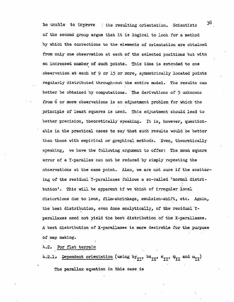
Let us consider an arbitrary cross-section (X. «* constant) A-B-C of the model (such that line a-b-c in the negative is parallel to the line 5-1-3)• See figure 3.1.

7 ------

Figure 3.1. Cross section through motant'aihous model

Also consider that the angular distance a is constant; so that tana = k = dA/ZA = dC/ZC . Again, as we considered in the previous section;

O o plet 1+k = K . This gives K = 1 + tan a = l/cos a .

Let us, as an example, consider the case of dependent orientation where

we move the elements of camera II.

Then from the general equation, 31

-PyA+ PyB= -(x-'b)k-dqxri+ (ZA- K-ZB)dxa I+ k-dbz^

"Pyc+ PyB= ♦(X-b)k*dqiri+ (ZQ- K-ZB)dto];i- k'dbz.^ .

Adding these two we get: ^ c + 2PyB= ^ZA* K+ZC* K-2ZB^d<U1II

i.e., -Py - Py + 2Py- Za -K + ZC.K- 2Zb ■ ; <3.1)

One could measure the parallaxes at A, B and C, find the Z values for these

3 points, compute the- value of K and thus could get the value od dm__ ButJ»-i. •

in empirical methods one does not measure parallaxes and the corrections

are "based on the elimination of parallaxes. "With this idea in mind if one first eliminates parallaxes at points A and B, for example, (this could he

-pycdone in any of various ways) one gets: = z •K + Z «K - 2Zk "

A C BIf now Pyc is simply eliminated by moving oi^, this element is moved

_PyCthrough we warrk to solve for dco^ . These areC doXj. +Z„-K

related to each other as = V K + V K - *That is, <1°^ = nC*dCUil ’

We may define the over-correction as (dca^- and. the over­correction factor as n_- 1. The value of n or n - 1 is obtained easilyC O v/from the above equation.

+zc'KThus ' nc B (zA -K - zb )+(zc -k - Zg) * (3*2)

2Substituting here the value of K = l/cos a we get_ •________ +V secg________________+_D_

nC “ (ZA *seca-Zg»cosa) + (z^*seca-Zg«cosa) E+F

where ^ = Zc* sec0JE = ZA » seca - Zg- cosa

and F “ ZC* seca " Z^'cosa .

The geometrical meaning of D, E and F will be clear from' figure 32 '

3«1» Here, D = Z^»seca = IC ; also IA = Z *seca. Also if we drop a perpendicular HR on line IA, we get IR = IB-cosa = Z -cosa. This will

give E = IA - IR = RAand, similarly F = IC - IS =-SC .Note that the negative sign of SC appears in the present example, as in the figure determined by the direction, positive away from I (theprojection centre) and negative towards I.

By knowing the Y and Z coordinates of I, A, B and C we can easily find the value of n,. But the coordinates could be precisely measured only after the model is properly oriented. We may thus start with approximate values and find an approximate nc and an approximate dcn^ . This, in turn, will lead to approximate solutions of other elements. A

process of reiteration will improve the situation. It will be interesting to note that if E + F = 0, nc = « . In that case dm^ is indeterminable. In that case all of these four points (i, A, B and C) lie on a circle, known as the critical circle. The advantage of such a construction is that we can directly find if the points are on the critical" circle. If so, we can solve for by selecting another cross-section in the model

suitable for a good solution of dai^ .This problem was discussed by Kasper (1956). He finds a general

graphical solution of the problem of finding nc . We can obtain the same results, it can be proved, by first drawing perpendiculars on IA and IB at points A and B, respectively, to intersect at G and next by dropping a perpendicular GH from G on IC. Then n = IC/HC. Further, Kasper finds that if point C is situated inside the circle determined

3 3"by I, A and B, the over-correction factor will he.negative,

otherwise positive always.

In case it is a model of flat terrain, we have ZA ° = Z^ *= Zc = Z.

2 2 K Z +clThen from expression (3.2), nc = '2('k -1) = ---2~ *2 2 Z “(iTherefore the over-correction factor = n_-l = ---— - (3-22.)

C 2d2

This gives the over-correction factor for a particular case where, to

start with, PyA = Py^ = 0 hut Pyc ^ 0 .

In some empirical methods, however, before finally coming to solve

do) we may have a situation when Py^ = Py , 0 hut Py^ = 0 . Then the

expression (3*1) reduces to

- 2pycZ -K - 2ZB

and - z^ic

These give a new value nn = v -tc dcu^

2V KZ.*K + Z„-K - 2Zg (3.3)A C

In the case of a flat terrain, this gives

2K K Z“+nC 2(K-1) ~ (K-l) “ d2

Z2 f2Therefore, the over-correction factor = n - 1 = = —?r . (3«3a)

The general expressions (3.1)* (3-2) and (3-3) can he used similarly

z £

to derive the particular over-correction factor in individual cases.

3.3. Further examples of empirical methodsThe empirical methods given earlier in this chapter are two

typical ones of many possibilities. Each method is completely differ­ent from the other inas-much as the handling of different cameras or different elements are involved. Also, changes in the sequence of the operations, selection of the points and their location in the model with

different operators may end up with different adjustments of the y- parallax over the whole model. The situation may not be serious for a single model as required in plotting work. However, in strip triangu­lation, these small errors may propagate to ultimately give very

irregular results in the end. Before presenting further examples, we should therefore.express that if a strip-triangulhtion is concerned, particularly involving more than one operator, each operator should use exactly the same orientation method. It can be theoretically (and only theoretically) established that the ideal method of orientation in such a case is the numerical one (particularly if it is based on a least square adjustment of the observed y-parallaxes in more than five points.

This may not be true in practice, however,3.3.I. Dependent orientation (using by , bz , K , ccl. and <p_),

for flat terrainThe orientation can be accomplished in the following steps:1) Make Py^ = 0 with by^ .. read by^

2) Make Pyg = 0 with K

3) Make Py_ = 0 with by_ read by_3 ' ** • j3

*0 Make Py^ = 0 with hy^ • • read hy5

5) Set hy . to read hy . *m

= |(hy + hy ) X3 5

6) Make Py^ = 0 now with bzl

7) Compute, for point 5: n = Z2/d2

8) Set by . now to read: ^ 1 - n(hy - m

9) Make Py^ = 0 with cUj.

10) Make Py^ - 0 with by^ • • read by_

11) Make Py^ = 0 with hy^ • • read byT 16

12) Set by_ to read: i=Khy_ + hy ) 1 2 \ Z6

13) Make Py^ = 0 with cp.j. .

Repeat all the steps if required.Note: This method seems to he slightly complicated.

3»3«2. Independent Orientation (using K , K-r-r> 9-1-* 9-r-r aa( assuming flat terrain X ^ X J"L

The steps may he as follows:

1) Make Py1 = 0 hy moving Kjr

2) Make Py2 = 0 hy moving

3) Make Py^ = 0 hy moving cp and <p simultainously.

4) Read the initial value of cn ., call it

Make Py^ = 0 hy moving now reading .

“ii + “xi “II 1:0 “iBn “ ----2— •

Make the new Py^ = 0 hy moving and 9 simnltainously.co" - a£

Set to <0 + n — ---

2 2where n = Z /d is the over-correction factor at point 6.5) Again make Py1 = 0 hy moving .6) Again make Py^ = 0 hy moving K .

7) Make Py^ = 0 hy moving cp , reading cpj. .8) Make Py^ = 0 hy moving cp , reading cp^ .

*11 + *11 Set ^ to <pIIm = g-----

All of the ahove steps may have to he repeated until the model is practically parallax-free.

For other orientation procedures suitable to individual resti­tution instruments the respective working manuals may he referred to. k. Numerical methods k.l. Introduction

Broadly speaking, the numerical method of relative orientation has to he different in different cases. Considering vertical photo­graphy, they fall in two major groups: (l) The ones for flat terrain and (2) the ones for mountainous terrain. For convergent photography, which is not going to he discussed here, reference may he made to

Ackermann (195&).Further, each method is completely different from the other inas­

much as the handling of different elements and different cameras, the

selection of points, their number and their locations give differences

in the final results. Also, different operators may start with

different parallax readings and end up with different adjustments

of the parallax discrepancies in the model. However, this is of no

serious consideration for a single model as is required in normal

plotting. In aerial triangulation (of strips and blocks), small

differences and errors may propagate to give completely irregular and

un-systematic behavior, of the errors in the strip or block, thus complicating the adjustment. It Is therefore necessary that in aerial

triangulation a systematic relative orientation process be followed

(that of dependent models). With empirical or graphical methods an individual operator may have his preference for a particular set of

operations (as there are so many), but with the numerical method for

the particular case he has only one way left. The numerical methods are somewhat impersonal. Apart from solving the relative orientation

in a systematic way, the eventual residual parallaxes are distributed

over the model according to a fixed principle (the least squares).For this reason the numerical methods have their greatest significance

in their use during an aerial triangulation with more than one oper­

ator working simultainously.From our knowledge of the empirical methods we know that the

minimum number of positions where y-parallaxes have to be eliminated

to complete the relative orientation is five (suitably located points).

There are two schools of thought. According to one school, if the number of observations at each point in increased we may be able to

increase the precision of orientation by way of adjustment. According

to the other school, this increased number of observations, obviously

involving an increased number of observational errors, may ultimately

"be unable to improve . the resulting orientation. Scientists

of the second group argue that it is logical to look for a method by which the corrections to the elements of orientation are obtained

from only one observation at each of the selected positions but with an increased number of such points. This idea is extended to one observation at each of 9 or 15 or more, symmetrically located points regularly distributed through-out the entire model. The results can

better be obtained by computations. The derivations of 5 unknowns from 6 or more observations is an adjustment problem for which the principle of least squares is used. This adjustment should lead to better precision, theoretically speaking. It is, however, question­able in the practical cases to say that such results would be better than those with empirical or graphical methods. Even, theoretically

speaking, we have the following argument to offer: The mean squareerror of a Y-parallax can not be reduced by simply repeating the

observations at the same point. Also, we are not sure if the scatter­

ing of the residual Y-parallaxes follows a so-called ’normal distri­bution’. This will be apparent if we think of irregular local distortions due to lens, film-shrinkage, emulsion-shift, etc. Again,

the best distribution, even done analytically, of the residual Y- parallaxes need not yield the best distribution of the X-parallaxes.A best distribution of X-parallaxes is more desirable for the purpose

of map making.4.2. For flat terrain

4.2.1* -Dependent orientation (using k j z > Qjj an<i <ajj)

The parallax equation in this case is

3 9

-py =-&-byXI + -(x-b)a+ zU+ cLo -(-^~|-^dcpII .z

Say, we have parallax observationsdstheishc standard locations in

the model. Since we have more observations than unknowns (i.e.,5).,

this is a case of adjustment. According to the generally accepted principle of least squares for such adjustment, we may rewrite the

above equation as a correction (or observation) equation:

v = Py - d-byi;i; + I*1132!! ‘ (X-b)dfCIX + Ztl+^Icu^ - - -^ - dcp^zwhere v is the correction.

For the 6 standard points we get, as in table a table of

coefficients. From these 6 observation equations we may form 5 normal equations, the solution of which give:

and

d*n = +3b py1+py3+i>y5-py2-pyj+-py6)

dCpII = +2bd^

^ 1 - + - # p y 1-py -Py5+2Py2-Py^-Py6) 4d

dbz!I - +2d(pi V Py6)

aby =xx 12d

|2(kd2+3Z2)Py2+(2d2+3Z2)(2Py1-Py3-py5)

+(2d2-3Z2)(Py),+Py6)}

(^.1)

Here the corrections to the angular (rotatory) elements are in

koradians, and to get them in the working units we have to multiply

the respective expressions by the appropriate value of p .

The orientation can be accomplished in the following steps:Step(l) Note the values Z, b and d in the model and compute

p

the constants p/3b, pZ/kd , z/2d and pZ/2bd.

Step (2) Measure the parallaxes Py^ Py2 . . . . Py with "byjj • This is done again by the method of elimination of parallax with byi;j. at each point and noting the reading each time. More than one

observation at each point would possibly increase the observational accuracy and would surely check blunders. The average value of the by^j readings at all the six points is subtracted from the indi­

vidual by reading at individual point. This gives the y-parallax at that particular point.

Step (3) Compute the changes to the elements (i.e., corrections), dK j, dcUj.., dcpjj and dbz^ with the formulae (k.l) and set the final values (i.e., initial plus correction) in the instrument.

Step(b) Measure the residual parallaxes at the 6 points again

with by-j-j ; set to the average value of these six readings. Ifthe residual parallaxes are not within permissible limits, the steps have to be repeated all over again.

During the computations the consideration of signs with respect to the particular instrument used is very important. A research paper by Jerie (1955) gives a good study of the consideration of signs in this respect. This could be consulted before setting-up the work­

ing system for regular work in any organization.Actual computation of dby^ as is done for the other elements is

slightly time-consuming. Also, since the element "by. does not

Hicontribute to model deformation, its setting precision may be

permitted to be of a different standard than for other elements. At

the same time, the observation of residual parallaxes gives an idea

of the accuracy obtained and of the eventual errors in the obser­

vations, of the computations or of the settings. This saves some

time in practice with no loss in precision (even theoretically).

It Is therefore recommended to finally set by-j-j to the average value.

A form for this purpose (form I) was devised in our laboratory and would be found to be extremely helpful in practical use. As a good initial check on the observation, it may be noted that the terms

happens on account of the symmetrical locations of the points. The

operator may have reasons to be suspicious about the observations if

the difference between these two terms is greater than 0.3 mm.,

e.g., when working on a very precise instrument like the Wild Autograph

A7, Zeiss Stereoplanigraph C8 or Santoni Stereocartograph Model XV.During a strip triangulation in an instrument having the

possibilities of changing over from base-in to base-out and vice

versa (i.e., with the parallelogram of Zeiss), where dependent numerical

method of orientation (co-orientation) has to be taken recourse to,

one can have two cases:A) When one triangulates from left to right in the strip, i.e.,

when the right-hand side camera is to be moved - this corresponds to

moving the elements of camera II with base-in and of camera I with

base-out; or,

should be very nearly equal. This

B) When one triangulates from right to left - a situation opposite of case (A).

For numerical orientation in both the cases the form I is

amazingly adaptable by simply considering interchanged numbering of points (between 3 and 1 and 2 and between 5 and 6) and the cameras (with II to the left and I to the right). This could be done without

changing the formulas and the computational steps and technique..2.2. Independent orientation (using by^, K (pj, cp , and

using byXI as the parallax measuring element

This particular type of orientation may have to be done in the case of the first model in a strip triangulation where y-parallaxes can be obtained from by^ (or by ) readings, the correction equations

can be derived in a way similar to that given in section l»-.2.1. above.In a way exactly similar to the one given in section .2.1. we

obtain the following formulas:

da^ = -^(2Py1-Py3-Py5+2Py2-Pylv-Py6)

and dby^ = [ 2( *fd2+3Z2)Py2 +(2d2+ 3Z 2)(aPy^Py^P^)

+(2d2-3Z2)(py^+Py6)|

.2.2.1. Independent orientation using oo^ as the parallax measuring element, (using k , IC , cpJ, cp^ and ox )

In case a particular instrument has no by^. or by^.^. movement, we can

not use our previous conception. Let us consider a more probable

possibility where we would use ox^ as the parallax measuring element.^

The relation can be expressed by coy - — p)Py where cuyis the y-Z + Y

parallax in terms of the ox^ scale graduations. The parallax equation for these elements in general terms is:

2-Py = X-dKj - (X-t)d^I:E + - i 2 ^ h dtpii + zd+^duijj .

zIn the present case this will change to:

“ y = ' ^ 5 ’ dKi i + a<pi - p ^ £ Yd<pi i + •

This general expression in our case gives the following table of co­efficients with respect to the situation at various points in the model:

Table ^.1.Coefficients of elements, independent case, ciXj.. being the parallax measuring element

Coefficients ofdcp.d K.&K II

o>y,b-Z

Z + dZ+d'

Z + d

Z + dZ + d

Z + dZ + d

From the above equations we get2bd. Z2+d£, ,

4<PX - - -2BT(a,V “l|r6)Cm + U

2bd . . . 2?+a2/ xqjr3Kqjr5 = *Pn - - •

Also, aaor1 + ouy2 = |CdKj + d«IX) + 2daJi!2t)Zand cpy3 + + o^5 + o^6 = g ^ d -nDc. .) ■Hfcdc&g. .Z +d

44

From these last two equations we get

A - ' A *84d£^ 1 1 = L (ayl^y2) - ^-±§- .

2dHere dx^ and dkjj are slightly complex. But similar considerations as for byTT in section 4.2.1. can be conveniently used. If corrections dtp , d(PjX and da..j. are introduced in the instrument the resulting residual parallaxes must be due to d/c and d/c^ only. The individual

equations show that coefficients to dx^ is zero for points 1, 3 and 5 (i.e., x^ has no effect on the parallaxes at these points). Similarly,

/Cj. has no effect on the other three points: 2, 4 and 6. pa fact, after

dqXj., d<PjX and dux^ are introduced, the remaining parallaxes at 1, 3 and 5 should be theoretically speaking, equal. We can remove the remaining

parallax at each'of points 1, 3 and 5 with x ^ and finally set it to the average value. A similar treatment can be given to dk with respect to the points 2, 4 and 6. Differences in the three values for each of

and x ^ would indicate a mistake in one or more of the foregoing manipulations or some other error in the process.

A similar derivation would result if coj. were the parallax-measuring

element.

The -utilization of a ca-movement as a tool of measuring y-

parallax does not give, as accurate a result as the by-movement. Theoreti­

cally speaking, this method would yield about 10 to 15 per cent less accuracy. * The reason for such reduction in accuracy is nainly due to t;.e

fact that an x-parallax is also introduced at various points when c d is moved. This forces the operator to move the carriage in Z, thus changing the projection distance and the distance d for the corner points.

^.2.2.2. Special case with instruments having no fby* movementsIn case we have to apply the numerical method of relative orien­

tation in an instrument not provided with accurate co-graduations, some

indirect procedures have to be devised. As a minimum, some means have

to be provided for measuring the parallaxes accurately. Tewinkel (1953)

describes a method for the Kelsh Plotter. Here he provides one pro­

jector with a dial gauge to enable the operator read *by* movements to

the nearest 0.01 mm. Thompson (195*0 uses a parallel plate micrometer which shifts the image in a direction perpendicular to the basal plane

of observation and tends to read the y-parallax with the least count of 0.01 mm. However, such instruments are manufactured primarily for

plotting individual models only and are not of the highest order, so

that any workable method of orientation can be used in them. In practice, only empirical methods are used in such instruments in all the

organizations throughout the world.

4.3» For mountainous terrain

In the specific problem of orienting a mountainous model (where

the ruggedness of the terrain is more than 10 per cent of the flying

height- above mean ground) by the dependent method (i.e., using by__,Y

b z ^ , ^tj) 113 assume 2 = a cons'baiv,; for each

corner points in the model (viz., 3, lj-, 5 and 6) as we did in2section 3.2. earlier. Also let us consider 1 + k = K as we did in

section 3-2. These substitutions, introduced by Pauwen, contribute

amazingly towards easier solution of the problem. Considering 1 these, the table of coefficients becomes:

Table k.<>.Coefficients to elements, dependent method,

mountainous model, with Pauwen*s substitutions

U6.

Coefficients to

JtI 1 d/cII 1 dCplI dctuT±1 dbZII dbyn

1 ►d: I i __

__ b 0 *1 0 -1

-py2 0 1 oI1 Z2 0 -1

"Py3 b j -b*k1

z3*k -k -1

o.. 0 Z^K -k -1

I 3 VJl b | b*k1

z5-k k -1

-Py6 0 ! °1 :

z6-k k -1

\

Applying the least square principle or a simple arrangement of the above six equations (as suggested by Brandenberger, in his lectures )*■ we arrive at the following equations:

2CPy-L+Py2) - (Py Py +Py +Pyg) dX1>11 2{Z^Z2) - K(Z3+Zu+Z5+Z6)

d*n “ {"^Pyl+Py3+Py5 + (p^2+Pyk+Py6

.[(zl-z£)+(z3+z5-z4-z6)k ] ^ j

d(pII g 2bk{^Py3~Fy4“:E>y +Py6 ~ K^z^“23~z6+zlt.) ^ n } J> (1;.3)1 A ls o s e e Z e l l e r , 11.; T e x t Book o f P h o to g ra m m e try ;L e tr is ,U .;- : .p .9 5 2 .

h7

dbzn CC +Py -Py -Pyg) - k(z5-z3+z6-z) dII-2b*k.dcpII]i 6

dbyII = E [5 i + [ zi+V + k(Z3+\ +z5+z6)^ d£DiI+ 3°*dACi:i:

Obviously these equations are arrived at by assuming equal wights for all the y-parallax observations in the model space. This as­

sumption, however, as initially considered by the scientists, is not correct. The photographic resolution can not be the same everywhere

in the model, thereby causing unequal weights for the observations.

Further, the resolution may be different in different pictures. Thus

resolution itself may create a very complicated situation, and conse­

quently prove the numerical methods of relative orientation to be of

much less precision than their advocates may claim. Also, unequal Z- distances of the model points are sure to impose unequal weights in the

observations, as also the location of the individual point with respect

to the others, since all tht observations are made against fixed (and dimentionally unchangable) pair of measuring marks. This is more of a

problem in instruments having optical projection system.

1+.3.1. Jerie1 s improvementThe corrections to the elements as given in equations (^.3)* how­

ever, make it quite clear that according to the presently applied principles, the initial solution of dox^ influences the solution of all

other elements. Therefore it is essential that this element should be

solved as precisely as possible. Jerie (1953) gave a solution in which dmiT is solved from two cross-sections of the model: 6-2-h and 5-1-3*

separately and the weighted average of the two solutions is first taken

as the final correction •

43For one cross-section, we get from table 4.3.+2Py1 - (Py3+Py5) =-[2^- K(Z3+Z5)3 dcnjj.

For the other cross-section, we get

2Py2 - (ryi+py6) = -fcZg - k(z^+z6)] a«* * .

These two give separate solutions for for the two cross-sections:

2Py- (Py +Py ) 2Py - (Py,+Py.)^ 1 = -2zI + k u 3+ z5> and ^11 = zJTTTz^rz^)

For a convenient solution of cku^ Jerie introduces the following sub­stitutions :

2Z^ - K(Z3 + Z ) = U and 2Zg - K(Z^ + Zg) = VThese give:

spy-, - (Py^+ Py.)- — A - -u A- --

2Py2- (pyu+ Py6) and da .j- ^------- -

g1.dm»I+g2*da IThe weighted average of these two is given by doirT - -------------

11 S1 s2where g and gg are weights and g = lfi/6 and gg = V2/^ .Then we get from the above

. + •

Here, with substitutions —=— = R and —x— p = T , we get finallyu +v ir+^r

dta^ = R-duij. + T'dcn^ . (4.5)

It is interesting to note certain relations here. Obviously,

R + T as 1. There also exist relationships amongst U, V, R and T, which can be expressed graphically and can be used in practice to save time

in the orientation of a model. In figure I4-.I, AB and AC are two straight lines at right angle to each other (at A), where AB = U and

AC = V in any convenient scale. The angle CBA = © helps us finding

the relations:

k9

A B

Figure 1<-.1 Graphical representation of the relations among U, V, R and T

= cos© = n/r and r A V— = sin© = v/t .-tiP* + V2) ^ + y2)

To obtain the values of R and T graphically, we may draw a semi-circlethrough the point B with its diameter BD having a unit length in any

scale on line AB. This semi-circle interBscts the line BC at E. Drop

a perpendicular EF from E on AB. Now BF = R and FD = T, i.e., their absolute values, both of these lengths being in terms of the unit used for

the diameter of the semi-circle. A proof of this construction is as follows:

oR = BF = BE»cos© = BD*cos©-cos© - BD/sec2© = BD/(l + tan2©) =Bd /l-k-.)

ITNow, BD being unity,

U2 .... m V2Rl^+ V2 and T = 1 - R =

u ^ v 2 '

The values of R and T have some influence on the final la theideal case R = T = 0.5* Also, since the values of R and T depend on

the values of U and V, in the ideal case U = V.

The geometrical significance of U and V can be obtained from a familiar figure (see figure 4.2); e.g., the situation on the vertical

plane through points 3-1-5 in the model space.

50

O'

Figure 4.2 Vertical plane of section of model through points 3-1-5

By definition , we have, U = 2Z^ - K(Z3+ z^)=(z1” K'Z^+CZ^-IOZ^)also,

Hence we get

In figure 4.2we have

2 Y 2 2K = 1+k = l+-o“ = 1+tan a = sec a .Z,

U = (Z^-Z^se^a) + (Z1-Z^»sec2ce) •

= 0*1, Z^ = 0*A, Z^ > 0*B

If we draw perpendiculars 3C and 5D on 0*3 and 0*5 at points 3 and ^

5 respectively, to intersect line 0*1 at C and D respectively, wre get2 2 thereby, Z^'sec a = 0*3*seca = 0*C and Z^*sec a = 0J5seca = 0*D-

Thus, then, U = (O'l-O’C) + (0*1 - 0*D) = Cl + D1 ; both Cl and D1 haveto be considered algebraically. In our figure &2 here U = Cl - ID .

It will be apparent from this figure that when U = 0, the three points

3, 1 and 5 and the projection center 0* lie on the same circle (whosediameter is 0*1). This is obviously a critical circle, and in such acase dfja j becomes indeterminate.

The value of V could also be obtained similarly from the other cross-section through the model, where again, the situation approaches

the critical circle as the value of V approaches zero. Also, when V

is comparatively smaller than U, T becomes comparatively smaller than R, and vice versa. When U is very small compared to V, we can say

that the cross-section 3-1-5 (corresponding to U) is nearer the critical

circle than the other section k-2-6 (corresponding to V), and automa­tically, flriYj-j- solved from this cross-section is less precise than for the other cross-section. In the extreme case obtained from

this cross-section may be indeterminate.The various .steps in this method of determining dca^ can be formu­

lated as follows:Step (l) Compute U and V.

Step (2) Compute and •Step (3) From the values of U and V, find out R and T. This can

be done graphically without losing any appreciable precision.

Step {h) Compute the weighted average 18 + •

<32Other corrections, viz., dby , dbz^, d/c^ and dtp j can next be easily computed using equations (4.3). The inherent difference in Jerie*s solutions, however, lies in the initial solution of .4.3.2. Kasper*s improvement

While the method given by Jerie is aimed at giving a more precise solution of doij-.j., it does not consider weighting the different parallax

observations. The weights g^ and gg and thus R and T (which depend on U and V) have a direct relationship with the location of the points in terms of the solvability of dcu^ only; whereas the correct solution of

the problem would have been with the consideration of proper weights of the individual parallax observations. In this respect, the next step towards a more rational treatment of the problem was taken by Kasper.

He assumed that the parallaxes (observations) in the picture plane have the same weight. This consideration, although it does not take all the aspects into account, is a near approach to reality for the Wild and Santoni type instruments, where the measuring marks move in planes parallel to the pictures and the dimensions of the measuring marks do not change with respect to the pictures during the observations. How­

ever, Kasper’s considerations will be involving more complications in case an instrument of the optical projection type (e.g., Zeiss Stereo- planigraph C8, Kelsh Plotter, etc.) is used. In such instruments the measuring marks are in the model space and do change their (or its) dimensions with respect to the picture depending 6n the location of the point of observation in the model space.

The parallaxes in the picture plane and the model space are related

to each other as expressed by: Z.py± - ^

53(U.6)

•where f is the principal distance for the photography,p^ is the y-parallax in the picture plane,Py^ is the y-parallax in the model space,

and Z is the Z coordinate of the model point.

By introducing expression (b.6) in the formulas we get:

_ 2Zl‘pl - < V P 3 * V p 5 > ^ E I " fL2Z1 - k c z3 + Z5) J

2Z2*p2 - (Z^-p^ .+ Z6-p6)(^-7)

^ 1 " F T ^ - ^ z ^ r z ^ T TThe weighted average of these two expressions would give the final dco^

However, in doing so, the weights in this case are not the same as in

section 4.3.1. (jerie*s solution.) We obtain the weights here as the

reciprocals of the squares of the standard errors of dco*^ and dco"^ .

Using the Gaussian Law of C’rror-propagation, the respective standard

errors are given by:

for ckn|.j. :m ,2 =“ f?[2Z1- K(Z3 +Z^)]2

and forxn = co £2[2Z2 - K(ZU + % ) V

where is the standard error of one observation of the parallax in the picture. From the above,weights are; using substitutions:

where U and V are the same as in section ^.3.1 and 5^

s = kZi + Z2 and t = Uz2 + Z2 + Z2 .

In a way similar to what we had in section if.3.1, the weighted average is

( M )

This expression with proper substitutions, is

*03; = -[2Py1-(Py3+ Py5)] U*t + [2Py2-(Py^+ Py6)] V-s

(h.10)T^-t + V^s

After dax__ is solved, the solutions for all other elements would

be accomplished easily by introducing the expression ( .6) in each of

the other equations ( -3)*However, Kasper*s views as considered above is not universal and

in no way the final in this respect.

In trying to find the correct approach to this problem the author (1963) observes that the parallax observations in the model space have to be properly weighted. The weight of an individual parallax observa­

tion depends on the following relevant factors:1) The attitude of intersection of the individual rays

coming from the two corresponding pictures, at the point of observation.

2) The obliquity of the epipolar plane through the point of intersection (on which the two intersecting rays lie in reality) with respect to the horizontal plane (along which the parallaxes are observed).

4.If. Suggested perfection with weighted observations

•3) Changes in the scale of the detail and thereby the change in the dimension of the measuring mark (or marks) with respect to the

detail at the particular location of the point in an individual

picture, and thereafter, jointly at different locations in the model.

I4.) Different photographic resolution and other image;

qualities at different points in each picture and ultimately at different

locations in the model.

5) The particular restitution instrument and its peculiarities,

and, (6) The operator and his personal observational capabilities.

While we have yet to come to a conclusion regarding the instrument and the operator (these may be set aside because the present one is a

general study of the problem), the other four geometrical and physical aspects are undoubtedly the most important ones. The author analyzed

each of these factors and has finally formulated the weights due to each

as well as their joint effect, as follows:

l) The weight due to different attitudes of intersection of

the rays is given by (also see Hallert, 1950);

G sin27 _ ______________ b2 (z2+ Y2)________________________ (lv.n)1 L2+L2 (x2+ Y2+ z2) { z2+ y2+(b- x ) 2] { 2Z2+ 2Y2+(b-X:)+X }

where is the weight,7 is the space-angle of intersection of the two rays,

are the* distances of the point from the two projection

centers,

b is the model base,

X, Y are the X and Y coordinates of the point,

and Z is the distance along the Z-axis of the point from the base

(called the projection distance).

562) The weight due to the obliquity of the epipolar plane through the point is given by:

Gp = sine = p (4.12)+ Y )

where Q is the angle of obliquity (see figure 4.3)> and Z, Y are the same as considered previously.

7 1 x

*V ,

< 7

p/ \K-

/

Figure 4.3. Showing obliquity of the epipolar plane

3) The.weight due to the change in the scale of the detailvaries inversely with the projection distance, and is given by

( .13)where w is a constant for the model and it should be determined suchthat at point 1 or 2 the value of G^ (is unity. In flat terrain with

vertical photography G^ is constant for all points.

*0 The weight due to the photographic resolution (G^) ^

will he directly proportional to the difference of the resolutions at

the particular point, without any regard to the algebraic sign, with

respect to the location of the point in the individual pictures.

A general average of the four weights at each point can he

considered to he appropriately the total effective weight for each

parallax observation at eahh point. In case the terrain is flat these would give the same weight at each of points 1 and 2, and a different

hut equal weights at each of points 3, *4-, 5 and 6. This happens on

account of symmetrical locations of the points. But in the case of a

mountainous model, the final weight would vary from point to point.

However, the general expression for the final weight at a point is

G = ^ (G-jJ- G2+ G^+ G^) . (l+.llj-)

Finally, for the numerical relative orientation with parallax

observations, we may consider the following general equation:p

V = dbyj. - |d b Z l + x-a/C j - z d - t - g j a t^ + S ^ a tP j - ab y l:r + | a b 2 l Iz*

(X"b)dKjj + Z(1+^r)<3mii i“^dcpII + ^

where v is the correction.Then the weighted correction equation at a point will he given by:

p

\Tg»v = -J~G»dhy^- VG«^dhzI+ 's/G-X'dK - * » /g » Z (1 -n — JdcUj. + _ •'/ii+dbyZi

+ ■7G» r»dbzTT- •>/G»(X-h)dXII+ -zCl+^^dai^- -Jg • d(p^*s/G»Py

(^.15)where G is the weight.

The corrections to the individual orientation elements will then follow directly from the normal equations formed on the "basis of

the observation equations with respect to the points of observation and

the relevant elements used.It has been found from practical experiments in the Ohio State

University laboratory with fifteen different models in various scales and with various types of terrain that the weights as arrived at in the studies and as utilized in the expression (U.15) give very satisfactory results in numerical orientation of the models. It was observed in general that a relative orientation with properly weighted six

parallax observations in the model yields better results than with nine un-weighted parallax observations in the model.

However, with such considerations of the weights, a numerical

relative orientation of a model becomes complicated and rather time- consuming. This remark also holds for the formulas. An experienced practioner automatically applies weights, (maybe sometimes in a different and un-scientific way), to his observations in performing an empirical or graphical relative orientation in normal practice. For further theoretical considerations, the above ideas could be extended to nine, fifteen or more number of points in the model in case a more precise

relative orientation is aimed at.5. Graphical or semi-graphical methods

k

5.1. IntroductionIt is intended to discuss the methods of graphical orientation

introduced by Pauwen (19^9 and 1951) > Poivilliers (19 -8, 1950 and i960) and Krames (1950). Excepting the first one all of the methods have one

common property that the construction (graphical) is divided in

parts, treating the parallaxes observed at points that lie in one

cross-section through the model at right angles to the base. Usually

a graphical construction is made for the situation in a plane, X = a constant, for deriving the corrections to the orientation elements. Insuch figures, for the sake of such solutions, the parallaxes are

presented in a scale much exaggerated e.g., 20:1 or 50 il,etc.whereas the projection situations are represented in a reduced scale, e.g., 1:3*

1:1+, 1:5, etc.5.2. Pauwen’s method

Pauwen (1950-51) claims that this method is1) useful in all kinds of terrain,2) allows the use of the parallaxes measured at many points

(e.g., 15 or more),3) points out rapidly and without any doubt the points where

there is a semisystematic error (which is accidental for a whole strip

but systematic for photographs and introduce systematic - <2efoaT££,tioft--af'

the apatlal model), and1+) practical and economical.

The basis of this method consists in selecting points whose Y/Z =

a constant. Pauwen selects theee series of points along 3 strips of about 5 mm.width; one series on the base line, the others at an equal

distance ’a* apart on the plate as exemplified in figure 5-1-

6o

To' ro ro

a—

Figure 5.1 Arrangement of points for Pauwen’s method

Thus for points we have Y^/z^ = a/f = k

and for points A^ we have Xj/Z^ = -a/f = -kbut 1 + Y2/Z2 = 1+k2 = K j as we had in section 3*2 earlier.

We will consider only a dependent orientation where only the elementsof camera II are moved. The parallax equation in this case is:

-Py --»*□+ f a T1 - (x-bjd/^ + (5.1)

In the present case, this equation reduces to:for points A? ; =-<lby - (X®-b)dk . + Z^dn^ (5*2)

for points At ; -Py =-dby + k*dbz . -(X|-b)d/f^ + EZ^dco^ -

-(jCJ-'bJk-dqx j. (5.3)

for points Aj J -PyV — dby^ - k-dbz^ - ( X ^ - b ) d + KZ^dm^+ (X -b)k.d<pII (5-!)

5.2.1. For flat terrain ox

Because of flat terrain, we consider Z. = a constant = Z .iFurther, let us consider the situation on one cross-section of the

model where X = a constant. Then the equations (5.2), (5-3) and (5-^) may be rewritten as:

-Py° = -dbyII - (X-b)!*^ + Z'dm^.

-Py* = -dby^ + k»dbzII-(X-b)d/CII+ Z-K’do^^-Cx-bJk-dcp^

-Py" = -dby^ - k*dbzII-(X-b)dKII+ Z«K*dairi+(X-b)k*dq)II .Adding the last two,

-Py’ -Py" = -PyS = -2dbyI][- 2(X-b)dkI3; + 2Z-K.dcori .Rearranging, it becomes

-|pyS = -X-d#CIZ+ [b.d/Cjj- tt>yXI+ Z-K-dm^]Rearranging (5-5a), we get

-Py° =-X-dJCi;j.+ [b-d/c^- dby^^- Z-dm j.]

These two equations, (5-7) and (5.8), are now in the forms to represent two straight lines (compare, y = mx + c). Thus, if we can plot (see figure 5*2) on a graph paper these -Py values against X for

various cross-sections (for practical reasons we have to select different scales for different direction^, we would get straight lines,

each having a slope of -d/cTT i.e., they are parallel straight lines.

Their separation in the -Py direction is Z(K-l)da rT = B , say. Both

the slope and the separation can be easily obtained with the help of

the graph.Therefore, d k ^ = - the slope of the lines (5*9)

= - tan X where X is the angle this line makes

with the X-axis.

(5.5a)

(5.5b)

(5-5c)

(5.6)

(5-7)

(5.8)

Now, for a particular cross-section where X = b, from equation (5.2), i.e., for model point 2 in our general consideration, we get,

-Py° = - + Z*doij.«j. = C , say (i.e., C corresponds to the-Py at point 2 in the model)

dbyIX = Z.duij-j - C. (5*H)

Theoretically speaking, the relations (5*9), (5.10) and (5.11) giveus the corrections to elements and by^. But in practicedbyxx i-> solved by first setting the corrections to other elementsand then using by^^ to eliminate the remaining parallaxes.

Next, by subtracting (5*5c) from (5.5b), we get

-Py' + Py" = -Pyd = 2k-db^ - 2(X-b)k.d<p (5.12)Rearranging this, we get

Pyd = ak-dq^j-X - (2k-dbzII+ 2b*k»dqx[I). (5.12a)This also represents a straight line with a slope of 2k»dcpxx , when

cLwe plot Py against X. This gives

d^I - *§* (5.13)

where d is the angle this line makes with the X-axis, with

proper consideration of the units used along different axes.Again, for a particular cross-section where X = b , we get from

expression (5*12):Pyd = -2k*dbzIX = D, say (difference of parallaxes at points k and 6)

i.e., dbzXI = - (5.1*0

Thus, with the help of two separate graphs, as exemplified in

figure 5*2, we obtain the corrections to all the elements. The values

for the angular elements here are in radians.

6 3

x=o

Figure 5.2. Graphical solutions in Pauwen*s method

The entire job could he done with at least two cross-sections

and parallax observations thereon, i.e., with Py readings in points at

specified distances from the base and on the base along one cross-

section having X = 0, i.e., section 3-1-5 in "the model, and the other along the cross-section having X = b, i.e., the section h-2.r& in the

model. However, better and improved results could be obtained with more cross-sections. In practice four or five cross-sections are

normally used and.are considered as sufficient. Any point falling

outside the best-fitting straight line would give an indication of the precision of the observations due to the operator, the instrument or

any other cause.

5.2.2. For mountainous terrain

An inspection of the general equations (5.2), (5*3) (5«1+)

"would reveal that cku^ is the only element that is influenced by the

mountainous terrain because is not a constant. This complicates

the whole situation. Thus in practice is made as small as ,

possible by other means (usually an empirical method) to start with, jI s o 1If - g-Py and -Py are obtained in the same way as we did in

section 5»2.1 [see expressions (5.7) and (5*8)] we would notice in this1 scase that the coefficient of in the case of - ^Py has second-order

terms and the plot would be complicated. But the case of -Py° is relatively simple and doi^ being constant, it (-Py°) is a direct function of Zi . Thus if we plot -Py° against X we may not get a straight line.

The fluctuations are due to the changes in Z from point to point along the base line. Also see figure 5-3» We can then obtain the value of dK^j as "the slope of the best fitting straight line through various points in the plot -Py° against X. After is obtained, now we pro­ceed to get other elements.

X=b

Figure 5*3« Solution of dXjj in Pauven’s graphical method for mountainous terrain

We obtain from equations ( 5 . 3 ) and (5»*0> *>y adding the equations of similar sub indices (i.e., corresponding to the same

cross-section):

- |(Pyj[+PyJ) = - |py® = -dbyn -(xjL-b)dicII+ |(z« + zpK.da^.

or -|pyf+ (Xi-b)dKII= -dbyII+ |(z^+Z")K-dax];I (5-15)

where i = 0, 1, 2, 3.

Equation (5*2) may be rewritten as:

-P y ° + ( x ± -b)d#cI I = -d b y i;E + ( 5 . 1 6 )

where 1 = 0, 1, 2, 3*In a graph paper we may put as abscissa the values of Z° and

i(Z!'+ ZV)K and as ordinates the values of -Py? +(X.-b)d/c__ and 2 i x x ' x II-i-Py + (X^-b)d/C^, respectively [equations (5-15) and (5.16); see

figure 5«^]« Now we get eight points that should be on a straight

line. It can be proved that if the quantities Z° and ij(Z + Z^)K are

equal, the corresponding points are situated on a critical circle.This may be noted as a check against the unsolvability of cLa-j-. We ^ y draw the best fitting straight line passing through the eight points; its slope gives | which may be measured directly as the ordinate

corresponding to a unit distance along the abscissa.

66

z

Figure 5.k. Solution of drn^ in Pauwen*s graphical method for mountainous terrain

The straight line intersects the axis of abscissa at a point F,which corresponds to the relation 0 = -dby^+ for theabscissa Z° .

This gives: = Zi,( ri ' (5-17)If, however, the straight line does not intersect the axis within the limit of the drawing, the sum of the four equations (5-16) can give

z [ P y ° - (X i ~b)d/cII + zj-dcuj-j]dbyH = (5.18)Now, subtracting equation (5* ) from (5*3) we get, for one cross-

section,

-Py* + PyV = -Py* = Zk-dbz^ - 2k(Xi-b)dcpII + K U ’-Zpdm^

being already very small to start with and also because the differ­

ences (Z.*-Z£) are small, they can be ignored in the first approximation,

and in that case we can rewrite the above expression as '

+Py^ = Sk-dcp^^ - (2k*dbg^ + ak-b-dcp ) (5-19)j

This could, now, be plotted as a straight line, with Pyi against Xi .The slope of this straight line is ak-dcp^. The ordinate of this lineat X = b gives the value of -2k*dbz^^_. Thus dcp^ and dbz.^ are directly

obtained. However, the accuracy of the determination of dqx__ and dbzJLX j.Xare dependent on the preliminary setting of daa^. To eliminate this approximation completely, a few repititions may have to be made for all

the steps.

5«3. PoivillieiB». method I

This method along with a second one given by Poivilliers (discussed

in section are used in the French Institut G^ographique National

and the Belgian Institut G^ographique Militaire. Its great value is to

require only three points in a cross-section of the model. It permits9the choice of the cross-section so as to avoid regions of near inde­terminate conditions for a model of high relief, or in the case of a partial model (e.g., models with large areas of water) to select the most favorable section for working with the graph.

Let us consider an arbitrary vertical section, A-B-C, of the model

where the plane of the section is at right angles to the model base. See figure 5.5. Let us also assume that the elements of camera II are used.

The observed Y-parallaxes at the points A, B and C can be repre­sented by using vectors in the Y-direction, as done in the figure with arrows. As far as the points A, B and C are concerned, our aim is to

move the bundle of rays emerging from the right-hand projection center (0") such that after orientation the individual rays pass through the

heads of the arrows that represent the parallaxes. In doing so with graphical means we have to take into account the fact that those

arrows have to he drawn in a scale different from and much larger than the one used to represent the locations of the projection center and the points A, B and C.

The general parallax equation (.5*1*) can he rewritten as:2 2

-Py = Z + Y-dmEI+ |[dhzII-(X-b)dcpII] - [dby^+CX-bJdK^]- (5.20)

A

Figure 5*5• Vertical section of a r.odel where Xwconstant

6 9

B' B

Figure 5*6. Pcivilliers' X construction of a locus of the projection center on one cross-section

For points in "the same cross-section, i.e., -when X = a -constant, we

can introduce substitutions: p = dbz^. - (X-b)dcp^ = a constant

and q = -dby^£- (X-b)dK . . = a constant

H5.21)

Then expression (5*20) becomes:

Z^+Y^ Y- P y + z’P + 1 (5.22)

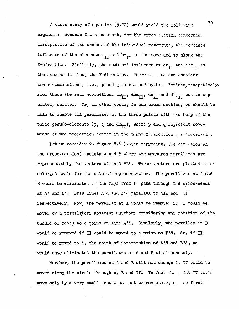
A close study of equation (5*20) wouj d yield the following

argument: Because X = a constant,, for the cross-.;.ction concerned,irrespective of the amount of the individual movements, the combined

influence of the elements cp^ and Dzjj is the same and is along the Z-direction. Similarly, the combined influence of and dby^ isthe same as is along the Y-direction. Therei'o. . we can consider their combinations, i.e., p and q as bz- and by-ti 1ations, resepctively. From these the real corrections dcp , dbz^, dK^ and db _.. can be sep­arately derived. Or, in other words, in one cross-section, we should be

able to remove all parallaxes at the three points with the help of the three pseudo-elements (p, q and dta .), where p and q represent move­ments of the projection center in the Z and Y directions, respectively.

Let us consider in figure 5*6 (which represents the situation on the cross-section), points A and B where the measured parallaxes are represented by the vectors AA1 and BB*. These vectors are plotted in an enlarged scale for the sake of representation. The parallaxes at A shd B would be eliminated if the rays from II pass through the arrow-heads at A* and 3*. Draw lines A’d and B'd parallel to All and .1 respectively. Now, the parallax at A would be removed if M could be moved by a translatory movement (without considering any rotation of the

bundle of rays) to a point on line A'd. Similarly, the parallax an B would be removed if II could be moved to a point on B’d. So, if II would be moved to d, the point of intersection of A'd and B'd, we would have eliminated the parallaxes at A and B simultaneously.

Further, the parallaxes at A and B will not change if II would be moved along the circle through A, B and II. In fact the ;int II could

move only by a very small amount so that we can state, a ae first

approximation (or, in case we start with an already approximately

correct situation) II could move along the tangent to the circle at II

without introducing any appreciable parallax at A or B. The direction

ol this tangent is represented in the figure by the line IIT. This

can be drawn by a simple construction as follows: Draw lines through

A and B, perpendicular to All and BII respectively to intersect in E.

Join E with II,which is the diameter of the circle through II. Line

IIT, drawn perpendicular to IIE at II is the tangent. Next, a line aS

is drawn through d and parallel to IIT. This line dS then represents,

in the enlarged scale of presentation of parallaxes, the locus of

positions for the projection center for which there will be no residual parallax at A and B. However, it should be noted that any movement of

the projection center along IIT (or, practically, dS) involves a

rotation (in to) of the entire bundle of rays. Thus, every combination of two points in the cross-section will enable one to draw an analogous

locus for the projection-center. For three points, A, B and C, one may

have three loci, one corresponding to the combination of two points each

time, A and B, B and C, and C and A. The three loci should, in case

nothing goes wrong, intersect at a point. This point of intersection

would give the final position of the projection-center which would eliminate the parallaxes at all the three points simultaneously. This

will make all other points in the cross-section also free from parallax.

Such a construction would give the translatory shifts p and q. and the

rotary movement dox^. This is demonstrated in figure 5.7, the practical

steps for which are:Step (l) Plot the points A, B, C and II in a suitable scale with

the help of the model coordinates.

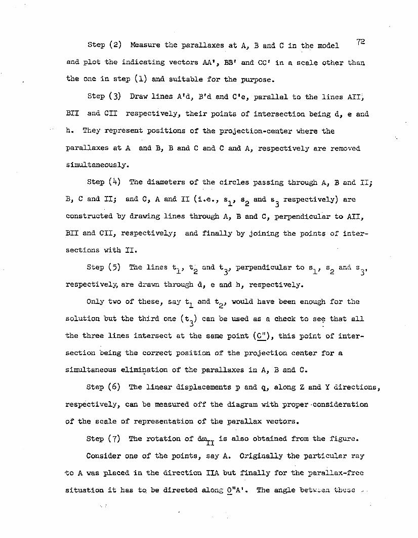
Step (2) Measure the parallaxes at A, B and C in the model ' and plot the indicating vectors AA*, BB* and CC' in a scale other than the one in step (l) and suitable for the purpose.

Step (3) Draw lines A'd, B'd and C'e, parallel to the lines AIIBII and CII respectively, their points of intersection being d, e andh. They represent positions of the projection-center where the

parallaxes at A and B, B and C and C and A, respectively are removed s imultane ously.

Step (4) The diameters of the circles passing through A, B and II;B, C and II; and C, A and II (i.e., s , s and s respectively) are

constructed by drawing lines through A, B and C, perpendicular to All,BII and CII, respectively; and finally by joining the points of inter­sections with II.

Step (5) The lines t-, t^ and t , perpendicular to s , s and s , respectively, are drawn through d, e and h, respectively.

Only two of these, say t^ and t , would have been enough for the solution but the third one (t ) can be used as a check to see that all the three lines intersect at the same point (G"), this point of inter­section being the correct position of the projection center for a simultaneous elimination of the parallaxes in A, B and C.

Step (6) The linear displacements p and q, along Z and Y directions,

respectively, can be measured off the diagram with proper consideration of the scale of representation of the parallax vectors.

Step (7) The rotation of doi^ is also obtained from the figure.

Consider one of the points, say A. Originally the particular ray -to A was placed in the direction IIA but finally for the parallax-free

situation it has to. be directed along C'A1. The angle between these -

7 ^directions would give the required rotation dcn^. The figure 1J

could he used to find the amount of rotation graphically, as follows:

Draw 0"xn parallel to IIA through 0", drop perpendicular A ’m from A ’ on

0"m. Then tan(dcurI) = i.e., d u ^ = arc tan (5-23)where A ’m is given in the scale of representation of the parallaxes and

0"m is in the scale of representing the locations of the points A, 3, C and II. However, in first approximation, one could as well consider

dOXLl II A (5-2oa)

One could, also, use more than three points in the cross-section.

For a number of i of points (^) independent loci are possible. Due to

observational or other errors all such loci may not pass through one

point. Then it becomes an adjustment problem or a question of discarding the parallax observations at individual points (that are possibly

influenced by local errors). In case the diameters s^ and s^, for example, are very nearly parallel to each other, the lines t^ and t^

will also be nearly parallel. Then their point of intersection is very

inaccurately determined. In fact the determination of da^, p and q

from that cross-section is impossible in case t^ and t^ are parallel lines. This happens when s^ and s^ coincide i.e., all of the four points

A, B, C and II lie on a critical circle.This way one can determine dcu^, p and q separately for various

cross-sections. As an initial check on the work done so far, all such dcn^ values should be the same. Now, p and q are linear functions of X,

thus if in two separate graphs p and q are plotted separately against X

(see figures 5*8 and. 5-9) £or various cross-sections, they should !:■ i on straight lines. If they do not, a best fitting straight line for cc.ch

7 4

//

/ny$r

IIY

r l l /

/

Figure-5»7» Poivilliers1 I construction for one cross-section of model

I

f■oi.

b

Figure 5»8* .p-X plot Figure 5-9* Q.-X plot

(p against X, and q against X) can be drawn. This becomes kind of

an adjustment. It is known, from the substitutions(5.21), when X = 0

Pq = + and qQ = “dby^ + b*dK:iiand when X = b,

Pb = dbzi;E

>

and q^ = -dby^ •(5.2U)

These amounts are now directly measured off the graphs as presented

in the figures 5.8 and 5»9* Then the rest of the corrections:

dbyu - i b

d b zn - pb

(5.25)dKII b^qcT qb^

dcP lI ‘ £ < V V

5.1+ Poivilliers1 method II

This method can be called as the modified Poivilliers1 method I. In

method I (section 5«3) for determining the psuedo-elements p, q and drn j. of expression 5-22, two intersecting arcs were replaced by their

tangents (e.g., see t^ and t^ in figure 5«7). Basically, in method II the operations are simplified further (i) by replacing the tangents by

their chords near the point of intersection, i.e., 0" in 5*7;

and (ii) without-using Y-parallax measurements. Thus, in a way, this

method is semi-empirical also. Consider here the same situation as for

method I, i.e., the elements of the right hand camera are to be used and let the arbitrary cross-section of the model A-B-C be considered.

To obtain the values of p, q and oQe cross-section thefollowing steps are necessary:

Step (l) At B, remove the parallax by moving any element (e.g.,

^ 1 1 9 ^11 °r *11^ t*13'*' could be used for the purpose.

Note the by^ reading and call it by . 1

Step (2) At A, remove the parallax with bz^. Note the reading and call it bz£.

Step (3) At C, remove the parallax with bz.. again, note the rending and call it bz^.

These values by , bz£ and hy1, bz^ are the coordinates of two points, in this plane of cross-sections located on circular arcs from AB and EG, respectively, indicating two specific locations of the projection center,

i.e., points corresponding to d and e of figure 5*7*Step (1*) Plot the two points d by. , bz£) and e'(by , bz ) on a sheeti

of graph paper (by against bz) in a suitable scale (see figure 5-10)•Step (5) At B, introduce a small movement of to introduce some

appreciable amount of parallax. Remove this parallax by moving by ,iinote the reading and call it by .

, .withStep (6) At A, remove the parallax/bz^, note the reading and callit bz .

Step (7) At C, remove the parallax with again, note the reading

and call it bz -Not* the values by2, bz£ and by2, bz^ are two other points on the

plane on the same corresponding arcs.Step (8) Plot the two points f’(by , bz'^) and g1(by2, bzp on the

same graph as used in step (h) above. The corresponding pairs of points are joined to find the point of intersection (0"), see figure 5*10 •

If the point of intersection does not fall in the vicinity of the points plotted on the graph, we can use another setting of in step

(5). The coordinates byQ and bzQ of the point of intersection (0") are

measured off the graph, the elements b y ^ and b z ^ are set in the ^

instrument and the parallax at any point A, B or C is removed with amovement. Here evidently, byQ = q + Q and bzQ = p + P where Q and P

are two constants.This means that p, q and cka^ are solved for this cross-section.

With several cross-sections, thus, several values of p and q are

obtained. The settings of should be the same in each case, whilep and q would vary with X of the cross-section. Finally, the elements

by .j, Kjj an< <?jj can be solved in the same way as described inmethod I (see expressions 5.2U- and 5*25)*

The difference between the two methods of Poivilliers can. be

expressed by stating,— In method I the points d and e (figure 5-7) are

obtained with the help of the parallax observations and the point of

intersection is obtained by constructing the lines (t^, t^ in figure

5-7) as tangents to the circles through A, B, II and B, C, II; whereas

. in method II a second set of observations are used resulting in the

determination of another set of two points (f* and g1 in figure 5-10) and the point of intersection is obtained automatically. Further, in

method II one does not actually measure parallax values, but use the

method of elimination of parallaxes, instead.However, both these methods of Poivilliers can be said to result in

an approximate solution of the so-called "plane resection problem". the approximation is mainly due to the fact that the corrections are derived by considering as if the projection center lies on every plane of cross- section jwhereas, it actually lies only in the X = b plane in the present case. However, with reiteration, or with an approximate solution to

start with, these two methods are workable. Method II is particularly suitable to instruments like Multiplex where accurate parallax measurements may not be practicable.

f'0" bz

S'

B' B

Figure 5»10. Graphical finding of the point ‘of intersection in Poivilliers* method II

5.5 Krames* method

Krames (1950) claims that all practical experiments with his method have brought results:that are in complete accord with the theoretical

considerations and the conclusions expected of them. The method, he claims further, permits complete utilization of the accuracy of the coordinates and the parallax values that form the given data.

In. presenting the underlying principles one can start with ^

the general parallax equation (2.^), which could he rearranged as:2 2

-Py = — Z (dtuI-dmII) + ^[X*d9I-(X-h)dcpl;i:-dozI++[X*d/cI-(X-h)dKII + dbyI - dby^] • (5-26)

For points on the same cross-section, i.e., where X = a constant, using substitutions:

X*dcp -(X-b)dqp -dbz +dbz = p ; = a constant *1X «LJL JL J»X I> (5.27a

X*d/C -(X-b)d/C^+dby -dby = q* = a constant JI v ' II I ■'II the equation 5*26 would read as:

y2,72, -y-Py = - - daxEI) + |.p» + q« (5-27)

This is the general equation. The dependent and independent methods of

orientation are two special cases obtained by simply considering the

relevant elements and equating each of the rest to zero. A study of

this expression would reveal that on each plane of cross-section there

exists a well defined point (G in figure 5.11) where -Py would always

be zero. Its coordinates in the model space are (obtained from

expression 5.27 ):

XG = X ; YG = gj and ZG = ----^ . (5-28)’ do -dcuL. am -dox__

Krames calls this point as the *base point* for the particular plane.

Since p ’ and q* are linearly related to X, it follows from

expressions (5«27) and (5.28) that the base-points of all planes of cross-section, in the model will form a well determined straight line in

space. Generally this straight line would not intersect the base (line

joining the two projection-centers). Naturally, on this line will be

-located two important and typical base-points for the planes X = 0 and

X = b (i.e.. G and G. ). The coordinates of G and G. may be * o b' o b Jobtained from expressions (5-27) and (5.28):

80

„ b*dc>,T-dbz_+dbz__ G Yxl I IIdoXj.-dcQj.j

r b-dK +dby -dby#....3 r7 II I — iand Z = -- 3----3----o dwT - dui-TI j.1>(5.29)

*b = * * *bn b.dcp_-dbz_+dbz__ „ b.dfc_+dby-dby_yj = J _ I II and z£ = - 1 1do^-do^y o da .-doij.

From what has been obtained so far, the corrections to the relevant elements can be easily computed. Consider two cases:

Case I. Independent orientation (using /Cy,Ky_,cpy,cpyy and cu__)

In this case dby^ = dbz .. = dby . = dbZy = do . = 0. Then from

expression (5*29)q o h

d/Cy = ---dXDyy ,

>

d K.II dcp.IIo j — ♦ amb II

(5.30)

Case II. Dependent orientation (using by__,bz__,K__,cp and co— )--------------------- — ■— — 11 11 11 .11 X*.In this case dbyy = dbZy = dKy = dq)y = duOj. = 0 . Then again from

expressions (5-29)

G - ZG odbyn = V ^ i ’ dKn = — — ’ i

dbz rGyG yGb o

II - - V ^ ii ’ d<pn = — — •

(5.30a)

y

Thus, a knowledge of the correction doo y and the coordinates ofthe points Gq and G,q would help solve all the elements in both the cases.

In case however, G q and G^ cannot he directly obtained; one may firs

determine the base-points of any two planes of cross-section, find the spatial line joining the two base points and get the points of inter­

section with the planes X = 0 and X » b, which would give G and C-, .J o o

On the other hand, by replacing the values of p* and q* in equation (5-27) according to equation (5-28), equation (5-27) becomes

-Py = S(dcur - dox^) (5-31)

Y2 ^ Y VG „G wnere S = - — - Z + — *Y + ZLa La

i.e., | . - S a t ) - . (5.32)Z Y - Y

Prom these relations, if one can get S, one can easily compute

doij - or (if = 0, as in the above two cases) by simplyobserving -Py at any point in the cross-section. Krames gives a

graphical method of finding the coordinates of G and the values S for

individual points in the cross-section. The steps are as follows

(see figure 5-H) :Step (l) Plot the points A, B, C and II in a suitable scale with

the help of the model coordinates, as was done in section 5. - earlier.Step (2) Measure the parallaxes at A, B, and C in the model and

plot them as vectors along the Z-axis through each point of observation

(see AA1, BB’, CC* in figure 5-H) after taking proper care of the signs

and amounts of the parallaxes. Any convenient scale can be used.

Step (3) From A, B and C draw lines perpendicular to IIA, IIB and

IIC respectively to form the triangle DEF.

82

Figure 5.11 Graphical solution by Krames’method

S 3

V* ...... — II

•y-Y

Figure 5*12 Explanation of Krames’ method

82*.Also, from A1, B* and C1 draw lines perpendicular to IIA, IIB andIIC respectively to form a similar triangle D’E’F*.

Step (k) Join the corresponding vertices of the two triangles, i.e.DD’, EE' and FF* to meet at a point G.

G GStep (5) Measure Y and Z off the figure.Step (6) From G draw lines parallel to the sides of the triangle

(DEF or D’E,FI) and let these lines intersect the parallax vectors AA‘, BB* and CC' (extend if required) at A", B" and C", respectively.

Step (7) Measure off SA = AA" , = BB" and Sn = CC" . TheA xJ Lmeasurements of S values in accordance with the expression (5*32) will be self-explanatory from figure 5-12, which is nothing but reproduction of the relevant portion of figure 5*H*

With the help of expression (5-3l).> one can obtain

^1= - V SA - - V SB - - V SC • (5-33)When, as in the present case dcUj. = 0, one gets

PyA PyB ■ Pyc ,= = sj" = s^T ' (5.33a)

The correction <34° here is in radians.P P P PNext, with the knowledge of dcn , Yq, Zq, Y , Z and b, with the

help of expressions (5*30) and (5*30a) all the other elements can besolved.

Note: When the points II, A, B and C all lie on a circle, thetriangle DEF is reduced to a point, which is eventually also the base- point in that case. Each of the distances SA, S , Sc in that case is equal to zero and dn | becomes indeterminate. In case is very

small the construction is inpossible. This gives the remarkable

contradiction that in case is approximately solved to start with,the graphical construction is unpractical. To avoid this, Krames

recommends that the operator should introduce a big error in Thi.-L

does not sound very logical, however.

6. Comparison of various methods, general sense

The peculiarities of each method have been discussed separately

and elaborately earlier. A thorough comparative study of the various

methods is possible only when all the aspects involved in each case are

properly considered. For the practical application of the methods each

should be studied with respect to (a) efficiency in the use; and (b) obtainable precision.

The efficiency of a method can be determined in terms of several

criteria:

1) Adaptability for different types of instruments:In this respect the elements of orientation usable in each

instrument should be considered. This criterion restricts the use of

the numerical methods and some of the Graphical methods (pauwen's, Poivilliers* I, and Krames*) to instruments- having possibility

of measuring Y- parallaxes... -Instruments ilke the Multiplex and Kelsh Plotter are incapable of using them unless some individual instrument

is suitably equipped for such parallax measurements. Thus, generally

speaking, the empirical methods are adaptable to any instrument, and

score above other methods in this respect.2) Applicability to different types of terrain:

With mountainous terrain, the scanning of the model during

orientation is more annoying than the orientation itself. Generally

speaking, the methods suitable for mountainous terrain are more

complicated than those for flat terrain. In practice, a few more

iterations of a method suitable for flat terrain work nicely for an average mountainous model (where AZ is less than 35 per cent of Z). However, a universal method of orientation that is applicable to any type of terrain, particularly in view of the critical surface is yet to be developed.

3) Applicability to special problems:Incomplete models (e.g., where specific portions are covered

by water, ice, sand, etc., to make stereo-observations practically impossible) or models coinciding generally with the critical surface, pose problems for the operator in which a graphical method or a graphical supplement to any other method is of great help to the operator.

h) State of educational standard required of the operator;

For normal day-to-day work a very high standard of education may not be required of the operator for any method. However, for complicated models or for the sake of improving the quality of orienta­

tion' an educated operator may be needed. This is particularly true in case the numerical methods are used. On the other hand for a good and successful empirical orientation, a fairly good experience for the operator is desirable. Experience may be deemed equivalent to education. An experienced and educated operator with good understanding would always give better service than others. This criterion is so different

in different cases that it is impossible to indicate how a decision

should be made in a particular case.5) Time required in the operations:

This, again, depends on various aspects. The number of operations involved, type of instrument used, type of terrain in the r.r1:h

and -the operator are some of the aspects. Data obtained from 1

various research projects for this item vary to a great extent. In an experimental research made by the author with eleven operators (each

fully educated and each having an experience of at least one and one-

half years) on the same model having flat terrain, using a dependent

numerical method at the Wild A7, the time required varied from 2 \ hours

as the maximum to 45 minutes as the minimum, the average time being 1 hour 20 minutes for a complete and satisfactory relative orientation. This included the time required for determining the constants, which,

normally would be decided once for all models in a system. In another experimental research made by the author (1964) with the same group of

operators on a: .model of slightly rugged terrain, using an independent

empirical method at the Wild a8, the time for a complete orientation

(relative and absolute) varied from 3 ^ hours as the maximum to 1 — hours

as the minimum, the average time being 2 ^ hours. This included the time required for studying the control, the setting of diapositives, scaling and leveling of the model, along with the relative orientation.

/ The e mpirical methods generally would take much less time than any

other method, for a normal model. Relative orientation takes 10 to 20 minutes for practically flat models in an empirical method and unlike in

the numerical or graphical methods, no time beyond that spent at the instrument is required for auxiliary operations like graphical construc­

tions or computations.The obtainable precision in a method is ultimately the most

important criterion, although, generally speaking, precision and

efficiency are very closely related. Apart from the inhere GZLOn

in each method there are various ways of increasing the precision of the photogrammetric procedure, e.g.

1) Using a more precise restitution instrument,2) Improving the photography, by increasing the scale or by using

a better camera and photographic material.3) Improving the ground control, by increasing the number of

control points or disproving the quality of the control.U) Employing a better operator.

However, all these ways of improving the precision also involve increased cost and time. Thus, from the efficiency point of view a more accurate system of orientation may be adaptable to the special circum­

stances in a particular case. It is not merely sufficient to find out (theoretically) which method of orientation is more accurate than anothe

but it is desirable to find the over-all efficiency in terms of the circumstances under which a method has to be used.

Official reports on relative orientation methods from various

countries were compiled in the "Archives Internationales de Photo- gramme -rie", volume XI, where the general report of Commission II of the

International Society of Photogrammetry (195*0 > although not complete up to the present date, gives a fairly good comment on the state of affairs. It states the general feeling about the numerical methods, that these are rather complicated and more convenient for air triangula­tion rather than plotting. The other two (graphical and empirical

methods) can be used by operators with very little knowledge of mathe­

matics. Most of the national reports considered the empirical methods to be sufficient for plotting and with very satisfactory results.

The graphical methods are not very widely used, although IGM of ^

Brussels and IGN of Paris use the graphical methods of Poiviliiers

while in Austria mostly for scientific purposes the Krames1 method is used.

7. Accuracy of relative orientation

Some typical methods of orientation will he studied theoretically, and will he checked with practical examples.

The accuracy of a relative orientation depends on:

1) The quality of the restitution instrument,2) The quality of the photography,

3) The ability of the operator,

and (lj-) the theoretically considered observational errors.The scope of the present studies is limited and the first three

items are beyond the present scope. So, the typical orientation methods

will be studied from a point of view of the' observational -errors and their propagation only. Indeed, this item can be safely considered as the most important base for a general comparison of the different methods. How­

ever, it should be kept in mind that the results obtained should be

always combined with the other circumstantial influences in case a

complete study of the situation is desired.

With a view to have a comparative study of the typical methods, one would analyze the situation of the observational errors in each case

and form the variance- covariance matrices, which would supply the tool

for such comparison.7.1. Analysis of errors in a typical Empirical method

Consider the dependent method (using by^, bz^, and tn__)which was described in section

90In order to study the situation of the observational errors, follow step by step all the different operations involved in the orientation. Each step involving an observation for the parallax- elimination would give an observational error. The errors will be indicated by v , the sub-index i referring to the point where the observation is made. ' In case more than one observation is made at a

point, the errors in the second, third, etc., observations will beindicated by y!, v , etc., respectively.

In the present case there are the following steps and the corres­ponding resultant errors:

Step (l) Make Py^ = 0 with by^ ; let the error be v .Step (2) Make Py^ = 0 with ; let the error be v .Step (3) Make Py^ = 0 with } let the error be v .Step (4) Compute the over-correction factor, so no observation

is involved, hence no observational error.

Step (5) Read initial ox^ ; no observational error.Make Py^ = 0 with oi^ ; let the error be v^.Set cUj. to j n° observation, so consider no error.Make Py = 0 with bz^ ; let the error be v^.

Set oij-j to II > no °^serva'tlon> so n0 error.Make Py^ = 0 with by^ ; let the error be v£ .

Step (6) Make Py^ = 0 with cp. ; let the error be v^ .Step (7) Make Py^ = 0 with cp^ ; let the error be v,_ .

Set to cp„ : no observation, so consider no error.\EI YIImThe parallax equation in this case is (see also section .2.1}:

Let the general egression of parallax at a point to start with he Py .

Step (l) After this step, the parallaxes at all points in the model

are affected equally. Let this he given hy the relation Py? = Py,- dhy_.where Py? is the parallax after step (l). Since *s used at point 2,if the involving observational error is considered, one gets

dbyII + V = Py2 - V2where v, is the error in by^» Now equating the error parts in the

above expression,

v, = y, . hy 2

Also obtained is the relation here: Py? = Py^ - Py^ - v^ for any point

in the model.Step (2) From the parallax equation (7*1) one obtains the relation

between Py^ and d-Kjj "to oe> after step (l), at point 1 where X = 0,

& k te = -Py?/ b.Now /c is used to remove the parallax here. Thus, considering the

involved observational error,

aKII+ VK = -E(Py? + V - - ^ Pyl-Py2-V2+Vl)-Equating the errors,

1/ * ' XVK - - b<vl- 2

Applying the law of propagation of errors, from this,

Sc b Sl” S?

1

and

Sc/c " ,2 Sl1+ 22 " 2Q12 ’

goFor the sake of subsequent comparison of the different methods,-7 we are assuming that all parallax observations have equal weight and they are uncorrelated. This is not correct, strictly speaking. But

this assumption is made to have the derivations less complicated for the sake of only comparing various methods, etc. This assumption mokesQ12 and all such mixed co-factors equal to Zero; also = .. =

. One can, further, assume the standard error of the elimination of a parallax as the unit in which are expressed the standard errors of the orientation elements. So, one can put = 1. These assump­tions would give

V = 2(1+1> = ^ -D DThe general expression of a parallax after step (2) is

Pyf = Py? -(X-b)dKIZ = Py. - SbyXJr (X-b)dKi;r ;

i.e., at point 4, it is

% 2)= % - d n - (x-b)dKir

Step (3) Now we eliminate this parallax at point h with bz^. The

relation is given by:2) d „ „ X 2). . _ . d t 2 i i O P , d t 2 i i = -.py^ .

Now, considering the involving error, at point b} where X = b,

«=zii+ T-oz = + Tit> • aiiyII-(x-b)aK11+ V

- - ^ 2 - v2 + V -

Therefore, equating the errors, at this atage,

At the end of step (3)^ the general expression of a parallax io

py®= p y f + |ib2lI - py± - dbyi:c -(x-b)dKlI + |dbZlI.

Step (^) does not involve any observational error; and

Py{ = Py?) . i xStep (5) The error at point 6 after step (3) can be estimated

from the above expression Py?^, as3) fh a a.Vr = - v, - (P.-b) *v + —*v, = - v, + — »v, .6 by v K Z d z by Z bz

Inserting the proper values of and v.^ obtained previously,

v6 = - v2 + - V2 = Vb - 2v2-This is the error at point 6 at the beginning of step (5)•

Here eliminate the parallax with cu^ . The relation is given by

93

-Py?} = Z ; d top. or, ^ = -Pyg.— Z

Considering the involving errors here,

a“ ii+ v» “ ( - ^ 6 - \ + 2v2 - v6>‘Z + aEquating the errors, at this stage,

vo> = ^ ' V6)*Z + d

This gives

^ - «6>Z + d

and, next is obtained

Q = 2 , 2 u (^ + 1 + 1) = . (7.3)0X0 (Z*+ d2)2 (Z2 + d2)*

Because of setting ox^ to a value at this stage the parallax xat point 6 is - explained in section 3*13- This is now rer.ovcdwith The relation is

- |-dbzn i-e" db2n - - k * H -

Now, considering the errors, finally,

V-0Z - - 2d (vl» - av2 + v6 +

1-e-> S jz = ■ 2d " 2®2 + % +and 2 „ 2

% z - hZ = (1 + h + 1 + 1} = \ * (7Ji-}^ Z'DZ l^2 ltd2°Sl “ “llNext QQj.j is set to + n * ---- an^ at this point is obtained a

parallax a*Py^ (explained in section 3*1*1) > which is removed with by_ .C. O ii.The relation is given by

2- b'?y6 ‘ ' d b jH o r ' d b y I I ' ^ 2 ,p y 6

Considering the errors, then

V ‘ (v6;+ \ 2v2 + v6 + v6 + v6>'• ' 2 d 2d

This gives

V - 5 - 2<32 + % + + «6>Next,

Z / - , . , 2ZQ, , = -1- (1 + 4 + 1 + 1 + 1) = —r- •^ 5 I T (7.5)

It is shown earlier (section 3-H) that at this stage all elements excepting cp^ are solved. Then the general expression of a

parallax is at this stage,

2 J2.

P y f = dtyn ' l ^ zii + ““ a -

From this expression, the error at point 3 after step (5) can he evaluated as

2 25) d Z + d= -v, + — • v + b»v + — -v -3 by Z bz K Z cd

Step (6) At point 3 we eliminate the parallax with 9-j-j - The

relation is given by

■r 5) z T-, 5)-Py"= - i.e., aq>1]; = 5a’Py3

and the error added at this stage is v^ . This gives at this stage,

v = r - (v~^+ v_) where v^ is as above.cp3 bd v 3 37 3

Step (7) In "the same way as in step (6), at point 52 2-Z/ 5) \ i_ 5) d. , Z + dv = r-Hv; + ) where v-y = - v, - t=-*v, + b • v + — =—<— • v •cp,_ bd 5 5 5 by Z bz K Z - o>

In the end set cp. at the average value. This would give

v = 4(v + v )cp 2 cp3 - cp5 J

i*e° v = —— (— -V + V - V—) •vcp 2bd bz 3 5Inserting the proper values obtained earlier,

'cp - aa [-|K- 2V v6+ v<P + v3" V1'e’\ “ 55d<2Q2 - - «6 - «6 + 2S - 2S ) '

This gives 95

(7.5)2 2

SlXD = Zp 2 ( + 1 + l + l + j4- + i<-) = --"p 'p W l6b d l6*b d

What has been obtained so far in this paragraph are summarized intable 7.1 giving the coefficients for the values Q, , Q . Q , Q and

oy1 oz' k ’ pQ , from which one can get finally the table of co-factors (table 7.2),

also called weight and correlation numbers or"variance-covariance" matrix.

Table 7*1*Coefficients to correlates in a typical

empirical method

Coefficients of

*1 1 2 s ®4 S Q6 | QS o

0 : z2 "d2

0r2Li

2d20 z2

2d2,,.2Ljo,22a

9Z~0_ 2dl_

0 zd 0 Z

"2d ■0 Z

” 2d ;Z

" 2d 0

1“5

15 0 0 0 i0 0 0

0 i z2bd

z2bd

Z"4bd

z" 2bd

iZ4bd |

Z" 45 d - 0

! 2Z A Z A z A 00‘(Z2+d2)

u(Z2+ a2) (Z2+ d2) i

U

From this table of coefficients is obtained the following

table of variance-covariances. In doing this it is assumed that there

is no correlation between different observations,i.e., Q^2=Q23=e^c*=^‘

9 7

Table 7.2Variance-covariance matrix, empirical method

°y

Or,'by oz

7z:^d: bd

Q,

72~6bd:

CD

32-,2/ „2d ( Z + a )

Q'K

72ltd2

Zbd

_2_,2

7Z 8b d2Z22o d

32d(Z2+ d2)

2Zb(Z2+ d2 )

Q,’9

Q.CD

15 Z 16 b2d2

32‘2bd( Z2+ d2 )

6z£(Z2+ d2)2

7.2. Analysis of errors in a typical Numerical method

For the sake of comparison consider the dependent method for flat

terrain (using bzIlJ *11 * ^11 and> *In this case there are only six observations, one at each of the

six points. Corresponding to Py^> Py2.» ^ 3 .... Py^ let the observa-

'tional errors be v^, v^, v^ .... v^, respectively.The correction equations can be used directly. Thus, from equations

dk 1x = ^ (Pyx+ Py3+ Py5- Py2- Py^- Py6)

This gives directly,

v* - (v v v V2’ V V6>98

38 1 3 5

i -e -’ \ - js < V v v v v %>•

From this

S« - Next, from dq^ = gf^Py,- Py?+ Py6- Py )

similarly, («3+ %- V Oj)

which gives 2

V = (1 + 1 + 1 + x) = 7 ? ( 7 ' S>

Similarly, from dox^ = Py5+ 2py2" Py4" Py6^

So = 2Q1‘ V S+ 292‘ V %) •This gives . _

Q = — r . (7-9)““

From dbzXI = fj(p^ “ ^

% z ^ 2d

and Sxz,^ " 2 * (7*10)i 2Finally, from dby^ = (Py2+ Py^+ Py^)-

z 2

aDy = -^2 {(8d2+ 6Z2)Q2+(2d2+3Z2)(2Q1-Q3-Q5)+(2d2-3Z2)(Qlv+Q6)}

9 9This givesk „ k 2 29Z + 8d + 12 Z d frr

V , * y ---------^ ------ ( ■ -1*'

However, as stated in section 14-.2.1, in usual practice clby is notcomputed directly; instead by is set to the average value afterresidual parallaxes are checked at the six points with another set of

observations. From this, one can get separately

Qby = \ « y + % * % * % * % ) •

This gives ' _ 1 ,7.11a)oy,by 6

As was obtained previously in section 7*1 » the table of

coefficients in this case is as in table 7«3«

Table 7.3Table of correlates; numerical method

Coefficients of

; Qx

—4

iif

|

V Q-

% y 1 0 01

0 0 0

0t

I 0 0 z2d o

Sc'i3*1

! i "3b

13b

13b

1 . 3b

1 01

i0

z2bd

Z~2bd

z**2bd

! rr i ^

1i! z Z z Z

2d2 ! 2 I 2d 14-d2 ltd2 ltd2

^6 % % 1 ‘sQ*

1 1 ii

i i 1 1u&

....

G G G !i G

. z_• 2d 0 ° 0

!

0 ! 0 0

i j

3Ih

'0 0 0 0 i!i

00

z2bd 0 0 0

i0 i

i0 ; 011

Z

ka2 0 i 00

io i

i0

1;

0

Table J.k

Variance-covariance matrix; numerical method

^by «bz

V1£

° !i

i 1

2d2

0

Q9

Q.'GO

Q,'K

0

3b

Q<P

0

z22bd2

0

b2d2

0

0

3Z2

7»3« Analysis of errors in a typical Graphical methodHere let us consider the PoivHliers’I method for the dependent case

(i.e., using by^, bz^, K _, 9^ and j) as described in section 5.3* Since this is aimed at a comparative study, let us consider here flat terrain and the use of six points in the model comprised of only two cross-sections X = 0 and X = b. Further, let us ignore the drafting error in the construction of the graphs as the observational errors only are dealt with. Thus for the derivations consider the computational

steps and the equations behind the construction of the graphs.

From the expressions (5*22) and (5.22), for any arbitrary cross-I-OJL

section A-B-C, one gets2 2 Z + d , d

- a = — 2— + r p + ^-PyB = z-daij.j + 4

2 2 Z + d-Pyc = — g---cUo^ - _ p + q .

Solying these simultaneous equations,

i£aEI 2d2^2pyB- pyA- pyc )

P - 2d (PyC~ ^

= . i ^ L l p y . + -5- (pyfl+ pyP ) -

(7-12)

B ' _,2 a 2aFor these pseudo-elements, one gets from the above equations by

applying the law of propagation of errors:

Sto = Z2 (2V V QC)2d

% 2d

yd 2d

These espreSsions, for the two particular cross-sections, 5-1-3 ar*u 6-2-14- of the model, i.e., where X = 0 and X = b, areQ,CD = — o(2Q, -2d x b .P

% “ % )

\ - 2<292‘ V Q6)

V - k < v Ss> ■( 7-1*0

Q. 2?= . ij ± +■q 72•o d 2d2 2 2

2 < V S )s ana V * £ V*vA'^ d 2a

102la normal practice is set to the average value obtained from the two cross-sections, i.e.,

-§(a^ +<j^ ). o b

From this,

Q“ = ¥ \ + V = i f ^ 2qi+ 2q^~ q3" Qir Qg)

i.e.,2 2

Q ■■ + l» + l + l + l + l)--^r-- (7.15)“ l 6 d I d *

From expression (5-25) one gets by-j-j = "Q. •

This gives = -Q^ which is expressed in (7-1*0 •

• 2 2\2 4 4 , 2 2 4(Z + d ) . Z^ 3Z + 4Z d + 2dDy.by = -- ^ + =- 5------ (T-Lo)y' y d 2d 2d

Also, from (5.25),abzTT = p. . II D

zThis gives ^ = Q ' = xr (Q - Q ) from expression (7-1*0D

X # S • j

i2d2

-

%z,Toz 2 (7-17)

Again,

dKIX ' I (V V giveS Qk - I (9q - \ )-

From this with proper insertions of values obtained from expressions

(7.110,h k 2 2

3Z + 2d + k-Z ak k = ------7275--------b d

And, finally,

a<PlI = I Cpo- V glves % = I (Qd - V '^ o b

From this, again, with proper insertions

V ? = 7 7 ' ( 7 ' ~

Note: . In reaching the above expressions, it is assumed that poand a have no correlation with p, and q, . This is clear from the •o b ^bfact that they are derived from different cross-sections and the

parallaxes observed at different points, which are assumed to be

uncorrelated to start with. Further, if be derived from

expressions (7.13), the resulting value is equal to zero. This shows that in each cross-section, there is no correlation between

p and q also.

As was done earlier in sections 7.1 and 7*2, for subsequent comparison, below are presented the table of coefficients (table 7«5) and the table of co-factors (table 7-6).

Table 7.5Table of correlates; graphical method

10’;-

Coefficients to

SL S> Q3 ; ! ! 0^

S>y 0 Z2+ d2 d2

0 Ir 2d21! 0

1 2 j Z?n2i 2a

S>Z 0 0 011 ai 2dl 1 0i

Z_2d

ScZ2+ d2 Z2+ d2 z2 1 Z2 : Z2 ‘ r/2

bd2 bd2 2bd2 ; 2bd2 2bd2 ; 2b d2

Q9 0 0 Z2bd

! z1 2bd1

1 Zi 2bd

Z2b d

Q •03z z Z : Z Z ; Z2d2 2d2 4d2 4d2 1 P4d2 1 P4d2

Table 7*6Variance-covariance matrix; graphical \-

method

!

1 Sdz Sc So4 , 2 2 4 :3Z +4z d +2d

^ :.... 2d^" ;j 0 3Z^+4Z2d2+2d

2bd^0

3 2 3Z-3 + 2Zd4d4

S>zj i_ ' 2d2

0 z22bd2

0.

Sc 13Z^+2d^+4z2d2

b2d0 0

Sp I27T2 2 b d

■0

S* ;ii

IS)on

1I

4d

t n. w-*.0 j7*7. Comparis’on of* the error analyses for the three typical mcthrds

The tables of cofactors (variance - covariance matrices) supply

the tool for such comparison of the accuracy of relative orientation

due to the observational errors by the various methods. For the soleof such comparison as an example, let us study the case of standard

2pnotography where b = d = — Z and b = d = 0.2m, and Z = 0 .3m. With

these substitutions the tables of cofactors i.e., tables 7.2, 7.7 and 7*6 become what are given in tables 7*7j 7*8, and. 7*9, respectively.

Table 7*7

For Empirical method

Qioy S>Z Sc Q9 QCD

Say 10.1 -5*9 -11.2 j -17.8i -15*6

%z 3*9 - 7*5 | 9*8I

10.7

Sc150.0 j 18.8 23*1

%----------!

i 52.7 26.0

32.0

Table 7*8

For Numerical method

Qr°y QrO Z K Sp Q

CD

Qby 0.17 0.0 0.0 0.0 0.0

^ b z1.1 0.0 -5.6 0.0

Q ! K ! 16.7 0.0 0.0

% 56.2 0.0

QTCD

k2.2

Table 7-9

For Graphical method

Qroy

1 1

OS’0 ^Sc 0-&

] Sd

13.1 0.0 65.5 0.0 16.14-

1.11i' 0.0 -5.6 0.0

Sc ; 65^.7 0.0 0.0

Q 56.2 0.0

QCD 14-2.2

The tables 7*7> 7*8 and 7*9 can now be compared for judging the relative accuracies in the methods. The values are based on observational errors and so can be used for the comparison of various methods in terms of each element and in terms of the amount of correlation between elements.

However, there are two important points of interest to be noted here'."’*i) Firstly, the studies are based on certain assumptions, e.g.,

no correlation between the parallax observations at different poinbs and between different observations even at the same point. These, strictly speaking, may not be very correct assumptions, although in practice they work nicely.

ii) Secondly, one is finally interested in the precision of the coordinates of points (as the functions of the orientation elements, in the model and not really in the precision of the orientation elements only. Thus, a system appearing to be more accurate from the point of view of the individual elements may not really be accurate from the point of view of the coordinates. Therefore, one should carefully consider not only the cofactors (variances) but also the mixed factors (correlation numbers or covariances). This can be illustrated as follows:

Let a coordinate Y of a point be expressed as a function of three elements, given by the relation,

Y = a-dK ^ + b-dq)^ + c-dcu^

where a, b and c are certain constants (coefficients). This would give

Thus, the final expression for the precision of the coordinate Y, i.e., the cofactor depends not only on each of the variances Q.KK,Q but also on the covariances and <3 So in comparing twof V i y n K C p CpCJO OjK

methods of relative orientation the variances (cofactors) in one may

appear to be smaller (thereby indicating more precision in

particular elements) while a consideration of possible negative covariances in the other method may ultimately result in a more precise coordinate at. the model point.

Generally speaking, one may conclude, the numerical method appears to be more accurate, not only in each element but also in terms of the correlations between elements. One may further note that in the numerical method there are only six parallax observations at six points. The same is the case with the graphical method considered here. In the empirical method one has more than six observations which brought in improved accuracy. Further, in the numerical method it was

a case of adjustment with superfluous observations to obtain better results with mathematical computations.

It will be studied in the following section how far the orientation

can be more precise (l) by using more than one observation at each point or, (2) by using more than six conventional points in the model.8. Improvement of relative orientation

8.1. By using more than six points in the modelOne could use 12, Ip, or more symmetrically located points in the

model. Let us consider, for example, the case of 9 points in the model located as indicated in figure 8.1. For the sake of specific comparison

let us study the numerical method, dependent case, using the elements of

camera II, for the flat terrain.

Here also, after starting from the observation, equations and

reducing them to 5 normal equations, ve get the following correction

equations:

dby.

109

IX - 2[-Py1(d‘s+ 2Z ) - Py2(3d + 2Z^) + (Py3+ Py_- 2Py8)(d^ Z6 d

- (Py^+ Py6)(d2- z2) + (Py?+ Py9)Z2]

dbzII = lld5"Py3+ 5PV Py5" 5Py6+ 2Py7" 2Py9)

dKn “ 1 5 (Pyl~ 2* Py3" Py5' Py6} dtpII = afa^- Py5+ Py6)aox. . =^ " 6d2

{-2Py1- 2Py2- 2PyQ+ Py3+ Py^+ Py5+-Py6+ Py^)

8

A

I 2 AI !

-i V

Figure 8.1. Location of nine points in model

In practice, in such case also ^yjj set to the average value

after residual parallaxes are checked at these 9 points.

noIn this case one gets the following table of co-efficients:

Table 3.1

Correlates in Numerical method -with nine points

Q1 % «4 % % % Qoj |Q* Q13 % Q- 7 Clo Cl'• i yV 0 0 0 0 0 0 0 0 0 1

919

1919

19

19

19

19 9

*bz 0 0''r—a12d

5Z12d

z12d

-r)Z\ 2Z 12d|12d 0 -22

12d 0 0 0 0 0 0 0 0 0

13’j it

13To

-15 b

1-3

-13* 0

0 0 0 0 0 0 0 0 0 0 0

% 0 0 z2b d

— zJ2bd

-Z2b d

' z 2bd 0 0 0 0 0 0 0 0 0 0 0 0

%-Z - 3d2

-Zz*2

Z6d2

Z,2oaJL6d2

-A6d2

z"I2od

-z3d2

Z6d2

0 0 0 0 0 0...

0 0 0

From the above table one gets the following table of co-factors (variance-ccvariance):

Table 8.2Variance-covariance matrix; Numerical orientation with nine points

% | N i Sc Q9 QCD•19 0 0 , 0 0

s*! 5Z2| 12d21

0 . z222bd 0

QK23b2

0 0

Q9£

_ > & 2 _0

2?

This, for the standard photography and for the particular cac. “

considered in section l.b, (where b = d = 0.2m. and Z = 0.3m) becomes:

Table 8.3

Variance-covariance matrix: Numericalorientation with nine points

S>y Qr0 z ! Q !i K </

> Q03

®by 0.11 0.0 = 0.0 iI . 0.0 O • ° 1

0.9 0 • 0 -5*6 O•O

Sc i 16.7 1i !

0.0 :I 0.0

%56.2 0•0

A comparison of table 8.3 with table 7*8 would show the improvement in the variances and covariances obtained by increasing the number of

points from 6 to 9 (i*®-* an increase of 50 per cent) as fellows:In it is 33 P®h cent, in ”zjj dh is 8 per cent, in ox _ it is 55per cent, and in both an<i there is no improvement, while there

is no change in t-he correlation numbers (covariances). The all over average improvement in the squares of the standard errors of the elements

of orientation is about 15 per cent only while the number of points was increased by 50 per cent. This means that the situation is only very

slightly improved. This phenomenon is explained automatically If one

notes that the additional points (numbers 7* 8 and 9) do not have the

most favorable locations in the model. This will be clear if one

carefully studies the coefficients in the observation equations

corresponding to Py , Pyg and Py . Only the six points (l, 2,5 and 6) have the most favorable locations. The effect of the additional points is thus very limited. The effects will be similar with 12, 15 or more points in the model. However, with an increased number of points (i.e., increased number of observations) the reliability of the standard error of unit weight is considerably in­creased. This statement is theoretically correct but its authen­ticity is uncertain in practical cases.8.2. By using more than one observation at each point

It is a well-known fact that in all types of observations the precision is increased by increasing the number of observations. This is generally the case. But it is desired to find how far this statement is applicable in the parallax observations. So far it was assumed that parallax-observations in the model are not correlated to each other. This may not be true particularly if the observations are

repeated at one and the same point.When the observation of a certain parallax is repeated at the

same point there is no reason for assigning different weights to the individual observations and in that case, it is known from the know­

ledge of the theory of errors, that the average value is the most probable value. Let n be the number of observations, the observations being

Pl* P2' P3' Pn * Let averase be given by

Py | ( V v V + C8-1)

Now two cases may "be considered:

I) If the observations are uncorrelated, by way of

computing the standard error of Py,

^ y = + S + %> + ...... + )y 1 2 3 n

i.e.,

Qpy py ~ ~ 2 (^P P + * P P + * P P + .... + ^P P *ry,ry ^ ^2 2 3 3 n n

One can also assume (quite correctly) here

S h P n = J U = ^Po^o" p = ^Pp * ^1 1 2 2 3 3 n nThis gives

^YjPy = n #QPP

II) If all the observations are correlated,

^Pv Pv = ~2^^P P + ^ P + * * + ^ p p + 2*^p "d +2^ p +••+2*^Ty,Py n2 1 1 x2 2 n n 1^2 1 3Here all the observations are made at the same point and under sir.!

circumstances. Hence, the correlation numbers may be considered to

equaly i.e.,

Qp p = Qp p = ... = Qp p = Qqq , say. This would give in thi 1 2 1 3 n-1.> n

case

^PyjPy ' | [nMiPP + n(n-l) ‘V ‘ I'^PP + (S

But, the possible value of such correlation is not known. For the sake of this theoretical investigation, let us consider, arbitrari­

ly = 1 and Q = ^ . With these substitutions, the relations (8.2JTJT H Oand (8.3) become:In case the observations are uncorrelated, Op^ p^ = (^

and, in case the observations are correlated,

n = i + . (p -^Py,Py n 3n ^

With a view to explaining the situation, the expressions (S.h) and (3.5) are illustrated in figure 8.2, by plotting the values of Qpy for different values of n . One obtains tvo graphs; I, corresponding to the first case (no correlation) and II, corresponding to the second case (correlation). From a close study of the graphs one obtains the following facts:

1) Increased number of observations definitely decrease the value of Qp ^ i.e., increase the accuracy; e.g., for n = 3 they j

value of Qpy p^ in the first case is 0.33 aud in the second case is o.55,i*e., an accuracy (as expressed by the square of the standard error) of 67 per cent in case I and k-5 per cent in case II is gained;

2) Both the graphs have sharp downward trend up to aboutn = h, i.e., the increase in accuracy up to 4 repeat-observations is considerable; thereafter, the improvement in accuracy, although increasing with the increasing value of n, is at a very slow rate. Finally, curve I becomes an assymptote for n = infinity, still maintaining a difference of approximately l/3 from curve II.

3) The foregoing facts suggest that there should be a practical limit up to which observations may be repeated. This limit may be determined by economical and other factors during the orientation.

Correlated (il)0

0.2 -i Uncorrelat e d (X'

1------------------i ------------------1----------------- 1 ~l 1 J I n1 2 3 4 5 6 7 8 9 10 11 12

Figure 6.2. Graphical representation of accuracy with increased number of observations

4-) In both cases one finds that n = 3 or k are good numbers, beyond which repeated observations do not give much improvement.

5) In general, if it be assumed that the subsequent observations

are not correlcated (rather than correlated) fairly good precision can

be obtained with fewer number of observations (compare n = 2. in graph

I against n = U in graph II). Or, in other words, with the same

number of repetitions, a better accuracy is obtained if the observa­

tions are not correlated.

great chance that the observations are correlated to each other to a considerable extent. There are several reasons suggesting this; e.g.,

1) Mechanical, all the observations being made at the same

instrument-space are affected equally by the local influences of the

Instrument.

2) Physical, imago quality,etc.,have the same influence.

If the observations are repeated at the same point there is a

3) Physiological and Psychological; since the sane operator °

is observing, his personal judgement and perception capabilities may

stay fairly constant through all the observations at the same point.

From the above one may conclude that a better solution of the

problem would be possible if the circumstances under which the observa­

tions are made could be varied, thereby introducing conditions there may

possibly reduce the correlation to a minimum. This could be achieved

by repeating the observations not at one and the same point but at

different points very near each other. However, these -oints should

be separated from each other such that the variation of the coefficients

in the parallax formula would be negligible. A suggested arrangement

of such points where repeat-observations can be made is as in figure

8.3, the center of gravity of all such points being the position of

the point where Py is supposed to be measured for the orientation.

^ +^ Point where Py is supposed tobe measured

Figure 8.3. Suggested arrangement of pointsfor repeat-observations

This principle could be followed in the observations for the numerical

methods to, finally,obtain a better orientation. The idea could be

extended in principle for other methods (empirical and graphical) as

well. However, although this is theoretically correct, such a

numerical relative orientation becomes very time-consuming; and less efficient in the long run.

9- Use of X-parallax for relative orientation 9«1» Easic equations

In r action 2.1, the X-parallax (correction) has been defined as-px = axj. - ax^ = Xj, - v . (9.1)

J.I IThis is fully expressed by relation (2.5).

Further, -Px = 5Z ^ - (9-2)

For all practical purposes, one can assume that the base b is identical

with bx. In practice, this is almost always true. Then

= 6Z-|.. (9-3)Introducing this substitution in expression (2.5), for the

relative orientation,

Z X .. Y«Z X*Y . Z2+ X2 , Z ..5Z = —*dbx- — «dbz_- —r— & K - — — «dco_+ — ; *dcp - .— dbx_ ■r o l b u b l o I o YI o j_I

+ * ^ II+ , (5-.)

However, 5Z and accordingly, Px is affected by elements of absolute

orientation also. This is expressed by

5Z = dZ - Y*d£ + X*d<E> (9.5)a owhere dZ is the datum correction and 0. and <P are rotations around an X oand Y axis respectively for the model.

Combining the two expressions for 5Z and SZ i.e., expressions& r(9.U-) and (9*5), and arranging the terms,

8Z = 8Z + SZ a rIlS

dbz dbzy yy Q t aozTT

-Y(|d/<I- | ^ n + dai1I+ dr.) +{fabxI- f-dbx^.- i-bzzl:

2 2Z J z + D , 1+ — '*dcp_--- - dcp__ + dZ > •D I b YII o J

Here, one may consider the following substitutions:

dbx . - = dAbxo

d<Pj. - dq^j = dAcp

doij. - dui - dAo

These give expression (9*6) in a simpler form:, 2

= Y^AC? - - X ( ^ - 2d<p - d$)-Y(|dAK + dcu + dfl)

and dbz^ - dbz = dAbz . ^

(9-7/

8Z

+• ( 2 7? "){ r-*dAbx - dbz__+ t—dAcp-b • dG__+ dZ > . \b II o •II oJ (9.7c.)

This shows that the elements of relative orientation are combined with the elements of absolute orientation in this case. One can not separate dAbz from d$, dAK from d&, and dAbx from dZQ . Even dcp^ and dm ._ can

not be separated. The on?.y parameters in this expression (9»7a) that are free from the elements of absolute orientation are dAcp and dAx> . Further, the coefficients indicate that the effect of dAcp is not linear.

Expression (9*7a) could, further, be simplified by considering Z = constant (i.e., flat terrain) and could be used in many models. Thus,

one could rewrite expression (9«7a) as

8Z = ^dAcp “ " X-dAF -Y-dAS + d£J

where AF, AG and AJ are speudo-elements consisting 01 different terms which link them to the usual elements, the separation cf id

is rather difficult and partly impossible. With this simplified expression (9-8) only dAcp and cLAa> could be separated from other

influences. The values of 'dAF, dAG and aAJ are apparently differ

in different cases. Typical cases are:

1) Independent orientation using k , k > cpv, cp and coJ . _L_L j . ± 1 _ L ±

terrain. Then

dAF = -2dcp . - dq>

dAG = ^ ‘dAK + am__ + d& b II2

Z t zdAJ = -T—dAcp - b-d0__-i- — *dAbx + dZ b ^ ‘II b o

2) Dependent orientation, using >zII-7 K±I’ ar* C°~terrain. Here

dAF = -^dbz__ - 2dcp__ - d<Pb II IIdAG = -^-d;c__ + dcD__ + dab II II

Z2 ZdAJ = - a'o z i x - W ’ dcpI I " b ‘ dcpI I • r db xI I + dZo

and (3) Dependent orientation, using bx^, bz ., K ., cp- and 0 .5 ftterrain. Here

Here one finds that the third one, using the elements of the left-siui

camera is considerably simpler than the other two. This is because

of the system of coordinates assumed to start with.9-2. Number of control points and their suitable locations

Expression (9-8) indicates that dAo) has its maximum obtainable effect when the situations in the four comers of the model are

\

compared (i.e., where X and Y coordinates have the maximum and minimum

possible values in the model). Therefore, points 5 nnd 6 (seefigure 8.1) are most favorably located for the determination of dAco.

One finds from expression (9*8) that the part of dAcp which is not correlated with the elements of absolute orientation has a second degre term of X; hence to solve it we need at least 3 points with differing X values. Thus, the six typical points, 1 through 6, cannot be used in the solution of dAcp. Thus, in this case at least one point along a

central cross-section of the model (line 7-8-9 in figure 8.1) is needed while points 1 and 2 are redundant.If only absolute orientation is considered, a knowledge of only 3

elevations would be sufficient, for this, again, the points in the corners of the model are favorably located. Considering the 3 elements of absolute orientation and the minimum of 5 elements of relative cricr. tion, then, at least 8 points (elevations only) would be required in th model. The eight ideal locations would be indicated by points 1, 2, 3*

5* 7 an<i 9 of figure 8.1. With a number larger than eight,theoretically speaking, a least squares adjustment would give a better

solution.

9-3. Precision

One may closely study the two elements that are separable fra:,

elements of absolute orientation, i.e., dAcp and d/Vn . it would cc

worthwhile to axaraine the precision of determining dAcp and d/yn from

X-parallax (i.e., elevation) observations as compared to their determination from Y-parallax observations. Here again, t n e nume r _l c

method for flat terrain would supply a standard situation for a good

comparison. In the present case the solutions- of d-<pjj 2nd dnx.._r (considering dcp. and do>_, each equal to zero; dependent orientation,

using the elements of the right-side camera) are obtained from simpi

arrangements as was considered in the case with Y-parallaxes.Let us consider six points whose coordinates are:

Point X Y Z3 0 -d Z

h b -d Z5 0 d Z6 0 d Z

7 b/2 -d Z0 b/2 d z

Then from expression (9-8):52^ = + d-dAG + dAJ6Z^ = b-dAcp + d-d/vn - b«dA? + d-dAG + dAJ5Z_ =■ - d-dAG + dAJ5Z^ = b*dAcp - d-dyvn - b'dAF - d*dAG + dAJFrom the above,6Z, - 5Z^ - 6Z„ + SZK = 2d.dAcn t o 3 5

i # e --'dAuJ = " SZ6 - SZ3 + 8Z5 ) .

Here again one can assume that all X-parallax observations arj un­correlated and have ecual weight (similar assumptions were made in the cases with Y-parallax).1 • 6 • j

Suxi) = ^ 2 ,QZZ(1 + 1 + 1 + !) = ^2 QZZ • (9.10)

zKelation (9-3) gives 5Z = - Px-rj

This givesZ2

QZZ “ 2 Sh^F;: ' (9— ;D ‘It has been empirically determined in The Ohio State University

Laboratory (see appendix I) from observations at each of three differentpoints in a model with flat terrain at the Wild AT that ^ can betaken to be approximately equal to 0.2 times p . This will give,

with proper substitutions,

z2 :oxn = 0,2 72~2 S?y,Py • (9-Ik,

For the sake of comparison, with standard photography, where b = d, from this expression

z2Qoia = ^Py,Py * (9*-3)pd J 3 J

With Y-parallax, from the corresponding numerical method (see table 7* ) was obtained

By conparing the expressions (9-13) ana (9-1 -) > one canconclude that the accuracy of the determining of d/Vn with X-psrallax

(or, corresponding elevation measurements) is greater (shout vy -y

times i.e., a'oout twice) than that with Y-parallax measurements, hove vor, with certain instruments e.g., Wild A7, the use of Dove Prisms to oV. ..-n

Y-parallax into apparent X-parallax, and the subsequent use of these

observations in the Y-parallax formulas would result in a different situation. In that case the accuracy of determining dAo with Y-parallax is about -7 times greater than that with X-parallax (because then cne

can assume - Q„ ) .^Py,Py r'x,Px/Next, with a view to solving dAcp, again, with the help of expression

(9.8),

5Z^ = + d*dAG + dAJSZ^ = b-dAcp + d-dAcn - b*dAF + d-dAG + dAJ

SZ7 = *clA<p + |ydAn - 8.*dAF + d-dAG + dAJ .

From above,2-5Z^ - SZ3 - &Z^ = - |-dAcp .

Also, similarly,2‘5Z9 - SZ5 - 5Z6 = - 8.-dAcp .

Now, adding these two expressions,dAcp = ™ (25Zt - 5Z3 - &Z^ + 2-5Z9 - SZ^ - 5Zg). (9-15)

This gives:

% - - «z3- % + 2%- %- Vand

Qcpcp = + 1 + 1 + 1+--+ 1 + 1;QZZ - (9-1-)

~ oliWhen Dove prisms are not considered, in the general case, from "u‘_ '

above:

Qc ~ 5.^ * *

Expression (9-17) can, now, be compared with the value of Q„. obtainedin table J.k, where, if standard photography is considered and b = d,

From the above it is clear that for the determination of dip the usw of Y-parallax yields a precision that is about l.p times that

obtained from the use of X-parallax, in case Dove prisms are not used;

parallax).

Let us point out, further, that the correlation situation, which is rather complicated in the case of X-parallax, has not been studied and the situation is worse. All these indicate that the use of X-

parallax cannot totally replace the use of Y-parallax in relative orientation. However, X-parallax observations could be used profitably only in some special cases where the use of Y-parallax may be prohibitive or impossible. Examples of such cases are:

1) Problem-models with cross-sections (along Y-Z plane) approaching

critical circles where d£o) is unsolvable with Y-parallax.2) Problem-models with difficulty in stereo-vision at one or more

of the typical 6 points (particularly points 1 and 2) e.g., a model with

the central area covered under water.X-parallax observations could also be profitably used in models

requiring extra care in terms of precision, where a combination of

7,2

otherwise it is even more (about -fl2 times more precision with Y-

X- and Y-parallax observations would result in a more precise ^

solution of the elements, as well as a better solution of the problem of model deformation.

10 r, Model deforma'tion; the use of the ideas in relative orient ator.After the execution of the orientation procedures (interior,

relative and absolute) the resulting model should be an exact replica

of the photographed terrain, in a particular scale and in perfect

agreement of the X-Y-Z coordinate system. However, this is never

complete due to several reasons, which can be divided into two groups

a) Non-orientative1) Errors due to the uncorrected atmospheric refraction;

generally following a system of its own;2) Errors due to residual objective distortion, regular

or irregular;3) Errors due to photographic materials (emulsion, film

shrinkage, etc.), regular or irregular;

k) Errors inherent in the camera and the instrument used,

regular or irregular;and (p) Personal error of the operator, also regular or

irregular.b) Orientative

1) Errors of interior orientation;

2) Errors of relative orientation;3) Errors of base setting (scale error);

and (*0 Errors of absolute orientationi Out of these four, th

first two cause deformation of the model, while others tend to change

the model in terms of the changes in the scale,rotation of the model

as a whole and the shifting of the model.The influence of all of the above errors on the shape of use model

can he complicated. However, apart from the localized irregular errors

Ox "CH e regular errors causing deformation of the model can he compensate: by only the elements of relative orientation provided the interior orientation is perfect.

10.1. Basic equations, and further discussionsThe variations (errors) in spatial coordinates of the points in the

model in a general sense have been derived by several scientists (e.g., Brandenberger; lectures in the course on Stereophotogrammetry at The Ohio State University also Brandenberger, Dissertation, 19 7). Assuming vertical photography and symmetrical placement of the measuring mark (or marks) -with respect to the model points, the errors are represented by

the following relations:

(with which the present investigations are not concerned) a major part

A correct knowledge of the X, Y and Z coordinates of several poin in the model would help us to determine the SX, 6Y and SZ values of each point. By utilizing an adequate number (derived later on) of sueerrors, one can determine the corrections to the elements of orientofi

with the help of the above relations.

A total solution of all the three errors SX, 5Y and SZ at every point of the model corresponds to a complete orientation of the r.ea_l

(not merely relative orientation). This may be economical in the long

run for specific problem-models.

The relations (10.l), (10.2) and (10.3) indicate the presence of

total of 12 elements viz., bx ., '^XT* t)ZlJ "^II* *1* K— s

cp_, cd_ n, on. and oj_ . A minimum of twelve equations would be reauiredv±' •II-’ I xlto solve them all. A complete knowledge of SX, SY and SZ at each of only four points would supply an adequate number of such equations; an

in that case points 2>> 5 and 6 (see figure 8.1) would be the ideal

locations of such points. But, there are certain complications. It 1

noted that certain coefficients (of dcp., an<2- cicojj) have secodegree expressions. This creates a problem and this neccessitates the presence of another point preferably along the central cross-sections

of the model (7-8-9 and 1-8-2 of figure 8.1). The ideal would be,

therefore, point 8. This makes a total number of five'^points' rcrufa

in the model), ideal locations being indicated by 3, h, 5, 6 and 8.

‘58This, however, would supply three extra equations and then it becomes an adjustment problem. In case a numerical solution is aimed

at, the'least squares’ solution may be recommended. If one is concerned

with only the problem of relative orientation, the elements required to be solved would be only five; then the knowledge of only SX or 51 or SZ at all of the five points would give the solution. With standard

photography; where b < Z, observation is more sensitive in SZ (than in

SX and 5Y) and thus its use is recommended.It is noticed further that the expression for SZ i.e., (10.3) is

identical with expression (9.4), cdT the case of X-parallax. Thus, the use of only SZ reduces; the problem to that of using X-parallax for only

relative orientation.

It will now be demonstrated how SX and 5Y could be used in several typical problems. For an example, let us solve the clbz_ by using 5Y

values. Assuming that all other elements are solved already, one finds from expression (10.2)

aT = I )dbzn •Let us consider the coordinates of points 3* 4, 5 and 6 in a model with flat terrain where Z = constant = h i.e., (0, -d, h), (b, -d, h),(0, d, h) and (b, d, h) respectively.

Then,

6Y3 “ an1152!! ' °Yh ° Si1112!! '

5Y5 “id 8Yg = .

Let As be the difference between the lengths of lines 3-5 and 4-6, then,

In a similar case with Y-parallax for numerical method earlier

(see expression: (h.l)) the following correction was obtained:

d 'o z n - - pdd-Nov, substituting, therefore, As = Py^ - Py^ .

This shovs that As is the same as the difference betveen the parallax

at points h and 6. So, to obtain corrections to the elements of the

same order of precision as obtained vith the help of the Y-parallaxes

the measurements of As should also have the same standard of precisic as the measurements of the Y-parailaxes. Further, the model seals is

involved in the measurement of As. Thus, this technique is not very

practical for only relative orientation. This is equally true for ca

vhere 5X are used.

11. Precision of the model-coordinates after relative orientation11.1. General discussions

In practice one is not really concerned with the precision of th elements of orientation only, but rather, with the precision of the coordinates of the individual points measured in the model. Theoretic

speaking, the precision of the coordinates are related to the precis!

of the orientation elements through the expressions (10.1), (10.2) an

(10.3). The precision of the location of a point can be expressed by

the precision of each coordinate (X , Y and Z) of the point and should

expressed by a variance-covariance matrix for the coordinates. In or

to study the over all precision in the whole model one should conside

several points evenly distributed throughout the model. Thus, with 9

points we have 27 coordinates which will give a matrix of 27 x 27 elements; while with 6 points we get a 18 x 18 matrix.

However, it becomes unmanageable and rather unpractical to form 120 such a matrix for each model only to study the situation of the final precision. One can, instead, study the entire situation partially. There are two possibilities:

Case (l) In terms of only one coordinate (X or Y or Z) for all points at a time. This would indicate the over-all situation in model for one coordinate.

Case (2) In terms of all coordinates for one point at a time. Th would indicate the ccplete situation at that point. In this case one would be able to study the situation in terms of an error-ellipsoid formed at each point and this would fairly agree with the general ideas prevalent in Geodesy.

However, in the application of Photogrammetry for topographic mapping one usually separates planimetry from elevation and generally for elevations the precision of a order higher than that for planimetry

is delancfed In such cases, to complete the analysis.- a table of variance covariance for the Z-coordinates of the specific points in the model ha

to be formed.In either case the variance-covariance matrix has to be very

carefully formed.11.2. Case of one coordinate for all points in the model at a time

An example of this case is given below with explanations for each step. Case for only Z coordinates at six conventional points (l, 2, 3 h, 5 and 6) in the model; Dependent orientation using the elements of

the right camera (i.e., and Numerical methofor flat terrain.

From the relation (10.3) one Gets the following expressions for the specific points in terms of the specific elements:

1 C "*

oZ,, = -dbz„ 1 xl2 2 Z + b d©_

* X X

SZ2 “2g„

8Z3 = -dbz^- ^ < xl-

SZ^ = d*Z, Z ,— — d/c_ - d<x> b xl b kEI

f- 11.1)

SZ5 “ "dbzll+ "b^*!! b dc?II_ d'daiii

5Z^ = oa*Z,, Z ,— — dK - - — dcp__ . o II o VII J

For the sake of this example, as was done in section 'J .h oa:2let us consider standard photography; b = d = -jZ = C.2m. Zh-.

substitutions giveoZ^ - “dbz

5Z2 =

- 0.6p

-0.1^5 dcp^

5Z3 = -dbz^- 0.3 d/Ci;[- O.op dcpi;r- 0.2 dmEI

SZ^ = - . 0 . 3 ^ n - 0.U5 dcp^

SZ_ = -dbz^+ 0.3 0-65 dcPIT- °*2

5Z/ = o + 0.3 dkjj- G.k-5 dcpi;[

These give

Q17 — “ Qn_1

QZ = 3

Qz = zi+

DZ - O.Cp QII '9II

- 0.1+5 Q

Sz " °*3 ScDZII *11

"11

°*b5 Q + 0.2 Qh i h i

- 0.3 <2 - 0.1+5 Q

QLz_5

II

% z + °*3 Sc bzII *11

,(pII0.65 Q - 0.2

TII II

% + 0.3 Q, - 0.1+5 Q„D K.II VII

t o

!• (

The expressions (11.3) help us compute the elements in the varianeo- ccvariance matrix. The values of the respective variances and co­variances of the orientation elements in this case are taken from

table J.Q (which has been obtained from numerical substitutions in table 7.1+). Sample items in this are, e.g.,

, . 1.1+23.3-7.'---Sl ,Z S>z,bz ' 2 qxp' b1 1 ’ b D Z , CD

+ ^-+g. )Z .Q = - 2.5 + 16.5 = ll+.OQ,’Z1*Z2 13 *^,9 ‘ b2 "9,9

etc., etc.

vn

By working this way the following table giving the numerical values in the variance-covariance matrix for the Z coordinates at

the model points is obtained:

Table 11.1

Variance-covariance matrix for Z coordinates

J1

Qr

Si Qr Qc Qr

1 7 . 0 i u.o

11. h

J J u17.6 ' 14.0

Q;

14.0 11. 4

Q.

Q,

| 2O_0 15.5

12.9

17.6

14.0

h

1 4 . 0

L2.5

Q,Z_ I? i

12.5

20.8

Q,z6

9-9

15.5

1 2 .9

Now, this table 11.1 gives the precision of the Z coordinates as

influenced by the errors in the numerical relative orientation (dependent case, using camera II, considering flat and horizontal terrain; standard

Ocamera and b = d "= ^ z = Q*2 ra) • One has now to add, to this, the variances and covariances due to the errors in the observations of the

elevations. This would then give finally the complete matrix for determining the precision of the Z coordinates at various points in the

model. It can be assumed here that there is no correlation between the

observations at different points., i.e. , in the observation of

elevations all the covariances are equal to zero. Further, as was obtained in expression (9.11),

.2 ?QZ,Z b2,Q?x,Px °*2 .rt2*Sy,Py

2Tf

bwhen no Dove prisms are used for measuring Y-parallaxes. Substitutinlthe corresponding numerical values of Z and b here and gets from any point,

V =

*py,?y *'= 1, one

(II .10

This gives the variance-covariance matrix for the elevation observations as:

Table 11.2

Variance-covariance matrix of Z coordinate’ observations

■\ Qz2 Qz: 3 Qzzl+ % Qz-00 .1+5 0 ! 0

i0 0 0

Q72

0.1+5 1 0j0 0 0

%j 0.1+5 0 0 0

\:1

0.1+5 0 0

QZ_D

; 1 0.1+51

0

Qz6 i0.1+5

4

An algebraic sum. of the two matrices (as given by tables

11.1 and 11.2) would then give the final variance-covariance matrix to determine' the precision of the Z coordinates at the model pair.os

as obtained in our case, as follows:

Table 11.3

Final variance-covariance matrix for Z coordinates

i \ j %i 1Qz 3 QZZ4 % 0

Qzl! 18.0 | 14 .0 17.6 14.0 17.6 1 14 .0

%j ' 11.81 — —• . 1 1 4.0 11 .4 14 .0

111 .4

Qz 1 21.2 15 .5 14. 4- ; 12 .53 1

Qzz4|! 13-^ 1 2 .5 ; 9 .9

Qzi 21.2 1 5 0i

Qz6 i13-4

11.3* Case of all coordinates for one point at a time

An example of this case is given below with explanations for each

step. Let us consider point 6, whose model coordinates are +'o} -rd and

+Z. Let us also consider dependent relative orientation (using by_

^zjj> KXX* ^11 anc horizontal terrain.

After considering the specific orientation elements and the

coordinates of point 6, one gets from relations (10.1), (10.2) arm

(10.3):SX,- = - d*d/c__+ Z*dcp_6 TT T

VII rII

cv l v , d ,, d , _ Z*d ,6 = 2z-aDZn + T ^ n ' — ‘dc?ii-

6Z6 “ ~iriKn “ t ‘ac?n

2Z “ul (11.5

Considering standard photography, d = d = — Z = 0.2 m., the above areSX,- = - 0.2.d/c__+ 0.3°d©__6 Ii 'II5Y- = C.5-dby + 0.3333*dbz + 0.2*d/c - 0.3*dcp_T- 0.217* dnx^

5Zg = 0.3*dKi;j.- 0.1;5*dcp .

]hese give

^ = - 0.2ft + o.3ft0O

0^ = 0.5aoy+ O.3333aoz+ 0-2Qk- 0.30^- 0.217Q(cn (11.6)Qz - 0.3Qk- 0.J+5Q o

!

.JThe expressions (11.6) help compute the elements in the variance-

covariance matrix. The values for the variances and covariances of the orientation elements are taken from table "J.8. Sample items in this

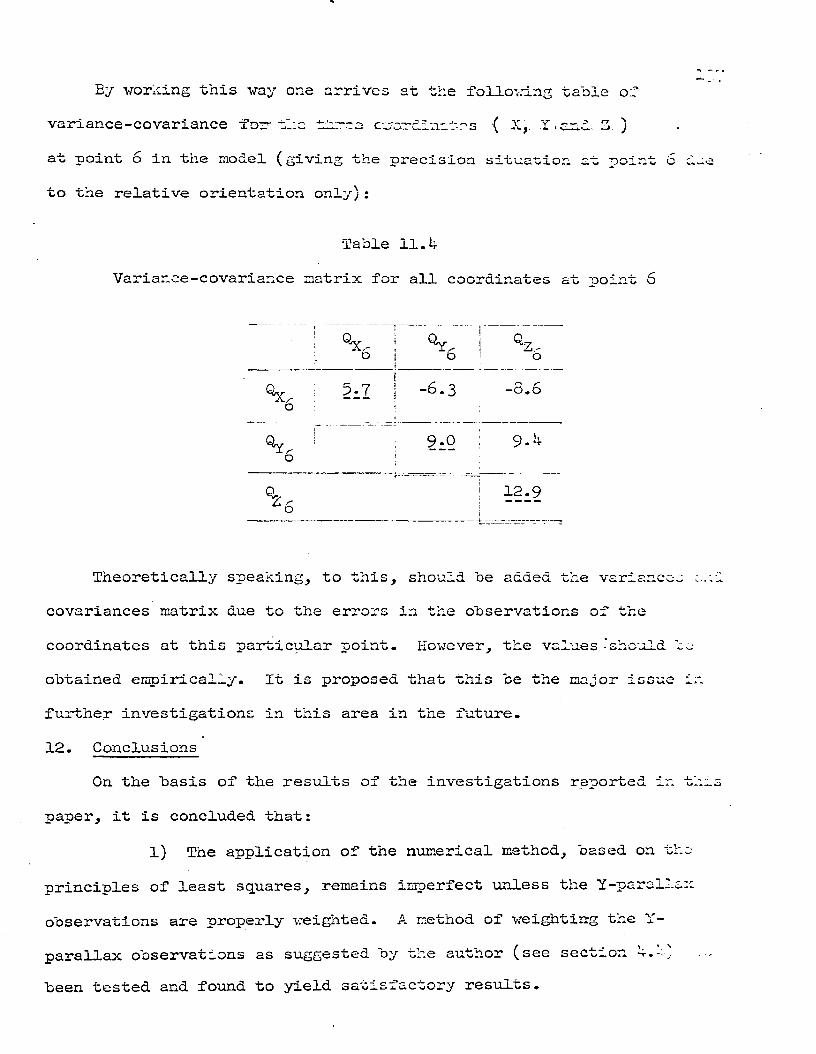
Ey wording this way one arrives at the following table of

variance-covariance -for- the thro a c-o0rd.in.afn5 { X, Y .end Z )

at point 6 in the model (giving the precision situation at poi to the relative orientation only):

Table 11. h

Variance-covariance matrix for all coordinates at ooint

Sc,- : j QZ.-o I O ' o

Qx- 5-7 S -6.36 ; !

S ' -\ r> S '^ 0 - 0.0

0* \ 9-0 : 9.K

Q.. 1 12.9•hr ---o

Theoretically speaking, to this, should be added the vari covariances matrix due to the errors in the observations of th

coordinates at this particular point. However, the values -sho obtained empirically. It is proposed that this be the major i further investigations in this area in the future.

12. ConclusionsOn the basis of the results of the investigations reporte

paper, it is concluded that:

l) The application of the numerical method, based

principles of least squares, remains imperfect unless the Y-pa observations are properly weighted. A method of weighting the parallax observations as suggested by the author (see section been tested and found to yield satisfactory results.

2) la comparing various methods of relative orientation, it has been observed that (l) In terms of efficiency, the empirical

methods are sufficient for plotting and give- very satisfactory rasu The numerical methods are complicated, less economical, but soma may find them to be more convenient for aerial triangulation rather t ■ ,n

for plotting; and (2) In terms of the obtainable precision, the numerical methods appear to yield, theoretically speaking, more precision, (it may be noted here that only for this comparative stu

is was assumed that all Y-parallax observations have equal weights and that the observations at different points are not correlated. T

is not a correct assumption, but was used with a view to avoid compl

derivations and because it does not affect the comparative study)3) The technique of forming the variance-covariar.ce matr

to represent the observational precision of the various methods of reli ;ive orientation are presented. Such matrices are found to be extremely helpful as tools to compare all the aspects of the various meth ods.

4) The quality of a relative orientation can be improved using more than the 6 standard points. The improvement in the squar of the standard errors of the elements is about 15 per cent with an increase of 50 per cent in the number of points. Thus, the improvem is not spectacular.

5) The quality of a relative orientation can also be improved by using more than one observation at each point. This impment is considerable only up to four repeat-observations at each poi

More than four repeat-observations do not yield any considerable

improvement.

6) It is empirically found (see Appendix i) that the standard error of X-parallax measurements is ahout O.h times the

standard error of Y-parallax measurements. Thus with the use of

devices ta change Y-parallaxes into X-parallaxes (e.g., Dove pri~. the observational precision of Y-parallaxes are greatly increase!, although this may not be economical in the long run.

7) For relative orientation, the use of X-parailaxes cc

totally replace the use of Y-parallaxes, which would generally yial

more precision.6) The variations in the spatial coordinates cf the poi

in the model (model-deformation) can be used in relative orientatic

However, the use of elevation errors only is recommended, for the s

of precision.9) The precision of the coordinates of the points in a

after the performance of relative orientation can be expressed by a

variance-covariance matrix. The formation of such a general matrix this purpose may be unmanageable and unpractical. Therefore, two possible simplifications are suggested and the techniques are press

A ) Studying only one coordinate for all points in

the model at a time; andB ) Studying only one point for all coordinates at

a time.

Appendix IEmpirical Determination of Comparative Precision

of X- and Y-parallax observations

For these investigations Wild Autograph A7 No. was used. Observations were made at three different points in a model with r.l; cot

flat terrain. Standard photography, f = 152.36 rcm. 23 cm x 23 cm. Picture scale 1:S000 approximately. Model scale 1: 000. One of the points was on a flat side-walk that was running East-West, the second point was on another flat side-walk that was running North-South and th third point was on a flat tennis court with lines crossing each other a right angles. Three hundred repeat-observations were taken at each point, thus making the total number of observations as 900. The 300 observations at each point were broken down as follows:

Case Al: 50 observations of Y-parallax elimination with by" andcorresponding by" counter readings by moving the right side measuring

mark from front to rear;Case A2: 50 observations of Y-parallax elimination with by" and

corresponding by" counter readings by moving the right side measuring

mark from rear to front;Next, after changing the Y-parallax into X-parallax with Dove prisCase Bl: 50 observations of Y-parallax elimination with by" and

corresponding counter readings by approaching the ground from above;Case B2: 50 observations of Y-parallax elimination with by" and

corresponding counter readings by approaching the ground surface from

below;Next, after coming back to the normal situation, by setting the

Dove prisms back to their original situations,

Case Cl: 50 observations of X-parallax elimination (i.e.,

reading of spot elevations)with tfca foot-disc and the corresponding

Z-counter readings by approaching the ground from above;

Case C2: 50 observations of X-parallax elimination ( _. e . ,

reading of spot elevations)with the foot-disc and corresponding Z- counter readings by approaching the ground from below.

The relevant elements were set in the oriented model to the following values:

f = 152-36 mm., Z = 30^.7 mm., and to: = 157.20 mm.Assuming the arithmetic mean to be the correct value for :.eh

case (i.e., Al, A2, Bl, B2, Cl and C2) the standard error for each can. eas computed. These are, as averages obtained from all of the three points:

Case Al: 15*7 microns,Case A2: 13*5 microns; their average gives the m.s.e. for

Case A .. It.6 microns.

Case Bl: 5*1 microns,Case B2: 5-7 microns; their average gives the m.s.e. for

Case B .. 5-t microns.

Case Cl: 10.9 microns,Case C2: l3.8 microns; their average gives the m.s.e. for

Case C .. It.3 microns.Case C gives the standard error of elevation determination in the

model, which is related to the X-parallax determination as given by

expression (9.2). This gives the standard error of X-parallax

11+2 'determination from Case C to be,.with proper substitutions in expression (9*2):

lk.8-^^*2 = 7.5 microns.

All the above are expressed as in the model. In these studies the model-scale was twice the picture-scale. From this consideration, for

the sake of standardization, one may finally express them at the picture-scale:

m.s.e. of Y-parallax determination 7*3 microns.m.s.e. of Y-parallax determination, by changing them to

X-parallaxes with Dove prisms - 2.7 microns.m.s.e. of X-parallax determination (from elevation

observations) 3*8 microns.

These show that the standard error of X-parallax determination isbetween 0.37 and 0.52 (i.e., between 2.7/7.3 and 3«8/7»3* depending on the element used for the puipose) times the standard error of Y- parallax measurements.; i.e., generally speaking,

®Px,Px = QPy,Py = 0,2 ^ P y *

In case the Dove prisms are used, it can be stated that

Spx,Px - S?y,Py •

NUMERICAL RELATIVE ORIENTATION (DEPENDENT METHOD)For Flat Terrain

AREA/STRIP NO. INSTRUMENT: WILD A7, No.CONSTANTS . SITUATION OF POINTS IN THE MODEL (MECHANICAL)

pC 6366 p/3b CASE A: 3 r ------! |CASE B:

Base in:Lt.camera new 2

---- -,31J,Z in mm. pz-Aa2b in mm. z/2a Base in:Rt.camera new 1 j--- _j2

Base out:Lt. " " 5 --- J611

cl in mm. pZ/2bd Base out:Rt. " " 6 1---- J5

PHOTO NO. LEFT: RIGHT:

’oint by. = by1-byin 3oint by. Pyi=byi‘bym

Zbyii average i average1 23 b %

=Zby./65 6I = 2]Pv-Py^Py, n= Py1+Py3+Py5 riI=2Py2-Py1(-Py6 IV=Py2+Py1|+Py6 |

(1)SIGN 'Constants

(2)jb-irection in mm. /min= (1K 2)

READINGS b y n after correction atCaseA

CaseB

. Initial Final=Inil.+con*11 II-IV + _ p/3b 3 b

11 I + III + + pzM 2 1 2

bZTI ‘W v _ _ z/2d 5 6*11 Py3_iy5"V + - PZ/2bd Final o y ^ (,= mean)

BibliographyAc nermann, F. Zur rechnerischen Orientierung von Konver;

Bildmessung und Luftbildyesen, Berlin. 19poBachmann, W. K. Theorie aes erreurs de l’Orientation relative.

Thise, Lausanne, 1943.Bachmann, W. K. Determination graph!cue de 11 inclination transversale.

Bull. Techn. de la Suisse Romande, 1953*Bachmann, W. K. Symbolische Berechnung der Gewichtskoeffizienten.

Schwei Z. Verm, u. Kult, 1945*Blum, jr. An Orientation Analysis of the Multiplex Model.

Photogrammetric Engineering., 1950.Brandenberger, A. J. Fehlertheorie der iiusseren Orientierung von

Steilaufnahmen. Diss. Z.T.H., Zurich, 19 7-Brandenberger, A. J. Theorie und Praxis der gegenseitigen Orientiervug

von Steilaufnahmen. Serve!. Zeit. fiir vermes sung und Kulturtechnik, Nr. 9} 19 7*

Brandenberger, A. J. Unpublished lecture notes on Stereophotogrammetry. Ghosh, S. K. Some Adjusted Thoughts on Errors in Aerial T: ■ bd. Uv* m

'£rPhotogrammetric Engineering, June, I960.Ghosh, S. K. Determination of weights of Parallax Observations for

Numerical Relative Orientation.Photogrammetric Engineering, September, 1963*

Ghosh, S. K. Experience of Model Orientation in Wild A8 Stereoplottors. Photogrammetric Engineering, January, 1964.

Grossmann, W. Grandzuge der Ausgleichungsreehnung, Berlin, I9SI.Hallert, B. Contribution to Theory of Errors for Double Point Inter­

section in Space. Royal Institute of Technology publication, Stockholm 70, 1950.

Hallert, B. Some Remarks Concerning the Theory of Errors for Convergent Aerial Pictures in Comparison with NearVertical Pictures. Photogrammetric Engineering, December, 1954.

Jerie, H. G. Numerische Orientierung gebirgigen GelSndes.Photogrammetria, 1953-54, No. 1.

Jerie, H. C-. Vorzeichenfragen- an raumlichen Auswertegeraten.Photogrammetria, 1955-56, No. 1.

Kasper, H. Zur Fehlertheorie der gegenseitigen Orientierung.Schwei. Zeit. ftir Verm., 1947.

Kasper, H. Die Auswirinng kritischer Kreisschnitte bei der gegenseitigen Orientierung.Schvei. Zeit. fiir Venn., 1948.

144

Kasper, H. Die Uberkorrektur bei der gegenseitigen Orientierung. Schwei. Zeit. fUr Verm, ±9^9•

Kasper, H. Graphic Determination of the Over-correction Factor fo Use in the Relative Orientation of Vertical Photogrcyus Any Terrain.Photogrammetric Engineering, April, 1956.

Krames, M. J. Uber ein graphisches Verfahren zum gegenseitigen Einpassen von Luftaufnahmen.Osterr. Zeitsch. fdr Verm., 19^9, Nr. 37-

Krames, M. J. About a New Graphic Method of Orienting a Pair of Aerial Photographs.Photogrammetric Engineering, September, 1950.

Kraraes, M. J. Graphische Ldsung der Hauptaufgabe in Sinne der Aus chsrechnung,Zeit. xiir angew. Math, und Mech., 195^-

Pauwen, L. J. Sur un proc^d^ d'orientation relative.Bull. Beige de Photogrammetrie, 19 -9> No. lo.

Pauwen, L. J. A Method of Relative Orientation Based on the Measurement of Vertical Parallaxes.Photogrammetria, 1950-51> No. k.

Poivilliers, G. Formation de 1*image plastique.International Archives, 19^o.

Poivilliers, G. A Method of Relative Orientation.International Archives, i960.

Schut, G. E. Precision de 1*orientation relative apres la methode Poivilliers.Photogrammetria, 19^9-50, No. 3.

Singleton, R. Vertical Exaggeration and Perceptual Models. Photogrammetric Engineering, March, 1956-

Tewinkel, G. C. Numerical Relative Orientation.Photogrammetric Engineering, December, 1953-

Thonpson, E. H.. Thompson-Watts Plotting Machine.The Photogrammetric Record, April, 195^> No. 3j V°1 1-

Tienstra, J. M. Het rekenen met Gewichtsgetallen.Tijdschrift voor Kadaster en Landmeetkunde, 193^-

v.d. Weele, A. J. Zur Fehlertheorie der gegenseitigen Orientierun Schwei. Zeit. fiir Verm., 19^8.

v.d. Weele, A. J. La methode num^rique de l*orientation relative. Bull. Beige de Photogrammetrie, 1951., No. 1.

Zeller, M. Zur Fehlertheorie der gegenseitigen Orientierung. Schwei. Zeit. fdr Verm., 19^7, Nr. 9-