THÈSE Pour obtenir le grade de

DOCTEUR DE L’UNIVERSITE GRENOBLE ALPES Spécialité : Informatique Arrêté ministériel : 25 mai 2016 Présentée par

Tiago TREVISAN JOST

Thèse dirigée par Frédéric PETROT, Professeur, Grenoble INP/Ensimag, Université Grenoble Alpes et codirigée par Albert COHEN, Ingénieur HDR, Google et Christian FABRE, ingénieur-chercheur, CEA LIST Grenoble préparée au sein du Laboratoire d'Intégration des Systèmes et des Technologies / CEA LIST Grenoble dans l'École Doctorale Mathématiques, Sciences et technologies de l'information, Informatique

Compilation et optimisations pour l'arithmétique à virgule flottante en précision variable : du langage et des bibliothèques à la génération de code Compilation and optimizations for Variable Precision Floating-Point Arithmetic: From Language and Libraries to Code Generation Thèse soutenue publiquement le 02/07/2021 devant le jury composé de :

Monsieur FREDERIC PETROT PROFESSEUR DES UNIVERSITES, UNIVERSITE GRENOBLE ALPES, Directeur de Thèse Monsieur PHILIPPE CLAUSS PROFESSEUR DES UNIVERSITES, UNIVERSITE STRASBOURG, Rapporteur Monsieur ERVEN ROHOU DIRECTEUR DE RECHERCHE, CNRS BRETAGNE et PAYS DE LA LOIRE, Rapporteur Monsieur SEBASTIAN HACK PROFESSEUR, Universität des Saarlandes, Examinateur Monsieur DAVID MONNIAUX DIRECTEUR DE RECHERCHE, CNRS DELEGATION ALPES, Président Madame NATHALIE REVOL CHARGE DE RECHERCHE, INRIA CENTRE GRENOBLE-RHONEALPES, Examinatrice Monsieur ALBERT COHEN INGENIEUR HDR, Google France, Co-directeur de thèse Monsieur CHRISTIAN FABRE INGENIEUR DE RECHERCHE, CEA-List, Invité et Co-Encadrant de Thèse

Abstract

Floating-Point (FP) units in processors are generally limited to supporting a subset of formatsdefined by the IEEE 754 standard, along with a few target-specific ones (X86 with an 80-bit FPformat, and PowerPC performing 128-bit FP arithmetic). As a result, high-efficiency languagesand optimizing compilers for high-performance computing are also limited by the FP typessupported by these units. However, the pursuit of efficiency and stability on applications hasled researchers to investigate a finer control of exponent and fraction bits for finding the rightbalance between accurate results and execution time and/or energy consumed. For example,numerical computations often involve iterative solvers where the residual error is a function ofthe input data, or where dynamically adaptive precision can accelerate convergence. Numericalanalysts have to resort to explicit conversions and multi-versioning, resulting in code bloat andmaking the intent of the program even less clear. Little attention in languages and compilershas been given to formats that disrupt the traditional FP arithmetics with runtime capabilitiesand allow the exploration of multiple configurations, a paradigm recently referred to as variableprecision computing. This thesis proposes to overcome the limiting language and compilersupport for traditional FP formats with novel FP arithmetic with runtime capabilities, showingthe intersection between compiler technology and variable precision arithmetic. We present anextension of the C type system that can represent generic FP operations and formats, supportingboth static precision and dynamically variable precision. We design and implement a compilationflow bridging the abstraction gap between this type system and low-level FP instructions orsoftware libraries. The effectiveness of our solution is demonstrated through an LLVM-basedimplementation, leveraging aggressive optimizations in LLVM including the Polly loop nestoptimizer. We provide support for two backend code generators: one for the ISA of a variableprecision FP arithmetic coprocessor, and one for the MPFR multi-precision floating-point library.We demonstrate the productivity benefits of our intuitive programming model and its abilityto leverage an existing compiler framework. Experiments on two high-performance benchmarksuites yield strong speedups for both our software and hardware targets. We also show interestinginsights on the use of variable precision computing in linear algebra kernels.

i

Résumé

Les unités de calcul à virgule flottante (FP) prennent en charge un sous-ensemble de formatsdéfinis par la norme IEEE 754, ainsi que quelques formats qui leur sont spécifiques (le format de80 bits sur de l’architecture x86, et le format 128 bit propriétaire des PowerPC). De fait, leslangages et les compilateurs optimisants utilisés en calcul intensif sont limités par les formatssupportés sur les machines cibles. Cependant, la recherche de l’efficacité et de la stabilitédes applications a conduit les numériciens à explorer d’autres tailles pour les exposants et lesparties fractionnaires afin de trouver un bon équilibre entre la précision des résultats, le tempsd’exécution et l’énergie consommée. C’est le cas pour les calculs numériques qui font appel à dessolveurs itératifs dont l’erreur résiduelle est une fonction des données d’entrée, ou ceux pourlesquels une précision adaptable dynamiquement peut accélérer la convergence. Les numériciensdoivent recourir à des conversions explicites et prévoir plusieurs versions du code, ce qui entraîneun accroissement de la taille de ce dernier au détriment de sa lisibilité Peu d’attention a étéaccordée au support d’autre formats flottants dans les langages et à leur compilation, ainsi qu’àleurs conséquences sur le processus d’analyse numérique. Le calcul en précision variable est unparadigme récent qui propose de faire varier les formats à l’exécution et d’en analyser les effets.Les travaux que nous présentons visent à surmonter les limites actuelles des langages et de leurcompilation en y ajoutant le support aux formats à précision variable, et en abordant certainsdes problèmes que ces formats font apparaître à la jonction de la compilation et de l’arithmétiqueà précision variable. Pour cela nous proposons une extension du système de types du langage Cpermettant de représenter de manière générique les formats flottants et leurs opérations, aussibien en précision statique que dynamique. Nous avons mis en œuvre un flot de compilationqui implémente ce système de type jusqu’à la génération de code vers des jeux d’instructionsou des bibliothèques supportant de tels formats. Notre solution basée sur LLVM a démontréson efficacité en tirant parti des puissantes optimisations de LLVM, notamment l’optimisationde nids de boucles par Polly. Nous proposons un support pour deux générateurs de code : unpremier pour le jeu d’instruction d’un coprocesseur arithmétique à précision variable, et undeuxième ciblant la bibliothèque MPFR de virgule flottante en multi précision. Ce supportdémontre les avantages de productivité de notre modèle de programmation intuitif et sa capacitéà tirer parti d’une chaîne de compilation existante. Les expérimentations réalisées sur deuxsuites de référence en calcul à haute performance ont permis d’obtenir de fortes accélérationsaussi bien pour nos cibles logicielles que matérielles. Nous présentons également des résultatsintéressants sur l’utilisation de la précision variable pour des noyaux d’algèbre linéaire.

iii

Acknownledgement

First, I would like to the jury for having accepted to be part of my defense and for all insightfulcomments, and questions. I would also like to thank Christian and Albert for giving me theopportunity to work on this subject since the beginning, and Frédéric for having accepted to geton board in the last year of my PhD. All of you have made these last three years much easierwith your availability, insights, feedbacks, and enormous help whenever I needed. I would like tothank Yves, my unofficial math-related advisor, who had the patience to explain many mathconcepts that I would, otherwise, have struggled with during this period. I extend my gratitudeto Vincent, Diego and Alexandre who welcomed me in their laboratories, and all my amazingco-workers from LIALP, LSTA and the whole CEA for their kindness and for their support.Special thanks to Andrea whose work have played an important role in the experiment sectionof this manuscript. Many thanks to all my friends here in France, in Brazil, and around theworld for helping to relax in times of stress, specially close to paper deadlines.

None of this would have been possible without the caring and loving support of my wholefamily. The awesome energy you have sent me from Brazil surely played a role on the output ofthis work. Thank you for believing in me. Love you guys! And last but not least, this work isdedicated to Jana, my amazing wife, who were always there for me and has agreed to embarkwith me in this journey. I can never thank you enough for all your love and support. Love youso much!

v

Contents

List of Figures xi

List of Tables xv

List of Listings xvii

1 Introduction 11.1 Contributions . . . . . . . . . . . . . . . . . . . . . . . . . . . . . . . . . . . . . . 21.2 Outline . . . . . . . . . . . . . . . . . . . . . . . . . . . . . . . . . . . . . . . . . 2

2 Problem Statement 52.1 Introduction . . . . . . . . . . . . . . . . . . . . . . . . . . . . . . . . . . . . . . . 52.2 Precision versus Accuracy . . . . . . . . . . . . . . . . . . . . . . . . . . . . . . . 52.3 Floating-Point Representation . . . . . . . . . . . . . . . . . . . . . . . . . . . . . 7

2.3.1 IEEE Formats . . . . . . . . . . . . . . . . . . . . . . . . . . . . . . . . . 72.3.2 UNUM . . . . . . . . . . . . . . . . . . . . . . . . . . . . . . . . . . . . . 92.3.3 Posit . . . . . . . . . . . . . . . . . . . . . . . . . . . . . . . . . . . . . . . 92.3.4 New FP Formats from a Compiler’s Point of View . . . . . . . . . . . . . 10

2.4 Variable Precision as a New Paradigm for FP Arithmetic . . . . . . . . . . . . . 102.4.1 Problem with Precision Cherry-picking: Numerical Stability and Numerical

Accuracy . . . . . . . . . . . . . . . . . . . . . . . . . . . . . . . . . . . . 112.4.1.1 Quantifying Errors in Floating Points . . . . . . . . . . . . . . . 112.4.1.2 Augmenting Precision to Remedy Stability . . . . . . . . . . . . 12

2.4.2 Linear Algebra from the Variable Precision Perspective . . . . . . . . . . 132.5 Languages and Data types . . . . . . . . . . . . . . . . . . . . . . . . . . . . . . . 142.6 Compilers and Optimizations . . . . . . . . . . . . . . . . . . . . . . . . . . . . . 152.7 Conclusion . . . . . . . . . . . . . . . . . . . . . . . . . . . . . . . . . . . . . . . 17

3 Programming Languages, Paradigms for FP Computation and exploration Tools 193.1 Computing paradigms for floating-point arithmetics . . . . . . . . . . . . . . . . 19

3.1.1 Mixed precision computing . . . . . . . . . . . . . . . . . . . . . . . . . . 203.1.2 Arbitrary precision . . . . . . . . . . . . . . . . . . . . . . . . . . . . . . . 20

3.1.2.1 MPFR Multi-precision library . . . . . . . . . . . . . . . . . . . 213.1.2.2 C++ Boost for Multi-precision . . . . . . . . . . . . . . . . . . . 22

vii

3.1.2.3 Dynamic-typed Languages: a Julia example . . . . . . . . . . . . 223.2 Exploration Tools (Hardware and Software) . . . . . . . . . . . . . . . . . . . . . 23

3.2.1 Software for Alternative FP Formats . . . . . . . . . . . . . . . . . . . . . 233.2.2 Precision-Awareness, Auto-Tuning, and Numerical Error Detection . . . . 243.2.3 Software for Scientific Computing Exploration . . . . . . . . . . . . . . . 25

3.2.3.1 Basic Linear Algebra Subprograms (BLAS) . . . . . . . . . . . . 253.2.3.2 Linear Algebra Package (LAPACK) . . . . . . . . . . . . . . . . 27

3.2.4 Characteristics of the Hardware Implementation of Variable Precision FPUnits . . . . . . . . . . . . . . . . . . . . . . . . . . . . . . . . . . . . . . 273.2.4.1 Round-off Error Minimization through Long Accumulators . . . 273.2.4.2 A Family of Variable Precision, Interval Arithmetic Processors . 273.2.4.3 Scalar Multiple-precision UNUM RISC-V Floating-point Accel-

erator (SMURF) . . . . . . . . . . . . . . . . . . . . . . . . . . . 283.2.4.4 Other (UNUM or Posit) accelerators . . . . . . . . . . . . . . . . 29

3.3 Conclusion . . . . . . . . . . . . . . . . . . . . . . . . . . . . . . . . . . . . . . . 29

4 Language and Type System Specifications for Variable Precision FP Arithmetic 314.1 Syntax . . . . . . . . . . . . . . . . . . . . . . . . . . . . . . . . . . . . . . . . . . 324.2 Semantics . . . . . . . . . . . . . . . . . . . . . . . . . . . . . . . . . . . . . . . . 344.3 A multi-format type system . . . . . . . . . . . . . . . . . . . . . . . . . . . . . . 35

4.3.1 MPFR . . . . . . . . . . . . . . . . . . . . . . . . . . . . . . . . . . . . . . 354.3.2 UNUM . . . . . . . . . . . . . . . . . . . . . . . . . . . . . . . . . . . . . 364.3.3 Alternatives Formats . . . . . . . . . . . . . . . . . . . . . . . . . . . . . . 38

4.4 Memory allocation schemes . . . . . . . . . . . . . . . . . . . . . . . . . . . . . . 394.4.1 Constant Types . . . . . . . . . . . . . . . . . . . . . . . . . . . . . . . . . 40

4.4.1.1 Representing constants . . . . . . . . . . . . . . . . . . . . . . . 404.4.2 Constant-Size Types with Runtime-Decidable Attributes . . . . . . . . . . 414.4.3 Dynamically-Sized Types . . . . . . . . . . . . . . . . . . . . . . . . . . . 41

4.4.3.1 Runtime verification . . . . . . . . . . . . . . . . . . . . . . . . . 424.4.3.2 Function __sizeof_vpfloat . . . . . . . . . . . . . . . . . . . . 434.4.3.3 Function Parameter and Return . . . . . . . . . . . . . . . . . . 454.4.3.4 Constants . . . . . . . . . . . . . . . . . . . . . . . . . . . . . . . 46

4.5 Type Comparison, Casting and Conversion . . . . . . . . . . . . . . . . . . . . . 464.6 Language Extension Limitations . . . . . . . . . . . . . . . . . . . . . . . . . . . 474.7 Libraries for Variable Precision . . . . . . . . . . . . . . . . . . . . . . . . . . . . 48

4.7.1 mpfrBLAS: A vpfloat<mpfr, ...> BLAS library . . . . . . . . . . . . . 494.7.1.1 Level 1: Vector-to-vector operations . . . . . . . . . . . . . . . . 494.7.1.2 Level 2: Matrix-vector operations . . . . . . . . . . . . . . . . . 504.7.1.3 Level 3: Matrix-matrix operations . . . . . . . . . . . . . . . . . 53

4.7.2 unumBLAS: A vpfloat<unum, ...> BLAS library . . . . . . . . . . . . . 544.7.2.1 Level 1: Vector-to-vector operations . . . . . . . . . . . . . . . . 54

viii

4.7.2.2 Level 2: Matrix-vector operations . . . . . . . . . . . . . . . . . 554.7.2.3 Level 3: Matrix-matrix operations . . . . . . . . . . . . . . . . . 56

4.8 Conclusion . . . . . . . . . . . . . . . . . . . . . . . . . . . . . . . . . . . . . . . 57

5 Compiler Integration for Variable Precision FP Formats 595.1 Frontend . . . . . . . . . . . . . . . . . . . . . . . . . . . . . . . . . . . . . . . . . 595.2 Intermediate Representation (IR) . . . . . . . . . . . . . . . . . . . . . . . . . . . 59

5.2.1 VPFloat Types . . . . . . . . . . . . . . . . . . . . . . . . . . . . . . . . . 605.2.2 Function Declarations . . . . . . . . . . . . . . . . . . . . . . . . . . . . . 615.2.3 Interaction with Classical Optimizations . . . . . . . . . . . . . . . . . . . 62

5.2.3.1 Type-value Relation . . . . . . . . . . . . . . . . . . . . . . . . . 635.2.3.2 Loop Idiom Recognition . . . . . . . . . . . . . . . . . . . . . . . 635.2.3.3 Inlining . . . . . . . . . . . . . . . . . . . . . . . . . . . . . . . . 645.2.3.4 Lifetime Marker Optimization . . . . . . . . . . . . . . . . . . . 655.2.3.5 OpenMP Multithread Programming . . . . . . . . . . . . . . . . 665.2.3.6 Loop nest Optimizations . . . . . . . . . . . . . . . . . . . . . . 665.2.3.7 Vectorization . . . . . . . . . . . . . . . . . . . . . . . . . . . . . 66

5.3 Code Generators . . . . . . . . . . . . . . . . . . . . . . . . . . . . . . . . . . . . 685.3.1 Software Target: MPFR . . . . . . . . . . . . . . . . . . . . . . . . . . . . 685.3.2 Hardware Target: UNUM . . . . . . . . . . . . . . . . . . . . . . . . . . . 74

5.3.2.1 Compiler-Controlled Status Registers . . . . . . . . . . . . . . . 755.3.2.2 FP Configuration Pass . . . . . . . . . . . . . . . . . . . . . . . 755.3.2.3 Array Address Calculation Pass . . . . . . . . . . . . . . . . . . 76

5.4 Conclusion . . . . . . . . . . . . . . . . . . . . . . . . . . . . . . . . . . . . . . . 77

6 Experimental results 796.1 The Benefits of Language and Compiler Integration . . . . . . . . . . . . . . . . 79

6.1.1 MPFR vpfloat vs. Boost Multi-precision . . . . . . . . . . . . . . . . . . 796.1.1.1 Polybench . . . . . . . . . . . . . . . . . . . . . . . . . . . . . . 806.1.1.2 RAJAPerf . . . . . . . . . . . . . . . . . . . . . . . . . . . . . . 85

6.1.2 Hardware(UNUM vpfloat) vs. Software (MPFR vpfloat) . . . . . . . . 886.2 Linear Algebra Kernels . . . . . . . . . . . . . . . . . . . . . . . . . . . . . . . . . 906.3 Conclusion . . . . . . . . . . . . . . . . . . . . . . . . . . . . . . . . . . . . . . . 102

7 Conclusion 103

A CG Experimental Results: Number of Iterations 109

B CG Experimental Results: Execution Time 115

Publications 121

ix

List of Figures

2.1 IEEE Formats (officially known as binary16, binary32, binary64, and binary128as defined by the standard. . . . . . . . . . . . . . . . . . . . . . . . . . . . . . . 8

2.2 The Universal NUMber (UNUM) Format . . . . . . . . . . . . . . . . . . . . . . 92.3 The Posit Format . . . . . . . . . . . . . . . . . . . . . . . . . . . . . . . . . . . . 92.4 Relationship between backward and forward errors. . . . . . . . . . . . . . . . . . 122.5 When applied on different MatrixMarket [24, 86] matrices, the number of iterations

for the conjugate gradient (CG) algorithm decreases when precision augments.This experiment aims to show the usage of variable precision in a real-life application. 13

4.1 Difference between Gustafson and Bocco et al. [21, 23] UNUM formats. . . . . . 374.2 Summary of vpfloat multi-format schemes. . . . . . . . . . . . . . . . . . . . . . 394.3 Memory Allocation Schemes for Constant-Size and Dynamically-Sized Types . . 40

6.1 Speedup of Polly’s loop nest optimizer in Polybench compiled for vpfloat<mpfr,

... types. . . . . . . . . . . . . . . . . . . . . . . . . . . . . . . . . . . . . . . . 826.2 Speedup of vpfloat<mpfr, ...> over the Boost library for multi-precision for

the Polybench benchmark suite, and compiled with optimization level -O3. Theexecution time reference taken are the best between compilations with and withoutPolly. Results are shown for two different machines: an Intel Xeon E5-2637v3with 128GB of RAM (M1), and an Intel Xeon Gold 5220 with 96 GB of RAM(M2), respectively. Y-axes are shown with the same limits to ease comparisonsbetween results in the two machines. . . . . . . . . . . . . . . . . . . . . . . . . . 83

6.3 Speedup of vpfloat<mpfr, ...> over the Boost library for multi-precision for thePolybench benchmark suite. vpfloat<mpfr, ...> applications were compiledwith optimization level -O1 and Boost with -O3. The execution time referencetaken are the best between compilations with and without Polly. Results areshown for two different machines: an Intel Xeon E5-2637v3 with 128GB of RAM(M1), and an Intel Xeon Gold 5220 with 96 GB of RAM (M2), respectively. Y-axesare shown with the same limit to ease comparisons between results in the twomachines. . . . . . . . . . . . . . . . . . . . . . . . . . . . . . . . . . . . . . . . . 84

6.4 Speedup of vpfloat<mpfr, ...> over the Boost library for multi-precision forthe RAJAPerf benchmark suite, both compiled with -O3 optimization level. . . . 87

xi

6.5 Speedup of vpfloat<unum, ...> over vpfloat<mpfr, ...> on the PolyBenchsuite . . . . . . . . . . . . . . . . . . . . . . . . . . . . . . . . . . . . . . . . . . . 89

6.6 CG variants with multiple formats with matrices nasa2910, bcsstk08, bcsstk11,bcsstk12, bcsstk13, and bcsstk16 from matrix market [24, 86]. Graph lines representdifferent matrices, and graph columns correspond to variants (from left to right:original CG, precond CG, pipelined CG, BiCG). Y-axes show the number ofiterations needed to converge for precision in bits between 150 and 2000 with astep=50. A missing type in a graph implies the algorithm did not converge. . . 97

6.7 CG variants with multiple formats with matrices bcsstk19, bcsstk20, bcsstk23,crystk01, s3rmt3m3, and plat1919 from matrix market [24, 86]. Graph linesrepresent different matrices, and graph columns correspond to variants (fromleft to right: original CG, precond CG, pipelined CG, BiCG). Y-axes show thenumber of iterations needed to converge for precision in bits between 150 and2000 with a step=50. A missing type in a graph implies the algorithm did notconverge. . . . . . . . . . . . . . . . . . . . . . . . . . . . . . . . . . . . . . . . . 98

6.8 Execution time for CG variants with multiple formats with matrices nasa2910,bcsstk08, bcsstk11, bcsstk12, bcsstk13, and bcsstk16 from matrix market [24, 86].Graph lines represent different matrices, and graph columns correspond to variants(from left to right: original CG, precond CG, pipelined CG, BiCG). A missingtype in a graph implies the algorithm did not converge. Results for double arenot displayed. . . . . . . . . . . . . . . . . . . . . . . . . . . . . . . . . . . . . . . 100

6.9 Execution time for CG variants with multiple formats with matrices bcsstk19,bcsstk20, bcsstk23, crystk01, s3rmt3m3, and plat1919 from matrix market [24,86]. Graph lines represent different matrices, and graph columns correspondto variants (from left to right: original CG, precond CG, pipelined CG, BiCG).A missing type in a graph implies the algorithm did not converge. Results fordouble are not displayed. . . . . . . . . . . . . . . . . . . . . . . . . . . . . . . . 101

A.1 CG variants with multiple formats with matrices bcsstk04, bcsstk05, bcsstk06,bcsstk07, bcsstk09, and bcsstk10 from matrix market [24, 86]. Graph linesrepresent different matrices, and graph columns correspond to variants (fromleft to right: original CG, precond CG, pipelined CG, BiCG). Y-axes show thenumber of iterations needed to converge for precision in bits between 150 and2000 with a step=50. A missing type in a graph implies the algorithm did notconverge. . . . . . . . . . . . . . . . . . . . . . . . . . . . . . . . . . . . . . . . . 110

xii

A.2 CG variants with multiple formats with matrices bcsstk14, bcsstk15, bcsstk21,bcsstk22, bcsstk24, and bcsstk26 from matrix market [24, 86]. Graph linesrepresent different matrices, and graph columns correspond to variants (fromleft to right: original CG, precond CG, pipelined CG, BiCG). Y-axes show thenumber of iterations needed to converge for precision in bits between 150 and2000 with a step=50. A missing type in a graph implies the algorithm did notconverge. . . . . . . . . . . . . . . . . . . . . . . . . . . . . . . . . . . . . . . . . 111

A.3 CG variants with multiple formats with matrices bcsstk27, bcsstk28, bcsstk34,bcsstm07, bcsstm10, and bcsstm12 from matrix market [24, 86]. Graph linesrepresent different matrices, and graph columns correspond to variants (fromleft to right: original CG, precond CG, pipelined CG, BiCG). Y-axes show thenumber of iterations needed to converge for precision in bits between 150 and2000 with a step=50. A missing type in a graph implies the algorithm did notconverge. . . . . . . . . . . . . . . . . . . . . . . . . . . . . . . . . . . . . . . . . 112

A.4 CG variants with multiple formats with matrices bcsstm27, 494_bus, 662_bus,685_bus, s1rmq4m1, and s1rmt3m1 from matrix market [24, 86]. Graph linesrepresent different matrices, and graph columns correspond to variants (fromleft to right: original CG, precond CG, pipelined CG, BiCG). Y-axes show thenumber of iterations needed to converge for precision in bits between 150 and2000 with a step=50. A missing type in a graph implies the algorithm did notconverge. . . . . . . . . . . . . . . . . . . . . . . . . . . . . . . . . . . . . . . . . 113

A.5 CG variants with multiple formats with matrices s2rmt3m1, s3rmq4m1, s3rmt3m1,and plat362 from matrix market [24, 86]. Graph lines represent different matrices,and graph columns correspond to variants (from left to right: original CG,precond CG, pipelined CG, BiCG). Y-axes show the number of iterations neededto converge for precision in bits between 150 and 2000 with a step=50. A missingtype in a graph implies the algorithm did not converge. . . . . . . . . . . . . . . 114

B.1 Execution time for CG variants with multiple formats with matrices bcsstk04,bcsstk05, bcsstk06, bcsstk07, bcsstk09, and bcsstk10 from matrix market [24, 86].Graph lines represent different matrices, and graph columns correspond to variants(from left to right: original CG, precond CG, pipelined CG, BiCG). A missingtype in a graph implies the algorithm did not converge. Results for double arenot displayed. . . . . . . . . . . . . . . . . . . . . . . . . . . . . . . . . . . . . . . 116

B.2 Execution time for CG variants with multiple formats with matrices bcsstk14,bcsstk15, bcsstk21, bcsstk22, bcsstk24, and bcsstk26 from matrix market [24, 86].Graph lines represent different matrices, and graph columns correspond to variants(from left to right: original CG, precond CG, pipelined CG, BiCG). A missingtype in a graph implies the algorithm did not converge. Results for double arenot displayed. . . . . . . . . . . . . . . . . . . . . . . . . . . . . . . . . . . . . . . 117

xiii

B.3 Execution time for CG variants with multiple formats with matrices bcsstk27,bcsstk28, bcsstk34, bcsstm07, bcsstm10, and bcsstm12 from matrix market [24,86]. Graph lines represent different matrices, and graph columns correspondto variants (from left to right: original CG, precond CG, pipelined CG, BiCG).A missing type in a graph implies the algorithm did not converge. Results fordouble are not displayed. . . . . . . . . . . . . . . . . . . . . . . . . . . . . . . . 118

B.4 Execution time for CG variants with multiple formats with matrices bcsstm27,494_bus, 662_bus, 685_bus, s1rmq4m1, and s1rmt3m1 from matrix market [24,86]. Graph lines represent different matrices, and graph columns correspondto variants (from left to right: original CG, precond CG, pipelined CG, BiCG).A missing type in a graph implies the algorithm did not converge. Results fordouble are not displayed. . . . . . . . . . . . . . . . . . . . . . . . . . . . . . . . 119

B.5 Execution time for CG variants with multiple formats with matrices s2rmt3m1,s3rmq4m1, s3rmt3m1, and plat362 from matrix market [24, 86]. Graph linesrepresent different matrices, and graph columns correspond to variants (from leftto right: original CG, precond CG, pipelined CG, BiCG). A missing type in agraph implies the algorithm did not converge. Results for double are not displayed.120

xiv

List of Tables

2.1 Residual error for some Polybench [98] applications. It illustrates the differencebetween accuracy, here calculated through the residual error of each application,and precision, represented by 24, 53, 128, and 512 bits. The residual error iscalculated as the norm function between measured and exact values of the outputvector or matrix. . . . . . . . . . . . . . . . . . . . . . . . . . . . . . . . . . . . . 6

3.1 Some of the data types supported in Schulte et al. [107] . . . . . . . . . . . . . . 283.2 Coprocessor’s Instruction Set Architecture . . . . . . . . . . . . . . . . . . . . . . 29

4.1 Comparison of the vpfloat type system and FP types, and data structures foundin the literature. . . . . . . . . . . . . . . . . . . . . . . . . . . . . . . . . . . . . 34

4.2 Sample UNUM declarations and their respective exponent, mantissa, and sizevalues. . . . . . . . . . . . . . . . . . . . . . . . . . . . . . . . . . . . . . . . . . . 39

4.3 Floating-point literal 1.3 represented with different types . . . . . . . . . . . . . . 41

5.1 Instructions supported by the UNUM Backend. . . . . . . . . . . . . . . . . . . . 745.2 ABI Convention for the VP registers . . . . . . . . . . . . . . . . . . . . . . . . . 755.3 Control registers inside the UNUM Coprocessor. . . . . . . . . . . . . . . . . . . 76

6.1 Machine configurations used for experiments. . . . . . . . . . . . . . . . . . . . . 806.2 Compilation time for Polybench with different optimization levels and types. . . 816.3 List of RAJAPerf applications classified according to their groups. . . . . . . . . 856.4 Average speedups for RAJA in machines M1 and M2 (from Table 6.1). . . . . . . . 866.5 Count on the number of matrices where vpfloat<mpfr, ...> outperforms other

types. Only matrix with types that converge are considered. For vpfloat andBoost, we cherry-pick the best execution time among the precision range (from150 to 2000 with a step=50) . . . . . . . . . . . . . . . . . . . . . . . . . . . . . . 99

xv

List of Listings

3.1 MPFR variable type as defined in [49] . . . . . . . . . . . . . . . . . . . . . . . . 213.2 Usage of the MPFR library in a matrix multiplication example . . . . . . . . . . 213.3 Usage of the C++ Boost library for Multi-precision in a matrix multiplication

example . . . . . . . . . . . . . . . . . . . . . . . . . . . . . . . . . . . . . . . . . 223.4 Implementation of matrix multiplication example in the Julia language: its

dynamic type system hides the types of variables until runtime evaluation . . . . 234.1 Backus normal form (BNF) like notation for the vpfloat language extension . . 334.2 MPFR variable type as defined in [49]. . . . . . . . . . . . . . . . . . . . . . . . . 354.3 axpy benchmark with vpfloat<mpfr, ...> type. . . . . . . . . . . . . . . . . . . 354.4 Usage of the vpfloat<mpfr, ...> in a matrix multiplication example. . . . . . . 364.5 Comparing naïve implementations of AXPY with a constant-size type (axpy_UnumConst

), a constant-size type with runtime attribute (axpy_UnumDyn), and GEMV witha dynamically-sized type (vgemv). . . . . . . . . . . . . . . . . . . . . . . . . . . . 38

4.6 Variable Length Array (VLA) example. . . . . . . . . . . . . . . . . . . . . . . . 424.7 Runtime checker implementation example of vpfloat<mpfr, ...> types. . . . . 434.8 __sizeof_vpfloat implementation example for vpfloat<unum, ...> and vpfloat

<mpfr, ...> types. . . . . . . . . . . . . . . . . . . . . . . . . . . . . . . . . . . 444.9 Uses of dynamically-sized types in function calls and returns. . . . . . . . . . . . 454.10 Uses of dynamically-sized types in function call and return. . . . . . . . . . . . . 474.11 Examples of implicit and explicit conversions between vpfloat<...> types . . . 485.1 Partial implementation of vpfloat types in the LLVM IR. . . . . . . . . . . . . . 605.2 IR code of the ex_dyn_type_ret function from Listing 4.9 types in the LLVM IR. 616.1 Calling a precision-generic implementation of CG . . . . . . . . . . . . . . . . . . 916.2 Implementation of algorithm 2 using mpfrBLAS 4.7.1. . . . . . . . . . . . . . . . 92

xvii

Chapter 1: Introduction

The dearth of compatible floating-point (FP) formats among companies in the early 1980shas significantly held back a plethora of applications, from signal and image processing toneural networks and numerical analysis, that leverage real numbers in their computation. Thestandardization of FP representations in the 1985 [45] was an important instrument to increasethe productivity and the usage of real numbers in a variety of research fields. In the samedirection, the progress of Very Large-Scale Integration (VLSI) technology has also contributedto allowing the generalization of hardware units for floating-point arithmetic.

The possibility of packing more transistors in the same die, predicted by Moore’s Law [89],has played an important role in the integration of multiple types of FP units in computersystems, for instance, scalar and single instruction, multiple data (SIMD) in single and multicoreprocessors, and single instruction, multiple threads (SIMT) in graphics processing units (GPU).The availability of hardware FP units is not only the rule nowadays, but they are also paramountto the performance of numerical applications. However, none of these major advancements bythe hardware industry would have been possible without the effort and robustness of computersystems and, especially, compiler technology.

Compilers play an important role and have long leveraged efficient usage of FP units.Compiler optimizations for FP operations target representations supported by the hardware: atbest, 16, 32, 64, and 128 bits IEEE formats, and perhaps some target-specific formats (X86 FP80and POWER9 128 bits). Although these representations are still well-suited for the majorityof applications, there is a need to rethink FP arithmetics as to improve performance, energyand/or accuracy. The reasoning is twofold:

(1) Exploring the trade-off between output quality, and accuracy has already motivated theadaptation of standard FP formats in applications. The main idea is to reduce precisionand exponent bits in use in the FP format in an attempt to trade quality by energy and/orperformance. By controlling the FP formats at a fine-grained granularity, this trade-offhas energy-saving and performance-increase potentials.

(2) A wide range of applications show optimal performance for FP representations that cannotbe represented with standard formats. On the one hand, Google’s bfloat16 [1] hasattracted a lot of interest for training and inference in neural networks [72] due to havinga higher exponent range than the IEEE 16-bit format. On the other hand, linear solvers,n-body problems [50], and other applications in mathematics and physics [14] have shownto benefit from higher-than-standard representations since (a) they may not converge withfewer bits of precision or (b) they can converge faster with higher precision [64]. Theseapplications may suffer from cancellation and accumulative errors when numbers cannotbe precisely represented using the standard formats.

1

Motivation (1) has gained a lot of research attention in the last years through approximatecomputing (AC) [88, 125]. AC aims to trade accuracy for energy savings and performance withthe assumption that a loss of accuracy in output results is irrelevant and can be tolerated.

The latter, especially for higher-than-standard representations, has not been explored to itsextent. The pursuit of efficiency and stability in the aforementioned domains has led researchersto reexamine the use of standard formats. Considering there is no unique precision value thatfits all targeted applications, variable precision (VP) computing has been used as an explorationtool to search for the most suitable solution for each.

This paradigm change has also led to the emergence of new FP formats and representations.New paradigms and representations must still rely on solid and robust languages and compilerinfrastructure in order to ease the exploration of further techniques and solutions. A gap betweenhardware designs for VP computing and their programming models still exists, as well as whatthe role of compilers is. This motivates the work of this thesis.

1.1 ContributionsThe main contributions of this thesis are:

(1) A multi-format, multi-representation language and compiler support for FP representationsthat are suitable for VP Computing. Among the sub-contributions related to it are:

(a) a C type-system extension for declaring FP numbers of arbitrary representation andsize. This generic class of FP types has attributes, such as the size of mantissa orexponent, or the size of the field encoding the mantissa or exponent, and the overallmemory footprint. These may be known statically or only at runtime,

(b) an IR embedding of the runtime and compile-time aspects of generic FP types.Thanks to a tight integration within a state-of-the-art compiler infrastructure, thisembedding allows benefiting from most existing compiler optimizations supportinghigh-performance numerical computing,

(c) two code generators implemented specifically to take advantage of VP Computing.

(2) A study demonstrating the exploration of VP in high-performance computing (HPC)applications, which includes:

(a) Basic Linear Algebra Subprograms (BLAS) libraries aimed at helping exploration ofVP in applications,

(b) A study that shows interesting insights to precision exploration in different variantsof the Conjugate Gradient algorithm, an iterative method for solving linear systems.

1.2 OutlineThis thesis is organized as follows:

Chapter 2 will present the main ideas within the literature and challenges that give basisto this thesis. We will cover aspects related to compiler and language support for novelFP representations, and how precision variation is being neglected on the software/hardwareintegration stack.

Chapter 3 will discuss the main state-of-the-art concepts related to this thesis, illustratinghardware and software aspects and how they co-related.

2

The first main contribution of this thesis, the vpfloat C-based language extension and typesystem, is described in Chapter 4, covering all aspects and details of the syntax, and semantics,along with library implementations.

Chapter 5 goes through the compiler integration requirements that are necessary to givesupport for our type system. It also presents the design and implementation of our codegenerators and target-specific passes.

Chapter 6 focus on the experimental setup and main results that give basis to the contributionsof this thesis.

Finally, chapter 7 summarizes the main contribution of this work and shows the maindirections envisioned as part of future work.

3

Chapter 2: Problem Statement

Contents2.1 Introduction . . . . . . . . . . . . . . . . . . . . . . . . . . . . . . . . . . . . . 52.2 Precision versus Accuracy . . . . . . . . . . . . . . . . . . . . . . . . . . . . . . 52.3 Floating-Point Representation . . . . . . . . . . . . . . . . . . . . . . . . . . . . 7

2.3.1 IEEE Formats . . . . . . . . . . . . . . . . . . . . . . . . . . . . . . . . 72.3.2 UNUM . . . . . . . . . . . . . . . . . . . . . . . . . . . . . . . . . . . . 92.3.3 Posit . . . . . . . . . . . . . . . . . . . . . . . . . . . . . . . . . . . . . . 92.3.4 New FP Formats from a Compiler’s Point of View . . . . . . . . . . . . 10

2.4 Variable Precision as a New Paradigm for FP Arithmetic . . . . . . . . . . . . 102.4.1 Problem with Precision Cherry-picking: Numerical Stability and Nu-

merical Accuracy . . . . . . . . . . . . . . . . . . . . . . . . . . . . . . . 112.4.2 Linear Algebra from the Variable Precision Perspective . . . . . . . . . 13

2.5 Languages and Data types . . . . . . . . . . . . . . . . . . . . . . . . . . . . . . 142.6 Compilers and Optimizations . . . . . . . . . . . . . . . . . . . . . . . . . . . . 152.7 Conclusion . . . . . . . . . . . . . . . . . . . . . . . . . . . . . . . . . . . . . . 17

2.1 IntroductionComputation techniques for real numbers is still an active field of research. Finding new computerrepresentations for real numbers that are optimized for an application remains challenging. Inthis chapter, we present the main ideas that form the basis for the research performed throughthe course of this thesis.

2.2 Precision versus AccuracyPrecision and accuracy are related concepts, although it is a mistake to think they are equivalent.The accuracy of a value relates to the proximity between the measurement of a value and its truevalue. In the context of the representation of real numbers, it is often expressed as the differencebetween the result of the computation and its exact result. On the other hand, precision makesreference to the current representation in use, and it is often expressed as a number of bits ordigits.

Table 2.1 illustrates the difference between accuracy, here calculated as the norm functionbetween measured and exact values of the output vector or matrix, and precision, represented by24, 53, 128, and 512 bits. One can notice that the accuracy is an application- and data-dependentconstraint, while precision is only subject to the value one chooses to adopt. The choice of

5

precision generally leads to high accuracy, however, rounding error and cancellation inherentto finite-sized representation may also influence output accuracy which can sometimes lead tohigh-precision representations to have less accurate results.

Table 2.1: Residual error for some Polybench [98] applications. It illustrates the differencebetween accuracy, here calculated through the residual error of each application, and precision,represented by 24, 53, 128, and 512 bits. The residual error is calculated as the norm functionbetween measured and exact values of the output vector or matrix.

DatasetMini Small Medium Large Xlarge

gemm 24 bits∗ 1.5e-5 2.1e-4 4.1e-3 2.3e-1 1.45e053 bits∗ 3.1e-14 4.0e-13 7.7e-12 4.33e-10 2.69e-9128 bits < 1e-600 < 1e-600 < 1e-600 1.49e-34 2.6e-33512 bits < 1e-600 < 1e-600 < 1e-600 < 1e-600 < 1e-600

3mm 24 bits∗ 6.7e-07 1.1e-04 3.1e-02 4.4e+01 998.453 bits∗ 1.3e-15 2.1e-13 5.8e-11 8.2e-08 1.8e-06128 bits 3.5e-38 5.6e-36 1.5e-33 2.13e-30 4.8e-29512 bits < 1e-600 < 1e-600 < 1e-600 < 1e-600 < 1e-600

covar 24 bits∗ 5.8e-5 5.6e-3 2.1e-1 41.02 5.7e+0253 bits∗ 1.2e-13 2.5e-12 2.37e-10 7.2e-8 1.0e-06128 bits 3.2e-36 6.6e-35 6.3e-33 1.9e-30 2.6e-29512 bits 9.1e-152 1.8e-150 1.6e-148 4.8e-146 6.7e-145

gram 24 bits∗ 28 71 220 616 86853 bits∗ 9.1 76 231 584 849128 bits 1.1e-21 7.0e-21 3.5e-20 1.7e-19 3.6e-6512 bits 4.6e-137 2.1e-136 7.5e-136 1.1e-134 1.3e-121

∗Correspond to IEEE 32 and IEEE 64 formats, respectively.

Without any need for a rounding operation, computers can only represent a small subset ofvalues (integers and few rational numbers, for example) in a finite number of bits. Predominantly,values cannot be precisely represented with a finite number of bits, and a rounding operation isneeded to bound the value to a fixed (and finite) representation. The accumulation of roundingoperations may cause the propagation of rounding errors, also known as round-off errors, that cancompromise the result of the application. The choice of precision used during the computationcan play an important role in binding the error to an expectable value. Table 2.1 shows howround-off errors influence the accuracy of multiple applications from the Polybench suite.

Cancellation is another property from finite-sized representations that can impact the qualityof results. It occurs when we subtract two values that are very close, but different. If thedifference is too small to be represented with the precision of the numeric format, the resultbecomes zero. It is usually overcome by analyzing its sources of issues and re-implementing thealgorithm [53].

A simple look at Table 2.1 shows that some algorithms are more susceptible to errors thanothers, and lower-precision implementations have, in general, lower accuracy. Some kernels arealso actually numerically unstable for 24, and 53 precision bits, even with small datasets, while

6

higher precision reaches stability (e.g. gramschmidt). If one strives for accuracy, it is paramountthat higher-than-standard precision be adopted.

While most modern processors have hardware support for variants with 24 bits and 53 bits,128-bit1 and 512-bit variants are more cumbersome. High precision is only supported throughsoftware libraries MPFR [49], GMP [54], and high-efficiency languages in high-performancecomputing do not provide any higher-level abstraction. This leads to tedious, error-proneand library-dependent implementations involving explicit memory management. Multiple-precision floating-point arithmetic, as provided by MPFR and GMP to explore different precisionlevels, is difficult to write and maintain, and more than the performance gap of a software FPimplementation, the productivity gap makes this approach inaccessible to potential users.

In that regard, the following questions may be asked: How can languages and compilersbe used to accelerate and improve the productivity of multi-precision FP libraries? Can oneimprove the integration between compilers and these libraries to take better advantage of classicalcompiler optimizations?

2.3 Floating-Point RepresentationFloating point is the most common way to represent real numbers in computer systems. Theyare written in the form of:

(−1)s× 1.m× 2e (2.1)

where s is a single bit specifying the sign of the number, 1.m denotes the mantissa part, alsoknown as precision or fraction part, and e represents the exponent of the number.

2.3.1 IEEE FormatsPrior to the standardization of floating-point representations in 19852, companies had their ownproprietary FP formats, with specific rules and format layout. For instance, IBM System/360 [66]introduced the Hexadecimal floating point (called HFP), Microsoft used the Microsoft BinaryFormat (MBF) for its BASIC [73] language products, and even the U.S. Air Force defineda formal specification of an ISA that included floating-point capabilities [108]. The IEEE754 standard technical document served as an important instrument to conform floating-pointformats to specific properties, and offer compatibility and portability for long-time use. Sincethen, the standard was widely adopted for representing real numbers in computer systems.

It defines a set of rules for rounding, exception handling, and operations in FP, along withdifferent encoding formats for FP arithmetics with representation ranging between 16 and 128bits (see Figure 2.1). Although equation 2.1 generalizes how FP numbers are calculated, onemust notice that format-specific features such as, Infinity, Not-a-Number (NaN), subnormals,and even biasing cannot be expressed through the formula. Instead, the IEEE 754 Standard forfloating-point arithmetic helps to address them individually.

The Intel 8087 [95], introduced in 1980, was the FP coprocessor for the Intel 8086 line ofmicroprocessors that is historically seen as the pioneer of the IEEE 754 standard. Although thecoprocessor did not implement it in all its details, it gave the basis for the standard specification.Subsequently, all major processor manufacturers have started to adopt IEEE formats in thedesign of FP units in order to leverage compatibility across multiple computing systems.

1Notice that 128 bits of precision does not correspondent to the IEEE FP128 format, which has 113 bits ofprecision

2The IEEE Standard for Floating-Point Arithmetic (IEEE 754) was established in 1985 [45], and revised in2008 [112] and 2019 [67])

7

sign

Binary16

exp.(5 bit)

frac.(10 bit)

sign

Binary32

exp.(8 bit)

frac.(23 bit)

sign

Binary64

exp.(11 bit)

frac.(52 bit)

sign

Binary128 . . .

exp.(15 bit)

frac.(112 bit)

Figure 2.1: IEEE Formats (officially known as binary16, binary32, binary64, and binary128 asdefined by the standard.

Programming languages and compilers have long contributed to support these formats inorder to ease the utilization of FP-capable hardware. In C-based languages, for example, typesfloat and double are typically used for binary32 and binary64 formats. Support for binary128is provided through __float128 type specifier, while binary16 has only recently been added toGCC [113] and LLVM [76] compilers.

Although these formats are sufficient for most applications, many works have shown thebenefit of using different representations:

(1) bfloat16 prevailed over IEEE’s binary16 for neural network applications due to its 8-bitexponent size that offers a wider dynamic range and allows IEEE32 to be truncateddirectly.

(2) IEEE’s course-grained format selection hinders the ability to fine-tune the number of expo-nent and mantissa bits actually needed for a computation. Additionally, one hypotheticalapplication may produce accurate output with a format that has the same number ofmantissa bits as binary32, and the same number of exponent bits as binary64. Exploringnew configurations and formats are still limited to library-dependent solutions, thus, thereis no downstream compiler support from these libraries.

(3) High precision has shown their importance on many scientific domains [13]. X86 FP803

and PowerPC Double-Double4 formats were proposed as non-standard alternatives forapplications that require more accuracy. In fact, even the IEEE committee has consideredthe growing interest in formats with larger encoding. The IEEE 754-2008 Standard showshow encodings for formats with footprints larger than or equal to 128 bits can be specified.No format definition is defined per se, but the specification and requirements necessary fora format to be considered IEEE beyond 128-bit width are provided. In spite of that, no

3X86 FP80 has a sign bit, 15 exponent bits, and 64 mantissa bits with no hidden bit.4PowerPC double-double uses pairs of double(binary64 ) to represent 128-bit numbers, with a sign bit, 11

exponent bits and 106 mantissa bits.

8

further discussion is given, and support for any type beyond 128 bits of a footprint is onlyachieved with multiple-precision libraries.

Alternatively, an important research venue in the past years lies on rethinking the FParithmetic in order to compensate for the IEEE’s deficiencies (cancellation, rounding). Twoalternative floating-point formats, which can provide finer-grained control on the numericprecision and accuracy are UNUM [57] and Posit [58], and are described in the following sections.

2.3.2 UNUM

The Universal NUMber (UNUM) format is a variable precision format proposed in 2015 toovercome some of the rounding-related issues of IEEE formats [57]. It is a self-descriptiveFP format with 6 subfields: the sign s, the exponent e, the fraction f (like in IEEE 754) andthree descriptor fields: u, es-1 and fs-1 (see in Fig. 2.2). Variable-length fields es-1 and fs-1encode the number of bits contained in the exponent e and fraction f, respectively. Thanks tothe "uncertainty" bit u, the format can also be used for interval arithmetic with values beingrepresented as a bounded pair of two UNUM numbers, an interval. The only sizing limitation ofa UNUM is given by the maximum length of es-1 and fs-1 fields, known as UNUM environment(ess, fss). Thus, UNUM encoding is characterized as having a variable precision footprint.

signs e f

exponent fractionu

ubit exponentsize

fraction size

es - 1 fs - 1es bits fs bits ess fss

Figure 2.2: The Universal NUMber (UNUM) Format

Hardware accelerators [21, 52] were proposed to facilitate performance comparison betweenthis new format and the IEEE standard. Its amount of flexibility has shown to (1) incur a higherhardware implementation cost when compared to traditional FP units; (2) demand extra, andmore complex memory management due to the variable-length capabilities.Applications that require higher-than-standard precision representations can, nonetheless, stillbenefit from its use to design solutions with smaller residual error [22].

2.3.3 Posit

Posit [58] was proposed as a simpler, more hardware-friendly alternative to the UNUM format.It uses a fixed-size encoding scheme but still enables variable-length exponent and mantissa fieldsthrough tapered accuracy. Along the usual sign, exponent, and fraction fields, posits specifiesthe regime bits fields to allow changes in the size of the exponent field.

2.1. The Posit Format

Here is the structure of an n-bit posit representation with es exponent bits (fig. 2).

s

signbit

regimebits

r r r r⋯ r

exponentbits, if any

e1 e2 e3⋯ ees

fractionbits, if any

f1 f2 f3 f4 f5 f6⋯

Figure 2. Generic posit format for finite, nonzero values

The sign bit is what we are used to: 0 for positive numbers, 1 for negative numbers. If

negative, take the 2’s complement before decoding the regime, exponent, and fraction.

To understand the regime bits, consider the binary strings shown in Table 1, with numerical

meaning k determined by the run length of the bits. (An “x” in a bit string means, “don’t care”).

Table 1. Run-length meaning k of the regime bits

Binary 0000 0001 001x 01xx 10xx 110x 1110 1111

Numerical meaning, k −4 −3 −2 −1 0 1 2 3

We call these leading bits the regime of the number. Binary strings begin with some number of

all 0 or all 1 bits in a row, terminated either when the next bit is opposite, or the end of the

string is reached. Regime bits are color-coded in amber for the identical bits r, and brown for

the opposite bit r̄ that terminates the run, if any. Let m be the number of identical bits in the

run; if the bits are 0, then k = −m; if they are 1, then k =m− 1. Most processors can “find first

1” or “find first 0” in hardware, so decoding logic for regime bits is readily available. The regime

indicates a scale factor of useedk, where useed = 22es

. Table 2 shows example useed values.

Table 2. Table 1. The useed as a function of es

es 0 1 2 3 4

useed 2 22 = 4 42 = 16 162 = 256 2562 = 65536

The next bits (color-coded blue) are the exponent e, regarded as an unsigned integer. There

is no bias as there is for floats; they represent scaling by 2e. There can be up to es exponent

bits, depending on how many bits remain to the right of the regime. This is a compact way of

expressing tapered accuracy ; numbers near 1 in magnitude have more accuracy than extremely

large or extremely small numbers, which are much less common in calculations.

If there are any bits remaining after the regime and the exponent bits, they represent the

fraction, f , just like the fraction 1.f in a float, with a hidden bit that is always 1. There are no

subnormal numbers with a hidden bit of 0 as there are with floats.

The system just described is a natural consequence of populating the u-lattice. Start from

a simple 3-bit posit; for clarity, fig. 3 shows only the right half of the projective reals. So far,

fig. 3 follows Type II rules. There are only two posit exception values: 0 (all 0 bits) and ±∞ (1followed by all 0 bits), and their bit string meanings do not follow positional notation. For the

other posits in fig. 3, the bits are color-coded as described above. Note that positive values in

fig. 3 are exactly useed to the power of the k value represented by the regime.

J. L. Gustafson, I. Yonemoto

2017, Vol. 4, No. 2 73

Figure 2.3: The Posit Format

9

Although UNUM was first proposed as a replacement for IEEE, its hard design cost andcomplexity has shortly been overruled by this hypothesis. Posit, however, has shown to be abetter competitor than UNUM for the IEEE standard. De Dinechin et al. [42] shows uses casesfor the posit system in machine learning, some Monte Carlo methods, and graphics rendering. Inother situations, posit formats present large degradations of accuracy than the IEEE counterparts.Regardless, authors also assert that, for a new floating-point to displace the current specification,tools, like compilers, must exist and can explore all properties and features of a new format. Yet,compiler support for Posit types are scarce and have not shown to be openly included in anymainstream infrastructure.

2.3.4 New FP Formats from a Compiler’s Point of View

The full exploration of IEEE formats was only possible through the integration between hardwareand the software stack, and compilers, capable of harnessing all the power of FP units. Havingdefined formats and proposed their arithmetics do not guarantee their utilization unless powerfultooling is also available. Effective ways to use programming languages are needed to drive novelFP formats. Additionally, the integration of new FP formats with an optimizing compilationflow is paramount for improving their productivity, and making use of FP units [23, 52, 69, 115]that implement them.

Compilers must take into consideration format-specific attributes, and how they can efficientlygenerate code for formats with different requirements. One must also verify how types areimpacted by classical compiler optimizations, as well as the need for new format-specific ones.For instance, UNUM’s variable size is a challenge for memory management of data types incompilers, and must not be overlooked.

Recent works evaluated the potential of UNUM and Posit formats in scientific computing [22,65] as well as machine learning [28, 70]. However, the lack of an integrated compilation flow stillhinders the comparison of numerical benchmarks across formats, precision control schemes, andhardware/software implementations. Languages, types, and code generation strategies integratedwith state-of-the-art compilers could enable a more thorough investigation of the impact of newformats across the hardware/software stack.

This leads to the following question: How can one extend languages and provide compilersupport for new formats taking into consideration their singular properties?

2.4 Variable Precision as a New Paradigm for FP Arithmetic

The rise of new formats has also contributed to a further investigation of real numbers and FPrepresentations in real-life applications. Variable precision (VP) computing is emerging as analternative computing paradigm for the utilization of real numbers in computer systems. Itdifferentiates from mixed precision [12] by having a finer granularity that exceeds the scope ofIEEE formats. VP also offers characteristics similar to arbitrary-precision computing [49, 87]as it is mostly used to address high-precision applications. However, while the latter targetsa platform for high-precision representations, VP embeds not only this platform but also aprogramming scheme to explore formats, precision values, and ultimately, trade-offs betweenaccuracy/precision, and performance/energy. In other words, variable precision encapsulatesand generalizes the ideas of mixed precision with finer granularity, and arbitrary-precisioncomputing. In this work, we focus on the exploration of variable precision in high-precisionscenarios, although no restrictions are imposed for low precision.

10

This section walks the reader into the main concepts of VP. Then, it overviews the main chal-lenges imposed to compiler and language designers for the provision of a full-fledged infrastructurefor VP exploration.

2.4.1 Problem with Precision Cherry-picking: Numerical Stability and NumericalAccuracy

Most numerical algorithms and techniques for linear algebra are built upon continuous math-ematics. The Newton-Raphson’s method (from equation [127]), Euler’s number calculation,and other mathematical formulas expressed through the Mathematics’s limit of a sequenceterm in convergence state have no exact representations in computer systems. Instead, theirdiscretization through finite representations adds a layer of complexity to the equation as onlyapproximate results can be computed.

There is no guarantee that those methods are fully compatible with discrete mathematics. Inparticular, the chosen representation may preclude the convergence of the numerical algorithm,an issue in the heart of numerical stability. Iterative methods for solving linear systems, whichwill be discussed herein, are good examples of techniques where numerical stability may notalways be reached. The Gramschmidt method, denoted gram in Table 2.1, is an example of anumerically unstable algorithm. In other cases, an algorithm may be convergent but deviatesfrom the expected value due to low numerical accuracy. Table 2.1 also shows that applications3mm and covar have low numerical accuracy for large and extra-large data sets when usingIEEE 32 format and, thus, may produce unsatisfactory results for further utilization.

2.4.1.1 Quantifying Errors in Floating Points

Numerical analysis techniques can be employed to remedy issues of stability and accuracy inapplications. The idea is centered on analyzing the main sources of errors through backwarderror or forward error analysis [64]. Backward error is the input error, commonly known as ∆x,associated with the approximate solution to a problem. Forward error is the distance betweenthe exact solution of a problem and the produced value. Fig. 2.4a illustrates these relations.

Higham [64] shows that the relationship between backward and forward error is given by:

forward error ≈ conditioning× backward error (2.2)

where conditioning represents how a small change in the input reflects in the output. A systemis said to be ill-conditioned when a small change in the input results in a large change in theoutput.

The use of backward and forward error analysis assess the nature of the accuracy and stabilityproblem of applications. Table 2.4b illustrates how they aid numerical analysts in the design ofmore stable algorithms. For instance, an algorithm with small forward error and large backwarderror is not sensitive to accuracy, so there is no need to reduce its backward error. On the otherhand, a problem is considered ill-conditioned when it has a small backward error and a largeforward error. In this case, a new implementation is unlikely to improve stability, and methodsto reduce its conditioning factor should be preferred (we will cover this topic in another chapter).

Additionally, an algorithm with large forward and backward errors can potentially improveaccuracy with a new implementation that minimizes the backward error. It is likely that theforward error is strongly connected to the backward error of the application. However, not onlyis it nontrivial to devise a new algorithm for a certain problem, but it may also be difficult toprecisely analyze their sources of uncertainties even with the availability of tools to perform it.

11

x

x + 𝝙x

𝑓(x)

𝑓(x + 𝝙x)

ComputedForward errorBackward error

Exact

Exact

(a) Backward and forward errors [64]

Forward Error Backward Error AnalysisSmall Small Problem has a good implementationSmall Large Not sensitive to accuracyLarge Large May increase accuracy with new implementation

Large Small Ill-conditioned problem.Unlikely to improve only with new implementation

(b) Backward and forward error analysis: what could we do?

Figure 2.4: Relationship between backward and forward errors.

2.4.1.2 Augmenting Precision to Remedy Stability

As an easier-employable alternative, numerical stability and accuracy issues can also be solvedby augmenting the computation precision in use5. This procedure is equivalent to lowering thequantification step, formally known as unit in the last place (ulp) or u, between two representableFP values [91]. Although u is directly connected to numerical stability and accuracy, it is oftenmore practical to make use of the relative error ε (given by f(x+∆x)−f(x)

f(x) or ∆yy ) so as to estimate

how numerically stable an algorithm or a solution to this algorithm is.In the general case, working with a smaller ulp automatically leads to better accuracy and

stability (although Higham 2002 [64] shows that is not always the case). A question we maywant to ask is: which value of u to use if we want to guarantee a minimum relative error ε? Orreformulating the question to a computer scientist: which precision can we use to guaranteestability and accuracy?

Considering there is no unique precision value that fits all targeted applications, variableprecision (VP) computing can be used as an exploration tool to search for the most suitablesolution for the stability of kernels or applications. Equally important, different representationsor formats can take advantage of this paradigm, i.e., there might not be a right solution for asingle problem. Input data that generate large numbers benefit from wide-range FP formats,while others may not have this same requirement.

Linear algebra algorithms have the potential to take advantage of precision alternation andhint at being an interesting investigation venue for VP approaches and techniques [16].

5Numerical analysis and augmenting precision are not mutually exclusive methods of stability/accuracyresolution. They can potentially be used in combination. However, this subject will not be discussed herein.

12

50 150 250 350 450 550 650 750 850 950Precision in bits

100

200

300

400

500

600

700

800

Num

ber o

f Ite

ratio

ns

bcsstk01bcsstk03bcsstk04bcsstk05bcsstk22

Figure 2.5: When applied on different MatrixMarket [24, 86] matrices, the number of iterationsfor the conjugate gradient (CG) algorithm decreases when precision augments. This experimentaims to show the usage of variable precision in a real-life application.

2.4.2 Linear Algebra from the Variable Precision Perspective

Linear algebra kernels are the actual working engine underneath many scientific applications.They are widely used in most modern software for physics, molecular chemistry, structuralengineering, and many other scientific fields. The most representative kernel is the linear solver,which computes the solution vector x for a linear system given by Ax= b. Each solver of thislinear system is a delicate trade-off between computing complexity, memory occupancy andnumerical stability. Within the last decades, considerable research in that area has providedhundreds of interchangeable libraries which diversely address those three criteria [43]. In somecases, the choice of the appropriate method is left to the scientist. In other cases, he/she mayeven be left with trial experimentation for selecting the most appropriate method.

Among the algorithms to solve this ubiquitous problem in scientific computing, direct solverssuch as Gaussian elimination or Cholesky propose to find the exact solution of a linear systemusing a finite number of steps/operations, while iterative linear solver methods aim at finding anapproximate solution to the problem that stays within a threshold limit. Due to the growthin the size of the linear systems to be solved, the latter have gained importance, and they arenow often preferred in many applications due to their low memory occupancy: typically with anO(N) memory cost rather than O(N3) for direct methods.

This improvement comes at the expense of numerical instability. For example, these methodstend to accumulate more round-off errors than their direct counterparts. There are compensationtechniques for restoring stability, such as preconditioning, or reorthogonalization, but they maybe impractical for the memory cost of computational complexity. Increasing the precision ofarithmetic computations can be used as a powerful alternative to address this problem. Theimpact on the computation is twofold: (1) to accelerate the convergence of the iterative algorithm,and (2) to avoid the need for complex compensations techniques.

The exploration of variable precision through high-precision representations becomes im-portant as applications are not only dependent on the algorithm itself. Input data can also

13

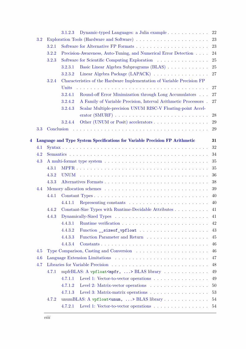
impact its accuracy and final results. Figure 2.5 shows an example of the conjugate gradient(CG) algorithm, an iterative solver for linear systems, executed for different MatrixMarket [24,86] matrices. One can observe that input data, and precision impact the number of iterationsneeded for the algorithm to converge. There is no exclusive value of precision that fits allcases in a common application since the input data also influences the number of iterationsneeded for convergence. Therefore, the investigation of variable precision is still limited by theavailability of hardware, and high-performance libraries for numerical analysts, but perhapsabove all, languages and compilers.

2.5 Languages and Data typesPrevious sections of this chapter summarize different issues regarding stability, precision, FPrepresentations, and their relation with programming languages, and/or compilers. Section 2.2describes precision and accuracy, and how it can be cumbersome to verify this relation withstate-of-the-art tools. Section 2.3 illustrates some of the FP formats available nowadays andtheir use, while Section 2.4 covers aspects of numerical stability, and how precision variationcould potentially be an asset for linear algebra kernels. It also comes downs to how programmersor numerical analysts can develop algorithms to minimize computational errors in the output,and how programming languages, data types, and compilers can provide the properties neededfor this exploration.

A largely relevant reason why languages have not explored VP yet is the recent realizationof the potential of variable precision in many fields [16]. Admittedly, researchers have alwaysbeen keen on precision control. However, the rise of new formats has given further motivationon the matter. With the state-of-the-art apparatuses, varying precision in applications can beachieved in different ways:

(1) Mixed precision [12] offers little flexibility for precision variation with the great advantageof compiler and hardware support for traditional IEEE formats. This greatly increasesuser productivity with a programming model that is simple and efficient. But it is stilllimited to the lack of support for other representations, such as UNUM and Posit.

(2) Multi-precision software libraries, such as MPFR [49] and GMP [54], and MPFun [15],yield to higher performance cost than mixed precision, but offer a larger flexibility with abit-wise mantissa configuration. Due to the programming model imposed by these librarieswritten in C and Fortran, higher-level programming languages (Julia, Python and C++,among others) provide wrappers to ease their use, with an additional cost in performance.

(3) Other representations have been explored mainly through libraries [82, 83, 84]. There aresoftware implementations for UNUM, and Posit formats, but the lack of integration with acompiler hinders the exploration and performance improvement of these formats in real-lifeapplications.

David Bailey, a well-known mathematician and computer scientist, states, in a recent publi-cation [16], that existing software facilities for variable precision computations are rather difficultto use, particularly for large, computationally demanding applications. Existing languages haveno direct syntax and semantics for the variation and dynamic precision. Programmers mustrely on high-level language (HLL) abstractions to implement data structures capable of thishandling. The composite data type struct can be used in C-based languages for that purpose.In objected-oriented languages like C++, Rust and Java, one may implement them as classabstractions. Even dynamically typed languages, such as Julia and Python, would rely onhigh-level abstractions to express the syntax requirements for variable precision. Programming

14

languages have yet to offer extensions to handle variable precision capabilities by default. Andyet, none of the aforementioned abstractions has a syntax that could benefit from hardwaresupport.

Along with the language support, it is paramount that a specific type (or a type system) beable to drive all properties that come along. Programming languages are not normally equippedwith types that allow this flexibility, i.e., variation of the precision in any simple fashion. Aconcise semantics must allow simple reusability, which is difficult to express using dynamictyping of any kind.

Equal importance should be given to the runtime requirements for dynamic precision code.A feature that clearly favors HLL abstractions is precision genericity, i.e., users can hide theprecision value in data structures so that it is only evaluated at runtime. This allows one towrite code that is precision-agnostic. By looking back at programming languages and their types,one may notice that this requirement are only possible through the abstractions mentionedpreviously. In those languages, there are no data types that are able to express this requirement,including how to properly manage the memory of types that are not inherently constant-sized.

Additionally, even the implementation of a type system with these requirements in a lower-lever language would greatly benefit HL languages. Python and Julia are inherently dependenton lower-level languages through code binding. As example, TensorFlow [1] is implemented inC++ and mostly used by Python users. Thus, even HL languages require low-level abstractionfor the generation of highly optimized code and libraries.

2.6 Compilers and OptimizationsCompilers and optimizations also play a central role as an interface between programminglanguages and powerful hardware architecture. Performance improvements in VP computing,and novel FP representations, pass through the integration with an optimized, state-of-the-artcompiler infrastructure. IEEE standard formats have long been supported by industry-standardcompilers, like the GNU C Compiler [113], and LLVM [76]. Few FP representations or types,however, have seen their support integrated into standard compiler toolchains. Akkaş et al.[5]proposed intrinsic compiler support for intervals in GCC in order to accelerate the execution ofinterval arithmetic algorithms.

Compilers, similarly to programming languages, struggle with alternative FP formats, missingon the essential, data-flow, control-flow and algebraic optimizations available for IEEE compatiblearithmetic. They also miss opportunities to leverage hardware implementations for alternativeFP arithmetic. As consequence, the exploration of variable precision, closely associated withthese formats, becomes difficult. The numerical analyst is left with the choice among HLabstractions that cannot deliver the expected flexibility and performance, as explained in theprevious section.

There has not been any investigation of type systems for variable precision explorationthat includes proper compiler specialization. The challenge and implementation complexity aretwofold:

(1) At runtime, compilers have similar constraints as programming languages: a variableprecision model should allow algorithms to be written in a precision-agnostic model, whichimplicates in a novel type system not compatible with current architectures. It also compelssuch a type system to be, in some way, dynamic. This implies a more complex memoryallocation strategy, as type declarations may not always infer variables with fixed (and

5Except for binary16 which was only introduced by the IEEE committee in 2008. Compilers nowadays cansupport half type for binary16, and Google’s bfloat data type, both 16-bit representations.

15

constant) sizes. While this is not a novelty to many languages, its integration with acompiler has not been shown yet.

(2) At compile time, implementations of these type systems must make the most of what isalready inside the infrastructure. The myriad of optimizations available should be reused,or revised so that new types can still profit from them.

• Multi-precision FP libraries offer the flexibility to handle many variations of realnumbers. However, they introduce performance overheads due to the lack of compilersupport. This prevents optimizations easily explored by traditional IEEE formats,namely, constant propagation, loop nest optimizations, inlining opportunities, andmany more. Compiler integration and compatibility to classical optimizations canpotentially harness the power of these libraries, and eliminate some of these overheads.Practically, this integration imposes an implementation challenge to properly typifytheir properties. This has yet to be proven in a well-established compiler toolchain.

• As new FP formats emerge, hardware implementations were proposed to drive theirarithmetics. Equally important is their interaction with compilers and classicaloptimizations. New optimizations may also be devised to enable compiler integration,and classical ones may need to be enhanced to handle different scenarios. For example,constant propagation, instruction selection, and register allocation should take intoconsideration not only the format itself but also the characteristics of the hardwareand architecture in use.

• The handling of precision-agnostic code should be largely integrated with classicaloptimizations so that types with these properties can also be boosted in performance.Additionally, code generators in compilers should grant these types an interfaceto specialized hardware units, enabling the acceleration of formats with variablefootprint.

All these requirements are far-fetched from today’s compilers. Variable precision, althoughcan be studied without much of the help of a compiler, would greatly benefit from it. Theimplementation of compilers that support dynamic type systems is also significant for HLlanguages. This specialization grants these languages a low-level substrate to which they can bebound, and thus enables a tighter integration with a downstream compilation flow.

Furthermore, there is a complementary aspect of the importance of language and compilerintegration: memory utilization. The memory wall [123], speed disparity between outside-chipmemory and processor, has long affected the performance of computer systems. From a variableprecision perspective that can deeply rely on multi-precision FP libraries, the urge to optimizememory usage is imminent and paramount to performance. The use of high-precision formatsincurs an additional memory overhead imposed by high-level data structures used in declarations.For instance, MPFR uses a 32-byte6 struct to represent values, an increase of 16× whencompared to IEEE 128-bit format7. The lack of specific register allocation support may alsoaugment the use of temporary values and, by consequence, significantly increase memory usage.Language and compiler integration can contribute to mitigating the effect of memory usage onhigh-precision formats, and this is, in fact, one of the main long-term goals and benefits of thiswork.

6In a 64-bit machine like x86-64, where sizes of pointers and integers types are 8 bytes.7The value is calculated without considering the mantissa field. Thus, 32/2 = 16, since 32 bytes are needed

for MPFR, and 2 bytes (1 sign bit and 15 exponent bits) are required for IEEE 128-bit format.

16

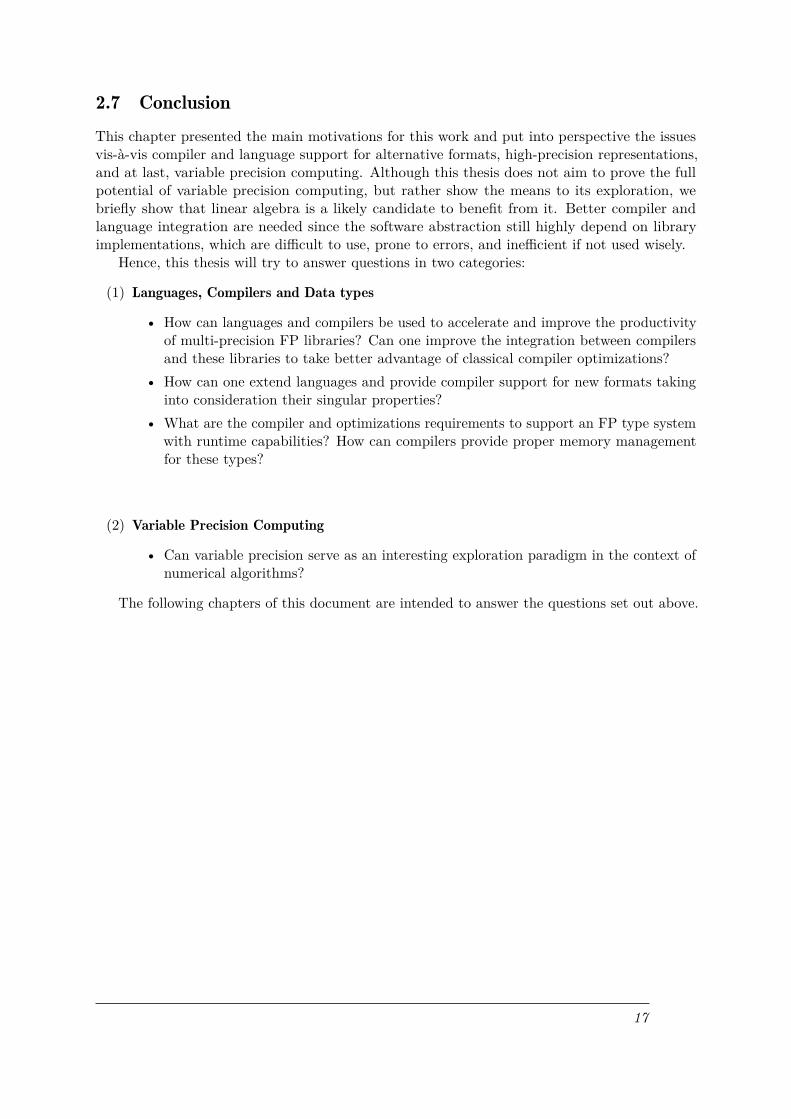
2.7 ConclusionThis chapter presented the main motivations for this work and put into perspective the issuesvis-à-vis compiler and language support for alternative formats, high-precision representations,and at last, variable precision computing. Although this thesis does not aim to prove the fullpotential of variable precision computing, but rather show the means to its exploration, webriefly show that linear algebra is a likely candidate to benefit from it. Better compiler andlanguage integration are needed since the software abstraction still highly depend on libraryimplementations, which are difficult to use, prone to errors, and inefficient if not used wisely.

Hence, this thesis will try to answer questions in two categories:

(1) Languages, Compilers and Data types

• How can languages and compilers be used to accelerate and improve the productivityof multi-precision FP libraries? Can one improve the integration between compilersand these libraries to take better advantage of classical compiler optimizations?

• How can one extend languages and provide compiler support for new formats takinginto consideration their singular properties?

• What are the compiler and optimizations requirements to support an FP type systemwith runtime capabilities? How can compilers provide proper memory managementfor these types?

(2) Variable Precision Computing

• Can variable precision serve as an interesting exploration paradigm in the context ofnumerical algorithms?

The following chapters of this document are intended to answer the questions set out above.

17

Chapter 3: Programming Languages,Paradigms for FP Computation and

exploration Tools

Contents3.1 Computing paradigms for floating-point arithmetics . . . . . . . . . . . . . . . 19

3.1.1 Mixed precision computing . . . . . . . . . . . . . . . . . . . . . . . . . 203.1.2 Arbitrary precision . . . . . . . . . . . . . . . . . . . . . . . . . . . . . . 20

3.2 Exploration Tools (Hardware and Software) . . . . . . . . . . . . . . . . . . . . 233.2.1 Software for Alternative FP Formats . . . . . . . . . . . . . . . . . . . . 233.2.2 Precision-Awareness, Auto-Tuning, and Numerical Error Detection . . . 243.2.3 Software for Scientific Computing Exploration . . . . . . . . . . . . . . 253.2.4 Characteristics of the Hardware Implementation of Variable Precision

FP Units . . . . . . . . . . . . . . . . . . . . . . . . . . . . . . . . . . . 273.3 Conclusion . . . . . . . . . . . . . . . . . . . . . . . . . . . . . . . . . . . . . . 29

This chapter will discuss the main state-of-the-art concepts and work that give basis to thisthesis. It will be divided into two main categories: (1) computing paradigms that cover the mainideas and approaches for the efficient use of real numbers, and (2) hardware and software solutionswithin the context of new representations, along with libraries and techniques that contributeto widening the exploration tooling. The former relates to the thesis since it overviews howdifferent paradigms handle precision control, its flexibility, and exploration potential, importantto justify our design choices, and implementation decisions of following chapters; while the lattersummarizes the main contributions to the exploration of new representations, and how they canpotentially be used in a broader context.

3.1 Computing paradigms for floating-point arithmeticsHaving representations for real numbers available by themselves is often not enough to providethe functionality or performance/energy needed by the user. In other words, assigning float,double, or __float128 types in applications (pseudo)randomly may offer meaningful results,but applications might not reach the expected performance and/or energy; or even worse,applications may execute fast, but results are out of bounds and do not reach expectation.Essentially, users are confronted with trade-offs between accuracy and performance/energy.Besides, indiscriminate use of large-footprint types can have a negative impact on memory usage,and as consequence, performance.

Although computing paradigms for FP arithmetics extends to many approaches (exactcomputing [87, 126], interval arithmetics [90, 100] and other alternative methods [9, 68], we

19

will focus on two principal paradigms that lay the foundation of variable precision computing:mixed precision and arbitrary precision.

3.1.1 Mixed precision computing

The mixed precision computing paradigm [12] involves the combination of IEEE FP types inorder to provide sufficient output accuracy and compatible hardware support. The paradigmmain focus is to find the right balance between IEEE types and numerical stability, prioritizingreduced-precision formats (binary16 and binary32 ) over higher-precision ones (binary64 ) andharnessing an increased computer power on applications. Its main benefit lies in the performanceboost and energy reduction it can achieve, considering that 16-bit and 32-bit operations canexecute more than 2× faster than their 64-bit counterparts, and reduce data movement due tosmall data types.

It has been widely explored in linear solver methods for high-performance computing (HPC)in conjunction with the iterative refinement process, a long-standing technique to improve theaccuracy of a computed solution by applying a correction factor to the final solution. Theapproach is based on Newton-Raphson’s method [127]:

xn+1 = xn− f(xn)/f ′(xn) (3.1)

which enables lower-precision solutions to be refined to the same accuracy as higher precision.Baboulin et al. [12] present an approach to mixing 32-bit and 64-bit floating-point arithmetic

and iterative refinement in direct and iterative methods for solving a linear system of equations.It argues that the reduction of data movement to/from the memory compensates the refinementprocess, and makes iterative refinement a valuable approach for linear solvers. The combinationof these two techniques yields performance results that are comparable to a full single (32bits) precision solver while still delivering the same accuracy as the double (64-bit) precisionimplementation.

The reduction of data movement in memory, computations cost in low precision, and suitableaccuracy are the principal reasons why mixed precision and iterative refinement are beingemployed together. The literature is extensive on the exploration of these techniques together.Carson and Higham [29] accelerate GMRES (an iterative solver for linear systems) by iterativerefinement employing three levels of precision (16, 32, and 64 bits). Adding another additionallevel of precision reduces communication with the memory even more, and improves performanceeven further. GPUs have also been used to explore these techniques [2, 59, 60, 61], confirmingtheir potentials and benefits.

Nevertheless, a major drawback of these approaches stems from the lack of flexibility vis-à-visFP types in use. They only work with a limiting number of types, at best binary16, bfloat,binary32, and binary64, and, thus, hinders the exploration of other representations. Lee etal. [79] goes further by controlling and adapting precision dynamically in FPGAs, which canachieve up to 2–3× speedups over other mixed precision techniques.

3.1.2 Arbitrary precision

Arbitrary precision extends the idea of FP operations to formats that go beyond the scope ofthe IEEE standard. Unlike mixed precision, it may offer gradual and bit-level customizationof exponent and mantissa values, which makes arbitrary precision an excellent tool to explorethe impact of precision in applications. In order to offer such flexibility, arbitrary precisiontoolchains have the downside of being much slower than mixed precision solutions, as they haveto resort to software implementation rather than taking advantage of hardware-specific FP units.

20

typedef struct {int _mpfr_prec ;int _mpfr_sign ;int _mpfr_exp ;int * _mpfr_d ;

} __mpfr_struct , *mpfr_ptr , mpfr_t [1];

Listing 3.1: MPFR variable type as defined in [49]

1 void mat_mult ( mpfr_t *matResult , mpfr_t *matA , mpfr_t *matB ,2 unsigned dim1 , unsigned dim2 , unsigned dim3 ,3 unsigned precision ) {4

5 mpfr_t sum;6 mpfr_init2 (sum , precision );7 mpfr_t tmp;8 mpfr_init2 (tmp , precision );9 mpfr_set_d (sum , 0.0, MPFR_RNDN );

10

11 for ( unsigned i = 0; i < dim1; ++i) {12 for ( unsigned j = 0; j < dim3; ++j) {13 for ( unsigned k = 0; k < dim2; ++k) {14 mpfr_mul (tmp , matA[i*dim2 + k], matB[k*dim3 + j], MPFR_RNDN )

;15 mpfr_add (sum , sum , tmp , MPFR_RNDN );16 }17 mpfr_set ( matResult [i*dim3 + j], sum , MPFR_RNDN );18 mpfr_set_d (sum , 0.0, MPFR_RNDN );19 }20 }21 mpfr_clear (sum);22 mpfr_clear (temp);23 }

Listing 3.2: Usage of the MPFR library in a matrix multiplication example

Ada [78], Fortran (MPFUN [15]), C (MPFR [49] and GMP [54]), and Cuda (Campary [71]) aresome of the programming languages for which arbitrary precision libraries were implemented.

3.1.2.1 MPFR Multi-precision library

MPFR [49] is the state-of-the-art multi-precision (or arbitrary-precision) library for floatingpoint computations, allowing bit-wise control of precision values. It was created as an effort toprovide floating-point operations with as much precision as necessary, without needing hardwaresupport. Although it makes use of GMP internally, precision values of MPFR variables havethe exact number of bits requested by the user, which is not true to its counterpart. It uses aregular base-2 notation in the form of ±1×mantissa×2exponent, where the value of mantissa isonly limited by the amount of memory in the system, and exponent takes a type according tothe machine word (32 or 64 bits), which gives enough dynamic range to represent essentially anyreal number needed [26].

An MPFR object is of type __mpfr_struct, as illustrated in Listing 3.1. Its API followsthe pattern mpfr_op(dest, src1[, src2, ...,][rounding mode]), in which the dest and srcparameters are mpfr_ptr. Op can be a basic operation (+,−,×,÷), a fused operation (fma, fms),

21

1 void mat_mult ( unsigned prec , mpfr_float *matResult ,2 mpfr_float *matA , mpfr_float *matB ,3 unsigned dim1 , unsigned dim2 , unsigned dim3) {4

5 mpfr_float :: default_precision (prec);6 mpfr_float tmp;7 for ( unsigned i = 0; i < dim1 , ++i) {8 tmp = 0.0;9 for ( unsigned j = 0; j < dim3; ++j)

10 for ( unsigned k = 0; k < dim2; ++k)11 tmp = matA[i*dimi2 + k] * matB[k*dim3 +j];12 matResult [i*dim3 + j] = tmp;13 }14 }

Listing 3.3: Usage of the C++ Boost library for Multi-precision in a matrix multiplicationexample

or one of many possible mathematical functions ( n√,cos,sin, log, ...). The parameters may havedifferent exponent and precision sizes, and the destination parameter can be identical to a sourceparameter. They need (destination included) to be allocated and have their precision definedwith mpfr_init before being used and freed with mpfr_clear once useless. These functionshave a high-performance penalty and should thus be called wisely. The value of an MPFRvariable is set using mpfr_set, which is useful in particular for spilling variables. Listing 3.2shows the code for a simple matrix multiplication implemented in MPFR. One can notice howverbose MPFR coding is, even for simple algorithms. MPFR’s programming model, althoughsimple to use and efficient, is error-prone to memory management, as programmers are in chargeof allocating and freeing resources.

Due to its popularity, MPFR has been widely used in high-level language abstractions, suchas in the C++ Boost library for multi-precision arithmetic [85], MFPI [101] and CGAL [48], aswell as in dynamic languages like Julia [19] and Python [117]. They provide high-level features(through classes and dynamic type systems) that abstract allocations and deallocations awayfrom programmers.

3.1.2.2 C++ Boost for Multi-precision

As an example, listing 3.3 illustrates the implementation of the same matrix multiplicationalgorithm using the Boost Multi-precision library. Except for the function default::precisionthat sets up the current precision, the compiler handles object allocations and deallocations,and the creation of intermediate temporaries, similar to an ordinary integer or floating-pointvariable declaration. However, these abstractions draw an additional overhead to the librarythat can compromise its performance even more.

Compilers have supported and are able to optimize floating-point types (IEEE types ingeneral) for a long time. However, the lack of compatibility between compilers and library-definedFP representations, like MPFR, is still a major challenge. Better integration with compilerswould allow faster execution, as well as improve the productivity of these libraries.

3.1.2.3 Dynamic-typed Languages: a Julia example

As an alternative to the high-level abstraction provided through classes, dynamic-typed languageslike Julia are more versatile, using a flexible type system that leaves type evaluation until runtime.

22

1 function mat_mult (matResult , matA , matB , dim1 , dim2 , dim3)2 for i = 1: dim13 tmp = zero( typeof ( matResult [1, 1]))4 for j = 1: dim35 for k = 1: dim26 tmp = matA[i,k] * mat[k, j]7 end8 matResult [i,j] = tmp9 end

10 end11 end

Listing 3.4: Implementation of matrix multiplication example in the Julia language: its dynamictype system hides the types of variables until runtime evaluation

This means that programmers are not obliged to specify the types of variables, and instead,types are only evaluated and check at runtime. Listing 3.4 exemplifies the power of Julia’s typesystem. One may notice that no information type has been given, and the type for each of thevariables will only be known at runtime.

As such, Julia’s type system has a property that greatly benefits the exploration of newtypes, and representations: precision genericity. Sections 2.5 and 2.6 in Chapter 2 shows thatvariable precision computing can leverage the use of precision-agnostic code, and hence, enablinga type system that resembles Julia’s is highly demanding and beneficial.

3.2 Exploration Tools (Hardware and Software)

Variable precision computing and its applicabilities intersect with different research topicsand approaches. Alternative FP formats widen the design space exploration on appropriaterepresentations for real numbers. Many researchers have proposed frameworks and tools toexplore the impact of different representations in real-life applications. Complementary, thestudy of precision-awareness approaches have highly contributed to make accuracy a mainstreamconstraint in many fields, and it collaborates to give significance to variable precision computing.Additionally, it is paramount that new libraries and hardware architectures drive the variableprecision paradigm to compete with existing models.

In the remainder of this chapter, we focus on giving the reader an overview of the state-of-the-art in all these topics. We start by presenting some software for alternative FP formats,including UNUM and Posit tooling. After, we cover methods to enable precision awareness andthe detection of numerical errors. An introduction to BLAS and LAPACK is later presented.We conclude by showing hardware implementations used to improve the numerical stability andnumerical error in applications, and the compiler or software support proposed for the usage ofeach unit.

3.2.1 Software for Alternative FP Formats

State-of-the-art compilers like GCC and LLVM have started to include support for a few non-standardized FP formats, from Google’s bfloat16 and Intel’s extended precision to POWER9double-double. Although proprietary compilers for Posit formats already exists, no much isknown about the hardware, ISA or the compiler toolchain available. Instead, many work focuson providing infrastructure for the exploration of alternative formats.

23

Tagliavini et al. [114] propose FlexFloat, a software library designed to aid the developmentof applications with fine-grained precision configuration. Unlike MPFR, FlexFloat enablesbit-width control of both mantissa and exponent fields, reducing the FP emulation time. Itachieves a significant performance speedup in comparison to other FP emulation libraries becauseit leverages native type support for float and double types. It later performs a user-transparentsanity check to guarantee that calculated values are representable in the specified type. FlexFloathas no support for high-precision representations, and although it could be extended, it stillcannot be used with the same flexibility as MPFR.

Anderson et al. [6] also take a similar approach as FlexFloat by proposing a set of non-standard byte-aligned FP types refer to as flytes, that still leverages native IEEE types. Theproposed scheme reduces the cost of data transfer volume and storage space requirements byusing reduced-precision representations in memory, while it still enables acceleration throughexisting hardware vector units of general-purpose processors. However, it still suffers fromoverheads imposed by format conversions, since operations are still highly dependent on IEEEformats. Similar to the previous work, it lacks support for high-precision representations whichlimits its utilization scope.

There are also work that focus on the implementation of format-specific software libraries.SoftPosit [84] is a software implementation of posit types that conforms to the specification asdefined in [58]. It borrows many ideas from the original IEEE-complaint Berkeley SoftFloatlibrary [62], and has been used to compare the accuracy of posit to IEEE types [32]. Softwareimplementation for the UNUM formats had also been proposed [83], but it is certainly lesspopular than SoftPosit due to the significant complexity of the UNUM representation.

Other researchers have focused on investigating the arithmetic design space of hardwareunits with alternative numerical representations. Johnson [70] uses tapered encodings fromthe posit format, logarithmic number system (LNS) [9, 74], and kulisch accumulator [75] todesign an accelerator that is effective for convolutional neural networks (CNNs). The work findsinspiration in previous research and shows momentum to explore alternative representation andrepurpose ideas.

Lindstrom et al. [81, 82] propose a modular framework for representing real numbers thatgeneralize posit, IEEE and other floating-point number systems. Similarly, Omtzigt et al. [93,94] present a high-performance number systems library for the exploration of custom numbersystems, from tapered types to arbitrary floating points, with support for reproducible arithmeticcomputation in concurrent environments. Additionally, all the recent publications w.r.t. customformats, their applicability, and hardware implementations show interesting opportunities forextending the role of compilers to novel numerical systems.

Nevertheless, none of the aforementioned work has all properties needed for variable pre-cision exploration. Anderson et al., Tagliavini et al. [6, 114] lack support for high-precisionrepresentations, and others [82, 94, 114] provide no hardware support. There is no solutionthat combines a language scheme for multiple representations, compiler integration capable ofsoftware or hardware compatibility.

3.2.2 Precision-Awareness, Auto-Tuning, and Numerical Error Detection

The variety of numerical errors in floating-point formats has often led developers to choosedata types that deliver sufficient accuracy but poor performance. For instance, the performancedifference between using float and double can be up to 2× in favor of the former. Precision-aware schemes can be used to detect and debug numerical errors in applications, and auto-tuningtechniques propose to find the right compromise between enough accuracy and speed. Weoverview some of the main schemes and techniques for precision awareness and auto-tuning.

24

Ansel et al. [7] propose language extensions to expose accuracy choices to the user, allowingthe user to incorporate trade-offs between time and accuracy directly at code level. Onceaccuracy information is set by the programmer in the PetaBricks programming language [8], thecompiler and auto-tuner employ a genetic algorithm approach to search valid candidates thatmeet the desired accuracy. The scheme uses a source-to-source compiler from the PetaBrickslanguage to C++, so its limitation is directly influenced by this integration. Its auto-tuning canbe further improved if C++ data structures or types were to allow a fine-grained accuracy con-figuration. Moreover, this work has widely known as a viable software approach for approximatecomputing [125].

Darulova et al. [40] presents a programming model, specification language, and compilationalgorithm that guarantees to meet the desired precision with respect to real numbers.

Precimonious [102] is a dynamic program analysis tool aimed to assist programmers to tunethe precision of FP applications. It relies on user-input configuration files in order to specifywhich variables in code can be submitted for auto-tuning analysis. The algorithm iterativelysearches for suitable sets of types within the specified files and variables that are satisfiablewithin an error threshold. Precimonious uses a more modern design since it is built on top ofLLVM, so it can potentially be used for a wider range of programming languages in differentarchitectures.

Herbie and Herbgrind [96, 105] are two related tools to help developers identify and addressroot causes of numerical instability in applications. Many works have proposed to use shadowprogram execution to measure numerical errors in applications. Rubio-Gonzales et al. [103]minimizes Precimonious’s analysis time through multiple shadow executions. Chowdhary etal. [33] employ shadow execution to detect and debug errors in posit formats by relying onhigh-precision values. And more recently, NSan [38] has been proposed as a new sanitizer forlocating and debugging floating-point numerical issues, fully integrated into the LLVM sanitizerinfrastructure.

All of the work described in the above paragraphs are great examples of how compilersupport for alternative formats can be beneficial. The limiting number of FP types natively hasa negative impact on the interaction of these work with the compiler.

3.2.3 Software for Scientific Computing Exploration

During the decades before the 2000s, the very active research in computational physics, andothers fields, drove the development of standard and efficient FP libraries. Two of the mostimportant software technologies put forward were the design and specification of the Basic LinearAlgebra Subprograms (BLAS) and the Linear Algebra Package (LAPACK).

3.2.3.1 Basic Linear Algebra Subprograms (BLAS)

Mixed precision techniques, as described in 3.1.1, took great advantage of the Basic LinearAlgebra Subprograms (BLAS), a set of standardized linear algebra routines that are intended tobe reliable, fast, and portable. It specifies the arithmetic computational routines which performcommon linear algebra operations such as vector addition, scalar multiplication, dot products,linear combinations, and matrix multiplication. It is further structured in three categories,according to their complexities.

Level 1 defines a set of linear algebra functions that operate on vectors only. These functionsshare the form:

y← αx+ y (3.2)

where α is a scalar and x,y are vectors

25

Level 2 functions are matrix-vector operations, such as multiple variations of the matrix-vectorproduct operation. These functions share the form:

y← αAx+βy (3.3)

where A is a Matrix, α,β are scalars and x,y are vectorsLevel 3 functions are intended for matrix-matrix operations. Typically, these functions

perform O(N3) operations on O(N2) data, therefore the algorithm structure, i.e. its interactionscheme between FPU and memory, is decisive for performance, but it is still very specific to theplatform it runs on. Most of these functions share the form:

y← αA×B+βC (3.4)

where A,B,C are matrices, α,β are scalars.The original BLAS implementation ([77]) is the reference for the arithmetic operations

involving vectors and matrices. As a sequel of the original work, several variants have beendeveloped: OpenBLAS [124], Intel Matrix Kernel Library (MKL) [120], and ATLAS [122]. All ofthese libraries are tailored for standard precision (and support multiple degrees of parallelism),and no high-precision specification of any kind is given.

The design of XBLAS [80] is the first attempt on the design of a representative subset ofBLAS routines that internally operate in extended precision (80- or 128-bit representations).Internal extra digits can aid the reduction of accumulated round-off errors and cancellationsand can justify the use of slower operations. External operands and function signatures are stillsimilar to classical BLAS routines and are easily adaptable to the proposed library. While manyfunctions, such as dot products, matrix-vector products, matrix-matrix multiplications, can beimproved with internal extra precision, others struggle to make them worth using. Particularly,scaling matrix or vector by a constant, vector additions, and computing norms of vectors andmatrices have shown no benefit of internal operating digits. From the perspective of adjustingprecision dynamically, however, XBLAS still hinders exploration by disallowing multi-precisioncomputation.

MPACK [92] goes further on the development of a true arbitrary/higher-precision linearalgebra (MBLAS). The library supports many multi-precision libraries, like MPFR [49], GMP [54],QD [17], as well as IEEE 754 binary128, and uses similar function signatures as the traditionalBLAS implementations. MPACK is the project that perhaps best captures a multi-precisionBLAS, with the significant drawback of neither having full hardware support nor a friendlyinterface to interact with compiler optimizations.

The BLAS-like Library Instantiation Software (BLIS) [118] framework was proposed as anew infrastructure for rapid instantiation of BLAS functionality. The framework shows that it ispossible to express all level-2 and level-3 BLAS operations in terms of a few simple kernels, andthus, it accelerates the instantiation of BLAS-like operations. By isolating BLIS operations tofew kernels, BLIS may aid those who wish to auto-tune operations for high performance.

In the previous chapter, we show VP computing as a use case in the context of linear algebra.Hence, a VP-specific BLAS library implementation would also contribute to the study of thetrade-off between precision and other constraints (energy, execution time, number of iterations,etc.) in many fields. While this is already achieved with MBLAS from MPACK, its use ofhigh-level structures means there are no support in compilers, or hardware specialization, whichtranslates to significant performance overheads in comparison to other hardware-compatibleBLAS libraries.

26

3.2.3.2 Linear Algebra Package (LAPACK)

The Linear Algebra Package (LAPACK) library is an effort to design and implement high-performance routines for solving linear systems and eigenvalue problems and finding least-square solutions of systems of equations. It also provides matrix factorization algorithms (LU,Cholesky, QR, SVD, etc) that are needed by other routines in the library. LAPACK routinesare implemented by relying on BLAS. Block algorithm techniques [44] are employed to improvethe locality of matrices and accelerate the code executed.

Other relevant projects associated to LAPACK are the Matrix Algebra on GPU and MulticoreArchitectures (MAGMA) [116], a LAPACK library for heterogeneous/hybrid architecture,ScaLAPACK [20] that targets distributed-memory platforms, and the Parallel Linear Algebra forScalable Multi-core Architectures (PLASMA) [27]. MPACK also implements an arbitrary/high-precision library for LAPACK kernels, MLAPACK. However, the library also suffers from thesame issues encountered in MBLAS, i.e, lack of hardware support, and no compiler integration.

3.2.4 Characteristics of the Hardware Implementation of Variable Precision FP UnitsCompilers and languages can certainly work as enablers to expand the use of new computerarchitectures. As is the case of variable precision computing, there needs to be coordinationbetween the software, i.e, compilers and languages, and hardware targets. One must takeinto account the specificities of the hardware in order to augment compiler support. Thefollowing section presents three interesting work proposed within the context of variable precisionarithmetics. We then highlight their main aspects, and the software interface proposed to enabletheir usage.

3.2.4.1 Round-off Error Minimization through Long Accumulators

Kulisch et al. [75] proposes a rather orthodox way of error-free calculations for FP arithmeticthrough long accumulations, known as kulisch accumulator. A kulisch accumulator is a fixed-pointregister wide enough to minimize the impact of round-off errors of FP arithmetic operations. Itaims to be used in long chains of arithmetic operations, such as dot products, in order to avoidvalues to be rounded when stored back to memory.

Two major issues can be spotted in kulisch accumulators: (1) an accumulator can operateonly in a single chain of arithmetic operations at a time. Multiple accumulators would have tobe added for parallel use. (2) automatic detection of long accumulators by the compiler canbe implemented. However, it prevents the user from evaluating which set of operations needadditional accuracy, and hence, an unnecessary overhead is introduced. Still, the simple designof a kulisch accumulator also inspired further exploration of these long accumulators in fusedoperations of the posit arithmetic [58], which means that it can be used for multiple formats,and integrated with different approaches.

3.2.4.2 A Family of Variable Precision, Interval Arithmetic Processors

Schulte et al. [107] presents a family of variable precision, interval arithmetic processors forimproved accuracy and reduced accumulation of errors. Contrary to previous architecture thatuses fixed-point arithmetic and relies on an internal accumulator to minimize round-off errors,this work takes an orthogonal approach of using FP arithmetic, and a register file to allowmultiple operations at a time.

The operating mode of these processors depends essentially on the data type declarationsprovided by the user in the program. Table 3.1 shows some of the supported data types. Thesoftware interface is provided by class declarations of each type in a similar fashion as in the

27

Table 3.1: Some of the data types supported in Schulte et al. [107]

Data Type Descriptionvp_float Variable-precision floating point numbervp_vector Variable-precision floating point vectorvp_matrix Variable-precision floating point matrixvp_interval Variable-precision intervalvp_ivector Variable-precision interval vectorvp_imatrix Variable-precision interval matrix

VPI software package [46], and provides support for arithmetic instructions and operations inscalar types, as well as intervals. Although this solution is able to add specialized hardwaresupport for this family of processors, a major drawback lies in the lack of compiler integration toenable classical optimizations for these types. C++ objects don’t provide the necessary low-levelabstraction for driving these new types to optimizations.

3.2.4.3 Scalar Multiple-precision UNUM RISC-V Floating-point Accelerator (SMURF)

Scalar Multiple-precision UNUM RISCV-V Floating-point Accelerator (SMURF) [23] is acoprocessor built up on top of a RISC-V [121] Rocketchip architecture [11] that operates in avariable precision fashion. As UNUM is a self-descriptive format, FP values in memory are storeusing this format, while arithmetics operations execute in a regular base-2 scientific notationform.

An important concept introduced with this coprocessor is the idea of the Maximum ByteBudget (MBB), a value that is configured through control status registers and which limits thesize of the number stored in memory. The main idea behind MBB is to reduce the memoryfootprint and memory pressure when dealing with high-precision numbers while maintainingoutputs within the same order of magnitude. Additionally, Working G-Layer Precision (WGP)is the nomenclature adopted to the precision used in the coprocessor.

The coprocessor uses a scratchpad as a register file of 32 interval registers. By keeping valueswithin the register file, we are able to significantly reduce memory pressure. Each of theseinterval registers has two endpoints divided in the header, containing sign, exponent, flags (NaN,∞, zero, ...), and mantissa which is divided into 64-bit chunks of up to 512 bits (with a total of8 chunks).

A RISC-V ISA extension, depicted in figure 3.2, was proposed in order to make use ofthe coprocessor. The supported operations (12-14) are comparisons, addition, subtraction,multiplication, interval midpoint (GGUESS) and interval radius (GRADIUS). Other operations(e.g. division) are implemented in software. The ISA has three main features: (i) It supports a setof instructions to control status registers for internal operation precision and MBB (mentionedin the previous section),( 1 - 4 ), etc.; (ii) It supports internal registers copies and on-the-flyconversion among IEEE and gbound formats ( 5 -11); (iii) and it also has a dedicated Loadand Store Unit (LSU) with compatible instructions which handle misaligned memory accesses(15-18).

The ISA extension proposed to help the integration between software and hardware. However,no compiler specification is given, which prevents complex code execution. Language, compilerand runtime support for the features presented in this work could further improve its use inapplications. Moreover, by using the values of MBB and WGP as knobs for the size of variables

28

Table 3.2: Coprocessor’s Instruction Set Architecture

31 25 24 20 19 15 14 13 12 11 7 6 00 func7 rs2 rs1 xd xs1 xs2 rd opcode

7 5 5 1 1 1 5 71 susr unused Xs1 0 1 0 unused CUST2 lusr unused unused 1 0 0 Xd CUST3 smbb/swgp/sdue/ssue unused Xs1 0 1 0 unused CUST4 lmbb/lwgp/ldue/lsue unused unused 1 0 0 Xd CUST5 mov_g2g unused gRs1 0 0 0 gRd CUST6 movll/movlr unused gRs1 0 0 0 gRd CUST7 movrl/movrr unused gRs1 0 0 0 gRd CUST8 mov_x2g #imm5 Xs1 0 1 0 gRd CUST9 mov_g2x #imm5 gRs2 1 0 0 Xd CUST10 mov_d2g/mov_f2g #imm5 Xs1 0 1 0 gRd CUST11 mov_g2d/mov_g2f #imm5 gRs2 1 0 0 Xd CUST12 fcvt.x.g/fcvt.g.x unused Xs1 0 1 0 gRd CUST13 fcvt.f.g/fcvt.g.f unused Xs1 0 1 0 gRd CUST14 fcvt.d.g/fcvt.g.d unused Xs1 0 1 0 gRd CUST15 gcmp gRs2 gRs1 1 0 0 Xd CUST16 gadd/gsub/gmul gRs2 gRs1 0 0 0 gRd CUST17 gguess/gradius unused gRs1 0 0 0 gRd CUST18 lgu/ldub unused Xs1 0 1 0 gRd CUST19 stul/stub gRs2 Xs1 0 1 0 unused CUST20 lgu_next/ldub_next gRs2 Xs1 1 1 0 Xd CUST21 stul_next/stub_next gRs2 Xs1 1 1 0 Xd CUST

in memory and precision in operations, respectively, the architecture enables a fair degree ofvariable precision computing.

3.2.4.4 Other (UNUM or Posit) accelerators

Along with the three main hardware units for variable precision computing, several researchershave shown the use of UNUM or Posit accelerators to facilitate comparison across formats.Tiwari [115] proposes a posit-enabled RISC-V core as the first-level replacement for IEEE units.It proposes to reinterpret float or double types as posit computing, avoiding specific nativecompiler support for these types. Other examples of accelerators for alternative formats can befound in [52, 69]. The main hurdle for their adoption still relates to the required software stacksupport: compiler, and language integration, along with scientific computing libraries like thosepresented in 3.2.3 for fast execution.

3.3 Conclusion

This chapter presented the main state-of-the-art contributions that give basis to the work ofthis thesis. From one side, we described different computing paradigms for efficiently use of real

29

numbers, presenting specific libraries and work that have been developed within this context. Inthe second part, we focused our attention on the principal hardware and software work thatcovers the exploration of new representations. These previous works present some caveats: whilemixed precision is fundamentally supported by compiler and hardware, it lacks the flexibilityof arbitrary precision libraries. Other previous works are either standalone solutions to handleprecision with no hardware and compiler support or hardware accelerators without compilersupport. There is a lack of synergy between software and computer paradigms, and the hardwarelayer, as well as a flexibility concern that has been poorly addressed so far. This will be themain focus of the following chapters.

30

Chapter 4: Language and Type SystemSpecifications for Variable Precision FP

Arithmetic

Contents4.1 Syntax . . . . . . . . . . . . . . . . . . . . . . . . . . . . . . . . . . . . . . . . . 324.2 Semantics . . . . . . . . . . . . . . . . . . . . . . . . . . . . . . . . . . . . . . . 344.3 A multi-format type system . . . . . . . . . . . . . . . . . . . . . . . . . . . . . 35

4.3.1 MPFR . . . . . . . . . . . . . . . . . . . . . . . . . . . . . . . . . . . . . 354.3.2 UNUM . . . . . . . . . . . . . . . . . . . . . . . . . . . . . . . . . . . . 364.3.3 Alternatives Formats . . . . . . . . . . . . . . . . . . . . . . . . . . . . . 38

4.4 Memory allocation schemes . . . . . . . . . . . . . . . . . . . . . . . . . . . . . 394.4.1 Constant Types . . . . . . . . . . . . . . . . . . . . . . . . . . . . . . . . 404.4.2 Constant-Size Types with Runtime-Decidable Attributes . . . . . . . . . 414.4.3 Dynamically-Sized Types . . . . . . . . . . . . . . . . . . . . . . . . . . 41

4.5 Type Comparison, Casting and Conversion . . . . . . . . . . . . . . . . . . . . 464.6 Language Extension Limitations . . . . . . . . . . . . . . . . . . . . . . . . . . 474.7 Libraries for Variable Precision . . . . . . . . . . . . . . . . . . . . . . . . . . . 48

4.7.1 mpfrBLAS: A vpfloat<mpfr, ...> BLAS library . . . . . . . . . . . 494.7.2 unumBLAS: A vpfloat<unum, ...> BLAS library . . . . . . . . . . 54

4.8 Conclusion . . . . . . . . . . . . . . . . . . . . . . . . . . . . . . . . . . . . . . 57

Albeit the IEEE 754 standard have met immense success across diverse areas, some applica-tions require alternative representation to approximate real numbers. Linear algebra solvers, asbriefly discussed in 2.4.2, can potentially benefit from high-precision representations. In directsolvers algorithms, such as Cholesky and Gaussian elimination, they can reduce the residualerror [29, 64] of the output. Besides, they can be even more beneficial for iterative methods,preferred for large-sized problems. Increasing the precision of the intermediate residual vector isan effective mean to reduce the number of iterations needed in an iterative solver. Chapter 6will show and discuss the benefits of using high-precision formats with these algorithms.

While a variable precision algorithm may be seen superficially similar to a typical model1,the estimation and configuration of the precision (in this case, the fractional part) value for partor all of the arithmetic operations is done at the algorithmic level. This estimation is generallycomplex to compute and may lead to unnecessary over-provisioning of fractional bits. Thus, a

1The programming model for C++ Boost Multi-precision is fundamentally similar to an IEEE-enabledimplementation, except by the line that sets the precision in use.

31

practical alternative is to adapt precision dynamically, i.e., instead of computing the necessaryprecision a priori, the algorithm is modified to use an outer loop to systematically check theresult for accuracy at predefined points, as depicted in Algorithm 1. If the residual is above apredefined threshold, or if convergence is too slow, the solver increases its internal precision andresumes computation. One should also notice a similar procedure can also be taken to dynamicadjustment of exponent bits.

Algorithme 1: Simplified variable precision algorithm: function is precision-agnostic,i.e., it is not restricted to a single precision value.1 output= function(precision)2 repeat3 if convergence is slow then4 increase speed5 end6 precision= precision+ speed7 output= function(precision)8 until output accuracy is greater than threshold;

Hence, a strong requirement for the software engineering, tools, and more importantly,compiler and languages supporting this variability is:

(1) the language used for variable precision development must be performance-oriented;

(2) the kernel source code must be unique, therefore the programming style must be agnosticof the underlying precision of its variable precision data, like described section 2.5;

(3) the required precision and exponent value depend on the conditioning of data: it may bedefined at kernel initiation time or dynamically and gradually increased in the case ofadaptive methods;

(4) a variable-precision implementation should be as similar as possible to its original referencealgorithm in C with standard IEEE arithmetic; in particular, extended precision shouldbe used only when necessary, which implies that applications may smoothly transitionbetween legacy support libraries (e.g., double-precision BLAS) and extended or adaptiveprecision solutions when required.

A programming model able to meet these requirements makes variable precision an extension(and a generalization) of mixed precision (3.1.1) and allows a deeper space exploration of precision,exponent, and in general FP representations. In the remainder of this chapter, we will focus onthe description of a type system and language definition that target the requirements specifiedabove.

4.1 SyntaxAs shown in previous chapters, programming languages struggle with IEEE-alternative formatsfor FP arithmetic, and as consequence, with the exploration of variable precision arithmetic.The user is left with no choice but to rely on (1) high-level managed languages like Julia [19] orPython [117] whose abstractions and type systems provides a high productivity variable-precisioninterface but fails to deliver competitive performance, (2) an efficient language like C withreduced flexibility due to manual memory management and calls to specific software libraries

32

1 vpfloat - declaration :2 vpfloat '<' vpfloat - attributes '>' declaration3

4 vpfloat - attributes :5 type ',' exp -info ',' prec -info ',' size -info6

7 type:8 unum | mpfr | posit | custom_ieee | ...9

10 exp -info:11 integer - literal | identifier12

13 prec -info:14 integer - literal | identifier15

16 size -info:17 integer - literal | identifier

Listing 4.1: Backus normal form (BNF) like notation for the vpfloat language extension

such as MPFR [49] or GMP [54], or (3) sacrificing much precision control by relying on a mixed-precision paradigm [12] based on IEEE-compatible formats. In any case, significant overheadsare encountered: from (1) and (2) performance-wise, and from (3) in terms of flexibility.

Approximate representations of real numbers in which the sizes of mantissa and exponentmay vary according to the user’s needs require runtime capabilities that are not easily expressedwith the semantics of programming languages in general. Julia, Python and class-based objectsin C++ (like Boost) offer underlying data structures to store the value of precision used. MPFRuses a C struct to reach the same effect. Nevertheless, FP formats with runtime capabilitiescannot be achieved with the semantics of primitive data types. Types float, double, longdouble, and every other primitive FP type have predefined exponent and mantissa values,

permitting the user only to select values statically in a course-grained fashion.As a way to improve the state of the art on languages and types for variable precision

exploration, we propose an extended type system for C-based languages capable of manipulatingFP operations with different representations and formats. It provides first-class support toprogramming with variable precision FP arithmetic, enabling hardware support when availableand offering the flexibility of numerical libraries that can operate with multiple precisions.It differs from the current C syntax by introducing a new parametrized type for multiplerepresentations named vpfloat that borrows the syntax of C++ template.

The new primitive type vpfloat is parameterized with attributes to control a given FPimplementation, such as its specific format, exponent, precision and/or storage size information.The syntax aims at providing a generic way for different formats to coexist within the samekeyword, while also enabling the addition of new formats or representations as they are proposed.Listing 4.1 shows the syntax rules of the vpfloat language extension in a Backus Normal Form(BNF) like notation.

Every declaration must provide a type attribute which (1) specifies its representation inmemory; and (2) if and how many subsequent attributes are needed, along with which informationthey carry. Attributes are specified in the following order: type, exponent, precision, and size.One should notice that, with the exception of type, attributes can all be defined with integralconstant literals or identifiers. This specific property demonstrates one of the main advantagesof vpfloat over their counterparts: types are not obliged to be declared to retain unmodifiedconstant exponent and mantissa values. Allowing FP attribute information to be declared

33

Table 4.1: Comparison of the vpfloat type system and FP types, and data structures found inthe literature.

Type Exponent(in bits)

Mantissa orprecision(in bits)

Compiler-integrated

Hardware-enabled

High-precisionsupport

Multi-format

half 5 11 Yes Yes No Nobfloat16 8 8 Yes Yes No Nofloat 8 24 Yes Yes No Nodouble 11 53 Yes Yes No Noquad 15 113 Yes No Yes Nodouble quad 19 237 No No Yes NoFlexFloat Variable Variable No Yes No NoFlytes Variable Variable Yes Yes No No__mpfr_struct Variable Variable No No Yes Yes*

BoostMulti-prec.

Variable Variable No No Yes Yes*

vpfloat<...> Variable Variable Yes Yes Yes Yes+

* Multi-format libraries can be implemented by relying on it+ New Formats can be added

with identifiers, our language extension supports constant-size and dynamically-sized types,which is always a technical hurdle in unmanaged languages like C, its associated IntermediateRepresentations (IRs) and Application Binary Interfaces (ABIs).

Table 4.1 illustrates how our type system contrasts with the most common FP types, anddata structures found in the literature when considering different constraints, such as compilerintegration, hardware capabilities, multi-format support, among others. Our solution is theonly one able to check all boxes. It combines the hardware and compiler support provided byprimitive types like float and double, with the multi-level flexibility of MPFR and the BoostMulti-precision library. In the following sections and chapters, we explain how these types areimplemented, their semantics and integration with an industry-level compiler infrastructure.

4.2 Semantics

After each declaration has been syntactically analyzed, it is during semantic analysis that thecompiler checks declarations to guarantee that FP attributes respect the semantics rules requiredby the specific type. While some types may hold meaning through their type attribute alone,others may require up to three additional attributes to provide meaningful information to thetype declaration.

As a practical example, one may use our type system substrate to implement support for thebfloat16 format. Variables for this format only need to specify the type attribute, as informationabout exponent and precision is embedded within the format’s name. Other declarations, suchas unum and mpfr, are parametrisable and require information about the exponent and mantissa,and an optional attribute that may hold the size of the variable’s memory footprint. For eachdifferent type, attributes shall be interpreted in different ways.

34

typedef struct {int _mpfr_prec ;int _mpfr_sign ;int _mpfr_exp ;int * _mpfr_d ;

} __mpfr_struct , *mpfr_ptr , mpfr_t [1];

Listing 4.2: MPFR variable type as defined in [49].

1 void axpy100 (int N,2 vpfloat <mpfr , 16, 100> alpha ,3 vpfloat <mpfr , 16, 100> *X,4 vpfloat <mpfr , 16, 100> *Y) {5 for ( unsigned i = 0; i < N; ++i)6 Y[i] = alpha * X[i] + Y[i];7 }8

9 void axpy256 (int N,10 vpfloat <mpfr , 16, 256> alpha ,11 vpfloat <mpfr , 16, 256> *X,12 vpfloat <mpfr , 16, 256> *Y) {13 for ( unsigned i = 0; i < N; ++i)14 Y[i] = alpha * X[i] + Y[i];15 }16

17 void vaxpy( unsigned prec , int N,18 vpfloat <mpfr , 16, prec > alpha ,19 vpfloat <mpfr , 16, prec > *X,20 vpfloat <mpfr , 16, prec > *Y) {21 for ( unsigned i = 0; i < N; ++i)22 Y[i] = alpha * X[i] + Y[i];23 }

Listing 4.3: axpy benchmark with vpfloat<mpfr, ...> type.

4.3 A multi-format type system

As proof of the power and flexibility of our type system, we designed and implemented a fullcompilation flow supporting the two representations: mpfr and unum. Even though the reasoningto categorize our type system according to formats is valid, it is also possible to distinguish typesin terms of other constraints, such as allocation schemes, and attribute groups. Viewing themfrom the perspective of allocation schemes, constant-size types have a fixed and always-constantallocation size, while dynamically-sized ones have a memory footprint which in most cases canonly be evaluated at runtime. When classifying types according to their attribute groups, atype can have constant or runtime attributes which means it was declared with integer-literal oridentifier, respectively, as depicted in Listing 4.1. As we progress into the details of our typesystem, examples are presented to walk the reader into these different categories.

4.3.1 MPFR

Variables declared as mpfr hold the number of bits of exponent and mantissa in the second andthird fields of the declaration, respectively. These values are used later to set up MPFR objectscreated during our MPFR backend transformation pass (see Section 5.3.1 in chapter 5). As

35

1 void mat_mult ( unsigned prec , vpfloat <mpfr , 32, prec > *matResult ,2 vpfloat <mpfr , 32, prec > *matA ,3 vpfloat <mpfr , 32, prec > *matB ,4 unsigned dim1 , unsigned dim2 , unsigned dim3) {5

6 vpfloat <mpfr , 32, prec > tmp;7 for ( unsigned i = 0; i < dim1 , ++i) {8 tmp = 0.0;9 for ( unsigned j = 0; j < dim3; ++j)

10 for ( unsigned k = 0; k < dim2; ++k)11 tmp = matA[i*dimi2 + k] * matB[k*dim3 +j];12 matResult [i*dim3 + j] = tmp;13 }14 }

Listing 4.4: Usage of the vpfloat<mpfr, ...> in a matrix multiplication example.

presented in 3.1.2.1, an MPFR object is of type __mpfr_struct (see Listing 3.1, reproducedin Listing 4.2). MPFR uses an assembly-like programming model that requires operands(destination included) to be pre-allocated and have their precision defined before being used andfreed once no longer needed. Moreover, there are no restrictions on a maximum exponent ormantissa used for each declaration.

Listing 4.3 shows examples of AXPY, a level-1 BLAS [77] routine for vector multiplication,for different MPFR types. Functions axpy100 and axpy256 implement AXPY with constant-sizeMPFR type of 100, and 256 bits of mantissa, respectively. Function vaxpy show the flexibility ofour language extension, illustrating the support for types with runtime attributes as the numberof mantissa bits (the precision) is not known at compile time. In this function, the numberof mantissa bits will be the one provided by the caller, and a simple analysis of the dynamicattributes is implemented to finalize the type-checking of function calls at runtime.

At heart, vpfloat<mpfr, ...> types work as a thin C-compatible wrapper for the MPFRlibrary in the fashion as other heavier higher-level ones (like in Julia, Python or C++ Boost forMulti-precision). However, because they are fully integrated at compiler level, more optimizationopportunities can be found, thus improving performance. Listing 4.4 shows the vpfloat<mpfr, ...> type implementation of the matrix multiplication algorithm found in Chapter 3for MPFR and Boost for Multi-precision. One may argue that our approach requires someinformation to be duplicated, particularly, type attributes (<mpfr, 16, prec>). While thisis true, it guarantees that underlying compiler layers until code generation hold the correctinformation for each variable type, and thus, justifying this duplication. Furthermore, we canpartially resolve duplications with typedef declarations: they work for constant types but arerather difficult to express with types that rely on runtime FP attributes.

4.3.2 UNUM

While attributes exp-info and prec-info for MPFR types are enough to be read as exponentand mantissa/precision, respectively, the UNUM format requires rethinking on how thoseattributes must be interpreted. As defined in the format specification (see Fig. 4.1a), meta-datainformation ess and fss not only act as fields bounding the number of bits of exponent andprecision, but also contribute to defining the size of a UNUM value [57]. One should notice thatthe language syntax does not specify exp-info and prec-info as the number of bits of exponentand precision, respectively, but rather attributes that relate to them. The UNUM format derives

36

this information from ess and fss, which means that the second field of a UNUM declarationholds the size of exponent and the third field holds the size of mantissa.

signs e f

exponent fractionu

ubit exponentsize

fraction size

es - 1 fs - 1es bits fs bits ess fss

(a) Gustafson’s Universal NUMber (UNUM) Format

es bits fs bitsess fss

signs e

exponentf

fractionexponentsize

es - 1fraction

size

fs - 1 uubit

(b) Universal NUMber (UNUM) Format as defined by Bocco et al. [21, 23].

Figure 4.1: Difference between Gustafson and Bocco et al. [21, 23] UNUM formats.

We provide a backend code generator targeting a simplified version of the instruction setarchitecture (ISA) proposed by Bocco et al. [21, 23]. It implements support for UNUM formatin memory, for both scalar and interval-based operations, although the latter has not beenconsidered in our work. Bocco also proposes a modification to UNUM, depicted in Fig. 4.1b,which changes the order of the header fields for a simplification in the decode stage of thecoprocessor. Our frontend semantically analyzes UNUM types and follows the requirementsof the target ISA. In particular, values of ess and fss range between 1 and 4, and 1 and 9,respectively, which allows exponents between 1 and 16 bits, and mantissas between 1 and 512bits. Since ess and fss produce exponent and mantissa values that grow exponentially, UNUMtypes may be declared with an optional size-info attribute that holds the maximum number ofbytes used to represent the number. This attribute value must be in the range 1..68 bytes and isin perfect conformity with the concept of the architecture’s Memory Byte Budget (MBB). MBBwas primarily design to reduce the growth of UNUM numbers due to ess and fss fields. The first6 examples in table 4.2 show that variables declared with no MBB practically double of size foran fss increase of one bit. MBB, and consequently, the size-info field for UNUM types not onlyimprove and correct that but allow many more format declarations, as depicted in table 4.2.

Declarations with no size-info convey that sizes are calculated according to the values of essand fss. Particularly, a variable has (2+2ess +2fss +7)/8 bytes, where 2 comes from sign and utagfields from the UNUM format, ess and fss are specified in the declaration, and 7 and 8 are usedto round the values to a multiple of 8. The presence of size-info implicates the truncation of adeclaration to a maximum of size bytes. Since the mantissa is the last field specified in the format,the size attribute may truncate bits of the mantissa. The formula used to calculate the numberof mantissa bits in this case is given by min(2fss,size ∗ 8− (2 + 2ess + 2fss)). Table 4.2 illustratesdifferent UNUM representations, showing the corresponding values of exponent, mantissa andtotal size, they may assume. Owing to the variable-length nature of UNUM, the number ofmantissa bits directly relates to the number of exponent bits needed for the represented number.For instance, vpfloat<unum,3,6,6> may have its precision truncated to 29 bits, if and only ifthe represented number requires 8 exponent bits. Otherwise, more mantissa bits are used. Thislevel of flexibility not only complexifies hardware design but is often misunderstood by users.

The ability of our language extension to handle the UNUM flexibility illustrates its genericnature and runtime capabilities. Listing 4.5 shows the implementation of three functions: (1)

37

1 void axpy_UnumConst (int N,2 vpfloat <unum , 4, 6, 8> alpha ,3 vpfloat <unum , 4, 6, 8> *X,4 vpfloat <unum , 4, 6, 8> *Y) {5 for ( unsigned i = 0; i < N; ++i)6 Y[i] = alpha * X[i] + Y[i];7 }8

9 void axpy_UnumDyn (int N, int fss ,10 vpfloat <unum , 4, fss , 18> alpha ,11 vpfloat <unum , 4, fss , 18> *X,12 vpfloat <unum , 4, fss , 18> *Y) {13 for ( unsigned i = 0; i < N; ++i)14 Y[i] = alpha * X[i] + Y[i];15 }16

17 void vgemv( unsigned fss , int M, int N,18 vpfloat <unum , 4, fss > alpha ,19 double *A,20 vpfloat <unum , 4, fss > *X,21 vpfloat <unum , 4, fss > beta ,22 vpfloat <unum , 4, fss > *Y) {23 for ( unsigned i = 0; i < M; ++i) {24 // Calls vpfloat_allocation_size (4, fss)25 // to enforce type consistency , see26 // Section III.A.5 " Dynamically -sized Types"27 vpfloat <unum , 4, fss > alphaAX = 0.0;28 for ( unsigned j = 0; j < N; ++j)29 alphaAX += A[i*N + j] * X[j];30 Y[i] = alpha * alphaAX ;31 // Free stack for 'alphaAX ' here32 }33 }

Listing 4.5: Comparing naïve implementations of AXPY with a constant-size type(axpy_UnumConst), a constant-size type with runtime attribute (axpy_UnumDyn), and GEMVwith a dynamically-sized type (vgemv).

AXPY (axpy_UnumConst) implemented using a constant-size UNUM type, (2) a second AXPYfunction (axpy_UnumDyn) with constant-size type and a runtime attribute, and (3) the GeneralMatrix Vector Multiplication (GEMV) from BLAS implemented with a dynamically-sized type.One can notice that even constant-size types may not be entirely constant. They can still holdattributes that can be analyzed at runtime, as illustrated in function axpy_UnumDyn.

4.3.3 Alternatives FormatsVariable precision computing does not boil down only to the dynamic adjustment of precision.It also encapsulates the tuning of exponent bits and, more importantly, the use of alternativerepresentations. Our language extension offers a general infrastructure that enables multipleFP formats to coexist. The main motivation for the template-like vpfloat syntax is to offer acommon ground to specify different FP formats.

Figure 4.2 summarizes the multi-format characteristic of our language extension. Twopotentially interesting additions are posit [58] and a customize IEEE-like format with a bit-wiseexponent and mantissa capabilities. Posit has already been proved to be a valuable alternative [42]to IEEE formats in some scenarios, but it is still very far from replacing them entirely.

38

Table 4.2: Sample UNUM declarations and their respective exponent, mantissa, and size values.

vpfloat<unum,ess,fss> or exponent precision sizevpfloat<unum,ess,fss,size> (in bits) (in bits) (in bytes)vpfloat<unum,3,4> 8 16 5vpfloat<unum,3,5> 8 32 9vpfloat<unum,3,6> 8 64 11vpfloat<unum,3,7> 8 128 19vpfloat<unum,3,8> 8 256 35vpfloat<unum,3,9> 8 512 67vpfloat<unum,3,6,6> 8 29 6vpfloat<unum,4,6,12> 16 64 12vpfloat<unum,3,8,60> 8 256 60vpfloat<unum,4,9,20> 16 129 20

vpfloat<...>Multiple Formats

MPFR

vpfloat<mpfr, ...>

exp-info: exponentprec-info: mantissa

UNUM

vpfloat<unum, ...>

exp-info: exponent size size(ess)prec-info: fraction size size(fss)size-info: number of bytes

Alternative Formats

Posit? Custom IEEE?

Figure 4.2: Summary of vpfloat multi-format schemes.

4.4 Memory allocation schemes

Two distinct allocation schemes are necessary to accommodate the flexibility of our languageextension. Viewing from perspective of how memory must be handled, we can divide them intwo categories: constant-size and dynamically-sized types.

As the name suggests, constant-size types are declarations with fixed (and constant) memoryfootprint. They can be further subdivided according to their attribute types and must satisfy oneof the three criteria: (1) its variable size can be derived from exp-info and prec-info attributesknown at compile time; (2) variable is declared by specifying all attributes (including size-info)known at compile time; or (3) size-info attribute is known at compile time. Variables that fulfilcriteria (1) or (2) are said to have constant types, while those that meet the requirement ofcriterion (3) have constant size but with some variability.

39

Figure 4.3 shows how types are divided according to these criteria. We survey the character-istics and differences among these three groups (constant types, constant-size types with runtimeattribute, and dynamically-sized types), highlighting the differences between MPFR and UNUMtypes if they exist.

vpfloat<...>Memory Allocation Schemes

Constant-size Types

Constant Types

Criterion (1)Constantexp-infoprec-info

Criterion (2)Constantexp-infoprec-infosize-info

With runtime attribute

Criterion (3)Runtime(exp-info OR prec-info)Constantsize-info

Dynamically-sized Types

With runtime attribute

Criterion

Runtimesize-info

Figure 4.3: Memory Allocation Schemes for Constant-Size and Dynamically-Sized Types

4.4.1 Constant Types

We allow the declaration of constant types in the same fashion as standard primitives types. Asthe name indicates, constant-type variables are declared by only specifying attributes knownat compile time. They can be declared as global, local variables, and arguments, just like anyprimitive type variable in C.

4.4.1.1 Representing constants

Variables of a constant-size type can be initialized providing a FP literal. A v suffix is used todenote a literal of vpfloat<unum, ...> types, and a y suffix is used for vpfloat<mpfr , ...>types. They can also be initialized with a IEEE 754 FP literal, i.e., using float and double FPliterals, however an implicit conversion is performed by the compiler in those cases which mayincur loss of precision through rounding.

Table III represents the FP literal 1.3 for different vpfloat UNUM and MPFR types.Representations are in hexadecimal, with the V prefix for UNUM types and Y for MPFR types.Each format shows a different representation for the closest approximation of the same value.Values are displayed in chunks of 64 bits such that the last chunk always contains the value

40

Table 4.3: Floating-point literal 1.3 represented with different types

vpfloat<unum, ...> or Representation of 1.3vpfloat<mpfr, ...> (hexadecimal)vpfloat<unum,3,6,6> 0xV001FE999999Avpfloat<unum,3,6,8> 0xV001FE9999999999Avpfloat<unum,4,9,20> 0xV999999999999999A9999

9999999999990001FFFEvpfloat<unum,4,9> 0xVCCCCCCCCCCCCCCCDCCCCCCCCCCC

CCCCCCCCCCCCCCCCCCCCCCCCCCCCCCCCCCCCCCCCCCCCCCCCCCCCCCCCCCCCCCCCCCCCCCCCCCCCCCCCCC4CCCC

CCCCCCCCCCCCCC0000FFFFvpfloat<mpfr,8,48> 0xY0FF4CCCCCCCCCCDvpfloat<mpfr,16,100> 0xYCCCCCCCCCCCCCCC

D0FFFF4CCCCCCCC

of the sign bit and other fields, with the mantissa being the last field of the format. If therepresentation exceeds 64 bits, the remaining chunks contain the rest of the mantissa. Valuesare biased according to the maximum exponent value, similar to the IEEE formats.

The 0s shown in UNUM formats are reserved for ess and fss values which are only properlyset later in the compilation flow. Indeed, constants are created everywhere in the compilationflow, and these fields depend on the evaluation context. This behavior is specific to the UNUMformat. Since it would be too intrusive to modify every LLVM transformation pass, we added adedicated finalization pass instead to properly set up all UNUM constant literals.

4.4.2 Constant-Size Types with Runtime-Decidable Attributes

Constant-size types can still offer some variability if exp-info or prec-info attributes are onlyknown at runtime. Its sole shared characteristic with constant types, as described above, comesfrom the constant memory footprint, which, from a compiler perspective, eases considerably thecalculation of addresses for multi-dimensional types, like arrays. Constant creation, runtimeverification of attributes, and type conversions are done in the fashion as for dynamically-sizedtypes, which are described below.

4.4.3 Dynamically-Sized Types

One challenging feature of variable precision FP formats is the need to declare types whosememory footprint is not known until runtime evaluation. Such functionality is an importantaspect of our extension and is one of the main requirements of variable precision computingexploration: to allow users to programmatically explore multiple configurations of exponent andmantissa in a single run. There are no restrictions on using dynamically-sized types for MPFR orUNUM representations as long as compatible backends are provided. More specifically, backendsare responsible for implementing the runtime capabilities, either through library calls (as is thecase of vpfloat<mpfr, ...>), or through a compatible ISA (as for vpfloat<unum, ...> in ourexamples). The runtime aspect of dynamically-sized types in regards to memory management

41

1 int f(int n) {2

3 int total = 0;4 for (int i = 1; i < n; ++i) {5

6 int j; // Allocation at the beginning7 // of the function8 int arr[i]; // Stack allocation here9 arr [0] = 0;

10

11 for (j = 1; j < i; ++j)12 arr[j] = f2(j) + arr[j - 1];13

14 total = arr[i - 1];15 // Free stack for 'arr ' here16 }17 return total;18 }

Listing 4.6: Variable Length Array (VLA) example.

is akin to how Variable Length Arrays (VLA), a feature from the C Standard, are handled bycompilers.

A VLA is an array declaration where its number of elements is not known at compile, andis, therefore, evaluated at runtime. The code snippet in Listing 4.6 shows the use of a VLAfor an array with n elements. The compiler is not able to infer the size of the array at thetime of compilation, for that reason, it generates code that evaluates it at runtime. VLAs shallonly be declared as local variables and function parameters, and their lifetime extends from thedeclaration of the object until the program leaves the scope of the declaration. In the example,the array declaration at line 8 is alive until the end of the loop at line 15, which means thatarr is dead (or does not exist) outside of the loop. VLAs are stack-allocated, and their memorylocations are only valid within their declaration scope. While VLAs are allocated on-demandaccording to their scope lifetime, compilers usually stack-allocated variables with constant sizesat the beginning of the function. In the example, arr allocates stack space within the loopscope while variable j (at line 6) is allocated, if needed, at the beginning of the function. Ofcourse, some optimizations attempt to promote variables to registers and, therefore avoid stackallocation for constant-size types; this is an important category of optimization we would like toleverage in this work (e.g. when targeting the UNUM ISA).

Like in VLAs, dynamically-sized vpfloat types can only be declared as local variables andfunction parameters, and their life cycles also follow those of VLAs. Hence, they are stack-allocated within their declaration scopes since it is not possible to guarantee that all values usedas attributes exist at the beginning of the function. Additionally, this aspect of the languageadds extra complexity to dynamically-sized types as dynamic values for the attributes are notassured to respect the limits for each specific type.

4.4.3.1 Runtime verification

The C Standard, for instance, provides no specification that guarantees VLA arrays are declaredwith a positive size expression. In practice, the user is free to pass a negative value as the sizeof a VLA array, leading to undefined behavior, according to the standard. Adopting the samebehavior for vpfloat declarations eases the role of the compiler as no verification is neededat runtime in order to ensure the programmer uses a valid expression. On the other hand,

42

1 void vpfloat_mpfr_checker (int attributeValue , mpfr_t op) {2

3 if (op -> _mpfr_prec != attributeValue ) {4 fprintf (stderr , "Error: Precision values do not match .\n"5 "Error: Passed %d to an object with %d precision bits .\n"6 "Error: Impossible to continue !\n",7 attributeValue , (int)op -> _mpfr_prec );8 exit( EXIT_FAILURE );9 }

10 }

Listing 4.7: Runtime checker implementation example of vpfloat<mpfr, ...> types.

no guarantees would be given that the executed code will perform the correct computation ifruntime attributes have not been checked for consistency.

We choose to err on the side of correctness, and compliance with the underlying numericallibraries when relying on them (such as MPFR), and implement runtime verification functionsto ensure that all parameters and the size of each declaration respect the boundaries defined bythe representation. Listing 4.7 implements a runtime verifier for the vpfloat<mpfr, ...> thatchecks if MPFR object’s precision holds the correct value, i.e., attributeValue. One shouldalso notice that all vpfloat<mpfr, ...> have already been converted to MPFR, which is whyno more reference for these types are presented. Our compiler generates verification calls forvpfloat parameters passed through a function call in order to guarantee that values passed asattributes still hold the same value upon creation. These calls, although not directly imposed bythe language, but rather compiler-generated, are important to ensure correctness from the code,or language, perspective.

4.4.3.2 Function __sizeof_vpfloat

Each dynamically-sized type declaration generates a call to __sizeof_vpfloat, a functionfrom our runtime library that checks for consistency of attributes and returns the number ofbytes needed for the specific type. Generating a call to this function ensures all attributesare well-defined and respect boundaries for the type. The function can be generated undertwo situations: (1) as a replacement to the user-specified sizeof function, or (2) when adynamically-sized type needs memory allocation.

In Listing 4.5, variable alphaAX of function gemm_unum is allocated and freed in everyiteration of the loop, with its allocation size given by calling __sizeof_vpfloat. A bettersolution would be to declare the variable outside of the loop, that way only one call to thefunction is required. However, the purpose of the example is not to show the optimal solutionbut to illustrate when our runtime library checks types and how memory management occurs.Furthermore, a mem2reg2 optimization can eliminate this allocation inside the loop, since thereis no loop dependency in the declaration.

Listing 4.8 shows an example implementation of __sizeof_vpfloat function. For vpfloat<mpfr, ...>, the only type verification needed concerns the precision attribute, which must be apositive value. These types always return the value of sizeof(mpfr), as they will be lowered toMPFR at a later compilation stage. In vpfloat<unum, ...> types, values ess, fss, and size arechecked according to target ISA. That is, ess must have a value between 1 and 4 (lines 19-22),fss between 1 and 9 (lines 25-28), and size between 1 and 68 (lines 33-36). Additionally, valuesare guaranteed to reserve bits for the mantissa (lines 39-43) and size is either already specified

2mem2reg promotes memory references to registers, avoiding the need for memory allocation.

43

1 int __sizeof_vpfloat (int type , int exp , int prec , int size) {2

3 int hasError = 0;4

5 if (type == 1) {6 // MPFR type == 17 // Only need to check prec > 08 if (prec <= 0) {9 fprintf (stderr , " precision must be a positive value .\n");

10 hasError = 1;11 }12 // And return sizeof ( mpfr_t )13 size = sizeof ( mpfr_t );14

15 } else if (type == 0) {16 // UNUM type == 017

18 // ess should be between 1 and 419 if (exp < 1 || exp > 4) {20 fprintf (stderr , "ESS out of bounds (1 <= exp <= 4).\n");21 hasError = 1;22 }23

24 // fss should be between 1 and 925 if (prec < 1 || prec > 9) {26 fprintf (stderr , "FSS out of bounds (1 <= fss <= 9).\n");27 hasError = 1;28 }29

30 if (size) {31

32 // size should be between 1 and 6833 if (size < 1 || size > 68) {34 fprintf (stderr , "SIZE out of bounds (1 <= size <= 68) .\n");35 hasError = 1;36 }37

38 // Checks for mantissa bits39 if (( size << 3) <= (2 + exp + prec + (1 << exp))) {40 fprintf (stderr , " Format has no mantissa bits. "41 "SIZE (=%d) too small .\n", size);42 hasError = 1;43 }44

45 } else46 size = (2 + exp + prec + (1 << exp) + (1 << prec) + 7) / 8;47

48 } else49 fprintf (stderr , "ERROR: Unknown type .\n");50

51 if ( hasError )52 exit( EXIT_FAILURE );53

54 return size;55 }

Listing 4.8: __sizeof_vpfloat implementation example for vpfloat<unum, ...> and vpfloat<mpfr, ...> types.

44

1 void example_dynamic_type ( unsigned p) {2

3 vpfloat <mpfr , 16, 256> a;4 vpfloat <mpfr , 16, 256> X[10] , Y[10];5 // here initialize a, X and Y here6

7 vpfloat <mpfr , 16, p> a_dyn;8 vpfloat <mpfr , 16, p> X_dyn [10] , Y_dyn [10];9 // initialize a_dyn , X_dyn and Y_dyn here

10

11 vaxpy (100 , 10, a, X, Y); // ERROR12 vaxpy (256 , 10, a, X, Y); // OK13

14 vaxpy (256 , 10, a_dyn , X_dyn , Y_dyn); // OK if p == 25615 vaxpy(p, 10, a_dyn , X_dyn , Y_dyn); // OK16 ++p;17 vaxpy(p, 10, a_dyn , X_dyn , Y_dyn); // ERROR18 }19

20 vpfloat <unum , 4, fss > // OK21 ex_dyn_type_ret ( unsigned fss , vpfloat <unum , 4, fss > a) {22 a = 1.3;23 return a;24 }25

26 vpfloat <unum , 4, fss > // ERROR27 ex_dyn_type_ret_error ( unsigned p, vpfloat <unum , 4, p> a) {28 a = 1.3;29 return a;30 }

Listing 4.9: Uses of dynamically-sized types in function calls and returns.

or calculated accordingly (line 46).

4.4.3.3 Function Parameter and Return

Declaring dynamically-sized types as a local variable is not enough to provide a robust languageextension. It is also important to integrate them to function calls through argument passingand parameters, so that is possible to bind function call arguments to function parameters.Listings 4.3, 4.5, and 4.9 show that programmers can also make use of these types as functionparameters, as long as attributes are known declarations for the specific context. In that case,a valid runtime attribute may come from a global integer variable declaration or a previously-declared parameter, as shown in the examples. Our compiler parses and analyzes the givenattributes in order to ensure that known attributes are being used. It is important to highlightthat dynamically-sized types are only valid within the scope in which they were created. Inother words, functions do not share dynamically-sized types, but dynamic (runtime) attributesare bound to formal arguments so that (dependent) types from different functions can be passedthrough function calls. Function vaxpy uses parameter prec as a bound attribute for precisionin Listing 4.3. Parameters alpha, X, beta, Y in Listing 4.5 have been bound to parameter fss,while local variables a_dyn, X_dyn, and Y_dyn in Listing 4.9 have made use of parameter p as aruntime attribute.

45

Function example_dynamic_type in Listing 4.9 also shows examples of how these typesinteract in a function call. Similarly to VLAs, the compiler ensures that each type attributein a formal argument of the callee depends on attributes properly bound in the declaration.Any inconsistency found by the compiler is reported back to the user through our compile-timeand runtime checks as shown in Listing 4.4.3.1. A compile-time error is raised at line 11, sincevalues of a, X, and Y were created with a constant value of 256, instead of 100. Lines 15 and 18show examples of how runtime verifications can guarantee correctness between attributes andvpfloat declaration in function calls. In line 15, a runtime error is reported back to the user ifp is not equal to 256, while in line 18 an error is raised since the value of p has changed.

Dynamically-sized types can also be declared as return types and their semantics are similarto function arguments. Our language allows attributes of return types to be bound to functionarguments, even though arguments are not yet available when parsing the return type. Ourcompiler delays the creation of the function’s return type until all function arguments have beenprocessed, and semantic analysis verifies that attributes given in a declaration exist and can beused to build a return type. While a parameter requires attributes to be declared previous toits declaration, this is not the case for return types. For example, example_dyn_type_returnshows how to use dynamically-sized types with a function argument as an attribute, andexample_dyn_type_return_error is caught by syntax analysis since prec is not declared inthat context.

4.4.3.4 Constants

Constant-size types have the advantage of having a fixed memory footprint, and thus constantvalues can be represented as soon as values of the exponent and mantissa are known. Dynamically-sized types pose another challenge as attributes are only known at runtime, which makes itimpossible to represent a constant value according to its statically unknown attributes. Wehandle them by creating a fixed-size representation of the constant in a maximum configurationat compile time and cast it at runtime to the dynamically-sized type in use. For UNUM types,the maximum configuration is 16 bits of exponent and 512 bits of mantissa; for MPFR types themaximum configuration is 16 bits of exponent and 240 bits of mantissa. UNUM’s maximumconfiguration comes directly from the target ISA specification that accepts maximum valuesof ess and fss as 4 and 9, respectively. The maximum configuration for MPFR was chosen tocorrespond to the number of bytes of sizeof(__mpfr_struct), that is, 32 bytes.

Additionally, we also enable binding constant values to dynamically-sized types in functioncalls. For these cases, the compiler is unable to properly infer bindings between runtimearguments and the constant, with function parameters. Hence, users are required to properlycast the specified constant, which means binding the constant accordingly in the function call.Listing 4.10 uses two examples of how function vaxpy from Listing 4.3 is being called with alphaparameter equals to 1. One can observe that only the first call succeeds as the proper bindingfor the constant is provided. Furthermore, since variables x and y in the function have also beendeclared as vpfloat<mpfr, 16, precision>, the same type for 1.0 is required.

4.5 Type Comparison, Casting and Conversion

Types are only considered to be equal if they hold the exact same attributes. Our type systemonly implements subtyping or implicit conversion in two situations: (1) when doing plain variableassignments, which means we can guarantee that truncation or extension of a source type to itsdestination can be done safely; (2) and between constant types, when it is possible to guaranteea correct conversion. For instance, constants whose types differ by one attribute. In these cases,

46

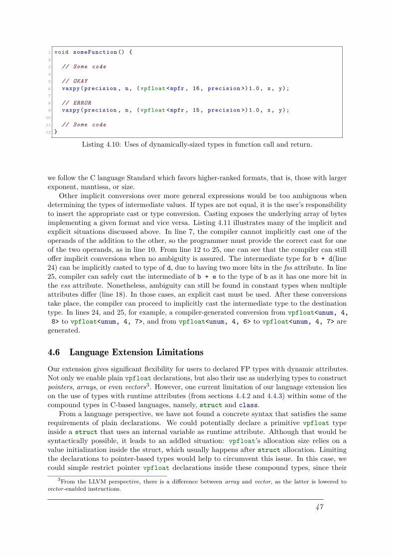
1 void someFunction () {2

3 // Some code4

5 // OKAY6 vaxpy(precision , n, (vpfloat <mpfr , 16, precision >)1.0, x, y);7

8 // ERROR9 vaxpy(precision , n, (vpfloat <mpfr , 15, precision >)1.0, x, y);

10

11 // Some code12 }

Listing 4.10: Uses of dynamically-sized types in function call and return.

we follow the C language Standard which favors higher-ranked formats, that is, those with largerexponent, mantissa, or size.

Other implicit conversions over more general expressions would be too ambiguous whendetermining the types of intermediate values. If types are not equal, it is the user’s responsibilityto insert the appropriate cast or type conversion. Casting exposes the underlying array of bytesimplementing a given format and vice versa. Listing 4.11 illustrates many of the implicit andexplicit situations discussed above. In line 7, the compiler cannot implicitly cast one of theoperands of the addition to the other, so the programmer must provide the correct cast for oneof the two operands, as in line 10. From line 12 to 25, one can see that the compiler can stilloffer implicit conversions when no ambiguity is assured. The intermediate type for b + d(line24) can be implicitly casted to type of d, due to having two more bits in the fss attribute. In line25, compiler can safely cast the intermediate of b + e to the type of b as it has one more bit inthe ess attribute. Nonetheless, ambiguity can still be found in constant types when multipleattributes differ (line 18). In those cases, an explicit cast must be used. After these conversionstake place, the compiler can proceed to implicitly cast the intermediate type to the destinationtype. In lines 24, and 25, for example, a compiler-generated conversion from vpfloat<unum, 4,8> to vpfloat<unum, 4, 7>, and from vpfloat<unum, 4, 6> to vpfloat<unum, 4, 7> are

generated.

4.6 Language Extension LimitationsOur extension gives significant flexibility for users to declared FP types with dynamic attributes.Not only we enable plain vpfloat declarations, but also their use as underlying types to constructpointers, arrays, or even vectors3. However, one current limitation of our language extension lieson the use of types with runtime attributes (from sections 4.4.2 and 4.4.3) within some of thecompound types in C-based languages, namely, struct and class.

From a language perspective, we have not found a concrete syntax that satisfies the samerequirements of plain declarations. We could potentially declare a primitive vpfloat typeinside a struct that uses an internal variable as runtime attribute. Although that would besyntactically possible, it leads to an addled situation: vpfloat’s allocation size relies on avalue initialization inside the struct, which usually happens after struct allocation. Limitingthe declarations to pointer-based types would help to circumvent this issue. In this case, wecould simple restrict pointer vpfloat declarations inside these compound types, since their

3From the LLVM perspective, there is a difference between array and vector, as the latter is lowered tovector-enabled instructions.

47

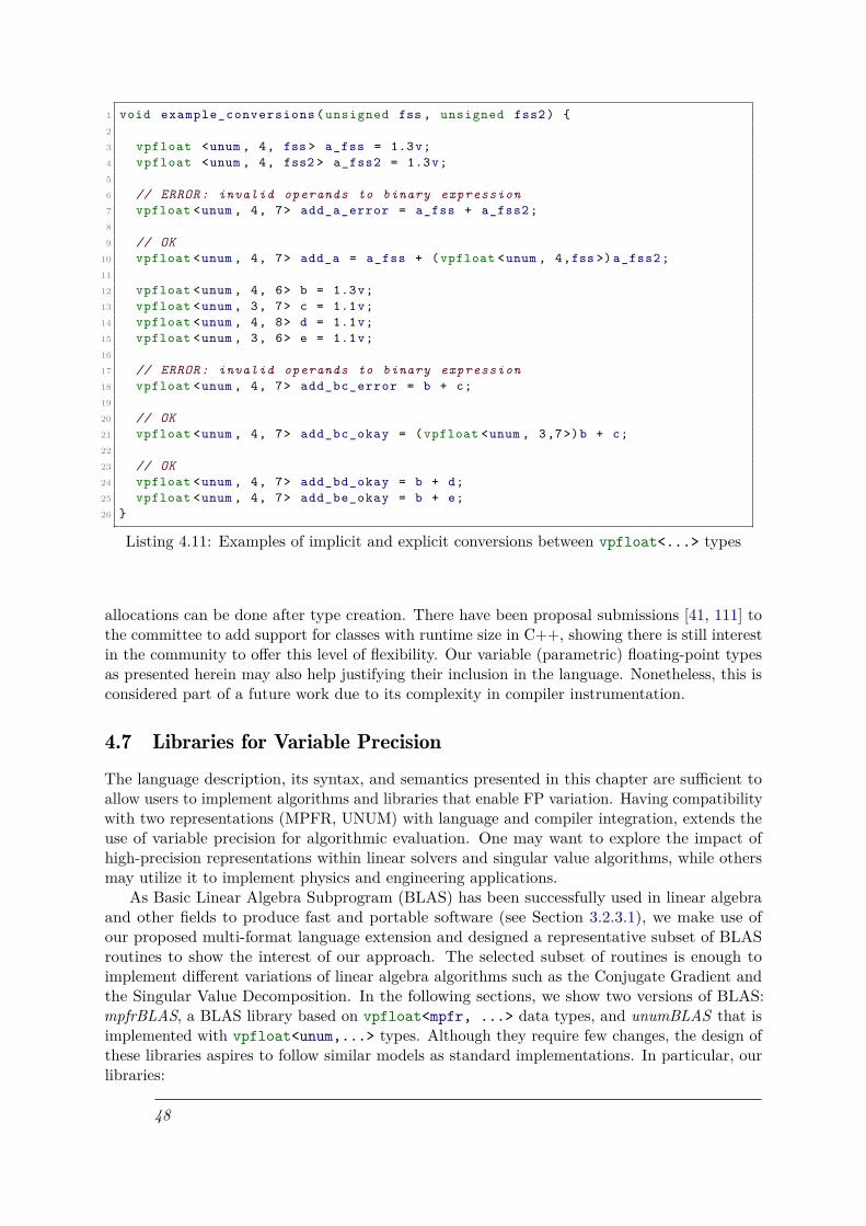
1 void example_conversions ( unsigned fss , unsigned fss2) {2

3 vpfloat <unum , 4, fss > a_fss = 1.3v;4 vpfloat <unum , 4, fss2 > a_fss2 = 1.3v;5

6 // ERROR: invalid operands to binary expression7 vpfloat <unum , 4, 7> add_a_error = a_fss + a_fss2 ;8

9 // OK10 vpfloat <unum , 4, 7> add_a = a_fss + (vpfloat <unum , 4,fss >) a_fss2 ;11

12 vpfloat <unum , 4, 6> b = 1.3v;13 vpfloat <unum , 3, 7> c = 1.1v;14 vpfloat <unum , 4, 8> d = 1.1v;15 vpfloat <unum , 3, 6> e = 1.1v;16

17 // ERROR: invalid operands to binary expression18 vpfloat <unum , 4, 7> add_bc_error = b + c;19

20 // OK21 vpfloat <unum , 4, 7> add_bc_okay = (vpfloat <unum , 3,7>)b + c;22

23 // OK24 vpfloat <unum , 4, 7> add_bd_okay = b + d;25 vpfloat <unum , 4, 7> add_be_okay = b + e;26 }

Listing 4.11: Examples of implicit and explicit conversions between vpfloat<...> types

allocations can be done after type creation. There have been proposal submissions [41, 111] tothe committee to add support for classes with runtime size in C++, showing there is still interestin the community to offer this level of flexibility. Our variable (parametric) floating-point typesas presented herein may also help justifying their inclusion in the language. Nonetheless, this isconsidered part of a future work due to its complexity in compiler instrumentation.

4.7 Libraries for Variable PrecisionThe language description, its syntax, and semantics presented in this chapter are sufficient toallow users to implement algorithms and libraries that enable FP variation. Having compatibilitywith two representations (MPFR, UNUM) with language and compiler integration, extends theuse of variable precision for algorithmic evaluation. One may want to explore the impact ofhigh-precision representations within linear solvers and singular value algorithms, while othersmay utilize it to implement physics and engineering applications.

As Basic Linear Algebra Subprogram (BLAS) has been successfully used in linear algebraand other fields to produce fast and portable software (see Section 3.2.3.1), we make use ofour proposed multi-format language extension and designed a representative subset of BLASroutines to show the interest of our approach. The selected subset of routines is enough toimplement different variations of linear algebra algorithms such as the Conjugate Gradient andthe Singular Value Decomposition. In the following sections, we show two versions of BLAS:mpfrBLAS, a BLAS library based on vpfloat<mpfr, ...> data types, and unumBLAS that isimplemented with vpfloat<unum,...> types. Although they require few changes, the design ofthese libraries aspires to follow similar models as standard implementations. In particular, ourlibraries:

48

(1) implement different flavors for the same algorithm. The goal is to minimize the number ofvariables in extended (high-) precision footprints. These representations should be usedonly when necessary and providing multiple implementations aid application designers tochoose the right function with the right balance between accuracy and performance. Forinstance, a variable-precision implementation of CG can bear to have the matrix stored asdouble and its extended-precision representation is not needed.

(2) try to use the same function signatures as standard BLAS implementations. That way, ap-plications may smoothly transition between legacy support libraries (e.g., double-precisionBLAS) and extended or adaptive precision solutions when required. Similar to xBLAS [80],our libraries use resembling function signatures to those of legacy code for rapid adaptation.

4.7.1 mpfrBLAS: A vpfloat<mpfr, ...> BLAS library

The mpfrBLAS is a vpfloat<mpfr, ...>-based BLAS implementation that targets the explo-ration of variable precision in, but not limited to, high-precision scenarios. No restrictions areimposed on employing it for lower precision, but it has the drawback over other implementationsby underlying the use of MPFR. It was implemented to enable execution in multi-threadedenvironments through the use of OpenMP directives.

The complete list of implemented routines is presented below, divided according to the BLASlevel to which they belong. The naming strategy used for them follows the type declarationsfor matrix and vector variables. For example, a DOT function where y is a vpfloat and x isa double is named as vpm_dot_vd. String "vpm_" is an indicator of a vpfloat<mpfr, ...>BLAS routine, while ’vd’ indicates that y and x have vpfloat and double types, respectively.

4.7.1.1 Level 1: Vector-to-vector operations

– COPY: Copy a vector to a new vector.

yi = xi

void vpm_copy (int precision , int n,vpfloat <mpfr , 16, precision > *x, int incx ,vpfloat <mpfr , 16, precision > *y, int incy)

void vpm_copy_2p (int precision1 , int precision2 , int n,vpfloat <mpfr , 16, precision1 > *x, int incx ,vpfloat <mpfr , 16, precision2 > *y, int incy)

Two COPY functions are provided: one where vectors X and Y have the same precisionvalue, and a more general implementation where precision may be different between vectors.As an example, one may want to increase the precision of a vector for a better estimationof the accuracy of the computed value.

– SCAL: Multiplies each vector element by a constant.

x= αx

void vpm_scal ( unsigned precision , int n,vpfloat <mpfr , 16, precision > alpha ,

49

vpfloat <mpfr , 16, precision > *X, int incx)

– DOT: Computes the DOT product between two vpfloat< mpfr,...> vectors.

r =∑

xi + yi

vpfloat <mpfr , 16, precision >vpm_dot_vd (int precision , int n, double *X, int incx ,

vpfloat <mpfr , 16, precision > *Y, int incy)

vpfloat <mpfr , 16, precision >vpm_dot_vv (int precision , int n,

vpfloat <mpfr , 16, precision > *X, int incx ,vpfloat <mpfr , 16, precision > *Y, int incy)

In some cases, it is important to perform accumulation in a high-precision container tominimize the effects of round-off errors. The kulisch accumulator [75] is based on thisconcept and it is also the reason why vdot_vd has been implemented.

– AXPY: Computes vector accumulation.

yi =∑

xi + yi

void vpm_axpy_vdd ( unsigned precision , int n, double alpha ,double *X, int incx ,vpfloat <mpfr , 16, precision > *Y, int incy)

void vpm_axpy_vvv ( unsigned precision , int n,vpfloat <mpfr , 16, precision > alpha ,vpfloat <mpfr , 16, precision > *X, int incx ,vpfloat <mpfr , 16, precision > *Y, int incy)

vpm_axpy* functions are simple implementations of vector accumulation, which is widelyused in linear algebra. More interestingly, vpm_axpy_vdd also works as a copy functionfrom double vector to a vpfloat one.

4.7.1.2 Level 2: Matrix-vector operations

– GEMV: General matrix-vector product.

y = αAx+βy

void vpm_gemv_vdd ( unsigned precision ,enum CBLAS_ORDER order ,enum CBLAS_TRANSPOSE trans ,int m, int n,vpfloat <mpfr , 16, precision > alpha ,

50

double *A, int k,double *X, int incx ,vpfloat <mpfr , 16, precision > beta ,vpfloat <mpfr , 16, precision > *Y, int incy)

void vpm_gemv_vdv ( unsigned precision ,enum CBLAS_ORDER order ,enum CBLAS_TRANSPOSE trans ,int m, int n,vpfloat <mpfr , 16, precision > alpha ,double *A, int lda ,vpfloat <mpfr , 16, precision > *X, int incx ,vpfloat <mpfr , 16, precision > beta ,vpfloat <mpfr , 16, precision > *Y, int incy)

void vpm_gemv_vvv ( unsigned precision ,enum CBLAS_ORDER order ,enum CBLAS_TRANSPOSE trans ,int m, int n,vpfloat <mpfr , 16, precision > alpha ,vpfloat <mpfr , 16, precision > *A, int lda ,vpfloat <mpfr , 16, precision > *X, int incx ,vpfloat <mpfr , 16, precision > beta ,vpfloat <mpfr , 16, precision > *Y, int incy)

int t1 , t2 , t3 , t4;int lb , ub , lbp , ubp , lb2 , ub2;register int lbv , ubv;

if ((m >= 1) && (n >= 1)) {lbp =0;ubp= floord (m -1 ,32);

# pragma omp parallel for private (lbv ,ubv ,t2 ,t3 ,t4)for (t1=lbp;t1 <= ubp;t1 ++) {

for (t2 =0;t2 <= floord (n -1 ,32);t2 ++) {for (t3 =32* t1;t3 <=( min(m -1 ,32* t1 +31)) -7;t3 +=8) {

for (t4 =32* t2;t4 <= min(n -1 ,32* t2 +31);t4 ++) {Y[t3*incy] = alpha * A[t3*lda + t4] * X[t4*incx]

+ beta * Y[t3*incy ];Y[(t3 +1)*incy] = alpha*A[(( t3 +1)*lda)+t4]*X[t4*incx]

+ beta*Y[(t3 +1)*incy ];Y[(t3 +2)*incy] = alpha*A[(( t3 +2)*lda)+t4]*X[t4*incx]

+ beta*Y[(t3 +2)*incy ];Y[(t3 +3)*incy] = alpha*A[(( t3 +3)*lda)+t4]*X[t4*incx]

+ beta*Y[(t3 +3)*incy ];Y[(t3 +4)*incy] = alpha*A[(( t3 +4)*lda)+t4]*X[t4*incx]

+ beta*Y[(t3 +4)*incy ];Y[(t3 +5)*incy] = alpha*A[(( t3 +5)*lda)+t4]*X[t4*incx]

+ beta*Y[(t3 +5)*incy ];Y[(t3 +6)*incy] = alpha*A[(( t3 +6)*lda)+t4]*X[t4*incx]

+ beta*Y[(t3 +6)*incy ];Y[(t3 +7)*incy] = alpha*A[(( t3 +7)*lda)+t4]*X[t4*incx]

+ beta*Y[(t3 +7)*incy ];}

}for (;t3 <= min(m -1 ,32* t1 +31);t3 ++) {

for (t4 =32* t2;t4 <= min(n -1 ,32* t2 +31);t4 ++) {Y[t3] = alpha * A[t3*lda + t4] * X[t4*incx]

+ beta * Y[t3*incy ];}

}}

51

}}

}

Above, we show an implementation example for vpm_gemv_vvv, automatically generated byPluto [25], an automatic parallelizer and locality optimizer. The only modifications doneconcern the inclusion of variables lda, incx, and incy, requirements for BLAS functions.We will further discuss support for Loop Nest optimizer within the context of our types(in Chapter 5), however, Pluto’s capabilities go beyond the support for types. That is,it optimizes the data locality by merely analyzing patterns of access, without requiringto have previous knowledge about the footprint of the type. This example intent is toshow that state-of-the-art optimizers can be used to design high-performance libraries forvpfloat types. Future implementations of our libraries will focus on these specializations,which require substantial work to guarantee performance improvement in most cases.

– SYMV: Sparse matrix vector product.

y = αAx+βy

void vpm_sparse_gemv_vdd ( unsigned precision , int m, int n,vpfloat <mpfr , 16, precision > alpha ,double *A, int *rowInd , int *colInd ,double *X,vpfloat <mpfr , 16, precision > beta ,vpfloat <mpfr , 16, precision > *Y)

void vpm_sparse_gemv_vdv ( unsigned precision , int m, int n,vpfloat <mpfr , 16, precision > alpha ,double *A, int *rowInd , int *colInd ,vpfloat <mpfr , 16, precision > *X,vpfloat <mpfr , 16, precision > beta ,vpfloat <mpfr , 16, precision > *Y)

void vpm_sparse_gemv_vvv ( unsigned precision , int m, int n,vpfloat <mpfr , 16, precision > alpha ,vpfloat <mpfr , 16, precision > *A,int *rowInd , int *colInd ,vpfloat <mpfr , 16, precision > *X,vpfloat <mpfr , 16, precision > beta ,vpfloat <mpfr , 16, precision > *Y)

– Sparse MV: Sparse matrix vector product.

y = αAx+βy

void vpm_sparse_symv_vdd ( unsigned precision , int m, int n,vpfloat <mpfr , 16, precision > alpha ,double *A, int *rowInd , int *colInd ,double *X,vpfloat <mpfr , 16, precision > beta ,vpfloat <mpfr , 16, precision > *Y)

52

void vpm_sparse_symv_vdv ( unsigned precision , int m, int n,vpfloat <mpfr , 16, precision > alpha ,double *A, int *rowInd , int *colInd ,vpfloat <mpfr , 16, precision > *X,vpfloat <mpfr , 16, precision > beta ,vpfloat <mpfr , 16, precision > *Y)

void vpm_sparse_symv_vvv ( unsigned precision , int m, int n,vpfloat <mpfr , 16, precision > alpha ,vpfloat <mpfr , 16, precision > *A,int *rowInd , int *colInd ,vpfloat <mpfr , 16, precision > *X,vpfloat <mpfr , 16, precision > beta ,vpfloat <mpfr , 16, precision > *Y)

We have implemented different variations of the matrix-vector multiplications in orderto handle different scenarios: dense, sparse and symmetric sparse matrices. Those witha sparse prefix are used for sparse matrices represented in the CSR (Compressed RowStorage) format.

4.7.1.3 Level 3: Matrix-matrix operations

C = αAB+βC

void vpm_gemm ( unsigned precision , enum CBLAS_ORDER order ,enum CBLAS_TRANSPOSE transA ,enum CBLAS_TRANSPOSE transB , int m, int n, int k,vpfloat <mpfr , 16, precision > alpha ,vpfloat <mpfr , 16, precision > *A, int lda ,vpfloat <mpfr , 16, precision > *B, int ldb ,vpfloat <mpfr , 16, precision > beta ,vpfloat <mpfr , 16, precision > *C, int ldc)

GEMM has, as have other routines, been implemented so that it has a signature close toBLAS original one. The sole difference is the presence of a precision variable as the firstfunction parameter. The remaining ones conform to the legacy code signature 4, easingportability. Furthermore, both transpose and non-transpose matrices are supported byour implementation.

Our mpfrBLAS is composed of 17 routines, ranging from simple vector-vector operations(Level 1) to a matrix product (Level 3). Even though there are many functions missing, thesefunctions already allow us to implement some linear algebra algorithms, which will be discussedin Chapter 6. Moreover, we should clarify that the exponent field, defined as a constant 16, has noreal effect on MPFR types. Its actual size value is predefined by the underlying mpfr_t struct.

4https://developer.apple.com/documentation/accelerate/1513282-cblas_dgemm

53

4.7.2 unumBLAS: A vpfloat<unum, ...> BLAS libraryWe also propose a subset of BLAS routines for vpfloat<unum, ...> types. Due to the flexibilityof our extension, many variations of vpfloat<unum,...>-enabled libraries can be created. Thisone, in particular, has been implemented considering all FP attributes being expressed asvariables, but other implementations may consider different constraints and use constant valuefor the declaration of any FP attribute. Function names are preceded by prefix "vpu_", while ’v’indicates vpfloat<unum, ...> types, ’d’ is used for double.

4.7.2.1 Level 1: Vector-to-vector operations

– COPY: Copy a vector to a new vector.

yi = xi

void vpu_copy (int ess , int fss , int size , int n,vpfloat <unum , ess , fss , size > *x, int incx ,vpfloat <unum , ess , fss , size > *y, int incy);

– SCAL: Multiplies each vector element by a constant.

x= αx

void vpu_scal (int ess , int fss , int size , int n,vpfloat <unum , ess , fss , size > alpha ,vpfloat <unum , ess , fss , size > *X, int incx);

– DOT: Computes the DOT product between two vpfloat< mpfr,...> vectors.

r =∑

xi + yi

vpfloat <unum , ess , fss , size >vpu_dot_vd (int ess , int fss , int size , int n,

double *X, int incx ,vpfloat <unum , ess , fss , size > *Y, int incy);

vpfloat <unum , ess , fss , size >vpu_dot_vv (int ess , int fss , int size , int n,

vpfloat <unum , ess , fss , size > *X, int incx ,vpfloat <unum , ess , fss , size > *Y, int incy);

– AXPY: Computes vector accumulation.

yi =∑

xi + yi

void vpu_axpy_vdd (int ess , int fss , int size , int n,double alpha , double *X, int incx ,vpfloat <unum , ess , fss , size > *Y, int incy);

54

void vpu_axpy_vvv (int ess , int fss , int size , int n,vpfloat <unum , ess , fss , size > alpha ,vpfloat <unum , ess , fss , size > *X, int incx ,vpfloat <unum , ess , fss , size > *Y, int incy);

4.7.2.2 Level 2: Matrix-vector operations

– GEMV: General matrix-vector product.

y = αAx+βy

void vpu_gemv_vdd (int ess , int fss , int size ,enum CBLAS_ORDER order , enum CBLAS_TRANSPOSE trans ,int m, int n, vpfloat <unum , ess , fss , size > alpha ,double *A, int lda , double *X, int incx ,vpfloat <unum , ess , fss , size > beta ,vpfloat <unum , ess , fss , size > *Y, int incy);

void vpu_gemv_vvd (int ess , int fss , int size ,enum CBLAS_ORDER order , enum CBLAS_TRANSPOSE trans ,int m, int n, vpfloat <unum , ess , fss , size > alpha ,double *A, int lda ,vpfloat <unum , ess , fss , size > *X, int incx ,vpfloat <unum , ess , fss , size > beta ,vpfloat <unum , ess , fss , size > *Y, int incy);

void vpu_gemv_vvv (int ess , int fss , int size ,enum CBLAS_ORDER order , enum CBLAS_TRANSPOSE trans ,int m, int n, vpfloat <unum , ess , fss , size > alpha ,vpfloat <unum , ess , fss , size > *A, int lda ,vpfloat <unum , ess , fss , size > *X, int incx ,vpfloat <unum , ess , fss , size > beta ,vpfloat <unum , ess , fss , size > *Y, int incy);

– Sparse MV: Sparse matrix vector product.

y = αAx+βy

void vpu_sparse_gemv_vdd (int ess , int fss , int size , int m, int n,vpfloat <unum , ess , fss , size > alpha ,double *A, int *rowInd , int *colInd ,double *X, vpfloat <unum , ess , fss , size > beta ,vpfloat <unum , ess , fss , size > *Y);

void vpu_sparse_gemv_vvd (int ess , int fss , int size , int m, int n,vpfloat <unum , ess , fss , size > alpha ,double *A, int *rowInd , int *colInd ,vpfloat <unum , ess , fss , size > *X,vpfloat <unum , ess , fss , size > beta ,vpfloat <unum , ess , fss , size > *Y);

55

void vpu_sparse_gemv_vvv (int ess , int fss , int size , int m, int n,vpfloat <unum , ess , fss , size > alpha ,vpfloat <unum , ess , fss , size > *A,int *rowInd , int *colInd ,vpfloat <unum , ess , fss , size > *X,vpfloat <unum , ess , fss , size > beta ,vpfloat <unum , ess , fss , size > *Y);

– SYMV Sparse: Sparse Symmetric matrix vector product.

y = αAx+βy

void vpu_sparse_symv_vdd (int ess , int fss , int size , int m, int n,vpfloat <unum , ess , fss , size > alpha ,double *A, int *rowInd , int *colInd ,double *X, vpfloat <unum , ess , fss , size > beta ,vpfloat <unum , ess , fss , size > *Y);

void vpu_sparse_symv_vvd (int ess , int fss , int size , int m, int n,vpfloat <unum , ess , fss , size > alpha ,double *A, int *rowInd , int *colInd ,vpfloat <unum , ess , fss , size > *X,vpfloat <unum , ess , fss , size > beta ,vpfloat <unum , ess , fss , size > *Y);

void vpu_sparse_symv_vvv (int ess , int fss , int size , int m, int n,vpfloat <unum , ess , fss , size > alpha ,vpfloat <unum , ess , fss , size > *A,int *rowInd , int *colInd ,vpfloat <unum , ess , fss , size > *X,vpfloat <unum , ess , fss , size > beta ,vpfloat <unum , ess , fss , size > *Y);

4.7.2.3 Level 3: Matrix-matrix operations

C = αAB+βC

void vpu_gemm (int ess , int fss , int size , enum CBLAS_ORDER order ,enum CBLAS_TRANSPOSE transA , enum CBLAS_TRANSPOSE transB ,int m, int n, int k, vpfloat <unum , ess , fss , size > alpha ,vpfloat <unum , ess , fss , size > *A, int lda ,vpfloat <unum , ess , fss , size > *B, int ldb ,vpfloat <unum , ess , fss , size > beta ,vpfloat <unum , ess , fss , size > *C, int ldc);

unumBLAS routines are very similar to the ones defined in mpfrBLAS. However, one maynotice that UNUM types have broader adaptability. MPFR types are declared with two FP

56

attributes, one of which has no effect on the representation. Types created as vpfloat<unum,...> are more flexible with up to three attributes to control.

4.8 ConclusionThis chapter introduced and presented all aspects of the C language extension and type systemfor variable precision FP computing that we propose. When comparing to state-the-art solutions,we hope to have proven that our language extension has similar capabilities and equivalentprogramming model as traditional formats (like programming with IEEE formats), with betterlanguage integration than high-level structures. This enables further integration with a compilertoolchain, which will be introduced in the next chapter. We also allow multiple formats to coexistwithin the same keyword, which can further improve the exploration of alternative formats andcan accelerate the integration with industry-level compiler infrastructures.

Along with the extension, we also provide implementations for a subset of BLAS routines thatuses our types. They allow developers to rapidly instantiate code for testing multiple formats andvariable precision. Furthermore, the main feature of these libraries is enabling programmaticallydriven experimentations in an attribute agnostic fashion for a given representation. That is,we may single-run applications in multiple precision configurations without requiring coderecompilation. Some of the experimental results from Chapter 6 were obtained this way.

57

Chapter 5: Compiler Integration forVariable Precision FP Formats

Contents5.1 Frontend . . . . . . . . . . . . . . . . . . . . . . . . . . . . . . . . . . . . . . . . 595.2 Intermediate Representation (IR) . . . . . . . . . . . . . . . . . . . . . . . . . 59

5.2.1 VPFloat Types . . . . . . . . . . . . . . . . . . . . . . . . . . . . . . . . 605.2.2 Function Declarations . . . . . . . . . . . . . . . . . . . . . . . . . . . . 615.2.3 Interaction with Classical Optimizations . . . . . . . . . . . . . . . . . . 62

5.3 Code Generators . . . . . . . . . . . . . . . . . . . . . . . . . . . . . . . . . . . 685.3.1 Software Target: MPFR . . . . . . . . . . . . . . . . . . . . . . . . . . . 685.3.2 Hardware Target: UNUM . . . . . . . . . . . . . . . . . . . . . . . . . . 74

5.4 Conclusion . . . . . . . . . . . . . . . . . . . . . . . . . . . . . . . . . . . . . . 77

We will demonstrate the value and realism of our language extension through its integrationinto an industry-level compiler. Our solution was implemented on top of the LLVM [76] infras-tructure, since it provides a modular compilation flow, a powerful Intermediate Representation(IR), and is widely used both in academia and industry. This chapter focuses on detailing thecompilation flow needed to support the vpfloat type system. We will cover the aspects of theproposed LLVM IR extension for variable precision FP arithmetic, and how it interacts withthe compilation flow and optimizations. Later we describe the backend code generators weimplemented in order to consume vpfloat<mpfr, ...> and vpfloat<unum, ...> types fromour language extension.

5.1 FrontendWe have implemented support for the vpfloat language extension and type system in LLVM’sfrontend for C/C++ (clang). Our frontend supports both representations MPFR and UNUM asdefined in the Language chapter (4). Aside from implementing the specification of our language,semantic and syntax analysis, the only work needed by this stage is the generation of LLVMIntermediate Representation (LLVM IR).

5.2 Intermediate Representation (IR)LLVM uses a target-independent intermediate language for a common infrastructure where codeoptimizations and transformations can be applied. The LLVM IR defines a set of assembly-likeinstructions that operate on values and types, and which are later used by the code generatorsof different architectures. More specifically, LLVM defines a set of types to represent different

59

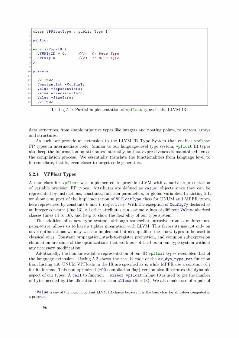
1 class VPFloatType : public Type {2

3 public :4

5 enum VPTypeID {6 UNUMTyID = 0, ///< 0: Unum Type7 MPFRTyID ///< 1: MPFR Type8 };9

10 private :11

12 // Code ...13 ConstantInt * ConfigTy ;14 Value * ExponentInfo ;15 Value * PrecisionInfo ;16 Value * SizeInfo ;17 // Code ...

Listing 5.1: Partial implementation of vpfloat types in the LLVM IR.

data structures, from simple primitive types like integers and floating points, to vectors, arraysand structures.

As such, we provide an extension to the LLVM IR Type System that enables vpfloatFP types in intermediate code. Similar to our language-level type system, vpfloat IR typesalso keep the information on attributes internally, so that expressiveness is maintained acrossthe compilation process. We essentially translate the functionalities from language level tointermediate, that is, even closer to target code generators.

5.2.1 VPFloat TypesA new class for vpfloat was implemented to provide LLVM with a native representationof variable precision FP types. Attributes are defined as Value1 objects since they can berepresented by instructions, constants, function parameters, or global variables. In Listing 5.1,we show a snippet of the implementation of VPFloatType class for UNUM and MPFR types,here represented by constants 0 and 1, respectively. With the exception of ConfigTy declared asan integer constant (line 13), all other attributes can assume values of different Value-inheritedclasses (lines 14 to 16), and help to show the flexibility of our type system.

The addition of a new type system, although somewhat intrusive from a maintenanceperspective, allows us to have a tighter integration with LLVM. This favors its use not only onnovel optimizations we may wish to implement but also qualifies these new types to be used inclassical ones. Constant propagation, stack-to-register promotion, and common subexpressionelimination are some of the optimizations that work out-of-the-box in our type system withoutany necessary modification.

Additionally, the human-readable representation of our IR vpfloat types resembles that ofthe language extension. Listing 5.2 shows the the IR code of the ex_dyn_type_ret functionfrom Listing 4.9. UNUM VPFloats in the IR are specified as 0, while MPFR use a constant of 1for its format. This non-optimized (-O0 compilation flag) version also illustrates the dynamicaspect of our types. A call to function __sizeof_vpfloat in line 10 is used to get the numberof bytes needed by the allocation instruction alloca (line 13). We also make use of a pair of

1Value is one of the most important LLVM IR classes because it is the base class for all values computed ina program.

60

1 ; Function Attrs: noinline nounwind optnone2 define vpfloat <0, 4, %fss >3 @ex_dyn_type_ret (i32 signext %fss , vpfloat <0, 4, %fss > %a) #0 {4 entry:5 call void @llvm. vpfloat . runtimeattr .mark.i32(i32 %fss)6 %fss.addr = alloca i32 , align 47 %saved_stack = alloca i8*, align 88 store i32 %fss , i32* %fss.addr , align 49 %0 = load i32 , i32* %fss.addr , align 4

10 %1 = call i64 @__sizeof_vpfloat (i32 0, i32 4, i32 %0 , i64 0)11 %2 = call i8* @llvm. stacksave ()12 store i8* %2 , i8** %saved_stack , align 813 %vla = alloca i8 , i64 %1 , align 814 %a.addr = bitcast i8* %vla to vpfloat <0, 4, %fss >*15 store vpfloat <0, 4, %fss > %a , vpfloat <0, 4, %fss >* %a.addr , align 816 store vpfloat <0, 4, %fss > fpext ( double 1.300000 e+00 to vpfloat <0, 4, ←↩

%fss >), vpfloat <0, 4, %fss >* %a.addr , align 817 %3 = load vpfloat <0, 4, %fss >, vpfloat <0, 4, %fss >* %a.addr , align 818 %4 = load i8*, i8** %saved_stack , align 819 call void @llvm. stackrestore (i8* %4)20 ret vpfloat <0, 4, %fss > %321 }22

23 declare extern_weak i64 @__sizeof_vpfloat (i32 , i32 , i32 , i64)

Listing 5.2: IR code of the ex_dyn_type_ret function from Listing 4.9 types in the LLVM IR.

instructions store and load to control the address pointer of the stack. Lines 11-12 and 18-19are used to record and recover the status of the stack, respectively, so that it can be dynamicallyallocated. To the best of our knowledge, this is the first work that proposes these levels ofinteraction between types and values in the program for FP arithmetic. LLVM types are usuallyself-sufficient, i.e., free from the interference of other values in the program (except for VLAs).This flexibility comes at the cost of evaluating their compatibility with the significant number ofoptimizations LLVM offers.

5.2.2 Function Declarations

LLVM IR has a particular way of representing function declarations that omits variables namesfor function parameters. As an example, __sizeof_vpfloat from Listing 5.2 (line 23) is printedas a function declaration, because it was either inserted by the compiler automatically or camefrom an included header file. One should notice that only parameter types are included, and nottheir names, simply because they are not needed.

Declaration-wise, parameters’ names are irrelevant. Although this works well for standardLLVM IR code and also conforms to the C specification (as in line 3 of Listing 5.3a), our typesystem cannot afford the use of the same approach. Types with runtime-decidable attributesmay have their declarations dependent on function parameters, which can lead these types to beinvalid. As values are used as binding operands for vpfloat types, it is important to make surethat function declarations have vpfloat types with proper attributes.

We propose to address this issue by using negative values as a way of expressing bindingrelations between parameters and vpfloat types. Since negative values have no meaning forfloating-point format parameters whatsoever, we can make use of them to specify these relations.We depict some examples of this approach in Listing 5.3: with Listing 5.3a showing the C-level code for different function declarations, and Listing 5.3b having their corresponding IR

61

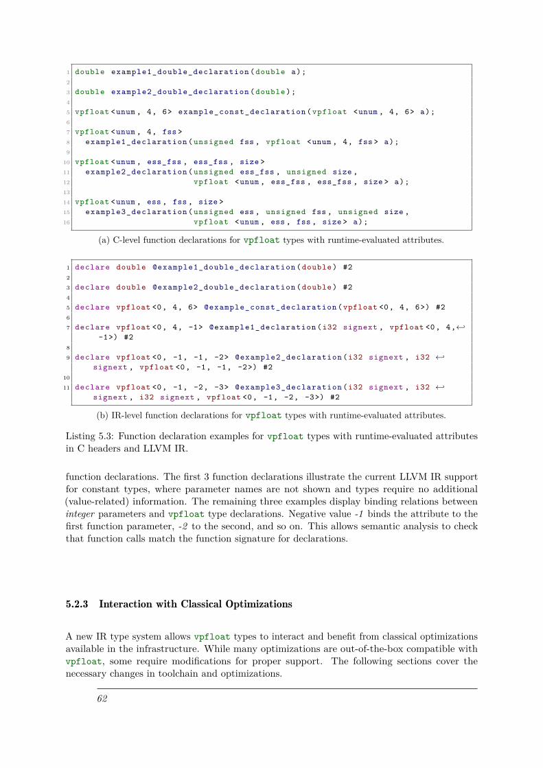
1 double example1_double_declaration ( double a);2

3 double example2_double_declaration ( double );4

5 vpfloat <unum , 4, 6> example_const_declaration ( vpfloat <unum , 4, 6> a);6

7 vpfloat <unum , 4, fss >8 example1_declaration ( unsigned fss , vpfloat <unum , 4, fss > a);9

10 vpfloat <unum , ess_fss , ess_fss , size >11 example2_declaration ( unsigned ess_fss , unsigned size ,12 vpfloat <unum , ess_fss , ess_fss , size > a);13

14 vpfloat <unum , ess , fss , size >15 example3_declaration ( unsigned ess , unsigned fss , unsigned size ,16 vpfloat <unum , ess , fss , size > a);

(a) C-level function declarations for vpfloat types with runtime-evaluated attributes.

1 declare double @example1_double_declaration ( double ) #22

3 declare double @example2_double_declaration ( double ) #24

5 declare vpfloat <0, 4, 6> @example_const_declaration (vpfloat <0, 4, 6>) #26

7 declare vpfloat <0, 4, -1> @example1_declaration (i32 signext , vpfloat <0, 4,←↩-1>) #2

8

9 declare vpfloat <0, -1, -1, -2> @example2_declaration (i32 signext , i32 ←↩signext , vpfloat <0, -1, -1, -2>) #2

10

11 declare vpfloat <0, -1, -2, -3> @example3_declaration (i32 signext , i32 ←↩signext , i32 signext , vpfloat <0, -1, -2, -3>) #2

(b) IR-level function declarations for vpfloat types with runtime-evaluated attributes.

Listing 5.3: Function declaration examples for vpfloat types with runtime-evaluated attributesin C headers and LLVM IR.

function declarations. The first 3 function declarations illustrate the current LLVM IR supportfor constant types, where parameter names are not shown and types require no additional(value-related) information. The remaining three examples display binding relations betweeninteger parameters and vpfloat type declarations. Negative value -1 binds the attribute to thefirst function parameter, -2 to the second, and so on. This allows semantic analysis to checkthat function calls match the function signature for declarations.

5.2.3 Interaction with Classical Optimizations

A new IR type system allows vpfloat types to interact and benefit from classical optimizationsavailable in the infrastructure. While many optimizations are out-of-the-box compatible withvpfloat, some require modifications for proper support. The following sections cover thenecessary changes in toolchain and optimizations.

62

5.2.3.1 Type-value Relation

Standard compilers usually use specific data structures to track the relation between a valuedefinition and its uses [4]. A Use-Definition (use-def) chain consists of a use (U) of a variable andall the definitions that can reach U directly without any other intermediate definition. It usuallyexpresses the assignment of a value to a variable. Its counterpart, Definition-Use (def-use)chain relates the definition (D) of a variable with all its uses that are reachable from D withoutany intervening definition. These concepts and structures are prerequisites for applying manycompiler optimizations and transformations, such as constant propagation, register allocation,and common subexpression elimination.

LLVM also makes use of these concepts to construct relations between value definitionsand uses throughout the compilation flow. Although LLVM’s def-use chain and use-def chainimplementations allows one only to track chains between Value objects, vpfloat types alsohave def-use relations with attribute Value objects. Hence, the current LLVM implementationis incompatible with our type extension, and a vpfloat type cannot be obtained by traversingthe def-use chain of an attribute. Due to the required modifications of many key components ofthe compiler for making the current def-use implementation compatible with our type system,we have chosen to keep a separated list of Value objects being used as types attributes. Oneshould notice that constant values do not require tracking, since they will never change. Oncethe list is constructed, two operations are possible:

(1) Update: optimizations may optimize values in the program that require the update ofreferences from our tracking list. If an object is replaced by a new one, our type systemmakes sure to update any type that uses the old value to the new reference.

(2) Deletion: Because LLVM classical optimizations have no knowledge about our trackingsystem, it is possible they wind up realizing that values being used as vpfloat attributesare no longer needed in the computation and, thus, can be deleted. However, an objectdeletion can invalidate types. Our compiler makes sure vpfloat attributes are neverdeleted by adding a mark through an intrinsic call. Because they are inherently seen ashaving side effects, adding intrinsic calls to mark values avoids their deletion. Althoughthis may have a negative impact on the generated code, we ensure that vpfloat types arenot invalidated.

5.2.3.2 Loop Idiom Recognition

Another optimization change for vpfloat compatibility is implemented for the Loop IdiomRecognizer. This pass implements a simple, yet efficient transformation that replaces a simpleloop structure into a non-loop form. Two of the implemented optimizations consist of detectingloop structures that can be replaced by memset and memcpy calls: the former is used to detectobject initialization in an array and the latter copies an object from one location to another.

These transformations can greatly improve application performance and are depicted inListing 5.4a. Constant vpfloat types are implemented in the same fashion as traditionalprimitive types. Lines 1-10 and Listings 5.4b-5.4d exemplify how the pass generates memset andmemcpy calls to initialize array values for constant types double and a 6-byte unum.

We have modified this pass to take into consideration dynamically-sized types where sizescannot be known at compile time. If a dynamically-sized type is found, the compiler usesthe __sizeof_vpfloat function to calculate the size of the type in use. Listing 5.4e showshow the pass optimizes a vector-copy for-loop by generating a memcpy call instead. Becausethe pass does not know the size of vec_unum1 and vec_unum2 a priori, it generates a call to__sizeof_vpfloat. Additionally, due to the definition of the base MPFR data type which

63

1 double * vec_double ;2 for ( unsigned i = 0; i < N; ++i)3 vec_double [i] = 0;4

5 double *vec1 , *vec2;6 for ( unsigned i = 0; i < N; ++i)7 vec1[i] = vec2[i];8

9 vpfloat <unum , 4, 6, 6> * vec_unum_c ;10 for ( unsigned i = 0; i < N; ++i)11 vec_unum_c [i] = 0;12

13 vpfloat <unum , 4, fss > * vec_unum1 ;14 vpfloat <unum , 4, fss > * vec_unum2 ;15 for ( unsigned i = 0; i < N; ++i)16 vec_unum1 [i] = vec_unum2 [i];17

18 vpfloat <mpfr , 16, 100> vec_mpfr ;19 for ( unsigned i = 0; i < N; ++i)20 vec_mpfr [i] = 0;

(a) Original code before Loop Idiom Recognition.

memset (vec_double , 0, N * 8);

(b) Optimized (memset) generation for double.

memcpy (vec1 , vec2 , N * 8);

(c) Optimized (memset) generation for constantvpfloat<unum, ...>.

memset (vec_unum_c , 0, N * 6);

(d) Optimized (memset) generation for vpfloat<unum, ...> with a runtime attribute.

memcpy (vec_unum1 , vec_unum2 , N *__sizeof_vpfloat (0, 4, fss , 0));

(e) Optimized (Optimized (memcpy) generationin constant vpfloat<unum, ...>.

for ( unsigned i = 0; i < N; ++i)vec_mpfr [i] = 0;

(f) Optimized (No optimization for vpfloat<mpfr, ...> types.

Listing 5.4: Loop idiom recognition pass for different types: double(5.4b, 5.4c), vpfloat<unum,...>(5.4d, 5.4e), and vpfloat<mpfr, ...>(5.4f).

includes a pointer variable in the struct (see in Listing 4.2), this pass has been disabled forthe vpfloat <mpfr, ...> types. Listing 5.4f shows that no optimization is performed for thevpfloat <mpfr, 16, 100> data type.

5.2.3.3 Inlining

Inlining Expansion replaces a function call site by the body of the function and is a relevantoptimization to improve code performance. Some inlining heuristics can lead to speedups of morethan 50% in execution time [10]. While constant types have out-of-the-box support, types withruntime attributes require additional work during inline expansion as they are only consideredvalid inside a function. This issue boils down to the def-use chains from the previous section(see 5.2.3.1).

We have expanded the pass to include support for these types. Values with dynamically-sizedtypes have their types changed (or mutated) in order to comply with the current function wherethey are being used in. We illustrate two examples of inlining expansions that may be generated:

(1) Constant-type generation mutates the original type to a constant one, thus replacing afunction-specific type by a global2 counterpart. The call to function func_sum (Lines

2Types such as float, double, integers, and constant vpfloat are considered global because they have aunique representation for the whole program unit.

64

1 double2 func_sum ( unsigned p,3 vpfloat <mpfr , 16, p> vec ,4 unsigned N) {5 vpfloat <mpfr , 16, p> sum = 0.0;6 for ( unsigned i = 0; i < N; ++i)7 sum += vec[i];8 return ( double ) sum;9 }

10

11 void func( unsigned prec) {12

13 double s = 0.014

15 vpfloat <mpfr , 16, 100> *vec1;16 // Do something with vec117 s += func_sum (100 , vec1 , 1000);18

19 vpfloat <mpfr , 16, prec > *vec2;20 // Do something with vec221 s += func_sum (prec , vec2 , 1000);22 }

(a) Original code before inlining expansion.

1 double2 func_sum ( unsigned p,3 vpfloat <mpfr , 16, p> vec ,4 unsigned N) {5

6 vpfloat <mpfr , 16, p> sum = 0.0;7 for ( unsigned i = 0; i < N; ++i)8 sum += vec[i];9 return ( double ) sum;

10 }11

12 void func( unsigned prec) {13

14 double s = 0.0;15

16 vpfloat <mpfr , 16, 100> *vec1;17 // Do something with vec118 vpfloat <mpfr , 16, 100> sum1 = 0.0;19 for ( unsigned i = 0; i < N; ++i)20 sum1 += vec1[i];21 s += ( double ) sum1;22

23 vpfloat <mpfr , 16, prec > *vec2;24 // Do something with vec225 vpfloat <mpfr , 16, prec > sum2 =

0.0;26 for ( unsigned i = 0; i < N; ++i)27 sum2 += vec2[i];28 s += ( double ) sum2;29 }

(b) C representation of the inlining optimization.

Listing 5.5: Inlining expansion examples for types with runtime attributes.

15-17) from Listing 5.5a is inline expanded to the code shown in lines 7-10 from 5.5b,which mutates vpfloat<mpfr, 16, p> to vpfloat<mpfr, 16, 100>.

(2) The callee vpfloat with runtime attributes needs to mutate to a caller one with thesame characteristics. Our implementation ensures that caller attributes are used, and noreference to the callee function remains to invalidate values of the new type. Function callto func_sum(Lines 19-21) has been inlined, and had values mutate from vpfloat<mpfr,16, p>, in function func_sum, to vpfloat<mpfr, 16, p>, in function func.

In both cases, we must also guarantee that constants, return types, and any call within theinlined function (and its type) are mutated.

5.2.3.4 Lifetime Marker Optimization

LLVM generates a pair of intrinsics, llvm.lifetime.start 3 and llvm.lifetime.end 4, tomark the lifetime of variables in the program. The main goal is to provide passes with hints onthe lifetime of variables for optimization opportunities. More precisely, the compiler implementsa stack coloring optimization that makes use of lifetime markers to represent the lifetime of stackslots. It then attempts to reduce the used stack space by merging disjoint stack slots. We must

3https://llvm.org/docs/LangRef.html#llvm-lifetime-end-intrinsic4https://llvm.org/docs/LangRef.html#llvm-lifetime-start-intrinsic

65

follow the same reasoning from loop idiom recognition and disable, or prevent, this optimizationto run for MPFR based types. Because code generation will transform them into MPFR structtypes, we are not able to guarantee proper memory management when stack locations betweenobjects overlap. The pointer variable _mpfr_d makes the mpfr_t struct non trivially-copyable.Removing lifetime intrinsics for MPFR-derived types resolves this issue. Although one may arguethat removing lifetime markers may incur an extra performance overhead, the stack coloringoptimization has shown negligible impact on performance in our experiments. Their removalasserts that deletions are executed for all objects.

5.2.3.5 OpenMP Multithread Programming

Improvements in performance have much to do with how much parallelism can be explored incomputer applications. Having first-class support for primitive types in the compiler enablestheir use within parallel programming schemes like OpenMP [39]. Looking at both language andcompiler perspectives, to the best of our knowledge, this is the first work that shows MPFR andUNUM types integrated within language and compiler, with multi-thread execution capabilities.Previous works are OpenMP-compatible through high-level abstractions and miss optimizationopportunities.

5.2.3.6 Loop nest Optimizations

Our LLVM type extension is also able to leverage advanced loop nest optimizers. Polly [55],LLVM’s loop nest optimizer, can also be used to optimize vpfloat memory accesses. Anylimitation of the polyhedral model in vpfloat is mostly given by the optimizer. Constant-sizedtypes, described in sections 4.4.1 and 4.4.2, are fully supported by Polly. Any potentialperformance slowdown is caused by suboptimal heuristic tuning, a well-known challenge withloop nest optimizers in general.

In the case of dynamically-sized types, the limitation stems from Polly’s lack of supportfor performing loop tiling with runtime loop bounds, i.e., the application of loop tiling wherebounds are not known at compile time. This requires heuristics to generate loops with a dynamic(runtime decidable) behavior, and full automatic support for dynamically-sized types are mostlydependent upon adding this functionality to Polly. Although we can trick the optimizer toassume these types to have constant sizes, it is likely to generate suboptimal heuristics withpoor performance. Nevertheless, we can still explore polyhedral techniques at code-level withother optimizers [25, 119], as shown in 4.7.1. Still, our experimental results 6.1 will show thebenefits of Polly for constant-sized types.

5.2.3.7 Vectorization

Vectorization has become one of the most essential techniques in today’s systems. Although ourbackends are not yet prepared to handle vector instructions, our LLVM IR type system has beenimplemented so that it does not hinder the use of vectorization. In other words, vectorization ofvpfloat types is possible if compatible code generators are provided. Perhaps more importantly,because of our extensible language and compiler extensions, developers can, more easily, definenew types that can potentially make use of vectorization strategies.

In Listing 5.6, we show an example axpy function implemented with an MPFR-derived type(Listing 5.6a) and its vectorized IR code for the loop body (Listing 5.6b). Code was compiledwith -O3 flag, which enables vectorization, and -mllvm -force-vector-width=128 option to forcevector size of 128 elements. There is no IR restriction for vectorization of vpfloat types with

66

1 void vec_axpy ( unsigned precision , int n,2 vpfloat <mpfr , 16, precision > alpha ,3 vpfloat <mpfr , 16, precision > *X, int incx ,4 vpfloat <mpfr , 16, precision > *Y, int incy) {5 for ( unsigned i = 0; i < n; ++i) {6 Y[i] = alpha * X[i] + Y[i];7 }8 }

(a) C code to be vectorized.

1 vector .body:2 %index = phi i64 [ 0, %vector .ph.new ], [ %index .next .1, %vector .body ]3 %niter = phi i64 [ %unroll_iter , %vector .ph.new ], [ %niter .nsub .1, ←↩

%vector .body ]4 %9 = getelementptr inbounds vpfloat <1, 16, %precision >, vpfloat <1, 16, ←↩

%precision >* %X , i64 %index5 %10 = bitcast vpfloat <1, 16, %precision >* %9 to <128 x vpfloat <1, 16, ←↩

%precision >>*6 %wide.load = load <128 x vpfloat <1, 16, %precision >>, <128 x vpfloat <1, ←↩

16, %precision >>* %107 %11 = fmul <128 x vpfloat <1, 16, %precision >> %wide.load , %broadcast .←↩

splat8 %12 = getelementptr inbounds vpfloat <1, 16, %precision >, vpfloat <1, 16, ←↩

%precision >* %Y , i64 %index9 %13 = bitcast vpfloat <1, 16, %precision >* %12 to <128 x vpfloat <1, 16, ←↩

%precision >>*10 %wide. load18 = load <128 x vpfloat <1, 16, %precision >>, <128 x vpfloat←↩

<1, 16, %precision >>* %1311 %14 = fadd <128 x vpfloat <1, 16, %precision >> %11 , %wide. load1812 store <128 x vpfloat <1, 16, %precision >> %14 , <128 x vpfloat <1, 16, ←↩

%precision >>* %1313 %index .next = or i64 %index , 12814 %15 = getelementptr inbounds vpfloat <1, 16, %precision >, vpfloat <1, 16, ←↩

%precision >* %X , i64 %index .next15 %16 = bitcast vpfloat <1, 16, %precision >* %15 to <128 x vpfloat <1, 16, ←↩

%precision >>*16 %wide.load .1 = load <128 x vpfloat <1, 16, %precision >>, <128 x vpfloat←↩

<1, 16, %precision >>* %1617 %17 = fmul <128 x vpfloat <1, 16, %precision >> %wide.load .1, %broadcast .←↩

splat18 %18 = getelementptr inbounds vpfloat <1, 16, %precision >, vpfloat <1, 16, ←↩

%precision >* %Y , i64 %index .next19 %19 = bitcast vpfloat <1, 16, %precision >* %18 to <128 x vpfloat <1, 16, ←↩

%precision >>*20 %wide. load18 .1 = load <128 x vpfloat <1, 16, %precision >>, <128 x vpfloat←↩

<1, 16, %precision >>* %1921 %20 = fadd <128 x vpfloat <1, 16, %precision >> %17 , %wide. load18 .122 store <128 x vpfloat <1, 16, %precision >> %20 , <128 x vpfloat <1, 16, ←↩

%precision >>* %1923 %index .next .1 = add i64 %index , 25624 %niter .nsub .1 = add i64 %niter , -225 %niter .ncmp .1 = icmp eq i64 %niter .nsub .1, 026 br i1 %niter .ncmp .1, label %middle .block.unr -lcssa , label %vector .body

(b) Vectorized IR code for the loop body.

Listing 5.6: Vectorization of vpfloat types.

67

current LLVM vectorizers. Rather than that, code generators are not yet designed to handlethem and are an important exploration venue to consider in the future.

5.3 Code Generators

From the application perspective, an IR type extension like vpfloat is not worthwhile unless acompatible backend for each type is provided to drive their capabilities. In order to evaluate theeffectiveness of this integration, we designed and implemented two backend code generators thatsupport each vpfloat representation.

Backends were selected to fit the requirements of our extension. In both cases, we chose thosethat effectively offer the flexibility we provide. That is, (1) support for variations of precision,exponent attributes with static and dynamic features. The MPFR backend consists of loweringthe vpfloat<mpfr, ...> to generate MPFR [49] code, hence, showing the integration with asoftware target. Our second backend makes use of the vpfloat<unum, ...> representation inorder to partially implement the RISC-V ISA [21, 23] extension for UNUM variable precisionarithmetic of [57], thus targeting a hardware solution. The remaining sections of this chapterdetail the aspects relative to each backend, showing code transformations, and target-specificoptimizations implemented for each backend.

5.3.1 Software Target: MPFR

The MPFR code generator takes the form of a middle-end transformation pass that lowers thevpfloat <mpfr, ...> type into MPFR references. It runs at a late stage of the middle-endLLVM compiler to guarantee that the main optimizations, if enabled, have already been executed.

Although the pass is used for MPFR code generation, we made it generic enough to handleany type expressible with vpfloat. This means that adding backend support for a softwaretarget can easily be achieved by implementing a few functions. Our transformation only requiresone to write callbacks to set up the external library information, such as, the base data typeused, names of function that implement each operation, allocation strategy and routines, amongothers. In fact, one could easily use the MPFR backend as a GMP [54] backend by providing theappropriate callback routines. Or even more, a software backend for the vpfloat<unum, ...>backend could also be derived in the same way.

In its essence, the pass traverses functions in the compilation unit (or module) searching forvpfloat<mpfr, ...> types and recreate them as MPFR objects. Lowering to MPFR calls andreferences involves the following transformations:

(1) MPFR represents its objects by a C struct (see Listing 4.2) that must be allocated andinitialized before first use. This characteristic imposes the first hurdle for MPFR codegeneration in an unmanaged language like C. While wrappers for higher-level languages likeC++, Python and Julia, can hide allocations and deallocations away from users throughtheir language abstractions, C has no automatic support for memory management.We thus provide similar functionality to enable automatic memory management of MPFRobjects by monitoring LLVM IR alloca instructions and their enclosing scope. This ispossible because vpfloat variables are typed as first-class scalar values, and are modeled asstack-allocated in upstream passes. This enables fully transparent creation and deletion ofMPFR objects. In addition, any optimization pass reducing the number of live variables willtranslate into more efficient memory management after lowering to MPFR. The pass is alsoin charge of generating proper object initialization, translating constant and dynamically-sized types to the appropriate MPFR configurations and calls. Our pass detects single and

68

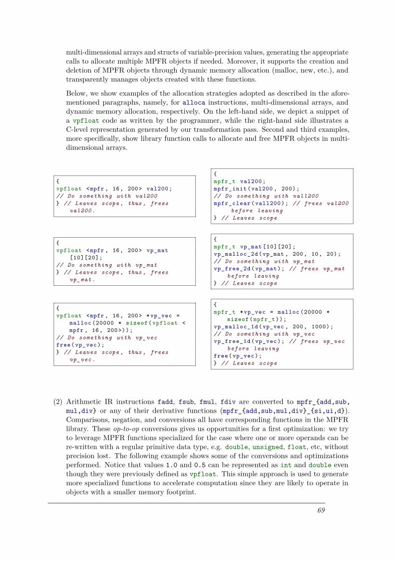
multi-dimensional arrays and structs of variable-precision values, generating the appropriatecalls to allocate multiple MPFR objects if needed. Moreover, it supports the creation anddeletion of MPFR objects through dynamic memory allocation (malloc, new, etc.), andtransparently manages objects created with these functions.

Below, we show examples of the allocation strategies adopted as described in the afore-mentioned paragraphs, namely, for alloca instructions, multi-dimensional arrays, anddynamic memory allocation, respectively. On the left-hand side, we depict a snippet ofa vpfloat code as written by the programmer, while the right-hand side illustrates aC-level representation generated by our transformation pass. Second and third examples,more specifically, show library function calls to allocate and free MPFR objects in multi-dimensional arrays.

{vpfloat <mpfr , 16, 200> val200 ;// Do something with val200} // Leaves scope , thus , frees

val200 .

{mpfr_t val200 ;mpfr_init (val200 , 200);// Do something with vall200mpfr_clear ( vall200 ); // frees val200

before leaving} // Leaves scope

{vpfloat <mpfr , 16, 200> vp_mat

[10][20];// Do something with vp_mat} // Leaves scope , thus , frees

vp_mat .

{mpfr_t vp_mat [10][20];vp_malloc_2d (vp_mat , 200, 10, 20);// Do something with vp_matvp_free_2d ( vp_mat ); // frees vp_mat

before leaving} // Leaves scope

{vpfloat <mpfr , 16, 200> * vp_vec =

malloc (20000 * sizeof ( vpfloat <mpfr , 16, 200 >));

// Do something with vp_vecfree( vp_vec );} // Leaves scope , thus , frees

vp_vec .

{mpfr_t * vp_vec = malloc (20000 *

sizeof ( mpfr_t ));vp_malloc_1d (vp_vec , 200, 1000);// Do something with vp_vecvp_free_1d ( vp_vec ); // frees vp_vec

before leavingfree( vp_vec );} // Leaves scope

(2) Arithmetic IR instructions fadd, fsub, fmul, fdiv are converted to mpfr_{add,sub,mul,div} or any of their derivative functions (mpfr_{add,sub,mul,div}_{si,ui,d}).Comparisons, negation, and conversions all have corresponding functions in the MPFRlibrary. These op-to-op conversions gives us opportunities for a first optimization: we tryto leverage MPFR functions specialized for the case where one or more operands can bere-written with a regular primitive data type, e.g. double, unsigned, float, etc, withoutprecision lost. The following example shows some of the conversions and optimizationsperformed. Notice that values 1.0 and 0.5 can be represented as int and double eventhough they were previously defined as vpfloat. This simple approach is used to generatemore specialized functions to accelerate computation since they are likely to operate inobjects with a smaller memory footprint.

69

void func(vpfloat <mpfr , 16, 1000 > val1 , vpfloat <mpfr , 16, 1000 > val2 ,vpfloat <mpfr , 16, 1000 > *res){

*res = -val1;*res -= val2;*res += -3.0v;*res = 0.5v/(* res);// Continue ...

void func( mpfr_t val1 , mpfr_t val2 , mpfr_t res){

mpfr_neg (res , val1 , MPFR_RNDN );mpfr_sub (res , res , val2 , MPFR_RNDN );mpfr_add_si (res , val1 , -3.0, MPFR_RNDN );mpfr_d_div (res , 0.5, val1 , MPFR_RNDN );// Continue ...

(3) Functions with vpfloat MPFR arguments are cloned and re-built as MPFR objects.Although previous examples show that references and value copies are passed similarly infunction calls, the pass respects the C standard for argument passing, such as, pass by value,pass by reference. They follow the same behavior as primitive scalar floating-point typesin regards to multi-dimensional arrays, pointers as function parameters. The compiler alsomakes sure that passed-by-value arguments are only affected in the callee function, whilechanges in the passed-by-reference values are also seen within the caller. Additionally,return types are handled through LLVM’s StructRet attribute, being returned as the firstargument of the function.

vpfloat <mpfr , 16, 1000 >vdot(int n, vpfloat <mpfr , 16, 1000 > *X,

vpfloat <mpfr , 16, precision > *Y);

void vdot( mpfr_t ret_result , int n, mpfr_t X, mpfr_t Y);

(4) Load instructions, Φ Nodes, dereferencing (element-indexing) instructions, and constantvalues of vpfloat arguments are all rewritten to use the MPFR struct type. Storeinstructions are converted to mpfr_set or any of its derivative functions (mpfr_set_{si,ui,d}) for performance purposes.

(5) C++ imposes particular challenges for MPFR code generation due to some object-orientedfeatures, such as VTables, lambda functions, and classes. Our code generator supports allthese features for constant types. The lack of support for types with runtime attributeswithin compound types (class, struct, and function types, etc.), as described in the LanguageExtension Limitations section 4.6 from the previous chapter, propagates this limitation tothe backend.Compound types that make use of vpfloat<mpfr, ...> and its compound-type variances(pointers, arrays, etc.) are reconstructed as MPFR struct types. VTables are all updatedto the newly recreated references so that the C++ polymorphism feature is supported.In the example above, our pass creates a new VPFloatClass with mpfr_t types andrecreates all objects with this new type. Although LLVM provides a mutateType method,it is strongly advised to recreated objects instead. Creating new compound types involves

70

class KernelBase {public :

virtual void updateChecksum ( VariantID vid) = 0;};

class VPFloatClass : public KernelBase {public :

void updateChecksum ( VariantID vid);private :

vpfloat <mpfr , 16, 1000 > x;vpfloat <mpfr , 16, 1000 >* vec;

};

class VPFloatClass : public KernelBase {public :

void updateChecksum ( VariantID vid);private :

mpfr_t x;mpfr_t vec;

};

a recursive operation to remake them in a bottom-up order due to type dependencies:type1 may declare an object of type2 that has vpfloat<mpfr, ...> inside. Not only dowe need to recreate type2, but type1 as well, and the associated structures that they use.Although Loop Idiom Recognition is disabled for vpfloat<mpfr, ...>, the compiler canstill make use of memory-related functions (memcpy, memmove, etc.) through the C++standard library, or when capturing lambda functions by value. From the languageperspective, vpfloat types are considered to have the same semantics as regular FP types.That is, they are seen as trivially copyable types. On the one hand, this facilitates IRcode generation from a C++ level since it does not require implementation of copy andmove constructors. On the other hand, it also adds extra complexity to the generation ofMPFR code, which, due to the pointer variable in the struct, is not trivially copyable. Tocircumvent this issue, our code generator detects memory-related functions and generatesthree additional functions (prepare_memcpy, clean_memcpy, vp_memcpy) to support forthem. Essentially, we are able to guarantee that the pointer to the mantissa field is notoverwritten, only its content is copied/moved accordingly. We illustrate this transformationin the example below:Function prepare_memcpy performs a simple memcpy to save the values of X which areoverwritten by the original memcpy operation. After memcpy is executed, the pass callsvp_memcpy to restore the correct values of the object and make a copy to their right locations.Lastly, clean_memcpy frees up the temporary memory allocated by prepare_memcpy.These functions were implemented to handle the manipulation of vpfloat types in twoscenarios: (1) when pure multi-dimensional arrays are copied/moved between locations,like in the example; (2) or when copies and moves are introduced due to lambda functionsand C++ standard library. For instance, in the case of having vpfloat declarations withina class object.

(6) Section 5.2.3.5 briefly states that having support for primitive types facilitates the use ofparallelization through programming models. Support for OpenMP is included almostout-of-the-box for MPFR-derived types. The only special treatment lies on handlingomp atomic directives, which generates a call to atomic_compare_exchange, a function

71

void mem_func_example (int n, vpfloat <mpfr , 16, 1000 > *X,vpfloat <mpfr , 16, 1000 > *Y) {

memcpy (X, Y, sizeof (vpfloat <mpfr , 16, 100 >)*n);// Some code

}

void mem_func_example (int n, mpfr_t X, mpfr_t Y) {

// Prepare memcpyvoid ** tmp;prepare_memcpy (tmp , X, sizeof ( mpfr_t )*n);

// memcpy executed , pointer is overwrittenmemcpy (X, Y, sizeof ( mpfr_t )*n);

// Restore correct values overwritten by memcpy and clenupvp_memcpy (X, tmp , &X, &Y, 1, 32, sizeof ( mpfr_t )*n);clean_memcpy (tmp);

// Some code}

that implements an atomic compare-and-swap.5 MPFR-derived types are not automat-ically handled by OpenMP in scenarios where objects need to be atomically modifiedwith a single IR or instruction (they use a library call). This occurs because, as men-tioned herein repeatedly, the pointer variable in the MPFR struct prevents atomicupdates. Our code generator enforces atomicity by inserting a critical section and callingour implementation of compare_and_exchange. The critical section uses a dedicatedmutex, properly nested to avoid interference with any other synchronization. Functionvp_atomic_compare_exchange has an equivalent implementation to those of traditionalatomic_compare_exchange functions, but targets MPFR objects. We present below theuse of omp atomic directive to calculate the value of π and pseudo-codes generated by thecompiler from the pragma directive. The code on the left follows the classical compila-tion flow and generates a call to atomic_compare_exchange to atomically manipulatedπ in double. On the right, π is calculated using vpfloat<mpfr, 16, 1000>, and ourtransformation adds a critical section in order to properly update the object value withvp_atomic_compare_exchange. Moreover, we also present a possible implementation forvp_atomic_compare_exchange.

(7) Eventually, the MPFR code generation pass attempts to optimize the number of dynamicallycreated MPFR objects by reusing old references if it is guaranteed that their values willno longer be needed. Notice that the pass operates on Static Single Assignment (SSA)form, making this step differ from a traditional copy elimination and coalescing, bothimplemented in target-specific backend compilers. Instead, we follow a backward traversalof use-def chains to identify MPFR objects that may be shared across variable renamingof invariant values, and across convergent paths with mutually exclusive live intervals.

In summary, the pass rewrites all vpfloat<mpfr, ...> operands by replacing them withMPFR objects and the appropriate initialization. Unlike higher-level MPFR abstractions such asthe C++ Boost library for multi-precision arithmetic [85], we are able to leverage the compilertoolchain and its existing optimizations (constant folding, inlining, common subexpression

5https://en.cppreference.com/w/c/atomic/atomic_compare_exchange

72

void prepare_memcpy (char ** temp_object , char *src , unsigned size) {* temp_object = (char *) malloc (size);memcpy (* temp_object , src , size);

}

void clean_memcpy (char ** temp_object ) {free (* temp_object );

}

void vp_memcpy ( mpfr_t * dst , void* src , char * initial_address ,unsigned num_elems , unsigned elem_size , unsigned size) {

unsigned num_objects = ceil (( double )size /( double )( elem_size * num_elems ));unsigned offset = ( unsigned )(( char *) dst - initial_address );

// Do nothing in the case offset is larger than size.// It means the compiler could not verify at compilation time// that a memcpy is not neededif ( offset > size || size < 32)

return ;else if ( num_objects == 0) {

printf (" Number of objects cannot be Zero .\n");exit (0);

} else if ( elem_size == 32)size = 32;

for ( unsigned i = 0; i < num_objects ; ++i) {for ( unsigned j = 0; j < num_elems ; ++j) {

mpfr_t * srcval = ( mpfr_t *)(( char *) src + offset + (i*size));mpfr_t * dstval = ( mpfr_t *)(( char *) dst + (i*size));// Copy the value of srcval to dstval and change// the pointer to that value.mpfr_set ( srcval [j], dstval [j], roundingMode );dstval [j]-> _mpfr_d = srcval [j]-> _mpfr_d ;

}}

}

# pragma omp parallel forfor (i = 0; i < 10000; ++i) {

double x=(i+0.5)*dx;# pragma omp atomicpi += (dx / (1.0 + x * x));

}

# pragma omp parallel forfor (i = 0; i < 10000; ++i) {

vpfloat <mpfr ,16 ,500 > x=(i+0.5)*dx;# pragma omp atomicpi += (dx / (1.0 + x * x));

}

// Coded in doublepi_local += (dx / (1.0 + x * x));calls atomic_compare_exchange to

compare / update pi and pi_local

// Coded in vpfloat <mpfr ,16 ,500 >pi_local += (dx / (1.0 + x * x));start critical sectioncalls vp_atomic_compare_exchange to

compare / update pi and pi_localend critical section

73

bool vp_atomic_compare_exchange ( unsigned size , void *ptr ,void *expected , void *desired ,int success_order , int failure_order ) {

bool ret;if ( mpfr_cmp (*(( mpfr_t *) ptr), *(( mpfr_t *) expected )) == 0) {

mpfr_set (*(( mpfr_t *) ptr), *(( mpfr_t *) desired ), roundingMode );ret = true;

} else {mpfr_set (*(( mpfr_t *) expected ), *(( mpfr_t *) ptr), roundingMode );ret = false;

}return ret;

}

Table 5.1: Instructions supported by the UNUM Backend.

Instruction group Instruction groupsusr fcvt.x.g/fcvt.g.xlusr fcvt.f.g/fcvt.g.f

smbb/swgp/sdue/ssue fcvt.d.g/fcvt.g.dlmbb/lwgp/ldue/lsue gcmp/gadd/gsub/gmul

movll/movlr gguess/gradiusmovrl/movrr lgu/lgu.s/ldub/ldub.s

mov_x2g/mov_g2x stu/stu.s/stub/stub.smov_d2g/mov_f2g lgu_next/ldub_nextmov_g2d/mov_g2f stul_next/stub_next

elimination, among others), with MPFR objects only being created at the end of the middle-endcompilation flow. Furthermore, since this backend is actually implemented as a middle-end pass,it is usable for all target ISAs with respective LLVM backends. In fact, because our pass istarget-independent, we have collected results for this target in two distinct systems: a RISC-VFPGA-based processor, as well as X86 systems.

5.3.2 Hardware Target: UNUM

Our second backend makes use of the vpfloat<unum, ...> representation in order to partiallyimplement the RISC-V ISA [121] extension for UNUM variable precision arithmetic of [23].Table 5.1 shows the instructions supported by our backend. We exclude all instructions relatedto interval arithmetic, since our types are only used for UNUM scalar representations, and arenot intended for interval endpoints.

The ABI specification for the ISA extension is similar to the standard RISC-V FP ABI.Table 5.2 lists the coprocessor registers and respective roles in the defined calling convention.Register naming uses the same convention as the FP registers in RISC-V. However, in lieu ofusing f as a prefix, the letter g is used to denote coprocessor registers. The calling conventionfor argument and return values also complies with the RISC-V FP ABI, as well as the registerspreserved across function calls.

74

5.3.2.1 Compiler-Controlled Status Registers

The compiler must work together with the proposed ISA to coordinate and control multipleparameters inside the coprocessor. This ISA extension supports generic FP instructions withprecision ranging from 64 to 512 bits, controlled at a 64-bit granularity. Since the UNUMformat [57] is used to represent values stored in memory, loads and stores must be parameterizedaccording to the variable size and positioning of the UNUM fields in the highly flexible format.Two control registers hold the ess and fss fields of the UNUM formats, controlling the maximumvalues of ess and fss defined by the coprocessor, also known as UNUM environment (ess,fss). Forinstance, a UNUM environment (4, 8) indicates maximum ess and fss values of 4, 8, respectively.These values are sufficient to represent numbers with at most 16 bits of exponent, and 256 bitsof mantissa. The ISA also defines concepts of WGP (Working G-layer precision) and MBB(Memory Byte Budget), which are, respectively, the precision used in computation and themaximum number of bytes read and written during load and store operations.

According to the ISA specification, the compiler is in charge of controlling six control registers.Table 5.3 gives a description of each control register with the minimum and maximum valuesthey can assume. The ISA specifies two UNUM environments that can be used simultaneouslyby operating with different memory instructions. Instructions lgu and stu use values of thedefault UNUM environment, while lgu.s and stu.s consider ess and fss values of the secondUNUM environment. In the following section 5.3.2.2, it will be shown that having two UNUMenvironments help the compiler handling constants for types with runtime attributes. Valueswgp and mbb, on the other hand, are have no duplication. That is, the compiler may need toalternate these values in order to allow multiple configurations simultaneously.

Additionally, we have designed and implemented two additional passes to properly handlethe generation of generic FP operations with the UNUM ISA: the first targets the configurationof status registers in the coprocessor, and the second addresses memory accesses for dynamically-sized types in multi-dimensional arrays.

5.3.2.2 FP Configuration Pass

The FP configuration pass consists on analyzing functions in the call graph and properlyconfigures the status registers (ess, fss, WGP, MBB) as to convey to high level type information.The pass runs in the middle-end phase since it is the lowest level to retain information about typeconfiguration. Types in the backend are lightweight and cannot fully represent FP attributes ofvpfloat. An IR pass also enables it to be target-independent and can potentially be used forarchitectures other than RISC-V.

The pass keeps track of values that come in and go out of basic blocks. By analyzing thecontrol flow graph (CFG), it guarantees that values are being properly assigned. If any change is

Table 5.2: ABI Convention for the VP registers

Register ABI Name Description Saverg0-7 gt0-7 Temporaries Callerg8-9 gs0-1 Saved Registers Calleeg10-11 ga0-1 Arguments/return values Callerg12-17 ga2-7 Arguments Callerg18-27 gs2-11 Saved Registers Calleeg28-31 gt8-11 Temporaries Caller

75

Table 5.3: Control registers inside the UNUM Coprocessor.

Category Name (min,max)Allowed Description

Default UNUM due.ess (1,4) Tells the coprocessor the maximum number of bitsin the ess field for load and store (lgu and stu)

Environment (DUE) due.fss (1,9) Tells the coprocessor the maximum number of bitsin the fss field for load and store (lgu and stu)

Second UNUM sue.ess (1,4) Tells the coprocessor the maximum number of bitsin the ess field for load and store (lgu.s and stu.s)

Environment (SUE) sue.fss (1,9) Tells the coprocessor the maximum number of bitsin the fss field for load and store (lgu.s and stu.s)

Precision wgp (0,7) Number of bits used for arithmetic operationsin the FPU unit

MemoryByte Budget mbb (1,68) Number of bits used in load and

store instructions

needed when entering a basic block, a new instruction is added. We make use of variations of thesusr instruction to configure each register separately: instructions susr.ess, susr.fss manipulateess and fss values of the default UNUM environment, and susr.wgp and susr.mbb are used toconfigure WGP, and MBB.

Although the coprocessor has two UNUM environments that could be used to alternate theused values of ess and fss, we reserve the second one to handle two situations:

(1) Load constants in dynamically-sized types: section 4.4.3.4 explains that constants for thesetypes are generated with a maximum configuration. For UNUM types, that correspondsto the maximum values of ess and fss supported by the coprocessor. Therefore, assigninga constant to a dynamically-sized variable implies the use of lgu.s in lieu of the lguinstruction6.

(2) Register spilling may be necessary when the number of live variables during the executionof the program is greater than the number of available registers. We use the secondenvironment to spill the register as a maximum configuration. Even though this slowsdown spilling and filling operations during register allocation, it does not require theregister allocator to have any previous knowledge of the FP configuration of variables beenspilled. Moreover, since there may be a significant difference between the spilling size of avariable and its actual memory size, techniques to avoid spilling [97] can play an importantrole to reduce the memory impact on high-precision representations.

5.3.2.3 Array Address Calculation Pass

Array address calculation pass is applicable only to dynamically-sized types and aims at providingproper array addresses. Since LLVM provides no support for dynamically-sized types, additionalcare is needed to compute the addresses of values whose sizes are only known at runtime. The__sizeof_vpfloat function allows to perform this task. The pass traverses every function

6Instructions lgu and lgu.s load UNUM variables from memory. They take into consideration values ess andfss of the default and second UNUM environment, respectively, as well as MBB.

76

searching for GetElementPtr instructions. These instructions are replaced by the appropriatelow-level address computation, accumulating over the number of elements and the dynamic sizeof every element.

5.4 ConclusionThis chapter presents the modifications and requirements needed to extend the support ofour vpfloat type system substrate to an industry-level compiler infrastructure. We showedmany aspects that justify why this integration improves the state-of-the-art. We showed whichoptimizations may and may not run in the compilation flow, and code modifications neededfor many of the language aspects, such as runtime capabilities and type compatibility. Wealso described how vpfloat<unum, ...> and vpfloat<mpfr, ...> go from the LLVM IR typesystem to their code generators: the former through a RISC-V ISA extension and the latter byrelying on the open-source MPFR library.

77

Chapter 6: Experimental results

Contents6.1 The Benefits of Language and Compiler Integration . . . . . . . . . . . . . . . 79

6.1.1 MPFR vpfloat vs. Boost Multi-precision . . . . . . . . . . . . . . . . 796.1.2 Hardware(UNUM vpfloat) vs. Software (MPFR vpfloat) . . . . . . 88

6.2 Linear Algebra Kernels . . . . . . . . . . . . . . . . . . . . . . . . . . . . . . . 906.3 Conclusion . . . . . . . . . . . . . . . . . . . . . . . . . . . . . . . . . . . . . . 102

In the previous chapters, we have described the whole compilation flow required to providevariable precision FP arithmetic. Language extension, type system and compiler support havebeen proposed as an intent to better explore different types, precision and exponent configurations,and at last variable precision computing. This chapter will focus on the experimental resultsthat give basis to the contributions of this thesis.

We start by presenting and hopefully convincing the reader on, the benefits of language andcompiler integration of a language extension for multiple FP formats. The second segment ofthis section consists of illustrating the use of variable precision within linear algebra kernels. Bymaking use of the mpfrBLAS library described in section 4.7.1, we provide implementationsto different variants of the Conjugate Gradient (CG) and show interesting insights that mayencourage the exploration of variable precision computing.

6.1 The Benefits of Language and Compiler IntegrationThis section is mainly divided into two parts. The first focuses on comparing our extension, typesystem and compiler solution to a state-of-the-art approach with equivalent functionality withthe intent of showing the benefits of compiler integration. The last part presents experimentalresults to demonstrate the advantage of having hardware support for high-precision formats.

6.1.1 MPFR vpfloat vs. Boost Multi-precisionThis section shows a comparison of our MPFR type vpfloat<mpfr, ...> with the Boost libraryfor multi-precision [85]. Both approaches rely on the MPFR library and execute code withequivalent precision values. The goal is to demonstrate that high-precision FP emulation librariescan further benefit from language and compiler integration. Because compilers cannot detectFP representations within high-level languages abstractions, optimizations opportunities aremissed. While traditional IEEE formats are handled through different compilation strategiesat a later stage of the compilation process1, our type system mimics the behavior of standard

1In LLVM, for instance, the choice between an FP-capable ISA and software implementation is only done atthe backend stage, when building Direct-Acyclic Graphs (DAGs).

79

Table 6.1: Machine configurations used for experiments.

Processor # # CoresFrequency

CachesRAM

Model Procs. # Threads L1 L2 L3

M1Intel XeonE5-2637v3 2 8 Cores

16 Threads 3.50 GHz

4 x 32KBD-Cache4 x 32KBI-Cache

4 x256KB 15MB 128GB

M2Intel XeonGold 5220 2 36 Cores

72 Threads 2.20 GHz

18 x 32KBD-caches18 x 32KBI-Caches

18 x1 MB 24.75MB 96GB

(compiler-compatible) types by relying on a middle-end pass but still leveraging much of thecompilation flow and optimizations. Experiments were conducted using two different systems: adual-processor Intel Xeon E5-2637v3 machine with 128GB of RAM, and a dual-processor IntelXeon Gold 5220 machine with 96 GB of RAM, labeled M1 and M2, respectively, and depicted inTable 6.1.

6.1.1.1 Polybench

The Polybench benchmark suite [98] is a collection of 30 kernels aimed to explore the impactof compiler optimizations in a variety of areas. It is widely used to measure the benefitsof applying polyhedral optimization techniques in a compiler and contains code for manycomputation-intensive algorithms in fields of linear algebra, stencil, and data-mining.

Two strategies were used to Polybench version 4.1: (1) first, we compiled Polybench for bothbaseline and vpfloat<mpfr, ...> types using optimization level -O3; (2) in the second scenario,we use optimization level -O1 for vpfloat<mpfr, ...> for reasons that will be explained later,while Boost continued to be compiled with -O3. In both scenarios, we enable and disable Polly’spolyhedral loop nest optimizations [55], and the best execution time reference, with and withoutPolly, is taken for each application. Each application was compiled for three different precisionconfigurations: 100 bits (≈30 decimal digits), 170 bits (≈50 decimal digits), and 500 bits (≈150decimal digits).

Figure 6.2 shows the speedup for each benchmark using Boost as the baseline and whencompiling both solutions with optimization level -O3. Figure 6.3 depicts the values of speedupsconsidering the same baseline but with vpfloat<mpfr, ...> applications being compiled withoptimization level -O1. We observe speedups over most of the test suite for all precisionconfigurations in the two machines where experiments were executed. A few kernels have shownsimilar performance to Boost: jacobi-1d and jacobi-2d at the lower precision settings, and doitgen,durbin and mvt at highest precision when executed in the M2. The only slowdowns occur on somespecific cases: adi and deriche at lower precisions only. These results are due to the complexityof the array access patterns in the stencil kernel, hitting limitations of the MPFR loweringpass in reusing MPFR objects over invariant or mutually exclusive values. In other cases, themeasures show that a late MPFR lowering dramatically improves performance, especially oncomputationally intensive kernels benefiting from greater cache locality and a proportionallymore significant decrease of MPFR memory management overhead.

The reason why we chose to plot results for -O1 optimization level is that we observed manybenchmarks exhibit better performance with this optimization flag rather than with -O3. In

80

fact, the overall speedup of -O1 has shown to be superior to -O3. This was originally a surprise,but can be explained as follows: as MPFR requires memory allocation for every object in use,suboptimal performance at -O3 stems from the higher number of allocations generated. Becausethe compiler runs many aggressive optimizations (inlining, loop unrolling, aggressive code motion,just to name a few), many more objects need allocation and incur an extra execution time in theapplication. In fact, finding optimization sequences that are likely to yield better performanceis challenging. However, recent work [109, 128] on the exploration of optimization space couldpotentially help us investigate better optimization heuristics in the presence of multi-precisionarithmetic, and is a relevant topic for future work.

We have also decided to run experiments in two different machines in order to show thatspeedups are not inherent to specific system configuration. Experimental results are similar inthe two configurations, and differences are, in the most part, within an acceptable tolerancerange. Kernels floyd, and lu show significantly better speedups in M2, because Boost versionsshow bad usage of the cache with an increase in the number of cache misses, and thus, impactingexecution time. A following experiment will demonstrate that cache misses in Boost have aneven greater impact when running applications with multiple threads of execution.

Overall, results show an average performance speedup (vpfloat<mpfr, ...> vs. Boostlibrary for MPFR) of 1.80× and 1.86× for M1 and M2, respectively in -O3. Additionally, itshould be pointed out that these results have been corroborated by peers through an ArtifactEvaluation (AE)2 submitted to a conference, and functional and reproduced badges had beengiven. For -O1, speedups of 1.88× and 1.91× were observed in the two machines.

Impact of the Loop nest optimizer

One of the major advantages of our solution, as we have been highlighting throughout thisdocument, relates to compiler integration and the possibility of using optimizations out-of-the-box. This is particularly true when considering Polly Loop nest Optimizer. Even withoutmodifications to support vpfloat, Polly is able to find optimal array access patterns in thePolybench suite compiled for vpfloat. To illustrate our argument, figure 6.1 shows the speedupof -O3 + Polly vs. -O3. Although many kernels have seen slowdowns when compiled with Polly,an overall speedup of 1.18× is observed. It shows that deeper compiler integration helps toaccelerate FP emulation libraries. On the other hand, Polly is unable to optimize Boost arrayaccesses. The optimizer gives up trying to find patterns that suit the complexity of the library.

Table 6.2: Compilation time for Polybench with different optimization levels and types.

Type Opt. Flags Compilation time (in seconds) Speedup over Boost

vpfloat<mpfr, ...>

-O3 13.02 8.91-O3 + Polly 91.79 1.27

-O1 8.81 13.17-O1 + Polly 69.87 1.68

Boost -O3 116.09 1.00-O3 + Polly 117.32 1.00

2https://www.acm.org/publications/policies/artifact-review-badging

81

2mm

3mm ad

iata

xbic

g

chole

sky

corre

lation

cova

rianc

e

deric

he

doitg

endu

rbin

fdtd-2

dfloy

dge

mm

gemve

r

gesu

mmv

gramsch

midt

heat

3d

jacob

i 1d

jacob

i 2d lu

ludcm

pmvt

nussi

nov

seide

l 2dsy

mmsy

r2k syrk

triso

lvtrm

m0

1

2Sp

eedu

p100 bits (≈30 decimal digits) 170 bits (≈50 decimal digits) 500 bits (≈150 decimal digits)

Figure 6.1: Speedup of Polly’s loop nest optimizer in Polybench compiled for vpfloat<mpfr,... types.

Compilation time

Another important metric to consider is the time needed to compile each application. Because themiddle-end pass implemented to transform vpfloat<mpfr, ...> to MPFR references incurs anextra compilation time to code generation, it is important to measure its impact in compilationtime. Table 6.2 shows significant speedups in terms of compilation time for the Polybenchapplications. In fact, Boost high compilation times stem from C++ template deduction, highlyused in the Boost Multi-precision library. The difference in compilation times between -O3and -O3 + Polly for vpfloat<mpfr, ...> types shows that the optimizer is, in fact, supportedby these types. Similar compilation times between -O3 and -O3 + Polly for Boost shows thecontrary.

82

2mm

3mm ad

iata

xbic

gch

olesk

yco

rrelat

ionco

varia

nce

deric

hedo

itgen

durbi

nfdt

d-2d

floyd

gemm

gemve

rge

summv

gramsch

midthe

at3d

jacob

i 1djac

obi 2d lu

ludcm

p

mvtnu

ssino

vsei

del 2d

symmsy

r2k syrk

triso

lvtrm

m

0

2

4

6

Spee

dup

2mm

3mm ad

iata

xbic

gch

olesk

yco

rrelat

ionco

varia

nce

deric

hedo

itgen

durbi

nfdt

d-2d

floyd

gemm

gemve

rge

summv

gramsch

midthe

at3d

jacob

i 1djac

obi 2d lu

ludcm

p

mvtnu

ssino

vsei

del 2d

symmsy

r2k syrk

triso

lvtrm

m

0

2

4

6

Spee

dup

100 bits (≈30 decimal digits) 170 bits (≈50 decimal digits) 500 bits (≈150 decimal digits)

Figure 6.2: Speedup of vpfloat<mpfr, ...> over the Boost library for multi-precision for the Polybench benchmark suite, and compiled withoptimization level -O3. The execution time reference taken are the best between compilations with and without Polly. Results are shownfor two different machines: an Intel Xeon E5-2637v3 with 128GB of RAM (M1), and an Intel Xeon Gold 5220 with 96 GB of RAM (M2),respectively. Y-axes are shown with the same limits to ease comparisons between results in the two machines.

83

2mm

3mm ad

iata

xbic

gch

olesk

yco

rrelat

ionco

varia

nce

deric

hedo

itgen

durbi

nfdt

d-2d

floyd

gemm

gemve

rge

summv

gramsch

midthe

at3d

jacob

i 1djac

obi 2d lu

ludcm

p

mvtnu

ssino

vsei

del 2d

symmsy

r2k syrk

triso

lvtrm

m

0

2

4

6

Spee

dup

2mm

3mm ad

iata

xbic

gch

olesk

yco

rrelat

ionco

varia

nce

deric

hedo

itgen

durbi

nfdt

d-2d

floyd

gemm

gemve

rge

summv

gramsch

midthe

at3d

jacob

i 1djac

obi 2d lu

ludcm

p

mvtnu

ssino

vsei

del 2d

symmsy

r2k syrk

triso

lvtrm

m

0

2

4

6

Spee

dup

100 bits (≈30 decimal digits) 170 bits (≈50 decimal digits) 500 bits (≈150 decimal digits)

Figure 6.3: Speedup of vpfloat<mpfr, ...> over the Boost library for multi-precision for the Polybench benchmark suite. vpfloat<mpfr,...> applications were compiled with optimization level -O1 and Boost with -O3. The execution time reference taken are the best betweencompilations with and without Polly. Results are shown for two different machines: an Intel Xeon E5-2637v3 with 128GB of RAM (M1), andan Intel Xeon Gold 5220 with 96 GB of RAM (M2), respectively. Y-axes are shown with the same limit to ease comparisons between results inthe two machines.

84

6.1.1.2 RAJAPerf

The RAJAPerf benchmark suite [99] is a collection of loop-based computational kernels commonlyfound in HPC applications. Kernels are written such that they can be implemented in differentvariants: sequential (single-threaded) execution, and parallel programming models like OpenMP,and CUDA. Examples of applications are the traditional AXPY and DOT product from BLASlibraries, Polybench kernels like 2mm, 3mm and adi, vector additions and multiplications, amongmany others. Table 6.3 shows the list of the 43 RAJAPerf applications used in this experimentand classified according to their groups.

We compiled the suite at optimization level -O3 for our vpfloat<mpfr, ...> type andcompare it with the Boost library for Multi-precision, both relying on the MPFR library withequivalent precision (≈ 30 decimal digits). The suite is implemented in C++, and makes useof high-level abstractions such as Lambda functions, polymorphism, dynamic dispatching, andthus, highly motivated the support of such features in our type system. All applications arecompiled for sequential and parallel execution. By leveraging the integration with OpenMP,described in Section 5.3.1, we also collect results for three OpenMP variants along with the threesequential variants for a total of 6 variants of each kernel, and a total of 258 variants.

Figure 6.4 shows the speedup of vpfloat<mpfr, ...> over Boost. Y-axes are depicted indifferent log scales in order to show the speedups achieved by OpenMP variants in each machine.As was the case for Polybench, we observe speedups over most of the test suite, and slowdownsare associate with additional copies and object allocations that are needed in these specificcases. Measurements also demonstrate that a late MPFR lowering pass significantly improvesperformance for the majority of cases. More interestingly, our solution scales much better thanBoost when using OpenMP in both systems. Hardware counter measurements, collected in M1,indicate that speedups in the 7–9× range stem from the reduction of memory accesses and cachemisses, with up to 90× reduction in last-level cache misses. The Boost implementation oftenconverts compute-bound kernels into memory-bound ones as memory transactions exceed theoff-chip bandwidth. Deep integration with the compiler and its optimizations and the reuse ofold MPFR objects contribute to reduce the memory pressure and allow our solution to scalemuch better in multi-threaded environments. Table 6.4 shows averages speedups in M1 and M2for all RAJAPerf variants. We notice that systems with many more processors/threads lead to

Table 6.3: List of RAJAPerf applications classified according to their groups.

Group Num. of apps. Applications

apps 7 del_dot_vec_2d, energy, fir, ltimes, ltimes_noview,pressure, vol3d

basic 9 daxpy, if_quad, int3, init_view1d, init_view1d_offset,mataddsubb, nested_init, reduced3_int, trap_int

lcals 10 diff_predict, eos, first_diff, first_sum, gen_lin_recur,hydro_1d, hydro_2d, int_predict, planckian, triad_elim

polybench 12 2mm, 3mm, adi, atax, fdtd_2d, floyd_warshall, gemm,gemver, gesummv, jacobi_1d, jacobi_2d, mvt

stream 5 add, copy, dot, mul, trial

85

Table 6.4: Average speedups for RAJA in machines M1 and M2 (from Table 6.1).

Sequential OpenMP

Base Lambda RAJA Base Lambda RAJA

M1 1.74 1.61 1.65 7.98 7.16 7.72M2 1.90 1.77 1.86 32.94 32.57 31.67

better overall speedups, especially in OpenMP variants. This shows an important property ofour solution: scalability. Because our solution scales better than the baseline, better speedupsare seen in more powerful systems. Finally, these results have also been corroborated by peersthrough an Artifact Evaluation (AE).

Compilation time

Similar to Polybench, we also estimate the compilation time needed for RAJAPerf in thetwo scenarios. Once more, our solution has shown to outperform the baseline in that metric.RAJAPerf with vpfloat<mpfr, ...> was compiled in 313 seconds, while the Boost versionrequired an average of 1054 seconds. In summary, with a compilation time speedup of 3.37× weare able to produce code that can be more than 32× faster than the baseline.

86

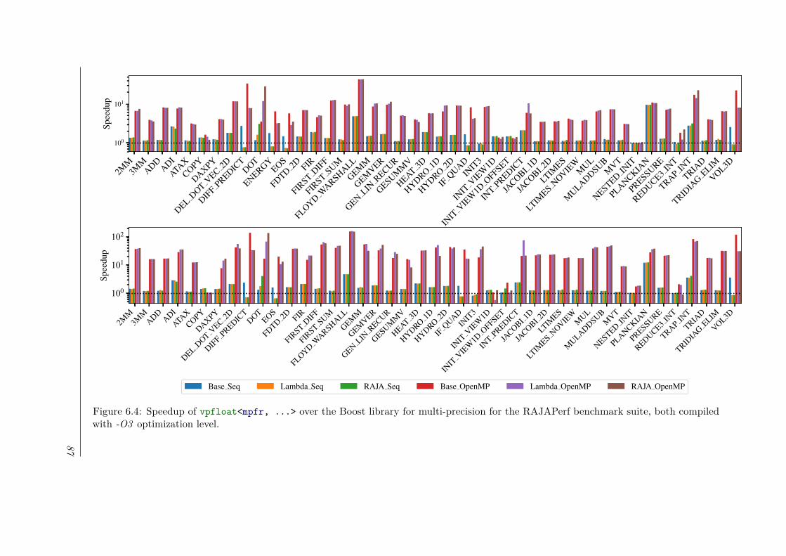
2MM

3MM

ADDADI

ATAX

COPYDAXPY

DELDOT

VEC2D

DIFF

PREDICT

DOTENERGY

EOSFDTD

2D FIR

FIRST

DIFF

FIRST

SUM

FLOYDWARSHALL

GEMM

GEMVER

GENLIN

RECUR

GESUMM

VHEAT

3D

HYDRO1D

HYDRO2D

IFQUADIN

IT3

INIT

VIEW

1D

INIT

VIEW

1DOFFSET

INT

PREDICT

JACOBI 1D

JACOBI 2D

LTIM

ES

LTIM

ESNOVIE

WM

UL

MULADDSUB

MVT

NESTEDIN

IT

PLANCKIAN

PRESSURE

REDUCE3IN

TTRAP

INT

TRIAD

TRIDIA

GELIM

VOL3D

100

101Sp

eedu

p

2MM

3MM

ADDADI

ATAX

COPYDAXPY

DELDOT

VEC2D

DIFF

PREDICT

DOTEOS

FDTD2D FIR

FIRST

DIFF

FIRST

SUM

FLOYDWARSHALL

GEMM

GEMVER

GENLIN

RECURGESUM

MV

HEAT3D

HYDRO1D

HYDRO2D

IFQUADIN

IT3

INIT

VIEW

1D

INIT

VIEW

1DOFFSET

INT

PREDICT

JACOBI 1D

JACOBI 2D

LTIM

ES

LTIM

ESNOVIE

WM

UL

MULADDSUB

MVT

NESTEDIN

IT

PLANCKIAN

PRESSURE

REDUCE3IN

TTRAP

INT

TRIAD

TRIDIA

GELIM

VOL3D

100

101

102

Spee

dup

Base Seq Lambda Seq RAJA Seq Base OpenMP Lambda OpenMP RAJA OpenMP

Figure 6.4: Speedup of vpfloat<mpfr, ...> over the Boost library for multi-precision for the RAJAPerf benchmark suite, both compiledwith -O3 optimization level.

87

6.1.2 Hardware(UNUM vpfloat) vs. Software (MPFR vpfloat)We also demonstrate the effectiveness of our type extension and its integration with LLVM ona hardware implementation of the UNUM format. The main purpose of this experiment is toshow the benefits of hardware support for high-precision representations. To the best of ourknowledge, until now, UNUM’s functionality could only be evaluated with software librariessince no hardware implementation supported a software stack capable of running representativebenchmarks. Owing to the better performance observed in Section 6.1.1.1 when compared toBoost, we used our vpfloat<mpfr, ...> implementation as the baseline for comparison withthe UNUM coprocessor.

Our target platform consists of an FPGA implementation of a RISC-V Rocket processor [11]connected to the UNUM coprocessor of [23]. All benchmarks including baseline MPFR imple-mentations have been compiled to the RISC-V ISA. As explained in section 5.3.1, our MPFRbackend is target independent, and hence, applications with vpfloat<mpfr, ...> types canpotentially be executed on any LLVM-compatible platform with MPFR support.

We compiled Polybench for both baseline (vpfloat<mpfr, ..>), and vpfloat<unum, ...>type using two strategies: -O3, and -O3 + polly. Each application was compiled using threeprecision configurations: 100 bits (≈30 decimal digits), 170 bits (≈50 decimal digits), and 500bits (≈150 decimal digits). The execution time for the baseline is obtained considering the besttime reference, with and without Polly. The main purpose of this experiment is to compare thebest result for the vpfloat<mpfr, ...> type with two compilation procedures for the UNUMtype (with and without Polly).

Figure 6.5 shows the speedup of applications normalized to the baseline MPFR performance(note the logarithmic scale). Unfortunately we hit hardware bugs when executing some bench-marks: gesummv and adi failed to run when compiled with Polly and 3 more benchmarks failedat the highest precision with Polly (3mm, ludcmp, nussinov). This is due to an issue in thecoprocessor memory subsystem.

We notice that Polly is able to significantly improve performance for many applications inthe test suite. This is solid validation of the robustness of our design and implementation, giventhe complexity of polyhedral compilation methods and their sensitivity to efficient memorymanagement. We notice a larger speedup gap in vpfloat<unum, ...> (with and without Polly)than in vpfloat<mpfr, ...> types. vpfloat<unum, ...> kernels compiled with Polly have anoverall speedup of 1.44× over its -O3, and this difference over vpfloat<mpfr, ...>(1.18×) isexplained as follows: because a UNUM type has an in-place layout, the array access patternsgenerated by Polly better match such characteristic. Although MPFR types are accelerated bythe optimizer, the heuristics available do not work as well as for UNUM types, and optimizingthem for MPFR types is an interesting venue to explore as future work.

It further validates the benefits of making variable precision FP arithmetic transparent toupstream optimization passes. Notably, gemm, 2mm and 3mm show speedups of more than 20×over the baseline, benefiting from cache and register reuse through polyhedral loop optimizationwith downstream loop unrolling and scalar promotion. Average speedups at the highest precision(150 digits) are 18.03× and 27.58× for O3, and -O3 + Polly, respectively. The rare slowdownswith Polly are caused by suboptimal heuristic tuning, a well-known challenge with loop nestoptimizations in general. As expected, having support for high-precision computation lead tosignificant performance gains over software targets. These results show great benefits of havingcompiler (and hardware) support for high-precision representations, especially now with the riseof the dark silicon era [47].

88

2mm

3mm ad

iata

xbic

gch

olesk

yco

rrelat

ionco

varia

nce

deric

hedo

itgen

durbi

nfdt

d-2d

floyd

gemm

gemve

rge

summv

gramsch

midthe

at3d

jacob

i 1djac

obi 2d lu

ludcm

pmvt

nussi

nov

seide

l 2dsy

mmsy

r2k syrk

triso

lvtrm

m

100

101

102

Spee

dup

-O3 (≈30 dec. digits)-O3 + Polly (≈30 dec. digits)

-O3 (≈50 dec. digits)-O3 + Polly (≈50 dec. digits)

-O3 (≈150 dec. digits)-O3 + Polly (≈150 dec. digits)

Figure 6.5: Speedup of vpfloat<unum, ...> over vpfloat<mpfr, ...> on the PolyBench suite

89

6.2 Linear Algebra Kernels

The first segment of this chapter showed that supporting a substrate of variable precisioncomputing in a language and compiler enable significant acceleration when comparing withstate-of-the-art solutions. These experiments demonstrate the potential of our proposal andthe benefits of a compiler-integrated solution. The remaining of this chapter is dedicated toillustrating the use of variable precision in the context of Linear Algebra and is used to showinteresting insights to encourage the exploration of variable precision computing in this area.

The experiments conducted in section 6.1 all made use of constant MPFR and UNUM types,as there was no need for dynamic type manipulation of any sort. In this section, we concentrateour attention on showing potential use cases of types with runtime-decidable attributes, whichare not only a great exploration tool for precision-awareness in numerical applications butalso essential to adaptive or variable precision computing. Although high-level languages likeJulia [19] or Python [117] provide dynamic type systems amenable to this kind of research, ourtype system has the great advantage of enabling C-level performance, as well as supportingboth hardware and software targets. We conclude this chapter by experimenting with multiplevariants of the Conjugate Gradient (CG) linear solver method.

Conjugate Gradient (CG)

To demonstrate how our type system can be beneficial to the exploration of variable precision,we used our vpfloat<mpfr, ...> to implement multiple variants of the Conjugate Gradientmethod. The CG algorithm solves linear systems in the form of Ax = b when matrix A isSymmetric Positive Definite (SPD), a common case for the resolution of partial differentialequations (PDEs). It is classified as an iterative method, a mathematical procedure that usesan initial value to generate improvements of the solution with successive operations. Contraryto direct methods that have a finite (predefined) number of operations, iterative methods arebased on a convergence state to determine the number of operations to execute. The methodis exact in theory, but the successive roundoff errors slow down or even destroy convergence.The projective iterative method, typically exemplified by CG, has gained importance due to alow memory occupancy, typically O(N) rather than O(N3) for direct methods. CG is a goodexample to illustrate the influence of arbitrary precision in an application’s output since thenumber of iterations needed for the algorithm to converge depends on the chosen precision. Inthe remaining sections that cover conjugate gradient, we go through a series of requirements,properties and descriptions for CG algorithms. Four CG variants are implemented: originalHestenes and Stiefel [63] CG, preconditioned CG, pipelined CG, and BiCG. We wrap up the CGsection by showing experiments and a discussion over them.

Stopping condition

A common characteristic of CG algorithms is the stopping condition required by the iterativeprocess. We adopt the common choice of using the value of rk, called recursive residual, as athreshold, usually called tolerance, for the stopping condition. When rk is under the threshold,the algorithm leaves the scope and stops the execution, and the result is kept within a predictableerror margin. CG algorithms have a complex behavior regarding the mathematical relationbetween tolerance and attainable accuracy. This involves in-depth analysis which is well beyondthe scope of this thesis.

90

1 for ( unsigned prec = 50; prec <= 2000; prec += 50) {2 cg_algo (prec , x, A, b)3 }

Listing 6.1: Calling a precision-generic implementation of CG

Precision-generic implementation

An important property we aimed to preserve in our type system is the ability to write code thatis unique so that no duplication is needed to handle the underlying precision in use. In otherwords, our main focus was to design a type system that is precision-generic, i.e., where code isnot attained to a single configuration. CG algorithms implemented with vpfloat<mpfr, ...>follow this requirement and, therefore, are precision-agnostic: the core CG iteration takes aprecision parameter, and every run of the function can make use of a different precision value.This allows us within a single run of the application, without recompilation, to programmaticallydrive experiments with multiple precision configurations. Listing 6.1 shows how one would callcg_algo, implemented as precision-agnostic. We iterate over a loop where precision, defined asprec, ranges from 50 to 2000 with a step of 50. Finally, translating a CG algorithm to vpfloatis straightforward: (1) there is no need to extend the precision of the matrix A, as it is read-only;(2) only working arrays have to be declared as vpfloat.

Original CG: Hestenes and Stiefel algorithm

The pseudo-code for the algorithm is given by Algorithm 2, where line 6 shows how rk controlsthe number of iterations.

Algorithme 2: conjugate gradient: original Hestenes and Stiefel algorithm [63]1: p0 := r0 := b−Ax02: while iteration count not exceeded do3: αk := rTk rk

pTk Apk4: xk+1 := xk +αkpk

5: rk+1 := rk−αkApk

6: if ‖ rk+1 ‖≤ tol then break7: βk := rTk+1rk+1

rTk rk8: pk+1 := rk+1 +βkpk

9: k+ +10: end while

One may notice how every operation can in fact be expressed as a BLAS function. The mainmotivation of implementing BLAS libraries for vpfloat types is to enable the exploration ofthese linear algebra algorithms. Listing 6.2 shows the implementation of the CG algorithm [63]with our mpfrBLAS library(from Section 4.7.1). Two stopping conditions can be seen: (1) atline 21 when the value of rs_next is below a threshold; (2) at line 4 when the maximum numberof iterations has been reached and the algorithm is unlikely to converge. We only replaced: (1)vector-scalar products by vpm_axpy_vvv, (2) matrix-vector products by vpm_sparse_gemv_vdv,(3) dot products by vpm_dot_vv, and (4) products of a vector by a scalar by vpm_scal. Becausethese functions have rather similar function signatures (with the exception from the precision)to standard BLAS, it is fairly simple to retarget this algorithm for other library instantiations.

91

1 // rs = rk '*rk2 vpfloat <mpfr , 16, precision > rs = vpm_dot_vv (precision , n, r_k , 1, r_k , 1);3

4 for ( unsigned num_iter = 1; num_iter < m * 1000; ++ num_iter ) {5

6 vpm_sparse_gemv_vdv (precision , m, n, (vpfloat <mpfr , 16, precision >)1.0,7 A, rowInd , colInd , p_k ,8 (vpfloat <mpfr , 16, precision >)0.0, Ap_k);9 alpha = rs / vpm_dot_vv (precision , n, p_k , 1, Ap_k , 1);

10

11 // x = x + alpha*p12 vpm_axpy_vvv (precision , n, alpha , p_k , 1, x_k , 1);13

14 // r = r - alpha *Ap15 vpm_axpy_vvv (precision , n, -alpha , Ap_k , 1, r_k , 1);16

17 // rk+118 rs_next = vpm_dot_vv (precision , n, r_k , 1, r_k , 1);19

20 if (sqrt (( double ) rs_next ) < tolerance ) {21 break;22

23 vpm_scal (precision , n, rs_next / rs , p_k , 1);24 vpm_axpy_vvv (precision , n, (vpfloat <mpfr , 16, precision >)1.0,25 r_k , 1, p_k , 1);26 rs = rs_next ;27 }

Listing 6.2: Implementation of algorithm 2 using mpfrBLAS 4.7.1.

In fact, our experiments take advantage of BLAS flexibility and retargetability, and we showdifferent implementations of CG and variants for different formats: vpfloat<mpfr, ...>,double, long double,__fp128, and Boost for Multi-precision.

Preconditioned CG

Preconditioned CG is a slightly modified algorithm3 that can significantly improve convergenceby relying on preconditionning techniques to reduce the condition number of the matrix (seesection 2.4.1). Incomplete LU or incomplete Cholesky are some examples of techniques thathelp in that task. However, we have only considered the Jacobi Preconditionner method (fromAlgorithm 3), since it has low computational cost and scales linearly according to matrix size.The modified algorithm is listed in 4, showing the use of both matrix A and preconditionedmatrix iM (which stands for inverse M ).

Pipelined CG

Our mpfrBLAS has been implemented to exploit thread-level parallelism through OpenMP.Extending beyond multi-core architectures, our type system could potentially benefit frommany-core systems with the use of MPI [110] or related models. Aside from matrix-vectorproducts, the original standard algorithm cannot be easily parallelized due to the reuse ofvariable arrays between lines. Ghysels and Vanroose [51] proposed to hide global synchronizationlatency of the preconditioned CG with a variant that offers further opportunities of parallelism

3In many libraries, the conjugate gradient algorithm implements the preconditionning by default.

92

Algorithme 3: Jacobi preconditioner1: for i = 1 to m do2: for j = 1 to n do3: if i == j then4: iM [i, j] := 1

A[i,j]5: else6: iM [i, j] := 07: end if8: end for9: end for

10: return(iM)

Algorithme 4: preconditionned conjugate gradient: general algorithm1: r0 := b−Ax02: z0 := iMr03: p0 := z04: while iteration count not exceeded do5: αk := rTk rk

pTk Apk6: xk+1 := xk +αkpk

7: rk+1 := rk−αkApk

8: if ‖ rk+1 ‖≤ tol then break9: zk+1 := iMrk+1

10: βk := zTk+1rk+1

zTk rk11: pk+1 := zk+1 +βkpk

12: k+ +13: end while

than those of traditional algorithms. Algorithm 5 shows the implementation of pipelined CG.Matrix-product A×wk (line 9) can be done in parallel to calculations from lines 10 and 11.Although this property adds more parallelism to CG, its drawback is the loss of numericalstability the algorithm is likely to observe when compared to traditional methods [31].

BiCG

While many problems lead to the handling and computation with SPD matrices, there are caseswhere a more general matrix must be employed and none of the CG algorithms previouslydescribed can be adopted. BiCG [104] extends the use of CG to general matrices (and not onlyto SPD). It is similar to the original CG but requires some additional computation to accountfor matrix generality.

Results and Discussion

To demonstrate the use of variable precision and how our type system can be beneficial to thisexploration, we have implemented and analyzed the impact of different precision values in allfour CG variants (Hestenes and Stiefel [63], preconditioned, pipelined CG, and BiCG) for twoconstraints: number of iterations and execution time. BLAS libraries have been implementedwith the following types: long double, __fp128, vpfloat<mpfr, ...>, and Boost mpfr_float

93

Algorithme 5: Pipelined conjugate gradient algorithm [37]1: p0 := r0 := b−Ax02: s0 :=A× p0,w0 :=A× r0

3: z0 :=A×w0,α0 := rT0 r0sT0 p0

4: while iteration count not exceeded do5: xk := xk−1 +αk−1pk−16: rk := rk−1−αk−1sk−17: wk := wk−1−αk−1zk−18: if ‖ rk ‖≤ tol then break9: qk =A×wk

10: βk := rTk rkrTk−1rk−1

11: αk := rTk rk

rTk wk−βk

αk−1 rTk rk

12: pk := rk +βkpk−113: sk := wk +βksk−114: zk := qk +βkzk−115: k+ +16: end while

Algorithme 6: biconjugate gradient: general algorithm1: p0 := r0 := b−Ax02: choose r∗0 such as (r0r∗0) , 03: p∗0 := r∗04: while iteration count not exceeded do5: αj := rTj r∗

j

p∗Tj Apj

6: xj+1 := xj +αjpj

7: rj+1 := rj −αjApj

8: if ‖ rj+1 ‖≤ tol then break9: r∗j+1 := r∗j −αjA

T p∗j

10: βk := r∗Tj+1rj+1

rTj r∗j

11: pj+1 := rj+1 +βjpj

12: p∗j+1 := r∗j+1 +βjp∗j

13: j+ +14: end while

type. We also use OpenBLAS [124] as a reference implementation, that way an optimized versionof each algorithm in double is also provided.

We used 40 squared SPD matrices from Matrix Market [24, 86] with problem sizes (N) inthe range of 132 to 5489. Matrices are stored as sparse using the Compressed Row Storage(CSR) format and can have up to 315891 non-zero elements (nnz). We selected 12 out of 40 tobe displayed in Figures 6.6 and 6.7 (for the results of Number of iterations vs. Precision) andFigures 6.8 and 6.9 (for the results of Execution Time vs. Precision). The remaining matricesare included as appendices of the thesis to keep this chapter at a reasonable length.

Every application and matrix was executed using five configurations: double (OpenBLAS),fp80, fp128, vpfloat<mpfr, ...> (from 150 to 2000 bits, step = 50), and Boost for Multi-precision (from 150 to 2000 bits, step = 50). The convergence threshold (tol) was selected as

94

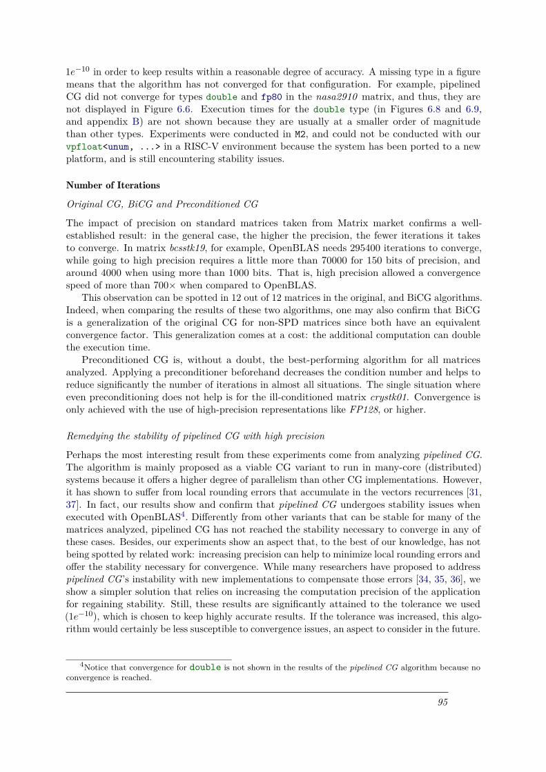
1e−10 in order to keep results within a reasonable degree of accuracy. A missing type in a figuremeans that the algorithm has not converged for that configuration. For example, pipelinedCG did not converge for types double and fp80 in the nasa2910 matrix, and thus, they arenot displayed in Figure 6.6. Execution times for the double type (in Figures 6.8 and 6.9,and appendix B) are not shown because they are usually at a smaller order of magnitudethan other types. Experiments were conducted in M2, and could not be conducted with ourvpfloat<unum, ...> in a RISC-V environment because the system has been ported to a newplatform, and is still encountering stability issues.

Number of Iterations

Original CG, BiCG and Preconditioned CG

The impact of precision on standard matrices taken from Matrix market confirms a well-established result: in the general case, the higher the precision, the fewer iterations it takesto converge. In matrix bcsstk19, for example, OpenBLAS needs 295400 iterations to converge,while going to high precision requires a little more than 70000 for 150 bits of precision, andaround 4000 when using more than 1000 bits. That is, high precision allowed a convergencespeed of more than 700× when compared to OpenBLAS.

This observation can be spotted in 12 out of 12 matrices in the original, and BiCG algorithms.Indeed, when comparing the results of these two algorithms, one may also confirm that BiCGis a generalization of the original CG for non-SPD matrices since both have an equivalentconvergence factor. This generalization comes at a cost: the additional computation can doublethe execution time.

Preconditioned CG is, without a doubt, the best-performing algorithm for all matricesanalyzed. Applying a preconditioner beforehand decreases the condition number and helps toreduce significantly the number of iterations in almost all situations. The single situation whereeven preconditioning does not help is for the ill-conditioned matrix crystk01. Convergence isonly achieved with the use of high-precision representations like FP128, or higher.

Remedying the stability of pipelined CG with high precision

Perhaps the most interesting result from these experiments come from analyzing pipelined CG.The algorithm is mainly proposed as a viable CG variant to run in many-core (distributed)systems because it offers a higher degree of parallelism than other CG implementations. However,it has shown to suffer from local rounding errors that accumulate in the vectors recurrences [31,37]. In fact, our results show and confirm that pipelined CG undergoes stability issues whenexecuted with OpenBLAS4. Differently from other variants that can be stable for many of thematrices analyzed, pipelined CG has not reached the stability necessary to converge in any ofthese cases. Besides, our experiments show an aspect that, to the best of our knowledge, has notbeing spotted by related work: increasing precision can help to minimize local rounding errors andoffer the stability necessary for convergence. While many researchers have proposed to addresspipelined CG’s instability with new implementations to compensate those errors [34, 35, 36], weshow a simpler solution that relies on increasing the computation precision of the applicationfor regaining stability. Still, these results are significantly attained to the tolerance we used(1e−10), which is chosen to keep highly accurate results. If the tolerance was increased, this algo-rithm would certainly be less susceptible to convergence issues, an aspect to consider in the future.

4Notice that convergence for double is not shown in the results of the pipelined CG algorithm because noconvergence is reached.

95

An interesting observation is the non-linear behavior of the number of iterations for a linearincrease in precision, an effect found in all variants, and mainly caused by the accumulation ofrounding errors [30] subjected through the multiple matrix-vector and vector-vector products.Another common characteristic of all instances relates to the precision in use: they all reacha minimum plateau value of the number of iterations needed for convergence. Some matricesreach this plateau with few hundreds of bits, while others may require thousands of bits. Theseresults are an interesting exploration venue on numerical analysis aiming to determine a priorithe best precision value to adopt as to exhibit a good trade-off between the number of iterationsand execution time.

Because our type system can be precision-agnostic, we are able to run experiments andcollect results for multiple-precision configurations with a single run of each application, withoutrecompilation, and code duplication. Although results for Boost are also collected using thesame approach, our solution still manages to outperform Boost by at least 1.35×, and it is stillthe only solution available with a real possibility of hardware integration, a venue that will beexplored as part of our future work.

We would like to emphasize that, by no means, these results should be seen as mathematicalproofs of how precision augmentation is beneficial. This study is merely an indicator thatincreasing precision in applications can have an interesting venue of exploration in CG benchmarks.Mathematically analyzing these results require a much more in-depth understanding of thenature and internal properties of CG, and is out of the scope of this thesis.

96

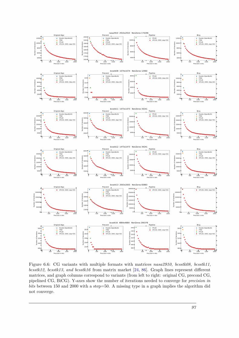
0.0 0.2 0.4 0.6 0.8 1.00.0

0.2

0.4

0.6

0.8

1.0

nasa2910 2910x2910 NonZeros 174296

0.0 0.2 0.4 0.6 0.8 1.00.0

0.2

0.4

0.6

0.8

1.0

bcsstk08 1074x1074 NonZeros 12960

0.0 0.2 0.4 0.6 0.8 1.00.0

0.2

0.4

0.6

0.8

1.0

bcsstk11 1473x1473 NonZeros 34241

0.0 0.2 0.4 0.6 0.8 1.00.0

0.2

0.4

0.6

0.8

1.0

bcsstk12 1473x1473 NonZeros 34241

0.0 0.2 0.4 0.6 0.8 1.00.0

0.2

0.4

0.6

0.8

1.0

bcsstk13 2003x2003 NonZeros 83883

0.0 0.2 0.4 0.6 0.8 1.00.0

0.2

0.4

0.6

0.8

1.0

bcsstk16 4884x4884 NonZeros 290378

0 500 1000 1500 2000Precision in bits

4000

6000

8000

10000

12000

Num

ber o

f Ite

ratio

nsOriginal Algo

Double (OpenBLAS)FP80FP128VP(150, 2000, step=50)

0 500 1000 1500 2000Precision in bits

1650

1700

1750

1800

1850

1900

1950

2000

Num

ber o

f Ite

ratio

ns

PrecondDouble (OpenBLAS)FP80FP128VP(150, 2000, step=50)

500 1000 1500 2000Precision in bits

4000

6000

8000

10000

Num

ber o

f Ite

ratio

ns

PipelineFP128VP(150, 2000, step=50)

0 500 1000 1500 2000Precision in bits

4000

6000

8000

10000

12000

Num

ber o

f Ite

ratio

ns

BicgDouble (OpenBLAS)FP80FP128VP(150, 2000, step=50)

0 500 1000 1500 2000Precision in bits

0

2000

4000

6000

8000

10000

Num

ber o

f Ite

ratio

ns

Original AlgoDouble (OpenBLAS)FP80FP128VP(150, 2000, step=50)

0 500 1000 1500 2000Precision in bits

216

218

220

222

224

Num

ber o

f Ite

ratio

ns

PrecondDouble (OpenBLAS)FP80FP128VP(150, 2000, step=50)

500 1000 1500 2000Precision in bits

2000

4000

6000

8000

Num

ber o

f Ite

ratio

ns

PipelineFP128VP(150, 2000, step=50)

0 500 1000 1500 2000Precision in bits

0

2000

4000

6000

8000

10000

Num

ber o

f Ite

ratio

ns

BicgDouble (OpenBLAS)FP80FP128VP(150, 2000, step=50)

0 500 1000 1500 2000Precision in bits

5000

10000

15000

20000

25000

Num

ber o

f Ite

ratio

ns

Original AlgoDouble (OpenBLAS)FP80FP128VP(150, 2000, step=50)

0 500 1000 1500 2000Precision in bits

2000

3000

4000

5000

6000

Num

ber o

f Ite

ratio

ns

PrecondDouble (OpenBLAS)FP80FP128VP(150, 2000, step=50)

500 1000 1500 2000Precision in bits

5000

10000

15000

20000

Num

ber o

f Ite

ratio

ns

PipelineFP128VP(150, 2000, step=50)

0 500 1000 1500 2000Precision in bits

5000

10000

15000

20000

25000

Num

ber o

f Ite

ratio

ns

BicgDouble (OpenBLAS)FP80FP128VP(150, 2000, step=50)

0 500 1000 1500 2000Precision in bits

5000

10000

15000

20000

25000

Num

ber o

f Ite

ratio

ns

Original AlgoDouble (OpenBLAS)FP80FP128VP(150, 2000, step=50)

0 500 1000 1500 2000Precision in bits

2000

3000

4000

5000

6000

Num

ber o

f Ite

ratio

ns

PrecondDouble (OpenBLAS)FP80FP128VP(150, 2000, step=50)

500 1000 1500 2000Precision in bits

5000

10000

15000

20000

Num

ber o

f Ite

ratio

ns

PipelineFP128VP(150, 2000, step=50)

0 500 1000 1500 2000Precision in bits

5000

10000

15000

20000

25000

Num

ber o

f Ite

ratio

ns

BicgDouble (OpenBLAS)FP80FP128VP(150, 2000, step=50)

500 1000 1500 2000Precision in bits

0

50000

100000

150000

200000

Num

ber o

f Ite

ratio

ns

Original AlgoVP(150, 2000, step=50)

0 500 1000 1500 2000Precision in bits

1300

1400

1500

1600

1700

Num

ber o

f Ite

ratio

ns

PrecondDouble (OpenBLAS)FP80FP128VP(150, 2000, step=50)

500 1000 1500 2000Precision in bits

0

50000

100000

150000

200000

250000

300000

Num

ber o

f Ite

ratio

ns

PipelineVP(150, 2000, step=50)

500 1000 1500 2000Precision in bits

0

50000

100000

150000

200000

Num

ber o

f Ite

ratio

ns

BicgVP(150, 2000, step=50)

0 500 1000 1500 2000Precision in bits

480

500

520

540

560

Num

ber o

f Ite

ratio

ns

Original AlgoDouble (OpenBLAS)FP80FP128VP(150, 2000, step=50)

0 500 1000 1500 2000Precision in bits

254

256

258

260

262

Num

ber o

f Ite

ratio

ns

PrecondDouble (OpenBLAS)FP80FP128VP(150, 2000, step=50)

500 1000 1500 2000Precision in bits

480

490

500

510

520

530

540

Num

ber o

f Ite

ratio

ns

PipelineFP128VP(150, 2000, step=50)

0 500 1000 1500 2000Precision in bits

480

500

520

540

560

Num

ber o

f Ite

ratio

ns

BicgDouble (OpenBLAS)FP80FP128VP(150, 2000, step=50)

Figure 6.6: CG variants with multiple formats with matrices nasa2910, bcsstk08, bcsstk11,bcsstk12, bcsstk13, and bcsstk16 from matrix market [24, 86]. Graph lines represent differentmatrices, and graph columns correspond to variants (from left to right: original CG, precond CG,pipelined CG, BiCG). Y-axes show the number of iterations needed to converge for precision inbits between 150 and 2000 with a step=50. A missing type in a graph implies the algorithm didnot converge.

97

0.0 0.2 0.4 0.6 0.8 1.00.0

0.2

0.4

0.6

0.8

1.0

bcsstk19 817x817 NonZeros 6853

0.0 0.2 0.4 0.6 0.8 1.00.0

0.2

0.4

0.6

0.8

1.0

bcsstk20 485x485 NonZeros 3135

0.0 0.2 0.4 0.6 0.8 1.00.0

0.2

0.4

0.6

0.8

1.0

bcsstk23 3134x3134 NonZeros 45178

0.0 0.2 0.4 0.6 0.8 1.00.0

0.2

0.4

0.6

0.8

1.0

crystk01 4875x4875 NonZeros 315891

0.0 0.2 0.4 0.6 0.8 1.00.0

0.2

0.4

0.6

0.8

1.0

s3rmt3m3 5357x5357 NonZeros 207123

0.0 0.2 0.4 0.6 0.8 1.00.0

0.2

0.4

0.6

0.8

1.0

plat1919 1919x1919 NonZeros 32399

500 1000 1500 2000Precision in bits

0

10000

20000

30000

40000

50000

60000

70000

Num

ber o

f Ite

ratio

nsOriginal Algo

VP(150, 2000, step=50)

0 500 1000 1500 2000Precision in bits

1000

2000

3000

4000

5000

6000

7000

8000

Num

ber o

f Ite

ratio

ns

PrecondDouble (OpenBLAS)FP80FP128VP(150, 2000, step=50)

500 1000 1500 2000Precision in bits

0

20000

40000

60000

80000

100000

Num

ber o

f Ite

ratio

ns

PipelineVP(150, 2000, step=50)

500 1000 1500 2000Precision in bits

0

10000

20000

30000

40000

50000

60000

70000

Num

ber o

f Ite

ratio

ns

BicgVP(150, 2000, step=50)

500 1000 1500 2000Precision in bits

0

2500

5000

7500

10000

12500

15000

17500

Num

ber o

f Ite

ratio

ns

Original AlgoFP128VP(150, 2000, step=50)

0 500 1000 1500 2000Precision in bits

1000

2000

3000

4000

Num

ber o

f Ite

ratio

ns

PrecondDouble (OpenBLAS)FP80FP128VP(150, 2000, step=50)

500 1000 1500 2000Precision in bits

0

5000

10000

15000

20000

25000

30000

35000

Num

ber o

f Ite

ratio

ns

PipelineFP128VP(150, 2000, step=50)

500 1000 1500 2000Precision in bits

0

2500

5000

7500

10000

12500

15000

17500

Num

ber o

f Ite

ratio

ns

BicgFP128VP(150, 2000, step=50)

500 1000 1500 2000Precision in bits

0

100000

200000

300000

400000

500000

Num

ber o

f Ite

ratio

ns

Original AlgoVP(150, 2000, step=50)

0 500 1000 1500 2000Precision in bits

4000

6000

8000

10000

Num

ber o

f Ite

ratio

ns

PrecondDouble (OpenBLAS)FP80FP128VP(150, 2000, step=50)

500 1000 1500 2000Precision in bits

0

100000

200000

300000

400000

500000

600000

700000

Num

ber o

f Ite

ratio

ns

PipelineVP(150, 2000, step=50)

500 1000 1500 2000Precision in bits

0

100000

200000

300000

400000

500000

Num

ber o

f Ite

ratio

ns

BicgVP(150, 2000, step=50)

500 1000 1500 2000Precision in bits

3000

4000

5000

6000

7000

8000

Num

ber o

f Ite

ratio

ns

Original AlgoFP128VP(150, 2000, step=50)

500 1000 1500 2000Precision in bits

3000

4000

5000

6000

7000

Num

ber o

f Ite

ratio

ns

PrecondFP128VP(150, 2000, step=50)

500 1000 1500 2000Precision in bits

3000

4000

5000

6000

Num

ber o

f Ite

ratio

ns

PipelineVP(150, 2000, step=50)

500 1000 1500 2000Precision in bits

3000

4000

5000

6000

7000

8000

Num

ber o

f Ite

ratio

ns

BicgFP128VP(150, 2000, step=50)

0 500 1000 1500 2000Precision in bits

50000

100000

150000

200000

Num

ber o

f Ite

ratio

ns

Original AlgoDouble (OpenBLAS)FP80FP128VP(150, 2000, step=50)

0 500 1000 1500 2000Precision in bits

10000

15000

20000

25000

Num

ber o

f Ite

ratio

ns

PrecondDouble (OpenBLAS)FP80FP128VP(150, 2000, step=50)

500 1000 1500 2000Precision in bits

25000

50000

75000

100000

125000

150000

Num

ber o

f Ite

ratio

ns

PipelineFP128VP(150, 2000, step=50)

0 500 1000 1500 2000Precision in bits

50000

100000

150000

200000

Num

ber o

f Ite

ratio

ns

BicgDouble (OpenBLAS)FP80FP128VP(150, 2000, step=50)

500 1000 1500 2000Precision in bits

0

50000

100000

150000

200000

250000

300000

Num

ber o

f Ite

ratio

ns

Original AlgoVP(150, 2000, step=50)

500 1000 1500 2000Precision in bits

0

50000

100000

150000

200000

250000

Num

ber o

f Ite

ratio

ns

PrecondVP(150, 2000, step=50)

500 1000 1500 2000Precision in bits

0

100000

200000

300000

400000

Num

ber o

f Ite

ratio

ns

PipelineVP(150, 2000, step=50)

500 1000 1500 2000Precision in bits

0

50000

100000

150000

200000

250000

300000

Num

ber o

f Ite

ratio

ns

BicgVP(150, 2000, step=50)

Figure 6.7: CG variants with multiple formats with matrices bcsstk19, bcsstk20, bcsstk23,crystk01, s3rmt3m3, and plat1919 from matrix market [24, 86]. Graph lines represent differentmatrices, and graph columns correspond to variants (from left to right: original CG, precond CG,pipelined CG, BiCG). Y-axes show the number of iterations needed to converge for precision inbits between 150 and 2000 with a step=50. A missing type in a graph implies the algorithm didnot converge.

98

Execution time

It may initially sound paradoxical that higher precision can lead to fewer iterations, however, thisalso demonstrates that higher precision may actually reduce the execution time of a numericalapplication, as depicted in Figures 6.8 and 6.9. We observe that many variants are indeed able tosignificantly improve execution time by relying on very high precision. For instance, all variantsrunning in matrix bcsstk13, except precond, with 2000 bits of precision show more than 5× speedwhen compared to 150 bits.

Although high-precision representation can improve performance in different variants andmatrices, the trend followed by execution time is not the same as for the number of iterations.We can observe that, for many situations, the reduced number of iterations is not able tocompensate for the increase of precision, which results in higher execution times. This is thecase for all variants in matrix bcsstk16, results that correlate to the small improvement in thenumber of iterations when precision is increased.

Precond has an interesting property: given that the condition number of the matrix is(highly) improved with a preconditioner, increasing the precision has two more perceptible effects:(1) either the plateau is reached earlier, (2) or increasing precision has a negative impact onexecution time and should be avoided. This variant has also shown the best overall executiontimes, which explains why it is the preferred implementation in numerical libraries.

Interestingly, numerical analysts can potentially make use of these results with the aim todetermine the best trade-off between precision and the number of iterations for an optimalexecution time. The objective would be to comprehend the behavior of the number of iterationsand the impact it has on execution time, as an Oracle for the best representation to be used5.

Table 6.5 summarizes how execution time in vpfloat<mpfr, ...> compares to other types,showing the counts of the number of matrices where our type outperforms its counterparts.Values for vpfloat and Boost are cherry-picked with the best execution time among the precisionrange (from 150 to 2000 with a step=50). We observe that vpfloat<mpfr, ...> can outperformlower-precision types, like long double and __float128, in many matrices and variants. Wealso show better performance of Boost in the majority of cases, which corroborates with theresults presented in previous sections of this chapter. Lastly, execution times for vpfloat areexpected to be improved when UNUM type is used.

Table 6.5: Count on the number of matrices where vpfloat<mpfr, ...> outperforms othertypes. Only matrix with types that converge are considered. For vpfloat and Boost, wecherry-pick the best execution time among the precision range (from 150 to 2000 with a step=50)

Algorithmdouble long double __float128

BoostVariant (All mat.) (N>1000) (N>2000)Original 4/32 19/32 25/35 40/40 27/27 15/15Precond 0/36 6/37 9/39 40/40 27/27 15/15Pipeline 0/0 7/7 29/34 32/40 26/27 15/15BiCG 4/32 18/32 25/35 40/40 27/27 15/15

5Assuming that all types are supported by hardware. Otherwise, the right choice will most likely be doublefor all situations.

99

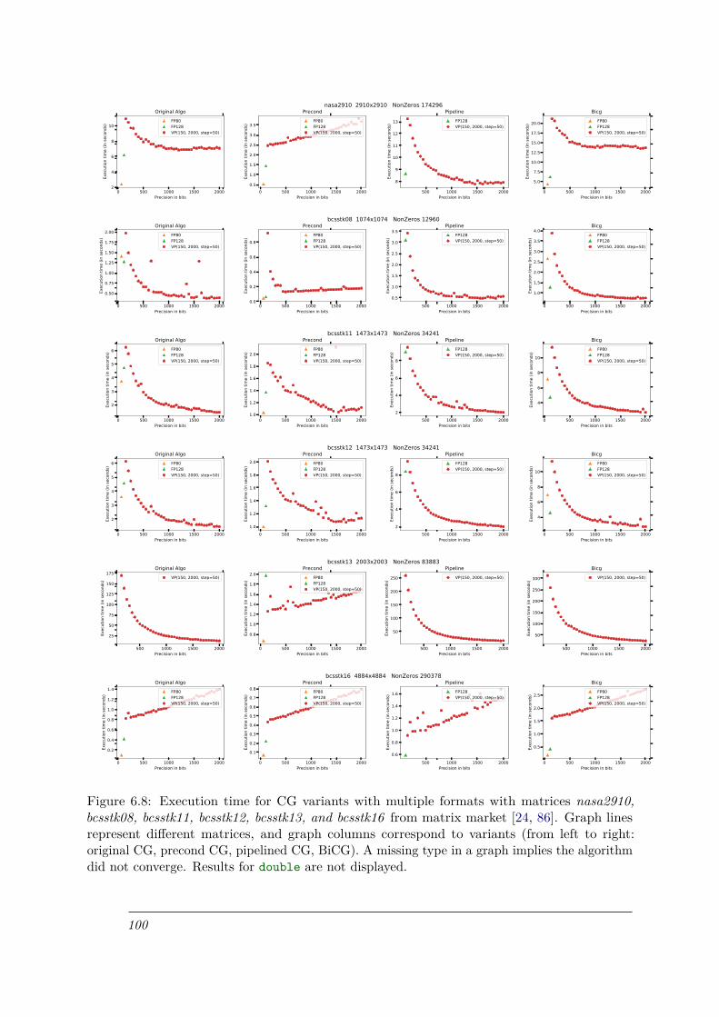
0.0 0.2 0.4 0.6 0.8 1.00.0

0.2

0.4

0.6

0.8

1.0

nasa2910 2910x2910 NonZeros 174296

0.0 0.2 0.4 0.6 0.8 1.00.0

0.2

0.4

0.6

0.8

1.0

bcsstk08 1074x1074 NonZeros 12960

0.0 0.2 0.4 0.6 0.8 1.00.0

0.2

0.4

0.6

0.8

1.0

bcsstk11 1473x1473 NonZeros 34241

0.0 0.2 0.4 0.6 0.8 1.00.0

0.2

0.4

0.6

0.8

1.0

bcsstk12 1473x1473 NonZeros 34241

0.0 0.2 0.4 0.6 0.8 1.00.0

0.2

0.4

0.6

0.8

1.0

bcsstk13 2003x2003 NonZeros 83883

0.0 0.2 0.4 0.6 0.8 1.00.0

0.2

0.4

0.6

0.8

1.0

bcsstk16 4884x4884 NonZeros 290378

0 500 1000 1500 2000Precision in bits

2

4

6

8

10

Exec

utio

n tim

e (in

seco

nds)

Original AlgoFP80FP128VP(150, 2000, step=50)

0 500 1000 1500 2000Precision in bits

0.5

1.0

1.5

2.0

2.5

3.0

3.5

Exec

utio

n tim

e (in

seco

nds)

PrecondFP80FP128VP(150, 2000, step=50)

500 1000 1500 2000Precision in bits

8

9

10

11

12

13

Exec

utio

n tim

e (in

seco

nds)

PipelineFP128VP(150, 2000, step=50)

0 500 1000 1500 2000Precision in bits

5.0

7.5

10.0

12.5

15.0

17.5

20.0

Exec

utio

n tim

e (in

seco

nds)

BicgFP80FP128VP(150, 2000, step=50)

0 500 1000 1500 2000Precision in bits

0.50

0.75

1.00

1.25

1.50

1.75

2.00

Exec

utio

n tim

e (in

seco

nds)

Original AlgoFP80FP128VP(150, 2000, step=50)

0 500 1000 1500 2000Precision in bits

0.0

0.2

0.4

0.6

0.8Ex

ecut

ion

time

(in se

cond

s)

PrecondFP80FP128VP(150, 2000, step=50)

500 1000 1500 2000Precision in bits

0.5

1.0

1.5

2.0

2.5

3.0

3.5

Exec

utio

n tim

e (in

seco

nds)

PipelineFP128VP(150, 2000, step=50)

0 500 1000 1500 2000Precision in bits

1.0

1.5

2.0

2.5

3.0

3.5

4.0

Exec

utio

n tim

e (in

seco

nds)

BicgFP80FP128VP(150, 2000, step=50)

0 500 1000 1500 2000Precision in bits

2

3

4

5

6

Exec

utio

n tim

e (in

seco

nds)

Original AlgoFP80FP128VP(150, 2000, step=50)

0 500 1000 1500 2000Precision in bits

1.0

1.2

1.4

1.6

1.8

2.0

Exec

utio

n tim

e (in

seco

nds)

PrecondFP80FP128VP(150, 2000, step=50)

500 1000 1500 2000Precision in bits

2

4

6

8

Exec

utio

n tim

e (in

seco

nds)

PipelineFP128VP(150, 2000, step=50)

0 500 1000 1500 2000Precision in bits

4

6

8

10

Exec

utio

n tim

e (in

seco

nds)

BicgFP80FP128VP(150, 2000, step=50)

0 500 1000 1500 2000Precision in bits

2

3

4

5

6

Exec

utio

n tim

e (in

seco

nds)

Original AlgoFP80FP128VP(150, 2000, step=50)

0 500 1000 1500 2000Precision in bits

1.0

1.2

1.4

1.6

1.8

2.0

Exec

utio

n tim

e (in

seco

nds)

PrecondFP80FP128VP(150, 2000, step=50)

500 1000 1500 2000Precision in bits

2

4

6

8

Exec

utio

n tim

e (in

seco

nds)

PipelineFP128VP(150, 2000, step=50)

0 500 1000 1500 2000Precision in bits

4

6

8

10

Exec

utio

n tim

e (in

seco

nds)

BicgFP80FP128VP(150, 2000, step=50)

500 1000 1500 2000Precision in bits

25

50

75

100

125

150

175

Exec

utio

n tim

e (in

seco

nds)

Original AlgoVP(150, 2000, step=50)

0 500 1000 1500 2000Precision in bits

0.8

1.0

1.2

1.4

1.6

1.8

2.0

Exec

utio

n tim

e (in

seco

nds)

PrecondFP80FP128VP(150, 2000, step=50)

500 1000 1500 2000Precision in bits

50

100

150

200

250

Exec

utio

n tim

e (in

seco

nds)

PipelineVP(150, 2000, step=50)

500 1000 1500 2000Precision in bits

50

100

150

200

250

300

Exec

utio

n tim

e (in

seco

nds)

BicgVP(150, 2000, step=50)

0 500 1000 1500 2000Precision in bits

0.2

0.4

0.6

0.8

1.0

1.2

1.4

Exec

utio

n tim

e (in

seco

nds)

Original AlgoFP80FP128VP(150, 2000, step=50)

0 500 1000 1500 2000Precision in bits

0.1

0.2

0.3

0.4

0.5

0.6

0.7

0.8

Exec

utio

n tim

e (in

seco

nds)

PrecondFP80FP128VP(150, 2000, step=50)

500 1000 1500 2000Precision in bits

0.6

0.8

1.0

1.2

1.4

1.6

Exec

utio

n tim

e (in

seco

nds)

PipelineFP128VP(150, 2000, step=50)

0 500 1000 1500 2000Precision in bits

0.5

1.0

1.5

2.0

2.5

Exec

utio

n tim

e (in

seco

nds)

BicgFP80FP128VP(150, 2000, step=50)

Figure 6.8: Execution time for CG variants with multiple formats with matrices nasa2910,bcsstk08, bcsstk11, bcsstk12, bcsstk13, and bcsstk16 from matrix market [24, 86]. Graph linesrepresent different matrices, and graph columns correspond to variants (from left to right:original CG, precond CG, pipelined CG, BiCG). A missing type in a graph implies the algorithmdid not converge. Results for double are not displayed.

100

0.0 0.2 0.4 0.6 0.8 1.00.0

0.2

0.4

0.6

0.8

1.0

bcsstk19 817x817 NonZeros 6853

0.0 0.2 0.4 0.6 0.8 1.00.0

0.2

0.4

0.6

0.8

1.0

bcsstk20 485x485 NonZeros 3135

0.0 0.2 0.4 0.6 0.8 1.00.0

0.2

0.4

0.6

0.8

1.0

bcsstk23 3134x3134 NonZeros 45178

0.0 0.2 0.4 0.6 0.8 1.00.0

0.2

0.4

0.6

0.8

1.0

crystk01 4875x4875 NonZeros 315891

0.0 0.2 0.4 0.6 0.8 1.00.0

0.2

0.4

0.6

0.8

1.0

s3rmt3m3 5357x5357 NonZeros 207123

0.0 0.2 0.4 0.6 0.8 1.00.0

0.2

0.4

0.6

0.8

1.0

plat1919 1919x1919 NonZeros 32399

500 1000 1500 2000Precision in bits

0

2

4

6

8

10

12

14

Exec

utio

n tim

e (in

seco

nds)

Original AlgoVP(150, 2000, step=50)

0 500 1000 1500 2000Precision in bits

0.4

0.6

0.8

1.0

1.2

Exec

utio

n tim

e (in

seco

nds)

PrecondFP80FP128VP(150, 2000, step=50)

500 1000 1500 2000Precision in bits

0

5

10

15

20

25

30

35

Exec

utio

n tim

e (in

seco

nds)

PipelineVP(150, 2000, step=50)

500 1000 1500 2000Precision in bits

0

5

10

15

20

25

Exec

utio

n tim

e (in

seco

nds)

BicgVP(150, 2000, step=50)

500 1000 1500 2000Precision in bits

0.5

1.0

1.5

2.0

2.5

Exec

utio

n tim

e (in

seco

nds)

Original AlgoFP128VP(150, 2000, step=50)

0 500 1000 1500 2000Precision in bits

0.2

0.3

0.4

0.5Ex

ecut

ion

time

(in se

cond

s)

PrecondFP80FP128VP(150, 2000, step=50)

500 1000 1500 2000Precision in bits

0

2

4

6

8

10

Exec

utio

n tim

e (in

seco

nds)

PipelineFP128VP(150, 2000, step=50)

500 1000 1500 2000Precision in bits

0.5

1.0

1.5

2.0

2.5

3.0

3.5

Exec

utio

n tim

e (in

seco

nds)

BicgFP128VP(150, 2000, step=50)

500 1000 1500 2000Precision in bits

50

100

150

200

Exec

utio

n tim

e (in

seco

nds)

Original AlgoVP(150, 2000, step=50)

0 500 1000 1500 2000Precision in bits

1.5

2.0

2.5

3.0

3.5

4.0

Exec

utio

n tim

e (in

seco

nds)

PrecondFP80FP128VP(150, 2000, step=50)

500 1000 1500 2000Precision in bits

100

200

300

400

Exec

utio

n tim

e (in

seco

nds)

PipelineVP(150, 2000, step=50)

500 1000 1500 2000Precision in bits

100

200

300

400

Exec

utio

n tim

e (in

seco

nds)

BicgVP(150, 2000, step=50)

500 1000 1500 2000Precision in bits

8

9

10

11

Exec

utio

n tim

e (in

seco

nds)

Original AlgoFP128VP(150, 2000, step=50)

500 1000 1500 2000Precision in bits

6.5

7.0

7.5

8.0

8.5

9.0

9.5

Exec

utio

n tim

e (in

seco

nds)

PrecondFP128VP(150, 2000, step=50)

500 1000 1500 2000Precision in bits

8

9

10

11

12

Exec

utio

n tim

e (in

seco

nds)

PipelineVP(150, 2000, step=50)

500 1000 1500 2000Precision in bits

7.5

10.0

12.5

15.0

17.5

20.0

22.5

Exec

utio

n tim

e (in

seco

nds)

BicgFP128VP(150, 2000, step=50)

0 500 1000 1500 2000Precision in bits

40

60

80

100

120

140

Exec

utio

n tim

e (in

seco

nds)

Original AlgoFP80FP128VP(150, 2000, step=50)

0 500 1000 1500 2000Precision in bits

5.0

7.5

10.0

12.5

15.0

17.5

20.0

Exec

utio

n tim

e (in

seco

nds)

PrecondFP80FP128VP(150, 2000, step=50)

500 1000 1500 2000Precision in bits

60

80

100

120

140

160

180

Exec

utio

n tim

e (in

seco

nds)

PipelineFP128VP(150, 2000, step=50)

0 500 1000 1500 2000Precision in bits

50

100

150

200

250

Exec

utio

n tim

e (in

seco

nds)

BicgFP80FP128VP(150, 2000, step=50)

500 1000 1500 2000Precision in bits

20

40

60

80

100

Exec

utio

n tim

e (in

seco

nds)

Original AlgoVP(150, 2000, step=50)

500 1000 1500 2000Precision in bits

0

20

40

60

80

100

Exec

utio

n tim

e (in

seco

nds)

PrecondVP(150, 2000, step=50)

500 1000 1500 2000Precision in bits

0

50

100

150

200

Exec

utio

n tim

e (in

seco

nds)

PipelineVP(150, 2000, step=50)

500 1000 1500 2000Precision in bits

50

100

150

200

Exec

utio

n tim

e (in

seco

nds)

BicgVP(150, 2000, step=50)

Figure 6.9: Execution time for CG variants with multiple formats with matrices bcsstk19,bcsstk20, bcsstk23, crystk01, s3rmt3m3, and plat1919 from matrix market [24, 86]. Graphlines represent different matrices, and graph columns correspond to variants (from left to right:original CG, precond CG, pipelined CG, BiCG). A missing type in a graph implies the algorithmdid not converge. Results for double are not displayed.

101

6.3 ConclusionThis chapter demonstrated the productivity benefits of our intuitive programming model andits ability to leverage an existing optimizing compiler framework. We presented a series ofexperiments on PolyBench and RAJAPerf suites that yield strong speedups for both softwareand hardware targets. Our compiler integrated solution is more capable of leveraging theclassical optimizations already implemented by the compiler, which helps to reason about thespeedup results observed. Experimental results also showed that significantly higher speedups areobserved when comparing a software to a hardware target. This result is particularly interestingwith the rise of the dark silicon area and may be an aspect for evaluation on future processordesigns. Our last experiments in CG are a step towards better understanding the impact of(high-)precision in linear algebra and illustrated how variable precision may raise its importancefor the future of high-performance computing. To that end, this thesis is a step towards makingvariable precision easier to use and better integrated into a language, compiler and hardware,and serves as an enabler for better exploration of variable precision computing.

102

Chapter 7: Conclusion

This thesis defines a compilation strategy to use and explore variable precision FP arithmeticand proposes a design and implementation of this strategy. We are mainly interested in howlanguages and compilers can support data structures, types, and both software- and hardware-enabled operations to accelerate applications with different FP requirements. No previoussolution has shown a complete integration of FP arithmetic with constant and variable memoryfootprint. Our proposed type system, embedded into the compiler’s intermediate representation,and lowering and backend code generation strategies provide both high-productivity and high-performance with variable precision FP formats. Our extension supports FP arithmetic ofarbitrary representation and precision, and the precision and exponent can be configured atcompilation time and runtime.

We exposed a list of questions in chapter 2 and the work presented in the context of thisthesis is intended to answer these questions. In the following paragraphs, we provide a summaryof how we answered these questions:

How can languages and compilers be used to accelerate and improve the productivity ofmulti-precision FP libraries? Can one improve the integration between compilers and theselibraries to take better advantage of classical compiler optimizations?

Chapters 4 and 5 show the solution we propose to enable the instantiation of multi-format FPtypes. Because of the genericity of our type system, types that hide underlying implementationwith multi-precision FP libraries can be supported. More precisely, an MPFR type (vpfloat<mpfr, ...>) has been added as a lightweight alternative to use the MPFR library in a moreprogrammer-friendly fashion. This type provides a functionality similar to high-level MPFRabstractions, like Boost Multi-precision library, Julia and Python’s dynamic type systems, but itoffers a C-level easy-to-use interface for MPFR.

We provide an integrated compiler solution that bridges the abstraction gap between multi-precision FP libraries and compiler transformations, permitting us to postpone the instantiationof library-related operations and objects until after optimizations are run. Experimental resultscorroborate on showing that a later transformation pass to generate library-specific code hasa positive impact on execution time since more optimization opportunities can be found. Wealso demonstrate through a practical code example (Figure 5.6) that even vectorization can besupported at least to some extend.

How can one extend languages and provide compiler support for new formats taking intoconsideration their singular properties?

Chapter 4 describes the language requirements, syntax, and semantics defined within thecontext of this thesis. We use a new primitive type vpfloat to encapsulate many properties of

103

FP types. The use of a single keyword, although not necessary, is employed to allow multipleformats to coexist within a single context, and differentiates language pre-existing types fromthose of our extension. The proposed syntax offers flexibility for the declaration of formats withdifferent attributes. Its use is not hindered by any constraint, such as precision and exponentvalues, or even size, and users should not be restrained by any form of type declaration. In otherwords, the support for FP arithmetic of arbitrary representation, whose precision and exponentcan be configured at compilation time and runtime, allows a high degree of flexibility that hasnot been explored in previous works.

The effectiveness of our type extension (and language syntax) in representing multiple formatsis shown through: (1) an MPFR-compatible type that views FP attributes as exponent andprecision fields, and (2) a UNUM type class where FP attributes are interpreted according tothe format specification, and so, differently from the former. To the best of our knowledge,no previous work tackled the integration within an optimizing compilation flow, taking intoconsideration format-specific attributes, and how the compiler can efficiently generate code fortypes that may not necessarily have constant size. Having support for two types with differentsemantics is proof of how extensible our solution is, not only from a language perspective butalso throughout the full compilation flow, enabling the design of software- and hardware-specificcode generators.

What are the compiler and optimizations requirements to support an FP type system withruntime capabilities? How can compilers provide proper memory management for these types?

Our proposal tackles a set of capabilities neglected by low-level programming languages:the ability to declare types with runtime capabilities. This feature has re-gained significancein the context of variable precision where the cost of increasing precision must be avoided forperformance purposes. We enable the use of types with runtime-decidable attributes by allowingtheir specialization with integer variables of the program.

Our compilation flow handles these types from language to the middle-end level representationthrough a new type extension that enable declarations to have constant or runtime-decidableattributes. We implemented this extension in LLVM to benefit from the optimizations availableon its intermediate representation. We also assessed that specific optimizations such as LoopIdiom Recognition and Inlining need modifications to handle types with runtime attributes.Backend code generation for such types is only possible thanks to the coordination between thecompiler infrastructure and the target backend, which means that a compatible ISA or softwaretarget solution is required to drive the flexibility of these types.

The use of MPFR is possible because objects can be constructed with the precision valuespecified upon object creation, and operations make use of this information to compute values.The synergy between the UNUM coprocessor and the compiler is done through an ISA agnosticto the format used for computation. The compiler sets status registers values inside the hardwareto control the FP format in use, which gives the compliance and full support for UNUM typeswith runtime capabilities.

Can variable precision serve as an interesting exploration paradigm in the context of numeri-cal algorithms?

Yes, our experiments on the conjugate gradient method and variants show a clear variableprecision exploration aspect in linear algebra. Experimental results show that increasing theprecision to be used can have a non-negligible impact on the number of iterations of an algorithm.It also demonstrates that precision is particularly important for the pipelined CG variant due

104

to instability caused by the accumulation of rounding errors. The stability of the algorithmis only achieved with high precision and using primitive data types only works for it to someextent, that is, when the tolerance threshold is increased. In that case, it means that anapproximate (and less accurate) solution is acceptable. The design of BLAS routines also permitsthe exploration of other high-performance algorithms, such as Singular Value Decomposition(SVD), and Generalized minimal residual method (GMRES).

Perspectives

Our future work can be divided into two main categories: (1) the first relates to additionalcompiler work and tooling that can be envisioned; (2) and the complementary work aimed inthe application side with many aspects to consider.

Compilation and Integration Tools

Chapters 4 and 5 show the main contributions found within the context of this thesis. Butthey also show some limitations and ideas that can be pursued as future work, as part of thelanguage, compilation, and tool integration process. Among them, we may refer to:

(1) Improve high-level structures integration: vpfloat support for compound types such asclass, and structs, is still limited to constant types. There are two challenges to resolve:(1) find a consistent syntax and semantic to express types with runtime attributes so thatusers are able to bind them to variable declarations; (2) instrument the compiler to supportthem is also a challenging part of the work, since none of the elements within the currentinfrastructure has functionality that resembles it,

(2) Generally work on the improvements of loop nest-related heuristics to better optimizevpfloat. Although we are able to leverage Polly, many heuristics are suboptimal and arenot capable of optimizing the code, even for constant types. Add support for dynamically-sized types in Polly heuristics is also a venue of exploration in order to improve cacheutilization within our BLAS library implementations,

(3) Our language proposal shows support for two formats (MPFR, and UNUM), but it isalso extensible to other representations. More interestingly, the Posit format, a UNUMsuccessor, has shown potential usage for many scientific fields [28, 42, 70], and is a valuablecandidate to appear as a vpfloat format within our extension. Ongoing work is alsounderway to support an IEEE-like representation, much similar to the MPFR format, butenabling hardware support to accelerate computation with high-precision representationseven further,

(4) Improve tooling integration with open-source projects like PetSC [3, 18], Armadillo [106],and Eigen [56]: many of the related work use, experiment, and validate their solutionwith open-source projects. The evaluation presented in [34, 35, 36], for example, areconducted in PetSc [3, 18], a modern and scalable ordinary differential equation (ODE)and differential algebraic equations (DAE) solver library. The Armadillo [106] and Eigenlibraries [56] are template-based metaprogramming C++ libraries for linear algebra andscientific computing and are also highly used within the context of the applications targetedto be explored in future work.

105

ApplicationsOn the application side, we can explore different aspects:

(1) Run CG experiments with our vpfloat<unum, ...> types once all stability issues areresolved in the system. We are mainly interested to understand how the reduced number ofiterations impacts execution time. Increasing precision may collaborate to reduce executiontime even if compared to optimized implementations with vectorization capabilities (forexample, applications with double and using vector instructions).

(2) Although this thesis focuses mainly on providing language and compiler integration asa mean to accelerate exploration of variable precision and other FP formats in general,our last experiments with CG show insights to increase the interest of numerical analystsin the exploration of variable precision. Future work will focus on new applications andconfigurations to accelerate linear algebra. We are keen to see if variable precision canbe used with the iterative refinement technique presented in chapter 3 as part of themixed-precision computing section. It is also envisioned that other applications, such asSVD and GMRES, be studied to widen the comprehension of the impact of precisionand FP formats in general. The outcome of this thesis can be seen as an enabler of thisexploration.

106

Annexes

107

Appendix A: CG Experimental Results:Number of Iterations

109

0.0 0.2 0.4 0.6 0.8 1.00.0

0.2

0.4

0.6

0.8

1.0

bcsstk04 132x132 NonZeros 3648

0.0 0.2 0.4 0.6 0.8 1.00.0

0.2

0.4

0.6

0.8

1.0

bcsstk05 153x153 NonZeros 2423

0.0 0.2 0.4 0.6 0.8 1.00.0

0.2

0.4

0.6

0.8

1.0

bcsstk06 420x420 NonZeros 7860

0.0 0.2 0.4 0.6 0.8 1.00.0

0.2

0.4

0.6

0.8

1.0

bcsstk07 420x420 NonZeros 7860

0.0 0.2 0.4 0.6 0.8 1.00.0

0.2

0.4

0.6

0.8

1.0

bcsstk09 1083x1083 NonZeros 18437

0.0 0.2 0.4 0.6 0.8 1.00.0

0.2

0.4

0.6

0.8

1.0

bcsstk10 1086x1086 NonZeros 22070

0 500 1000 1500 2000Precision in bits

200

300

400

500

600

Num

ber o

f Ite

ratio

nsOriginal Algo

Double (OpenBLAS)FP80FP128VP(150, 2000, step=50)

0 500 1000 1500 2000Precision in bits

86

87

88

89

90

91

Num

ber o

f Ite

ratio

ns

PrecondDouble (OpenBLAS)FP80FP128VP(150, 2000, step=50)

500 1000 1500 2000Precision in bits

150

200

250

300

350

400

450

Num

ber o

f Ite

ratio

ns

PipelineFP128VP(150, 2000, step=50)

0 500 1000 1500 2000Precision in bits

200

300

400

500

600

Num

ber o

f Ite

ratio

ns

BicgDouble (OpenBLAS)FP80FP128VP(150, 2000, step=50)

0 500 1000 1500 2000Precision in bits

150

175

200

225

250

275

300

Num

ber o

f Ite

ratio

ns

Original AlgoDouble (OpenBLAS)FP80FP128VP(150, 2000, step=50)

0 500 1000 1500 2000Precision in bits

138

140

142

144

146

148

150

Num

ber o

f Ite

ratio

ns

PrecondDouble (OpenBLAS)FP80FP128VP(150, 2000, step=50)

0 500 1000 1500 2000Precision in bits

150

175

200

225

250

275

300

Num

ber o

f Ite

ratio

ns

PipelineFP80FP128VP(150, 2000, step=50)

0 500 1000 1500 2000Precision in bits

150

175

200

225

250

275

300

Num

ber o

f Ite

ratio

ns

BicgDouble (OpenBLAS)FP80FP128VP(150, 2000, step=50)

0 500 1000 1500 2000Precision in bits

1000

2000

3000

4000

Num

ber o

f Ite

ratio

ns

Original AlgoDouble (OpenBLAS)FP80FP128VP(150, 2000, step=50)

0 500 1000 1500 2000Precision in bits

360

380

400

420

440

460

480

Num

ber o

f Ite

ratio

ns

PrecondDouble (OpenBLAS)FP80FP128VP(150, 2000, step=50)

500 1000 1500 2000Precision in bits

500

1000

1500

2000

2500

3000

Num

ber o

f Ite

ratio

ns

PipelineFP128VP(150, 2000, step=50)

0 500 1000 1500 2000Precision in bits

1000

2000

3000

4000

Num

ber o

f Ite

ratio

ns

BicgDouble (OpenBLAS)FP80FP128VP(150, 2000, step=50)

0 500 1000 1500 2000Precision in bits

1000

2000

3000

4000

Num

ber o

f Ite

ratio

ns

Original AlgoDouble (OpenBLAS)FP80FP128VP(150, 2000, step=50)

0 500 1000 1500 2000Precision in bits

360

380

400

420

440

460

480

Num

ber o

f Ite

ratio

ns

PrecondDouble (OpenBLAS)FP80FP128VP(150, 2000, step=50)

500 1000 1500 2000Precision in bits

500

1000

1500

2000

2500

3000

Num

ber o

f Ite

ratio

ns

PipelineFP128VP(150, 2000, step=50)

0 500 1000 1500 2000Precision in bits

1000

2000

3000

4000

Num

ber o

f Ite

ratio

ns

BicgDouble (OpenBLAS)FP80FP128VP(150, 2000, step=50)

0 500 1000 1500 2000Precision in bits

246.0

246.5

247.0

247.5

248.0

248.5

249.0

Num

ber o

f Ite

ratio

ns

Original AlgoDouble (OpenBLAS)FP80FP128VP(150, 2000, step=50)

0 500 1000 1500 2000Precision in bits

195

200

205

210

215

Num

ber o

f Ite

ratio

ns

PrecondDouble (OpenBLAS)FP80FP128VP(150, 2000, step=50)

0 500 1000 1500 2000Precision in bits

246

247

248

249

250

Num

ber o

f Ite

ratio

ns

PipelineFP80FP128VP(150, 2000, step=50)

0 500 1000 1500 2000Precision in bits

246.0

246.5

247.0

247.5

248.0

248.5

249.0

Num

ber o

f Ite

ratio

ns

BicgDouble (OpenBLAS)FP80FP128VP(150, 2000, step=50)

0 500 1000 1500 2000Precision in bits

2000

3000

4000

5000

Num

ber o

f Ite

ratio

ns

Original AlgoDouble (OpenBLAS)FP80FP128VP(150, 2000, step=50)

0 500 1000 1500 2000Precision in bits

850

900

950

1000

Num

ber o

f Ite

ratio

ns

PrecondDouble (OpenBLAS)FP80FP128VP(150, 2000, step=50)

500 1000 1500 2000Precision in bits

1500

2000

2500

3000

3500

4000

4500

5000

Num

ber o

f Ite

ratio

ns

PipelineFP128VP(150, 2000, step=50)

0 500 1000 1500 2000Precision in bits

2000

3000

4000

5000

Num

ber o

f Ite

ratio

ns

BicgDouble (OpenBLAS)FP80FP128VP(150, 2000, step=50)

Figure A.1: CG variants with multiple formats with matrices bcsstk04, bcsstk05, bcsstk06,bcsstk07, bcsstk09, and bcsstk10 from matrix market [24, 86]. Graph lines represent differentmatrices, and graph columns correspond to variants (from left to right: original CG, precond CG,pipelined CG, BiCG). Y-axes show the number of iterations needed to converge for precision inbits between 150 and 2000 with a step=50. A missing type in a graph implies the algorithm didnot converge.

110

0.0 0.2 0.4 0.6 0.8 1.00.0

0.2

0.4

0.6

0.8

1.0

bcsstk14 1806x1806 NonZeros 63454

0.0 0.2 0.4 0.6 0.8 1.00.0

0.2

0.4

0.6

0.8

1.0

bcsstk15 3948x3948 NonZeros 117816

0.0 0.2 0.4 0.6 0.8 1.00.0

0.2

0.4

0.6

0.8

1.0

bcsstk21 3600x3600 NonZeros 26600

0.0 0.2 0.4 0.6 0.8 1.00.0

0.2

0.4

0.6

0.8

1.0

bcsstk22 138x138 NonZeros 696

0.0 0.2 0.4 0.6 0.8 1.00.0

0.2

0.4

0.6

0.8

1.0

bcsstk24 3562x3562 NonZeros 159910

0.0 0.2 0.4 0.6 0.8 1.00.0

0.2

0.4

0.6

0.8

1.0

bcsstk26 1922x1922 NonZeros 30336

0 500 1000 1500 2000Precision in bits

2500

5000

7500

10000

12500

15000

17500

20000

Num

ber o

f Ite

ratio

nsOriginal Algo

Double (OpenBLAS)FP80FP128VP(150, 2000, step=50)

0 500 1000 1500 2000Precision in bits

620

640

660

680

Num

ber o

f Ite

ratio

ns

PrecondDouble (OpenBLAS)FP80FP128VP(150, 2000, step=50)

500 1000 1500 2000Precision in bits

5000

7500

10000

12500

15000

17500

Num

ber o

f Ite

ratio

ns

PipelineFP128VP(150, 2000, step=50)

0 500 1000 1500 2000Precision in bits

2500

5000

7500

10000

12500

15000

17500

20000

Num

ber o

f Ite

ratio

ns

BicgDouble (OpenBLAS)FP80FP128VP(150, 2000, step=50)

0 500 1000 1500 2000Precision in bits

10000

15000

20000

25000

30000

Num

ber o

f Ite

ratio

ns

Original AlgoDouble (OpenBLAS)FP80FP128VP(150, 2000, step=50)

0 500 1000 1500 2000Precision in bits

700

710

720

730

740

750

760

Num

ber o

f Ite

ratio

ns

PrecondDouble (OpenBLAS)FP80FP128VP(150, 2000, step=50)

500 1000 1500 2000Precision in bits

10000

15000

20000

25000

Num

ber o

f Ite

ratio

ns

PipelineFP128VP(150, 2000, step=50)

0 500 1000 1500 2000Precision in bits

10000

15000

20000

25000

30000

Num

ber o

f Ite

ratio

ns

BicgDouble (OpenBLAS)FP80FP128VP(150, 2000, step=50)

0 500 1000 1500 2000Precision in bits

6000

8000

10000

12000

14000

Num

ber o

f Ite

ratio

ns

Original AlgoDouble (OpenBLAS)FP80FP128VP(150, 2000, step=50)

0 500 1000 1500 2000Precision in bits

650

660

670

680

690

700

710

720

Num

ber o

f Ite

ratio

ns

PrecondDouble (OpenBLAS)FP80FP128VP(150, 2000, step=50)

500 1000 1500 2000Precision in bits

6000

8000

10000

12000

Num

ber o

f Ite

ratio

ns

PipelineFP128VP(150, 2000, step=50)

0 500 1000 1500 2000Precision in bits

6000

8000

10000

12000

14000

Num

ber o

f Ite

ratio

ns

BicgDouble (OpenBLAS)FP80FP128VP(150, 2000, step=50)

0 500 1000 1500 2000Precision in bits

150

200

250

300

350

400

Num

ber o

f Ite

ratio

ns

Original AlgoDouble (OpenBLAS)FP80FP128VP(150, 2000, step=50)

0 500 1000 1500 2000Precision in bits

124

125

126

127

128

129

130

131

Num

ber o

f Ite

ratio

ns

PrecondDouble (OpenBLAS)FP80FP128VP(150, 2000, step=50)

0 500 1000 1500 2000Precision in bits

150

200

250

300

350

400

450

Num

ber o

f Ite

ratio

ns

PipelineFP80FP128VP(150, 2000, step=50)

0 500 1000 1500 2000Precision in bits

150

200

250

300

350

400

Num

ber o

f Ite

ratio

ns

BicgDouble (OpenBLAS)FP80FP128VP(150, 2000, step=50)

500 1000 1500 2000Precision in bits

0

100000

200000

300000

400000

500000

Num

ber o

f Ite

ratio

ns

Original AlgoVP(150, 2000, step=50)

0 500 1000 1500 2000Precision in bits

5000

6000

7000

8000

9000

10000

11000

Num

ber o

f Ite

ratio

ns

PrecondDouble (OpenBLAS)FP80FP128VP(150, 2000, step=50)

500 1000 1500 2000Precision in bits

0

100000

200000

300000

400000

500000

600000

700000

Num

ber o

f Ite

ratio

ns

PipelineVP(150, 2000, step=50)

500 1000 1500 2000Precision in bits

0

100000

200000

300000

400000

500000

Num

ber o

f Ite

ratio

ns

BicgVP(150, 2000, step=50)

0 500 1000 1500 2000Precision in bits

10000

20000

30000

40000

50000

Num

ber o

f Ite

ratio

ns

Original AlgoDouble (OpenBLAS)FP80FP128VP(150, 2000, step=50)

0 500 1000 1500 2000Precision in bits

2000

2200

2400

2600

2800

3000

3200

3400

Num

ber o

f Ite

ratio

ns

PrecondDouble (OpenBLAS)FP80FP128VP(150, 2000, step=50)

500 1000 1500 2000Precision in bits

10000

20000

30000

40000

Num

ber o

f Ite

ratio

ns

PipelineFP128VP(150, 2000, step=50)

0 500 1000 1500 2000Precision in bits

10000

20000

30000

40000

50000

Num

ber o

f Ite

ratio

ns

BicgDouble (OpenBLAS)FP80FP128VP(150, 2000, step=50)

Figure A.2: CG variants with multiple formats with matrices bcsstk14, bcsstk15, bcsstk21,bcsstk22, bcsstk24, and bcsstk26 from matrix market [24, 86]. Graph lines represent differentmatrices, and graph columns correspond to variants (from left to right: original CG, precond CG,pipelined CG, BiCG). Y-axes show the number of iterations needed to converge for precision inbits between 150 and 2000 with a step=50. A missing type in a graph implies the algorithm didnot converge.

111

0.0 0.2 0.4 0.6 0.8 1.00.0

0.2

0.4

0.6

0.8

1.0

bcsstk27 1224x1224 NonZeros 56126

0.0 0.2 0.4 0.6 0.8 1.00.0

0.2

0.4

0.6

0.8

1.0

bcsstk28 4410x4410 NonZeros 219024

0.0 0.2 0.4 0.6 0.8 1.00.0

0.2

0.4

0.6

0.8

1.0

bcsstk34 588x588 NonZeros 21418

0.0 0.2 0.4 0.6 0.8 1.00.0

0.2

0.4

0.6

0.8

1.0

bcsstm07 420x420 NonZeros 7252

0.0 0.2 0.4 0.6 0.8 1.00.0

0.2

0.4

0.6

0.8

1.0

bcsstm10 1086x1086 NonZeros 22092

0.0 0.2 0.4 0.6 0.8 1.00.0

0.2

0.4

0.6

0.8

1.0

bcsstm12 1473x1473 NonZeros 19659

0 500 1000 1500 2000Precision in bits

1000

1200

1400

1600

Num

ber o

f Ite

ratio

nsOriginal Algo

Double (OpenBLAS)FP80FP128VP(150, 2000, step=50)

0 500 1000 1500 2000Precision in bits

280

285

290

295

300

305

Num

ber o

f Ite

ratio

ns

PrecondDouble (OpenBLAS)FP80FP128VP(150, 2000, step=50)

0 500 1000 1500 2000Precision in bits

1000

1200

1400

1600

1800

Num

ber o

f Ite

ratio

ns

PipelineFP80FP128VP(150, 2000, step=50)

0 500 1000 1500 2000Precision in bits

1000

1200

1400

1600

Num

ber o

f Ite

ratio

ns

BicgDouble (OpenBLAS)FP80FP128VP(150, 2000, step=50)

0 500 1000 1500 2000Precision in bits

4000

6000

8000

10000

12000

14000

16000

Num

ber o

f Ite

ratio

ns

Original AlgoDouble (OpenBLAS)FP80FP128VP(150, 2000, step=50)

0 500 1000 1500 2000Precision in bits

4000

4500

5000

5500

Num

ber o

f Ite

ratio

ns

PrecondDouble (OpenBLAS)FP80FP128VP(150, 2000, step=50)

500 1000 1500 2000Precision in bits

4000

6000

8000

10000

Num

ber o

f Ite

ratio

ns

PipelineFP128VP(150, 2000, step=50)

0 500 1000 1500 2000Precision in bits

4000

6000

8000

10000

12000

14000

16000

Num

ber o

f Ite

ratio

ns

BicgDouble (OpenBLAS)FP80FP128VP(150, 2000, step=50)

0 500 1000 1500 2000Precision in bits

400

600

800

1000

1200

1400

Num

ber o

f Ite

ratio

ns

Original AlgoDouble (OpenBLAS)FP80FP128VP(150, 2000, step=50)

0 500 1000 1500 2000Precision in bits

198

200

202

204

206

208

210

Num

ber o

f Ite

ratio

ns

PrecondDouble (OpenBLAS)FP80FP128VP(150, 2000, step=50)

0 500 1000 1500 2000Precision in bits

400

600

800

1000

1200

1400

Num

ber o

f Ite

ratio

ns

PipelineFP80FP128VP(150, 2000, step=50)

0 500 1000 1500 2000Precision in bits

400

600

800

1000

1200

1400

Num

ber o

f Ite

ratio

ns

BicgDouble (OpenBLAS)FP80FP128VP(150, 2000, step=50)

0 500 1000 1500 2000Precision in bits

250

300

350

400

450

500

Num

ber o

f Ite

ratio

ns

Original AlgoDouble (OpenBLAS)FP80FP128VP(150, 2000, step=50)

0 500 1000 1500 2000Precision in bits

64

65

66

67

68

69

70

Num

ber o

f Ite

ratio

ns

PrecondDouble (OpenBLAS)FP80FP128VP(150, 2000, step=50)

0 500 1000 1500 2000Precision in bits

250

300

350

400

450

500

Num

ber o

f Ite

ratio

ns

PipelineFP80FP128VP(150, 2000, step=50)

0 500 1000 1500 2000Precision in bits

250

300

350

400

450

500

Num

ber o

f Ite

ratio

ns

BicgDouble (OpenBLAS)FP80FP128VP(150, 2000, step=50)

0 500 1000 1500 2000Precision in bits

2500

5000

7500

10000

12500

15000

17500

Num

ber o

f Ite

ratio

ns

Original AlgoDouble (OpenBLAS)FP80FP128VP(150, 2000, step=50)

0 500 1000 1500 2000Precision in bits

1000

2000

3000

4000

5000

6000

7000

Num

ber o

f Ite

ratio

ns

PrecondDouble (OpenBLAS)FP80FP128VP(150, 2000, step=50)

500 1000 1500 2000Precision in bits

1000

1500

2000

2500

3000

3500

Num

ber o

f Ite

ratio

ns

PipelineFP128VP(150, 2000, step=50)

0 500 1000 1500 2000Precision in bits

2500

5000

7500

10000

12500

15000

17500

Num

ber o

f Ite

ratio

ns

BicgDouble (OpenBLAS)FP80FP128VP(150, 2000, step=50)

0 500 1000 1500 2000Precision in bits

2000

3000

4000

5000

Num

ber o

f Ite

ratio

ns

Original AlgoDouble (OpenBLAS)FP80FP128VP(150, 2000, step=50)

0 500 1000 1500 2000Precision in bits

520

540

560

580

600

Num

ber o

f Ite

ratio

ns

PrecondDouble (OpenBLAS)FP80FP128VP(150, 2000, step=50)

500 1000 1500 2000Precision in bits

1500

2000

2500

3000

3500

4000

Num

ber o

f Ite

ratio

ns

PipelineFP128VP(150, 2000, step=50)

0 500 1000 1500 2000Precision in bits

2000

3000

4000

5000

Num

ber o

f Ite

ratio

ns

BicgDouble (OpenBLAS)FP80FP128VP(150, 2000, step=50)

Figure A.3: CG variants with multiple formats with matrices bcsstk27, bcsstk28, bcsstk34,bcsstm07, bcsstm10, and bcsstm12 from matrix market [24, 86]. Graph lines represent differentmatrices, and graph columns correspond to variants (from left to right: original CG, precond CG,pipelined CG, BiCG). Y-axes show the number of iterations needed to converge for precision inbits between 150 and 2000 with a step=50. A missing type in a graph implies the algorithm didnot converge.

112

0.0 0.2 0.4 0.6 0.8 1.00.0

0.2

0.4

0.6

0.8

1.0

bcsstm27 1224x1224 NonZeros 56126

0.0 0.2 0.4 0.6 0.8 1.00.0

0.2

0.4

0.6

0.8

1.0

494_bus 494x494 NonZeros 1666

0.0 0.2 0.4 0.6 0.8 1.00.0

0.2

0.4

0.6

0.8

1.0

662_bus 662x662 NonZeros 2474

0.0 0.2 0.4 0.6 0.8 1.00.0

0.2

0.4

0.6

0.8

1.0

685_bus 685x685 NonZeros 3249

0.0 0.2 0.4 0.6 0.8 1.00.0

0.2

0.4

0.6

0.8

1.0

s1rmq4m1 5489x5489 NonZeros 262411

0.0 0.2 0.4 0.6 0.8 1.00.0

0.2

0.4

0.6

0.8

1.0

s1rmt3m1 5489x5489 NonZeros 217651

500 1000 1500 2000Precision in bits

0

10000

20000

30000

40000

50000

60000

Num

ber o

f Ite

ratio

nsOriginal Algo

FP128VP(150, 2000, step=50)

500 1000 1500 2000Precision in bits

2500

5000

7500

10000

12500

15000

Num

ber o

f Ite

ratio

ns

PrecondFP128VP(150, 2000, step=50)

500 1000 1500 2000Precision in bits

0

10000

20000

30000

40000

50000

60000

Num

ber o

f Ite

ratio

ns

PipelineFP128VP(150, 2000, step=50)

500 1000 1500 2000Precision in bits

0

10000

20000

30000

40000

50000

60000

Num

ber o

f Ite

ratio

ns

BicgFP128VP(150, 2000, step=50)

0 500 1000 1500 2000Precision in bits

400

600

800

1000

1200

1400

1600

1800

Num

ber o

f Ite

ratio

ns

Original AlgoDouble (OpenBLAS)FP80FP128VP(150, 2000, step=50)

0 500 1000 1500 2000Precision in bits

411.0

411.5

412.0

412.5

413.0

Num

ber o

f Ite

ratio

ns

PrecondDouble (OpenBLAS)FP80FP128VP(150, 2000, step=50)

500 1000 1500 2000Precision in bits

400

600

800

1000

1200

Num

ber o

f Ite

ratio

ns

PipelineFP128VP(150, 2000, step=50)

0 500 1000 1500 2000Precision in bits

400

600

800

1000

1200

1400

1600

1800

Num

ber o

f Ite

ratio

ns

BicgDouble (OpenBLAS)FP80FP128VP(150, 2000, step=50)

0 500 1000 1500 2000Precision in bits

400

500

600

700

800

Num

ber o

f Ite

ratio

ns

Original AlgoDouble (OpenBLAS)FP80FP128VP(150, 2000, step=50)

0 500 1000 1500 2000Precision in bits

255

260

265

270

275

280

Num

ber o

f Ite

ratio

ns

PrecondDouble (OpenBLAS)FP80FP128VP(150, 2000, step=50)

0 500 1000 1500 2000Precision in bits

400

500

600

700

800

900

1000

Num

ber o

f Ite

ratio

ns

PipelineFP80FP128VP(150, 2000, step=50)

0 500 1000 1500 2000Precision in bits

400

500

600

700

800

Num

ber o

f Ite

ratio

ns

BicgDouble (OpenBLAS)FP80FP128VP(150, 2000, step=50)

0 500 1000 1500 2000Precision in bits

350

400

450

500

550

600

650

700

Num

ber o

f Ite

ratio

ns

Original AlgoDouble (OpenBLAS)FP80FP128VP(150, 2000, step=50)

0 500 1000 1500 2000Precision in bits

280.0

280.2

280.4

280.6

280.8

281.0

Num

ber o

f Ite

ratio

ns

PrecondDouble (OpenBLAS)FP80FP128VP(150, 2000, step=50)

500 1000 1500 2000Precision in bits

350

400

450

500

550

Num

ber o

f Ite

ratio

ns

PipelineFP128VP(150, 2000, step=50)

0 500 1000 1500 2000Precision in bits

350

400

450

500

550

600

650

700

Num

ber o

f Ite

ratio

ns

BicgDouble (OpenBLAS)FP80FP128VP(150, 2000, step=50)

0 500 1000 1500 2000Precision in bits

4000

5000

6000

7000

8000

9000

10000

Num

ber o

f Ite

ratio

ns

Original AlgoDouble (OpenBLAS)FP80FP128VP(150, 2000, step=50)

0 500 1000 1500 2000Precision in bits

800

820

840

860

880

900

Num

ber o

f Ite

ratio

ns

PrecondDouble (OpenBLAS)FP80FP128VP(150, 2000, step=50)

500 1000 1500 2000Precision in bits

4000

5000

6000

7000

8000

9000

Num

ber o

f Ite

ratio

ns

PipelineFP128VP(150, 2000, step=50)

0 500 1000 1500 2000Precision in bits

4000

5000

6000

7000

8000

9000

10000

Num

ber o

f Ite

ratio

ns

BicgDouble (OpenBLAS)FP80FP128VP(150, 2000, step=50)

0 500 1000 1500 2000Precision in bits

4000

5000

6000

7000

8000

9000

10000

Num

ber o

f Ite

ratio

ns

Original AlgoDouble (OpenBLAS)FP80FP128VP(150, 2000, step=50)

0 500 1000 1500 2000Precision in bits

970

980

990

1000

1010

1020

Num

ber o

f Ite

ratio

ns

PrecondDouble (OpenBLAS)FP80FP128VP(150, 2000, step=50)

500 1000 1500 2000Precision in bits

4000

5000

6000

7000

8000

9000

10000

Num

ber o

f Ite

ratio

ns

PipelineFP128VP(150, 2000, step=50)

0 500 1000 1500 2000Precision in bits

4000

5000

6000

7000

8000

9000

10000

Num

ber o

f Ite

ratio

ns

BicgDouble (OpenBLAS)FP80FP128VP(150, 2000, step=50)

Figure A.4: CG variants with multiple formats with matrices bcsstm27, 494_bus, 662_bus,685_bus, s1rmq4m1, and s1rmt3m1 from matrix market [24, 86]. Graph lines represent differentmatrices, and graph columns correspond to variants (from left to right: original CG, precond CG,pipelined CG, BiCG). Y-axes show the number of iterations needed to converge for precision inbits between 150 and 2000 with a step=50. A missing type in a graph implies the algorithm didnot converge.

113

0.0 0.2 0.4 0.6 0.8 1.00.0

0.2

0.4

0.6

0.8

1.0

s2rmt3m1 5489x5489 NonZeros 217681

0.0 0.2 0.4 0.6 0.8 1.00.0

0.2

0.4

0.6

0.8

1.0

s3rmq4m1 5489x5489 NonZeros 262943

0.0 0.2 0.4 0.6 0.8 1.00.0

0.2

0.4

0.6

0.8

1.0

s3rmt3m1 5489x5489 NonZeros 217669

0.0 0.2 0.4 0.6 0.8 1.00.0

0.2

0.4

0.6

0.8

1.0

plat362 362x362 NonZeros 5786

0 500 1000 1500 2000Precision in bits

10000

15000

20000

25000

30000

35000

40000

Num

ber o

f Ite

ratio

ns

Original AlgoDouble (OpenBLAS)FP80FP128VP(150, 2000, step=50)

0 500 1000 1500 2000Precision in bits

2400

2600

2800

3000

3200

3400

Num

ber o

f Ite

ratio

ns

PrecondDouble (OpenBLAS)FP80FP128VP(150, 2000, step=50)

500 1000 1500 2000Precision in bits

10000

15000

20000

25000

30000

35000

Num

ber o

f Ite

ratio

ns

PipelineFP128VP(150, 2000, step=50)

0 500 1000 1500 2000Precision in bits

10000

15000

20000

25000

30000

35000

40000

Num

ber o

f Ite

ratio

ns

BicgDouble (OpenBLAS)FP80FP128VP(150, 2000, step=50)

0 500 1000 1500 2000Precision in bits

20000

40000

60000

80000

100000

Num

ber o

f Ite

ratio

ns

Original AlgoDouble (OpenBLAS)FP80FP128VP(150, 2000, step=50)

0 500 1000 1500 2000Precision in bits

6000

8000

10000

12000

Num

ber o

f Ite

ratio

ns

PrecondDouble (OpenBLAS)FP80FP128VP(150, 2000, step=50)

500 1000 1500 2000Precision in bits

10000

20000

30000

40000

50000

60000

Num

ber o

f Ite

ratio

ns

PipelineFP128VP(150, 2000, step=50)

0 500 1000 1500 2000Precision in bits

20000

40000

60000

80000

100000

Num

ber o

f Ite

ratio

ns

BicgDouble (OpenBLAS)FP80FP128VP(150, 2000, step=50)

0 500 1000 1500 2000Precision in bits

20000

40000

60000

80000

100000

120000

140000

Num

ber o

f Ite

ratio

ns

Original AlgoDouble (OpenBLAS)FP80FP128VP(150, 2000, step=50)

0 500 1000 1500 2000Precision in bits

6000

8000

10000

12000

14000

16000

18000

Num

ber o

f Ite

ratio

ns

PrecondDouble (OpenBLAS)FP80FP128VP(150, 2000, step=50)

500 1000 1500 2000Precision in bits

20000

40000

60000

80000

100000

Num

ber o

f Ite

ratio

ns

PipelineFP128VP(150, 2000, step=50)

0 500 1000 1500 2000Precision in bits

20000

40000

60000

80000

100000

120000

140000

Num

ber o

f Ite

ratio

ns

BicgDouble (OpenBLAS)FP80FP128VP(150, 2000, step=50)

0 500 1000 1500 2000Precision in bits

0

2000

4000

6000

8000

10000

12000

14000

Num

ber o

f Ite

ratio

ns

Original AlgoDouble (OpenBLAS)FP80FP128VP(150, 2000, step=50)

0 500 1000 1500 2000Precision in bits

0

5000

10000

15000

20000

25000

Num

ber o

f Ite

ratio

ns

PrecondFP80FP128VP(150, 2000, step=50)

500 1000 1500 2000Precision in bits

1000

2000

3000

4000

5000

6000

Num

ber o

f Ite

ratio

ns

PipelineFP128VP(150, 2000, step=50)

0 500 1000 1500 2000Precision in bits

0

2000

4000

6000

8000

10000

12000

14000

Num

ber o

f Ite

ratio

ns

BicgDouble (OpenBLAS)FP80FP128VP(150, 2000, step=50)

Figure A.5: CG variants with multiple formats with matrices s2rmt3m1, s3rmq4m1, s3rmt3m1,and plat362 from matrix market [24, 86]. Graph lines represent different matrices, and graphcolumns correspond to variants (from left to right: original CG, precond CG, pipelined CG,BiCG). Y-axes show the number of iterations needed to converge for precision in bits between150 and 2000 with a step=50. A missing type in a graph implies the algorithm did not converge.

114

Appendix B: CG Experimental Results:Execution Time

115

0.0 0.2 0.4 0.6 0.8 1.00.0

0.2

0.4

0.6

0.8

1.0

bcsstk04 132x132 NonZeros 3648

0.0 0.2 0.4 0.6 0.8 1.00.0

0.2

0.4

0.6

0.8

1.0

bcsstk05 153x153 NonZeros 2423

0.0 0.2 0.4 0.6 0.8 1.00.0

0.2

0.4

0.6

0.8

1.0

bcsstk06 420x420 NonZeros 7860

0.0 0.2 0.4 0.6 0.8 1.00.0

0.2

0.4

0.6

0.8

1.0

bcsstk07 420x420 NonZeros 7860

0.0 0.2 0.4 0.6 0.8 1.00.0

0.2

0.4

0.6

0.8

1.0

bcsstk09 1083x1083 NonZeros 18437

0.0 0.2 0.4 0.6 0.8 1.00.0

0.2

0.4

0.6

0.8

1.0

bcsstk10 1086x1086 NonZeros 22070

0 500 1000 1500 2000Precision in bits

0.03

0.04

0.05

0.06

0.07

0.08

Exec

utio

n tim

e (in

seco

nds)

Original AlgoFP80FP128VP(150, 2000, step=50)

0 500 1000 1500 2000Precision in bits

0.015

0.020

0.025

0.030

0.035

0.040

0.045

0.050

Exec

utio

n tim

e (in

seco

nds)

PrecondFP80FP128VP(150, 2000, step=50)

500 1000 1500 2000Precision in bits

0.05

0.10

0.15

0.20

0.25

Exec

utio

n tim

e (in

seco

nds)

PipelineFP128VP(150, 2000, step=50)

0 500 1000 1500 2000Precision in bits

0.06

0.08

0.10

0.12

0.14

Exec

utio

n tim

e (in

seco

nds)

BicgFP80FP128VP(150, 2000, step=50)

0 500 1000 1500 2000Precision in bits

0.030

0.035

0.040

0.045

0.050

0.055

Exec

utio

n tim

e (in

seco

nds)

Original AlgoFP80FP128VP(150, 2000, step=50)

0 500 1000 1500 2000Precision in bits

0.03

0.04

0.05

0.06Ex

ecut

ion

time

(in se

cond

s)

PrecondFP80FP128VP(150, 2000, step=50)

0 500 1000 1500 2000Precision in bits

0.05

0.10

0.15

0.20

0.25

0.30

0.35

0.40

Exec

utio

n tim

e (in

seco

nds)

PipelineFP80FP128VP(150, 2000, step=50)

0 500 1000 1500 2000Precision in bits

0.04

0.05

0.06

0.07

0.08

Exec

utio

n tim

e (in

seco

nds)

BicgFP80FP128VP(150, 2000, step=50)

0 500 1000 1500 2000Precision in bits

0.2

0.3

0.4

0.5

0.6

Exec

utio

n tim

e (in

seco

nds)

Original AlgoFP80FP128VP(150, 2000, step=50)

0 500 1000 1500 2000Precision in bits

0.08

0.10

0.12

0.14

0.16

Exec

utio

n tim

e (in

seco

nds)

PrecondFP80FP128VP(150, 2000, step=50)

500 1000 1500 2000Precision in bits

0.2

0.4

0.6

0.8

1.0

1.2

Exec

utio

n tim

e (in

seco

nds)

PipelineFP128VP(150, 2000, step=50)

0 500 1000 1500 2000Precision in bits

0.4

0.6

0.8

1.0

Exec

utio

n tim

e (in

seco

nds)

BicgFP80FP128VP(150, 2000, step=50)

0 500 1000 1500 2000Precision in bits

0.2

0.3

0.4

0.5

Exec

utio

n tim

e (in

seco

nds)

Original AlgoFP80FP128VP(150, 2000, step=50)

0 500 1000 1500 2000Precision in bits

0.08

0.10

0.12

0.14

0.16

0.18

Exec

utio

n tim

e (in

seco

nds)

PrecondFP80FP128VP(150, 2000, step=50)

500 1000 1500 2000Precision in bits

0.2

0.3

0.4

0.5

0.6

0.7

0.8

0.9

Exec

utio

n tim

e (in

seco

nds)

PipelineFP128VP(150, 2000, step=50)

0 500 1000 1500 2000Precision in bits

0.4

0.6

0.8

1.0

1.2

Exec

utio

n tim

e (in

seco

nds)

BicgFP80FP128VP(150, 2000, step=50)

0 500 1000 1500 2000Precision in bits

0.050

0.075

0.100

0.125

0.150

0.175

0.200

Exec

utio

n tim

e (in

seco

nds)

Original AlgoFP80FP128VP(150, 2000, step=50)

0 500 1000 1500 2000Precision in bits

0.04

0.05

0.06

0.07

0.08

0.09

0.10

Exec

utio

n tim

e (in

seco

nds)

PrecondFP80FP128VP(150, 2000, step=50)

0 500 1000 1500 2000Precision in bits

0.1

0.2

0.3

0.4

0.5

0.6

0.7

Exec

utio

n tim

e (in

seco

nds)

PipelineFP80FP128VP(150, 2000, step=50)

0 500 1000 1500 2000Precision in bits

0.050

0.075

0.100

0.125

0.150

0.175

0.200

Exec

utio

n tim

e (in

seco

nds)

BicgFP80FP128VP(150, 2000, step=50)

0 500 1000 1500 2000Precision in bits

0.6

0.8

1.0

1.2

1.4

1.6

Exec

utio

n tim

e (in

seco

nds)

Original AlgoFP80FP128VP(150, 2000, step=50)

0 500 1000 1500 2000Precision in bits

0.25

0.50

0.75

1.00

1.25

1.50

Exec

utio

n tim

e (in

seco

nds)

PrecondFP80FP128VP(150, 2000, step=50)

500 1000 1500 2000Precision in bits

1.0

1.2

1.4

1.6

1.8

Exec

utio

n tim

e (in

seco

nds)

PipelineFP128VP(150, 2000, step=50)

0 500 1000 1500 2000Precision in bits

1.0

1.5

2.0

2.5

Exec

utio

n tim

e (in

seco

nds)

BicgFP80FP128VP(150, 2000, step=50)

Figure B.1: Execution time for CG variants with multiple formats with matrices bcsstk04,bcsstk05, bcsstk06, bcsstk07, bcsstk09, and bcsstk10 from matrix market [24, 86]. Graph linesrepresent different matrices, and graph columns correspond to variants (from left to right:original CG, precond CG, pipelined CG, BiCG). A missing type in a graph implies the algorithmdid not converge. Results for double are not displayed.

116

0.0 0.2 0.4 0.6 0.8 1.00.0

0.2

0.4

0.6

0.8

1.0

bcsstk14 1806x1806 NonZeros 63454

0.0 0.2 0.4 0.6 0.8 1.00.0

0.2

0.4

0.6

0.8

1.0

bcsstk15 3948x3948 NonZeros 117816

0.0 0.2 0.4 0.6 0.8 1.00.0

0.2

0.4

0.6

0.8

1.0

bcsstk21 3600x3600 NonZeros 26600

0.0 0.2 0.4 0.6 0.8 1.00.0

0.2

0.4

0.6

0.8

1.0

bcsstk22 138x138 NonZeros 696

0.0 0.2 0.4 0.6 0.8 1.00.0

0.2

0.4

0.6

0.8

1.0

bcsstk24 3562x3562 NonZeros 159910

0.0 0.2 0.4 0.6 0.8 1.00.0

0.2

0.4

0.6

0.8

1.0

bcsstk26 1922x1922 NonZeros 30336

0 500 1000 1500 2000Precision in bits

3

4

5

6

7

Exec

utio

n tim

e (in

seco

nds)

Original AlgoFP80FP128VP(150, 2000, step=50)

0 500 1000 1500 2000Precision in bits

0.2

0.3

0.4

0.5

0.6

Exec

utio

n tim

e (in

seco

nds)

PrecondFP80FP128VP(150, 2000, step=50)

500 1000 1500 2000Precision in bits

4

5

6

7

8

9

10

11

Exec

utio

n tim

e (in

seco

nds)

PipelineFP128VP(150, 2000, step=50)

0 500 1000 1500 2000Precision in bits

6

8

10

12

14

Exec

utio

n tim

e (in

seco

nds)

BicgFP80FP128VP(150, 2000, step=50)

0 500 1000 1500 2000Precision in bits

5.0

7.5

10.0

12.5

15.0

17.5

20.0

22.5

Exec

utio

n tim

e (in

seco

nds)

Original AlgoFP80FP128VP(150, 2000, step=50)

0 500 1000 1500 2000Precision in bits

0.2

0.4

0.6

0.8

1.0

1.2Ex

ecut

ion

time

(in se

cond

s)

PrecondFP80FP128VP(150, 2000, step=50)

500 1000 1500 2000Precision in bits

16

18

20

22

24

26

28

Exec

utio

n tim

e (in

seco

nds)

PipelineFP128VP(150, 2000, step=50)

0 500 1000 1500 2000Precision in bits

10

15

20

25

30

35

40

45

Exec

utio

n tim

e (in

seco

nds)

BicgFP80FP128VP(150, 2000, step=50)

0 500 1000 1500 2000Precision in bits

2.0

2.5

3.0

3.5

4.0

Exec

utio

n tim

e (in

seco

nds)

Original AlgoFP80FP128VP(150, 2000, step=50)

0 500 1000 1500 2000Precision in bits

0.2

0.4

0.6

0.8

1.0

Exec

utio

n tim

e (in

seco

nds)

PrecondFP80FP128VP(150, 2000, step=50)

500 1000 1500 2000Precision in bits

4.5

5.0

5.5

6.0

6.5

Exec

utio

n tim

e (in

seco

nds)

PipelineFP128VP(150, 2000, step=50)

0 500 1000 1500 2000Precision in bits

3

4

5

6

7

Exec

utio

n tim

e (in

seco

nds)

BicgFP80FP128VP(150, 2000, step=50)

0 500 1000 1500 2000Precision in bits

0.025

0.050

0.075

0.100

0.125

0.150

0.175

Exec

utio

n tim

e (in

seco

nds)

Original AlgoFP80FP128VP(150, 2000, step=50)

0 500 1000 1500 2000Precision in bits

0.02

0.03

0.04

0.05

0.06

0.07

0.08

Exec

utio

n tim

e (in

seco

nds)

PrecondFP80FP128VP(150, 2000, step=50)

0 500 1000 1500 2000Precision in bits

0.05

0.10

0.15

0.20

0.25

0.30

0.35

Exec

utio

n tim

e (in

seco

nds)

PipelineFP80FP128VP(150, 2000, step=50)

0 500 1000 1500 2000Precision in bits

0.05

0.10

0.15

0.20

0.25

Exec

utio

n tim

e (in

seco

nds)

BicgFP80FP128VP(150, 2000, step=50)

500 1000 1500 2000Precision in bits

100

200

300

400

500

Exec

utio

n tim

e (in

seco

nds)

Original AlgoVP(150, 2000, step=50)

0 500 1000 1500 2000Precision in bits

3

4

5

6

7

8

Exec

utio

n tim

e (in

seco

nds)

PrecondFP80FP128VP(150, 2000, step=50)

500 1000 1500 2000Precision in bits

200

400

600

800

Exec

utio

n tim

e (in

seco

nds)

PipelineVP(150, 2000, step=50)

500 1000 1500 2000Precision in bits

200

400

600

800

1000

Exec

utio

n tim

e (in

seco

nds)

BicgVP(150, 2000, step=50)

0 500 1000 1500 2000Precision in bits

4

6

8

10

Exec

utio

n tim

e (in

seco

nds)

Original AlgoFP80FP128VP(150, 2000, step=50)

0 500 1000 1500 2000Precision in bits

0.8

1.0

1.2

1.4

1.6

Exec

utio

n tim

e (in

seco

nds)

PrecondFP80FP128VP(150, 2000, step=50)

500 1000 1500 2000Precision in bits

4

6

8

10

12

14

16

18

Exec

utio

n tim

e (in

seco

nds)

PipelineFP128VP(150, 2000, step=50)

0 500 1000 1500 2000Precision in bits

5.0

7.5

10.0

12.5

15.0

17.5

20.0

Exec

utio

n tim

e (in

seco

nds)

BicgFP80FP128VP(150, 2000, step=50)

Figure B.2: Execution time for CG variants with multiple formats with matrices bcsstk14,bcsstk15, bcsstk21, bcsstk22, bcsstk24, and bcsstk26 from matrix market [24, 86]. Graph linesrepresent different matrices, and graph columns correspond to variants (from left to right:original CG, precond CG, pipelined CG, BiCG). A missing type in a graph implies the algorithmdid not converge. Results for double are not displayed.

117

0.0 0.2 0.4 0.6 0.8 1.00.0

0.2

0.4

0.6

0.8

1.0

bcsstk27 1224x1224 NonZeros 56126

0.0 0.2 0.4 0.6 0.8 1.00.0

0.2

0.4

0.6

0.8

1.0

bcsstk28 4410x4410 NonZeros 219024

0.0 0.2 0.4 0.6 0.8 1.00.0

0.2

0.4

0.6

0.8

1.0

bcsstk34 588x588 NonZeros 21418

0.0 0.2 0.4 0.6 0.8 1.00.0

0.2

0.4

0.6

0.8

1.0

bcsstm07 420x420 NonZeros 7252

0.0 0.2 0.4 0.6 0.8 1.00.0

0.2

0.4

0.6

0.8

1.0

bcsstm10 1086x1086 NonZeros 22092

0.0 0.2 0.4 0.6 0.8 1.00.0

0.2

0.4

0.6

0.8

1.0

bcsstm12 1473x1473 NonZeros 19659

0 500 1000 1500 2000Precision in bits

0.3

0.4

0.5

0.6

Exec

utio

n tim

e (in

seco

nds)

Original AlgoFP80FP128VP(150, 2000, step=50)

0 500 1000 1500 2000Precision in bits

0.050

0.075

0.100

0.125

0.150

0.175

0.200

0.225

Exec

utio

n tim

e (in

seco

nds)

PrecondFP80FP128VP(150, 2000, step=50)

0 500 1000 1500 2000Precision in bits

1.0

1.5

2.0

2.5

Exec

utio

n tim

e (in

seco

nds)

PipelineFP80FP128VP(150, 2000, step=50)

0 500 1000 1500 2000Precision in bits

0.4

0.6

0.8

1.0

Exec

utio

n tim

e (in

seco

nds)

BicgFP80FP128VP(150, 2000, step=50)

0 500 1000 1500 2000Precision in bits

2

4

6

8

10

12

14

Exec

utio

n tim

e (in

seco

nds)

Original AlgoFP80FP128VP(150, 2000, step=50)

0 500 1000 1500 2000Precision in bits

2

4

6

8

10

Exec

utio

n tim

e (in

seco

nds)

PrecondFP80FP128VP(150, 2000, step=50)

500 1000 1500 2000Precision in bits

10

11

12

13

14

15

16

Exec

utio

n tim

e (in

seco

nds)

PipelineFP128VP(150, 2000, step=50)

0 500 1000 1500 2000Precision in bits

5

10

15

20

25

Exec

utio

n tim

e (in

seco

nds)

BicgFP80FP128VP(150, 2000, step=50)

0 500 1000 1500 2000Precision in bits

0.16

0.18

0.20

0.22

0.24

0.26

Exec

utio

n tim

e (in

seco

nds)

Original AlgoFP80FP128VP(150, 2000, step=50)

0 500 1000 1500 2000Precision in bits

0.04

0.05

0.06

0.07

0.08

0.09

Exec

utio

n tim

e (in

seco

nds)

PrecondFP80FP128VP(150, 2000, step=50)

0 500 1000 1500 2000Precision in bits

0.5

1.0

1.5

2.0

2.5

3.0

Exec

utio

n tim

e (in

seco

nds)

PipelineFP80FP128VP(150, 2000, step=50)

0 500 1000 1500 2000Precision in bits

0.20

0.25

0.30

0.35

0.40

0.45

0.50

Exec

utio

n tim

e (in

seco

nds)

BicgFP80FP128VP(150, 2000, step=50)

0 500 1000 1500 2000Precision in bits

0.0550

0.0575

0.0600

0.0625

0.0650

0.0675

0.0700

0.0725

Exec

utio

n tim

e (in

seco

nds)

Original AlgoFP80FP128VP(150, 2000, step=50)

0 500 1000 1500 2000Precision in bits

0.01

0.02

0.03

0.04

0.05

Exec

utio

n tim

e (in

seco

nds)

PrecondFP80FP128VP(150, 2000, step=50)

0 500 1000 1500 2000Precision in bits

0.1

0.2

0.3

0.4

0.5

Exec

utio

n tim

e (in

seco

nds)

PipelineFP80FP128VP(150, 2000, step=50)

0 500 1000 1500 2000Precision in bits

0.075

0.100

0.125

0.150

0.175

0.200

0.225

Exec

utio

n tim

e (in

seco

nds)

BicgFP80FP128VP(150, 2000, step=50)

0 500 1000 1500 2000Precision in bits

0.4

0.6

0.8

1.0

1.2

Exec

utio

n tim

e (in

seco

nds)

Original AlgoFP80FP128VP(150, 2000, step=50)

0 500 1000 1500 2000Precision in bits

0.4

0.5

0.6

0.7

Exec

utio

n tim

e (in

seco

nds)

PrecondFP80FP128VP(150, 2000, step=50)

500 1000 1500 2000Precision in bits

0.6

0.8

1.0

1.2

1.4

Exec

utio

n tim

e (in

seco

nds)

PipelineFP128VP(150, 2000, step=50)

0 500 1000 1500 2000Precision in bits

0.75

1.00

1.25

1.50

1.75

2.00

2.25

Exec

utio

n tim

e (in

seco

nds)

BicgFP80FP128VP(150, 2000, step=50)

0 500 1000 1500 2000Precision in bits

0.6

0.7

0.8

0.9

Exec

utio

n tim

e (in

seco

nds)

Original AlgoFP80FP128VP(150, 2000, step=50)

0 500 1000 1500 2000Precision in bits

0.10

0.15

0.20

0.25

0.30

Exec

utio

n tim

e (in

seco

nds)

PrecondFP80FP128VP(150, 2000, step=50)

500 1000 1500 2000Precision in bits

0.8

1.0

1.2

1.4

1.6

1.8

2.0

2.2

Exec

utio

n tim

e (in

seco

nds)

PipelineFP128VP(150, 2000, step=50)

0 500 1000 1500 2000Precision in bits

0.8

1.0

1.2

1.4

1.6

Exec

utio

n tim

e (in

seco

nds)

BicgFP80FP128VP(150, 2000, step=50)

Figure B.3: Execution time for CG variants with multiple formats with matrices bcsstk27,bcsstk28, bcsstk34, bcsstm07, bcsstm10, and bcsstm12 from matrix market [24, 86]. Graphlines represent different matrices, and graph columns correspond to variants (from left to right:original CG, precond CG, pipelined CG, BiCG). A missing type in a graph implies the algorithmdid not converge. Results for double are not displayed.

118

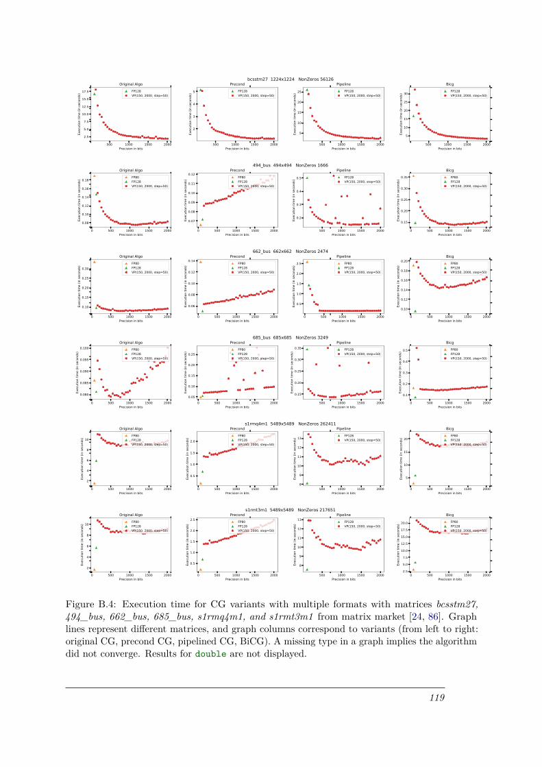
0.0 0.2 0.4 0.6 0.8 1.00.0

0.2

0.4

0.6

0.8

1.0

bcsstm27 1224x1224 NonZeros 56126

0.0 0.2 0.4 0.6 0.8 1.00.0

0.2

0.4

0.6

0.8

1.0

494_bus 494x494 NonZeros 1666

0.0 0.2 0.4 0.6 0.8 1.00.0

0.2

0.4

0.6

0.8

1.0

662_bus 662x662 NonZeros 2474

0.0 0.2 0.4 0.6 0.8 1.00.0

0.2

0.4

0.6

0.8

1.0

685_bus 685x685 NonZeros 3249

0.0 0.2 0.4 0.6 0.8 1.00.0

0.2

0.4

0.6

0.8

1.0

s1rmq4m1 5489x5489 NonZeros 262411

0.0 0.2 0.4 0.6 0.8 1.00.0

0.2

0.4

0.6

0.8

1.0

s1rmt3m1 5489x5489 NonZeros 217651

500 1000 1500 2000Precision in bits

2.5

5.0

7.5

10.0

12.5

15.0

17.5

Exec

utio

n tim

e (in

seco

nds)

Original AlgoFP128VP(150, 2000, step=50)

500 1000 1500 2000Precision in bits

2

3

4

5

Exec

utio

n tim

e (in

seco

nds)

PrecondFP128VP(150, 2000, step=50)

500 1000 1500 2000Precision in bits

5

10

15

20

25

Exec

utio

n tim

e (in

seco

nds)

PipelineFP128VP(150, 2000, step=50)

500 1000 1500 2000Precision in bits

5

10

15

20

25

30

Exec

utio

n tim

e (in

seco

nds)

BicgFP128VP(150, 2000, step=50)

0 500 1000 1500 2000Precision in bits

0.08

0.10

0.12

0.14

0.16

0.18

Exec

utio

n tim

e (in

seco

nds)

Original AlgoFP80FP128VP(150, 2000, step=50)

0 500 1000 1500 2000Precision in bits

0.07

0.08

0.09

0.10

0.11

0.12

Exec

utio

n tim

e (in

seco

nds)

PrecondFP80FP128VP(150, 2000, step=50)

500 1000 1500 2000Precision in bits

0.2

0.3

0.4

0.5

Exec

utio

n tim

e (in

seco

nds)

PipelineFP128VP(150, 2000, step=50)

0 500 1000 1500 2000Precision in bits

0.15

0.20

0.25

0.30

0.35

Exec

utio

n tim

e (in

seco

nds)

BicgFP80FP128VP(150, 2000, step=50)

0 500 1000 1500 2000Precision in bits

0.10

0.15

0.20

0.25

0.30

Exec

utio

n tim

e (in

seco

nds)

Original AlgoFP80FP128VP(150, 2000, step=50)

0 500 1000 1500 2000Precision in bits

0.06

0.08

0.10

0.12

0.14

Exec

utio

n tim

e (in

seco

nds)

PrecondFP80FP128VP(150, 2000, step=50)

0 500 1000 1500 2000Precision in bits

0.5

1.0

1.5

2.0

2.5

Exec

utio

n tim

e (in

seco

nds)

PipelineFP80FP128VP(150, 2000, step=50)

0 500 1000 1500 2000Precision in bits

0.10

0.12

0.14

0.16

0.18

0.20

Exec

utio

n tim

e (in

seco

nds)

BicgFP80FP128VP(150, 2000, step=50)

0 500 1000 1500 2000Precision in bits

0.080

0.085

0.090

0.095

0.100

Exec

utio

n tim

e (in

seco

nds)

Original AlgoFP80FP128VP(150, 2000, step=50)

0 500 1000 1500 2000Precision in bits

0.05

0.10

0.15

0.20

0.25

Exec

utio

n tim

e (in

seco

nds)

PrecondFP80FP128VP(150, 2000, step=50)

500 1000 1500 2000Precision in bits

0.15

0.20

0.25

0.30

0.35

Exec

utio

n tim

e (in

seco

nds)

PipelineFP128VP(150, 2000, step=50)

0 500 1000 1500 2000Precision in bits

0.1

0.2

0.3

0.4

0.5

Exec

utio

n tim

e (in

seco

nds)

BicgFP80FP128VP(150, 2000, step=50)

0 500 1000 1500 2000Precision in bits

2

4

6

8

10

Exec

utio

n tim

e (in

seco

nds)

Original AlgoFP80FP128VP(150, 2000, step=50)

0 500 1000 1500 2000Precision in bits

0.5

1.0

1.5

2.0

Exec

utio

n tim

e (in

seco

nds)

PrecondFP80FP128VP(150, 2000, step=50)

500 1000 1500 2000Precision in bits

8

9

10

11

12

13

Exec

utio

n tim

e (in

seco

nds)

PipelineFP128VP(150, 2000, step=50)

0 500 1000 1500 2000Precision in bits

5

10

15

20

Exec

utio

n tim

e (in

seco

nds)

BicgFP80FP128VP(150, 2000, step=50)

0 500 1000 1500 2000Precision in bits

2

4

6

8

10

Exec

utio

n tim

e (in

seco

nds)

Original AlgoFP80FP128VP(150, 2000, step=50)

0 500 1000 1500 2000Precision in bits

0.5

1.0

1.5

2.0

2.5

Exec

utio

n tim

e (in

seco

nds)

PrecondFP80FP128VP(150, 2000, step=50)

500 1000 1500 2000Precision in bits

8

9

10

11

12

13

Exec

utio

n tim

e (in

seco

nds)

PipelineFP128VP(150, 2000, step=50)

0 500 1000 1500 2000Precision in bits

2.5

5.0

7.5

10.0

12.5

15.0

17.5

20.0

Exec

utio

n tim

e (in

seco

nds)

BicgFP80FP128VP(150, 2000, step=50)

Figure B.4: Execution time for CG variants with multiple formats with matrices bcsstm27,494_bus, 662_bus, 685_bus, s1rmq4m1, and s1rmt3m1 from matrix market [24, 86]. Graphlines represent different matrices, and graph columns correspond to variants (from left to right:original CG, precond CG, pipelined CG, BiCG). A missing type in a graph implies the algorithmdid not converge. Results for double are not displayed.

119

0.0 0.2 0.4 0.6 0.8 1.00.0

0.2

0.4

0.6

0.8

1.0

s2rmt3m1 5489x5489 NonZeros 217681

0.0 0.2 0.4 0.6 0.8 1.00.0

0.2

0.4

0.6

0.8

1.0

s3rmq4m1 5489x5489 NonZeros 262943

0.0 0.2 0.4 0.6 0.8 1.00.0

0.2

0.4

0.6

0.8

1.0

s3rmt3m1 5489x5489 NonZeros 217669

0.0 0.2 0.4 0.6 0.8 1.00.0

0.2

0.4

0.6

0.8

1.0

plat362 362x362 NonZeros 5786

0 250 500 750 1000 1250 1500 1750 2000Precision in bits

5

10

15

20

25

30

35

40

Exec

utio

n tim

e (in

seco

nds)

Original AlgoFP80FP128VP(150, 2000, step=50)

0 250 500 750 1000 1250 1500 1750 2000Precision in bits

1

2

3

4

5Ex

ecut

ion

time

(in se

cond

s)

PrecondFP80FP128VP(150, 2000, step=50)

250 500 750 1000 1250 1500 1750 2000Precision in bits

30

35

40

45

50

Exec

utio

n tim

e (in

seco

nds)

PipelineFP128VP(150, 2000, step=50)

0 250 500 750 1000 1250 1500 1750 2000Precision in bits

10

20

30

40

50

60

70

80

Exec

utio

n tim

e (in

seco

nds)

BicgFP80FP128VP(150, 2000, step=50)

0 250 500 750 1000 1250 1500 1750 2000Precision in bits

10

20

30

40

50

60

Exec

utio

n tim

e (in

seco

nds)

Original AlgoFP80FP128VP(150, 2000, step=50)

0 250 500 750 1000 1250 1500 1750 2000Precision in bits

2

4

6

8

10

12

14

Exec

utio

n tim

e (in

seco

nds)

PrecondFP80FP128VP(150, 2000, step=50)

250 500 750 1000 1250 1500 1750 2000Precision in bits

30

40

50

60

70

80

Exec

utio

n tim

e (in

seco

nds)

PipelineFP128VP(150, 2000, step=50)

0 250 500 750 1000 1250 1500 1750 2000Precision in bits

20

40

60

80

100

120

Exec

utio

n tim

e (in

seco

nds)

BicgFP80FP128VP(150, 2000, step=50)

0 250 500 750 1000 1250 1500 1750 2000Precision in bits

20

30

40

50

60

70

80

Exec

utio

n tim

e (in

seco

nds)

Original AlgoFP80FP128VP(150, 2000, step=50)

0 250 500 750 1000 1250 1500 1750 2000Precision in bits

2

4

6

8

10

12

14

16

Exec

utio

n tim

e (in

seco

nds)

PrecondFP80FP128VP(150, 2000, step=50)

250 500 750 1000 1250 1500 1750 2000Precision in bits

40

60

80

100

Exec

utio

n tim

e (in

seco

nds)

PipelineFP128VP(150, 2000, step=50)

0 250 500 750 1000 1250 1500 1750 2000Precision in bits

40

60

80

100

120

140

160

Exec

utio

n tim

e (in

seco

nds)

BicgFP80FP128VP(150, 2000, step=50)

0 250 500 750 1000 1250 1500 1750 2000Precision in bits

0.0

0.5

1.0

1.5

2.0

2.5

3.0

3.5

Exec

utio

n tim

e (in

seco

nds)

Original AlgoFP80FP128VP(150, 2000, step=50)

0 250 500 750 1000 1250 1500 1750 2000Precision in bits

0

1

2

3

4

5

Exec

utio

n tim

e (in

seco

nds)

PrecondFP80FP128VP(150, 2000, step=50)

250 500 750 1000 1250 1500 1750 2000Precision in bits

0.2

0.4

0.6

0.8

1.0

1.2

1.4

Exec

utio

n tim

e (in

seco

nds)

PipelineFP128VP(150, 2000, step=50)

0 250 500 750 1000 1250 1500 1750 2000Precision in bits

0.5

1.0

1.5

2.0

Exec

utio

n tim

e (in

seco

nds)

BicgFP80FP128VP(150, 2000, step=50)

Figure B.5: Execution time for CG variants with multiple formats with matrices s2rmt3m1,s3rmq4m1, s3rmt3m1, and plat362 from matrix market [24, 86]. Graph lines represent differentmatrices, and graph columns correspond to variants (from left to right: original CG, precondCG, pipelined CG, BiCG). A missing type in a graph implies the algorithm did not converge.Results for double are not displayed.

120

Publications

Publications in International Conferences and Workshops• Tiago Trevisan Jost, Yves Durand, Christian Fabre, Albert Cohen, Frédéric Pétrot. Seam-

less Compiler Integration of Variable Precision Floating-Point Arithmetic InternationalSymposium on Code Generation and Optimization (CGO 2021)

• Tiago Jost, Yves Durand, Christian Fabre, Albert Cohen, Frédéric Pétrot. VP Float: FirstClass Treatment for Variable Precision Floating Point Arithmetic. ACM InternationalConference on Parallel Architectures and Compilation Techniques (PACT 2020) (pp.355–356)

• Andrea Bocco, Tiago T. Jost, Albert Cohen, Florent de Dinechin, Yves Durand, Chris-tian Fabre. Byte-Aware Floating-point Operations through a UNUM Computing Unit.IFIP/IEEE International Conference on Very Large Scale Integration (VLSI-SoC 2019)(pp. 323-328)

• Tiago T. Jost, Andrea Bocco, Yves Durand, Christian Fabre, Florent de Dinechin, andAlbert Cohen. Variable Precision Floating-Point RISC-V Coprocessor Evaluation usingLightweight Software and Compiler Support. Third Workshop on Computer ArchitectureResearch with RISC-V (CARRV’19).

121

Bibliography

[1] M. Abadi, A. Agarwal, P. Barham, E. Brevdo, Z. Chen, C. Citro, G. S. Corrado, A. Davis,J. Dean, M. Devin, S. Ghemawat, I. Goodfellow, A. Harp, G. Irving, M. Isard, Y. Jia,R. Jozefowicz, L. Kaiser, M. Kudlur, J. Levenberg, D. Mane, R. Monga, S. Moore, D.Murray, C. Olah, M. Schuster, J. Shlens, B. Steiner, I. Sutskever, K. Talwar, P. Tucker, V.Vanhoucke, V. Vasudevan, F. Viegas, O. Vinyals, P. Warden, M. Wattenberg, M. Wicke,Y. Yu, and X. Zheng. “TensorFlow: Large-Scale Machine Learning on HeterogeneousDistributed Systems”. In: arXiv:1603.04467 [cs] (Mar. 2016). url: http://arxiv.org/abs/1603.04467 (visited on 11/24/2020) (pages 1, 15).

[2] A. Abdelfattah, S. Tomov, and J. Dongarra. “Towards Half-Precision Computationfor Complex Matrices: A Case Study for Mixed Precision Solvers on GPUs”. In: 2019IEEE/ACM 10th Workshop on Latest Advances in Scalable Algorithms for Large-ScaleSystems (ScalA). Nov. 2019, pp. 17–24. doi: 10.1109/ScalA49573.2019.00008 (page 20).

[3] S. Abhyankar, J. Brown, E. M. Constantinescu, D. Ghosh, B. F. Smith, and H. Zhang.“PETSc/TS: A Modern Scalable ODE/DAE Solver Library”. In: arXiv preprint arXiv:1806.01437 (2018) (page 105).

[4] A. V. Aho, R. Sethi, and J. D. Ullman. “Compilers, principles, techniques”. In: Addisonwesley 7.8 (1986), p. 9 (page 63).

[5] A. Akkaş, M. J. Schulte, and J. E. Stine. “Intrinsic compiler support for interval arith-metic”. In: Numerical Algorithms 37.1 (2004), pp. 13–20 (page 15).

[6] A. Anderson and D. Gregg. “Vectorization of multibyte floating point data formats”.In: 2016 International Conference on Parallel Architecture and Compilation Techniques(PACT). Sept. 2016, pp. 363–372. doi: 10.1145/2967938.2967966 (page 24).

[7] J. Ansel, Y. L. Wong, C. Chan, M. Olszewski, A. Edelman, and S. Amarasinghe. “Languageand compiler support for auto-tuning variable-accuracy algorithms”. In: InternationalSymposium on Code Generation and Optimization (CGO 2011). Apr. 2011, pp. 85–96.doi: 10.1109/CGO.2011.5764677 (page 25).

[8] J. Ansel, C. Chan, Y. L. Wong, M. Olszewski, Q. Zhao, A. Edelman, and S. Amarasinghe.“PetaBricks: a language and compiler for algorithmic choice”. In: ACM SIGPLAN Notices44.6 (June 2009), pp. 38–49. issn: 0362-1340. doi: 10.1145/1543135.1542481. url:https://doi.org/10.1145/1543135.1542481 (visited on 02/12/2021) (page 25).

[9] M. G. Arnold. “The residue logarithmic number system: theory and implementation”. In:17th IEEE Symposium on Computer Arithmetic (ARITH’05). IEEE, 2005, pp. 196–205(pages 19, 24).

[10] M. Arnold, S. Fink, V. Sarkar, and P. F. Sweeney. “A comparative study of staticand profile-based heuristics for inlining”. In: ACM SIGPLAN Notices 35.7 (Jan. 2000),pp. 52–64. issn: 0362-1340. doi: 10.1145/351403.351416. url: https://doi.org/10.1145/351403.351416 (visited on 03/05/2021) (page 64).

123

[11] K. Asanović, R. Avizienis, J. Bachrach, S. Beamer, D. Biancolin, C. Celio, H. Cook,D. Dabbelt, J. Hauser, A. Izraelevitz, S. Karandikar, B. Keller, D. Kim, J. Koenig, Y.Lee, E. Love, M. Maas, A. Magyar, H. Mao, M. Moreto, A. Ou, D. A. Patterson, B.Richards, C. Schmidt, S. Twigg, H. Vo, and A. Waterman. The Rocket Chip Generator.UCB/EECS-2016-17. EECS Department, University of California, Berkeley, Apr. 2016.url: http://www2.eecs.berkeley.edu/Pubs/TechRpts/2016/EECS-2016-17.html(pages 28, 88).

[12] M. Baboulin, A. Buttari, J. Dongarra, J. Kurzak, J. Langou, J. Langou, P. Luszczek, andS. Tomov. “Accelerating scientific computations with mixed precision algorithms”. In:Computer Physics Communications 180.12 (Dec. 2009), pp. 2526–2533. doi: 10.1016/j.cpc.2008.11.005. url: https://www.research.manchester.ac.uk/portal/en/publications/accelerating-scientific-computations-with-mixed-precision-algorithms(5b73720d- 719c- 40dd- 8dad- d6262e5921cd)/export.html (visited on11/27/2020) (pages 10, 14, 20, 33).

[13] D. H. Bailey, R. Barrio, and J. M. Borwein. “High-precision computation: Mathematicalphysics and dynamics”. In: Applied Mathematics and Computation 218.20 (June 2012),pp. 10106–10121. issn: 0096-3003. doi: 10.1016/j.amc.2012.03.087. url: http://www.sciencedirect.com/science/article/pii/S0096300312003505 (visited on11/24/2020) (page 8).

[14] D. Bailey and J. Borwein. “High-Precision Arithmetic in Mathematical Physics”. In:Mathematics 3 (May 2015), pp. 337–367. doi: 10.3390/math3020337 (page 1).

[15] D. H. Bailey. “MPFUN: A portable high performance multiprecision package”. In: NASAAmes Research Center (1990) (pages 14, 21).

[16] D. H. Bailey. “Reproducibility and variable precision computing”. In: The InternationalJournal of High Performance Computing Applications 34.5 (Sept. 2020), pp. 483–490.issn: 1094-3420. doi: 10.1177/1094342020938424. url: https://doi.org/10.1177/1094342020938424 (visited on 12/13/2020) (pages 12, 14).

[17] D. H. Bailey, X. S. Li, and Y. Hida. QD: A Double-Double/Quad-Double Package.Lawrence Berkeley National Laboratory, 2003 (page 26).

[18] S. Balay, S. Abhyankar, M. F. Adams, J. Brown, P. Brune, K. Buschelman, L. Dalcin, A.Dener, V. Eijkhout, W. D. Gropp, D. Karpeyev, D. Kaushik, M. G. Knepley, D. A. May,L. C. McInnes, R. T. Mills, T. Munson, K. Rupp, P. Sanan, B. F. Smith, S. Zampini, H.Zhang, and H. Zhang. PETSc Web page. 2021. url: https://www.mcs.anl.gov/petsc(page 105).

[19] J. Bezanson, S. Karpinski, V. B. Shah, and A. Edelman. “Julia: A Fast Dynamic Languagefor Technical Computing”. In: arXiv:1209.5145 [cs] (Sept. 2012). url: http://arxiv.org/abs/1209.5145 (visited on 11/27/2020) (pages 22, 32, 90).

[20] L. S. Blackford, J. Choi, A. Cleary, E. D’Azevedo, J. Demmel, I. Dhillon, J. Dongarra, S.Hammarling, G. Henry, A. Petitet, et al. ScaLAPACK users’ guide. SIAM, 1997 (page 27).

[21] A. Bocco, Y. Durand, and F. d. Dinechin. “Dynamic Precision Numerics Using a Variable-Precision UNUM Type I HW Coprocessor”. In: 2019 IEEE 26th Symposium on ComputerArithmetic (ARITH). June 2019, pp. 104–107. doi: 10.1109/ARITH.2019.00028 (pages 9,37, 68).

124

[22] A. Bocco, T. T. Jost, A. Cohen, F. d. Dinechin, Y. Durand, and C. Fabre. “Byte-AwareFloating-point Operations through a UNUM Computing Unit”. In: 2019 IFIP/IEEE27th International Conference on Very Large Scale Integration (VLSI-SoC). Oct. 2019,pp. 323–328. doi: 10.1109/VLSI-SoC.2019.8920387 (pages 9, 10).

[23] A. Bocco, Y. Durand, and F. d. Dinechin. “SMURF: Scalar Multiple-precision UnumRisc-V Floating-point Accelerator for Scientific Computing”. In: ACM, Mar. 2019, pp. 1–8.doi: 10.1145/3316279.3316280. url: https://hal.inria.fr/hal-02087098 (visitedon 11/27/2020) (pages 10, 28, 37, 68, 74, 88).

[24] R. F. Boisvert, R. Pozo, K. Remington, R. F. Barrett, and J. J. Dongarra. “Matrix market:a web resource for test matrix collections”. In: Proceedings of the IFIP TC2/WG2.5working conference on Quality of numerical software: assessment and enhancement. GBR:Chapman & Hall, Ltd., Jan. 1997, pp. 125–137. isbn: 978-0-412-80530-1. (Visited on11/27/2020) (pages 13, 14, 94, 97, 98, 100, 101, 110–114, 116–120).

[25] U. Bondhugula, A. Hartono, J. Ramanujam, and P. Sadayappan. “A Practical Auto-matic Polyhedral Program Optimization System”. In: ACM SIGPLAN Conference onProgramming Language Design and Implementation (PLDI). June 2008 (pages 52, 66).

[26] R. P. Brent. “An idealist’s view of semantics for integer and real types”. In: AustralianComputer Science Communications 4 (1982), pp. 130–140 (page 21).

[27] A. Buttari, J. Langou, J. Kurzak, and J. Dongarra. “A class of parallel tiled linearalgebra algorithms for multicore architectures”. In: Parallel Computing 35.1 (2009),pp. 38–53. issn: 0167-8191. doi: https://doi.org/10.1016/j.parco.2008.10.002.url: http://www.sciencedirect.com/science/article/pii/S0167819108001117(page 27).

[28] Z. Carmichael, H. F. Langroudi, C. Khazanov, J. Lillie, J. L. Gustafson, and D. Ku-dithipudi. “Deep Positron: A Deep Neural Network Using the Posit Number System”. In:arXiv:1812.01762 [cs] (Jan. 2019). url: http://arxiv.org/abs/1812.01762 (visitedon 11/27/2020) (pages 10, 105).

[29] E. Carson and N. J. Higham. “Accelerating the Solution of Linear Systems by IterativeRefinement in Three Precisions”. In: SIAM Journal on Scientific Computing 40.2 (Jan.2018), A817–A847. issn: 1064-8275. doi: 10.1137/17M1140819. url: https://epubs.siam.org/doi/abs/10.1137/17M1140819 (visited on 11/27/2020) (pages 20, 31).

[30] E. Carson and Z. Strakoš. “On the cost of iterative computations”. In: PhilosophicalTransactions of the Royal Society A: Mathematical, Physical and Engineering Sciences378.2166 (Mar. 2020), p. 20190050. issn: 1364-503X, 1471-2962. doi: 10.1098/rsta.2019.0050. url: https://royalsocietypublishing.org/doi/10.1098/rsta.2019.0050(visited on 11/25/2020) (page 96).

[31] E. C. Carson, M. Rozložník, Z. Strakoš, P. Tichý, and M. Tůma. “The NumericalStability Analysis of Pipelined Conjugate Gradient Methods: Historical Context andMethodology”. In: SIAM Journal on Scientific Computing 40.5 (2018), A3549–A3580.doi: 10.1137/16M1103361. url: https://doi.org/10.1137/16M1103361 (pages 93,95).

[32] S. W. D. Chien, I. B. Peng, and S. Markidis. “Posit NPB: Assessing the PrecisionImprovement in HPC Scientific Applications”. In: arXiv:1907.05917 [cs] 12043 (2020),pp. 301–310. doi: 10.1007/978-3-030-43229-4_26. url: http://arxiv.org/abs/1907.05917 (visited on 11/27/2020) (page 24).

125

[33] S. Chowdhary, J. P. Lim, and S. Nagarakatte. “Debugging and detecting numerical errorsin computation with posits”. In: Proceedings of the 41st ACM SIGPLAN Conference onProgramming Language Design and Implementation. PLDI 2020. New York, NY, USA:Association for Computing Machinery, June 2020, pp. 731–746. isbn: 978-1-4503-7613-6.doi: 10.1145/3385412.3386004. url: https://doi.org/10.1145/3385412.3386004(visited on 12/10/2020) (page 25).

[34] S. Cools, J. Cornelis, and W. Vanroose. “Numerically Stable Recurrence Relations for theCommunication Hiding Pipelined Conjugate Gradient Method”. In: IEEE Transactionson Parallel and Distributed Systems 30.11 (2019), pp. 2507–2522. doi: 10.1109/TPDS.2019.2917663 (pages 95, 105).

[35] S. Cools, J. Cornelis, P. Ghysels, and W. Vanroose. “Improving strong scaling of theConjugate Gradient method for solving large linear systems using global reductionpipelining”. In: CoRR abs/1905.06850 (2019). url: http://arxiv.org/abs/1905.06850(pages 95, 105).

[36] S. Cools, W. Vanroose, E. F. Yetkin, E. Agullo, and L. Giraud. “On rounding errorresilience, maximal attainable accuracy and parallel performance of the pipelined Conju-gate Gradients method for large-scale linear systems in PETSc”. In: Proceedings of theExascale Applications and Software Conference 2016. EASC ’16. New York, NY, USA:Association for Computing Machinery, Apr. 2016, pp. 1–10. isbn: 978-1-4503-4122-6.doi: 10.1145/2938615.2938621. url: https://doi.org/10.1145/2938615.2938621(visited on 04/03/2021) (pages 95, 105).

[37] J. Cornelis, S. Cools, and W. Vanroose. “The Communication-Hiding Conjugate GradientMethod with Deep Pipelines”. In: CoRR abs/1801.04728 (2018). url: http://arxiv.org/abs/1801.04728 (pages 94, 95).

[38] C. Courbet. “NSan: a floating-point numerical sanitizer”. In: Proceedings of the 30th ACMSIGPLAN International Conference on Compiler Construction. CC 2021. New York, NY,USA: Association for Computing Machinery, Mar. 2021, pp. 83–93. isbn: 978-1-4503-8325-7. doi: 10.1145/3446804.3446848. url: https://doi.org/10.1145/3446804.3446848(visited on 04/01/2021) (page 25).

[39] L. Dagum and R. Menon. “OpenMP: an industry standard API for shared-memoryprogramming”. In: IEEE Computational Science and Engineering 5.1 (Jan. 1998), pp. 46–55. issn: 1558-190X. doi: 10.1109/99.660313 (page 66).

[40] E. Darulova and V. Kuncak. “On Sound Compilation of Reals”. In: arXiv:1309.2511[cs] (Sept. 2013). url: http://arxiv.org/abs/1309.2511 (visited on 11/25/2020)(page 25).

[41] L. Deniau and A. Naumann. Proposal for classes with runtime size. Document number:N4188. 2014. url: http://www.open-std.org/JTC1/SC22/wg21/docs/papers/2014/n4188.pdf (page 48).

[42] F. de Dinechin, L. Forget, J.-M. Muller, and Y. Uguen. “Posits: the good, the bad and theugly”. In: Proceedings of the Conference for Next Generation Arithmetic 2019. CoNGA’19.New York, NY, USA: Association for Computing Machinery, Mar. 2019, pp. 1–10. isbn:978-1-4503-7139-1. doi: 10.1145/3316279.3316285. url: https://doi.org/10.1145/3316279.3316285 (visited on 11/27/2020) (pages 10, 38, 105).

[43] J. Dongarra. Freely Available Software for Linear Algebra (September 2018). 2018. url:http://www.netlib.org/utk/people/JackDongarra/la-sw.html (page 13).

126

[44] J. J. Dongarra, D. C. Sorensen, and S. J. Hammarling. “Block reduction of matrices tocondensed forms for eigenvalue computations”. In: Journal of Computational and AppliedMathematics 27.1 (1989), pp. 215–227. issn: 0377-0427. doi: https://doi.org/10.1016/0377-0427(89)90367-1. url: http://www.sciencedirect.com/science/article/pii/0377042789903671 (page 27).

[45] I. o. Electrical, E. E. C. S. S. Committee, and D. Stevenson. IEEE standard for binaryfloating-point arithmetic. IEEE, 1985 (pages 1, 7).

[46] J. S. Ely. “The VPI software package for variable precision interval arithmetic”. In:Interval Computations 2.2 (1993), pp. 135–153 (page 28).

[47] H. Esmaeilzadeh, E. Blem, R. S. Amant, K. Sankaralingam, and D. Burger. “Dark siliconand the end of multicore scaling”. In: 2011 38th Annual International Symposium onComputer Architecture (ISCA). 2011, pp. 365–376 (page 88).

[48] A. Fabri, G.-J. Giezeman, L. Kettner, S. Schirra, and S. Schönherr. “On the designof CGAL a computational geometry algorithms library”. In: Software: Practice andExperience 30.11 (2000), pp. 1167–1202. issn: 1097-024X. doi: https://doi.org/10.1002/1097-024X(200009)30:11<1167::AID-SPE337>3.0.CO;2-B. url: https://onlinelibrary.wiley.com/doi/abs/10.1002/1097-024X%28200009%2930%3A11%3C1167%3A%3AAID-SPE337%3E3.0.CO%3B2-B (visited on 12/04/2020) (page 22).

[49] L. Fousse, G. Hanrot, V. Lefèvre, P. Pélissier, and P. Zimmermann. “MPFR: A multiple-precision binary floating-point library with correct rounding”. In: ACM Transactions onMathematical Software 33.2 (June 2007), 13–es. issn: 0098-3500. doi: 10.1145/1236463.1236468. url: https://doi.org/10.1145/1236463.1236468 (visited on 11/27/2020)(pages xvii, 7, 10, 14, 21, 26, 33, 35, 68).

[50] A. M. Frolov and D. H. Bailey. “Highly accurate evaluation of the few-body auxiliaryfunctions and four-body integrals”. In: Journal of Physics B: Atomic, Molecular andOptical Physics 36.9 (Apr. 2003), pp. 1857–1867. issn: 0953-4075. doi: 10.1088/0953-4075/36/9/315. url: https://doi.org/10.1088%2F0953-4075%2F36%2F9%2F315(visited on 11/24/2020) (page 1).

[51] P. Ghysels and W. Vanroose. “Hiding global synchronization latency in the preconditionedConjugate Gradient algorithm”. In: Parallel Computing. 7th Workshop on Parallel MatrixAlgorithms and Applications 40.7 (July 2014), pp. 224–238. issn: 0167-8191. doi: 10.1016/j.parco.2013.06.001. url: https://www.sciencedirect.com/science/article/pii/S0167819113000719 (visited on 03/30/2021) (page 92).

[52] F. Glaser, S. Mach, A. Rahimi, F. K. Gürkaynak, Q. Huang, and L. Benini. “An 826MOPS, 210uW/MHz Unum ALU in 65 nm”. In: 2018 IEEE International Symposium onCircuits and Systems (ISCAS). May 2018, pp. 1–5. doi: 10.1109/ISCAS.2018.8351546(pages 9, 10, 29).

[53] D. Goldberg. “What every computer scientist should know about floating-point arith-metic”. In: ACM Computing Surveys 23.1 (Mar. 1991), pp. 5–48. issn: 0360-0300. doi:10.1145/103162.103163. url: https://doi.org/10.1145/103162.103163 (visited on11/27/2020) (page 6).

[54] T. Granlund. GNU Multiple Precision Arithmetic Library 6.1.2. Dec. 2016 (pages 7, 14,21, 26, 33, 68).

[55] T. Grosser, H. Zheng, R. Aloor, A. Simbürger, A. Größlinger, and L.-N. Pouchet. “Polly– Polyhedral optimization in LLVM”. In: Proceedings of the First International Workshopon Polyhedral Compilation Techniques (IMPACT). 2011, pp. 1–6 (pages 66, 80).

127

[56] G. Guennebaud, B. Jacob, et al. Eigen v3. 2010. url: http://eigen.tuxfamily.org(page 105).

[57] J. L. Gustafson. The End of Error: Unum Computing. CRC Press, 2017 (pages 9, 36, 68,75).

[58] Gustafson and Yonemoto. “Beating Floating Point at its Own Game: Posit Arithmetic”.In: Supercomputing Frontiers and Innovations: an International Journal 4.2 (June 2017),pp. 71–86. issn: 2409-6008. doi: 10.14529/jsfi170206. url: https://doi.org/10.14529/jsfi170206 (visited on 11/27/2020) (pages 9, 24, 27, 38).

[59] A. Haidar, S. Tomov, J. Dongarra, and N. J. Higham. “Harnessing GPU Tensor Coresfor Fast FP16 Arithmetic to Speed up Mixed-Precision Iterative Refinement Solvers”. In:SC18: International Conference for High Performance Computing, Networking, Storageand Analysis. Nov. 2018, pp. 603–613. doi: 10.1109/SC.2018.00050 (page 20).

[60] A. Haidar, H. Bayraktar, S. Tomov, J. Dongarra, and N. J. Higham. “Mixed-precisioniterative refinement using tensor cores on GPUs to accelerate solution of linear systems”.In: Proceedings of the Royal Society A: Mathematical, Physical and Engineering Sciences476.2243 (2020), p. 20200110 (page 20).

[61] A. Haidar, P. Wu, S. Tomov, and J. Dongarra. “Investigating Half Precision Arithmeticto Accelerate Dense Linear System Solvers”. In: Proceedings of the 8th Workshop onLatest Advances in Scalable Algorithms for Large-Scale Systems. ScalA ’17. New York,NY, USA: Association for Computing Machinery, 2017. isbn: 978-1-4503-5125-6. doi:10.1145/3148226.3148237. url: https://doi.org/10.1145/3148226.3148237(page 20).

[62] J. Hauser. SoftFloat. 1997. url: http://www.jhauser.us/arithmetic/SoftFloat.html(page 24).

[63] M. R. Hestenes, E. Stiefel, et al. “Methods of conjugate gradients for solving linearsystems”. In: Journal of research of the National Bureau of Standards 49.6 (1952),pp. 409–436 (pages 90, 91, 93).

[64] N. J. Higham. Accuracy and stability of numerical algorithms. SIAM, 2002 (pages 1, 11,12, 31).

[65] J. Hou, Y. Zhu, S. Du, and S. Song. “Enhancing Accuracy and Dynamic Range ofScientific Data Analytics by Implementing Posit Arithmetic on FPGA”. In: Journalof Signal Processing Systems 91.10 (Oct. 2019), pp. 1137–1148. issn: 1939-8115. doi:10.1007/s11265-018-1420-5. url: https://doi.org/10.1007/s11265-018-1420-5(visited on 11/27/2020) (page 10).

[66] IBM. IBM System/360 Principles of Operation. IBM Press, 1964 (page 7).[67] IEEE. “IEEE Standard for Floating-Point Arithmetic, IEEE Std 754-2019 (Revision of

IEEE 754-2008)”. In: Institute of Electrical and Electronics Engineers New York, 2019(page 7).

[68] K. Isupov. “Using Floating-Point Intervals for Non-Modular Computations in ResidueNumber System”. In: IEEE Access 8 (2020), pp. 58603–58619. issn: 2169-3536. doi:10.1109/ACCESS.2020.2982365 (page 19).

[69] M. K. Jaiswal and H. K. So. “PACoGen: A Hardware Posit Arithmetic Core Generator”.In: IEEE Access 7 (2019), pp. 74586–74601. issn: 2169-3536. doi: 10.1109/ACCESS.2019.2920936 (pages 10, 29).

128

[70] J. Johnson. “Rethinking floating point for deep learning”. In: arXiv:1811.01721 [cs] (Nov.2018). url: http://arxiv.org/abs/1811.01721 (visited on 11/27/2020) (pages 10, 24,105).

[71] M. Joldes, J.-M. Muller, V. Popescu, andW. Tucker. “CAMPARY: Cuda multiple precisionarithmetic library and applications”. In: International Congress on Mathematical Software.Springer, 2016, pp. 232–240 (page 21).

[72] D. Kalamkar, D. Mudigere, N. Mellempudi, D. Das, K. Banerjee, S. Avancha, D. T.Vooturi, N. Jammalamadaka, J. Huang, H. Yuen, J. Yang, J. Park, A. Heinecke, E.Georganas, S. Srinivasan, A. Kundu, M. Smelyanskiy, B. Kaul, and P. Dubey. “A Studyof BFLOAT16 for Deep Learning Training”. In: arXiv:1905.12322 [cs, stat] (June 2019).url: http://arxiv.org/abs/1905.12322 (visited on 11/24/2020) (page 1).

[73] J. G. Kemeny, T. E. Kurtz, and D. S. Cochran. Basic: a manual for BASIC, the elementaryalgebraic language designed for use with the Dartmouth Time Sharing System. DartmouthPublications, 1968 (page 7).

[74] N. G. Kingsbury and P. J. Rayner. “Digital filtering using logarithmic arithmetic”. In:Electronics Letters 7.2 (1971), pp. 56–58 (page 24).

[75] U. Kulisch. Computer arithmetic and validity: theory, implementation, and applications.Vol. 33. Walter de Gruyter, 2013 (pages 24, 27, 50).

[76] C. Lattner and V. Adve. “LLVM: a compilation framework for lifelong program analysistransformation”. In: International Symposium on Code Generation and Optimization,2004. CGO 2004. Mar. 2004, pp. 75–86. doi: 10.1109/CGO.2004.1281665 (pages 8, 15,59).

[77] C. L. Lawson, R. J. Hanson, D. R. Kincaid, and F. T. Krogh. “Basic Linear AlgebraSubprograms for Fortran Usage”. In: ACM Transactions on Mathematical Software5.3 (Sept. 1979), pp. 308–323. issn: 0098-3500. doi: 10.1145/355841.355847. url:https://doi.org/10.1145/355841.355847 (visited on 11/27/2020) (pages 26, 36).

[78] R. Leavitt. “Adjustable precision floating point arithmetic in Ada”. In: ACM SIGAdaAda Letters VII.5 (Sept. 1987), pp. 63–78. issn: 1094-3641. doi: 10.1145/36077.36082.url: https://doi.org/10.1145/36077.36082 (visited on 11/27/2020) (page 21).

[79] J. Lee, G. D. Peterson, D. S. Nikolopoulos, and H. Vandierendonck. “AIR: Iterativerefinement acceleration using arbitrary dynamic precision”. In: Parallel Computing 97(Sept. 2020), p. 102663. issn: 0167-8191. doi: 10.1016/j.parco.2020.102663. url:http://www.sciencedirect.com/science/article/pii/S0167819120300569 (visitedon 01/06/2021) (page 20).

[80] X. S. Li, J. W. Demmel, D. H. Bailey, G. Henry, Y. Hida, J. Iskandar, W. Kahan, S. Y.Kang, A. Kapur, M. C. Martin, B. J. Thompson, T. Tung, and D. J. Yoo. “Design,implementation and testing of extended and mixed precision BLAS”. In: ACM Trans-actions on Mathematical Software 28.2 (June 2002), pp. 152–205. issn: 0098-3500. doi:10.1145/567806.567808. url: https://doi.org/10.1145/567806.567808 (visited on12/09/2020) (pages 26, 49).

[81] P. Lindstrom. “Universal Coding of the Reals using Bisection”. In: Proceedings of theConference for Next Generation Arithmetic 2019. CoNGA’19. New York, NY, USA:Association for Computing Machinery, Mar. 2019, pp. 1–10. isbn: 978-1-4503-7139-1.doi: 10.1145/3316279.3316286. url: https://doi.org/10.1145/3316279.3316286(visited on 12/15/2020) (page 24).

129

[82] P. Lindstrom, S. Lloyd, and J. Hittinger. “Universal coding of the reals: alternatives toIEEE floating point”. In: Proceedings of the Conference for Next Generation Arithmetic.CoNGA ’18. New York, NY, USA: Association for Computing Machinery, Mar. 2018,pp. 1–14. isbn: 978-1-4503-6414-0. doi: 10.1145/3190339.3190344. url: https://doi.org/10.1145/3190339.3190344 (visited on 11/27/2020) (pages 14, 24).

[83] G. S. Lloyd. unum. url: https://github.com/LLNL/unum (pages 14, 24).[84] C. Long. Softposit. 2019. url: https://gitlab.com/cerlane/SoftPosit/-/wikis/

home (pages 14, 24).[85] J. Maddock and C. Kormanyos. Boost.Multiprecision. 2020 (pages 22, 72, 79).[86] Matrix Market repository. 2007. url: https://math.nist.gov/MatrixMarket/ (pages 13,

14, 94, 97, 98, 100, 101, 110–114, 116–120).[87] V. Ménissier-Morain. “Arbitrary precision real arithmetic: design and algorithms”. In:

The Journal of Logic and Algebraic Programming. Practical development of exact realnumber computation 64.1 (July 2005), pp. 13–39. issn: 1567-8326. doi: 10.1016/j.jlap.2004.07.003. url: http://www.sciencedirect.com/science/article/pii/S1567832604000748 (visited on 12/22/2020) (pages 10, 19).

[88] S. Mittal. “A Survey of Techniques for Approximate Computing”. In: ACM ComputingSurveys 48.4 (Mar. 2016), 62:1–62:33. issn: 0360-0300. doi: 10.1145/2893356. url:https://doi.org/10.1145/2893356 (visited on 11/24/2020) (page 2).

[89] G. E. Moore. “Cramming more components onto integrated circuits, Reprinted fromElectronics, volume 38, number 8, April 19, 1965, pp.114 ff.” In: IEEE Solid-State CircuitsSociety Newsletter 11.3 (Sept. 2006), pp. 33–35. issn: 1098-4232. doi: 10.1109/N-SSC.2006.4785860 (page 1).

[90] R. E. Moore, R. B. Kearfott, and M. J. Cloud. Introduction to interval analysis. SIAM,2009 (page 19).

[91] J.-M. Muller, N. Brunie, F. de Dinechin, C.-P. Jeannerod, M. Joldes, V. Lefèvre, G.Melquiond, N. Revol, and S. Torres. Handbook of Floating-Point Arithmetic, 2nd edition.Birkhäuser Boston, 2018 (page 12).

[92] M. Nakata. The MPACK (MBLAS/MLAPACK) a multiple precision arithmetic versionof BLAS and LAPACK. http://mplapack.sourceforge.net/, 2010 (page 26).

[93] E. T. L. Omtzigt, P. Gottschling, M. Seligman, and W. Zorn. Universal Number Library.url: https://github.com/stillwater-sc/universal (page 24).

[94] E. T. L. Omtzigt, P. Gottschling, M. Seligman, and W. Zorn. “Universal Numbers Library:design and implementation of a high-performance reproducible number systems library”.In: arXiv e-prints (2020), arXiv–2012 (page 24).

[95] J. F. Palmer. “The Intel® 8087 numeric data processor”. In: Proceedings of the May19-22, 1980, national computer conference. 1980, pp. 887–893 (page 7).

[96] P. Panchekha, A. Sanchez-Stern, J. R. Wilcox, and Z. Tatlock. “Automatically improvingaccuracy for floating point expressions”. In: Proceedings of the 36th ACM SIGPLANConference on Programming Language Design and Implementation. PLDI ’15. New York,NY, USA: Association for Computing Machinery, June 2015, pp. 1–11. isbn: 978-1-4503-3468-6. doi: 10.1145/2737924.2737959. url: https://doi.org/10.1145/2737924.2737959 (visited on 02/12/2021) (page 25).

130

[97] F. M. Q. Pereira and J. Palsberg. “SSA Elimination after Register Allocation”. In:Compiler Construction. Ed. by O. de Moor and M. I. Schwartzbach. Lecture Notes inComputer Science. Berlin, Heidelberg: Springer, 2009, pp. 158–173. isbn: 978-3-642-00722-4. doi: 10.1007/978-3-642-00722-4_12 (page 76).

[98] L.-N. Pouchet et al. PolyBench: The polyhedral benchmark suite. 2012 (pages 6, 80).[99] RAJAPerf. url: https://github.com/LLNL/RAJAPerf (page 85).

[100] N. Revol. “Introduction to the IEEE 1788-2015 Standard for Interval Arithmetic”. In:10th International Workshop on Numerical Software Verification - NSV 2017, workshopof CAV 2017. Ed. by A. Abate and S. Boldo. LNCS. Heidelberg, Germany: Springer, July2017, pp. 14–21. doi: 10.1007/978-3-319-63501-9. url: https://hal.inria.fr/hal-01559955 (page 19).

[101] N. Revol. “The MPFI Library: Towards IEEE 1788–2015 Compliance”. In: InternationalConference on Parallel Processing and Applied Mathematics. Springer, 2019, pp. 353–363(page 22).

[102] C. Rubio-González, Cuong Nguyen, Hong Diep Nguyen, J. Demmel, W. Kahan, K. Sen,D. H. Bailey, C. Iancu, and D. Hough. “Precimonious: Tuning assistant for floating-pointprecision”. In: SC ’13: Proceedings of the International Conference on High PerformanceComputing, Networking, Storage and Analysis. Nov. 2013, pp. 1–12. doi: 10.1145/2503210.2503296 (page 25).

[103] C. Rubio-González, C. Nguyen, B. Mehne, K. Sen, J. Demmel, W. Kahan, C. Iancu,W. Lavrijen, D. H. Bailey, and D. Hough. “Floating-Point Precision Tuning Using BlameAnalysis”. In: 38th International Conference on Software Engineering. Ed. by W. Visserand L. Williams. Austin, Texas: IEEE TCSE and ACM SIGSOFT, May 2016 (page 25).

[104] Y. Saad. Iterative Methods for Sparse Linear Systems. Other Titles in Applied Mathemat-ics. Society for Industrial and Applied Mathematics, Jan. 2003. isbn: 978-0-89871-534-7.doi: 10.1137/1.9780898718003. url: https://epubs.siam.org/doi/book/10.1137/1.9780898718003 (visited on 12/01/2020) (page 93).

[105] A. Sanchez-Stern, P. Panchekha, S. Lerner, and Z. Tatlock. “Finding root causes of floatingpoint error”. In: Proceedings of the 39th ACM SIGPLAN Conference on ProgrammingLanguage Design and Implementation. PLDI 2018. New York, NY, USA: Associationfor Computing Machinery, June 2018, pp. 256–269. isbn: 978-1-4503-5698-5. doi: 10.1145/3192366.3192411. url: https://doi.org/10.1145/3192366.3192411 (visitedon 02/12/2021) (page 25).

[106] C. Sanderson and R. Curtin. “Armadillo: a template-based C++ library for linear algebra”.In: Journal of Open Source Software 1.2 (2016), p. 26. doi: 10.21105/joss.00026. url:https://doi.org/10.21105/joss.00026 (page 105).

[107] M. J. Schulte and E. E. Swartzlander. “A family of variable-precision interval arithmeticprocessors”. In: IEEE Transactions on Computers 49.5 (May 2000), pp. 387–397. issn:1557-9956. doi: 10.1109/12.859535 (pages 27, 28).

[108] S. Shrimpton. An Implementation of MIL-STD-1750 Airborne Computer Instruction SetArchitecture. ROYAL AIRCRAFT ESTABLISHMENT FARNBOROUGH (ENGLAND),1981 (page 7).

131

[109] A. F. d. Silva, B. N. B. de Lima, and F. M. Q. Pereira. “Exploring the Space ofOptimization Sequences for Code-Size Reduction: Insights and Tools”. In: Proceedingsof the 30th ACM SIGPLAN International Conference on Compiler Construction. CC2021. New York, NY, USA: Association for Computing Machinery, 2021, pp. 47–58. isbn:978-1-4503-8325-7. doi: 10.1145/3446804.3446849. url: https://doi.org/10.1145/3446804.3446849 (page 81).

[110] M. Snir, W. Gropp, S. Otto, S. Huss-Lederman, J. Dongarra, and D. Walker. MPI–theComplete Reference: the MPI core. Vol. 1. MIT press, 1998 (page 92).

[111] J. Snyder and R. Smith. Exploring classes of runtime size. Document number: N4025. 2014.url: http://www.open-std.org/jtc1/sc22/wg21/docs/papers/2014/n4025.pdf(page 48).

[112] I. C. Soc. IEEE Standard for Floating-Point Arithmetic (IEEE Std 754-2008). IEEE NewYork, 2008 (page 7).

[113] R. Stallman et al. The GNU project. 1998 (pages 8, 15).[114] G. Tagliavini, A. Marongiu, and L. Benini. “FlexFloat: A Software Library for Trans-

precision Computing”. In: IEEE Transactions on Computer-Aided Design of IntegratedCircuits and Systems 39.1 (Jan. 2020), pp. 145–156. issn: 1937-4151. doi: 10.1109/TCAD.2018.2883902 (page 24).

[115] S. Tiwari, N. Gala, C. Rebeiro, and V. Kamakoti. “PERI: A Posit Enabled RISC-VCore”. In: arXiv:1908.01466 [cs] (Aug. 2019). url: http://arxiv.org/abs/1908.01466(visited on 11/27/2020) (pages 10, 29).

[116] S. Tomov, J. Dongarra, and M. Baboulin. “Towards dense linear algebra for hybridGPU accelerated manycore systems”. In: Parallel Matrix Algorithms and Applications36.5 (June 2010), pp. 232–240. issn: 0167-8191. doi: 10.1016/j.parco.2009.12.005(page 27).

[117] G. Van Rossum and F. L. Drake Jr. Python reference manual. Centrum voor Wiskundeen Informatica Amsterdam, 1995 (pages 22, 32, 90).

[118] F. G. Van Zee and R. A. Van De Geijn. “BLIS: A framework for rapidly instantiatingBLAS functionality”. In: ACM Transactions on Mathematical Software (TOMS) 41.3(2015), pp. 1–33 (page 26).

[119] S. Verdoolaege, J. Carlos Juega, A. Cohen, J. Ignacio Gómez, C. Tenllado, and F.Catthoor. “Polyhedral parallel code generation for CUDA”. In: ACM Transactions onArchitecture and Code Optimization 9.4 (Jan. 2013), 54:1–54:23. issn: 1544-3566. doi:10.1145/2400682.2400713. url: https://doi.org/10.1145/2400682.2400713(visited on 03/19/2021) (page 66).

[120] E. Wang, Q. Zhang, B. Shen, G. Zhang, X. Lu, Q. Wu, and Y. Wang. “Intel math kernellibrary”. In: High-Performance Computing on the Intel® Xeon Phi™. Springer, 2014,pp. 167–188 (page 26).

[121] A. Waterman, Y. Lee, D. A. Patterson, and K. Asanovic. “The RISC-V instruction setmanual, volume i: User-level ISA”. In: CS Division, EECE Department, University ofCalifornia, Berkeley (2014) (pages 28, 74).

[122] R. C. Whaley and J. Dongarra. “Automatically Tuned Linear Algebra Software”. In:SuperComputing 1998: High Performance Networking and Computing. 1998 (page 26).

[123] W. A. Wulf and S. A. McKee. “Hitting the memory wall: Implications of the obvious”.In: ACM SIGARCH computer architecture news 23.1 (1995), pp. 20–24 (page 16).

132

[124] Z. Xianyi, W. Qian, and Z. Chothia. “OpenBLAS”. In: URL: http://xianyi. github.io/OpenBLAS (2012), p. 88 (pages 26, 94).

[125] Q. Xu, T. Mytkowicz, and N. S. Kim. “Approximate Computing: A Survey”. In: IEEEDesign Test 33.1 (Feb. 2016), pp. 8–22. issn: 2168-2364. doi: 10.1109/MDAT.2015.2505723 (pages 2, 25).

[126] C. Yap and T. Dubé. “The exact computation paradigm”. In: Computing in EuclideanGeometry. Vol. Volume 4. Lecture Notes Series on Computing Volume 4. WORLD SCIEN-TIFIC, Jan. 1995, pp. 452–492. isbn: 978-981-02-1876-8. doi: 10.1142/9789812831699_0011. url: https://www.worldscientific.com/doi/abs/10.1142/9789812831699_0011 (visited on 12/02/2020) (page 19).

[127] T. J. Ypma. “Historical Development of the Newton-Raphson Method”. In: SIAM Review37.4 (1995), pp. 531–551. issn: 0036-1445. url: https://www.jstor.org/stable/2132904 (visited on 12/01/2020) (pages 11, 20).

[128] A. F. Zanella, A. F. da Silva, and F. M. Quintão. “YACOS: A Complete Infrastructureto the Design and Exploration of Code Optimization Sequences”. In: Proceedings of the24th Brazilian Symposium on Context-Oriented Programming and Advanced Modularity.SBLP ’20. New York, NY, USA: Association for Computing Machinery, 2020, pp. 56–63.isbn: 978-1-4503-8943-3. doi: 10.1145/3427081.3427089. url: https://doi.org/10.1145/3427081.3427089 (page 81).

133