Thermodynamics, Solubility and Environmental Issues - E-Library

Thermodynamics, Solubility and Environmental Issues by Trevor M. Letcher (Editor)

• ISBN: 0444527079

• Publisher: Elsevier Science & Technology Books

• Pub. Date: June 2007

Preface

Environmental problems are becoming an important aspect of our lives as industries grow apace with populations throughout the world. Solubility is one of the most basic and important of thermodynamic properties, and a property that underlies most environmental issues. This book is a collection of twenty-five chapters of fundamental principles and recent research work, coming from disparate disciplines but all related to solubility and environmental pollution. Links between these chapters, we believe, could lead to new ways of solving new and also old environmental issues. Underlying this philosophy is our inherent belief that a book is an important vehicle for the dissemination of knowledge.

Our book "Thermodynamics, Solubility and Environmental Issues" had its origins in committee meetings of the International Association of Chemical Thermodynamics and in discussions with members of the International Union of Pure and Applied Chemistry (IUPAC) subcommittee on Solubility, in particular Professor Glenn Hefter of the University of Monash, Perth, Dr Justin Salminen of the University of California, Berkeley and Professor Heinz Gamsj~ieger of the University of Leoben, Austria. It is a project produced under the auspices of the IUPAC. In true IUPAC style, the authors, important names in their respective fields, come from many countries around the world, including: Australia, Austria, Canada, Brazil, Finland, France, Greece, Italy, Japan, Poland, Portugal, South Africa, Spain, United Kingdom and the United States of America.

The book highlights environmental issues in areas such as mining, polymer manufacture and applications, radioactive wastes, industries in general, agro-chemicals, soil pollution and biology, together with the basic theory and recent developments in the modelling of environmental

Preface

pollutants - all of which are linked to the basic property of solubility. It includes chapters on:

• Environmental remediation • C O 2 in natural systems and in polymer synthesis • Supercritical fluids in reducing pollution • Corrosion problems • Plasticizers and environmental pollution • Surfactants • Radioactive waste disposal problems • Ionic liquids in separation processes • Biodegradable polymers • Pesticide contamination in humans and in the environment • Pollution in a mining context • Green chemistry • Environmental pollution in soils • Heavy metal and groundwater issues • Biological uptake of aluminium • Environmental problems related to gasoline and its additives • Ionic liquids in the environment • Body fluids and solubility • B iosurfactants and the environment • Problems related to polymer production • Basic theory and modelling, linking thermodynamics and environ-

mental pollution

I wish to record my special thanks to Professor Glenn Hefter, Professor Heinz Gamsj/ieger and Dr Justin Salminen, who were part of the task team, to the 49 authors and to Joan Anuels of Elsevier, our publishers. They have all helped in producing, what we believe will be a useful and informative book on the importance and applications of solubility and thermodynamics, in understanding and in reducing chemical pollution in our environment.

Trevor M. Letcher Stratton-on-the-Fosse, Somerset

2 September 2006

vii

Foreword

Thermodynamics, Solubility and Environmental Issues - this book project was started in 2005; it consists of 25 chapters which highlight the importance of solubility and thermodynamic properties to environmental issues.

The opening chapter "An introduction to modelling of pollutants in the environment" by Trevor M. Letcher demonstrates convincingly that equilibrium concepts and simple models lead to realistic predictions of, for example, the concentration of a polychlorinated biphenyl in the fishes of the St. Lawrence River. Relative solubilities expressed by octanol-water and air-water partition coefficients play a crucial role for estimating the distribution of chemicals in the environment. This is pointed out in the introductory chapter as well as in others such as "Estimation of volatilization of organic chemicals from soil" by Epaminondas Voutsas.

Solubility phenomena between solid and aqueous phases are treated in the chapters "Leaching from cementitious materials used in radioactive waste disposal sites" by Kosuke Yokozeki, "An evaluation of solubility limits on maximum uranium concentrations in groundwater" by Teruki Iwatsuki and Randolf C. Arthur, and "The solubility of hydroxyaluminosilicates and the biological availability of aluminium" by Christopher Exley.

Supercritical fluids can be applied to remove polluting materials from the environment. Theory and practice of this technology is of increasing interest at the present time. In "Supercritical fluids and reductions in environmental pollution" by Koji Yamanaka and Hitoshi Ohtaki focus their attention to start with the thermodynamics and structure of supercritical fluids and then describe the supercritical water oxidation process, the extraction of pollutant from soils with supercritical carbon dioxide and other supercritical fluids, and recycle of used plastic bottles with supercritical methanol. Andrew I. Cooper et al. report on "Supercritical carbon dioxide as a green solvent for

Foreword

polymer synthesis". Carbon dioxide is an attractive solvent alternative for the synthesis of polymers; it is non-toxic, non-flammable, inexpensive, and readily available in high purity. These authors have also developed methods for producing CO2-soluble hydrocarbon polymers or "CO2-philes" for solubilization, emulsification, and related applications.

Prashant Reddy and Trevor M. Letcher outline the possibilities to use ionic liquids for industrial separation processes in their chapter "Phase equilibrium studies on ionic liquid systems for industrial separation processes of complex organic mixtures". Ionic liquids are a very promising class of solvents which, after extensive research and development, will eventually be applied for the separation of industrially relevant organic mixtures.

Regarding the chapters not yet mentioned suffice it to say that this book altogether elucidates the interplay of solubility phenomena, thermodynamic concepts, and environmental problems. I congratulate the editor and the authors on this remarkable achievement in such a comparatively short time.

Heinz Gamsj~iger Chairman of the IUPAC Analytical Chemistry Division (V),

Subcommittee on Solubility and Equilibrium Data Professor Emeritus, Montanuniversitiiit, Leoben, Austria

List of Contributors

Part I: Basic Theory and Modelling

1. An Introduction to Modelling of Pollutants in the Environment by Trevor M. Letcher. Email: [email protected]

Professor Trevor Letcher, School of Chemistry, University of KwaZulu- Natal, Durban 4041, South Africa. Phone and Fax + 44-1761-232311.

2. Modeling the Solubility in Water of Environmentally Important Organic Compounds by Ernesto Estrada, Eduardo J. Delgado and Yamil Sim6n-Manso. Email: [email protected]

Dr Ernesto Estrada, Edificio CACTUS, University of Santiago de Compostela, 15782 Santiago de Compostela, Spain. Phone + 34 981 563100, Fax 547077.

3. Modeling of Contaminant Leaching by Maria Diaz and Defne Apul. Email: [email protected]

Professor Defne Apul, Department of Civil Engineering, University of Toledo, 2801 W Bancroft St, Mail Stop 307, Toledo, OH 43606, USA. Phone + 1-419-5308132.

Part II: Industry and Mining

4. Supercritical Fluids and Reductions in Environmental Pollution by Koji Yamanaka and Hitoshi Ohtaki*. Email: [email protected]

Dr Koji Yamanaka, Organo Co. of Japan, 1-4-9 Kawagishi Toda, Saitama 335-0015, Japan. Phone +81-48-446-1881, Fax +81-48-446-1966.

*Deceased


5. Phase Equilibrium Studies on Ionic Liquid @stems for Industrial Separation Processes of Complex Organic Mixtures by Prashant Reddy and Trevor M. Letcher. Email: [email protected]

Professor Trevor Letcher, School of Chemistry, University of KwaZula-Natal, Durban 4041, South Africa. Phone and Fax + 44-1761-232311.

6. Environmental and Solubility Issues Related to Novel Corrosion Control by William J. van Ooij and R Puomi. Email: vanooijwj @email.uc.edu

Professor William van Ooij, Department of Chemical and Materials Engin- eering, 497 Rhodes Hall, University of Cincinnati, Cincinnati, OH 45221- 0012, USA. Phone + 1 513 5563194, Fax + 1 513 5563773.

7. The Behavior of Iron and Aluminum in Acid Mine Drainage: Speciation, Mineralogy, and Environmental Significance by Javier S. Espafia. Email: [email protected]

Professor Javier S~inchez Espafia, Mineral Resources and Geology Division, Geological Survey of Spain, Rios Rosas 23, 28003 Madrid, Spain. Phone + 34-913-495740, Fax + 34-913-495834.

Part III: Radioactive Wastes

8. An Evaluation of Solubility Limits on Maximum Uranium Concentra- tions in Groundwater by Teruki Iwatsuki and Randolf C. Arthur. Email: iwatsuki.teruki @jaea.go.jp

Dr Teruki Iwatsuki, Mizunami Underground Research Laboratory, 1-64 Yamanouchi, Akeyo-Cho, Mizunami-Shi, Gifu 509-6132 JNC, Japan. Phone + 81 572 662244, Fax + 81 572 662245.

9. Leaching from Cementitious Materials Used in Radioactive Waste Disposal Sites by Kosuke Yokozeki. Email: yokozeki @kajima.com

Dr Kosuke Yokozeki, Kajima Technical Research Institute, 19-1-2 Tobitakyu, Chofu-shi, Tokyo 182-0036, Japan. Phone + 81-424-897816, Fax + 81-424- 897078.

Part IV: Air, Water, Soil and Remediation

10. Solubility of Carbon Dioxide in Natural Systems by Justin Salminen, Petri Kobylin and Anne Ojala. Email: [email protected]

List of Contributors xi

Dr Justin Salminen, Department of Chemical Engineering, University of California, Berkeley, CA 94720-1462, USA. Phone 1(510) 642 1972, Fax 1 (510) 642 4778.

11. Estimation of Volatilization of Organic Chemicals from Soil by Epaminondas Voutsas. Email: [email protected]

Professor Epaminondas C. Voutsas, School of Chemical Engineering, National Technical University of Athens, 9 Heroon Polytechniou Street, Zographou Campus, GR-15780 Athens, Greece. Phone +30 210-7723971, Fax +30 210-7723155.

12. Solubility and the Phytoextraction of Arsenic from Soil by Two Different Fern Species by Valquiria Campos. Email: [email protected]

Dr Valquiria Campos, Polytechnic School, Chemical Engineering Department, University of S~o Paulo, Rua Marie Nader Calfat, 351 apto 71 Evoluti, Morumbi, S~o Paulo, SP, Brazil 05713-520. Phone +55 30914663, Fax +55 30313020.

13. Environmental Issues of Gasoline Additives -Aqueous Solubility and Spills by John Bergendahl. Email: [email protected]

Professor John Bergendahl, Department of Civil and Environmental Engineering, Worcester Polytechnic Institute, Worcester, MA, USA. Phone + 1 508-8315772, Fax + 1 508-8315808.

14. Ecotoxicity of Ionic Liquids in an Aquatic Environment by Daniela Pieraccini, Cinzia Chiappe, Luigi Intorre and Carlo Pretti. Email" dpieraccini @ tiscali.it

Dr Daniela Pieraccini, Dipartimento di Chimica Bioorganica e B iofarmacia, University di Pisa, Via Bonanno 33, 56126 Pisa, Italy. Phone +39 050- 2219700, Fax + 39 050-2219660.

15. Rhamnolipid Biosurfactants: Solubility and Environmental Issues by Catherine N. Mulligan. Email: [email protected]

Professor Catherine Mulligan, Department of Building, Civil and Environ- mental Engineering, 1455 de Maisonneuve Boulevard West, Concordia University, Montreal H3G 1M8, Canada.

16. Sorption, Lipophilicity and Partitioning Phenomena of Ionic Liquids in Environmental Systems by Piotr Stepnowski. Email: [email protected]


Professor Piotr Stepnowski, Faculty of Chemistry, University of Gdansk, ul. Sobieskiego 18/19, PL80-952 Gdarisk, Poland. Phone +48 58 5235448, Fax +48 58 5235577.

17. The Solubility of Hydroxyaluminosilicates and the Biological Availability of Aluminium by Christopher Exley. Email: [email protected]

Professor Christopher Exley, B irchall Centre for Inorganic Chemistry and Materials Science, Lennard-Jones Labs, Keele University, Staffordshire ST5 5BG, UK. Phone +44 1782 584080, Fax +44 1782 712378.

18. Apatite Group Minerals: Solubility and Environmental Remediation by M. Clara E Magalh~es and Peter A. Williams. Email: [email protected]

Professor Clara Magalhaes, Departamento de Quimica, Universidade de Aveiro, P-3810 Aveiro, Portugal. Phone +351 234-370200, Fax +351 234- 370084.

Part V: Polymer Related Issues

19. Solubility of Gases and Vapors in Polylactide Polymers by Rafael Auras. Email: [email protected]

Dr Rafael Auras, School of Packaging, Michigan State University, East Lansing, MI 48824-1223, USA, Phone +1 517-4323254, Fax +1 517- 3538999.

20. Biodegradable Material Obtained from Renewable Resource: Plasticized Sodium Caseinate Films by Jean-Luc Audic, Florence Fourcade and Bernard Chaufer. Email: [email protected]

Dr Jean-Luc Audic, Laboratoire Rennais de Chimie et d'Ingenierie, ENSCR- Universite Rennes 1, 35700 Rennes, France. Phone +33-223-235760, Fax +33 223 235765.

21. Supercritical Carbon Dioxide as a Green Solvent for Polymer Synthesis by Colin D. Wood, Bien Tan, Haifei Zhang and Andrew I. Cooper. Email: aicooper@ liverpool.ac.uk

Professor Andrew I. Cooper, Donnan and Robert Robinson Laboratories, Department of Chemistry, University of Liverpool, Liverpool L69 3BX, UK.

22. Solubility of Plasticizers, Polymers and Environmental Pollution by Ewa Bialecka-Florjaficzyk and Zbigniew Florjaficzyk. Email: [email protected]


Professor Zbigniew Florjaficzyk, Faculty of Chemistry, Warsaw University of Technology, ul. Noakowskiego 3, PL-00 664 Warsaw, Poland. Phone +48 22 2347303, Fax +48 22 2347271.

Part VI: Pesticides and Pollution Exposure in Humans

23. Solubility Issues in Environmental Pollution by Alberto Acre and Ana Soto. Email: [email protected]

Professor Alberto Arce, Department of Chemical Engineering, University of Santiago de Compostela, E-15782 Santiago de Compostela, Spain. Tel. +34 981 563100 ext 16790, Fax + 34 981 528050.

24. Hazard Identification and Human Exposure to Pesticides by Antonia Garrido Frenich, F.J. Egea Gonz~ilez, A. Mar/n Juan and J.L. Martinez Vidal. Email: agarrido @ual.es

Dr Antonia Garrido Frenich, Department of Hydrogeology and Analytical Chemistry, University of Almeria, 04071 Almeria, Spain. Phone +34 950015985, Fax + 34 950015483.

25. Solubility and Body Fluids by Erich K6nigsberger and Lan-Chi K6nigsberger. Email: koenigsb @murdoch.edu.au

Dr Erich K6nigsberger, School of Chemical and Mathematical Sciences, Murdoch University, Murdoch, WA 6150, Australia.

Table of Contents

Basic Theory and Modelling

CHAPTER 1: An introduction to modelling of pollutants in the environment (T.M.

Letcher).

CHAPTER 2: Modelling the solubility in water of environmentally important

organic compounds (E. Estrada et al.).

CHAPTER 3: Modeling of contaminant leaching (M. Diaz, D. Apul).

Industry and Mining

CHAPTER 4: Supercritical fluids and reductions in environmental pollution (K.

Yamanaka, H. Ohtaki).

CHAPTER 5: Phase equilibrium studies on ionic liquid systems for industrial

separation processes of complex organic mixtures (P. Reddy, T.M. Letcher).

CHAPTER 6: Environmental and solubility issues related to novel corrosion control

(W.J. van Ooij, P. Puomi).

CHAPTER 7: The behaviour of iron and aluminum in acid mine drainage:

speciation, mineralogy, and environmental significance (J.S. España).

Radioactive Wastes

CHAPTER 8: An evaluation of solubility limits on maximum uranium

concentrations in groundwater (T. Iwatsuki, R.C. Arthur).

CHAPTER 9 : Leaching from cementitious materials used in radioactive waste

disposal sites (K. Yokozeki).

Air, Water, Soil and Remediation

CHAPTER 10: Solubility of carbon dioxide in natural systems (J. Salminen et al.).

CHAPTER 11: Estimation of the volatilization of organic chemicals from soil (E.

Voutsas).

CHAPTER 12: Solubility and the phytoextraction of arsenic from soils by two

different fern species (V. Campos).

CHAPTER 13: Environmental issues of gasoline additives — aqueous solubility and

spills (J. Bergendahl).

CHAPTER 14: Ecotoxicity of ionic liquids in an aquatic environment

(D. Pieraccini etal.).

CHAPTER 15: Rhamnolipid biosurfactants: solubility and environmental issues

(C.N. Mulligan).

CHAPTER 16: Sorption, lipophilicity and partitioning phenomena of ionic liquids in

environmental systems (P. Stepnowski).

CHAPTER 17: The solubility of hydroxyaluminosilicates and the biological

availability of aluminium (C. Exley).

CHAPTER 18: Apatite group minerals: solubility and environmental remediation

(M.C.F. Magalhães, P.A. Williams).

Polymer Related Issues

CHAPTER 19: Solubility of gases and vapors in polylactide polymers (R.A. Auras).

CHAPTER 20: Biodegradable material obtained from renewable resource :

plasticized sodium caseinate films (J-L. Audic et al.).

CHAPTER 21: Supercritical carbon dioxide as a green solvent for polymer synthesis

(C.D. Wood et al.).

CHAPTER 22: Solubility of plasticizers, polymers and environmental pollution (E.

Bia&lstrok;ecka—Florja&nacute;czyk, Z. Florja&nacute;czyk).

Pesticides and Pollution Exposure in Humans

CHAPTER 23: Solubility issues in environmental pollution (A. Arce, A. Soto).

CHAPTER 24: Hazard identification and human exposure to pesticides (A. Garrido

Frenich et al.).

CHAPTER 25: Solubility and body fluids (E. Königsberger, LC Königsberger).

Chapter 1

An Introduction to Modelling of Pollutants in theEnvironment

Trevor M. Letcher

School of Chemistry, University of KwaZulu-Natal, Durban, 4041, South Africa

1. INTRODUCTION

This chapter serves as an introduction to our book. We will consider wherea pollutant (for example, a fertilizer or herbicide), once introduced into theenvironment, will end up. When any chemical is released into the air or water,or sprayed on the ground, it will ultimately appear in all parts of the envi-ronment which includes the upper and lower atmosphere, lakes and oceansand the soil, and in all animal and vegetable matter, including our bodies.We will use simple models [1] for estimating the amount of a chemical dis-tributed in various parts of the environment, commonly called environmentalcompartments, and throughout the food chain. We will show the importanceof solubility data in these calculations and predictions. Furthermore, ourapproach will be underpinned by basic thermodynamic principles.

Even at equilibrium, a chemical will be present in quite different con-centrations in the different environmental compartments. For example, if avolatile chemical is dissolved in water, its molar concentration in the air abovethe water, at equilibrium, is generally quite different from its concentrationin the water [1, 2].

2. PARTITION COEFFICIENTS

The modelling of the partitioning of a chemical (pollutant) between waterand lipid material (body fat) is usually done through a knowledge of theoctanol–water partition coefficient, defined as:

(1)Kc

ci

i

iOW,

O

W�

Thermodynamics, Solubility and Environmental IssuesT.M. Letcher (editor)© 2007 Elsevier B.V. All rights reserved.

CH001.qxd 2/7/2007 2:45 PM Page 3

4 T.M. Letcher

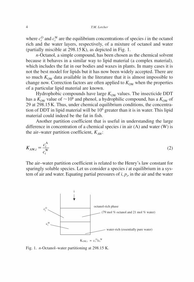
where ciO and ci

W are the equilibrium concentrations of species i in the octanolrich and the water layers, respectively, of a mixture of octanol and water(partially miscible at 298.15 K), as depicted in Fig. 1.

n-Octanol, a simple compound, has been chosen as the chemical solventbecause it behaves in a similar way to lipid material (a complex material),which includes the fat in our bodies and waxes in plants. In many cases it isnot the best model for lipids but it has now been widely accepted. There areso much KOW data available in the literature that it is almost impossible tochange now. Correction factors are often applied to KOW when the propertiesof a particular lipid material are known.

Hydrophobic compounds have large KOW values. The insecticide DDThas a KOW value of �106 and phenol, a hydrophilic compound, has a KOW of29 at 298.15 K. Thus, under chemical equilibrium conditions, the concentra-tion of DDT in lipid material will be 106 greater than it is in water. This lipidmaterial could indeed be the fat in fish.

Another partition coefficient that is useful in understanding the largedifference in concentration of a chemical species i in air (A) and water (W) isthe air–water partition coefficient, KAW:

(2)

The air–water partition coefficient is related to the Henry’s law constant forsparingly soluble species. Let us consider a species i at equilibrium in a sys-tem of air and water. Equating partial pressures of i, pi, in the air and the water

Kc

ci

i

iAW,

A

W�

i

ciO

octanol-rich phase

(79 mol % octanol and 21 mol % water)

ciW

water-rich (essentially pure water)

KOW,i = c iO/ci

W

Fig. 1. n-Octanol–water partitioning at 298.15 K.

CH001.qxd 2/7/2007 2:45 PM Page 4

(or equating fugacities or chemical potentials) and using the ideal gas lawequation and Henry’s law (see Fig. 2):

(3)

where ni is the amount (moles) of i in the air. Applying Raoult’s law at lowsolute concentrations (Henry’s law) with one correction factor (the activitycoefficient, gi

�):

(4)

where xiW is the mole fraction of i in the water. Rearranging and equating we

obtain:

(5)

(6)

where Hi and Hi� are the Henry’s law constants related to mole fractions andconcentrations, respectively. Hence, KAW,i � ci

A/ciW � Hi�/RT.

At saturation or the solubility limit, ciW is the solubility in water, ci

WS, and

cp

RTiiAvap

�

p x p x H c Hi i i i i i i i� � ��W vap W Wg ′

pn

VRT c RTi

ii� � A

p x pi i i i� �W vapg

p V n RTi i�

An Introduction to Modelling of Pollutants in the Environment 5

Hi

pi = xiγipivap

pi pi = xiHi

vappi

Raoult’s law (γ = 1)

00 xi

Fig. 2. Ideal behaviour, Raoult’s law and Henry’s law.

CH001.qxd 2/7/2007 2:45 PM Page 5

thus

This only applies if the solubility is low, which is the case for many pollu-tants. By way of example [1, 2], the KAW for n-hexane is 74 and for DDT itis �1 � 10�3. Thus, if a species i is in chemical equilibrium in differentphases there can be orders of magnitude difference in the concentration of iin the different phases (see Fig. 3).

The Henry’s law constant, KAW, and the activity coefficient, g, can beestimated for a specific chemical from its measured solubility in water. Thisrepresents saturation conditions. At saturation, for a very sparingly solublecompound, a pure chemical phase can exist in equilibrium with the satu-rated solution; thus, Eq. (4) becomes:

(7)

and thus, xiWgi

� � 1.0 and xiWgi

� � 1/gi�.

The mole fraction solubility is thus the reciprocal of the activity coefficient.Substances that are sparingly soluble in water have large activity coefficients.They also tend to have large Henry’s law constants and air–water partitioncoefficients, because, as Eq. (6) shows:

The very low vapour pressure of DDT is largely offset by its large activitycoefficient. Solubility thus plays a key role in determining the partitioningof chemicals from water to air, lipids and other phases such as soil and sediments.

H pi i i�g∞ vap

p p x pi i i i i� � �vap W vapg

Kp

c RTi

i

iAW,

vap

WS�

6 T.M. Letcher

ADDT 10−3c =

air

0DDT 106c = octanol/water

1cWDDT = water

Fig. 3. The partitioning of DDT between water in octanol–water–air mixture based onEqs. (1 and 2).

CH001.qxd 2/7/2007 2:45 PM Page 6

3. MODEL ENVIRONMENTS

In order to predict the concentrations of a chemical species in the variousregions of a given environment, it is necessary to know the size of each region.These regions or compartments can include the atmosphere (air), water(rivers and lakes), soil (usually to a depth of �15 cm), river and lake sedi-ments, fish (aquatic biota) and plant material (terrestrial biota). In this chapterwe will focus on air, water, soil and aquatic biota. Other compartments suchas aerosols, concrete surfaces, etc., can also be considered. The size of eachdepends on the particular circumstance. By way of example, the sizes of fourcompartments, including a lake and fish, are given in Table 1 together withrelevant properties, needed for the modelling process [1, 2]. These values willbe used throughout this chapter.

4. EQUILIBRIUM PARTITION

The criterion for phase equilibrium of a chemical, i, between two phases isequal chemical potential or fugacity, i.e.

(8)

or in the case of ideal vapours:

(9)

The equilibrium condition for a species i, partitioning between two liquidphases, e.g. water (W) and chemical (c), is:

(10)x p x pi i i i i iW W vap c c vap

g g�

′ ′′p pi i�

′ ′′ ′ ′′m mi i i if f� �and


Table 1Properties of a model environment

Environmental region Volume, V (m3) f Density, d (kg m�3)

Air 1 � 109 1.2Water 1 � 106 1000Soil 15 � 104 0.02 1500Biota 10 0.05 1000

Note: Here f is the mass fraction of organic material in the particular region, soil or biota.

CH001.qxd 2/7/2007 2:45 PM Page 7

8 T.M. Letcher

This would apply to the octanol–water phases and

(11)

For very hydrophobic species, xiW is very small, gi

W � gi�, xi

0 � 1 and gi0 � 1,

so xiW � 1/gi

�. As a result, the insecticide, DDT, has a gi� value of �106.

Substituting these values and assuming thermodynamic equilibrium, we seethat there can be a difference of many orders of magnitude between the con-centration of a particular chemical species in one phase and the concentrationof the same species in another phase (see Fig. 3).

We can use these concepts to calculate the relative concentrations of achemical in equilibrium with air and water. For example, let us consider1,1,1-trichloroethylene (T) – a common industrial pollutant in the environ-ment defined in Table 1 [1, 2].

At 25�C, its vapour pressure, pTvap, is 12800 Pa and its solubility in

water, cTW, is 730gm�3. Because it melts at �32�C we know that it is a liquid

at 25�C. Its molar mass (MW) is equal to 133.4 g mol�1, so xT � (cTW/MW)/

(106/18) � 0.99 � 10�4, where the molar volume of water is 18/106 mol m�3,and hence, from Eq. (11), gT

� � 10100, HTgT� pT

vap � 1.29 � 108 Pa (molefraction)�1 and HT� � (HT � 18)/106 � 2322 Pa m3 mol�1; hence, KAW,T � HT�/RT � 9.4 � 10�1.

The concentration of trichloroethylene in air thus will be 0.94 times itsconcentration in water, if equilibrium conditions are met.

The value of KOW for 1,1,1-trichloroethylene is 295. Using this valuewe can quantify the concentration of the pollutant in the fish (biota) from aknowledge of KBW for the pollutant, as the two terms are related by:

(12)

where fB is the mass fraction of lipid material (assumed to be equivalent insolvent properties to octanol) in the biota and ci

B the equilibrium concentra-tion of i in the biota. Table 1 indicates that in fish, the fB value is 0.05. If theconcentration in water, ci

W, for 1,1,1-trichloroethylene, is 1 ppm (1 mg L�1

or 1 gm�3), then ciB is �15 ppm. Hence, we can say that a fish, swimming

in water contaminated with this particular trichloroethylene at a concentrationof 1ppm, will be contaminated with the pollutant at a concentration of 15ppm.The group, fBKOW,i, is usually known as the bioconcentration factor.

Following on from Eq. (12) the more hydrophobic the pollutingspecies, the greater will be ci

B. Let us consider the concentration of one type

Kc

cf Ki

i

iiBW,

B

W B OW,�

x p x pi i i i i iW W vap 0 0 vap

g g�

CH001.qxd 2/7/2007 2:45 PM Page 8

of hydrophobic pollutant – a polychlorinated biphenyl (one of the infamousPCBs), namely 2,2�,4,4�-tetrachlorobiphenyl in a river such as the St. LawrenceRiver, and estimate its concentration in the fish in the river [1, 2]. An averagevalue given for PCBs in this river has been reported as 0.3 ppb (0.003 g m�3).Let us assume that the only PCB in the river is 2,2�,4,4�-tetrachlorobiphenyl.For this PCB, log KOW � 5.90.Hence,

The predicted equilibrium concentration of PCB in fish is thus �40000times the concentration of the PCB in the water, an amazing magnification!

The experimental value of ciB for PCBs in the St. Lawrence River is

7 � 103 ppb which is within an order of magnitude of our prediction basedon a very simple model.

A similar treatment can be made for soil contamination. Taking intoaccount that soil contamination (ci

S) is measured in mg kg�1 and water isusually mg L�1 we have for soil (S):

(13)

where dS refers to the soil density.We conclude that the substances of low solubility and high activity

coefficients in water will tend to bioconcentrate into fish and any other ani-mal and reach concentrations that are many orders of magnitude higher thanthe concentrations in water. These are usually referred to as hydrophobic or“water hating”.

5. ENVIRONMENTAL DISTRIBUTION

With the above information we can describe the partitioning of a speciesbetween the different regions of the environment as described in Table 1.The total mass Mi of a pollutant is:

Mi � mass i in air � mass i in water� mass i in aquatic biota � mass i in soil

Mi �ciAVA �ci

WVW �ciBVB �ci

SVS�KAW,ici

WVA �ciWVW �KBW,ici

WVB �KSW,iciWVS

′Kc

c

K

d

f K

di

iSW

S

WSW

S

S OW

S

� � �( )′

c f K ci i iB

B OW,W ppb 11.9 ppb or gm� � � � � � � �( . . . ) .0 05 7 9 10 0 3 105 3 3


CH001.qxd 2/7/2007 2:45 PM Page 9

10 T.M. Letcher

and hence

(14)

Let us consider the distribution, in an environment defined in Table 1, of1.00 kg of each of the three polluting chemicals: trichloroethylene (T), hexane(H) and DDT (D). The necessary data are [1]:

The density of air at 25�C and 1 atm is 1185 g m�3. Using the abovedata, together with the data of Table 1 and Eq. (14), we calculate that cT

W �0.020mgm�3. This is well below the solubility in water of trichloroethylene,which is 1100 g m�3.

The results given in Table 2 require careful analysis. Most of the trichloroeth-ylene and the hexane are to be found in the air but the highest concentrationsare found in the biota, i.e. fish. For the DDT, however, most reside in the soilbut again, the highest concentrations are to be found in the fish. The calcu-lations performed here suggest that the biota or the soil (which have thehighest chemical concentrations) would be the best to sample if one wishedto monitor chemicals in the environment.

We have shown that given only KOW and KAW (or the Henry’s law con-stant) for a pollutant, its concentration in various environmental regions canbe predicted. This model is a simple one and assumes that equilibrium takesplace at every compartment interface. It ignores flows in and out of the envi-ronment, the rate of diffusional processes and other time dependant effects.In the next section we will consider these effects.

c K c f K cTB

BW,T TW

B OW,T TW mgm= = = −0 195 3.

c K c f K cTS

SW,T TW

S OW,T TW mgm= = = −0 04 3.

Mass of T in air 0.96 kg TA

A� �c V

c K cTA

AW TW 3 30.96 10 mgm� � � � �

Pollutant KAW log KOW

Trichloroethylene (T) 0.048 2.29Hexane (H) 74 4.11DDT (D) 1 � 10�3 6.19

cM

K V V K V K Vii

i i i

W

AW, A W BW, B SW, S

��

CH001.qxd 2/7/2007 2:45 PM Page 10

6. ENVIRONMENTAL DISTRIBUTION USING A FLOWMODEL [1]

This model takes into account both the flow of a chemical into and out ofthe environmental region and the degradation, and formation of the chemi-cal within the region. The model like the previous one assumes that there isphase equilibrium between the environmental regions. The model is basedon the mass balance:

Rate of change of �

Rate at which�

Rate at whichi in the i enters the i leaves theenvironment environment environment

(15)

d

dd

d

d

d

d

d

d

AA

WW

SS

BB

AIN

A A A

tc V c V c V c V

M

t

Q

tc

Q

tc

Q

i i i i

ii i

( )

,

� � �

� � � � WWIN

W W W

AA

A WW

W BB

B Sc

d

d

dtc

Q

tc

k c V k c V k c iV k

i i

i i i i

,

( ( )

�

� � � � SSSV )


Table 2Results of analysis

Region Concentration (cT) ppb (by mass) (T) Percentage of(mg m�3) total (T)

TrichloroethyleneAir 0.96 � 10�3 0.810 97.0Water 0.020 0.020 3.0Soil 0.040 0.026 0.0Biota 0.195 0.195 0.0

Hexane (cH) (H) (H)Air 1 � 10�3 0.843 100.0Water 13.5 � 10�6 13.5 � 10�6 0.001Soil 1.74 � 10�3 1.16 � 10�3 0.003Biota 8.40 � 10�3 8.40 � 10�3 0.000

DDT (cD) (D) (D)Air 4.25 � 10�6 3.586 � 10�3 0.005Water 4.25 � 10�3 4.25 � 10�3 0.005Soil 65 43 99.8Biota 329 329 0.003

Note: The concentrations, ciW, were calculated from Eq. (14).

CH001.qxd 2/7/2007 2:45 PM Page 11

12 T.M. Letcher

The dQA/dt term is the air flow rate and the dQW/dt term the water flowvelocity. These terms would have units of m3 s�1. The k terms are degrada-tion first order values (dc/dt � –kc) [3] specific to each environment region.

The differential equation can be simplified as:

(16)

where

(17)

(18)

and

(19)

The solution of the equation is:

(20)

One way of simplifying this equation is to assume a steady state condition(t � �) which gives:

(21)

Using the above theory, let us apply it to the real case of DDT pollution.Although DDT has been out of production for almost two decades,

its concentration in water in a particular fresh water lake was found to be 1.00mg m�3. That is 1 part per 109, i.e. 1 ppb. This is below its solubility in watervalue which is 3.1 mg m�3. In this problem we will use the data below: (a) tocalculate the DDT concentrations in the air, biota and soil; (b) assuming thatthe surrounding environment has the same DDT (no flow in or out), to calcu-late the time that will be required for the DDT concentration to fall by 50%.

c tiW ( ) = b

g

c tt

iW ( )� �

�b

g

g

a1 exp

g � � � � �

�

d

d

d

dA

A A AW,W

W W B B BW,

S S SW

Q

tV k K

Q

tV k V k K

V k K

i i

,,i

b� �d

d

d

dA

,INA W

,INWQ

tc

Q

tci i

a� � � �K V V K V K Vi i iAW, A W BW, B SW, S

a b gd

d

WWc

tci

i� �

CH001.qxd 2/7/2007 2:45 PM Page 12

For DDT, KAW � 1 � 10�3 and log KOW � 6.19 (i.e. KOW � 1.549 � 106).In our answer we will assume the model environment given in Table 1 andthe first order rate constant for DDT degradation:

by photolysis in water is 5.3 � 10�7 h�1;by hydrolysis in water is 3.6 � 10�6 h�1;by biodegradation in soil is 5.42 � 10�6 h�1.

Assuming that the DDT has reached chemical equilibrium (after all, the timescale is about two decades!) then as

then

and similarly,

Again, the highest concentrations of DDT are found in the fish and the soilis also contaminated. Note that the DDT in the fish is 77000 times the con-centration of the DDT in the water.

Of interest, the total mass of DDT in this environment (1 km �1 km � 1 km) (see Table 1) is:

As we found before, most of the DDT resides in the soil – in this case it is232 kg out of a total of 234.8 kg.

M � 234 8. kg

M ( ) . . .kg� � � � �1 1 00 1 00 232 0 8

M ( ) ( . ) ( . ) ( . . )( .

mg� ��

�

1 6 3 9 3 41 00 10 1 00 10 10 15 5 10 1 5 1077 44 10 103� � )

M c V c V c V c V� � � �DW

W DA

A DS

S DB

B

c c KDB

DW

BW,D mgm= = × × × = × −1 00 0 05 1 549 10 77 4 106 3 3. . . .

c c KDS

DW

SW,D mgm= = × × × = × −1 00 0 01 1 549 10 15 49 106 3 3. . . .

c c KDA

DW

AW,D3mgm� � � � � �� 1 00 1 10 1 00 103 3. .

Kc

cAW,D

DA

DW

�


CH001.qxd 2/7/2007 2:45 PM Page 13

14 T.M. Letcher

Since there is no net inflow of DDT and there is no production ofDDT, the terms involving dQ/dt and dM/dt are zero and we have:

where

Getting back to our differential equation

This first order equation [3]:

has

and hence the half life can be calculated:

Thus, starting with a concentration of 1.00 mg m�3, the concentration will dropto half this level, i.e. 0.50 mg m�3, in 14.7 years. This shows how persistentDDT is in the environment.

tk1 2 6

52 2

5 365 101 29 10/ h 14.7years� �

��

�ln ln

..

k � � � �5 365 10 6 1. h

d

d

c

tkc��

d

dhD

W

DW 1

DWc

tc c�� ′

′g

a5 365 10 6. ( )

′g � �

� � � � � � � ��

V K V K KW W S SW,D S

1 10 5 3 10 3 6 10 15 10 0 01 1 56 7 6 4( . . ) ( . . 449 105 42 10

4 13 1259 3 1263 4

6

6

3 1 3 1

�

� �

� � ��

).

( . . ) .

−

m h m h

′−

a � � � �

� � � � � �

K V V K V S VAW,D A W BW,D B SW,D S

( ) ( . .1 10 10 10 0 05 1 5493 9 6 ��

� � � � �

� �

10 100 01 1 549 10 1 5 10

234 8 10

6

6 4

6 3

)( . . . )

. m

′ ′a gd

dDW

DWc

tc��

CH001.qxd 2/7/2007 2:45 PM Page 14

7. ACCUMULATION OF CHEMICALS IN THE FOOD CHAIN

Experimental analysis of chemicals in animals has shown that in some casesthe concentration increases with increasing position of the animal in the foodchain. Fish eating eagles, for example, have been found to have a much greaterconcentration of some pesticides than do the fish that the eagles feed upon.This process is known as biomagnification and appears to be a function of themagnitude of the KOW of the chemical species involved. It is found that bio-magnification occurs for chemical species with log KOW values greater than 5.0.

Values of log KOW for various insecticides are given in Table 3 [1].The answer lies in mass transfer effects. A fish loses much of its pollu-

tant in the respired water passing through the gills. If KOW is very large, theconcentration in that water will be very low; hence, the flux of chemical isconstrained to a low level. Elimination is slow; thus, there is a build up orbiomagnification of the chemical that is adsorbed from the food. There mayalso be increased resistance to transfer through membranes if KOW is verylarge, i.e. 108. This biomagnification effect is much smaller (reported valuesrange from 3 to 30) than the enormous effects (40000 and 77000 times) foundunder equilibrium conditions of the partitioning of a pesticide between waterand fish (see Sections 4 and 6).

Many of the concepts and terms introduced in this chapter will be used inchapters in this book, and especially in Chapters 3, 13, 14 and 24.

ACKNOWLEDGEMENT

I wish to thank Professor Donald MacKay of Trent University, Canada, formany helpful suggestions and to professor Stan Sandler of the University ofDelaware, USA, who introduced me to the modelling of pollutants.


Table 3Values of log KOW for some insecticides

log KOW

Malathion 2.9Lindane 3.85Dieldrin 5.5DDT 6.19Mirex 6.9

CH001.qxd 2/7/2007 2:45 PM Page 15

16 T.M. Letcher

REFERENCES

[1] D. Mackay, Multimedia Environmental Models, 2nd edn., CRC Press, LewisPublishers, New York, 2001 (ISBN 1-56670-542-8).

[2] S.I. Sandler, in “Chemical Thermodynamics – Chemistry for the 21st Century”(T.M. Letcher, ed.), Blackwell Science, Oxford, 1999 (Chapter 2).

[3] P. Atkins, Physical Chemistry, 6th edn., p. 767, Oxford University Press, Oxford, 1998.

CH001.qxd 2/7/2007 2:45 PM Page 16

Chapter 2

Modeling the Solubility in Water ofEnvironmentally Important Organic Compounds

Ernesto Estradaa, Eduardo J. Delgadob and Yamil Simón-Mansoc

aComplex Systems Research Group, X-Rays Unit, RIAIDT, Edificio CACTUS,University of Santiago de Compostela, 15782 Santiago de Compostela, SpainbTheoretical and Computational Chemistry Group (QTC), Faculty ofChemical Sciences, Casilla 160-C, Universidad de Concepción,Concepción, ChilecINEST Group, PM-USA and Center for Theoretical and ComputationalNanosciences, National Institute of Standards & Technology (NIST), 100Bureau Drive, Stop 8380, Gaithersburg, MD 20899-8380, USA

1. INTRODUCTION

Solubility in water is one of the most important physico-chemical proper-ties of a substance and a knowledge of solubility plays an important part inthe environmental fate and transport of xenobiotics (man-made chemicals)in the environment. Substances, which are readily soluble in water, will dis-solve freely in water if accidentally spilled and will tend to remain in aque-ous solution until degraded. On the other hand, sparingly soluble substancesdissolve more slowly and, when in solution, have stronger tendency to par-tition out of aqueous solution into other phases. They tend to have large air–water partition coefficients or Henry’s law constants, and they tend to partitionmore into soils, sediments and biota. As a result, it is common to correlatepartition coefficients from water to these media with solubility in water.

From a qualitative point of view, solubility can be viewed as the maximumconcentration that an aqueous solution will tolerate just before the onset ofthe phase separation. From a thermodynamic point of view, solubility is theconcentration of solute A required to reach the following equilibrium:

A A(p) (aq.)�


CH002.qxd 2/3/2007 4:02 PM Page 17

where p refers to a specific aggregation state of the solute, namely, solid,liquid or gas state. The condition of thermodynamic equilibrium at T and P constants requires the equality of the chemical potential of the solute A inboth phases, namely: mA(T, P, xA) � mA(p)(T, P), where xA is the solute molarfraction in the saturated solution, in other words it is the solubility of thesolute in the molar fraction scale.

Although, the experimental determination of solubility is not difficult,there are some justifications to develop models that allow predicting it. Thisis especially important in environmental studies where the compounds ofinterest are toxic, carcinogenic or undesirable for other reasons. In addition,the ability to predict this property is important for designing novel pharma-ceutical products and agrochemicals whose solubility can be predicted beforecarrying out the synthesis. Design of novel compounds may, in this way, beguided by the results of calculations.

Accordingly, very extensive studies have been carried out on solubilityresulting in diverse theories of solute–solvent interactions that form the basisof the knowledge for the understanding of solubility. These theories are basedon concepts ranging from quantitative analysis to statistical and quantummechanics.

Molecular sciences look for explanations of macroscopic properties,e.g., solubility, from the microscopic properties of matter. Statistical mechan-ics is one of such disciplines, which links those two pictures through theprobabilistic treatment of particle ensembles. The application of Kirkwood’scontinuum solvent approach to nondissociating fluids resulted in a varietyof simulation techniques. Applications of such techniques to study phaseequilibria have been reported widely in literature [1–10]. Although somesimple hydrocarbons can nowadays be reasonably well described by molec-ular modeling (molecular dynamics and Monte Carlo simulations), water andespecially water mixtures, still represent challenges for such simulationstechniques despite 30 years of active parameterization of appropriate force-fields. This is due to the extremely strong and complicated electrostatic andhydrogen-bond interactions.

Quantum-chemical methods, with the explicit inclusion of solvation freeenergy into the framework of the MO SCF method, have been developed to the point that they are useful tools for predicting thermodynamic proper-ties and phase behavior of some substances to an accuracy useful in engi-neering calculations [11–20]. Among these methods, the SMx solvationmodels of Cramer and Truhlar, and the Conductor-like Screening Model forReal Solvents, COSMO-RS, of Klamt, are presumably the most widely used

18 E. Estrada et al.

CH002.qxd 2/3/2007 4:02 PM Page 18

methods to study phase equilibria. For instance, the aqueous solubility of 150drug-like compounds and 107 pesticides were calculated using COSMO-RSmethod [21].

The above-mentioned methods based on either statistical mechanics or quantum mechanics allow the prediction of rather accurate values of sol-ubility, but these methods are time-consuming and can hardly be applied tothe solubility modeling of large biomolecules or to the large-scale modelingof many hundreds of small molecules [22]. Several less sophisticated, but alsomuch less time-consuming methods based on quantitative structure–propertyrelationships (QSPR) methodology have been developed recently for theprediction of solubility. This family of methods is divided into two groups:methods based on experimentally determined descriptors and methods basedsolely on molecular structure.

2. QUANTUM CHEMISTRY METHODS

Despite the huge progress in calculating free energies of solvation withdielectric continuum models (DCMs) [17, 23–25], such as COSMO [17] andSM5.42R [25], there has been little work to predict solubilities using them. InDCMs, the solute is considered to be located in a cavity of a dielectric con-tinuum. The solvent polarization is included in the calculation as a boundarycondition. Then, the Schrödinger equation is solved self-consistently.

COSMO-RS [21] is a two-step methodology for the prediction of equi-librium properties such as vapor pressure, heat of vaporization, activity andsolvent partition coefficients, phase diagrams and solubility. In the first step,COSMO is used to simulate a virtual conductor environment for the moleculeand evaluate the screening charge density, s, on the surface of the molecule.In a second step, the statistical thermodynamics of the molecular interactionsis used to quantify the interaction energy of the pair-wise interacting surfacesegments (s,s�). Three major interactions between surface segments are takeninto account using appropriate functional forms. The Coulomb interactionbetween the screening charges s and s� on surface pairs, so-called the misfitterm, the hydrogen bonding interaction and the van der Waals interactions[20, 26–28].

COSMO-RS is able to calculate the chemical potential (the partialGibbs free energy) of a compound, either pure or in a mixture from the prob-ability distribution of s. The solubility of a compound, X, can be calculatedfrom the differences between the chemical potentials of X in solution andpure [21, 26]. COSMOS-RS not only predicts reasonable solubility values

Modeling the Solubility in Water of Environmentally Important Organic Compounds 19

CH002.qxd 2/3/2007 4:02 PM Page 19

but also the correct temperature dependence of solubility, with deviations fromexperiment below 0.3log(x) [26]. However, some “lack of thermodynamicconsistency” has been reported [27].

Truhlar et al. [28] predict the aqueous solubilities of 75 liquid solutesand 15 solid solutes by utilizing a relation between solubility, free energy of solvation and solute vapor pressure. The method is based on SM5.42R solvation model and the classical thermodynamic theory of solutions. In the SM5.42R solvation model the free energy of solvation is written as,�GS

0 � �EE � GP � GCDS, where �EE is the change of electronic energy dueto the embedding of the solute into the dielectric environment, GP the elec-tronic polarization energy, i.e., the mutual polarization of the solute and thesolvent, GCDS a semiempirical term that takes into account the nonbulk contri-butions, i.e., inner solvation-shell effects. It is a parametric function of severalsolvent descriptors.

Based on the theory of solutions of classical thermodynamics, the standard-state free energy for the solvation processes A(p) � A(aq.), at temperature T, can be expressed as:

(1)

where MAsol is the solubility of A (in molarity units), PA

• and PA� are respectively

the equilibrium vapor pressure of A over pure A and the pressure of an idealgas at 1 molar concentration and temperature of 298 K. This equation isobtained under the assumption of infinite dilution, i.e., the activity coefficientsare equal to 1. Truhlar et al. used a training set of 75 liquid solutes and 15solid solutes. This set can be considered relatively small for comparison withother solubility models, however their results are very promising with a mean-unsigned error in the logarithm of 0.33–0.88.

In general, the quantum methods need relatively few parameters, are ableto handle exotic molecules, transition states and do not make assumptions suchas group transferability or additive properties. However, at the present time,they are not very accurate and need at least one time-consuming quantumcalculation which limits their use for extremely large pools of molecules.

3. EXPERIMENT-BASED QSPR MODELING

Hansch et al. [29] showed that solubility and octanol–water partition coef-ficient, KOW, are well correlated for liquid solvents. Numerous further

��

G RT P

PRT MS A A

0 ( ) ln ln.

sol sol� �


CH002.qxd 2/3/2007 4:02 PM Page 20

studies have explored and refined this relationship for different classes ofcompounds, e.g., halogenated hydrocarbons [30, 31], polycyclic aromaticshydrocarbons [32].

The General Solubility Equation of Yalkowsky includes two experimen-tal parameters: the melting point of the solute and its octanol–water partitioncoefficient. The aqueous solubility of 150 physiologically active compoundshas been estimated using this equation [33].

In the solvatochromic or linear solvation energy method, developed byKamlet et al. [34] and Taft et al. [35], the solubility is predicted from molarvolume, melting point and two parameters which express dipolarity/polar-izability and hydrogen bond basicity. It has been applied to predict the solubility of very diverse type of compounds.

The mobile order theory (MOT) approach, developed by Huyskens [36],has been widely used by Ruelle et al. to predict the solubility of a diverse setof chemicals of environmental relevance [37, 38]. Paasivirta et al. [39] usingthis approach estimated the solubility of 73 persistent organic pollutants asa function of temperature.

4. STRUCTURE-BASED QSPR MODELING

These models exploit two different paradigms [22]. One relies on the conceptof the structural additivity of properties. According to this hypothesis, anyproperty in the form of a continuous smooth function can be expanded intoa linear function in some predefined structural features such as atoms, bondsand chemical functional groups. This approach – also known as fragment-based or group contribution scheme – has been actively pursued by thegroups of Klopman and Zhu [40] and Wendoloski et al. [41]. Klopman et al.derived contribution coefficients for many groups and successfully corre-lated them with the aqueous solubilities of 1168 organic compounds. TheUNIFAC (universal quasi chemical method (UNIQUAC) functional groupactivity coefficient) method, an extension of the UNIQUAC, has been testedby different authors [42–44] to ascertain its applicability to water solubility.

The other approach involves the derivation of various molecular char-acteristics (descriptors) solely from molecular structure. Depending on thelevel of consideration, one can use constitutional, topological, geometric,electrostatic or quantum-chemical descriptors.

Jurs et al. have published several articles on the correlation of aqueoussolubility with molecular structure using both multilinear regression (MLR)and artificial neural networks (ANN). Successful nine-parameter regression


CH002.qxd 2/3/2007 4:02 PM Page 21

models are reported for three sets of compounds (hydrocarbons, halogenatedhydrocarbons and ethers) and a fourth model is also reported for the com-bined set of all compounds [45]. Later the same authors reported MLR andANN models for the prediction of aqueous solubility for a diverse set of het-eroatom-containing organic compounds [46]. A set of nine descriptors wasfound that effectively linked the aqueous solubility to each structure. It isalso reported that PCBs have larger errors associated with them than anyother class of compounds in the dataset. In an attempt to improve the over-all error of the model, the set of nine descriptors was used to build ANNmodel. The root of mean squared (rms) error of the PCBs alone was 0.51log units, which was significantly higher than the overall errors in the model.Later, Jurs and Mitchell [47] also reported an ANN model for the predictionof solubility of 332 organic compounds. The model involving nine descrip-tors has an rms error of 0.395 log units, and the squared correlation coeffi-cient between the experimental and calculated values is 0.97. A large datasetof diverse organic compounds was used by Huuskonen [48] who reported a QSPR model for predicting aqueous solubility of 1297 organic compoundsusing topological and electrotopological indices.

Delgado reports a QSPR model [49] for the prediction of log(1/S) fora set of 50 chlorinated hydrocarbons including chlorinated benzenes,dibenzo-p-dioxins and PCBs. The model involves only two moleculardescriptors, one geometry-dependent descriptor and one charged partial surface area (CPSA) descriptor. The geometric descriptor is the area of theshadow of the molecule projected on a plane defined by the X and Y axes(XY shadow); the CPSA descriptor is the surface weighted atomic partialnegative surface area (WNSA-3). The model has a squared correlation coef-ficient of 0.97 and standard deviation of 0.45 log units.

On the other hand, Gao et al. [50], using principal component regres-sion analysis, derived a QSPR model for the prediction of solubility of a setof 930 diverse compounds, including pharmaceuticals, pollutants, nutrients,herbicides and pesticides. The model, which involves 24 molecular descrip-tors, predicts the log(S) with a squared correlation coefficient of 0.92 andrms error of 0.53 log units.

Delgado et al. [51] reported QSPR models for the solubility of herbi-cides stressing the importance of considering the aggregation state of thesolute. It is found that the phase of the solutes plays a fundamental role inthe development of QSPR model from both a statistical and a physical pointof view. From a statistical point of view, it is observed that the predictiveperformance of the models drops drastically when the QSPR model, obtained


CH002.qxd 2/3/2007 4:02 PM Page 22

for a given phase, is used to predict the solubility of the same set of com-pounds in another phase. From a physical point of view, when the compoundsconsidered in the training set are in different phases, the physical interpre-tation of the descriptors involved in the model is obscured because thedescriptors which appear in the correlation equation are a sort of averageencoding the different physical mechanisms existing for the different phasesin the solubility phenomenon.

The above-mentioned models use different types of molecular descrip-tors to quantitatively predict solubility using multiple linear regression andartificial neural network. These molecular descriptors encode topological,geometric, electronic and quantum-chemical molecular features responsiblefor the observed solubility. Even though these models predict solubility rel-atively well, the number of descriptors involved in the models is rather high.It is highly desirable to have models with fewer descriptors which allowtheir application in a more straight forward way, and, on the other hand, topreserve the principle of parsimony. In this direction Estrada [52–55] havedefined the quantum-connectivity indices by using a combination of topo-logical invariants, such as interatomic connectivity, and quantum-chemicalinformation, such as atomic charges and bond orders. These indices also con-tain important three-dimensional information, incorporated by the quantum-chemical parameters used in their definition. Therefore, these indices arericher in chemical information than traditional molecular descriptors sincethey encode, at the same time, both topological and quantum-chemical fea-tures of molecules. They have been successfully applied to the prediction ofaqueous solubility of environmentally important compounds [56].

5. THE QUANTUM-CONNECTIVITY INDICES

“Classical” connectivity indices are based on the concept of vertex degree,which is the number of edges incident to a vertex [57, 58]. The degree of avertex designated by k is represented by dk. In the simple graph representa-tion of acetone, 2-methylpropene and 2-methylpropane there is one vertexwith degree 3 and three vertices with degree 1. However, when pseudo-graphsare considered it is necessary to use the concept of valence degree dk

v intro-duced by Kier and Hall [58]. In this case the valence degree for a vertex kis defined as a count of electrons s, p and n orbitals (excluding hydrogenatoms). It is equivalent to consider the number of multiple edges and loopsincident to a vertex in the pseudo-graph (loops are doubly incident to a vertex). In this case the oxygen atoms of the acetone has dk

v � 6, which


CH002.qxd 2/3/2007 4:02 PM Page 23

differentiates it from the CH2 group in 2-methylpropene, dkv � 2 and from

CH3 of 2-methylpropane, dkv � 1. However, with this molecular representa-

tion the atom of the carbonyl group of acetone is not differentiated fromthe of the ethylenic group, i.e., they have dk

v �4. In addition to this pseudo-graph representation, there is no differentiation of geometric isomers as itdoes not take into consideration the three-dimensional molecular structure.

We have overcome these difficulties by considering weighted pseudo-graphs in the context of quantum-chemical molecular orbital approaches[52–55]. Instead of using simple entire numbers for counting the number ofmultiple bonds and loops in the pseudo-graph we employ quantum-chemicalparameters for weighting the edges and vertices of the graph, respectively.As a measure of the bond multiplicity we use the bond order, which is definedas the sum of the products of the corresponding atomic orbital coefficientsover all the occupied molecular spin-orbitals. On the other hand, we weighta vertex of the graph by means of the charge density of the correspondingatoms in the molecule, Qi, which is defined as the number of valence electrons,Zi, minus the atomic charge, qi: Qi � Zi � qi.

Then, we introduce several new definitions of vertex degree in the con-text of quantum-connectivity. The first is defined as the sum of bond ordersof all bonds that are incident with the corresponding vertex [52]:

(2)

A second vertex degree is defined as the number of edges (including loops)which are incident with the corresponding vertex minus the atomic chargeassigned to it. In other words, it is the charge density minus the number ofhydrogen atoms bonded to the corresponding vertex [53]:

(3)

A correction for hydrogen atoms is introduced in this scheme according tothe following formula [53]:

(4)

where Qhj is the atomic charge density of the jth hydrogen atom bonded to theatom i. For elements beyond the second row of the periodic table of elementsthe values of di(q) and di

c(q) are calculated in a similar way as for the

di i hjj

q Q Qc ( )� �∑

di i iq Q h( )� �

d r i iji

( )r �∑

Csp2

Csp2


CH002.qxd 2/3/2007 4:02 PM Page 24

valence connectivity [57] index by dividing the right part of expressions (3)and (4) by (Zi � Zi

v � 1), where Zi and Ziv are the total number of electrons and

the number of valence electrons in the ith atom.In a similar way that vertex degree is defined, an edge degree is also

known in graph theory. It corresponds to the number of edges that are adja-cent to the corresponding edge. The following relationship exists betweenvertex and edge degrees:

(5)

where d(ek) is the degree of the edge k in G, which is incident with verticesi and j. Thus, using this expression we have extended the vertex degrees previously defined to edge degrees.

Quantum-connectivity indices are finally calculated by an expressionanalogous to that of the connectivity indices but using weighted vertex degreesinstead of simple vertex degrees [52, 53]:

(6)

where w represents the weighting scheme used, e.g., bond orders, chargedensity or charge density corrected for hydrogen atoms. The product is overthe h � 1 vertex degrees in the subgraph having h edges, and the summationis carried out over all subgraphs of type t in the molecule. The different typesof subgraphs studied in the molecular connectivity scheme are: path, clusters,path-clusters and rings, which are designed as p, C, pC and Rg, respectivelyaccording to their original definitions [58].

The bond quantum-connectivity indices based on weighted moleculargraphs, are calculated in a similar way to that of their topological analogues[59, 60]. They are defined as follows [54]:

(7)

6. MODELING SOLUBILITY WITH QUANTUM-CONNECTIVITY

We have used quantum-connectivity indices to model the solubility of a setof organic compounds of environmental relevance. This dataset is formed

ht i j h p

p

w e w e w e w� ( ) ( )( ) ( )( ) ( )( ).

��

�

d d d� ∑ 0 5

1

ht i j h s

s

w w w w� � �

�

�

( ) ( ) ( ) ( ).

d d d� 1

0 5

1

∑

d d d( )ek i j� � �2


CH002.qxd 2/3/2007 4:02 PM Page 25

by 53 compounds, including 30 pesticides chemicals and other chemicalswhich can be found as contaminants in the environment, such as polycyclicaromatic compounds (PAHs) and chlorobiphenyls. The solubility of thesecompounds is expressed as ln(S) and covers a wide range of solubility val-ues, from the very low solubility of Benzo[a]pyrene ln(S) � �11.96 to thevery soluble pesticide Amitrole, ln(S) � 8.11. Using quantum-connectivityindices we have developed the following quantitative model to predict thesolubility of these compounds [56]:

(8)

where R is the correlation coefficient, s is the standard deviation and F is theFisher ratio of the regression model.

The first index is the quantum-connectivity index of path order two,based on charge density weighted graphs. The second is a bond quantum-connectivity index for rings of order six, based on bond order weightedgraphs. We tested the predictability of this model using an external predic-tion series of 30 compounds. In Fig. 1, it can be seen that the model obtainedby using quantum-connectivity indices show good predictability for theexternal prediction dataset of compounds, which are not directly related tothose in the training set. This is, of course, an important characteristic ofquantitative models toward their usability in practical problems of predict-ing properties for new chemicals.

The mean effects, i.e., the coefficient of the variable in the QSAR/QSPRmodel multiplied by the mean value of the variable in the dataset, for 2�p

C(q)and 6�Rg(r) in the model are 8.817 and 2.810, respectively. This indicatesthat the first descriptor plays the most important role in predicting water sol-ubility for this dataset of compounds. This descriptor, 2�p

C(q), is defined on thebasis of paths of order two, i.e., a sequence of three consecutive atoms: A-B-C. The number of this fragment increases rapidly with the number ofsubstituents on a specific site. Thus, the quantum-connectivity index 2�p

C(q)controls the influence of the number of substitutions at different sites in amolecule. For instance, 1,1,2-trichloroethane is more soluble in water,ln(S) � 3.54, than 1,1,2,2-tetrachloroethane, ln(S) � 2.82. It could be thoughthat this is due to the increase in the number of chlorine atoms in the secondmolecule with respect to the first one. However, if we consider 1,1,1-trichloroethane we can see that it is the least soluble of the three compounds,ln(S) � 2.27, despite it has a chlorine atom less than 1,1,2,2-tetrachloroethane.

ln( ) . . [ ( )] . [ ( )]

, . ,

S q

N RpC� � � �

� �

10 487 2 575 112 61

53 0 9257

2 6

2

�Rg r

ss F� �1 007 311 26. , .


CH002.qxd 2/3/2007 4:02 PM Page 26

The differences arise, however, because 1,1,1-trichloroethane has more A-B-C fragments due to the fact that the three substitutions are at the samecarbon atom. Consequently, it has the largest value of 2�p

C(q) � 3.560, while1,1,2,2-tetrachloroethane has 2�p

C(q) � 3.054 and 1,1,2-trichloroethane has2�p

C(q) � 2.068.The other quantum-connectivity index 6�Rg(r) accounts for the influence

of bond order weighted cyclic fragments of six bonds, i.e., six-atoms rings.The higher the number of such rings in the molecule, the higher the valueof this descriptor. The bond order weighting scheme used, also ensures adifferentiation among six-membered rings in different chemical environ-ments. The compound in our dataset with the higher value of 6�Rg(r) isbenzo[a]pyrene followed by benz[a]anthracene. The first has five condensedbenzene rings and the second has four. They have the lowest solubilities ofall the compounds studied here. All these rings are clearly hydrophobic units,which will decrease water solubility in any molecular framework in whichthey are present. In Fig. 2 it can be observed that the general trend is thatthe rings with more propensity to be in contact with the solvent have higher


-14 -12 -10 -8 -6 -4 -2 0 2 4 6 8 10 12ln (S)exp

-16

-14

-12

-10

-8

-6

-4

-2

0

2

4

6

8

10

12

ln (

S) c

alcd

Training setPrediction set

Fig. 1. Plot of the experimental versus predicted values of aqueous solubility of environ-mentally relevant organic compounds according to the model developed using quantum-connectivity indices.

CH002.qxd 2/3/2007 4:02 PM Page 27

contribution to 6�Rg(r) compared to those having less propensity to be in con-tact with water. In consequence the first contributes more significantly todecrease water solubility of these compounds. In other words, those rings whichare more exposed to solvent, such as terminal rings in benz[a]anthracene,have more chance to be in contact with water, having more influence in watersolubility than those with less contacts, such as internal rings.

On the left side of Fig. 2 we give the contribution of each aromatic ringto the quantum-connectivity index 6�Rg(r). The sum of the values of thesecontributions gives the value of the index 6�Rg(r) for the respective com-pound. On the right side of this figure we give the contribution of each aro-matic ring to the water solubility expressed as ln(S). The sum of these valuesplus the contribution of the other quantum-connectivity index and the inter-cept of the model gives the solubility predicted for the respective compound.For instance, for benzo[a]pyrene, the sum of these contributions is �9.21,which after summing the contributions of the other index and intercept gives�12.00, in agreement with the experimental value for this compound whichis �11.96.

7. CONCLUDING REMARKS

Today there is a large arsenal of methods and tools for predicting the aque-ous solubility of organic compounds which can impact the environment in


Fig. 2. Contribution of the aromatic rings of two polycylic aromatic hydrocarbons (PAHs)to the quantum-connectivity index (left) and to aqueous solubility expressed asln(S) (right). The compound at the top is benzo[a]pyrene and the one at the bottom isbenz[a]anthracene.

6Rg )� (r)

CH002.qxd 2/3/2007 4:03 PM Page 28

different ways. These methods range from empirical and semiempirical QSPRapproaches to more sophisticated quantum-chemical approaches. The electionof one or another method depends very much on the characteristics of theproblem we are trying to solve. In making this election we have to considerthat “models are to be used, not believed” [61] in such a way that the electedmethod solves our problem in the best possible way using the minimumamount of resources. In this sense we have illustrated here the use of thequantum-connectivity indices in modeling aqueous solubility of a series ofenvironmentally important organic compounds. These molecular descriptorscondense quantum-chemical, geometrical and topological information intosingle indices. Thus, they are appropriated for describing quantitatively theaqueous solubility of organic compounds using QSPRs methodologies.

ACKNOWLEDGMENTS

E.E. thanks the program “Ramón y Cajal”, Spain for partial financial support. Partial financial support from FONDESYT Project 7020464 forinternational cooperation is also acknowledged.

REFERENCES

[1] M.P. Allen and D.J. Tildesley, Computer Simulation of Liquids, Oxford UniversityPress, Oxford, 1987.

[2] D. Frenkel and B. Smit, Understanding Molecular Simulation, Academic Press, San Diego, CA, 1996.

[3] J.I. Siepmann, Adv. Chem. Phys., 105 (1999) 443.[4] E.M. Duffy, W.L. Jorgensen, J. Am. Chem. Soc., 122 (2000) 2878.[5] J.J. Potoff, J.R. Errington and A.Z. Panagiotopoulos, Mol. Phys., 97 (1999) 1073.[6] J.M. Stubbs, B. Chin, J.J. Potoff and J.I. Siepmann, Fluid Phase Equilib., 183–184

(2001) 301.[7] J.R. Errington and A.Z. Panagiotopoulos, J. Chem. Phys., 111 (1999) 9731.[8] W.L. Jorgensen and J. Tirado-Rives, Perspect. Drug Discov. Des., 3 (1995) 123.[9] P. Kollman, Chem. Rev., 93 (1993) 2395.[10] W.L. Jorgensen, in “Encyclopedia of Computational Chemistry” (P.v.R. Schleyer,

ed.), p. 1061, Vol. 2, Wiley, New York, 1998.[11] J. Tomasi and M. Persico, Chem. Rev., 94 (1994) 2027.[12] J. Li, T. Zhu, G.D. Hawkins, P. Winget, D.A. Liotard, C.J. Cramer and D.G. Truhlar,

Theor. Chem. Acc., 103 (1999) 9.[13] G.D. Hawkins, D.A. Liotard, C.J. Cramer and D.G. Truhlar, J. Org. Chem., 63 (1998)

4305.[14] P. Winget, C.J. Cramer and D.G. Truhlar, Environ. Sci. Technol., 34 (2000) 4733.[15] S.I. Sandler, J. Chem. Thermodyn., 31 (1999) 3.


CH002.qxd 2/3/2007 4:03 PM Page 29

[16] S.I. Sandler, Fluid Phase Equilib., 210 (2003) 147–160.[17] A. Klamt and G. Schüürmann, J. Chem. Soc. Perkin Trans., 2 (1993) 799.[18] A. Klamt, in “Encyclopedia of Computational Chemistry” (P.v.R. Schleyer, ed.),

Vol. 2, Wiley, New York, 1998.[19] A. Klamt and F. Eckert, Fluid Phase Equilib., 172 (2000) 43.[20] A. Klamt, J. Phys. Chem., 99 (1995) 2224.[21] A. Klamt, F. Eckert, M. Horning, M.E. Beck and T. Bürger, J. Comput. Chem., 23

(2002) 275.[22] A.R. Katritzky, A.A. Oliferenko, P.V. Oliferenko, R. Petrukhin, D.B. Tatham,

U. Maran, A. Lomaka and W.E. Acree, Jr., J. Chem. Inf. Comput. Sci., 43 (2003) 1794.[23] C.J. Cramer and D.G. Truhlar, Chem. Rev., 99 (1999) 2161.[24] J. Tomasi, B. Menucci and R. Cammi, Chem. Rev., 105 (2005) 2999.[25] T. Zhu, J. Li, G.D. Hawkins, C.J. Cramer and D.G. Truhlar, J. Chem. Phys., 109

(1998) 9117.[26] A. Klamt and F. Eckert, AIChE J., 48 (2002) 369.[27] S.T. Lin and S.I. Sandler, Ind. Eng. Chem. Res., 41 (2002) 899.[28] J.D. Thompson, C.J. Cramer and D.G. Truhlar, J. Chem. Phys., 119 (2003) 1661.[29] C. Hansch, J.E. Quinlan and G.L. Lawrence, J. Org. Chem., 33 (1968) 347.[30] Y.B. Tewari, M.M. Miller, S.P. Wasik and D.E. Martire, J. Solution Chem., 11 (1982)

435.[31] C.T. Chiou, V.H. Freed, D.W. Schmedding and R.L. Kohnert, Environ. Sci. Technol.,

11 (1977) 475.[32] S.H. Yalkowsky and S.C. Valvani, J. Chem. Eng. Data, 24 (1979) 127.[33] Y. Ran and S.H. Yalkowsky, J. Chem. Inf. Comput. Sci., 41 (2001) 354.[34] M.J. Kamlet, R.M. Doherty, P.W. Carr, D. Mackay, M.H. Abraham and R.W. Taft,

Environ. Sci. Technol., 22 (1988) 503.[35] R.W. Taft, J.L.M. Abboud, M.J. Kamlet and M.H. Abraham, J. Solution Chem., 14

(1985) 153.[36] P.L. Huyskens, J. Mol. Struct., 270 (1992) 197.[37] P. Ruelle and U.W. Kesselring, Chemosphere, 34 (1997) 275.[38] J.S. Chickos, G. Nichols and P. Ruelle, J. Chem. Inf. Comput. Sci., 42 (2002) 368.[39] J. Paasivirta, S. Sinkkonen, P. Mikkelson, T. Rantio and F. Wania, Chemosphere, 39

(1999) 811.[40] G. Klopman and H. Zhu, J. Chem. Inf. Comput. Sci., 41 (2001) 439.[41] V.N. Viswanadhan, A.K. Ghose and J.J. Wendoloski, Perspect. Drug. Discov., 19

(2000) 85.[42] S. Banerjee, Environ. Sci. Technol., 19 (1985) 369.[43] S. Banerjee and P.H. Howard, Environ. Sci. Technol., 22 (1988) 839.[44] W.B. Arbuckle, Environ. Sci. Technol., 20 (1986) 1060.[45] T.M. Nelson and P.C. Jurs, J. Chem. Inf. Comput. Sci., 34 (1994) 601.[46] J.M. Sutter and P.C. Jurs, J. Chem. Inf. Comput. Sci., 36 (1996) 100.[47] B.E. Mitchell and P.C. Jurs, J. Chem. Inf. Comput. Sci., 38 (1998) 489.[48] J. Huuskonen, J. Chem. Inf. Comput. Sci., 40 (2000) 773.[49] E.J. Delgado, Fluid Phase Equilib., 199 (2002) 101.[50] H. Gao, V. Shanmugasundaram and P. Lee, Pharm. Res., 19 (2002) 497.


CH002.qxd 2/3/2007 4:03 PM Page 30

[51] E.J. Delgado, J.B. Alderete, A.R. Matamala and G.A. Jaña, J. Chem. Inf. Comput.Sci., 44 (2004) 958.

[52] E. Estrada and L.A. Montero, Mol. Eng., 2 (1992) 363.[53] E. Estrada, J. Chem. Inf. Comput. Sci., 35 (1995) 708.[54] E. Estrada, J. Chem. Inf. Comput. Sci., 36 (1996) 837.[55] E. Estrada and E. Molina, J. Chem. Inf. Comput. Sci., 41 (2001) 791.[56] E. Estrada, E.J. Delgado, J.B. Alderete and G.A. Jaña, J. Comput. Chem., 25 (2004)

1787.[57] M. Randic, J. Am. Chem. Soc., 97 (1975) 6609.[58] L.B. Kier and L.H. Hall, Molecular Connectivity in Chemistry and Drug Research,

Academic Press, Letchworth, Herts, UK, 1976.[59] E. Estrada, J. Chem. Inf. Comput. Sci., 35 (1995) 31.[60] E. Estrada, N. Guevara and I. Gutman, J. Chem. Inf. Comput. Sci., 38 (1998) 428.[61] H. Theil, Principles of Econometrics, p. vi, Wiley, New York, 1971.


CH002.qxd 2/3/2007 4:03 PM Page 31

Chapter 3

Modeling of Contaminant Leaching

Maria Diaz and Defne Apul

Department of Chemical Engineering, Department of Civil Engineering,University of Toledo, Toledo, OH, USA

1. OVERVIEW OF SIGNIFICANCE

An understanding of leaching of contaminants from waste matrices has tradi-tionally been important for managing landfills and contaminated soils. Morerecently, leaching of contaminants has also become important for proper man-agement of byproduct materials (e.g. coal ashes, foundary sand, steel slag)that can be reused in various applications (e.g. road construction). Leachingand transport of pollutants in the subsurface are often studied in the contextof the hydrogeology and geochemistry of the system, associated modeling ofthe release and transport of pollutants, the risk posed by the pollutants to thehuman health and the interpretation of these scientific results in the contextof environmental regulations [1]. To accurately estimate the risk an accuratecharacterization of the source term is necessary since if leaching of contam-inants is not properly assessed the remainder of the analysis is also flawed.

The extent and rate of leaching of contaminants depends on two majorphenomena: (1) the hydrology and therefore the hydraulic properties (e.g. soilmoisture retention curve, both saturated and unsaturated hydraulic conduc-tivity) of the matrix, and (2) the geochemistry of the matrix. To model trans-port, the advective–dispersion equation is used which is based on Darcy’s law.In unsaturated conditions, the advective velocity necessary for the advective–dispersion equation is estimated from Richards equation. Appropriate equa-tions necessary for modeling the geochemistry of leaching are various but theyare often based on equilibrium mass action laws. There are various degreesof sophistication in contaminant leaching modeling. While more detailed mod-els translate into more accurate predictions, they also require a deeper under-standing of the system and more computational effort, resulting in higher costs.A compromise needs to be reached between accuracy, practicality and cost.


CH003.qxd 2/6/2007 9:23 AM Page 33

In this chapter, we present various equilibrium-based geochemical mod-eling approaches that can be used for the analysis of leaching of variousspecies from contaminated media. We focus on two important processes thatcan chemically limit the concentration of the contaminant released or leached:dissolution/precipitation and adsorption. We progress from a simpler approachbased on aqueous speciation of chemicals to more complicated approaches thatin addition require dissolution/precipitation and/or adsorption calculations.Examples for applications of the geochemical modeling approaches discussedin this chapter are provided in Table 1.

2. GEOCHEMICAL MODELING

Geochemical modeling is usually approached in two different ways: timedependent or equilibrium way. Therefore, we can find chemical kinetic mod-els where reaction rates data are needed and time is a primary factor, orchemical equilibrium models, where reactions are assumed to take place ina very short period of time and the system is in equilibrium. Chemical equi-librium is the most common approach to geochemical modeling and it is thefocus of this chapter. Within equilibrium modeling, forward models refer tothe case where the starting water chemistry is defined and an attempt is madeto model water evolution by dissolution and precipitation of mineral phasesand gases. The output of such a program has the following form [13]:

2.1. Dissolution/PrecipitationThe first step in forward modeling is the calculation of the equilibrium

distribution of mass among complexes and redox couples. The goal in thisstep is to analyze the presence of possible minerals in the system that maycontrol the release and concentration of certain contaminants. In this step,solid precipitation is suppressed, allowing the calculation of saturationindices (SI) of the water sample with respect to different mineral phases.

(1)

where log(IAP) is the logarithm of the ion activity product calculated accord-ing to the stoichiometry of each mineral and Ksp the solubility product con-stant of that mineral. The activity is defined as a surrogate of concentration

SI log IAP log sp� �( ) K

Initialwater Reactingphases Predicted water Product phases� � �

34 M. Diaz and D. Apul

CH003.qxd 2/6/2007 9:23 AM Page 34

Modeling of C

ontaminant L

eaching35

Table 1Examples of geochemical modeling applications

Approach Data Program Application Reference

Geochemical speciation Leaching experiments at MINTEQA2 Study of the weathering [2]various pH values mechanisms of municipal

solid waste incinerator bottom ash

Geochemical speciation SEM/EDX and XRD SOLTEQ-B (a modified Prediction of leaching [3]mineralogical version of MINTEQA2 from cement-stabilized composition of the that includes Berner’s wasteunleached material model of CSH dissolution)

Geochemical speciation Batch experiments ORCHESTRA Leaching of Cr(VI) from [4]chromite ore processing residue

Dissolution/precipitation Leaching experiments EQ3/6 Rel.7.2a package Leaching from cemented [5]waste forms

Modeling geochemical pH-stat leaching MINTEQA2 Identification of controlling [6]speciation and experiments processes for pH-stat dissolution/precipitation leaching behavior of

contaminantsDissolution/precipitation Column experiments PHREEQC, HGC and Study of contaminant [7]and adsorption MINTEQA2 movement in alluvium

Geochemical speciation Sorption edges and MINTEQ Study of sorption of [8]combined with ion sorption isotherms divalent metals in calciteexchange

CH003.qxd 2/6/2007 9:23 AM Page 35

36M

. Diaz and D

. Apul

Table 1 (Continued)

Approach Data Program Application Reference

Surface complexation Potentiometric titration FITEQL, MICROQL Heavy metal adsorption on [9]modeling natural sediment

Multi-surface adsorption Selective extractions for ORCHESTRA Prediction of leachate [10]modeling site concentration and concentration from

total metal concentration contaminated soilsMulti-surface Selective extractions for ECOSAT Prediction of leaching [11]geochemical modeling site concentration and from sandy soil and

total metal concentration evaluation of the contribution of different surfaces to metal binding

Multi-surface WHAM and SCAMP Solid–solution partitioning [12]geochemical modeling of metals in different

environmental systems

CH003.qxd 2/6/2007 9:23 AM Page 36

to take into account the interaction of ions with other ions that can maskthem. The activity can be expressed as:

(2)

where g is the activity coefficient (usually less than 1) and C the molar con-centration of the substance (mol/L). The activity coefficient is a function ofthe ionic strength. For dilute solutions (I � 0.1) the theoretical Debye–Hückelequation can be used to estimate the activity coefficient [14]:

(3)

where Z is the charge, a the effective hydrated radius of the ion for which gis being calculated and I the ionic strength. B and D are functions of the den-sity of water, temperature and dielectric constant; at 25�C, B � 0.5092 andD � 0.3283. For intermediate ionic strengths (0.1 � I � 0.7) positive termscan be added to the Debye–Hückel equation to generate an extended versionsuch as the empirical Davies equation [14]:

(4)

Suppressing solid precipitation will allow the identification of potential solubility controlling minerals. When SI � 0 the water is at thermodynamicequilibrium with respect to the mineral. When SI � 0, water is supersatu-rated with respect to the mineral and this mineral should precipitate. On theother hand, if SI � 0, water is under-saturated with respect to the mineraland this mineral should dissolve. Minerals with an SI value close to 0 (usually�1 � SI � 1) are considered to be present in the system. Once the possibleminerals present have been identified the leachate composition in equilib-rium with the selected minerals is calculated.

The main assumption in this step is that equilibrium has been reached;however, there is no way to determine the certainty of this assumption. The timeto reach equilibrium depends on the system matrix and on each element. Thesystem boundary, which will determine the residence time, will also affect thevalidity of the equilibrium assumption. Also, an important limitation of this stepis the uncertainty about the values of thermodynamic constants for the mineralphase because pure minerals are more of the exception than the rule [13].

logg ��

�BZI

II2

10 3.

logga

��

�BZ I

D I

2

1

A C�g[ ]

Modeling of Contaminant Leaching 37

CH003.qxd 2/6/2007 9:23 AM Page 37

The geochemical modeling of mineral dissolution/precipitation has beenwidely used in applications of diverse nature. Meima and Comans [2] usedforward modeling to study the leaching process from municipal incineratorbottom ash. They used the speciation code MINTEQA2 with a few modifi-cations to the stability constant database. They were able to identify themineral phases that controlled the leaching of elements such as Al. In a dif-ferent work from Meima et al. [15] the same modeling approach was usedto study the effect of carbonation processes in municipal solid waste bottomash in the leaching of copper and molybdenum. They found that concentra-tions of Mo were very close to equilibrium concentrations with powellite(CaMoO4) while for Cu they could not identify a specific mineral thatwould control the leaching process suggesting that other processes may behaving an effect. Van Herreweghe et al. [6] used the geochemical modelingapproach to identify chemical associations of heavy metals in contaminatedsoils and controlling factors of the leaching process. Geelhoed et al. [4] triedto identify the process controlling the leaching of Cr(VI) from chromite oreprocessing residue (COPR). Chemical speciation calculations were per-formed within the ORCHESTRA modeling framework resulting in an accu-rate prediction of Cr(VI) concentration and other elements present in solutionin the pH range 10–12. Ettler et al. [16] also included speciation calcula-tions in their study of heavy metal liberation from metallurgical slags. Theyused the models PHREEQC and EQ3NR to calculate the speciation of Pb,Zn and As from Pb–Zn metallurgical slags under different leaching condi-tions. Li et al. [17] used geochemical modeling to study heavy metal speci-ation and leaching behavior in cement based solidified/stabilized wastematerials. They used MINTEQA2 model; their results showed that Cu andZn oxides were very important during the leaching process. Mijno et al. [3]also studied compositional changes in cement-stabilized waste duringleaching tests. They used the geochemical equilibrium model SOLTEQ-B (amodification of MINTEQA2) to incorporate the solubility behavior of cal-cium silicate hydrate. They successfully predicted leachate concentrationsof Ca, Si, S and to a certain extent Al, Pb and Zn. Carlsson et al. [18] usedspeciation calculations to study infiltrating water composition in the vadosezone of a remediated tailings’ impoundment.

2.2. Adsorption/Desorption ProcessesAt low concentrations, a substance can be unsaturated with respect to its

minerals in which case the dissolution/precipitation of minerals would notbe the mechanism that controls the concentration of the substance. In suchcases, adsorption/desorption processes may be more relevant. Adsorption/


CH003.qxd 2/6/2007 9:23 AM Page 38

desorption processes refer to conditions where matter accumulates in theinterface between a solid and an aqueous phase. According to the EPA [19]these are most likely the processes controlling contaminant movement whenchemical equilibrium exists. In order to characterize these processes adsorp-tion isotherm models have been proposed. Adsorption isotherms can beclassified into high affinity, Langmuir, constant partition and sigmoidal-shape isotherm classes ([20] and references therein).

2.2.1. Adsorption Isotherm Models2.2.1.1. Freundlich isotherms This isotherm provides a relationship betweensorbed concentration and dissolved concentration as follows:

(5)

where is the sorbed concentration (M/M), C the dissolved concentration(M/L3), and Kf and a must be determined for each chemical in each porousmedium (Ma/L3a).

Moradi et al. [21] used nonlinear Freundlich isotherm to account forthe sorption of cadmium in a sewage-amended soil. Köhne et al. [22] usedthe nonlinear Freundlich isotherm to incorporate sorption in their multi-process herbicide transport analysis in structured soils. At low concentrationthe constant a becomes unity and a linear relation is obtained:

(6)

In this case the slope of the isotherm (Kd) is called the distribution coefficient.Kd values are determined for specific materials under specific conditions, sothe extent of their applicability is very limited. This approach describes thesorption process as if there was no limit on the amount of sorbing sitesavailable although this might not be a problem if working at low concentra-tions. Also, this approach neglects the competitive effect from other dis-solved species [23, 24].

Steefel et al. ([23] and references therein) noted that the Kd approachdoes not account for pH, competitive ion effects or oxidation–reductionreactions. As a consequence, Kd values may vary by orders of magnitude fromone set of conditions to another. Chen [25] also highlighted these limitationsby comparing numerical modeling results of contaminant transport using amulti-component coupled reactive mass transport model and a Kd based trans-port model. The conclusion from this work was that Kd values vary with loca-tion and time and this variation could not be accounted for in the model.

C K C� d

C

C K Ca� f


CH003.qxd 2/6/2007 9:23 AM Page 39

Several attempts have been made in order to correlate the Kd values tophysico-chemical properties of soils; however, not much success has beenaccomplished. Carlon et al. [26] reported a correlation between pH andsoil–water distribution coefficient (Kd) for Pb: logKd � 1.99 � 0.42pH. TheEPA [19] collected Kd values for cadmium, cesium, chromium, lead, pluto-nium, radon, strontium, thorium, tritium and uranium in soils. The variabil-ity in Kd values can be many orders of magnitude as shown in Table 2.

Many organic contaminants show high affinity for solid organic mat-ter. For the sorption of organic compounds into organic matter the distribu-tion coefficient can be written as:

(7)

where Koc is the partition coefficient of the solute in an organic carbonmedium and foc the mass fraction of organic carbon. The Koc value is oftenestimated through empirical relationships with the octanol–water partitioncoefficient or the solubility for that compound; for example, for chlorinatedhydrocarbons Koc can be estimated through logKoc � �0.557 log S� 4.277,where S is the solubility in �mol/L ([27] and references therein).

The Kd approach is very commonly used in transport models becausemathematically it is relatively easy to incorporate. Goyette and Lewis [28]highlighted the utility of Kd values in screening level ground water contam-inant transport models of inorganic ions with the caution that experimentalconditions such as pH, electrolyte composition and soil type are similar tothose being modeled. Viotti et al. [29] used Kd values to model phenol trans-port in an unsaturated soil. Schroeder and Aziz [30] used this approach toaccount for PCBs sorption into dredged materials. Buczko et al. [31] usedthe Freundlich approach to model chromium transport in unsaturated zone.

K K fd oc oc�


Table 2Descriptive statistics and distribution coefficients (Kd) data set for soils [19]

Cadmium Kd Cesium Kd Strontium Kd Thorium Kd(mL/g) (mL/g) (mL/g) (mL/g)

Mean 226.7 651 355 54000Standard deviation 586.6 1423 1458 123465Minimum 0.50 7.1 1.6 100Maximum 4360 7610 10200 500000No. of samples 174 57 63 17

CH003.qxd 2/6/2007 9:23 AM Page 40

Seuntjens et al. [32] also used Freundlich isotherms cadmium sorption ontosoil in their study of the aging effect on Cd transport in sandy soils. Huanget al. [33] used Kd approach in their transport model of fly ash landfills.Casey et al. [34] used Kd values to model transport of hormones in agricul-tural soils. Berkvist and Jarvis [35] used Kd values to model cadmium trans-port in sludge-amended soils. Bahaminyakamwe et al. [36] used Kd valuesto account for sorption in their study of copper mobility in sewage sludge-amended soils. Piggott and Cawlfield [37] used Kd values to incorporatesorption in their one dimensional transport model. They used a probabilis-tic approach to study the sensitivity of the model to the different parameters.The probabilistic approach allows accounting for the limitations of the Kdapproach discussed earlier. Bou-Zeid and El-Fadel [38] also included parti-tioning coefficient in order to account for the sorption process in a landfillfacility. A sensitivity analysis of their model suggested that the partitioningcoefficient was among the most important parameters of the model andshould be selected carefully.

2.2.1.2. Langmuir isotherms This isotherm has the following form:

(8)

where Kl is the Langmuir constant (M�1/L3), the sorbed concentration(M/M), C the dissolved concentration (M/L3) and the maximum sorptioncapacity (M/M).

Manderscheid et al. [39] determined Langmuir parameters for SO42�

sorption in soils from two forested catchments in Germany. These parameterswere included in the chemical equilibrium model, Model of Acidification ofGroundwater in Catchments (MAGIC), in order to study the effect of isothermvariability on the prediction of SO4

2� fluxes with seepage. Langmuir isothermsare not commonly used in transport models because of the computationalburden they introduce due to their nonlinearity and also because manyresearchers, perhaps unjustifiably, often report just the Kd.

2.2.2. Ion ExchangeThe previous sorption models are based on experimental data and come

in very handy when the system is very complex and not a lot of knowledgeon the chemistry is available. However, chemical principles provide meansfor calculating sorption isotherms and a variety of ion exchange models are

SC

CK SC

K C�

�l

l1


CH003.qxd 2/6/2007 9:23 AM Page 41

available. An example of one kind of ion exchange process is described bythe following equation:

where n is the valence for ion 1, m the valence for ion 2, Ci the concentra-tion of the ionic species i in solution phase (M/L3) and the concentrationof the ionic species i in solid phase (M/M).

The equilibrium constant for that reaction can be written as:

(9)

Zachara et al. [8] described sorption of divalent metals (Ba, Sr, Cd, Mn, Zn,Co and Mo) on calcite with a model that included aqueous speciation andMe2� � Ca2� exchange on cation specific surface sites. Engesgaard andTraberg [40] included ion exchange in the modeling of contaminant trans-port at a waste residue deposit. They found that ion exchange was the dom-inant process, with Na�, K� and NH4 from the leachate exchanging with aninitial soil population of Ca2� and Mg2�.

2.2.3. Surface Complexation Models (SCMs)As the system becomes more complex the applicability of adsorption

isotherms and ion exchange models becomes inadequate. Surface complex-ation models offer a more universal description of the sorption process bytaking into account important variables affecting sorption processes such aspH, ionic strength and aqueous speciation. This chapter provides an overviewof the SCMs; more detailed explanations of the derivations of these modelscan be found in geochemistry and environmental geochemistry textbookssuch as those by Langmuir [14] and Benjamin [41]. Assumptions made inthese models are:

– Sorption takes place at sites having specific coordinative proper-ties which will react with sorbing solutes to form surface com-plexes similar to aqueous complex formation.

– Mass law equations can be applied to reactions at these sites.– Electric double layer (EDL) theory can account for the effect of sur-

face charge on sorption. Surface charge (s) and electric potential

KC C

C C

m n

m neq �[ ] [ ]

[ ] [ ]1 2

1 2

Ci

mC nC mC nCn m1 2 1 2� ��


CH003.qxd 2/6/2007 9:23 AM Page 42

(c) are consequences of chemical reactions involving the surfacefunctional groups.

– The apparent binding constants determined for the mass lawadsorption equations are empirical parameters related to thermo-dynamic constants via activity coefficients of the surface species.

– Three frequently used SCMs can be found based on the EDLstructure used: constant capacitance model (CCM), double layermodel (DLM) and triple layer model (TLM). For all three modelsthe electrostatic variables are fitting parameters and the availablecomplexation reaction constants are model dependent.

2.2.3.1. Modeling single sorbent systems SCMs have originally been devel-oped for specific minerals but have been applied to complicated matrices(i.e., soils, sediments). Martin-Garin et al. [42] used a CCM SCM and a cationexchange model in order to reproduce cadmium uptake by calcite in a stirredflow through reactor. They were able to account for the effect of variable solu-tion composition on Cd2� adsorption on the calcite–aqueous solution inter-face. Both models were able to predict the experimental results for the mostpart. However, the CCM was able to account for the effect of pH and onCd2� binding to calcite surfaces. Pokrovsky and Schott [43] incorporated aCCM to describe brucite’s dissolution kinetics. Dzombak and Morrel [44]conducted extensive studies in order to describe the DLM for specific bindingof metal cations and oxy-anions at the hydrous ferric oxide/aqueous interface(DMDLM). Dzombak and Morrel’s model has been widely used in applica-tions of diverse nature. Brown et al. [7] used DMDLM to incorporate adsorp-tion into a reactive transport model of a creek basin. Dijkstra et al. [45]included the DMDLM to account for sorption onto iron hydrous oxides inmunicipal solid waste incinerator bottom ash. Karthikeyan and Elliot [46]combined the DMDLM for hydrous oxides of iron and aluminum in order tosimulate the adsorption of Cu over a range of pH and surface loading condi-tions. Csoban and Joo [47] selected the DMDLM to model sorption of Cr(III)onto silica and aluminum oxide.

The TLM offers a more comprehensive description of the solid–solutioninterface ([48] and references therein). For this reason Smith [48] determinedTLM parameters to describe Pb, Cd and Zn adsorption in a recycled ironbearing material that is treated as a hydrous oxide in aqueous solution. Sarkaret al. [49] applied the TLM to represent the adsorption of Hg by quartz andgibbsite. Villalobos et al. [50] also used the TLM to model carbonate sorption

pCO2


CH003.qxd 2/6/2007 9:23 AM Page 43

onto goethite in order to study variability in goethite surface site density.Lumsdon and Evans [51] determined surface complexation parameters forgoethite for the three models.

2.2.3.2. Modeling multiple sorbent systems Two different approaches canbe used when modeling complicated matrices or matrices where more than onesorbent is present. The first approach consists of defining the matrix as anensemble of different mineral phases. It describes the entire process as thesum of the contribution of the process on each surface. Dijkstra et al. [10] usedthis multi-surface approach to model the leaching process in contaminatedsoils. They defined three different surfaces: organic matter, iron/aluminum(hydr)oxides and clay. The iron/aluminum (hydr)oxides were modeled usingDMDLM [44] mentioned in Section 2.2.3.1. Weng et al. [11] also used amulti-surface approach to study Cu2�, Cd2�, Zn2�, Ni2� and Pb2� activity insandy soils. They defined organic matter, clay silicate and iron hydroxides asthe available surface sites. They were able to predict measured activities overa wide pH range for all metals except Pb2�. They found that organic matter wasthe most relevant sorptive surface for Cu2�, Cd2�, Zn2� and Ni2� in this soil.

The second approach is to consider the material as a whole and determinemodel parameters for it. Wen et al. [9] used the three SCMs to describe thesorption process of Cu and Cd on natural aquatic sediment. They concludedthat all three models were able to simulate the experimental results very well.Davis et al. [52] used both approaches to model Zn2� adsorption by sedimentdescribing them as the general composite and the component additivityapproach. They were able to determine model parameters for the general com-posite model and successfully predict Zn2� adsorption onto the sediment overa range of chemical conditions. They concluded that the component additivityapproach requires a deep characterization of the sorbents present in the matrix.

Wersin ([53] and references therein) used PHREEQC to include a com-bination of ion exchange and surface complexation processes to describe abentonite backfill pore water. Vico [54] also used the ion exchange–surfacecomplexation combination to model the sorption process of Cu on sepiolite.

2.2.4. Organic Matter ComplexationOrganic matter plays an important role in the binding of pollutants in nat-

ural environments. Several models are available to replicate the interaction ofcontaminants with natural organic matter. Nonideal competitive adsorption(NICA)-Donnan (ND) model is among the most popular ones. This modeldescribes the interaction between cations and humic substances. ND is a


CH003.qxd 2/6/2007 9:23 AM Page 44

combination of the NICA model, which accounts for the adsorption onto aheterogeneous material and the electrostatic interactions between ions andthe humic material, and the Donnan model which considers the humic mate-rial as an electrically neutral phase having a particular volume throughoutwhich there is a uniform electrostatic potential known as the Donnan poten-tial [55–58]. ND model is described by the following set of equations:

(10)

where Qi is the total amount of component i bound to the humic acid(mol/kg), Qmax the number of sites (mol/kg), the median affinity constantfor component j, CD, j the local concentration of j near the binding sites(mol/L), nj the ion specific nonideality and p the width of the affinity distri-bution, which is common to all components.

Electrostatic interactions are taken into account by relating the localand bulk concentrations through a Boltzmann factor which is linked to theDonnan potential as shown in Eq. (11):

(11)

where Cj is the concentration (or activity) of species j in solution (mol/L), e the charge of the electron, cD the uniform Donnan potential, k theBoltzmann’s constant and T the absolute temperature.

The electroneutrality condition is given by:

(12)

where Z is the net charge of the humic substance (equiv/kg), VD the volumeof water in the Donnan phase (L/kg) and Zj the charge of j including its sign.

The volume of the Donnan phase is related to the ionic strength by Eq. (13):

(13)log ( log )V b ID � � �1 1

Z

VZ C Cj j j

jDD� � �( ),∑ 0

C Ce

kTj jDDexp, �

� c

�K j

ui Ti i

n

jn

j

D, jn

j

P

Q

Q

K C

K C

K Ci

i

j

j

j

j

,,

,

( )

( )� �

�max

D

D

( )

(

�

�

�

∑∑

1 ��K Cj

j

D, jn

j

P

)∑


CH003.qxd 2/6/2007 9:23 AM Page 45

where b is the coefficient dependent on the type of humic substance and Ithe ionic strength.

Milne et al. [59, 60] compiled an extensive data set for proton and ionbinding by humic and fulvic acids. This work led to the NICA-Donnangeneric parameters that can be used in the absence of specific data. Genericparameters are reported for 23 metal ions: Al, Am, Ba, Ca, Cd, Cm, Co,CrIII, Cu, Dy, Eu, FeII, FeIII, Hg, Mg, Mn, Ni, Pb, Sr, ThIV, UVIO2, V

IIIO andZn. Weng et al. [11] incorporated the NICA-Donnan model with genericparameters to model organic matter from a sandy soil. Dijkstra et al. [10]also used NICA-Donnan with generic parameters to model organic matterfrom different soils.

3. SUMMARY

Modeling of contaminant leaching is a complex and diverse discipline.From simplified to more complicated models there are several options avail-able. The selection of the appropriate model is based on the needs and mostimportantly on the resources available such as data, sorbent and sorbatecharacteristics, and reaction constants, among others. The literature reviewpresented in this chapter includes a wide range of applications for contam-inant leaching: from natural systems that have been contaminated to engi-neered systems where a byproduct needs to be evaluated for potential reuseas opposed to disposal.

REFERENCES

[1] F.M. Dunnivant and E. Anders, A Basic Introduction to Pollutant Fate and Transport,p. 480, Wiley, 2006.

[2] J.A. Meima and R.N.J. Comans, Environ. Sci. Technol., 31 (1997) 1269.[3] V. Mijno, L.J.J. Catalan, F. Martin and J. Bollinger, J. Colloid Interface Sci., 280

(2004) 465.[4] J.S. Geelhoed, J.C.L. Meeussen, S. Hillier, D.G. Lumsdon, R.P. Thomas, J.G. Farmer

and E. Paterson, Geochim. Cosmochim. Acta, 66 (2002) 3927.[5] B. Kienzer, P. Vejmelka, H. Herbert, H. Meyer and C. Altenhein-Haese, Nucl. Technol.,

129 (2000) 101.[6] S. Van Herreweghe, R. Swennen, V. Cappuyns and C. Vandecasteele, J. Geochem.

Explor., 76 (2002) 113.[7] J.G. Brown, R.L. Bassett and P.D. Glynn, Appl. Geochem., 15 (2000) 35.[8] J.M. Zachara, C.E. Cowan and C.T. Resch, Geochim. Cosmochim. Acta, 55 (1991)

1549.[9] X. Wen, Q. Du and H. Tang, Environ. Sci. Technol., 32 (1998) 870.


CH003.qxd 2/6/2007 9:23 AM Page 46

[10] J.J. Dijkstra, J.C.L. Meeussen and R.N.J. Comans, Environ. Sci. Technol., 38 (2004)4390.

[11] L. Weng, E.J.M. Temminghoff and W.H. Van Riemsdijk, Environ. Sci. Technol., 35(2001) 4436.

[12] S. Lofts and E. Tipping, Environ. Geochem. Health, 21 (1999) 299.[13] O. Sracek, P. Bhattacharya, G. Jacks, J. Gustafsson and M. von Brömssen, Appl.

Geochem., 19 (2004) 169.[14] D. Langmuir, Aqueous Environmental Geochemistry, 600 pp., Prentice Hall, Upper

Saddle River, NJ, 1997.[15] J.A. Meima, R.D. van der Weijden, T.T. Eighmy and R.N.J. Comans, Appl. Geochem.,

17 (2002) 1503.[16] V. Ettler, M. Mihaljevic, J. Touray and P. Piantone, Bull. Soc. Geol. France, 173(2)

(2002) 161.[17] X.D. Li, C.S. Poon, H. Sun, I.M.C. Lo and D.W. Kirk, J. Hazard. Mater., A82

(2001) 215.[18] E. Carlsson, B. Öhlander and H. Holmström, Appl. Geochem., 18 (2003) 659.[19] USEPA, Understanding Variation in Partitioning Coefficient, Kd, Values, USEPA,

Washington, DC, 1999.[20] C. Hinz, Geoderma, 99 (2001) 225.[21] A. Moradi, K.C. Abbaspour and M. Afyuni, J. Contam. Hydrol., 79 (2005) 187.[22] J.M. Köhne, S. Köhne and J. Šimu° nek, J. Contam. Hydrol., 85 (2006) 1.[23] C.I. Steefel, D.J. DePaolo and P.C. Lichtner, Earth Planet. Sci. Lett., 240 (2005) 539.[24] C.M. Bethke and P.V. Brady, Ground Water, 38 (2000) 435.[25] Z. Chen, Comput. Geosci., 29 (2003) 351.[26] C. Carlon, M.D. Valle and A. Marcomini, Environ. Pollut., 127 (2004) 109.[27] M.D. La Grega, P.L. Buckingham and J.C. Evans, Hazardous Waste Management,

1202 pp., McGraw-Hill, Boston, MA, 2001.[28] M.L. Goyette and B.G. Lewis, J. Environ. Eng., 121(7) (1995) 537.[29] P. Viotti, M.P. Papini, N. Stracqualursi and C. Gamba, Ecol. Modell., 182 (2005) 131.[30] P.R. Schroeder and N.M. Aziz, J. Environ. Eng., 125(9) (1999) 835.[31] U. Buczko, L. Hopp, W. Berger, W. Durner, S. Peiffer and M. Scheithauer, J. Plant

Nutr. Soil Sci., 167 (2004) 284.[32] P. Seuntjens, K. Tirez, J. Šimu° nek, M.Th. van Genuchten, C. Cornelis and P. Geuzens,

J. Environ. Qual., 30 (2001) 1040.[33] C. Huang, C. Lu and J. Tzeng, J. Environ., Eng., 124 (8) (1998) 767.[34] F.X.M. Casey, H. Hakk, J. Šimu° nek and G.L. Larsen, Environ. Sci. Technol., 38

(2004) 790–798.[35] P. Berkvist and N. Jarvis, J. Environ. Qual., 33 (2004) 181.[36] L. Bahaminyakamwe, J. Šimu° nek, J.H. Dane, J.F. Adams and J.W. Odom, Soils Sci.,

171(1) (2006) 29.[37] J.H. Piggott and J.D. Cawlfield, J. Contam. Hydrol., 24 (1996) 97.[38] E. Bou-Zeid and M. El-Fadel, Waste Manag., 24 (2004) 681.[39] B. Manderscheid, C. Jungnickel and C. Alewell, Soil Sci., 165(11) (2000) 848.[40] P. Engesgaard and R. Traberg, Water Resour. Res., 32 (1996) 939.[41] M. Benjamin, Water Chemistry, 668 pp., McGraw-Hill, Boston, MA, 2002.


CH003.qxd 2/6/2007 9:23 AM Page 47

[42] A. Martin-Garin, P. Van Cappellen and L. Charlet, Geochim. Cosmochim. Acta, 67(2003) 2763.

[43] O.S. Pokrovsky and J. Schott, Geochim. Cosmochim. Acta, 68 (2004) 31.[44] D.A. Dzombak and F.M.M. Morrel, Surface Complexation Modelling: Hydrous

Ferric Oxide, Wiley, New York, 1990.[45] J.J. Dijkstra, H.A. van der Sloot and R.N.J. Comans, Waste Manag., 22 (2002) 531.[46] K.G. Karthikeyan and H.A. Elliot, J. Colloid Interface Sci., 220 (1999) 88.[47] K. Csoban and P. Joo, Colloids Surf., 151 (1999) 97.[48] E.H. Smith, Water Res., 30 (10) (1996) 2424.[49] D. Sarkar, M.E. Essington and K.C. Misra, Soil Sci. Soc. Am. J., 63 (1999) 1626.[50] M. Villalobos, M.A. Trotz and J.O. Leckie, J. Colloid Interface Sci., 268 (2003) 273.[51] D.G. Lumsdon and L.J. Evans, J. Colloid Interface Sci., 164 (1994) 119.[52] J.A. Davis, J.A. Coston, D.B. Kent and C.C. Fuller, Environ. Sci. Technol., 32 (1998)

2820.[53] P. Wersin, J. Contam. Hydrol., 61 (2003) 405.[54] L.I. Vico, Chem. Geol., 198 (2003) 213.[55] M.F. Bennedetti, W.H. Van Riemsdijk and L.K. Koopal, Environ. Sci. Technol., 30

(1996) 1805.[56] D.G. Kinniburgh, C.J. Milne, M.F. Benedetti, J.P. Pinheiro, J. Filius, L.K. Koopal

and W.H. Van Riemsdijk, Environ. Sci. Technol., 30 (1996) 1687.[57] L.K. Koopal, W.H. Van Riemsdijk and D. Kinniburgh, Pure Appl. Chem., 73 (2001)

2005.[58] E. Tipping, Cation Binding by Humic Substances, 434 pp., Cambridge University

Press, New York, NY, 2002.[59] C.J. Milne, D.G. Kinniburgh and E. Tipping, Environ. Sci. Technol., 35 (2001) 2049.[60] C.J. Milne, D.G. Kinniburgh, W.H. Van Riemsdijk and E. Tipping, Environ. Sci.

Technol., 30 (2003) 958.


CH003.qxd 2/6/2007 9:23 AM Page 48

Chapter 4

Supercritical Fluids and Reductions inEnvironmental Pollution

Koji Yamanaka and Hitoshi Ohtaki†

Organo Co. of Japan, 1-4-9 Kawagishi, Toda, Saitama 335-0015, Japan

1. INTRODUCTION

The development of high temperature–high pressure techniques in recentyears has meant that supercritical fluids (SCFs) can now be used in industry.SCFs are currently being used to decompose organic wastes, used in super-critical extraction of materials, preparation of extra-small particles and inhigh temperature–high pressure steam in power stations and nuclear reactors.

The density, r, of a SCF is intermediate between the density of its liquidand gas phases and varies drastically around the critical points of tc and pc.Fluids with this wide range of density can be used successfully as solvents.

In supercritical water (SCW), the solubility of inorganic electrolytesdecreases enormously, and this change can be applied to the preparation ofnano-size particles of inorganic substances.

SCFs have extremely high diffusibility, due to the large thermal mobil-ities of the molecules, and thus can penetrate into micropores of substancesto extract target compounds and can clean surfaces with complicated shapes.

In this chapter, we focus our attention on the thermodynamics andstructure of SCFs and the application to the treatment of removing pollut-ing materials from our environment.

2. SUPERCRITICAL FLUIDS

An SCF is defined as a fluid in the state where both the temperature andpressure are higher than the critical points. The critical temperature, tc, the


†Deceased on 5 November 2006.

CH004.qxd 2/21/2007 3:45 PM Page 51

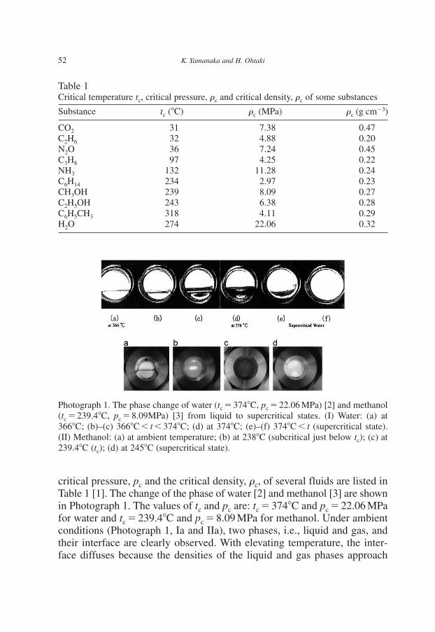
critical pressure, pc and the critical density, rc, of several fluids are listed inTable 1 [1]. The change of the phase of water [2] and methanol [3] are shownin Photograph 1. The values of tc and pc are: tc � 374�C and pc � 22.06 MPafor water and tc � 239.4�C and pc � 8.09 MPa for methanol. Under ambientconditions (Photograph 1, Ia and IIa), two phases, i.e., liquid and gas, andtheir interface are clearly observed. With elevating temperature, the inter-face diffuses because the densities of the liquid and gas phases approach

52 K. Yamanaka and H. Ohtaki

Table 1Critical temperature tc, critical pressure, rc and critical density, rc of some substances

Substance tc (�C) rc (MPa) rc (g cm�3)

CO2 31 7.38 0.47C2H6 32 4.88 0.20N2O 36 7.24 0.45C3H8 97 4.25 0.22NH3 132 11.28 0.24C6H14 234 2.97 0.23CH3OH 239 8.09 0.27C2H5OH 243 6.38 0.28C6H5CH3 318 4.11 0.29H2O 274 22.06 0.32

Photograph 1. The phase change of water (tc � 374�C, pc � 22.06 MPa) [2] and methanol(tc � 239.4�C, pc � 8.09MPa) [3] from liquid to supercritical states. (I) Water: (a) at366�C; (b)–(c) 366�C � t � 374�C; (d) at 374�C; (e)–(f) 374�C � t (supercritical state).(II) Methanol: (a) at ambient temperature; (b) at 238�C (subcritical just below tc); (c) at239.4�C (tc); (d) at 245�C (supercritical state).

CH004.qxd 2/21/2007 3:45 PM Page 52

each other. Under a subcritical condition, fluids become reddish opaque,due to the scattering of light with short wavelengths caused by density fluc-tuations resulting from the formation of microscopic agglomerates. At thecritical point the density of the two phases become identical and the inter-face disappears (Photograph 1, Ie and IIc), and the fluids turn into one trans-parent phase (Photograph 1, If and IId) as the agglomerates decompose tomuch smaller clusters as a result of increased thermal motions.

The phase diagram of water [4, 50, 51] is shown in Fig. 1. SCW is clas-sified into three categories, low-, medium- and high-density regions becauseof the parameter’s importance in relation to thermodynamic and dynamicproperties. In the supercritical region many physicochemical properties ofwater can be represented by the single parameter, density, rather than theparameters, temperature and pressure [50, 51].

In the low-density region, the density of water, r, is less than the crit-ical density (r � rc). The density in the medium density region is an inter-mediate between rc and 1 g cm�3 (rc � r � 1 g cm�3), while for SCW in thehigh-density region, it is larger than 1 g cm�3 (1 g cm�3 � r).

The phase diagram of carbon dioxide is represented in Fig. 2 [5], inwhich the supercritical region is depicted by the gray area. Above the criti-cal temperature, fluids are usually not liquefied under pressure except for

Supercritical Fluids and Reductions in Environmental Pollution 53

Fig. 1. Phase diagram of water [4, 50, 51].

CH004.qxd 2/21/2007 3:45 PM Page 53

some substances which are solid under extremely high pressures. Carbondioxide is one example, which solidifies at a pressure above 570 MPa at tc.

Under the supercritical conditions the solubility of electrolytes inwater dramatically decreases, while solubility of non-electrolytes in watersteeply increases. Therefore, SCW can be a good solvent for making inor-ganic microparticles and also for oxidizing organic wastes by dissolvingorganic oxidizing substances in water containing the waste. This charac-teristic property of water can play a key role in the supercritical water oxidation (SCWO) process for removal of hazardous organic wastes and


Fig. 2. Phase diagram of carbon dioxide [5].

CH004.qxd 2/21/2007 3:45 PM Page 54

chlorinated hydrocarbons by decomposing them to carbon dioxide, waterand inorganic acids [6].

Among various physicochemical properties of SCW, the dielectricconstant, �, and the autoprolysis constant, Kw, play significant roles in theintermolecular interactions of water and ionic solutes.

Various SCFs, other than SCW, have been examined for the treatmentof organic wastes and chlorinated hydrocarbons, and some of them havebeen commercially used. Supercritical methanol is often used, instead ofSCW, under the conditions of t � 240–300�C and p � 8–15 MPa for selec-tive decomposition or methylation of organic materials. One example is therecycle of polyethylene terephthalate (PET) bottles decomposing to itsmonomers by supercritical methanol [7].

Supercritical carbon dioxide (SCCO2) is another useful solvent inindustry. The critical temperature and pressure of carbon dioxide aretc � 30.9�C and pc � 7.4 MPa, which can easily be achieved by using rela-tively simple and inexpensive equipment. From the 1960s, SCCO2 has beenused to extract flavors and other compounds. It is also used as the mobilephase in chromatographic separation of various substances. Coffee decaf-feinating and hop extraction by SCCO2 (developed in Germany in 1970s)are successful examples of the application of SCFs in industry. A hopextraction industry reached a capacity of 50000 ton per year in 1990 inGermany [5]. SCCO2 is used as an extracting solvent for organic com-pounds from wastes as a pretreatment, before decomposition or chemicalanalysis [8]. Further details of the use of SCFs in the reduction of pollutantsin our environment will be discussed later.

3. REFERENCES FOR THERMODYNAMIC PROPERTIES OFSUPERCRITICAL FLUIDS

3.1. References for Thermodynamic Properties of Supercritical Water

The largest industrial SCW application is in thermal power stations. Herethe temperature and pressure of the SCW are 538–560�C and 24.3–31.0 MPa,respectively. The SCW is used as an energy transmission medium to turbines.Because of the large heat capacity of water, it has been used as an energycarrier since the development of steam engines by James Watt in 1769.Chemical thermodynamics was largely developed for the improvement ofthe energy efficiency of engines, and thus the thermodynamic properties of


CH004.qxd 2/21/2007 3:45 PM Page 55

water and its vapor have been extensively investigated over a wide range oftemperature and pressure.

Numerical values of the thermodynamic properties of water, vapor andSCW were compiled in the International Skeleton Steam Table (IST) pub-lished by the International Conference on the Properties of Water and Steam(ICPWS), which was hosted by the International Association for theProperties of Water and Steam (IAPWS) [9]. The latest version of IST wasreleased in 1985 (IST-1985), which covered specific volumes and enthalpiesof water, vapor and SCW over the temperature and pressure ranges of273.15–1073.15 K and 0.1–1,000 MPa, respectively. Data for surface ten-sion [10], dielectric constants (permittivities) [11], ionic products of sol-vents [12], critical points [13], viscosities [14–16], heat capacities [14, 15]and refractive indices [17] of light and heavy water have been published.IAPWS provides equations by which necessary data can be evaluated overa wide range of temperature and pressure. The most recent publication offormulae appeared in 1995 [18], and the software implementing the formu-lae is available from National Institute of Standards and Technology (NIST)[19]. Thermodynamic data for industrial use of SCW are also provided byIAPWS-IF97 [20, 21] and the software is distributed through the AmericanSociety of Mechanical Engineers (ASME) [22, 23].

Three-dimensional diagrams of t-p-r [6, 24] and t-r-h (h: viscosity)[4, 25, 26] of water are shown in Fig. 3a (also in Fig. 1) and b, respectively.

In Fig. 3a, it is seen that the density of SCW is sensitive to both temperature and pressure around the critical point. As a result, the sol-ubility of substances in water can easily be controlled by changing the density.

The variation of the viscosity, h, of water with temperature and den-sity is shown in Fig. 3b. The viscosity of water decreases sharply with tem-perature from 0 to �200�C, and then, gradually decreases further. However,the density dependence of viscosity is, by contrast, rather simple.

The behavior of the relative dielectric constant of water (�r � �/�0,where �0 denotes the dielectric constant of vacuum) is more or less similarto that of viscosity (Fig. 4) [4, 11, 27]. Due to the breaking of hydrogenbonds of water, the dielectric constant rapidly decreases with temperature.For comparison, the relative dielectric constants of acetonitrile (CH3CN),methanol (CH3OH) and liquid ammonia (NH3) at room temperature areindicated in Fig. 4.

The autoprotolysis constant of water, Kw, changes with temperature,pressure and density. The t-r-Kw and t-p-r-Kw diagrams of water are shown in


CH004.qxd 2/21/2007 3:45 PM Page 56

Fig. 5a and b, respectively [4, 12]. From the figures, one could expect that onemole of water might dissociate into 10�1.5 mol dm�3 H� and 10�1.5 mol dm�3

OH� ions under 105 atmospheric pressure (104 MPa or 10GPa) at 1000�C. Thiswould mean that under these conditions, the water was both highly acidic andbasic at the same time. This condition might be achieved deep underground,


Fig. 3. Three-dimensional diagrams of physicochemical properties of water. (a) t-p-r [6,24]. (b) t-r-h [4, 26, 27].

CH004.qxd 2/21/2007 3:45 PM Page 57

where rocks and stones might be dissolved. However, no evidence has beenfound for this even under such ultra-supercritical conditions with a veryhigh density of r � 1.5 g cm�3. Fig. 5c shows another plot of the autoprotol-ysis constant, log Kw, and relative dielectric constant, �r, of water againsttemperature at 25 MPa [11, 12]. With the increase in temperature, the valueof log Kw increases slightly, and then sharply decreases at �400�C. The rel-ative dielectric constant of water also decreases with temperature and asharp drop in �r occurs around 400�C.

3.2. References for Thermodynamic Properties of Supercritical Carbon Dioxide and Other Fluids

The thermodynamic data of carbon dioxide and other fluids are com-piled in “International Thermodynamic Tables of the Fluid State” publishedby the International Union of Pure and Applied Chemistry (IUPAC) [28] in theform of tables and equations of state. Thermodynamic data and equations of state are also provided by “Journal of Physical and Chemical ReferenceData” for argon [29], nitrogen [29], oxygen [29], carbon dioxide [30], methane[31], ethane [31], propane [31], butane [31, 32], isobutene [31, 32], ethylene[29] and methanol [33]. “Fluid Phase Equilibria”, “Journal of SupercriticalFluids” and “Chemical Engineering Science” are also good sources of ther-modynamic and thermochemical data of SCFs. Data for phase diagrams,


Fig. 4. The three-dimensional t-r-�r diagram of water [4, 11, 25].

CH004.qxd 2/21/2007 3:45 PM Page 58

Supercritical Fluids and R

eductions in Environm

ental Pollution59

Fig. 5. The diagram of the autoprotolysis constant, Kw, of water with temperature and pressure. (a) The three-dimensional t-r-log Kw diagram, (b) the four-dimensional t-p-r-log Kw diagram, (c) the variation of log Kw and dielectric constant, �r, with tem-perature under 25 MPa [11, 12, 42].

CH004.qxd 2/21/2007 3:45 PM Page 59

diffusion coefficients of molecules in pure and mixed fluids are available[34–39]. One can access various thermodynamic databases of pure fluidsthrough the websites of NIST database [19] and “Chemical Web Book”[40]. Data for mixed fluids for engineering purposes can be found in the“Dortmund Data Bank” [41].

4. SOLUBILITY OF ELECTROLYTES AND NON-ELECTROLYTES IN SUPERCRITICAL FLUIDS

4.1. Solubility of Organic and Inorganic Substances in Supercritical Water

Around the critical point, the dissolving power of water for soluteschanges dramatically. In SCW, the solubility of inorganic electrolytesdecreases sharply, while non-polar hydrophobic organic substances exhibita high solubility and sometimes become completely miscible. The charac-teristic change in the dissolving ability of SCW plays a key role in theSCWO technology, where waste organics and oxidants (oxidizing reagentor air) are well mixed with SCW. The changes in �r and Kw with temperatureand density (Fig. 5) essentially contribute to the SCWO method. Althoughthe autoprotolysis constant, Kw behaves as if SCW is a mixture of a strongacid and a strong base at extremely high temperatures, pressures and den-sity, the value of Kw is �10�23 mol2 dm�6 around the critical point, wherethe density becomes one-third of that of normal water [12].

An example is the solubility of benzene in water at high temperatureand pressure [43, 44]. The solubility of benzene in water is �0.07 wt% atambient conditions, but is 7–8 wt% at 260�C, and the solubility is practi-cally independent of pressure at any particular temperature. The solubilityincreases to 18 and 35 wt% at 287 and 295�C, respectively, and at 20–25 MPa,benzene becomes totally miscible at 300�C. Fig. 6 shows the critical solu-bility curves of binary mixtures of water with H2, N2, CO2, Ar, Xe, CH4and benzene [45]. On the left-hand side of the curves the mixtures are sep-arated into two phases and on the right-hand side they exist as one-phasefluids.

In contrast to the case of non-polar organic substances, the solubilityof inorganic compounds decreases exponentially in SCW as seen in Fig. 7.Sodium chloride dissolves in water up to 37 wt% at 300�C, but the solubilitydecreases to only 120 ppm in SCW at 550�C and 25 MPa. The maximumsolubility of calcium chloride is 70 wt% in subcritical water, but the solubil-ity goes down to 3 ppm at 500�C and 25 MPa. Most inorganic salts are spar-


CH004.qxd 2/21/2007 3:45 PM Page 60

ingly soluble in water under sub- and supercritical conditions due to insuf-ficient formation of hydration shells around ions because of the low densityof the water and high mobility of water molecules.

4.2. Solubility of Organic and Inorganic Substances in Supercritical Carbon Dioxide

The solubility of solid ionic solutes is low in non-polar solvents, whilenon-polar solutes show higher solubilities than ionic salts. The solubility of non-polar solutes is affected by intermolecular interactions in the solid and solute–solvent interactions and the number density of molecules in thesolvents. The vapor pressure of the solid solute can be a good indicator ofintermolecular interactions in the solid state. Carbon dioxide is non-polar


Fig. 6. Critical solubility curves for binary system of water and non-polar substances. CP:critical point of pure water [45].

CH004.qxd 2/21/2007 3:45 PM Page 61

(dipole moment, m � 0), but has a quadrupole moment. The solubility of asolute in SCCO2 depends on the molecular weight and the polarity of thesolute.

Fig. 8 shows the variation of the mole fraction, y2, of naphthalene insaturated SCCO2 solutions with temperature and pressure [46]. Subscript 2denotes the solute, i.e., naphthalene, and the component 1 is of course CO2.The solubility of naphthalene in CO2 is strongly affected by pressure around


Fig. 7. Solubility of electrolytes in supercritical water at 25 MPa [6].

CH004.qxd 2/21/2007 3:45 PM Page 62

the critical point, pc � 7.38 MPa, but at higher pressures the effect is small.The steep increase in the solubility of naphthalene in SCCO2, with pressurearound pc, is convenient for extracting naphthalene from a mixture. The tar-get solute is dissolved in SCCO2 from a solid mixture by pressurizing thesolution and is precipitated by releasing the pressure.

Fatty acids and alcohols dissolve in SCCO2 and the concentration offatty acids at saturation increase steeply with pressure around pc of CO2(Fig. 9) [47, 48]. The general trend is that the larger the polarity and molec-ular size of the solute molecules, the smaller the solute solubility.

SCCO2 is not a good solvent for polar substances when compared with the usual organic liquids. In order to improve the dissolving ability of substances in SCCO2, an entrainer or a co-solvent is added to SCCO2[49]. In Fig. 10 the effect of ethanol and octane as the entrainer (co-solvent)is shown for the maximum solubility of stearic acid in SCCO2. The molefraction of stearic acid, y2, at saturation in SCCO2 increases with the con-centration of the entrainers. Ethanol has a larger effect than octane, becausepolar ethanol can better interact with polar stearic acid than non-polaroctane.


Fig. 8. Solubility of naphthalene in supercritical CO2. y2 denotes the mole fraction ofnaphthalene at saturation [45]. �: 35�C, �: 45�C, and �: 55�C.

CH004.qxd 2/21/2007 3:45 PM Page 63


Fig. 9. Solubility of fatty acids and alcohols in supercritical CO2 at 35�C. y2 denotes themole fraction of solutes at saturation [47, 48]. �:myristic acid, �: palmitic acid, �:stearic acid, �: cetyl alcohol, �: stearyl alcohol, �: arahydryl alcohol.

Fig. 10. The entrainer effect of ethanol and octane on the solubility of stearic acid insupercritical CO2 [49]. �: 9.9 MPa, �: 14.8 MPa, �: 19.7 MPa for ethanol, and �:9.9 MPa, �: 19.7 MPa for octane.

CH004.qxd 2/21/2007 3:45 PM Page 64

5. STRUCTURE OF SUPERCRITICAL WATER

Structural information on SCFs is essentially important not only for the under-standing of thermodynamic and thermochemical properties, and the uniquereactions of substances in the SCFs, but also for the improvement and exten-sion of industrial applications of SCFs. However, due to technical problems,few studies have been done on the structure of SCFs. The recent progress inanalytical methods and equipment has improved the situation. High-speedcomputers are now widely used to simulate the behavior of molecules in SCFsat high temperatures and pressures, which is sometimes difficult to realize byexperiments. Since water is the most attractive substance for chemists, struc-tural investigations of SCW have been carried out by various workers usingmethods such as X-ray and neutron diffraction techniques, NMR, Raman andinfrared spectroscopies. Computer simulations provide useful information forthe molecular arrangements and dynamics in SCW [50, 51].

Interatomic spatial correlations are represented by the radial distribu-tion function, D(r), which can be obtained by the X-ray and neutron diffrac-tion methods. From the peak position, the peak area, and the peak width, theinteratomic distance, r, the number of atoms within the atom pair, n and themean-square amplitude of the distance of the atom-pair, s, respectively, canbe estimated.

The X-ray diffraction method at high temperatures and high pressureshas been applied to the study on the structure of SCW since the 1980s [52,53], but the early results were not reliable due to technical difficulties. In1993 Yamanaka and his coworkers reported X-ray diffraction results for thestructure of high temperature and high pressure water at T � 300–649 K andp � 0.1–98.1 MPa by using an imaging plate detector [54]. The radial distri-bution curves in the form of D(r)�4�r2r0 at various temperatures and pres-sures are represented in Fig. 11, where r0 denotes the average electrondensity in the system. The peaks appearing at r � 290, 450 and 670 pm indi-cate the tetrahedral ice-like hydrogen-bonded structure of liquid water [55].

The peaks at higher r values gradually disappeared with an increase intemperature and pressure, indicating the breaking of the ice-like hydrogen-bonded tetrahedral structure of water. The peak analysis was performed forthe first peak around 200–400 pm of the radial distribution function in theform of D(r)/4�r2r0, and the peak was de-convoluted into two peaks, I andII, as seen in Fig. 12. The structure parameters, r, n and half-width at thehalf-height of the peak, s, which corresponds to the mean-square amplitudeof bonds, are summarized in Table 2.


CH004.qxd 2/21/2007 3:45 PM Page 65


Fig. 11. Radial distribution functions, D(r)�4�r2r0 of water at various temperatures andpressures [54].

CH004.qxd 2/21/2007 3:45 PM Page 66

The water–water distance at the nearest neighbor, rI, increased and thenumber of water molecules at the nearest neighbor, nI, decreased with theincrease in temperature and pressure. The results indicated that the hydro-gen bonds between water molecules were elongated and the hydrogen-bonded water structure was going to be decomposed at elevated temperatureand pressure. The sI value also increases with t and p, and the result showedthat the water–water interaction was weakened when t and p were elevated.


Fig. 12. The peak analysis of radial distribution functions of water, D(r)/4�r2r0 at vari-ous temperatures and pressures given in Fig. 10. The experimental values are given bysolid lines and the calculated peaks I and II with the structural parameters given in Table2 are indicated by dots [54].

CH004.qxd 2/21/2007 3:45 PM Page 67

In contrast to the change in nI, nII increased with the increase in t and p, andrII and sII also increased with t and p.

The values of n, r and s obtained from peaks I and II are plotted againsttemperature and density in Fig. 13. In the figure, the sum of nI � nII is alsoplotted, which is practically unchanged in spite of the change in the density.

The nI value was 1.6–1.8 in the SCW at r � 0.7 g cm�3, and the resultindicated that �40% of hydrogen-bonds in the ice-like water structure(n � 4) still remain in the SCW. The s value increased, which suggested thatthe H2O–H2O bonds in the SCW were largely fluctuating.

An interesting result is given in Fig. 14 for the H2O–H2O distance (r)in water collected from the literature plotted against r�1/3 [50, 51, 56]. Sincer�1/3 corresponds to the statistically averaged intermolecular distance in liquids, the plot represents the comparison of the experimentally obtainedwater–water distance (r) with the statistically averaged intermolecular dis-tance. In high and medium density water with r � 1.04–0.9 g cm�3 underambient and subcritical conditions, the water–water distance was pro-portional to the average distance, and the fact suggested that the thermalexpansion of water was mainly caused by the elongation of the water–water hydrogen bond distance. However, in SCW of low density where


Table 2The structural data of water molecules at the nearest (peak I) and the second nearest(peak II) neighbors determined by the analysis of radial distribution functions at varioustemperatures and pressures including the supercritical region

t (�C) p r Peak I Peak II(MPa) (g cm�3)

nI rI (pm) sI (pm) nII rII (pm) sII (pm)

300 0.1 1.0 3.1 287 28 1.3 341 37416 52.9 0.95 2.8 291 27 1.8 341 34441 98.1 0.95 2.8 290 27 1.9 340 32469 47.8 0.9 2.5 287 26 2.4 342 36498 98.1 0.9 2.4 290 27 2.4 342 36532 5.0 0.8 2.1 287 26 2.2 339 34557 51.6 0.8 2.1 289 25 2.1 344 35592 98.1 0.8 2.0 287 30 2.4 343 34610 36.5 0.7 1.8 293 31 1.9 348 42637 67.7 0.7 1.7 293 33 2.0 343 42649 80.4 0.7 1.6 292 35 2.3 342 44

n: the number of water molecules, r: the intermolecular distance, s: the half-width at thehalf-height of the peak [54]. Estimated errors in n, r and are 0.1, 1, 1 pm, respectively.

CH004.qxd 2/21/2007 3:45 PM Page 68

r�1/3 1.02 g�1/3 cm, the intermolecular distance, r, was practicallyunchanged, although the data were scattered to some extent. The result indi-cated that water molecules were still hydrogen-bonded even in the SCWwith a distance of �293 � 3 pm.

In the low density SCW, small clusters should be formed in which theH2O–H2O hydrogen-bonded distance is kept �293 pm. The clusters may be


Fig. 13. The structural parameters of water with density and temperature. (a) The number of water molecules at the nearest neighbors n, (b) interatomic distance r, (c) half-width at half-height s of the peaks I (�) and II (�) and their sum (�) [54].

CH004.qxd 2/21/2007 3:45 PM Page 69

dispersed in the SCW, although the co-existence of monomerly dispersedgas-like water molecules together with clusters cannot be denied.

The average number of the nearest water molecules in water, n (nI inFig. 13) is plotted against the density of water, r in Fig. 15. The plot monot-onously decreases with a decrease in density from normal water (n � 4.4under an ambient condition) to SCW (n � 1.6–1.8). From the two plots inFigs. 14 and 15, it can be concluded that the clusters formed in SCW are notso large that many of water molecules in the clusters locate around the sur-face of the clusters, but have smaller numbers of adjacent molecules thanthose in the bulk. Therefore, water molecules are heterogeneously dispersedin SCW by forming small clusters, in which water molecules are bound byhydrogen-bonds with the intermolecular distance of r �293 pm, probablytogether with monomer dispersed molecules.

The position of hydrogen atoms can be estimated experimentally bymeans of neutron diffraction and theoretically by computer simulations, andon the basis of these data, the orientation of water molecules in SCW can


Fig. 14. The adjacent water–water distance r at high temperatures and pressures plottedagainst r�1/3. The straight line represents the change in r calculated by assuming a homo-geneous expansion of water with r�1/3, r � kr0r

�1/3 and k � 1 (r0: O–O distance in ambi-ent water) [56].

CH004.qxd 2/21/2007 3:45 PM Page 70

be discussed. Molecular dynamic simulations of SCW were performed byemploying TIP4P [57, 58], SPC [59] and SPCE [60] potentials. A neutrondiffraction measurement was examined for SCW [61]. The pair correlationfunctions, gOO(r) of the O–O atom pair found by molecular dynamics sim-ulations and neutron diffraction experiment, together with the gOO(r) func-tion derived from the X-ray diffraction data [54], are compared in Fig. 16.

The shape of the gOO(r) functions obtained from MD simulations andX-ray diffraction data are similar, but that from the neutron diffractionmeasurement is very different from the others. The result from the neutrondiffraction study is today considered to be less reliable.

High temperature–high pressure NMR techniques provide usefulinformation on the intermolecular interactions of SCW. The 1H NMR signalof water observed at 30�C was sharp and shifted toward the low field sidewith temperature at constant density (r � 0.4 g cm�3 at high temperaturesand pressures; the pressure was changed in an NMR tube with a constantvolume) [62, 63]. The signal was broadened with the increase in the tem-perature as seen in Fig. 17a. The chemical shift s of water is plotted againsttemperature in the liquid and gas phases in Fig. 17b.


Fig. 15. The number of water molecules at the first hydration shell, n, plotted against r [56].

CH004.qxd 2/21/2007 3:45 PM Page 71


Fig. 16. Comparison of pair correlation functions gOO(r) of supercritical water obtainedby various methods.

Method Potential function T/K r (g cm�3) Reference

(a) MD TIP4P 725 0.75 57(b) MC TIP4P 673 0.7 58(c) MD SPC 647 0.48 59(d) MD SPCE 652 0.33 60(e) ND – 673 0.66 61(f) XD – 649 0.7 54

MD: molecular dynamics, MC: Monte Carlo, ND: neutron diffraction, XD: X-ray diffraction.

CH004.qxd 2/21/2007 3:45 PM Page 72

The plot of chemical shift depicted in Fig. 17b shows that the NMRchemical shifts of liquid water move to the high field side on the equilib-rium curve with an increase in temperature, while reverse is true for waterin the gas phase. A plot of the number of hydrogen-bonded water molecules,nHB, estimated from the NMR chemical shifts at various temperatures anddensities is given in Fig. 18. The result shows that hydrogen bonds still existin SCW even at 400�C and r � 0.2 g cm�3.

Studies by IR and Raman spectrometry provide important informationon the nature of water–water bonds. The O–D stretching vibration band inHDO solution containing 8.5 mol% D2O in H2O was measured at 303–673 Kand 5–400 MPa and the result is depicted in Fig. 19 [64]. The O–D band wasobserved at 2520 cm�1 under ambient condition. A sharp band appearing at2719 cm�1 in the solution of r � 0.0165 g cm�3 and T � 673 K was ascribedto free HOD molecules. The band disappeared in SCW with r�0.095gcm�3.On the other hand, a new band was observed around 2650 cm�1 in water withr � 0.036 g cm�3 and the intensity of the band increased and shifted towardthe low frequency side with increasing density. In water with r � 0.9 g cm�1

the band appeared at 2600 cm�1. The band was ascribed to the O–D fre-quency of hydrogen-bonded water in SCW.


Fig. 17. 1H NMR signals of water. (a) The shape and position of 1H NMR signals at var-ious temperatures. (b) 1H NMR chemical shift d as a function of temperature and density.The filling factor of water is 0.4, which makes density of supercritical water to ber � 0.4 g cm�3 [62, 63].

CH004.qxd 2/21/2007 3:45 PM Page 73


Fig. 18. The average number of hydrogen bonds, nHB, of water estimated by 1H NMRmeasurements [62, 63].

Fig. 19. The frequency of the O–D stretching vibration, n, in the IR spectra of waterobserved at 673 K at various densities. k denotes the molar extinction coefficient in thecm2 mol�1 unit [64].

CH004.qxd 2/21/2007 3:45 PM Page 74

The O–D stretching vibration band was observed by the Raman spectroscopy over the temperature range of 298–673 K within a relativelynarrow density range of 0.8–1.0 g cm�3 and a wide density range from 0.04 to 0.8 g cm�3 at 673 K (Fig. 20) [65]. The band around 2500 cm�1

was attributed to the hydrogen bonded O–D stretching vibration, and the band around 2700 cm�1 was assigned to the O–D bond in non-hydrogen-bonded water. The band assignment is consistent with the IR meas-urement [64]. Although the two state model (hydrogen-bonded and freewater molecules) may be too simple to explain the IR and Raman spec-tra, these results showed the existence of hydrogen bonds in relatively dense SCW.

Since SCW consists of heterogeneously dispersed small clusters,oligomers and probably gas-like monomer water molecules, non-polarorganic substances can easily be mixed with it. On the other hand, due tothe lack of the number density of water molecules, insufficient hydrationshells are formed around the inorganic ions and the dissociation of inor-ganic salts is suppressed.


Fig. 20. Isotropic Raman spectra for the D–O stretching frequency, n, in 9.7 mol% HDOin H2O at various temperatures and densities [65].

CH004.qxd 2/21/2007 3:45 PM Page 75

6. APPLICATION OF SUPERCRITICAL FLUIDS FOR REDUCING POLLUTANTS

6.1. Supercritical Water Oxidation ProcessOne of the major problems we have today is the disposal of various

organic wastes and hazardous compounds. The ideal solution would be todecompose them into innocuous substances. Chemical oxidation processesby ozone and hydrogen peroxide, photo oxidation processes by ultravioletirradiation, wet oxidation processes by applying high temperature and highpressure (200–300�C and 1.5–10 MPa) and incineration processes at 800–2000�C have been examined at a laboratory scale and some of them havealready been scaled up. However for most of these techniques, the effi-ciency of decomposition of the wastes and polluting materials are not highenough. Although the incineration process could achieve the effective decom-position, the process produces hazardous and toxic by-products such asdioxanes, NOx and SOx, which are often discharged into the atmosphere.

In 1982 it was reported that the oxidation process by using SCW iseffective in the decomposition of persistent organic wastes, and the decom-position could be greater than 99.99% for most wastes. The SCWO processfor the treatment of pollutants, wastes and hazardous compounds attractedmuch attention in recent years [6, 66–74]. Efficiencies for decomposition ofchlorinated organic compounds are listed in Table 3 [72, 73]. The SCWOprocesses are usually operated at �600–650�C, which is lower than thetemperature of incineration processes.

Organic wastes including chlorine, sulfur and nitrogen atoms are oxi-dized and decomposed into water, CO2, N2, HCl, H2SO4 and HNO3. Theacids formed are usually neutralized by a sodium hydroxide solutioninjected into a reactor. The neutralized acids are precipitated as salts. For thetreatment of aqueous solutions containing organic wastes of 1–20 wt%, theSCWO process is more effective in energy and cost than the incinerationprocess. Slurries containing organic wastes such as human metabolic wastes[74], biomass and organic polluted soils are pumped into a reactor. TheSCWO process is performed in a fully closed system, and no additionalabatement facilities for exhaust gases and discharged water are required.

Major problems of the SCWO process are (1) the removal of precipi-tates formed in the reactor and scales accumulated in the equipment [75, 76].They reduce heat efficiencies of the reactor and prevent the stable operationof the process. Metals included in the wastes are often oxidized to metaloxides, which are also precipitated in the reactor. (2) Corrosion of reactors is


CH004.qxd 2/21/2007 3:45 PM Page 76

another serious matter in the SCWO process. Oxidation of materials used forreactors is accelerated by the acids produced. As a result, corrosion resistivematerials have to be used for the equipment, and this is usually costly.

In order to solve the problem caused by precipitates in reactors, a two-zone technique involving supercritical and subcritical chambers wasexploited. A flow-chart of an SCWO process (MODAR process) featuringa two-zone reactor is shown in Fig. 21 [66]. In the upper zone, which is forSCW at �600�C, the wastes are decomposed and the products are neutral-ized. In the lower zone (subcritical), in which the temperature of water is�200�C, the precipitates which formed in the upper zone are dissolved.


Table 3Destruction efficiencies of chlorinated organic compounds bySCWO [71–73]

Compound Destruction rate (%)

Carbon tetrachloride 96.53Chlorinated dibenzo-1,4-dioxanesa 99.9999Chloroform 98.832-Chlorophenol 99.9972-Chlorotoluence 99.998DDTb 99.9974,4�-Dichlorobiphenyl 99.9931,2-Dichloroethane 99.99PCBsc 99.9951,1,2,2-Tetrachloroethylene 99.99Trichlorobenzenesd 99.991,1,1,-Trichloroethane 99.999971,1,2-Trichloroethane 99.981

aMixtures of chloro-substituted dibenzo-1,4-dioxane.bDichlorodiphenytrichloroethane.cPolychlorinated biphenyl (or polychlorobiphenyl).dMixtures of 1,2,3-, 1,2,4- and 1,3,5-trichlorobenzene.

O

O

Chloro-substituted dibenzo-1,4-dioxane

Clx Cly

Cl C

H

DDT

C

ClCl

Cl

Cl

CH004.qxd 2/21/2007 3:45 PM Page 77

78K

. Yamanaka and H

. Ohtaki

Fig. 21. Flow diagram of SCWO process (“MODAR process”) featuring two-zone reactor [66].

CH004.qxd 2/21/2007 3:45 PM Page 78

Organic wastes, an alkaline solution (used for the neutralization of theacids produced), air as an oxidant and supercritical water, are mixed andpreheated, and then injected into the supercritical zone of the reactor. Thewastes are oxidized and neutralized in this area. The SCF flows downwardsduring the reaction, and precipitates formed during the reaction fall downinto the subcritical zone and are dissolved in subcritical water. The hightemperature fluid turns back and upward due to convection, and then goesout from a vent.

The two-zone type reactor has been improved with the introduction of a dual shell pressure type reactor (Fig. 22) [67, 77]. In the dual shell reac-tor, pressurized air is introduced between the wall of the pressure vessel and a reaction cartridge. A pilot plant of the dual shell type reactor can treattwo tons of aqueous solutions containing 10% organic wastes per day(Photograph 2).

The corrosion problem could be avoided by using highly corrosionresistive material. Nickel alloys like Inconel 625 or Hastelloy C-276 areexamples. Even some noble metals are used for the cartridge. Since thethickness of the wall of the cartridge can be reduced in dual shell type reactors, the cost for constructing the SCWO reactor can be drasticallyreduced.

6.2. Extraction of Pollutant from Soils with Supercritical CarbonDioxide and Other Supercritical Fluids

The dissolving capacity of SCCO2 depends on the temperature and pres-sure. When a target material is dissolved in SCCO2 at a high pressure, thematerial is precipitated when the pressure is released. As a result, SCCO2can be used for extraction of various materials. Usually no distillation and


Fig. 22. Schematic presentation of dual shell pressure-balanced vessel for SCWO [77].

CH004.qxd 2/21/2007 3:45 PM Page 79

other additional processes are required. Extraction of caffeine and hop areexamples. SCCO2 can also be employed for extracting polluting materialsfrom soil. By extracting contaminants, together with a preconcentrationstep, it is possible to analyze minute amounts of contaminants by conven-tional analytical methods. The use of SCCO2 together with an entrainer at thepretreatment step for the contamination analysis in soils, a high recovery rateof contaminants was realized compared with the standard analytical processof SW846 Method 8330 in USA [78]. The recovery of dioxanes from soilwas improved from 40 to 90% by adding 2% of methanol to SCCO2 [79].The addition of 2% methanol to supercritical N2O could extract dioxanesfrom soil with the extraction efficiency of greater than 98% [79]. It is possi-ble with a combination of gas chromatography and SCCO2 extraction, toanalyze volatile contaminants in soils within 10 min [80, 81]. Successfulremovals of dichlorodiphenyltrichloroethane (DDT) [82] and chlorinatedaromatic compounds such as trichlorophenyl and polychlorinated biphenyls(PCBs) [83] have been reported. Since the 1990s, SCF extraction processesfor soil remedy have been scaled up for commercial use.


Photograph 2. Supercritical water oxidation reactor situated at Organo Corporation,Saitama, Japan. (Partly funded by New Energy and Industrial Technology DevelopmentOrganization (NEDO), which is an auxiliary organization of the Ministry of Economy,Trade and Industry of Japan).

CH004.qxd 2/21/2007 3:45 PM Page 80

Supercritical propane has been applied to the treatment of sludge fromwastewater treatment facilities in petroleum refineries with a treatmentcapacity of 300 barrels per day [84].

6.3. Recycle of Used Plastic Bottles with Supercritical MethanolSupercritical methanol can be used under milder conditions than those

used in SCW. Supercritical methanol is used for recycling processes of wasteplastics to monomers. PET is decomposed by supercritical methanol todimethylterephthalate and ethylene glycol. Supercritical methanol can per-form the process within 1/10 reaction time with 100% recovery of recyclingwithout the use of catalysts. The method is more advantageous than othermethods using liquid methanol and liquid ethylene glycol with catalysts.The decomposition of PET can be made at 330�C and 8.1 MPa [7, 85].Another advantage of this process is that the evolution of gaseous productsis negligible, because the decomposition reactions stop at the formation ofmonomers and do not proceed to CO2. The monomers can be used again forproducing PET, and the “bottle-to-bottle” recycle is realized.


The application of SCFs to the treatment of wastes and pollutants and to theextraction of contaminants from soil will be extended to other fields in the near future. The cost for the construction of plants will be reduced by theimprovement of equipment and materials. The kind of fluids to be used willalso be improved and many other technologies will be developed accordingto world needs. On the other hand, reactivities of SCFs, the nature ofintramolecular bonds and intermolecular interactions, which are closelyrelated to the reactivities, are not well elucidated yet. Studies on thermody-namics and thermochemistry and intra- and intermolecular interactions frommicroscopic points of view of SCFs will help solve some of these problems.Furthermore structural studies of SCFs have rarely been made for com-pounds other than water. Structural investigations of liquids at high temper-ature and high pressure are also very attractive and important in relation tolife sciences. Further investigations into this area should be encouraged.

REFERENCES

[1] T. Furuya and Y. Arai, Chem. Ind. (KAGAKU KOGYO) (in Japanese), 46 (1995) 14.[2] N. Asahi, Private Communication.


CH004.qxd 2/21/2007 3:45 PM Page 81

[3] T. Sako, Chemistry (KAGAKU) (in Japanese), 52 (1997) 31.[4] E.U. Franck, in “The Physics and Chemistry of Aqueous Ionic Solutions” (M.-C.

Bellissent-Funel and G.W. Neilson, eds.), p. 337, D. Reidel Publ. Co., Dordrecht,The Netherlands, 1987.

[5] K. Nagahama, in “Handbook of Supercritical Fluids. Application in Food Industries(in Japanese)” (K. Nagahama and I. Suzuki, eds.), p. 18, Science Forum, Tokyo,Japan, 2002.

[6] J.W. Tester, H.R. Holgate, F.J. Armellini, P.A. Webley, W.R. Killilea, G.T. Hong andH.E. Barner, ACS Symposium Series, Emerging Technologies for Hazardous WasteManagement III (1991), and references therein.

[7] T. Sako, T. Sugata, K. Otake, Y. Nakazawa, S. Sato, K. Namiki and M. Tsugumi, J. Chem. Eng. Jpn., 30 (1997) 342.

[8] W. McGovern and P.N. Rice, Pollut. Eng., September (1988) 122.[9] http://www.iapws.org/[10] N.B. Vargaftik, B.N. Volkov and L.D. Voljak, J. Phys. Chem. Ref. Data, 12 (1983)

817.[11] M. Uematsu and E.U. Franck, J. Phys. Chem. Ref. Data, 9 (1980) 1291.[12] W.L. Marshall and E.U. Franck, J. Phys. Chem. Ref. Data, 10 (1981) 295.[13] J.M.H. Levelt Sengers, J. Straub, K. Watanabe and P.G. Hill, J. Phys. Chem. Ref.

Data, 14 (1985) 193.[14] N. Matsunaga and A. Nagashima, J. Phys. Chem. Ref. Data, 12 (1983) 933.[15] J.V. Sengers and J.T.R. Watson, J. Phys. Chem. Ref. Data, 15 (1986) 1291.[16] A. Nagashima, J. Phys. Chem. Ref. Data, 6 (1977) 1133.[17] I. Thormählen, J. Straub and U. Grigull, J. Phys. Chem. Ref. Data, 14 (1985) 933.[18] W. Wagner and A. Pruss, J. Phys. Chem. Ref. Data, 31 (2002) 387.[19] http://www.nist.gov/srd/nist10.htm[20] W. Wagner, J.R. Cooper, A. Dittmann, J. Kijima, H.J. Kretzschmar, A. Kruse,

R. Mares, K. Oguchi, I. Stocker, O. Sifner, Y. Takaishi, I. Tanishita, J. Trubenbachand T. Willkommen, J. Eng. Gas Turb. Power, 122 (2000) 150.

[21] W.T. Parry, J.C. Bellows, J.S. Gallagher and A.H. Harvey, ASME InternationalSteam Tables for Industrial Use, ASME press, New York, NY, 2000.

[22] http://www.asme.org/research/wsts/steam.html[23] http://members.asme.org/catalog/ItemView.cfm?ItemNumber�I00420 [24] L. Haar, J.S. Gallagher and G.S. Kell, NBS/NRC Steam Tables, Hemisphere

Publishing Corp., New York, 1984.[25] U. Grigull (ed.), “Properties of Water and Steam in SI-Units”, Springer-Verlag,

Heidelberg, Germany, 1982.[26] K.H. Dudziak, and E.U. Franck, Ber. Bunsenges., Phys. Chem., 70 (1966) 1120.[27] K. Heger, M. Uematsu and E.U. Franck, Ber. Bunsenges., Phys. Chem., 84 (1980) 758.[28] S. Angus, B. Armstrong and K.M. Reduck, “Carbon Dioxide: International

Thermodynamic Tables of the Fluid State-3”, Pergamon Press, Oxford, 1976.[29] B.A. Younglove, J. Phys. Chem. Ref. Data, 11(1) (1982).[30] R. Span and W. Wagner, J. Phys. Chem. Ref. Data, 25 (1996) 1509.[31] B.A. Younglove and J.F. Ely, J. Phys. Chem. Ref. Data, 16 (1987) 577.[32] S.S. Chen, R.C. Wilhoit and B.J. Zwolinsky, J. Phys. Chem. Ref. Data, 4 (1975) 859.


CH004.qxd 2/21/2007 3:45 PM Page 82

[33] R.D. Goodwin, J. Phys. Chem. Ref. Data, 16 (1987) 799.[34] R.E. Fornari, P. Alessi and I. Kikic, Fluid Phase Equilib., 57 (1990) 1.[35] R. Dohrn and G. Brunner, Fluid Phase Equilib., 106 (1995) 213.[36] M. Christov and R. Dohrn, Fluid Phase Equilib., 202 (2002) 153.[37] T. Adrian, M. Wendland, H. Hasse and G. Maurer, J. Supercrit. Fluids, 12 (1998) 185.[38] F.P. Lucien and N.R. Foster, J. Supercrit. Fluids, 17 (2000) 111.[39] H. Higashi, Y. Iwai and Y. Arai, Chem. Eng. Sci., 56 (2001) 3027.[40] http://webbook.nist.gov.chemistry/[41] http://www.ddbs.de[42] E.U. Franck, S. Rosenzweig and M. Christoforakos, Ber. Bunsenges., Phys. Chem.,

94 (1990) 199.[43] J. Connolly, J. Chem. Eng. Data, 11 (1966) 13.[44] C.J. Robert and W.B. Key, AIChE J., 5 (1959) 285.[45] E.U. Franck, Pure Appl. Chem., 98 (1981) 1401.[46] Y. Tsekhanskaya, Russ. J. Phys. Chem., 38 (1964) 1173.[47] Y. Iwai, J. Chem. Eng. Data, 36 (1991) 430.[48] Y. Iwai, J. Chem. Eng. Data, 38 (1993) 506.[49] Y. Koga, Fluid Phase Equilib., 125 (1996) 115.[50] H. Ohtaki, T. Radnai and T. Yamaguchi, Chem. Soc. Rev., (1997) 41.[51] M. Nakahara, T. Yamaguchi and H. Ohtaki, Recent Res. Dev. Phys. Chem., 1

(1997) 17.[52]. N. Dem’yanets, Zh. Struk. Khim., 24 (1983) 66.[53] Yu. E. Gorbatyi and Yu. N. Dem’yanets, Zh. Struk. Khim., 24 (1983) 74.[54] K. Yamanaka, T. Yamaguchi and H. Wakita, J. Chem. Phys., 101 (1994) 9830.[55] A.H. Narten and H.A. Levy, J. Chem. Phys., 55 (1971) 2263.[56] T. Radnai and H. Ohtaki, Mol. Phys., 87 (1996) 103.[57] R.D. Mountain, J. Chem. Phys., 90 (1989) 1866.[58] A.G. Kalinichev, Z. Naturforsch., 46a (1991) 433.[59] P.T. Cummings, H.D. Cochran, J.M. Simonson, R.E. Mesmer and S. Karaborni,

J. Chem. Phys., 94 (1991) 5606.[60] Y. Guissani and B. Guillot, J. Chem. Phys., 98 (1993) 8221.[61] P. Postorino, R.H. Tromp, M.-A. Ricci, A.K. Soper and G.W. Neilson, Nature, 366

(1993) 668.[62] N. Matubayasi, C. Wakai and M. Nakahara, Phys. Rev. Lett., 78 (1997) 2573, 4309.[63] N. Matubayasi, C. Wakai and M. Nakahara, J. Chem. Phys., 107 (1997) 9133.[64] E.U. Franck and K. Roth, Disc. Faraday Soc., 43 (1967) 108.[65] W. Kohl, H.A. Lindner and E.U. Franck, Ber. Bunsenges., Phys. Chem., 95 (1991)

1586.[66] J.E. Barner, C.Y. Huang, T. Johnson, G. Jacobs, M.A. Martch and W.R. Killilea,

J. Hazardous Mater., 31 (1992) 1.[67] H.R. Holgate and J.W. Tester, J. Phys. Chem., 98 (1994) 800.[68] H.R. Holgate and J.W. Tester, J. Phys. Chem., 98 (1994) 810.[69] S.B. Hawthorne, Yu Yang and D.J. Miller, Anal. Chem., 66 (1994) 2912.[70] G.E. Bennet and K.P. Johnston, J. Phys. Chem., 98 (1994) 441.[71] US Patent 4,338,199, July 6 (1982).


CH004.qxd 2/21/2007 3:45 PM Page 83

[72] T.B. Thomason and M. Modell, Hazard. Wastes, 1 (1984) 453.[73] M. Modell, in “Supercritical Water Oxidation, Standard Handbook of Hazardous

Waste Treatment and Disposal” (H.M. Freeman, ed.), p. 8 and p. 153, McGraw Hill,New York, NY, 1989.

[74] Y. Ohba, K. Nojiri, H. Suzugaki and A. Suzuki, Proceedings of Water EnvironmentFederation Technical Conference, Singapore, March, 1998.

[75] M. Hodes, P.A. Marrone, G.T. Hong, K.A. Smith and J.W. Tester, J. Supercrit.Fluids, 29 (2004) 265.

[76] P.A. Marrone, M. Hodes, K.A. Smith and J.W. Tester, J. Supercrit. Fluids, 29 (2004)289.

[77] A. Suzuki, T. Oe, N. Anjo, H. Suzugaki and T. Nakamura, Proceedings of 4thInternational Symposium on Supercritical Fluids, May 11–14, Sendai, Japan, p. 895, 1997.

[78] P.G. Thrne, Gov. Rep. Announce. Index (US), 94 (1994) 463.[79] F.I. Onuska and K.A. Terry, J. High Res. Chromatogr., 12 (1989) 357.[80] L. Zaiyou, J. Microcolumn Sep., 4 (1992) 199.[81] W. Mingin, Anal. Chem., 65 (1993) 2185.[82] F.C. Knopf, B. Brady and F.R. Groves, CRC Crit. Rev. Environ. Control, 15 (1985)

237.[83] C.A. Eckert, J.G. Van Alsten and T. Stoicos, Environ. Sci. Technol., 20 (1986) 319.[84] D.W. Hall, Environ. Prog., 9 (1990) 98.[85] T. Sako, I. Okajima, T. Sugata, K. Otake, T. Yorita, Y. Takebayashi and C. Kanzawa,

Polymer J., 32 (2000) 178.


CH004.qxd 2/21/2007 3:45 PM Page 84

Chapter 5

Phase Equilibrium Studies on Ionic Liquid Systemsfor Industrial Separation Processes of ComplexOrganic Mixtures

Prashant Reddya and Trevor M. Letcherb

aDepartment of Chemical Engineering, University of KwaZulu-Natal,Durban 4041, South AfricabSchool of Chemistry, University of KwaZulu-Natal, Durban 4041, SouthAfrica

1. INTRODUCTION

The emergence of room temperature ionic liquids (RTILs) or low temperaturemolten salts as “green designer solvents” [1] with highly unusual, yet desir-able, physico-chemical properties has challenged the inherent limitations ofconventional molecular solvents and subsequently culminated in a plethora ofpotential applications [2]. Although the first report of a “useful” ionic liquid1

dates back to 1914 [3], the synthesis of the first air-stable ionic liquid in 1992[4] and the commercial availability of ionic liquids as research chemicals in1999 [5] provided impetus for stimulating research activities. Consequently,investigations on ionic liquids related to their potential applications havebecome an active hub of research efforts in recent years, as apparent in themarked increase in journal publications [6] and workshops [7] devoted toionic liquids.

The concentration of research efforts on ionic liquid research is attrib-uted to increasing concerns over the deleterious impact of inefficient andunsafe chemical process technologies on the integrity of the environment


1The terms ionic liquid and room temperature ionic liquid will be used interchangeably from thispoint, unless otherwise stated, where the former would ordinarily refer to an ionic liquid that is ina liquid state under ambient conditions and the latter to an ionic liquid that has a melting pointlower than 373.15 K.

CH005.qxd 2/3/2007 4:02 PM Page 85

and human health [2]. The greatest costs, coupled with solvent and energyusage and effluent generation, are most frequently incurred in separation unitoperations [8]. This trend is most evident in the chemical and petrochemicalindustries, where complex mixtures of paraffins, cyclo-paraffins, olefins, aro-matics and oxygenates must be subjected to sufficient number of separationprocesses or stages to obtain the required product streams. The methods ofchoice for industrial separation processes have been solvent-intensive orsolvent-enhanced separation processes involving extractive distillation,azeotropic distillation [8] and liquid–liquid extraction [9].

It has been estimated that despite the significantly high energy con-sumption, distillation processes account for 90% of all separation operationsin the chemical industry [8]. Common to the above processes is the additionof a selective solvent (usually polar) to alter the distribution of the componentsbetween the two respective phases to allow for a more efficient separationprocess. Traditionally, solvent-intensive industrial separation processes havebeen plagued by toxicity, flammability, corrosiveness and flammability in theuse of solvents such as N-methyl-2-pyrrolidone (NMP), tetrahydrothiophene-1,1-dioxide (sulpholane), dimethylsulphoxide (DMSO), ethylene glycols[10], etc.

The feasibility of the use of alternative, cleaner and relatively environ-mentally benign separation technologies such as supercritical fluid extraction[11] and membrane separation processes [12] has been explored as a possiblesolution. However, the inherent advantages of distillation and traditionalextraction processes over these methods [8] coupled with the high costsassociated with plant shutdown and the replacement of well-established tech-nologies currently make these alternative processes quite unattractive. A morepragmatic approach for the development of cleaner separation technologiesis the search for viable alternatives for the replacement of traditional solventsin these processes, at the forefront of which is ionic liquids.

The distinguishing feature of ionic liquids is that they are a non-aqueousliquid phase composed entirely of ions, which are bulky, polar and asymmet-rical (especially the cation). This allows for a large liquidus range in the faceof strong Coulombic forces. This unusual structure endows ionic liquids withequally unusual physical and chemical properties such as negligible vapourpressures under ambient conditions, a large liquidus range, high densities, highdecomposition temperatures (up to 473 K) and variable miscibility charac-teristics in organic, inorganic and polymeric materials [2]. The generalizedstructure of an ionic liquid is based on the combination of organic cations,

86 P. Reddy and T.M. Letcher

CH005.qxd 2/3/2007 4:02 PM Page 86

which can be categorized as “aromatic” or “onium” and inorganic or organicanions, which are either “conjugate” or “ate” bases [11]. The cations that havebeen typically employed in ionic liquid synthesis have been stable nitrogen-containing aromatic heterocycles in the form of pyridinium and imida-zolium ions, together with quarternary ammonium and phosphonium salts.The substituents on the cations are usually n-alkyl chains of variable lengthbut other functional groups such as hexyloxymethyl and methoxy can alsobe employed. Greater freedom is exercised in the choice of anion to coupleor “mate” with the organic cation in the form of the poorly nucleophilictetrafluoroborate [BF4], hexafluorophosphate [PF6], acetate [CH3CO2], p-toluenesulphonate [C7H7SO3], methylsulphate [CH3SO4] or bis(trifluo-romethylsulphonyl)imide [(CF3SO2)2N] ions. Through an intuitive or “trialand error” approach to the variation in the structures of ionic liquids (cations,anions and substituents), often marked variation in the physico-chemicalproperties such as hydrophobicity, density, conductivity, viscosity, liquidusrange and solvation behaviour is observed. This allows for the design oftask-specific ionic liquids, whose structure can be “optimized” for a specificpurpose, which is highly critical for applications such as the specific extractionof toxic heavy metals from industrially polluted wastewater [13]. It has beenestimated that the number of potential ionic liquid structures from possibleanion–cation couplings is 106 [14], which is an unprecedented occurrence forany class of chemical substances. Consequently, it is this flexibility in thedesign and function of a solvent which is indeed a great advantage over con-ventional molecular solvents, which belong to distinct structural classes withchemical and solvent properties determined by the functional groups present.

To extend ionic liquids from the realm of mere theoretical interest inresearch laboratories to actual implementation in industrial separationprocesses, conclusive experimental studies, which allow for an effectiveassessment of the feasibility of ionic liquids in industrial separation processes,are required. For the design engineer trying to size separation equipment,optimizing separation sequences, predicting operating costs and design controlschemes [15], reliable knowledge of the phase equilibrium behaviour (sol-ubilities, vapour–liquid equilibria, liquid–liquid equilibria) of the system inthe presence of the added solvent is required.

In this chapter, the application of key experimental techniques for thedetermination of thermodynamic properties of ionic liquid–organic mixturewill be discussed as a means for the effective screening of ionic liquids assolvents in industrial separation processes.

Phase Equilibrium Studies on Ionic Liquid Systems 87

CH005.qxd 2/3/2007 4:02 PM Page 87

2. SOLUBILITY STUDIES ON IONIC LIQUID–ORGANIC MIXTURES AND APPLICATION TO LIQUID–LIQUIDEXTRACTION

Solvent extraction or more correctly, liquid–liquid extraction [10] is a majorindustrial separation process employed in the chemical and petrochemicalindustries. It is an attractive, less-energy-intensive alternative to solvent-enhanced distillation processes (extractive/azeotropic distillation) for theseparation of close-boiling or azeotropic systems. However, in the petro-chemical industry, an extractive distillation step in the liquid–liquid extrac-tion sequence is necessary to obtain the desired product in high purity aswell as to effect solvent regeneration. Consequently, separation sequencessuch as the sulpholane process [16] are seen as hybrid processes which allowfor the processing of feedstocks of a much wider boiling and compositionrange than would be possible for either process alone, i.e. for aromatic–aliphatic mixtures, liquid–liquid extraction is suitable for 20–65 wt.% aro-matics and extractive distillation is suitable for 65–90 wt.% aromatics [17].In liquid–liquid extraction, separation is achieved purely as result of selec-tive solvent–solute interactions and liquid phase splitting, dependant on thechemical natures of the components, and extractive distillation combinesthe selective properties of a solvent in significantly altering the relative volatil-ity of the system to allow for separation in the generated vapour and liquidphases.

2.1. Description of the Liquid–Liquid Extraction ProcessThe origin of the large-scale industrial implementation of the liquid–

liquid extraction process for organic mixtures dates back to the early 1930 sfor the separation of aliphatic–aromatic mixtures. The Edeleanu process [10]employed the use of liquid sulphur dioxide for the selective extraction ofaromatics from the kerosene fraction of an oil refinery process to producelow aromatic lamp oil. As a result of shifting trends in energy and heatingtechnologies, coupled with the identification of new solvent systems, interestin this process has been superseded by other processes. The benzene, toluene,xylene (BTX) aromatic fraction, obtainable from an aliphatic–aromaticmixture produced from various hydrocarbon processing operations such asreformed petroleum naptha (reformate), pyrolysis gasoline by-products fromethylene crackers (pygas) and coal liquid by-products from coke ovens, i.e.coke oven light oil (COLO) [16], is an invaluable feedstock for the petro-chemical industry. Commercial liquid–liquid extraction processes [10, 16, 18]


CH005.qxd 2/3/2007 4:02 PM Page 88

that have been of interest include the Arosolvan process (NMP/water),sulpholane process (2,3,4,5-tetrahydrothiophene-1,1-dioxide or sulpholane),IFP (DMSO), Formex (N-formyl morpholine), Udex (glycol/water), Tetra(tetraethylene glycol) and newer processes such as the Carom process(tetraethylene glycol/Carom concentrate).

Further information on the above processes can be obtained from thereview articles by Bailes et al. [10, 19], Treybal [20], Hanson [21] and theUOP website [16].

The generalized liquid–liquid extraction process for an aromatic–aliphatic separation is based on the introduction of the upstream hydrocar-bon (aromatic–aliphatic) feedstock into the extractor, which is then contactedwith a stream of lean solvent on trays in a counter-current fashion. This resultsin the creation of two immiscible or partially miscible phases, i.e. an organic(aliphatic)-rich phase and a solvent-rich phase, with which the aromaticcomponents then selectively interact with and dissolve into, resulting infavourable separations. The phase containing the desired component (knownas the solute) dissolved in the added solvent, i.e. the solvent-rich phase, isknown as the extract phase, which is the aromatics-laden stream with asmall amount of non-aromatics. The second stream, known as the raffinatephase, is the remaining organic content of the original feedstock, not extractedinto the solvent phase, i.e. the aliphatic hydrocarbons together with a residualamount of aromatics. The raffinate phase usually exits the extractor at the topand the denser aromatics-rich solvent phase exits at the bottom. As a result ofboth streams not being of the desired purity due to the selective nature ofthe solvent, both streams have to be subjected to work-up processes. Thearomatics-rich solvent stream is firstly purged of the non-aromatic contentthrough the use of extractive distillation and/or steam stripping in a strippersection and then sent to a solvent recovery section where the large boilingpoint difference between the solvent and the aromatics content is exploitedto effect the product separation and solvent recovery. In the sulpholaneprocess [16], this is conducted under vacuum to allow for energy savings.The solvent stream is then recycled back into the extractor and the aromat-ics fraction can then be separated into the respective components throughthe use of a distillation train. Additional post-purification of the aromaticsfraction in the form of clay treatment can be employed to remove traceolefins. The raffinate stream is treated in a water-washing sequence to removethe water-soluble solvent, which can then be recovered to maximize solventregeneration. The raffinate stream can be used in gasoline formulation or asaliphatic solvents.


CH005.qxd 2/3/2007 4:02 PM Page 89

2.2. Solvent Choice Criteria for Liquid–Liquid ExtractionSolvent choice criteria for liquid–liquid extraction require consideration

of key solvent thermo-physical and chemical properties; some of these arelisted below.

2.2.1. Selectivity and CapacityThe favourable partitioning of the desired solute between the raffinate and

the extract phases is dependant on the relative affinities (physical interactions)of the solute species for the two phases. This is expressed through a ratio of thedistribution coefficients for the separation of an aliphatic–aromatic mixture,partitioning between two phases, known as the selectivity (S) [22], as definedbelow:

(1)

where x refers to a composition, i.e. the component mole fraction. As can beinferred from Eq. (1), a selectivity of much greater than unity is required foran efficient separation.

The capacity of a solvent is defined by the distribution coefficient ofthe aromatic content in the two phases, i.e.

(2)

The solvent capacity indicates the amount of the solute phase that can beaccommodated in the solvent-rich phase; hence, a large capacity is desirablefrom the perspective of the economy of the process as it allows for a smallersolvent-to-feed ratio for a given selectivity or extraction efficiency. Unfortu-nately, the solvent selectivity and capacity are frequently inversely related,as is the case for solvents such as NMP with a high capacity and a low selec-tivity. Sulpholane has the highest selectivity and capacity of all the commer-cially significant extraction solvents [16] for aliphatic–aromatic separations.Both capacity and selectivity can vary quite markedly across the feedstockcomposition range, i.e. as a function of the aromatic concentration. Conse-quently, these two factors, as a function of feedstock composition, have to becumulatively assessed to allow for a process that is both economical (largecapacity) and efficient (large selectivity). The selectivities and capacities of

Cx

x�

[ ]

[ ]aromatic extract

aromatic raffinate

Sx

x x�

[ ]

[ ]

xaromatic aliphatic extract

aromatic aliphatic raffi

/

/ nnate


CH005.qxd 2/3/2007 4:02 PM Page 90

ionic liquid solvents, as determined in experimental liquid–liquid equilibrium,will be compared to those of commercial solvents in a later discussion.

2.2.2. Boiling PointA large boiling point difference between the solvent and the mixture

components is desirable to facilitate the product separation from the solventand for solvent regeneration through extractive distillation or stripping. Ifthe volatility of the solvent is extremely small, flash distillation and vacuumdistillation are extremely attractive processes, where the latter minimizesenergy consumption and solvent decomposition. The higher boiling pointalso extends the flexibility of the process in terms of the feedstock compo-sition by allowing for the processing of components with higher boilingpoint ranges. The normal boiling points of NMP and sulpholane are 475 Kand 560.5 K, respectively [23]. In the sulpholane process for aromatic–aliphatic mixtures with up to 68% aromatics [16], solvent recovery isachieved with minimal energy input as vacuum distillation is employed.Under ambient conditions, the volatility of ionic liquids is negligible andthis would have tremendous consequences for energy savings in solventrecovery.

2.2.3. Thermal StabilityIn addition to air, moisture and photochemical stability, the thermal sta-

bility is an important aspect of improving the economy of the process. Theoccurrence of thermally induced polymerization or decomposition reactionsresults in a loss of solvent recovery potential, specialized facilities for the treat-ment and post-purification of solvents and product streams and poor flexibil-ity in the optimization of the thermal profile of the process (solvent extractionand extractive distillation steps). N-Methyl pyrrolidone has been shown tobe chemically and thermally stable in the Arosolvan process. Sulpholane isreported to be stable to 493 K and undergoes some decomposition at 558 K[23]. In the sulpholane process, the influence of oxygen on solvent stabilityin the form of minor oxidative degradation has been observed under normaloperating conditions. Consequently, the exclusion of air in the feed to theextraction unit has been advocated for this process together with the inclu-sion of a solvent regenerator unit. The latter operates by removing oxidizedsolvent from a small side-stream of the circulating solvent that is directedtowards the solvent regenerator unit [16]. Ionic liquids exhibit excellentthermal stability and lack of sensitivity to oxygen would be advantageouswith respect to the processing and recovery of the solvent.


CH005.qxd 2/3/2007 4:02 PM Page 91

2.2.4. Density and ViscosityA large difference between the solvent and the raffinate phases (as pro-

vided by a solvent with a high density) is desirable to allow for rapid and effi-cient phase separation in the liquid–liquid extraction. However, a low viscositysolvent is preferred from a theoretical and practical standpoint as it allowsfor an improved phase separation and mass transfer, together with a decreasedload in terms of pumping duties for the solvent. NMP has an intermediatedensity (1.0259 g cm–3 at 298.15 K) [23] and an optimum viscosity (viscositycoefficient � 1.666 cP at 298.15 K) [23]. Sulpholane, on the other hand, has arather high density (1.2604 g cm–3 at 303.15 K) [23] and a high viscosity (vis-cosity coefficient�10.286cP at 303.15K) [23]. As with NMP and sulpholane,the majority of ionic liquids have densities that are higher than that of water,with values ranging from 0.949 g cm–3 to as high as 1.85 g cm–3 [24] beingreported. Ionic liquid viscosities, as with densities, are equally as variablewith values from 18 cP to 33070 cP and are generally quite high.

2.2.5. Extract Products (Aromatics) RangeThe product range is a limiting factor in determining the capacity of the

solvent as it determines the maximum amount of the solute that can be accom-modated in the solvent phase. If this limit is exceeded, phase splitting ceasesand the separation process breaks down.

2.2.6. Melting Point and Liquidus RangeThe melting point of the solvent of choice should ideally be below

ambient temperature so as not to necessitate the introduction of any specialrequirements such as steam-tracing of equipment and process lines to preventsolidification of the solvent. In this regard, the sulpholane process is burdenedby the rather high melting point (301.60 K) [23] of its solvent. A large liquidusrange for the solvent also facilitates the storage and the containment of the sol-vent, together with maximizing solvent recovery and the efficiency of the extra-ction process. The melting point of RTILs is frequently below 273.15 K anda large liquidus range (�200 K) is generally observed for most ionic liquids.

2.2.7. Handling AbilityA solvent which is non-toxic (for human health and environmental con-

cerns), non-flammable and non-corrosive facilitates handling and processing.The latter consideration is particularly important for the economical designof extraction plants, e.g. a plant constructed from carbon steel would sufficefor a fairly non-corrosive solvent (e.g. sulpholane). Where corrosion rates


CH005.qxd 2/3/2007 4:02 PM Page 92

are significant, the use of stainless steel as a construction material for theplant is necessitated. The majority of ionic liquids have low corrosion ten-dencies. Unfortunately, toxicity data on ionic liquids are still rather scarce [29].

2.2.8. Availability and CostLiquid–liquid extraction is a solvent-intensive process and since solvent

recovery is a finite process, the solvent should be available in high purity atmoderate cost. Both sulpholane and other commercially significant solventsare obtained at a lower cost than ionic liquids due to a current lack of com-mercial significance and large-scale preparation of ionic liquids.

2.2.9. Solvent and Process FlexibilityThe possibility of optimizing or enhancing the solvent’s properties for a

more effective extraction through fairly simple, inexpensive means is an invalu-able option for the process engineer. This has most frequently been achievedthrough the addition of modifiers or polar mixing components to the solventto alter the selectivity, capacity, aromatics range and boiling point. An exam-ple of this is to be found in the Arosolvan process, where a polar mixingcomponent (water or monoethylene glycol) is employed to improve the capac-ity of NMP. Process flexibility primarily relates to the ability of the processto maintain high levels of recovery of a pure product in response to variationin the aromatics content and the boiling point range of the feedstock.

2.3. Measurement and Representation of Ternary Liquid–Liquid Equilibria

The acquisition of experimental liquid–liquid equilibria data for solvent–organic mixtures of interest is invaluable for the screening of potential sol-vents for liquid–liquid extraction. The graphical representation of ternaryliquid–liquid equilibria is most suitably represented through the use of a tri-angular phase diagram (Fig. 1), where the miscibility characteristics of thesystem as a function of overall composition are shown.

Each vertex represents a pure component and the arrangement shownin Fig. 1 for the solvent, original solvent and solute is most convenient foran assessment of the extraction efficiency of the solvent for the solute. Theconcentration units are mole fractions such that the sum of the mole fractionsof three components A, B and C for each point on the diagram satisfies thefollowing:

(3)x x xA B C� � �1


CH005.qxd 2/3/2007 4:02 PM Page 93

The binodal curve separates the single-phase region from the two-phase region.Any overall system composition (M) in that region will spontaneously splitinto two phases, i.e. the extract phase (E) and the raffinate phase (R). The com-positions of the equilibrium conjugate phases lie on the curve on either endof the tie line that passes through the overall system composition. As the tielines become shorter, the plait point is approached, at which concentration,only one liquid phase exists.

In general, the size of the immiscibility region and the favourable slop-ing of the tie lines are the key graphical criteria used for liquid–liquid equi-libria ternary diagrams in the assessment of the suitability of a solvent for aseparation process. A large region under the bimodal curve affords greaterflexibility for the extraction process as the integrity of the extraction process,i.e. the existence of two immiscible phases, is maintained for a wider rangeof overall system compositions, resulting in higher capacities and aromaticsranges. In addition to the basic requirement of the sloping of the tie linestowards the solvent axis, the steeper the tie lines, the larger is the disparity inthe relative concentration of the solute in the extract and raffinate, i.e. higherselectivities.

For a discussion of the different types of binodal curves encountered,experimental acquisition of liquid–liquid equilibrium data and the theoreticaltreatment of liquid–liquid equilibria (correlation and prediction), the reviewarticles by Sorensen et al. [9, 25, 26] can be consulted.


Solvent OriginalSolvent

Solute

x1

x2x3

1

E

0

Single phaseregion

Two-phaseregion

M

R

Fig. 1. Representation of ternary liquid–liquid equilibria.

CH005.qxd 2/3/2007 4:02 PM Page 94

2.4. Current Trends in Liquid–Liquid Extraction Processes and the Screening of Ionic Liquid Solvents

With the advent of the diversification of specialty chemical markets, thedevelopment of new technologies and processes, a dire need for greener chem-ical processes, the availability of renewable chemical feedstocks and energyresources, together with an increased need for ultra-pure chemicals, greaterdemands have been placed on process engineers for the design of more effi-cient, economical and flexible separation processes for new and more chal-lenging separations (alkane–alkene, water–alkanol, carboxylic acid–water,alkene–alkanol, etc.). Ionic liquids have been identified as a class of sub-stances with favourable properties to be employed as potential solvents inliquid–liquid extraction processes. As with most other fields of interest, 1,3-dialkylimidazolium ionic liquids have been the focus of attention for research-ers investigating the liquid–liquid equilibria of ionic liquid–organic mixtures.

The measurement of partition coefficients or distribution ratios of variousclasses of organic solutes in an ionic liquid–water biphasic system throughthe use of the shake-flask or slow-stirring methods has been the subject ofnumerous investigations [24, 27–31]. In the studies of Huddleston et al. [27]and Carda-Broch et al. [28, 29], the charged state of the organic solute, i.e.pH of the extraction medium, was found to influence the relative magnitudeof the partition coefficients. These findings are significant for the design ofliquid–liquid extraction processes as it allows for flexibility and an improve-ment in the selectivity of the extraction through the use of the charged stateof a solute as a control variable. However, the use of partition coefficientsin the design of separation processes is not always very useful as these areoften not reported as a function of composition.

The measurement of the solubility characteristics of ionic liquid–organicsolute mixtures, i.e. binary liquid–liquid equilibria, has also been an activearea of research [32–42]. In particular, the study of the miscibility charac-teristics of 1,3-dialkylimidazolium–alcohol systems has been studied by sev-eral research groups. In these studies, the effects of alkyl chain length on thecation, the nature of the anion and the alkyl chain length of the alcohol wereinvestigated to elucidate the structure–property correlations responsible forinfluencing the solubility behaviour (upper critical solution temperature orUCST) of ionic liquid–alcohol mixtures. The study of Marsh et al. [42] wasparticularly significant as it involved an investigation of the effect of a waterimpurity on the UCST of a water–alcohol binary system. It was shown thatthe addition of a 1.7 mass% water impurity results in a 10 K decrease in theUCST, from which Marsh et al. [42] concluded that a water content of lower


CH005.qxd 2/3/2007 4:02 PM Page 95

than 0.02 mass% is required to obtain a UCST within the range of experi-mental uncertainty of 0.05 K. Although binary liquid–liquid equilibria datado not allow for a direct screening or assessment of the separation efficiencyof an ionic liquid for a particular separation problem, they do allow for anisolation of the structure–phase equilibrium (solubility) behaviour of the ionicliquid to allow for a better understanding of solute–solvent interactions inoptimizing the structure of an ionic liquid for a specific separation problem.

Studies on ternary liquid–liquid equilibria have centred on specific chal-lenges facing the chemical, petrochemical, pharmaceutical and biochemicalindustries. A summary of the ternary liquid–liquid equilibria data (selectivities,capacities) for aliphatic–aromatic separations with ionic liquids is presented inTable 1. The aromatic content (expressed as a percentage) is included to pro-vide an indication of the region in which the selectivity and capacity values aredetermined (since these are a function of the overall composition). Selectivityand capacity values of traditionally or commercially employed solvents havebeen included for comparative purposes. The favourable characteristicsrequired for solvents suitable for aromatic–aliphatic separations are the fol-lowing: large selectivity and capacity values, high solubility of the aromaticcomponents in the ionic liquid, poor solubility of the aliphatic componentsin the ionic liquid and the availability of fairly simple and inexpensive meansto recover the ionic liquid from the extract and raffinate phases.

An examination of Table 1 reveals that the ionic liquid solvents, with theexception of [emim][I3]

2 and [bmim][I3] in the study of Selvan et al. [45],are in general inferior as extraction solvents to sulpholane. However, even theformer ionic liquid solvents have to be excluded as potential candidates forliquid–liquid extraction due the corrosive nature of halide-containing ionicliquids [17, 50]. There is in general a high solubility of the aromatic compo-nents coupled with a low solubility of the aliphatic components in the ionicliquid, which is quite favourable for aromatic–aliphatic separations. This is asa result of the delocalized � electron clouds associated with aromatic systemsproducing a strong electrostatic field for greater interaction with the ionicliquid than is possible for a saturated aliphatic molecule [51]. With increas-ing chain length of the aliphatic component, there is decreased solubility ofthe alkane in the ionic liquid and in general higher selectivity values. A com-parison of the anion effect for [hmim][BF4] versus [hmim][PF6] in the work ofLetcher and Reddy [47] yields very little difference between the two ionic liq-uids in an aromatic–aliphatic separation, with the exception of a slighter higher


2See Appendix I for an explanation of ionic liquid abbreviations.

CH005.qxd 2/3/2007 4:02 PM Page 96

Phase E

quilibrium Studies on Ionic L

iquid Systems

97Table 1Selectivities, capacities and solubilities of traditional and ionic liquid solvents in liquid–liquid equilibria investigations of aromatic–aliphatic mixtures

Solvent Mixture Temperature Alkane Aromatic Aromatics Selectivity Capacity(K) solubilitya solubility content

(MF%) (MF%) (MF%)

Sulpholane [43] Benzene–heptane 303.15 1.5 – 5.4 22.2 0.46Sulpholane [43] Benzene–dodecane 303.15 – – 18.0 43.6 0.62Sulpholane [17] Toluene–heptane 313.15 0.5 – 5.9 30.9 0.31NMP [44] Toluene–hexadecane 298.2 1.2 – 10.2 17.6 0.36[emim][I3] [45] Toluene–heptane 318.15 – 70.7 37.0 48.8 2.20[bmim][I3] [45] Toluene–heptane 308.15 – 77.7 39.5 30.1 2.30[omim][Cl] [46] Benzene–heptane 298.2 13.1 67.3 15.4 7.7 0.58[omim][Cl] [46] Benzene–dodecane 298.2 2.4 67.3 21.6 38.3 0.87[omim][Cl] [46] Benzene–hexadecane 298.2 1.9 67.3 15.6 43.3 0.51[hmim][BF4] [47] Benzene–heptane 298.2 9.8 74.6 10.4 8.4 0.81[hmim][BF4] [47] Benzene–dodecane 298.2 3.6 74.6 10.0 12.1 0.49[hmim][BF4] [47] Benzene–hexadecane 298.2 1.2 74.6 6.6 11.2 0.27[hmim][PF6] [47] Benzene–heptane 298.2 8.4 78.4 13.9 11.2 0.92[hmim][PF6] [47] Benzene–dodecane 298.2 5.3 78.4 12.8 8.8 0.50[hmim][PF6] [47] Benzene–hexadecane 298.2 2.2 78.4 7.5 18.5 0.43[emim][OSO4] [48] Benzene–heptane 298.2 14.0 88.0 13.4 2.7 0.49[emim][OSO4] [48] Benzene–hexadecane 298.2 0.56 88.0 24.6 8.0 1.53[omim] [MDEGSO4] [48] Benzene–heptane 298.2 10.9 97.0 18.5 1.5 0.32[omim] [MDEGSO4] [48] Benzene–hexadecane 298.2 4.7 97.0 19.1 12.4 0.87[emim][Tf2N] [49] Benzene–cyclohexane 297.65 – – 27.8 17.7 –aMole fraction percentage.

CH005.qxd 2/3/2007 4:02 PM Page 97

solubility of the aromatic component in [hmim][PF6]. As for the [I3]-basedionic liquids, ionic liquids containing fluorinated anions such as [BF4] and[PF6] are now becoming unpopular due to the tendency of these ionic liquidsto undergo hydrolysis [42, 52]. This is highly undesirable as it results in theformation of hydrogen fluoride, which is corrosive and toxic. Consequently,the current trends in ionic liquid synthesis and research are in the developmentand study of halogen-free and hydrolysis-stable ionic liquids [53] such as thoseinvestigated by Deenadayalu et al. [48]. As can be seen from Table 1, the selec-tivities and capacities of these ionic liquids for aromatic–aliphatic separationsare low; however, the solubility of the aromatic components in the ionic liquids(especially [omim] [MDEGSO4]) is reasonably high.

Meindersma et al. [17] conducted a comprehensive study on the selec-tion of ionic liquids for aromatic–aliphatic separations by investigating theextraction efficiency of ionic liquids as a function of cation, anion, alkyl chainlength, temperature and composition. As in the study of Selvan et al. [45],it was observed that a shorter alkyl group on the cation was desirable forhigher selectivities (but lower capacities).

This effect was, however, heavily anion-dependant as the reverse trendwas observed for [emim][BF4] versus [bmim][BF4]. Interestingly enough,the absence of one alkyl group on the imidazolium cation such as in [Hmim](where H is hydrogen) results in a lower selectivity. In general, it wasobserved that ionic liquids based on pyridinium cations such as 4-methyl-N-methylpyridinium or [mebupy] in the form of [mebupy][BF4] and [mebupy][MeSO4] had higher selectivities and capacities than sulpholane.

Other separations of relevance to the chemical and petrochemical indus-tries, including mixtures such as alkene–alkanol, alkanol–water, alkanol–ether,alkane–alkanol, etc., have also been the subjects of investigations. This issummarized in Table 2. The study of Letcher and Reddy [54] yielded inter-esting results for the alkene–alkanol separation, where superior extractionefficiency was observed for [hmim][BF4] relative to [hmim][PF6]. This couldprobably be attributed to stronger hydrogen-bonding between the alcoholand the [BF4] anion as opposed to the [PF6] anion, an effect that was observedin solubility study of Crosthwaite et al. [40].

The results observed for the alkene–alkanol systems in the study ofLetcher et al. [55], i.e. very high selectivities and capacities, are explainedin terms of a high preferential affinity of the ionic liquid for the alcohol(hydrogen-bonding, polar interactions) over the aliphatic component. How-ever, as explained above, ionic liquids based on halogen anions are undesir-able. The studies of the research group of Arce et al. [56–58] in the selective


CH005.qxd 2/3/2007 4:02 PM Page 98

Phase E


iquid Systems

99

Table 2Selectivities, capacities and solubilities of traditional and ionic liquid solvents in liquid–liquid equilibria investigations of mis-cellaneous mixtures

Solvent Mixture Temperature (K) Solute content (MF%) Selectivity Capacity

[bmim][PF6] [42] Water–ethanola 298.15 10.0 – 0.17[hmim][PF6] [54] 1-Hexene–ethanola 298.2 21.2 6.5 0.92[hmim][PF6] [54] 1-Heptene–ethanola 298.2 35.5 6.0 0.85[hmim][BF4] [54] 1-Hexene–ethanola 298.2 32.6 42.7 5.9[bmim][BF4] [54] 1-Heptene–ethanola 298.2 47.5 32.6 3.5[omim][Cl] [55] Heptane–methanola 298.2 44.7 7800 447[omim][Cl] [55] Heptane–ethanola 298.2 37.1 400 53[omim][Cl] [55] Dodecane–ethanola 298.2 53.2 1800 76[omim][Cl] [55] Hexadecane–methanola 298.2 85.9 730000 859[omim][Cl] [55] Hexadecane–ethanola 298.2 67.9 46000 679[omim][Cl] [56] tert-Amylethylether–ethanola 298.15 22.1 122.2 18.6[bmim][TfO] [57] tert-Amylethylether–ethanola 298.15 24.7 44.6 4.1[bmim][TfO] [58] Ethyl tert-butylether–ethanola 298.15 14.4 20.3 3.4aThe solute to be extracted in the binary mixture.

CH005.qxd 2/3/2007 4:02 PM Page 99

extraction of ethanol from ether–ethanol mixtures show that the use of ionicliquid solvents in this type of separation is indeed feasible as a result offavourable selectivity and capacity values. Furthermore, the use of [bmim][TfO] in the purification of ethyl tert-butylether through the efficient extrac-tion of ethanol has been shown to be superior than that of water [58], whichis the commonly used solvent for this type of separation.

As can be inferred from Tables 1 and 2, liquid–liquid equilibrium stud-ies have largely been limited to ionic liquid–organic mixtures containingimidazolium-based ionic liquids. Consequently, an accurate assessment isnot feasible with such a limited pool of phase equilibrium data. However, ingeneral, the ionic liquid solvents have shown to be inferior to commercialsolvents currently employed in liquid–liquid equilibrium processes.

3. THE DETERMINATION OF ACTIVITY COEFFICIENTS AT INFINITE DILUTION FOR THE SELECTION OFENTRAINERS IN EXTRACTIVE DISTILLATION

Solvent-enhanced distillation processes such as extractive and azeotropicdistillation are necessary for the separation of close-boiling or azeotropicmixtures, where the use of liquid–liquid extraction is not feasible (e.g.aliphatic–aromatic mixtures with an aromatics content higher than 65% [16],poor selectivities or capacities for liquid–liquid extraction), and for solventregeneration in a liquid–liquid extraction plant. The selection of suitable sol-vents or entrainers for extractive distillation is an integral part of ensuringthat an efficient and economical extractive distillation process is achieved.There are currently four broad categories [59] of entrainers that have beenproposed in the form of solid ionic salts, high-boiling organic liquids, acombination of ionic salts and organic liquids and ionic liquids. Although thefirst three categories of potential entrainers have been suitable for incorpo-ration into commercial extractive distillation processes [59], the high selec-tivities and favourable thermo-physical properties offered by ionic liquidsprovide an opportunity to lower energy usage and operating costs, and toimprove the process efficiency.

Activity coefficients at infinite dilution (g13� ) of a solute (1) in a solvent

phase (3) are invaluable for the development of correlative and predictivethermodynamic models and for the selection of solvents for extractive/azeotropic distillation, liquid–liquid extraction and solvent-aided crystal-lization. The experimental determination of g13

� can be achieved through the useof techniques such as ebulliometry [60], headspace chromatography [61],


CH005.qxd 2/3/2007 4:02 PM Page 100

static methods [62], the dilutor technique [63] and gas–liquid chromatography(glc). The latter technique has the advantage that it is a relatively inexpensive,simple, reliable, well-established and rapid technique for the measurementof g13

� . However, the limitations associated with the use of the glc techniqueinclude the following: (i) the injected solute must be appreciably volatile atthe column temperature, (ii) there must be instant equilibration of the solutebetween the mobile and the stationary phases, (iii) the carrier gas must beinert and insoluble in the stationary phase, (iv) surface effects, in the formof adsorption of the solute onto either the liquid solvent or the inert supportmaterial on which it is immobilized, must be non-existent and (v) column bleedmust be negligible at the column operating temperature. A more comprehen-sive review of the glc theory and the experimental technique for g13

� deter-mination is provided in the works of Letcher [64] and Conder and Young[65]. Ionic liquids are well suited to the use of the glc method for physico-chemical measurements due to their negligible volatilities ensuring that columnbleeding does not take place.

3.1. Solvent Choice Criteria for Extractive DistillationThe selection of a suitable solvent for extractive distillation is roughly

guided by the same considerations that influence the selection of solvents forliquid–liquid extraction (see Section 2.2). However, the acquisition of exper-imental phase equilibrium (VLE) data to obtain phase compositions or finiteconcentration activity coefficients, in the definition of a selectivity factor foran extractive distillation process, is a time-consuming, tedious and expensiveexercise.

Through the measurement of g13� , selectivity and capacity can be defined

for the condition of infinite dilution as follows:

(4)

(5)

where components 1 and 2 are to be separated (g1� � g2

�) by the solvent (3)and component 2 is to be extracted (in the definition of C12

� ). The smallerthe value of g13

� , the stronger is the interaction between the solvent and thesolute, with values much lower than unity indicating particularly strongaffinity of the solvent for the solute.

C122

1� ��g

S121

2

��

��

g

g


CH005.qxd 2/3/2007 4:02 PM Page 101

In terms of the S12� value, an effective entrainer is capable of different

types of physical interactions (polar, dispersive, hydrogen-bonding, etc.) withthe two components to be separated to allow for the S12

� value to be muchlarger than unity to allow for a better separation by altering the relativevolatility of the system, where the relative volatility at infinite dilution is:

(6)

In terms of capacity (C12� ), it can be seen that components with small g13

� val-ues (strong interaction and solubility in the solvent phase) will have a largecapacity, which is favourable for an economical process as a lower solvent-to-feed ratio and circulation rate are possible.

The use of the above quantities in the selection of potential solvents forextractive distillation has to be approached with caution as the physico-chemical properties of the system at infinite dilution can differ quite markedlyfrom that at finite concentration [16], where for conventional extractive distil-lation, the latter represents the technically relevant composition range. Sincethe condition at infinite dilution is one of maximum non-ideality and thevalue of the activity coefficient is highly concentration-dependant, selectivityvalues at finite concentration can be much lower than those at infinite dilu-tion [59].

3.2. Experimental g13� Determinations for Organic Solutes in

Ionic Liquid SolventsThe current pool of g13

� data for ionic liquid–organic solute interactionsexceeds those obtained by alternative techniques such as headspace chro-matography, dilutor and the static technique. As mentioned previously, exper-imental investigations on ionic liquids from an industrial perspective havelargely been guided by separation problems of interest to the chemical andpetrochemical industries such as alkane–aromatic, cyclo-alkane–aromatic andalkane–alkene mixtures. In this regard, selectivities at infinite dilution (S12

� )are presented in Table 3 for (i) n-hexane–benzene, (ii) cyclohexane–benzeneand (iii) n-hexane–1-hexene separations in various ionic liquid and commer-cially significant solvents.

It can be observed from Table 3 that the g13� values decrease in the fol-

lowing hierarchy: n-hexane � cyclohexane � 1-hexene � benzene. This isof course in accordance with the relative strengths of the ionic liquid–organicsolute interactions. Saturated non-polar aliphatic molecules in the form of

ag

g12

1s

1

2s

2

��

��

P

P


CH005.qxd 2/3/2007 4:02 PM Page 102

Phase E


iquid Systems

103Table 3A summary of the S12

� values for the separation problems: (i) n-hexane–benzene, (ii) cyclohexane–benzene and (iii) n-hexane–1-hexene

Solvent T (K) g13� (benzene) g13

� (n-hexane) g13� (cyclohexane) g13

� (1-hexene) S12�

(i) (ii) (iii)

NMP [66] 298.15 1.3 15.4 7.9 9.5 11.8 6.1 1.6Sulpholane [67] 303.15 2.16 75.0 34.2 – 34.7 2.19 –[hmim][BF4] [68] 298.15 0.96 22.1 12.9 10.9 23.0 13.4 2.03[hmim]PF6] [69] 298.15 1.03 22.50 12.65 10.42 21.8 12.3 2.16[mmim][TF2N]a [70] 303.15 1.34 39.9 22.7 17.2 29.8 16.9 2.32[memim][Tf2N] [71] 313 1.097 25.267 14.859 – 23.0 13.5 –[emim][TF2N]a [70] 303.15 1.19 27.9 15.6 12.7 23.4 13.1 2.20[bmim][TF2N]a [70] 303.15 0.881 14.2 8.64 7.34 16.1 9.81 1.93[hmim][TF2N] [72] 298.15 0.674 8.33 5.50 4.74 12.4 8.16 1.76[omim][TF2N] [73] 303.15 0.63 5.32 3.64 3.29 8.44 5.78 1.62[omim][Cl] [74] 298.15 1.99 17.2 10.5 11.1 8.64 5.28 1.55[emim][ESO4]

a [70] 303.15 2.73 106 56.7 48.2 38.8 20.8 2.20[emim][Tos]b [75] 323.15 2.61 142.52 38.57 44.78 55.8 14.8 3.25[bmim][OSO4]

b [75] 323.15 0.95 4.75 2.83 3.38 5.00 2.98 1.41[moim][MDEGSO4] [76] 298.15 1.40 12.9 7.86 8.24 9.20 5.61 1.40[epy][TF2N] [77] 303.15 1.26 33.5 18.5 14.6 26.6 14.7 2.29[py][EOESO4]

a [77] 303.15 3.81 45.2 36.5 19.7 11.9 9.58 2.29[mebupy][BF4] [78] 313 1.639 60.44 29.03 – 36.9 17.7 –[TdH3P][TPfEPF3] [79] 308.15 0.20 0.66 0.49 0.53 3.30 2.45 1.25[MeBu3P][MeSO4] [80] 308.15 1.01 10.28 5.52 6.40 10.2 5.5 1.6aUsing the dilutor technique.bCorrected for interfacial adsorption.

CH005.qxd 2/3/2007 4:02 PM Page 103

n-hexane interact very weakly with the ionic liquid solvent through disper-sive forces and consequently have the largest values. Values of g13

� that areless than unity are frequently obtained for aromatic compounds, indicatinga very strong affinity of the ionic liquid solvent for aromatic compounds (aswas observed in the high solubilities of the aromatic compounds in the ionicliquid solvents in Table 1). The existence of delocalized or mobile � electronclouds above and below the plane of the aromatic ring creates a very strongelectrostatic field available for interaction with the ionic liquid solvent, withsimulation studies [51] indicating a great deal of ordering in the ionic liquidcation–aromatic and ionic liquid anion–aromatic interactions.

A wide range of g13� and values have been obtained for the organic

solutes in the ionic liquid solvents in Table 3 indicating that the (i) cation,(ii) anion and (iii) substituent chain length have a major influence on thenature of the ionic liquid–organic solute interaction. The effect of the anionin the [hmim][BF4] and [hmim][PF6] structures has a negligible effect on anaromatic–aliphatic separation (similar S12

� values), which is consistent withthe ternary liquid–liquid equilibria studies of Letcher and Reddy [54].However, for the [Tf2N] analogue, a much lower selectivity is observed dueto a relatively greater interaction of the ionic liquid with the alkane phase.Lei et al. [59] postulate that the interaction between an ionic liquid and ahydrocarbon solute with a mobile electron cloud (alkenes, aromatics) isenhanced favourably through the incorporation of anions which have stericshielding (number and bulk of attached groups) around the anion chargecentre. However, since the [BF4], [PF6] and [Tf2N] anions all conform to theabove, this cannot be used as a basis for the discrepancy in the S12

� values.It is probably related to the packing effects in liquid phase structure of theionic liquid, where a bulky anion inhibits the close packing of the cationsand anions, allowing for greater dispersive interactions between the alkylsubstituents on the cation and the alkane. For [omim][Cl], the lack of stericshielding around the anion contributes to low S12

� values.The high selectivity of [emim][Tos] is due to the aromatic ring present

in the tosylate anion, which allows for greater discrimination in an aromatic–aliphatic separation, favouring the former.

Despite the advantage of sulphate-based anions in ionic liquids overfluorinated or halide-containing anions in terms of “greenness”, the former([bmim][OSO4] and [moim][MDEGSO4]) have in general not proven to beeffective in the separation of aromatic–aliphatic mixtures, with the excep-tion of [emim][ESO4]. This indicates that a small sulphate-based anion ismore effective for the separation of the separation problems presented in


CH005.qxd 2/3/2007 4:02 PM Page 104

Table 3. For the pyridinium-based ionic liquids, a much stronger interactionis expected between the pyridinium ring of the cation and the aromaticsolute [24]. However, it can be observed that the incorrect choice of anionand the alkyl substituents on the pyridinium ring can adversely affect this.Pyridinium ionic liquids based on the [mebupy] cation, such as [mebupy][BF4], have proven to be quite effective as entrainers, as observed byMeindersma et al. [17] in liquid–liquid equilibria studies.

Quaternary ammonium or phosphonium ionic liquids have not beenconsidered as serious candidates as potential solvents as the selectivitiesobtained are generally very low [16]. This is clearly observed in Table 3 for thetwo phosphonium-based ionic liquids. The relative magnitude of the g13

� val-ues for [TdH3P][TfEPF3] are surprising, as values much lower than unity havebeen obtained for saturated non-polar aliphatic solutes such as hexane. Thisis uncharacteristic for dispersive interactions.

The work done by Muletet and Jaubert [75] is significant and raisesconcerns over the accuracy of g13

� values which have been obtained withouta correction for interfacial adsorption at the gas–liquid interface.

Based on the evidence of the research findings presented above, pyridinium-based ionic liquids, in particular, those with alkyl substituents,and aromatic-based anions seem to show the greatest promise in being themost effective for the separation of saturated–unsaturated/aromatic hydro-carbons. Consequently, an ideal candidate for the above separations wouldbe obtained through the coupling of the [mebupy] cation and the [Tos] anion,i.e. [mebupy] [Tos].

4. ASSESSMENT OF THE POTENTIAL OF IONIC LIQUIDS AS SOLVENTS IN SEPARATION PROCESSES

An effective assessment of the use of ionic liquids as solvents in commercialliquid–liquid extraction and extractive distillation processes requires con-sideration of numerous factors associated with the thermo-physical and chem-ical properties of ionic liquids as well as the economical and environmentalimpact of the use of ionic liquids in the chemical and petrochemical industry.

The advantages of the use of ionic liquid solvents over commerciallyemployed solvents such as sulpholane and NMP can be summarized as follows:

(i) Flexibility in the pure component physico-chemical and thermo-physical properties of ionic liquids such as viscosity, density, heat capacity,liquidus range, etc., allows for flexibility in the design of separation processes


CH005.qxd 2/3/2007 4:02 PM Page 105

and in the processing of fluid streams. This allows for the phase equilibriumproperties (solubility, VLE) of ionic liquid–organic mixtures to be optimizedthrough the judicious variation of the cation, anion and substituents in theionic liquid structure. This was clearly evident in the studies of Letcher andReddy [54], Meindersma et al. [17] and Crosthwaite et al. [40].

(ii) The high density of ionic liquid solvents makes them ideal for liquid–liquid extraction processes as this allows for rapid and efficient phase sepa-ration.

(iii) The general non-corrosive, non-toxic and non-flammable nature ofsome ionic liquids eradicates concerns over safety, handling and containmentof ionic liquids.

(iv) The high thermal stabilities, boiling points and liquidus range of ionicliquids maximize solvent recovery and allow for the use of novel, less expen-sive techniques for solvent regeneration (vacuum distillation, flash distilla-tion, pervaporation). Studies by Meindersma et al. [17] on the regenerationof ionic liquids from hydrocarbon mixtures showed that this process had noeffect on the integrity of the ionic liquid, even after repeated recycling.

(v) Due to the low solubility of the ionic liquid in the raffinate phase,especially for aromatic–aliphatic separations, recovery of ionic liquid fromthe raffinate phase is a fairly simple process, where the water solubility ofthe ionic liquid can be exploited in water-washing stage for solvent recovery.

The disadvantages or impediments associated with the incorporationof ionic liquids in separation technology are the following:

(i) The corrosive nature of ionic liquids containing halogenated anions(e.g. [I3]) as in the study by Selvan et al. [45] and the tendency of fluori-nated anions such as [BF4] and [PF6] to undergo hydrolysis [42, 53] do notbode well for the use of these types of ionic liquids. It is for these types ofionic liquids that a great deal of experimental data have been accumulatedand great promise (favourable selectivities) has been displayed by thesetypes of ionic liquids for the separation of complex organic mixtures.

(ii) The availability of ionic liquids at moderate cost and in high purityis unfortunately not a reality at this stage [53, 81], with costs of �a300 toa2600 L�1. Consequently, unless an economical commercial scale produc-tion of ionic liquids is realized, commercially employed solvents such assulpholane and NMP will not be displaced by ionic liquids.

(iii) The investigation of ionic liquids in biotechnology applications [82]has revealed that there is considerable anti-microbial activity on the part ofionic liquids. Coupled with the aqueous solubility of ionic liquids, the effectof ionic liquids on aquatic ecosystems has to be assessed.


CH005.qxd 2/3/2007 4:02 PM Page 106

(iv) Despite claims by researchers that the presence of minute amountsof impurities in ionic liquids does not adversely affect the phase equilibriumproperties of ionic liquids, studies by researchers such as Marsh et al. [42]have shown that the effect of a small amount of water (1.7%) shifts the UCSTof a [bmim][PF6]–alcohol mixture 10 K. This clearly indicates a concernover ionic liquid purity.

(v) The high viscosity of ionic liquids is undesirable for the liquid–liquidextraction process and in general the processing of a viscous liquid is unde-sirable (as high solvent regeneration and circulation rates are difficult toachieve).

5. CONCLUSION

The acquisition of experimental phase equilibrium data for ionic liquid–organicmixtures has displayed that ionic liquids are suitable for the separation ofindustrially relevant organic mixtures, in particular, for aromatic–aliphaticseparation problems. Ionic liquids are indeed a very promising class of sol-vents that offer numerous advantages over commercially applicable solvents,most notably in flexibility, separation efficiency and economy. However,considerable challenges (biotoxicity, viscosity, solvent production cost andpurity) have to be addressed before the full scale industrial implementationof ionic liquids in separation processes can be realized.

APPENDIX I: LIST OF ABBREVIATIONS FOR IONIC LIQUIDNOMENCLATURE

Cations [�][mmim] 1,3-dimethylimidazolium[memim] 1,2-dimethyl-3-ethylimidazolium[emim] 1-ethyl-3-methylimidazolium[bmim] 1-butyl-3-methylimidazolium[hmim] 1-methyl-3-hexylimidazolium[omim] 1-octyl-3-methylimidazolium[py] pyridinium[epy] 1-ethylpyridinium[mebupy] 1-butyl-4-methylpyridinium[TdH3P] trihexyl (tetradecyl) phosphonium[MeBu3P] tributylmethylphosphonium


CH005.qxd 2/3/2007 4:02 PM Page 107

Anions [–][BF4] tetrafluoroborate[Cl] chloride[I3] triiodide[PF6] hexafluorophosphate[MeSO4] methylsulphate[ESO4] ethylsulphate[OSO4] ocytlsulphate[EOESO4] ethoxyethylsulphate[Tos] p-toluenesulphonate[Tf2N] bis (trifluorosulphonyl) imide[TfO] trifluoromethanesulphonate[MDEGSO4] diethyleneglycolmonomethylethersulphate[TPfEPF3] tris (pentafluoroethyl) trifluorophosphate

REFERENCES

[1] M. Freemantle, Chem. Eng. News, 76 (1998) 32–37.[2] M. Freemantle, Chem. Eng. News, 78 (2000) 37–50.[3] P. Walden, Bull. Acad. Imper. Sci. (St. Petersburg), (1914) 1800.[4] J.S. Wilkes and M.J. Zaworotko, J. Chem. Soc., Chem. Commun., (1992) 965.[5] Solvent Innovation, available from http://www.solvent-innovation.de.[6] ISI, Essential Science Indicators Special Topics: Ionic Liquids, ISI, 2004, avail-

able from http://www.esitopics.com/ionic-liquids/index.html. ISI, 3501 Market St,Philadelphia, PA 19104, USA.

[7] NATO Advanced Research Workshop, Green Industrial Applications of Ionic Liquids,Heraklion, Crete, Greece, 2000.

[8] J. Gmehling, in “The Basis for the Synthesis, Design and Optimization of ThermalSeparation Processes” (T.M. Letcher, ed.), pp. 1–13, Chemical Thermodynamics: A Chemistry for the 21st Century, Blackwell Science, Oxford, 1999.

[9] J.M. Sorensen, T. Magnussen, P. Rasmussen and A. Fredenslund, Fluid Phase Equilib.,2(4) (1979) 297–309.

[10] P.J. Bailes, C. Hanson and M.A. Hughes, in “Liquid–Liquid Extraction: Non-MetallicMaterials” (L. Ricci, ed.), pp. 232–237, Separation Techniques 1: Liquid–LiquidSystems, McGraw-Hill, New York, NY, 1980.

[11] R.M. Pagni, “Ionic liquids as alternatives to traditional organic and inorganic solvents”,presented at NATO Advanced Research Workshop, Green Industrial Applications ofIonic Liquids, Heraklion, Crete, Greece, 2000.

[12] G.W. Meindersma and M. Kuczynski, Fluid Phase Equilib., 113 (1996) 285–292.[13] A.E. Visser, R.P. Swatloski, W.M. Reichert, R. Mayton, S. Sheff, A. Wierzbicki,

J.H. Davis, Jr. and R.D. Rogers, Chem. Commun., (2001) 135–136.


CH005.qxd 2/3/2007 4:02 PM Page 108

[14] M.J. Earl and K.R. Seddon, Pure Appl. Chem., 72 (2000) 1391–1398.[15] M.A. Gess, R.P. Danner and M. Nagvekar, Thermodynamic Analysis of Vapour–Liquid

Equilibria: Recommended Models and a Standard Database, American Institute ofChemical Engineers, New York, 1991.

[16] UOP, available from http://www.uop.com.[17] G.W. Meindersma, A.J.G. Podt and A.B. de Haan, Fuel Proc. Technol., 87 (2005)

59–70.[18] Process Economics Program Report 30: BTX, Aromatics, available from http://

www.sriconsulting.com/PEP/Public/Reports/Phase_II/RP030/.[19] P.J. Bailes, C. Hanson and M.A. Hughes, Chem. Eng., 19 (January) (1976) 86–100.[20] R.E. Treybal, Liquid Extraction, 2nd edn., McGraw-Hill, New York, 1963.[21] C. Hanson (ed.), Recent Advances in Liquid–Liquid Extraction, Pergamon Press,

Oxford, 1971.[22] T.M. Letcher and N. Deenadayalu, J. Chem. Eng. Data, 44 (1999) 1178–1182.[23] J.A. Riddick, W.B. Bunger and T.K. Sakano, Organic Solvents: Physical Properties

and Methods of Purification, 4th edn., Wiley, New York, 1986.[24] C.F. Poole, J. Chromatogr. A, 1037 (2004) 49–82.[25] J.M. Sorensen, T. Magnussen, P. Rasmussen and A. Fredenslund, Fluid Phase Equilib.,

3(1) (1979) 47–82.[26] T. Magnussen, J.M. Sorensen, P. Rasmussen and A. Fredenslund, Fluid Phase Equilib.,

4(1–2) (1979) 151–163.[27] J.G. Huddleston, H.D. Willauer, R.P. Swatloski, A.E. Visser and R.D. Rogers, J. Chem.

Soc. Chem. Commun., (1998) 1765.[28] S. Carda-Broch, A. Berthod and D.W. Armstrong, Anal. Bioanal. Chem., 375 (2003)

191.[29] A. Berthod and S. Carda-Broch, J. Liquid Chromatogr. Relat. Technol., 26 (2003) 1493.[30] M.H. Abraham, A.M. Zissimos, J.G. Huddleston, H.D. Willauer, R.D. Rogers and

W.E. Acree, Jr., Ind. Eng. Chem. Res., 42 (2003) 413–418.[31] J. Liu, Y. Chi, J. Peng, G. Jiang and J.A. Jonsson, J. Chem. Eng. Data, 49 (2004)

1422–1424.[32] U. Domanska, E. Bogel-Lukasik and R. Bogel-Lukasik, Chem. Eur. J., 9 (2003)

3033–3049.[33] U. Domanska, E. Bogel-Lukasik and R. Bogel-Lukasik, J. Phys. Chem. B, 107 (2003)

1858–1863.[34] U. Domanska and E. Bogel-Lukasik, Ind. Eng. Chem. Res., 42 (2003) 6986–6992.[35] U. Domanska and A. Marciniak, J. Chem. Eng. Data, 48 (451) (2003) 451–456.[36] U. Domanska and A. Marciniak, J. Phys. Chem. B, 108 (2004) 2376–2382.[37] U. Domanska and L. Mazurowska, Fluid Phase Equilib., 221 (2004) 73–82.[38] U. Domanska, Pure Appl. Chem., 77 (2005) 543–557.[39] U. Domanska, A. Pobudkowska and F. Eckert, J. Chem. Therm., 38(6) (2005)

685–695.[40] J.M. Crosthwaite, S.N.V.K. Aki, E.J. Maginn and J.F. Brennecke, Fluid Phase Equilib.,

228–229 (2005) 303–309.[41] A. Heintz, J.K. Lehmann and C. Wertz, J. Chem. Eng. Data, 48 (2003) 472–474.


CH005.qxd 2/3/2007 4:02 PM Page 109

[42] K.N. Marsh, A. Deev, A.C.-T. Wu, E. Tran and A. Klamt, Korean J. Chem. Eng., 19(3)(2003) 67–76.

[43] T.M. Letcher, G.G. Redhi, S.E. Radloff and U. Domanska, J. Chem. Eng. Data, 41(1996) 634–638.

[44] T.M. Letcher and P.K. Naicker, J. Chem. Eng. Data, 43 (1998) 1034–1038.[45] M.S. Selvan, M.D. Mckinley, R.H. Dubois and J.L Atwood, J. Chem. Eng. Data, 45

(2000) 841–845.[46] T.M. Letcher and N. Deenadayalu, J. Chem. Therm., 35 (2003) 67–76.[47] T.M. Letcher and P. Reddy, J. Chem. Therm., 37 (2005) 415–421.[48] N. Deenadayalu, K.C. Ngcongo, T.M. Letcher and D. Ramjugernath, J. Chem. Eng.

Data, 51(3) (2006) 988–991.[49] J. Gmehling and M. Krummen, German Patent Application, DE 101 54 052 A1,

10-07-2003 (2003).[50] J.F. Brennecke and E.J. Maginn, AIChE J., 47(11) (2001) 2384–2389.[51] C.G. Hanke, A. Johansson, J.B. Harper and R.M. Lynden-Bell, Chem. Phys. Lett., 374

(2003) 85–90.[52] R.P. Swatloski, J.D. Holbrey and R.D. Rogers, Green Chem., 5(4) (2003) 361–363.[53] C. Jork, M. Seiler, Y.A. Beste and W. Arlt, J. Chem. Eng. Data, 49 (2004) 852–857.[54] T.M. Letcher and P. Reddy, Fluid Phase Equilib., 219 (2004) 107–112.[55] T.M. Letcher, N. Deenadayalu, B. Soko, D. Ramjugernath and P.K. Naicker, J. Chem.

Eng. Data, 48(4) (2003) 904–907.[56] A. Arce, O. Rodriguez and A. Soto, J. Chem. Eng. Data, 49 (2004) 514–517.[57] A. Arce, O. Rodriguez and A. Soto, Ind. Eng. Chem. Res., 43 (2004) 8323–8327.[58] A. Arce, H. Rodriguez and A. Soto, Chem. Eng. J., 115 (2006) 219–223.[59] Z. Lei, W. Arlt and P. Wasserscheid, Fluid Phase Equilib., 241 (2006) 290–299.[60] D.M. Trampe and C.A. Eckert, J. Chem. Eng. Data, 35 (1990) 156.[61] A. Hussam and P.W. Carr, Anal. Chem., 57 (1985) 793.[62] P. Alessi, M. Fermeglia and S.I. Sandler, J. Chem. Eng. Data, 37 (1992) 484.[63] J.C. Leroi, J.C. Masson, H. Renon, J.C. Fabries and H. Sannier, Ind. Eng. Chem. Proc.

Des. Dev., 16 (1977) 139–144.[64] T.M. Letcher, in “Activity Coefficients at Infinite Dilution from Gas–Liquid Chro-

matography”, (M.L. McGlashan, ed.), pp. 46–70, Chemical Thermodynamics, Vol. II,Specialist Periodical Reports, The Chemical Society, London, 1978.

[65] J.R. Conder and C.L. Young, Physicochemical Measurement by Gas Chromatography,Wiley, Chichester, 1979.

[66] T.M. Letcher and P.G. Whitehead, J. Chem. Thermodyn., 29 (1997) 1261–1268.[67] T.M. Letcher and W.C. Moollan, J. Chem. Thermodyn., 27 (1995) 867–872.[68] T.M. Letcher, B. Soko, P. Reddy and N. Deenadayalu, J. Chem. Eng. Data, 48 (2003)

1587–1590.[69] T.M. Letcher, B. Soko, D. Ramjugernath, N. Deenadayalu, A. Nevines and P.K.

Naicker, J. Chem. Eng. Data, 48 (2003) 708–711.[70] M. Krummen, P. Wasserscheid and J. Gmehling, J. Chem. Eng. Data, 47 (2002)

1411–1417.[71] A. Heintz, D.V. Kulikov and S.P. Verevkin, J. Chem. Thermodyn., 34 (2002)

1341–1347.


CH005.qxd 2/3/2007 4:02 PM Page 110

[72] T.M. Letcher, A. Marciniak, M. Marciniak and U. Domanska, J. Chem. Thermodyn.,37 (2005) 1327–1331.

[73] R. Kato and J. Gmehling, J. Chem. Thermodyn., 37 (2006) 603–620.[74] W. David, T.M. Letcher, D. Ramjugernath and J.D. Raal, J. Chem. Thermodyn., 35

(2003) 1335–1341.[75] F. Mutelet and J.N. Jaubert, J. Chromatogr. A, 1102 (2006) 256–267.[76] N. Deenadayalu, S.H. Thango, T.M. Letcher and D. Ramjugernath, J. Chem.

Thermodyn., 38(5) (2005) 542–546.[77] R. Kato and J. Gmehling, Fluid Phase Equilib., 226 (2004) 37–44.[78] A. Heintz, D.V. Kulikov and S.P. Verevkin, J. Chem. Eng. Data, 46 (2001) 1526–1529.[79] T.M. Letcher and P. Reddy, Fluid Phase Equilib., 235 (2005) 11–17.[80] T.M. Letcher and P. Reddy, Fluid Phase Equilib., in press (2007).[81] A. Soto, A. Arce and M.K. Khoshkbarchi, Sep. Purif. Technol., 44 (2005) 242–246.[82] A.G. Fadeev and M.M. Meagher, Chem. Commun., (2001) 295.


CH005.qxd 2/3/2007 4:02 PM Page 111

Chapter 6

Environmental and Solubility Issues Related toNovel Corrosion Control

W.J. van Ooij and P. Puomi

Department of Chemical and Materials Engineering, University ofCincinnati, Cincinnati, OH 45221-0012, USA

1. INTRODUCTION

Steels, galvanized steels and aluminum alloys, which are used in construc-tions, vehicles and appliances are usually painted with a protective polymercoating for decorative purposes and for extending the life-cycle of the coatedmetal. Without the protective coating these metals would corrode due toelectrochemical dissolution of the metal. However, the paint on the metalonly retards the initiation of corrosion and still, even if metals are painted,the costs of corrosion of metals are surprisingly high. The total direct costof corrosion in USA is determined to be around $280 billion per year, whichis �3% of the US gross domestic product (GDP) [1]. The onset and rate ofcorrosion in a metal depends on the type of metal and the environment sur-rounding the metal. Some metals produce porous corrosion products, throughwhich corrosion occurs fast and if the metal has been painted, the corrosionproducts may lift and delaminate the paint near scratches and the corrosionspreads. Other metals may corrode slower due to, e.g., dense oxide layers pro-tecting the metal and if the metal eventually starts to corrode it may proceedslowly due to thick and dense corrosion products formed on the metal.

Metals and their alloys can corrode in many ways. The forms of corro-sion are numerous including galvanic, filiform, cell, crevice, pitting, intergran-ular, high temperature, uniform, erosion, hydrogen embrittlement, microbialcorrosion and stress corrosion cracking. Any form of wet corrosion involvestwo electrochemical reactions taking place simultaneously on the metal. In theanodic half reaction metal ions are dissolved and in the cathodic half reactionthe electrons produced in the first reaction are consumed by hydrogen ionsforming hydrogen or are combined with oxygen to form water [2].


CH006.qxd 2/3/2007 6:02 PM Page 113

(1)

(2)

(3)

The corrosion reaction between the anode and the cathode proceeds, if thereis a solution present enabling the transfer of metal ions of the corrosion reac-tion. The transfer of electrons between the anodic and cathodic areas occurs inthe metal. The reaction can, however, be stopped or inhibited, if either the anodeor the cathode is passivated or the solution, enabling the corrosive reaction, isremoved [3].

Organic paint systems on metals prevent or retard corrosion of metalsmainly by preventing water, electrolytes and oxygen to permeate to themetal/paint interface, i.e., they mainly function as physical barriers on met-als. The bonding of the paint to the metal is essential in order to prevent premature delamination of the paint layer from the metal [4, 5]. Thin pre-treatment layers are usually deposited onto metals before painting in orderto improve the adhesion between the paint and the metal. Before pretreat-ment and painting the metal is thoroughly cleaned in order to remove oil,dust and other impurities that could adversely affect the adhesion of thepaint to the metal. Novel corrosion control methods involve treatments thatcombine several methods of corrosion inhibition. Formerly chromates wereused in the pretreatment and primer layers to inhibit corrosion of paintedmetals. Nowadays, chromate is being replaced by almost equally activenon-chromate inhibitors [6]. This has been accomplished by introducingnew types of water-borne polymer paint coatings from which the chromate-free (Cr-free) inhibitors can leach out on-demand as from the conventionalchromate-containing (Cr-containing) systems [7–11]. The novel methodshave also included the improvement of adhesion between the metal and the primer.

This chapter will discuss the thickness and the chemistry of the layers ofa conventional three layer paint system, consisting of a pretreatment, primerand topcoat layer. Description of a new intermediate system for corrosioncontrol will be given along with a future system. First however, the corrosioncharacteristics of a few industrially important metals will be discussed beforedescribing the novel silane-based pretreatments and primers of the new andfuture systems.

O H e H O cathodic reaction2 24 4� ��

2 2 2H e H cathodic reaction� ��

Fe Fe e anodic reaction� 2 2� ��

114 W.J. van Ooij and P. Puomi

CH006.qxd 2/3/2007 6:02 PM Page 114

2. CORROSION OF INDUSTRIALLY IMPORTANT METALS

Steels, galvanized steels and aluminum alloys are industrially importantmetals that are produced in large quantities. Of these materials the corrosionprotection of steel is most challenging, even if iron is more noble than zinc or aluminum [2]. Fig. 1 shows a schematic of the corrosion process oniron along with the possible half-cell reactions depending on the type ofenvironment [12].

The hydrated ferric oxide (Fe2O3 � 3H2O) that is formed in the reactionsbetween iron, water and oxygen is the red rust that is usually referred withthe generic term, rust. Pretreated and painted cold-rolled steel (CRS) whenscratched is particularly susceptible for red rust bleeding especially in acidiccorrosive conditions [12]. Therefore, steel is often galvanized to protect thesteel with a sacrificial zinc alloy coating, which will corrode instead of steel,if the galvanized steel is cut or scratched [13].

The reactivity of metals in different conditions, can be anticipated tosome degree by studying Pourbaix diagrams, which provide information on

Environmental and Solubility Issues Related to Novel Corrosion Control 115

Fig. 1. Chemical corrosion reactions on iron, in aqueous environments [12].

CH006.qxd 2/3/2007 6:02 PM Page 115

the stability of the oxides/hydroxides on metals. These diagrams illustrateareas of conditions where the metal is passive, corrosive or immune [14].These regions are, however, only indications, actual corrosion rates cannot bederived from the diagrams. From the Pourbaix diagram of aluminum, shownin Fig. 2a, it can be concluded that aluminum is an amphoteric metal forwhich the protective oxide film dissolves at low (below pH 4) and high pH(above pH 8–9). Also for aluminum there is a large potential difference (driv-ing force) between the lines representing the cathodic and anodic half-cellreactions. However, aluminum is an excellent example of the fact that thecorrosion rate is relatively low due to kinetic limitations, despite the largedriving force for the corrosion reactions [2].


Fig. 2. Pourbaix diagrams of (a) aluminum; (b) iron; and (c) zinc [2, 14].

CH006.qxd 2/3/2007 6:02 PM Page 116

Iron is similar to aluminum in that a protective oxide forms in nearlyneutral solutions. However, for iron the field of oxide stability is substantiallygreater at elevated pH, and iron is far more resistant to alkaline solutions com-pared with aluminum. Contributing to the overall resistance of iron, is thegenerally more noble half-cell electrode potential for the anodic dissolutionreactions which lower the driving force for corrosion reactions. It is, how-ever, apparent from Fig. 2b that this resistance disappears in more acidicsolutions [2].

For zinc the passive region is even narrower than for aluminum. Zinchas soluble forms of compounds under pH 9 and above pH 11 (Fig. 2c). Thefigure also shows that in moderately alkaline solutions (pH 9–11) Zn(OH)2will precipitate, but in a strongly alkaline solution, the solid hydroxide willdissolve as zincate ions, Zn(OH)4

2�.It is well known that aluminum as such is fairly passive, because a very

dense and uniform aluminum oxide Al2O3 layer is formed onto the metal toprotect the metal from corrosion. Highly ductile light weight aluminum alloysthat are passed through specific heat treatments can, however, make aluminumsusceptible to corrosion. These materials may contain alloying elements suchas magnesium and/or copper, which alter and complicate the corrosion behav-ior of aluminum. Typical forms of corrosion for the alloys are localized andpit corrosion. Due to the dense structure of the aluminum oxide layer, the cor-rosion rate of aluminum alloys is, however, substantially slower comparedwith corrosion/dissolution of CRS or HDG steel [15].

Regular HDG steel coatings corrode by dissolving and re-precipitatingas zinc-oxide crystals over the surface. Thus, the surface attains an irregularappearance. The corrosion products of zinc are Zn(OH)2, ZnO (dehydrationof Zn(OH)2) and basic salts formed as a result of compounding of Zn(OH)2with ZnCl2 or ZnCO3. The corrosion products are porous and allow freeaccess of corrosive electrolytes to the zinc coating [18]. This mechanismusually creates preferential pathways through areas of higher porosity andcauses locally accelerated corrosion. Therefore, the rate of corrosion ofHDG steel has been established to be essentially linear [16].

3. THE LAYERS PROTECTING THE BASE METALS

3.1. The Protective Paint SystemsAs mentioned earlier, industrially important metals are often protected by

a Cr-containing pretreatment, a Cr-containing primer and a topcoat, as shownin Fig. 3. It is, however, well known that the chromate in the pretreatment


CH006.qxd 2/3/2007 6:02 PM Page 117

layer as well as in the primer layer is highly toxic and environmentally unde-sirable [17, 18]. Therefore, possibilities to replace the chromate in both layersare being explored all over the world.

3.2. The Chromate Pretreatment LayerThe chromate pretreatment layer, which is also called the chromate con-

version coating (CCC) varies in thickness depending on the chemistry of theprocess and the application method used. The CCC layer is, however, usuallynot thicker than a few microns, which in coating weight is somewhere between5 and 25 mg/m2, expressed as Cr [19]. This CCC layer improves the adhesionbetween the metal and the primer, it aids in the protection of scratches anddefects and it also protects cut edges of the metal to some extent [20]. Thehexavalent chromate in the CCC layer is known for its low solubility and theself-healing effect, which means that it only leaches out on demand whenthe base metal has been scratched [21].

3.3. The Primer Layer Containing the Corrosion ProtectiveInhibitors

The primer paint layer is, however, much thicker than the CCC layer. Forinstance in aerospace applications the primer coating is usually 25 �m thick,in coil coatings it is around 8 or 20 �m depending on the type of coating[22–24]. Still in many applications the primer coating is loaded with chro-mate, typically strontium chromate, because its solubility is optimal in primercoatings [6].


Current System New System Future System

A B C

Fig. 3. Concept of the superprimer system [7].

CH006.qxd 2/3/2007 6:02 PM Page 118

Naturally, when comparing the film thicknesses of the CCC and primerlayer it is obvious that the replacement of the chromate in the paint layer hasa more substantial effect on reducing the amount of chromate that may leach/dissolve out into the environment than replacing the pretreatment layer. Thefirst step in improving the conventional three layer paint system shown inscheme A was to replace the CCC layer with a Cr-free pretreatment and the Cr-containing primer with a primer loaded with Cr-free inhibitors. Thisresulted in scheme B [25, 26]. In recent years attempts have been made toincorporate the silane into the primer, which results in 2-in-1 primers, wherethe pretreatment layer is built in the primer paint layer. This idea was firstintroduced by van Ooij et al., who have investigated these types of silane-containing Cr-free primers on aluminum alloys, HDG steel and CRS [7–11,27–30].

The function of the duplex paint coatings on all systems shown in Fig. 3is to protect the metal by providing a good barrier against, e.g., water, elec-trolytes and pollutants. It is well known that in typical duplex systems, themost important layer for active corrosion protection of the metal is the primerlayer [20, 23]. When the primer is loaded with chromates (scheme A) thenthe chromate in the primer coating protects the metal in the same way as inthe thinner CCC layer. Due to its low and selective solubility, it leaches outfrom the primer only on-demand, when the painted metal gets scratched ortorn. The chromate CrO4

2� ion is a powerful oxidizing agent. In order to pro-tect the metal the hexavalent Cr in CrO4

2� gets reduced to trivalent state andpassive trivalent Cr(OH)3 is formed on the metal where the corrosion started.Remarkably for chromates they work in the whole pH region providing bothanodic as well as cathodic protection to metals [6, 31, 32].

In summary, it is the chromate in the primer that actively inhibits corro-sion of the metal. Several Cr-free inhibitors have been investigated as replace-ments for chromates in organic coatings. These can be classified as inorganic,organic and hybrid inorganic–organic inhibitors. Inorganic inhibitors studiedfor paint applications include nitrites, phosphates, molybdates, metaborates,silicates and cyanamides, but actually very few of these possess inhibitor prop-erties suitable for use in paints [6]. Inorganic inhibitors work by leaching anddissolving out from the coating and acting as anodic or cathodic inhibitors.Organic inhibitors such as azoles typically function by forming a film on themetal and providing protection by sealing the location of corrosion. Hybridinhibitors possess inhibition action of both the types of inhibitors. These typesof Cr-free inhibitors are incorporated into both solvent- and water-basedprimers, because simultaneously as legislation is pressing paint producers to


CH006.qxd 2/3/2007 6:02 PM Page 119

discontinue the use of chromates, there is pressure to reduce the amount ofvolatile organic compounds (VOCs) in paints as well.

It is, however, not so easy to just replace the chromate in an existingpaint with a Cr-free inhibitor, because none of the Cr-free inhibitors are activeover the whole pH range as chromate is and they also do not possess similaroptimal solubility properties as, e.g., strontium chromate does. Therefore, forthe Cr-free primers to perform equally to Cr-containing primers they need tocontain a mixture of Cr-free inhibitors to cover the entire pH-range and thepaint layer matrix needs to be designed so that they are able to leach out ondemand to protect the base metal [6].

The future system (scheme C) involves only two layers, the primer andthe topcoat. The VOC problem is solved by dispersing the resin, the cross-linker, the silane and the Cr-free inhibitors into a water-based solution[7–11, 27–31]. The silane improves the adhesion of the primer to the metal, the Cr-free inhibitors incorporated in the primer protect the metal from corro-sion and the functionality of the silane-containing polymer matrix ensuresgood adhesion to the subsequently applied topcoat [33].

3.4. The TopcoatThe topcoat which is usually �50 �m thick in many paint systems, e.g.,

aerospace coatings as well as coil coatings, provides a decorative anddurable exterior surface to the metal. In applications such as aerospace coat-ings the whole coating system including the topcoat needs to withstandlarge temperature variations (from �65 to �150�C) and also corrosivehydraulic fluids, which sets high demands on the topcoat as well as theentire coating system [34].

3.5. Silane PretreatmentsNumerous types of alternatives for the CCC have been proposed, some of

these are based on silicates and/or silanes [35–48], acids of Ti and Zr [49–52],molybdates and permanganates [53–54] and rare earth metals such as Ce[55–58].

Silane-based pretreatments, based on trialkoxysilanes have been shownto be competitive replacements for CCCs [59]. They provide good corrosionprotection to the metal substrate by improving adhesion between the primerand the substrate and imparting hydrophobicity to the metal surface. The silaneon the metal is mainly in the form of siloxane Si-O-Si, which is an inorganicpolymer network. The thickness of the siloxane layer is between 0.1 and 3 �m[38–41].


CH006.qxd 2/3/2007 6:02 PM Page 120

Trialkoxysilanes can be divided into two categories: mono-silanes andbis-silanes. Mono-silanes have the general formula: R� (CH2)nSi(OR)3, whereR� is an organo-functional group and R is an alkyl group and n is the numberof CH2 groups. R� represents an organo-functional group such as chlorine,primary or secondary amines, or vinyl. Typically the value of n is around 3, butindividual moieties can vary. Both the type of R� the group and the value of n,have a strong influence on whether a particular monomer is water-soluble, butin general most of them are. As can be seen from the general formula, mono-silanes have only a single leg of alkoxy groups. Bis-silanes have the generalformula: (OR)3Si(CH2)nR�(CH2)nSi(OR)3. They have, therefore, two legs ofalkoxy groups which can hydrolyze in the presence of water to producesilanol groups Si(OH)3 [38–41]. The silanol groups can further condensewith each other to form siloxane, –Si-O-Si–. The first reaction is known asthe hydrolyzation and the second as the condensation of silanes [38–41].Because of the described difference in the structures of mono- and bis-silanesthe latter result in more densely formed Si-O-Si networks than the former,which further result in good barrier properties of the coatings and thereforebetter corrosion resistance of the metal. Silanes used in pretreatments andsuperprimers are shown in Fig. 4 [7–11, 27–30].

On some metals, such as aluminum, the condensation of the silanolgroups may occur with the metal substrate, which results in metallo-siloxane(–Me-O-Si–) on the interface. These metallo-siloxane bonds are, however,hydrolytically unstable, which means that the metallo-siloxane groups are ina reversible equilibrium with silanols and metal-hydroxide groups. Hence, tomaintain the adhesion of the silane film to the metal and for adequate corro-sion protection, the silane film should be made hydrophobic enough to preventwater permeation into the metallo-siloxane layer [59].

If the bis-silane has an organo-functional group, then it can bond chemi-cally to the primer layer. If it does not contain a functional group then a mono-silane can be added to the solution to impart organic functionality. Thus,combinations of silanes (mixtures) usually perform better than films of silanesalone. Unfortunately, many of the bis-silanes are not water-soluble whichlimits their immediate industrial use to those silanes with water stabilizingfunctional groups such as amines. Regardless, certain optimal mixtures havebeen developed, clearly showing the potential of silane deposited films to beable to give equivalent performance to chromate underneath paint systems andeven as stand alone passivation treatments [38–41].

For silane treatments under paint a silane solution concentration of 2% istypical and for bare corrosion protection purposes a solution concentration


CH006.qxd 2/3/2007 6:02 PM Page 121


Fig. 4. Chemical structures of commonly used silanes in pretreatments and superprimers[7–11, 27–30].

of 5% is usually used [40–43]. For bare corrosion protection the hydrophobicsilanes; bis-1,2-(triethoxysilyl) ethane (BTSE) and bis-[triethoxysilylpropyl]tetrasulfide (bis-sulfur) have already demonstrated their corrosion protec-tiveness for many metals [37–43]. Unfortunately, their hydrophobic naturerequires a large amount of organic solvents such as ethanol or methanol inthe preparation of the silane solutions.

A solvent-based silane system which has proven to give excellent corro-sion resistance in un-painted state is the mixture of the bis-sulfur and bis-aminosilanes with the ratio 3:1. This system is able to protect many metals, forinstance, aluminum, HDG steel and Mg alloys. Fig. 5 presents the scanned

CH006.qxd 2/3/2007 6:02 PM Page 122

Environm

ental and Solubility Issues Related to N

ovel Corrosion C

ontrol123

Fig. 5. HDG panels after 8 days of immersion in 0.6 M NaCl solution: (a) untreated; (b) bis-sulfur silane-treated; (c) mixture-treated;and (d) bis-aminosilane-treated [41].

CH006.qxd 2/3/2007 6:02 PM Page 123

images of silane-treated HDG panels after EIS measurements. It is clearly seenthat no corrosion is shown on the mixture-treated HDG panel (Fig. 5c), indi-cating that the combination provides good corrosion protection for this metal.

One of the main objectives in recent years has been to develop water-soluble silane solution mixtures with corrosion protection properties as power-ful as the systems based on ethanol–water solutions. In this respect a universalwater-soluble silane system based on bis-amino and vinyltriacetoxy silaneswas invented by Zhu and van Ooij [38]. They studied this mixture on severalmetals.

The bis-amino/VTAS mixture is, by itself, quite stable and hydrolyzesreadily in the aqueous mixture. The mixture works well, because with the addi-tion of a small amount of bis-aminosilane, the VTAS solution becomes lessacidic and the condensation of SiOH can be effectively suppressed. A likelymechanism is that the secondary amine groups in the bis-aminosilane form amore stable hydrogen bond with silanol groups than the one between silanolsthemselves. As a result, condensation of silanols is prevented in the solution.

Fig. 6 displays the salt spray testing (SST) results of AA 6061-T6 treatedwith the bis-amino/VTAS mixture, as compared with untreated and chromatedpanels. It is seen that the bis-amino/VTAS mixture treated AA 6061-T6 surfacedoes not show any sign of corrosion after 336 h of SST, while the chromatedsurface exhibits a certain degree of discoloration. The bare AA 6061-T6 sur-face on the other hand, has corroded heavily. Performance tests also showed


Fig. 6. AA 6061-T6 panels after 336 h of SST: (a) untreated (20 h of exposure); (b) chromated (Alodine-series); and (c) silane-treated (bis-aminosilane/VTAS � 1.5/1, 5%, pH 3.7) [38].

CH006.qxd 2/3/2007 6:02 PM Page 124

that the water-based bis-aminosilane/VTAS mixture provides comparable cor-rosion protection in the painted state, e.g., with polyurethane and polyesterpowder-paints on aluminum alloys, as compared with chromates [38].

4. SUPERPRIMERS ON METALS

4.1. The Concept of SuperprimersOne major drawback to the widespread use of silane films as pretreat-

ment or passivating treatments is that despite their hydrophobicity, eventuallymoisture reaches the metal–silane interface. The hydrolysis reaction thatallowed the formation of Si-O-Si and Si-O-Me bonds is reversible, especiallyif the substrate’s metal hydroxide is somewhat soluble [39–41]. This enablesa mechanism by which the coating can be undermined. The use of bis-silanesresult in higher concentration of both Si-O-Si as well as Si-O-Me bonds,which can mitigate this reversible effect to varying degrees [59]. The first stepin making the silane films more robust was to incorporate nano-sized fillersand inhibitors into the films, which resulted in more protective hybrid silanefilms [60]. The next step included the idea of mixing silanes, resins andinhibitors. The advantage of incorporating resins into the silane films playedthe major improving role, because the resin makes the resulting film morehydrophobic and additionally the coating layer can be substantially increasedcompared with silane mixture films, which become brittle upon increasing thelayer thickness above 3 �m. The resin-containing silane films can, however,be made to a thickness of 25 �m [7–11, 27–30].

The ingredients of a typical superprimer are:

• a binder based on a major resin or resins and minor binders;• cross-linkers, e.g., amine adducts for epoxies;• silane or silanes;• non-chromate pigments and fillers;• additives.

4.2. Major and Minor BindersThe superprimer formulation is usually based on an ionic or non-ionic

aqueous resin dispersion. The solid content of the water-borne resin is oftenaround 55 wt% and it may contain small amounts of organic solvents.Typical resins used in the primers are epoxies, acrylates and polyurethanes.The minor binder is incorporated in order to improve a particular coatingproperty such as cold formability. Table 1 gives an overview of the familyof superprimers based on different resin–cross-linker–silane–pigment com-binations invented and investigated in our laboratory [7–11].


CH006.qxd 2/3/2007 6:02 PM Page 125

The epoxy used in the epoxy–acrylate system and in the epoxy-basedsystem for HDG steel, is a typical DGEBA type epoxy formulated fromepichlorohydrin and bisphenol A [11, 61]:

The acrylate in the epoxy–acrylate formulation is an anionic dispersionof a polyacrylate copolymer based on methylacrylate for which a small amountof the acrylate groups has been replaced by acrylic groups as follows [61]:

The bisphenol A novolac epoxy resin is a non-ionic aqueous dispersionof a polyfunctional aromatic epoxy resin. It contains reactive epoxide func-tionality and is intended for high performance applications which requiremaximum chemical and solvent resistance and/or elevated temperature serv-ice. This thixotropic dispersion contains no organic solvent and is completelywater reducible. Upon evaporation of water, the novolac epoxy coalesces to


Table 1The family of superprimers based on different resin–cross-linker–silane–pigment combi-nations [30]

Substrate For AA 2024-T3 For AA For AA HDG and AA 7075-T6 2024-T3 2024-T3 steel

Resin system Epoxy–acrylate Novolac epoxy– Polyurethane Two epoxies �polyurethane polyurethane

Cross-linker Isocyanate silane Amine adduct None Amine adductSilane Bis-sulfur Bis-sulfur BTSE Bis-sulfur or

bisbenzeneTypical pigment Zinc phosphate Zinc phosphate Calcium zinc NaVO3

�

molybdate Corrostain (Ca,(CZM) Zn, P, Si and O)

CH006.qxd 2/3/2007 6:02 PM Page 126

form a clear, continuous, tacky film at ambient temperature, while in combina-tion with a suitable cross-linking agent, it will form a clear, highly cross-linked, tough, chemical resistant film. The generic structure of a novolac epoxyis given below [62].

Polyurethane coatings are known for their flexibility, abrasion resistance,acid rain resistance, gloss retention and impact resistance. As can be seen fromTable 1 polyurethanes are used as major and minor binders in superprimer for-mulations [11, 62, 63]. Polyurethanes are synthetized by reacting polyols withpolyisocyanates. The structure of a simple linear polyurethane is shown below:

4.3. Cross-LinkersSome of the resins introduced may form a film of their own but it is

preferable to react them with a hardener or curing/cross-linking agent in orderto produce a cross-linked resin network that cures fairly fast in either roomtemperature (RT) or at elevated temperatures. For instance, the epoxy–acrylatesystem can be cross-linked with an isocyanate-based silane with a structureshown below [61]:


CH006.qxd 2/3/2007 6:02 PM Page 127

Polyamines, polyamides, organic acids, anhydrides, boron trifluorideand tertiary amine catalysts are among the more frequently used curing agentsfor epoxy resins. The curing agents open up the oxirane ring and act asbridges, binding the epoxy polymers into a dense three-dimensional network.Among the types of curing agents mentioned above, the first two types, i.e.,polyamines and polyamides, are widely used in anticorrosive primers. Thepolyamines are suitable for superprimers [11].

Most of the amines, may irritate skin, possess a noxious odor or emit cor-rosive fumes. Hence they are mostly sold as modified variations with reducedvapor pressures and tendency to irritate. One approach to formulate aminecross-linkers with higher equivalent weight and lower toxic hazard is tomake ‘amine-adducts’ by reacting standard liquid bisphenol A epoxy withexcess of a multifunctional amine. A variety of amines can be used to pro-vide adducts with a range of cure rates and pot lives. A simple epoxy–amineadduct is shown below. In two of the superprimer formulations water-borneepoxy–amine adducts are used as the curing agents [11, 62].

4.4. SilanesBoth mixtures of silanes as well as individual silanes have been investi-

gated for use in superprimers. Usually, hydrophobic bis-silanes such as BTSEand bis-sulfur silane, shown in Fig. 4, work well in the primers.

4.5. Chromate-Free Inhibitors and Performance of SuperprimerCoatings

Inorganic pigments have widely been investigated as inhibitors in organiccoatings. The inorganic inhibitors are based on salts of , or basic saltsof , where n, m � 2 or 3, and An� is Zn(II), Ca(II), Sr(II), Al(III),Ba(II), Mg(II), while Bm� is CrO4

2�, PO43�, MoO4

2�, BO2�, (SiO3

2�)n, n�1,HPO3

2�, P3O105�, NCN2�, CO3

2� or various combinations of the same.Additionally, OH� is a constituent of basic salts. It is the anion that is mainlyresponsible for the anodic or cathodic protection of the metal. The cations’

A Bmn

n zm��

A Bmmn

n� �


CH006.qxd 2/3/2007 6:02 PM Page 128

contribution to inhibitive performances of pigments is secondary, however,they determine essential quality parameters such as solubility, hydrolysis pHand storage capacity for inhibitor species of pigments [6]. Specific qualityparameters for corrosion inhibitor pigments are summarized in Table 2.

John Sinko also defined the following selected parameter values of pig-ment grade inhibitors: Ci, B

m�/Amn�Bn

m� weight ratio; , specific gravity of pigment (g/cm3); , solubility of pigment (mmol/l); , specific inhibitorcapacity of pigment (mmol/cm3) and Ii, inhibitor activity parameter.

The specific inhibitor capacity of a pigment is conveniently defined by

(1)

where is the molar weight of Bm�. The inhibitor activity parameter isgiven by

(2)

where is the critical concentration of Bm�, i.e., the minimum concentra-tion of a distinct inhibitor species necessary to maintain passivity on a metalexposed to aqueous environment. The inhibitor activity parameter should be 1 Ii 100 in order for the pigment inhibitor to be suitable for use inorganic coatings. Overall the parameters listed above should be close to thevalues of strontium chromate in order for the Cr-free pigment to be activeas an inhibitor in paints. Sinko listed these parameters for some phosphates,

cicrt

I nc

cii

i

� sat

crt

WBi

�

e Cg

Wi i

i

Bi

sp

sp��

eispcisat

gisp


Table 2Specific quality parameters for corrosion inhibitor pigments [6]

Quality parameters Exclusive values

Solubility in water 2 g/100 mlpH of saturated solution 7–9.5Specific gravity 1.5–5Particle size distribution average 2–6 �mSolubility in organic medium Practically insolubleVapor pressure at 20�C 1/10000 mmHgMelting point �100�C

CH006.qxd 2/3/2007 6:02 PM Page 129

orthophosphates, molybdates, metaborates, silicates, cyanamides and nitrites.Only two namely ZnMoO4 and Ba(BO2)2 ·H2O came close to strontium chro-mate. For the others the inhibitor activity parameter was substantially lower,except for NaNO2, for which it was extremely high (83000) [6]. Conclusively,none of the Cr-free pigments have the unique features that the chromate anionespecially combined with the strontium cation possesses. It is thus under-standable that in order to try to come even close to the protective action ofSrCrO4, mixtures of Cr-free inorganic pigments are used in anticorrosiveprimers.

However, since little can be done to modify Cr-free anions and mixturesthereof, another approach is to modify the chemistry, structure and propertiesof the organic coating. The first step is to incorporate the Cr-free pigmentsinto a water-borne primer paint coating that could be expected to be morehydrophilic in nature compared with organic coatings deposited from solvent-based formulations. Another step is to further change the chemistry of thepolymer coating by incorporating silane coupling agents into the resinmatrix. This has been our approach, to modify the resin matrix with silanesand to deposit the networks from water-dispersed formulations. The siloxanein the resin matrix is able to play with the water penetrating into the coat-ing and to adjust the water content in such a way that an optimal protectiveelectrolytic environment is maintained in the coating and at the coating/metal interface. In this environment Cr-free pigments may act as built inreservoirs of inhibitor species, even if they might not have suitable proper-ties to act as active inhibitors in traditional organic coatings made from solvent-borne paints. Fig. 7 shows ASTM B-117 salt spray test results ofsuperprimer coatings containing Cr-free pigments on aluminum alloys andHDG steel [30].

The systems shown in Fig. 7 are compared with Cr-containing controlsystems. Optimized coating systems all performed well over 2000 h in thetest, which is usually a typical requirement in the industry. Thepolyurethane-based system on AA 6061 even survived 4000 h in ASTM B-117 (Fig. 7d). This gives ample proof of that the modification of the resinmatrix might be a key factor in order to make the Cr-free pigments work on metals in a similar way as the strontium chromate works in traditionalcoatings.

Organic inhibitors, ion exchanged inhibitors and coated inhibitors suchas plasma-polymerized inhibitors have also been investigated as pigments insilane pretreatments and/or superprimers. More on this subject can be foundin Refs. [8, 61–63].


CH006.qxd 2/3/2007 6:02 PM Page 130

4.6. The Corrosion Protective Mechanism of SuperprimersIncluding the Pigments

The superprimers developed in our laboratory have been characterizedwith various techniques such as Fourier transform infrared (FTIR) spec-troscopy, nuclear magnetic resonance (NMR) spectroscopy, X-ray reflectionmethods, water and electrolyte uptake measurements, scanning electron micro-scope (SEM) combined with energy dispersive X-ray (EDX) analysis andtime-of-flight secondary ion mass spectroscopy (TOF-SIMS). The characteri-zation results have revealed how the coating ingredients react with each otherand how the resulting coating on the metal protects the metal from corrosion[7–11, 27–30, 61–64].

The characterization results have shown that the coating componentsreact with each other forming an interpenetrating network (IPN). The siloxaneformed in the primer especially protects the metal–primer interface as it


Fig. 7. ASTM B-117 salt spray test results of (a) the chromate control on AA 2024-T3; (b)the acrylate–epoxy based system on AA 2024-T3; (c) the novolac epoxy–polyurethanebased coating on AA 2024-T3; (d) the polyurethane-based coating on AA 6061; (e) theepoxy-based system on HDG; and (f) the chromate control on HDG [30].

CH006.qxd 2/3/2007 6:02 PM Page 131

deposits as a cross-linked layer in this interface. The silane also assuresgood adhesion both to the substrate and the topcoat of the system [30].

The superprimer network is fairly hydrophilic. X-ray reflection results ofsilane–resin films have shown that these siloxane-containing primers actuallycontain small voids that attract water into the coating. As the water penetratesthe voids, it does not make the coating swell [64]. It only allows the less solu-ble Cr-free pigments to move in the voids and leach out on-demand to protectthe metal from corrosion. This on-demand protection behavior has beenstudied by exposing scribed panels to corrosive environments and subse-quently the surfaces and the cross-sections of the samples have been exam-ined by SEM/EDX for residues of pigments and corrosion products [7–11,27–30, 61–63].

Some of the superprimers are more or less homogeneous, which meansthat the formulation ingredients have homogeneously reacted with eachother and are evenly distributed in the coating [11, 62]. The epoxy–acrylatecoating forms, however, a self-assembled three-layer coating, as shown inFig. 8. The mechanism by which this coating system protects the aluminumalloy is illustrated in Fig. 9 [30].

The layered structure in Fig. 8 consists of a silane-rich layer at the metal/primer interface, a hydrophilic acrylate–silane–pigment layer in the centerand a hydrophobic epoxy-rich layer on top. As illustrated in Fig. 9 the zinc


EPOXY

SILANEMETAL OXIDE

AA 7075-T6

Fig. 8. The superprimer on AA 7075-T6 consists of three layers, which are self-assembledupon drying of the coating [30].

CH006.qxd 2/3/2007 6:02 PM Page 132

phosphate can only leach out from the hydrophilic acrylate–silane–zinc phos-phate layer, creating a reservoir of saturated zinc phosphate in the salt solutionwhile the hydrophobic epoxy layer protects the acrylate-containing layer andthereby the remainder of the coated metal [30].

5. SUMMARY/CONCLUSIONS

It has been shown here that the hexavalent chromium can already be elimi-nated from the pretreatment step of several metals. In the interface betweenthe metal and the primer the Cr6� mainly improves adhesion and can, there-fore, be replaced with silanes and other Cr-free replacement options.

The chromate pigment in the primer is more difficult to replace, butthere is a new class of primers based on silane technology that have beentailored to boost the performance of less soluble Cr-free pigments like zincphosphate. The chemical structure of these primers is unique, as they con-tain molecular voids, which enable lateral and vertical movement of pig-ments in the coating when the coating is exposed to corrosive conditions.This future technology also simplifies the coating process as the pretreat-ment step can be eliminated by incorporating the silane into the primer. Thesteps of the future process consist of cleaning, priming and topcoating with-out the need of environmentally hazardous pigments or VOCs.


Acrylate + Silane - Hydrophilic Pigment

No leaching here

Epoxy - Hydrophobic

Oxide

Metal

No film formedLeaches here

Saturated solutionof Zn3(PO4)2 in

3% NaCl

30µm

Electrolyte penetration

Acrylic groups

Fig. 9. Principle of the corrosion inhibiting mechanism of the epoxy–acrylate–silane super-primer containing the zinc phosphate pigments, which protect the metal on-demand [30].

CH006.qxd 2/3/2007 6:02 PM Page 133

REFERENCES

[1] Report by CC Technologies Laboratories, Inc. to Federal Highway Administration(FHWA), Office of Infrastructure Research and Development, Corrosion Costs andPreventive Strategies in the United States, Report FHWA-RD-01-156, September2001. Available at http://corrosioncost.com/.

[2] D.A. Jones, Principles and Prevention of Corrosion, Prentice-Hall, Inc., Upper SaddleRiver, NJ, 1996.

[3] W.J. van Ooij and A. Sabata, Effect of paint adhesion on the underfilm corrosion ofpainted precoated steels, Corrosion’91 (NACE), Cincinnati, OH, M-15, March,Paper No. 517, pp. 1–17, Houston, TX, 1991.

[4] J.F.H. Eijnsbergen, Duplex Systems. Hot-Dip Galvanizing Plus Painting, Elsevier,Amsterdam, 1994.

[5] S. Maeda, Prog. Org. Coat., 28 (1996) 227.[6] J. Sinko, Prog. Org. Coat., 42 (2001) 267.[7] W.J. van Ooij, A. Seth, T. Mugada, G. Pan and D.W. Schaefer, A Novel Self-Priming

Coating for Corrosion Protection, Proceedings of the 3rd International SurfaceEngineering Congress, Orlando, FL, August 2–4, 2004 (on CD).

[8] A. Seth and W.J. van Ooij, J. Mat. Eng. Perf., 13 (2004) 292.[9] K. Suryanarayanan, M.S. Thesis, University of Cincinnati, Chemical and Materials

Engineering, 2006.[10] T. Mugada, M.S. Thesis, University of Cincinnati, Chemical and Materials

Engineering, 2006.[11] C. Shivane, M.S. Thesis, University of Cincinnati, Chemical and Materials

Engineering, 2006.[12] http://hyperphysics.phy-astr.gsu.edu/Hbase/chemical/corrosion.html[13] F.C. Porter, in “Corrosion Resistance of Zinc and Zinc Alloys” (Philip A. Schweitzer,

ed.), Marcel Dekker, Inc., New York, NY, 1994.[14] J. West, Basic Corrosion and Oxidation, Ellis Horwood Limited, Chichester, 1986.[15] J.R Davis, Corrosion of Aluminum and Aluminum Alloys, ASM International,

Materials Park, OH, 2000.[16] J.L. Hostetler, Corrosion Resistance of Unpainted Galfan Steel, Galfan Constant

Improvement Program, GTRC, 1992.[17] U.S. Public Health Service, Agency for Toxic Substances, Toxicological Profile for

Chromium, Report No. ATSDR/TP-88/10, July, 1989.[18] S.M. Cohen, Corrosion, 51 (1995) 71.[19] P.J. Mitchell, Sheet Metal Industries, 2 (1987) 74.[20] P. Puomi, H.M. Fagerholm and A. Sopanen, Anti-Corros. Methods Mater., 48 (2001)

160.[21] M.W. Kendig, Corros. Sci., 34 (1993) 41.[22] A.K. Chattopadhyay and M.R. Zentner, Aerospace and Aircraft Coatings, Federation

Series on Coatings Technology, Federation of Societies for Paint Technology,Philadelphia, PA, 1990.

[23] P. Puomi, Ph.D. Dissertation, Department of Physical Chemistry, Abo AkademiUniversity, Finland, 2000.


CH006.qxd 2/3/2007 6:02 PM Page 134

[24] B.M. Rosales, A.R. Di Sarli, O. de Rincon, A. Rincon, C.I. Elsner and B. Marchisio,Prog. Org. Coat., 49 (2004) 209.

[25] T.F. Child and W.J. van Ooij, Chemtech, 28 (1998) 26.[26] D. Zhu, Ph.D. Dissertation, Department of Material Science and Engineering,

University of Cincinnati, 2002.[27] A. Seth and W.J. van Ooij, “Optimization of One-Step, Low-VOC, Chromate-Free

Novel Primer Coatings Using Taguchi Method Approach” (P. Zarras, ed.), ACSSymposium Series Book, in press.

[28] A. Seth and W.J. van Ooij, in ‘‘A Novel, Low-VOC, Chromate-Free, One-Step PrimerSystem for the Corrosion Protection of Metals and Alloys” (K.L. Mittal, ed.), pre-sented at the Fifth International Symposium on Silanes and Other Coupling Agents,Toronto, Canada, June 22–24, 2005; and has been accepted for publication in Silanesand Other Coupling Agents.

[29] L. Yang, N. Simhadari, A. Seth and W.J. van Ooij, “Novel Corrosion Inhibitors forSilane Systems on Metals” (K.L. Mittal, ed.), presented at the Fifth InternationalSymposium on Silanes and Other Coupling Agents, Toronto, Canada, June 22–24,2005; and has been accepted for publication in Silanes and Other Coupling Agents..

[30] A. Seth, W.J. van Ooij, P. Puomi, Z. Yin, A. Ashirgade, S. Bafna and C. Shivane,Novel, One-Step, Chromate-Free Coatings Containing Anticorrosion Pigments forMetals – An Overview and Mechanistic Study, Prog. Org. Coat., 2006, available on-linefrom December 22, 2006.

[31] R.L. Howard, I.M. Zin, J.D. Scantlebury and S.B. Lyon, Prog. Org. Coat., 37 (1999) 83.[32] T. Prosek and D. Thierry, Prog. Org. Coat., 49 (2004) 209.[33] A. Ashirgade, P. Puomi, W.J. van Ooij, S. Bafna, A. Seth, C. Shivane and Z. Yin,

‘Novel, One-Step, Chromate-Free Coatings Containing Anticorrosion Pigments forMetals that can be Used in a Variety of Industries’, paper published on a conferenceCD, Eurocorr 2006 in Maastricht, Sept. 24–28, 2006.

[34] G.P. Bierwagen and D.E. Tallman, Prog. Org. Coat., 41 (2001) 201.[35] V. Subramanian and W.J. van Ooij, Corrosion, 54 (1998) 204.[36] V. Subramanian, Ph.D. Dissertation, Department of Material Science and

Engineering, University of Cincinnati, 1999.[37] W.J. van Ooij and V. Subramanian, to the University of Cincinnati, US Pat.

6,261,638, July 17, 2001, Method of Preventing Corrosion of Metals Using Silanes.[38] W.J. van Ooij and D. Zhu, Prog. Org. Coat., 49 (2004) 42.[39] D. Zhu and W. J. van Ooij, J. Adhesion Sci. Technol., 16 (2002) 1235.[40] D. Zhu and W. J. van Ooij, Corros. Sci., 45 (2003) 2177.[41] D. Zhu and W. J. van Ooij, Electrochim. Acta, 49 (2004) 1113.[42] A. Franquet, Characterization of Silane Films on Aluminum, Ph.D. Thesis, Vrije

Universiteit Brussel, Brussel, 2001–2002.[43] A. Franquet, H. Terryn and J. Vereecken, Surf. Interf. Anal., 36 (2004) 681.[44] A. Franquet, J. De Laet, T. Schram, H. Terryn, V. Subramanian, W.J. van Ooij and

J. Vereecken, Thin Solid Films, 348 (2001) 37.[45] A., Franquet, C. Le Pen, H. Terryn and J. Vereecken, Electrochim. Acta, 48 (2003)

1245.[46] A. Franquet, H. Terryn and J. Vereecken, Appl. Surf. Sci., 211 (2003) 259.


CH006.qxd 2/3/2007 6:02 PM Page 135

[47] T. van Schaftighen, C. Le Pen, H. Terryn and F. Hörzenberger, Electrochim. Acta, 49(2004) 2997.

[48] A.M. Cabral, R.G. Duarte, M.F. Montemor and M.G.S. Ferreira, Prog. Org. Coat., 54(2005) 322.

[49] J. Karlsson, Alternatives to Chromates for Pretreatment of Metal Coated Steel,Licentiate Thesis, Centre for Industrial Engineering and Development (CITU),Dalarna University, 1996.

[50] D. Deck and D.W. Reichgott, Metal Finishing, 9 (1992) 29.[51] P. Puomi, H.M. Fagerholm, J.B. Rosenholm and R. Sipilä, Surf. Coat. Technol., 115

(1999) 79.[52] N. Tang, W.J. van Ooij and G. Gorecki, Prog. Org. Coat., 30 (1997) 255.[53] F. Mansfeld and Y. Wang, Mater. Sci. Eng. A, 198 (1995) 51.[54] L. Guangyu, N. Liyuan, L. Jianshe and L. Zhonghao, Surf. Coat. Technol., 176 (2004)

215.[55] J.H. Osborne, Prog. Org. Coat., 41 (2001) 217.[56] A.E. Hughes, J.D. Gorman and P.J.K. Paterson, Corros. Sci., 38 (1996) 1957.[57] V. Poulain, J.-P. Petitjean, E. Dumont and B. Dugnoille, Electrochim. Acta, 41

(1996) 1223.[58] A.L. Rudd, C.B. Breslin and F. Mansfeld, Corrosion Sci., 42 (2000) 275.[59] W.J. van Ooij, D. Zhu, M. Stacy, A. Seth, T. Mugada, J. Gandhi and P. Puomi, Tsinghua

Sci. Technol., 10 (2005) 639.[60] W.J. van Ooij, V. Palanivel and D. Zhu, Prog. Org. Coat., 47 (2003) 384.[61] A. Seth, Ph.D. Thesis, University of Cincinnati, Chemical and Materials Engineering,

2006.[62] A. Ashirgade, M.S. Thesis, University of Cincinnati, Chemical and Materials

Engineering, 2006.[63] S. Bafna, M.S. Thesis, University of Cincinnati, Chemical and Materials

Engineering, 2007.[64] P. Wang and D.W. Schaefer, Characterization of Epoxy-Silane Films by Combined

Scattering Techniques, presented at the American Crystallographic Association’sAnnual Meeting held in Honolulu, Hawaii, 2006.


CH006.qxd 2/3/2007 6:02 PM Page 136

Chapter 7

The Behavior of Iron and Aluminum in Acid Mine Drainage: Speciation, Mineralogy, andEnvironmental Significance

Javier Sánchez España

Mineral Resources and Geology Division, Geological Survey of Spain,Rios Rosas 23, 28003 Madrid, Spain

1. INTRODUCTION

The behavior of iron and aluminum in acid mine drainage (AMD) has beenthoroughly studied during the last three decades [1–5] and the minerals con-trolling their solubility have been identified and investigated in detail [6–14].Thus, ferric iron is known to be mostly dissolved under very acidic conditions(pH � 2), and above this pH, Fe(III) is usually hydrolyzed and precipitatedas different ochreous minerals such as jarosite (pH � 2), schwertmannite(pH 2.5–4), or ferrihydrite (pH � 5). Fe(II) is much more soluble than Fe(III),and remains in solution below pH � 8. Then, hydrolysis and precipitationtend to occur and highly amorphous hydrous iron oxides (called “green rust”in the AMD literature) are formed upon neutralization. Aluminum is normallyconservative below pH 4.5–5.0, and tends to precipitate above this pH in the form of several oxyhydroxysulfates like hydrobasaluminite, basaluminite,and/or hydroxides like gibbsite [1, 9, 11–14].

The precipitation of Fe(III) and Al compounds can retain, by adsorp-tion and/or coprecipitation, many other toxic elements present in the mineeffluents like As, Pb, Cr, Cu, Zn, Mn, Cd, Co, Ni, or U. Therefore, Fe(III)and Al act simultaneously as (i) strong buffering systems of the AMD solu-tions (at pH 2.5–3.5 and 4.5–5.0, respectively) and (ii) natural scavengers oftoxic trace elements.

In this chapter, we describe the typical speciation of Fe(III) and Al inAMD, as well as the solid phases which act as solubility controls for thesemetals at different pH ranges. Finally, some examples of their environmentalsignificance from the Iberian Pyrite Belt (IPB) are reported.


CH007.qxd 2/21/2007 3:44 PM Page 137

2. GEOCHEMISTRY AND MINERALOGY OF IRON AND ALUMINUM IN AMD

2.1. Formation of AMD and Dissolution of Metal IonsIn the presence of oxygen and water, pyrite is quickly oxidized by the

overall reaction [15–18]:

(1)

Ferrous iron is then oxidized by one of the following overall reactions:

(2)

(3)

Finally, Fe(III) enhances the further oxidation of pyrite by the reaction:

(4)

Reactions (1) and (2) are usually catalyzed by iron-oxidizing bacteria (such as Acidithiobacillus ferrooxidans, Leptospirilum ferrooxidans, orFerrimicrobium ssp.) which increase the oxidation rate by up to 105 over theabiotic rate [2–5]. Field and laboratory studies have shown that the ferrousiron dissolved in mine effluents is normally oxidized at rates of between 10�5

and 10�9 (average �10�7) mol L�1 s�1 [2, 5, 19, 20]. These rates depend on factors like (1) water temperature, (2) dissolved oxygen content, and (3)density of bacterial populations. The iron-oxidizing microbes are usuallypresent at numbers of �103–108 mL�1 [4, 19, 21].

Reactions (1) and (4) result in strongly acidified solutions which, inaddition to dissolve large amounts of Fe(II) and SO4

2�, also leach importantquantities of many other major and trace metals from the mineralizationsand the host rocks, including Al, Mg, and Ca (with minor Na, K, and Ba)from the accompanying aluminosilicates, carbonates, and sulfates, in addi-tion to Cu, Zn, Mn, As, Pb, or Cd from other sulfides (sphalerite, chalcopy-rite, galena, arsenopyrite) and sulfosalts (tetrahedrite-tennantite). Iron andaluminum are usually the most abundant metal cations of those present inAMD [5, 9, 12, 22].

FeS Fe H O Fe SO H423

22 214 8 15 2 16� � � ��

Fe O g H O Fe OH s H pH2 14 2

52 2 3 2 3� �� ( ) ( ) ( ) ( )� �

Fe O g H Fe H O pH2 14 2

3 12 2 3� � �� ( ) ( )� �

FeS O H O Fe SO H4272 2 2

2 22 2� � � ��

138 J.S. España

CH007.qxd 2/21/2007 3:44 PM Page 138

2.2. Ionic SpeciationThe pH-dependent distribution of dissolved ionic species of Fe and Al has

been traditionally modeled for pure water (at 25�C, 1 bar), where the hydroxocomplexes (Fe–OH and Al–OH species) are dominant [17, 18]. However,AMD normally shows high concentrations of the SO4

2� ion, which stronglydetermines the complexation of Fe and Al, that is usually dominated by metal-sulfate and metal-bisulfate species of the type Fe–SO4

2� and Al–SO42�. Thus,

at typical conditions of pH and sulfate concentration in AMD solutions (e.g.,pH �2.5–3.5 and 0.1M SO4

2�), Fe(III) and Al(III) are chiefly present as sulfatecomplexes (FeSO4

�, Fe(SO4)2�, AlSO4

�, Al(SO4)2�), with a minor presence of

the free aqueous ions (Fe3�, Al3�), and with the hydroxyl-containing ioniccomplexes (FeOH2�, Fe(OH)2

�, Fe3(OH)45�, etc.) having very minor or neg-

ligible presence [12, 14]. However, this ionic speciation strongly varies with pHand the activity of the sulfate anion, as shown in Fig. 1, which plots the distri-bution of different ionic species of Fe(III) and Al in a solution with 0.1M SO4

2�

as a function of pH. This figure shows that the free aqueous cations (Fe3�, Al3�)are only dominant at extremely acidic conditions (pH � 1.0), while the metal-sulfate complexes are dominant in the pH ranges 1–4.5 for Fe(III) and 1.5–6for Al. As pH increases, the sulfated ionic complexes are progressively replacedby hydroxide forms (e.g., Fe(OH)2

�, Al(OH)30, Al(OH)4

�), which become dom-inant at near-neutral conditions (pH � 5 for Fe(III) and pH � 6 for Al).

Such Fe(III) and Al speciation has important implications for the geo-chemical evolution of AMD. At typical conditions of pH (1.5–4) and sulfateconcentrations (0.01–0.1 M SO4

2�), the mineralogy of the precipitates will bedominated by sulfates and hydroxysulfates, instead of oxides or hydroxides,as described in the next section. Further, this metal speciation can imply impor-tant differences in their sorption behavior. For example, at sulfate activitiesof �10�4 to 10�2, aluminum is present as free aqueous cation, being essen-tially conservative. However, at higher activities of the SO4

2� anion (from10�2 to �10�1), Al forms bisulfate anionic species (Al(SO4)2

�) which can besorbed onto positively charged mineral surfaces at low pH [14].

2.3. Mineral Phases Controlling the Solubility of Fe(III) and AlBoth Fe(III) and Al show amphoterism, with a solubility minimum at

near-neutral conditions, and enhanced solubility at acidic and basic condi-tions [5, 17, 18]. Thus, at pH values well below 2, both iron and aluminum arechiefly dissolved, and these metals may only precipitate from highly concen-trated brines in evaporative pools, where oversaturation of secondary sulfatesis eventually reached. As pH increases (for example, by partial neutralization

The Behavior of Iron and Aluminum in Acid Mine Drainage 139

CH007.qxd 2/21/2007 3:44 PM Page 139

during mixing with moderately alkaline waters), iron is hydrolyzed and precipitates at pH � 2 (first hydrolysis constant is pK1 � 2.2), whereas Altends to be hydrolyzed at pH � 4.5–5.0 [5, 9, 12].

The most common Fe(III) and Al minerals associated to, and pre-cipitating from, AMD, along with their respective formulae and usual pH

140 J.S. España

0.0

0.2

0.4

0.6

0.8

1.0

0 1 2 3 4 5 6 7 8pH

Mo

le F

ract

ion

ΣF

e(III

)(aq

)

Fe3+

FeSO4+

Fe(SO4)2-

FeOH2+

Fe(OH)2+

Fe(OH)3°

Fe(OH)4-

Fe 3(OH)45+

[SO42-]=0.1M

[Fe(III)]=0.02M

A

0.0

0.2

0.4

0.6

0.8

1.0

0 1 2 3 4 5 6 7 8

pH

Mo

le F

ract

ion

ΣA

l(aq

)

Al3+

AlSO4+ Al(SO4)2

-

AlOH2+ Al(OH)2+

Al(OH)3°

Al(OH)4-[SO4

2-]=0.1M[Al]=0.03M

B

Fig. 1. Speciation of Fe(III) (A) and Al (B) as a function of pH. Calculated with PHREEQC2.7 (25�C, 1 bar). The concentrations used as input to the program (0.1 M SO4

2�, 0.02 MFe(III), and 0.03 M Al) were selected from the average value of more than 70 acidic minewaters of the Iberian Pyrite Belt [12, 45].

CH007.qxd 2/21/2007 3:44 PM Page 140

ranges of occurrence, are given in Table 1. This table includes from highlycrystalline sulfate salts (e.g., melanterite, rozenite, copiapite, halotrichite),which are formed by evaporative processes from very acidic brines in smallpools or in the margins of AMD-impacted streams, to nearly amorphouscompounds of Fe(III) (schwertmannite, ferrihydrite) and Al (basaluminiteand hydrobasaluminite, gibbsite). The typical XRD patterns of some of thesesolids are provided in Fig. 2.

2.3.1. Fe(III) HydroxysulfatesThe solid formed by precipitation of Fe(III) at pH 2.0–4.0 during mixing

and neutralization of the AMD solutions is usually schwertmannite [6–9]. Thismineral is a poorly crystallized iron oxyhydroxysulfate whose formation fromacid-sulfate waters can be described as follows [8]:

(5)8 14 223 22 8 8 4 6Fe SO H O Fe O SO OH H4

� � �� ( )( )


Table 1Common secondary minerals of iron and aluminum precipitating from AMD

Mineral Formula pH range Reference

Soluble iron sulfate saltsMelanterite FeIISO4 · 7H2O �1 [12, 33–41]Rozenite FeIISO4 · 4H2O �1 [12, 33–41]Szomolnokite FeIISO4 · H2O �1 [12, 33–41]Copiapite FeIIFe4

III(SO4)6(OH)2 · 20H2O 2–3 [12, 33–41]Coquimbite Fe2

III(SO4)3 · 9H2O 2–3 [12, 33–41]Rhomboclase (H3O)FeIII(SO4)2 · 3H2O 2–3 [12, 33–41]Halotrichite FeIIAl2(SO4)4 · 22H2O 2–3 [12, 33–41]

Iron hydroxides/hydroxysulfatesJarosite KFe3

III(SO4)2(OH)6 �2 [5–14]Natrojarosite NaFe3

III(SO4)2(OH)6 �2 [5–14]Hydronium jarosite (H3O)Fe3

III(SO4)2(OH)6 �2 [5–14, 37]Schwertmannite Fe8

IIIO8(SO4)(OH)6 2–4 [5–14]Goethite �-FeIIIO(OH) 2.5–7 [5–14]Ferrihydrite Fe5

IIIHO8·4H2O 5–8 [5–14]

Aluminum hydroxides/hydroxysulfatesGibbsite �-Al(OH)3 �4.5–5.0 [1, 5, 9–14]Alunite KAl3(SO4)2(OH)6 3.5–5.5 [1, 5, 9–14]Jurbanite Al(SO4)(OH) · 5H2O �4 [1, 5, 9–14, 29–32]Basaluminite Al4(SO4)(OH)10 · 5H2O �4.5–5.0 [1, 5, 9–14, 29–32]Hydrobasaluminite Al4(SO4)(OH)10 · 12–36H2O �4.5–5.0 [9–14]

CH007.qxd 2/21/2007 3:44 PM Page 141

In addition to schwertmannite, some other minerals of Fe(III) are commonly recognized in the AMD systems, with a close relation between their occurrenceand the water pH (Table 1). Jarosite is usually favored to precipitate from veryacidic solutions, normally at pH � 2. Schwertmannite precipitates near thedischarge points at pH 2.0–4.0, whereas ferrihydrite usually forms in fluvialenvironments (as in the confluences between AMD and unpolluted rivers) at

142 J.S. España

20 30 40 50 60 70 80100º2θ Cu Kα

Jarosite

Fer

Fer

Sch

SchSchSch

SchSch

Sch

Sch

Qtz

Bas

Bas

JarJar

Jar

Jar

Jar

Jar

Jar

Jar

Jar Jar

Jar

Basaluminite

Ferrihydrite

Schwertmannite

Dec

reas

ing

crys

talli

nity

Fig. 2. XRD patterns of selected Fe(III) and Al precipitates found in AMD of the IPB (com-piled from Refs. 13, 14 with kind permission of Springer Science and Business Media).

CH007.qxd 2/21/2007 3:44 PM Page 142

pH � 5 [6–9, 12–14]. These three minerals are meta-stable with respect togoethite, which is the most stable form of Fe(III) at low temperature [1].Goethite can also precipitate from AMD (especially at lower redox conditionsand/or sulfate content [5–9]), although its presence in the particulate fractionof AMD waters is very minor in relation to schwertmannite or ferrihydrite.

The concentration and/or activity of dissolved Fe(III) is thus controlledby different mineral phases depending on the pH. This is illustrated in Fig. 3, which plots the pH-dependent variation in the concentration and spe-ciation of dissolved iron in different mine pit lakes of the IPB. Among the15 pit lakes studied, jarosite was only observed to precipitate in Corta Atalaya,so that this mineral controls the apparent equilibrium which seems to existbetween dissolved and particulate Fe(III) in this lake. Conversely, ferrihy-drite is the mineral form under which Fe(III) precipitates in Los Frailes pitlake. Most lakes, however, seem to be at or near equilibrium with respect toschwertmannite, which not only controls the solubility of Fe(III), but alsobuffers the systems at pH 2.5–3.5 (through reaction (5)), and sorbs toxic traceelements like As [5–14, 24–28].


-2

-1

0

1

2

3

4

5

6543210 7 8pH

Lo

g [

Fe(

aq)]

(m

g/L

)Jar Schw Fer

ΣFe(III) (aq)

FeSO4+

Fe(SO4)2-

Fe3+

Corta Atalaya pit lake( pH 1.2, SO4

2- 0.4M)

ΣFe(III) (aq)

Los Frailes pit lake

(pH 7.2, SO42- 0.01M)

Fe(OH)2+

Fe(OH)3°

Fe(OH)4-

Fig. 3. Concentration of total dissolved iron as a function of pH in the pit lakes of theIPB. The mineral phases controlling the solubility of Fe(III) at different pH ranges areindicated (Jar, jarosite; Schw, schwertmannite; Fer, ferrihydrite). The ionic speciation ofFe(III) (calculated with PHREEQC 2.7) is also indicated for the two end-members of thecompositional range (Corta Atalaya and Los Frailes). Data taken from Ref. 45.

CH007.qxd 2/21/2007 3:44 PM Page 143

2.3.2. Al HydroxysulfatesIf compared with the Fe(III) solids, aluminum minerals formed at pH

� 4.5–5.0 are less well characterized. These solids are nearly amorphous toXRD, although two broad reflections (near 7� and 20� 2u) are usually recog-nized by XRD (Fig. 2). This diffraction pattern, along with their chemicalcomposition, suggests that the Al precipitates probably consist of poorlyordered hydroxysulfates with composition intermediate between basalumi-nite and hydrobasaluminite [1, 5, 9, 14, 29–32]. Calculations of saturationindices [14] suggest precipitation of alunite in some cases, although thismineral is rarely found as a direct precipitate. Finally, aluminite has beenalso suggested to precipitate from waters with high concentrations of Al andsulfate (0.1 and 0.4 M, respectively [14]).

Hydrobasaluminite is meta-stable with respect to basaluminite, whichforms by dehydration of the former [9]. Basaluminite is a common Alhydroxysulfate in mine drainage environments, although it also tends to betransformed to alunite during maturation or heating [1, 9, 29–32]. Thehydrolysis of Al3� to form hydrobasaluminite is written as follows:

(6)

As discussed below, the formation of this mineral during neutralization canalso imply a significant removal of toxic trace elements (e.g., Cu, Zn, Cr, U)from the aqueous phase.

3. ENVIRONMENTAL SIGNIFICANCE

3.1. Evaporative Sulfate Salts as Temporal Sinks of Metals and Acidity

The formation of efflorescent, evaporative sulfates from AMD watersis especially abundant during the dry season. The mineralogy of these solublesulfates is closely associated with their spatial distribution and the pH of thebrines from which these salts are precipitated [12, 34–41]. Thus, the Fe(II)-sulfates like melanterite, rozenite, or szomolnokite are dominant in isolatedand highly concentrated pools near the pyrite sources, under conditions typicalof green, ferrous AMD with very low pH (normally below 1). On the otherhand, mixed Fe(II)–Fe(III) and/or Fe(III)–Al sulfates like copiapite,coquimbite, or halotrichite are common in the margins of rivers impacted byAMD, where the Fe and Al concentrations of the evaporating waters arelower, and the pH is higher (typically between 2 and 3). These sulfates have

4 22 46 12 36 103 22 4 4 10 2Al SO H O Al SO OH H O H4

� �� ( )( ) � �

144 J.S. España

CH007.qxd 2/21/2007 3:44 PM Page 144

been observed to follow a paragenetic sequence of dehydration and miner-alogical maturation, with melanterite � rozenite � szomolnokite � copi-apite � coquimbite � rhomboclase � halotrichite [5, 34–41].

Chemical analyses of mixtures of these sulfates have reported very highconcentrations of trace metals like Cu and Zn (up to several percent units insome instances [12, 36]). Because these sulfates are highly soluble, the firstrainstorm events taking place in the early autumn usually imply the re-dissolution of large amount of these salts accumulated during the spring-summer, and the subsequent incorporation of these toxic metals to the rivers.This seasonal pattern of background Cu and Zn values during the summer,followed by sharp increases in their concentrations during the first rainfallsin autumn, has been reported in many mine districts [42, 43]. The dissolutionof these salts can also imply a rapid acidification and conductivity increase for the affected streams, as they release important amounts of sulfate and free acidity to the water [5, 12]. Therefore, seasonal cycles of precipitation/re-dissolution of salts may imply environmental consequences for water quality.

3.2. Natural Attenuation of Metal ConcentrationsDownstream from the sources, the geochemical evolution of AMD is

usually controlled by (1) oxidation of Fe(II) to Fe(III), (2) progressive pHincrease and dilution of metal concentrations by mixing with pristine waters,(3) hydrolysis and precipitation of different metal cations as pH increases,and (4) sorption of different trace elements (As, Pb, Cr, Cu, Zn, Mn, Cd) ontothe solid surfaces of precipitated metal hydroxides/hydroxysulfates [14]. ThepH-dependent sequences of precipitation and adsorption are very similar andfollow the order: Fe(III) � Pb � Al � Cu � Zn � Fe(II) � Cd [5, 23]. Theoverall result of these processes represents a mechanism of natural attenua-tion with environmental benefits for the water quality [12–14, 44].

As an example of this self-mitigating capacity, the graphs provided inFig. 4 show the spatial evolution of metal loadings in an acidic effluentemerging from a waste-pile in Tharsis mine (SW Spain) [44]. To study thenatural attenuation of metal contents provoked by precipitation and sorption,and not by dilution, metal loadings were calculated from measured metalconcentrations and flow rate measurements in several sampling stations, sothat dilution effects were not taken into account. This effluent emerged witha pH of 2.2, and subsequently converged with a number of small creeks ofunpolluted water, thus provoking a slight but progressive pH increase up to values around 5. This pH increase allowed the precipitation of Fe(III)(mostly schwertmannite) during the first 11 km of the AMD course (pH � 3),


CH007.qxd 2/21/2007 3:44 PM Page 145

and of Fe(III) and Al compounds (Al as amorphous hydrobasaluminite) dur-ing the next 9 km of the stream course (pH 3–5). The evolution shows thatthe precipitation of Fe(III) resulted in a strong decrease of the total iron load-ing to around one-tenth of its initial content at only 10 km from the source.

146 J.S. España

10

100

1,000

Met

al lo

adin

g (

µg/s

)M

etal

load

ing

(m

g/s

)M

etal

load

ing

(m

g/s

)

0 5 10 15 20Distance (km)

0.01

0.1

1

10

100

1,000

As Cr

1

10

100

1,000

0 5 10 15 20Distance (km)

pH 2-3

Fe

Al

pH 3-5

pH 2-3 pH 3-5

0 5 10 15 20

Distance (km)

pH 2-3 pH 3-5

MnCuZn

A

B

C

Fig. 4. Spatial evolution of metal loadings in the Tharsis-Dehesa Boyal acidic mine effluent (Tharsis mine, IPB): (A) Fe and Al; (B) As and Cr; (C) Cu, Zn, and Mn. Metalloadings calculated from analyzed aqueous metal concentrations and measured flow ratesat distinct sampling stations downstream from the source point. Modified from Ref. 44with kind permission of Springer Science and Business Media.

CH007.qxd 2/21/2007 3:44 PM Page 146

The precipitation of Al compounds in the last reach also accounted for an important loss of the Al loading. Interestingly, the Fe and Al solids acted asefficient sorbents for a number of trace elements, though these elementsshowed different affinities for these mineral phases depending on their ioniccharge and the water pH. Thus, elements like arsenic (present as HAsO4

2�)showed a strong tendency to be adsorbed by the ferric iron colloids at lowpH (�3), having been totally removed from the water at less than 10 kmfrom the discharge point. Other trace metals such as Cr (present as HCrO4

�)showed a clear affinity for sorption onto the Al compounds formed at pH� 4.5–5, which also implied a total scavenging of this toxic element at 20 kmfrom the source. Finally, divalent metal cations like Cu2�, Zn2�, and Mn2�

behaved conservatively until pH � 5, above which they were only slightlyremoved by sorption onto the Al minerals during the final reach.

Such metal scavenging may imply important water quality improve-ments at a basin scale. For example, it was estimated that only 1% of thetotal Fe and As dissolved load and �20–40% of the total Al, Mn, Cu, Zn,Cd, Pb, and SO4 dissolved load initially released from the mine sites wouldhave been transferred from the Odiel river basin (including more than 25studied mines) to the Huelva estuary in 2003 [12]. Thus, most of the ironand arsenic load would have remained in solid form in the vicinity of thepyrite sources within the mines, mainly as ochreous Fe(III) precipitates andsulfate minerals covering the stream channel, whereas the rest of metalcations (Al, Cu, Zn, Mn) can migrate further downstream.

3.3. The Concept of Mineral AcidityA remarkable consequence of the presence of Fe(III) and Al in AMD

is related with the concept of mineral or potential acidity, which is the acid-ity released during the hydrolysis of different metal cations like Fe(III), Al,Cu, Zn, Mn, or Fe(II). The common pH measurements provide a good indi-cator of the proton (or free) acidity of AMD (i.e., the acidity consisting infree protons (H�) present in the solution). However, it is useful to carry outtitrations or neutralization experiments to see the acidity distribution over agiven pH range.

An example of titration curve of a typical AMD containing Fe(III) andAl is given in Fig. 5. This curve shows two steep inflection points (followedby their respective plateaus) at pH �3.0 and 4.5. The mineral acidity releasedduring the hydrolysis of Fe(III) and Al, respectively, provokes a strongbuffering of the waters. The existing plateaus at pH � 3.5 and �5.0 suggestthat Fe(III) and Al have been almost totally hydrolyzed and precipitated at


CH007.qxd 2/21/2007 3:44 PM Page 147

these pH values. The gentle slope existing in the pH range 5–9 indicates theprogressive hydrolysis of other metal cations present in the waters, such asCu, Zn, Mn, and/or Fe(II). An excellent correlation between the aciditymeasured at pH 8.3 (i.e., total acidity) in several mine waters and theirrespective concentrations of [Fe(III) � Al � Cu � Zn � Fe(II) � Mn] isalso shown in Fig. 5.

An overall conclusion from the examination of these curves is that themineral (total) acidity resulting only from the hydrolysis of Fe(III) and Alcan be as high as 10 times the free acidity of these waters (i.e., that neutral-ized before the hydrolysis of metals) [12]. These calculations highlight theimportance that the mineral acidity may have on any attempt of treatmentor remediation initiative, especially if based on neutralization.

4. CONCLUSIONS

The water chemistry of acidic effluents draining abandoned metal and coalmines is usually characterized by low pH and high sulfate concentrations,and commonly includes high contents of iron and aluminum. This aqueouscomposition determines not only the complexation of both metals (domi-nated by sulfate and bisulfate ionic species), but also the mineralogy of their

148 J.S. España

65432 7 8 9

pH

Ad

ded

alk

alin

ity

Hydrolysisof Fe(III)

Hydrolysisof Al

0.1

1

10

100

0.01 0.1 1 10 100

[Fe(III)+Al+Fe(II)+Cu+Zn+Mn] (g/L)A

dd

ed A

lkal

init

y p

H 8

.3(g

/L C

aCO

3 eq

.)

R2 = 0.999

Hydrolysisof Cu+Zn+Fe(II)+Mn

Fig. 5. Typical titration curve of an acidic mine water. The inset shows the correlationbetween the acidity released during titration of waters from acidic mine pit lakes of theIPB to a target pH of 8.3 (i.e., total acidity) and the respective concentrations of majorcations (Fe(III) � Al � Fe(II) � Cu � Zn � Mn). Data taken from Refs. 14 and 45.

CH007.qxd 2/21/2007 3:44 PM Page 148

hydrolysis products, which mainly consist of oxyhydroxysulfates andhighly soluble sulfate salts. The former are highly amorphous and havesmall particle size and high specific surface area, physical properties whichmake them efficient adsorbants of toxic trace metals, whereas the latter arehighly crystalline and may incorporate large amounts of Cu and Zn in theircrystalline lattices, so that their re-dissolution during rainstorm events is ofenvironmental concern. Iron and aluminum represent, in addition, strongbuffering systems of AMD solutions and hence additional sources of (min-eral) acidity which must be taken into account in remediation or treatmentattempts, either from a technical or an economic perspective.

REFERENCES

[1] D.K. Nordstrom, Geochim. Cosmochim. Acta, 46 (1982) 681.[2] D.K. Nordstrom, U.S. Geol. Surv. Water-Supply Pap., 2270 (1985) 113.[3] D.K. Nordstrom, Int. Geol. Rev., 42 (2000) 499.[4] D.K. Nordstrom, Miner. Assoc. Can. Short Course, 31 (2003) 227.[5] D.K. Nordstrom and C.N. Alpers, Rev. Econ. Geol., 6A (1999) 133.[6] J.M. Bigham, L. Carlson and E. Murad, Miner. Mag., 58 (1994) 641.[7] J.M. Bigham, U. Schwertmann, L. Carlson and E. Murad, Geochim. Cosmochim.

Acta, 54 (1990) 2743.[8] J.M. Bigham, U. Schwertmann, S.J. Traina, R.L. Winland and M. Wolf, Geochim.

Cosmochim. Acta, 60 (1996) 2111.[9] J.M. Bigham and D.K. Nordstrom, Rev. Miner. Geochem., 40 (2000) 351.[10] J. Yu, B. Heo, I. Choi and H. Chang, Geochim. Cosmochim. Acta, 63 (1999) 3407.[11] J.J. Kim and S.J. Kim, Environ. Sci. Technol., 37 (2003) 2120.[12] J. Sánchez-España, E. López Pamo, E. Santofimia, O. Aduvire, J. Reyes and

D. Barettino, Appl. Geochem., 20-7 (2005) 1320.[13] J. Sánchez-España, E. López-Pamo, E. Santofimia, J. Reyes and J.A. Martín Rubí,

Water, Air Soil Pollut., 173 (2006) 121.[14] J. Sánchez-España, E. López-Pamo, E. Santofimia, J. Reyes and J.A. Martín Rubí,

Aquat. Geochem., 12 (2006) 269.[15] D.K. Nordstrom, Soil Sci. Soc. Am. Spec. Pub., 10 (1982) 37.[16] P.C. Singer and W. Stumm, Science, 167 (1970) 1121.[17] W. Stumm and J.J. Morgan, Aquatic Chemistry, 3rd edn., Wiley, NY, USA, 1996.[18] D. Langmuir, Aqueous Environmental Geochemistry, Prentice-Hall, Inc., Upper

Saddel River, NJ, 1997.[19] N. Wakao, K. Hanada, Y. Sakurai and H. Shiota, Soil Sci. Plant Nutr., 24 (1978) 491.[20] J. Sánchez-España, E. López-Pamo and E. Santofimia, J. Geochem. Explor., (2006),

doi; 10.1016/j.gexplo.2006.08.010.[21] D.B. Johnson, Water Air Soil Pollut., 3 (2003) 47.[22] G.S. Plumlee, K.S. Smith, M.R. Montour, W.H. Ficklin and E.L. Mosier, Rev. Econ.

Geol., 6B (1999) 373.


CH007.qxd 2/21/2007 3:44 PM Page 149

[23] D.A. Dzombak and F.M.M. Morel, Surface Complexation Modeling: Hydrous FerricOxide, 393 pp., Wiley, New York, 1990.

[24] S. Regenspurg and S. Peiffer, Appl. Geochem., 20 (2005) 1226.[25] M. Leblanc, B. Achard, D. Ben Othman and J.M. Luck, Appl. Geochem., 11 (1996)

541.[26] L. Carlson, J.M. Bigham, U. Schwertmann, A. Kyek and F. Wagner, Environ. Sci.

Technol., 36 (2002) 1712.[27] C. Casiot, G. Morin, F. Juillot, O. Bruneel, J.C. Personné, M. Leblanc, K. Duqesne,

V. Bonnefoy and F. Elbaz-Poulichet, Water Res., 37 (2003) 2929.[28] K. Fukushi, M. Sasaki, T. Sato, N. Yanese, H. Amano and H. Ikeda, Appl.

Geochem., 18 (2003) 1267.[29] F. Adams and Z. Rawajfih, Soil Sci. Soc. Am. J., 41 (1977) 686.[30] F.A. Bannister and S.E. Hollingworth, Am. Miner., 33 (1948) 787.[31] H. Basset and T.H. Goodwin, J. Chem. Soc., (1949) 2239.[32] T. Clayton, Miner. Mag., 43 (1980) 931.[33] D.K. Nordstrom, C.N. Alpers, Proc. Natl. Acad. Sci. U.S.A., 96 (1999) 3455.[34] D.K. Nordstrom, C.N. Alpers, C.J. Ptacek and D.W. Blowes, Environ. Sci. Technol.,

34 (2000) 254.[35] J.L. Jambor, D.K. Nordstrom and C.N. Alpers, Rev. Miner. Geochem., 40 (2000)

303.[36] T. Buckby, S. Black, M.L. Coleman and M.E. Hodson, Miner. Mag., 67-2 (2003)

263.[37] F. Velasco, A. Alvaro, S. Suarez, M. Herrero and I. Yusta, J. Geochem. Explor., 87-2

(2005) 45.[38] R.J. Bowell and J.V. Parshley, Chem. Geol., 215 (2005) 373.[39] J.M. Hammarstrom, R.R. Seal II, A.L. Meier and J.M. Kornfeld, Chem. Geol., 215

(2005) 407.[40] H.E. Jamieson, C. Robinson, C.N. Alpers, R.B. McCleskey, D.K. Nordstrom and

R.C. Peterson, Chem. Geol., 215 (2005) 387.[41] R.M. Joeckel, B.J. Ang Clement and L.R. VanFleet Bates, Chem. Geol., 215 (2005)

433.[42] C.N. Alpers, D.K. Nordstrom and J.M. Thompson, Am. Chem. Soc. Symp. Ser., 550

(1994) 324.[43] M. Olías, J.M. Nieto, A.M. Sarmiento, J.C. Cerón and C.R. Cánovas, Sci. Total

Environ., 333 (2004) 267.[44] J. Sánchez-España, E. López-Pamo, E. Santofimia, J. Reyés and J.A. Martín-Rubí,

Environ. Geol., 49 (2005) 253.[45] J. Sánchez-España, E. López-Pamo and E. Santofimia, IGME, 190 pp., Unpublished

report, 2005.

150 J.S. España

CH007.qxd 2/21/2007 3:44 PM Page 150

Chapter 8

An Evaluation of Solubility Limits on MaximumUranium Concentrations in Groundwater

Teruki Iwatsukia and Randolf C. Arthurb

aMizunami Underground Research Laboratory, 1-64 Yamanouchi, Akeyo-Cho, Mizunami-Shi, Gifu, 509-6132 JNC, JapanbMonitor Scientific, LLC, 3900S, Wadsworth Blvd. 555, Denver, CO 80235,USA

1. INTRODUCTION

This paper presents a summary of on-going work by the Japan Atomic EnergyAgency (JAEA) addressing solubility constraints on maximum uranium (U)concentrations in natural waters. The impetus for this work comes from thefact that similar constraints are assumed in most international performanceassessments (PA) of deep geologic repositories for the permanent disposalof high-level radioactive wastes (HLW) [1]. Numerical models and com-puter codes used in PA predict how a repository’s engineered and naturalbarriers to radionuclide migration1 would respond to a variety of plausiblescenarios governing the initial repository environment and its possiblefuture evolution. Solubility constraints adopted in these scenarios allow forgradual increases to occur in the aqueous concentration of a given radioele-ment released from the waste until the solubility of a corresponding solid isreached. These solids are generally assumed to be idealized pure phases,such as simple oxides or hydrous oxides of the actinides and fission prod-ucts in HLW [2]. The solution then equilibrates with the solid, and the aque-ous concentration of the radioelement is thereafter fixed at this solubility


1Engineered barriers generally include a waste form (spent nuclear fuel or glass containing radioac-tive wastes) encapsulated within a metallic container (e.g., steel and copper), which may be sur-rounded by a low-permeability, clay-rich buffer and backfill. Natural barriers include the repositoryhost rock and a volume of rock between the repository and biosphere. The engineered barriers andimmediately adjacent host rock are referred to as the near field [1].

CH008.qxd 1/20/2007 12:57 PM Page 153

limit. In reality, sorption, co-precipitation and/or solid–solution reactionsinvolving various minerals in the engineered barriers and host rock, or sec-ondary minerals produced by the interaction of these materials with ground-water, are more likely to control radioelement concentrations in a HLWrepository. Estimated solubilities are useful, however, because they repre-sent credible and defensible upper bounds on these concentrations. This isconservative (i.e., pessimistic) for PA purposes because releases of radioele-ments to the biosphere tend to increase or decrease in proportion to theirpredicted concentrations in the near field.

JAEA have been evaluating such solubility limits specifically for Uusing field data characterizing the Tono Uranium Deposit in central Japan.The Tono Uranium Deposit provides evidence that U, which is an importantcomponent of HLW, is effectively immobilized within the deposit in achemically reducing environment over long periods of time at depths withina few hundred meters of oxidizing conditions at the Earth’s surface. Thisnatural system is analogous in these respects to expected conditions in aHLW repository. A comprehensive and critically evaluated database charac-terizing the geology, hydrogeology, hydrochemistry and geomicrobiologyof the deposit and its environs has been developed as a result of numerousfield studies and drilling campaigns carried out in the Tono area over thepast two decades. These data provide a rare opportunity to test whethermaximum U concentrations in groundwaters circulating through the depositare controlled by the solubility of various minerals that have been assumedto be solubility controlling in HLW repository.

The geology of the Tono deposit is briefly summarized below. This isfollowed by a discussion of bounding constraints on geochemical parame-ters that are believed to control the aqueous-speciation and solubility behav-iour of U in groundwaters of the Tono area. This behaviour is evaluated inSection 4, and preliminary conclusions are summarized in Section 5.

2. GEOLOGIC SETTING OF THE TONO URANIUM DEPOSIT

Itoigawa [3], Yusa et al. [4], Shikazono and Utada [5] and Sasao et al. [6]described the regional geology of the Tono District, which includes the TonoUranium Deposit. Basement granitic rocks overlain by essentially flat-lyingsedimentary formations are distinguishing features of the region (Fig. 1).

The Toki Granite was emplaced �72 Ma. The upper part of the gran-ite, extending a few hundred meters below the palaeo-erosional surface, isa moderately fractured and relatively permeable zone. The granite has been

154 T. Iwatsuki and R.C. Arthur

CH008.qxd 1/20/2007 12:57 PM Page 154

locally altered by early hydrothermal fluids, which circulated through thegranite as it cooled, and later by dilute and saline groundwaters. These solu-tions are distinguished by carbon and oxygen isotope ratios in calcites liningfractures in the granite [7].

An unconformity separates the Toki Granite from overlying sedimentaryformations of the Miocene Mizunami Group (27–15 Ma). The MizunamiGroup includes, in ascending order, the Lower Toki Lignite-bearingFormation, Upper Toki Lignite-bearing Formation (also referred to as theHongo Formation [6]), Akeyo Formation and Oidawara Formation. The firsttwo formations consist of carbonaceous fluvial-lacustrine sediments. TheAkeyo and Oidawara Formations consist of alternating shallow to deepmarine siltstones and sandstones.

The Mizunami Group is unconformably overlain by Pliocene toPleistocene rocks of the Seto Group (5–0.7 Ma). These rocks consist ofpoorly consolidated fluvial sediments containing clays, silts and conglom-erates with rhyolite or chert clasts.

The Tsukiyoshi Fault cuts the Toki Granite and Mizunami Group in thevicinity of the Tono Mine (Fig. 1). This fault was initially activated �17 Mawith 10–20 m normal displacement. It was reactivated �15–12 Ma with40–50 m reverse displacement [6].

Starting �1.5 Ma and continuing to the present, the Tono region hasrisen by �150–300 m as a result of 500 m of uplift and 200–350 m of erosion.Earlier periods of uplift and subsidence correlate with respective periods ofsediment deposition from freshwater (Upper and Lower Toki Lignite-bearing

An Evaluation of Solubility Limits on Maximum Uranium Concentrations in Groundwater 155

Fig. 1. Overview of the geology of the Tono Uranium Deposit showing locations ofselected boreholes, shafts and drifts in the Tono Mine.

CH008.qxd 1/20/2007 12:57 PM Page 155

Formations and Seto Group) and from brackish and marine waters (AkeyoFormation and Oidawara Formation) [4].

The Tono Uranium Deposit is located within the Lower Toki Lignite-bearing Formation. It is a sandstone type deposit with mineralization local-ized along channel structures that follow the palaeo-erosional surface of the basement granite. The mineralization lies above this surface in a 2–5 mthick zone covering an area several hundred meters wide and 2–3 km long.Uranium enrichments may have occurred during periods of erosion result-ing in the unconformity between the Upper Toki Lignite-bearing Formationand Akeyo Formation, or that between the Oidawara Formation and SetoGroup [4]. A single fission-track age indicates that the deposit formed�10 Ma [8].

The Toki Granite appears to be the source of U in the Tono UraniumDeposit [9, 10]. Relatively oxidizing groundwaters are believed to haveleached U from the upper fractured and relatively permeable zone. Thesesolutions then transported U into the overlying Lower Toki Lignite-bearingFormation, where the porewaters are chemically reducing. This transitionfrom oxidizing to reducing conditions appears to be a key factor causing Uto be enriched in the Tono Uranium Deposit.

Uranium deposition is associated with a variety of minerals andorganic substances [11]. Some of the U is sorbed by carbonaceous materi-als (including lignite), dioctahedral micas and clay minerals, some is co-precipitated in calcite and possibly other authigenic minerals, and some isprecipitated mainly as uraninite or coffinite (USiO4) in amorphous, botry-oidal (probably cryptocrystalline) or crystalline form [6, 11–14]. Isotopicratios among natural decay-series nuclides (238U, 234U, 230Th, 226Ra, 210Pb)suggest that U has been locally redistributed within the deposit during thepast several hundred thousand years [15]. Such remobilization could resultfrom local variations in groundwater chemistry, and may have been more orless continuous up to the present time [16].

3. GEOCHEMICAL CONSTRAINTS ON URANIUM SOLUBILITY

Uranium geochemistry is controlled by the ambient redox environment, pHand concentrations of inorganic and organic complexing ligands [17, 18].Constraints on Eh, pH and carbonate concentrations are interpreted belowbased on hydrochemical and mineralogical data obtained in field studies ofthe Tono Uranium Deposit and nearby vicinity. Iwatsuki et al. [19] and


CH008.qxd 1/20/2007 12:57 PM Page 156

Arthur et al. [20] provide tabulations and assessments of the analytical qual-ity and representativeness of these data.

3.1. Redox EnvironmentsRedox potentials are plotted in Fig. 2 as a function of vertical distance

between the sampling location and the unconformity between the LowerToki Lignite-bearing Formation and Toki Granite (Fig. 1). This unconfor-mity appears to be an important hydrogeological boundary separatingaquifers in the overlying sedimentary rocks from those of the upper weath-ered zone and deeper regions of the Toki Granite [11]. As can be seen, redoxconditions in groundwaters of the Tono region are distinctly layered.Reducing waters are present in sedimentary formations of the MizunamiGroup and in the Toki Granite at depths greater than �400 m. Relativelyoxidizing waters lie between these two reducing horizons in the upper,weathered zone of the granite. The available in situ Eh measurements in


-1000

-800

-600

-400

-200

0

200

-500 -400 -300 -200 -100 0 100

Dis

tanc

e fr

om to

p of

gra

nite

(m

)

Eh (mV)

Fig. 2. Eh as a function of sampling depth from the unconformity between the LowerToki Lignite-bearing Formation and Toki Granite (modified from Arthur et al. [20] withpermission from Geological Society Publishing House). The plotted data include in situEh measurements (solid symbols), and calculated potentials assuming equilibrium for theSO4

2�/HS� half-cell reaction (open symbols). In situ Eh measurements in porewatersabove the unconformity are from the Lower Toki Lignite-bearing Formation. CalculatedEh values are for porewater samples from this formation, and from overlying formationsin the Mizunami Group.

CH008.qxd 1/20/2007 12:57 PM Page 157

porewaters of the Lower Toki Lignite-bearing Formation agree reasonablywell with potentials in other sedimentary porewaters that were estimatedassuming equilibrium for the SO4

2�/HS� couple.Redox interpretations based on the chemistry of contemporaneous

groundwaters, as discussed above, are compatible with mineralogical obser-vations in the Tono area. Relatively oxidizing conditions in sedimentary for-mations at depths shallower than �30 m below ground level are indicatedqualitatively by the presence of ferric oxyhydroxides. Conversely, pyrite,which is stable only under reducing conditions, is present in these rocks atdepths greater than �60 m. Shikazono and Nakata [16] suggest that diage-nesis of the Upper and Lower Toki Lignite-bearing Formations causedframboidal pyrite to precipitate as a result of microbially mediated sulphatereduction.

Fig. 3 illustrates a conceptual model of operative redox environmentsin the Tono region since the present geological structure formed (i.e., atleast over the past few tens of thousands of years) [19, 21]. Microbial sul-phate reduction, oxidation of organic matter and pyrite precipitation appearto be dominant reactions controlling the redox chemistry of sedimentaryporewaters.


Depth (m)

-100

-200

0

Uranium ore body

Lacu

strin

e fo

rmat

ion

Gra

nite

Organic matter

Mar

ine

form

atio

n

Lim

onite

zone

CO2 O2 O2 LimoniteSO4

2-

SO42-

Sulphate bearingmarine sulfur

H2S

PyriteSRB

Sulphate reduction

Pyr

ite z

one

Fe2+

pH 8-10Eh -250~ -410mV

Present ground surface

Past erosion after uplift above sea-level (5-0.7 Ma)

Fig. 3. Conceptual model of redox environments in and around the Tono UraniumDeposit [19].

CH008.qxd 1/20/2007 12:57 PM Page 158

3.2. Carbonate Equilibria and pHThe pH and carbonate content of groundwaters in the Tono area appear

to be buffered by heterogeneous equilibria involving calcite [CaCO3(s)],and possibly other carbonate minerals [11, 22]. Fig. 4 plots variations in pHand , which has been calculated using analyses of pH and total car-bonate concentrations in modern groundwaters of the Tono region [20]. Theclose correlation that is evident between these parameters includes ground-waters from a variety of rock types, which suggests that the variations in pHand may be controlled by a common reaction.

This possibility has been evaluated using a highly simplified model ofcalcite–water equilibria at 25�C [20]. It was assumed in this model that dis-solved carbonate concentrations are controlled by calcite solubility and thatCa concentrations are fixed by charge balance in an open system withrespect to . Model results are represented by the curve in Fig. 4, whichindicates that the predictions are in reasonable agreement with the empiricaltrend in pH- observed in deep groundwaters. However, the agreementis not as good for relatively acidic shallow groundwaters. This is consistentwith the observation that these solutions are generally from Quaternary allu-vium and sediments of the Seto Group, where calcite is notably absent [5].With the exception of the shallow groundwaters, these model results andempirical observations suggest that calcite equilibrium is an important con-straint on the pH and carbonate content of Tono groundwaters.

pCO g2 ( )

pCO g2 ( )

pCO g2 ( )

pCO g2 ( )


-6

-5

-4

-3

-2

-1

5 6 7 8 9 10

log

p CO

2(g) (

bar)

pH

Shallow groundwaterOidawara Fm.Akeyo Fm.U. Toki Lignite-bearing FmL. Toki Lignite-bearing Fm.Toki Granite

Fig. 4. Comparison of regional trends among pH and in Tono groundwaters withcalculated variations in these parameters assuming simple calcite buffering in a closedsystem (line) (modified from Arthur et al. [20] with permission from Geological SocietyPublishing House).

pCO g2 ( )

CH008.qxd 1/20/2007 12:57 PM Page 159

This conclusion is also supported by other mineralogical evidence. TheAkeyo Formation and Oidawara Formation contain abundant marine shellfossils composed dominantly of carbonate (most likely in the form of arag-onite, which is a metastable polymorph of calcite). These fossils exhibit dis-solution and re-crystallization textures at depths shallower than �20–60 mbelow ground level, but these textures are not evident in deeper sections ofthese formations, nor do they appear in the underlying Upper and LowerToki Lignite-bearing Formations. This suggests that the geochemical envi-ronment deep within the Mizunami Group has been compatible with thepreservation of carbonate minerals since the Miocene. Carbonates tend toequilibrate rapidly with groundwater (e.g., Langmuir [23]) and it is there-fore reasonable to assume that the buffering of pH and shown in Fig. 4was as important in these Miocene groundwaters as it appears to be today.

4. EVALUATION OF URANIUM SOLUBILITY

The aqueous-speciation and solubility behaviour of U in groundwaters asso-ciated with the Tono Uranium Deposit is evaluated in this section using thegeochemical constraints discussed above. Supporting calculations were car-ried out using the Geochemist’s Workbench software package [24] and athermodynamic database described by Arthur et al. [20, 25].

4.1. Aqueous Speciation of UraniumArthur et al. [20] defined two solution compositions that may be con-

sidered as being representative of relatively oxidizing and reducing ground-waters in the Tono region. The oxidizing solution represents groundwatersfrom the upper weathered and fractured zone of the Toki Granite (Fig. 2). Forillustrative purposes it was assumed that is fixed at 10�47 bar over thepH range 5–10 (see Fig. 4). Assuming equilibrium for the water-dissociationhalf cell [4H� �4e� �O2(g)�2H2O(l)], this assumption constrains Eh to varylinearly with increasing pH from �0.25 V at pH 5 to �0.06 V at pH 10 [17].

The other groundwater is a strongly reducing solution representinggroundwaters of the Lower Toki Lignite-bearing Formation (and other for-mations of the Mizunami Group), which, as discussed above, is the host for-mation of the Tono Uranium Deposit. For these solutions it was assumed that

bar, which gives a corresponding Eh range between �0.25 V at pH 5 and �0.54 V at pH 10.

Constraints on U and complexing-ligand concentrations in both repre-sentative groundwaters were bounded by the hydrochemical data compiledby Iwatsuki et al. [19]. A value of 0.5 ppb U was assumed to be representative

pO g210 8

( ) � �

pO g2 ( )

pCO g2 ( )


CH008.qxd 1/20/2007 12:57 PM Page 160

of groundwaters in the Tono region (values range from 0.01 to 28 ppb). Upperconcentration bounds on inorganic carbon (150 ppm as HCO3

�.), F� (20 ppm)and HPO4

2� (0.1 ppm) were assumed in order to consider the maximumeffects these ligands could have on U speciation. Scoping calculations indicatedthat the concentrations of other inorganic ligands (SO4

2� and NO3�) and sim-

ple organic ligands (acetate, citrate, oxalate and lactate) are too low in Tonogroundwaters to significantly affect U speciation. The organic-complexationbehaviour of U in Tono groundwaters is the subject of on-going investiga-tions by JAEA.

Fig. 5a and b summarize the results of speciation calculations for the tworepresentative groundwaters. As can be seen in Fig. 5a, U speciation in thereducing groundwater is dominated by the neutral species U(OH)4(aq) atpH � 6. Other species having concentrations �1% of total U over the pHrange 5�10 include UF4(aq), UF3

� and UF5�.

Uranium speciation is somewhat more complex in the reference oxidiz-ing groundwater (Fig. 5b). Three uranyl carbonate complexes dominate whenpH � 6. Scoping calculations indicate that phosphate complexes becomeimportant over the neutral to slightly acidic pH range as F� concentrationsdecrease. Such calculations also indicate that the hydroxide complex,UO2(OH)3

�, is important at pH � 8.4 in groundwaters having carbonate con-centrations near the minimum value observed in the Tono region (15ppm), butit does not exceed 2% of total U in the high-carbonate reference water. Poly-nuclear, multi-ligand complexes, such as (UO2)2(CO3)3(OH)3

�, are unimpor-tant in Tono groundwaters because total U concentrations are too low.

In summary, the aqueous speciation of U in solutions that are believed tobe representative of the relatively oxidizing and reducing groundwaters of theTono region is dominated by U(OH)4(aq) under reducing conditions, and bythe uranyl mono-, di- and tri-carbonato complexes, and (or) UO2(OH)3

�, underrelatively oxidizing conditions. Uranous fluoride or phosphate complexes, ortheir uranyl counterparts, are important in these respective solutions only ifpH is less than �6 or 7.

4.2. Solubility Controlling PhasesIwatsuki et al. [19] calculated saturation indices for various U miner-

als using available analyses of Tono groundwaters having both a measuredU concentration and either an in situ Eh measurement or a calculated Ehvalue based on the SO4

2�/HS� redox couple [20]. The dimensionless satura-tion index, SI, is given by:

SI � log(IAP/K),


CH008.qxd 1/20/2007 12:57 PM Page 161

where IAP stands for the ion-activity product for a balanced dissolutionreaction involving the mineral of interest and K denotes the correspondingequilibrium constant [23]. SI values less than 0 indicate a thermodynamicpotential for dissolution and positive values indicate a corresponding poten-tial for precipitation. Equilibrium is indicated when SI � 0. Given inherentuncertainties in thermodynamic data and those associated with groundwatersampling and analysis, it is generally assumed that such equilibrium is indi-cated when SI� 0 � 0.5. The U minerals considered include those that are


-11

-10.5

-10

-9.5

-9

-8.5

-8

5 6 7 8 9

10

Con

cent

ratio

n (m

ol k

g-1)

pH

UF4(aq)

UF3+

UF5-

U(OH)4(aq)

a

-11

-10.5

-10

-9.5

-9

-8.5

5 6 7 8 9 10

Con

cent

ratio

n (m

ol k

g-1)

pH

UO2CO3(aq)

UO2(OH)

3

-

UO2(CO3)22-

UO2(CO

3)3

4-UO2F2(aq)

UO2F+

UO2F

3-

UO2HPO

4(aq)

UO2OH+

UO2PO

4-

b

Fig. 5. Aqueous speciation of U in representative Tono groundwaters under reducing condi-tions (a) and relatively oxidizing conditions (b).

CH008.qxd 1/20/2007 12:57 PM Page 162

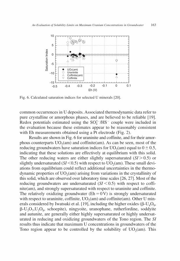
common occurrences in U deposits. Associated thermodynamic data refer topure crystalline or amorphous phases, and are believed to be reliable [19].Redox potentials estimated using the SO4

2�/HS� couple were included inthe evaluation because these estimates appear to be reasonably consistentwith Eh measurements obtained using a Pt electrode (Fig. 2).

Results are shown in Fig. 6 for uraninite and coffinite, and for their amor-phous counterparts UO2(am) and coffinite(am). As can be seen, most of thereducing groundwaters have saturation indices for UO2(am) equal to 0 � 0.5,indicating that these solutions are effectively at equilibrium with this solid.The other reducing waters are either slightly supersaturated (SI � 0.5) orslightly undersaturated (SI �0.5) with respect to UO2(am). These small devi-ations from equilibrium could reflect additional uncertainties in the thermo-dynamic properties of UO2(am) arising from variations in the crystallinity ofthis solid, which are observed over laboratory time scales [26, 27]. Most of thereducing groundwaters are undersaturated (SI � 0.5) with respect to coffi-nite(am), and strongly supersaturated with respect to uraninite and coffinite.The relatively oxidizing groundwater (Eh � 0 V) is strongly undersaturatedwith respect to uraninite, coffinite, UO2(am) and coffinite(am). Other U min-erals considered by Iwatsuki et al. [19], including the higher oxides (�-U4O9,�-U3O7,U3O8, schoepite), ningyoite, uranophane, rutherfordine, soddyiteand autunite, are generally either highly supersaturated or highly undersat-urated in reducing and oxidizing groundwaters of the Tono region. The SIresults thus indicate that maximum U concentrations in groundwaters of theTono region appear to be controlled by the solubility of UO2(am). This


-15

-10

-5

0

5

10

-0.5 -0.4 -0.3 -0.2 -0.1 0 0.1

UO2(am)UraniniteCoffinite(am)Coffinite

Sat

urat

ion

Inde

x

Eh (V)

Fig. 6. Calculated saturation indices for selected U minerals [20].

CH008.qxd 1/20/2007 12:57 PM Page 163

includes porewaters in the Lower Toki Lignite-bearing Formation, whichhosts the Tono Uranium Deposit, and in porewaters of the other formationsin the Mizunami Group that are chemically similar.

It is worthwhile emphasizing that UO2(am) rather than its crystallinecounterpart, uraninite, appears to be solubility controlling in this natural sys-tem. This distinction is further illustrated by the Eh—pH diagrams shown inFig. 7a and b. Both diagrams are drawn assuming that the activity of the rele-vant U aqueous species � 10�8.7, which corresponds to a representative totalU concentration equal to 0.5 ppb (see Section 4.1). The figures cover a rangeof CO2(g) partial pressures that are representative of groundwaters in theTono region (Fig. 4). As can be seen, the stability field of UO2(am) is muchsmaller than that of uraninite over this range. This suggests that if uraninitewere solubility controlling, aqueous U concentrations would have to muchlower at a given pH (i.e., by roughly eight orders of magnitude) than is actu-ally observed. A comparison of the figures leads to the same (albeit notindependent) conclusion drawn from the SI calculations: redox conditionsin Tono groundwaters (indicated by the symbols) are compatible with solu-bility control by of UO2(am).


5 6 7 8 9 10 11-0.5

-0.4

-0.3

-0.2

-0.1

0

0.1

0.2

Eh

(vol

ts)

UO2F2(aq)

UF

4(aq

)

UO2(CO3)22-

UO2CO3

UO2(CO3)34-

UO2(am)

H2S

(aq

)

SO4 2-

a

HS

-

pH pH5 6 7 8 9 10 11

UO2F2(aq)

UO2(OH)2(aq)

UO2(OH)3-

UF

4(aq

)

UO2(am)

H2S

(aq)

HS

-

SO4

2-

b

-0.5

-0.4

-0.3

-0.2

-0.1

0

0.1

0.2

Eh

(vol

ts)

UO

2(C

O3)

34-

Fig. 7. Stability relations among U minerals and aqueous species at 25�C, 0.1 bar, with(a) and 10�5 bar (b) [19]. Activities of U, S and F species � 10�8.7, 10�5 and

10�3.3, respectively. Solid lines delineate stability boundaries for UO2(am) and predomi-nance fields for aqueous U species. Bold lines indicate uraninite stability boundaries.Dashed lines refer to predominance fields for aqueous species of S. Open symbols denotemeasured or estimated redox conditions in sedimentary formations in the Mizunami Group.Solid symbols refer to their counterparts in groundwaters of the Toki Granite.

pCO g310

2 ( ) � �

CH008.qxd 1/20/2007 12:57 PM Page 164

This conclusion seems inconsistent with mineralogical observations indi-cating that uraninite is in fact present in the Tono Uranium Deposit (Section 2).A possible explanation for this apparent dichotomy is the experimentalobservation of Neck and Kim [28] that uraninite surfaces in contact with anaqueous phase at pH �3 may be coated with a thin layer of UO2(am). Undersuch conditions, uraninite dissolution is effectively irreversible, and solubilityis controlled by the amorphous surface layer. Additional experimental studiesand observations of relevant natural systems are needed to test this hypothesis.

Berke [14] attempted to confirm the presence of UO2(am) in rock sam-ples from the Lower Toki Lignite-bearing Formation using a variety of min-eralogical techniques. The selected samples were not from the Tono UraniumDeposit, but they did have U concentrations above background levels. Berke[14] found that U deposition is associated with fine-grained, poorly crys-talline matrix minerals, either as poorly crystalline or amorphous U mineralsor sorbed onto other non-U phases such as Ti-oxides. A definite conclusionregarding the crystalline or amorphous nature of any U minerals in thesesamples could not be made due to the poor crystallinity of the matrix.

4.3. Solubility Constraints on Maximum Uranium ConcentrationsSolubility limits on U concentrations in groundwaters of the Tono

Uranium Deposit can be estimated using the aqueous-speciation and solu-bility constraints discussed above. These constraints suggest that the solu-bility of UO2(am) will mainly be controlled by variations in Eh, pH anddissolved carbonate concentrations. Fig. 8a–c plot calculated UO2(am) sol-ubilities as a function of Eh at pH 8, 9 and 10, respectively. Three curves areshown in each figure corresponding to the nominal, maximum and minimum

values given by the best-fit curve through a selection of the pH-data shown in Fig. 4 for porewaters in the Lower Toki Lignite-bearing

Formation [19]. Also shown in each figure are Eh values corresponding tothe HS�/SO4

2� and pyrite/goethite equilibrium redox couples. These valuesare considered because the available Eh measurements in groundwaters ofthe Lower Toki Lignite-bearing formation, the presence of detectable sulphideand sulphate-reducing bacteria in these groundwaters [22], and the presenceof authigenic pyrite in this formation [5], all point to reducing conditions thatmay be reasonably bounded by redox potentials corresponding to theHS�/SO4

2� and pyrite/goethite couples [19, 20]. The results shown in Fig. 8a–c suggest that UO2(am) solubilities could vary by nearly three orders of magnitude (10�6.1–10�8.7 molal) over the selected range of , Ehand pH values that are considered to be representative of conditions in the

pCO g2 ( )

pCO g2 ( )

pCO g2 ( )


CH008.qxd 1/20/2007 12:57 PM Page 165

Tono Uranium Deposit. Local variations in these parameters in time and spacecould lead to a cycle of dissolution and re-precipitation of UO2(am), which maybe consistent with the isotopic evidence among natural decay-series nuclidesnoted in Section 2.1 suggesting that U has been locally remobilized in thedeposit during the past several hundred thousand years. Such mobilization/re-precipitation of U would be most sensitive to local variations in .

5. CONCLUSIONS

Natural systems that may be analogous in certain respects to a geologic repos-itory for nuclear wastes provide a useful basis for testing assumptions, modelsand concepts used in repository performance assessments. The present studydemonstrates that maximum U concentrations in groundwaters of the TonoUranium Deposit appear to be limited by the solubility of the amorphous,hydrous oxide, UO2(am). This conclusion, drawn from observations of ageologic system that has evolved over long periods of time, supports the

pCO g2 ( )


-9

-8.5

-8

-7.5

-7-6.5

-6

-5.5

-5

-0.4 -0.35 -0.3 -0.25 -0.2 -0.15

log

U(m

ol k

g-1)

Eh (V)

-2.75 -3.25 -3.75

a

-9

-8.5

-8

-7.5

-7

-6.5

-6

-5.5

-5

-0.5 -0.45 -0.4 -0.35 -0.3 -0.25 -0.2

log

U(m

ol k

g-1)

Eh (V)

-3.65 -4.15 -4.65

b

-9

-8.5

-8

-7.5

-7

-6.5

-6

-5.5

-5

-0.6 -0.55 -0.5 -0.45 -0.4 -0.35 -0.3

log

U (

mol

kg-1

)

Eh (V)

-5.10-4.60 -5.60

c

Fig. 8. Solubility of UO2(am) as a function of Eh and at 25�C and 1 bar. Verticallines indicate Eh values for the pyrite/goethite (dotted-dashed line; drawn assuming log

and SO42�/HS� (dashed line) redox couples at pH 8 (a), pH 9 (b) and pH 10 (c).a

SO4)

42� ��

pCO g2 ( )

CH008.qxd 1/20/2007 12:57 PM Page 166

assumption adopted in many international performance assessments that thesolubility of UO2(am), or an analogous UO2 solid, would limit the aqueousconcentrations of U released from a HLW repository over similar time scales[2]. Equilibrium calculations suggest that UO2(am) solubilities could varyroughly between 10�6 and 10�9 mol kg�1 over the range of environmentalconditions presently observed in the Tono Uranium Deposit and environs.Further study is needed to better characterize the organic geochemistry of Tonogroundwaters and related impacts on the aqueous-speciation and solubilitybehaviour of U.

REFERENCES

[1] D. Savage (ed.), The Scientific and Regulatory Basis for the Geological Disposal ofRadioactive Waste, Wiley, Chichester, UK, 1995.

[2] I.G. McKinley and D. Savage, J. Contam. Hydrol., 21 (1996) 335.[3] J. Itoigawa, Monographs of the Mizunami Fossil Museum 1 (1980) 1.[4] Y. Yusa, K. Ishimaru, K. Ota and K. Umeda, Proceedings of paleohydrogeological

methods and their applications for radioactive waste disposal, OECD/NEA, p. 117,1993.

[5] N. Shikazono and M. Utada, Mineral. Dep., 32 (1997) 596.[6] E. Sasao, K. Ota, T. Iwatsuki, T. Niizato, R.C. Arthur, M.J. Stenhouse, W. Zhou,

R. Metcalfe, H. Takase and A.B. Mackenzie, Geochem. Explor. Environ. Anal., 6(2006) 5.

[7] T. Iwatsuki, H. Satake, R. Metcalfe, H. Yoshida and K. Hama, Applied Geochem.,17 (2002) 1241.

[8] Y. Ochiai, M. Yamakawa, S. Takeda and F. Harashima, CEC Nuclear Science andTechnology Series, EUR, 11725 (1989) 126.

[9] K. Doi, S. Hirono and Y. Sakamaki, Econ. Geol., 70 (1975) 628.[10] Y. Sakamaki, IAEA-TECDOC, 328 (1985) 135.[11] JNC, JNC TN 1400 2000-002, Japan Nuclear Cycle Development Institute, Japan,

2000.[12] K. Komuro, M. Yamamoto, S. Suzuki, T. Nohara and S. Takeda, Mining Geol., 40

(1990) 44.[13] K. Komuro, Y. Otsuka and M. Yamamoto, Mining Geol., 41 (1991) 177.[14] M.A. Berke, M.Sc. Thesis, University of California, Riverside, CA, 2003.[15] T. Nohara, Y. Ochiai, T. Seo and H. Yoshida, Radiochim. Acta, 58/59 (1992) 409.[16] N. Shikazono and M. Nakata, Res. Geol., Special Issue 20 (1999) 55.[17] R.M. Garrels and C.I. Christ, Solutions, Minerals and Equilibria, Harper Row, New

York, 1965.[18] D.L. Langmuir, Geochim. Cosmochim. Acta, 42 (1978) 547.[19] T. Iwatsuki, R.C. Arthur, K. Ota and R. Metcalfe, Radiochim. Acta, 92 (2004) 789.[20] R.C. Arthur, T. Iwatsuki, E. Sasao, R. Metcalfe, K. Amano and K. Ota, Geochem.

Explor. Environ. Anal., 6 (2006) 33.


CH008.qxd 1/20/2007 12:57 PM Page 167

[21] Y. Murakami, Y. Fujita, T. Naganuma and T. Iwatsuki, Microbes Environ., 17(2002) 63.

[22] T. Iwatsuki, K. Sato, T. Seo and K. Hama, Proc. Mater. Res. Soc. Symp., 353 (1995)1251.

[23] D.L. Langmuir, Aqueous Environmental Geochemistry, Prentice Hall, Upper SaddleRiver, NJ, 1997.

[24] C.M. Bethke, Geochemical Reaction Modeling, Oxford University Press, Oxford, UK,1996.

[25] R.C. Arthur, H. Sasamoto, M. Shibata, M. Yui and A. Neyama, JNC TN8400 99-079,Japan Nuclear Cycle Development Institute, Japan, 1999.

[26] T. Yajima, Y. Kawamura and S. Ueta, Mater. Res. Soc. Proc., 353 (1995) 1137.[27] D. Rai, A.R. Felmy, N.J. Hess and D.A. Moore, Radiochim. Acta, 82 (1998) 17.[28] V. Neck and J.I. Kim, Radiochim. Acta, 89 (2001) 1.


CH008.qxd 1/20/2007 12:57 PM Page 168

Chapter 9

Leaching from Cementitious Materials Used inRadioactive Waste Disposal Sites

Kosuke Yokozeki

Civil Structure and Materials Group, Kajima Technical Research Institute,19-1-2 Tobitakyu, Chofu-shi, Tokyo 182-0036, Japan

1. INTRODUCTION

Cementitious materials are being studied for use in waste disposal facilitiesfor radioactive waste discharged from nuclear power stations and the like. Tosuppress leakage of radioactive nuclides, the facilities should have long-termdurability, that is, durability over a period quite distinctly different from theperformance period of ordinary structures, such as a period of several thou-sands or several tens of thousands of years, which needs to be explainedlogically as well as technically [1–5]. Furthermore, assessment methods formaterials and structures, and development of high durability materials are anti-cipated considering aspects of design service life and importance of structures.

This report describes the degradation of concrete structures, that is,mainly structures over thousand years and about ten thousand years old witha history longer than that of Portland cement, due to soft water. In the under-water environment of radioactive waste repositories especially, as shown in Fig. 1, cement hydrates leach into the groundwater. An overview of themethods to predict degradation and methods to suppress degradation, withthe focus on the phenomenon of degradation of cementitious material, isdescribed here.

2. RADIOACTIVE WASTE DISPOSAL SITE AND CONCRETE

Radioactive waste disposal facilities are investigated for construction in deepstrata 50–1000m under the ground [1–5]. As shown in Fig. 2, the use of clayeymaterials such as bentonite, and cementitious materials, such as concrete and


CH009.qxd 2/10/2007 4:54 PM Page 169

mortar either independently or in combination as back filling materials orengineered barrier materials, has been studied. Radioactive waste disposalfacilities are generally constructed in a calm and stable environment wheredegradation does not occur easily. Therefore, the study of degradation overthe long term, such as leaching of components into groundwater, is moreimportant for engineered barrier materials than severe degradation over theshort term [6]. On the other hand, when clayey materials such as bentonite andcementitious materials are combined, concerns of various problems due totheir mutual interaction also arise. That is, the ion exchange reaction betweenthe calcium that leaches from the cement hydrates and the sodium in the ben-tonite brings about cation exchange (of Na ion with Ca ion) in the bentonite,giving rise to the possibility of degradation in the swelling behavior of ben-tonite or degradation in its imperviousness. The degradation due to sulfate ionsdischarged from the bentonite is also a cause for concern in cementitious mate-rials. Furthermore, the alkali that leaches from the cement hydrate changesthe pH of the surrounding environment, degrading the protective ability ofthe metallic waste container, and also affecting the nuclide migration rate.

3. LEACHING FROM CEMENTITIOUS MATERIALS

The deterioration of concrete due to leaching has been reported in Swedenwhen a dam deteriorated because of soft water in the 1920s, and in Scotland

170 K. Yokozeki

Access Tunnel

m

Main Tunnel

Acc

ess

Tun

nel

Ground Facilities

Access Tunnel

Repository Tunnel

One Partitionof Repository

100m

Image of radioactive waste repository

500 m

Fig. 1. Illustrative image of radioactive waste repository.

CH009.qxd 2/10/2007 4:54 PM Page 170

when the strength of dams 10–60 years after construction deteriorated withthe passage of time [7]. Results of organizational studies of a similar naturehave also been reported from South Africa [8]. Additionally, deteriorationof concrete has also been reported because of contact with soft water of low

Leaching from Cementitious Materials Used in Radioactive Waste Disposal Sites 171

Concrete

Rock

Radioactive waste

Bentonite

Mortar

Ca2+ concentration

Ca(OH)2→Ca2++2OH-

C-S-H→xCa2++yOH-+zSiO2

Ca2+

Ca2+

Ca2+

Ca2+Ca2+

Ca2+

Ca2+

Ca2+

Hydraulic gradient

50-1000m

Fig. 2. Images of leaching degradation in radioactive waste disposal site.

CH009.qxd 2/10/2007 4:54 PM Page 171

hardness such as the secondary lining of tunnels and water treatment facil-ities. Studies have also been carried out on the effects of safety especiallythe effects of leached components into drinking water in water supply facil-ities [9]. On the other hand, in the 1980s, the long-term soundness assessmentof radioactive waste repositories became an important topic, and the leach-ing of components from concrete has become a popular research topic [10].

Both short-term accelerated tests in the laboratory and analytical methodshave been proposed for the research on the long-term degradation of concreteused in radioactive waste repositories. Past experimental investigations havefocused on the analysis of solutions with the aim of simulating the poresolution into which hydrates leach, and many batch-type experimental inves-tigations have been carried out with the focus on solid–liquid solubilityequilibrium [6, 11]. However, it was not possible to directly evaluate degra-dation with the passage of time from the results of such investigations. Newconditions had to be tentatively set up, such as assumptions regarding inflowsof water from external sources to allow for evaluation with respect to thepassage of time. Typically, these experimental investigations involved deter-mining the solid-phase components of the hydrates and the components of thepore solution. Moreover, investigations were carried out to evaluate changesin physical properties as the balance of solid-phase–liquid-phase compo-nents varied, and also to show up the differences between accelerated testsand actual phenomena. Although models have been proposed specificallyfor paste in analytical investigations [11, 12], methods applicable to actualstructures have not yet been established. This is because of problems suchas: (1) there are practically no models of concrete or mortar that take theaggregate into account; (2) there is no clear method of modeling diffusioncoefficients; (3) there is no method for estimating physical properties; and(4) no verifications against actual structures have been carried out.

4. METHOD FOR PREDICTING DURABILITY OF CONCRETE [13–16]

Although various kinds of accelerated test methods [17] have been studiedfor evaluating and predicting degradation of concrete due to leaching, suchmethods require long periods of time that have never been experienced before;thus, finally, the dependence on analytical methods has become a necessity.Analytical prediction methods may be broadly divided into three types: (1)methods using empirical formula [18], (2) methods using diffusion equa-tions [12], and (3) methods using geochemical mass transfer analysis [19].

172 K. Yokozeki

CH009.qxd 2/10/2007 4:54 PM Page 172

Deterioration of existing structures due to leaching has been occurringwithout any doubt in structures acted upon by soft water such as water sup-ply facilities, canals, dams, and vessel-type structures. Fig. 3 shows the resultsof studies on concrete structures of age in the range of 30–100 years (depthto which calcium hydroxide has decreased). Even after 100 years, the degra-dation thickness is a few tens of millimeters, and the degradation rate wasextremely slow. Consequently, very few problems are anticipated in ordinarystructures. The maximum value of these investigation results is extrapolatedto estimate the degradation after 1000 years or 10000 years. It can be observedthat when the data are subjected to linear regression and to regression on theroot-t law, the degradation depth becomes three times at 1000 years, whileit increases to 10 times at 10000 years.

Thus, an analysis method with a much better estimation accuracy isnecessary. For a more detailed analysis, a method using the diffusion equationor the geochemical mass transfer analysis must be used. The biggest differ-ence in these two methods is the chemical reaction model. The method isfrequently used for predicting neutralization or salt attack of concrete struc-tures in the civil engineering fields. Regarding mass transfer, the law of con-servation of mass relating to the solid-phase element concentration CPi and


0

20

40

60

80

100

120

140

160

0 20 40 60 80 100 120

Time (years)

Deg

rada

tion

dept

h of

Ca(

OH

) 2 (

mm

)Actual data (running water)

Actual data (hydrostatic)

Lagerblad 2001

Saito et al. 2003

Prediction by root−t law (maximum)

1,000years: 300mm

10,000years: 900mm

Prediction by linear line

1,000years: 900mm10,000years: 9,000mm

Fig. 3. Time-dependent degradation depths by Ca leaching.

CH009.qxd 2/10/2007 4:54 PM Page 173

the concentration of each ion in pore solution shown in Eq. (1) is used(details are omitted for both Eqs. (2) and (3) because of the lack of space).In Eq. (1), the left hand side expressing diffusion, convection, electric migra-tion, and sink terms, the terms to be finally considered, should be decided fromthe grade of the study and the environment of the structure to be studied.

(1)

However, in cementitious material, research related to the diffusion coeffi-cient, the permeation coefficient, and quantification of the electric mobilityhas just made a start, and models corresponding to various materials andenvironmental conditions have not yet been constructed as of this stage. Inthe past, apparent diffusion coefficients were used including aggregates asshown on the left side of Fig. 4, but in practice, substances such as poresolution and ions did not move within the aggregates or the hydrates them-selves, but they can move in capillary porosity and transition zones. Thus,an effective diffusion coefficient Di,eff calculation equation is proposed as

� �

�

�

��

�

�

� �

�

� � �

�

( ( ( )eff

duu

uC

t xD

C

x

v C

x

u C

xi

ii i i i) )

,� � � �

��

�

C

tPi

174 K. Yokozeki

AggregatePaste

ITZ

Capillarypore

1.0

Ca2+

(�) D0fPvol =

GSGelpore

Solid-phase

T

Paste

Aggregate

1.0

paste

TransitionZone(ITZ)

Ca2+

f (�)

Pvol 1−d . Svol

1−c . GvolDeff =

GSCapillary

pore

e

= . . .

Fig. 4. Pore and micropore torsion modeling.

CH009.qxd 2/10/2007 4:54 PM Page 174

shown in Eq. (2) taking the electrochemical theory for ion transfer in aque-ous solution, that is, by taking the Nernst–Planck equation as the basis, andconsidering the effects of concentration according to the Debye–Hückeltheory, the effects of torsion of the porosity or aggregate and transition zone,and the increase in porosity with leaching. This enables a wide range ofparameters such as type of cement, hydration, temperature, aggregateamount, and ion type to be considered. Fig. 5 shows the experimental resultsof porosity and diffusion coefficient, together with the results predictedbased on Eq. (2). The diffusion coefficient decreases with the decrease inporosity; however, the relationship is not linear, but curve, suggesting thatthe assessment accuracy is satisfactory.

Moreover, the diffusion coefficient of each ion is different according toEq. (2). However, in practice, the ion balance does not collapse because ofdiffusion; the mass exists maintaining electric neutrality at all times. Thus,the mutual interaction between the electric ions can be expressed by the dif-fusion coefficient by assuming that the pore solution always maintains itselectrically neutral condition. The electric mobility ui in this case is givenby Eq. (3). This enables the mass transfer considering the mutual electricinteraction of each ion to be treated within the law of conservation of massof Eq. (1).


1.0E−12

1.0E−11

1.0E−10

1.0E−09

0

Porosity (%)

Effe

ctiv

e di

ffusi

on c

oeffi

cien

t of t

ritiu

mD

eff (

m2/

s)

Mock-up test

Permeability test

Numata et al.

Terashima et al.

Diffusion model

Mortar

20 40 60 80 100

Fig. 5. Comparison of diffusion coefficients.

CH009.qxd 2/10/2007 4:54 PM Page 175

(2)

(3)

For modeling the dissolution reaction of cement hydrate, the method ofusing a thermodynamic database related to chemical reactions based on theexperimental results for dissolution equilibrium of cement hydrates shown inFig. 6 is also available. However, that is not applicable to concrete made ofcomplex hydrates that are changeable as in the dissolution of cement hydrate.Moreover, the reaction also varies considerably depending on the type and

u Z DZ D C x

Z D Ci i i

i i ii

i i ii

� � ��

� �,

,

,

( )eff

eff

eff

/∑∑ 2

Dc G

d SPi, { . . ( )

.

effvol

volvol total gel�

�

��

1

10 001 0 07

1

2�

��

�

u u

88 0 18 0 18

1

2� �

��

��

( . ) ( . )}u u u u

l

total gel total gel� � � �

�

H

k T

Z e Fi

i lln.

( )10

0 51

4 1

4

2� �

�

�C

Z

I Ii

i

176 K. Yokozeki

0.001

0.01

0.1

1

10

0 5 10 15 20 25

CaO concentration (mmol/l)

SiO

2 co

ncen

trat

ion

(mm

ol/l)

This study: 20°CThis study: 40°CThis study: 60°CFlint & Well(30°C)

Roller & Ervin Jr.(30°C)

Taylor (17°C)

Kalousek(25°C)

Greenberg & Chang(25°C)

Fig. 6. Relationship between liquid-phase calcium ion and liquid-phase silica ion concentration.

CH009.qxd 2/10/2007 4:54 PM Page 176

mix proportion of the cement; therefore, it cannot be treated easily from theaspects of theoretical chemistry. Consequently, dissolution tests of severalkinds of cement under different temperature conditions were carried out.Calcium, which is proportionately large, or calcium silica ratio (Ca/Si) wastaken as the parameter of cement component, so that the dissolution behav-ior can be easily expressed. Fig. 7 shows the dissolution equilibrium modelof calcium in the solid and the liquid phases. Substituting this relationshipin the sink term, and calculating the mass transfer per unit time of the com-ponents in the liquid phase by the difference method, the change in mass inthe solid phase can be calculated.

Fig. 8 shows an example of comparison of the analysis results andactually measured results of solid-phase calcium concentration after leach-ing. The actually measured results are for concrete of age 30–100 years invarious kinds of environments such as distribution reservoir in a water sup-ply facility, building foundation structure in contact with groundwater, dam,and so on, similar to Fig. 3. Variation exists in actually measured resultsalso, and although calculated accuracy cannot be discussed unconditionally,satisfactory predictions can be made depending on various conditions.


0.0

0.1

0.2

0.3

0.4

0.5

0.6

0.7

0.8

0.9

1.0

0 0.005 0.01 0.015 0.02 0.025Liquid−phase Ca concentration in pore water C

(mol/l−pore water)

Rat

io o

f so

lid-p

hase

Ca

conc

entr

atio

nC

P/C

P0 (

−)

Experiment: 20°C

Experiment: 40°C

Experiment: 60°C

Model: 20°C

Model: 40°C

Model: 60°C

logKsp

C1

=0.0015C0

1n

CP0

CP1

C0

CACP1

ACP1 =

⋅

Fig. 7. Equilibrium model of solid-phase calcium concentration and liquid-phase calciumion concentration.

CH009.qxd 2/10/2007 4:54 PM Page 177

178 K. Yokozeki

0

5

10

15

20

0 5 10 15 20

Measured solid-phase Ca concentration

(mol/L−paste)

Cal

cula

ted

solid

-pha

se C

a co

ncen

trat

ion

(mol

/L−p

aste

)+15%

-45%

Y=X

Fig. 8. Verification of concentration of solid-phase calcium.

Since the past, it has been said in relation to the changes in mechani-cal properties after leaching that if the calcium hydrate decreases by 1%, thecompressive strength decreases by 1.5% [21]. However, the calcium hydrate incement paste is �30%, and the strength of the part in which the calcium hydratewas completely lost was not known. Fig. 9 shows a comparison of Vickershardness and concentration of solid-phase calcium for the core from actualstructures is suggesting good correlation. It is also known that the Vickershardness has a good correlation with compressive strength. Accordingly, ifthe calcium concentration in the solid phase is known, the strength charac-teristics after leaching can be predicted. Fig. 10 shows the distribution ofsolid-phase calcium concentration in laboratory leaching tests [20]. It canbe observed that the higher the value of W/C, the deeper is the degradation;degradation progresses due to diffusion at the corners since degradation hasoccurred above the two directions at the corners. The estimated Vickers hard-ness and the measured values can be compared by substituting the solid-phase calcium concentration measured in these tests in the relationship ofFig. 9. This comparison is shown in Fig. 11. The Vickers hardness can thusbe estimated with good accuracy by this method.

CH009.qxd 2/10/2007 4:54 PM Page 178

5. MEASURES AGAINST LEACHING DEGRADATION

It is known from the past that hydrates leach from concrete. Taylor [21] hasproposed various measures against leaching by using Pozzolanic materials,alumina cement, dense concrete, carbonated concrete, autoclave curing, andso on. Even ancient concrete used 5000 years ago in China [22] did not usesteel; the cement close to today’s low-heat Portland cement had carbonated,and had helped to maintain the long-term soundness of the material. Basedon such information, the leaching resistance of carbonated concrete andPozzolan material was evaluated. The dissolution equilibrium relationships


Fig. 10. Calcium concentration distributions after leaching.

y=0.171e1.65x

R2 = 0.643

0.0

0.2

0.4

0.6

0.8

1.0

0.0 0.2 0.4 0.6 0.8 1.0Ratio of solid−phase calcium concentration (-)

Vic

kers

har

dnes

s ra

tio (

−)

dotted line:±50%

Fig. 9. Model of Vickers hardness ratio (paste, mortar, and concrete).

CH009.qxd 2/10/2007 4:54 PM Page 179

of ordinary Portland OPC, concrete LPC�FA using Pozzolan material, andcarbonated concrete HDC using �-C2S shown in Fig. 12 were used.

Fig. 13 shows the degradation prediction results when Pozzolan materi-als were used. The degradation depth of low-heat Portland cement was smallercompared to that of ordinary cement; the effect due to calcium hydroxideconsumption by fly ash and the effect due to micropore torsion of fly ashconcrete were large. In cements that included Pozzolan materials in whichhydrates of lower solubility are formed, the degradation depth can be reducedto as much as one-fifth that of ordinary cement at an age of 5000 years. Fig. 14shows the predicted results of the effects of carbonation curing on calciumleaching. Compared to water curing, the degradation depth at 10000 yearscan be reduced to about one-fifth, as suggested in the figure. This is consid-ered to be due to the calcium hydroxide that has changed to calcium carbon-ate with low solubility.

Based on these predicted results, it was concluded that the leachingamount can be suppressed by using appropriate Pozzolan materials, carbon-ation curing, and using low water to binder ratio. If cement is used with low-heat Portland cement, �-CaO � 2SiO2 (�-C2S), fly ash, and silica fume asadmixtures, and carbonation curing is performed at the initial stage ofhydration, the porosity can be reduced significantly, the calcium leaching

180 K. Yokozeki

0

10

20

30

40

50

60

0 2 4 6 8 10 12

Depth(mm)

Vic

kers

har

dnes

s (−

)marks: analysis

lines: calculation

W/C=40%

W/C=85%

W/C=70%

W/C=55%

Fig. 11. Verification of predicted Vickers hardness.

CH009.qxd 2/10/2007 4:54 PM Page 180


0.0

0.1

0.2

0.3

0.4

0.5

0.6

0.7

0.8

0.9

1.0

0.000 0.005 0.010 0.015 0.020 0.025

Concentration of Ca2+ in paste (mol/l)

Rat

io o

f sol

id-p

hase

cal

cium

(−)

OPC

LPC+FA

HDC

OPC model

LPC+FA model

HDC model

Fig.12. Equilibrium of calcium ion in cement paste.

0

10

20

30

40

50

60

1 10 100 1,000

Time (years)

Deg

rada

tion

dept

h of

Ca(

OH

) 2 (

mm

)

OPC

LPC

LPC+FA

LPC+FA+SF

Fig. 13. Predicted results of degradation depth, when Pozzolanic materials are used.

CH009.qxd 2/10/2007 4:54 PM Page 181

amount can be reduced considerably, and the pH value can be reduced (sup-presses the degradation of bentonite and rock in the surroundings), as shownin Figs. 15–17 [23, 24]. Especially, �-C2S does not show any hydrationreaction, and since it has the property of reacting with carbon dioxide gas,

182 K. Yokozeki

0

50

100

150

200

250

300

1 10 100 1000 10000 100000

Elapsed time (years)

Max

imum

deg

rada

tion

dept

h (m

m)

HDC-carbonation

HDM-carbonation

HDC-water curing

NC-water curing

Fig. 14. Predicted results of degradation depth, when carbonation-cured materials are used.

0

5

10

15

20

25

0 10 20 30

Age(day)

Por

osity

(%)

HDC-carbonation curing

HDC-water curing

NC-water curing

Filling of pores

due to carbonation

Fig. 15. Reduction of porosity by carbonation curing of HDC using �-2CaO � SiO2.

CH009.qxd 2/10/2007 4:54 PM Page 182

it had not been used conventionally with cementitious material; however, itsuse is anticipated in a big way in the future, considering low solubility andlow porosity aspects. By using such leaching suppression techniques, theperformance required in radioactive waste repositories, such as reduction dueto: (1) load-bearing capacity, (2) water-sealing ability, (3) chemical stability,


0

0.005

0.01

0.015

0.02

0.025

1 10 100 1000 10000

Liquid/solid ratio

Cal

cium

con

cent

ratio

n in

filtr

ated

wat

er (

mol

/L)

Standard curing

Carbonation curing

: P-1

: P-2

: P-3

Fig. 16. Calcium concentration in immersed water on leaching test.

7

8

9

10

11

12

13

14

1 10 100 1000 10000Liquid/solid ratio

pH

Standard curing

Carbonation curing

: P-1

: P-2

: P-3

Fig. 17. pH value in immersed water on leaching test.

CH009.qxd 2/10/2007 4:54 PM Page 183

and (4) solubility on natural barriers, is likely to be achieved. Moreover, thismaterial can also improve the mass transfer suppression performance by reduc-ing the volume of porosity significantly and by ensuring long-term chemicalstability. Thus, resistance to salt attack and suppression of neutrality is improveddramatically, and it is a technique that can be applied not only to radioactivewaste disposal, but also to a wide range of fields in civil engineering.

6. CONCLUSIONS

Although degradation owing to solubility of cement hydrates has been knownsince the past, quantitative evaluation related to leaching until now has beeninadequate because of lack of information such as cementitious material is a composite material that includes changeable hydrates and is a porousmaterial, various kinds of reactions occur because of the environmental con-ditions in the surroundings, and so on. However, ever since studies on theconstruction of radioactive waste repositories in ground started, researchrelated to leaching of cement components from concrete has accelerated.Henceforth, the understanding and modeling of solubility characteristics andmass transfer mobility of cement hydrates will play important roles, and thedevelopment of materials and construction methods that satisfy the requiredperformance, such as confinement of radioactive nuclides, is anticipated.

In the near future, many countries in the world will have to start dis-posal of wastes with a higher concentration of radioactive waste than has beendisposed until now. Moreover, aging of many concrete structures such as dams,water supply facilities, and underground foundation structures is likely toprogress. Only 200 years have elapsed since the development of cementconcrete, but with mankind’s intelligence, structures with a durability in theorder of tens of thousands of years are not impossible to build.

REFERENCES

[1] M. Hironaga, The view and technology of concrete for the disposal of radioactivein the future, Concrete J. (JCI), 37(3) (1999) 3 (in Japanese).

[2] M. Furuichi, Research on sealing systems of high level waste repository, Doctordegree thesis from Hokkaido University, 2000 (in Japanese).

[3] Japan Nuclear Cycle Development Institute, Technical reliability of high-level nuclearwaste stratum disposal in Japan, JNC TN1400 99-020, 1999 (in Japanese).

[4] Japan Nuclear Cycle Development Institute, The Federation of Electric PowerCompanies of Japan Joint Team: Concept Research Report on TRU Waste Disposal,JNC TY1400 2000-001, TRU TR-2000-01, 2000 (in Japanese).

184 K. Yokozeki

CH009.qxd 2/10/2007 4:54 PM Page 184

[5] A. Tamura and Y. Akiyama, The cement and concrete used in low level radioactivewaste disposal facility, Cement & Concrete, December (620) (1998) 30 (in Japanese).

[6] Y. Furusawa, Research trends on degradation of concrete caused by calcium leach-ing and modeling, Concrete J. (JCI), 35(12) (1997) 29 (in Japanese).

[7] P.J. Mason, The effect of aggressive water on dam concrete, Construction BuildingMater., 4(3) (1990) 115.

[8] Y. Ballim, Deterioration of concrete in soft waters: a review and limited laboratorystudy, SAICE J., Third Quarter (1993) 1.

[9] A. Neville, Effect of cement paste on drinking water, Mater. Struct., 34 (240) (2001)367.

[10] A. Atkinson and J.A. Hearne, An Assessment of the Long-Term Durability ofConcrete in Radioactive Waste Repositories, UK Atomic Energy Authority Report,AERE-R-11465, 1984.

[11] U. Berner, A Thermodynamic Description of the Evolution of Pore Water Chemistryand Uranium Speciation During the Degradation of Cement, PSI-Bericht No. 62,1990.

[12] M. Buil, E. Revertegat and J. Oliver, in “A Model to the Attack of Pure Water or Undersaturated Lime Solutions on Cement”, Stabilization and Solidification ofHazardous, Radioactive, and Mixed Wastes, Vol. 2, STP 1123 (T.M. Gilliam andC.C. Wiles, eds.), ASTM, Philadelphia, (1992) 227.

[13] K. Yokozeki, K. Watanabe, Y. Furusawa, M. Daimon, N. Otsuki and M. Hisada,Analysis of old structures and numerical model for degradation of concrete by calciumion leaching, Concrete Library Int., December (40) (2002) 209.

[14] K. Yokozeki, K. Watanabe, D. Hayashi, N. Sakata and N. Otsuki, Modeling of iondiffusion coefficients in concrete considering with hydration and temperatureeffects, Concrete Library International, December (42) (2003) 105.

[15] K. Yokozeki, K. Watanabe, N. Sakata and N. Otsuki, Modeling of leaching fromcementitious materials used in underground environment, clay in natural and engi-neered barriers for radioactive waste confinement, Appl. Clay Sci., 26 (2004) 293.

[16] K. Yokozeki, Long-term durability design of 1,000-year level on leaching of cementhydrates from concrete, Doctor degree thesis from Tokyo Institute of Technology,2004 (in Japanese).

[17] Japan Society of Civil Engineer Concrete Committee, Leaching and reaction due tochemical attack, Concrete Eng. Ser., 53, JSCE, Tokyo, (2003) (in Japanese).

[18] S. Kamali, B. Gérard and M. Moranville, Modeling the leaching kinetics of cement-based materials – influence of materials and environment, Cement & ConcreteComposites, 25 (2003) 451.

[19] W. Pfingsten, Experimental and modeling indications for self-sealing of a cementi-tious low- and intermediate-level waste repository by calcite precipitation. Radioactivewaste management and disposal, Nucl. Technol., 140 (2002) 63.

[20] K. Yokozeki, K. Watanabe, N. Sakata and N. Otsuki, Prediction of changes in phys-ical properties due to leaching of hydration products from concrete, J. Adv. ConcreteTechnol., 1(2) (2003) 161.

[21] W.H. Taylor, Concrete Technology and Practice, American Elsevier PublishingCompany, Inc., New York, 1965.


CH009.qxd 2/10/2007 4:54 PM Page 185

[22] K. Asaga and Y. Furusawa, Reproduction of ancient cement used 5000 years ago inChina, Cement & Concrete, November (633) (1999) 1 (in Japanese).

[23] K. Watanabe, K. Yokozeki, E. Sakai and M. Daimon, Improvement durability ofcementitious materials by carbonation curing with �C2S, Proc. Jpn. Concrete Inst.,26-1 (2004) 735 (in Japanese).

[24] K. Watanabe, K. Yokozeki, R. Ashizawa, N. Sakata, M. Morioka, E. Sakai and M. Daimon, High durability cementitious material with mineral admixtures andcarbonation curing, Waste Manag., 26 (2006) 752.

186 K. Yokozeki

CH009.qxd 2/10/2007 4:54 PM Page 186

Chapter 10

Solubility of Carbon Dioxide in Natural Systems

Justin Salminena,b, Petri Kobylinb and Anne Ojalac

aDepartment of Chemical Engineering, University of California, Berkeley,CA 94720, USAbLaboratory of Physical Chemistry and Electrochemistry, HelsinkiUniversity of Technology, FIN-02015 TKK, FinlandcDepartment of Ecological and Environmental Sciences, University ofHelsinki, FIN-15140 Lahti, Finland

1. CARBON DIOXIDE: A NATURAL REAGENT

Carbon dioxide and its carbonate minerals play an important role in envi-ronmental chemistry and atmospheric physics. In natural waters, atmos-pheric CO2 has a significant influence on pH, which varies from alkalineseawaters to acidic low mineral lakes, rivers, and soil water. In freshwatersand in oceans the equilibrium relationships between the carbon dioxide, thechemical and biological components, temperature, and the pH are complexfunctions. Chemical thermodynamics provide quantitative relationshipsbetween chemical energy, ionic reactions, solubilities, speciation, pH, andalkalinity. In natural systems these relationships are also complex functionsof chemical and biological effects.

In this chapter we look at the basic relationships between CO2 in nat-ural waters that are important in the environment and also investigate CO2utilizing processes in the environment. As an example of natural systems weconsider a boreal low mineral lake and discuss the effects of acidification ofaquatic ecosystems in context of multiphase thermodynamics.

In low-mineral freshwaters with low buffer capacity, atmospheric CO2has a significant influence on pH. The effect of increased atmospheric CO2composition on the pH of seawater is small due to its large buffering capac-ity. Seawater pH is ca. 8.2, while low-mineral lakes have often low buffer-ing capacities and can exhibit a pH as low as 3, partly due to anthropogenic


CH010.qxd 2/21/2007 3:45 PM Page 189

acidification. Besides acid rain caused by sulphur- and nitric oxide emis-sions, this lowering of the pH can be due to CO2.

Green plants and certain other organisms (e.g., cyanobacteria) synthe-size carbohydrates from carbon dioxide and water using light as an energysource. In this photosynthesis process, oxygen is released as a by-product.Due to anthropogenic emissions and release of ancient photosynthates fromfossil sediments, the concentration of CO2 in the atmosphere is increasing.As shown by direct monitoring and various proxy data, the CO2 composi-tion in the atmosphere has increased 100 ppm to the present 380 ppm in justover 100 years [1]. The present rate of 0.5% annual increase is a very rapidchange in a geological timescale. New energy and environmental technolo-gies are focussing on minimizing CO2 emissions [2–4].

Approximately 98% of the carbon in the ocean–atmosphere system isin the oceans in the form of dissolved carbon and calcite. Estimated annualocean–atmosphere exchange of carbon is �100 GT(C), which is manytimes the annual amount of 7 GT(C) of anthropogenic CO2 emissions to theatmosphere [1].

Calcite, with its vast reservoirs on the ocean floor, plays a major rolein the oceanic CO2 balance, acting as an effective buffer against pH changes.Consequently the change in pH is small as CO2 or other acids dissolve inthe ocean or fresh waters with calcite buffer. The growth and erosion ofcoral material (calcium carbonate) is sensitive to pH fluctuations [5]. Thelowering of pH in the sea causes dissolution of coral material. Inorganicchemical acidification, introduced in natural aqueous systems, causes dis-solution of solid calcium carbonate [6, 7].

Besides being an elemental part of the biosphere CO2 is utilized as a reactive substance in modern industrial processes where solubility playsan important role [8–10]. The weakly acid character of CO2 is used in theneutralization and acidification of slightly alkaline aqueous mixtures. Bycontrolling the pH with CO2 gas one can control the precipitation and dis-solution of solid carbonates. Biological activity is known to be highest,close to and around a neutral pH and at temperatures greater than 20�C.Many industrial aqueous processes operate at 20–50�C and close to a neutralpH, in conditions favourable to biochemical activity. CO2 gas can be usedin acidification of waters below the pH levels favouring undesirable biolog-ical activity. Aerobic decomposition of organic matter forms CO2 gas whileanaerobic decomposition – among other things – can produce ammonia,NH3. While CO2 lowers pH, ammonia increases pH. Because pH has a largeinfluence on bioreactions, CO2 can be used as controlling agent.

190 J. Salminen et al.

CH010.qxd 2/21/2007 3:45 PM Page 190

2. AQUEOUS SPECIATION OF CO2

The physical equilibria for CO2 dissolved in water is:

(1)

and the chemical equilibria are:

(2)

(3)

The dissociation reactions (2) and (3) define the acid–base chemistry ofaqueous CO2. These are related to the physical reaction in Eq. (1) as givenby Henry’s law.

In a closed system, the increase in the concentration of CO2, ,increases the partial pressure of CO2. Scheme 1 shows the speciation of CO2in an aquatic solution as a function of pH.

xCO2

HCO H CO3 32� ��

CO aq H O H HCO2 2 3( )� ��

CO g CO aq2 2( ) ( )�

Solubility of Carbon Dioxide in Natural Systems 191

pH

log(

conc

entr

atio

n)

-8

-6

-4

-2

0

OH-H+

CO32-

HCO3-

CO2(aq)

2 4 6 8 10 12 14

Scheme 1. Speciation of CO2 as a function of pH.

CH010.qxd 2/21/2007 3:45 PM Page 191

In an aqueous metal–carbonate systems, the following main reactionsoccur where M2� represent metal cations like Mg2�, Ca2�, Zn2�, Cd2�,Pb2�. The overall reaction can be written as follows:

(4)

The dissociation of a metal carbonate salt M2�CO32� can be written as

(5)

Eqs. (4) and (11) show that an increase of proton activity a(H�) in the solu-tion raises the solubility of carbonate minerals and lowers the solubility ofCO2. A decrease in proton activity and subsequent increase in basicity,results in a precipitation of mineral carbonates. The decrease of the solubil-ity of M2�CO3, e.g. can be caused by a common anion introduced by dis-solved sodium or potassium carbonate or bicarbonate salts.

3. MULTIPHASE THERMODYNAMIC SYSTEM

Four equilibrium relations describe a multiphase aqueous system containingCO2 and MCO3. Equilibria for reactions in Eqs. (1–3) and (5) are writtenusing total pressure P, gas-phase mole fraction yi, liquid-phase molality mi,activity ai, fugacity coefficient fi, and activity coefficient gi, where i standsfor a species that takes part in the chemical reaction. An activity coefficientmodel is needed to relate the liquid-phase activities of individual species totheir molalities.

(6)

(7)

(8)Ka a

a

m m

m2 � ��H CO

HCO

H H CO CO

HCO HCO

32

3

32

32

3 3

�

�

� � � �

� �

g g

g

Ka a

a a

m m

m1

2 2 2 2

� �� H HCO

CO aq H O

H H HCO HCO

CO aq CO aq

3 3 3� � �

( ) ( ) (

g g

g ))mH O H O2 2g

Ka

f

m

y PHCO aq

CO g

CO aq CO aq

CO g CO g

� �2

2

2 2

2 2

( )

( )

( ) ( )

( ) ( )

g

f

M CO s M aq CO aq32

322 2� � �� ( ) ( ) ( )�

M CO s H aq M aq H O CO g322 2

2 22� � �� ( ) ( ) ( ) ( )� �


CH010.qxd 2/21/2007 3:45 PM Page 192

(9)

Eq. (10) shows the relation between Henry’s constant , equilibriumconstant KH, and the solubility of the neutral CO2(aq):

(10)

where, x is mole fraction and p the partial pressure. Henry’s constant hasunits of pressure (MPa). Henry’s law is strictly valid only at infinite dilutionof CO2 and at this concentration, the activity coefficient and fugacity coef-ficient have the numerical value of unity, assuming also, that the gas phaseis ideal.

The solubility of a M2� carbonate salt can be increased by adding anacid. Further, the M2� carbonate salt can be precipitated by adding elec-trolytes with anions like OH�, HCO3, HS�, CO3

2�. The relation betweensolubility product, CO2 partial pressure, proton activity, and M2� ion activ-ity is:

(11)

Since CO2 gas can be used as an acidifying agent in chemical or biochemi-cal processes, it can also be used to dissolve or precipitate metal carbonatesalts through these common-ion effects. The chemical state of a system isdescribed by means of Gibbs energy G, chemical potential mi of species i,and mole amount ni [11–14].

For the Gibbs energy change at constant T and P in a single phase isgiven by relation:

(12)

In chemically reactive systems, the change of chemical amounts, dni, can beexpressed as:

(13)dn v di i� j

dG dn� mi ii

∑

K a p asp M 2 H2 CO� � ��( ) 2

Kx

p HHCO aq

CO CO

� �2

2 2

1( )

HCO2

K a a m msp M CO M M CO CO232 2 2

32

32� �� g g


CH010.qxd 2/21/2007 3:45 PM Page 193

where vi is the stoichiometric number of the species in the reaction and j theextent of the reaction in moles, and is given by:

(14)

The values of the stoichiometric coefficients are positive (vi � 0) for prod-ucts and negative (vi � 0) for reactants.

At equilibrium, the Gibbs energy is at a minimum, which correspondsto a zero slope in the two-dimensional phase space, and the right-hand sideof Eq. (15) is zero. Writing the chemical potential by means of standardstate chemical potentials and activities:

(15)

(16)

The thermodynamic equilibrium constant is defined by means of the prod-uct of activities:

(17)

that is related to the standard molar Gibbs energy of a reaction:

(18)

The extensive quantity of Gibbs energy of the system is obtained as a sumof the chemical potentials multiplied by their chemical amounts over all thespecies and phases:

(19)G n� i ii

a a

a

m∑∑

� �r mG RT K�� ln

K av� ii

i∏

v RT a RT av vi i i i

iii

i im� ��

ln ln1

∏∑∑

�

��

Gv v RT v a

T Pjm m

∑ ∑∑

,

ln� � � �i ii

i i i iii

0

�

�

Gv

T Pjm

∑

,

� i ii


CH010.qxd 2/21/2007 3:45 PM Page 194

In the case where there exist one gas phase a, one liquid phase b, and invari-ant pure solid phases ki one can write:

(20)

The total Gibbs energy of a system is constructed by writing the chemicalpotential or the partial molar Gibbs energy mi for each species. The totalGibbs energy Ga of a gas phase is the sum of all the components in the gasphase:

(21)

The total Gibbs energy Gb of an aqueous liquid phase is the sum of theGibbs energies of water, dissolved salts, and dissolved gases:

(22)

The total Gibbs energy Gk of the solid phases is:

(23)

Chemical equilibrium in a closed system at constant temperature and pres-sure is achieved at the minimum of the total Gibbs energy, min(G) con-strained by material-balance and electro-neutrality conditions. For aqueouselectrolyte solutions, we require activity coefficients for all species in themixture. Well-established models, e.g. Debye–Hückel, extended Debye–Hückel, Pitzer, and the Harvie–Weare modification of Pitzer’s activity coef-ficient model, are used to take into account ionic interactions in natural systems [15–20].

G nkk k

k

m��

°∑1

G n RT x n RTm

mx

mb

m g mg

��

w w w w i ii i

i

( ln( )) ln��

� � �

�

�

∑

1

nn RTm

mn nn n

m

n

mg

��

ln

∑�1

G n RTy P

Pn

n n

n

am

f�

�n�

�� ln

∑

1

G G T P n n G T P n n

G T P n G n

� a a a b b b

k k k

( , , , , ) ( , , , , )

( , , )

i j i j

S

… …

…

�

� � �1 1 (( , , )T P n nnk


CH010.qxd 2/21/2007 3:45 PM Page 195

4. MODELING NATURAL SYSTEMS

4.1. A Boreal LakeThe increasing interest in global carbon cycling and attempts to create

extensive carbon budgets for terrestrial as well as aquatic systems, has put moreemphasis on studies on lacustrine carbon cycling. Although lakes together withreservoirs cover only �2% of the global land surface, they seem to have a sig-nificant role in carbon cycling. For instance, they have high carbon accumula-tion rates per surface area compared with oceans and due to the allochthonouscarbon load from surrounding catchments they are usually supersaturated withCO2 relative to the atmosphere. The carbon accumulation rates are especiallyhigh in small lakes in the boreal zone where lakes cover approximately 7% ofthe total land area [21]. Small lakes are numerous and for instance in Finland,the number of lakes with a surface area less than 0.01 km2 is over 130000 [22].Lakes can act as carbon sinks and also as sources of carbon and thus havean ambivalent character. The bulk of the carbon accumulating in the bottomsediments originates from autochthonous production, but part of the boundcarbon – autochthonous as well as allochthonous – in the organic materialis released as CO2 at the end of its life cycle (Scheme 2).


Gas exchange

Thermocline/oxycline

::::::PP :::.¨¨::

MineralizationDissolution

Inflow

Outflow

Scheme 2. A simple model for carbon cycling in a low mineral boreal lake. PP refers toprimary production. Note that carbonate precipitation is not relevant in these systemslocated on the ancient Precambrian shield and is thus omitted from the figure. Note alsothat methanogenesis releasing CH4 gas is an important mineralization process in anoxichypolimnion and bottom sediment; at least part of methane is then oxidized to CO2 in thewater column through the activity of methanotrophic bacteria before escaping the system.During the stratification periods the biogenic gases accumulate in the hypolimnion andescape to the atmosphere mainly during the spring and fall mixing periods [25].

CH010.qxd 2/21/2007 3:45 PM Page 196

The release takes place mainly through biological mineralization butcan also be released by non-biological photochemical processes. In boreallakes the high concentration of dissolved organic carbon creates an effectiveshield against short wave length radiation and thus photodegradation is ofminor importance [23]. The mineralized organic carbon shows increasedalkalinity, defined as a sum of following ions:

(24)

Alkalinity is expressed in millimole per cubic decimetre (mmol dm�3) andmole per cubic decimetre (mol dm�3) is equal to equivalents per litre (eqdm�3), i.e. moles of protons neutralized by the alkalinity in litre of solution.Another commonly used unit is milligrams of CaCO3 per litre (mg dm�3)which is based on the neutralization reaction (4), where M2� is Ca2�. Therelationship between alkalinity units is:

Decomposition of organic matter is a dynamic process. The oxidation oforganic matter eventually produces CO2 and in anaerobic environmentsmicrobiological process called methanogenesis produces methane (CH4)gas [24].

In Scheme 3, the alkalinity concentration is plotted against pH fromLake Horkkajärvi, in southern Finland (61�13N, 25�10E). Lake Horkkajärviis a truly meromictic lake where water column mixing periods, due tohomothermal conditions, are absent [26]. In northern temperate zones, lakesusually circulate twice a year, i.e. in spring and fall, but in a meromictic lakepermanent stratification separates the lake into two layers. The stabilisingforces in Lake Horkkajärvi are high electrolyte concentration and the shel-tered position of the landscape. The lake is 1.1 ha in area with a maximumand mean depth of 13 and 7 m, respectively. It is a humic lake greatlyaffected by the allochthonous carbon load; the water colour in units of mg Pt l�1 is �200.

The thermodynamic model shows the influence of the organic matterin the system. Using only dissolved atmospheric CO2 yields higher pH val-ues at a given alkalinity value. It is worth noticing that the biochemical reac-tions which result in shifting the curve to left are the same which lead to themeromixis through electrolyte accumulation.

1 1 1 50 0453 33

3moldm eqdm and mmoldm mgCaCO dm3� � � �� .

C C C C CAlk HCO CO OH H3 32� �� 2


CH010.qxd 2/21/2007 3:45 PM Page 197

4.2. Anthropogenic Acidification of Surface WatersAnthropogenic acidification, i.e. atmospheric deposition of weak solu-

tions of sulphuric and nitric acids, is in general a serious threat to livingorganisms, particularly in sensitive low-mineral, nutrient-poor lakes in thePrecambrian shield. These ecosystems have naturally low buffering capaci-ties whereas in more fertile areas, calcium concentrations in the bedrockand soils are higher, helping to prevent acidification. The phenomena aredisplayed in Scheme 4, which shows the effect of sulphuric acid on the pHin non-buffered and in calcite-saturated solution.

In nature a slight increase in acidity of an aqueous system, can benoticed when CO2 is dissolved. This raises a question on CO2 dissolutioninto water, in the case of an aqueous system which has an increased H� con-centration, i.e. a low pH value. Scheme 5 shows pH changes as a functionof sulphuric acid addition in open and closed systems using artificial sea-water with 3.5 wt.% salinity. The salt composition is also displayed.


pH

Alk

alin

ity, m

ol/k

gH2O

0.0

0.2

0.4

0.6

0.8

1.0

Horkkajärvi measuredcalculated, t = 25 °C

Dissolved CO2from air

Biologicaldecomposition

Surface

Bottom

5 6 7 8 9

Scheme 3. Alkalinity as a function of pH in Lake Horkkajärvi. The experimental resultsfrom the lake are compared with thermodynamic calculations. The curve on the right-hand side shows the alkalinity–pH relation in a situation where CO2 is dissolved from the air. The left-hand side curve shows experimental results and model calculation in asystem where biological decomposition also takes place. The surface water (1–2 m) in the lake has been found to be well mixed but the bottom, at a mean depth of 7 m, is notwell mixed. The figure shows that biological decomposition takes place at the bottom ofthe lake.

CH010.qxd 2/21/2007 3:45 PM Page 198


m(H2SO4) / mol kg-1

0.0 1.0e-4 2.0e-4 3.0e-4 4.0e-4 5.0e-4

pH

2.0

2.5

3.0

3.5

4.0

4.5

5.0

5.5

6.0

6.5

7.0

7.5

8.0

8.5

9.0

Sat. CaCO3

non buffered water

0.2 pH unit decrease ofsaturated CaCO3 solutionis equalent to doubling theCO2 partial pressure

Scheme 4. pH decrease in saturated CaCO3 solution and non-buffered CO2–water systemat 25�C with the addition of H2SO4. According to the model, in saturated calcite solutioncirca. 0.2 decrease of pH in the solution is reached by doubling the CO2 partial pressurefrom a value of p(CO2) � 3.80 10�4 bar.

m(H2SO4) / mol kg-1

pH

2.0

3.0

4.0

5.0

6.0

7.0

8.0

9.0

10.0

Open system,p(CO2) is constant

Closed system,n(CO2) is constant

0 1x10-3 2x10-3 3x10-3 4x10-3

Scheme 5. Calculated pH change due to addition of sulphuric acid in open and closed sys-tems. In open system p(CO2) is constant. In a closed system the chemical amount n(CO2) isconstant. The composition of the artificial seawater was: H2O (966g), NaCl (26.5g), MgSO4(3.3g), MgCl2 (2.4g), NaHCO3 (0.2g), CaCl2 (1.1g), NaBr (0.08g), and KCl (0.7g).

CH010.qxd 2/21/2007 3:45 PM Page 199

In an open system the CO2 partial pressure is kept constant and in a closedsystem the amount of CO2 is constant. Thus, in open system CO2 gas is allowedto leave the system and partial pressure of CO2 equals atmospheric pressure(380ppm). In closed system the total amount of CO2 is constant and partialpressure of carbon dioxide p(CO2) will change. The calculated curves are com-parable to the results obtained by Pilson [27]. In a closed system, even a smallincrease in sulphuric acid decreases the pH, which lowers the liquid’s ability toform dissolved carbon and calcite. In an open system, the change of pH issmaller but important in natural systems. At higher acid concentrations, the pHof the open and closed systems becomes the same. The actual measured sul-phuric acid concentration in natural waters is less than 210�4 molkg(H2O)�1.In terms of aquatic ecosystems the CO2 partial pressure is relatively constantdespite the observed increase of atmospheric CO2 concentration during the last100 years and the ecosystems thus resemble the open system.

4.3. Solubility of CaCO3 in Salt SolutionsThe solubility of CaCO3 as a function of added Na2CO3, CaCl2, and

CaSO4 salts and a partial pressure of CO2 initially at p(CO2) � 380 ppm and25�C yield different changes in CaCO3 solubility and pH. Scheme 6 showshow the solubility of calcite changes as function of CO2 partial pressure and


p (CO2) / bar

0.0 0.1 0.2 0.3 0.4 0.5 0.6 0.7 0.8 0.9 1.0 1.1 1.2 1.3 1.4 1.5 1.6

Ca2+

/ m

mol

kg

(H2O

)-1

0

1

2

3

4

5

6

7

8

9

10

11

Saturated CaCO3 solution

m(CaSO4) = 7 mmol kg-1

m(CaCl2) = 7 mmol kg-1

m(Na2CO3) = 7 mmol kg-1

Scheme 6. The effect of CO2 partial pressure on the solubility of saturated calcite solu-tion with and without added common-ion salt. The multiphase thermodynamic modelallows the determination of the solubilities of carbonates in different p(CO2)s.

CH010.qxd 2/21/2007 3:45 PM Page 200

with added 7 mmol kg�1 common-ion salt, CaSO4, CaCl2, or Na2CO3. Asexpected Na2CO3 has the greatest effect on reducing the solubility of calcitein the system. The addition of CaCl2 and CaSO4 (0–7 mmol/kg) drops thepH from 8.25 to the values 7.78 and 7.77. The addition of Na2CO3 has theopposite effect increasing the pH from initial 8.25 to 9.24. Highly solubleNa2CO3 or NaHCO3 salts can be used to precipitate M2� carbonates withwell-known common-ion technique [28].

Scheme 7 shows more comparisons between solubility of CaCO3 asfunction of CO2 partial pressure with different salt additions at 25�C. As can


25 °C, salt addition = 7 mmol/kg

p(CO2), bar

0.0 0.2 0.4 0.6 0.8 1.0 1.2 1.4 1.6

m(C

a2+)

/ mm

ol/k

gH2O

0

2

4

6

8

10

12


p(CO2), bar0.0 0.2 0.4 0.6 0.8 1.0 1.2 1.4 1.6

m(C

a2+)

/ mm

ol/k

gH2O

0

2

4

6

8

10

12


p(CO2), bar0.0 0.2 0.4 0.6 0.8 1.0 1.2 1.4 1.6

m(C

a2+)

/ mm

ol/k

gH2O

0

2

4

6

8

10

12


p(CO2), bar

0.0 0.2 0.4 0.6 0.8 1.0 1.2 1.4 1.6

m(C

a2+)

/ mm

ol/k

gH2O

0

2

4

6

8

10

12

No salt addition

CaSO4

CaCl2

Na2CO3

No salt addition

No salt additionNo salt addition

CaSO4

CaSO4

CaSO4

CaCl2

CaCl2

CaCl2

Na2CO3

Na2CO3

Na2CO3

Scheme 7. The solubility of CaCO3 as a function of CO2 partial pressure with differentadded common-ion salts at 25�C.

CH010.qxd 2/21/2007 3:45 PM Page 201

be seen CaSO4 additions higher than 7 mmol kg(H2O)�1 do not noticeablychange the CaCO3 solubility while CaCl2 and Na2CO3 salt additions furtherdecrease the solubility of CaCO3. Increase in temperature results in decreaseof CaCO3 solubility.


In low-mineral freshwaters with low buffering capacity, both atmosphericCO2 and biological decomposition has a huge impact on the pH. The effectof atmospheric CO2 on the pH of seawater is much smaller but multiphaseequilibria follows from the interaction with dissolved and solid mineral carbonates.

The biological impact due to increased acidification of sea and disso-lution of coral matter could be detrimental and irreversible. That is becausethe timescales of physical dissolution and biological recovery are different.Dissolution and precipitation processes of aqueous CaCO3 solutions arecontrolled by acid–base chemistry; these processes are thermodynamicallydriven.

REFERENCES

[1] IPCC, in “The Scientific Basis” (J.T. Houghton, Y. Ding, D.J. Griggs, M. Noguer, P.J.van der Linden, X. Dai, K. Maskell and C.A. Johnson, eds.), Contribution of WorkingGroup I to the Third Assessment Report of the Intergovernmental Panel on ClimateChange, Cambridge University Press, Cambridge, UK, New York, NY, USA, 2001.

[2] Scientific American, Energy Solutions for Sustainable Future, September, 2006.[3] M.I. Hoffert, K. Caldeira, G. Benford, D.R. Criswell, C. Green, H. Herzog, A.K. Jain,

H.S. Kheshgi, K.S. Lackner, J.S. Lewis, H.D. Lightfoot, W. Manheimer, J.C. Mankins,M.E. Mauel, L.J. Perkins, M.E. Schlesinger, T. Volk and T.M.L. Wigley, Science, (1 Nov). 298(2002) 981. DOI: 10.1126/science.1072357 (in review).

[4] T. Takahashi, Science, 305 (2004) 352.[5] J. Ruttimann, Nature, 442 (2006) 987.[6] R.A. Freely, C.L. Sabine, K. Lee, W. Berelson, J. Kleypas, V.J. Farby and F.J. Millero,

Science, 305 (2004) 362.[7] C.L. Sabine, R.A. Feely, N. Gruber, R.M. Key, K. Lee, J.L. Bullister, R. Wanninkhof,

C.S. Wong, D.W.R. Wallace, B. Tilbrook, F.J. Millero, T-H. Peng, A. Kozyr, T. Onoand F. Rios, Science (16 July) 305 (2004) 367.

[8] G.T. Hefter and R.P.T. Tomkins, The Experimental Determination of Solubilities,Wiley Series in Solution Chemistry, Vol. 6, Wiley, London, 2003.

[9] E.J. Beckman, Ind. Eng. Chem. Res., 42 (2003) 1598.[10] S.A. Newman (ed.), Thermodynamics of Aqueous Systems with Industrial Applica-

tions, ASC symposium series 133, ACS, Washington, 1980.


CH010.qxd 2/21/2007 3:45 PM Page 202

[11] K. Denbigh, The Principles of Chemical Equilibrium, 3rd edn., Cambridge UniversityPress, Cambridge, 1971.

[12] M.L. McGlashan, Chemical Thermodynamics, Academic Press, London, 1979.[13] R.J. Silbey and R.A. Alberty, Physical Chemistry, 3rd edn., Wiley, New York, 2001.[14] D. Kondepudi and I. Prigogine, Modern Thermodynamics – From Heat Engines to

Dissipative Structures, Wiley, New York, 1998.[15] P. Debye and E. Huckel, Phys. Z., 24 (1923) 185; H. Harned and B. Owen, The

Physical Chemistry of Electrolyte Solutions, 2nd edn, Reinhold Publishing Corp.,New York, 1950.

[16] K.S. Pitzer, Thermodynamics, 3rd edn, McGraw-Hill, New York, 1995.[17] C. Harvie and J. Weare, Geochim. Cosmochim. Acta, 44 (1980) 997.[18] C. Harvie, N. Möller and J. Weare, Geochim. Cosmochim. Acta, 48 (1984) 723.[19] F.J. Millero, Geochim. Cosmochim. Acta, 45 (1983) 2121.[20] F.J. Millero, Pure Appl. Chem., 57 (1985) 1015.[21] P. Kortelainen, H. Pajunen, M. Rantakari and M. Saarnisto, Glob. Change Biol., 10

(2004) 1648.[22] M. Raatikainen and E. Kuusisto, Terra, 102 (1990) 97, in Finnish.[23] A.V. Vähätalo, M. Salkinoja-Salonen, P. Taalas and K. Salonen, Limnol. Oceanogr.,

45 (2000) 664.[24] K.M. Walter, S.A. Zimov, J.P. Chanton, D. Verbyla and F.S. Chapin III, Nature, 443

(2006) 71.[25] P. Kankaala, J. Huotari, E. Peltomaa, T. Saloranta and A. Ojala, Limnol. Oceanogr.,

51 (2006) 1195–1204.[26] A. Hakala, Boreal Environ. Res., 9 (2004) 37.[27] M.E.Q. Pilson, Introduction to the Chemistry of the Sea, Pearson Education POD,

New Jersey, 1998.[28] D. Langmuir, Aqueous Environmental Geochemistry, Prentice Hall, New Jersey,

1997.


CH010.qxd 2/21/2007 3:45 PM Page 203

Chapter 11

Estimation of the Volatilization of OrganicChemicals from Soil

Epaminondas Voutsas

Thermodynamics and Transport Phenomena Laboratory, School of ChemicalEngineering, National Technical University of Athens, 9 Heroon PolytechniouStreet, Zographou Campus, 157 80 Athens, Greece

1. INTRODUCTION

Soil contamination by organic chemicals, mainly pesticides, has been thesubject of several studies, mainly due to its important role in the distributionof contaminants to other environmental compartments such as air, plantsand the water table [1–6]. When a chemical substance is introduced into thesoil, it may follow many different transport or loss pathways [7]. Some of theinitially applied chemical is vapourized through the soil surface and some istransformed into intermediate products called metabolites. Furthermore someof the chemical’s mass may be adsorbed onto the soil particulate surface andit may undergo further degradation. Chemicals can partition into the vapourphase and may then be transported by the mechanism of advection and/orgaseous diffusion within the gas filled portion of the soil voids. Solutes diffuselaterally into soil regions occupied by stagnant waters and may be absorbedinto interior surfaces. The solute is also available in the solution phase foruptake by the plant roots. Finally, a part of the initially applied chemical mayleach below the vadose zone to groundwater by the mechanism of advectionand dispersion.

Volatilization and air transport are the principal means for widespreaddispersion of pesticides and other organic chemicals in the atmosphere. Asdefined by Lyman et al. [8] volatilization is the process by which a compoundevaporates into the atmosphere from another environmental compartment.In the case where the latter is soil, volatilization may be the most importantmechanism for the loss of chemicals from it and their transfer to the air. This


CH011.qxd 1/20/2007 12:55 PM Page 205

is more pronounced for chemicals that may persist in the environment formany years due to their resistance to transformation by biological or physicaldegradation processes.

Most studies on the volatilization from soils have been conducted forpesticides. Since the early sixties post-application losses of pesticides byvolatilization have been increasingly recognized as a pathway for environ-mental contamination and also as a process limiting their effectiveness [9].Volatile soil losses of pesticides have been measured for several pesticides infield situations, and were found to vary from as low as 1.1% of soil-surface-applied simazine in 24 days to 90% of soil-surface-applied trifluralin lost in6 days [4]. Pesticides include several groups of compounds such as insec-ticides, herbicides, fungicides, rodenticides and fumigants, consisting ofseveral hundred individual chemicals of different kinds with a wide rangeof properties. As pointed out by Lyman et al. [8], other than their use, thereis apparently little which distinguishes pesticides from other organics, andtherefore, it can be assumed that the observations based on pesticides areapplicable to organic chemicals in general.

The rate at which a chemical volatilizes from soil is controlled by simul-taneous interactions between soil properties, chemical’s properties and envi-ronmental conditions. Soil properties that affect volatilization include soilwater content, organic matter, porosity, sorption/diffusion characteristics ofthe soil, etc.; chemical’s properties that affect volatilization include vapourpressure, solubility in water, Henry’s law constant, soil adsorption coeffi-cient, etc.; and finally, environmental conditions that affect volatilizationinclude airflow over the surface, humidity, temperature, etc. Volatilization ratefrom a surface deposit depends only on the rate of movement of the chem-ical away from the evaporating surface and its vapour pressure. In contrast,volatilization of soil-incorporated organic chemicals is controlled by theirrate of movement away from the surface, their effective vapour pressure atthe surface or within the soil, and their rate of movement through the soil tothe vapourizing surface.

A comprehensive model for the estimation of the volatilization of organicchemicals from soil surfaces should take, of course, explicitly into accountall the above factors. Models developed for estimating volatilization ratesare based on equations describing the rate of movement of the chemical tothe surface by diffusion and/or by convection, and away from the surfacethrough the air boundary layer by diffusion [10–16]. Additionally, the partof the chemical in soil that will be lost by volatilization depends on the resis-tance of the chemical to degradation. The application of most of these models

206 E. Voutsas

CH011.qxd 1/20/2007 12:55 PM Page 206

requires, however, a number of input information, e.g. adsorption isothermcoefficients, diffusion coefficients in soil etc., which in most cases are notexperimentally known and neither can they be accurately predicted.

In the following section some physicochemical properties of chemicalsthat affect the volatilization from soil are briefly introduced. Next, the fac-tors influencing the volatilization process of a chemical from the soil andmethods for measuring volatilization fluxes are discussed. Following, modelsthat estimate the rate of volatilization of chemicals from soil are presented,and finally, some thermodynamic aspects of persistent organic chemicalsand the concept of equilibrium partitioning are discussed.

2. PHYSICOCHEMICAL PROPERTIES OF CHEMICALS

2.1. Vapour PressureVapour pressure of a pure compound is the pressure characteristic at any

given temperature of a vapour in equilibrium with its liquid or solid form.Vapour pressure is a measure of the ability of a compound to bond withitself; compound molecules that bond well with each other will have a lowvapour pressure (less tendency to escape to the vapour phase), while poorlybonding compounds will have a high vapour pressure.

From a thermodynamic standpoint, this can be viewed from the well-known Clausius–Clapeyron expression:

(1)

where �Hvap is the heat of vapourization, i.e. the energy needed to breakintermolecular bonds in the pure condensed liquid. Since breaking bondsrequires the input of energy, we would expect the vapour pressure of a com-pound to increase with increasing temperature. For solids, the direct con-version process of a solid to a vapour is called sublimation. The analogousproperty in Eq. (1) is the heat of sublimation, rather than the heat of vapour-ization. This is also a function of temperature, and a unit increase in tem-perature will produce a larger change in vapour pressure of solid–gasequilibrium than the comparable liquid–vapour equilibrium. This would beexpected considering the stronger intermolecular bonding implied by thesolid versus liquid state. Several models for vapour pressure prediction havebeen proposed in the literature [8, 17–19].

d

dVP vapln P

T

H

RT�

�2

Estimation of the Volatilization of Organic Chemicals from Soil 207

CH011.qxd 1/20/2007 12:55 PM Page 207

2.2. Henry’s Law Constant and Air-to-Water Partition CoefficientHenry’s law states that when a liquid and a gas are in contact, the weight

of the gas that is dissolved in a given quantity of liquid is proportional to thepressure of the gas above the liquid (partial pressure). The value of the con-stant of proportionality is called the Henry’s law constant (H) and is depen-dant on the solute–solvent pair, temperature and pressure. Henry’s lawconstant is a measure of a chemical’s volatility from a solvent (in this chap-ter it is water): the larger a compound’s H value, the more volatile it is, andit is also easier to be transferred from the aqueous phase into air.

A reliable method for the prediction of H values for chemicals withenvironmental interest is the bond-contribution model of Meylan andHoward [20]. This model calculates the water-to-air partition coefficient ofa compound, which is the reciprocal of the Henry’s law coefficient, as thesummation of the contributions of the individual bonds that comprise thecompound. Values of bond contributions are given in the original publica-tion of Meylan and Howard [20].

In environmental applications the air–water partition coefficient (KH)is also used, which is in fact the Henry’s law constant. KH is defined as:

(2)

where Pi is the partial pressure of the chemical and Caq the concentration ofthe chemical in the aqueous phase. Using standard units of atmospheres forpartial pressure and moles per litre for concentration, the air–water partitioncoefficient has units of atm L mol�1.

2.3. Octanol–Water Partition CoefficientOctanol–water partition coefficient (Kow) is a very valuable parameter with

numerous environmental applications, where it is used as a primary character-izing parameter since it represents a measure of the tendency of a compoundto move from the aqueous phase into lipids. Kow, is defined as following:

(3)

where Cop and Cw are the concentrations, in g L�1, of the species in the octanol-rich phase and in the water-rich phase respectively. It should be noted that

KC

Cowop

w

�

KP

CH � i

aq

208 E. Voutsas

CH011.qxd 1/20/2007 12:55 PM Page 208

in octanol/water partitioning at 25�C, the water-rich phase is essentially purewater (99.99 mol% water) while the octanol-rich phase is a mixture of octanoland water (79.3 mol% octanol). Numerous models have been proposed inthe literature for the estimation of Kow values. Sangster [21] and Howard andMeylan [22] have reviewed the predictive capabilities of various such models.The atom fragment contribution (AFC) model [23] seems to be better thanthe other methods. In the AFC model a compound is divided into appropri-ate atoms or fragments and values of each group are summed together(sometimes with structural correction factors) to yield the log Kow. It mustbe noted that the limitation of all models that belong to the atom/fragmentcontribution approach is that they give the Kow value only at 25�C.

2.4. Soil Organic Carbon–Water Partition CoefficientThe soil organic carbon–water partition coefficient (Koc) is a parameter

that is used to express the extent to which an organic chemical partitions itselfbetween the soil and solution phases (i.e., dissolved in the soil water). Kocis defined as the ratio of the chemical’s concentration in a state of sorption(i.e., adhered to soil particles) and the solution phase. Thus, for a givenamount of a chemical, the smaller the Koc value, the greater the concentra-tion of the chemical in solution. Chemicals with a small Koc value are morelikely to leach into groundwater than those with a large Koc value. Sorptionfor a given chemical is greater in soils with a higher organic matter content,and thus their leaching is thought to be slower in those soils than in soilslower in organic matter. Because experimental Koc data are not available forall chemicals in use, numerous correlations with some other property suchas octanol–water partition coefficient, solubility in water, bioconcentrationfactor have been proposed [8, 24].

A reliable model for predicting Koc values is the one proposed by Meylanet al. [25], which is based on the first order molecular connectivity index ofthe compound. Meylan et al. [25] report that their model accounts for 96%of the variation in measured log Koc values for the training set (189 chemicals)and 86% of the variation for the validation set (205 chemicals).

2.5. Solubility in WaterWater solubility is a determining factor in the fate and transport of a

chemical in the environment as well as the potential toxicity of a chemical.Of the various parameters that affect soil/air partitioning, water solubility is one of the most important. The solubility of a chemical in water may bedefined as the maximum amount of the chemical that will be dissolved in


CH011.qxd 1/20/2007 12:55 PM Page 209

pure water at a specified temperature. Above this concentration, two phaseswill exist if the organic chemical is a solid or a liquid at the system temper-ature: a saturated aqueous solution and a solid or liquid organic phase. A greatdeal of literature is available concerning the estimation of water solubility, espe-cially using regression-derived equations and fragment constant approaches.For a review of such estimation methods see Refs. [8, 22].

3. FACTORS INFLUENCING VOLATILIZATION

The rate at which a chemical volatilizes from soil is influenced by many factors, including soil properties, chemical properties and environmentalconditions.

Soil properties include clay content, organic matter content, soil drainage,soil pH, water content, structure, porosity and density [8]. Soil clay miner-alogy influences chemical adsorption and co-precipitation and affects con-taminant solubility and mobility. Soil organic matter is an important adsorbentfor many inorganic and organic soil contaminants. Soil drainage affects thedirection and rates of water and chemical movement within a soil. Soil pH is probably the most important transient property affecting inorganiccontaminant solubility on a wide range of soils. Subsoil acidity may eitherincrease or decrease the subsoil’s capacity to retard downward contaminantmovement, depending on pH-dependant binding of the contaminant. Soilwater content affects volatilization since it is competing with the chemicalfor absorption sites on the soil. Soil structure and porosity refer to the spa-tial distribution and total organization of the soil subsystem. Although mod-els assume the soil to be homogenous in structure, real soil varies greatly incomposition down its profile and can also contain many cracks and fissures,which could greatly influence transport of chemicals to the soil surface andthus their volatilization.

Vapour pressure, solubility in water, Henry’s law constant, diffusionconstants are some of the chemical’s properties that influence the volatili-zation rate. Ryan et al. [26] suggested that chemicals with dimensionlessHenry law constant greater than 10�4 should be readily volatilized from soil.Wang and Jones [27] suggested that volatilization of organic chemicals fromsoil is related to the ratio of the Henry’s law constant to the octanol–waterpartition coefficient. Later Harner and Mackay [28] suggested the use of theoctanol–air partition coefficient to describe the partitioning of organic chem-icals between soil and air, considering that most organic chemicals partitioninto organic phases for which octanol is a recognized surrogate. Woordow

210 E. Voutsas

CH011.qxd 1/20/2007 12:55 PM Page 210

and Seiber [29] have shown good correlation of the logarithm of volatilizationflux with the logarithm of the quantity PVP/KocS, where PVP is the vapourpressure, Koc the organic carbon–water partition coefficient and S the solu-bility of the chemical in water.

Atmospheric conditions such as wind speed, temperature and relativeair humidity are some environmental conditions that influence the volatiliza-tion rate. Increased wind speed tends to reduce the resistance to gas phasetransport. This has the effect of increasing the dry gaseous deposition fluxto the soil, but can also clearly increase the revolatilization of the chemicalfrom the soil [5, 30]. Temperature has a profound effect on the vapour/soilpartitioning. Volatilization rates are influenced by soil and ambient air tem-perature mainly through its effect on vapour pressure, i.e. increase of tem-perature increases vapour pressure. If the relative humidity of the air is not100%, increases in airspeed will hasten the drying of soil. This indirecteffect alters the soil water content, which as it was previously mentionedhas an effect on volatilization [30, 31].

As discussed by Lyman et al. [8] all the above can be categorized infactors affecting (a) the movement away from the evaporating surface intothe atmosphere, (b) the vapour density of the chemical and (c) the rate ofmovement to the evaporating surface.

3.1. Chemical Movement from the Soil Surface into the AtmosphereThe rate of movement away from the evaporating surface is a diffusion-

controlled process [32]. The vapourizing substance is transported by mole-cular diffusion through an air layer that is close to the evaporating surfaceand is relatively still. The thickness of this air layer depends on the airflowrate and the temperature [33]. Diffusion away from the surface is related tothe vapour density and the molecular weight of the chemical substance.Changes in temperature can influence the vapour density of the substanceand subsequently the diffusion process. The molecules of the chemical sub-stance volatilize independently with respect to water molecules.

3.2. Vapour DensityVapour density is the concentration of a chemical in the air. When the

concentration reaches a maximum, the vapour is saturated. The vapour densityof a compound in the soil air determines the volatilization rate. Some chem-icals require only a low total soil concentration to have a saturated vapourin moist soil. Thus, weakly absorbed compounds may volatilize rapidly, espe-cially if applied only to soil surface. If the chemicals are incorporated into


CH011.qxd 1/20/2007 12:55 PM Page 211

the soil, the concentration at the evaporating surface of the soil particles isreduced and the total volatilization rate decreases [10].

The nature of the chemical is an important factor that affects vapour den-sity. Chemical’s properties such as vapour pressure, solubility in water, etc. areimportant properties of a chemical that influence its vapour density. The chem-ical’s absorption capacity also affects vapour density and the volatilization rate.Absorption of the chemical by the organic and inorganic soil components maybe the result of chemical absorption (Coulombic forces), physical absorption(van der Waals forces) and hydrogen bonding [30]. Absorption reduces thechemical activity below that of the pure compound and affects the vapour den-sity and subsequently the volatilization rate [10]. This is because the concen-tration of the compound present in a desorbed state in solution in the soil watercontrols the vapour density of the compound in soil air.

Soil water content affects volatilization losses by competing with thechemical for absorption sites on the soil [8, 30, 34, 35]. When the soil surfacesare saturated with just a molecular layer of water, the vapour density of aweakly polar compound in the soil air is greatly increased and any addi-tional soil water will not influence the tendency of the compound to leaveits sorbed site.

In general an increase of temperature on a soil-chemical system shouldcause an increase in the volatilization rate, through an increase of the equi-librium vapour density [30]. However, complicating factors may alter theexpected result and an increase in temperature may not lead to an increasein volatilization rate. In addition, low temperature may not eliminate entir-ely the volatilization process since diffusion may continue even in frozensoil [35].

3.3. Chemical Movement Towards the Evaporating SurfaceVolatilization of a soil incorporated chemical is mainly dependant on

desorption of the pesticide from the soil and its upward movement to thesoil surface. There are two general mechanisms whereby chemicals move tothe evaporating surface: diffusion and mass flow. The total rate of movementis the sum of diffusion and mass flow [36].

Diffusion occurs whenever a concentration gradient is present. Anincrease in the difference of the concentration gradient will increase the dif-fusion rate. The depleted chemical on the soil surface due to volatilizationwill be replaced by additional chemical, which will be diffused upwards.Diffusion may occur along the vapour phase, the air–water interface, thewater–water pathway and the water–solid interface. Even though only small

212 E. Voutsas

CH011.qxd 1/20/2007 12:55 PM Page 212

quantities of the solution are in the vapour phase in respect to the amountabsorbed on the soil, the amount of total mass transported by diffusion throughthe vapour phase is approximately equal to that of non-vapour phases. Thisis because the coefficients of diffusion in air are thousands times greaterthan those for water or surface diffusion [8]. The diffusion rate of a chemi-cal is dependant on the temperature, soil bulk density, chemical substanceconcentration, soil water, organic matter and clay contents.

Mass flow occurs as a result of external forces. The chemical that isincorporated into soil is dissolved or suspended in water, present in thevapour phase or absorbed on solid mineral or organic components of thesoil. Thus, mass flow of the chemical is the result of the mass flow of waterand soil particles that the molecule is associated with. Mass flow due to airmovement in soil is considered negligible [36]. When water evaporatesfrom the soil surface the suction gradient produces results in an upwardwater movement. The upward movement of the chemical in the soil solutionby mass flow with the evaporating water is called the wick effect. The mag-nitude of the wick effect is related to water evaporation rate, vapour pres-sure of the chemical and the chemical’s concentration in the soil solution.The wick effect enhances much more the volatilization in wet soils becausethe degree of enhancement is related to the water evaporation rate. In gen-eral, when the water’s evaporation rate is higher than the volatilization rateof the chemical, i.e. when the soil surface is dry, the chemical will accumu-late on the soil surface. On the other hand, if the soil is rewetted again, thenthe chemical will volatilize.

3.4. Techniques for Measuring Volatilization Fluxes from SoilExperimental measurements of concentrations and volatilization fluxes

have been carried out for a wide range of organic chemicals, mainly pesticides,in the laboratory or in the field [37–41]. For laboratory measurements, theexperimental apparatus usually comprises a chamber, e.g. a jar, in which thesoil is placed. In the chamber air at specified velocity is drawn across orblown over, the soil surface or in some cases through the soil. The exhaustair is trapped, e.g. in air filters, polyurethane foam plugs, etc., and analysedmainly by gas chromatography. The laboratory experiments can be carefullycontrolled to provide useful information about the range of factors affectingvolatilization fluxes in real field conditions. However, there are problemswith designing laboratory volatilization experiments which accurately sim-ulate the environment. For example, most laboratory studies use treated soils,e.g. sieved or artificially contaminated. A sieved soil is easier to handle, but


CH011.qxd 1/20/2007 12:55 PM Page 213

the volatilization fluxes from a sieved soil are likely to be very different froman intact soil structure. Furthermore, in laboratory experiments it is usualpractice to pre-clean the incoming air to the volatilization chamber, becauseotherwise it would be impossible to determine if the presence of a com-pound in the exhaust was due to volatilization from the soil, or whether itwas already in the inlet air. In the field, however, the overlying air will con-tain some of the volatilizing compound and a concentration gradient willexist between the soil and air.

Field measurements of organic chemical concentrations and volatilizationfluxes have been carried out for pesticides applied to soil. There are severaldifferent available techniques and these have been reviewed by Majewski et al. [42]. The basis of these techniques is to measure the vertical pesticidevapour gradient by measuring air concentrations at several different heightsabove the soil surface and to relate this gradient to the volatilization fluxusing theoretical techniques and field measurements such as wind speed,wind profiles, air temperature, etc. Air sampling and chemical analyses arethe same as in the case of laboratory studies.

4. ESTIMATION OF VOLATILIZATION OF CHEMICALS FROM SOIL

As mentioned by Mackay [43], the best environmental model is the leastbad set of simplifying assumptions that yields a model which is not toocomplex, but at the same time sufficiently detailed to be useful. A compre-hensive model for the estimation of the volatilization of organic chemicalsfrom soil surfaces should take, of course, explicitly into account all the fac-tors mentioned in the previous section. The complexity and difficulty ofincorporation of the above factors into a single model clearly indicate theexpected shortcomings and uncertainties of the theoretical studies of soilvolatilization. This is because the approximations that are used in the exist-ing developed models do not sufficiently explain or cover the great numberof complexities during the volatilization process.

Many different models have been developed in order to estimate thequantity of a chemical that is volatilized from soil on specific time intervalsafter its application. The models appear to be valid when compared withresults of laboratory experiments and conditions. When, however, they arecompared with field conditions they are often subjected to errors becausethe boundaries and/or environmental and atmospheric conditions are not

214 E. Voutsas

CH011.qxd 1/20/2007 12:55 PM Page 214

well defined and predictable as they are under the controlled and easilymanipulated laboratory conditions.

The selection of the most appropriate model will be dictated by thenature of the chemical and the particular set of the conditions. The modelspresented here are distinguished in two categories: (a) those applied to chem-icals that are incorporated and distributed into soil and (b) those applied tochemicals volatilized from the soil surface, i.e. chemicals not incorporatedinto soil.

4.1. Models Applicable to Chemicals Incorporated into SoilSeveral models have been proposed for estimating volatilization of

chemicals incorporated into soil, but not all of them are applicable to agiven situation. Moreover, no simple model for the estimating the volatiliza-tion rate for chemicals distributed and incorporated into soil, is available.The application of these complex models requires a number of input data,e.g. adsorption isotherm coefficients, diffusion coefficients, environmentalproperties, which in most cases are not experimentally known nor can beaccurately predicted.

4.1.1. Wet SoilFor wet soil, where water is flowing up through the soil column to the

soil surface and is evaporating there, the relatively simple model of Hamaker[35] and the more complex one of Jury et al. [12] can be used for estimatingthe volatilization rate.

4.1.1.1. The model of Hamaker In Hamaker’s model for the case of non-zero water flux, the total loss of chemical per unit area over some time, Qt,is calculated from the following expression:

(4)

where PVP refers to the vapour pressure of the chemical, the vapour pres-sure of water, DV the diffusion coefficient of the chemical, the diffusioncoefficient of water, fw,V the vapour flux of water, fw,L the liquid flux of waterand the initial concentration of the chemical in the soil solution.ct0

DH O2

PH O2

QP

P

D

Df c ft t� VP

H O

V

H Ow,V w,L

2 2

0�


CH011.qxd 1/20/2007 12:55 PM Page 215

4.1.1.2. The model of Jury et al. For the case of non-zero water flux, theconcentration of the chemical in the gas phase as a function of time anddepth, c(z,t), is given by:

(5)

where is the initial total concentration of the chemical in soil; g � b·rb,where b is an adsorption isotherm parameter and rb the soil bulk density; � �rb·H·a � u·H � h, where H is the Henry’s law constant, a an adsorptionisotherm parameter and h the soil air content; VE the effective conventionvelocity; DE the effective diffusion coefficient where DE � Dg�H·Dl, andDg and Dl are the diffusion coefficients in the gas and liquid phase respec-tively and erf(x) the error function of value x.

The flux at the surface for any time is given by the equation:

(6)

where

Finally, the total chemical loss, Qt, can be found by integrating Eq. (6).

4.1.2. Dry SoilIn the case where the soil is dry, or if no water is flowing in the soil

column because of reduced evaporation at the surface, the volatilization iscontrolled by slow diffusion. Two methods can be used in order to calculatethe volatilization in the case of no water flux: the relatively simple model ofHartley [32] and the more complex one of Jury et al. [12].

4.1.2.1. The model of Hartley Hartley proposed a method that is based onan analysis of the heat balance between the evaporating chemical and air.The flux is expressed as:

(7)fh

D H M kRT�

r d

r

max

max

( )

( )

1

1 2 2

− /

/ /v vap w� �

wV t

D� E

E

2

4

f cD

tw V

cwt

t��

�( ) exp( ) [ ( )]

0

02

21g

p

gE

E erf� �

�

ct0

c z tc z V t

D t

t( , ) .

( )�

�� 0 1 0 5 1

2

g

�

� �

�

erf

/

/E

E

� � ��

0 5 12

. exp( )V z

D

z V t

D tE

E

E

E

erf/

/

�

�

216 E. Voutsas

CH011.qxd 1/20/2007 12:55 PM Page 216

where rmax refers to the chemical’s saturated vapour concentration, h thehumidity of the air, d the thickness of the stagnant layer through which thechemical must pass, Dv the vapour diffusion coefficient, �Hvap the chemi-cal’s latent heat of vapourization, Mw the chemical’s molecular weight, k thethermal conductivity of air, R the gas constant and T the temperature.

For less volatile compounds Eq. (7) is simplified to the following form:

(8)

The total chemical loss in both cases, Qt, over a given time period, can becalculated as the product of the flux and the time.

4.1.2.2. The model of Jury et al. According to this model, for the case of nowater flux, the concentration of the chemical in the gas phase as a functionof time and depth, c(z,t), is given by the following equation:

(9)

The chemical’s flux at the surface for any time is given by the equation:

(10)

Finally, the total chemical loss, Qt, can by found by integrating Eq. (10).Notations are the same as in Eqs. (5) and (6).

4.1.3. Comments on the Performance of the ModelsApart from the models mentioned here, many others have been proposed

in the literature, e.g. [6, 11, 13–16]. As mentioned before, no simple modelis available, and for many of the complex models, input information is some-times not available. Furthermore, special care should be paid in the appli-cation of the models, especially when applied to chemicals other than thosefor which the model was developed. For example, Lyman et al. [8] appliedthe model of Jury et al. for dry soil (described in Section 4.1.2.2) for thecase of trichloroethylene, which requires ten input parameters. The estimated

f cD

tt�� ( )0

gp

E

�

c z tc z D tt

( , )��

0

2

g

�

�

erf

/E

fD h

��vr

d

max ( )1


CH011.qxd 1/20/2007 12:55 PM Page 217

total amount of trichloroethylene lost per day, for an initial total concentra-tion of 0.05 g cm�3, was found to be 1.6 g cm�2. This value is considered veryhigh, since in a 1-cm2 soil column the model indicates that trichloroethylenewould have to be removed entirely to a depth of 32 cm.

4.2. Models Applicable to Volatilization of Chemicals from the Soil Surface

For estimating the rate of volatilization from soil surface, i.e. for chem-ical not incorporated and distributed into soil, two simple methods can be used:the so-called Dow method [8] developed by scientists of the Dow Chemicalcompany and the one by Voutsas et al. [44]. Application of both methodsdoes not require special chemical properties such as diffusion coefficients, norenvironmental properties such as soil moisture, soil type, temperature, etc.

4.2.1. The Dow MethodThis method was developed in Dow Chemical Company using a limited

dataset of nine chemicals. Dow method is a very simple and fast method forthe estimation of the half-life for depletion of an organic chemical from thesoil surface, t1/2, which is given by the following equation:

(11)

where t1/2 is the half-life for depletion of the chemical from the soil surface,Koc the chemical’s soil adsorption coefficient, S the solubility of the chemi-cal in water and PVP the chemical’s vapour pressure.

Assuming that the volatilization process follows first order kinetics,the concentration of the chemical, at any time, can be calculated by the fol-lowing expression:

(12)

where is the concentration at t � 0, t the time since the chemical’s appli-cation and kv the volatilization rate constant .

As discussed by Voutsas et al. [44], despite the empirical nature of theDow model, it can be considered as a two step equilibrium partitioningmodel: compound from a sorption site on the soil particles � compound inthe soil water � compound in the atmospheric air.

k tv /� ln /2 1 2

ct0

c t c etk t( )� �

0

V

tK S

P1 281 58 10/ .� ��

�oc

VP

218 E. Voutsas

CH011.qxd 1/20/2007 12:55 PM Page 218

4.2.2. The Methods of Voutsas et al.Voutsas et al. [44] have examined several simple correlations for the

estimation of the half-life for the depletion of an organic chemical from asoil surface to air. They proposed different correlations that have been pre-sented for wet and dry soils.

4.2.2.1. Wet soil For wet soils Voutsas et al. proposed two models. The first,Eq. (13), requires the knowledge of the soil/organic carbon partition coeffi-cient and the Henry’s law constant and the second, Eq. (14), the vapourpressure of the chemical involved.

(13)

where Koc is the chemical’s soil adsorption coefficient, H the Henry’s lawconstant of the chemical in water, and

(14)

where PVP is the chemical’s vapour pressure.If reliable experimental PVP values are not experimentally available,

the use of Eq. (13) is suggested. In cases when Henry’s law constant valuesare not available, predicted ones by the bond-contribution method of Meylanand Howard [20] can be used. Also, due to uncertainties in the experimen-tal Koc values, e.g. for lindane the experimental Koc values reported from dif-ferent sources are in the range of 686–12400, while for trifluralin in therange of 1200–13700, Voutsas et al. proposed that predicted values by thegroup-contribution model of Meylan et al. [25] should be used.

4.2.2.2. Dry soil For dry soils Voutsas et al. presented similar expressionssuch as those for wet soils:

(15)

and

tK

H1 2

0 3108

1 3216/

.

.� oc

t P1 20 38170 132/..� �

VP

tK

H1 2

0 53787

0 033965/

.

.� oc


CH011.qxd 1/20/2007 12:55 PM Page 219

(16)

where notations are the same as in Eqs. (13) and (14). The presence of theHenry constant in Eq. (15) in the absence of water indicates the empiricalcharacter of the correlation.

4.2.3. Comments on the Performance of the ModelsTable 1 presents experimental and calculated t1/2 values from the Dow

model and the models of Voutsas et al. for wet soils. The models of Voutsaset al. give better results than Dow method with Eq. (13) and are consideredto be in general superior to Eq. (14). Using logarithmic values, Eq. (13)accounts for 50% variation in the measured t1/2 data yielding a meanabsolute error lower than 0.5, and represents a substantial improvement overthe Dow method that accounts for just the 23% variation, yielding a meanabsolute error of 0.8. Table 2 presents a comparison between experimentaland predicted chemicals’ per cent volatilization after 1 and 5 days applica-tion, which is defined as:

(17)

where cx is the chemical’s concentration at t � x days, calculated from Eq.(12) and the chemical’s concentration at t � 0 days.

Table 3 presents experimental and calculated t1/2 values from the Dowmodel and the models of Voutsas et al. for dry soils. The results for dry soilsare poorer than those obtained for moist soils. Order-of-magnitude agree-ment between experimental and predicted t1/2 values should be expected inthis case. Also, Table 4 presents chemicals’ per cent volatilization after 1and 5 days application for the same chemicals.

5. THERMODYNAMICS OF PERSISTENT ORGANIC CHEMICALS: THE EQUILIBRIUM PARTITIONINGAPPROACH

Persistent (slowly bio-degrading) organic chemicals, such as pesticides,PCBs, etc. occur throughout the environment, and in a matter of years, bymany different transport mechanisms, they appear in all environmentalcompartments: air, water, soil, sediment, aerosols, water-suspended partic-ulates and vegetative and animal biota. Mackay [43] developed the so-called

ct0

%volatilized � �100 1000

c

cx

t

�

t P1 20 26881 7543/

..� �VP

220 E. Voutsas

CH011.qxd 1/20/2007 12:55 PM Page 220

Estim

ation of the Volatilization of Organic C

hemicals from

Soil221

Table 1Chemicals, chemical properties, experimental and predicted half-life values for moist soils

Chemical PVP (mmHg) Koc S (mg L�1) t1/2, experimental t1/2, calculated (days)(days) Dow method Eq. (13) Eq. (14)

trans-Chlordane 5.03E-05 8.67E � 04 0.056 10.7 1.5 9.0 5.8cis-Chlordane 3.60E-05 8.67E � 04 0.056 11.3 2.1 9.0 6.6Pendimethalin 3.00E-05 2.62E � 03 0.3 107 0.4 12.1 7.0Methyl parathion 3.50E-06 5.23E � 02 37.7 13.5 89.0 16.1 16.0Carbofuran 4.85E-06 7.09E � 01 320 24 73.9 35.7 14.1DDT 1.6E-07 2.20E � 05 0.01 55.4 119.7 38.6 51.8Dieldrin 5.89E-06 1.06E � 04 0.195 17.4 5.5 6.8 13.1Endrin 3.00E-06 1.06E � 04 0.25 19.1 14.0 8.7 16.9Heptachlor 4E-04 5.24E � 04 0.18 8.4 0.4 2.6 2.6Heptachlor epoxide 1.95E-05 5.26E � 03 0.20 13.8 0.9 3.1 8.3Lindane 4.2E-05 3.38E � 03 7.3 4.8 9.3 5.3 6.2Chlorpyrifos 2.03E-05 6.83E � 03 1.12 3 6.0 10.4 8.2Diuron 6.90E-08 1.36E � 02 42 12 1308.0 134.5 71.5Dinoseb 7.50E-05 3.54E � 03 52 26 38.8 19.9 5.0Endosulfan 1.73E-07 2.20E � 04 0.325 5.4 653.0 3.7 50.3p,p�-DDD 1.35E-06 1.52E � 05 0.09 12 160.1 35.8 23.0Fenpropimorph 2.63E-05 2.69E � 04 4.3 11.2 69.5 24.1 7.4Metolachlor 3.14E-005 2.92E � 02 530 88 77.9 43.0 6.9Atrazine 2.89E-07 2.30E � 02 34.7 162 437.1 77.9 41.4Trifluralin 4.58E-05 9.68E � 03 0.184 5 0.6 1.9 6.0Dacthal (DCPA) 2.50E-06 2.83E � 02 0.5 49.7 0.9 2.2 18.2EPTC 2.4E-02 2.58E � 02 375 1.19 0.06 0.72 0.55Alachlor 2.05E-05 1.85E � 02 240 161 34.2 35.1 8.1Fonofos 3.38E-04 8.36E � 02 15.7 11.4 0.6 2.12 2.8

Note: Sources of experimental data can be found in ref. [44].

CH011.qxd 1/20/2007 12:55 PM Page 221

222E

. VoutsasTable 2Experimental and predicted per cent volatilization from moist soils

Chemical % Volatilized % Volatilized % Volatilized after % Volatilized afterafter 1 day, after 5 days, 1 day, calculated 5 days, calculated

experimental experimental Dow method Eq. (13) Eq. (14) Dow method Eq. (13) Eq. (14)

trans-Chlordane 6.3 27.7 37.0 7.4 11.3 90.1 32.0 45.0cis-Chlordane 6.0 26.4 28.1 7.4 10.0 80.8 32.0 40.9Pendimethalin 0.7 3.2 82.3 5.6 9.4 100.0 24.9 39.1Methyl parathion 5.0 22.6 0.8 4.2 4.2 3.8 19.4 19.5Carbofuran 2.9 13.5 0.9 1.9 4.8 4.6 9.3 21.8DDT 1.2 6.1 0.6 1.8 1.3 2.9 8.6 6.5Dieldrin 3.9 18.1 11.8 9.7 5.2 46.8 39.9 23.3Endrin 3.6 16.6 4.8 7.7 4.0 21.9 32.9 18.5Heptachlor 7.9 33.8 82.3 23.4 23.4 100.0 73.6 73.6Heptachlor epoxide 4.9 22.2 53.7 20.0 8.0 97.9 67.3 34.1Lindane 13.5 51.4 7.2 12.3 10.6 31.1 48.0 42.8Chlorpyrifos 20.6 68.5 10.9 6.5 8.1 43.9 28.3 34.5Diuron 5.6 25.1 0.1 0.5 1.0 0.3 2.5 4.7Dinoseb 2.6 12.5 1.8 3.4 12.9 8.5 16.0 50.0Endosulfan 12.1 47.4 0.1 17.1 1.4 0.5 60.8 6.7p,p�-DDD 5.6 25.1 0.4 1.9 3.0 2.1 9.2 14.0Fenpropimorph 6.0 26.6 1.0 2.8 8.9 4.9 13.4 37.4Metolachlor 0.8 3.9 0.9 1.6 9.6 4.4 7.7 39.5Atrazine 0.4 2.1 0.2 0.9 1.7 0.8 4.4 8.0Trifluralin 12.9 50.0 68.5 30.6 10.9 99.7 83.9 43.9Dacthal (DCPA) 1.4 6.7 53.7 27.0 3.7 97.9 79.3 17.3EPTC 44.2 94.6 100.0 61.8 71.6 100.0 99.2 99.8Alachlor 0.4 2.1 2.0 2.0 8.2 9.6 9.4 34.8Fonofos 5.9 26.2 68.5 27.9 21.9 99.7 80.5 71.0

CH011.qxd 1/20/2007 12:55 PM Page 222

Estim

ation of the Volatilization of Organic C

hemicals from

Soil223

Table 3Chemicals, chemical properties, experimental and predicted half-life values for dry soils

Chemical PVP (mmHg) Koc S (mg L�1) t1/2, experimental t1/2, calculated (days)(days) Dow method Eq. (15) Eq. (16)

Atrazine 2.89E-07 2.30E � 02 34.7 599 437.1 115.5 100.4Simazine 2.21E-08 1.49E � 02 6.20 1112.00 660.5 134.2 200.4Trifluralin 4.58E-05 9.68E � 03 0.184 9.5 0.6 13.3 25.7Dieldrin 5.89E-06 1.06E � 04 0.195 1433 5.5 28.3 44.7Chlordane 9.75E-06 8.67E � 04 0.056 70.3 7.9 33.3 39.0Heptachlor 4E-04 5.24E � 04 0.18 4.40 0.4 16.3 14.4Lindane 4.2E-05 3.38E � 03 7.3 7.48 9.3 24.4 26.3Toxaphene 6.69E-06 9.93E � 04 0.55 39 129.0 66.5 43.2EPTC 2.4E-02 2.58E � 02 375 3.3 0.1 7.7 4.8Alachlor 2.05E-05 1.85E � 02 240 69 34.2 72.9 31.9

Note: Sources of experimental data can be found in ref. [44].

CH011.qxd 1/20/2007 12:55 PM Page 223

224E

. Voutsas

Table 4Experimental and predicted per cent volatilization from dry soils

Chemical % Volatilized % Volatilized % Volatilized after % Volatilized afterafter 1 day, after 5 days, 1 day, calculated 5 days, calculated

experimental experimental Dow method Eq. (15) Eq. (16) Dow method Eq. (15) Eq. (16)

Atrazine 0.12 0.58 0.16 0.60 0.69 0.79 2.96 3.39Simazine 0.06 0.31 0.10 0.52 0.35 0.52 2.55 1.71Trifluralin 7.04 30.57 68.50 5.08 2.66 99.69 22.94 12.62Dieldrin 0.05 0.24 11.84 2.42 1.54 46.75 11.53 7.46Chlordane 0.98 4.81 8.40 2.06 1.76 35.51 9.88 8.50Heptachlor 14.58 54.51 82.32 4.16 4.70 99.98 19.15 21.39Lindane 8.85 37.08 7.18 2.80 2.60 31.11 13.24 12.35Toxaphene 1.76 8.50 0.54 1.04 1.59 2.65 5.08 7.71EPTC 18.95 65.01 99.90 8.61 13.45 100.00 36.24 51.42Alachlor 1.00 4.90 2.01 0.95 2.15 9.64 4.64 10.30

CH011.qxd 1/20/2007 12:55 PM Page 224

level I fugacity model, which is based on the assumption that a persistentchemical will be in thermodynamic phase equilibrium in all environmentalcompartments over the time period which it persists.

For the case of soil/air partitioning and speaking the language of ther-modynamics, for having equilibrium of a chemical between soil and air, thefollowing standard thermodynamic equation has to be satisfied:

(18)

where f and x are the fugacity and mole fraction of species i, in the soil andair phases. Fugacity is a thermodynamic property that describes a chemi-cal’s tendency to escape from one phase to another and has units of pres-sure. For example if a chemical has a fugacity in the soil phase greater thanthat in air then there will be a tendency of the chemical to move from thesoil to the air phase in order to establish equilibrium conditions.

Mackay [43] proposed the calculation of fugacities in the various envi-ronmental compartments through the concentrations and fugacity capacitiesof the compounds in the compartments. According to this approach:

(19)

where: is the concentration of the chemical in the compartment (g m�3), MW the molecular weight of the chemical (g mol�1), thefugacity capacity of the chemical in the compartment (mol m�3 Pa�1) andR the gas constant (8.314 J mol�1 K�1).The fugacity capacity for air is calculated using:

(20)

The fugacity capacity of soils is estimated using:

(21)

where foc is the faction of organic carbon in soil (typical 7%), rs the soil den-sity (typical 1.5 g cm�3), Koc the soil organic carbon–water partition coeffi-cient and Hi the Henry’s law constant.

zf K

Hisoil oc s i oc

i

�r ,

zRTi

air�

1

zicompartment

c icompartment

f c T Pc

zicompartment

icompartment i

compartment

icompartMW

( , , )��

mment

f x T P f x T Pisoil

isoil

iair

iair( , , ) ( , , )�


CH011.qxd 1/20/2007 12:55 PM Page 225

226 E. Voutsas

Cousins and Jones [45] have used soil to air fugacity ratios to investigatethe equilibrium in soil and air for some semi-volatile organic compounds.Fugacity ratios near indicate an equilibrium between soil and air, fugacityratios greater than unity indicate a tendency of the chemical to volatilize fromsoil, while fugacity ratios less than unity, indicates a tendency of the chem-ical to remain in the soil and a capacity of the air to supply the soil withmore chemical. Using this approach Cousins and Jones [45] have found thatfor the case of spiked soils, the fugacity ratios were all larger than one,which consisted of the observed losses during the field experiments. On theother hand, for the unspiked soils most of the chemicals and especiallyPCBs were close to the equilibrium, which explained the small uptake ofPCBs in the unspiked soils.

Of course, the equilibrium partition approach has some limitations: (a) itconsiders only a phase equilibrium situation and does not take into accountthe rate of transport between air and soil, (b) the fine distribution of com-pounds within surface soils may influence the calculation of fugacities and(c) it provides only a snap-shot for a given set of environmental conditions.

REFERENCES

[1] W.F. Spencer and M.M. Gliath, Environ. Sci. Technol., 3 (1969) 670.[2] A.W. Taylor, J. Air Pollut. Contam. Assoc., 28 (1978) 922.[3] G.H. Willis, L.L. McDowell, S. Smith, L.M. Southwick and E.R. Lemon, Agron. J.,

72 (1980) 627.[4] A.W. Taylor and D.E. Glotfelty, in “Evaporation From Soils and Crops” (R. Grover,

ed.), Environmental Chemistry of Herbicides, CRC Press, Boca Raton, FL, 1988.[5] I.T. Cousins, A.J. Beck and K.C. Jones, Sci. Total Environ., 228 (1999) 5.[6] M.M. Hantush, M.M. Marino and M.R. Islam, J. Hydrol., 227 (2000) 66.[7] M.M. Hantush, R.S. Govindaraju, M.M. Marino and Z. Zhang, J. Hydrol., 260

(2002) 58.[8] W.J. Lyman, W.F. Reehl and D.H. Rosenblatt, Handbook of Chemical Property

Estimation Methods, American Chemical Society, Washington, DC, 1990.[9] G.H. Willis, L.L. McDowell, L.A. Harper, L.M. Southwick and S. Smith, J. Environ.

Qual., 12 (1983) 80.[10] W.F. Spencer, W.J. Farmer and M.M. Gliath, Residue Rev., 49 (1973) 1.[11] R. Mayer, L. Letey and W. Farmer, Soil Sci. Soc. Am. Proc., 38 (1974) 563.[12] W. Jury, R. Grover, W. Spencer and W. Farmer, Soil Sci. Soc. Am. J., 44 (1980) 445.[13] W. Jury, W. Spencer and W. Farmer, J. Environ. Qual., 12 (1983) 558.[14] W. Jury, W. Spencer and W. Farmer, J. Environ. Qual., 13 (1984) 567.[15] W. Jury, W. Spencer and W. Farmer, J. Environ. Qual., 13 (1984) 573.[16] W. Jury, W. Spencer and W. Farmer, J. Environ. Qual., 13 (1984) 580.

CH011.qxd 1/20/2007 12:55 PM Page 226

[17] B.E. Poling, J.M. Prausnitz and J.P. O’Connell, The Properties of Gases andLiquids, 5th edn., McGraw-Hill, New York, 2001.

[18] E. Voutsas, M. Lampadariou, K. Magoulas and D. Tassios, Fluid Phase Equilib., 198(2002) 81.

[19] Ph. Coutsikos, E. Voutsas, K. Magoulas and D. Tassios, Fluid Phase Equilib., 207(2003) 263.

[20] W. Meylan and P. Howard, Environ. Toxicol. Chem., 10 (1991) 1283.[21] H. Sangster, Octanol–Water Partition Coefficients: Fundamentals and Physical

Chemistry, Wiley, New York, 1997.[22] P.H. Howard and W.M. Meylan, Prediction of Physical Properties, Transport, and

Degradation for Environmental Fate and Exposure Assessments, Syracuse ResearchCorporation, Syracuse, NY, 1998.

[23] W.M. Meylan and P.H. Howard, J. Pharm. Sci., 84 (1995) 83.[24] J.R. Baker, J.R. Mihelcic and E. Shea, Chemosphere, 41 (2000) 813.[25] W. Meylan, P. Howard and R. Boethling, Environ. Sci. Technol., 26 (1992) 1560.[26] J. Ryan, R. Bell, J. Davidson and G.A. Connor, Chemosphere, 17 (1988) 2299.[27] M.-J. Wang and K.C. Jones, Environ. Sci. Technol., 28 (1994) 1843.[28] T. Harner, D. Mackay and K.C. Jones, Environ. Sci. Technol., 29 (1995) 1200.[29] J.E. Woordow and J.N. Seiber, Environ. Sci. Technol., 31 (1997) 523.[30] W. Guenzi and W. Beard, in “Volatilization of Pesticides” (W. Guenzi, ed.), Pesticides

in Soil and Water, Soil Science Society of America, Madison, WI, 1974.[31] B. Grass, B.W. Wenclawiak and H. Rudel, Chemosphere, 28 (1994) 491.[32] G.S. Hartley, in “Evaporation of Pesticides”, Pesticidal Formulations, Research,

Physical and Colloidal Chemical Aspects, Advances in Chemistry Series, 86, AmericanChemical Society, Washington, DC, 1969.

[33] J.V. Parochetti and G.F. Warren, Weeds, 14 (1966) 281.[34] L.W. Petersen, D.E. Rolston and P. Moldrup, J. Environ. Qual., 23 (1994) 799.[35] J. Hamaker, in “Diffusion and Volatilization” (C. Goring and J. Hamaker, eds.),

Organic Chemicals in the Soil Envinonment, Marcel Dekker, New York, 1972.[36] L. Letey and W. Farmer, in “Movement of Pesticides in Soil” (W.D. Guenzi, ed.),

Pesticides in Soil and Water, Soil Science Society of America, Madison, WI, 1974.[37] W.F. Spencer and M.M. Gliath, J. Environ. Qual., 2 (1973) 284.[38] B. Lindhardt and T.H. Christensen, Water Air Soil Pollut., 92 (1996) 375.[39] R.G. Nash, J. Agric. Food Chem., 31 (1983) 210.[40] H. Rudel, Chemosphere, 35 (1997) 143.[41] A.I., Garcia-Valcarcel and J.L. Tadeo, J. Agric. Food Chem., 51 (2003) 999.[42] M.S. Majewski, D.E. Glotfelty, U.K.T. Paw and J.N. Seiber, Environ. Sci. Technol.,

24 (1990) 1490.[43] D. Mackay, Multimedia Environmental Models. The Fugacity Approach, Lewis

Publishers Inc., Chelsea, MI, 1991.[44] E. Voutsas, C. Vavva, K. Magoulas and D. Tassios, Chemosphere, 58 (2005) 751.[45] I.T. Cousins and K.C. Jones, Environ. Pollut., 102 (1998) 105.


CH011.qxd 1/20/2007 12:55 PM Page 227

Chapter 12

Solubility and the Phytoextraction of Arsenic fromSoils by Two Different Fern Species

Valquiria Campos

University of São Paulo, Rua Marie Nader Calfat, 351 apto 71 Evoluti,Morumbi, São Paulo 05713–520, SP, Brazil

1. INTRODUCTION

As soils are increasingly used in the society for purposes other than agri-culture, the frequency and extent of soil contamination by toxic trace ele-ments will increase. Phytoextraction on metals or metalloids is an uncommonphenomenon in terrestrial higher plants. In 2001, Ma et al. [1] reported that thePteris vittata was extremely efficient in extracting arsenic from soils. Thestudy by Ma was the first to report a fern P. vittata grown on a chromium–copper–arsenium-contaminated site as an arsenic hyper-accumulator. Otherplant species have been reported by researchers as being able to removetrace elements [2–9]. Because of solubility, mobility, bioavailability, andtoxicity of arsenic, studies on arsenic speciation and removal are essentialin attempting to reduce the negative impact on the environment of arsenic.

Arsenic is a toxic element that can be found in anthropogenic wastes andsome geochemical environments. Arsenic is a semi-metallic element and italso may be present as organometallic forms, such as methylarsinic acid anddimethylarsinic acid, which are active ingredients in many pesticides [10].Levels of arsenic in soils (1–40 mg As kg�1) may be elevated due to miner-alization and contamination from industrial activity and agrochemicals [11].Arsenic can be added to soils through the use of synthetic fertilizers and As-based pesticides. The continued application of these products can result inan accumulation of toxic residues that, even in relatively low concentrations,could compromise or limit the use of water. The complexation of arsenic bydissolved organic matter in natural environments prevents sorption and co-precipitation with solid-phase organic and inorganic compounds, thus increas-ing the mobility of arsenic in aquatic systems and soil [12]. Inorganic forms

Thermodynamics, Solubility and Environmental IssuesT.M Letcher (editor)© 2007 Elsevier B.V. All rights reserved.

CH012.qxd 2/3/2007 4:01 PM Page 229

of arsenic can be present as either arsenate As (V) or arsenite As (III). Arsenateis tetrahedral oxyanions that can compete for adsorption sites on soil min-eral surfaces. Arsenate is the predominant inorganic species of arsenic underoxidizing soil conditions and is retained in soils by adsorption reactions.

The main exposure to inorganic arsenic experienced by the generalpublic is through ingestion. Long-term exposure to low concentrations ofarsenic in drinking water can lead to skin, bladder, lung, and prostate can-cer. Non-cancer effects of ingesting arsenic at low levels include cardiovas-cular disease, diabetes, and anemia, as well as reproductive and developmental,immunological, and neurological effects [13]. Substantial evidence led theInternational Agency for Research on Cancer to conclude that ingestion ofinorganic arsenic can cause skin cancer [14]. Arsenic exposure is a poten-tial health risk to local populations around gold mining areas in southeast-ern Brazil, where 20% of the total sample population showed elevated Asconcentrations (2.2–106 �g L�1) [15]. In the Iron Quadrangle region thepublic supply of water comes mainly from local watersheds. However, insome places the population uses spring water or groundwater from areasclose to closed mines, for human consumption. The main natural sources ofarsenic in the Iron Quadrangle come from rocks that contain lode golddeposits. The anthropic sources of arsenic are contaminated refuse piles,soil, and sediments. It was found that total As concentration is 2980 �g L�1

and As3� is 86 �g L�1 in water samples collected from underground goldmines, artesian wells, and springs in Ouro Preto and Mariana counties [16].Speciation is important since mobility and toxicity of As (III) are supposedto be much higher than those of As (V). The toxicity of such compoundsdecreases in the order: arsine � arsenite � arsenate � alkyl arsenic acids �arsenium compounds and metallic arsenic [17].

Arsenic is distributed widely among plant species. In plant tissues itsnormal concentration is 0.01–5 mg kg�1 on a dry-weight basis [18]. Thesoil–plant system is an open system subject to inputs, such as contaminantsand agrochemicals, and to losses, such as the removal of trace elements inharvested plant material, leaching, erosion, and volatilization. The factorsaffecting the amounts of trace elements absorbed by a plant are those con-trolling (a) the concentration and speciation of the element in the soil solu-tion; (b) the movement of the element from the bulk soil to the root surface;(c) the transport of element from the root surface into the root; (d) its translo-cation from the root to the shoot. Plant uptake of mobile ions present in thesoil solution is largely determined by the total quantity of the ions in the soil.In the case of strongly adsorbed ions, absorption is more dependent on theamount of root produced [19].

230 V. Campos

CH012.qxd 2/3/2007 4:01 PM Page 230

Certain species of plants have been found to accumulate very high concentrations of certain trace elements and these are referred as “hyper-accumulator” species. Plants can also intercept significant amounts of someelements through foliar absorption. Foliar absorption of solutes depends onthe plant species, its nutritional status, the thickness of its cuticle, the age ofthe leaf, the presence of stomata guard cells, the humidity at the leaf surface,and the nature of the solutes.

P. vittata L. is characterized by having 1-pinnate-imparipinnate fronds,pinnae linear, not articulate to the rachis and with truncate base, free vena-tion with simple or furcate veins, and trilete spores. The pinnae display a widevariation in size, angle of divergence from the rachis (acute or right angle),and shapes (straight to shortly falcate). Plants terrestrial or rupestral are gen-erally found in sunny, open places, such as banks along highways and oncity walls (like weeds), at �2000 m. The typical plant’s habit and morpho-logical characteristics of P. vittata, respectively, can be observed in Figs 1and 2; Linnaeus [20] classified ferns into genera based on the shape of thespores. It is native to the Old World (China) and was introduced in California,Mexico, Cuba, Bahamas, Dominica, Martinique, Barbados, Trinidad, Guiana,Peru, Brazil, and Argentina. It can be found in Brazil from the northern tothe southern region [21].

A widespread and highly variable tropical/subtropical epiphytic fern,which adapts easily to cultivation and is popularly grown as a commonhouse fern, is the golden polypody Phlebodium aureum (L.) J. Sm. It is anepiphytic fern, native to Florida, the Caribbean, Mexico, and Central andSouth America. Golden polypody is a member of the Polypodiaceae, themany-footed fern family. Polypodies grow by a creeping horizontal rhi-zome. The leaves arise alternately along the rhizome. Linnaeus originallynamed the fern P. aureum in 1753. The current generic name first came fromRobert Brown (Brownian motion fame) in 1838, but was not applied as ageneric name until made official by John Smith in 1841. Phlebodium isderived from the Greek phlebodes, “full of veins,” and refers to the internalstructure of the rhizome; aureum refers to the golden brown scales thatcover the outside of the plant. The rhizomes creep along the ground or onthe surface to which the climbing plant is attached. The fronds vary greatlyin size and color, from gray-green, through silvery-green to rich, powdery,blue-green. In their native areas, they are commonly found growing on palmtrunks or tree limbs, rarely terrestrial in habit [22]. The morphological char-acteristics of P. aureum can be observed in Fig. 3. The objective of thisstudy was to evaluate the relationships between soil type and trace elementremoval status of the vascular plants P. vittata Linnaeus and P. aureum (L.)

Solubility and the Phytoextraction of Arsenic from Soils by Two Different Fern Species 231

CH012.qxd 2/3/2007 4:01 PM Page 231

J. Sm. using the phytoremediation method. The interaction of soil-plant systemis fundamental for controlling the migration of arsenic species to ground-water and its impact on drinking water.

2. MATERIALS AND METHODS

Interpretations are based on results of green house experiments with soils con-taminated with arsenic. Two soils were used as adsorbents: Red and YellowLatosols. Both P. vittata and P. aureum have relatively large biomass and arespecies of common ferns. The two species were planted individually into pots,

232 V. Campos

Fig. 1. Pteris vittata L. general characteristics [21]: (A) habit; (B and –C) rhizome scales;(D) detail of the cells of a rhizome scale; (E) stipe; (F) detail of non-articulated pinnae;(G) costa, abaxial view showing scales; (H) venation of the sterile lamina; (I) venationand pseudoindusium of the fertile lamina; (J) detail of the venation and pseudoindusium.

CH012.qxd 2/3/2007 4:01 PM Page 232

each containing 250 g general purpose compost with Red and Yellow Latosols.The soil classification of Piracicaba, São Paulo, was based on the BrazilianSoil Taxonomy and Classification System [23], which assumes soil genesis ina higher order and considers morphological characteristics at another level fordiscrimination of soils regarding their potential for agricultural use.

Scanning electron microscope (SEM) studies are directed toward thedelineation of systematic relationships of the genera. The morphological prop-erties of the P. vittata and P. aureum may be recognized by microscopicobservation, especially by SEM that reveals important aspects of tissue, size,and morphology.

Samples were collected from the top soil layer (0.0–0.30 m) from theRed and Yellow Latosols. Soil samples were air dried, crushed, sieved through


Fig. 2. Scanning electron microscope of the Pteris vittata L: (A) abaxial surface of a pinnashowing hairs, stomata, costa, secondary veins, and free venation pattern (500�); (B) detailof abaxial surface of a pinna showing stomata and epidermal cells (2000�); (C) generalview of the trilete spores (1500�); (D) detail of a trilete spore and its surface (4500�)having large areoles on the distal face and a well-developed equatorial flange.

CH012.qxd 2/3/2007 4:01 PM Page 233

2-mm sieve, and reserved for subsequent analysis. Exchangeable cationswere extracted from the soil by 1 M NH4OAc [24], and then extractionswere analyzed by an atomic absorption spectroscopy [25]. Cation exchangecapacity (CEC) was determined by the ammonium saturation method at pH7.0. Selected properties of the soils are given in Table 1.

Arsenic sorption is a function of several chemical factors, includingsolution pH, competing anion concentration, and Fe oxide concentration inthe soil. Impact of soil oxalate extractable Fe contents on As sorption in twoPiracicaba soils was determined previously (Table 2). The solubility ofamorphous forms is greater than it is for highly crystalline forms. The amountof Fe in the soil solution was determined by the colorimetric method usingo-phenanthroline [26].

Very low Feo content indicates small quantities of non-crystalline form.Free iron, extracted with dithionite (Fed), corresponds to 58.1 and 17.9 g kg�1

234 V. Campos

Fig. 3. Scanning electron microscope of the Phlebodium aureum (L.) J. Sm.: (A) freevenation pattern (250�); (B) detail of abaxial surface of apinna and epidermal cells(500�); (C) fertile pinnule with sorus (75�); (D) sporangia with monolete spores.Monolete spores predominate in large genera such as Polypodiaceae (250�).

CH012.qxd 2/3/2007 4:01 PM Page 234

Solubility and the Phytoextraction of A

rsenic from Soils by Tw

o Different Fern Species

235

Table 1Chemical and physical analyses: the total organic matter (OM), pH, sulfur, phosphorus, exchangeable cations, cation exchangecapacity (CEC), texture, and volume for soil classification

Soil OM (g pH S (mg P (mg K (mmol Ca (mmol Mg (mmol H � Al CEC (mmol Texture Vdm�3) (CaCl2) dm�3) dm�3) dm�3) dm�3) dm�3) (mmol dm�3) dm�3) (%) (%)

1 28 4.3 78 2 1.2 11 2.5 94 110.1 Clay 132 19 4.8 26 2 0.9 13 5.7 27 46.9 Clay 37

Note: (1) Red Latosol; (2) Yellow Latosol.

CH012.qxd 2/3/2007 4:01 PM Page 235

of the total Red and Yellow Latosols, respectively. The relationship Feo/Fedgoes from medium to very low (from 5.81–1.79 to 1.8–0.6 g kg�1) indicat-ing the dominance of crystalline Fe oxides in both soils in this study. Therelationship clay/Fed decreased in Yellow Latosol and Fe oxides’ solubilityvaries in hardened layers, as a consequence of pedological processes. Inboth soils, Fe extraction with oxalate (amorphous Fe oxides) decreases,while Fe extraction with dithionite increases with clay texture (Red Latosol73% and Yellow Latosol 14%). The Red Latosol contains more iron andcrystalline Fe oxides. Fe in the form of goethite and hematite (crystallineiron oxides) was estimated by X-ray diffraction analysis. To make the dia-gram more useful, the redox couples Fe (OH)3/Fe (II) were also included in Fig. 4.

The experiments were conducted using trace elements solution con-taining different concentrations. Each treatment was replicated three times.The rhizome and frond were analyzed for inorganic arsenic. Total arseniccontents in soil and plant were determined by instrumental neutron activa-tion analyses (INAA), Nuclear Reactor IEA-R1m. The sample irradiationwas carried out at the nuclear reactor for 8 h and under thermal neutron fluxof 2.7 � 1012 ncm�2 s�1; subsequently, a decay time of 3 days and 3 h count-ing time were employed. The radionuclide activities were measured using agamma-ray spectrometer comprising a hyper-pure GE detector and associ-ated electronic system. The spectra of the samples were measured under thesame experimental conditions of the standard photopeak of 657 keV of 76As.The amount of anion absorbed was calculated as the difference between theanion concentration before and after reaction with the soil–plant systems.

3. RESULTS AND DISCUSSION

Redox conditions are an important regulator of aqueous biogeochemistrybecause the oxidation state of elements affects their solubility, adsorption

236 V. Campos

Table 2The amount of Fe (amorphous and crystalline forms)

Soil Feo Fed

% g kg�1 % g kg�1

1 1.80 18.42 5.81 58.12 0.6 6.12 1.79 17.9

Note: (1) Red Latosol; (2) Yellow Latosol.

CH012.qxd 2/3/2007 4:01 PM Page 236

behavior, toxicity, and distribution of soil systems. The influence of redoxpotential on arsenic speciation and solubility was studied in two differentsoils: Red and Yellow Latosols. In the first experiment, some arsenic wasreduced and released into solution before the solubilization of the ferriclayer. Solubilization of arsenic was occurring simultaneously with thereduction of As (V) to As (III) after 30-day equilibration period under con-trolled redox and pH 7.0 conditions (Fig. 5).

Redox status, pH, and Fe presence affected the speciation and solubil-ity of arsenic. The Yellow Latosol had a higher concentration of the As (V)than did the Red Latosol. At redox potentials of 200 and 400 mV, As (V)was the major dissolved arsenic species. The experimental data indicatedthat As solubility was mainly controlled by an iron phase. Under moderatelyreduced Red Latosol conditions (0 and �200 mV) in the Red Latosol, arsenite


4 6 8

-400

-200

0

200

400

600

H2 (aq)

H2 O

(l)

Fe 2+(aq)

Fe(OH

)3(c)H3AsO3(aq)

HAsO42-

(aq)

H2AsO4-(aq)

As(c)

Eh

(mV

)

pH

-400

-200

0

200

400

600

5 7 9

4 6 85 7 9

Fig. 4. Eh–pH diagram for the system As–H2O; system activities of arsenic and iron wereall taken to be 10�4.

CH012.qxd 2/3/2007 4:01 PM Page 237

238 V. Campos

-200 0 200 4000

40

80

120

160

Solu

ble

arse

nic

(mg

kg-1

)

Yellow Latosol with different redox potential (mV)

As (III) As (V) As (III+V)

-200 0 200 4000

40

80

120

160

Solu

ble

arse

nic

(mg

kg-1

)

Red Latosol with different redox potential (mV)


Fig. 5. Distribution of soluble arsenic species at two soils after 30 days of contact (pH 7.0for �200, 0, 200, and 400 mV).

became the main dissolved arsenic species and As solubility increased.Arsenic was co-precipitated as arsenate with iron hydroxides according tothe following equation:

H AsO Fe OH H FeAsO H O H Oaq aq (aq) c l2 4 3 4 2 22( ) ( ) ( ) ( )( )� ��

CH012.qxd 2/3/2007 4:01 PM Page 238

The results indicate that Fe oxides and potential redox are the main soilproperties controlling arsenic sorption rate. Yellow Latosol adsorbed lessarsenic presumably because of its kaolinite content. Kaolin particles whichhad clean surfaces and low ferric oxide contents showed no uptake of As(V). The soluble arsenate was controlled by adsorption/co-precipitation insoils. Both parameters (redox potential and Fe presence) are important inassessing the fate of arsenic-containing compounds in soil; therefore, athigher redox levels arsenate were the predominant As species and their sol-ubility was low. Due to the slow kinetics of the As (V) – As (III) transfor-mation, a considerable amount of the thermodynamically unstable arsenatespecies was observed under reducing conditions.

In the second experiment, sodium arsenate and Na arsenite were addedto the soils to the level of 120 mg As kg�1 soil. All the experiments were runin triplicate. Two vascular ferns were tested in this experiment (P. vittataLinnaeus and P. aureum (L.) J. Sm.). After 12 weeks of growth, the vascu-lar plants were extracted and the soil suspensions were shaken for 1 h on amechanical shaker, centrifuged, and filtered (Figs 6 and 7).

While the first experiment gave an idea of arsenic transformations undernatural conditions (pH 7.0), the second experiment indicated similar trans-formations rates. The results in Fig. 6 indicate that in the second experiment,arsenic removal was influenced by the effect of the redox-pH chemistry of arsenic and the high concentrations of Fe present. In both the soils onreduction to �200 mV, the soluble arsenic content increased as comparedto 400 mV. Similar mechanisms controlling As solubility were observed inboth experiments.

4. CONCLUSIONS

The effects of arsenic uptake were shown to vary with in situ soil conditions.Arsenic removal and decontamination of the soils was more pronounced underreduced conditions. There was a great difference between the two fern species.The P. vittata showed a good absorption capacity for soluble arsenic. Theresults revealed that the majority of As was present as inorganic arsenite. Inaddition to P. vittata, the results show that P. aureum also accumulate arsenicunder similar redox conditions but most of the arsenic was present as inor-ganic As (III).

The absorption status of P. vittata L. plants is a function the soil andpedological characteristics. Correlation analysis showed that most of the solu-ble arsenic was related to the type of soil. When the soil type and redox-pH 7.0


CH012.qxd 2/3/2007 4:01 PM Page 239

conditions were considered the Yellow Latosol showed a higher capacity forabsorption than the Red Latosol. The absorption of arsenic species by the twoferns was significantly reduced by the presence of iron oxyhydroxides in theRed Latosol. This was attributed to competitive interactions. The presence offern species in a system that contains iron oxides might have several important

240 V. Campos

-200 0 200 400

Pteris vittata L.



-200 0 200 4000

40

80

120

160

Pteris vittata L.

Rem

oval

ars

enic

fro

m s

oil (

mg

kg-1

)

0

40

80

120

160

Rem

oval

ars

enic

fro

m s

oil (

mg

kg-1

)



Fig. 6. Removal of soluble arsenic species by Pteris vittata L. after a 90-day equilibrationperiod under controlled redox and pH conditions (pH 7.0 for �200, 0, 200, and 400 mV).

CH012.qxd 2/3/2007 4:01 PM Page 240

effects. The presence of iron tended to reduce arsenic absorption in all fern–soil systems. Moreover, the absorption of arsenic by P. vittata and P. aureumincreases under reducing conditions. An alkaline pH, or the reduction of As (V) to As (III), released substantial proportions of arsenic into solution.Under moderately reduced soil conditions (0–100 mV) arsenic solubility was


-200 0 200 4000

40

80

120

160

Phlebodium aureum(L.) J.Sm.R

emov

al a

rsen

ic f

rom

soi

l (m

g kg

-1)


As (III) As (V)As (III+V)

-200 0 200 400

Phlebodium aureum (L.) J.Sm.


As (III) As (V)As (III+V)

0

40

80

120

160

Rem

oval

ars

enic

fro

m s

oil (

mg

kg-1

)

Fig. 7. Removal of soluble arsenic species by Phlebodium aureum (L.) J. Sm. after a 90-dayequilibration period under controlled redox and pH conditions (pH 7.0 for �200, 0, 200,and 400 mV).

CH012.qxd 2/3/2007 4:01 PM Page 241

controlled by the dissolution of iron oxyhydroxides. Although it is very dif-ficult to distinguish between adsorption and co-precipitation reactions withoutdirect examination of the solid surfaces involved, consideration of the molarFe/As ratios released on reduction suggests that arsenic was co-precipitatedwith the iron oxyhydroxides.

The rate of absorption within plants depends on the species, redoxpotential, and Fe presence. The P. vittata has a higher potential for in situcleaning-up of arsenic-contaminated soils and suggests that As phytoex-traction is a constitutive property in P. vittata.

ACKNOWLEDGMENTS

Financial support from Conselho Nacional de Desenvolvimento Científicoe Tecnológico – CNPq (grant 300713/01-0) has made this work possible.The author is grateful to Dr. Isaac Jamil Sayeg (Laboratório de MicroscopiaEletrônica de Varredura, Instituto de Geociências, Universidade de São Paulo).Thanks are also extended to Dr. Jefferson Prado (Instituto de Botânica doEstado de São Paulo), Mr. Luiz Alberto Campos, and Ms. Lourdes LossurdoCampos for their assistance in the project.

REFERENCES

[1] L.Q. Ma, K.M. Komar, C. Tu, W. Zhang, Y. Cai and E.D. Kennelley, Nature, 409(2001) 579.

[2] R.R. Brooks, Plants that Hyperaccumulate Heavy Metals, p. 380, CAB International,New York, 1998.

[3] A.J.M. Baker, S.P. McGrath, R.D. Reeves and J.A.C. Smith, in “Phytoremediationof Contaminated Soil and Water” (N. Terry and G. Bañuelos, eds.), p. 8, LewisPublishers, Boca Raton, 2000.

[4] K. Francesconi, P. Visoottiviseth, W. Sridokchan and W. Goessler, Sci. Total. Environ.,284 (2002) 27.

[5] P. Visoottiviseth, K. Francesconi and W. Sridokchan, Environ. Pollut., 118 (2002) 453.[6] S.P. McGrath, F.J. Zhao and E. Lombi, Adv. Agron., 75 (2002) 1.[7] F.J. Zhao, S.J. Dunham and S.P. McGrath, New Phytol., 156 (2002) 27.[8] M.X. Zheng, J.M. Xu, L. Smith and R. Naidu, J. Phys., 107 (2003) 1409.[9] V. Campos and M.A.F. Pires, Commun. Soil Sci. Plant Anal., 35(15, 16) (2004)

2137.[10] L.A. Smith, J.L. Means, A. Chen, B. Alieman, C.C. Chapman, J.S. Tixier, Jr.,

S.E. Brauning, A.R. Gavaskar and M.D. Royer, Remedial Options for Metals-Contaminated Sites, p. 221, Lewis Publishers, Boca Raton, 1995.

[11] M. Sadiq, Water Air Soil Pollut., 93 (1997) 117.

242 V. Campos

CH012.qxd 2/3/2007 4:01 PM Page 242

[12] V. Campos, Environ. Geol., 42 (2002) 83.[13] A. Renzoni, N. Mattei, L. Lari and M.C. Fossi, Contaminants in the Environment,

p. 286, Lewis Publishers, Boca Raton, 1994.[14] International Agency for Research on Cancer, IARC Summary and Evaluation,

IARC, Vol. 84, Lyon, 2004.[15] J. Matschullat, R.P. Borba, E. Deschamps, B.R. Figueiredo, T. Gabrio and M. Schwenk,

Appl. Geochem., 15 (2000) 181.[16] R.P. Borba, B.R. Figueiredo and J.A. Cavalcanti, Rev. Escola Minas, 57 (2004) 45.[17] World Health Organization, Environmental Health Criteria, Arsenic, p. 1774, Vol. 18,

WHO, Geneva, 1981.[18] A. Wild, Russells’s Soil Conditions and Plant Growth, 11th edn., p. 364, Longman,

London, 1988.[19] N.W. Lepp, Effect of Heavy Metal Pollution on Plants, p. 275, Applied Science

Publishers, London, 1981.[20] C. Linnaeus, Species Plantarum, p. 516, 1st edn., Stockholm, 1753.[21] J. Prado and P.G. Windisch, Boletim Inst. Botânico, 13 (2000) 103.[22] D.L. Jones, Encyclopedia of Ferns, Timber Press, Portland, 1987.[23] Empresa Brasileira de Pesquisa Agropecuária, Sistema Brasileiro de Classificação

de Solos, Brasília, p. 412, SPI/Embrapa-CNPS, Rio de Janeiro, 1999.[24] G.W. Thomas, in “Methods of Soil Analysis” (A.L. Page, R.H. Miller and D.R. Keeney,

eds.), 2nd edn., Vol. 9, American Society of Agronomy, Madison, 1982 (Part II).[25] M.L. Jackson, Soil Chemical Analysis, Vol. 2, UW, Madison, 1969.[26] R.L. Loeppert and W.P. Inskeep, Soil Sci. Soc. Am., 53 (1996) 639.


CH012.qxd 2/3/2007 4:01 PM Page 243

Chapter 13

Environmental Issues of Gasoline Additives – Aqueous Solubility and Spills

John Bergendahl

Department of Civil & Environmental Engineering, Worcester PolytechnicInstitute, Worcester, MA, USA

1. INTRODUCTION

Gasoline is a complex mixture of many organic compounds, with variousadditives that provide for a suitable automobile fuel. It is produced throughrefining operations from crude oil, which is a natural blend of many differenthydrocarbons found in underground reservoirs in certain parts of the world.The chemical composition of gasoline is variable as the crude oil feedstockvaries in its properties from place-to-place and refineries are configured andoperated differently.

The refining process consists of many steps occurring in series and par-allel, which produce different useful fractions from crude oil feedstock. Thefractions produced may include gasoline, kerosene, diesel, heavy gas oil, fueloil, and others. The initial refining step is distillation, which separates the crudeoil feedstock into fractions of increasing boiling points. Cracking, includingcatalytic cracking, coking, hydrocracking, steam cracking, thermal crack-ing, and visbreaking, can then break heavier fractions to lighter ones. Catalyticreforming is a step where the anti-knock characteristics of the naphtha fractionare increased, primarily by the formation of aromatic compounds. In catalyticreforming, precious metal catalysts on an alumina support are utilized for thereforming step. Catalytic reforming also results in isomerization, dehydro-cyclization, hydrocracking, and dealkylation reactions. Further alkylation,polymerization, and isomerization processes to increase octane are part ofthe refining operation. Finishing steps such as caustic washing, oxidation ofmercaptans, and desulfurization must be done to produce an acceptablegasoline fuel [1].

The final gasoline product produced by the refining operation is a mix-ture of aromatic and aliphatic organic compounds with the number of carbons


CH013.qxd 1/17/2007 9:52 AM Page 245

ranging from C4 to C12 [2]. The average molecular weight of the final gaso-line blend varies from �92 to 95 [2]. Blending operations ensure that thegasoline is within specifications.

Subsequent to the refining operation, constituents are added to gasolineto provide for better performance characteristics of gasoline as an automobilefuel. These additives include oxidation and corrosion inhibitors, demulsifiers,deposit controls, anti-icers, markers and dyes, and oxygenates and octaneboosters [2]. The oxygenates and octane boosters are present in gasoline inmuch higher concentrations than the other additives and are therefore of thegreatest environmental concern and will be discussed further.

2. COMMON OXYGENATES AND OCTANE BOOSTERS

In the pursuit of additives to gasoline to reduce detonation, tetraethyl leadand other lead constituents were found to be successful octane boosters.Lead compounds had been used in automotive gasoline from the 1920s tothe 1970s [1]. Lead anti-knock compounds have mostly been phased out ingasoline due to the recognition of the health hazards of lead and the poten-tial for catalyst fouling in automobile catalytic converters that were man-dated in the U.S. to alleviate air pollution. In lieu of leaded octane boosters,various ethers and alcohols have been used in gasolines to provide anti-knock benefits.

In addition to providing octane boost, ethers and alcohols are also usedas oxygenates to provide for “cleaner,” more complete combustion of auto-mobile fuels. In the U.S., the use of oxygenated gasoline and reformulatedgasoline (RFG) is required in areas with air pollution problems. Therequired oxygen content of gasoline is specified, and ethers and alcoholscan meet this oxygen specification as well as boost octane. Oxygenatesthemselves do not provide free, “excess” oxygen to the combustion process;the oxygenates require stoichiometrically less oxygen for complete com-bustion than the other major constituents in gasoline, thereby resulting in anoverall excess of oxygen when used as an additive to improve the combus-tion process.

The ethers and alcohols that are added to gasoline as oxygenates andoctane boosters include: methyl tertiary-butyl ether (MTBE), ethyl tertiary-butyl ether (ETBE), tertiary-amyl methyl ether (TAME), tertiary-amyl ethylether (TAEE), diisopropyl ether (DIPE), ethanol, methanol, isopropanol,and tertiary-butyl alcohol. Relevant properties of these compounds arelisted in Table 1 and molecular structures are shown in Table 2.

246 J. Bergendahl

CH013.qxd 1/17/2007 9:52 AM Page 246

Environm

ental Issues of Gasoline A

dditives – Aqueous Solubility and Spills

247Table 1Properties of common gasoline oxygenates

Property MTBE ETBE TAME TAEE DIPE Methanol Ethanol Tertiary-butyl Isopropanolalcohol

Molecular C5H12O C6H14O C6H14O C7H16O C6H14O CH4O C2H6O C4H10O C3H8Oformula

Molecular 88.15 102.17 102.17 116.2 102.17 32.04 46.07 74.12 60.10weight

Pure liquid 0.7404 0.7404 0.7703 0.70 0.75 0.7913 0.7894 0.7866 0.7855density [3] [3] [3] [3] [3] [4] [4] [4] [4][g/mL]@20�C

Pure liquid 0.31 cSt 0.528 cSt n/a n/a n/a 0.918 cP 1.1 cP 4.2 cP 2.38 cPviscosity @37.8�C [3] @40�C [3] @20�C [5] @40�C [3] @25.5�C [3] @20�C [1]

Vapor pressure 250 124 75.2 n/a 149 127 59.3 40.7 45.4[mmHg] @25�C [6]

Boiling point 55.05 72.82 86.25 102.0 68.25 64.65 78.35 82.35 82.35[�C] [5]

Henry’s law 5.87 � 10�4 1.39 � 10�3 2.68 � 10�3 n/a 2.28�10�3 4.55 �10�6 5.00�10�6 9.05�10�6 8.10�10�6

constant [atm m3/mol] @25�C [6]

log Kow 1.24 [7], 1.920 [6] 1.920 [6] n/a 1.52 [6] �0.77 [6] �0.31 [6] 0.35 [6] 0.05 [6]0.94 [6]

log Kom 0.911 1.714 1.714 n/a 1.39 �0.49 �0.11 0.43 0.18[log L (kg)]a

CH013.qxd 1/17/2007 9:52 AM Page 247

248J. B

ergendahl

Table 2Molecular structures of common gasoline oxygenates

O

CH3

CH3

CH3

CH3

O

CH2

CH3

CH3

CH3

CH3CH2

O

CH3

CH3

CH3

CH3

OCH2

CH3

CH3

CH2

CH3

CH3O

CH

CH

CH3

CH3

CH3

CH3

CH2

OH

CH3

OH

CH3

CHCH3 CH3

OH

CH3

CH3CH3

OH

MTBE ETBE TAME TAEE DIPE

Ethanol Methanol Isopropanol Tertiary butyl alcohol

Table 1 (Continued)Properties of common gasoline oxygenates

Property MTBE ETBE TAME TAEE DIPE Methanol Ethanol Tertiary-butyl Isopropanolalcohol

Pure phase 51000 12000 2640 4000 8800 1 � 106 1 � 106 1 � 106 1 � 106

aqueous @25�C [6] @20�C [6] @25�C [6] @20�C [3] @20�C [6] @25�C [6] @25�C [6] @25�C [6] @25�C [6]solubility [mg/L]

aCalculated from log Kom � 0.82 log Kow � 0.14 [8].

CH013.qxd 1/17/2007 9:52 AM Page 248

2.1. EthersEthers are a class of organic compounds that consist of an oxygen bonded

to two alkyl groups (R-O-R). MTBE is a colorless organic liquid with a highaqueous solubility, and it mixes well with gasoline. It has been used at up to15% (v/v) in gasoline in the U.S. to successfully alleviate air pollution andprovide octane, yet has resulted in contamination of many drinking wateraquifers due to gasoline spills [9]. In 2004 alone, 47.6 million barrels of MTBEwere added to gasoline by refiners [10]. It is manufactured by reactingisobutene with methanol in the presence of a catalyst, and boosts octane asit has a high octane number: 117 Research Octane Number (RON) and 101Motor Octane Number (MON). It possesses 18.2% oxygen content and has adistinctive odor and taste which usually defines the regulatory level in drinkingwater. The odor threshold is reported to be 53 �g/L [11], and the taste thresh-old between 20 and 40 �g/L [11]. The scientific reports on the health effectsof MTBE exposure are limited, controversial, and not conclusive [12]. Somestudies indicated that very high doses of MTBE through inhalation and inges-tion may cause cancerous and non-cancerous health problems, but the validityand applicability of these studies is still being debated [12]. The U.S. EPAhas advised limiting MTBE levels to below 20–40 �g/L MTBE in potablewater based on taste and odor concerns, and considers MTBE at high dosesto be a potential human carcinogen. It is on EPA’s Contaminant CandidateList for the possibility of regulation due to health effects [13]. Some degrada-tion products of MTBE have recognized health concerns (e.g., formaldehyde).

ETBE is a colorless ether similar to MTBE, which is produced fromisobutene and ethanol. It has a slightly greater octane rating than MTBE, with118 RON and 101 MON. It has a lower vapor pressure providing for more flex-ibility in producing gasoline formulations as the vapor pressure of gasoline islimited by standards. The oxygen content of ETBE is 15.7% and the thresholdfor taste and odor is reported to be 47 and 13 �g/L, respectively [11].

TAME is manufactured by reacting methanol with tertiary-amylene.The octane ratings of TAME are lower than MTBE with RON of 112 andMON of 98. The oxygen content of TAME is 15.7%. The threshold for tasteand odor is reported to be 128 and 27 �g/L, respectively [11].

TAEE is produced by reaction of ethanol with tertiary-amylene. It has alower octane than MTBE and ETBE with an RON of 105 and an MON of 95.

DIPE is the result of reaction of water and propylene which producesisopropanol as intermediate, and DIPE as the final product [3]. DIPE has alower octane rating than MTBE and ETBE with an RON of 105 and an MONof 95. It has an oxygen content of 15.7%.

Environmental Issues of Gasoline Additives – Aqueous Solubility and Spills 249

CH013.qxd 1/17/2007 9:52 AM Page 249

2.2. AlcoholsThe alcohols are a group of organic compounds containing hydroxyl

groups (R-OH). Ethanol is a colorless organic liquid with infinite aqueoussolubility. It is commonly added to gasoline at up to 10% (v/v) for octaneenhancement and to produce an oxygenated fuel, but it is increasingly beingused as an alternative fuel at high percentages (i.e., E85). It is useful as anoctane booster as it has an RON of 123 and an MON of 96 [3]. Ethanol isderived through fermentation of sugars in agricultural stocks such as sugarcane and sugar beets, and from starches in crops like corn which are easily con-verted to sugars. Research is underway to cost-effectively obtain ethanol fromcellulose-containing biomass, which is ubiquitous around the world. U.S.refineries used 74.1 million barrels of ethanol in 2004 [10]. Ethanol hasgreat affinity for water and will absorb water into gasoline/ethanol mixtures.At high water concentrations, the ethanol can separate from gasoline into aseparate alcohol/water phase, so ethanol is typically added to gasolineimmediately preceding distribution.

In the event of an environmental release of gasoline containing ethanol,the ethanol may end up in surface waters and aquifers where it is readilybiodegradable. While the human health effects from long-term exposure toethanol in potable water are not completely known, ethanol itself is notexpected to be a health concern at low levels. Humans have ingested ethanol-containing beverages for many generations, and health effects such as liverdamage and fetus damage have been connected to consumption of beveragescontaining ethanol at much higher concentrations than expected in aquifersimpacted by ethanol from gasoline. However, due to its co-solvency effect,high concentrations of ethanol may mobilize deleterious organics into water(discussed below).

Methanol is an organic compound with infinite solubility in water. It isused in gasoline as an oxygenate and octane booster, but has a greater phaseseparation tendency in comparison to ethanol (and the ethers). Co-solventssuch as tertiary-butyl alcohol are used in gasoline/methanol mixtures to assistin keeping the mixture as a single phase. It has an RON of 123 and an MONof 91 [3]. Methanol is usually manufactured from natural gas via steamreforming. It is readily metabolized in the human body, and biodegradable inthe environment.

Isopropanol is a clear colorless organic liquid with an RON of 121 and anMON of 98 [14], which is produced by the oxidation of propylene. In additionto its use as an oxygenate and octane booster, it is frequently used as a gasolineadditive to assist in keeping water from forming a separate phase in gasoline.

250 J. Bergendahl

CH013.qxd 1/17/2007 9:52 AM Page 250

Tertiary-butyl alcohol is commonly used as a co-solvent in gasoline/methanol blends and as an oxygenate and octane booster by itself. It is pre-dominantly produced from isobutene, but may also be a product of fermen-tation reactions [15]. It is biodegradable in the environment, and is infinitelysoluble in water.

3. RELEASES TO THE ENVIRONMENT

In the event of substantial spills of gasoline to the environment, the gasolinephase will move due to gravity until a barrier is encountered, as shown inFig. 1. Gasoline typically has a relative density between 0.72 and 0.78 [1],significantly lower than water, so the barrier to downward movement is fre-quently the water table. Gasoline can persist as a light non-aqueous phaseliquid (LNAPL) at the water table, with soluble constituents continuouslydissolving into the surrounding groundwater (see Fig. 1). The gasoline LNAPLconstituents may have a tendency to transfer to the gas phase in the unsaturatedzone above the water table and LNAPL, but dissolution of the constituentsfrom the LNAPL into flowing groundwater is typically the environmental con-cern as the groundwater plume created by dissolution can travel significantdistances. Gasoline may also be trapped as residual in soil pores providinga continuous source for dissolution. Gasoline releases to the environment


Fig. 1. Spill of gasoline forming LNAPL with continuous dissolution of gasoline constituents.

Gasoline Spill

CH013.qxd 1/17/2007 9:52 AM Page 251

may also occur due to runoff from roadways and from small releases to surface waters.

3.1. Molecular Interactions in the EnvironmentMolecular interactions dictate the behavior of gasoline constituents and

additives, and specifically drive partitioning of the gasoline componentsbetween the gasoline, air, water, and soil phases. Intermolecular forces thatgovern the behavior of these organics in the phases include: van der Waalsattraction due to instantaneous induced polarization of electrons associatedwith the molecule, polar interactions due to the variable electronegativity ofatoms comprising the molecule (i.e., permanent dipole), and hydrogen bond-ing from the difference in electronegativity between hydrogen and oxygen ornitrogen [8]. The overall (sum) of the intermolecular forces acting on anorganic molecule in each of the phases present determines the tendency ofthe molecules of a substance to partition between the phases.

For an organic molecule to translate from an organic phase to theaqueous phase, the energetics of dissolution consist of enthalpic and entropicconsiderations. The enthalpy of dissolution is due to organic : organic, organic :water, and water : water molecular interactions during dissolution. Dissolutionalso brings about enthalpic changes from increased randomness from themixing, cavity formation in the water phase, and structure formation of thewater molecules around the organic molecule in the water phase [8].

For a gasoline LNAPL in contact with water, the fractions with the great-est aqueous solubility have a greater tendency to dissolve into the surroundinggroundwater than the constituents with lower aqueous solubilities. Due to themolecular structures of the oxygenates, the oxygenates are much more sol-uble in water than the other gasoline constituents. For example, the aqueoussolubility of benzene is 1780 mg/L [16], which is 29 times lower than thesolubility of MTBE, the most widely used oxygenate until recently. EvenTAME, the oxygenate with the lowest solubility, has a solubility that is 50%greater than benzene. Note that the aqueous solubility of the alcohols is infiniteat room temperature, due to ability of the hydroxyl groups to hydrogen bondwith water molecules.

The thermodynamics of dissolution of the oxygenates from gasolineLNAPL is defined using chemical potential. Equilibrium occurs when thechemical potentials in each phase are equal [8]:

(1)m mgasoline water�

252 J. Bergendahl

CH013.qxd 1/17/2007 9:52 AM Page 252

for each constituent in the gasoline and water phases.From the definition for chemical potential [8]:

(2)

where m0 is the standard state chemical potential, R the gas constant, T thetemperature, x the mole fraction in the respective phase, and g the activitycoefficient in each phase.

As the standard state chemical potentials in each phase are equal (m0in the gasoline phase = m0 in the water phase), Eq. (2) can be simplified to:

(3)

So the aqueous solubility of a constituent in contact with gasoline LNAPLcontaining the constituent is dependent on the amount of the constituent in thegasoline phase (xgasoline), and the activity coefficients in the gasoline andwater phases (ggasoline, gwater) which resolve the degree of non-ideality of theconstituent in each phase. The behavior of a molecule in a phase (degree ofnon-ideality) results from net molecular interactions. And the greater the dif-ference in molecular interactions of a constituent molecule from the moleculesmaking up the phase, the greater the deviation from ideality (where g � 1 forideality). The current oxygenates possess either hydroxyl groups for the alco-hols (R-OH) or ether groups (R-O-R). These groups result in a greater degreeof non-ideality (due to the net molecular interactions) in the gasoline phasethan many of the other organic compounds comprising the phase (ggasoline �1).And the oxygenates are more similar to the water molecules than many ofthe other constituents in the gasoline phase (manifested in lower gwater),thereby having a greater affinity for the aqueous phase (lower gwater).

Once gasoline constituents have dissolved into groundwater moving bythe LNAPL, the constituents will partition between the water and any soilphase present. While the oxygenates have moieties that enhance aqueousdissolution, they are organic compounds and have some affinity for naturalorganic matter present in groundwater aquifers. Natural organic matter is theresult of degradation of biological sources into recalcitrant residues calledhumic substances. While natural organic matter is not completely character-ized or understood, it is composed of 40–50% carbon (m/m) [8] and has vari-ous surface functional groups such as hydroxyl, carboxy, and phenoxy groups.

xx

watergasoline gasoline

water

�g

g

m g m g0 0� � �RT ln RT lngasoline gasoline water water( ) ( )x x


CH013.qxd 1/17/2007 9:52 AM Page 253

Organic substances moving with water through the aquifer partition into thestationary natural organic matter phase, thereby retarding the rate of transportof the organic contaminant plume. The degree of retardation is a function ofthe amount of organic matter present, as well as the affinity of the contaminantfor the stationary organic matter phase.

The partitioning of organic contaminants between water and n-octanolhas become a recognized analytical method useful for determining the envi-ronmental fate and transport of organic contaminants. A contaminant with agreater Kow, the octanol–water partition constant, will have a greater affinityfor organic phases in the environment. Log Kow values for the typical oxy-genates are listed in Table 1. The ethers, specifically ETBE and TAME, havethe greater Kow values, and the alcohols have the lower values. Generally, theaddition of groups composed of carbon and hydrogen to an organic moleculeincreases the value of Kow, providing for an increased tendency of the organicmolecule to partition into the organic phase in lieu of the aqueous phase. Forthe ethers and alcohols that contain R-O-R and R-OH groups, respectively, thepresence of the oxygen atom decreases Kow [8]. Therefore, the ether and alco-hol oxygenates have an increased tendency to partition from the gasolineLNAPL phase to the aqueous phase due to the presence of these groups.

A strong correlation (a linear free energy relationship) exists between Kowand the partitioning constant between organic matter in soil and water, Kom [8].Values for log Kom are listed in Table 1. Partitioning of a contaminant betweenwater and the natural organic matter in the soil is manifested in retardation ofthe contaminant transport in the aquifer in relation to the water advection, andis quantified with a retardation factor, R.

The governing equation describing contaminant transport with advec-tion and sorption through an aquifer is:

(4)

where rbulk is the bulk density of soil, � the porosity, fom the fraction of organicmatter in the soil, C the concentration, t the time, vwater the velocity of waterthrough the aquifer, and x the distance. If the quantity [1 � (rbulk/�)Kom fom)]is equal to 1.0, the contaminant moves through the aquifer at the same velo-city as the water. As the quantity increases above 1.0, the transport of the contaminant is retarded in the aquifer. The retardation factor, R, is defined as:[1 � (rbulk/�)Kom fom)]. Retardation factors calculated from this definition arelisted in Table 3 for the common oxygenates as well as benzene and m-xylene,

1 bulkom om water�

��

r

�K f

C

tv

C

x

254 J. Bergendahl

CH013.qxd 1/17/2007 9:52 AM Page 254

common gasoline constituents, for given soil conditions (rbulk � 1.8 kg/L,� � 0.30, and fom � 0.1%). It can be seen that the alcohols (methanol, ethanol,tertiary-butyl alcohol, and isopropanol) and MTBE travel within �5% of thevelocity of the water, retarded by only a small amount. The other ethers havea slightly higher retardation factor with R � 1.311 for ETBE and TAME, and1.147 for DIPE. The retardation factors for these oxygenates are lower than theretardation factors for benzene (R=1.425) and m-xylene (R=3.389), both con-stituents of interest in gasoline. Therefore, the gasoline oxygenates are typi-cally much more mobile in groundwater than the other gasoline components.

Organic compounds with high aqueous solubilities (e.g., ethanol,methanol) may be present in water at high concentrations and may function asco-solvents with the ability to solubilize other organic gasoline constituentsthat are more harmful to human health and the environment. At high co-solvent concentrations, the surface of the solubilized organic molecules inthe water is surrounded by the organic co-solvent as well as water, therebyaffecting the net molecular interactions. The aqueous activity coefficient isinfluenced by the co-solvent in the aqueous phase, thereby solubilizinggreater amounts of gasoline constituents than pure water alone. However, itis thought that the co-solvency effect only occurs to any significant extentabove �10% (v/v) ratio [8], in that below this volume ratio the co-solventsmay be fully hydrated by water molecules. The enhancement of solvency inthe presence of a co-solvent is an exponential function of the co-solventconcentration, so the ability of a co-solvent to enhance solubility drops offrapidly with concentration [8]. It is also a function of the hydrophobicity ofthe constituent (hydrophobic surface area) [8], so the more hydrophobiccontaminates would be expected to be affected to a greater extent.

Investigation with saturated column experiments mimicking fuel spillsindicated that the co-solvency characteristics of ethanol from a gasoline spill(with 10% ethanol) are minimal, with 9% increase in peak benzene con-centration, 12% increase in toluene concentration, 19% increase in m-xyleneconcentration, 24% increase in 1,2,4-trimethylbenzene concentration, and54% increase in octane concentration [17]. However, the results pointed tosignificant solubility enhancements when neat ethanol was used in theexperiments – a solubility enhancement of up to 75� for benzene and23000� for octane. And in other research, high aqueous concentrations ofmethanol (�8%) were found to increase the aqueous concentrations of ben-zene, toluene, ethylbenzene, xylenes (BTEX) in batch tests, while MTBE didnot act as a co-solvent under the conditions tested [18]. The co-solvency effectof the oxygenates in the event of a gasoline spill is expected to be negligible


CH013.qxd 1/17/2007 9:52 AM Page 255

Table 3Retardation factors for oxygenates transport for rbulk � 1.8 kg/L, e � 0.30, and fom � 0.1%

Contaminant MTBE ETBE TAME DIPE Methanol Ethanol Tertiary-butyl Isopropanol Benzene m-Xylenealcohol

log Kom 0.911 1.714 1.714 1.39 �0.49 �0.11 0.43 0.18 1.85a 2.6a

log (L/kg)

Retardation 1.049 1.311 1.311 1.147 1.002 1.005 1.016 1.009 1.425 3.389factor, R

aAverage of values listed in ref. 16.

256J. B

ergendahl

CH013.qxd 1/17/2007 9:52 AM Page 256


under the conditions of low (15%) amendment of gasoline with these oxy-genates, and sufficient groundwater flow in the impacted aquifer that will keepthe co-solvent concentration fairly low (10%) due to water replenishment.However, there may be conditions where a spill of pure or near pure alcoholsuch as E85 or M85 (or another organic that may act as a co-solvent) near anexisting gasoline LNAPL may facilitate mobilization of other gasoline con-stituents in the aquifer.

4. CONCLUSIONS

Ethers and alcohols are added to gasoline to increase octane and provide anoxygenate in current gasoline formulations. These additives have differentproperties (molecular weights, vapor pressures, octanol–water partitioncoefficients), yet are very soluble in water and may be quite mobile in theenvironment when gasoline spills occur.

REFERENCES

[1] K. Owen and T. Coley, Automobile Fuels Reference Book, 2nd edn., 1995, Societyof Automotive Engineers, Inc., Warrendale, PA.

[2] Chevron USA, Motor Gasolines Technical Review, Chevron USA, San Ramon, CA,2006, http://www.chevron.com/products/prodserv/fuels/bulletin/motorgas/.

[3] M.A. Ali and H. Hamid, in “Properties of MTBE and Other Oxygenates” (H. Hamidand M.A. Ali, eds.), Handbook of MTBE and Other Gasoline Oxygenates, MarcelDekker, Inc., New York, 2004.

[4] SAE, Surface Vehicle Recommended Practice, J312, Society of Automobile Engineers,Warrendale, PA, 2001.

[5] E.W. Lemmon, M.O. McLinden and D.G. Friend, in “Thermophysical Properties ofFluid Systems” (P.J. Linstrom and W.G. Mallard, eds.), NIST Chemistry WebBook,NIST Standard Reference Database Number 69, National Institute of Standards andTechnology, Gaithersburg, MD, 2005, http://webbook.nist.gov.

[6] NIH, US National Library of Medicine, National Institutes of Health, Bethesda,MD, 2006, http://chem.sis.nlm.nih.gov/chemidplus.

[7] ATSDR, Toxicological Profile for Methyl t-Butyl Ether (MTBE), Agency for ToxicSubstances and Disease Registry (ATSDR), US Department of Health and HumanServices, Public Health Service, Atlanta, GA, 1996.

[8] R.P. Schwarzenbach, P.M. Gschwend and D.M. Imboden, Environmental OrganicChemistry, Wiley, New York, NY, 1993.

[9] R. Johnson, J. Pankow, D. Bender, C. Price and J. Zogorski, Environ. Sci. Technol., 34(2000) 210A.

[10] S.C. Davis and S.W. Diegel, Transportation Energy Data Book, 25th edn., ORNL-6974, Oak Ridge National Laboratory, Oak Ridge, TN, 2006.

CH013.qxd 1/17/2007 9:52 AM Page 257

[11] US EPA, Achieving Clean Air and Clean Water: The Report of the Blue Ribbon Panelon Oxygenates in Gasoline, US Environmental Protection Agency, Washington, DC,EPA420-R-99-021, 1999.

[12] J.M. Davis, in “Health Risk Issues for Methyl tert-Butyl Ether” (A.F. Diaz and D.L.Drogos, eds.), Oxygenates in Gasoline, Environmental Aspects, ACS SymposiumSeries 799, American Chemical Society, Washington, DC, 2002.

[13] US EPA, Methyl tertiary-Butyl Ether, US Environmental Protection Agency,Washington, DC, 2006, http://www.epa.gov/mtbe/water.htm.

[14] D.L. Drogos and A.F. Diaz, in “Appendix A: Physical Properties of Fuel Oxygenates”(A.F. Diaz and D.L. Drogos, eds.), Oxygenates in Gasoline, Environmental Aspects,American Chemical Society, Washington, DC, 2002.

[15] Wikipedia, http://en.wikipedia.org/wiki/Butanol.[16] API, Strategies for Characterizing Subsurface Releases of Gasoline Containing

MTBE, API Publication No. 4699, American Petroleum Institute, Washington, DC,2000.

[17] W.G. Rixey, X. He and B.P. Stafford, The Impact of Gasohol and Fuel-Grade Ethanolon BTX and Other Hydrocarbons in Ground Water: Effect on Concentrations Near aSource, API Soil and Groundwater Research Bulletin No. 23, American PetroleumInstitute, Washington, DC, 2005.

[18] J.F. Barker, R.W. Gillham, L. Lemon, C.I. Mayfield, M. Poulsen and E.A. Sudicky,Chemical Fate and Impact of Oxygenates in Groundwater: Solubility of BTEX fromGasoline-Oxygenate Compounds, API Publication No. 4531, American PetroleumInstitute, Washington, DC, 1991.

258 J. Bergendahl

CH013.qxd 1/17/2007 9:52 AM Page 258

Chapter 14

Ecotoxicity of Ionic Liquids in an AquaticEnvironment

Daniela Pieraccinia, Cinzia Chiappea, Luigi Intorreb and Carlo Prettib

aDipartimento di Chimica Bioorganica e Biofarmacia, Università di Pisa,Via Bonanno 33, Pisa, ItalybDipartimento di Patologia Animale, Profilassi ed Igiene degli Alimenti,Università di Pisa, Viale delle Piagge 2, Pisa, Italy

1. INTRODUCTION

Ionic liquids (ILs) are considered highly promising, neoteric solvents. Thelarge number of possible combinations of anions and cations, and thus thefine-tuning of their chemical properties, has given the chemical industry a newtarget-oriented reaction media for synthesis, extraction and catalysis [1, 2].The non-volatility of ILs was once considered to be one of their most prom-ising features. It is however not enough for defining them as green solvents.Other environment-related properties such as ecotoxicity, lipophilicity andbiodegradability need to be assessed in order to fully understand the conse-quences of introducing ILs into the environment. Indeed, a moderately toxicbut highly persistent compound may exert the same effect as a highly toxicbut readily biodegradable one.

The effect of ILs on the environment may be approached from two different but related levels:

• Performing specific tests in order to get direct information on IL prop-erties linked to the environment.

• Estimating (eco)toxicity, biodegradability and lipophilicity throughstructure–activity relationship, or structure–property correlations of ILs.Experimental data are used to corroborate predictions.

The delay in using ILs as solvents is due to the lack of information oftheir impact on the environment. However, this is changing and information


CH014.qxd 2/8/2007 9:45 AM Page 259

on the environmental effects (both experimental and theoretical) of ILs haveappeared in the literature over the past few years, showing an increasinginterest in the subject [3]. With respect to this chapter, attention has beengiven to data published on the ecotoxicity of ILs towards aquatic environ-ments, as well as on their biodegradability and lipophilicity. The aim of thework is to provide the reader with an understanding of the impact of ILs onthe environment, pointing out, where possible, which structures will causethe least damage to the aquatic environment.

2. LIPOPHILICITY

Experimentally determined 1-octanol/water partitioning coefficients of sev-eral imidazolium salts have been reported by Brennecke and co-workers [4]and reproduced in Table 1 in logarithmic form. Despite differences in theabsolute value of Kow, which may be attributed to different concentrationranges investigated, the pattern is consistent with the expectations concern-ing the importance of the alkyl chain length and anion hydrophobicity. Foranionic as well as cationic surfactants a relationship between acute fishlethality, expressed as log LC50, and the hydrophobicity of a chemical compounds, expressed as log Kow, has been reported [4]. In the case of ILs,only a few data points on partitioning coefficients as well as on toxicity profiles for fish have been reported, so a correlation is not possible at themoment.

Several methods, other than the partition coefficient, have been developedto assess the lipophilicity of ILs. In a recent paper, Stepnowski and Storoniak[5] used reversed phase chromatography to obtain information on cationpartitioning (regardless of the identity of the anion), in order to simulatewhat happens when ILs enter an aquatic environment. All the ILs investi-gated showed a preferential partitioning into the aqueous phase. It is worthnoting that, even if this behaviour may account for the fate of well solvateddissociated cations, it does not take into account possible interactions withbiological membranes.

3. BIODEGRADABILITY

According to one of the principles of green chemistry, “a chemical compoundshould be designed so that at the end of its function, it does not persist in the environment, but breaks down into innocuous degradation products” [6].

260 D. Pieraccini et al.

CH014.qxd 2/8/2007 9:45 AM Page 260

At present, two different kinds of studies have been reported to assess thebiodegradability of ILs and thus their persistence in the environment:

• The evaluation of methods used to oxidise ILs. These methods aregenerally based on the assumption, which in the case of ILs has still tobe verified, that any remaining oxidation products are more

Ecotoxicity of Ionic Liquids in an Aquatic Environment 261

Table 1Hydrophobicities of imidazolium-based ionic liquids, expressed as log Kow

Structure log Kow Reference

Cation Anion

[Tf2N] �1.05/�0.96 [3]

[Tf2N] �1.15/�0.92 [3]

[Cl] �2.4 [3][BF4] �2.5[PF6] �1.7[Tf2N] �0.96/�0.2

[Tf2N] 0.15/0.22 [3]

[Tf2N] 0.13/0.25 [3]

[Tf2N] 0.8/1.05 [3]N

N

CH3

C8H17

+

N

N

CH3

C7H15

+

N

N

CH3

C6H13

+

N

N

CH3

C4H9

+

N

N

CH3

C2H5

CH3

+

N

N

CH3

C2H5

+

CH014.qxd 2/8/2007 9:45 AM Page 261

hydrophilic and, above all, are less toxic than the parent compound.According to Stepnowski and Zaleska [7] and Morawski et al. [8], thebest results, in terms of oxidation, are achieved with a combination ofUV light and a catalytic amount of an oxidant such as hydrogen per-oxide or titanium dioxide. The efficiency of the oxidation process isrelated to the alkyl chain length of the cation and the presence of par-ticular functional groups appended on the side chain of the anion moi-ety. As an example, 360 min is necessary to remove 85% of [C14mim]+.

• The determination of those structural modifications which result inreadily biodegradable ILs. According to the detailed studies performedby Gathergood and Scammells [9�12], conventional ILs with non-functionalised alkyl chain are generally less biodegradable than cationicsurfactants. A higher level of biodegradability may be obtained by intro-ducing an ester in the alkyl chain of imidazolium salts (see Table 2).With respect to the anion, while [bmim][C8SO4] underwent a modestamount of biodegradation after 28 days (25%), less than 5% biodegra-dation was achieved with other anions. As expected, the presence ofester functionality together with the octylsulphate anion had a synergiceffect, and the biodegradability reached a maximum of 56% under thesame conditions.

4. AQUATIC TOXICITY

Hydric bodies are the ultimate recipients of most toxic substances generatedby industrial, agricultural and domestic activities and released into the envi-ronment. The management of chemical compounds entering natural watersis difficult because contaminants often enter an aquatic system from multipleor diffuse sources. Although aquatic ecosystems are adaptable, with a varietyof physical, chemical and biological mechanisms by which chemical com-pounds may be assimilated without serious implications for endemic biota,when contaminants reach levels in excess of the assimilative capacity of thereceiving waters, they may affect survival, development, growth, reproductionor behaviour of organisms.

4.1. MicroorganismSeveral groups have focussed their attention on the use of Vibrio fischeri

as test organism to assess the effect of several ILs towards the aquatic envi-ronment [13–15]. V. fischeri is a rod-shaped bacterium, which possesses


CH014.qxd 2/8/2007 9:45 AM Page 262

bioluminescent properties, and it is found predominantly in symbiosis withvarious marine animals, such as the bobtail squid. The tests that exploit thisbacterium rely on the measurements of the decrease in luminescence fromthe bacterium itself (bioluminescence inhibition assay): a decrease in thelight output is indeed linked to a decrease in respiration and is used as anindirect measure of the toxicity of the test compound. Because this method


Table 2Biodegradability of ionic liquids by means of OECD 301D test

Structure Closed bottle,OECD 301D References

Cation Functional groups Anion (28 days) (%)

[Br], [BF4], [PF6] 0–3 [9–12]

R�C1�C8 [Br] 16–32 [9–12]

R�H; R1�nBu [Br] ��5 [9–12]

R�Me; R1�nBu

R�R1�Et

[Br], [Cl], [BF4], ��5 [9–12][PF6], [Tf2N],[N(CN)2][C8SO4] 25 [9–12]

R�C3; R1�H [Br] 23–24 [9–12]R�C3; R1�C1R�C5; R1�H [Br] 32–33 [9–12]R�C5; R1�C1R�C3; R1�H [C8SO4] 49–55 [9–12]R�C3; R1�C1R�C5; R1�H [C8SO4] 54–56 [9–12]R�C5; R1�C1

NNCH3

R1

O

OR

N

N

CH3

C4H9

+

N

N

CH3

O

N

R

R1+

N

N

CH3

O

OR

+

N

N

CH3

C14H29

+

CH014.qxd 2/8/2007 9:45 AM Page 263


Fig. 1. Acute toxicity values of [bmim]+ ionic liquids for V. fischeri, expressed as aver-age log EC50 in micromolar.

is very rapid and cost-effective, it has been widely used to determine thetoxicity of pure substances as well as to monitor the quality of industrialeffluents [16, 17]. Moreover, as bacteria have short generation times, theyserve as ideal starting points for structure–activity relationship investigations.

Pioneering work in this field was done by Ranke et al. [13] who usedthe bioluminescence inhibition assay to determine acute toxicity of severalimidazolium salts. The samples were carefully chosen in order to system-atically study the influence of different structural modifications on the biological activity of the ILs (T-SAR approach). Subsequently, Docherty andKulpa [14] extended the bioluminescence inhibition assay to pyridiniumderivatives. Data published by these authors constituted the rationale for aquantitative structure–property relationship (QSPR) modelling recently per-formed by Maginn and co-workers [15], where structures other than imida-zolium and pyridinium have been tested. Despite very promising results inpredicting log10 EC50 for aromatic ILs, the correlation developed by theauthors was less useful in modelling the behaviour of ammonium and phos-phonium salts.

Although it is well known that anion modification leads to changes inthe physico-chemical properties of ILs, all the works published so far showedno systematic effect of the anion, indicating that ILs’ toxicity is largely drivenby the alkyl chain branching and hydrophobicity of the cation (Fig. 1).

CH014.qxd 2/8/2007 9:45 AM Page 264

The influence of the n-alkyl chain length in imidazolium-based tetra-fluoroborate is clearly seen in Fig. 2, where log10 EC50 is reported as a func-tion of the number of carbon atoms of the substituent in the 1 position:toxicity towards V. fischeri increased almost linearly with increasing alkylchain length, R1. Moreover, substituting an ethyl moiety for the methyl oneattached to the second nitrogen atom leads to a further increase in toxicity.These results suggest that the use of R1-methylimidazolium derivativesshould be preferred to R1-ethylimidazolium compounds. Generally, shortchain derivatives seem to be less toxic. Docherty and Kulpa [14] studying1-alkyl-3-methylpyridinium bromides also confirmed the trend of theincreasing toxicity towards V. fischeri on increasing the alkyl chain length.

A trend similar to that reported for 1-alkyl-3-methylimidazolium saltswas found by studying acute toxicity in Photobacterium phosphoreum [11].Indeed, even in this case, the longer the alkyl chain resulted in a lower EC50value. The estimated concentration, resulting in a 50% reduction of the lightproduced by the bacteria, ranged from 10 �M in the case of the [omim][Br]to 2200 �M for [bmim][Cl] (that is, from 0.95 to 3.34 in the logarithmicform), indicating a lower sensitiveness of this bacterium towards ILs whencompared with V. fischeri (Table 3).


Fig. 2. Effect of alkyl chain length on acute toxicity of [CnMIM][BF4] salts towards V. fischeri, expressed as average log10 EC50 in micromolar.

CH014.qxd 2/8/2007 9:45 AM Page 265

266D

. Pieraccini et al.

Table 3Acute toxicity values for several classes of ionic liquids towards V. fischeri

Anion Cation Side chain Endpoints Range References

[Cl], [Br], R1�C3�C10 log10 EC50 �M: �2.67/1.61 [13–15][BF4], [PF6], R2�C1�C2 ppm: (0.66/8710)[OTs], [N(CN)2], [Tf2N]

[Cl], [Br], R1�C4�C8 log10 EC50 �M: �2.21/0.31 [14, 15][N(CN)2], [Tf2N] R2�H; C1 ppm: (1.17/538.40)

R3�H; C1

[Br] R1�C1�C4 log10 EC50 �M: �0.54/>2 [15]R2�C1�C6 ppm: (72/�19500)

[Br], [diethylphosphate] R1�C4�C6 log10 EC50 �M: �0.29/0.41 [15]R2�C2�C30 ppm: (175/2030)

[Cl], [Tf2N] log10 EC50 �M: 1.15/>2 [15]ppm: (5424/13900)N

+ OH

P+

R1 R2

R1 R1

N+

R1 R2

R1 R1

N

R1

R2R3

N

N

R1

R2

CH014.qxd 2/8/2007 9:45 AM Page 266

4.2. MicroalgaeAlgae, which are associated with the plankton and represent the lowest

step of most food chains, produce oxygen and are important in the cyclingof nutrients. Algae also play a role in controlling the physical and chemicalqualities of natural water. Because of their ecological importance, freshwaterand saltwater algae may be used as biomonitors of environmental change:indeed, as phytoplanktons have such short life cycles, they respond quicklyto environmental change and their diversity and density can indicate thequality of their habitat. It is therefore not surprising that aquatic ecologistshave used freshwater algae to monitor and determine the impact of pollu-tants on ponds, lakes and rivers.

The first work reporting the effect of ILs on marine algae was per-formed by Latala et al. [18], who selected Oocystis submarina and Cyclotellameneghiniana as testing organisms. Following the T-SAR approach, amongall the ILs available, 1,3-dialkylimidazolium tetrafluoroborate with differentalkyl chains (C2 � R1�C6) or an aromatic substituent at the N2 position havebeen selected. In this way it would have been possible, at least in principle,to correlate the activity of imidazolium salts to the length or type of sidechain (Fig. 3).

Although no precise EC50 data have been published by the authors,several interesting features have emerged from this work. First, evaluationof the temporal relationships between algal population density and ILs’ con-centrations in batch cultures of the algae revealed that ILs effectively inhibitalgal growth. Second, significant differences in the responses of the two speciestowards ILs have emerged. Whereas Oocystis cultures appeared to acclima-tize to imidazolium ILs in concentration ranging from 5 to 50 �M (after 10days they recovered their growth ability), the growth of C. meneghinianawas effectively inhibited through the period test, regardless of the ILs’ con-centration used. This difference in behaviour has been attributed by the authorsto structural differences in the cell walls, which in the case of green algae is


N

N

N

N

N

N

N

N+ + +

[emim][BF4] [bmim][BF4] [hmim][BF4] [Bzmim][BF4]

BF4- BF4

- BF4-

BF4-

+

Fig. 3. Ionic liquids employed.

CH014.qxd 2/8/2007 9:45 AM Page 267

mainly cellulose, whereas in diatoms the cells are surrounded by siliceousfrustule. It is however necessary to point out that the effect exerted by ILson the algal growth is also related to the salinity of the medium, as the toxic-ity of ILs is reduced in saline water. As an example, the cell density ofOocystis was reduced to 50% after 3 days exposure to a 500 �M solution of[hmim][BF4] but the reduction fell to 30% at a salinity of 8 PSC and wasfurther reduced to 10% in higher saline waters. With respect to the structureof the ILs tested, it appears that the shortest alkyl-substituted derivative,[emim][BF4], was the most effective in inhibiting the growth of the algae,even if a higher sensitiveness could be envisaged for the O. submarina:indeed, while a 500 �M solution of [emim][BF4] caused an 80% inhibitionfor former, only 40% inhibition was recorded in the case of C. meneghiniana.Moreover, the structure–activity relationship obtained for marine algae(emim � bmim � hmim) is opposite to that obtained using other organisms,where the shorter alkyl chain length resulted in a reduction of the toxiceffect. This is a clear example to demonstrate that in order to obtain reliabledata on the environmental effect of ILs towards aquatic organisms, it is nec-essary to take into consideration not only each of the trophic levels, but alsoseveral species among each of the levels selected.

A detailed study on the effect of ILs on Selenastrum capricornutumhas recently been published by Wells and Coombe [19] and is summarisedin Table 4. S. capricornutum is probably the most widely applied organismused to perform freshwater ecotoxicological tests, thanks to its ease of cul-ture, sensitiveness and quick response to the exposure of chemicals. Thetest, based on this microorganism, is a growth inhibition one, aimed at eval-uating changes in number and biomass of the algal population.

Contrary to what was reported for Oocystis and C. meneghiniana,there seemed to be a similar pattern of toxicity between S. capricornutumand Daphnia magna: in both cases, the most and the least toxic salts wereseparated by more than four orders of magnitude in concentration. Moreover,even for these particular algae a strong correlation between the length of thealkyl side chain and toxicity was found: indeed, while the C4 species may beclassified as moderately toxic, derivatives bearing C12, C16 and C18 alkylsubstituents belonged to the class of highly toxic chemical compounds.These authors showed that with respect to the cation structure, a direct com-parison is possible with imidazolium and pyridinium salts, with the latterbeing less toxic. Differences in the length and substitution of the alkyl chainin phosphonium and ammonium salts make it impossible to obtain a clearrelationship between these ILs.


CH014.qxd 2/8/2007 9:45 AM Page 268

Ecotoxicity of Ionic L

iquids in an Aquatic E

nvironment

269

Table 4Ecotoxicity of several ionic liquids to S. capricornutum

Anion Cation Side chain Endpoints (48 h) Range References

[Cl], [PF6] R1�C4; C12; C16; C18 EC50 �M: 0.0038/158 [19]R2�C1 ppm: 0.0011/45

[Cl] R1�C4 EC50 �M: 368 [19]ppm: 63

[Tf2N], [MeSO4] R1�[C2O (C2O)4C1] EC50 �M: 0.089/0.11 [19]C14; R2�C1

R1�C8; R2�C1 ppm: 0.058/0.088

[Cl], [(EtO)2PO2] R1�C4; R2�C2 EC50 �M: 16.1/0.081 [19]R1�C6; R2�C14 ppm: 6.2/0.042P

+R1 R2

R1 R1

N+

R1 R2

R1 R1

N

R1

N

N

R1

R2

+

CH014.qxd 2/8/2007 9:45 AM Page 269

4.3. InvertebratesMost of the data published with respect to the toxic effect of ILs for inver-

tebrates are focussed on the use of D. magna as test organisms [11, 15, 18, 20].D. magna are freshwater crustaceans, which, thanks to their ease of growthand sensitivity to a variety of pollutants, have been exploited as modelorganisms in standard comparative toxicity bioassays. In the natural ecosystemthere is an important link between the primary producers (microalgae) and thehigher trophic levels such as fish and hence microalgae have been the subjectof intensive ecological studies. Acute toxicity data, derived from experimentsexploiting these organisms, are expressed as IC50 or log IC50, that is, on the esti-mated concentration necessary to immobilize 50% of the crustacean popula-tion. Pioneering works have been performed by Lamberti and co-workers [20]who first demonstrated that even in the case of D. magna, the toxic effectexerted by imidazolium-based ILs is mainly due to the cationic moiety. Theestimated IC50 ranged from 0.006 to 0.085 �M (�1.07 to �2.22 in the loga-rithmic form): these data therefore indicate that the D. magna are much moresensitive to the toxic effect of 1-butyl-3-methylimidazolium salts than arebacteria. Similar results have been reported by Gathergood and co-workers[11] who extended the study, evaluating the effect of elongated alkyl chains onthe mobility of the crustacean population (Fig. 4). The quantitative structure–activity relationships obtained between toxicity and alkyl chain length provideevidence that biological activity is closely related to structural parameters thatdetermine the hydrophobicity of the molecule and hence its Kow. Once again,results published so far clearly suggest that the nature of the anion has onlya small effect. ILs, not necessary belonging to the class of dialkylimidazoliumsalts, have also been tested by Maginn and co-workers [15], who used experi-mental data to determine which part of the molecule is responsible for theobserved toxic effect through a QSPR analysis. In this way, a correlativeand predictive equation was generated: in agreement with experimentaldata, the model predicted that acute toxicity of ILs for D. magna is highlydependent on the length of the alkyl chain attached to the aromatic nitrogenatoms. Moreover, toxicity was predicted to increase slightly with increasingnumber of aromatic nitrogen atoms on the cation: this indicates that ammo-nium salts are less toxic than pyridinium salts, which in turn are less toxicthan imidazolium salts. Moreover, methylation of the aromatic cation gen-erally reduces the toxic effect and hence picolinium salts are less toxic thanpyridinium ones. A further improvement on the determination of the toxiceffect of ILs for D. magna came from a study recently reported by Wells andCoombe [19], where salts belonging to the four most common classes of ILs


CH014.qxd 2/8/2007 9:45 AM Page 270

have been considered. All the data available are collected in Table 5, andconfirm the strong correlation between toxicity and the alkyl side chain foreach of the classes involved. IL toxicity to D. magna ranged from the highlytoxic [C18mim][Cl], with an IC50 � 0.004 �M/L, to the less toxic 1-butyl-3,5-dimethylpyridinium bromide (IC50 � 97 �M/L). With respect to othersolvents, imidazolium salts generally proved to be much more toxic thanmethanol, acetonitrile and dichloromethane but less toxic than cationic surfactants [19].

Lamberti and co-workers [20] also investigated the chronic toxicity ofimidazolium-based ILs towards D. magna. According to their results, allILs, independent of the anion, negatively affected the reproductive output ofthe crustaceans, with the lowest number of neonates being produced at thehigher concentrations of the IL tested.

Physa acuta is a common pulmonate snail that inhabits streams, pondsand lakes throughout North America and has been used as an organism to obtain more information on the effects of ILs on aquatic environments.Four different classes of compounds have been considered, namely imida-zolium, picolinium, ammonium and phosphonium salts. According to data published by Lamberti and co-workers [21] and summarised in Table 6the most toxic IL to P. acuta was 1-octyl-3-methylpyridinium bromide(LC50 � 1.0 ppm) and the least toxic was tetrabutylammonium bromide(LC50 � 580.2 ppm).


Fig. 4. Acute toxicity values of imidazolium-based ionic liquids for D. magna, expressedas average log EC50 in micromolar.

CH014.qxd 2/8/2007 9:45 AM Page 271

272D

. Pieraccini et al.

Table 5Acute toxicity of different classes of ionic liquids for D. magna


[Cl], [Br], R1�C4�C18 log10 IC50 �M: �5.33/�1.07 [11, 15, 19, 20][BF4], [PF6] R2�C1 ppm: 0.00017/19.91

R3�C1

[Br], [Cl] R1�C4�C8 log10 IC50 �M: �2.60/�1.01 [15, 19]R2�H; C1 ppm: 0.715/23.84R3�H; C1

[Br] R1�C6 log10 IC50 �M: �3.28/�2.79 [15]R2�C1 ppm: 0.15/0.41

[Br], [Tf2N], R1�R2�C4 log10 IC50 �M: �3.51/�1.53 [15, 19][MeSO4] R1�[C2O (C2O)4C1]C14; ppm: 0.2/9.5

R2�C1R1�C8; R2�C1

[Br], [Cl], R1�R2 � C4 log10 IC50 �M: �1.42/�3.85 [19, 15][(EtO)2PO2] R1�C4; R2�C2 ppm: 0.072/11

R1�C6; R2�C14

P+

R1 R2

R1 R1

N+

R1 R2

R1 R1

N

R1

R2

N

N

R1

R2R3

N

N

R1

R3

R2+

CH014.qxd 2/8/2007 9:45 AM Page 272

Ecotoxicity of Ionic L

iquids in an Aquatic E

nvironment

273

Table 6Median lethal concentration (LC50) of different ionic liquids to P. acuta in 96 h acute toxicity bioassay


[Br], [PF6] R1�C4�C8 EC50 �M: 0.03/1.04 [21]ppm: 8.2/229

[Br] R1�C4�C8 EC50 �M: 0.003/1.41 [21]ppm: 1.0/325.2

[Br] R1�C4 EC50 �M: 1.80 [21]ppm: 580.2

[Br] R1�C4 EC50 �M: 0.6 [21]ppm: 208P

+R1 R1

R1 R1

N+

R1 R1

R1 R1

N

R1

CH3

N

N

CH3

R1

+

CH014.qxd 2/8/2007 9:45 AM Page 273

As in the case of other aquatic organisms (D. magna, V. fischeri, P. phosphoreum) a relationship was found relating alkyl chains to toxicity,regardless of the structure of the cation: the higher the number of carbonatoms appended to the aromatic nitrogen, the greater was the toxic effect.On the other hand, no consistent trend of toxicity was obtained by compar-ing imidazolium and picolinium salts bearing the same substituent: indeed,whereas [hmim][Br] was more toxic than the corresponding picoliniumsalts, the opposite was found for the octyl series. No appreciable differencescould be interpreted for the butyl-derivatives.

The similarities between ILs and many cationic surfactants, togetherwith the effect of increasing alkyl chain on the cation, seem to point to thefact that the toxic effect is exerted through a disruption of the phospholipidbilayer. Exposure of Physa snail to sub-lethal doses of ILs causes a reduc-tion in movements as well as grazing rates of the organisms, with a typicalnon-linear dose�response relationship. The attempt of the snail to escapethe toxicant, searching for clean water, may well account for the U-shapedrelationships found by the authors [21].

4.4. Freshwater FishThe importance of freshwater fish in ecotoxicology is a logical conse-

quence of ecological and economic factors. At maturity, fish often occupy theniche of top predator in their ecosystem and at the same time, they are exploitedas a food resource. Although they have often been adopted as the sentinelorganisms for the health of the freshwater environment, at the time of writingonly one paper has focussed on their use for the assessment of ILs’ effect onaquatic environment. Acute toxicity of ILs to the zebrafish (Danio rerio) hasrecently been investigated by Pretti et al. [22] who measured the lethaleffect of 15 widely used ILs, bearing different anions and cations, after 96 hof exposure. The results clearly revealed that ILs might cause a completelydifferent effect on fish according to their chemical structure. Indeed 13 outof 15 of the ILs tested, that is, imidazolium, pyridinium and pyrrolidiniumILs, had a 96 h LC50 of greater than 100 mg/L and therefore can be regardedas non-lethal towards fish. On the other hand, mortality occurred when fishwere treated with AMMOENG 100™ and AMMOENG 130™ (see Table 7),which showed similar LC50, respectively, 5.9 mg/L and 5.2 mg/L. It is inter-esting to note that these values are remarkably lower than those reported fororganic solvents and tertiary amines. Moreover, these data seemed to showthat fish are less sensitive to the effect of ILs than species belonging tolower trophic levels. According to observations by the authors, treated fish


CH014.qxd 2/8/2007 9:45 AM Page 274


Table 7Acute toxicity for D. rerio

Solvent Limit test, LC50 Full test, Reported Cation Anion (96 h) (mg/L) LC50 (96 h) LC50 (mg/L)

[EtSO4], [OTs] �100

[PF6], [BF4], �100[Tf2N], [N(CN)2],[OTf], [NO3]

[PF6] �100

[Tf2N] �100

[Tf2N] �100

�100

�100

�100 5.9 (4.3; 8.0)

�100 5.2 (3.8; 7.0)N

+C2H5

CH3

Stearyl

StearylCl

AMMOENG 130™

N+C2H5

C2H5

CH2CH2(OCH2CH2)nOH

CH2CH2(OCH2CH2)nOHMeSO4-

AMMOENG 100™

N+C2H5

C2H5

CH2CH2(OCH2CHCH3)nOH

CH2CH2OH H2PO4-

AMMOENG 112™

N+C2H5

C2H5

CH2CH2(OCH2CHCH3)nOH

CH3 Cl

AMMOENG 110™

NC4H9

+

N

C4H9

N

N

CH3

C4H9

CH3

+

N

N

CH3

C4H9

+

N

N

CH3

C2H5

+

CH014.qxd 2/8/2007 9:45 AM Page 275

exposed to both AMMOENG 100™ and AMMOENG 130™ at concentra-tions of 10 mg/L showed reduction in general activity, loss of equilibrium,erratic swimming and staying motionless at mid-water for prolonged periods. Through a hystopathological examination of fish after exposure to ILs, it has been possible to hypothesize that skin alteration was the origin of the lethal effect, as is usual when fish are exposed to cationic surfactants. Although in principle it is not possible to identify which part ofthe molecule is responsible for the detrimental effect on D. rerio, as both the anion and the cation have been changed in these two latter compounds,data presented by the authors [22], together with the well known effectexerted by cationic surfactants, seem to suggest that modifications of thecationic moiety are responsible. These data are therefore in agreement with those published by other authors with respect to different trophicaquatic levels.

5. CONCLUSIONS

As shown in this chapter, preliminary information on the environmental fateof ILs is now available. It is known that imidazolium ILs, which normallybiodegrade slowly, may be effectively decomposed by advanced oxidationtechniques, and their biodegradation can be improved by the incorporationof one or more oxygen atoms in the alkyl chain. Ecotoxicity studies pointedout that at least for some of the most commonly employed IL salts, therewill be a significant environmental risk associated with their use. ILs showa varying degree of toxicity according to the organism tested, but in eachcase, it has been possible to demonstrate that the cation plays an importantrole in determining the effect of the salts on aquatic environments. With few

276 D. Pieraccini, et al

Table 7 (Continued)

Solvent Limit test, LC50 Full test, Reported Cation Anion (96 h) (mg/L) LC50 (96 h) LC50 (mg/L)

MeOH 12700�29400DCM �100AcN �100Aniline Up to 100Et3N 44

Note: 96 h LC50 (mg/L; confidence limits 95%).

CH014.qxd 2/8/2007 9:45 AM Page 276

exceptions, structure–activity relationships showed that simple ammoniumand cholinium salts are less toxic towards aquatic environment than pyri-dinium salts, which in turn are less toxic than imidazolium. Moreover, acutetoxicity of ILs to several microorganisms and invertebrates is highlydependent on the length of the alkyl chain appended on the aromatic nitro-gen, and is independent of the cation under investigation. The data availablemay therefore serve as the base for a rationale design of a new class of ILs,which have to be readily biodegradable and with an acceptable environ-mental profile. Obviously more detailed studies on the chronic effect asso-ciated with the exposure of ILs to the aquatic environment are necessary,together with an accurate risk profile of each of the metabolites derivedfrom the degradation of these salts.

REFERENCES

[1] P. Wasserscheid and T. Welton, Ionic Liquids in Synthesis, Wiley-VCH, Verlag Gmbh& Co., 2003.

[2] Ionic Liquids Workshop Background, State-of-the-Art, and Academic/IndustrialApplications, March 23–24, The University of Alabama, Tuscaloosa, AL, 2006.

[3] Ionic Liquids: Not Just Solvents Anymore or Ionic Liquids: Parallel Futures, 231stACS National Meeting, March 26–30, Division of Environmental Chemistry,Atlanta, GA, 2006.

[4] L. Ropel, L.S. Belveze, S.N.V.K. Aki, M.A. Stadtherr and J.F. Brennecke, GreenChem., 7 (2005) 83.

[5] P. Stepnowski and P. Storoniak, Environ. Sci. Pollut. Res., 12 (2005) 199.[6] P.A. Anastas and J.C. Warner, Green Chemistry: Theory and Practice, Oxford

University Press, Oxford, 1998.[7] P. Stepnowski and A. Zaleska, J. Photochem. Photobiol. A Chem., 170 (2005) 45.[8] A.W. Morawski, M. Janus, I. Goc-Maciejewska, A. Syguda and J. Pernak, Pol.

J. Chem., 79 (2006) 1929.[9] N. Gathergood and P.J. Scammells, Aust. J. Chem., 55 (2002) 557.[10] N. Gathergood, M.T. Garcia and P.J. Scammells, Green Chem., 6 (2004) 166.[11] M.T. Garcia, N. Gathergood and P.J. Scammells, Green Chem., 7 (2005) 9.[12] N. Gathergood, P.J. Scammells and M.T. Garcia, Green Chem., 8 (2006) 156.[13] J. Ranke, K. Molter, F. Stock, U. Bottin-Weber, J. Poczobutt, J. Hoffmann,

B. Ondruschka, J. Filser and B. Jastorff, Ecotoxicol. Environ. Saf., 58 (2004) 396.[14] K.M. Docherty and F.C. Kulpa, Jr., Green Chem., 7 (2005) 185.[15] D.J. Couling, R.J. Bernot, K.M. Docherty, J.K. Dixon and E.J. Maginn, Green Chem.,

8 (2006) 82.[16] Standard Test Method for Assessing the Microbial Detoxification of Chemically

Contaminated Water and Soil Using Toxicity Test with a Luminescent MarineBacterium, ASTM Designation: D 5660-96, 1996.


CH014.qxd 2/8/2007 9:45 AM Page 277

[17] K.L.E. Kaiser and V.S. Palabrica, Water Pollut. Res. J. Can., 26 (1991) 361.[18] A. Latala, P. Stepnowski, M. Nedzi and W. Mrozik, Aquat. Toxicol., 73 (2005) 91.[19] A.S. Wells and V.T. Coombe, Org. Proc. Res. Dev., 10 (2006) 794.[20] R.J. Bernot, M.A. Brueseke, M.A. Evans-White and G.A. Lamberti, Environ.

Toxicol. Chem., 24 (2005) 87.[21] R.J. Bernot, E.E. Kennedy and G.A. Lamberti, Environ. Toxicol. Chem., 24 (2005)

1759.[22] C. Pretti, C. Chiappe, D. Pieraccini, M. Gregori, F. Abramo, G. Monni and L. Intorre,

Green Chem., 8 (2006) 238.


CH014.qxd 2/8/2007 9:45 AM Page 278

Chapter 15

Rhamnolipid Biosurfactants: Solubility andEnvironmental Issues

Catherine N. Mulligan

Department of Building, Civil and Environmental Engineering, ConcordiaUniversity, 1455 de Maisonneuve Boulevard West, Montreal, Quebec H3G1M8, Canada

1. INTRODUCTION

Surface active agents (surfactants) are amphiphilic compounds with twoopposing portions, one part is hydrophilic and the other is hydrophobic [1].They reduce the free energy of the system by replacing the bulk moleculesof higher energy at an interface. By reducing the interfacial tension and form-ing micelles, surfactants or biosurfactants have shown many environmentalapplications including enhanced oil recovery, removal of heavy metals fromcontaminated soil and remediation of hydrophobic organic compounds fromsoil [2–4]. They are used in environmental applications to enhance solubilityof organic or inorganic components for soil washing or flushing. Typicaldesirable properties include solubility enhancement, surface tension reductionand low critical micelle concentrations (CMC).

Yeast and bacteria can produce biosurfactants, biological surfactantsfrom various substrates including sugars, oils, alkanes and wastes [5]. Sometypes of biosurfactants are glycolipids, lipopeptides, phospholipids, fattyacids, neutral lipids, polymeric and particulate compounds [6]. Most areeither anionic or neutral, while only a few with amine groups are cationic.The hydrophobic part of the molecule is based on long-chain fatty acids,hydroxy fatty acids or a-alkyl-b-hydroxy fatty acids. The hydrophilic portioncan be a carbohydrate, amino acid, cyclic peptide, phosphate, carboxylic acidor alcohol.

A wide variety of microorganisms can produce these compounds [7].The CMCs of the biosurfactants generally range from 1 to 200 mg/L and their


CH015.qxd 2/7/2007 4:52 PM Page 279

molecular masses are usually from 500 to 1500Da [8]. They can be potentiallyeffective with some distinct advantages over the highly used synthetic sur-factants including high specificity, biodegradability and biocompatibility [9].Biosurfactants are surfactants produced by bacterial and yeasts that arepotentially more biodegradable than synthetic ones.

Biosurfactants have been tested in enhanced oil recovery and the trans-portation of crude oils [10]. They were demonstrated to be effective in thereduction of the interfacial tension of oil and water in situ, the viscosity ofthe oil, the removal of water from the emulsions prior to processing and in therelease of bitumen from tar sands. The high molecular weight Emulsan hasbeen commercialized for this purpose [11]. It contains a polysaccharide withfatty acids and proteins attached. Other high-molecular weight biosurfactantsare reviewed by Ron and Rosenberg [12].

In this chapter, very effective, low molecular weight biosurfactants, calledrhamnolipids are discussed. In each case, environmental applications will beexamined including enhancing solubilization and biodegradation, soil andwaste treatment (in situ and ex situ) and water treatment. Areas of potentialresearch will be identified.

2. BACKGROUND ON RHAMNOLIPIDS

A group of biosurfactants that has been studied extensively is the rhamno-lipids from Pseudomonas aeruginosa [13–15] and are commercially available(Jeneil Biosurfactant). Up to seven homologues have now been identified[16]. These biosurfactants can lower surface tensions of water to 29 mN/m.Critical micelle concentrations can vary from 10 to 230 mg/L, depending onthe structure. Two types of rhamnolipids contain either two rhamnoses attachedto b-hydroxydecanoic acid or one rhamnose connected to the identical fatty acid (Scheme 1). Type I, (R1) is L-rhamnosyl-b-hydroxydecanoyl-b-hydroxydecanoate, molecular mass � 504 Da; Type II, (R2) is L-rhamnosyl-b-L-rhamnosyl-b-hydroxydecanoyl-b-hydroxydecanoyl-b-hydroxydecanoate,molecular mass � 660 Da; Type III (R3) is one rhamnose attached to b-hydroxydecanoic acid and Type IV (R4) is two rhamnoses attached to b-hydroxydecanoic acid. P. aeruginosa can produce rhamnolipids from awide variety substrates including C11 and C12 alkanes, succinate, pyruvate,citrate, fructose, glycerol, olive oil, glucose and mannitol [17]. Compositionand yields depend on the fermentor design, pH, nutrient composition, substrateand temperature [18].

280 C.N. Mulligan

CH015.qxd 2/7/2007 4:52 PM Page 280

3. ENHANCED BIODEGRADATION OF RECALCITRANTCOMPOUNDS

3.1. Aqueous SystemsSeveral studies have examined the effects of rhamnolipid on the biodegra-

dation of organic contaminants; especially focussing on various hydrocarbons

Rhamnolipid Biosurfactants: Solubility and Environmental Issues 281

OH

CH3

HO

O

OH

(CH2)6

CH3

HO

OH

CCH

CH3 O

(CH2)6

CH3

CCH CH2

CH2

OH

HO

CH3

OH

O

CCH2

R4

OH

OH

OOH

(CH2)6

HOCCH

CH3

OH

O

CCH2 CH2R1

OH

CH3

OH

CH3

HO

OHHO

OH

CH3

OCCH2

OH

R2

R3

(CH2)6

CH3

O

O

CH

(CH2)6

CH3

CH

(CH2)6

CH3

CH

Scheme 1. Structure of four different rhamnolipids (R1–R4) produced by P. aeruginosa.

CH015.qxd 2/7/2007 4:52 PM Page 281

of low solubility. The low solubility and high hydrophobicity of organic com-pounds limits their ability to be transported into microbial cells and thus bebiodegraded. Rhamnolipid addition can enhance biodegradation of variouspure compounds such as hexadecane, octadecane, n-paraffin and phenanthrenein liquid systems [19] in addition to hexadecane, tetradecane, pristine, creo-sote and hydrocarbon mixtures in soils. Two mechanisms for enhancedbiodegradation are possible. They include enhanced solubility of the substratefor the microbial cells, and interaction with the cell surface, which increasesthe hydrophobicity of the cell surface allowing hydrophobic substrates toassociate more easily [20, 21]. Zhang and Miller [21] demonstrated that aconcentration of 300 mg/L of rhamnolipids increased the mineralization ofoctadecane to 20% compared with 5% for the controls. Beal and Betts [22]showed that the cell surface hydrophobicity increased by the biosurfactantstrain (50.5%) more than a non-biosurfactant producing strain (33.7%) dur-ing growth on hexadecane. The rhamnolipids also increased the solubilityof the hexadecane from 1.8 to 22 �g/L. Therefore, both the changes in thecell surface and increased solubilization occurred simultaneously.

The spilling of oil into the sea is a major problem that can destroy coast-lines. The Amoco Cadiz spill off the Britanny coast in 1978 and the ExxonValdez near Prince William Sound in 1989 are examples of significant coastlinecontamination. Biosurfactants can be useful for oil spills since they would beless toxic and persistent than synthetic surfactants but fewer studies have beenperformed on the enhanced biodegradation of complex mixtures. Chakrabarty[23] showed that an emulsifier produced by P. aeruginosa SB30 could disperseoil into fine droplets which could enhance biodegradation. Shafeeq et al. [24]showed that biosurfactants were produced during biodegradation of a hydro-carbon mixture by P. aeruginosa S8. Chhatre et al. [25] found that four typesof bacteria isolated from crude oil were able to degrade 70% of the Gulf andBombay High Crude Oil. One of the isolates produced a rhamnolipid bio-surfactant that enhanced biodegradation by emulsification of the crude oil.

Abalos et al. [26] studied the effect of the rhamnolipid produced by P. aeruginosa AT10 on Casablanca crude oil degradation. They determinedthat the biodegradation level could be increased from 32 to 61% at 10 days.However, the effect was particularly significant for isoprenoids and alkylatedpolycyclic aromatic hydrocarbons (PAHs) that increased in biodegradationfrom 16 to 70% and 9 to 44%, respectively. Micelles increased the apparentsolubility of the oil and formed oil in water and oil emulsions.

Rahman et al. [27] showed that addition of rhamnolipid produced byPseudomonas sp. DS10-129 along with poultry litter and coir pith enhanced

282 C.N. Mulligan

CH015.qxd 2/7/2007 4:52 PM Page 282

ex situ bioremediation of a gasoline-contaminated soil. Research with anotherstrain, P. marginalis, also indicated that the produced biosurfactants solubi-lized PAHs such as phenanthrene and enhanced biodegradation [28]. Otherresearch by Garcia-Junco et al. [29] indicated that addition of rhamnolipidsled to attachment to the phenanthrene that enhanced bioavailability and hencedegradation of the contaminant by P. aeruginosa.

The feasibility of biosurfactants for dispersing oil slicks was also exam-ined by Holakoo and Mulligan [30]. At 25�C and a salinity of 35%, a solutionof 2% rhamnolipids diluted in saline water and applied at a dispersant to oilratio (DOR) of 1:2, immediately dispersed 65% of crude oil. Co-addition of60% ethanol and 32% octanol with 8% rhamnolipids applied at a DOR of1:8 improved dispersion to 82%. Dispersion efficiency decreased in freshwater and at lower temperatures.

Subsequent work by Dagnew [31] was performed to determine theability of the rhamnolipid to act as a biodispersant for oil. The effect of rhamnolipid concentration was evaluated. Fig. 1 shows the dispersion offresh crude oil at different rhamnolipid concentrations at a pH 7.5-bufferedsolvent. The dispersion of crude oil increased dramatically with an increasein rhamnolipid concentration. At 22 � 2�C and 35% salinity, the rhamno-lipid biosurfactant dispersed from 10 to 82% of oil into the water columnwhen the rhamnolipid solution was applied at concentrations between 0.1and 12%, respectively. In comparison to natural dispersion, the rhamnolipid


0

20

40

60

80

100

0% 2% 4% 6% 8% 10% 12% 14%

Rhamnolipid concentration (mg/L)

Eff

ecti

vnes

s (%

)

Fig. 1. Effect of rhamnolipid concentration (mg/L) on its effectiveness [31].

CH015.qxd 2/7/2007 4:52 PM Page 283

biosurfactant enhanced dispersion of crude oil by more than 50 orders ofmagnitude, from 1.6 to 82%. The rhamnolipid was applied at a concen-tration greater than its CMC value (0.0035%), showing that the enhance-ment of crude oil dispersion is dominated by the physical biosurfactantinteraction with hydrocarbon compounds which resulted in dispersion of thecrude oil into the water column by encapsulation of hydrocarbon compoundsinto micellar aggregates (Fig. 2). Overall in terms of effectiveness, deliver-ing the same rhamnolipid concentration either using concentrates at a lowerDOR or less concentrated at a higher DOR showed no significant difference.

Mata-Sandoval et al. [32] compared the ability of the rhamnolipid mix-ture to solubilize the pesticides, trifluralin, coumaphos and atrazine, withthe synthetic surfactant Triton X-100. The synthetic surfactant was able tosolubilize approximately twice as much of all pesticides as the rhamnolipid.The biosurfactant seems to bind trifluralin tightly in the micelle and releasesthe pesticide slowly to the aqueous phase, which could have implications formicrobial uptake. This approach utilizing micellar solubilization capacities andaqueous–micelle solubilization rate coefficients and micellar–aqueous transferrate coefficients could be useful for future studies on microbial uptake.Addition of rhamnolipid in the presence of cadmium enabled biodegradationof the hydrocarbon naphthalene to occur as if no cadmium was present [33].

3.2. Soil SystemsA review by Maier and Soberon-Chavez [19] showed that hexadecane,

tetradecane, pristine, creosote and hydrocarbon mixture in soils. Otherresearchers [35] compared the solubilization of naphthalene by a rhamno-lipid, sodium dodecyl sulphate (SDS), an anionic surfactant and Triton X-100,a non-ionic surfactant. The biosurfactant increased the solubility of naph-thalene by 30 times. However, biodegradation of naphthalene (30 mg/L)took 40 days in the presence of biosurfactant (10 g/L) compared with 100 hfor an equal concentration of Triton X-100 (10 g/L). It appeared that the bio-surfactant was used as a carbon source instead of the naphthalene which did

284 C.N. Mulligan

WATER

Rhamnolipid-enriched oil readily disperses into droplets

Fine oil droplets break away

Fig. 2. Detailed mechanism of chemical dispersion (adapted from Fiocco and Lewis [34]).

CH015.qxd 2/7/2007 4:52 PM Page 284

not occur in the case of Triton X-100. In the presence of SDS naphthalenebiodegradation did not occur.

Rhamnolipids from the UG2 strain were able to enhance the solubiliza-tion of four-ring PAHs in a bioslurry more significantly than three-ring PAHsand that the biosurfactants were five times more effective than SDS [36].However, high molecular weight PAHs were not biodegraded despite sur-factant addition. Providenti et al. [37] also studied the effect of UG2 bio-surfactants on phenanthrene mineralization in soil slurries and showed that lagtimes decreased and degradation increased.

Noordman et al. [38] studied the effect of the biosurfactant from P. aeruginosa on hexadecane degradation. They determined that the biosur-factant could enhance biodegradation if the process is rate-limited as in thecase of small soil pore sizes (6 nm), where the hexadecane is entrapped andis of limited availability. The rhamnolipid stimulates the release of entrappedsubstrates (if mixing conditions are low such as in a column) and enhancesuptake by cells (if the substrate is available). This could then become impor-tant in the stimulation of bacterial degradation under in situ conditions.

Further experiments were carried out by Dean et al. [39] who investi-gated the bioavailability of phenanthrene in soils to two strains of microor-ganisms known to biodegrade this substrate. Either rhamnolipid was addedor a biosurfactant-producing strain of P. aeruginosa ATCC 9027. Resultswere mixed and difficult to interpret. One strain (strain R) showed enhancedbiodegradation when the surfactant was added but the other (strain P5-2)did not. Co-addition of the strain–strain enhanced mineralization of phenan-threne only by strain R. There seemed to be some interaction between the twostrains, which will need further investigation. Addition of the rhamnolipidenhanced release of the phenanthrene but did not necessarily enhance biodegra-dation. A summary of the cases where rhamnolipid addition has enhancedbiodegradation is shown in Table 1.

4. EX SITU WASHING

4.1. Hydrocarbon RemovalBesides studies on biodegradation, rhamnolipid surfactants have been

tested to enhance the release of low solubility compounds from soil and othersolids. They have been found to release three times as much oil as water alonefrom the beaches in Alaska after the Exxon Valdez tanker spill [40]. Removalefficiency varied according to contact time and biosurfactant concentration.Scheibenbogen et al. [41] found that the rhamnolipids from P. aeruginosaUG2 were able to effectively remove a hydrocarbon mixture from a sandy


CH015.qxd 2/7/2007 4:52 PM Page 285

loam soil and that the degree of removal (from 23 to 59%) was dependent onthe type of hydrocarbon removed and the concentration of the surfactant used.Van Dyke et al. [42] had previously found that the same strain could removeat a concentration of 5 g/L, approximately 10% more hydrocarbons from asandy loam soil than a silt loam soil and that SDS was less effective than thebiosurfactants in removing hydrocarbons. Lafrance and Lapointe [43] alsoshowed that injection of low concentrations of UG2 rhamnolipid (0.25%)enhanced transport of pyrene more than SDS with less impact on the soil.

Bai et al. [52] showed that after only two pore volumes, a 500 mg/L con-centration of rhamnolipid could remove 60% of the hexadecane at pH 6 with320 mM sodium. They also showed that pH and ionic strength can influencesolubilization. The addition of 500 mM of Na could increase hexadecanesolubilization by 7.55-fold and 25-fold by 1 mM of magnesium by reducinginterfacial tension. Decreasing the pH from 7 to 6 also reduced the interfacialtension.

286 C.N. Mulligan

Table 1Summary of biodegradation studies with a positive effect of the rhamnolipid on biodegra-dation

Medium Microorganism Contaminant Reference

Soil slurry P. aeruginosa UG2 Hexachlorobiphenyl [45]Soil slurry P. aeruginosa UG2 Phenanthrene [37]Soil P. aeruginosa UG2 Aliphatic and aromatic [41]

hydrocarbonsSoil P. aeruginosa UG2 Phenanthrene and [38, 46, 47]

hexadecaneSoil P. aeruginosa #64 Phenanthrene, fluoranthrene, [48]

pyrene, pentachlorophenolbenzo[a]pyrene

Soil P. aeruginosa ATCC 9027 Napthalene and phenanthrene [49]Soil P. aeruginosa ATCC 9027 Octadecane [21]Soil P. aeruginosa ATCC 9027 Phenanthrene and cadmium [33]Soil P. aeruginosa ATCC 9027 Naphthalene and cadmium [50]

mono-rhamnolipidLiquid Pseudomonas Toluene, ethyl benzene, [51]

di-rhamnolipid butyl benzeneLiquid Mixed culture with Crude oil [31]

rhamnolipid additionLiquid Mixed culture with Styrene [56]

rhamnolipid addition

Adapted from Makkar and Rockne [44].

CH015.qxd 2/7/2007 4:52 PM Page 286

Various biological surfactants were compared by Urum et al. [53] fortheir ability to wash a crude oil-contaminated soil. They included rhamnolipid,aescin, lecithin, saponin, tannin and SDS. Temperature (5, 20, 35 and 50�C),surfactant concentration (0.004, 0.02, 0.1 and 0.5%), surfactant volume (5, 10,15 and 20 ml), shaker speed (80, 120, 160 and 200 strokes/min) and wash time(5, 10, 15 and 20 min) were evaluated. The conditions of 50�C and 10 minwere optimal for most of the surfactants such as the rhamnolipid, SDS andsaponin were able to remove more than 79% of the oil.

Southam et al. [54] studied the effect of biosurfactants on the biodegra-dation of waste hydrocarbons. To degrade hydrocarbons, bacteria must adsorbonto the surfactant–oil interface of 25–50 nm in thickness. Approximately1% of all the biosurfactant was needed to emulsify the oil. This type ofstudying with a transmission electron microscope showed that the micro-organisms were able to uptake nanometre-sized oil droplets during growth.More of this type of research is required to determine the mechanism ofhydrocarbon metabolism and biosurfactant applications.

A completely different approach for oil cleanup was performed byShulga et al. [55]. They examined the use of the biosurfactants in cleaningoil from coastal sand, and from the feathers and furs of marine birds andanimals. The strain Pseudomonas PS-17 produced a biosurfactant/biopoly-mer that reduced the surface tension of water to 29.0 mN/m and the inter-facial tension against heptane to between 0.01 and 0.07 mN/m. Thebiopolymer had a molecular weight of 3–4 � 105. The results indicated thatthis biosurfactant/biopolymer was able to remove oil from marine birds andanimals.

The ability of the rhamnolipid to remove styrene from contaminated soilwas evaluated by Guo and Mulligan [56]. It was shown that it was feasibleto use rhamnolipid as a washing agent to remove styrene. The results showthat more than 70% of removal could be achieved for 32,750 mg/kg styreneafter 1 day and 88.7% removal after 5 days while a 90% removal was obtainedfor 16340 mg/kg of styrene after 1 day. In the preliminary tests, time was animportant factor. Longer contact times (5 days) could achieve higherremoval efficiencies (90%). The influence of biosurfactant concentration onstyrene solubility is shown in Fig. 3 (unpublished data). It can be seen bythe correlation factor that the correlation is quite linear. From the slope, aweight solubilization ratio of 0.29 g styrene is solubilized per gram of rham-nolipid added. After removal from the soil by rhamnolipid, more than 70%of the styrene could be biodegraded by an anaerobic biomass [56], in acombined soil flushing and leachate treatment.


CH015.qxd 2/7/2007 4:52 PM Page 287

4.2. Heavy Metal RemovalDue to the anionic nature of rhamnolipids, they are able to remove metals

from soil and ions such as cadmium, copper, lanthanum, lead and zinc dueto their complexation ability [57–59]. More information is required to estab-lish the nature of the biosurfactant–metal complexes. Stability constants wereestablished by an ion exchange resin technique [60]. Cations of lowest tohighest affinity for rhamnolipid were K� � Mg2� � Mn2� � Ni2� � Co2�

� Ca2� � Hg2� � Fe3� � Zn2� � Cd2� � Pb2� � Cu2� � Al3�. These affini-ties were approximately the same or higher than those with the organic acids,acetic, citric, fulvic and oxalic acids. This indicated the potential of the rham-nolipid for metal remediation. Molar ratios of the rhamnolipid to metal forselected metals were 2.31 for copper, 2.37 for lead, 1.91 for cadmium, 1.58for zinc and 0.93 for nickel. Common soil cations, magnesium and potas-sium, had low molar ratios, 0.84 and 0.57, respectively.

Mulligan [61] determined that the rhamnolipid ratio to metal ratio was�3:1 in soil washing experiments with 0.01% but this ratio increased sub-stantially as the concentration of surfactant increased. Solubilization in themicelle was also examined using the following equation:

where Km � micelle–water partitioning coefficient which includes Xmic �MSR/(1�MSR), the mole fraction of total metal in the micelle, and wheremolar solubilization ratio (MSR) is the mole of metal in the micelle/mole of

KX

Xmmic

aq

�

288 C.N. Mulligan

y = 0.2855x - 107.3

R2 = 0.9738

0

2000

4000

6000

8000

10000

0 10000 20000 30000 40000

Rhamnolipid conc. (mg/L)

Sty

ren

e ap

par

ent

con

cen

trat

ion

(m

g/L

)

Fig. 3. Solubilization of styrene by rhamnolipids.

CH015.qxd 2/7/2007 4:52 PM Page 288

surfactant. Xaq is the mole fraction in the aqueous phase [62]. The overallmechanism for this is shown in Fig. 4.

From Table 2, it can be seen that for the rhamnolipid at lower biosur-factant concentrations, the ratio of metal in the micelle to that in the aqueousphase is lower. Concentrations of 1% rhamnolipid unfortunately made itdifficult to determine the Kow due to emulsification. Metals appeared to havehigher affinities at low surfactant concentrations which agrees with solubi-lization trends. This also explains why multiple washes at low concentrationsare successful.


Fig. 4. Potential mechanism for metal removal by the rhamnolipid biosurfactant. (1)Adsorption of the biosurfactant on the soil surface and interaction via electrostatic attrac-tion and solubilization of soil fractions containing the metal. (2) Removal of the metalfrom the soil surface. To maintain electrostatic neutrality, two carboxylic groups areneeded per divalent metal. (3) Incorporation of the metal–biosurfactant complex intomicelles (adapted from Mulligan et al. [68]).

Table 2Relationship between Km and Kow for the rhamnolipid [61]

Rhamnolipid concentration (%) Kow for the total metal concentration Km

0.01 9 33.90.1 30 85.4

CH015.qxd 2/7/2007 4:52 PM Page 289

Rhamnolipids were applied to a soil in the presence of oil contamination[15] and from sediments to remove heavy metals [63]. Although 80–100%of cadmium and lead can be removed from artificially contaminated soil, infield samples the results were more in the range of 20–80% [64]. Clay andiron oxide contents affected the efficiency of the biosurfactants but this hasnot been researched. Biosurfactant could be added as a soil washing processfor excavated soil. Due to the foaming property of the biosurfactant, metal–biosurfactant complexes can be removed by addition of air to cause foamingand then the biosurfactant can be recycled through precipitation by reducingthe pH to 2.

Neilson et al. [65] studied lead removal by rhamnolipids. A 10 mMsolution of rhamnolipid removed about 15% of the lead after 10 washes.High levels of Zn and Cu did not impact lead removal. Similar to the studieson zinc by Mulligan et al. [15, 63], lead could be removed from the iron oxide,exchangeable and carbonate fractions. These removal levels are very low andthe process could be improved if the biosurfactants could be recycled [65].

Rhamnolipids have also been added to another metal contaminatedmedia, mining ores, to enhance metal extraction [66]. Batch tests were per-formed at room temperature. Using a 2% rhamnolipid concentration, 28%of the copper was extracted. Although concentrations higher than 2% extractedmore copper, the rhamnolipid solution became very viscous and difficult towork with. Addition of 1% NaOH with the rhamnolipid enhanced the removalup to 42% at a concentration of 2% rhamnolipid but decreased at higher sur-factant concentrations. Sequential extraction studies were also being per-formed to characterize the mining ore and to determine the types of metalsbeing extracted by the biosurfactants. Approximately 70% of the copperwas associated with the oxide fraction, 10% with the carbonate, 5% with theorganic matter and 10% with the residual fraction. After washing with 2%biosurfactant, pH 6, for 6 days, it was determined that 50% of the carbonatefraction and 40% of the oxide fraction were removed.

A study by Massara et al. [67] was conducted on the removal of Cr(III)to eliminate the hazard imposed by its presence in kaolinite. The effect ofaddition of negatively charged biosurfactants (rhamnolipids) on chromium-contaminated soil was studied. Results showed that the rhamnolipids havethe capability of extracting a portion of the stable form of chromium, Cr(III),from the soil. The removal of hexavalent chromium was also enhanced usinga solution of rhamnolipids. Results from the sequential extraction procedureshowed that rhamnolipids remove Cr(III) mainly from the carbonate, andoxide/hydroxide portions of the soil. The rhamnolipids had also the capability

290 C.N. Mulligan

CH015.qxd 2/7/2007 4:52 PM Page 290

of reducing close to 100% of the extracted Cr(VI) to Cr(III) over a periodof 24 days.

5. IN SITU FLUSHING APPLICATIONS

5.1. Hydrocarbon RemovalTo simulate in situ flushing conditions, soil column experiments were

performed by Noordman et al. [46]. They determined that 500 mg/L of rham-nolipids removed two to five times more phenanthrene than without therhamnolipids. For optimal use of rhamnolipids in in situ soil remediation, theymust not adsorb strongly to the soil. Noordman et al. [47], then, investigatedadsorption of the biosurfactant to the soil. The unitless retardation factor, R,used in models for transport estimation was determined. R � 1� (r/�)kd,where r is the soil density, � the soil porosity and kd the soil water partitioncoefficient. Without the rhamnolipid, R was found to be between 2 for naph-thalene with silica to 700 for phenanthrene with octadecyl-derivatized silica.The addition of 500 mg/L of rhamnolipid decreased R by a factor of eight.To avoid adsorption, biosurfactant concentrations higher than the CMC shouldbe used to limit interfacial hydrophobic adsorption of surfactant aggregatessuch as hemimicelles to the soil. Adsorption of the biosurfactant was notrelated to the organic content of the soil which indicates that adsorption isdue to interfacial phenomena not partitioning. The biosurfactant most effec-tively enabled the transport of the more hydrophobic compounds while theless hydrophobic ones were retarded due to the sorption of surfactant admi-celles (micelles adsorbed to the soil surface). The interactions could includeion exchange reactions with the anionic carboxylate portion of the rhamno-lipid, complexation at the surface and hydrogen bonding of the rhamnoseheadgroups [69]. Further studies by Herman et al. [70] on the biosurfactantinteraction mechanisms determined that low concentrations of rhamnolipidsbelow the CMC enhance mineralization of entrapped hydrocarbons whileconcentrations above the CMC enhance hydrocarbon mobility.

Attempts are being made to determine non-aqueous phase liquid (NAPL)mole fraction and micelle–aqueous partition coefficients with rhamnolipidsto understand equilibrium solubilization behaviour in surfactant-enhancedsoil remediation situations [51]. A modification of Raoult’s law was usedfor surfactant-enhanced solubilization but deviation from this ideal behaviourdepended on the hydrophobicity of the compounds and the NAPL-phasemole fraction. Micelle–water partition coefficients were non-linear in relationto the NAPL-phase mole fraction. Also enhancements by the surfactant were


CH015.qxd 2/7/2007 4:52 PM Page 291

greater than predicted for hydrophobic and less than predicted for the morehydrophilic compounds, possibly due to the preference of the hydrophobicmicelle interior for hydrophobic compounds. Empirical relationships weredeveloped between multicomponent NAPLs and the biosurfactant. Correla-tions would be incorporated into transport models after validation by soilcolumn experiments.

The effect of rhamnolipids on the partitioning of the PAHs, naphthalene,fluorene, phenanthrene and pyrene from NAPLs was examined [71]. Enhancedpartitioning of the PAHs, occurred even with humic acid–smectite clay com-plexes, with the exception of naphthalene. The rhamnolipids sorbed onto thesolids increasing the amount of solid phase PAHs. These solids are typicalof those found in the subsurface and thus indicate the potential for enhance-ment of the in situ partitioning of PAHs. The equation dC/dt � k(Ceq C) wasused where Ceq is the equilibrium aqueous phase concentration and C thePAH in the aqueous and solid phases. At biosurfactant concentrations abovethe CMC, k values were lower since there was competition for the PAHbetween the sorbed biosurfactants and micelles.

A rhamnolipid produced by P. putida was evaluated for the desorptionof phenanthrene from clay-loam soil. The biosurfactant (250 mg/L) improveddesorption of the PAH substantially following a linear model and thereforea linear k (kl) was determined [72]. Desorption with water (reference) gavea kl,ref � 139 ml/g and with the biosurfactant, it was kl � 268 ml/g. Therefore,there was close to a twofold improvement of the availability enhancementfactor (AEF) � kl/kl,ref � 1.93 by the biosurfactant.

Studies by Cheng et al. [73] showed that solubilization of the PAHs(phenanthrene and pyrene) increased linearly as the concentration of thebiosurfactant produced by the P. aeruginosa P-CG3 strain increased (Fig. 5)and from the strain ATCC 9027. The weight of phenanthrene and pyrenesolubilized per gram of rhamnolipid was approximately 0.0025 and 0.0068,respectively, which is much less that shown earlier for styrene (Fig. 3). Thesize of the micelles increases as the amount of solubilized hydrocarbonincreases [71]. Concentrations of the biosurfactant above the CMC in theaqueous phase increased desorption from the soil phase.

The capability of a rhamnolipid was evaluated for its ability to removeanother organic contaminant, pentachlorophenol (PCP), from soil by foamproduction [2]. The stability of the rhamnolipid foam was excellent and thequality was 99%. When the foam was injected into contaminated soil witha 1000 mg/kg level of PCP, 60 and 61% of the PCP could be removed froma fine sand and sandy-silt soil, respectively. The advantage of the foam is

292 C.N. Mulligan

CH015.qxd 2/7/2007 4:52 PM Page 292

that the fluid can be injected into the soil at low pressures which will avoidproblems like soil heaving. The high-quality foams, such as those generatedin this study, contain large amounts of air and thus large bubbles with thinliquid films. The foam then collapses easily and is thus less resistant to thesoil upon introduction, resulting in lower soil pressures.

5.2. Heavy Metal RemovalMetal removal from a sandy soil contaminated with 1710 mg/kg of Cd

and 2010mg/kg of Ni was later evaluated [3]. Maximum removal was obtainedby foam produced by 0.5% rhamnolipid solution, after 20 pore volumes.Removal efficiency for the biosurfactant foam was 73.2% of Cd and 68.1%of Ni. For the biosurfactant liquid solution, 61.7% Cd and 51.0% Ni wereremoved. This was superior to Triton X-100 foam which removed 64.7% Cdand 57.3% Ni and liquid Triton X-100 which removed 52.8% Cd and 45.2%Ni. Distilled water removed only 18% of both Cd and Ni. Concentrations of0.5, 1.0 and 1.5% rhamnolipid at pH values of 6.8, 8 and 10 were also eval-uated but did not show significant effects. For a 90% foam quality, the averagehydraulic conductivity was 4.1 � 104 cm/s, for 95%, it was 1.5 � 104 cm/sand for 99%, it was 2.9 � 103 cm/s. Increasing foam quality decreases sub-stantially the hydraulic conductivity. All these values are lower than the con-ductivity of water at 0.02 cm/s. This higher viscosity will allow better controlof the surfactant mobility during in situ use. Therefore, rhamnolipid foam maybe an effective and non-toxic method of remediating heavy metal, hydrocarbon


0

10

20

30

40

50

0 20 40 60

Surfactant Concentration

(xCMC)

So

lub

ilize

d P

AH

(mg

/L)

Phe

Pyr

Fig. 5. Solubilization of phenanthrene(phe) and pyrene(pyr) at 55�C by a biosurfactantproduced by the P. aeruginosa P-CG3 strain (adapted from Cheng et al. [73]).

CH015.qxd 2/7/2007 4:52 PM Page 293

or mixed contaminated soils. Further efforts will be required to enable its useat field scale.

Solutions to heavy metal-contaminated sediment require the under-standing of the availability of heavy metals, interaction of the contaminantswith soil and sediment particles, and metal retention mechanisms, which arecomplicated phenomena. The objective of the investigation by Dahrazmaand Mulligan [74] was to study the removal of heavy metals (copper, zincand nickel) from sediments by employing a biosurfactant rhamnolipid incontinuous flow tests in a column. This type of setup since the configura-tion simulates the process of soil flushing. In the case of heavy metals, theflowing washing agent appeared to reduce the possibility of readsorption ofthe metals on to the soil and sediment. The present study shows that in theshort term, the column tests can improve the removal of copper up to threetimes more than batch tests. In addition, since the distribution of heavy mealsbetween soil and solute is the key to evaluating the environmental impact ofthe metals, in determining the mobility of metals and recommending reli-able removal techniques, selective sequential extraction tests were used todetermine the fraction of sediment from which the metal was removed.Exchangeable, carbonate, reducible oxide and organic fractions respondedto washing techniques while residually bound contaminants are not eco-nomical or feasible to remove. This information is vital in proposing the mostappropriate conditions for sediment washing.

6. MICELLAR ENHANCED ULTRAFILTRATION OF CONTAMINATED WATER

Using a technique called micellar enhanced ultrafiltration, Mulligan [61]studied the removal of various concentrations of metals from water by var-ious concentrations of rhamnolipid by a 10000 Da molecular weight cutoffultrafiltration membrane. Cadmium and zinc rejection ratios were optimalfor 0.1% rhamnolipid at pH 6.7 (90% for copper, 85% for cadmium and100% for zinc) for initial metal concentrations of 10, 20 and 10 mg/L respec-tively. For concentrations of 1% rhamnolipid, almost 100% rejection ratioswere obtained. The addition of 0.4% oil as a co-contaminant decreasedslightly the retention of the metals by the membrane. The ultrafiltrationmembranes also indicated that metals became associated with the micellesas the metals remained in the retentate and did not pass through the permeate.Assuming an average molecular weight of the rhamnolipids of approximately500Da, the micelles are composed of at least 20 monomers. Previous work had

294 C.N. Mulligan

CH015.qxd 2/7/2007 4:52 PM Page 294

shown that the 10000 molecular weight cutoff membrane was more effectivethan the 30000 molecular cutoff membrane [75]. In summary, rhamnolipidswere effective for hydrocarbon and heavy metal removal. Studies have notbeen performed at large scale, however.

7. CONCLUSIONS

Rhamnolipids have shown their potential for remediation of contaminatedsoil and water. Both organic and inorganic contaminants can be treatedthrough desorption or biodegradation processes. The biosurfactants seem toenhance biodegradation by influencing the bioavailability of the contami-nant through solubilization and affecting the surface properties of the bac-terial cells. Due to their biodegradability and low toxicity biosurfactantssuch as rhamnolipids are very promising for use in remediation technolo-gies. In addition, there is the potential for in situ production, a distinctadvantage over synthetic surfactants. However, further research regardingprediction of their behaviour in the fate and transport of contaminants willbe required. More investigation into the solubilization mechanism of bothhydrocarbons and heavy metals by rhamnolipids is needed to enable modelpredictions for transport and remediation.

REFERENCES

[1] K. Tsujii, Surface Activity, Principles, Phenomena, and Applications, Academic Press,San Diego, CA, 1998.

[2] C.N. Mulligan and F. Eftekhari, Eng. Geol., 70 (2003) 269.[3] C.N. Mulligan and S. Wang, Eng. Geol., 85 (2006) 75.[4] K. Urum, T. Pekdemir and M. Gopur, Trans. Inst. Chem. Eng., 81B (2003) 203.[5] S.C. Lin, J. Chem. Technol. Biotechnol., 63 (1996) 109.[6] M. Biermann, F. Lange, R. Piorr, U. Ploog, H. Rutzen, J. Schindler and R. Schmidt, in

“Surfactants in Consumer Products, Theory, Technology and Application” (J. Falbe,ed.), Springer-Verlag, Heidelberg, 1987.

[7] C.N. Mulligan, Environ Pollut., 133 (2005) 183.[8] S. Lang and F. Wagner, in “Biosurfactants and Biotechnology” (N. Kosaric, W.L.

Cairns and N.C.C. Gray, eds.), p. 21, Marcel Dekker, New York, 1987.[9] D.G. Cooper, Microbiol. Sci., 3 (1986) 145.[10] M.E. Hayes, E. Nestau and K.R. Hrebenar, Chemtech., 16 (1986) 239.[11] Anonymous, Chemical Week, 135 (1984) January, 58.[12] E.Z. Ron and E. Rosenberg, Curr. Opin. Biotechnol., 13 (2002) 249.[13] K. Hitsatsuka, T. Nakahara, N. Sano and K. Yamada, Agric. Biol. Chem., 35 (1971)

686.


CH015.qxd 2/7/2007 4:52 PM Page 295

[14] L.H. Guerra-Santos, O. Käppeli and A. Feichter, Appl. Environ. Microbiol., 48 (1984)301.

[15] C.N. Mulligan, R.N. Yong and B.F. Gibbs, Environ. Prog., 18 (1999) 50.[16] A. Abalos, A. Pinaso, M.R. Infante, M. Casals, F. Garcia and M.A. Manresa,

Langmuir, 17 (2001) 1367.[17] M. Robert, M.E. Mercadé, M.P. Bosch, J.L. Parra, M.J. Espiny, M.A. Manresa and

J. Guinea, Biotechnol. Lett., 11 (1989) 87.[18] C.N. Mulligan and B.F. Gibbs, in “Biosurfactants, Production, Properties, Applica-

tions” (N. Kosaric, ed.), pp. 329–371, Marcel Dekker, New York, 1993.[19] R.M. Maier and G. Soberon-Chavez, Appl. Microbiol. Biotechnol., 54 (2000) 625.[20] G.S. Shreve, S. Inguva and S. Gunnan, Mol. Mar. Biol. Biotechnol., 4 (1995) 331.[21] Y. Zhang and R.M. Miller, Appl. Environ. Microbiol., 58 (1992) 3276.[22] R. Beal and W.B. Betts, J. Appl. Microbiol., 89 (2000) 158.[23] A.M. Chakrabarty, Trends Biotechnol., 3 (1996) 32.[24] M. Shafeeq, D. Kokub, Z.M. Khalid, A.M. Khan and K.A. Malik, MIRCEN J. Appl.

Microbiol. Biotechnol., 5 (1989) 505.[25] S. Chhatre, H. Purohit, R. Shanker and P. Khanna, Water Sci. Technol., 34 (1996) 187.[26] A. Abalos, M. Vinas, J. Sabate, M.A. Manresa and A.M. Solanas, Biodegradation,

15 (2004) 249.[27] K.S.M. Rahman, I.M. Banat, T.J. Rahman, T. Thayumanavan and

P. Lakshmanaperumalsamy, Bioresource Technol., 81 (2002) 25.[28] G. Burd and O.P. Ward, Biotechnol. Tech., 10 (1996) 371.[29] M. Garcia-Junco, E. De Olmedo and J.-J. Ortega-Calvo, Environ. Microbiol., 3 (2001)

561.[30] L. Holakoo and C.N. Mulligan, Proceedings of the Annual Conference of Canadian

Society for Civil Engineering, June 5–8, Montreal, Canada, 2002.[31] M. Dagnew, Rhamnolipid assisted biodegradation of crude oil spilled on water,

Concordia University, M.A.Sc. Thesis, Montreal, Canada, 2004.[32] J.C. Mata-Sandoval, J. Karns and A. Torrents, Environ. Sci. Technol., 34 (2000) 4923.[33] P. Maslin and R.M. Maier, Biorem. J., 4 (2000) 295.[34] R.J. Fiocco and A. Lewis, Pure Appl. Chem., 71 (1999) 27.[35] C. Vipulanandan and X. Ren, J. Environ. Eng., 126 (2000) 629.[36] L. Deschênes, P. Lafrance, J.-P. Villeneuve and R. Samson, Fourth Annual Symposium

on Groundwater and Soil Remediation, September 21–23, Calgary, Alberta, 1994.[37] M.A. Providenti, C.A. Fleming, H. Lee and J.T. Trevors, FEMS Microbiol. Ecol.,

17 (1995) 15.[38] W.H. Noordman, J.J.J. Wachter, G.J. de Boer and D.B. Janssen, J. Biotechnol., 94

(2002) 195.[39] S.M. Dean, Y. Jin, D.K. Cha, S.V. Wilson and M. Radosevich, J Environ. Qual., 30

(2001) 1126.[40] S. Harvey, I. Elashi, J.J. Valdes, D. Kamely and A.M. Chakrabarty, Biotechnology,

8 (1990) 228.[41] K. Scheibenbogen, R.G. Zytner, H. Lee and J.T. Trevors, J. Chem. Technol.

Biotechnol., 59 (1994) 53.

296 C.N. Mulligan

CH015.qxd 2/7/2007 4:52 PM Page 296

[42] M.I. Van Dyke, P. Couture, M. Brauer, H. Lee and J.T. Trevors, Can. J. Microbiol.,39 (1993) 1071.

[43] P. Lafrance and M. Lapointe, Ground Water Monit. Remed., 18 (1998) 139.[44] R.S. Makkar and K.J. Rockne, Environ. Toxicol. Chem., 22 (2003) 2280.[45] G. Berg, A. Seech, H. Lee and J. Trevors, J. Environ. Sci. Health, 7 (1990) 753.[46] W. Noordman, N. Brusseau and D. Janssen, Environ. Sci. Technol., 31 (1998) 2211.[47] W.H. Noordman, M.L. Brusseau and D.B. Janssen, Environ. Sci. Technol., 34 (2000)

832.[48] W.L. Straube, C.C. Nestler, L.D. Hansen, D. Ringleberg, P.J. Pritchard and J.H.

Jones-Meehan, Acta Biotechnol., 2–3 (2003) 179.[49] Y. Zhang, W. Maier and R. Miller, Environ. Sci. Technol., 31 (1997) 3276.[50] T.R. Sandrin, A.M. Chech and R.M. Maier, Appl. Environ. Microbiol., 66 (2000) 4585.[51] J.E. McCray, G. Bai, R.M. Maier and M.L Brusseau, J. Contam. Hydrol., 48 (2001) 45.[52] G. Bai, M.L. Brusseau and R.M. Miller, J. Contam. Hydrol., 30 (1998) 265.[53] K. Urum, T. Pekdemir and M. Gopur, Trans. Inst. Chem. Eng., 81B (2003) 203.[54] G. Southam, M. Whitney and C. Knickerboker, Int. Biodeterior. Biodegrad., 47 (2001)

197.[55] A. Shulga, E. Karpenko, R. Vildanova-Martishin, A. Turovsky and M. Soltys, Adsorp.

Sci. Technol., 18 (2000) 171.[56] Y. Guo and C.N. Mulligan, in Hazardous Materials in the Soil and Atmosphere:

Treatment, Removal and Analysis (R.C. Hudson, ed.), pp. 1–37, Nova Publishers,Hauppage, NY, 2006.

[57] D.C. Herman, J.F. Artiola and R.M. Miller, Environ. Sci. Technol., 29 (1995) 2280.[58] F. Ochoa-Loza, Physico-chemical factors affecting rhamnolipid biosurfactant appli-

cation for removal of metal contaminants from soil, Ph.D. dissertation, University ofArizona, Tucson, 1998.

[59] H. Tan, J.T. Champion, J.F Artiola, M.L Brusseau and R.M. Miller, Environ. Sci.Technol., 28 (1994) 2402.

[60] F.J. Ochoa-Loza, J.E. Artiola and R.M. Maier, J. Environ. Qual., 30 (2001) 479.[61] C.N. Mulligan, On the capability of biosurfactants for the removal of heavy metals

from soil and sediments, Department of Civil Engineering and Applied Mechanics,Ph.D. Thesis, McGill University, Montreal, Canada, 1998.

[62] D.A. Edwards, Z. Liu and R.G. Luthy, J. Environ. Eng., 120 (1994) 5.[63] C.N. Mulligan, R N. Yong and B.F. Gibbs, J. Hazard. Mater., 85 (2001) 111.[64] L. Fraser, Environ. Health Perspect., 108 (2000) A320.[65] J.W. Neilson, J.F. Artiola and R.M. Maier, J. Environ. Qual., 32 (2003) 899.[66] B. Dahr Azma and C.N. Mulligan, Pract. Periodical Hazard. Toxic Radioact. Waste

Manage., 8 (2004) 166.[67] H. Massara, C.N. Mulligan and J. Hadjinicolaou, Soil Sediment Contam. Int. J., 16

(2007) 1–14.[68] C.N. Mulligan, R.N. Yong and B.F. Gibbs, Environ. Sci. Technol., 33 (1999) 3812.[69] P. Somasundaran and S. Krishnakumar, Colloids Surf. A, 123–124 (1997) 491.[70] D.C. Herman, R.J. Lenhard and R.M. Miller, Environ. Sci. Technol., 31 (1997)

1290.


CH015.qxd 2/7/2007 4:52 PM Page 297

[71] M. Garcia-Junco, C. Gomez-Lahoz, J.-L. Niqui-Arroyo and J.-J. Ortego-Calvo,Environ. Sci. Technol., 37 (2003) 2988.

[72] H.M. Poggi-Varaldo and N. Rinderknecht-Seijas, Acta Biotechnol., 2–3 (2003) 271.[73] K.Y. Cheng, Y. Zhao and W.C. Wong, Environ. Technol., 25 (2004) 1159.[74] B. Dahrazma and C.N. Mulligan, ASTM STP, 1482 (2006) 200.[75] C.N. Mulligan and B.F. Gibbs, J. Chem. Technol. Biotechnol., 47 (1990) 23.

298 C.N. Mulligan

CH015.qxd 2/7/2007 4:52 PM Page 298

Chapter 16

Sorption, Lipophilicity and PartitioningPhenomena of Ionic Liquids in Environmental Systems

Piotr Stepnowski

Faculty of Chemistry, University of Gdansk, Gdansk, Poland

1. INTRODUCTION

Nowadays, more than one hundred thousand chemicals are known to the inter-national trade, and every year more than two thousand new chemicals areregistered in Europe and North America [1]. Since the production and uti-lization of these substances almost inevitably lead to their presence in theenvironment, the management of their risk represents an international chal-lenge [2]. Most industrially developed nations have established agenciesthat assess the risks posed by chemicals to human health and the environment.In the case of substances known to come into direct contact with humans orliving organisms in general (in the form of food additives, drugs, cosmeticsor pesticides), risk assessment measures are introduced and harmonized innational and international legislation systems. These usually involve a numberof steps: hazard identification, effect or dose–response assessment, exposureassessment and risk characterization and classification [3]. In the case of newindustrial chemicals, such as novel reaction media, solvents or electrolytes,only very rough evaluations of their acute toxicity are made prior to theirintroduction. That is why until now “safer chemical” has usually translatedinto “less toxic”. However, in order to be able to predict the behavior of achemical substance in environmental and biological systems, it is important toknow their physical chemical properties, for example, their various partitionand sorption coefficients, solubility in water, Henry’s law constant, melting/boiling temperature, vapor pressure, bioconcentration factors and diffusionproperties. Environmental chemistry is therefore an important aspect in thedesign of chemicals, since those that persist in the environment remain


CH016.qxd 3/21/2007 10:57 AM Page 299

available to exert toxic effects for longer periods of time than those whichdo not, and they may bioaccumulate [4]. The incorporation of prospectiveenvironmental chemical assessments in the design of new industrial chemicalsis thus of the utmost importance. This is very well put in the 10th principleof Green Chemistry, which states that “any chemicals should be designed sothat at the end of their function they do not persist in the environment andbreak down into innocuous degradation products” [5].

2. IONIC LIQUIDS

Ionic liquids are a good example of the industrial chemicals of the future. Theyconsist of an organic cation, such as alkylimidazolium, alkylpyridinium,alkylphosphonium or alkylammonium, and an organic or inorganic anion,such as tetrafluoroborate, hexafluorophosphate, tosylate or bis(trifluoro-methylsulfonyl)imide. Table 1 presents some common examples of ionic

300 P. Stepnowski

Table 1Common examples of ionic liquids

Ionic liquid type Structure Ionic liquid type Structure

Alkylammonium Alkylpyridinium

Alkylphosphonium Alkylpyrolidinium

Alkylsulfonium Alkyltioazolium

Alkylimidazolium Alkyltriazolium

X�: BF4�, PF6

�, AlCl4�, SbF6

�, CF3SO3�, (CF3SO2)2N

�, etc. Rx: From �CH3 to �C9H19.

N

N N

R1 R2

R4

R5

+

X −

N NR2 R1

+

X−

S NR3

R1 R2

R4

+

X −

R4

SR3 R1

+ X−

NR1

R2+

X−

R4

PR3

R2R1

+ X−

N R1+

X −

R4

NR3

R2R1

+−X

CH016.qxd 3/21/2007 10:57 AM Page 300

liquids. Their liquidity at room temperature is due mainly to the cation’shigh degree of asymmetry, which inhibits crystallization at low temperatures,whereas the anion is usually characterized by considerable delocalization ofthe electron cloud, which tends to decrease interionic interaction. Ionic liquidsare thermally and water stable, liquid at room temperature (more preciselybelow 100�C), have a non-measurable vapor pressure and are able to solvatea variety of organic and inorganic species. Moreover, the vast numbers ofpossible cation and anion combinations possess widely tunable propertieswith regard to polarity, hydrophobicity and solvent miscibility. With thegreat variety of such combinations enabling the fine-tuning of their chemicalproperties, ionic liquids have already become recognized by the chemicalindustry as new, target-oriented reaction media. Nowadays, ionic liquids areemerging as alternative green solvents, in other words, as alternative reactionmedia for synthesis, catalysis and biocatalysis [6–10].

The “green” aspect of ionic liquids derives mainly from their practicallyundetectable vapor pressure, but this is obviously insufficient justificationfor calling a technology “cleaner”. Since so many ion combinations are pos-sible, it is of the greatest importance to outline rational guidelines for devel-oping ionic liquids that are both technologically suitable and environmentallyinnocuous [11–12]. Once their large-scale implementation has begun, it willnot be long before ionic liquids become a permanent component of industrialeffluents. In view of their great stability, they could slip through classicaltreatment systems to become persistent components of the environment,where the long-term consequences of their presence are still unknown. Thecurrent review by Jastorff et al. [12] summarizes the studies of ionic liquidtoxicology done so far. The “alkyl side chain length effect” with a multitudeof cation and anion combinations has been compared for several biologicaltest systems. In every case it was found that the shorter the alkyl side chainlength, the lower the cytotoxicity. It is therefore the side chain length, i.e., thelipophilicity, of the cation that seems to be one of the major determinants ofthe overall observed biological effect.

3. SORPTION OF IONIC LIQUIDS IN THE ENVIRONMENT

The extent to which a compound is sorbed on to soil and sediment particlesis extremely important, because it may dramatically affect its fate in and itsimpact on the environment. Transport of the compound in porous media,such as soils, sediments and aquifers, is strongly influenced by its tendencyto sorb on to the various components of the solid matrix. Furthermore, since

Sorption, Lipophilicity and Partitioning Phenomena 301

CH016.qxd 3/21/2007 10:57 AM Page 301

molecular transfer is a prerequisite for the uptake of organic pollutants byorganisms, the bioavailability of a given compound, and thus its rate of bio-transformation, is affected by sorption as well [13]. Therefore, if we are to fullyunderstand the behavior of ionic liquids in the environment, it is of primeinterest to analyze the possible interaction sites available as a result of thechemical structure of these entities. Several molecular interactions are pos-sible between ionic liquids and the environmental compartments. Table 2summarizes them, using the imidazolium cation as an example. The predom-inant sorption mechanism of ionic liquids in the soil and/or sediment matrixappears to be ion exchange. The high electron acceptor potential of delocal-ized aromatic systems in the cationic compartments of ionic liquids will beresponsible for electrostatic attractions with polar moieties on the particlesurfaces, such as oxides, oxyhydroxides, aluminosilicates or clay minerals,but also with the ionized carboxylic groups in humic and fulvic acids. It isalso clear that elongating the alkyl chain of ionic liquids will result in themolecule’s elevated hydrophobicity. It is therefore also possible that, withgreater loadings, ionic liquids will be retained in the soil by both ion exchangeand hydrophobic interactions. The latter can occur between the ionic liq-uid’s alkyl chain and soil organic matter, as well as with other alkyl chainsof ionic liquid cations previously bound to the soil surface. This mechanism,moreover, will be strongly dependent on the anions present in the aquifer,with which selected cations will form ion-pairs, thereby enabling the moleculeto be partitioned.

Recently, Gorman-Lewis and Fein [15] measured the adsorption of the1-butyl-3-methylimidazolium chloride ionic liquid on to a range of surfacesdesigned to represent those commonly found in the near-surface environment.Ionic liquids were also found to interact with the mineral montmorillonite;this is attributed solely to electrostatic interaction between the cation and theouter and interlayer surface of clay.

In a recent contribution of ours, the sorption of selected imidazoliumionic liquid cations with different alkyl side chain lengths (from C3 to C6)was determined and compared [16]. This enabled us to follow the changes insorption behavior due only to the variation in lipophilicity of the cations underscrutiny. Three types of soils differing in their physical and chemical prop-erties were chosen for this experiment. A batch-equilibrium technique wasemployed to determine the sorption of the ionic liquid cations. The experi-ments were performed according to OECD guidelines [17]. The determina-tions of the residual concentrations of ionic liquids were performed usingHPLC methods developed by our group [18–21].

302 P. Stepnowski

CH016.qxd 3/21/2007 10:57 AM Page 302


Table 2Bonding types and energies of interaction between ionic liquid cations and certain envi-ronmental compartments

Kind of Energy Possible environmental Example systeminteraction (kJ/mol) compartment

Strong ionic �40 Soils and sediments (e.g.,binding humic and fulvic acids)

Ionic binding �20 Saline- and freshwaters(e.g., Cl�, HCO3

�),mineral surfaces of suspensions and soils (e.g., oxides, silanols)

Ion–dipole �(4–17) Reductive sediments interaction (e.g., amines, proteins,

humic acids)

Dipole–dipole �(4–17) Bioactive surfaces interaction (e.g., lignins, cutins)

Hydrogen �(4–17) Biogenic organic matterbinding (e.g., unsaturated fattyinteraction acids, waxes)

Hydrophobic �4 Incomplete degradationinteraction matter (e.g., black carbon)

Note: Concept adapted from ref. [14].

N

NH

Cl +−

N

NH

R3N:+

N

N

HO

+

N

NH

C

C

+

N

NHC

O

OR

+−

N

NH

R

+

CH016.qxd 3/21/2007 10:57 AM Page 303

304 P. Stepnowski

The results showed that all ionic liquid cations were strongly bound toall the soils studied. As shown in Fig. 1, the sorption of the 1-alkyl-3-methylimidazolium species decreased in the order C6MIM � A C5MIM �C4MIM�C3MIM, i.e., with decreasing lipophilicity. The sorption coefficientsof the most strongly sorbed ionic liquid – the 1-hexyl-3-methylimidazoliumentity – obtained for the three soils at the initial concentration of 1 mM were226, 81 and 24 ml g�1 for agricultural, clayey and peaty soils respectively.We further fitted experimental data from agricultural and clayey soils to thenon-linear Freundlich isotherm (Fig. 2), expressed by the following equation:

where S is the adsorbed quantity per unit mass of sorbents, Kf is known asthe Freundlich coefficient, C the equilibrium concentration and 1/n theFreundlich exponent describing the isothermal slope. Many studies havedemonstrated that this type of isotherm supports the assumption of a het-erogeneous surface, which fairly accurately characterizes the sorption to thesoil. Table 3 sets out the isotherm parameters obtained. In the case of theshorter alkyl chain entities (C3–C5) the slopes of the isotherms (1/n) are lessthan one. This means that the isotherm is concave downward, which proba-bly indicates that added sorbates are bound by ever weaker free energies. Inthe case of the longest alkyl chain ionic liquid (C6), the isothermal slope isgreater than unity, which indicates that the isotherm is convex upward, fromwhich it may be inferred that the greater sorbate presence in the sorbentenhances the free energies of further sorption. Theoretically, it is likely thationic liquids with longer alkyl chains will substantially modify the availablesoil surface, enhancing the sorptive capabilities of the soil. This effect isillustrated schematically in Fig. 3. In our study, referred to above [16], wealso determined the desorption of sorbed ionic liquids with 0.01 M calciumchloride solutions after a 24-h dynamic extraction. Desorption from the soilsunder investigation decreased with increasing alkyl chain length. In practice,therefore, compounds such as C6MIM or C5MIM become irreversibly boundto the soil component.

Apart from sorption to the soil component, interaction between thecompound and the sediment is equally important if we are to understand thebehavior and fate of ionic liquids in aquatic systems. It is likely that boththe soil and the aquatic environment will be recipients of ionic liquid con-tamination. We ran one preliminary experiment with marine sediment col-lected in Puck Bay (southern Baltic Sea) [16]. The sediments from this part

S K C n� f � 1/

CH016.qxd 3/21/2007 10:57 AM Page 304

0

50

100

150

200

250

0

10

20

30

40

50

60

70

80

90

100

sorption (ml/g) desorption %

agricultural AG1

0

10

20

30

40

50

60

70

80

90

PMIM BMIM AMIM HMIM

PMIM BMIM AMIM HMIM

0

10

20

30

40

50

60

70

80

90

100sorption (ml/g) desorption %

clayey CL

0

500

1000

1500

2000

2500

3000

0

10

20

30

40

50

60

70

80

90

100sorption (ml/g) desorption %

sediment SE

0

5

10

15

20

25

30

PMIM BMIM AMIM HMIM

PMIM BMIM AMIM HMIM

0

10

20

30

40

50

60

70

80

90

100sorption (ug/ml) desorption %

peaty PE

Fig. 1. Sorption coefficients at equilibrium Kd (left y-axis) obtained for three soils at aninitial concentration of 1 mM and desorption characteristics (right y-axis) of ionic liq-uids. AG1, agricultural soil; CL, clayey soil; PE, peaty soil; SE, marine sediment. Valuesare the means of two determinations. Reprinted from ref. [12] with the permission ofCSIRO PUBLISHING (http://www.publish.csiro.au/journals/ajc).

CH016.qxd 3/21/2007 10:57 AM Page 305

of the bay are a greenish-gray sapropel, a mixed mineral suite, which fits themodel of “swelling clays” that can dominate the sorption of cationic com-pounds in sediments. We found that all the ionic liquids were strongly andpractically irreversibly sorbed on to the sediment from the southern BalticSea, and the capacity factors obtained were one to two orders of magnitudehigher than those obtained for soils.

306 P. Stepnowski

0.00

0.50

1.00

1.50

2.00

2.50

3.00

3.50

-2.00 -1.50 -1.00 -0.50 0.00 0.50 1.00 1.50 2.00

log C

log

S

Fig. 2. Examples of Freundlich isotherms of ionic liquid sorption on agricultural soil(AG1). (�), 1-butyl-3-methylimidazolium; (�), 1-hexyl-3-methylimidazolium and (�),1-butyl-3-ethylimidazolium entities. Values are the means of two determinations. Reprintedfrom ref. [12] with the permission of CSIRO PUBLISHING (http://www.publish.csiro.au/journals/ajc).

Table 3Freundlich isotherm coefficients determined by linear regression of data for ionic liquidsorption on agricultural soil

Ionic liquid Freundlich isotherm

Kf 1/n R2

1-propyl-3-methylimidazolium 1.59 0.72 0.991-butyl-3-methylimidazolium 1.63 0.89 0.961-amyl-3-methylimidazolium 2.16 0.56 0.981-hexyl-3-methylimidazolium 2.37 1.03 0.99

CH016.qxd 3/21/2007 10:57 AM Page 306

Though only a preliminary study, this work outlined the general prin-ciples of ionic liquid cation sorption on soil components. Several questionsare now open, which should be resolved by future research. Those requiringthe most urgent attention are the effect of pH, ionic strength and temperature,and also biodegradability potential, on the sorption and desorption of thesecompounds. Future studies should also use a larger pool of compounds,including the very common pyridinium and phosphonium liquid derivatives.

4. LIPOPHILICITY AND THE PARTITIONING OF IONIC LIQUIDS

As outlined in the previous paragraphs, the most important factor contribut-ing to the sorption, desorption, toxicity and bioaccumulation of ionic liquids


Mineral surface

Mineral surface

(A)

(B)

Fig. 3. Hypothetical types of sorption of ionic liquid cations in natural soils. (A) Monolayerof short chain cations; (B) admicelle of longer chain cations on a mineral surface.

CH016.qxd 3/21/2007 10:57 AM Page 307

is the length of the alkyl chain in the cationic structure. Though different in thedetailed mode of action, these effects are attributed to changes in the lipophilic-ity of the compound. The reference lipophilicity scale is defined by the log-arithm of the partition coefficient determined in the 1-octanol:water partitionsystem (log Kow). The coefficient defining the equilibrium partitioning of achemical is nowadays a well-recognized parameter in environmental chem-istry for its usefulness in predicting the tendency of a substance to interactwith geochemical and biological surfaces. Therefore, any prospective riskanalysis of ionic liquids should include data on lipophilicity, a key parameterin hazard assessment, which provides an understanding of their potential tocause adverse effects in all environmental compartments.

In a recent study, Domanska et al. [22] were the first to calculate the 1-octanol:water partition coefficients of 1-alkyl-3-methylimidazolium chlo-rides. The experimental partition coefficients (log Kow) for a homologousseries of four compounds differing in their alkyl chain lengths were foundto be negative at room temperature and ranged from �0.31 to �0.14. Inanother study, Ropel et al. [23] measured the partition coefficients of 12imidazolium-based ionic liquids at room temperature, using the slow-stirringmethod. For the butylmethylimidazolium cation, values of log Kow rangedfrom �2.52 to 1.04, depending on the choice of anion. It seems, however,that the results obtained by these procedures are hard to extrapolate to thereal environmental situation, where it is likely that partitioning of the cationto organic phases will occur together with the anions already present in theenvironment, and not with those with which it entered the environment. Thepossible pathway of ionic liquids entering the environment is graphicallysketched in Fig. 4.

In another recent study we therefore chose the chromatographic method-ology, since it yields average values corresponding to cation partition regard-less of the anion present in the native structure of the ionic liquid [24]. As aresult, this somewhat simplified technique minimizes uncertainty in lipophilic-ity measurements and also eliminates the influence of the anionic part on theoverall solubility of the organic cation; the anion effect is averaged by theuse of a high-concentration buffer system in the mobile phase. The relativelipophilicity of a series of 1-alkyl-3-methylimidazolium salts (alkyl chainfrom C3 to C6) was measured on a high performance liquid chromatographysetup equipped with an octyl-bonded silica reversed phase (RP) and animmobilized artificial membrane (IAM) phase that is believed to closelymimic the surface of a biological membrane (Fig. 5). We also examined thelipophilicity question with the use of theoretical calculations, using a classical

308 P. Stepnowski

CH016.qxd 3/21/2007 10:57 AM Page 308

fragmental approach modified by manual calculations of the geometric bondfactor for quaternary ammonium and of the electronic bond factor.

The experimentally measured lipophilicity coefficients obtained for allthe ionic liquids studied generally indicated a relatively low value of thisparameter, which implied their preferential partitioning to the aqueousphase. Values determined on the reversed phase (log KRP) ranged from�0.39 to 1.23 for 1-propyl- and 1-hexyl-3-methylimidazolium salts respec-tively, whereas the retention-derived lipophilicities on the IAM (log KIAM)were substantially higher, varying from 0.92 to 1.7 for this set of compounds.The higher values were the net result of several interactions occurring duringpartitioning to this phase. It is clear that not only hydrophobic bonding but alsointeractions of positively charged nitrogen with the carbonyl and phosphate


Discharge into the environment

Partitioning to the natural organic matterIon exchange

Solvatation

Partitioning to the natural organic matter

Sorption onto mineral surface

Deposition in soil/sediment

Groundwaters

Sorption onto mineral surface

Deposition in soil/sediment

Free anions

Free anions

Natural waters

Fig. 4. The possible pathway of ionic liquids entering the environment.

CH016.qxd 3/21/2007 10:57 AM Page 309

groups present in the IAM stationary phase occurred here. The results sug-gest that ionic liquids, so far considered to be highly polar entities, can alsointeract with biological membranes.

In the theoretical calculation of lipophilicity (log P) we used the pro-cedure proposed by Hansch and Leo [25]. This combined the fragmentaryvalue for all carbons, hydrogens and quaternary nitrogens, the geometric

310 P. Stepnowski

OSi

O O

N

C

H

O

OSi

O O

N

C

H

O

O

O

O

OO

PO

N+

CH3

CH3 CH3

O

O

OSi

O O

N

C

H

O

OSi

O O

O

Si

OSi

O O

OH

OSi

O O

O

Si

(A) (B)

silica gel silica gel

Fig. 5. Chemical structures of stationary phases used to determine relative lipophilicity. (A)Reversed (n-octyl) stationary phase; (B) immobilized artificial membrane stationary phase.

CH016.qxd 3/21/2007 10:57 AM Page 310

bond factor and the electronic bond factor describing electronic portion ofthe bond factor extending through a chain of up to five alkane carbons [24].

The square correlation coefficient of the linear relationship betweenthe theoretically predicted log P and chromatographic log KRP values is0.996, whereas the correlation between log P and log KIAM is much less significant (R2 � 0.936). Since the calculation method includes only the par-tial hydrophobicities of the cation molecule, it is likely that in the case ofreversed phase chromatography the molecular mechanisms of the ionic liquidseparation are outweighed by hydrophobic interactions. In the case of IAMchromatography it is clear that the weak correlation is due to more than thehydrophobic interactions taking place when ionic liquid cations are parti-tioning into this phase. The result shows that when approaching the biolog-ical membrane, the ionic liquid cation may not only partition with its alkyltail into the hydrophobic part of the phospholipid bilayer but also becomepermanently built into the membrane structure via additional ion exchangeand ion–dipole interactions.

5. CONCLUSIONS

On entering the environment, anions and cations of ionic liquids will be sub-stantially solvated and to a large extent separated. Furthermore, these anionsand cations will interact in various ways with different environmental com-partments. Ion exchange will be the preferred type of bonding for cations,though at elevated concentrations, and for compounds with longer alkylchains, hydrophobic interactions will also be of importance. The extent towhich any particular soil type adsorbs ionic liquids will therefore dependnot only on the nature and properties of the soil but also on the type ofcation. Sorption of ionic liquids on to soils will increase with increasing alkylside chain length (lipophilicity) of the ionic liquid cation. Stronger interactionsof the more lipophilic ionic liquids on soils are the net effect of bondingbetween the ionic liquid alkyl chain and soil organic matter, as well as withother alkyl chains of ionic liquid cations already bound to the soil surface.It is also understood that sorption on to fine-textured mineral sediments willbe extremely strong and practically irreversible, so that any remobilizationof these compounds in marine environments with such sediments is ratherunlikely.

The importance of the lipophilicity parameter in the environmental dis-tribution of ionic liquids induced us to study further the partitioning of theseentities in model systems. The experimentally measured and theoretically


CH016.qxd 3/21/2007 10:57 AM Page 311

estimated lipophilicity obtained for alkylimidazolium ionic liquids generallyindicate a relatively low partitioning availability, and hence a preference forthe aqueous phase. This can only be interpreted in the light of the well solvated,dissociated cation of the ionic liquid, and not the ionic liquid in its native, ion-pair form. Moreover, the data obtained on an IAM does not exclude possibleinteractions with biological and environmental barriers.

ACKNOWLEDGMENT

Financial support was provided by the Polish Ministry of Research andHigher Education under grants 2PO4G 083 29, 2P04G 118 29 and DS8390-4-0141-6.

REFERENCES

[1] P. Calow, Controlling Environmental Risks from Chemicals, Principles and Practice,Wiley, New York, 1997.

[2] G. Vollmer, L. Giannoni, B. Sokull-Kluüttgen and W. Karcher (eds.), RiskAssessment – Theory and Practice, ECSC-EC, Luxemburg, 1996.

[3] C.J. van Leeuwen and J.L.M. Hermens (eds.), Risk Assessment of Chemicals, AnIntroduction, Kluwer, Dordrecht, 1996.

[4] R.S. Boethling and D. Mackay, Handbook of Property Estimation Methods forChemicals. Environmental and Health Sciences, Lewis Publishers, Boca Rota, FL,2000.

[5] P.T. Anastas and J.C. Warner, Green Chemistry: Theory and Practice, OxfordUniversity Press, New York, 1998.

[6] M.J. Earle and K.R. Seddon, Pure Appl. Chem., 72 (2000) 1391.[7] P. Wasserscheid and W. Keim, Angew. Chem., 112 (2000) 3926.[8] T. Welton, Chem. Rev., 99 (1999) 2071.[9] J.D. Holbrey, K.R. Seddon and R. Wareing, Green Chem., 3 (2001) 33.[10] C.M. Gordon, Appl. Catal. A, 222 (2001) 101.[11] B. Jastorff, R. Störmann, J. Ranke, K. Mölter, F. Stock, B. Oberheitmann, W. Hoffman,

J. Hoffmann, M. Nüchter, B. Ondruschka and J. Filser, Green Chem., 5 (2003) 136.[12] B. Jastorff, K. Mölter, P. Behrend, U. Bottin-Weber, J. Filser, A. Heimers,

B. Ondruschka, J. Ranke, M. Schaefer, H. Schröder, A. Stark, P. Stepnowski, F. Stock, R. Störmann, S. Stolte, U. Welz-Biermann, S. Ziegert and J. Thöming,Green Chem., 7 (2005) 362.

[13] R.P. Schwarzenbach, P.M. Gschwend, D.M. Imboden, Environmental OrganicChemistry, Wiley, New York, 1993.

[14] R. Kaliszan, Structure and Retention in Chromatography, Harwood AcademicPublishers, Amsterdam, 1997.

[15] D.J. Gorman-Lewis and J.B. Fein, Environ. Sci. Technol., 38 (2004) 2491.[16] P. Stepnowski, Aust. J. Chem., 58 (2005) 170.

312 P. Stepnowski

CH016.qxd 3/21/2007 10:57 AM Page 312

[17] OECD, Adsorption–Desorption Using a Batch Equilibrium Method, p. 106, OECD,Paris, 2000.

[18] Stepnowski, A. Müller, P. Behrend, J. Ranke, J. Hoffmann and B. Jastorff, J. Chromatogr. A, 993 (2003) 173.

[19] P. Stepnowski and W. Mrozik, J. Sep. Sci., 28 (2005) 149.[20] S. Kowalska, B. Buszewski and P. Stepnowski, J. Sep. Sci., 29 (2005) 1116.[21] P. Stepnowski., Anal. Bioanal. Chem., 381 (2005) 189.[22] U. Domanska, E. Bogel-Lukasik and R. Bogel-Lukasik, Chem. Eur. J., 9 (2003) 3033.[23] L. Ropel, L.S. Belveze, S.N.V.K. Aki, M.A. Stadtherr and J.F. Brennecke, Green

Chem., 7 (2005) 83.[24] P. Stepnowski and P. Storoniak, Environ. Sci. Pollut. Res., 12 (2005) 199.[25] C. Hansch and A. Leo, Exploring QSAR – Fundamentals and Applications in

Chemistry and Biology, ACS, Washington DC, 1995.


CH016.qxd 3/21/2007 10:57 AM Page 313

Chapter 17

The Solubility of Hydroxyaluminosilicates and theBiological Availability of Aluminium

Christopher Exley

Birchall Centre for Inorganic Chemistry and Materials Science, Lennard-Jones Laboratories, Keele University, Staffordshire, UK

1. WHAT ARE HYDROXYALUMINOSILICATES?

Hydroxyaluminosilicates (HAS(s)) are formed from the reaction of neutralmonomeric silicic acid (Si(OH)4(aq)) with aluminium hydroxide (Al(OH)3(s))[1]. HAS(s) are not formed via the hydrolysis/condensation of soluble alu-minosilicates such as the putative AlOSi(OH)3(aq)

2� [2]. The evidence to sup-port the formation of the latter soluble complex is exclusively potentiometricand thus has relied on the precise measurement of differences in [H�] in acidicsolutions [3]. There is no direct experimental evidence to support the for-mation and existence of AlOSi(OH)3(aq)

2�. The identification of this solublealuminosilicate is not accessible through 27Al NMR since it is not possibleto discriminate between it and Al(H2O)6(aq)

3�. The confirmation of its identitymight be obtained if it was formed in solutions which included 29Si-enrichedSi(OH)4(aq) and 29Si NMR was used to either observe it directly as a shiftwhich was distinguishable from Si(OH)4(aq) or indirectly as a quantifiabledepletion in the Si(OH)4(aq) signal. In the absence of direct evidence of itsexistence one must rely on the aforementioned potentiometric data whichhave ascribed a weak binding constant to the complex and have predicted itsdissolution at solution pH above ca. 4.00. It is this binding constant whichhas been used in myriad modelling exercises to discount the importance ofSi(OH)4(aq) in aluminium solubility control in soil and surface waters [4].However, there is a burgeoning recognition that Si(OH)4(aq) is a significantinfluence on the biological availability of aluminium and it has been our con-tention for more than 20 years that it exerts its influence through the formationof HAS(s) [5]. These are neither soluble aluminosilicates nor are they derivedfrom soluble aluminosilicates per se; they are the result of the condensation


CH017.qxd 2/6/2007 9:22 AM

of Si(OH)4(aq) at solid surfaces of Al(OH)3(s). This reaction is arguably theonly environmentally significant inorganic chemistry of Si(OH)4(aq) thoughit is not yet deemed to be sufficiently important to warrant inclusion in lead-ing textbooks on inorganic chemistry.

We now know a great deal about the formation and structures of HAS(s)and all of what we know to-date continues to reinforce the contention that theyare discrete solid phases which have analogues in the natural environment andare unrelated to soluble aluminosilicates such as the putative AlOSi(OH)3(aq)

2�.For example:

(i) HAS(s) are only formed in solutions which are saturated with respectto Al(OH)3(s)amorphous.

(ii) HAS(s) are formed in solutions in which the precipitation of Al(OH)3(s)is approached from either acidic or basic conditions or whereSi(OH)4(aq) is mixed with preformed Al(OH)3(s).

(iii) The initial step in the formation of HAS(s) is the ‘competitive’ con-densation of Si(OH)4(aq) across adjacent hydroxyl groups on a frame-work of Al(OH)3(s).

(iv) There are two discrete and structurally distinct forms of HAS(s). Theyare not simply an amorphous ‘mixture’ of Al(OH)3(s) and Si(OH)4(aq).

(v) HASA(s) is composed of aluminium and silicon in the ratio of 2:1 andis the predominant form of HAS(s) in solutions in which the initial[Si(OH)4(aq)] is less than or equal to [AlT].

(vi) HASB(s) is composed of aluminium and silicon in the ratio of 1:1 andis the predominant form of HAS(s) in solutions in which the initial[Si(OH)4(aq)] is significantly in excess (more than twice) of [AlT].

(vii) The formation of HASA(s) is a prerequisite to the formation of HASB(s)and this is irrespective of the initial solution ratio of Si(OH)4(aq) andAlT. Thus, HASB(s) is formed via the further condensation of Si(OH)4(aq)across adjacent hydroxyl groups on a framework of HASA(s).

2. A SUMMARY OF THE EVIDENCE

The evidence to support each of the aforementioned statements can be sum-marised as follows:

HAS(s) are only formed in solutions which are saturated with respect toAl(OH)3(s)amorphous.

We have used both indirect and direct methods in identifying the for-mation of HAS(s) in solutions which were either under- or over-saturated

316 C. Exley

CH017.qxd 2/6/2007 9:22 AM

with respect to Al(OH)3(s)amorphous. We used the formation of the morin–Alcomplex as an estimate of [Al(aq)

3�] and showed that for all solutions wherepH�4.00 and [AlT] �1mmol/L all Al(aq)

3� was bound by morin irrespectiveof the presence of [Si(OH)4(aq)] up to 2 mmol/L. Similar solutions though inthe pH range �4.00 to �5.50, where Al(OH)3(s) was predicted to be formed,showed significant reductions in the binding of Al(aq)

3� by morin and in par-ticular in the presence of Si(OH)4(aq) and suggested that HAS(s) were formedin these solutions. Following the collection by membrane filtration of pre-cipitated materials we used SEM–EDX to confirm that the precipitates whichwere formed in the presence of Si(OH)4(aq) had Si:Al ratios in the range0.50–1.00 [6, 7]. Recently we have shown that when the formation ofAl(OH)3(s) was prevented, not by a too acidic pH but, for example, due to asignificant excess of either fluoride (soluble aluminium fluoride complexespredominate) or phosphate (insoluble aluminium hydroxyphosphate pre-dominates), then in both situations HAS(s) were not formed [8] which onceagain pointed towards Al(OH)3(s) as a prerequisite to the formation of HAS(s).

HAS(s) are formed in solutions in which the precipitation of Al(OH)3(s) isapproached from either acidic or basic conditions or where Si(OH)4(aq) ismixed with preformed Al(OH)3(s).

We have shown that once formed HAS(s) are slower to aggregate towardsa filterable size than the corresponding phase of Al(OH)3(s) [1, 9]. We haveused this property to discriminate between the pH-dependent solubilities ofAl(OH)3(s) and HAS(s) and to demonstrate that HAS(s) are formed whetherminimum solubility for Al(OH)3(s) (ca. pH 6.2) was approached from acidic(pH 3.0) or basic (pH 9.0) solution. Titration of acidic solutions indicatedthe formation of HAS(s) from ca. pH 4.5 and showed an HAS(s) solubilityminimum at ca. pH 5.5, whereas titration of basic solutions resulted in theformation of HAS(s) at ca. pH 8.5 with, again, a recognisable solubility mini-mum at pH ca. 5.5. When aggregates of Al(OH)3(s) were preformed over arange of pH and mixed with Si(OH)4(aq) it was shown that Si(OH)4(aq)reduced the aggregate size and suggested that the formation of HAS(s) involvedthe disaggregation of preformed frameworks of Al(OH)3(s) [1].

The initial step in the formation of HAS(s) is the ‘competitive’ condensationof Si(OH)4(aq) across adjacent hydroxyl groups on a framework ofAl(OH)3(s).

The observation that Si(OH)4(aq) slowed the rate of growth of the solidphase formed was interpreted as a ‘poisoning’ of the polymerisation of

The Solubility of Hydroxyaluminosilicates and the Biological Availability of Aluminium 317

CH017.qxd 2/6/2007 9:22 AM

Al(OH)3(s) [9]. In its simplest form the reaction was described as the conden-sation of Si(OH)4(aq) across adjacent hydroxyl groups on a dimer of aluminiumhydroxide. A similar reaction had been described previously for the interactionof a dimeric silicate anion with a calcium hydroxide lattice in the mechanismwhich describes the retardation of ordinary portland cement by sugars [10].We shall see that the suggested mechanism of formation of HAS(s) is stronglysupported by the known stoichiometries and structures of the HAS(s) which areformed. We speculated that the interaction between Si(OH)4(aq) and Al(OH)3(s)was unique in that adjacent hydroxyl groups on the aluminium hydroxidetemplate were ideally spaced to accommodate Si(OH)4(aq) [5, 11] and we testedthis hypothesis by studying the potential interaction of the substituted silicicacids, dimethylsilane-diol (DMSD; Si(OH)2(CH3)2) and tetramethyldisilane-diol (TMDS; Si2O(OH)2(CH3)4), with Al(OH)3(s). If our speculation was soundthen neither of these substituted silicic acids should co-precipitate withAl(OH)3(s) since in DMSD the silanol groups are separated by methyl groupsand in TMDS the silanol groups are on either silicon. We used solution, 27Al,29Si and 13C, and solid state, 27Al and 29Si, NMR to demonstrate that neither ofthese substituted silicic acids either reacted with Al(aq)

3� or were co-precipitatedwith Al(OH)3(s). SEM–EDX of collected solid phases confirmed the totalabsence of Si in these solids [12]. Thus, the unique geometries/orientation ofSi(OH)4(aq) and the hydroxyl groups on aluminium hydroxide templates arecritical to the formation of HAS(s); however, the reaction is also competitivewith the autocondensation of Al(OH)3(s). For example, as will be explained later,a significant excess of Si(OH)4(aq) (i.e. with respect to the stoichiometry ofthe solid phase) is required before the formation of HAS(s) is preferred overAl(OH)3(s) [13]. The reaction is truly a competitive condensation reaction!

There are two discrete and structurally distinct forms of HAS(s). They are notsimply an amorphous ‘mixture’ of Al(OH)3(s) and Si(OH)4(aq).

Our earlier attempts to identify both the formation and the stoichiome-tries of HAS(s) involved their retention on cation exchange resins and sub-sequent elution using dilute acid [1, 9]. The technique relied on the assumptionsthat HAS(s) were small enough to enter the matrix of the resin (�100 nm), thatthey were positively charged and that their retention by the resin functionalgroups would not alter the form in which they had entered the resin. We suc-cessfully applied this method in dilute mildly acidic solutions to identify HAS(s)with Si:Al ratios between ca. 0.2 and 0.7 and, at that time, we interpretedthese results as confirmation of the existence of one general form of HAS(s)with an ideal Si:Al ratio of 0.5. It was not until we had developed a method to

318 C. Exley

CH017.qxd 2/6/2007 9:22 AM

collect significant quantities (hundreds of milligrams) of precipitated HAS(s)that we were able to use a battery of structural and compositional techniquesto positively identify and characterise two distinct forms of HAS(s) [6].

HASA(s) is composed of aluminium and silicon in the ratio of 2:1 and is thepredominant form of HAS(s) in solutions in which the initial [Si(OH)4(aq)] isless than or equal to [AlT].

When 10 L volumes of acidic (pH 3.0) solutions which included [AlT]� [Si(OH)4(aq)] ([Si(OH)4(aq)] �2.0 mmol/L) were titrated up to pH 6.2 andsubsequently aged in the dark at a constant temperature for 3 months it was,thereafter, possible to collect up to 500 mg of solid phase by filtration using0.2 �m membrane filters. Larger pore size filters collected substantially lesssolid phase, suggesting that the precipitate was extremely slow to aggregatetowards an easily filterable size. The precipitates were air-dried to a constantweight and ground to a fine powder in an agate mortar and pestle. Analysisof these precipitates by SEM–EDX revealed the ‘expected’ Si:Al ratio of ca.0.5 while solid state 27Al and 29Si NMR showed that the structure of theseHAS(s) was dominated by Si coordinated through three Si–O–Al linkages(Q3(3Al)) to Al in an octahedral geometry (AlVI). Contact AFM images ofHAS(s) precipitated under the same conditions revealed flat (1–2 nm thick)rectangular (up to 170 nm long) particles [6, 7]. We called this solid phaseHASA(s) and we speculated that it was similar to the naturally occurring sec-ondary mineral phase known as protoimogolite [14].

HASB(s) is composed of aluminium and silicon in the ratio of 1:1 and isthe predominant form of HAS(s) in solutions in which the initial [Si(OH)4(aq)]is significantly in excess (more than twice) of [AlT].

In the same series of experiments as described above solid phases wererapidly and visibly precipitated from solutions where [Si(OH)4(aq)] �� [AlT](again, [Si(OH)4(aq)] �2.0 mmol/L). Following ageing for 3 months theseprecipitates were easily collected by filtration using a 2.0�m membrane filter.Clearly under the identical conditions of pH and ionic strength these solidphases aggregated very much more quickly to a filterable size and this imme-diately suggested a difference to those solid phases collected from solution inwhich [AlT] � [Si(OH)4(aq)]. Analysis of air-dried, finely ground precipitatesby SEM–EDX revealed an Si:Al ratio of ca. 1.0 while solid state 27Al and 29SiNMR showed the totally unexpected finding of up to 50% of the constituentAl in tetrahedral geometry (AlIV). This shift from octahedral to tetrahedralgeometry was supported by changes in the organisation of Si from Q3(3Al),


CH017.qxd 2/6/2007 9:22 AM

the signature for HASA(s), to predominantly Q3(1–2Al). When these HAS(s)were imaged using AFM they were found to be flat (1–2 nm in height), dis-coid (up to ca. 40 nm in diameter) structures which were sometimes foundto be in chain-like assemblies [6, 7]. We called this solid phase HASB(s) andagain likened it to a naturally occurring secondary mineral phase known asprotoimogolite allophane [14].

The formation of HASA(s) is a prerequisite to the formation of HASB(s)and this is irrespective of the initial solution ratio of Si(OH)4(aq) and AlT. Thus,HASB(s) is formed via the further condensation of Si(OH)4(aq) across adjacenthydroxyl groups on a framework of HASA(s).

The unexpected structural identity of HASB(s) required additional think-ing on the mechanism of formation of HAS(s) and we speculated that HASB(s)would be formed via the further reaction of Si(OH)4(aq) with HASA(s) [6].Recent research has suggested that there may, additionally, be an intermediatebetween the two forms, which we have called HASAB(s), in which Si(OH)4(aq)has reacted with HASA(s) but has not, yet, fuelled the dehydroxylation toHASB(s) whereupon up to 50% of the total AlVI is converted to AlIV [8]. Wehave tested the hypothesis that the formation of HASA(s) is a prerequisite toHASB(s) by initiating the time-dependent precipitation of solid phases fromsolutions in which HASB(s) was predicted to predominate and by applying abattery of analytical techniques to determine the form of HAS(s) which pre-cipitated at each time point [13]. The earliest time point at which sufficientsolid phase could be precipitated and collected by membrane filtration was ca.30 min. Electron probe microanalysis of this phase revealed an Si:Al ratio of0.6 while solid phases collected under the same conditions after longer periodsof ageing showed increased content of Si up to an Si:Al ratio of 0.92 forsolid phases collected after ageing for 336 h. We were able to use thermo-gravimetric analysis to discount the possibility that any of the solid phasesincluded Al(OH)3(s) [13, 15] and so we concluded that these precipitatesincluded both HASA(s) and HASB(s) with proportionately larger amounts ofthe latter with increased ageing time. These conclusions were supported furtherby solid state 27Al and 29Si NMR, in particular, the former which indicated anincreased content of AlIV over AlVI with increased ageing time [13].

3. WHAT NEXT FOR HYDROXYALUMINOSILICATES?

We are continuing to apply proven analytical methods and develop new ana-lytical tools to understand further the structure and properties of HAS(s). For

320 C. Exley

CH017.qxd 2/6/2007 9:22 AM

example, preliminary investigations with X-ray photoelectron spectroscopy(XPS) have been very useful in discriminating between HASA(s) and HASB(s)in only a few milligrams of solid phase while a novel method of particle siz-ing has been used to identify different populations of particles of HASA(s)and HASB(s) under a range of solution conditions. We are also investigatingsmall angle X-ray scattering (SAXS) using synchrotron radiation to identifythe earliest stages of HAS formation and in particular the nature of thesolids (nanoparticles) which are formed.

4. HYDROXYALUMINOSILICATES AND THE BIOLOGICALAVAILABILITY OF ALUMINIUM

The overriding aim of our research on HAS(s) is to elucidate their role in thebiogeochemical cycle of aluminium [16] and specifically to understand howthey keep aluminium out of biota [17]. This has led us to try to define a sol-ubility expression for HASB(s) in order that such might be used quantita-tively in predictive models of aluminium solubility control in soil andsurface waters [18]. The solubility constant which we derived from ourunconventional solubility expression:

explained the lower solubility of HASB(s) compared with Al(OH)3(s) and hasbeen successfully applied to the solubility of aluminium and silicon in nat-ural waters [19]. However, it is informative to consider how a constantwhich is used to define thermodynamic equilibrium (if only arbitrarilydefined in the case of HASB(s)) might also inform about biological avail-ability. This immediately raises issues of definition, for example, what inthe current context do we mean by ‘biological availability’ and ‘thermody-namic equilibrium’? There are properties of the latter, which necessarilyrender it an inaccurate assessment of the former. For example, in biologicalsystems thermodynamic equilibrium is rarely achieved and though it mayact in driving a chemical reaction in much the same way as gravity acts onthe Earth, thermodynamic equilibrium is not approached asymptotically butthrough ‘waves’ of concentrations of free ions which involve periods of bothunder- and over-saturation. In addition, any concentration which is definedby thermodynamic equilibrium, in this case for Al(aq)

3�, is a completely‘static’ concept, it has no kinetic component. This means that it defines the

KK n

*

* . .[ ][ ( ) ] [ ]

( )(HAS Al Si OH OHHAS C

B r

B

�

� � �

4

2 4

40 6 0 1510 17 20 // . )I � 0 1mol/L


CH017.qxd 2/6/2007 9:22 AM

concentration of Al(aq)3� which is immediately (instantaneously) available

to be bound by a ‘biological’ ligand but it does not offer any insight intohow quickly or slowly the equilibrium concentration is maintained duringsuch binding events by the subsequent equilibrium processes. The biologi-cally available fraction of AlT is defined as a biological response to a criti-cal proportion of target ligands binding Al(aq)

3� [20] and will be determinedby kinetic constraints as much as by thermodynamic equilibrium. Thus, the[Al(aq)

3�] which is predicted by our solubility constant for HASB(s) is suffi-ciently small to ensure that, strictly speaking, aluminium is not biologicallyavailable. Biological ligands will bind a proportion of the [Al(aq)

3�] which isin equilibrium with the solid phase but neither the equilibrium [Al(aq)

3�] northe rate at which it might be replaced by equilibrium-fuelled dissolution ofthe solid phase will be sufficient to elicit a biological response.

HAS(s) are effective in limiting the biological availability of aluminiumbecause of their kinetic inertia. While there are not any stability or equilib-rium constants to describe them quantitatively (they are, after all, not solublecomplexes) their formation is dependent on the prior formation of Al(OH)3(s)and thus the existence of these ultimately highly insoluble secondary miner-als is controlled by a more soluble (though insoluble) precursor. We can usethis to explain how the formation of HAS(s) has been shown to both increaseand decrease the biological availability of aluminium [21, 22]. For example(see Fig. 1), in acidic media one can postulate that the simplest form of HAS(s)will be the reaction of a single molecule of Si(OH)4(aq) with a dimeric unitof Al(OH)3(s). In solutions in which [AlT] � [Si(OH)4(aq)] the formation of thissimplest form of HASA(s) will be competitive with the formation of Al(OH)3(s)and the stabilities of both of these forms will depend on how rapidly theyself-aggregate towards critically stable nuclei (nanoparticles). Before theyreach these critical sizes they are prone to equilibrium-fuelled disaggregationand, therefore, they remain sources of relatively rapidly available Al(aq)

3�.Under certain conditions HAS(s) have been shown to aggregate much moreslowly towards their critical size than Al(OH)3(s) and it is under such conditionsthat HAS(s) are less stable towards dissolution than Al(OH)3(s) and, conse-quently, more potent as sources of biologically available aluminium. We are,only now, beginning to understand the driving forces which underlie the for-mation and aggregation of HAS(s) and how these impact on the biologicalavailability of aluminium. For example, the simplest theoretical form ofHASB(s) would involve the reaction of a further single molecule of Si(OH)4(aq)with the dimeric form of HASA(s). One significant difference between the prop-erties of the simplest forms of HASA(s) and HASB(s) is that in acidic media the

322 C. Exley

CH017.qxd 2/6/2007 9:22 AM

The Solubility of H

ydroxyaluminosilicates and the B

iological Availability of A

luminium

323

Fig. 1. The formation of hydroxyaluminosilicates and the biological availability of aluminium. The rate at which the solid phase(blue circle – Al(OH)3(s); orange diamond – HASA(s); red hexagon – HASB(s)) self-aggregates towards critically sized stable nuclei(nanoparticles) will determine the availability of Al(aq)

3� to biological ligands. The reversible arrows give qualitative estimates of therelative stabilities of the different aggregates and illustrate how the formation of HAS(s) could both increase and decrease the bio-logical availability of Al(aq)

3� relative to Al(OH)3(s). Where the rate of the forward reaction, KF, is very much greater than the rateof the reverse reaction, KR, equilibrium-fuelled dissolution of unstable solid phases will promote the biological availability (andpossibly, toxicity) of aluminium.

CH017.qxd 2/6/2007 9:22 AM

latter self-aggregate at a much greater rate than HASA(s) such that they achievea critical size more rapidly and hence, may become a less potent source ofAl(aq)

3� more rapidly than HASA(s). We believe that one factor which influencesthe rates of self-aggregation of HASA(s) and HASB(s) is the greater number ofsilanol (Si–OH) groups which ‘surround’ HASB(s). These appear to confer agreater degree of hydrolytic stability such that in mildly acidic milieu HASB(s)are uncharged while HASA(s) carry a net positive charge.

In summary the kinetic inertia of HAS(s) is maximised under conditionsin which they form critically sized nuclei (nanoparticles) as rapidly as possible(see Fig. 1). A major driving force is the [Si(OH)4(aq)] and specifically anexcess of Si(OH)4(aq) relative to AlT. For example, while HASA(s) is composedof Si and Al in the ratio 1:2 it is unusual for all of the available aluminium tobe precipitated as HASA(s) unless the initial ratio of Si(OH)4(aq) to AlT is at least1:1. Similarly, HASB(s), which is composed of Si and Al in the ratio 1:1, isonly the predominant precipitated phase when the initial ratio of Si(OH)4(aq)to AlT is at least 2:1. Thus, both HASA(s) and HASB(s) depend on an excessof Si(OH)4(aq) to stabilise them relative to Al(OH)3(s) and HASA(s), respectively[13]. The excess of Si(OH)4(aq) provides the longevity or timeframe requiredfor either HAS(s) to self-aggregate to their respective ultra-stable critical nuclei.However, the [Si(OH)4(aq)] is not the only critical factor as in dilute solutions(i.e. low [AlT]) the time required for HAS(s) to self-aggregate and achievestable nuclei may be extended beyond a biological limit!

ACKNOWLEDGEMENTS

Many thanks to F.J. Doucet, C. Schneider and S. Strekopytov for theirinvaluable contributions to this research. Thanks to O. Exley for her helpwith Fig. 1. The majority of this research was funded by EPSRC, NERC,The Royal Society of London and Dow Corning Ltd.

REFERENCES

[1] C. Exley and J.D. Birchall, Polyhedron, 12 (1993) 1007.[2] C. Exley and J.D. Birchall, Geochim. Cosmochim. Acta, 59 (1995) 1017.[3] V.C. Farmer and D.G. Lumsdon, Geochim. Cosmochim. Acta, 58 (1994) 3331.[4] P. van Hees, U. Lundström, R. Danielsson and L. Nyberg, Chemosphere, 45 (2001)

1091.[5] C. Exley, C. Schneider and F.J. Doucet, Coord. Chem. Rev., 228 (2002) 127.[6] F.J. Doucet, C. Schneider, S.J. Bones, A. Kretchmer, I. Moss, P. Tekely and C. Exley,

Geochim. Cosmochim. Acta, 65 (2001) 2461.

324 C. Exley

CH017.qxd 2/6/2007 9:22 AM

[7] F.J. Doucet, M. Rotov and C. Exley, J. Inorg. Biochem., 87 (2001) 71.[8] S. Strekopytov and C. Exley, Polyhedron, 24 (2005) 1585.[9] C. Exley and J.D. Birchall, Polyhedron, 11 (1992) 1901.[10] J.D. Birchall and N.L. Thomas, Br. Ceram. Proc., 35 (1984) 305.[11] C. Exley, J. Inorg. Biochem., 69 (1998) 139.[12] C. Schneider, Ph.D. Thesis, Keele University, UK, 2003.[13] S. Strekopytov, E. Jarry and C. Exley, Polyhedron, 25 (2006) 3399.[14] P. Cradwick, V.C. Farmer, J. Russell, C. Masson, K. Wada and N. Yoshinaga, Nat.

Phys. Sci., 240 (1972) 187.[15] S. Strekopytov and C. Exley, Polyhedron, 25 (2006) 1707.[16] C. Exley, J. Inorg. Biochem., 97 (2003) 1.[17] J.D. Birchall, C. Exley, J.S. Chappell and M.J. Phillips, Nature, 338 (1989) 146.[18] C. Schneider, F. Doucet, S. Strekopytov and C. Exley, Polyhedron, 23 (2004) 3185.[19] D. Dobrzynski, Acta Geol. Pol., 55 (2005) 445.[20] C. Exley and J.D. Birchall, J. Theor. Biol., 159 (1992) 83.[21] C. Exley, N.C. Price and J.D. Birchall, J. Inorg. Biochem., 54 (1994) 297.[22] C. Exley, J.K. Pinnegar and H. Taylor, J. Theor. Biol., 189 (1997) 133.


CH017.qxd 2/6/2007 9:22 AM

Chapter 18

Apatite Group Minerals: Solubility andEnvironmental Remediation

M. Clara F. Magalhãesa and Peter A. Williamsb

aDepartment of Chemistry and CICECO, University of Aveiro, P-3810-193Aveiro, PortugalbSchool of Natural Sciences, University of Western Sydney, Locked Bag1797, Penrith South DC NSW 1797, Australia

1. INTRODUCTION

Soils, wastes and waters contaminated by hazardous geochemical trace ele-ments represent actual or potential threats to living organisms. Depending onthe degree of environmental threat or the level of risk, contaminated systemsmay be subjected to remediation with the primary aim of reduction of the threatto an acceptable level. In this connection it is noted that the acceptable max-imum contaminant level of a chemical element or substance is defined on acountry-by-country basis, and may involve national or international standards.Several remediation techniques are available to remove, reduce or immobilizehazardous elements in wastes, soils and waters. Remediation processes basedon chemical treatments aim to destroy contaminants or convert them into lessenvironmentally hazardous forms [1]. Environmental problems that resultfrom the contaminant’s high solubility can sometimes be solved by in situimmobilization by addition of appropriate reactants. Here, attention is drawnto the apatite group of minerals, and especially to the arsenate and phosphatemembers that contain calcium and lead. These have recognised applications,and limitations, in stabilization processes used for soils, wastes and waterscontaminated by certain hazardous geochemical trace elements.

2. APATITE GROUP MINERALS

The apatite group minerals are hexagonal or pseudohexagonal monoclinicarsenates, phosphates and vanadates of general formula A5(XO4)3Z, where


CH018.qxd 2/7/2007 6:23 PM Page 327

A � Ba, Ca, Ce, K, Na, Pb, Sr, Y, X � As, P, Si, V and Z � F, Cl, O, OH,H2O. Solid-solution between end-members is extensive, but complete only incertain cases. Carbonate ion may partially replace the XO4 group, with appro-priate charge compensation [2, 3]. Fluorapatite (Ca5(PO4)3F) is the most com-mon member of the group and the major constituent of phosphorites, whichare the main raw materials for the manufacture of phosphoric acid derivativesincluding fertilizers, foods, pharmaceuticals and other chemicals. Fluorapatitein phosphorites is usually partially carbonated and hydroxylated. Hydroxy-apatite (Ca5(PO4)3OH) is the primary mineral constituent of bones and teethand hosts a variety of chemical substituents in its structure. These materialsare stable for billions of years, even during tectonic events, and over a widerange of solution pH and geological conditions, as can be inferred from theexistence of ancient sedimentary phosphorites [4].

Solids belonging to the apatite group have been investigated as hostmaterials for long-term immobilization of a large number of stable and radio-active elements including cadmium, copper, lead, nickel, uranium, zinc,iodide and bromide [4–28]. This body of work demonstrates conclusivelythat members of the apatite group have great potential in remediation tech-niques, and field experiments are now being implemented [28]. In situ soilremediation by addition of calcium phosphate rock reduces cadmium, leadand zinc solubility, and decreases human bioavailability associated withaccidental ingestion of soil, and phytoavailability [27, 28]. Permeable reactivebarriers containing hydroxyapatite are a promising technology for removingcadmium, lead and zinc from highly contaminated mining drainage waterswith a substantial reduction of costs [4, 29].

The apatite group of minerals displays a large solubility range, withcalcium-bearing species being more soluble than their lead analogues, ascan be seen from the data of Table 1. Many reports of solubility propertiesof these compounds have appeared in the literature in the past. The data in Table 1 represent a critical compilation that may be used for modellingpurposes. Earlier data have been summarised elsewhere [30]. Nevertheless,solubility relations are complex and subtle solid-solution phenomena serveto modify them to considerable extent. For example, the presence of traceforeign metal ions in the hydroxyapatite structure tends to stabilize it,decreasing its solubility and increasing its kinetic inertness [44]. Aside fromthis, the solubilities of the end-member A5(XO4)3Z species display an extra-ordinary dependence on the nature of the Z group at 298.15 K, and this relationship is quite different for Ca versus Pb analogues. For Ca5(PO4)3Z the magnitude of log K varies in the order F �� OH �� Cl, whereas for

328 Magalhães and Williams

CH018.qxd 2/7/2007 6:23 PM Page 328

Pb5(PO4)3Z the order is Cl �� OH �� F. This situation is further compli-cated in the case of the arsenate-bearing phases. For both Pb5(AsO4)3Z andCa5(AsO4)3Z, the above order is Cl �� OH, a situation that reflects a verysubtle combination of lattice and hydration energies. It is further noted thatthe Pb members of the group are much less soluble than their Ca congeners.Nevertheless, these relationships have been used to considerable effect inremediation studies and pilot projects.

3. LEAD PHOSPHATE MINERALS

Lead is widespread in nature and has been widely mined and used sinceancient Roman times. Lead is not an essential element for living organismsand is quite toxic. The main anthropic sources of lead in the environmentcome from agricultural activities such as application of lead-containing bio-cides (lead arsenates) and sewage sludge, industrial activities such as min-ing and ore processing, disposal of lead batteries and other lead-containingmaterials, and urban activities such as the use of leaded gasoline, which has,however, been phased out in most countries.

Apatite Group Minerals: Solubility and Environmental Remediation 329

Table 1Apatite group Ca and Pb phosphates and arsenates

Mineral Chemical composition log K References

Chlorapatite Ca5(PO4)3Cl �53.08 [31]Fluorapatite Ca5(PO4)3F �59.99 [31–34]Hydroxyapatite Ca5(PO4)3OH �56 [35]Johnbaumite Ca5(AsO4)3OH �38.04 [36]Fermorite Ca5(AsO4)3OHSvabite Ca5(AsO4)3FTurneaureite Ca5(AsO4)3Cl �51.7a [37]Pyromorphite Pb5(PO4)3Cl �83.61 [38–41]Fluorpyromorphite Pb5(PO4)3F �71.56 [39, 41]Hydroxypyromorphite Pb5(PO4)3OH �76.71 [39, 41, 42]Mimetite Pb5(AsO4)3Cl �83.37 [38]Clinomimetite Pb5(AsO4)3ClHydroxymimetite Pb5(AsO4)3OH �73 � log K � �70 [42, 43]Hedyphane Ca2Pb3(AsO4)3Cl

Note: Solubility products at 298.15 K are listed where known. Members of the group initalics are not yet recognised as discrete mineral species. Solid solution phenomena areimportant features of the group and only end-member compositions are listed.aAt 310.15 K.

CH018.qxd 2/7/2007 6:23 PM Page 329

Soils with a high lead content are potentially toxic to humans and otherliving beings. Soils contaminated with lead are found in both rural and urbansettings [45, 46]. In situ lead immobilization in soils, wastes and waters byphosphates is now recognized as an appropriate technology for the recla-mation of lead-contaminated systems [12–17, 20, 21, 25, 28, 42, 47–51].Procedures have involved the addition of solid phosphates with the apatitestructure, including synthetic hydroxyapatite [5–9, 12, 29, 49, 52–55], bio-genic apatite derived from bones [4, 22], rock phosphate [12, 15, 28, 45, 54,55], phosphate fertilizers [45, 54, 55], or aqueous phosphate ions, to soilwater solutions containing dissolved lead [12, 41, 45, 49, 51].

Lead immobilization by phosphates arises from the low solubility ofpyromorphite (Pb5(PO4)3Cl). As stated, lead members of the apatite groupminerals are much less soluble than their calcium congeners. Nriagu [39],as early as 1974, proposed the removal of lead from wastewaters and thestabilization of lead in contaminated soils and sediments by reaction withphosphate ions to precipitate pyromorphite.

These techniques are based not only on the principle that lead-containingphosphates with the apatite structure are highly insoluble, but also that rapidreactions occur with apatite and lead ions at the solid/aqueous solution inter-face [12, 13, 15, 20, 29, 48, 53, 56]. Removal of lead from aqueous solu-tions using synthetic hydroxyapatite gives aqueous lead concentrations belowthe maximum contamination level after 1 h [12, 53]. Other workers [9]observed the formation of calcium–lead apatite solid-solutions after 3 minscontact between synthetic hydroxyapatite and aqueous solutions containinglead, and no lead was detected in the aqueous solution after 24 h contact.However, the efficiency of lead removal depends on the characteristics ofthe phosphate rock employed [15]. It has been shown that the compositionand crystallinity of the phosphate influence the speed of the surface reac-tions [4, 44]. More highly crystalline solids have lower solubilities and dis-solution rates, making the apatite less reactive [4]. The presence of fluoridein the hydroxyapatite structure decreases its solubility and dissolution rate,while the presence of carbonate decreases structural stability, and increasessolubility and the dissolution rate [4, 35].

Several authors [11–16, 18, 19, 41, 42] have suggested that the precip-itation of the lead-bearing apatites pyromorphite and hydroxypyromorphiteresults from prior dissolution of hydroxyapatite, which is much more solublethan the lead phases. Continuous dissolution of hydroxyapatite was observedas the result of the formation of less soluble species [12, 15, 29, 53]. Someworkers have studied the effect of different phosphate amendments (synthetic


CH018.qxd 2/7/2007 6:23 PM Page 330

hydroxyapatite, phosphate fertilizers, phosphoric acid, calcium hydrogen-phosphate, phosphate rock) on in situ lead immobilization in contaminatedsoils [45, 54, 55], the bioaccessibility of lead in soils for humans by in vitrotests with simulated gastric and intestinal solutions [54] and the bioaccessibi-lity for plants by a sequential extraction technique [27, 54, 55]. The forma-tion of hydroxypyromorphite and pyromorphite has also been observed withan increase in the original, residual lead in soil using a sequential extractionmethod [45]. These authors, as well as many others [12–15], concluded thathydroxyapatite is the best amendment to remediate lead-contaminated soilsin that it leads to the lowest levels of bioaccessibility of the heavy element.This is explained by dissolution of hydroxyapatite to provide phosphate forformation of insoluble lead phosphate phases as well as calcium ions to replacelead ions at exchangeable sites in the soil [12]. The lower effectiveness ofphosphate rock compared with hydroxyapatite in relation to lead bioacces-sibility is a consequence of the lower solubility of the phosphate rock min-erals, limiting the amounts of phosphate available in solution. Solublephosphate fertilizers performed best in minimizing lead bioaccessibility insimulated gastric solutions [54]. In this connection, the solubility of phos-phate rock (considered as mixtures of fluor- and hydroxyapatites) increaseswith an increase in phosphate substitution by carbonate [5, 35]. The higherthe solubility of the phosphate rock the more effective it is in reducing leadconcentrations [12, 15]. Synthetic hydroxyapatite is much more effective inreducing lead concentrations from aqueous solutions than phosphate rock,as it is able to remove more lead per mass unit of the solid used [15, 55].

The decrease of available lead in aqueous solutions in contact with mediacontaining phosphate ions both in solution and adsorbed on goethite surfaceshas been studied by several authors [49, 51]. They observed the formationof pyromorphite in the bulk solution by homogeneous nucleation from theions present as well as heterogeneous nucleation induced by goethite thatspecifically adsorbs phosphate ions. It was shown that phosphate ions adsorbedon goethite react directly with dissolved lead in aqueous solution to givepyromorphite crystallized directly on the goethite surface. It was further con-cluded that pyromorphite precipitation is faster than phosphate desorptionfrom the goethite surface.

Pyromorphite, hydroxypyromorphite and fluorpyromorphite form rap-idly when lead and phosphate ions are available [12, 15, 29, 39, 45], depend-ing on relative prevailing concentrations of chloride, hydroxide and fluorideions [13, 15, 45]. Several researchers [12, 29, 45, 53] reported the formationof hydroxypyromorphite on reacting synthetic hydroxyapatite with aqueous


CH018.qxd 2/7/2007 6:23 PM Page 331

lead (II) solutions. Members of the solid-solution between hydroxyapatite andhydroxypyromorphite are formed as intermediate phases during the contin-uous dissolution of hydroxyapatite crystals in the presence of aqueous ions,ending with the formation of hydroxypyromorphite [29, 53]. Phosphate rockscontaining mixtures of carbonated hydroxyl- and fluorapatites give rise tocalcium-bearing pyromorphite solid-solutions with a similar total composi-tion of the initial phosphate rock as a result of partial or total calcium sub-stitution by lead [15].

The natural occurrence of pyromorphite has been observed in road-sidesoils [17, 24, 39, 46, 57], contaminated soils and wastes and mine wastes[17, 24, 57]. Cotter-Howells et al. [57] reported the presence of calcium-richpyromorphite in mine waste-contaminated soils from the South Pennine ore-field in the United Kingdom. Pyromorphite is the main lead component ofgarden soils of a village in a related area having highly elevated lead levelsfrom mining activities over an extended period [58]. Normal blood leadcontents in the population of the village were explained by the presence ofthe insoluble lead phosphate limiting bioavailable lead. Several other authors[24, 28, 54] have similarly concluded that pyromorphite can limit humanlead bioavailability.

4. ARSENATE MINERALS

The environmental impact of arsenic is one of the most important challengesin environmental geochemistry. Millions of people from countries in allcontinents experience severe health risk through the ingestion of arsenic-contaminated waters. In India and Bangladesh alone, nearly 100 millionpeople are affected by arsenic-contaminated drinking water and food crops[59], and will have no access to arsenic-free drinking water in the nearfuture [59, 60]. Arsenic concentrations in ground waters of the West Bengaland Bangladesh regions can reach values of up to 2 mg/L [59, 60] and aftertreatment in columns with different fillings the total arsenic content in thetreated water is very often �0.05 mg/L. The World Health Organization(WHO) established 0.010 mg/L arsenic as a provisional guideline for themaximum contaminant level for total arsenic in potable water. This has beenadopted by many countries but not in all the arsenic-affected developingcountries, where the maximum contaminant level is set at 0.050 mg/L As[59, 61].

Mobilization of arsenic in the environment arises either by the naturaloxidation of arsenic-bearing sulphosalt minerals or from anthropic activities


CH018.qxd 2/7/2007 6:23 PM Page 332

related to mining and ore processing, metallurgy, agriculture, wood preser-vation and sewage treatment. Major sources for soil arsenic contaminationare irrigation with arsenic-contaminated water and the use of arsenic-basedherbicides and pesticides.

Precipitation of arsenic-bearing solid phases under oxidizing condi-tions by calcium and iron(III) ions (as low solubility arsenates) has been acommon technique to remove arsenic from contaminated waters or metal-lurgical effluents [62, 63]. Distribution of arsenic-free water is seen as theoptimal solution for the problem, but such an outcome is not foreseen forthe near future in many of the affected regions [59, 60]. Meanwhile, remedi-ation technologies are available mainly for industrial scale arsenic removal[61]. Chemical processes for removing arsenic from waters must includeredox reactions to convert As(III) into As(V) to achieve more effectiveremoval [64], followed by procedures that transfer the dissolved contami-nant from solution to a solid phase (precipitation, co-precipitation, adsorptionand ion exchange) [61]. Water treatment by chemical methods comprisesthe addition of coagulants (the two main coagulants are aluminium sulphateand iron(III) chloride) and lime softening; adsorption of arsenic species onactivated alumina, activated carbon and iron oxide coated sand are the mostused methods. New treatment technologies use iron filings, granular ferricoxides, kimberlite tailings, etc. [61]. Laboratory experiments show that thesetechniques are efficient for arsenic removal from waters with arsenic con-centrations below the maximum contaminant level. An evaluation of arsenictreatment plants in West Bengal showed that 46, 38 and 16% of them haveto deal with waters with arsenic concentrations greater than 0.010, 0.050and 0.300 mg/L, respectively [65].

4.1. Calcium ArsenatesSvabite (Ca5(AsO4)3F) and other calcium arsenates have been consid-

ered for safe arsenic disposal, in treating industry and mineral processingwastes with lime, and it has been assumed that these solids are extremelyinsoluble and stable [23, 36, 66–68]. Currently this technique has beenabandoned as there is evidence that calcium arsenate compounds slowlydecompose either by change of pH of the media or by contact with atmos-pheric carbon dioxide that under alkaline conditions gives rise to the for-mation of calcium carbonate with slow release of arsenate ions back into theenvironment [69].

At the beginning of the 20th century considerable attention was givento the preparation and properties of calcium arsenates because of their use


CH018.qxd 2/7/2007 6:23 PM Page 333

as insecticides for certain crops [70]. These materials were used widely inthe United States until the middle of the second half of the 20th century [71].Several different calcium arsenates were employed for the purpose. Botheand Brown [36] studied the stability of several of them at 23�C, with pHranging between 6.5 and 12.5, and presented refined values for their solubil-ity constants; among them was a solid with a chemical composition corres-ponding to that of johnbaumite (Ca5(AsO4)3OH). The solids/aqueous solutionsystem for this species was continued for a period of 4 years. They observedthat this phase only crystallized when the calcium source was very pure, pHwas in the range 9.5–10 and Ca/As ratios lay between 1.67 and 1.90. Theyalso noted that it was not possible to form this solid in the presence of mag-nesium ions. For higher pH and the Ca/As between 2.0 and 2.5, a solid withthe composition Ca2(AsO4)OH, sometimes mixed with johnbaumite, wasobtained. Other solids, including Ca3(AsO4)2�xH2O, Ca5H2(AsO4)4�9H2Oand CaHAsO4�H2O (haidingerite) were obtained under different experimen-tal conditions. Fig. 1 is constructed using the published values [36] and showsrelationships between the most stable calcium arsenates. From the figure it can be concluded that johnbaumite is a stable phase only under alkalineconditions.

The true value for the solubility constant of johnbaumite must be closerto the Bothe and Brown [36] value than those presented by other authors.Values of pK � 45 obtained by Mahapatra et al. [40] and Narasaraju et al. [37]


Fig. 1. Equilibrium relations at 298.15 K for selected calcium arsenates in terms of pHand calcium ion activities. The dotted curve (··········) corresponds to equilibrium condi-tions between solid phases and aqueous solutions of total arsenate activity 10�3 and thedashed curve (� � � �) to a total aqueous arsenate activity of 10�7.

CH018.qxd 2/7/2007 6:23 PM Page 334

for the solubility constant of johnbaumite are much lower than that of Botheand Brown [36]. Narasaraju et al. [37] also determined the solubility con-stant for a solid of composition Ca5(AsO4)3Cl, and obtained the value listedin Table 1. If johnbaumite behaves in a similar fashion to hydroxyapatite, thesolid/aqueous solution system will only attain equilibrium after long periodsof time, probably more than 1 year. The lower values [37, 40] were obtainedunder acid conditions and with much shorter equilibration times, and mostprobably refer to undersaturated solutions. Fig. 1 shows that the data of Botheand Brown [36] gives a coherent phase diagram, which can be used toexplain reported observations on crystallization conditions for each solidphase. It shows that johnbaumite has a broad region of stability that contra-dicts the observations reported by Nishimura and Robins [72]. These latterauthors re-evaluated the solubility and stability regions of various calciumarsenates and concluded that johnbaumite must be of high temperature origin.They conducted experiments at 25�C and did not obtain any calcium arsen-ate with the apatite structure. However, they noted that johnbaumite hadbeen synthesized by several researchers at temperatures above 90�C andwith pH ranging between 8 and 11. The difficulty in obtaining johnbaumite atroom temperature seems to be kinetic rather than thermodynamic in origin.Johnbaumite has a narrower stability field than hydroxyapatite [35] butmany stable calcium arsenates exist under different solution compositions.The inhibitory effect of magnesium on hydroxyapatite crystallization anddissolution is well known. While it is possible to crystallize hydroxyapatitecontaining traces of magnesium, laboratory experiments show that syntheticjohnbaumite crystallizes only in the absence of magnesium under alkalineconditions [23, 37, 40, 70, 72, 73].

As can be seen from the data in Table 1, johnbaumite, in spite of belong-ing to the apatite group, is much more soluble than any other of the relatedsolid phases. Turneaureite is also more soluble than chlorapatite and svabiteis probably more soluble than fluorapatite. Minute amounts of arsenic-richspecies from the apatite group, mainly hedyphane and members of the solid-solution between turneaurite and johnbaumite, were found in rocks recoveredfrom the Långban mine dumps located at Värmland, Sweden [74]. Calcium-rich phases enriched in phosphate and depleted in lead, arsenate and chlo-ride, were classified as phosphatian johnbaumites, while lead-rich phases hadtrace amounts of phosphate with a composition approaching that of purehedyphane [74]. Thus the johnbaumite structure must be stabilized by thepresence of phosphate while hedyphane must be a rather stable calcium con-taining arsenate. Indeed, Bothe and Brown [23] observed that small amounts


CH018.qxd 2/7/2007 6:23 PM Page 335

of phosphate facilitated the synthesis of johnbaumite even in the presenceof magnesium.

4.2. Lead ArsenatesSynthetic lead arsenates have been used from the beginning of the 20th

century as insecticides, causing some soils to be contaminated with both leadand arsenic. Nevertheless, some apatite group lead phosphates display thesame solubility characteristics as those of pyromorphite. The crystallizationof mimetite gives rise to very low concentrations of dissolved arsenic andlead, removing them from solution even under conditions where other leadcontaining phases normally crystallize [75]. On the other hand, Rao [43]published results for the solubility of hydroxypyromorphite and its solidsolution with hydroxymimetite that show that hydroxymimetite is muchmore soluble than hydroxypyromorphite. Unfortunately, it is not possible tocalculate solubility constants for these phases from the data presented, sinceonly pH and total lead concentrations were reported.

Of course, there can be no suggestion of remediation of arsenic-contaminated environments by addition of lead and chloride to cause theprecipitation of mimetite; that would be quite counterproductive. It is noted,however, that when pyromorphite crstallization is promoted by addition ofphosphate to environments rich in lead, the gratuitous scavenging of arsenateby the pyromorphite–mimetite solid-solution [38] may be a useful subsidiaryoutcome.

5. CONCLUSIONS

In situ metal immobilization employing phosphate is a cost-effective andenvironmental friendly technique of less disruptive nature [24, 28, 47, 76]than other remediation techniques such as soil removal, washing or leaching.This technique was suggested by the United States Environmental ProtectionAgency in 1996 as an alternative to soil removal for the amendment of urbanlead-contaminated soils [27]. The treatment of waters with calcium oxide orhydroxide can precipitate dissolved arsenate. To attain a total dissolved arseniclevel lower than the maximum permissible concentration for total arsenic inpotable water (0.010 mg/L arsenic) it is necessary to have a pH higher than12.5, which poses other environmental problems. Under these conditionscalcium carbonate will be the thermodynamically stable solid phase underambient surface conditions. Transformation of calcium arsenates into cal-cium carbonate will re-release arsenic into the environment. For pH � 12


CH018.qxd 2/7/2007 6:23 PM Page 336

the stable phase is a solid of chemical composition Ca2(AsO4)(OH) · 2H2O[23, 36]. From Fig. 1 it can be seen that johnbaumite is stable under alkalineconditions, and is moderately soluble when compared with hydroxyapatite.The use of hydroxyapatite to decrease the arsenate content of contaminatedwaters is not effective as johnbaumite is much more soluble than the phosphateanalogue and substitution of phosphate by arsenate in the apatite lattice canoccur only for very high concentrations of arsenate. McNeill and Edwards [77],in a study of arsenic removal during water softening, concluded that solidapatite was not effective for removing arsenate from waters, and they could notcrystallize solids with the apatite structure from solutions supersaturated inrelation to hydroxyapatite. The crystallization of hydroxyapatite from dilutesupersaturated solutions is a very slow process, and is thus not suitable forwater treatment. No calcium arsenate is suitable for lowering dissolved arsenicin aqueous solutions unless the pH is high and large amounts of calcium arepresent. This situation is far removed from the usual values of calcium con-centrations and pH in natural waters, which are mostly governed by geo-chemical processes involving calcium carbonate under alkaline conditions.

The approaches outlined in this brief review are however of great appli-cation with respect to decontamination of lead and arsenic streams and theresults of field trials [78] and related environmental issues [79] continue tobe aired in the literature. It is anticipated that further thermodynamic datafor some of the phases that can not at present be modelled satisfactorily willbe forthcoming as a result of the importance of the problems that have beenmentioned. These are of particular importance with respect to long-termenvironmental modelling and will have to be viewed in conjunction withrelated kinetic studies, areas which have received much less attention thatequilibrium approaches [80].

REFERENCES

[1] P.A. Wood, in “Contaminated Land and its Reclamation” (R.E. Hester and R.M.Harrison, eds.), p. 47, Vol. 7, The Royal Society of Chemistry, Cambridge, 1997.

[2] J.W. Anthony, R.A. Bideaux, K.W. Bladh and M.C. Nichols, Handbook of Mineralogy,Vol. IV. Arsenates, Phosphates, Vanadates, Mineral Data Publishing, Tucson, 2000.

[3] M. Fleischer and J.A. Mandarino, Glossary of Mineral Species, The MineralogicalRecord, Inc., Tucson, 1995.

[4] J.L. Conca and J. Wright, Appl. Geochem., 21 (2006) 1288.[5] J.O. Nriagu, Inorg. Chem., 11 (1972) 2499.[6] T. Suzuki, T. Hatsushika and Y. Hayakawa, J. Chem. Soc. Faraday Trans. I, 77 (1981)

1059.


CH018.qxd 2/7/2007 6:23 PM Page 337

[7] T. Suzuki, T. Hatsushika and M. Miyake, J. Chem. Soc. Faraday Trans. I, 78 (1982)3605.

[8] T. Suzuki, K. Ishigaki and M. Miyake, J. Chem. Soc. Faraday Trans. I, 80 (1984) 3157.[9] Y. Takeuchi and H. Arai, J. Chem. Eng. Japan, 23 (1990) 75.[10] R. Gauglitz, M. Holterdorf, W. Franke and G. Marx, Radiochimica Acta, 58/59

(1992) 253.[11] L.Q. Ma, J. Environ. Qual., 25 (1996) 1420.[12] Q.Y. Ma, S.J. Traina, T.J. Logan and J.A. Ryan, Environ. Sci. Technol., 27 (1993) 1803.[13] Q.Y. Ma, T.J. Logan, S.J. Traina and J.A. Ryan, Environ. Sci. Technol., 28 (1994) 408.[14] Q.Y. Ma, S.J. Traina, T.J. Logan and J.A. Ryan, Environ. Sci. Technol., 28 (1994)

1219.[15] Q.Y. Ma, T.J. Logan and S.J. Traina, Environ. Sci. Technol., 29 (1995) 1118.[16] Y. Xu and F.W. Schwartz, J. Contam. Hydrol., 15 (1994) 187.[17] M.V. Ruby, A. Davis and A. Nicholson, Environ. Sci. Technol., 28 (1994) 646.[18] V. Laperche, S.J. Traina, P. Gaddam and T.J. Logan, Environ. Sci. Technol., 30

(1996) 3321.[19] V. Laperche, T.J. Logan, P. Gaddam and S.J. Traina, Environ. Sci Technol., 31

(1997) 2745.[20] X.-B. Chen, J.V. Wright, J.L. Conca and L.M. Peurrung, Environ. Sci. Technol., 31

(1997) 624.[21] T.T. Eighmy, B.S. Crannell, L.G. Butler, F.K. Cartledge, E.F. Emery, D. Oblas,

J.E. Krzanowski, J.D. Eusden, Jr., E.L. Shaw and C.A. Francis, Environ. Sci.Technol., 31 (1997) 3330.

[22] W.D. Bostick, R.J. Jarabek, D.A. Bostick and J. Conca, Adv. Environ. Res., 3(1999) 488.

[23] J.V. Bothe, Jr. and P.W. Brown, Environ. Sci. Technol., 33 (1999) 3806.[24] P. Zhang and J.A. Ryan, Environ. Sci. Technol., 33 (1999) 625.[25] M. Manecki, P.A. Maurice and S.J. Traina, Soil Sci., 165 (2000) 920.[26] C.C. Fuller, J.R. Bargar, J.A. Davis and M.J. Piana, Environ. Sci. Technol., 36

(2002) 158.[27] J.C. Zwonitzer, G.M. Pierzynski and G.M. Hettiarachchi, Water Air Soil Pollut.,

143 (2003) 193.[28] S.B. Chen, Y.G. Zhu and Y.B. Ma, J. Hazard. Mater., 134 (2006) 74.[29] E. Mavropoulos, N.C.C. Rocha, J.C. Moreira, A.M. Rossi and G.A. Soares, Mater.

Charact., 53 (2004) 71.[30] P. Viellard and Y. Tardy, in “Phosphate Minerals” (J.O. Nriagu and P.B. Moore, eds.),

p. 171, Springer-Verlag, Berlin, 1984.[31] V.M. Valyashko, L.N. Kogarko and I.L. Kodakovsky, Geochem. Int., 5 (1968) 21.[32] E.P. Egan, Z.T. Wakefield and K.E. Elmore, J. Am. Chem. Soc., 73 (1951) 5581.[33] H.G. McCann, Arch. Oral Biol., 13 (1968) 987.[34] Z. Amjad, P.G. Koutsoukos and G.H. Nancollas, J. Colloid Interface Sci., 82 (1981)

394.[35] M.C.F. Magalhães, P.A.A.P. Marques and R.N. Correia, in “Biomineralization –

Medical Aspects of Solubility” (E. Königsberger and L.-C. Königsberger, eds.), p. 71, Wiley, Chichester, 2006.


CH018.qxd 2/7/2007 6:23 PM Page 338

[36] J.V. Bothe, Jr. and P.W. Brown, J. Hazard. Mater., B69 (1999) 197.[37] T.S.B. Narasaraju, P. Lahiri, P.R. Yadav and U.S. Rai, Polyhedron, 4 (1985) 53.[38] A.I. Inegbenebor, J.H. Thomas and P.A. Williams, Miner. Mag., 53 (1989) 363.[39] J.O. Nriagu, Geochim. Cosmochim. Acta, 38 (1974) 887.[40] P.P. Mahapatra, L.M. Mahapatra and B. Mishra, Polyhedron, 6 (1987) 1049.[41] M. Manecki, P.A. Maurice and S.J. Traina, Am. Miner., 85 (2000) 932.[42] S.K. Lower, P.A. Maurice and S.J. Traina, Geochim. Cosmochim. Acta, 62 (1998)

1773 (data from [5, 39]).[43] S.V.C. Rao, J. Indian Chem. Soc., 53 (1976) 587.[44] P.A.A.P. Marques, Reacções de Superfície de Cerâmicos de Fosfato de Cálcio em

plasma simulado, University of Aveiro, Unpublished Ph.D. Thesis, 2003.[45] M. Chen, L.Q. Ma, S.P. Singh. R.X. Cao and R. Melamed, Adv. Environ. Res.,

8 (2003) 93.[46] J. Cotter-Howells, Environ. Pollut., 93 (1996) 9.[47] J.D. Cotter-Howells and S. Caporn, Appl. Geochem., 11 (1996) 335.[48] X.-B. Chen, J.V. Wright, J.L. Conca and L.M. Peurrung, Water Air Soil Pollut., 98

(1997) 57.[49] P. Zhang, J.A. Ryan and L.T. Bryndzia, Environ. Sci. Technol., 31 (1997) 2673.[50] P. Zhang, J. Ryan and J. Yang, Environ. Sci. Technol., 32 (1998) 2763.[51] M. Manecki, A. Bogucka, T. Bajda and O. Borkiewicz, Environ. Chem. Lett., 3

(2006) 178.[52] T. Suzuki and I. Kyoichi, Chem. Eng. Commun., 34 (1985) 143.[53] S. Bailliez, A. Nzihou, E. Beche and G. Flamant, Process Safety Environ. Protect.,

82 (2004) 175.[54] X.-Y. Tang, Y.-G. Zhu, S.-B. Chen, L.-L. Tang and X.-P. Chen, Environ. Int., 30

(2004) 531.[55] Y.G. Zhu, S.B. Chen and J.C. Yang, Environ. Int., 30 (2004) 351.[56] D. Koeppenkastrop and E.J. De Carlo, Chem. Geol., 95 (1990) 251.[57] J.D. Cotter-Howells, P.E. Champness, J.M. Charnock and R.A.D. Pattrick, Eur.

J. Soil Sci., 45 (1994) 393.[58] J.D. Cotter-Howells and I. Thornton, Environ. Geochem. Health, 13 (1991) 127.[59] M.F. Hossain, Agric. Ecosyst. Environ., 113 (2006) 1.[60] S. Sarkar, A. Gupta, R.K. Biswas, A.K. Deb, J.E. Greenleaf and A.K. SenGupta,

Water Res., 39 (2005) 2196.[61] H. Garelick, A. Dybowska, E. Valsami-Jones and N.D. Priest, J. Soils Sediments,

5 (2005) 182.[62] D.H. Moon, D. Dermatas and N. Menounou, Sci. Total Environ., 330 (2004) 171.[63] P. Navarro, C. Vargas, E. Araya, I. Martin and F.J. Alguacil, Rev. Metalurgia, 40

(2004) 409.[64] R.W. Fuessle and M.A. Taylor, J. Environ. Eng. ASCE, 130 (2004) 1063.[65] M.A. Hossain, M.K. SenGupta, S. Ahamed, M.M. Rahman, D. Mondal, D. Lodh,

B. Das, B. Nayak, B.K. Roy, A. Mukherjee and D. Chakraborti, Environ. Sci.Technol., 39 (2005) 4300.

[66] T. Nishimura, C.T. Ito, K. Tozawa and R.G. Robins, Impurity, Control and Disposal,Proceedings of the 15th Annual Hydrometallurgical Meeting, Vancouver, p. 2.1, 1985.


CH018.qxd 2/7/2007 6:23 PM Page 339

[67] J.V. Bothe, Jr. and P.W. Brown, J. Am. Ceram. Soc., 85 (2002) 221.[68] M. Kucharski, W. Mroz, J. Kowalczyk, B. Szafirska and M. Gluzinska, Arch. Metall.,

47 (2002) 119.[69] P.A. Riveros, J.E. Dutrizac and P. Spencer, Canad. Metall. Q., 40 (2001) 395.[70] H.V. Tartar, L. Wood and E. Hiner, J. Am. Chem. Soc., 46 (1924) 809.[71] E.A. Murphy and M. Aucott, Sci. Total Environ., 218 (1998) 89.[72] T. Nishimura and R.G. Robins, Miner. Process. Extr. Metal. Rev., 18 (1998) 283.[73] R. Stahl-Brasse, N. Ariguib-Kbir and H. Guérin, Bull. Soc. Chim. France, (8) (1971)

2828.[74] A.G. Christy and K. Gatedal, Miner. Mag., 69 (2005) 995.[75] M.C.F. Magalhães and M.C.M. Silva, Monatsh. Chem., 134 (2003) 735.[76] X.D. Cao, L.Q. Ma, D.R. Rhue and C.S. Appel-Environ. Pollut., 131 (2004) 435.[77] L.S. McNeill and M. Edwards, J. Environ. Eng.-ASCE, 123 (1997) 453.[78] R. Melamed, X. Cao, M. Chen and L.Q. Ma, Sci. Total Environ., 305 (2003) 117.[79] D.J. Vaughan, Elements, 2 (2006) 71; P. O’Day, ibid 77; G. Morin and G. Calas,

ibid 97.[80] P.A. Williams, Pure Appl. Chem., 77 (2005) 643.


CH018.qxd 2/7/2007 6:23 PM Page 340

Chapter 19

Solubility of Gases and Vapors in PolylactidePolymers

Rafael A. Auras

140, School of Packaging, Michigan State University, East Lansing, MI48824-1223, USA

1. INTRODUCTION

Polylactide (PLA) polymers are environment-friendly biodegradable materialsthat have garnered growing attention in the last few years as food packagingmaterials since packages made from PLA have the advantage of being pro-duced from renewable resources, provide significant energy savings, and canbe recyclable and compostable [1–3]. Economic and life cycle analysis studieshave shown that PLA is an economically feasible material to be used as a pack-aging polymer [4–6]. Moreover, medical studies have shown that the level oflactic acid (LA) that migrates to food from packaging containers is much lowerthan the amount of LA used in common food ingredients [7]. Therefore, poly-mers derived from LA are good candidates for packaging applications.

Currently, PLA is being used as a food packaging polymer for short shelflife products with common applications such as containers, drinking cups,sundae and salad cups, overwrap and lamination films, and blister packages[8, 9]. It is also being used for bottled water. PLA’s optical, physical, andmechanical properties have been compared to those of polystyrene (PS) andpolyethylene terephthalate (PET) [10] although studies comparing the actualperformance of PLA packages versus other plastics are scarce. PLA plasticsare still in the early developmental stage for packaging applications. At thistime, some of the basic properties such as optical, physical, and mechanicalproperties have been determined as a function of lactide content and environ-mental parameters such as temperature and humidity [1, 3]. Barrier proper-ties of these polymers (i.e., solubility, diffusion, and permeation) have barelybeen studied. This chapter summarizes the state of the knowledge regardingthe interaction and solubility of gases, vapors, and organic compounds in


CH019.qxd 2/7/2007 6:22 PM Page 343

PLA polymers. First, it describes the main factors that influence polymer/chemical interactions. Second, it details the basic properties of PLA poly-mers, and finally it describes the interaction of PLA with gases, vapors, andorganic compounds.

2. POLYMER/CHEMICAL INTERACTIONS

Unlike glass, metals, and ceramics, polymeric materials are relatively perme-able to small molecules such as gases, water and organic vapors, and liquids.Chemical permeability through polymeric membranes may result in contin-uing change of the polymer structure. For example, in packaging applications,the loss of specific chemical compounds, aroma or flavor constituents or thegain of off-odors due to mass transfer processes can lead to a reduction ofproduct quality, resulting in a reduction in shelf life of products. Mass transferprocesses between the polymer, a permeant, and/or the environment includesorption, permeation, and migration processes. Sorption is the uptake of prod-uct components, such as aroma, flavor, odor, or coloring compounds by thepolymer material. The permeation process is a diffusion-controlled processwhere a permeant is sorbed by, diffused through, and then desorbed from apolymeric membrane. Migration is the transfer of substances originally pres-ent in the plastic material into a packaged product [11].

For polymer application, safety, and optimization, it is important to knowhow a permeant transfers both into and through the polymer. Neglectingobvious troubles such as leakage through cracks or pinholes in the material,to analyze and predict these mass transfer processes one needs to (a) esti-mate the solubility of a chemical in a specified material and (b) characterizethe diffusion coefficient.

3. THEORETICAL CONSIDERATIONS

3.1. SolubilityThe thermodynamic criterion of solubility is based on the free energy

of mixing �GM, which states that two substances are mutually soluble if�GM is zero or negative. The free energy of mixing for a solution processbetween a solvent and a polymer is given by the relation

(1)

where �HM is the enthalpy of mixing per unit volume, T the absolute temper-ature, and �SM the entropy of mixing per unit volume. As �SM is generally

� � � � �G H T SM M M

344 R.A. Auras

CH019.qxd 2/7/2007 6:22 PM Page 344

small and positive, there is a certain limiting positive value of �HM belowwhich dissolution is possible.

Hildebrand and Scott [12] first correlated the enthalpy of mixing withthe cohesive properties of the permeant, and for a binary mixture of a polymerand a solvent, the Hildebrand–Scatchard equation is expressed as:

(2)

(3)

(4)

where �P and �S are the volume fractions, XP and XS the mole fractions, VPand VS the molar volumes, and dP and dS the solubility parameters of thepolymer and the organic compound. The term “solubility parameter” wasalso first introduced by Hildebrand and Scott [12]. The solubility parameter,d, is defined as the square root of the cohesive energy density (CED):

(5)

where �Ev is the molar energy of vaporization and Vl the molar volume ofthe liquid.

To derive the enthalpy of mixing �HM per mole of organic compound,�hM is differentiated by the mole fraction XS of organic compound.

(6)

taking into account that the change in volume of mixing is negligible,�P

2�1. So,

(7)� � �H VM S P S( )d d2

d

dd d

��

h

XH VM

S XP

M S P P S

2 2( )

d� ��

( ) //

CED v

l

1 21 2

E

V

� ��

SS S

P P S S

X V

X X VV

� ��

PP P

P P S S

X V

X V X V

� � � � � �h X V X VM P S P P S S P S( )( )d d2

Solubility of Gases and Vapors in Polylactide Polymers 345

CH019.qxd 2/7/2007 6:22 PM Page 345

which can also be correlated with the Flory–Huggins parameter (�) [13].

(8)

A basic assumption of solubility parameter theory is that a correlation existsbetween the CED of pure substances and their mutual solubility. Therefore,Eq.(6) predicts that �HM � 0 if dP � dS; hence, two substances with equalsolubility parameters should be mutually soluble. This is in accordance with thegeneral rule that chemical and structural similarities favor solubility. Therefore,the relative affinity of a polymer and solvent can be assessed using solubilityparameters.

Hansen and Skaarup [14] proposed an extension of the solubility para-meter approach to polar and hydrogen-bonding systems. Their approach dividesthe contributions to the overall solubility parameter into three componentsrepresenting non-polar (dD), polar (dP), and hydrogen-bonding (dH) contri-butions to the CED. Hansen’s three-dimensional solubility parameters, dD,dP, and dH, are among the most extensively used. However, to apply this the-ory some restrictions are applied. Only energetic contributions to the mix-ing process are involved and entropic effects are not considered. Moreover,the heat of mixing is estimated from properties of the pure substances.Despite these shortcomings, the solubility parameter approach is convenientto use and helpful as a means of estimating the expected compatibilitybetween the polymer phase and the solvents. Thus, the Hansen solubilityparameters (dD, dP, dH) have been combined as follows:

(9)

The total solubility parameter, dT, corresponds to the overall Hildebrand sol-ubility parameter, and the Hansen solubility parameters, dD, dP, and dH, arecontributions from non-polar interaction, polar interaction, and hydrogenbonding, respectively [15]. The end point of the radius vector represents thesolubility parameter. This means that each solvent and each polymer can belocated in a three-dimensional space.

Using an Arrhenius-type relationship [16], sorption coefficient of a per-meant or chemical compound in an amorphous polymer can be represented as

(10)S SH

RTaS�

��0 exp

d d d dT D P H2 2 2 2� � �

x d d� �V

RTS

P S

( )2

346 R.A. Auras

CH019.qxd 2/7/2007 6:22 PM Page 346

where �HS is the enthalpy of sorption per unit mole that is a function of theenthalpy of condensation (�HC) and the enthalpy of mixing (�HM)

(11)

The enthalpy of condensation of a penetrant is related to its enthalpy ofvaporization: �HC � ��HV. Experimentally, there are strong correlationsbetween �HV and any of the scales of gas condensability such as criticaltemperature.

Now, if we replace Eq. (7) in Eq. (10) the following expression isobtained:

(12)

Paik and Tigani [17] found that the value dP � dS does not lead to good cor-relation due to incomplete treatment of mutual molecular interaction forces.Matsui et al. [13] proposed the use of Chen’s theory [18] where polymer-aroma compound compatibility (dC) is calculated from the energy of mixingcaused by dispersion and dipole forces. Although the use of Chen’s theoryshowed a good correlation between the solubility parameters and dC [13, 19],it does not take into account the importance of hydrogen bonding to solubility.By using Hansen’s solubility parameters, which take into account the differentinteraction forces between a polymer and a permeant to calculate the enthalpyof mixing, Eq. (7) becomes

(13)

The three components, dD, dP, and dH, lie as vectors along orthogonal axes. Thedistance �d between the end points of the vectors representing the polymerand solvent is given as

(14)

Good solubility is typically predicted when �d is smaller than 2.5 MPa1/2

or 5 (J/cm3)1/2 [20]. Extensive tabulations of three-dimensional solubility

� � � � � � �d d d d d d d DP DS PP PS HP HS[( ) ( ) ( ) ] /2 2 2 1 2

� � � � � � �H VM S DP DS PP PS HP HS [( ) ( ) ( ) ]d d d d d d2 2 2

S SV

RTaS P S�

� �0

2

exp( )d d

� � � ��H H HS C M


CH019.qxd 2/7/2007 6:22 PM Page 347

parameters of different solvents are available in the literature and a partiallist of values of dD, dP, and dH for a number of solvents can be found inHansen and Barton [15, 21]. By introducing the concept from Eq. (14), andreplacing dP � dS in Eq. (12) with the value �d, the solubility coefficient canbe computed as:

(15)

where g is a constant characteristic of polymer property.

3.2. DiffusionThe diffusion process for the steady state is described by the general

Fick’s law, where the left-hand side is the divergence of F and the right-handside is the Laplacian of the chemical potential.

(16)

The unsteady-state process is described by Fick’s second law

(17)

where t is time. In the case of a membrane, and if the diffusion coefficientD is independent of the concentration and the chemical potential can beexpressed by the concentration, the one-dimensional form of Eq. (17) isequal to

(18)

Regarding Eq. (18), values of D are normally assumed to be independent ofboth penetrant concentration and polymer relaxations at low concentration.This is especially true for gases such as oxygen and carbon dioxide at atmos-pheric pressure, and some organic compounds. Many theories have beenproposed and many models have been developed to describe diffusion in poly-mers; a detailed description of these models can be found elsewhere [22].The diffusion processes through the membrane are generally unidirectional

�

��

c

tD

cd

d

2

2x

�

��

C

tDdiv grad( )m

F D� �m

S SV

RTaS�

�0

2

expgd

348 R.A. Auras

CH019.qxd 2/7/2007 6:22 PM Page 348

and perpendicular to the flat surface, and solutions to the diffusion equationsare obtained from the boundary conditions where Henry’s or Langmuir–Henry’s law are applied.

When the diffusion coefficient (D) is independent of concentration (c),the one-dimensional solution of Eq. (18) can be expressed as Eq. (19), whichdescribes the process mentioned above with boundary conditions accordingto Fick’s second law [23] for a film sheet tested under isostatic conditions[24].

(19)

where Ft is the flow rate of the compound permeating the film in the transientstate at time t, F the transmission rate in the steady state, l the film thick-ness, and D the diffusion coefficient. From the transient flow rate profile, thediffusion coefficient, D, can be estimated from Eq. (20) [23].

(20)

3.3. PermeabilityUsing the value of permeant flow at steady state F, the permeability

coefficient P is determined by Eq. (21)

(21)

where A is the area of the film and �p the partial pressure gradient acrossthe polymer film. Then, if Henry’s law of solubility is applied, such as in thecase of oxygen diffusion and carbon dioxide in films at low pressure (i.e.,up to 1 atm), the solubility coefficient, S, can be calculated from

(22)

4. FACTORS AFFECTING MASS TRANSFER IN POLYMERS

Sorption of gases, vapors, or organic permeants into semi-crystalline polymersis mainly described and modeled as a function of different factors or parameters

P S D� �

PF l

A p�

�

Dl

t�

�

2

0 57 199. .

F

F

l

Dt

n l

Dtt

n �

��4

4 4

2 2 2

1 3 5p

∑ exp

, , ,…


CH019.qxd 2/7/2007 6:22 PM Page 349

such as the (i) polymer-organic molecule chemistry; (ii) free volume in theamorphous phase; (iii) crystallinity; (iv) molecular orientation; and (v) phys-ical aging and polymer thermal history [25–28]. Factors affecting the sorp-tion of organic compounds in polymeric materials are summarized in Fig. 1.In this chapter, only the effects of the temperature, crystallinity, and free vol-ume are addressed. More information about these effects and other factorsthat affect polymer permeant interactions can be found elsewhere [29].

4.1. TemperatureThe temperature dependence of P, S, and D can be described by Van’t

Hoff’s–Arrhenius equations [31].

(23)

(24)

(25)

where �HS is the molar heat of sorption, ED the activation energy of diffusion,and EP the apparent activation energy of permeation. It is easy to see that

P T PE

RT( ) exp�

�0

P

D T DE

RT( ) exp�

�0

D

S T SH

RT( ) exp�

��0

S

350 R.A. Auras

SORPTION

Organic Compounds

Molecular SizeFunctional GroupChemical Potential

Environmental FactorsTemperature

Relative HumiditypH, Additives

Affinity

PolymerMorphologyOrientation

Free VolumeCohesion & Adhesion

Forces

Fig. 1. Factors affecting sorption, adapted from Osajima and Matsui [30].

CH019.qxd 2/7/2007 6:22 PM Page 350

(26)

(27)

where �HS is expressed by Eq. (11). As can be observed, P0, S0, D0, EP,�HS, and ED can be derived from the isostatic permeation experiment.

4.2. Free VolumeFree volume is an intrinsic property of the polymer matrix and is cre-

ated by the gaps left between entangled polymer chains. Under the free vol-ume model the absorption and diffusion of molecules in polymers dependgreatly on the available free volume. For instance, many polymers show asorption increase as the amount of free volume increases. One of the earli-est models describing this behavior was developed by Fujita et al. [32].Since then many researchers have worked with different models based onthe free volume concept to describe sorption and diffusion in the glassy state[33–36].

The simplest and most used way to calculate the specific free volumein a polymer is as follows:

(28)

where VSP (cm3/g) is the specific volume of a polymer and is equal to 1/r,where r (g/cm3) is the polymer density, 1.3VW the occupied volume, and VWis the sum of the increments of individual Van der Waals volumes (tabulatedin Van Krevelen [20]). In general, the fractional free volume (FFV � Vf/VSP)is used to express transport correlations within a family of polymers.

4.3. CrystallinitySince crystalline regions are highly ordered as compared to amorphous

regions, the free volume is lower or not existent in these regions. The crys-talline regions act as excluded phases for the sorption process and as imper-meable barriers for diffusion and sorption. Furthermore, crystalline regionspresent a constraint on the polymer chains in the amorphous region. This chainrestriction influences the sorption process in the amorphous phase by limit-ing the effective path length of diffusion and reducing the polymer chainmobility, which creates a higher activation energy for diffusion. It should benoted that for many polymer/gas or vapor systems, the solubility coefficients

V Vf SP W� �1 3. V

E H EP S D� � �

P S D0 � 0 0


CH019.qxd 2/7/2007 6:22 PM Page 351

are directly proportional to the free volume fraction of the amorphous phase[37–39], and for some semi-crystalline polymers it has been demonstrated[20] that Eq. (10) can be rewritten as follows:

(29)

where Ssc is the solubility of a semi-crystalline polymer, xc the degree ofcrystallinity of the polymer, and Sa the solubility of the amorphous structureas defined by Eq. (15). So, Eq. (15) will be expressed as:

(30)

Finally, as a first approximation and since some permeants such as oxygenand carbon dioxide are insoluble in the crystalline part of polymer films [40, 41], the diffusion, solubility, and permeation coefficients for semi-crystalline polymers can be estimated as:

(31)

(32)

(33)

where xc is the degree of crystallinity, Sa and Da the diffusion and solubilitycoefficients in the amorphous part of the polymer as expressed by Eqs. (15and 20), respectively, and Dsc the diffusion of the semi-crystalline polymer.

5. POLYLACTIDES

In the case of PLA as well as other polymers, the physical properties aredetermined by the constitutional unit, especially the non-functional struc-tural groups, which are the real “building blocks” of the polymer chain, thefunctional structural groups or end groups such as –OH and –H, the molec-ular architecture (i.e., stereochemistry and arrangement, Scheme 1), and themolecular mass distribution.

The configurational and conformational differences between meso-and L-lactide result in different physical properties, such as melting point,

P D S D S� � sc sc a a c⋅ ⋅� ( )1 2x

S Ssc a c� ⋅( )1�x

D Dsc a c� ⋅( )1�x

SV

RTscS

c� ′

S0

2

1exp ( )gd

x�

�

S Ssc a c� � �( )1 x

352 R.A. Auras

CH019.qxd 2/7/2007 6:22 PM Page 352

solubility, and relative volatility. Depending on the preparation conditions,poly (L-lactide) crystallizes in three forms (�-, -, and �-) [1]. The stable �-form exhibits a well-defined diffraction pattern with a space group ortho-rhombic P212121, with a unit cell containing two antiparallel chains. The chainconformation is a twofold (15 � 2/7) helix distorted periodical form of theregular s(3 � 10/7 helix). The lattice parameters are a � 10.66 Å, b � 6.16 Å,and c (chain axis) � 28.88 Å, with a crystal density �1.26 g/cm3. The -formof PLA is generally prepared at a high draw ratio and a high drawing tem-perature. The chain conformation is a left-handed threefold helix. The -formof PLA has an orthorhombic unit cell (containing six chains) containing a 3 l (3 Å rise/1 monomeric unit) polymeric helix. The lattice parameters ofthe unit cell are: a � 10.31 Å, b � 18.21 Å, and c � 9.0 Å. The �-structureis more stable than the -structure, with a melting point of 185�C comparedto 175�C for the -structure. Chain packing in the -form has recently been termed a frustrate structure, where the crystal structure rests on a frus-trated packing of three threefold helices in a trigonal unit cell of parametersa � b � 10.52 Å and c � 8.8 Å, space group P32 [42]. The �-form isformed by epitaxial crystallization and contains two antiparallel s(3/2)helices in the pseudoorthorhombic unit cell a � 9.95 Å, b � 6.25 Å, andc � 8.8 Å, and it assumes the known threefold helix of PLA [1].

High molecular weight PLAs are either amorphous or semi-crystallineat room temperature, depending on the amounts of L-, D-, and meso-lactidethat are in the structure. For amorphous PLA, the glass transition tempera-ture (Tg) is one of the most important parameters since dramatic changes inthe motion of polymer chains take place at and above Tg. In the case ofsemi-crystalline PLA, both the Tg and melting temperature (Tm) are impor-tant physical parameters for predicting PLA behavior. The glass–rubbertransition temperature is not a real thermodynamic transition point, but it isan indication of the transition between the glassy and the rubbery states ofpolymers. In the case of PLA, the glass transition temperature is also deter-mined by the proportion of different lactides. Table 1 shows the glass andmelting temperatures of two PLA polymers compared to those of two otherstandard polymers.


n

C

CH3

H

C

O

O

Scheme 1. PLA constitutional unit.

CH019.qxd 2/7/2007 6:22 PM Page 353

6. POLYLACTIDE BARRIER PROPERTIES

6.1. GasesPermeability is an intrinsic property of a gas–polymer membrane sys-

tem. Correlations that relate diffusion, solubility, and permeability coeffi-cients of diverse gases in polymers are available. Models and groupcontribution theories have been developed to predict permeability of gasesin polymers. However, general rules or universal correlations are usually notas good at predicting permeability as rules for a particular set of polymers.A detailed description of these correlations can be found elsewhere [29].This section presents the main barrier properties of PLA to O2, CO2 and N2.

6.1.1. OxygenFig. 2 presents the oxygen permeability coefficient for PLA 98%

L-lactide (98L-PLA) as a function of water activity. A significant increase ofthe oxygen permeability coefficient as temperature increases can be observedfor 98L-PLA. 98L-PLA shows an increase of the oxygen permeability coef-ficients from 3.5 � 10�18 kg m/(m2 s Pa) at 5�C to 11 � 10�18 kg m/(m2 s Pa)at 40�C when moisture is not present. At a higher water activity level(Aw � 0.9), the value of the oxygen permeability coefficient increases onlyto 8.5 � 10�18 kg m/(m2 s Pa) at 40�C. This reduction of the oxygen perme-ability coefficient as water activity increases at a constant temperature isobserved in Fig. 2 for the three temperatures tested. The reduction is morepronounced at 40�C.

The difference between the values of oxygen permeability measured byAuras et al. [43] and the values measured in previous studies by Lehermeier

354 R.A. Auras

Table 1Physical properties of 98% L-lactide, 94% L-lactide, PS, and PET

98% L-lactide 94% L-lactide PS (atactic)a PET

Tg (�C) 71.4 66.1 100 80Relaxation enthalpy (J/g) 1.4 2.9 N/A N/ATm (�C) 163.4 140.8 N/A 245Enthalpy of fusion (J/g) 37.5 21.9 N/A 47.7Crystallinity (%) 40 25 N/A 38

aPS used in packaging is atactic, so it does not crystallize. Since it is an amorphous polymer,it does not have a defined melting point, but gradually softens through a wide range oftemperatures.

CH019.qxd 2/7/2007 6:22 PM Page 354

et al. [44] of 3.53 � 10�17 kg m/(m2 s Pa) at 30�C and Aw � 0 for biaxiallyoriented PLA films can be explained by differences in the crystallinity andfinal processing conditions of the films.

The oxygen diffusion coefficient as a function of water activity for98L-PLA is presented in Fig. 3a. An exponential increase of the oxygen dif-fusion coefficients from 2 � 10�14 to 9 � 10�14 m2/s at 23�C can be observedas water activity increased from 0 to 0.9. The observed increase of the oxygendiffusion coefficient in the range of Aw � 0–0.9 can be attributed to the plas-ticization effect on the amorphous phase by the water molecules. Plasticizationeffects tend to increase the mobility of the oxygen molecules in the polymermatrix. Plasticization effects are evidenced by a reduction of the polymer’sTg [43].

Fig. 3b presents the values of the oxygen solubility coefficient in 98L-PLA films. The oxygen solubility coefficient increased as the temper-ature increased. A linear reduction of the solubility coefficient from 5 to1.5 � 10�4 kg/(m3 Pa) at 40�C can be observed as water activity increasedfrom 0 to 0.9. This reduction can be explained, as in the case of other poly-mers such as PET, by the occupancy of the free volume by water moleculesat higher water content, so a reduction of the oxygen solubility as water con-tent increased is observed. PET and PLA are both hydrophobic films thatabsorb very low amounts of water, and show similar barrier property behavior.


Water Activity

0.0 0.2 0.4 0.6 0.8 1.0

Px1

018, K

g.m

/m2

.s.P

a

0.02.0

3.0

4.0

5.0

6.0

7.0

8.0

9.0

10.0

11.0

12.0

13.0

5 °C

23 °C 40 °C

Fig. 2. Oxygen permeability coefficient as a function of water activity for 98L-PLA.

CH019.qxd 2/7/2007 6:22 PM Page 355

Oliveira et al. [45] determined the solubility of oxygen in PLA at 293, 303,and 313 K, and pressures between 0.11 and 0.995 bar. They reported a sol-ubility parameter determined at 293 K of 2.24 � 10�5 kg/(m3 Pa). The val-ues measured by Oliveira et al. are an order of magnitude lower than theprevious reported values. This difference could be attributed to the differentmethodology to measure oxygen permeability (i.e., quartz crystal microbal-ance). They also reported a Flory–Huggins parameter for O2 in PLA between293 and 313 K of x12 � 1.40–2.10.

6.1.2. Carbon DioxideTable 2 presents the CO2 permeability coefficient values as a function

of temperature in the range of 25–45�C at 0% RH. The activation energywas calculated according to the Arrhenius equation (25).

356 R.A. Auras

Water Activity0.0 0.2 0.4 0.6 0.8 1.0

Dif

fusi

on x

1014

, m2 /s

0

2

3

4

5

6

7

8

9

10

11

Water Activity0.0 0.2 0.4 0.6 0.8 1.0

Solu

bilit

y C

oeff

icie

nt x

104 , K

g/m

3 .Pa

0.0

1.0

2.0

3.0

4.0

5.0 5 °C23 °C40 °C

5 °C23 °C40 °C

(a)

(b)

Fig. 3. (a) Oxygen diffusion coefficient of 98L-PLA films as a function of water activity;(b) solubility coefficient of 98L-PLA films as a function of water activity.

CH019.qxd 2/7/2007 6:22 PM Page 356

The CO2 permeability coefficients reported here for PLA films are lowerthan the reported value for crystal PS at 25�C and 0% RH (1.55 � 10�16 kg m/(m2 s Pa)) [46], but higher than those for PET (1.73 and 3.17 � 10�18 kg m/(m2 s Pa) at 0% RH at 25 and 45�C, respectively). Carbon dioxide perme-ability values for PET are concomitant with the PLA values.

Oliveira et al. [45] also measured the solubility of carbon dioxide in80% L-lactide–20% D-lactide (80L–20D) film at 293, 303, and 313 K and 0% RH. At 293 K they reported a solubility or carbon dioxide in PLA of6.82 � 10�5 kg/(m3 Pa), and a Flory–Huggins parameter for CO2 in PLA atthe same temperature of x12 � 0.06.

6.1.3. NitrogenThe nitrogen permeability for plastic materials is generally 1/4–1/5

times smaller with respect to oxygen permeability. Therefore, if the perme-ability value of one of the three types of gases considered is known, it isalways possible to estimate the permeability values of the other gases.Solubility of nitrogen in PLA has been studied by Oliveira et al. [45] andcorrelated with Flory–Huggins model. They reported nitrogen solubility coef-ficients of �1.59 � 10�5 kg/(m3 Pa) at 293 K and Flory–Huggins parameterfor N2 in PLA at 293 K of x12 � 2.11.

6.2. VaporsBarrier properties to organic vapors in PLA have barely been investi-

gated. Permeability to water and few organic compounds is reported in theliterature. This section will present the barrier of PLA to water, and thoseorganic compounds already studied in the literatures which are ethyl acetateand D-limonene. As PLA polymers become more commonly used, manyother permeants are expected to be assessed.

6.2.1. WaterFig. 4 shows the water vapor permeability coefficient (WVPC) of 98L-

PLA determined at 10, 20, 30, and 37.8�C in the range of 40–90% RH. This


Table 2CO2 permeability coefficients and activation energy for PLA resin (P�1017 kg m/(m2 s Pa))

Resin Temperature (�C) EP (kJ/mol)

25 30 35 40 45

98L-PLA 2.77�0.05 3.12�0.05 3.42�0.06 3.78�0.06 4.18�0.15 15.65�0.63

CH019.qxd 2/7/2007 6:22 PM Page 357

figure indicates that, surprisingly, the value of permeability for 98L-PLA ispractically constant over the range studied, despite PLA being a polar polymer.

The WVPC increases slightly as temperature decreases, as seen in Fig. 4.Regression analysis showed the difference in values to be statistically sig-nificant, with p � 0.05 in all cases. Further characteristics of the analysiscan be found elsewhere [8]. The WVPC of PLA film is higher than that of PET.The average WVPC for PET is 1.1 � 0.1 � 10�15 kg m/(m2 s Pa) at 25�C inthe 40–90% RH range. The reported WVPC of PS is 6.7�10�15 kgm/(m2 sPa)at 25�C [46].

The activation energy of water vapor permeation in PLA films is neg-ative and equal to –9.73 � 0.27 kJ/mol. Very few polymers show negative EPvalues for water, and usually their magnitudes are smaller. Fig. 5 comparesthe activation energy of four hydrophobic polymers: PET (a hydrophobicsynthetic polyester film), PS (a hydrophobic synthetic film), LDPE (a hydrophobic synthetic polyolefin film), and 98L-PLA (a hydrophobicpolyester biodegradable film). PLA and PS polymers present negative wateractivation energies.

According to Eq. (11), the heat of sorption is a function of the heat ofcondensation and the heat of mixing. The heat of condensation is the energyreleased by a gas when it changes from the gas to liquid state. For water, theheat of condensation �HC is negative and equal to �42 kJ/mol [31] while�HM is positive for hydrophobic polymers and near zero or negative forpolar polymers. The enthalpies of formation of water hydrogen bonds have

358 R.A. Auras

1.25

1.5

1.75

2

2.25

2.5

35 45 55 65 75 85 95

Relative Humidity, %

Px10

14,k

g.m

.m-2

.s-1

.Pa-1

10 ºC

20 ºC

30 ºC

37.8º

Fig. 4. Water vapor permeability coefficient of 98L-PLA as a function of percent relativehumidity (% RH). Error bars represent cumulative imprecision in measurements.

CH019.qxd 2/7/2007 6:22 PM Page 358

been measured between 14 and 27 kJ/mol. Therefore, the activation energycould be negative for polymers with low positive energy of diffusion andnear zero or negative values of enthalpy of mixing �HM. Further details canbe found elsewhere [43].

Water solubility coefficients in PLA polymers (80L:20D) have beenreported by Oliveira et al. [45]. They reported water solubility coefficientsbetween 6.51 and 5.83 � 10�3 kg/(m3 Pa) at 293 K. They fitted their experi-ment using a Flory–Huggins model with values of x12 between 3.52 at 293 Kand 3.67 at 313 K. Finally, Tsuji et al. [47] reported that for PLA films withmolecular number between 9 � 104 and 5 � 105 g/mol and D-lactide contentbetween 0 and 50% the WVTR changes significantly, mainly due to the factthat the change in lactide (i.e., lower D-lactide) content results in highercrystallinity. Especially, a linear decrease of WVTR was found until crys-tallinity amount of 20%, after that (i.e., crystallinity values >20%), theWVTR values level off.

6.2.2. Ethyl Acetate and D-LimoneneEthyl acetate is a solvent found in nature and is environmentally safe

and acceptable for food applications. For instance, it is used in the packag-ing industry because it provides high printing resolution on plastics andmetals. D-Limonene is a major compound found in oil extracted from citrusand is present in orange and fruit juices. It is also used in cleaning productsas a solvent or a water dilutable product. It is a very versatile chemical andtherefore used in a wide variety of applications. Scalping of D-limonene from


-20 -1 0 0 1 0 20 30 40

Activation Energy, kJ/mol Aw=0.6 Aw=1

PS

PLA

LDPE

PET

Fig. 5. Activation energy in kilojoules per mole of PET, LDPE, PLA, and PS at Aw � 0.6and 1.

CH019.qxd 2/7/2007 6:22 PM Page 359

citrus juices can lead to loss of citrus flavor. Determination of the barrier prop-erties of plastics to these organic compounds is very important in industrialapplications.

Solubility and permeability coefficient values of ethyl acetate obtainedfrom gravimetric experiments are presented in Fig. 6a and b. At 30�C, equi-librium sorption took more than 30 days, which is an indication of the lowsorption of ethyl acetate in PLA. Fig. 6a presents the values of ethyl acetatesorption in PLA, PET, PP, and LDPE polymers. PS solubility coefficientsare not reported in the literature, and according to Wang [48] PS dissolvesin ethyl acetate. Fig. 6a shows that sorption of ethyl acetate in PLA is higher

360 R.A. Auras

PLA PET PP LDPE

Sx10

3 , kg.

m-3

.Pa-1

0

1

2

3

4

5

6

7

PLA PET PP LDPE

ln(P

x1021

), ln

(Kg.

m.m

-2. s-1

.Pa-1

)

0

2

4

6

8

10

12

14

16

18

(a)

(b)

Fig. 6. (a) Ethyl acetate sorption coefficients for PLA at 30�C, p � 3030 Pa (this work);PET at 30�C, p � 9435 Pa [51]; PP at 22�C, p � 6088 Pa [50]; and LDPE at 22�C andp � 4348 Pa [49]. (b) Ethyl acetate permeability coefficients for PLA at 30�C, p � 7560 Pa(this work); PET at 30�C, p � 9435 Pa [51]; LDPE at 22�C, p � 4348 Pa [49]; and PP at22�C, p � 6088 Pa [50].

CH019.qxd 2/7/2007 6:22 PM Page 360

than that in PET, PP, and LDPE. According to the Regular Solution Theory(RST) prediction, ethyl acetate sorption in PET (�d � 5.51 (J/cm3)1/2) shouldbe higher than that in PLA (�d � 7.80 (J/cm3)1/2). However, as Fig. 7ashows, ethyl acetate sorption in PLA is higher than that in PET. PS, with a �d � 5.79 (J/cm3)1/2, is dissolved in ethyl acetate. RST is useful to esti-mate the expected solubility coefficients but cannot exactly predict the kindof interaction (i.e., swelling, dissolution, or immiscibility) between PS orPET and ethyl acetate.


Sx10

6, k

g.m

-3.P

a-1

0

1e+5

2e+5

3e+5

4e+5

PLA PET PP LDPE

PLA PET PP LDPE

ln(P

x1019

), ln

(kg.

m.m

-2.s

-1.P

a-1)

0

2

4

6

8

10

12

14

16

(a)

(b)

Fig. 7. (a) D-Limonene sorption coefficients for PLA at 45�C, p � 258 Pa (this work);PET at 23�C, p � 40 Pa [55]; PP at 22�C, p � 62 Pa [50]; and LDPE at 22�C, p � 13 Pa[55] (the arrow indicates that the values of PLA solubility coefficients are lower than S � 4.88 � 10�6 kg/(m3 Pa)). (b) D-Limonene permeability coefficients for PLA at 45�C,p � 258 Pa (this work); PET at 23�C, p � 40 Pa [55]; PP at 22�C, p � 62 Pa [50]; andLDPE at 22�C, p � 13 Pa [55] (the arrow indicates that the values of PLA permeabilitycoefficients are lower than P � 9.96 � 10�21 kg m/(m2 s Pa)).

CH019.qxd 2/7/2007 6:22 PM Page 361

Solubility coefficient values are of great use in predicting permeant–polymer compatibility; however, for packaging applications permeabilitycoefficient values better describe the quality of the barrier of a material, andare more useful in calculating the shelf life of a product. Fig. 6b comparesthe ethyl acetate permeability coefficient values of PLA, LDPE [49], PP[50], and PET [51]. Ethyl acetate permeability coefficients in PLA are lowerthan those for PP and LDPE and slightly higher than those for PET. RSTcannot be used to predict permeability coefficients since it helps only to obtainthe relation between solubility and �d, which is not enough to predict per-meability and also depends on the diffusion coefficient.

RST calculations predicted lower sorption values of D-limonene in PLAcompared to those in PET, PP, LDPE, and PS [52]. The D-limonene solubilityparameter at 45�C at a partial pressure of 258 Pa was estimated by Eq. (23)as S � 4.88 � 10�6 kg/(m3 Pa). On the other hand, assuming a conservativecase scenario that the sample reaches steady state at day 1, the diffusion coef-ficient can be calculated using Eq. (20) (D � 2.04 � 10�15 m2/s), and the per-meability coefficient values can be calculated from Eq. (22). Therefore, forD-limonene, permeability coefficients lower than 9.96 � 10�21 kg m/(m2 s Pa)can be expected. Fig. 7a shows a comparison of the D-limonene sorptioncoefficients of PLA, PET, PP, and LDPE. Values for PS were not found inthe literature.

Haugaard et al. [53] compared the impact of PLA, HDPE, and PS onquality changes in fresh and unpasteurized orange juice stored at 4�C for 14days. They found that PLA is better suited for storage of orange juice thanHDPE and PS due to an effective prevention of color changes, ascorbic aciddegradation, and D-limonene scalping. For packaging applications perme-ability values are more meaningful since they can be used to calculate the shelflife of products. Fig. 7b shows the estimated D-limonene permeability coef-ficients of PLA, and the values reported in the literature for PET, LDPE, andPP. It is observed in Fig. 7b that PLA is a very good barrier to D-limonene.Similar findings have been reported by other researchers [53, 54]. PLA hasmuch lower D-limonene permeability coefficients than PET, PP, and LDPE.

7. REGULAR SOLUTION THEORY: SOLUBILITY PARAMETER PREDICTIONS

Experimental determinations of polymer/chemical interactions are time con-suming and expensive, requiring slow and tedious testing. Therefore, meth-ods to predict affinity and interaction in these systems can reduce testing

362 R.A. Auras

CH019.qxd 2/7/2007 6:22 PM Page 362

requirements by permitting experimental evaluations to concentrate on thespecific chemical compounds identified as likely to be of concern becauseof interaction and affinity.

A modern set of methods can be used to determine interaction or affinitybetween chemical compounds and polymers. These methods were in generaldeveloped to allow chemical engineers to estimate activity coefficients in


PLA

DBE

PS

MEL

PXP

PET

ANI

BCE

THD

DME

14D

FUR

4.00

5.00

6.00

7.00

8.00

9.00

10.00

11.00

12.00

15.00 16.00 17.00 18.00 19.00 20.00 21.00

δv, Mpa1/2

δh, M

pa1/

2

Fig. 8. Volume-dependent cohesion parameter (dv) versus Hansen hydrogen-bondingparameter for polylactide and ethers. Values indicated for solvents with �d � 5 MPa1/2

(FUR, furan; EPH, epichlorohydrin; THD, tetrahydrofuran; 14D, 1,4-dioxane; MEL,methylal (dimethoxymethane); BCE, bis(2-chloroethyl) ether; ANI, anisole (methoxyben-zene); DME, di-(2-methoxyethyl) ether; DBE, dibenzyl ether; PXP, bis-(m-phenoxyphenol)ether).

CH019.qxd 2/7/2007 6:22 PM Page 363

gas–liquid polymeric systems. Of these methods, three are worth mention-ing: (a) RST [15, 21]; (b) UNIFAP (UNIFAC for polymers) [16]; and (c)Retention Indices Method (RIM) [56]. The first method is easy to use althoughsometimes lacks quantitativeness. The second method, UNIFAP, requires a large amount of effort and computing power, and the third one, RIM, isbased on the potential recognized in gas chromatography that the partitionof a substance between a gas and a polymer liquid can be estimated basedon its structural increments. The last two methods, although simple, are more

364 R.A. Auras

EME

BLA

2EB

DGN

DBU

DTA

IOL

ELA

DAL

1P L

2EH

3CP

PET

1DH

PS

DGM

PLA

EME

EGB

TDA

OA9 NON

1DE

4.00

5.00

6.00

7.00

8.00

9.00

10.00

11.00

12.00

13.00

14.00

15.00

14 15 16 17 18 19 20 21 22

δv, Mpa1/2

δh, M

pa1/

2

Fig. 9. Volume-dependent cohesion parameter (dv) versus Hansen hydrogen-bondingparameter for polylactide and alcohol. Values indicated for solvents with �d � 5 MPa1/2

(3CP, 3-chloropropanol; BEA, benzyl alcohol; CHL, cyclohexanol; 1PL, 1-pentanol; 2EB,2-ethyl-1-butanol; DAL, diacetone alcohol; DBU, 1,3-dimethyl-1-butanol; ELA, ethyllactate; BLA, n-butyl lactate; EME, ethylene glycol monoethyl ether; DGM, diethyleneglycol monoethyl ethermethyl; DGE, diethylene glycol monoethyl ether; EGB, ethyleneglycol mono-n-butyl ether; 2EH, 2-ethyl-1-hexanol; IOL, 1-octanol; 2OL, 2-octanol;DGN, diethylene glycol mono n-butyl ether; 1DE, 1-decanol; TDA, 1-tridecanol; NON,nonyl; OA9, oleyl alcohol).

CH019.qxd 2/7/2007 6:22 PM Page 364

complex to apply than RST. In the next section, the RST methodology is usedto estimate the interaction between PLA and some chemical compound groupssuch as ethers and alcohols. These interactions can be used as an indicationof the kinds of interactions which should be expected between these permeantsand PLA.

Figs. 8 and 9 show the affinity between a number of different permeants(ethers and alcohols) and PLA, as well as PET and PS. The solubility regionsof PLA, PET, and PS are approximated by a circle with a radius of �2.5 d

units with centers at dv � 19.01; dH � 10.01 for PLA, dv � 19.77; dH � 10.97for PET, dv � 15.90; dH � 5.00 for PS, which are the corresponding solubil-ity parameters. dD, dP, and dH for PLA, PET, and PS were calculated by theaverage of the Hoftyzer–Van Krevelen and Hoy group contribution methodsand confirmed by experimental values obtained from the literature [31, 57].Note that the distortions from perfect circles in the figures are due to the differing scales of the x and y axes.

REFERENCES

[1] R. Auras, B. Harte and S. Selke, An overview of polylactides as packaging materials,Macromol. Biosci., 4 (2004) 835–864.

[2] D. Garlotta, A literature review of poly (lactic acid), J. Polym. Environ., 9 (2001)63–84.

[3] H. Tsuji, in “Polylactides” (Y. Doi and A. Steinbuchel, eds.), pp. 129–177, Biopolymers.Polyesters III. Applications and Commercial Products, Vol. 4, Wiley-VCH VerlagGmbH, Weinheim, 2002.

[4] R. Dattaa, S.P. Tsaia, P. Bonsignorea, S.-H. Moona and J.R. Frank, Technologicaland economic potential of poly (lactic acid) and lactic acid derivatives, FEMSMicrobiol. Rev., 16 (1995) 221–231.

[5] E.T.H. Vink, K.R. Rábago, D.A. Glassner and P. Gruber, Applications of life cycleassessment to NatureWorks™ polylactide (PLA) production, Polym. Degrad. Stab.,80 (2003) 403–419.

[6] G.M. Bohlmann, Biodegradable packaging life-cycle assessment, Environ. Prog.,23 (2004) 342–346.

[7] R.E. Conn, J.J. Kolstad, J.F. Borzelleca, et al., Safety assessment of polylactide(PLA) for use as a food-contact polymer, Fd. Chem. Toxic., 33 (1995) 273–283.

[8] R. Auras, B. Harte, S. Selke and R. Hernandez, Mechanical, physical, and barrierproperties of poly (lactide) films, J. Plast. Film Sheet., 19 (2003) 123–135.

[9] R. Auras, S.P. Singh and J.J. Singh, Evaluation of oriented poly (lactide) polymersvs. existing PET and oriented PS for fresh food service containers, Packag. Technol.Sci., 18 (2005) 207–216.

[10] R. Auras, J.J. Singh and S.P. Singh, Performance evaluation of PLA existing PETand PS containers, J. Test. Eval., 34 (6) (2006) 530–536.


CH019.qxd 2/7/2007 6:22 PM Page 365

[11] R.J. Hernandez and J.R. Giacin, in “Factors Affecting Permeation, Sorption, andMigration Processes in Package-Product Systems” (I.A. Taub and R.P. Singh, eds.),Food Storage Stability, CRC Press LLC, Boca Raton, FL, 1997.

[12] J. Hildebrand and R.L. Scott, The Solubility of Nonelectrolytes, Reinhold, NewYork, 1950.

[13] T. Matsui, M. Fukamachi, M. Shimoda and Y. Osajima, Derivation of thermody-namic sorption equation of flavors with packaging films: 1, J. Agric. Food Chem.,42 (1994) 2889–2892.

[14] C.M. Hansen and K. Skaarup, Three dimensional solubility parameter – key to paintcomponent affinities: III. Independent calculation of the parameter components, J. Paint Technol., 39 (1967) 511–514.

[15] C.M. Hansen, Hansen Solubility Parameters: A User’s Handbook, CRC Press LLC,New York, 1999.

[16] J.M. Prausnitz, R.N. Lichtenthaler and E. Gomes de Azevedo, Molecular Thermo-dynamics of Fluid-Phase Equilibria, Prentice-Hall, Inc., Upper Saddle River, NJ,1999.

[17] J.S. Paik and M.A. Tigani, Application of regular solution theory in predicting equi-librium sorption of flavor compounds by packaging polymers, J. Agric. Food Chem.,41 (1993) 806–808.

[18] S.-A. Chen, Polymer miscibility in organic solvents and in plasticizers – a two-dimensional approach, J. Appl. Polym. Sci., 15 (1971) 1247–1266.

[19] M. Fukamachi, T. Matsui, M. Shimoda and Y. Osajima, Derivation of thermody-namic sorption equation of flavors with packaging films: 2, J. Agric. Food Chem.,42 (1994) 2893–2895.

[20] D.W. Van Krevelen, Properties of Polymers, Ch 18. Properties Determining MassTransfer in Polymeric Systems. p. 861, Elsevier Science B.V., Amsterdam, TheNetherlands, 1997.

[21] A.F.M. Barton, Handbook of Solubility Parameters and Other Cohesion Parameters,CRC Press LLC, Boca Raton, FL, 1999.

[22] P. Neogi, Diffusion in Polymers, Marcel Dekker, Inc., New York, NY, 1996.[23] J. Crank, in “The Mathematics of Diffusion”, Publications OS, Oxford University

Press, Great Britain, 1975.[24] R. Gavara and R.J. Hernandez, Consistency test for continuous flow permeability

experimental data, J. Plast. Film Sheet., 9 (1993) 126–138.[25] M. Fujita, T. Sawayanagi, T. Tanaka, et al., Synchrotron SAXS and WAXS studies

on changes in structural and thermal properties of poly[(R)-3-hydroxybutyrate] singlecrystals during heating, Macromol. Rapid Commun., 26 (2005) 678–683.

[26] J.F. Mano, Y. Wang, J.C. Viana, Z. Denchev and M.J. Oliveira, Cold crystallizationof PLLA studied by simultaneous SAXS and WAXS, Macromol. Mater. Eng., 289(2004) 910–915.

[27] M.E. Cagiao, D.R. Rueda, R.K. Bayer and F.J. Baltá Calleja, Structural changes ofinjection molded starch during heat treatment in water atmosphere: simultaneouswide and small-angle X-ray scattering study, J. Appl. Polym. Sci., 93 (2004) 301–309.

[28] R.A. Phillips, Macro-morphology of polypropylene homo-polymer tacticity mixtures,J. Polym. Sci. Polym. Phys. Ed., 38 (2000) 1947.

366 R.A. Auras

CH019.qxd 2/7/2007 6:22 PM Page 366

[29] Y. Yampolskii, I. Pinnau and B.D. Freeman, Materials Science of Membranes for Gasand Vapor Separation, John Wiley & Sons Ltd, Chichester, West Sussex, England, 2006.

[30] Y. Osajima and T. Matsui, Dynamic approach to the sorption of flavors into a foodpackaging film, Anal. Sci., 9 (1993) 753–765.

[31] D.W. Van Krevelen, Properties of Polymers, Elsevier Science B.V., Amsterdam, TheNetherlands, 1997.

[32] H. Fujita, A. Kishimoto and K. Matsumoto, Concentration and temperature depend-ence of diffusion coefficients for systems polymethyl acrylate and n-alkyl acetates,Trans. Faraday Soc., 56 (1960) 424–437.

[33] J.S. Vrentas and J.L. Duda, Diffusion in polymer–solvent systems: I. Reexaminationof the free-volume theory, J. Polym. Sci. Polym. Phys. Ed., 15 (1977) 405–416.

[34] J.E. Palamara, K.A. Mulcahy, A.T. Jones, R.P. Danner and L.J. Duda, Solubility anddiffusivity of propylene and ethylene in atactic polypropylene by the static sorptiontechnique, Ind. Eng. Chem. Res., 44 (2006) 9943–9950.

[35] M.J. Misovich and E.A. Grulke, Prediction of solvent activities in polymer solutionsusing an empirical free volume correction, Ind. Eng. Chem. Res., 27 (1988) 1033–1041.

[36] S.H. Jacobson, Molecular modeling studies of polymeric gas separation and barriermaterials: structure and transport mechanisms, Polym. Adv. Technol., 5 (1994)724–732.

[37] W.J. Koros, D.R. Paul and G.S. Huvard, Energetics of gas sorption in glassy poly-mers, Polymer, 20 (1979) 956–960.

[38] E.S. Sanders, W.J. Koros, H.B. Hopfenberg and V.T. Stannett, Pure and mixed gassorption of carbon dioxide and ethylene in poly (methyl methacrylate), J. Membr.Sci., 18 (1984) 53–74.

[39] S. Kanehashi and K. Nagai, Analysis of dual-mode model parameters for gas sorp-tion in glassy polymers, J. Membr. Sci., 253 (2005) 117–138.

[40] A.S. Michaels, W.R. Vieth and J.A. Barrie, Diffusion of gases in polyethyleneterephthalate, J. Appl. Phys., 34 (1963) 13–20.

[41] A.S. Michaels, W.R. Vieth and J.A. Barrie, Solution of gases in polyethyleneterephthalate, J. Appl. Phys., 34 (1963) 1–12.

[42] J. Puiggali, Y. Ikada, H. Tsuji, L. Cartier, T. Okihara and B. Lotz, The frustratedstructure of poly (L-lactide), Polymer, 41 (2000) 8921–8930.

[43] R. Auras, B. Harte and S. Selke, Effect of water on the oxygen barrier properties ofpolyethylene terephthalate and poly (lactide) films, J. Appl. Polym. Sci., 92 (2004)1790–1803.

[44] H.J. Lehermeier, J.R. Dorgan and D.J. Way, Gas permeation properties of poly (lactic acid), J. Membr. Sci., 190 (2001) 243–251.

[45] N.S. Oliveira, J. Oliveira, T. Gomes, A. Ferreira, J.R. Dorgan and I.M. Marrucho,Gas sorption in poly (lactic acid) and packaging materials, Fluid Phase Equilib.,222–223 (2004) 317–324.

[46] S. Pauly, in “Permeability and Diffusion Data” (J.I. Brandup and E.H. Grulke, eds.),p. 547, Polymer Handbook, Wiley, New York, 1999.

[47] H. Tsuji, R. Okino, H. Daimon and K. Fujie, Water vapor permeability of poly (lactide)s: effects of molecular characteristics and crystallinity, J. Appl. Polym. Sci., 99 (2006) 2245–2252.


CH019.qxd 2/7/2007 6:22 PM Page 367

[48] T.C. Wang, Pouch method for measuring permeability of organic vapors throughplastic films, American Chemical Society, Division of Organic and Plastic Chemistry,Coat. Plast. Preprints, 31 (1975) 442–447.

[49] C.D. Barr, J.R. Giacin and R.J. Hernandez, A determination of solubility coefficientvalues determined by gravimetric and isostatic permeability techniques, Packag.Technol. Sci., 13 (2000) 157–167.

[50] T.J. Nielsen and J.R. Giacin, The sorption of limonene/ethyl acetate binary vapormixtures by a biaxially oriented polypropylene film, Packag. Technol. Sci., 7 (1994)247–258.

[51] R.J. Hernandez, J.R. Giacin, A. Shirakura and K. Jayaraman, Diffusion and Sorptionof Organic Vapors through Oriented Poly (Ethylene Terephthalate) Films of VaryingThermomechanical History, Antec’90, Dallas, TX, May 7–11, 1990.

[52] R. Auras, Investigation of Polylactides as Packaging Materials, p. 268, The Schoolof Packaging, Michigan State University, East Lansing, 2004.

[53] B.K. Haugaard, C.J. Weber, B. Danielsen and G. Bertelsen, Quality changes inorange juice packed in materials based on polylactate, Eur. Food Res. Technol., 214(2002) 423–428.

[54] N. Whiteman, P. DeLassus and J. Gunderson, New Flavor and Aroma BarrierThermoplastic, Polylactide, Polyolefins 2002, International Conference onPolyolefins, Houston, TX, USA, 2002.

[55] S.C. Fayoux, A.M. Seuvre and A. Voilley, Aroma transfers in and through plasticpackagings: orange juice and D-limonene. A review. Part I. Orange juice aromasorption, Packag. Technol. Sci., 10 (1997) 69–82.

[56] A.L. Baner, in “Partition Coefficients” (O. Piringer and A. Baner, eds.), pp. 79–123,Plastic Packaging Materials for Food, Vol. 1, Wiley-VCH Verlag GmbH, Weinheim,Germany, 2000.

[57] H. Tsuji and K. Sumida, Poly (L-lactide): V. Effects of storage in swelling solventson physical properties and structure of poly (L-lactide), J. Appl. Polym. Sci., 79 (2001) 1582–1589.

368 R.A. Auras

CH019.qxd 2/7/2007 6:22 PM Page 368

Chapter 20

Biodegradable Material Obtained from RenewableResource: Plasticized Sodium Caseinate Films

Jean-Luc Audic, Florence Fourcade and Bernard Chaufer

Laboratoire Chimie et Ingénierie des Procédés (CIP), Sciences Chimiquesde Rennes (UMR CNRS 6226), Université de Rennes 1/ENSCR, Avenue duGénéral Leclerc, 35700 Rennes, France

1. INTRODUCTION

During the past 20 years research interest in the use of natural biopolymersfor the manufacture of “green” biodegradable materials such as films andcoatings has greatly increased. The reason for this is the drive to solve envi-ronmental problems associated with the use of synthetic petroleum polymersbut also to find new markets for the excess production of Western agriculturalproducts. Natural polymers available for forming films and coatings generallyfall into three main categories; proteins, polysaccharides and lipids/fats, asseen in Table 1. Among the natural polymers cited in Table 1 that could beused in packaging applications, proteins can most easily replace conven-tional synthetic polymers. Proteins can be considered as thermoplastic hetero-polymers based on 20 amino acid monomers that have different side groupattached to the central carbon. These side groups can be chemically or enzy-matically modified to improve film properties. Protein films also generallyexhibit good mechanical properties and also good barrier properties to gasessuch as O2 or CO2. Among these proteins, sodium caseinate (NaCAS) wasselected in this work, for the manufacture of films and coatings. NaCAS isa commercially available protein obtained by acid precipitation of casein,the main protein in cow’s milk. This protein is obtained with good purity(up to 90%) and its thermoplastic and film forming properties are due to itsrandom coil nature and its ability to form weak intermolecular interactions,i.e. hydrogen, electrostatic and hydrophobic bonds [1, 2]. This makes caseinatean interesting raw material for packaging applications in substitution of


CH020.qxd 2/3/2007 4:00 PM Page 369

petroleum polymers. Considering their transparency, biodegradability andgood technical properties (high barrier for gases like O2) [3], caseinate-basedfilms can find applications, not only in packaging [4, 5], but in edible or pro-tective films and coatings [6, 7] or in mulching films [8]. Such films are easilyobtained from casting aqueous solutions of NaCAS.

The objective in this work, was to achieve caseinate-based films withimproved properties as close as possible to available packaging films basedon synthetic polymers like polyethylene [6] or plasticized PVC [9]. Such filmshave good elongation at break point (from 150 to �400%) and a rather lowtensile strength ranging from 20 to 30 MPa. However, compared with syntheticfilms, casein-based films (like most protein films) have two major drawbacks[10–12]:

(i) poor mechanical properties (lower tensile strength and elongation atbreak point);

(ii) a high water sensitivity, i.e. high water solubility and water vapour per-meability.

The aim of the present work was focused on the improvement of themechanical properties as well as the water resistance of caseinate-basedfilms. The first part of this study deals with the control of the mechanicalproperties through addition of a plasticizer. A plasticizer is defined as a lowvolatile organic compound which causes a decrease in polymer glass tran-sition temperature (Tg) and an increase in flexibility and extensibility. Bydecreasing intermolecular forces between polymer coils, plasticizers causean increase in material flexibility and conversely a decrease in the barrierproperties due to the augmentation of the free volume [13, 14]. To summarize,an initially hard and brittle material becomes soft and flexible when sufficiently

370 J-L. Audic et al.

Table 1Natural biopolymers used in films and coating formulations

Natural polymer Origin Examples

Proteins Animal Casein, whey, egg white, collagen/gelatine, etc.Vegetable Corn zein, pea protein, soy protein, wheat gluten,

cottonseed…Polysaccharides Animal Chitine/chitosane

Microbial Xanthan, pullulan, dextran, gellanVegetable Starch, cellulose, pectins…

Lipids/fats Animal Bees wax, fatty acids…Vegetable Fatty acids, milk fat…

CH020.qxd 2/3/2007 4:00 PM Page 370

plasticized. Plasticizer efficiency is mostly governed by its molecular weightand polarity. The most compatible plasticizers are also generally the mostefficient. Polyols are typical plasticizers [15, 16] for protein-based materialsdue to their ability to reduce intermolecular hydrogen bonding while increas-ing intermolecular spacing. Among different polyols tested in a previous paper[17] (different polyethylene glycols, glycerol, triethanolamine [TEA], etc.),TEA was found to be the most efficient plasticizer for NaCAS. Since wateralso behaves as a plasticizer [18], the plasticizing effect of TEA was meas-ured at 53% relative humidity (RH).

In addition, caseinate-based films were crosslinked with formaldehyde(HCHO). The occurrence of covalent bridges between protein chains allowswater-insoluble three-dimensional network to be achieved. The crosslinkingwas combined with plasticizing to produce caseinate films with improvedmechanical properties and water resistance which are able to replace syn-thetic films and to overcome protein film deficiencies. Nevertheless, in spiteof crosslinked protein material being water insoluble, it was also shown thatduring water immersion, plasticizer exuded out of the film, even for highlycrosslinked samples.

2. EXPERIMENTAL SECTION

2.1. Materials and ReagentsNaCAS was purchased from Eurial (France). Its composition accord-

ing to manufacturer was: proteins 90.2%, water 5.7%, minerals 3.5%, fat�1%. TEA and trinitrobenzene sulphonic acid were of analytical grade(purity 99�%, Acros Organics). All other reagents including magnesiumnitrate (99�%), sodium azide (99%), sodium bicarbonate (99%) andHCHO (37 wt% solution in water stabilized with 10–15% methanol) wereobtained from Acros Organics and used as received.

2.2. Film PreparationAn aqueous mixture of protein (5% w/v) and TEA (TEA/protein ratios�

25%, 50% and 100% w/w, respectively) was magnetically stirred at 800 rpmfor �12 h at room temperature in order to obtain a homogeneous solution.Caseinate films were then obtained by the casting method: the film formingsolution was spread onto a polystyrene plate and after the excess water wasevaporated the film was peeled off. All samples were kept for 7 days at20 � 2�C in a closed tank containing a saturated solution of Mg(NO3)2 tomaintain 53% RH.

Biodegradable Material Obtained from Renewable Resource 371

CH020.qxd 2/3/2007 4:00 PM Page 371

2.3. Chemical Treatment2.3.1. Crosslinking of Plasticized Films

Protein modification was performed with increasing aliquots of HCHO(37% w/v in water) in solution of NaCAS (5% w/w) and the pH was con-trolled by TEA to 8.6 without the use of any buffer. The reaction with HCHOwas performed with HCHO/NaCAS w/w ratios of 1%, 2%, 5% and 10%,respectively, corresponding to HCHO/Lys molar ratios of 0.67, 1.35, 3.37and 6.75. Molar ratios were calculated in consideration of the 12.4 mol ofpotentially reactive amino acid residue, i.e. lysine (Lys), contained in 1 molof NaCAS [19]. The �-amino group of Lys was considered the primary reac-tive site between proteins and aldehydes [20]. The protein/HCHO dispersionwas left to react with gentle stirring at room temperature or at 40�C for 6 h.

2.3.2. Determination of the Degree of SubstitutionThe amount of free �-amino groups was determined by the modified

2,4,6-trinitrobenzenesulfonic acid (TNBS) procedure adapted for poorly sol-uble material [21]. An aliquot of 1 mL of NaCAS (�2 mg mL�1) dissolvedin 4% NaHCO3 (buffer solution pH � 8.6) and 1 mL of 0.5% TNBS wereplaced in a screw cap test tube before heating at 40�C for 4 h. Any insolublematerial was further hydrolyzed and dissolved by the addition of 3 mL of 6 NHCl at 120�C and 15–17 psi for 1 h. The hydrolysate was then diluted with5 mL of H2O and extracted with 3 � 20 mL portions of diethyl ether to removeboth excess unreacted TNBS and trinitrophenyl--amino groups. A 5 mLaliquot of the aqueous phase was taken and heated for 15 min in a hot waterbath to evaporate residual ether. The aliquot was diluted with 5mL of H2O andthe absorbance was measured at 346 nm (Thermospectronic Helios spec-trophotometer, Fisher-Bioblock, Illkirch, France). A caseinate blank was pre-pared according to the same procedure as the samples, except that HCl wasadded before TNBS. To determine the efficiency of the chemical modification,Lys residues were assumed as the more reactive amino acid. As mentionedabove, Lys content in pure NaCAS was considered to be 8% [19]. Amount ofLys per moles of NaCAS was obtained by the following equation [21] (1):

(1)

where is the average protein molecular weight ( � 22600 g mol�1),14600 L mol�1 cm�1 the molar absorptivity of TNP–Lys, b the cell path

MwMw

mol Lys

mol proteinw�

2 0 01

14600346( . )( )( )

( )( )( )

M A

b x


CH020.qxd 2/3/2007 4:00 PM Page 372

length (in centimetres) and x the protein weight (in grams). Prior to experi-ments with caseinate, it was checked that bovine serum albumin free �-aminogroups reacted according to this modified TNBS procedure.

2.4. Water Solubility2.4.1. Protein Specific Solubility

The specific solubility [22] of NaCAS was determined by assaying for protein using the 280 nm absorbance method [22]. The NaCAS films(20 � 20 mm; �100 mg) were immersed in distilled water (75 mL) at 20�Cand magnetically stirred at 250 rpm. From the absorbance at 280 nm of thesupernatant, the remaining soluble protein was determined. The specificsolubility is expressed in weight percentage of initial amount of dry caseinin the film.

Absorbance at 280 nm of NaCAS solutions in distilled water was firstmeasured. It was also checked that TEA and NaN3 absorbance was negligibleat 280nm. The calibration straight line (y�1.457x�0.016) of the absorbanceof NaCAS solutions versus NaCAS concentration was obtained with a cor-relation coefficient r � 0.9981. The calculated molar extinction coefficientwas � � 32920 L mol�1 cm�1. NaCAS content in films can be determinedwith an accuracy of better than 5% [17]. The solubility of TEA plasticizedfilms crosslinked with HCHO was determined after 2, 5, 10, 20, 40 min and24 h from the 280 nm absorbance of the supernatant.

2.4.2. TEA Exudation RatioTEA is known to have the ability to chelate certain metallic ions in highly

alkaline medium (pH � 12), such as the ferric ion. In this work TEA concen-tration was obtained using a voltammetric technique based on the measure-ment of the concentration of TEA–Fe3+ complex [23, 24]. The NaCAS films(20�20mm; �100mg) were immersed in distilled water (75 mL) at 20�C andmagnetically stirred at 250 rpm for 2 min, 5 min, 10 min, 20 min, 40 min, and24 h respectively. A 100 �L of the supernatant was then transferred to thevoltammetric cell and diluted with 10 mL 1 M NaOH solution as supportingelectrolyte. A 15–290 �L of 0.5 g L�1 solution NH4FeIII(SO4)2 12H2O wasadded into the voltammetric cell (see Table 2). The solutions were de-aeratedwith nitrogen gas for 10 min and an inert atmosphere (N2) was maintainedover the solutions during measurements. Electrochemical experiments wereperformed using three electrodes. The voltammograms of these solutionswere obtained with a micro autolab polarographic analyser Metrohm pilotedby the GPES software. The working electrode was a hanging mercury-drop


CH020.qxd 2/3/2007 4:00 PM Page 373

electrode (HMDE), the reference electrode was Ag/AgCl/Cl� and the counter elec-trode was a Pt electrode. The setting parameters were as follows: pulse height50mV, step potential 0.0012V, potential �1.2 to �0.7V versus Ag/AgCl/Cl�.It was assumed that the TEA was fully converted to the TEA–Fe3� complex.The amount of TEA was determined from the TEA–Fe3� complex peakintensity. The calibration straight line (y � 4E-8x � 2E-9) of the TEA–Fe3�

peak intensity versus TEA concentration was obtained with a correlationcoefficient r � 0.9897.

2.5. Stress–Strain TestingTensile strength, elongation at break point and Young’s modulus were

obtained using a model 1011 testing system (Instron, Engineering Corp.,Canton, MA). Uniaxial stress–strain and ultimate properties were performedon 25 mm � 20 mm � 180 �m samples employing rubber jaws and a cross-head speed of 10 or 50 mm min�1. The data obtained were each calculatedfrom an average of five samples. Stress–strain curves plotted in Figs. 1 and3 were obtained from experimental data as close as possible to the meanmechanical properties.

3. RESULTS AND DISCUSSION

3.1. Plasticized Caseinate Films: Mechanical TestingAmong different polyols tested in a previous paper [17], TEA was

selected as the best candidate for plasticizing NaCAS. Both polyol plasti-cizers and water molecules contain hydroxyl groups that interact with pro-tein through hydrogen bonding. Equilibrium moisture content affects themechanical strength of protein films through water plasticization: water


Table 2Samples preparation for voltammetric analysis

Immersion time in 1 M NaOH 0.5 g L�1 NH4FeIII(SO4)2 12H2Odistilled water solution (mL) solution (�L)

2 min 10 405 min 10 4010 min 10 4020 min 10 5040 min 10 5024 h 10 70

CH020.qxd 2/3/2007 4:00 PM Page 374

molecules soften the structure of films [18] giving the materials a highmolecular lubricity. For the present study, all the tests were performed atconstant RH of 53%.

Mechanical performances of NaCAS films versus the content of TEAare given in Fig. 1. The film containing only 25% TEA exhibited poor ultimateelongations (�55%) for tensile strength up to 19 MPa. The stress increasedcontinuously until a maximum, corresponding to the yield point and thendecreased until the sample broke. With 50 and 100% plasticizer, the loadincreased continuously with an increase of strain until the film broke. Themaximum tensile stress decreased significantly as plasticizer concentrationincreased. Elongation at the breakdown of NaCAS films was also depend-ent on plasticizer content: tensile strain increased from �50% for samplescontaining 25% TEA to over 100% for samples containing 50% TEA.Nevertheless, further increase in plasticizer content decreased the strain to30%. This behaviour is in close agreement with the excess content of plas-ticizers (TEA � H2O) already described. The simultaneous action of waterand excess plasticizer resulted in a weak film with low cohesion which wasdifficult to handle.

These results are in agreement with the data dealing with plasticizationof protein and NaCAS material. The plasticizer decreases the interactionsbetween protein chains and this is closely connected to a decrease in cohe-sive tensile strength and to the glass transition temperature.

At 53% RH, the best tensile properties were obtained for 50% plasti-cized TEA–NaCAS films which showed �175% elongation for a tensile


0

2

4

6

8

10

12

14

16

18

20

0 25 500

1

2

3

4

5

0 25 50 75 100 125 150 175

Strain (%)

Str

ess

(Pa)

50%

100%

Fig. 1. Stress–strain curves of TEA plasticized samples at 53% RH. The plasticizer content(w/w) is indicated on each curve.

CH020.qxd 2/3/2007 4:00 PM Page 375

strength of 4.5 MPa. The general trend of the tensile curve of 50% plasti-cized film with a continuous increase of strain with stress and without anyyield point, is typical of rubber-like behaviour. When plasticized enough,NaCAS films exhibited ultimate properties and elastic modulus very closeto those of commercial PE or PVC-based packaging films. With respect tothese results the formulations containing 50% TEA were selected for theirability to produce the best mechanical properties for NaCAS films.

3.2. Crosslinking of Plasticized Caseinate FilmsAs a general rule for synthetic as well as natural polymers, an increase

in plasticizer content lead to higher elongation and lower tensile strength.Nevertheless, plasticized protein films presents two main drawbacks: on onehand, extensible films from NaCAS exhibit rather low stresses at break point,inferior to that of synthetic polymers. On the other hand, such plasticizedNaCAS films are water-soluble which greatly limit their applications. As aresult, in order to improve both tensile properties and reduce their water sen-sibility, NaCAS-based films have been reacted with HCHO. This reactionbetween HCHO and protein is a two-step process: the first step correspondsto the formation of the methylol derivative and the second one correspondsto the formation of methylene bridges, i.e. crosslinks between protein chains.Crosslinking was chemically determined and its influence on mechanicalproperties and water solubility was studied.

3.3. Determination of Crosslinking EfficiencyThe reaction of HCHO with NaCAS was followed by measuring the

amount of residual �-amino groups in the protein. Commercial HCHO con-tained methanol and was used without further treatment. Data given beloware only representative of the occurrence of crosslinking. Fig. 2 shows theamount of unreacted amino groups in modified NaCAS as a function of themolar ratio of HCHO to the initial amount of �-amino groups. By increas-ing the HCHO content, the amount of free �-NH2 decreased rapidly from�50 mmoles -NH2/100 g NaCAS to less than 25 mmoles -NH2/100 g NaCAS.For HCHO/-NH2 ratios upper than 3 a plateau below 25 was reached at roomtemperature. When the reaction was performed at 40�C, the crosslinkingwas more efficient, and 66% of the �-amino groups were involved in thecrosslinking procedure for HCHO/�-NH2 ratios higher than 3. The crosslink-ing of NaCAS by HCHO can accordingly be adjusted by varying the con-centration of the reagent and temperature.


CH020.qxd 2/3/2007 4:00 PM Page 376

3.4. Effect of Crosslinking on Mechanical PropertiesFig. 3 deals with the stress–strain curves of 50% TEA plasticized NaCAS

films containing 0–10% w/w HCHO. At low HCHO concentration (1% w/w;HCHO/-NH2 �0.67), the ultimate properties of NaCAS films were improved:the stress and elongation at break point increased from 4.5 to 6.9 MPa and


10

15

20

25

30

35

40

45

50

0 1 2 3 4 5 6 7 8

HCHO/NH2 (mol/mol)

NH

2 (m

mo

l/100

g N

aCA

S)

NaHCO3RT

TEA RT

TEA 40°C

Fig. 2. Amount of residual amino groups in modified NaCAS versus molar ratio offormaldehyde to the initial amount of amino groups (RT � room temperature).

0

1

2

3

4

5

6

7

8

9

10

0 25 50 75 100 125 150 175 200 225 250

Strain (%)

Str

ess

(MP

a)

0

0.67

1.353.37

6.75

Fig. 3. Stress–strain properties of 50% w/w TEA plasticized NaCAS films crosslinkedwith formaldehyde (HCHO/�-NH2 molar ratios reported on each curve) at 53% RH.

CH020.qxd 2/3/2007 4:00 PM Page 377

from 175 to more than 260%, respectively. The general trend of the stress–straincurve of TEA plasticized samples crosslinked by 1% HCHO only is closeto the shape of the non-crosslinked samples. For TEA plasticized filmscrosslinked with 2–10% w/w HCHO (HCHO/�-NH2 ratios from 1.35 to6.75), the stresses at break point, at �8–9 MPa, were more than twice the val-ues of TEA/NaCAS films without HCHO and ultimate strain values were upto 110–125% (Fig. 3). Table 3 gives the Young’s modulus of TEA plasticizedfilms containing 0–10% w/w HCHO. Compared with only plasticized sam-ples, small amounts (1% w/w; HCHO/�-NH2 � 0.67) of HCHO did not causemajor changes in elastic modulus (�46 MPa in both cases). For HCHO/�-NH2 ratios ranging from 1.35 to 6.75 the Young’s modulus increased to�100–110 MPa which is more than twice the value of TEA/NaCAS filmswithout HCHO. The mechanical properties of crosslinked plasticized NaCASfilms increased with the concentration of crosslinking agent. HCHO/�-NH2ratio of 1.35 seemed to be a threshold for enhancing mechanical propertiesof plasticized caseinate films. Mechanical properties are dependent on theratio of the crosslinker to protein in a limited range; further crosslinkingseems not involved in film performance from a mechanical point of view.

3.5. Effect of Crosslinking on Water Solubility3.5.1. Protein Solubility

TEA plasticized NaCAS films with various ratios of crosslinker wereimmersed into distilled water. The specific water solubility of NaCAS (per-centage of initial dry weight of NaCAS in films) versus immersion time isshown in Fig. 4. For the unreacted NaCAS film, the NaCAS specific solu-bility increased rapidly and after 10 min the film was completely dissolved.However, for the crosslinked films, the solubility remained less than 6% after40 min of immersion in water, whatever the HCHO/NaCAS ratio, indicating


Table 3Elastic modulus of 50% TEA plasticized NaCAS films crosslinked with different HCHO/�-NH2 ratios

HCHO/�-NH2 (mol/mol) Elastic modulus (MPa) Standard deviation

0 46.0 2.10.67 46.6 2.331.35 109.7 133.37 97.5 6.46.75 103.3 15.2

CH020.qxd 2/3/2007 4:00 PM Page 378

the water resistance of crosslinked samples. Nevertheless, after 24 h immer-sion in water release of protein was checked versus crosslinker ratio. Proteinspecific solubility ranged from 11.4% for the lowest HCHO/�-NH2 molar ratio(0.67) to 1.8% for the highest ratio (6.75). Fig. 4 clearly points out that thehigher the HCHO/�-NH2 ratio the lower is the solubility, contrary to tensilestress which did not increase further for HCHOH/�-NH2 molar ratio greaterthan 1.35 (Fig. 3). Specific solubility of NaCAS determined from the 280nmabsorbance method is in good agreement from a qualitative point of view withthe decrease of residual amino groups versus HCHO/�-NH2 ratio (Fig. 2).

3.5.2. Triethanolamine ExudationFifty percent of TEA plasticized NaCAS films with various ratios of

crosslinker were immersed into distilled water. The exudation ratio of TEA(percentage of initial dry weight of TEA initially present in films) versusimmersion time is shown in Fig. 5. As suspected, the water-soluble plasti-cizer exudes out of the film and after 10 min immersion in distilled water�80% of the TEA migrated out of the film, whatever the crosslinking. Forall the NaCAS films, the whole TEA exuded out of the film after 24 h inwater. Nevertheless, for short time of contact with water (2min), the plasticizer


0 min 2 min 5 min 10 min 20 min 40 min 24 h

0

10

20

30

40

50

60

70

80

90

100S

olu

bili

ty (

%)

Time

6.753.37

1.350.67

0

Fig. 4. NaCAS specific solubility of 50% TEA plasticized films from 280 nm absorbancemethod versus immersion time in water for HCHO/�-NH2 molar ratios reported on the righthand side.

CH020.qxd 2/3/2007 4:00 PM Page 379

migration decreased with increased crosslinker content, indicating a sterichindrance to TEA exudation. In fact, TEA is a water-soluble plasticizer thatmigrates out of the film: it is the reason why solubility is sometimes expressedwithout taking into account the plasticizer content in the dry matter of the film[25], considering that the water soluble plasticizer is automatically exudedfrom the film during the water solubility test. However, these data needs furtherinvestigation for a better understanding of the role of crosslinking on plasticizerexudation in order to avoid pollution of the surrounding medium by plasticiz-ers but also to confer protein films permanent mechanical properties.

4. CONCLUSION

Biodegradable protein films with improved mechanical properties close tosynthetic polymer films can be achieved from NaCAS. Enhanced tensile


0 min

2 min

5 min

10 min

20 min

40 min

24 h0

10

20

30

40

50

60

70

80

90

100

TE

A E

xud

atio

n r

ate

(%)

Time

00.67

1.353.37 6.75

Fig. 5. TEA exudation rate for 50% TEA plasticized films from voltammetric analysisversus water immersion time and HCHO/�-NH2 molar ratios reported on the front side.

CH020.qxd 2/3/2007 4:00 PM Page 380

properties were obtained by using TEA as plasticizer. Chemical crosslinkingof NaCAS with HCHO is an efficient way to increase tensile properties andto overcome water sensitivity of the protein film. Crosslinking with HCHO/�-NH2 ratio of 1.35 at least improved mechanical strengths to 8–9 MPa witha strain at break point of �110–125% and a Young’s modulus greater than100 MPa. The specific solubility of NaCAS obtained from a UV absorbancemethod shows the improvement of NaCAS film water resistance is closelyrelated to crosslinker content. Nevertheless, it was also shown that duringwater immersion TEA plasticizer extensively migrate out of the films to thesurrounding solution, whatever the ratio of crosslinker to reactive groups. Infuture work a longer and more branched molecule should be used as plasti-cizer in order to resist to exudation and water extraction.

REFERENCES

[1] I. Arvanitoyannis and C.G. Biliaderis, Food Chem., 62 (1998) 333.[2] T.E. Creighton, Proteins: Structure and Molecular Principles, W.H. Freeman Publisher,

New York, 1984.[3] J. Chick and Z. Ustunol, J. Food Sci., 63 (1998) 1024.[4] J.E. Kinsella, D.M. Whitehead, J. Brady and N.A. Bringe, Milk Proteins: Possible

Relationships of Structure and Function, Elsevier Applied Science, London, 1989.[5] J.M. Krochta, A.E. Pavlath and N. Goodman, in “Engineering and Food – Vol. 2”,

Preservation Processed Fruits and Vegetables, pp. 329–340, Elsevier Applied Science,New York, 1990.

[6] H. Chen, J. Dairy Sci., 78 (1995) 2563.[7] R. Banerjee, H. Chen, G. Hendricks and J.E. Levis, J. Dairy Sci., 77 (1994) 7, 24.[8] L.A. De Graaf and P. Kolster, Macromol. Symp., 127 (1998) 51.[9] J.L. Audic, F. Poncin-Epaillard, D. Reyx and J.C. Brosse, J. Appl. Polym. Sci., 79

(2001) 1384.[10] J. Grevellec, C. Marquié, L. Ferry, A. Crespy and V. Vialettes, Biomacromolecules,

2 (2001) 1104.[11] L.J. Mauer, D.E. Smith and T.P. Labuza, Int. Dairy J., 10 (2000) 353.[12] H. Chen and W. Wang, J. Dairy Sci., 77 (1994) 8.[13] J. Borek and W. Osoba, J. Polym. Sci.: Part B: Polym. Phys., 34 (1996) 1903.[14] R. Gätcher and H. Müller, Plastics Additives Handbook, 3rd edn., Hanser

Publishers, New York, 1990.[15] A.C. Sanchez, Y. Popineau, C. Mangavel, C. Larré and J. Gueguen, J. Agric. Food

Chem., 46 (1998) 4539.[16] J. Gueguen, G. Viroben, P. Noireaux and M. Subirade, Ind. Crops Prod., 7 (1998) 149.[17] J.L. Audic and B. Chaufer, Eur. Polym. J., 41 (2005) 1934.[18] M.T. Kalichevsky, J. Blanshard and P. Tokarczuk, Int. J. Food Sci. Technol., 28

(1993) 139.


CH020.qxd 2/3/2007 4:00 PM Page 381

[19] C. Dinnella, M.T. Gargaro, R. Rossano and E. Monteleone, Food Chem., 78 (2002)363.

[20] J.W. Rhim, A. Gennadios, C.L. Weller, C. Cezeirat and M.A. Hanna, Ind. CropsProd., 8 (1998) 195.

[21] W.A. Bubnis and C.M. Ofner III, Anal. Biochem., 207 (1992) 129.[22] R.P. Konstance and E.D. Strange, J. Food Sci., 56 (1991) 556.[23] N. Menek and Z. Heren, Cem. Concr. Res., 29 (1999) 777.[24] N. Menek and Z. Heren, Cem. Concr. Res., 30 (2000) 1615.[25] C. Marquié, C. Aymard, B. Cuq and S. Guilbert, J. Agric. Food Chem., 43 (1995) 2762.


CH020.qxd 2/3/2007 4:00 PM Page 382

Chapter 21

Supercritical Carbon Dioxide as a Green Solvent for Polymer Synthesis

Colin D. Wood, Bien Tan, Haifei Zhang and Andrew I. Cooper

Department of Chemistry, Donnan and Robert Robinson Laboratories,University of Liverpool, Liverpool L69 3BX, UK

1. INTRODUCTION

Supercritical carbon dioxide (scCO2) is an inexpensive, non-toxic, and non-flammable solvent for materials synthesis and processing [1–3]. As such, it has emerged as the most extensively studied environmentally benignmedium for organic transformations and polymerization reactions. Thisstems from a list of advantages ranging from solvent properties to practicalenvironmental and economic considerations. Aside from the gains providedby CO2 as a reaction medium in general, it finds particular advantages in thesynthesis and processing of porous materials and this will be discussed here[1, 4, 5]. Although CO2 is attractive in a range of different applications a sig-nificant technical barrier remains in that it is a relatively weak solvent:important classes of materials which tend to exhibit low solubility in scCO2include polar biomolecules, pharmaceutical actives, and high-molecularweight polymers [1, 2, 4, 6–9]. Until recently, the only polymers found tohave significant solubility in CO2 under moderate conditions (�100�C,�400 bar) were amorphous fluoropolymers [2] and, to a lesser extent, poly-siloxanes [8]. Therefore, the discovery of inexpensive CO2-soluble materi-als or “CO2-philes” has been an important challenge [10–12]. We will focuson the application of carbon dioxide in the synthesis of porous polymers andrecently developed CO2-soluble hydrocarbon polymers. The general prop-erties of supercritical fluids (SCFs) in relation to chemical synthesis [9] andextraction [13] have been reviewed previously and will not be emphasizedhere.


CH021.qxd 2/6/2007 9:22 AM Page 383

2. POROUS MATERIALS AND SUPERCRITICAL FLUIDS

Porous materials are used in a wide range of applications, including catalysis,chemical separations, and tissue engineering [4]. However, the synthesis ofthese materials is often solvent intensive. scCO2 as an alternative solvent forthe synthesis of functional porous materials can circumvent this issue aswell as affording a number of specific physical, chemical, and toxicologicaladvantages. For example, energy-intensive drying steps are required in orderto dry porous materials, whereas the transient “dry” nature of CO2 overcomesthese issues. Pore collapse can occur in certain materials when removing con-ventional liquid solvents; this can be avoided using SCFs because they donot possess a liquid–vapour interface. Porous structures are important in bio-medical applications (e.g., tissue engineering) where the low toxicity of CO2offers specific advantages in terms of minimizing the use of toxic organicsolvents. In addition, the wetting properties and low viscosity of CO2 offersspecific benefits in terms of surface modification.

A number of new approaches have been developed in the past few yearsfor the preparation of porous materials [4]. Current routes include foaming[14–18], CO2-induced phase separation [19, 20], reactive [21–23], and non-reactive [24, 25] gelation of CO2 solutions, nanoscale casting using scCO2[26, 27], and CO2-in-water (C/W) emulsion templating [28, 29]. Each ofthese methods uses a different mechanism to generate the porosity in thematerial. In the following sections we will discuss some of the methods thatwe have developed.

3. CO2 AS A PRESSURE-ADJUSTABLE TEMPLATE/POROGEN

Cooper et al. [21, 30] demonstrated the formation of permanently porouscrosslinked poly(acrylate) and poly(methacrylates) monoliths using scCO2as the porogenic solvent. Materials of this type [31, 32] are useful in appli-cations such as high-performance liquid chromatography, high-performancemembrane chromatography, capillary electrochromatography, microfluidics[33], and high-throughput bioreactors [34]. In this process, no organic solventsare used in either the synthesis or purification. It is possible to synthesizethe monoliths in a variety of containment vessels, including chromatogra-phy columns and narrow-bore capillary tubing. Moreover, the variable den-sity associated with SCF solvents was exploited in order to “fine-tune” thepolymer morphology. The apparent Brunnauer–Emmet–Teller (BET) surfacearea and the average pore size of the materials varied substantially for a

384 C.D. Wood et al.

CH021.qxd 2/6/2007 9:22 AM Page 384

series of crosslinked monoliths synthesized using scCO2 as the porogen overa range of reaction pressures [23]. This approach was also extended to syn-thesize well-defined porous, crosslinked beads by suspension polymerization,again without using any organic solvents [22]. The surface area of the beadscould be tuned over a broad range (5–500 m2/g) simply by varying the CO2density. The ability to fine-tune the polymer morphology in materials of thistype can be rationalized by considering the variation in solvent quality as a func-tion of CO2 density and the resulting influence on the mechanism of nucleation,phase separation, aggregation, monomer partitioning, and pore formation [35].

Recently, an entirely new approach to prepare porous materials wasdeveloped by templating the structure of solid CO2 by directional freezing[36]. In this process, a liquid CO2 solution was frozen in liquid nitrogen uni-directionally. The solid CO2 was subsequently removed by direct sublimationto yield a porous, solvent-free structure with no additional purification steps(Fig. 1). Other CO2-soluble actives could be incorporated into the porousstructure uniformly. This was demonstrated by dispersing oil red uniformlyin the aligned porous sugar acetates [36]. This method differs fundamentallyfrom the other CO2-based techniques [14–29], and offers the unique advantage

Supercritical Carbon Dioxide as a Green Solvent for Polymer Synthesis 385

Fig. 1. Aligned porous sugar acetate produced by directional freezing of liquid CO2 solution.The red arrow represents the approximate direction of freezing. Reproduced with permis-sion: copyright 2005 American Chemical Society [36].

CH021.qxd 2/6/2007 9:22 AM Page 385

of generating materials with aligned pore structures. Materials with alignedmicrostructures and nanostructures are of interest in a wide range of appli-cations such as organic electronics [37], microfluidics [38], molecular fil-tration [39], nanowires [40], and tissue engineering [41].

In addition to producing materials with aligned porosity, there are anumber of additional advantages associated with this new technique. Themethod avoids the use of any organic solvent, thus eliminating toxic residues inthe resulting material. The CO2 can be removed by simple sublimation, unlikeaqueous-based processes where the water must be removed by freeze-drying[42–44]. Moreover, the method can be applied to relatively non-polar, water-insoluble materials. These aligned porous structures may find numerousapplications, for example, as biomaterials. Aligned porous materials withmicrometre-sized pores are of importance in tissue engineering where mod-ification with biological cells is required. We are particularly interested inthe use of such porous materials as scaffolds for aligned nerve cell growth. Thelatter application will be greatly facilitated by the recent development ofbiodegradable CO2-soluble hydrocarbon polymers as potential scaffoldmaterials [45].

4. TEMPLATING OF SUPERCRITICAL FLUID EMULSIONS

Emulsion templating is useful for the synthesis of highly porous inorganic[46–49], and organic materials [50–52]. In principle, it is possible to accessa wide range of porous hydrophilic materials by reaction-induced phase sep-aration of concentrated oil-in-water (O/W) emulsions. A significant drawbackto this process is that large quantities of a water-immiscible oil or organicsolvent are required as the internal phase (usually �80 vol. %). In addition,it is often difficult to remove this oil phase after the reaction. Inspired bystudies on SCF emulsion stability and formation [53], we have developedmethods for templating high internal phase C/W emulsions (HIPE) to gen-erate highly porous materials in the absence of any organic solvent – onlywater and CO2 are used [28]. If the emulsions are stable one can generatelow-density materials (�0.1 g/cm3) with relatively large pore volumes (upto 6 cm3/g) from water-soluble vinyl monomers such as acrylamide andhydroxyethyl acrylate. Fig. 2 shows a crosslinked poly(acrylamide) materialsynthesized from an HIPE, as characterized by SEM and confocal microscopy(scale � 230 �m � 230 �m). Comparison of the two images illustrates quiteclearly how the porous structure shown in the SEM image is templated fromthe C/W emulsion (as represented by the confocal microscopy image of the


CH021.qxd 2/6/2007 9:22 AM Page 386


Fig. 2. Emulsion-templated crosslinked poly(acrylamide) materials synthesized by poly-merization of a high internal phase CO2-in-water emulsion (C/W HIPE). (a) SEM imageof sectioned material. (b) Confocal image of same material, obtained by filling the porestructure with a solution of fluorescent dye. As such (a) shows the “walls” of the mate-rial while (b) show the “holes” formed by templating the scCO2 emulsion droplets. Bothimages � 230 �m � 230 �m. Ratio of CO2/aqueous phase � 80:20 (v/v). Pore volume �3.9 cm3/g. Average pore diameter � 3.9 �m. Reprinted with permission: copyright 2001WILEY VCH Verlag GmbH & Co. [28].

CH021.qxd 2/6/2007 9:22 AM Page 387

pores). In general, the confocal image gives a better measure of the CO2emulsion droplet size and size distribution immediately before gelation ofthe aqueous phase. Initially we used low molecular weight (Mw � 550 g/mol)perfluoropolyether ammonium carboxylate surfactants to stabilize the C/Wemulsions [28] but there are some practical disadvantages of using thesesurfactants in this particular process such as cost and the fact that the sur-factant is non-degradable. It was subsequently shown that it is possible touse inexpensive hydrocarbon surfactants to stabilize C/W emulsions and thatthese emulsions can also be templated to yield low-density porous materials[29]. In this study it was shown that all of the problems associated with theinitial approach could be overcome and it was possible to synthesize C/Wemulsion-templated polymers at relatively modest pressures (60–70 bar) andlow temperatures (20�C) using inexpensive and readily available hydrocarbonsurfactants. Moreover, we demonstrated that this technique can, in principle,be extended to the synthesis of emulsion-templated HEA and HEMA hydro-gels that may be useful, for example, in biomedical applications [54–56].

5. POLYMER SOLUBILITY IN CO2

One of the fundamental issues that one must consider when implementingCO2 for polymer synthesis or processing is polymer solubility. As mentioned,CO2 is a weak solvent and there has been considerable research effort focusedon discovering inexpensive biodegradable CO2-soluble polymers from whichinexpensive CO2-soluble surfactants, ligands, and phase transfer agents couldbe developed. However, it is very difficult to predict which polymer struc-tures would be CO2-soluble, despite recent attempts to rationalize specificsolvent–solute interactions by using ab initio calculations [57]. Only a fewexamples of CO2-soluble polymers currently exist and, as such, there are alimited number of “design motifs” to draw upon. Moreover, it is clear thatpolymer solubility in CO2 is influenced by a large number of interrelatedfactors [8] such as specific solvent–solute interactions [11, 57–59], back-bone flexibility [11, 58, 60], topology [60], and the nature of the end-groups[60]. Given the current limits of predictive understanding, the discovery of new CO2-soluble polymers might be accelerated using parallel or ‘high-throughput’ methodology. The synthetic approaches for such a strategy arealready well in place; for example, a growing number of methods exist wherebyone may synthesize and characterize polymer libraries [61]. By contrast,there are no examples of techniques for the rapid, parallel determination ofsolubility for libraries of materials in scCO2 or other SCFs. The conventional


CH021.qxd 2/6/2007 9:22 AM Page 388

method for evaluating polymer solubility in SCFs is cloud point measurement[8, 11, 58, 60], which involves the use of a variable-volume view cell. Thistechnique is not suitable for rapid solubility measurement and would beimpractical for large libraries of materials. Previously, we developed a simplemethod involving a 10-well reaction vessel whereby 10 solubilities could bemeasured in parallel using compressed fluid solvents such as liquid R134a [62].This method was used to discover a new, inexpensive R134a-soluble stabilizerfor dispersion polymerization, but suffers from a number of limitations; forexample, the pressure limit is low (50 bar) and only compressed liquid solvents(as opposed to SCFs) can be used with this particular equipment [62].

In order to try and develop more rapid methods for elucidating polymersolubility in any solvent an understanding of the characteristics of the sol-vent in question must be fully understood. A brief discussion concerning thesolubility of polymers in CO2 will be presented followed by a novel high-throughput solubility screening method.

A number of research groups have synthesized ‘CO2-philic’ fluoropoly-mers or silicone-based materials for use as steric stabilizers in dispersionpolymerization [3, 63–66], phase transfer agents for liquid–liquid extraction[67], supports for homogeneous catalysis [68, 69], and surfactants for theformation of water/CO2 emulsions and microemulsions [70, 71]. Unfortunately,the high cost of fluorinated polymers may prohibit their use on an industrialscale for some applications. Fluoropolymers also tend to have poor envi-ronmental degradability, and this could negate the environmental advan-tages associated with the use of scCO2. The lack of inexpensive CO2-solublepolymers and surfactants is a significant barrier to the future implementationof this solvent technology [72].

Beckman and coworkers [11, 58] reported that inexpensive poly(ethercarbonate) (PEC) copolymers have been reported to be soluble in CO2 undermoderate conditions and could function as building blocks for inexpensive sur-factants, but numerous practical difficulties remain. These hydrocarbon sys-tems involve PECs synthesized by aluminium-catalyzed copolymerization ofcyclic ethers with CO2 (i.e., M1 � ethylene oxide, propylene oxide, cyclohex-ene oxide; M2 � CO2). These copolymers were found to be soluble in liquidCO2 at concentrations of 0.2–1.5% (w/v) at ambient temperatures and pres-sures in the range 120–160 bar – that is, significantly above the liquid–vapour pressure for CO2. These statistical copolymers were generated fromvery inexpensive feed-stocks and are thus appealing as ‘building blocks’ forcheap surfactants. The enhanced solubility of these copolymers with respectto poly(propylene oxide) is speculated to arise, at least in part, from specific


CH021.qxd 2/6/2007 9:22 AM Page 389

Lewis acid–base interactions that exist between CO2 and the carbonyl groupsof the carbonate moieties [11, 58, 73].

Step-growth polymerization is a method that can be used to synthesizepolymers with well-defined chemical compositions; indeed, unlike non-idealstatistical chain growth polymerizations, the composition of step-growthpolymers mirrors exactly the composition of the monomer feed. We recentlydeveloped step-growth polymerization routes to synthesize PEC and alsopoly(ether ester) (PEE) materials as potential inexpensive hydrocarbon CO2-philes [74]. These polymers are soluble in CO2, but only up to moderatemolecular weights (�10000 g/mol).

Similarly, sugar acetates are highly soluble and have been proposed asrenewable CO2-philes [57]. Such materials could, in principle, function asCO2-philic building blocks for inexpensive ligands and surfactants, but thispotential has not yet been realized and numerous practical difficulties remain.For example, CO2 solubility does not in itself guarantee performance in thevarious applications of interest. Effective surfactants, in particular, tend torequire specific asymmetric topologies such as diblock copolymers [65, 70].This in turn necessitates a flexible and robust synthetic methodology to pro-duce well-defined architectures for specific applications.

6. HIGH-THROUGHPUT SOLUBILITY MEASUREMENTS IN CO2

We reported a new method which allows for the rapid parallel solubility mea-surements for libraries of materials in SCFs [75]. The technique was used toevaluate the solubility of a mixed library of 100 synthetic polymers includingpolyesters, polycarbonates, and vinyl polymers. It was found that poly(vinylacetate) (PVAc) showed the highest solubility in CO2; the anomalously highsolubility of PVAc has been shown previously [72]. This method is at least50 times faster than other techniques in terms of the rate of useful informationthat is obtained and has broad utility in the discovery of novel SCF-solubleligands, catalysts, biomolecules, dyes, or pharmaceuticals for a wide rangeof materials applications.

7. INEXPENSIVE AND BIODEGRADABLE CO2-PHILES

PVAc is an inexpensive, high-tonnage bulk commodity polymer which, unlikemost vinyl polymers, is moderately biodegradable and has been used in phar-maceutical excipient formulations. PVAc has also been shown to exhibit


CH021.qxd 2/6/2007 9:22 AM Page 390

anomalously high solubility in CO2 with respect to other vinyl hydrocarbonpolymers [72], although the polymer is soluble only at relatively low molecularweights under conditions of practical relevance (P � 300 bar, T � 100�C).

We recently presented a simple and generic method for producinginexpensive and biodegradable polymer surfactants for scCO2 for solubi-lization, emulsification, and related applications [45]. In this method, theterminal hydroxyl group of a PVAc oligomer is transformed into an imida-zole ester by reaction with carbonyl diimidazole (CDI). This route has anumber of advantages. First, the oligomer vinyl acetate (OVAc) imidazolideintermediate can be isolated, purified, and then coupled with a wide rangeof alcohols (or amines) to produce a variety of structures. Second, the routeintroduces a carbonate linkage that may further enhance CO2 solubility [58,74], and could also improve the biodegradability of the resulting materials.To illustrate the use of OVAc as a solubilizing group, an organic dye,Disperse Red 19 (DR19), was functionalized with OVAc (Mn 1070 g/mol, Mw1430 g/mol) to produce 1 (Fig. 3). The stoichiometry of the reaction wascontrolled such that one OVAc chain was attached to each DR19 molecule,as confirmed by GPC and 1H NMR. DR19 itself had negligible solubility inCO2 up to pressures of 300 bar/25�C (no colour was observed in the CO2phase). By contrast, the functionalized dye, 1, was found to be soluble inCO2 (100–200 bar) at least up to concentrations of �1 wt% (Fig. 3). Thissuggests that fractionated OVAc has potential as a less expensive and morebiodegradable replacement for the highly fluorinated materials used previ-ously to solubilize species such as dyes, catalysts, proteins, and nanoparticlesin CO2 [2, 3, 66–68, 71, 76, 77]. As mentioned previously, another impor-tant area in scCO2 technology is the formation of water-in-CO2 (W/C) and


Fig. 3. Photograph showing the dissolution of an OVAc-functionalized dye, 1, in CO2 (200bar, 20�C, 0.77 wt%). Reproduced with permission: copyright 2005 American ChemicalSociety [45].

CH021.qxd 2/6/2007 9:22 AM Page 391

C/W emulsions and microemulsions [71, 78–81]. The same CDI route wasused to couple OVAc with poly(ethylene glycol) monomethyl ethers (HO-PEG-OMe) and poly(ethylene glycol) diols (PEG) to produce diblock (Fig.4, 2a) and triblock (2b) copolymers, respectively.

These polymers were found to be useful surfactants. For example, anOVAc-b-PEG-OVAC triblock surfactant was found to emulsify up to 97%(v/v) C/W emulsion which was stable for at lease 48 h. An OVAc-b-PEGdiblock copolymer was used to form a 90% (v/v) C/W emulsion. The poly-merization of the continuous aqueous phase led to the formation of highlyporous crosslinked poly(acrylamide) (Fig. 5), which was comparable to thatprepared with perfluoropolyether ammonium carboxylate surfactants [28].

8. CONCLUSIONS

In general, CO2 is an attractive solvent alternative for the synthesis of poly-mers because it is ‘environment friendly’, non-toxic, non-flammable, inexpen-sive, and readily available in high purity from a number of sources. Productisolation is straightforward because CO2 is a gas under ambient conditions,removing the need for energy-intensive drying steps. CO2 affords a numberof specific advantages for the synthesis and modification of porous materi-als; moreover, it offers the potential of reducing organic solvent usage in theproduction of materials. We have shown a simple and generic method forproducing inexpensive, functional hydrocarbon CO2-philes for solubiliza-tion, emulsification, and related applications. We have also shown that thesestructures can outperform perfluorinated analogues in specific applications.


Fig. 4. Structures of CO2-philic surfactants for C/W emulsion formation: OVAc-b-PEGdiblock polymer (2a) and OVAc-b-PEG-b-OVAc triblock polymer (2b) [45]. Reproducedwith permission: copyright 2005 American Chemical Society.

CH021.qxd 2/6/2007 9:22 AM Page 392

This synthetic route should allow the design of a wide range of related CO2-philic materials.

ACKNOWLEDGEMENTS

We thank EPSRC for financial support (EP/C511794/1) and the Royal Societyfor a Royal Society University Research Fellowship (to A.I.C.).

REFERENCES

[1] A.I. Cooper, J. Mater. Chem., 10 (2000), 207–234.[2] J.M. DeSimone, Z. Guan and C.S. Elsbernd, Science, 257 (1992), 945–947.[3] J.M. DeSimone, E.E. Maury, Y.Z. Menceloglu, J.B. McClain, T.J. Romack and J.R.

Combes, Science, 265 (1994), 356–359.[4] A.I. Cooper, Adv. Mater., 15 (2003) 1049.[5] C.D. Wood, A.I. Cooper and J.M. DeSimone, Curr. Opin. Solid State Mater. Sci.,

8 (2004) 325.[6] J.L. Kendall, D.A. Canelas, J.L. Young and J.M. DeSimone, Chem. Rev., 99 (1999)

543.[7] H.M. Woods, M. Silva, C. Nouvel, K.M. Shakesheff and S.M. Howdle, J. Mater.

Chem., 14 (2004) 1663.[8] C.F. Kirby and M.A. McHugh, Chem. Rev., 99 (1999) 565.


Fig. 5. (a) Photograph of highly concentrated CO2-in-water (C/W) emulsion (97%, v/v, CO2)stabilized by a triblock copolymer surfactant. A water-soluble dye, methyl orange, wasincluded in the aqueous phase. (b) Emulsion-templated poly(acrylamide) material syn-thesized by polymerization of a concentrated C/W emulsion (90%, v/v, CO2) stabilizedwith a diblock surfactant [45]. Reproduced with permission: copyright 2005 AmericanChemical Society.

CH021.qxd 2/6/2007 9:22 AM Page 393

[9] P.G. Jessop and W. Leitner, Chemical Synthesis Using Supercritical Fluids, Wiley-VCH, Weinheim, 1999.

[10] E.J. Beckman, Chem. Commun., (2004) 1885–1888.[11] T. Sarbu, T.J. Styranec and E.J. Beckman, Ind. Eng. Chem. Res., 39 (2004) 678.[12] J. Eastoe, A. Paul, S. Nave, D.C. Steytler, B.H. Robinson, E. Rumsey, M. Thorpe

and R.K. Heenan, J. Am. Chem. Soc., 123 (2001) 988.[13] M.A. McHugh and V. Krukonis, Supercritical Fluid Extraction, 2nd edn., Butterworth

Heinemann, Boston, 1994.[14] S.K. Goel and E.J. Beckman, Polymer, 34 (1993) 1410.[15] S.M. Howdle, M.S. Watson, M.J. Whitaker, V.K. Popov, M.C. Davies, F.S. Mandel,

J.D. Wang and K.M. Shakesheff, Chem. Commun., 109 (2001).[16] S. Siripurapu, Y.J. Gay, J.R. Royer, J.M. DeSimone, R.J. Spontak and S.A. Khan,

Polymer, 43 (2002) 5511.[17] B. Krause, G.H. Koops, N.F.A. van der Vegt, M. Wessling, M. Wubbenhorst and

J. van Turnhout, Adv. Mater., 14 (2002) 1041.[18] S. Siripurapu, J.M. DeSimone, S.A. Khan and R.J. Spontak, Adv. Mater., 16 (2004) 989.[19] H. Matsuyama, H. Yano, T. Maki, M. Teramoto, K. Mishima and K.J. Matsuyama,

Membr. Sci., 194 (2001) 157.[20] H. Matsuyama, A. Yamamoto, H. Yano, T. Maki, M. Teramoto, K. Mishima and

K.J. Matsuyama, Membr. Sci., 204 (2002) 81.[21] A.I. Cooper and A.B. Holmes, Adv. Mater., 11 (1999) 1270.[22] C.D. Wood and A.I. Cooper, Macromolecules, 34 (2001) 5.[23] A.K. Hebb, K. Senoo, R. Bhat and A.I. Cooper, Chem. Mater., 15 (2003) 2061.[24] C. Shi, Z. Huang, S. Kilic, J. Xu, R.M. Enick, E.J. Beckman, A.J. Carr, R.E. Melendez

and A.D. Hamilton, Science, 286 (1999) 1540.[25] F. Placin, J.P. Desvergne and F.J. Cansell, Mater. Chem., 10 (2000) 2147.[26] H. Wakayama, H. Itahara, N. Tatsuda, S. Inagaki and Y. Fukushima, Chem. Mater.,

13 (2001) 2392.[27] Y. Fukushima and H. Wakayama, J. Phys. Chem. B, 103 (1999) 3062.[28] R. Butler, C.M. Davies and A.I. Cooper, Adv. Mater., 13 (2001) 1459.[29] R. Butler, I. Hopkinson and A.I. Cooper, J. Am. Chem. Soc., 125 (2003) 14473.[30] A.I. Cooper, C.D. Wood and A.B. Holmes, Ind. Eng. Chem. Res., 39 (2000) 4741.[31] F. Svec and J.M.J. Fréchet, Science, 273 (1996) 205.[32] F. Svec and J.M.J. Fréchet, Ind. Eng. Chem. Res., 38 (1998) 34.[33] C. Yu, M.C. Xu, F. Svec and J.M.J. Fréchet, J. Polym. Sci. A, Polym. Chem.,

40 (2002) 755.[34] M. Petro, F. Svec and J.M.J. Fréchet, Biotechnol. Bioeng., 49 (1996) 355.[35] D.C. Sherrington, Chem. Commun., 21 (1998) 2275.[36] H. Zhang, J. Long and A.I. Cooper, J. Am. Chem. Soc., 127 (2005) 13482.[37] H. Gu, R. Zheng, X. Zhang and B. Xu, Adv. Mater., 16 (2004) 1356.[38] S.R. Quake and A. Scherer, Science, 290 (2000) 1536.[39] A. Yamaguchi, F. Uejo, T. Yoda, T. Uchida, Y. Tanamura, T. Yamashita and N. Teramae,

Nat. Mater., 3 (2004) 337.[40] R. Adelung, O.C. Aktas, J. Franc, A. Biswas, R. Kunz, M. Elbahri, J. Kanzow,

U. Schuramann and F. Faupel, Nat. Mater., 3 (2004) 375.


CH021.qxd 2/6/2007 9:22 AM Page 394

[41] C.Y. Xu, R. Inai, M. Kotaki and S. Ramakrishna, Biomaterials, 25 (2004) 877.[42] W. Mahler and M.F. Bechtold, Nature, 285 (1980) 27.[43] S.R. Mukai, H. Nishihara and H. Tamon, Chem. Commun., (2004) 874.[44] H. Nishihara, S.R. Mukai, D. Yamashita and H. Tamon, Chem. Mater., 17 (2005) 683.[45] B. Tan and A.I. Cooper, J. Am. Chem. Soc., 127 (2005) 8938.[46] A. Imhof and D.J. Pine, Adv. Mater., 10 (1998) 697.[47] P. Schmidt-Winkel, W.W. Lukens, P.D. Yang, D.I. Margolese, J.S. Letlow, J.Y. Ying

and G.D. Stucky, Chem. Mater., 12 (2000) 686.[48] V.N. Manoharan, A. Imhof, J.D. Thorne and D.J. Pine, Adv. Mater., 13 (2001) 447.[49] H. Zhang, G.C. Hardy, M.J. Rosseinsky and A.I. Cooper, Adv. Mater., 15 (2003) 78.[50] N.R. Cameron and D.C. Sherrington, Adv. Polym. Sci., 126 (1996) 163.[51] W. Busby, N.R. Cameron and C.A.B. Jahoda, Biomacromolecules, 2 (2001) 154.[52] H. Zhang and A.I. Cooper, Chem. Mater., 14 (2002) 4017.[53] C.T. Lee, P.A. Psathas, K.P. Johnston, J. deGrazia and T.W. Randolph, Langmuir,

15 (1999) 6781.[54] J. Song, E. Saiz and C.R. Bertozzi, J. Am. Chem. Soc., 125 (2003) 1236.[55] Y. Luo, P.D. Dalton and M.S. Shoichet, Chem. Mater., 13 (2001) 4087.[56] F. Chiellini, R. Bizzari, C.K. Ober, D. Schmaljohann, T.Y. Yu, R. Solaro and

E. Chiellini, Macromol. Rapid. Commun., 22 (2001) 1284.[57] P. Raveendran and S.L. Wallen, J. Am. Chem. Soc., 124 (2002) 12590.[58] T. Sarbu, T. Styranec and E.J. Beckman, Nature, 405 (2000) 165.[59] S.G. Kazarian, M.F. Vincent, F.V. Bright, C.L. Liotta and C.A. Eckert, J. Am. Chem.

Soc., 118 (1996) 1729.[60] C. Drohmann and E.J. Beckman, J. Supercrit. Fluids, 22 (2002) 103.[61] R. Hoogenboom, M.A.R. Meier and U.S. Schubert, Macromol. Rapid Commun.,

24 (2003) 15.[62] C.D. Wood and A.I. Cooper, Macromolecules, 36 (2003) 7534.[63] K.A. Shaffer, T.A. Jones, D.A. Canelas, J.M. DeSimone and S.P. Wilkinson,

Macromolecules, 29 (1996) 2704.[64] C. Lepilleur and E.J. Beckman, Macromolecules, 30 (1997) 745.[65] A.I. Cooper, W.P. Hems and A.B. Holmes, Macromolecules, 32 (1999) 2156.[66] P. Christian, S.M. Howdle and D.J. Irvine, Macromolecules, 33 (2000) 237.[67] A.I. Cooper, J.D. Londono, G. Wignall, J.B. McClain, E.T. Samulski, J.S. Lin,

A. Dobrynin, M. Rubinstein, A.L.C. Burke, J.M.J. Fréchet and J.M. DeSimone,Nature, 389 (1997) 368.

[68] W.P. Chen, L.J. Xu, Y.L. Hu, A.M.B. Osuna and J.L Xiao, Tetrahedron, 58 (2002) 3889.[69] I. Kani, M.A. Omary, M.A. Rawashdeh-Omary, Z.K. Lopez-Castillo, R. Flores,

A. Akgerman and J.P. Fackler, Tetrahedron, 58 (2002) 3923.[70] K.P. Johnston, Curr. Opin. Colloid Interface Sci., 5 (2000) 351.[71] K.P. Johnston, K.L. Harrison, M.J. Clarke, S.M. Howdle, M.P. Heitz, F.V. Bright,

C. Carlier and T.W. Randolph, Science, 271 (1996) 624.[72] Z. Shen, M.A. McHugh, J. Xu, J. Belardi, S. Kilic, A. Mesiano, S. Bane, C. Karnikas,

E.J. Beckman and R. Enick, Polymer, 44 (2003) 1491.[73] T. Tsukahara, Y. Kayaki, T. Ikariya and Y. Ikeda, Angew Chem. Int. Ed., 43 (2004)

3719.


CH021.qxd 2/6/2007 9:22 AM Page 395

[74] B. Tan, H.M. Woods, P. Licence, S.M. Howdle and A.I. Cooper, Macromolecules,38 (2005) 1691.

[75] C.L. Bray, B. Tan, C.D. Wood and A.I. Cooper, J. Mater. Chem., 15 (2005) 456.[76] M.A. Carroll and A.B. Holmes, Chem. Commun., (1998) 1395.[77] P.G. Shah, J.D. Holmes, R.C. Doty, K.P. Johnston and B.A. Korgel, J. Am. Chem.

Soc., 122 (2000) 4245.[78] S.R.P. da Rocha, P.A. Psathas, E. Klein and K.P. Johnston, J. Colloid Interface Sci.,

239 (2001) 241.[79] C.T. Lee, P.A. Psathas, K.P. Johnston, J. deGrazia and T.W. Randolph, Langmuir,

15 (1999) 6781.[80] J.L. Dickson, B.P. Binks and K.P. Johnston, Langmuir, 20 (2004) 7976.[81] J.L. Dickson, P.G. Smith, V.V. Dhanuka, V. Srinivasan, M.T. Stone, P.J. Rossky,

J.A. Behles, J.S. Keiper, B. Xu, C. Johnson, J.M. DeSimone and K.P. Johnston, Ind. Eng. Chem. Res., 44 (2005) 1370.


CH021.qxd 2/6/2007 9:22 AM Page 396

Chapter 22

Solubility of Plasticizers, Polymers andEnvironmental Pollution

Ewa Bial/ecka-Florjanczyka and Zbigniew Florjanczykb

aAgricultural University, Institute of Chemistry, ul. Nowoursynowska 159c,02-787 Warsaw, PolandbDepartment of Chemistry, Warsaw University of Technology, ul.Noakowskiego 3, 00-664 Warsaw, Poland

1. INTRODUCTION

The plasticizing effect of various organic substances on brittle natural orsynthetic polymers is well recognized and has been applied for a long timeto improve the processibility, flexibility and stretchability of many polymericmaterials. The most important reason for using a plasticizer is to decreasethe glass transition temperature of the polymer that is closely related to thelowest temperature limit of retention of elastic properties. The extent towhich a plasticizer reduces the glass transition temperature of a polymer isoften treated as a simple measure of plasticizer efficiency.

(1)

where Tg is the glass transition temperature of polymer plasticizer mixture;Tgp the glass transition temperature of unplasticized polymer; k the plast-cizer efficiency parameter; and wpl the weight fraction of plasticizer.

Plasticizers can also affect other properties of polymers such as thedegree of crystallinity, optical clarity, electric conductivity, fire behaviour,resistance to biological degradation, etc.

In the last decade the worldwide production of plasticizers was around5 million tons per year [1]. These were applied to �60 polymers and morethan 30 groups of products. Poly(vinyl chloride) processing is by far themost important use of plasticizers, consuming over 80% of plasticizer prod-uction. Considerable amount of plasticizers is also used in combination with

T T k wg gp pl � �


CH022.qxd 2/3/2007 4:00 PM Page 397

poly(vinylidene chloride), polyamides, polyacrylates, poly(vinyl acetate),poly(vinyl butyral), cellulose derivatives and various kind of elastomers.They are also present in paints, printing inks, lubricants and some cosmeticproducts.

The current database of commercially manufactured plasticizers con-tains more than 1200 items [2], however, only �100 products have achievednoticeable market significance. Most of them are based on carboxylic acidesters with linear or branched aliphatic alcohols of moderate chain lengths(predominantly C6–C11). Esters of phthalic acid constitute more than 85%of the total plasticizer consumption and di-(2-ethylhexyl) phthalate (DEHP)appears to be the most widely used in Europe and North America. The otherimportant groups of plasticizers include esters of aliphatic dicarboxylic acids,citrates, benzoates, trimellitates, epoxidized vegetable oils, phopsphates, eth-ylene glycols, ethylene glycols esters and polyesters. Typical chemical struc-tures of common plasticizers are given in Table 1.

The great advantage of external plasticizing lies in the simple prepara-tion of various formulations which are used to regulate the final propertiesof polymeric materials over a wide range and thus allowing one to tailor-make the product to a given application. In practical formulations the plas-ticizer concentration usually varied from 5 to 40 wt%. Plasticizers play alsoan important role as processing aids. They act as lubricants, reduce adhesion tometal surface, lower processing temperature, reduce melt viscosity, improveductility and lower film forming temperature in dispersions. Furthermore,they are often used to prepare concentrates of several groups of additivesincluding adhesion promoters, antistatic, biocides, curing agents, UV stabi-lizers to obtain a product which is easy to disperse in polymeric matrix.

The principle disadvantage of external plasticizing is the migration ofplasticizers from the plasticized material to other contacting media. Thisprocess includes diffusion of plasticizers from the material bulk towards thesurface, interface phenomena and sorption or evaporation into the surround-ing medium. One of the consequences of the plasticizer loss is the gradualalterations to the properties of plasticized products. However, the most impor-tant issue is that plasticizers are released into the environment during theirmanufacture, polymer processing, and in the use of the finished product by theconsumer and finally in their waste disposal stage. More than 1% of appliedDEHP and �5% of dibutyl phthalate plasticizers are estimated to be dis-persed into the environment [1c]. Approximately 15% of DEHP used in paints,is known to evaporate to the atmosphere [3]. Although plasticizers have highboiling points many of them have been detected in air samples collected in

398 E. Bial/ecka-Florjanczyk and Z. Florjanczyk

CH022.qxd 2/3/2007 4:00 PM Page 398

Solubility of Plasticizers, Polymers and Environmental Pollution 399

Table 1Chemical structures and boiling points of selected plasticizers

MW BPa (�C)

Phthalates

Dibutyl phthalate (DBP) 278 340

Di(2-ethylhexyl) phthalate390 361(DEHP)

Dioctyl phthalate (DOP) 390 384

Esters of alkane-dicarboxylic acids

Dibutyl sebacate (DBS) 314 178/3 mmHg

Di(2-ethylhexyl) adipate 370 214/5 mmHg(DOA)

Glycols and glycols esters

Tetraethylene glycol 194 314

Tripropylene glycol 192 265

314 235–7/7 mmHgTriethylene glycol dibenzoate

Citrates

Acetyltributyl citrate (ATBC) 402 173/1 mmHg

Phosphates

Tricresylphosphate (TCP) 368 265/10 mmHg

aAccording to Aldrich.

COOR

COOR

R = CH2CH(CH2)3CH3

CH2CH3

C(CH2)nC

O O

RO OR

R = CH2CH(CH2)3CH3, n = 4

CH2CH3

RO CH2(CH)O nR

R′

C

O

R =

n = 3R′ = H

C

CH2COOR

CH2COOR

R′O COOR

C

O

R′ = CH3 , R = C4H9

PRO OR

O

OR

R =CH3

R = (CH2)3CH3

R = (CH2)7CH3

R = (CH2)3CH3, n = 8

R = H, R′=H, n = 4

R = H, R′= CH3, n = 3

CH022.qxd 2/3/2007 4:00 PM Page 399

buildings, automobiles as well as in rural and remote location. The plasticiz-ers have also been found in drinking water, food, soil and living organisms.

2. SOLUBILITY PARAMETERS AS A GUIDE FOR PLASTICIZER SELECTION

The compatibility of a plasticizer with a given polymer is very important. Themaximum amount of plasticizer incorporated into a polymer at the process-ing temperature and retained by it without exudation during the storage, iscommonly accepted as the practical limit of compatibility. From a theoreticalconsideration, compatibility is regarded as the miscibility on a molecular scale.As a result the classical thermodynamic theory of binary polymer–solventsystem have been used to describe plasticized materials.

The Gibbs free energy of the polymer and plasticizer mixing can bedescribed by the following equation:

(2)

where xp and xpl are the mole fractions of polymer and plasticizer, �p and �plthe volume fractions of components and x the interaction parameter whichprovides a measure of the thermodynamic affinity of plasticizer to polymer [4].The smaller x is, the more stable the solution is, relative to pure components,and the more likely that the system is miscible over a wide range of concen-tration. The interaction parameter is empirical and can be determined exp-erimentally, but it can also be calculated using the Flory–Huggins andHildebrand–Scatchard theories in terms of solubility parameters [5a].

(3)

where Vr is an average volume of plasticizer molecule and polymer repeatedunits and dp and dpl are solubility parameters for polymer and plasticizer.Therefore, one of the most common approaches is to use the d values ofboth components for the initial estimation of compatibility. The Hansen sol-ubility parameters are usually employed because the classical Hildebrandapproach neglects the existence of polar and specific interactions which arecrucial for many plasticized systems. The values of Hansen parameters forselected polymers and plasticizers are included in Tables 2 and 3, respec-tively. According to the Huggins criterion the value of interaction para-meter must be less than 0.5 for the complete compatibility of plasticizer

x d� � �( ) ( )dp pl r2 1V RT

� � � � � � � �G RT x xmix p p pl pl p pl( ln ln )x


CH022.qxd 2/3/2007 4:00 PM Page 400


Table 2Hansen solubility parameters for selected polymers according to [6]

Polymer Solubility parameter d (MPa)0.5

Poly(acrylonitrile) 25.2Poly(butadiene) 17.0Poly(methyl methacrylate) 22.7Poly(styrene) 22.5Poly(vinyl butyral) 23.1Poly(vinyl chloride) 21.4

with a linear polymer of high molecular weight. It means that the differencebetween solubility parameters of compatible polymer and plasticizer shouldbe less than approximately 4 MPa0.5. For example, PVC having a d value of21.4 MPa0.5 is compatible with DBP, DEHP and ditridecyl phthalate overthe whole range of concentration. The x values for the system (calculatedaccording to Eq. (3)) with the most polar butyl ester are in the range0.02–0.03 and increase up to 0.2–0.3 for the plasticizers containing longeraliphatic chains. On the other hand polyacrylontrile with a d value of 25.2MPa0.5 is hardly soluble in phthalates and only butyl ester can be consideredas a primary plasticizer (x values are in the range 0.4–0.5).

The conclusions drawn from the analysis of interaction parametersmust always be verified by further solubility and gelling investigation overa broad range of concentration and performance condition. The gellingbehaviour of plasticizers in different polymers is monitored in practice by arheological analysis, using laboratory compounders or cone–plate and plate–plate rheometers. The data are collected as a function of time either at con-stant temperature or constant rate of temperature increase. The other methodsinvolving visual evaluation of the plasticizers solvating capabilities, theobservation of morphological changes by means of scanning electron micro-scopy and glass transition measurements are also used to determine condi-tions at which the plasticized system becomes homogeneous. Plasticizersare classified into several groups, based on their behaviour. The classificationof organic substances into primary and secondary plasticizers is the mostcommon one. Primary plasticizers are considered as good solvents of highcompatibility. They can be used alone to form stable homogeneous gels withthe polymer at the usual processing temperature. Secondary plasticizers havelimited compatibility and thus they are usually applied in combination witha primary plasticizer.

CH022.qxd 2/3/2007 4:00 PM Page 401

402E

. Bial /ecka-F

lorjanczyk and Z. F

lorjanczyk

Table 3Physicochemical properties and environmental fate data for selected plasticizersa

Solubility H2O KH – estimated KOC – organic Biodegradation log KOWparameter, solubility Henry’s law carbon–water half-lives octanol–waterd (MPa)0.5 (mg/dm3) constants partition coefficients partition

(atm m3/mole) (dm3/kg) coefficients

Dimethyl phthalate 21.4 4000 2.0 � 10�7, 190–1590 1–7 days 1.601.1 � 10�7

Diethyl phthalate 20.6 1080 6.1 � 10�7 69–1726 3 days–8 weeks 1.4–3.3Dibutyl phthalate 19.6 11.2 4.6 � 10�7 1386 2–23 days 4.45–4.90Di(2-ethylhexyl) 18.4 0.3 1.1 � 10�5, 482000, 82429 5–23, 21–54 days 4.2–7.6

phthalate 1.3 � 10�7

Dioctyl phthalate 18.6 3.0 4.5 � 10�7 610000 4 days–4 weeks 8.10Ditridecyl phthalate 18.1 0.34 2.2 � 10�4 1200000 –b �8Benzylbutyl phthalate 20.9 2.7 4.8 � 10�6, 17000 1–7days 4.6–4.9

1.3 �10�6

Dibutyl sebacate 17.8 40 4.8 � 10�8 575 – –Di(2-ethylhexyl) 17.4 0.20 8.5 � 10�5 560000 – 10.1sebacate

Triethylene glycol 21.2 30.4 1.8 � 10�9 1580 6–28 h 3.2dibenzoatec

Acetyltributyl citrate 19.2 5.0 3.8 � 10�10 5100 – 4.30Tricresyl phosphate 23.1 0.36 8.1 � 10�7, 79000 – 5.1

1.1–2.8 � 10�7

aThe data according to Ref. [1] except of solubility parameters, which were calculated according to Ref. [5b].bLack of data.cAll the values for triethylene glycol dibenzoate, which were taken from Ref. [17].

CH022.qxd 2/3/2007 4:00 PM Page 402

Plasticizers that have a good compatibility with the polymer are muchless prone to migrate when the polymeric material comes into contact withliquids or other polymeric materials. There were several attempts to corre-late resistance to migration with solubility parameters of contacting media.It turned out, however, that the solubility parameter method, while helpfulin initial assessment, is limited for reliably predicting a plasticizer’s extractabil-ity from a polymeric matrix because common cleaners, lubricants and otherfluids or solid materials that come in contact with plasticized materials, areoften made of mixtures of proprietary chemical formulations. In addition,standardized chemical compatibility data neglect the effect of internal stressin final products and interaction with other additives which may stronglyaffect the plasticizer solubility and migration resistance. Therefore, for precisedescription of plasticizers extraction, several testing procedures have beendeveloped and normalized.

3. ENVIRONMENTAL AND HEALTH ISSUES

Plasticizers are key additives in many plastics and are therefore importantconstituents of a variety of products – not only electrical insulation, wallcoverings, lubricants and floor carpets but also such items as food packag-ing, bottled water containers, toys, cosmetics and medical materials. Due tothe high volume of the production of phthalates many reviews focus on theirimplications on human exposure and public health. We will discuss here theproperties of some other representative plasticizers besides phthalic esters.Some of their relevant physicochemical parameters are collected in Table 3.

3.1. Outdoor EnvironmentPlasticizers are released into the environment during their synthesis and

the preparation of plastic products as well as during the use of the productsby consumers. Most of them are relatively non-volatile (see BP in Table 1),however, they have been detected at nanogram per cubic metre (ng/m3) scaleeven in rural locations (in the case of phthalates 1–5 ng/m3 [7]). In urban air,especially in office buildings the reported concentrations of phthalates areconsiderably greater (even up to 1–2 g/m3 [8]). In the atmosphere thevolatile plasticizers can be subjected to degradation via the reaction withhydroxyl radicals. The half-life for this reaction has been estimated to varyfrom several days (diallylphthalate) to over 100 days (DMP) [7].

The solubility in water is one of the most important properties of plasti-cizers in the natural environment, because it determines the extent of leaching


CH022.qxd 2/3/2007 4:00 PM Page 403

of plasticizers molecules. It arises from hydrophilic–hydrophobic propertiesof the molecules. Plasticizers, which are mainly the esters of relatively longalcohols, have a solubility in water of less than several milligrams per cubicdecimetre (mg/dm3) (see Table 3). Moreover, the solubility in water canaffect the equilibrium between concentrations of plasticizer in vapour phaseand aqueous solution – the appropriate Henry’s law constants KH are givenin Table 3 – but because of their limited volatility the volatilization fromwater is a slow process.

The environmental fate of plasticizers results from their chemical con-stitution. Most of them contain the ester group and thus the hydrolysis ofester bond is the main reaction in aqueous medium. According to Wolfe et al. [9] it appears that this reaction at pH 7 may be too slow and is negli-gible (the half-life time exceeds 100 days).

The biodegradation processes are of greater importance in surface aswell as in groundwater (see Table 2). The degradation process is sometimesdifficult to analyse, as it appears to depend on the environmental conditions(e.g., mixing, temperature, aerobic or anaerobic conditions) and the results arerather incomparable. Nevertheless, it appears, that biodegradation of butyl-benzyl and dibutyl phthalates proceeds more easily. Some aerobic biodegra-dation of phthalates or glycols dibenzoates were studied in the presence ofRhodotorula rubra [10a] or Rhodococcus rhodococcus [10b] and Pseudomonasspecies [10c].

The other way of removing plasticizers from water is their adsorptionat liquid–solid interface (i.e., soil or sediments) [11]. This process dependson hydrophobicity of the substance, i.e. is proportional to organic carbon–waterpartition coefficient KOC – plasticizers with KOC value greater than 1000dm3/kg are regarded as having relatively significant affinity for sedimentsand soil. It means that it is of greater importance in the case of 2-ethylhexyl(hydrophobic alkyl chain) than in the case of dimethyl phthalate (see Table 3).

Another factor influencing the occurrence of phthalates in the environ-ment is their potential for persisting and accumulating in organic matrices.The extent of the biocummulation process, resulting from lipophilicity, canbe correlated with octanol–water partition coefficient KOW (see Table 3),because octanol is believed to imitate the properties of fatty organic struc-tures and aqueous phases of plants and animal tissues. In the case of stronglyhydrophobic molecules, KOW exceeds 104. A comparison of bio-concentrationfactors (BCF � concentration in organism/mean concentration in water) forvarious organisms and plasticizers suggests the importance of this processfor hydrophobic molecules (dinonyl phthalate or di(2-ethylhexyl)sebacate


CH022.qxd 2/3/2007 4:00 PM Page 404

[12]), but it appears that such a bio-concentration of most of the plasticizersby aquatic organisms such as fishes may not be significant [13]. Phthalates,unlike other hydrophobic chemicals, e.g. polychlorinated biphenyls, appearto be more readily metabolized, particularly by enzymes.

3.2. Indoor Environment and Toxicological EffectsThe reports on plasticizers known to be present in indoor environments,

involve mainly phthalates and organophosphates. Phthalates are ubiquitousindustrial chemicals used as plasticizers for PVC in most applications – wireand cables, films and sheeting, spread coatings, paints. They are also presentin textiles, carpeted floor and electronic goods. Organophosphates are used asplasticizers and also as fire-retardant agent in PVC formulations. They arealso used as pigment dispersants and additives in adhesives, lacquer coatingsand wood preservatives.

Indoor contamination with plasticizers results mainly from leaching,depending on the characteristics of particular polymeric materials, temper-ature and the volatility of compound. Normally the concentrations of plas-ticizers in indoor air are in nanogram per cubic metre (ng/m3) range, butplasticizers having lower boiling points and higher vapour pressure (e.g.,DMP, DEP, DBP, TBP) usually show higher concentrations. Their adsorptionby dust particles is responsible for the widespread distribution of phthalatesin office buildings [8].

The exposure of humans to plasticizer contamination, indoors, is viainhalation of house dust, dermal penetration and non-dietary ingestion. Inthis context the exposure to consumer products especially food, medical andpharmaceutical materials or toys is of particular interest. The entire toxico-logical effect of plasticizers depends not only on their biological activity butalso on their migration, solubility and leaching rates [14]. These are affectedby the compatibility of plasticizer and matrix polymer [15] – molecules ofplasticizer are not chemically bounded to the product and may therefore leachinto surrounding medium. On the other hand, the rate of leaching dependson extracting solvent. For example saliva extracts plasticizers from denturesoft-lining materials more than 20 times faster than water [16]). Plasticizersinvolved, other than phthalates include glycols and their esters [17], sorbitol,polyadipates [18] and acetyltributyl citrate (ATBC – its intake increasesbecause of usage of vinylidene chloride copolymer films in microwave ovens).Recently, a new class of more environmentally benign plasticizers has beenderived from vegetable oils, e.g. the epoxidized soybean oil (ESO), and haswidespread acceptance in food contact applications [19].


CH022.qxd 2/3/2007 4:00 PM Page 405

In medical applications the migration of a plasticizer is an importantproblem, and concerns the direct contact of a plastic material with openwounds. Contact with plastics should not generate any changes in plasmaproteins, enzymes, cellular elements of blood and they should not causethrombosis or toxic or allergic reactions. Plasticized PVC is currently usedin many medical devices, ranging from intravenous fluid containers and bloodbags to medical tubings [20]. Plasticizers such as phthalates (DEHP, DBP),adipates, tri(2-ethylhexyl) trimellitate (TOM) and citrates [21] in appropriateconcentrations, are used. From a pharmaceutical point of view, plasticizerscan regulate the release rate of active compounds. Furthermore by selectingthe type of plasticizer and its concentration [22], improvements to film form-ing properties or a decrease in the glass transition temperature (in some appli-cations the low processing temperature is necessary) can be made.

The most frequently used material in the production of flexible toys isplasticized PVC. The evidences indicating the health risk associated withPVC are so far unknown, but various methods have been developed to inves-tigate the migration and toxicity of phthalates from teething rings or otherflexible PVC toys which can be chewed by children. The results were scat-tered over a wide range and in 1999 the European Union banned the utiliza-tion of phthalates in toys for children under 3 years old. Orally ingestedphthalates are hydrolysed to appropriate monoesters by endogenous esterasesof many tissues, e.g. small intestine, which are thought to be hepatocarcino-genic [23]. Instead of phthalates, other plasticizers such as ATBC, benzoatesor some adipates, sebacates or azelates can be used.

Inhalation exposure to DEHP, which is the major indoor plasticizer,may increase the risk of asthma, but the acute toxicity of phthalates is lowand depends on the structure (chain length) of the alcohol part of molecule[24]. Dimethyl and diethyl phthalates (used extensively in insect repellentsand in cosmetics, exhibit no significant toxicological effect despite their rel-atively high volatility. The higher chain phthalates do show some toxic effectsdocumented mainly on rats and mice at high doses (like liver tumours or ter-atogenicity) [25]. In general, the health effects of phthalic esters are wellstudied in animals but there is the paucity of data in humans by any route ofexposure. Quantitative estimates of risk to humans at various stages of lifeor health, or of save levels of exposure cannot be established with confidenceat this time. Regarding carcinogenic properties, the International Agency forResearch on Cancer classify only BBP and DEHP as a result of some exper-iments on animals.


CH022.qxd 2/3/2007 4:00 PM Page 406

Besides these phthalates belong to so-called xenoestrogenes, i.e. haveendocrine disrupting properties, although their estrogenic potency is rathersmall compared with the reference compound, 17-estradiol [26].


At present we do not have a sufficient number of experimental data to explic-itly determine the threats towards the environment and health shown byplasticizers present in polymeric materials. There are various speculationsregarding potential replacements for di(2-ethylhexyl) phthalate, but thesepredications may be far from future reality because various research studiesstill produce conflicting results. There are, however, no doubts that demandsmade on ecological and toxicological performance will become increas-ingly stringent. Because of this, low volatile plasticizers, preferentially newfamilies of oligomeric esters which are also difficult to extract, will becomemore important in all areas of applications, especially in plastics which comeinto contact with food, body fluids, lubricating oils or fuels. The develop-ment and implementation of new plasticizers that can be used in combina-tion with environment-friendly polymers based on polylactide is becominga new and important challenge. The annual production of these materials is�200 ktons, but a number of predictions indicate that during the nearestdecade it will rapidly increase and that they will be widely used in packingapplications [27]. One of the common expectation from a plasticizer is thatit will be biologically degradable and it will increase the biodegradation rateof a polymeric material. Although many suggestions can be found in the lit-erature of such polymers, including citrate plasticizers, triacetine, oligomericesteramides, glycerine and fatty acid derivatives, this area is still in its infancyand needs new synthetic strategies and new data on their fundamental physico-chemical and biochemical properties to enable the design and production ofdesirable polymers and compatible plasticizers.

RERERENCES

[1] (a) A.H. Tullo, Chem. Eng. News, 83 (2005) 29; (b) G. Wypych (ed.), “Handbook ofPlasticizer”, ChemTech Publishing, Toronto, New York, 2004, Chapter 2; (c) W. Butte,ibid. Chapter 17.

[2] A. Wypych, Plasticizers Database, ChemTech Publishing, Toronto, 2004 (CD-version).[3] T.J. Wams, Sci. Total Environ., 78 (1987) 1.


CH022.qxd 2/3/2007 4:00 PM Page 407

[4] (a) P.J. Flory, J. Chem. Phys., 9 (1941) 660; (b) M.L. Huggins, J. Chem. Phys., 9 (1941)440; (c) P.J. Flory, J. Chem. Phys., 10 (1942) 51.

[5] (a) C.F. Hammer, in “Polymer Blends” (D.R. Paul and S. Newman, eds.), AcademicPress, New York, 1978; (b) A.M.F. Barton, in “Expanded Cohesion ParameterFormulation,” Handbook of Solubility Parameters and other Cohesion Parameters,pp. 37–60, CRC Press, Boca Raton, FL, 1983.

[6] J. Brandrup and E.H. Immergut, Polymer Handbook, 3rd edn., Wiley, New York, 1989.[7] Hazardous Substances Data Bank, National Library of Medicine [Online].[8] C.J. Wechsler, J. Environ. Sci. Technol., 18 (1984) 648.[9] N.L. Wolfe, W.C. Steen and L.A. Burns, Chemosphere, 9 (1980) 403.[10] (a) J. Gartshore, D.G. Cooper and J.A. Nicell, Environ. Toxicol. Chem., 22 (2003)

1244; (b) S. Nalli, D.G. Cooper and J.A. Nicell, Biodegradation, 13 (2002) 343; (c)S. Bhaumik, C. Christodoulatos and B.W. Brodman, DTIC Conference Paper, May1996.

[11] K. Po-Hsu, L. Fang-Yin and H. Zeng-Yei, J. Environ. Sci. Health, Part A, 40 (2005)103.

[12] C.A. Staples, D.R. Peterson, T.F. Parkerton and W.J. Adams, Chemosphere, 35(1997) 667.

[13] C.E. Mackintosh, J. Maldonado, J. Hongwu, N. Hoover, A. Chong, M.G. Ikonomouand F.A. Gobas, Environ. Sci. Technol., 38 (2004) 2011.

[14] C.O. Hemmerlin and Q.T. Pham, Polymer, 41 (2000) 4401.[15] M. Hamdani and A. Feigenbaum, Food Addit. Contam., 13 (1996) 717.[16] E.C. Munksgaard, Eur. J. Oral Sci., 113 (2005) 166.[17] B. Stanhope and N. Netzel, Polimery, 48 (2003) 421.[18] M. Biedermann and K. Grab, Packag. Technol. Sci., 19 (2006) 159.[19] J. Murphy, Plast. Addit. Compound., 2 (2000) 18.[20] B. Demoré, J. Vigneron, A. Perrin, M.A. Hoffman and M. Hoffman, J. Clin. Pharm.

Ther., 27 (2002) 139.[21] H.Q. Yin, X.B. Zhao, J.M. Courtney, C.R. Blass, R.H. West and G.D.O. Loewe,

J. Mater. Sci. Mater. Med., 10 (1999) 527.[22] M.A. Frohoff-Hulsmann, B.C. Lippold and J.W. McGinity, Eur. J. Pharm. Biopharm.,

48 (1999) 67.[23] T. Niino, T. Ishibasi, T. Itho, S. Sakai, H. Ishiwata, T. Yamada and S. Ondera, J. Health

Sci., 47 (2001) 318.[24] P.M. Lorz, F.K. Towae, W. Enke, R. Jäckh and N. Bhargawa, Phthalic Acid

and Derivatives in Ullmann’s Encyclopedia of Industrial Chemistry, Wiley-VCH,Weinheim, Germany, 2000.

[25] R. Kavlock, K. Boekelheide, R. Chapin, et al., Reprod. Toxicol., 16 (2002) 721 andreferences cited therein.

[26] C.A. Harris, P. Henttu, M.G. Parker and J.P. Sumpter, Environ. Health Perspect.,105 (1997) 802.

[27] R.E. Drumright, P.R. Gruber and D.E. Henton, Adv. Mater., 12 (2000) 1841.


CH022.qxd 2/3/2007 4:00 PM Page 408

Chapter 23

Solubility Issues in Environmental Pollution

Alberto Arce and Ana Soto

Department of Chemical Engineering, University of Santiago de Compostela,E-15782 Santiago de Compostela, Spain

1. SOLUBILITY ISSUES IN ENVIRONMENTAL POLLUTION

The forms adopted by chemical pollutants, and their distribution among thevarious phases of the environment, are determined by their thermodynamicproperties. In particular, thermodynamics is fundamental in the spread ofpollutants from their natural or anthropogenic sources, which requires theirdispersion in water, air or soil (Fig. 1).

Most atmospheric pollution is due to means of transport: road vehicles,trains, ships and aircraft. The main pollutants emitted by these sources areCO2, organic volatiles (VOCs), nitrogen oxides (NOx) and particles of heavymetals such as lead or mercury. The main immobile sources of atmosphericpollution are certain kinds of industrial plant, and power stations or heatersthat burn fossil fuels. The combustion of fossil fuels releases sulphur com-pounds (H2S, SO2, etc.) as well as NOx, CO2, VOCs and particulate matter.


HYDROSPHERE ATMOSPHERE

SOLID PHASESLITHOSPHERE

LIVING BEING

CONTAMINANT

Solubility Volatility

Kair-water

Kgr

ound

-airK

ground-water

Adsorption andabsorption capacity

Fig. 1. Dispersion of pollutants in the environment.

CH023.qxd 2/3/2007 4:00 PM Page 411

Most of these pollutants both affect human health and cause environmentalproblems such as acid rain and global warming.

The most common pollutants of surface waters and groundwater onland are bacteria and other organic matter, hydrocarbons, industrial waste,pesticides and other agrochemicals, and household products. Efforts to limitwater pollution centre on the treatment of urban and industrial wastewaters,and unchannelled inflows, such as those of agricultural origin, are more dif-ficult to control. Mention must also be made of marine pollution, oil spillsin particular.

Soil is often polluted by seepage from solid industrial and urban wastedumps and from mine spoil benches. Though spatially limited (except whereseepage reaches groundwater), such pollution is frequently highly persistent.

Many of the types of pollution mentioned above involve the dissemi-nation of the pollutant following its dissolution in water or diffusion into air.Thermodynamic analysis not only throws light onto the nature of theseprocesses, but can also play an important role in the development of solu-tions to pollution problems. Thermodynamically or kinetically controlledseparation operations can often both remedy existing pollution and preventnew incidents. In the remainder of this chapter we sketch three cases inpoint. As an example of the absorption of gaseous pollutants by a liquid,which is currently one of the most common approaches to purification ofwaste gases, we describe the use of seawater to absorb sulphur dioxide pro-duced by the combustion of fossil fuels. Secondly, we review the antiknockpetrol additives that have replaced methyl tert-butyl ether (MTBE) since thelatter was found to give rise to significant pollution of surface and groundwaters. Finally, with a view to the possibly not-too-distant future, we con-sider the desulphurization of oil refinery streams by ionic liquids.

2. ABSORPTION OF SO2 BY SEAWATER

As noted above, the combustion of fossil fuels causes the release into theatmosphere of gases such as CO2 or SO2 that are harmful to human healthand/or the environment. The reaction of these compounds with airbornewater results in the formation of ions such as HCO3

�, CO32�, SO3

� or H+,which in turn react to form other compounds. Over the sea, which is slightlyalkaline, the equilibria controlling the distribution of the various forms ofCO2 and SO2 between air and water lead to the sea acting as a sink for thesepollutants, which tends to limit both the greenhouse effect and the effects ofacid rain on land. The carbonates and sulphates into which CO2 and SO2 are

412 A. Arce and A. Soto

CH023.qxd 2/3/2007 4:00 PM Page 412

converted are natural components of seawater, and seawater is sufficientlyabundant for its composition (Table 1) [1] to remain practically unaffectedby these inputs.

The absorption by the sea of SO2 released into the atmosphere fromchimneys can be viewed as a particular case of flue gas desulphurization(FGD). In what follows we consider two examples of FGD processes usingseawater: the inertion of engine exhaust on oil tankers and the reduction ofSO2 emission on coastal industrial plants. Because of its alkalinity, seawatercan absorb approximately three times as much SO2 as fresh water.

Current marine transport legislation establishes that the tanks in whichcrude oil and its liquid derivatives are transported must have an inert atmos-phere in order to eliminate the risk of explosion and fire. In particular, theoxygen content of the atmosphere should be less than 5% and its SO2 contentless than 300 ppm (elimination of SO2 is necessary both for immediate safetyreasons and to prevent corrosion of tank structure). In oil tankers this inertatmosphere is provided by the exhaust gases from their engines, which burnfuel oil that, by weight, is typically 80–90% carbon, 12–15% hydrogen,1.5–7.0% sulphur and up to 0.5% ash. Burning this fuel using an �20%excess of air in order to ensure complete combustion produces a flue gas,the average composition of which is 75–80% nitrogen, 13% CO2, 6–7%water, 4–5% oxygen and 0.5–1.0% SO2, together with small quantities ofNOx and ash. To reduce the SO2 content to the required level, the flue gas isscrubbed with seawater in a counterflow packed tower.

The design of efficient scrubbers for flue gas inertion requires knowledgeof the solubility of relevant gases in seawater and an understanding of thechemical equilibria in which they are involved in this medium. Although rig-orous studies of these equilibria have been carried out (for SO2, for example,see Refs. 2, 3), in practice it is common to ignore minority gases such asNOx, HCl or Cl2 and to use simple models such as that of Abdulsattar et al.[4], which considers the only dissolved gases to be SO2 and CO2 (Table 2).

Solubility Issues in Environmental Pollution 413

Table 1Composition of seawater with a salinity of �35 g/kg

Ion g/kg Ion g/kg

Cl� 19.35 K+ 0.40Na� 10.77 SO4

2� 2.71Mg2� 1.29 HCO3

� 0.14Ca2� 0.40 Br� 0.07

CH023.qxd 2/3/2007 4:00 PM Page 413

Using an experimental counterflow scrubber packed with Intalox ceramicsaddles (Fig. 2) to scrub simulated flue gas at 14.5�C and atmospheric pres-sure, Baaliña et al. [5, 6] verified the accuracy of the Abdulsattar model undera range of FGD operating conditions (Figs. 3 and 4). Under conditions result-ing in effluent acidities typical of on-board scrubbers (pH 2–3), over 97% ofSO2 was removed from the flue gas. Table 3 shows the average compositionof inert gas produced by seawater FGD. Note that because of its usuallyhigh acidity, discharge of the scrubber effluent in near-shore waters is bannedby industrialized countries.

Seawater FGD can be employed not only for atmosphere inertion on oiltankers, but also to reduce SO2 emission by on-land industrial plants located


Table 2Fundamental equilibria involved in the model of Abdulsattar et al. [4]

CO2 (aq.) � H2O � H2CO3H2CO3 � HCO3

� � H+

HCO3� � CO3

2� � H+

SO2 (aq.) � H2O � HSO3� � H�

HSO3� � SO3

2� � H�

HSO4� � SO4

2� � H�

Proton concentration of seawater of pH 8[H�] = 10�8.00/ � [HSO3

�] � 2[SO32�] � [H2CO3

*] � [HSO4�]

With [H2CO3*] � [H2CO3] � [CO2 (aq.)]

gH�

Seawater

Effluent

Simulated gas

Gas outlet

Packed towerof Intalox saddles

Air SO2

Demister

Fig. 2. Counterflow packed tower for absorption of flue gas SO2 by seawater.

CH023.qxd 2/3/2007 4:00 PM Page 414

on the coast. In particular, for fossil-fuel-burning power stations it consti-tutes an attractive alternative to wet FGD systems based on the use of lime,limestone or magnesium hydroxide, because seawater is already used forgas cooling purposes [7, 8]. It is also employed by the canning industry toremove SO2 from gases produced by anaerobic fermentation of waste, whichallows the methane content of these gases to be used as fuel. The pH of theeffluent produced in these applications is generally high enough to allow direct


SO2 concentration Inlet Gas (ppm)

1.51500 3300 5100 6900 8700 10500

2.4

3.3

4.2

5.1

6.0O

utle

t Sea

wat

er p

H

G/L Ratios(G, L: kg/m2s)

0.1 / 7.00.1 / 3.50.3 / 7.0

38 mm Intalox Saddles, Packing Height: 92 cm

Fig. 3. Influence of input SO2 concentration on effluent pH, for various gas/liquid flowrate ratios in the tower of Fig. 2.

19 mm Intalox Saddles

ExperimentalAbdulsattar et al.'smodel

10-3

10-2

Tot

al S

O2

abso

rbed

(m

ol·k

g-1)

1.6 3.2 4.8 6.4

pH

Fig. 4. SO2 absorption by the tower of Fig. 2 plotted against effluent pH, together withthe predictions of Abdulsattar et al. [4].

CH023.qxd 2/3/2007 4:00 PM Page 415

discharge into the sea, but can in any case easily be brought to an accept-able value by means of a simple neutralization treatment before discharge.

3. REPLACEMENT OF MTBE BY OTHER TERTIARY ETHERS

Since 1970s, when the use of tetraethyl lead as an antiknock petrol additivebegan to be phased out because of its toxicity, its place has been occupiedby alcohols and ethers. These additives increase octane rating and reduceboth carbon monoxide emission and, by decreasing the reactivity of emittedVOCs, the increase in tropospheric ozone. Ethers are generally preferable toalcohols as regards compliance with oxygen content and vapour pressurespecifications, although ethanol was widely employed in the 1990s, andtert-butyl alcohol has also sometimes been used.

Oxygenated petrol additives, like the hydrocarbon components of petrol,can enter the environment at all stages of the production and use of this fuel [9].In refineries, for example, they can be released into the atmosphere throughevaporation, and into waterbodies via wastewater. However, most losses intothe environment arise during the storage, distribution and use of the additivesor additive-treated petrol, in particular because of leaks or spills from under-ground tanks, pipelines or fuelling points. Depending on their solubility, addi-tives contained in petrol polluting waterbodies will be transferred to the water,in some cases to a significant extent.

The most widely employed ether petrol additive in the 1990s was MTBE,but MTBE can be harmful to health [10–12], and even in the 1980s hadbegun to pose environmental problems, leaky underground petrol tanks andother sources having caused significant pollution of aquifers, surface watersand even water supplies [10, 13]. MTBE pollution of air has also beendetected in the neighbourhood of refineries, petrol stations, car parks,garages and motorways. Although recent studies [10, 14] have shown thatconventional preventive and remedial methods are capable of dealing withMTBE, as well as pointing towards future improvements in this area, it was


Table 3Average composition of inert gas produced by seawater FGD

Component Concentration (wt%) Component Concentration (wt%)

O2 4–5 N2 � rare gases 82–83CO2 13 NOx �100 ppmSO2 300 ppm Soot and ash 7–9 mg/m3

CH023.qxd 2/3/2007 4:00 PM Page 416

natural for attention to turn to alternative ethers [15–18] that, because of theirgreater molecular mass, are less soluble in water than is MTBE (Fig. 5)[19–24]. Most of the compounds featured in Fig. 5 endow petrol with slightlylower octane ratings than does MTBE, but they also give it a lower vapourpressure, which reduces loss of unburnt fuel. Table 4 orders these ethers bytheir suitability for use as antiknock additives with respect to some of theproperties considered by Diaz and Drogos [10]. Unfortunately all thesecompounds are very resistant to biodegradation [9, 10], unlike alcohols.

It should be borne in mind that the solubility of all organic antiknockadditives in water depends on the presence or absence of other solutes. Forexample, Fig. 6 shows how the solubilities of the ethers of Fig. 5 are affectedby the presence of ethanol [19–24]. Analysis of their transfer to water is


Ether

Sol

ubili

ty o

f eth

er in

wat

er(g

eth

er/g

wat

er)

Fig. 5. Solubility of various ethers in water at 25�C [19–24]. Abbreviations: MTBE,methyl tert-butyl ether; ETBE, ethyl tert-butyl ether; TAME, tert-amyl methyl ether;TAEE, tert-amyl ethyl ether; DIPE, diisopropyl ether; BTBE, butyl tert-butyl ether.

Table 4Rankings of five ethers by suitability for use as antiknock additives, according to five criteria (abbreviations as in Fig. 5)

Vapour pressure Organic carbon Blending octane Oxygen contentsorption

MTBE 5� 1� 1� 1�ETBE 3� 4� 1� 2�TAME 2� 2� 3� 2�TAEE 1� – 4� 3�DIPE 4� 3� 2� 2�

CH023.qxd 2/3/2007 4:00 PM Page 417

418A

. Arce and A

. Soto

Fig. 6. Liquid–liquid equilibria of ether�ethanol�water systems (abbreviations as in Fig. 5).

CH023.qxd 2/3/2007 4:00 PM Page 418

therefore a complex problem, commercial petrol being a mixture of more than30 different components. Most of the literature on the pollution of water bypetrol only focuses on measured concentrations of ethers [9, 25–27] andbenzene, toluene, ethylbenzene and xylenes (BTEX) fraction components [9]in aquifers, lakes and water supplies.

In practice, since MTBE began to be phased out it has mainly beenreplaced by TAME or ETBE. TAME was already the second most widely usedether antiknock additive, and MTBE-producing facilities were easily convertedto ETBE production because both ethers are produced by reaction of isobutenewith an alcohol (ethanol or methanol) using a cationic ion-exchange resinas catalyst (Fig. 7); the reaction with ethanol is somewhat less efficient, but thisdrawback does not outweigh other factors. Apart from the plant conversionissue, the chief advantages of ETBE over TAME are its lower solubility inwater, its higher octane rating (very similar to that of MTBE) and the pos-sibility of producing it from bioethanol, which in Europe brings tax advan-tages [28].

Isobutene, from which both MTBE and ETBE are obtained, is the olefinof lowest molecular mass from which an ether with antiknock capacity canbe obtained. Currently, attention is being turned to ethers of heavier olefins inthe range C5–C7 [15–18, 29, 30]. As well as those mentioned above (TAEE,DIPE and BTBE), these heavier ethers include tert-hexyl ethyl ether (THxEE)and tert-heptyl ethyl ether (THpEE). TAEE, THxEE and THpEE are allobtained by reaction of the corresponding olefin with ethanol, BTBE by reac-tion of isobutene with n-butanol and DIPE as a by-product of the production


Fig. 7. Manufacture of MTBE or ETBE by catalytic etherification (abbreviations as inFig. 5).

CH023.qxd 2/3/2007 4:00 PM Page 419

of isopropyl alcohol by reaction of isopropylene with water. All these ethersraise the octane rating of petrol without raising its Reid vapour pressure, andtheir poor solubility in water to a large extent precludes the environmentalpollution problems associated with MTBE.

4. DESULPHURIZATION OF FUEL OILS WITH IONIC LIQUIDS

Within the framework of the Kyoto Protocol on atmospheric pollution, theEuropean Union has imposed a maximum sulphur content of 50 ppm for fos-sil fuels, to be lowered to 10 ppm by 2009 (Fig. 8). The U.S. EnvironmentalProtection Agency (EPA) has imposed limits of 30 ppm for petrol and 15 ppmfor diesel fuel. With current catalytic hydrodesulphurization technology it isvery difficult to satisfy these limits. One of the most promising alternatives isthe use of room-temperature ionic liquids (RTILs). Although these substanceswere once prohibitively expensive, their prices have already begun to fall andshould continue to do so.

RTILs are salts with melting points below 100�C that are composed ofa large organic cation and an inorganic anion. Research into RTILs has blos-somed in recent years, and is regarded by the EPA as a field to be prioritizedin the 21st century. RTILs are widely expected to be the solvents of the future[31, 32]. They dissolve most organic and inorganic compounds, whether polaror non-polar; are thermally stable and non-inflammable; and their negligiblevapour pressure means reduced losses from evaporation and reduced riskfor those who use them. Furthermore, they are highly flexible in that the phys-ical and chemical properties of an ionic solvent can often be custom-designedby modification of its anion and/or cation.


GASOIL

0

500

1000

1500

2000

2500

3000

3500

1995 2000 2005 2010

Year

sulfu

r (p

pm)

GASOLINE

0

200

400

600

800

1000

1200

1400

1995 2000 2005 2010

Year

sulfu

r (p

pm)

Fig. 8. Evolution of the sulphur contents of European motor fuels.

CH023.qxd 2/3/2007 4:00 PM Page 420

According to recent studies [33–48], RTILs are ideal, readily recoverableextractants for desulphurization of petrol and diesel oil, although the desiredlow residual contents mean that even with the most sulphur-avid RTIL it isnecessary to use a multi-stage separation process involving, for example, atray tower, a rotating disc contactor or an Oldshue-Rushton extractor (Fig. 9).In designing such processes using the standard MESH equations the heat equa-tion can probably be ignored if, as is usual, the extraction is isothermal, butaccurate knowledge of the relevant liquid–liquid equilibria is essential.

The main sulphur-bearing impurities of fuel oils are generally mercap-tans, sulphides, disulphides, thiophenes and benzothiophenes. Because of dif-ferences between petrol and diesel oil compositions, they will have differentoptimal desulphurization RTILs. In both cases, the central task in designing anRTIL-based separation system is to find an RTIL that dissolves the sulphur-bearing compounds without dissolving the hydrocarbons. Because of the greatsolvent power of most RTILs, this task is not easy. For example, [Omim][BF4]dissolves thiophene very well, and is practically immiscible with cyclohexane


Fig. 9. An extraction unit for desulphurization of petrol or diesel oil using an ionic liquidextractant.

CH023.qxd 2/3/2007 4:00 PM Page 421

and n-hexane (Fig. 10), but it also dissolves aromatics that are good for octanerating, such as toluene (Table 5). Most studies that have identified RTILscapable of desulphurizing fuels (some of which simultaneously remove nitro-genated impurities) have ignored the effects on the hydrocarbon composi-tion of the fuel. Only through quantitative liquid–liquid equilibrium studieswill it be possible to identify RTILs providing an optimal balance betweenextraction of sulphur compounds and extraction of hydrocarbons.

Properties other than liquid–liquid equilibria that should be consideredin choosing an RTIL as a desulphurizing extractant include thermal sta-bility, toxicity (virtually no ecotoxicological data are yet available forRTILs), corrosivity and immediately process-related variables such as den-sity, viscosity and surface tension – the extremely high viscosity of somehalogenated RTILs makes them very difficult to handle. Then there is thequestion of how to recover the extractant: the negligible vapour pressure ofRTILs suggests their recovery by distillation, but the sulphur compoundsfrom which they are to be separated also have high boiling points; one solution might be to work under vacuum. Other options are extraction with water (for hydrosoluble RTILs) or extraction with supercritical CO2,


Fig. 10. Liquid–liquid equilibria of the system {n-hexane, cyclohexane, thiophene, [Omim][BF4]}.

CH023.qxd 2/3/2007 4:00 PM Page 422

although the initial results with the latter technique are not especiallyencouraging [48].

The engineering aspects of RTIL desulphurization have received par-ticular attention from Jess and coworkers [33–37], who regard extraction withRTILs as best deployed as a final desulphurization stage following conven-tional catalytic hydrodesulphurization. Like us, these authors point to theneed for accurate thermodynamic data on which to base the design of RTILdesulphurization processes, and to the critical importance of the RTIL recov-ery stage. Among the chloroaluminates and other ionic liquids they examined,they found [BMIM][OcSO4] and [EMIM][EtSO4] to be particularly promis-ing because they are halogen-free and relatively inexpensive. Table 6 high-lights the most important work and conclusions established at the momentabout desulphurization of fuel oils with ionic liquids. High solubility of sul-phur compounds on RTILs could be the solution to an environmental pollutionproblem.


Table 5Solubility of thiophene and various hydrocarbons in various ionic liquids (unpublisheddata obtained in our laboratory)

Hexane Dodecane Hexadecane Cyclohexane Toluene Tiofene

[C5mim][NTf2] I I I I P P[C6mim][NTf2] I I I I P P[C8mim][NTf2] I I I I P P[C9mim][NTf2] I I I I P P[P6,6,6,14][NTf2] P P I S S P[Choline][NTf2] I I I I I I[C2mim][OTf] I I I I I P[C4mim][OTf] I I I I P P[P6,6,6,14][OTf] P I I S S S[C2mim][EtSO4] I I I I I P[C2mim][OMs] I I S I I P[P6,6,6,14][(CH3)2 P P I S S S

NCS2][P6,6,6,14][Cl] P I I S S S[C8mim][Cl] I I I I I S[C4mim][BF4] I I I I I P[C8mim][BF4] I I I I P P[C6mim] I I I I P P

[P(C2F5)3F3]

Note: S, totally or highly soluble; P, partially soluble; I, insoluble or practically insoluble.

CH023.qxd 2/3/2007 4:00 PM Page 423

424A

. Arce and A

. SotoTable 6Summary of work done on desulphurization of fuel oils with ionic liquids

Reference Tested ionic liquids Conclusions

[34] [BMIM]Cl/AlCl3; [EMIM]Cl/AlCl3; Ionic liquid’s extraction power for DBT is not uniquely [HN(C6H11)Et2][CH3SO3]/[HNBu3][CH3SO3] based on chemical interactions involving the acid proton

[BMIM]X Desulphurization is hardly affected by the chemicalnature of the anion. The size of the anion is rather important for the extraction effect

[CnMIM]BF4 Pronounced effect of the cation’s size on the extraction power of the ILs. A possible explanation for this behaviour may be that the physical solubility of DBT in the IL is dependant on stearic factors

[37] [BMIM]Cl/AlCl3; [BMIM][BF4]; The use of halogen-free ionic liquids avoids stability and [BMIM][PF6]; [BMIM][OcSO4]; corrosion problems. Extraction is only to a small extent [EMIM][EtSO4]; [MMIM][Me2PO4] influenced by the degree of alkylation of the DBT

derivatives, which is a major advantage compared to HDS

[40] [BMIM]Cl/AlCl3; [BMIM][BF4]; Cu–Cl ionic liquids exhibit remarkable extraction [BMIM]Cu2Cl3 desulphurization ability from gasoline and their most

considerable advantage is no polymerization reaction of the olefins in the gasoline

[41] [BMIM][PF6]; [BMIM][BF4] Chemical oxidation in conjunction with ionic liquid extraction improves the yield of desulphurization of light oil

[42] [EMIM][BF4]; [BMIM][PF6] Considerable structural sensitivity towards selective absorption of S-containing aromatics from gasoline (thiophene �� methylthiophene � toluene �� trimetyl-benzene > isobutylthiol > hexene > 2-methylpentane,methylcyclopentane)

CH023.qxd 2/3/2007 4:00 PM Page 424

Solubility Issues in Environm

ental Pollution425

[43] [EMIM][BF4]; [BMIM][PF6]; [BMIM][BF4] The ionic liquids can be used in multiple cycles for the removal of S-containing compounds from fuels. The absorption capacity of ionic liquids is sensitive to both the anion and the cation compositions

[45] [EMIM][BF4]; [BMIM][PF6]; [BMIM][BF4] High selectivity, particularly towards aromatic sulphur and nitrogen compounds, for extractive desulphurization and denitrogenation from transportation fuels. The absorbed aromatic S-containing compounds were quantitatively recovered. The Lewis acidic AlCl3-TMAC ionic liquids were found to have remarkably high absorption capacities for aromatics, particularly S-containing aromatic compounds, but their regenerationis problematic

[46] [CnMIM] NTf2, BF4, PF6, Cl Use of supercritical fluid extraction (SFE), for a more effective separation of products from ILs

[47] [HMIM][NTf2] Continuous bicyclic process of extraction of sulphur-containing aromatic compounds (SAs) from diesel fuel and gasoline with ionic liquids and reextraction of SAs from ILs with supercritical carbon dioxide (scCO2)

CH023.qxd 2/3/2007 4:00 PM Page 425

REFERENCES

[1] W. Stumm and J.J. Morgan, Aquatic Chemistry: Chemical Equilibria and Rates inNatural Waters, 3rd edn., Wiley, New York, 1996.

[2] G. Al-Enezi, H. Ettouney, H. El-Dessouky and N. Fawzi, Ind. Eng. Chem. Res., 40(2001) 1434.

[3] J. Rodriguez-Sevilla, M. Alvarez, M.C. Diaz and M.C. Marrero, J. Chem. Eng. Data,49 (2004) 1710.

[4] A.H. Abdulsattar, S. Sridhar and L.A. Bromley, AIChE J., 23 (1977) 62.[5] A. Baaliña, E. Rodriguez, J.A. Santaballa and A. Arce, Environ. Technol., 17 (1996)

331.[6] A. Baaliña, E. Rodriguez, J.A. Santaballa and A. Arce, Environ. Technol., 18 (1997)

545.[7] R.K. Srivastava and W. Jozewicz, J. Air Waste Manag. Assoc., 51 (2001) 1676.[8] K. Oikawa, C. Yongsiri, K. Takeda and T. Harimoto, Environ. Prog., 22 (2003) 67.[9] Office of Science and Technology Policy, Interagency Assessment of Oxygenated

Fuels, 1997.[10] A.F. Diaz and D.L. Drogos (eds.), Oxygenates in Gasoline: Environmental Aspects.

ACS Symposium Series 799, American Chemical Society, Washington, 2002.[11] J.M. Davis and W.H. Farland, Toxicol. Sci., 61 (2001) 211.[12] A. Hirose, A. Nishikawa, M. Ema, H. Kurebayashi, M. Yamada and R. Hasegawa,

Mizu Kankyo Gakkaishi, 25 (2002) 491.[13] O.C. Braids, Environ. Forensics, 2 (2001) 189.[14] R.A. Deeb, K.H. Chu, T. Shih, S. Linder, I. Suffet, M.C. Kavanaugh and L. Alvarez-

Cohen, Environ. Eng. Sci., 20 (2003) 433.[15] J. Kivi, A. Rautiola, J. Kokko, J. Pentikainen, P. Aakko, M. Kyto and M. Lappi, Soc.

Automot. Eng. Spec. Publ., SP-1277 (1977) 81.[16] J. Ignatius, H. Jaervelin and P. Lindqvist, Hydrocarbon Process. Int. Ed., 74 (1995) 51.[17] V. Macho, J. Mikulec and M. Kralik, Petroleum Coal, 41 (1999) 155.[18] E.J. Chang Preprints Pap. – Am. Chem. Soc., Div. Fuel Chem., 39 (1994) 330.[19] A. Arce, M. Blanco, R. Riveiro and I. Vidal, Can. J. Chem. Eng., 74 (1996) 419.[20] A. Arce, J.M. Martínez-Ageitos, O. Rodríguez and A. Soto, J. Chem. Thermodyn., 33

(2001) 139.[21] A. Arce, A. Machiaro, O. Rodríguez and A. Soto, J. Chem. Eng. Data, 47 (2002) 529.[22] A. Arce, O. Rodríguez and A. Soto, Fluid Phase Equilib., 224 (2004) 185.[23] T.M. Letcher, S. Ravindran and S. Radloff, Fluid Phase Equilib., 71 (1992) 177.[24] M.S.H. Fandary, A.S. Aljimaz, J.A. Al-Kandary and M.A. Fahim, J. Chem. Eng. Data,

44 (1999) 1129.[25] R. Johnson, J. Pankow, D. Bender, C. Price and J. Zogorski, Environ. Sci. Technol., 34

(2000) 210A.[26] Y. Rong and W. Tong, Environ. Forensics, 6 (2005) 355.[27] R.W. Gullick and M.W. LeChevallier, J. Am. Water Works Assoc., 92 (2000) 100.[28] R. Koenen and W. Puettmann, Grundwasser, 10 (2005) 227.[29] E. Pescarollo, R. Trotta and P.R. Sarathy, Hydrocarbon Process. Int. Ed., 72 (1993) 53.


CH023.qxd 2/3/2007 4:00 PM Page 426

[30] T. Zhang, K. Jensen, P. Kitchaiya, C. Phillips and R. Datta, Ind. Eng. Chem. Res., 36(1997) 4586.

[31] M.J. Earle and K.R. Seddon, Pure Appl. Chem., 72 (2000) 1391.[32] M.C. Uzagare and M. Salunkhe, Asian Chem. Lett., 8 (2004) 269.[33] A. Jess and J. E�er, in “Ionic Liquids IIIB: Fundamentals, Progress, Challenges,

and Opportunities” (R.D. Rogers and K.R. Seddon, eds.), p. 83, ACS SymposiumSeries 902, American Chemical Society, Washington, 2005.

[34] A. Bösmann, L. Datsevich, A. Jess, A. Lauter, C. Schmitz and P. Wasserscheid, Chem.Commun., 23 (2001) 2494.

[35] J. E�er, A. Jess and P. Wasserscheid, Chem. Ing. Tech., 75 (2003) 1149.[36] A. Jess, P. Wasserscheid and J. E�er, Chem. Ing. Tech., 76 (2004) 1407.[37] J. E�er, P. Wasserscheid and A. Jess, Green Chem., 6 (2004) 316.[38] L.A. Aslanov and A.V. Anisimov, Neftekhimiya, 44 (2004) 83.[39] J. Feng, C. Li, M. Hong and Z. Wang, Shiyou Huagong, 35 (2006) 272.[40] C. Huang, B. Chen, J. Zhang, Z. Liu and Y. Li, Energy Fuels, 18 (2004) 1862.[41] W.H. Lo, H.Y. Yang and G.T. Wei, Green Chem., 5 (2003) 639.[42] S. Zhang and Z.C. Zhang, Green Chem., 4 (2002) 376.[43] S. Zhang and Z.C. Zhang, Preprints Symp. – Am. Chem. Soc., Div. Fuel Chem., 47

(2002) 449.[44] C.Z. Zhang, C.P. Huang, J.W. Li and C.Z. Qiao, Huaxue Yanjiu, 16 (2005) 23.[45] S. Zhang, Q. Zhang and Z.C. Zhang, Ind. Eng. Chem. Res., 43 (2004) 614.[46] H. Zhao, S. Xia and P. Ma, J. Chem. Technol. Biotechnol., 80 (2005) 1089.[47] H.C. Zhou, N. Chen, F. Shi and Y.Q. Deng, Fenzi Cuihua, 19 (2005) 94.[48] J. Planeta, P. Karasek and M. Roth, Green Chem., 8 (2006) 70.


CH023.qxd 2/3/2007 4:00 PM Page 427

Chapter 24

Hazard Identification and Human Exposure toPesticides

A. Garrido Frenich, F.J. Egea González, A. Marín Juan and J.L. Martínez Vidal

Department of Analytical Chemistry, University of Almería, 04120Almería, Spain

1. INTRODUCTION

Each day humans come into contact with thousands of chemicals presentedin a multitude of consumer products and some of these products contain pes-ticides. Exposure takes place through occupational activity, through contactin the environment and by ingestion of food and water. This exposure is ofgreat concern to governments who wish to estimate health risks to the generalpublic and to workers.

Risk assessment procedures are largely concerned with hazard identi-fication and exposure estimation. It is the basis of regulatory evaluation ofpesticides and is defined as the evaluation of the potential for adverse healtheffects in humans from exposure to chemicals [1]. On a conceptual level, riskassessment is the bringing together of the probabilities of hazards and expo-sures, to produce an understanding of the likelihood of some type of adverseoutcome. The process involves three components: data gathering to estimatethe hazard and exposure; characterisation (combining the factors) to producean estimate of the magnitude and estimating the probability of the anticipatedadverse effect. The United States Environmental Protection Agency (EPA)[2] divides the risk assessment process into four steps: hazard identification,dose–response assessment, exposure assessment and risk characterisation.

Hazard identification refers to the potential health effects that may occurfrom different types of pesticide exposure. It is strongly related to the extentand the type of a pesticide’s toxic properties. This phase, usually involves thegathering of data on whether exposure to a pesticide causes an adverse effect,


CH024.qxd 2/3/2007 4:00 PM Page 429

for example, cancer or endocrine disruption. This is usually determined bya battery of studies on several species of laboratory animals. It is importantto know whether the adverse effects observed in one species will occur inother species. Hazard identification may also involve characterising the behav-iour of a pesticide or metabolite within the human body and chemical inter-actions within organs, cells, or even parts of cells.

The dose–response assessment considers the magnitude or incidence ofeffects that occur, or are predicted to occur, at a given dose level, having takeninto account the amount of a substance a person is exposed to. Dose–responseassessment considers the dose levels at which adverse effects are observedin test animals, and using these dose levels to calculate a corresponding dosefor humans.

The third EPA step, exposure assessment, estimates how often a personcomes in contact with a particular pesticide. In some cases a given pesticidemay be highly labile and will not persist in the environment while other prod-ucts may have a longer lifespan, resulting in greater probability of people com-ing in contact with it. It is necessary to identify the exposed population, theroutes of exposure (inhalation exposure, dermal exposure and oral exposure)and the different exposure sources. Distinguishing between non-occupationalexposure and worker exposure, we have the following exposure sources: (i)food; (ii) residential uses; (iii) drinking water; (iv) bystander exposure andfinally (v) worker exposure (e.g., pesticide manufacturers, agricultural workersand pesticide applicators).

Risk characterisation integrates data from hazard identification, dose–response and exposure assessments to describe the overall risk from a pesti-cide. It develops a qualitative or quantitative estimate of the likelihood thatany of the hazards associated with the pesticide will occur in exposed people.It also involves the assumptions used in assessing exposure as well as theuncertainties that are built into the dose–response assessment [3].

The European Union (EU) follows a similar scheme [4], but it combineshazard identification and dose response effect into a unique step called,“assessment of effects”.

Once the risk assessment process is completed for a given pesticide,regulators begin the risk management step; to decide how much exposurewill be allowed and, if necessary, establish risk reduction options to ensurethat with reasonable certainty, a pesticide will not be harmful to humans.These risk assessments support two major types of regulatory decisions [5]:the approval and registration of pesticides and the setting of standards foracceptable exposure levels in air, water and food. Using the conclusions of the

430 A.G. Frenich et al.

CH024.qxd 2/3/2007 4:00 PM Page 430

risk assessment, regulators can approve a pesticide as proposed, or adoptprotective measures to limit its exposure (occupational or non-occupational).

Decisions taken by regulators have important economical consequencesfor the industry that manufactures pesticides, the farmers, the workers and theconsumers. Such consequences, justify the need for regulators to have wellsupported data related to the four steps of the risk assessment process. Riskassessment requires a robust analytical basis; studies addressed either to haz-ard identification or exposure estimation. Both have to be conducted undergood laboratory practice (GLP) certification [6]. This paper deals with the keypoints of hazard identification and exposure assessment, both aspects highlyinfluenced by the solubility and physical-chemical properties of pesticides.

2. PRIORITY PROPERTIES AFFECTING THE HAZARDS OF PESTICIDES

A knowledge of the physicochemical properties of pesticides is very impor-tant in environmental risk assessment, because they influence the distribu-tion, persistence and fate of either parent compounds or metabolites in theenvironment. The importance was considered by Marino [7] who evaluateddifferent data sources of physical properties of chemicals for their consis-tency. The more important properties are: molecular weight, melting point,boiling point, vapour pressure, water solubility (WS), Henry’s law constant(which assess the ability of a chemical to partition between air and water) andthe octanol–water partition coefficient (Kow). The latter property is very impor-tant in distribution processes such as sorption to soils and sediments. Thetechnical guide issued by the EU [4], highlights the determination of the aboveparameters, and includes others properties which may be required, dependingon the environmental compartment to be assessed, such as photodegradationrates, soil-organic carbon partition coefficients and sediment–aquatic fatedata. Finizio et al. [8] compared the different methodologies used in obtain-ing Kow for chemicals, including pesticides. He showed that often resultsdepended on the methodology used. He also included a large set of Kow dataobtained from the literature. Shen and Wania compile a set of physicochem-ical properties of organochlorine (OC) pesticides by treating existing data inthe literature, indicating the difficulties in assessing such properties as a resultof insufficient experimental data [9]. Halfon et al. [10] published a set ofpriority data for use in the environmental risk assessment and potentialtransfer of pesticides from soils to the River Po. The properties selected were:the half-life of microbial transformation in soil (T0.5), as an indication of

Hazard Identification and Human Exposure to Pesticides 431

CH024.qxd 2/3/2007 4:00 PM Page 431

persistence; the WS, as a measure of leaching potential; the vapour pressure toindicate pesticide losses due to volatilisation and the pesticide usage habitsas an indication of the intake source.

Physicochemical properties and chemical functionality can be usefulin hazard assessments relating to human health, in cases lacking in experi-mental data [11]. For example, the uptake and absorption by inhalation, maybe calculated from melting point, boiling point and vapour pressure at ambienttemperature data. In summary, it is possible that compounds with a vapourpressure greater than 20 Pa at 20�C and a boiling point below 200�C canenter the body by inhalation. Furthermore, particles of 5 mm diameter areunable to reach alveoli, whereas pulmonary re-sorption is possible for par-ticles smaller than 2 mm. Dermal absorption is assumed to be negligible forpollutants having a log Kow value of below �1 or above 6 and a molecularmass of greater than 500. Absorption from the gastrointestinal tract can beregarded as negligible when log Kow is below 2 or above 7 and the molecu-lar mass is above 1000. The presence of structural elements and functionalgroups may give some indication about the metabolic fate and also aboutprobable reactivity towards biological molecules (e.g., proteins).

When a toxic compound enters the body, the following processes shouldbe considered: absorption, distribution, metabolism and excretion [12]. Theextent and the rate of absorption of a pollutant, is a function of the molecularmass, charge, physical state, solubility, stability and reactivity. Lipid-solublechemicals such as OC pesticides can readily dissolve in the membranes andtherefore can diffuse across cell walls. In contrast, ionic substances do notreadily enter the lipid membrane matrix in an ionised form and thereforeonly un-ionised forms freely diffuses across membranes, except in the caseof very low molecular mass substances, which may diffuse through aqueouspores.

Distribution is the process by which an absorbed substance and/or itsbio-transformation products circulate and partition within the body. The mostimportant chemical characteristics that affect distribution are lipophilicity,molecular size and shape and degree of ionisation. Lipophilic, small, non-ionicmolecules can diffuse readily across cellular membranes. Very low molecular,hydrophilic substances may diffuse through aqueous pores. A number of tissueparameters also affect tissue distribution, such as blood flow rate, the perme-ability of capillary and cell membranes and the nature of the extracellularfluid matrix.

Metabolism involves the bio-transformation of chemicals. Many com-pounds entering the systemic circulation are lipophilic and weakly ionisable,


CH024.qxd 2/3/2007 4:00 PM Page 432

being poorly excreted because of re-absorption from the renal tubule afterfiltration in the glomerulus. The bio-transformation of xenobiotics generallyleads to the formation of more polar, hydrophilic metabolites that may bemore readily excreted via urine. In first phase xenobiotics are oxidised,reduced or hydrolysed (through enzymes such as P450), and in a secondphase they are conjugated with glucuronic acid, sulphate, acetate, aminoacids or glutathione. Finally, excretion, the process involving to removal ofxenobiotics from the body, involves one of three paths: urine is excreted viathe kidneys; faeces via the liver and bile and exhalated air, via the lungs. Themolecular mass is important for kidney excretion; glomeruli can filter outcompounds of molecular masses which are below 40–60 kDa. Lipophilicityand pKa are also important, because these properties determine whether ornot a pollutant will be re-absorbed in the tubules and returned to circulation.Highly bound compounds (to proteins) will show slower elimination ratesthan weakly bound compounds.

3. HAZARD IDENTIFICATION AND MECHANISMS OF TOXICITY

The extent of a hazard is dependent on the mechanism of the toxicity, whichinvolves the metabolic pathway, transport, distribution and interaction pro-cesses of the pesticide or metabolites in the different human tissues. Thishazard must be assessed not only from isolated studies, but also by consid-ering common mechanisms of toxicity that different pesticides may share.

The annex V of Directive 67/548/EEC, in the EU document, OECDguidelines for testing method for chemicals, addressing three areas of con-cern: (i) determination of physical-chemical properties; (ii) methods for deter-mining effects on human health and (iii) methods for environmental effects.Annex IA of Directive 93/67/EEC is involved with the risk assessment ofpotential toxic effects concerning human health. The technical guidancedocument on risk assessment published by the European Commission [4],is involved with human health assessment. Analysis of hazard identificationand dose–response assessment is based on the following key points:

1. toxic-kinetics, metabolism and distribution;2. acute toxicity;3. irritation;4. corrosivity;5. sensitisation;


CH024.qxd 2/3/2007 4:00 PM Page 433

6. repeated dose toxicity;7. mutagenicity;8. carcinogenicity;9. toxicity for reproduction.

EPA considers the following toxicity tests for hazard identification: (i) acute testing; (ii) sub-chronic testing; (iii) chronic toxicity testing; (iv)developmental and reproductive testing; (v) mutagenicity testing: assess thepotential of a pesticide to affect the genetic components of the cell and (vi)hormone disruption.

The primary purpose of the acute toxicity tests and other short-term stud-ies are to identify hazards, provide a basis for classification and labelling, andenable the selection of exposure ranges for long-term studies. Usually, acutestudies are conducted in young adult animals and involve measuring, mortality,body mass, changes at necropsy, histopathological examination of organsshowing gross pathology, etc. Other studies may cover the assessment of aspecific organ, such as liver, kidney and several indicators of cellular dam-age. Apart from these studies, acute neuro-toxicity studies can be developedto assess the motor activity and the control of the central and peripheral nerv-ous system. Most of studies assessing hazard of pesticides aims to establishreference doses or reference concentrations to limit the intake of such pesti-cide in humans (hazard characterisation). The EPA sets reference dose val-ues and reference dose concentrations referred to the intake of pesticides viaoral/dermal or via inhalation respectively. Solecki et al. [13] reviewed thework developed by the Joint FAO/WHO Meeting on Pesticide Residues foracute health risk assessment of agricultural pesticides. The review addressesgeneral considerations in the setting of acute reference doses (ARfDs) andselecting different toxicological endpoints. Haematotoxicity, immunotoxicity,neuro-toxicity, liver and kidney toxicity, endocrine effects, as well as devel-opmental effects are taken into account as acute toxic alerts, relevant for theconsideration of ARfDs for pesticides.

Sub-chronic and chronic toxicity tests provide an in-depth look at anumber of organ systems, prenatal developmental toxicity and reproductionand fertility effects. A complete set of all these tests is available at the inte-grated risk information system (IRIS) of EPA [14].

Concerning carcinogenic effects, genotoxicity information is very use-ful as part of a weight-of-evidence approach to evaluate potential humancarcinogenicity [5]. Cimino reviews the tiers of different regulatory agenciesfor conducting genetic toxicological tests [15]. In general, most of regulatory


CH024.qxd 2/3/2007 4:00 PM Page 434

entities use the following three genotoxicity tests: a bacterial gene mutationassay, an in vitro mammalian cell assay for gene mutation and/or chromo-some aberrations and an in vivo assay for chromosomal effects using eithermetaphase aberrations or micro-nucleus analysis. If geno-toxicity is identi-fied, assessment of the ability of the chemical to interact with DNA in thegonad may be required. Mutagens that show a positive test in this secondstage may be tested in a third stage with in vivo rodent tests to provide datafor a quantitative risk assessment.

4. HUMAN EXPOSURE ASSESSMENT

An exposure assessment consists of quantifying the level of pesticides towhich human populations, population subgroups and individuals, are exposedto, in terms of magnitude, duration and frequency. There are several approachesto estimate or quantifying human exposures. Direct methods involve mea-surements of exposure in the exposed subject, for example, personal moni-toring and bio-monitoring. Indirect methods involve extrapolating exposureestimates from other measurements and existing data, for example, environ-mental monitoring, food monitoring or dietary and exposure models [16].

Exposure models represent important tools for indirect exposure assess-ments. They are typically used where direct measurements of exposure orbiological monitoring data are not available or where these techniques arenot appropriate for the exposure assessment situation. An exposure model isdefined as a logical or empirical construct which allows the estimation ofindividual or population exposure parameters from available input data [17].

The exposure models can be categorised in terms of the types of expo-sure sources, such as: (i) environmental, (ii) dietary, (iii) consumer product,(iv) occupational, (v) aggregate and (vi) cumulative. Aggregate exposuremodels consider multiple exposure pathways, while cumulative models con-sider multiple chemicals. Fryer et al. [18] review different current approachesand assess its policy implications. The use of models is necessary for pre-liminary public health assessment, and most countries do have monitoringprograms.

Despite the usefulness of exposure models to estimate exposure ofpopulation in different scenarios, the necessity of quantitative exposure dataeither for registration or for epidemiological studies, is widely recognised [19].The quantification of the exposure is a critical issue and can be addressedfrom many different points of view. It is not always easy to select the cor-rect strategy. Biomarkers for monitoring pesticides, among other chemicals,


CH024.qxd 2/3/2007 4:00 PM Page 435

can be divided into three categories [20]: (i) biomarkers of exposure, (ii)biomarkers of susceptibility and (iii) biomarkers of effect. The first ones pro-vide information on the dose of a pesticide that can be related to the exposure.Biomarkers of susceptibility indicate the variables that affect the responseof an individual to a particular pesticide. Biomarkers of effect provide infor-mation on an event, usually in the pre-clinical stage, occurring at a target siteafter exposure that directly correlates to the manifestation of the disease. Asthe later two types of biomarkers are more related to clinical and medicalsciences, in this paper we will deal with the first type of biomarkers (bio-markers of exposure), which are more related to the properties of chemicals.

4.1. Biomarkers of ExposureConsidering the multi-route and multimedia exposure of pesticides,

the exposure assessment can be considered from three aspects: (i) external(or potential) dose, (ii) internal or absorbed dose and (iii) biologically activedose. The external dose measurements determine the potential exposure ofindividuals or population. It involves a proper monitoring of the exposedenvironment, including air, water, food consumptions and workplace envi-ronment, to achieve an accurate quantification of the potential exposure ofindividuals. This kind of monitoring does not give information about theabsorption of pesticides into the body.

Biomarkers of internal dose integrate all pathways of exposure by esti-mating the amount of a pesticide that is absorbed into the body via mea-surements of the pesticide, its metabolite, or its reaction product in biologicalmedia. The most studied biological samples have been urine and blood, butalso breast milk, saliva, placenta, etc. Finally the biologically effective doseis the amount of a pesticide that has interacted with a target site and altereda physiological function, for example, the inhibition of cholinesterase enzymesor the development of DNA adducts.

4.1.1. Biomarkers of Internal Dose Bio-MonitoringIn most of developed countries, programs to monitor the presence of

pesticides in the environment are being carried out, dealing with air, waterand soil contamination. These programs detect exposures to pesticides orother chemicals that are likely to cause disease. The goal for public healthagencies is to obtain the amounts of these pesticides that are to be found inthe population [21].

Bio-monitoring is the assessment of internal dose by measuring theparent chemical or its metabolite or reaction product in human blood, urine,


CH024.qxd 2/3/2007 4:00 PM Page 436

milk, saliva, adipose or other tissue [22]. The advances of analytical techniquesand extraction methods allow one to obtain a picture of the actual absorbeddose into the body at very low concentrations. Several papers deal with anal-ytical methods for quantifying internal dose of pesticides in body fluids andhuman tissues [23–25].

Attending to the likely cumulative effects, pesticides with similar func-tional groups are supposed to have a similar behaviour in terms of body absorp-tion and toxicological properties. In a first classification we can distinguishbetween persistent and non-persistent pesticides. The convention of Stockholm[26] classified OC pesticides as persistent organic pollutants, because they havehigh environmental half-lives, being accumulated in adipose tissues and bio-magnified through the food chain. They are transported by migratory birdsand through a process involving volatilisation, condensation, evaporation anddeposit, known as the grasshopper effect [27]. Most other pesticides are listedin a group of non-persistent chemicals which can be classified in terms of itsfunctional groups, such as organophosphate, carbamate, pyrethroids, triazineherbicides, phenoxyacid, chloroacetanilides, quats, dithiocarbamates, etc.

Bio-monitoring requires accurate analytical methods to comply withregulatory requirements. Method development is being carried out in orderto achieve selectivity, sensitivity and accuracy in the identification of pesti-cides (parent compounds and metabolites) in the different body media. Suchproperties are being improved either in the sample processing steps or in thedetection step.

Sample processing efforts focus on the minimisation of the solvent con-sumption, and the time reduction, by developing automated methodologies,which may involve extraction, clean-up, concentration and derivatisation, stepson-line. The most lipophilic compounds are OC pesticides (log Kow � 3, mostof them �6 [8]). Urine has been used occasionally for analysing pollutants.However, because of the tendency for most pollutants, including OCs, manymetabolites of pesticides, such as endosulfan [28], to bioaccumulation in lipidparts of the body, it makes sense to choose blood, human adipose tissues,breast milk, etc. for analysis. The extraction from such lipid matrixes are oftendifficult. The use of solid phase disk extraction (SPDE) [29–31] has beenused to analyse OC pesticides in several human body fluids achieving a high-throughput sample processing. Effective liquid extraction, with clean-up stepsbased on automatised solid phase extraction (SPE) or liquid chromatogra-phy (LC) based clean-up methods, allows automatisation in the sample pro-cessing of human adipose tissues diminishing the uncertainty of the analyticalresults [32–34].


CH024.qxd 2/3/2007 4:00 PM Page 437

The more hydrophilic pesticides, such as organophosphorus (OPs), havea log Kow value of less than 3, and as a result tend to be excreted by urine andas expected most of bio-monitoring on these substances are performed inurine or serum samples. Several researchers have used a solid phase micro-extraction (SPME) technique, which has the advantages of integrating sam-pling, sample extraction, pre-concentration and sample introduction in asingle step. It has been applied to the analysis of OPs and metabolites inblood and urine (either specific metabolite of individual pesticides as com-mon alkylphosphate derivatives). Reported methods based on SPME, eithersampling the head space of samples [35, 36] or by immersion of fibres inthe samples [37]. The influence of the physicochemical parameters in theextraction step is very important [38], and WS and hydrophobicity (log Kow)are properties that influence the transference of pesticides from the sampleto the fibre. In addition the vapour pressure and the Henry’s law constant,governs the distribution between the headspace and the liquid phase, mak-ing the assessment of the transfer of matter between sample and fibre, morecomplex. Most of the reported extraction methods for OPs and metabolitesin urine or blood (plasma, serum) are based on SPE [39–43].

LC technique has proved to be very good for analysing polar compounds,such as pesticide metabolites. It is done without derivatisation and this reducesthe sample extraction time considerably [62, 63]. The compatibility with polarmobile phases and aqueous samples makes this technique one of the best forthe bio-monitoring of polar compounds in human fluids.

4.1.2. Biomarkers of Active DoseAnother strategy for exposure assessment analysis is based on the mea-

surable binding of pesticides or metabolites to specific cell receptors. In the areas of hazard assessment and exposure assessment, in vitro studies toassess mechanistic processes of toxicity, have been developed. These studiesutilise new and innovative technologies such as genomics, transcriptomicsand proteomics which allows the identification of in vitro clusters of genesand proteins that can be induced or silenced by pesticides or metabolites.The key point in these cases is to validate in vitro studies with in vivo exposureassessment by testing if mechanistic responses found in vitro correlates within vivo exposure doses. This type of integrated, mechanism-driven in vitroto in vivo approach relies extensively on the use of cell assays to developnew biomarkers.

Examples of this kind of biomarker can be specific DNA adducts,DNA breaks, oxidative DNA damage or micro-nuclei cells (e.g., in blood


CH024.qxd 2/3/2007 4:00 PM Page 438

lymphocytes and selected somatic cells), which may be indicative of anincreased hazard derived from exposure. DNA damage will enhance theprobability of mutations occurring in critical target genes and cells. Thedamage may be detected in peripheral blood lymphocytes, in any primaryor cultured cell system, or by analysing the excretion in urine or plasma ofreaction products indicative of genotoxic interactions [64].

One of the most used tests for genotoxicity, is the alkaline comet assaythat has also been proposed as a tool for bio-monitoring [65–67]. It was firstused by Östling and Johanson [68] and modified by Singh et al. [69]. Cometassay detects DNA single-strand breaks, alkali labile sites and DNA cross-linking in individual cells. It is based on the electrophoresis of cells embed-ded and lysed in agarose on a microscope slide, liberating the DNA. Otherauthors have emphasised the necessity of harmonisation with data inter-comparison purposes [70, 71]. Comet assay, in combination with micro-nucleus analysis, chromosome aberrations and sister chromatic exchangeshave been used for bio-monitoring occupational exposure to atrazine, alachlor,cyanazine, 2,4-dichloro-phenoxy-acetic acid, malathion and other OC pes-ticides [72–75], revealing the strong probability that pesticides cause DNAdamage.

From another point of view, the toxic effect of a xenobiotic compoundon a biological system can be reflected at the cellular level by its impact ongene expression. Consequently, measurements of the transcription (mRNA)and translation products of gene expression (proteins) can reveal valuableinformation about the potential toxicity of chemicals. Furthermore it can beused as the basis of new biomarkers by developing appropriate measure-ment methods for detecting likely changes.

The rapid progress in DNA sequentiation (genomic), in gene expression(transcriptomic) and the development of techniques which allow one to analysechanges in proteins expressed (proteomic), together with the availability ofdatabases and libraries, presents a great potential for hazard characterisationand for biomarker development.

The sensitive requirements for exposure assessment have been met bythe recent development of mass spectrometry (MS) techniques for the char-acterisation of proteins expressed by a genome, tissue or cell. Of particularinterest is the matrix-assisted laser-desorption/ionisation (MALDI), whichmakes it possible to obtain protein mass fingerprinting for a wide range ofproteins by MS. This method involves selectively cutting proteins by enzy-matic actions, and comparing the fragment masses with theoretical peptidesavailable in bio-informatic databases.


CH024.qxd 2/3/2007 4:00 PM Page 439

5. CONCLUSIONS

Risk assessment is a multidisciplinary task related to toxicology, analyticalchemistry, biochemistry, molecular biology, health disciplines, politics, etc.The four key aspects of risk assessment are; hazard identification, dose res-ponse, exposure assessment and risk characterisation. They are all driven bydynamics based on intake, absorption and effect.

Physical-chemical properties of pesticides are fundamental in suchdynamics, governing the processes of environment contamination, absorp-tion, distribution, metabolism and finally excretion from the body. The mostimportant parameters determining the fate of pesticides in the environmentand the body are; solubility, Kow, lipophilicity, molecular mass, charges andvolatility. The reactivity to bind to proteins also influences the bioaccumu-lation process.

Important advances have recently occurred in analytical methodolo-gies that allow the determination of biomarkers of internal dose as part ofnational monitoring programmes. These advances are responsible for: (i)the development of high-throughput methodologies such as those describedin Section 4.1.1 allows the analysis of a high number of samples per day;(ii) the development of LC techniques as well as detection strategies such asMS in tandem mode (MS/MS) allow to identify pesticides and polar metabo-lites on the basis of confident structural information at low levels; (iii) thedevelopment quality assurance programmes and the inclusion of qualitycontrol measures in the methodologies allowing a comparison of data oninternal doses, which is essential in risk assessment. There are remainingdifficulties associated with the availability of samples and the metabolitestandards (either isotope as native). In this content the creation of inter-national bio-banks, where biological samples can be stored in optimal con-ditions, and documented with well-planned sampling protocols, can be usefulfor epidemiological studies.

Biomarkers of effective dose have a great potential either in hazard char-acterisation or in exposure assessment. The rapid progress in genomic, trans-criptomic and proteomic technologies, in combination with the ever-increasingpower of bio-informatics, creates a unique opportunity to test genotoxic effects,such as DNA damage and protein modifications at low levels, which is essen-tial in hazard identification and acute and chronic exposure assessment. Theweak points are: the lack of standardisation of methodologies (mainly thosereferred to as comet assays) that make it difficult to compare results; and themany factors that can interfere in the analysis, such as age, smoking habits,


CH024.qxd 2/3/2007 4:00 PM Page 440

sex, diet, etc. Despite these inconveniences, their potential as screening meth-ods for epidemiologic studies, as well as the relevant information on the effectproduced by the xenobiotics as consequence of exposure, is interesting andimportant. The most important aspect is the use of biomarkers to determinean effective dose and to correlate exposure with effect. Furthermore thesekinds of biomarkers can provide evidence of exposure and probability ofdeveloping diseases, which is one of the main goals of risk assessment.

REFERENCES

[1] Risk Assessment, Toxicology Steering Committee (RATCS), Risk assessmentapproaches used by UK Government for evaluating human health effects of chem-icals, Institute for Environment and Health, Leicester, UK, 1999.

[2] National Research Council (NRC), Risk Assessment in the Federal Government:Managing the Process, National Academy Press, Washington, DC, March, 1983.

[3] J.R. Fowlle and K.L. Dearfield, Risk Characterization Handbook, USEPA, Washington,DC, 2000.

[4] Technical Guidance Document on Risk Assessment (Parts I to III), EuropeanCommission Joint Research Centre, EUR 20418 EN/1, 2003.

[5] K.L. Dearfield and M.M. Moore, Environ. Mol. Mutagen., 46 (2005) 236.[6] OCDE Principles on Good Laboratory Practices, 1997, OECD Environment

Directorate, Environmental Health and Safety Division, http://www.oecd.org/ehs/[7] D.J. Marino, Risk Anal., 26 (2006) 185.[8] A. Finizio, M. Vighi and D. Sandroni, Chemosphere, 34 (1997) 131.[9] L. Shen and F. Wania, J. Chem. Eng. Data, 50 (2005) 742.[10] E. Halfon, S. Galassi, R.B. Oggemann and A. Provini, Chemosphere, 33 (1996)

1543.[11] U. Bernauer, A. Oberemm, S. Madle and U. Gundert-Remy, Basic Clin. Pharmacol.

Toxicol., 96 (2005) 176.[12] E. Dybinga, J. Doeb, J. Grotenc, J. Kleinerd, J. O’Briene, A.G. Renwickf, J. Schlatterg,

P. Steinbergh, A. Tritscheri, R. Walkerj and M. Younesk, Food Chem. Toxicol., 40 (2002) 237.

[13] R. Solecki, L. Davies, V. Dellarco, I. Dewhurst, M. van Raaij and A. Tritscher, FoodChem. Toxicol., 43 (2005) 1569.

[14] http://www.epa.gov/iris/backgr-d.htm.[15] M.C. Cimino, Environ. Mol. Mutagen., 47 (2006) 362.[16] M.J. Nieuwenhuijsen (ed.), Exposure Assessment in Occupational and Environmental

Epidemiology, Oxford University Press, Oxford, 2003.[17] World Health Organisation (WHO), Methods of Assessing Risk to Health from

Exposure to Hazards Released from Landfills, World Health Organization,Copenhagen, 2000.

[18] M. Fryer, C.D. Collins, H. Ferrier, R.N. Colvile and M.J. Nieuwenhuijsen, Environ.Sci. Policy, 9 (2006) 261.


CH024.qxd 2/3/2007 4:00 PM Page 441

[19] R.E. Shore, Am. J. Public Health, 85 (1995) 474.[20] Committee on Advances in Assessing Human Exposure to Airborne Pollutants, Human

Exposure Assessment for Airborne Pollutants: Advances and Opportunities, NationalAcademy of Sciences, Washington, DC, 1991.

[21] J.L. Pirkle, J. Osterloh, L.L. Needham and E.J. Sampson, Int. J. Hyg. Environ.Health, 208 (2005) 1.

[22] D. Paustenbach and D. Galbraith, Reg. Toxicol. Pharmacol., 44 (2006) 249.[23] D.B. Barr and L.L. Needham, J. Chromatogr. B, 778 (2002) 5.[24] C. Aprea, C. Colosio, T. Mammone, C. Minoia and M. Maroni, J. Chromatogr. B,

769 (2002) 191.[25] J.L. Martinez Vidal and A. Garrido Frenich (eds.), Pesticide Protocols, Humana

Press, New Jersey, 2006.[26] United Nations Environment Program, Final Act of the Conference of Plenipoten-

tiaries on Stockholm Convention on Persistent Organic Pollutants, May 2001.[27] F. Wania and D. Mackay, Ambio, 22 (1993) 10.[28] J.L. Martinez Vidal, F.J. Arrebola, A. Fernandez and M.A. Rams, J. Chromatogr. B,

719 (1998) 71.[29] A. Covaci and P. Schepens, Chemosphere, 43 (2001) 439.[30] A. Covaci, P. Jorens, Y. Jacquemyn and P. Schepens, Sci. Total Environ., 298

(2002) 45.[31] A. Covaci, in “Methods in Biotechnology, Pesticide Protocols” (J.L. Martínez Vidal

and A. Garrido Frenich, eds.), p. 49, Vol. 19, Humana Press, New Jersey, 2006.[32] J.L. Martínez Vidal, A. Garrido Frenich, F.J. Egea Gonzalez and F.J. Arrebola

Liebanas, in “Methods in Biotechnology, Pesticide Protocols” (J.L. Martínez Vidaland A. Garrido Frenich, eds.), p. 3, Vol 19, Humana Press, New Jersey, 2006.

[33] J.L. Martínez Vidal, M. Moreno Frías, A. Garrido Frenich, F. Olea-Serrano and N. Olea, Anal. Bioanal. Chem., 372 (2002) 766.

[34] F. Hernández, E. Pitarch, R. Serrano, J.V. Gaspar and N. Olea, J. Anal. Toxicol., 26 (2002) 94.

[35] H. Tsoukali, G. Theodoridis, N. Raikos and I. Grigoratou, J. Chromatogr. B, 822(2005) 194.

[36] F. Hernandez, E. Pitarch, J. Beltran and F.J. Lopez, J. Chromatogr. B, 769 (2002) 65.[37] F.J. López, E. Pitarch, S. Egea, J. Beltran and F. Hernández, Anal. Chim. Acta, 433

(2001) 217.[38] J. Dugay, C. Miege and M.C. Hennion, J. Chromatogr. A, 795 (1998) 27.[39] A.O. Olsson, J.V. Nguyen, M.A. Sadowski and D.B. Barr, Anal. Bioanal. Chem.,

376 (2003) 808.[40] J.V. Sancho, O. Pozo, F.J. López and F. Hernández, Rapid Commun. Mass Spectrom.,

16 (2002) 639.[41] F. Hernández, J.V. Sancho and O.J. Pozo, J. Chromatogr. B, 808 (2004) 229.[42] J. Ueyama, I. Saito, M. Kamijima, T. Nakajima, M. Gotoh, T. Suzuki, E. Shibata,

T. Kondo, K. Takagi, K. Miyamoto, J. Takamatsu, T. Hasegawa and K. Takagi, J. Chromatogr. B, 832 (2006) 58.

[43] G.K. Hemakanthi De Alwis, L.L. Needham and D.B. Barr, J. Chromatogr. B, 83(2006) 34.


CH024.qxd 2/3/2007 4:00 PM Page 442

[44] S.E. Baker, A.O. Olsson and D.B. Barr, Arch. Environ. Contam. Toxicol., 46 (2004)281.

[45] G. Leng and W. Gries, in “Methods in Biotechnology”, Pesticide Protocols (J.L. Martínez Vidal and A. Garrido Frenich, eds.), p. 17, Vol. 19, Humana Press,New Jersey, 2006.

[46] G. Leng, K.H. Kuehn and H. Idel, Toxicol. Lett., 88 (1996) 215.[47] C. Aprea, A. Stridori and G. Sciarra, J. Chromatogr. B, 695 (1997) 227.[48] D.L. Hughes, D.J. Ritter and R.D. Wilson, J. Environ. Sci. Health, 36 (2001) 755.[49] C. Aprea, G. Sciarra, N. Bozzi and L. Lunghini, in “Methods in Biotechnology”,

Pesticide Protocols (J.L. Martínez Vidal and A. Garrido Frenich, eds.), p. 91, Vol. 19,Humana Press, New Jersey, 2006.

[50] K. Wittke, H. Hajimiragha, L. Dunemann and J. Begerow, J. Chromatogr. B, 755(2001) 215.

[51] S. Fustinoni, L. Campo, C. Colosio, S. Birindelli and V. Foa, J. Chromatogr. B, 814(2005) 251.

[52] M. Cruz Márquez, F.J. Arrebola, F.J. Egea González, J.L. Martínez Vidal and M.L. Castro Cano, J. Chromatogr. A, 939 (2001) 79.

[53] M.R. Driss, S. Sabbah and M.L. Bouguerra, J. Chromatogr., 552 (1991) 213.[54] E.S. DiPietro, C.R. Lapeza, W.E. Turner, V.G. Green, J.B. Gill and D.G. Patterson,

Jr., Organohalogen Comp., 31 (1997) 26.[55] J.A. van Rhijn, W.A. Traag, P.F. van de Spreng and L.G. Tuinstra, J. Chromatogr.,

630 (1993) 297.[56] J.R. Barr, V.L. Maggio, D.B. Barr, W.E. Turner, A. Sjodin, C.D. Sandau, J.L. Pirkle,

L.L. Needham and D.G. Patterson, J. Chromatogr. B, 794 (2003) 137.[57] C.D. Sandau, A. Sjodin, M.D. Davis, J.R. Barr, V.L. Maggio, A.L. Waterman,

K.E. Preston, J.L. Preau, D.B. Barr, L.L. Needham and D.G. Patterson, Anal.Chem., 75 (2003) 71.

[58] D.B. Barr, R. Bravo, J.R. Barr and L.L. Needham, in “Methods in Biotechnology”,Pesticide Protocols (J.L. Martínez Vidal and A. Garrido Frenich, eds.), p. 35, Vol. 19,Humana Press, New Jersey, 2006.

[59] M. Nichkova and M.P. Marco, in “Methods in Biotechnology”, Pesticide Protocols(J.L. Martínez Vidal and A. Garrido Frenich, eds.), p. 133, Vol. 19, Humana Press,New Jersey, 2006.

[60] J.M. Van Emon, J. AOAC Int., 84 (2001) 125.[61] J.C. Chuang, J.M. Van Emon, J. Durnford and K. Thomas, Talanta, 67 (2005) 658.[62] J.M. Pozzebon, W. Vilegas and I. Jardim, J. Chromatogr. A, 987 (2003) 375.[63] A.O. Olsson, S.E. Baker, J.V. Nguyen, L.C. Romanoff, S.O. Udunka, R.D. Walker,

K.L. Flemmen and D.B. Barr, Anal. Chem., 76 (2004) 2453.[64] G. Eisenbrand, B. Pool-Zobel, V. Baker, M. Balls, B.J. Blaauboer, A. Boobis, A. Carere,

S. Kevekordes, J.C. Lhuguenot, R. Pieters and J. Kleiner, Food Chem. Toxicol., 40 (2002) 193.

[65] R.J. Albertini, D. Anderson, G.R. Douglas, L. Hagmar, K. Hemminki, F. Merlo,A.T. Natarajan, H. Norppa, D.E.G. Shu-ker, R. Tice, M.D. Waters and A. Aitio,Mutat. Res., 463 (2000) 111.

[66] E. Rojas, M.C. Lopez and M. Valverde, J. Chromatogr. B, 722 (1999) 225.


CH024.qxd 2/3/2007 4:00 PM Page 443

[67] R.R. Tice, E. Agurell, D. Anderson, B. Burlison, A. Hartmann, H. Kobayashi, Y. Miyamae, E. Rojas, J.C. Ryu and Y.F. Sasaki, Environ. Mol. Mutagen., 35 (2000)206.

[68] O. Östling and K.J. Johanson, Biochem. Biophys. Res. Commun., 123 (1984) 291.[69] N.P. Singh, M.T. McCoy, R.R. Tice and E.L. Schneider, Exp. Cell Res., 175 (1988)

184.[70] P. Møller, Mutat. Res., 612 (2006) 84.[71] F. Faust, F. Kassie, S. Knasmüller, R.H. Boedecker, M. Mann and

V. Mersch-Sundermann, Mutat. Res., 566 (2004) 209.[72] V. Garaj-Vrhovac and D. Zeljezic, Mutat. Res., 469 (2000) 279.[73] D. Zeljezic and V. Garaj-Vrhovac, Mutagenesis, 16 (2001) 359.[74] P. Grover, K. Danadevi, M. Mahboob, R. Rozati, B. Saleha and M.F. Rahman,

Mutagenesis, 18 (2003) 201.[75] L. Yañez, V.H. Borja-Aburto, E. Rojas, H. de la Fuente, R. Gonzalez-Amaro,

H. Gomez, A.A. Longitud and F. Diaz-Barriga, Environ. Res., 94 (2004) 18.


CH024.qxd 2/3/2007 4:00 PM Page 444

Chapter 25

Solubility and Body Fluids

Erich Königsberger and Lan-Chi Königsberger

School of Chemical and Mathematical Sciences, Murdoch University,Murdoch, WA 6150, Australia

1. INTRODUCTION

Solubility phenomena (i.e. dissolution and precipitation reactions) are thephysicochemical basis of numerous biological processes. These include, forinstance:

• gas solubilities in respiratory and photosynthetic processes; the solu-bility of volatile anaesthetics;

• the crystallisation, both in biologically controlled and pathologicalprocesses, of biogenic minerals in a variety of body fluids; the resorp-tion of mineralised tissue;

• the accumulation, due to their higher solubility, of lipophilic substances,such as pesticides, in liquid fat contained, e.g. in adipose tissue orhuman milk;

• the incorporation of metal ions such as strontium (including theradioactive 90Sr isotope) in bone, by co-precipitation and solid-solutionformation. Since Sr stabilises bone apatite crystals (i.e. decreases sol-ubility), it may retard the resorption of the calcified matrix and thushave therapeutic potential in the prevention and treatment ofosteopenic disorders [1]. In dental enamel, a combination of strontiumand fluoride was reported to be more effective in stabilising theapatetic structure than each element alone [2]. This results in animproved crystal resistance to degradation by bacterial acids and hencemay be useful for the prevention of dental caries [3].

All of these solubility phenomena are governed by the laws of thermo-dynamics and kinetics. The human body is essentially an isothermal system(a notable exception, related to gout, has been reported in the literature – see


CH025.qxd 2/3/2007 4:03 PM Page 445

below). Thus, the pertinent in vitro measurements have almost always beenperformed at 37�C. However, reactions in body fluids are complicated by thepresence of organic complexing agents which affect the speciation of metalions (i.e. their distribution among these complexes). Computer speciationmodelling of biofluids, which has a long history [4], has also to be consideredin the modelling of solubility equilibria. The presence of organic macromol-ecules such as proteins provides templates or matrices which control the crys-tallisation of biogenic minerals and modify their morphologies. The mineralphase in organic/inorganic composites (such as teeth or bone) may formnanosized crystals, which exhibit unusual dissolution and crystallisationbehaviour [5]. A new biomineralisation mechanism invoking liquid precursorsand their importance for normal and pathological biomineralisation processeshas been proposed [6]. These and other aspects of normal and pathologicalbiomineralisation processes have been reviewed recently [7].

2. BODY FLUIDS

The human body contains 60% water, which is an excellent solvent for electrolytes and plasma proteins [8]. Because all cell membranes are freelypermeable to water, intra- and extracellular fluids are generally consideredto be in osmotic equilibrium. Therefore, the osmolality (the total molality of individual ionic and neutral solute species that contribute to the osmoticpressure) of the extracellular fluid is approximately equal to that of theintracellular fluid (ICF) and hence plasma osmolality is a guide to intracellu-lar osmolality. Normal osmolality in plasma is �0.30 ‘osmoles’ (kg water)�1.This is contributed mainly by sodium, chloride, potassium, urea and glu-cose, and additionally by other ions and substances in the blood. Most of thebody fluids are isotonic (“of equal osmotic pressure”, when only imperme-ant solutes are taken into account), with the notable exceptions of urine,sweat and saliva [9].

Forty-two litres of solutions involved in the major body fluids of a70 kg human are distributed as follows [8]:

1. Intracellular fluid (ICF, 28 l) is the sum of all the solutions inside theca. 1014 cells of the body. Although each of them contains a separateindividual solution and different cell types are chemically different,their internal solutions all share a few common features that distin-guish them from extracellular fluids. For instance, intracellular solu-tions are high in potassium, magnesium and phosphate ions and low in

446 E. Königsberger and L-C. Königsberger

CH025.qxd 2/3/2007 4:03 PM Page 446

sodium and chloride, and contain high concentrations of organic acidsand proteins. These bind metal ions efficiently so that crystallisation ofsolids does not normally occur in ICF.

2. Extracellular fluids have various functions that are beneficial to theorganism [9]. These include heat homeostasis (through blood andsweat), transport functions (energy sources, nutrients, electrolytes, dis-solved gases, hormones, excretory products, etc.), wetting (saliva),lubrication (tears, synovial fluid) and neutralisation (saliva, biliary andpancreatic juices), among others [9]. Various extracellular fluids areprone to pathological calcification and stone formation. They are com-monly subdivided as follows:a. Interstitial fluid (ISF, 10.5 l) is the sum of all the thin layers of tis-

sue fluid in the interstices between cells throughout the body andconstitutes the internal environment whose stable composition isessential for homeostasis. Its major chemical features are low potas-sium and magnesium ion concentrations, high sodium, chloride andbicarbonate concentrations, and very low or negligible concentra-tions of proteins or other organic acids. A special subset of ISF isthe lymphatic fluid, or lymph, which plays a part in the transport oftissue fluid until it rejoins the blood. Since tissue fluid passes intothe surrounding lymph vessels and lymph can thus be sampled andanalysed, measurements of lymph composition are often cited asapproximations of the composition of ISF.

b. Blood plasma (3 l) is the ISF of a very special (liquid) tissue, namelywhole blood. It circulates rapidly throughout the body and is ineffective diffusion equilibrium with the ISF for most solutes exceptmacromolecules. Plasma therefore differs in composition from ISFmainly in its protein content.

c. Other fluids amount to 0.5 l. This category includes a variety ofsmall volumes of special, usually rather small and localised, solu-tions such as aqueous humour (the clear, watery fluid in the eye thatfills the space between the back surface of the cornea and the frontsurface of the vitreous humour [10]), synovial fluid (in joints), bile,saliva and many others. These are sometimes referred to as ‘trans-cellular’ fluids. Two of these special fluids have extreme pH values:gastric and pancreatic secretion. Gastric acid can be as concentratedas 0.15 mol kg�1 HCl, and the alkaline pancreatic juice containshigh concentrations of sodium, calcium and hydrogen carbonate,but almost no chloride.

Solubility and Body Fluids 447

CH025.qxd 2/3/2007 4:03 PM Page 447

3. SOLUBILITY PHENOMENA IN BODY FLUIDS

3.1. Gas SolubilitiesExcept for blood plasma passing the pulmonary capillaries, body fluids

are not even in contact with, let alone at equilibrium with, a gas phase. Theynonetheless contain dissolved gases, especially CO2, whose concentration isan important determinant of pH and therefore of acid–base behaviour in allbody fluids [11]. Attempts to correlate and predict the solubilities of non-electrolytes, particularly gases and volatile anaesthetics [12], in biologicaltissues and fluids are more complicated compared to pure solvents, sincebiological systems are heterogeneous and cases of specific binding of solutemolecules are common. In these situations, Henry’s law is no longer obeyed.For instance, oxygen solubility in blood plasma is ca. 5 ml l�1 at 37�C butconsiderably higher (ca. 200 ml l�1) in whole blood due to the binding ofoxygen to haemoglobin, which follows a well-known sigmoid binding curveresulting from the cooperative action of the haemoglobin alpha and betachains. The effect of haematocrit (the fraction of blood composed of red bloodcells) on the solubility of several volatile anaesthetics in blood is much lesspronounced but significant (10–20%) [13].

Abraham et al. [14] have reported solubility correlations for a widevariety of systems that follow Henry’s law. Gas/liquid partition coefficientsfor biofluids are modelled by a suitable combination of gas/water and gas/oilpartition coefficients, thus allowing for the hydrophobicity of a given bio-logical tissue or fluid. This method is furthermore able to provide a measurefor the tissue/blood distribution of non-electrolytes (which may also be esti-mated using octanol–water partition coefficients [15]).

3.2. Normal Biogenic MineralisationBiomineralisation commonly refers to the complex biological process

by which living organisms synthesise the inorganic materials of their hardtissues. Normal (as opposed to pathological) biomineralisation is frequentlycharacterised by a high degree of specificity and control, which is exerted dur-ing the interaction between the mineral and the organic constituents on dif-ferent hierarchical levels and directs the nucleation, growth and morphologyof ‘normal’ biomaterials such as bone and teeth. The structure and mechanismof formation of these organic/mineral biocomposites, as well as the amazingdiversity and beauty of the very elaborate and complex crystal morpholo-gies produced by various organisms, have been comprehensively describedin classical and modern textbooks, e.g. [16–18], and reviews, e.g. [6].


CH025.qxd 2/3/2007 4:03 PM Page 448

The authors of the latter review present a somewhat different perspective onbiomineralisation, with emphasis on the role of amorphous precursor phases,which may be relevant to biologically controlled mineralisation in bones andteeth (and also to pathological mineralisation such as in kidney stones) [6].

The solubilities of the various calcium phosphates found in mineralisedtissues at different states of maturation have been systematically reviewed [19].Besides its skeletal support function, bone also provides an important meta-bolic function in the regulation of the ionic composition of the body fluids,serving as a reservoir for cationic and anionic species by resorption and depo-sition of this mineralised tissue [20]. The mineral phase in bones and teethconsists of apatite nanocrystals, which are not only crucial for the superiormechanical properties of these biocomposites, but also exhibit some unusualsolubility behaviour. While these nanocrystals are usually considered to bestabilised by their intimate association with the organic matrix and thusbecome unstable once the collagen is removed (such as by osteoclastic secre-tion of enzymes enabling the biological resorption of bone) [6], studies of their dissolution kinetics have shown that they can become dynamicallystabilised (i.e. they do not dissolve any further) even at considerable under-saturation. These and other aspects of peculiar solubility phenomena con-cerning nanosized biominerals have been discussed recently [5].

3.3. Pathogenic ‘Calcifications’Pathological intra- and extracellular calcifications are frequently initiated

at the biologic membranes of mitochondria or matrix vesicles, respectively,through the interaction of phosphatase enzymes with calcium-binding phos-pholipids, both of which are membrane-bound [21]. Sequestration of calciumby mitochondria is a common biochemical mechanism mediating variousforms of toxic cell death. Pathological cellular calcification may therefore becharacterised by mineral-laden mitochondria, as described for a case of hepa-tocellular calcification [22]. Cellular microcalcification has also been observedin a diversity of human pathologies, such as vascular dementia, Alzheimer’sdisease, Parkinson’s disease, astrogliomas and post-traumatic epilepsy. Rodentmodels of central nervous system neurodegeneration indicate that this is dueto the inability of neurons to regulate intracellular calcium levels properly[23]. Hydroxyapatite crystals are formed first within the protective micro-environment of the membrane-enclosed microspace, aggregate progressivelythroughout the cell and at exposure to the Ca2�-rich extracellular fluid, forinstance, after cell death, they can serve as nuclei or templates supportingprogressive, autocatalytic mineral crystal proliferation [21]. The nucleoside


CH025.qxd 2/3/2007 4:03 PM Page 449

triphosphates have been found to have a significant inhibiting effect on thehydroxyapatite crystal growth process and thus may play a beneficial rolein regulating intracellular calcification [24].

In dystrophic calcifications, the mineralisation occurs without a sys-temic mineral imbalance as a response to previous cell injury on the micro-scopic level or any soft tissue damage, including that involved in implantationof medical devices or bioprosthetic heart valves [25]. Injury and cell deathcan cause the release of intracellular phosphate ions and fatty acids into theextracellular environment, where sparingly soluble calcium salts are precipi-tated in tissues. This type of calcification is particularly common in athero-sclerosis and diseases associated with chronic inflammation.

Pathological intracellular calcifications can also occur in conditionsassociated with hypercalcaemia [26] – excess levels of calcium in the blood,caused, e.g. by hyperparathyroidism (excess secretion of parathyroid hormoneby overactive parathyroid glands which normally regulate calcium levelstightly) or malignancy [27]. Intramitochondrial calcifications often precedenecrosis, and fusion or rupture of calcified mitochondria results in calcareousmasses in the cytoplasm or outside of the cell. Much progress has been madein the ultramicroscopic identification and systematic classification of thesecalcifications [28].

Since extracellular body fluids exhibit high calcium concentrations,many of them are supersaturated with respect to calcium compounds, evenin the healthy organism. Examples of supersaturated body fluids are urine(oxalates, phosphates), blood plasma and saliva (phosphates), pancreaticsecretions and bile (carbonates). Body fluids may also become supersatu-rated with respect to intermediate or final metabolic products, e.g. urine (uricacid, xanthine, cystine), bile and blood plasma (cholesterol), and synovialfluid (sodium hydrogenurate monohydrate). Despite considerable researcheffort, it is presently not clear why pathological mineralisation does not occurindiscriminately in the supersaturated body fluids occurring in all humans.It seems that (i) the presence of heterogeneous nucleants and (ii) a deficit ofcrystallisation inhibitors play a crucial role in pathological situations [29]. Forinstance, magnesium has found to be an important inhibitor of many patho-logical calcifications [30]. Macromolecules can interact with crystals both asinhibitors and as promoters of crystallisation and the relationship betweenpathological and benign mineralisation is not fully understood as yet [31].A paramount example is the multifaceted role of the glycoprotein osteopontinin bone remodelling, urolithiasis, atherosclerosis, inflammatory and immuneresponse, and cancer progression [32]. A somewhat controversial debate


CH025.qxd 2/3/2007 4:03 PM Page 450

concerns the role of putative nanobacteria in various forms of calcification(see the discussion in Ref. 5).

3.3.1. Renal CalculiApproximately 10% of the human population (with regional differences

indicating both genetic and environmental factors [33]) is affected by theformation of stones or calculi in the urinary tract. Urolithiasis is not only apainful condition, but also causes annual costs to the health system in theorder of billions of dollars in the USA alone [34, 35]. Based on their com-position, structure and location in the urinary tract, renal stones have beenclassified into 11 groups and their formation mechanisms have been discussedtogether with alterations in urinary parameters and metabolic risk factors forrenal lithiasis [35]. Approximately 70% of these stones contain calciumoxalate monohydrate (COM) and dihydrate as major components, whileother calculi are composed of ammonium magnesium phosphate (struvite),calcium phosphates (hydroxyapatite and brushite), uric acid and urates, cystineand xanthine. An accurate knowledge of the solubilities of these substancesis necessary to understand the cause of renal or bladder calculi formationand find ways towards its prevention and treatment [36].

Due to its vital functions related to water balance and the excretion ofmetabolic end products, the composition and pH of urine can vary widely(which is in contrast to the homeostatic internal environment provided bymost other body fluids). Although the solubilities of uric acid (the end productof purine metabolism in humans), xanthine (an intermediate product of purinemetabolism) and L-cystine (the least soluble amino acid) strongly depend onpH, accurate measurements performed by our group (Fig. 1) have shown thatthey hardly depend on the nature and concentration of urinary constituents[36–41], including organic urine components such as urea and creatinine [38].The solubility of cystine in real urine was found to be comparable to that insynthetic solutions [39]. For xanthine [40] and uric acid [42], thermodynamicconsistency of solubility and calorimetric data has been demonstrated.

Calcium oxalate and phosphate solubilities, on the other hand, stronglydepend on the concentration of ions that form complexes with calcium, phos-phate or oxalate, particularly citrate or magnesium ions [43–45]. Due to theprotonation of these anions, the concentration of these complexes depends onpH, which contributes to the pH dependence of solubility. Whereas the solu-bility of calcium oxalate is only slightly pH dependant in the urinary pHrange [45], the solubility of phosphates decreases with pH [43, 44]. We havedeveloped a urine model [43–45] based on the JESS Expert Speciation


CH025.qxd 2/3/2007 4:03 PM Page 451

System [46–49] that permits reliable solubility calculations by taking all ofthese complexes into account. This and other urine models and their appli-cations have been reviewed recently [5].

Due to deprotonation reactions occurring at higher pH, the solubilitiesof uric acid, xanthine and cystine increase with pH. For cystine and particularlyfor uric acid stones, therapies based on the administration of substances thatincrease the urinary pH have been successfully applied. However, the solu-bility increase of xanthine at high pH is of little therapeutical use, as is thatof cystine at low pH (caused by the protonation of the amino groups). Bothof these pH ranges are outside the normal urinary pH range and attempts toaccess them by medication may cause the precipitation of uric acid andphosphates at low and high pH, respectively. It should be noted that the solu-bility of the metastable uric acid dihydrate, which is also found in kidneystones and is regarded as the kinetically favoured precipitation product, istwice as high as that of anhydrous uric acid [37].

The solubility of COM in artificial urine is almost pH independent (at low pH the solubility increases because of the protonation of the oxalate


1 2 3 4 5 6 7 8 9-4.0

-3.6

-3.2

-2.8

-2.4

-2.0

Cys

COM

UAA

Xan

log

(S /

mol

dm

-3)

pH

Fig. 1. Solubilities S of stone-forming substances in urine-like liquors at 37�C. (Cys) L-Cystine in standard-reference artificial urine (dots), real urine (circles) and 0.30 mol kg�1

NaCl (triangles) [39]. (COM) Calcium oxalate monohydrate (as [Ca2�]tot) in standard-reference artificial urine (dots) [45]. (UAA) Anhydrous uric acid in standard-referenceartificial urine (diamonds) and 0.30 mol kg�1 NaCl � 0.30 mol kg�1 urea (squares) [37, 38].(Xan) Xanthine in 0.30 mol kg�1 NaCl (squares) [40]. The experimental data are comparedto model calculations (lines) described in the respective publications.

CH025.qxd 2/3/2007 4:03 PM Page 452

ion and at high pH it increases slightly because of the deprotonation of cit-rate which then complexes Ca2�). The solubility of calcium oxalate dihy-drate, which is also found in kidney stones and whose precipitation in complexsolutions is often kinetically controlled, in artificial urine is three timeshigher than that of the monohydrate [45].

Renal lithiasis is a multifactorial disease, with numerous factors con-tributing to the actual stone formation [6, 33, 35]. Although various condi-tions promote, or fail to inhibit, the crystallisation of stone-forming substances,supersaturation is an indispensable factor. Solubility modelling can there-fore give crucial information on the risk of pathological mineralisation ingeneral and renal lithiasis in particular. A variety of computer codes havebeen applied to assess the effects of diet, fluid intake and medication [5], andan application of a JESS speciation model similar to ours [43–45] has beenreported [50].

3.3.2. AtherosclerosisCardiovascular disease due to atherosclerosis is the major cause of

mortality and morbidity in industrialised countries. Atherosclerosis is char-acterised by hardening (and loss of elasticity) of medium or large arteries,eventually leading to narrowing of the vessel lumen. Initial steps are animmune reaction to cell damage caused by oxidation of low-density lipopro-tein (LDL) in the blood vessel lining (endothelium), which involves redox-active copper and iron ions [51]. The resulting inflammation response leadsto deposition of atheromatous plaques in the inner wall of the arteries(intima), followed by intracellular microcalcifications within vascular smoothmuscle cells of the muscular layer surrounding the plaques. As cells die,extracellular calcium salt deposits are formed between the muscular wall andthe outer portion of the atheromatous plaques [52]. The main components ofhuman atherosclerotic lesions are calcium salts, particularly apatites, and cho-lesterol crystals [53, 54], which accumulate predominantly within the centralcore region of the lesions and probably nucleate the deposition of apatite [55].

3.3.3. Crystal Arthritis: Gout and PseudogoutThe very painful inflammations associated with gouty arthritis are

induced by the deposition of needle-shaped sodium hydrogenurate mono-hydrate crystals in synovial fluids around joints [56]. The solubility ofsodium hydrogenurate monohydrate is strongly pH dependant and is lowestat physiological pH [37]. It has been observed that only a small percentageof individuals with hyperuricaemic body fluids (which are supersaturated


CH025.qxd 2/3/2007 4:03 PM Page 453

with respect to sodium hydrogenurate monohydrate) have ever had a goutyattack. Indeed, normal synovial fluids, serum albumin and heparin have beenfound to inhibit sodium hydrogenurate monohydrate crystallisation, whereassynovial fluids of gouty patients have nucleated this substance [57]. It hasalso been established in our solubility study [37] that even in 0.15 mol kg�1

NaCl at higher pH, saturated uric acid solutions can become highly super-saturated with respect to sodium hydrogenurate monohydrate without anycrystallisation occurring. The solubility of sodium hydrogenurate mono-hydrate is markedly temperature dependant (Fig. 2) [37] and it has beenspeculated that the preferred occurrence of gouty attacks in the joints of theextremities is due to the lower temperature of these parts of the body [58].

Pseudogout refers to the clinical syndrome associated with the deposi-tion of calcium diphosphate dihydrate crystals in the hyaline articular carti-lage or fibrocartilage. The shedding of crystals in the joint space after ruptureof a calcium diphosphate dihydrate deposit produces an acute inflammatorysynovitis, which resembles a classic gouty attack and is thus often misdiag-nosed as gout. Calcium diphosphate dihydrate crystal deposition is often theresult of an underlying disease (such as haemochromatosis or hyper-parathyroidism) and cannot be reversed. These and other aspects of pseudo-gout and the solubilities of the substances involved have been reviewedrecently [19].


3.15 3.20 3.25 3.30 3.35

-3.8

-3.7

-3.6

-3.5

-3.4

-3.3

log

([U

] tot/m

ol d

m-3

)

1000 K/T

Fig. 2. Solubility of sodium hydrogenurate monohydrate in 0.15 mol kg�1 NaCl at physiological pH at 25, 32, 37 and 42�C [37].

CH025.qxd 2/3/2007 4:03 PM Page 454

3.3.4. GallstonesMore than 80% of gallstones in the Western world are cholesterol gall-

stones [59]. Other gallstones contain bilirubin as their main constituent, butinorganic or organic calcium salts (carbonate, phosphate, bilirubinate, palmi-tate) are almost always present [19].

Crystallisation of biliary cholesterol monohydrate is a multiphaseprocess not yet fully understood [60]. Bile is normally supersaturated withrespect to cholesterol [61] which is solubilised by bile salts (the soluble endproduct of cholesterol metabolism, such as sodium glycocholate and sodiumtaurocholate [9]) within micelles, whose solubilising capacity is considerablyincreased by the incorporation of phospholipid molecules such as lecithin[62]. Biliary vesicles contain virtually no bile salts but may accumulate cho-lesterol up to a cholesterol/phospholipid ratio of 2:1 (by phospholipid transferto micelles) [63]. These thermodynamically unstable (but kinetically stabilised)vesicles then aggregate and nucleate cholesterol crystals [64, 65]. The mecha-nism of this crucial micelle-to-vesicle transition has been the subject of variousphysicochemical studies, including, e.g. calorimetric, turbidimetric, dynamiclight and neutron scattering methods [66–69].

The solubility of cholesterol has been studied as a function of severalphysiologically important variables, such as the concentrations of variousbile salts and phospholipids, e.g. [70, 71]. Carey [72] has generated exten-sive cholesterol solubility tables for native bile by identifying two keyphysicochemical variables, the bile salt-to-lecithin ratio and the total lipidconcentration (bile salts � lecithin � cholesterol), that determine the solu-bility of cholesterol in bile [70]. These tables permit calculation of the litho-genic index or percent cholesterol saturation of native bile.

3.3.5. Pancreatic StonesCalcium carbonate is a major constituent of pancreatic stones

(consisting of ca. 95% calcite) and is found occasionally in salivary stonesand many pigment gallstones, since these three gastrointestinal secretionshave high pH values and contain high hydrogen carbonate concentrations.The normal function of pancreatic secretion is to contribute to the neu-tralisation of gastric acid and support digestion by a variety of enzymes. A physicochemical model of calcite solubility in pancreatic juice has beendeveloped that takes the complexation constants of calcium ions with(hydrogen-) carbonate and proteins into account [73]. All of these ligandsare important buffers for calcium ions in the juice [73] and various in vitrostudies have been performed to investigate the dissolution of stones as well


CH025.qxd 2/3/2007 4:03 PM Page 455

as the influence of additives on calcium carbonate saturation in pancreaticsecretions (see Ref. 5).

3.3.6. Salivary and Dental CalculiWilliams et al. [74] have developed a thermodynamic model of saliva

which is able to simulate the distribution and speciation of metal ions in thisbiological fluid. The model predicts that in the pH range of 5–6, saliva becomessupersaturated with respect to calcium phosphates in the order octacalciumphosphate � hydroxyapatite � fluoroapatite. This indicates that under nor-mal conditions, no demineralisation of teeth should occur. However, dietaryacids are detrimental and are thus normally neutralised by increased secretionof saliva.

Therefore, a thermodynamic driving force also exists for the formationof pathological calcifications that obstruct the salivary glands. These sali-vary calculi or sialoliths usually contain organic matter and various calciumphosphates [19], particularly carbonateapatites and hydroxyapatite. The lat-ter exhibit macro- and microstructures that are practically identical to thosefound in hydroxyapatite renal calculi [35]. It has also been reported that thesaliva of stone formers, when compared to that of healthy subjects, wascharacterised by a higher calcium phosphate supersaturation and deficit ofcrystallisation inhibitors (magnesium, phytate). These factors thus favouredcrystallisation, particularly when combined with morphoanatomic disorders(stenosis, diverticuli) within the salivary duct [35].

Dental calculi, i.e. calcifications of the dental plaque biofilm, containvarious calcium phosphates, since these inorganic ions are provided by salivaor crevicular fluids. Although the pattern of calcification of oral micro-organisms, either intra- or extracellularly, is mainly a characteristic of eachbacterial species or strain [75], it may be influenced by nutritional factors, suchas saliva proteins, as well [76]. The interactions of saliva with dental calculiand its role in preventing dental caries by controlling the enamel de- andremineralisation processes have been reviewed [19].

3.4. Solubility of Other Metal CompoundsThe deposition of other sparingly soluble metal compounds is usually

associated with disturbances in homeostasis, i.e. the delicate regulation ofmetal ion concentrations in body fluids, due to various forms of disease. Ifthese disorders result in metal overload of body fluids, solids may depositin various tissues and damage them. In humans, metal overload diseasesconcern primarily iron and copper ions, which are moreover intimately


CH025.qxd 2/3/2007 4:03 PM Page 456

involved in free radical reactions associated with, e.g. atherosclerosis andcentral nervous system diseases [77]. The toxicity due to oxidative cell dam-age of iron oxyhydroxide deposits has been related to their solubilities [78].

Iron overload in humans can be non-anaemic (primary haemochro-matosis) or anaemic (thalassemia). While non-anaemic iron overload is effec-tively treated by phlebotomy (bloodletting), a chelating agent is necessaryto increase iron excretion in the case of thalassemia [79]. Without treatment,excess iron deposits as haemosiderin, which may contain iron(III) oxyhy-droxides that are either amorphous or based on ferrihydrite or goethite struc-tures [78]. Recent progress on the (Mössbauer) spectroscopic characterisationof these deposits and their reactivity with chelating agents has been reviewed[78]. Copper overload in humans is mainly caused by Wilson’s disease and hasto be treated by life-long chelation therapy, cf. [5].

Other metals, which may precipitate in body fluids or affect the solu-bilities of other biominerals, are sometimes ingested with food or medications.A prominent example is aluminium, which is contained in food and variousantacids in variable amounts. Although acute aluminium intoxications are veryrare, subacute and chronic forms of aluminium intoxications due to oral intakehave been debated [80]. In particular, a combination of aluminium-containingmedications with (complexing) citrate or tartrate solutions (often admini-stered to uraemic patients or contained in soft drinks, respectively) can sub-stantially elevate the absorption of aluminium [81] and has been repeatedlyassociated with the onset of neurological illness [80]. The evidence impli-cating aluminium with Alzheimer’s disease is controversial [82]. Aluminiumhydroxide has a very low solubility at physiological (and intestinal) pH, butthe metal rather complexes with phosphate in the intestine, resulting in excessphosphate excretion, inhibition of phosphate adsorption and reduced urinaryand serum phosphate levels. This phosphorous depletion syndrome inducesadverse effects on calcium metabolism and may cause severe calcium losswhich eventually leads to the development of osteoporosis or osteomalacia[83]. Aluminium also forms complexes with intestinal fluoride, an elementimportant for the normal bone structure [83].

4. CONCLUSION

With the exception of urine whose composition can vary over wide ranges,physiological solutions are usually not highly supersaturated with respect tobiominerals. A careful control of ion balance, which must be maintained forphysiological function, including avoidance of undesirable precipitates, can


CH025.qxd 2/3/2007 4:03 PM Page 457

then be accomplished by biologically controlled resorption and depositionof mineralised tissue. Homeostatic regulation of ion concentration is true ofall biological systems, and most likely lies at the evolutionary foundation ofregulating biomineral deposition [6].

Considerable research has been devoted to the study of solubility pheno-mena in body fluids, particularly in the field of pathological mineralisation,aiming at its prevention and treatment. Although the underlying mechanismsand interactions with low-molecular-weight ligands and biological macro-molecules are inherently complex, computerised modelling of solubility equi-libria in body fluids has proven a valuable tool for predicting supersaturationand hence the risk of undesirable precipitation.

REFERENCES

[1] P.J. Marie, P. Ammann, G. Boivin and C. Rey, Calcif. Tissue Int., 69 (2001) 121.[2] M.E.J. Curzon, Nutr. Res., 8 (1988) 321.[3] J. Featherstone, C. Shields, B. Khademazad and M.D. Oldershaw, J. Dent. Res., 62

(1983) 1049.[4] P.M. May, in “Handbook of Metal–Ligand Interactions in Biological Fluids.

Bioinorganic Chemistry” (G. Berthon, ed.), p. 1184, Marcel Dekker, New York,1995.

[5] E. Königsberger and L.-C. Königsberger (eds.), in “Biomineralization – MedicalAspects of Solubility”, p. 1, Wiley, Chichester, 2006.

[6] F.F. Amos, M.J. Olszta, S.R. Khan and L.B. Gower, in “Biomineralization –Medical Aspects of Solubility” (E. Königsberger and L.-C. Königsberger, eds.), p. 125, Wiley, Chichester, 2006.

[7] E. Königsberger and L.-C. Königsberger (eds.), Biomineralization – MedicalAspects of Solubility, Wiley, Chichester, 2006.

[8] A.C. Guyton and J.E. Hall, Textbook of Medical Physiology, Elsevier, Amsterdam,2006.

[9] A.F. Hofmann, in “Handbook of Metal–Ligand Interactions in Biological Fluids.Bioinorganic Medicine” (G. Berthon, ed.), p. 38, Marcel Dekker, New York, 1995.

[10] B. Cassin and S. Solomon, Dictionary of Eye Terminology, Triad PublishingCompany, Gainesville, FL, 1990.

[11] P.A. Stewart, How to Understand Acid-Based: a Quantitative Acid–Base Primer forBiology and Medicine, Elsevier, Amsterdam, 1981.

[12] J.C. Shim, Y. Kaminoh, C. Tashiro, Y. Miyamoto and H.K. Yoo, J. Anesth., 10(1996) 276.

[13] J. Lerman, G.A. Gregory and E.I. Eger, Anesth. Analg., 62 (1984) 911.[14] M.H. Abraham, M.J. Kamlet, R.W. Taft, R.M. Doherty and P.K. Weathersby,

J. Med. Chem., 28 (1985) 865.[15] J. Sangster, Octanol–Water Partition Coefficients: Fundamentals and Physical

Chemistry, Wiley, Chichester, 1997.


CH025.qxd 2/3/2007 4:03 PM Page 458

[16] H.A. Lowenstam and S. Weiner, On Biomineralization, Oxford University Press,New York, 1989.

[17] S. Mann, J. Webb and R.J.P. Williams (eds.), Biomineralization: Chemical andBiochemical Perspectives, Wiley-VCH, Weinheim, 1989.

[18] S. Mann, Biomineralization: Principles and Concepts in Bioinorganic MaterialsChemistry, Oxford University Press, Oxford, 2001.

[19] M.C.F. Magalhães, P.A.A.P. Marques and R.N. Correia, in “Biomineralization –Medical Aspects of Solubility” (E. Königsberger and L.-C. Königsberger, eds.), p. 71, Wiley, Chichester, 2006.

[20] W.J. Landis, Phosphorus Sulfur Silicon Relat. Elem., 146 (1999) 185.[21] H.C. Anderson, Rheum. Dis. Clin. North Am., 14 (1988) 303.[22] D.J. Pounder, Pathology, 17 (1985) 115.[23] D. Ramonet, L. de Yebra, K. Fredriksson, F. Bernal, T. Ribalta and N. Mahy,

J. Neurosci. Res., 83 (2006) 147.[24] J.L. Meyer, J.T. McCall and L.H. Smith, Calcif. Tissue Res., 15 (1974) 287.[25] F.J. Schoen and R.J. Levy, Eur. J. Cardiothorac. Surg., 6 (2006) S91.[26] B. Leyland-Jones, Semin. Oncol., 30 (2003) 13.[27] L.H.J. Riley, H.A. Paschall and R.A. Robinson, J. Surg. Res., 6 (1966) 171.[28] F.N. Ghadially, Ultrastruct. Pathol., 25 (2001) 243.[29] F. Grases and A. Costa-Bauzá, Anticancer Res., 19 (1999) 3717.[30] M.S. Seelig, in “Handbook of Metal–Ligand Interactions in Biological Fluids.

Bioinorganic Medicine” (G. Berthon, ed.), p. 914, Marcel Dekker, New York, 1995.[31] G.M. Parkinson, Curr. Opin. Urol., 8 (1998) 301.[32] H. Rangaswami, A. Bulbule and G.C. Kundu, Trends Cell Biol., 16 (2006) 79.[33] R.W.E. Watts, Q. J. Med., 98 (2005) 241.[34] J.H. Parks and F.L. Coe, Kidney Int., 50 (1996) 1706.[35] F. Grases and A. Costa-Bauzá, in “Biomineralization – Medical Aspects of Solubility”

(E. Königsberger and L.-C. Königsberger, eds.), p. 39, Wiley, Chichester, 2006.[36] E. Königsberger and L.-C. Königsberger, Pure Appl. Chem., 73 (2001) 785.[37] Z. Wang and E. Königsberger, Thermochim. Acta, 310 (1998) 237.[38] E. Königsberger and Z. Wang, Monatsh. Chem., 130 (1999) 1067.[39] E. Königsberger, Z. Wang and L.-C. Königsberger, Monatsh. Chem., 131 (2000) 39.[40] E. Königsberger, Z. Wang, J. Seidel and G. Wolf, J. Chem. Thermodyn., 33 (2001) 1.[41] G. Sadovska, I. Kron and E. Königsberger, Monatsh. Chem., 134 (2003) 787.[42] Z. Wang, J. Seidel, G. Wolf and E. Königsberger, Thermochim. Acta, 354 (2000) 7.[43] F. Grases, A.I. Villacampa, O. Söhnel, E. Königsberger and P.M. May, Cryst. Res.

Technol., 32 (1997) 707.[44] E. Königsberger and L.-C. Tran-Ho, Curr. Top. Solut. Chem., 2 (1997) 183.[45] J. Streit, L.-C. Tran-Ho and E. Königsberger, Monatsh. Chem., 129 (1998) 1225.[46] P.M. May and K. Murray, Talanta, 38 (1991) 1409.[47] P.M. May and K. Murray, Talanta, 38 (1991) 1419.[48] P.M. May and K. Murray, Talanta, 40 (1993) 819.[49] P.M. May and K. Murray, J. Chem. Eng. Data, 46 (2001) 1035.[50] A. Rodgers, S. Allie-Hamdulay and G. Jackson, Nephrol. Dial. Transplant., 21

(2006) 361.


CH025.qxd 2/3/2007 4:03 PM Page 459

[51] J.W. Heinecke, in “Handbook of Metal–Ligand Interactions in Biological Fluids.Bioinorganic Medicine” (G. Berthon, ed.), p. 986, Marcel Dekker, New York, 1995.

[52] H.C. Stary, Z. Kardiol., 89 (2000) 28.[53] D. Hirsch, R. Azoury and S. Sarig, J. Cryst. Growth, 104 (1990) 759.[54] D. Hirsch, R. Azoury, S. Sarig and H.S. Kruth, Calcif. Tissue Int., 52 (1993) 94.[55] S. Sarig, T.A. Weiss, I. Katz, F. Kahana, R. Azoury, E. Okon and H.S. Kruth, Lab.

Invest., 71 (1994) 782.[56] A. Weinberger, Curr. Opin. Rheumatol., 7 (1995) 359.[57] R.W. Fiddis, N. Vlachos and P.D. Calvert, Ann. Rheum. Dis., 42 (1983) 12.[58] J.N. Loeb, Arthritis Rheum., 15 (1972) 189.[59] G. Paumgartner and T. Sauerbruch, Lancet, 338 (1991) 1117.[60] F.M. Konikoff, A. Kaplun and T. Gilat, Scanning Microsc., 13 (1999) 381.[61] R.T. Holzbach, M. Marsh, M. Olszewski and K. Holan, J. Clin. Invest., 52 (1973)

1467.[62] T. Gilat and G.J. Somjen, Biochim. Biophys. Acta, 1286 (1996) 95.[63] K.J. van Erpecum, Biol. Cell, 97 (2005) 815.[64] B.J.M. van de Heijning, M.F.J. Stolk, K.J. van Erpecum, W. Renooij, A.K. Groen

and G.P. van Berge-Henegouwen, J. Lipid Res., 35 (1994) 1002.[65] Z. Halpern, M.A. Dudley, M.P. Lynn, J.M. Nader, A.C. Breuer and R.T. Holzbach,

J. Lipid Res., 27 (1986) 295.[66] C.H. Spink, V. Lieto, E. Mereand and C. Pruden, Biochemistry, 30 (1991) 5104.[67] E.-O. Lee, J.-G. Kim and J.-D. Kim, J. Biochem., 112 (1992) 671.[68] M.A. Long, E.W. Kaler and S.P. Lee, Biophys. J., 67 (1994) 1733.[69] J. Leng, S.U. Egelhaaf and M.E. Cates, Biophys. J., 85 (2003) 1624.[70] M.C. Carey and D.M. Small, J. Clin. Invest., 61 (1978) 998.[71] A. Bandyopadhyay and S.P. Moulik, J. Phys. Chem., 95 (1991) 4529.[72] M.C. Carey, J. Lipid Res., 19 (1978) 945.[73] E.W. Moore and H.J. Verine, Am. J. Physiol., 252 (1987) G707.[74] D.R. Williams, C.C. Coombes and L. Wu, in “Handbook of Metal–Ligand Interactions

in Biological Fluids. Bioinorganic Chemistry” (G. Berthon, ed.), p. 1195, MarcelDekker, New York, 1995.

[75] J. Ennever, J.L. Streckfuss and I. Takazoe, J. Dent. Res., 52 (1973) 305.[76] T. Lie and K.A. Selvig, Scand. J. Dent. Res., 82 (1974) 135.[77] G. Minotti, A. Mordente and A.F. Cavaliere, in “Handbook of Metal–Ligand

Interactions in Biological Fluids. Bioinorganic Medicine” (G. Berthon, ed.), p. 962,Marcel Dekker, New York, 1995.

[78] W. Chua-anusorn and T.G. St. Pierre, in “Biomineralization – Medical Aspects ofSolubility” (E. Königsberger and L.-C. Königsberger, eds.), p. 219, Wiley,Chichester, 2006.

[79] G.E. Jackson and N. Jarvis, in “Handbook of Metal–Ligand Interactions in BiologicalFluids. Bioinorganic Chemistry” (G. Berthon, ed.), p. 1206, Marcel Dekker, NewYork, 1995.

[80] A. Lione, in “Handbook of Metal–Ligand Interactions in Biological Fluids.Bioinorganic Medicine” (G. Berthon, ed.), p. 1401, Marcel Dekker, New York,1995.


CH025.qxd 2/3/2007 4:03 PM Page 460

[81] C. Orvig and G. Berthon, in “Handbook of Metal–Ligand Interactions in BiologicalFluids. Bioinorganic Chemistry” (G. Berthon, ed.), p. 1266, Marcel Dekker, NewYork, 1995.

[82] D.R. McLachlan, W.J. Lukiw and T.P.A. Kruck, in “Handbook of Metal–LigandInteractions in Biological Fluids. Bioinorganic Medicine” (G. Berthon, ed.), p. 935,Marcel Dekker, New York, 1995.

[83] H. Spencer, in “Handbook of Metal–Ligand Interactions in Biological Fluids.Bioinorganic Medicine” (G. Berthon, ed.), p. 954, Marcel Dekker, New York, 1995.


CH025.qxd 2/3/2007 4:03 PM Page 461

Index

A Absorption of flue gas SO 2 by seawater,

414 Absorption of SO 2 by Seawater, 412 Accumulation, 15 Acid mine drainage (AMD), 137 Activation energy, 359 Activity Coefficients

for D. rerio, 275 of [CnMIM][BF 4] salts, 265 values of [bmim] + ionic liquids, 264 values of imidazolium-based ionic

liquids, 271 Acute toxicity, 272 Additives, 245 Adsorption Isotherm Models, 39 Adsorption/Desorption Processes, 38 After leaching, 179 Air-to-Water Partition Coefficient, 208 Alcohols, 250 Aligned porous sugar acetate, 385 Alkalinity, 198 Alkylammonium, 300 Alkylimidazolium, 300 Alkylphosphonium, 300 Alkylpyridinium, 300 Alkylpyrolidinium, 300 Alkylsulfonium, 300 Alkyltioazolium, 300 Alkyltriazolium, 300 Aluminium Hydroxysulfates, 144 Amino groups, 377 Amphiphilic compounds, 279

An ionic liquid, 421 ANN, 22 Anthropogenic Acidification, 198 Antiknock additives, 417 Anti-microbial activity, 106 Apatite Group Minerals, 327 Apatite group, 329 Application of Supercritical Fluids, 76 Aquatic Toxicity, 262 Aqueous Speciation

of CO2, 191 of U, 162 of Uranium, 160 process, 89

Arosolvan, 91 Arsenate Mineral, 332 Arsenic, 229-230 Artificial neural networks (ANN), 21 At Infinite Dilution, 100 Atherosclerosis, 453 Autoprotolysis constant, 59 Availability and Cost, 93 Azeotropic distillation, 100

B Benzene, toluene, xylene (BTX), 88 B inodal curve, 94 Bioconcentration factor, 8 Biodegradability, 260, 263 Biodegradable

CO2-philes, 390 materials, 369

Biodegradation, 13 studies, 286

Biological availability, 322 of Aluminium, 215, 321

Biomagnification, 15 Biomarkers

of Active Dose, 438 of exposure, 436 internal dose, 436

Biopolymers, 369 Biosurfactants, 279, 280, 283

464 Index

Biotechnology, 106 Bis-

amino (bis- [3-(trimethoxysilylpropyl)] amine), 122

amino/VTAS mixture, 124 benzene (bis [trimethoxysilylethyl)

benzene, 122 silane, 121 sulfur (bis [3-(triethoxysilylpropyl)]

tetrasulfide), 122 sulfur, 122

Bisaminosilanes, 122 Blood plasma, 447 Body Fluids, 446 Boiling Point, 90 Boltzmann factor, 45 Bonding types, 303 BTSE (bis-(triethoxysilylpropyl)]

ethane), 122

C Ca leaching, 173 Calcium arsenates, 333

concentration, 179 ion in cement paste, 181-182 oxalate, 451

Capacities, 97, 99 Capacity, 90 Carbon cycling, 196 Carbon Dioxide, 189 Carbonate Equilibria, 159 Caseinate-based films, 370 Cementitious materials, 169 Chemical Movement

from the Soil Surface, 211 towards Evaporating Surface, 212 potential, 7, 18, 19 structures, 310

Chromate conversion coating (CCC), 118

CrO4 2- 119

Chromate Pretreatment Layer, 118 Chromate, 133

Free Inhibitors, 128 C O 2 permeability coefficients, 357 CO2-in-water (C/W) emulsion, 393 Coefficient (Kow), 431 Coke oven light oil (COLO), 88 Cold-rolled steel (CRS), 114 Concentration of solid-phase calcium,

178 Concept of Mineral Acidity, 147 Concept of Superprimers, 125 Contaminant Leaching, 33 Corrosion, 113, 114

inhibitor pigments, 129 protective Mechanism, 131 reaction, 114

Corrosive nature of ionic liquids, 106 COSMO, 19 COSMO-RS, 19 Cross-Linkers, 127 Crosslinking

efficiency, 376 of plasticized caseinate films, 376 of plasticized films, 372

Crystal Arthritis: Gout and Pseudogout, 453

Crystallinity, 351

D D, Limonene sorption, 361 DDT, 6, 10, 12-13 Debye-Htickel equation, 37 Degradation in radioactive waste

disposal site, 171 Degradation of concrete structures,

169 Density and Viscosity, 91 Desulphurization of fuel oils, 424 Desulphurization, 420, 421,423 Determination of the Degree of

Substitution, 372 Dielectric continuum models (DCMs),

19 Diffusion, 348

coefficient of, 175 coefficients, 175

Dioxanes, 80 Dipole-dipole interaction, 303 Dispersing oil slicks, 283 Dissolution

of an OVAc-functionalized dye, 391 of Metal Ions, 138 precipitation, 34

Distribution of soluble arsenic, 238 Donnan

phase, 45 potential, 45

Dow Method, 218 Dry soils, 216, 223 Dual shell pressure-balanced vessel, 79 Duplex paint, 119 Durability of Concrete, 172

E Ecotoxicity, 269

of Ionic Liquids, 259 Edeleanu process, 88 Effect of Crosslinking, 377

on Water Solubility, 378 Eh-pH diagram, 237 Electrostatic interactions, 45 Emulsion-templated crosslinked

poly(acrylamide), 387 Environmental

and health issues, 403 contamination, 206 distribution, 11 distribution, 9 issues of Gasoline, 245 pollution, 411 remediation, 327 significance, 144

EPA, 430 Epoxy, 126

acrylate-silane superprimer, 133 Equilibrium

distribution, 34

partition approach, 226 partition, 7 partitioning Approach, 220 relations, 334

Estimation of Volatilization, 214 Ethers, 249, 417 Ethyl acetate

and d, Limonene, 359 sorption, 360

European Union, 430 Evaluation of Solubility Limits, 153 Evaporative Sulfate Salts, 144 Extracellular

body fluids, 450 fluids, 447

Extract phase, 94 Products, 92

Extraction of Pollutant from Soils, 79 Extractive Distillation, 101

F Factors affecting sorption, 350 Factors Influencing Volatilization, 210 Fatty acids and alcohols, 63 Fe(III) Hydroxysulfates, 141 Flow model, 11 Flushing Applications, 291 Food chain, 15 Formation of AMD, 138 Formation of hydroxyaluminosilicates,

323 Free Volume, 351 Freshwater Fish, 274 Freundlich isotherms of ionic liquid,

306 Freundlich isotherms, 39 Fuel spills, 255 Fugacity, 7

G Gallstones, 455 Gas Solubilities, 448

Gases, 354 Gasoline, 245

oxygenates, 247-248 General Solubility Equation, 21 Geochemical, 34, 35, 38

constraints, 156 model, 34, 36 modeling, 34, 35

Geochemical modeling, 38 Geochemistry, 138 Geologic Setting of the Tono Uranium,

154 Geology of the Tono Uranium, 155 Gibbs energy, 194-195

change, 193 Green

aspect, 301 solvent, 383

Groundwater, 160

H Handling Ability, 92 Hansen solubility parameters, 401 Hazard Identification, 429, 433 Hazards of Pesticides, 431 HDG panels, 123 Heavy Metal Removal, 288, 293 Henry's law, 4, 17

constant, 193, 208 Henry's law constant, 6 Hexane, 10 High viscosity of ionic liquids, 107 High-level radioactive wastes (HLW),

153 Human Exposure Assessment, 435 Hydrocarbon Removal, 285, 291 Hydrogen binding interaction, 303 Hydrogen bonds, 74 Hydrogen-bonding, 98 Hydrolysis, 13 Hydrophilic, 279 Hydrophobic, 279

interaction, 303

Hydrophobicities of imidazolium-based ionic liquids, 261

Hydroxyaluminosilicates (HAS(s~), 315

I Ideal behaviour, Raoult's law and

Henry's law, 5 Immiscibility region, 94 Impurities in ionic liquids, 107 Indoor Environment and Toxicological

Effects, 405 Industrial separation, 86 Inert gas produced by seawater FGD,

416 Inorganic arsenic, 230 Interatomic spatial correlations, 65 International Skeleton Steam Table, 56 Interstitial fluid, 447 Intracellular fluid, 446 Invertebrates, 270 Ion Exchange, 41 Ion-dipole interaction, 303 Ionic

binding, 303 liquid solvents, 99 liquids (ILs), 85, 259, 300 speciation, 139

IR and Raman spectrometry, 73 Iron, 117 Isotropic Raman spectra, 75

K KAW, 4, 10, 13, K m and Kow, 289 Kow, 4, 10, 13, 15, 8 Ksp, 34

L Langmuir isotherms, 41 Leaching, 169

degradation, 179 from Cementitious Materials, 170 test, 183, 183

Index 467

Lead arsenates, 336 phosphate Minerals, 329

Linear solvation energy method, 21 Lipids/fats, 370 Lipophilicity, 260 Liquid-Liquid

equilibria, 93, 97, 99, 104, 418, 422 extraction, 88, 89

Liquid-phase calcium ion, 176, 177 silica ion, 176

Liquidus Range, 92 Low solubility of the ionic liquid, 106

M Major and Minor Binders, 125 Manufacture of MTBE or ETBE, 419 Mass Transfer in Polymers, 349 Mechanism of chemical dispersion,

284 Median lethal concentration, 273 Melting Point, 92 Metabolism, 432 Metal removal, 289 Methane, 52 Methods of Voutsas, 219 Micellar Enhanced Ultrafiltration, 294 Microalgae, 267 Microbial sulphate reduction, 158 Microorganism, 262 Mineral dissolution, 38 Mineral Phases Controlling the

Solubility, 139 Mineralogy, 138 MINTEQA2, 38 MLR, 22 Mobile order theory (MOT), 21 Model environment, 7 Model of

Hamaker, 215 Hartley, 216 Jury, 217

Modeling, 33, 34, 35 multiple sorbent systems, 44 natural systems, 196 single sorbent systems, 43 solubility with quantum-connectivity,

25 the Solubility in Water, 17

Models Applicable to Chemicals, 215 Moist soils, 221 Molecular Interactions in the

Environment, 252 Multilinear regression (MLR), 21 Multiphase Thermodynamic System,

192

N Naphthalene, 62, 63 Natural Attenuation of Metal

Concentrations, 145 Natural biopolymers, 370 Neoteric solvents, 259 Nitrogen, 357 N-Methyl pyrrolidone, 91 NMP, 105, 91 NMR signals of water, 73 Non-Electrolytes, 60 Normal Biogenic Mineralisation,

448 Novel Corrosion Control, 113, 114 Nuclear power stations, 169

O Octanol-water, 8

partition Coefficient, 208 partition coefficient, 3 air mixture, 6

O-D stretching vibration, 74 Oil spills, 282

microorganisms, 279 Organic Matter Complexation, 44 Other fluids, 447 Outdoor Environment, 403 Oxygen, 354

diffusion coefficient, 356 permeability coefficient, 355

Oxygenates, 245

P P. vittata L., 231 Pair correlation functions, 72 Pancreatic Stones, 455 Partition coefficient, 3, 40 Pathogenic 'Calcifications', 449 Pathway of ionic liquids, 309 PCBs, 22, 9 Pco ,159

2 ( g ) . .

Permeablhty, 349 pH, 159, 199 Phase

change of water, 52 diagram, 52 equilibrium of, 7

Phlebodium aureum (L.), 231 Phosphate, 133 Phosphonium, 105 Photolysis, 13 Physicochemical properties, 431 Phytoextraction of Arsenic, 229 PLA constitutional unit, 353 Plasticized Caseinate Films:, 374 Plasticizers, 397, 399 Pollutants in the environment, 411 Polylactides, 352

(PLA) polymers, 343 barrier, 354

Polymer solubility in CO 2, 388 Polymer/chemical Interactions, 344 Polysaccharides, 370 Polyurethane, 127 Pore and micropore torsion modeling, 174 Porous materials, 384 Pourbaix diagrams, 114

of aluminum, 116 Pressure-adjustable template, 384 Process Flexibility, 93 Protective Paint Systems, 117

Proteins, 369, 370 solubility, 378 specific Solubility, 373

Pteris vittata L., 232 Primer Layer, 118 Pyridinium, 104

Q QSAR/QSPR, 26 QSPR Modeling, 20 QSPR, 22 Quantitative structure-property

relationships (QSPR), 19 Quantum chemistry methods, 18,

19 Quantum-connectivity

index, 26 indices, 23, 25, 27

Quaternary ammonium, 104

R Radial distribution function, 65,

67 Radioactive waste

discharged, 169 disposal sites, 169 disposal, 169

Radioactive waste repository, 170 Raffinate phase, 89, 94 Range, 92 Raoult's law, 5 Recycle of Used Plastic Bottles, 81 Redox

environments, 157 status, 237

Reduction of porosity, 182 Regular solution Theory, 362 Releases to the Environment, 251 Renal Calculi, 451 Replacement of MTBE, 416 Retardation factor, R, 254 Rhamnolipids, 280, 283, 290 Risk assessment, 429

Index 469

S S12 ~ values, 103 Salivary and Dental Calculi, 456 Salt spray

test, 131 testing (SST), 124

Saturation indices for selected U minerals, 163

Scanning electron microscope of the Phlebodium aureum (L.), 234 Pteris vittata L, 233

Screening of Ionic Liquid Solvents, 95 SCWO process, 78 Selected plasticizers, 402 Selectivities, 95, 99 Selectivity, 90 Separation Processes, 105 Silane, 122, 133

Pretreatments, 120 treatments, 121

Silanes, 128 Silanol, 121 SM5.42R, 19, 20 S O 2 absorption, 415 Sodium hydrogenurate monohydrate, 454 Soil

classification, 235 contamination, 205 organic carbon-water partition

coefficient, 209 properties, 210 Systems, 284

Solid-phase calcium concentration, 177 Solubilities, 97, 99 Solubility, 17, 193, 344

stone-forming substances, 452 and Body Fluid, 445 constraints, 165 controlling phases, 161 in water, 209 issues, 411 measurements in CO 2, 390 of CaCO 3 in Salt Solutions, 200

of CaCO 3, 201 of carbon dioxide, 189 of electrolytes in supercritical water,

62 of electrolytes, 60 of fatty acids and alcohols, 64 of gases, 343 of organic and inorganic substances,

60, 61 of plasticizers, 397 of thiophene, 423 of UO 2, 166 of various ethers, 417 parameters, 346, 400 phenomena, 445, 448 studies, 88

Solubilization, 293 Solvatochromic, 21 Solvent, 93

choice criteria, 101, 90 extraction, 88 rich phase, 89

Sorption coefficients, 305 of ionic liquid cations in natural soils,

307 of ionic liquids, 301

Spatial evolution of metal loadings, 146 Stability relations among U minerals,

164 Stress-strain

curves, 375 properties, 377 testing, 374

Strong ionic binding, 303 Structural

data, 68 parameters of water, 69

Structure of rhamnolipid, 281 Structure of Supercritical Water, 65 Structure-based qspr modeling, 21 Sulpholane, 105

process, 88, 89

Index

Sulphur contents of European motor fuels, 420

Supercritical carbon dioxide ( scCO2) ,

55, 58, 61,383 Supercritical

fluids, 51 methanol, 81 propane, 81 water oxidation process, 76 water oxidation reactor, 80 water, 51, 55, 60

Superprimer, 126, 131,132 on metals, 125

Surface active agents, 279 Surface Complexation Models (SCMs),

42

T TEA Exudation Ratio, 373 Temperature, 350 Templating of supercritical fluid

emulsions, 386 TEOS (tetraethoxysilane), 122 Ternary, 93 Thermal Stability, 91 Tono Uranium Deposit, 166 Topcoat, 120 Transport model, 39, 40 Trialkoxysilanes, 121 Trichloroethylene, 8, 10 Triethanolamine Exudation, 379 Typical titration curve of an acidic mine

water, 148

U UNIFAC, 21 UNI QUAC, 21

Uranium concentrations in groundwater, 153 deposition, 156 geochemistry, 156 solubility, 156, 160 speciation, 161

¥

Vapors, 357 density, 211 pressure, 207

Volatile Organic Compounds (VOCs), 120

Volatilization fluxes from Soil, 213 from soils, 206 of Chemicals, 218 of Organic Chemicals, 205

Volume, dependent cohesion parameter, 363, 364

VTAS (vinyltriacetoxy silane), 122

W Waste disposal facilities, 169 Water, 357

borne polymer paint coatings, 114

Solubility, 373 vapor permeability, 358

Wet Soil, 215

X X-ray diffraction method, 65

Z Zinc, 117

Thermodynamics, Solubility and Environmental Issues - E-Library

Documents

Transcript of Thermodynamics, Solubility and Environmental Issues - E-Library