Scholars' Mine Scholars' Mine

Masters Theses Student Theses and Dissertations

1969

Thermochemical investigations of the methanol-isopropanol Thermochemical investigations of the methanol-isopropanol

system system

Elmer Lee Taylor

Follow this and additional works at: https://scholarsmine.mst.edu/masters_theses

Part of the Chemistry Commons

Department: Department:

Recommended Citation Recommended Citation Taylor, Elmer Lee, "Thermochemical investigations of the methanol-isopropanol system" (1969). Masters Theses. 5297. https://scholarsmine.mst.edu/masters_theses/5297

This thesis is brought to you by Scholars' Mine, a service of the Missouri S&T Library and Learning Resources. This work is protected by U. S. Copyright Law. Unauthorized use including reproduction for redistribution requires the permission of the copyright holder. For more information, please contact scholarsmine@mst.edu.

THERMOCHEMICAL INVESTIGATIONS

OF THE

METHANOL-ISOPROPANOL SYSTEM

BY "JL/ f ELMER LEE TAYLOR I I q .s 7

A

THESIS

submitted to the faculty of

THE UNIVERSITY OF MISSOURI - ROLlA

in partial fulfillment of the requirements for the

Degree of

MASTER OF SCIE~E IN CHEMISTRY

Rolla~ Missouri

1969

Approved by

This Thesis is dedicated to my Mother,

Jewell Taylor,

born January 6, 1914.

ii

iii

ABSTRACT

Heats of solution and partial molar excess volumes at infinite

dilution were determined for n-butanol, acetone, chloroform, and

water in pure methanol, pure isopropanol, and several mixtures of

the two at 25.0°C. The partial molar excess enthalpies of methanol

and isopropanol were also determined and were combined to obtain

integral heats of mixing.

All heat data were obtained using a calorimeter of the heat­

leak design, containing approximately 300 ml of solvent. Sample

sizes ranged from 0.1 to 8 ml. Individual heat measurements were

reproducible to 0.05 calories and reported values are considered

to be accurate to 1~ + 0.5 calorie per mole.

Dilatometers of approximately 50 ml capacity were used for

volumetric measurements. Sample sizes ranged from 0.1 to 1 ml.

The volumetric measurements are considered to be accurate to lt

+ 0.02 ml.

The heat of mixing of methanol - isopropanol is exothermic with

a minimum of -19.0 calories per mole at 0.6 mole fraction isopro­

panol. All heats of solution and partial molar volumes showed

negative deviations from the mole fraction average of the values

obtained in the pure solvents. Heats of solution were combined

with excess volumes to obtain values for Ev as a function of sol­

vent composition.

iv

ACKN<X-lLEDGMENT

I wish to express my appreciation to Dr. G. L. Bertrand who

directed this investigation. Thanks are extended to Dr. W. H.

Webb and the members of the Chemistry Department of the University

of Missouri - Rolla for their support and encouragement during

this investigation and for the opportunity to do this work.

Special thanks go to my wife for moral encouragement and typ­

ing assistance. Thanks are due to our families and friends for

moral support. Thanks are due for final typing of the manuscript

to Mrs. Lee Bowman.

Acknowledgment is made to the Research Corporation for partial

financial support and the Board of Curators of the University of

Missouri for partial financial support during this work.

v

TABLE OF CONTENTS

Page TITLE • I . ~ DEDICATION. • . ii ABSTRACT. • • . iii ACKNOWLEDGMENT. . iv

TABLE OF CONTENTS • v

LIST OF FIGURES • vii

LIST OF TABLES • • • viii

I. INTRODUCTION. • . 1

II. LITERATURE REVIEW • . 4

III. EXPERIMENTAL. . 8

A. Materials . 8

B. Apparatus . 8

1. Calorimeter . 8

2. Dilatometers. • • . ·~ . • '11

C. Experimental Procedure. 14

1. Calorimetry . 14

a. Preparation Procedure . ' 14

b. Measurement Procedure • 16

2. Dilatometry 18

D. Calculations 19

1. Calorimetry 19

2. Di1atometry 22

vi

LABLE OF CONTENTS (cont.)

IV. THEORY . • • • • • • • . • • • • • • Page 28

A. General Considerations, Enthalpy Changes 28

B. Experimental Considerations ... . • 30

1. Differential Heats of Solution •. . 30

2. Heats of Mixing ..• . . . . . 31

3. Heats of Solution at Infinite Dilution . 31

C. General Considerations, Volume Changes . . • . 32

D. Experimental Considerations, Apparent Partial Molar Excess Volumes • . • • • • 34

v. RESULTS. • • • 35

A. Relative Partial MOlar Heats and Integral Heats of Mixing. • •.•. • . 35

B. Heat of Solution at Infinite Dilution .• • 37

c. Apparent Partial Molar Excess Volumes. . 43

VI. DISCUSSION OF RESULTS ••• • • 50

VII. SUMMARY AND RECOMMENDATIONS. . . . . • 58

BIBLIOGRAPHY • • • 60

VITA •• . . . . . • 62

APPENDIX I. Heat:; of Solution in Binary Solvent Systems • 63

LIST OF FIGURES

FIGURE

1. CALORIMETER . . . . . . . . . . 2. CIRCUIT DIAGRAM OF MLORIMETER ••

3. DILATOMETER ••••••••••

4. EX:fERIMENTAL DATA, CALORUf.ETRY.

5. TEST OF INTERNAL CONSISTE~Y •••

6. REIA TIVE PARTlAL MOlAR ~ TS AND THE HEATS OF MIXING OF METHANOL AND ISOPROPANOL. • •

7. HEATS OF SOLUTION AT INFINITE DILUTION ••••

Page

9

• 12

• • • '13

• 25

• 38

• • • 40

• • 42

8. PARTIAL MOiAR EXCESS VOLUMES AT INFINITE DILUTION •• 46

SA. PARTIAL MOlAR EXCESS VOLUME OF ACETONE AT INFINITE DILUTION • • • • • • • • • • • • • • • • • • 47

vii

viii

LIST OF TABLES

TABLE Page

I. EXPERIMENTAL DATA, CALORIMETRY • • . . . . . . • 23

II. CALCUlATIONS, CALORIMETRY. • • • . . • 24

III. EXPERIMENTAL DATA, DIIATCMETRY • 26

IV. EXPERIMENTAL VALUES OF THE RELATIVE PARTIAL MOlAR HEATS OF METHANOL AND ISOPROPANOL. • • • • • • • • • 36

V. SMOOTHED RElATIVE PARTIAL MOlAR HEATS AND THE HEATS OF MIXING OF METHANOL AND ISOPROPANOL. 39

VI. HEATS OF SOLUTION AT INFINITE DILUTION • • • • 41

VII. COMPARISON VALUES FOR HEATS OF SOLUTION AT INFINITE DILUTION • • • • • • . . . . . . . . . . . • 44

VIII. PARTIAL MOLAR EXCESS VOLUMES AT INFINITE DILUTION •• 4.S

IX. COMPARISON VALUES FOR PARTIAL MOlAR EXCESS VOLUMES AT INFINITE DILUTION • • • • • • 48

X. VALUES OF PARAMETERS • . . . . • • 57

I. Introdu.ction

Binary solvent systems have been of considerable interest to

physical and physical organic chemists for many years. The ability

to affect rate constants or the position of chemical equilibria with

changes in the solvent composition appears to be an excellent tool

for gaining insight into the molecular interactions which are in­

volved in solvation. The usefulness of thermochemical data in the

explanation of kinetic solvent effects has been demonstrated in the

water-ethanol systeml. While the measurement of heats of solution

in binary solvent systems provides some answers to the kinetic sol­

vent effect, a new problem arises, the explanation of the variation

of the heat of solution with solvent composition.

Some explanations have been advanced for the variation in the

heats of solution in terms of the effects on the "structure" of the

solvent by the presence of the solute. In the water-ethanol system

the explanation appears to have a strong basis. The fact that all

the solutes that have been studied in the water-ethanol system show

endothermic maxima in their heats of solution in the same general

region of solvent composition indicates that "destructuring" has

a large effect on the observed heats of solution. This effect is

probably related in some way to the partial molar heats of water

and ethanol 2 ' 3 •

These explanations appear to be qualitatively correct; however,

the "solvent-solvent" interactions do not account for the variation

in positions and shapes of the endothermic maxima for different

l

2

solutes. These variations must be due to some prop·erty of the solute;

such as the number of solvent molecules affected, size, preferential

solvation, ionization effects, or any combination of these and other

effects.

It is apparent that with all the possible contributions to the

solvent effect, explanation becomes nearly impossible. However, by

a suitable choice of the solvent system some of the possible contri­

butions to the solvent effect may be minimized. The choice of non­

ionic solutes removes any problems due to the dielectric constant

of the solvent .•

The methanol-isopropanol solvent system was chosen for this in­

vestigation. Since the solvent components have similar structures,

any effects due to structuring or destructuring of the solvent

should be minimized. Also the components of the system have similar

chemical properties, and the solvent system should exhibit fairly

random solvation. The components of the system were chosen also

for their variation in size. The solutes chosen for this inves­

tigation are all non-electrolytes to avoid any problems due to ion­

ization. They cover a wide range of molecular sizes and chemical

properties.

In this investigation the heats of solution of four solutes

were determined in methanol-isopropanol mixtures as well as in the

pure components. The apparent partial molar excess volumes of the

same four solutes were also determined in the solvent system. In

the course of this work it was convenient to determine quantities

that closely approximate the differential heats of solution and

•

3

from these quantities the relative partial molar heats of solution

of methanol-isopropanol were determined. The relative partial

molar heats of solution were utilized to calculate the heat of mix­

ing of the methanol-isopropanol system •

4

II. Literature Review

Heats of solution of an infinitely dilute third component in

a mixed solvent system have not been investigated extensively. Sys­

tems that have been chosen for investigation have generally contained

water as one component of the system.

C. M. Slansky4 in 1940 determined the heat of solution at in­

finite dilution of electrolytes consisting of some of the alkali

metal chlorides, bromides, and iodides at various solvent composi­

tions in the water-methanol system. He observed that thes·e salts

all exhibited endothermic maxima in their heats of solution at a

solvent composition of about 85 mole per cent water. He did not

propose an explanation for the maxima. Arnett and his groupl have

reported data obtained in the water-ethanol system for a number of

electrolytes and non-electrolytes. The solutes cover a wide range

of sizes. Their results for electrolytes show behavior similar to

that reported by Slansky. Arnett found that on comparing electro­

lytes with nonelectrolytes of very nearly the same size, the heats

of solution of the electrolytes exhibited a smaller endothermic

maximum than did the nonelectrolytes. Arnett has proposed an

explanation for the maxima in the heats of solution in terms of

structural effects on the solvent. This explanation is based on

Franks and Ives•S evaluation of the literature on aqueous alcohol

solutions. They found that the addition of the first increments

of a low molecular weight alcohol and possibly other solvents to

water causes an increase in the degree of structure. The heats of

solution of alcohols go through endothermic

containing primarily water.

5

maxima in the region

Bertrand et a1. 2 have reported measurements in the water-ethanol

and water-methanol solvent systems. They have shown by the results

of calculations of the excess partial molar entropy that the addi­

tion of either component to the other pure component has a structure­

forming influence in the water-ethanol system. The solutes studied

in these two systems are exclusively electrolytes. Their reported

results on the heats of solution of electrolytes are in general

agreement with those of Arnettt and Slansky.

Bertrand, Larson, and Hepler3 have also reported data on the

heats of solution at infinite dilution of several solutes in the

water-triethylamine system. They have shown by calculations of the

excess partial molar entropies that triethylamine increases the

amount of structuring in dilute aqueous solutions. They have meaa

sured the heats of solution of ethanol, n-propanol, the four isomers

of butanol, benzene, and chloroform.. The solutes give results that

are similar to the results in the water-ethanol system. The heats

of solution of these solutes go through a maxima at a solvent compo­

sition greater than 70 mole per cent water. The heights of the max­

ima are greater for large solute molecules than for small solute

molecules as was observed for the water-ethanol system.

Ben-Naim and Baer6 have measured the solubility of argon in

water-ethanol solvent system as a function of temperature. From

their data they were able to calculate the heat of solution of

argon over the composition range from 0. 985 to 0. 75 mole fraction

6

of water. They interpret their data in terms of increasing the

structure of the solvent. The range covered is not great enough

to show the presence or absence of a maxima in this system. In

work reported by Ben-Naim and Moran7 the solubility of argon in

mixtures of water-p-dioxane have been determined. The results of

this work are explained in terms of p-dioxane destabilizing the

structure of the water. The calculated heat of solution of argon

does not exhibit a maxima in this system, however.

All of the above studies are concerned with data obtained in

systems where one component of the solvent is water. The results

all point out that methanol, ethanol, and triethylamine have a

structure-forming influence on water at compositions of about 70-85

mole per cent water. Dioxane probably has a structure-destabilizing

effect, however. The heats of solution are similar, except for

argon, in systems containing water.

Investigations on solubilities and heats of solution of elec­

trolytes in mixtures of methanol-ethanol have been reported.

Samoilov, Rabinovich. and Dudnikova8 have reported solubility data

for sodium chloride. They observed a maximumin the solubility of

sodium chloride in the methanol rich region of the solvent and a

minimum in the solubility of sodium chloride in the ethanol rich

region of the solvent. They interpret their data in terms of

stabilization and break down of the structure of the solvent.

Stabilization of the solvent structure occurs when the molecules of

the solute fit within "holes" in the liquid structure. Break down

of the structure occurs when the solute molecules are too large in

7

size and shape to fit within the holes. There is no mention in

the article as to the amount of sodium chloride in the ionized form.

Krestov and Klopov9 have determined the heat of solution at in­

finite dilution of calcium nitrate in mixtures of methanol-ethanol.

They report a maximum in the heat of solution in the region con­

taining predominantly ethanol and a minimum in the region contain­

ing predominantly methanol.· They explain their results in the same

manner as Samoilov and his group, also without any mention of the

amount of ionization of the calcium nitrate, though complete ion­

ization is normally assumed at infinite dilution.

8

III. Experimental

A. Materials:

The methanol,isopropanol, and acetone used in this investi-

gation were Matheson, Coleman and Bell Spectro-quality reagent

grade and the chloroform and n-butanol were Matheson, Coleman

and Bell Chr.omato-quality and were used without further puri-

fication. Several different lots of the solvents were used in

the course of this work. There were no discernible variations

in the properties _.measured that could be attributed to use of

different lots of either solvent.

The water used was distilled once through an all glass dis-

tilling apparatus. Further purification appeared to have no

effect on the measured heat of solution. In the measurement of

the apparent partial molar excess volume, the most consistent

results were obtain.ed when the water was_ .£freshly boiled to re­

move any dissolved gases. It was also necessary to use freshly

boiled chloroform to prevent the formation of air bubbles in

the measurement of the apparent partial molar excess volume of

chloroform.

B. Apparatus:

10 1. Calorimeter . (fig. 1):

The calorimeter consists of a silvered glass Dewar

flask (a) of about 300 ml capacity with a chrome plated

brass flange secured to it with epoxy cement. The flange,

with a silicone rubber (b) gasket, bolts to a chrome plated

brass lid (c). The lid has two 5mm i.d. Trubore glass

a. Dewar flask e. tube for thermistors j. stirring m~tor

b. gasket £. spiral glass tube-heater k. sample bulb

c. lid g. aluminum plate 1. breaker shaft

d. glass bearings h. wood plate m. spur

i. stirrer \.0

Figure 1. Calorimeter

10

bearings (d), a glass tube for the thermistors (e), and a

spiral glass tube (f) for the heater cemented to it. The

lid is suspended by the glass bearings from an aluminum

plate (g), and this plate is suspended from a larger wood

plate (h). The wood plate serves as a mount for the stir­

ring motor. The entire unit is surrounded by a metal sub­

marine which bolts to the wood plate and is suspended in an

oil bath. The solution in the Dewar flask is stirred by

glass impellors on a glass Trubore shaft (i), driven by a

500 rpm stirring motor (j). Samples of solute are weighed

into fragile glass bulbs (k) of various capacities dependent

on the sample size, and sealed by closing off the side arm.

These bulbs are tied onto the breaker shaft (1). During

the experiment the reaction is initiated by depressing the

breaker shaft and causing the bulb to be. crushed when it

strikes the spur (m) mounted on the .. heating coil. It was

found that crushing a bulb filled with liquid of the same

composition as that contained in the Dewar flask absorbs

0.02, ± 0.02 calories. All calorimetric measurements were

corrected for this effect.

The heat capacity of the calorimeter is determined with

a 325.74 ohm bifilarly wound maganin heater, mounted in the

glass spiral (f), filled with transformer oil. Current is

supplied to the heater by a Heathkit Model IP-20 regulated

power supply, operating at 18 volts.

11

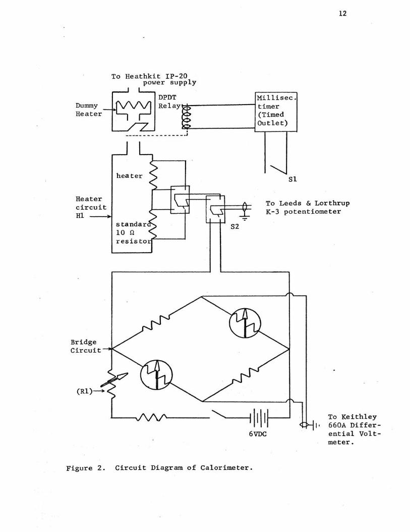
The thermometer circuit consists of two thermistors

(YSl, 10,000 ohms at 250C.) comprising opposite arms of a

Maier bridge circuit11 • The other arms consist of fixed

10,000 ohm resistors. (fig. 2)

During an experiment the bridge input potential is kept

constant at 1.0000 volt. The potential across the bridge

circuit is monitored by a Leeds and Northrup K-3 Universal

Potentiometer and the null position determined by a Hewlett

Packard 419A D.C. Null Voltmeter. The out of balance poten­

tial of the bridge circuit is determined with a Keithley

Model 660A Differential Voltmeter with a sensitivity of 2

microvolts.

2. Dilatometers:

For this portion of the investigation, two dilatometers

(fig. 3) were constructed in the laboratory. The two differ­

ed in the sizes of the sample chambers, so that large or

small samples could be used depending on the magnitude of

the volume change. The body (a) of the dilatometer was con­

structed with a slight bend so that the sample could be

trapped in the arm by mercury (c). The body of the dila­

tometer was fitted with a standard taper 10/30 ground glass

joint (d). The male member of the joint has attached to it

a precision capillary tube with a bore of about 0. 05 em. (e)·.

The two portions of the dilatometer were held together firm­

ly by rubber bands stretched over the glass hooks (f). Dur­

ing operation the height of liquid in the capillary tube

Dummy Heater

Heater circuit Hl

Bridge Circuit

To Heathkit IP-20 power supply

DPDT Millisec. Relay~---------------------------~ timer

(Timed Outlet)

• ----- - - - - - - - - - - .J

heater Sl

12

To Leeds & Lorthrup K-3 potentiometer

S2

To Keithley I • 660A Differ­

ential Volt­meter.

Figure 2. Circuit Diagram of Calorimeter.

13

Reference Mark

~--- Capillary tubing (e)

(f)--~ (d)

~(a}

Figure 3 . Dilatometer

14

was determined by a cathometer to 0.01 em. The dilatometer

was suspended in a constant temperature bath maintained at

25.00 + 0.01°C by a Sargent~ Model ST, Thermonitor tempera­

ture controller and was constant to within 0.002°C during

an experiment. The temperature of the bath was monitored

during each experiment by a Beckman thermometer, calibrated

against a Platinium Resistance Thermometer calibrated by

the National Bureau of Standards.

C. Experimental Procedure:

1. Calorimetry:

a. Preparat.ion Procedure:

A weighed sample bulb was filled with solute, sealed,

and the weight of sample determined by difference. The

amount of solute to be used in the experiment was deter­

mined by the amount of heat expected from the reaction.

The solute was generally chosen to give a heat effect

of slightly over 10 calories since this is in the range

of greatest sensitivity. In those cases where the beat

effect was very small the sample size was limited to

about 8 ml by the design of the calorimeter. A hypo­

dermic syringe was used to inject the sample into the

bulb (fig. 1) through the side arm. Glass tubing was

inserted into side arm after filling and the side arm

sealed with a flame. The sample bulb was allowed to cool

to room temperature and weighed to 0.01 mg. The sample

15

bulb was tied securely with thread to the breaker shaft.

Solvent of the desired composition was prepared by

pipetting the requisite volume of each component into a

500 ml flask and then weighing to 0.1 g. The solvent

temperature was adjusted to about 24.0°C~ approximately

300 mls pipetted into the Dewar flask, and the weight

of solvent determined by difference. The Dewar flask

was bolted to the calorimeter lid and the submarine

bolted around it. The entire unit was suspended in a

constant temperature bath filled with transformer oil

at 2s.oo ± 0.2oc. The electrical connections were made

and the calorimeter allowed to thermally equilibrate

for one hour. During the equilibration period the

temperature inside the Dewar flask was adjusted to the

appropriate starting temperature by operation of the

heater. It had been dete~ined previously that 25.0°C

gave a reading of -1700~v on the differential voltmeter.

To determine this valu~ the temperature sensing part

of the calorimeter (e) was submerged in a water bath.

The temperature of the water was measured and the out

of balance potential of the bridge determined at that

temperature. This procedure was repeated for a number

of temperatures~ below and above 25.ooc. The change

in temperature in microvolts was fitted to equation 1.

(t - 25. 0°) ... 52.24 (1700 + EBr> lo-6, +o. 02°C (1)

16

In equation 1, Ear is the out of balance potential of

the bridge (in microvolts) and t is the temperature in

centigrade degrees. The starting temperature for the

experiment was chosen so that the temperature change

would cause .the differential voltmeter deflection to

cross -1700JJ.v.

b. Measurement Procedure:

At the start of the experime.nt switches are closed

completing. the circuits to the Maier bridge and poten­

tiometer , sothat the batteries and circuit components

have 45-60 minutes to stabilize thermally and electri­

cally. At this time the power switches for the differ­

ential voltmeter and the null voltmeter are turned on,

since these require 30-45 minutes to warm up. Switches

Sl and 52 (fig. 2) are in the down position; heater off,

potentiometer across bridge circuit.

When the equilibration was complete the bridge

potential was adjusted to 1. 0000 volt by adjusting re­

sistor (R-1). Since the calorimeter was not completely

adiabatic, compensation was made for the flow of heat

between the system and surroundings by determining the

rate of change of the temperature of the system due to

the heat leak and extrapolating these "drift" rates from

before and after the process to the point in time at

which one half of the heat of the process had been

detected.

17

The differential voltmeter determines the out of

balance potential of the Maier Bridge. By observing

and recording the change in potential at constant time

intervals (one minute) the drift rate was determined.

Switches Sl and S2 were placed in their uppermost posi-

tions. Switch Sl supplies power to the timer and ener-

gizes a relay wh'ich completes the beater circuit (Fig.

2, Hl). Switch S2 transfers the potentiometer from the

bridge cireuit to the standard 10 ohm resistor. The I

potential drop '&cross the standard resistor was deter-

mined several times and the values obtained were averaged

for the determination of the heat capacity. Current was

supplied to the heater circuit for one ·or two minutes,

. depending on the amount of heat expected from the solu-

tion process. "Switches Sl and S2 were returned to their

former positions and the time that current had been flow-

ing was recorded. The potential across the bridge cir-

cuit was again adjusted to 1.0000 volts and the deflec-

tions of the differential voltmeter were recorded until

the drift rate was determined to be constant. The sample

was then introduced by depressing the breaker shaft (fig.

1, 1). After the drift rate was again constant the heat

capacity determination was repeated as described previ-

ously. After the heat capacity determination, all switches

were returned to their starting positions. The calori•

meter was then prepared for another experiment.

18

2. Dilatometry:

The cross-sectional area of the capillary tube was deter­

mined by filling a portion of it with mercury. The length

and weight of the column of mercury was determined. From

the weight and density of the mercury the volume was deter­

mined and by dividing the volume by the length, the cross

sectional area of the capillary tube was obtained.

About 60 ml of solvent mixture was prepared by pipetting

the required amount of each compo.nent into a flask and weigh­

ing to O.lg. The sample chamber of the dilatometer was filled

with clean mercury and a small magnetic stirring bar placed

in the body of the dilatometer. The weight of the dila­

tometer was obtained to 0.01 mg. Solute was placed in the

salllPle chamber of the dilatometer and the sample trapped in

place by the mercury (fig. 3). The excess sample was evapor­

ated from the body of the dilatome:ter by passing air through

it. The weight of the dilatometer with the solute was de­

termined. The dilatometer was filled with the solvent and

the capillary fitted into place. The dilatometer was sus­

pended in a constant temperature bath. The height of the

liquid in the capillary was adjusted and the dilatometer

allowed to thermally equilibrate for one hour. After equili­

bration, the height of the liquid in the capillary relative

to a reference mark on the stem was observed and recorded

at 10 minute intervals. After 30 minutes, during which the

19

height of the liquid in the capillary remained constant,

the.dilatometer was removed from the constant temperature

bath and the contents were mixed by tilting the dilatometer

to spill the mercury out of the sample chamber. To insure

thorough mixing the small magnetic stirring bar was operated

at high speed for 2-3 minutes. The dilatometer was returned

to the constant temperature bath and again allowed to equili­

brate. The height of the liquid in the capillary was ob­

served and recorded at 10 minute intervals until it was

determined to be constant. The dilatometer was then re­

moved from the constant temperature bath and prepared for

another experiment.

Since the capillary tube was at room temperature rather

than the bath temperature, it was felt that it would be

necessary to correct the observed height change for this

temperatqre difference. This correction was made and

found to have negligible effect on the apparent partial

molar volume.

D. Calculations·:

1. Calorimetry:

The calorimeter has an internal calibrating heater

built into it. The heater was constructed from manganin

wire which has a negligible change in resistance with tem­

perature. The resistance of the heater was determined

relative t .o a standard resistance. The resistance value

of the heater was checked periodically during this work

and changed by 0.04'7.. over an eight month period.

20

The heat capacity of the system was determined by ob-

serving the change in the out of balance potential of the

Maier bridge resulting from the input of a measured quan-

tity of electrical energy. The time that current was being

supplied to the heater and the potential drop across a stan-

dard 10 ohm resistor in series with the heater was deter-

mined. From these quantities the heat capacity given by

equation 2 was determined.

c II: qh EEh

(2)

In equation 2, C is the heat capacity of the system, ,6.Eh is

the change in temperature of the system obtained from the

out of balance potential of the Maier bridge in microvolts,

and qh is the electrical heat in calories produced by the

flow of current (I) through a resistance (Rh) for a time

(t, sec.). qh was determined from equation 3.

The curr.ent through the heater (Ih) can be obtained from

the potential drop (Es) across the 10 ohm standard re-

sistor. The potential drop (E5 ) is related to the cur-

(3)

r~nt (Ih), since the standard 10 ohm resistor is in series

circuit with the heater. In a series circuit the current

flowing is the same in all points of the circuit and from

Ohm"s Law

Eh E Ih = -"" Is • 8

Rh 'R; • (4)

21

In equation 4, the subscripts (h) and (s) refer to the heater

and the standard 10 ohm resistance respectively. Substitut-

ing the value of Ih from equation (4) into equation (2), equa-

tion 5 is obtained.

2 Es Rh t

R~ 4.184 (5)

Since the value of the heater resistance and the standard

1,.0 ohm resistance are constant they are grouped together

with tbe factor for conversion of joules to calories into

a fct.ct.or

F = R~ 4.184

.. (6)

The factor has a value of 0.77890 cal/ohm-joule. The

final expressiotl- used to calculate the heat capacities

was

(7)

From independent measurements it had been determdned that

one half · of the heat has been detected after about 6~ of

the heating period was completed. For a one minute heat-

ing period, the fore drifts and af~er drifts are extrapol-

ated to a point in time, 0.6 minutes, after the heater was

activated. The change in temperature in microvolts (6E)

was obtained by difference and is the heat effect of the

flow of curre.nt through t .he heater. In table I and II

22

data obtained from a typical experiment and the calcula­

tions are presented. In Figure 4 the data is shown graph­

ically.

The value calculated for the electrical heat is divided

by (.6.E) to give the heat capacity of the system in calories

per microvolt. The heat capacity was determined before

and after the solution process and the values obtained

were averaged. This gives an average heat capacity over

the range of temperature at which the solution process

occurs.

The (.6.E) for the reaction was calculated in a similar

manner as the (.6.E) for the heat capacity determination.

This (.6.E) was multiplied by the average heat capacity and

the result was the heat effect due to the solution process

in calories~ (q). The observed heat was corrected for the

heat effect of breaking a sample bulb. The corrected heat

effect is divided by the number of millimoles of solute to

obtain the heat effect for one gram molecular weight 9f

solute in a large amount of solvent.

2. Dilatometry:

In table III the data that was obtained from a typical ·

experiment is given. The number of millimoles of solute

were divided into the cress sectional area of the capil­

lary tubing. The value obtained was multiplied by the

change in height of the liquid in the capillary to obtain

the change in volume on mixing. If the change in volume~

23

TABLE I

EXPERIMENTAL DATA, CALORIMETRY

Page 146 Book 2 Acetone (2nd Sample) Solvent Make Up

27 June 1968 (100 mls IprOH 78.6) (250 mls meOH 196.8)

F = 0. 77890 Wt. of bulb + solute 2.67502 Mw ... 58.08 Wt. of empty bulb 1.89143 103n = 13.491 moles Wt. solute 0.78359 gm. Wt. solvent 220.5gm.

Bath Temperature 24.6°C

Time

o. 1. 2. 3. 4. 5. heater on

heater time 60.06 sec.

6. heater off 7. 8. 9.

10. 11. 12. 13. sample bulb crushed 14. 15. 16. 17. 18. heater on

heater time 59.99 sec.

19. heater off 20. 21. 22. 23. 24. 25.

•'. ::·

-EBr (Differential Reading)

Voltmeter

2587 2616 2645 2671 2698 2724 Es = .54963

.54954

.54958

0956 0979 1009 1039 1066 1093 1120 2499 2515 2530 2545 2560 Es • .54930

.54939

.54946

0778 0794 0819 0843 0866 0892

24

TABLE II

CALCULATIONS-CALORIMETRY

Page 147 Book T-2 n = 13 .. 491 m moles

1st heat capacity determination

Time of extrapolation reading drift extr~polated reading point f-l.V rate reading f-l.V

5 min. -2724 -26.3~ -2740 5.6 min

8 min. -0979 28.2 -0911

temperature change ~ = 1829f-l.v

qn = ~ F t = (.54958)2 (.77890)(60.06 sec.) • 14.13 calories C '"' qh = 0. 7725xlo-2 cal/J.I.v

2SE

Time of reading

18 min.

21 min.

Process;

Time of reading

13 min

14 min.

extrapolation reading drift extrapolated point f.J.V rate reading J.I.V

-2560 15 .2u..:L_ -2569 18.6 min

-0794 24.5 -0735

.6.E • 1834J.I.v

qh = (.54938)2(.77890)(59.99) • 14.10 calories c = qh .,. 0. 7690xlo-2cal/J.I.v

.6.E

C .. 0. 7798xlo-2 cal/f-l.v ave.

extrapolation point

reading J.I.V

drift rate

extrapolated reading f-l.V

-1120 13.5

-2499

l!Y. 27min

15.2

-1134

-2491

.6.E = 135 7J.I. v

q = ~E·C = 10.46 calories Correction for bulb breakiX~ "" -0.02 calories

q corr • 10.44 calories ~H • q corr ... +o. 774 kcal/mole

n

{/)

oi.J M 0 > 0 J-1 ()

•.-1 a c: ....

M cd

•.-1 oi.J c: (1) oi.J 0 ~

-700 . 2

---

---

-------------.-----

13 14 15 16 17 18 19 20 21 22 23 24

Time - minutes

Figure 4. Experimental Data, Calorimetry I'.) \.11

26

TABLE III

EXPERIMENTAL DATA - DIIATOMETRY

Page 231 Book T-2

Solute-Acetone Solvent-Isopropanol (Xi = 1.000}

Dilatometer B

Mark height above water level

Weight of dilatometer with sample Weight of dilatometer empty Weight of sample

24.5 em

58.72303 58.33924 . 0.38379 gm

MOlecular weight solute 58.08 number of moles solute 6.608xl0-3

mark liquid stem average Time height height (l-in) temperature height

9:00 placed in bath 10:55 13.99 em 13.24 em -0.75 em 27.8°C 11:05 13.82 12.94 -0.88 28.0 11:15 13.96 13.13 -0.83 28.1 -0.86 em 11:27 13.71 12.85 -0.86 28.1 11:30 mixed 13:29 14.26 18.53 4.27 28.9 13:45 14.09 18.44 4.35 29.1 13:55 15.25 19.59 4.24 29.0 4.~7 14:04 15.37 . 19.59 4.25 28.1

Cross sectional area of capillary bore:

Change in volume: (1.854Xl0-3cm2x5.13 em)

Apparent partial molar excess volume: 9.5lxl0-3ml

change in height

+5.13 em

1.8:4xl<f3cm2

-= 9. 5lxl03ml ml

... 1.44 mole 6.608xlo-3mole

27

~V, was constant to within ± 0.02 ml/mole the observed

values were averaged and this value taken as the apparent

partial molar excess volume at infinite dilution. For

changes in volume that showed a deviation gr~ater than

± 0.02 ml/mole on two successive samples, at least one

more solute sample was added to the solvent and the values

obtained were extrapolated to infinite dilution.

28

IV. Theory

A. General Considerations, Enthalpy Changes:

In considering the solution process, distinction must be

made between the integral or total heat of mixing and the dif-

fere,ntial heats of solution. The integral heat of mixing pro-

cess can be represented as

I

In this process nA and nB refer to the number of moles of com•

ponents A and B respectively. The change in enthalpy for this

process is given by

_6. A • ..mix • (~· H ) ~.n: . . nA '"A. - ~ (8)

In this equation, the quantities HA and HB refer to the partial

molar enthalpies of components A and B in solution and the sup-

erscript ~) refers to the pure components. The partial molar

enthalpies are defined by12

.. (9)

The heat of solution can be represented by the process

II

This process is a special case of I. The change in enthalpy

fQ~ this process is given by the equation

.6.H • (Hs - ~) + nB (~ - Hi) •• (10)

'i'Jle final process to be considered is represented by

29

[nAA J A(1) + nBB sol'n

T,P rA+l) ~] > nB B sol 1 n III )

The ~nthalpy change for this process is given by the «quation

I -· -D. 6H• nA(HA - ~) + nB(HB - HB) + !'A - HA (11)

In equation (11) the su.perscript ( 1 ) refers to the partial

molar enthalpies of the components in the final solution.

The heat of this process (III) is referred to as the differ-

ential heat of solution if the amount of the solvent is very

large, such that the fi~l composition is essentially the same

as the initial composition. As nA and nB become much greater

than one, equation (11) can be reduced to

_, -· -· ~ !:J.H = nAd~ + nBd~ + HA - ~ (12)

From the Gibbs-Duhem relationship

(13)

e.quation (12) becomes I -1:!.

D.H = HA - HA • (14)

Since it is impossible to determine the absolute enthalpy of

a substance and measurements give the change in enthalpy in I

going from one state to some other state, a reference state

can be chosen and the change in enthalpy determined relative

to the reference state. Lewis and Randa1113 have defined a

quantity, L, referred to as the relative partial molar enthalpy

by

(15)

30

The superscrlpt (O) ref.ers to the standard state, which ln thls

work iS···chosen as the pure liquid. The reference state is chosen

as the pure liquid ln either case and subtraction of the refer-

ence state enthalpies from equation (15) gives

In process III, component B could have been chosen for the

solute and by a simllar treatment L is obtained, B

-· 6-H = (~ - H;> ., ~

(16)

(17)

In process I, the enthalpies of the pure liquids are sub-

tracted from equation (8) to give

A1fllx • nALA + nBLB (18)

Referrlng to process II, if the amount of solvent (B) . is very

much greater than the amount of solute (S), the enthalpy.of the

solvent is the same in the initial and final states,

~(i) - "a(f) ,

and equation (10) becomes

A~ol'n- (Hs - Hg~

B. Experimental Considerations:

1. Differential Heats of Solution:

(19)

(20)

Th~ heats of solution of small amounts, less than 8

ml, of the pure components have been determined in rela-

tively much larger amounts of solvent mixtures and the

- ' <

31

pure components, approximately 300 ml~ over a broad range

of compositions. Process II is considered to represent

these measurements. Since the change in composition is

small, less than 0.010 mole fraction, the heat affects

observed can be considered to approximate the differential

beat of solution 9f the solute. The relative partial molar

beats were plotted versus composition and a smooth curve

drawn through the points to give the L's over the whole

composition range . Since both components of the solvent

were used as solutes the L curves of methanol and isopro-

panel were -_obtained.

2. Hea_ts of Mixing:

The values of the heat of mixing of methanol and iso­

propanol were obtained by calculation from the (L's). To

obtain the heat effect of formation of one mole of solu-

tion equation 18 is divided by (nA + nB) to give

(21)

3. ijeats of Solution at Infinite Dilution:

The heat of solution at infinite dilution is defined

such that the solute is dissolved in such a large quantity

of solvent that the addition of more solvent produces no

additional heat effect. In this investigation the heats

of solution of successive small portions of solute, sample

volume ranging from 0.1 ml to 3 ml, in much larger amounts

of solvent, 3.00 ml, were de-termined. The measured values

32

are considered to be represented by process II and the

enthalpy of the process is obtained from equation 20.

The heat effects observed for successive samples of acetone

and n-butanol going into solution were constant to within

experimental error. The heat effects observed for succes-

sive samples of chloroform and water exhibited a consis-

tent deviation. These values were plotted versus the

number of moles of solute and extrapolated to infinite

dilution.

C. General Considerations, Volume Changes:

Initially the dilatometer contained pure solute, a relative-

ly much larger volume of solvent, and a quantity of mercury.

The total initial volume may be represented by

·-b. Vi ... (ns Vs + nA VA) + VHg + nA VA (22)

(nsVs + nAVA) represents the volume of the solvent. This form

is used since successive amounts of pure solute were mixed into

the same solvent. n.A,vf represents the volume of the pure solute

trapped in the sample arm by the volume of mercury, VHg

The apparent partial molar volume is defined by

v- n v~ s s

Rearranging equation (23) gives

V ... nA 41 VA + ns V 8 6

An alternative representation of the initial volume is

(23)

(24)

(25)

33

After mixing, . the volume of the final solution is

v£ -= nsVs + (nA + nA_) v• A + VHg , (26)

which can also be represented as

v£ ... VA+ ns s (nA + nA.) $V1 + VHg (27)

The volume change on mixing obtained by subtracting equation

(28)

' By dividing equation (28) by nA and rearranging, equation

(29) is obtained.

A ~ix , _ ... _, -h. = nA (4> VA- $V ) + .... VA - v nA iii A A

(29)

As the number of moles of solute becomes small, equation

(29) becomes in the limit

mix Lim A~· Jl----nA and nA. _. o nA

-A .. ~v - vA· A~

(30)

As the solution becomes infinitely dilute (nA ...... o) .the limit--. .

ting value of 4> VA becomes VA 15, which is the partial molar

volume of A in an infinitely dilute solution and is not nee-

essarily the same as the partial molar volume of pure A.

An excess thermodynamic property is defined such that

e J = 3real - 3ideal

16

The partial molar excess volume is defined as the volume

34

exhibited by the pure liquid solute (ideal partial molar volume)

subtracted from the volume exhibited by the solute in the in-

finitely dilute solution;

(3·2)

D. Experimental Considerations~ Apparent Partial Molar Excess Volumes:

The measurement of the change of volume on mixing of sue-

cessive small portions of solute~ 0.1 ml to 0 . 5 ml, in approx-

imately 50 ml of solvent gave values for chloroform and n-

butanol that were constant to within experimental error~ +

0.02 mls. The volume changes observed for water and acetone

deviated in a consistant manner and were extrapolated to in-

finite dilution.

35

V. Results

A. Relative Partial Molar Heats and Integral Heats of Mixing:

The heats of solution of pure methanol and isopropanol were

determined by introducing small amounts (1 to 8 ml) of the pure

components into much larger quantities (300 ml) of solvents

consisting of methanol, isopropanol, and mixtures of these

components. In table IV the initial and final value of the

compositions are given along with the observed heat effects.

The heat quantities closely approximate relative partial molar

enthalpies as was previously explained. The heat values are

felt to be accurate to 2.0 per cent or 0.5 cal/mole, which-

ever is .larger.

The integral heat of mixing curve for the methanol-isopro-

panol was calculated from smoothed curves of the L data at 0.05

mole fraction intervals from equation 21. The heat of mixing

curve was fitted to an equation of the form

(33)

The values obtained for A and B were 72.3 cal/mole and 28.2

cal/mole respectively. The L values were recalculated from

the heat of mixing by the relations13

L = l1JFiX + X i · m J

mix ~ • &I -Xi

The agreement between measured and calculated L1 s is good,

Solute

MeOH .. .. .. " .. " .. .. " " "

IprOH .. " " " " " " n

II

"

TABLE IV

EXPERIMENTAL VALU~ES OF THE RELATIVE PARTIAL MOLAR HEATS OF METHANOL AND ISOPROPANOL

Comp·osition of Solution initial final

. xi xi

:1.000 0.994 0.981 0.969 0.882 0.865 0.762 0.682 0.673 0.493 0.136 0.096

0.846 0. 7~0 o. 671 0.680 0.489 0.29)2 0.131 0.126 0.008 0.008 0.000

0.994 0.981 0.969 0.956 0.865 0.846 0.755 0.671 0.662 0.486 0.133 0.094

0.848 0. 762 0.673 0.682 0.493 0.299 0.136 0.131 0.096 0.017 0.008

-103.2 -98.0 -95.7 -94.1 -64.6 -60.3 -43.1 -28.0 -27 .o - 9. 7

0.0 0.0

Li

-4.0 -8.8

-13.5 -13.6 -26.3 -37.9 -43.9 -44.1 -44.4 .. 44.5 -44.6

36

37

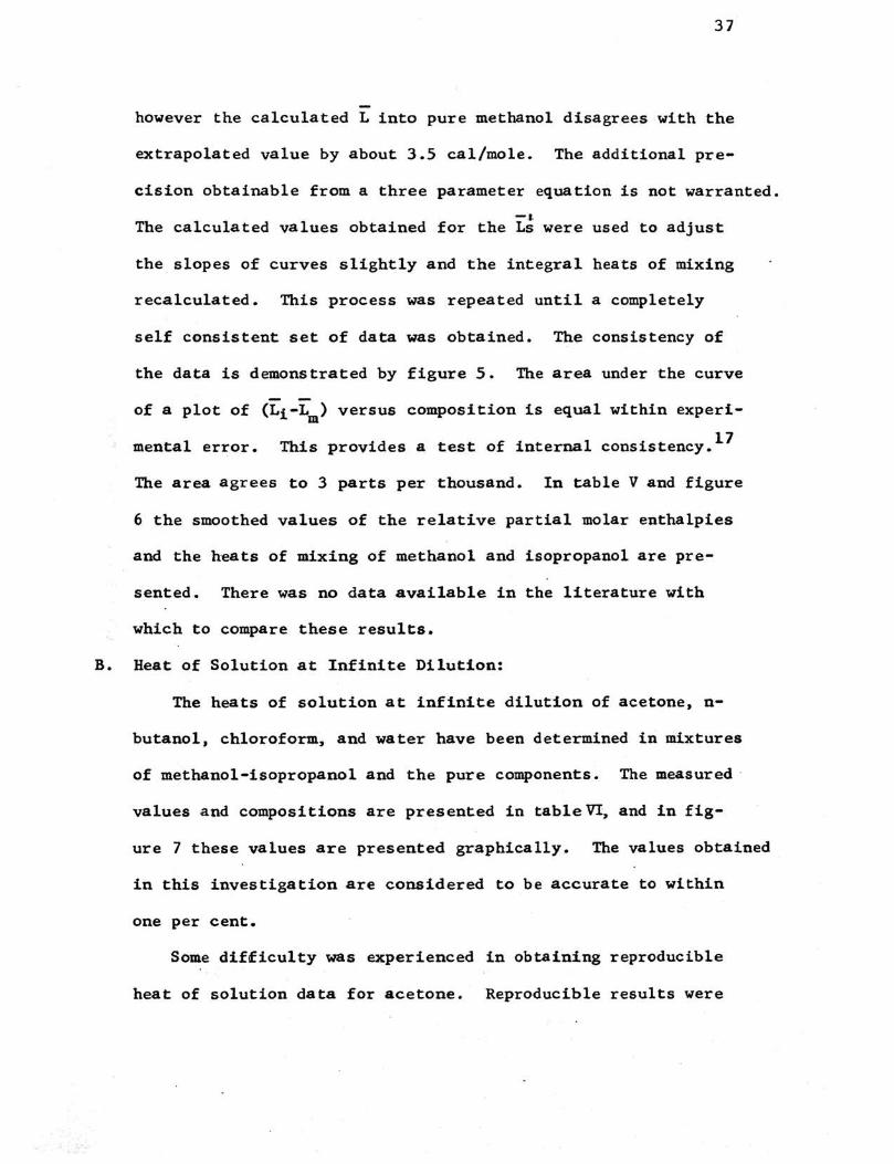
however the calculated L into pure methanol disagrees with the

extrapolated value by about 3.5 cal/mole. The additional pre-

cision obtainable from a three parameter equation is not warranted. -.,

The calculated values obtained for the Ls were used to adjust

the slopes of curves slightly and the integral heats of mixing

recalculated. This process was repeated until a completely

self consistent set of data was obtained. The consistency of

the data is demonstrated by figure 5. The area under the curve

of a plot of (Li-Lm) versus composition is equal within experi­

mental error. This provides a test of internal consistency. 17

The area agrees to 3 parts per thousand. In table V and figure

6 the smoothed values of the relative partial molar enthalpies

and the h~ats of mixing of methanol and isopropanol are pre-

sented. There was no data available in the literature with

which to compare these results.

B. Heat of Solution at Infinite Dilution:

The heats of solution at infinite dilution of acetone, n-

butanol, chloroform, and water have been determined in mixtures

of methanol-isopropanol and the pure components. The measured

values and compositions are presented in table VI, and in fig-

ure 7 these values are presented graphically. The values obtained

in this investigation are considered to be accurate to within

one per cent.

Some difficulty was experienced in obtaining reproducible

heat of solution data for acetone. Reproducible results were

+100

+90

+80

+70

+60

+50

+40

+30

+20

•.-I I ....:I

+10 --10

-20

-30

-40

0 0 .1 0. 2 0 • 3 0. 4 0. 5 0. 6 o. 7 0. 8 0. 9 1.0

Xi

Figure 5. Test of Internal Consistency

38

Solvent

0

0.1

0.2

0.3

0.4

0.5

0.6

0.7

0.8

0.9

1.0

TABLE V

SMOOTHED RELATIVE PARTIAL MOLAR HEATS AND THE HEATS OF MIXING OF METHANOL AND ISOPROPANOL

_cal _ cal L1m.ole Lm mole

-44.6 0

-44.o 0

-42.2 -0.4

-37 ·9 -2.0

-31.3 -5.5

-25. 0 -12.o

-18.2 -20.1

-12.0 -32.5

-6.2 -50.5

-1.2 -72.o

0 -104.5

39

,6.JfliX £!.l mole

0

-4.4

-8.8

-12.7

-16.1

-18.8

-19.1

-18.2

-15.2

-8.8

0

+10

0

-10

-20

-30

-40

-50

-60

-70

-80

-90

-100

-110 0

Legend o Li c Lm 6. 6Hmix

.2 .4 .6 .8 Xi

Figure 6. Relative Partial Molar Heats and the Heats of Mixing of Methanol-Isopropanol.

40

1.0

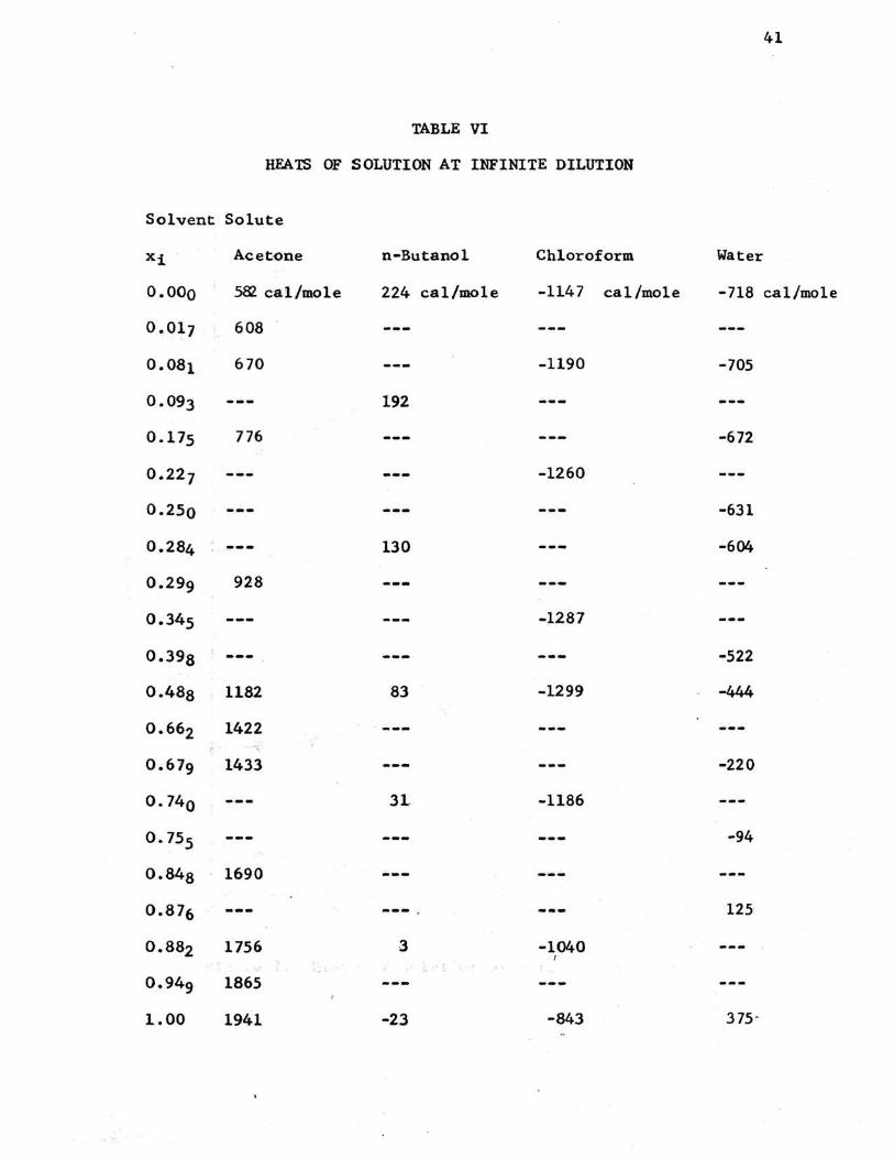
41

TABLE VI

HEATS OF SOLUTION AT INFINITE DILUTION

Solvent Solute

Xi Acetone n-Butanol Chloroform Water

o.ooo 58l cal/mole 224 cal/m.ole -1147 cal/mole -718 cal/mo1e

0.017 608

0.081 670 -1190 -705

0.093 192

0.175 776 -672

0.227 -1260

o.2so -631

0.284 ~-- 130 -604

0.299 928

o.345 -1287

o.398 -522

0.488 1182 83 -1299 -444

0.662 1422 ·'

0.679 1433 -220

o. 740 3L -1186

o. 755 -94

o.848 1690 ---0.876 --- 125

0.882 1756 3 -1040 : ... ' ·~

0.949 1865 ---1.00 1941 -23 -843 375-

-400

-800

-1200

0·

Legend

o Acetone An-butanol CJ chloroform '\]water

0.2 0.4 0.6 0.8

Figure 7. Heats of Solution at Infinite Dilution

42.

1.0

43

obtained by cooling the 4cetone to 15°C or less immediately be-

fore filling the sample bulbs.

Not many values of the heat of solution at infinite dilution

for non-electrolytes have been tabulated in the literature. How-

ever, values of the heat at infinite dilution can be obtained by

extrapolation techniques from heat of mixing data. The values

obtained in this manner generally have large uncertainties

associated with them. I~ table~ the values obtained from the ~.-. ,

literature are tabulated along with the values obtained in this

investigation. The values obtained in this investigation are

believed to be the best values presently available for these . ' quanti ties.

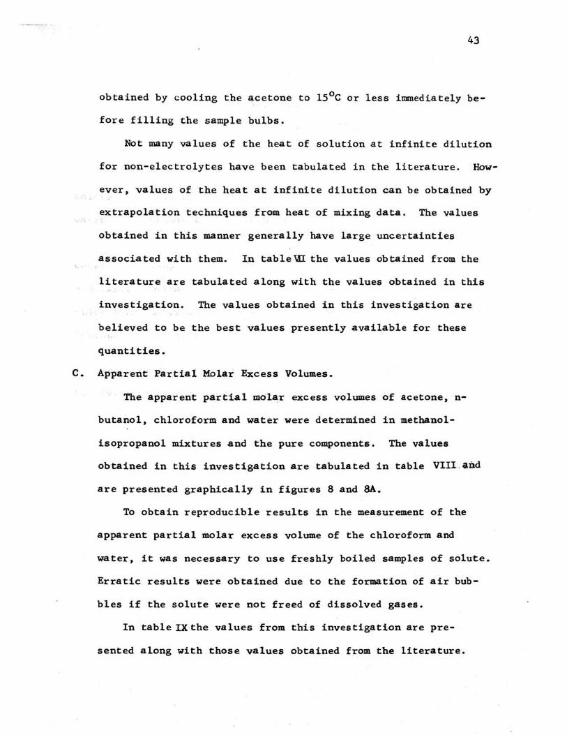
C. App'arent Partial Molar Excess Volumes.

The apparent partial ll1dlar excess volumes of acetone, · n-

butanol, chloroform and water were determined in methanol-

isopropanol mixtures and the pure components . The values

obtained in this investigation are tabulated in table VIII. and

are presented graphically in figures 8 and SA.

To obtain reproducible results in the measurement of the

apparent partial molar excess volume of the chloroform and

water, it was necessary to use freshly boiled samples of solute.

Erratic results were obtained due to the formation of air bub-

bles if the solute were not freed of dissolved gases.

In table IX the values from this investigation are pre-

sented along with those values obtained from the literature.

Solute

water

water

n-Butanol

Chloroform

Acetone

TABLE VII

COMPARISON VALUES FOR REA TS OF SOLUTION AT INFINITE DILUTION

Solvent This work Literature Ref.

methanol -718 i~le -719 cal mtrre 2

-738 18

isopropanol 375 400 19

methanol 224 227 20

methanol -1148 -7B935oc 21

methanol 582 523 22

44

Method used to obtain Literature

a.

b.

b.

b.

b.

b.

a. Measurement of heat of solution near infinite dilution.

b. Extrapolation of heat of mixing data.

Value

45

TABLE VIII

PARTIAL MOLAR EXCESS VOLUMES AT INFINITE DILUTION

Solvent Solute

Xi Acetone n-Butanol Chloroform Water

0.00 -1.71 ml/mole 0.57 m1/mole -0.15 m1/mole -3.75 ml/mole

0.03 -1.60

0.08 -1.50 -0.27

0.09 -3.95

0.13 0.45

0.17 -1.23

0.29 0.24 -0.70 -4.25

0.34 -0.89

0.48 -0.48 +(). 09 -1.14 -4.34

0.51 -4.33

0.66 0~06

0.69 -0.06 -4.25

0.77 0.46 -1.57

0.88 0.89 -0.12 . . ~ ..

0.91 -l. 76 -3.90

l.OO 1.43 -0.15 '!!1.78 -3.58

-4.4 0 0.2 0.4 0.6

Xi

Legend ~ n-butanol o chloroform '\7 water

0.8

46

1,.0

Fi:gu:r.e &. Partial Molar Excess Volumes at Infip..it,e Dilution

<U r-1

~ -r-1 a

-1.6~--~--J---~--~--~~--~--J---~--~--~

0 0.2 0.6 0.8 1.0.

Figure 8A. Partial Molar Excess Vol~e of Acetone at Infinite Dilution.

47

Solute

water

water

n-butanol

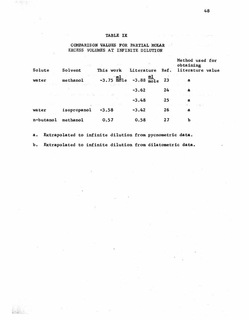
TABLE IX

COMPARISON VALUES ·FOR PARTIAL MOlAR EXCESS VOLUMES AT INFINITE DILUTION

Solvent This work Literature Ref. . tnl xDI

methanol -3.75 iii~le -3.88 mole 23

-3.62 24 '

-3.48 ·25

isopropanol -3.58 -3.42 26

methanol 0.57 0.58 27

Method used obtaining literature

a

a

a

a

b

a. Extrapolated to infinite dilution from pycnometric data.

b. Extrapolated to infinite dilution from dilatometric data.

for

value

49

The comparison valpes were obtained by extrapolation techniques

from density data and have fairly large uncertainties associated

with them, except where ot:herwise indicated. It is difficult

to obtain very good precision in the density determinations

of infinitely dilute solutions, eonsequently density measure­

ments are not: made at compositions very close to infinite di­

lution. The values presented here are probably the best avail­

able values of the apparent partial molar excess volumes for

thes.e solutes.

50

VI. Discussion of Results

The exothermic heat of mixing of methanol and isopropanol sets

this system apart from systems of normal alcohols. The heats of

mixing of 21 binary systems of normal alcohols have been reported.12 , 13

The systems are made up of al.l the binary combinations of normal al­

cohols from methanol to d~canol. The heat of mixing in all the sys­

tems studied is endothermic. In this investigation the heats of

mixing of methanol and n-butanol with isopropanol have been deter­

mined and are exothermi~.

The methanol-is9propanol system was chosen in part for the rela­

tively s~ll change in structuring with changes in the composition.

HQweve~ a slight amount o! structuring is indicated by the exother­

mic heat of mixing of -19.0 cal/mole. In comparison, the water­

ethanol and water-m~thanol systems have exothermic minima in their

heats of mixing of -186 cal/mole and -210 cal/mole respectively.

It is evident that the majority of the previous measurements of

heats of solution at infinite dilution in binary solvent systems

were made in systems that exhibit substantially more structure . ·

than the methanol-isopropanol system. Since the change in free

energy o~ mixing of the methanol-isopropanol system is not avail­

able, no attempts to explain heats of solution in this system in

terms of structuring effects will beattempted. The heats of sol­

ution can be compared with the results of the investigation in

oth.er systems howeve-r. With the exception of argon, all other

.s.olu,t_e:~ in the water-ethanol and water-methanol system have been

51

observed to give an endothermic maxima in the heats of solution at

infinite dilution.

If the components of a binary solvent system form an ideal solu-

tion, the heat of mixing of the components is zero, the heat of solu-

tion of a third component which does not form an ideal solution with

either component should obey the relation

(35)

In equation (35) ~and ~! are the heat of solution at infinite

dilution of solut~ A in solvents 1 and 2, respectively; . x1 and x 2

are the mole fractions of the solvent components. The line con-

necting the heats of solution at infinite dilution in the pure com-

ponents over the solvent composition range can be obtained from

equation (35) and will henceforth be referred to as the "ideal"

heat of solution.

the deviation of the heats of solution in systems containing

water from the ideal heat of solution is in a positive direction;

the heat effect is more endothermic than the mole fraction average

of the heats of solution in the pure solvents. In the methanol-

isopropanol system, the values obtained in this investigation de-

viate in a negative direction; they are more exothermic than the

mole fraction average of the heats of solution in the pure com-

ponents. From the results given in figure 7, the heat of solu-

tion of chloroform goes ' tlirough a minimum and clearly cannot be

equated to any type of arithmetic average of the pure solvent

values. ··

Arnett et al. 1 have proposed an explanation for the bea .~s of

solution which assumes that enthalpy is an indicst·or of structural

change, and that the position and height of the endothermic maxima

observed in the ethanol-water sys.tem is a function of the size of

the solute molecule. Bertrand, Lars,on, and Hepler3 also O'bserved

chang.es in position and hei:.ght of endothermic maxima f .or solute

molecules 'of ,diff"eri.ng" ·sizes :in the water-triethylamine system.

While the proposed explanation is qualitatively correct for the

systems~ containing water, it is impossible to extend it to the

methanol-isopropanol syste,ms .•

The explanation proposed by Krestov9 in terms of the solute

molecule occupyip.g holes in the solvent structure of the methanol-

ethanol system does not explain the heat effects observed in the

methanol-isopropanol .system·. The miniUlUDl observed in the h.eat of

so1ution of ealcium nitrate in the low concentration re.gion .;o,f

ethanol is explained in !"terms o£ the disruption of the .meehano·l

structure by the etha110l molecules. They have also reported a

maximum in the heat of solution in the region of low methanol ·

co.ncentration. The max-imum is attributed to an enchanceme.at of

the stability of the ·ethanol structure since the molecules of

methanol fit . into ·the hole.s in the ethanol structur e. The appli-

cation of this interpretation to methanol-isopropanol predicts

' ' an endothermic maximum in the heat of solution of the solute in

the region of . lew methano·l concentration. For all o·f the s:olutes

stt1died in tohis . :work, no ·endothermic maximum i .s obs erv-ed; ·oo .the

contrar~ the heat observed is more exothermic than would be

expected from their explanation. In applying their explanation to

the region of low isopropanol concentration, the effect due to size

should be enchanced in this system due to the size of isopropanol

relative to ethanol. None of the solutes studied in this investi-

ga,tion exhibit a minimum in the region of low concentration of iso-

propanol. The effects that Krestov observed apparently do not occur

for non-electrolytes and must be assumed to be related to ionization

of the solute.

Scatchard theory, as applied to three component systems with

one component very dilute, indicates that the heat of solution

should obey the equation,

.6Hsol 'n .. P H' + P H' _ a .MFix A AA B B 12

(36)

PA and PB are either mole fractions or volume fractions of

the solvent and !.. is a positive constant dependent on the sol.ute.

This equation can not predict heats of solution that deviate neg-

atively from the 11 ideal11 heat of solution for a solvent with a

negative heat of mixing. Appendix I gives the derivation of an

equation (A-8) that can be applied to heats of solution that show 28

either positive or negative deviations. The equation is in terms

of the energy change on solution at constant volume.

+ (2CX1 - 2C%2)(P1-v1 ~ Lower case v~s are volume fractions and 1 2 &.A and !::$)A are the

cbanges in energy of solute A dissolving in the pure so'lvents.

(AS)

VA is the molar volume of pure A, V is the molar volume of the sol­

vent. The term (2C~1 - 2C~) is a solute-dependent parameter of the

solvent system and P1 is a weighted volume fraction, as explained'

in Appendix I. Substituting the relation given in Appendix I for

~< t '

(AlO)

into equattion A8 and rearranging . te~,

The term -on the left of equation (3 7) can be evaluated fr<>m the

data ohtaiaed in this investigation. Dividing equation (37) by

(38)

(,J/1

Equation (38) is a linear form from which the parameters {2C0 -2C0 ) ~: f '

.t\1 . A2

and B can be evaluated. "':\ ..

Heats of solution are measured at constant pressure and must

be converted to the energy at constant volume. They were converted

r¥' 6~ ,.. 6-Hp-T tt• ve (~'9.' )

by use of the equatio·n (39 ). In this relation, a and f3 are tb:"e co-

efficients ·of thermal expansion and isothermal compressibility·~ ' re-

of the· pure compon·ents by the following relationships, which are

valid for a solvent system which bas no excess volume.

a = vl al + vz az f3 = vl f31 + vz t?t.l

Values fo·r a were dete~iQed exper.imentally for · the .pqre com~

ponents -4 ' -1 4 1 (ameOH • 1L8x.l0 deg , aiPrOH = 10.4xl0- <leg· ) and

(40)

for the equal ·vohune mix,t14~e ·<anu.x = ll.Oxlo-4 deg -l). ~e ~x ... ,

perimental value obtained for the mixture was within o1;1e per :~~nt;

of the calculated value .• .

Since the change in volume on mixing of methanol 404: i s.opr(lpanol

is small~ about 0.03 ml/mole~ the heat of mixing at constant pres-

sure is approximately equal to the change in energy of mixing at

constant volume. The values obtained for the parameters by cal-

culation are presented in table x. Since in some cases it is

impossible to obtain experimental values for the apparent partial

molar excess volume and would be impossible to convert the heat of

solution at constant pressure to the energy of solution at con-

stant volume~ the ~·s in equation A-8 have been replaced by tR

to give equation (41).

By a treatment sitili.lar to that given equation A-8, equation (41)

can be converted to a linear form. The values of the parameter

• • (2C~1 -zc~2 ) and B have been evaluated for this equation and are

presented in table .X also.

The value of (c11-c22 ) has been calculated from equation A-9.

c~l-&:i> (c11 -c22 ) == 2 (cX1 -c~) + VA (42)

This quantity should have a constant value since it is a function

of the energy ,of inter~ction of pure solvent components. +here is

considerable variation in the value obtained, however. -..: · ·

The variations in mapes of the heat of solution curves in this . '

"simple" system show that there are considerable solvent effects.

Although these effects are smaller in magnitude than those in the

water-ethanol system they are not amenable to simple explanations.

•'}. '! .• '.

Parameter

B

~5 (cal}

5 max(cal) cal

(Cll-c22) CiiiT)

Parameter

B'

2 (Co -co >'(cal) Al A2 ml

5 (cal)

t:max (cal)

• c~r . ' <ell -c22 > <mr>

TABLE X

VALUES OF PARAMETERS (from Equation 38)

Water

0.35·0

+3

13 . l

-23.4

Solute Acetone

0 . 52

cal .21""'mt"

+1.5

3

-5.7

n-Butanol

1.0

undefined

+1

2

(from equation 41)

Water Acetone n-Butanol

0.33 .46 0.29

88.8 21.9 .32

+3 +2 +1.5

11 3 9

-28.3 -3.6 -3.0

Chloroform

0.20

c:,a1 11.-1' ll:tl

+6.-·0 .,, .

14

f'

• 6 ~'" '" '<'

Chloroform .-:"• ·J:· '

.18

11.0

+7 :I

15

-7.2 . ; 'l f' j

B is the average deviation of the calculated energies and energies of solution from the s mo·othed values obtained · from :t:b~' 'ctir-Ves:l. ·

B is the maximum deviation· o:f the calculated beat,&·and · keat!S oif' ·· solution from the smoothed values.

,(:

VII. Summary and Reconmendations '·

In this investigation the heats of solution at infinite dilution

and the partial molar excess volume of four solutes have been deter-

mined in the methanol-isopropanol solvent system, and the measured

values are shown to correspond to the defined thermodynamic func-

tions. The results of this investigation have been presented along

with the relative partial molar enthalpies and the heat of mixing

curve of methanol and isopropanol. The values of the heats of solu-

tion and the apparent partial molar enthalpies were compared where

possible with literature values.

The values were compared with the explanations for the heats of

solution in ethanol-water and methanol-ethanol solvent systems. The

explanations presented for those systems were found to be inadequate

to explain the results in the methanol-isopropanol systen.

The relative partial molar enthalpies of two different normal

alcohols were found to be negative in isopropanol while they are

always positive in normal alcohol systems. The heats of solution

of normaland branched alcohols have not been studied extensively.

The apparent partial molar excess volumes of the solutes were

determined and these values utilized to convert the heat of solu-

tion at constant pressure to the energies of solution at co'nstant

volume. The energy changes were used to compute the values of tbe

parameters in an equation for the energy of solution derived by

28 G.L. Bertrand and presented in Appendix 1.

It is felt that a continuation of this study in tenus of more

solutes in this system an~ ~lso e~tending to other systems will

provide data on the effects of the solutes and insight into the

energies of interaction of the solvents so that the solvent effects

may be better understoo~ and explained.

~. J )

BIBLIOGRAPHY

i . . . '

1. Arnett, E., M. , Bentrude, W. G., Burke, J. J., and Duggleby, P.M. J. Am. Chern. Soc., 87, 1541 (1965).

2. Bertrand, G. L., Millero, F. J., Wu, C. H., and Hepler, L. G., J. Phys. Chern., 70, 699 (1966).

3. Bertrand, G. L., Larson, J. W., and Hepler, L. G., J. Phys. •Chern., 72, 4194 (1968).

4. Slansky, C. M., J. Am. Chem. Soc., 62, 2430 (1940).

5. Franks, F. and Ives, D. J. G., Quarterly Reviews, 20, 1. (19·66). ~·;.. 1 ~ ,~· tn~.tt it· ,J.

6. Ben-Naim, A. and Baer, S., Trans. Faraday Soc., 60,. 1736 (1965).

7.

8.

9.

10.

11.

12.

13.

14.

15.

16.

17.

18.

Ben-Naim, A. and Moran, G., Trans. Faraday Soc., 61, 821 (1965).

Samoi1ov, 0. Ya., Rabinovich, · I. B., and Dudnikova ;"-'-Ki,, 'f J~~hur. Strukt. Khimii (Eng. translation),£., 768 (1965). · · .

. ,, .{

Krestov, G. A. and Kl.opov, V. I., Zhur. Strukt. Khim!i (Eng. tra-ns­lation}, Y, 608 (1966).

Bertrand, G. L., Beaty, R. D., and Burns, H. A., J. Chern. Eng. Data, 13, 436 (1968).

Maier, C. G., J. Phys. Chern., ?4, 2860 (1930).

Klotz, Irving M. :"Chemical Thermodynamics,'' p. 2 71, W. A. Benjamin, Inc., New York, N. Y., 1964.

Lewis, G. N. and Randall, M., Revised _by Pitzer, K. S. and Brewer, L.: "Thermodynamics," pp 381-382, McGraw-Hill Book .Co., blc., New York, N. Y., 1961. 2 ed.

Klotz, 2.E. £1!_., p. 259.

Klotz, .Q.E_cit.,p. 261.

Van Ness, H. C.: "Classical Thermodynamics of Non-Electrolyt:.e Solutions," p. 73, The MacMillan Company, New York, N. Y., 1964 •.

Ibid., pp. 105-110.

Benjamin, L. and Benson, G. C., J. Phys. Chem., U ·, 85-8 (l!.963J .

19. Lama, R. F. and Benjamin, C. Y. Lu, J. Chern. Eng. Data, ~' 216 (1965).

61

20. Pope, A. E., Pflug, H. D., Dacre, B., and Benson, G. C., Can. J. Chern., 45, 2665 (1967).

21. Moelwyn-Hughes, E . A., and Miss en, R. W., J. Phys. Chem., .§1., 518 n95 n ...

22. Hirobe, H., J. Coll. Sci. (Tokyo) ~ 2.., 25 (1908).

23. Griffiths, V. S., J. Chem. Soc., 860 (1954).

24. Carr, C. and Riddick, J. A., Ind. Eng. Chem., 43, 692 (1951).

25. Clifford, G. and Campbell, J. A., J. Am. Chem. Soc., 73, 5449 (1951).

26. Wilson,A. and Simons, E. L., Ind. Eng. Chem., 44, 2214 (1952).

27. Pflug, H. D. and Benson,G. C., Can. J. Chem., 46, 287 (1968).

28. B~rtrand, G. L.~ personal communication (1969).

62

'. VITA

Elmer Lee Taylor was born on November 25, 1937 at Red Top,

Missouri. He received his primary education at Red Top, Missouri . .

and his secondary education at Buffalo, Missouri. In May, 1966, ¥ .. • :·

he received a :Bache~or. of Science Degree in Chemistry from South-

west Missouri State College in Springfield, Missouri.

He has seven years experience working in the chemical industry,

the latest position as a chemist. He is a member of the American

Chemical Society.

He served in the United States Air Force Reserves program from

April 1959 to April 1965.

On April 10, 1965 he was married to Barbara Linn Sears. They

have two daughters, Marta Linn and Jodie Lea.

• ~ s

63

Appendix I

HEATS OF SOLUTION IN BINARY SOLVENT SYSTEMS

The major prople~ ipyolved in attempts to develop theories • · .. ;ol,:··

and eq\lations pertaining to the heats of mixing of liquid mixtures

are: desc;:ription of' the .,ayerage environment of a given molecule,

estimation of the total . n'!.l~ber of interactions in which that mole-

cule is involved, and description of the average energy of the

molecule in te~ of its interactions with its environment. The

different equations that have been derived for heats of mixing

differ only in the model chosen for the three effects listed above.

In the case o.f a binary system with one component very dilute

{approaching infinite dilution) all of the equations yield a re­

lationship similar to the one which Scatchard 1 derived:

9-A Partial. molar excess energy of the solute, A, at infinite dilution in solvent, S.

Molar volume of pure solute

Average absolute value of the energy of inter- ' action between the solute and the solvent {per unit volume).

This equation is independent of the model chosen to describe the

environment of a solute molecule, since only solute molecules

surround the solute at infinite dilution. To apply this equation

to a binary solvent system (components 1 and 2), a model must be

chosen to describe the parameters CAS and c55 in terms of the

solvent composition (Xl). Both Scatchard1 and Hildebrand2 have

64

chosen an approximation

for the energy of the interactions within a pure solvent. Applying

this approximation to a mixed solvent (assuming no excess volume)

we obtaia

where the lower case v•s represent volume fractions and the upper

case V represents the molar volume of the mixture.

There is no precedent in the literature for a model on which

to base approximations for CAS in terms of solvent composition.

This term can be described with the equation

(4)

where pi represents the probability that the solute will interact

• with a solvent molecule of type i and C represents the energy - Ai

of the interactions between the solute and that type of solvent

in the environment that prevails at ·that particular solvent com:.;.

position. As a first appt'oximation, we choose

(5 ) c~1 ... c~1 ,

independent of solvent composition. Substituting equations 3, 4,

and 5 into 1, we obtai& .

(6)

Solving equation 6 foT the cas.es of the two pure solvents,

-1 - 0 ~ EA =·VA (2CA1-CAA -ell)

-2 -~ EA ... -VA (2C~2 .oCAA•Cz2)

(7)

65

Combining equations 7 with 6, we obtain

(8)

Equation 8 may be recognized as very similar to the equation that

may be derived from the equation of Hildebrand3 with two exceptions:

this equation should apply equally well to positive and negative

heats of solution and the final term of equation 8 does not appear

in the Hildebrand equation. Two difficulties remain in equation 8;

the terms cxi and the probability term, p1 • Equations 7 can be com­

bined to yield the difference in the cxi values in terms of the 6E! values and a parameter which is a property of the solvent system.

(9)

The simplest approximation for the probability term is to assume

that it can be represented as a weighted volume fraction:

(10) p 1 = Bv1/(Bv1 + v2)•

This allows the representation of data by a two parameter equation.

The validity of the approximations and assumptions of this treat­

ment will depend on whether the parameter (Cj1 - cX2 > for several

solutes in a single solvent system can be reduced to a single para-

meter through equation 9.

In applying this equation one must be aware of the types of

systems in which the approximations may be expected to be valid.

At the present time it is felt that the only sy.stems to which this

treatment might apply are those in which the solvent components are

very similar, such as mixtures of two alcohols, two hydrocarbons, etc.

1 Scatchard, G., Chem. Rev., 8, 321 (1931}

2 Hildebrand, J. H. and Scott, R. L., Regular Solutions, (Prentice-ball, Inc., Englewqod Cliffs, 1962), p. 91.