Possible thermochemical disequilibrium in the atmosphere of the exoplanet GJ 436b

Publisher: NPG; Journal: Nature: Nature; Article Type: Physics letter

DOI: 10.1038/nature09013

of 42

Possible thermochemical disequilibrium in the atmosphere of the

exoplanet GJ 436b

Kevin B. Stevenson1, Joseph Harrington1, Sarah Nymeyer1, Nikku Madhusudhan2, Sara Seager2, William C.

Bowman1, Ryan A. Hardy1, Drake Deming3, Emily Rauscher4 & Nate B. Lust1

1Planetary Sciences Group, Department of Physics, University of Central Florida, Orlando, Florida 32816,

USA. 2Department of Physics and Department of Earth, Atmospheric and Planetary Sciences, Massachusetts

Institute of Technology, Cambridge, Massachusetts 02159, USA. 3Planetary Systems Laboratory, NASA

Goddard Space Flight Center, Greenbelt, Maryland 20771, USA. 4Department of Astronomy, Columbia

University, New York, New York 10027, USA.

The nearby extrasolar planet GJ 436b—which has been labelled as a ‘hot Neptune’—

reveals itself by the dimming of light as it crosses in front of and behind its parent star

as seen from Earth. Respectively known as the primary transit and secondary eclipse,

the former constrains the planet’s radius and mass1,2

, and the latter constrains the

planet’s temperature3,4

and, with measurements at multiple wavelengths, its

atmospheric composition. Previous work5 using transmission spectroscopy failed to

detect the 1.4-m water vapour band, leaving the planet’s atmospheric composition

poorly constrained. Here we report the detection of planetary thermal emission from

the dayside of GJ 436b at multiple infrared wavelengths during the secondary eclipse.

The best-fit compositional models contain a high CO abundance and a substantial

methane (CH4) deficiency relative to thermochemical equilibrium models6 for the

predicted hydrogen-dominated atmosphere7,8

. Moreover, we report the presence of

some H2O and traces of CO2. Because CH4 is expected to be the dominant carbon-

bearing species, disequilibrium processes such as vertical mixing9 and polymerization

of methane10

into substances such as ethylene may be required to explain the hot

Neptune’s small CH4-to-CO ratio, which is at least 105 times smaller than predicted

6.

Using the Spitzer Space Telescope11

, the Spitzer Exoplanet Target of Opportunity

program observed multiple secondary eclipses at wavelengths of 3.6, 4.5, 5.8, 8.0, 16 and

24 m. Previous analyses3,4

of our 8.0-m secondary eclipse data confirm an eccentric orbit

around GJ 436, which is a cool, M-dwarf star. Standard image calibration and photometry


DOI: 10.1038/nature09013

of 42

produced light curves (tables of system flux versus time at each wavelength) that are

available as Supplementary Information, as are details of centring and photometry. Some

channels have well documented systematic effects that our Metropolis-Hastings Markov-

chain Monte Carlo (MCMC) model12

fits simultaneously with the eclipse parameters.

Systematics include positional sensitivity variation13

at 3.6, 4.5 and 5.8 m, where the

measured flux correlates with the sub-pixel location of the stellar centre, and time-varying

sensitivity14

at 4.5, 5.8, 8.0 and 16 m. Responsivity of the 24-m channel is relatively

stable15

. Figure 1 shows the observed secondary eclipses with best-fit models, and Table 1

presents the relevant eclipse parameters.

The phase of secondary eclipse imposes a tight constraint on the planet‟s

eccentricity, e, and argument of periapsis, . Using the secondary eclipse times listed in

Table 1, in addition to published transit16

and radial-velocity data17

, a single-planet

Keplerian orbit for GJ 436b has a period of 2.6438983 ± 0.0000016 days and an ephemeris

time of Julian date 2,454,222.61587 ± 0.00012 (all errors are 1). These are nearly

identical to the published results16

, which do not consider secondary eclipses. Using either

result, the weighted average of the five measured secondary eclipse phases is

0.5868 ± 0.0003. This significant improvement from previous analyses3,4

is due to the more

precise ephemeris time and the use of multiple secondary eclipses over a long baseline. The

weighted average of the minimum eccentricities, defined as emin e cos(), is

0.1368 ± 0.0004. Using = 351 ± 1.2° (ref. 17), we find e = 0.1385 ± 0.0006. To compute

all of the orbital parameters (Supplementary Information), we used the published results

referenced above in addition to the eclipse times presented here. Our best-fit value for e is

0.0048

0.000130.1371

.

Our broadband observations constrain a one-dimensional atmospheric model, using

a new temperature and abundance retrieval method18

. This method searches over a wide

parameter space using a functional form for the pressure–temperature profile (based on

prior „hot Jupiter‟ and Solar System studies), a grid of abundance combinations, and energy

conservation. We calculated ~106 models, which considered both inversion and non-

inversion temperature profiles and abundances that varied over several orders of magnitude


DOI: 10.1038/nature09013

of 42

per constituent. Figure 2 shows two representative models (the red and blue lines) that fit

the data, and Table 2 compares them to seven other objects with hydrogen-dominated

atmospheres. The red model has a dayside-to-nightside energy redistribution ratio of <0.04;

the blue model favours a more efficient distribution ratio of <0.31. The red model fits the

data better.

Chemical equilibrium predicts H2, H2O, CH4, CO and NH3 to be the most abundant

molecules in GJ 436b‟s atmosphere (helium must also be present but contributes minimally

to the spectrum and to active chemistry). Conventional chemical composition models

predict6 the major emission contributions to come from spectroscopically active H2O, CH4,

and, to a lesser extent, CO, and possibly CO2. In a reduced, hydrogen-dominated

atmosphere at ~700 K, CH4 is thermochemically favoured to be the main carbon-bearing

molecule. Assuming solar abundances for the elements and the pressure–temperature

profile shown in Supplementary Fig. 5, chemical equilibrium predicts6 a CH4-to-H2 mixing

ratio of 7 × 104

and an H2O mixing ratio of 2 × 103

. However, the strong planetary

emission at 3.6 m, combined with the non-detection at 4.5 m, calls for a methane

abundance that is depleted by a factor of ~7,000. The low H2O abundance favoured by our

red model could, in principle, result from carbon and oxygen abundances that are ~0.01

times solar values; however, the resulting CH4 mixing ratio would still be too high, by two

orders of magnitude, to explain the data.

Methane absorbs strongly in the 3.6-m band. CO and CO2 have absorption features

at 4.5 m, CO2 being the stronger absorber. The high flux at 3.6 m suggests very low

absorption due to methane, while the low flux at 4.5 m implies high absorption due to CO

and/or CO2. The degeneracy between the two molecules is solved by the low CO2

concentration needed at 16 m. The absence of observed flux in the 4.5-m channel thus

requires large amounts of CO, which is not expected in such a reduced atmosphere under

thermochemical equilibrium, and makes a future detection at 4.5 m important.

The flux modulation at 3.6 m is our strongest detection, with a signal-to-noise ratio

of 12.1, and has been confirmed by an independent analysis. Using 2 error bars for this


DOI: 10.1038/nature09013

of 42

observation and the 3 upper limit at 4.5 m, the low-methane requirement cannot be lifted

(this result is relatively insensitive to the remaining wavelengths). An increased methane

mixing ratio of 106

would result in a higher blackbody continuum, thus requiring a CO2

mixing ratio 103

in order to fit the flux constraint at 4.5 m (Figure 3). However,

thermochemical equilibrium and photochemical models predict a CO2 mixing ratio of ~107

in hydrogen-dominated atmospheres at solar abundance (~105

for 30 times solar

metallicities)19,20

.

We also explored other possibilities to explain the observations. A temperature

inversion does not fit the data well, assuming thermochemical equilibrium, because H2O

and CH4 would emit much more strongly than we observe in the 5.8- and 8.0-m channels,

respectively. Non-local thermodynamic equilibrium emission from the dayside of exoplanet

HD 189733b is attributed21

to CH4 fluorescence near 3.25 m. However, our 3.6-m

detection is too strong to be explained by fluorescence alone. Alternatively, the methane

deficiency could be explained by a lack of hydrogen; however, mass and radius constraints

placed by transit and radial-velocity observations call for a hydrogen-dominated

atmosphere7,8

, which we explored above. Atmospheric compositions dominated by an

alternative species (such as He or N2) are difficult to invoke plausibly. Hydrogen is the

most abundant species in planet-forming disks and atmospheric escape rates are small for

Neptune-mass planets. Although the observations were not made simultaneously, planet

variability and stellar activity are unlikely explanations for our observations. A global,

planetary temperature variation of 400 K manifesting in 2.64 days (the time between the

3.6- and 4.5-m observations) would be unprecedented in planetary science, as would a

transient hot vortex22

with one-third the planetary radius and T 2,200 K that appeared

during only one of our six observations. Stellar activity, which is common among M

dwarfs, would need to be timed precisely with the secondary eclipse for us not to detect and

mask it.

The brown dwarf GJ 570D has an effective temperature similar to that of GJ 436b

(800 K), but at atmospheric levels where T < 1,100 K, CH4 is the dominant carbon-bearing

molecule, with a CH4-to-CO ratio of ~102 (ref. 9). We estimate a ratio of 1 × 10

3 for GJ


DOI: 10.1038/nature09013

of 42

436b (Table 2); however, the exoplanet is strongly irradiated on one side, which can drive

atmospheric dynamics and disequilibrium chemistry. Vertical mixing9 can dredge CO up

from deeper and hotter parts of the atmosphere, where CO is favoured, resulting in a small

CH4-to-CO ratio if the rate of dredging is faster than the rate of the reaction that converts

CO to CH4 (CO + 3H2 CH4 + H2O). However, the observed CH4-to-CO mixing ratio

would require large amounts of vertical mixing. Alternatively, CH4 may be depleted by

polymerization into hydrocarbons such as ethylene (C2H4). This is a major methane

reaction pathway at these temperatures10

. These possibilities represent starting points for

future theoretical work with this atmosphere.

Received 18 November 2009; accepted 5 March 2010; doi:10.1038/nature09013.

1. Gillon, M. et al. Detection of transits of the nearby hot Neptune GJ 436 b. Astron. Astrophys. 472, L13–

L16 (2007). 0705.2219.

2. Torres, G. The Transiting Exoplanet Host Star GJ 436: A Test of Stellar Evolution Models in the Lower

Main Sequence, and Revised Planetary Parameters. Astrophys. J. 671, L65–L68 (2007). 0710.4883.

3. Deming, D. et al. Spitzer Transit and Secondary Eclipse Photometry of GJ 436b. Astrophys. J. 667,

L199–L202 (2007). 0707.2778.

4. Demory, B.-O. et al. Characterization of the hot Neptune GJ 436 b with Spitzer and groundbased

observations. Astron. Astrophys. 475, 1125–1129 (2007). 0707.3809.

5. Pont, F., Gilliland, R. L., Knutson, H., Holman, M. & Charbonneau, D. Transit infrared spectroscopy of

the hot Neptune around GJ 436 with the Hubble Space Telescope. Mon. Not. R. Astron. Soc. 393, L6–

L10 (2009). 0810.5731.

6. Burrows, A. & Sharp, C. M. Chemical Equilibrium Abundances in Brown Dwarf and Extrasolar Giant

Planet Atmospheres. Astrophy. J. 512, 843–863 (1999). arXiv:astro-ph/9807055.

7. Figueira, P. et al. Bulk composition of the transiting hot Neptune around GJ 436. Astron. Astrophys. 493,

671–676 (2009). 0904.2979.

8. Rogers, L. A. & Seager, S. A Framework for Quantifying the Degeneracies of Exoplanet Interior

Compositions. ArXiv e-prints (2009). 0912.3288.

9. Saumon, D. et al. Ammonia as a Tracer of Chemical Equilibrium in the T7.5 Dwarf Gliese 570D.

Astrophy. J. 647, 552–557 (2006). arXiv:astro-ph/0605563.

10. Zahnle, K., Marley, M. S. & Fortney, J. J. Thermometric Soots on Hot Jupiters? ArXiv e-prints (2009).

0911.0728.


DOI: 10.1038/nature09013

of 42

11. Werner, M. W. et al. The Spitzer Space Telescope Mission. Astrophy. J. Suppl. Ser. 154, 1–9 (2004).

arXiv:astro-ph/0406223.

12. Ford, E. B. Quantifying the Uncertainty in the Orbits of Extrasolar Planets. Astrophys. J. 129, 1706–1717

(2005). arXiv:astro-ph/0305441.

13. Knutson, H. A., Charbonneau, D., Allen, L. E., Burrows, A. & Megeath, S. T. The 3.6-8.0 μm Broadband

Emission Spectrum of HD 209458b: Evidence for an Atmospheric Temperature Inversion. Astrophys. J.

673, 526–531 (2008). 0709.3984.

14. Harrington, J., Luszcz, S., Seager, S., Deming, D. & Richardson, L. J. The hottest planet. Nature 447,

691–693 (2007).

15. Deming, D., Seager, S., Richardson, L. J. & Harrington, J. Infrared radiation from an Extrasolar planet.

Nature 434, 740–743 (2005). arXiv:astro-ph/0503554.

16. Caceres, C. et al. High Cadence Near Infrared Timing Observations of Extrasolar Planets: I. GJ 436b and

XO-1b. ArXiv e-prints (2009). 0905.1728.

17. Maness, H. L. et al. The M Dwarf GJ 436 and its Neptune-Mass Planet. Publ. Astron. Soc. Pac. 119, 90–

101 (2007). arXiv:astro-ph/0608260.

18. Madhusudhan, N. & Seager, S. A Temperature and Abundance Retrieval Method for Exoplanet

Atmospheres. Astrophys. J. 707, 24–39 (2009). 0910.1347.

19. Lodders, K. & Fegley, B. Atmospheric Chemistry in Giant Planets, Brown Dwarfs, and Low-Mass Dwarf

Stars. I. Carbon, Nitrogen, and Oxygen. Icarus 155, 393-424 (2002)

20. Zahnle, K., Marley, M. S., Freedman, R. S., Lodders, K. & Fortney, J. J. Atmospheric Sulfur

Photochemistry on Hot Jupiters. Astrophy. J. Lett. 701, L20–L24 (2009). 0903.1663.

21. Swain, M. R. et al. A ground-based near-infrared emission spectrum of the exoplanet HD189733b.

Nature 463, 637-639 (2010).

22. Cho, J., Menou, K., Hansen, B. M. S. & Seager, S. Atmospheric Circulation of Close-in Extrasolar Giant

Planets. I. Global, Barotropic, Adiabatic Simulations. Astrophys. J. 675, 817–845 (2008).

23. Alonso, R. et al. Limits to the planet candidate GJ 436c. Astron. Astrophys. 487, L5–L8 (2008).

0804.3030.

24. Castelli, F. & Kurucz, R. L. New Grids of ATLAS9 Model Atmospheres. ArXiv Astrophysics e-prints

(2004). arXiv:astro-ph/0405087.

25. Bean, J. L., Benedict, G. F. & Endl, M. Metallicities of M Dwarf Planet Hosts from Spectral Synthesis.

Astrophys. J. 653, L65–L68 (2006). arXiv:astro-ph/0611060.


DOI: 10.1038/nature09013

of 42

26. Swain, M. R. et al. Molecular Signatures in the Near-Infrared Dayside Spectrum of HD 189733b.

Astrophy. J. Lett. 690, L114–L117 (2009).

27. Atreya, S. K., Mahaffy, P. R., Niemann, H. B., Wong, M. H. & Owen, T. C. Composition and origin of

the atmosphere of Jupiter-an update, and implications for the extrasolar giant planets. Planet. Space Sci.

51, 105–112 (2003).

28. Lodders, K. & Fegley, B., Jr. The origin of carbon monoxide in Neptunes‟s atmosphere. Icarus 112, 368–

375 (1994).

29. Mandel, K. & Agol, E. Analytic Light Curves for Planetary Transit Searches. Astrophys. J. 580, L171–

L175 (2002). arXiv:astro-ph/0210099.

30. Reiners, A. Activity-induced radial velocity jitter in a flaring M dwarf. Astron. Astrophys. 498, 853–861

(2009). 0903.2661.

Supplementary Information is linked to the online version of the paper at www.nature.com/nature.

Acknowledgements We thank the Spitzer staff for rapid scheduling; M. Gillon, A. Lanotte and T. Loredo for

discussions; D. Wilson for contributed code; and A. Wright for manuscript comments. We thank the

following for software: the Free Software Foundation, W. Landsman and other contributors to the Interactive

Data Language Astronomy Library, contributors to SciPy, Matplotlib, and the Python programming language,

and the open-source community. This work is based on observations made with the Spitzer Space Telescope,

which is operated by the Jet Propulsion Laboratory, California Institute of Technology, under a contract with

NASA. This material is based on work supported by the US NSF and by the US NASA through an award

issued by JPL/Caltech.

Author Contributions K.B.S. wrote the paper and Supplementary Information with contributions from J.H.,

N.M. and R.A.H.; N.M. and S.S. produced the atmospheric models; S.N., K.B.S. and W.C.B. reduced the

data; K.B.S., J.H. and D.D. analysed the results; D.D. ran an independent analysis; R.A.H. produced the

orbital parameter results; and J.H., K.B.S., S.N., R.A.H., E.R. and N.B.L. wrote the analysis pipeline.

Author Information The original data are available from the Spitzer Space Telescope archive, programs

30129 and 40685. Reprints and permissions information is available at www.nature.com/reprints. The authors

declare no competing financial interests. Correspondence and requests for materials should be addressed to

K.B.S. ([email protected]).


DOI: 10.1038/nature09013

of 42

Figure 1. Secondary eclipses of GJ 436b at six Spitzer wavelengths. The flux values are

corrected for sensitivity effects, normalized to the system brightness, and vertically

separated for ease of comparison. a, Binned 3.6-, 4.5- and 5.8-m data (with 1 error bars),

b, binned 8.0-, 16- and 24-m data (with 1 error bars), both with best-fit models and for

orbital phases greater than 0.54. Note the different vertical scales used in each panel. The

phase calculation uses an ephemeris time of Julian date 2,454,222.61588 and a period of

2.6438986 days (ref. 16). Because the planet passes behind the star, we ignore stellar limb

darkening and use the uniform-source equations29

for the eclipse shape. The position

sensitivity model used either a quadratic13

or a cubic function in the two spatial variables,

including the cross terms to account for any correlation. An asymptotically constant

exponential function14

models the time-varying sensitivity. The 3.6- and 4.5-m channels

exhibit strong position sensitivity while the 5.8-m channel reveals a weak correlation with

pixel position. The unmodelled region at 3.6 m may be the result of stellar activity30

; a

similar region at 5.8 m is unmodelled for reasons presented in Supplementary


DOI: 10.1038/nature09013

of 42

Information. We detect no eclipse at 4.5 m, but constrain the flux modulation at its 3

upper bound by fixing the secondary eclipse phase to the mean weighted value of the other

channels. We use asymptotically constant exponential and linear functions to model the

time-varying sensitivities at 8.0 and 16 m, respectively. Our 8.0-m analysis agrees with

prior analyses3,4

but we obtain a slightly higher brightness temperature (Table 1) due, in

part, to a more recent Kurucz model24

. No correction is necessary at 24 m.

Figure 2. Broadband spectrum constraints for GJ 436b. The two atmospheric models

(red and blue lines) have the same temperature structure and no thermal inversion. The red

model has uniform mixing ratios for H2O, CH4, CO and CO2 of 3 × 106

, 1 × 107

, 7 × 104

and 1 × 107

, respectively. For the blue model, these are 1 × 104

, 1 × 107

, 1 × 104

and

1 × 106

. The 3.6-m channel is the key measurement in terms of constraining the methane

abundance. It also limits the amount of H2O to less than that of CO, with little to no energy

redistribution. Chemical equilibrium also requires some NH3. The coloured circles are the

bandpass-integrated models, the black squares are our data (with 1 error bars), and the

black arrow depicts the 3 upper limit at 4.5 m. The dashed green curves show blackbody

spectra at 650 K (bottom) and 1,050 K (top) divided by the Kurucz stellar spectrum

model24

. The red and blue models have effective (equivalent blackbody) temperatures of


DOI: 10.1038/nature09013

of 42

860 K and 790 K, respectively. We need not invoke an internal heat source3. Assuming

zero albedo and planet-wide redistribution of heat, GJ 436b has an equilibrium temperature

(Teq, where emitted and absorbed radiation balance for an equivalent blackbody) of 770 K

at periapse. For instantaneous reradiation of absorbed energy at secondary eclipse, the

hemispheric effective temperature is 800 K and the peak temperature is 1,030 K.

Figure 3. Contours showing the explored mixing ratios of methane. The purple, red,

orange and green contours show error surfaces within 2 of 1, 2, 3 and 4, where 2

is 2

divided by the number of channels. We use the 3 upper limit for the 4.5-m observation.

The black surfaces show models with 2 < 1 and CH4/H2 > 10

6. The figure demonstrates

that models with CH4 mixing ratios close to 106

or above (panel a) require extremely large

(>103

) CO2 mixing ratios (panel b), which are unphysical based on current understanding

of CO2 photochemistry. The parameter space was explored with ~106 models. The 2

parameter, which is related to the temperature gradient in the lower atmosphere18

, was

chosen arbitrarily for the abscissa.


DOI: 10.1038/nature09013

of 42

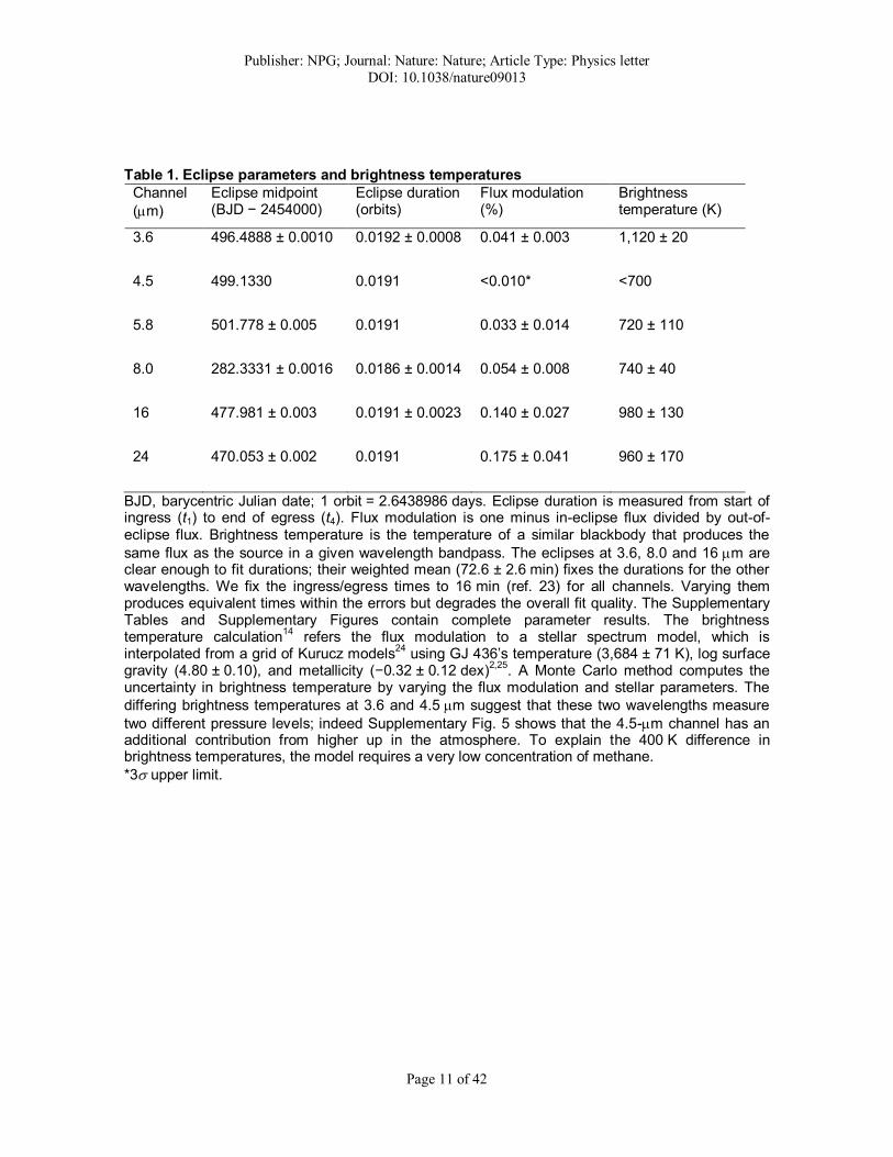
Table 1. Eclipse parameters and brightness temperatures

Channel

(m)

Eclipse midpoint (BJD − 2454000)

Eclipse duration (orbits)

Flux modulation (%)

Brightness temperature (K)

3.6 496.4888 ± 0.0010 0.0192 ± 0.0008 0.041 ± 0.003 1,120 ± 20

4.5 499.1330 0.0191 <0.010* <700

5.8 501.778 ± 0.005 0.0191 0.033 ± 0.014 720 ± 110

8.0 282.3331 ± 0.0016 0.0186 ± 0.0014 0.054 ± 0.008 740 ± 40

16 477.981 ± 0.003 0.0191 ± 0.0023 0.140 ± 0.027 980 ± 130

24 470.053 ± 0.002 0.0191 0.175 ± 0.041 960 ± 170

BJD, barycentric Julian date; 1 orbit = 2.6438986 days. Eclipse duration is measured from start of ingress (t1) to end of egress (t4). Flux modulation is one minus in-eclipse flux divided by out-of-eclipse flux. Brightness temperature is the temperature of a similar blackbody that produces the

same flux as the source in a given wavelength bandpass. The eclipses at 3.6, 8.0 and 16 m are clear enough to fit durations; their weighted mean (72.6 ± 2.6 min) fixes the durations for the other wavelengths. We fix the ingress/egress times to 16 min (ref. 23) for all channels. Varying them produces equivalent times within the errors but degrades the overall fit quality. The Supplementary Tables and Supplementary Figures contain complete parameter results. The brightness temperature calculation

14 refers the flux modulation to a stellar spectrum model, which is

interpolated from a grid of Kurucz models24

using GJ 436’s temperature (3,684 ± 71 K), log surface gravity (4.80 ± 0.10), and metallicity (−0.32 ± 0.12 dex)

2,25. A Monte Carlo method computes the

uncertainty in brightness temperature by varying the flux modulation and stellar parameters. The

differing brightness temperatures at 3.6 and 4.5 m suggest that these two wavelengths measure

two different pressure levels; indeed Supplementary Fig. 5 shows that the 4.5-m channel has an additional contribution from higher up in the atmosphere. To explain the 400 K difference in brightness temperatures, the model requires a very low concentration of methane.

*3 upper limit.


DOI: 10.1038/nature09013

of 42

Table 2. Atmospheric data for various planets

Planet H2O CH4 CO CO2 Teff (K) CH4/CO

HD 209458b18

(Spitzer broadband) 108

105

4 × 108

3 × 102

4 × 104

4 × 109

7 × 108

1,310

1,690≳107

≲102

HD 189733b18

(Spitzer broadband) 105

103

2 × 106

7 × 108

2 × 102

7 × 107

7 × 105

1,480

1,560≳1010

≲10

HD 189733b26

(HST/NICMOS) 1 × 104

1 × 103

1 × 107

1 × 104

3 × 104

1 × 106

1 × 105

NA ≲103

GJ 436b (red) 3 × 106 1 × 107

7 × 104 1 × 107

860 ~104

GJ 570D2 7 × 104

5 × 104 2 × 106

NA 800 ~102

GJ 436b (blue) 1 × 104 1 × 107

1 × 104 1 × 106

790 ~103

Jupiter27

2 × 109

2 × 108*

2.1 × 103 1.6 × 109

3 × 109 110 ~10

6

Saturn27

2 × 109

2 × 108*

4.5 × 103 1 × 109

3 × 1010 100 ~10

6

Uranus28

Ice 2.3 × 102 1.2 × 108

NA 60 ~106

Neptune28

Ice 2.9 × 102 ~1 × 106

NA 60 ~104

Values given under headings H2O, CH4, CO and CO2 are mixing ratios relative to hydrogen. Teff, effective temperature; HST/NICMOS, Hubble Space Telescope Near Infrared Camera and Multi-Object Spectrometer. The planets are ordered in descending effective temperature. Chemical equilibrium predicts a roughly increasing CH4-to-CO ratio. GJ 436b does not follow this general trend, as seen in the rightmost column. Its CH4-to-H2 mixing ratio is >10

3 times less than that of a

brown dwarf of similar temperature and its CH4-to-CO ratio is >105 times less. Excess CO may be

the result of relatively strong vertical mixing9. A significant fraction of the methane may have

polymerized into hydrocarbons10

, resulting in a shortage in observed CH4. For comparison, GJ

436b’s required methane mixing ratio of 107 is about 10

5 times less than that on Uranus and

Neptune, 104 times less than that on Jupiter and Saturn, and ~20 times less than that on Earth,

where methane is oxidized, not polymerized. NA, not available. *Above cloud.


DOI: 10.1038/nature09013

of 42

Supplementary Information

At a relative flux level of just ~0.1% compared to the host star, exoplanet secondary

eclipses are well below Spitzer's 2% relative photometric accuracy requirement31

. This and

their low intrinsic signal-to-noise ratios (SNR, often below 10) require that we attend

closely to analysis details. Because different analysis approaches may obtain significantly

different results, we also present more than the usual level of detail about our fits, so that

future investigators who choose to analyze these data can compare their work to ours. This

Supplementary Information (SI) presents how we determined the centres of the photometric

apertures, adjusted for varying array sensitivity with respect to aperture centre location

(“position sensitivity”) and time (“ramp”), and fit models to the data. The final section

presents the results of our fits in sufficient detail for evaluation of alternative analyses.

Many other methods appear in the SI to Ref. 14.

Centring and Photometry

Spitzer‟s instrumental point-spread functions (PSFs) are stable in time and vary

little with the normal pointing wander (<1”) over a few-hour staring observation. Since

zodiacal light and instrumental effects contribute significant noise, we use a small aperture

plus an aperture correction at short wavelengths and optimal photometry15,32

at longer

wavelengths. In either case, mismatching the aperture or PSF model to the data produces

additional error, so one must determine PSF centres accurately. Here we compare three

methods. The first33

computes the centre of light of pixels within a circular aperture and

above the frame's median value by at least 0.1% of the median-subtracted peak value. The

second fits a two-dimensional (2D) Gaussian with free position parameters. The third,

called least asymmetry, optimizes the stellar radial profile by calculating:

max

1

4Asym

i

=ii

ri

rσn=y)(x, , (1)


DOI: 10.1038/nature09013

of 42

where (x, y) is the current pixel location and σr is the standard deviation of the nr pixels at

the radial distance ri in pixels from the current central pixel. The first few discrete values

for ri are 1, √2, 2, √5, 2√2, 3, etc. We find using imax = 5 provides comparable precision

and computes faster than larger values. An inverted 2D Gaussian with free position

parameters finds the minimum in asymmetry space, which defines the centre of the object.

Tests using real datasets show that the 2D Gaussian and least-asymmetry methods

are more precise than the centre-of-light method (see Supplementary Figure 1). For the

example data, the Gaussian method is the most precise, but this is not always true. We

tested the accuracy with a fake dataset made from a 100 oversampled Spitzer Point

Response Function34

(PRF) centred at 50 locations along a pixel diagonal. We rebinned

each image to the nominal resolution, copied it 100 times, and added Gaussian noise.

Supplementary Figure 2 plots the median residuals between the known and computed

centres for the Gaussian and least-asymmetry methods. Both methods are comparable near

the corners, but the least-asymmetry method is more accurate near a pixel centre. The

Gaussian method is more consistent over the entire pixel range. For the observations of GJ

436b at 5.8 and 8.0 m, the mean radial distances from their respective pixel centres are

~0.2 pixels, so, as indicated in Supplementary Table 1, the best centring method is least

asymmetry. The evaluation metric is the standard deviation of the normalized (with respect

to the stellar flux) residuals between the measured and model flux values.

The IRS and MIPS channels typically achieve their best results using optimal

photometry, but 5-interpolated aperture photometry14

is best for the IRAC channels.

Supplementary Table 1 gives the best aperture sizes, found by varying the size and

minimizing the standard deviation of the normalized residuals. Changing the aperture size

by 0.25 pixels from the best value increases this standard deviation by <0.4% and typically

by much less, so smaller pixel increments are unnecessary.


DOI: 10.1038/nature09013

of 42

Supplementary Figure 1. Three centring methods track the vertical position of GJ

436b for a small portion of the 3.6 m data. For this dataset, the Gaussian centring

method most precisely tracks the spacecraft pointing. Small pointing oscillations occur on

a ~5-second timescale. Gaps occur every 64 frames as the camera transfers data to the

spacecraft's data system.


DOI: 10.1038/nature09013

of 42

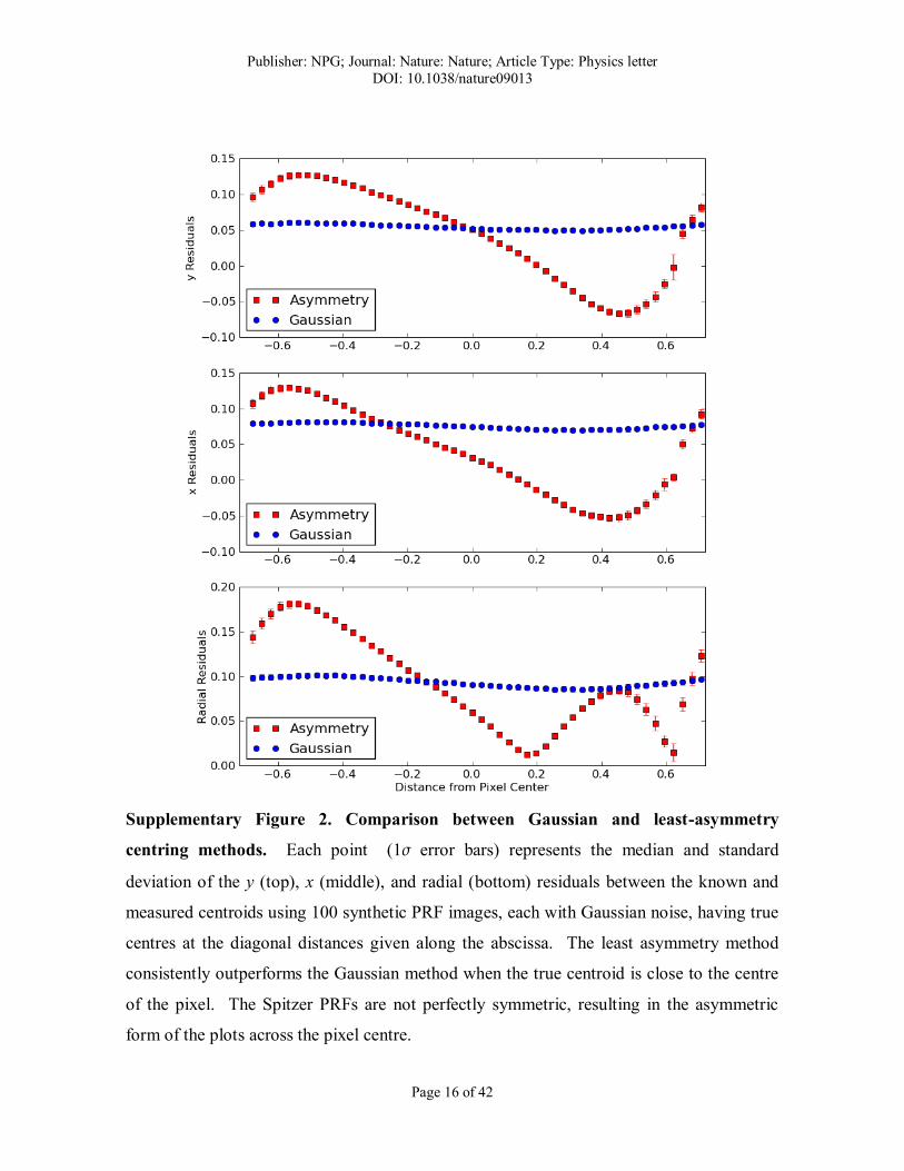
Supplementary Figure 2. Comparison between Gaussian and least-asymmetry

centring methods. Each point (1σ error bars) represents the median and standard

deviation of the y (top), x (middle), and radial (bottom) residuals between the known and

measured centroids using 100 synthetic PRF images, each with Gaussian noise, having true

centres at the diagonal distances given along the abscissa. The least asymmetry method

consistently outperforms the Gaussian method when the true centroid is close to the centre

of the pixel. The Spitzer PRFs are not perfectly symmetric, resulting in the asymmetric

form of the plots across the pixel centre.


DOI: 10.1038/nature09013

of 42

Supplementary Table 1. Centring method and photometry apertures.

Channel

[m]

Camera Centring Method Aperture Size

[Pixels]

3.6 IRAC Gaussian 2.75

4.5 IRAC Gaussian 4.75

5.8 IRAC Least Asymmetry 3.25

8.0 IRAC Least Asymmetry 3.75

16 IRS Gaussian N/A

24 MIPS Gaussian N/A

IRAC = Infrared Array Camera31

.

IRS = Infrared Spectrograph (blue peak-up array)35

.

MIPS = Multiband Imaging Photometer for Spitzer36

.

Position Sensitivity

In the 3.6- and 4.5-m Spitzer channels, sensitivity varies up to 3.5% with centroid

position. We detect for the first time much smaller variations at 5.8 m, which may be due

to intra-pixel sensitivity variations or residual flat-field errors. Polynomial models in the

two position variables fit the position sensitivity:

1+ex+dy+cyx+bx+ayφ=φ'22

(2)

1+ix+hy+gyx+fx+ey+dyx+xcy+bx+ayφ=φ'222233

(3)

where ’ and are the measured and corrected fluxes, respectively, x and y denote the PSF

centre relative to the pixel centre, and a – i are (potential) free parameters. In general (but

not for these particular datasets), if many of the PSF centres fall on two or more pixels, the

sensitivity difference between pixels (uncorrected flat field) becomes important. In this

case, each of the visited pixels has its own correction.


DOI: 10.1038/nature09013

of 42

Time-Varying Sensitivity

Two functions model the time-varying sensitivity: an asymptotically constant

exponential14

and a combination of logarithmic plus linear functions (similar to Ref. 3):

0

exp1 tta±φ=φ' (4)

,+ttb+ttaφ=φ' 1ln00

(5)

where, in Eqn. 4, the positive and negative signs are used for exponentially decreasing and

increasing variability, t is the observation time, and the free parameters are a, b, and t0. If

both intra-pixel and time-varying sensitivities apply, their multiplied corrections use only

one . Although ' in Eqn. 5 tends toward infinity at large t, this physical impossibility is

not a problem for observations of a few hours. Eqn. 4 curves more, so it generally produces

slightly deeper eclipses than Eqn. 5. Without any physical reason to prefer either funct ion,

we test both and report the one with the lowest Bayesian Information Criterion value

(described below).

Determining the Best Model

The Metropolis-Hastings algorithm, a specific Markov-Chain Monte Carlo

(MCMC) method12

, explores the model phase space to estimate the values and uncertainties

of the free parameters. The position sensitivity, time-varying sensitivity, and eclipse model

elements evaluate simultaneously. The eclipse element has parameters for the phase of

secondary eclipse (the fraction of one orbital period from mid-transit to mid-eclipse), the

duration between the first and fourth contact points, the eclipse flux ratio (or modulation,

one minus the in- versus out-of-eclipse flux values), the ingress and egress durations, and

in the absence of any sensitivity model elements. These parameters define the shape of the

eclipse following Ref. 29 for a uniform source. Spitzer Basic Calibrated Data (BCD) come

with calculated flux uncertainties per pixel, which are typically too large14

. After a "burn-


DOI: 10.1038/nature09013

of 42

in" of at least 105 iterations to forget the starting conditions, we rescale the uncertainties to

give a reduced χ2 of ~ 1. After 10

6 or more iterations, the best-fit parameters are those with

the least χ2 value. We calculate the 34

th percentile in both directions from the median value

to obtain uncertainties (averaged if close, quoted separately otherwise).

The Bayesian Information Criterion (BIC)37,38

compares models with differing numbers of

free parameters, heavily penalizing those with more, relative to the least χ2 method. The

preferred model has the lowest BIC value:

,nk+ε=

n

i

iln

1BIC

1

2

2

(6)

where i and is the residual of the ith data point, σ2 is the error variance, n is the number of

data points, and k is the number of free parameters. Supplementary Table 2 lists the

combinations of model elements used in each channel, the resulting standard deviation of

the normalized residuals, and the BIC values. Position sensitivity terms that contribute

negligibly to the fit are removed from the model. The type of position sensitivity model

element used does not significantly affect the eclipse parameters but can reduce their

uncertainties.

Supplementary Discussion

The short-lived spike that occurred after the eclipse at 3.6 m may be the result of

stellar activity30,39

. If this sharp increase in observed flux had affected the eclipse, the flux

ratio would have been larger and the duration longer, thus requiring even lower levels of

methane in the models and an inexplicably long duration. We contend that this is not the

case and do not fit the affected points. The high interest in M-dwarf planets calls for

observational study of M-dwarf activity, notably flares, across the spectrum.


DOI: 10.1038/nature09013

of 42

Supplementary Table 2. Eclipse free parameters and best models

Channel

[m]

Eclipse Free Parameters

Time-Varying Sensitivity

Position Sensitivity

Std. Dev. Of Norm. Residuals

BIC

3.6 Depth,

Duration, Phase -

Quadratic 0.003839 100548

Cubic 0.003830 100136

4.5 Depth Falling

Exponential

Quadratic 0.002449 37738 x

2, x & y

terms only 0.002450 37718

5.8 Depth,

Phase

Falling

Exponential

- 0.007208 35423

Quadratic 0.007194 35335

y2 term only 0.007194 35293

8.0 Depth,

Duration, Phase

Rising

Exponential

- 0.004985 37802

Log + Linear - 0.004984 37809

16 Depth,

Duration, Phase

Linear - 0.002939 875

Quadratic - 0.002923 1022

24 Depth, Phase - - 0.006344 1179

The residuals are normalized to the stellar flux.

The last ~2500 photometry points (~5%) at 5.8 m drop unexpectedly and are

difficult to model. Including these values in the fit causes the best-fit flux ratio to decrease

from 0.033% to 0.020% using the quadratic position sensitivity model. In addition, the

eclipse phase changes drastically with the additional points, resulting in relatively large

errors. The weaker flux ratio is comparable in magnitude to the remaining deviations from

the model, attracting the Metropolis-Hastings algorithm to nearby local minima that mimic

eclipses. Without the position sensitivity model, the best fit has a physically impossible

negative flux ratio. By fixing the eclipse phase, as we did for the 4.5-m photometry, the

flux ratio histogram of the MCMC trials are Gaussian distributed (see below); however, the

ramp curvature and phase offset parameters possess distinct bimodal distributions with


DOI: 10.1038/nature09013

of 42

standard deviations ~5 times larger than leaving the eclipse phase as a free parameter. We

exclude these points from the final model.

The 5.8 and 8.0 m channels use Si:As detectors and are not expected to have intra-

pixel sensitivity variations like the In:Sb detectors for the 3.6- and 4.5-m channels13

.

Nonetheless, the weak position sensitivity effect at 5.8 m clearly improves the fit, as

indicated by the lower BIC value in Supplementary Table 2 and as shown in Supplementary

Figure 3. The oscillatory motion of the flux (top panel) is in phase with that of the position

on the detector (bottom panel) and the best-fit curve mimics the flux motion with high

precision. This may be due to intra-pixel sensitivity or uncorrected flat field errors. A

possible micrometeoroid impact caused a sudden shift in position at phase = 0.58 (BJD =

2454501.7555). This did not affect the measured flux values, so we did not remove any

frames from this event that were not already flagged as bad. There are small oscillations in

the flux at 8.0 m, but we find no correlation between flux and position.

The relative dependences of position sensitivity on the measured flux are apparent

at the three lowest wavelengths in Supplementary Figure 4. The time-varying

sensitivities14

at 5.8, 8.0, and 16 m are also evident. Previous analyses3,4

at 8.0 m used

log plus linear and asymptotic exponential functions, respectively, to model the time-

varying sensitivity. We use the latter, which typically results in slightly larger flux ratios

compared to the log-plus-linear expression. The pixel sensitivity at 16 m increases by

~1.5% until the phase reaches 0.54. It then stabilizes before decreasing in sensitivity. We

only model the decreasing section, using a linear function. Other models produced larger

BIC values. The mean images in the MIPS dataset, with bad pixels removed, revealed a

clear, roughly quadratic rise in the background level along the y axis. This effect varied

with position but was consistent at each scan mirror tilt angle. We thus subtracted the

median value along the x-axis from each row of each image. However, the photometric

results from the background-subtracted images did not show improvement, so we used the

uncorrected data.


DOI: 10.1038/nature09013

of 42

Supplementary Figure 3. Position sensitivity at 5.8 m. The top panel plots the binned

fluxes and best-fit model vs. phase. The bottom panel shows the unbinned vertical pixel

positions (least asymmetry method, Gaussian is similar), which correlate with the measured

flux values. Note the position excursion – possibly a micrometeoroid hit – at phase ~0.58.


DOI: 10.1038/nature09013

of 42

Supplementary Figure 4. Binned, normalized, raw photometry of the GJ 436 system

in all six channels with eclipse and systematic models. The channels are vertically offset

for clarity. The black curves do not include the eclipse model elements. At 4.5 m, the

eclipse depth is too small to distinguish.


DOI: 10.1038/nature09013

of 42

Supplementary Tables

Supplementary Table 3. Best-fit orbital parameters with corresponding errors.

Parameter Best Fit Error

Period (Days) 2.6438983 ± 0.0000016

Ephemeris Time (JD) 2454222.61587 ± 0.00012

Argument of Periapsis (°) 357 ± 10.

Eccentricity 0.1371 + 0.0048

- 0.00013

Semi-Amplitude (m/s) 18.2 ± 0.4

Linear Slope (m/s/yr) 1.27 ± 0.20

Linear Offset (m/s) 4.1 ± 0.7

We used published transit16

and RV17

data but removed two points due to the Rossiter-

McLaughlin effect40

. Our MCMC orbit routine fit the period, ephemeris time, argument of

periapsis (ω), eccentricity (e), semi-amplitude (K), a linear correction slope (dv/dt), and an

offset (γ) term.


DOI: 10.1038/nature09013

of 42

Supplementary Table 4. Best-fit free parameters at 3.6 m.

Parameter Best Fit Low Error High Error SNR

Eclipse Phase [orbits] 0.5867 -0.0004 0.0004 1,600

Eclipse Duration [orbits] 0.0192 -0.0008 0.0008 23.0

Flux Ratio [%] 0.041 -0.003 0.003 12.1

Star Flux [μJy] 1,287,800 -500 600 2,350

Intra-pixel, Cubic Term in y 0.11 -0.02 0.02 5.3

Intra-pixel, Cubic Term in x -0.057 -0.004 0.004 12.8

Intra-pixel, y2x Cross Term 0.12 -0.02 0.04 3.9

Intra-pixel, yx2 Cross Term 0.185 -0.035 0.014 7.5

Intra-pixel, Quadratic Term in y -0.710 -0.04 0.05 15.1

Intra-pixel, Quadratic Term in x -0.0200 -0.0020 0.0017 10.9

Intra-pixel, yx Cross Term -0.011 -0.006 0.007 1.7

Intra-pixel, Linear Term in y -0.058 -0.005 0.009 8.6

Intra-pixel, Linear Term in x 0.0127 -0.0010 0.0010 12.4



Flux Ratio [%] 0.0002 -0.0032 0.0034 0.075

Star Flux [μJy] 861,900 -200 300 3,470

Ramp,Curvature 29.04 -0.08 0.11 307

Ramp,Phase Offset 0.281 -0.004 0.003 76.7

Intra-pixel, Quadratic Term in x 0.083 -0.003 0.004 22.7

Intra-pixel, Linear Term in y 0.1471 -0.0006 0.0005 267

Intra-pixel, Linear Term in x 0.0747 -0.0017 0.0022 37.7


DOI: 10.1038/nature09013

of 42



Eclipse Phase [orbits] 0.5873 -0.0042 0.0016 202

Flux Ratio [%] 0.033 -0.015 0.014 2.3

Star Flux [μJy] 562,190 -190 230 2,690

Ramp, Curvature 22.8 -1.2 2.2 13.3

Ramp, Phase Offset 0.293 -0.019 0.022 13.3

Intra-pixel, Quadratic Term in y -0.032 -0.003 0.003 12.0





Flux Ratio [%] 0.054 -0.008 0.008 7.3

Star Flux [μJy] 305,464 -16 16 19,500

Ramp, Curvature 41.69 -0.18 0.12 278

Ramp, Phase Offset 0.4068 -0.0008 0.0008 505

Supplementary Table 8. Best-fit free parameters at 16 m.




Flux Ratio [%] 0.140 -0.025 0.029 5.3

Star Flux [μJy] 85,949 -14 15 5,880

Ramp, Linear Term -0.082 -0.008 0.006 11.6


DOI: 10.1038/nature09013

of 42

Supplementary Table 9. Best-fit free parameters at 24 m.



Flux Ratio [%] 0.175 -0.042 0.041 4.2

Star Flux [μJy] 38,017 -7 7 5,310

Supplementary Figures

Supplementary Figure 5 presents the contribution functions41

and temperature

profile vs. pressure (or depth) for all six observed channels. Supplementary Figures 6 - 11

present histograms of the free parameter values in the MCMC chains. To remove the

correlation of the steps, the plots include only a fraction of the values plotted. For the low

S/N datasets such as 4.5 and 5.8 m, the chains explore physically impossible negative

eclipse depths in order to ascertain the error. Most of the histograms are roughly Gaussian

in shape but some parameters exhibit non-Gaussian errors.

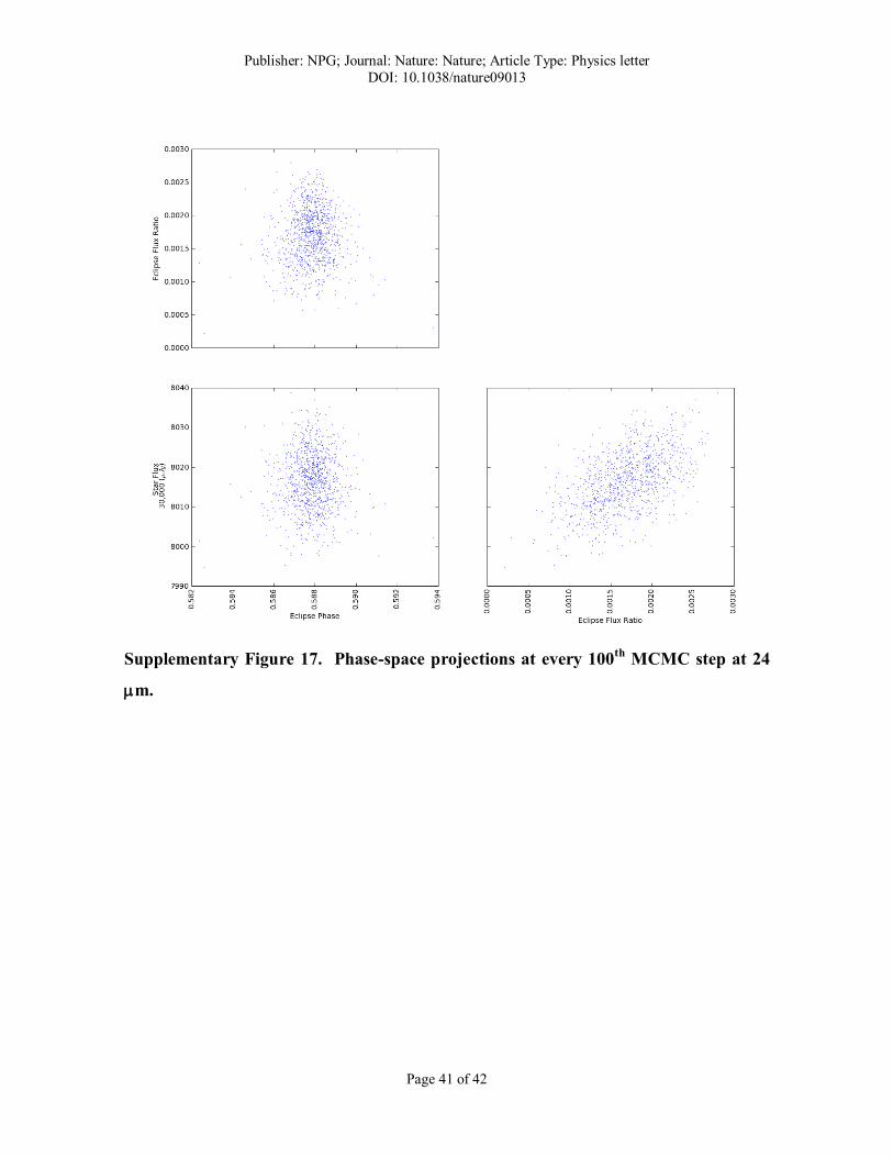
Supplementary Figures 12 - 17 show correlations between free parameters in a

small (for clarity) but representative percentage of the Markov steps. The MCMC random

walk does not always produce smooth distributions. Outlier clumps can occur where the

phase space has nearby local minima. Narrow paths can result from an ergodic probability

distribution, which can reach any point in the bounded phase space. The eclipse parameters

are generally uncorrelated with the intra-pixel and time-varying sensitivity parameters.

However, strong correlations do occur between the star flux and certain intra-pixel terms

and amongst the intra-pixel terms themselves. Due to the form of Eqns. 2 and 3, we expect

some degree of correlation.


DOI: 10.1038/nature09013

of 42

Supplementary Figure 5. Normalized contribution functions41

of GJ 436b in all six

observed channels (left) and the corresponding temperature profile (right). In the left

frame, the solid lines are from the red model of Figure 2 (main paper); the dashed lines are

from the blue model.


DOI: 10.1038/nature09013

of 42

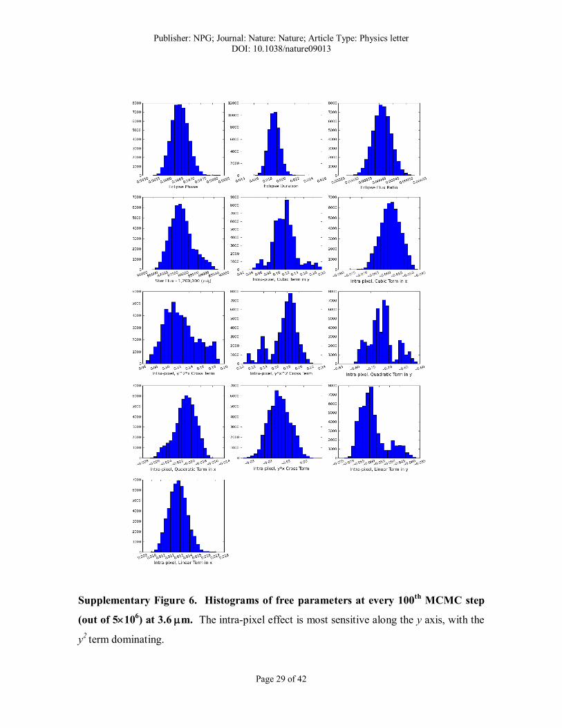
Supplementary Figure 6. Histograms of free parameters at every 100th

MCMC step

(out of 5106) at 3.6 m. The intra-pixel effect is most sensitive along the y axis, with the

y2 term dominating.


DOI: 10.1038/nature09013

of 42


MCMC step

(out of 106) at 4.5 m. The y term is the most dominant intra-pixel term at this

wavelength.


DOI: 10.1038/nature09013

of 42


MCMC step

(out of 106) at 5.8 m. Only the y axis intra-pixel dependence is significant.


DOI: 10.1038/nature09013

of 42


MCMC step

(out of 106) at 8.0 m.


DOI: 10.1038/nature09013

of 42


MCMC step

(out of 106) at 16 m.


MCMC step

(out of 106) at 24 m.


DOI: 10.1038/nature09013

of 42

Supplementary Figure 12a. See description below.


DOI: 10.1038/nature09013

of 42

Supplementary Figure 12b. See description below.


DOI: 10.1038/nature09013

of 42

Supplementary Figure 12c.

Supplementary Figure 12. Phase-space projections for every 1000th

MCMC step at

3.6 m. Due to the large number of free parameters in this particular model, the phase-

space projections are subdivided into three figures, labeled 12a, 12b, and 12c. The y and y2

terms are strongly correlated, with a coefficient of 0.94. The x, x2, and x

3 terms of the

intra-pixel sensitivity show very strong correlations (>0.9 or < -0.9) amongst themselves

and with the star flux. Removing any of these parameters results in a larger BIC value.


DOI: 10.1038/nature09013

of 42

Supplementary Figure 13. Phase-space projections at every 1000th

MCMC step at 4.5

m. There are correlations of 0.96, 0.93, and 0.99 between the star flux and the x term of

the intra-pixel sensitivity, the star flux and the x2

term, and the x2 and x terms, respectively.

Again, removing one or more of these parameters results in a larger BIC value.


DOI: 10.1038/nature09013

of 42


MCMC step at 5.8

m. The ramp curvature and phase offset show a correlation of 0.97. Neither parameter

can be removed without deteriorating the fit.


DOI: 10.1038/nature09013

of 42


MCMC step at 8.0

m.


DOI: 10.1038/nature09013

of 42


MCMC step at 16

m.


DOI: 10.1038/nature09013

of 42


MCMC step at 24

m.


DOI: 10.1038/nature09013

of 42

Supplementary References:

31. Fazio, G. G. et al. The Infrared Array Camera (IRAC) for the Spitzer Space

Telescope. Astrophy. J. Suppl. Ser. 154, 10–17 (2004). arXiv:astro-ph/0405616.

32. Horne, K. An optimal extraction algorithm for CCD spectroscopy. Publ. Astron.

Soc. Pac. 98, 609–617 (1986).

33. Howell, S. B. Handbook of CCD Astronomy (Cambridge University Press, 2000).

34. http://ssc.spitzer.caltech.edu/irac/psf.html.

35. Houck, J. R. et al. The Infrared Spectrograph (IRS) on the Spitzer Space Telescope.

Astrophy. J. Suppl. Ser. 154, 18–24 (2004). arXiv:astro-ph/0406167.

36. Rieke, G. H. et al. The Multiband Imaging Photometer for Spitzer (MIPS).

Astrophy. J. Suppl. Ser. 154, 25–29 (2004).

37. Schwarz, G. Estimating the dimension of a model. The Annals of Statistics 6, 461–

464 (1978). URL http://www.jstor.org/stable/2958889.

38. Liddle, A. R. Information criteria for astrophysical model selection. Mon. Not. R.

Astron. Soc. 377, L74–L78 (2007). arXiv:astro-ph/0701113.

39. Rubenstein, E. P. & Schaefer, B. E. Are Superflares on Solar Analogues Caused by

Extrasolar Planets? Astrophys. J. 529, 1031–1033 (2000). arXiv:astro-ph/9909187.

40. Rossiter, R. A. On the detection of an effect of rotation during eclipse in the

velocity of the brigher component of beta Lyrae, and on the constancy of velocity of

this system. Astrophys. J. 60, 15–21 (1924).

41. Knutson, H. A. et al. Multiwavelength Constraints on the Day-Night Circulation

Patterns of HD 189733b. Astrophys. J. 690, 822–836 (2009). 0802.1705.

Possible thermochemical disequilibrium in the atmosphere of the exoplanet GJ 436b

Documents

Transcript of Possible thermochemical disequilibrium in the atmosphere of the exoplanet GJ 436b