March 2017 IKE 8-127

Thermal mixing characteristics of

flows in horizontal T-junctions

A doctoral dissertation by

P. Karthick Selvam

Thermal mixing characteristics of flows in

horizontal T-junctions

Von der Fakultät 4 – Energie-, Verfahrens- und Biotechnik der Universität

Stuttgart zur Erlangung der Würde eines Doktors der

Ingenieurwissenschaften (Dr. -Ing.) genehmigte Abhandlung

Vorgelegt von

P. Karthick Selvam

aus Dharmapuri, Indien

Vorsitzender: Prof. Dr. -Ing. Andreas Kronenburg (Universität Stuttgart)

Hauptberichter: Prof. Dr. -Ing. habil. Eckart Laurien (Universität Stuttgart)

Mitberichter: Prof. Dr. -Ing. Horst-Michael Prasser (ETH Zürich)

Tag der Einreichung: 11 November 2016

Tag der mündlichen Prüfung: 29 März 2017

ISSN-Nr. : 0173-6892

Institut für Kernenergetik und Energiesysteme der Universität Stuttgart

März 2017

II

III

ACKNOWLEDGEMENTS

I would like to firstly thank my Doktorvater Prof. Eckart Laurien for giving me a chance to

work on the topic investigated in this study. His guidance and encouragement provided me

the motivation to stay the course, especially during challenging times. I am also thankful to

Dr. Rudi Kulenovic who facilitated my integration and subsequent development at the

institute.

Dr. -Ing. Mario Kuschewski and David Klören – my predecessors from whom I inherited this

work for my doctoral study – are sincerely acknowledged by the author. They took me

under their wings and shared with me their accumulated knowledge for which I am always

indebted. Their mentoring enabled me to stand on their shoulders and approach my work

from a completely different perspective for which I do not have words to thank. But for the

day-to-day interactions and frequent discussions with them, this work would not have been

possible.

I am greatly thankful to all my fellow colleagues and the staff with whom I had the

opportunity to spend my time here at the Institute of Nuclear Technology and Energy

Systems (IKE). Special thanks to my students, Patrick Buchwald and Patrick Gauder from

whom I had the opportunity to learn more about my work from a fresh perspective which

made it possible to move my work forward. Technicians from the Materials testing institute

(MPA), namely, Hermann Huber and Thomas Pfeiffer are gratefully acknowledged by the

author for their invaluable contributions in setting up the measurements.

The author is also thankful to the High Performance Computing Center Stuttgart (HLRS) for

the generous computational hours offered which made possible the work presented here. It

was a great learning experience to work together with Dr. sc. John Kickhofel and Prof.

Horst-Michael Prasser from the Laboratory of Nuclear Energy Systems (LKE), ETH Zürich

during our joint experimental studies which improved my understanding of the flow

dynamics within pipes.

Finally, I would like to sincerely acknowledge the scholarship awarded by the German

Academic Exchange Service (DAAD) for the entire duration of my doctoral studies.

IV

This work is dedicated to my beloved parents Panneer Selvam and Vijayalakshmi.

“Water does not resist. Water flows.

When you plunge your hand into it, all you feel is a caress.

Water is not a solid wall, it will not stop you.

But water always goes where it wants to go, and nothing in the end can stand against it.

Water is patient. Dripping water wears away a stone. Remember that, my child.

Remember you are half water. If you can't go through an obstacle, go around it. Water does.“

- Margaret Atwood, The Penelopiad

V

CONTENTS

Acknowledgements III

Abstract VII

Zusammenfassung IX

Nomenclature XI

1 Introduction 1

1.1 Motivation 1

1.2 Literature Review 8

1.3 Aim of the present study 23

2 Experimental setup 25

2.1 Instrumentation 27

2.2 System start-up, heating, and cooling 29

3 Numerical approach 32

3.1 Background 32

3.2 Large-eddy simulation (LES) 34

3.2.1 Filtered governing equations 35

3.2.2 Subgrid-scale modeling 36

3.2.3 Near-wall flow modeling 37

3.3 Computational mesh 37

3.4 Assessment of mesh resolution 39

3.4.1 y-plus (𝒚+) value estimation 39

3.4.2 Non-dimensional grid size (∆𝒙+, ∆𝒚+, ∆𝒛+) estimation 39

3.4.3 Energy scale (𝐿𝑅) and Taylor micro-scale (λ) estimation 40

3.5 Initial and boundary conditions 41

4 Results 43

VI

4.1 Mixing behavior of flows at ∆T = 60 °C – 180 °C 45

4.1.1 Velocity field in the mixing region 46

4.1.2 Thermal field in the mixing region 51

4.1.3 Flow penetration in the main and branch pipes 54

4.1.4 Near-wall mean temperature distribution 58

4.1.5 Temperature fluctuations 61

4.1.6 Frequency analysis of temperature fluctuations 69

4.2 Mixing behavior of flows at ∆T = 233 °C 73

4.2.1 Turbulent Penetration and Pipe Bending 74

4.2.2 Near-wall mean and RMS temperature distribution 76

4.2.3 Frequency Spectrum Analysis 78

4.3 Mixing behavior of flows at increased branch flow velocities 80

4.3.1 Qualitative analysis of the mixing region 80

4.3.2 Quantitative analysis 90

4.3.2.1 Mean temperature distribution 90

4.3.2.2 Temperature fluctuation distribution 92

4.3.2.3 Frequency spectrum of temperature fluctuations 98

Summary and Outlook 101

Bibliography 103

Appendix 118

VII

ABSTRACT

Thermal striping induced fatigue cracking incidents in the vicinity of a T-junction – where

coolant streams at different temperatures mix together intensively – has been reported in

several Nuclear Power Plants (NPPs) and is considered a challenge to the safe operation of

NPPs. The complex underlying turbulent flow behavior following the T-junction makes it

difficult to monitor the extent of fatigue damage employing the surface thermocouple

instrumentation. While there are isolated guidelines issued by regulatory bodies on how to

approach the issue, no general consensus exists internationally regarding the fatigue

assessment approach induced by such incidents.

The existing literature predominantly contains T-junction mixing experiments where the

temperature difference (∆T) between the fluids is lower in relation to the ∆Ts experienced

in NPPs. Experiments carried out at realistic ∆T between the fluids, on the other hand, lack

detailed numerical studies analyzing the different aspects of the flow mixing behavior. This

work deals with the coupled experimental and numerical studies of flow mixing occurring

in a horizontal T-junction piping from a thermal-hydraulic standpoint. The chosen range of

temperature difference (∆T) between the mixing fluids lie between 60 °C and 240 °C which

is highly representative of operating temperatures encountered in an NPP. Experiments

have been conducted at the horizontally aligned Fluid-Structure Interaction (FSI) test loop

at the University of Stuttgart using deionized water as the working fluid. Numerical studies

were performed using the large-eddy simulation (LES) turbulence model to capture the T-

junction mixing flow behavior in greater detail using the ANSYS CFX solver.

The observed mixing behavior could be summarized as follows: Thermally stratified flow

behavior is observed in all the investigated cases with (i) an oscillating flow at lower ∆T (<

140 °C) between the fluids and (ii) a stably stratified flow at higher ∆T (> 140 °C) where

buoyant forces significantly come into play. Hot flow penetration into the cold branch and

vice versa occurs at higher ∆T (> 140 °C) resulting in the partial mixing of fluids even before

they converge at the T-junction. Results from the study reveal that significant thermal

gradients exist near the stratification layer, a potential region of high amplitude thermal

fluctuations (a factor in thermal fatigue analysis). Frequency analyses of thermal

fluctuations using the power spectral density (PSD) method highlight the absence of any

VIII

specific dominant frequency (spectral peak) in the thermal fatigue relevant frequency range

of 0.1 – 10 Hz. Comparison of measurement data and LES predictions exhibits very good

agreement with one another highlighting the utility of LES as a useful tool in nuclear safety

based research.

In addition, LES calculations to analyze the flow mixing scenario at inflow conditions that

could not be presently realized at the FSI test facility (e.g. higher branch velocity) were also

performed in the present study. With rise in branch velocities, the flow nature changes from

an unstably stratified flow to a completely mixed flow at lower ∆T (< 140 °C) between the

fluids. At higher ∆T (> 140 °C) between the fluids, a transition from a stably stratified flow

to an unstably stratified flow is observed.

IX

ZUSAMMENFASSUNG

Thermisch induzierte Ermüdungsrissereignisse in der Nähe einer T-Stück Rohrverbindung

– wo sich Kühlmittelströme unterschiedlicher Temperaturen intensiv miteinander

vermischen – sind für mehrere Kernkraftwerke bekannt geworden und werden als

technisch relevante Herausforderung bezüglich des sicheren Betriebs von Kernkraftwerken

betrachtet. Das zugrunde liegende komplexe turbulente Strömungsverhalten nach dem T-

Stück erschwert die Erfassung des Ermüdungsschadensausmaßes anhand üblich

eingesetzter Messtechnik mit Oberflächenthermoelementen. Obwohl es einzelne, von

Kontrollbehörden herausgegebene Richtlinien gibt, wie diese Problemstellung zu

behandeln ist, besteht international kein allgemeiner Konsens hinsichtlich der Erfassungs-

und Beurteilungsmethodik der Materialermüdung, die durch solche Ereignisse verursacht

wird.

Die verfügbare Literatur beinhaltet hauptsächlich Untersuchungen zu

Vermischungsexperimenten an T-Stück Rohrverbindungen, die mit einem vergleichsweise

kleineren Temperaturunterschied (∆T) zwischen den Fluidströmen als den zu erwartenden

∆Ts in Kernkraftwerken durchgeführt wurden. Andererseits fehlen für Experimente mit

einem realitätsnahen ∆T der Fluidströme detaillierte numerische Untersuchungen, die die

verschiedenen Aspekte des Strömungsvermischungsverhaltens analysieren. Die

vorliegende Arbeit befasst sich daher unter einem thermohydraulischen Gesichtspunkt mit

gemeinsam verbundenen experimentellen und numerischen Untersuchungen zur

Strömungsvermischung in einer horizontalen T-Stück Rohrverbindung. Der gewählte

Temperaturdifferenzbereich (∆T) für die Fluidströme liegt hierbei zwischen 60 °C und 240

°C, der äußerst repräsentativ in Bezug auf die in Kernkraftwerken vorzufindenden

Betriebstemperaturen ist. Die Experimente wurden an dem horizontal ausgerichteten

Strömung-Struktur-Wechselwirkung-Versuchskreislauf (Fluid-Structure-Interaction, FSI)

an der Universität Stuttgart mit deionisiertem Wasser als Arbeitsmittel durchgeführt. Die

numerischen Untersuchungen erfolgten unter Anwendung der Grobstruktur-

Turbulenzmodellierung (Large-Eddy Simulation, LES), um das

Strömungsvermischungsverhalten in der T-Stück Rohrverbindung unter Verwendung des

ANSYS CFX Solvers mit einem erhöhten Detaillierungsgrad zu erfassen.

X

Das beobachtete Mischungsverhalten kann wie folgt zusammengefasst werden: Ein

thermisch geschichtetes Strömungsverhalten ist in allen untersuchten Fällen bei (i) einer

oszillierenden Strömung mit kleinerem ∆T (< 140 °C) der Fluidströme und bei (ii) einer

stabil geschichteten Strömung mit größerem ∆T (> 140 °C), in der Auftriebskräfte

signifikant zum Tragen kommen, beobachtbar. Ein Eindringen der heißen Strömung in den

kalten Nebenstrang des T-Stücks und umgekehrt entsteht bei höherem ∆T (> 140 °C) und

erzeugt eine Teilvermischung der Fluide noch bevor sie im T-Stück zusammenströmen. Die

Ergebnisse der Untersuchung zeigen, dass beachtliche thermische Gradienten in Nähe der

Schichtungsschicht bestehen, ein potenzielles Gebiet für hohe

Temperaturfluktuationsamplituden (ein Faktor in der Analyse thermischer

Materialermüdung). Frequenzuntersuchungen der thermischen Fluktuationen unter

Anwendung der Methode der spektralen Leistungsdichte (Power Spectral Density, PSD)

erbringen, dass keine spezifische dominante Frequenz (Frequenzmaximum) im für die

thermische Materialermüdung relevanten Frequenzbereich von 0,1 – 10 Hz vorhanden ist.

Der Vergleich zwischen Messergebnissen und LES Vorhersagen weist eine sehr gute

beiderseitige Übereinstimmung nach, die die Anwendbarkeit der LES als zweckdienliches

Werkzeug für die nukleare Sicherheitsforschung aufzeigt.

Zusätzlich wurden in vorliegender Arbeit LES Rechnungen durchgeführt, um die

Strömungsvermischung für Einströmbedingungen zu analysieren, die zur Zeit am FSI-

Versuchskreislauf nicht realisiert werden können (z. B. höhere

Nebenstranggeschwindigkeit). Bei kleinem ∆T (< 140 °C) zwischen den Fluiden verändert

sich mit Zunahme der Strömungsgeschwindigkeiten im Nebenstrang die Strömungsstruktur

von einer instabilen Schichtenströmung zu einer vollständig vermischten Strömung. Bei

einem höheren ∆T (> 140 °C) zwischen den Fluidströmen wird ein Übergang von einer

stabilen Schichtenströmung zu einer instabilen Schichtenströmung beobachtet.

XI

NOMENCLATURE

LATIN LETTERS

D Pipe diameter, m

f Source term

g Acceleration due to gravity, m s-2

h Specific enthalpy, J kg-1

N Number of sampled data points

P Pressure, bar

t Time, s

T Temperature, °C

u Velocity, m s-1

x, y, z Cartesian coordinates

GREEK LETTERS

𝜎𝑖𝑗 Stress tensor due to molecular viscosity, N m-2

𝜏𝑖𝑗 Residual stress tensor, N m-2

∆ Difference / Grid Size

θ Angular position, °

𝑘 Turbulent kinetic energy, m2 s-2

𝛿 Kronecker delta

휀 Rate of dissipation of turbulent kinetic energy, m2 s-3

𝜆 Thermal conductivity (W m-1 K-1) / Taylor microscale (mm)

𝜇 Dynamic viscosity, N s m-2

𝜈 Kinematic viscosity, m2 s-1

XII

𝜌 Density, kg m-3

NON-DIMENSIONAL PARAMETERS

𝑇∗̅̅ ̅ Normalized mean temperature

𝑢∗̅̅ ̅ Normalized mean fluid velocity

𝑀𝑅 Momentum ratio

𝑇∗ Normalized instantaneous temperature

𝑇𝑟𝑚𝑠∗ Normalized root mean square temperature

𝑢∗ Normalized instantaneous fluid velocity

𝑢𝑟𝑚𝑠∗ Normalized root mean square fluid velocity

∆𝑥𝑖+ Non-dimensional grid spacing

Pr Prandtl number

Re Reynolds number

Ri Richardson number

y+ Distance of the first node from the wall expressed in wall units

SUPERSCRIPT/SUBSCRIPT

m Main pipe

b Branch pipe

t Turbulent

ref Reference

i, j, k Tensor indices

mix Mixing

eff Effective

XIII

ABBREVIATIONS

BMBF Federal Ministry of Education and Research, Germany

BWR Boiling Water Reactor

CFD Computational Fluid Dynamics

CV Control Volume

CVP Counter-rotating Vortex Pair

DNS Direct Numerical Simulation

EPRI Electric Power Research Institute

FAMOS Fatigue Monitoring System

FEM Finite Element Method

FFT Fast Fourier Transform

FSI Fluid Structure Interaction

FVM Finite Volume Method

HCTF High Cycle Thermal Fatigue

HSV Horseshoe Vortex

IAEA International Atomic Energy Agency

IEA International Energy Agency

IKE Institute of Nuclear Technology and Energy Systems

KTA Nuclear Safety Standards Commission

LES Large Eddy Simulation

LKE Laboratory of Nuclear Energy Systems

LMFBR Liquid Metal Fast Breeder Reactor

LWR Light Water Reactor

MPA Materials Testing Institute

XIV

NEA Nuclear Energy Agency

NPP Nuclear Power Plant

NRC Nuclear Regulatory Commission

OECD Organization for Economic Co-operation and Development

PSD Power Spectral Density

PWR Pressurized Water Reactor

RANS Reynolds Average Navier-Stokes

RHRS Residual Heat Removal System

rms Root Mean Square

SGS Sub-grid Scale

SST Shear Stress Transport

WALE Wall-Adapting Local Eddy-Viscosity

WMS Wire Mesh Sensor

1

1.1 Motivation

Consistent, reliable supply of electricity is the foundation and a key driver of economic,

technological and social growth in any country. The world energy outlook 2015 special

report on energy and climate change [152] from the International Energy Agency (IEA)

estimates the total worldwide electricity generation in 2030 to be 30,620 terawatt-hours

(TWh), a 32 % increase from the 23,234 TWh generated in 2013. In the midst of such a lofty

outlook, there is a growing consensus regarding the need to substantially reduce the

greenhouse gas emissions due to power generation. Base load power generation supplying

round-the-clock electricity throughout the year – the foundation of the modern electrical

grid – comes from two primary fuel sources: coal and nuclear. Coal-based electricity

generation is set to be significantly curbed over the coming years as part of the clean energy

initiative adopted by many countries around the world. On the other hand, nuclear-based

electricity generation is set to become an important part of the energy mix in many

countries over the next decade. The latest data from the International Atomic Energy

Agency (IAEA) point to the fact that there are 441 nuclear power reactors currently in

operation worldwide generating nearly 383 GW electrical power output [48, 94]. 67

reactors are presently under construction, 172 reactors are either ordered or planned and a

further 337 reactors are proposed worldwide [153]. Thus the trend clearly points towards

significant expansion in the global nuclear capacity over the next decade due to the low-

carbon, low-cost base load electricity produced in a nuclear power plant.

2

Fig. 1 Simplified illustration of a Nuclear Power Plant, Pressurized Water Reactor [95]

Table 1: Types of nuclear power plants worldwide (Source: IAEA [94])

Reactor type Fuel Coolant Moderator #

Pressurized Water Reactor

(PWR)

Enriched UO2 Water Water 282

Boiling Water Reactor (BWR) Enriched UO2 Water Water 78

Pressurized Heavy Water

Reactor ‘CANDU’ (PHWR)

Natural UO2 Heavy water Heavy water 49

Gas-cooled Reactor (AGR &

Magnox)

Natural U

(metal),

enriched UO2

CO2 Graphite 14

Light Water Graphite Reactor

(RBMK & EGP)

Enriched UO2

Water Graphite 15

Fast Neutron Reactor (FBR) PuO2 and UO2 Liquid sodium none 3

Total number of reactors 441

A nuclear power plant (NPP) is basically a thermal power station where heat is generated

by splitting the atoms (nuclear fission) of fuel elements (typically, enriched UO2) in the

3

nuclear reactor. The generated heat is absorbed by the surrounding coolant (e.g. water) to

produce steam which then drives a steam turbine connected to an electrical generator to

produce electricity (see Fig. 1). A vast majority of the commercial nuclear reactors (> 80 %)

currently in operation worldwide are light water reactors (LWRs) using ordinary (light)

water as the coolant. LWRs are further classified as pressurized water reactors and boiling

water reactors. A classification of the different types of NPPs currently in operation is

summarized in Table 1.

Piping systems perform the essential function of facilitating coolant transport within an

NPP. Being a vast infrastructure, an extensive network of piping serving different purposes

are available within an NPP. Ensuring the integrity and functional capability of piping

systems throughout their service life are important for the safe operation of an NPP. The

quality and the properties of the piping are initially controlled during the design and

manufacturing stage. It may change during its service life due to the operating conditions

(e.g. ≈ 290 °C, 155 bar in the reactor core of a PWR [151]) to which it is exposed.

Additionally, the quality of the piping is also influenced by new knowledge and experience

acquired during the operation of the power plant along with other technical and scientific

progress. These changes are collectively indicated by the term ‘ageing’. There are six

identified ageing mechanisms that tend to reduce the working life of components in an NPP,

namely, thermal fatigue, vibrational fatigue, thermal ageing, primary water stress corrosion

cracking, boric acid corrosion and atmospheric corrosion [47]. This work is primarily

focused on thermal fatigue induced piping degradation.

Thermal loading imposed on the piping structure by the underlying fluid flow results in

some of the unexpected material degradation and failure reported in nuclear power plants

(NPPs). Thermal fatigue was identified as a challenge to the nuclear safety during the early

operation of NPPs during the 1970s and 1980s when new loading conditions (e.g. thermal

stratification, vortex penetration in tees, dead leg and valve leaks) that were not considered

during the design stage resulted in fatigue cracks at different locations during the operation

[1]. Research efforts were subsequently made to understand these issues by the nuclear

community. The regulatory agencies – based on the findings – issued guidelines to the

utility operators to put in place practical systems capable of identifying and safeguarding

the components from such occurrences at the earliest possible time. For example, the

4

nuclear regulatory commission (NRC) in the United States issued Bulletin 88-08 and

subsequent guidelines establishing Licensee actions ensuring appropriate degradation

management [137, 138, 139, 140, 141, and 142]. The German nuclear safety standards

commission (KTA) mandated the use of additional measuring equipment including the

installation of long-term temperature measuring devices in order to obtain comprehensive

information about the real loading experienced by the components during operation. Since

thermal fatigue is a highly local phenomenon, knowledge of both the local geometry of

components and their loading conditions are required. Thus, the German nuclear rule KTA

3201.4 [69] mandated the use of local monitoring systems to tackle this issue. Excerpts

from this rule detailing local monitoring measures are given below.

“9.2 Monitoring of loadings

9.2.1 Monitoring of quasi-static mechanical and thermal loadings

(1) It shall be ensured that temporal and local temperature changes relevant to fatigue are

monitored by a sufficiently dense net of measuring points of the standard instrumentation.

When selecting the measuring points the effects of the mode of operation (little mass flows,

indifferent pressure conditions, switching operations, temperature differentials) and the

design (pipeline installation, isolating function of valves) shall be taken into account.

(2) Where thermal stratification is expected to occur, the temperature measuring points shall

be located such that all relevant loading variables across the pipe cross-section and axially to

the pipe run can be measured.”

The nuclear industry responded by developing monitoring systems to address the issue of

thermal degradation induced fatigue in piping components. An example would be the in-

service fatigue monitoring system (FAMOS) developed by Siemens – KWU (Kraftwerk

Union) during the 1980s. The monitoring strategy employed by FAMOS and its application

in the German NPPs are discussed in Golembiewski and Miksch [38]. Similar fatigue

monitoring systems used in commercial NPPs include the FatiguePro [109] developed by

the Electric Power Research Institute (EPRI) in the United States, Operating Transients

Monitoring System (OTMS) and Fatiguemeter [8] developed in France, K-FAMS developed

in Korea [154], Westinghouse thermal event monitoring system (WESTEMSTM) by the

5

Westinghouse Electric company [143, 149] and the more recent fatigue monitoring system

integrated (FAMOSi) developed by AREVA [1].

Data from the earlier application of fatigue monitoring systems, to everyone’s surprise,

showed that the transients observed during the operation are significantly different from

what was envisioned during the design stage. This provided further impetus for enhanced

monitoring of the plant operation using additional instrumentation at different locations in

order to obtain the most recent information about the thermal loading in the structure. The

data served an additional purpose in assessing changes in the structural thermal loading

behavior in response to changes in the operating conditions of the plant (e.g. during plant

startup and shutdown). Thus fatigue analyses were performed based on operational data

obtained after years of monitoring with lower fatigue damage factors than what was used

during the design stage with more conservative assumptions [104]. This process naturally

resulted in the early detection and possible prevention of components being exposed to

potentially damaging thermal loads. An example would be the redesigning of the feedwater

sparger of the steam generator in a German NPP to minimize the stresses brought about by

cyclically occurring stratification transients [1]. Also, the development of predictive models

during the mid-1990s contributed to the decline of through-wall thermal fatigue cracking

events [84]. Thus the common thermal fatigue issues caused by clearly identifiable thermal

loadings on the structure appeared to be well understood over the years. Monitoring them

could also be adequately performed using the existing plant instrumentation systems.

But incidents reported in recent years highlight the occurrence of thermal fatigue in

structures caused by low-amplitude thermal loading that could not be monitored using

conventional plant instrumentation systems. Predominantly caused by mixing between

flows at significant temperature differences (∆Ts), the issue is still being widely

investigated and no consensus exists internationally on assessing the fatigue damage

caused by such thermal mixing events.

The above-mentioned mixing between flows at significant ∆T is technically denoted by the

term ‘Thermal Striping’. In essence, thermal striping is defined as the random thermal

fluctuations caused by the incomplete mixing of coolant streams at different temperatures.

The mixing of fluids induces thermal fluctuations on the surface of the structure and causes

6

surface strains. Material fatigue may occur when the amplitude and number of strain cycles

are sufficiently high [145]. Understanding the mixing characteristics of the flow is

important in tackling the reported occurrences of high-cycle thermal fluctuation induced

cracking in the structure.

A well-known example is the T-junction (also called ‘mixing tee’) piping where the coolant

streams at significant ∆T mix together intensively. The mixing causes significant thermal

stresses on the inner surface of the structure. Damage is typically initiated as a network of

surface cracks. Depending on the material properties, the component geometry and the

thermal loading in the structure, the cracks (i) may remain at the surface or (ii) propagate

and arrest at a certain depth or (iii) propagate to form a through-wall crack [98]. The

evolution of these cracks over time and the subsequent failure in the structural integrity of

the piping results in the phenomenon of high-cycle thermal fatigue (HCTF). As opposed to

common thermal fatigue issues arising due to thermal stratification, vortex penetration in

tees, dead leg and valve leaks where the underlying flow behavior could be reasonably

identified using instrumentation, thermal striping induced fatigue poses several distinct

challenges in performing structural integrity assessment [100]. They are:

(i) The inherent difficulty in determining local thermal loads since the underlying flow

behavior is complex. Also, monitoring using thermocouple instrumentation is

inadequate due to the delayed response of the sensors. Thus piping integrity

evaluations mainly rely on estimations and boundary conditions that might lead to

either too conservative or non-conservative results [50].

(ii) Availability of appropriate high-cycle fatigue data.

(iii) Fatigue damage assessment process for variable loading histories.

Another important challenge is the multi-disciplinary nature of the thermal loading and the

associated damage involving three complementary scientific disciplines: (i) Thermal-

hydraulic field, (ii) Thermo-mechanical field, and (iii) Materials science [32]. Thus any effort

to understand the issue of HCTF caused by thermal striping should involve a multi-

disciplinary strategy.

Piping prone to HCTF damage are identified in the residual heat removal system (RHRS),

surge and spray lines, emergency core cooling systems, several branch lines and nozzles

7

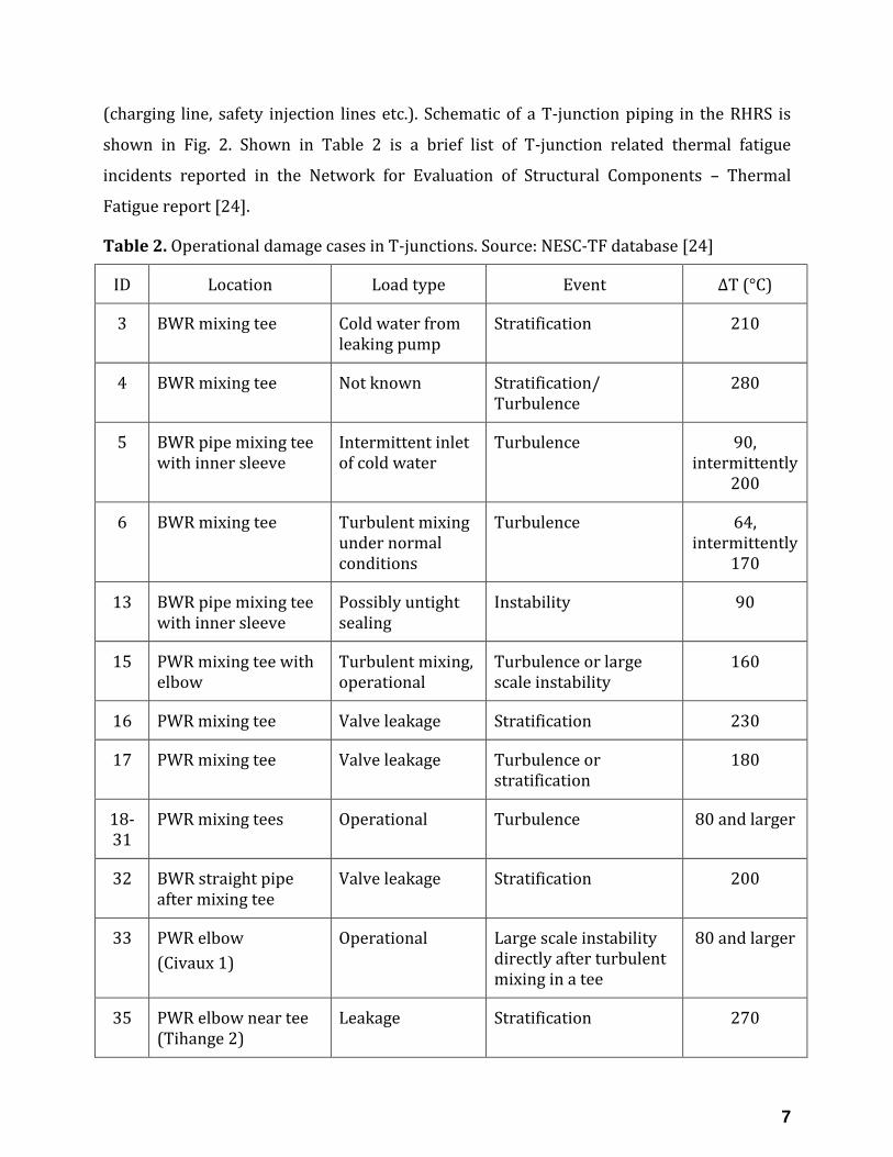
(charging line, safety injection lines etc.). Schematic of a T-junction piping in the RHRS is

shown in Fig. 2. Shown in Table 2 is a brief list of T-junction related thermal fatigue

incidents reported in the Network for Evaluation of Structural Components – Thermal

Fatigue report [24].

Table 2. Operational damage cases in T-junctions. Source: NESC-TF database [24]

ID Location Load type Event ∆T (°C)

3 BWR mixing tee Cold water from leaking pump

Stratification 210

4 BWR mixing tee Not known Stratification/ Turbulence

280

5 BWR pipe mixing tee with inner sleeve

Intermittent inlet of cold water

Turbulence 90, intermittently

200

6 BWR mixing tee Turbulent mixing under normal conditions

Turbulence 64, intermittently

170

13 BWR pipe mixing tee with inner sleeve

Possibly untight sealing

Instability 90

15 PWR mixing tee with elbow

Turbulent mixing, operational

Turbulence or large scale instability

160

16 PWR mixing tee Valve leakage Stratification 230

17 PWR mixing tee Valve leakage Turbulence or stratification

180

18-31

PWR mixing tees Operational Turbulence 80 and larger

32 BWR straight pipe after mixing tee

Valve leakage Stratification 200

33 PWR elbow

(Civaux 1)

Operational Large scale instability directly after turbulent mixing in a tee

80 and larger

35 PWR elbow near tee (Tihange 2)

Leakage Stratification 270

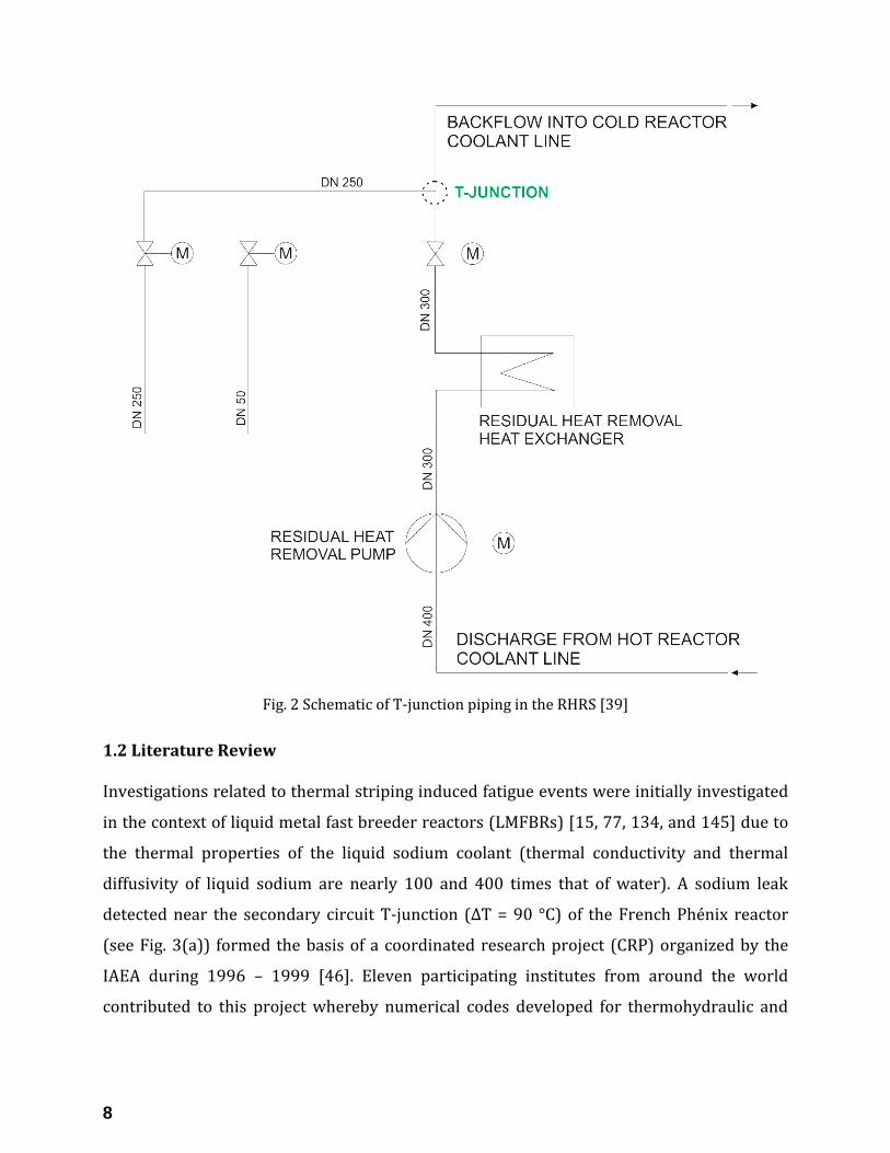
8

Fig. 2 Schematic of T-junction piping in the RHRS [39]

1.2 Literature Review

Investigations related to thermal striping induced fatigue events were initially investigated

in the context of liquid metal fast breeder reactors (LMFBRs) [15, 77, 134, and 145] due to

the thermal properties of the liquid sodium coolant (thermal conductivity and thermal

diffusivity of liquid sodium are nearly 100 and 400 times that of water). A sodium leak

detected near the secondary circuit T-junction (∆T = 90 °C) of the French Phénix reactor

(see Fig. 3(a)) formed the basis of a coordinated research project (CRP) organized by the

IAEA during 1996 – 1999 [46]. Eleven participating institutes from around the world

contributed to this project whereby numerical codes developed for thermohydraulic and

9

thermomechanical analyses were applied to studying thermal mixing behavior and its effect

on the piping structure of the Phénix T-junction.

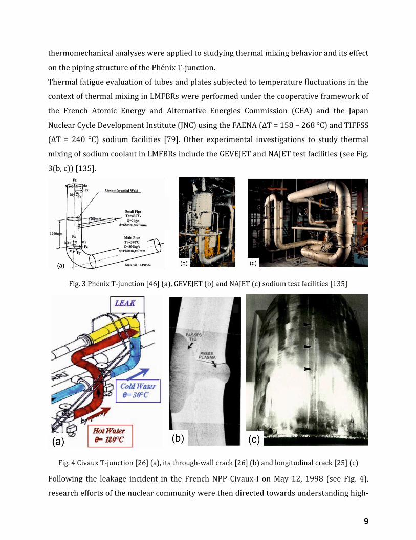
Thermal fatigue evaluation of tubes and plates subjected to temperature fluctuations in the

context of thermal mixing in LMFBRs were performed under the cooperative framework of

the French Atomic Energy and Alternative Energies Commission (CEA) and the Japan

Nuclear Cycle Development Institute (JNC) using the FAENA (∆T = 158 – 268 °C) and TIFFSS

(∆T = 240 °C) sodium facilities [79]. Other experimental investigations to study thermal

mixing of sodium coolant in LMFBRs include the GEVEJET and NAJET test facilities (see Fig.

3(b, c)) [135].

Fig. 3 Phénix T-junction [46] (a), GEVEJET (b) and NAJET (c) sodium test facilities [135]

Fig. 4 Civaux T-junction [26] (a), its through-wall crack [26] (b) and longitudinal crack [25] (c)

Following the leakage incident in the French NPP Civaux-I on May 12, 1998 (see Fig. 4),

research efforts of the nuclear community were then directed towards understanding high-

10

cycle fatigue issues in light water reactor components. The incident took place in the

vicinity of a T-junction piping in the RHRS where hot and cold coolant streams (∆T = 150

°C) mixed together intensively. A through-wall crack and a host of part-wall cracks

developed in the elbow section following the T-junction within 1500 hours of operation.

The outer and inner surface lengths of the through-wall crack were 180 mm and 350 mm,

respectively [30]. Metallurgical examinations concluded that the origin of this degradation

phenomenon was brought about by thermal fatigue [16, 31]. HCTF issues in T-junctions in

the context of the Civaux incident became an important topic of discussion in the

subsequent international conferences [31, 112, and 113].

Fig. 5 FATHER [26] (a) and FATHERINO [14] (b, c) T-junction test facilities

In the aftermath of this incident, several national level research and development (R&D)

programs to understand this phenomenon were initiated. In France, all the RHRS mixing

zones were replaced with manufacturing improvements following the Civaux incident. Also,

an endurance thermal fatigue test named FATHER [18, 26, and 32] where flow mixing in a

T-junction piping with geometry and inflow conditions (velocity, ∆T) similar to the Civaux

NPP T-junction (see Fig. 5(a)) was performed. The test lasted 300 hours and more than 50

thermal fatigue cracks (observed mainly on geometrical discontinuities like weld toes or

grinding striations) with depths ranging from 100 to 1000 µm were detected in the mock-

up. In addition, the CEA conducted another experiment called FATHERINO [14] with two T-

junction mock-ups (∆T = 75 °C) – one to investigate and select the zones of high-

temperature fluctuation (‘the skin of fluid’ mock-up, see Fig. 5(b)) and the other for applying

advanced instrumentation to assess fluctuating temperature, thermal flux and heat transfer

coefficient (‘the stainless steel’ mock-up, see Fig. 5(c)).

The European Commission has also supported research efforts in this area through the

project on thermal fatigue evaluation of piping system Tee-connections (THERFAT) [85].

11

This was mainly initiated to advance the reliability and the accuracy of thermal fatigue load

determination with the aim of providing a practical methodology in managing thermal

fatigue risks. Another European project involving both the utilities and the R&D

organizations to produce a consensus methodology for assessing HCTF with a special focus

on T-junctions in LWRs was organized by the Network for Evaluation of Structural

Components (NESC) [24] which is coordinated by the European Commission’s Joint

Research Centre (Project: EUR 22763 EN). The primary objectives of this project are (i) the

creation of a service and mock-up investigations based database, and (ii) the development

of a European level procedure for assessing thermal fatigue that reflects the multi-

disciplinary nature of the phenomenon. The Japanese Society of Mechanical Engineers

(JSME) conducted investigations of their own and issued guidelines on dealing with HCTF

[52]. In the United States, the EPRI’s Materials Reliability Project (MRP) was used as a

platform to address utilities regarding thermal fatigue issues in T-junction piping

components [29]. The German initiative, sponsored by the Federal Ministry of Education

and Research (BMBF), resulted in the commissioning of a Fluid-Structure Interaction (FSI)

T-junction facility at the University of Stuttgart to investigate the various facets of the flow

mixing processes at ∆T between fluids up to 240 °C [73, 74, and 116].

Several other thermal striping experimental investigations – carried out over a wide range

of ΔT between the mixing fluids – are reported in existing literature, of which a selected few

are described below.

Water experiments in a T-junction (named WATLON, ΔT = 15 °C) with upstream elbow was

performed by Ogawa et al. (2005) [97]. Based on the momentum ratio (𝑀𝑅) formulation,

flow patterns emerging from the branch jet were classified as (i) wall jet, (ii) deflecting jet,

and (iii) impinging jet (see Fig. 6 (a, b, c)). In case of wall jet flows, temperature fluctuation

intensity was observed to be larger in a T-junction with upstream elbow than without it.

𝑀𝑅 = 4 ∗ 𝜌𝑚 ∗ (𝐷𝑚 ∗ 𝐷𝑏) ∗ 𝑈𝑚

2

𝜌𝑏 ∗ (𝜋 ∗ 𝐷𝑏2) ∗ 𝑈𝑏

2 (1)

where 𝜌, 𝐷 and 𝑈 represent the density, inner diameter and velocity of the fluids,

respectively. Suffixes m and b denote the fluids flowing in the main and branch pipes,

respectively. A similar study in a vertical T-junction was performed by Hosseini et al.

(2008) [43] to classify branch jet induced flow pattern – based on momentum ratio (𝑀𝑅) –

12

as (i) Wall jet, (ii) Reattached jet, (iii) Turn jet, and (iv) Impinging jet (see Fig. 6 (d, e, f, g)).

Turn jet flow was identified as the optimum flow condition to reduce near-wall thermal

fluctuations in the mixing zone.

Fig. 6 Classification of turbulent jets in a vertical T-junction based on (a, b, c) Ogawa et al. (2005)

[97], (d, e, f, g) Hosseini et al. (2008) [43]

Thermal mixing experiments were performed in a vertical T-junction piping (∆T = 15 °C, see

Fig. 7(a)) at the Älvkarleby lab of Vattenfall research and development. Near-wall

temperature data from thermocouples, inlet velocity profiles measured using laser Doppler

velocimetry were collected during the experiments and later served as the basis of an

international computational fluid dynamics (CFD) benchmarking exercise [131] organized

13

by the OECD/NEA. Additionally, single point laser-induced fluorescence technique was also

used to collect concentration data at isothermal mixing conditions.

A similar project (∆T = 15 °C, [4]) involving pan-European participation from the research

institutes and the industry is called MOTHER (Modelling T-junction Heat Transfer, see Fig.

7(b)). Experiments using two different geometries – T-junction with a sharp corner and

round corner – were performed for the purpose of conducting a benchmarking exercise

similar to Vattenfall experiments [131] to improve the thermal fatigue predictive

capabilities using CFD.

Fig. 7 Vattenfall [131] (a), MOTHER [4] (b) and EXTREME [17] (c) T-junction test facilities

Thermal mixing behavior of coolant streams (∆T = 70 °C, see Fig. 7(c)) at various flow rates

in the main and branch pipes were performed by Chen et al. (2014) [17] at the EXTREME

(Experiments with T-junction on rapid and emergent mixing effects) test facility. It was

observed that the occurrence of reverse flow (which may produce cracks in pipes) took

place in measurements where the branch velocity is much higher than the main flow

velocity.

Kuschewski et al. (2014) [74] performed a range of measurements in a horizontal 90° T-

junction (FSI test facility) with ∆T between fluids from 30 – 130 °C. Different aspects of the

flow, viz, buoyancy effects, thermal stratification of flows, recirculation, and backflow

observed under the investigated inflow conditions were discussed in the study.

Isothermal flow mixing experiments employing alternative techniques to obtain flow field

information in the mixing zone have also been performed in existing literature and is

discussed below.

Kuschewski et al. (2013) [73] applied a novel image-based measurement technique called

the near-wall light emitting diode induced fluorescence (NWLED-IF) to study isothermal

mixing of flows at the IKE cold test facility (see Fig. 8(a)). A density difference between

fluids – equivalent to ∆T of 106 °C – was established by mixing sugar in the branch flow.

14

Spatially resolved flow field information in the mixing region were captured in the midst of

high-density differences and results from this study indicated that the positioning of

thermocouples in practical installations can have a significant effect on the observed local

root mean square (RMS) temperature fluctuation amplitudes.

Fig. 8 IKE (a) and LKE [59] (b) isothermal T-junction test facilities

Similar isothermal mixing experiments at the LKE T-junction test facility at ETH Zürich

involved the application of wire mesh sensors (WMSs) which exploited the difference in

electrical conductivity between the participating fluids to characterize the turbulent mixing

in the vicinity of T-junction. Walker et al. (2009) [147] performed mixing experiments in a

T-junction using the wire-mesh sensor (Fig. 8(b)). The main and branch pipes are supplied

with water having different electrical conductivities. The transient structures of the

transport scalar downstream of T-junction were characterized, and a two-point correlation

of the signal in the axial direction and within the cross-section was performed, providing a

database for CFD validation.

A list of T-junction mixing experiments conducted over the past two decades has been

summarized in Table 3. In addition to the T-junction mock-up based investigations

discussed above, thermal fatigue tests on specimens being subjected to alternate heating

and cooling effects are also available in literature and a list of such tests are summarized in

Table 4.

Aside from investigations related to the T-junction mixing of flows over a wide range of

temperature differences, experiments investigating different methods to reduce thermal

fluctuations in the mixing zone of T-junctions have also been performed in the existing

literature.

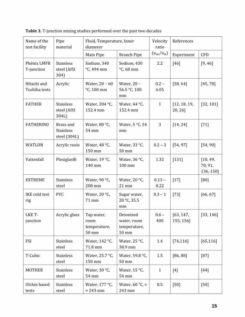
15

Table 3. T-junction mixing studies performed over the past two decades

Name of the

test facility

Pipe

material

Fluid, Temperature, Inner

diameter

Velocity

ratio

(𝑢𝑚 𝑢𝑏⁄ )

References

Main Pipe Branch Pipe Experiment CFD

Phénix LMFR

T-junction

Stainless

steel (AISI

304)

Sodium, 340

°C, 494 mm

Sodium, 430

°C, 68 mm

2.2 [46] [9, 46]

Hitachi and

Toshiba tests

Acrylic Water, 20 – 60

°C, 100 mm

Water, 20 –

56.5 °C, 100

mm

0.2 –

6.05

[58, 64] [45, 78]

FATHER Stainless

steel (AISI

304L)

Water, 204 °C,

152.4 mm

Water, 44 °C,

152.4 mm

1 [12, 18, 19,

20, 26]

[32, 101]

FATHERINO Brass and

Stainless

steel (304L)

Water, 80 °C,

54 mm

Water, 5 °C, 54

mm

3 [14, 24] [71]

WATLON Acrylic resin Water, 48 °C,

150 mm

Water, 33 °C,

50 mm

0.2 – 3 [54, 97] [54, 90]

Vattenfall Plexiglas® Water, 19 °C,

140 mm

Water, 36 °C,

100 mm

1.32 [131] [10, 49,

70, 91,

136, 150]

EXTREME Stainless

steel

Water, 90 °C,

208 mm

Water, 20 °C,

21 mm

0.13 –

0.22

[17] [80]

IKE cold test

rig

PVC Water, 20 °C,

71 mm

Sugar water,

20 °C, 35.5

mm

0.3 – 1 [73] [66, 67]

LKE T-

junction

Acrylic glass Tap water,

room

temperature,

50 mm

Deionized

water, room

temperature,

50 mm

0.6 –

400

[63, 147,

155, 156]

[33, 146]

FSI Stainless

steel

Water, 142 °C,

71.8 mm

Water, 25 °C,

38.9 mm

1.4 [74,116] [65,116]

T-Cubic Stainless

steel

Water, 25.7 °C,

150 mm

Water, 59.8 °C,

50 mm

1.5 [86, 88] [87]

MOTHER Stainless

steel

Water, 30 °C,

54 mm

Water, 15 °C,

54 mm

1 [4] [44]

Ulchin based

tests

Stainless

steel

Water, 177 °C,

≈ 243 mm

Water, 60 °C, ≈

243 mm

0.5 [50] [50]

16

Suzuki et al. (2005) [133] conducted T-junction mixing experiments using a

countermeasure structure nicknamed ‘Elephant Nose’ with the objective of reducing

thermal fluctuations in the flow. It consists of a smaller bore elbow from the branch pipe

leading up to the run pipe (see Fig. 9). As the branch fluid is discharged in parallel with the

main flow, the shear force between them results in enhanced mixing of fluids and the high

thermal fluctuation regions are located farther downstream of T-junction. Data from

experiments have shown that thermal fluctuations are highly attenuated by using the

countermeasure structure than without it.

Table 4. Specimen based thermal fatigue tests performed in literature

Test name Specimen

material

Test conditions References

Fluid Temperature Experiments Numerical

INTHERPOL Stainless steel

(304L)

Water ΔT = 120 – 140 °C [22, 23, 24,

132]

[22, 23,

132]

FAT3D Stainless steel

(316L)

Water Hot: 650 °C

Cold: 17 – 20 °C

[3, 21, 24] [21]

JRC Cyclic

down-shock

Stainless steel

(316L)

Water Hot: 300 – 550 °C

Cold: Ambient

[3, 24, 98, 99,

100]

[98, 99,

100]

SPLASH Stainless steel

(304L)

Water-Air

mixture

ΔT = 125 – 200 °C [3, 24, 40] [40]

FAENA Stainless steel

(316L(N))

Sodium ΔT = 158 – 268 °C [79] [79]

TIFFSS Stainless steel

(316(FR))

Sodium ΔT = 240 °C [79] [79]

SPECTRA Stainless steel

(304SS)

Sodium Hot: 650 °C

Cold: 250 °C

[55] -

Gao et al. (2015) [36] performed similar experiments (ΔT = 17 °C) using a branch

distributor (see Fig. 9) to weaken thermal fluctuations in the T-junction mixing zone.

Numerical calculations were also performed using the large-eddy simulation (LES)

turbulence model. Results have shown that that the inclusion of branch distributor moves

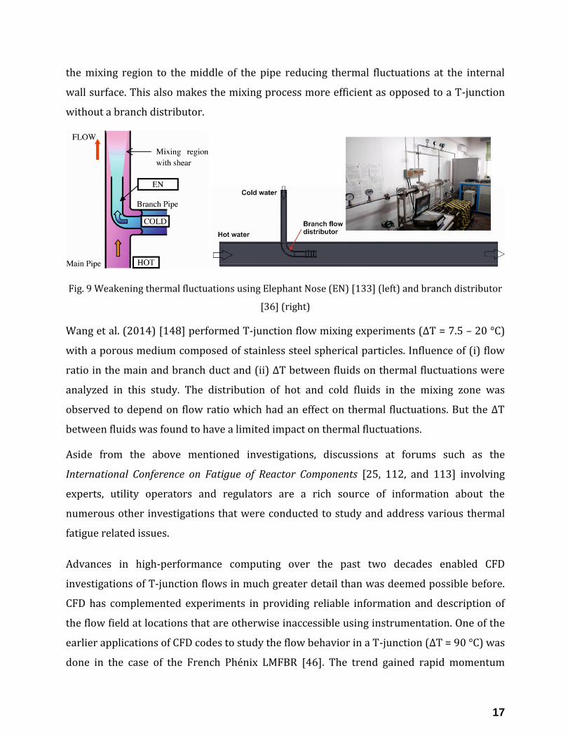
17

the mixing region to the middle of the pipe reducing thermal fluctuations at the internal

wall surface. This also makes the mixing process more efficient as opposed to a T-junction

without a branch distributor.

Fig. 9 Weakening thermal fluctuations using Elephant Nose (EN) [133] (left) and branch distributor

[36] (right)

Wang et al. (2014) [148] performed T-junction flow mixing experiments (ΔT = 7.5 – 20 °C)

with a porous medium composed of stainless steel spherical particles. Influence of (i) flow

ratio in the main and branch duct and (ii) ΔT between fluids on thermal fluctuations were

analyzed in this study. The distribution of hot and cold fluids in the mixing zone was

observed to depend on flow ratio which had an effect on thermal fluctuations. But the ΔT

between fluids was found to have a limited impact on thermal fluctuations.

Aside from the above mentioned investigations, discussions at forums such as the

International Conference on Fatigue of Reactor Components [25, 112, and 113] involving

experts, utility operators and regulators are a rich source of information about the

numerous other investigations that were conducted to study and address various thermal

fatigue related issues.

Advances in high-performance computing over the past two decades enabled CFD

investigations of T-junction flows in much greater detail than was deemed possible before.

CFD has complemented experiments in providing reliable information and description of

the flow field at locations that are otherwise inaccessible using instrumentation. One of the

earlier applications of CFD codes to study the flow behavior in a T-junction (ΔT = 90 °C) was

done in the case of the French Phénix LMFBR [46]. The trend gained rapid momentum

18

following the Civaux leakage incident in 1998. Best practice guidelines and code

assessments [82, 126, 127, 128, and 129] are periodically updated by the CFD community to

reflect the new knowledge gained through experience. Few of the numerical studies

investigated in literature dealing with T-junction mixing is discussed below.

Hu and Kazimi (2006) [45] performed LES studies of T-junction mixing (ΔT = 31 – 40 °C)

based on thermal striping experiments performed by a Japanese working group aimed to

help the Japan Society of Mechanical Engineers (JSME) establish guidelines for high-cycle

fatigue. Mean and fluctuating temperatures predicted by LES showed good agreement with

experimental data.

Westin et al. (2008) [150] performed numerical studies of T-junction mixing (ΔT = 15 °C)

using both LES and Detached Eddy Simulation (𝑘−𝜔 based Shear Stress Transport (SST)

model) turbulence models. Two boundary conditions were studied: (i) without inlet

perturbations and (ii) with inlet perturbations to understand their influence on flow mixing

behavior. The strong large-scale instabilities in the mixing region are seen to be triggered

independent of the applied inlet perturbations. LES and measurement data exhibited good

agreement with one another.

Odemark et al. (2009) [96] performed experimental and numerical studies of turbulent

mixing in a T-junction for three different flow ratios. Velocity and temperature data

predicted by the LESs are compared with experimental results and a good agreement is

obtained between them. The sensitivity of the different inlet velocity profiles on

temperature fluctuations downstream of the T-junction is studied and is seen to have very

little effect on the results.

Kamide et al. (2009) [54] performed numerical analyses of the WATLON experiments (ΔT =

15 °C) using the finite difference method based AQUA code to analyze the temperature and

velocity fields in the mixing zone downstream of the T-junction. Quantitative comparison of

data showed numerical predictions exhibiting close correlation with the measurement data.

Lee et al. (2009) [78] performed LES analyses of temperature fluctuations in a mixing tee

for four investigated test cases (ΔT = 31 – 35 °C) along with the corresponding structural

response analysis. Two factors were highlighted to be the dominant factors causing thermal

fatigue failure in T-junctions: (i) temperature difference between the mixing fluids (ΔT) and

19

(ii) enhanced heat transfer coefficient due to turbulent mixing. LES predictions exhibited

reasonable agreement with measurement data.

Kuhn et al. (2010) [71] studied the FATHERINO experiments (ΔT = 75 °C) numerically using

LES. The influence of subgrid-scale (SGS) models on LES predictions was analyzed using the

classical Smagorinsky model and dynamic procedure. Results from the dynamic procedure

exhibited good agreement with measurement data.

The idea of utilizing the predictive qualities of various CFD codes to analyzing turbulent T-

junction flow mixing resulted in the blind CFD benchmarking exercise organized by

OECD/NEA based on the Vattenfall experiments [130, 131]. A total of 29 participants took

part in this exercise and 19 used the LES turbulence model to study the mixing behavior.

Results showed LES predictions exhibiting close agreement with the measurement data as

it occupied at least the first 8 positions of the rankings in terms of degree of correspondence

to velocity, temperature, and spectral data. Reynolds Average Navier-Stokes (RANS) based

approach fell short in its predictive capabilities of near-wall temperature fluctuations, an

important factor in HCTF analysis.

Walker et al. (2010) [146] performed steady state CFD calculations of T-junction mixing

based on adiabatic experiments at the LKE T-junction facility. Three turbulence models

were employed: 𝑘−휀 model, 𝑘−𝜔 based SST model and the baseline Reynolds Stress Model

(BSL-RSM). Turbulent mixing and turbulent momentum transport downstream of the T-

junction were seen to be underestimated by all three models. Better results were obtained

with increase in model coefficient in the 𝑘−휀 model, resulting in improved concentration

and velocity profiles.

Frank et al. (2010) [33] numerically studied isothermal and thermal mixing (ΔT = 15 °C)

experiments in a T-junction using RANS [SST, BSL-RSM], Unsteady RANS and scale-

resolving [Scale Adaptive Simulation (SAS) with SST model (SAS-SST)] turbulence models.

Turbulent mixing phenomenon in isothermal test case predicted by the RANS models

exhibited good agreement with measurement data. But results obtained from scale-

resolving simulations based on thermal mixing experiments were seen to be unsatisfactory

in terms of obtained accuracy in comparison with measurement data in spite of thermal

striping and large-scale turbulence structure development being qualitatively well

reproduced by the simulations.

20

Naik-Nimbalkar et al. (2010) [89] performed cross flow thermal mixing experiments (ΔT =

15 °C) in a T-junction and three-dimensional steady state simulations were subsequently

performed using the k-ε turbulence model along with a temperature variance transport

equation to analyze temperature fluctuations. The predicted mean temperature and

velocity fields along with temperature fluctuations were consistent with the trend exhibited

by measurement data.

Jayaraju et al. (2010) [49] analyzed the suitability of wall-functions in predicting thermal

fluctuations caused by turbulent mixing of flows in a T-junction using the LES turbulence

model. Reynolds number scaling was performed and the numerical results obtained using

wall-function approach showed good agreement with the wall-resolved approach in

predicting the mean velocity and temperature field. But the near-wall velocity and

temperature fluctuations were consistently under-estimated by the wall-function approach.

Hannink and Blom (2011) [41] performed a numerical investigation of turbulent mixing of

hot and cold fluids in a T-junction by linking two numerical models, namely, coupled CFD-

FEM model and a sinusoidal model. LES was used for CFD modeling. A comparison of

temperature fluctuations and stress intensity fluctuations obtained from both models are

found to be in good agreement with each other.

Ndombo and Howard (2011) [91] performed LES analysis of T-junction mixing of fluids

using the dynamic Smagorinsky model. Turbulent inlet conditions were applied using

Synthetic Eddy Method. The addition of turbulence at the inlet had an effect on the near-

wall flow in terms of variation in the near-wall temperature fluctuations and temperature-

velocity correlation.

Höhne (2014) [42] performed numerical studies based on the Vattenfall T-junction

experiment. The computational results showed that RANS (k-ω SST model) based

simulations fail to predict a realistic mixing between the fluids. LES predicted the velocity

field and mean temperatures with good accuracy. Spectral peaks are found in the range of 3

– 5 Hz in both the numerical and experimental data.

Galpin and Simoneau (2011) [35] carried out LES studies investigating the thermal mixing

of fluids in a T-junction and compared the numerical results with measurement data. Two

sub-grid scale models, namely, the Smagorinsky model and the structure-function model,

21

are used to study the sensitivity of the sub-grid scale closure. Results from the structure-

function model were in better agreement with the measurement data.

Table 5. List of CFD calculations to investigate T-junction mixing over the past two decades

Investigated

test facility CFD Solver

Turbulence

model

Subgrid-scale model No. of

nodes Reference

Phénix LMFR

T-junction

Trio-VF, AQUA,

DINUS-3, Star-

CD etc.

LES, pseudo-

DNS, DNS,

RANS

Selective structure

function

up to 0.4

million

[9, 46]

Hitachi and

Toshiba tests

FLUENT LES RNG, Smagorinsky-Lilly 1.3 million [45, 78]

FATHER CAST3M,

Trio_U, Code

Saturne

RANS, LES - 0.54 million [32, 101]

FATHERINO FLUENT LES Smagorinsky-Lilly 2 million [71]

WATLON CFX DES - 1.3 million [54, 90]

Vattenfall FLUENT, CFX,

OpenFOAM,

Star-CCM+, etc.

LES, SAS-

SST, DES-

SST, ILES,

V2F, RNG,

etc.

WALE, Dynamic

Smagorinsky, Spectral

damping, Dynamic

kinetic energy, Vreman,

etc.

0.28 – 70.5

million

[131]

EXTREME FLUENT Standard

𝑘 − 휀,

Realizable

𝑘 − 휀, SST

𝑘 − 𝜔; V2F

- 2.35 million [80]

IKE cold test

rig

FLUENT LES Dynamic Smagorinsky ≈ 5 million [66, 67]

LKE T-

junction

CFX URANS - 0.44 – 7.8

million

[33, 146]

FSI CFX LES WALE 7 million [65,116]

T-Cubic CFX DES - 1.73 million [87]

MOTHER Code_Saturne

2.0

Implicit-LES Dissipation of numerical

scheme deals with

small-scales

9.12 million [44]

Ulchin based

tests

CFX SST 𝑘 − 𝜔 - 0.54 million [50]

22

Kloeren and Laurien (2011) [65] performed two LESs of thermal mixing in a T-junction (ΔT

= 100 °C) using the adiabatic boundary condition and the conjugate heat transfer boundary

condition. The mixing region was characterized by a wavy flow movement and stable

stratification. Temperature fluctuations in the near-wall region were smaller when using

the conjugate heat transfer approach.

Ayhan and Sökmen (2012) [10] studied turbulent mixing in a T-junction (ΔT = 15 °C) using

the RANS (𝑘−휀 model) and the LES turbulence models to estimate the frequency of near-

wall velocity and temperature fluctuations in the mixing region. LES results, even with a

coarse mesh, exhibited good agreement with experimental results. On the other hand, RANS

computations, either steady or unsteady, failed to reliably predict measurement data. A list

of numerical studies on T-junction mixing at different ΔT performed over the last two

decades is summarized in Table 5.

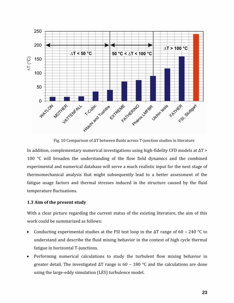
The review of existing literature discussed above point to a clear lack of experimental T-

junction mock-up studies at ΔT > 100 °C. The available literature predominantly contains T-

junction mixing studies at ΔT < 100 °C (see Fig. 10). Only a handful of literature (e.g.

FATHER [18]) are publicly available dealing with ΔT > 100 ºC between mixing fluids. That

being said, problems related to the operational safety in the new and the ageing NPPs

caused by thermal striping induced fatigue related incidents are critically important to be

overlooked. In a Phenomena Identification and Ranking Table (PIRT) study [125], thermal

fatigue was ranked moderately high among the list of single phase nuclear reactor safety-

related issues. In an OCED/NEA organized pipe failure data exchange project (OPDE) [81],

over 3700 piping failure related events were analyzed and cataloged. Of these, over 128

thermal fatigue-related events (non-through wall crack/wall thinning, leak) were recorded

along with 3 cases of structural failure. International Atomic Energy Agency (IAEA) has also

identified thermal fatigue as one of the six ageing mechanisms that tend to reduce the

working life of components in an NPP [47]. Such information highlight the need for detailed

fluid mixing investigations to be performed close to the power plant conditions to gain

valuable information about potential factors causing and accelerating piping degradation

induced fatigue in NPPs.

23

Fig. 10 Comparison of ∆T between fluids across T-junction studies in literature

In addition, complementary numerical investigations using high-fidelity CFD models at ΔT >

100 °C will broaden the understanding of the flow field dynamics and the combined

experimental and numerical database will serve a much realistic input for the next stage of

thermomechanical analysis that might subsequently lead to a better assessment of the

fatigue usage factors and thermal stresses induced in the structure caused by the fluid

temperature fluctuations.

1.3 Aim of the present study

With a clear picture regarding the current status of the existing literature, the aim of this

work could be summarized as follows:

Conducting experimental studies at the FSI test loop in the ΔT range of 60 – 240 °C to

understand and describe the fluid mixing behavior in the context of high cycle thermal

fatigue in horizontal T-junctions.

Performing numerical calculations to study the turbulent flow mixing behavior in

greater detail. The investigated ΔT range is 60 – 180 °C and the calculations are done

using the large-eddy simulation (LES) turbulence model.

24

LES predictions of critical parameters that serve as inputs to thermal fatigue analyses

like near-wall mean temperature, temperature fluctuations and the frequency spectrum

of thermal fluctuations will be validated against experimental data.

Performing additional LES calculations to study the changes in the flow mixing behavior

caused by higher mass flow rates in the branch pipe. This exercise is specifically done as

turbulent inflow conditions could not be experimentally realized in the branch flow

currently (for reasons explained in section 2.2) leading to various degrees of incomplete

fluid mixing at all the investigated ∆T levels. This aspect of utilizing LES to study ‘beyond

design operating conditions’ answers the currently unanswered question of ‘What

happens to the fluid mixing behavior at the FSI test loop at higher mass flow rates in the

branch pipe ?’

25

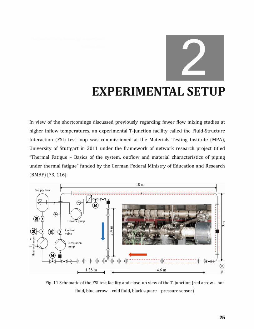
In view of the shortcomings discussed previously regarding fewer flow mixing studies at

higher inflow temperatures, an experimental T-junction facility called the Fluid-Structure

Interaction (FSI) test loop was commissioned at the Materials Testing Institute (MPA),

University of Stuttgart in 2011 under the framework of network research project titled

“Thermal Fatigue – Basics of the system, outflow and material characteristics of piping

under thermal fatigue” funded by the German Federal Ministry of Education and Research

(BMBF) [73, 116].

Fig. 11 Schematic of the FSI test facility and close-up view of the T-junction (red arrow – hot

fluid, blue arrow – cold fluid, black square – pressure sensor)

26

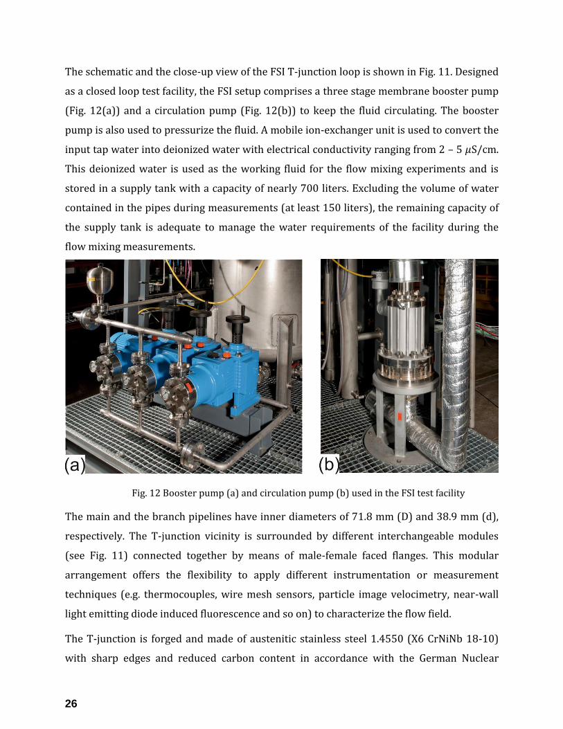
The schematic and the close-up view of the FSI T-junction loop is shown in Fig. 11. Designed

as a closed loop test facility, the FSI setup comprises a three stage membrane booster pump

(Fig. 12(a)) and a circulation pump (Fig. 12(b)) to keep the fluid circulating. The booster

pump is also used to pressurize the fluid. A mobile ion-exchanger unit is used to convert the

input tap water into deionized water with electrical conductivity ranging from 2 – 5 𝜇S/cm.

This deionized water is used as the working fluid for the flow mixing experiments and is

stored in a supply tank with a capacity of nearly 700 liters. Excluding the volume of water

contained in the pipes during measurements (at least 150 liters), the remaining capacity of

the supply tank is adequate to manage the water requirements of the facility during the

flow mixing measurements.

Fig. 12 Booster pump (a) and circulation pump (b) used in the FSI test facility

The main and the branch pipelines have inner diameters of 71.8 mm (D) and 38.9 mm (d),

respectively. The T-junction vicinity is surrounded by different interchangeable modules

(see Fig. 11) connected together by means of male-female faced flanges. This modular

arrangement offers the flexibility to apply different instrumentation or measurement

techniques (e.g. thermocouples, wire mesh sensors, particle image velocimetry, near-wall

light emitting diode induced fluorescence and so on) to characterize the flow field.

The T-junction is forged and made of austenitic stainless steel 1.4550 (X6 CrNiNb 18-10)

with sharp edges and reduced carbon content in accordance with the German Nuclear

27

Safety Standards Commission [68]. The piping material in the vicinity of the T-junction

(both upstream and downstream regions) is made of austenitic stainless steel 1.4404 (X2-

CrNiMo 17-12-2). Upstream of the T-junction, there is a straight pipe section extending for

more than 60 diameters in the main and branch pipes, respectively. Flow straighteners are

used at the beginning of the straight pipe sections to reduce any secondary flow effects

stemming from the upstream elbows.

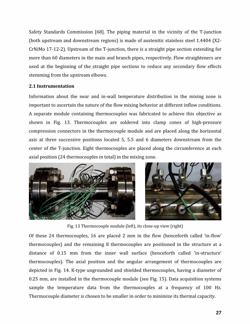
2.1 Instrumentation

Information about the near and in-wall temperature distribution in the mixing zone is

important to ascertain the nature of the flow mixing behavior at different inflow conditions.

A separate module containing thermocouples was fabricated to achieve this objective as

shown in Fig. 13. Thermocouples are soldered into clamp cones of high-pressure

compression connectors in the thermocouple module and are placed along the horizontal

axis at three successive positions located 5, 5.5 and 6 diameters downstream from the

center of the T-junction. Eight thermocouples are placed along the circumference at each

axial position (24 thermocouples in total) in the mixing zone.

Fig. 13 Thermocouple module (left), its close-up view (right)

Of these 24 thermocouples, 16 are placed 2 mm in the flow (henceforth called ‘in-flow’

thermocouples) and the remaining 8 thermocouples are positioned in the structure at a

distance of 0.15 mm from the inner wall surface (henceforth called ‘in-structure’

thermocouples). The axial position and the angular arrangement of thermocouples are

depicted in Fig. 14. K-type ungrounded and shielded thermocouples, having a diameter of

0.25 mm, are installed in the thermocouple module (see Fig. 15). Data acquisition systems

sample the temperature data from the thermocouples at a frequency of 100 Hz.

Thermocouple diameter is chosen to be smaller in order to minimize its thermal capacity.

28

Fig. 14 Thermocouple module and its sectional view (a, b). Angular positions of thermocouples

along the circumference (c)

Fig. 15 View of the sheathed ungrounded thermocouple [27]

Extensive analyses have been previously carried out to decide on the size of the

thermocouple used in the thermocouple module. The influence of thermocouple on the

29

flow, its dynamic and attenuation characteristics have been previously studied in detail by

Kuschewski (2015) [72].

Apart from thermocouple module in the mixing zone, in-structure (0.25 mm diameter, 100

Hz, 2 mm into the structure) and surface thermocouple instrumentation (1 mm diameter,

30 Hz frequency) are placed upstream of the T-junction in both the main and branch pipes

to characterize the upstream flow behavior with rise in ∆T between the fluids or with

changes to the inflow velocity of fluids.

The pressure in the system is continuously monitored using three pressure transmitters in

the FSI test loop. Their positions are indicated by the black colored squares shown in Fig.

11. Two Coriolis mass flow meters are used in the main and branch pipes to measure the

flow rates of fluids. The accuracy of the instrumentation used in the FSI test loop is detailed

in Table 6.

Table 6. Instrumentation used in the FSI test facility

Device Measurement range Accuracy

Thermocouple [27] - 200 °C to +1150 °C Max [< 1.5 °C or 0.4 % of Temperature]

Mass flow meter [28] up to 1 kg/s ± 0.2 % of the mass flow rate

Pressure sensor [115] 0 – 100 bar ± 0.3 % of the upper range value

The following section describes the start-up procedure used to initiate fluid mixing

experiments along with the fluid heating procedure used in the FSI test loop.

2.2 System start-up, fluid heating, and cooling

Firstly, the piping system is filled with deionized water using the following procedure: The

Booster pump is switched on and deionized water from the supply tank flows continuously

through the branch pipe (see Fig. 11), reaches the T-junction and the entire test loop is filled

within 10 – 15 minutes. Fluid pressure is then slowly increased and air in the system is

subsequently vented out manually using the venting outlets installed in the facility. The

circulation pump is then switched on enabling continuous flow of water in the main pipe.

Heating the fluid flowing through the main pipe is the next step is and is accomplished using

heating mats made from ceramic pad elements (Fig. 16) attached to the outer surface of the

30

pipe. A total of 8 heating mats are attached along the length of the main pipe section and are

controlled using the proportional-integral-derivative controllers (PIDs) to achieve the

desired temperature level on the outer pipe surface. In general, fluid flow inside the main

pipe is sequentially heated at the rate of 40 °C/hour. The heating mats are powered using

three separate heat treatment units [111] as shown in Fig. 16 with each unit having an

output power of 84 kW.

Fig. 16 Heating mat (top left), its arrangement on the pipe surface (top right), and the powering heat

treatment units (bottom)

Since the FSI setup has a closed loop design, part of the mixed flow during measurements

(at a higher temperature than the cold fluid) downstream of the T-junction is diverted to a

heat exchanger unit where the fluid temperature is brought down to about 18 – 20 °C and

fed back again into the supply tank. This ensures that the volumetric capacity of the cold

deionized water in the supply tank is always maintained within an acceptable limit to allow

for continuous operation of the FSI test loop. The remaining part of the mixed flow simply

keeps circulating within the main pipe and is reheated to the required temperature level as

it flows through regions covered by heating mats. Thus the hot and cold fluid temperatures

are maintained at their respective levels using heating mats and the heat exchanger unit,

respectively. In terms of thermal mixing, the FSI test facility is designed to operate at a

31

maximum ΔT between the fluids of nearly 240 °C and the system pressure during such

measurements could be as high as 75 bar.

Reynolds number (𝑅𝑒) calculations are used to categorize the pipe flows as laminar (𝑅𝑒 <

2300), transitional (2300 < 𝑅𝑒 < 4000) or turbulent (𝑅𝑒 > 4000) [105]. It is defined using

the formula

𝑅𝑒 = 𝑢𝐷 𝜈⁄ (2)

where 𝑢 is fluid velocity, 𝐷 the pipe diameter and 𝜈 the kinematic viscosity of the fluid

flowing through the pipe. Based on this formulation, turbulent fluid flow conditions could

be easily achieved in the main pipe (𝑅𝑒𝑚 > 20000) due to the maximum operational mass

flow rate of 1 kg/s offered by the circulation pump. On the other hand, transitional flow is

the maximum achievable flow condition in the branch pipe (𝑅𝑒𝑏 = 3200 – 3600) due to the

fact that the booster pump used in the branch pipe could not be operated beyond the mass

flow rate limit of 0.1 kg/s. Such large Reynolds number differences between the main and

branch pipes have clear consequences on the flow mixing behavior as discussed later in the

results section.

32

3.1 Background

The turbulent mixing of fluids produces a wide range of flow scales in the vicinity of the T-

junction. The turbulence could be considered to be composed of eddies of different sizes.

Eddies of the largest size could be comparable with the diameter of the pipe. The idea of

energy cascade within eddies was put forth by Richardson [110] and excerpts explaining

this idea [105] is as follows:

“Richardson’s notion is that the large eddies are unstable and break up, transferring their

energy to somewhat smaller eddies. These smaller eddies undergo a similar break-up process,

and transfer their energy to yet smaller eddies. This energy cascade – in which energy is

transferred to successively smaller and smaller eddies – continues until the Reynolds number is

sufficiently small that the eddy motion is stable, and molecular viscosity is effective in

dissipating the kinetic energy. Richardson (1922) succinctly summarized the matter thus:

Big Whorls have little whorls,

Which feed on their velocity;

And little whorls have lesser whorls,

And so on to viscosity

(in the molecular sense).”

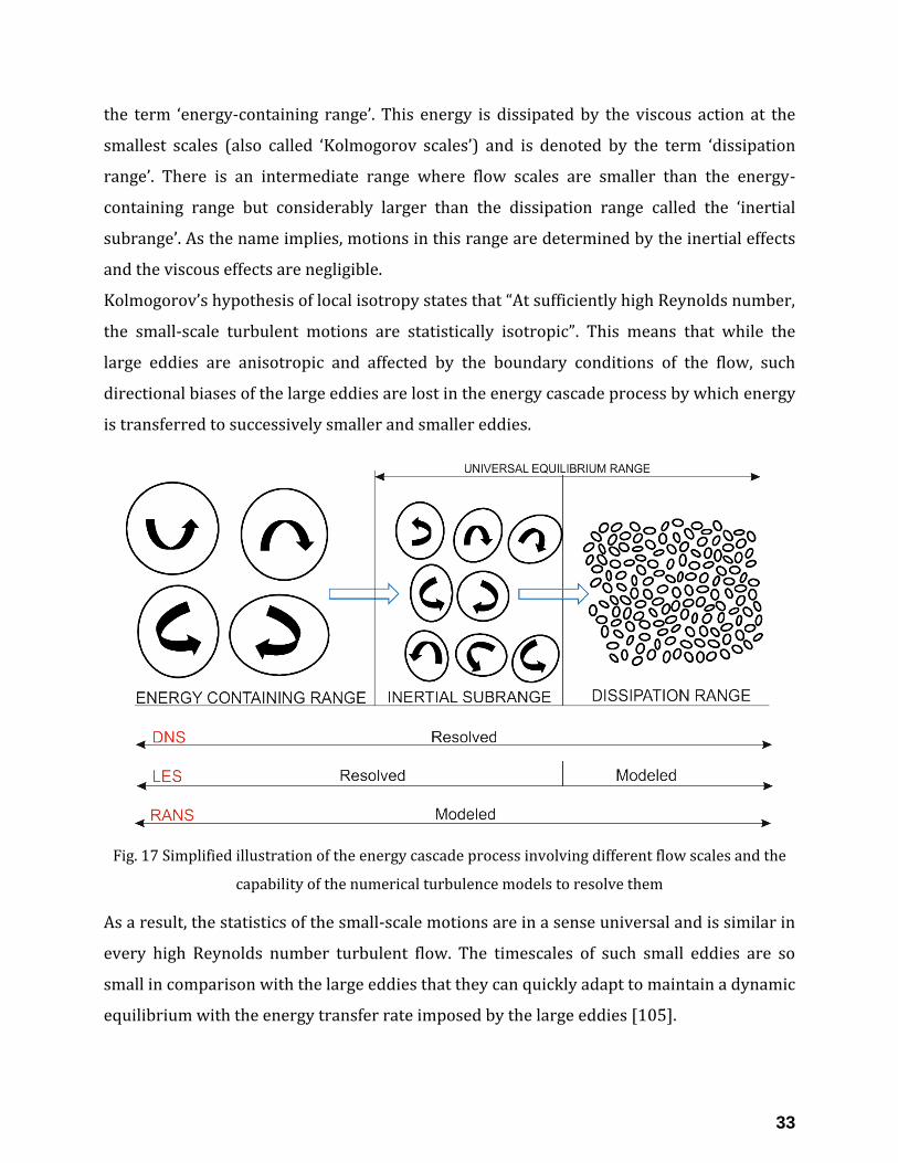
Fig. 17 depicts the energy cascade process involving eddies of different sizes. This

classification is done on the basis of Kolmogorov’s second similarity hypothesis explained in

Pope (2000) [105]. Most of the energy is contained in the larger eddies and is denoted by

33

the term ‘energy-containing range’. This energy is dissipated by the viscous action at the

smallest scales (also called ‘Kolmogorov scales’) and is denoted by the term ‘dissipation

range’. There is an intermediate range where flow scales are smaller than the energy-

containing range but considerably larger than the dissipation range called the ‘inertial

subrange’. As the name implies, motions in this range are determined by the inertial effects

and the viscous effects are negligible.

Kolmogorov’s hypothesis of local isotropy states that “At sufficiently high Reynolds number,

the small-scale turbulent motions are statistically isotropic”. This means that while the

large eddies are anisotropic and affected by the boundary conditions of the flow, such

directional biases of the large eddies are lost in the energy cascade process by which energy

is transferred to successively smaller and smaller eddies.

Fig. 17 Simplified illustration of the energy cascade process involving different flow scales and the

capability of the numerical turbulence models to resolve them

As a result, the statistics of the small-scale motions are in a sense universal and is similar in

every high Reynolds number turbulent flow. The timescales of such small eddies are so

small in comparison with the large eddies that they can quickly adapt to maintain a dynamic

equilibrium with the energy transfer rate imposed by the large eddies [105].

34

The attempt to numerically investigate and resolve the different scales of motion in a

turbulent flow gave rise to three broadly classified CFD approaches that are commonly used

today, namely, (i) Direct numerical simulation (DNS), (ii) Large-eddy simulation (LES), and

(iii) Reynolds-averaged Navier-Stokes (RANS) approach.

DNS approach resolves the entire spectrum of flow scales ranging from the largest eddies to

the smallest eddies (see Fig. 17). The conservation equations (mass, momentum, and

energy) are solved directly, making the solution highly accurate but computationally very

expensive. This method is not feasible for analyzing flows involving high Reynolds numbers

for the foreseeable future barring any breakthroughs in high-performance computing. The

opposite is the RANS based approach where the conservation equations are time-averaged

instead of solving for directly making it computationally affordable. This method is

predominantly used everywhere including industrial applications where the mean flow

field information is mainly desired. Nonetheless, it falls short in its predictions of fluctuating

components since the equations are time-averaged making it the least accurate method.

LES, motivated by the limitations of the DNS and the RANS based approaches, incorporates

both the traits whereby the large eddies which are geometry dependent are solved for

directly (as in DNS) and the small eddies which are statistically isotropic and universal are

modeled (similar to RANS). Computationally, it is less expensive than DNS but more

accurate than RANS making it the suitable choice for studying the complex flow

phenomenon like the T-junction mixing.

3.2 Large-eddy simulation (LES)

This study makes use of the LES method to numerically study T-junction mixing flows

involving high ∆T between the fluids. ANSYS CFX solver is used to perform the LES

calculations. The basic concept behind this approach involves the separate treatment of

large eddies (which are geometry dependent) and the small eddies (which are considered

isotropic).

Governing equations for LES are derived by applying a filtering process to the time-

dependent conservation equations. By this process, a governing variable (𝜑) is split into a

filtered component (�̅�) and a residual component (𝜑′). So the filtering process effectively

separates eddies with sizes smaller than the grid spacing used in the numerical calculations

[114]. Such smaller eddies are accounted for using the sub-grid scale (SGS) modeling

35

approach while the filtered component – being three dimensional and time dependent –

represents the motion of large eddies.

3.2.1 Filtered governing equations

The filtered equations of mass and momentum conservation are as follows [6]

𝜕𝜌

𝜕𝑡+

𝜕(𝜌�̅�𝑖)

𝜕𝑥𝑖= 0 (3)

𝜕(𝜌�̅�𝑖)

𝜕𝑡+

𝜕

𝜕𝑥𝑗(𝜌�̅�𝑖�̅�𝑗) = −

𝜕�̅�

𝜕𝑥𝑖+

𝜕𝜎𝑖𝑗

𝜕𝑥𝑗−

𝜕𝜏𝑖𝑗

𝜕𝑥𝑗+ 𝑓𝑖 (4)

where �̅� and �̅� represent the filtered component of velocity and pressure. i, j, k are the

tensor indices while 𝜏𝑖𝑗 is the subgrid-scale shear stress tensor, 𝑓𝑖 is the source term

accounting for buoyancy effects and is defined as

𝑓𝑖 = 𝑔(𝜌 − 𝜌𝑟𝑒𝑓) (5)

where 𝑔 is the acceleration due to gravity, 𝜌𝑟𝑒𝑓 is the reference density, usually taken to be

the average density of mixing fluids. The density difference (𝜌 − 𝜌𝑟𝑒𝑓) is evaluated directly

during the calculations.

𝜎𝑖𝑗 is the stress tensor due to molecular viscosity (𝜇) and is defined as

𝜎𝑖𝑗 = 𝜇 [𝜕�̅�𝑖

𝜕𝑥𝑗+

𝜕�̅�𝑗

𝜕𝑥𝑖] −

2

3𝜇

𝜕�̅�𝑘

𝜕𝑥𝑘𝛿𝑖𝑗 (6)

The conservation of energy equation is defined as

𝜕(𝜌ℎ̅)

𝜕𝑡+

𝜕

𝜕𝑥𝑗(𝜌ℎ̅�̅�𝑗) =

𝜕

𝜕𝑥𝑗(𝜆eff

𝜕�̅�

𝜕𝑥𝑗) (7)

where ℎ̅ and �̅� represent filtered enthalpy and temperature, 𝜆eff represents an effective

coefficient which includes both molecular conduction and SGS contribution and is defined

as

𝜆eff = 𝜆 +𝜇𝑡𝑐𝑝

𝑃𝑟𝑡 (8)

where 𝜆 is thermal conductivity, 𝑐𝑝 is specific heat capacity at constant pressure, 𝜇𝑡 is

turbulent eddy viscosity and 𝑃𝑟𝑡 is subgrid-scale turbulent Prandtl number.

36

3.2.2 Subgrid-scale modeling

Subgrid-scale (SGS) stresses resulting from the filtering operation are unknown and require

modeling. Eddy viscosity modeling approach is used in ANSYS CFX for SGS modeling, which

presumes a linear relation between the SGS stress tensor and the filtered rate of strain

tensor. It is defined as

(𝜏𝑖𝑗 − 1

3𝜏𝑘𝑘𝛿𝑖𝑗) = −2𝜇𝑡𝑆�̅�𝑗 (9)

where 𝜇𝑡 is the eddy viscosity to be modeled. 𝑆�̅�𝑗 is the rate of strain tensor for the resolved

scale and is given by

𝑆�̅�𝑗 =1

2[𝜕�̅�𝑖

𝜕𝑥𝑗+

𝜕�̅�𝑗

𝜕𝑥𝑖] (10)

The SGS eddy viscosity is modeled using the Wall-Adapting Local Eddy-Viscosity (WALE)

model. The generic form of eddy-viscosity model could be written as

𝜈𝑡 = (𝐶𝑚∆)2 𝑂𝑃 ̅̅ ̅̅ ̅(𝑥, 𝑡) (11)

where 𝐶𝑚 is the model constant, ∆ the sub-grid characteristic length scale and 𝑂𝑃 ̅̅ ̅̅ ̅(𝑥, 𝑡) is

“an operator in space and time, homogenous to a frequency, and defined from the resolved

fields” [93]. The operator 𝑂𝑃 ̅̅ ̅̅ ̅(𝑥, 𝑡) used in the WALE model is defined based on the

following properties as defined in Nicoud and Ducros (1999) [93]: (i) it should be invariant

to any coordinate translation or rotation, (ii) it could be easily accessed in any kind of

computational grid, (iii) it is a function of both the strain and rotation rates, (iv) it goes to

zero at the wall so that neither damping function nor dynamic procedure are needed to

reproduce the effect of no-slip condition. Thus the WALE model is based on a tensor

invariant and reproduces appropriate scaling at the wall. It is defined as

𝜈𝑡 = (𝐶𝑤∆)2(𝑆𝑖𝑗

𝑑 𝑆𝑖𝑗𝑑)

3/2

(𝑆�̅�𝑗 𝑆�̅�𝑗)5/2

+ (𝑆𝑖𝑗𝑑 𝑆𝑖𝑗

𝑑)5/4

(12)

𝐶𝑤 = 0.5 is the WALE model constant, 𝑆𝑖𝑗𝑑 denotes the traceless part of the square of the

velocity gradient tensor (�̅�𝑖𝑗) and both are defined as follows

𝑆𝑖𝑗𝑑 =

1

2(�̅�𝑖𝑗

2 + �̅�𝑗𝑖2 ) −

1

3𝛿𝑖𝑗�̅�𝑘𝑘

2 (13)

37

�̅�𝑖𝑗 = 𝜕�̅�𝑖

𝜕𝑥𝑗 (14)

3.2.3 Near-wall flow modeling

Strong gradients of flow variables exist near the wall due to the no-slip condition. In

addition, molecular viscosity plays a significant role in the transport of momentum and heat

inside the boundary layer. The above mentioned flow phenomenon should be realistically

reproduced in a numerical model in order to obtain the best possible results. Near-wall

modeling in ANSYS CFX is based on two approaches:

(i) The wall function method which imposes empirical formulas near the wall without

resolving the boundary layer. This method is an extension of the method described

in Launder and Spalding (1974) [76].

(ii) The Low Reynolds number (low-Re) method which resolves the details of the

boundary layer using very small mesh length scales in the direction normal to the

wall. Here, the Reynolds number refers to the turbulent Reynolds number in the

near-wall region. Unlike the wall function method, computations in the low-Re

method are extended through the viscosity affected regions near the wall.

LES turbulence model in ANSYS CFX utilizes the automatic wall treatment method which

allows for a gradual switch between the wall function method and the low-Re method as the

mesh resolution becomes higher near the wall. Similar to the velocity boundary layer, the

thermal boundary layer in the near-wall region is modeled using the thermal law-of-the-

wall function of Kader (1981) [53]. Further details are elaborately described in ANSYS CFX

modeling and theory guide [5, 6].

3.3 Computational mesh

Two different upstream lengths (see Fig. 18) have been selected for the present study to

perform the numerical T-junction mixing calculations: Hot inflow length – 4D or 15D; Cold

inflow length – 5d or 10d; Mixing zone length – 20D. The decision to use two different

upstream domain lengths was based on the observation of cold flow penetration into the

main pipe and hot flow into the branch pipe occurring over longer distances at higher ∆T (>

140 °C) during the measurements.

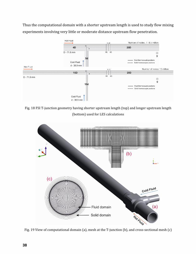
38

Thus the computational domain with a shorter upstream length is used to study flow mixing

experiments involving very little or moderate distance upstream flow penetration.

Fig. 18 FSI T-junction geometry having shorter upstream length (top) and longer upstream length

(bottom) used for LES calculations

Fig. 19 View of computational domain (a), mesh at the T-junction (b), and cross-sectional mesh (c)

39

On the other hand, the computational domain with a longer upstream length is used to

study flow mixing experiments where the measurement data indicated a longer distance

upstream flow penetration in both the main and the branch pipe, respectively.

3.4 Assessment of mesh resolution

It is essential to ensure adequate resolution of the numerical mesh in order to expect LES

results of good accuracy. Standard methods are established in literature to assess the

appropriate mesh size based on the inflow conditions. They are (i) y-plus (𝑦+) value

estimation, (ii) assessment of non-dimensional grid size (∆𝑥+, ∆𝑦+, ∆𝑧+), and (iii) energy

length scale (𝐿𝑅) and Taylor micro-scale (𝜆) based estimation. Each method is briefly

discussed below.

3.4.1 y-plus (𝒚+) value estimation

This non-dimensional parameter – representing the distance of the first node from the wall

measured in wall units – is used to assess the near-wall mesh resolution. It is defined as

follows:

𝑦+ ≡ (𝑦 ∗ 𝑢𝜏) 𝜈⁄ (15)

where y is the distance of the nearest node from the wall, 𝑢𝜏 the friction velocity and 𝜈 the

kinematic viscosity. Near-wall regions are categorized on the basis of 𝑦+ values as follows

[45, 105]:

Viscous stress dominated laminar sublayer is defined as y+ < 5;

The buffer layer, a transition region between viscosity dominated and turbulence

dominated regions, is defined as y+ < 30;

The contribution of viscosity to wall shear stress diminishes beyond y+ > 50 through

y = 0.05D.

The distance of the nearest node from the wall used in this study ranges between 0.025 and

0.04 mm, which corresponds to 0 < y+ < 3 throughout the computational domain with the

exception at the T-junction where the highest y-plus values are registered (5 < y+ < 9) in all

the LES cases.

3.4.2 Non-dimensional grid size (∆𝒙+, ∆𝒚+, ∆𝒛+) estimation

The method formulated by Piomelli (2001) [103] to calculate the non-dimensional grid

spacing (∆𝑥𝑖+) is defined as follows

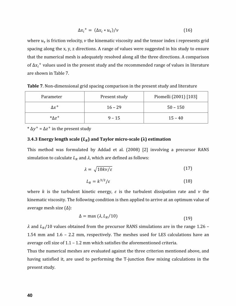
40

∆𝑥𝑖+ = (∆𝑥𝑖 ∗ 𝑢𝜏) 𝜈⁄ (16)

where 𝑢𝜏 is friction velocity, 𝜈 the kinematic viscosity and the tensor index i represents grid

spacing along the x, y, z directions. A range of values were suggested in his study to ensure

that the numerical mesh is adequately resolved along all the three directions. A comparison

of ∆𝑥𝑖+ values used in the present study and the recommended range of values in literature

are shown in Table 7.

Table 7. Non-dimensional grid spacing comparison in the present study and literature

Parameter Present study Piomelli (2001) [103]

∆𝑥+ 16 – 29 50 – 150

*∆𝑧+ 9 – 15 15 – 40

* ∆𝑦+ = ∆𝑧+ in the present study

3.4.3 Energy length scale (𝑳𝑹) and Taylor micro-scale (λ) estimation

This method was formulated by Addad et al. (2008) [2] involving a precursor RANS

simulation to calculate 𝐿𝑅 and 𝜆, which are defined as follows:

𝜆 = √10𝑘𝜈 휀⁄ (17)

𝐿𝑅 = 𝑘3/2/휀 (18)

where 𝑘 is the turbulent kinetic energy, 휀 is the turbulent dissipation rate and 𝜈 the

kinematic viscosity. The following condition is then applied to arrive at an optimum value of

average mesh size (Δ):

Δ = max (𝜆, 𝐿𝑅 10)⁄ (19)

𝜆 and 𝐿𝑅/10 values obtained from the precursor RANS simulations are in the range 1.26 –

1.54 mm and 1.6 – 2.2 mm, respectively. The meshes used for LES calculations have an

average cell size of 1.1 – 1.2 mm which satisfies the aforementioned criteria.

Thus the numerical meshes are evaluated against the three criterion mentioned above, and

having satisfied it, are used to performing the T-junction flow mixing calculations in the

present study.

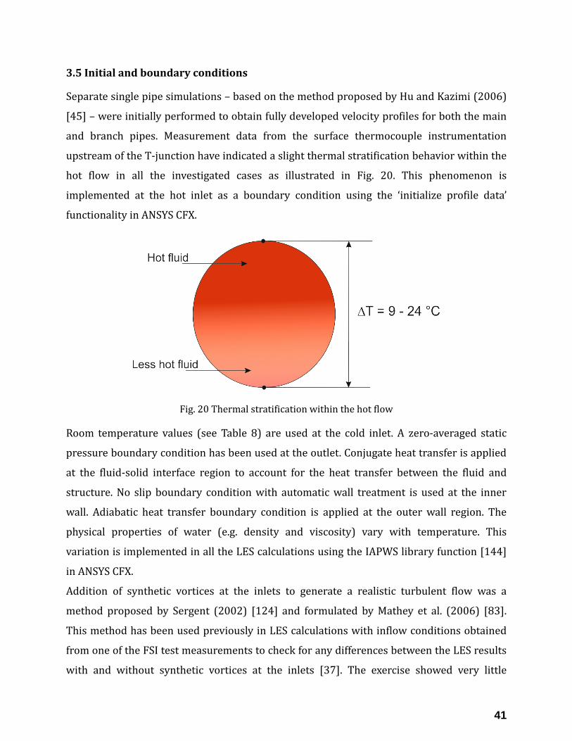
41

3.5 Initial and boundary conditions

Separate single pipe simulations – based on the method proposed by Hu and Kazimi (2006)

[45] – were initially performed to obtain fully developed velocity profiles for both the main

and branch pipes. Measurement data from the surface thermocouple instrumentation

upstream of the T-junction have indicated a slight thermal stratification behavior within the

hot flow in all the investigated cases as illustrated in Fig. 20. This phenomenon is

implemented at the hot inlet as a boundary condition using the ‘initialize profile data’

functionality in ANSYS CFX.

Fig. 20 Thermal stratification within the hot flow

Room temperature values (see Table 8) are used at the cold inlet. A zero-averaged static

pressure boundary condition has been used at the outlet. Conjugate heat transfer is applied

at the fluid-solid interface region to account for the heat transfer between the fluid and

structure. No slip boundary condition with automatic wall treatment is used at the inner

wall. Adiabatic heat transfer boundary condition is applied at the outer wall region. The

physical properties of water (e.g. density and viscosity) vary with temperature. This

variation is implemented in all the LES calculations using the IAPWS library function [144]

in ANSYS CFX.

Addition of synthetic vortices at the inlets to generate a realistic turbulent flow was a

method proposed by Sergent (2002) [124] and formulated by Mathey et al. (2006) [83].

This method has been used previously in LES calculations with inflow conditions obtained

from one of the FSI test measurements to check for any differences between the LES results

with and without synthetic vortices at the inlets [37]. The exercise showed very little

42

differences in analyzing relevant quantities like the mean and fluctuating quantities of

temperature and velocity confirming the fact that the main generation of turbulence in T-

junction flows is caused by the mixing of fluids. Thus all the LES cases presented here

contain no perturbation of flow whatsoever at the inlets.

With all the boundary conditions mentioned above, steady state simulations of T-junction

fluid mixing are performed using the 𝑘 − 𝜔 SST turbulence model in the next step. LES cases

are finally initialized using the previously converged solution from the steady state

simulations. This method of initializing LES based on steady state simulation result is a

standard best practice guideline recommended by ANSYS (2015) [7]. A description of this

method is depicted below in Fig. 21.

Fig. 21 Flowchart of the numerical approach used in the present study

A second order high-resolution scheme is used for the spatial discretization of the mass and

energy conservation equations while a second order central differencing scheme in used for

discretizing the momentum equation. Second order backward Euler method is used for

temporal discretization in the present study. More details on the element based finite-

volume method along with the spatial and temporal discretization schemes used in this

study are described in the section A.1.

Time step (Δt) for all the LES cases is chosen to be 0.2 ms, which keeps the Courant number

less than unity in each coefficient loop iteration. The total physical time simulated is 30 – 35

seconds and the last 20 – 22 seconds of data, being statistically steady, are used to analyze

the turbulent statistics.

43

Each case shall be identified using the ΔT between fluids while explaining the flow

characteristics in the mixing region for the sake of clarity and clear understanding. Unless

otherwise stated, all the temperature and velocity data are normalized. The formulation

used for normalization is given below.

The instantaneous fluid temperature (T) is normalized using the formula:

𝑇∗ = 𝑇 − 𝑇𝑏

∆𝑇 (20)

where ∆𝑇 = 𝑇𝑚 − 𝑇𝑏 is the temperature difference between the mixing fluids. The terms 𝑇𝑚

and 𝑇𝑏 denote fluid temperatures in the main and branch pipes, respectively.

The normalized mean temperature is defined as:

𝑇∗̅̅ ̅ = 1

𝑁∑𝑇∗

𝑁

𝑖=1

(21)

Normalized temperature fluctuation intensity is defined using the root mean square (RMS)

formulation as follows:

𝑇𝑟𝑚𝑠∗ = √

1

𝑁∑(𝑇∗ − 𝑇∗̅̅ ̅)2𝑁

𝑖=1

(22)

where N represents the number of sampled data points.

The instantaneous fluid velocity (𝑢) is normalized using the formula:

𝑢∗ = 𝑢

𝑢𝑚𝑖𝑥 (23)

44

where 𝑢𝑚𝑖𝑥 = √𝑢𝑚2 + 𝑢𝑏

2 is the mixing velocity of the fluids with 𝑢𝑚 and 𝑢𝑏 being the inflow

velocities in the main and branch pipes, respectively. The normalized mean velocity is

defined as:

𝑢∗̅̅ ̅ = 1

𝑁∑𝑢∗

𝑁

𝑖=1

(24)

Normalized temperature fluctuation intensity is defined using the root mean square (RMS)

formulation as follows:

𝑢𝑟𝑚𝑠∗ = √

1

𝑁∑(𝑢∗ − 𝑢∗̅̅ ̅)2𝑁

𝑖=1

(25)

Also, most of the figures discussed below contain red and blue arrows upstream of the T-

junction representing the hot and cold inflows. Additionally, the main and the branch flows

in the figures are identified by their mass flow rates rather than velocities. The results

presented in this study are discussed in three separate parts as follows:

(i) Mixing behavior of flows at ∆T = 60 °C – 180 °C

The mass flow rate in the main and the branch pipes are fixed at 0.4 kg/s and 0.1 kg/s,

respectively. Hot inflow temperature is increased gradually yielding ∆T amplitude between

the fluids in the range of 60 – 180 °C. Flow field characteristics are initially analyzed

followed by quantitative analysis and comparison of measurements and LES data. For the

aforementioned ∆T range between the fluids, measurements have also been performed at

different mass flow rates in the main pipe of 0.3 kg/s and 0.5 kg/s while the branch flow

rate is maintained at 0.1 kg/s. These results are discussed in the Appendix section A.2.

(ii) Mixing behavior of flows at ∆T = 233 °C

This measurement is a special case scenario whereby the FSI test facility is taken to its

highest operating temperature resulting in the ∆T amplitude between fluids of 233 °C. No

LES calculation is performed for this case, the reasons for which shall be described when

elaborately discussing the results. The mass flow rate in the main and branch pipes for this

measurement are set at 0.4 kg/s and 0.1 kg/s, respectively.

45

(iii) Mixing behavior of flows at increased branch flow velocities

The main limitation of the FSI facility is the maximum mass flow rate of the branch pipe (0.1

kg/s) being inadequate to cause complete turbulent mixing of flows. So it was decided to

perform LES analyses where the branch flow rates were doubled and tripled to 0.2 kg/s and

0.3 kg/s, respectively while maintaining a flow rate in the main pipe of 0.4 kg/s. The ∆T

amplitude between the fluids were 65 °C and 143 °C, respectively. Results of the flow mixing

at elevated branch flow rates offers valuable insights into the flow behavior that could be

expected when the FSI test loop is upgraded to operate at such branch flow rates.

4.1 Mixing behavior of flows at ∆T = 60 °C – 180 °C

Table 8 contains the inflow conditions at the main pipe and the branch pipe for the

measurements performed with ∆T between the fluids in the range of 60 – 180 °C.

Table 8: Inflow conditions at the FSI test facility

Case # ∆T

(°C)

𝑇𝑚*

(°C)

�̇�𝑚

(kg/s)

𝑢𝑚

(m/s)

𝑇𝑏*

(°C)

�̇�𝑏

(kg/s)

𝑢𝑏

(m/s)

𝑢𝑚𝑖𝑥

(m/s)

1 65 85 0.4 0.101 20 0.1 0.084 0.132

2 107 128 0.4 0.105 21 0.1 0.084 0.135

3 126 147 0.4 0.107 21 0.1 0.084 0.136

4 143 165 0.4 0.109 22 0.1 0.084 0.138

5 159 181 0.4 0.112 22 0.1 0.084 0.14

6 178 201 0.4 0.115 23 0.1 0.084 0.142

Pressure – 30 to 70 bar

* suffixes m and b denote the main and the branch pipe, respectively

Table 9 shows the non-dimensional parameters calculated for the inflow conditions in

Table 8 such as relative density (∆𝜌 �̅�⁄ ), Reynolds number in the main and branch pipes

(𝑅𝑒𝑚, 𝑅𝑒𝑏), Richardson number (Ri), and Viscosity ratio (𝜇𝑚 𝜇𝑏⁄ ).

46

Table 9: Non-dimensional parameters for inflow conditions in Table 8

Case # ∆T

(°C)

∆𝜌 �̅�⁄

(in %) 𝑅𝑒𝑚 𝑅𝑒𝑏 Ri

𝑅𝑒𝑚 𝑅𝑒𝑏⁄

(R)

𝜇𝑚 𝜇𝑏⁄

1 65 3 21200 3200 1.2 6.6 0.33

2 107 6.5 33160 3300 2.5 10.1 0.22

3 126 8.5 38950 3340 3.2 11.6 0.185

4 143 10.3 43920 3540 3.8 12.4 0.174

5 159 12.4 48850 3500 4.4 13.9 0.155

6 178 15 54060 3500 5.2 15.4 0.14

4.1.1 Velocity field in the mixing region

Figs. 22 and 23 show the instantaneous and the mean velocity distribution at the T-junction

for all the investigated cases. Cold flow (𝑅𝑒𝑏 = 3200 – 3600) from the branch pipe enters the

main pipe and travels a short distance before being turned towards the downstream

direction by the high Reynolds number hot flow.

Fig. 22 Instantaneous velocity field (t = 30s) at the T-junction mid-plane (x-y axis)

47

Fig. 23 Mean velocity field at the T-junction mid-plane (x-y axis)

Fig. 24 Mean velocity field illustrating the entry of the cold fluid into the main pipe (view oriented

towards T-junction)

The entry of the cold flow into the main pipe results in flow separation and recirculation

zones being established in the vicinity of the sharp edges at the T-junction. Also, the flow

mixing is incomplete in all the cases due to the low Reynolds number cold flow coming from

the branch pipe. Highest 𝑢∗̅̅ ̅ is usually observed at the mixing interface of hot and cold flows

48

till ∆Ts up to 140 °C (cases 1, 2, and 3). Beyond this point, the relative density (∆𝜌 �̅�⁄ )

between the fluids become considerably higher (see Table 9) such that there is increased

penetration of hot flow into the cold branch and vice versa. Also, the cold flow clearly sinks

to the bottom of the pipe instead of moving straight ahead at ∆T > 140 °C (see Fig. 24). The

sunken cold flow then interacts with the already pre-mixed hot flow at the bottom of the T-

junction (caused by the partial penetration of the cold flow upstream of the main pipe)

which is indicated by the dotted squares in Fig. 24. This phenomenon results in pockets of

low velocity zones being established in the downstream region (see Figs. 22 and 23). The

turbulent penetration behavior of the flows with rising ∆Ts is discussed in detail in section

4.1.3.

Fig. 25 Counter-rotating vortex pair (CVP) following the T-junction (y = -15 mm) at different ΔT

between fluids (dark circle indicates branch pipe opening)

The entry of the cold flow into the T-junction results in certain coherent structures in the

flow caused by the interaction between the mixing fluids in the near field of the T-junction.

Fig. 25 shows the average velocity field as viewed from the branch pipe located 15 mm

away (y = -15 mm) from the center of the T-junction. At ∆T < 140 °C (cases 1, 2, and 3), the

entry of cold fluid into the main pipe results in the hot fluid skirting around and shearing

the cold fluid along its upper and lower interfaces to form a recirculation zone with two

counter-rotating eddies. The formation of this structure – also termed counter-rotating

vortex pair (CVP) – in the context of cross-flow mixing has been previously discussed in

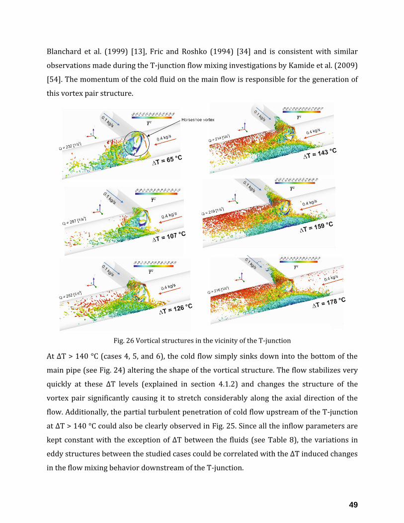
49

Blanchard et al. (1999) [13], Fric and Roshko (1994) [34] and is consistent with similar

observations made during the T-junction flow mixing investigations by Kamide et al. (2009)

[54]. The momentum of the cold fluid on the main flow is responsible for the generation of

this vortex pair structure.

Fig. 26 Vortical structures in the vicinity of the T-junction

At ∆T > 140 °C (cases 4, 5, and 6), the cold flow simply sinks down into the bottom of the

main pipe (see Fig. 24) altering the shape of the vortical structure. The flow stabilizes very

quickly at these ∆T levels (explained in section 4.1.2) and changes the structure of the

vortex pair significantly causing it to stretch considerably along the axial direction of the

flow. Additionally, the partial turbulent penetration of cold flow upstream of the T-junction

at ∆T > 140 °C could also be clearly observed in Fig. 25. Since all the inflow parameters are

kept constant with the exception of ∆T between the fluids (see Table 8), the variations in

eddy structures between the studied cases could be correlated with the ∆T induced changes

in the flow mixing behavior downstream of the T-junction.

50

Distribution of the vortical structures in the flow can be analyzed using the Q-criterion

which is defined in Ndombo and Howard (2011) [91] as follows

𝑄 = 1

4[(

𝜕�̅�𝑖

𝜕𝑥𝑗+

𝜕�̅�𝑗

𝜕𝑥𝑖)

2

− (𝜕�̅�𝑖

𝜕𝑥𝑗−

𝜕�̅�𝑗

𝜕𝑥𝑖)

2

] (26)

Fig. 26 depicts the evolution of the vortical structures with mean temperature contours.

The shape of the vortex structure at the cold flow outlet at ∆T = 65 °C is of particular

interest. It is primarily formed due to the boundary layer separation induced by the adverse

pressure gradients as the cold flow approaches the T-junction. The vortex structure has the

shape of a horseshoe and henceforth called ‘Horseshoe Vortex (HSV)’. The legs of the HSV

extend for a certain distance along the downstream direction. These structures could have

an influence on the flow properties (e.g. local heat transfer) at the T-junction. Each

subsequent rise in ∆T between fluids makes this structure less obvious and gives rise to

increasing number of small-scale structures in the flow. This effect could be attributed to

the increasing Reynolds number in the main pipe (see Table 8) brought about by the rising

hot inflow temperatures.

At ∆T > 140 °C, the vortical structures are also observed upstream of the T-junction in both

the main and branch pipes caused by the partial penetration of the hot and cold fluids into

the branch and main pipes, respectively. Thus Fig. 26 highlights the ∆T induced transition

from a clearly visible HSV structure at ∆T < 100 °C (case 1) to that of less obvious HSV

structure at 100 °C < ∆T < 140 °C (cases 2, 3) followed by numerous small-scale structures

along the downstream and upstream directions at ∆T > 140 °C (cases 4, 5, and 6). Buoyancy

effects, triggered by the density difference between the fluids, are identified as the primary

factor in causing this transition in the shape of the vortical structures.

Evolution of the mean velocity field in the mixing zone at different cross-sectional positions

is illustrated in Fig. 27. Velocity near the upper region is observed to be higher in all the

investigated cases due to the unmixed hot fluid flow. Since buoyancy tends to dampen any

extreme oscillations, the rise in ∆T between the fluids subjects the mixing region to shorter

oscillations occurring over smaller distances (at ∆T > 140 °C) as opposed to longer distance

flow oscillations observed at ∆T < 140 °C caused by strong forced convection effects.

Besides, partial upstream flow penetration observed in the main and branch pipes at ∆T >

51

140 °C considerably slows down the mean fluid velocity in the lower region of the pipe as

shown in the LES predictions in Fig. 27.

Fig. 27 Mean velocities along different cross-sections downstream of the T-junction

4.1.2 Thermal field in the mixing region

Mean temperature (𝑇∗̅̅ ̅) field along the axial flow direction is shown in Fig. 28. As explained

earlier, flow mixing in all the cases is incomplete resulting in a thermally stratified flow in

the mixing zone. The nature of the thermally stratified flow is directly related to the ΔT

amplitude between the fluids as all other inflow parameters are kept constant. Mixing

between the hot and cold flows at ΔT < 140 °C produces oscillations occurring over

relatively longer distances following the T-junction. Such oscillations are identified by the

alternating contours over relatively longer distances following the T-junction as illustrated

in Fig. 28 and are induced by considerable forced convective effects in the flow. Rise in ΔT

between the fluids reduces the oscillation distance as buoyancy forces rein the oscillations

52

brought about by the mixing between the flows. At ΔT > 140 °C, this effect becomes more

profound and the flow stabilizes very quickly as indicated by the 𝑇∗̅̅ ̅ contours in Fig. 28.

Fig. 28 Mean temperature field at the T-junction along the streamwise direction

Fig. 29 Mean temperature field along the cross-sectional direction

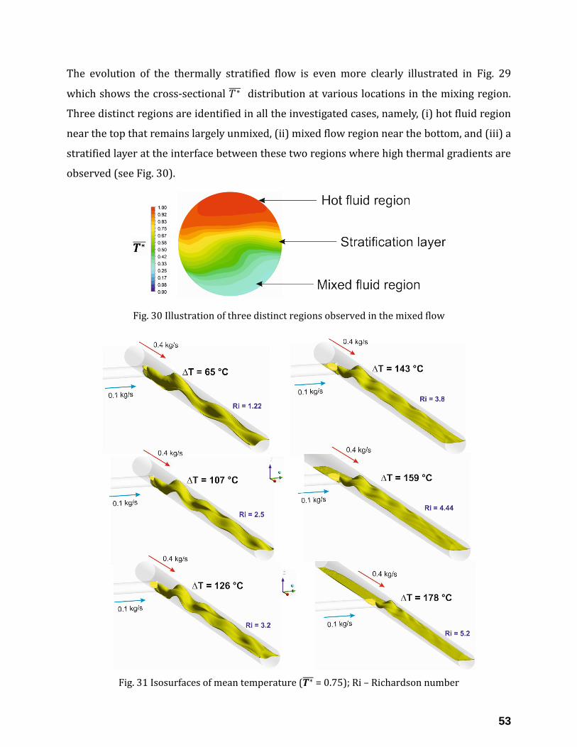
53

The evolution of the thermally stratified flow is even more clearly illustrated in Fig. 29

which shows the cross-sectional 𝑇∗̅̅ ̅ distribution at various locations in the mixing region.

Three distinct regions are identified in all the investigated cases, namely, (i) hot fluid region

near the top that remains largely unmixed, (ii) mixed flow region near the bottom, and (iii) a

stratified layer at the interface between these two regions where high thermal gradients are

observed (see Fig. 30).

Fig. 30 Illustration of three distinct regions observed in the mixed flow

Fig. 31 Isosurfaces of mean temperature (𝑻∗̅̅ ̅ = 0.75); Ri – Richardson number

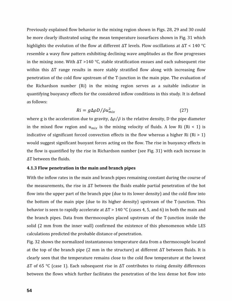
54

Previously explained flow behavior in the mixing region shown in Figs. 28, 29 and 30 could

be more clearly illustrated using the mean temperature isosurfaces shown in Fig. 31 which

highlights the evolution of the flow at different ΔT levels. Flow oscillations at ΔT < 140 °C

resemble a wavy flow pattern exhibiting declining wave amplitudes as the flow progresses

in the mixing zone. With ΔT >140 °C, stable stratification ensues and each subsequent rise

within this ΔT range results in more stably stratified flow along with increasing flow

penetration of the cold flow upstream of the T-junction in the main pipe. The evaluation of

the Richardson number (Ri) in the mixing region serves as a suitable indicator in

quantifying buoyancy effects for the considered inflow conditions in this study. It is defined

as follows:

𝑅𝑖 = 𝑔∆𝜌𝐷 �̅�𝑢𝑚𝑖𝑥2⁄ (27)

where g is the acceleration due to gravity, ∆𝜌 �̅�⁄ is the relative density, D the pipe diameter

in the mixed flow region and 𝑢𝑚𝑖𝑥 is the mixing velocity of fluids. A low Ri (Ri < 1) is

indicative of significant forced convection effects in the flow whereas a higher Ri (Ri > 1)

would suggest significant buoyant forces acting on the flow. The rise in buoyancy effects in

the flow is quantified by the rise in Richardson number (see Fig. 31) with each increase in

ΔT between the fluids.

4.1.3 Flow penetration in the main and branch pipes

With the inflow rates in the main and branch pipes remaining constant during the course of

the measurements, the rise in ΔT between the fluids enable partial penetration of the hot

flow into the upper part of the branch pipe (due to its lower density) and the cold flow into

the bottom of the main pipe (due to its higher density) upstream of the T-junction. This

behavior is seen to rapidly accelerate at ΔT > 140 °C (cases 4, 5, and 6) in both the main and

the branch pipes. Data from thermocouples placed upstream of the T-junction inside the

solid (2 mm from the inner wall) confirmed the existence of this phenomenon while LES

calculations predicted the probable distance of penetration.

Fig. 32 shows the normalized instantaneous temperature data from a thermocouple located

at the top of the branch pipe (2 mm in the structure) at different ΔT between fluids. It is

clearly seen that the temperature remains close to the cold flow temperature at the lowest

ΔT of 65 °C (case 1). Each subsequent rise in ΔT contributes to rising density differences

between the flows which further facilitates the penetration of the less dense hot flow into

55

the branch pipe. This scenario reaches its peak at the highest ΔT of 178 °C (case 6) with 𝑇∗ >

0.7 indicating substantial hot flow penetration.

Fig. 32 Instantaneous temperature data (at y = -1.92d, θ = 0 °) from the in-surface thermocouples

showing the hot fluid penetration into the branch pipe with rising ∆T

The same is seen from the LES predictions shown in Fig. 33 depicting the hot flow

penetration into the branch pipe and the results are truly surprising. For a near three-fold

rise in ΔT from 65 °C (case 1) to 178 °C (case 6), the penetration distance of the hot flow

into the branch pipe rises by more than six times from 67 mm (in case 1) to 427 mm (in

case 6). The T-junction piping also begins to bend at ΔT > 150 °C [116] which aids this

process even further. The consequence of the partial flow penetration is that part of the cold

flow near the top is now already mixed with the hot fluid and this certainly contributes to

lowering the mean temperature (𝑇∗̅̅ ̅) magnitude of fluids in the downstream region with

rise in ΔT between the fluids.

56

Fig. 33 Turbulent penetration of hot flow into branch pipe

Fig. 34 shows the normalized instantaneous temperature data from a thermocouple located

at the bottom of the main pipe (2 mm in the structure) during investigations performed at

different ΔT between the fluids. A different trend is seen here in the main pipe where the

cold flow doesn’t penetrate the thermocouple location until ΔT = 126 °C (case 3) which

could be the result of a higher Reynolds number hot flow preventing the cold flow from

traveling farther upstream into the main pipe. This scenario is seen to abruptly change in

case 4 (ΔT = 143 °C) where there is a significant decline in the temperature magnitudes

indicating the onset of cold flow penetration beyond that location. Each subsequent rise in

ΔT causes the cold flow to penetrate even farther into the main pipe. The same is also

predicted by the LES calculations depicting the cold flow penetration into the main pipe

with rising ΔT illustrated in Fig. 35. The distance of penetration by the cold flow is seen to

be even greater than the extent of the hot flow penetration into the branch pipe. For a near

three-fold rise in ΔT from 65 °C (case 1) to 178 °C (case 6), the penetration distance of cold

flow into the main pipe rises by more than 27 times from nearly 40 mm (in case 1) to

greater than 1077 mm (in case 6).

It goes without saying that more mixing occurs upstream of T-junction in the main pipe

with rising ΔT between the fluids which significantly brings down 𝑇∗̅̅ ̅ amplitude near the

lower part of the pipe in the mixing zone. Since the mass flow rates are fixed in each case,

the primary cause of the partial penetration of hot and cold flows into the branch and main

pipes is the density difference that arises in the flow with each uptick in ΔT between the

fluids.

57

Fig. 34 Instantaneous temperature data (at x = -1.6D, θ = 180 °) from the in-surface thermocouples

revealing the cold fluid penetration into main pipe with rising ∆T

Fig. 35 Turbulent penetration of cold flow into the main pipe

58

4.1.4 Near-wall mean temperature distribution

Fig. 36 shows the near-wall mean temperature (𝑇∗̅̅ ̅) data obtained from the circumferential

thermocouples during the measurements and the corresponding LES predictions. A

common feature observed in all the investigated cases is the repeated occurrence of higher

𝑇∗̅̅ ̅ amplitudes near the upper region (angular positions with 𝑇∗̅̅ ̅ > 0.9). This confirms the

earlier LES predictions that the flow remains largely unmixed near the top due to the low

branch velocity.

Lowest 𝑇∗̅̅ ̅ amplitudes are seen near the bottom of the pipe where intense fluid mixing

occurs. Comparison of lowest 𝑇∗̅̅ ̅ amplitudes (marked by dotted lines in Fig. 36) across all

the cases portray a declining trend in 𝑇∗̅̅ ̅ with rising ΔT between the fluids. The reasons

could be as follows: (i) at ΔT < 140 °C, the lateral momentum of the cold flow takes a while

integrating itself into the main pipe. Since the relative density between the fluids is lower, it

takes a certain distance for the mixed flows to settle and actively mix with each other. This

has the effect of producing relatively higher 𝑇∗̅̅ ̅ amplitudes at the investigated thermocouple

positions (x = 5D, 5.5D, and 6D) at ΔT < 140 °C. (ii) at ΔT > 140 °C, the relative density

between the fluids are sufficiently high that the cold flow easily sinks to the bottom of the

main pipe on reaching the T-junction. Besides, partial penetration of flows in the upstream

direction at these ΔT levels already bring pre-mixed flows to the T-junction resulting in a

sharp drop in 𝑇∗̅̅ ̅ amplitudes at the investigated thermocouple positions.

The stratified interface between the hot and cold layers of the flow, important in the context

of its high thermal gradients, could be probably identified by the significant jumps in 𝑇∗̅̅ ̅

between the circumferential thermocouple positions. In all the investigated cases, this

interface is found to invariably occur between θ = 80.5 ° and 125.5 ° on left-wall side and θ

= 215.5 ° and 260.5 ° on the right-wall side.

Difference in mean temperature (∆𝑇∗̅̅ ̅) amplitude between the top (θ = 350.5 °) and the

bottom (θ = 170.5 °) of the pipe (see Fig. 37) has a maximum value in each case as follows:

0.60 (39.5 °C) in case 1, 0.64 (70 °C) in case 2, 0.68 (88.6 °C) in case 3, 0.74 (105.6 °C) in

case 4, 0.79 in case 5 (131 °C) and 0.82 in case 6 (155.7 °C). This parameter is important in

the context of thermally stratified flows as bending moments and local stresses could be

induced in the structure [75] when strong temperature differences occur between the top

and the bottom of the pipes.

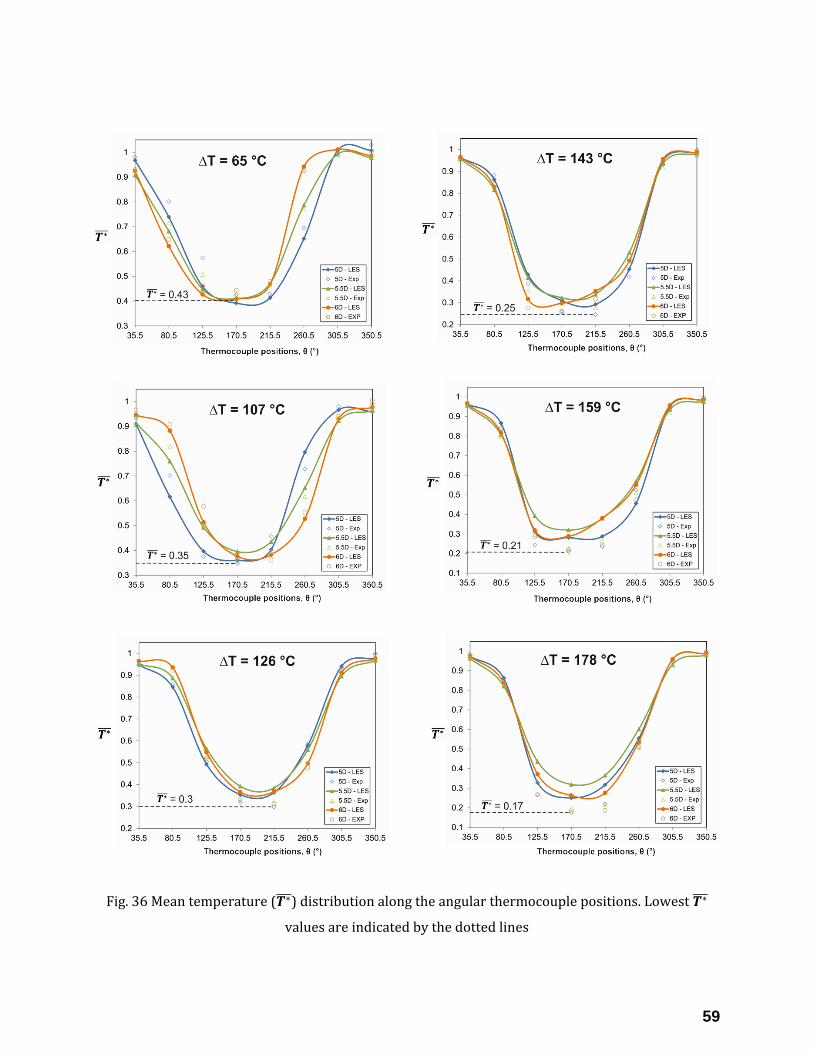
59

Fig. 36 Mean temperature (𝑻∗̅̅ ̅) distribution along the angular thermocouple positions. Lowest 𝑻∗̅̅ ̅

values are indicated by the dotted lines

60

Fig. 37 Illustration of ∆𝑻∗̅̅ ̅ between the top and bottom thermocouple positions

Fig. 38 Axial 𝑻∗̅̅ ̅ distribution along the angular positions, θ = 0°, 90°, 180° and 270°

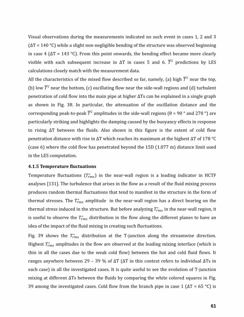
61

Visual observations during the measurements indicated no such event in cases 1, 2 and 3

(∆T < 140 °C) while a slight non-negligible bending of the structure was observed beginning

in case 4 (∆T = 143 °C). From this point onwards, the bending effect became more clearly

visible with each subsequent increase in ∆T in cases 5 and 6. 𝑇∗̅̅ ̅ predictions by LES

calculations closely match with the measurement data.

All the characteristics of the mixed flow described so far, namely, (a) high 𝑇∗̅̅ ̅ near the top,

(b) low 𝑇∗̅̅ ̅ near the bottom, (c) oscillating flow near the side-wall regions and (d) turbulent

penetration of cold flow into the main pipe at higher ∆Ts can be explained in a single graph

as shown in Fig. 38. In particular, the attenuation of the oscillation distance and the

corresponding peak-to-peak 𝑇∗̅̅ ̅ amplitudes in the side-wall regions (θ = 90 ° and 270 °) are

particularly striking and highlights the damping caused by the buoyancy effects in response

to rising ∆T between the fluids. Also shown in this figure is the extent of cold flow

penetration distance with rise in ∆T which reaches its maximum at the highest ∆T of 178 °C

(case 6) where the cold flow has penetrated beyond the 15D (1.077 m) distance limit used

in the LES computation.

4.1.5 Temperature fluctuations

Temperature fluctuations (𝑇𝑟𝑚𝑠∗ ) in the near-wall region is a leading indicator in HCTF

analyses [131]. The turbulence that arises in the flow as a result of the fluid mixing process

produces random thermal fluctuations that tend to manifest in the structure in the form of

thermal stresses. The 𝑇𝑟𝑚𝑠∗ amplitude in the near-wall region has a direct bearing on the

thermal stress induced in the structure. But before analyzing 𝑇𝑟𝑚𝑠∗ in the near-wall region, it

is useful to observe the 𝑇𝑟𝑚𝑠∗ distribution in the flow along the different planes to have an

idea of the impact of the fluid mixing in creating such fluctuations.

Fig. 39 shows the 𝑇𝑟𝑚𝑠∗ distribution at the T-junction along the streamwise direction.

Highest 𝑇𝑟𝑚𝑠∗ amplitudes in the flow are observed at the leading mixing interface (which is

thin in all the cases due to the weak cold flow) between the hot and cold fluid flows. It

ranges anywhere between 29 – 39 % of ∆T (∆T in this context refers to individual ∆Ts in

each case) in all the investigated cases. It is quite useful to see the evolution of T-junction

mixing at different ∆Ts between the fluids by comparing the white colored squares in Fig.

39 among the investigated cases. Cold flow from the branch pipe in case 1 (∆T = 65 °C) is

62

deflected by the oncoming hot flow and the mixing process ensues after a certain distance.

The area near the white colored square remains unaffected. With subsequent rise in ∆T, the

mixing between flows occurs sooner as buoyancy facilitates a much easier integration of the

cold flow into the main pipe. This is confirmed by the mixed flow regions moving closer

towards the white square. With significant cold flow penetration coming into play at ∆T >

140 °C, the premixed flow in the main pipe is easily pushed towards the opposite wall of the

T-junction by the cold flow as it enters the main pipe. Thus the 𝑇𝑟𝑚𝑠∗ distribution at the T-

junction changes in response to the rising ∆Ts between the fluids.

Fig. 39 Temperature fluctuations (𝑻𝒓𝒎𝒔∗ ) at the T-junction along the streamwise direction

Downstream flow 𝑇𝑟𝑚𝑠∗ distribution at different cross-sections is shown in Fig. 40. There is a

drop in the downstream 𝑇𝑟𝑚𝑠∗ amplitudes in comparison with the amplitudes at the T-

junction and it continues to decline as the flow progresses farther away from the T-junction.

The reason for this being the reduction in the turbulent mixing intensity (which is highest at

the T-junction) between the fluids as the flow progresses downstream which brings down

the 𝑇𝑟𝑚𝑠∗ amplitudes. Similar to the mean flow field shown in Fig. 30, cross-sectional thermal

fluctuation field could be characterized by three distinct regions as shown in Fig. 41. Lowest

𝑇𝑟𝑚𝑠∗ amplitudes are observed close to the top where no fluid mixing occurs. Slightly higher

63

𝑇𝑟𝑚𝑠∗ amplitudes are observed along the bottom of the pipe where complete mixing of fluids

occurs. But the highest 𝑇𝑟𝑚𝑠∗ amplitudes, pointed above as one of the factor in HCTF

analyses, occurs along the stratification layer where 𝑇𝑟𝑚𝑠∗ amplitudes in all the investigated

cases range from 22 – 36 % of ∆T (refers to individual ∆T in each case).

Fig. 40 Cross-sectional thermal fluctuations predicted by LES

Fig. 41 Illustration of three distinct thermal fluctuation regions observed in the mixed flow

64

Fig. 42 Thermal fluctuations in the main pipe (x = -1.6D) caused by cold flow penetration (view

oriented towards the T-junction)

Fig. 43 Thermal fluctuations in the branch pipe (y = -1.92d mm) caused by hot flow penetration

(view oriented towards the T-junction)

Fig. 42 shows the 𝑇𝑟𝑚𝑠∗ distribution along the cross-section upstream of the T-junction in the

main pipe (x = -1.6D). Rise in ∆T between the fluids did not result in cold flow penetration

till 140 °C. Beyond this ∆T, a substantial amount of cold flow penetrated the monitoring

region at x = -1.6D that results in thermal fluctuations within the penetrated region. The

65

predicted 𝑇𝑟𝑚𝑠∗ amplitudes range from 0.6 – 0.8 % of ∆T. Another observation is the rising

volume of occupied by the penetrated cold flow in response to rising ∆T between the fluids.

Thus a thermally stratified flow is formed even before the hot flow reaches the T-junction.

Especially at ∆T = 178 °C (case 6), half the cross-sectional region is occupied by penetrated

flow resulting in substantial mixing of flows upstream of the T-junction.

Similarly Fig. 43 depicts the 𝑇𝑟𝑚𝑠∗ distribution upstream of the T-junction in the branch pipe

(y = -1.92d). Starting from case 1 (∆T = 65 °C) the hot flow penetrates the monitoring region

in the branch pipe and volume of hot flow steadily rises with increase in ∆T between the

fluids. At the highest ∆T of 178 °C (case 6) the upper-half of the branch pipe is penetrated

by the hot fluid resulting in substantial 𝑇𝑟𝑚𝑠∗ amplitudes being generated within this mixing

region. Highest 𝑇𝑟𝑚𝑠∗ amplitudes in the branch pipe region as predicted by the LES

calculations lie in the range of 0.4 – 29 % of ∆T. This flow penetration could also be seen at

the cold flow outlet in Fig. 39.

Distribution of thermal fluctuations at the in-flow and in-structure thermocouple positions

and the corresponding LES predictions are shown in Fig. 44. The common features

exhibited in all the investigated cases could be summarized as follows: (i) two peak 𝑇𝑟𝑚𝑠∗

amplitudes (located near the stratification layer) are identified at each of the axial

thermocouple location (x = 5D, 5.5D, 6D), and (ii) a strong attenuation of thermal

fluctuation inside the solid region in relation to the fluid region.

Fluctuation amplitudes are the lowest at thermocouple positions representing the upper

part of the flow (any combination of θ = 35.5 °, 305.5 ° and 350.5 ° depending on the case

under investigation) and such lowest 𝑇𝑟𝑚𝑠∗ amplitudes in all the investigated cases range

from 0.13 – 0.5 % of ∆T between the fluids. As explained earlier, thermocouples close to the

stratification layer recorded the hightest 𝑇𝑟𝑚𝑠∗ amplitudes. A case-by-case peak 𝑇𝑟𝑚𝑠

∗

amplitudes on both the side-wall regions recorded by the in-flow thermocouples are shown

below in Table 10. Also, the peak 𝑇𝑟𝑚𝑠∗ amplitude recorded by the in-structure

thermocouples are also given in Table 10. With the exception of a few positions, LES results

exhibited reasonable agreement with the measurement data obtained from thermocouples.

Drop in peak 𝑇𝑟𝑚𝑠∗ amplitudes within the fluid region with increase in ∆T between fluids

confirms the buoyancy induced dampening of the flow oscillations. Data also shows that the

66

peak 𝑇𝑟𝑚𝑠∗ in the solid occurs near the stratification layer. The extent of the drop in 𝑇𝑟𝑚𝑠

∗

amplitudes inside the solid in comparison with the fluid 𝑇𝑟𝑚𝑠∗ amplitudes is significantly

higher given the magnitude of the attenuation (see Table 10).

Fig. 44 Distribution of thermal fluctuations (𝑻𝒓𝒎𝒔∗ ) at near-wall thermocouples for all the

investigated cases

67

Close to at least 90 % drop in 𝑇𝑟𝑚𝑠∗ amplitudes are observed in the solid in all the

investigated cases without exception. The effect of thermal inertia in dampening the

fluctuations emanating from the fluid as it gets transmitted to the structure could be clearly

observed from the above mentioned numbers.

Table 10. Fluid and solid thermal fluctuations as recorded from the measurements

∆T

(°C)

Peak 𝑇𝑟𝑚𝑠∗ (as % of ∆T) along the 𝑇𝑟𝑚𝑠

∗ (as % of ∆T) inside solid

Left wall region Right wall region Peak amplitude Attenuation

from peak fluid

level

65 7.5 (θ = 125.5 °) 11.4 (θ = 260.5 °) 1.1 (θ = 260.5 °) 90 %

107 4.4 (θ = 125.5 °) 6.5 (θ = 260.5 °) 0.64 (θ = 80.5 °) 90 %

126 3.7 (θ = 125.5 °) 3.8 (θ = 260.5 °) 0.4 (θ = 260.5 °) ≈ 90 %

143 4.6 (θ = 125.5 °) 6.4 (θ = 260.5 °) 0.42 (θ = 260.5 °) ≈ 93 %

159 2.6 ( θ = 80.5 °) 6.3 (θ = 260.5 °) 0.47 (θ = 80.5 °) ≈ 93 %

178 2.3 (θ = 125.5 °) 5.4 (θ = 260.5 °) 0.5 (θ = 260.5 °) 91 %

Fluid temperature fluctuations along the near-wall region (2 mm into the flow) predicted by

LES along the four corners of the cross-section are shown in Fig. 45. 𝑇𝑟𝑚𝑠∗ amplitudes near

the top (θ = 0 °) in all the cases remain below 1.5 % of ∆T (attributed to no fluid mixing at

the top) throughout the computational domain. There is a spike in 𝑇𝑟𝑚𝑠∗ amplitudes in all the

cases to more than 27 % of ∆T at θ = 90 ° as the cold flow enters the T-junction. The

amplitudes subsequently decline and then exhibit repeated rise and fall as the flow

oscillates in the mixing zone. A similar pattern is also observed on the other end of the wall

at θ = 270 ° where flow oscillations result in the rise and fall of 𝑇𝑟𝑚𝑠∗ amplitudes along the

mixing region. Such flow oscillations induced rise and fall of 𝑇𝑟𝑚𝑠∗ amplitudes in the side-

wall region (θ = 90 °, 270 °) is greatly diminished as ∆T rises beyond 140 °C (cases 4, 5 ,6)

due to buoynacy induced damping effects in the mixing region. The bottom region (θ = 180

°) gives a clear indication on the effects of rising ∆T between flows. Cold flow penetration

upstream of the main pipe results in rising 𝑇𝑟𝑚𝑠∗ amplitudes and this is limited to within a

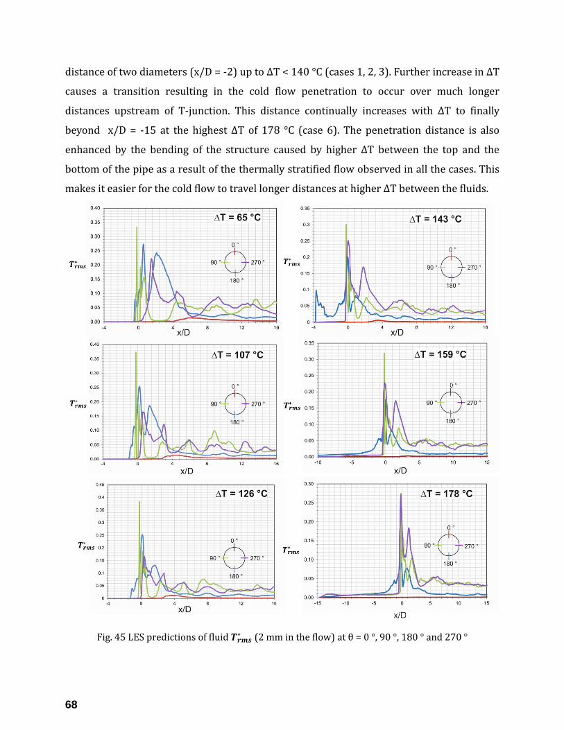
68

distance of two diameters (x/D = -2) up to ∆T < 140 °C (cases 1, 2, 3). Further increase in ∆T

causes a transition resulting in the cold flow penetration to occur over much longer

distances upstream of T-junction. This distance continually increases with ∆T to finally

beyond x/D = -15 at the highest ∆T of 178 °C (case 6). The penetration distance is also

enhanced by the bending of the structure caused by higher ∆T between the top and the

bottom of the pipe as a result of the thermally stratified flow observed in all the cases. This

makes it easier for the cold flow to travel longer distances at higher ∆T between the fluids.

Fig. 45 LES predictions of fluid 𝑻𝒓𝒎𝒔∗ (2 mm in the flow) at θ = 0 °, 90 °, 180 ° and 270 °

69

While thermocouple instrumentation is placed beginning at x = 5D, LES predictions shown

in Fig. 45 indicate the occurrence of much higher amplitude 𝑇𝑟𝑚𝑠∗ before 5 diameters

downstream of the T-junction. This is a valuable insight whereby additional thermocouple

instrumentation could now be placed much closer to the T-junction in the near-wall region

which might reveal additional information that has gone unnoticed during previous

measurements due to the non availability of thermocouples in the vicinity of the T-junction.

4.1.6 Frequency analysis of temperature fluctuations

Since it has been established that near-wall thermal fluctuations induce cyclical thermal

stresses in the structure, it becomes important to study the frequency content of such

fluctuations which might lead to much needed information about the energy distribution of

the eddies as a function of frequency. The application of Fast Fourier Transform (FFT)

method on a time domain signal 𝑓(𝑡) and the subsequent squaring its absolute magnitude

provides the power spectral density (PSD) of thermal fluctuations which is defined as

follows [63]

𝑃𝑆𝐷 = |𝑓(𝜔)|2= |∫ 𝑓(̅𝑡)𝑒−𝑖𝜔𝑡𝑑𝑡

𝑡/𝑛

0

|

2

(28)

where 𝑡 is the duration of the raw time signal and 𝑓(̅𝑡) is the n-times ensemble averaged

signal.

It has been established in the literature that there are attenuation factors in the process of

fluid thermal fluctuations converting to thermal stresses in the structure [56, 57] that could

be correlated with the fluctuation frequency (see Fig. 46). At high frequencies, fluid thermal

fluctuations are transferred to the structure with attenuation due to heat transfer loss

related to the heat transfer coefficient resulting in low amplitude thermal stresses. On the

other hand, low-frequency thermal fluctuations result in thermal diffusivity homogenizing

the structural temperature, failing to once again induce high amplitude thermal stresses.

Intermediate frequency fluctuations may have the potential to induce high amplitude

thermal stresses in the structure. On the basis of Civaux-I NPP leakage incident analysis,

Chapuliot et al. (2005) [16] estimated such critical frequencies of thermal fluctuations

responsible for possible thermal fatigue damage in the T-junction piping to be in the range

of 0.1 – 10 Hz. The Vattenfall T-junction benchmark exercise report [131] additionally

70

suggested the presence of a dominant frequency (spectral peak) of fluctuations in the 0.1 –

10 Hz frequency range that might indicate the occurrence of high thermal stresses in the

structure.

Fig. 46 Turbulent mixing and the attenuation mechanism of thermal fluctuations [56]

Thus the primary objective of power spectral density (PSD) analyses in this section is to

look for thermal fluctuations exhibiting spectral peak (if any) in the 0.1 – 10 Hz range. The

secondary objective is to compare the LES spectra with that of measurement spectra. Fig. 47

shows the normalized PSD of the peak amplitude thermal fluctuations within the fluid

domain.

The shape of the spectra illustrates the cascading phenomenon where energy is

successively transferred from the larger eddies (low frequency) to the smaller eddies (high

frequency) in the flow. Power content of temperature fluctuations remains fairly stable

(nearly 1 [-/Hz] in all the cases) until the frequency of 1 Hz. Beyond this, a waterfall-type

drop in the power content of fluctuations is noticed. At 10 Hz the power content of

fluctuations has already dropped by several orders of magnitude (indicated in Fig. 47) from

where it was within the frequency range of 0.1 – 1 Hz. No distinct peak in the power content

of fluctuations was observed in the 0.1 – 10 Hz range indicating that the relevance for

thermal fatigue is not obvious from the in-flow thermocouple data.

Further drop in the power content of temperature fluctuations is observed beyond 10 Hz as

seen from the measurement data (which is correctly followed by the LES predictions). The

PSD of fluid fluctuations also follows the -5/3 slope based on the Kolmogorov spectrum

71

[105] in the inertial sub-range, a region between the energy containing eddy range and the

dissipation range in the energy spectrum (see Fig. 17).

Fig. 47 PSD of peak fluid thermal fluctuations. Dotted lines show the -5/3 trend line in the inertial

sub-range of the power spectrum

A different trend unfolds when analyzing the PSD of thermal fluctuations inside the solid as

shown in Fig. 48. Unlike the fluid, the energy content of thermal fluctuations inside the solid

is not concentrated within in a particular frequency range. The decline in the energy of

thermal fluctuations with frequency is nearly linear from 0.1 till 10 Hz. Within this interval

72

the power content of solid thermal fluctuations are comparatively lower than the fluid

fluctuations discussed in Fig. 47. Beyond 10 Hz, the PSD amplitudes within solid tend to

stabilize and have higher magnitudes than the fluid PSD amplitudes.

Fig. 48 PSD of peak solid thermal fluctuation in all the investigated cases

This completes the first part of the results section where flow behavior at ∆T between the

mixing fluids in 60 – 180 °C range is discussed at constant main and branch flow rates of 0.4

kg/s and 0.1 kg/s, respectively. Changes in the flow mixing behavior caused by variation of

the main flow rates are illustrated in the section A.2 of the appendix.

73

4.2 Mixing behavior of flows at ∆T = 233 °C

It has been established in the previous section that the thermally stratified flow in the

mixing region becomes increasingly stable with rising ∆T between the fluids. An auxiliary

effect is a rise in the flow penetration distance of hot fluid into the branch pipe and vice

versa triggered by the rising density differences between the fluids and the low Reynolds

number of the cold fluid coming from the branch pipe. With this understanding, it was

decided to perform a single experiment in which the FSI test facility was taken to its highest

operable fluid temperature to observe the mixing nature of the flow in the vicinity of the T-

junction. The inflow conditions related to this experiment are shown in Table 10.

Table 11. Case 7 – Inflow conditions for experiments at ∆T = 233 °C

Parameters Main pipe Branch pipe

Temperature (°C) 257 24

Mass flow rate (kg/s) 0.4 0.1

Velocity (m/s) 0.13 0.084

Density (kg m-3) 775 999

Dynamic viscosity (Pa s) 9.95 e-5 9.13e-4

Reynolds number (Re) 71324 3580

𝑢𝑚𝑖𝑥 (m/s) 0.153

𝑅𝑖 7.6

Relative density (∆𝜌 �̅�⁄ ) 25.2 %

Relative viscosity (∆𝜇 �̅�⁄ ) 160.7 %

Pressure 70 bar

Turbulent hot fluid flowing in the main pipe (257 °C, 𝑅𝑒𝑚 = 71324) combines with the

transitional cold fluid flowing through the branch pipe (24 °C, 𝑅𝑒𝑏 = 3580) at the T-junction.

Assessment of non-dimensional parameters in Table 11 points to the highest possible

buoyancy effects to be expected in the flow. For example, the Richardson number is

calculated to be 7.6, nearly 50 % higher than in case 6 (∆T = 178 °C) discussed in the

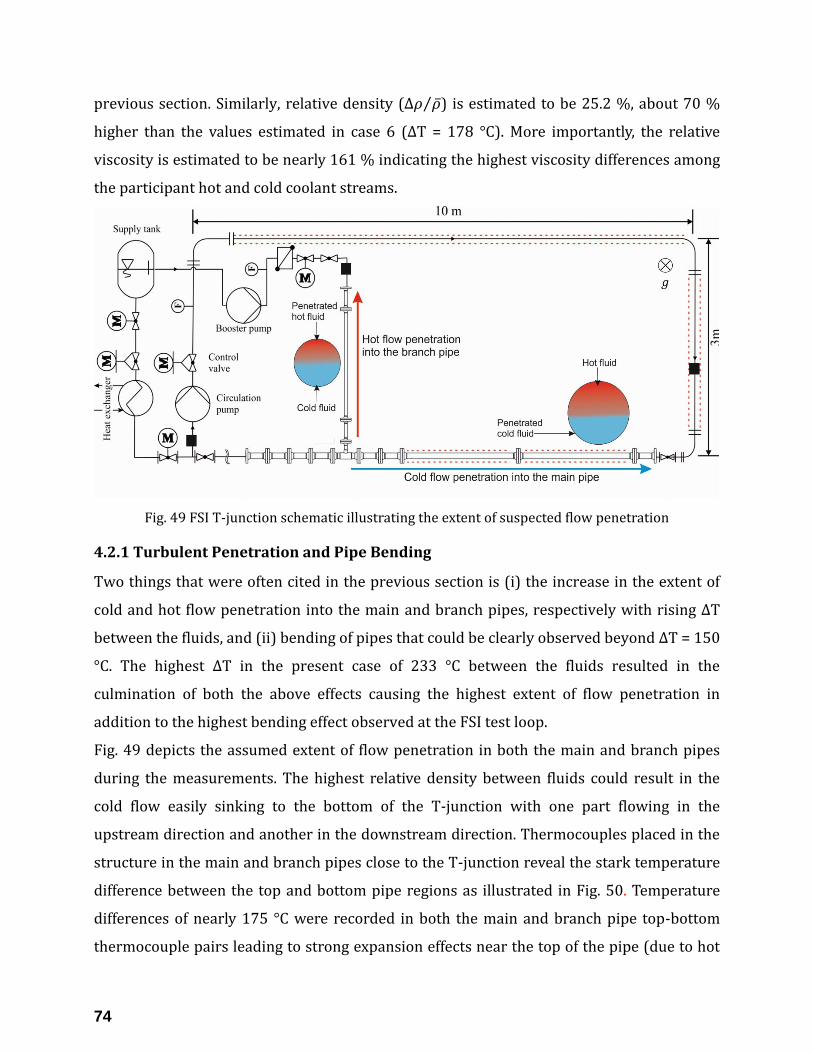
74

previous section. Similarly, relative density (∆𝜌 �̅�⁄ ) is estimated to be 25.2 %, about 70 %

higher than the values estimated in case 6 (∆T = 178 °C). More importantly, the relative

viscosity is estimated to be nearly 161 % indicating the highest viscosity differences among

the participant hot and cold coolant streams.

Fig. 49 FSI T-junction schematic illustrating the extent of suspected flow penetration

4.2.1 Turbulent Penetration and Pipe Bending

Two things that were often cited in the previous section is (i) the increase in the extent of

cold and hot flow penetration into the main and branch pipes, respectively with rising ∆T

between the fluids, and (ii) bending of pipes that could be clearly observed beyond ∆T = 150

°C. The highest ∆T in the present case of 233 °C between the fluids resulted in the

culmination of both the above effects causing the highest extent of flow penetration in

addition to the highest bending effect observed at the FSI test loop.

Fig. 49 depicts the assumed extent of flow penetration in both the main and branch pipes

during the measurements. The highest relative density between fluids could result in the

cold flow easily sinking to the bottom of the T-junction with one part flowing in the

upstream direction and another in the downstream direction. Thermocouples placed in the

structure in the main and branch pipes close to the T-junction reveal the stark temperature

difference between the top and bottom pipe regions as illustrated in Fig. 50. Temperature

differences of nearly 175 °C were recorded in both the main and branch pipe top-bottom

thermocouple pairs leading to strong expansion effects near the top of the pipe (due to hot

75

fluid) and compression effects that could be induced at the bottom of the pipe (due to cold

fluid). This automatically induces strong bending moments in the pipe structure. Previous

numerical studies performed in 2012 indicated that possibility of the piping lift-up with the

T-junction as its vertex [116]. That prediction is confirmed through the current experiment

where thermally stratified flows are observed in all the directions (due to flow penetration

in the upstream directions and due to mixing in the downstream direction).

Fig. 50 Temporal evolution of in-structure temperatures in the main and branch pipes

There is a strong possibility that the hot fluid might have traveled all the way up to the

beginning of the straight section of the branch pipe (nearly 2.4 m long) partly aided by the

pipe bending effects which exacerbates the situation. There is no empirical evidence

confirming this effect due to the fact that surface thermocouples were not placed that far

upstream in the branch pipe.

On the other hand, there is an even greater possibility that the cold flow might have

penetrated and traveled all the way till the beginning of the straight section of the main pipe

(nearly 4.6 m long) also aided partly by the pipe bending effects. There is empirical evidence

76

of this phenomenon from the surface thermocouple instrumentation (see Fig. 51) primarily

placed to monitor the heating mat temperatures. A temperature difference of greater than

60 °C within the top-bottom region of the hot flow close to 3 meters upstream of the T-

junction confirms the cold flow penetration beyond this distance.

Fig. 51 Cold flow penetration in the main pipe (2.92 m upstream of T-junction) as recorded by

surface thermocouple instrumentation

As a result of the flow penetration upstream of the T-junction and the stable thermal

stratification in the downstream region, the piping structure is seen to lift up from its rest

position with the T-junction as the vertex, described in the literature as ‘banana effect’ [92].

Excerpts detailing such a phenomenon involving thermal stratification are as follows:

“If the velocity of the medium in a pipe flow is small, temperature stratification may occur in

horizontal pipe sections which might superimpose a significant contribution to global bending

stresses (“banana effect”) and fatigue”

Visual observations indicate that the T-junction might have lifted up by nearly 80 mm from

its rest position as shown in the photographs in Fig. 52.

4.2.2 Near-wall mean and RMS temperature distribution

With arguably the most predictable flow behavior downstream of the T-junction in the FSI

facility, the stark buoyancy effect keeps the flow in the mixing region very stable by

77

dampening flow oscillations quickly and this is illustrated by the mean temperature data

shown in Fig. 53.

Fig. 52 Bent T-junction piping [marked in red] (a), its close-up view (b) at ΔT = 233 °C

Fig. 53 𝑻∗̅̅ ̅ distribution (left) and 𝑻∗̅̅ ̅ contour (right) at angular thermocouple positions

Nearly no change is observed in the 𝑇∗̅̅ ̅ profile at all the axial locations (x = 5D, 5.5D and 6D)

indicating a stably stratified flow that settles quickly following the initial mixing at the T-

junction. Highest and lowest 𝑇∗̅̅ ̅ values are observed near the upper (θ = 35.5 °, 80.5 °, 305.5

° and 350.5 °) and lower (θ = 170.5 °) regions, respectively. It goes without saying that the

very low temperatures at the bottom of the pipe in the mixing region is influenced by the

pre-mixing that occurs upstream of the T-junction due to cold flow penetration in the main

pipe described earlier. The stratified interface is found to occur between θ = 80.5 ° and

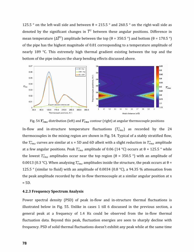
78

125.5 ° on the left-wall side and between θ = 215.5 ° and 260.5 ° on the right-wall side as

denoted by the significant changes in 𝑇∗̅̅ ̅ between these angular positions. Difference in

mean temperature (∆𝑇∗̅̅ ̅) amplitude between the top (θ = 350.5 °) and bottom (θ = 170.5 °)

of the pipe has the highest magnitude of 0.81 corresponding to a temperature amplitude of

nearly 189 °C. This extremely high thermal gradient existing between the top and the

bottom of the pipe induces the sharp bending effects discussed above.

Fig. 54 𝑻𝒓𝒎𝒔∗ distribution (left) and 𝑻𝒓𝒎𝒔

∗ contour (right) at angular thermocouple positions

In-flow and in-structure temperature fluctuations (𝑇𝑟𝑚𝑠∗ ) as recorded by the 24

thermocouples in the mixing region are shown in Fig. 54. Typical of a stably stratified flow,

the 𝑇𝑟𝑚𝑠∗ curves are similar at x = 5D and 6D albeit with a slight reduction in 𝑇𝑟𝑚𝑠

∗ amplitude

at a few angular positions. Peak 𝑇𝑟𝑚𝑠∗ amplitude of 0.06 (14 °C) occurs at θ = 125.5 ° while

the lowest 𝑇𝑟𝑚𝑠∗ amplitudes occur near the top region (θ = 350.5 °) with an amplitude of

0.0013 (0.3 °C). When analyzing 𝑇𝑟𝑚𝑠∗ amplitudes inside the structure, the peak occurs at θ =

125.5 ° (similar to fluid) with an amplitude of 0.0034 (0.8 °C), a 94.35 % attenuation from

the peak amplitude recorded by the in-flow thermocouple at a similar angular position at x

= 5D.

4.2.3 Frequency Spectrum Analysis

Power spectral density (PSD) of peak in-flow and in-structure thermal fluctuations is

illustrated below in Fig. 55. Unlike in cases 1 till 6 discussed in the previous section, a

general peak at a frequency of 1.4 Hz could be observed from the in-flow thermal

fluctuation data. Beyond this peak, fluctuation energies are seen to sharply decline with

frequency. PSD of solid thermal fluctuations doesn’t exhibit any peak while at the same time

79

the energy decline with frequency inside the solid is gradual in comparison with the

relevant data from the fluid. Beyond 7 Hz, a change in trend is observed where the energy of

solid thermal fluctuations becomes higher than that of the fluid.

Fig. 55 PSD of temperature fluctuations at the in-flow and in-structure thermocouple positions

While the currently investigated ∆T of 233 °C induces considerable bending stresses in the

structure which in turn induces flow penetration over longer distances upstream of the

main and branch pipes, it is still not obvious if fatigue cracks could be initiated due to the

mixing of flows under these inflow conditions. The previous numerical study carried out in

2012 [116] at an even higher ∆T of 260 °C also highlighted this fact. LES investigation for

the present experiment has not been performed due to the deformation of the T-junction

observed during measurements.

The next obvious advancement at the FSI test loop is the investigation of T-junction mixing

at higher flow rates in the branch pipe which might shed more light into the flow mixing

processes under turbulent inflow conditions (presently not the case due to low branch flow

rate). While the experimental capability to do such measurements is currently in

development at the moment, a precursor numerical study performed using LES could

provide a valuable glimpse into the flow mixing phenomenon at higher branch flow rates.

80

4.3 Mixing behavior of flows at increased branch flow velocities

The obvious question that arises during the course of analyzing flow mixing at increasing

∆T between flows in section 4.1 is

“How is the mixing behavior affected/What happens to the mixing behavior when there is

an increase in branch flow rates ?”

Table 12: Inflow conditions for increased branch flow studies

Case # ∆T

(°C)

𝑇𝑚*

(°C)

�̇�𝑚

(kg/s)

𝑢𝑚

(m/s)

𝑇𝑏*

(°C)

�̇�𝑏

(kg/s)

𝑢𝑏

(m/s)

𝑢𝑚𝑖𝑥

(m/s)

1

65

85 0.4 0.101 20 0.1 0.084 0.132

1a 85 0.4 0.101 20 0.2 0.168 0.196

1b 85 0.4 0.101 20 0.3 0.252 0.272

4

143

165 0.4 0.109 22 0.1 0.084 0.138

4a 165 0.4 0.109 22 0.2 0.168 0.2

4b 165 0.4 0.109 22 0.3 0.252 0.275

* suffixes m and b denote main and branch pipes, respectively

As discussed before, the main limitation of the FSI test facility is its maximum operational

branch flow rate (𝑚𝑏̇ ) of 0.1 kg/s is not turbulent enough to cause considerable mixing

between the fluids. To analyze this issue numerically, it was decided to perform LES

calculations to analyze flow mixing characteristics at increased branch flow rates while the

flow rates in the main pipe were kept constant at 0.4 kg/s. Inflow conditions of cases 1 and

4, representative of lower and higher ∆Ts, were chosen from section 4.1 for this exercise.

Branch flow rates were increased to 0.2 kg/s and 0.3 kg/s, respectively. Results from the

original cases 1 and 4 are also included here so as to easily compare and understand the

effects of the rise in branch flow rates on the flow mixing dynamics in the vicinity of the T-

junction. Details of the inflow conditions are shown in Table 12.

4.3.1 Qualitative analysis of the mixing region

The entry of the cold flow into the main pipe at high branch flow rates produces some

distinct unsteady structures, namely, the shear layer vortices. Fig. 56 shows the

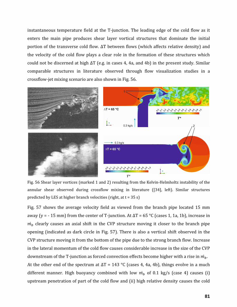
81

instantaneous temperature field at the T-junction. The leading edge of the cold flow as it

enters the main pipe produces shear layer vortical structures that dominate the initial

portion of the transverse cold flow. ∆T between flows (which affects relative density) and

the velocity of the cold flow plays a clear role in the formation of these structures which

could not be discerned at high ∆T (e.g. in cases 4, 4a, and 4b) in the present study. Similar

comparable structures in literature observed through flow visualization studies in a

crossflow-jet mixing scenario are also shown in Fig. 56.

Fig. 56 Shear layer vortices (marked 1 and 2) resulting from the Kelvin-Helmholtz instability of the

annular shear observed during crossflow mixing in literature ([34], left). Similar structures

predicted by LES at higher branch velocities (right, at t = 35 s)

Fig. 57 shows the average velocity field as viewed from the branch pipe located 15 mm

away (y = - 15 mm) from the center of T-junction. At ∆T = 65 °C (cases 1, 1a, 1b), increase in

𝑚𝑏̇ clearly causes an axial shift in the CVP structure moving it closer to the branch pipe

opening (indicated as dark circle in Fig. 57). There is also a vertical shift observed in the

CVP structure moving it from the bottom of the pipe due to the strong branch flow. Increase

in the lateral momentum of the cold flow causes considerable increase in the size of the CVP

downstream of the T-junction as forced convection effects become higher with a rise in 𝑚𝑏̇ .

At the other end of the spectrum at ∆T = 143 °C (cases 4, 4a, 4b), things evolve in a much

different manner. High buoyancy combined with low 𝑚𝑏̇ of 0.1 kg/s (case 4) causes (i)

upstream penetration of part of the cold flow and (ii) high relative density causes the cold

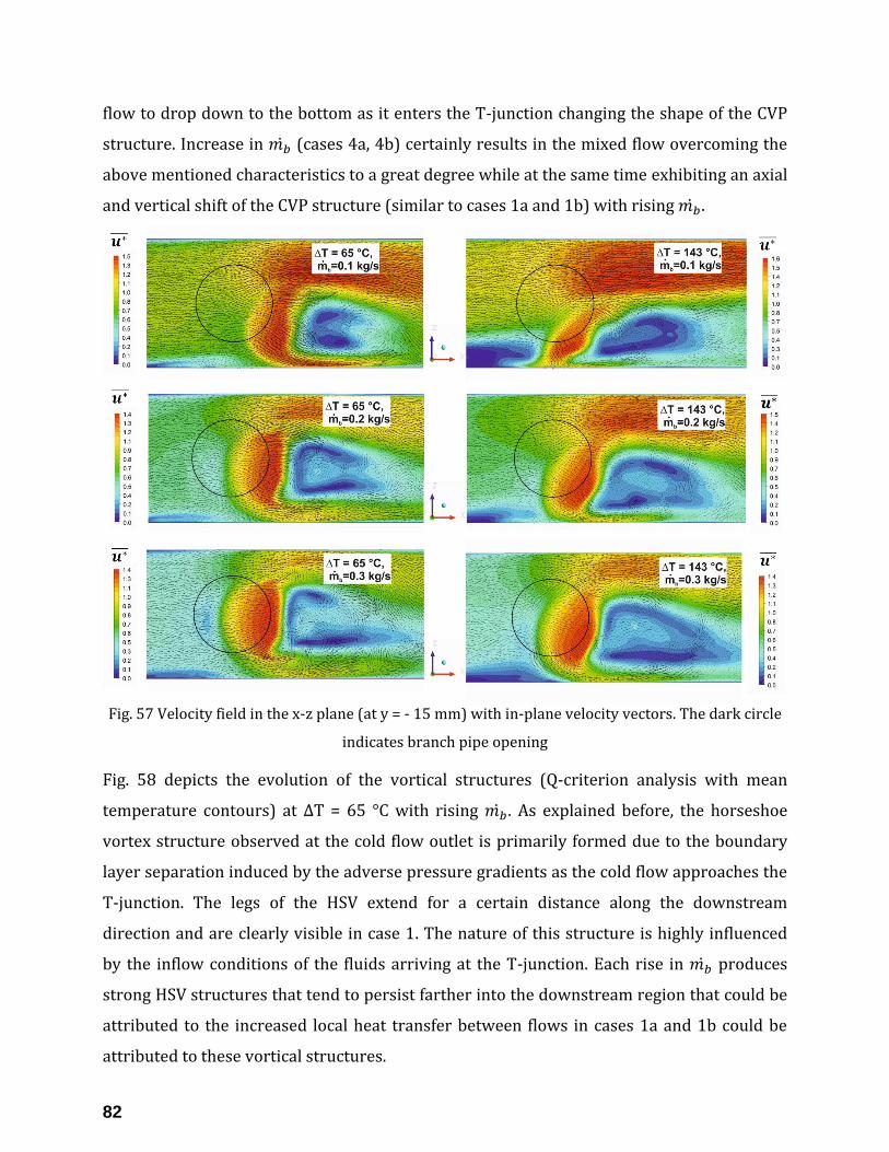
82

flow to drop down to the bottom as it enters the T-junction changing the shape of the CVP

structure. Increase in 𝑚𝑏̇ (cases 4a, 4b) certainly results in the mixed flow overcoming the

above mentioned characteristics to a great degree while at the same time exhibiting an axial

and vertical shift of the CVP structure (similar to cases 1a and 1b) with rising 𝑚𝑏̇ .

Fig. 57 Velocity field in the x-z plane (at y = - 15 mm) with in-plane velocity vectors. The dark circle

indicates branch pipe opening

Fig. 58 depicts the evolution of the vortical structures (Q-criterion analysis with mean

temperature contours) at ∆T = 65 °C with rising 𝑚𝑏̇ . As explained before, the horseshoe

vortex structure observed at the cold flow outlet is primarily formed due to the boundary

layer separation induced by the adverse pressure gradients as the cold flow approaches the

T-junction. The legs of the HSV extend for a certain distance along the downstream

direction and are clearly visible in case 1. The nature of this structure is highly influenced

by the inflow conditions of the fluids arriving at the T-junction. Each rise in 𝑚𝑏̇ produces

strong HSV structures that tend to persist farther into the downstream region that could be

attributed to the increased local heat transfer between flows in cases 1a and 1b could be

attributed to these vortical structures.

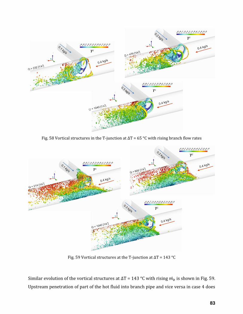
83

Fig. 58 Vortical structures in the T-junction at ∆T = 65 °C with rising branch flow rates

Fig. 59 Vortical structures at the T-junction at ∆T = 143 °C

Similar evolution of the vortical structures at ∆T = 143 °C with rising 𝑚𝑏̇ is shown in Fig. 59.

Upstream penetration of part of the hot fluid into branch pipe and vice versa in case 4 does

84

not result in any distinct HSV structure, but it produces multiple small-scale structures

extending along the upstream and downstream directions. Elevated cold flow rates

contribute to reversing this situation resulting in more mixing near the upper part of the

pipe as seen from the 𝑇∗̅̅ ̅ distribution of the structures. Nonetheless, no distinct vortical

structures (like the HSV) are observed at the T-junction in cases 4a and 4b.

Fig. 60 Mean velocity field at the T-junction along the y-z axis

The nature of the cold flow entry into the T-junction could be a factor in the formation of

these structures. At ∆T = 65 °C, the relative density is lower (≈ 3 %) which enables the cold

flow to push farther into the T-junction with rising 𝑚𝑏̇ (see Fig. 60) resulting in the

formation of the HSV structure. At ∆T = 143 °C, the relative density has nearly tripled (≈ 10

%) causing the cold flow to sink to the bottom of the main pipe (case 4) which results in

such structures not being produced. Increase in 𝑚𝑏̇ (cases 4b, 4c) results in the cold flow

trying to overcome the tendency to sink into the main pipe and could be a reason why no

distinct HSV structures are formed at ∆T = 143 °C despite an increase in 𝑚𝑏̇ .

Fig. 61 shows the mean temperature distribution at the T-junction along the streamwise

direction. Rise in 𝑚𝑏̇ clearly results in the cold flow pushing farther into the main pipe

causing complete mixing (at ∆T = 65 °C) or enhanced mixing resulting in higher oscillations

of flow in the downstream region (at ∆T = 143 °C).

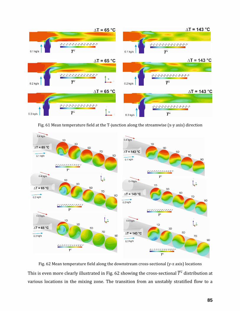
85

Fig. 61 Mean temperature field at the T-junction along the streamwise (x-y axis) direction

Fig. 62 Mean temperature field along the downstream cross-sectional (y-z axis) locations

This is even more clearly illustrated in Fig. 62 showing the cross-sectional 𝑇∗̅̅ ̅ distribution at

various locations in the mixing zone. The transition from an unstably stratified flow to a

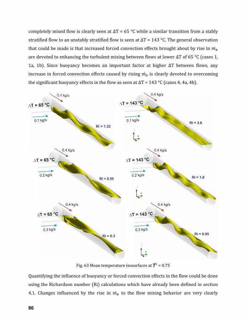
86

completely mixed flow is clearly seen at ∆T = 65 °C while a similar transition from a stably

stratified flow to an unstably stratified flow is seen at ∆T = 143 °C. The general observation

that could be made is that increased forced convection effects brought about by rise in 𝑚𝑏̇

are devoted to enhancing the turbulent mixing between flows at lower ∆T of 65 °C (cases 1,

1a, 1b). Since buoyancy becomes an important factor at higher ∆T between flows, any

increase in forced convection effects caused by rising 𝑚𝑏̇ is clearly devoted to overcoming

the significant buoyancy effects in the flow as seen at ∆T = 143 °C (cases 4, 4a, 4b).

Fig. 63 Mean temperature isosurfaces at 𝑻∗̅̅ ̅ = 0.75

Quantifying the influence of buoyancy or forced convection effects in the flow could be done

using the Richardson number (Ri) calculations which have already been defined in section

4.1. Changes influenced by the rise in 𝑚𝑏̇ to the flow mixing behavior are very clearly

87

illustrated using the mean temperature isosurfaces shown in Fig. 63. An oscillating wavy

flow occurring over longer distances is observed at ∆T = 65 °C while a stably stratified flow

becoming a unstably stratified flow with an oscillating wavy flow pattern is seen at ∆T =

143 °C.

Fig. 64 Mean velocity field along various downstream cross-sectional (y-z axis) locations

The mean velocity field at various cross-sectional positions downstream of the T-junction

for all the investigated cases is shown in Fig. 64. Velocity near the top is clearly higher at the

lowest 𝑚𝑏̇ of 0.1 kg/s as the hot flow travels unmixed at both ∆T levels of 65 °C and 143 °C,

respectively. A rise in 𝑚𝑏̇ enables enhanced mixing which greatly brings down the velocity

near the top at ∆T = 65 °C as reflected in the vertical mean velocity profile shown in Fig. 65

which becomes nearly symmetric with the rise in 𝑚𝑏̇ . On the other hand, a rise in 𝑚𝑏̇ is still

insufficient to cause complete mixing between the flows at ∆T = 143 °C for reasons

described above in Figs. 61, 62 and 63. This causes the highest mean velocity of flows to be

concentrated near the upper region and the shape of the mean velocity profile in Fig. 65

confirms this trend.

88

Fig. 65 Mean velocity along the vertical direction (z-axis) at downstream positions

Fig. 66 Mean temperature field at the T-junction along the y-z axis

89

Fig. 67 Mean temperature field along the axial flow direction (x-z axis)

The density and inflow rate differences between the hot and cold flows sets up the stage for

partial penetration of hot flow into the branch pipe and cold flow into the main pipe. It has

been elaborately discussed in section 4.1 where it was established that the distance of

penetration is influenced by ∆T between the fluids since all other inflow parameters are

kept constant. Rise in 𝑚𝑏̇ at ∆T = 65 °C (cases 1a, 1b) results in nearly negligible penetration

of hot flow into the branch pipe (see Fig. 66) while at the same time there is a reduced

penetration of cold flow into the main pipe (see Fig. 67).

The same could not be observed with rising 𝑚𝑏̇ at ∆T = 143 °C (cases 4a, 4b). Firstly, there

is a great degree of cold flow penetration over longer distance at 𝑚𝑏̇ = 0.1 kg/s (case 4)

caused by dominant buoyancy forces in the flow. Thus rise in 𝑚𝑏̇ contributes to reducing

the extent of cold flow penetration although it is not completely accomplished. Hot flow

penetration into the branch pipe is reduced by more than 50 % from 3.6d (case 4) to 1.45d

(case 4b) as shown in Fig. 66. Similarly, there is more than 50 % reduction in penetration

distance of cold flow into the main pipe from 3.5D (case 4) to 1.5D (case 4b) as illustrated in

Fig. 67.

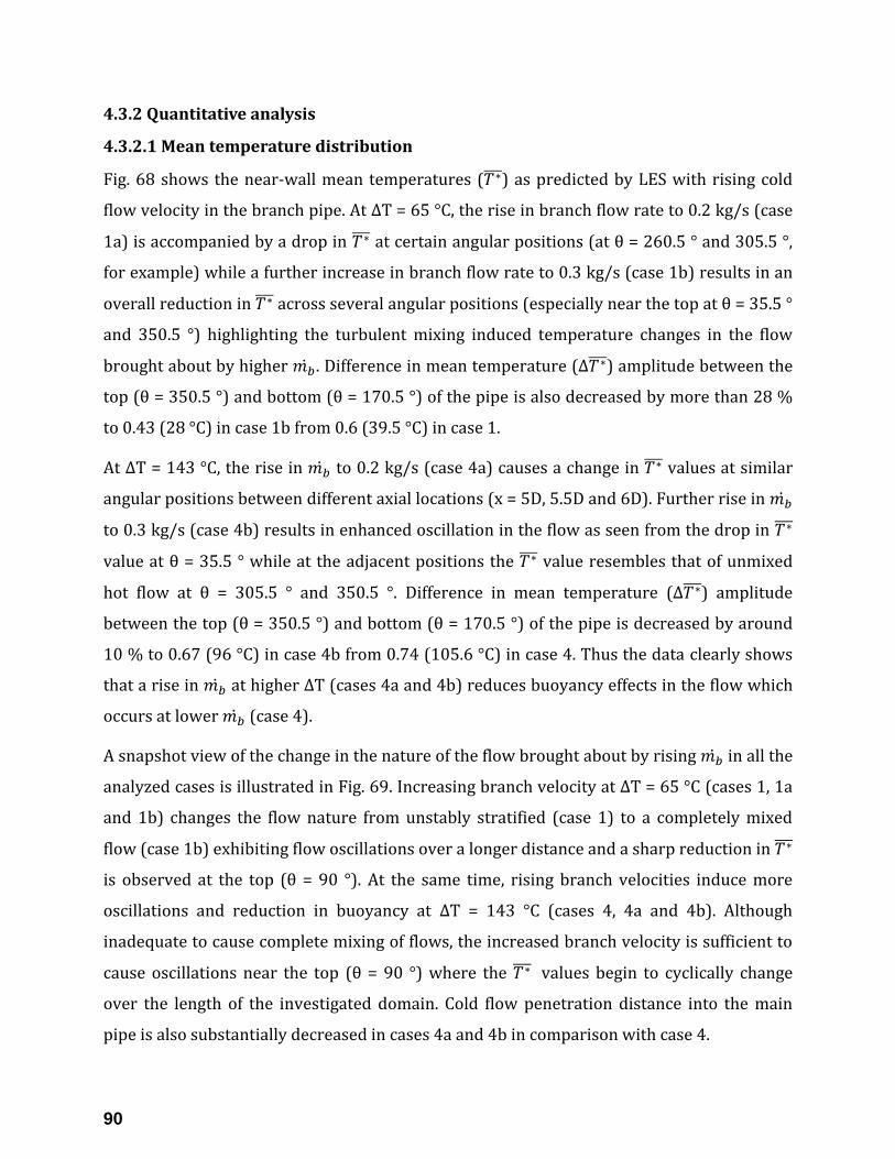
90

4.3.2 Quantitative analysis

4.3.2.1 Mean temperature distribution

Fig. 68 shows the near-wall mean temperatures (𝑇∗̅̅ ̅) as predicted by LES with rising cold

flow velocity in the branch pipe. At ΔT = 65 °C, the rise in branch flow rate to 0.2 kg/s (case

1a) is accompanied by a drop in 𝑇∗̅̅ ̅ at certain angular positions (at θ = 260.5 ° and 305.5 °,

for example) while a further increase in branch flow rate to 0.3 kg/s (case 1b) results in an

overall reduction in 𝑇∗̅̅ ̅ across several angular positions (especially near the top at θ = 35.5 °

and 350.5 °) highlighting the turbulent mixing induced temperature changes in the flow

brought about by higher 𝑚𝑏̇ . Difference in mean temperature (∆𝑇∗̅̅ ̅) amplitude between the

top (θ = 350.5 °) and bottom (θ = 170.5 °) of the pipe is also decreased by more than 28 %

to 0.43 (28 °C) in case 1b from 0.6 (39.5 °C) in case 1.

At ΔT = 143 °C, the rise in 𝑚𝑏̇ to 0.2 kg/s (case 4a) causes a change in 𝑇∗̅̅ ̅ values at similar

angular positions between different axial locations (x = 5D, 5.5D and 6D). Further rise in 𝑚𝑏̇

to 0.3 kg/s (case 4b) results in enhanced oscillation in the flow as seen from the drop in 𝑇∗̅̅ ̅

value at θ = 35.5 ° while at the adjacent positions the 𝑇∗̅̅ ̅ value resembles that of unmixed

hot flow at θ = 305.5 ° and 350.5 °. Difference in mean temperature (∆𝑇∗̅̅ ̅) amplitude

between the top (θ = 350.5 °) and bottom (θ = 170.5 °) of the pipe is decreased by around

10 % to 0.67 (96 °C) in case 4b from 0.74 (105.6 °C) in case 4. Thus the data clearly shows

that a rise in 𝑚𝑏̇ at higher ∆T (cases 4a and 4b) reduces buoyancy effects in the flow which

occurs at lower 𝑚𝑏̇ (case 4).

A snapshot view of the change in the nature of the flow brought about by rising 𝑚𝑏̇ in all the

analyzed cases is illustrated in Fig. 69. Increasing branch velocity at ∆T = 65 °C (cases 1, 1a

and 1b) changes the flow nature from unstably stratified (case 1) to a completely mixed

flow (case 1b) exhibiting flow oscillations over a longer distance and a sharp reduction in 𝑇∗̅̅ ̅

is observed at the top (θ = 90 °). At the same time, rising branch velocities induce more

oscillations and reduction in buoyancy at ∆T = 143 °C (cases 4, 4a and 4b). Although

inadequate to cause complete mixing of flows, the increased branch velocity is sufficient to

cause oscillations near the top (θ = 90 °) where the 𝑇∗̅̅ ̅ values begin to cyclically change

over the length of the investigated domain. Cold flow penetration distance into the main

pipe is also substantially decreased in cases 4a and 4b in comparison with case 4.

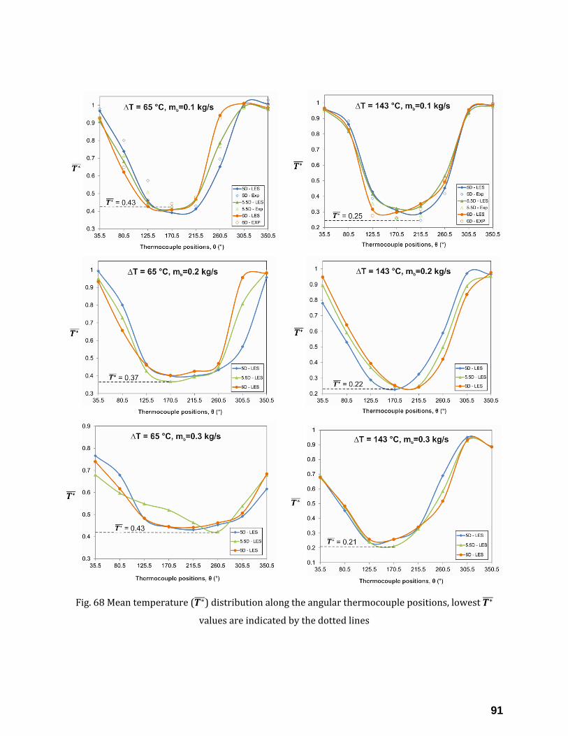
91

Fig. 68 Mean temperature (𝑻∗̅̅ ̅) distribution along the angular thermocouple positions, lowest 𝑻∗̅̅ ̅

values are indicated by the dotted lines

92

Fig. 69 Axial 𝑻∗̅̅ ̅ distribution along the angular positions, θ = 0°, 90°, 180° and 270°

4.3.2.2 Temperature fluctuation distribution

Fig. 70 shows the 𝑇𝑟𝑚𝑠∗ distribution at the T-junction along the streamwise direction. At ∆T =

65 °C, the weaker branch flow is easily deflected by the hot flow in case 1. The interface of

the hot-cold fluid region is also very thin. These characteristics change with rise in branch

flow rates (cases 1a and 1b) where the turbulent cold flow is now able to travel farther into

the main pipe and reaches the opposite wall at the highest branch flow rate of 0.3 kg/s (case

93

1b). Besides, the hot-cold fluid interface is also seen to broaden with rising branch flow

rates and is the principal location of highest 𝑇𝑟𝑚𝑠∗ amplitudes at the T-junction.

Fig. 70 Temperature fluctuations (𝑻𝒓𝒎𝒔∗ ) at the T-junction along the streamwise direction

Peak 𝑇𝑟𝑚𝑠∗ amplitudes range between 36 – 43 % of ∆T (∆T in this context refers to individual

∆T in each case) in the investigated cases 1, 1a and 1b. At ∆T = 143 °C, the prevailing issue

at the lowest branch flow rate (case 4) is the significant intrusion of cold flow upstream of

the main pipe and hot flow in the branch pipe. Rise in branch flow rates (cases 4a, 4b)

increases the thickness of the hot-cold fluid interface, a focal point of peak 𝑇𝑟𝑚𝑠∗ amplitudes

(about 34 – 40 % of ∆T). Also, cold flow is able to travel farther into the main pipe close to

the opposite wall at the T-junction indicating the significant forced convection effects in

play.

The cross-sectional distribution of thermal fluctuations downstream of the T-junction is

illustrated in Fig. 71. Observations on the effect of increased branch flow rates at ∆T = 65 °C

is summarized as follows: While it has already been established that an unstably stratified

flow occurs in case 1, a doubling of 𝑚𝑏̇ (to 0.2 kg/s) causes increased mixing between fluids.

High amplitude 𝑇𝑟𝑚𝑠∗ are seen to shift towards the inner mixing interface between fluids

94

quite different from the stratified interface observed in case 1. Lowest 𝑇𝑟𝑚𝑠∗ values are still

observed close to the top indicating that the mixing is still incomplete. This scenario is

completely changed as the branch flow rate is increased to its highest level (0.3 kg/s in case

1b) where complete turbulent mixing of flows occur and distinct flow patterns that were

ascertained in cases 1 and 1a (like unstable stratification) does not occur here. Similar

observations on the effect of increased branch flow rates at ∆T = 143 °C is summarized as

follows: Mixing area increases and more high amplitude 𝑇𝑟𝑚𝑠∗ zones in the flow are

identified in case 4a [𝑚𝑏̇ – 0.2 kg/s] in comparison with case 4. Flow oscillations result in

slightly unstable stratification with lowest 𝑇𝑟𝑚𝑠∗ values observed near the top. A subsequent

rise in branch flow rate to 0.3 kg/s [case 4b] enhances and intensifies the mixing effects

observed in case 4a and the unmixed area is seen to be reduced even further. Highest 𝑇𝑟𝑚𝑠∗

amplitudes for all the cases at ∆T = 143 °C lie in the vicinity of the stratification layer.

Fig. 71 Cross-sectional thermal fluctuations (𝑻𝒓𝒎𝒔∗ ) with increase in branch flow rates at ∆T = 65 °C

(left) and ∆T = 143 °C (right)

95

Fig. 72 Thermal fluctuations (𝑻𝒓𝒎𝒔∗ ) at in-flow and in-structure thermocouple positions

Fig. 72 shows the change in 𝑇𝑟𝑚𝑠∗ amplitudes along the circumferential thermocouple

positions in response to increase in branch flow rates. 𝑇𝑟𝑚𝑠∗ amplitudes near the top and its

vicinity (θ = 35.5 °, 305.5 ° and 350.5 °) are seen to considerably increase with flow rates at

∆T = 65 °C and 143 °C. Angular positions of peak 𝑇𝑟𝑚𝑠∗ have changed as follows: at ∆T = 65

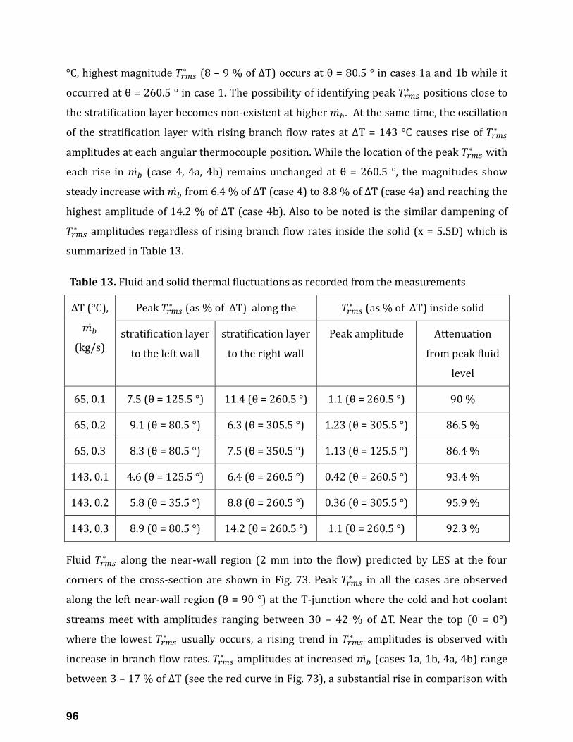
96

°C, highest magnitude 𝑇𝑟𝑚𝑠∗ (8 – 9 % of ∆T) occurs at θ = 80.5 ° in cases 1a and 1b while it

occurred at θ = 260.5 ° in case 1. The possibility of identifying peak 𝑇𝑟𝑚𝑠∗ positions close to

the stratification layer becomes non-existent at higher 𝑚𝑏̇ . At the same time, the oscillation

of the stratification layer with rising branch flow rates at ∆T = 143 °C causes rise of 𝑇𝑟𝑚𝑠∗

amplitudes at each angular thermocouple position. While the location of the peak 𝑇𝑟𝑚𝑠∗ with

each rise in 𝑚𝑏̇ (case 4, 4a, 4b) remains unchanged at θ = 260.5 °, the magnitudes show

steady increase with 𝑚𝑏̇ from 6.4 % of ∆T (case 4) to 8.8 % of ∆T (case 4a) and reaching the

highest amplitude of 14.2 % of ∆T (case 4b). Also to be noted is the similar dampening of

𝑇𝑟𝑚𝑠∗ amplitudes regardless of rising branch flow rates inside the solid (x = 5.5D) which is

summarized in Table 13.

Table 13. Fluid and solid thermal fluctuations as recorded from the measurements

∆T (°C),

𝑚𝑏̇

(kg/s)

Peak 𝑇𝑟𝑚𝑠∗ (as % of ∆T) along the 𝑇𝑟𝑚𝑠

∗ (as % of ∆T) inside solid

stratification layer

to the left wall

stratification layer

to the right wall

Peak amplitude Attenuation

from peak fluid

level

65, 0.1 7.5 (θ = 125.5 °) 11.4 (θ = 260.5 °) 1.1 (θ = 260.5 °) 90 %

65, 0.2 9.1 (θ = 80.5 °) 6.3 (θ = 305.5 °) 1.23 (θ = 305.5 °) 86.5 %

65, 0.3 8.3 (θ = 80.5 °) 7.5 (θ = 350.5 °) 1.13 (θ = 125.5 °) 86.4 %

143, 0.1 4.6 (θ = 125.5 °) 6.4 (θ = 260.5 °) 0.42 (θ = 260.5 °) 93.4 %

143, 0.2 5.8 (θ = 35.5 °) 8.8 (θ = 260.5 °) 0.36 (θ = 305.5 °) 95.9 %

143, 0.3 8.9 (θ = 80.5 °) 14.2 (θ = 260.5 °) 1.1 (θ = 260.5 °) 92.3 %

Fluid 𝑇𝑟𝑚𝑠∗ along the near-wall region (2 mm into the flow) predicted by LES at the four

corners of the cross-section are shown in Fig. 73. Peak 𝑇𝑟𝑚𝑠∗ in all the cases are observed

along the left near-wall region (θ = 90 °) at the T-junction where the cold and hot coolant

streams meet with amplitudes ranging between 30 – 42 % of ∆T. Near the top (θ = 0°)

where the lowest 𝑇𝑟𝑚𝑠∗ usually occurs, a rising trend in 𝑇𝑟𝑚𝑠

∗ amplitudes is observed with

increase in branch flow rates. 𝑇𝑟𝑚𝑠∗ amplitudes at increased 𝑚𝑏̇ (cases 1a, 1b, 4a, 4b) range

between 3 – 17 % of ∆T (see the red curve in Fig. 73), a substantial rise in comparison with

97

the less than 1.5 % of ∆T observed in cases 1 and 4. Reduction in cold flow penetration

upstream into the main pipe at ∆T = 143 °C is quantitatively confirmed in Fig. 73. While

thermocouple instrumentation is placed in the FSI test facility starting at x = 5D, LES

predictions indicate the occurrence of higher amplitude 𝑇𝑟𝑚𝑠∗ to occur within x = 0D to 5D in

the mixing zone. This is a valuable insight whereby additional thermocouple

instrumentation could be placed much closer to the T-junction in the near-wall region when

upgrading the FSI facility to operate at higher branch flow rates. This might reveal some

additional information that have gone unnoticed during previous measurements due to the

unavailability of thermocouples at those locations.

Fig. 73 LES predictions of fluid 𝑻𝒓𝒎𝒔∗ (2 mm in the flow) at θ = 0 °, 90 °, 180 ° and 270 °

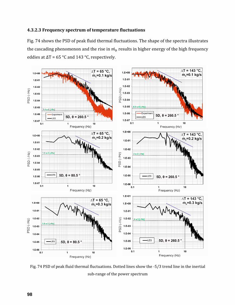
98

4.3.2.3 Frequency spectrum of temperature fluctuations

Fig. 74 shows the PSD of peak fluid thermal fluctuations. The shape of the spectra illustrates

the cascading phenomenon and the rise in 𝑚𝑏̇ results in higher energy of the high frequency

eddies at ∆T = 65 °C and 143 °C, respectively.

Fig. 74 PSD of peak fluid thermal fluctuations. Dotted lines show the -5/3 trend line in the inertial

sub-range of the power spectrum

99

Energy content of the temperature fluctuations remains fairly stable (0.1 - 1 [-/Hz] at

increased 𝑚𝑏̇ in cases 1a, 1b, 4a, and 4b) until the frequency of 3 Hz. Beyond this, a linear

type of decline in the energy content of fluctuations is noticed at elevated 𝑚𝑏̇ . At 10 Hz, the

energy of fluid thermal fluctuations at increased 𝑚𝑏̇ is considerably higher than at 𝑚𝑏̇ = 0.1

kg/s at ∆T = 65 °C and 143 °C, respectively.

Fig. 75 PSD of peak solid thermal fluctuations

100

No distinct peak in the power content of fluctuations was observed in the 0.1 – 1 Hz range

indicating that the relevance for thermal fatigue is not obvious from the in-flow monitor

points.

PSD of thermal fluctuations within the solid is shown in Fig. 75. The trend in the decline of

the energy content of thermal fluctuations is linear from 0.1 till 10 Hz at 𝑚𝑏̇ = 0.1 kg/s while

it continues to be linear beyond 10 Hz at 𝑚𝑏̇ = 0.2 kg/s and 0.3 kg/s at ∆T = 65 °C and 143

°C, respectively. Within this interval the power content of solid thermal fluctuations are

comparatively lower than the fluid fluctuations discussed in Fig. 75. Rise in 𝑚𝑏̇ increases

the energy content of thermal fluctuations within the solid at both ∆T = 65 °C and 143 °C as

shown in Fig. 74. No distinct peak in the energy content of solid thermal fluctuations was

observed.

Aside from the flow phenomenon discussed for the various inflow conditions in sections

4.1, 4.2 and 4.3, investigations at the FSI test facility related to various other inflow

temperatures and velocities within the scope of this study have also been published in the

existing literature [61, 62, 117, 118, 119, 120, 121, 122, and 123].

101

SUMMARY AND OUTLOOK

Thermal mixing characteristics of flows in a horizontal T-junction piping system with ∆T

between fluids ranging from 65 °C – 235 °C has been experimentally investigated at the

Fluid-Structure Interaction (FSI) test facility at the University of Stuttgart. Numerical

studies at the aforementioned ∆T range have also been performed using large-eddy

simulation turbulence model to gain more insights into the mixing behavior and to validate

the data against measurements. Hot fluid flow in the main pipe is turbulent (Reynolds

number: 15000 – 72000) while the cold flow is transitional (Reynolds number: 3100 –

3600) due to the operational limits of the booster pump used in the FSI test facility. The

traits of the mixed flow downstream of the T-junction could be summarized as follows:

Flow mixing is observed to be incomplete in all the investigated cases due to the low

Reynolds number flow from the branch pipe being insufficient to cause complete mixing

of fluids. Thus a thermally stratified flow pattern emerges after the mixing between

fluids at the T-junction.

The nature of the thermally stratified flow illustrates the difference caused by ∆T

between the mixing fluids. An unstable stratified flow being subjected to extreme

oscillations is seen at low ∆T (e.g. 65 °C) whereas the opposite case of stable

stratification is observed at higher ∆T (> 140 °C) between flows. This could be attributed

to the significant increase in buoyancy forces that is brought about by the substantial

increase in ∆T between fluids.

Strong turbulent penetration of hot fluid into branch pipe and vice versa was observed

at ∆T > 140 °C. Stable stratification also gives rise to strong thermal gradients between

the top and bottom of the pipe leading to bending of the structure at ∆T beyond 140 °C.

Mean temperature predictions by LES showed good agreement with measurement data.

Thermal fluctuations are seen to have the highest amplitudes near the stratification

layer as seen from both LES and measurement data. Comparison between measurement

and LES data exhibit reasonable agreement with one another with the exception of a few

positions where LES predictions either over- or understate measurement data.

Power spectral density (PSD) analysis of thermal fluctuations showed no dominant

frequency in the fatigue relevant range of 0.1 – 10 Hz and the energy of fluctuations are

102

contained mainly in the 0.1 – 1 Hz range. Comparison of PSD between measurement and

LES data exhibited good agreement with one another.

Beyond design LES analysis was also performed whereby thermal mixing of flows at

increased branch velocities (Reynolds number: 3100 – 11000) was performed at ∆T = 65 °C

and 143 °C, respectively. A transition from unstable thermal stratification to complete

mixing of fluids is observed at ∆T = 65 °C. Correspondingly, a similar transition from stable

stratification to unstable stratification in the flow marked by extreme oscillations was

observed at ∆T = 143 °C. These characteristics were confirmed by the mean and fluctuation

temperature distribution around the angular thermocouple positions in the mixing zone.

PSD of fluctuations still do not register a peak at increased flow velocities in the branch pipe

and the energy of fluctuations are contained mainly in the 0.1 – 3 Hz range. Thus thermal

mixing experiments have been performed in this study at realistic ∆T between fluids and

the thermocouples instrumentation in the vicinity of the T-junction provided valuable data

in identifying the nature of flow mixing behavior in response to changes in inflow

conditions. This was further reinforced by the application of high-fidelity CFD calculations

using the LES turbulence model to studying the flow mixing behavior which provided a

wealth of information that could not be otherwise obtained using instrumentation.

The results discussed above pertain to measurements in the FSI test facility where the

branch flow is not turbulent (Reynolds number: 3100 – 3600) due to its operating

limitations. The next level of advancement will be the upgradation of the facility to enable

turbulent flow conditions in the branch pipe (Reynolds number > 6000). The addition of

weld seams in the piping might reveal useful information on the influence of weld seams in

propagating the cracks in the mixing zone which is a realistic scenario encountered in

power plants. Leakage flow measurements for certain defined crack sizes in the piping

structure following the T-junction under different inflow conditions is another ongoing

research area which is an attempt to answer questions regarding the leakage following the

through-wall cracks in the structure.

103

BIBLIOGRAPHY

1. Abib, E., Bergholz, S., Rudolph, J. German experiences in local fatigue monitoring.

International Journal for Nuclear Power, vol. 58, pp. 284 – 289 (2013).

2. Addad, Y., Gaitonde, U., Laurence, D., Rolfo, S. Optimal unstructured meshing for large

eddy simulations. ERCOFTAC Series, Quality and Reliability of Large-Eddy Simulations,

vol. 12, Springer, pp. 93–103 (2008).

3. Ancelet, O., Chapuliot, S., Henaff, G. Comparative analysis of three thermal fatigue

experiments. Fatigue and Fracture of Engineering Materials and Structures, vol. 31, pp.

788 – 802 (2008).

4. Angele, K. MOTHER: Modelling T-junction heat transfer – A project in the NULIFE

framework portfolio. CONSORTIUM AGREEMENT–Number 8610 – AAP – 5910083925.

Vattenfall R&D, EDF, PSI, NRG, TU-D, Onsala, SPG, CEA, E-ON and AREVA (2013).

http://s538600174.onlinehome.fr/nugenia/wp-

content/uploads/2014/02/NUGENIA_MOTHER1.pdf

5. ANSYS CFX-Solver Modeling Guide (2011).

6. ANSYS CFX-Solver Theory Guide (2011).

7. ANSYS, Best Practice: Scale-Resolving Simulations in ANSYS CFD (2015).

8. Aufort, P., Bimont, G., Chau, T. H., Fournier, I., Morilhat, P., Souchois, T., Codrdier, G. On

Line Fatiguemeter: a Large Experiment in French Nuclear Plants, Nuclear Engineering

and Design, vol. 129, pp. 177-184 (1991).

9. Aulery, F., Toutant, A., Monod, R., Brillant, G., Bataille, F. Numerical simulations of

sodium mixing in a T-junction. Applied Thermal Engineering 37, pp. 38-43 (2012).

10. Ayhan, H., Sökmen, C.N., 2012. CFD modeling of thermal mixing in a T-junction geometry

using LES model. Nuclear Engineering and Design, vol. 253, pp. 183 – 191 (2012).

11. Barth, T.J., and Jesperson, D.C. The Design and Application of Upwind Schemes on

Unstructured Meshes, AIAA Paper 89-0366 (1989).

http://arc.aiaa.org/doi/pdf/10.2514/6.1989-366

12. Beaufils, R., Courtin. Analysis of the Father Experiment with an Engineering Method

Devoted to High Cycle Thermal Fatigue. In: Proceedings of the ASME 2011 Pressure

Vessels & Piping Conference (PVP 2011), Baltimore, Maryland, USA, July 17-21, 2011.

104

13. Blanchard, J.N., Brunet, Y., Merlen, A. Influence of a counter rotating vortex pair on the

stability of a jet in a cross flow: an experimental study by flowvisualizations.

Experiments in Fluids, vol. 26, pp. 63–74 (1999).

14. Braillard, O., Edelin, D. Advanced experimental tools designed for the assessment of the

thermal load applied to the mixing tee and nozzle geometries in the PWR plant. In:

Advancements in Nuclear Instrumentation, Measurement Methods and their

Applications, ANIMMA 2009, Marseille, France, June 7–10, 2009.

15. Brunnings, J.E. LMFBR Thermal-Striping Evaluation, EPRI NP-2672, Project 1704-11,

Interim Report (1982). http://www.osti.gov/scitech/servlets/purl/6887039

16. Chapuliot, S., Gourdin, C., Payen, T., Magnaud, J.P., Monavon, A. Hydro-thermal-

mechanical analysis of thermal fatigue in a mixing tee. Nuclear Engineering and Design,

vol. 235, pp. 575 – 596 (2005).

17. Chen, M.S., Hsieh, H.E., Ferng, Y.M., Pei, B.S. Experimental observations of thermal mixing

characteristics in T-junction piping. Nuclear Engineering and Design, vol. 276, pp. 107 –

114 (2014).

18. Courtin, S. High Cycle Thermal Fatigue Damage Prediction in Mixing Zones of Nuclear

Power Plants: Engineering Issues Illustrated on the FATHER Case. Procedia Engineering,

vol. 66, pp. 240 – 249 (2013).

19. Courtin, S., Beaufils, R. Engineering Analyses on the High Cycle Thermal Fatigue FATHER

Case. In: International Conference on Structural Mechanics in Reactor Technology

(SMiRT-21), India, November 6-11, 2011.

20. Courtin, S., Duff, J. A. L., Tacchini, B., Fissolo, A., Vincent, L., Stephan, J. M., Tampigny, R.

High Cycle Thermal Fatigue FATHER Experiment: Non Destructive and Metallographic

Examinations. In: International Conference on Structural Mechanics in Reactor

Technology (SMiRT-21), India, 2011.

21. CSNI Integrity and Ageing Working Group. FAT3D – An OECD/NEA benchmark on

thermal fatigue in fluid mixing areas. NEA/CSNI/R(2005)2, 2005.

22. Curtit, F. INTHERPOL thermal fatigue test. In: Proceedings of the third international

conference on fatigue of nuclear reactor components, Seville, Spain, October 3 – 6, 2004.

NEA/CSNI/R(2004)21.

105

23. Curtit, F., Stephan, J,M. INTHERPOL thermal fatigue test. In: Proceedings of the ASME

Pressure Vessels and Piping Conference (PVP-2005), Denver, Colorado, USA, July 17-21,

2005.

24. Dahlberg, M., Nilsson, K.F., Taylor, N., Faidy, C., Wilke, U., Chapuliot, S., Kalkhof,

D.,Bretherton, I., Church, J.M., Solin, J., Catalano, J. Development of a European procedure

for assessment of high cycle thermal fatigue in light water reactors. Final Report of the

NESC-Thermal Fatigue Project, EUR 22763 EN, ISSN 1018-5593, 2007.

25. Deardorff, A, F., McGill, R. O. Materials Reliability Program: Third International

Conference on Fatigue in Reactor Components (MRP-151), EPRI, Palo Alto, CA, 2005.

26. Duff, J. A. L., Tacchini, B., Stephan, J,M., Tampigny, R., Fissolo, A., Vincent, L. High cycle

thermal fatigue issues in RHRS mixing tees and thermal fatigue test on a representative

304L mixing zone. In: Proceedings of the ASME Pressure Vessels and Piping Conference

(PVP-2011), Baltimore, Maryland, USA, July 17-21, 2011.

27. ELECTRONIC SENSOR GmbH. Common technical data of sheathing thermocouple:

http://www.electronic-sensor.com/en/sheathing-thermocouple

28. Emerson Electric Co. Technical details of the micro-motion flow and density meters:

http://www2.emersonprocess.com/siteadmincenter/PM%20Micro%20Motion%20Doc

uments/F-Series-PDS-PS-00603.pdf

29. EPRI: Material Reliability Program: Assessment of Residual Heat Removal Mixing Tee

Thermal Fatigue in PWR Plants (MRP-192, Revision 2), 1024994, August 2012.

30. Faidy, C. Thermal fatigue in French RHR system. In: Proceedings of International

conference on Fatigue of Reactor Components, Napa, California, USA, July 31 - August 2,

2000.

31. Faidy, C. High Cycle Thermal Fatigue: Lessons Learned From Civaux Event. In: Materials

Reliability Program: Second International Conference on Fatigue of Reactor Components

(MRP-84), Snowbird, Utah, July 29 – August 1, 2002.

32. Fissolo, A., Forestier, A., Chapuliot, S., Gourdin, C., Magnaud, J.P., Ducros, F., Quéméré, P.,

Emonot, P., Chatelain, A., Dolias, Y., Braillard, O., Vincent, L., Robertson, C., Guilbaud, D.,

Le Corre, L., Maillot, V., Haddar, N., Amiable, S., Constantinescu, A., Degallaix, G.,

Degallaix, S. Advances in thermal fatigue investigations performed in CEA for French

106

PWR piping. In: Materials Reliability Program: Third International Conference on

Fatigue in Reactor Components (MRP-151), EPRI, 1011958, Palo Alto, CA, 2005.

33. Frank, Th., Lifante, C., Prasser, H.-M., Menter, F. Simulation of turbulent and thermal

mixing in T-junctions using URANS and scale-resolving turbulence models in ANSYS

CFX. Nuclear Engineering and Design, vol. 240, pp. 2313 – 2328 (2010).

34. Fric, T. F., and Roshko, A. Vortical structure in the wake of a transverse jet. Journal of

Fluid Mechanics, vol. 279, pp. 1 – 47 (1994).

35. Galpin, J., Simoneau, J.P. Large eddy simulation of a thermal mixing tee in order to

assess the thermal fatigue. International Journal of Heat and Fluid Flow, vol. 32, pp. 539

– 545 (2011).

36. Gao, K., Wang, P., Lu, T., Song, T. Experimental investigation and numerical simulation

for weakening the thermal fluctuations in a T-junction. Annals of Nuclear Energy, vol. 78,

pp. 180-187 (2015).

37. Gauder, P., Selvam, P.K., Kulenovic, R., Laurien, E. Large eddy simulation studies on the

influence of turbulent inlet conditions on the flow behavior in a mixing tee. Nuclear

Engineering and Design, vol. 298, pp. 51 – 63 (2016).

38. Golembiewski, H.-J and Miksch, M. Fatigue monitoring in German nuclear power plants.

Nuclear Engineering and Design, vol. 144, pp. 409 – 421 (1993).

39. Golembiewski, H.-J., Kleinöder, W. Monitoring for fatigue-Examples for unexpected

component loading. In: International conference on Nuclear Energy in Central Europe,

Bled, Slovenia, September 11-14, 2000.

40. Haddar, N., Fissolo, A., Maillot, V. Thermal fatigue crack networks: an computational

study. International Journal of Solids and Structures, vol. 42, pp. 771-788 (2005).

41. Hannink, M.H.C., Blom, F.J. Numerical methods for the prediction of thermal fatigue due

to turbulent mixing. Nuclear Engineering and Design, vol. 241, pp. 681 – 687 (2011).

42. Höhne, T. Scale resolved simulations of the OECD/NEA-Vattenfall T-junction benchmark.

Nuclear Engineering and Design, vol. 269, pp. 149 – 154 (2014).

43. Hosseini, S.M., Yuki, K., Hashizume, H. Classification of turbulent jets in a T-junction area

with a 90-deg bend upstream. International Journal of Heat and Mass Transfer, vol. 51,

pp. 2444 – 2454 (2008).

107

44. Howard, R.J.A., Serre, E. Large-eddy simulation in a mixing tee junction: High-order

turbulent statistics analysis. International Journal of Heat and Fluid Flow, vol. 51, pp. 65 –

77 (2015).

45. Hu, L.W., Kazimi, M.S. LES benchmark study of high cycle temperature fluctuations

caused by thermal striping in a mixing tee. International Journal of Heat and Fluid Flow,

vol. 27, pp. 54 – 64 (2006).

46. IAEA. Validation of Fast Reactor Thermomechanical and Thermalhydraulic Codes,

Report, TECDOC-1318, International Atomic Energy agency, Vienna, 2002.

47. IAEA. Assessment and Management of Ageing of Major Nuclear Power Plant

Components Important to Safety: Primary piping in PWRs. IAEA-TECDOC 1361. Vienna,

Austria, 2003.

48. International Atomic Energy Agency (IAEA) Pris Database. www.iaea.org/pris

49. Jayaraju, S.T., Komen, E.M.J., Baglietto, E. Suitability of wall-functions in Large Eddy

Simulation for thermal fatigue in a T-junction. Nuclear Engineering and Design, vol. 240,

pp. 2544 – 2554 (2010).

50. Jhung, M.J. Assessment of thermal fatigue in mixing tee by FSI analysis. Nuclear

Engineering and Technology, vol. 45, pp. 99 – 106 (2013).

51. Johnson I.D. Method and apparatus for measuring water in crude Oil, United States

Patent, No: 4,644,263 (1987).

52. JSME. Guideline for evaluation of high-cycle thermal fatigue of a pipe. In: JSME, S017-

2003.

53. Kader, B.A. Temperature and Concentration Profiles in Fully Turbulent Boundary

Layers. International Journal of Heat and Mass Transfer, vol. 24, pp. 1541 – 1544 (1981).

54. Kamide, H., Igarashi, M., Kawashima, S., Kimura, N., Hayashi, K. Study on mixing behavior

in a tee piping and numerical analyses for evaluation of thermal striping Nuclear

Engineering and Design, vol. 239, pp. 58 – 67 (2009).

55. Kasahara, N., Hasebe, S., Kobaysashi, S., Masanori, A., Kawasaki, N., Morita, H. SPECTRA

thermal fatigue tests under frequency controlled fluid temperature variation –

Development of test equipment and preliminary tests. In: Proceedings of the Pressure

Vessels & Piping Conference (PVP) – Elevated temperature and design analysis,

108

nonlinear analysis, and plastic components, San Diego, California, USA, July 25 – 29,

2004.

56. Kasahara, N., Kimura, N., Kamide, H. Thermal fatigue evaluation method based on power

spectrum density functions against fluid temperature fluctuation. In: Proceedings of the

ASME 2005 Pressure Vessels & Piping Conference (PVP 2005), Denver, Colorado, USA,

July 17-21, 2005.

57. Kasahara, N., Takasho, H., Yacumpai, A. Structural response function approach for

evaluation of thermal striping phenomena. Nuclear Engineering and Design, vol. 212, pp.

281 – 292 (2002).

58. Kawamura, T., Shiina, K., Ohtsuka, M. Study on high-cycle fatigue evaluation for thermal

striping in mixing tees with hot and cold water. In: 11th Int. Conf. Nuclear Engineering,

ICONE-11, Tokyo, Japan, April 20 – 23, 2003.

59. Kickhofel, J. L. Mixing phenomena relevant to thermal fatigue in T-junctions. Doctoral

dissertation, No. 22904, ETH Zürich (2015).

http://e-collection.library.ethz.ch/eserv/eth:48693/eth-48693-02.pdf

60. Kickhofel, J., and Prasser, H.-M. Grid Sensor Package. European Patent Application

EP14198142, ETH-Invention-No. 2014-053, Priority date December 16, 2014.

61. Kickhofel, J., Prasser, H. M., Selvam, P.K., Kulenovic, R., Laurien, E. T-junction cross-flow

mixing with thermally driven density stratification. Nuclear Engineering and Design, vol.

309, pp. 23 – 39 (2016).

62. Kickhofel, J., Selvam, P.K., Kulenovic, R., Laurien, E., Prasser, H. M., Huber, H. Wire mesh

sensor for high temperature high pressure applications. In: Proceedings of the 16th

International Topical Meeting on Nuclear Reactor Thermalhydraulics (NURETH-16),

Chicago, USA, Paper – 13930, August, 30 – September 4, 2015.

63. Kickhofel, J., Valori, V., Prasser, H.-M. Turbulent penetration in T-junction branch lines

with leakage flow. Nuclear Engineering and Design, vol. 276, pp. 43–53 (2014).

64. Kimura, K. et al. Thermal striping in mixing tees with hot and cold water (Type A;

Characteristics of flow visualization and temperature fluctuations in collision type

mixing tees with same pipe diameter), NTHAS3: Third Korea-Japan Symposium on

Nuclear Thermal Hydraulics and Safety (NTHAS3), Korea, October 13–16, 2002.

109

65. Klören, D., and Laurien, E. Coupled Large-Eddy Simulation of thermal mixing in a T-

Junction, International Topical Meeting on Nuclear Reactor Thermalhydraulics,

NURETH-14, Ontario, Canada, 2011.

66. Klören, D., and Laurien, E. Large-Eddy Simulations of Stratified and Non-stratified T-

junction Mixing Flows. High Performance Computing in Science and Engineering ‘12:

Transactions of the High Performance Computing Center, Stuttgart (HLRS), pp. 311-324

(2013).

67. Klören, D., Kuschewski, M., Laurien, E. Large-eddy simulations of stratified flows in pipe

configurations influenced by a weld seam. In: Proc. of the CFD for Nuclear Reactor Safety

Applications (CFD4NRS) Workshop, Daejon, Korea (2012).

68. KTA 3201.1. Components of the Reactor Coolant Pressure Boundary of Light Water

Reactors – Part 1: Materials and Product Forms (1998).

http://www.kta-gs.de/e/standards/3200/3201_1_engl_1998_06.pdf

69. KTA 3201.4. Components of the Reactor Coolant Pressure Boundary of Light Water

Reactors Part 4: In-service Inspections and Operational Monitoring (1982).

http://www.kta-gs.de/e/standards/3200/3201_4_engl_2010_11.pdf

70. Kuczaj, A.K., Komen, E.M.J., Loginov, M.S. Large-eddy simulation study of turbulent

mixing in a T-junction. Nuclear Engineering and Design, vol. 240, pp. 2116 – 2122

(2010).

71. Kuhn, S., Braillard, O., Ničeno, B., Prasser, H.M. Computational study of conjugate heat

transfer in T-junctions. Nuclear Engineering and Design, vol. 240, pp. 1548 – 1557

(2010).

72. Kuschewski, M. Entwicklung und Anwendung von Strömungsmessverfahren zur

Untersuchung wandnaher Temperaturfelder. Doctoral dissertation, Universität

Stuttgart, No: D93, 2015.

73. Kuschewski, M., Kulenovic, R., Laurien, E. Experimental setup for the investigation of

fluid-structure interactions in a T-junction. Nuclear Engineering and Design, vol. 264, pp.

223 –230 (2013).

74. Kuschewski, M., Kulenovic, R., Laurien, E. Experimental Investigation of Stratified Pipe

Flow Mixing in a Horizontal T-Junction. In: Proc. of the CFD for Nuclear Reactor Safety

Applications (CFD4NRS) Workshop, Zürich, Switzerland, 2014.

110

75. Kweon, H. D., Kim, J. S., Lee, K. Y. Fatigue design of nuclear class 1 piping considering

thermal stratification. Nuclear Engineering and Design, vol. 238, pp. 1265–1274 (2008).

76. Launder, B. E., and Spalding, D. B. The numerical computation of turbulent flows.

Computer Methods in Applied Mechanics and Engineering, vol. 3, pp. 269 – 289 (1974).

77. Lawn, C. J. The attenuation of temperature oscillations by liquid metal boundary layers.

Nuclear Engineering and Design, vol. 42, pp. 209 – 222 (1977).

78. Lee, J.I., Hu, L.W., Saha, P., Kazimi, M.S. Numerical analysis of thermal striping induced

high cycle thermal fatigue in a mixing tee. Nuclear Engineering and Design, vol. 239, pp.

833 – 839 (2009).

79. Lejeail, Y., Kasahara, N. Thermal fatigue evaluation of cylinders and plates subjected to

fluid temperature fluctuations. International Journal of Fatigue, vol. 27, pp. 768 – 772

(2005).

80. Lin, C. H., Ferng, Y. M. Investigating thermal mixing and reverse flow characteristics in a

T-junction using CFD methodology. Applied Thermal Engineering, vol. 102, pp. 733 – 741

(2016).

81. Lydell, B., Riznic, J. OPDE – The international pipe failure data exchange project. Nuclear

Engineering and Design, vol. 238, pp. 2115 – 2123 (2008).

82. Mahaffy, J., Chung, B., Dubois, F., Ducros, F., Graffard, E., Heitsch, M., Henriksson, M.,

Komen, E., Moretti, F., Morii, T., Mühlbauer, P., Rohde, U., Scheuerer, M., Smith, B. L.,

Song, C., Watanabe, T., Zigh, G. Best practice guidelines for the use of CFD in nuclear

reactor safety applications. NEA/CSNI/R(2007)5, 2007.

83. Mathey, F., Cokljat, D., Bertoglio, J.P., Sergent,E. Assessment of the vortex method for

large eddy simulation inlet conditions. Progress in Computational Fluid Dynamics, vol. 6,

pp. 58 – 67, (2006).

84. McDevitt, M., Childress, T., Hoehn, M., McGill, R. Analysis and impact of recent thermal

fatigue operating experience in the USA. In: Proceedings of the fourth international

conference on fatigue of nuclear reactor components, Seville, Spain, 28 September –

October 1, 2015.

85. Metzner, K.-J., Wilke, U. European THERFAT project—thermal fatigue evaluation of

piping system “Tee”-connections. Nuclear Engineering and Design, vol. 235, pp. 473–484

(2005).

111

86. Miyoshi, K., Kamaya, M., Utanohara, Y., Nakamura, A. An investigation of thermal stress

characteristics by wall temperature measurements at a mixing tee. Nuclear Engineering

and Design, vol. 298, pp. 109 – 120 (2016).

87. Miyoshi, K., Nakamura, A., Takenaka, N. Numerical evaluation of wall temperature

measurement method developed to estimate thermal stress at T-junction pipe.

Mechanical Engineering Journal 1 (2), tep0006 (2014).

88. Miyoshi, K., Nakamura, A., Utanohara, Y., Takenaka, N. An investigation of wall

temperature characteristics to evaluate thermal fatigue at a T-junction pipe. Mechanical

Engineering Journal 1 (5), tep0050 (2014).

89. Naik-Nimbalkar, V.S., Patwardhan, A.W., Banerjee, I., Padmakumar, G., Vaidyanathan, G.

Thermal mixing in T-junctions. Chemical Engineering Science, vol. 65, pp. 5901 – 5911

(2010).

90. Nakamura, A., Oumaya, T., Takenaka, N. Numerical investigation of thermal striping at a

mixing tee using detached eddy simulation. In: Proc. of the 13th International Topical

Meeting on Nuclear Reactor Thermal Hydraulics (NURETH-13), N13P1074 (2009).

91. Ndombo, J., Howard, R.J.A. Large Eddy Simulation and the effect of the turbulent inlet

conditions in the mixing Tee. Nuclear Engineering and Design, vol. 241, pp. 2172 – 2183

(2011).

92. NEA. Specialists meeting on experience with thermal fatigue in LWR piping caused by

mixing and stratification, NEA/CSNI/R(98)8, OECD Nuclear Energy Agency, Issy-les-

Moulineaux, France, 1998.

93. Nicoud, F., Ducros, F. Subgrid-scale modelling based on the square of the velocity

gradient tensor. Flow, Turbulence and Combustion, vol. 62, pp. 183 – 200 (1999).

94. Nuclear power reactors in the world, May 2016. Reference data series no. 2,

International atomic energy agency (IAEA).

95. Nuclear Power: http://www.nuclear-power.net/nuclear-power-plant/

96. Odemark, Y., Green, T.M., Angele, K., Westin, J., Alavyoon, F., Lundström, S. High-cycle

thermal fatigue in mixing tees: New Large-Eddy Simulations validated against new data

obtained by PIV in Vattenfall experiment. In: ICONE17 Proceedings, July 12–16, 2009,

Brussels, Belgium.

112

97. Ogawa, H., Igarashi, M., Kimura, N., Kamide, H. Experimental study on fluid mixing

phenomena in T-pipe junction with upstream elbow. In: Proc. of the 11th International

Topical Meeting on Nuclear Reactor Thermal Hydraulics (NURETH-11), Avignon, France,

(2005).

98. Paffumi, E., Nilsson, K. F., Szaraz, Z.. Experimental and numerical assessment of thermal

fatigue in 316 austenitic steel pipes. Engineering Failure Analysis, vol. 47, pp. 312–327

(2015).

99. Paffumi, E., Nilsson, K-F., Taylor, N., Hurst, R., Bache, M.R. Cracks initiation, propagation

and arrest in 316L model pipe components under thermal fatigue. Journal of ASTM

International 2(5), pp. 1 – 18 (2005).

100. Paffumi, E., Nilsson, K-F., Taylor, N.G. Simulation of thermal fatigue damage in a 316L

model pipe component. International Journal of Pressure Vessels and Piping, vol. 85, pp.

798–813 (2008).

101. Pasutto, T., Péniguel, C., Sakiz, M. Chained computations using an unsteady 3D

approach for the determination of thermal fatigue in a T-junction of a PWR nuclear

plant. Nuclear Engineering and Technology, vol. 38, pp. 147 – 154 (2006).

102. Peña, H.F.V., and Rodriguez, O.M.H. Applications of wire-mesh sensors in multiphase

flows. Flow Measurement and Instrumentation, vol. 45, pp. 255-273 (2015).

103. Piomelli, U.. An introduction to direct and large-eddy simulations. In: CFD2001, 9th

Annual Conference of the CFD Society of Canada, Kitchener, Canada, 2001.

104. Pöckl, C., Kleinöder, W. Developing and implementation of a fatigue monitoring

system for the new European pressurized water reactor EPR. International conference

on nuclear energy for new Europe, Slovenia, September 10-13, 2007.

105. Pope, S.B. Turbulent Flows. Cambridge University Press, Cambridge, United Kingdom

(2000).

106. Prasser, H. –M., Böttger, A., Zschau, J. A new electrode-mesh tomograph for gas–

liquid flow. Flow Measurement and Instrumentation, vol. 9, pp. 111 – 119 (1998).

107. Prasser, H.-M. Generalized cross-correlation technique for the measurement of time-

dependent velocities. In: Proceedings of the 15th international topical meeting on

nuclear reactor thermal-hydraulics (NURETH-15), May 12-17, 2013, Pisa, Italy.

108. Reinecke, N., Boddem, M., Petritsch, G., Mewes, D., 1996. Tomographisches Messen

113

der relativen Phasenanteile in zweiphasigen Stroemungen fluider Phasen, Chemie

Ingenieur Technik, vol. 68(11), pp. 1404-1412.

109. Riccardella, P. C., Kuo, A. Y., Tang, S. S., Gustin, H. L. FatiguePro: On-Line Fatigue

Usage Transient Monitoring System, EPRI NP-5835M, Electric Power Research Institute

(1988).

110. Richardson, L. F. Weather prediction by numerical process. Cambridge university

press (1922).

111. RICHTER Wärmebehandlungen GmbH. Technical details of the heat treatment unit:

http://www.richter-waerme.de/de/gluehanlagen

112. Rosinski, S. Proceedings of the 2000 International Conference on Fatigue of Reactor

Components (MRP-46): PWR Materials Reliability Program (PWRMRP), EPRI, Palo Alto,

CA, and Organisation for Economic Co-operation and Development

(OECD/NEA/CSNI/R[2000] 24), and the U.S. NRC (2001).

113. Rosinski, S. Materials Reliability Program: Second International Conference on

Fatigue of Reactor Components (MRP-84), EPRI, Palo Alto, CA, and Organisation for

Economic Co-operation and Development (OECD/NEA/CSNI/R[2003] 2), and the U.S.

NRC (2003).

114. Sagaut, P. Large Eddy Simulation for Incompressible Flows – An Introduction (Third

edition). ISBN 978-3-540-26403-3 (2006), Springer-Verlag.

http://www.springer.com/gp/book/9783540263449

115. SAMSOMATIC GmbH. Technical details of Electric Transmitter for pressure and

absolute pressure measurement: http://www.samsomatic.de/pdf/t39940050en.pdf

116. Schuler, X., Laurien, E., Herter, K.-H., Moogk, S., Klören, D., Kulenovic, R., Kuschewski,

M. Thermal fatigue: Fluid-structure interaction at thermal mixing events, 38th MPA

Seminar: "Energieerzeugung und Energieeffizienz - Werkstoffe und Bauteilverhalten",

Stuttgart, 2012.

117. Selvam, P.K., Kulenovic, R., Laurien, E. Large Eddy Simulation on Thermal Fluid

Mixing in a T-Junction Piping System. International Journal for Nuclear Power, Vol. 59,

Issue 11, pp. 648-649 (2014).

118. Selvam, P.K., Kulenovic, R., Laurien, E. Large eddy simulation of fluid mixing at high

temperature differences in a T-junction piping system. In: Proceedings of the

114

International Congress on Advances in Nuclear Power Plants (ICAPP), April 6 - 9, 2014,

Charlotte, NC, USA.

119. Selvam, P.K., Kulenovic, R., Laurien, E., 2015. Experimental and numerical analyses of

turbulent mixing of coolant streams in a mixing tee. In: Proceedings of the Fourth

International Conference on Fatigue of Nuclear Reactor Components, Seville, Spain,

Paper – 40, September 28 – October 1, 2015.

120. Selvam, P.K., Kulenovic, R., Laurien, E. Experimental Investigation of High Cycle

Thermal Fatigue in a T-Junction Piping System. International Journal for Nuclear Power,

Vol. 60, Issue 10, pp. 606-608 (2015).

121. Selvam, P.K., Kulenovic, R., Laurien, E. Large eddy simulation on thermal mixing of

fluids in a T-junction with conjugate heat transfer. Nuclear Engineering and Design, vol.

284, pp. 238 – 246 (2015).

122. Selvam, P.K., Kulenovic, R., Laurien, E. Numerical analyses of influence of branch flow

on thermal mixing in a T-junction piping system. In: Proceedings of the 16th

International Topical Meeting on Nuclear Reactor Thermalhydraulics (NURETH-16),

August, 30 – September 4, 2015, Chicago, USA, Paper – 12873.

123. Selvam, P.K., Kulenovic, R., Laurien, E. Experimental and numerical analyses on the

effect of increasing inflow temperatures on the flow mixing behavior in a T-junction.

International Journal of Heat and Fluid Flow, vol. 61, part B, pp. 323 – 342 (2016).

124. Sergent, E. Vers une mthodolgie de couplage entre la simulation des grandes echelles

et les modles statistique. Ph.D. thesis, L’ecole centrale de Lyon (2002).

125. Smith, B. L. Identification and Prioritization of Generic Nuclear Safety Problems

Requiring CFD Analysis, Paper 75482, Proc. 17th Int. Conf. on Nuclear Engineering

(ICONE-17), July 12-16, 2009, Brussels, Belgium.

126. Smith, B. L. Assessment of CFD codes used in nuclear reactor safety simulations.

Nuclear Engineering and Technology, vol. 42, pp. 339-364 (2010).

127. Smith, B. L., Andreani, M., Bieder, U., Ducros, F., Graffard, E., Heitsch, M., Henrikkson,

M., Höhne, T., Houkema, M., Komen, E., Mahaffy, J., Menter, F., Moretti, F., Morii, T.,

Mühlbauer, P., Rohde, U., Scheuerer, M., Song, C. –H., Watanabe, T., Zigh, G. Assessment of

CFD Codes for Nuclear Reactor Safety Problems – revision 2 (OECD/NEA/CSNI/R(2014)

12), 2015.

115

128. Smith, B. L., Bestion, D., Hassan, Y. Experiments and CFD Code Applications to

Nuclear Reactor Safety (XCFD4NRS). Special Issue: Nuclear Engineering and Design, vol.

240, pp. 2075-2382 (2010).

129. Smith, B. L., Hassan, Y. CFD4NRS: Benchmarking of CFD Codes for Application to

Nuclear Reactor Safety. Special Issue: Nuclear Engineering and Design, vol. 238, pp. 443-

785 (2008).

130. Smith, B.L., Mahaffy, J.H., Angele, K. A CFD benchmarking exercise based on flow

mixing in a T-junction. Nuclear Engineering and Design, vol. 264, pp. 80 – 88 (2013).

131. Smith, B.L., Mahaffy, J.H., Angele, K., Westin, J. Report of the OECD/NEA-Vattenfall T-

Junction Benchmark exercise (2011).

132. Stephan, J,M., Curtit, F. Mechanical aspects concerning thermal fatigue initiation in

the mixing zones of piping. In: International Conference on Structural Mechanics in

Reactor Technology (SMiRT-18), China, August 7-12, 2005.

133. Suzuki, S., Tanimoto, K., Kondoh, Y. Prevention of piping high cycle thermal fatigue at

design stage. In: Proceedings of the Nuclear Pressure Equipment Expertise and

Regulation (NuPEER) symposium, June 22 – 24, 2005, Dijon, France.

134. Tenchine, D. Boundary layer attenuation in turbulent sodium flows. In: IAEA

Specialists Meeting on Correlation Between Material Properties and Thermal Hydraulic

Conditions in LMFBR, Aix en Provence, France, November 22–24, 1994.

135. Tenchine, D. Some thermal hydraulic challenges in sodium cooled fast reactors.

Nuclear Engineering and Design, vol. 240, pp. 1195 – 1217 (2010).

136. Timperi, A. Conjugate heat transfer LES of thermal mixing in a T-junction. Nuclear

Engineering and Design, vol. 273, pp. 483 – 496 (2014).

137. USNRC Bulletin 88-08. Thermal Stresses in Piping Connected to Reactor Coolant

Systems. Washington, D.C., U.S.A (1988).

138. USNRC Bulletin 88-08, Supplement 1: Thermal Stresses in Piping Connected to

Reactor Coolant Systems, June 24, 1988.

139. USNRC Bulletin 88-08, Supplement 2: Thermal Stresses in Piping Connected to

Reactor Coolant Systems, August 4, 1988.

140. USNRC Bulletin 88-08, Supplement 3: Thermal Stresses in Piping Connected to

Reactor Coolant Systems, April 11, 1989.

116

141. USNRC Bulletin 88-08: Thermal Stresses in Piping Connected to Reactor Coolant

Systems, June 22, 1988.

142. USNRC Bulletin 88-11: Pressurizer Surge Line Thermal Stratification, December 20,

1988.

143. Vermaut, M., Cranford, E. L., Gray, M. A., Barbier, C. Use of Westinghouse thermal

event monitoring system WESTEMS[TM] for on-line transient and fatigue monitoring.

In: Proceedings of the PLIM and PLEX conference, Prague, pp. 177 – 184 (1997).

144. Wagner, W., Kruse, A. Properties of water and steam. The industrial standard IAPWS-

IF97 for thermodynamic properties and supplementary equations for other properties.

Springer-Verlag, Berlin (1998).

145. Wakamatsu, M., Nei, H., Hashiguchi, K. Attenuation of temperature fluctuations in

thermal striping. Journal of Nuclear Science and Technology, vol. 32, pp. 752 – 762

(1995).

146. Walker, C., Manera, A., Niceno, B., Simiano, M., Prasser, H.-M. Steady-state RANS-

simulations of the mixing in a T-junction. Nuclear Engineering and Design, vol. 240, pp.

2107 – 2115 (2010).

147. Walker, C., Simiano, M., Zboray, R., Prasser, H.M. Investigations on mixing

phenomena in single-phase flow in a T-junction geometry. Nuclear Engineering and

Design, vol. 239, pp. 116 –126 (2009).

148. Wang, Y., Wang, P., Lu, T. Experimental investigation of the thermal fluctuations in

hot and cold fluids mixing in a T-junction filled with spherical particles. Applied Thermal

Engineering, vol. 71, pp. 310 – 316 (2014).

149. WESTEMSTM Integrated Diagnostics and Monitoring Systems.

http://www.westinghousenuclear.com/LinkClick.aspx?fileticket=uo6hKKcuEFw%3d&p

ortalid=0

150. Westin, J., ’t Mannetje, C., Alavyoon, F., Veber, P., Andersson, L., Andersson, U.,

Eriksson, J., Henriksson, M., Andersson, C. High-cycle thermal fatigue in mixing tees.

Large-Eddy Simulations compared to a new validation experiment. In: ICONE16

Proceedings, May 11–15, 2008, Orlando, FL, USA.

151. Westinghouse PWR manual

www4.ncsu.edu/~doster/NE405/Manuals/PWR_Manual.pdf

117

152. World Energy Outlook Special Report 2015 on Energy and Climate Change.

International Energy Agency

www.iea.org/publications/freepublications/publication/WEO2015SpecialReportonEne

rgyandClimateChange.pdf

153. World nuclear power reactors. http://www.world-nuclear.org/information-

library/facts-and-figures/world-nuclear-power-reactors-and-uranium-requireme.aspx

154. Yoo, B. Development of Fatigue Monitoring System in Nuclear Power Plants,

KAERI/RR-1307/93, Korea Atomic Energy Research Institute (1994).

155. Zboray, R., Manera, A., Niceno, B., Prasser, H.-M. Investigations on mixing phenomena

in single-phase flows in a T-junction geometry. In: Proceedings of the 12th international

topical meeting on nuclear reactor thermal-hydraulics (NURETH-15), September 30 –

October 4, 2007, Pittsburg, Pennsylvania, USA.

156. Zboray, R., Prasser, H.-M. On the relevance of low side flows for thermal loads in T-

junctions. Nuclear Engineering and Design, vol. 241, pp. 2881-2888 (2011).

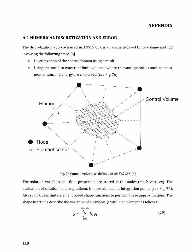
118

APPENDIX

A.1 NUMERICAL DISCRETIZATION AND ERROR

The discretization approach used in ANSYS CFX is an element-based finite volume method

involving the following steps [6]

Discretization of the spatial domain using a mesh

Using the mesh to construct finite volumes where relevant quantities such as mass,

momentum, and energy are conserved (see Fig. 76).

Fig. 76 Control volume as defined in ANSYS CFX [6]

The solution variables and fluid properties are stored at the nodes (mesh vertices). The

evaluation of solution field or gradients is approximated at integration points (see Fig. 77).

ANSYS CFX uses finite-element based shape functions to perform these approximations. The

shape functions describe the variation of a variable 𝜑 within an element as follows:

𝜑 = ∑ 𝑁𝑖𝜑𝑖

𝑁𝑛𝑜𝑑𝑒

𝑖=1

(29)

119

where 𝑁𝑖 is the shape function of the node i and 𝜑𝑖 is the value of 𝜑 at node i. The

summation is performed all over the nodes of an element. The key properties of shape

function include

∑ 𝑁𝑖

𝑁𝑛𝑜𝑑𝑒

𝑖=1

= 1 (30)

At node j, 𝑁𝑖 = {1, 𝑖 = 𝑗0, 𝑖 ≠ 𝑗

Fig. 77 Mesh element as defined in ANSYS CFX

Fig. 78 Description of the hexahedral element used in the T-junction mesh

Shape functions used in ANSYS CFX are linear in terms of parametric coordinates. They are

used to calculate various geometric quantities, including integration point coordinates and

120

surface area vectors. It is possible due to the above equation (31) also hold valid for the

coordinates:

𝑦 = ∑ 𝑁𝑖𝑦𝑖

𝑁𝑛𝑜𝑑𝑒

𝑖=1

(32)

The tri-linear shape functions for the hexahedral mesh elements (see Fig. 78) used in this

study are given below:

𝑁1 (𝑠, 𝑡, 𝑣) = (1 − 𝑠)(1 − 𝑡)(1 − 𝑣)

𝑁2 (𝑠, 𝑡, 𝑣) = 𝑠(1 − 𝑡)(1 − 𝑣)

𝑁3 (𝑠, 𝑡, 𝑣) = 𝑠𝑡(1 − 𝑣)

𝑁4 (𝑠, 𝑡, 𝑣) = (1 − 𝑠)𝑡(1 − 𝑣)

𝑁5 (𝑠, 𝑡, 𝑣) = (1 − 𝑠)(1 − 𝑡)𝑣

𝑁6 (𝑠, 𝑡, 𝑣) = 𝑠(1 − 𝑡)𝑣

𝑁7 (𝑠, 𝑡, 𝑣) = 𝑠𝑡𝑣

𝑁8 (𝑠, 𝑡, 𝑣) = (1 − 𝑠)𝑡𝑣

The evaluation of gradients might be required in some situations at the nodes and ANSYS

CFX uses a formulation of Gauss’s divergence theorem to evaluate such gradients which are

defined as follows:

∇𝜑 =1

𝑉∑(𝜑 ∆�⃗� )𝑖𝑝𝑖𝑝

(33)

Where V is the element volume and ∆�⃗� is the outward surface vector at the integration

point. Thus the above formulation requires 𝜑 to be evaluated at integration points using

shape-functions.

Also, the advection term requires the integration point values of 𝜑 to be approximated in

terms of the nodal values of 𝜑, which is implemented in ANSYS CFX as follows

𝜑𝑖𝑝 = 𝜑𝑢𝑝 + 𝛽 ∇𝜑. ∆𝑟 (34)

where 𝜑𝑢𝑝 is the value of 𝜑 at the upwind node and 𝑟 is the vector from the upwind node to

the integration point. Individual choices of 𝛽 and ∇𝜑 yield different schemes.

121

Central Difference Scheme

Here the value of 𝛽 is set to 1 and ∇𝜑 is set to the local element gradient. Another form of

interpretation is that 𝜑𝑖𝑝 is evaluated using the tri-linear shape functions:

𝜑𝑖𝑝 = ∑𝑁𝑛(𝑥𝑖𝑝, 𝑦𝑖𝑝, 𝑧𝑖𝑝)𝜑𝑛

𝑛

(35)

Thus the resulting scheme is second-order accurate while an undesirable attribute is that

this scheme may suffer from serious decoupling issues.

High-Resolution Scheme

This scheme uses a non-linear recipe for 𝛽 at each node which is computed to be as close to

1 as possible without introducing new extrema. ∇𝜑 is evaluated using 𝛽 and ∇𝜑 from the

upwind node. The formulation of 𝛽 is based on the boundedness principles of Barth and

Jesperson [11] involving initial computation of 𝜑𝑚𝑖𝑛 and 𝜑𝑚𝑎𝑥 at each node using a stencil

involving adjacent nodes and including the node itself. Nextly, each integration point

around the node is solver for 𝛽 to ensure that 𝜑𝑚𝑖𝑛 is not undershot and 𝜑𝑚𝑎𝑥 is not

overshot. The equation used is the same as (36).

Nodal value for 𝛽 is taken to be the minimum value of all integration point values

surrounding the node and is not allowed to exceed 1.

Temporal discretization

The discretization of the transient term for the nth time step for control volumes that do not

deform in time is given by

𝜕

𝜕𝑡∫ 𝜌𝜑 𝑑𝑉 ≈ 𝑉

(𝜌𝜑)𝑛+12 − (𝜌𝜑)𝑛−

12

∆𝑡

𝑉

0

(37)

Values at the start and end of the time step are assigned the superscripts 𝑛 +1

2 and 𝑛 −

1

2,

respectively. These time step values for the second order backward Euler scheme used in

the present study is defined as

(𝜌𝜑)𝑛−12 = (𝜌𝜑)𝑜 +

1

2((𝜌𝜑)𝑜 − (𝜌𝜑)𝑜𝑜) (38)

(𝜌𝜑)𝑛+12 = 𝜌𝜑 +

1

2(𝜌𝜑 − (𝜌𝜑)𝑜) (39)

122

(40) and (41) substituted into (42) yields the resulting discretization as follows

𝜕

𝜕𝑡∫ 𝜌𝜑 𝑑𝑉 ≈

𝑉

∆𝑡(3

2(𝜌𝜑) − 2(𝜌𝜑)𝑜 +

1

2(𝜌𝜑)𝑜𝑜)

𝑉

0

(43)

The superscripts o and oo represent the first and second partial derivative, respectively.

This scheme is considered robust, implicit, conservative in time, second order accurate and

does not have a time step size limitation.

Pressure-Velocity Coupling

ANSYS CFX uses a co-located (non-staggered) grid layout such that the control volumes are

identical for all transport equations. More detailed explanation is available in the CFX-solver

theory guide [6].

Discretization Errors

Discretization Errors arise due to differences between the exact analytical solution of the

modeled differential equations and the fully converged solution of their discrete

representations. Like the principal variables being solved for, errors in these values are

generated both by localized sources and propagated (i.e. amplified, convected or diffused)

throughout the computational domain.

Localized sources of error result from high-order terms that are excluded from the discrete

approximations of terms in the modeled equations while error propagation results from the

form of terms that are included in the discrete approximations. The current simulations

performed using ANSYS CFX are second order accurate in space and time.

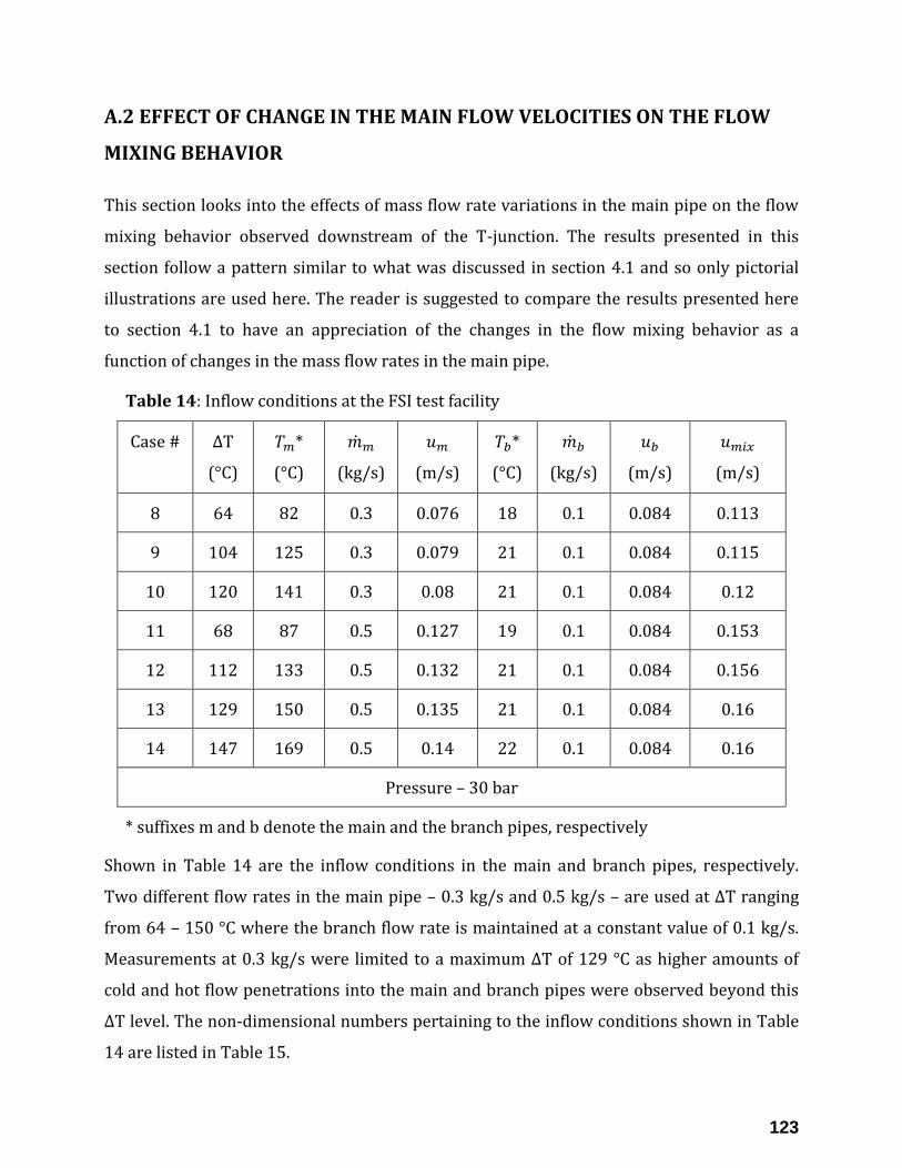
123

A.2 EFFECT OF CHANGE IN THE MAIN FLOW VELOCITIES ON THE FLOW

MIXING BEHAVIOR

This section looks into the effects of mass flow rate variations in the main pipe on the flow

mixing behavior observed downstream of the T-junction. The results presented in this

section follow a pattern similar to what was discussed in section 4.1 and so only pictorial

illustrations are used here. The reader is suggested to compare the results presented here

to section 4.1 to have an appreciation of the changes in the flow mixing behavior as a

function of changes in the mass flow rates in the main pipe.

Table 14: Inflow conditions at the FSI test facility

Case # ∆T

(°C)

𝑇𝑚*

(°C)

�̇�𝑚

(kg/s)

𝑢𝑚

(m/s)

𝑇𝑏*

(°C)

�̇�𝑏

(kg/s)

𝑢𝑏

(m/s)

𝑢𝑚𝑖𝑥

(m/s)

8 64 82 0.3 0.076 18 0.1 0.084 0.113

9 104 125 0.3 0.079 21 0.1 0.084 0.115

10 120 141 0.3 0.08 21 0.1 0.084 0.12

11 68 87 0.5 0.127 19 0.1 0.084 0.153

12 112 133 0.5 0.132 21 0.1 0.084 0.156

13 129 150 0.5 0.135 21 0.1 0.084 0.16

14 147 169 0.5 0.14 22 0.1 0.084 0.16

Pressure – 30 bar

* suffixes m and b denote the main and the branch pipes, respectively

Shown in Table 14 are the inflow conditions in the main and branch pipes, respectively.

Two different flow rates in the main pipe – 0.3 kg/s and 0.5 kg/s – are used at ∆T ranging

from 64 – 150 °C where the branch flow rate is maintained at a constant value of 0.1 kg/s.

Measurements at 0.3 kg/s were limited to a maximum ∆T of 129 °C as higher amounts of

cold and hot flow penetrations into the main and branch pipes were observed beyond this

∆T level. The non-dimensional numbers pertaining to the inflow conditions shown in Table

14 are listed in Table 15.

124

Table 15: Non-dimensional numbers calculated for all the cases

Case # ∆T

(°C)

∆𝜌 �̅�⁄

(in %) 𝑅𝑒𝑚 𝑅𝑒𝑏 Ri

𝑅𝑒𝑚 𝑅𝑒𝑏⁄

(R)

𝜇𝑚 𝜇𝑏⁄

8 64 2.8 15340 3100 1.56 4.95 0.33

9 104 6.5 24870 3340 3.43 7.45 0.22

10 120 8.4 28990 3340 4.36 8.68 0.18

11 68 3.2 27150 3220 0.95 8.43 0.32

12 112 6.7 42810 3340 1.94 12.8 0.21

13 129 8.6 49010 3340 2.4 14.7 0.18

14 147 10.7 55940 3420 2.9 16.4 0.16

Fig. 79 Instantaneous velocity field at the T-junction with �̇�𝒎 = 0.3 kg/s, �̇�𝒃 = 0.1 kg/s

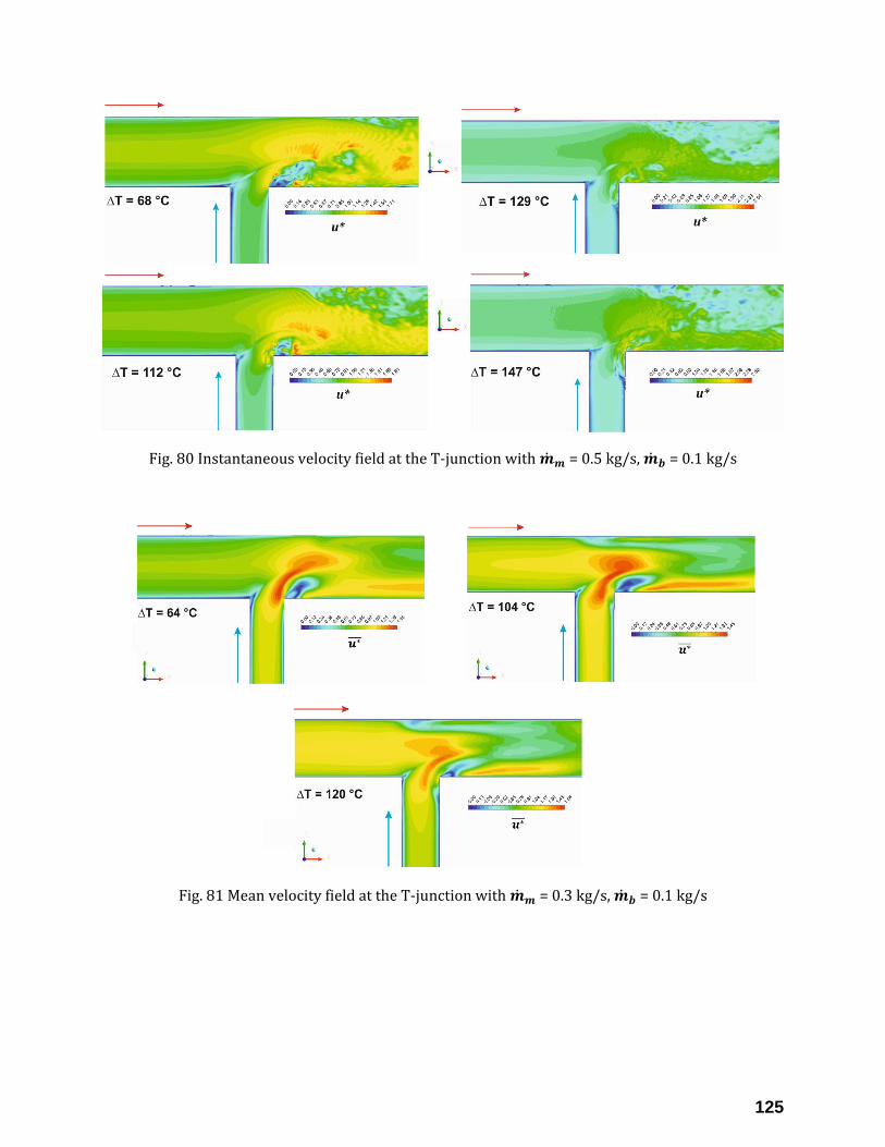
125

Fig. 80 Instantaneous velocity field at the T-junction with �̇�𝒎 = 0.5 kg/s, �̇�𝒃 = 0.1 kg/s

Fig. 81 Mean velocity field at the T-junction with �̇�𝒎 = 0.3 kg/s, �̇�𝒃 = 0.1 kg/s

126

Fig. 82 Mean velocity field at the T-junction with �̇�𝒎 = 0.5 kg/s, �̇�𝒃 = 0.1 kg/s

Fig. 83 Mean velocity field illustrating the CVP structurer with �̇�𝒎 = 0.3 kg/s, �̇�𝒃 = 0.1 kg/s

Fig. 84 Mean velocity field illustrating the CVP structurer with �̇�𝒎 = 0.5 kg/s, �̇�𝒃 = 0.1 kg/s

127

Fig. 85 Vortical structures illustrated using the Q-criterion in the vicinity of the T-junction with �̇�𝒎

= 0.3 kg/s, �̇�𝒃 = 0.1 kg/s

Fig. 86 Vortical structures illustrated using the Q-criterion in the vicinity of the T-junction with �̇�𝒎

= 0.5 kg/s, �̇�𝒃 = 0.1 kg/s

128

Fig. 87 Mean velocity field illustrating the entry of the cold fluid into the main pipe (�̇�𝒎 = 0.3 kg/s,

�̇�𝒃 = 0.1 kg/s)

Fig. 88 Mean velocity field illustrating the entry of the cold fluid into the main pipe (�̇�𝒎 = 0.5 kg/s,

�̇�𝒃 = 0.1 kg/s)

129

Fig. 89 Hot flow penetration into the branch pipe illustrated using mean temperature field along the

y-z axis (�̇�𝒎 = 0.3 kg/s, �̇�𝒃 = 0.1 kg/s)

Fig. 90 Hot flow penetration into the branch pipe illustrated using mean temperature field along the

y-z axis (�̇�𝒎 = 0.5 kg/s, �̇�𝒃 = 0.1 kg/s)

130

Fig. 91 Cold flow penetration into the main pipe illustrated using mean temperature field along the

x-z axis (�̇�𝒎 = 0.3 kg/s, �̇�𝒃 = 0.1 kg/s)

Fig. 92 Cold flow penetration into the main pipe illustrated using mean temperature field along the

x-z axis (�̇�𝒎 = 0.5 kg/s, �̇�𝒃 = 0.1 kg/s)

131

Fig. 93 Mean temperature field at the T-junction along the streamwise direction (�̇�𝒎 = 0.3 kg/s, �̇�𝒃

= 0.1 kg/s)

Fig. 94 Mean temperature field at the T-junction along the streamwise direction (�̇�𝒎 = 0.5 kg/s, �̇�𝒃

= 0.1 kg/s)

132

Fig. 95 Mean temperature field along the cross-sectional direction (�̇�𝒎 = 0.3 kg/s, �̇�𝒃 = 0.1 kg/s)

Fig. 96 Mean temperature field along the cross-sectional direction (�̇�𝒎 = 0.5 kg/s, �̇�𝒃 = 0.1 kg/s)

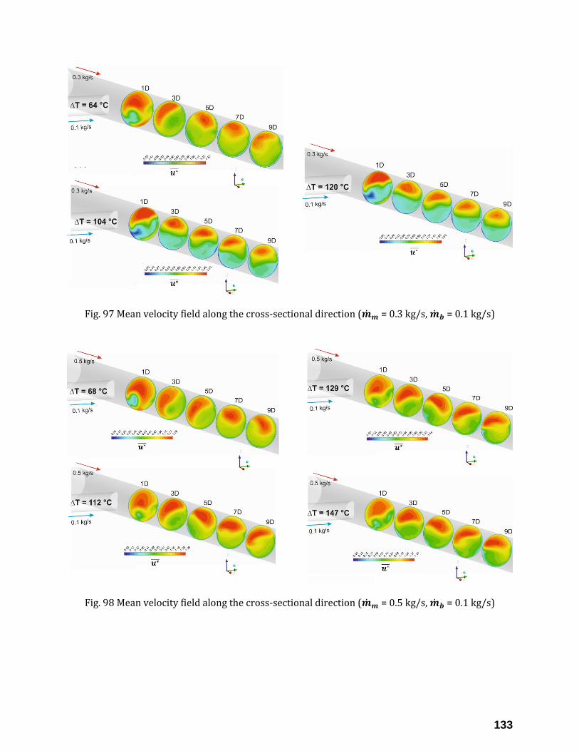
133

Fig. 97 Mean velocity field along the cross-sectional direction (�̇�𝒎 = 0.3 kg/s, �̇�𝒃 = 0.1 kg/s)

Fig. 98 Mean velocity field along the cross-sectional direction (�̇�𝒎 = 0.5 kg/s, �̇�𝒃 = 0.1 kg/s)

134

Fig. 99 Isosurfaces of mean temperature at 𝑻∗̅̅ ̅ = 0.75 (�̇�𝒎 = 0.3 kg/s, �̇�𝒃 = 0.1 kg/s)

Fig. 100 Isosurfaces of mean temperature at 𝑻∗̅̅ ̅ = 0.75 (�̇�𝒎 = 0.5 kg/s, �̇�𝒃 = 0.1 kg/s)

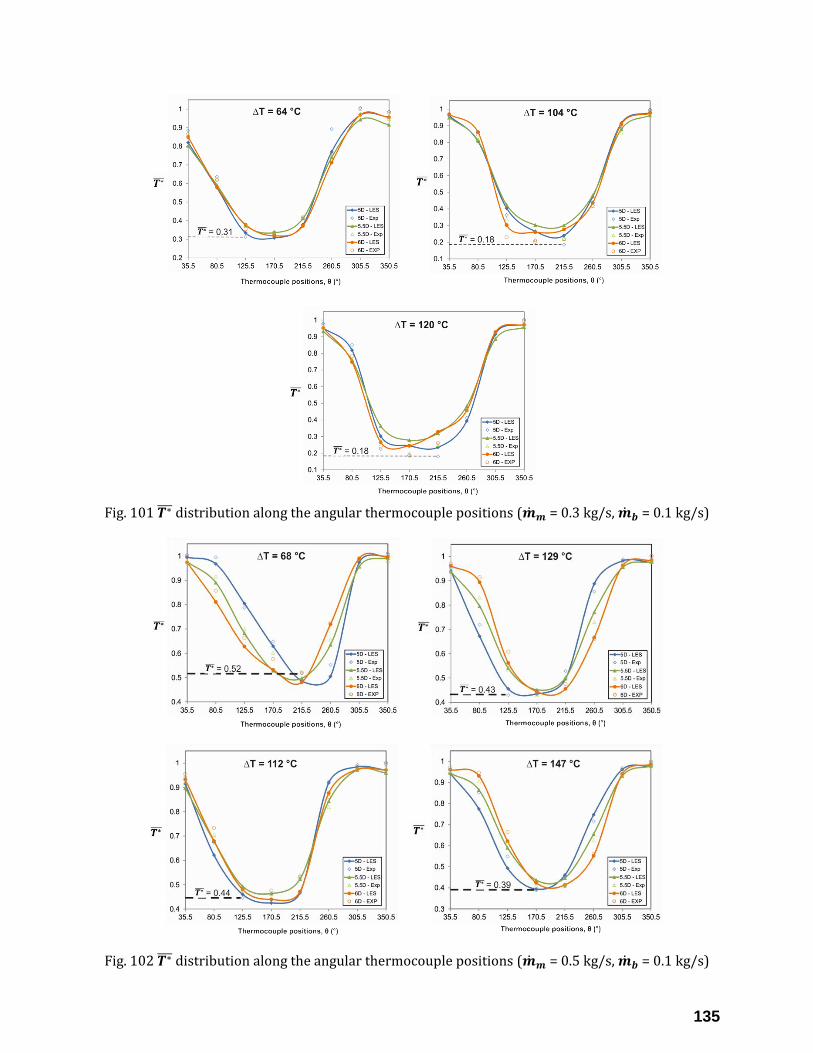
135

Fig. 101 𝑻∗̅̅ ̅ distribution along the angular thermocouple positions (�̇�𝒎 = 0.3 kg/s, �̇�𝒃 = 0.1 kg/s)

Fig. 102 𝑻∗̅̅ ̅ distribution along the angular thermocouple positions (�̇�𝒎 = 0.5 kg/s, �̇�𝒃 = 0.1 kg/s)

136

Fig. 103 Axial 𝑻∗̅̅ ̅ distribution at θ = 0°, 90°, 180° and 270° (�̇�𝒎 = 0.3 kg/s, �̇�𝒃 = 0.1 kg/s)

Fig. 104 Axial 𝑻∗̅̅ ̅ distribution at θ = 0°, 90°, 180° and 270° (�̇�𝒎 = 0.5 kg/s, �̇�𝒃 = 0.1 kg/s)

137

Fig. 105 Temperature fluctuations (𝑻𝒓𝒎𝒔∗ ) at the T-junction along the streamwise direction (�̇�𝒎 =

0.3 kg/s, �̇�𝒃 = 0.1 kg/s)

Fig. 106 Temperature fluctuations (𝑻𝒓𝒎𝒔∗ ) at the T-junction along the streamwise direction (�̇�𝒎 =

0.5 kg/s, �̇�𝒃 = 0.1 kg/s)

138

Fig. 107 𝑻𝒓𝒎𝒔∗ field along the cross-sectional direction (�̇�𝒎 = 0.3 kg/s, �̇�𝒃 = 0.1 kg/s)

Fig. 108 𝑻𝒓𝒎𝒔∗ field along the cross-sectional direction (�̇�𝒎 = 0.5 kg/s, �̇�𝒃 = 0.1 kg/s)

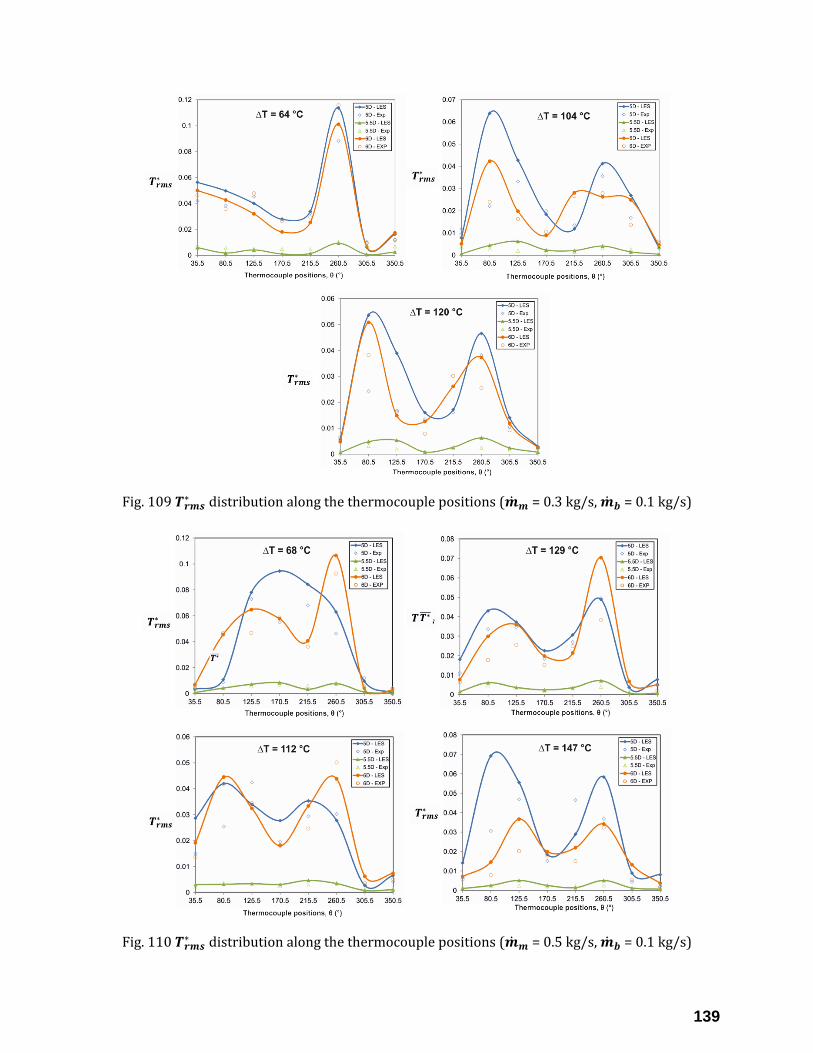
139

Fig. 109 𝑻𝒓𝒎𝒔∗ distribution along the thermocouple positions (�̇�𝒎 = 0.3 kg/s, �̇�𝒃 = 0.1 kg/s)

Fig. 110 𝑻𝒓𝒎𝒔∗ distribution along the thermocouple positions (�̇�𝒎 = 0.5 kg/s, �̇�𝒃 = 0.1 kg/s)

140

Fig. 111 𝑻𝒓𝒎𝒔∗ distribution at θ = 0°, 90°, 180° and 270° (�̇�𝒎 = 0.3 kg/s, �̇�𝒃 = 0.1 kg/s)

Fig. 112 𝑻𝒓𝒎𝒔∗ distribution at θ = 0°, 90°, 180° and 270° (�̇�𝒎 = 0.5 kg/s, �̇�𝒃 = 0.1 kg/s)

141

Fig. 113 PSD of peak fluid and solid thermal fluctuations (�̇�𝒎 = 0.3 kg/s, �̇�𝒃 = 0.1 kg/s)

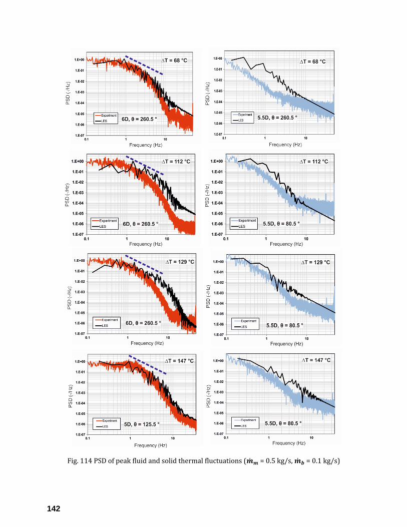
142

Fig. 114 PSD of peak fluid and solid thermal fluctuations (�̇�𝒎 = 0.5 kg/s, �̇�𝒃 = 0.1 kg/s)

143

A.3 MEASUREMENTS USING WIRE MESH SENSOR

The Laboratory of Nuclear Energy Systems at ETH Zürich has developed a conductivity

based wire-mesh sensor (WMS) for characterizing single-phase turbulent mixing processes

in T-junction piping systems encountered in industrial flows, e.g. piping system in power

plants, chemical reactor, combustion chamber. This sensor was successfully tested in the

Fluid-Structure Interaction (FSI) T-junction test facility, University of Stuttgart at its highest

operating temperature and pressure of 257 °C and 70 bar.

A measurement technique developed to obtain high density of information about the flow

with a high time resolution is the wire mesh sensor. The principle of WMS is based on a

matrix like arrangement of the measuring points. Two sets of wire electrodes,

perpendicular to each other, are stretched along the diameter of the pipe with a small axial

separation between them as illustrated in Fig. 115. The transmitter electrodes are activated

sequentially while the receiver electrodes are all parallel sampled such that the electrical

property of the fluid (conductivity or permittivity) is measured at each crossing point.

Processing the data at all the crossing points enables the instantaneous distribution of fluid

across the cross-section.

Fig. 115 Schematic view of a typical wire mesh sensor [102]

Wire-mesh sensors are widely used to characterize gas-liquid two-phase flows and single-

phase mixing processes. The first concept was patented by Johnson (1987) [51], who

proposed it for measuring the volumetric fraction of water in crude oil. The measurement of

two-dimensional hold-up profiles was achieved for the first time by Reinecke et al. (1996)

[108] by applying tomographic reconstruction techniques. A signal acquisition method

allowing a high spatial and temporal resolution without the need of a tomographic

144

reconstruction was introduced by Prasser et al. (1998) [106] and is currently in use in

numerous laboratories worldwide. A comprehensive overview of WMS in multiphase flows

is given by Peña and Rodriguez (2015) [102]. The past two decades witnessed successful

application of the WMS technology in both single- and multi-phase flows, often with a

particular focus on flows encountered during nuclear power generation.

The high-temperature high-pressure wire mesh sensor module (see Fig. 116) used in this

study is specifically designed and built to be operated in the FSI test facility. Based on a

patented design by Kickhofel and Prasser (2014) [60], the WMS comprises 16 transmitter

and 16 receiver electrodes forming a 16 x 16 electrode mesh (see Fig. 116(b)) placed at 90°

angle to one another. The electrodes are made of stainless steel (316L) capillaries.

Fig. 116 Wire mesh sensor module (a) and close-up view of the electrode mesh (b)

Two ceramic substrate plates (made of Photoveel II and each 3 mm thick) with grooves and

arranged one above the other hold the transmitter and receiver electrodes. The pitch of the

electrodes is 4.49 mm and 208 crossing points are exposed to the fluid domain such that the

electrical conductivity of the fluid flow between each crossing point can be measured. The

WMS along with the substrate plates are placed between two housing flanges (primary

flange and lid flange) which surround and secure the sensor. A detailed description of the

WMS, the housing flanges, and the calibration methodology are described in Kickhofel

(2015) [59].

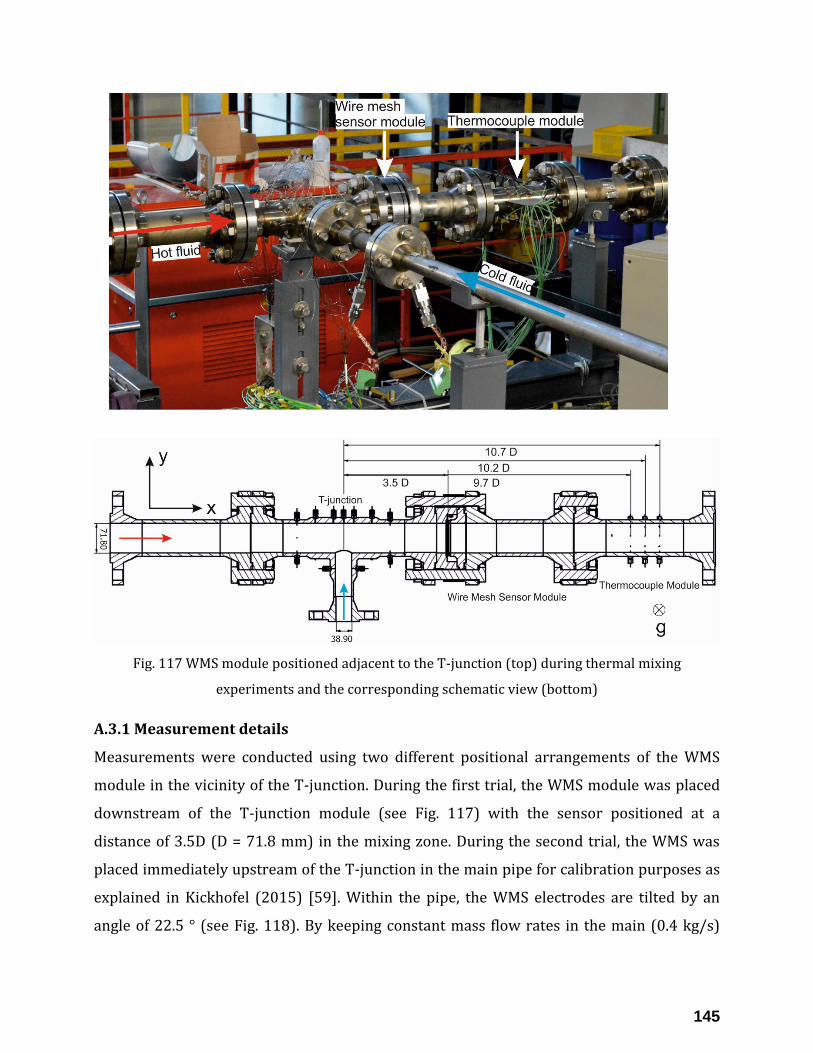
145

Fig. 117 WMS module positioned adjacent to the T-junction (top) during thermal mixing

experiments and the corresponding schematic view (bottom)

A.3.1 Measurement details

Measurements were conducted using two different positional arrangements of the WMS

module in the vicinity of the T-junction. During the first trial, the WMS module was placed

downstream of the T-junction module (see Fig. 117) with the sensor positioned at a

distance of 3.5D (D = 71.8 mm) in the mixing zone. During the second trial, the WMS was

placed immediately upstream of the T-junction in the main pipe for calibration purposes as

explained in Kickhofel (2015) [59]. Within the pipe, the WMS electrodes are tilted by an

angle of 22.5 ° (see Fig. 118). By keeping constant mass flow rates in the main (0.4 kg/s)

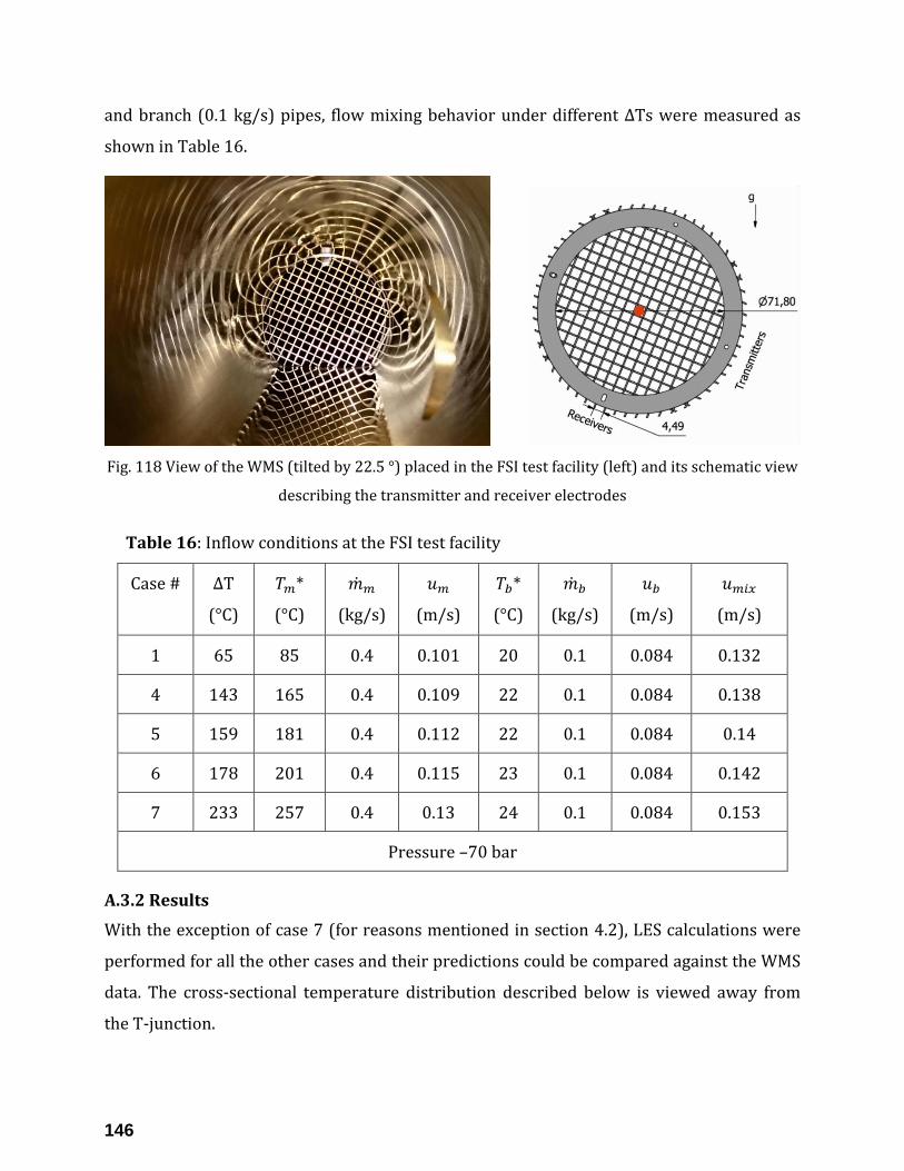
146

and branch (0.1 kg/s) pipes, flow mixing behavior under different ∆Ts were measured as

shown in Table 16.

Fig. 118 View of the WMS (tilted by 22.5 °) placed in the FSI test facility (left) and its schematic view

describing the transmitter and receiver electrodes

Table 16: Inflow conditions at the FSI test facility

Case # ∆T

(°C)

𝑇𝑚*

(°C)

�̇�𝑚

(kg/s)

𝑢𝑚

(m/s)

𝑇𝑏*

(°C)

�̇�𝑏

(kg/s)

𝑢𝑏

(m/s)

𝑢𝑚𝑖𝑥

(m/s)

1 65 85 0.4 0.101 20 0.1 0.084 0.132

4 143 165 0.4 0.109 22 0.1 0.084 0.138

5 159 181 0.4 0.112 22 0.1 0.084 0.14

6 178 201 0.4 0.115 23 0.1 0.084 0.142

7 233 257 0.4 0.13 24 0.1 0.084 0.153

Pressure –70 bar

A.3.2 Results

With the exception of case 7 (for reasons mentioned in section 4.2), LES calculations were

performed for all the other cases and their predictions could be compared against the WMS

data. The cross-sectional temperature distribution described below is viewed away from

the T-junction.

147

Figs. 119, 120, 121, 122 and 123 depicts the cross-sectional mean temperature distribution

as seen from WMS data and the corresponding LES predictions at X = 3.5D. Mixed flow is

seen to exhibit extreme oscillation in case 1 (∆T = 65 °C) while the flow is seen to exhibit

stable stratification in cases 4 5, 6, and 7. LES predictions also reflect this shift in flow

behavior brought about by rising ∆T between the fluids. Another interesting aspect to be

noted is the reducing area occupied by the mixed flow along the cross-section with rise in

∆T between the fluids which culminates with lowest area occupied by the mixed flow being

observed at ∆T = 233 °C.

Fig. 119 Mean thermal field –WMS (left) and LES (right) at ∆T = 65 °C

Fig. 120 Mean thermal field –WMS (left) and LES (right) at ∆T = 143 °C

148

Fig. 121 Mean thermal field –WMS (left) and LES (right) at ∆T = 159 °C

Fig. 122 Mean thermal field –WMS (left) and LES (right) at ∆T = 178 °C

Fig. 123 Mean thermal field from WMS data at ∆T = 233 °C

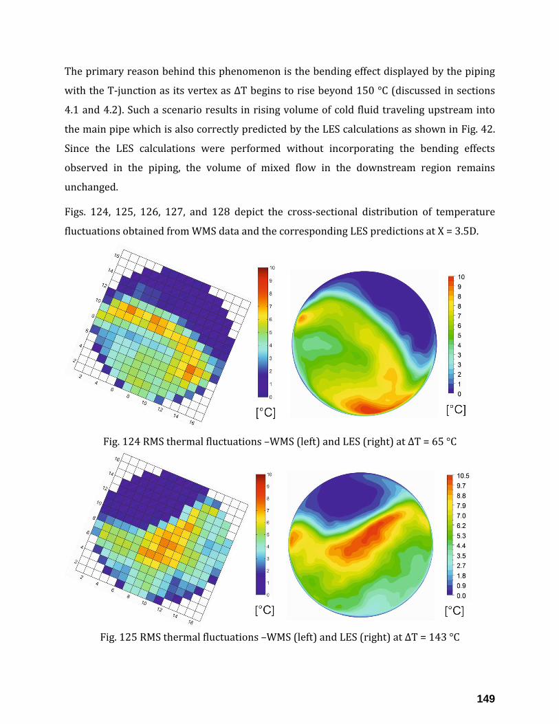
149

The primary reason behind this phenomenon is the bending effect displayed by the piping

with the T-junction as its vertex as ∆T begins to rise beyond 150 °C (discussed in sections

4.1 and 4.2). Such a scenario results in rising volume of cold fluid traveling upstream into

the main pipe which is also correctly predicted by the LES calculations as shown in Fig. 42.

Since the LES calculations were performed without incorporating the bending effects

observed in the piping, the volume of mixed flow in the downstream region remains

unchanged.

Figs. 124, 125, 126, 127, and 128 depict the cross-sectional distribution of temperature

fluctuations obtained from WMS data and the corresponding LES predictions at X = 3.5D.

Fig. 124 RMS thermal fluctuations –WMS (left) and LES (right) at ∆T = 65 °C

Fig. 125 RMS thermal fluctuations –WMS (left) and LES (right) at ∆T = 143 °C

150

Fig. 126 RMS thermal fluctuations –WMS (left) and LES (right) at ∆T = 159 °C

Fig. 127 RMS thermal fluctuations –WMS (left) and LES (right) at ∆T = 178 °C

Fig. 128 RMS thermal fluctuations from WMS data at ∆T = 233 °C

151

Initial observations point out that the orientation of the mixed flow as recorded by the WMS

and the corresponding LES predictions show good agreement with one another. Lowest

amplitude fluctuations are observed near the top region while the highest amplitudes are

seen to occur in the vicinity of the stratification layer. One thing that is clearly noticeable is

the discrepancy in amplitudes between the WMS and LES data. While the LES predictions

show higher fluctuation amplitudes, corresponding data from WMS exhibits attenuation in

fluctuations (compare the WMS and LES predictions in Figs. 124, 125, 126, and 127).

Fig. 129 Comparison of PSD between WMS and LES predictions at ∆T = 143 °C This could be attributed to the operating principle of the WMS, which in essence is the

volume averaging that occurs between the transmitter and receiver electrodes at each

crossing point that is exposed to the flow. Electric current passes between the volume of

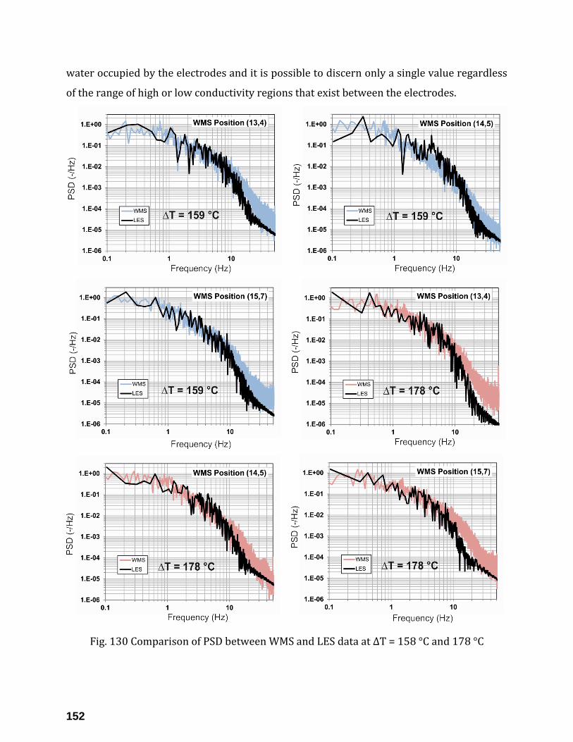
152

water occupied by the electrodes and it is possible to discern only a single value regardless

of the range of high or low conductivity regions that exist between the electrodes.

Fig. 130 Comparison of PSD between WMS and LES data at ∆T = 158 °C and 178 °C

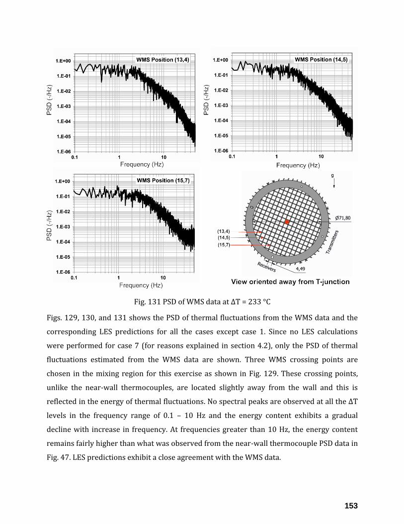
153

Fig. 131 PSD of WMS data at ∆T = 233 °C

Figs. 129, 130, and 131 shows the PSD of thermal fluctuations from the WMS data and the

corresponding LES predictions for all the cases except case 1. Since no LES calculations

were performed for case 7 (for reasons explained in section 4.2), only the PSD of thermal

fluctuations estimated from the WMS data are shown. Three WMS crossing points are

chosen in the mixing region for this exercise as shown in Fig. 129. These crossing points,

unlike the near-wall thermocouples, are located slightly away from the wall and this is

reflected in the energy of thermal fluctuations. No spectral peaks are observed at all the ∆T

levels in the frequency range of 0.1 – 10 Hz and the energy content exhibits a gradual

decline with increase in frequency. At frequencies greater than 10 Hz, the energy content

remains fairly higher than what was observed from the near-wall thermocouple PSD data in

Fig. 47. LES predictions exhibit a close agreement with the WMS data.