Physica A 315 (2002) 616–642www.elsevier.com/locate/physa

Theory of the microscopic maserphase transitions

Bo-Sture K. Skagerstama;b; ∗, Per K. RekdalaaDepartment of Physics, The Norwegian University of Science and Technology,

N-7491 Trondheim, NorwaybMicrotechnology Center at Chalmers MC2, Department of Microelectronics and Nanoscience,Chalmers University of Technology and G$oteborg University, S-412 96, G$oteborg, Sweden

Received 10 April 2002

Abstract

Phase diagrams of the micromaser system are mapped out in terms of the physical parametersat hand like the atom cavity transit time �, the atom–photon frequency detuning -!, the numberof thermal photons nb and the probability a for a pump atom to be in its excited state. Critical0uctuations are studied in terms of correlation measurements on atoms having passed throughthe micromaser or on the microcavity photons themselves. At su1ciently large values of thedetuning, we 2nd a “twinkling” mode of the micromaser system. Detailed properties of thetrapping states are also presented. c© 2002 Elsevier Science B.V. All rights reserved.

PACS: 32.80.−t; 42.50.−p; 42.50.Ct

Keywords: Micromaser; Phase transitions; Phase diagrams; Correlations

1. Introduction

There are few systems in physics which exhibit a rich structure of phase tran-sitions that can be investigated under clean experimental conditions and which atthe same time can be studied by exact theoretical methods. Recent developmentsin cavity quantum electrodynamics, and in particular the use of beams of highlyexcited Rydberg atoms and resonant microcavities, have opened up an avenue tostudy one class of such systems in great detail. The micromaser system, which is a

∗ Corresponding author. Department of Physics, The Norwegian University of Science and Technology,N-7491 Trondheim, Norway. Tel.: +47-73591866; fax: +47-73597710.E-mail addresses: boskag@phys.ntnu.no (B.-S.K. Skagerstam), perr@phys.ntnu.no (P.K. Rekdal).

0378-4371/02/$ - see front matter c© 2002 Elsevier Science B.V. All rights reserved.PII: S 0378 -4371(02)01006 -3

B.-S.K. Skagerstam, P.K. Rekdal / Physica A 315 (2002) 616–642 617

remarkable experimental realization of the idealized system of a two-level atominteracting with a second-quantized single-mode electromagnetic 2eld, provides us withsuch an example (for reviews and references see e.g. Ref. [1]). The microlaser [2] isthe counterpart in the optical regime.Many features of the micromaser are of general interest. It can, for example, be

argued that the micromaser system is a very simple illustration of the conjecturedtopological origin of second-order phase transitions [3], as will be brie0y discussedlater in the present paper. Various aspects of stochastic resonance can, furthermore,be studied in this system [4]. The micromaser also illustrates a remarkable featureof non-linear dynamical systems: turning on randomness may lead to an increasedsignal-to-noise ratio [5–7].The basic theory of the micromaser system as developed in Refs. [8,9], which is

limited to the case a=1 and -!=0, suggests the existence of various phase transitionsin the large N limit. Here N is the number of atoms passing the cavity in a single pho-ton cavity decay time. A natural order parameter is then the average photon “density”〈n〉=N , where 〈n〉 denotes the average photon number with respect to the stationarymicromaser photon distribution. By making use of an approximative approach in termsof a Fokker–Planck equation, details of the various transitions were worked out, liketunneling times between the various phases [8,9]. An exact treatment, in the large Nlimit, of the micromaser phase structure and the corresponding critical 0uctuations, interms of a conventional correlation function of either the atoms leaving the micromaseror the photons in the cavity, has been given in Ref. [10], where deviations from theFokker–Planck equation approach were reported. It is of great interest to notice thatspontaneous jumps in 〈n〉=N and large correlation lengths close to micromaser phasetransitions have been observed experimentally [1,11]. Most of the experimental andtheoretical studies have, however, been limited to the case a=1 and -!=0. It is thepurpose of the present paper to study the phase structure of the micromaser systemand extend the results of Ref. [10] to the general case with a �=1 and -! �=0 usingmethods which are exact in the large N limit. As will be argued below, several newintriguing physical properties of the micromaser system are then unfolded. A shortpresentation of the main results of this paper has appeared elsewhere [12].The paper is organized as follows. In Section 2 the theoretical framework is out-

lined, and a rapidly convergent large N limit is derived for the stationary micromaserphoton probability distribution. The phase structure and the order parameter 〈n=N 〉 isinvestigated in Section 3. The correlation length is analysed numerically in Section 4as well as in terms of various approximation schemes leading to explicit dependenceof the physical parameters at hand. The results of extensive numerical investigationsof trapping states are presented in Section 5. Final remarks are given in Section 6including comments on collective pump atom eKects.

2. The probability distribution

The pump atoms, which enter the cavity, are assumed to be prepared in an incoherentstatistical mixture, i.e., the initial density matrix A of the atoms is of the diagonal

618 B.-S.K. Skagerstam, P.K. Rekdal / Physica A 315 (2002) 616–642

form

A =

(a 0

0 b

); (1)

where a + b = 1. This form of the atomic density matrix is not of the most generalform, but it leads to the possibility of an exact analytical treatment provided the initialphoton 2eld density matrix also is diagonal, which from now on we assume. The rateR of the injected atoms is assumed to be high enough to pump up the cavity, i.e.,R¿ = 1=Tcav, or N ¿ 1 in terms of the dimensionless 0ux variable N = R= . HereTcav is the decay time of the cavity and hence is the typical decay rate for photonsin the cavity. Furthermore, let � denote the atomic transit-time through the resonantphoton cavity.For our purposes the continuous time formulation of the micromaser system [13] is

suitable as a theoretical framework. Each atom is assumed to have the same probabilityR dt of arriving in an in2nitesimal time interval dt, i.e., they are Poisson distributed.Provided the interaction with the radiation 2eld of the cavity takes less time than thisinterval, i.e., if ��dt, we may consider the atomic transitions to be instantaneous. Thevector p formed by the diagonal density matrix elements of the photon 2eld then obeysthe master equation [13,10]:

dpdt

=− Lp ; (2)

where

L= LC − N (M − 1) : (3)

Here LC describes the damping of the cavity (see e.g. Ref. [14] for an excellentaccount), i.e.,

(LC)nm = (nb + 1)[n�n;m − (n+ 1)�n+1;m] + nb[(n+ 1)�n;m − n�n;m+1] ; (4)

and M = M (+) + M (−) has its origin in the Jaynes–Cummings (JC) model [15,10]where

M (+)nm = bqn+1�n+1;m + a(1− qn+1)�n;m (5)

and

M (−)nm = aqn�n;m+1 + b(1− qn)�n;m : (6)

We observe the unitarity constraints∞∑n=0

Mnm = 1;∞∑n=0

(LC)nm = 0 : (7)

The stationary solution of Eq. (2) is well known [8,13] and is given by

Npn = Np0

n∏m=1

nbm+ Naqm

(1 + nb)m+ Nbqm; (8)

where qm ≡ q(m=N ) and

q(x) =x

x + �2 sin2(�√

x + �2) : (9)

B.-S.K. Skagerstam, P.K. Rekdal / Physica A 315 (2002) 616–642 619

Here we have de2ned the natural and dimensionless parameter

�2 = �2=N ; (10)

where

�=-!=2g ; (11)

since it is always this particular combination of -!, N and g which is involved. gis the single-photon Rabi frequency at zero detuning of the JC model [15]. nb is theinitial mean value of thermal photons in the cavity. Furthermore, the probability isexpressed in terms of the scaled dimensionless pump parameter �=g�

√N . The overall

constant Np0 in (8) is determined by the normalization condition∞∑n=0

Npn = 1 : (12)

In passing, we observe that at thermal equilibrium, i.e., whenab=

nb

1 + nb; (13)

the probability distribution in Eq. (8) is in fact, as it should be, a Planck distribution.This particular distribution depends only on nb, which then is the corresponding meanvalue photon number, i.e.,

〈n〉 ≡∞∑n=0

n Npn = nb : (14)

If Eq. (13) is not ful2lled, then Npn describes a stationary photon distribution which,therefore, can be far from thermal equilibrium, i.e., the micromaser can actually beused to study various aspects of non-equilibrium thermodynamics.

2.1. Large N expansion

The large N behaviour of the stationary photon probability distribution Npn as givenby Eq. (8) is di1cult to handle. In order to obtain an appropriate expression whichis rapidly convergent in the large N limit, and which neatly expresses the variousmicromaser phases, we can make use of a Poisson summation technique [16]. It isthen natural to de2ne the scaled photon number variable x, de2ned by x = n=N . Thestationary probability distribution, Eq. (8), then takes the form

Np(x) = Np0

√w(x)w(0)

e−N V (x) ; (15)

where

V (x) =∞∑

k=−∞Vk(x) : (16)

The eKective potential V (x) is expressed in terms of

Vk(x) =−∫ x

0d! ln[w(!)] cos(2"Nk!) ; (17)

620 B.-S.K. Skagerstam, P.K. Rekdal / Physica A 315 (2002) 616–642

where

w(x) =nbx + aq(x)

(1 + nb)x + bq(x): (18)

In this expression for w(x), q(x) is given by Eq. (9) We stress that Eq. (15) is exact.In the large N limit, Eq. (15) can be simpli2ed since the Vk(x)-terms in Eq. (17) do

not contribute in this limit for k �=0. In fact, in terms of the maximal value of |ln[w(x)]|we immediately see from Eqs. (16)–(18) that the Vk(x)-terms for k �=0 are of the formO(log[1 + 1=nb])=2N for a6 nb=(1 + 2nb), or O(log[(nb + a� 2)=(1 + nb + b� 2)])=2Nfor a¿ nb=(1 + 2nb). In order to see this one may use that 06 q(x)=x6 � 2. Apartfrom 1=N corrections, we can therefore put V (x) = V0(x). It is, therefore, the natureof the global minima of V0(x) which determines the probability distribution and themicromaser phase structure, apart from the zeros of w(x) which correspond to trappingstates [17–21]. The physics of trapping states will be discussed in Section 5.

2.2. The thermal distribution

If the only global minimum of V0(x) occurs at x = 0, we can expand the eKectivepotential V0(x) around the origin. A straightforward expansion of V0(x) then leads to

V0(x) = x ln

[1 + nb + b� 2

e9

nb + a� 2e9

]+ O(x2) ; (19)

where we have de2ned an eKective pump �-parameter

�2e9 = � 2 sin2(��)

(��)2: (20)

Eq. (19) leads to the following properly normalized thermal photon probability distri-bution:

Npn =1 + (1− 2a)�2e91 + nb + b�2e9

(nb + a�2e9

1 + nb + b�2e9

)n

; (21)

which is convergent provided

�2e9 (2a− 1)¡ 1 : (22)

Eq. (21) is exact in the large N limit, and corresponds to an increase of the temperaturein the cavity. If a¡ 1

2 + �2=2, then the distribution equation (21) is therefore alwaysvalid. If �= 0 convergence requires that � 2(2a− 1)¡ 1, i.e., � has to be su1cientlysmall when a¿ 1

2 . We 2nd, by numerical simulations, that Eq. (21) also can be used tocompute expectation values for 2nite N , even though the accuracy then depends on theactual micromaser parameters. When the micromaser is described by the distributionequation (21), we say that the system is in the thermal phase. In the thermal phasethe order parameter is given by

〈x〉= 1N

nb + a�2e91 + (1− 2a)�2e9

; (23)

B.-S.K. Skagerstam, P.K. Rekdal / Physica A 315 (2002) 616–642 621

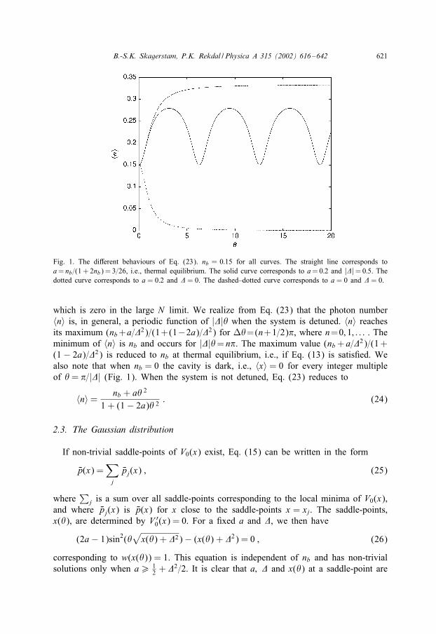
Fig. 1. The diKerent behaviours of Eq. (23). nb = 0:15 for all curves. The straight line corresponds toa= nb=(1+ 2nb)= 3=26, i.e., thermal equilibrium. The solid curve corresponds to a=0:2 and |�|=0:5. Thedotted curve corresponds to a = 0:2 and � = 0. The dashed–dotted curve corresponds to a = 0 and � = 0.

which is zero in the large N limit. We realize from Eq. (23) that the photon number〈n〉 is, in general, a periodic function of |�|� when the system is detuned. 〈n〉 reachesits maximum (nb+a=�2)=(1+(1−2a)=�2) for -�=(n+1=2)", where n=0; 1; : : : . Theminimum of 〈n〉 is nb and occurs for |�|�= n". The maximum value (nb + a=�2)=(1+(1− 2a)=�2) is reduced to nb at thermal equilibrium, i.e., if Eq. (13) is satis2ed. Wealso note that when nb = 0 the cavity is dark, i.e., 〈x〉 = 0 for every integer multipleof �= "=|�| (Fig. 1). When the system is not detuned, Eq. (23) reduces to

〈n〉= nb + a� 2

1 + (1− 2a)� 2 : (24)

2.3. The Gaussian distribution

If non-trivial saddle-points of V0(x) exist, Eq. (15) can be written in the form

Np(x) =∑j

Npj(x) ; (25)

where∑

j is a sum over all saddle-points corresponding to the local minima of V0(x),and where Npj(x) is Np(x) for x close to the saddle-points x = xj. The saddle-points,x(�), are determined by V ′

0(x) = 0. For a 2xed a and �, we then have

(2a− 1)sin2(�√

x(�) + �2)− (x(�) + �2) = 0 ; (26)

corresponding to w(x(�)) = 1. This equation is independent of nb and has non-trivialsolutions only when a¿ 1

2 + �2=2. It is clear that a; � and x(�) at a saddle-point are

622 B.-S.K. Skagerstam, P.K. Rekdal / Physica A 315 (2002) 616–642

restricted by the condition

x(�) + �26 2a− 1 ; (27)

for any �. The saddle-points x = x(�) can conveniently be parametrically representedin the form [10]

x(%) + �2 = (2a− 1)sin2 % ; (28)

�(%) =1√

2a− 1%

|sin%| (29)

with

%¿%0 ≡ arcsin(|�|=√2a− 1) : (30)

We de2ne branches of %, labelled by k = 0; 1; 2; : : : such that % varies in the intervals

%0 + k"6%6 (k + 1)"− %0; k = 0; 1; 2; : : : : (31)

Except for the 2rst branch k = 0, the saddle-points corresponding to each of thesebranches are double-valued, that is, there are at most two values of x(�) for a given�. The 2rst branch k = 0 is single-valued.For a given a, � and �, let x = xj(a;-; �) ≡ xj be a saddle-point corresponding to

a local minimum of V0(x). The equilibrium distribution in the neighbourhood of thisminimum value xj is then given in the following Gaussian form:

Npj(x) =Tj√2"N

e−(N=2)V ′′0 (xj)(x−xj)2 : (32)

Here Tj is determined by the normalization condition for Np(x), i.e.,

Tj =e−NV0(xj)∑

m e−NV0(xm)=√

V ′′0 (xm)

; (33)

and where

V ′′0 (x) =

(2a− 1)2

a+ nb(2a− 1)q(x)− xq′(x)

x2: (34)

For the given parameters, the sum in Eq. (33) is supposed to be taken over allsaddle-points corresponding to a minimum of V0(x), i.e., all saddle-points correspond-ing to V ′′

0 (x)¿ 0. If x= xj does not correspond to a global minimum for the eKectivepotential V0(x), then Tj is exponentially small in the large N limit. If x=xj correspondsto one and only one global minimum, we can neglect all the terms in the sum in Tj

but m= j, in which case Tj is reduced to Tj =√

V ′′0 (xj). In the neighbourhood of such

a global minimum xj, the probability distribution in Eq. (32) is, therefore, reduced to

Npj(x) =

√V ′′0 (xj)2"N

e−(N=2)V ′′0 (xj)(x−xj)2 (35)

which is, strictly speaking, only valid in a su1ciently small neighbourhood of xj.

B.-S.K. Skagerstam, P.K. Rekdal / Physica A 315 (2002) 616–642 623

However, since Npj(x) in Eq. (32) is exponentially small when x is not in the neigh-bourhood of xj, the probability distribution for any x is given by

Np(x) =∑j∗

Npj(x) ; (36)

where∑

j∗ denotes the sum over the global minima of V0(x) only. Hence, when thereare several saddle-points, the actual maser phase is described by the saddle-points whichcorrespond to the global minima of V0(x) only. In the next section, we will actuallyargue that, for a 2xed a, � and �, we can have at most two competing global minimain the large N limit, i.e., there can be at most two terms in the

∑j∗ -sum in Eq. (36).

When the micromaser is described by a distribution like Eq. (35), the mean occu-pation number 〈n〉 is proportional to the pumping rate N . The cavity then acts as amaser, i.e., the system is in a maser phase.

3. The phase diagram

The probability distribution equation (8) determines micromaser phases as a functionof the physical parameters at hand. In this section we will map out phase diagrams inthe a- and �-parameter space for a given nb �=0 and �. In general, a phase diagram isthen determined by mapping out the global minima of the eKective potential V0(x).By the substitution %= �

√x + �2, the eKective potential in Eq. (17) can be written

in the form

V0(x) = V0(%; �) =− 2� 2

∫ %

�|�|d& & ln[w(&; �)] : (37)

Here we have de2ned

w(&; �) =nb + aq(&; �)

1 + nb + bq(&; �)(38)

and

q(&; �) = � 2 sin2&

&2: (39)

In Eq. (37), the upper integration limit % and the pump parameter � may take onarbitrary values. However, by choosing x(%) and �(%) according to Eqs. (28) and(29), the eKective potential is always at an extremum. We then arrive at an eKectivemulti-branched potential as given by V0(%) = V0(%; �(%)). For a given branch k, thevariable % is limited by Eq. (31).If we regard V0(%) as a function of �, each branch of V0(�)=V0(%; �(%)) is at most

double-valued except for branch k=0. One sub-branch then corresponds to a maximum(V ′′

0 (x(%))¡ 0), which is swept out 2rst as % increases, and the other corresponds to

624 B.-S.K. Skagerstam, P.K. Rekdal / Physica A 315 (2002) 616–642

a minimum (V ′′0 (x(%))¿ 0). Here the V ′′

0 (x(%)) is explicitly given by

V ′′0 (x(%)) =

1− % cot%

sin2 %[a+ nb(2a− 1)]: (40)

To reconstruct the actual value of V0(x) for the kth minimum (maximum), we writeV0(x) = V0(%), evaluated for the sub-branch with V ′′

0 (x(%))¿ 0 (V ′′0 (x(%))¡ 0).

A convenient representation of V0(%) for the branch k (given a; nb; �) is

V0(%) = [a+ nb(2a− 1)]I(%) ; (41)

where

I(%) ≡∫ %

%0+k"d& &4

sin(2&)− 2 sin2 (&)=&

[&2nb + a�(%)2 sin2 &][&2(1 + nb) + b�(%)2 sin2 &]: (42)

Here the upper integration limit % has to be chosen according to Eq. (31). We noticethe characteristic pre-factor a+ nb(2a− 1) in Eq. (41) which then actually determinesthe typical dependence of the parameters a and nb at a saddle-point.

3.1. The critical parameters �∗0 and �k

As a function of �, the 2rst extremum of V0(x) occurs at �∗0 ≡ �(%0), where %0 isgiven by Eq. (30). The critical pump parameter �∗0 = �∗0 (a; �) is therefore given by

�∗0 =arcsin(|�|=√2a− 1)

|�| ; (43)

which is equivalent to

a=12+

�2

2 sin2 (�∗0�): (44)

When the system is not detuned, i.e., when �= 0, this equation reduces to

a=12+

12(�∗0 )2

: (45)

Eq. (43) determines the 2rst thermal–maser critical line in the a- and �-phase diagram.In the maser phase, the order parameter 〈x〉=〈n〉=N approaches zero when � approaches�∗0 (a; �). Furthermore, in the large N limit, 〈x〉 is always zero in the thermal phase.Hence, the order parameter is continuous on this critical line. The 2rst derivative of〈x〉 with respect to � is, however, discontinuous. In the maser phase we actually have

d〈x〉d�

= 2(√2a− 1)3

sin3 %tan%− %

; (46)

with %¿%0. When approaching the critical line from the maser phase, we see fromEq. (46) that d〈x〉=d� is non-zero (except for a= 1

2). The 2rst thermal–maser criticalline, therefore, corresponds to a line of second-order phase transitions.

B.-S.K. Skagerstam, P.K. Rekdal / Physica A 315 (2002) 616–642 625

In passing, we mention that in a topological analysis of the second-order phasetransitions [3] of the micromaser system, V0(x) will play the role of a Morse func-tion. The con2guration space M is then the one-dimensional space of x(≡ n=N ). Thesub-manifold Mv de2ned by

Mv = {x∈M| Np(x) exp(−NV0(x))6 v} ; (47)

then describes the change of topology close to the second-order phase transitions �∗0 .This will be true for all second-order transitions discussed below. We observe that for2nite N the change in topology, i.e., the appearance of an additional disjoint x-intervaldue to the appearance of a new local maximum in Np(x), in general, occurs before theactual second-order phase transition.Critical points where new extrema of V0(x) appear are determined by V ′′

0 (x) = 0,i.e., non-trivial solutions of

tan%= % ; (48)

independent of the physical parameters of the micromaser. This equation has in2nitelymany positive solutions %= %k , where k = 1; 2; : : : . Corresponding to these solutions,we have the critical pump parameters �k ≡ �(%k), i.e.,

�k =1√

2a− 1%k

|sin%k | ; k = 1; 2; 3; : : : ; (49)

independent of nb and �, for which the kth branch comes into existence. For a givenbranch k¿ 1, the V ′′

0 (x(%))¿ 0 sub-branches and the V ′′0 (x(%))¡ 0 sub-branch coin-

cide at this particular critical point �k (see e.g. Fig. 2). The critical point � = �k alsocorresponds to x′(�k) =∞ as seen from Eq. (46).Each sub-branch with V ′′

0 (x(%))¿ 0 of the eKective potential V0(�) has one andonly one minimum. This can be seen from the expression

dV0(�)d�

=− 2�(%)

[a+ nb(2a− 1)]J (%) ; (50)

where

J (%) ≡∫ %

%0+k"d& &4

sin(2&)

[&2nb + a�(%)2 sin2 &][&2(1 + nb) + b�(%)2 sin2 &](51)

and V0(�)=V0(%; �(%)). The upper integration limit % must then be chosen accordingto Eq. (31) where we, of course, only consider the V ′′

0 (x(%))¿ 0 sub-branch for k¿ 1.We can now study the actual intersections of the various branches at a common

global minimum by making use of numerical and analytical methods. The procedureis, for example, illustrated in Figs. 2 and 3. We 2nd that V0(�) is such that if twobranches do intersect at a common global minimum, these branches correspond to kand k + 1, i.e., they are consecutive branches. A given branch can also intersect withV0(�) = 0, i.e., the thermal phase. In addition, two consecutive branches can intersectwhen V0(�) = 0. We then have a triple point.

626 B.-S.K. Skagerstam, P.K. Rekdal / Physica A 315 (2002) 616–642

Fig. 2. The order parameter 〈x〉 = 〈n〉=N , as a function of �, when a = 1, � = 0, nb = 0:15 and N = 1000.A dotted vertical line at � = �k , where �0 = �∗0 , indicates where the kth branch comes into existence. �∗0corresponds to a second-order phase transition. The numerical values of the pump parameters are: �∗0 = 1,�1 = 4:603, �2 = 7:790, �3 = 10:950, �4 = 14:102 and �5 = 17:250. The various branches at the extremum ofthe eKective potential, i.e., V0(�) = V0(%; �(%)), are also shown. The intersection between two neighbouringV ′′0 (x(%))¿ 0 sub-branches at � = �∗kk+1 is marked by a circle when this coincidence occurs at a global

minimum of V0(�). At these 2rst-order maser-to-maser phase transitions, the order parameter 〈x〉 makesa discontinuous change in the large N limit. The numerical values of the transition parameters �∗kk+1 are:�∗01 ≈ 6:6610, �∗12 ≈ 12:035 and �∗23 ≈ 17:413. The horizontal line at 〈x〉 ≈ 0:34 corresponds to theasymptotic value of the order parameter which can be evaluated analytically [7].

3.2. The critical parameters �∗kk+1, �∗tk and �∗kt

If, for a given a, nb and �, we have a transition from the maser branch k to theneighbouring maser branch k + 1, then there exist %∗

k and %∗k+1 such that

V0(%∗k ) = V0(%∗

k+1) and �(%∗k ) = �(%∗

k+1) ≡ �∗kk+1 ; (52)

where

V0(%∗k ) =− 2

�(%∗k )

2

∫ %∗k

�(%∗k )|�|

d%% ln[w(%; �(%∗k ))] ; (53)

and where %∗k is in the interval %k ¡%∗

k ¡ (" − %0) + k". The reason why we chose%∗

k ¿%k is that we are looking for solutions of Eq. (52) for which V ′′0 (x(%))¿ 0. The

pump parameter according to Eq. (52) can be expressed as

�∗kk+1 =1√

2a− 1

%∗k

|sin%∗k |¿%∗

k : (54)

Furthermore, for this particular combination of the parameters, the order parameter〈x〉 = 〈n〉=N makes a discontinuous change as can be seen from Eq. (28), i.e., thediscontinuity in 〈x〉 is given �〈x〉 = x(%∗

k+1) − x(%∗k ). We therefore have a 2rst-order

phase transition.

B.-S.K. Skagerstam, P.K. Rekdal / Physica A 315 (2002) 616–642 627

Fig. 3. The order parameter 〈x〉 = 〈n〉=N , as a function of �, when |�| = 0:5 and all other parameters asin Fig. 2. A dotted vertical line at � = �k , where �0 = �∗0 , indicates where the kth branch comes intoexistence. The numerical value of �∗0 is �∗0 =1:047. The numerical value of �k , k �=0, is the same as in Fig.2 since this critical � only depends on a. The various branches at the extremum of the eKective potential,i.e., V0(�) = V0(%; �(%)), are also shown. First-order thermal-to-maser phase transitions occur at the pumpparameters �∗tk and second-order maser-to-thermal transitions occur at �∗0 , �

∗0t and �∗kt . The circle at � = �∗23

in the 2gure indicates a maser-to-maser transition. The numerical values of the critical transition parametersin the 2gure are: �∗0 ≈ 1:047, �∗0t ≈ 5:236, �∗t1 ≈ 6:193, �∗1t ≈ 11:519, �∗t2 ≈ 11:906 and �∗23 ≈ 17:425.The horizontal line at 〈x〉 ≈ 0:09 corresponds to the asymptotic value of the order parameter which can beevaluated analytically [7].

If, on the other hand, a given maser branch corresponding to a global minima doesnot intersect with a neighbouring maser branch, it is the intersection with the thermalbranch which determines the phase transition (see e.g. Fig. 3). For a given branchk¿ 1, let �∗tk ≡ �(%∗

tk) denote the pump parameter of this thermal-to-maser transition.The value of %∗

tk is then determined by the solution of

V0(%∗tk) = 0 ; (55)

where

V0(%∗tk) =− 2

�(%∗tk)

2

∫ %∗tk

�(%∗tk )|�|

d%% ln[w(%; �(%∗tk))] : (56)

We determine %∗tk numerically, where %k ¡%∗

tk ¡ (" − %0) + k" and k = 1; 2; 3; : : : .The corresponding pump parameters are �∗tk ≡ �(%∗

tk), i.e.,

�∗tk =1√

2a− 1

%∗tk

|sin%∗tk |

; k = 1; 2; 3; : : : : (57)

Due to the same reasons as discussed above, such thermal-to-maser transitions corre-spond to 2rst-order phase transitions.

628 B.-S.K. Skagerstam, P.K. Rekdal / Physica A 315 (2002) 616–642

Furthermore, let �∗kt ≡ �(%∗kt) denote the maser-to-thermal transition for a given

branch k¿ 0 (see e.g. Fig. 3). The value of %∗kt is determined by one of the solutions

of

V0(%∗kt) = 0 ; (58)

where

V0(%∗kt) =− 2

�(%∗kt)

2

∫ %∗kt

�(%∗kt)|�|

d%% ln[w(%; �(%∗kt))] : (59)

We see that

%∗kt = ("− %0) + k" (60)

for all branches k¿ 0. When � �=0, Eq. (58) is trivially ful2lled since the upperintegration limit is equal to the lower. If, on the other hand, � = 0, then Eq. (58) isful2lled since �(%∗

kt) =∞. The pump parameter �∗kt ≡ �(%kt) is given by

�∗kt =(k + 1)"− arcsin(|�|=√2a− 1)

|�| ; k = 0; 1; 2; : : : : (61)

This equation is equivalent to

a=12+

�2

2sin2(�∗kt�); k = 0; 1; 2; : : : ; (62)

which is of the same form as Eq. (44). Due to the same reasons as discussed above,such a maser-to-thermal transition corresponds to a second-order phase transition.Equipped with these results, we can now construct a complete phase diagram in e.g.

the a- and �-parameter space for a given nb and �.

3.3. Phase diagrams

The phase diagram when nb = 0:15 and � = 0 is shown in Fig. 4. The 2rst crit-ical line in this 2gure is given by Eq. (45). As already mentioned, this correspondsto a second-order thermal-to-maser phase transition. In the region above this line, themean occupation number 〈n〉 grows proportionally with the pumping rate N . The cav-ity, therefore, behaves like a maser in this regime. For values of a and � below thisline, the only global minimum of V0(x) occurs at x = 0. In this particular region,the probability Npn is given by the thermal distribution in Eq. (21), i.e., the micro-maser is in the thermal phase. We notice that Eq. (44) also determines the radiusof convergence of the thermal probability distribution in Eq. (21). The other criticallines in Fig. 4 are determined by Eq. (52) since for nb = 0:15 and � = 0, all neigh-bouring V ′′

0 (x(%))¿ 0 sub-branches of V0(�) = V0(%(�); �) intersect for some a¿ 12

(see Fig. 2).When the micromaser is detuned the phase diagram is more complicated. Fig. 5

shows a typical example of a phase diagram when � �=0. As we can see from this2gure, the 2rst two maser phases are well separated. The critical value of � for such

B.-S.K. Skagerstam, P.K. Rekdal / Physica A 315 (2002) 616–642 629

Fig. 4. The phase diagram for the micromaser system when nb = 0:15 and � = 0. All the critical linesconverge to 1

2 in the large � limit. The thermal-to-maser critical line �∗0 (a) is determined analytically byEq. (45). The other critical lines �∗kk+1(a), which are maser-to-maser transitions, are determined by Eq. (54).

Fig. 5. The phase diagram for the micromaser system when nb = 0:15 and |�| = 0:5. In this diagramwe have plotted the range of validity of the thermal distribution (dotted lines). When not visible, thesedotted lines overlap with the solid critical lines. The minima of the critical lines are determined by thecondition sin2(-�) = 1 and are marked by a short vertical lines. The 2rst critical line �∗0 (a) in this phasediagram is determined analytically by Eq. (43). The critical lines �∗tk (a) are given by Eq. (57) and �∗kt(a)are given by Eq. (61). Triple points are indicated by circles. The numerical values of these triple points are(a23; �23)triple = (0:98; 17:78) and (a34; �34)triple = (0:96; 24:04).

630 B.-S.K. Skagerstam, P.K. Rekdal / Physica A 315 (2002) 616–642

a separation of phases is, in general, determined by considering phase separation onthe line a = 1. For a given nb, let � = �kk+1 be the corresponding critical value forphase separation. With the de2nition %∗

t0 ≡ %0, where %0 is given in Eq. (30), �kk+1

is determined by the transcendental equation

�(%∗kt) = �(%∗

tk); k = 0; 1; 2; : : : ; (63)

i.e., the solution of

|�|= |sin%∗tk |

%∗tk

[(k + 1)"− arcsin|�|] : (64)

Here %∗tk is determined numerically according to Eq. (55). For nb=0:15 the 2rst critical

value of detuning is |�01| ≈ 0:408. When the detuning is larger than �kk+1, branch kwill separate from branch k + 1 (see e.g. Fig. 5). In passing, we notice that �kk+1 isrestricted by �2

kk+1 ¡ 1, for all possible branches.The 2rst critical line in Fig. 5 corresponds to a second-order thermal-to-maser

(maser-to-thermal)transition to the left (right) of its minimum. The minima of thecritical lines are marked by short vertical lines. For any other critical line in Fig. 5,the transition is a 2rst-order thermal-to-maser (second-order maser-to-thermal) phasetransition to the left (right) of its minimum unless it intersects with another criticalline. In the region between any thermal-to-maser line and the neighbouring dotted line,the thermal probability distribution does not correspond to a global minimum of V0(x).The phase diagram in Fig. 5 also contains triple points. These points are marked bycircles. They are mathematically determined by

V0(%∗tk) = V0(%∗

kt) = 0 and �(%∗tk) = �(%∗

kt) : (65)

The order parameter 〈x〉 can also be studied as a function of the probability a for thepump atoms to be in an excited state. Varying a over all allowed values keeping otherphysical parameters 2xed, the order parameter 〈x〉 makes a discontinuous change forevery combination of the physical parameters corresponding to a critical line. Hence,〈x〉 as a function of a exhibits a plateau-like behaviour when N is su1ciently large.Such a behaviour is illustrated in Fig. 6. In this 2gure, we observe a rather slow Nconvergence to this plateau-like behaviour.Above, we have observed that the mean value 〈n〉 may oscillate as a function of

� when the micromaser is in the thermal phase. We then say that the system is ina twinkling mode. This twinkling behaviour has a close resemblance to the observedatomic Rabi oscillations in the micromaser system [22,23]. A somewhat diKerent twin-kling behaviour of the micromaser system occurs when the thermal phase intersectswith a maser phase. This feature is illustrated in Fig. 5 with |�|= 0:5 and nb = 0:15.For a given a¿ 1

2 + �2=2 we then see that the system has repeated thermal-to-maserand maser-to-thermal transitions as � increases. This twinkling behaviour is not strictlyperiodic in �. The twinkling phenomena will now, however, be more pronounced since,for large N , the maser will be “dark” in the thermal phase, but 〈n〉 is large in the maserphase since 〈n〉 is proportional to N in this region.

B.-S.K. Skagerstam, P.K. Rekdal / Physica A 315 (2002) 616–642 631

Fig. 6. The order parameter 〈x〉=〈n〉=N as a function of a when nb=0:15, �=0, �=25 and N=100; 500; 1000.Each step in 〈x〉 corresponds to a point on one of the transition curves in Fig. 4.

4. The correlation length

In this section, we study long-time correlations in the large N limit. This notionof a long-time correlation length for the micromaser system was 2rst introduced inRefs. [10]. These correlations have a surprisingly rich structure and re0ect global prop-erties of the micromaser stationary photon probability distribution. The probability P(s)of 2nding an atom in a state s=± after the interaction with the cavity, where + rep-resents the excited state and − represents the ground state, can be expressed in thefollowing matrix form [10]:

P(s) = u 0TM (s) Np ; (66)

such that P(+) + P(−) = 1. The elements of the vector Np are given the equilibriumdistribution in Eq. (8), and the matrix M (s) is given by Eqs. (5) and (6). The quantityNu 0 is a vector with all entries equal to 1, Nu0n = 1. It can be shown that the orderparameter 〈x〉 and P(+) are related by [7]

〈x〉= a+nb

N−P(+) : (67)

In order to study the statistical correlations of the atoms leaving the micromaser cavity,with the injection time intervals between them Poisson-distributed, we will need thejoint probability for observing two atoms in the states s1 and s2 with k unobservedatoms between them [10], i.e.,

Pk(s1; s2) = u0TS(s2)SkS(s1)p0 (68)

and where

S(s) = (1 + LC=N )−1M (s) : (69)

632 B.-S.K. Skagerstam, P.K. Rekdal / Physica A 315 (2002) 616–642

Here LC is given by Eq. (4) and S = S(+) + S(−). For su1ciently large k, we writek = Rt and it follows that

P(s1; s2; t)≡Pk(s1; s2) = u 0TS(s2) e− LtS(s1) Np

= u 0TM (s2) e− LtS(s1) Np ; (70)

in the large N limit [10] and where L is given by Eq. (3).We observe that P(+;−; t)=P(−;+; t) [10]. Other de2nitions for such joint probabilities have appeared in the litera-ture. In the de2nition for the two-time coincidence probability used in e.g.Refs. [24,25], S(s1) in Eqs. (68) and (70) is replaced by M (s1). With the Poisson-statistics assumption behind the derivation of Eq. (68), this would, however, seem likean unnatural thing to do. Since the correlation length de2ned below is only sensitive tothe eigenvalues of the operator L, our discussion is, nevertheless, not aKected by sucha modi2cation. In view of the fact that diKerent expressions for the joint probabilitiesabove do appear in the literature, it would actually be interesting to experimentallystudy the relationship between P(+;−; t) and P(−;+; t) for the micromaser operatingunder stationary conditions.A properly normalized correlation function is then de2ned and can, in fact, be

expressed in diKerent but equivalent manners, i.e.,

A(t)≡ 〈ss〉t − 〈s〉21− 〈s〉2 =

P(+;+; t)−P(+)2

P(+)P(−)

=P(−;−; t)−P(−)2

P(+)P(−)=

P(+)P(−)−P(+;−; t)P(+)P(−)

; (71)

where 〈ss〉t =∑

s1 ; s2 s1s2P(s1; s2; t) and 〈s〉=∑s sP(s). This correlation function satis-2es −16 A(t)6 1. At large times t → ∞, we then de2ne the atomic beam correlationlength 0A by [10]

A(t) e−t=0A : (72)

By making use of the analysis of e.g. Ref. [24] we see that this asymptotic form ofthe correlation function, Eq. (71), leads to a correlation length 0A that does not dependon the detection e1ciency.The lowest eigenvalue 1 = 0 of L determines the stationary equilibrium solution

Np. The next non-zero eigenvalue 1nz of L, on the other hand, determines the typicaltime scales for the approach to the stationary situation. This eigenvalue can be deter-mined numerically. The relation between 1nz and the atomic beam correlation lengthis 1=0A = 1nz. For photons we de2ne a similar correlation length 0C . It follows thatthe correlation lengths are identical, i.e., 0A = 0C ≡ 0 [10].The correlation length 0 is shown in Fig. 7 (�=0) and Fig. 8 (|�|=0:5) for various

values of N . Furthermore, Fig. 9 shows 0 for various values of the detuning. Whenthe detuning is su1ciently small, we observe from these 2gures that the correlationlength exhibits large peaks for diKerent values of �. In the large N limit, numericalstudies reveal that these large peaks occur at the transition parameters �∗0 , �

∗kk+1 and=or

B.-S.K. Skagerstam, P.K. Rekdal / Physica A 315 (2002) 616–642 633

Fig. 7. The logarithm of the correlation length 0 as a function of � for various values of N =25; 50; : : : ; 125when nb = 0:15, � = 0 and a = 1. The numerical values of the vertical lines are as in Fig. 2.

Fig. 8. The logarithm of the correlation length 0 as a function of � for various values of N =25; 50; : : : ; 125when nb = 0:15, |�| = 0:5 and a = 1. The numerical values of the vertical lines are as in Fig. 3.

� ∗tk , depending on the values of the given nb and � (see e.g. Figs. 7 and 8). We

will discuss the behaviour of these peaks in more detail below. When the detuning issu1ciently large, i.e., �2 ¿ 2a− 1, the correlation becomes smaller and behaves in astrictly periodic manner as a function of the pump parameter � (see e.g. Fig. 9).

634 B.-S.K. Skagerstam, P.K. Rekdal / Physica A 315 (2002) 616–642

Fig. 9. The logarithm of the correlation length 0 as a function of � for various values of|�| = 0; 0:25; 0:50; 0:75 and 1:25 when nb = 0:15, a = 1 and N = 100.

4.1. Parameter dependence

In order to arrive at a better physical understanding of the behaviour of the correlationlength as de2ned above, we will now derive various approximative expressions. Thiswill allow us to make statements about how the peak-values of the correlation lengthclose to phase transitions depend on the micromaser parameters. The scaling behaviourderived at various mircomaser transitions could e.g. be confronted with experimentalin order to see the approach to the large N limit behaviour in an actual 2nite Nexperimental situation.By making use of the orthonormality conditions for the left (un) and right (pn)

eigenvectors corresponding to the eigenvalue problem as de2ned by Eq. (2), i.e., uTL=1uT and Lp= 1p, it is shown in Ref. [10] that an eigenvalue satis2es the equation

1=∞∑n=0

pnBn(un − un−1)2 ; (73)

where

Bn = (nb + 1)n+ Nbqn (74)

and pn= Np0nun. The left eigenfunction un corresponding to the 2rst non-zero eigenvalue

1nz has one node. It is natural to assume that this node occurs at 〈n〉. This is so sincein the neighbourhood of 〈n〉, we can then use the Ansatz

un =n− 〈n〉

4n; (75)

B.-S.K. Skagerstam, P.K. Rekdal / Physica A 315 (2002) 616–642 635

where 42n = 〈n2〉 − 〈n〉2 as usual. The average values are assumed to be taken over the

stationary distribution Npn. The Ansatz equation (75) is then properly ortho-normalized,i.e., u Np= 〈un〉= 0 and up= 〈u2n〉= 1. It now follows that

0 0E(�) =42n

(nb + 1)〈n〉+ Nb〈qn〉 (76)

since 0=1=1nz. It is important to stress that 0 describes the long-time features of thesystem. The expression given in Eq. (76) relates this long-time observable to short-timeobservables like 42

n; 〈n〉 and 〈qn〉, i.e., temporal variations in e.g. 42n are, therefore, also

revealed in 0.If the micromaser is in the thermal phase, Eq. (76). In this case we have 〈qn〉 ≈

�2e9 〈n〉=N for su1ciently large N . By making use of Eq. (23) and that 42n=〈n〉(1+〈n〉)

for a thermal distribution, we obtain

0E(�) =1

1− (2a− 1)�2e9: (77)

We also observe that 0E(�)= 1 when a= 12 , independent of any of the other physical

parameters at hand.The correlation length exhibits a peak at � = �∗0 (see e.g. Figs. 8 and 9). In order

to 2nd the corresponding parameter dependence we proceed as follows. For �= �∗0 thelinear term in Eq. (19) vanishes and we have to expand to second order in x, i.e.,

V0(x) =12

(x

&(�∗0 |�|))2 1

a+ nb(2a− 1)+ O(x3) ; (78)

where

&(x) =

√sin2 x

1− x cot x: (79)

At �= �∗0 the corresponding probability distribution then leads to

〈x〉=√

2(a+ nb(2a− 1))"N

&(�∗0 |�|) (80)

and

42x =

42n

N 2 =&(�∗0 |�|)2(a+ nb(2a− 1))

N

(1− 2

"

): (81)

The correlation equation (76) at this particular peak then is

0M (�∗0 ) =2a− 1

2

√N

a+ nb(2a− 1)&(�∗0 |�|) : (82)

636 B.-S.K. Skagerstam, P.K. Rekdal / Physica A 315 (2002) 616–642

In Eq. (82) the probability a can only be chosen in the interval 12 + �2=26 a6 1.

This equation shows that the correlation at �=�∗0 grows as√N . The correlation length

in Eq. (82) is then in agreement with Ref. [10] for � = 0. Numerically, we 2nd thatEq. (76) describes the correlation length quite well close to the 2rst thermal-to-maserphase transition.As we have seen above, the correlation length exhibits large peaks for the pump

parameters �∗0 , �∗kk+1 and=or �∗tk . The correlation grows as√N at � = �∗0 . At �∗kk+1

and �∗tk , the large N dependence is, however, diKerent. At these values of the pumpparameter, there is instead a competition between two neighbouring minima of theeKective potential V0(x) corresponding to, say, x=x0 and x=x2. A barrier, correspondingto a local maximum of V0(x) at, say, x = x1, then separates these two minima. Usingthe technique of Ref. [10], it can be shown that the peak in the correlation length closeto �= �∗kk+1 is described by the expression

0 2"

[x1(1 + nb) + bq(x1)]√−V ′′

0 (x1)f(x0; x1; x2); (83)

where we have de2ned

f(x0; x1; x2) =√

V ′′0 (x0) e

−N [V0(x1)−V0(x0)] +√

V ′′0 (x2) e

−N [V0(x1)−V0(x2)] : (84)

We therefore conclude that

0 eN -V0 ; (85)

where -V0 is the smallest potential barrier between the two competing minima ofthe eKective potential V0(x). This equation shows explicitly that the correlation lengthgrows exponentially with N . Here we observe that V0(x), and hence also -V0, isproportional to the combination a+ nb(2a− 1) according to Eq. (41).

5. Trapping states

The stationary photon probability distribution equation (8) has a special propertywhen nb = 0 and qm = 0. We then have that Npn = 0 for all n¿m. The cavity thencannot be pumped above m by photon emission from the pump atoms. The micromaseris then said to be in a trapping state [8,17–20]. Actually, such trapping states haverecently been observed in the stationary state of the micromaser system [21]. For agiven � and k = 1; 2; 3; : : : ; we now de2ne the function

�k(x) =k"√

x + �2(86)

or equivalently

xk(�) =(k")2

� 2 − �2 : (87)

For a given N , trapping states then occur at the pump parameters

�trmk = �k(xtr) ; (88)

where xtr = m=N and m= 0; 1; 2; 3; : : : .

B.-S.K. Skagerstam, P.K. Rekdal / Physica A 315 (2002) 616–642 637

Fig. 10. The solid line shows the order parameter 〈x〉= 〈n〉=N as a function of � when nb =0; a=1, �=0and N = 100. As a guide to the eye we have also plotted the mean 2eld solution (see Eqs. (28) and (29)).The dashed–dotted curve is xk (�) (see Eq. (87)). For a given k¿ 1, this curve lies between the mean 2eldsolutions corresponding to the branches k and k − 1.

The eKect of trapping states on the order parameter 〈x〉 is illustrated in Fig. 10 withan atomic 0ux parameter N =100. We then clearly observe dips in the order parameter〈x〉 due to the presence of trapping states. The observed structure of the dips in 〈x〉can be explained as follows. For a given k¿ 1, one can prove that the curve describedby Eq. (87) lies between the mean 2eld solution corresponding to branch k and k − 1(cf. Fig. 10). Because of this fact, and since 〈n〉6m, the trapping-dip at �tr

mk reachesdown to (in fact, just below) the mean 2eld curve corresponding to branch k − 1(cf. Fig. 10).In general, for a given k, trapping states, such that the value of m=N is larger than the

order parameter 〈x〉, have a minor eKect on the order parameter. When �. �∗01 (or �∗t1)the presence of trapping states, therefore, have little eKect on the order parameter (seee.g. Fig. 10) since the curve described by Eq. (87) lies above the order parameter 〈x〉.It is easy to realize that trapping eKects become less signi2cant when the system

is detuned. In this case, we see from Eqs. (28) and (87) that xk(�) and the mean2eld solution is just reduced by the same amount �2. Numerical studies also showthat the micromaser phase transitions occur at values of the pump parameter � almostindependent of the value of the detuning �26 1. Due to these facts the order parameter〈x〉, xk(�) in Eq. (87) as well as the mean 2eld solution will intersect with a shiftedhorizontal �-line and hence trapping eKects become less important for increasing valuesof �. For a given value of the detuning �, trapping eKects cannot occur for �6 �tr

min ≡"=√1 + �2. This is due to the fact that the order parameter corresponding to the mean

2eld solution (see Eqs. (28) and (29)) can never exceed unity.As the atomic 0ux N increases, the dips in 〈x〉 due to trapping states become denser

as a function of the pump parameter � [18]. In the large N limit and for nb = 0, 〈x〉

638 B.-S.K. Skagerstam, P.K. Rekdal / Physica A 315 (2002) 616–642

Fig. 11. The logarithm of 0 as a function of � when N =25, N =50 and N =100 and where nb =0, a=1and � = 0.

therefore ceases to be an appropriate order parameter and the system appears to befrustrated. Since the observable 〈x〉 then varies rapidly, it is natural to ask whether itis well de2ned at all. When the system is in a maser phase and when N is su1cientlylarge, numerical studies of the standard deviation - x=

√〈x2〉 − 〈x〉2 as a function of� show that - x=〈x〉�1 for all possible values of �, except for values of � near thephase transitions � = � ∗

kk+1 and=or � = � ∗tk . Hence, the observable 〈x〉 is actually well

de2ned except near these particular pump parameters.In Fig. 11, we have studied the correlation length for diKerent values of N . The

eKect of trapping states becomes more pronounced when N increases. We observe thatthe peaks in the correlation length corresponding to trapping states get denser for largevalues of N . Because of the same reasons as discussed earlier in this section, the eKectof trapping states on the correlation length become less signi2cant when the system isdetuned.As mentioned in Section 4, the correlation length reaches a maximal value when the

potential barrier between the two competing minima of the eKective potential V0(x) isat its lowest value. If the system is not in a trapping state, the probability distributionNpn then essentially consists of two Gaussian peaks with heights which are of the sameorder of magnitude. Furthermore, due to the pre-factor w(x) in Np(x) (cf. Eq. (15)),a micromaser system which is close to a trapping state will also have a probabilitydistribution which essentially consists of two Gaussian peaks of the same order ofmagnitude, even though the potential barrier between the two competing minima ofthe eKective potential V0(x) will then be smaller. Hence, the correlation length againreaches a large value. Exactly at a trapping state, however, the probability distribu-tion consists essentially of one dominating Gaussian peak in the large N limit. Thismeans that we should expect the correlation length to become large close to a trappingstate, however, not exactly at the occurrence of such a state. Numerical studies are in

B.-S.K. Skagerstam, P.K. Rekdal / Physica A 315 (2002) 616–642 639

Fig. 12. The logarithm of 0 and 15〈x〉 as a function of � when the parameters are as in Fig. 10. Thereis no visible diKerence between the �-positions of the correlation trapping-peaks and the �-positions of theorder parameter trapping-dips as given by Eq. (88). The dotted lines are the mean 2eld solution, Eqs. (28)and (29) for branch k = 0, k = 1 and k = 2 for some limited interval of %.

accordance with these observations. As illustrated in Fig. 12, there is, furthermore, novisible diKerence between the �-positions of the peaks of 0 and the �-positions ofthe dips of the 〈x〉. This is not an obvious fact since 0 measures long-time featuresof the micromaser system but 〈x〉 is an instantaneous observable. As the number ofbranches increases, that is, the number of local maxima in Np(x) increases, the connec-tion between the heights of the peaks of 0 and the depths of the dips of 〈x〉 becomesincreasingly more complex.

6. Final remarks

We have studied the micromaser phase transitions at non-zero detuning and for pumpatoms prepared in a diagonal statistical mixture. New novel features of the micromasersystem then emerge as plateaus in the order parameter 〈x〉 as a function of the atomicdensity matrix as well as a twinkling behaviour at non-zero detuning. By introduc-ing 0uctuations in the pump-parameter �, one can decrease the signal-to-noise ratioin observables like P(+) and P(+;+; t) [8,10,6]. The micromaser phase transitionstend to disappear with increasing noise in �. Elsewhere [7] we will investigate thisfeature of noise synchronization in more detail and also study the situation in whichcase the detuning � parameter is a random variable. It turns out that 0uctuationsin � also lead to features similar to 0uctuations in �, as was already anticipated inRef. [8]. In this case the micromaser transitions do not, however, disappear as fast asfor 0uctuations in �. Fluctuations in the atomic density matrix parameter a or in thenumber of thermal photons nb lead, however, not to an output signal of the micromaserwith less 0uctuations.

640 B.-S.K. Skagerstam, P.K. Rekdal / Physica A 315 (2002) 616–642

The present analysis is based on the assumption of not more than one pump atom ata time in the cavity. Due to the random arrival statistics of the pump atoms, there is,however, in an actual experimental situation, a 2nite probability of more than one pumpatom in the cavity [26]. Since the average number of pump atoms inside the cavity is7 ≡ �R =

√N�=g, 7 naturally parameterizes the probability of collective pump atom

eKects. Since 7 is assumed to be small, i.e., 7�1, we see that the dimensionless pumpparameter N is bounded by

√N�g= �. Arbitrarily large values of N can then only be

reached by making g= arbitrarily large which, of course, is di1cult to achieve in an ac-tual experimental realization of the micromaser. If 7 is su1ciently small, corrections tothe observables as discussed in the present paper can, however, be calculated in a ratherstraightforward manner [27]. At 2nite N and including collective pump atom eKects,signals of the large N phase transitions in the order parameter 〈x〉 are still clearly exhib-ited, at least in the case when a=1 and �=0 [27]. A similar calculation can be carriedout for the correlation length [28]. The critical point � ∗

0 of the 2rst maser transitionremains the same. For � � ∗

0 the corrections to log( 0) is only of the order of7. The critical parameters � ∗

kk+1 are changed to N�∗kk+1 √

f(7)� ∗kk+1, which actually

corresponds to an expected rescaling of the N dependence in the pump parameter �by the probability for one-atom events in the micromaser cavity (for 76 0:1, f(7) exp(−27)). The corresponding peak values of the correlation length are changed ina manner which is compatible with the large N behaviour of the correlation lengthas mentioned above, i.e., they are changed to f(7) log( 0(� = N�

∗kk+1)) provided 7 is

su1ciently small. One actually 2nds that a change to√

f(7) log( 0(�= N�∗kk+1)) works

better for a larger range of 7. The essential point is, however, that collective pumpatom eKects due to 2nite 7 are calculable and that actual experimental data of themicromaser system can be corrected for such eKects if such data are to be comparedwith large N predictions.

Acknowledgements

The authors wish to thank the members of the TH-division at CERN and NORDITAfor the warm hospitality while the present work was completed. The research has beensupported in part by the Research Council of Norway under Contract no. 118948=410and NorFA. One of the authors (B.-S.S.) wishes to thank H. Walther and B.T.H. Varcoefor discussions and useful correspondence and GQoran Wendin and the Applied Quan-tum Physics Theory Group=Department of Microelectronics and Nanoscience, ChalmersUniversity of Technology, for providing a stimulating environment during the 2nal partof the present work.

References

[1] H. Walther, The single atom maser and the quantum electrodynamics in a cavity, Phys. Scripta T 23(1988) 165;H. Walther, Experiments on cavity quantum electrodynamics, Phys. Rep. 219 (1992) 263;H. Walther, Experiments with single atoms in cavities and traps, in: D.M. Greenberger, A. Zeilinger

B.-S.K. Skagerstam, P.K. Rekdal / Physica A 315 (2002) 616–642 641

(Eds.), Fundamental Problems in Quantum Theory, Ann. N.Y. Acad. Sci. 755 (1995) 133;H. Walther, Single atom experiments in cavities and traps, Proc. Roy. Soc. A 454 (1998) 431;H. Walther, Quantum optics of a single atom, Laser Phys. 8 (1998) 1;H. Walther, Phys. Scripta T 76 (1998) 138.

[2] K. An, J.J. Childs, R.R. Dasari, M.S. Feld, Microlaser: a laser with one atom in an optical resonatorPhys. Rev. Lett. 73 (1994) 3375.

[3] L. Caiani, L. Casetti, C. Clementi, M. Pettini, Geometry of dynamics, Lyapunov exponents, and phasetransitions, Phys. Rev. Lett. 79 (1997) 4361;L. Casetti, E.G.D. Cohen, M. Pettini, Topological origin of the phase transition in a mean-2eld model,Phys. Rev. Lett. 82 (1999) 4160.

[4] A. Buchleitner, R.N. Mantegna, Quantum stochastic resonance in a micromaser, Phys. Rev. Lett. 80(1998) 3932.

[5] A. Maritan, J.R. Banavar, Chaos, noise, and synchronization, Phys. Rev. Lett. 72 (1994) 1451.[6] B.-S. Skagerstam, Topics in Modern Quantum Optics, in: C. Lee, H. Min, Q.-H. Park (Eds.), Applied

Field Theory, Chungbum Publ. House, Seoul, 1999.[7] P.K. Rekdal, B.-S. Skagerstam, Noise and order in cavity quantum electrodynamics, Phys. A 305 (2002)

404.[8] D. Filipowicz, J. Javanainen, P. Meystre, The microscopic maser, Opt. Commun. 58 (1986) 327;

D. Filipowicz, J. Javanainen, P. Meystre, Theory of a Microscopic Maser, Phys. Rev. A 34 (1986)3077.

[9] A.M. Guzman, P. Meystre, E.M. Wright, Semiclassical theory of the micromaser, Phys. Rev. A 40(1989) 2471.

[10] P. Elmfors, B. Lautrup, B.-S. Skagerstam, Correlations as a handle on the quantum state of themicromaser, CERN=TH 95-154 (cond-mat=9506058);P. Elmfors, B. Lautrup, B.-S. Skagerstam, Phys. Scripta 55 (1997) 724;P. Elmfors, B. Lautrup, B.-S. Skagerstam, Correlations in the Micromaser, Phys. Rev. A 54 (1996)5171.

[11] O. Benson, G. Raithel, H. Walther, Quantum jumps of the micromaser 2eld: dynamic behavior closeto phase transition points Phys. Rev. Lett. 72 (1994) 3506;O. Benson, G. Raithel, H. Walther, Dynamics of the micromaser Field, in: J.P. Dowling (Ed.), ElectronTheory and Quantum Electrodynamics: 100 years later, Plenum Press, New York, 1997.

[12] P.K. Rekdal, B.-S. Skagerstam, On the phase structure of the micromaser, Opt. Commun. 184 (2000)195 quant-ph=9910110.

[13] L. Lugiato, M. Scully, H. Walther, Connection between microscopic and macroscopic maser theory,Phys. Rev. A 36 (1987) 740.

[14] M.O. Scully, M.S. Zubairy, Quantum optics, Cambridge University Press, Cambridge, 1996.[15] E.T. Jaynes, F.W. Cummings, Comparison of quantum and semiclassical radiation theories with

application to the beam maser, Proc. IEEE 51 (1963) 89.[16] R. Courant, D. Hilbert, Methods of Mathematical Physics, Interscience, New York, 1953;

M. Fleischhauer, W.P. Schleich, Revivals made simple: Poisson summation formula as a key to therevivals in the Jaynes–Cummings model Phys. Rev. A 47 (1993) 4258.

[17] P. Filipowicz, J. Javanainen, P. Meystre, Quantum and semiclassical steady states of a kicked cavitymode, J. Opt. Soc. Am. B 3 (1986) 906.

[18] P. Meystre, G. Rempe, H. Walther, Very-low-temperature behavior of a micromaser, Opt. Lett. 13(1988) 1078.

[19] P. Meystre, J.J. Slosser, Destruction of quantum coherence in a micromaser by 2nite detection e1ciency,Opt. Commun. 70 (1989) 103.

[20] J.J. Slosser, P. Meystre, Tangent and cotangent states of the electromagnetic 2eld, Phys. Rev. A 41(1990) 3867.

[21] M. Weidinger, B.T.H. Varcoe, R. Heerlein, H. Walther, Trapping states in the micromaser, Phys. Rev.Lett. 82 (1999) 3795.

[22] M. Brune, F. Schmidt-Kaler, A. Maali, J. Dreyer, E. Hagley, J.M. Raimond, S. Haroche, Quantum Rabioscillation: a direct test of 2eld quantization in a cavity Phys. Rev. Lett. 76 (1996) 1800.

642 B.-S.K. Skagerstam, P.K. Rekdal / Physica A 315 (2002) 616–642

[23] B.T. Varcoe, S. Brattke, M. Weidinger, H. Walther, Preparing pure photon number states of the radiation2eld, Nature 403 (2000) 743.

[24] U. Herzog, Statistics of photons and de-excited atoms in a micromaser with poisson pumping, Phys.Rev. A 50 (1994) 783;U. Herzog, Micromaser intensity correlations and coincidence probabilities, Appl. Phys. B 60 (1995)S21.

[25] B.-G. Englert, M. LQoVer, O. Benson, M. Weidinger, H. Walther, Entangled atoms in micromaserphysics, Fortschr. Phys. 46 (1998) 897.

[26] E. Wehner, R. Seno, N. Sterpi, B.-G. Englert, H. Walther, Atom pairs in the micromaser, Opt. Commun.110 (1994) 655.

[27] M.I. Kolobov, F. Haake, Collective eKects in the microlaser, Phys. Rev. A 55 (1997) 3033.[28] B.-S. Skagerstam, On collective eKects in cavity quantum electrodynamics, in preparation.