First-Order Phase Transitions in One-Dimensional Steady States

Journal of Statistical Physics, Vol. 90, Nos. 3/4, 1998

First-Order Phase Transitions in One-DimensionalSteady States

Peter F. Arndt,1'2 Thomas Heinzel,1 2 and Vladimir Rittenberg1-2

Received July 31, 1997: final November 6, 1997

The steady states of the two-species (positive and negative particles) asymmetricexclusion model of Evans, Foster, Godreche, and Mukamel are studied usingMonte Carlo simulations. We show that mean-field theory does not give thecorrect phase diagram. On the first-order phase transition line which separatesthe CP-symmetric phase from the broken phase, the density profiles can beunderstood through an unexpected pattern of shocks. In the broken phase thefree energy functional is not a convex function, but looks like a standardGinzburg-Landau picture. If a symmetry-breaking term is introduced in theboundaries, the Ginzburg-Landau picture remains and one obtains spinodalpoints. The spectrum of the Hamiltonian associated with the master equationwas studied using numerical diagonalization. There are massless excitations onthe first-order phase transition fine with a dynamical critical exponent z = 2, asexpected from the existence of shocks, and at the spinodal points, where we find: = 1. It is the first time that this value, which characterizes conformal invariantequilibrium problems, appears in stochastic processes.

KEY WORDS: Stochastic lattice gas; phase transitions; shocks; spinodalpoints; spontaneous symmetry breaking; free energy functional.

1. INTRODUCTION

Several years ago Krug(1) suggested the existence of boundary inducedphase transitions in one-dimensional steady states. A line of first-orderphase transitions (the so-called coexistence line) was found in the one-species asymmetric exclusion model*2'3'4) in which particles (call thempositive) hop among vacancies (call them negative particles). On thecoexistence line, the system is CP-symmetric (C corresponds to changing

1 SISSA, 34014 Trieste, Italy.2 Physikalisches Institut, 53115 Bonn, Germany.

783

0022-4715/98/0200-0783$15.00/0 © 1998 Plenum Publishing Corporation

the sign of the particles, P is the parity operation) and the symmetry isspontaneously broken (some aspects of this phase transition which are rele-vant to this paper are reviewed in Appendix A). Since we want to comparethe nature of the phase transitions in equilibrium and non-equilibriumphenomena, the phase transition just described would correspond to thetwo-dimensional «-state Potts model(5) with «>4 at the critical tem-perature. The exclusion model does not have the equivalent of the low tem-perature domain which corresponds to the broken phase.

The two-species model of Evans, Foster, Godreche and Mukamel (6>7)

presents a broken phase (the equivalent of the low temperature domain ofthe «-states Potts models) and this motivated us to study this model indetail. In our investigation we got a few surprises.

We will just reproduce from ref. 7 the definition of the model, intro-ducing also symmetry breaking boundary terms, and send the reader to thesame paper in order to find out why the model is physically relevant. Eachsite of a one-dimensional lattice with L sites may be occupied by a positiveparticle or a negative particle or be empty. In each infinitesimal time stepdt the following events may occur at each nearest-neighbor sites k, k + 1:

784 Arndt et al.

all with probability dt. Where ( + )*,( — )* and (0)^ indicate a positive par-ticle, a negative particle or a vacancy at the site k. In the same time stepdt the following events may occur at the left boundary (k= 1)

and at the right boundary (k = L)

One notices that for h = 0 the probabilities are CP-invariant, the case hbigger than zero will be considered in Section 4.

The time evolution of the system is given by a master equation or itsequivalent imaginary time Schrodinger equation'8'

First-Order Phase Transitions in 1D Steady States 785

where |P> is the probability vector and H is the hamiltonian of a one-dimensional quantum chain which is given in Appendix B. For most of thispaper we will be interested in the properties of the steady state.

Let us introduce some notations: p(k), m(k) and v(k) will denote thesteady state density of positive, negative particles and vacancies at the site k.Their average values being p, m respectively v. It is also useful to define thequantities

their average values being d and .s.The phase diagram corresponding to the steady state was obtained in

mean-field theory for the CP-symmetric case171 and is shown in Fig. 1. Onedistinguishes four phases, we will give the average densities of particles ineach one. The power law phase (A):

Fig. 1. Phase diagram for h — 0. The phases A, B, C and D are obtained in meanfield anddefined in the text. Since the C phase is very narrow it is shown in an insert. The diamondsdescribe the boundary between the phase B and the phase D as obtained in Monte Carlosimulations. (No phase C is observed.)

786 Arndt et al.

The low densities (p = m< 1/2) symmetric phase ( B ) :

The low densities (p,m<\/2) broken phase (C): Here mean-field givesthree solutions, A symmetric unstable solution

and two stable solutions

The low density/high density phase (D) : mean-field gives again three solu-tions. A symmetric unstable one which is again described by equation (1.8)like in phase C, a second solution in which the positive particles have a highdensity (p > 1/2) and the negative particles have a low density (m < 1/2):

and a third solution in which in Eq. (1.10) p is exchanged with m. Forreasons which will become apparent immediately we have checked whichsolutions are stable with respect to the mean-field dynamics.

In mean-field theory the transitions between the phases A and Brespectively B and C are continuous and the transition between C and Dis first-order.

An exact calculation'7' using the matrix product ansatz for the wavefunction on the line ft ~ 1 has confirmed the existence of phases A and B.Limited Monte Carlo simulations'7' showed a strong similarity between thetrue and mean-field phase diagrams for a = 1. Since for the two-speciesmodel'2"4-9'8' the phase diagram obtained by mean-field is exact, it mightbe tempting to conclude that in the present case the mean-field phasediagram is exact.

In Section 2 we show a detailed Monte Carlo analysis of the modelwith an unexpected result. The D phase exists only up to a line goingthrough the diamonds in Fig. 1 where a first-order phase transition takesplace. We will denote the domain under this line by D. The C phase doesnot exist, the B phase extends down to the D phase and will be denotedby B (see Fig. 14). In this picture the role of mean-field is quite perverse.In the D domain (broken phase) one has the two solutions described byequation (1.10). Above the line of diamonds the system picks up the sym-metric unstable solution given by equation (1.8). This solution coincideswith the one which defines phase B.

A useful tool in this analysis is played by the free energy functionalwhich is defined as follows:00' Take an order parameter w and let P(L, w)be the probability to have w for a lattice with L sites. Defining

For equilibrium systems this is a convex function. As we are going to seethis is not true for steady states which do not describe Gibbs ensembles. Inthe D domain if we take d as order parameter the FEF looks like aGinzburg-Landau picture in the case of spontaneous breaking of a sym-metry.(18) On the first-order transition line separating the phases B and Dthe FEF is convex, looking like the FEF corresponding to a first-orderphase transition in equilibrium phenomena. Above the diamond-line theFEF is a convex function with one minimum only. We have also looked atthe spectrum of the hamiltonian (see Appendix B) on the separation line.It is gapless with a critical dynamical exponent111' z = 2. This suggests,from the experience with the one-species model, the existence ofshocks.'12'13) The problems of convergence coming from the definition(1.12) are discussed in Appendix A. (Some of the ideas developed here arealready in the paper of Bennett and Grinstein(14)).

In Section 3 we study in detail (for a = 1) the nature of the first-orderphase transition. A novel feature comes from the fact that we have not onebut two order parameters (p and m or s and d). In the p — m-plane theminima of the FEF lie on a boomerang like figure. We show how thisfigure can be obtained by an interesting combination of shocks. The exist-ence of shocks allows the prediction of different density profiles which areindeed observed in several Monte Carlo simulations.

First-Order Phase Transitions in ID Steady States 787

the free energy functional (FEF) is

In Section 4 we consider the effect of a symmetry breaking term on theprocess (we take h bigger than zero in Eqs. (1.2-1.3)). We show that theFEFs look like text book Ginzburg-Landau pictures including the exist-ence of spinodal points in the D phase. As is well known'15) such pointsdo not exist in equilibrium phenomena. The meanfield calculations arepresented in Appendix C. They are compared here with the Monte Carlosimulations. It looks like mean-field theory gives a good approximation tothe data only for small values of ft and large values of h.

Moreover, we show that the spectrum of the hamiltonian defined inAppendix B shows massless excitations at the spinodal point with adynamical critical exponent r = l . This is a very surprising result forstochastic processes. This exponent is typical for continuous equilibriumphase transitions. In Section 5 we present our conclusions.

2. THE PHASE TRANSITION BETWEEN THE BROKENAND UNBROKEN PHASES

In order to clarify the phase structure of the model, let us take a = 1.(This is a vertical line in Fig. 1). If one wants to compare equilibrium withnon-equilibrium phenomena, it is useful to have in mind the two-dimen-sional «-state Potts model with n > 4 and interpret the parameter ft as atemperature. Mean-field gives the following values of fi for the separationsamong the various phases:

• /? = 0.3289 (between phase D and phase C)

• fi = 0.3333 = 1/3 (between phase C and phase B)

• ft = 1 (between phase B and phase A)

In order to check the mean-field predictions we have done Monte Carlosimulations to get fL(d) taking d (the difference between the averages ofpositive and negative particles) as order parameter.

In Fig. 2 we show our results for L = 400 and different values of ft (allbelonging to the D phase). In order to present the data in a clearer way,we have substracted the values of fL(0) from fL(d). The data shown inFig. 2 are interesting for two reasons: the shape of the FEF and the failureof mean-field predictions. First we notice that a dramatic change occursaround ft = 0.274. As will be shown below the precise value is /?crit = 0.275.Below /?crit the FEF is not a convex function, it has the behavior of a text-book Ginzburg-Landau picture, and shows two minima at the values givenby mean-field (see Eq. (1.10) and the definition (1.5)).

At /?crit the FEF behaves like the FEF of an equilibrium first-orderphase transition. For /?>/?crit the FEF has the expected behavior for a

788 Arndt et al.

First-Order Phase Transitions in ID Steady States

disordered phase. Notice that all the changes in the behavior offL(d) occurat values of /? below the value 0.3289 where, according to mean-field, thetransition between the C and D phases is supposed to take place.

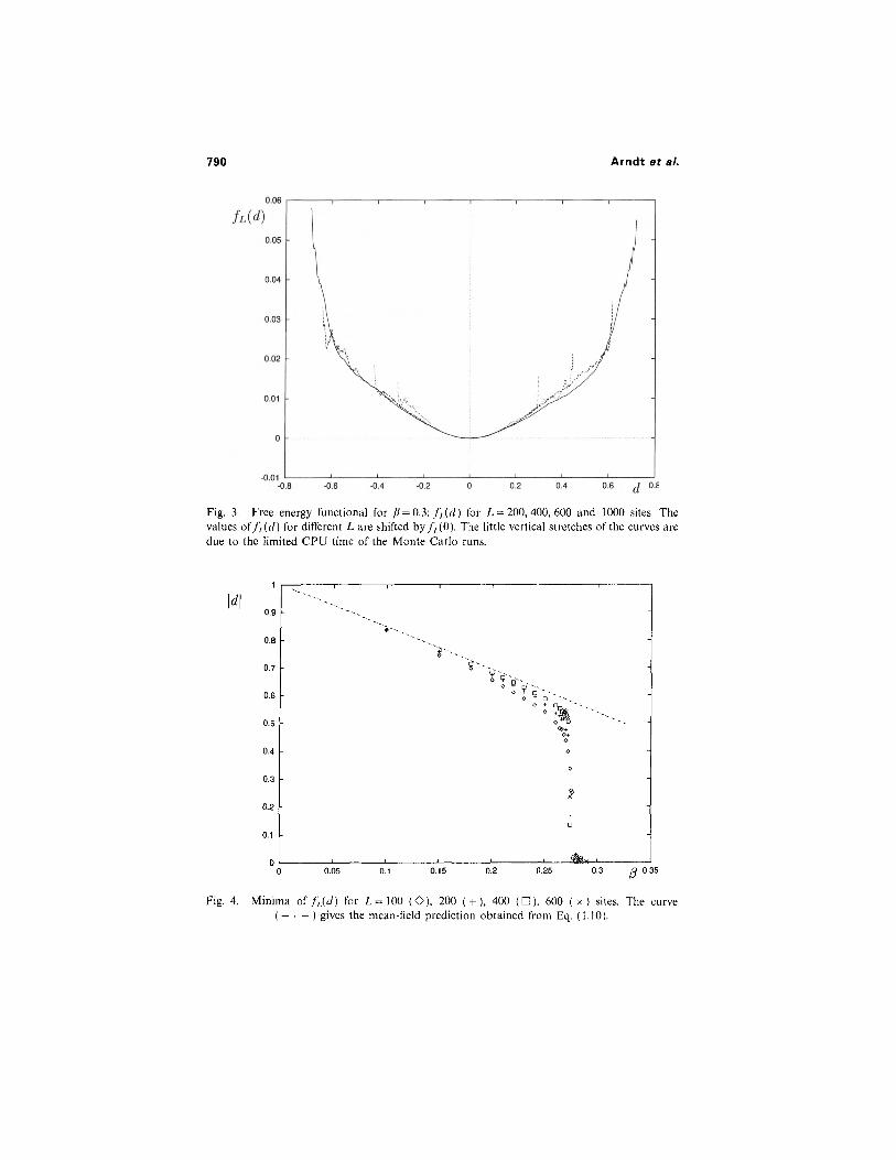
In order to make sure that we are not dealing with finite-size effects wehave computed fL(d) for /? = 0.3 (still below 0.3289) for various number ofsites up to L = 1000. The data are shown in Fig. 3 (we have substracted thevalue//.(O)). One can see t h a t f L ( d ) is practically independent of L (the Ldependence is in/£(0)—see Appendix A). This implies that one does nothave finite-size effects, and ihalfL(d) —fL(0) is a convex function with oneminimum as one expects to have if one is in the "disordered" phase.

We now present more data which show what goes wrong with themean-field prediction. In Fig. 4 we show the positions of the minima offL(d) for various numbers of sites and various values of/?. One can observethat below /?crit the minima converge to their mean-field values obtainedfrom Eq. (1.10) and that a dramatic change takes place at /?crit. Above /?crit

the CP symmetry is not broken anymore (d = G).In Fig. 5 we show the minima o(fL(s) as a function of/? for various L.

The upper curve is given by the average value of ^ for the two phases(low/high density). This value is obtained from Eq. (1.10):

822/90/3-4-18

789

Fig. 2. /,(;/) for /? = 0.164, 0.270, 0.274, 0.276, 0.280, 0.285, 0.290 and L = 400 sites. Thevalues of/ ,((/) are shifted by their value/ /(O).

790 Arndt et at.

Fig. 3. Free energy functional for /? = 0.3: f,_(d) for 1 = 200,400,600 and 1000 sites. Thevalues of f/_(d) for different L are shifted by/A(0). The little vertical stretches of the curves aredue to the limited CPU time of the Monte Carlo runs.

Fig. 4. Minima of f,,(d) for L=100 (O) , 200 ( +), 400 ( D ) , 600 (x) sites. The curve(— • - ) gives the mean-field prediction obtained from Eq. (1.10).

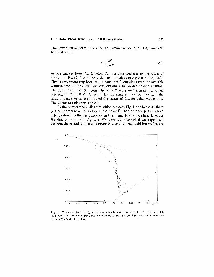
As one can see from Fig. 5, below /?cril the data converge to the values ofs given by Eq. (2.1) and above /?crit to the values of s given by Eq. (2.2).This is very interesting because it means that fluctuations turn the unstablesolution into a stable one and one obtains a first-order phase transition.The best estimate for /?crit comes from the "fixed point" seen in Fig. 5, onegets &rit = 0.275 ±0.001 for a = l . By the same method but not with thesame patience we have computed the values of /?cril for other values of a.The values are given in Table I.

In the correct phase diagram which replaces Fig. 1 one has only threephases: the phase A like in Fig. 1, the phase B (the unbroken phase) whichextends down to the diamond-line in Fig. 1 and finally the phase D underthe diamond-line (see Fig. 14). We have not checked if the seperationbetween the A and 6 phases is properly given by mean-field but we believe

Fig. 5. Minima of/,.U) (s = (p + m)/2) as a function of £ for L=100 ( O ) , 200 ( +), 400(D) , 600 ( x ) sites. The upper curve corresponds to Eq. (2 .1) (broken phase), the lower oneto Eq. (2.2) (unbroken phase).


The lower curve corresponds to the symmetric solution (1.8), unstablebelowy?=l/3:

792 Arndt of a/.

Table 1. The Critical Points for Various a

<X

0.250.500.751.00

Acri,

0.1865(5)0.259( 1 )0.274( 1 )0.275(1)

a

1.251.501.752.00

A*.

0.269(1)0.264(1)0.258(2)0.253(1)

this to be the case because of the analytical calculation on the ft = 1 linedone in ref. 7.

A final test of our picture can be obtained looking at the spectrum ofthe hamiltonian, which is explicitly given in Appendix B. We consider thefirst three levels and take oc = 1 only. Since the ground state has energyzero, the values of the energies of the next two levels, denoted by E\ and E2,coincide with the energy gaps. If our picture is correct El should vanishfor large values of L for ft < /?crit since in the large L limit one needs twostates, the ground state and the first excited state, to describe the two vacua.

Fig. 6. Estimates of the first (O) and second (+) excitations of the CF-symmetrichamiltonian (Eq. B . I ) with /i = 0). The estimates were obtained using the spectra of thehamiltonian up to eleven sites and extrapolating the results in standard ways. Since all eigen-values of H are positive the errors of the values shown are estimated to be 0.0003.

E2 should be finite. For /? > /?crit both El and E2 should be finite. Using themodified Arnoldi algorithm of ref. 16 we have calculated, for various valuesof ft and chain lengths (up to L = 11) the values of El and E2. In order toget their large L limit we have used Bulirsch-Stoer approximants."7' Theresults are shown in Fig. 6 which confirms the existence of a critical pointaround ft = 0.27'5. If one takes /? = /?crit one can estimate the dynamicalcritical exponent z defined as follows:

3. DESCRIPTION OF THE FIRST-ORDER PHASE TRANSITION

We are now going to study in detail the point a= 1, /? = /?crit = 0.275where as explained in the last section we have seen a first-order phasetransition. The physics of the steady state can be understood only if oneconsiders the two order parameters p and m.

In Fig. 7 we show, in the p — m-plane, the contour lines of the FEFfL(p,tn) near its minima. The figure suggests a large L limit in which weget the following picture: one line segment parallel to the p-axis (from Uto V in Fig. 7), one line segment parallel to the w-axis (from S to R),a smooth curve joining the points S, T and U. Let us give the (p, m) coor-dinates of these five points: V = (0.725, 0.149) where p and m are obtainedfrom the mean-field equation (1.10), R = (0.149, 0.725), obtained fromEq. (1.10) exchanging/? and m, T = (0.216, 0.216), obtained from Eq. (1.8).It is convenient to denote by p^ and raA the p and m coordinates of thepoint A. With this notation the coordinates of the points U and S areU = (l — pv, mv) and S = (/?R, 1 — WR). The points V and R are to beexpected to play a special role since they represent the broken phase for avalue of fi slightly smaller than /?crit. Also the point T is to be expectedsince it corresponds to the symmetric phase (ft slightly higher than /?crit).The points S and U are unexpected since they do not correspond to anyphase. Their coordinates have however a remarkable property: pv = 1 — pv

and similarly ms=l— mR. These relations are typical for shocks (seeAppendix A and ref. 12). The following simple model captures the physicsof the phase transition. First let us introduce the scaling variable z = k/L,


where E^L) represents the energy of the first exited state for a chain oflength L. We find r = 2.0 + 0.1. (A better estimate of z is not possible, since/?crit is known only up to three digits.) This result is also interesting becausefrom our experience with the one-species problem (see Appendix A) a valueof z = 2 suggests the existence of shocks. In the next section we are goingto find them.

Arndt et al.

Fig, 7. Contour lines of /,.(;>, m) for /? = 0.275 and L=1000 sites. The "height" differencebetween lines is constant.

where k is the site variable and L the length of the lattice. The model willapply in the limit where k and L are large. We assume that the followingprocesses take place:

• With a probability P, we have shocks of uncorrelated positive par-ticles as described by Fig. 8a. The probability to find a positive particle atthe left of the point g with a density pu and to the right of the point g witha density pv is independent of z. One has fronts for 0 < g < 1 with equalprobability (this corresponds to the U-V line segment). The negativeparticles are also uncorrelated and have a constant density mv.

• Also with a probability P} we have shocks of negative particles (seeFig. 8b) which are just the CP-reflected shocks of the positive particles(this corresponds to the R-S line segment).

794


Fig. 8. The shocks appearing at the first-order phase transition. The solid and broken linesgive the profile of positive and negative, respectively.

• With a probability P2 we have configurations (Fig. 8c) of constantdensity (independent of :) corresponding to all pairs of values p and malong the line segment S-U, all with the same probability.

Obviously

The assumption that we have a line segment between S and U is anapproximation since this line segment intersects the p = m line in the pointof coordinates ( ( p u + pR)/2, (ms + mv)/2) = (0.212, 0.212) which does notcoincide with T but is very close to it. We did not try to find a betterdescription of the S-T-U curve because this would imply many moreMonte Carlo data than we were able to collect.

The probabilities /", and P2 are determined from the condition thatfL(p, m} has the same value everywhere on the "boomerang." We get

Let us now check the model, in this way we can present the data inan organized way. First, we can compute f ( d ) . One obtains a functionwhich is flat between — (pv — mv) and (pv~mv). This is just what onesees in Fig. 2 for /?c,.it. Next we compute m(z) and get

Arndt ef a/.

Fig. 9. Density profile of the negative particles for L = 50 ( D), 100 ( O ) , 200 ( +) at thephase transition jj = 0.275. The straight line is given by Eq. (3.4).

Fig. 10. Density profile of the negative particles for /. = 50 (O) , 100 ( + ) , 200 (D) at/? = 0.26, below the phase transition. The line gives the mean-field prediction, i.e. the averageof the densities of Eq. (1 .10) .

796


Obviously p(z) = m(\ — z). In Fig. 9 we show the density of negativeparticles as a function of z for various numbers of sites. One notices thatthe straight line given by Eq. (3.4) fits the data.

In order to make sure that the linear density distribution observed inFig. 9 is not a finite-size effect, in Fig. 10 we show for /? = 0.26 (below thecritical point) the function m(z). One observes that the data converge(slowly) from below to the mean-field value m = QA4 obtained taking theaverage of the two equations (1.10).

In Fig.ll we show m(z] for /? = 0.3 (above /?crit). The data convergefrom above to the value w = 0.23 which is obtained from Eq. (1.8). In con-clusion, the non-constant distributions seen just below and just above /?crit

are cross-over phenomena.In order to "see" the shocks, we have looked at configurations where

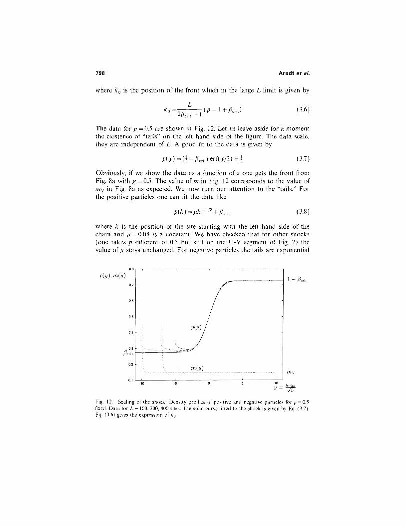
the density of positive particles p, averaged over the lattice, is fixed. Thiscorresponds to a point on the U-V line segment in Fig. 7 and one expectsto see a shock like in Fig. 8a. Since we are also interested to see what kindof finite-size effects exist (see Appendix A), we have chosen to present thedensities as functions not of z but in terms of the variable

797

Fig. II. Density profile of the negative particles for £ = 50 (O), 100 ( + ) , 200 (D) at/? = 0.30, above the phase transition. The line gives the (unstable) mean-field solution (1.8).

798 Arndt ef a/.

where k0 is the position of the front which in the large L limit is given by

The data for p = 0.5 are shown in Fig. 12. Let us leave aside for a momentthe existence of "tails" on the left hand side of the figure. The data scale,they are independent of L. A good fit to the data is given by

Obviously, if we show the data as a function of z one gets the front fromFig. 8a with g = 0.5. The value of m in Fig. 12 corresponds to the value ofmv in Fig. 8a as expected. We now turn our attention to the "tails." Forthe positive particles one can fit the data like

where k is the position of the site starting with the left hand side of thechain and /u = 0.08 is a constant. We have checked that for other shocks(one takes p different of 0.5 but still on the U-V segment of Fig. 7) thevalue of n stays unchanged. For negative particles the tails are exponential

Fig. 12. Scaling of the shock: Density profiles of positive and negative particles for p = 0.5fixed. Data for L = 100, 200, 400 sites. The solid curve fitted to the shock is given by F,q. (3.7).Eq. (3.6) gives the expression of A,, .


with a correlation length independent of L. This observation is intriguingbecause common sense would suggest that in this case one should havea finite correlation length also in the time direction, i.e. masses in thespectrum of the problem and not only the massless excitations discussed inSection 2.

Another test of the model, this time on a part of it on which wecertainly expect to be less precise, is to "cut" through the handle of theboomerang. We have taken d = 0.05 in order to check if profiles like inFig. 8c are seen. The data are shown in Fig. 13 together with the expectedconstant values (take the intersection of the line d = 0.05 with the linesegment S-U in Fig. 7). As one notices we find agreement although somemini-shocks are not excluded. After presenting the data we are left witha puzzle. We have expected the point T to be singled out in some way(it represents the symmetric phase), but it is not.

4. THE BROKEN PHASE IN THE PRESENCE OF ASYMMETRY BREAKING EXTERNAL SOURCE

4.1. The Free Energy Functional

As explained in Section 2 and shown in Fig. 14, the phase diagram ofthe CP-symmetric model consists of a power law phase A and a broken

799

Fig. 13. Density profile /> (z ) and 111(2) for </ = 0.05 and L = 200.

Arndt at al.

phase D separated by a first-order phase transition line from the unbrokenphase B. In equilibrium systems, if one has a transition from an ordered toa disordered phase, the broken phase corresponds to first-order phasetransitions (and the FEF is a flat function between the two phases). As wehave seen this is not the case for steady states and for this reason we usethe expression "first-order" only on the separation line where the FEF isflat and the expression "broken phase" for the domain where the FEF isnot convex and has two minima.

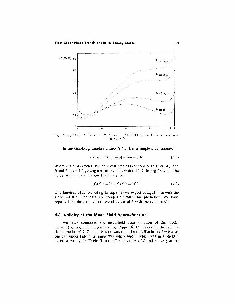
We consider now the effect of an explicit CP symmetry breaking in themodel. We take h>0 in the boundary rates given by equations (1.2) and(1.3). Using Monte Carlo simulations, we have computed the FEF fL(d, h)taking a = 1 and several values of /? and h; d is again the difference betweenthe average densities of positive and negative particles. In Fig. 15 we showfL(d, h} for /? = 0.1 (in the D phase) and several values of h. We observethat below hcrit = 0.2281 the FEF shows two minima and only one mini-mum for A>/!cri l. For h = hcrh the first and second derivative of fL(d, h)with respect to d vanishes. This is the definition of a spinodal point."51

The behavior offL(d, h) is the one expected from a Ginzburg-Landauansatz."8' Our data are of course not precise enough to give an estimatewith four digits for /zcrit, the value we give is obtained in mean-field. Wewill return soon to the problem of the validity of mean-field.

800

Fig. 14. Phase diagram of the two-species model for h=0 obtained from the Monte Carlosimulations. The phase A is given by mean field.


Fig. IS. /,.((/,/!) for L = 30, a= l.O, /? = 0.l and h = 0.1, 0.2281, 0.3. For /i = 0 the system is inthe phase D.

In the Ginzburg-Landau ansatz/((/, h) has a simple h dependence:

where v is a parameter. We have collected data for various values of ft andh and find v = 1.4 getting a fit to the data within 10%. In Fig. 16 we fix thevalue of h = 0.02 and show the difference

as a function of d. According to Eq. (4.1) we expect straight lines with theslope —0.028. The data are compatible with this prediction. We haverepeated the simulations for several values of h with the same result.

4.2. Validity of the Mean Field Approximation

We have computed the mean-field approximation of the model(1.1-1.3) for h different from zero (see Appendix C), extending the calcula-tion done in ref. 7. Our motivation was to find out if, like in the h = 0 case,one can understand in a simple way where and in which way mean-field isexact or wrong. In Table II, for different values of ft and h, we give the

Arndt et at.

values of d™m which denotes the minima of the FEF as determined byMonte Carlo simulations as well as the values of dm_( obtained in mean-field. Comparing the Monte-Carlo simulations with the mean-field resultswe reach the conclusion that probably mean-field is not exact anywhere. Itremains, however, a good approximation for small values of ft and largevalues of h.

4.3. The Dynamical Critical Exponent at the Spinodal Point

We are now going to discuss some aspects of the dynamics of themodel when one includes the symmetry breaking term. Our attention goesfirst to the spinodal point and we look at the spectrum of the hamiltonian(see Appendix B). We notice that the first excited state has an energy whichvanishes in the large L limit. The dynamical critical exponent (seeEq. (2.3)) determined using the values of the first excited state of chainsup to 11 sites ft = 0.1 and hcr-n =0.22810 as given by mean-field is z =1.00 ±0.01. We have repeated the same calculation for /? = 0.05(/zcrit = 0.28096) and found z = 1.000 ±0.001. (Notice that we have takensmall values of /? and that the values of Acri, are large.)

From previous experience with quantum chains,(28) for a three-statemodel 11 sites are enough for a reasonable estimate of the asymptoticbehaviour of energy gaps if the critical point is known. In order to check

802

Fig. 16. /,.(</, A = 0)-/,.(</, h = 0.02) for /? = 0.20, 0.26, 0.28, 0.30 and £ = 100 sites.


Table II. The Minima d?" of fL(d) (Error ±0.01) and the Mean-FieldPredictions </m_ f for a= 1, Various P and h"

ft

0.6

0.35

0.329

0.3

0.26

0.1

A

00.1

00.020.1

00.020.1

00.020.1

00.010.020.07

00.020.050.1

L

200200

400100100

400200200

400400400

200100100100

20010010050

jmin

0.00-0.08

0.00-0.05-0.45

0.00-0.06-0.52

0.00-0.15-O.S8

-O.S3/+0.53-O.S3/ + 0.43-0.54-0.61

-0.84/+0.84-0.84/+0.84-0.85/+0.83-0.86/+0.81

(lm-f

0

-0.0943

0-0.468-0.512

-0.490/ + 0.490/0-0.501-0.543

-0.537/ + 0.537/0-0.546/ + 0.527/ + 0.098-0.584

-0.600/ + 0.600/0-0.604/ + 0.596/ + 0.019-0.607/ + 0.592/ + 0.038-0.629

-0.849/ + 0.849/0-0.852/ + 0.846/ + 0.005 19-0.856/ + 0.841/ + 0.013-0.864/ + 0.833/ + 0.026

if the mean field estimates of hcrit are correct, we have computed the con-nected two-point function in the bulk using Monte-Carlo simulations. It isindeed zero. To our knowledge it is for the first time that the exponentz = 1 appears in stochastic processes.

In ref. 19 the toy-model of Godreche et a/.(20) is examined (whichcorresponds to the /? -»0 limit of the present model) and again : = 1 isfound. More than that, in ref. 19 it is shown that the spectrum has masslessexcitations which are universal and also massive excitations. (As opposedto the present model where we could study properly only one level, in thetoy-model we can study many of them.) The toy-model has two parameters,one which corresponds to a in the original model and h. Normalizing thehamiltonian such that the sound velocity is the same, at the spinodal point

the spectra corresponding to the massless regime do not depend on theformer parameter.

One can ask which implications has a z = 1 exponent. Since instochastic processes one computes quantities which correspond in fieldtheory to form factors and not to vacuum expectation values, the applica-tion of ideas coming from conformal invariance as suggested by z — 1 arenot obvious. In ref. 19 several properties of the time dependence of theorder parameter are given. The simplest one being that the flip time'61 froma configuration with the d value of the spinodal point to a configurationcorresponding to the minimum offL(d, h) (see Fig. 15) should be propor-tional to L.

4.4. Flip Time and Barriers of the Free Energy Functional

We would like to make an observation on the flip times related tobarriers in the FEF. Let us take /? = 0.1 and h = 0.1 in Fig. 15 and denoteby A l ( A 2 ) the difference between the maximum of the FEF and the mini-mum of the FEF for negative (positive) values of d (A2 = 0 at the spinodalpoint). From the Monte Carlo data (L = 50 sites) we get A^ = 0.178 + 0.002and A2 = 0.041 + 0.002. The two flip times from the stable (unstable) to theunstable (stable) phase are r,ong (rshort). They have been measured for

Fig. 17. Logarithmic plot of the flip times for a = 1.0, /) = 0.1 and h = 0.1. The dotted curvesare given by (4.3).

804 Arndt et al.

The agreement between the ansatz (4.3) and the data shows a connectionbetween the dynamics of the model (flip times) and the properties of thesteady state (the FEF). Repeating the same procedure for a different valueof gives the same result. More about this subject can be found in ref. 19.

5. CONCLUSIONS

We have shown in the framework of the two-species model the followingpattern of spontaneous CP symmetry breaking for steady states. If we startin the "disordered" phase (where the free energy functional as a function ofthe order parameter has only one minimum) and lower the "temperature"(the parameter /?) we have a first-order phase transition at /?crit with a flatfree energy functional (like in equilibrium problems). At /?crit the densityprofiles and correlation functions in the scaling regime can be explainedusing a certain combination of shocks. Below the critical "temperature"/?crit, in the broken phase, the free energy functional is not a convex func-tion of the order parameter (unlike in equilibrium problems) but has twominima corresponding to two phases defined by their average densities ofpositive and negative particles. If the CP symmetry of the model is brokenby a small perturbation (parameter h), one has only one minimum for thefirst-order phase transition (like in equilibrium) but still two minima in thebroken phase. If we increase h one gets spinodal points.

At the first-order phase transition we have seen massless excitations inthe spectrum of the quantum chain hamiltonian associated with thedynamics of the process with a critical dynamical exponent z = 2. This doesnot exclude the presence of massive excitations which are suggested bythe exponential tails seen in Fig. 9 and Fig. 12 in the density profiles.Massive excitations are not seen for the one-species model described inAppendix A.(21)

At the spinodal points we have also seen massless excitations withz = 1 as well as massive excitations. The latter are suggested by exponentialtails observed in the density profiles not shown in this paper. These obser-vations are confirmed by the investigation of the low /? limit of themodel.'19> At this point it is not clear if the exponent z = 1 has profoundimplications like in equilibrium problems where it implies conformalinvariance or is just one dynamical critical exponent among others. We

822/90/3-4-19

chains of different lengths L and their values are shown in Fig. 17. Thestraight lines in Fig. 17 are given by the ansatz

First-Order Phase Transitions in ID Steady States 805

Defining a = a + ft and h=(J — aL one notices that for h = 0 the modelis CP-invariant. We denote by c the average density of positive particles.The model presents three phases:

• the power law phase (a > 1/2, /? > 1/2) where c = 1/2

• the low density phase (a< 1/2, /?>a) where c = a

• the high density phase (a> /? , / ?< 1/2) where c=l —fi

A coexistence line (« = /?< 1/2) separates the low density from the highdensity phase. The concentration has a discontinuity along this line fromc = /? to c=l- /? .

Using Monte Carlo simulations we have computed the FEF fL(c, h)keeping a A fixed and using several values of h. The results are shown inFig. 18. We notice that for / i=0, the FEF is a flat function between c = fland c = 1 — /?. A small positive h(h = 0.004) gives a FEF with only one min-imum at c = [3 just like in equilibrium first-order phase transitions. A largervalue of h (A = 0.1) moves the minimum away. We have studied the con-vergence of the function fL(c, h) lo f(c, h) taking c'min the value of c where

806 Arndt et al.

have looked to conformal towers in the spectrum of the hamiltonian butthe data of our short quantum chains did not give any clean results. Thisis probably due to the fact that the critical point is not known exactly (weused the values obtained from mean-field) and that in general the con-vergence to the thermodynamic limits is slower in stochastic quantitiesthan in equilibrium ones. This is an empirical observation. We think thata further investigation of the model is necessary by taking the second ratein (1 .1 ) not equal to the other two. Some preliminary results are describedin ref. 7. This study can be done not only by Monte Carlo simulations butalso using the analytical methods developed recently in ref. 22.

APPENDIX A. THE ASYMMETRIC EXCLUSION PROCESS

The physics of this model is well understood,<2^t) here we are going todiscuss some aspects of it which are necessary for the understanding of thefinite-size effects of the two-species model. We consider a chain of length Lwith two types of particles (+ and — ). In an infinitesimal time step d; thefollowing processes take place:


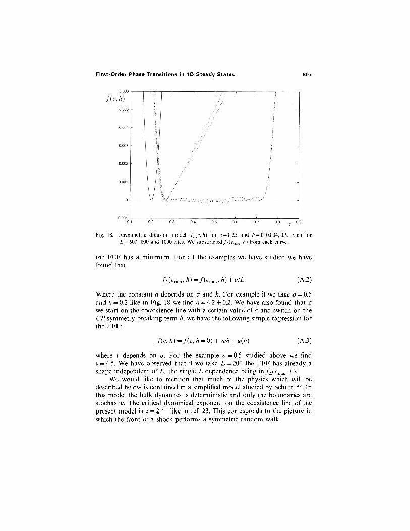
where v depends on a. For the example a = 0.5 studied above we findv = 4.5. We have observed that if we take L = 200 the FEF has already ashape independent of L, the single L dependence being in/L(cmin, h).

We would like to mention that much of the physics which will bedescribed below is contained in a simplified model studied by Schutz.'231 Inthis model the bulk dynamics is deterministic and only the boundaries arestochastic. The critical dynamical exponent on the coexistence line of thepresent model is z = 2 ( 2 1 ) like in ref. 23. This corresponds to the picture inwhich the front of a shock performs a symmetric random walk.

807

Fig. 18. Asymmetric diffusion model: J ' , ( c , h ) for s = 0.25 and h = 0,0.004,0.5, each forL = 600, 800 and 1000 sites. We substracted /,„(<•,„,„,/O from each curve.

the FEF has a minimum. For all the examples we have studied we havefound that

Where the constant a depends on a and h. For example if we take a = 0.5and h = 0.2 like in Fig. 18 we find a = 4.2 + 0.2. We have also found that ifwe start on the coexistence line with a certain value of a and switch-on theCP symmetry breaking term /j, we have the following simple expression forthe FEF:

808 Arndt et at.

On the coexistence line the density of positive particles is high at theright hand side of the chain (c= 1 — /?) and low at the left hand side of thechain (c = /?,/?< 1/2). The two regimes are joined by a shock front. Onemeasures such a shock by constraining the average density of positive par-ticles to a given value between ft and 1 —/?. If c(k) is the concentration atlattice site k, it is useful to define the variable

where

is the position of the shock front. In Fig. 19 we show the Monte Carlo datafor c = 0.5 and a = /? = 0.25. The existence of a front with width of orderLl / 2 is to be expected from the model studied by Schutz,<23) from the exclu-sion model with a blockage'24'25' and from the asymmetric model with an

Fig. 19. Scaling of the shock: Density profiles for <x = /? = 0.25 (with r = 0.5 fixed) and forZ,= 100, 200. The dotted curve is given by Eq. (A.6). The wriggled curves represent the MonteCarlo data which coincide with Eq. (A.6) within 1%.


impurity,<26> and by some other models considered in ref. 27. These modelssuggest the following expression for the front profile:

The Monte Carlo data are fitted within 1 % by this function.Our purpose in studying the finite-size behavior of the shocks was to

find out how many lattice sites are necessary to be in the scaling limit inorder to know for the threestates model which lattice size are necessary tosee shocks. It turns out that L= 100 are enough.

APPENDIX B. THE HAMILTON OPERATOR

The time evolution operator H of the master equation (1.4) for theprocesses (!.!)-(1.3) can be written as a sum of operators acting non-trivially on adjacent sites only (hopping) and of two operators acting onthe first and last site (input and output):(8)

The matrices are

810 Arndt et al.

where the subscripts denotes the sites the matrices act on and / is the 3 x 3unit matrix. The order of the basis at each site is chosen a s | 0 > , + > , | — >.Note that H is not hermitian.

APPENDIX C. MEAN-FIELD THEORY FOR H>0

In this appendix we present the extension of the mean-field theory17'to the h > 0 case. The time evolution of the average values of the densitiesis given by the following equations

For the stationary state one takes the left hand sides of Eqs. (C.I )equal to zero. The resulting equations can be written as the condition thatthe current of the positive and negative particles is site-independent:

Notice that in the bulk the equations for p(k) and m(k) decouple. It isconvenient to denote


The problem of solving equations (C.2) and (C.3) is reduced to solving twomodels each with one type of totally asymmetric diffusing particles andwith input and output rates a + ,/?+ and < x ~ , / ? ~ respectively. The solutionof the latter problem is known. (2~4) Each of the decoupled chains is in oneof the phases of the asymmetric diffusion model. Depending on a, ft and h,only certain combinations of phases can occur, since the two chains arecoupled through the boundaries (C.5) and (C.6).

Let us first consider the phases of the two-species model where thecurrent of positive particles equals the current of negative particles,j+ = j~. In this case equations (C.5) and (C.6) simplify to

One finds

In this phase both currents are/= 1/4 and the densities of the particles isps = 1/2. We find this phase for

These conditions reduce to

This corresponds to the regions A* in Fig. 20 which shows the phasediagram obtained in mean field approximation for h = 0.\.

° the power-law symmetric phase

812 Arndt et al.

Fig. 20. Mean-field phase diagram for asymmetry /i=0.1.

° the low-density symmetric phase

For h = 0 there exists a symmetric low-density phase (B) withy'+ =j~. Theconditions for this phase are

If we turn on the asymmetry h, this phase does not exist anymore. Instead,one still finds a phase with the two types of particles in the low-densityphase of the single-species chain but with different currents. One has todistinguish between the favoured and unfavoured low-density/low-densityphase.

° the favoured low-densityjlow-density phase

A positive h favours the output of positive particles, such that morenegative particles can be injected. Therefore the current of negative par-ticles is more likely to be bigger than the current of positive particles. Forthe existence of the favoured low-density/low-density phase we have


and need a solution of (C.5) and (C.6), which can be rewritten as

with

This gives the region C* of Fig. 20.

° The unfavoured low-density I low-density phase

occupies the smaller region E* in the phase diagram and can be foundwhere a solution of (C.13) and (C.14) under the conditions (C.15) witha.+ > a ~ instead of a ~ > a+ exists. The respective region in the phasediagram shrinks with increasing h, since the asymmetry favours the otherlow-density/low-density phase.

° The favoured high-density/low-density phase

is the phase where the negative particle is in the high-density phase, sincethe input of negative particles is favoured and it is more probable to finda high density of negative particles. The positive particles are in the low-density phase and we have

The solution of (C.5) and (C.6) has to fulfill

This gives the regions D* and E* of Fig. 20.

° The unfavoured high-density flow-density phase

In this case one has

814 Arndt et al.

and the conditions

These conditions are fulfilled in region E*.For /?-»0 equations (C.20) and (C.21) can be replaced by

o The low-density/power-law phase

This phase does not occur in the original model with h = 0. But for h > 0one finds a phase where the negative particle is in the power-law phase andthe positive is in the low-density phase. The conditions are

and give B* in Fig. 20.Note, that in E* three different stationary solutions of (C.I) are

allowed: the unfavoured low-density/low-density and the favoured andunfavoured high-density/low-density phases. However, only the favouredhigh-density/low-density phase is a dynamically stable solution of (C.I).Increasing the asymmetry region E* shrinks, whereas the regime D* grows.

ACKNOWLEDGMENTS

We would like to thank M. Evans, C. Godreche, J. M. Luck, D.Mukamel and especially B. Derrida for discussions. We would like also tothank SISSA for hospitality. The work of P. F. A. and T. H. was supportedby the DAAD programme HSP II-AUFE. V. R. acknowledges partial sup-port by the EC TMR programmer grant FMRX-CT96-0012.

REFERENCES

1. J. Krug, Phys. Rev. Lett. 67:1882 (1991).2. B. Derrida, E. Domany, and D. Mukamel, J Slat. Phys. 69:667 (1992).3. B. Derrida, M. R. Evans, V. Hakim, and V. Pasquier, J. Phys. A: Math. Gen. 26:1493

(1993).4. G. Schutz and E. Domany, /. Slat. Phys. 72:277 (1993).

5. P. P. Martin, Potts models and related problems in statistical mechanics (World Scientific,Singapore).

6. M. R. Evans, D. P. Foster, C. Godreche, and D. Mukamel, Phys. Rev. Lett. 74:208 (1995).7. M. R. Evans, D. P. Foster, C. Godreche, and D. Mukamel, J. Slat. Phys. 80:69 (1995).8. F. H. L. EBler, and V. Rittenberg, J. Phys. A: Math. Gen. 29:3375 (1996).9. S. Sandow, Phys. Rev. E50:2660 (1994).

10. R. B. Griffiths, C. -Y. Weng, and J. S. Langer, Phys. Rev. 149:301; J. D. Gunton, M. SanMiguel, and P. S. Sahni, in Phase Transitions and Critical Phenomena, C. Domb andJ. L. Lebowitz, eds. (Academic Press), Vol. 8, p. 267, 1989.

11. M. den Nijs, in Proceedings of the 4th workshop on Statistical Physics, Seoul, January27-31 (1997).

12. J. L. Lebowitz, E. Presusti, and H. Spohn, J. Slat. Phys. 51:841 (1988).13. K. Mallick, Ph.D. thesis, Saclay (1996).14. C. H. Bennett and G. Grinstein, Phys. Rev. Lett. 55:657 (1985).15. V. Privman and L. S. Schulman, J. Phys. A: Math. Gen. 15:L238 (1982), and J. Stal. Phys.

29:205.16. U. Bilstein, diploma thesis, BONN-IB-96-33 (1996).17. R. Bulirsch and J. Stoer, Numer. Math. 6:413 (1964), M. Henkel and G. Schutz, J. Phys.

A: Math. Gen. 21:2617 (1988).18. M. Le Bellac, Quantum and statistical field theory (Oxford University Press, Oxford,

1991).19. P. F. Arndt and T. Heinzel, cond-mat 9710287 (1997).20. C. Godreche, J. M. Luck, M. R. Evans, D. Mukamel, S. Sandow, and S. R. Speer, J. Phys.

A: Math. Gen. 28:6039 (1995).21. U. Bilstein and B. Wehefritz, J. Phys. A: Math. Gen. 30:4925 (1997).22. F. C. Alcaraz, S. Dasmahapatra, and V. Rittenberg, cond-mat 9705172 (1997).23. G. Schutz, Phys. Rev. E47:4265 (1993).24. S. A. Janowsky and J. L. Lebowitz, Phys. Rev. A45:618 (1992).25. G. Schutz, J. Slat. Phys. 71:471 (1993).26. K. Mallick, / Phys. A: Math. Gen. 29:5375 (1996).27. K. Krebs, to be published (1997).28. G. von Gehlen and-V. Rittenberg, J. Phys. A: Math. Gen. 19:L625 (1986).


First-Order Phase Transitions in One-Dimensional Steady States

Documents

Transcript of First-Order Phase Transitions in One-Dimensional Steady States