arX

iv:1

304.

0253

v1 [

quan

t-ph

] 3

1 M

ar 2

013

Theoretical formulation of finite-dimensional

discrete phase spaces: II. On the uncertainty

principle for Schwinger unitary operators

M.A. Marchiolli a, P.E.M.F. Mendonca b

aAvenida General Osorio 414, centro, 14.870-100 Jaboticabal, SP, Brazil

E-mail: marcelo march@bol.com.br

bAcademia da Forca Aerea, C.P. 970, 13.643-970 Pirassununga, SP, Brazil

E-mail: pmendonca@gmail.com

Abstract

We introduce a self-consistent theoretical framework associated with the Schwingerunitary operators whose basic mathematical rules embrace a new uncertainty prin-ciple that generalizes and strengthens the Massar-Spindel inequality. Among otherremarkable virtues, this quantum-algebraic approach exhibits a sound connectionwith the Wiener-Kinchin theorem for signal processing, which permits us to deter-mine an effective tighter bound that not only imposes a new subtle set of restric-tions upon the selective process of signals and wavelets bases, but also representsan important complement for property testing of unitary operators. Moreover, weestablish a hierarchy of tighter bounds, which interpolates between the tightestbound and the Massar-Spindel inequality, as well as its respective link with thediscrete Weyl function and tomographic reconstructions of finite quantum states.We also show how the Harper Hamiltonian and discrete Fourier operators can becombined to construct finite ground states which yield the tightest bound of a givenfinite-dimensional state vector space. Such results touch on some fundamental ques-tions inherent to quantum mechanics and their implications in quantum informationtheory.

1 Introduction

Initially introduced by Schwinger [1] for treating finite quantum systems cha-racterized by discrete degrees of freedom immersed in a finite-dimensionalcomplex Hilbert space [2], the unitary operators gained their first immediateapplication in the formal description of Pauli operators. Ever since, an expres-sive number of manuscripts [3] proposed similar theoretical frameworks withintrinsic mathematical virtues and concrete applications in a wide family of

Preprint submitted to Elsevier Science 10 January 2014

physical systems — here supported by a finite space of states. With regardsto these state spaces, it is worth mentioning that certain algebraic approachesrelated to quantum representations of finite-dimensional discrete phase spaceswere constructed from this context in the past [4], and tailored in order toproperly describe the quasiprobability distribution functions [5] in completeanalogy with their continuous counterparts [6]. Thus, applications associatedwith the discrete distribution functions covering different topics of particularinterest in physics — e.g., quantum information theory and quantum com-putation [7,8], as well as the qualitative description of spin-tunneling effects[9], open quantum systems [10] and magnetic molecules [11], among others —emerge from these approaches as a natural extension of an important robustmathematical tool.

Although the efforts in constructing a sound theoretical framework to dealwith finite-dimensional discrete phase spaces have recently achieved great ad-vances (e.g., see Ref. [12]), certain fundamental questions particularly associ-ated with the factorization properties of finite spaces [13], uncertainty principle[14] and property testing [15] for the unitary operators still remain withoutsatisfactory answers in the literature (indeed, some of them represent openproblems which do not share the same rhythm of progress). In this paper, wefocus on the problem of deriving a general uncertainty principle for Schwingerunitary operators in physics. In what follows, we discuss the relevance of sucha principle and, subsequently, briefly review the results obtained by Massarand Spindel [14] on this specific subject.

To begin with, it is necessary to remember that, through an original algebraicapproach which encompasses the description of finite quantum systems, Weyl[16] was the first to describe quantum kinematics as an Abelian group of rayrotations in the system space. According to Weyl: “The kinematical structureof a physical system is expressed by an irreducible Abelian group of unitaryray rotations in system space. The real elements of the algebra of this groupare the physical quantities of the system; the representation of the abstractgroup by rotations of system space associates with each such quantity a def-inite Hermitian form which ‘represents’ it.” With respect to the particularcase of finite state vector space, one of Weyl’s most significant achievementswas that the observation of pairs of unitary rotation operators obey specialcommutation relations (bringing, as a result, the roots of unity) which are theunitary counterparts of the fundamental Heisenberg relations. Moreover, it isworth mentioning that such a ray representation of the Abelian group of rota-tions can be connected with some representations of the generalized Cliffordalgebra, this fact being thoroughly explored by Ramakrishnan and coworkers[17] through extensive studies of certain physical problems. Still within theaforementioned Weyl approach for quantum kinematics, let us briefly mentionthat some authors have also addressed the problem of discussing quantummechanics in finite-dimensional state vector spaces, where the coordinate and

2

momentum operators (characterized by discrete spectra) play an essential rolein this context [18].

Although both Weyl and Schwinger’s theoretical approaches have made se-minal and complementary contributions upon the scope of unitary operatorsin finite physical systems, the relevance of a general uncertainty principle forsuch operators has not been clearly discussed or even mentioned with due em-phasis in the past. Reflecting on this, Massar and Spindel [14] have recentlyestablished a first uncertainty principle for the discrete Fourier transform [19]whose range of applications in physics covers, among other topics, the Paulioperators, the coordinate and momentum operators with finite discrete spec-tra, the modular variables, as well as signal processing. Furthermore, theirresult can also be employed to determine a modified discrete version of theHeisenberg-Kennard-Robertson (HKR) uncertainty principle which resemblesthe generalized uncertainty principle (GUP) in the quantum-gravity frame-work [12]. However, if one adopts an essentially pragmatic point of view, cer-tain natural questions arise: “Can Massar-Spindel inequality be recognizedas a ‘generalized uncertainty principle’ for all finite quantum states?” If not,“What is the reliable starting point for obtaining a realistic description of thisgeneralized uncertainty principle?”

The main goal of this paper is to present a self-consistent theoretical fra-mework for the Schwinger unitary operators which embodies, within othervirtues, an important set of convenient inherent mathematical properties thatallows us to construct suitable answers for the aforementioned questions. Thistheoretical framework, constituted of numerical and analytical results, can beinterpreted as a “generalized version” of that one by Massar and Spindel, withimmediate applications in quantum information theory and quantum compu-tation, as well as in foundations of quantum mechanics. Next, we emphasizecertain essential points of our particular construction process: (i) Numericalcomputations related to a huge number (' 106) of randomly generated finitestates demonstrate the existence of a nontrivial hierarchical relation amongthe different bounds, the Massar-Spindel inequality being considered in sucha case as a zeroth-order approximation. (ii) The existence of a tightest boundfor different dimensions of state vector space leads us to produce a sufficientnumber of formal results related to the Hermitian trigonometric operators (de-fined through well-known specific combinations of unitary operators) and theircorresponding Robertson-Schrodinger (RS) uncertainty principles [20], whichculminates in the formulation of a new inequality which takes into account thequantum correlation effects. This tighter bound represents a new and impor-tant paradigm for signal processing with straightforward implications on finitequantum states [21] and discrete approaches in GUP [22]. (iii) Numerical andanalytical approaches [23,24] confirm the special link between the ground stateinherent to the Harper Hamiltonian and the tightest bound for any Hilbertspace dimensions. Finally, (iv) the connection with tomographic measurements

3

of finite quantum states via discrete Weyl function represents, in this case, atour de force in our investigative journey on unitary operators that allows tojoin both the Weyl and Schwinger quantum-algebraic approaches in an elegantway.

This paper is structured as follows. In Section 2, we fix a preliminary ma-thematical background on the Schwinger unitary operators, which allows usto discuss the implications and limitations of the Massar-Spindel inequalityfor signal processing. In Section 3, we introduce four Hermitian trigonomet-ric operators through effective combinations of the Schwinger unitary ope-rators. Together, these operators provide a self-consistent quantum-algebraicframework, leading us to determine a new tighter bound for Massar-Spindelinequality. Section 4 is dedicated to discuss certain important aspects of thetightest bounds and their respective kinematical link with the Harper Ha-miltonian. In addition, Section 5 presents an elegant mathematical procedurefor measuring a particular family of expectation values — here mapped uponfinite-dimensional discrete phase spaces and related to the unitary operatorsunder investigation — via discrete Weyl function. Section 6 contains our sum-mary and conclusions. Finally, Appendix A concerns the Harper functions andtheir respective connection with the tightest bounds verified in the numericalcalculations.

2 Preliminaries

In order to make the presentation of this section more clear and self-contained,we begin by reviewing some essential mathematical prerequisites related tothe Schwinger unitary operators. Only then we establish the Massar-Spindelinequality and its inherent limitations.

2.1 Schwinger unitary operators

Definition (Schwinger). Let {U,V} be a pair of unitary operators definedin a N -dimensional state vector space, and {|uα〉, |vβ〉} denote their respectiveorthonormal eigenvectors related by the inner product 〈uα|vβ〉 = 1√

Nωαβ with

ω := exp(2πiN

). The general properties

Uη|uα〉 = ωαη|uα〉, Vξ|vβ〉 = ωβξ|vβ〉, Uη|vβ〉 = |vβ+η〉, Vξ|uα〉 = |uα−ξ〉,

together with the fundamental relations

UN = 1, VN = 1, VξUη = ωηξUηVξ,

4

constitute an important set of mathematical rules that are related to thegeneralized Clifford algebra [17]. Here, the discrete labels {α, β, η, ξ} obeythe arithmetic modulo N and 〈uα|vβ〉 represents a symmetrical finite Fourierkernel. A compilation of results and properties associated with U and V canbe found in Ref. [1].

In the following, let ρ describe a set of physical systems labeled by a finitespace of states, whereas VU := 1 − |〈U〉|2 and VV := 1 − |〈V〉|2 denote thevariances related to the respective unitary operators U and V — in thiscase, 〈U〉 and 〈V〉 represent the mean values of U and V defined in a N -dimensional state vectors space. Since ρ refers to a normalized density opera-tor, the Cauchy-Schwarz inequality allows us to prove that |〈U〉|2 and |〈V〉|2are restricted to the closed interval [0, 1]; consequently, both the variances aretrivially bounded by 0 ≤ VU(V) ≤ 1. Indeed, the upper and lower bounds arepromptly reached when one considers the localized bases {|uα〉〈uα|}0≤α≤N−1

and {|vβ〉〈vβ|}0≤β≤N−1, i.e., for a given ρ = |uα〉〈uα| ⇒ VU = 0 and VV = 1;otherwise, if ρ = |vβ〉〈vβ| ⇒ VU = 1 and VV = 0. Furthermore, note that VU

and VV are invariant under phase transformations, namely, U → eiϕU andV → eiθV for any {ϕ, θ} ∈ R.

2.2 Massar-Spindel inequality

This inequality is based on the Wiener-Kinchin theorem for signal processing

and provides a constraint between the values of 〈Vξ〉 (correlation function)and 〈Uη〉 (discrete Fourier transform of the intensity time series). Accordingto Massar and Spindel: ‘This kind of constraint should prove useful in signalprocessing, as it constrains what kinds of signals are possible, or what kind ofwavelet bases one can construct.’ We state this result in the theorem below(proved in the supplementary material from Ref. [14]), for then proceedingwith a numerical study of its content and first implications.

Theorem (Massar and Spindel). Let U and V denote two unitary operators

such that UV = eiΦVU and U†V = e−iΦVU

†with Φ ∈ [0, π). The variances

VUand V

V— here defined for a given quantum state ρ and limited to the closed

interval [0, 1] — satisfy the inequality

(1 + 2A)VUV

V≥ A2(1− V

U− V

V) (1)

where A = tan(Φ2

). The saturation is reached for localized bases.

This theorem leads us, in principle, to consider the different possibilities ofconnections between the Schwinger unitary operators {U,V} (defined in the

5

previous subsection) and {U,V}. A first immediate link yields the relationU = U and V = V for Φ = −2π

N, which implies in the apparent violation

of Eq. (1) since Φ /∈ [0, π). The second connection establishes the alternativerelation U = V and V = U with Φ = 2π

N, this result being responsible for

validating the Massar-Spindel inequality. It is important to mention that theapparent problem detected in the first situation can be properly circumventedmaking Φ → −Φ and A → −A with Φ = 2π

Nfixed. That is, the modified

bound

(1− 2A)VUVV ≥ A2(1− VU − VV)

holds for any A = tan(πN

)and integer N ∈ [2,∞).

For the sake of simplicity and convenience, let us now introduce the shiftoperator ∆O ≡ O−〈O〉 with 〈O〉 6= 0 for a given arbitrary unitary operatorO and density operator ρ, which leads to define 1 its non-unitary counterpartas follows [25]:

δO :=∆O

〈O〉 =O − 〈O〉

〈O〉 . (2)

Following, it is straighforward to show that both the variances VO and VδO arerelated through the expressions

VδO =VO

1− VO

(0 ≤ VδO <∞) and VO =VδO

1 + VδO, (3)

which substituted into inequality (1) for U = V and V = U gives

VδUVδV ≥ ε2 with ε =A

1 + A. (4)

To illustrate Eq. (4) and corroborate the analytic results obtained by Massarand Spindel, let us introduce the parameters SδU = ε−1VδU and SδV = ε−1VδV

such that SδUSδV ≥ 1. This particular inequality defines a region in the two-dimensional space limited by the rectangular hyperbola SδV = S−1

δU that pre-serves the original equation VδUVδV ≥ ε2. Figure 1 shows the plots of SδVversus SδU for approximately 106 states of randomly generated ρ, within thevisualization window 0 < SδU,SδV ≤ 10, with (a) N = 2 (ε → 1), (b) N = 3,(c) N = 4, and (d) N = 5. Note that, excepting picture (a), all the subsequent

1 It is important to note a certain level of arbitrariness in this definition becausethere is no especification whatsoever of which density operator ρ is used to evaluatethe mean value in the denominator of Eq. (2). Henceforth, this arbitrariness willbe removed by exploring the fact that, in our computations, the operator δO willalways appear as an argument of a variance function — in such a situation, we willunderstand that the expectation value 〈O〉 is computed with respect to the samestate used in the computation of 〈δO〉.

6

Fig. 1. Plots of SδV versus SδU for different values of N — 2 (a), 3 (b), 4 (c),and 5 (d) — with approximately 106 randomly generated states, illustrating theMassar-Spindel inequality (SδUSδV ≥ 1) for the Schwinger unitary operators. Notethat 0 < SδU,SδV ≤ 10 characterizes a particular visualization window which leadsus to guess the existence of a tightest bound (see dashed curves) for each value ofdimension N , since the distance between the saturation curve SδUSδV = 1 (solidline) and the cloud of points — generated by numerical calculations — increases forN > 2. The dot-dashed curves showed in pictures (b,c,d) represent the intermediateinequality SδUSδV ≥ 1+sin

(2πN

), this result being considered as a first approximation

to our initial intents.

cases exhibit a gap between the distribution of states and the rectangular hy-perbola, the size of such a gap being dependent on the value of N (such anevidence motivates the search for a tightest bound that corroborates the nu-merical calculations). In fact, the dashed lines in (b,c,d) describe hyperboliccurves of the form SδUSδV = x, where the value of x was chosen as the smallestvalue of SδUSδV amongst the ones computed with the randomly sampled states.Later in this paper, a more rigorous procedure for obtaining such values willbe outlined. Finally, let us briefly mention that the dot-dashed lines exhibitedin these pictures correspond to the intermediate result SδUSδV ≥ 1 + sin

(2πN

),

which will be properly demonstrated in the next section.

7

3 A Hierarchy of Tighter Bounds

In the first part of this paper, we established a basic theoretical framework re-lated to the Schwinger unitary operators where the Massar-Spindel inequalityand its inherent limitations occupied an important place in our discussion onuncertainty principles for physical systems labeled by a finite space of states.At this moment, let us clarify some fundamental points raised by those results:(i) the aforementioned state spaces consist of N -dimensional Hilbert spaces;(ii) the Massar-Spindel inequality represents a “zeroth-order approximation”in the hierarchy of uncertainty principles; and finally, (iii) the results obtainedfrom the numerical calculations reveal certain unexplored intrinsic propertiesof some finite quantum states [26,27] with potential applications in quantuminformation theory and quantum computation. In this second part, we beginthe construction of a solid algebraic framework based on the RS uncertaintyprinciple, which leads us, in a first moment, to determine a self-consistent setof results for the unitary operators U and V that permits to generalize theMassar-Spindel inequality. Indeed, these results represent an important toolin our search for tighter bounds (see numerical evidence exhibited in Fig. 1),whose intermediate uncertainty principles will constitute a hierarchical rela-tion between the Massar-Spindel inequality and the tightest bound.

3.1 Quantum-algebraic framework

Let {A,B} denote a pair of Hermitian operators defined in a N -dimensionalstate vectors space which obey the RS uncertainty principle [20]

VAVB ≥ C2(A,B) +

1

4|〈[A,B]〉|2 , (5)

where C (A,B) := 〈12{A,B}〉−〈A〉〈B〉 represents the covariance function, and

[A,B] ({A,B}) corresponds to the commutator (anticommutator) between Aand B. 2 Next, since U and V are generally non-Hermitian operators, let usconsider the cartesian decomposition of an arbitrary non-Hermitian operator

2 It is important to emphasize that, according to Cauchy-Schwarz inequality, thecovariance function C (A,B) is restricted to the closed interval

[−√

VAVB,√

VAVB

],

namely, |C (A,B)| ≤√

VAVB. Indeed, for a given operator C := A− C (A,B)2VB

B with

VB 6= 0 and VC ≥ 0, it turns immediate to obtain the relation VC = VA − C 2(A,B)VB

,which demonstrates the previous result for C (A,B). Moreover, let us also state avery useful result for both the commutation and anticommutation relations betweenA and B, that is |〈[A,B]〉|2 + |〈{A,B}〉|2 = 4|〈AB〉|2.

8

O into its ‘real’ and ‘imaginary’ parts as follows [28]:

O =

(O +O

†

2

)+ i

(O −O

†

2i

)= Re[O] + i Im[O].

Note that Re[O] and Im[O] represent two Hermitian operators that complywith the RS uncertainty principle and allow to introduce, in particular, thecosine and sine operators through the Schwinger unitary operators.

Definition. Let {CU,SU,CV,SV} denote four Hermitian operators written interms of simple combinations associated with U and V, i.e., CU := Re[U],SU := Im[U], CV := Re[V], and SV := Im[V]. The commutation relationsinvolving these operators exhibit a direct connection with certain anticommu-tation relations:

[CU,CV] = iA {SU,SV} , [CU,SV] = −iA {SU,CV} ,[SU,SV] = iA {CU,CV} , [SU,CV] = −iA {CU,SV} ,

where the parameter A was previously defined in Eq. (1). These results lead us,in principle, to conclude that partial information on two particular elements ofthe set is not complete, since the complementary elements are also necessaryto fully characterize the commutator [U,V]. In this sense, let us now considerthe four RS uncertainty principles below:

VCUVCV

≥C2(CU,CV) +

1

4|〈[CU,CV]〉|2 , (6)

VCUVSV ≥C

2(CU,SV) +1

4|〈[CU,SV]〉|2 , (7)

VSUVCV≥C

2(SU,CV) +1

4|〈[SU,CV]〉|2 , (8)

VSUVSV ≥C2(SU,SV) +

1

4|〈[SU,SV]〉|2 . (9)

In addition, the extra result C2U(V)+S2

U(V) = 1 resembles a well-known mathe-matical property associated with the trigonometric functions cosine and sine.For this reason, these Hermitian operators will be henceforth termed ‘cosine’and ‘sine’ operators, whose respective variances can be shown to obey themathematical identity

(VCU+ VSU)(VCV

+ VSV) = VUVV.

To make complete this definition, it is interesting to observe that certain com-binations of 〈CU(V)〉2 and 〈SU(V)〉2 also yield the additional result

(〈CU〉2 + 〈SU〉2

) (〈CV〉2 + 〈SV〉2

)= (1− VU)(1− VV),

9

which proves itself useful in our subsequent calculations.

Next, by means of mathematical remarks, we establish an important set ofother useful results for the sine and cosine operators, whose relevance is in-trinsically connected with the hierarchy relations involving the uncertaintyprinciples related to U and V which generalize the Massar-Spindel inequality.It is worth mentioning that some proofs demand a logical sequence of algebraicmanipulations to be detailed in the text.

Remark 1. Although the sine and cosine operators are genuinely definedfor unitary operators, we shall employ, in due time, the same definition for ageneral operator X as well. In this general case, it can be easily demonstratedthat the following properties hold: 〈C2

X〉+〈S2

X〉 = 〈1

2{X,X†}〉, 〈CX〉2+〈SX〉2 =

|〈X〉|2, and VCX+VSX = C (X,X†). Note that for a normal operator N (which

satisfies [N,N†] = 0), the covariance function between N and N† matches thevariance of N, namely, VCN

+ VSN = VN.

Remark 2. Let us initially consider the sum of all aforementioned RS uncer-tainty principles for the sine and cosine operators, as well as the connectionbetween the commutation and anticommuation relations of such Hermitianoperators. Adequate algebraic manipulations allow, in principle, to obtain aninequality for the product VUVV with remarkable mathematical features, i.e.,

(1 + A2)VUVV ≥ (1 + A2)F(U,V) + A2H(U,V) (10)

where

F(U,V)=C2(CU,CV) + C

2(CU,SV) + C2(SU,CV) + C

2(SU,SV),

H(U,V)= |〈CUCV〉|2 + |〈CUSV〉|2 + |〈SUCV〉|2 + |〈SUSV〉|2 .

Note that F and H show a nontrivial dependence on the unitary operators Uand V, which will be properly discussed in the subsequent remarks. Moreover,if compared with Massar-Spindel inequality (1), such a result yields subtleadditional corrections that will depend explicitly on the dimension of the statespace.

For completeness sake, let us now establish a first numerical evaluation on thefunctions F and H. Figure 2 exhibits the plots of F versus H for (a) N = 4and (b) N = 5 with the same number of normalized random states used in theprevious figure. Since the solid line represents F = H in both the situations,this preliminary numerical search demonstrates a greater contribution coming

10

Fig. 2. Plots of F(U,V) versus H(U,V) with 106 states of randomly generated ρ

for two different values of dimension N , namely, (a) N = 4 and (b) N = 5. The solidline corresponds to the case F = H in both the pictures, where the limit situationF = H = 0 describes the localized bases. Our numerical computations demonstratethat, in principle, the contributions due to H are more significant than those comingfrom F for a large number of random states.

from H than from F for most states of low dimension N . This fact appeals fora detailed formal investigation on the origins of such contributions, in whicheach term of F and H would be examined separately.

Remark 3. Important mathematical properties of H(U,V) are easily at-tained examining each of its terms separately: for instance, to calculate themodulus squared of 〈CUCV〉, we initially expand the cosine operators CU andCV in terms of the Schwinger unitary operatorsU andV; the next step consistsin decomposing the resulting terms into their real and imaginary Hermitianparts, whose final expression assumes the form

〈CUCV〉=1

4(〈CUV〉+ 〈C

UV†〉+ 〈C

U†V〉+ 〈C

U†V†〉)

+i

4(〈SUV〉+ 〈S

UV†〉+ 〈S

U†V〉+ 〈S

U†V†〉) .

Once the remaining terms are obtained in the same way, some algebraic sim-plification gives rise to the following expression for H:

H(U,V)=1

4

(〈CUV〉2 + 〈C

UV†〉2 + 〈C

U†V〉2 + 〈C

U†V†〉2)

+1

4

(〈SUV〉2 + 〈S

UV†〉2 + 〈S

U†V〉2 + 〈S

U†V†〉2).

However, this result does not represent a convenient form ofH since the propersummation of 〈CO〉2+ 〈SO〉2 = 1−VO with 〈C2

O〉+ 〈S2

O〉 = 1 (in this situation,

11

one considers all possible matches of O ≡ UV,UV†,U†V,U†V†) permits usto derive a simplified expression for such a function that includes the variancesVUV and V

UV† . Indeed, since V

U†V≡ V

UV† and V

U†V† ≡ VUV, it turns immediate

to prove that

H(U,V) = 1− 1

2(VUV + V

UV†) = |〈UV〉|2 + |〈UV†〉|2 (11)

which is invariant under the transformations U → eiϕU and V → eiθV for{ϕ, θ} ∈ R.

Remark 4. Note that Eq. (11) represents a lower bound for any element of 3

{|〈CUCV〉|2, |〈CUSV〉|2, |〈SUCV〉|2, |〈SUSV〉|2

}≥ 1

4H(U,V),

this fact being discussed by Massar and Spindel [14] through different mathe-matical arguments. In fact, the authors demonstrated that for a given choiceof phases of the Schwinger unitary operators, the restrictions 〈CU(V)〉 ∈ R+ ⇒〈SU(V)〉 = 0 select a set {ρ} of finite quantum states for which the inequality

|〈CUCV〉| ≥√(1− VU)(1− VV)−

√VUVV

can be formally verified and also numerically tested. Despite the correlationsbetween U and V do not appear in such an expression, the comparison withH is unavoidable in this case, since correlations represent an important quan-tum effect that deserve our attention. The saturation is reached in both thesituations for localized bases.

Remark 5. Let us now decompose F into three terms F1, F2 and F3, whosedifferent contributions will be formally calculated with the help of the mathe-matical procedure sketched in the previous remarks. We initially consider theterm

F1 =1

4

(〈{CU,CV}〉2 + 〈{CU,SV}〉2 + 〈{SU,CV}〉2 + 〈{SU,SV}〉2

)

3 Let ‖U‖HS = ‖V‖HS =√N and

∥∥CU(V)

∥∥HS

=∥∥SU(V)

∥∥HS

=√

N2 characterize the

Hilbert-Schmidt norms associated with the Schwinger unitary operators and theirrespective related trigonometric operators, where ‖X‖HS :=

√Tr [X†X] defines the

aforementioned norm [28]. The further mathematical property

{‖CUCV‖HS , ‖CUSV‖HS , ‖SUCV‖HS , ‖SUSV‖HS

}≤ N

2

represents an effective gain in this stage, since it brings out relevant information onthe different products of cosine and sine operators used in the text.

12

responsible for contributions associated with squared mean values of all anti-commutation relations involved in F through the covariance functions. So, let〈{CU,CV}〉 admit the form

〈{CU,CV}〉=1

4[(1 + ω) (〈CUV〉+ 〈C

U†V†〉) + (1 + ω∗) (〈C

UV†〉+ 〈C

U†V〉)]

+i

4[(1 + ω) (〈SUV〉+ 〈S

U†V†〉) + (1 + ω∗) (〈S

UV†〉+ 〈S

U†V〉)]

in complete analogy with 〈CUCV〉. Writing the remaining mean values in ananalogous way, subsequent computations allow to prove that F1 is connectedwith H(U,V) through the relation F1 = cos2

(Φ2

)H for Φ = 2π

Nfixed.

Following, in what concerns the second term

F2= 〈CU〉〈CV〉〈{CU,CV}〉+ 〈CU〉〈SV〉〈{CU,SV}〉+ 〈SU〉〈CV〉〈{SU,CV}〉+ 〈SU〉〈SV〉〈{SU,SV}〉,

it can be expressed by means of the convenient form

2F2=Re[〈U〉〈V〉]Re[(1 + ω)〈UV〉] + Re[〈U〉〈V†〉]Re[(1 + ω∗)〈UV†〉]+Im[〈U〉〈V〉]Im[(1 + ω)〈UV〉] + Im[〈U〉〈V†〉]Im[(1 + ω∗)〈UV†〉]

which represents an important formal result in our calculations.

Finally, let us briefly mention that F3 coincides with (1 − VU)(1 − VV) sinceit is equivalent to the product (〈CU〉2 + 〈SU〉2) (〈CV〉2 + 〈SV〉2); consequently,the function

F(U,V) = F1(U,V)− F2(U,V) + F3(U,V) (12)

can be immediately obtained. Note that the nontrivial dependence of Eq. (10)on the Schwinger unitary operators is completely justified in these remarks.

This set of mathematical remarks establishes a first solid algebraic frameworkfor the unitary operatorsU andV, whose intrinsic virtues lead us to formulatea theorem which generalizes the Massar-Spindel inequality (1) in order toinclude the quantum correlation effects between the aforementioned operators.In fact, this theorem consists of an initial compilation of efforts in our futuresearch for the tightest bound, where the correlation function has occupied animportant place in the investigative process.

13

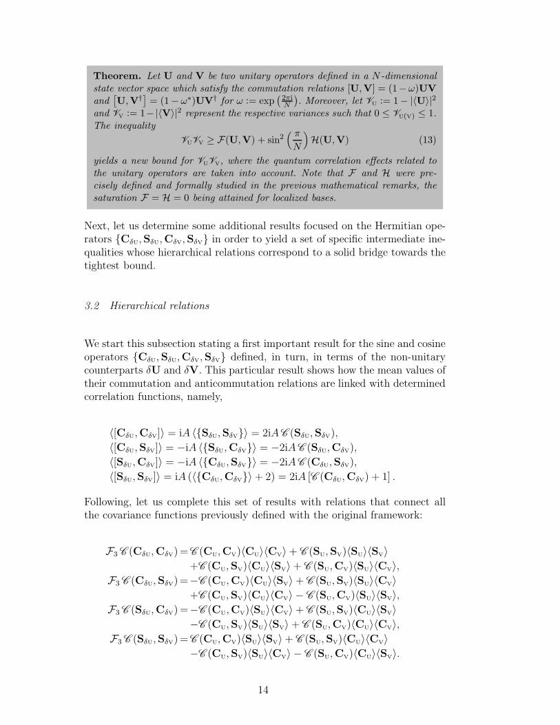
Theorem. Let U and V be two unitary operators defined in a N -dimensional

state vector space which satisfy the commutation relations [U,V] = (1−ω)UVand

[U,V†] = (1− ω∗)UV† for ω := exp

(2πiN

). Moreover, let VU := 1− |〈U〉|2

and VV := 1−|〈V〉|2 represent the respective variances such that 0 ≤ VU(V) ≤ 1.The inequality

VUVV ≥ F(U,V) + sin2( π

N

)H(U,V) (13)

yields a new bound for VUVV, where the quantum correlation effects related to

the unitary operators are taken into account. Note that F and H were pre-

cisely defined and formally studied in the previous mathematical remarks, the

saturation F = H = 0 being attained for localized bases.

Next, let us determine some additional results focused on the Hermitian ope-rators {CδU,SδU,CδV,SδV} in order to yield a set of specific intermediate ine-qualities whose hierarchical relations correspond to a solid bridge towards thetightest bound.

3.2 Hierarchical relations

We start this subsection stating a first important result for the sine and cosineoperators {CδU,SδU,CδV,SδV} defined, in turn, in terms of the non-unitarycounterparts δU and δV. This particular result shows how the mean values oftheir commutation and anticommutation relations are linked with determinedcorrelation functions, namely,

〈[CδU,CδV]〉 = iA 〈{SδU,SδV}〉 = 2iAC (SδU,SδV),

〈[CδU,SδV]〉 = −iA 〈{SδU,CδV}〉 = −2iAC (SδU,CδV),

〈[SδU,CδV]〉 = −iA 〈{CδU,SδV}〉 = −2iAC (CδU,SδV),

〈[SδU,SδV]〉 = iA (〈{CδU,CδV}〉+ 2) = 2iA [C (CδU,CδV) + 1] .

Following, let us complete this set of results with relations that connect allthe covariance functions previously defined with the original framework:

F3 C (CδU,CδV) =C (CU,CV)〈CU〉〈CV〉+ C (SU,SV)〈SU〉〈SV〉+C (CU,SV)〈CU〉〈SV〉+ C (SU,CV)〈SU〉〈CV〉,

F3 C (CδU,SδV) =−C (CU,CV)〈CU〉〈SV〉+ C (SU,SV)〈SU〉〈CV〉+C (CU,SV)〈CU〉〈CV〉 − C (SU,CV)〈SU〉〈SV〉,

F3 C (SδU,CδV) =−C (CU,CV)〈SU〉〈CV〉+ C (SU,SV)〈CU〉〈SV〉−C (CU,SV)〈SU〉〈SV〉+ C (SU,CV)〈CU〉〈CV〉,

F3 C (SδU,SδV) =C (CU,CV)〈SU〉〈SV〉+ C (SU,SV)〈CU〉〈CV〉−C (CU,SV)〈SU〉〈CV〉 − C (SU,CV)〈CU〉〈SV〉.

14

These equations enable us to rewrite F in the compact form

FF3

= C2(CδU,CδV) + C

2(CδU,SδV) + C2(SδU,CδV) + C

2(SδU,SδV), (14)

while (VCδU+VSδU)(VCδV

+VSδV) = VδUVδV brings out a completely analogousexpression to that established for VUVV; consequently,

VδUVδV ≥ FF3

+ sin2(π

N

) HF3

(15)

represents an alternative form of Eq. (13) since VUVV ≡ F3VδUVδV.

Now, let us rewrite Eq. (15) according to definitions employed for SδU and SδVin the previous section,

SδUSδV ≥[1 + sin

(2π

N

)][csc2

(π

N

) FF3

+HF3

]. (16)

From this result, it is relatively easy to derive a number of simpler (but looser)inequalities: for instance, given the non-negativity of F

F3[cf. Eq. (14)], the first

term in the second bracket can be dropped to give

SδUSδV ≥[1 + sin

(2π

N

)] HF3,

which corresponds, in such a case, to the HKR uncertainty principle; alterna-tively, H

F3can also be dropped (for the same reason, i.e., its non-negativity) in

order to yield

SδUSδV ≥[1 + sin

(2π

N

)]csc2

(π

N

) FF3

.

Consequently, such inequalities are then combined in order to give a tighterone,

SδUSδV ≥[1 + sin

(2π

N

)]max

[csc2

(π

N

) FF3,HF3

]. (17)

At this point, one is led to ask if there exists a general ordering relation betweencsc2

(πN

)FF3

and HF3. To answer this question, let us establish a set of numerical

calculations associated with the different values of dimension N , where, foreach specific case, one has approximately 106 randomly generated states. Inorder to make the presentation of these numerical results more self-contained,Fig. 3 depicts the plots of csc2

(πN

)FF3

versus HF3

forN = 2, 3, 4, 6 and 20. In thiscase, note that the maximum can indeed arise from either terms, dependingon the particular chosen state ρ. As a rule of thumb, one has the following:for low dimensional states (e.g., N = 2, 3), the term H

F3usually dominates;

however, as the dimension N increases (N ≥ 6), csc2(πN

)FF3

becomes theusually dominant term. Finally, if one considers N = 4, it is visible that thereis not a usually dominant term — in this case, the result of the optimizationis strongly dependent on the particular input state.

15

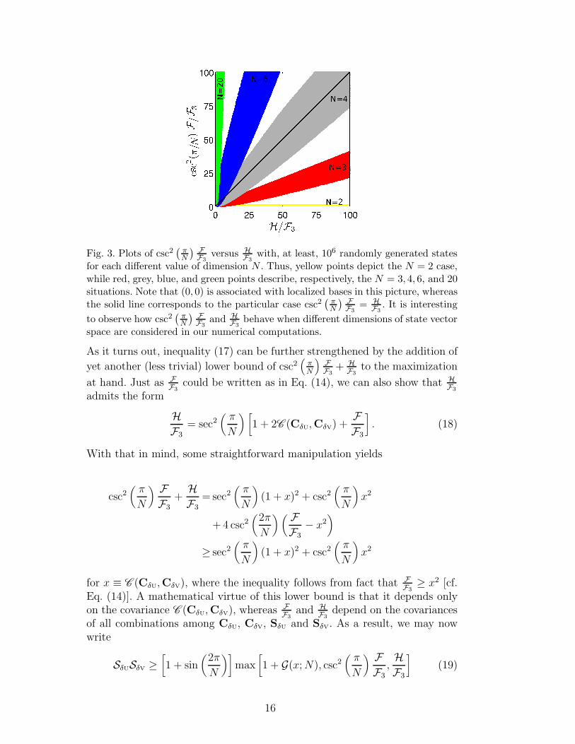
Fig. 3. Plots of csc2(πN

) FF3

versus HF3

with, at least, 106 randomly generated statesfor each different value of dimension N . Thus, yellow points depict the N = 2 case,while red, grey, blue, and green points describe, respectively, the N = 3, 4, 6, and 20situations. Note that (0, 0) is associated with localized bases in this picture, whereasthe solid line corresponds to the particular case csc2

(πN

) FF3

= HF3

. It is interesting

to observe how csc2(πN

) FF3

and HF3

behave when different dimensions of state vectorspace are considered in our numerical computations.

As it turns out, inequality (17) can be further strengthened by the addition of

yet another (less trivial) lower bound of csc2(πN

)FF3

+ HF3

to the maximization

at hand. Just as FF3

could be written as in Eq. (14), we can also show that HF3

admits the form

HF3

= sec2(π

N

) [1 + 2C (CδU,CδV) +

FF3

]. (18)

With that in mind, some straightforward manipulation yields

csc2(π

N

) FF3

+HF3

= sec2(π

N

)(1 + x)2 + csc2

(π

N

)x2

+4 csc2(2π

N

)( FF3

− x2)

≥ sec2(π

N

)(1 + x)2 + csc2

(π

N

)x2

for x ≡ C (CδU,CδV), where the inequality follows from fact that FF3

≥ x2 [cf.Eq. (14)]. A mathematical virtue of this lower bound is that it depends onlyon the covariance C (CδU,CδV), whereas

FF3

and HF3

depend on the covariancesof all combinations among CδU, CδV, SδU and SδV. As a result, we may nowwrite

SδUSδV ≥[1 + sin

(2π

N

)]max

[1 + G(x;N), csc2

(π

N

) FF3,HF3

](19)

16

with G(x;N) := 4 csc2(2πN

)x2+2 sec2

(πN

)x+tan2

(πN

). Note that 1+G(x;N)

coincides, in such a situation, with sec2(πN

)(1+x)2+csc2

(πN

)x2. Once again,

numerical calculations demonstrate that there is not a general ordering be-tween the arguments of the maximization of such an equation.

It is worth stressing that both bounds of Eqs. (16) and (19) explicitly dependon the Hilbert space dimension, as well as on the particular state under con-sideration. Henceforth, we further loose the bound (19) to provide yet anotherbound, but now a state-independent one (i.e., solely dependent on the Hilbertspace dimension). In this way, let us initially consider the inequality

SδUSδV ≥[1 + sin

(2π

N

)][1 + G(x;N)] .

So, for a given N , G(x;N) describes a parabola with upwards concavity andminimum value equal to 0 (y-coordinate of the vertex), namely, G(x;N) ≥ 0,which implies that

SδUSδV ≥ 1 + sin(2π

N

). (20)

Despite of all the mathematical assumptions used in the relaxation processof inequality (16), the bound above is still tighter than the one proposed inRef. [14], which is now trivially proved by disregarding the sine function inthe inequality (20), that is, SδUSδV ≥ 1.

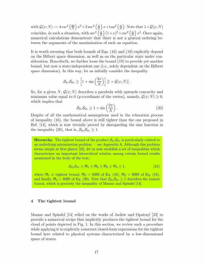
Hierarchy. The tightest bound of the product SδUSδV is particularly related toan underlying minimization problem — see Appendix A. Although this problemseems simple at first glance [23], let us now establish a set of inequalities whichcharacterizes an important hierarchical relation among certain formal resultsmentioned in the body of the text:

SδUSδV ≥ R1 ≥ R2 ≥ R3 ≥ R4 ≥ 1, (21)

where R1 ≡ tightest bound, R2 = RHS of Eq. (16), R3 = RHS of Eq. (19),and finally, R4 = RHS of Eq. (20). Note that SδUSδV ≥ 1 describes the loosestbound, which is precisely the inequality of Massar and Spindel [14].

4 The tightest bound

Massar and Spindel [14] relied on the works of Jackiw and Opatrny [23] toprovide a numerical recipe that implicitly produces the tightest bound for thecloud of points depicted in Fig. 1. In this section, we review such a procedurewhile applying it to explicitly construct closed-form expressions for the tightestbound here related to physical systems characterized by a low-dimensionalspace of states.

17

Generally, the tightest bound can be obtained by the following reasoning:

SδUSδV ≥ min|ψ〉

SδUSδV = ε−2min|ψ〉

VδUVδV = ε−2V

(0)δU V

(0)δV =

[ε−1

V(0)δU

]2= S(0)

δU

2.

In such a case, the super-index (0) indicates that the corresponding normalizeddiscrete wavefunction is associated with the nondegenerate ground state |ψ0〉,which minimizes the product VUVV. In fact, this ground state will also minimizeVδUVδV, since VδO is monotonically increasing with VO [cf. Eq. (3)] — thisobservation justifies the second equality. Besides, both the variances evaluatedwith respect to the ground state satisfy V

(0)δU = V

(0)δV , which justifies the third

equality.

Now, let us establish a sequence of mathematical steps based on the respectiveeigenvalues and eigenvectors of the Harper Hamiltonian [24]

H = − sin(θ)CU − cos(θ)CV

for 0 ≤ θ ≤ π2. Initially, we look for the smallest eigenvalue of such a Her-

mitian operator, as well as for its corresponding eigenvector in a given fixedN -dimensional state vector space. Since the eigenvalues and eigenvectors re-lated to the Harper Hamiltonian are dependent on the angle θ, let us considerthat eigenvector evaluated at the first step in order to estimate the maximumof cos(θ)|〈U〉|+sin(θ)|〈V〉| for all θ ∈

[0, π

2

]– which exactly coincides with the

smallest eigenvalue in this case. In particular, such a mathematical procedureallows us to obtain, through numerical evaluations, the value of θ = π

4for

any dimension N , and also to characterize the ground state |ψ0〉 ≡ |0〉N withwell-defined mathematical properties (see Appendix A for possible connectionwith Harper functions).

Table 1 illustrates the hierarchical relation depicted in Eq. (21) where, in par-ticular, certain numerical results directly related to the analytical calculationsperformed for {R1,R2,R3,R4} with N ∈ [2, 6] are exhibited — closed-form

expressions for S(0)δU can be viewed in Appendix A and their respective squared

values R1 ≡ S(0)δU

2compared with those results previously obtained in Fig. 1.

Note that for higher dimensions, some numerical methods (for instance, La-guerre method or even Newton-Raphson method) should be applied in order

to obtain approximate numerical values for S(0)δU (this statement is supported

by the Abel-Galois irreducibility theorem [29], which asserts that polynomialequations of degree ≥ 5 do not produce, in general, algebraic solutions, onlynumerical solutions).

18

Table 1Numerical values for {Ri}1≤i≤4 considering the ground state {|0〉N}2≤N≤6 describedin Appendix A. It is important to stress that such results were inferred from theirrespective exact algebraic counterparts, which illustrate, in principle, not only thehierarchical relation depicted in Eq. (21) but also the quantum-algebraic frameworkdeveloped in the previous sections. In addition, note that eigenvalues extracted fromthe Harper Hamiltonian for N > 6 do not yield easy-to-compute expressions for thetightest bounds R1, this fact being supported by Abel-Galois irreducibility theoremfor polynomial equations.

N R1 R2 R3 R4

2 1 1 1 1

3 ≈ 3.254 ≈ 2.182 ≈ 1.895 ≈ 1.866

4 4 3 2 2

5 ≈ 3.781 ≈ 3.469 ≈ 2.987 ≈ 1.951

6 ≈ 3.348 ≈ 1.915 ≈ 1.915 ≈ 1.866

5 The connection with discrete Weyl function

How the discrete Weyl function [5] can be employed to measure a particularfamily of expectation values — for instance, 〈UαVβ〉 for {α, β} ∈ ZN — heremapped into finite-dimensional discrete phase spaces? To answer this specificquestion, we initially recall certain basic mathematical tools which correspondto the central core of that theoretical formulation presented in Ref. [12]. Thisprocedure will lead us to establish a parallel quantum-algebraic framework forthose results obtained in Section 3, whose connection with the discrete Weylfunction represents a first step towards effective experimental measurementsvia tomographic reconstructions of finite quantum states [8]. Throughout thissection, we will assume N odd. 4

The particular set ofN2 operators {∆(µ, ν)}µ,ν=−ℓ,...,ℓ characterizes a completeorthonormal unitary operator basis which leads us to construct all possiblekinematical and/or dynamical quantities belonging to a given N -dimensionalstate vector space. For instance, the decomposition of any linear operator Oin this basis assumes the expression

O =1

N

ℓ∑

µ,ν=−ℓO(µ, ν)∆(µ, ν), (22)

where O(µ, ν) ≡ Tr[∆(µ, ν)O] represent coefficients evaluated through trace

4 For completeness reasons, it is important to stress that even dimensionalities canalso be dealt with simply by working on non-symmetrized intervals.

19

operation and

∆(µ, ν) :=1

N

ℓ∑

η,ξ=−ℓω−(ην−ξµ)D(η, ξ) (23)

defines the aforementioned operator basis here expressed in terms of a discreteFourier transform of the displacement operator

D(η, ξ) = ω−{2−1ηξ}ℓ∑

γ=−ℓωγη|uγ〉〈uγ−ξ| = ω−{2−1ηξ}

ℓ∑

γ=−ℓω−γξ|vγ+η〉〈vγ|.

In such a case, note that ω−{2−1ηξ} consists of a specific phase whose argumentsatisfies the mathematical rule 2{2−1ηξ} = ηξ + kN for all k ∈ ZN ; further-more, note that these labels assume integer values in the symmetric interval[−ℓ, ℓ] with ℓ = N−1

2fixed.

According to expansion (22), the decomposition of any density operator ρ inthe mod(N)-invariant unitary operator basis (23) has as coefficients the dis-crete Wigner function Wρ(µ, ν) := Tr[∆(µ, ν)ρ], which leads us, in principle,to establish an analytical expression for the mean value 〈O〉 ≡ Tr[Oρ], thatis

〈O〉 = 1

N

ℓ∑

µ,ν=−ℓO(µ, ν)Wρ(µ, ν). (24)

In what concerns to Wρ(µ, ν), it is particularly worth mentioning that such a

function is connected to the Weyl function Wρ(η, ξ) := Tr[D(η, ξ)ρ] by meansof a mere discrete Fourier transform, and its complexity basically depends onthe initial quantum state adopted for the physical system under investigation.

To illustrate the mathematical steps used in the evaluation of O(µ, ν), let usconsider those specific combinations of cosine and sine operators exhibited inSection 3, as well as the intermediate result

D†(η, ξ)UαVβD(η, ξ) = ωαξ+βηUαVβ

since the trace operation

Tr[D(η, ξ)UαVβ] = Nω−{2−1ηξ}+ηβδ[N ]η+α,0 δ

[N ]ξ−β,0

will be necessary in the next steps. Thus, after some repetitive calculations,we achieve the set of formal expressions

20

Tr[D(η, ξ)CUCV] =N

4ω−{2−1ηξ}

(δ[N ]η+1,0 + δ

[N ]η−1,0

) (ω−ηδ

[N ]ξ+1,0 + ωηδ

[N ]ξ−1,0

)

Tr[D(η, ξ)CUSV] = iN

4ω−{2−1ηξ}

(δ[N ]η+1,0 + δ

[N ]η−1,0

) (ω−ηδ

[N ]ξ+1,0 − ωηδ

[N ]ξ−1,0

)

Tr[D(η, ξ)SUCV] =−iN

4ω−{2−1ηξ}

(δ[N ]η+1,0 − δ

[N ]η−1,0

) (ω−ηδ

[N ]ξ+1,0 + ωηδ

[N ]ξ−1,0

)

Tr[D(η, ξ)SUSV] =N

4ω−{2−1ηξ}

(δ[N ]η+1,0 − δ

[N ]η−1,0

) (ω−ηδ

[N ]ξ+1,0 − ωηδ

[N ]ξ−1,0

)

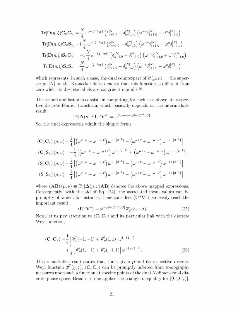
which represents, in such a case, the dual counterpart of O(µ, ν) — the super-script [N ] on the Kronecker delta denotes that this function is different fromzero when its discrete labels are congruent modulo N .

The second and last step consists in computing, for each case above, its respec-tive discrete Fourier transform, which basically depends on the intermediateresult

Tr[∆(µ, ν)UαVβ] = ωβµ+αν−αβ+{2−1αβ}.

So, the final expressions admit the simple forms

(CUCV) (µ, ν)=1

4

[(ωµ−ν + ω−µ+ν

)ω1−{2−1} +

(ωµ+ν + ω−µ−ν

)ω−1+{2−1}

]

(CUSV) (µ, ν)=− i

4

[(ωµ−ν − ω−µ+ν

)ω1−{2−1} +

(ωµ+ν − ω−µ−ν

)ω−1+{2−1}

]

(SUCV) (µ, ν)=i

4

[(ωµ−ν − ω−µ+ν

)ω1−{2−1} −

(ωµ+ν − ω−µ−ν

)ω−1+{2−1}

]

(SUSV) (µ, ν)=1

4

[(ωµ−ν + ω−µ+ν

)ω1−{2−1} −

(ωµ+ν + ω−µ−ν

)ω−1+{2−1}

]

where (AB) (µ, ν) ≡ Tr [∆(µ, ν)AB] denotes the above mapped expressions.Consequently, with the aid of Eq. (24), the associated mean values can bepromptly obtained: for instance, if one considers 〈UαVβ〉, we easily reach theimportant result

〈UαVβ〉 = ω−αβ+{2−1αβ}Wρ(α,−β). (25)

Now, let us pay attention to 〈CUCV〉 and its particular link with the discreteWeyl function,

〈CUCV〉=1

4

[Wρ(−1,−1) + Wρ(1, 1)

]ω1−{2−1}

+1

4

[Wρ(1,−1) + Wρ(−1, 1)

]ω−1+{2−1}. (26)

This remarkable result states that, for a given ρ and its respective discreteWeyl function Wρ(η, ξ), 〈CUCV〉 can be promptly inferred from tomographymeasures upon such a function at specific points of the dualN -dimensional dis-crete phase space. Besides, if one applies the triangle inequality for |〈CUCV〉|,

21

both the upper and lower bounds can be easily established in this context, 5

|〈CUCV〉| S1

4

(|Wρ(−1,−1) + Wρ(1, 1)| ± |Wρ(1,−1) + Wρ(−1, 1)|

).

Similar procedure leads us to prove that |〈SUSV〉| shares exactly the samebounds, while the remaining quantities are bounded by the inequalities

{|〈CUSV〉|, |〈SUCV〉|}S1

4

(|Wρ(−1,−1)− Wρ(1, 1)|

)

±1

4

(|Wρ(1,−1)− Wρ(−1, 1)|

).

As a last note, let us mention that VU and VV can also be expressed in termsof specific Weyl functions with the help of Eq. (25), i.e., VU = 1 − |Wρ(1, 0)|2and VV = 1− |Wρ(0,−1)|2.

In particular, it is worth stressing that the compilation of results obtained inthis section allows us to rewrite inequality (13) into a new quantum-algebraicframework, since F(U,V) and H(U,V) now depend on specific combina-tions of discrete Weyl functions. From an experimental point of view, thisobservation represents an effective gain towards tomographic measurementsin N -dimensional discrete phase spaces of such a generalized inequality forany finite quantum state ρ [8].

6 Concluding remarks

Through a well succeeded concatenation of efforts in a recent past [5,12], wehave made great advances (from a theoretical point of view) in constructingcertain sound quantum-algebraic frameworks for finite-dimensional discretephase spaces. Since unitary operators represent the basic constituent blocksof these theoretical frameworks (in particular, the Schwinger’s approach for

5 Let A and B characterize two general matrices of same size, as well as ρ denotethe density matrix related to a physical system described by a finite-dimensionalstate vector space. The additional inequality |Tr[ABρ]|2 ≤ Tr[AA†

ρ]Tr[BB†ρ] (see

Ref. [27, page 230]) establishes a new upper bound for Eq. (26) since |〈CUCV〉|2 ≤〈C2

U〉〈C2

V〉, where

〈C2U〉 = 1

2+

1

4

[Wρ(2, 0) + Wρ(−2, 0)

]

and

〈C2V〉 = 1

2+

1

4

[Wρ(0, 2) + Wρ(0,−2)

].

This complementary result basically represents a step forward in our comprehensionon hierarchical relations involving those means values listed in Remark 4.

22

unitary operators [1]), let us focus our attention on some real and effectivegains obtained from this paper whose formal implications deserve to be care-fully discussed.

• The Massar-Spindel inequality does not explain the tightest bounds exhibi-ted in Fig. 1 for the product SδUSδV when dimensions N ≥ 3 are consideredin the numerical evaluations. This concrete evidence suggests the implemen-tation of an effective search for different inequalities and new finite quantumstates whose implications lead us not only to obtain a reasonable set of im-proved mathematical results, but also to answer certain important questionsthat emerge from such an evidence.

• The mathematical background for achieving different inequalities related tothe aforementioned unitary operators has the RS uncertainty principle assolid starting-point [12]. The initial algebraic advantage of this investigativeapproach is the inclusion of that contribution coming from the anticommu-tation relation between two Hermitian non-commuting operators connectedvia discrete Fourier transform (and/or also related through the Pontryaginduality [30]). In fact, this particular contribution allows to include, into thealgebraic approach, some additional terms — here associated with the meanvalues of different products of the cosine and sine operators — which areresponsible for correlations between the unitary operators. In principle, thetheorem derived from this constructive process represents a first importantpoint to be strongly emphasized since Eq. (13) introduces a tighter boundwhose mathematical properties depend on the N -dimensional state vectorspace in which the initial quantum state is defined.

• The hierarchical relation (21) derived from the tighter bound characterizes asolid bridge between two ‘distant’ bounds: the first one consists of a zeroth-order approximation that confirms the Massar-Spindel result [14] (however,it does not depend on the initial quantum state or even on the dimensionwhich the state vector space is embedded, these facts being considered as asevere limitation for their result); while the second one describes the tightestbound for the left-hand side of Eq. (13) and depicts the importance of theinitial quantum state for a given dimension N . This simple (but important)observation justifies our search for finite ground states which quantitativelydescribe those numerical values obtained in Fig. 1 for the tightest bounds.

• How to construct a finite quantum state which formally explains the tightestbounds verified in the numerical calculations? To answer this fundamentalquestion, it is necessary to establish an adequate mathematical prescriptionthat leads us to obtain a set of normalized eigenfunctions which constitutesa complete orthonormal basis in a N -dimensional state vector space. In thissense, Appendix A deals with such a task presenting a reliable mathematicalrelation between Harper functions and tightest bounds by means of groundstates {|0〉N} specifically constructed for dimensions N ∈ [2, 6]. These finitequantum states indeed describe perfectly all the numerical values exhibitedin Fig. 1 for the tightest bounds, and illustrate the hierarchical relation (21)

23

as well — see Table 1.• The bounds determined in this paper for the product SδUSδV exhibit a spe-cial link with the theoretical formulation of finite-dimensional discrete phasespaces through the discrete Weyl funtion. In fact, this connection establishesan interesting link between both the Schwinger and Weyl prescriptions forunitary operators, which leads us to guess on the possibility of experimentalobservation with the help of tomographic measurements.

Now, let us discuss some pertinent points associated with the uncertaintyprinciple for Schwinger unitary operators. The first point concerns the Harperfunctions and their remarkable connection with the tightest bounds throughthe ground states {|0〉N} for a given dimension N fixed. Despite the worked-examples in Appendix A belonging to the closed interval 2 ≤ N ≤ 6, this factdoes not represent any apparent limitation related to the quantum-algebraicframework here exposed. In fact, these results consist of a solid starting pointfor a future search of {〈uα|n〉}0≤n≤N−1 with α ∈ ZN , whose general expressionwill correspond to a new paradigm for finite quantum states with immediateimplications in the Fourier analysis on finite groups [19,30] (and/or finite fields[31]), as well as in the analysis of signal processing [32,33]. This particular taskis currently in progress and the results will be presented in elsewhere.

The second point focus on the systematic study recently developed in Ref. [15]for property testing of unitary operators, where D2(U,V) := 1− 1

N|Tr[U†V]|

represents a ‘normalized distance measure that reflects the average differencebetween unitary operators’. With respect to this specific measure, Wang showsthat both the Clifford and orthogonal groups can be efficiently tested throughalgorithms with intrinsic mathematical virtues (namely, query complexitiesindependent of the system’s size and one-sided error). Since the results hereobtained describe an uncertainty principle for unitary operators, it seems rea-sonable to investigate how these different — but complementary — approachescan be juxtaposed in order to produce a unified framework for determinedtasks in quantum information theory [7].

As a final comment, let us briefly mention that our results also touch on somefundamental questions inherent to quantum mechanics (such as spin-squeezingand entanglement effects [34]), discrete fractional Fourier transform [35], andgeneralized uncertainty principle into the quantum-gravity context [12].

Acknowledgements

The authors thank Diogenes Galetti for helpful discussions and comments onhighly pertinent questions related to this work.

24

A Harper’s equation, quantum Fourier transform, tightest boundand their inherent connections with unitary operators

Definition (Harper functions). Let {|n〉}0≤n≤N−1 describe a particular setof eigenvectors defined in a N -dimensional state vector space that simultane-ously diagonalizes both the Hamiltonian (H) and Fourier (F) operators, thatis, H|n〉 = hn|n〉 and F|n〉 = fn|n〉 for a given dimension N fixed. In such acase, {hn, fn}0≤n≤N−1 represents the corresponding set of eigenvalues relatedto the respective Hamiltonian and Fourier operators. Since

HF|n〉 = FH|n〉 = fnhn|n〉 ⇒ [H,F] |n〉 = 0|n〉,

the intrinsic mathematical properties associated with the discrete representa-tion {|uα〉}0≤α≤N−1 allow to obtain the general equation

〈uα|HF|n〉 = fnhn〈uα|n〉, (A.1)

whose solution set {〈uγ|n〉} ∈ R yields a complete orthonormal basis of realeigenfunctions genuinely labelled by discrete variables. The Harper functionsare here attained when one considers H as being a Harper-type operator [32].

As a first application, let us, for now, adopt the discrete Fourier operator 6

F :=N−1∑

β=0

|vβ〉〈uβ| =1√N

N−1∑

β,β′=0

ωββ′|uβ′〉〈uβ| ⇒ FF

† = F†F = 1,

as well as that Harper Hamiltonian operator previously discussed in Section4, namely, H = − sin(θ)CU−cos(θ)CV for θ ∈

[0, π

2

]. Thus, Eq. (A.1) assumes

the functional form

N−1∑

β=0

O(α, β;N)〈uβ|n〉 = fnhn〈uα|n〉, (A.2)

where

O(α, β;N) ≡ 〈uα|H|vβ〉 = −[sin(θ) cos

(2πα

N

)+ cos(θ) cos

(2πβ

N

)]〈uα|vβ〉

represents the mapped expression of the Hamiltonian operator in the discreterepresentations {|uα〉, |vβ〉} with 〈uα|vβ〉 = 1√

Nωαβ and ω = exp

(2πiN

); besides,

6 For N odd and discrete labels assuming integer values in the symmetric interval[−ℓ, ℓ] with ℓ = N−1

2 fixed, it is worth stressing that F2 coincides with that parityoperator P previously defined in Ref. [12].

25

{〈uγ|n〉} ∈ R denotes the Harper functions for a given N ∈ N∗. In fact, such

a result can also be split up into two combined equations as follows:

sin(θ) cos(2πα

N

)〈uα|n〉+

1

2cos(θ) (〈uα−1|n〉+ 〈uα+1|n〉) = −hn〈uα|n〉 (A.3)

and1√N

N−1∑

β=0

ωαβ〈uβ|n〉 = fn〈uα|n〉. (A.4)

The first one describes a three-term recurrence relation and also depicts thewell-known Harper’s equation, whose link with discrete harmonic oscillatorand discrete fractional Fourier transform was already discussed by Barker andcoworkers [24]; whilst the second one reflects exactly the eigenvalue probleminvestigated by Mehta [36] when fn = in (in this particular case, see Ref. [19]for supplementary material), although his ansatz solution

〈uα|n〉 = Nn

(−i)n√N

∞∑

κ=−∞exp

(− π

Nκ2 +

2πi

Nκα)Hn

√2π

Nκ

does not represent a complete set of orthonormal eigenfunctions [37] — insuch ansatz solution, Nn corresponds to a normalization constant and Hn(z)denotes the Hermite polynomials.

Summarizing, Eq. (A.3) yields, in general, a set of real eigenvalues {hn} whoserespective eigenfunctions {〈uα|n〉} constitute a complete orthonormal basis ina N -dimensional state vector space. In this specific case, both the eigenvaluesand eigenfunctions are dependent on the angle variable θ ∈

[0, π

2

], which leads

us to determine the maximum of cos(θ)|〈U〉|+sin(θ)|〈V〉| 7 for each particularsituation hn ⇋ 〈uα|n〉 with N fixed. Thus, the global maximum obtainedfrom this mathematical procedure allows not only to fix a given value of θ,but also to estimate the smallest eigenvalue of the Hermitian operator H;consequently, the corresponding eigenvector will describe the ground state |0〉characterized by θ = π

4and f0 = +1 for any dimension N (it is worth stressing

that theoretical and numerical calculations confirm these results). Next, let usconsider the N = 2, . . . , 6 cases for θ = π

4fixed, in order to provide a complete

list of results exhibited in Table 1 associated with the normalized ground state.

• Case N = 2 (prime dimension) and h0 = −1. This first example obeys thecriterion “easy to calculate”, once the corresponding ground state

|0〉2 =√2 +

√2

2|u0〉+

√2−

√2

2|u1〉

7 Such a quantity implicitly defines the boundary — or, more precisely, the convexhull — of the accessible region related to the {|〈U〉|, |〈V〉|}-space [14].

26

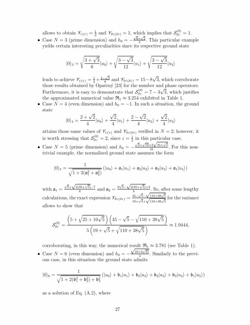
allows to obtain VU(V) =12and VδU(δV) = 1, which implies that S(0)

δU = 1.

• Case N = 3 (prime dimension) and h0 = −√6+

√2

4. This particular example

yields certain interesting peculiarities since its respective ground state

|0〉3 =√3 +

√3

6|u0〉+

√3−

√3

12|u1〉+

√3−

√3

12|u2〉

leads to achieve VU(V) =12+ 2−

√3

8and VδU(δV) = 15−8

√3, which corroborate

those results obtained by Opatrny [23] for the number and phase operators.

Furthermore, it is easy to demonstrate that S(0)δU = 7− 3

√3, which justifies

the approximated numerical value R1 ≈ 3.254 exhibited in Table 1.• Case N = 4 (even dimension) and h0 = −1. In such a situation, the groundstate

|0〉4 =2 +

√2

4|u0〉+

√2

4|u1〉+

2−√2

4|u2〉+

√2

4|u3〉

attains those same values of VU(V) and VδU(δV) verified in N = 2; however, it

is worth stressing that S(0)δU = 2, since ε = 1

2in this particular case.

• Case N = 5 (prime dimension) and h0 = −√2+

√10+2

√35+

√5

16. For this non-

trivial example, the normalized ground state assumes the form

|0〉5 =1√

1 + 2(a21 + a22)(|u0〉+ a1|u1〉+ a2|u2〉+ a2|u3〉+ a1|u4〉)

with a1 =√5+√

2(35+√5)−7

8and a2 =

3√5−√

2(35+√5)+3

8. So, after some lengthy

calculations, the exact expression VδU(δV) =45−

√5−√

110+38√5

19+√5+√

110+38√5for the variance

allows to show that

S(0)δU =

(5 +

√25 + 10

√5)(

45−√5−

√110 + 38

√5)

5(19 +

√5 +

√110 + 38

√5) ≈ 1.9444,

corroborating, in this way, the numerical result R1 ≈ 3.781 (see Table 1).

• Case N = 6 (even dimension) and h0 = −√

10+2√21

4. Similarly to the previ-

ous case, in this situation the ground state admits

|0〉6 =1√

1 + 2(b21 + b22) + b23

(|u0〉+ b1|u1〉+ b2|u2〉+ b3|u3〉+ b2|u4〉+ b1|u5〉)

as a solution of Eq. (A.2), where

27

b1=−2 +

√5 +

√21

2=

−4 +√6 +

√14

4

b2=5 +

√21− 3

√5 +

√21

2=

10− 3√6− 3

√14 + 2

√21

4

b3=−4 +√6−

√21 + 2

√5 +

√21 = −4 + 2

√6 +

√14−

√21

represent the respective coefficients. Note that VδU(δV) = 19− 4√21, which

implies in S(0)δU = 19(1 +

√3)− 4

√42(2 +

√3) ≈ 1.8297 (this result justifies

that numerical value R1 ≈ 3.348 appeared in Table 1 for N = 6).

As an initial purpose, these first theoretical results related to the ground stateare sufficient to clarify the numerical results depicted in Fig. 1 for the tightestbound. In fact, the results exhibited in this appendix indeed represent a firstinvestigative step towards a general mathematical recipe that presents as aprimary product the eigenfunctions {〈uα|n〉}0≤n≤N−1, which differ from thatMehta’s ansatz solution.

References

[1] J. Schwinger, Quantum Mechanics: Symbolism of Atomic Measurements,Springer-Verlag, Berlin, 2001.

[2] E. Prugovecki, Quantum Mechanics in Hilbert Space, Academic Press, NewYork, 1981;P.R. Halmos, Finite-Dimensional Vector Spaces, Springer-Verlag, New York,1987;A. Bohm, Quantum Mechanics: Foundations and Applications, Springer-Verlag,New York, 1993.

[3] A. Vourdas, Rep. Progr. Phys. 67 (2004) 267.

[4] W.K. Wootters, Ann. Phys. (NY) 176 (1987) 1;D. Galetti, A.F.R. de Toledo Piza, Physica A 149 (1988) 267;R. Aldrovandi, D. Galetti, J. Math. Phys. 31 (1990) 2987;P. Leboeuf, A. Voros, J. Phys. A: Math. Gen. 23 (1990) 1765;D. Galetti, A.F.R. de Toledo Piza, Physica A 186 (1992) 513;D. Galetti, M.A. Marchiolli, Ann. Phys. (NY) 249 (1996) 454;T. Hakioglu, J. Phys. A: Math. Gen. 31 (1998) 6975;D. Galetti, M. Ruzzi, Physica A 264 (1999) 473;S. Zhang, A. Vourdas, J. Phys. A: Math. Gen. 37 (2004) 8349;A.B. Klimov, C. Munoz, J. Opt. B: Quantum Semiclass. Opt. 7 (2005) S588;A.B. Klimov, C. Munoz, J.L. Romero, J. Phys. A: Math. Gen. 39 (2006) 14471;A.B. Klimov, J.L. Romero, G. Bjork, L.L. Sanchez-Soto, Ann. Phys. (NY) 324(2009) 53;

28

E.R. Livine, J. Phys. A: Math. Theor. 43 (2010) 075303;N. Cotfas, J.P. Gazeau, A. Vourdas, J. Phys. A: Math. Theor. 44 (2011) 175303.

[5] T. Opatrny, D.G. Welsch, V. Buzek, Phys. Rev. A 53 (1996) 3822;M. Ruzzi, M.A. Marchiolli, D. Galetti, J. Phys. A: Math. Gen. 38 (2005) 6239;C. Ferrie, Rep. Progr. Phys. 74 (2011) 116001;M.A. Marchiolli, M. Ruzzi, J. Russ. Laser Res. 32 (2011) 381.

[6] K.E. Cahill, R.J. Glauber, Phys. Rev. 177 (1969) 1857;K.E. Cahill, R.J. Glauber, Phys. Rev. 177 (1969) 1882.

[7] V. Vedral, Introduction to Quantum Information Science, Oxford, New York,2006;J. Audretsch, Entangled Systems: New Directions in Quantum Physics, Wiley-VCH, Berlin, 2007;G. Jaeger, Quantum Information: An Overview, Springer, New York, 2007;N.D. Mermim, Quantum Computer Science, Cambridge University Press, NewYork, 2007;E. Desurvire, Classical and Quantum Information Theory: An Introduction forthe Telecom Scientist, Cambridge University Press, New York, 2009;D.C. Marinescu, G.M. Marinescu, Classical and Quantum Information, Elsevier,Oxford, 2012.

[8] C. Miquel, J.P. Paz, M. Saraceno, E. Knill, R. Laflamme, C. Negrevergne,Nature 418 (2002) 59;M.A. Marchiolli, M. Ruzzi, D. Galetti, Phys. Rev. A 72 (2005) 042308;A. Vourdas, C. Banderier, J. Phys. A: Math. Theor. 43 (2010) 042001.

[9] M.A. Marchiolli, E.C. Silva, D. Galetti, Phys. Rev. A 79 (2009) 022114.

[10] C.C. Lopez, J.P. Paz, Phys. Rev. A 68 (2003) 052305;M.L. Aolita, I. Garcıa-Mata, M. Saraceno, Phys. Rev. A 70 (2004) 062301.

[11] D. Galetti, Physica A 374 (2007) 211;E.C. Silva, D. Galetti, J. Phys. A: Math. Theor. 42 (2009) 135302.

[12] M.A. Marchiolli, M. Ruzzi, Ann. Phys. (NY) 327 (2012) 1538.

[13] A. Mann, M. Revzen, J. Zak, J. Phys. A: Math. Gen. 38 (2005) L389;B. Simkhovich, A. Mann, J. Zak, J. Phys. A: Math. Theor. 43 (2010) 045301.

[14] S. Massar, P. Spindel, Phys. Rev. Lett. 100 (2008) 190401. Supplementarymaterial available from: quant-ph/0710.0723/.

[15] G. Wang, Phys. Rev. A 84 (2011) 052328.

[16] H. Weyl, The Theory of Groups and Quantum Mechanics, Dover Publications,New York, 1950.

[17] A. Ramakrishnan, L-Matrix Theory or the Grammar of the Dirac Matrices,Tata McGraw-Hill, Bombay/New Delhi, 1972;R. Jagannathan, On Generalized Clifford Algebras and their Physical

29

Applications, in: The Legacy of Alladi Ramakrishnan in the MathematicalSciences, K. Alladi, J.R. Klauder, C.R. Rao (Eds.), Springer, New York, 2010,pp. 465-489.

[18] T.S. Santhanam, A.R. Tekumalla, Found. Phys. 6 (1976) 583;R. Jagannathan, T.S. Santhanam, R. Vasudevan, Int. J. Theor. Phys. 20 (1981)755;R. Jagannathan, T.S. Santhanam, Int. J. Theor. Phys. 21 (1982) 351;R. Jagannathan, Int. J. Theor. Phys. 22 (1983) 1105.

[19] A. Terras, Fourier Analysis on Finite Groups and Applications, CambridgeUniversity Press, Cambridge, 1999;B. Luong, Fourier Analysis on Finite Abelian Groups, Birkhauser Boston, NewYork, 2009;J.W. Cooley, P.A.W. Lewis, P.D. Welch, IEEE Trans. Audio Electroacoust.AU-17 (1969) 77;J.H. McClellan, T.W. Parks, IEEE Trans. Audio Electroacoust. AU-20 (1972)66.

[20] W. Heisenberg, Z. Phys. 43 (1927) 172;E.H. Kennard, Z. Phys. 44 (1927) 326;H.P. Robertson, Phys. Rev. 34 (1929) 163;V.V. Dodonov, V.I. Man’ko, Invariants and the Evolution of NonstationaryQuantum Systems, in: Proc. Lebedev Phys. Inst. Acad. Sci. USSR, vol. 183,Nova Science, New York, 1989.

[21] N.M. Atakishiyev, G.S. Pogosyan, K.B. Wolf, Int. J. Mod. Phys. A 18 (2003)317;E.I. Jafarov, N.I. Stoilova, J. Van der Jeugt, J. Phys. A: Math. Theor. 44 (2011)265203.

[22] A.F. Ali, S. Das, E.C. Vagenas, Phys. Lett. B 678 (2009) 497;J.Y. Bang, M.S. Berger, Phys. Rev. A 80 (2009) 022105.

[23] R. Jackiw, J. Math. Phys. 9 (1968) 339;T. Opatrny, J. Phys. A: Math. Gen. 28 (1995) 6961.

[24] L. Barker, C. Candan, T. Hakioglu, M.A. Kutay, H.M. Ozaktas, J. Phys. A:Math. Gen. 33 (2000) 2209.

[25] L.A. Goodman, Journal of the American Statistical Association 55 (1960) 708;L.A. Goodman, Journal of the American Statistical Association 57 (1962) 54.

[26] M.A. Marchiolli, M. Ruzzi, D. Galetti, Phys. Rev. A 76 (2007) 032102.

[27] I. Bengtsson, K. Zyczkowski, Geometry of Quantum States: An Introduction toQuantum Entanglement, Cambridge University Press, Cambridge, 2008.

[28] R. Bhatia, Matrix Analysis, Springer-Verlag, New York, 1997.

[29] E. Artin, A.N. Milgram, Galois Theory, in: Lectures Delivered at the Universityof Notre Dame by Emil Artin, Notre Dame Mathematical Lectures, Number 2,

30

Dover Publications, New York, 1997;J. Bewersdorff, Galois Theory for Beginners: A Historical Perspective, in:Student Mathematical Library, vol. 35, American Mathematical Society, RhodeIsland, 2006.

[30] W. Rudin, Fourier Analysis on Groups, Interscience Publishers, New York, 1962;L.S. Pontryagin, Topological Groups, Gordon and Breach, New York, 1966;H. Reiter, J.D. Stegeman, Classical Harmonic Analysis and Locally CompactGroups, Claredon Press, Oxford, 2000.

[31] R. Lidl, H. Niederreiter, Introduction to finite fields and their applications,Cambridge University Press, Cambridge, 1994.

[32] B. Dickinson, K. Steiglitz, IEEE Trans. Acoustics, Speech, Signal Process. 30(1982) 25.

[33] R.S. Stankovic, C. Moraga, J.T. Astola, Fourier Analysis on Finite Groups withApplications in Signal Processing and System Design, Wiley-Interscience, NewJersey, 2005.

[34] M.A. Marchiolli, D. Galetti, T. Debarba, Int. J. Quantum Inform. 11 (2013)1330001.

[35] N. Cotfas, D. Dragoman, New definition of the discrete fractional Fouriertransform (2013). Available from: math-ph/1301.0704/.

[36] M.L. Mehta, J. Math. Phys. 28 (1987) 781.

[37] M. Ruzzi, J. Math. Phys. 47 (2006) 063507.

31