Theoretical and numerical modeling of solid–solid phase change: Application to the description of...
32
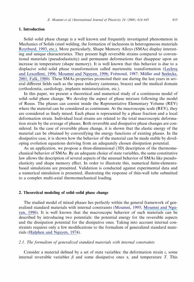
Theoretical and numerical modeling of solid–solid phase change: Application to the description of the thermomechanical behavior of shape memory alloys Ziad Moumni a, * , Wael Zaki a , Quoc Son Nguyen b a Unite ´ de Me ´canique, E ´ cole Nationale Supe ´rieure de Techniques Avance ´ es, 91761 Palaiseau, France b LMS, E ´ cole Polytechnique, 91128 Palaiseau, France Received 25 January 2007; received in final revised form 10 July 2007 Available online 31 July 2007 Abstract The mechanical behavior of a solid capable of undergoing internal phase change is considered. Reversible and dissipative constitutive equations are established within the framework of generalized standard materials with internal constraints. These constraints are accounted for using Lagrange multipliers. The presented model is based upon a phenomenological configuration in series (Reuss model). In the case of reversible phase change, it is shown that the elastic energy of the material can be obtained by convexifying the energy functions of existing phases. In the dissipative case, it is shown how the behavior of the material can be made stable by developing evolution equations deriving from an adequately chosen dissipation potential. As an application, we propose a descrip- tion of the thermomechanical behavior of shape memory alloys (SMAs). The obtained constitutive equations can be used to simulate the pseudoelastic response of SMAs as well as the one-way shape memory effect. Validation against experimental data is performed in the case of multi-axial complex thermomechanical loading for NiTi as well as Cu-based alloys. Ó 2007 Elsevier Ltd. All rights reserved. Keywords: Phase transformation; Internal constraints; Convexification; Dissipation; Shape memory alloys 0749-6419/$ - see front matter Ó 2007 Elsevier Ltd. All rights reserved. doi:10.1016/j.ijplas.2007.07.007 * Corresponding author. Tel.: +33 169319724; fax: +33 169319906. E-mail address: [email protected] (Z. Moumni). Available online at www.sciencedirect.com International Journal of Plasticity 24 (2008) 614–645 www.elsevier.com/locate/ijplas
-
Upload
independent -
Category
Documents
-
view
1 -
download
0
Transcript of Theoretical and numerical modeling of solid–solid phase change: Application to the description of...
Available online at www.sciencedirect.com
International Journal of Plasticity 24 (2008) 614–645
www.elsevier.com/locate/ijplas
Theoretical and numerical modelingof solid–solid phase change: Application
to the description of the thermomechanical behaviorof shape memory alloys
Ziad Moumni a,*, Wael Zaki a, Quoc Son Nguyen b
a Unite de Mecanique, Ecole Nationale Superieure de Techniques Avancees, 91761 Palaiseau, Franceb LMS, Ecole Polytechnique, 91128 Palaiseau, France
Received 25 January 2007; received in final revised form 10 July 2007Available online 31 July 2007
Abstract
The mechanical behavior of a solid capable of undergoing internal phase change is considered.Reversible and dissipative constitutive equations are established within the framework of generalizedstandard materials with internal constraints. These constraints are accounted for using Lagrangemultipliers. The presented model is based upon a phenomenological configuration in series (Reussmodel). In the case of reversible phase change, it is shown that the elastic energy of the materialcan be obtained by convexifying the energy functions of existing phases. In the dissipative case, itis shown how the behavior of the material can be made stable by developing evolution equationsderiving from an adequately chosen dissipation potential. As an application, we propose a descrip-tion of the thermomechanical behavior of shape memory alloys (SMAs). The obtained constitutiveequations can be used to simulate the pseudoelastic response of SMAs as well as the one-way shapememory effect. Validation against experimental data is performed in the case of multi-axial complexthermomechanical loading for NiTi as well as Cu-based alloys.� 2007 Elsevier Ltd. All rights reserved.
Keywords: Phase transformation; Internal constraints; Convexification; Dissipation; Shape memory alloys
0749-6419/$ - see front matter � 2007 Elsevier Ltd. All rights reserved.
doi:10.1016/j.ijplas.2007.07.007
* Corresponding author. Tel.: +33 169319724; fax: +33 169319906.E-mail address: [email protected] (Z. Moumni).
Z. Moumni et al. / International Journal of Plasticity 24 (2008) 614–645 615
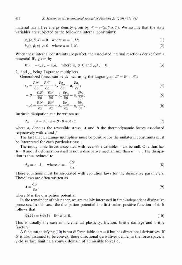
1. Introduction
Solid–solid phase change is a well known and frequently investigated phenomenon inMechanics of Solids (steel welding, the formation of inclusions in heterogeneous materialsRoytburd, 1993, etc.). More particularly, Shape Memory Alloys (SMAs) display interest-ing and unique characteristics. They present high reversible strains compared to conven-tional materials (pseudoelasticity) and permanent deformations that disappear upon anincrease in temperature (shape memory). It is well known that this behavior is due to adisplacive solid–solid phase transformation called martensitic transformation (Leclerqand Lexcellent, 1996; Moumni and Nguyen, 1996; Fremond, 1987; Muller and Seelecke,2001; Falk, 1980). These SMAs properties promoted their use during the last years in sev-eral different fields such as the space industry (antennas, braces) and the medical domain(orthodontia, cardiology, implants miniaturization, etc.).
In this paper, we present a theoretical and numerical study of a continuous model ofsolid–solid phase change. We develop the aspect of phase mixture following the modelof Reuss. The phases can coexist inside the Representative Elementary Volume (REV)where the material can be considered as continuum. At the macroscopic scale (REV), theyare considered as finely mixed. Each phase is represented by a phase fraction and a localdeformation strain. Individual local strains are related to the total macroscopic deforma-tion strain by the average of phases. Both reversible and dissipative phase changes are con-sidered. In the case of reversible phase change, it is shown that the elastic energy of thematerial can be obtained by convexifying the energy functions of existing phases. In thedissipative case, it is shown how the behavior of the material can be made stable by devel-oping evolution equations deriving from an adequately chosen dissipation potential.
As an application, we propose a three-dimensional (3D) description of the thermome-chanical behavior of SMAs. By an adequate choice of state variables, the same constitutivelaw allows the description of several aspects of the unusual behavior of SMAs like pseudo-elasticity and shape memory effect. In order to illustrate this, numerical finite-elements-based simulations are presented. Validation is conducted against experimental data anda numerical simulation is presented, illustrating the response of thin-wall tube submittedto a complex multi-axial thermomechanical loading.
2. Theoretical modeling of solid–solid phase change
The studied model of mixed phases lies perfectly within the general framework of gen-eralized standard materials with internal constraints (Moumni, 1995; Moumni and Ngu-yen, 1996). It is well known that the macroscopic behavior of such materials can bedescribed by introducing two potentials: the potential energy for the reversible aspectsand the dissipation potential for the dissipative ones. Taking into account internal con-straints requires only a few modifications to the formalism of generalized standard mate-rials (Halphen and Nguyen, 1974).
2.1. The formalism of generalized standard materials with internal constraints
Consider a material defined by a set of state variables: the deformation strain e, someinternal reversible variables b and some dissipative ones a, and temperature T. This
616 Z. Moumni et al. / International Journal of Plasticity 24 (2008) 614–645
material has a free energy density given by W ¼ W ðe; b; a; T Þ. We assume that the statevariables are subjected to the following internal constraints:
gmðe;b; aÞ ¼ 0 where m ¼ 1;M ; ð1Þhnðe; b; aÞP 0 where n ¼ 1;N : ð2Þ
When these internal constraints are perfect, the associated internal reactions derive from apotential W ‘ given by
W ‘ ¼ �kmgm � lnhn where ln P 0 and lnhn ¼ 0; ð3Þkm and ln being Lagrange multipliers.
Generalized forces can be defined using the Lagrangian L ¼ W þ W ‘:
rr ¼oL
oe¼ oW
oe� km
ogm
oe� ln
ohn
oe; ð4Þ
� B ¼ oL
ob¼ oW
ob� km
ogm
ob� ln
ohn
ob; ð5Þ
� A ¼ oL
oa¼ oW
oa� km
ogm
oa� ln
ohn
oa: ð6Þ
Intrinsic dissipation can be written as
d in ¼ ðr� rrÞ � _eþ B � _bþ A � _a; ð7Þwhere rr denotes the reversible stress, A and B the thermodynamic forces associatedrespectively with a and b.
The fact that Lagrange multipliers must be positive for the unilateral constraints mustbe interpreted for each particular case.
Thermodynamic forces associated with reversible variables must be null. One thus hasB = 0 and, if deformation itself is not a dissipative mechanism, then r ¼ rr. The dissipa-tion is thus reduced to
d in ¼ A � _a; where A ¼ � oL
oa: ð8Þ
These equations must be associated with evolution laws for the dissipative parameters.These laws are often written as
A ¼ oD
o _a; ð9Þ
where D is the dissipation potential.In the remainder of this paper, we are mainly interested in time-independent dissipative
processes. In this case, the dissipation potential is a first order, positive function of _a. Itfollows that
Dðk _aÞ ¼ kDð _aÞ for k P 0: ð10ÞThis is usually the case in incremental plasticity, friction, brittle damage and brittlefracture.
A function satisfying (10) is not differentiable at _a ¼ 0 but has directional derivatives. IfD is also assumed to be convex, these directional derivatives define, in the force space, ayield surface limiting a convex domain of admissible forces C.
Z. Moumni et al. / International Journal of Plasticity 24 (2008) 614–645 617
Eq. (9) means that whenever _a 6¼ 0, the normality rule holds:
_a ¼ N CðAÞ; ð11Þwhere N CðAÞ is an operator that associates an external normal vector to each A at theboundary of C.
2.2. The solid–solid phase change model
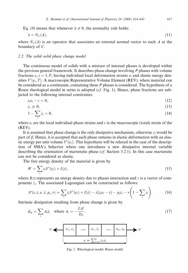
The continuous model of solids with a mixture of internal phases is developed withinthe previous general framework. It describes phase change involving P phases with volumefractions zi; i ¼ 1; P , having individual local deformation strains ei and elastic energy den-sities V iðei; T Þ. A macroscopic Representative Volume Element (REV), where material canbe considered as a continuum, containing these P phases is considered. The hypothesis of aReuss rheological model in series is adopted (cf. Fig. 1). Hence, phase fractions are sub-jected to the following internal constraints:
ziei � � ¼ 0; ð12Þzi P 0; ð13Þ1�
Xi
zi ¼ 0; ð14Þ
where ei are the local individual phase strains and � is the macroscopic (total) strain of the(REV).
It is assumed that phase change is the only dissipative mechanism, otherwise zi would bepart of b. Hence, it is accepted that each phase remains in elastic deformation with an elas-tic energy per unit volume V iðeiÞ. This hypothesis will be relaxed in the case of the descrip-tion of SMA’s behavior where one introduces a new dissipative internal variabledescribing the orientation of martensite phase (cf. Section 3.2.1). In this case martensitecan not be considered as elastic.
The free energy density of the material is given by
W ¼X
i
ziV iðeiÞ þ IðzÞ; ð15Þ
where I(z) represents an energy density due to phases interaction and z is a vector of com-ponents zi. The associated Lagrangian can be constructed as follows:
Lðe; z; e; k; li; mÞ ¼X
i
ziV iðeiÞ þ IðzÞ � kðziei � eÞ � lizi � m 1�X
i
zi
!: ð16Þ
Intrinsic dissipation resulting from phase change is given by
d in ¼X
i
Ai _zi where Ai ¼ �oL
ozi: ð17Þ
Fig. 1. Rheological model: Reuss model.
618 Z. Moumni et al. / International Journal of Plasticity 24 (2008) 614–645
2.3. Reversible phase change and convexification
If phase change is reversible, the state equations can be written as
oL
oe¼ rr;
oL
oei¼ 0;
oL
ozi¼ 0; ð18Þ
where
8i; li P 0 and lizi ¼ 0: ð19Þ
Eqs. (18) and (19) are enough for determining r; ei; zi; k; li and m in terms of e. Hence,the material is nonlinear elastic and the corresponding elastic energy density W cðeÞ isimplicitly defined.
The characteristics of the resulting elastic material depend on the elastic properties ofthe individual phases.
Energies Vi are assumed to be strictly convex and differentiable functions of the localdeformation strains. For non-differentiable energies, derivatives at angular points shouldbe understood as sub-gradients (cf. Moreau, 1967 or Rockafellar, 1972). In this case, if z isan admissible phase distribution, i.e. satisfying zi P 0 and 1�
Pizi ¼ 0, function F cðe; zÞ
defined as
F cðe; zÞ ¼ mine
W ¼ mine;ziei¼e
Xi
ziV iðeiÞ þ I zð Þ ð20Þor as
F cðe; zÞ ¼ mine
maxr
L0ðe; z; e; rÞ ¼ maxr
mine
L0ðe; z; e; rÞ;
where L0ðe; z; e; rÞ ¼ W � r : ðziei � eÞ is convex with respect to variables ðe; zÞ. Moreover,if all the functions Vi are strictly convex, then Fc is also strictly convex with respect to e fora fixed z.
If V �i is the dual function of Vi via Legendre–Fenchel transformation, the constraintassociated with z and e must verify e ¼ zi
oV �i
or . It follows that the expressions of individuallocal strains can be written as ei ¼ oV �i
or .The elastic energy density of the material can be written as
W cðeÞ ¼ minz
F cðe; zÞ ¼ minz
mine;ziei¼e
Xi
ziV iðeiÞ þ IðzÞ: ð21Þ
If Vi and I are (strictly) convex, the elastic energy W cðeÞ is also (strictly) convex. WhenIðzÞ ¼ 0, (21) shows that the elastic energy of the material is obtained by convexificationof the phase energy functions (cf. Rockafellar, 1972, p. 37, Theorem 5.6).
The strict convexity of the elastic energy allows us to analyze the stability of the mate-rial response, using the criterion of the second variation of the Lagrangian established forelastic systems under perfect constraints (Nguyen, 2000).
In case of reversible phase change, the model simplifies the study of the equilibrium of astructure subjected to mechanical and thermal loading. For example, in the case of smalltransformations, the convexity of the energy as well as its behavior at infinity imply thatthe problem of minimizing the total potential energy of the loaded structure has at leastone solution. This solution is unique if the interaction energy I(z) is strictly convex. Themodel completes other approaches in literature, particularly those developed by Ball
Z. Moumni et al. / International Journal of Plasticity 24 (2008) 614–645 619
and James (1987). It also bears some similarities with the work of Silling (1988) and Abey-aratne (1981) involving trilinear elastic materials (eventually introducing a line of Max-well), even though phase fractions were not used in describing phase mixtures.
2.4. Dissipative phase change
If phase change is dissipative, the associated thermodynamic forces, given by
Ai ¼ �oL
ozi¼ �V iðeiÞ þ kei þ li � m; ð22Þ
are not necessarily null.Irreversibility can be accounted for by complementary laws that relate these forces to
the rate of phase change _z. For example, if only two phases are present, power dissipationdue to phase change can be estimated as follows:
d in ¼ A _f where A ¼ � oF c
ofðe; fÞ � oWðfÞ;
where f ¼ z1—the only variable needed to describe phase transition in this case—and wðfÞis the indicator function of interval ½0; 1�. Notice that the thermodynamic force A is mul-tivalued for f = 0 or f = 1. The Lagrange multipliers associated with the inequality0 6 f 6 1 are thus undefined.
If the process of phase change is considered to be instantaneous and rate-independent(like in plasticity) with a potential of dissipation given by
Dð _f; fÞ ¼ k12ðfÞh _fiþ þ k21ðfÞh _fi�;
where haiþ is the positive part and hai� the negative part of a, then the evolution of phasefraction f satisfies
_f ¼ 0 if k21 < A < k12; _f P 0 if A ¼ k12; and _f 6 0 if A ¼ �k21: ð23Þk12ðfÞ is the dissipated energy density associated with forward phase change (1! 2), whilek21ðfÞ represents the dissipated energy density during reverse transformation (2! 1). Itfollows that the area of the hysteresis loop of the stress–strain curve can be expressedas follows:
W d ¼Z 1
0
k12 fð ÞdfþZ 1
0
k21 fð Þdf: ð24Þ
The stability of the material response can be investigated using a criterion applicable forstandard dissipative systems (Nguyen, 1994). For example, for 0 < f < 1, the material isstable if the following is strictly positive:
dr : de ¼ d2F c þ d2D ¼ de : F c;ee : deþ 2de : F c;efdfþ F c;ffdf2 þ k012hdfi
2þ þ k021hdfi2� > 0
for all ðd�; dfÞ 6¼ ð0; 0Þ compatible with the normality law, i.e. verifying
dz ¼ 0 if � k21 < A < k21; dz 6 0 if A ¼ �k21 and dz P 0 if A ¼ k12: ð25ÞConstitutive equations for viscous phase change can be can also be established by choos-ing an adequate expression of the dissipation potential Dð _f; fÞ.
620 Z. Moumni et al. / International Journal of Plasticity 24 (2008) 614–645
3. Application to the modeling of the thermomechanical behavior of shape memory alloys
3.1. Introduction
Shape memory alloys components are being used increasingly in advanced applica-tions. For example, NiTi components are utilized in surgical applications as orthodonticwires, staples, and of course as stents, which are small wire meshes used mainly in pre-venting the occlusion of large arteries. The interesting behavior of SMAs is mainly due totheir ability to undergo a reversible, diffusionless, solid–solid phase transformationknown as ‘‘the martensitic transformation”. At the micro-level, this transformation ischaracterized by a change in the lattice structure of the crystal, which can be inducedby altering the material temperature and/or the applied stress; hence a strongly coupledthermomechanical behavior. At high temperature, the microstructure of a shape memoryalloy consists of a relatively more-ordered parent phase called austenite, which trans-forms by cooling into a less-ordered product phase called martensite. In the absenceof stress, the multiple martensite variants ‘‘self-accommodate”, i.e. lattice twins areformed without causing any macroscopic deformation. ‘‘Detwinning” of martensiteplates may occur when the material is subjected to mechanical loading (Liu et al.,1999); this results in large macroscopic inelastic strains that can not be recovered byunloading. Finally, if the SMA is heated, it can transform back to its undeformed austen-itic shape. It is as if the alloy ‘‘remembers” its high-temperature state, hence the name‘‘shape memory”.
Pseudoelasticity is another uncommon behavior of shape memory alloys. It refers to theability of a SMA to accommodate large strains (up to 8%) when stress is applied, and thento recover its initial shape upon unloading. The stress–strain response in this case presentsa characteristic hysteresis loop.
SMAs may exhibit other interesting effects like the two-way shape memory effect(TWSME), which can be described as the ability of a SMA to ‘‘remember” two deformedstates: one at high temperature as austenite, and another one at low temperature as mar-tensite. In contrast with the one-way shape memory effect and with pseudoelasticity, thetwo-way shape memory is not an intrinsic material property (Wayman and Otsuka,1999): It is usually achieved by ‘‘training”, which can be accomplished by subjecting thematerial to cyclic loading.
Many of the existing models of SMAs are limited to pseudoelasticity (see for instanceRaniecki and Lexcellent, 1998; Fremond, 1987; Xu and Muller, 1993; Lagoudas and Shu,1999, etc.) and few can simulate a wide range of their effects. In this regard, some of themore complete models are due to Leclerq and Lexcellent (1996) and Bo and Lagoudas(1999); the numerical simulations they present are generally limited, however, to the caseof uniaxial loading.
In the following, the phase change modeling framework developed in previous sectionsis extended to account for martensite orientation and reorientation in shape memoryalloys by the introduction of second internal dissipative variable describing the orientationof martensite. The resulting macroscale model accounts for pseudoelasticity, twinning anddetwinning of martensite as well as one-way shape memory; it is applicable to 3D structureanalysis under multi-axial loading. Validation is conducted against experimental data anda numerical simulation is presented, illustrating the response of thin-wall tube submittedto a complex multi-axial thermomechanical loading.
Z. Moumni et al. / International Journal of Plasticity 24 (2008) 614–645 621
3.2. Constitutive equations
Developing the macroscale model requires defining appropriate state variables, individ-ual phase energy densities, as well as an interaction energy density and the dissipationpotential Dð _a; aÞ.
3.2.1. State variables and free energy densities
A phenomenological model in series is used and the following state variables areconsidered:
� The macroscopic total strain e.� Temperature T.� Volume fraction of martensite z.� Local strains of austenite ea and martensite em.� Local martensite orientation strain, etr.
The expression of the material free energy density is constructed as follows:
W ¼ ð1� zÞWa þ zWm þIðz; etrÞ; ð26Þwhere Wa and Wm represent free energy densities of austenite and martensite respectively.They are given by
WaðeaÞ ¼1
2ea : Ka : ea; ð27Þ
Wmðem; etr; T Þ ¼1
2ðem � etrÞ : Km : ðem � etrÞ þ CðT Þ: ð28Þ
Ka and Km are the elastic tensors of austenite and martensite, CðT Þ is a latent heat densityand Iðz; etrÞ is an interaction energy density due to incompatibilities between phase defor-mations. The following expression of Iðz; etrÞ is considered:
I ¼ Iðz; etrÞ ¼ Gz2
2þ z
2½azþ bð1� zÞ� 2
3etr : etr
� �: ð29Þ
G; a and b being material parameters that can be interpreted physically:
� b zð1�zÞ2
23etr : etr
� �represents interaction between austenite and martensite. Following sev-
eral published papers [etc.] (Leclerq and Lexcellent, 1996; Lexcellent and Bourbon,1996; Raniecki et al., 1992; Patoor and Berveiller, 1993), this interaction is assumedto be proportional to the volume fractions of interacting phases. b determines how amechanical loading applied to an initially austenitic shape memory material affectsthe orientation of martensite during phase change;� The term G z2
2measures the inter-variants interaction energy within the martensite
regardless of the orientation of these variants. where G is a material parameter. The per-tinence of this expression is corroborated by a micro-mechanical analysis presented byPeultier et al. (2006).� Finally, a z2
223etr : etr
� �accounts for oriented martensite variants interaction; this expres-
sion is inspired from classical plasticity. Indeed, the average macroscopic orientationstrain over a Representative Volume element (RVE) is zetr; hence, the above expression

622 Z. Moumni et al. / International Journal of Plasticity 24 (2008) 614–645
is similar to the free energy associated with linear kinematic hardening where a is thehardening coefficient. Hence, a controls the slope of the stress–strain curve representingan orientation process. The fact that this term depends on etr, which is a way of mea-suring martensite orientation, makes it ”orientation-dependent”.
3.2.2. State equations and kinetics of dissipative processes
State variables obey certain physical constraints:
� Since the model is in series:
ð1� zÞea þ zem � e ¼ 0: ð30Þ� Volume fractions are positive and their sum is equal to one:
z P 0 and ð1� zÞP 0: ð31Þ� The equivalent inelastic strain due to martensite orientation can not exceed a certain
limit e0, characteristic of the material:
e0 �ffiffiffiffiffiffiffiffiffiffiffiffiffiffiffiffi2
3etr : etr
rP 0: ð32Þ
These constraints are supposed to be perfect. As such, the associated reactions can bederived from a potential Wl given by
Wl ¼ �k : ½ð1� zÞea þ zem � e� � l e0 �ffiffiffiffiffiffiffiffiffiffiffiffiffiffiffiffi2
3etr : etr
r !� m1z� m2ð1� zÞ: ð33Þ
k; l; m1 and m2 are Lagrange multipliers. Since m1; m2 and l are associated with unilateralconstraints, the following holds:
m1 P 0; m1z ¼ 0; m2 P 0; m2ð1� zÞ ¼ 0 and l P 0; l e0 �ffiffiffiffiffiffiffiffiffiffiffiffiffiffiffiffi2
3etr : etr
r !¼ 0:
ð34ÞBased on the Clausius–Duhem inequality, it is possible to derive state equations by substi-tuting the free energy density W by the Lagrangian
L ¼WþWl ¼ ð1� zÞ 1
2ea : Ka : ea
� �þ z
1
2ðem � etrÞ : Km : ðem � etrÞ þ CðT Þ
� �
þ Gz2
2þ z
2½azþ bð1� zÞ� 2
3etr : etr
� �� k : ½ð1� zÞe1 þ ze2 � e�
� l e0 �ffiffiffiffiffiffiffiffiffiffiffiffiffiffiffiffi2
3etr : etr
r !� m1z� m2ð1� zÞ; ð35Þ
where
m1 P 0; m1z ¼ 0; m2 P 0; m2ð1� zÞ ¼ 0 and l P 0; l e0 �ffiffiffiffiffiffiffiffiffiffiffiffiffiffiffiffi2
3etr : etr
r !¼ 0:
ð36ÞIndeed, if Atr and Az denote the thermodynamic forces associated with martensite orien-tation and with phase change, the state equations are given by:
Z. Moumni et al. / International Journal of Plasticity 24 (2008) 614–645 623
oL
oe¼ r) k� r ¼ 0; ð37Þ
� oL
oea
¼ 0) ð1� zÞðKa : ea � kÞ ¼ 0; ð38Þ
� oL
oem
¼ 0) z½Km : ðem � etrÞ� � k ¼ 0; ð39Þ
� oL
oz¼Az )Az ¼
1
2½ea : Ka : ea � ðem � etrÞ : Km : ðem � etrÞ�
� CðT Þ � Gz� ða� bÞzþ b2
� �2
3etr : etr
� �� k : ðea � emÞ;
ð40Þ
� oL
oetr
¼Atr )Atr ¼ z Km : ðem � etrÞ �2
3½azþ bð1� zÞ�etr
� 2l
3
etrffiffiffiffiffiffiffiffiffiffiffiffiffiffiffi23etr : etr
q ;
ð41Þ
� oL
ok¼ 0) ð1� zÞea þ zem � e ¼ 0: ð42Þ
Eqs. (37)–(42) give
r ¼ K : ðe� zetrÞ; ð43Þwhere K is the equivalent elasticity tensor given by
K ¼ ½ð1� zÞK�1aþ zK�1
m��1: ð44Þ
Phase change kinetics can be derived, given the expression of a dissipation potential. Sincephase change and martensite orientation and reorientation are considered to be instanta-neous phenomena, this potential is chosen to be a first-order, convex and homogeneousfunction of _z and _etr:
D ¼def Dð_z; _etrÞ ¼ P ðz; _zÞ_zþ RðzÞffiffiffiffiffiffiffiffiffiffiffiffiffiffiffiffi2
3_etr : _etr
r; ð45Þ
where P ðz; _zÞ and R (z) are given by
P ðz; _zÞ ¼ ½að1� zÞ þ bz�sgn _z ð46Þand
RðzÞ ¼ z2Y : ð47Þa, b and Y are material parameters whose positivity ensures that of the dissipation poten-tial D.
Within the framework of generalized standard materials, phase change and transforma-tion kinetics satisfy the normality rule:
Az 2 o_zD; ð48ÞAtr 2 o_etrD: ð49Þ
(48) and (49) can be written as a set of inequalities:
F16 0; F2
6 0 and Ftr 6 0; ð50Þ
z z
624 Z. Moumni et al. / International Journal of Plasticity 24 (2008) 614–645
where F1z ; F2
z and Ftr are yield functions, respectively associated with forward martens-ite transformation, reverse transformation, and with martensite orientation and reorienta-tion. Their expressions are as follows:
F1z ¼Az � að1� zÞ � bz ¼ 1
2½ea : Ka : ea � ðem � etrÞ : Km : ðem � etrÞ� � CðT Þ
� ðGþ bÞz� að1� zÞ � ða� bÞzþ b2
� �2
3etr : etr
� �� k : ðea � emÞ; ð51Þ
F2z ¼ �Az � að1� zÞ � bz ¼ � 1
2½ea : Ka : ea � ðem � etrÞ : Km : ðem � etrÞ� þ CðT Þ
þ ðG� bÞz� að1� zÞ þ ða� bÞzþ b2
� �2
3etr : etr
� �þ k : ðea � emÞ; ð52Þ
Ftr ¼ kAtrkvm� z2Y : ð53Þ
In order to simplify further analysis, austenite and martensite are assumed to be isotropicand homogeneous, having the same Poisson coefficient:
ma ¼ mm ¼ m: ð54Þ
The notations used throughout this paper are listed in Table 1.Given the expressions in Table 1, for values of z strictly between zero and one, local
strains ea and em can be written in terms of stress r and macroscopic strain e. Indeed,Eqs. (37)–(42) give:
ea ¼ Elarþ P aðtrrÞI; ð55Þem ¼ Elmrþ P mðtrrÞIþ etr: ð56Þ
If one considers that volume change accompanying martensite orientation is negligible, thefollowing stress–strain relation holds:
r ¼ 2leqðe� zetrÞ þ keqðtr eÞI: ð57Þ
Corresponding yield functions for 0 < z < 1 are given by
F1z ¼
1
3Elmar
2vmþ 1
2
1
3Elma þ P ma
� �ðtrrÞ2 � CðT Þ
þ r : etr � ðGþ bÞz� að1� zÞ � ða� bÞzþ b2
� �2
3etr : etr
� �; ð58Þ
F2z ¼ �
1
3Elmar
2vmþ 1
2
1
3Elma þ P ma
� �ðtrrÞ2 � CðT Þ
� r : etr þ ðG� bÞz� að1� zÞ þ ða� bÞzþ b2
� �2
3etr : etr
� �; ð59Þ
Ftr
z¼ r� 2
3½azþ bð1� zÞ�etr �
2l3z
etrffiffiffiffiffiffiffiffiffiffiffiffiffiffiffi23etr : etr
q�������
�������vm
� zY : ð60Þ
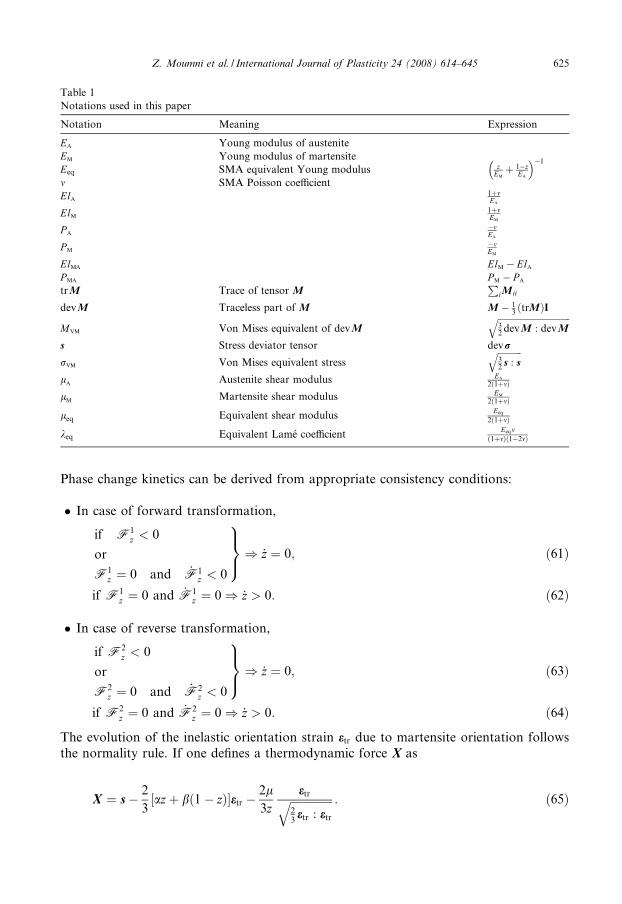
Table 1Notations used in this paper
Notation Meaning Expression
Ea Young modulus of austeniteEm Young modulus of martensiteEeq SMA equivalent Young modulus z
Em
þ 1�zEa
� �1
m SMA Poisson coefficientEla
1þmEa
Elm
1þmEm
P a
�mEa
P m
�mEm
Elma Elm � Ela
P ma P m � P a
trM Trace of tensor MP
iM ii
devM Traceless part of M M � 13 ðtrMÞI
Mvm Von Mises equivalent of devMffiffiffiffiffiffiffiffiffiffiffiffiffiffiffiffiffiffiffiffiffiffiffiffiffiffiffiffiffiffiffiffiffi32 devM : devM
qs Stress deviator tensor devr
rvm Von Mises equivalent stressffiffiffiffiffiffiffiffiffiffiffi32 s : s
ql
aAustenite shear modulus Ea
2ð1þmÞ
lm
Martensite shear modulus Em
2ð1þmÞ
leq Equivalent shear modulusEeq
2ð1þmÞ
keq Equivalent Lame coefficientEeqm
ð1þmÞð1�2mÞ
Z. Moumni et al. / International Journal of Plasticity 24 (2008) 614–645 625
Phase change kinetics can be derived from appropriate consistency conditions:
� In case of forward transformation,
if F1z < 0
or
F1z ¼ 0 and _F1
z < 0
9>=>;) _z ¼ 0; ð61Þ
if F1z ¼ 0 and _F1
z ¼ 0) _z > 0: ð62Þ
� In case of reverse transformation,
if F2z < 0
or
F2z ¼ 0 and _F2
z < 0
9>=>;) _z ¼ 0; ð63Þ
if F2z ¼ 0 and _F2
z ¼ 0) _z > 0: ð64Þ
The evolution of the inelastic orientation strain etr due to martensite orientation followsthe normality rule. If one defines a thermodynamic force X as
X ¼ s� 2
3½azþ bð1� zÞ�etr �
2l3z
etrffiffiffiffiffiffiffiffiffiffiffiffiffiffiffi23etr : etr
q : ð65Þ
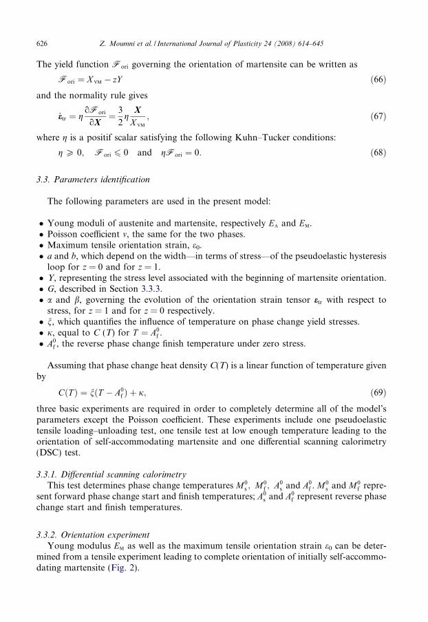
626 Z. Moumni et al. / International Journal of Plasticity 24 (2008) 614–645
The yield function Fori governing the orientation of martensite can be written as
Fori ¼ X vm � zY ð66Þand the normality rule gives
_etr ¼ goFori
oX¼ 3
2g
X
X vm
; ð67Þ
where g is a positif scalar satisfying the following Kuhn–Tucker conditions:
g P 0; Fori 6 0 and gFori ¼ 0: ð68Þ
3.3. Parameters identification
The following parameters are used in the present model:
� Young moduli of austenite and martensite, respectively Ea and Em.� Poisson coefficient m, the same for the two phases.� Maximum tensile orientation strain, e0.� a and b, which depend on the width—in terms of stress—of the pseudoelastic hysteresis
loop for z = 0 and for z = 1.� Y, representing the stress level associated with the beginning of martensite orientation.� G, described in Section 3.3.3.� a and b, governing the evolution of the orientation strain tensor etr with respect to
stress, for z = 1 and for z = 0 respectively.� n, which quantifies the influence of temperature on phase change yield stresses.� j, equal to C (T) for T ¼ A0
f .� A0
f , the reverse phase change finish temperature under zero stress.
Assuming that phase change heat density C(T) is a linear function of temperature givenby
CðT Þ ¼ nðT � A0f Þ þ j; ð69Þ
three basic experiments are required in order to completely determine all of the model’sparameters except the Poisson coefficient. These experiments include one pseudoelastictensile loading–unloading test, one tensile test at low enough temperature leading to theorientation of self-accommodating martensite and one differential scanning calorimetry(DSC) test.
3.3.1. Differential scanning calorimetry
This test determines phase change temperatures M0s ; M0
f ; A0s and A0
f . M0s and M0
f repre-sent forward phase change start and finish temperatures; A0
s and A0f represent reverse phase
change start and finish temperatures.
3.3.2. Orientation experiment
Young modulus Em as well as the maximum tensile orientation strain e0 can be deter-mined from a tensile experiment leading to complete orientation of initially self-accommo-dating martensite (Fig. 2).
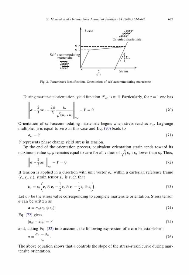
Strain
Stress
"0
Self-accommodatingmartensite
Oriented martensite
E M
σσ
ε
rf
rs
Fig. 2. Parameters identification. Orientation of self-accommodating martensite.
Z. Moumni et al. / International Journal of Plasticity 24 (2008) 614–645 627
During martensite orientation, yield function Fori is null. Particularly, for z = 1 one has
r� 2
3aetr �
2l3
etrffiffiffiffiffiffiffiffiffiffiffiffiffiffiffi23etr : etr
q�������
�������vm
� Y ¼ 0: ð70Þ
Orientation of self-accommodating martensite begins when stress reaches rrs. Lagrangemultiplier l is equal to zero in this case and Eq. (70) leads to
rrs ¼ Y : ð71ÞY represents phase change yield stress in tension.
By the end of the orientation process, equivalent orientation strain tends toward its
maximum value e0. l remains equal to zero for all values offfiffiffiffiffiffiffiffiffiffiffiffiffiffiffi23etr : etr
qlower than e0. Thus,
r� 2
3aetr
��������
vm
� Y ¼ 0: ð72Þ
If tension is applied in a direction with unit vector ex, within a cartesian reference frameðex; ey ; ezÞ, strain tensor etr is such that
etr ¼ e0 ex � ex �1
2ey � ey �
1
2ez � ez
� �: ð73Þ
Let rrf be the stress value corresponding to complete martensite orientation. Stress tensorr can be written as
r ¼ rrfðex � exÞ: ð74ÞEq. (72) gives
jrrf � ae0j ¼ Y ð75Þand, taking Eq. (32) into account, the following expression of a can be established:
a ¼ rrf � rrs
e0
: ð76Þ
The above equation shows that a controls the slope of the stress–strain curve during mar-tensite orientation.
628 Z. Moumni et al. / International Journal of Plasticity 24 (2008) 614–645
b can also be identified. If austenite transforms into completely oriented martensite forstresses greater or equal to rrf , one has for z = 0
b ¼ rrf
e0
: ð77Þ
Hence, b determines the orientation level of martensite created during forward phasechange.
3.3.3. Pseudoelastic tensile experiment
A shape memory specimen is subjected to a tensile loading cycle at a temperature T0,where T 0 > A0
f . For easier parameters identification, T0 is taken to be high enough for
phase change to occur at stresses higher than rrf . In this case, martensite is completely ori-
ented andffiffiffiffiffiffiffiffiffiffiffiffiffiffiffi23etr : etr
q¼ e0.
Let rms be the yield stress corresponding to the beginning of the forward pseudoelastictransformation at temperature T0. When rms is reached, F1
z becomes equal to zero forz = 0, because the material is initially austenitic. Hence,
1
Em
� 1
Ea
� �r2
ms
2� CðT 0Þ þ rmse0 � a� b
2e2
0 ¼ 0: ð78Þ
At the end of forward transformation, z becomes equal to one. If rmf is the forward trans-formation finish stress, Eq. (78) can be written as:
1
Em
� 1
Ea
� �r2
mf
2� CðT 0Þ þ rmfe0 � ðGþ bÞ � a� b
2
� �e2
0 ¼ 0: ð79Þ
Yield function F2z controls reverse phase change during unloading. When stress reaches
ras, volume fraction z starts decreasing until it reaches zero for a stress value of raf . Thus,
� 1
Em
� 1
Ea
� �r2
as
2þ CðT 0Þ � rase0 þ ðG� bÞ þ a� b
2
� �e2
0 ¼ 0 ð80Þ
and
� 1
Em
� 1
Ea
� �r2
af
2þ CðT 0Þ � rafe0 � aþ b
2e2
0 ¼ 0: ð81Þ
Eqs. (78)–(81) yield the following expressions of parameters a, b and G:
a ¼ 1
2
1
Em
� 1
Ea
� �r2
ms � r2af
2þ ðrms � rafÞe0
� �; ð82Þ
b ¼ 1
2
1
Em
� 1
Ea
� �r2
mf � r2as
2þ ðrmf � rasÞe0
� �; ð83Þ
G ¼ 1
2
1
Em
� 1
Ea
� �r2
mf � r2ms þ r2
as � r2af
2þ ðrmf � rms þ ras � rafÞe0 � 2ða� bÞe2
0
� �:
ð84Þ
a and b are associated with the hysteresis loop width: a depends on the difference betweenforward phase change start stress rms and reverse transformation finish stress raf while b ismainly related to the difference between forward transformation finish stress rmf and
Z. Moumni et al. / International Journal of Plasticity 24 (2008) 614–645 629
reverse transformation start stress ras. G, which measures interaction between martensiteplates, affects the stress–strain curve slope during phase transition; it also depends on theorientation yield stress via a and b.
The same experiment allows the identification of the heat density value at temperatureT0.
CðT 0Þ ¼1
2
1
Em
� 1
Ea
� �r2
ms þ r2af
2þ ðrms þ rafÞe0 � be2
0
� �: ð85Þ
C(T) being a linear function of temperature T, it is sufficient to determine its value at A0f
for example in order to identify j and n.A0
f characterizes the end of the reverse martensite transformation under zero stress. For
completely oriented martensite, this transformation starts at F2z ¼ 0; z ¼ 0;
ffiffiffiffiffiffiffiffiffiffiffiffiffiffiffi23etr : etr
q¼
e0 and r ¼ 0, hence
CðA0f Þ ¼ a� b
e20
2: ð86Þ
It follows from the above equation that
j ¼ a� be2
0
2: ð87Þ
Finally, n is given by
n ¼ CðT 0Þ � CðA0f Þ
T 0 � A0f
¼ CðT 0Þ � j
T 0 � A0f
: ð88Þ
Temperature A0f can be determined using differential scanning calorimetry.
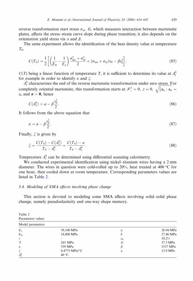
We conducted experimental identification using nickel–titanium wires having a 2 mmdiameter. The wires in question were cold-rolled up to 20%, heat treated at 400 �C forone hour, then cooled down at room temperature. Corresponding parameters values arelisted in Table 2.
3.4. Modeling of SMA effects involving phase change
This section is devoted to modeling some SMA effects involving solid–solid phasechange, namely pseudoelasticity and one-way shape memory.
Table 2Parameters values
Model parameters
Ea 39,100 MPa a 28.94 MPaEm 18,000 MPa b 27.46 MPam – e0 10.2%Y 265 MPa G 37.3 MPaa 539 MPa b 3137 MPan 0.4775 MPa/�C j 13.9 MPaA0
f 40 �C
Strain
Stress
ε0
Austenite
Oriented martensite
E A
σmf
σms
σas
σaf
Temperature T = T0
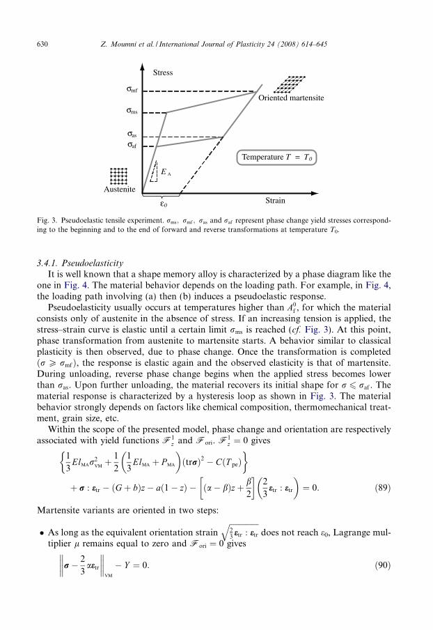
Fig. 3. Pseudoelastic tensile experiment. rms; rmf ; ras and raf represent phase change yield stresses correspond-ing to the beginning and to the end of forward and reverse transformations at temperature T0.
630 Z. Moumni et al. / International Journal of Plasticity 24 (2008) 614–645
3.4.1. PseudoelasticityIt is well known that a shape memory alloy is characterized by a phase diagram like the
one in Fig. 4. The material behavior depends on the loading path. For example, in Fig. 4,the loading path involving (a) then (b) induces a pseudoelastic response.
Pseudoelasticity usually occurs at temperatures higher than A0f , for which the material
consists only of austenite in the absence of stress. If an increasing tension is applied, thestress–strain curve is elastic until a certain limit rms is reached (cf. Fig. 3). At this point,phase transformation from austenite to martensite starts. A behavior similar to classicalplasticity is then observed, due to phase change. Once the transformation is completedðr P rmfÞ, the response is elastic again and the observed elasticity is that of martensite.During unloading, reverse phase change begins when the applied stress becomes lowerthan ras. Upon further unloading, the material recovers its initial shape for r 6 raf . Thematerial response is characterized by a hysteresis loop as shown in Fig. 3. The materialbehavior strongly depends on factors like chemical composition, thermomechanical treat-ment, grain size, etc.
Within the scope of the presented model, phase change and orientation are respectivelyassociated with yield functions F1
z and Fori. F1z ¼ 0 gives
1
3Elmar
2vmþ 1
2
1
3Elma þ P ma
� �ðtrrÞ2 � CðT peÞ
þ r : etr � ðGþ bÞz� að1� zÞ � ða� bÞzþ b2
� �2
3etr : etr
� �¼ 0: ð89Þ
Martensite variants are oriented in two steps:
� As long as the equivalent orientation strainffiffiffiffiffiffiffiffiffiffiffiffiffiffiffi23etr : etr
qdoes not reach e0, Lagrange mul-
tiplier l remains equal to zero and Fori ¼ 0 gives
r� 2
3aetr
��������
vm
� Y ¼ 0: ð90Þ
Temperature
Str
ess
Austenite
(a)
(b)Oriented martensite
Self-accommodatingmartensite
M 0f M 0
s A 0s A 0
f
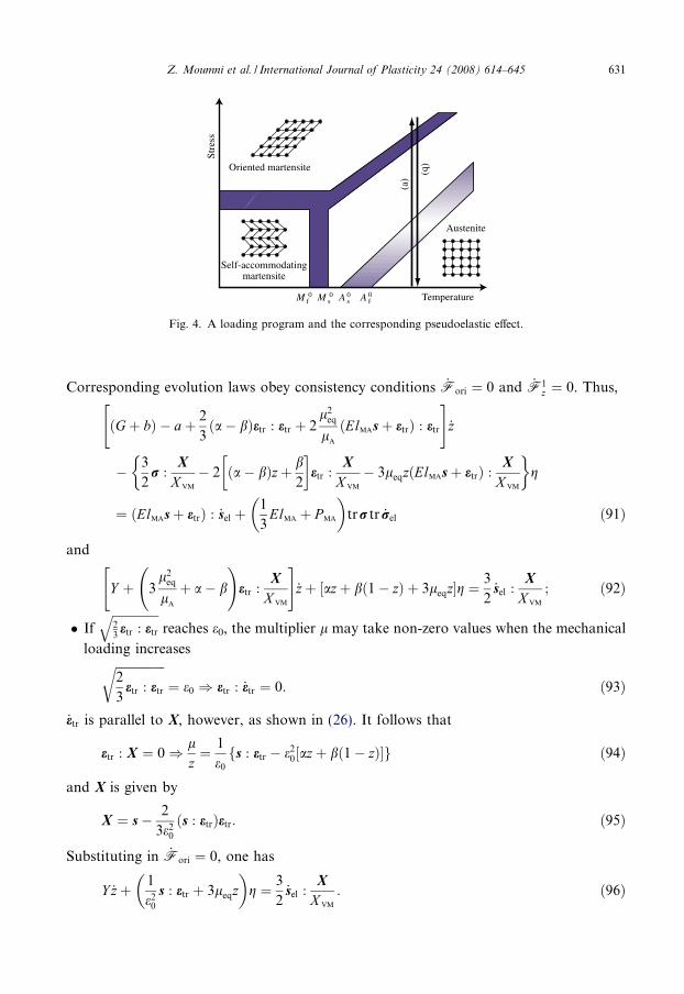
Fig. 4. A loading program and the corresponding pseudoelastic effect.
Z. Moumni et al. / International Journal of Plasticity 24 (2008) 614–645 631
Corresponding evolution laws obey consistency conditions _Fori ¼ 0 and _F1z ¼ 0. Thus,
ðGþ bÞ � aþ 2
3ða� bÞetr : etr þ 2
l2eq
la
ðElmasþ etrÞ : etr
" #_z
� 3
2r :
X
X vm
� 2 ða� bÞzþ b2
� �etr :
X
X vm
� 3leqzðElmasþ etrÞ :X
X vm
g
¼ ðElmasþ etrÞ : _sel þ1
3Elma þ P ma
� �trr tr _rel ð91Þ
and
Y þ 3l2
eq
la
þ a� b
!etr :
X
X vm
" #_zþ ½azþ bð1� zÞ þ 3leqz�g ¼ 3
2_sel :
X
X vm
; ð92Þ
� Ifffiffiffiffiffiffiffiffiffiffiffiffiffiffiffi23etr : etr
qreaches e0, the multiplier l may take non-zero values when the mechanical
loading increasesffiffiffiffiffiffiffiffiffiffiffiffiffiffiffiffi2
3etr : etr
r¼ e0 ) etr : _etr ¼ 0: ð93Þ
_etr is parallel to X, however, as shown in (26). It follows that
etr : X ¼ 0) lz¼ 1
e0
fs : etr � e20½azþ bð1� zÞ�g ð94Þ
and X is given by
X ¼ s� 2
3e20
ðs : etrÞetr: ð95Þ
Substituting in _Fori ¼ 0, one has
Y _zþ 1
e20
s : etr þ 3leqz� �
g ¼ 3
2_sel :
X
X vm
: ð96Þ

632 Z. Moumni et al. / International Journal of Plasticity 24 (2008) 614–645
Evolution laws are determined via Eqs. (57) and (64).
Reverse phase change can be induced by unloading. In this case, the evolution of vol-ume fraction z obeys consistency condition _F2
z ¼ 0, which can be written as
ðG� bÞ þ aþ 2
3ða� bÞetr : etr þ 2
l2eq
la
ðElmasþ etrÞ : etr
" #_z
� 3
2r :
X
X vm
� 2 ða� bÞzþ b2
� �etr :
X
X vm
� 3leqzðElmasþ etrÞ :X
X vm
� �g
¼ ðElmasþ etrÞ : _sel þ1
3Elma þ P ma
� �trr tr _rel: ð97Þ
Determining _z and g in (97) requires one more equation:
� If Fori < 0 or if Fori ¼ 0 and _Fori < 0,
g ¼ 0: ð98Þ� If Fori ¼ 0 and _Fori ¼ 0, for
ffiffiffiffiffiffiffiffiffiffiffiffiffiffiffi23etr : etr
qlower than e0, the evolution of etr obeys (92).
� If Fori ¼ 0 and _Fori ¼ 0, whenffiffiffiffiffiffiffiffiffiffiffiffiffiffiffi23etr : etr
qtends to exceed e0, (96) holds.
If unloading continues until z reaches zero, martensite becomes non-existing and etr
becomes physically undefined: the material ‘‘forgets” its loading history once it transformsinto austenite, which is purely elastic.
3.4.2. Self-accommodation of martensite
In the absence of stress, local martensite inelastic strain etr remains constant and themacroscopic inelastic strain tensor zetr is zero if the material is purely austenitic.
Austenite to martensite phase change obeys _F1z ¼ 0:
_z ¼ �_CðT Þ
Gþ b� a: ð99Þ
At the end of forward transformation, austenite transforms completely into self-accommo-dating martensite, i.e. martensite for which etr ¼ 0. Reverse phase change is associatedwith yield function F2
z . When temperature increases, z increases according to consistencycondition _F2
z ¼ 0. Hence,
_z ¼ �_CðT Þ
G� bþ a: ð100Þ
The denominators in (99) and (100) are positive. Indeed, given the expressions of a, b andG
Gþ b� a ¼ 1
Em
� 1
Ea
� �r2
mf � r2ms
2þ ðrmf � rmsÞe0 þ rrse0; ð101Þ
G� bþ a ¼ 1
Em
� 1
Ea
� �r2
as � r2af
2þ ðras � rafÞe0 þ rrse0: ð102Þ
Z. Moumni et al. / International Journal of Plasticity 24 (2008) 614–645 633
Since rmf P rms; ras P raf ; rrs > 0; Ea P Em and e0 > 0; Gþ b� a and G� bþ a arepositive; it follows that z increases when the SMA is cooled and decreases when it isheated.
3.4.3. Orientation of self-accommodating martensiteWhen subjected to mechanical loading, martensite variants can be oriented; inelastic
strainffiffiffiffiffiffiffiffiffiffiffiffiffiffiffi23etr : etr
qincreases in this case, while volume fraction z remains equal to 1 (one).
When etr evolves, Fori remains equal to zero:
r� 2
3aetr �
2l3
etrffiffiffiffiffiffiffiffiffiffiffiffiffiffiffi23etr : etr
q�������
�������vm
� Y ¼ 0: ð103Þ
As long asffiffiffiffiffiffiffiffiffiffiffiffiffiffiffi23etr : etr
qdoes not reach e0, Lagrange multiplier l remains equal to zero. As a
result, (103) gives
r� 2
3aetr
��������
vm
� Y ¼ 0: ð104Þ
The associated evolution of etr corresponds to
g ¼ 3
2a_s :
X
X vm
; ð105Þ
where
X ¼ s� 2
3aetr ð106Þ
and
_etr ¼3
2g
X
X vm
: ð107Þ
Whenffiffiffiffiffiffiffiffiffiffiffiffiffiffiffi23etr : etr
qreaches e0 under increasing mechanical loading, X can be written as
X ¼ s� 2
3e20
ðs : etrÞetr: ð108Þ
It follows that
g ¼ 3e20
2s : etr
_s :X
X vm
: ð109Þ
The inelastic strain does not evolve during unloading (Fig. 2), because of the yield functionFori becoming negative.
3.4.4. One-way shape memory
The one-way shape memory effect can be obtained as a result of a special thermome-chanical loading path, like the one shown in Fig. 5: starting from an initially austeniticmaterial ðT > A0
f Þ and cooling (path (a)) until temperature becomes lower than M0f , the
parent phase transforms into self-accommodating martensite. The material is then sub-jected to mechanical loading (path (b)) causing orientation of the self-accommodatingmartensite and, as a result, important inelastic strains that remain after unloading along
Temperature
Stre
ss
Austenite
(a)
(b)
(c)
(d)
Oriented martensite
Self-accommodatingmartensite
M 0f M 0
s A 0s A 0
f
(a) Loading Path.
Strain
Stre
ss
Tempera
ture
Austenite
Self-accommodatingmartensite
Orientation
Oriented martensite
Reversetransformation
(b) One way shape memory.
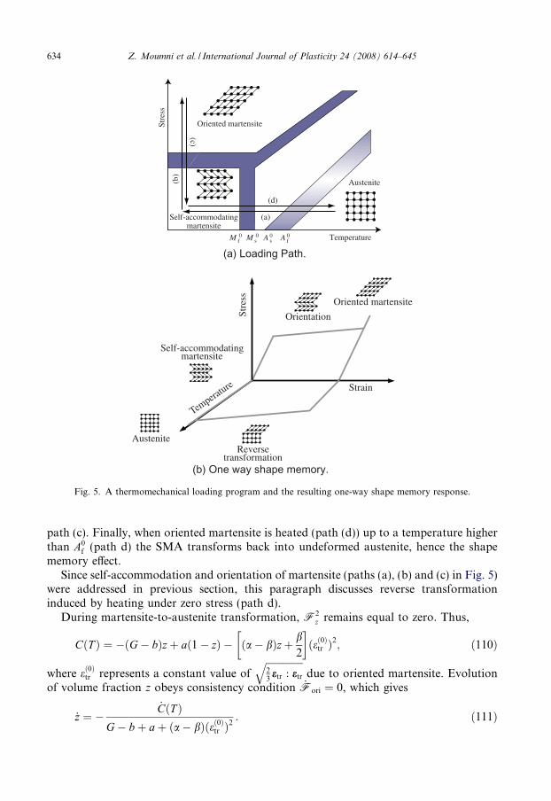
Fig. 5. A thermomechanical loading program and the resulting one-way shape memory response.
634 Z. Moumni et al. / International Journal of Plasticity 24 (2008) 614–645
path (c). Finally, when oriented martensite is heated (path (d)) up to a temperature higherthan A0
f (path d) the SMA transforms back into undeformed austenite, hence the shapememory effect.
Since self-accommodation and orientation of martensite (paths (a), (b) and (c) in Fig. 5)were addressed in previous section, this paragraph discusses reverse transformationinduced by heating under zero stress (path d).
During martensite-to-austenite transformation, F2z remains equal to zero. Thus,
CðT Þ ¼ �ðG� bÞzþ að1� zÞ � ða� bÞzþ b2
� �ðeð0Þtr Þ2; ð110Þ
where eð0Þtr represents a constant value offfiffiffiffiffiffiffiffiffiffiffiffiffiffiffi23etr : etr
qdue to oriented martensite. Evolution
of volume fraction z obeys consistency condition _Fori ¼ 0, which gives
_z ¼ �_CðT Þ
G� bþ aþ ða� bÞðeð0Þtr Þ2: ð111Þ
Z. Moumni et al. / International Journal of Plasticity 24 (2008) 614–645 635
Taking into account the expressions of G; a; b; a and b, one has
G� bþ aþ ða� bÞðeð0Þtr Þ2 ¼1
Em
� 1
Ea
� �r2
as � r2af
2þ ðras � rafÞe0 þ
rrs
e0
ðeð0Þtr Þ2: ð112Þ
(112) shows that the denominator in (111) is positive: z decreases during reverse transfor-mation. If z reaches zero, inelastic macroscopic strain zetr is recovered, allowing for mate-rial shape recovery.
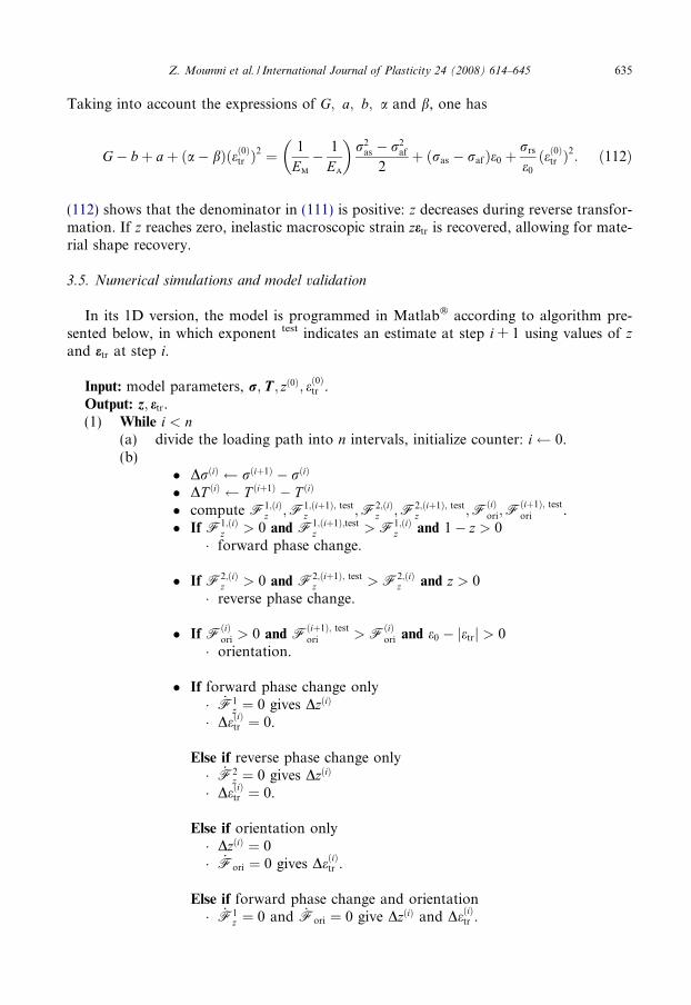
3.5. Numerical simulations and model validation
In its 1D version, the model is programmed in Matlab� according to algorithm pre-sented below, in which exponent test indicates an estimate at step i + 1 using values of zand etr at step i.
Input: model parameters, r;T; zð0Þ; eð0Þtr .Output: z; etr.(1) While i < n
(a) divide the loading path into n intervals, initialize counter: i 0.(b)
� DrðiÞ rðiþ1Þ � rðiÞ
� DT ðiÞ T ðiþ1Þ � T ðiÞ
� compute F1;ðiÞz ;F1;ðiþ1Þ; test
z ;F2;ðiÞz ;F2;ðiþ1Þ; test
z ;FðiÞori;F
ðiþ1Þ; testori .
� If F1;ðiÞz > 0 and F1;ðiþ1Þ;test
z >F1;ðiÞz and 1� z > 0
� forward phase change.
� If F2;ðiÞz > 0 and F2;ðiþ1Þ; test
z >F2;ðiÞz and z > 0
� reverse phase change.
� If FðiÞori > 0 and F
ðiþ1Þ; testori >F
ðiÞori and e0 � jetrj > 0
� orientation.
� If forward phase change only
� _F1z ¼ 0 gives DzðiÞ
� DeðiÞtr ¼ 0.
Else if reverse phase change only
� _F2z ¼ 0 gives DzðiÞ
� DeðiÞtr ¼ 0.
Else if orientation only
� DzðiÞ ¼ 0� _Fori ¼ 0 gives DeðiÞtr .Else if forward phase change and orientation
� _F1z ¼ 0 and _Fori ¼ 0 give DzðiÞ and DeðiÞtr .
Strain ε (%)
Stre
ssσ
(MPa
)
ModelExperiment
0 1 2 3 40
50
100
150
200
Strain ε (%)
Stre
ssσ
(MPa
)
ModelExperiment
0 2 4 6 80
100
200
300
400
500
600
700
800
Strain ε (%)
Stre
ssσ
(MPa
)
ModelExperiment
0 1 2 3 4 5 60
50
100
150
200
250
300
350
Strain ε (%)
Stre
ssσ
(MPa
)
ModelExperiment
0 1 2 3 4 5 60
50
100
150
200
250
300
350
400
Strain ε (%)
Stre
ssσ
(MPa
)
ModelExperiment
0 1 2 3 4 5 60
100
200
300
400
500
Strain ε (%)
Stre
ssσ
(MPa
)
ModelExperiment
0 2 4 6 80
100
200
300
400
500
600
Strain ε (%)
Stre
ssσ
(MPa
)
ModelExperiment
0 1 2 3 4 50
50
100
150
200
(a) Temperature T = −17,6 °C.
(c) Temperature T = 0 °C.
(e) Temperature T = 20 °C.
(g) Temperature T = 40 °C.
(b) Temperature T = −10 °C.
(d) Temperature T = 10 °C.
(f) Temperature T = 30 °C.
(h) Temperature T = 50 °C.
Strain ε (%)
Stre
ssσ
(MPa
)
ModelExperiment
0 1 2 3 40
50
100
150
200
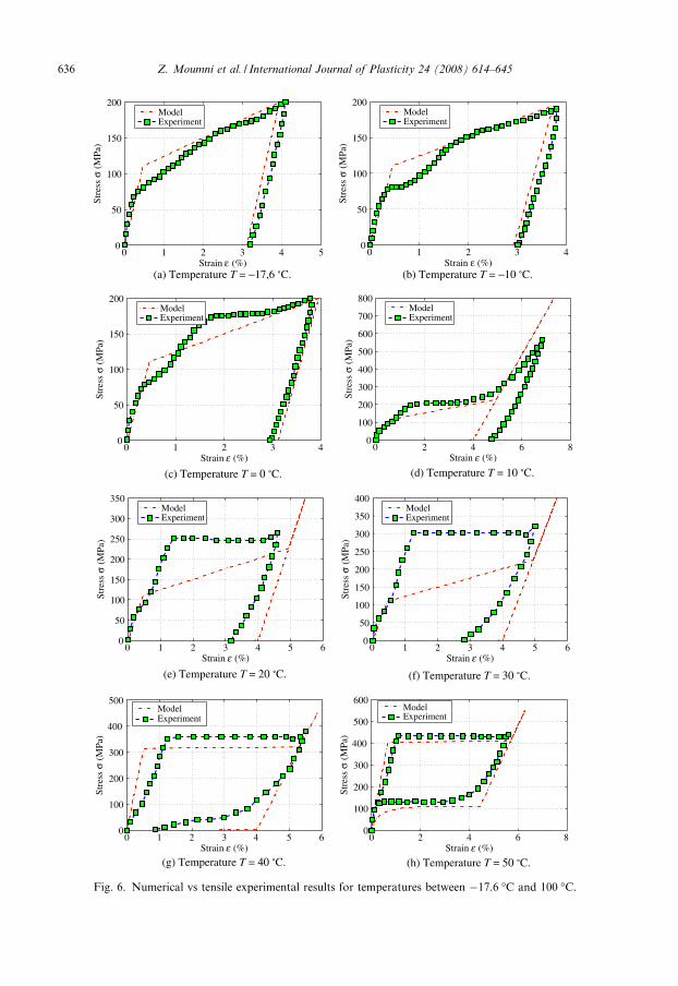
Fig. 6. Numerical vs tensile experimental results for temperatures between �17.6 �C and 100 �C.
636 Z. Moumni et al. / International Journal of Plasticity 24 (2008) 614–645
Strain ε (%)
Stre
ssσ
(MPa
)
ModelExperiment
0 2 4 60
100
200
300
400
500
600
700
(i) Temperature T = 60 °C
(k) Temperature T = 60 °CStrain ε (%)
Stre
ssσ
(MPa
)
ModelExperiment
0 2 4 60
200
400
600
800
1000
Stre
ssσ
(MPa
)
00
200
400
600
800
1000
1200
Z. Moumni et al. / International Journal of Plasticity 24 (2008) 614–645 637
Else if reverse phase change and orientation
� _F2z ¼ 0 and _Fori ¼ 0 give DzðiÞ and DeðiÞtr .
Else if no active transformations
� DzðiÞ ¼ 0 and DeðiÞtr ¼ 0.Else
� unexpected transformation: warn then exit.
8Strain ε (%)
Stre
ssσ
(MPa
)
ModelExperiment
0 2 4 6 80
100
200
300
400
500
600
700
800
.
.
(j) Temperature T = 70 °C.
(l) Temperature T = 70 °C.
(m) Temperature T = 70 °C.
8Strain ε (%)
Stre
ssσ
(MPa
)
ModelExperiment
0 2 4 6 80
200
400
600
800
1000
Strain ε (%)
ModelExperiment
2 4 6 8
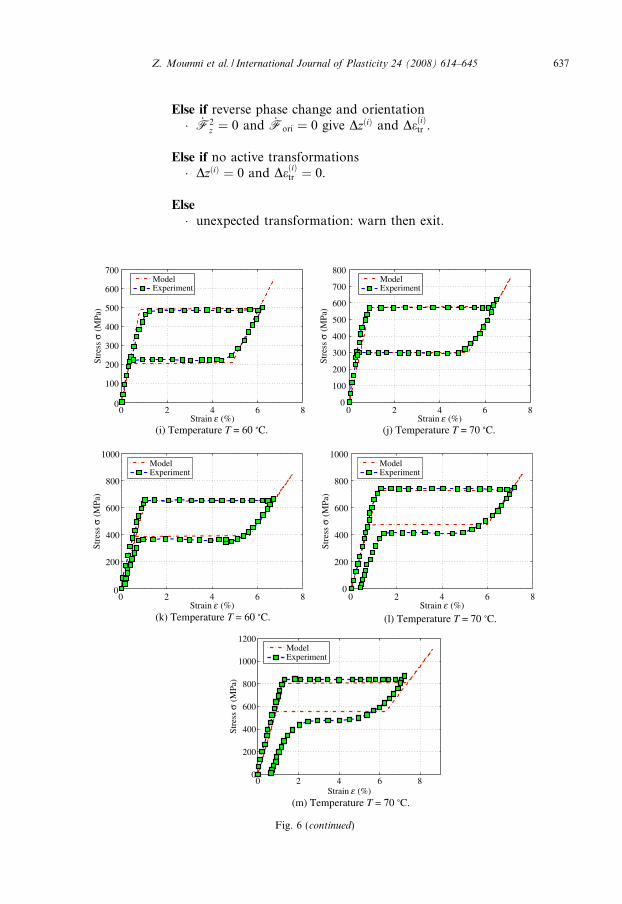
Fig. 6 (continued)
End W
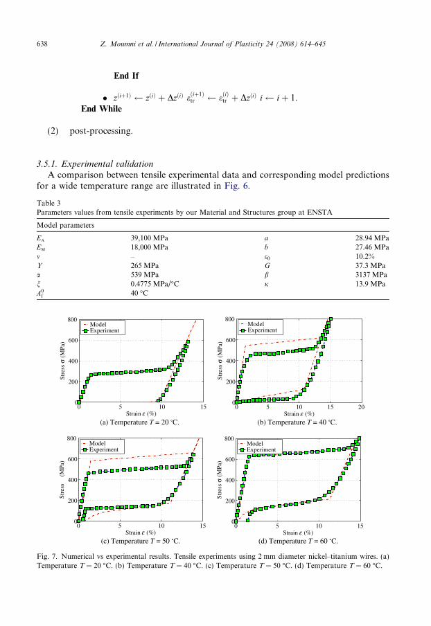
Table 3Parameters values from tensile experiments b
Model parameters
Ea 39,100 MPaEm 18,000 MPam –Y 265 MPaa 539 MPan 0.4775 MPa/�CA0
f 40 �C
Strain ε (%)
Stre
ss(M
Pa)
ModelExperiment
0 5 100
200
400
600
800
Strain ε (%)
Stre
ssσ
(MPa
)
ModelExperiment
0 5 100
200
400
600
800
(a) Temperature T = 20 °C
(c) Temperature T = 50 °C
Fig. 7. Numerical vs experimental results. TTemperature T = 20 �C. (b) Temperature T =
638 Z. Moumni et al. / International Journal of Plasticity 24 (2008) 614–645
End If
� zðiþ1Þ zðiÞ þ DzðiÞ eðiþ1Þtr eðiÞtr þ DzðiÞ i iþ 1.
hile
(2) post-processing.
3.5.1. Experimental validation
A comparison between tensile experimental data and corresponding model predictionsfor a wide temperature range are illustrated in Fig. 6.
y our Material and Structures group at ENSTA
a 28.94 MPab 27.46 MPae0 10.2%G 37.3 MPab 3137 MPaj 13.9 MPa
15Strain ε (%)
Stre
ssσ
(MPa
)
ModelExperiment
0 5 10 150
200
400
600
800
15Strain ε (%)
Stre
ssσ
(MPa
)
ModelExperiment
0 5 10 15 200
200
400
600
800
.
.
(b) Temperature T = 40 °C.
(d) Temperature T = 60 °C.
ensile experiments using 2 mm diameter nickel–titanium wires. (a)40 �C. (c) Temperature T = 50 �C. (d) Temperature T = 60 �C.
Z. Moumni et al. / International Journal of Plasticity 24 (2008) 614–645 639
Fig. 6a–f represent martensite orientation, while Fig. 6g–m represent pseudoelasticity.Experiments at �10 �C and at 70 �C were used in identifying the parameters in Table 2.Experimental validation is satisfying, except for temperature between 10 �C and 30 �C: thisis due to R-phase formation, a phenomenon not accounted for by the current model andto hard-to-define initial conditions in the mixture zone.
We attempted further validation, using nickel–titanium wires having a 2 mm diameter.The wires in question were cold-rolled up to 20%, heat treated at 400 �C for one hour, thencooled down at room temperature. Corresponding parameters values are listed in Table 3.
Even in this case, Fig. 7 shows good agreement between simulated and experimentalbehaviors.
Time
Tem
pera
ture
(°C
)
Time
Stre
ss(M
Pa)
Stre
ss(M
Pa)
0 10 20 30 40 50
0 0.2 0.4 0.6 0.8 1
0 0.2 0.4 0.6 0.8 1
1
0
1
1
0
1
0
50
(a) Thermomechanical loading.The NiTi is cooled under zerostress.
Time
Vol
ume
frac
tions
Austenite volume fractionMartensite volume fraction
0 0.2 0.4 0.6 0.8 1
0
0.2
0.4
0.6
0.8
1
(b) Volume fractions evolution.Austenite completely transformsinto martensite.
Temperature (°C)
Temperature (°C)
Temperature (°C)
Vol
ume
frac
tions Austenite volume fraction
Martensite volume fraction
0 10 20 30 40 50
0
0.2
0.4
0.6
0.8
1
(c) Evolution of volume fractionsas functions of temperature. Atlow temperature, the material be-comes completely martensitic.
Tra
nsfo
rmat
ion
stra
in (
%)
0 10 20 30 40 501
0.5
0
0.5
1
(d) Evolution of inelastic strainzεtr with temperature. Self-accommodation of martensitedoes not lead to inelastic defor-mation of the material.
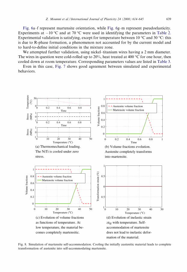
Fig. 8. Simulation of martensite self-accommodation. Cooling the initially austenitic material leads to completetransformation of austenite into self-accommodating martensite.
640 Z. Moumni et al. / International Journal of Plasticity 24 (2008) 614–645
3.5.2. Simulation of martensite self-accommodation
Fig. 8b and d illustrate the response of an initially austenitic SMA cooled from 50 �C(> A0
f ) to 0 �C. One can see from Fig. 8d that in the absence of stress, phase change doesnot induce inelastic strain: austenite transforms into self-accommodating martensite.
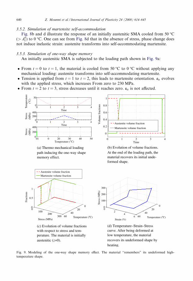
3.5.3. Simulation of one-way shape memory
An initially austenitic SMA is subjected to the loading path shown in Fig. 9a:
� From t = 0 to t = 1, the material is cooled from 50 �C to 0 �C without applying anymechanical loading: austenite transforms into self-accommodating martensite.� Tension is applied from t = 1 to t = 2, this leads to martensite orientation. etr evolves
with the applied stress, which increases From zero to 230 MPa.� From t = 2 to t = 3, stress decreases until it reaches zero. etr is not affected.
Time
Tem
pera
ture
(°C
)
Time
Stre
ss(M
Pa)
Temperature (°C)
Stre
ss(M
Pa)
01 0 20 30 40 50
0 1 2 3 4
0 1 2 3 4
0
200
400
0
200
400
0
50
(a) Thermo mechanical loadingpath inducing the one-way shapememory effect.
Time
Vol
ume
frac
tions
Austenite volume fraction
Martensite volume fraction
0 1 2 3 4
0
0.2
0.4
0.6
0.8
1
(b) Evolution of volume fractions.At the end of the loading path, thematerial recovers its initial unde-formed shape.
Temperature (°C)Stress (MPa)
Frac
tions
Austenite volume fraction
Martensite volume fraction
020
4060
0100
200300
0
0.5
1
(c) Evolution of volume fractionswith respect to stress and tem-perature. The material is initiallyaustenitic (z=0).
Temperature (°C)Strain (%)
Stre
ss(M
Pa)
020
4060
02
46
0
100
200
300
(d) Temperature–Strain–Stresscurve. After being deformed atlow temperature, the materialrecovers its undeformed shape byheating.
Fig. 9. Modeling of the one-way shape memory effect. The material ‘‘remembers” its undeformed high-temperature shape.
Z. Moumni et al. / International Journal of Plasticity 24 (2008) 614–645 641
� Finally, the material is heated between t = 3 and t = 4. As a result, reverse phase changeoccurs and the initial undeformed shape is recovered.
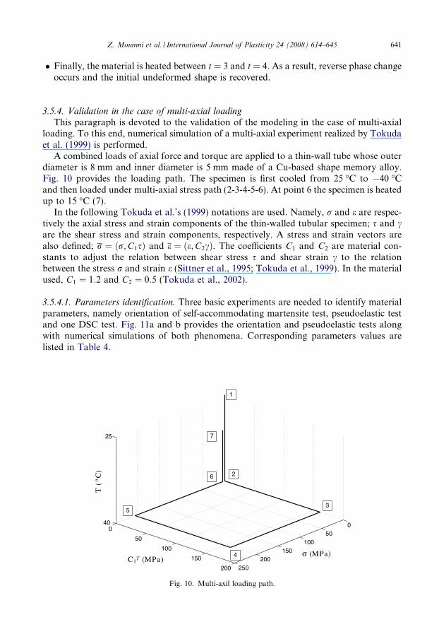
3.5.4. Validation in the case of multi-axial loadingThis paragraph is devoted to the validation of the modeling in the case of multi-axial
loading. To this end, numerical simulation of a multi-axial experiment realized by Tokudaet al. (1999) is performed.
A combined loads of axial force and torque are applied to a thin-wall tube whose outerdiameter is 8 mm and inner diameter is 5 mm made of a Cu-based shape memory alloy.Fig. 10 provides the loading path. The specimen is first cooled from 25 �C to �40 �Cand then loaded under multi-axial stress path (2-3-4-5-6). At point 6 the specimen is heatedup to 15 �C (7).
In the following Tokuda et al.’s (1999) notations are used. Namely, r and e are respec-tively the axial stress and strain components of the thin-walled tubular specimen; s and care the shear stress and strain components, respectively. A stress and strain vectors arealso defined; r ¼ ðr;C1sÞ and e ¼ ðe;C2cÞ. The coefficients C1 and C2 are material con-stants to adjust the relation between shear stress s and shear strain c to the relationbetween the stress r and strain e (Sittner et al., 1995; Tokuda et al., 1999). In the materialused, C1 ¼ 1:2 and C2 ¼ 0:5 (Tokuda et al., 2002).
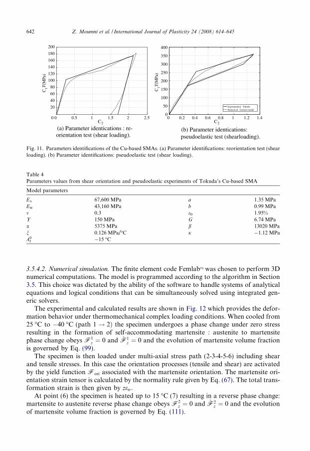
3.5.4.1. Parameters identification. Three basic experiments are needed to identify materialparameters, namely orientation of self-accommodating martensite test, pseudoelastic testand one DSC test. Fig. 11a and b provides the orientation and pseudoelastic tests alongwith numerical simulations of both phenomena. Corresponding parameters values arelisted in Table 4.
050
100150
200250
0
50
100
150
200
40
25
σ (MPa)C1 (MPa)
T(o
C) 2
3
4
6
7
5
1
T
Fig. 10. Multi-axil loading path.
0 0.5 1 1.5 2 2.50
20
40
60
80
100
120
140
160
180
200
C2 C2
C1T(
MPa
)
C1T(
MPa
)
(a) Parameter identications : re-orientation test (shear loading).
0 0.2 0.4 0.6 0.8 1 1.2 1.40
50
100
150
200
250
300
350
400
Experimental TokudaNumerical Current model
(b) Parameter identications:pseudoelastic test (shearloading).
Fig. 11. Parameters identifications of the Cu-based SMAs. (a) Parameter identifications: reorientation test (shearloading). (b) Parameter identifications: pseudoelastic test (shear loading).
Table 4Parameters values from shear orientation and pseudoelastic experiments of Tokuda’s Cu-based SMA
Model parameters
Ea 67,600 MPa a 1.35 MPaEm 43,160 MPa b 0.99 MPam 0.3 e0 1.95%Y 150 MPa G 6.74 MPaa 5375 MPa b 13020 MPan 0.126 MPa/�C j �1.12 MPaA0
f �15 �C
642 Z. Moumni et al. / International Journal of Plasticity 24 (2008) 614–645
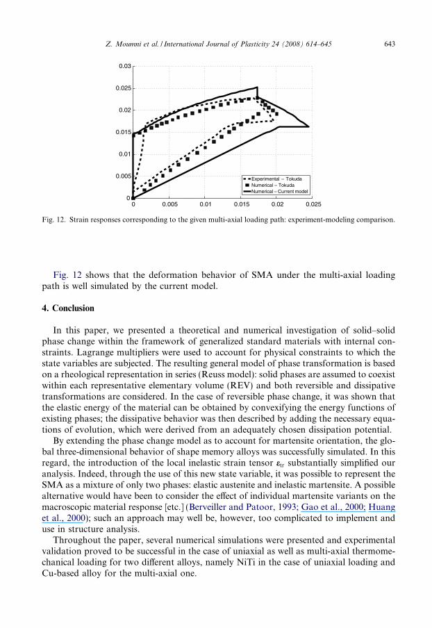
3.5.4.2. Numerical simulation. The finite element code FemlabTM was chosen to perform 3Dnumerical computations. The model is programmed according to the algorithm in Section3.5. This choice was dictated by the ability of the software to handle systems of analyticalequations and logical conditions that can be simultaneously solved using integrated gen-eric solvers.
The experimental and calculated results are shown in Fig. 12 which provides the defor-mation behavior under thermomechanical complex loading conditions. When cooled from25 �C to �40 �C (path 1! 2Þ the specimen undergoes a phase change under zero stressresulting in the formation of self-accommodating martensite : austenite to martensitephase change obeys F1
z ¼ 0 and _F1z ¼ 0 and the evolution of martensite volume fraction
is governed by Eq. (99).The specimen is then loaded under multi-axial stress path (2-3-4-5-6) including shear
and tensile stresses. In this case the orientation processes (tensile and shear) are activatedby the yield function Fori associated with the martensite orientation. The martensite ori-entation strain tensor is calculated by the normality rule given by Eq. (67). The total trans-formation strain is then given by zetr.
At point (6) the specimen is heated up to 15 �C (7) resulting in a reverse phase change:martensite to austenite reverse phase change obeys F2
z ¼ 0 and _F2z ¼ 0 and the evolution
of martensite volume fraction is governed by Eq. (111).
0 0.005 0.01 0.015 0.02 0.0250
0.005
0.01
0.015
0.02
0.025
0.03
Experimental – TokudaNumerical – TokudaNumerical – Current model
Fig. 12. Strain responses corresponding to the given multi-axial loading path: experiment-modeling comparison.
Z. Moumni et al. / International Journal of Plasticity 24 (2008) 614–645 643
Fig. 12 shows that the deformation behavior of SMA under the multi-axial loadingpath is well simulated by the current model.
4. Conclusion
In this paper, we presented a theoretical and numerical investigation of solid–solidphase change within the framework of generalized standard materials with internal con-straints. Lagrange multipliers were used to account for physical constraints to which thestate variables are subjected. The resulting general model of phase transformation is basedon a rheological representation in series (Reuss model): solid phases are assumed to coexistwithin each representative elementary volume (REV) and both reversible and dissipativetransformations are considered. In the case of reversible phase change, it was shown thatthe elastic energy of the material can be obtained by convexifying the energy functions ofexisting phases; the dissipative behavior was then described by adding the necessary equa-tions of evolution, which were derived from an adequately chosen dissipation potential.
By extending the phase change model as to account for martensite orientation, the glo-bal three-dimensional behavior of shape memory alloys was successfully simulated. In thisregard, the introduction of the local inelastic strain tensor etr substantially simplified ouranalysis. Indeed, through the use of this new state variable, it was possible to represent theSMA as a mixture of only two phases: elastic austenite and inelastic martensite. A possiblealternative would have been to consider the effect of individual martensite variants on themacroscopic material response [etc.] (Berveiller and Patoor, 1993; Gao et al., 2000; Huanget al., 2000); such an approach may well be, however, too complicated to implement anduse in structure analysis.
Throughout the paper, several numerical simulations were presented and experimentalvalidation proved to be successful in the case of uniaxial as well as multi-axial thermome-chanical loading for two different alloys, namely NiTi in the case of uniaxial loading andCu-based alloy for the multi-axial one.
644 Z. Moumni et al. / International Journal of Plasticity 24 (2008) 614–645
References
Abeyaratne, A., 1981. Discontinuous deformation gradients away from the tip of a crack in anti-plane shear.
Journal of Elasticity 11, 373–393.
Ball, J.M., James, R.D., 1987. Fine phase mixtures as minimizers of energy. Archive for Rational Mechanics and
Analysis 100, 13–52.
Berveiller, M., Patoor, E., 1993. Comportement thermomecanique des materiaux usuels et des alliages a memoire
de forme. Technologie des Alliages a Memoire de Forme, pp. 43–62. Hermes.
Bo, Z., Lagoudas, D., 1999. Thermomechanical modeling of polycrystalline SMAs under cyclic loading. Part III:
Evolution of plastic strains and two-way shape memory effect. International Journal of Engineering Science
37, 1175–1203.
Falk, F., 1980. Model free energy, mechanics, and thermodynamics of shape memory alloys. Acta Metallurgica
28, 1773–1780.
Fremond, M., 1987. Materiaux a memoire de forme. Compte Rendu de l’Academie des Sciences, Paris, Tome 34,
s.II, n.7, pp. 239–244.
Gao, X., Huang, M., Brinson, L.C., 2000. A multivariant micromechanical model for SMAs. Part 1.
Crystallographic issues for single crystal model. International Journal of Plasticity 16, 1345–1369.
Halphen, B., Nguyen, Q.S., 1974. Plastic and visco-plastic materials with generalized potential. Mechanical
Research Communications 1, 43–47.
Huang, M., Gao, X., Brinson, L.C., 2000. A multivariant micromechanical model for SMAs. Part 2. Polycrystal
model. International Journal of Plasticity 16, 1371–1390.
Lagoudas, D.C., Shu, S.G., 1999. Residual deformation of active structures with SMA actuators. International
Journal of Mechanical Sciences 41, 595–619.
Leclerq, S., Lexcellent, C., 1996. A general macroscopic description of the thermomechanical behavior of shape
memory alloys. Journal of the Mechanics and Physics of Solids 44, 953–980.
Lexcellent, C., Bourbon, G., 1996. Thermodynamical model of cyclic behaviour of Ti–Ni and Cu–Zn–Al shape
memory alloys under isothermal undulated tensile tests. Mechanics of Materials 24, 59–73.
Liu, Y., Xie, Z., Van Humbeeck, J., Delaey, L., 1999. Some results on the detwinning process in NiTi shape
memory alloys. Scripta Materialia 41, 1273–1281.
Moreau, J.J., 1967. Fonctionnelles convexes. College de France.
Moumni, Z., 1995. Sur la modelisation du changement de phase a l’etat solide. Ph.D. thesis, Ecole Nationale
Superieure des Ponts et Chaussees.
Moumni, Z., Nguyen, Q.S., 1996. A model of material with phase change and applications. Journal de Physique
IV 6, 335–345.
Muller, I., Seelecke, S., 2001. Thermodynamic aspects of shape memory alloys. Mathematical and Computer
Modelling 34, 1307–1355.
Nguyen, Q.S., 1994. Bifurcation and stability in dissipative media. Applied Mechanics Review 47, 1–31.
Nguyen, Q.S., 2000. Stability and Nonlinear Solid Mechanics. Wiley.
Patoor, E., Berveiller, M., 1993. Lois de comportement et calcul de structures en alliage a memoire de forme.
Technologie des Alliages a Memoire de Forme, pp. 195–224. Hermes.
Peultier, B., Ben Zineb, T., Patoor, E., 2006. Macroscopic constitutive law of shape memory alloy
thermomechanical behaviour. Application to structure computation by FEM. Mechanics of Materials 38,
510–524.
Raniecki, B., Lexcellent, C., 1998. Thermodynamics of isotropic pseudoelasticity in shape memory alloys.
European Journal of Mechanics A/Solids 17, 185–205.
Raniecki, B., Lexcellent, C., Tanaka, K., 1992. Thermodynamic models of pseudoelastic behaviour of shape
memory alloys. Archives of Mechanics 44, 261–284.
Rockafellar, R.T., 1972. Convex Analysis. Princeton University Press.
Roytburd, A., 1993. Elastic domains and polydomain phases in solids. Phase Transition 45, 1–33.
Silling, S.A., 1988. Consequences of the Maxwell relations for anti-plane shear. Journal of Elasticity 19, 241–284.
Sittner, P., Hara, Y., Tokuda, M., 1995. Experimental study on the thermoelastic martensitic transformation in
shape memory alloy polycrystal induced by combined external forces. Metallurgical and Materials
Transactions 26A, 2923–2935.
Tokuda, M., Ye, M., Takakura, M., Sittner, P., 1999. Thermomechanical behavior of shape memory alloy under
complex loading conditions. International Journal of Plasticity 15, 223–239.
Z. Moumni et al. / International Journal of Plasticity 24 (2008) 614–645 645
Tokuda, M., Sittner, P., Takakura, M., Haze, M., 2002. Multi-axial constitutive equations of polycrystalline
shape memory alloy experimental background. JSME International Journal, Series A 45, 276–281.
Wayman, C.M., Otsuka, K., 1999. Shape Memory Alloys. Cambridge University Press.
Xu, H., Muller, I., 1993. Non-equilibrium thermodynamics of pseudoelasticity. Continuum Mechanics and
Thermodynamics 5, 163–204.