The Use of Global Trade and Energy Volume Data for the ...

1

The Use of Global Trade and Energy Volume Data for the Analysis ofGlobal Energy-Environmental Issues – Some Illustrative Experiments.

Truong P. Truong1

Center for Global Trade AnalysisPurdue University

AbstractThe analysis of global energy and environmental issues have often been hampered by thelack of a comprehensive energy-economy wide-global data set. Recently the Center forGlobal Trade Analysis at Purdue University has produced a special version of the GTAPdata base called GTAP 4-E together with an energy price and volume data set. Thispaper utilises these data set in some illustrative experiments. The experiments involvesimulating the effects of the cutting back on the world CO2 emission level by some 25 percent in a comparative static framework. The results show that using the standard GTAPversion 4 data base and the special purpose GTAP 4-E data base can producesignificantly different results.

1. Introduction

Up to now, the analysis of global energy and environmental issues have been hamperedby the lack of a comprehensive energy-economy wide-global data set, and a suitablemodel which can make use of this data set. The comprehensive data set needs to containinformation on both the physical energy flows at the end-use sectoral level, as well asvalue flows at the economy-wide and global level. Quantity – or volume - information onenergy flows is important for certain calculations such as the energy intensities orembodied carbon intensities of production and consumption activities2. These intensitiesare indispensable parameters in the calculation of the economic impact of certain energy-environmental policies such as the reduction of the world’s CO2 emission level. Thesuitable model needs to take account of important energy-economy interactions such asinter-fuel and inter-factor substitutions involving the energy variables.

Motivated by the need for a comprehensive energy-economy wide-global data set, aspecial project funded by the Department of Energy (DOE) was carried out jointly byresearchers at Purdue university (the Center for Global Trade Analysis (CGTA)), theUniversity of Colorado, Boulder, and the OECD Development Centre3. The objective ofthe Project was to construct a data base which contains the necessary combination of (a)

1 Visiting Associate Professor, Department of Agricultural Economics, Purdue University, and on leavefrom the University of New South Wales, Sydney, Australia. Address for Correspondence at PurdueUniversity: Center for Global Trade Analysis, 1145 Krannert Building, West Lafayette, IN 47907-1145.Email: [email protected].

2 Babiker and Rutherford (1997).3 For more information on this Project, see the Web site of CGTA at:

http://www.agecon.purdue.edu/gtap

2

comprehensive input-output data by region, (b) bilateral trade and protection data, and (c)energy price, quantity and tax data. The Project started with the collection of data onenergy quantity flows, prices and taxes, from various sources4. Next, these independentinformation were then checked for accuracy and consistency with the energy data in theGTAP data base5. Where there are significant differences, the GTAP data set is thenmodified and re-balanced. The result is a ‘special purpose’ data base known as GTAP 4-E which is intended to be used, firstly, by researchers analyzing the energy-economy-trade-environment issues, but also in the future by regular users of the standard GTAPdata base6.

In this paper, we make use of this special purpose GTAP 4-E data base, the companionenergy volume data set, and also the extended GTAP model which includes inter-fuel andinter-factor substitution in its structure7, to carry out some illustrative experimentslooking at energy-environmental issues. One of the experiments involves simulating theeffects of a reduction of the world CO2 emission level by 25 per cent, firstly, by allregions of the world, and then, by the Annex 1 regions8 only (no participation of non-Annex 1 countries). The economic impact of this reduction in different regions, ondifferent types of fuels, and among various sectors of the economy, are analyzed. Tohighlight the importance of the integrated data set, we first carry out the experiment usingthe GTAP 4 data base. We then repeat the experiment using the GTAP 4-E data base. Inboth cases, we use the volume data to calculate the CO2 emission level for targeting. Acomparison of the two different sets of results will reveal how important the use of theenergy volume data set can be, and also the usefulness of ‘integrating’ this data set intothe GTAP 4-E data base.

The outline of this paper is as follows. Section 2 describes the main elements of thetheoretical framework for the experiments. Section 3 briefly describes main differencesbetween the GTAP 4 and GTAP 4-E data sets. Section 4 describes the experiment set upand reports on the results. Section 4 concludes the paper.

2. Theoretical Framework

At the center of the experiment is the calculation of the (percentage change in the)volume of CO2 emission across different regions and over the whole world. Thiscalculation depends on the availability of energy volume (i.e. quantity) flows. In the

4 Energy volume data were collected from the International Energy Agency (IEA). Energy pricesand tax data were obtained from the IEA as well as the World Bank (Survey of Asia’s Energy Prices), theOrganizacion Latino Americana de Energia (OLADE), the Asian Development Bank (ADB), the USDepartment of Energy (DOE), China Energy Databook (CED), and the Tata Energy Research Institute(TERI).5 GTAP stands for Global Trade Analysis Project. For information on this Project, see the CGTAweb-site. For details about the latest version 4 of the GTAP data base, see McDougall et al. (1998).6 GTAP 4-E is going to be integrated into the next release (version 5) of the GTAP data base. Forinformation on the process of constructing the GTAP 4-E data base, see Malcolm and Truong (1999).7 The model is called GTAP-E. For details on the construction of this model, see Truong (1999).8 Annex 1 countries are those listed in the Annex 1 of the Kyoto Protocol to the United NationsFramework Convention on Climate Change which consist mainly of Western industrialized countries.

3

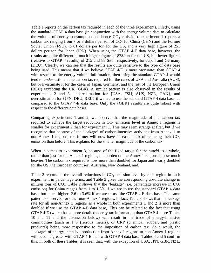
absence of such information (for example, when we use the GTAP 4 or GTAP 4-E databases on their ‘stand alone’ mode) the assumption often made by researchers is that thevalue flows of a basic input-output data base will also represent the relativity of thevolume flows. This means different end-users (industries, household) face the sameaverage price for their energy inputs9. Such an assumption is clearly unrealistic, since itimplies that in practice, there is no price discrimination exercised by the energy supplierswith respect to the different types of users, and that the price charged to any user isconstant with respect to the quantity supplied (uniform pricing). It also assumes that themargin costs (of distribution, transmission, retailing, government taxes and subsidies onthese energy commodities) are all the same for all users10. Clearly, this does not reflectreality in the energy market. To overcome this deficiency, an alternative approach is tomake use of the actual volume flow information (in the calculation of certain importantparameters such as energy and CO2 intensities of various economic activities), and usethis information in conjunction with the value flow data contained in the standard input-output and trade data base (such as GTAP). In what follows, we illustrate how suchcalculations can be carried out, and compare these with so-called ‘naïve’ calculations,being based mainly on the value flows of the input-output data base.

2.1 Embodied CO2 intensities using volume data

To calculate the CO2 content embodied in the output of a particular production orconsumption activity, we need both the information on energy volume flows (from theenergy volume data base) and the information on the value of output or consumptionactivity (from GTAP 4 or GTAP 4-E).

Let j � U={set of users}i � E={set of energy commodities}r � R={set of regions}Y(r) = value of output (in US95$million) in region r from the GTAP 4 data base.Q(i,j,r) = quantity, or volume flow of energy commodity i11 (in million of ton of

oil equivalent – mtoe) to user j in region r, obtained from the energyvolume data base.

κ(i) = CO2 coefficient for fuel i (in tons of CO2 per toe).

The average CO2 content embodied in fuel i for all economic activities in region r isgiven by:

∑∈Uj

rj,i,QirY=riA )(*)(*))(/1(),( κ (1)

9 Note that these prices (in dollar per unit of energy such as ton of oil equivalent (toe)) can still varybetween different types of fuels, to take account of their differences in qualities (such as ease of use,impurity content, etc), but the price of each fuel is assumed to be the same for all users.10 A standard input-output table can take account of different user margins and taxes, but often dueto lack of information, the table often assumes uniform margin for all domestic users. This is the case withthe GTAP data base (and GTAP model, see Hertel (1997)).11 In the actual model calculation, we distinguish between the quantity from domestic source and thequantity from imported source.

4

2.2 Embodied CO2 intensities using mainly the input-output value flows

When the actual volume information is not available, we can infer these quantities fromthe input-output value flows together with some aggregate information on the totalvolume flow, as follow:

∑∈Uj

rj,i,QirY=riA )(ˆ*)(*))(/1(),(ˆ κ (2)

where the symbol (^) is used to denote the estimated or inferred value, calculated fromthe value data base. The inferred quantity flow to each user j is calculated as:

),(*ˆ riQr)j,V(i,

r)j,V(i,=r)j,(i,Q

Uj∑∈

(3)

where V(i,j,r ) is the value flow of energy commodity i to user j in region r and Q(i,r) isthe total usage of i in r.

2.3 Carbon tax imposition

We assume that a (carbon) tax is levied on all primary energy commodities12 for itsaverage CO2 content. To calculate the carbon tax rate for each region, we assume that thetax rate is uniform for all users within the region13, and therefore, we only need tocalculate the average CO2 content for all economic activities within a particular region.This is calculated as follows.

Let τ(r) be the carbon tax rate ($/ton of CO2) for each region r. The percentage increasein the power of the tax (i.e. one plus the tax rate) on energy commodity i in region r willthen be related to the carbon tax and the average carbon content of the energy commodityas follows:

),(*)(),,( riArrjit τ= (4)

12 This includes coal (COL), natural and manufactured gas (GAS), and petroleum and coal products(P_C). In theory, crude oil (OIL) should be counted as primary energy rather than petroleum and coalproducts to avoid double counting of coal consumption. However, for the purpose of calculating CO2

emission level, it is more accurate to calculate this from the consumption of petroleum products rather thanfrom crude oil consumption. Furthermore, except for one region (FSU: former Soviet Union), whereapproximately 0.27% of the total coal usage is in the P_C sector, all other regions have zero consumptionof coal in the P_C sector.13 Although in principle, we can levy different tax rates on different users, based on the CO2 contentlevel in their activities, for simplicity, however, we impose a uniform tax rate for all users within a region.

5

The tax on each energy commodity i, to user j, in region r, will have an effect on its totaldemand, i.e. on the volume flow Q(i,r). This will then have an impact on the total volumeof CO2 emission from energy usage region r, denoted by the variable X(r):

∑∈

=Ei

riQirX ),(*)( )( κ (5)

The percentage change form for this equation is given by14:

∑∈

=Ei

riqriSrx ),(*),()( (6)

Here, x(r) and q(i,r) are the percentages in X(r) and Q(i,r) respectively, and aredetermined by the model15. S(i,r) is the share of CO2 emission from fuel i over all fuels inregion r and is derived from the volume data base as follows16:

∑∈

=Ei

riQiriQiriS ),(*)(/),(*)(),( κκ (7)

q(i,r) is one of the existing variables in the standard GTAP model.

2.4 The issue of ‘leakage’

In carrying out the experiment on CO2 emission reduction, we make a distinctionbetween Annex 1 and non Annex 1 regions. Let A denotes the former, and N, the latterset. We have R = A ∪ N. The percentage change in the total amount of CO2 emissionfrom these two different sets of regions (xA, xN ), and from the world as a whole (xW), canthen be calculated as follows

NA

RrW

NrN

ArA

xx

rxrSx

rxrSx

rxrSx

+=

=

=

=

∑∑∑

∈

∈

∈

)(*)(

)(*)(

)(*)(

(8)

where S(r) is the share of CO2 emission from region r over all regions of the world, and isderived from the data base:

14 A lower case letter is used to denote ‘percentage change’.15 In the standard GTAP model (see Chapter 2 of Hertel (1997)), q(i,r), and hence x(r), is alsodistinguished by sources: qds(i,r) to stand for the demand of commodity i in region r from domestic source,and qim(i,r) for the similar demand but from imported source.16 Where volume data is not available, Q(i,r) is approximated by its ‘inferred’ value, as estimatedfrom equation (3) of section 2.2.

6

∑∑∑∈ ∈∈

=Rr EiEi

riQiriQirS ),(*)(/),(*)()( κκ (9)

To simulate an experiment where the world CO2 emission level is reduced by c per cent,and the burden is shared equally among all regions, we impose the following conditions:

Rrcrx ∈−= allfor ;)( :“Experiment 1” (10)

A different experiment is to assume that only Annex 1 regions are to share the burden ofCO2 reduction in equal percentages, while non-Annex 1 regions face with no suchcommitments. A set of conditions for this experiment is then given by:

Nrr

Arcrx

∈=∈−=

allfor ;0)(

allfor ;)(

τ:“Experiment 2” (11)

Here, non-Annex 1 regions are assumed to impose zero carbon tax on their energyconsumption. As a result, the demand for energy commodities, and therefore the CO2

emission levels, in these regions, may even increase. Such an increase is called‘leakage’17: the reduction in CO2 emission in Annex 1 regions are made ineffective byoffsetting increases in CO2 emissions in non-Annex 1 regions. The ‘leakage rate’ isdefined as the ratio: xN /(-xA). For example, if there is a 50% leakage rate, then xN=-0.5 xA,and xW = 0.5 xA, i.e the world CO2 emission is reduced by only half of what is achievedby Annex 1 regions. If there is a 100% leakage rate, then xN= -xA, and xW = 0, i.e theeffect on the world as a whole is zero, irrespective if what is achieved by the Annex 1regions.

Assume that the leakage rate is less than 100 per cent and if the Annex 1 regions are setout to achieve a fixed target for the reduction in the world CO2 emissions level, then athird experiment can be defined as follows:

Nrr

Arxrx

cxW

∈=∈=

−=

allfor ;0)(

allfor ;)(

τ: “Experiment 3” (12)

In this case, the necessary reduction in the level of CO2 emission for each of the Annex 1regions (i.e. x ) will be determined endogenously by the model.

3 Data description

We use a 14 sectors by 14 regions aggregation, based on the GTAP version 4 data base.The list of the sectors and regions are given in the Appendix. To understand thedifferences of the results when we run the experiments with the different data bases, it isimportant to look at the detailed information contained in the data bases themselves.

17 See Perroni and Rutherford (1993), and Felden and Rutherford (1993).

7

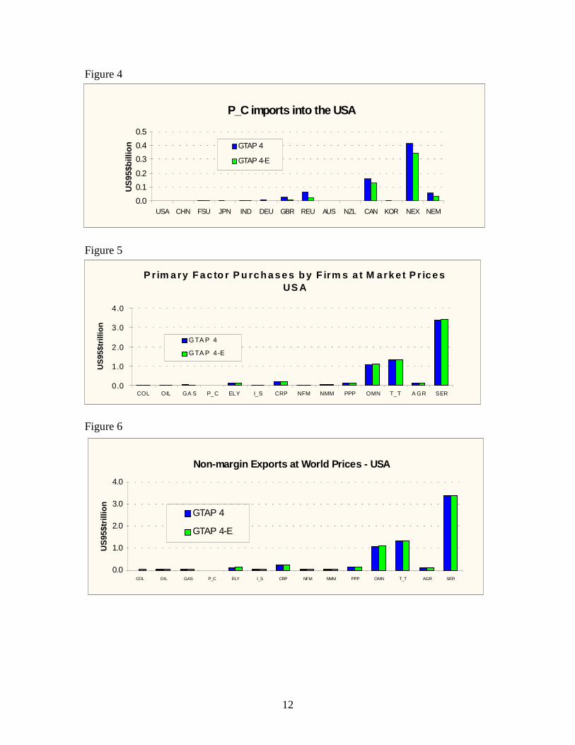
First, we look at the aggregate energy and CO2 intensities. These are shown in Figures 1and 2. In Figure 1, we divide the total energy usage (calculated from the volume database) by the GDP value (from the GTAP 4 or GTAP 4-E data bases). In Figure 2, asimilar procedure is carried out, but with the energy usage converted into CO2 emissionlevel18. From Figures 1 and 2, we can see that the results are very similar, and this is asexpected because at the aggregate level of GDP calculation, GTAP 4 and GTAP 4-E givealmost identical results. But if we look at the individual components of GDP, and inparticular, if we look at the energy sector, then GTAP 4 and GTAP 4-E can producedifferent results. In Figure 3, for example, crude oil exports from the UK are seen to behigher with GTAP 4-E than with GTAP 4. The converse is true with petroleum and coalproducts imports into the USA (Figures 4). Non-energy commodities, however, showmuch more consistency when we move from GTAP 4 to GTAP 4-E, and this is asexpected. In Figure 5, for example, the value of primary factor purchases by firms in theUSA are seen to be almost identical for GTAP 4 and GTAP 4-E. Figure 6 also shows thesame consistency with respect to the different data bases for non-margin exports of theUSA at world prices.

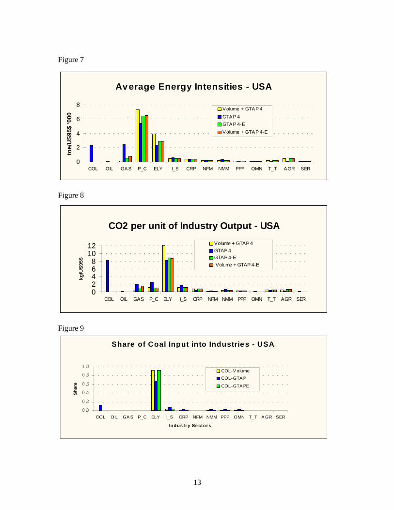
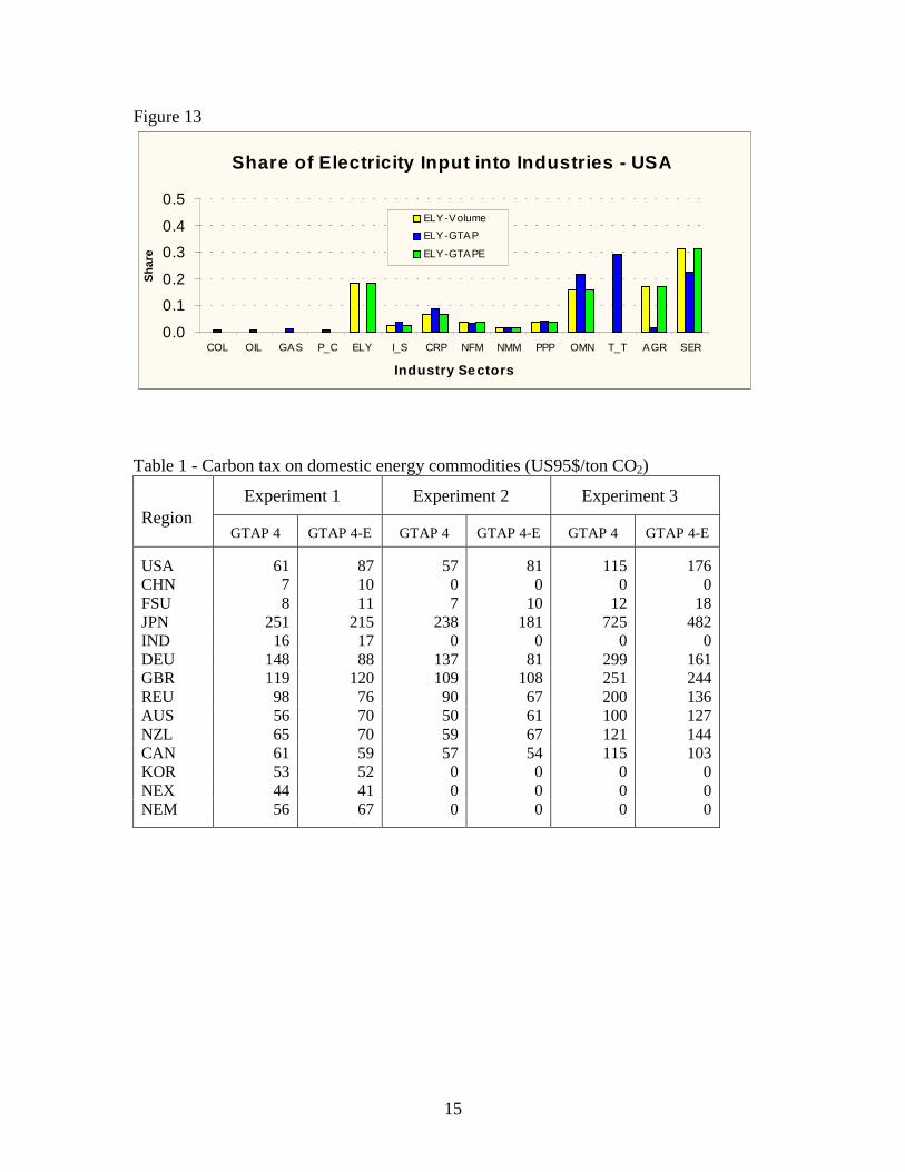
When we move to a more disaggregated level, the differences between GTAP 4 andGTAP 4-E become more pronounced, especially with respect to the energy commodities.In Figures 7 and 8, the average energy intensities and CO2 intensities at the industry levelfor the USA are seen to be significantly different, depending on whether we use theGTAP 4, or GTAP 4-E data base, and whether each data base on a stand-alone basis (i.e.using value shares to infer quantity shares and distribute the aggregate quantity accordingto the value shares – see section 2.2), or each in conjunction with the volume data base(i.e. using the volume information directly from the volume data base)19. For example,GTAP 4 gives a higher estimate of the energy and CO2 intensities for the coal (COL), gas(GAS) industries in the USA, but a lower estimate for the electricity (ELY) industry. Theresults can be traced back to the fact that the share of energy inputs into the coal and gasindustries are always higher for the GTAP 4 value data base, but much lower for thevolume data base (see Figures 9-13). The converse can be true for other industries (suchas ELY, in the case of COL and GAS inputs, or trade and transport (T_T), in the case ofpetroleum products (P_C) input). Therefore, while the aggregate intensities are verysimilar, when it comes down to the end-use (sectoral) level, the GTAP 4 value data baseand the energy volume information diverge significantly.

When the GTAP 4 and the energy volume information are different, the approach takenin the GTAP 4-E data base construction process was to ‘adjust’ the GTAP 4 valuestowards the direction of the energy volume (and price) information. As a result, theestimates on the energy intensities and CO2 intensities from the GTAP 4-E value database (on its stand alone mode) are always much closer to the estimates from the energyvolume data base, as compared to those from the GTAP 4 data base (also on its standalone mode). This means that if we are to use the GTAP data bases to calculate certain

18 We use the following coefficients for CO2 emission: (3.8107, 1.8844, 2.7638) tons of CO2 per tonof oil equivalent (toe), for (coal, gas, petroleum and coal products) respectively.19 There are thus four different combinations: GTAP 4 stand alone, GTAP 4-E stand alone, Volumedata plus GTAP 4, and Volume data plus GTAP 4-E.

8

important energy and environmental variables (such as energy intensities and CO2

intensities) then it is ‘better’20 to use the GTAP 4-E version rather than the standardGTAP 4 version.

4 Experiment set up and results

We use an extended version of the GTAP model called GTAP-E which allows for thepossibility of inter-fuel and inter-factor substitution in the production structure of firmsand in the consumption behavior of private households and government sector (Truong,1999). We assume that there is a target reduction of the world CO2 emission level by -25%. This may sound like a very large reduction. However, since the model iscomparative static, the reduction is therefore to be interpreted as ‘relative to the levelwhich would have been arrived at in the target year if there is business-as-usual (BaU)’.According to the International Energy Agency, the world CO2 emission is projected toincrease (roughly linearly) by about 9723 million tons from 21401 tons in 1990 to about31124 tons in 2010 in the BaU projection21. To meet the Kyoto commitments22, theremust be a massive reduction of CO2 emissions of about 10793 tons, or 35% in the targetyear from the BaU projection. Thus, a 25% decrease is judged to be within the reasonablerange relative to the objectives of the Kyoto Protocol.

In Experiment 1, we assume that all countries will agree to reduce their CO2 emissionlevels by the same 25%, i.e. all share equally in the burden of CO2 reduction. Theinstrument used for reducing CO2 emission is a carbon tax, to be levied on energyconsumption and based on their embodied CO2 content. In Experiment 2, we assume thatonly Annex 1 countries23 will agree to reduce their CO2 emission levels by the same 25%.The non-Annex 1 countries will continue to maintain the existing level of taxes/subsidieson the energy commodities, and therefore their CO2 emission level may not reducesignificantly (or even increase), and the world CO2 emission level as a whole will nottherefore reduce by 25%. In Experiment 3, we assume that the Annex 1 countries willnow set out to reduce the world CO2 emission level by the fixed target of 25%,irrespective of the ‘leakage’ from non-Annex 1 countries. This will mean a largercommitment from each Annex 1 region, and the exact level for this commitment is goingto be determined endogenously by the model.

20 The word ‘better’ is used here with some qualifications. Firstly, it is based on the assumption thatthe energy volume information at the end-use level in the energy volume data base is more reliable than theGTAP input-output information. Secondly, it is also based on the existing adopted structure of the GTAPdata base (and model) which does not distinguish between domestic end-users with respect to the marginsand average prices for their energy commodities (see the discussion in previous section 2). If such astructure is to be modified, then clearly the value shares should not always follow the quantity shares moreclosely in order to become ‘better’, and therefore, the comparison between GTAP 4 and GTAP 4-E shouldalso be based on a different criterion.21 IEA (1998, Table 3).22 The Kyoto Protocol commits the developed countries to reduce their collective emissions ofgreenhouse gases by at least 5% compared to 1990 levels by the period 2008-2012.23 Corresponding to the following regions in our data set: {USA, FSU, JPN, DEU, GBR, REU, AUS,NZL, CAN}. The non-Annex 1 regions are thus: {CHN, IND, KOR, NEX, NEM}. For an explanation ofthese region codes, see the Appendix.

9

Table 1 reports on the carbon tax required in each of the three experiments. Firstly, usingthe standard GTAP 4 data base (in conjunction with the energy volume data to calculatethe volume of energy consumption and hence CO2 emission), experiment 1 reports acarbon tax ranging from 7 or 8 dollars per ton of CO2 for China (CHN) and the FormerSoviet Union (FSU), to 61 dollars per ton for the US, and a very high figure of 251dollars per ton for Japan (JPN). When using the GTAP 4-E data base, however, theresults are quite different: a much higher figure of 87$/ton for the US, but lower figures(relative to GTAP 4 results) of 215 and 88 $/ton respectively, for Japan and Germany(DEU). Clearly, we can see that the results are quite sensitive to the type of data basebeing used. This means that if we believe GTAP 4-E is more ‘accurate’ than GTAP 4with respect to the energy volume information, then using the standard GTAP 4 wouldtend to under-estimate the carbon tax required for the cases of USA and Australia (AUS),but over-estimate it for the cases of Japan, Germany, and the rest of the European Union(REU) excepting the UK (GBR). A similar pattern is also observed in the results ofexperiments 2 and 3: underestimation for {USA, FSU, AUS, NZL, CAN}, andoverestimation for {JPN, DEU, REU} if we are to use the standard GTAP 4 data base, ascompared to the GTAP 4-E data base. Only the {GBR} results are quite robust withrespect to the different data bases.

Comparing experiments 1 and 2, we observe that the magnitude of the carbon taxrequired to achieve the target reduction in CO2 emission level in Annex 1 regions issmaller for experiment 2 than for experiment 1. This may seem strange at first, but if werecognize that because of the ‘leakage’ of carbon-intensive activities from Annex 1 tonon-Annex 1 regions, the former will now have an easier task of reducing their CO2

emission than before. This explains for the smaller magnitude of the carbon tax.

When it comes to experiment 3, because of the fixed target for the world as a whole,rather than just for the Annex 1 regions, the burden on the Annex 1 regions is now muchheavier. The carbon tax required is now more than doubled for Japan and nearly doubledfor the US, the European countries, Australia, New Zealand, and.

Table 2 reports on the overall reductions in CO2 emission level by each region in eachexperiment in percentage terms, and Table 3 gives the corresponding absolute change inmillion tons of CO2. Table 2 shows that the ‘leakage’ (i.e. percentage increase in CO2

emission) for China ranges from 1 to 1.3% if we are to use the standard GTAP 4 database, but much higher: 2.6 to 3.6% if we are to use the GTAP 4-E data base. The samepattern is observed for other non-Annex 1 regions. In fact, Table 3 shows that the leakagerate for all non-Annex 1 regions as a whole in both experiments 1 and 2 is more thandoubled if we use the GTAP 4-E data base,. This can be related to the fact that usingGTAP 4-E (which has a more detailed energy tax information than GTAP 4 – see Tables10 and 11 and the discussion below) will result in the trade of energy-intensivecommodities (such as I_S (ferrous metals), or CRP (chemical, rubber, and plasticproducts)) being more responsive to the imposition of carbon tax. As a result, the‘leakage’ of energy-intensive production from Annex 1 regions to non-Annex 1 regionswill become greater with GTAP 4-E than with GTAP 4 data base. Tables 4 and 5 confirmthis: in both of these Tables, it is seen that, with the exception of USA, JPN, GBR, NZL,

10

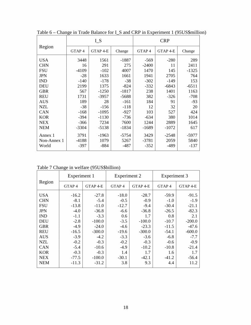
and CAN, the rest of the Annex 1 regions (FSU, DEU, REU, AUS) have their tradebalance in energy-intensive commodities (I_S and CRP) worsened when we use GTAP 4-E as compared to the case of GTAP 4. This means that either their net imports haveincreased, or net exports decreased. The reverse is true for non-Annex 1 regions. FromTable 4, we see that for all Annex 1 regions as a whole, moving from GTAP 4 to GTAP4-E will increase their net imports of I_S by an additional $6310 million, while non-Annex 1 regions will increase their net exports of this commodity by an additional $6028million (experiment 2). The ‘leakage’ of energy-intensive production from Annex 1 tonon-Annex 1 regions thus has increased if we use the GTAP 4-E data base. This is alsotrue for experiment 3. Note that in experiment 1 (Table 6), going from GTAP 4 to GTAP4-E data base can change the sign of the trade balance (in I_S and CRP) of the Annex 1regions from a positive to a negative figure, and the reverse is true for non-Annex 1regions.

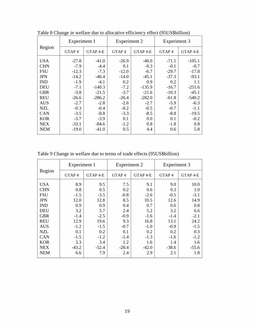
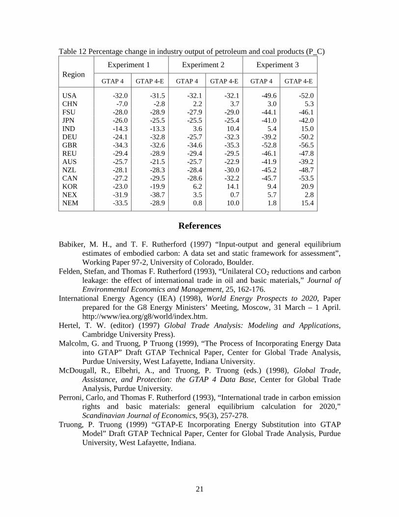
Next we consider the welfare effect of the imposition of the carbon tax. Table 7 showsthat the change in welfare in all experiments are much more magnified if we use theGTAP 4-E rather than the GTAP 4 data base, especially for the USA, DEU, REU, andalso to some lesser extent, JPN. In Tables 8 and 9, these welfare changes are decomposedinto the ‘allocative efficiency’ effects and the terms of trade effects. It can be seen fromTable 8 that the allocative effciency effect dominates the results on welfare change. Thiscan be explained by the fact that the shock to the energy commodity prices (by the carbontax) will cause distortions to the economy, reducing demand and output of the energycommodity (see Table 12). The loss is also seen to be much higher for GTAP 4-E thanfor GTAP 4 results. This can be traced back to the fact that GTAP 4-E shows higherlevels of energy taxation than GTAP 4 (especially for some countries such as Germany:see Tables 10 and 11), and therefore, the distortion of the carbon tax is much greaterbecause it is imposed on an already high existing tax.

Together with the magnified trade effects shown in Tables 4-6, the magnified welfareeffect in Table 8 illustrates the importance of having a data base which contains adequateinformation on the existing (energy) taxes. When we impose some additional taxes (suchas a carbon tax), these will added on to the existing ones. Without information on thelatter, the results will tend to be more subdued, as has been shown to be the case with theGTAP 4 results when compared to the GTAP 4-E results.

5 Conclusion

In this paper, we have briefly described the main reasons for the construction and use ofthe energy volume information, and the ‘energy-enhanced’ GTAP 4-E data base. Theyare important for calculating certain energy and environmental parameters (such asenergy and CO2 intensities) which are of crucial importance in energy-environmentalsimulation studies. We then use the GTAP 4 and GTAP 4-E data bases (together with theenergy volume information) in some illustrative simulations. The results indicate thatusing the GTAP 4-E data base and the energy volume information will produce resultswhich can be greatly different from those produced by the GTAP 4 (and volume database). In general, GTAP 4-E results will show greater effects on the economy when a

11

carbon tax is imposed on the economy than does GTAP 4, and this should have importantimplications for policy analysts who may want to use the existing standard GTAP 4 database to conduct studies into energy-environmental issues.

Figure 1

Figure 2

Figure 3

CO2 per GDP

012345

USA CHN FSU JPN IND DEU GBR REU A US NZL CA N KOR NEX NEM

kg/U

S95

$

GTA P 4

GTA P 4-E

Average Energy Intensities

0

1

2

3

USA CHN FSU JPN IND DEU GBR REU AUS NZL CAN KOR NEX NEM

toe/

US

95$

'000

GTA P 4

GTA P 4-E

Crude Oil Exports from the UK (GBR)

0

1

2

3

4

5


US

95$b

illio

n

GTAP 4

GTAP 4-E

12

Figure 4

Figure 5

Figure 6

P r im a ry F a c to r P u rc h a s e s b y F irm s a t M ark e t P r ic e sUS A

0.0

1.0

2.0

3.0

4.0

COL OIL GA S P_C ELY I_S CRP NFM NMM PPP OMN T_T A GR SER

US

95$t

rillio

n

G TA P 4

G TA P 4-E

Non-margin Exports at World Prices - USA

0.0

1.0

2.0

3.0

4.0

COL OIL GAS P_C ELY I_S CRP NFM NMM PPP OMN T_T AGR SER

US

95$t

rillio

n

GTAP 4

GTAP 4-E

P_C imports into the USA

0.0

0.1

0.2

0.3

0.4

0.5


US

95$b

illio

n GTAP 4

GTAP 4-E

13

Figure 7

Figure 8

Figure 9

Average Energy Intensities - USA

0

2

4

6

8

COL OIL GAS P_C ELY I_S CRP NFM NMM PPP OMN T _T AGR S ER

toe/

US

95$

'000

Volume + GT AP 4

GT AP 4

GT AP 4-E

Volume + GT AP 4-E

CO2 per unit of Industry Output - USA

02468

1012


kg/U

S95

$

Volume + GTAP 4GTAP 4GTAP 4-E Volume + GTAP 4-E

Share of Coal Input into Industrie s - USA

0.0

0.2

0.4

0.6

0.8

1.0

COL OIL GAS P_C EL Y I_S CRP NFM NMM PPP OMN T _T AGR S ER

Indus try Se ctor s

Sha

re

COL -Volume

COL -GT AP

COL -GT APE

14

Figure 10

Figure 11

Figure 12

Share of P_C Input into Industries - USA

0.0

0.1

0.20.3

0.4

0.5

0.6


Industry Sectors

Sha

re

P_C-Volume

P_C-GTAP

P_C-GTAPE

Share of Crude Oil Input into Industries - USA

0.0

0.2

0.4

0.6

0.8

1.0


Industry Sectors

Sha

re

OIL-Volume

OIL-GT AP

OIL -GT APE

Share of Gas Input into Industries - USA

0.0

0.1

0.2

0.3

0.4

0.5


Industry Sectors

Sha

re

GAS -Volume

GAS -GT AP

GAS -GT APE

15

Figure 13

Table 1 - Carbon tax on domestic energy commodities (US95$/ton CO2)

Experiment 1 Experiment 2 Experiment 3Region

GTAP 4 GTAP 4-E GTAP 4 GTAP 4-E GTAP 4 GTAP 4-E

USA 61 87 57 81 115 176CHN 7 10 0 0 0 0FSU 8 11 7 10 12 18JPN 251 215 238 181 725 482IND 16 17 0 0 0 0DEU 148 88 137 81 299 161GBR 119 120 109 108 251 244REU 98 76 90 67 200 136AUS 56 70 50 61 100 127NZL 65 70 59 67 121 144CAN 61 59 57 54 115 103KOR 53 52 0 0 0 0NEX 44 41 0 0 0 0NEM 56 67 0 0 0 0

Share of Electricity Input into Industries - USA

0.0

0.1

0.2

0.3

0.4

0.5


Industry Se ctors

Sha

re

ELY -Volume

ELY -GT AP

ELY -GT APE

16

Table 2 - Percentage change in the level of CO2 emission



USA -25.0 -25.0 -25.0 -25.0 -40.3 -41.3CHN -25.0 -25.0 1.0 2.6 1.3 3.6FSU -25.0 -25.0 -25.0 -25.0 -39.8 -40.9JPN -25.0 -25.0 -25.0 -25.0 -38.1 -39.6IND -25.0 -25.0 0.2 1.9 0.2 2.5DEU -25.0 -25.0 -25.0 -25.0 -38.9 -40.2GBR -25.0 -25.0 -25.0 -25.0 -39.9 -40.9REU -25.0 -25.0 -25.0 -25.0 -38.2 -39.6AUS -25.0 -25.0 -25.0 -25.0 -40.4 -41.4NZL -25.0 -25.0 -25.0 -25.0 -40.1 -41.1CAN -25.0 -25.0 -25.0 -25.0 -40.0 -41.1KOR -25.0 -25.0 2.8 7.7 3.5 10.5NEX -25.0 -25.0 2.6 3.8 3.6 5.5NEM -25.0 -25.0 2.8 5.7 3.6 8.0

Table 3 - Absolute change in the level of the level of CO2 emission (million tons)



USA -1213 -1474 -1355 -1451 -2447 -2693CHN -809 -831 23 68 29 88FSU -503 -584 -655 -646 -1159 -1188JPN -374 -322 -357 -326 -604 -574IND -223 -228 3 16 3 22DEU -213 -205 -231 -223 -399 -399GBR -135 -146 -143 -150 -256 -275REU -443 -409 -490 -468 -826 -822AUS -58 -82 -82 -81 -147 -151NZL -9 -10 -9 -9 -16 -17CAN -129 -133 -126 -132 -226 -243KOR -131 -116 15 31 19 41NEX -690 -796 71 107 96 153NEM -526 -568 49 109 63 151

Annex 1 -3077 -3364 -3447 -3485 -6079 -6363Non-Annex 1 -2380 -2539 160 330 210 455Leakage (%) 0 0 4.6 9.5 3.5 7.1World -5457 -5903 -3288 -3155 -5869 -5909

17

Table 4 – Change in Trade Balance for ferrous metals (95US$million)

Experiment 2 Experiment 3Region

GTAP 4 GTAP 4-E Change GTAP 4 GTAP 4-E Change

USA -1191 -866 325 -2184 -1829 355CHN 294 663 369 528 1224 696FSU 289 -726 -1015 189 -1575 -1764JPN -269 933 1202 -94 2003 2097IND 100 175 75 176 336 160DEU -1145 -7246 -6101 -1880 -12608 -10728GBR -77 984 1061 -125 1789 1914REU -1172 -1974 -802 -2085 -4280 -2195AUS 11 -48 -59 9 -131 -140NZL -1 20 21 -2 40 42CAN -46 355 401 -49 727 776KOR 222 391 169 404 756 352NEX 1831 3633 1802 2984 6462 3478NEM 1037 3461 2424 1905 6517 4612

Annex 1 -3601 -8568 -4967 -6221 -15864 -9643Non-Annex 1 3484 8323 4839 5997 15295 9298World -117 -245 -128 -224 -569 -345

Table 5 – Change in Trade Balance for Chemical, Rubber, and Plastics (95US$million)

Experiment 2 Experiment 3Region


USA 461 -1798 -2259 1089 -3742 -4831CHN 443 1210 767 813 2282 1469FSU -4368 -526 3842 -7132 -1028 6104JPN -1811 -260 1551 -4017 -209 3808IND 154 347 193 278 616 338DEU 238 -668 -906 939 -287 -1226GBR -252 -2006 -1754 -612 -4289 -3677REU -1233 -6723 -5490 -1776 -11432 -9656AUS 110 -67 -177 213 -163 -376NZL -45 -183 -138 -78 -368 -290CAN -423 -1402 -979 -777 -2943 -2166KOR 203 799 596 410 1464 1054NEX 5008 7942 2934 7880 13745 5865NEM 1453 2991 1538 2526 5586 3060

Annex 1 -7323 -13633 -6310 -12151 -24461 -12310Non-Annex 1 7261 13289 6028 11907 23693 11786World -62 -344 -282 -244 -768 -524

18

Table 6 – Change in Trade Balance for I_S and CRP in Experiment 1 (95US$million)

I_S CRPRegion


USA 3448 1561 -1887 -569 -280 289CHN 16 291 275 -2400 11 2411FSU -4109 -102 4007 1470 145 -1325JPN -28 1633 1661 1941 2705 764IND -140 -178 -38 -302 -149 153DEU 2199 1375 -824 -332 -6843 -6511GBR 567 -1250 -1817 238 1401 1163REU 1731 -3957 -5688 382 -326 -708AUS 189 28 -161 184 91 -93NZL -38 -156 -118 12 32 20CAN -168 -1095 -927 103 527 424KOR -394 -1130 -736 -634 380 1014NEX -366 7234 7600 1244 2889 1645NEM -3304 -5138 -1834 -1689 -1072 617

Annex 1 3791 -1963 -5754 3429 -2548 -5977Non-Annex 1 -4188 1079 5267 -3781 2059 5840World -397 -884 -487 -352 -489 -137

Table 7 Change in welfare (95US$billion)



USA -16.2 -27.8 -18.0 -28.7 -59.9 -91.5CHN -8.1 -5.4 -0.5 -0.9 -1.0 -1.9FSU -13.8 -11.0 -12.7 -9.4 -30.4 -21.1JPN -4.0 -36.8 -6.6 -36.8 -26.5 -82.3IND -1.1 -3.3 0.6 1.7 0.8 2.1DEU -2.8 -100.0 -3.5 -100.0 -10.7 -200.0GBR -4.9 -24.0 -4.6 -23.3 -11.5 -47.6REU -16.5 -300.0 -19.6 -300.0 -54.1 -600.0AUS -3.9 -4.2 -3.3 -3.6 -6.8 -7.7NZL -0.2 -0.3 -0.2 -0.3 -0.6 -0.9CAN -5.4 -10.6 -4.9 -10.2 -10.8 -21.4KOR -0.3 -0.3 1.4 1.7 1.6 1.7NEX -77.5 -100.0 -30.1 -42.1 -41.2 -56.4NEM -11.3 -31.2 3.8 9.3 4.4 11.2

19

Table 8 Change in welfare due to allocative efficiency effect (95US$billion)



USA -27.8 -41.0 -26.9 -40.0 -71.1 -105.1CHN -7.9 -4.4 0.1 -0.3 -0.1 -0.7FSU -12.3 -7.3 -12.0 -6.7 -29.7 -17.8JPN -14.2 -46.4 -14.0 -45.1 -37.3 -93.1IND -1.9 -4.1 0.2 0.9 0.2 1.1DEU -7.1 -140.3 -7.2 -135.9 -16.7 -251.6GBR -3.8 -21.5 -3.7 -21.6 -10.3 -45.1REU -26.6 -286.2 -26.4 -282.0 -61.8 -540.2AUS -2.7 -2.8 -2.6 -2.7 -5.9 -6.3NZL -0.3 -0.4 -0.2 -0.5 -0.7 -1.1CAN -3.5 -8.8 -3.3 -8.5 -8.8 -19.5KOR -3.7 -3.9 0.1 0.0 0.1 -0.2NEX -33.1 -84.6 -1.2 0.8 -1.8 0.8NEM -19.0 -41.0 0.5 4.4 0.6 5.8

Table 9 Change in welfare due to terms of trade effects (95US$billion)



USA 8.9 9.5 7.5 9.1 9.0 10.0CHN 0.8 0.5 0.2 0.6 0.3 1.0FSU -1.5 -3.5 -0.8 -2.6 -0.5 -3.1JPN 12.0 12.8 8.5 10.5 12.6 14.9IND 0.9 0.9 0.4 0.7 0.6 0.8DEU 3.2 5.7 2.4 5.2 3.2 6.6GBR -1.4 -2.5 -0.9 -1.6 -1.4 -2.1REU 12.9 19.6 9.3 16.8 13.1 24.2AUS -1.2 -1.5 -0.7 -1.0 -0.9 -1.5NZL 0.1 0.2 0.1 0.2 0.2 0.3CAN -1.5 -1.2 -1.4 -1.3 -1.6 -1.2KOR 3.3 3.4 1.2 1.6 1.4 1.6NEX -43.2 -52.4 -28.4 -42.0 -38.6 -55.6NEM 6.6 7.9 2.4 2.9 2.1 1.8

20

Table 10 –Purchase of domestic energy commodities by firms (US95$mill)

GTAP 4 GTAP 4-E Difference

MarketValue

Tax Agent’svalue

MarketValue

Tax Agent’svalue

MarketValue

Tax Agent’svalue

DEUCOL 604 0 604 682 0 682 78 0 78OIL 0 0 0 0 0 0 0 0 0GAS 975 0 975 15 4 19 -960 4 -956P_C 1426 0 1426 4256 9409 13665 2830 9409 12238ELY 1693 0 1693 991 138 1129 -702 138 -564

USACOL 2201 200 2401 965 0 965 -1236 -200 -1435OIL 11 0 12 0 0 0 -11 0 -12GAS 2804 129 2933 654 0 654 -2150 -129 -2279P_C 294 17 311 2036 0 2036 1742 -17 1725ELY 2998 187 3184 5318 0 5318 2320 -187 2133

JPNCOL 90 0 90 6 0 7 -83 0 -83OIL 1 0 1 0 0 0 -1 0 -1GAS 7554 21 7575 105 14 119 -7449 -8 -7457P_C 717 0 717 596 507 1103 -121 507 386ELY 8841 -15 8826 16897 390 17287 8056 405 8460

Table 11 – Purchase of domestic energy commodities by firms (break up of marketexpenditure and tax into shares of total)

GTAP 4 GTAP 4-E Difference

MarketValue

Tax MarketValue

Tax MarketValue

Tax

DEUCOL 1.00 0 1.00 0 0 0OIL 1.00 0 1.00 0 0 0GAS 1.00 0 0.78 0.22 -0.22 0.22P_C 1.00 0 0.31 0.69 -0.69 0.69ELY 1.00 0 0.88 0.12 -0.12 0.12

USACOL 0.92 0.08 1.00 0 0.08 -0.08OIL 0.97 0.03 1.00 0 0.03 -0.03GAS 0.96 0.04 1.00 0 0.04 -0.04P_C 0.95 0.05 1.00 0 0.05 -0.05ELY 0.94 0.06 1.00 0 0.06 -0.06

JPNCOL 1.00 0 0.97 0.03 -0.03 0.03OIL 1.00 0 1.00 - - -GAS 1.00 0 0.88 0.12 -0.11 0.11P_C 1.00 0 0.54 0.46 -0.46 0.46ELY 1.00 0 0.98 0.02 -0.03 0.03

21

Table 12 Percentage change in industry output of petroleum and coal products (P_C)



USA -32.0 -31.5 -32.1 -32.1 -49.6 -52.0CHN -7.0 -2.8 2.2 3.7 3.0 5.3FSU -28.0 -28.9 -27.9 -29.0 -44.1 -46.1JPN -26.0 -25.5 -25.5 -25.4 -41.0 -42.0IND -14.3 -13.3 3.6 10.4 5.4 15.0DEU -24.1 -32.8 -25.7 -32.3 -39.2 -50.2GBR -34.3 -32.6 -34.6 -35.3 -52.8 -56.5REU -29.4 -28.9 -29.4 -29.5 -46.1 -47.8AUS -25.7 -21.5 -25.7 -22.9 -41.9 -39.2NZL -28.1 -28.3 -28.4 -30.0 -45.2 -48.7CAN -27.2 -29.5 -28.6 -32.2 -45.7 -53.5KOR -23.0 -19.9 6.2 14.1 9.4 20.9NEX -31.9 -38.7 3.5 0.7 5.7 2.8NEM -33.5 -28.9 0.8 10.0 1.8 15.4

References

Babiker, M. H., and T. F. Rutherford (1997) “Input-output and general equilibriumestimates of embodied carbon: A data set and static framework for assessment”,Working Paper 97-2, University of Colorado, Boulder.

Felden, Stefan, and Thomas F. Rutherford (1993), “Unilateral CO2 reductions and carbonleakage: the effect of international trade in oil and basic materials,” Journal ofEnvironmental Economics and Management, 25, 162-176.

International Energy Agency (IEA) (1998), World Energy Prospects to 2020, Paperprepared for the G8 Energy Ministers’ Meeting, Moscow, 31 March – 1 April.http://www/iea.org/g8/world/index.htm.

Hertel, T. W. (editor) (1997) Global Trade Analysis: Modeling and Applications,Cambridge University Press).

Malcolm, G. and Truong, P Truong (1999), “The Process of Incorporating Energy Datainto GTAP” Draft GTAP Technical Paper, Center for Global Trade Analysis,Purdue University, West Lafayette, Indiana University.

McDougall, R., Elbehri, A., and Truong, P. Truong (eds.) (1998), Global Trade,Assistance, and Protection: the GTAP 4 Data Base, Center for Global TradeAnalysis, Purdue University.

Perroni, Carlo, and Thomas F. Rutherford (1993), “International trade in carbon emissionrights and basic materials: general equilibrium calculation for 2020,”Scandinavian Journal of Economics, 95(3), 257-278.

Truong, P. Truong (1999) “GTAP-E Incorporating Energy Substitution into GTAPModel” Draft GTAP Technical Paper, Center for Global Trade Analysis, PurdueUniversity, West Lafayette, Indiana.

22

Appendix

Table 1: List of Sectors and Regions

Sector Description

COL CoalOIL Crude oilGAS GasP_C Petroleum, coal productsELY ElectricityI_S Ferrous metalsCRP Chemical, rubber, plastic productsNFM Metals necNMM Mineral products necPPP Paper products, publishingOMN Other ManufacturingT_T Trade, transportAGR Agriculture, forestry and fishSER Commercial/public services/Dwellings

Region Description

USA United States of America CHN China FSU Former Soviet Union JPN Japan IND India DEU Germany GBR United Kingdom REU Rest of European Union AUS Australia NZL New Zealand CAN Canada KOR Korea NEX Net Energy Exporters NEM Net Energy Importers

The Use of Global Trade and Energy Volume Data for the ...

Documents

Transcript of The Use of Global Trade and Energy Volume Data for the ...