Trade and the Environment: Economic and Environmental Impacts of

Global Dairy Trade Liberalisation

C.S. Saunders S. Cagatay

and A.P. Moxey

Research Report No. 267 February 2004

'0 lOX ", lINtOU' ultlvumT. (ANIUIU.' ITJG. II[W lUlJ.lID

Research to improve decisions and outcomes in agribusiness, resource, environmental, and social issues.

The Agribusiness and Economics Research Unit (AERU) operates from Lincoln University providing research expertise for a wide range of organisations. AERU research focuses on agribusiness, resource, environment, and social issues. Founded as the Agricultural Economics Research Unit in 1962 the AERU has evolved to become an independent, major source of business and economic research expertise. The Agribusiness and Economics Research Unit (AERU) has five main areas of focus. These areas are trade and environment; economic development; business and sustainability, non-market valuation, and social research. Research clients include Government Departments, both within New Zealand and from other countries, international agencies, New Zealand companies and organisations, individuals and farmers. Two publication series are supported from the AERU Research Reports and Discussion Papers. DISCLAIMER While every effort has been made to ensure that the information herein is accurate, the AERU does not accept any liability for error of fact or opinion which may be present, nor for the consequences of any decision based on this information. A summary of AERU Research Reports, beginning with #242, are available at the AERU website www.lincoln.ac.nz/aeru/ Printed copies of AERU Research Reports are available from the Secretary. Information contained in AERU Research Reports may be reproduced, providing credit is given and a copy of the reproduced text is sent to the AERU.

Trade and the Environment: Economic and Environmental Impacts of

Global Dairy Trade Liberalisation

C.S. Saunders S. Cagatay

and A.P. Moxey *

February 2004

Research Report No. 267

Agribusiness and Economics Research Unit PO Box 84

Lincoln University Canterbury

New Zealand

Ph: (64)(3) 325 3627 Fax: (64)(3) 325 3847

http://www.lincoln.ac.nz/AERU/

ISSN 1170-7682 ISBN 0-909042-49-7

* Caroline Saunders is a Professor and Selim Cagatay is a Research Associate at Lincoln University, New Zealand, and Andrew Moxey is an Economic Advisor, Scottish Executive. The work here is funded by the Public Good Science Fund of New Zealand. The authors are grateful to Stuart Ledgard, Alan Younger, Robert Sheil and Vince Bidwell for scientific advice on how to represent different production systems and the effect of dairy production on groundwater nitrate concentrations.

Abstract

This paper presents on a partial equilibrium model of international trade in dairy products that has been extended to include physical dairy production systems and their effect on water quality. This combined model, LTEM (Lincoln Trade and Environment Model), is then used to simulate the effects of liberalisation policies on trade flows, dairy production systems and groundwater nitrate levels across different countries. The results show expected variation in price and production impacts, but also unequal changes in groundwater quality between and within countries. More specifically, whilst liberalisation lowers dairy production in the EU and reduces the EU nitrate pollution slightly, the balancing production increases elsewhere lead to marginally higher pollution in other countries. This is of policy relevance given contemporary debates about the likely net environmental effect of further trade liberalisation. Keywords: Trade Modelling, Trade Liberalization, Trade and the Environment JEL Classification: F18, Q17, Q18

Contents

LIST OF TABLES i SUMMARY iii CHAPTER 1 INTRODUCTION 1 CHAPTER 2 LITERATURE REVIEW 3 CHAPTER 3 THE EMPIRICAL MODEL 7 CHAPTER 4 EMPIRICAL RESULTS 11 CHAPTER 5 CONCLUSIONS 15 REFERENCES 17 APPENDICES 19

i

List of Tables

1. Estimated Production and Trade in Dairy Products in 2010 Under Baseline and EU and OECD Liberalisation Scenario 11 2. Estimated Regional Resource Usage and Nitrate Pollution in 2010 Under Baseline and EU and OECD Liberalisation 12

ii

iii

Summary

This report examines the link between trade and the environment. In particular the paper focuses on the agricultural sector and the environmental consequences of changes in agricultural production. The report, as a case study, uses groundwater nitrate as an example of an environmental impact of agricultural production. Initially the report reviews the growing emphasis, at the national and international level, on the link between trade, production and the environment, especially in agriculture. The report then reviews various studies that have evaluated this link. The review assesses the pros and cons of the various techniques, especially in relation to the trade and environmental issues that are most relevant for New Zealand. In particular the report concentrates on studies that have involved the livestock sector. The report then describes the LTEM (Lincoln Trade and Environmental Model), a multi commodity and country, partial equilibrium model. The basic framework of the LTEM trade model is described, and then in more detail the modification of the model to include production inputs and their impact on groundwater nitrates, thus providing a link between the trade model, the production system used and its environmental impact. The model is then used to estimate the impact on trade and the environment of various liberalisation scenarios. Firstly the EU is assumed to remove its policies that distort agricultural markets, and secondly the whole of the OECD is assumed to do the same. The results of the liberalisation of EU policy, not surprisingly, shows an increase in exports from countries like New Zealand and Australia and a fall in exports from the EU (which in fact become an importer of cheese and skim milk powder). Liberalisation of the OECD shows similar but more marked effects for New Zealand and Australia and also a fall in exports and a rise in imports from Japan, the EU and the US. The impact of this on input use is as expected, with rises in concentrates, feed and fertiliser use in New Zealand and Australia. However, the impact on groundwater nitrates was not significant with the change in input use being offset by the yield of milk.

iv

1

Chapter 1 Introduction

Agricultural trade liberalisation and its potential environmental consequences are currently a politically emotive topic. Proponents of free-trade argue that continued liberalisation will deliver significant economic efficiency, and therefore welfare gains, as global resource allocations shift to better reflect international comparative advantages. Moreover, since much environmental degradation may be attributed to ‘inappropriate’ agricultural activities induced by market distortions, liberalisation will cause production and associated resource usage to revert to a more environmentally benign pattern. By contrast, opponents of free-trade contend that heterogeneity of environmental characteristics both between and within trading nations means that environmental degradation may increase locally, if not globally. That is, since the assimilative capacity of the environment with respect to agriculture varies spatially, if production patterns relocate geographically then the net change in environmental damage will depend partly upon the relative environmental fragility of the old and new locations. Moreover, rigidities in production structures mean that it is by no means certain that reducing market distortions will necessarily lead to more environmentally or socially benign production patterns in locations currently experiencing degradation (Parikh et al., 1988; Abler & Shortle, 1992; Potter, 1998; Redclift et al., 1999). Identifying the relationship between freer agricultural trade and environmental impacts across different trading nations is thus important. However, it is not a trivial task. Representing production and environmental heterogeneity requires careful consideration of not only the trade flows arising from international market and policy interactions, but also the production structures and constraints underpinning domestic supplies and (localised) environmental susceptibility to changes in both the levels and mixes of outputs generated and inputs used. This paper reports an attempt to build a modelling structure to do this for selected countries. The paper uses the example of nitrate concentrations in groundwater arising from dairy production in order to explore how the distribution of environmental damage may change under different trade scenarios. The next section of the paper provides a review of applied studies that focus on the linkage between international trade and groundwater nitrate level whilst section 3 describes the chosen empirical model. Section 4 presents and discusses some results for both economic and environmental impacts. Section 5 concludes.

2

3

Chapter 2 Literature Review

There have been a few economic modelling studies that quantify the linkages between international trade and environment with an emphasis on nitrogen fertiliser use in various contexts. Abler and Shortle (1992) is one of the earliest which focus on the impact of fertiliser usage restrictions on agricultural sector. They analyse the medium to long-term impacts of quantitative restrictions on agricultural fertiliser use on output prices and quantities, land rental rate and demand price of fertilisers. Abler and Shortle use a partial equilibrium (PE) framework in which the world is disaggregated into 3 regions and they focus on the production of 4 products. This framework allows for comparative static analysis both at regional and global level but provides non-spatial solution. They employ a nested CES (constant elasticity of substitution) production structure on the supply side, which comprised of two levels. With the given technology, at the upper level, the commodity is produced from a composite mechanical input and a composite biological input. At the lower level, while the mechanical input is produced from capital and labour the composite biological inputs are generated from land and agricultural chemicals (a composite of pesticides, fertilisers, fungicides, herbicides, etc.). Abler and Shortle (1992) however, focus only on fertiliser use because of the lack of data. Their policy focus emphasize unilateral and multilateral quota restrictions on agricultural fertilizer use and elimination of multilateral commodity programs (domestic price and income policies that cover removal of price floor and/or intervention prices, removal of output and export subsidies, and acreage restrictions) without any restrictions or fertilisers. Anderson (1992) utilise the outcomes of a PE trade model developed by Tyers and Anderson (1992) to quantify the impact of trade liberalization on fertiliser, pesticides and land use instead of incorporating explicitly environmental damage functions or input and factor markets. His focus is on the impact on food markets of both industrial and developing countries of trade liberalization. Anderson (1992) incorporates trade or domestic policies through the price transmission equations and he specifically evaluates the policy impact on price incentives. According to him, effects on environment of the production changes, depends on the shifts in the use of inputs and primary factors of production as a result of policy reforms. Therefore, he seeks for reasonable relationships between output price increases and input use or land distribution. In order to locate the geographic position and source of environmental degradation/pollution Anderson (1992) highlights some points to be clarified. The first one is the relationship between changing price incentives and agricultural input usage. He finds fertiliser and pesticides usage strongly correlated with producer price incentives. So, he expects an increase in fertiliser and pesticide related pollution in the areas where price incentives are pushing to produce more. His second point relates price incentives to location of livestock production. According to Anderson, relocation of livestock and related production from intensive grain-feeding enterprises to pasture-based extensive enterprises would be associated with lower use of chemicals. The greater use of these less-intensive production methods would reduce not only air, soil and water contamination but also the chemical intake by the world's food consumers on average. Again price incentives play a key role in location of livestock-based production and pollution. Anderson lastly mentions that the extent that land use is affected by international relocation of agricultural production depends on the incentives that pushes for alternative uses of forest. The alternative uses of forests/deforestation may depend on various factors including high prices for tropical logs and tax incentives to develop rangeland or coal mines.

4

Haley (1993) evaluates effects of unilateral domestic policy reform, Mac Sharry Plan of European Community, on the level of fertiliser use and on manure from livestock production. Haley (1993) also examines effects of unilateral environmental policy measures on agricultural production and trade. He uses a static, PE model, SWOPSIM, which covers 5 countries and 7 regions explicitly, and 13 crop and 9 livestock products. SWOPSIM is a synthetic framework, which provides solution both at national and global level, and which accounts for net trade. The Mac Sharry Plan covers policies that consist of price support reductions, compensatory direct payments and land set-aside program, and the Plan is implemented as a unilateral policy change only in the EC. The land set-aside provisions are useful to examine the switches from arable crop production to grasslands or woodlands in vulnerable areas. In Haley’s (1993) framework the total land area that is set aside and the changes in specific crop acreage is estimated exogenously. The environmental policies consist of the provisions of the EC Nitrate Directive, especially regarding livestock density restrictions, and a hypothetical tax on nitrogen fertiliser use. In order to analyse the impact of policy changes on domestic market and environment Haley (1993) incorporates the nitrogen fertiliser sector explicitly to the SWOPSIM framework. The constant elasticity demand and supply equations of fertiliser market allow the substitution effects in both functions through the use of substitute good’s prices and cross price elasticities. The price of substitute good is also used as the price of intermediate input in supply function. The effects of nitrogen fertilizer tax is simulated through the price equations. The impact of fertiliser tax on crop markets is reflected through the fertiliser cross price elasticity. Haley (1993) adapts the methodology of Koopmans (1987) to examine the changes in soil nitrate balance after a policy shock that affects livestock and crop supply. Koopmans (1987) calculates nitrogen from various livestock manure and the amounts of nitrogen retained in crops and grassland. Food and Agriculture Organisation’s (FAO) World Food Model (WFM) is a PE, multi-commodity, multi-country model, which is used to analyse the impact of trade liberalization on world prices, supply, demand and net trade of commodities. In a recent study, FAO (1997), this model is used to evaluate the trade liberalization impact on use of fertilisers, such as nitrogen, phosphate and potash. WFM covers 14 crops and 130 countries but it doesn’t account for the bilateral trade. The model solutions for changes in production, harvested area and yield are used to quantify the effects on fertiliser use. The methodology they utilise requires several additional data including the crop specific application rates and rates of intensification or extensification in order to translate production impacts into fertiliser use. In addition, the country and crop specific yield curves and the current positions on the yield curves are required to perform a comparative static analysis. However, because of the lack of information about typical national crop fertiliser yield curves, they utilise nutrient use elasticities with respect to crop production volume to approximate the movement along the yield curves for developing countries. In FAO (1997) the country and crop level data on the average crop/fertiliser use in terms of various fertilisers is obtained from FAO/IFA/IFDC. They simulate trade liberalization scenarios to find the rates of change for area harvested, yield, and production. In the next step, by employing nutrient arc-elasticities with respect to changes in the value of crop production (Alexandratos, 1995), as a proxy for fertiliser elasticities with respect to crop production, they calculate the impact on nitrogen, phosphate and potash use for all countries. They assume that the same fertiliser elasticities with respect to crop production in each country are valid for all the crops in the study. In the calculations, they use yield changes for developing countries, and changes in harvested area for developed countries. Tsigas et al. (1998) provide an assessment of the trade and environmental impact of economic integration in the Western Hemisphere with a special emphasis on agriculture and the food sectors. They use an 8 region, 12 commodity version of the GTAP computable general

5

equilibrium (CGE) model. Their policy scenarios include the elimination of trade barriers between the five Western Hemisphere countries without and with harmonization of environmental policies. Tsigas et al.’s modified version of GTAP accounts also explicitly for the welfare implications of pollution emissions and environmental policies. Their model integrates trade policies as ad-valorem distortions, which in addition to transportation costs form a price wedge between domestic and world prices. Tsigas et al. (1998) separate total pollution into industrial and agricultural pollution and the latter is divided into soil erosion, pesticide toxic releases, and livestock waste. Soil erosion is used as a proxy for sediment runoff and is assumed to be proportional to value of output. Pesticide toxic release is used as a proxy for risks posed by pesticides for food safety, farm worker and commercial handler safety, and the environment (ground water contamination). Pollution from the livestock sector is measured by the total nitrogen content of waste from beef cattle, dairy cows, hogs, sheep, and chicken layers and broilers. Although the emission rates vary due to type of animal and feed, Tsigas et al. compute average nitrogen emission rates for each type of animal in the United States using data from the Soil Conservation Service. In addition, they assume that each animal type produces waste at the same rate in all regions. Industrial pollution is measured for manufacturing sectors using the data compiled by the Industrial Pollution Projection System (IPPS) under World Bank (Hettige, et al. 1994). To estimate emission releases for each sector in all regions Tsigas et al. (1998) assume that emissions are proportional to value of output in each sector. To derive the cost shares of abatement expenditures, the total operating costs of pollution abatement are divided by value of production for each U.S. sector. They assume that cost shares for sectors in other regions are equal to the corresponding U.S. shares multiplied by the region's per capita GDP. Tsigas et al. (1998) take the amount of pollution generated by each industry as a proportion of industrial production in that sector. The land is allocated between conservation area and agricultural production and a two-level nested CET (constant elasticity of transformation) structure is used to model the land supply. Furthermore, land used for agricultural production is allocated between grains, non-grains and livestock. They distinguish soil erosion from other emissions and they assume that soil erosion, pesticide toxic releases and livestock waste contribute equally to total agricultural pollution. Finally, Tsigas et al. assume that the contributions of manufacturing and agriculture to pollution are 80 and 20 %, respectively. In Rae (1999) the changing nitrogen balance is examined. He evaluates the impact of trade reforms on gross nitrogen production from animal manure1 which he uses as a proxy for nitrogen balances. Rae decomposes the total impact due to the economic growth and to the trade reforms. Rae (1999) utilises the GTAP model in which he disaggregates agriculture and related industries into 5 crop and 6 livestock products, forestry and fisheries. The GTAP in his study is modified to allow for substitution between various feeds in livestock and milk production, and the stock of farmland in each region is held constant. Rae (1999) specifically implements Uruguay Round agreement in forms of reductions in all import tariffs and export subsidies of agricultural goods to examine the resulting changes in product market, trade and nitrogen production from animal manure. In order to examine the impact on manure production of changes in livestock and milk sector outputs, he also estimates the animal numbers. The research conveyed in this paper reflects partial or full similarity with Haley (1993), Tsigas et al. (1998) and Rae (1999) regarding the specific environmental impact to be derived from trade policy changes. However, this research differentiates from the ones above with

1 See Rae (1999) for various data sources on gross nitrogen production from animal manure.

6

respect to the approach used to link the environment and trade and to quantify environmental damage. The research here emphasises the link between trade modelling and soil science modelling of groundwater inputs. Moreover, the model allows different production systems at farm level to be incorporated. In addition, the particular emphasis on the dairy group and regional disaggregation arise as the two other specifics of this study.

7

Chapter 3 The Empirical Model

Model background The model, LTEM (Lincoln Trade and Environment Model), is based upon VORSIM which has evolved from SWOPSIM and associated trade-database used to conduct analyses during the Uruguay Round (Roningen, 1986; Roningen et al., 1991). LTEM is a multi-country, multi-commodity PE framework which focuses on the agricultural sector i.e. the linkages of the agricultural sector with the rest of the economy are not considered. LTEM is used to quantify the price, supply, demand and net trade effects of trade and domestic agricultural support policies. The model is used to derive the long-term policy impact in a comparative static fashion. The included products are treated as homogenous and therefore perfectly substitutable in international markets. It is a non-spatial model in which the framework derives the net trade of each regions, however, the supply and demand shares of countries in trade can also be traced down. It allows the application of various domestic and border policies explicitly such as production quotas, set-aside policies, input and/or output related producer subsidies/taxes, consumer subsides/taxes, minimum prices, import tariffs and export subsidies. The economic welfare implications of policy changes are also calculated in the LTEM framework by using the producer and consumer surplus measures.

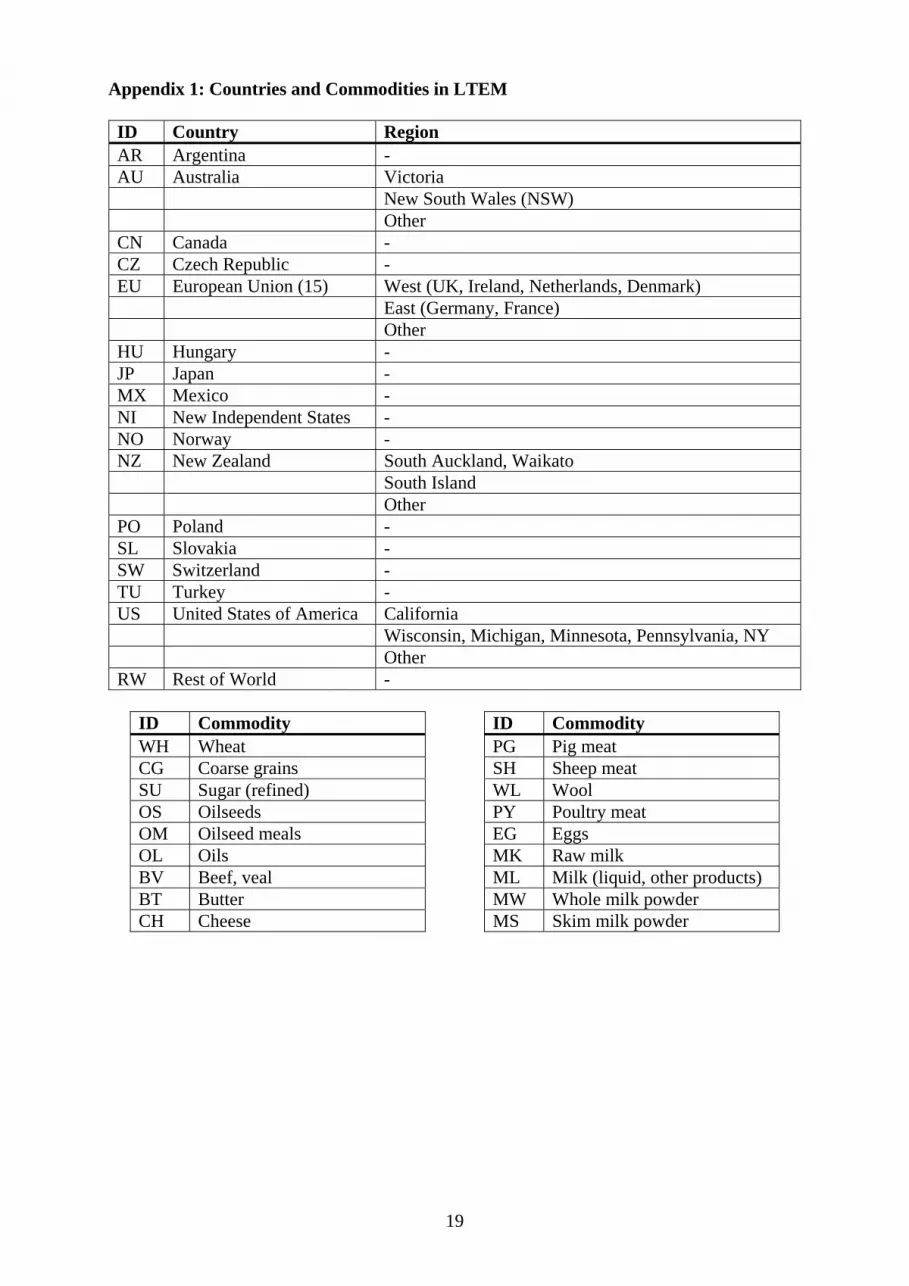
The LTEM framework includes 18 commodities and 17 countries. These are presented in Appendix Tables A1. The dairy sector is modelled as five commodities. Raw milk is defined as the farm gate product and then is allocated to either the liquid milk, butter, cheese, whole milk powder or skim milk powder markets depending upon their relative prices subject to physical constraints. The meat sector is disaggregated into sheepmeat, beef and pig meat in the current version of LTEM. Six crop products (wheat, sugar, coarse grains, oilseeds, oil meals, oil) as well as the poultry sector (poultry meat and eggs) and wool are also explicitly modelled in LTEM framework. The general equation structure of each commodity at country level in LTEM framework is represented by six (eight for crops) behavioural equations and one economic identity as in the equations (1) to (9). The trade price (pt) of a commodity (i) in a country (j) is determined as a function of world market price (WDpti) of that commodity and the exchange rate (exj), equation 1. The total effect of world market price on trade price of the country is determined by the price transmission elasticity. The domestic producer (ppij) and consumer prices (pcij) are defined as functions of trade price of the related commodity and commodity specific production and consumption related domestic support/subsidy policies, (Zsj, Zdj), which are represents the price wedge, equations 2 and 3.

),( jiij exWDptfpt = (1) ),( jijij Zsptgpp = (2) ),( jijij Zdpthpc = (3)

The domestic supply and demand equations are specified as constant elasticity functions that incorporate both the own and cross-price effects. Domestic supply (qsij) is specified as a function of the supply (ssftij) shifter, which represents the economic factors that may cause shifts, a policy variable (Zj) that may reflect the production quota or set-aside policy, and producer prices of the own and other substitute and complementary commodities (ppijk), equation 4.

8

),,( ikjjijij ppZssftlqs = (4) Domestic demand (qdij) is specified as a function of the demand (dsftij) shifter, consumer prices of the own and other substitute and complementary commodities (pcijk) and per capita real income (pincj) created in the economy, equation 5. The total demand for crops is separated into feed and food demand (and processing industry demand (qdij,pr) in some cases, equation 6). In feed demand (qdij,fe) function domestic supply of livestock (qsij,liv) sector is also included as an explanatory variable, equation 7.

),,(, jikjijfoij pincpcdsftmqd = (5) ),,(' ,,, livijikjfeijfeij qspcdsftmqd = (6)

),('' ,, ikjprijprij pcdsftmqd = (7) The stocks (qstij) are determined as a function of the stock shifter (stsftij), quantity supplied (qsij) and consumer price (pcij) of the commodity, equation 8. Finally, net trade (qtij) of the country (j) in commodity (i) is determined as the difference between domestic supply and the sum of domestic demand (also includes (qdij,fe) and (qdij,pr) in case of crops) and stock changes in the related year, equation 9. LTEM is a synthetic model since the parameters are adopted from the literature.

),,( ijijijij pcqsstsftnqst = (8)

ijijijij qstqdqsqt Δ−−= (9) Basically, the model works by simulating the commodity based world market clearing price on the domestic quantities and prices, which may or may not be under the effect of policy changes, in each country by basing on 1997. Excess domestic supply or demand in each country spills over onto the world market to determine world prices. The world market-clearing price is determined at the level that equilibrates the total demand and supply of each commodity in the world market. Sectoral focus: dairy The empirical focus selected for this study is dairy. This sector is currently highly influenced by protectionist policies, most notably in the EU. Consequently, the location of raw milk production and the trade in processed dairy products are widely regarded as likely to change following liberalisation (Tyres and Anderson, 1986). In addition, dairy farming is responsible for various forms of environmental degradation including a significant contribution to nitrate concentrations in groundwater, both directly through nitrogenous fertiliser applications on grassland and indirectly through the nitrogen content of grass and other feeds excreted in dung and urine (Rae, 1999). Different dairy production systems generate different levels of nitrate emissions and different environmental conditions display different capacities to assimilate these (Cameron et al., 1998). Since groundwater quality is a policy issue in several countries, there is interest not only in the distribution of economic impacts following trade liberalisation (e.g. output gains and losses) but also in the distribution of nitrate pollution between and within countries.

9

Groundwater nitrates In principle, the economic value of damage arising from nitrate contamination, rather than the physical level of contamination, should be addressed. This would allow direct comparison of social costs and benefits associated with dairy production. However, in practice, consensus has yet to be achieved on how to measure such damage and physical indicators remain the most commonly used measure for policy purposes (Moxey, 1999). Hence, for the purposes of this study, the environmental effect of dairy production was expressed in physical units as in equation 10 (Bidwell et al., 1999).

W

qskCkhaNkk

GNCij )( 4310 −++

= (10)

where :- GNC: average groundwater nitrate concentration (g/m3/yr) N: nitrogen usage (kg/ha/yr) C: feed grain (concentrate) usage (kg/ha/yr) qsij: quantity milk produced (l/ha/yr) W: annual average drainage per year (mm) Parameter values for this equation were obtained from relevant literature and discussions with scientists in the UK and NZ. Basically, nitrogenous fertiliser and concentrate feed both contribute to nitrate emissions, but some of their nitrogen content is removed in milk. The effect of emissions on groundwater concentrations depends on the degree of dilution offered by annual drainage (Whitehead, 1995). Model extensions In order to incorporate (10) within the LTEM structure, two extensions were made. First, the major dairy producing trading blocs were each sub-divided into regions to better reflect internal heterogeneity with respect to dairy production systems and environmental conditions. These divisions were based on observed variation in, for example, yields, stocking rates and drainage characteristics (see Appendix 2). Data on production systems were taken from a number of sources, including farm advisory recommendations, census and survey reports, and field trials. Second, whilst the quantity of concentrate feed used in dairy production was automatically generated by the existing LTEM structure2, usage of nitrogenous fertiliser had to be estimated separately via a conditional input demand equation:

2)(1b

N

Cij P

pbqsN = (11)

Where N is the usage of nitrogen per hectare, qsij is the regional quantity of raw milk produced per hectare (determined by the equation 4 or a binding policy output quota), PC and

2 That is, since grains are a traded agricultural output included in the basic model, feed usage for dairy production is specified in their demand function.

10

PN are the input prices, and b1 and b2 describe the substitution possibilities between the inputs (Varian, 1992). The use of the Cobb-Douglas form for equation 11 is arbitrary. Although alternative demand specifications were considered, including more flexible forms such as the Translog, the Cobb-Douglas offers a relatively transparent approach. In particular, it was accessible to non-economists involved in providing parameter values for different production systems across different countries and regions. However, one concern here is a potential tension between the implicit production relationships represented by the market-level elasticities in equation 4 and the explicit production relationship represented by the input demand equation 11. Given that the choice of a Cobb-Douglas form is arbitrary, it is unlikely that neither this functional form nor its parameter values will (except by happy coincidence) match with the trade flow equations. Two defences may be invoked here. First, as long ago as 1958, Hothakker demonstrated that farm-level production relationships may aggregate into very different sector-level relationships, whilst more recently Diewert (1981) and Hertel et al. (1996) show that sector level elasticities need not resemble firm-level elasticities. Stoker (1993) offers an interesting review of aggregation issues in the presence of heterogeneity. Second, the real problem here is actually one of incomplete information in that whilst the outputs may be reported, the inputs have not been observed directly and have to be inferred from other, sometimes oblique sources (Jakeman et. al. 1995; Hertel et al., 1996). In the absence of reliable information, any functional form is arbitrary and erring on the side of simplicity and transparency may be justifiable (Taylor & Howitt, 1993; Wallace, 1994)

11

Chapter 4 Empirical Results

The LTEM was calibrated using 1997 data as the base year. It was then used to simulate forward to 2010 under three different liberalisation scenarios: no liberalisation; EU liberalisation; and OECD liberalisation. The first of these assumes that trade policies in 1997 remain in place and represents a baseline. The second that the EU unilaterally liberalises (as measured by producer support estimate, PSEs), including the removal of internal dairy quotas. The third that all OECD member states remove trade barriers, driving their PSEs to zero. For presentational ease, only changes in selected key variables, and only for the main countries/regions, under the second and third scenarios are summarised in Tables 1 and 2.

Table 1 Estimated Production and Trade in Dairy Products in 2010 Under Baseline

and EU and OECD Liberalisation Scenarios

Net Trade (000t)* Country Scenario Raw Milk Price (US$/t)

Raw Milk Output (000t)

Butter

Cheese

Whole milk

powder

Skim milk

powderAustralia Baseline 250 11677 +116 +183 +145 +169 EU 284 12177 +124 +233 +161 +181 OECD 283 12018 +123 +210 +150 +188 EU Baseline 409 117493 +408 -535 +636 +238 EU 329 109027 +51 -1800 +472 -9 OECD 371 114318 +117 -812 +535 +79 Japan Baseline 568 9209 -48 -181 +70 -371 EU 588 9468 -36 -140 +91 -331 OECD 524 8474 -67 -233 +17 -387 NZ Baseline 194 12391 +368 +258 +433 +234 EU 196 12278 +379 +267 +439 +238 OECD 217 12908 +419 +290 +465 +264 USA Baseline 313 78918 +213 -170 +58 -61 EU 353 82598 +268 +551 +68 +50 OECD 306 76991 +100 -288 +42 -106

* '+' denotes net exports, '-' net imports Raw milk prices The simulated results suggest that EU liberalisation leads to a rise in the producer price of raw milk in all of the main countries, with the exception of the EU itself, which suffers a price drop of 20 percent. The biggest price rises are in Australia at 14 percent and the USA at 13 percent with modest changes in Japan and NZ at 3 and 1 percent respectively. Under OECD liberalisation, prices in the EU drop by 10 percent from base but Japan and the USA now also experience a price fall of 8 and 2 percent, whilst in NZ and Australia price rises by more significant, 11 percent.

12

Table 2

Estimated Regional Resource Usage and Nitrate Pollution in 2010 Under Baseline and EU and OECD Liberalisation

N usage (kg/ha) C usage (kg/cow) GNC (g/m2/yr) Country Region Base EU OECD Base EU OECD Base EU OECD

Australia Victoria 251 266 267 722 747 707 10.7 10.9 10.9 NSW 188 199 199 1443 1494 1414 9.2 9.3 9.3 Other 124 131 131 1241 1285 1216 12.9 13.0 13.0 EU West 400 331 359 2686 2102 2193 5.0 4.6 4.8 East 139 115 123 1279 1001 1044 7.2 7.0 7.0 Other 283 234 252 2686 2102 2193 6.7 6.3 6.5 NZ S.Auckland etc 122 126 139 0 0 0 4.9 4.9 5.0 S. Island 244 248 267 21.4 20.7 21.5 10.7 10.8 10.9 Other 187 192 209 11.9 11.5 12.0 9.0 9.1 9.2 USA California 0 0 0 7140 7454 6608 6.3 6.3 6.3 Wisconsin etc 344 366 347 3765 3930 3484 4.7 4.9 4.8 Other 173 185 177 2596 2710 2403 5.8 5.9 5.8 Global All 205 199 206 1966 1905 1775 7.76 7.75 7.79

NB. S. Auckland etc. is assumed here to be a solely grazing-based production system with no concentrate feed usage. California dairy production is assumed to be feedlots, with no grazing and therefore no nitrogen usage.

13

Raw milk production The changes in prices described above are associated with shifts in raw milk production. The predicted impact of EU liberalisation is a fall in the EU production of 7 percent, with modest increases in Australia, Japan and the US of 4, 3 and 5 percent, but little change in NZ. Under OECD liberalisation, production drops by less in the EU by 3 percent also drops in Japan and the USA by 8 and 2.5 percent, with Australian and New Zealand output rising 4 and 3 percent. Traded dairy products Under EU liberalisation, exports of processed dairy products from the EU fall whilst exports from Australia, New Zealand and the USA rise. Imports into the EU, particularly for cheese, increase. Under OECD liberalisation, the picture as expected with the EU exports generally dropping by less than under the EU liberalisation. The USA exports of butter fall rather than rise. It is interesting to note that whilst Australia gains under both scenarios, NZ is affected more by OECD liberalisation, perhaps reflecting preferential access into the EU under current policy. Resource usage Table 2 reports estimated resource usage and groundwater nitrate levels at the regional level in Australia, the EU, NZ and the USA (Japan is excluded here since it is not sub-divided within the model). Under the EU liberalisation, fertiliser and feed usage fall in the EU by 20 and 28 percent respectively but rise elsewhere by 6 percent in Australia. Under the OECD liberalisation, the fall in the EU is less marked and 22 percent rise in the USA being smaller. There is some variation across regions within each country, reflecting differences in production systems. It is also interesting to note that under EU liberalisation, global average nitrogen usage and feed usage per hectare for dairying both decline. However, under OECD liberalisation, nitrogen usage rises marginally as feed usage declines. This perhaps reflects the greater shift away from feed-based systems, common in parts of the EU and USA, to grass-based systems within the USA more common in, for example, New Zealand. Groundwater nitrates As with resource usage, the pattern of groundwater nitrate concentrations varies between countries but also within countries under the two scenarios. Under both EU and OECD liberalisation, nitrate concentrations fall in the EU but rise in Australia and New Zealand. The USA experiences a rise under EU liberalisation, but only marginal changes under OECD liberalisation. However, none of the changes are particularly dramatic.

14

15

Chapter 5 Conclusions

This paper quantified explicitly the linkage between trade liberalisation and how the changing geographical distribution of nitrogen fertiliser and feed used in dairy production may impact upon groundwater nitrate concentrations. This was achieved by modifying an existing partial-equilibrium trade model to incorporate sub-national regions of major dairy producing countries and the inclusion of physical relationships. The results presented above fall into two categories: production and trade estimates; and resource usage and environmental impact estimates. The first group represents standard outputs from a trade model. As such, the specific findings presented here are familiar items and can be compared with other studies of agricultural trade liberalisation. The estimates presented are broadly in-line with expectations. That is, if the EU liberalises unilaterally, then the EU will shoulder major price and production reductions whereas if all OECD member states liberalise then EU adjustments are less severe due to changes elsewhere. In addition, Australia and New Zealand stand to gain most from full OECD liberalisation due to their comparative advantage in dairy production. The second group of results represents a natural extension to the first, yet is rarely considered explicitly in trade modelling. Changes in production patterns may be implicitly associated with changes in resource usage, but the link is rarely quantified. However, concern over possible environmental impacts of trade-policy-induced shifts in production patterns necessitates explicit consideration of this. The results presented here should be considered as indicative rather than definitive, representing as they do a first attempt to articulate the linkage between dairy trade liberalisation and nitrate concentrations. Nevertheless, they do support the notion that production and environmental heterogeneity both between and within trading partners will lead to spatially differential changes in patterns of resource usage and environmental impacts. Such findings may help to inform policy debates. To conclude, formal agricultural economic analysis is credited with providing valuable and timely information for the Uruguay Round of the General Agreement on Tariffs and Trade (GATT) which concluded in 1992 (Meilke et al., 1996). The raised profile of both agriculture and the environment within the inaugural World trade Organisation (WTO) negotiations ensures that there will be a continued need for formal analysis of these two factors and their interactions. This paper represents an attempt to meet this need and suggests that further modelling work of this type is merited.

16

17

References Abler, D.G. and Shortle, J. (1992). Environmental and Farm Commodity Policy Linkages in

the US and the EC. European Review of Agricultural Economics 19: 197-217. Alexandratos, N. (1995). World Agriculture: Towards 2000, A FAO Study. Chichester: FAO

and John Wiley & Sons. Anderson, K. (1992). Effects on the Environment and Welfare of Liberalising World Trade:

the Cases of Coal and Food. In K. Anderson and R. Blackhurst (eds.), The Greening of World Trade Issues. Harvester Wheatsheaf.

Bidwell, V. (1999). World Trade and the Environment Formulas Relating Nitrate Leaching,

Nitrogen Fertiliser and Milk Production. Report to Lincoln Environmental. Canterbury: Lincoln University.

Cameron, K., Silva, R.G., Di, .J. and Hendry, T. (1998). Impacts of Cow Urine, Dairy Shed

Effluent and Nitrogen Fertiliser on Drainage Water Quality. Paper presented to the 6th World Congress of Soil Science. France.

Diewert, W.E. (1981). The Comparative Statics of Industry Long-run Equilibrium. Canadian

Journal of Economics 17: 78-92. FAO (1997). The Impact of Trade Liberalization on Production of Agricultural Commodities

and Related Fertiliser Use. Technical Report, Food and Agricultural Organisation of the United Nations.

Haley, S.L. (1993). Environmental and Agricultural Policy Linkages in The European

Community: The Nitrate Problem and CAP Reform. Working Paper No. 1993-3, IATRC (International Agricultural Trade Research Consortium).

Hansen, L.P. and Heckman, J.J. (1996). The Empirical Foundations of Calibration. Journal

of Economic Perspectives 10/1: 87-104. Hertel, T., Stiegent, K. and Vroomen, H. (1996). Nitrogen-land Substitution in Corn

Production: a Reconciliation of Aggregate and Firm-level Evidence. American Journal of Agricultural Economics 78/1: 30-40.

Hettige, H., Martin, P., Singh, M. and Wheeler, D. (1994). IPPS: The Industrial Pollution

Projection System. unpublished World Bank paper. Washington D.C., December. Jakeman, A.J., Beck, M.B. and McAleer, M.J. (eds.) (1995). Modelling Change in

Environmental Systems. Chichester: John Wiley & Sons. Koopmans, T.TH. (1987). An Application of an Agro-economic Model to Environmental

Issues in the EC: a Case Study. European Review of Agricultural Economics 14: 147-59.

Meilke, K.D., MacClatchy, D. and de Gorter, H. (1996). Challenges in Quantitative

Economic Analysis in Support of Multilateral Trade Negotiations. Agricultural Economics 14: 185-200.

18

Moxey, A.P. (1999). Cross-cutting Issues in Developing Agri-environmental Indicators. In Environmental Indicators for Agriculture Volume 2: Issues and Design. The York Workshop, Paris: OECD.

Parikh, K.S., Fischer, G., Frohberg, K. and Gulbrandson, O. (1988). Towards Free Trade in

Agriculture. Dordrecht: Martinus Nijhoff. Potter, C. (1998). Against the Grain. Wallingford: CAB International. Rae, A. (1999). Livestock Production and the Environment. Working Paper No 6. NZ Trade

Consortium. Redclift, M.R., Lekakis, J.N. and Zanias, G.P. (eds.) (1999). Agriculture and World Trade

Liberalisation. Wallingford: CAB International. Roningen, V.O. (1986). A Static Policy Simulation Modeling (SWOPSIM) Framework.

Staff Report AGES 860625, Economic Research Service. Washington: USDA. Roningen, V.O., Dixit, P., Sullivan, J. and Hart, T. (1991). Overview of the Static World

Policy Simulation (SWOPSIM) Modelling Framework. Staff Report AGES 9114, Economic Research Service. Washington: USDA.

Stoker, T.M. (1993). Empirical Approaches to the Problem of Aggregation Over Individuals,

Journal of Economic Literature XXXI/4: 1827-1874. Taylor, C. R. and Howitt, R. (1993). Aggregate Evaluation Concepts and Models. In G.A.

Carlson, D. Zilberman and J.A. Miranowski (eds), Agricultural and Environmental Resource Economics. Oxford: Oxford University Press.

Tsigas, M., Gray, D., Hertel, T. and Krisoff, B. (1998). Environmental Consequences of

Trade Liberalization in the Western Hemisphere. Economic Research Service. Washington: USDA.

Tyers, R. and Anderson, K. (1992). Disarray in World Food Markets. Cambridge:

Cambridge University Press. Tyers, R., and Anderson, K. (1986). Distortions in World Food Markets: A Quantitative

Assessment. Background paper for the World Development Report, 1986. Varian, H.R. (1992). Micro-economic analysis. New York: Norton. Wallace, W.A. (ed.) (1994). Ethics in Modelling. Oxford: Pergamon Press. Whitehead, D.C. (1995). Grassland Nitrogen. CAB International.

19

Appendix 1: Countries and Commodities in LTEM ID Country Region AR Argentina - AU Australia Victoria New South Wales (NSW) Other CN Canada - CZ Czech Republic - EU European Union (15) West (UK, Ireland, Netherlands, Denmark) East (Germany, France) Other HU Hungary - JP Japan - MX Mexico - NI New Independent States - NO Norway - NZ New Zealand South Auckland, Waikato South Island Other PO Poland - SL Slovakia - SW Switzerland - TU Turkey - US United States of America California Wisconsin, Michigan, Minnesota, Pennsylvania, NY Other RW Rest of World -

ID Commodity ID Commodity WH Wheat PG Pig meat CG Coarse grains SH Sheep meat SU Sugar (refined) WL Wool OS Oilseeds PY Poultry meat OM Oilseed meals EG Eggs OL Oils MK Raw milk BV Beef, veal ML Milk (liquid, other products) BT Butter MW Whole milk powder CH Cheese MS Skim milk powder

20

Appendix 2: Technical Data

Region Productionper cow (litres)

Average stocking rate/ha

Area (000ha)

Average Drainage (mm/yr)

EU (15) West EU 5310 2.4 3174.8 400 East EU 4680 1.8 6639.6 200 Other EU 4991 2.3 3302.2 300 Australia: Victoria 4715 1.0 1267.9 300 NSW 4972 0.5 504.02 300 Rest of Australia 4608 0.5 1046.0 200 USA: 7238 California 8439 10 149.2 200 WI, MI, MN, PA, NY 7182 3 1251.2 500 Rest of USA 6770 2.7 1727.8 300 New Zealand Auckland 3278 2.8 494.6 700 South Island 3874 2.6 274.8 350 Rest of NZ 3300 2 570.4 400

21

Contact Address: Prof. Caroline Saunders ph. +64 3 325 2811/8287 fax. +64 3 325 3847 e-mail. saunderc@lincoln.ac.nz Commerce Division Lincoln University P.O. Box 84 Canterbury-8150 New Zealand