
The use of Bayesian networks to guide investments in flow and catchment restoration for impaired...
18
The use of Bayesian networks to guide investments in flow and catchment restoration for impaired river ecosystems B. STEWART-KOSTER*, S. E. BUNN*, S. J. MACKAY*, N. L. POFF † , R. J. NAIMAN ‡ AND P. S. LAKE § * eWater Cooperative Research Centre, Australian Rivers Institute, Griffith University, Nathan, Qld, Australia † Department of Biology, Colorado State University, Fort Collins, CO, U.S.A. ‡ School of Aquatic and Fishery Sciences, University of Washington, Seattle, WA, U.S.A. § School of Biological Sciences, Monash University, Monash, Vic., Australia SUMMARY 1. The provision of environmental flows and the removal of barriers to water flow are high priorities for restoration where changes to flow regimes have caused degradation of riverine ecosystems. Nevertheless, flow regulation is often accompanied by changes in catchment and riparian land-use, which also can have major impacts on river health via local habitat degradation or modification of stream energy regimes. 2. The challenges are determining the relative importance of flow, land-use and other impacts as well as deciding where to focus restoration effort. As a consequence, flow, catchment and riparian restoration efforts are often addressed in isolation. River managers need decision support tools to assess which flow and catchment interventions are most likely to succeed and, importantly, which are cost-effective. 3. Bayesian networks (BNs) can be used as a decision support tool for considering the influence of multiple stressors on aquatic ecosystems and the relative benefits of various restoration options. We provide simple illustrative examples of how BNs can address specific river restoration goals and assist with the prioritisation of flow and catchment restoration options. This includes the use of cost and utility functions to assist decision makers in their choice of potential management interventions. 4. A BN approach facilitates the development of conceptual models of likely cause and effect relationships between flow regime, land-use and river conditions and provides an interactive tool to explore the relative benefits of various restoration options. When combined with information on the costs and expected benefits of intervention, one can derive recommendations about the best restoration option to adopt given the network structure and the associated cost and utility functions. Keywords: cost-benefit, environmental flows, multiple stressors, riparian revegetation, river restoration Introduction There is little doubt that flow regulation has impaired river ecosystems globally (Nilsson et al., 2005) via the alteration of natural hydrologic regimes (Magilligan & Nislow, 2005; Poff et al., 2007). In recognition of the widespread degradation of rivers due to flow regula- tion there have been increasing calls to include aquatic Correspondence: B. Stewart-Koster, eWater Cooperative Research Centre, Australian Rivers Institute, Griffith University, Nathan, 4111 Qld, Australia. E-mail: b.stewart-koster@griffith.edu.au Freshwater Biology (2010) 55, 243–260 doi:10.1111/j.1365-2427.2009.02219.x Ó 2009 Blackwell Publishing Ltd 243
-
Upload
independent -
Category
Documents
-
view
3 -
download
0
Transcript of The use of Bayesian networks to guide investments in flow and catchment restoration for impaired...
The use of Bayesian networks to guide investments inflow and catchment restoration for impaired riverecosystems
B. STEWART-KOSTER*, S . E . BUNN*, S . J . MACKAY*, N. L. POFF†, R. J . NAIMAN ‡
AND P. S . LAKE §
*eWater Cooperative Research Centre, Australian Rivers Institute, Griffith University, Nathan, Qld, Australia†Department of Biology, Colorado State University, Fort Collins, CO, U.S.A.‡School of Aquatic and Fishery Sciences, University of Washington, Seattle, WA, U.S.A.§School of Biological Sciences, Monash University, Monash, Vic., Australia
SUMMARY
1. The provision of environmental flows and the removal of barriers to water flow are high
priorities for restoration where changes to flow regimes have caused degradation of
riverine ecosystems. Nevertheless, flow regulation is often accompanied by changes in
catchment and riparian land-use, which also can have major impacts on river health via
local habitat degradation or modification of stream energy regimes.
2. The challenges are determining the relative importance of flow, land-use and other
impacts as well as deciding where to focus restoration effort. As a consequence, flow,
catchment and riparian restoration efforts are often addressed in isolation. River managers
need decision support tools to assess which flow and catchment interventions are most
likely to succeed and, importantly, which are cost-effective.
3. Bayesian networks (BNs) can be used as a decision support tool for considering the
influence of multiple stressors on aquatic ecosystems and the relative benefits of various
restoration options. We provide simple illustrative examples of how BNs can address
specific river restoration goals and assist with the prioritisation of flow and catchment
restoration options. This includes the use of cost and utility functions to assist decision
makers in their choice of potential management interventions.
4. A BN approach facilitates the development of conceptual models of likely cause and
effect relationships between flow regime, land-use and river conditions and provides an
interactive tool to explore the relative benefits of various restoration options. When
combined with information on the costs and expected benefits of intervention, one can
derive recommendations about the best restoration option to adopt given the network
structure and the associated cost and utility functions.
Keywords: cost-benefit, environmental flows, multiple stressors, riparian revegetation, riverrestoration
Introduction
There is little doubt that flow regulation has impaired
river ecosystems globally (Nilsson et al., 2005) via the
alteration of natural hydrologic regimes (Magilligan &
Nislow, 2005; Poff et al., 2007). In recognition of the
widespread degradation of rivers due to flow regula-
tion there have been increasing calls to include aquatic
Correspondence: B. Stewart-Koster, eWater Cooperative
Research Centre, Australian Rivers Institute, Griffith University,
Nathan, 4111 Qld, Australia.
E-mail: [email protected]
Freshwater Biology (2010) 55, 243–260 doi:10.1111/j.1365-2427.2009.02219.x
� 2009 Blackwell Publishing Ltd 243
ecosystems as legitimate users of water and to
improve methods for the allocation of environmental
flows (Naiman et al., 2002; Arthington et al., 2006; Poff
et al., 2010). Considerable investments have been
made in some countries to release water as environ-
mental flows intended to restore aquatic habitat and
biotic assemblages (Richter et al., 2006). These envi-
ronmental flow releases are often controversial (Poff
et al., 2003), particularly in dry regions (Arthington &
Pusey, 2003; Bond, Lake & Arthington, 2008).
Flow regulation seldom occurs in isolation from
changes in catchment and riparian land-use with
vegetation removal, intensive agriculture and urban-
isation also having wide ranging and cascading effects
on river ecosystems (Strayer et al., 2003; Allan, 2004;
Doledec et al., 2006; Paul, Meyer & Couch, 2006). To
address these and other related land-use impacts, a
range of strategies has been used by river managers to
improve water quality and river conditions. These
strategies include the construction of artificial wet-
lands and other water-sensitive urban design mea-
sures (e.g. Mitchell et al., 2007) and the creation of
buffer strips and replanting of riparian vegetation
(Lowrance, 1998; Broadmeadow & Nisbet, 2004).
While it is well recognised that river conditions,
including biodiversity, are affected by a combination
of land-use and flow-related drivers; restoration
efforts are often focused on one or the other. In some
instances it may be relatively clear as to which has the
overriding influence (e.g. increased urban develop-
ment compared to riparian degradation, Walsh et al.,
2007), but the interaction among key drivers in many
systems may be less apparent (Bunn & Arthington,
2002; Allan, 2004). Constrained by limited budgets, it
can be difficult to determine objectively the most
effective restoration approach when faced with multi-
ple drivers of river condition decline.
Our objective is to outline an approach that may be
used as a decision support tool to identify an
appropriate restoration strategy in the presence of
multiple drivers of a river’s ecological condition. We
use Bayesian networks (BNs) to model key ecological
relationships in terms of their potential for restoration
in impaired streams. The use of BNs in natural
resource management has grown rapidly in recent
years, either to model the system under study or as a
decision support tool (Varis & Kuikka, 1999; Borsuk,
Stow & Reckhow, 2004; Arthington et al., 2007; Cas-
telletti & Soncini-Sessa, 2007). Examples of BNs as
decision support tools in aquatic ecosystem manage-
ment include the evaluation of different management
scenarios for in-stream phosphorus loadings (Ames
et al., 2005), the ecological impact of dryland salinity
management (Sadoddin et al., 2005), competing
stream flow allocations (Said, 2006) and different
water treatment sequences (Zhu & McBean, 2007).
Although many published examples apply to single
response variables, the BN framework also can be
used to identify effective management actions for
multiple response variables, such as water quality and
quantity (e.g. Said et al., 2006).
In this study, we present two case studies using
BNs where flow and land-use related factors combine
to influence a specific aspect of river health. The first is
a hypothetical example to demonstrate the modelling
approach, focused on dissolved oxygen (DO) in a
small regulated and degraded stream. The second is
based on empirical data on factors influencing aquatic
macrophytes in coastal streams in south-east Queens-
land, Australia (Mackay, 2007). Finally, we illustrate
how the costs of restoration can be incorporated into
these conceptual models to identify the most cost-
effective restoration approach and to help prioritise
competing management actions using Bayesian deci-
sion networks (BDNs).
Methods
We constructed BNs and BDNs using the software
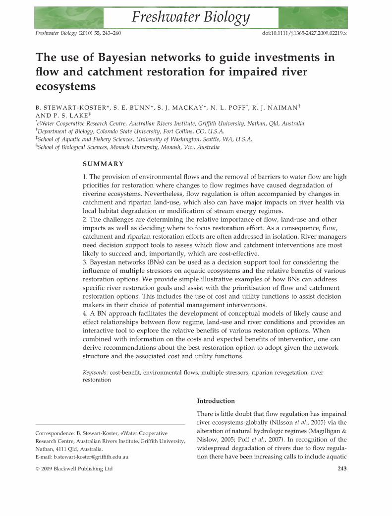
package, NETICANETICA (Norsys, 2005). A BN is a graphical
Z
(a) (b)
UX
Y
Z
UX
Y
Decision Cost
Utility
Fig. 1 (a) An example of the structure of a Bayesian network
with common parent nodes (X and U) and potentially condi-
tionally independent nodes (Y and Z) and (b) an example of a
Bayesian decision network, showing a decision node with
associated cost node representing the costs of implementing the
states of the decision node and a utility node representing the
desirability of the states of the child node.
244 B. Stewart-Koster et al.
� 2009 Blackwell Publishing Ltd, Freshwater Biology, 55, 243–260
model representing the key factors of a system (nodes)
and their conditional dependencies (Fig. 1a; Varis,
1997; Korb & Nicholson, 2004; Jensen & Nielsen,
2007). The dependencies are depicted as directed links
or arrows connecting a ‘parent node’ to a ‘child node’,
resulting in a directed acyclic graph (DAG). In a DAG,
no path starts and ends at the same node and no
feedback loops are allowed so that connecting nodes do
not become ancestors of their ancestors (Jensen &
Nielsen, 2007). The network is quantified by populating
conditional probability tables (CPTs) associated with
the nodes in the network. The CPTs can be specified by
experts or learned from data using one of several
learning algorithms depending on the complexity of
the network, such as the Bayesian counting–learning
algorithm or the expectation-maximisation algorithm
(Korb & Nicholson, 2004; Jensen & Nielsen, 2007).
Conditional independence is fundamental to BNs
(Korb & Nicholson, 2004). This property allows an
examination of both the independent and interactive
(conditional) effects of some environmental change on
the modelled response variable. Furthermore, a BN
requires the assumption of the Markov property
which means that each CPT can be populated by
only considering the immediate parent nodes of the
node being quantified. By specifying the probabilities
of the states of a parent node(s) in a BN, the
probabilities of any child nodes are updated via the
process of belief updating. Thus, when a particular state
of a parent node is observed, subsequent probabilities
of any child nodes, P(Y|X = x), are estimated using
Bayes Theorem (eqn 1) and the chain rule from
probability theory (Korb & Nicholson, 2004).
PðyjxÞ ¼ PðxjyÞPðyÞPðxÞ ð1Þ
where P(y) is the prior probability of the child node
and P(x) is a normalising constant. Prior probabilities
can come from expert opinion, preliminary data from
the system or data from research on similar systems.
Prior probabilities can be informative, thereby influ-
encing model outputs, or uninformative, making little
or no difference to model outputs. The use of Bayes
theorem to estimate the CPTs provides the opportu-
nity to use data and expert opinion, together or in
isolation, to populate the network (Korb & Nicholson,
2004; Pollino et al., 2007). Further information on BNs
and their development can be found in Charniak
(1991), Reckhow (1999), Korb & Nicholson (2004) and
Jensen & Nielsen (2007).
In addition to modelling relationships between
environmental drivers and ecological response vari-
ables, we modified the BNs to incorporate the relative
costs and benefits of potential management actions
(e.g. Ames et al., 2005; Said, 2006). Such models are
known as BDNs (Fig. 1b), and are used to identify the
most appropriate decision (here, restoration action)
given estimated costs and benefits (Korb & Nicholson,
2004; Jensen & Nielsen, 2007). A decision node(s) is
included in the network whose states are the possible
restoration actions; for example, different kinds of
environmental flow releases. The effect of the decision
node is to alter the states of its child nodes according
to the possible restoration actions. Decision nodes can
have an associated cost function that represents the
actual or relative cost of each decision state (Jensen &
Nielsen, 2007). The terminal node or response variable
can have an associated utility function that reflects
how desirable each management intervention is in
terms of its modelled outcome (Zhu & McBean, 2007).
By including a cost and utility node in the network,
the BDN can identify the most cost-effective restora-
tion decision, that which maximises the expected
utility within the network (Jensen & Nielsen, 2007).
The expected utility is the sum of the possible utilities
associated with the terminal node resulting from each
restoration action, weighted by the probabilities of
each state of the terminal node (Jensen & Nielsen,
2007). The restoration decision that maximises the
expected utility is that which provides the most
desirable ecological outcome relative to its costs,
thereby combining ecological response with economic
constraints.
Case study 1 – reducing low DO extremes
The concentration of DO in a stream can fluctuate
widely in response to physical factors that influence
solubility (e.g. temperature, atmospheric pressure,
turbulence and re-aeration), chemical factors (e.g.
oxidation of pollutants) and biological factors (e.g.
photosynthesis and respiration). In degraded
streams and rivers, low oxygen can result from a
combination of low flows, high water temperatures
and ⁄or excessive aquatic plant or organic matter
respiration. Some of these causal factors, such as in-
stream temperature, are in turn a function of other
Guiding investments in river restoration 245
� 2009 Blackwell Publishing Ltd, Freshwater Biology, 55, 243–260
physical factors such as riparian shading and
groundwater inputs (Rutherford et al., 2004; Webb
et al., 2008). Similarly, aquatic plant production and
respiration are primarily driven by light regime (e.g.
turbidity and riparian shading), temperature and
nutrients (Bunn, Davies & Mosisch, 1999; Wetzel,
2001).
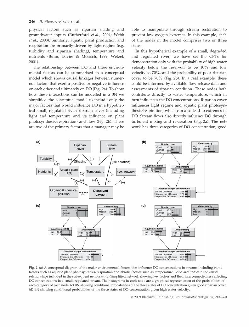
The relationship between DO and these environ-
mental factors can be summarised in a conceptual
model which shows causal linkages between numer-
ous factors that exert a positive or negative influence
on each other and ultimately on DO (Fig. 2a). To show
how these interactions can be modelled in a BN we
simplified the conceptual model to include only the
major factors that would influence DO in a hypothet-
ical small, regulated river: riparian cover (including
light and temperature and its influence on plant
photosynthesis ⁄ respiration) and flow (Fig. 2b). These
are two of the primary factors that a manager may be
able to manipulate through stream restoration to
prevent low oxygen extremes. In this example, each
of the nodes in the model comprises two or three
states.
In this hypothetical example of a small, degraded
and regulated river, we have set the CPTs for
demonstration only with the probability of high water
velocity below the reservoir to be 10% and low
velocity as 70%, and the probability of poor riparian
cover to be 70% (Fig. 2b). In a real example, these
could be informed by available flow release data and
assessments of riparian condition. These nodes both
contribute directly to water temperature, which in
turn influences the DO concentrations. Riparian cover
influences light regime and aquatic plant photosyn-
thesis ⁄respiration, which can also lead to extremes in
DO. Stream flows also directly influence DO through
turbulent mixing and re-aeration (Fig. 2a). The net-
work has three categories of DO concentration; good
devlossiDnegyxo
erutarepmeTtnalpcitauqA
R/P
maertSwolf
nairapiRrevoc
retawdnuorGstneirtuN
lacimehc&cinagrOnoitullop )–(
(+)
(+)
ytidibruT
devlossiDnegyxo
erutarepmeTtnalpcitauqA
R/P
maertSwolf
nairapiRrevoc
retawdnuorGstneirtuN
lacimehc&cinagrOnoitullop
(Re-aeration)(Shading)
)–(
(+)
(+)
ytidibruT
(–)
(a) (b)
(c) (d)
(–) (–)
(–) (–)(–)
(–)
(+)
(+)
(–)
stneveODwoloreZstneveODwoltneuqerfnI
stneveODwoltneuqerF
6.239.715.94
dooGegarevA
rooP
0.010.020.07
Ambient temp
Riparian cover
hgiHwoL
1.979.02
R/PtnalpcitauqAhgiH
woL0.360.73
yticolevretaWhgiH
muideMwoL
0.010.020.07
Dissolved oxygen concentration
Dissolved oxygen concentrationstneveODwoloreZ
stneveODwoltneuqerfnIstneveODwoltneuqerF
5.774.8140.4
dooGegarevA
rooP
00100
Ambient temphgiH
woL0.610.48
stneveODwoloreZstneveODwoltneuqerfnI
8.060.1302.8
dooGegarevA
rooP
0.010.020.07
hgiHwoL
0.550.54
Dissolved oxygen concentration
Ambient temp
Riparian cover
Dissolved oxygen concentrationstneveODwoloreZ
stneveODwoltneuqerfnIstneveODwoltneuqerF
5.774.8140.4
Riparian cover
Ambient temphgiH
woL0.610.48
muideM
stneveODwoloreZstneveODwoltneuqerfnI
stneveODwoltneuqerF
8.060.1302.8
dooGegarevA
rooP
0.010.020.07
hgiHwoL
0.550.54
R/PtnalpcitauqA
yticolevretaWhgiH
muideMwoL
00100
Dissolved oxygen concentration
Ambient temp
Riparian coveryticolevretaWhgiH
woL
R/PtnalpcitauqAhgiH 0.01
woL 0.09
0.020.07
0.01
hgiHwoL
0.360.73
Fig. 2 (a) A conceptual diagram of the major environmental factors that influence DO concentrations in streams including biotic
factors such as aquatic plant photosynthesis ⁄ respiration and abiotic factors such as temperature. Solid arcs indicate the causal
relationships included in the subsequent networks. (b) Simplified network showing key factors and their interconnectedness affecting
DO concentrations in a small, regulated stream. The histograms in each node are a graphical representation of the probabilities of
each category of each node. (c) BN showing conditional probabilities of the three states of DO concentration given good riparian cover.
(d) BN showing conditional probabilities of the three states of DO concentration given high water velocity.
246 B. Stewart-Koster et al.
� 2009 Blackwell Publishing Ltd, Freshwater Biology, 55, 243–260
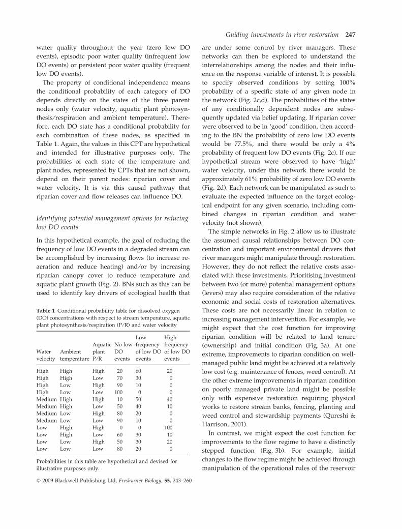
water quality throughout the year (zero low DO
events), episodic poor water quality (infrequent low
DO events) or persistent poor water quality (frequent
low DO events).
The property of conditional independence means
the conditional probability of each category of DO
depends directly on the states of the three parent
nodes only (water velocity, aquatic plant photosyn-
thesis ⁄ respiration and ambient temperature). There-
fore, each DO state has a conditional probability for
each combination of these nodes, as specified in
Table 1. Again, the values in this CPT are hypothetical
and intended for illustrative purposes only. The
probabilities of each state of the temperature and
plant nodes, represented by CPTs that are not shown,
depend on their parent nodes: riparian cover and
water velocity. It is via this causal pathway that
riparian cover and flow releases can influence DO.
Identifying potential management options for reducing
low DO events
In this hypothetical example, the goal of reducing the
frequency of low DO events in a degraded stream can
be accomplished by increasing flows (to increase re-
aeration and reduce heating) and ⁄or by increasing
riparian canopy cover to reduce temperature and
aquatic plant growth (Fig. 2). BNs such as this can be
used to identify key drivers of ecological health that
are under some control by river managers. These
networks can then be explored to understand the
interrelationships among the nodes and their influ-
ence on the response variable of interest. It is possible
to specify observed conditions by setting 100%
probability of a specific state of any given node in
the network (Fig. 2c,d). The probabilities of the states
of any conditionally dependent nodes are subse-
quently updated via belief updating. If riparian cover
were observed to be in ‘good’ condition, then accord-
ing to the BN the probability of zero low DO events
would be 77.5%, and there would be only a 4%
probability of frequent low DO events (Fig. 2c). If our
hypothetical stream were observed to have ‘high’
water velocity, under this network there would be
approximately 61% probability of zero low DO events
(Fig. 2d). Each network can be manipulated as such to
evaluate the expected influence on the target ecolog-
ical endpoint for any given scenario, including com-
bined changes in riparian condition and water
velocity (not shown).
The simple networks in Fig. 2 allow us to illustrate
the assumed causal relationships between DO con-
centration and important environmental drivers that
river managers might manipulate through restoration.
However, they do not reflect the relative costs asso-
ciated with these investments. Prioritising investment
between two (or more) potential management options
(levers) may also require consideration of the relative
economic and social costs of restoration alternatives.
These costs are not necessarily linear in relation to
increasing management intervention. For example, we
might expect that the cost function for improving
riparian condition will be related to land tenure
(ownership) and initial condition (Fig. 3a). At one
extreme, improvements to riparian condition on well-
managed public land might be achieved at a relatively
low cost (e.g. maintenance of fences, weed control). At
the other extreme improvements in riparian condition
on poorly managed private land might be possible
only with expensive restoration requiring physical
works to restore stream banks, fencing, planting and
weed control and stewardship payments (Qureshi &
Harrison, 2001).
In contrast, we might expect the cost function for
improvements to the flow regime to have a distinctly
stepped function (Fig. 3b). For example, initial
changes to the flow regime might be achieved through
manipulation of the operational rules of the reservoir
Table 1 Conditional probability table for dissolved oxygen
(DO) concentrations with respect to stream temperature, aquatic
plant photosynthesis ⁄ respiration (P ⁄ R) and water velocity
Water
velocity
Ambient
temperature
Aquatic
plant
P ⁄ R
No low
DO
events
Low
frequency
of low DO
events
High
frequency
of low DO
events
High High High 20 60 20
High High Low 70 30 0
High Low High 90 10 0
High Low Low 100 0 0
Medium High High 10 50 40
Medium High Low 50 40 10
Medium Low High 80 20 0
Medium Low Low 90 10 0
Low High High 0 0 100
Low High Low 60 30 10
Low Low High 50 30 20
Low Low Low 80 20 0
Probabilities in this table are hypothetical and devised for
illustrative purposes only.
Guiding investments in river restoration 247
� 2009 Blackwell Publishing Ltd, Freshwater Biology, 55, 243–260
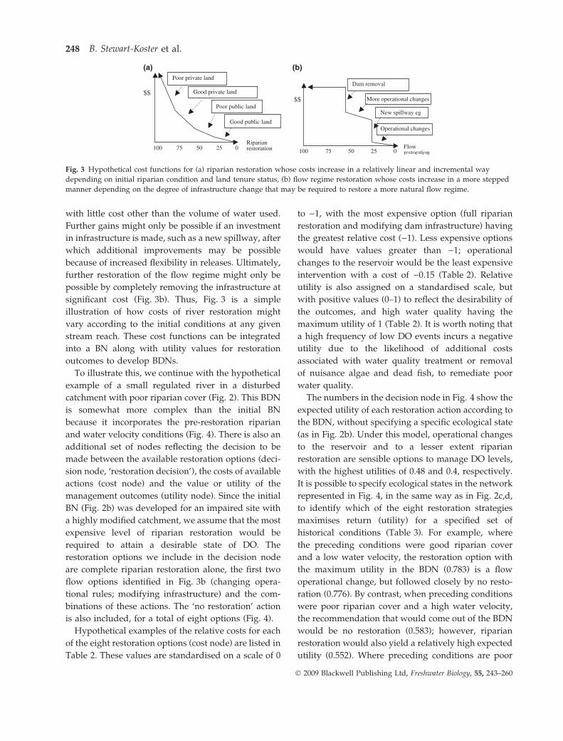
with little cost other than the volume of water used.
Further gains might only be possible if an investment
in infrastructure is made, such as a new spillway, after
which additional improvements may be possible
because of increased flexibility in releases. Ultimately,
further restoration of the flow regime might only be
possible by completely removing the infrastructure at
significant cost (Fig. 3b). Thus, Fig. 3 is a simple
illustration of how costs of river restoration might
vary according to the initial conditions at any given
stream reach. These cost functions can be integrated
into a BN along with utility values for restoration
outcomes to develop BDNs.
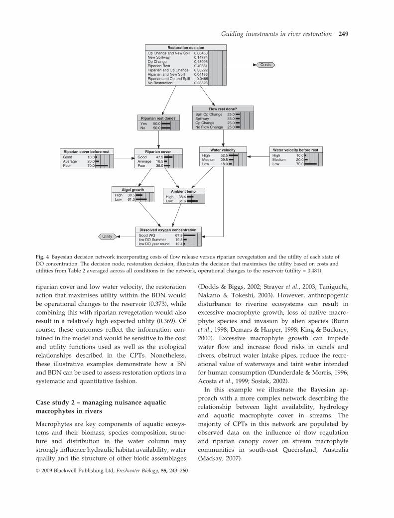
To illustrate this, we continue with the hypothetical
example of a small regulated river in a disturbed
catchment with poor riparian cover (Fig. 2). This BDN
is somewhat more complex than the initial BN
because it incorporates the pre-restoration riparian
and water velocity conditions (Fig. 4). There is also an
additional set of nodes reflecting the decision to be
made between the available restoration options (deci-
sion node, ‘restoration decision’), the costs of available
actions (cost node) and the value or utility of the
management outcomes (utility node). Since the initial
BN (Fig. 2b) was developed for an impaired site with
a highly modified catchment, we assume that the most
expensive level of riparian restoration would be
required to attain a desirable state of DO. The
restoration options we include in the decision node
are complete riparian restoration alone, the first two
flow options identified in Fig. 3b (changing opera-
tional rules; modifying infrastructure) and the com-
binations of these actions. The ‘no restoration’ action
is also included, for a total of eight options (Fig. 4).
Hypothetical examples of the relative costs for each
of the eight restoration options (cost node) are listed in
Table 2. These values are standardised on a scale of 0
to )1, with the most expensive option (full riparian
restoration and modifying dam infrastructure) having
the greatest relative cost ()1). Less expensive options
would have values greater than )1; operational
changes to the reservoir would be the least expensive
intervention with a cost of )0.15 (Table 2). Relative
utility is also assigned on a standardised scale, but
with positive values (0–1) to reflect the desirability of
the outcomes, and high water quality having the
maximum utility of 1 (Table 2). It is worth noting that
a high frequency of low DO events incurs a negative
utility due to the likelihood of additional costs
associated with water quality treatment or removal
of nuisance algae and dead fish, to remediate poor
water quality.
The numbers in the decision node in Fig. 4 show the
expected utility of each restoration action according to
the BDN, without specifying a specific ecological state
(as in Fig. 2b). Under this model, operational changes
to the reservoir and to a lesser extent riparian
restoration are sensible options to manage DO levels,
with the highest utilities of 0.48 and 0.4, respectively.
It is possible to specify ecological states in the network
represented in Fig. 4, in the same way as in Fig. 2c,d,
to identify which of the eight restoration strategies
maximises return (utility) for a specified set of
historical conditions (Table 3). For example, where
the preceding conditions were good riparian cover
and a low water velocity, the restoration option with
the maximum utility in the BDN (0.783) is a flow
operational change, but followed closely by no resto-
ration (0.776). By contrast, when preceding conditions
were poor riparian cover and a high water velocity,
the recommendation that would come out of the BDN
would be no restoration (0.583); however, riparian
restoration would also yield a relatively high expected
utility (0.552). Where preceding conditions are poor
2550 0100 75Riparian restoration
$$
(a) (b)
Good public land
Poor public land
Good private land
Poor private land
2550 0100 75Flow restoration
$$
Operational changes
New spillway eg
More operational changes
Dam removal
Fig. 3 Hypothetical cost functions for (a) riparian restoration whose costs increase in a relatively linear and incremental way
depending on initial riparian condition and land tenure status, (b) flow regime restoration whose costs increase in a more stepped
manner depending on the degree of infrastructure change that may be required to restore a more natural flow regime.
248 B. Stewart-Koster et al.
� 2009 Blackwell Publishing Ltd, Freshwater Biology, 55, 243–260
riparian cover and low water velocity, the restoration
action that maximises utility within the BDN would
be operational changes to the reservoir (0.373), while
combining this with riparian revegetation would also
result in a relatively high expected utility (0.369). Of
course, these outcomes reflect the information con-
tained in the model and would be sensitive to the cost
and utility functions used as well as the ecological
relationships described in the CPTs. Nonetheless,
these illustrative examples demonstrate how a BN
and BDN can be used to assess restoration options in a
systematic and quantitative fashion.
Case study 2 – managing nuisance aquatic
macrophytes in rivers
Macrophytes are key components of aquatic ecosys-
tems and their biomass, species composition, struc-
ture and distribution in the water column may
strongly influence hydraulic habitat availability, water
quality and the structure of other biotic assemblages
(Dodds & Biggs, 2002; Strayer et al., 2003; Taniguchi,
Nakano & Tokeshi, 2003). However, anthropogenic
disturbance to riverine ecosystems can result in
excessive macrophyte growth, loss of native macro-
phyte species and invasion by alien species (Bunn
et al., 1998; Demars & Harper, 1998; King & Buckney,
2000). Excessive macrophyte growth can impede
water flow and increase flood risks in canals and
rivers, obstruct water intake pipes, reduce the recre-
ational value of waterways and taint water intended
for human consumption (Dunderdale & Morris, 1996;
Acosta et al., 1999; Sosiak, 2002).
In this example we illustrate the Bayesian ap-
proach with a more complex network describing the
relationship between light availability, hydrology
and aquatic macrophyte cover in streams. The
majority of CPTs in this network are populated by
observed data on the influence of flow regulation
and riparian canopy cover on stream macrophyte
communities in south-east Queensland, Australia
(Mackay, 2007).
Dissolved oxygen concentration Good WQ low DO Summer low DO year round
67.8 19.8 12.4
Riparian cover Good Average Poor
47.5 16.5 36.0
Ambient temp High Low
38.4 61.6
Algal growth High Low
38.5 61.5
Water velocity High Medium Low
52.5 29.5 18.0
Costs
Riparian cover before rest Good Average Poor
10.0 20.0 70.0
Water velocity before rest High Medium Low
10.0 20.0 70.0
Utility
Riparian rest done? Yes No
50.0 50.0
Flow rest done? Spill Op Change Spillway Op ChangeNo Flow Change
25.0 25.0 25.0 25.0
Restoration decision Op Change and New SpillNew SpillwayOp ChangeRiparian RestRiparian and Op ChangeRiparian and New SpillRiparian and Op and Spill No Restoration
0.06453 0.14774 0.48096 0.40381 0.38222 0.04186 –0.0485 0.28828
Fig. 4 Bayesian decision network incorporating costs of flow release versus riparian revegetation and the utility of each state of
DO concentration. The decision node, restoration decision, illustrates the decision that maximises the utility based on costs and
utilities from Table 2 averaged across all conditions in the network, operational changes to the reservoir (utility = 0.481).
Guiding investments in river restoration 249
� 2009 Blackwell Publishing Ltd, Freshwater Biology, 55, 243–260
Data collection
Data for the network were obtained from macrophyte
surveys conducted at 19 locations (32 sites) in
regulated and non-regulated river systems in south-
east Queensland, Australia (Mackay, 2007). Sixteen of
the 32 sites were regulated directly by dams or weirs.
All sites were surveyed on two occasions (November
2003 and February–March 2004). Each site was an
individual hydraulic unit (riffle, run, pool) varying in
length from 20 to 40 m. Macrophyte cover was
estimated in 10 randomly positioned belt transects
(1 m wide) at each site as a proportion of the substrate
covered by macrophytes. Macrophyte cover exceeded
100% when multiple layers of macrophyte growth
occurred within a transect. The wetted width of each
transect was measured to the nearest 0.1 m with a
tape. Riparian canopy cover was estimated using a
spherical densiometer (Lemmon, 1956). Three mea-
surements were taken at equally spaced points on
each belt transect. Turbidity was recorded in situ with
a TPS WP89 data logger and TPS 125192 turbidity
probe (TPS, Brisbane, Australia) three measurements
per site, recorded in NTUs. Discharge data were
supplied by the Queensland Department of Natural
Resources and Water. A full description of data
collection methods is outlined in Mackay (2007).
Description of the macrophyte network
The BN describing macrophyte cover (MAC_COV) is
based on the conceptual model of Riis & Biggs (2001),
which describes the key environmental drivers of
macrophyte assemblage structure in terms of resource
supply (nutrients, light) and disturbance frequency
(hydrologic and hydraulic factors; Fig. 5), which can
be characterised by a variety of variables. We have
chosen factors that influence light conditions and
availability (LIGHT_AVAIL) and those that influence
hydrologic conditions (FLOOD_DIST) as drivers of
MAC_COV (Fig. 5), as these variables are known to
influence macrophyte assemblage structure in south-
east Queensland (Mackay, 2007) and they represent
environmental drivers potentially under management
control.
LIGHT_AVAIL is a function of two observed
predictor variables, riparian canopy cover (RIPCOV)
and turbidity (TURB; Fig. 5). RIPCOV indicates the
percentage of stream area that is directly covered by
the riparian canopy. As such RIPCOV is a function
of stream width and has a single parent node in the
network, (WIDTH). LIGHT_AVAIL has three catego-
ries (high, moderate, low). High LIGHT_AVAIL
represents favourable light conditions for macro-
phyte growth (i.e. low riparian canopy cover and
turbidity) whereas low LIGHT_AVAIL represents
poor light conditions for macrophyte growth (i.e.
high riparian canopy cover and turbidity). The
Table 2 Cost and utility functions for the restoration options in
Fig. 4
Restoration action Cost
Operational changes + new spillway )0.6
New spillway )0.5
Initial operational changes )0.15
Riparian restoration )0.4
Riparian + initial operational changes )0.55
Riparian + new spillway )0.9
Riparian + operational change + new spillway )1
No restoration 0
Water quality outcome Utility
No low DO events 1
Low risk of low DO events 0.4
High risk of low DO events all year )0.2
Relative costs are standardised from 0 to )1 and devised from
the cost functions illustrated in Fig. 3 with the most expensive
restoration action, riparian revegetation + operational chan-
ges + new spillway assigned a value of )1. The utility function
is also on a (0, 1) interval with the best water quality outcome
assigned a value of +1. The most undesirable water quality
outcome has a utility of )0.2 which represents likely costs of
clean up due to poor water quality.
Table 3 Expected utilities of different restoration options for
dissolved oxygen under three scenarios of preceding conditions
from Fig. 4
Preceding conditions
Water velocity Low High Low
Riparian cover Good Poor Poor
Restoration option Utility Utility Utility
Spill Op Change 0.354 0.024 )0.036
Spillway 0.443 0.124 0.043
OpChange 0.783 0.474 0.373
Level 4 Riparian 0.402 0.552 0.349
Level 4 Rip OpChange 0.397 0.424 0.369
Level 4 Rip Spill 0.057 0.074 0.03
Level 4 Rip SpillOp )0.034 )0.025 )0.059
No restoration 0.776 0.584 )0.02
Utility values for the restoration option with the maximum
expected utility for each scenario are bolded.
250 B. Stewart-Koster et al.
� 2009 Blackwell Publishing Ltd, Freshwater Biology, 55, 243–260
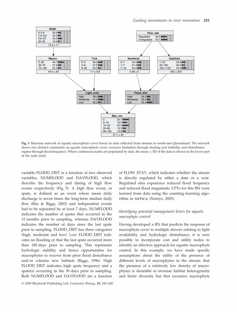
variable FLOOD_DIST is a function of two observed
variables, NUMFLOOD and DAYFLOOD, which
describe the frequency and timing of high flow
events respectively (Fig. 5). A high flow event, or
spate, is defined as an event where mean daily
discharge is seven times the long-term median daily
flow (Riis & Biggs, 2003) and independent events
had to be separated by at least 7 days. NUMFLOOD
indicates the number of spates that occurred in the
12 months prior to sampling, whereas DAYFLOOD
indicates the number of days since the last spate
prior to sampling. FLOOD_DIST has three categories
(high, moderate and low). Low FLOOD_DIST indi-
cates no flooding or that the last spate occurred more
than 180 days prior to sampling. This represents
hydrologic stability and hence opportunities for
macrophytes to recover from prior flood disturbance
and ⁄or colonise new habitats (Biggs, 1996). High
FLOOD_DIST indicates high spate frequency and a
spate(s) occurring in the 30 days prior to sampling.
Both NUMFLOOD and DAYFLOOD are a function
of FLOW_STAT, which indicates whether the stream
is directly regulated by either a dam or a weir.
Regulated sites experience reduced flood frequency
and reduced flood magnitude. CPTs for this BN were
learned from data using the counting–learning algo-
rithm in NETICANETICA (Norsys, 2005).
Identifying potential management levers for aquatic
macrophyte control
Having developed a BN that predicts the response of
macrophyte cover to multiple drivers relating to light
availability and hydrologic disturbance, it is now
possible to incorporate cost and utility nodes to
identify an effective approach for aquatic macrophyte
control. In this example, we have made specific
assumptions about the utility of the presence of
different levels of macrophytes in the stream: that
the presence of a relatively low density of macro-
phytes is desirable to increase habitat heterogeneity
and biotic diversity but that excessive macrophyte
Mac_cov00–1010–3333–6666–130
25.719.525.515.513.8
27.7 ± 34
Light_availHighModerateLow
38.041.820.2
Flood_distHighModerateLow
28.226.445.5
Dayflood1–3030–180180–1150
32.826.640.5
303 ± 350
Numflood0–11–77–16
34.431.334.4
5.38 ± 5
Turb0–33–88–35
39.037.523.5
7.7 ± 8.8
Ripcov0–3030–7070–100
49.727.922.4
40.5 ± 30
Width0–5.95.9–9.69.6–2020–50
26.923.033.516.6
13.4 ± 11
Flow_statRegulatedUnregulated
46.953.1
Fig. 5 Bayesian network of aquatic macrophyte cover based on data collected from streams in south-east Queensland. The network
shows two distinct constraints on aquatic macrophyte cover, resource limitation through shading and turbidity and disturbance
regime through flood frequency. Where continuous nodes are populated by data, the mean ± SD of the data is shown in the lower part
of the node itself.
Guiding investments in river restoration 251
� 2009 Blackwell Publishing Ltd, Freshwater Biology, 55, 243–260
cover is detrimental to ecosystem structure and
function. A utility value of )0.2 is assigned to high
macrophyte cover to reflect the cost of manual
removal that may be necessary with excessive
macrophyte growth. A utility of 1 is assigned to zero
macrophyte cover and values in the low range, which
provides some habitat and structural diversity with-
out clogging the channel. Finally, a utility of 0 is
assigned to intermediate cover values as this level of
cover is approaching the level of infestation. How-
ever, the utility values assigned to cover values in
practice would depend upon the position of the site(s)
of interest within the stream network. In heavily
shaded headwater streams that are naturally devoid
of vascular macrophytes (or characterised by non-
vascular macrophytes) greater utility value would be
assigned to zero or low cover categories. The utility
values used in this example are representative of
lowland streams.
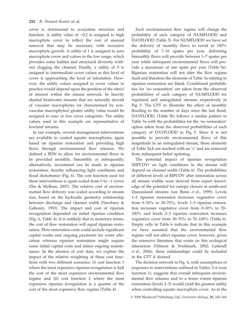
In our example, several management interventions
are available to control aquatic macrophytes, again
based on riparian restoration and providing high
flows through environmental flow releases. We
defined a BDN to allow for environmental flows to
be provided monthly, bimonthly or infrequently;
alternatively, investment can be made in riparian
restoration, thereby influencing light conditions and
flood disturbance (Fig. 6). The cost function used for
these interventions is again scaled from 0 to )1 (sensu
Zhu & McBean, 2007). The relative cost of environ-
mental flow delivery was scaled according to stream
size, based on the hydraulic geometry relationship
between discharge and channel width (Newbury &
Gaboury, 1993). The impact and cost of riparian
revegetation depended on initial riparian condition
(Fig. 6, Table 4). It is unlikely that in monetary terms,
the cost of flow restoration will equal riparian resto-
ration. Flow restoration costs could include significant
capital works and ongoing payments for water allo-
cation whereas riparian restoration might require
some initial capital costs and minor ongoing mainte-
nance. In the absence of cost data, we explore the
impact of the relative weighting of these cost func-
tions with two different scenarios: (i) cost function 1
where the most expensive riparian revegetation is half
the cost of the most expensive environmental flow
regime and (ii) cost function 2 where the most
expensive riparian revegetation is a quarter of the
cost of the most expensive flow regime (Table 4).
Each environmental flow regime will change the
probability of each category of NUMFLOOD and
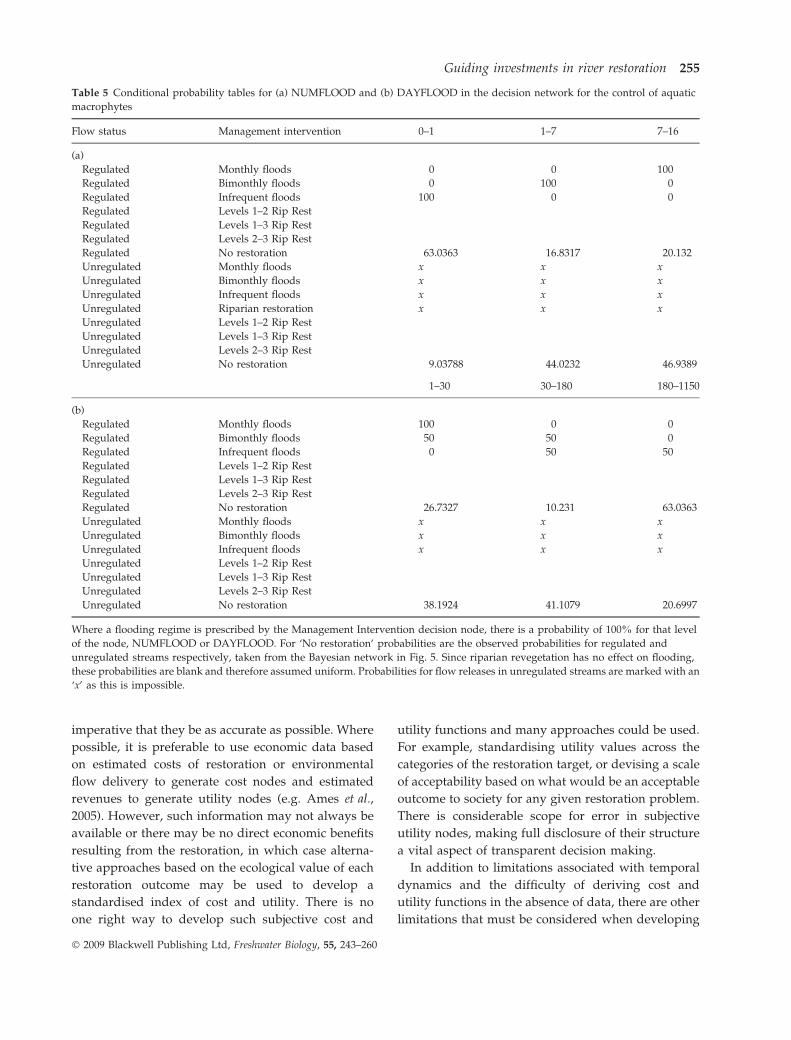
DAYFLOOD (Table 5). For NUMFLOOD we have set
the delivery of monthly flows to result in 100%
probability of 7–16 spates per year, delivering
bimonthly flows will provide between 1–7 spates per
year while infrequent environmental flows will pro-
vide a maximum of one spate per year (Table 5a).
Riparian restoration will not alter the flow regime
itself and therefore the elements of Table 5a relating to
riparian restoration are blank. Conditional probabili-
ties for ‘no restoration’ are taken from the observed
probabilities of each category of NUMFLOOD for
regulated and unregulated streams respectively in
Fig. 5. The CPT to illustrate the effect of monthly
flooding to the number of days since the last flood,
DAYFLOOD, (Table 5b) follows a similar pattern to
Table 5a with the probabilities for the ‘no restoration’
option taken from the observed probabilities of each
category of DAYFLOOD in Fig. 5. Since it is not
possible to provide environmental flows of this
magnitude in an unregulated stream, these elements
of Table 5a,b are marked with an ‘x’ and are removed
from subsequent belief updating.
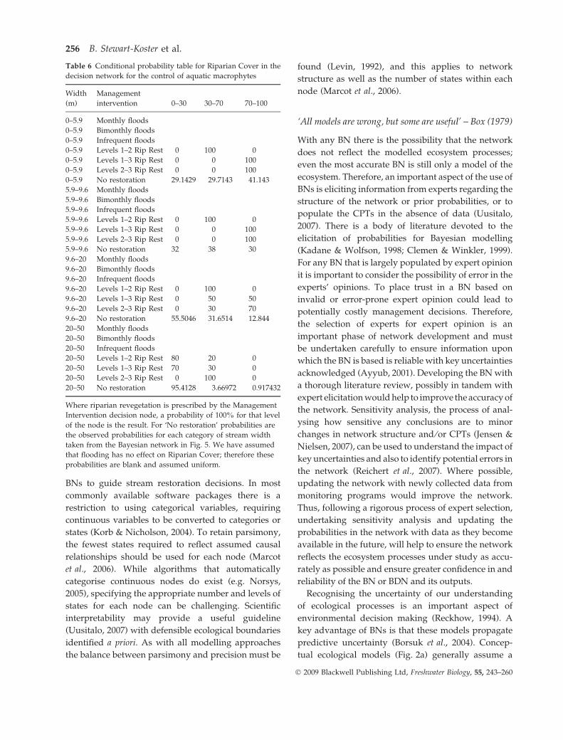
The potential impact of riparian revegetation
(RIPCOV) on light conditions in the stream will
depend on channel width (Table 6). The probabilities
of different levels of RIPCOV after restoration across
all stream widths were derived from expert knowl-
edge of the potential for canopy closure in south-east
Queensland streams (see Bunn et al., 1999). Levels
1–2 riparian restoration increases vegetative cover
from 0–30% to 30–70%, levels 1–3 riparian restora-
tion increases vegetative cover from 0–30% to 70–
100% and levels 2–3 riparian restoration increases
vegetative cover from 30–70% to 70–100% (Table 6).
Empty cells in Table 6 indicate that in this example
we have assumed that the environmental flow
regime will not affect riparian cover, however, given
the extensive literature that exists on this ecological
interaction (Nilsson & Svedmark, 2002; Latterell
et al., 2006), these relationships could be included
in the CPT if desired.
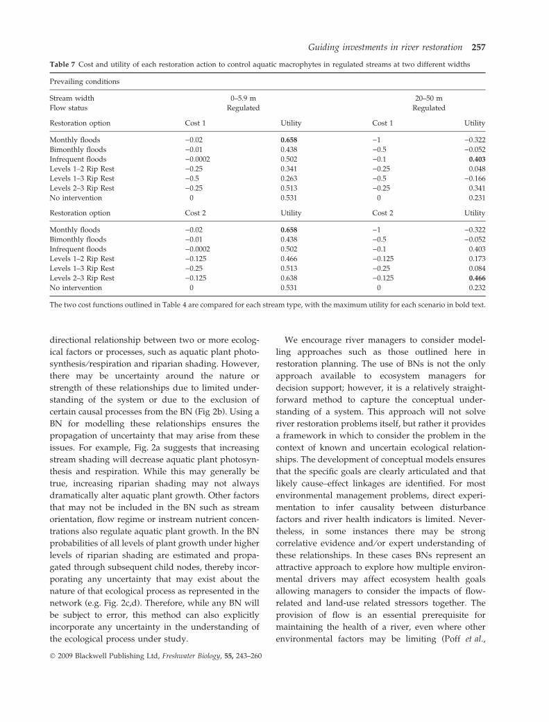
The decision network in Fig. 6, with assumptions of
responses to interventions outlined in Tables 3–6 (cost
function 1), suggests that overall infrequent environ-
mental flow releases and to a lesser extent riparian
restoration (levels 2–3) would yield the greatest utility
when controlling aquatic macrophyte cover. As in the
252 B. Stewart-Koster et al.
� 2009 Blackwell Publishing Ltd, Freshwater Biology, 55, 243–260
first case study, it is possible to manipulate the
network to identify the management action that
maximises utility at different stream types. It is also
apparent that predictions of maximum expected
utility depend on the cost function used (Table 7). In
narrow regulated streams, where the volume of water
required for a flood (and therefore the cost of
delivering it) is relatively low, the decision network
suggests that the provision of monthly environmental
flows is the management action that maximises utility,
under cost functions 1 and 2. Note that utility is
comparably high (0.638) for levels 2–3 riparian resto-
ration under cost function 2. However, in large
streams under cost function 1, providing infrequent
environmental flows maximises the expected utility in
the network, while levels 2–3 riparian restoration
maximises utility under cost function 2 (Table 7).
Thus there are recommendations of which restoration
option to adopt given the BDN and the associated cost
and utility functions.
Discussion
Anthropogenic impacts to rivers, such as flow regime
changes from river regulation and catchment and
riparian changes from land-use, seldom occur in
isolation from each other. However, in the presence
of multiple drivers of river health decline, it is often
difficult to identify a primary cause–effect relation-
ship to make rational decisions about river restoration
approaches. It therefore becomes necessary to incor-
porate ecological theory and understanding into the
restoration process (Lake, Bond & Reich, 2007). Even
if the potential causal factors are known, there is a
Light_conditionsGoodModeratePoor
17.235.047.8
Day flood1–3030–180180–1150
37.632.130.3
241 ± 320
Flood disturbanceHighModerateLow
31.831.436.8
Num flood0–11–77–16
33.533.033.5
5.34 ± 4.9
Turbidity0–33–88–35
39.037.523.5
7.7 ± 8.8
Riparian cover0–3030–7070–100
22.538.838.7
55.7 ± 29
Management interventionMonthly FlowsBi monthly FlowsInfrequent flowslvl1–lvl2 Riplvl1–lvl3 RipLvl2–lvl3 RipNo Intervention
0.427680.322740.478110.291900.162860.467010.44553
Costs
Utility
Flow statusRegulatedUnregulated
60.739.3
Stream width0–5.95.9–9.69.6–2020–50
26.923.033.516.6
13.4 ± 11
Macrophyte cover (%)00–1010–3333–6666–130
36.423.518.311.510.2
20.8 ± 31
Fig. 6 Bayesian decision network for the control of aquatic macrophytes in south-east Queensland streams. The decision node,
Management Intervention, illustrates that based on cost function 1 from Table 4 and utilities described in text, the decision that
maximises utility averaged across all conditions in the network is infrequent flows (utility = 0.478).
Guiding investments in river restoration 253
� 2009 Blackwell Publishing Ltd, Freshwater Biology, 55, 243–260
need to consider the costs of available river restoration
options with respect to their efficacy. BNs and BDNs
can be used to incorporate the costs of restoration
actions as well as the expected benefits (utility). Using
BNs in this way allows managers to make decisions
based on the ecological understanding of a system
with a quantitative basis.
Selecting restoration strategies under multiple stressors
We have demonstrated how BDNs can be used to
determine a restoration decision in the common
situation of multiple stressors impacting riverine
conditions. In this context, there can be various
restoration options available to a river manager.
However, it may not be clear as to which is going to
be the most effective relative to the costs of imple-
mentation and the expected ecological response.
Implementing a BDN approach provides decision
makers with a method of combining ecological
responses with budget constraints. We used simple
examples of specific ecosystem health goals, minimis-
ing low DO events and reducing nuisance macro-
phytes, to illustrate the approach without requiring
detailed and potentially confusing descriptions of
network structure and CPTs. As a consequence, the
results from the BDNs we developed may seem
unsurprising. However, in other scenarios with dif-
ferent river health goals such as biodiversity outcomes
or multiple indices of ecosystem health (e.g. Borsuk
et al., 2004; Said et al., 2006) the most effective resto-
ration option is unlikely to be so obvious. This
approach encourages river managers to consider
multiple stressors and potential restoration measures
in a transparent framework incorporating costs, ben-
efits and expected ecological response.
Dealing with the different timing of investment for
restoration strategies
When investing in vegetation restoration a large
proportion of the investment is incurred in the initial
phases, whereas the delivery of environmental flows
is likely to incur costs on an ongoing basis with costs
dependent on the volume of water released over time.
This presents an important challenge to consider as it
is difficult to incorporate temporal dynamics or
feedback loops in BNs (Uusitalo, 2007). However,
accounting for the difference in timing of the costs of
restoration and the accrual of utilities can be ap-
proached in various ways. In the networks presented
in this paper, we have treated costs and utilities over
the long-term assuming they will eventually be
recouped or incurred by including total costs and
utilities in a single node for each. An alternative
approach would be to include one utility node for
each time step over which the network was developed
(e.g. monthly) to represent the accrual of economic
benefits through a given year (Ames, 2002). Each
separate utility node then contributes to the overall
utility within the BN. The same approach can be used
for costs incurred over time. It is important to
consider the timing of the costs and utilities to be
incurred when developing the cost and utility func-
tions to successfully implement a BDN approach and
ensure transparent decision making.
Challenges when using Bayesian networks
It is clear that the nature of the cost and utility
functions will influence any conclusions about opti-
mal restoration options (Table 7); therefore it is
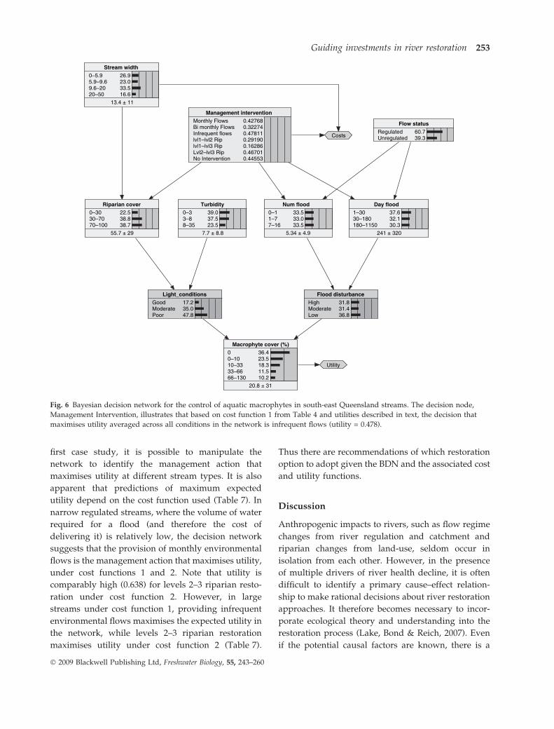
Table 4 Two possible cost functions for the control of aquatic
macrophytes standardised to a negative (0, 1) interval where the
action with the greatest cost, monthly floods in the widest
stream, has a cost of )1
Restoration action
Stream
width (m)
Cost
function 1
Cost
function 2
Monthly floods 0–5.9 )0.02 )0.02
Monthly floods 5.9–9.6 )0.05 )0.05
Monthly floods 9.6–20 )0.2 )0.2
Monthly floods 20–50 )1 )1
Bimonthly floods 0–5.9 )0.01 )0.01
Bimonthly floods 5.9–9.6 )0.025 )0.025
Bimonthly floods 9.6–20 )0.1 )0.1
Bimonthly floods 20–50 )0.5 )0.5
Infrequent floods 0–5.9 )0.0002 )0.0002
Infrequent floods 5.9–9.6 )0.005 )0.005
Infrequent floods 9.6–20 )0.02 )0.02
Infrequent floods 20–50 )0.1 )0.1
Levels 1–2 Rip Rest )0.25 )0.125
Levels 1–3 Rip Rest )0.5 )0.25
Levels 2–3 Rip Rest )0.25 )0.125
No intervention 0 0
Costs of flooding decrease according to the relationship between
channel width and discharge volume. The cost of riparian
revegetation is assumed constant across stream widths. Under
cost function 1, the most expensive riparian revegetation is half
the cost of the most expensive flood regime and under cost
function 2, the most expensive riparian revegetation is a quarter
of the cost of the most expensive flood regime.
254 B. Stewart-Koster et al.
� 2009 Blackwell Publishing Ltd, Freshwater Biology, 55, 243–260
imperative that they be as accurate as possible. Where
possible, it is preferable to use economic data based
on estimated costs of restoration or environmental
flow delivery to generate cost nodes and estimated
revenues to generate utility nodes (e.g. Ames et al.,
2005). However, such information may not always be
available or there may be no direct economic benefits
resulting from the restoration, in which case alterna-
tive approaches based on the ecological value of each
restoration outcome may be used to develop a
standardised index of cost and utility. There is no
one right way to develop such subjective cost and
utility functions and many approaches could be used.
For example, standardising utility values across the
categories of the restoration target, or devising a scale
of acceptability based on what would be an acceptable
outcome to society for any given restoration problem.
There is considerable scope for error in subjective
utility nodes, making full disclosure of their structure
a vital aspect of transparent decision making.
In addition to limitations associated with temporal
dynamics and the difficulty of deriving cost and
utility functions in the absence of data, there are other
limitations that must be considered when developing
Table 5 Conditional probability tables for (a) NUMFLOOD and (b) DAYFLOOD in the decision network for the control of aquatic
macrophytes
Flow status Management intervention 0–1 1–7 7–16
(a)
Regulated Monthly floods 0 0 100
Regulated Bimonthly floods 0 100 0
Regulated Infrequent floods 100 0 0
Regulated Levels 1–2 Rip Rest
Regulated Levels 1–3 Rip Rest
Regulated Levels 2–3 Rip Rest
Regulated No restoration 63.0363 16.8317 20.132
Unregulated Monthly floods x x x
Unregulated Bimonthly floods x x x
Unregulated Infrequent floods x x x
Unregulated Riparian restoration x x x
Unregulated Levels 1–2 Rip Rest
Unregulated Levels 1–3 Rip Rest
Unregulated Levels 2–3 Rip Rest
Unregulated No restoration 9.03788 44.0232 46.9389
1–30 30–180 180–1150
(b)
Regulated Monthly floods 100 0 0
Regulated Bimonthly floods 50 50 0
Regulated Infrequent floods 0 50 50
Regulated Levels 1–2 Rip Rest
Regulated Levels 1–3 Rip Rest
Regulated Levels 2–3 Rip Rest
Regulated No restoration 26.7327 10.231 63.0363
Unregulated Monthly floods x x x
Unregulated Bimonthly floods x x x
Unregulated Infrequent floods x x x
Unregulated Levels 1–2 Rip Rest
Unregulated Levels 1–3 Rip Rest
Unregulated Levels 2–3 Rip Rest
Unregulated No restoration 38.1924 41.1079 20.6997
Where a flooding regime is prescribed by the Management Intervention decision node, there is a probability of 100% for that level
of the node, NUMFLOOD or DAYFLOOD. For ‘No restoration’ probabilities are the observed probabilities for regulated and
unregulated streams respectively, taken from the Bayesian network in Fig. 5. Since riparian revegetation has no effect on flooding,
these probabilities are blank and therefore assumed uniform. Probabilities for flow releases in unregulated streams are marked with an
‘x’ as this is impossible.
Guiding investments in river restoration 255
� 2009 Blackwell Publishing Ltd, Freshwater Biology, 55, 243–260
BNs to guide stream restoration decisions. In most
commonly available software packages there is a
restriction to using categorical variables, requiring
continuous variables to be converted to categories or
states (Korb & Nicholson, 2004). To retain parsimony,
the fewest states required to reflect assumed causal
relationships should be used for each node (Marcot
et al., 2006). While algorithms that automatically
categorise continuous nodes do exist (e.g. Norsys,
2005), specifying the appropriate number and levels of
states for each node can be challenging. Scientific
interpretability may provide a useful guideline
(Uusitalo, 2007) with defensible ecological boundaries
identified a priori. As with all modelling approaches
the balance between parsimony and precision must be
found (Levin, 1992), and this applies to network
structure as well as the number of states within each
node (Marcot et al., 2006).
‘All models are wrong, but some are useful’ – Box (1979)
With any BN there is the possibility that the network
does not reflect the modelled ecosystem processes;
even the most accurate BN is still only a model of the
ecosystem. Therefore, an important aspect of the use of
BNs is eliciting information from experts regarding the
structure of the network or prior probabilities, or to
populate the CPTs in the absence of data (Uusitalo,
2007). There is a body of literature devoted to the
elicitation of probabilities for Bayesian modelling
(Kadane & Wolfson, 1998; Clemen & Winkler, 1999).
For any BN that is largely populated by expert opinion
it is important to consider the possibility of error in the
experts’ opinions. To place trust in a BN based on
invalid or error-prone expert opinion could lead to
potentially costly management decisions. Therefore,
the selection of experts for expert opinion is an
important phase of network development and must
be undertaken carefully to ensure information upon
which the BN is based is reliable with key uncertainties
acknowledged (Ayyub, 2001). Developing the BN with
a thorough literature review, possibly in tandem with
expert elicitation would help to improve the accuracy of
the network. Sensitivity analysis, the process of anal-
ysing how sensitive any conclusions are to minor
changes in network structure and ⁄or CPTs (Jensen &
Nielsen, 2007), can be used to understand the impact of
key uncertainties and also to identify potential errors in
the network (Reichert et al., 2007). Where possible,
updating the network with newly collected data from
monitoring programs would improve the network.
Thus, following a rigorous process of expert selection,
undertaking sensitivity analysis and updating the
probabilities in the network with data as they become
available in the future, will help to ensure the network
reflects the ecosystem processes under study as accu-
rately as possible and ensure greater confidence in and
reliability of the BN or BDN and its outputs.
Recognising the uncertainty of our understanding
of ecological processes is an important aspect of
environmental decision making (Reckhow, 1994). A
key advantage of BNs is that these models propagate
predictive uncertainty (Borsuk et al., 2004). Concep-
tual ecological models (Fig. 2a) generally assume a
Table 6 Conditional probability table for Riparian Cover in the
decision network for the control of aquatic macrophytes
Width
(m)
Management
intervention 0–30 30–70 70–100
0–5.9 Monthly floods
0–5.9 Bimonthly floods
0–5.9 Infrequent floods
0–5.9 Levels 1–2 Rip Rest 0 100 0
0–5.9 Levels 1–3 Rip Rest 0 0 100
0–5.9 Levels 2–3 Rip Rest 0 0 100
0–5.9 No restoration 29.1429 29.7143 41.143
5.9–9.6 Monthly floods
5.9–9.6 Bimonthly floods
5.9–9.6 Infrequent floods
5.9–9.6 Levels 1–2 Rip Rest 0 100 0
5.9–9.6 Levels 1–3 Rip Rest 0 0 100
5.9–9.6 Levels 2–3 Rip Rest 0 0 100
5.9–9.6 No restoration 32 38 30
9.6–20 Monthly floods
9.6–20 Bimonthly floods
9.6–20 Infrequent floods
9.6–20 Levels 1–2 Rip Rest 0 100 0
9.6–20 Levels 1–3 Rip Rest 0 50 50
9.6–20 Levels 2–3 Rip Rest 0 30 70
9.6–20 No restoration 55.5046 31.6514 12.844
20–50 Monthly floods
20–50 Bimonthly floods
20–50 Infrequent floods
20–50 Levels 1–2 Rip Rest 80 20 0
20–50 Levels 1–3 Rip Rest 70 30 0
20–50 Levels 2–3 Rip Rest 0 100 0
20–50 No restoration 95.4128 3.66972 0.917432
Where riparian revegetation is prescribed by the Management
Intervention decision node, a probability of 100% for that level
of the node is the result. For ‘No restoration’ probabilities are
the observed probabilities for each category of stream width
taken from the Bayesian network in Fig. 5. We have assumed
that flooding has no effect on Riparian Cover; therefore these
probabilities are blank and assumed uniform.
256 B. Stewart-Koster et al.
� 2009 Blackwell Publishing Ltd, Freshwater Biology, 55, 243–260
directional relationship between two or more ecolog-
ical factors or processes, such as aquatic plant photo-
synthesis ⁄ respiration and riparian shading. However,
there may be uncertainty around the nature or
strength of these relationships due to limited under-
standing of the system or due to the exclusion of
certain causal processes from the BN (Fig 2b). Using a
BN for modelling these relationships ensures the
propagation of uncertainty that may arise from these
issues. For example, Fig. 2a suggests that increasing
stream shading will decrease aquatic plant photosyn-
thesis and respiration. While this may generally be
true, increasing riparian shading may not always
dramatically alter aquatic plant growth. Other factors
that may not be included in the BN such as stream
orientation, flow regime or instream nutrient concen-
trations also regulate aquatic plant growth. In the BN
probabilities of all levels of plant growth under higher
levels of riparian shading are estimated and propa-
gated through subsequent child nodes, thereby incor-
porating any uncertainty that may exist about the
nature of that ecological process as represented in the
network (e.g. Fig. 2c,d). Therefore, while any BN will
be subject to error, this method can also explicitly
incorporate any uncertainty in the understanding of
the ecological process under study.
We encourage river managers to consider model-
ling approaches such as those outlined here in
restoration planning. The use of BNs is not the only
approach available to ecosystem managers for
decision support; however, it is a relatively straight-
forward method to capture the conceptual under-
standing of a system. This approach will not solve
river restoration problems itself, but rather it provides
a framework in which to consider the problem in the
context of known and uncertain ecological relation-
ships. The development of conceptual models ensures
that the specific goals are clearly articulated and that
likely cause–effect linkages are identified. For most
environmental management problems, direct experi-
mentation to infer causality between disturbance
factors and river health indicators is limited. Never-
theless, in some instances there may be strong
correlative evidence and ⁄or expert understanding of
these relationships. In these cases BNs represent an
attractive approach to explore how multiple environ-
mental drivers may affect ecosystem health goals
allowing managers to consider the impacts of flow-
related and land-use related stressors together. The
provision of flow is an essential prerequisite for
maintaining the health of a river, even where other
environmental factors may be limiting (Poff et al.,
Table 7 Cost and utility of each restoration action to control aquatic macrophytes in regulated streams at two different widths
Prevailing conditions
Stream width 0–5.9 m 20–50 m
Flow status Regulated Regulated
Restoration option Cost 1 Utility Cost 1 Utility
Monthly floods )0.02 0.658 )1 )0.322
Bimonthly floods )0.01 0.438 )0.5 )0.052
Infrequent floods )0.0002 0.502 )0.1 0.403
Levels 1–2 Rip Rest )0.25 0.341 )0.25 0.048
Levels 1–3 Rip Rest )0.5 0.263 )0.5 )0.166
Levels 2–3 Rip Rest )0.25 0.513 )0.25 0.341
No intervention 0 0.531 0 0.231
Restoration option Cost 2 Utility Cost 2 Utility
Monthly floods )0.02 0.658 )1 )0.322
Bimonthly floods )0.01 0.438 )0.5 )0.052
Infrequent floods )0.0002 0.502 )0.1 0.403
Levels 1–2 Rip Rest )0.125 0.466 )0.125 0.173
Levels 1–3 Rip Rest )0.25 0.513 )0.25 0.084
Levels 2–3 Rip Rest )0.125 0.638 )0.125 0.466
No intervention 0 0.531 0 0.232
The two cost functions outlined in Table 4 are compared for each stream type, with the maximum utility for each scenario in bold text.
Guiding investments in river restoration 257
� 2009 Blackwell Publishing Ltd, Freshwater Biology, 55, 243–260
1997, 2010; Bunn & Arthington, 2002). However, in
heavily regulated and sometimes over-allocated sys-
tems, the costs and benefits of purchasing water for
the environment need to be compared with the costs
and benefits of investing in other forms of restoration.
The use of BDNs provides a transparent, probabilistic
approach to support such decisions.
Acknowledgments
eWater Cooperative Research Centre provided the
funding for the senior author. Funding support was
also provided by the former CRC for Freshwater
Ecology and the CRC for Catchment Hydrology. We
thank Carmel Pollino for useful discussions on build-
ing BNs. We also thank David Strayer, Christer
Nilsson, Sandra Johnson and Angela Arthington for
providing helpful comments on earlier drafts of the
manuscript.
References
Acosta L.W., Sabbatini M.R., Fernandez O.A. & Burgos
M.A. (1999) Propagule bank and plant emergence of
macrophytes in artificial channels of a temperate
irrigation area in Argentina. Hydrobiologia, 415, 1–5.
Allan J.D. (2004) Landscapes and riverscapes: the
influence of land use on stream ecosystems. Annual
Review of Ecology, Evolution and Systematics, 35, 257–
284.
Ames D.P. (2002) Bayesian Decision Networks for Watershed
Management. PhD Thesis, Utha State University, Utah.
Ames D.P., Neilson B.T., Stevens D.K. & Lall U. (2005)
Using Bayesian networks to model watershed man-
agement decisions: an East Canyon Creek case study.
Journal of Hydroinformatics, 7, 267–282.
Arthington A.H. & Pusey B.J. (2003) Flow restoration and
protection in Australian rivers. River Research and
Applications, 19, 377–395.
Arthington A.H., Bunn S.E., Poff N.L. & Naiman R.J.
(2006) The challenge of providing environmental flow
rules to sustain river ecosystems. Ecological Applica-
tions, 16, 1311–1318.
Arthington A., Baran E., Brown C.A., Dugan P., Halls
A.S., King J.M., Minte-Vera C.V., Tharme R.E. &
Welcomme R.L. (2007) Water Requirements of Floodplain
Rivers and Fisheries: Existing Decision Support Tools and
Pathways for Development. International Water Manage-
ment Institute (Comprehensive Assessment of Water
Management in Agriculture Research Report 17),
Colombo, 74 pp.
Ayyub B.M. (2001) Elicitation of Expert Opinions for
Uncertainty and Risks. CRC Press, Boca Raton, FL.
Biggs B.J.F. (1996) Hydraulic habitat of plants in
streams. Regulated Rivers: Research and Management,
12, 131–144.
Bond N.R., Lake P.S. & Arthington A.H. (2008) The
impacts of drought on freshwater ecosystems: an
Australian perspective. Hydrobiologia, 600, 3–16.
Borsuk M.E., Stow C.A. & Reckhow K.H. (2004) A
Bayesian network of eutrophication models for syn-
thesis, prediction, and uncertainty analysis. Ecological
Modelling, 173, 219–239.
Box G.E.P. (1979) Robustness in the strategy of scientific
model building. In: Robustness in Statistics (Eds R.L.
Launer & G.N. Wilkinson), pp. 201–236. Academic
Press, New York, NY.
Broadmeadow S. & Nisbet T.R. (2004) The effects of
riparian forest management on the freshwater environ-
ment: a literature review of best management practice.
Hydrology and Earth System Sciences, 8, 286–305.
Bunn S.E. & Arthington A.H. (2002) Basic principles and
ecological consequences of altered flow regimes for
aquatic biodiversity. Environmental Management, 30,
492–507.
Bunn S.E., Davies P.M., Kellaway D.M. & Prosser I.P.
(1998) Influence of invasive macrophytes on channel
morphology and hydrology in an open tropical low-
land stream, and potential control by riparian shading.
Freshwater Biology, 39, 171–178.
Bunn S.E., Davies P.M. & Mosisch T.D. (1999) Ecosystem
measures of river health and their response to riparian
and catchment degradation. Freshwater Biology, 41,
333–345.
Castelletti A. & Soncini-Sessa R. (2007) Bayesian net-
works and participatory modelling in water resource
management. Environmental Modelling and Software, 22,
1075–1088.
Charniak E. (1991) Bayesian networks without tears. AI
Magazine, 12, 50–63.
Clemen R.T. & Winkler R.L. (1999) Combining probabil-
ity distributions from experts in risk analysis. Risk
Analysis, 19, 187–203.
Demars B.O.L. & Harper D.M. (1998) The aquatic
macrophytes of an English lowland river system:
assessing response to nutrient enrichment. Hydrobiolo-
gia, 384, 75–88.
Dodds W.K. & Biggs B.J.F. (2002) Water velocity atten-
uation by stream periphyton and macrophytes in
relation to growth form and architecture. Journal of
the North American Benthological Society, 21, 2–15.
Doledec S., Phillips N., Scarsbrook M., Riley R.H. &
Townsend C.R. (2006) Comparison of structural and
258 B. Stewart-Koster et al.
� 2009 Blackwell Publishing Ltd, Freshwater Biology, 55, 243–260
functional approaches to determining landuse effects
on grassland stream invertebrate communities. Journal
of the North American Benthological Society, 25, 44–60.
Dunderdale J.A.L. & Morris J. (1996) The economics of
aquatic vegetation removal in rivers and land drainage
systems. Hydrobiologia, 340, 157–161.
Jensen F.V. & Nielsen T.D. (2007) Bayesian Networks and
Decision Graphs. Springer, New York, NY.
Kadane J.B. & Wolfson L.J. (1998) Experiences in elicita-
tion. The Statistician, 47, 3–19.
King S.A. & Buckney R.T. (2000) Urbanization and exotic
plants in northern Sydney streams. Austral Ecology, 25,
455–461.
Korb K.B. & Nicholson A.E. (2004) Bayesian Artificial
Intelligence. Chapman and Hall, Boca Raton, FL.
Lake P.S., Bond N. & Reich P. (2007) Linking ecological
theory with stream restoration. Freshwater Biology, 52,
597–615.
Latterell J.J., Bechtold J.S., Naiman R.J., O’Keefe T.C. &
Van Pelt R. (2006) Dynamic patch mosaics and channel
movement in an unconfined river valley of the Olym-
pic Mountains. Freshwater Biology, 51, 523–544.
Lemmon P.E. (1956) A spherical densiometer for estimat-
ing forest overstorey density. Forest Science, 2, 314–320.
Levin S.A. (1992) The problem of pattern and scale in
ecology: the Robert H. MacArthur Award Lecture.
Ecology, 73, 1943–1967.
Lowrance R. (1998) Riparian forest ecosystems as filters
for nonpoint-source pollution. In: Successes, Limitations
and Frontiers in Ecosystem Science (Eds M.L. Pace & P.M.
Groffman), pp. 113–141. Springer, New York, NY.
Mackay S.J. (2007) Drivers of Macrophyte Assemblage
Structure in Southeast Queensland Streams. PhD Thesis,
Griffith University, Brisbane, Qld.
Magilligan F.J. & Nislow K.H. (2005) Changes in hydro-
logic regime by dams. Geomorphology, 71, 61–78.
Marcot B.G., Steventon J.D., Sutherland G.D. & McCann
R.K. (2006) Guidelines for developing and updating
Bayesian belief networks applied to ecological model-
ing and conservation. Canadian Journal of Forest
Research, 36, 3063–3074.
Mitchell V.G., Deletic A., Fletcher T.D., Hatt B.E. &
McCarthy D.T. (2007) Achieving multiple benefits
from stormwater harvesting. Water Science and Tech-
nology, 55, 135–144.
Naiman R.J., Bunn S.E., Nilsson C., Petts G.E., Pinay G. &
Thompson L.C. (2002) Legitimizing fluvial ecosystems
as users of water: an overview. Environmental Manage-
ment, 30, 455–467.
Newbury R. & Gaboury M. (1993) Exploration and
rehabilitation of hydraulic habitats in streams using
principles of fluvial behaviour. Freshwater Biology, 29,
195–210.
Nilsson C. & Svedmark M. (2002) Basic principles and
ecological consequences of changing water regimes:
riparian plant communities. Environmental Manage-
ment, 30, 468–480.
Nilsson C., Reidy C.A., Dynesius M. & Revenga C. (2005)
Fragmentation and flow regulation of the world’s large
river systems. Science, 308, 405–408.
Norsys (2005) NETICA. Available at: http://www.nor-
sys.com. (last accessed on 15 April 2009).
Paul M.J., Meyer J.L. & Couch C.A. (2006) Leaf break-
down in streams differing in catchment land use.
Freshwater Biology, 51, 1684–1695.
Poff N.L., Allan J.D., Bain M.B., Karr J.R., Prestegaard
K.L., Richter B.D., Sparks R.E. & Stromberg J.C. (1997)
The natural flow regime: a paradigm for river conser-
vation and restoration. BioScience, 47, 769–784.
Poff N.L., Allan J.D., Palmer M.A., Hart D.D., Richter
B.D., Arthington A.H., Rogers K.H., Meyer J.L. &
Stanford J.A. (2003) River flows and water wars:
emerging science for environmental decision making.
Frontiers in Ecology and the Environment, 1, 298–306.
Poff N.L., Olden J.D., Merritt D.M. & Pepin D.M. (2007)
Homogenization of regional river dynamics by dams
and global biodiversity implications. Proceedings of the
National Academy of Sciences of the United States of
America, 104, 5732–5737.
Poff N.L., Richter B.D., Arthington A.H. et al. (2010)
The ecological limits of hydrologic alteration
(ELOHA): a new framework for developing regional
environmental flow standards. Freshwater Biology, 55,
147–170.
Pollino C.A., Woodberry O., Nicholson A., Korb K. & Hart
B.T. (2007) Parameterisation and evaluation of a Bayes-
ian network for use in an ecological risk assessment.
Environmental Modelling and Software, 22, 1140–1152.
Qureshi M.E. & Harrison S.R. (2001) A decision support
process to compare riparian revegetation options in
Scheu Creek catchment in North Queensland. Journal of
Environmental Management, 62, 101–112.
Reckhow K.H. (1994) Importance of scientific uncertainty
in decision making. Environmental Management, 18,
161–166.
Reckhow K.H. (1999) Water quality prediction and
probability network models. Canadian Journal of Fish-
eries and Aquatic Sciences, 56, 1150–1158.
Reichert P., Borsuk M., Hostmann M., Schweizer S.,
Sporri C., Tockner K. & Truffer B. (2007) Concepts of
decision support for river rehabilitation. Environmental
Modelling and Software, 22, 188–201.
Richter B.D., Warner A.T., Meyer J.L. & Lutz K. (2006) A
collaborative and adaptive process for developing
environmental flow recommendations. River Research
and Applications, 22, 297–318.
Guiding investments in river restoration 259
� 2009 Blackwell Publishing Ltd, Freshwater Biology, 55, 243–260
Riis T. & Biggs B.J.F. (2001) Distribution of macrophytes
in New Zealand streams and lakes in relation
to disturbance frequency and resource supply: a
synthesis and conceptual model. New Zealand Journal
of Marine and Freshwater Research, 35, 255–267.
Riis T. & Biggs B.J.F. (2003) Hydrologic and hydraulic
control of macrophyte establishment and perfor-
mance in streams. Limnology and Oceanography, 48,
1488–1497.
Rutherford J.C., Marsh N.A., Davies P.M. & Bunn S.E.
(2004) Effects of patchy shade on stream water
temperature: how quickly do small streams heat and
cool? Marine and Freshwater Research, 55, 737–748.
Sadoddin A., Letcher R.A., Jakeman A.J. & Newham
L.T.H. (2005) A Bayesian decision network approach
for assessing the ecological impacts of salinity man-
agement. Mathematics and Computers in Simulation, 69,
162–176.
Said A. (2006) The implementation of a Bayesian network
for watershed management decisions. Water Resources
Management, 20, 591–605.
Said A., Sehlke G., Stevens D.K., Glover T., Sorenson D.,
Walker W. & Hardy T. (2006) Exploring an innovative
watershed management approach: from feasibility to
sustainability. Energy, 31, 2373–2386.
Sosiak A. (2002) Long-term response of periphyton
and macrophytes to reduced municipal nutrient load-
ing to the Bow River (Alberta, Canada). Canadian
Journal of Fisheries and Aquatic Sciences, 59, 987–
1001.
Strayer D.L., Beighley R.E., Thompson L.C., Brooks S.,
Nilsson C., Pinay G. & Naiman R.J. (2003) Effects of
land cover on stream ecosystems: roles of empirical
models and scaling issues. Ecosystems, 6, 407–423.
Taniguchi H., Nakano S. & Tokeshi M. (2003) Influences
of habitat complexity on the diversity and abundance
of epiphytic invertebrates on plants. Freshwater Biology,
48, 718–728.
Uusitalo L. (2007) Advantages and challenges of Bayes-
ian networks in environmental modelling. Ecological
Modelling, 203, 312–318.
Varis O. (1997) Bayesian decision analysis for environ-
mental and resource management. Environmental Mod-
elling and Software, 12, 177–185.
Varis O. & Kuikka S. (1999) Learning Bayesian decision
analysis by doing: lessons from environmental and
natural resources management. Ecological Modelling,
119, 177–195.
Walsh C.J., Waller K.A., Gehling J. & Mac Nally R. (2007)
Riverine invertebrate assemblages are degraded more
by catchment urbanisation than by riparian deforesta-
tion. Freshwater Biology, 52, 574–587.
Webb B.W., Hannah D.M., Moore R.D., Brown L.E. &
Nobilis F. (2008) Recent advances in stream and river
temperature research. Hydrological Processes, 22, 902–
918.
Wetzel R.G. (2001) Limnology: Lake and River Ecosystems.
Academic Press, San Diego, CA.
Zhu Z.J.Y. & McBean E.A. (2007) Selection of water
treatment processes using Bayesian decision network
analyses. Journal of Environmental Engineering and
Science, 6, 95–102.
(Manuscript accepted 11 March 2009)
260 B. Stewart-Koster et al.
� 2009 Blackwell Publishing Ltd, Freshwater Biology, 55, 243–260