Seediscussions,stats,andauthorprofilesforthispublicationat:http://www.researchgate.net/publication/272302570

TheTreatmentEffectofSchoolExclusiononUnemployment

ARTICLEinSSRNELECTRONICJOURNAL·JANUARY2014

DOI:10.2139/ssrn.2380956

CITATION

1

DOWNLOADS

11

VIEWS

20

2AUTHORS:

AlexSutherland

UniversityofCambridge

15PUBLICATIONS17CITATIONS

SEEPROFILE

ManuelPEisner

UniversityofCambridge

104PUBLICATIONS582CITATIONS

SEEPROFILE

Availablefrom:ManuelPEisner

Retrievedon:09September2015

Electronic copy available at: http://ssrn.com/abstract=2380956

The treatment effect of school exclusion onunemployment∗

Alex Sutherland†

Institute of Criminology

Manuel Eisner‡

Institute of Criminology

January 29, 2014

Abstract

Objectives: Fixed-term school exclusions are disciplinary sanctions on pupilsin response to serious aggressive or disruptive behaviour in schools. It is unclearwhether these sanctions aggravate future problems. Here we assess what impactfixed term exclusions have on later unemployment.Methods: We use data from the Longitudinal Study of Young People in Eng-land (LSYPE), a prospective cohort study of over 15,000 adolescents. We treatschool exclusion as an ‘intervention’ and apply propensity score matching to as-sess whether it has a treatment effect on unemployment.Results: We find a consistent difference between excluded and non-excludedchildren in their likelihood of being unemployed at aged 18/19. This effect rangesbetween 6-16 percentage points depending on the methodological approach taken.Conclusions: Our results suggest an independent effect of school exclusion onthe probability of being unemployed two years later, over and above numerousbaseline individual/family characteristics. To truly understand the effect exclu-sion has on young people, we suggest that high-quality cluster randomised trialsare needed.Keywords: school exclusion; unemployment; propensity score matching; multi-level modelling; cohort study.

∗We thank participants at the 2012 European Society of Criminology conference in Budapest for their commentson a presentation based on this paper. We are also grateful to Philippe Sulger and Ian White for their help and advicewith the research that lead to this article.†Institute of Criminology, Sidgwick Avenue, University of Cambridge, CB3 9DA Cambridge, UK; Phone: +44

(0)1223 746519, E-mail: as2140@cam.ac.uk.‡Institute of Criminology, Sidgwick Avenue, University of Cambridge, CB3 9DA Cambridge, UK; +44 (0)1223

335374, E-mail: mpe23@cam.ac.uk.

Electronic copy available at: http://ssrn.com/abstract=2380956

1 Introduction

In England, school exclusions are a disciplinary measure governed by the 2002 Educa-

tion Act (The Centre for Social Justice, 2011). The Act defines two types of exclusion:

Permanent exclusion means that a pupil is permanently removed from a school; fixed

period exclusions1 are exclusions from school for between one and a maximum of 45

days per school year (i.e. up to nine weeks in a given school year of 39 weeks). Across

England, substantial numbers of pupils are affected by school exclusion. In 2009/10,

there were 5,740 permanent exclusions, corresponding to 0.08% of the school popula-

tion. Fixed period exclusions are much more frequent. In 2009/10 there were 331,380

fixed period exclusions across all maintained primary, state-funded secondary and spe-

cial schools, meaning that 2.4% of the school population experience at least one fixed

period exclusion during a school year (Department for Education, 2011b).

Most school exclusions occur during secondary school, i.e. between ages 11 and 16,

with a peak during the last three years of compulsory school (i.e. Years 9-11). Amongst

these cohorts, 8.8% of male pupils and 4.1% of female pupils are excluded at least once

from school annually. In 2010/11 about 6.5% of pupils in England who were in the last

two years of compulsory education (years 10 and 11) experienced one or more fixed

period school exclusions for disciplinary reasons (Department for Education, 2011c).

These pupils are at a greatly increased risk of failing exams, not being in education,

employment or training (NEET) at ages 16-24, and having criminal convictions as

adolescents or young adults. Whilst there is evidence from a range of disciplines on the

association between exclusion and a host of negative outcomes, much of this evidence

relies on methodologies which are unsuited to establishing causal effects. In this paper

we use propensity score matching (PSM) to assess the impact of exclusion at aged

1These are also known as fixed term exclusions or ‘suspension’, all three terms are used inter-changeably throughout this paper.

1

15/16 on young people’s chance of being NEET at aged 18/19. This is important

as being NEET has significant economic costs. Coles et al. (2010:17) estimated, for

example, that the lifetime costs to the economy, the individual, their family and wider

society of a person who is NEET at ages 16-18 are about £105,000. With one-in-ten

16-18 year olds NEET at any one time in the UK — between two- and three-hundred

thousand young people — these costs are a significant burden on society.

2 Background

‘...there is little, if any, empirical evidence that school exclusions are

associated with a reduction or elimination of problematic behavior’ (Theriot

et al., 2010:13).

Despite being exposed to a series of individual, academic, socio-economic and fam-

ily risk factors, children who experience fixed period exclusions receive little specific

support. For pupils excluded for less than six days the only requirement is that schools

provide homework. For children excluded for six days or more schools must provide al-

ternative full-time education (the so-called ‘six-day rule’). Furthermore, head-teachers

arrange a reintegration interview with the parents for any child excluded at primary

school and for pupils excluded for more than five days at secondary schools.

National data show that the most frequent reasons for fixed term exclusions in the

UK were disruptive or aggressive behaviour, constituted by physical assault against a

pupil or an adult (24.2%), ‘persistent disruptive behaviour’ (23.8%) and verbal abuse

or threatening behaviour against an adult or pupil (24.9%) (Department for Education,

2011c). This pattern has been fairly consistent in recent years (see Petras et al. forth-

coming). As such, exclusions are largely responses to aggressive externalising behaviour

by children and young people at school. However, while exclusions are a disciplinary

2

tool mainly used in reaction to disruptive behaviours, headteachers have considerable

discretion about whether to exclude or not, and the length of the exclusion, as others

have noted (e.g. Macrae et al., 2003; Theriot et al., 2010). We know that, for instance,

enforcement around correct school uniform varies between schools: ‘One fundamental

factor in the decision to exclude is the ethos of the school, the discipline policies of

individual schools and the degree of tolerance maintained by different head teachers’

(Macrae et al., 2003:95). This suggests that a clearer understanding of perhaps idiosyn-

cratic differences (Galloway et al., 1985; Hayden, 2009) in school behavioural policies

and their enforcement is needed to capture, at the institutional level, what is driving

exclusion.2

2.1 Who is excluded?

Fixed term school exclusions affect some children disproportionately: Male pupils are

2.7-times more likely to be suspended from school than female pupils. Furthermore,

school exclusions affect children from poor and some minority backgrounds significantly

more often (Department for Education, 2011b). Thus, 21% of secondary-school pupils

eligible for free school meals experienced one or more fixed term exclusions in compar-

ison to 6.5% of other pupils. Similarly, pupils of ‘Caribbean’ (17.2%), ‘white and black

Caribbean’ (17.2%) and ‘Black’ (13.5%) background are considerably overrepresented,

while pupils of ‘Indian’ (2.5%) and ‘Asian’ (4.1%) background are underrepresented.

At the family level, excluded children are more likely to come from families that are

under stress, have no employment, are experiencing multiple disadvantage and where

2‘School ethos’ (AKA ‘school climate’ in the US) features heavily in discussions about thepossible criminogenic effects of school, and the extent to which school effects exist (see Rut-ter et al., 1979; Boxford, 2006). There is even a ‘National School Climate Center’ in the UShttp://www.schoolclimate.org/climate/. A principal component of climate/ethos is discipline,but to suggest that schools with ‘better’ discipline have lower levels of problem behaviour is hardlygroundbreaking. What is more interesting is understanding why school disciplinary climate varies.

3

parents themselves had experienced difficulties at school (Macrae et al., 2003). Fur-

thermore, children with special educational needs (SEN) are around eight times more

likely to be excluded than those without SEN (Department for Education, 2011b). For

example, in secondary schools across England, 12.3% of pupils with SEN who had a

statement (a document that obliges schools to provide specific help) were suspended in

2009/10. Rates of exclusion are very similar for pupils with special educational needs

but without a statement (12.0%). In comparison, only 2.8% of students without SEN

experienced school exclusion (Department for Education, 2011b). Furthermore, many

of those who end up being excluded from secondary school may have had educational

difficulties which were ‘inadequately appreciated or addressed during their years in pri-

mary education’ (Macrae et al., 2003:91). Finally, rates of fixed period and permanent

exclusions have been found to be 10-25 times higher for children with persistent mental

disorders, especially conduct disorder and hyperkinetic disorders (Meltzer et al., 2003).

Whilst there is some variation over time, patterns of exclusion do not appear to

have changed substantially since the mid-1990s. In short, it is still the same ‘sorts’

of children being excluded from school in terms of family breakdown, deprivation and

other social issues (Munn et al., 2000).

2.2 Effects of school exclusion

School exclusion has been found to be related to poor academic and occupational

outcomes (Massey, 2011; Sparkes, 1999), externalizing behavior including crime (Gra-

ham, 1988) and negative internalizing outcomes, such as self-harm (McAra and McVie,

2010). Gilbertson (1998) showed that 42% of sentenced juvenile offenders had expe-

rienced previous school exclusion. Speilhofer et al. (2009) showed that amongst those

young people who were in sustained NEET, the majority had experienced previous

prior exclusions and truancy. A recent study also suggests that approximately 50%

4

of excluded children become NEET within two years after their exclusion (Massey,

2011). Taken together these data suggest that children who are subject to temporary

or permanent school exclusion are at a much greater risk of behavioral, health-related,

occupational and educational difficulties.

While there is evidence supporting a correlation between school exclusion and later

adverse outcomes, it is currently unclear whether the disciplinary action itself has a

causal effect over and beyond the social, familial and behavioral characteristics of the

affected children. To date, studies have used analytical approaches that are unable

to reliably establish a robust link between exclusion and outcomes such as criminal

behavior. Typically, exclusion has not been the focus of these studies and is simply

a ‘risk factor’ that is ‘controlled for’ during analyses. Our aim is to use data from a

pre-existing longitudinal study to examine the short- and long-term effects of school

exclusion on a range of behavioral outcomes utilizing statistical approaches which are

more appropriate for estimating causal effects from observational data.

Theoretically, there exist (at least) three possible relationships between school ex-

clusion and being NEET. The first is that the exclusions are mere markers of levels

of problem behaviour without any genuine causal effects on subsequent behaviour. If

true, one would expect that excluded and non-excluded children with the same combi-

nation of characteristics and behaviour will not differ in later behaviour. The second

possibility is that exclusions achieve a deterrent or ‘correctional effect’ on the child

and reduce the risk of later negative developments. The third possibility is that exclu-

sions are linked to a series of unfavourable effects such as negative labelling, further

disengagement from school, exposure to criminogenic environments (Wikstrom et al.,

2012) and fewer learning opportunities - which all increase the risk of later problem

behaviours over and above the likelihood of such behaviours prior to the exclusionary

event.

5

3 Data and methods

The data used here come from the Longitudinal Study of Young People in England

(LSYPE) which is funded and run by the Department for Education (DfE). LSYPE is

a multi-site panel study of school children across England and was primarily intended

to study the progress of a cohort of young people through secondary school, further

and higher education, as well as transitions into work. A summary is given here of the

sampling strategy and attrition rates, more information about the study can be found

on the Department for Education website (www.education.gov.uk) and the LSYPE

user guide (Department for Education, 2011a). In addition, we combined data from

LSYPE with administrative data from the National Pupil Database (NPD), which is

also held by the DfE. Data were linked using anonymous Pupil Matching Reference

Numbers (PMR). We use NPD exclusion data corresponding to wave three of LSYPE

(2006) because this is the first year that these data were collated centrally by the

Department for Education.

3.1 LSYPE: sampling

Sampling for the study was achieved via a stratified random sample with dispropor-

tionate sampling for deprived schools. Schools were the primary sampling units, then

children within schools. Children from major ethnic minority backgrounds were over-

sampled at pupil level (Department for Education, 2011a). Data collection initially

took place in schools and began in 2004 when children were in Year 9 (aged 13/14),

continuing until 2010 (resulting in seven waves of data).

The initial sample for LSYPE was 15,770 children from 658 schools. There was

attrition between waves (see Table 1). Two strategies were employed by the DfE

research team to account for non-response: analytic weights and a booster sample

6

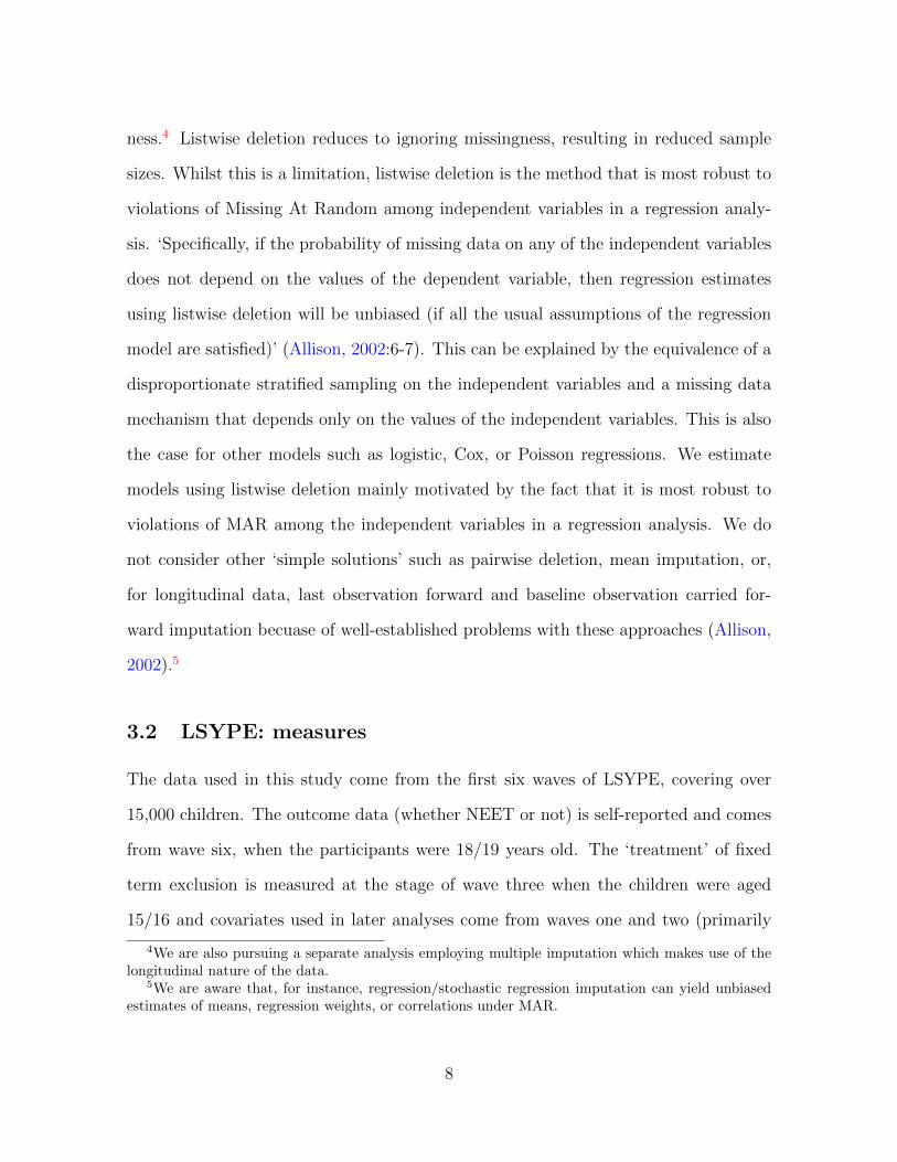
in wave four.3 Table 1 shows that there is attrition from the study from wave four

onwards, which reached nearly 40% by wave six. Data loss presents us with difficulties

- namely that analyses may be biased by selective attrition and suffer a loss of statistical

power.

Table 1: Attrition in LSYPE

Wave 1 Wave 2 Wave 3 Wave 4 Wave 5 Wave 6Surveys issued 21,000 15,678 13,525 12,410 11,793 11,225Responses 15,770 13,539 12,439 11,801 10,430 9,799Response rate 75% 86% 92% 95% 88% 87%Response rate from w1 sample 100% 86% 79% 75% 66% 62%

Note: In wave four a ‘booster’ sample consisted of 600 surveys was issued, with 352 responses (59%),taking the total sample for wave four to 16,122 but we ignore these cases in our analysis.

Of concern is missingness on the outcome variable, being NEET at aged 18/19. The

missing rate for this variable is nearly 40% (there were 9,554 out of 15,770 potential

observations, see Table A in Appendix A). When faced with attrition and missingness,

the question is whether the available data still ‘represent’ the population of interest,

i.e. whether the statistical procedure leads to valid and efficient inferences about the

population the sample is drawn from (Schafer and Graham, 2002:149). Many articles

do not acknowledge these issues instead opting to overlook missingness or otherwise

pretend it does not matter for results. We feel it is important to spell out the potential

impact missing data may have and how we deal with the issue in this paper.

3.1.1 Missing data

Our approach to missing data in this paper is to assume that data are Missing Com-

pletely At Random (MCAR) and employ listwise deletion as our approach to missing-

3The booster sample consisted of 352 new participants, taking the total possible sample in thatwave to 16,122 (see note for Table 1). We exclude observations from the booster sample becausewe base our propensity score estimation on measures gathered in earlier waves that do not containinformation from these individuals.

7

ness.4 Listwise deletion reduces to ignoring missingness, resulting in reduced sample

sizes. Whilst this is a limitation, listwise deletion is the method that is most robust to

violations of Missing At Random among independent variables in a regression analy-

sis. ‘Specifically, if the probability of missing data on any of the independent variables

does not depend on the values of the dependent variable, then regression estimates

using listwise deletion will be unbiased (if all the usual assumptions of the regression

model are satisfied)’ (Allison, 2002:6-7). This can be explained by the equivalence of a

disproportionate stratified sampling on the independent variables and a missing data

mechanism that depends only on the values of the independent variables. This is also

the case for other models such as logistic, Cox, or Poisson regressions. We estimate

models using listwise deletion mainly motivated by the fact that it is most robust to

violations of MAR among the independent variables in a regression analysis. We do

not consider other ‘simple solutions’ such as pairwise deletion, mean imputation, or,

for longitudinal data, last observation forward and baseline observation carried for-

ward imputation becuase of well-established problems with these approaches (Allison,

2002).5

3.2 LSYPE: measures

The data used in this study come from the first six waves of LSYPE, covering over

15,000 children. The outcome data (whether NEET or not) is self-reported and comes

from wave six, when the participants were 18/19 years old. The ‘treatment’ of fixed

term exclusion is measured at the stage of wave three when the children were aged

15/16 and covariates used in later analyses come from waves one and two (primarily

4We are also pursuing a separate analysis employing multiple imputation which makes use of thelongitudinal nature of the data.

5We are aware that, for instance, regression/stochastic regression imputation can yield unbiasedestimates of means, regression weights, or correlations under MAR.

8

one). Overall there were 905 fixed-term exclusions, meaning that roughly 6% of the

sample were excluded in that school year.

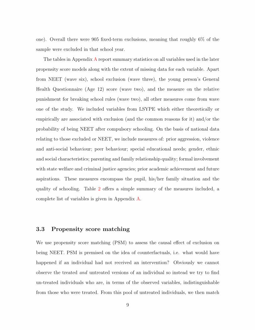
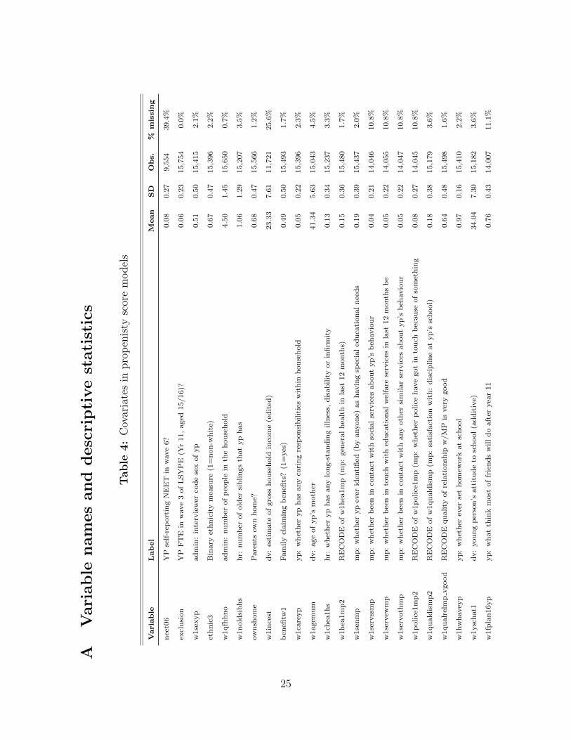
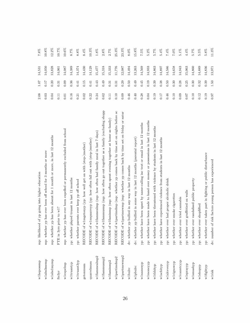
The tables in Appendix A report summary statistics on all variables used in the later

propensity score models along with the extent of missing data for each variable. Apart

from NEET (wave six), school exclusion (wave three), the young person’s General

Health Questionnaire (Age 12) score (wave two), and the measure on the relative

punishment for breaking school rules (wave two), all other measures come from wave

one of the study. We included variables from LSYPE which either theoretically or

empirically are associated with exclusion (and the common reasons for it) and/or the

probability of being NEET after compulsory schooling. On the basis of national data

relating to those excluded or NEET, we include measures of: prior aggression, violence

and anti-social behaviour; peer behaviour; special educational needs; gender, ethnic

and social characteristics; parenting and family relationship quality; formal involvement

with state welfare and criminal justice agencies; prior academic achievement and future

aspirations. These measures encompass the pupil, his/her family situation and the

quality of schooling. Table 2 offers a simple summary of the measures included, a

complete list of variables is given in Appendix A.

3.3 Propensity score matching

We use propensity score matching (PSM) to assess the causal effect of exclusion on

being NEET. PSM is premised on the idea of counterfactuals, i.e. what would have

happened if an individual had not received an intervention? Obviously we cannot

observe the treated and untreated versions of an individual so instead we try to find

un-treated individuals who are, in terms of the observed variables, indistinguishable

from those who were treated. From this pool of untreated individuals, we then match

9

Table 2: Summary of variables

Type Wave Example variablesDemographics 1 YP gender, ethnicity, month of birthParental characteristics 1 age of motherFamily structure 1 married, no. people in HH, no. older siblingsFamily socioeconomic status 1 housing tenure, NS-SEC class, HH incomeFamily relationships 1 quality of relationship, frequency of arguingYPs health 1&2 physical health, concentration, sleep, GHQ scoreSpecial Educational Needs 1 whether YP ever identified as having SENYP truancy or prior exclusion 1 times truant, prior temp. or perm. exclusionsYP ed. aspirations of YP/peers 1 future schooling plansYP victimisation 1 being bullied, violenceYP anti-social behaviour 1 substance use, fighting, bullyingYP prior attainment 1 YP Key Stage 2 average point scoreParental supervision 1 child whereabouts, compliance with disciplineParental satisfaction 1 with schooling, school disciplineAgency involvement 1 Criminal justice or social servicesExclusion (NPD) 3 National Pupil DatabaseNEET 6 Self-report from LSYPE

to the treated based upon the predicted probability of receiving ‘treatment’ (in this

case, being excluded from school). So if two individuals have a p=.25 chance of being

excluded based on a given set of covariates, those covariates will then not distinguish

between those who did and did not receive treatment. This approach means that two

individuals with different characteristics can be matched if their probabilities are very

close to each other. The predicted probability acts as a ‘balancing score’ between

the two groups of intervention and non-intervention, where ‘balance’ refers to equity

of factors which are relevant for both intervention assignment and the outcome of

interest.6 In short, we want the two groups to be as similar as possible except for the

intervention. It is important to note that achieving balance depends on the quality of

the covariates. Here, we use variables that closely match the characteristics of those

6Guidance on this point is inconsistent, e.g. ‘matching variables should affect both the outcomeand treatment equations’ (Blundell et al., 2003:12); versus ‘unless a variable can be excluded becausethere is a consensus that it is unrelated to outcome or is not a proper covariate, it is advisable toinclude it in the propensity score model even if it is not statistically significant’ (Rubin and Thomas,1996:253).

10

who are excluded or NEET based on national statistics: prior aggressive, violent or

anti-social behaviour; special educational needs; academic ability; family background;

ethnic and social characteristics; parenting, as well as other factors such as physical

and mental health.

The precise matching approach depends largely on the size of the pool of potential

comparison cases (Dehejia and Wahba, 2002). We apply a three-to-one matching ap-

proach with replacement and a caliper setting, meaning we try to match each treated

individual to three non-treated individuals who were indistinguishable in terms of co-

variates from the treated group. ‘With replacement’ means that non-treated individu-

als who are similar to many treated individuals can be used repeatedly, which has the

advantage of reducing bias (Stuart, 2010). The matches are then equally weighted. We

set the caliper to 0.25 of a standard deviation of the propensity score, meaning that

we are demanding matches with individuals similar in terms of propensity and thus we

can be more confident of a ‘like with like’ comparison. In the case of tied propensity

scores, we specified that ties were randomly broken.

As with any method, PSM has its limitations. The primary issue is that PSM relies

upon the explicit assumption that given a set of observed confounders, assignment to

intervention is exogenous in the sense that the assignment to the treatment or control

group and (potential) outcomes are conditionally independent (Rosenbaum and Rubin,

1983; Dehejia and Wahba, 2002). In other words, taking into account what we observe

(e.g., the demographic or criminogenic variables and by implication the propensity

score), treatment assignment is viewed ‘as random’. As with any modelling approach,

this means that PSM is only as good as the data being used and the technique is largely

premised on complete data (Stuart, 2010).

A final consideration for matching is that LSYPE data are, by the nature of the

sampling design, clustered by school. Therefore it is likely that unobserved school-

11

specific characteristics (e.g., school disciplinary policies) affect the likelihood of being

excluded and also the outcome (being NEET). Following Arpino and Mealli (2011), we

account for the hierarchical nature of the data when estimating the propensity score

by using multilevel models7 via the xtmelogit command in Stata 12 (StataCorp., 2011)

In the following sections we employ a variety of approaches, either singly or in

combination, which deal with clustering and/or confounding. We pursue different

strategies in order to assess the sensitivity of results to model specification and to

show the effect of different adjustments on results.

4 Results

We first present a ‘crude’ comparison between the means of the treated and untreated

group. This provides a basis for judging how much confounding we have adjusted for

in later models. The first set of results in Table 3, a simple t-test, shows that the

unadjusted likelihood of becoming NEET for excluded youths is about 15 percentage

points higher than those in the non-excluded group. As a next step, we present results

from a multilevel linear probability model (LPM) with NEET as the outcome.8 Here,

we are implicitly assuming that the treatment assignment is unconfoundend conditional

on the covariates we include in the regression alongside school exclusion. The set of

these covariates is the same as those we believe are important in influencing and/or

moderating the likelihood of being excluded or not and its effect on the likelihood of

7Arpino and Mealli (2011)’s simulations suggest that a dummy variable approach to account forclustering is the ‘best’ performing method to reduce potential bias in the propensity score due toomitted cluster-characteristics, and that the incidental parameter problem (Neyman and Scott, 1948)does not seem to affect the quality in terms of bias and efficiency. However, we have about 650schools and due to missingness in the data and lack of sufficient degrees of freedom, a dummy variableapproach is not feasible. Instead we opted for the ‘second-best’ approach (according to Arpino andMealli, 2011), by modelling the treatment-outcome by means of a multilevel random intercept logitmodel (Model 2 in Arpino and Mealli, 2011:1773).

8With all linear probability models presented, we use robust standard errors.

12

being NEET later on. A legend for the confounders’ is given in Appendix A. Result

(2) in Table 3 presents the result from this showing a positive but marginally non-

significant effect of exclusion on the likelihood being NEET (b 0.058, p 0.054). However,

the regression approach assumes that for each combination of covariates we have good

comparison pairs between treated and untreated individuals, which is unlikely to be

the case. We next turn to matching in order to tackle this.

We run a multilevel logistic regression with exclusion as the outcome variable to

derive the propensity score and do three-to-one matching with replacement and a

caliper set to 0.25 of a standard deviation of the propensity score, where ties are

randomly broken. The matching was successful as only one of the matching variables

was out of balance based on a t-test at the 5%-significance level.9 The results are

given as model (3) in Table 3. We report the Average Treatment Effect on the Treated

(ATT), finding a significant difference between treated and untreated groups amounting

to roughly thirteen percentage points (b 0.126; se 0.025; p ≤ .001).

As a means of checking our matching approach we also estimate models using

inverse probability weighting (IPW) which attempts to make two groups comparable

using the inverse of the propensity score as a regression weight.10 This weight generates

‘replicas’ of individuals in the treatment and control groups (referred to as ‘potential

samples’ or ‘pseudo-populations’; Williamson et al. (2012)). These serve as proxies

for samples where everyone received treatment or no-one received treatment. We then

compare the outcomes for the two potential samples. The results from the IPW are

given below. We estimated a linear probability model with NEET as the dependent

variable and exclusion as the independent variable, with weights as specified above.

Using this approach we again observe a positive relationship between being excluded

9We would expect to observe 4.7 variables (94 × 0.05) to be out of balance by chance if we hadimplemented a randomized experiment with 94 covariates.

10The weight to estimate the ATT is 1 if excluded and pscore/(1−pscore) if not (Williamson et al.,2012).

13

and being NEET, equating to roughly eight percentage points (b 0.083, p 0.14, 95% CI

2–15%).11

Table 3: Treatment effect of fixed term exclusion on the probability of being NEET

Model Result SE p 95% CI LB 95% CI UB

1. t-test 0.157a 0.021 .000 0.115 0.199

2. Multilevel Linear Probability Model 0.058a 0.030c .054 -0.001 0.117

3. Propensity Score Matching 0.126a,b 0.025 .000 0.077 0.175

4. Linear Probability Model w/IPW 0.083a 0.034c .014 0.017 0.149

a: Difference in proportion NEET at aged 18/19 between excluded and non-excluded groups.b: Average Treatment Effect on the Treated (ATT).c: Cluster robust standard errors.

5 Discussion

The relationship between school exclusion and later outcomes is rarely the direct focus

of research. Here, we have attempted to disentangle the relationship between school ex-

clusion and the later probability of educational or economic inactivity using a variety of

methods. As set out earlier in this paper, there are at least three possible relationships

between school exclusion and being NEET. The first is that exclusions are proxies for

problematic behaviour, with variation in exclusions being a function of, for example,

school-level differences in behaviour management policy/enforcement. If this were the

case then after adjustment for prior problem behaviour and other measures we would

expect to find no difference in the likelihood of later outcomes for excluded versus non-

excluded young people. The second is that exclusion might exert a corrective effect on

11Running the IPW model as a logistic model (also with cluster-robust standard errors) gives anodds-ratio of 1.74 (se .420, p .022, 95% CI 1.08–2.79).

14

those subject to it and thus reduce the later risk of negative outcomes. The third is

that exclusions are part of a series of additional barriers to acquiring social and edu-

cational capital that include labelling, school disengagement (perhaps arising from the

exclusion) and the resultant reduction in opportunities for education or employment.

Here exclusion may serve to actually increase the risk of later problems, even when

taking into account the problem behaviours which triggered the exclusion(s) in the

first place (e.g. by introducing ‘problem’ children to unsupervised ‘free time’ which is

likely to exacerbate anti-social behaviour, especially those more sensitive to situational

triggers – see Wikstrom et al., 2012).

Using a variety of models that adjust for confounding and clustering we find that

breaching school rules and being temporarily excluded from school at aged 15/16 is pos-

itively associated with being NEET at 18/19 years of age. Specifically, our results show

an average 10 percentage point difference in the likelihood of being Not in Education,

Employment or Training (NEET) at aged 18/19 between excluded and non-excluded

young people. So, for every 100 NEET young adults who were not excluded, there

would be 110 who had been excluded. This is not a large effect, but given everything

else which influences being NEET (e.g. the job market, business cycles), it is perhaps

surprising to find an effect at all.

However, it would be wrong to assert that exclusion itself solely or even directly

‘caused’ the higher proportion of NEET excludees. In our dataset, the intervention

(fixed term exclusion) took place during Year 11, at the time, the final year for com-

pulsory schooling in England. The outcome, being NEET, is observed two-to-three

years later. Being excluded in the final year of compulsory schooling could have had

a detrimental effect on exam performance due to the disruption to studying caused

by not being at school. Poor exam performance is then related to a higher likelihood

of being NEET because of the premium placed on school grades by employers and

15

education establishments (Bynner and Parsons, 2002). This is just one, fairly obvious,

factor between being excluded from school and being NEET after leaving school. But

this does not mean we should not think about the policy of exclusion or attempt to

address its potential (in)direct consequences. Given the association between exclusion

and negative consequences such as dropping out of education, delinquency and gen-

erally poor academic attainment, it seems sensible to place this policy under further

theoretical and empirical scrutiny.

6 Limitations

This study has a number of important strengths. First, it uses a large, longitudinal

and nationally representative survey/administrative dataset to tackle the question at

hand. Second, we employ a combination of methods that adjust for problems such as

clustering of observations and we explicitly focus on the estimation of causal effects of

exclusion by using an approach novel to this area of research. However, there remain

some limitations with our paper that we discuss below.

Conscious of the potential difficulty in defending the Missing Completely At Ran-

dom (MCAR) assumption with respect to being NEET, and illustrating that selection

on the dependent variable might be of concern, we were motivated to model the joint

distribution of the data and the missing data mechanism by means of a Heckman

selection model (Heckman, 1979). However, we encountered two problems with the

Heckman approach which is why we did not report the results here. First, when run-

ning the Heckman two-step model in Stata 12 (via the heckprob command) the second

stage probit model would not converge.12 Second, and more importantly, one assump-

12We also ran the model with a linear probit model at the second stage using the heckman commandwhich did converge, producing a similar point estimate and standard error for the impact of exclusionon being NEET (b 0.078; se 0.027).

16

tion for Heckman models to be plausible is that the model for predicting observing

NEET is somehow different than the one for predicting being NEET. This is the so-

called ‘exclusion restriction’ wherein we require variables that we believe affect selection

(here the observation of NEET) but not the value of NEET itself. For example, we

have run this model with ‘school exclusion’ left out of the first stage selection model,

then included in the second stage reduced model. The implicit assumption is that the

fact of exclusion does not affect the likelihood of observing NEET, but that exclusion

does affect the value of NEET itself. This assumption is made whenever the exclusion

restriction is invoked, but it seems implausible that a variable would affect observing

NEET but not the value of NEET itself.

We have also undertaken modelling of whether NEET is observed or not using those

variables included in the multivariate models. The results (not shown) demonstrate

that all between school variation in observing NEET is accounted for by these measures,

suggesting that they do a good job of capturing the selective observation of the outcome

variable. Finally, we are working on a follow-up paper that directly tackles missingness

via multiple imputation – preliminary results suggest that the estimates from imputed

models do not vary substantially from those presented here (but these are of course

subject to change).

To summarise our results: whether we use regression adjustment or matching, we

find the same positive relationship between fixed-term exclusion and the later proba-

bility of being NEET. Given that many of these results are also in the same order of

magnitude (between 6-16%) again suggests that we are finding evidence of some real

relationship.

17

7 Concluding remarks

Parsons (2005) points out that the discussion surrounding school exclusion can be

emotive and often vitriolic, with those expressing doubts about the purpose or effi-

cacy of exclusion branded as ‘soft’ on school violence or disruptive behaviour. This

is frequently coupled with rhetoric that appeals to simple ‘common-sense’ solutions to

dealing with ‘problem’ children. Little is known about school disciplinary policies in

the UK, but in the US they are typified by increasingly punitive responses to (increas-

ingly minor) misdemeanours (see Fenning et al., 2012). Evidence on the effectiveness

of school-based policies in reducing crime, drug use and victimisation is quite weak

(Mendez, 2003), with programmes typically being launched ‘in response to high-profile

events without doing a high-quality evaluation’ (Gottfredson et al., 2012:271). In the

US questions have been repeatedly raised about the efficacy of school exclusion, par-

ticularly when underpinned by a ‘zero tolerance’ approach (see e.g. Fenning et al.,

2012; Magg, 2012; Fabelo et al., 2011). Yet, with few exceptions there has been little

empirical engagement with this aspect of school discipline in the UK, which is a sur-

prise given the much publicised 15,000 hours (Rutter et al., 1979) children spend at

school.13

To conclude, there are two clear empirical questions raised by this paper and two

areas for intervention highlighted. First, studies that assess the efficacy of exclusion

are typically confounded by (or otherwise ignore) selection effects, which might lead to

an endogeneity problem. That is, it is not clear whether the effect of school discplinary

procedures control behaviour or whether school policies are introduced because of the

13Approaches that emphasise building positive school environments, the fair application and en-forcement of rules, and the use of proportionate punishments all have evidence demonstrating effec-tiveness (Gottfredson et al., 2012). There is some evidence on the efficacy on restorative justice basedapproaches to school discipline (McCluskey et al., 2011) as well as so-called School-wide Positive Be-havioral Interventions (e.g. Waasdorp et al., 2012) but see the discussion in Bear (2012) in relationto the ‘blanket’ application of behavioural policies.

18

children attending a given school (e.g. Maimon et al., 2012). In relation to school

exclusion, there is an ongoing study looking at changes to how permanent exclusions

are managed,14 but we believe there is a good case to run field experiments examining

exclusion ‘or not’, to determine the effects of fixed term exclusions (and indeed there is

anecdotal evidence that more schools now routinely try to avoid fixed term exclusions).

Second, so far we have only explored the effect of one episode of exclusion, but a

sub-sample of children go on to be excluded many times. It is of both academic and

political interest to determine whether there is a dose-response effect, either positive

or negative, in relation to school exclusion, something it would be possible to capture

via non-bipartite matching (see Guo and Fraser, 2010).

In terms of interventions, both the DfE data presented earlier and other research

(e.g. Petras et al. forthcoming) suggests that aggression is the main driver behind

exclusion. We know that aggression is a fairly stable externalising behaviour (see e.g.

Olweus, 1979), so focusing on (the antecedents of) aggression - be they individual

or otherwise - seems to be a sensible approach to minimising school disruption and

reducing exclusion. One area that seems ripe for intervention but is under-explored

is aiming to improve children’s self-control before they reach secondary school (and

whilst there) (Heckman, 2006). In an era when we need to monitor how much we eat,

what we spend, resist the many addictive substances that abound and not ‘give in’ to

the temptation of impulsive acts that can have long-lasting consequences, self-control

has never been more important to human-beings (Moffitt et al., 2011; Piquero et al.,

2010).

Finally, and more speculatively, exclusion as a policy emphasises individual respon-

sibility for one’s actions - ignoring the fact that it is often structural issues such as

deprivation that are more strongly linked to exclusion. As noted above, the poor are

14http://www.education.gov.uk/schools/pupilsupport/behaviour/exclusion/b00200074/

exclusion-trial/

19

generally those being excluded, a pattern that has not changed dramatically over time.

Following on from this, one of the strongest predictors of aggression is growing up

in poverty, so addressing structural inequalities might be an over-arching strategy to

reduce both aggression in children and their exclusion from school for aggressive acts.

20

References

Allison, P. D. (2002). Missing data. No. 136 in Quantitative Applications in the SocialSciences, Sage Publications.

Arpino, B. and Mealli, F. (2011). The specification of the propensity score in multilevelobservational studies. Computational Statistics and Data Analysis, 55, 1770–1780.

Bear, G. C. (2012). Both suspension and alternatives work, depending on one’s aim. Journalof School Violence, 11 (2), 174–186.

Blundell, R., Dearden, L. and Sianesi, B. (2003). EVALUATING THE IMPACT OFEDUCATION ON EARNINGS IN THE UK: MODELS, METHODS AND RESULTSFROM THE NCDS. London: The Institute for Fiscal Studies.

Boxford, S. (2006). Schools and the Problem of Crime. Cullompton, Devon: Willan.

Bynner, J. and Parsons, S. (2002). Social exclusion and the transition from school towork: The case of young people not in education, employment, or training (neet). Journalof Vocational Behavior, 60, 289–309.

Coles, B., Godfrey, C., Keung, A., Parrott, S. and Bradshaw, J. (2010). Estimatingthe life-time cost of NEET: 16-18 year olds not in Education, Employment or Training(Report undertaken for the Audit Commission). York: University of York. Retrieved fromhttp://www.york.ac.uk/spsw/research/neet/.

Dehejia, R. H. and Wahba, S. (2002). Propensity score-matching methods for nonexperi-mental causal studies. Review of Economics and Statistics, 84 (1), 151–161.

Department for Education (2011a). LSYPE User Guide to the Datasets: Wave 1 toWave 7, November 2011. Department for Education.

Department for Education (2011b). NEET Statistics – Quarterly Brief (Retrieved fromhttp: // www. education. gov. uk/ rsgateway/ DB/ STR/ d001019/ osr13-2011. pdf ).Department for Education.

Department for Education (2011c). Permanent and fixed period exclusions from schoolsand exclusion appeals in England, 2009/10 (Retrieved from http: // www. education.

gov. uk/ rsgateway/ DB/ SFR/ s001016/ index. shtml ). Department for Education.

Fabelo, T., Thompson, M. D., Plotkin, M. and et al. (2011). Breaking Schools’ Rules:A Statewide Study of How School Discipline Relates to Students’ Success and JuvenileJustice Involvement. Texas: Council of State Governments Justice Center.

Fenning, P. A., Pulaski, S., Gomez, M. and et al. (2012). Call to action: A criticalneed for designing alternatives to suspension and expulsion. Journal of School Violence,11 (2), 105–117.

21

Galloway, D., Martin, R. and Wilcox, B. (1985). Persistent absence from school andexclusion from school: The predictive power of school and community variables. BritishEducational Research Journal, 11 (1), 51–61.

Gilbertson, D. (1998). Exclusion and crime. In N. Donovan (ed.), Second Chances: Exclu-sion from school and equality of opportunities, London: New Policy Institute.

Gottfredson, D. C., Cook, P. J. and Na, C. (2012). Schools and prevention. In B. C.Welsh and D. P. Farrington (eds.), The Oxford Handbook of Crime Prevention, Oxford:Oxford University Press.

Graham, J. (1988). Schools, disruptive behavior and delinquency - a review of research(Research Study 96). London: Home Office.

Guo, S. and Fraser, M. W. (2010). Propensity Score Analysis: Statistical Methods andApplications. Advanced Quantitative Techniques in the Social Sciences, Thousand Oaks,CA: Sage.

Hayden, C. (2009). Deviance and violence in schools: A review of the evidence in England.International Journal of Violence and School, 9, 8–35.

Heckman, J. J. (1979). Sample selection bias as a specification error. Econometrica, 47 (1),153–161.

— (2006). Skill formation and the economics of investing in disadvantaged children. Science,312, 1900–1902.

Macrae, S., Maguire, M. E. G. and Milbourne, L. (2003). Social exclusion: exclusionfrom school. International Journal of Inclusive Education (doi: 10.1080/13603110304785),7 (2), 89–101.

Magg, J. W. (2012). School-wide discipline and the intransigency of exclusion. Children andYouth Services Review, 34, 2094–2100.

Maimon, D., Antonaccio, O. and French, M. T. (2012). Severe sanctions, easy choice?Investigating the role of school sanctions in preventing adolescent violent offending. Crim-inology, 50 (2), 495–524.

Massey, A. (2011). Best behaviour: School discipline, intervention and exclusion.Retrieved from http: // www. policyexchange. org. uk/ images/ publications/ pdfs/

Best_ Behaviour_ Apr_ 11. pdf .

McAra, L. and McVie, S. (2010). Youth crime and justice: Key messages from the ed-inburgh study of youth transitions and crime. Criminology and Criminal Justice, 10 (2),179–209.

McCluskey, G., Kane, J., Lloyd, G., Stead, J., Riddell, S. and Weedon, E. (2011).‘teachers are afraid we are stealing their strength’: A risk society and restorative approachesin school. British Journal of Educational Studies, 31 (2), 205–221.

22

Meltzer, H., Gatward, R., Corbin, T., Goodman, R. and Ford, T. (2003). Persis-tence, onset, risk factors and outcomes of childhood mental disorders. London: Office ofNational Statistics.

Mendez, L. M. R. (2003). Predictors of suspension and negative school outcomes: A longi-tudinal investigation. New Directions for Youth Development, 99, 17–33.

Moffitt, T. E., Arseneault, L., Belsky, D., Dickson, N., Hancox, R. J., Har-rington, H., Houts, R., Poulton, R., Roberts, B. W., Ross, S., Sears, M. R.,Thomson, W. M., and Caspi, A. (2011). A gradient of childhood self-control predictshealth, wealth, and public safety. PNAS, 108 (7), 2693–2698.

Munn, P., Lloyd, G. and Cullen, M. A. (2000). Alternatives to Exclusion from School.London: Paul Chapman Publishing Ltd.

Neyman, J. and Scott, E. L. (1948). Consistent estimates based on partially consistentobservations. Econometrica, 16, 1–32.

Olweus, D. (1979). Stability of aggressive reaction patterns in males: A review. PsychologicalBulletin, 86, 852–875.

Parsons, C. (2005). School exclusion: The will to punish. British Journal of EducationalStudies, 53 (2), 187–211.

Petras, H., Maysn, K. E. and Kellam, S. (). Who is most at risk for school removal?A multilevel discrete-time survival analysis of individual and contextual-level influences.Journal of Educational Psychology, forthcoming.

Piquero, A., Jennings, W. G. and Farrington, D. P. (2010). Self-control interventionsfor children under age 10 for improving self-control and delinquency and problem behaviors.Oslo, Norway: Campbell Collaboration.

Rosenbaum, P. R. and Rubin, D. B. (1983). The central role of the propensity score inobservational studies for causal effects. Biometrika, 70 (1), 41–55.

Rubin, D. B. and Thomas, N. (1996). Matching using estimated propensity scores: relatingtheory to practice. Biometrics, 52, 249–264.

Rutter, M., Maughan, B., Mortimore, P. and Outston, J. (1979). Fifteen Thou-sand Hours: Secondary Schools and their Effects on Children. Cambridge, M.A.: HarvardUniversity Press.

Schafer, J. L. and Graham, J. W. (2002). Missing data: Our view of the state of the art.Psychological Methods, 7 (2), 147–177.

Sparkes, J. (1999). Schools, education and social exclusion. CASEpaper, 29. Retrieved fromhttp: // eprints. lse. ac. uk/ id/ eprint/ 6482 .

23

Speilhofer, T., Benton, T., Evans, K., Featherstone, G., Golden, S., Nelson, J.and Smith, P. (2009). Increasing participation: Understanding young people who do notparticipate in education or training at 16 or 17. London National Foundation for Educa-tional Research.

StataCorp. (2011). Stata Statistical Software: Release 12. College Station, TX: StataCorpLP.

Stuart, E. (2010). Matching methods for causal inference: A review and a look forward.Statistical Science, 25 (1), 1–21.

The Centre for Social Justice (2011). No excuses: A review of educational exclusion.London: The Centre for Social Justice.

Theriot, M. T., Craun, S. W. and Dupper, D. R. (2010). Multilevel evaluation of factorspredicting school exclusion among middle and high school students. Children and YouthServices Review, 32, 13–19.

Waasdorp, T. E., Bradshaw, C. P. and Leaf, P. J. (2012). The impact of schoolwidepositive behavioral interventions and supports on bullying and peer rejection. Archives ofPediatrics & Adolescent Medicine, 166 (2), 149–156.

Wikstrom, P.-O. H., Oberwittler, D., Treiber, K. and Hardie, B. (2012). BreakingRules: The Social and Situational Dynamics of Young People’s Urban Crime. Oxford:OUP.

Williamson, E., Morley, R., Lucas, A. and Carpenter, J. (2012). Propensity scores:From naıve enthusiasm to intuitive understanding. Stat Methods Med Res, 21 (3), 273–293.

24

AV

ari

able

nam

es

and

desc

ripti

ve

stati

stic

s

Table

4:

Cov

aria

tes

inpro

pen

isty

scor

em

odel

s

Variable

Label

Mean

SD

Obs.

%m

issing

nee

t06

YP

self

-rep

ort

ing

NE

ET

inw

ave

6?

0.0

80.2

79,5

54

39.4

%

excl

usi

on

YP

FT

Ein

wave

3of

LS

YP

E(Y

r11,

aged

15/16)?

0.0

60.2

315,7

54

0.0

%

w1se

xyp

ad

min

:in

terv

iew

erco

de

sex

of

yp

0.5

10.5

015,4

15

2.1

%

eth

nic

3B

inary

eth

nic

ity

mea

sure

(1=

non

-wh

ite)

0.6

70.4

715,3

96

2.2

%

w1qfh

hn

oad

min

:nu

mb

erof

peo

ple

inth

eh

ou

seh

old

4.5

01.4

515,6

50

0.7

%

w1n

old

sib

hs

hr:

nu

mb

erof

old

ersi

blin

gs

that

yp

has

1.0

61.2

915,2

07

3.5

%

ow

nsh

om

eP

are

nts

ow

nh

om

e?0.6

80.4

715,5

66

1.2

%

w1in

cest

dv:

esti

mate

of

gro

ssh

ou

seh

old

inco

me

(ed

ited

)23.3

37.6

111,7

21

25.6

%

ben

efitw

1F

am

ily

claim

ing

ben

efits

?(1

=yes

)0.4

90.5

015,4

93

1.7

%

w1ca

reyp

yp

:w

het

her

yp

has

any

cari

ng

resp

on

sib

ilit

ies

wit

hin

hou

seh

old

0.0

50.2

215,3

96

2.3

%

w1agem

um

dv:

age

of

yp

’sm

oth

er41.3

45.6

315,0

43

4.5

%

w1ch

ea1h

sh

r:w

het

her

yp

has

any

lon

g-s

tan

din

gil

lnes

s,d

isab

ilit

yor

infi

rmit

y0.1

30.3

415,2

37

3.3

%

w1h

ea1m

p2

RE

CO

DE

of

w1h

ea1m

p(m

p:

gen

eral

hea

lth

inla

st12

month

s)0.1

50.3

615,4

80

1.7

%

w1se

nm

pm

p:

wh

eth

eryp

ever

iden

tifi

ed(b

yanyon

e)as

havin

gsp

ecia

led

uca

tion

al

nee

ds

0.1

90.3

915,4

37

2.0

%

w1se

rvss

mp

mp

:w

het

her

bee

nin

conta

ctw

ith

soci

al

serv

ices

ab

ou

typ

’sb

ehavio

ur

0.0

40.2

114,0

46

10.8

%

w1se

rvew

mp

mp

:w

het

her

bee

nin

tou

chw

ith

edu

cati

on

al

wel

fare

serv

ices

inla

st12

month

sb

e0.0

50.2

214,0

55

10.8

%

w1se

rvoth

mp

mp

:w

het

her

bee

nin

conta

ctw

ith

any

oth

ersi

milar

serv

ices

ab

ou

typ

’sb

ehavio

ur

0.0

50.2

214,0

47

10.8

%

w1p

olice

1m

p2

RE

CO

DE

of

w1p

olice

1m

p(m

p:

wh

eth

erp

olice

have

got

into

uch

bec

au

seof

som

eth

ing

0.0

80.2

714,0

45

10.8

%

w1qu

ald

ism

p2

RE

CO

DE

of

w1qu

ald

ism

p(m

p:

sati

sfact

ion

wit

h:

dis

cip

lin

eat

yp

’ssc

hool)

0.1

80.3

815,1

79

3.6

%

w1qu

alr

elm

pvgood

RE

CO

DE

qu

ality

of

rela

tion

ship

w/M

Pis

ver

ygood

0.6

40.4

815,4

98

1.6

%

w1hw

havey

pyp:

wh

eth

erev

erse

th

om

ework

at

sch

ool

0.9

70.1

615,4

10

2.2

%

w1ysc

hat1

dv:

you

ng

per

son

’satt

itu

de

tosc

hool

(ad

dit

ive)

34.0

47.3

015,1

82

3.6

%

w1fp

lan

16yp

yp:

wh

at

thin

km

ost

of

frie

nd

sw

ill

do

aft

eryea

r11

0.7

60.4

314,0

07

11.1

%

25

w1h

eposs

mp

mp

:likel

ihood

of

yp

goin

gin

toh

igh

ered

uca

tion

2.0

81.0

714,5

31

7.8

%

w1ab

s3m

emp

mp

:w

het

her

yp

has

ever

bee

noff

sch

ool

for

3m

onth

sor

more

0.0

30.1

714,0

50

10.8

%

w1ab

s1m

ym

pm

p:

wh

eth

eryp

has

bee

nab

sent

for

1m

onth

or

more

,in

last

12

month

s0.0

40.2

013,8

28

12.2

%

fte3

yr

FT

Ein

3yrs

pri

or

tow

1?

0.1

10.3

114,0

61

10.7

%

w1ex

pel

mp

mp

:w

het

her

yp

has

ever

bee

nex

pel

led

or

per

man

entl

yex

clu

ded

from

sch

ool

0.0

10.0

914,0

87

10.6

%

w1tr

uanty

pyp

:w

het

her

pla

yed

tru

ant

inla

st12

month

s0.1

60.3

614,3

89

8.7

%

w1tr

uant3

yp

yp

:w

het

her

pare

nts

ever

kee

pyp

off

sch

ool

0.2

10.4

114,3

74

8.8

%

get

on

mu

mR

EC

OD

Eof

w1m

get

onyp

(yp

:h

ow

wel

lget

on

wit

h(s

tep

-)m

oth

er)

0.0

20.1

514,4

30

8.4

%

qu

arr

elm

um

RE

CO

DE

of

w1m

qu

arr

eyp

(yp

:h

ow

oft

enfa

llou

tw

ith

(ste

p-)

moth

er)

0.2

20.4

114,1

29

10.3

%

w1fa

mm

ealm

p2

RE

CO

DE

of

w1fa

mm

ealm

p(m

p:

how

oft

enh

ad

fam

ily

mea

lin

last

7d

ays)

0.2

40.4

315,4

77

1.8

%

w1fa

mm

usm

p2

RE

CO

DE

of

w1fa

mm

usm

p(m

p:

how

oft

engo

ou

tto

get

her

as

afa

mily

(excl

ud

ing

shop

p0.6

20.4

915,3

18

2.8

%

w1fa

min

mp

2R

EC

OD

Eof

w1fa

min

mp

(mp

:h

ow

oft

ensp

ent

even

ing

toget

her

at

hom

eas

fam

ily)

0.1

10.3

115,3

33

2.7

%

w1p

art

imd

mp

2R

EC

OD

Eof

w1p

art

imd

mp

(mp

:w

het

her

yp

com

esb

ack

by

tim

ese

ton

nig

hts

bef

ore

sc0.1

00.3

111,7

76

25.3

%

w1p

art

mew

mp

2R

EC

OD

Eof

w1p

art

mew

mp

(mp

:w

het

her

yp

com

esb

ack

by

tim

ese

ton

frid

ay

or

satu

r0.0

90.2

912,0

87

23.3

%

w1b

ulr

cd

v:

wh

eth

eryp

bu

llie

din

any

way

inla

st12

month

s0.4

60.5

014,4

94

8.0

%

w1p

bu

lrc

dv:

wh

eth

eryp

bu

llie

din

som

ew

ay

inla

st12

month

s(p

are

nta

lre

port

)0.4

00.4

913,2

63

15.8

%

w1n

am

esyp

yp:

wh

eth

erh

ave

bee

nu

pse

tby

nam

e-ca

llin

gin

cte

xt

or

email

inla

st12

month

s0.2

80.4

514,5

69

7.5

%

w1m

on

eyyp

yp

:w

het

her

have

bee

nm

ad

eto

han

dover

mon

eyor

poss

essi

on

sin

last

12

month

s0.0

40.1

914,9

33

5.2

%

w1th

hit

yp

yp

:w

het

her

have

bee

nth

reate

ned

wit

hvio

len

ceby

stu

den

tsin

last

12

month

s0.1

90.3

914,8

63

5.7

%

w1ach

ityp

yp

:w

het

her

have

exp

erie

nce

dvio

len

cefr

om

stu

den

tsin

last

12

month

s0.1

70.3

814,8

97

5.4

%

w1alc

ever

yp

yp

:w

het

her

ever

had

pro

per

alc

oh

olic

dri

nk

0.4

60.5

014,5

86

7.4

%

w1ci

gn

ow

yp

yp

:w

het

her

ever

smoke

cigare

ttes

0.1

00.3

014,6

58

7.0

%

w1ca

nntr

yyp

yp

:w

het

her

ever

trie

dca

nn

ab

is0.0

90.2

814,9

43

5.1

%

w1sp

rayyp

yp

:w

het

her

ever

gra

ffitt

ied

on

walls

0.0

70.2

515,0

63

4.4

%

w1sm

ash

yp

yp

:w

het

her

ever

van

dali

sed

pu

blic

pro

per

ty0.1

00.3

014,8

60

5.7

%

w1sh

opyp

yp

:w

het

her

ever

shop

lift

ed0.1

20.3

214,8

89

5.5

%

w1fi

ghty

pyp

:w

het

her

ever

taken

part

infi

ghti

ng

or

pu

blic

dis

turb

ance

0.1

90.3

914,8

36

5.8

%

w1ri

skd

v:

nu

mb

erof

risk

fact

ors

you

ng

per

son

has

exp

erie

nce

d0.9

71.5

013,9

71

11.3

%

26

w2gh

q12sc

rd

v:

you

ng

per

son

gh

q12

score

-12

poin

tsc

ale

1.6

92.5

212,7

10

19.3

%

cvap

2ap

sks2

aver

age

poin

tsc

ore

(usi

ng

fin

egra

din

g)

for

conte

xtu

al

valu

ead

ded

.26.8

64.1

214,5

59

7.6

%

27

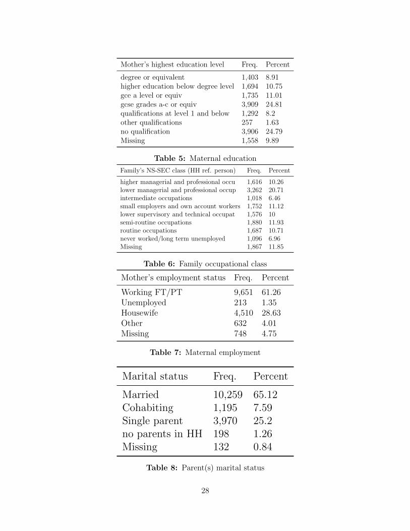
Mother’s highest education level Freq. Percent

degree or equivalent 1,403 8.91higher education below degree level 1,694 10.75gce a level or equiv 1,735 11.01gcse grades a-c or equiv 3,909 24.81qualifications at level 1 and below 1,292 8.2other qualifications 257 1.63no qualification 3,906 24.79Missing 1,558 9.89

Table 5: Maternal education

Family’s NS-SEC class (HH ref. person) Freq. Percent

higher managerial and professional occu 1,616 10.26lower managerial and professional occup 3,262 20.71intermediate occupations 1,018 6.46small employers and own account workers 1,752 11.12lower supervisory and technical occupat 1,576 10semi-routine occupations 1,880 11.93routine occupations 1,687 10.71never worked/long term unemployed 1,096 6.96Missing 1,867 11.85

Table 6: Family occupational class

Mother’s employment status Freq. Percent

Working FT/PT 9,651 61.26Unemployed 213 1.35Housewife 4,510 28.63Other 632 4.01Missing 748 4.75

Table 7: Maternal employment

Marital status Freq. Percent

Married 10,259 65.12Cohabiting 1,195 7.59Single parent 3,970 25.2no parents in HH 198 1.26Missing 132 0.84

Table 8: Parent(s) marital status

28

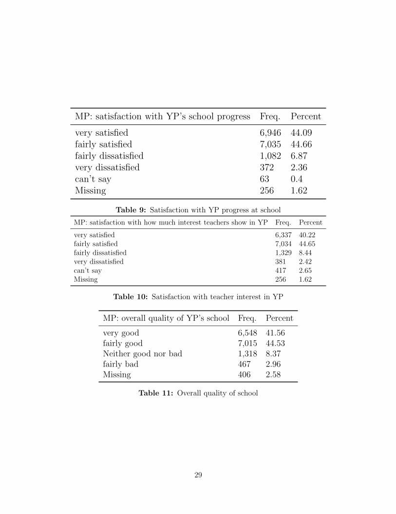
MP: satisfaction with YP’s school progress Freq. Percent

very satisfied 6,946 44.09fairly satisfied 7,035 44.66fairly dissatisfied 1,082 6.87very dissatisfied 372 2.36can’t say 63 0.4Missing 256 1.62

Table 9: Satisfaction with YP progress at school

MP: satisfaction with how much interest teachers show in YP Freq. Percent

very satisfied 6,337 40.22fairly satisfied 7,034 44.65fairly dissatisfied 1,329 8.44very dissatisfied 381 2.42can’t say 417 2.65Missing 256 1.62

Table 10: Satisfaction with teacher interest in YP

MP: overall quality of YP’s school Freq. Percent

very good 6,548 41.56fairly good 7,015 44.53Neither good nor bad 1,318 8.37fairly bad 467 2.96Missing 406 2.58

Table 11: Overall quality of school

29

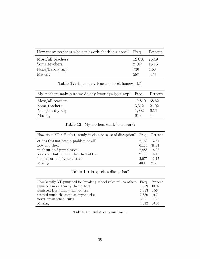
How many teachers who set hwork check it’s done? Freq. Percent

Most/all teachers 12,050 76.49Some teachers 2,387 15.15None/hardly any 730 4.63Missing 587 3.73

Table 12: How many teachers check homework?

My teachers make sure we do any hwork (w1yys14yp) Freq. Percent

Most/all teachers 10,810 68.62Some teachers 3,312 21.02None/hardly any 1,002 6.36Missing 630 4

Table 13: My teachers check homework?

How often YP difficult to study in class because of disruption? Freq. Percent

or has this not been a problem at all? 2,153 13.67now and then 6,114 38.81in about half your classes 2,888 18.33less often but in more than half of the 2,115 13.43in most or all of your classes 2,075 13.17Missing 409 2.6

Table 14: Freq. class disruption?

How heavily YP punished for breaking school rules rel. to others Freq. Percentpunished more heavily than others 1,579 10.02punished less heavily than others 1,033 6.56treated much the same as anyone else 7,830 49.7never break school rules 500 3.17Missing 4,812 30.54

Table 15: Relative punishment

30

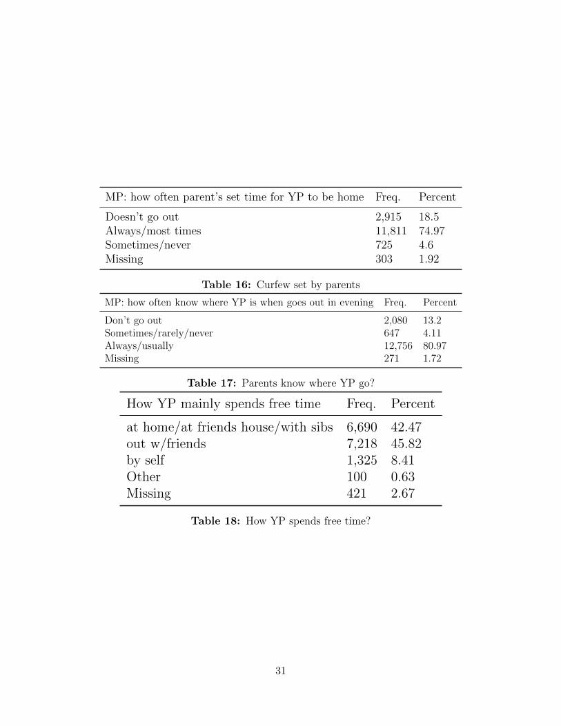
MP: how often parent’s set time for YP to be home Freq. Percent

Doesn’t go out 2,915 18.5Always/most times 11,811 74.97Sometimes/never 725 4.6Missing 303 1.92

Table 16: Curfew set by parents

MP: how often know where YP is when goes out in evening Freq. Percent

Don’t go out 2,080 13.2Sometimes/rarely/never 647 4.11Always/usually 12,756 80.97Missing 271 1.72

Table 17: Parents know where YP go?

How YP mainly spends free time Freq. Percent

at home/at friends house/with sibs 6,690 42.47out w/friends 7,218 45.82by self 1,325 8.41Other 100 0.63Missing 421 2.67

Table 18: How YP spends free time?

31

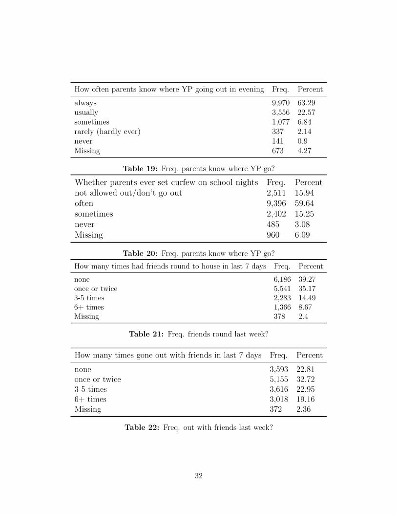
How often parents know where YP going out in evening Freq. Percent

always 9,970 63.29usually 3,556 22.57sometimes 1,077 6.84rarely (hardly ever) 337 2.14never 141 0.9Missing 673 4.27

Table 19: Freq. parents know where YP go?

Whether parents ever set curfew on school nights Freq. Percentnot allowed out/don’t go out 2,511 15.94often 9,396 59.64sometimes 2,402 15.25never 485 3.08Missing 960 6.09

Table 20: Freq. parents know where YP go?

How many times had friends round to house in last 7 days Freq. Percent

none 6,186 39.27once or twice 5,541 35.173-5 times 2,283 14.496+ times 1,366 8.67Missing 378 2.4

Table 21: Freq. friends round last week?

How many times gone out with friends in last 7 days Freq. Percent

none 3,593 22.81once or twice 5,155 32.723-5 times 3,616 22.956+ times 3,018 19.16Missing 372 2.36

Table 22: Freq. out with friends last week?

32