UC San DiegoUC San Diego Electronic Theses and Dissertations

TitleApplications of Coherent X-Ray Scattering to Two Important Problems in Condensed Matter Physics

Permalinkhttps://escholarship.org/uc/item/2rh8n3m8

AuthorYang, Yi

Publication Date2021 Peer reviewed|Thesis/dissertation

eScholarship.org Powered by the California Digital LibraryUniversity of California

UNIVERSITY OF CALIFORNIA SAN DIEGO

Applications of Coherent X-Ray Scattering to Two Important Problems in CondensedMatter Physics

A dissertation submitted in partial satisfaction of therequirements for the degree

Doctor of Philosophy

in

Physics

by

Yi Yang

Committee in charge:

Professor Sunil K. Sinha, ChairProfessor Prabhakar Rao BandaruProfessor Leonid Victorovich ButovProfessor M. Brian MapleProfessor Congjun Wu

2021

Copyright

Yi Yang, 2021

All rights reserved.

The dissertation of Yi Yang is approved, and it is acceptable

in quality and form for publication on microfilm and electron-

ically.

University of California San Diego

2021

iii

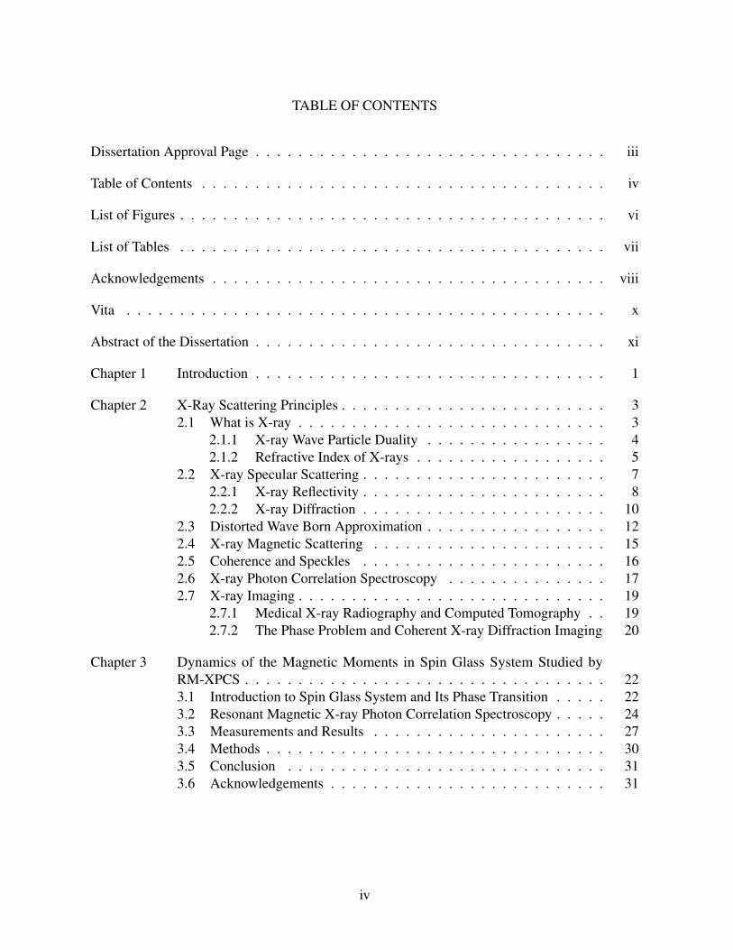
TABLE OF CONTENTS

Dissertation Approval Page . . . . . . . . . . . . . . . . . . . . . . . . . . . . . . . . . iii

Table of Contents . . . . . . . . . . . . . . . . . . . . . . . . . . . . . . . . . . . . . . iv

List of Figures . . . . . . . . . . . . . . . . . . . . . . . . . . . . . . . . . . . . . . . . vi

List of Tables . . . . . . . . . . . . . . . . . . . . . . . . . . . . . . . . . . . . . . . . vii

Acknowledgements . . . . . . . . . . . . . . . . . . . . . . . . . . . . . . . . . . . . . viii

Vita . . . . . . . . . . . . . . . . . . . . . . . . . . . . . . . . . . . . . . . . . . . . . x

Abstract of the Dissertation . . . . . . . . . . . . . . . . . . . . . . . . . . . . . . . . . xi

Chapter 1 Introduction . . . . . . . . . . . . . . . . . . . . . . . . . . . . . . . . . 1

Chapter 2 X-Ray Scattering Principles . . . . . . . . . . . . . . . . . . . . . . . . . 32.1 What is X-ray . . . . . . . . . . . . . . . . . . . . . . . . . . . . . 3

2.1.1 X-ray Wave Particle Duality . . . . . . . . . . . . . . . . . 42.1.2 Refractive Index of X-rays . . . . . . . . . . . . . . . . . . 5

2.2 X-ray Specular Scattering . . . . . . . . . . . . . . . . . . . . . . . 72.2.1 X-ray Reflectivity . . . . . . . . . . . . . . . . . . . . . . . 82.2.2 X-ray Diffraction . . . . . . . . . . . . . . . . . . . . . . . 10

2.3 Distorted Wave Born Approximation . . . . . . . . . . . . . . . . . 122.4 X-ray Magnetic Scattering . . . . . . . . . . . . . . . . . . . . . . 152.5 Coherence and Speckles . . . . . . . . . . . . . . . . . . . . . . . 162.6 X-ray Photon Correlation Spectroscopy . . . . . . . . . . . . . . . 172.7 X-ray Imaging . . . . . . . . . . . . . . . . . . . . . . . . . . . . . 19

2.7.1 Medical X-ray Radiography and Computed Tomography . . 192.7.2 The Phase Problem and Coherent X-ray Diffraction Imaging 20

Chapter 3 Dynamics of the Magnetic Moments in Spin Glass System Studied byRM-XPCS . . . . . . . . . . . . . . . . . . . . . . . . . . . . . . . . . . 223.1 Introduction to Spin Glass System and Its Phase Transition . . . . . 223.2 Resonant Magnetic X-ray Photon Correlation Spectroscopy . . . . . 243.3 Measurements and Results . . . . . . . . . . . . . . . . . . . . . . 273.4 Methods . . . . . . . . . . . . . . . . . . . . . . . . . . . . . . . . 303.5 Conclusion . . . . . . . . . . . . . . . . . . . . . . . . . . . . . . 313.6 Acknowledgements . . . . . . . . . . . . . . . . . . . . . . . . . . 31

iv

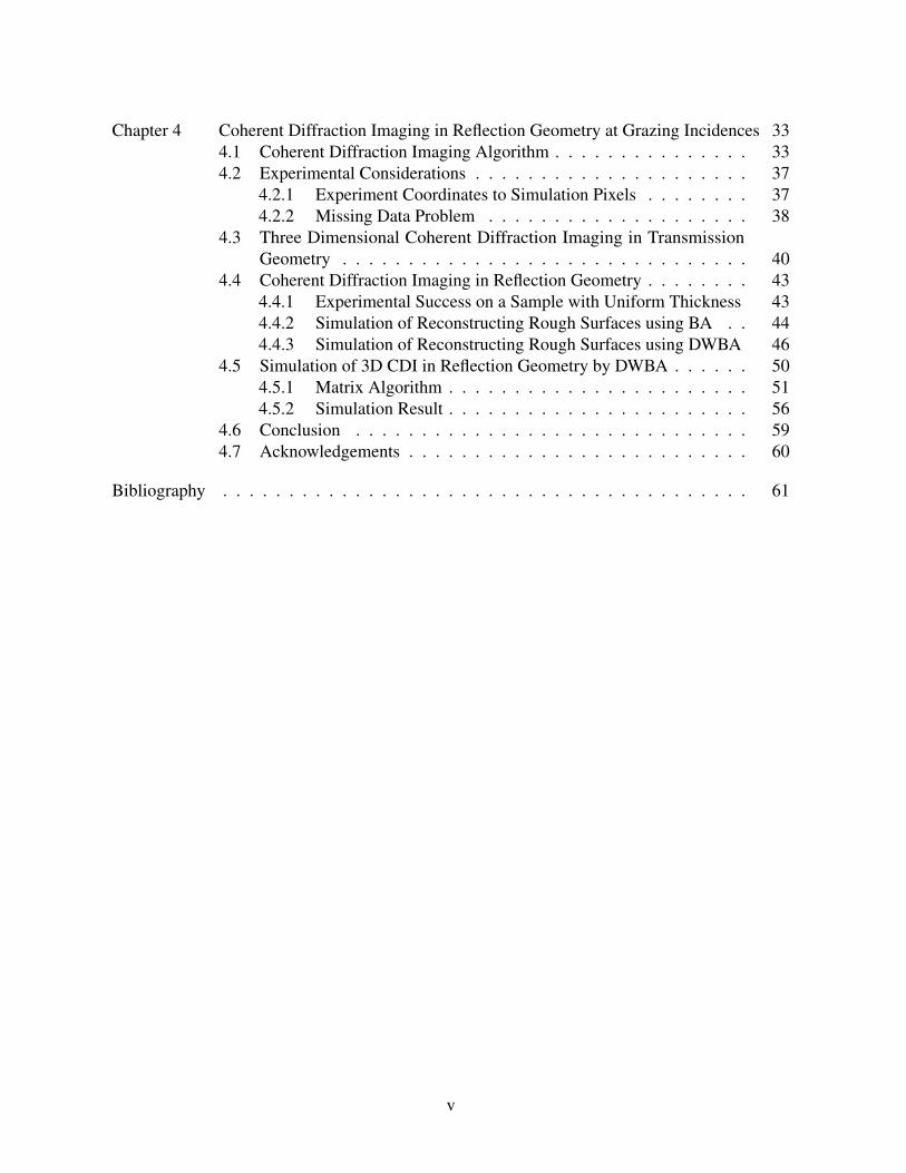
Chapter 4 Coherent Diffraction Imaging in Reflection Geometry at Grazing Incidences 334.1 Coherent Diffraction Imaging Algorithm . . . . . . . . . . . . . . . 334.2 Experimental Considerations . . . . . . . . . . . . . . . . . . . . . 37

4.2.1 Experiment Coordinates to Simulation Pixels . . . . . . . . 374.2.2 Missing Data Problem . . . . . . . . . . . . . . . . . . . . 38

4.3 Three Dimensional Coherent Diffraction Imaging in TransmissionGeometry . . . . . . . . . . . . . . . . . . . . . . . . . . . . . . . 40

4.4 Coherent Diffraction Imaging in Reflection Geometry . . . . . . . . 434.4.1 Experimental Success on a Sample with Uniform Thickness 434.4.2 Simulation of Reconstructing Rough Surfaces using BA . . 444.4.3 Simulation of Reconstructing Rough Surfaces using DWBA 46

4.5 Simulation of 3D CDI in Reflection Geometry by DWBA . . . . . . 504.5.1 Matrix Algorithm . . . . . . . . . . . . . . . . . . . . . . . 514.5.2 Simulation Result . . . . . . . . . . . . . . . . . . . . . . . 56

4.6 Conclusion . . . . . . . . . . . . . . . . . . . . . . . . . . . . . . 594.7 Acknowledgements . . . . . . . . . . . . . . . . . . . . . . . . . . 60

Bibliography . . . . . . . . . . . . . . . . . . . . . . . . . . . . . . . . . . . . . . . . 61

v

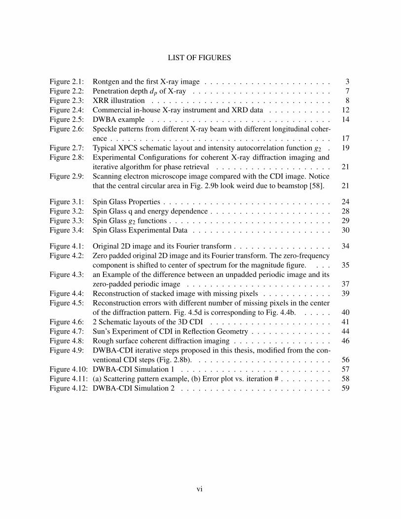
LIST OF FIGURES

Figure 2.1: Rontgen and the first X-ray image . . . . . . . . . . . . . . . . . . . . . . 3Figure 2.2: Penetration depth dp of X-ray . . . . . . . . . . . . . . . . . . . . . . . . 7Figure 2.3: XRR illustration . . . . . . . . . . . . . . . . . . . . . . . . . . . . . . . 8Figure 2.4: Commercial in-house X-ray instrument and XRD data . . . . . . . . . . . 12Figure 2.5: DWBA example . . . . . . . . . . . . . . . . . . . . . . . . . . . . . . . 14Figure 2.6: Speckle patterns from different X-ray beam with different longitudinal coher-

ence . . . . . . . . . . . . . . . . . . . . . . . . . . . . . . . . . . . . . . 17Figure 2.7: Typical XPCS schematic layout and intensity autocorrelation function g2 . 19Figure 2.8: Experimental Configurations for coherent X-ray diffraction imaging and

iterative algorithm for phase retrieval . . . . . . . . . . . . . . . . . . . . 21Figure 2.9: Scanning electron microscope image compared with the CDI image. Notice

that the central circular area in Fig. 2.9b look weird due to beamstop [58]. 21

Figure 3.1: Spin Glass Properties . . . . . . . . . . . . . . . . . . . . . . . . . . . . . 24Figure 3.2: Spin Glass q and energy dependence . . . . . . . . . . . . . . . . . . . . . 28Figure 3.3: Spin Glass g2 functions . . . . . . . . . . . . . . . . . . . . . . . . . . . . 29Figure 3.4: Spin Glass Experimental Data . . . . . . . . . . . . . . . . . . . . . . . . 30

Figure 4.1: Original 2D image and its Fourier transform . . . . . . . . . . . . . . . . . 34Figure 4.2: Zero padded original 2D image and its Fourier transform. The zero-frequency

component is shifted to center of spectrum for the magnitude figure. . . . 35Figure 4.3: an Example of the difference between an unpadded periodic image and its

zero-padded periodic image . . . . . . . . . . . . . . . . . . . . . . . . . 37Figure 4.4: Reconstruction of stacked image with missing pixels . . . . . . . . . . . . 39Figure 4.5: Reconstruction errors with different number of missing pixels in the center

of the diffraction pattern. Fig. 4.5d is corresponding to Fig. 4.4b. . . . . . 40Figure 4.6: 2 Schematic layouts of the 3D CDI . . . . . . . . . . . . . . . . . . . . . 41Figure 4.7: Sun’s Experiment of CDI in Reflection Geometry . . . . . . . . . . . . . . 44Figure 4.8: Rough surface coherent diffraction imaging . . . . . . . . . . . . . . . . . 46Figure 4.9: DWBA-CDI iterative steps proposed in this thesis, modified from the con-

ventional CDI steps (Fig. 2.8b). . . . . . . . . . . . . . . . . . . . . . . . 56Figure 4.10: DWBA-CDI Simulation 1 . . . . . . . . . . . . . . . . . . . . . . . . . . 57Figure 4.11: (a) Scattering pattern example, (b) Error plot vs. iteration # . . . . . . . . . 58Figure 4.12: DWBA-CDI Simulation 2 . . . . . . . . . . . . . . . . . . . . . . . . . . 59

vi

LIST OF TABLES

Table 2.1: The EM spectrum . . . . . . . . . . . . . . . . . . . . . . . . . . . . . . . 5Table 2.2: Refractive index for some common materials . . . . . . . . . . . . . . . . . 6

Table 4.1: Angle pairs and corresponding wavetransfers . . . . . . . . . . . . . . . . . 47

vii

ACKNOWLEDGEMENTS

Thank my thesis advisor Professor Sunil Sinha for guiding me in my research work as

well as my life.

Thank Professor Oleg Shpyrko and Professor Congjun Wu for recruiting me to UC San

Diego.

Thank Professors Prabhakar Rao Bandaru, Leonid Victorovich Butov and M. Brian Maple

for rounding out my dissertation committee.

Thank Jiang Zhang, Jin Wang, Peco Myint and Miaoqi Chu for helpful discussions on my

CDI project in Chapter 4.

Thank my lab mates, Sudip Pandey, Marta Salvador, Ben Holladay, Jingjin Song, Rupak

Bhattacharya, Sambhunath Bera, Yicong Ma, David Dilena, Hongyu Guo, Vince Chen and Sajal

K. Ghosh.

Thank Hyunki Kim, Jooyoung Chang, Hyeyound Kim, Thomas P. Russell, Tsung-Yeh

Tang, Gaurav Arya, Suresh Narayanan, KALYAN Sasmal, Claudio Mazzoli, Eric Fullerton,

Chandra Varma, Xi Chen, Xiaoqian Chen, Sujoy Roy, Sheena Patel for collaborating research

projects.

Thank Tom Murphy, Susan Marshall, Judy Winstead, Catherine McConney, Toni Moore

and Sharmila Poddar for their administrative help at UCSD physics department.

Thank the doctors and nurses in Arrowhead Regional Medical Center and Sharp Momorial

Hospital rehab for saving my life after my ski accident.

Thank my friends, my therapists and charities who helped me going through my darkest

days in my life.

Thank my family for supporting me all the time.

We wish to acknowledge the help from the staff of the CSX beamline at NSLS II, and staff

members at ALS in the experiments at the 12.0.2 coherent beamline at ALS. We thank Sheng Ran

for assistance with magnetic measurements made at UCSD. The research was supported by grant

viii

no. DE-SC0003678 from the Division of Basic Energy Sciences of the Office of Science of the

U.S. Dept. of Energy. MBM acknowledges the support of the US Department of Energy, Office

of Basic Energy Sciences, Division of Materials Sciences and Engineering, under Grant No.

DE-FG02-04ER46105. This research used beamline 23-ID-1of the National Synchrotron Light

Source II, a U.S. Department of Energy (DOE) Office of Science User Facility operated for the

DOE Office of Science by Brookhaven National Laboratory under Contract No. DE-SC0012704.

Work at the ALS, LBNL was supported by the Director, Office of Science, Office of Basic Energy

Sciences, of the US Department of Energy (Contract No. DE-AC02-05CH11231).

Chapter 3, in part is currently submitted for publication of the material. Jingjin Song,

Sheena K.K. Patel, Rupak Bhattacharya, Yi Yang, Sudip Pandey, Xiao M. Chen, Xi Chen, Kalyan

Sasmal, M. Brian Maple, Eric E. Fullerton, Sujoy Roy, Claudio Mazzoli,Chandra M. Varma and

Sunil K. Sinha. “Direct measurement of temporal correlations above the spin-glass transition by

coherent resonant magnetic x-ray spectroscopy”. The disseration author contributed to collect

and analyze the data at the synchrotron sources and was a co-author on this material.

This work in Chapter 4 was supported by grant no. DE-SC0003678 from the Division of

Basic Energy Sciences of the Office of Science of the U.S. Dept. The content in this chapter is

based on material prepared for submission by Yi Yang and Sunil K. Sinha. “Coherent GISAXS

Scattering and Phase Retrieval Using DWBA”. The dissertation author was the primary researcher

and author of this material.

ix

VITA

2012 B. S. in Physics, University of Science and Technology of China, Hefei,China

2015 National School on Neutron and X-ray Scattering, Argonne NationalLaboratory, Chicago, Illinois

2021 Ph. D. in Physics, University of California San Diego

x

ABSTRACT OF THE DISSERTATION

Applications of Coherent X-Ray Scattering to Two Important Problems in CondensedMatter Physics

by

Yi Yang

Doctor of Philosophy in Physics

University of California San Diego, 2021

Professor Sunil K. Sinha, Chair

In the last decades, the commissioning of high-energy, third-generation synchrotrons

presents new opportunities for research with brilliant coherent X-ray beams. It allows us to

study the structures and dynamics of various systems at shorter length scale than laser via their

diffraction patterns. In Chapter 3, we discuss the use of Photon Correlation Spectroscopy extended

to X-rays to study the dynamical correlations of the spin-glass transition using X-rays. We have

implemented this method to observe and accurately characterize the critical slowing down of the

spin orientation fluctuations in the classic metallic spin glass alloy CuMn over time scales of 100

to 103 secs. In Chapter 4, we discuss the diffraction imaging method to retrieve the phase of the

xi

speckle pattern produced by the scattering of a coherent X-ray beam to reconstruct the image of

3D objects at nanometer length scales. We have extended the well-known oversampling methods

and iterative schemes to use the full Distorted-Wave Born Approximation (DWBA) expression

for the speckle pattern. The results obtained from detailed computer simulations of the scattering

and reconstruction are very encouraging in showing that the method works. Verification with real

experiments is planned.

xii

Chapter 1

Introduction

The classic Young’s double-slit experiment first demonstrated the optical interference

from coherent light in 1801. Later on, Theodore H. Maiman at Hughes Research Laboratories

built the first laser in 1961, which is used widely in industry and labs as a coherent light source.

Physicists and material scientists use it to study the exact structure and dynamics of a variety of

systems. In the last decades, the commissioning of high-energy, third-generation synchrotrons

presents new opportunities for research with brilliant coherent X-ray beams. It allows us to

apply the coherent laser techniques to X-rays, such as photon correlation spectroscopy (also

known as dynamic light scattering) and coherent diffraction imaging. Now with coherent X-rays,

investigating the dynamics of condensed matter at molecular length scales using X-ray photon

correlation spectroscopy is possible, as is the diffraction imaging of tiny objects.

This work described how we applied resonant coherent X-rays to study the slow dynamics

of the magnetic spin glass system, despite the strong charge scattering as background, and to

reconstruct 3D images of tiny objects from the coherent X-ray diffraction patterns with ultra fine

resolution. The strong penetrating power of X-rays allows us to study the spin fluctuations of a

spin glass buried in the surface and reconstruct 3D images from the diffraction patterns.

This thesis is organized as follows. Chapter 2 introduces some fundamental properties of

1

X-rays and their applications related to this thesis. In particular, Distorted Wave Born Approxi-

mation (DWBA), X-Ray Magnetic Scattering (XRMS), X-Ray Photon Correlation Spectroscopy

(XPCS), Coherent Diffraction Imaging (CDI) with X-rays are of most importance and related to

the next chapters. Chapter 3 presents the experimental study of a spin glass system via Resonant

Magnetic X-Ray Photon Correlation Spectroscopy (RM XPCS). The chapter explains why our

work is important to determine whether there is phase transition of CuMn spin glass at the “critical

temperature”. Chapter 4 demonstrates the iteration algorithms to retrieve phases of the diffraction

patterns. The chapter includes some common problems that one may encounter when trying the

iteration algorithms. In this chapter, we also modified the algorithm to fit for Grazing Incidence

Smaller Angle X-ray Scattering (GISAXS) using DWBA. With some simulation results, we

showed that it is possible to retrieve phase of the 3D diffraction pattern in reflection geometry.

Some experimental difficulties are also brought up.

2

Chapter 2

X-Ray Scattering Principles

2.1 What is X-ray

Wilhelm Rontgen discovered X-rays from cathode ray tubes in 1895. He found that

X-rays would pass through most substances but leave shadows of solid objects. Fig. 2.1 (right) is

the world first X-ray image of his wife’s hand.

Figure 2.1: Wilhelm Rontgen and the first medical X-ray by Wilhelm Rontgen of his wife AnnaBertha Ludwig’s hand in 1895

X-rays are generated mainly via 2 methods: 1. matter irradiated by a beam of high-energy

charged particles like electrons, such as sealed-tube and rotating anode, which are commonly

3

used for in-house instruments. 2. high-energy charged particles traveling in circular orbits, also

known as synchrotron radiation, produced by big facilities, such as Advanced Photon Source in

Argonne National Laboratory, NSLS-II in Brookhaven National Laboratory, and so on.

2.1.1 X-ray Wave Particle Duality

X-rays are electromagnetic radiation as well as group of photons. They have all the

radiation and matter properties, such as wavelength, wavevector, momentum, and energy, see

Table 2.1 for details. They are related as below:

E = hc/λ

p = h/λ

k = 2π/λ

where E is the photon energy, p is the photon momentum, k is the wavevector, λ is the wavelength,

h = 6.63×10−34m2 · kg/s is the Planck constant and c the light speed.

Given any one of E, p,λ,k, the others can be calculated from the above equations. Hence-

forth, we may use one of them to describe the X-ray beam. Here are the parameters of Cu

Kα X-ray, which is very common and will be used multiple times for the rest of the thesis:

E = 8.04keV , λ = 1.54A, k0 = 4.078A−1.

X-rays with high photon energies above 5 ∼ 10keV (below 2 ∼ 1A wavelength) are called

hard X-rays, while those with lower energy (and longer wavelength) are called soft X-rays.

4

Table 2.1: The electromagnetic wave spectrum

Type of Radiation Wavelength Range Energy Rangegamma-rays < 10−12m > 1.24MeV

x-rays 10−12 ∼ 10−8m 124eV ∼ 1.24MeVultraviolet 10−8 ∼ 4∗10−7m 3.1eV ∼ 124eV

visible 4∗10−7m ∼ 7.5∗10−7m 1.65eV ∼ 3.1eVnear-infrared 7.5∗10−7m ∼ 2.5∗10−6m 0.5eV ∼ 1.65eV

infrared 2.5∗10−6m ∼ 2.5∗10−5m 0.05eV ∼ 0.5eVmicrowaves 2.5∗10−5m ∼ 10−3m 0.24meV ∼ 0.05eVradio waves > 10−3m < 0.24meV

2.1.2 Refractive Index of X-rays

An X-ray plane wave is described by its electric field vector |Ψ(r)⟩= E0eik·r (Note that,

E0 contains the polarization direction, which will be mentioned in Chapter 3). When the X-rays

interact with matter, the Helmholtz equation is:

(∇2 + k2n2) |Ψ⟩= 0 (2.1)

where k is the wavevector, re = e2/(4πε0mec2) = 2.814 ∗ 10−15m is the Thompson scattering

length, also known as classical electron radius. The complex refractive index n is related to the

electron density ρ(r) of the matter:

n(r,k) = 1−δ(r,k)+ iβ(r,k) (2.2)

δ(r,k) =2πreρ(r)

k2 (2.3)

β(r,k) =µ(r,k)

2k(2.4)

where µ(r,k) is the linear absorption coefficient. In Ref. [87], µ(r,k) is written as µ(r), which

is not accurate, as the linear absorption coefficient is a function of the X-ray wavevector. reρ, δ

and µ for some common materials, at X-ray energy 8.04keV (Cu Kα radiation, commonly used in

laboratory) are listed in Table 2.2 [87].

5

Table 2.2: Refractive index for some common materials [87]. Scattering length densities reρ,dispersions δ, linear absorption coefficients µ, and critical angles αc for X-ray with photonenergy 8.04keV .

Material reρ(1010cm−2) δ(10−6) µ(cm−1) αc()

Vacuum 0 0 0 0Polystyrene(PS) 9.5 3.5 4 0.153

Silicon(Si) 20 7.6 141 0.223Gold(Au) 131.5 49.6 4170 0.570

Note that, 0 < β << δ << 1. For incident X-ray from vacuum/air to medium surface,

there is a critical angle for total reflection: cosαc = 1−δ, imaginary part of n is neglected since

β is too small:

αc ≈√

2δ = λ

√reρ

π(2.5)

In brief, the refractive indices of matters are complex numbers, with real part very close

but smaller than 1 and imaginary part even smaller. They are functions of electron density and

X-ray wavelength. And the critical angle of a substance surface from air/vacuum is proportional

to λ√

ρ.

We can calculate the penetration depth dp, which is defined as the depth at which the

intensity of the X-ray inside the material falls to 1/e of its original value at the surface. The

electric field under the surface is |Ψ⟩ = eikt ·r = e−Im(ktz)zeiRe(kt)·r, where kt

z = k0√

n2 − cos2 αi

and kx,ky are real.

dp =1

Im(ktz)

(2.6)

At critical angle, ktz = k0

√2iβ, Im(kt

z)= k0√

β and dp =√

2/k0µ, where µ is the linear absorption

coefficient. Penetration depth of Si at critical angle for Cu Kα X-ray is dp = 382λ= 590A. Fig. 2.2

shows the penetration depth as a function of incident angle. In transmission geometry, |Ψ⟩= eiktz,

assuming the beam propagates along the z direction, and dp = 1/Im(kt), where kt = nk0 and

Im(kt) = βk0. That is, dp = 2/µ. For Si and Cu Kα X-ray, it is 142µm.

6

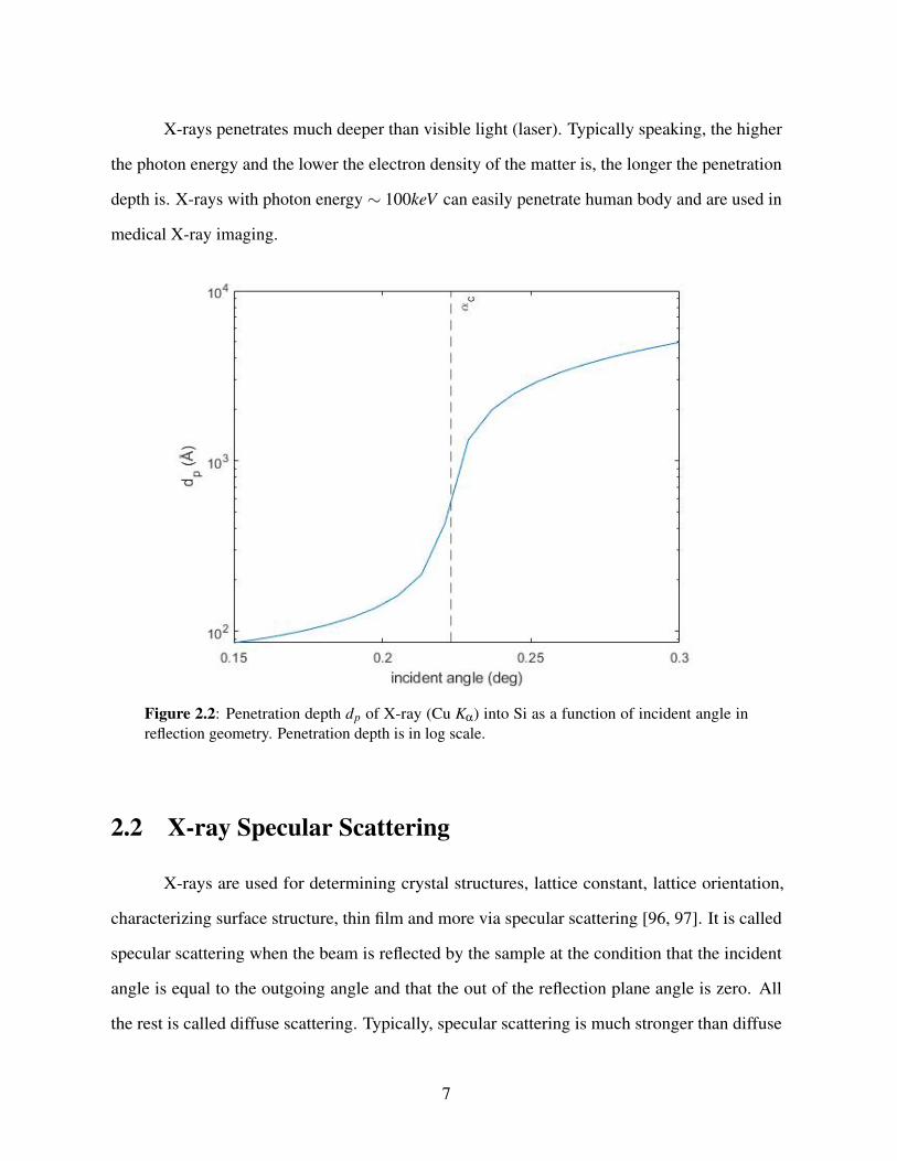
X-rays penetrates much deeper than visible light (laser). Typically speaking, the higher

the photon energy and the lower the electron density of the matter is, the longer the penetration

depth is. X-rays with photon energy ∼ 100keV can easily penetrate human body and are used in

medical X-ray imaging.

Figure 2.2: Penetration depth dp of X-ray (Cu Kα) into Si as a function of incident angle inreflection geometry. Penetration depth is in log scale.

2.2 X-ray Specular Scattering

X-rays are used for determining crystal structures, lattice constant, lattice orientation,

characterizing surface structure, thin film and more via specular scattering [96, 97]. It is called

specular scattering when the beam is reflected by the sample at the condition that the incident

angle is equal to the outgoing angle and that the out of the reflection plane angle is zero. All

the rest is called diffuse scattering. Typically, specular scattering is much stronger than diffuse

7

scattering. Thus, it is easy to build up a small in-house X-ray instrument to conduct specular

scattering experiment with not so brilliant X-ray source, such as a rotating anode. In the following

subsections, the 2 most used X-ray specular scattering techniques are introduced.

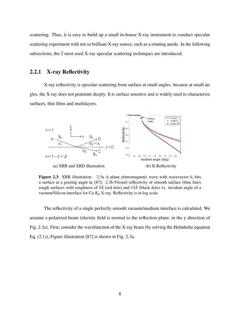
2.2.1 X-ray Reflectivity

X-ray reflectivity is specular scattering from surface at small angles. because at small an-

gles, the X-ray does not penetrate deeply. It is surface sensitive and is widely used to characterize

surfaces, thin films and multilayers.

(a) XRR and XRD illustration (b) Si Reflectivity

Figure 2.3: XRR illustration. 2.3a A plane eletromagnetic wave with wavevector ki hitsa surface at a grazing angle αi [87]; 2.3b Fresnel reflectivity of smooth surface (blue line),rough surfaces with roughness of 5A (red dots) and 15A (black dots) vs. incident angle of avacuum/Silicon interface for Cu Kα X-ray. Reflectivity is in log scale.

The reflectivity of a single perfectly smooth vacuum/medium interface is calculated. We

assume s-polarized beam (electric field is normal to the reflection plane, in the y direction of

Fig. 2.3a). First, consider the wavefunction of the X-ray beam (by solving the Helmholtz equation

Eq. (2.1)), Figure illustration [87] is shown in Fig. 2.3a.

8

|Ψ⟩=

eiki·r +Reik f ·r z ≥ 0

Teikt ·r z < 0(2.7)

R = r =ki

z − ktz

kiz + kt

z(2.8)

T = t =2ki

z

kiz + kt

z= 1+ r (2.9)

where ktz = k0

√n2 − cos2 αi. r and t are called Fresnel coefficients and can be calculated via the

continuity of the wavefunction and its first derivative at the surface z = 0. Note that, kx,ky remain

the same no matter whether in air or medium, according to the boundary conditions of Maxwell’s

Equations of the electric field. For this thesis, we assume elastic scattering, with no energy loss

of the photon. That is, |k f |= |ki|= k0. The reflectivity I is given by (see Fig. 2.3b):

I = |R|2 (2.10)

For stratified media with N interfaces, the wavefunction in jth layer is:

|Ψ j⟩= Tjeiki

j·r +R jeik f

j ·r (2.11)

Parratt [72] first described a recursive approach to solve the Tj and R j.

X j =R j

Tj=

r j, j+1 +X j+1e2ikz, j+1d j

1+ r j, j+1X j+1e2ikz, j+1d je−2ikz, jd j (2.12)

where d j is the thickness and kz, j is the z component of the wavevector of the jth layer, and r j, j+1

9

is the Fresnel coefficient at the jth interface:

r j, j+1 =kz, j − kz, j+1

kz, j + kz, j+1(2.13)

kz, j = k0

√n2

j − cos2 α2i (2.14)

where n j = 1−δ j + iβ j is the refractive index. The derivation of X j is also from the continuity of

the wavefunction and its first derivative at all the interfaces.

Given the top layer is air, T1 = 1. The N +1 layer is the substrate, RN+1 = 0. All X j can

be calculated successively. And the reflectivity:

I = |R1|2 = |X1|2 (2.15)

Roughness of each interface can also be accounted for by adding the factor [38]

r j, j+1,rough = r j, j+1e−2kz, jkz, j+1σ2j (2.16)

where σ j is the roughness of the jth interface.

If each layer in the thin film is not uniform, then electron density in each layer is not a

constant. We can slice each layer into multilayers and assume in each slice the electron density is

uniform. One can calculate the reflectivity from arbitrary electron density profile. Details can be

found in Ref. [87] Chapter 2.4.

2.2.2 X-ray Diffraction

Because the X-ray wavelength is comparable to the distance between atoms in crystals

and X-rays has strong penetrating power, X-ray is used to characterize the structure, defects of

crystals, and so on. A X-ray scattering event is basically Fourier transform the eletron density

10

f (r) into reciprocal space (aka. Fourier space), according to Born Approximation:

F(q) =∫

Vf (r)dr (2.17)

dσ

dΩ= r2

e |F(q)|2 (2.18)

where q = k f −ki is the wavevector transfer, ki and k f are incident and outgoing wavevectors. re

is Thompson scattering length. dσ

dΩis the differential cross section.

The derivation of Eq. (2.17) is, assuming there is incoming X-ray which is describled as

|Ψi⟩= exp(iki · r), scattered by the electrons of the substance. The outgoing X-ray is described

as |Ψ f ⟩= exp(ik f · r). The transition matrix T is defined as [80]:

⟨Ψ f |T|Ψi⟩= re ⟨Ψ f | f (r)|Ψi⟩

= re

∫dreik f ·r f (r)e−iki·r

= re

∫dr f (r)e−iq·r

= reF(q) (2.19)

Differential cross section is the square of transition matrix.

If the substance is periodic in space, as in the case of a crystalline substance, the cor-

responding Bragg peaks can be found in reciprocal space. X-ray Diffraction (XRD) patterns

(Bragg peak locations in reciprocal space), provide detailed information about the internal lattice,

including unit cell dimensions, bond-lengths, bond-angles, and details of site-ordering.

A typical XRD instrument includes a X-ray generator, a sample stage (goniomenter),

a X-ray detector, shown in Fig 2.4. The XRD instrument is also used to do X-ray reflectivity,

because XRR is similar to XRD. The difference is the incident and outgoing angles in XRR

is much smaller. Generalized XRD is diffraction of substances no matter whether it is crystal.

11

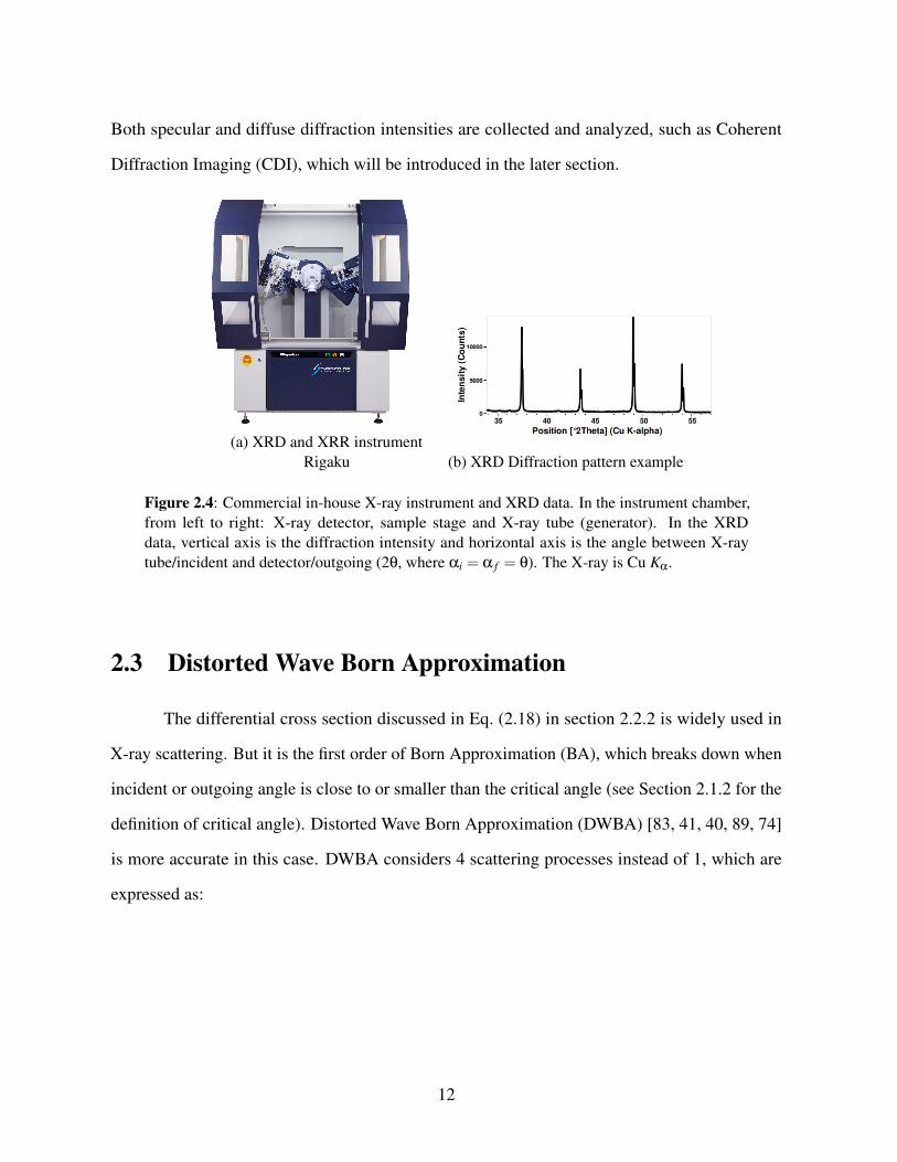
Both specular and diffuse diffraction intensities are collected and analyzed, such as Coherent

Diffraction Imaging (CDI), which will be introduced in the later section.

(a) XRD and XRR instrumentRigaku (b) XRD Diffraction pattern example

Figure 2.4: Commercial in-house X-ray instrument and XRD data. In the instrument chamber,from left to right: X-ray detector, sample stage and X-ray tube (generator). In the XRDdata, vertical axis is the diffraction intensity and horizontal axis is the angle between X-raytube/incident and detector/outgoing (2θ, where αi = α f = θ). The X-ray is Cu Kα.

2.3 Distorted Wave Born Approximation

The differential cross section discussed in Eq. (2.18) in section 2.2.2 is widely used in

X-ray scattering. But it is the first order of Born Approximation (BA), which breaks down when

incident or outgoing angle is close to or smaller than the critical angle (see Section 2.1.2 for the

definition of critical angle). Distorted Wave Born Approximation (DWBA) [83, 41, 40, 89, 74]

is more accurate in this case. DWBA considers 4 scattering processes instead of 1, which are

expressed as:

12

G(qx,qy,kiz,k

fz ) =D1(ki

z,kfz )F(qx,qy,q1

z )+D2(kiz,k

fz )F(qx,qy,q2

z )

+D3(kiz,k

fz )F(qx,qy,q3

z )+D4(kiz,k

fz )F(qx,qy,q4

z ) (2.20)

(dσ

dΩ)di f f ≈ r2

e |G(qx,qy,kiz,k

fz )|2 (2.21)

where ( dσ

dΩ)di f f is the diffuse scattering differential cross section. Scattering at any directions that

qx = 0 or qy = 0 is called diffuse scattering (this definition of specular and diffuse scattering is

the same as that in section 2.2). Diffuse scattering is always much weaker than specular. The

DWBA specular scattering is omitted here, as it is not relevant to this thesis work. G is called the

DWBA form factor, while F is the Fourier transform of electron density. D1 ∼ D4 are defined as:

D1 = T (α f )T (αi), D2 = R(α f )T (αi),

D3 = T (α f )R(αi), D4 = R(α f )R(αi) (2.22)

and qz are defined as:

q1z = k f

z − kiz, q2

z =−k fz − ki

z,

q3z =−q2

z , q4z =−q1

z (2.23)

The complete wavevector transfer [87, 89] from the angles shown in Fig. 2.5(a) is defined

13

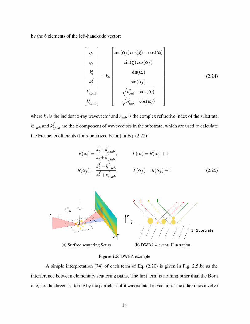
by the 6 elements of the left-hand-side vector:

qx

qy

kiz

k fz

kiz,sub

k fz,sub

= k0

cos(α f )cos(χ)− cos(αi)

sin(χ)cos(α f )

sin(αi)

sin(α f )√n2

sub − cos(αi)√n2

sub − cos(α f )

(2.24)

where k0 is the incident x-ray wavevector and nsub is the complex refractive index of the substrate.

kiz,sub and k f

z,sub are the z component of wavevectors in the substrate, which are used to calculate

the Fresnel coefficients (for s-polarized beam) in Eq. (2.22):

R(αi) =ki

z − kiz,sub

kiz + ki

z,sub, T (αi) = R(αi)+1,

R(α f ) =k f

z − k fz,sub

k fz + k f

z,sub

, T (α f ) = R(α f )+1 (2.25)

(a) Surface scattering Setup (b) DWBA 4 events illustration

Figure 2.5: DWBA example

A simple interpretation [74] of each term of Eq. (2.20) is given in Fig. 2.5(b) as the

interference between elementary scattering paths. The first term is nothing other than the Born

one, i.e. the direct scattering by the particle as if it was isolated in vacuum. The other ones involve

14

a reflection of either the incident or the scattered beams on the substrate surface.

The DWBA formalism is suitable for the case: either incident or outgoing angles is

smaller than 3 times the critical angle of the substrate. Because at larger angle α (αi,α f ), the

corresponding Fresnel reflection coefficient R (Ri,R f ) is so small that can be neglected, while

T ≈ 1. Thus only the first term of Eq. (2.20) remains non-zero, which is essentially the BA term.

For example, for a smooth Si surface, |R|= 0.03 at α = 3αc for Cu Kα X-ray, see Fig. 2.3b for

details about R(α) (do not forget to square root the Y scale in the figure).

2.4 X-ray Magnetic Scattering

The differential cross section derived so far is for X-ray scattered by electrons in the

substances, which is also called charge scattering. X-rays also interact with the electronic spins

(magnetic moments, dipoles) in the substances. When X-ray photon energy is different from the

magnetic electron transition energy (off-resonance), the pure charge scattering is larger than the

pure magnetic scattering by a significant factor [9]:

σmag

σcharge≈ (

Ep

mec2 )2 N2

mN2 ⟨s⟩

2 f 2m

f 2 (2.26)

where Ep is the X-ray photon energy, Nm is the number of magnetic electrons/atom, N the number

of electrons/atom, fm and f are magnetic and charge form factors, s is the magnetic electron

spin (⟨s⟩=1 below Curie temperature), σmag and σcharge are magnetic and charge scattering cross

sections.

Magnetic atoms (Fe, Mn, etc.) have magnetic electrons, typically in orbit 3d. As an

example, for Fe and 10keV photons,

σmag

σcharge∼ 4×10−6 (2.27)

15

But when the photon energy is tuned to the magnetic electron absorption edge, the

magnetic cross section significantly increases [17, 34]. And the rare earth elements’ M-edge

(electron transition from orbit 3d) and L-edge (from orbit 2p) transition energy are around

102 ∼ 103eV , which lie in the soft X-ray energy range. Thus, soft X-rays are commonly used

for magnetic scattering experiments. In an actual resonant magnetic scattering experiment, the

photon energy is always tuned to be off resonance by several eV. Because at the exact resonant

energy, the absorption is large (imaginary part of the refractive index increases dramatically).

2.5 Coherence and Speckles

In section 2.2.2, we talked about the X-ray Diffraction. We assumed plane wave |Ψi⟩=

exp(iki · r), which is perfect coherent beam. The beam wavelength and waveform is unique. But

in reality, even the best X-ray source synchrotron radiation is not fully coherent. We can assume

it is coherent in a limited volume inside the beam. The size of the coherent volume in terms of

transverse coherent length in x,y direction and longitudinal coherent length [84]

ξx =λR

2πσx, ξy =

λR2πσy

ξl = λ

(λ

∆λ

)

where λ is the average photon wavelength and R is the distance to the photon source. σx and σy

is the size of the X-ray source in the x,y direction. and ∆λ is the Full Width at Half Maximum

(FWHM) of the wavelength spread of the beam.

The diffraction pattern of an object from a coherent beam is also called speckle pattern.

Speckle pattern is essentially diffuse scattering from a coherent beam, which is weak compared

to specular scattering. Most X-ray diffuse scattering experiments are carried out in sychrotron

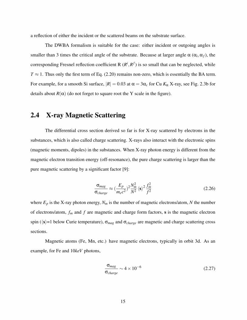
radiation facilities because sychrotron provides very brilliant and coherent X-ray beam. Fig. 2.6

16

(a) Speckle pattern from monochromatic X-ray(b) Speckle pattern from X-ray with broad

energy bandwidth

Figure 2.6: Speckle patterns from different X-ray beam with different longitudinal coher-ence [77, 84]. Copyright 1999, Intl. Union of Crystallography.

shows a typical speckle pattern from a coherent beam and a speckle pattern from a beam without

longitudinal coherence [84, 77]. We will assume the X-ray beam is coherent for the rest of this

thesis (samples are all in the coherent volume).

2.6 X-ray Photon Correlation Spectroscopy

From last section, we know that the speckle pattern is the scattered intensity of an coherent

beam to a system. If the system is not static, the speckles also move around. About 50 years ago,

people established a method of studying dynamic systems using highly coherent laser beams.

This method is called Dynamical Light Scattering [7]. Later on, X-ray people adopted such idea

and started to study systems at shorter length scales as X-rays have larger wavevector than visible

light (laser) [84]. Such method is called X-ray Photon Correlation Spectroscopy (XPCS).

A typical XPCS experiment is illuminating a dynamical system with coherent X-rays, and

collecting the scattered intensities of the speckle pattern as a function of time I(q, t), where q is

the wavevector transfer. The intensity autocorrelation function g2 is studied:

17

g2(q,τ) =⟨I(q, t)I(q, t + τ)⟩t

⟨I(q, t)⟩2t

(2.28)

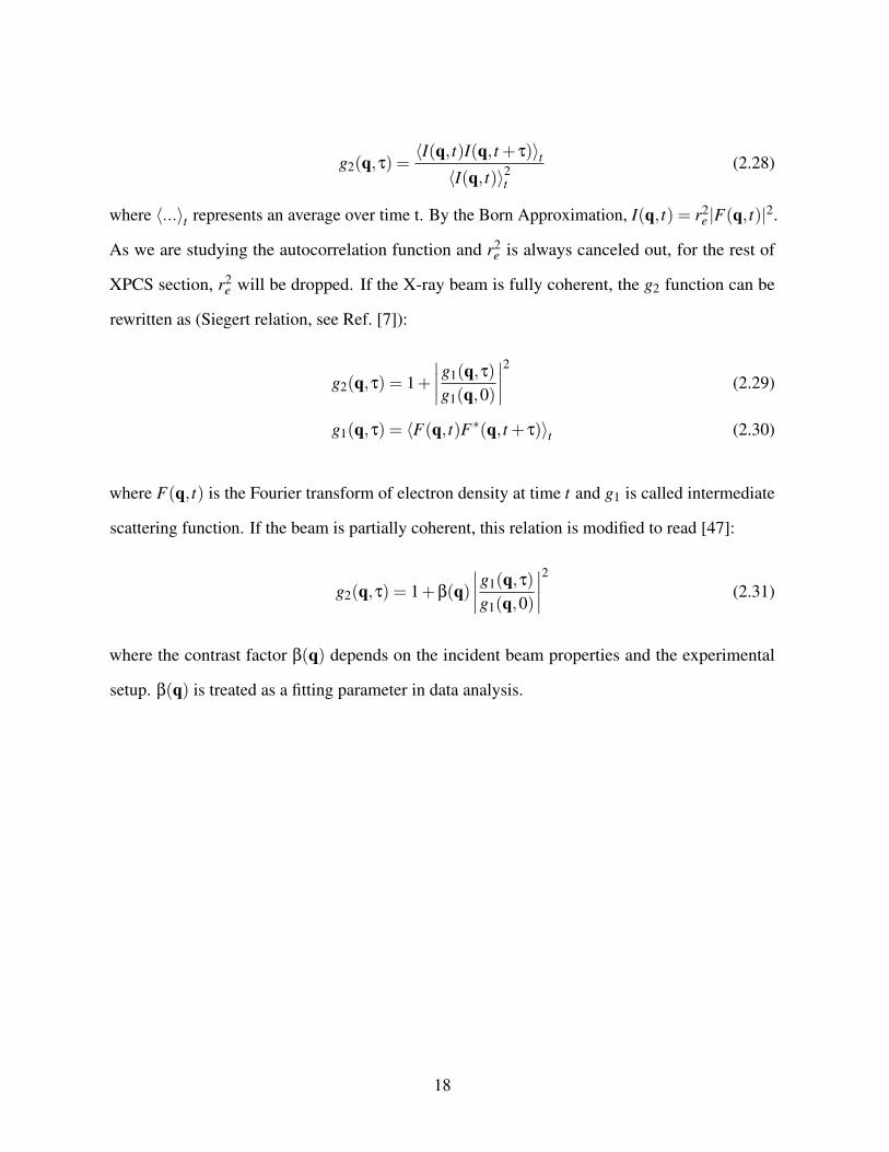
where ⟨...⟩t represents an average over time t. By the Born Approximation, I(q, t) = r2e |F(q, t)|2.

As we are studying the autocorrelation function and r2e is always canceled out, for the rest of

XPCS section, r2e will be dropped. If the X-ray beam is fully coherent, the g2 function can be

rewritten as (Siegert relation, see Ref. [7]):

g2(q,τ) = 1+∣∣∣∣g1(q,τ)g1(q,0)

∣∣∣∣2 (2.29)

g1(q,τ) = ⟨F(q, t)F∗(q, t + τ)⟩t (2.30)

where F(q, t) is the Fourier transform of electron density at time t and g1 is called intermediate

scattering function. If the beam is partially coherent, this relation is modified to read [47]:

g2(q,τ) = 1+β(q)∣∣∣∣g1(q,τ)g1(q,0)

∣∣∣∣2 (2.31)

where the contrast factor β(q) depends on the incident beam properties and the experimental

setup. β(q) is treated as a fitting parameter in data analysis.

18

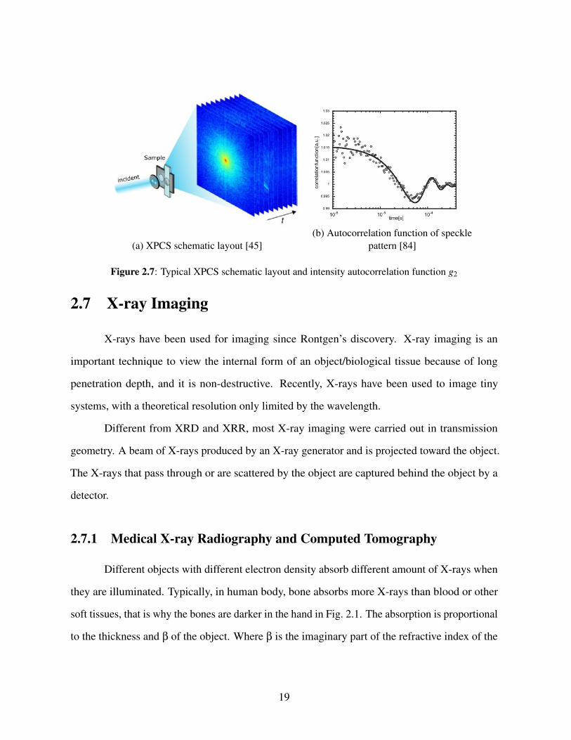
(a) XPCS schematic layout [45](b) Autocorrelation function of speckle

pattern [84]

Figure 2.7: Typical XPCS schematic layout and intensity autocorrelation function g2

2.7 X-ray Imaging

X-rays have been used for imaging since Rontgen’s discovery. X-ray imaging is an

important technique to view the internal form of an object/biological tissue because of long

penetration depth, and it is non-destructive. Recently, X-rays have been used to image tiny

systems, with a theoretical resolution only limited by the wavelength.

Different from XRD and XRR, most X-ray imaging were carried out in transmission

geometry. A beam of X-rays produced by an X-ray generator and is projected toward the object.

The X-rays that pass through or are scattered by the object are captured behind the object by a

detector.

2.7.1 Medical X-ray Radiography and Computed Tomography

Different objects with different electron density absorb different amount of X-rays when

they are illuminated. Typically, in human body, bone absorbs more X-rays than blood or other

soft tissues, that is why the bones are darker in the hand in Fig. 2.1. The absorption is proportional

to the thickness and β of the object. Where β is the imaginary part of the refractive index of the

19

object. See section 2.1.2 for details about β.

The generation of flat 2 dimensional images by this technique is called projectional

radiography. In addition, if the X-ray generator rotates around the object, and detectors positioned

on the opposite side of the circle from the X-ray source, a 3D image of the object can be

tomographically reconstructed from the 2D images [94, 91].

2.7.2 The Phase Problem and Coherent X-ray Diffraction Imaging

X-ray crystallography has been an enormously successful technique to solve the structure

of proteins down to the 2A level provided they can be crystallized because the phases of the Bragg

reflections can be obtained by tricks, such as heavy atom substitutions. However, finding the

structure of non-crystalline materials has proved far more challenging due to the problem of not

knowing the phase. However, there now exist methods [26, 52, 58] for retrieving the phases of an

“oversampled” speckle pattern by iterative techniques described below and known as Coherent

Diffraction Imaging (CDI).

The coherent X-ray beam scattered by the nano object produces a diffraction pattern

(speckle pattern) which can be interpreted by the Born approximation Eq. (2.18) (in transmission

geometry, BA is appropriate, see Fig. 2.8a for the experimental configuration). The diffraction

pattern has the magnitude information of the Fourier transform of the object’s electron density, but

the phase information is lost, which is needed to reconstruct the electron density. Sayre proposed

the crystallography methods might be adapted for the phase retrieval in 1980 [79, 14]. Miao

et.al first demonstrated it in 1999 [58]. Miao et.al successfully reconstructed an array of gold

dots, shown in Fig. 2.9. The phase was retrieved by oversampling the diffraction pattern using

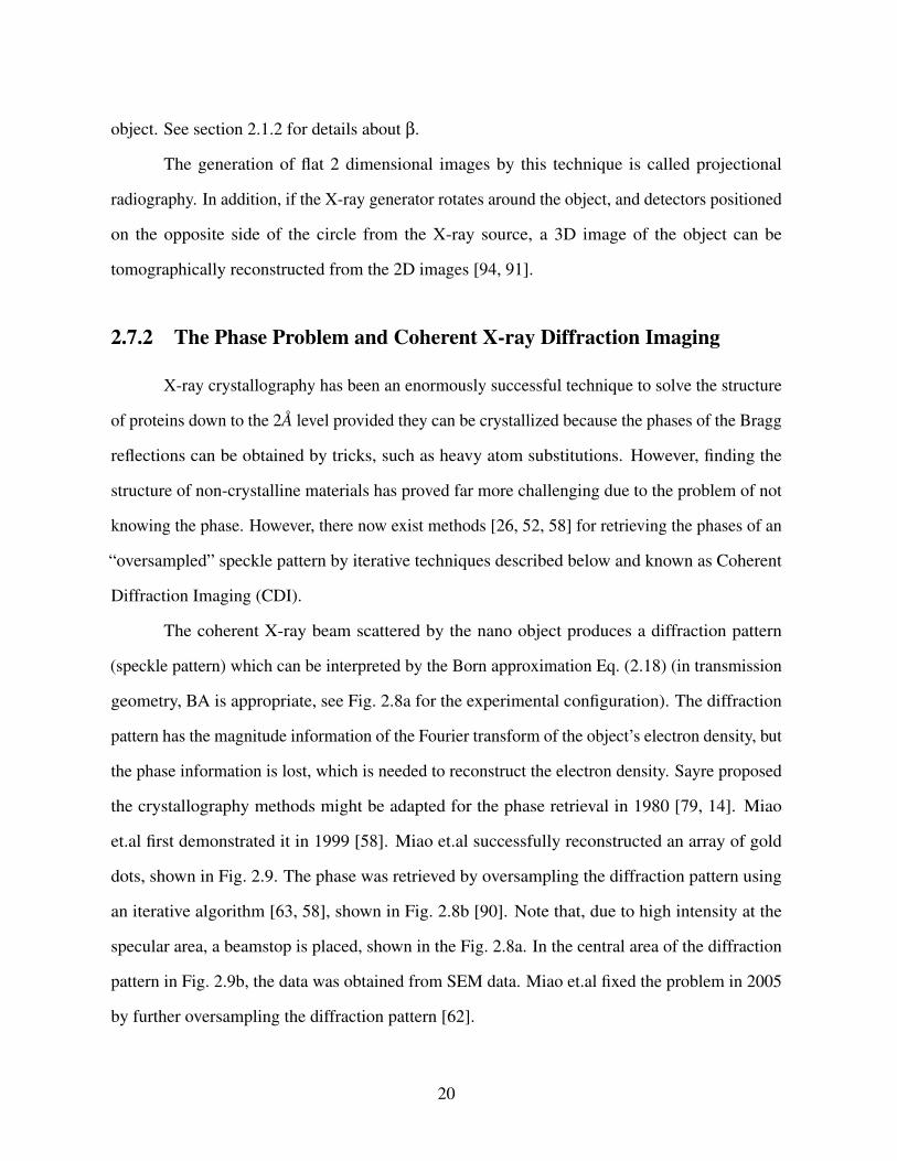
an iterative algorithm [63, 58], shown in Fig. 2.8b [90]. Note that, due to high intensity at the

specular area, a beamstop is placed, shown in the Fig. 2.8a. In the central area of the diffraction

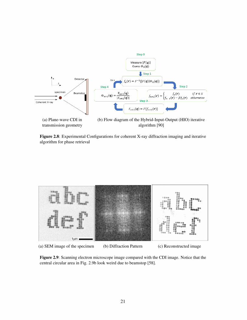
pattern in Fig. 2.9b, the data was obtained from SEM data. Miao et.al fixed the problem in 2005

by further oversampling the diffraction pattern [62].

20

(a) Plane-wave CDI intransmission geometry

(b) Flow diagram of the Hybrid-Input-Output (HIO) iterativealgorithm [90]

Figure 2.8: Experimental Configurations for coherent X-ray diffraction imaging and iterativealgorithm for phase retrieval

(a) SEM image of the specimen (b) Diffraction Pattern (c) Reconstructed image

Figure 2.9: Scanning electron microscope image compared with the CDI image. Notice that thecentral circular area in Fig. 2.9b look weird due to beamstop [58].

21

Chapter 3

Dynamics of the Magnetic Moments in Spin

Glass System Studied by RM-XPCS

3.1 Introduction to Spin Glass System and Its Phase Transition

To understand what a spin glass is, we first introduce the Heisenberg Hamiltonian [93] and

Ruderman-Kittel-Kasuya-Yosida (RKKY) interaction [95, 76] for magnetic materials. Heisenberg

Hamiltonian is also called exchange Hamiltonian:

H = ∑i, ji= j

J(ri j)Si ·S j

where J(ri j) is the coupling parameter (aka. exchange integral) between the magnetic moments

(spins, dipoles) Si and S j. Typically, J(r) drops very fast when the distance r between magnetic

moments increases. The magnetic metal is in the ground states (the most stable states) when its

Hamiltonian reaches minimum. That is, if J < 0, the magnetic spins tends to align themselves in

parallel, which is also known as ferromagnetic, and if J > 0, spins tends to align in anti-parallel,

aka. anti-ferromagnetic.

22

A conventional spin glass consists of a random (usually dilute) alloy of magnetic spins in

a non-magnetic metal crystal, e.g. Fe in Au or Mn in Cu [67]. The distance of magnetic spins

between nearest neighbors is not a constant in spin glasses. The oscillatory coupling parameter

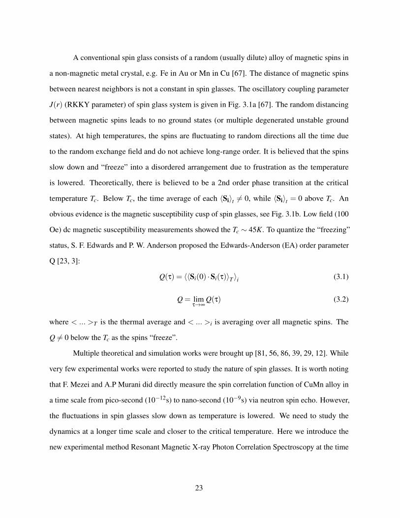
J(r) (RKKY parameter) of spin glass system is given in Fig. 3.1a [67]. The random distancing

between magnetic spins leads to no ground states (or multiple degenerated unstable ground

states). At high temperatures, the spins are fluctuating to random directions all the time due

to the random exchange field and do not achieve long-range order. It is believed that the spins

slow down and “freeze” into a disordered arrangement due to frustration as the temperature

is lowered. Theoretically, there is believed to be a 2nd order phase transition at the critical

temperature Tc. Below Tc, the time average of each ⟨Si⟩t = 0, while ⟨Si⟩t = 0 above Tc. An

obvious evidence is the magnetic susceptibility cusp of spin glasses, see Fig. 3.1b. Low field (100

Oe) dc magnetic susceptibility measurements showed the Tc ∼ 45K. To quantize the “freezing”

status, S. F. Edwards and P. W. Anderson proposed the Edwards-Anderson (EA) order parameter

Q [23, 3]:

Q(τ) = ⟨⟨Si(0) ·Si(τ)⟩T ⟩i (3.1)

Q = limτ→∞

Q(τ) (3.2)

where < ... >T is the thermal average and < ... >i is averaging over all magnetic spins. The

Q = 0 below the Tc as the spins “freeze”.

Multiple theoretical and simulation works were brought up [81, 56, 86, 39, 29, 12]. While

very few experimental works were reported to study the nature of spin glasses. It is worth noting

that F. Mezei and A.P Murani did directly measure the spin correlation function of CuMn alloy in

a time scale from pico-second (10−12s) to nano-second (10−9s) via neutron spin echo. However,

the fluctuations in spin glasses slow down as temperature is lowered. We need to study the

dynamics at a longer time scale and closer to the critical temperature. Here we introduce the

new experimental method Resonant Magnetic X-ray Photon Correlation Spectroscopy at the time

23

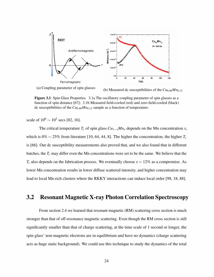
(a) Coupling parameter of spin glasses (b) Measured dc susceptibilities of the Cu0.88Mn0.12

Figure 3.1: Spin Glass Properties. 3.1a The oscillatory coupling parameter of spin glasses as afunction of spin distance [67]; 3.1b Measured field-cooled (red) and zero-field-cooled (black)dc susceptibilities of the Cu0.88Mn0.12 sample as a function of temperature.

scale of 100 ∼ 103 secs [82, 16].

The critical temperature Tc of spin glass Cu1−xMnx depends on the Mn concentration x,

which is 0% ∼ 25% from literature [10, 64, 44, 8]. The higher the concentration, the higher Tc

is [66]. Our dc susceptibility measurements also proved that, and we also found that in different

batches, the Tc may differ even the Mn concentrations were set to be the same. We believe that the

Tc also depends on the fabrication process. We eventually choose x = 12% as a compromise. As

lower Mn concentration results in lower diffuse scattered intensity, and higher concentration may

lead to local Mn-rich clusters where the RKKY interactions can induce local order [98, 18, 88].

3.2 Resonant Magnetic X-ray Photon Correlation Spectroscopy

From section 2.4 we learned that resonant magnetic (RM) scattering cross section is much

stronger than that of off-resonance magnetic scattering. Even though the RM cross section is still

significantly smaller than that of charge scattering, at the time scale of 1 second or longer, the

spin glass’ non-magnetic electrons are in equilibrium and have no dynamics (charge scattering

acts as huge static background). We could use this technique to study the dynamics of the total

24

scattered intensity (including both charge and magnetic scattering) to interpret to magnetic spin

fluctuations. We collect the total scattered intensity Itot(q, t) on the detector:

Itot(q, t) = Ic(q, t)+ Im(q, t) (3.3)

where Ic(q, t) is the intensity of the charge scattering and Im(q, t) that of the magnetic scattering,

at the measurement time t. Note that, charge scattering is static. that is, Ic(q, t) = Ic(q). Plug

Eq. (3.3) into Eq. (2.28), we get:

g2(q,τ) =⟨Itot(q, t)Itot(q, t + τ)⟩t

⟨Itot(q, t)⟩2t

= 1+⟨Im(q, t)Im(q, t + τ)⟩t −⟨Im(q, t)⟩2

t

I2c (q)+2Ic(q)⟨Im(q, t)⟩t + ⟨Im(q, t)⟩2

t

(3.4)

From Eq. (3.4), we see that g2 −1 is a measure of the fluctuation of Im(q, t). g2 −1 << 1

given Ic > ⟨Im⟩t by a lot. Henceforth, we normalize g2(q,τ)−1 to be (g2(q,τ)−1)/(g2(q,∆t)−

1), where ∆t is the minimum time step of our XPCS measurement.

In the dipolar approximation for quasi-elastic resonance exchange scattering [34], Im(q, t)

is given by

Im(q, t) =C∑i, j

⟨(ein × eout) ·Si(t)(ein × eout) ·S j(t)

⟩e−iq·(Ri−R j) (3.5)

where eout and ein are outgoing and incident beam polarizations. Here we use the subscripts in

and out instead of i and f to avoid confusion of the lattice subscript i in previous section. This

equation is derived from Eq.(4) in Ref. [34]. Details are given below: Eq.(4) in Ref [34] is the

scattering magnitude of transition from 2p3/2 → 5d:

f (xres)EL = F [e∗out · einnh + i(e∗out × ein) ·SiP/4]

25

where nh is the number of holes in the 5d band. In our case, which is transition of Mn 2p3/2 → 3d,

Mn 3d band is half filled and nh = 0. The first term is zero, and e∗out = eout for linear polarized

beam. F and P are constants. The resonant magnetic cross section is:

|Ψin⟩= eikin·r

|Ψout⟩= eikout ·r

Im = | ⟨Ψout | f xresEL |Ψin⟩ |2

= |∑i

FP/4((e∗out × ein) ·Si)e−i(kout−kin)·Ri|2 (3.6)

Note that, the imaginary unit in f (xres)EL is dropped as we are taking its modulus square. Eq. (3.5)

is the same as Eq. (3.6) (constants are not important). If the scattered beam makes a small angle

θ to the incident beam direction (small angle approximation),

(ein × eout) ·Si ≈ Szi (3.7)

where Szi is the component of Si along the incident beam direction:

Im(q, t) = ∑i, j

⟨Sz

i (t)Szj(t)⟩

Te−iq·(Ri−R j)

=12 ∑

i, j

⟨Sz

i (t)Szj(t)⟩

Tcos(q · (Ri −Rj)) (3.8)

Constants are dropped here. Note that ein × eout ≈ z. Assuming the incident beam is s polarized,

and the outgoing beam has both s and p polarized beam. |es,in× es,out | ≤ sinθ and es,in× ep,out ≈ z.

The s→s scattering is neglected since θ is small. The term ⟨Im(q, t)Im(q, t + τ)⟩t is essentially a

4-spin correlation function, and can be used to study the dynamics of 2-spin fluctuations (EA

order parameter).

26

3.3 Measurements and Results

We have conducted XPCS experiments following section 2.6. Experimental details are

given in the next Methods section. The susceptibility measurement result is given in Fig. 3.1b

and we found Tc ≈ 45K. We compared the experimental results g2(q,τ)−1 at the conditions that

sample temperature is above/at/below Tc and that photon energy is on and off resonance. The

results are summarized as follows:

1. No dynamics shown in the (g2−1) at any q at any sample temperature at photon energy off-

resonance. Magnetic scattering is so weak at off-resonance photon energy, see Eq. (2.27).

Charge scattering is dominating and showed no dynamics as expected. See Fig. 3.2b.

2. No dynamics when sample temperature is below Tc at resonance photon energy. The

magnetic spins “freeze” below Tc. Thus there is no spin fluctuations.

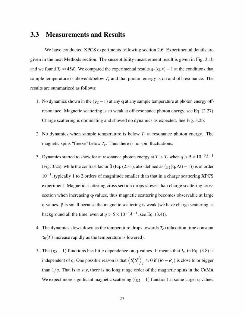
3. Dynamics started to show for at resonance photon energy at T > Tc when q > 5×10−3A−1

(Fig. 3.2a), while the contrast factor β (Eq. (2.31), also defined as (g2(q,∆t)−1)) is of order

10−3, typically 1 to 2 orders of magnitude smaller than that in a charge scattering XPCS

experiment. Magnetic scattering cross section drops slower than charge scattering cross

section when increasing q-values, thus magnetic scattering becomes observable at large

q-values. β is small because the magnetic scattering is weak (we have charge scattering as

background all the time, even at q > 5×10−3A−1, see Eq. (3.4)).

4. The dynamics slows down as the temperature drops towards Tc (relaxation time constant

τ0(T ) increase rapidly as the temperature is lowered).

5. The (g2 −1) functions has little dependence on q-values. It means that Im in Eq. (3.8) is

independent of q. One possible reason is that⟨

Szi S

zj

⟩T≈ 0 if (Ri −R j) is close to or bigger

than 1/q. That is to say, there is no long range order of the magnetic spins in the CuMn.

We expect more significant magnetic scattering ((g2 −1) function) at some larger q-values.

27

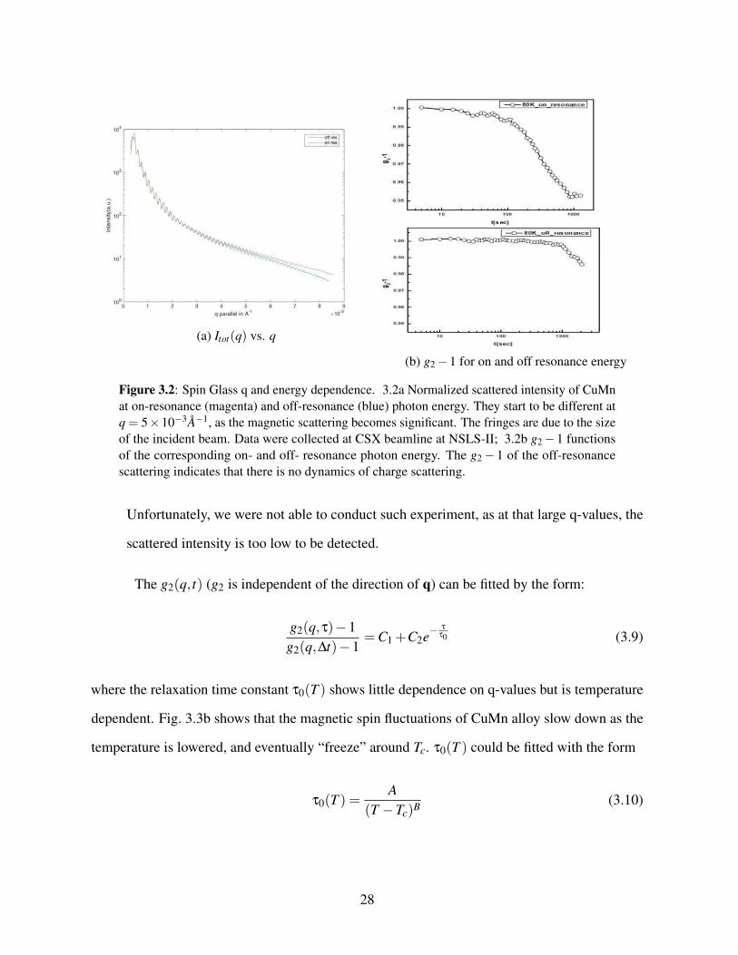
(a) Itot(q) vs. q

(b) g2 −1 for on and off resonance energy

Figure 3.2: Spin Glass q and energy dependence. 3.2a Normalized scattered intensity of CuMnat on-resonance (magenta) and off-resonance (blue) photon energy. They start to be different atq = 5×10−3A−1, as the magnetic scattering becomes significant. The fringes are due to the sizeof the incident beam. Data were collected at CSX beamline at NSLS-II; 3.2b g2 −1 functionsof the corresponding on- and off- resonance photon energy. The g2 − 1 of the off-resonancescattering indicates that there is no dynamics of charge scattering.

Unfortunately, we were not able to conduct such experiment, as at that large q-values, the

scattered intensity is too low to be detected.

The g2(q, t) (g2 is independent of the direction of q) can be fitted by the form:

g2(q,τ)−1g2(q,∆t)−1

=C1 +C2e−τ

τ0 (3.9)

where the relaxation time constant τ0(T ) shows little dependence on q-values but is temperature

dependent. Fig. 3.3b shows that the magnetic spin fluctuations of CuMn alloy slow down as the

temperature is lowered, and eventually “freeze” around Tc. τ0(T ) could be fitted with the form

τ0(T ) =A

(T −Tc)B (3.10)

28

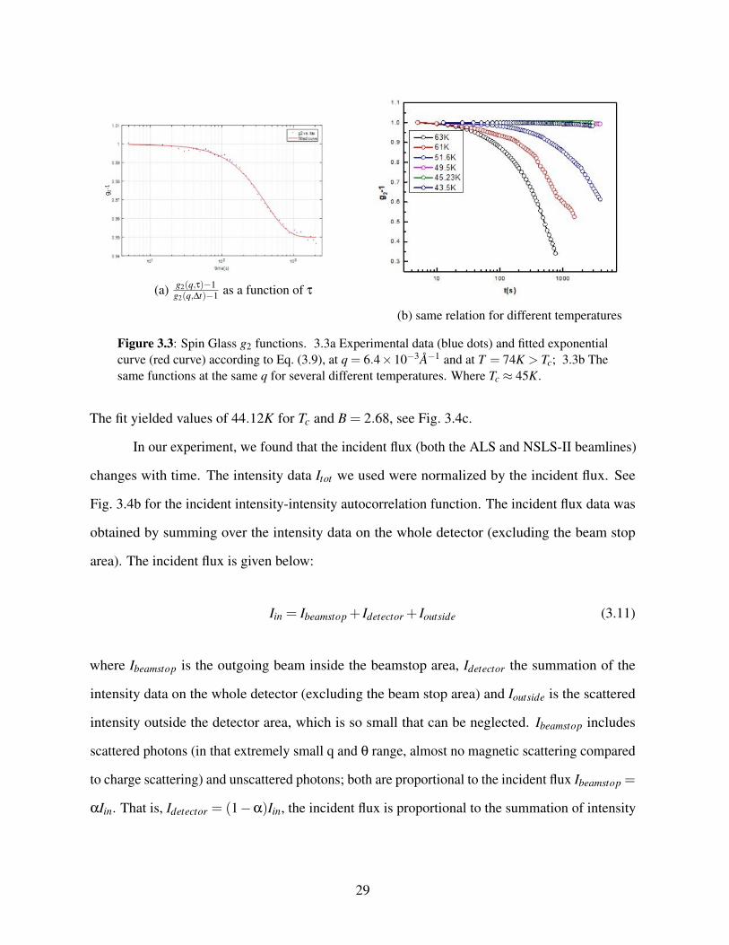
(a) g2(q,τ)−1g2(q,∆t)−1 as a function of τ

(b) same relation for different temperatures

Figure 3.3: Spin Glass g2 functions. 3.3a Experimental data (blue dots) and fitted exponentialcurve (red curve) according to Eq. (3.9), at q = 6.4×10−3A−1 and at T = 74K > Tc; 3.3b Thesame functions at the same q for several different temperatures. Where Tc ≈ 45K.

The fit yielded values of 44.12K for Tc and B = 2.68, see Fig. 3.4c.

In our experiment, we found that the incident flux (both the ALS and NSLS-II beamlines)

changes with time. The intensity data Itot we used were normalized by the incident flux. See

Fig. 3.4b for the incident intensity-intensity autocorrelation function. The incident flux data was

obtained by summing over the intensity data on the whole detector (excluding the beam stop

area). The incident flux is given below:

Iin = Ibeamstop + Idetector + Ioutside (3.11)

where Ibeamstop is the outgoing beam inside the beamstop area, Idetector the summation of the

intensity data on the whole detector (excluding the beam stop area) and Ioutside is the scattered

intensity outside the detector area, which is so small that can be neglected. Ibeamstop includes

scattered photons (in that extremely small q and θ range, almost no magnetic scattering compared

to charge scattering) and unscattered photons; both are proportional to the incident flux Ibeamstop =

αIin. That is, Idetector = (1−α)Iin, the incident flux is proportional to the summation of intensity

29

data on detector.

We initially carried out the experiment at CSX in NSLS-II. But the data showed that the

incident beam had a constant period and decayed with time. Then we continued the experiment at

ALS, which is more stable (see Fig. 3.4b). There are multiple possible reasons for periodicity

and decaying at CSX, saying the X-ray source instability, possible periodical movement of the

beamstop, the efficiency of the CCD detector (which may be periodic and decay with time). All

the data shown in this chapter were collected from ALS beamline, unless specified.

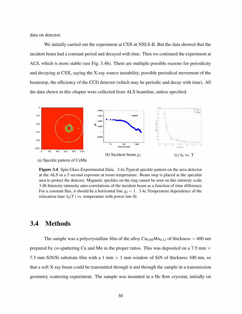
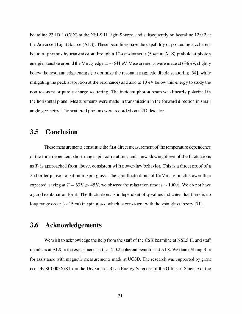
(a) Speckle pattern of CuMn(b) Incident beam g2 (c) τ0 vs. T

Figure 3.4: Spin Glass Experimental Data. 3.4a Typical speckle pattern on the area detectorat the ALS in a 5 second exposure at room temperature. Beam stop is placed at the speculararea to protect the detector. Magnetic speckles on the ring cannot be seen on this intensity scale.3.4b Intensity-intensity auto-correlations of the incident beam as a function of time difference.For a constant flux, it should be a horizontal line g2 = 1. 3.4c Temperature dependence of therelaxation time τ0(T ) vs. temperature with power law fit.

3.4 Methods

The sample was a polycrystalline film of the alloy Cu0.88Mn0.12 of thickness ∼ 400 nm

prepared by co-sputtering Cu and Mn in the proper ratios. This was deposited on a 7.5 mm ×

7.5 mm SiN/Si substrate film with a 1 mm × 1 mm window of SiN of thickness 100 nm, so

that a soft X-ray beam could be transmitted through it and through the sample in a transmission

geometry scattering experiment. The sample was mounted in a He flow cryostat, initially on

30

beamline 23-ID-1 (CSX) at the NSLS-II Light Source, and subsequently on beamline 12.0.2 at

the Advanced Light Source (ALS). These beamlines have the capability of producing a coherent

beam of photons by transmission through a 10-µm-diameter (5 µm at ALS) pinhole at photon

energies tunable around the Mn L3 edge at ∼ 641 eV. Measurements were made at 636 eV, slightly

below the resonant edge energy (to optimize the resonant magnetic dipole scattering [34], while

mitigating the peak absorption at the resonance) and also at 10 eV below this energy to study the

non-resonant or purely charge scattering. The incident photon beam was linearly polarized in

the horizontal plane. Measurements were made in transmission in the forward direction in small

angle geometry. The scattered photons were recorded on a 2D detector.

3.5 Conclusion

These measurements constitute the first direct measurement of the temperature dependence

of the time-dependent short-range spin correlations, and show slowing down of the fluctuations

as Tc is approached from above, consistent with power-law behavior. This is a direct proof of a

2nd order phase transition in spin glass. The spin fluctuations of CuMn are much slower than

expected, saying at T = 63K ≫ 45K, we observe the relaxation time is ∼ 1000s. We do not have

a good explanation for it. The fluctuations is independent of q-values indicates that there is no

long range order (∼ 15nm) in spin glass, which is consistent with the spin glass theory [71].

3.6 Acknowledgements

We wish to acknowledge the help from the staff of the CSX beamline at NSLS II, and staff

members at ALS in the experiments at the 12.0.2 coherent beamline at ALS. We thank Sheng Ran

for assistance with magnetic measurements made at UCSD. The research was supported by grant

no. DE-SC0003678 from the Division of Basic Energy Sciences of the Office of Science of the

31

U.S. Dept. of Energy. MBM acknowledges the support of the US Department of Energy, Office

of Basic Energy Sciences, Division of Materials Sciences and Engineering, under Grant No.

DE-FG02-04ER46105. This research used beamline 23-ID-1of the National Synchrotron Light

Source II, a U.S. Department of Energy (DOE) Office of Science User Facility operated for the

DOE Office of Science by Brookhaven National Laboratory under Contract No. DE-SC0012704.

Work at the ALS, LBNL was supported by the Director, Office of Science, Office of Basic Energy

Sciences, of the US Department of Energy (Contract No. DE-AC02-05CH11231).

Chapter 3, in part is currently submitted for publication of the material. Jingjin Song,

Sheena K.K. Patel, Rupak Bhattacharya, Yi Yang, Sudip Pandey, Xiao M. Chen, Xi Chen, Kalyan

Sasmal, M. Brian Maple, Eric E. Fullerton, Sujoy Roy, Claudio Mazzoli,Chandra M. Varma and

Sunil K. Sinha. “Direct measurement of temporal correlations above the spin-glass transition by

coherent resonant magnetic x-ray spectroscopy”. The disseration author contributed to collect

and analyze the data at the synchrotron sources and was a co-author on this material.

32

Chapter 4

Coherent Diffraction Imaging in Reflection

Geometry at Grazing Incidences

Coherent X-ray Diffraction Imaging has high resolution without optical lens. The penetrat-

ing nature of X-rays allows imaging of objects much thicker than optical and electron microscopes

(e.g. TEM, STM, SEM, AFM etc.). This chapter is about how iterative algorithms solve the phase

problem from the diffraction pattern of an object; and we further developed such method to fit for

the Distorted Wave Born Approximation which is more accurate at grazing incidence close to

or smaller than the critical angle than Born Approximation. Continuing from section 2.7.2, let’s

start with the CDI algorithm:

4.1 Coherent Diffraction Imaging Algorithm

We have a picture of 256× 256 pixels. It is Fourier transformed to a 256× 256 pixel

diffraction pattern, shown in Fig. 4.1. The magnitude together with phase can be inverse Fourier

transformed back to the original image. But in an actual experiment, the phase information is lost.

Please refer to Eq. (2.18) to see why phase is lost. Keep in mind that the diffraction magnitude

33

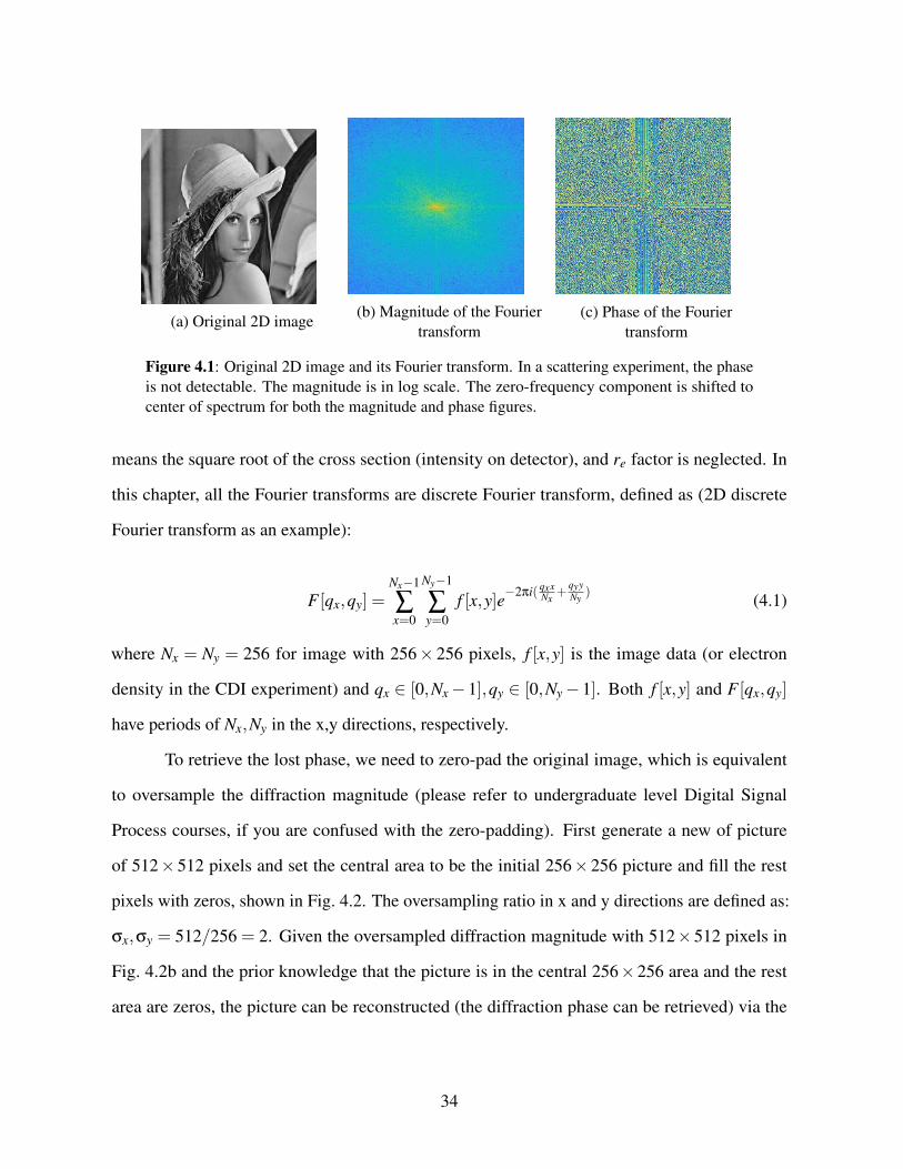
(a) Original 2D image(b) Magnitude of the Fourier

transform(c) Phase of the Fourier

transform

Figure 4.1: Original 2D image and its Fourier transform. In a scattering experiment, the phaseis not detectable. The magnitude is in log scale. The zero-frequency component is shifted tocenter of spectrum for both the magnitude and phase figures.

means the square root of the cross section (intensity on detector), and re factor is neglected. In

this chapter, all the Fourier transforms are discrete Fourier transform, defined as (2D discrete

Fourier transform as an example):

F [qx,qy] =Nx−1

∑x=0

Ny−1

∑y=0

f [x,y]e−2πi( qxxNx +

qyyNy ) (4.1)

where Nx = Ny = 256 for image with 256× 256 pixels, f [x,y] is the image data (or electron

density in the CDI experiment) and qx ∈ [0,Nx − 1],qy ∈ [0,Ny − 1]. Both f [x,y] and F [qx,qy]

have periods of Nx,Ny in the x,y directions, respectively.

To retrieve the lost phase, we need to zero-pad the original image, which is equivalent

to oversample the diffraction magnitude (please refer to undergraduate level Digital Signal

Process courses, if you are confused with the zero-padding). First generate a new of picture

of 512× 512 pixels and set the central area to be the initial 256× 256 picture and fill the rest

pixels with zeros, shown in Fig. 4.2. The oversampling ratio in x and y directions are defined as:

σx,σy = 512/256 = 2. Given the oversampled diffraction magnitude with 512×512 pixels in

Fig. 4.2b and the prior knowledge that the picture is in the central 256×256 area and the rest

area are zeros, the picture can be reconstructed (the diffraction phase can be retrieved) via the

34

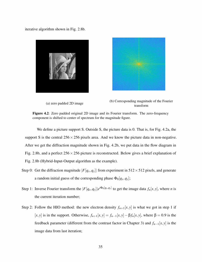
iterative algorithm shown in Fig. 2.8b.

(a) zero padded 2D image(b) Corresponding magnitude of the Fourier

transform

Figure 4.2: Zero padded original 2D image and its Fourier transform. The zero-frequencycomponent is shifted to center of spectrum for the magnitude figure.

We define a picture support S. Outside S, the picture data is 0. That is, for Fig. 4.2a, the

support S is the central 256×256 pixels area. And we know the picture data in non-negative.

After we get the diffraction magnitude shown in Fig. 4.2b, we put data in the flow diagram in

Fig. 2.8b, and a perfect 256×256 picture is reconstructed. Below gives a brief explanation of

Fig. 2.8b (Hybrid-Input-Output algorithm as the example).

Step 0: Get the diffraction magnitude |F [qx,qy]| from experiment in 512×512 pixels, and generate

a random initial guess of the corresponding phase Φ0[qx,qy];

Step 1: Inverse Fourier transform the |F [qx,qy]|eiΦ0[qx,qy] to get the image data fn[x,y], where n is

the current iteration number;

Step 2: Follow the HIO method: the new electron density fn+1[x,y] is what we got in step 1 if

[x,y] is in the support. Otherwise, fn+1[x,y] = fn−1[x,y]−β fn[x,y], where β = 0.9 is the

feedback parameter (different from the contrast factor in Chapter 3) and fn−1[x,y] is the

image data from last iteration;

35

Step 3: Fourier transform the new image data fn+1[x,y] to get Fn+1[qx,qy]

Step 4: Keep the phase of Fn+1[qx,qy] and discard the magnitude, plug the new phase back into

step 1.

By iterating step 1 ∼ 4 for a few thousand times, Φ[qx,qy] will converge. There are

numerous algorithms to deal with the phase retrieval, including Error Reduction (ER) [26, 32, 43],

Relaxed Averaged Alternating Reflection [46], Difference Map [24] and more [2, 6, 5]. The

difference of the algorithms is in step 2. For example, the ER replace the step 2 with: fn+1[x,y] = 0,

if fn+1[x,y] < 0 or [x,y] is outside the support. Because electron density (image data) is non-

negative. The HIO is often used in conjunction with the ER, by alternating several HIO and one

or more ER iterations [52] (HIO(60)+ER(1) in our case). One or more ER steps are used at the

end of the iterations.

Speaking of the periodicity of the f [x,y], it is not true in reality. But we have to treat it as

periodic when doing simulation. Because we are using Fast Fourier Transform, which is based on

discrete Fourier transform. The periodicity does not affect the experiment or simulation result, as

we are studying the image in one period. Fig. 4.3 illustrates the periodicity of an unpadded image

and that of its zero-padded image.

We have tested Error Reduction (ER), Difference Map (DM), and Relaxed Averaged

Alternating Reflection (RAAR), as mentioned before. For 3D CDI, The error of HIO is around

10−7 if there is no missing pixels, while DM’s and RAAR’s errors are around 10−2, and ER may

not converge. If there is a beamstop at the zero-frequency area (diffraction pattern center), there

is no big difference among the 3 algorithms (except ER). Mathematically speaking, HIO is the

simplest. Thus we use HIO for our CDI reconstruction. The definition of error and beamstop

problem can be found in the next section.

36

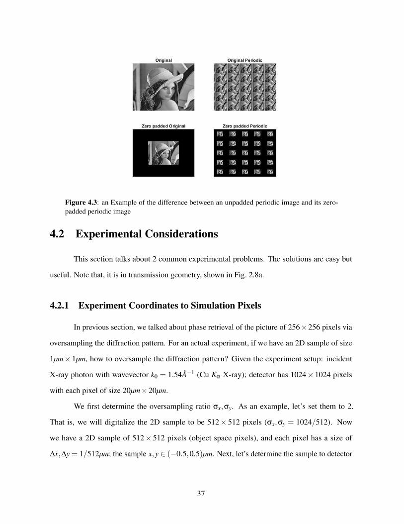
Figure 4.3: an Example of the difference between an unpadded periodic image and its zero-padded periodic image

4.2 Experimental Considerations

This section talks about 2 common experimental problems. The solutions are easy but

useful. Note that, it is in transmission geometry, shown in Fig. 2.8a.

4.2.1 Experiment Coordinates to Simulation Pixels

In previous section, we talked about phase retrieval of the picture of 256×256 pixels via

oversampling the diffraction pattern. For an actual experiment, if we have an 2D sample of size

1µm× 1µm, how to oversample the diffraction pattern? Given the experiment setup: incident

X-ray photon with wavevector k0 = 1.54A−1 (Cu Kα X-ray); detector has 1024× 1024 pixels

with each pixel of size 20µm×20µm.

We first determine the oversampling ratio σx,σy. As an example, let’s set them to 2.

That is, we will digitalize the 2D sample to be 512× 512 pixels (σx,σy = 1024/512). Now

we have a 2D sample of 512× 512 pixels (object space pixels), and each pixel has a size of

∆x,∆y = 1/512µm; the sample x,y ∈ (−0.5,0.5)µm. Next, let’s determine the sample to detector

37

distance. We want the q ranges from qx,qy ∈ (−π/∆x,π/∆x). On the detector, qx = k0xd/L,

where xd is the detector pixel x coordinate and L is the sample to detector distance. In this case,

we want qx,max = k0xd,max/L, where xd,max = 1024 ∗ 20µm/2 = 0.01024m. Note that xd,max is

divided by 2 because xd ∈ (−xd,max,xd,max). We will place the detector behind the sample by

L = k0xd,max/qx,max = 9.8cm, where qx,max = π/∆x.

After collecting the diffraction data, one does not have to worry about anything like

∆x,∆y = 1/512µm. All you have to bear in mind is that the diffraction pattern has a size of

1024×1024. The reconstructed image of size 1024×1024 should have a 512×512 support.

4.2.2 Missing Data Problem

Because of the beamstop, dead pixels on a real detector (typically Charge-Coupled Device,

aka. CCD), the diffraction pattern we get from experiment is unlikely to be complete. Miao et.al

were not able to reconstruct a 2D image without the data in the center of the diffraction pattern

in 1999 [58]. They used the Fourier transform of the SEM data at the diffraction center to fix it.

Later on, Miao proposed that missing pixels are allowed, depending on the oversampling ratio σ

in each dimension [62], which is proved to be consistent in this thesis. The strategy is updating

the Fourier transform magnitude within the missing data area in each iteration according to the

reconstructed diffraction magnitude. Miao et.al. defined the number of missing waves:

ηi =Di −1

2σi, i = x,y,z (4.2)

where Di is the number of missing pixels.

Miao showed that for a 2D picture reconstruction, the reconstruction result is good when

ηx = ηy = 2 and bad when ηx = ηy = 4. In this thesis, we will confirm it by demonstrating recon-

struction a stack of same pictures (pseudo 3D image). First, let’s define the Error (convergence)

38

function of the iterations:

Error =

√∑r | fi(r)− fi+1(r)|2

∑r | fi(r)+ fi+1(r)|2(4.3)

where fi(r) is the reconstructed electron density (image data) in the ith iteration. Note that, the

error function between the reconstructed and original images may be huge, due to the translational

shift of the image. This is unavoidable in CDI but not important.

The projection of the stacked images is given in Fig. 4.4. S is a sphere support without

a rectangular volume (to improve the accuracy of the reconstruction, as reconstruction with a

symmetric support is always with bad quality). The oversampling ratio σ ≈ 2.8 in all directions.

In the Fig. 4.5, the reconstruction error jumps when D > 5 and the electron density converges

rapidly when D = 1, with a final error of ∼ 10−7. The fluctuations of the error in the Fig. 4.5 are

due to the ER iterations in the HIO iterations mentioned in previous section.

Missing pixels away from the diffraction pattern center is not a problem. I tested the

above example with D=0 and missing 10% of the total number of pixels far away from the center,

and the result error is ∼ 10−5.

(a) Original projection of stacked image(b) Reconstructed projection of stacked image

when D = 9

Figure 4.4: Reconstruction of stacked image with missing pixels in the diffraction pattern center.Note that, the reconstruction is bad when D=9. But sometimes with good guess of initial phase,the reconstruction can be much better.

39

(a) D=3 error (b) D=5 error (c) D=7 error (d) D=9 error

Figure 4.5: Reconstruction errors with different number of missing pixels in the center of thediffraction pattern. Fig. 4.5d is corresponding to Fig. 4.4b.

4.3 Three Dimensional Coherent Diffraction Imaging in Trans-

mission Geometry

In previous sections, phase retrieval of a 2D diffraction pattern was given. A new question

arises, is it possible to image a 3D object? The answer is yes. Similar to the CT scan in

section 2.7.1, we can utilize the Computed Tomography (CT) method to reconstruct a 3D object

from the 2D diffraction magnitudes of the object by rotating it about an axis normal to the beam.

There are 2 main CT method to realize the 3D CDI (see Fig. 4.6):

1. Interpolate the multiple 2D diffraction magnitude to 3D diffraction magnitude then retrieve

the phase via CDI (CT in the reciprocal space) [13], see Fig. 4.6a.

2. Retrieve the phase of each 2D diffraction pattern and Fourier transform them back to 2D

projections of the object in different angles, then CT the projections to the 3D image (CT

in the object space) [59], see Fig. 4.6b.

In transmission geometry, for a pixel on detector located at (xd,yd) (assuming the pixel at

the specular spot has coordinate of (0,0)), the corresponding wavevector transfer is: (qx,qy,qz) =

k0(xdL ,

ydL ,0), where L is the sample to detector distance. That is, the diffraction pattern in

reciprocal space is on the meshgrid in qz = 0 plane (qz and z directions are defined along the

40

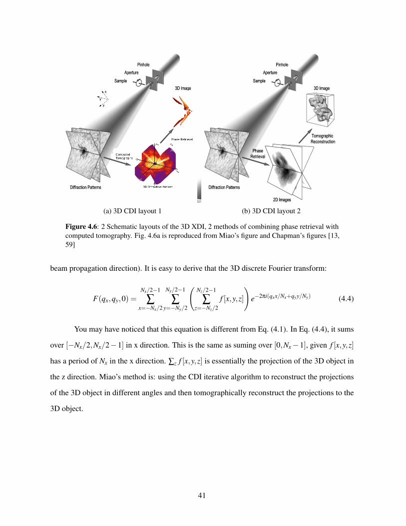
(a) 3D CDI layout 1 (b) 3D CDI layout 2

Figure 4.6: 2 Schematic layouts of the 3D XDI, 2 methods of combining phase retrieval withcomputed tomography. Fig. 4.6a is reproduced from Miao’s figure and Chapman’s figures [13,59]

beam propagation direction). It is easy to derive that the 3D discrete Fourier transform:

F(qx,qy,0) =Nx/2−1

∑x=−Nx/2

Ny/2−1

∑y=−Ny/2

(Nz/2−1

∑z=−Nz/2

f [x,y,z]

)e−2πi(qxx/Nx+qyy/Ny) (4.4)

You may have noticed that this equation is different from Eq. (4.1). In Eq. (4.4), it sums

over [−Nx/2,Nx/2−1] in x direction. This is the same as suming over [0,Nx −1], given f [x,y,z]

has a period of Nx in the x direction. ∑z f [x,y,z] is essentially the projection of the 3D object in

the z direction. Miao’s method is: using the CDI iterative algorithm to reconstruct the projections

of the 3D object in different angles and then tomographically reconstruct the projections to the

3D object.

41

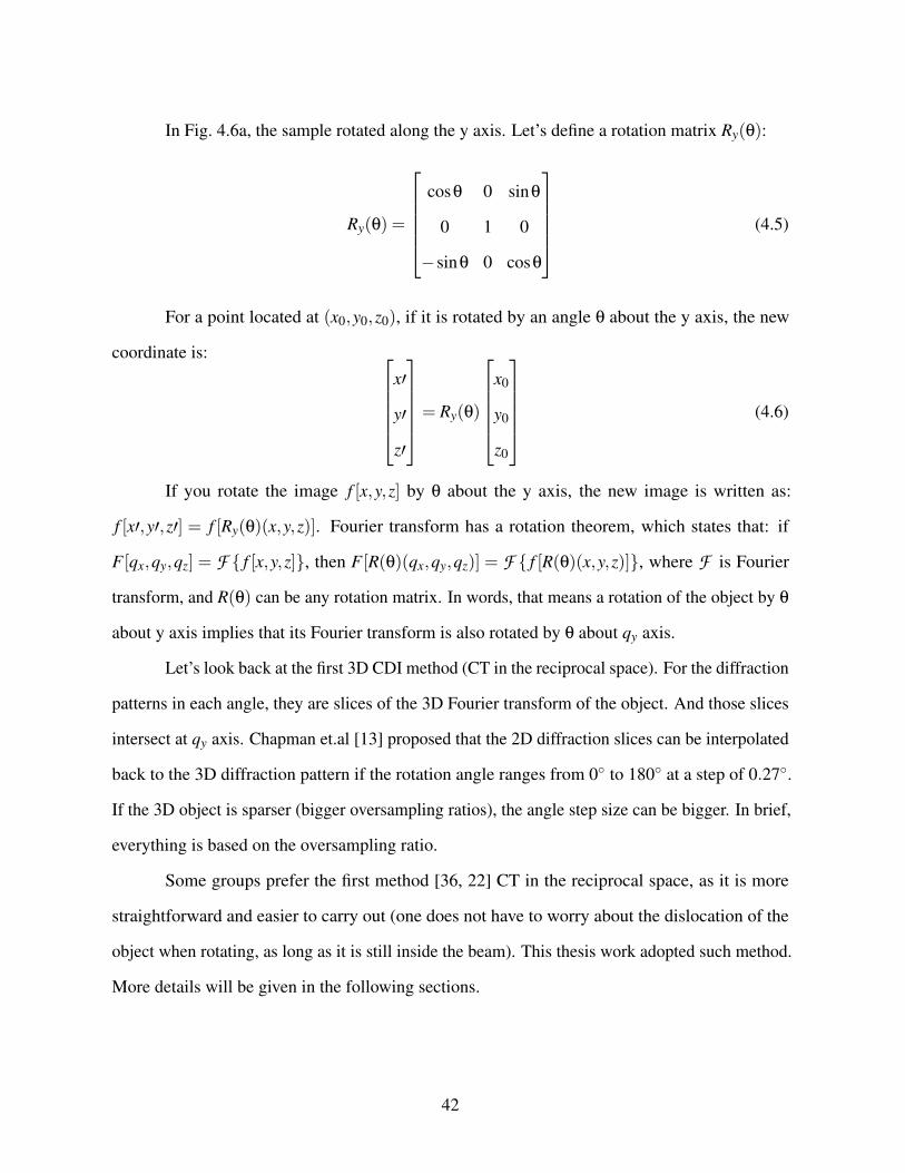
In Fig. 4.6a, the sample rotated along the y axis. Let’s define a rotation matrix Ry(θ):

Ry(θ) =

cosθ 0 sinθ

0 1 0

−sinθ 0 cosθ

(4.5)

For a point located at (x0,y0,z0), if it is rotated by an angle θ about the y axis, the new

coordinate is: x′

y′

z′

= Ry(θ)

x0

y0

z0

(4.6)

If you rotate the image f [x,y,z] by θ about the y axis, the new image is written as:

f [x′,y′,z′] = f [Ry(θ)(x,y,z)]. Fourier transform has a rotation theorem, which states that: if

F [qx,qy,qz] = F f [x,y,z], then F [R(θ)(qx,qy,qz)] = F f [R(θ)(x,y,z)], where F is Fourier

transform, and R(θ) can be any rotation matrix. In words, that means a rotation of the object by θ

about y axis implies that its Fourier transform is also rotated by θ about qy axis.

Let’s look back at the first 3D CDI method (CT in the reciprocal space). For the diffraction

patterns in each angle, they are slices of the 3D Fourier transform of the object. And those slices

intersect at qy axis. Chapman et.al [13] proposed that the 2D diffraction slices can be interpolated

back to the 3D diffraction pattern if the rotation angle ranges from 0 to 180 at a step of 0.27.

If the 3D object is sparser (bigger oversampling ratios), the angle step size can be bigger. In brief,

everything is based on the oversampling ratio.

Some groups prefer the first method [36, 22] CT in the reciprocal space, as it is more

straightforward and easier to carry out (one does not have to worry about the dislocation of the

object when rotating, as long as it is still inside the beam). This thesis work adopted such method.

More details will be given in the following sections.

42

4.4 Coherent Diffraction Imaging in Reflection Geometry

CDI in reflection geometry is not common, because the detector plane is a distorted curved

surface in reciprocal space, which makes it hard to do discrete inverse Fourier transform (as

discrete Fourier transform requires data on the meshgrid points). Zhu et.al [99] tried a big incident

angle (αi = 15.3) and assumed that on the detector plane, qz is a constant of 2k0 sinαi, which

is not accurate. The actual wavevector transfer (Born Approximation) is (details were given in

section 2.3):

qx

qy

qz

= k0

cos(α f )cos(χ)− cos(αi)

sin(χ)cos(α f )

sin(αi)+ sin(α f )

(4.7)

The result of Ref [99] is also confusing (not desirable). Sun et.al [85] tried another method.

They used a sample with uniform thickness, similar to the stacked images in previous section in

this thesis. With such prior knowledge, they were able to normalize the qz factor out.

4.4.1 Experimental Success on a Sample with Uniform Thickness

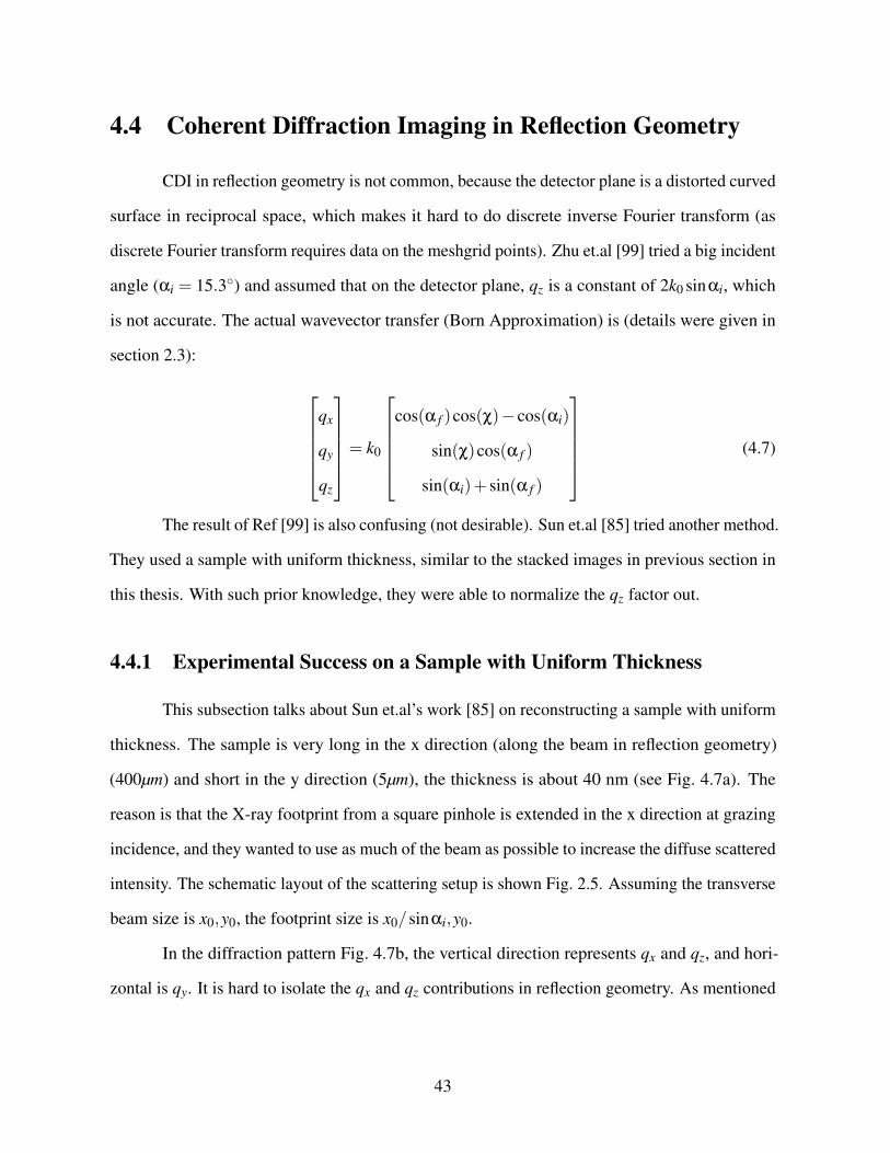
This subsection talks about Sun et.al’s work [85] on reconstructing a sample with uniform

thickness. The sample is very long in the x direction (along the beam in reflection geometry)

(400µm) and short in the y direction (5µm), the thickness is about 40 nm (see Fig. 4.7a). The

reason is that the X-ray footprint from a square pinhole is extended in the x direction at grazing

incidence, and they wanted to use as much of the beam as possible to increase the diffuse scattered

intensity. The schematic layout of the scattering setup is shown Fig. 2.5. Assuming the transverse

beam size is x0,y0, the footprint size is x0/sinαi,y0.

In the diffraction pattern Fig. 4.7b, the vertical direction represents qx and qz, and hori-

zontal is qy. It is hard to isolate the qx and qz contributions in reflection geometry. As mentioned

43

before, Zhu et.al [99] assumed qz to be a constant when incident angle is big. Here, Sun et.al

developed a simulation model to isolate the qz contribution. The model fits the experimental

result, see Fig. 4.7c. But the model only works when the samples with uniform thickness and

identical in-plane electron density distribution. And they found the thickness of the sample using

another method, rather than CDI, see Fig. 4.7d.

(a) Original sampledimension

(b) Diffraction Pattern (c) Experimental dataand simulation (d) ESW amplitude

Figure 4.7: Sun’s Experiment of CDI in Reflection Geometry [85]. 4.7a Schematic of thesample with a thickness of 36nm; 4.7b Diffraction pattern from the sample (logarithmic scale).ROI, region of interest; 4.7c data and simulation of intensity as a function of incident angle atthe region of interest (ROI) at a fixed (qx,qy); 4.7d ESW amplitude as a function of z (normalto the surface). The FWHM is 36.9nm, equal to the sample thickness.

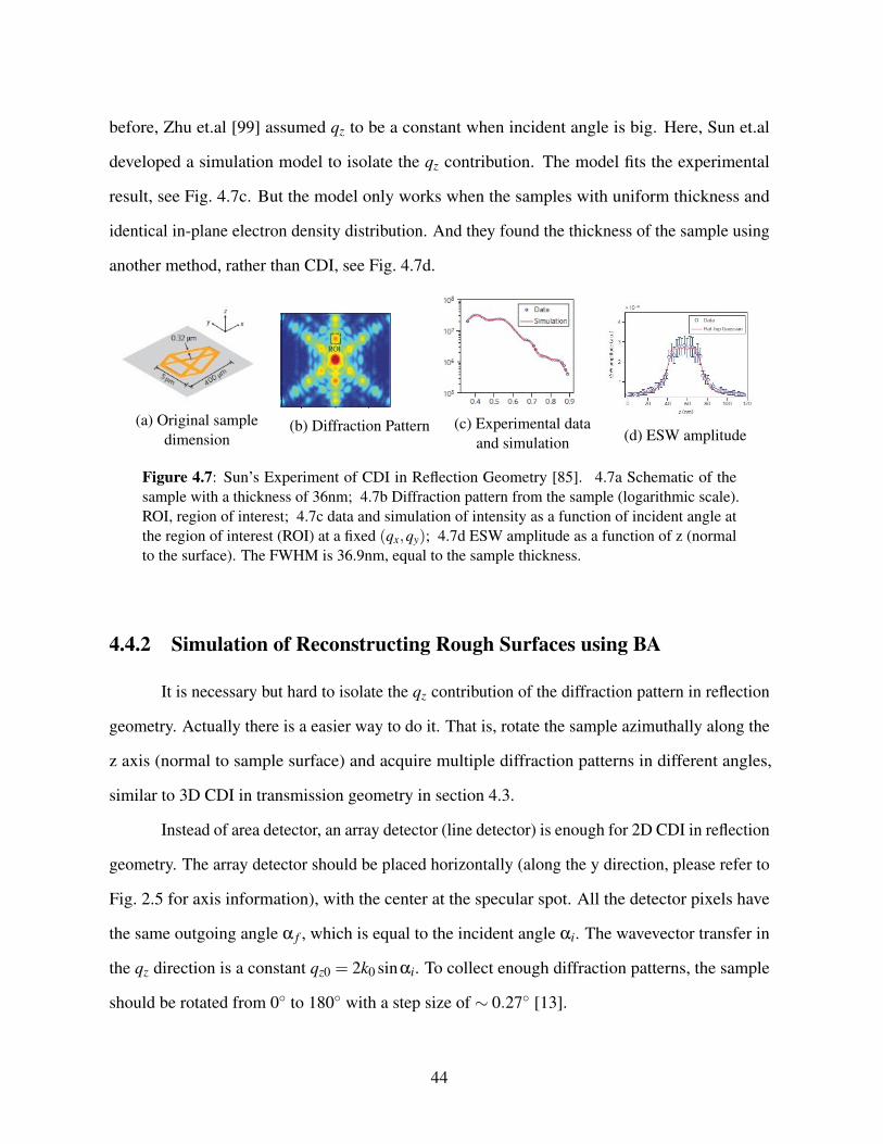
4.4.2 Simulation of Reconstructing Rough Surfaces using BA

It is necessary but hard to isolate the qz contribution of the diffraction pattern in reflection

geometry. Actually there is a easier way to do it. That is, rotate the sample azimuthally along the

z axis (normal to sample surface) and acquire multiple diffraction patterns in different angles,

similar to 3D CDI in transmission geometry in section 4.3.

Instead of area detector, an array detector (line detector) is enough for 2D CDI in reflection

geometry. The array detector should be placed horizontally (along the y direction, please refer to

Fig. 2.5 for axis information), with the center at the specular spot. All the detector pixels have

the same outgoing angle α f , which is equal to the incident angle αi. The wavevector transfer in

the qz direction is a constant qz0 = 2k0 sinαi. To collect enough diffraction patterns, the sample

should be rotated from 0 to 180 with a step size of ∼ 0.27 [13].

44

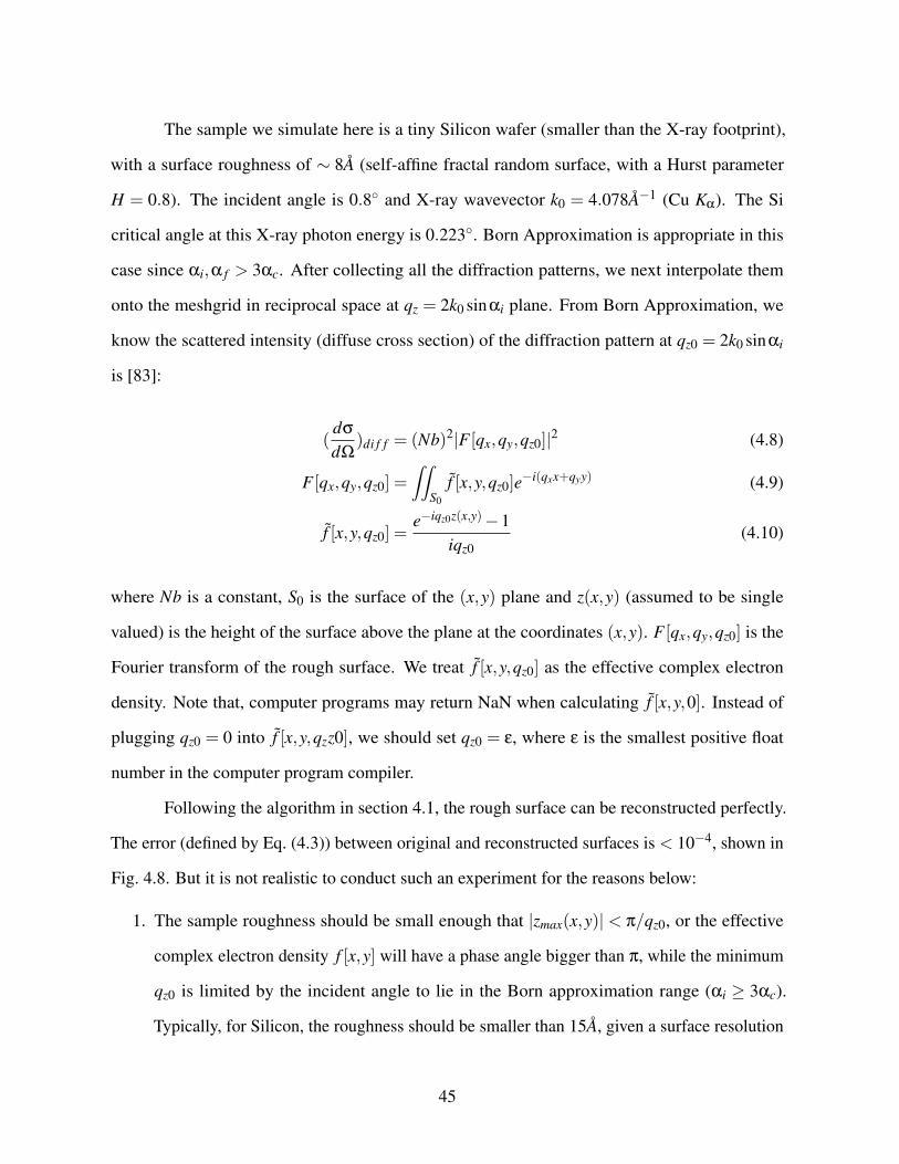
The sample we simulate here is a tiny Silicon wafer (smaller than the X-ray footprint),

with a surface roughness of ∼ 8A (self-affine fractal random surface, with a Hurst parameter

H = 0.8). The incident angle is 0.8 and X-ray wavevector k0 = 4.078A−1 (Cu Kα). The Si

critical angle at this X-ray photon energy is 0.223. Born Approximation is appropriate in this

case since αi,α f > 3αc. After collecting all the diffraction patterns, we next interpolate them

onto the meshgrid in reciprocal space at qz = 2k0 sinαi plane. From Born Approximation, we

know the scattered intensity (diffuse cross section) of the diffraction pattern at qz0 = 2k0 sinαi

is [83]:

(dσ

dΩ)di f f = (Nb)2|F [qx,qy,qz0]|2 (4.8)

F [qx,qy,qz0] =∫∫

S0

f [x,y,qz0]e−i(qxx+qyy) (4.9)

f [x,y,qz0] =e−iqz0z(x,y)−1

iqz0(4.10)

where Nb is a constant, S0 is the surface of the (x,y) plane and z(x,y) (assumed to be single

valued) is the height of the surface above the plane at the coordinates (x,y). F [qx,qy,qz0] is the

Fourier transform of the rough surface. We treat f [x,y,qz0] as the effective complex electron

density. Note that, computer programs may return NaN when calculating f [x,y,0]. Instead of

plugging qz0 = 0 into f [x,y,qzz0], we should set qz0 = ε, where ε is the smallest positive float

number in the computer program compiler.

Following the algorithm in section 4.1, the rough surface can be reconstructed perfectly.

The error (defined by Eq. (4.3)) between original and reconstructed surfaces is < 10−4, shown in

Fig. 4.8. But it is not realistic to conduct such an experiment for the reasons below:

1. The sample roughness should be small enough that |zmax(x,y)| < π/qz0, or the effective

complex electron density f [x,y] will have a phase angle bigger than π, while the minimum

qz0 is limited by the incident angle to lie in the Born approximation range (αi ≥ 3αc).

Typically, for Silicon, the roughness should be smaller than 15A, given a surface resolution

45

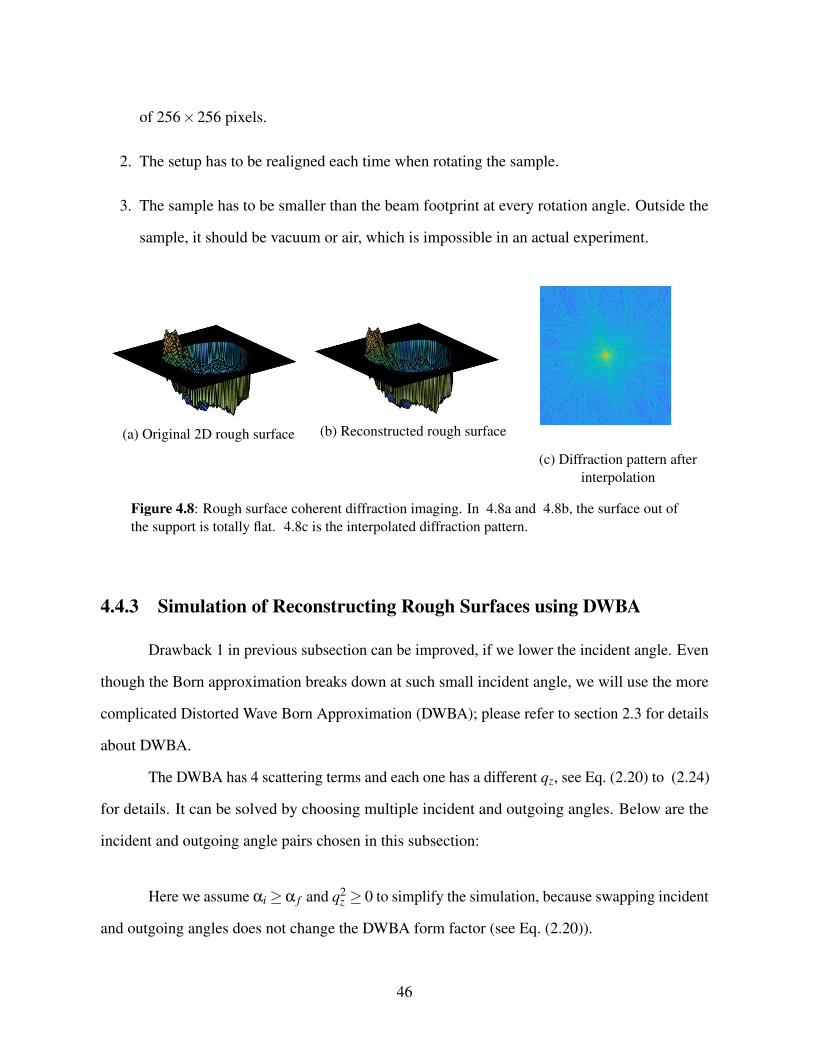
of 256×256 pixels.

2. The setup has to be realigned each time when rotating the sample.

3. The sample has to be smaller than the beam footprint at every rotation angle. Outside the

sample, it should be vacuum or air, which is impossible in an actual experiment.

(a) Original 2D rough surface (b) Reconstructed rough surface

(c) Diffraction pattern afterinterpolation

Figure 4.8: Rough surface coherent diffraction imaging. In 4.8a and 4.8b, the surface out ofthe support is totally flat. 4.8c is the interpolated diffraction pattern.

4.4.3 Simulation of Reconstructing Rough Surfaces using DWBA

Drawback 1 in previous subsection can be improved, if we lower the incident angle. Even

though the Born approximation breaks down at such small incident angle, we will use the more

complicated Distorted Wave Born Approximation (DWBA); please refer to section 2.3 for details

about DWBA.

The DWBA has 4 scattering terms and each one has a different qz, see Eq. (2.20) to (2.24)

for details. It can be solved by choosing multiple incident and outgoing angles. Below are the

incident and outgoing angle pairs chosen in this subsection:

Here we assume αi ≥α f and q2z ≥ 0 to simplify the simulation, because swapping incident

and outgoing angles does not change the DWBA form factor (see Eq. (2.20)).

46

Table 4.1: Angle pairs and corresponding wavetransfers. The incident and outgoing angles,with a unit of ∆α = αc/2. The wavetransfer qzs have a unit of ∆q = k0 sin∆α, where k0 is theincident X-ray beam wavevector.

αi(∆α) α f (∆α) q1z (∆qz) q2

z (∆qz) q3z (∆qz) q4

z (∆qz)1 1 2 0 0 -22 2 4 0 0 -43 1 4 2 -2 -43 3 6 0 0 -64 2 6 2 -2 -65 1 6 4 -4 -6

The simulation steps are:

1. Use the method in previous subsection to collect the cross section for each incident and

outgoing angle pair. That is, for each incident and outgoing angle pair, use a line detector

to collect the data and rotate the sample from 0 to 180 with a step size of ∼ 0.27;

2. Interpolate the data into the qx,qy meshgrid for each incident and outgoing angle pair; (Do

not forget to square root the cross section to get the magnitude |G[qx,qy,kiz,k

fz ]|.)

3. Regroup the data according to the qx,qy meshgrid. That is, group the data with the same

qx,qy. Each group has 6 data (number of the incident and outgoing angle pairs).

Till now, we have 6 linear equations (See Table 4.1; each row is correpsonding to 1

47

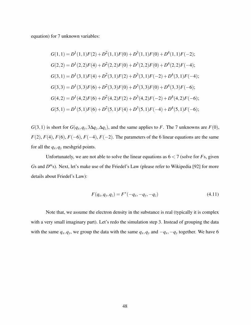
equation) for 7 unknown variables:

G(1,1) = D1(1,1)F(2)+D2(1,1)F(0)+D3(1,1)F(0)+D4(1,1)F(−2);

G(2,2) = D1(2,2)F(4)+D2(2,2)F(0)+D3(2,2)F(0)+D4(2,2)F(−4);

G(3,1) = D1(3,1)F(4)+D2(3,1)F(2)+D3(3,1)F(−2)+D4(3,1)F(−4);

G(3,3) = D1(3,3)F(6)+D2(3,3)F(0)+D3(3,3)F(0)+D4(3,3)F(−6);

G(4,2) = D1(4,2)F(6)+D2(4,2)F(2)+D3(4,2)F(−2)+D4(4,2)F(−6);

G(5,1) = D1(5,1)F(6)+D2(5,1)F(4)+D3(5,1)F(−4)+D4(5,1)F(−6);

G(3,1) is short for G(qx,qy,3∆qz,∆qz), and the same applies to F . The 7 unknowns are F(0),

F(2), F(4), F(6), F(−6), F(−4), F(−2). The parameters of the 6 linear equations are the same

for all the qx,qy meshgrid points.

Unfortunately, we are not able to solve the linear equations as 6 < 7 (solve for Fs, given

Gs and Dms). Next, let’s make use of the Friedel’s Law (please refer to Wikipedia [92] for more

details about Friedel’s Law):

F(qx,qy,qz) = F∗(−qx,−qy,−qz) (4.11)

Note that, we assume the electron density in the substance is real (typically it is complex

with a very small imaginary part). Let’s redo the simulation step 3. Instead of grouping the data

with the same qx,qy, we group the data with the same qx,qy and −qx,−qy together. We have 6

48

extra linear equations and 7 more unknowns now:

G−(1,1) = D1(1,1)F−(2)+D2(1,1)F−(0)+D3(1,1)F−(0)+D4(1,1)F−(−2);

G−(2,2) = D1(2,2)F−(4)+D2(2,2)F−(0)+D3(2,2)F−(0)+D4(2,2)F−(−4);

G−(3,1) = D1(3,1)F−(4)+D2(3,1)F−(2)+D3(3,1)F−(−2)+D4(3,1)F−(−4);

G−(3,3) = D1(3,3)F−(6)+D2(3,3)F−(0)+D3(3,3)F−(0)+D4(3,3)F−(−6);

G−(4,2) = D1(4,2)F−(6)+D2(4,2)F−(2)+D3(4,2)F−(−2)+D4(4,2)F−(−6);

G−(5,1) = D1(5,1)F−(6)+D2(5,1)F−(4)+D3(5,1)F−(−4)+D4(5,1)F−(−6);

where G−(5,1) stands for G(−qx,−qy,5,1), and the same applies to F−.

The 7 new unknowns are related to the 7 previous unknowns by the Friedel’s Law, such

as F−(−6) = F∗(6). Let’s rewrite the linear equations in matrix form:

Re[G+]

Re[G−]

Im[G+]

Im[G−]

24×1

= A24×14 ∗

Re[F ]

Im[F ]

14×1

(4.12)

49

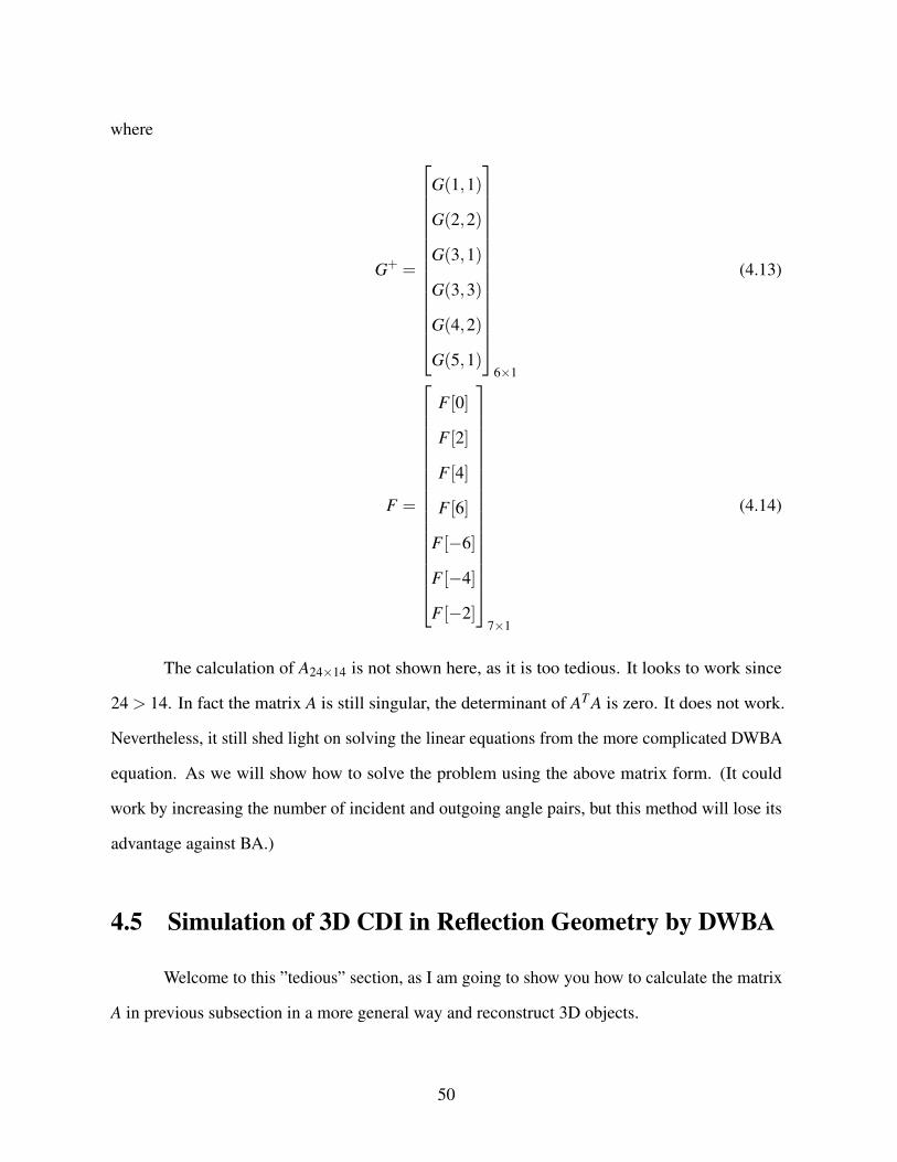
where

G+ =

G(1,1)

G(2,2)

G(3,1)

G(3,3)

G(4,2)

G(5,1)

6×1

(4.13)

F =

F [0]

F [2]

F [4]

F [6]

F [−6]

F [−4]

F [−2]

7×1

(4.14)

The calculation of A24×14 is not shown here, as it is too tedious. It looks to work since

24 > 14. In fact the matrix A is still singular, the determinant of AT A is zero. It does not work.

Nevertheless, it still shed light on solving the linear equations from the more complicated DWBA

equation. As we will show how to solve the problem using the above matrix form. (It could

work by increasing the number of incident and outgoing angle pairs, but this method will lose its

advantage against BA.)

4.5 Simulation of 3D CDI in Reflection Geometry by DWBA

Welcome to this ”tedious” section, as I am going to show you how to calculate the matrix

A in previous subsection in a more general way and reconstruct 3D objects.

50

4.5.1 Matrix Algorithm

Actually, the DWBA matrix shown in previous section works. But we need more angle

pairs. Moreover, we can use the method to reconstruct 3D object, other than the 2D rough surface.

Assume we have a 3D object of Nx ×Ny ×Nz pixels, including the volume outside the support

(oversampling). Similar to Eq. (4.1), its Fourier transform is given:

F [qx,qy,qz] =Nx−1

∑x=0

Ny−1

∑y=0

Nz−1

∑z=0

f [x,y,z]e−2πi( qxxNx +

qyyNy +

qzzNz ) (4.15)

where f [x,y,z] is the object electron denisty and qx ∈ [0,Nx −1], qy ∈ [0,Ny −1], qz ∈ [0,Nz −1].

Both f [x,y,z] and F [qx,qy,qz] have periods of Nx,Ny,Nz in the x,y,z directions, respectively.

First, let’s get F if we have both the magnitude and phase of G (See Eq. (2.20) for the

DWBA form factor G). As we want equally spaced qx,qy,q1z ∼ q4

z data, we need to rotate the

sample about the z axis, and interpolate the data into the qx,qy meshgrid. In the qz direction, we

should choose suitable incident and outgoing angle pairs to equally space q1z ∼ q4

z . For example,

if Nz = 64, we can choose αi,α f from 0.01 to 0.63 with a step of 0.02. By the way, to reduce

the redundancy of the data, we assume αi ≥ α f .

At fixed qx,qy, we have:

G+ = D1F [q1z ]+D2F [q2

z ]+D3F [−q2z ]+D4F [−q1

z ] (4.16)

G− = D1F∗[−q1z ]+D2F∗[−q2

z ]+D3F∗[q2z ]+D4F∗[q1

z ] (4.17)

where G+,G−,F are the same in the previous section.

We have M pairs of (αi,α f ). That is, we have M linear equations of both G+ and G−. We

51

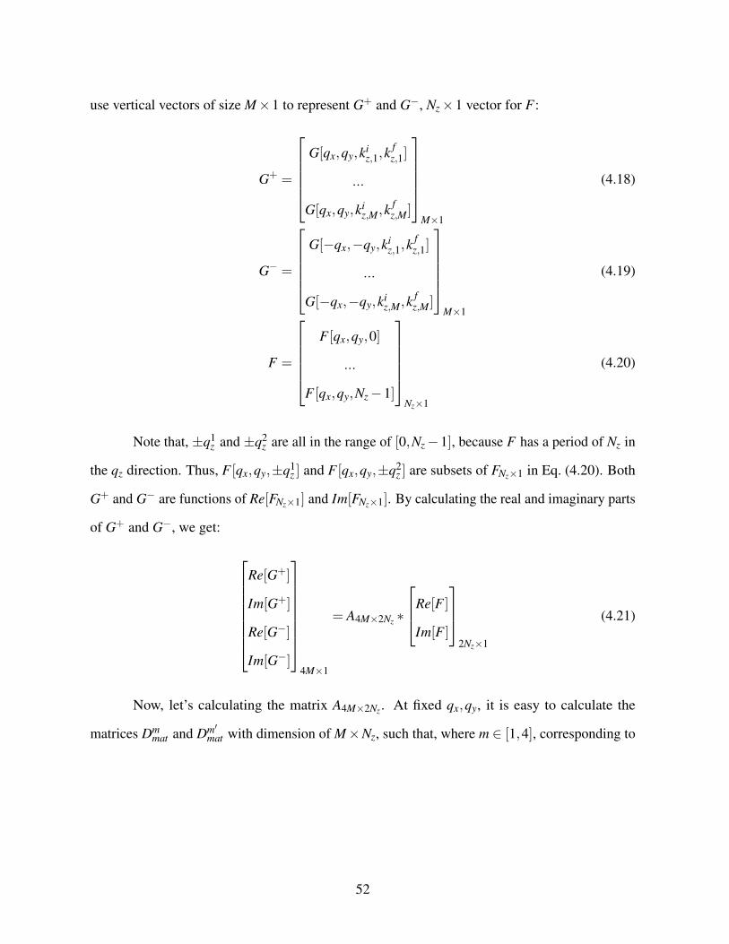
use vertical vectors of size M×1 to represent G+ and G−, Nz ×1 vector for F :

G+ =

G[qx,qy,ki

z,1,kfz,1]

...

G[qx,qy,kiz,M,k f

z,M]

M×1

(4.18)

G− =

G[−qx,−qy,ki

z,1,kfz,1]

...

G[−qx,−qy,kiz,M,k f

z,M]

M×1

(4.19)

F =

F [qx,qy,0]

...

F [qx,qy,Nz −1]

Nz×1

(4.20)

Note that, ±q1z and ±q2

z are all in the range of [0,Nz −1], because F has a period of Nz in

the qz direction. Thus, F [qx,qy,±q1z ] and F [qx,qy,±q2

z ] are subsets of FNz×1 in Eq. (4.20). Both

G+ and G− are functions of Re[FNz×1] and Im[FNz×1]. By calculating the real and imaginary parts

of G+ and G−, we get:

Re[G+]

Im[G+]

Re[G−]

Im[G−]

4M×1

= A4M×2Nz ∗

Re[F ]

Im[F ]

2Nz×1

(4.21)

Now, let’s calculating the matrix A4M×2Nz . At fixed qx,qy, it is easy to calculate the

matrices Dmmat and Dm′

mat with dimension of M×Nz, such that, where m ∈ [1,4], corresponding to

52

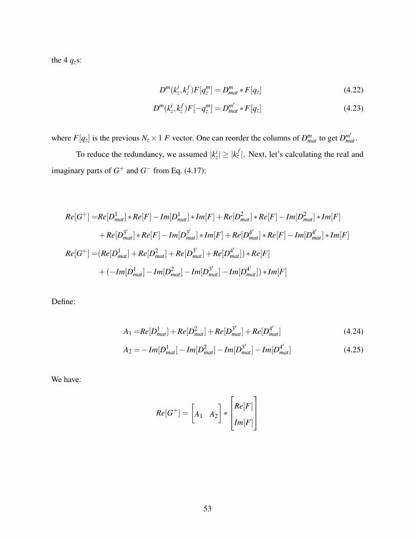
the 4 qzs:

Dm(kiz,k

fz )F [qm

z ] = Dmmat ∗F [qz] (4.22)

Dm(kiz,k

fz )F [−qm

z ] = Dm′mat ∗F [qz] (4.23)

where F [qz] is the previous Nz ×1 F vector. One can reorder the columns of Dmmat to get Dm′

mat .

To reduce the redundancy, we assumed |kiz| ≥ |k f

z |. Next, let’s calculating the real and

imaginary parts of G+ and G− from Eq. (4.17):

Re[G+] =Re[D1mat ]∗Re[F ]− Im[D1

mat ]∗ Im[F ]+Re[D2mat ]∗Re[F ]− Im[D2

mat ]∗ Im[F ]

+Re[D3′mat ]∗Re[F ]− Im[D3′

mat ]∗ Im[F ]+Re[D4′mat ]∗Re[F ]− Im[D4′

mat ]∗ Im[F ]

Re[G+] =(Re[D1mat ]+Re[D2

mat ]+Re[D3′mat ]+Re[D4′

mat ])∗Re[F ]

+ (−Im[D1mat ]− Im[D2

mat ]− Im[D3′mat ]− Im[D4′

mat ])∗ Im[F ]

Define:

A1 =Re[D1mat ]+Re[D2

mat ]+Re[D3′mat ]+Re[D4′

mat ] (4.24)

A2 =− Im[D1mat ]− Im[D2

mat ]− Im[D3′mat ]− Im[D4′

mat ] (4.25)

We have:

Re[G+] =

[A1 A2

]∗

Re[F ]

Im[F ]

53

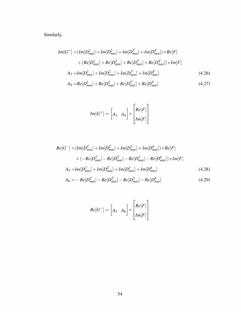
Similarly,

Im[G+] =(Im[D1mat ]+ Im[D2

mat ]+ Im[D3′mat ]+ Im[D4′

mat ])∗Re[F ]

+ (Re[D1mat ]+Re[D2

mat ]+Re[D3′mat ]+Re[D4′

mat ])∗ Im[F ]

A3 =Im[D1mat ]+ Im[D2

mat ]+ Im[D3′mat ]+ Im[D4′

mat ] (4.26)

A4 =Re[D1mat ]+Re[D2

mat ]+Re[D3′mat ]+Re[D4′

mat ] (4.27)

Im[G+] =

[A3 A4

]∗

Re[F ]

Im[F ]

Re[G−] =(Im[D1′mat ]+ Im[D2′

mat ]+ Im[D3mat ]+ Im[D4

mat ])∗Re[F ]

+ (−Re[D1′mat ]−Re[D2′

mat ]−Re[D3mat ]−Re[D4

mat ])∗ Im[F ]

A5 =Im[D1′mat ]+ Im[D2′

mat ]+ Im[D3mat ]+ Im[D4

mat ] (4.28)

A6 =−Re[D1′mat ]−Re[D2′

mat ]−Re[D3mat ]−Re[D4

mat ] (4.29)

Re[G−] =

[A5 A6

]∗

Re[F ]

Im[F ]

54

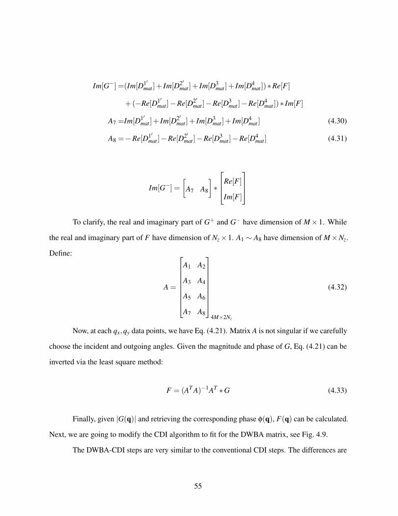
Im[G−] =(Im[D1′mat ]+ Im[D2′

mat ]+ Im[D3mat ]+ Im[D4

mat ])∗Re[F ]

+ (−Re[D1′mat ]−Re[D2′

mat ]−Re[D3mat ]−Re[D4

mat ])∗ Im[F ]

A7 =Im[D1′mat ]+ Im[D2′

mat ]+ Im[D3mat ]+ Im[D4

mat ] (4.30)

A8 =−Re[D1′mat ]−Re[D2′

mat ]−Re[D3mat ]−Re[D4

mat ] (4.31)

Im[G−] =

[A7 A8

]∗

Re[F ]

Im[F ]

To clarify, the real and imaginary part of G+ and G− have dimension of M×1. While

the real and imaginary part of F have dimension of Nz ×1. A1 ∼ A8 have dimension of M×Nz.

Define:

A =

A1 A2

A3 A4

A5 A6

A7 A8

4M×2Nz

(4.32)

Now, at each qx,qy data points, we have Eq. (4.21). Matrix A is not singular if we carefully

choose the incident and outgoing angles. Given the magnitude and phase of G, Eq. (4.21) can be

inverted via the least square method:

F = (AT A)−1AT ∗G (4.33)

Finally, given |G(q)| and retrieving the corresponding phase φ(q), F(q) can be calculated.

Next, we are going to modify the CDI algorithm to fit for the DWBA matrix, see Fig. 4.9.

The DWBA-CDI steps are very similar to the conventional CDI steps. The differences are

55

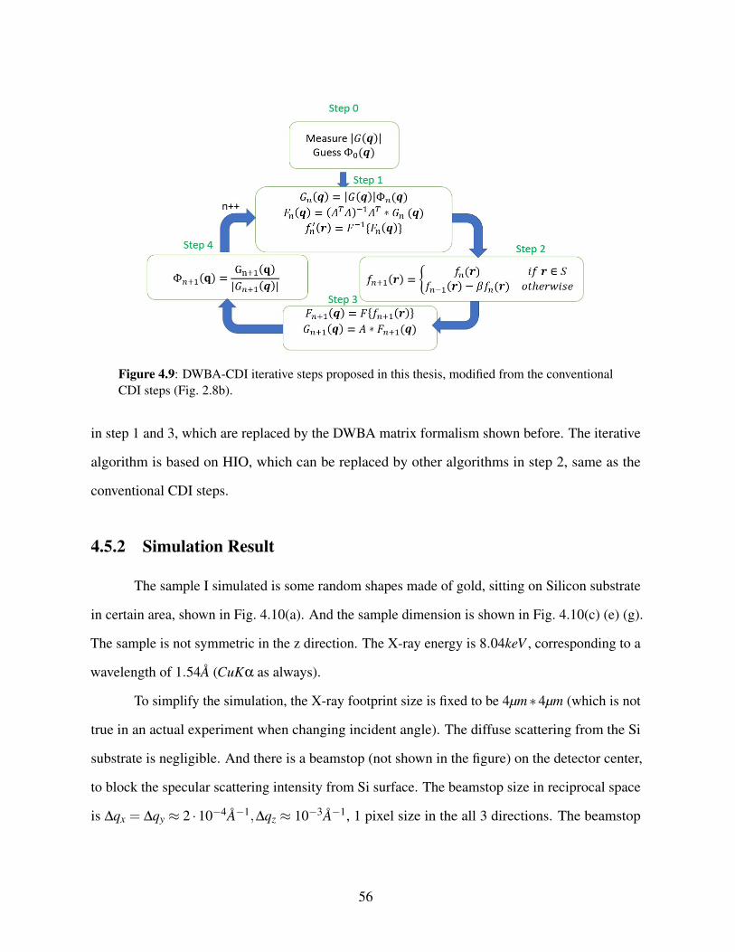
Figure 4.9: DWBA-CDI iterative steps proposed in this thesis, modified from the conventionalCDI steps (Fig. 2.8b).

in step 1 and 3, which are replaced by the DWBA matrix formalism shown before. The iterative

algorithm is based on HIO, which can be replaced by other algorithms in step 2, same as the

conventional CDI steps.

4.5.2 Simulation Result

The sample I simulated is some random shapes made of gold, sitting on Silicon substrate

in certain area, shown in Fig. 4.10(a). And the sample dimension is shown in Fig. 4.10(c) (e) (g).

The sample is not symmetric in the z direction. The X-ray energy is 8.04keV , corresponding to a

wavelength of 1.54A (CuKα as always).

To simplify the simulation, the X-ray footprint size is fixed to be 4µm∗4µm (which is not

true in an actual experiment when changing incident angle). The diffuse scattering from the Si

substrate is negligible. And there is a beamstop (not shown in the figure) on the detector center,

to block the specular scattering intensity from Si surface. The beamstop size in reciprocal space

is ∆qx = ∆qy ≈ 2 ·10−4A−1,∆qz ≈ 10−3A−1, 1 pixel size in the all 3 directions. The beamstop

56

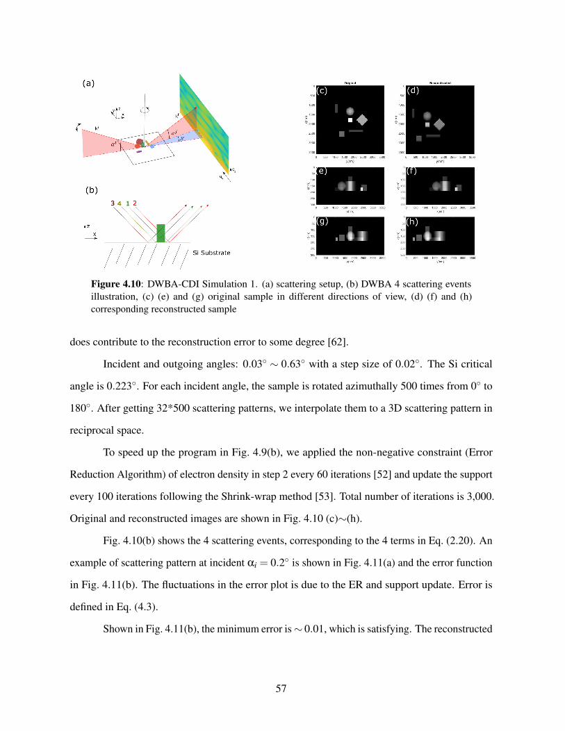
Figure 4.10: DWBA-CDI Simulation 1. (a) scattering setup, (b) DWBA 4 scattering eventsillustration, (c) (e) and (g) original sample in different directions of view, (d) (f) and (h)corresponding reconstructed sample

does contribute to the reconstruction error to some degree [62].

Incident and outgoing angles: 0.03 ∼ 0.63 with a step size of 0.02. The Si critical

angle is 0.223. For each incident angle, the sample is rotated azimuthally 500 times from 0 to

180. After getting 32*500 scattering patterns, we interpolate them to a 3D scattering pattern in

reciprocal space.

To speed up the program in Fig. 4.9(b), we applied the non-negative constraint (Error

Reduction Algorithm) of electron density in step 2 every 60 iterations [52] and update the support

every 100 iterations following the Shrink-wrap method [53]. Total number of iterations is 3,000.

Original and reconstructed images are shown in Fig. 4.10 (c)∼(h).

Fig. 4.10(b) shows the 4 scattering events, corresponding to the 4 terms in Eq. (2.20). An

example of scattering pattern at incident αi = 0.2 is shown in Fig. 4.11(a) and the error function

in Fig. 4.11(b). The fluctuations in the error plot is due to the ER and support update. Error is

defined in Eq. (4.3).

Shown in Fig. 4.11(b), the minimum error is ∼ 0.01, which is satisfying. The reconstructed

57

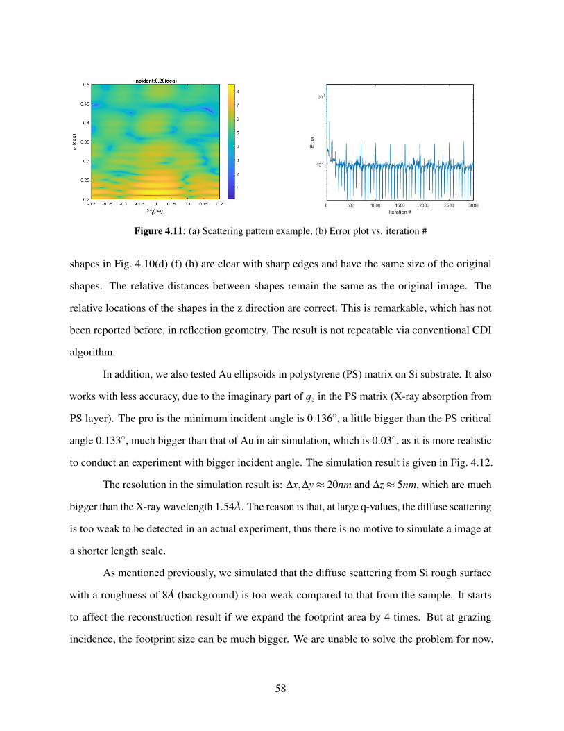
Figure 4.11: (a) Scattering pattern example, (b) Error plot vs. iteration #

shapes in Fig. 4.10(d) (f) (h) are clear with sharp edges and have the same size of the original

shapes. The relative distances between shapes remain the same as the original image. The

relative locations of the shapes in the z direction are correct. This is remarkable, which has not

been reported before, in reflection geometry. The result is not repeatable via conventional CDI

algorithm.

In addition, we also tested Au ellipsoids in polystyrene (PS) matrix on Si substrate. It also

works with less accuracy, due to the imaginary part of qz in the PS matrix (X-ray absorption from

PS layer). The pro is the minimum incident angle is 0.136, a little bigger than the PS critical

angle 0.133, much bigger than that of Au in air simulation, which is 0.03, as it is more realistic

to conduct an experiment with bigger incident angle. The simulation result is given in Fig. 4.12.

The resolution in the simulation result is: ∆x,∆y ≈ 20nm and ∆z ≈ 5nm, which are much

bigger than the X-ray wavelength 1.54A. The reason is that, at large q-values, the diffuse scattering

is too weak to be detected in an actual experiment, thus there is no motive to simulate a image at

a shorter length scale.

As mentioned previously, we simulated that the diffuse scattering from Si rough surface

with a roughness of 8A (background) is too weak compared to that from the sample. It starts

to affect the reconstruction result if we expand the footprint area by 4 times. But at grazing

incidence, the footprint size can be much bigger. We are unable to solve the problem for now.

58

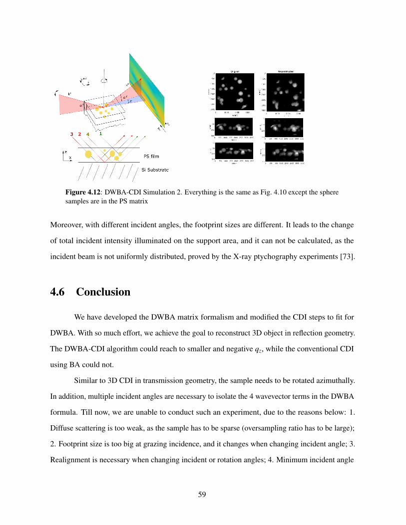
Figure 4.12: DWBA-CDI Simulation 2. Everything is the same as Fig. 4.10 except the spheresamples are in the PS matrix

Moreover, with different incident angles, the footprint sizes are different. It leads to the change

of total incident intensity illuminated on the support area, and it can not be calculated, as the

incident beam is not uniformly distributed, proved by the X-ray ptychography experiments [73].

4.6 Conclusion

We have developed the DWBA matrix formalism and modified the CDI steps to fit for

DWBA. With so much effort, we achieve the goal to reconstruct 3D object in reflection geometry.

The DWBA-CDI algorithm could reach to smaller and negative qz, while the conventional CDI

using BA could not.

Similar to 3D CDI in transmission geometry, the sample needs to be rotated azimuthally.

In addition, multiple incident angles are necessary to isolate the 4 wavevector terms in the DWBA

formula. Till now, we are unable to conduct such an experiment, due to the reasons below: 1.

Diffuse scattering is too weak, as the sample has to be sparse (oversampling ratio has to be large);

2. Footprint size is too big at grazing incidence, and it changes when changing incident angle; 3.

Realignment is necessary when changing incident or rotation angles; 4. Minimum incident angle

59

is too small.

4.7 Acknowledgements

This work in Chapter 4 was supported by grant no. DE-SC0003678 from the Division of

Basic Energy Sciences of the Office of Science of the U.S. Dept. The content in this chapter is

based on material prepared for submission by Yi Yang and Sunil K. Sinha. “Coherent GISAXS

Scattering and Phase Retrieval Using DWBA”. The dissertation author was the primary researcher

and author of this material.

60

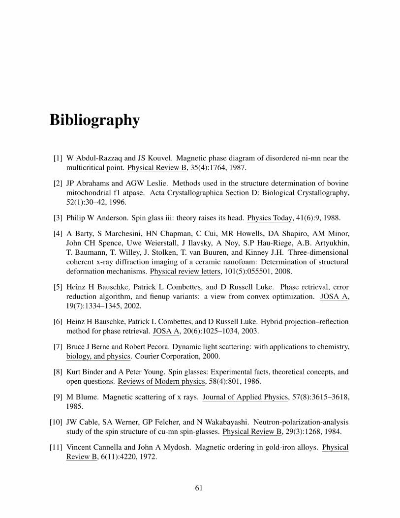
Bibliography

[1] W Abdul-Razzaq and JS Kouvel. Magnetic phase diagram of disordered ni-mn near themulticritical point. Physical Review B, 35(4):1764, 1987.

[2] JP Abrahams and AGW Leslie. Methods used in the structure determination of bovinemitochondrial f1 atpase. Acta Crystallographica Section D: Biological Crystallography,52(1):30–42, 1996.

[3] Philip W Anderson. Spin glass iii: theory raises its head. Physics Today, 41(6):9, 1988.

[4] A Barty, S Marchesini, HN Chapman, C Cui, MR Howells, DA Shapiro, AM Minor,John CH Spence, Uwe Weierstall, J Ilavsky, A Noy, S.P Hau-Riege, A.B. Artyukhin,T. Baumann, T. Willey, J. Stolken, T. van Buuren, and Kinney J.H. Three-dimensionalcoherent x-ray diffraction imaging of a ceramic nanofoam: Determination of structuraldeformation mechanisms. Physical review letters, 101(5):055501, 2008.

[5] Heinz H Bauschke, Patrick L Combettes, and D Russell Luke. Phase retrieval, errorreduction algorithm, and fienup variants: a view from convex optimization. JOSA A,19(7):1334–1345, 2002.

[6] Heinz H Bauschke, Patrick L Combettes, and D Russell Luke. Hybrid projection–reflectionmethod for phase retrieval. JOSA A, 20(6):1025–1034, 2003.

[7] Bruce J Berne and Robert Pecora. Dynamic light scattering: with applications to chemistry,biology, and physics. Courier Corporation, 2000.

[8] Kurt Binder and A Peter Young. Spin glasses: Experimental facts, theoretical concepts, andopen questions. Reviews of Modern physics, 58(4):801, 1986.

[9] M Blume. Magnetic scattering of x rays. Journal of Applied Physics, 57(8):3615–3618,1985.

[10] JW Cable, SA Werner, GP Felcher, and N Wakabayashi. Neutron-polarization-analysisstudy of the spin structure of cu-mn spin-glasses. Physical Review B, 29(3):1268, 1984.

[11] Vincent Cannella and John A Mydosh. Magnetic ordering in gold-iron alloys. PhysicalReview B, 6(11):4220, 1972.

61

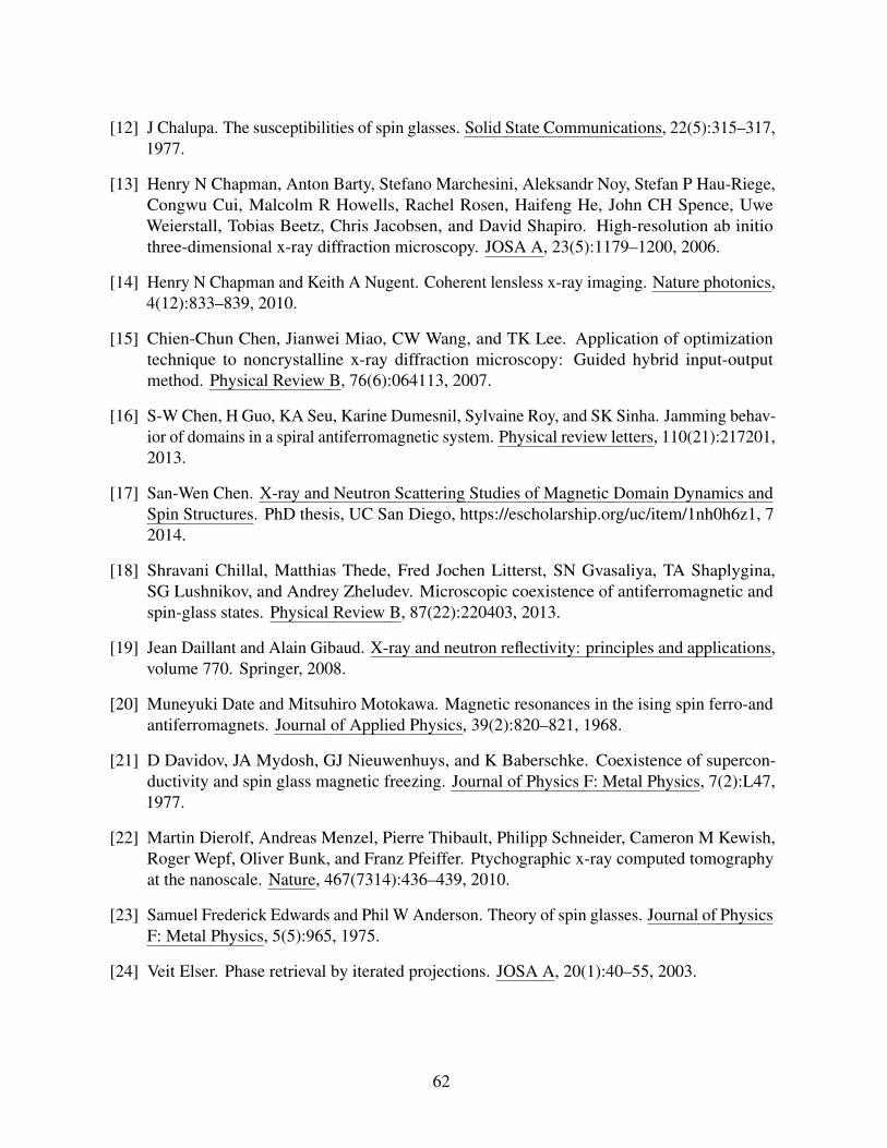
[12] J Chalupa. The susceptibilities of spin glasses. Solid State Communications, 22(5):315–317,1977.

[13] Henry N Chapman, Anton Barty, Stefano Marchesini, Aleksandr Noy, Stefan P Hau-Riege,Congwu Cui, Malcolm R Howells, Rachel Rosen, Haifeng He, John CH Spence, UweWeierstall, Tobias Beetz, Chris Jacobsen, and David Shapiro. High-resolution ab initiothree-dimensional x-ray diffraction microscopy. JOSA A, 23(5):1179–1200, 2006.

[14] Henry N Chapman and Keith A Nugent. Coherent lensless x-ray imaging. Nature photonics,4(12):833–839, 2010.

[15] Chien-Chun Chen, Jianwei Miao, CW Wang, and TK Lee. Application of optimizationtechnique to noncrystalline x-ray diffraction microscopy: Guided hybrid input-outputmethod. Physical Review B, 76(6):064113, 2007.

[16] S-W Chen, H Guo, KA Seu, Karine Dumesnil, Sylvaine Roy, and SK Sinha. Jamming behav-ior of domains in a spiral antiferromagnetic system. Physical review letters, 110(21):217201,2013.

[17] San-Wen Chen. X-ray and Neutron Scattering Studies of Magnetic Domain Dynamics andSpin Structures. PhD thesis, UC San Diego, https://escholarship.org/uc/item/1nh0h6z1, 72014.

[18] Shravani Chillal, Matthias Thede, Fred Jochen Litterst, SN Gvasaliya, TA Shaplygina,SG Lushnikov, and Andrey Zheludev. Microscopic coexistence of antiferromagnetic andspin-glass states. Physical Review B, 87(22):220403, 2013.

[19] Jean Daillant and Alain Gibaud. X-ray and neutron reflectivity: principles and applications,volume 770. Springer, 2008.

[20] Muneyuki Date and Mitsuhiro Motokawa. Magnetic resonances in the ising spin ferro-andantiferromagnets. Journal of Applied Physics, 39(2):820–821, 1968.

[21] D Davidov, JA Mydosh, GJ Nieuwenhuys, and K Baberschke. Coexistence of supercon-ductivity and spin glass magnetic freezing. Journal of Physics F: Metal Physics, 7(2):L47,1977.

[22] Martin Dierolf, Andreas Menzel, Pierre Thibault, Philipp Schneider, Cameron M Kewish,Roger Wepf, Oliver Bunk, and Franz Pfeiffer. Ptychographic x-ray computed tomographyat the nanoscale. Nature, 467(7314):436–439, 2010.

[23] Samuel Frederick Edwards and Phil W Anderson. Theory of spin glasses. Journal of PhysicsF: Metal Physics, 5(5):965, 1975.

[24] Veit Elser. Phase retrieval by iterated projections. JOSA A, 20(1):40–55, 2003.

62

[25] J Ferre, J Rajchenbach, and H Maletta. Faraday rotation measurements of time dependentmagnetic phenomena in insulating spin glasses. Journal of Applied Physics, 52(3):1697–1702, 1981.

[26] James R Fienup. Phase retrieval algorithms: a comparison. Applied optics, 21(15):2758–2769, 1982.

[27] James R Fienup. Reconstruction of a complex-valued object from the modulus of its fouriertransform using a support constraint. JOSA A, 4(1):118–123, 1987.

[28] DK Finnemore, LJ Williams, FH Spedding, and DC Hopkins. Neutron diffraction andsusceptibility study of dilute la-rare-earth alloys. Physical Review, 176(2):712, 1968.

[29] KH Fischer. Static properties of spin glasses. Physical Review Letters, 34(23):1438, 1975.

[30] Daniel S Fisher and David A Huse. Nonequilibrium dynamics of spin glasses. PhysicalReview B, 38(1):373, 1988.

[31] RR Galazka, Shoichi Nagata, and PH Keesom. Paramagnetic—spin-glass—antiferromagnetic phase transitions in cd 1- x mn x te from specific heatand magnetic susceptibility measurements. Physical Review B, 22(7):3344, 1980.

[32] Ralph W Gerchberg. A practical algorithm for the determination of phase from image anddiffraction plane pictures. Optik, 35:237–246, 1972.

[33] Pierre Godard, G Carbone, Marc Allain, Francesca Mastropietro, G Chen, L Capello,A Diaz, TH Metzger, J Stangl, and Virginie Chamard. Three-dimensional high-resolutionquantitative microscopy of extended crystals. Nature communications, 2(1):1–6, 2011.

[34] JP Hannon, GT Trammell, M Blume, and Doon Gibbs. X-ray resonance exchange scattering.Physical review letters, 61(10):1245, 1988.

[35] Ross Harder, M Liang, Y Sun, Y Xia, and IK Robinson. Imaging of complex densityin silver nanocubes by coherent x-ray diffraction. New Journal of Physics, 12(3):035019,2010.

[36] Mirko Holler, Manuel Guizar-Sicairos, Esther HR Tsai, Roberto Dinapoli, Elisabeth Muller,Oliver Bunk, Jorg Raabe, and Gabriel Aeppli. High-resolution non-destructive three-dimensional imaging of integrated circuits. Nature, 543(7645):402–406, 2017.

[37] F Holtzberg, JL Tholence, H Godfrin, and R Tournier. New magnetic properties of a dilutespin-glass. Journal of Applied Physics, 50(B3):1717–1719, 1979.

[38] V. Holy´, J. Kubeˇna, I. Ohli´dal, K. Lischka, and W. Plotz. X-ray reflection from roughlayered systems. Phys. Rev. B, 47:15896–15903, Jun 1993.

[39] Koji Hukushima and Koji Nemoto. Exchange monte carlo method and application to spinglass simulations. Journal of the Physical Society of Japan, 65(6):1604–1608, 1996.

63

[40] Zhang Jiang. X-ray scattering studies of structure and dynamics of surfaces and interfacesof polymeric liquids. PhD thesis, UC San Diego, https://escholarship.org/uc/item/1304106d,7 2007.

[41] Zhang Jiang, Dong Ryeol Lee, Suresh Narayanan, Jin Wang, and Sunil K Sinha. Waveguide-enhanced grazing-incidence small-angle x-ray scattering of buried nanostructures in thinfilms. Physical Review B, 84(7):075440, 2011.

[42] Charles Kittel. Introduction to solid state physics eighth edition. 2021.

[43] Aharon Levi and Henry Stark. Image restoration by the method of generalized projectionswith application to restoration from magnitude. JOSA A, 1(9):932–943, 1984.

[44] Laurent P Levy. Critical dynamics of metallic spin glasses. Physical Review B, 38(7):4963,1988.

[45] Yuan Hung Lo, Lingrong Zhao, Marcus Gallagher-Jones, Arjun Rana, Jared J Lodico,Weikun Xiao, BC Regan, and Jianwei Miao. In situ coherent diffractive imaging. Naturecommunications, 9(1):1–10, 2018.

[46] D Russell Luke. Relaxed averaged alternating reflections for diffraction imaging. Inverseproblems, 21(1):37, 2004.

[47] D Lumma, LB Lurio, SGJ Mochrie, and Mark Sutton. Area detector based photon correlationin the regime of short data batches: Data reduction for dynamic x-ray scattering. Review ofScientific Instruments, 71(9):3274–3289, 2000.

[48] L Lundgren, P Svedlindh, P Nordblad, and O Beckman. Dynamics of the relaxation-timespectrum in a cumn spin-glass. Physical review letters, 51(10):911, 1983.

[49] Davide Magatti and Fabio Ferri. Fast multi-tau real-time software correlator for dynamiclight scattering. Applied optics, 40(24):4011–4021, 2001.

[50] H Maletta and W Felsch. Insulating spin-glass system eu x sr 1- x s. Physical review B,20(3):1245, 1979.

[51] H Maletta, W Felsch, and JL Tholence. Spin glass behaviour in the non-metallic system(eusr) s. Journal of Magnetism and Magnetic Materials, 9(1-3):41–43, 1978.

[52] Stefano Marchesini. Invited article: A unified evaluation of iterative projection algorithmsfor phase retrieval. Review of scientific instruments, 78(1):011301, 2007.

[53] Stefano Marchesini, H He, Henry N Chapman, Stefan P Hau-Riege, Aleksandr Noy, Mal-colm R Howells, Uwe Weierstall, and John CH Spence. X-ray image reconstruction from adiffraction pattern alone. Physical Review B, 68(14):140101, 2003.

[54] Robert D. Martin. Human Brain Evolution in an Ecological Context. American Museumof Natural History, 1983.

64

[55] W McBride, NL O’Leary, and LJ Allen. Retrieval of a complex-valued object from itsdiffraction pattern. Physical review letters, 93(23):233902, 2004.

[56] Marc Mezard, Giorgio Parisi, and Miguel Angel Virasoro. Spin glass theory and beyond:An Introduction to the Replica Method and Its Applications, volume 9. World ScientificPublishing Company, 1987.

[57] F Mezei, W Knaak, and B Farago. Neutron spin echo study of dynamic correlations nearliquid-glass transition. Physica Scripta, 1987(T19B):363, 1987.

[58] Jianwei Miao, Pambos Charalambous, Janos Kirz, and David Sayre. Extending the method-ology of x-ray crystallography to allow imaging of micrometre-sized non-crystalline speci-mens. Nature, 400(6742):342–344, 1999.

[59] Jianwei Miao, Chien-Chun Chen, Changyong Song, Yoshinori Nishino, Yoshiki Kohmura,Tetsuya Ishikawa, Damien Ramunno-Johnson, Ting-Kuo Lee, and Subhash H Risbud. Three-dimensional gan- ga 2 o 3 core shell structure revealed by x-ray diffraction microscopy.Physical review letters, 97(21):215503, 2006.

[60] Jianwei Miao, Friedrich Forster, and Ofer Levi. Equally sloped tomography with oversam-pling reconstruction. Physical Review B, 72(5):052103, 2005.

[61] Jianwei Miao, Tetsuya Ishikawa, Qun Shen, and Thomas Earnest. Extending x-ray crys-tallography to allow the imaging of noncrystalline materials, cells, and single proteincomplexes. Annu. Rev. Phys. Chem., 59:387–410, 2008.

[62] Jianwei Miao, Yoshinori Nishino, Yoshiki Kohmura, Bart Johnson, Changyong Song,Subhash H Risbud, and Tetsuya Ishikawa. Quantitative image reconstruction of gan quantumdots from oversampled diffraction intensities alone. Physical review letters, 95(8):085503,2005.

[63] Jianwei Miao, David Sayre, and HN Chapman. Phase retrieval from the magnitude of thefourier transforms of nonperiodic objects. JOSA A, 15(6):1662–1669, 1998.

[64] AFJ Morgownik and JA Mydosh. High-temperature susceptibility of the cu mn spin-glass.Physical Review B, 24(9):5277, 1981.

[65] CAM Mulder, AJ Van Duyneveldt, and JA Mydosh. Susceptibility of the cu mn spin-glass:Frequency and field dependences. Physical Review B, 23(3):1384, 1981.

[66] JA Mydosh. Spin glasses—recent experiments and systems. Journal of Magnetism andMagnetic Materials, 7(1-4):237–248, 1978.

[67] JA Mydosh. Spin glasses: redux: an updated experimental/materials survey. Reports onProgress in Physics, 78(5):052501, 2015.

65

[68] Shoichi Nagata, RR Galazka, DP Mullin, H Akbarzadeh, GD Khattak, JK Furdyna, andPH Keesom. Magnetic susceptibility, specific heat, and the spin-glass transition in hg 1- xmn x te. Physical Review B, 22(7):3331, 1980.

[69] Shoichi Nagata, PH Keesom, and HR Harrison. Low-dc-field susceptibility of cu mn spinglass. Physical Review B, 19(3):1633, 1979.

[70] Yoshinori Nishino, Jianwei Miao, and Tetsuya Ishikawa. Image reconstruction of nanostruc-tured nonperiodic objects only from oversampled hard x-ray diffraction intensities. PhysicalReview B, 68(22):220101, 2003.

[71] Andrew T Ogielski. Dynamics of three-dimensional ising spin glasses in thermal equilibrium.Physical Review B, 32(11):7384, 1985.

[72] Lyman G Parratt. Surface studies of solids by total reflection of x-rays. Physical review,95(2):359, 1954.

[73] Franz Pfeiffer. X-ray ptychography. Nature Photonics, 12(1):9–17, 2018.

[74] Gilles Renaud, Remi Lazzari, and Frederic Leroy. Probing surface and interface morphologywith grazing incidence small angle x-ray scattering. Surface Science Reports, 64(8):255–380, 2009.

[75] James K. Rilling and Thomas R. Insel. The primate neocortex in comparative perspectiveusing magnetic resonance imaging. Journal of Human Evolution, 37(2):191–223, 1999.

[76] Melvin A Ruderman and Charles Kittel. Indirect exchange coupling of nuclear magneticmoments by conduction electrons. Physical Review, 96(1):99, 1954.

[77] AR Sandy, LB Lurio, SGJ Mochrie, A Malik, GB Stephenson, JF Pelletier, and M Sutton.Design and characterization of an undulator beamline optimized for small-angle coherentx-ray scattering at the advanced photon source. Journal of Synchrotron Radiation, 6(6):1174–1184, 1999.

[78] D Sayre, HN Chapman, and J Miao. On the extendibility of x-ray crystallography tononcrystals. Acta Crystallographica Section A: Foundations of Crystallography, 54(2):232–239, 1998.

[79] David Sayre and M Schlenker. Imaging processes and coherence in physics. SpringerLecture Notes in Physics, 112:229–235, 1980.

[80] Leonard I. (Leonard Isaac) Schiff. Quantum mechanics. International series in pure andapplied physics. McGraw-Hill, New York, 3d ed edition, 1968.

[81] David Sherrington and Scott Kirkpatrick. Solvable model of a spin-glass. Physical reviewletters, 35(26):1792, 1975.

66

[82] OG Shpyrko, ED Isaacs, JM Logan, Yejun Feng, G Aeppli, Rafael Jaramillo, HC Kim,TF Rosenbaum, Paul Zschack, Michael Sprung, S Narayanan, and A.R. Sandy. Directmeasurement of antiferromagnetic domain fluctuations. Nature, 447(7140):68–71, 2007.

[83] SK Sinha, EB Sirota, Garoff, S, and HB Stanley. X-ray and neutron scattering from roughsurfaces. Physical Review B, 38(4):2297, 1988.

[84] Sunil K Sinha, Zhang Jiang, and Laurence B Lurio. X-ray photon correlation spectroscopystudies of surfaces and thin films. Advanced Materials, 26(46):7764–7785, 2014.

[85] Tao Sun, Zhang Jiang, Joseph Strzalka, Leonidas Ocola, and Jin Wang. Three-dimensionalcoherent x-ray surface scattering imaging near total external reflection. Nature Photonics,6(9):586–590, 2012.

[86] David J Thouless, Philip W Anderson, and Robert G Palmer. Solution of’solvable model ofa spin glass’. Philosophical Magazine, 35(3):593–601, 1977.

[87] Metin Tolan. X-ray scattering from soft-matter thin films, volume 148. Springer BerlinHeidelberg, 1999.

[88] VH Tran, Z Bukowski, J Stepien-Damm, AJ Zaleski, D Badurski, R Gorzelniak,Cz Sułkowski, and R Troc. Coexistence of antiferromagnetic and spin-glass behaviour inu3rh3sb4. Journal of Physics: Condensed Matter, 17(23):3597, 2005.

[89] SV Venkatakrishnan, Jeffrey Donatelli, Dinesh Kumar, Abhinav Sarje, Sunil K Sinha,Xiaoye S Li, and Alexander Hexemer. A multi-slice simulation algorithm for grazing-incidence small-angle x-ray scattering. Journal of Applied Crystallography, 49(6):1876–1884, 2016.

[90] Eric Welch, Sara Mohamed, Ling Zeng, and Weilun Qin. Coherent diffraction imaging(lensless imaging). SLAC, presentation, Aug, 2015.

[91] Wikipedia. CT scan — Wikipedia, the free encyclopedia. http://en.wikipedia.org/w/index.php?title=CT%20scan&oldid=1050562421, 2021. [Online; accessed 23-October-2021].

[92] Wikipedia. Friedel’s law — Wikipedia, the free encyclopedia. http://en.wikipedia.org/w/index.php?title=Friedel’s%20law&oldid=867223025, 2021. [Online; accessed 07-November-2021].

[93] Wikipedia. Quantum Heisenberg model — Wikipedia, the free encyclope-dia. http://en.wikipedia.org/w/index.php?title=Quantum%20Heisenberg%20model&oldid=1041443940, 2021. [Online; accessed 03-November-2021].

[94] Wikipedia. Radiography — Wikipedia, the free encyclopedia. http://en.wikipedia.org/w/index.php?title=Radiography&oldid=1039902548, 2021. [Online; accessed 23-October-2021].

67

[95] Wikipedia. RKKY interaction — Wikipedia, the free encyclopedia. http://en.wikipedia.org/w/index.php?title=RKKY%20interaction&oldid=1012453113, 2021. [Online; accessed03-November-2021].

[96] Wikipedia. X-ray crystallography — Wikipedia, the free encyclopedia. http://en.wikipedia.org/w/index.php?title=X-ray%20crystallography&oldid=1046168902, 2021. [Online; ac-cessed 27-October-2021].

[97] Wikipedia. X-ray reflectivity — Wikipedia, the free encyclopedia. http://en.wikipedia.org/w/index.php?title=X-ray%20reflectivity&oldid=1032252552, 2021. [Online; accessed27-October-2021].

[98] Po-zen Wong, S Von Molnar, TTM Palstra, JA Mydosh, H Yoshizawa, SM Shapiro, andA Ito. Coexistence of spin-glass and antiferromagnetic orders in the ising system fe 0.55mg 0.45 cl 2. Physical review letters, 55(19):2043, 1985.

[99] Chenhui Zhu, Ross Harder, Ana Diaz, Vladimir Komanicky, Andi Barbour, Ruqing Xu,Xiaojing Huang, Yaohua Liu, Michael S Pierce, Andreas Menzel, and Hoydoo You. Pty-chographic x-ray imaging of surfaces on crystal truncation rod. Applied Physics Letters,106(10):101604, 2015.

68