Citation: Teleszewski, T.J.; Krawczyk,

D.A.; Fernandez-Rodriguez, J.M.;

Lozano-Lunar, A.; Rodero, A. The

Study of Soil Temperature

Distribution for Very

Low-Temperature Geothermal

Energy Applications in Selected

Locations of Temperate and

Subtropical Climate. Energies 2022,

15, 3345. https://doi.org/

10.3390/en15093345

Academic Editor: Carlo Roselli

Received: 3 April 2022

Accepted: 30 April 2022

Published: 4 May 2022

Publisher’s Note: MDPI stays neutral

with regard to jurisdictional claims in

published maps and institutional affil-

iations.

Copyright: © 2022 by the authors.

Licensee MDPI, Basel, Switzerland.

This article is an open access article

distributed under the terms and

conditions of the Creative Commons

Attribution (CC BY) license (https://

creativecommons.org/licenses/by/

4.0/).

energies

Article

The Study of Soil Temperature Distribution for VeryLow-Temperature Geothermal Energy Applications in SelectedLocations of Temperate and Subtropical ClimateTomasz Janusz Teleszewski 1,* , Dorota Anna Krawczyk 1 , Jose María Fernandez-Rodriguez 2 ,Angélica Lozano-Lunar 2 and Antonio Rodero 3

1 Department of HVAC Engineering, Bialystok University of Technology, 15-351 Bialystok, Poland;d.krawczyk@pb.edu.pl

2 Facultad de Ciencias, Campus de Rabanales, Edificio Marie Curie, 14071 Córdoba, Spain;um1feroj@uco.es (J.M.F.-R.); angelica.lozano@uco.es (A.L.-L.)

3 Grupo de Física de Plasma: Modelos, Diagnosis y Aplicaciones, Universidad de Córdoba,Campus of Rabanales, Ed. Albert Einstein, 14071 Córdoba, Spain; fa1rosea@uco.es

* Correspondence: t.teleszewski@pb.edu.pl; Tel.: +48-797-995-926

Abstract: The publication presents the results of research on soil temperature distribution at a depthof 0.25–3 m in three measurement locations. Two boreholes were located in Białystok in the temperateclimatic zone and one measuring well was installed in Belmez in the subtropical climatic zone.Measurements were made in homogeneous soil layers in sand (Białystok) and in clay (Białystok andBelmez). Based on the results of the measurements, a simplified model of temperature distributionsas a function of depth and the number of days in a year was developed. The presented model canbe used as a boundary condition to determine heat losses of district heating pipes located in theground and to estimate the thermal efficiency of horizontal heat exchangers in very low-temperaturegeothermal energy applications.

Keywords: ground temperature distribution; horizontal heat exchangers; pre-insulated heating pipes;very low temperature geothermal energy; temperate climate; subtropical climate

1. Introduction

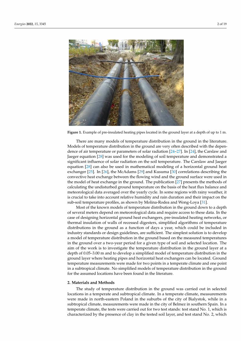
Research on temperature distributions in the ground is most often carried out interms of vertical or horizontal heat exchangers associated with heat pumps. Sliwa et al. [1]developed a methodology for determining the energy efficiency of borehole heat exchang-ers based on temperature profiling. In the case of vertical heat exchangers, the groundtemperature distributions concern considerable depths as a function of the length of theboreholes [2–7]. Horizontal ground heat exchangers usually require knowledge of tempera-ture distributions in the ground up to several meters [8–12]. The knowledge of temperaturedistributions in the ground is the basic boundary condition for designing undergroundheating pipes. In designing district heating networks, the most common methods are calcu-lation methods, in which a constant average annual ground temperature is assumed [13–17].In the case of recreating the actual operating conditions of the pre-insulated networks,the actual ground temperatures should be set. An example of the location of pipes indistrict heating in Poland is shown in Figure 1. In the case of two- and three-dimensionalcalculations, the soil temperature at the assumed depth is determined for the boundarytemperature condition at the depth of 8 m, equal to 8 ◦C [18–20].

Temperature distributions in the ground can also be useful for determining heat lossesin fermentation chambers of biogas plants, if the fermentation chambers are immersed inthe ground [21–23].

Energies 2022, 15, 3345. https://doi.org/10.3390/en15093345 https://www.mdpi.com/journal/energies

Energies 2022, 15, 3345 2 of 19Energies 2022, 15, x FOR PEER REVIEW 2 of 21

Figure 1. Example of pre-insulated heating pipes located in the ground layer at a depth of up to 1

m.

Temperature distributions in the ground can also be useful for determining heat

losses in fermentation chambers of biogas plants, if the fermentation chambers are im-

mersed in the ground [21–23].

There are many models of temperature distribution in the ground in the literature.

Models of temperature distribution in the ground are very often described with the de-

pendence of air temperature or parameters of solar radiation [24–27]. In [24], the Carslaw

and Jaeger equation [28] was used for the modeling of soil temperature and demon-

strated a significant influence of solar radiation on the soil temperature. The Carslaw and

Jaeger equation [28] can also be used in mathematical modeling of a horizontal ground

heat exchanger [25]. In [26], the McAdams [29] and Kusuma [30] correlations describing

the convective heat exchange between the flowing wind and the ground surface were

used in the model of heat exchange in the ground. The publication [27] presents the

methods of calculating the undisturbed ground temperature on the basis of the heat flux

balance and meteorological data averaged over the yearly cycle. In some regions with

rainy weather, it is crucial to take into account relative humidity and rain duration and

their impact on the sub-soil temperature profiles, as shown by Molina-Rodea and

Wong-Loya [31].

Most of the known models of temperature distribution in the ground down to a

depth of several meters depend on meteorological data and require access to these data.

In the case of designing horizontal ground heat exchangers, pre-insulated heating net-

works, or thermal insulation of walls of recessed digesters, simplified algorithms of

temperature distributions in the ground as a function of days a year, which could be in-

cluded in industry standards or design guidelines, are sufficient. The simplest solution is

to develop a model of temperature distribution in the ground based on the measured

temperatures in the ground over a two-year period for a given type of soil and selected

location. The aim of the work is to investigate the temperature distribution in the ground

layer at a depth of 0.05–3.00 m and to develop a simplified model of temperature distri-

bution in the ground layer where heating pipes and horizontal heat exchangers can be

located. Ground temperature measurements were made for two points in a temperate

climate and one point in a subtropical climate. No simplified models of temperature dis-

tribution in the ground for the assumed locations have been found in the literature.

2. Materials and Methods

The study of temperature distribution in the ground was carried out in selected lo-

cations in a temperate and subtropical climate. In a temperate climate, measurements

were made in north-eastern Poland in the suburbs of the city of Bialystok, while in a

subtropical climate, measurements were made in the city of Belmez in southern Spain. In

a temperate climate, the tests were carried out for two test stands: test stand No. 1, which

Figure 1. Example of pre-insulated heating pipes located in the ground layer at a depth of up to 1 m.

There are many models of temperature distribution in the ground in the literature.Models of temperature distribution in the ground are very often described with the depen-dence of air temperature or parameters of solar radiation [24–27]. In [24], the Carslaw andJaeger equation [28] was used for the modeling of soil temperature and demonstrated asignificant influence of solar radiation on the soil temperature. The Carslaw and Jaegerequation [28] can also be used in mathematical modeling of a horizontal ground heatexchanger [25]. In [26], the McAdams [29] and Kusuma [30] correlations describing theconvective heat exchange between the flowing wind and the ground surface were used inthe model of heat exchange in the ground. The publication [27] presents the methods ofcalculating the undisturbed ground temperature on the basis of the heat flux balance andmeteorological data averaged over the yearly cycle. In some regions with rainy weather, itis crucial to take into account relative humidity and rain duration and their impact on thesub-soil temperature profiles, as shown by Molina-Rodea and Wong-Loya [31].

Most of the known models of temperature distribution in the ground down to a depthof several meters depend on meteorological data and require access to these data. In thecase of designing horizontal ground heat exchangers, pre-insulated heating networks, orthermal insulation of walls of recessed digesters, simplified algorithms of temperaturedistributions in the ground as a function of days a year, which could be included inindustry standards or design guidelines, are sufficient. The simplest solution is to developa model of temperature distribution in the ground based on the measured temperaturesin the ground over a two-year period for a given type of soil and selected location. Theaim of the work is to investigate the temperature distribution in the ground layer at adepth of 0.05–3.00 m and to develop a simplified model of temperature distribution in theground layer where heating pipes and horizontal heat exchangers can be located. Groundtemperature measurements were made for two points in a temperate climate and one pointin a subtropical climate. No simplified models of temperature distribution in the groundfor the assumed locations have been found in the literature.

2. Materials and Methods

The study of temperature distribution in the ground was carried out in selectedlocations in a temperate and subtropical climate. In a temperate climate, measurementswere made in north-eastern Poland in the suburbs of the city of Bialystok, while in asubtropical climate, measurements were made in the city of Belmez in southern Spain. In atemperate climate, the tests were carried out for two test stands: test stand No. 1, which ischaracterized by the presence of clay in the tested soil layer, and test stand No. 2, which

Energies 2022, 15, 3345 3 of 19

consists of a sand layer. The test site No. 3, which is located in Belmez, is characterizedby the presence of clay. In the case of test stands No. 1 and 2, there is a humus layerto a depth of about 5 cm, while in the case of test stand No. 3, there is clay throughoutthe entire thickness of the layer. The geographical coordinates, climate, and groundwaterlevel are presented in Table 1. All three measurement points were characterized by a lowgroundwater level.

Table 1. Description of the location of measurement points.

Measurement Point ID Location Climate Type Geographic Coordinates Type of Soil Groundwater Level

1 Bialystok (Poland) Temperate 53◦05′19.8′′ N 23◦13′49.1′′ E Clay 20 m2 Bialystok (Poland) Temperate 53◦05′21.4′′ N 23◦13′50.3′′ E Sand 20 m3 Belmez (Spain) Subtropical 38◦15′57.8′′ N 5◦12′32.4′′ W Clay 100 m

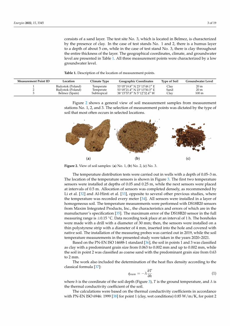
Figure 2 shows a general view of soil measurement samples from measurementstations No. 1, 2, and 3. The selection of measurement points was dictated by the type ofsoil that most often occurs in selected locations.

Energies 2022, 15, x FOR PEER REVIEW 3 of 21

is characterized by the presence of clay in the tested soil layer, and test stand No. 2, which

consists of a sand layer. The test site No. 3, which is located in Belmez, is characterized by

the presence of clay. In the case of test stands No. 1 and 2, there is a humus layer to a

depth of about 5 cm, while in the case of test stand No. 3, there is clay throughout the

entire thickness of the layer. The geographical coordinates, climate, and groundwater

level are presented in Table 1. All three measurement points were characterized by a low

groundwater level.

Figure 2 shows a general view of soil measurement samples from measurement sta-

tions No. 1, 2, and 3. The selection of measurement points was dictated by the type of soil

that most often occurs in selected locations.

(a) (b) (c)

Figure 2. View of soil samples: (a) No. 1, (b) No. 2, (c) No. 3.

Table 1. Description of the location of measurement points.

Measurement

Point ID Location Climate Type Geographic Coordinates Type of Soil Groundwater Level

1 Bialystok (Poland) Temperate 53°05′19.8″ N 23°13′49.1″ E Clay 20 m

2 Bialystok (Poland) Temperate 53°05′21.4″ N 23°13′50.3″ E Sand 20 m

3 Belmez (Spain) Subtropical 38°15′57.8″ N 5°12′32.4″ W Clay 100 m

The temperature distribution tests were carried out in wells with a depth of 0.05–3

m. The location of the temperature sensors is shown in Figure 3. The first two tempera-

ture sensors were installed at depths of 0.05 and 0.25 m, while the next sensors were

placed at intervals of 0.5 m. Allocation of sensors was completed densely, as recom-

mended by Li et al. [32] and Al-Hinti et al. [33], opposite to several other previous stud-

ies, where the temperature was recorded every meter [34]. All sensors were installed in a

layer of homogeneous soil. The temperature measurements were performed with

DS18B20 sensors from Maxim Integrated Products, Inc., the characteristics and errors of

which are in the manufacturer’s specification [35]. The maximum error of the DS18B20

sensor in the full measuring range is ±0.15 °C. Data recording took place at an interval of

1 h. The boreholes were made with a drill with a diameter of 30 mm; then, the sensors

were installed on a thin polystyrene strip with a diameter of 4 mm, inserted into the hole

and covered with native soil. The installation of the measuring probes was carried out in

2019, while the soil temperature measurements in the presented study were taken in the

years 2020–2021.

Based on the PN-EN ISO 14688-1 standard [36], the soil in points 1 and 3 was classi-

fied as clay with a predominant grain size from 0.063 to 0.002 mm and up to 0.002 mm,

while the soil in point 2 was classified as coarse sand with the predominant grain size

from 0.63 to 2 mm.

The work also included the determination of the heat flux density according to the

classical formula [37]:

num

Tq

h

= −

(1)

Figure 2. View of soil samples: (a) No. 1, (b) No. 2, (c) No. 3.

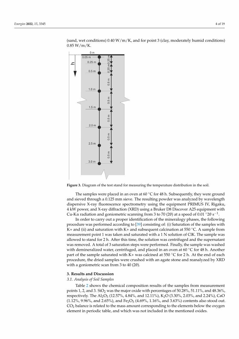
The temperature distribution tests were carried out in wells with a depth of 0.05–3 m.The location of the temperature sensors is shown in Figure 3. The first two temperaturesensors were installed at depths of 0.05 and 0.25 m, while the next sensors were placedat intervals of 0.5 m. Allocation of sensors was completed densely, as recommended byLi et al. [32] and Al-Hinti et al. [33], opposite to several other previous studies, wherethe temperature was recorded every meter [34]. All sensors were installed in a layer ofhomogeneous soil. The temperature measurements were performed with DS18B20 sensorsfrom Maxim Integrated Products, Inc., the characteristics and errors of which are in themanufacturer’s specification [35]. The maximum error of the DS18B20 sensor in the fullmeasuring range is ±0.15 ◦C. Data recording took place at an interval of 1 h. The boreholeswere made with a drill with a diameter of 30 mm; then, the sensors were installed on athin polystyrene strip with a diameter of 4 mm, inserted into the hole and covered withnative soil. The installation of the measuring probes was carried out in 2019, while the soiltemperature measurements in the presented study were taken in the years 2020–2021.

Based on the PN-EN ISO 14688-1 standard [36], the soil in points 1 and 3 was classifiedas clay with a predominant grain size from 0.063 to 0.002 mm and up to 0.002 mm, whilethe soil in point 2 was classified as coarse sand with the predominant grain size from 0.63to 2 mm.

The work also included the determination of the heat flux density according to theclassical formula [37]:

qnum = −λ∂T∂h

(1)

where h is the coordinate of the soil depth (Figure 3), T is the ground temperature, and λ isthe thermal conductivity coefficient of the soil.

The calculations were based on the thermal conductivity coefficients in accordancewith PN-EN ISO 6946: 1999 [38] for point 1 (clay, wet conditions) 0.85 W/m/K, for point 2

Energies 2022, 15, 3345 4 of 19

(sand, wet conditions) 0.40 W/m/K, and for point 3 (clay, moderately humid conditions)0.85 W/m/K.

Energies 2022, 15, x FOR PEER REVIEW 4 of 21

where h is the coordinate of the soil depth (Figure 3), T is the ground temperature, and λ

is the thermal conductivity coefficient of the soil.

The calculations were based on the thermal conductivity coefficients in accordance

with PN-EN ISO 6946: 1999 [38] for point 1 (clay, wet conditions) 0.85 W/m/K, for point 2

(sand, wet conditions) 0.40 W/m/K, and for point 3 (clay, moderately humid conditions)

0.85 W/m/K.

Figure 3. Diagram of the test stand for measuring the temperature distribution in the soil.

The samples were placed in an oven at 60 °C for 48 h. Subsequently, they were

ground and sieved through a 0.125 mm sieve. The resulting powder was analyzed by

wavelength dispersive X-ray fluorescence spectrometry using the equipment PRIMUS

IV, Rigaku, 4 kW power, and X-ray diffraction (XRD) using a Bruker D8 Discover A25

equipment with Cu-Kα radiation and goniometric scanning from 3 to 70 (2θ) at a speed

of 0.01 °2θ s-1.

In order to carry out a proper identification of the mineralogy phases, the following

procedure was performed according to [39] consisting of: (i) Saturation of the samples

with K+ and (ii) and saturation with K+ and subsequent calcination at 550 °C. A sample

from measurement point 1 was taken and saturated with a 1 N solution of ClK. The

sample was allowed to stand for 2 h. After this time, the solution was centrifuged and the

supernatant was removed. A total of 3 saturation steps were performed. Finally, the

sample was washed with demineralized water, centrifuged, and placed in an oven at 60

°C for 48 h. Another part of the sample saturated with K+ was calcined at 550 °C for 2 h.

At the end of each procedure, the dried samples were crushed with an agate stone and

reanalyzed by XRD with a goniometric scan from 3 to 40 (2θ).

3. Results and Discussion

3.1. Analysis of Soil Samples

Table 2 shows the chemical composition results of the samples from measurement

points 1, 2, and 3. SiO2 was the major oxide with percentages of 50.28%, 51.11%, and

48.36%, respectively. The Al2O3 (12.57%, 4.84%, and 12.11%), K2O (3.30%, 2.03%, and

Figure 3. Diagram of the test stand for measuring the temperature distribution in the soil.

The samples were placed in an oven at 60 ◦C for 48 h. Subsequently, they were groundand sieved through a 0.125 mm sieve. The resulting powder was analyzed by wavelengthdispersive X-ray fluorescence spectrometry using the equipment PRIMUS IV, Rigaku,4 kW power, and X-ray diffraction (XRD) using a Bruker D8 Discover A25 equipment withCu-Kα radiation and goniometric scanning from 3 to 70 (2θ) at a speed of 0.01 ◦2θ s−1.

In order to carry out a proper identification of the mineralogy phases, the followingprocedure was performed according to [39] consisting of: (i) Saturation of the samples withK+ and (ii) and saturation with K+ and subsequent calcination at 550 ◦C. A sample frommeasurement point 1 was taken and saturated with a 1 N solution of ClK. The sample wasallowed to stand for 2 h. After this time, the solution was centrifuged and the supernatantwas removed. A total of 3 saturation steps were performed. Finally, the sample was washedwith demineralized water, centrifuged, and placed in an oven at 60 ◦C for 48 h. Anotherpart of the sample saturated with K+ was calcined at 550 ◦C for 2 h. At the end of eachprocedure, the dried samples were crushed with an agate stone and reanalyzed by XRDwith a goniometric scan from 3 to 40 (2θ).

3. Results and Discussion3.1. Analysis of Soil Samples

Table 2 shows the chemical composition results of the samples from measurementpoints 1, 2, and 3. SiO2 was the major oxide with percentages of 50.28%, 51.11%, and 48.36%,respectively. The Al2O3 (12.57%, 4.84%, and 12.11%), K2O (3.30%, 2.03%, and 2.24%), CaO(1.12%, 9.96%, and 2.65%), and Fe2O3 (4.69%, 1.16%, and 3.63%) contents also stood out.CO2 balance is related to the mass amount corresponding to the elements below the oxygenelement in periodic table, and which was not included in the mentioned oxides.

Energies 2022, 15, 3345 5 of 19

Table 2. Chemical composition of samples.

Compound Measurement Point 1 Measurement Point 2 Measurement Point 3

Na2O 0.61 0.85 0.68MgO 1.87 0.81 0.85Al2O3 12.57 4.84 12.11SiO2 50.28 51.11 48.36P2O5 0.19 0.21 0.23SO3 0.05 - 0.19Cl - 0.01 0.01

K2O 3.30 2.03 2.24CaO 1.12 9.96 2.65TiO2 0.51 0.11 0.71

Cr2O3 0.02 0.13 0.09MnO 0.06 0.04 0.10Fe2O3 4.69 1.16 3.63NiO - 0.01 -

Rb2O 0.01 - -SrO - 0.02 -

ZrO2 0.04 - 0.04BaO 0.03 0.15 0.09

CO2 balance 24.65 28.57 28.01

Total mass 100.00 100.00 100.00

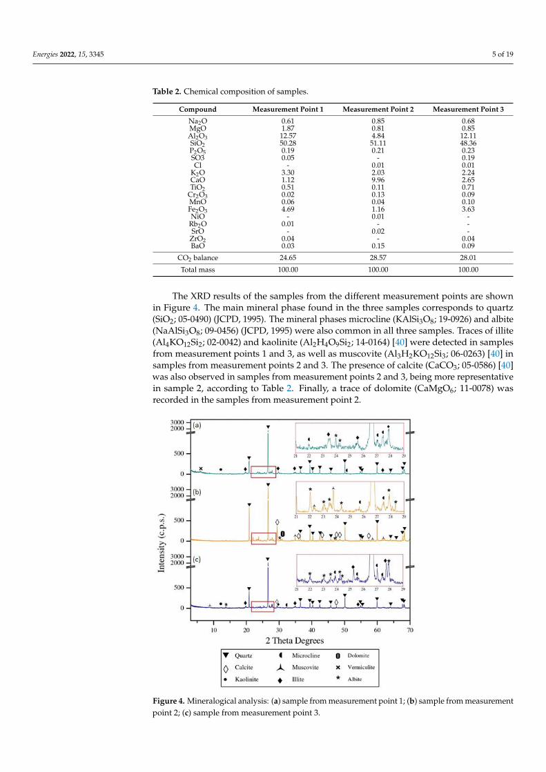
The XRD results of the samples from the different measurement points are shownin Figure 4. The main mineral phase found in the three samples corresponds to quartz(SiO2; 05-0490) (JCPD, 1995). The mineral phases microcline (KAlSi3O8; 19-0926) and albite(NaAlSi3O8; 09-0456) (JCPD, 1995) were also common in all three samples. Traces of illite(Al4KO12Si2; 02-0042) and kaolinite (Al2H4O9Si2; 14-0164) [40] were detected in samplesfrom measurement points 1 and 3, as well as muscovite (Al3H2KO12Si3; 06-0263) [40] insamples from measurement points 2 and 3. The presence of calcite (CaCO3; 05-0586) [40]was also observed in samples from measurement points 2 and 3, being more representativein sample 2, according to Table 2. Finally, a trace of dolomite (CaMgO6; 11-0078) wasrecorded in the samples from measurement point 2.

Energies 2022, 15, x FOR PEER REVIEW 6 of 21

Figure 4. Mineralogical analysis: (a) sample from measurement point 1; (b) sample from meas-

urement point 2; (c) sample from measurement point 3.

In Figure 4a, a reflection at 6.1 °2θ (d = 14.4 Å) was observed that could correspond

to vermiculite (Si4O12Mg3H2; 16-0613) [40] or chlorite (Si2O9Mg3H4; 13-0003) [40]. In Figure

5a, a magnification (4–12 °2θ) of this XRD pattern is shown, as well as the patterns re-

sulting from the treatment with a saturated solution in K+ (Figure 5b) and with a satu-

rated solution in K+ solution and subsequently calcined at 550 °C (Figure 5c). A shift in

the plane was shown that appears in Figure 5a towards 9 °2θ (d = 10 Å) (Figure 5b,c) that

is in accordance with the presence of vermiculite (Si4O12Mg3H2; 16-0613) [40].

Figure 4. Mineralogical analysis: (a) sample from measurement point 1; (b) sample from measurementpoint 2; (c) sample from measurement point 3.

Energies 2022, 15, 3345 6 of 19

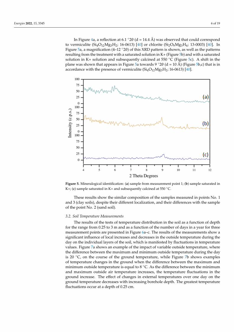
In Figure 4a, a reflection at 6.1 ◦2θ (d = 14.4 Å) was observed that could correspondto vermiculite (Si4O12Mg3H2; 16-0613) [40] or chlorite (Si2O9Mg3H4; 13-0003) [40]. InFigure 5a, a magnification (4–12 ◦2θ) of this XRD pattern is shown, as well as the patternsresulting from the treatment with a saturated solution in K+ (Figure 5b) and with a saturatedsolution in K+ solution and subsequently calcined at 550 ◦C (Figure 5c). A shift in theplane was shown that appears in Figure 5a towards 9 ◦2θ (d = 10 Å) (Figure 5b,c) that is inaccordance with the presence of vermiculite (Si4O12Mg3H2; 16-0613) [40].

Energies 2022, 15, x FOR PEER REVIEW 7 of 21

Figure 5. Mineralogical identification: (a) sample from measurement point 1; (b) sample saturated

in K+; (c) sample saturated in K+ and subsequently calcined at 550 °C.

These results show the similar composition of the samples measured in points No. 1

and 3 (clay soils), despite their different localization, and their differences with the sam-

ple of the point No. 2 (sand soil).

3.2. Soil Temperature Measurements

The results of the tests of temperature distribution in the soil as a function of depth

for the range from 0.25 to 3 m and as a function of the number of days in a year for three

measurement points are presented in Figures 6a-c. The results of the measurements show

a significant influence of local increases and decreases in the outside temperature during

the day on the individual layers of the soil, which is manifested by fluctuations in tem-

perature values. Figure 7a shows an example of the impact of variable outside tempera-

ture, where the difference between the maximum and minimum outside temperature

during the day is 20 °C, on the course of the ground temperature, while Figure 7b shows

examples of temperature changes in the ground when the difference between the maxi-

mum and minimum outside temperature is equal to 8 °C. As the difference between the

minimum and maximum outside air temperature increases, the temperature fluctuations

in the ground increase. The effect of changes in external temperatures over one day on

the ground temperature decreases with increasing borehole depth. The greatest temper-

ature fluctuations occur at a depth of 0.25 cm.

Figure 5. Mineralogical identification: (a) sample from measurement point 1; (b) sample saturated inK+; (c) sample saturated in K+ and subsequently calcined at 550 ◦C.

These results show the similar composition of the samples measured in points No. 1and 3 (clay soils), despite their different localization, and their differences with the sampleof the point No. 2 (sand soil).

3.2. Soil Temperature Measurements

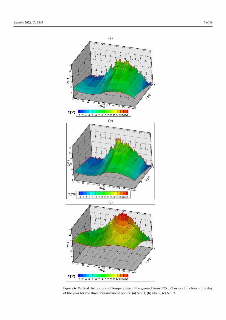
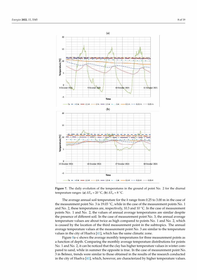
The results of the tests of temperature distribution in the soil as a function of depthfor the range from 0.25 to 3 m and as a function of the number of days in a year for threemeasurement points are presented in Figure 6a–c. The results of the measurements show asignificant influence of local increases and decreases in the outside temperature during theday on the individual layers of the soil, which is manifested by fluctuations in temperaturevalues. Figure 7a shows an example of the impact of variable outside temperature, wherethe difference between the maximum and minimum outside temperature during the dayis 20 ◦C, on the course of the ground temperature, while Figure 7b shows examplesof temperature changes in the ground when the difference between the maximum andminimum outside temperature is equal to 8 ◦C. As the difference between the minimumand maximum outside air temperature increases, the temperature fluctuations in theground increase. The effect of changes in external temperatures over one day on theground temperature decreases with increasing borehole depth. The greatest temperaturefluctuations occur at a depth of 0.25 cm.

Energies 2022, 15, 3345 7 of 19Energies 2022, 15, x FOR PEER REVIEW 8 of 21

(a)

(b)

(c)

Figure 6. Vertical distribution of temperature in the ground from 0.25 to 3 m as a function of the

day of the year for the three measurement points: (a) No. 1, (b) No. 2, (c) No. 3. Figure 6. Vertical distribution of temperature in the ground from 0.25 to 3 m as a function of the dayof the year for the three measurement points: (a) No. 1, (b) No. 2, (c) No. 3.

Energies 2022, 15, 3345 8 of 19Energies 2022, 15, x FOR PEER REVIEW 9 of 21

(a)

(b)

Figure 7. The daily evolution of the temperatures in the ground of point No. 2 for the diurnal

temperature ranges: (a) Ta = 20 °C, (b) Ta = 8 °C.

The average annual soil temperature for the h range from 0.25 to 3.00 m in the case of

the measurement point No. 3 is 19.03 °C, while in the case of the measurement points No.

1 and No. 2, these temperatures are, respectively, 10.3 and 10 °C. In the case of meas-

urement points No. 1 and No. 2, the values of annual average temperatures are similar

despite the presence of different soil. In the case of measurement point No. 3, the annual

average temperature values are about twice as high compared to points No. 1 and No. 2,

which is caused by the location of the third measurement point in the subtropics. The

annual average temperature values at the measurement point No. 3 are similar to the

temperature values in the city of Huelva [41], which has the same climatic zone.

Figure 8a–c shows the average monthly temperatures for three measurement points

as a function of depth. Comparing the monthly average temperature distributions for

Figure 7. The daily evolution of the temperatures in the ground of point No. 2 for the diurnaltemperature ranges: (a) ∆Ta = 20 ◦C, (b) ∆Ta = 8 ◦C.

The average annual soil temperature for the h range from 0.25 to 3.00 m in the case ofthe measurement point No. 3 is 19.03 ◦C, while in the case of the measurement points No. 1and No. 2, these temperatures are, respectively, 10.3 and 10 ◦C. In the case of measurementpoints No. 1 and No. 2, the values of annual average temperatures are similar despitethe presence of different soil. In the case of measurement point No. 3, the annual averagetemperature values are about twice as high compared to points No. 1 and No. 2, whichis caused by the location of the third measurement point in the subtropics. The annualaverage temperature values at the measurement point No. 3 are similar to the temperaturevalues in the city of Huelva [41], which has the same climatic zone.

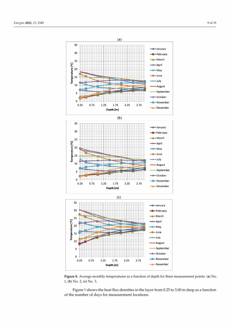
Figure 8a–c shows the average monthly temperatures for three measurement points asa function of depth. Comparing the monthly average temperature distributions for pointsNo. 1 and No. 2, it can be noticed that the clay has higher temperature values in winter com-pared to sand, while in summer the opposite is true. In the case of measurement point No.3 in Belmez, trends were similar to those obtained in the results of the research conductedin the city of Huelva [41], which, however, are characterized by higher temperature values.

Energies 2022, 15, 3345 9 of 19

Energies 2022, 15, x FOR PEER REVIEW 10 of 21

points No. 1 and No. 2, it can be noticed that the clay has higher temperature values in

winter compared to sand, while in summer the opposite is true. In the case of measure-

ment point No. 3 in Belmez, trends were similar to those obtained in the results of the

research conducted in the city of Huelva [41], which, however, are characterized by

higher temperature values.

(a)

(b)

(c)

Energies 2022, 15, 3345 11 of 21

(c)

Figure 8. Average monthly temperatures as a function of depth for three measurement points: (a) No. 1, (b) No. 2, (c) No. 3.

Figure 9 shows the heat flux densities in the layer from 0.25 to 3.00 m deep as a function of the number of days for measurement locations.

The heat flux density was determined according to the classical formula (1):

3.00 0.25T Tqh

λ −= −Δ

(2)

where λ is the thermal conductivity coefficient of the soil, T0.25 is the temperature at a depth of 0.25 m, T3.00 is the temperature at a depth of 3 m, and Δh = 2.75 m is the soil layer for which heat conduction calculations were made.

In summer, the ground is heated both in a temperate climate (points No. 1 and No. 2) and in a subtropical climate (point No. 3), while in winter heat is transferred from the ground to the outside air. The highest heat flux values occur in the subtropical climate compared to the climate moderate, which is caused by greater direct solar radiation and higher outside temperatures in a subtropical climate [42]. When comparing the type of soil, it was noticed that the highest absolute values of heat flux density are conducted by clay (points No. 1 and No. 3), while the smallest are in the case of sand (point No. 2), which is due to the lower thermal conductivity coefficient for sand compared to clay.

Figure 9. Heat flux density in the ground layer 0.25–3.00 m as a function of the day of the year.

Figure 8. Average monthly temperatures as a function of depth for three measurement points: (a) No.1, (b) No. 2, (c) No. 3.

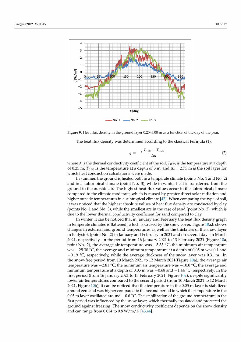
Figure 9 shows the heat flux densities in the layer from 0.25 to 3.00 m deep as a functionof the number of days for measurement locations.

Energies 2022, 15, 3345 10 of 19

Energies 2022, 15, x FOR PEER REVIEW 11 of 21

Figure 8. Average monthly temperatures as a function of depth for three measurement points: (a)

No. 1, (b) No. 2, (c) No. 3.

Figure 9 shows the heat flux densities in the layer from 0.25 to 3.00 m deep as a

function of the number of days for measurement locations.

The heat flux density was determined according to the classical formula (1):

3.00 0.25T Tq

h

−= −

(2)

where λ is the thermal conductivity coefficient of the soil, T0.25 is the temperature at a

depth of 0.25 m, T3.00 is the temperature at a depth of 3 m, and h = 2.75 m is the soil layer

for which heat conduction calculations were made.

In summer, the ground is heated both in a temperate climate (points No. 1 and No.

2) and in a subtropical climate (point No. 3), while in winter heat is transferred from the

ground to the outside air. The highest heat flux values occur in the subtropical climate

compared to the climate moderate, which is caused by greater direct solar radiation and

higher outside temperatures in a subtropical climate [42]. When comparing the type of

soil, it was noticed that the highest absolute values of heat flux density are conducted by

clay (points No. 1 and No. 3), while the smallest are in the case of sand (point No. 2),

which is due to the lower thermal conductivity coefficient for sand compared to clay.

Figure 9. Heat flux density in the ground layer 0.25–3.00 m as a function of the day of the year.

In winter, it can be noticed that in January and February the heat flux density graph

in temperate climates is flattened, which is caused by the snow cover. Figure 10a,b shows

Figure 9. Heat flux density in the ground layer 0.25–3.00 m as a function of the day of the year.

The heat flux density was determined according to the classical Formula (1):

q = −λT3.00 − T0.25

∆h(2)

where λ is the thermal conductivity coefficient of the soil, T0.25 is the temperature at a depthof 0.25 m, T3.00 is the temperature at a depth of 3 m, and ∆h = 2.75 m is the soil layer forwhich heat conduction calculations were made.

In summer, the ground is heated both in a temperate climate (points No. 1 and No. 2)and in a subtropical climate (point No. 3), while in winter heat is transferred from theground to the outside air. The highest heat flux values occur in the subtropical climatecompared to the climate moderate, which is caused by greater direct solar radiation andhigher outside temperatures in a subtropical climate [42]. When comparing the type of soil,it was noticed that the highest absolute values of heat flux density are conducted by clay(points No. 1 and No. 3), while the smallest are in the case of sand (point No. 2), which isdue to the lower thermal conductivity coefficient for sand compared to clay.

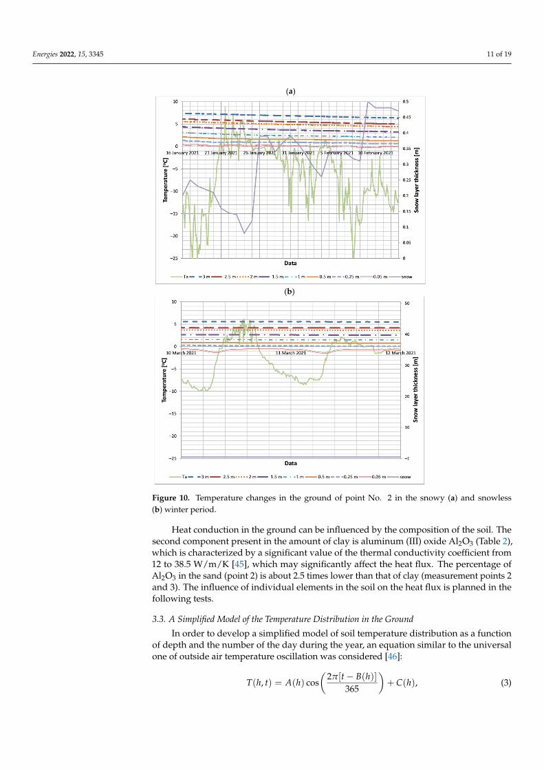
In winter, it can be noticed that in January and February the heat flux density graphin temperate climates is flattened, which is caused by the snow cover. Figure 10a,b showschanges in external and ground temperatures as well as the thickness of the snow layerin Bialystok (point No. 2) in January and February in 2021 and on several days in March2021, respectively. In the period from 16 January 2021 to 13 February 2021 (Figure 10a,point No. 2), the average air temperature was −5.35 ◦C, the minimum air temperaturewas −25.38 ◦C, the average and minimum temperature at a depth of 0.05 m was 0.1 and−0.19 ◦C, respectively, while the average thickness of the snow layer was 0.31 m. Inthe snow-free period from 10 March 2021 to 12 March 2021(Figure 10a), the average airtemperature was −2.81 ◦C, the minimum air temperature was −10.0 ◦C, the average andminimum temperature at a depth of 0.05 m was −0.68 and −1.44 ◦C, respectively. In thefirst period (from 16 January 2021 to 13 February 2021, Figure 10a), despite significantlylower air temperatures compared to the second period (from 10 March 2021 to 12 March2021, Figure 10b), it can be noticed that the temperature in the 0.05 m layer is stabilizedaround zero and was higher compared to the second period in which the temperature in the0.05 m layer oscillated around −0.6 ◦C. The stabilization of the ground temperature in thefirst period was influenced by the snow layer, which thermally insulated and protected theground against freezing. The snow conductivity coefficient depends on the snow densityand can range from 0.024 to 0.8 W/m/K [43,44].

Energies 2022, 15, 3345 11 of 19

Energies 2022, 15, x FOR PEER REVIEW 12 of 21

changes in external and ground temperatures as well as the thickness of the snow layer in

Bialystok (point No. 2) in January and February in 2021 and on several days in March

2021, respectively. In the period from 16 January 2021 to 13 February 2021 (Figure 10a,

point No. 2), the average air temperature was −5.35 °C, the minimum air temperature was

−25.38 °C, the average and minimum temperature at a depth of 0.05 m was 0.1 and −0.19

°C, respectively, while the average thickness of the snow layer was 0.31 m. In the

snow-free period from 10 March 2021 to 12 March 2021(Figure 10a), the average air

temperature was −2.81 °C, the minimum air temperature was −10.0 °C, the average and

minimum temperature at a depth of 0.05 m was −0.68 and −1.44 °C, respectively. In the

first period (from 16 January 2021 to 13 February 2021, Figure 10a), despite significantly

lower air temperatures compared to the second period (from 10 March 2021 to 12 March

2021, Figure 10b), it can be noticed that the temperature in the 0.05 m layer is stabilized

around zero and was higher compared to the second period in which the temperature in

the 0.05 m layer oscillated around −0.6 °C. The stabilization of the ground temperature in

the first period was influenced by the snow layer, which thermally insulated and pro-

tected the ground against freezing. The snow conductivity coefficient depends on the

snow density and can range from 0.024 to 0.8 W/m/K [43,44].

Heat conduction in the ground can be influenced by the composition of the soil. The

second component present in the amount of clay is aluminum (III) oxide Al2O3 (Table 2),

which is characterized by a significant value of the thermal conductivity coefficient from

12 to 38.5 W/m/K [45], which may significantly affect the heat flux. The percentage of

Al2O3 in the sand (point 2) is about 2.5 times lower than that of clay (measurement points

2 and 3). The influence of individual elements in the soil on the heat flux is planned in the

following tests.

(a)

(b)

Energies 2022, 15, 3345 13 of 21

(b)

Figure 10. Temperature changes in the ground of point No. 2 in the snowy (a) and snowless (b) winter period.

3.3. A Simplified Model of the Temperature Distribution in the Ground In order to develop a simplified model of soil temperature distribution as a function

of depth and the number of the day during the year, an equation similar to the universal one of outside air temperature oscillation was considered [46]: 𝑇 ℎ, 𝑡 𝐴 ℎ cos 𝐶 ℎ , (3)

where A is the amplitude of temperature oscillation, B is the change of phase, and C is the horizontal translation. A dependence of this coefficient with the depth is assumed.

Modeling of meteorological parameters of the outside air by means of trigonometric functions is optionally performed in the commercial program WuFi [47,48]. The idea of proposed models based on the cyclical nature of the occurrence of temperatures in the ground results from the fact that the temperature in the ground changes daily at similar intervals close to the meteorological time series [49]. Equation (2) is most often used in many scientific papers and computational programs for simplified simulation of the outside air temperature during the year. The use of the cosine function in the equation for simulating temperatures is related to the occurrence of seasons that are a consequence of the Earth’s orbital movement around the Sun and the inclination of the Earth’s axis to the orbit plane of this movement, which translates into changes in the outside air temperature. Due to the large temperature fluctuations in the soil layer of 0.05 m, resulting from the significant influence of air temperature and solar radiation on this layer, a soil layer from 0.25 to 3.0 m was selected for the model development.

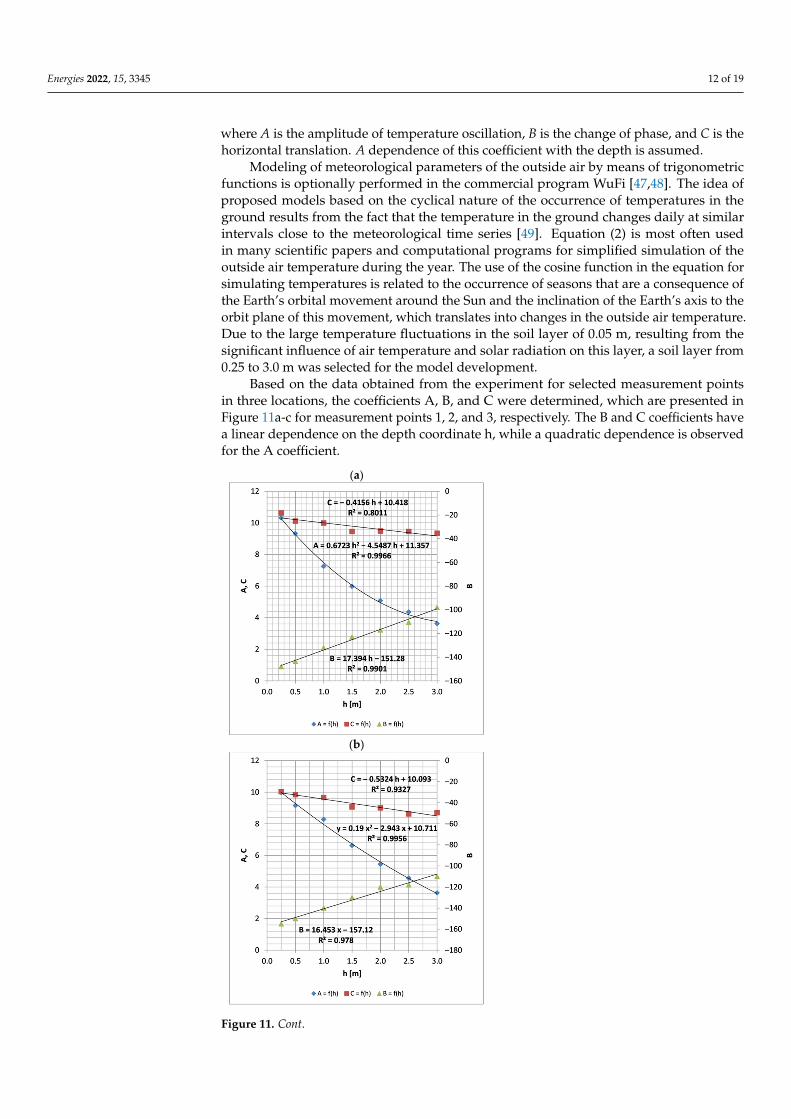
Based on the data obtained from the experiment for selected measurement points in three locations, the coefficients A, B, and C were determined, which are presented in Figure 11a–c for measurement points 1, 2, and 3, respectively. The B and C coefficients have a linear dependence on the depth coordinate h, while a quadratic dependence is observed for the A coefficient.

Figure 10. Temperature changes in the ground of point No. 2 in the snowy (a) and snowless(b) winter period.

Heat conduction in the ground can be influenced by the composition of the soil. Thesecond component present in the amount of clay is aluminum (III) oxide Al2O3 (Table 2),which is characterized by a significant value of the thermal conductivity coefficient from12 to 38.5 W/m/K [45], which may significantly affect the heat flux. The percentage ofAl2O3 in the sand (point 2) is about 2.5 times lower than that of clay (measurement points 2and 3). The influence of individual elements in the soil on the heat flux is planned in thefollowing tests.

3.3. A Simplified Model of the Temperature Distribution in the Ground

In order to develop a simplified model of soil temperature distribution as a functionof depth and the number of the day during the year, an equation similar to the universalone of outside air temperature oscillation was considered [46]:

T(h, t) = A(h) cos(

2π[t− B(h)]365

)+ C(h), (3)

Energies 2022, 15, 3345 12 of 19

where A is the amplitude of temperature oscillation, B is the change of phase, and C is thehorizontal translation. A dependence of this coefficient with the depth is assumed.

Modeling of meteorological parameters of the outside air by means of trigonometricfunctions is optionally performed in the commercial program WuFi [47,48]. The idea ofproposed models based on the cyclical nature of the occurrence of temperatures in theground results from the fact that the temperature in the ground changes daily at similarintervals close to the meteorological time series [49]. Equation (2) is most often usedin many scientific papers and computational programs for simplified simulation of theoutside air temperature during the year. The use of the cosine function in the equation forsimulating temperatures is related to the occurrence of seasons that are a consequence ofthe Earth’s orbital movement around the Sun and the inclination of the Earth’s axis to theorbit plane of this movement, which translates into changes in the outside air temperature.Due to the large temperature fluctuations in the soil layer of 0.05 m, resulting from thesignificant influence of air temperature and solar radiation on this layer, a soil layer from0.25 to 3.0 m was selected for the model development.

Based on the data obtained from the experiment for selected measurement pointsin three locations, the coefficients A, B, and C were determined, which are presented inFigure 11a-c for measurement points 1, 2, and 3, respectively. The B and C coefficients havea linear dependence on the depth coordinate h, while a quadratic dependence is observedfor the A coefficient.

Energies 2022, 15, 3345  14  of  21  

 

(a) 

 (b) 

 (c) 

  

Figure 11. Cont.

Energies 2022, 15, 3345 13 of 19

Energies 2022, 15, 3345  14  of  21  

 

(a) 

 (b) 

 (c) 

  

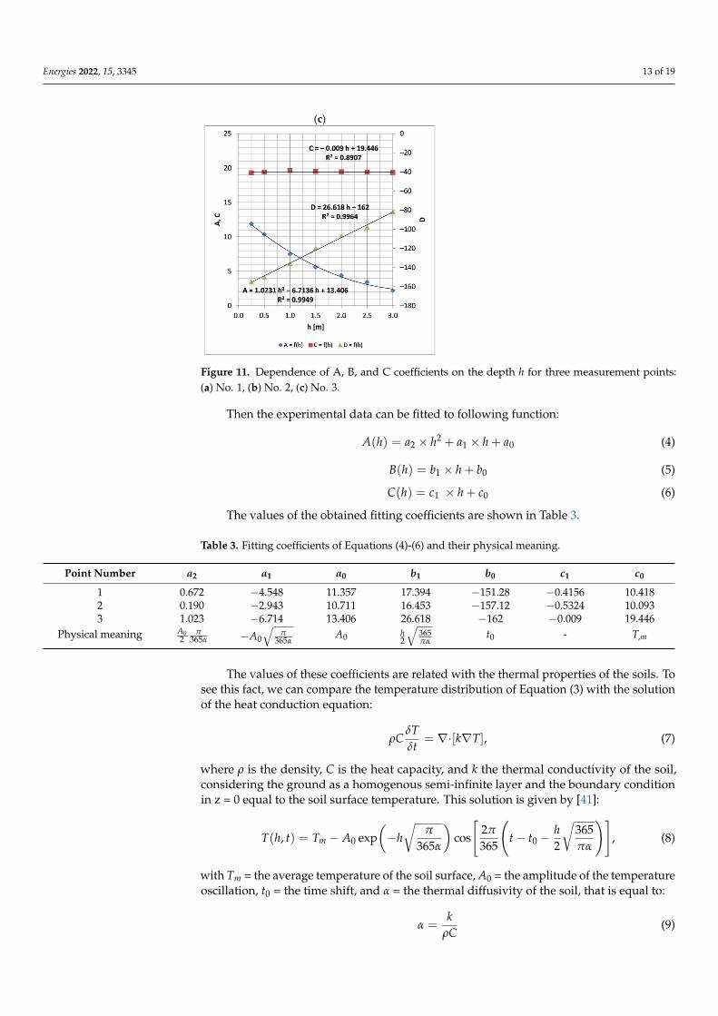
Figure 11. Dependence of A, B, and C coefficients on the depth h for three measurement points:(a) No. 1, (b) No. 2, (c) No. 3.

Then the experimental data can be fitted to following function:

A(h) = a2 × h2 + a1 × h + a0 (4)

B(h) = b1 × h + b0 (5)

C(h) = c1 × h + c0 (6)

The values of the obtained fitting coefficients are shown in Table 3.

Table 3. Fitting coefficients of Equations (4)-(6) and their physical meaning.

Point Number a2 a1 a0 b1 b0 c1 c0

1 0.672 −4.548 11.357 17.394 −151.28 −0.4156 10.4182 0.190 −2.943 10.711 16.453 −157.12 −0.5324 10.0933 1.023 −6.714 13.406 26.618 −162 −0.009 19.446

Physical meaning A02

π365α −A0

√π

365αA0 h

2

√365πα

t0 - T,m

The values of these coefficients are related with the thermal properties of the soils. Tosee this fact, we can compare the temperature distribution of Equation (3) with the solutionof the heat conduction equation:

ρCδTδt

= ∇·[k∇T], (7)

where ρ is the density, C is the heat capacity, and k the thermal conductivity of the soil,considering the ground as a homogenous semi-infinite layer and the boundary conditionin z = 0 equal to the soil surface temperature. This solution is given by [41]:

T(h, t) = Tm − A0 exp(−h√

π

365α

)cos

[2π

365

(t− t0 −

h2

√365πα

)], (8)

with Tm = the average temperature of the soil surface, A0 = the amplitude of the temperatureoscillation, t0 = the time shift, and α = the thermal diffusivity of the soil, that is equal to:

α =k

ρC(9)

Energies 2022, 15, 3345 14 of 19

For shallow positions (h < 2.5 m), the exponential term can be approximated (Taylorseries) by:

exp(−h√

π

365α

)= 1− h

√π

365α+

h2

2π

365α(10)

and the temperature distribution of the Equation (7) by:

T(h, t) = Tm − A0

(1− h

√π

365α+

h2

2π

365α

)cos

[2π

365

(t− t0 −

h2

√365πα

)], (11)

Comparing the Equations (3) and (8) for the temperature distribution, the physicalmeanings of the coefficients of Equations (4)–(6) can be obtained (see Table 3).

Using the relationships of Table 3, the values of thermal diffusivity and other parame-ters of Equation (11) can be obtained from the experimental measures. The experimentalvalues of these parameters for the three measurement points are presented in Table 4. Inthis table, the thermal diffusivity α(A) and α(B) are the diffusivity values obtained from theamplitude and phase variations, respectively (from a and b coefficients, respectively).

Table 4. Values of the thermal diffusivities α(A) and α(B), and other parameters of Equation (10) formeasurement points No. 1, No. 2, and No. 3.

Point Number α(A) 10−6 m2/s α(B) 10−6 m2/s Tm◦C A0

◦C t0 day

1 0.73 1.10 10.418 11.357 −151.282 1.27 1.24 10.093 10.711 −157.123 0.52 0.47 19.446 13.406 −162

The obtained values of the average temperature of the soil surface, Tm, agree withthe measured values 10.3, 10, and 19.03 ◦C, presented in Section 3.2. It must be noted thatthe C coefficient of Equation (6) should have to be theoretically constant and equal to thistemperature in the homogenous semi-infinite approximation. However, Figure 11 showsthat it only happened for the point No. 3 in Belmez. In the case of points No. 1 and 2,the C coefficients decrease with the depth h. It can be explained by the soil humidity inthese points, that causes the homogeneity condition to not be fully fitted. The different soilhumidity causes the heat capacity, the thermal conductivity, and the thermal diffusivity tovary from a depth position to another one. This effect is not happening in the dry soil ofthe point No. 3.

Regarding the amplitude of the temperature oscillation Ao, the maximum value corre-sponds to Belmez localization, by the higher values of outdoor temperature in this point.

The differences between the thermal diffusivities calculated from amplitude and phasevariations could be due to different reasons. Kusuda and Achenbach [50] proposed errorsof the fitting by inconsistent temperature depth data or errors of the phase determinationby temporal fluctuation. In our case, highest differences correspond to the points No. 1 and2. So, the differences could also result from the inhomogeneities of the wet soils. The resultspresented in Table 4 show that the lowest value of the thermal diffusivity is for the Belmezwith 0.5 × 10−6 m2/s, which is typical of a dry clay (see Table 1 in [41]). The point No. 1,with a similar type of soil, presents a higher thermal diffusivity about 0.73 × 10−6 m2/sby the humidity of this localization. The highest value of this diffusivity is for point No. 2with a value typical of wet sand.

Based on the experimental results [51,52], the relationship between thermal diffusivityand the moisture content in the clay can be seen, that thermal diffusivity increases withincreasing soil moisture content. Estimated values of α (A) and α (B) indicate higher mois-ture content in measurement point 1 compared to measurement point 3, which is causedby higher outside temperatures and much greater direct solar radiation at measurementpoint 3. It should be noted here that a thorough examination of the moisture content in thesoil requires thorough laboratory tests.

Energies 2022, 15, 3345 15 of 19

The relative error of the model (3) was determined as the temperature difference ofthe Texp experiment and the solution of the temperature of the simplified Tnum model (3)related to the temperature from the experiment:

δT =

∣∣∣∣Texp − Tnum

Texp

∣∣∣∣100% (12)

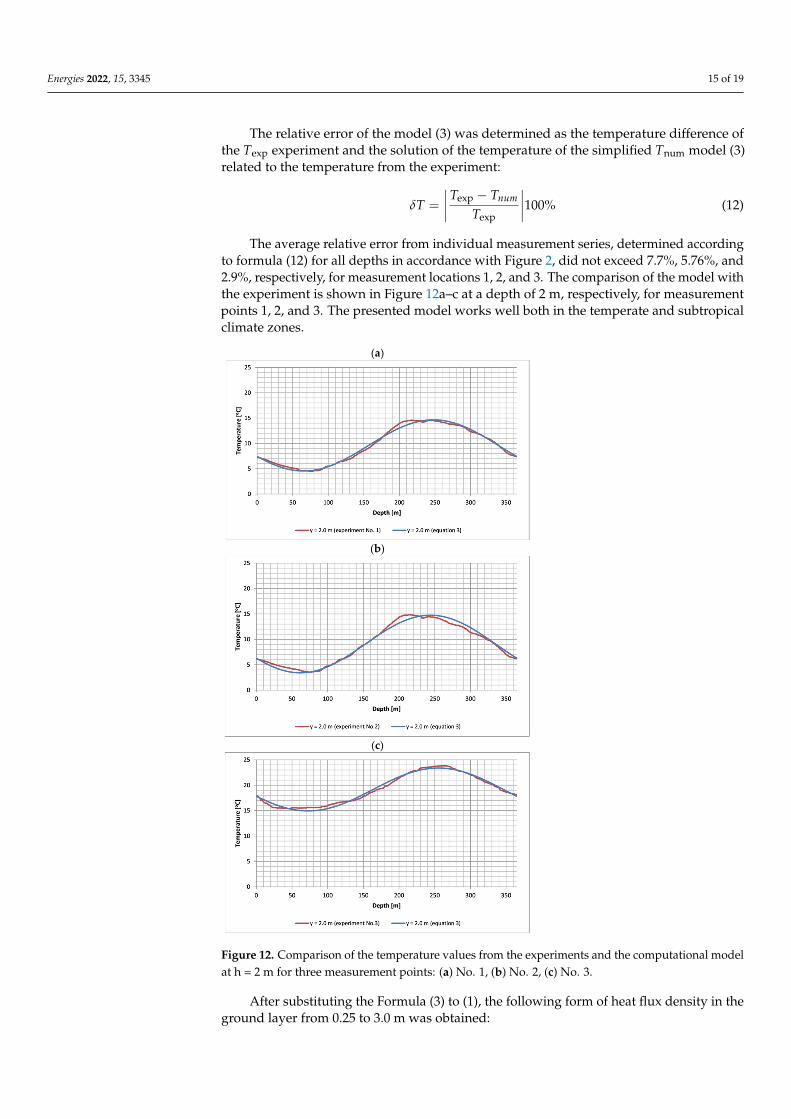
The average relative error from individual measurement series, determined accordingto formula (12) for all depths in accordance with Figure 2, did not exceed 7.7%, 5.76%, and2.9%, respectively, for measurement locations 1, 2, and 3. The comparison of the model withthe experiment is shown in Figure 12a–c at a depth of 2 m, respectively, for measurementpoints 1, 2, and 3. The presented model works well both in the temperate and subtropicalclimate zones.

Energies 2022, 15, 3345 17 of 21

(a)

(b)

(c)

Figure 12. Comparison of the temperature values from the experiments and the computational model at h = 2 m for three measurement points: (a) No. 1, (b) No. 2, (c) No. 3.

After substituting the formula (3) to (1), the following form of heat flux density in the ground layer from 0.25 to 3.0 m was obtained: 𝑞 𝜆 2𝑎 ℎ 𝑎 𝑐𝑜𝑠 𝐴 ℎ 𝑠𝑖𝑛 𝑐 , (13)

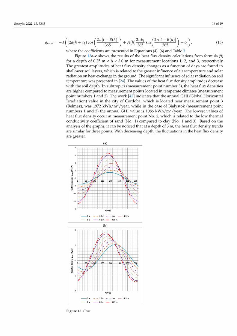
where the coefficients are presented in Equations (4)–(6) and Table 3. Figure 13a–c shows the results of the heat flux density calculations from formula (9)

for a depth of 0.25 m < h < 3.0 m for measurement locations 1, 2, and 3, respectively. The greatest amplitudes of heat flux density changes as a function of days are found in shallower soil layers, which is related to the greater influence of air temperature and solar

Figure 12. Comparison of the temperature values from the experiments and the computational modelat h = 2 m for three measurement points: (a) No. 1, (b) No. 2, (c) No. 3.

After substituting the Formula (3) to (1), the following form of heat flux density in theground layer from 0.25 to 3.0 m was obtained:

Energies 2022, 15, 3345 16 of 19

qnum = −λ

((2a2h + a1) cos

(2π[t− B(h)]

365

)+ A(h)

2πb1

365sin(

2π[t− B(h)]365

)+ c1

), (13)

where the coefficients are presented in Equations (4)–(6) and Table 3.Figure 13a–c shows the results of the heat flux density calculations from formula (9)

for a depth of 0.25 m < h < 3.0 m for measurement locations 1, 2, and 3, respectively.The greatest amplitudes of heat flux density changes as a function of days are found inshallower soil layers, which is related to the greater influence of air temperature and solarradiation on heat exchange in the ground. The significant influence of solar radiation on soiltemperature was presented in [24]. The values of the heat flux density amplitudes decreasewith the soil depth. In subtropics (measurement point number 3), the heat flux densitiesare higher compared to measurement points located in temperate climates (measurementpoint numbers 1 and 2). The work [42] indicates that the annual GHI (Global HorizontalIrradiation) value in the city of Cordoba, which is located near measurement point 3(Belmez), was 1972 kWh/m2/year, while in the case of Białystok (measurement pointnumbers 1 and 2) the annual GHI value is 1086 kWh/m2/year. The lowest values ofheat flux density occur at measurement point No. 2, which is related to the low thermalconductivity coefficient of sand (No. 1) compared to clay (No. 1 and 3). Based on theanalysis of the graphs, it can be noticed that at a depth of 3 m, the heat flux density trendsare similar for three points. With decreasing depth, the fluctuations in the heat flux densityare greater.

Energies 2022, 15, 3345 18 of 21

radiation on heat exchange in the ground. The significant influence of solar radiation on soil temperature was presented in [24]. The values of the heat flux density amplitudes decrease with the soil depth. In subtropics (measurement point number 3), the heat flux densities are higher compared to measurement points located in temperate climates (measurement point numbers 1 and 2). The work [42] indicates that the annual GHI (Global Horizontal Irradiation) value in the city of Cordoba, which is located near measurement point 3 (Belmez), was 1972 kWh/m2/year, while in the case of Białystok (measurement point numbers 1 and 2) the annual GHI value is 1086 kWh/m2/year. The lowest values of heat flux density occur at measurement point No. 2, which is related to the low thermal conductivity coefficient of sand (No. 1) compared to clay (No. 1 and 3). Based on the analysis of the graphs, it can be noticed that at a depth of 3 m, the heat flux density trends are similar for three points. With decreasing depth, the fluctuations in the heat flux density are greater.

(a)

(b)

Figure 13. Cont.

Energies 2022, 15, 3345 17 of 19Energies 2022, 15, 3345 19 of 21

(c)

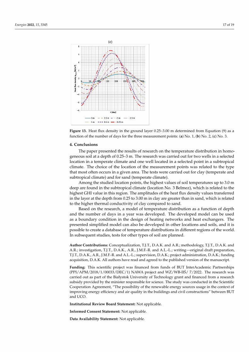
Figure 13. Heat flux density in the ground layer 0.25–3.00 m determined from Equation (9) as a function of the number of days for the three measurement points: (a) No. 1, (b) No. 2, (c) No. 3.

4. Conclusions The paper presented the results of research on the temperature distribution in

homogeneous soil at a depth of 0.25–3 m. The research was carried out for two wells in a selected location in a temperate climate and one well located in a selected point in a subtropical climate. The choice of the location of the measurement points was related to the type that most often occurs in a given area. The tests were carried out for clay (temperate and subtropical climate) and for sand (temperate climate).

Among the studied location points, the highest values of soil temperatures up to 3.0 m deep are found in the subtropical climate (location No. 3 Belmez), which is related to the highest GHI value in this region. The amplitudes of the heat flux density values transferred in the layer at the depth from 0.25 to 3.00 m in clay are greater than in sand, which is related to the higher thermal conductivity of clay compared to sand.

Based on the research, a model of temperature distribution as a function of depth and the number of days in a year was developed. The developed model can be used as a boundary condition in the design of heating networks and heat exchangers. The presented simplified model can also be developed in other locations and soils, and it is possible to create a database of temperature distributions in different regions of the world. In subsequent studies, tests for other types of soil are planned.

Author Contributions: Conceptualization, T.J.T., D.A.K. and A.R.; methodology, T.J.T., D.A.K. and A.R.; investigation, T.J.T., D.A.K., A.R., J.M.F.-R. and A.L.-L.; writing—original draft preparation, T.J.T., D.A.K., A.R., J.M.F.-R. and A.L.-L.; supervision, D.A.K.; project administration, D.A.K.; funding acquisition, D.A.K. All authors have read and agreed to the published version of the manuscript.

Funding: This scientific project was financed from funds of BUT InterAcademic Partnerships (PPI/APM/2018/1/00033/DEC/1) NAWA project and WZ/WB-IIŚ/ 7/2022. The research was carried out as part of the Białystok University of Technology grant and financed from a research subsidy provided by the minister responsible for science. The study was conducted in the Scientific Cooperation Agreement, “The possibility of the renewable energy sources usage in the context of improving energy efficiency and air quality in the buildings and civil constructions” between BUT and UCO.

Institutional Review Board Statement: Not applicable.

Figure 13. Heat flux density in the ground layer 0.25–3.00 m determined from Equation (9) as afunction of the number of days for the three measurement points: (a) No. 1, (b) No. 2, (c) No. 3.

4. Conclusions

The paper presented the results of research on the temperature distribution in homo-geneous soil at a depth of 0.25–3 m. The research was carried out for two wells in a selectedlocation in a temperate climate and one well located in a selected point in a subtropicalclimate. The choice of the location of the measurement points was related to the typethat most often occurs in a given area. The tests were carried out for clay (temperate andsubtropical climate) and for sand (temperate climate).

Among the studied location points, the highest values of soil temperatures up to 3.0 mdeep are found in the subtropical climate (location No. 3 Belmez), which is related to thehighest GHI value in this region. The amplitudes of the heat flux density values transferredin the layer at the depth from 0.25 to 3.00 m in clay are greater than in sand, which is relatedto the higher thermal conductivity of clay compared to sand.

Based on the research, a model of temperature distribution as a function of depthand the number of days in a year was developed. The developed model can be usedas a boundary condition in the design of heating networks and heat exchangers. Thepresented simplified model can also be developed in other locations and soils, and it ispossible to create a database of temperature distributions in different regions of the world.In subsequent studies, tests for other types of soil are planned.

Author Contributions: Conceptualization, T.J.T., D.A.K. and A.R.; methodology, T.J.T., D.A.K. andA.R.; investigation, T.J.T., D.A.K., A.R., J.M.F.-R. and A.L.-L.; writing—original draft preparation,T.J.T., D.A.K., A.R., J.M.F.-R. and A.L.-L.; supervision, D.A.K.; project administration, D.A.K.; fundingacquisition, D.A.K. All authors have read and agreed to the published version of the manuscript.

Funding: This scientific project was financed from funds of BUT InterAcademic Partnerships(PPI/APM/2018/1/00033/DEC/1) NAWA project and WZ/WB-IIS/ 7/2022. The research wascarried out as part of the Białystok University of Technology grant and financed from a researchsubsidy provided by the minister responsible for science. The study was conducted in the ScientificCooperation Agreement, “The possibility of the renewable energy sources usage in the context ofimproving energy efficiency and air quality in the buildings and civil constructions” between BUTand UCO.

Institutional Review Board Statement: Not applicable.

Informed Consent Statement: Not applicable.

Data Availability Statement: Not applicable.

Energies 2022, 15, 3345 18 of 19

Conflicts of Interest: The authors declare no conflict of interest.

References1. Sliwa, T.; Sojczynska, A.; Rosen, A.M.; Kowalski, T. Evaluation of Temperature Profiling Quality in Determining Energy

Efficiencies of Borehole Heat Exchangers. Geothermics 2019, 78, 129–137. [CrossRef]2. Sakata, Y.; Katsura, T.; Serageldin, A.A.; Nagano, K.; Ooe, M. Evaluating Variability of Ground Thermal Conductivity within a

Steep Site by History Matching Underground Distributed Temperatures from Thermal Response Tests. Energies 2021, 14, 1872.[CrossRef]

3. Sliwa, T.; Sapinska-Sliwa, A.; Gonet, A.; Kowalski, T.; Sojczynska, A. Geothermal Boreholes in Poland—Overview of the CurrentState of Knowledge. Energies 2021, 14, 3251. [CrossRef]

4. Katsura, T.; Sakata, Y.; Ding, L.; Nagano, K. Development of Simulation Tool for Ground Source Heat Pump Systems Influencedby Ground Surface. Energies 2020, 13, 4491. [CrossRef]

5. Mitchell, M.S.; Spitler, J.D. An Enhanced Vertical Ground Heat Exchanger Model for Whole-Building Energy Simulation. Energies2020, 13, 4058. [CrossRef]

6. Gao, S.; Tang, C.; Luo, W.; Han, J.; Teng, B. A New Analytical Model for Calculating Transient Temperature Response of VerticalGround Heat Exchangers with a Single U-Shaped Tube. Energies 2020, 13, 2120. [CrossRef]

7. Shimada, Y.; Uchida, Y.; Takashima, I.; Chotpantarat, S.; Widiatmojo, A.; Chokchai, S.; Charusiri, P.; Kurishima, H.; Tokimatsu, K.A Study on the Operational Condition of a Ground Source Heat Pump in Bangkok Based on a Field Experiment and Simulation.Energies 2020, 13, 274. [CrossRef]

8. Leski, K.; Luty, P.; Gwadera, M.; Larwa, B. Numerical Analysis of Minimum Ground Temperature for Heat Extraction inHorizontal Ground Heat Exchangers. Energies 2021, 14, 5487. [CrossRef]

9. Gwadera, M.; Kupiec, K. Modeling the Temperature Field in the Ground with an Installed Slinky-Coil Heat Exchanger. Energies2021, 14, 4010. [CrossRef]

10. Zhou, Y.; Bidarmaghz, A.; Makasis, N.; Narsilio, G. Ground-Source Heat Pump Systems: The Effects of Variable Trench Separationsand Pipe Configurations in Horizontal Ground Heat Exchangers. Energies 2021, 14, 3919. [CrossRef]

11. Kim, K.; Kim, J.; Nam, Y.; Lee, E.; Kang, E.; Entchev, E. Analysis of Heat Exchange Rate for Low-Depth Modular Ground HeatExchanger through Real-Scale Experiment. Energies 2021, 14, 1893. [CrossRef]

12. Sorokins, J.; Borodinecs, A.; Zemitis, J. Application of ground-to-air heat exchanger for preheating of supply air. IOP Conf. Ser.Earth Environ. Sci. 2017, 90, 012002. [CrossRef]

13. EN 15698-1:2020-01; District Heating Pipes—Bonded Twin Pipe Systems for Directly Buried Hot Water Networks—Part 1: FactoryMade Twin Pipe Assembly of Steel Service Pipes, Polyurethane Thermal Insulation and One Casing of Polyethylene. EuropeanCommittee for Standardization: Brussels, Belgium, 2019.

14. EN 13941-1:2019; District Heating Pipes—Design and Installation of Thermal Insulated Bonded Single and Twin Pipe Systems forDirectly Buried Hot Water Networks—Part 1: Design. European Committee for Standardization: Brussels, Belgium, 2019.

15. Bøhm, B.; Kristjansson, H. Single, twin and triple buried heating pipes: On potential savings in heat losses and costs. Int. J. EnergyRes. 2005, 29, 1301–1312. [CrossRef]

16. Van der Heijde, B.; Aertgeerts, A.; Helsen, L. Modelling steady-state thermal behavior of double thermal network pipes. Int. J.Therm. Sci. 2017, 117, 316–327. [CrossRef]

17. Krawczyk, D.A.; Teleszewski, T.J. Optimization of Geometric Parameters of Thermal Insulation of Pre-Insulated Double Pipes.Energies 2019, 12, 1012. [CrossRef]

18. Danielewicz, J.; Sniechowska, B.; Sayegh, M.A.; Fidorów, N.; Jouhara, H. Three-dimensional numerical model of heat losses fromdistrict heating network pre-insulated pipes buried in the ground. Energy 2016, 108, 172–184. [CrossRef]

19. Danielewicz, J.; Fidorow, N.; Jadwiszczak, P.; Szulgowska-Zgrzywa, M. The exploitation costs for various heating systemsaccording to the energetic certification law in Poland. Energy Sources Part B Econ. Plan. Policy 2014, 9, 301–306. [CrossRef]

20. Information Materials of Logstor Companies. 2012. (01/02). Available online: http://www.logstor.com/ (accessed on1 March 2022).

21. Terradas-III, G.; Triolo, J.M.; Pham, C.H.; Martí-Herrero, J.; Sommer, S.G. Thermic model to predict biogas production in unheatedfixed dome digesters buried in the ground. Environ. Sci. Technol. 2014, 48, 3253–3262. [CrossRef]

22. Rainier, H.; Nouceiba, A.; Yves, J.; Marie-Noëlle, P. Modeling and simulation of heat transfer phenomena in a semi-buriedanaerobic digester. Chem. Eng. Res. Des. 2017, 119, 101–116.

23. Teleszewski, T.J.; Zukowski, M. Analysis of Heat Loss of a Biogas Anaerobic Digester in Weather Conditions in Poland. J. Ecol.Eng. 2018, 19, 242–250. [CrossRef]

24. Larwa, B. Heat Transfer Model to Predict Temperature Distribution in the Ground. Energies 2019, 12, 25. [CrossRef]25. Kupiec, K.; Larwa, B.; Gwadera, M. Heat transfer in horizontal ground heat exchangers. Appl. Therm. Eng. 2015, 75, 270–276.

[CrossRef]26. Ouzzane, M.; Eslami-Nejad, P.; Aidoun, Z.; Lamarche, L. Analysis of the convective heat exchange effect on the undisturbed

ground temperature. Sol. Energy 2014, 108, 340–347. [CrossRef]27. Gwadera, M.; Larwa, B.; Kupiec, K. Undisturbed ground temperature—Different methods of determination. Sustainability 2017,

9, 2055. [CrossRef]

Energies 2022, 15, 3345 19 of 19

28. Carslaw, H.S.; Jaeger, J.C. Conduction of Heat in Solids, 2nd ed.; Clarendon Press: Oxford, UK, 1959; ISBN 978-0198533030.29. Rao, K.G. Estimation of the exchange coefficient of heat during low wind convective conditions. Bound. Layer Meteorol. 2004,

111, 247–273. [CrossRef]30. McAdams, W.H. Heat Transmission; McGraw-Hill: New York, NY, USA, 1954.31. Molina-Rodea, R.; Wong-Loya, J.A. A new model to predict subsoil-thermal profiles based on seasonal rain conditions and soil

properties. Geothermics 2021, 97, 102261. [CrossRef]32. Le, A.T.; Wang, L.; Wang, Y.; Li, D. Measurement investigation on the feasibility of shallow geothermal energy for heating and

cooling applied in agricultural greenhouses of Shouguang City: Ground temperature profiles and geothermal potential. Inf.Processing Agric. 2021, 8, 251–269. [CrossRef]

33. Al-Hinti, I.; Al-Muhtady, A.; Al-Kouz, W. Measurement and modelling of the ground temperature profile in Zarqa, Jordan forgeothermal heat pump applications. Appl. Therm. Eng. 2017, 123, 131–137. [CrossRef]

34. Tong, C.; Li, X.; Duanmu, L.; Wang, H. Prediction of the temperature profiles for shallow ground in cold region and cold winterhot summer region of China. Energy Build. 2021, 242, 110946. [CrossRef]

35. Available online: https://datasheets.maximintegrated.com/en/ds/DS18B20.pdf (accessed on 23 April 2022).36. PN-EN ISO 14688-1:2018-05; Geotechnical Investigation and Testing—Identification and Classification of Soil—Part 1: Identifica-

tion and Description (ISO 14688-1:2017). European Committee for Standardization: Brussels, Belgium, 2017.37. Rose, C.W. Agricultural Physics; Pergamon: Oxford, UK, 1966; p. 230.38. PN-EN ISO 6946: 1999; Building Components and Building Elements—Thermal Resistance and Thermal Transmittance—

Calculation Method. European Committee for Standardization: Brussels, Belgium, 1996.39. Whittig, L.D.; Allardice, W.R. X-ray diffraction techniques. In Methods of Soil Analysis. Part 1. Physical and Mineralogical Methods,

2nd ed.; Klute, A., Ed.; Agron. Monogr. 9; ASA and SSSA: Madison, WI, USA, 1986; pp. 331–362.40. JCPD. Joint Committee on Powder Diffraction Standards; International Center for Diffraction Data: Swarthmore, PA, USA, 1995.41. Andújar Márquez, J.M.; Martínez Bohórquez, M.Á.; Gómez Melgar, S. Ground Thermal Diffusivity Calculation by Direct Soil

Temperature Measurement. Application to very Low Enthalpy Geothermal Energy Systems. Sensors 2016, 16, 306. [CrossRef]42. Available online: https://solargis.com/maps-and-gis-data/overview (accessed on 1 March 2022).43. PN-EN 12524:2003; Building Materials and Products—Hygrothermal Properties—Tabulated Design Values. European Committee

for Standardization: Brussels, Belgium, 2000.44. Riche, F.; Schneebeli, M. Thermal conductivity of snow measured by three independent methods and anisotropy considerations.

Cryosphere 2013, 7, 217–227. [CrossRef]45. Available online: https://www.azom.com/properties.aspx?ArticleID=52 (accessed on 23 April 2022).46. Ottestad, P. Time-series described by trigonometric functions and the possibility of acquiring reliable forecasts for climatic and

other biospheric variables. J. Interdiscip. Cycle Res. 1986, 17, 29–49. [CrossRef]47. WTA. Simulation of Heat and Moisture Transfer. Guideline 6-2-01/E; WTA-Publications: München, Germany, 2004.48. WUFI®2D Calculation Example Step by Step. Available online: https://wufi.de/en/wp-content/uploads/sites/9/2014/09/

WUFI2D-3_Example.pdf (accessed on 23 April 2022).49. Leaf, J.S.; Erell, E. A model of the ground surface temperature for micrometeorological analysis. Theor. Appl. Climatol. 2018,

133, 697–710. [CrossRef]50. Kusuda, T.; Achenbach, P.R. Earth temperature and thermal diffusivity at selected stations in the United States. ASHRAE Trans.

1965, 71, 61–75.51. Nidal, H. Abu-Hamdeh Ground Thermal Properties of Soils as affected by Density and Water Content. Biosyst. Eng. 2003,

86, 97–102. [CrossRef]52. Arkhangelskaya, T.A.; Lukiashchenko, K.I. Estimating soil thermal diffusivity at different water contents from easily available

data on soil texture, bulk density, and organic carbon content. Biosyst. Eng. 2018, 168, 83–95. [CrossRef]