Climate change impact on snow and soil temperaturein boreal Scots pine stands

Per-Erik Mellander & Mikaell Ottosson Löfvenius &

Hjalmar Laudon

Received: 9 May 2006 /Accepted: 12 March 2007 / Published online: 27 April 2007# Springer Science + Business Media B.V. 2007

Abstract Scenarios indicate that the air temperature will increase in high latitude regions incoming decades, causing the snow covered period to shorten, the growing season tolengthen and soil temperatures to change during the winter, spring and early summer. Toevaluate how a warmer climate is likely to alter the snow cover and soil temperature inScots pine stands of varying ages in northern Sweden, climate scenarios from the Swedishregional climate modelling programme SWECLIM were used to drive a Soil-Vegetation-Atmosphere Transfer (SVAT)-model (COUP). Using the two CO2 emission scenarios A andB in the Hadley centres global climate model, HadleyA and HadleyB, SWECLIM predictsthat the annual mean air temperature and precipitation will increase at most 4.8°C and315 mm, respectively, within a century in the study region. The results of this analysisindicate that a warmer climate will shorten the period of persistent snow pack by 73–93 days, increase the average soil temperature by 0.9–1.5°C at 10 cm depth, advance soilwarming by 15–19 days in spring and cause more soil freeze–thaw cycles by 31–38%. Theresults also predict that the large current variations in snow cover due to variations in treeinterception and topography will be enhanced in the coming century, resulting in increasedspatial variability in soil temperatures.

1 Introduction

The winter climate plays a profound ecological role in high latitude boreal regions of theworld; the timing, duration and extent of snow cover being particularly important variables.Due to the insulating properties of snow it has a strong influence on below groundtemperatures during the winter (Brooks et al. 1996), and the extent and duration of snowcover strongly influence the timing and rapidity of soil warming in spring (Mellander et al.2004). In many snow covered regions snow-melt is also the major hydrological event of theyear and, hence, strongly affects fresh water supplies and nutrient fluxes (Stewart et al.2004; Laudon et al. 2004). Following global warming the length of the snow-covered

Climatic Change (2007) 85:179–193DOI 10.1007/s10584-007-9254-3

P.-E. Mellander (*) :M. Ottosson Löfvenius : H. LaudonDepartment of Forest Ecology, Swedish University of Agricultural Sciences, SE-901 83 Umeå, Swedene-mail: Per-Erik.Mellander@sek.slu.se

season is expected to shorten and consequently the growing season to lengthen in highlatitude ecosystems (Sparks and Menzel 2002). At an ecosystem or stand level, elevatedsoil temperature could increase rates of heterotrophic respiration and decay bydecomposers, thereby enhancing rates of CO2 release (Eliasson et al. 2005). Changes inthe soil temperature regime during winter could also affect root mortality (Tierney et al.2001), the substrate quality of soil organic matter (Öquist 2001), carbon, nitrogen andphosphorus concentrations in soil solutions (Fitzhugh et al. 2001), nitrate levels in runoff(Mitchell et al. 1996; Fitzhugh et al. 2003) and the quality of dissolved organic matterduring spring floods (Stepanauskas et al. 2000).

In the boreal forests of northern Sweden the ground is covered with snow forapproximately half of the year on average (Ottosson Löfvenius et al. 2003), but there aremajor small-scale spatial variations in its depth and duration due to variations in treeinterception, topography and forest management practices. For instance, OttossonLöfvenius et al. (2003) found a correlation between the stem density of shelterwood standsthey examined and depths of both snow and soil frost. Recent observations of permafrostmelting in Alaska are also more strongly related to changes in snow-cover than increases inair temperature (Stiegliz et al. 2003). Furthermore, it has been demonstrated that the largestspatial variations in the timing of snow ablation and soil warming in spring occur duringyears with little snow (Mellander et al. 2005). Most studies on forest ecosystems haveneglected the roles of snow and soil frost on soil temperature and, thus, the consequences ofchanges in the timing of soil warming on water, carbon and nutrient uptake by trees (whichcannot occur if the soil is frozen; Jarvis and Linder 2000). Field studies have shown notonly that delays in soil warming can reduce water and carbon uptakes by mature Scots pinetrees, but also that early soil warming makes the system more sensitive to variations in airtemperature (Strand et al. 2002; Mellander et al. 2004). Trees in the boreal forestphotosynthesise as effectively as trees grown in temperate regions, and the differences inannual growth between them are mainly due to differences in the length of the growingseason (Bergh et al. 1999) and soil nutrient constraints (Tamm 1991).

Climate models indicate that warming will be greater in northern latitudes than insouthern latitudes, and especially strong during the winter months (e.g. Rummukainen2003), while the precipitation in northern regions is expected to increase throughout theyear (Houghton et al. 2001). Dankers and Christensen (2005) predicted that global warmingwill lead to a shorter snow season, a shift in the runoff peak, decreased sublimation andincreased evapotranspiration in the sub-arctic Tana-basin in northern Fennoscandia. In highlatitude stands a climate change towards warmer conditions will not necessarily lead towarmer soil temperatures in springtime. Paradoxically, as suggested by Hardy et al. (2001)and discussed by Groffman et al. (2001), a climate shift leading to snow covering theground for shorter durations could even result in increases in soil freezing in northernhardwood forests. Venäläinen et al. (2001) also predicted that the probability of frozenground would increase in southern Finland as an effect of climate warming.

Since there are large uncertainties in the way climate change is likely to affect snowcover and associated ecological processes in the boreal forest landscape, the objective ofthis study was to investigate the duration of snow cover, the frequency of freeze–thawcycles and springtime soil warming in eight Scots pine stands in northern Sweden withrespect to two future climate scenarios. For this purpose, climate change scenarios from theSWEdish regional CLImate Modelling programme SWECLIM (Rossby Centre, SMHI,Norrköping, Sweden) (Rummukainen 2003) were used to run the COUP-model (Janssonand Karlberg 2004), a physically based Soil-Vegetation-Atmosphere Transfer (SVAT)model. This model has successfully reproduced the variability in snow depths and soil

180 Climatic Change (2007) 85:179–193

temperature, due to variations in the canopy, in the same stands as used in this study(Mellander et al. 2005).

2 Materials and methods

2.1 Description of sites

The model study was performed on eight Scots pine stands in northern Sweden, within and nearthe Vindeln Experimental Forests (64°13′N, 19°41′E, 170–220 m above sea level (m a.s.l.)). Themean annual air temperature is +1.6°C and annual precipitation is 613 mm, a third of whichfalls as snow (mean values for 1981–2004 from a reference climate station in VindelnExperimental Forests). The growing season is relatively short, normally lasting from themiddle of May to the end of September (Odin 1992). The chosen stands were of differingages and densities, all growing on sandy soils (Table 1). Three of the stands were classifiedas young (15–30 years old; Y1, Y2 and Y3), two as middle-aged (70 years; M1 and M2),and three as old (190–200 years; O1, O2 and O3). All sites lie within 10 km of a referenceclimate station.

2.2 Meteorological data

Standard meteorological measurements were obtained from a reference climate station in a1.4 ha open clear-cut (220 m a.s.l.) covering the period 1981–2000. The climate variableswere measured at some distance from each stand. However, data from the nearby climatestation, located in a representative site for the area, were judged to be adequate for thepurposes of this study since daily sums and averages were used in the analyses. Additionalmeasurements of snow depth and soil temperature were obtained at each stand for theperiod October 1998–August 1999 (Kluge 2001). Snow depth was measured with ca. 20snow sticks per stand and the soil temperature was measured with thermistors at 10 cmdepth. Manual readings were taken once or twice a month during winter and late summer.During spring and early summer, readings were taken once or twice a week. At one site

Table 1 Description of the eight Scots pine stands, in which snow-cover and soil temperature weresimulated with the COUP-model

Stand

Y1 Y2 Y3 O1 O2 O3 M1 M2

Site altitude (m a.s.l.) 170 170 175 170 170 220 220 175Distance from reference weather station (km) 10.0 10.0 10.0 2.9 3.1 0.1 0.2 1.5Tree age (year) 30 15 15 190 190 200 70 70Stem density (stem/ha) 1,990 12,600 3,400 64 669 1,465 995 1,294Basal area (m2/ha) 12.0 10.3 4.7 5.5 17.5 26.4 30.6 25.3Leaf area index 2.0 1.5 1.5 4.0 2.0 2.5 2.0 2.5Direct precipitation throughfall 0.35 0.40 0.40 0.50 0.30 0.30 0.10 0.10Soil organic Layer* (m) 0.08 0.10 0.10 0.05 0.05 0.10 0.10 0.02

All stands lie within 10 km of each other and within or near to Vindeln Experimental Forests, in the borealforest of northern Sweden

Climatic Change (2007) 85:179–193 181

(M2) soil temperature measurements were automatically collected every 10 min from threesoil profiles, and two-h averages were stored by data loggers (model CR10, CampbellScientific, Logan, UT, USA) during the period November 1998–January 2001.

2.3 Climate scenario data

Scenario data sets for future climate were extracted from SWECLIM (Rossby Centre,SMHI, Norrköping, Sweden) (Rummukainen 2003), based on simulations derived using acoupled regional model, RCAO, presented by Doscher et al. (2002) and two scenarios (Aand B) regarding future levels of greenhouse gases in the atmosphere. These scenarios arepresented in IPCC’s Special Report on Emission Scenarios (IPCC 2000) and are based ontwo differing sets of socioeconomic assumptions, the A-scenario describing changesleading to higher emissions than the B-scenario. The regional model of the SWECLIMprogram needs boundary conditions, which are obtained from a global model in the Hadleycentre in the UK. The two scenarios A and B are used as input to the global model (heredesignated HadleyA and HadleyB). SWECLIM also presents a control simulation coveringa 30 year period. This simulation is based on the assumed anthropogenic related changes inatmospheric composition and thereby climate forcing. Ten years of data, including airtemperature, relative humidity, precipitation, global radiation and wind speed, from thescenarios (2091–2100) and control data (1981–1990) were extracted from a pixelrepresenting a 44×44 km area where the stands examined in our study are located.

2.4 Data preparation

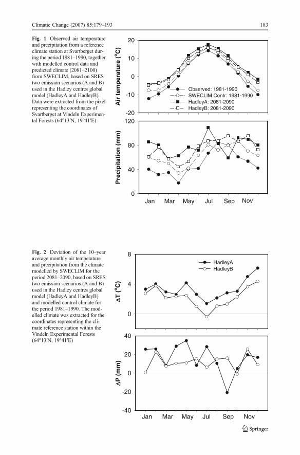
The SWECLIM control simulations were not year-to-year matches with the covered years(1981–1990), but rather model products of the period. The SWECLIM control dataregarding air temperature and precipitation were therefore compared with the air temper-atures and precipitation measured at the reference climate station during the same period(Fig. 1). The differences in the 10-year average monthly mean air temperatures between theSWECLIM control data and the measured data were rather large and therefore used to adjustthe SWECLIM scenario temperatures for 2091–2100. No adjustment was made for theprecipitation as this deviated more heterogeneously. Although daily data was available fromSWECLIM, and the COUP-model requires at least daily time resolution, our preference wasto use monthly averages and totals generated by SWECLIM and downscale the data to welldocumented regional climatic patterns of the observed area. Therefore, a 10-year time seriesof observed reference data (1991–2000) was used to introduce day to day variability into thetwo climate scenarios (2091–2100). The differences in monthly averages for each yearbetween the SWECLIM control data and scenario data were added to the observed referencedata for each day. Similarly, for precipitation the monthly total for each year was divided bythe number of days on which precipitation fell, and added to the reference data for each day.

The largest differences in air temperature between the climate scenarios and SWECLIMcontrol climate were found during the winter months (Fig. 2). In one summer month, July,temperatures were even slightly colder in HadleyB than in the SWECLIM control data forthe present climate. However, air temperatures were consistently higher in HadleyA, whichis based on higher emissions of greenhouse gases, compared to both HadleyB and thepresent climate. The increase in the 10-year average air temperature compared to theSWECLIM control data was +3.3°C for HadleyA and +2.2°C for HadleyB, whichincreased the length of the growing season, in comparison to the observed climate, by43 days and 30 days in HadleyA and HadleyB, respectively.

182 Climatic Change (2007) 85:179–193

Δ Δ P (

mm

)

-40

-20

0

20

40

Δ Δ T (

oC

)

0

4

8HadleyA HadleyB

Jan Mar May Jul Sep Nov

Fig. 2 Deviation of the 10–yearaverage monthly air temperatureand precipitation from the climatemodelled by SWECLIM for theperiod 2081–2090, based on SREStwo emission scenarios (A and B)used in the Hadley centres globalmodel (HadleyA and HadleyB)and modelled control climate forthe period 1981–1990. The mod-elled climate was extracted for thecoordinates representing the cli-mate reference station within theVindeln Experimental Forests(64°13′N, 19°41′E)

Air

tem

per

atu

re (

oC

)-20

-10

0

10

20

Observed: 1981-1990SWECLIM Contr: 1981-1990HadleyA: 2081-2090 HadleyB: 2081-2090

Pre

cip

itat

ion

(m

m)

0

40

80

120

Jan Mar May Jul Sep Nov

Fig. 1 Observed air temperatureand precipitation from a referenceclimate station at Svartberget dur-ing the period 1981–1990, togetherwith modelled control data andpredicted climate (2081–2100)from SWECLIM, based on SREStwo emission scenarios (A and B)used in the Hadley centres globalmodel (HadleyA and HadleyB).Data were extracted from the pixelrepresenting the coordinates ofSvartberget at Vindeln Experimen-tal Forests (64°13′N, 19°41′E)

Climatic Change (2007) 85:179–193 183

2.5 Model description

The model used was the COUP-model (Jansson and Halldin 1979; Eckersten and Jansson1991; Jansson and Moon 2001; Jansson and Karlberg 2004, ftp://www.lwr.kth.se/CoupModel/CoupModel.pdf), which is a numerical, one-dimensional SVAT-model thatcalculates vertical heat and water fluxes, in the soil-snow-vegetation-atmosphere system. Inthis model, water flow is based on Richard’s equation (Richards 1931), and the heat flow onFourier’s law and a surface energy balance approach according to Stähli and Jansson 1998.The soil compartment is regarded as multi-layered, each layer having specific physical andthermal properties, and the snow is treated as a single, homogenous layer. The canopy canbe treated either as a single big leaf (implicitly or explicitly), or as multiple canopies.Processes such as water uptake, transpiration by vegetation, rain and snow interception,soil-evaporation, evaporation of intercepted water, surface runoff, soil freezing andthawing, and plant growth may be optionally included. The transpiration is defined as apotential rate when there are no stress factors to influence the water losses. In such cases thepotential evaporation is derived from the combined Penman-Monteith equation (Monteith1965). The model accounts for differences in meteorological conditions caused byvariations in canopy heights between the stands. Important parameters describing the standinclude site altitude, leaf area index (LAI), direct precipitation through-fall, the lightextinction coefficient and the interception capacity of rain and snow. Important snowparameters are the density of new snow, the snow melt coefficient associated with globalradiation, air temperature and the thermal conductivity coefficient of snow. Drivingvariables are the standard climate parameters: air temperature, relative humidity,precipitation, global radiation and wind speed.

2.6 Model settings

A daily time step with 96 iterations was applied. The lower boundary level of the soil wasset to 3 m and the whole profile was divided into 10 layers, with thinner layers in the uppermetre (0.05, 0.10, 0.10, 0.20, 0.25 and 0.30 m) and thicker layers in the lower 2 m (0.50 m).Information on volumetric fractions of solid materials, liquid water and ice were used toderive the volumetric heat capacity and thermal conductivity. The coefficients used in thefunctions for each of the layers varied according to the dominant fractions in them.

Key parameters of the snow pack were simulated as follows. The snow surfacetemperature was derived from the energy balance, and the density of new snow from thedensity of totally frozen and mixed precipitation as an exponential function of airtemperature. The snow density was calculated as a function of its ice and water contentsand age. An empirical approach was used to calculate the mass balance of the snow pack.The snow’s thermal conductivity was sensitively related to the snow density by a quadraticfunction, and its seasonal variation was accounted for. Snow and rain interception wereseparated with an approach based on parameters describing the water and snow capacity perunit LAI and the fraction of direct precipitation through-fall (Jansson and Karlberg 2004).

The transpiration and soil evaporation were treated as separate flows. The canopy wasexplicitly treated as a single big leaf and the partitioning of light between the canopy andthe soil surface was estimated using Beer’s Law (Impens and Lemeur 1969). Seasonalvariations in surface resistance were calculated from the LAI and global radiation using theLohammar equation (Lohammar et al. 1980). The function derived by Shaw and Pereira(1982) was used to estimate the canopy roughness length and displacement height from thecanopy height. This function has been adjusted to include snow in the simulation (Jansson

184 Climatic Change (2007) 85:179–193

and Karlberg 2004). Aerodynamic resistance was calculated as the sum of functions ofwind speed and temperature gradients, which were corrected for atmospheric stability andadditional resistance proportional to the LAI.

2.7 Parameterisation, calibration and validation

The same parameters (some measured, some estimated or calibrated) were used as in aprevious study of the same forest stands (Mellander et al. 2005). The measured values wereseveral variables related to stand structure, including tree height, stem density and basalarea (BA) (Kluge 2001), and the thickness of the organic layer (Table 1). Estimates of soiltexture and saturated hydrological conductivity, obtained using pedo-transfer functionsdeveloped for one of the sites by Mellander et al. (2004) together with in-situ measurementsof the pF-curve by Giesler et al. (2000) were used to derive the Brooks-Corey waterretention function (Brooks and Corey 1964). The same root distribution (measured at anearby site by Mellander et al. 2004, with an exponential decrease of fine root biomassdown to 40 cm depths) was used for all stands.

Estimates of the LAI and direct precipitation through-fall were determined from sky-facing photographs of the stands using the Ocular LAI Comparator for Loblolly PineVersion 4.1 (Sampson et al. 1997). The model was also tested with higher values of LAIand direct precipitation through-fall to simulate a denser stand. The radiation extinctioncoefficient was derived from the LAI, using the relationship between these variablessuggested by Smith et al. (1991). The snow interception capacity per LAI was estimated tobe 3.0 mm m−2, the density of new snow to be 115 kg/m3 and the snow melt coefficientassociated with global radiation to be 1.4E-8 kg J−1. The snow melt coefficient associatedwith air temperature and the snow’s thermal conductivity coefficient were found, bycalibration against measured snow depth and soil temperature to be 1.3 kg °C−1 m−2 day−1

and 2.0E-6 W m5 °C−1 kg−2 respectively.The correlations between observed and modelled snow depths were significant for all the

stands (p<0.0001) with a range in determination coefficient (R2) from 0.82 to 0.90, bias (B)from −0.08 to 0.03, root mean square error (RMSE) from 0.08 to 0.15 m and efficiency (E,Nash and Sutcliffe 1971) from 0.77 to 0.88. For the observed and modelled soil temperature(10 cm) the correlations were also significant (p<0.0001) with R2 values ranging between0.90 and 0.99, B from −0.08 to 1.18, RMSE °C and E from 0.85 to 0.99 (Mellander et al.2005).

3 Results

A principal component analysis of the canopy parameters and observed snow depths in thestands during 1998/1999 revealed that snow depth was positively correlated with theopenness of the stand (“direct precipitation through-fall”), and negatively correlated withboth LAI and tree height (data not shown). The linear relationships between directprecipitation and (1) LAI and (2) tree height explained 92% of the variation in themaximum snow depths between stands. The soil temperature was positively correlated tothe thickness of the soil organic layer and direct precipitation through-fall. Stands of thesame age group had most in common since most of the biometric characters that affectsnow depths and soil temperature are related to tree age.

The predicted seasonal snow-cover was considerably thinner and lasted for a shortertime during the period 2091–2100 than in the modelled period for which empirical data

Climatic Change (2007) 85:179–193 185

were also available, 1991–2000 (Fig. 3 and Table 2). This resulted in predicted futurewinters with several freeze–thaw cycles in the soil, higher soil temperatures during thesummer and longer periods with soil temperatures above 0°C. However, in some years(1996/2096 and 1998/2098) the soil warming was only marginally earlier (4–6 days) thanwhen the model was driven with the 1991–2000 reference climate. The snow layer wasthicker and persisted longer in the younger stands (Y1, Y2 and Y3) in both the referenceclimate and climate scenarios, while the middle-aged stands (M1 and M2) had thethinnest and least persistent snow cover (Table 2). For both the reference climate andclimate scenarios the 10-year average soil temperature (10 cm) was highest in the oldstand O1 and lowest in the middle-aged stand M1. Under present conditions the 10-yearaverage date at which the soil temperature (10 cm) reached +3°C was earliest in the M2stand (19 May) and latest in stands Y2 and Y3 (27 May). In HadleyA the earliest soilwarming was found in the O1 and O2 stands, where the soil reached +3°C on 2 May, and6 days later in the M1 stand (8 May). In HadleyB the soil warmed to +3°C earliest in theO2 stand (5 May) and latest in the M1 stand (13 May). The number of freeze–thaw cycleswas highest in the older stands and increased in average for all stands by 31% in HadleyBand 38% in HadleyA.

The ten-year-average date of final snow ablation in the eight stands was 40 days earlier(31 March) in HadleyA, and 37 days (3 April) earlier in HadleyB, than in the 1991–2000reference climate (10 May) (Fig. 4). The variation between the stands was also larger inHadleyA and B than in the reference climate. The ten-year-average date at which the soil at10 cm reached +3°C in spring was 19 days earlier (4 May) in HadleyA, and 15 days earlier(8 May) in HadleyB, than in the period 1991–2000 (23 May). The variation in the timing ofsoil warming between the stands was larger for the period 1991–2000 than in HadleyA andB. It took, on average, 34 days after the final snow ablation date to reach +3°C in HadleyAand 35 days in HadleyB, compared to 13 days for the period 1991–2000. The ten-year-average soil temperature at 10 cm depth for all the stands was 3.1°C for the present climate,

Sn

ow

dep

th (

m)

0.0

0.5

1.01991-20002091-2100 HadleyA

'91 '92 '93 '94 '95 '96 '97 '98 '99 '00 '01

So

il te

mp

erat

ure

(oC

)

-10

-5

0

5

10

15

Fig. 3 Time series of modelledsnow depth and soil temperatureat 10 cm depth in a young Scotspine stand (Y1) near VindelnExperimental Forests in northernSweden. Observed climate data(1991–2000) and a scenario fromSWECLIM (2091–2100) wereused for the model runs

186 Climatic Change (2007) 85:179–193

2091-21002091-2100

Mar

Apr

May

Jun

1991-2000 HadleyA HadleyB

Dat

e

Tsoil > 3oC

Final snow ablation day

Fig. 4 The median of the 10–year average dates when snowfinally ablated and the soil tem-perature at 10 cm depth reached+3°C for eight Scots pine standsof three age classes, modelledwith climate forcing based onobserved climate data for 1991–2000 and two scenarios (HadleyAand HadleyB, 2091–2100) fromSWECLIM

Table 2 Ten-year averages of the modelled number of days with snow on the ground, average, maximumand minimum soil temperatures at 10 cm depth, date when the soil temperature at 10 cm reached +3°C andnumber of freeze–thaw cycles for eight Scots pine stands within or near the Vindeln Experimental Forests

No. snowdays

max. snowdepth

Tsaverage

Tsmax.

Tsmin

DateTs ≥ 3°C

No. freeze–thawcycles

Ref. Y1 194 0.83 3.2 13.5 −10.7 23 May 10Y2 202 0.93 3.0 13.0 −11.2 27 May 14Y3 199 0.92 3.0 13.0 −11.4 27 May 14M1 188 0.76 2.8 12.4 −11.5 25 May 13M2 182 0.72 3.5 16.4 −15.3 19 May 12O1 187 0.78 4.0 17.5 −4.6 20 May 15O2 198 0.80 3.3 14.8 −13.4 21 May 12O3 196 0.71 3.0 12.4 −9.5 23 May 13

HadA Y1 98 0.43 4.7 14.8 −6.3 03 May 23Y2 110 0.54 4.6 14.2 −6.4 05 May 20Y3 114 0.53 4.6 14.2 −6.5 04 May 14M1 78 0.40 4.3 13.7 −6.7 08 May 20M2 86 0.34 5.2 18.0 −9.0 04 May 23O1 109 0.45 5.7 19.2 −4.4 02 May 21O2 103 0.40 5.1 16.2 −7.6 02 May 24O3 106 0.35 4.4 13.7 −5.8 05 May 22

HadB Y1 112 0.57 4.0 13.9 −8.2 06 May 21Y2 128 0.68 3.8 13.3 −8.6 09 May 19Y3 135 0.68 3.8 13.3 −8.9 08 May 14M1 110 0.42 3.6 12.8 −8.2 13 May 17M2 109 0.41 4.4 17.0 −9.7 09 May 19O1 126 0.59 4.9 18.2 −4.4 08 May 19O2 120 0.56 4.2 15.2 −10.1 05 May 21O3 123 0.51 3.7 12.8 −7.1 09 May 20

Climate forcing was done using observed reference climate data (1991–2000) and the scenarios (2091–2100)from SWECLIM (HadleyA and HadleyB)

Climatic Change (2007) 85:179–193 187

4.6°C for HadleyA and 4.0°C for HadleyB (Fig. 5). The variation between the stands wasalso largest in the warmer HadleyA. At 20 and 40 cm depths the ten-year-average soiltemperature for all the stands increased by 0.8–1.5 and 0.7–1.4°C respectively (data notshown).

The ten-year monthly average soil temperature was highest in HadleyA throughout theyear in all stands (Fig. 6). In HadleyB the monthly average soil temperature was mostlyhigher than in the observed reference period, but from January to April and in July thedifferences were small, and in July it was even colder than in the observed reference periodin the O1 stand (the stand for which within-year differences were largest). In all stands andfor both scenarios the largest difference in soil temperature compared to the observedreference period was found in May.

4 Discussion

The climate by the end of this century is predicted to be warmer than the current climate,especially during winter (e.g. Houghton et al. 2001). The 30-year average air temperature inthe area of this study was predicted to increase from +1.6°C to ca. +6.4°C using HadleyA andto +5.2°C using HadleyB. When using climate scenarios for climate forcing in complex SVAT-models, such as the COUP-model, they should be handled critically for several reasons. In thiscase, for instance, the air temperatures in the SWECLIM control data were higher than the airtemperatures measured at a weather station that was very close to and had a very similarclimate to the study sites. When this systematic overestimation was accounted for in theclimate scenarios, the deviations between predicted and current air temperatures were weaker.

Assuming that the predicted future climate scenarios are reliable we can expect thinnersnow layers, shorter periods of snow cover and increases in the average growing season of30 (HadleyB) to 43 days (HadleyA). However, the precipitation was underestimated bySWECLIM during the winter months and it is possible that future snow depths are deeperthan predicted in this study, which would affect the expected length of snow season.Generally the trends were the same in all stands, but years with relatively little snowresulted in greater inter-annual variability due to the greater proportional effects ofinterception. Furthermore, the soil warmed more quickly after the final snow ablation date

1991-2000 HadleyA HadleyB

10-y

ear

aver

age

soil

tem

per

atu

re (

oC

)

0

1

2

3

4

5

6

2091-2100 2091-2100

Fig. 5 The median of the 10–year average soil temperature(10 cm depth) for eight Scotspine stands of three age classes,modelled with climate forcingbased on observed climate datafor 1991–2000 and two scenarios(HadleyA and HadleyB, 2091–2100) from SWECLIM

188 Climatic Change (2007) 85:179–193

in the present observed reference climate period than in the future climate scenarios (Fig. 4).This is because snow finally disappears later in the present climate (mid May), when the airtemperature is relatively high so the soil can warm more rapidly. In the two scenarios thefinal snow ablation dates were in early April, when the air temperatures were colder than thepresent reference air temperatures in mid May (Fig. 1). Furthermore, although the averagesoil temperatures were higher in the scenarios, they predicted that several soil frosts wouldoccur in the stands, which would require substantial energy to thaw.

Δ Δ Tso

il (o

C)

0

2

4

6HadleyA HadleyB

Δ Δ Tso

il (o

C)

0

2

4

6

Y1

M1

Δ Δ Tso

il (o

C)

0

2

4

6O1

Jan Mar May Jul Sep Nov

Fig. 6 The deviation of 10–yearmonthly averages of soil temper-ature (10 cm depth) modelledwith observed weather data(1991–2000) from the 10–yearmonthly averages of soil temper-ature modelled with HadleyA andHadleyB (2091–2100). Y1, M1and O1 are 30-, 70- and 190 year-old stands, respectively, that con-sist of Scots pine and are situatedwithin or near to the VindelnExperimental Forests

Climatic Change (2007) 85:179–193 189

A major finding in this study is that the largest spatial variability in soil temperaturesoccurred during snow-poor years, especially in HadleyA, in which the warmer climategenerates thin snow cover and hence increased variability in soil temperatures between sites(Fig. 5). This agrees well with the work by Zhang et al. (2005) who predicted that theannual temperature increase in Canadian soils will vary more spatially in winter and springthan in summer and autumn. Due to differences in the timing of soil warming in springbetween the present and predicted future climate, the largest difference in monthly 10-yearaverage soil temperature was found in May in all of the stands (Fig. 6), especially for thewarmer HadleyA.

The warmer climate caused thinner snow packs which increased the average soiltemperature and induced more freeze–thaw cycles during winter and earlier soil warming inspring. Changes in climate and snow cover that influence soil freezing and soil warming arelikely to affect high latitude forest ecosystems in several ways. A warmer climate can alterforest productivity by increasing the length of the growing season, advancing the release ofmelt water from snow melt and frost thaw, and enhancing rates of fine root mortality, nutrientturnover and respiration. Shifts in runoff peaks and biogeochemical changes in streams mayalso occur (see, for instance, Dankers and Christensen 2005; Stewart et al. 2004). Increasesin the frequency of freeze–thaw cycles have been found to increase N2O fluxes during thewinter and the thawing period in spring (Syvasalo et al. 2004). The availability of Csubstrates plays an important role in freeze–thaw related N2O emissions (Sehy et al. 2004).Microbially available organic C is released during freezing and metabolized during thesubsequent thawing. It has also been suggested that soil freezing events may increase rates ofN and P losses, with potential effects on soil N and P availability, ecosystem productivity,surface water acidification and eutrophication (Fitzhugh et al. 2001). Repeated freeze–thawcycles have also been speculated to be a reason for winter-embolism in coniferous forests(Mayr et al. 2003), which may cause permanent damage and affect productivity.

An increased greenness changes the surface albedo which was found to be a potentialcontributing factor to the amplified polar effects of global warming (Zhang and Walsh2006). Another potential effect of increases in the length of the growing season is thatcarbon availability may increase, resulting in reductions in net carbon uptake (Brooks et al.2004). In northern forests the carbon balance is often near equilibrium, so minor changes inthe ecosystem may switch the forest from being a net carbon source or sink, or vice versa(Lindroth et al. 1998). Soil temperature is a key factor regulating net soil respiration inboreal forests (Valentini et al. 2000). Changes in the depth of the insulating snow cover maychange soil carbon sequestration rates in forest ecosystems (Monson et al. 2006). If thesnow pack prevents soil freezing microbial activity may continue during the winter andcontribute CO2 fluxes representing as much as 20% of the annual soil CO2 budget in someareas (Brooks et al. 1996). The wintertime fluxes of CO2 have been found to followseasonal patterns in subalpine forests of various ages (Hubbard et al. 2005). Other variablesthat may be influenced by changes in the snow-pack and soil temperature include fine rootand microbial mortality, hydrological and gaseous losses of N, and the acid-base status ofdrainage water (Groffman et al. 2001). The snow cover as a source of water supply isanother issue where the dynamics in the timing of spring snow melt was found to be aprimary control over the annual rate of carbon sequestration (Monson et al. 2002).

An important economic and cultural activity for northern Scandinavia is reindeerhusbandry. Changes in snow cover in northern Sweden may influence the populationdemography of reindeer due to spatial and temporal changes in the distribution of highquality food (Marell et al. 2006).

190 Climatic Change (2007) 85:179–193

5 Conclusions

The model analysis of eight stands in the boreal zone of northern Sweden revealed that awarmer climate by the end of this century, as predicted by SWECLIM, will increase thegrowing season by 30–43 days, shorten the duration of a consistent snow pack by 73–93 days, increase the average soil temperature at 10 cm depth by 0.9–1.5°C, advance soilwarming by 15–19 days and increase the frequency of freeze–thaw cycles by 31–38%. Thelarge current variability in snow cover due to variations in tree interception and topographyis predicted to increase in the coming century, resulting in increased spatial variability insoil temperatures.

Acknowledgements The study was financiered by the Kempe Foundation.

References

Bergh J, Linder S, Lundmark T et al (1999) The effect of water and nutrient availability on the productivityof Norway Spruce in northern and southern Sweden. For Ecol Manag 119:51–62

Brooks RH, Corey AT (1964) Hydraulic properties of porous media. Colorado State University, Fort Collins,Colorado. Hydrology paper No. 3, 27pp.

Brooks PD, Williams MW, Schmidt SK (1996) Microbial activity under alpine snowpacks, Newot Ridge,Colorado. Biogeochemistry 32:93–113

Brooks PD, McKnight D, Elder K (2004) Carbon limitation of soil respiration under winter snowpacks:potential feedbacks between growing season and winter carbon fluxes. Glob Chang Biol 11:231–238

Dankers R, Christensen OB (2005) Climate change impact on snow coverage, evaporation and riverdischarge in the sub-arctic Tana-basin northern Fennoscandia. Clim Change 69:367–392

Doscher R, Willén U, Jones C et al (2002) The development of the coupled regional ocean–atmospheremodel RCAO. Boreal Environ Res 7:183–192

Eckersten H, Jansson P-E (1991) Modelling water flow, nitrogen uptake and production of wheat. Fertil Res27:313–329

Eliasson PE, McMurtrie RE, Pepper DA et al (2005) The response of heterotrophic CO2 flux to soilwarming. Glob Chang Biol 11:167–181

Fitzhugh RD, Driscoll CT, Groffman PM et al (2001) Effects of soil freezing disturbance on soil solutionnitrogen, phosphorus, and carbon chemistry in a northern hardwood ecosystem. Biogeochemistry56:215–238

Fitzhugh RD, Likens GE, Driscoll CT et al (2003) Role of soil freezing events in interannual patterns ofstream chemistry at the Hubbard Brook experimental forest, New Hampshire. Environ Sci Technol37:1575–1580

Giesler R, Ilvesniemi H, Nyberg L et al (2000) Distribution and mobilization of Al, Fe and Si in the podzolicsoil profiles in relation to the humus layer. Geoderma 94:249–263

Groffman PM, Driscoll CT, Fahey TJ et al (2001) Colder soils in a warmer world: a snow manipulation studyin a northern hardwood forest ecosystem. Biogeochemistry 56:135–150

Hardy JP, Groffman PM, Fitzhugh RD et al (2001) Snow depth manipulation and its influence on soil frostand water dynamics in a northern hardwood forest. Biogeochemistry 56:151–174

Houghton JT, Ding Y, Griggs DJ et al (eds) (2001) Climate change 2001: the scientific basis. CambridgeUniversity Press, Cambridge

Hubbard RM, Ryan MG, Elder K et al (2005) Seasonal patterns in soil surface CO2 flux under snow cover in50 and 300 year old subalpine forests. Biogeochemistry 73:93–107

Impens I, Lemeur R (1969) Extinction of net radiation in different canopies. Arch for Geoph Bioclimatol SerB 17:403–412

IPCC (2000) Emissions scenarios 2000. In: Nakicenovic N, Swart R (eds) Special report of theintergovernmental panel on climate change. Cambridge University Press, UK, p 570

Jansson P-E, Halldin S (1979) Model for the annual water and energy flow in a layered soil. In: Halldin S(ed) Comparison of forest and energy models. Society for Ecological Modelling, Copenhagen, pp 145–163

Jansson P-E, Karlberg L (2004) Coupled heat and mass transfer model for soil-plant-atmosphere systems.Royal Institute of Technology, Department of Civil and Environmental Engineering, Stockholm, p 435

Climatic Change (2007) 85:179–193 191

Jansson P-E, Moon D (2001) A coupled model of water, heat and mass transfer using object orientation toimprove flexibility and functionality. Environ Model Softw 16:37–46

Jarvis P, Linder S (2000) Botany – Constraints to growth of boreal forests. Nature 405:904–905Kluge M (2001) Snow, soil frost and springtime soil temperature regimes in a boreal forest. Licentiate thesis,

Swedish University of Agricultural Sciences, Department of Forest Ecolology, Umeå, SwedenLaudon H, Köhler S, Buffam I (2004) Seasonal dependence of DOC export in five boreal catchments in

northern Sweden. Aquat Sci 66:223–230Lindroth A, Grelle A, Morén AS (1998) Long-term measurements of boreal forest carbon balance reveal

large temperature sensitivity. Glob Chang Biol 4:443–450Lohammar T, Larsson S, Linder S et al (1980) Fast simulation models of gaseous exchange in Scots pine.

Ecol Bull (Stockholm) 32:505–523Marell A, Hofgaard A, Danell K (2006) Nutrient dynamics of reindeer forage species along snowmelt

gradients at different ecological scales. Basic Appl Ecol 7:13–30Mayr S, Gruber A, Bauer H (2003) Repeated freeze–thaw cycles induce embolism in drought stressed

conifers. Planta 217:436–441Mellander P-E, Bishop K, Lundmark T (2004) The influence of soil temperature on transpiration: a plot scale

manipulation in a young Scots pine stand. For Ecol Manag 195:15–28Mellander P-E, Laudon H, Bishop K (2005) Modelling variability of snow depths and soil temperatures in

Scots pine stands. J Agric For Meteorol 133:109–118Mitchell MJ, Driscoll CT, Kahl JS et al (1996) Climatic control of nitrate loss from forested watersheds in the

northeast United States. Environ Sci Technol 30:2609–2612Monson RK, Turnipseed AA, Sparks JP et al (2002) Carbon sequestration in high-elevation, subalpine forest.

Glob Chang Biol 8:459–478Monson RK, Lipson DL, Burns SP et al (2006) Winter forest soil respiration controlled by climate and

microbial community composition. Nature 439:711–714Monteith JL (1965) Evaporation and environment. In: Fogg GE (ed) The state and movement of water in

living organisms, 19th Symposium of the Society of Experimental Biology. The Company of Biologists,Cambridge, pp 205–234

Nash LE, Sutcliffe JV (1971) River flow forecasting through conceptual models. Part 1: a discussion ofprinciples. J Hydrol 10:282–290

Odin H (1992) Climate and conditions in forest soils during winter and spring at Svartberget ExperimentalStation. Swedish University of Agricultural Sciences, Department of Ecological and EnvironmentalResearch, Report 56

Oquist M (2001) Northern Peatland carbon biogeochemistry: the influence of vascular plants and edaphicfactors on carbon dioxide and methane exchange. PhD thesis, Linköping University, Linköping

Ottosson Löfvenius MO, Kluge M, Lundmark T (2003) Snow and soil frost depth in two types ofshelterwood and clear-cut area. Scand J For Res 18:54–63

Richards LA (1931) Capillary conduction of liquids in porous mediums. Physics 1:318–333Rummukainen M (2003) The Swedish regional climate modelling program, SWECLIM 1996–2003. Final

report. Meteorology and Climatology Reports 104, SMHI, Norrköping, Sweden, 44ppSampson DA, Lee Allen H, Lunk EM et al (1997) The Ocular LAI comparator for Loblolly Pine Version 4.1.

Forest Nutrition Cooperative, Department of Forestry, NCSU, Raleigh, NC, p 12Sehy U, Dyckmans J, Ruser R et al (2004) Adding dissolved organic carbon to simulate freeze–thaw related

N2O emissions from soil. J Plant Nutr Soil Sci 167:471–478Shaw RH, Pereira AR (1982) Aerodynamic roughness of plant canopy: a numerical experiment. Agric For

Meteorol 26:51–65Smith FW, Sampson DA, Long JN (1991) Comparison of leaf area index estimates from tree allometrics and

measured light interception. For Sci 37:1682–1688Sparks TH, Menzel A (2002) Observed changes in seasons: an overview. Int J Climatol 22:1715–1725Stähli M, Jansson P-E (1998) Test of two SVAT snow submodels during different winter conditions. Journal

of Agricultural and Forest Meteorology 92:29–41Stepanauskas R, Laudon H, Jorgensen NOG (2000) High DON bioavailability in boreal streams during a

spring flood. Limnol Oceanogr 45:1298–1307Stewart IT, Cayan DR, Dettinger MD (2004) Changes in snowmelt runoff timing in western North America

under a ‘business as usual’ climate change scenario. Clim Change 62:217–232Stiegliz M, Dery SJ, Romanovsky VE et al (2003) The role of snow cover in the warming of arctic

permafrost. Geophys Res Lett 30:541–544Strand M, Lundmark T, Söderbergh I et al (2002) Impact of seasonal air and soil temperatures on

photosynthesis in Scots pine trees. Tree physiol 22:839–847

192 Climatic Change (2007) 85:179–193

Syvasalo E, Regina K, Pihlatie M et al (2004) Emission of nitrous oxide from boreal agricultural clay andloamy sand soils. Nutr Cycl Agroecosyst 69:155–165

Tamm C-O (1991) Nitrogen in terretrial ecosystems. Questions of productivity, vegetational changes, andecosystem stability. In Ecological Studies 81. Springer, Berlin Heidelberg New York, p 115

Tierney GL, Fahey TJ, Groffman PM et al (2001) Soil freezing alters fine root dynamics in a northernhardwood forest. Biogeochemistry 56:175–190

Valentini R, Matteucci G, Dolman AJ et al (2000) Respiration as the main determinant of carbon balance inEuropean forests. Nature 404:861–865

Venäläinen A, Tuomenvirta H, Heikinheimo M et al (2001) Impact of climate change on soil frost undersnow cover in forested landscape. Clim Res 17:63–72

Zhang J, Walsh JE (2006) Thermodynamic and hydrological impacts of ncreasing greenness in northern highlatitudes. J Hydrometeorol 7:1147–1163

Zhang Y, Chen WJ, Smith SL et al (2005) Soil temperature in Canada during the twentieth century: complexresponses to atmospheric climate change. J Geophy Res 110, Art. No. DO1105

Climatic Change (2007) 85:179–193 193