The structure of the vorticity field in turbulent channel flow. II - Study of ensemble-averaged...

J . Fluid Mech. (1986), vol. 165, p p . 441464

Printed in treat Britain 441

The structure of the vorticity field in turbulent channel flow.

Part 1. Analysis of instantaneous fields and statistical correlations

By PARVIZ MOIN AND JOHN KIM NASA Amea Remarch Center, Moffett Field, California 94035

(Received 17 September 1984 and in revieed form 26 December 1984)

An investigation into the existence of hairpin vortices in turbulent channel flow is conducted using a database generated by the large-eddy simulation technique. It is shown that away from the wall the distribution of the inclination angle of vorticity vector gains its maximum at about 45' to the wall. Two-point correlations of velocity and vorticity fluctuations strongly support a flow model consisting of vortical structures inclined at 45' to the wall. The instantaneous vorticity vectors plotted in planes inclined at 45' show that the flow contains an appreciable number of hairpins. Vortex lines are used to display the three-dimensional structure of hairpins, which are shown to be generated from deformation (or roll-up) of sheets of transverse vorticity .

1. Introduction In 1952 Theodorsen characterized turbulent boundary layers as being composed

of large-scale horseshoe-shaped vortices which are responsible for turbulent transport. Since then a number of investigators have proposed physical models of turbulent boundary layers that contain as their dominant feature pairs of counter-rotating vortices with axes either parallel or inclined to the flow direction. Recently, Wallace (1982) has collected ce number of experimental results consistent with the vortex-pair model of boundary layers. He proposes a hairpin-like vortex as the dominant flow structure, which is formed from the deformation, stretching, and lifting of the transverse vortex lines.

Quantitative evidence in support of the existence of pairs of counter-rotating vortical structures inclined to the wall and streamwise direction waa obtained from extensive spacetime correlation measurements by Willmarth t Tu (1967). Isocorrelation contours of the correlation between pressure fluctuations at a fixed point on the wall and the spanwise velocity component w in planes perpendicular to the wall and the mean-stream direction ((y, 2)-planes) show sign reversal, with the line of zero correlation moving away from the wall in the downstream direction. This result is consistent with the presence of lifting streamwise vortices which produce reversal in w (and hence the correlation pW) across the horizontal planes containing the vortex centres. The correlation between fluctuations of the streamwise velocity u at the edge of the sublayer and the streamwise vorticity w, at various points above and downstream of the velocity probe was also measured. These data were later analysed by Willmarth & Lu (1972). The location of maximum correlation between u and w, was along a line through the fixed velocity point inclined at an angle of

442 P. Moin and J . Kim

about 10'. A quadrant analysis of the motions contributing to the W, correlation showed that, for large negative values of u, w, was positive for z > 0 and negative for z < 0, where the u-probe was located at z = 0 and clockwise rotation was denoted as positive. Based on these measurements, Willmarth & Tu (1967) proposed a model for the wall layer consisting of hairpin vortices generated from deformation of transverse vortex lines'and inclined downstream and away from the wall. In their model, the vortex filaments are deformed in a regular sinusoidal manner with regions of flow moving toward and away from the wall alternating in the spanwise direction. This model, with a 10' vortex-inclination angle, was proposed only for the wall region, and is in contrast to Theodorsen's large-scale horseshoes inclined a t 45" to the flow and extending across the entire boundary layer. In passing, we remark that the undisturbed flow consists of sheets of transverse vorticity and not isolated vortex tubes or filaments (representing vortices).

Townsend (1970,1976) shows that an eddy model consisting of a pair of roller eddies inclined at about 30' to the flow direction is generally consistent with two-point correlation functions calculated from the rapid-distortion theory. He suggests the double-roller eddies as the dominant structures in turbulent shear flows. Perry & Chong (1982) formulated a model of turbulent boundary layers with a random array of A-shaped vortices inclined at a fixed angle to the wall but of different scales. In order to reproduce the logarithmic mean-velocity profile, it was assumed that the A vortices were confined to a plane and were subject only to plane strain. This model provides a structural link between the mean flow and turbulent stresses.

There is an extensive collection of experimental data pointing to the existence of organized structures or disturbance fronts inclined to the wall and the stream direction. Kovasznay , Kibens & Blackwelder (1 970) constructed an isocorrelation contour plot of spacetime streamwise velocity correlations using a probe fixed at y/6 = 0.5 and another at different y-locations. The contour lines (in (y, t)-planes) clearly show a downstream tilt. The same feature is also apparent in the correlation measurements of Blackwelder & Kovasznay (1972), where the location of the fixed probe was close to the wall (y/6=0.03). Tritton's (1967) two-point velocity correlations decay more slowly when the probe separation line is directed downstream away from the wall. This behaviour is also evident in the correlations of Favre, Gaviglio & Dumas (1957). Using spacetime correlation between fluctuations of wall shear stress and streamwise velocity with optimum time delays, Kreplin & Eckelmann (1979) detected a disturbance 'front ' which had an inclination angle of about 14" to the wall at y+ = 50.t However, the front that can be deduced from correlating spanwise fluctuations (w, aw/ay l v - o ) does not extend beyond y+ = 30. Brown & Thomas (1977), using spacetime correlation of the streamwise velocity and wall shear stress, also detected an inclined disturbance front. However, in contrast to Kreplin & Eckelmann's measurements, which were limited to the wall region, they measured the inclination angle of the front to be 18' across the entire boundary layer. They also propose a model in which the organized structure appears as a horseshoe vortex. In coqtrast to Willmarth & Tu (1967) and Wallace (1982), who describe the origin of the.horseshoe vortices as due to the deformation of the mean-vortex lines (initially pointing in the spanwise direction) by random velocity and vorticity fluctuations, Brown & Thomas attribute their origin to streamline curvature and the resulting Taylor4ortler vortices. Coles (1978) also attributes the origin of sub-layer vortices to Taylol-Gortler instability. Finally, Chen & Blackwelder (1978), in a boundary

t The superscript + denotes non-dimensionalization with the wall friction velocity, u, = ( ~ / p ) i , and kinematic viscosity, u.

The vorticity field in turbulent channel Jlow 443

layer over a slightly heated wall, observed a well-defined temperature ‘front ’ across the entire boundary layer with an inclination angle of about 48’.

There is also evidence for the existence of inclined vortical structures from flow-visualization experiments. In their hydroger .bubble flow visualizations, Clark & Markland (1971) observed strong streamwise vortex motions close to the wall with axis inclined to the wall at about 5’-7’. They point out that ‘these vortices seem to travel downstream in counter-rotating pairs ’. They also observed transverse vortices and suggest that the observed vortical structures are part of a horseshoe vortex. However, these vortical structures were confined to the wall region (y+ < 120). Experiments of Head & Bandyopadhyay (1981) have provided very strong support for the hairpin vortices as the dominant structures in turbulent boundary layers. In a smoke-filled boundary layer, planes inclined at 45’ and 135’ to the flow direction were illuminated by an intense light source. The inclined planes in the downstream direction (45’) clearly show elongated features, whereas those inclined upstream (135’) exhibit rounded features that in many cases occur in adjacent pairs. The structure of the flow in the vicinity of the wall is not discernible from the above visualizations, and hence the link between the wall layer and the structures appearing in the inclined planes could not be established. Using illuminated planes perpendicular to the wall and the flow directions, some vortex pairs were observed, but many solitary vortices were also observed. This finding is consistent with the dual-view, hydrogen-bubble flow-visualization experiments of Smith & Schwartz (1983), who observed at least as many solitary vortices as vortex pairs in a transverse (y, %)-plane. In order to establish the relationship between the visual patterns and hairpin vortices, Acarlar & Smith (1984) generated synthetic hairpins by placing a hemisphere on the wall in a laminar boundary layer. The hydrogen-bubble flow patterns were very similar to those observed in turbulent boundary layers. They also showed that the visual pattern observed is very much dependent upon the location and orientation of the bubble wire.

As was mentioned earlier, a number of investigators have proposed an eddy structure for the inner region of boundary layers that consists of a pair of counter-rotating vortices that are highly elongated in the streamwise direction and are parallel to the wall (Blackwelder 1978; Blackwelder & Eckelmann 1979; Lee, Eckelman & Hanratty 1974; Bakewell & Lumley 1967). The streaks of low-speed fluid (Kline et al. 1967) are postulated to be lying between the counter-rotating vortices. To be consistent with this proposed wall-layer structure and with the observation that the streaks are very persistent, the topology of some hairpin-vortex models include trailing vortex legs extending upstream and parallel to the walls. For instance, Smith (1978) refers to the longitudinal vortex pairs as ‘essentially the legs of the lifted vortex loop model of a burst proposed by Offen & Kline (1973) ’ (see also Head & Bandyopadhyay 1981 and Perry & Chong 1982). Head & Bandyopadhyay (1981) indicate that it is very likely that the hairpins have their origin in the longitudinal vortex motions close to the wall. However, as pointed out also by Head & Bandyopadhyay (1981) (page 323), it is not possible to deduce from the available experimental data whether the legs of the hairpins are extended in the streamwise direction forming the longitudinal vortex pairs or the hairpins are formed from the ‘warping of transverse vorticity ’.

It should be pointed out that the elongated-vortex model is not a necessary condition for the existence of streaks. For example, a hairpin vortex (with legs not elongated in the streamwise direction) travelling with a convection velocity higher than mean velocity in the sublayer can leave a wake of low-speed streamwise velocity.

15 BLI 155


In any case, i t is possible by only kinematical considerations to construct a velocity field with elongated u-eddies but without a pair of counter-rotating streamwise vortices surrounding it. In fact, in calculations of Kim & Moin (1979), contours of constant streamwise vorticity in a horizontal plane ,near the wall do not show elongated patterns, whereas the contours of streamwise velocity in the same plane do show the elongated streaky structures. We believe that there is a dearth of experimental measurements supporting the streamwise elongation of the proposed structures. It appears that an inner-region-flow model consisting of vortical structures with small inclination angles is more in accordance with the calculations or existing experimental data (Willmarth & Tu 1967) than is the longitudinal- vortex-pair model.

The above studies, particularly those of Head & Bandyopadhyay (1981) and Willmarth & Tu (1967), provide strong evidence for the existence of hairpin vortices as one of the dominant structures in wall-bounded turbulent flows, and they certainly provide the foundation and a great deal of insight for the present investigation. However, there are some deficiencies in the data presented. The most important is that a hairpin vortex has never actually been observed (or detected) in a turbulent boundary layer; rather, the response of the visual indicators to the velocity field is observed. For example, in the visualizations of Head & Bandyopadhyay (1981), it is not clear that the elongated features seen in the planes inclined a t 45" to the flow direction are necessarily vortex tubes. This is particularly true since the still photographs from illuminated planes inclined at 135" to the flow were not obtained simultaneously with those in planes inclined at 45", raising the possibility of the presence of two different structures. Flow visualization with smoke (or dye) depicts the history of the flow rather than its local behaviour (see Smith 1984). In addition, visualization fields are limited to two dimensions, and one needs to extrapolate the three-dimensional structures (Smith 1984 provides some examples illustrating the difficulty and uncertainties involved in this process). The probe data are limited by the number of spatial points at which correlations are obtained and by the small number of different quantities that have been measured. Clearly, all three components of the vorticity vector at several spatial locations are needed to describe a hairpin vortex. A hairpin vortex is defined as an agglomeration of vortex lines in a compact region (with higher vorticity than the neighbouring points) that has a hairpin or horseshoe shape and therefore can best be represented and visualized by vortex lines drawn in three-dimensional space. In addition, in order to establish the spatial extent of the eddies and whether they extend throughout the boundary layer, velocity (or vorticity) correlations should be provided a t several spatial locations.

The objective of the present study is to search for, identify, and analyse hairpin vortices in turbulent channel flow. We will use a database generated by the large-eddy simulation (LES) technique (Moin & Kim 1982), which consists of instantaneous three-dimensional velocity and pressure fields collected at widely separated flow times. The calculations were performed at Reynolds number Re = 13800 based on centreline velocity and channel half-width, 6. The physical realism of the data has been verified by detailed comparison of statistical correlations and both instantaneous and conditionally averaged flow patterns with available experimental data (Moin & Kim 1982; Kim 1983) and recent direct numerical simulations (Moser & Moin 1984). In $2, we examine the distribution of the inclination angle of the vorticity vector at several distances from the wall. In 9 3, velocity and vorticity two-point correlations with directions of separations along different inclined planes are presented. These correlations indicate the presence of strong vortical structures inclined at about 45"

The vorticity jield in turbulent channel flow 445

t wy

y p = 2 5 3 y / a = 0

t OU - 180

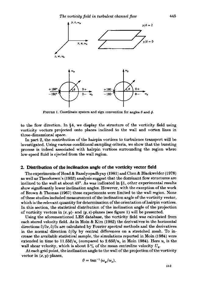
FIGURE 1. Coordinate system and sign convention for angles 0 and 4.

to the flow direction. In $4, we display the structure of the vorticity field using vorticity vectors projected onto planes inclined to the wall and vortex lines in three-dimensional space.

In part 2, the contribution of the hairpin vortices to turbulence transport will be investigated. Using various conditional sampling criteria, we show that the bursting process is indeed associated with hairpin vortices surrounding the region where low-speed fluid is ejected from the wall region.

2. Distribution of the inclination angle of the vorticity vector field The experiments of Head & Bandyopadhyay (1981) and Chen & Blackwelder (1978)

as well as Theodorsen's (1952) analysis suggest that the dominant flow structures are inclined to the wall a t about 45O. As was indicated in § 1, other experimental results show significantly lower inclination angles. However, with the exception of the work of Brown & Thomas (1967) these experiments were limited to the wall region. None of these studies included measurement of the inclination angle of the vorticity vector, which is the relevant quantity for determination of the orientation of hairpin vortices. In this section, the statistical distribution of the inclination angle of the projection of vorticity vectors in (2, y)- and (y, 2)-planes (see figure 1) will be presented.

Using the aforementioned LES database, the vorticity field was calculated from each stored velocity field. As in Moin & Kim (1982) the derivatives in the horizontal directions a/&, 3/32 are calculated by Fourier spectral methods and the derivatives in the normal direction a/ay by central differences on a stretched mesh. To increase the available statistical sample, the simulations reported in Moin (1 984) were extended in time to 11.536/u, (compared to 2.656/uT in Moin 1984). Here u, is the wall shear velocity, which is about 5 % of the mean centreline velocity U,,.

At each grid point, the inclination angle to the wall of the projection of the vorticity vector in (2, y)-planes,

8 = tan-l (ug/uz), 15-2


5 1.6

0 0.2

1.4 1.4

0.8 0.8

0.2 0.2

1.4 1.4

-180 -90 0 90 180 -180 -90 0 90 180 e e

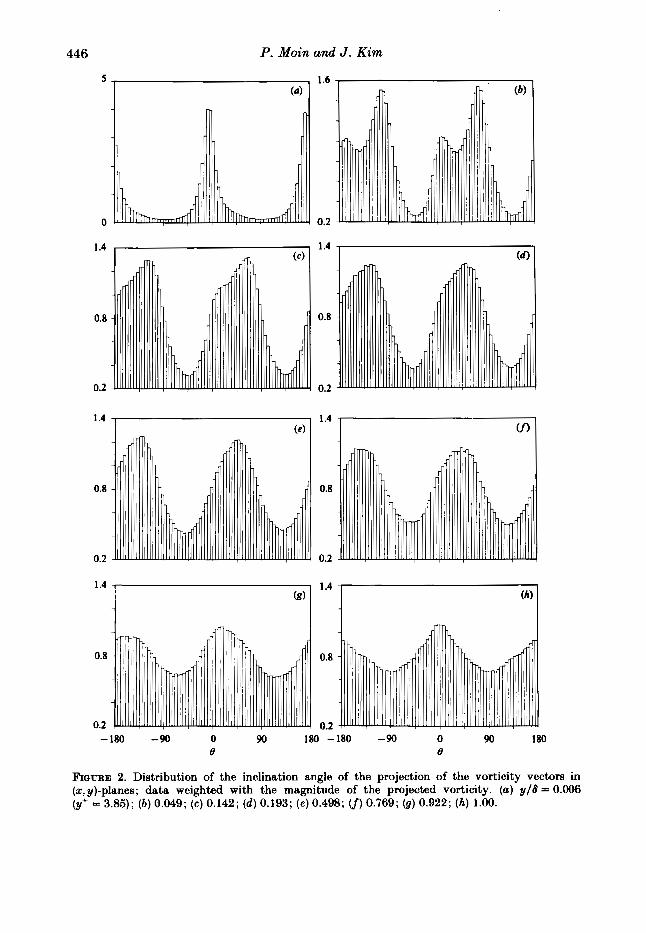
FIGURE 2. Distribution of the inclination angle of the projection of the vorticity vectors in (z,y)-planes; data weighted with the magnitude of the projected vorticity. (a) y/S = 0.006 (y+ = 3.85); ( b ) 0.049; (c) 0.142; (d) 0.193; (e) 0.498; (f) 0.769; (8) 0.922; (h) 1.00.

The vorticity field in turbulent channel $ow 447

0.8

0.2 -180 -90 0 90 180

e

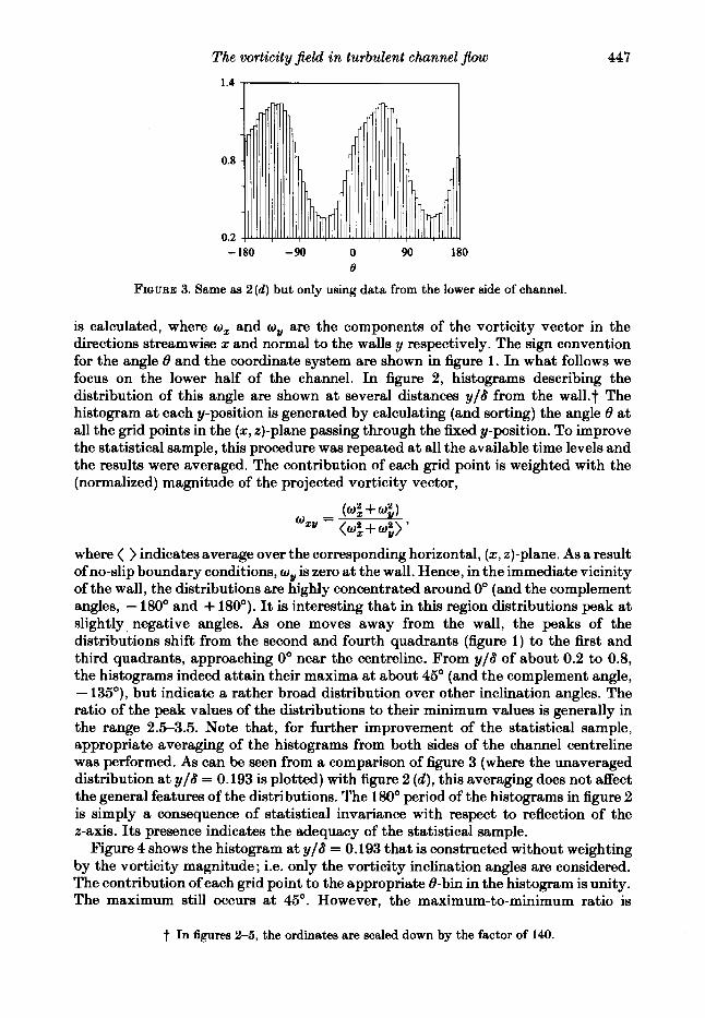
FIQURE 3. Same aa 2 ( d ) but only using data from the lower side of channel.

is calculated, where w, and coy are the components of the vorticity vector in the directions streamwise x and normal to the walls y respectively. The sign convention for the angle 0 and the coordinate system are shown in figure 1. In what follows we focus on the lower half of the channel. In figure 2, histograms describing the distribution of this angle are shown at several distances y/S from the wall.? The histogram at each y-position is generated by calculating (and sorting) the angle 8 at all the grid points in the (2, 2)-plane passing through the fixed y-position. To improve the statistical sample, this procedure was repeated at all the available time levels and the results were averaged. The contribution of each grid point is weighted with the (normalized) magnitude of the projected vorticity vector,

where ( ) indicates average over the corresponding horizontal, (z, 2)-plane. As a result of no-slip boundary conditions, wy is zero at the wall. Hence, in the immediate vicinity of the wall, the distributions are highly concentrated around 0" (and the complement angles, - 180" and + 180"). It is interesting that in this region distributions peak at slightly, negative angles. As one moves away from the wall, the peaks of the distributions shift from the second and fourth quadrants (figure 1) to the first and third quadrants, approaching 0" near the centreline. From y/S of about 0.2 to 0.8, the histograms indeed attain their maxima at about 45" (and the complement angle, - 135"), but indicate a rather broad distribution over other inclination angles. The ratio of the peak values of the distributions to their minimum values is generally in the range 2.5-3.5. Note that, for further improvement of the statistical sample, appropriate averaging of the histograms from both sides of the channel centreline was performed. As can be seen from a comparison of figure 3 (where the unaveraged distribution at y/S = 0.193 is plotted) with figure 2 (d), this averaging does not affect the general features of the distributions. The 180" period of the histograms in figure 2 is simply a consequence of statistical invariance with respect to reflection of the z-axis. Its presence indicates the adequacy of the statistical sample.

Figure 4 shows the histogram at y/6 = 0.193 that is constructed without weighting by the vorticity magnitude; i.e. only the vorticity inclination angles are considered. The contribution of each grid point to the appropriate &bin in the histogram is unity. The maximum still occurs at 45". However, the maximum-to-minimum ratio is

t In figures 2-5, the ordinates are scaled down by the factor of 140.

448 P . Moin and J . Kim

1.4 ~

-180 -90 0 90 180

e

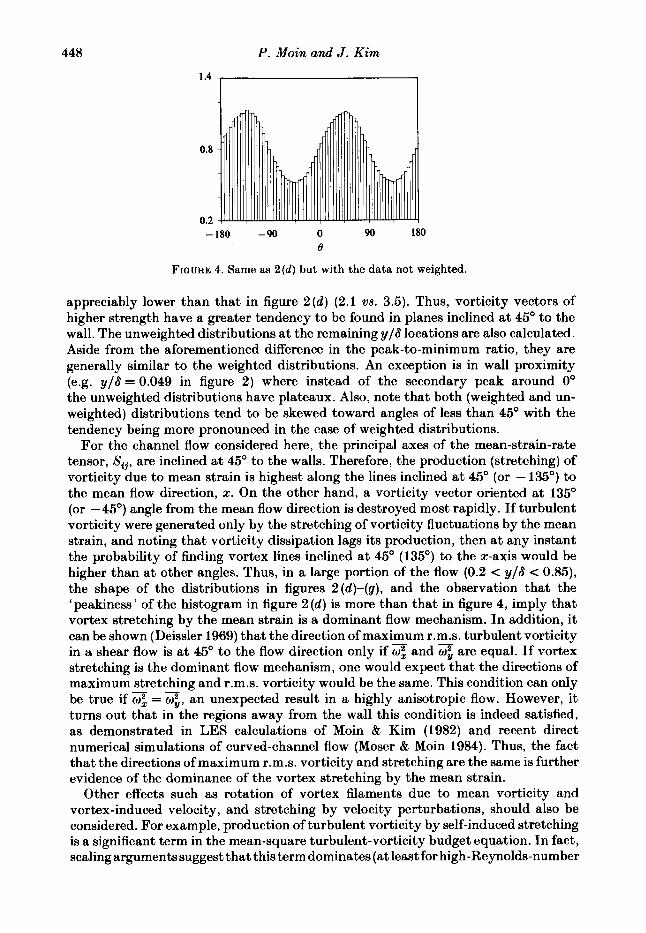
FIQURE 4. Same as 2 ( d ) but with the data not weighted.

appreciably lower than that in figure 2(d) (2.1 vs. 3.5). Thus, vorticity vectors of higher strength have a greater tendency to be found in planes inclined at 45' to the wall. The unweighted distributions at the remaining y/S locations are also calculated. Aside from the aforementioned difference in the peak-to-minimum ratio, they are generally similar to the weighted distributions. An exception is in wall proximity (e.g. y/S = 0.049 in figure 2) where instead of the secondary peak around 0' the unweighted distributions have plateaux. Also, note that both (weighted and unweighted) distributions tend to be skewed toward angles of less than 45' with the tendency being more pronounced in the case of weighted distributions.

For the channel flow considered here, the principal axes of the mean-strain-rate tensor, S,,, are inclined at 45" to the walls. Therefore, the production (stretching) of vorticity due to mean strain is highest along the lines inclined at 45" (or - 135') to the mean flow direction, x. On the other hand, a vorticity vector oriented at 135O (or -45") angle from the mean flow direction is destroyed most rapidly. If turbulent vorticity were generated only by the stretching of vorticity fluctuations by the mean strain, and noting that vorticity dissipation lags its production, then at any instant the probability of finding vortex lines inclined a t 45' (135') to the x-axis would be higher than at other angles. Thus, in a large portion of the flow (0.2 < y/6 < 0.85), the shape of the distributions in figures 2(d)-(g), and the observation that the ' peakiness' of the histogram in figure 2 (d) is more than that in figure 4, imply that vortex stretching by the mean strain is a dominant flow mechanism. In addition, it can be shown (Deissler 1969) that the direction of maximum r.m.8. turbulent vorticity in a shear flow is at 45' to the flow direction only if 3 and are equal. If vortex stretching is the dominant flow mechanism, one would expect that the directions of maximum stretching and r.m.s. vorticity would be the same. This condition can only be true if = q, an unexpected result in a highly anisotropic flow. However, it turns out that in the regions away from the wall this condition is indeed satisfied, as demonstrated in LES calculations of Moin & Kim (1982) and recent direct numerical simulations of curved-channel flow (Moser & Moin 1984). Thus, the fact that the directions of maximum r.m.s. vorticity and stretching are the same is further evidence of the dominance of the vortex stretching by the mean strain.

Other effects such as rotation of vortex filaments due to mean vorticity and vortex-induced velocity, and stretching by velocity perturbations, should also be considered. For example, production of turbulent vorticity by self-induced Stretching is a significant term in the mean-square turbulent-vorticity budget equation. In fact, scaling arguments suggest that this term dominates (at least for high-Reynolds-number


2.5 1.6

0.8

0

1.6 1.6

0.8 0.8

a 0

-180 -90 0 90 180 -180 -90 0 90 180 4 4

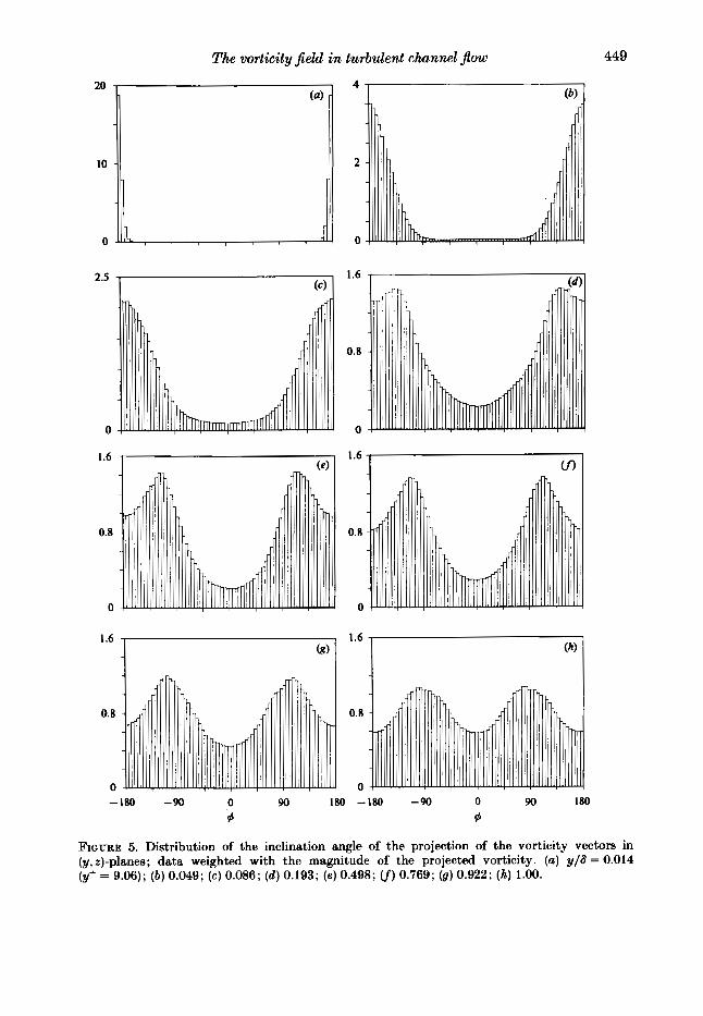
FIQURE 5. Distribution of the inclination angle of the projection of the vorticity vectors in (y, %)-planes; data weighted with the magnitude of the projected vorticity. (a) y/8 = 0.014 (y+ = 9.06); ( b ) 0.049; (c) 0.086; ( d ) 0.193; (e) 0.498; cf) 0.769; (9) 0.922; (h) 1.00.


flows) stretching due to mean motion (Tennekes & Lumley 1972). One physical explanation for the dominance of the mean-stretching term may be the special characteristics of the flow structure. For example, in a flow consisting essentially of hairpin vortices, there is little self-induced stretching (except near the tips), and the stretching due to mean motion is dominant. Note that the legs of the hairpins comprise most of the volume occupied by them.

The inclination angles to the z-axis of the projection of vorticity vectors in (y, z)-planes, q5 = tan-' ( w g / w z ) ,

were also calculated. Note that w, includes the mean vorticity. The sign convention for the angle q5 is also indicated in figure 1. The weighted distribution of q5 is shown in figure 5. These distributions are calculated in the same manner as those for angle 8 shown in figure 2. In the vicinity of the wall, because of no-slip boundary conditions and strong mean spanwise vorticity, the distributions are narrow and peak at 180' (or - 180'). From the wall to about y/S = 0.1 the distributions become broader with their peak still at 180' and maximum-to-minimum ratio of about 8. Beyond y/S = 0.1, the maxima consistently occur at about 110" to 120" (or - 110' to - 120'). However, the concentration of vorticity vectors pointing in the spanwise direction (the direction of the mean-vortex lines) remains appreciable even a t large distances from the walls. The symmetry of the distributions about q5 = 0 is a consequence of the statistical invariance of the flow with respect to reflection in the z-direction.

The above study clearly shows the preferential alignment of the vorticity vectors in planes inclined at 45' to the flow direction. In addition, there is a strong indication that vortex stretching by the mean strain is a dominant flow mechanism. However, the information about the structure of the flow that can be extracted from this study is limited. In particular, the connection between vorticity vectors and hairpin vortices cannot be established solely from the above histograms. For example, even though, in a large portion of the flow, the distributions attain their maxima at 45', one cannot conclude that this behaviour is due to the existence of a given large vortical structure with axis of circulation inclined a t 45' to the flow and extending through all the locations where the distributions peak at 45'. This issue leads us to the examination of two-point velocity and vorticity correlations.

3. Two-point correlations of velocity and vorticity There are two methods of using two-point correlation functions to extract

information on the spatial structure of the flow. One method, used by Townsend (1976), Grant (1.958), and others, is to examine two-point-correlation profiles for their consistency with a proposed model. This is the method used here. Another method, primarily due to Lumley (1967), is based on orthogonal decomposition of the two-point-correlation tensor, and is used to extract the deterministic structures contributing to all of the components of the correlation tensor. A two-dimensional variant of this method was recently applied to the LES database used in this work (Moin 1984).

If the flow truly contains a dominant structure, distributed stochastically in space, its presence should clearly be marked in two-point correlation functions. However, as will be illustrated below, the degree of clarity is highly dependent on the choice of the directions of ('probe') separation. Ibis much more instructive to obtain two- point correlation functions with directions of separation aligned with the primary axes of the proposed eddy than aligned with the Cartesian coordinate axes.

The vorticity field in turbulent channel $ow 45 1

1 .o 0.8

3 q3 0.6

2 0.4

a 0.2

0 %a

-0.2 3 1 .o 0.8

q3 0.6

q' 0.4

0.2

0

-0.2

3

0

I 0

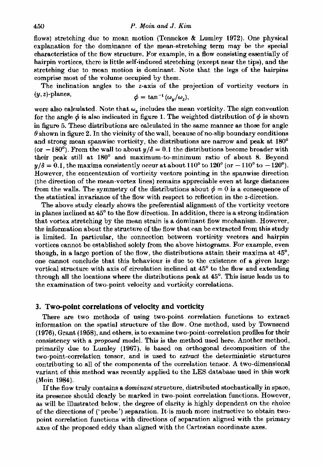
FIGURE 6. Two-point correlations of the velocity components with the direction of separation in

(y+ = 16.08); (6) 0.086; (c) 0.298; (d) 0.498; (e) 0.769; cf) 1.00. (x,y)-plane and inclined at 45' to the wall: -, Ruu; ----, R . ---, Rww. (a) y/6 = 0.025

In $2, i t was shown that in a large portion of the flow the vorticity exhibits a preferred inclination of about 45' to the flow direction. Correlations of the three components of velocity at two points along lines inclined at 45" and 135" (see figure 1) are shown in figures 6 and 7, respectively. Correlation between two quantities p, q at spatial points x and x' is defined as

P(X) q(x') R,,(x, x') = ___I- (P(x)2)' (a(xO2? *

Using the flow homogeneity in the x- and z-directions, R,, is only a function of (y, r), where y is the vertical location of the fixed point and r is the separation vector, x' -x. In the present work, r = r, is separation along a line in the (2, y)-plane inclined at 45" to the flow; r = rn, along a line inclined at 135'; r = ru, along the y-direction; and r = rz indicates separation in the spanwise z-direction. The striking difference between the correlations presented in figure 6 and 7 is in the behaviour of R,,, the correlation between spanwise velocity components separated along rs and rn. In figure 6, except when the fixed point is located in the vicinity of the wall (y' < 50), R,,(y, rg) does not become negative. The two-point correlation profiles show a

452 P. Moin and J . Kim 1 .o 0.8

2 0.6

es 0.4

0.2

0

-0.2

pi

1 .o 0.8

4' 0.6

q' 0.4

3

q: 0.2

0

- 0.2

1 .o 0.8

2 0.6

&. 0.4

= 0.2

0

-0.2

4

0 9 0

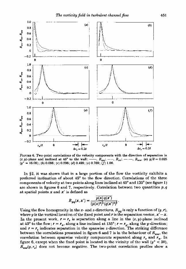
FIQURE 7. Two-point correlations of the velocity components with the direction of separation in (x, y)-plane and inclined at 1 3 5 O to the wall; -, Rul ; - - - - , Rvv; ---, Rww. See the caption of figure 6 for the y-location of the fixed point for each figure.

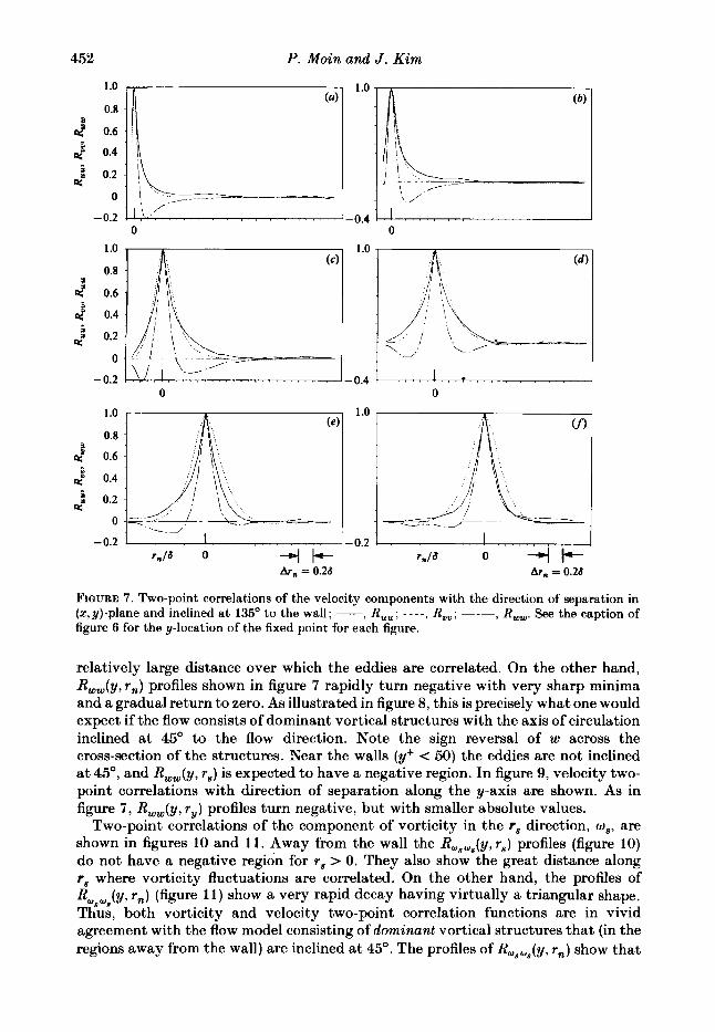
relatively large distance over which the eddies are correlated. On the other hand, R,,(y, r,) profiles shown in figure 7 rapidly turn negative with very sharp minima and a gradual return to zero. As illustrated in figure 8, this is precisely what one would expect if the flow consists of dominant vortical structures with the axis of circulation inclined at 45' to the flow direction. Note the sign reversal of w across the cross-section of the structures. Near the walls (y+ < 50) the eddies are not inclined at 45O, and R,,(y, r,) is expected to have a negative region. In figure 9, velocity two- point correlations with direction of separation along the y-axis are shown. As in figure 7 , R,,(y, r y ) profiles turn negative, but with smaller absolute values.

Two-point correlations of the component of vorticity in the r, direction, w,, are shown in figures 10 and 11. Away from the wall the RWgWg(y, r,) profiles (figure 10) do not have a negative region for r , > 0. They also show the great distance along r, where vorticity fluctuations are correlated. On the other hand, the profiles of R (y, rn) (figure 11) show a very rapid decay having virtually a triangular shape. Thus, both vorticity and velocity two-point correlation functions are in vivid agreement with the flow model consisting of dominant vortical structures that (in the regions away from the wall) are inclined a t 45O. The profiles of R,sos(y, r n ) show that

WE W 8

The vorticity field in turbulent channel flow

rn

/ /

w5; /

/

FIQURE 8. Sketch of the vortical structures inclined at 45' to the wall.

1 .o 0.8

0.6

0.4

0.2

0

-0.2

I .O

0.8

0.6

0.4

0.2

0

0 0

0 0

453

FIQV~E 9. Two-point correlations of the velocity components with the direction of separation in the y-direction (i.e. inclined at 90" to the wall): -, Ruu; ----, Rvv; ---, R-. See the caption of figure 6 for the y-location of the fixed point for each figure.


0.8 . 0.6 -

c 0.4 -

(4

ai

(b) mi -- I , -0.4

1 .o 0.8

0.6

0.4

0.2

0

0

-0.2 i 0

1 .o 0.8

0.6

0.4

0.2

0

-0.2 Y r,/a 0 4I t

Ar8 = 0.28

0

L 0

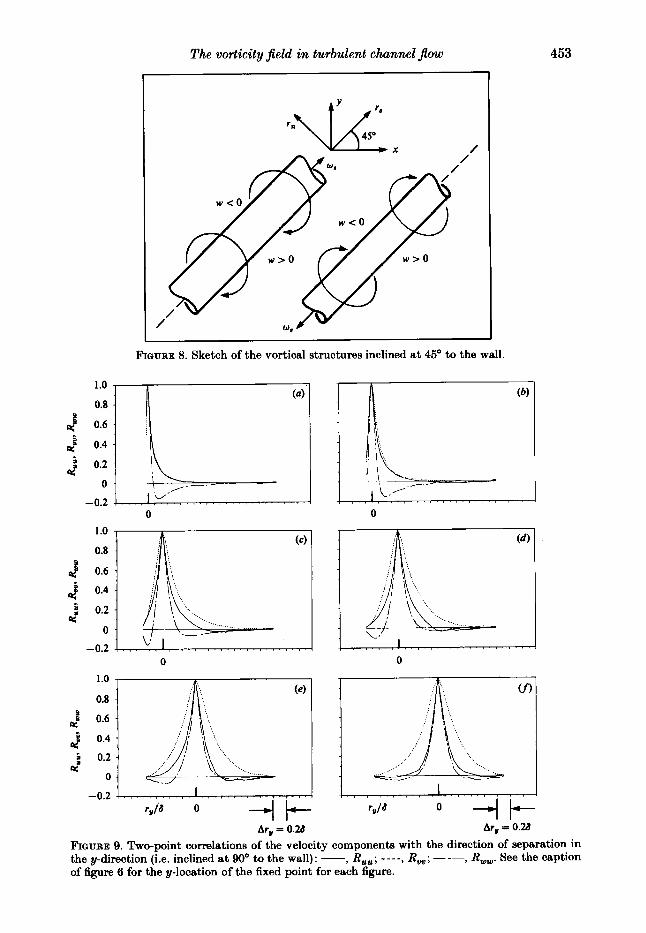
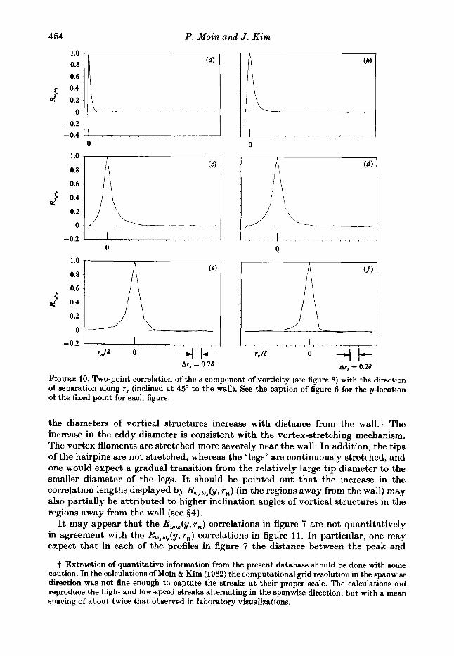
FIGURE 10. Two-point correlation of the s-component of vorticity (see figure 8) with the direction of separation along r8 (inclined at 45’ to the wall). See the caption of figure 6 for the y-location of the fixed point for each figure.

the diameters of vortical structures increase with distance from the wal1.t The increase in the eddy diameter is consistent with the vortex-stretching mechanism. The vortex filaments are stretched more severely near the wall. In addition, the tips of the hairpins are not stretched, whereas the ‘legs’ are continuously stretched, and one would expect a gradual transition from the relatively large tip diameter to the smaller diameter of the legs. It should be pointed out that the increase in the correlation lengths displayed by RmswS!y, r,) (in the regions away from the wall) may also partially be attributed to higher inclination angles of vortical structures in the regions away from the wall (see 54).

It may appear that the R,,(y, r,) correlations in figure 7 are not quantitatively in agreement with the RwnwS(y, r,) correlations in figure 11. In particular, one may expect that in each of the profiles in figure 7 the distance between the peak and

t Extraction of quantitative information from the present database should be done with some caution. In the calculations of Moin & Kim (1982) the computational grid resolution in the spanwise direction was not fine enough to capture the streaks at their proper scale. The calculations did reproduce the high- and low-speed streaks alternating in the spanwise direction, but with a mean spacing of about twice that observed in laboratory visualizations.

The vorticity jield in turbulent channel flow 455

1 .o 0.8

0.6

4 0.4

0.2

0

- 0.2

c

d

0

1 .o 0.8

0.6

0.4

0.2

0

-0.2 r 0

1 .o 0.8

0.6

0.4

0.2

0

-0.2 1 + I + r.18 0

Ar,, = 0.26

0

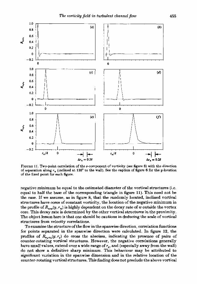
FIGURE 11. Two-point correlation of the s-component of vorticity (see figure 8) with the direction of separation along r , (inclined at 135" to the wall). See the caption of figure 6 for the y-location of the fixed point for each figure.

negative minimum be equal to the estimated diameter of the vortical structures (i.e. equal to half the base of the corresponding triangle in figure 11). This need not be the case. If we assume, as in figure 8, that the randomly located, inclined vortical structures have cores of constant vorticity, the location of the negative minimum in the profile of R,,(y, r,) is highly dependent on the decay rate of w outside the vortex core. This decay rate is determined by the other vortical structures in the proximity. The object lesson here is that one should be cautious in deducing the scale of vortical structures from velocity correlations.

To examine the structure of the flow in the spanwise direction, correlation functions for points separated in the spanwise direction were calculated. In figure 12, the profiles of Ru8u8(y,rz) do cross the abscissa, indicating the presence of pairs of counter-rotating vortical structures. However, the negative correlations generally have small values, extend over a wide range of rz, and (especially away from the wall) do not show a definitive sharp minimum. This behaviour may be attributed to significant vl;riation in the spanwise dimension and in the relative location of the counter-rotating vortical structures. This finding does not preclude the above vortical


1 .o 0.8

0.6

2 0.4

0.2

0

-0.2

1 .o 0 :8

0.6

d 0.4

0.2

0

-0.2

i

-0 .21 1 . , I I I I I 0 0.8 1.6

rZl8

0 0.8 1.6

rZl8

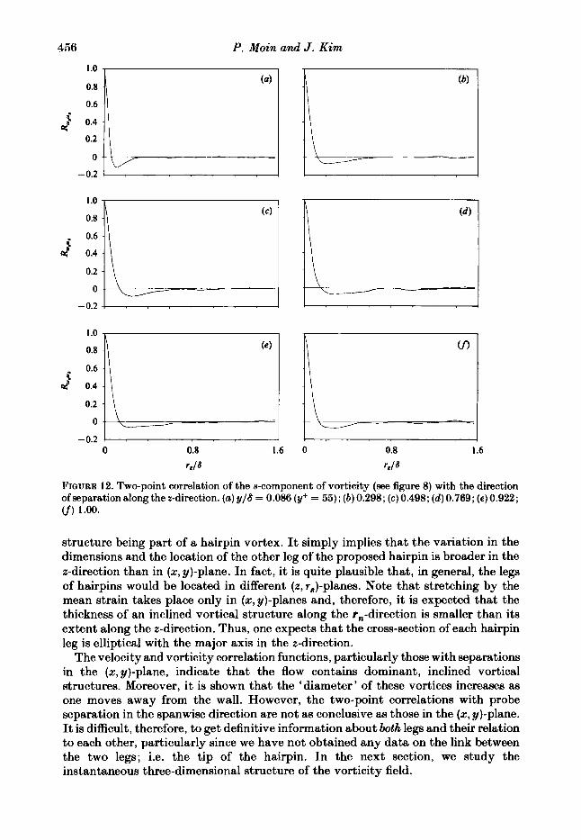
FIQURE 12. Two-point correlation of the 8-component of vorticity (see figure 8) with the direction of separation along the z-direction. (a )y /6 = 0.086 (y’ = 55); (b)0.298; (c)0.498; (d) 0.769; (e)0.922; (f) 1.00.

structure being part of a hairpin vortex. It simply implies that the variation in the dimensions and the location of the other leg of the proposed hairpin is broader in the z-direction than in (x, y)-plane. In fact, it is quite plausible that, in general, the legs of hairpins would be located in different (z, r,)-planes. Note that stretching by the mean strain takes place only in (5, y)-planes and, therefore, it is expected that the thickness of an inclined vortical structure along the r,-direction is smaller than its extent along the z-direction. Thus, one expects that the cross-section of each hairpin leg is elliptical with the major axis in the z-direction.

The velocity and vorticity correlation functions, particularly those with separations in the (x, y)-plane, indicate that the flow contains dominant, inclined vortical structures. Moreover, i t is shown that the ‘diameter’ of these vortices increases as one moves away from the wall. However, the two-point correlations with probe separation in the spanwise direction are not as conclusive as those in the (x, y)-plane. It is difficult, therefore, to get definitive information about both legs and their relation to each other, particularly since we have not obtained any data on the link between the two legs; i.e. the tip of the hairpin. In the next section, we study the instantaneous three-dimensional structure of the vorticity field.

The vorticity field in turbulent channel flow 457

4. Structure of the instantaneous vortidty field In this section, we examine the structure of the vorticity field at one instant in

time, selected randomly from the aforementioned database. Figure 13 shows the projection of vorticity vectors in three (2, r,)-planes (inclined

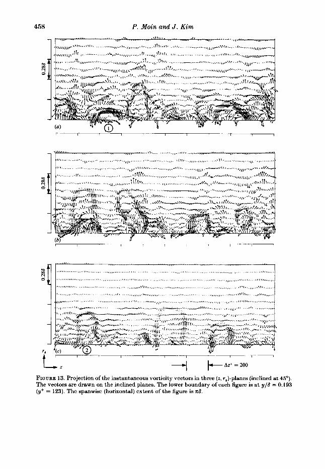
at 45'). The lower boundary of each plot is at y / S = 0.193 (y+ = 123), and its upper boundary is at the channel centreline. Recall that in figure 2 the distributions attained their maxima at 45' in the regions away from the wall (i.e. y / S 2 0.193). In figure 13, some of the structures resembling hairpin vortices are shaded. The structures are identified as those having two regions (legs) with opposite w, signs connected at the top by a region with w, = 0 and finite w,. These plots provide an indication of the population density of hairpins in the instantaneous flow fields. It appears that the flow contains an appreciable number of structures with this general form. However, each structure has its own distinct configuration and individual height extended above the wall. It should be pointed out that our view is limited to a two-dimensional plane, and we are identifying only those hairpins with legs in approximately the same (2, r,)-plane. Except for one or two exceptions, the hairpin- like structures appearing in these planes are such that the leg with positive w, is to the right of the one with negative w,. This finding is consistent with the notion that these vortices are formed as a result of deformation or roll-up of sheets of transverse vorticity with the resulting induced normal velocity away from the wall. The same feature can also be seen in plots of constant w, contours in 45' inclined planes (Moin 1984). The contours of w, in planes inclined at 135' generally show rounded features whereas elongated patterns can be seen in 45'-inclined planes (Moin 1984).

In conformation to its definition, a hairpin vortex is best displayed by vortex lines drawn in three-dimensional space. The location of a vortex line in space, x, is defined by

d x w ds 1 0 1 ' _ - --

where s is the distance along the vortex line. Starting from an initial location, x,, in the three-dimensional vorticity field, o(x), this equation can be integrated for x(s). For this purpose the second-order Runge-Kutta method was used for the numerical integration, and second-order Lagrange interpolation was used to compute the vorticity o(x) from the grid values. It turns out that the choice of x, is very important. Infinitely many vortex lines can be drawn in the flow. If we choose X, arbitrarily, the resulting vortex line is likely to wander over the whole flow field like a badly tangled fishing line, and it would be very difficult to identify the organized structures (if any) through which the line may have passed. This difficulty is partly due to the rapid variation of vorticity fluctuations in the domain, and the resulting sensitivity of x to small perturbations in o. If x, is within an organized vortical structure, then the coherence of the structure would have a self-correcting effect in realigning the vortex line in the direction of the circulation axis of the structure. In this case, the vortex line will probably be confined to the core of the structure for large values of s. In order to study the three-dimensional structure of the hairpin vortices, we use vorticity-vector plots such as those in figure 13 to guide the selection of x,. After selecting one of the shaded structures in figure 13, x, is chosen as a point in the shaded area (in the leg region). Starting from x,, (4.1) is integrated in both directions until the line intersects one of the side boundaries. This process results in a vortex line that starts from one side boundary, passes through x,, and ends in another side boundary.


I

f . .\I\\\\\. . . . . . . __. . . . ,

.._._..\I,. ___.

*s I I I 1 -- A t I

I

I,, k A r + =200

FIQURE 13. Projection of the instantaneous vorticity vectors in three (2, r,)-planes (inclined at 45'). The vectors are drawn on the inclined planes. The lower boundary of each figure is at y/8 = 0.193 (y' = 123). The spanwise (horizontal) extent of the figure is rr8.


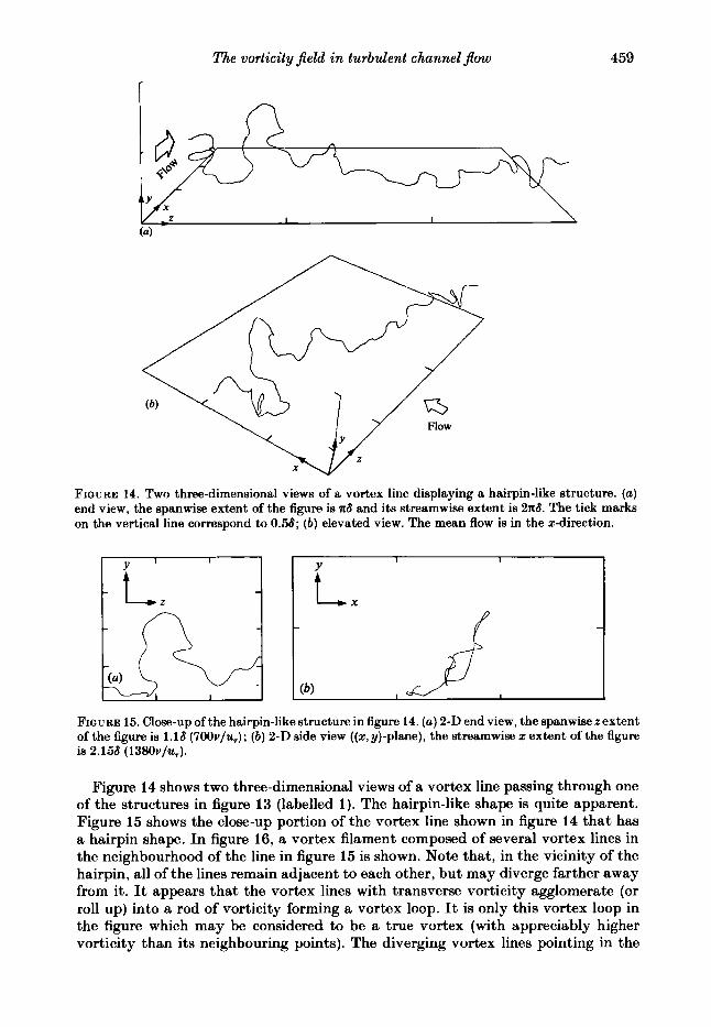
FIGURE 14. Two three-dimensional views of a vortex line displaying a hairpin-like structure. (a) end view, the spanwise extent of the figure is a6 and its streamwise extent is 2 ~ 6 . The tick marks on the vertical line correspond to 0.58; (a) elevated view. The mean flow is in the z-direction.

FIGURE 15. Close-up of the hairpin-like structure in figure 14. (a) 2-D end view, the spanwise 2 extent of the figure is 1.18 (700v/u7); (b) 2-D side view ((x, y)-plane), the streamwise x extent of the figure is 2.156 (1380v/u7).

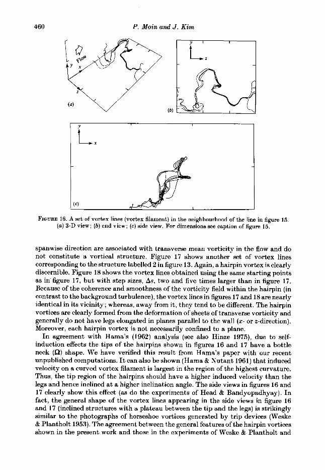
Figure 14 shows two three-dimensional views of a vortex line passing through one of the structures in figure 13 (labelled 1). The hairpin-like shape is quite apparent. Figure 15 shows the close-up portion of the vortex line shown in figure 14 that has a hairpin shape. In figure 16, a vortex filament composed of several vortex lines in the neighbourhood of the line in figure 15 is shown. Note that, in the vicinity of the hairpin, all of the lines remain adjacent to each other, but may diverge farther away from it. It appears that the vortex lines with transverse vorticity agglomerate (or roll up) into a rod of vorticity forming a vortex loop. It is only this vortex loop in the figure which may be considered to be a true vortex (with appreciably higher vorticity than its neighbouring points). The diverging vortex lines pointing in the


FIGURE 16. A set of vortex lines (vortex filament) in the neighbourhood of the line in figure 15. (a ) 3-D view; ( b ) end view; (c) side view. For dimensions see caption of figure 15.

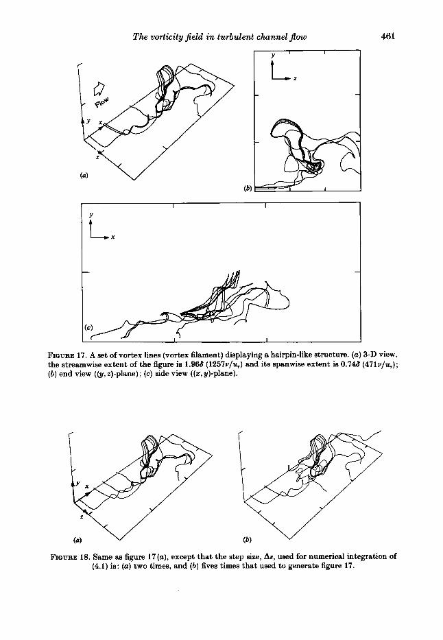
spanwise direction are associated with transverse mean vorticity in the flow and do not constitute a vortical structure. Figure 17 shows another set of vortex lines corresponding to the structure labelled 2 in figure 13. Again, a hairpin vortex is clearly discernible. Figure 18 shows the vortex lines obtained using the same starting points as in figure 17, but with step sizes, As, two and five times larger than in figure 17. Because of the coherence and smoothness of the vorticity field within the hairpin (in contrast to the background turbulence), the vortex lines in figures 17 and 18 are nearly identical in its vicinity; whereas, away from i t , they tend to be different. The hairpin vortices are clearly formed from the deformation of sheets of transverse vorticity and generally do not have legs elongated in planes parallel to the wall (x- or z-direction). Moreover, each hairpin vortex is not necessarily confined to a plane.

In agreement with Hama’s (1962) analysis (see also Hinze 1975), due to self- induction effects the tips of the hairpins shown in figures 16 and 17 have a bottle neck (Q) shape. We have verified this result from Hama’s paper with our recent unpublished computations. It can also be shown (Hama & Nutant 1961) that induced velocity on a curved vortex filament is largest in the region of the highest curvature. Thus, the tip region of the hairpins should have a higher induced velocity than the legs and hence inclined at a higher inclination angle. The side views in figures 16 and 17 clearly show this effect (as do the experiments of Head & Bandyopadhyay). In fact, the general shape of the vortex lines appearing in the side views in figure 16 and 17 (inclined structures with a plateau between the tip and the legs) is strikingly similar to the photographs of horseshoe vortices generated by trip devices (Weske & Plantholt 1953). The agreement between the general features of the hairpin vortices shown in the present work and those in the experiments of Weske & Plantholt and

The vorticity field in turbulent channel flow

(b)

46 1

FIGURE 17. A set of vortex lines (vortex filament) displaying a hairpin-like structure. (a) 3-D view, the streamwise extent of the figure is 1.968 (1257v/u1) and its spanwise extent is 0.748 (471v/u1); (b) end view ((y, %)-plane); (c) side view ((5,~)-plane).

FIGURE 18. Same as figure 17 (a), except that the step size, A8, used for numerical integration of (4.1) is: (a) two times, and (b) fives times that used to generate figure 17.

462 P. Moin and J . Kim studies of Hama provides evidence that the present computations have been faithful to the dynamics of the hairpins at least throughout part of their evolution. However, it should also be pointed out that, as each vortex loop is continuously stretched, its cross-section area decreases while its vorticity increases. Since the computational- grid resolution is not sufficiently fine for the effect of molecular viscosity to be significant at the grid scale, one cannot expect the calculations to represent explicitly the final stages in the evolution of the hairpins.

Finally, we point out an interesting result related to the fact that tips of the hairpins are bulged out. Hama's (1962) computations show that the rounded or R-shaped tip of the hairpins progressively becomes more pronounced and can be closely fitted by a circular arc resembling a ring vortex. This result provides a mechanism for the generation of ring vortices and hence establishes a consistency link between Falco's (1977) observations of ring vortices in the outer regions of turbulent boundary layers and the hairpin or loop vortices detected in the present study. Moreover, in a smoke-filled turbulent boundary layer, the pattern resulting from illumination of an (2, y)-plane that intersects the bulged-out portion of the tip of the hairpins is identical with that of the cross-section of a ring vortex.

5. Summary and conclusions In this study, using an LES data base, we searched for, identified, and analysed

hairpin vortices in turbulent channel flow. The study was conducted in three parts. It was shown that in a large portion of the flow the distribution of the inclination angleofvorticity vector attainsits maximum a t 45" (and - 135") to the wall. Two-point correlations of velocity and vorticity fluctuations were calculated. A novel feature of some of these correlation functions was that the direction of ('probe ') separation was inclined at 45' and 135" to the flow direction. The correlations provide definitive support for a flow model consisting of dominant vortical structures inclined a t 45" to the wall. The 'diameter' of these structures increases with distance from the walls.

Instantaneous vorticity vectors projected onto planes inclined at 45" to the flow direction indicate the presence of an appreciable number of hairpin vortices. These two-dimensional vector plots were also used to find starting points from which vortex lines in three-dimensional space were traced out. These vortex lines clearly display the three-dimensional structure of the hairpins. It is shown that the hairpins are formed from the deformation (or roll-up) of sheets of transverse vorticity, and are not necessarily confined to a two-dimensional plane. In constructing a mathematical model of turbulent boundary layers, one should consider the relative locations of the legs of the hairpin vortices as a random variable.

The previous studies cited in $1 provided evidence for the existence of hairpin vortices in turbulent boundary layers, whereas, in this investigation, they are found in turbulent channel flow. The two flows have significantly different outer-layer structures, but are very similar in the inner layer. This finding suggests that the hairpin vortices are the characteristic structures of all wall-bounded flows, irrespective of their outer boundary conditions.

We are indebted to Drs Robert Rogallo, Anthony Leonard and Robert Moser for helpful discussions during the course of this study.


R E F E R E N C E S

ACARLAR, M. S. & SMITH, C. R. 1984 Dept. Mech. Engng & Mech. Report Lehigh University, Bethlehem, PA.

BAKEWELL, H. P. & LUMLEY, J. L. 1967 Viscous sublayer and adjacent wall region in turbulent pipe flow. Plqs . Fluids 10, 1880.

BLACKWELDER, R. F. 1978 The bursting process in turbulent boundary layers. In Coherent Structure of Turbulent Boundary Layers (ed. C. R. Smith & D. E. Abbott), p. 211. AFOSR/Lehigh University Workshop, Dept Mech. Engng & Mech., Bethlehem, PA.

BLACKWELDER, R. F. & ECKELMANN, H. 1979 Streamwise vortices associated with the bursting phenomenon. J. Fluid Mech. 94,577.

BLACKWELDER, R. F. & KOVASZNAY, L. S. G. 1972 Time scales and correlations in a turbulent boundary layer. Phys. Fluids 15, 1545.

BROWN, G. L. & THOMAS, A. S. W. 1977 Large structure in a turbulent boundary layer. Phys. Fluids 20, S243.

CHEN, C. H. P. & BLACKWELDER, R. F. 1978 Large scale motion in a turbulent boundary layer: a study using temperature contamination. J. Fluid Mech. 89, 1.

CLARK, J. A. & MARKLAND, E. 1971 Flow visualization in turbulent boundary layers. J. Hydr. Div. ASCE 97, 1653.

COLES, D. 1978 A model for flow in the viscous sublayer. In Coherent Structure of Turbulent Boundary Layers (ed. C . R. Smith & D. E. Abbott), p. 462. AFOSR/Lehigh University Workshop, Dept Mech. Engng & Mech., Bethlehem, PA.

DEISSLER, R. G. 1969 Direction of maximum turbulent vorticity in a shear flow. Phys. Fluids 12, 426.

FALCO, R. E. 1977 Coherent motions in the outer region of turbulent boundary layers. Phys. Fluids 20, 5124.

FAVRE, A. J., GAVIGLIO, J. J. & DUMAS, R. 1957 Space-time double correlation and spectra in a turbulent boundary layer. J. Fluid Mech. 2 , 313.

GRANT, H. L. 1958 The large eddies of turbulent motion. J. Fluid Mech. 4, 149. HAMA, F. R. 1962 Progressive deformation of a curved vortex filament by its own induction. Phys.

Fluids 5 , 1156. HAMA, F. R. & NUTANT, J. 1961 Self-induced velocity on a curved vortex. Phys. Fluids

4, 28.

HEAD, M. R. & BANDYOPADHYAY, P. 1981 New aspects of turbulent boundary layer structure. J . Fluid Mech. 107, 297.

HINZE, J. 0. 1975 Turbulence, 2nd edn. McGraw-Hill. KIM, J. 1983 On the structure of wall-bounded turbulent flows. Phys. Fluids 26, 2088. KIM, J. & MOIN, P. 1979 Large eddy simulation of turbulent channel flow - ILLIAC IV calculation.

In Turbulent Boundary-layers - Experiments, Theory, and Modeling, The Hague, Netherlands. AGARD Conf. Proc. no. 271.

KLINE, S. J., REYNOLDS, W. C., SCHRAUB, F. A. & RUNSTADLER, P. W. 1967 The structure of turbulent boundary layers. J. Fluid Mech. 30, 741.

KOVASZNAY, L. S. G., KIBENS, V. & BLACKWELDER, R. F. 1970 Large-scale motion in the intermittent region of a turbulent boundary layer. J. Fluid Mech. 41,283.

KREPLIN, H. & ECKELMANN, H. 1979 Propagation of perturbations in the viscous sublayer and adjacent wall regions. J. Fluid Mech. 95, 305.

LEE, M. K., ECKELMAN, L. D. & HANRATTY, T. J. 1974 Identification of turbulent wall eddies through the phase relation of the components of the fluctuating velocity gradient. J. Fluid Mech. 66, 17.

LUMLEY, J. L. 1967 The structure of inhomogeneous turbulent flows. In Atvmspheric Turbulence and Radio Wave Propagation (ed. A. M. Yaglom & V. I. Tatarsky), pp. 166. NAUKA, Moscow.

MOIN, P. 1984 Probing turbulence via large eddy simulation. AIAA paper 84-0174. MOIN, P. & KIM, J. 1982 Numerical investigation of turbulent channel flow. J. Fluid Mech. 118,

341.

464 P. Moin and J . Kim MOSER, R. D. & MOIN, P. 1984 Direct numerical simulation of curved turbulent channel flow.

NASA TM 85974. Also, Report TF-20, Department of Mech. Engng, Stanford Univ., Stanford

OFFEN, G. R. & KLINE, S. J. 1973 Experiments on the velocity characteristic of ‘bursts’ and on the interaction between the inner and outer regions of the turbulent boundary layer. Stanford Univ. Mech. Engng Dept. Rep. MD-31.

PERRY, A. E. & CHONO, M. S. 1982 On the mechanism of wall turbulence. J. Fluid Mech. 119, 173.

SMITH, C. R. 1978 Visualization of turbulent boundary layer structure using a moving hydrogen bubble wire probe. In Coherent Structure of Turbulent Boundary Layers (ed. C. R. Smith & D. E. Abbott), p. 48. AFOSR/Lehigh University Workshop, Dept Mech. Engng & Mech., Bethlehem, PA.

SMITH, C. R. 1984 A synthesized model of the near-wall behavior in turbulent boundary layers. In Proc. of 8th Symp. on Turbulence (ed. G . K. Patterson & J. L. Zakin), Dept of Chem. Engng, University of Missouri-Rolla.

SMITH, C. R. & SCHWARTZ, S. P. 1983 Observation of streamwise rotation in the near-wall region of a turbulent boundary layer. Phys. Fluids 26, 641.

TENNEKES, H. & LUMLEY, J. L. 1972 A First Course in Turbulence. MIT Press. THEODORSEN, T. 1952 Mechanism of turbulence. In Proc. 2nd Midwestern Conf. on Fluid Mech.

TOWNSEND, A. A. 1970 Entrainment and the structure of turbulent flow. J. Fluid Mech. 41, 13. TOWNSEND, A. A. 1976 The structure of turbulent shearaow. Cambridge University Press. TRITTON, D. J. 1967 Some new correlation measurements in a turbulent boundary layer. J. Fluid

Mech. 28, 439. WALLACE, J. M. 1982 On the structure of bounded turbulent shear flow: a personal view. In

Developmenta in Theoretical and Applied Mechanics, XI (ed. T. J. Chung & G. R. Karr), p. 509. Dept of Mech. Engng, University of Alabama in Huntsville.

WESKE, J. R. & POLANTHOLT, A. H . 1953 Discrete vortex systems in the transition range in fully developed flow in a pipe. J. Aero. Sci. 20, 717.

WILLMARTH, W. W. & Lu, S. S. 1972 Structure of the Reynolds stress near the wall. J. Fluid Mech. 55, 65.

WILLMARTH, W. W. & Tu, B. J. 1967 Structure of turbulence in the boundary layer near the wall. Phys. Fluids 10, S134.

C d V .

Ohio State University, Columbus, Ohio.

The structure of the vorticity field in turbulent channel flow. II - Study of ensemble-averaged...

Documents

Transcript of The structure of the vorticity field in turbulent channel flow. II - Study of ensemble-averaged...