HYDROLOGICAL PROCESSESHydrol. Process. 20, 1525–1540 (2006)Published online 18 October 2005 in Wiley InterScience (www.interscience.wiley.com). DOI: 10.1002/hyp.5942

The strategy of building a flood forecast model byneuro-fuzzy network

Shen-Hsien Chen,1 Yong-Huang Lin,1 Li-Chiu Chang2 and Fi-John Chang3*1 Department of Construction Engineering, National Taiwan University of Science and Technology, Taipei, Taiwan, ROC

2 Department of Water Resources and Environmental Engineering, Tamkang University, Tamsui, Taiwan, ROC3 Department of Bioenvironmental Systems Engineering, National Taiwan University, Taipei, Taiwan, ROC

Abstract:

A methodology is proposed for constructing a flood forecast model using the adaptive neuro-fuzzy inference system(ANFIS). This is based on a self-organizing rule-base generator, a feedforward network, and fuzzy control arithmetic.Given the rainfall-runoff patterns, ANFIS could systematically and effectively construct flood forecast models. Theprecipitation and flow data sets of the Choshui River in central Taiwan are analysed to identify the useful inputvariables and then the forecasting model can be self-constructed through ANFIS. The analysis results suggest that thepersistent effect and upstream flow information are the key effects for modelling the flood forecast, and the watershed’saverage rainfall provides further information and enhances the accuracy of the model performance. For the purposeof comparison, the commonly used back-propagation neural network (BPNN) is also examined. The forecast resultsdemonstrate that ANFIS is superior to the BPNN, and ANFIS can effectively and reliably construct an accurate floodforecast model. Copyright 2005 John Wiley & Sons, Ltd.

KEY WORDS flood forecast; neuro-fuzzy; artificial neural network; BPNN; ANFIS

INTRODUCTION

Taiwan, with its tropical climate and high mountain watersheds all over the island, is susceptible to naturaldisasters such as floods and debris flows, which cause a great amount of damage. For this reason, buildinga forecast model to reduce flood damage is crucial. A key limitation of accurate streamflow forecastingis that the commonly used physical and/or statistical models still do not fully represent the complicatedhydrological process (Anderson and Burt, 1985). These models are generally affected by a wide range ofsensitive hydrographic and physiographic factors associated with the change of time and space. Consequently,such hydrological models are difficult to use and lack practicality in our case.

Artificial neural networks (ANNs) were created to simulate the nervous system and brain activity. In recentdecades, a number of neural networks, such as the Hopfield neural network (Hopfield, 1982), the back-propagation neural network (BPNN; Rumelhart et al., 1986), the recurrent neural network (Williams andZipser, 1989), and the fuzzy neural network (Nie and Linkens, 1994), have been developed to solve a widevariety of problems (Schalkoff, 1997), demonstrating their great ability of functional mapping between inputand output and generalization. One of the advantages of neural networks is their adaptive nature in dealingwith nonlinear problems, such as highly complicated hydrological systems, that are difficult to formulate andsolve (Chang and Hwang, 1999; Sajikumar and Thandaveswara, 1999; Chang et al., 2004; Huang et al., 2004).The ASCE Task Committee report (ASCE Task Committee on Application of Artificial Neural Networks inHydrology, 2000a,b) carried out a comprehensive review of the application of ANNs to hydrology, as didMaier and Dandy (2000).

* Correspondence to: Fi-John Chang, Department of Bioenvironmental Systems Engineering, National Taiwan University, Taipei, Taiwan,ROC. E-mail: changfj@ntu.edu.tw

Received 20 November 2003Copyright 2005 John Wiley & Sons, Ltd. Accepted 9 February 2005

1526 S.-H. CHEN ET AL.

In this study, we present a novel neuro-fuzzy approach, i.e. the adaptive neuro-fuzzy inference system(ANFIS), for flood forecasting. The motivation lies primarily in evaluating the feasibility of applying a hybridscheme to the problem, thereby providing an alternative to fuzzy and neural approaches. It is assumed thatthe streamflow series can be estimated by using a set of if–then rules that relate future streamflows based onantecedent streamflows. The rules are extracted from the historical data sets (input–output patterns) througha self-organizing fuzzy clustering method. The predicted values into the future are inferred from those ruleswith a fuzzy reasoning model. To verify its applicability and suitability, the longest river in Taiwan, theChoshui River, was chosen as the study area, and the BPNN was also used for comparison. In the following,the methodology of constructing the ANFIS and BPNN models for streamflow forecasting is presented. Thetheorem, network structure, and parameter estimating algorithms are described first. Next, a presentation of thestudy watershed and available data is given. The data sets are analysed to identify the useful input variablesand then the flood forecast models are constructed through ANFIS.

METHODOLOGY

This study proposes a methodology for constructing a flood forecast model using ANFIS. For the purposeof comparison, the commonly used BPNN is also examined. ANFIS is based on a fuzzy inference systemwith the supervised learning scheme of a multilayer feedforward network. Through some self-organizingfuzzy clustering method, such as the subtractive clustering method, fuzzy if–then rules can be extracted fromnumerical data to provide the fuzzy reasoning processes of the ANFIS. These algorithms are described first,and then we briefly describe the architectures and learning algorithms of the popular BPNN model.

The ANFIS

Intelligent computation methods, i.e. ANNs and fuzzy inference, are state-of-the-art technology thatresembles the human thinking process in decision making and strategy learning; they are well recognizedfor their outstanding ability in modelling complex systems. Recently, there has been a growing interestin integrating the ANN and fuzzy inference; as a result, neuro-fuzzy networks have been developed. Aneuro-fuzzy network combines the semantic transparency of fuzzy if–then rules with the learning capabilityof neural networks. This flexible framework is widely recognized, because it not only provides a tool foraccurate nonlinear modelling, but also is able to learn from the environment (input–output pairs), self-organize its structure, and adapt to it in an interactive manner. For this reason, we propose the use of theANFIS methodology (Jang, 1993) to self-organize the network structure and to adapt parameters of the fuzzysystem for flood forecasting.

Architecture and algorithm. The ANFIS is a multilayer feedforward network that uses neural networklearning algorithms and fuzzy reasoning to map an input space to an output space. With the ability to combinethe verbal power of a fuzzy system with the numeric power of a neural system adaptive network, ANFIS hasbeen shown to be powerful in modelling numerous processes, e.g. motor fault detection and diagnosis (Altuget al., 1999), power systems dynamic load (Djukanovic et al., 1997; Oonsivilai and El-Hawary, 1999), andreal-time reservoir operation (Chang and Chang, 2001; Chang et al., 2005).

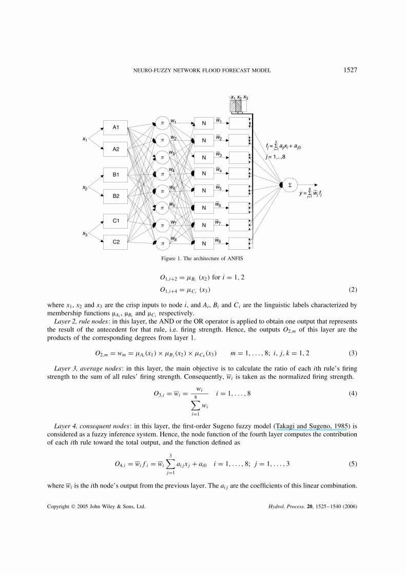
For simplicity, we assume the fuzzy inference system under consideration has three inputs (x1, x2 and x3) andone output (y). The architecture of ANFIS consists of five layers (Figure 1), and the functions correspondingto nodes of the same layer are similar. Each input has two rules (A1 and A2, B1 and B2, C1 and C2) in thefirst layer (input nodes), which can generate eight rules in the second layer (rule nodes). A brief sketch of theoperations of the five layers is given in the following.

Layer 1, input nodes: each node of this layer generates membership grades to which they belong to eachof the appropriate fuzzy sets using membership functions.

O1,i D �Ai �x1� �1�

Copyright 2005 John Wiley & Sons, Ltd. Hydrol. Process. 20, 1525–1540 (2006)

NEURO-FUZZY NETWORK FLOOD FORECAST MODEL 1527

A2

B1

C1

B2

N

N

N

N

A1

C2

N

N

N

N

x1 x2 x3

x1

x2

x3

w1

w8

w7

w6

w5

w4

w3

w2

w7

w6

w5

w4

w3

w2

w1

w8

p

p

p

p

p

p

p

p

j = 1,..,8

Σ

fj = Σ ajixi + aj03

i=1

y = Σ wj fj 8

j=1

Figure 1. The architecture of ANFIS

O1,iC2 D �Bi �x2� for i D 1, 2

O1,iC4 D �Ci �x3� �2�

where x1, x2 and x3 are the crisp inputs to node i, and Ai, Bi and Ci are the linguistic labels characterized bymembership functions µAi , µBi and µCi respectively.

Layer 2, rule nodes: in this layer, the AND or the OR operator is applied to obtain one output that representsthe result of the antecedent for that rule, i.e. firing strength. Hence, the outputs O2,m of this layer are theproducts of the corresponding degrees from layer 1.

O2,m D wm D �Ai�x1� ð �Bj�x2� ð �Ck �x3� m D 1, . . . , 8; i, j, k D 1, 2 �3�

Layer 3, average nodes: in this layer, the main objective is to calculate the ratio of each ith rule’s firingstrength to the sum of all rules’ firing strength. Consequently, wi is taken as the normalized firing strength.

O3,i D wi D wi

8∑

iD1

wi

i D 1, . . . , 8 �4�

Layer 4, consequent nodes: in this layer, the first-order Sugeno fuzzy model (Takagi and Sugeno, 1985) isconsidered as a fuzzy inference system. Hence, the node function of the fourth layer computes the contributionof each ith rule toward the total output, and the function defined as

O4,i D wifi D wi

3∑

jD1

aijxj C ai0 i D 1, . . . , 8; j D 1, . . . , 3 �5�

where wi is the ith node’s output from the previous layer. The aij are the coefficients of this linear combination.

Copyright 2005 John Wiley & Sons, Ltd. Hydrol. Process. 20, 1525–1540 (2006)

1528 S.-H. CHEN ET AL.

Layer 5: output nodes: the single node computes the overall output by summing all the incoming signals.Accordingly, the defuzzification process transforms each rule’s fuzzy results into a crisp output in this layer.

O5,1 D8∑

iD1

wifi D

8∑

iD1

wifi

8∑

iD1

wi

�6�

This network training is based on supervised learning. Our goal is thus to train adaptive networks to beable to approximate unknown functions given by training data and then find the precise value of the aboveparameters.

The distinguishing characteristic of the approach is that ANFIS applies a hybrid-learning algorithm, thegradient descent method and the least-squares method, to update parameters. The gradient descent methodis employed to tune premise nonlinear parameters, whereas the least-squares method is used to identifyconsequent linear parameters.

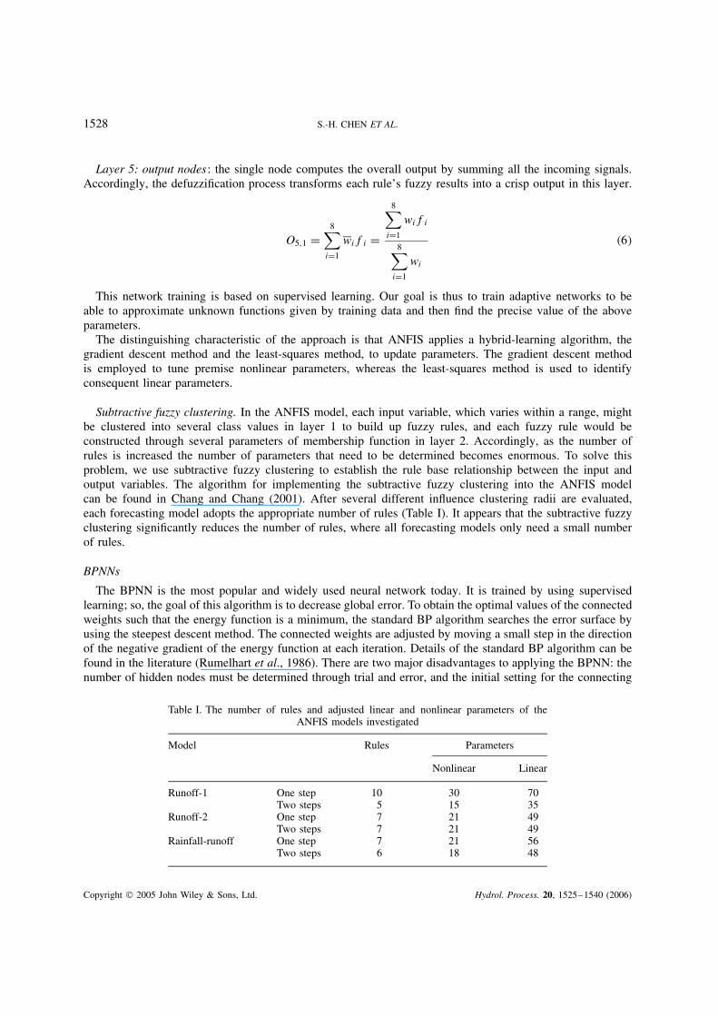
Subtractive fuzzy clustering. In the ANFIS model, each input variable, which varies within a range, mightbe clustered into several class values in layer 1 to build up fuzzy rules, and each fuzzy rule would beconstructed through several parameters of membership function in layer 2. Accordingly, as the number ofrules is increased the number of parameters that need to be determined becomes enormous. To solve thisproblem, we use subtractive fuzzy clustering to establish the rule base relationship between the input andoutput variables. The algorithm for implementing the subtractive fuzzy clustering into the ANFIS modelcan be found in Chang and Chang (2001). After several different influence clustering radii are evaluated,each forecasting model adopts the appropriate number of rules (Table I). It appears that the subtractive fuzzyclustering significantly reduces the number of rules, where all forecasting models only need a small numberof rules.

BPNNs

The BPNN is the most popular and widely used neural network today. It is trained by using supervisedlearning; so, the goal of this algorithm is to decrease global error. To obtain the optimal values of the connectedweights such that the energy function is a minimum, the standard BP algorithm searches the error surface byusing the steepest descent method. The connected weights are adjusted by moving a small step in the directionof the negative gradient of the energy function at each iteration. Details of the standard BP algorithm can befound in the literature (Rumelhart et al., 1986). There are two major disadvantages to applying the BPNN: thenumber of hidden nodes must be determined through trial and error, and the initial setting for the connecting

Table I. The number of rules and adjusted linear and nonlinear parameters of theANFIS models investigated

Model Rules Parameters

Nonlinear Linear

Runoff-1 One step 10 30 70Two steps 5 15 35

Runoff-2 One step 7 21 49Two steps 7 21 49

Rainfall-runoff One step 7 21 56Two steps 6 18 48

Copyright 2005 John Wiley & Sons, Ltd. Hydrol. Process. 20, 1525–1540 (2006)

NEURO-FUZZY NETWORK FLOOD FORECAST MODEL 1529

weights could influence the network performance significantly. To overcome these problems, we investigatedthe BPNN through a different number of hidden nodes, and for each case the model was performed with agreat number of initial settings of the connecting weights.

STUDY WATERSHED AND MODELLING

To illustrate the practical application of the forecasting models, the Choshui River is used as a case study. TheChoshui River is the longest river in Taiwan and is renowned for its dark and muddy water. The river originatesfrom the highest peak of Mt Hohuan and east peak of Mt Hohuan at about 3220 m altitude. The river winds186Ð6 km, and the watershed, which extends from the mountains (elevation 3220m) to sea level, drains anarea of 3157 km2. Within this area, the average slope is 5Ð3%. The catchment receives an average of 2459 mmof rainfall each year; however, the rainfall is uneven. Typhoons, accompanied by torrential rainfall, whichusually occur in the summer, are mainly responsible for the floods. Consequently, flood forecasting becomesone of the most important tasks of hydrologists. The administration regions, where the stream passes, includefour counties. There is a population of about 0Ð6 million living in this area. The abundant water resourcesand particular geographic characteristics of the Choshui River nurture a diversified socioeconomic culture.

The available data

There are two water-level gauging stations and 10 rain-gauging stations in this river basin, which wererecently equipped with automatic recorders and wireless transmitters (Figure 2 and Table II). Consequently,real-time flow forecasting becomes a reality. There were 23 typhoon (or heavy rainfall) events recorded inthe period 1992 to 2002, as published by the Water Resources Agency (WRA), Taiwan. The hourly rainfalland water levels of the gauging stations are used. A total of 1998 data sets are obtained.

The data for the 23 events were divided into three independent subsets: the training, validating, and testingsubsets. The training subset includes 1554 sets of data, the validating subset has 222 sets, and the testing subset

Shigau

Ziuchian Bridge

Chunyun BridgeTanta

Hersher

Alishan

Chingyun

Shinyi

HsiaolinWanshian

Tuntou

Tsuetfen

Figure 2. Location of gauging stations (�: water level; ž: rain stations) in the Choshui River, Taiwan

Copyright 2005 John Wiley & Sons, Ltd. Hydrol. Process. 20, 1525–1540 (2006)

1530 S.-H. CHEN ET AL.

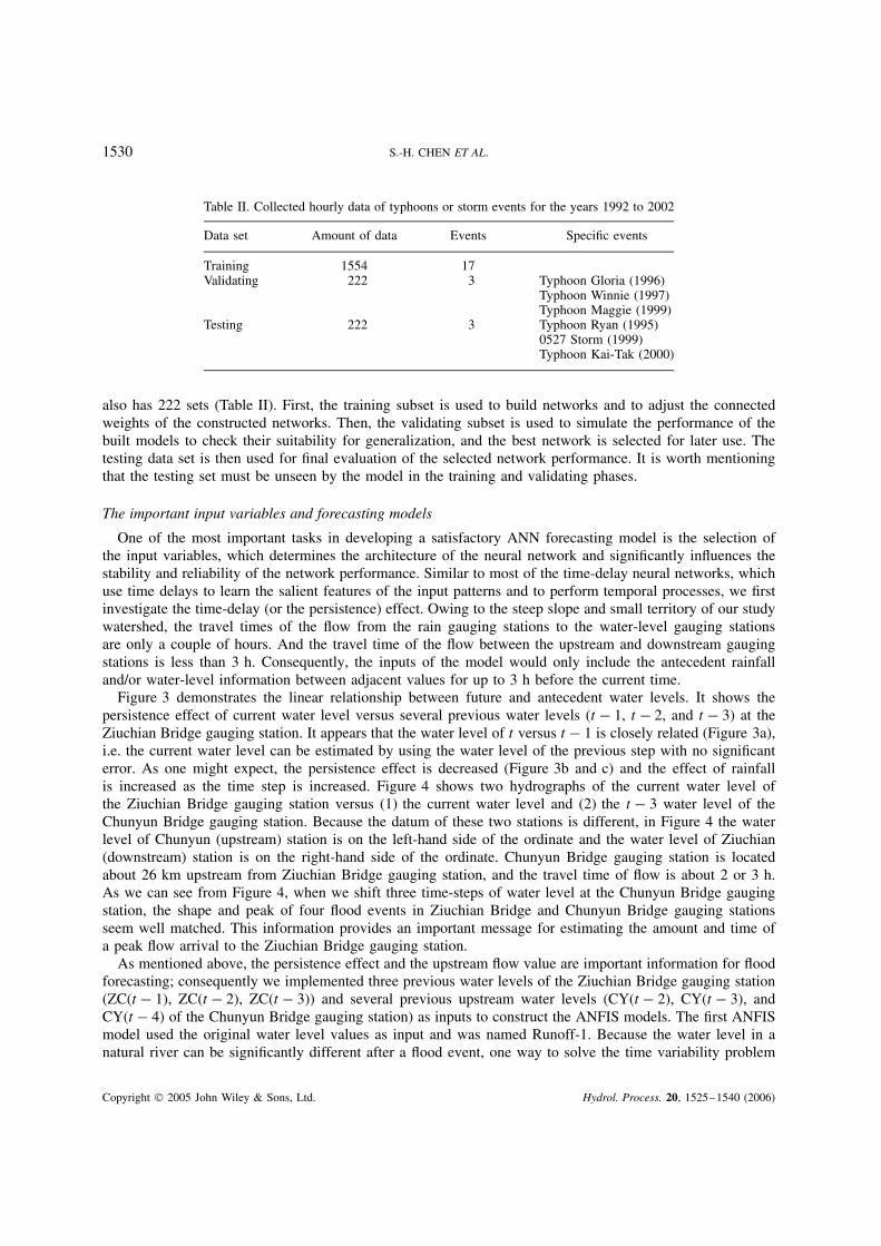
Table II. Collected hourly data of typhoons or storm events for the years 1992 to 2002

Data set Amount of data Events Specific events

Training 1554 17Validating 222 3 Typhoon Gloria (1996)

Typhoon Winnie (1997)Typhoon Maggie (1999)

Testing 222 3 Typhoon Ryan (1995)0527 Storm (1999)Typhoon Kai-Tak (2000)

also has 222 sets (Table II). First, the training subset is used to build networks and to adjust the connectedweights of the constructed networks. Then, the validating subset is used to simulate the performance of thebuilt models to check their suitability for generalization, and the best network is selected for later use. Thetesting data set is then used for final evaluation of the selected network performance. It is worth mentioningthat the testing set must be unseen by the model in the training and validating phases.

The important input variables and forecasting models

One of the most important tasks in developing a satisfactory ANN forecasting model is the selection ofthe input variables, which determines the architecture of the neural network and significantly influences thestability and reliability of the network performance. Similar to most of the time-delay neural networks, whichuse time delays to learn the salient features of the input patterns and to perform temporal processes, we firstinvestigate the time-delay (or the persistence) effect. Owing to the steep slope and small territory of our studywatershed, the travel times of the flow from the rain gauging stations to the water-level gauging stationsare only a couple of hours. And the travel time of the flow between the upstream and downstream gaugingstations is less than 3 h. Consequently, the inputs of the model would only include the antecedent rainfalland/or water-level information between adjacent values for up to 3 h before the current time.

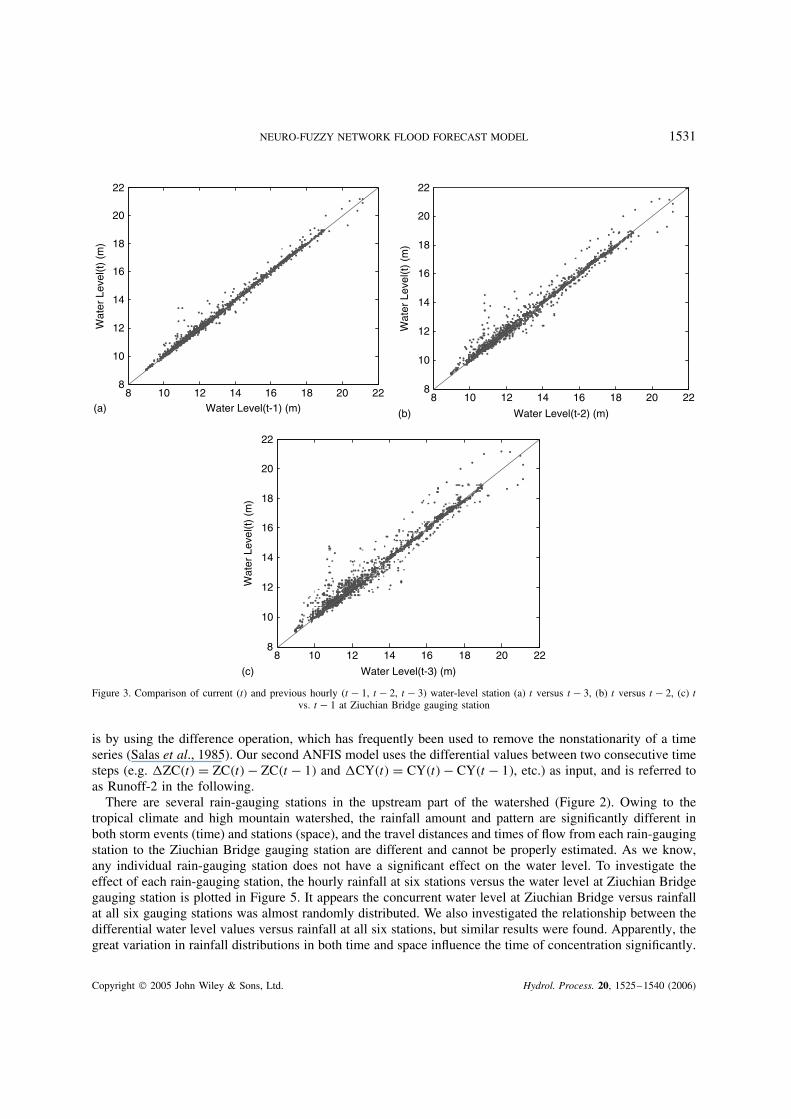
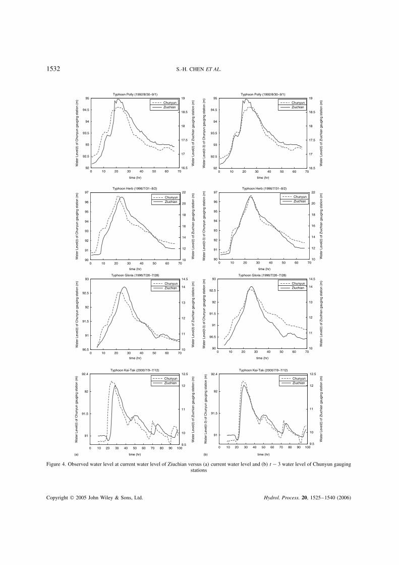
Figure 3 demonstrates the linear relationship between future and antecedent water levels. It shows thepersistence effect of current water level versus several previous water levels (t � 1, t � 2, and t � 3) at theZiuchian Bridge gauging station. It appears that the water level of t versus t � 1 is closely related (Figure 3a),i.e. the current water level can be estimated by using the water level of the previous step with no significanterror. As one might expect, the persistence effect is decreased (Figure 3b and c) and the effect of rainfallis increased as the time step is increased. Figure 4 shows two hydrographs of the current water level ofthe Ziuchian Bridge gauging station versus (1) the current water level and (2) the t � 3 water level of theChunyun Bridge gauging station. Because the datum of these two stations is different, in Figure 4 the waterlevel of Chunyun (upstream) station is on the left-hand side of the ordinate and the water level of Ziuchian(downstream) station is on the right-hand side of the ordinate. Chunyun Bridge gauging station is locatedabout 26 km upstream from Ziuchian Bridge gauging station, and the travel time of flow is about 2 or 3 h.As we can see from Figure 4, when we shift three time-steps of water level at the Chunyun Bridge gaugingstation, the shape and peak of four flood events in Ziuchian Bridge and Chunyun Bridge gauging stationsseem well matched. This information provides an important message for estimating the amount and time ofa peak flow arrival to the Ziuchian Bridge gauging station.

As mentioned above, the persistence effect and the upstream flow value are important information for floodforecasting; consequently we implemented three previous water levels of the Ziuchian Bridge gauging station(ZC(t � 1), ZC(t � 2), ZC(t � 3)) and several previous upstream water levels (CY(t � 2), CY(t � 3), andCY(t � 4) of the Chunyun Bridge gauging station) as inputs to construct the ANFIS models. The first ANFISmodel used the original water level values as input and was named Runoff-1. Because the water level in anatural river can be significantly different after a flood event, one way to solve the time variability problem

Copyright 2005 John Wiley & Sons, Ltd. Hydrol. Process. 20, 1525–1540 (2006)

NEURO-FUZZY NETWORK FLOOD FORECAST MODEL 1531

8 10 12 14 16 18 20 228

10

12

14

16

18

20

22

Water Level(t-3) (m)

Wat

er L

evel

(t)

(m)

(c)

8 10 12 14 16 18 20 228

10

12

14

16

18

20

22

Water Level(t-1) (m)

Wat

er L

evel

(t)

(m)

(a)8 10 12 14 16 18 20 22

8

10

12

14

16

18

20

22

Water Level(t-2) (m)W

ater

Lev

el(t

) (m

)(b)

Figure 3. Comparison of current (t) and previous hourly (t � 1, t � 2, t � 3) water-level station (a) t versus t � 3, (b) t versus t � 2, (c) tvs. t � 1 at Ziuchian Bridge gauging station

is by using the difference operation, which has frequently been used to remove the nonstationarity of a timeseries (Salas et al., 1985). Our second ANFIS model uses the differential values between two consecutive timesteps (e.g. ZC�t� D ZC�t� � ZC�t � 1� and CY�t� D CY�t� � CY�t � 1�, etc.) as input, and is referred toas Runoff-2 in the following.

There are several rain-gauging stations in the upstream part of the watershed (Figure 2). Owing to thetropical climate and high mountain watershed, the rainfall amount and pattern are significantly different inboth storm events (time) and stations (space), and the travel distances and times of flow from each rain-gaugingstation to the Ziuchian Bridge gauging station are different and cannot be properly estimated. As we know,any individual rain-gauging station does not have a significant effect on the water level. To investigate theeffect of each rain-gauging station, the hourly rainfall at six stations versus the water level at Ziuchian Bridgegauging station is plotted in Figure 5. It appears the concurrent water level at Ziuchian Bridge versus rainfallat all six gauging stations was almost randomly distributed. We also investigated the relationship between thedifferential water level values versus rainfall at all six stations, but similar results were found. Apparently, thegreat variation in rainfall distributions in both time and space influence the time of concentration significantly.

Copyright 2005 John Wiley & Sons, Ltd. Hydrol. Process. 20, 1525–1540 (2006)

1532 S.-H. CHEN ET AL.

0 10 20 30 40 50 60 7092

92.5

93

93.5

94

94.5

95

time (hr)

Wat

er L

evel

(t)

of C

huny

un g

augi

ng s

tatio

n (m

)

16.5

17

17.5

18

18.5

19

Wat

er L

evel

(t)

of Z

iuch

ian

gaug

ing

stat

ion

(m)

Typhoon Polly (1992/8/30~9/1)

ZiuchianChunyun

ZiuchianChunyun

ZiuchianChunyun

ZiuchianChunyun

ZiuchianChunyun

ZiuchianChunyun

ZiuchianChunyun

ZiuchianChunyun

0 10 20 30 40 50 60 7092

92.5

93

93.5

94

94.5

95

time (hr)

Wat

er L

evel

(t-3

) of

Chu

nyun

gau

ging

sta

tion

(m)

16.5

17

17.5

18

18.5

19

Wat

er L

evel

(t)

of Z

iuch

ian

gaug

ing

stat

ion

(m)

Typhoon Polly (1992/8/30~9/1)

0 10 20 30 40 50 60 7090

91

92

93

94

95

96

97

time (hr)

Wat

er L

evel

(t)

of C

huny

un g

augi

ng s

tatio

n (m

)

10

12

14

16

18

20

22W

ater

Lev

el(t

) of

Ziu

chia

n ga

ugin

g st

atio

n (m

)Typhoon Herb (1996/7/31~8/2)

700 10 20 30 40 50 6090

91

92

93

94

95

96

97

time (hr)

Wat

er L

evel

(t-3

) of

Chu

nyun

gau

ging

sta

tion

(m)

10

12

14

16

18

20

22

Wat

er L

evel

(t)

of Z

iuch

ian

gaug

ing

stat

ion

(m)

Typhoon Herb (1996/7/31~8/2)

0 10 20 30 40 50 6090.5

91

91.5

92

92.5

93

time (hr)

Wat

er L

evel

(t)

of C

huny

un g

augi

ng s

tatio

n (m

)

7010

11

12

13

14

14.5

Wat

er L

evel

(t)

of Z

iuch

ian

gaug

ing

stat

ion

(m)

Typhoon Gloria (1996/7/26~7/28)

91

91.5

92

92.4

time (hr)

Wat

er L

evel

(t)

of C

huny

un g

augi

ng s

tatio

n (m

)

0 10 20 30 40 50 60 70 80 90 1009.5

10

11

12

12.5

Wat

er L

evel

(t)

of Z

iuch

ian

gaug

ing

stat

ion

(m)

Typhoon Kai-Tak (2000/7/9~7/12)

(a)

91

91.5

92

92.4

time (hr)

Wat

er L

evel

(t-3

) of

Chu

nyun

gau

ging

sta

tion

(m)

Typhoon Kai-Tak (2000/7/9~7/12)

0 10 20 30 40 50 60 70 80 90 1009.5

10

11

12

12.5

Wat

er L

evel

(t)

of Z

iuch

ian

gaug

ing

stat

ion

(m)

(b)

10 20 30 40 50 60 7090

90.5

91

91.5

92

92.5

93

time (hr)

Wat

er L

evel

(t-3

) of

Chu

nyun

gau

ging

sta

tion

(m)

010

11

12

13

14

14.5

Wat

er L

evel

(t)

of Z

iuch

ian

gaug

ing

stat

ion

(m)

Typhoon Gloria (1996/7/26~7/28)

Figure 4. Observed water level at current water level of Ziuchian versus (a) current water level and (b) t � 3 water level of Chunyun gaugingstations

Copyright 2005 John Wiley & Sons, Ltd. Hydrol. Process. 20, 1525–1540 (2006)

NEURO-FUZZY NETWORK FLOOD FORECAST MODEL 1533

0 10 20 30 40 50 608

10

12

14

16

18

20

22

Rainfall (mm)

0 10 20 30 40 50 60

Rainfall (mm)

0 10 20 30 40 50 60 70 80 90

Rainfall (mm)

Wat

er L

evel

(m

)

8

10

12

14

16

18

20

22

Wat

er L

evel

(m

)

8

10

12

14

16

18

20

22W

ater

Lev

el (

m)

8

10

12

14

16

18

20

22

Wat

er L

evel

(m

)

8

10

12

14

16

18

20

22

Wat

er L

evel

(m

)

8

10

12

14

16

18

20

22

Wat

er L

evel

(m

)

(a)

70

0 10 20 30 40 50 60

Rainfall (mm)

70

(b)

(c)

0 20 40 60 80 100 120

Rainfall (mm)(e) (f)

80

0 10 20 30 40 50 60

Rainfall (mm)

70 80 90 100

(d)

Figure 5. Comparison of current water level at Ziuchian Bridge gauging station and current rainfall at (a) Tsueyfen, (b) Tanta, (c) Chingyun,(d) Shinyi, (e) Shigauko and (f) Tuntou gauging stations

Because the effect of rainfall on the water level varied with time at all six rain-gauging stations and could notbe identified as a solid relation (as matter of fact, it is more like a noise), the information on rainfall amountat each individual station is, hence, not used as input. Otherwise, we would encounter a very complex model.

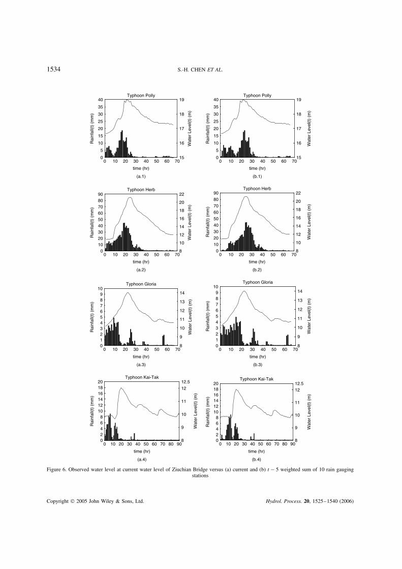
Instead of using individual rain-gauge information, we investigated the lumped rainfall effect on thedownstream water level. The lumped rainfall was obtained by using the weighted sum of the 10 rain-gaugingstations shown in Figure 2. Although the lumped rainfall would lose the individual information for a particularrain-gauging station, it also can filter the noise generated by an individual rain-gauging station. Figure 6

Copyright 2005 John Wiley & Sons, Ltd. Hydrol. Process. 20, 1525–1540 (2006)

1534 S.-H. CHEN ET AL.

0 10 20 30 40 50 60 700

5

10

15

20

25

30

35

40

time (hr)

Rai

nfal

l(t)

(mm

)

15

16

17

18

19

Wat

er L

evel

(t)

(m)

Typhoon Polly

(a.1)

0

5

10

15

20

25

30

35

40

Rai

nfal

l(t)

(mm

)

0 10 20 30 40 50 60 70

time (hr)

15

16

17

18

19

Wat

er L

evel

(t)

(m)

Typhoon Polly

(b.1)

0 10 20 30 40 50 60 700

102030405060708090

time (hr)

Rai

nfal

l(t)

(mm

)

8

10

12

14

16

18

20

22W

ater

Lev

el(t

) (m

)Typhoon Herb

(a.2)

0 10 20 30 40 50 60 700

10

20

30

40

50

60

70

80

90

time (hr)

Rai

nfal

l(t)

(mm

)

8

10

12

14

16

18

20

22

Wat

er L

evel

(t)

(m)

Typhoon Herb

(b.2)

0 10 20 30 40 50 60 700123456789

10

time (hr)

Rai

nfal

l(t)

(mm

)

8

9

10

11

12

13

14

Wat

er L

evel

(t)

(m)

Typhoon Gloria

(a.3)

0 10 20 30 40 50 60 700123456789

10

time (hr)

Rai

nfal

l(t)

(mm

)

8

9

10

11

12

13

14

Wat

er L

evel

(t)

(m)

Typhoon Gloria

(b.3)

(a.4)

0 10 20 30 40 50 60 70 80 9002468

101214161820

time (hr)

Rai

nfal

l(t)

(mm

)

8

9

10

11

12

12.5

Wat

er L

evel

(t)

(m)

Typhoon Kai-Tak

(b.4)

0 10 20 30 40 50 60 70 80 9002468

101214161820

time (hr)

Rai

nfal

l(t)

(mm

)

8

9

10

11

1212.5

Wat

er L

evel

(t)

(m)

Typhoon Kai-Tak

Figure 6. Observed water level at current water level of Ziuchian Bridge versus (a) current and (b) t � 5 weighted sum of 10 rain gaugingstations

Copyright 2005 John Wiley & Sons, Ltd. Hydrol. Process. 20, 1525–1540 (2006)

NEURO-FUZZY NETWORK FLOOD FORECAST MODEL 1535

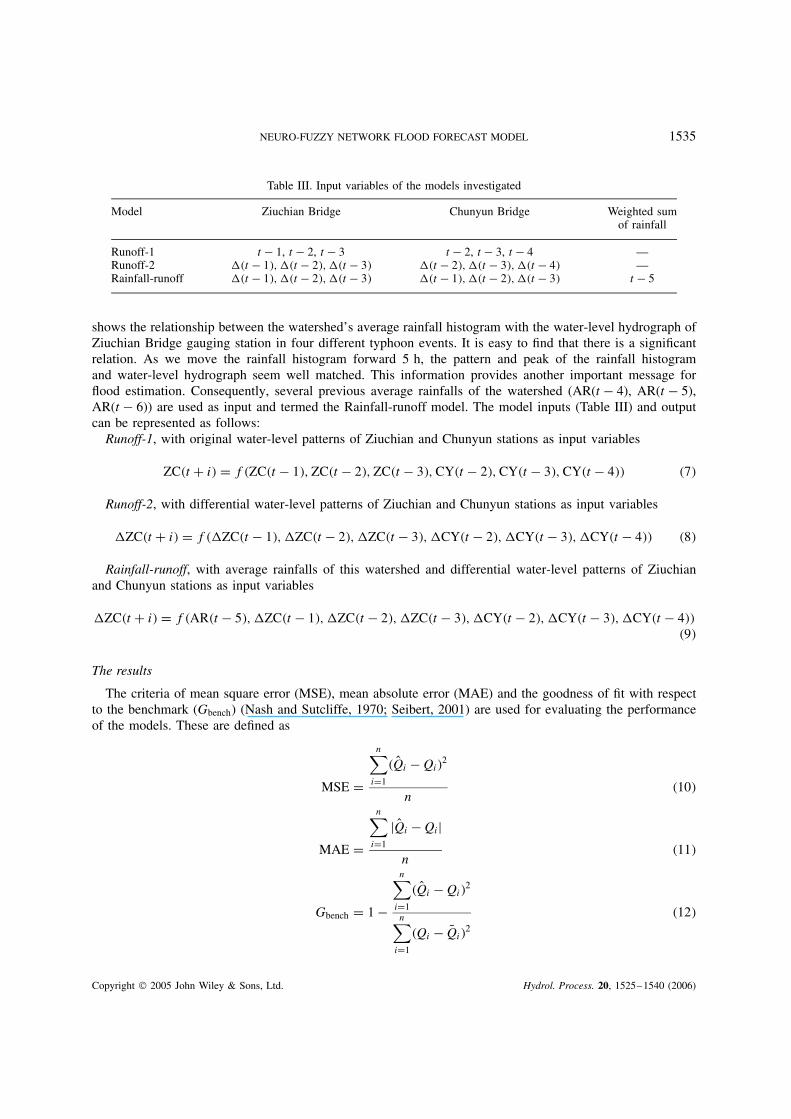
Table III. Input variables of the models investigated

Model Ziuchian Bridge Chunyun Bridge Weighted sumof rainfall

Runoff-1 t � 1, t � 2, t � 3 t � 2, t � 3, t � 4 —Runoff-2 �t � 1�, �t � 2�, �t � 3� �t � 2�, �t � 3�, �t � 4� —Rainfall-runoff �t � 1�, �t � 2�, �t � 3� �t � 1�, �t � 2�, �t � 3� t � 5

shows the relationship between the watershed’s average rainfall histogram with the water-level hydrograph ofZiuchian Bridge gauging station in four different typhoon events. It is easy to find that there is a significantrelation. As we move the rainfall histogram forward 5 h, the pattern and peak of the rainfall histogramand water-level hydrograph seem well matched. This information provides another important message forflood estimation. Consequently, several previous average rainfalls of the watershed (AR(t � 4), AR(t � 5),AR(t � 6)) are used as input and termed the Rainfall-runoff model. The model inputs (Table III) and outputcan be represented as follows:

Runoff-1, with original water-level patterns of Ziuchian and Chunyun stations as input variables

ZC�t C i� D f�ZC�t � 1�, ZC�t � 2�, ZC�t � 3�, CY�t � 2�, CY�t � 3�, CY�t � 4�� �7�

Runoff-2, with differential water-level patterns of Ziuchian and Chunyun stations as input variables

ZC�t C i� D f�ZC�t � 1�, ZC�t � 2�, ZC�t � 3�, CY�t � 2�, CY�t � 3�, CY�t � 4�� �8�

Rainfall-runoff, with average rainfalls of this watershed and differential water-level patterns of Ziuchianand Chunyun stations as input variables

ZC�t C i� D f�AR�t � 5�, ZC�t � 1�, ZC�t � 2�, ZC�t � 3�, CY�t � 2�, CY�t � 3�, CY�t � 4���9�

The results

The criteria of mean square error (MSE), mean absolute error (MAE) and the goodness of fit with respectto the benchmark (Gbench) (Nash and Sutcliffe, 1970; Seibert, 2001) are used for evaluating the performanceof the models. These are defined as

MSE D

n∑

iD1

� OQi � Qi�2

n�10�

MAE D

n∑

iD1

j OQi � Qij

n�11�

Gbench D 1 �

n∑

iD1

� OQi � Qi�2

n∑

iD1

�Qi � QQi�2

�12�

Copyright 2005 John Wiley & Sons, Ltd. Hydrol. Process. 20, 1525–1540 (2006)

1536 S.-H. CHEN ET AL.

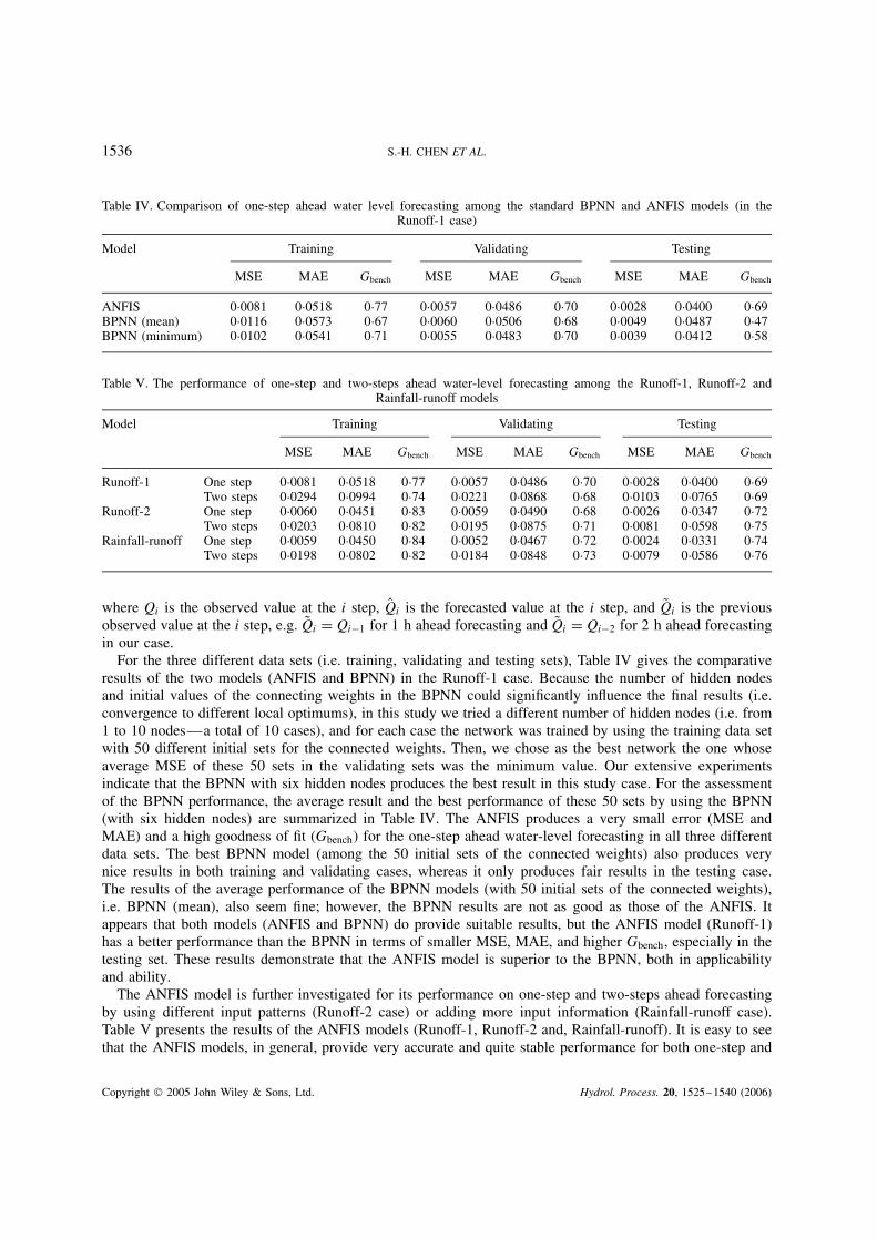
Table IV. Comparison of one-step ahead water level forecasting among the standard BPNN and ANFIS models (in theRunoff-1 case)

Model Training Validating Testing

MSE MAE Gbench MSE MAE Gbench MSE MAE Gbench

ANFIS 0Ð0081 0Ð0518 0Ð77 0Ð0057 0Ð0486 0Ð70 0Ð0028 0Ð0400 0Ð69BPNN (mean) 0Ð0116 0Ð0573 0Ð67 0Ð0060 0Ð0506 0Ð68 0Ð0049 0Ð0487 0Ð47BPNN (minimum) 0Ð0102 0Ð0541 0Ð71 0Ð0055 0Ð0483 0Ð70 0Ð0039 0Ð0412 0Ð58

Table V. The performance of one-step and two-steps ahead water-level forecasting among the Runoff-1, Runoff-2 andRainfall-runoff models

Model Training Validating Testing

MSE MAE Gbench MSE MAE Gbench MSE MAE Gbench

Runoff-1 One step 0Ð0081 0Ð0518 0Ð77 0Ð0057 0Ð0486 0Ð70 0Ð0028 0Ð0400 0Ð69Two steps 0Ð0294 0Ð0994 0Ð74 0Ð0221 0Ð0868 0Ð68 0Ð0103 0Ð0765 0Ð69

Runoff-2 One step 0Ð0060 0Ð0451 0Ð83 0Ð0059 0Ð0490 0Ð68 0Ð0026 0Ð0347 0Ð72Two steps 0Ð0203 0Ð0810 0Ð82 0Ð0195 0Ð0875 0Ð71 0Ð0081 0Ð0598 0Ð75

Rainfall-runoff One step 0Ð0059 0Ð0450 0Ð84 0Ð0052 0Ð0467 0Ð72 0Ð0024 0Ð0331 0Ð74Two steps 0Ð0198 0Ð0802 0Ð82 0Ð0184 0Ð0848 0Ð73 0Ð0079 0Ð0586 0Ð76

where Qi is the observed value at the i step, OQi is the forecasted value at the i step, and QQi is the previousobserved value at the i step, e.g. QQi D Qi�1 for 1 h ahead forecasting and QQi D Qi�2 for 2 h ahead forecastingin our case.

For the three different data sets (i.e. training, validating and testing sets), Table IV gives the comparativeresults of the two models (ANFIS and BPNN) in the Runoff-1 case. Because the number of hidden nodesand initial values of the connecting weights in the BPNN could significantly influence the final results (i.e.convergence to different local optimums), in this study we tried a different number of hidden nodes (i.e. from1 to 10 nodes—a total of 10 cases), and for each case the network was trained by using the training data setwith 50 different initial sets for the connected weights. Then, we chose as the best network the one whoseaverage MSE of these 50 sets in the validating sets was the minimum value. Our extensive experimentsindicate that the BPNN with six hidden nodes produces the best result in this study case. For the assessmentof the BPNN performance, the average result and the best performance of these 50 sets by using the BPNN(with six hidden nodes) are summarized in Table IV. The ANFIS produces a very small error (MSE andMAE) and a high goodness of fit (Gbench) for the one-step ahead water-level forecasting in all three differentdata sets. The best BPNN model (among the 50 initial sets of the connected weights) also produces verynice results in both training and validating cases, whereas it only produces fair results in the testing case.The results of the average performance of the BPNN models (with 50 initial sets of the connected weights),i.e. BPNN (mean), also seem fine; however, the BPNN results are not as good as those of the ANFIS. Itappears that both models (ANFIS and BPNN) do provide suitable results, but the ANFIS model (Runoff-1)has a better performance than the BPNN in terms of smaller MSE, MAE, and higher Gbench, especially in thetesting set. These results demonstrate that the ANFIS model is superior to the BPNN, both in applicabilityand ability.

The ANFIS model is further investigated for its performance on one-step and two-steps ahead forecastingby using different input patterns (Runoff-2 case) or adding more input information (Rainfall-runoff case).Table V presents the results of the ANFIS models (Runoff-1, Runoff-2 and, Rainfall-runoff). It is easy to seethat the ANFIS models, in general, provide very accurate and quite stable performance for both one-step and

Copyright 2005 John Wiley & Sons, Ltd. Hydrol. Process. 20, 1525–1540 (2006)

NEURO-FUZZY NETWORK FLOOD FORECAST MODEL 1537

8 10 12 14 16 18 20 228

10

12

14

16

18

20

22

observation(m)

estim

atio

n(m

)es

timat

ion(

m)

Training Data

(a-1)

8 10 12 14 16 18 20 228

10

12

14

16

18

20

22

observation(m)

estim

atio

n(m

)

Training Data

(b-1)

10 11 12 13 14 15 16

observation(m)

Validating Data

(a-2)

10 11 12 13 14 15 1610

11

12

13

14

15

16

observation(m)

estim

atio

n(m

)

Validating Data

(b-2)

9 10 11 12 13 14 15 169

10

11

12

13

14

15

16

10

11

12

13

14

15

16

observation(m)

estim

atio

n(m

)

Testing Data

(a-3)

9 10 11 12 13 14 15 169

10

11

12

13

14

15

16

observation(m)

estim

atio

n(m

)

Testing Data

(b-3)

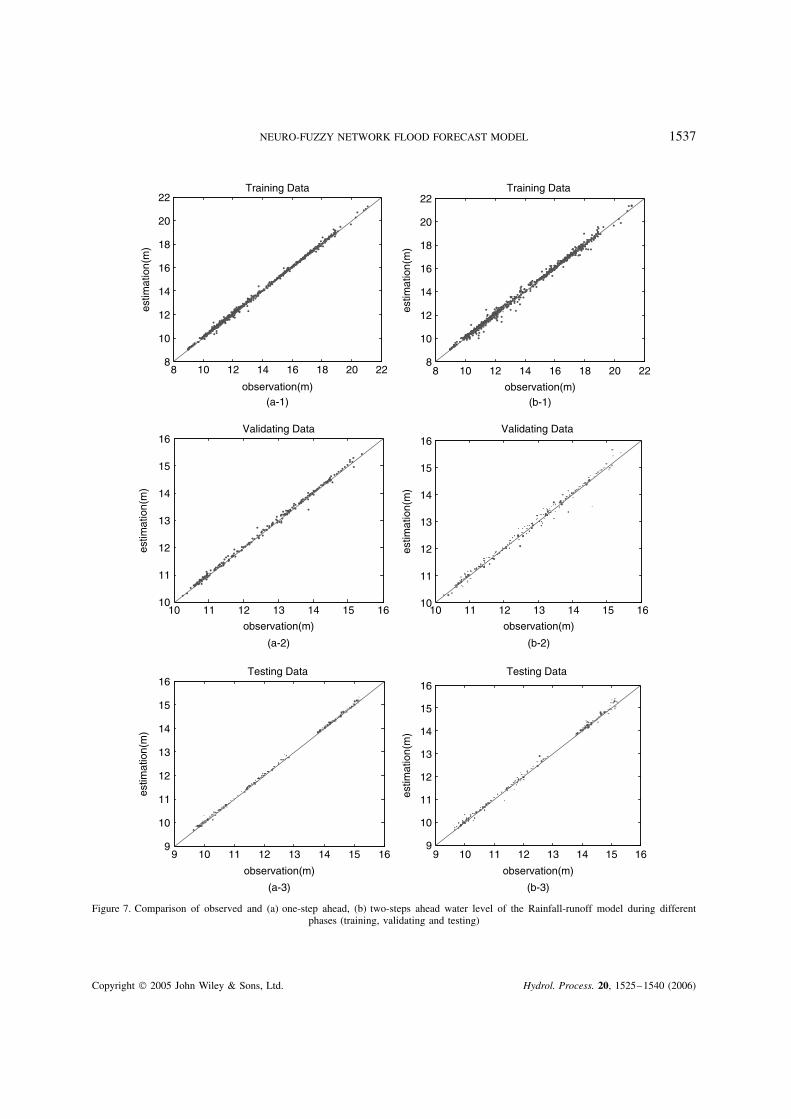
Figure 7. Comparison of observed and (a) one-step ahead, (b) two-steps ahead water level of the Rainfall-runoff model during differentphases (training, validating and testing)

Copyright 2005 John Wiley & Sons, Ltd. Hydrol. Process. 20, 1525–1540 (2006)

1538 S.-H. CHEN ET AL.

two-steps ahead forecasting, where the results of the MSE and MAE are very small in all three stages (training,validating and testing sets). Among these models, the Runoff-2 model is slightly better than the Runoff-1model, and the Rainfall-runoff model provides the most accurate results. These results can be interpreted as(1) a downstream water level can be suitably estimated by just using several of the previous downstream andupstream water levels as input to the ANFIS model; (2) adding the watershed average rainfall information inaddition to water-level information could slightly enhance the forecasting accuracy.

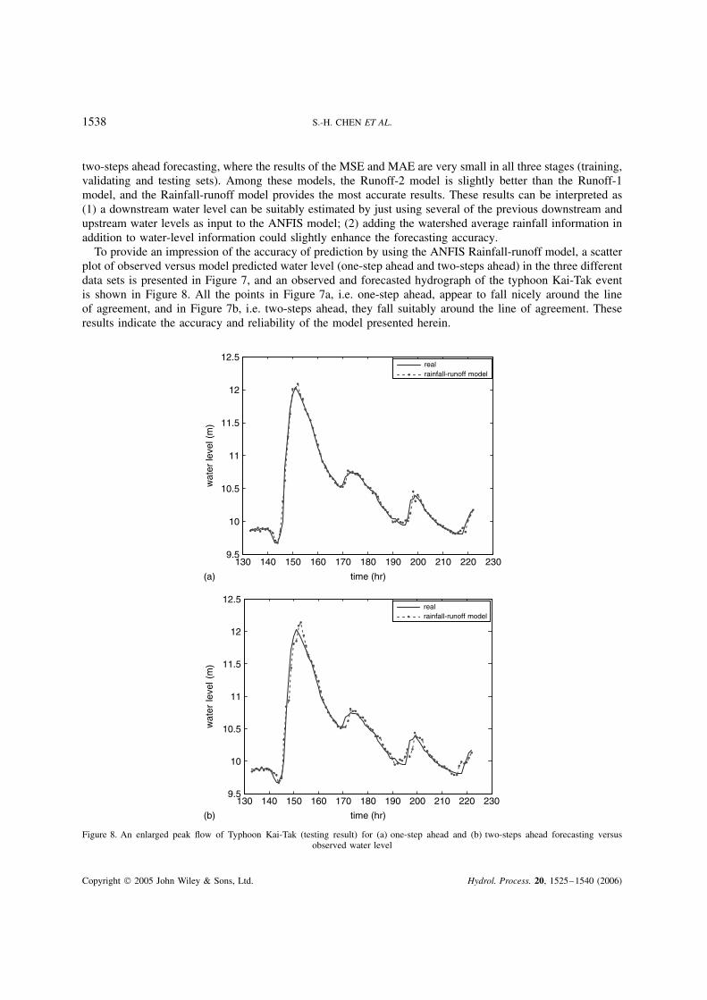
To provide an impression of the accuracy of prediction by using the ANFIS Rainfall-runoff model, a scatterplot of observed versus model predicted water level (one-step ahead and two-steps ahead) in the three differentdata sets is presented in Figure 7, and an observed and forecasted hydrograph of the typhoon Kai-Tak eventis shown in Figure 8. All the points in Figure 7a, i.e. one-step ahead, appear to fall nicely around the lineof agreement, and in Figure 7b, i.e. two-steps ahead, they fall suitably around the line of agreement. Theseresults indicate the accuracy and reliability of the model presented herein.

130 140 150 160 170 180 190 200 210 220 2309.5

10

10.5

11

11.5

12

12.5

9.5

10

10.5

11

11.5

12

12.5

time (hr)

130 140 150 160 170 180 190 200 210 220 230

time (hr)

wat

er le

vel (

m)

(a)

wat

er le

vel (

m)

realrainfall-runoff model

realrainfall-runoff model

(b)

Figure 8. An enlarged peak flow of Typhoon Kai-Tak (testing result) for (a) one-step ahead and (b) two-steps ahead forecasting versusobserved water level

Copyright 2005 John Wiley & Sons, Ltd. Hydrol. Process. 20, 1525–1540 (2006)

NEURO-FUZZY NETWORK FLOOD FORECAST MODEL 1539

CONCLUSIONS

Neural networks have a complex connection structure and simple computing elements that provide a greatability to learn by example and to generalize. In the last few decades, a great number of researches regardingthe application of ANNs in water resources problems have demonstrated their applicability. Nevertheless,there are a few of problems that might limit their applicability. One major problem is lack of data. A riverbasin usually has many rain and water-level gauging stations, and it is easy to build up a forecasting modelby means of regression or ANN approaches. However, if we only have a limited number of data sets, themodels built might only be good for the training sets due to overtraining and could not be used for futureevents. One way to solve this problem is to identify the crucial inputs and then reduce the input dimensions.This is especially important in developing a satisfactory ANN forecasting model. Based on 23 flood eventsin the Choshui River, we find that the persistence effect and the upstream flow information are crucial forflood forecasting. The effect of rainfall on the water level varies from time to time in all rain gauging stationsand cannot be identified as a solid relation, whereas the watershed’s average rainfall provides other usefulinformation for flood forecasting.

After identifying the important inputs, we proposed the ANFIS for constructing the flood forecasting models.The ANFIS is an integration of a neural network and fuzzy arithmetic. For the purpose of comparison, theBPNN model was also performed. Compared to BPNN, the principal advantage of the proposed method isthat the ANFIS can automatically construct a rainfall-runoff model and estimate the needed parameters byan approach converging to an optimal solution. The comparative results obtained by the BPNN and ANFISprovide evidence that the ANFIS can offer a higher degree of reliability and accuracy than BPNN in floodforecasting.

For further investigation, three ANFIS models, based on different input information, were built to performone- and two-steps ahead flood forecasting. The results show that: (1) a downstream water level can besuitably estimated by just using several of the previous downstream and upstream water levels as input to theANFIS model; (2) using the differential values, which could remove the nonstationarity of a time series, couldprovide better performance than the original values; and (3) adding the watershed average rainfall informationin addition to water-level information would enhance the forecasting accuracy. The ANFIS models, in general,provide very accurate and quite stable performance for both one-step and two-step ahead forecasting, wherethe results of MSE and MAE are very small in all three stages (training, validating and testing sets).

ACKNOWLEDGEMENTS

This paper is based on partial work supported by 4th River Basin Management Bureau, WRA, Ministry ofEconomic Affairs, Taiwan. In addition, we are sincerely grateful to the reviewers for their valuable commentsand suggestions.

REFERENCES

Altug S, Chow MY, Trussell HJ. 1999. Fuzzy inference systems implemented on neural architectures for motor fault detection and diagnosis.IEEE Transactions on Industrial Electronics 46(6): 1069–1079.

ASCE Task Committee on Application of Artificial Neural Networks in Hydrology. 2000a. Artificial neural networks in hydrology I:preliminary concepts. Journal of Hydrologic Engineering 5(2): 115–123.

ASCE Task Committee on Application of Artificial Neural Networks in Hydrology. 2000b. Artificial neural networks in hydrology II:hydrology applications. Journal of Hydrologic Engineering 5(2): 124–137.

Anderson MG, Burt TP. 1985. Hydrological Forecasting . Wiley: New York.Chang FJ, Hwang YY. 1999. A self-organization algorithm for real-time flood forecast. Hydrological Processes 13: 123–138.Chang LC, Chang FJ. 2001. Intelligent control for modelling of real-time reservoir operation. Hydrological Processes 15(9): 1621–1631.Chang LC, Chang FJ, Chiang YM. 2004. A two-step ahead recurrent neural network for streamflow forecasting. Hydrological Processes

18: 81–92.Chang YT, Chang LC, Chang FJ. 2005. Intelligent control for modelling of real-time reservoir operation, part II: artificial neural with

operating rule curves. Hydrological Processes 19: 1431–1444.

Copyright 2005 John Wiley & Sons, Ltd. Hydrol. Process. 20, 1525–1540 (2006)

1540 S.-H. CHEN ET AL.

Djukanovic MB, Calovic MS, Vesovic BV, Sobajic DJ. 1997. Neuro-fuzzy controller of low head hydropower plants using adaptive-networkbased fuzzy inference. IEEE Transactions on Energy Conversion 14(4): 375–381.

Hopfield JJ. 1982. Neural networks and physical systems with emergent collective computational abilities. Proceeding of the NationalAcademy of Scientists 79: 2554–2558.

Huang W, Xu B, Chan Hilton A. 2004. Forecasting flows in Apalachicola River using neural networks. Hydrological Processes 18:2545–2564.

Jang J-SR. 1993. ANFIS: Adaptive-Network-Based Fuzzy Inference System. IEEE Transactions on Systems, Man, and Cybernetics 23(3):665–685.

Maier HR, Dandy GC. 2000. Neural networks for the prediction and forecasting of water resource variables: a review of modeling issuesand applications. Environmental Modelling and Software 15(1): 101–124.

Nash JE, Sutcliffe JV. 1970. River flow forecasting through conceptual model, part I—a discussion of principles. Journal of Hydrology 10:282–290.

Nie J, Linkens DA. 1994. Fast self-learning multivariable fuzzy controllers constructed from a modified CPN network. International Journalon Control 60: 369–393.

Oonsivilai A, El-Hawary ME. 1999. Power system dynamic load modeling using adaptive-network-based fuzzy inference system. InProceedings of the 1999 IEEE Canadian Conference on Electrical and Computer Engineering, Shaw Conference Center, Edmonton,Alberta, Canada.

Rumelhart DE, Hinton GE, Williams RJ. 1986. Learning internal representation by error propagation. Parallel Distributed Processing 1:318–362.

Sajikumar N, Thandaveswara BS. 1999. A non-linear rainfall-runoff model using an artificial network. Journal of Hydrology 216: 32–55.Salas JD, Delleur JW, Yevjevich V, Lane WL. 1985. Applied Modeling of Hydrologic Time Series . Water Resources Publications: Littleton,

CO.Schalkoff RJ. 1997. Artificial Neural Network . McGraw-Hill: New York.Seibert J. 2001. On the need for benchmarks in hydrological modelling. Hydrological Processes 15: 1063–1064.Takagi T, Sugeno M. 1985. Fuzzy identification of systems and its application to modeling and control. IEEE Transactions Systems, Man

and Cybernetics 15(1): 116–132.Williams R, Zipser D. 1989. A learning algorithm for continually running fully recurrent neural networks. Neural Computation 1: 270–280.

Copyright 2005 John Wiley & Sons, Ltd. Hydrol. Process. 20, 1525–1540 (2006)