
On some critical problems for the fractional Laplacian operator
Upload
independentCategory
view
0download
0
Linear Algebra and its Applications 403 (2005) 97–117www.elsevier.com/locate/laa
The spectra of the adjacency matrix andLaplacian matrix for some balanced trees �
Oscar Rojo ∗, Ricardo Soto 1
Departamento de Matemáticas, Universidad Católica del Norte, Casilla 1280, Antofagasta, Chile
Received 19 May 2004; accepted 20 January 2005Available online 2 March 2005
Submitted by R.A. Brualdi
Abstract
Let T be an unweighted rooted tree of k levels such that in each level the vertices haveequal degree. Let dk−j+1 denotes the degree of the vertices in the level j. We find the eigen-values of the adjacency matrix and of the Laplacian matrix of T. They are the eigenvaluesof principal submatrices of two nonnegative symmetric tridiagonal matrices of order k × k.The codiagonal entries for both matrices are
√dj − 1, 2 � j � k − 1, and
√dk , while the
diagonal entries are zeros, in the case of the adjacency matrix, and dj , 1 � j � k, in the caseof the Laplacian matrix. Moreover, we give some results concerning to the multiplicity of theabove mentioned eigenvalues.© 2005 Elsevier Inc. All rights reserved.
AMS classification: 5C50; 15A48
Keywords: Tree; Balanced tree; Binary tree; m-Ary tree; Laplacian matrix; Adjacency matrix
� Work supported by Fondecyt 1040218, Chile.∗ Corresponding author. Tel.: +56 55 355593; fax: +56 55 355599.
E-mail addresses: [email protected], [email protected] (O. Rojo), [email protected] (R. Soto).1 Part of this research was conducted while the authors were visitors at the Instituto Nacional de
Matematica Pura e Aplicada, Rio de Janeiro, Brasil.
0024-3795/$ - see front matter � 2005 Elsevier Inc. All rights reserved.doi:10.1016/j.laa.2005.01.011
98 O. Rojo, R. Soto / Linear Algebra and its Applications 403 (2005) 97–117
1. Notations and preliminaries
Let G be a simple graph. Let A(G) be the adjacency matrix of G and let D(G) bethe diagonal matrix of vertex degrees. The Laplacian matrix of G is L(G) = D(G) −A(G). Clearly, L(G) is a real symmetric matrix. From this fact and Geršgorin’s the-orem, it follows that its eigenvalues are nonnegative real numbers. Moreover, sinceits rows sum to 0, 0 is the smallest eigenvalue of L(G). In [4], some of the manyresults known for Laplacian matrices are given. Fiedler [2] proved that G is a con-nected graph if and only if the second smallest eigenvalue of L(G) is positive. Thiseigenvalue is called the algebraic connectivity of G.
We recall that a tree is a connected acyclic graph. Here we consider an unweightedrooted tree T such that in each level the vertices have equal degree. We agree thatthe root vertex is at level 1 and that T has k levels. Thus the vertices in the level k
have degree 1.For j = 1, 2, 3, . . . , k, the numbers dk−j+1 and nk−j+1 denote the degree of
the vertices and the number of vertices in the level j , respectively. Then, for j =2, 3, . . . k − 1,
nk−j = (dk−j+1 − 1)nk−j+1. (1)
Observe that dk is the degree of the root vertex, d1 = 1 is the degree of the verticesin the level k, nk = 1, nk−1 = dk , nj+1 divides nj for all j = 1, . . . , k − 1 and thatthe total number of vertices in the tree is
n =k−1∑j=1
nj + 1.
We introduce the following notations:If all the eigenvalues of an n × n matrix A are real numbers, we write
λn(A) � λn−1(A) � · · · � λ2(A) � λ1(A).
0 is the all zeros matrix.The order of 0 will be clear from the context in which it is used.Im is the identity matrix of order m × m.em is the all ones column vector of dimension m.For j = 1, 2, . . . , k − 1, Cj is the block diagonal matrix defined by
Cj =
e njnj+1
0 · · · 0
0 e njnj+1
...
.... . . 0
0 · · · 0 e njnj+1
, (2)
O. Rojo, R. Soto / Linear Algebra and its Applications 403 (2005) 97–117 99
with nj+1 diagonal blocks. Thus, the order of Cj is nj × nj+1. Observe that Ck−1 =enk−1 .
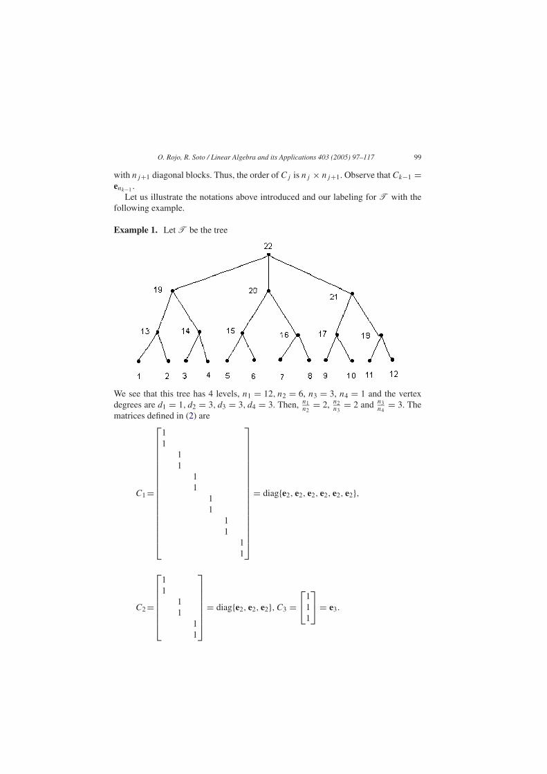
Let us illustrate the notations above introduced and our labeling for T with thefollowing example.
Example 1. Let T be the tree
We see that this tree has 4 levels, n1 = 12, n2 = 6, n3 = 3, n4 = 1 and the vertexdegrees are d1 = 1, d2 = 3, d3 = 3, d4 = 3. Then, n1
n2= 2, n2
n3= 2 and n3
n4= 3. The
matrices defined in (2) are
C1 =
11
11
11
11
11
11
= diag{e2, e2, e2, e2, e2, e2},
C2 =
11
11
11
= diag{e2, e2, e2}, C3 =
111
= e3.

100 O. Rojo, R. Soto / Linear Algebra and its Applications 403 (2005) 97–117
In general, using the labels 1, 2, 3, . . . , n, in this order, our labeling for the verti-ces of T is: Label the vertices from the bottom to the root vertex and, in each level,from the left to the right.
For this labeling the adjacency matrix A(T) and Laplacian matrix L(T) of thetree in Example 1 become
A(T) =
0 C1 0 0CT
1 0 C2 00 CT
2 0 C3
0 0 CT3 0
and
L(T) =
I12 −C1 0 0−CT
1 3I6 −C2 00 −CT
2 3I2 −C3
0 0 −CT3 3
.
with C1, C2 and C3 as in Example 1.In general, our labeling yields to
A(T) =
0 C1 0 · · · · · · 0
CT1 0 C2
. . ....
0 CT2
. . .. . .
. . ....
.... . .
. . .. . . Ck−2 0
.... . . CT
k−2 0 Ck−1
0 · · · · · · 0 CTk−1 0
(3)
and
L(T) =
In1 −C1 0 · · · · · · 0
−CT1 d2In2 C2
. . ....
0 −CT2
. . .. . .
. . ....
.... . .
. . . dk−2Ink−2 −Ck−2 0...
. . . −CTk−2 dk−1Ink−1 −Ck−1
0 · · · · · · 0 −CTk−1 dk
. (4)

O. Rojo, R. Soto / Linear Algebra and its Applications 403 (2005) 97–117 101
The following lemma plays a fundamental role in this paper.
Lemma 1. Let
M =
α1In1 C1 0 · · · · · · · · · 0
CT1 α2In2 C2
. . .
0 CT2
. . ....
. . .. . .
.... . . αk−2Ink−2 Ck−2 0
.... . . CT
k−2 αk−1Ink−1 Ck−1
0 · · · · · · · · · 0 CTk−1 αk
.
Let
β1 = α1
and
βj = αj − nj−1
nj
1
βj−1, j = 2, 3, . . . , k, βj−1 /= 0.
If βj /= 0 for all j = 1, 2, . . . , k − 1,
det M = βn11 β
n22 . . . β
nk−2k−2 β
nk−1k−1 βk. (5)
Proof. Suppose βj /= 0 for all j = 1, 2, . . . , k − 1. We apply the Gaussian elim-ination procedure, without row interchanges, to reduce the matrix M to an uppertriangular matrix. Just before the last step, we have the matrix
β1In1 C1 0 · · · · · · · · · 0
0 β2In2 C2...
0 0 β3In3 C3...
... 0. . .
. . ....
.... . .
. . . Ck−2 0... 0 βk−1Ink−1 Ck−1
0 · · · · · · · · · 0 CTk−1 αk
.

102 O. Rojo, R. Soto / Linear Algebra and its Applications 403 (2005) 97–117
Finally, the Gaussian elimination gives
β1In1 C1 0 · · · · · · · · · 0
0 β2In2 C2...
0 0 β3In3 C3...
... 0. . .
. . ....
.... . .
. . . Ck−2 0... 0 βk−1Ink−1 Ck−1
0 · · · · · · · · · 0 0 αk − nk−11
βk−1
. (6)
Thus, (5) is proved. �
2. The spectrum of the Laplacian matrix of T
Let� = {1, 2, 3, . . . , k − 1}.
We consider the following subset of �,� = {j ∈ � : nj > nj+1}.
Since nk−1 > nk = 1, the index k − 1 ∈ �. Observe that if i ∈ � − � then ni =ni+1 and thus, from (2), Ci = Ini
.
Theorem 2. Let
P0(λ) = 1, P1(λ) = λ − 1and
Pj (λ) = (λ − dj )Pj−1(λ) − nj−1
nj
Pj−2(λ) for j = 2, 3, . . . , k. (7)
Hence
(a) If Pj (λ) /= 0, for all j = 1, 2, . . . , k − 1, then
det(λI − L(T)) = Pk(λ)∏j∈�
Pnj −nj+1j (λ). (8)
(b)
σ (L(T)) = (∪j∈�{λ ∈ R : Pj (λ) = 0}) ∪ {λ ∈ R : Pk(λ) = 0}. (9)
Proof. (a) We apply Lemma 1 to the matrix M = λI − L(T). For this matrix α1 =λ − 1 and αj = λ − dj for j = 2, 3, . . . , k. Let β1, β2, . . . , βk be as in Lemma 1.Suppose that λ ∈ R is such that Pj (λ) /= 0 for all j = 1, 2, . . . , k − 1. We have

O. Rojo, R. Soto / Linear Algebra and its Applications 403 (2005) 97–117 103
β1 = λ − 1 = P1(λ)
P0(λ)/= 0,
β2 = (λ − d2) − n1
n2
1
β1= (λ − d2) − n1
n2
P0(λ)
P1(λ)
= (λ − d2)P1(λ) − n1n2
P0(λ)
P1(λ)= P2(λ)
P1(λ)/= 0,
β3 = (λ − d3) − n2
n3
1
β2= (λ − d3) − n2
n3
P1(λ)
P2(λ)
= (λ − d3)P2(λ) − n2n3
P1(λ)
P2(λ)= P3(λ)
P2(λ)/= 0,
...
βk−1 = (λ − dk−1) − nk−2
nk−1
1
βk−2= (λ − dk−1) − nk−2
nk−1
Pk−3(λ)
Pk−2(λ)
=(λ − dk−1)Pk−2(λ) − nk−2
nk−1Pk−3(λ)
Pk−2(λ)= Pk−1(λ)
Pk−2(λ)/= 0,
βk = (λ − dk) − nk−1
nk
1
βk−1= (λ − dk) − nk−1
nk
Pk−2(λ)
Pk−1(λ)
= (λ − dk)Pk−1(λ) − nk−1nk
Pk−2(λ)
Pk−1(λ)= Pk(λ)
Pk−1(λ).
From (5)
det(λI − L(T)) = Pn11 (λ)
Pn10 (λ)
Pn22 (λ)
Pn21 (λ)
Pn33 (λ)
Pn32 (λ)
. . .P
nk−2k−2 (λ)
Pnk−2k−3 (λ)
Pnk−1k−1 (λ)
Pnk−1k−2 (λ)
Pk(λ)
Pk−1(λ)
= Pn1−n21 (λ)P
n2−n32 (λ)P
n3−n43 (λ) . . . P
nk−1−1k−1 (λ)Pk(λ)
= Pk(λ)∏j∈�
Pnj −nj+1j (λ).
Thus, (8) is proved.
(b) From (8), if λ ∈ R is such that Pj (λ) /= 0, for all j = 1, 2, . . . , k − 1, k, thendet(λI − L(T)) /= 0. That is
∩kj=1{λ ∈ R : Pj (λ) /= 0} ⊆ (σ (L(T)))c.
That is
σ(L(T)) ⊆(
∪k−1j=1 {λ ∈ R : Pj (λ) = 0}
)∪ {λ ∈ R : Pk(λ) = 0}. (10)

104 O. Rojo, R. Soto / Linear Algebra and its Applications 403 (2005) 97–117
We claim that
σ(L(T)) ⊆ (∪j∈�{λ ∈ R : Pj (λ) = 0}) ∪ {λ ∈ R : Pk(λ) = 0}. (11)
If � = � = {1, 2, . . . , k − 1} then (11) is (10) and there is nothing to prove. Supposethat � is a proper subset of �. Clearly, (11) is equivalent to
∩j∈�{λ ∈ R : Pj (λ) /= 0} ∩ {λ ∈ R : Pk(λ) /= 0} ⊆ (σ (L(T)))c.
Suppose that λ ∈ R is such that Pj (λ) /= 0 for all j ∈ � and Pk(λ) /= 0. Sincek − 1 ∈ �, Pk−1(λ) /= 0. If in addition Pj (λ) /= 0 for all j ∈ � − � then (8) holdsand consequently det(λI − L(T)) /= 0. That is, λ ∈ (σ (L(T)))c. If Pi(λ) = 0 forsome i ∈ � − �, let l be the first index in � − � such that Pl(λ) = 0. Then, βj /= 0for all j = 1, 2, . . . , l − 1, βl = 0 and
Pl+2(λ) = (λ − dl+2)Pl+1(λ).
We observe that Pl+1(λ) /= 0. Otherwise, a back sustitution in (7) gives P0(λ) = 0.Therefore, βl+2 = Pl+2(λ)
Pl+1(λ)= λ − dl+2. Since l ∈ � − �, then nl = nl+1, Cl = Inl
and the Gaussian elimination procedure applied to M = λI − L(T) yields to theintermediate matrix
β1In1 C1 0 · · · · · · · · · 0
0. . .
. . .. . .
...... 0 0 Inl
0...
.... . . Inl
(λ − dl+1)Inl+1 Cl+1. . .
......
. . . CTl+1 (λ − dl+2)Inl+2
. . . 0...
. . .. . .
. . . Ck−1
0 · · · · · · · · · 0 Ck−1 λ − dk
=
β1In1 C1 0 · · · · · · · · · 0
0. . .
. . .. . .
...... 0 0 Inl
0...
.... . . Inl
(λ − dl+1)Inl+1 Cl+1. . .
......
. . . CTl+1 βl+2Inl+2
. . . 0...
. . .. . .
. . . Ck−1
0 · · · · · · · · · 0 Ck−1 λ − dk
.
O. Rojo, R. Soto / Linear Algebra and its Applications 403 (2005) 97–117 105
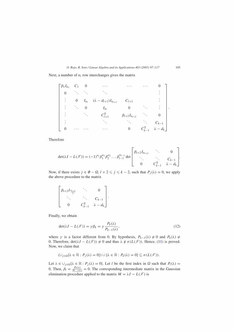
Next, a number of nl row interchanges gives the matrix
β1In1 C1 0 · · · · · · · · · 0
0. . .
. . .. . .
...... 0 Inl
(λ − dl+1)Inl+1 Cl+1...
.... . . 0 Inl
0. . .
......
. . . CTl+1 βl+2Inl+2
. . . 0...
. . .. . .
. . . Ck−1
0 · · · · · · · · · 0 CTk−1 λ − dk
.
Therefore
det(λI − L(T)) = (−1)nl βn11 β
n22 . . . β
nl−1l−1 det
βl+2Inl+2
. . . 0. . .
. . . Ck−1
0 CTk−1 λ − dk
.
Now, if there exists j ∈ � − �, l + 2 � j � k − 2, such that Pj (λ) = 0, we applythe above procedure to the matrix
βl+2I nl+22
. . . 0
. . .. . . Ck−1
0 CTk−1 λ − dk
.
Finally, we obtain
det(λI − L(T)) = γβk = γPk(λ)
Pk−1(λ), (12)
where γ is a factor different from 0. By hypothesis, Pk−1(λ) /= 0 and Pk(λ) /=0. Therefore, det(λI − L(T)) /= 0 and thus λ /∈ σ(L(T)). Hence, (11) is proved.Now, we claim that
(∪j∈�{λ ∈ R : Pj (λ) = 0}) ∪ {λ ∈ R : Pk(λ) = 0} ⊆ σ(L(T)).
Let λ ∈ ∪j∈�{λ ∈ R : Pj (λ) = 0}. Let l be the first index in � such that Pl(λ) =0. Then, βl = Pl(λ)
Pl−1(λ)= 0. The corresponding intermediate matrix in the Gaussian
elimination procedure applied to the matrix M = λI − L(T) is

106 O. Rojo, R. Soto / Linear Algebra and its Applications 403 (2005) 97–117
β1In1 C1 0 · · · · · · 0
0. . .
. . ....
0. . . 0 Cl
......
. . . CTl (λ − dl+1)Inl+1
......
. . .. . .
. . . Ck−1
0 · · · · · · 0 CTk−1 λ − dk
. (13)
Since l ∈ �, nl > nl+1 and Cl is a matrix with more rows than columns. Therefore,the matrix in (13) has at least two equal rows. Thus, det(λI − L(T)) = 0. That is,λ ∈ (L(T)). Hence
∪j∈� {λ ∈ R : Pj (λ) = 0} ⊆ σ(L(T)). (14)
Now let λ ∈ {λ ∈ R : Pk(λ) = 0}. Observe that Pk−1(λ) /= 0. Otherwise, a back sub-stitution in (7) yields to P0(λ) = 0. If Pj (λ) = 0 for some j ∈ � then the use of (14)gives λ ∈ σ(L(T)). Hence, we may suppose that Pj (λ) /= 0 for all j ∈ �. If inaddition Pj (λ) /= 0 for all j ∈ � − � then (8) holds and thus det(λI − L(T)) = 0because Pk(λ) = 0. If Pi(λ) = 0 for some i ∈ � − � then we have the assumptionsunder which (12) was obtained. Therefore
det(λI − L(T)) = γβk = γPk(λ)
Pk−1(λ)= 0.
Thus, we have proved that
{λ ∈ R : Pk(λ) = 0} ⊆ σ(L(T)). (15)
From (14) and (15),
(∪j∈�{λ ∈ R : Pj (λ) = 0}) ∪ {λ ∈ R : Pk(λ) = 0} ⊆ σ(L(T)). (16)
Finally, (11) and (16) imply (9). �
Lemma 3. For j = 1, 2, 3, . . . , k − 1, let Tj be the j × j principal submatrix ofthe k × k symmetric tridiagonal matrix
Tk =
1√
d2 − 1 0 · · · · · · 0√
d2 − 1 d2√
d3 − 1. . .
...
0√
d3 − 1 d3. . .
. . ....
.... . .
. . .. . .
√dk−1 − 1 0
.... . .
√dk−1 − 1 dk−1
√dk
0 · · · · · · 0√
dk dk
.
O. Rojo, R. Soto / Linear Algebra and its Applications 403 (2005) 97–117 107
Then
det(λI − Tj ) = Pj (λ), j = 1, 2, . . . , k.
Proof. It is well known (see for instance [1, p.229]) that the characteristic poly-nomials, Qj , of the j × j principal submatrix of the k × k symmetric tridiagonalmatrix
a1 b1 0 · · · · · · 0
b1 a2 b2. . .
...
0 b2. . .
. . .. . .
......
. . .. . .
. . .. . . 0
.... . .
. . . ak−1 bk−10 · · · · · · 0 bk−1 ak
,
satisfy the three-term recursion formula
Qj(λ) = (λ − aj )Qj−1(λ) − b2j−1Qj−2(λ),
with
Q0(λ) = 1 and Q1(λ) = λ − a1.
In our case, a1 = 1, aj = dj for j = 2, 3, , . . . , k and bj =√
nj
nj+1for j = 1, 2, . . . ,
k − 1. For these values, the above recursion formula gives the polynomials Pj , j =0, 1, 2, . . . , k. Now, we use (1), to see that
√nj
nj+1= √
dj − 1 for j = 1, 2, . . . , k −2 and
√nk−1nk
= √nk−1 = √
dk. �
Theorem 4. Let Tj , j = 1, 2, . . . , k − 1 and Tk be the symmetric tridiagonal matri-ces defined in Lemma 3. Then
(a)
σ(L(T)) = (∪j∈�σ(Tj )) ∪ σ(Tk).
(b) The multiplicity of each eigenvalue of the matrix Tj , as an eigenvalue of L(T),
is at least (nj − nj+1) for j ∈ � and 1 for j = k.
Proof. We recall that the eigenvalues of any symmetric tridiagonal matrix withnonzero codiagonal entries are simple. Then, (a) and (b) are immediate consecuencesof this fact, Theorem 2 and Lemma 3. �
Example 2. Let T be the tree in Example 1. For this tree, k = 4, d1 = 1, d2 = 3,d3 = 3, d4 = 3, n1 = 12, n2 = 6 and n3 = 3. Hence

108 O. Rojo, R. Soto / Linear Algebra and its Applications 403 (2005) 97–117
T4 =
1√
2 0 0√2 3
√2 0
0√
2 3√
30 0
√3 3
and � = {1, 2, 3}. The eigenvalues of L(T) are the eigenvalues of T1, T2, T3 andT4. To four decimal places these eigenvalues are:
T1 : 1T2 : 0.2679 3.7321T3 : 0.0968 2.1939 4.709T4 : 0 1.1864 3.4707 5.3429
Example 3. Let T be the tree
For this tree, k = 5, n1 = 8, n2 = n3 = 4, n4 = 2, n5 = 1, d1 = 1, d2 = 3, d3 = 2,d4 = 3 and d5 = 2. Hence the matrix T5 is
T5 =
1√
2 0 0 0√2 3 1 0 0
0 1 2√
2 00 0
√2 3
√2
0 0 0√
2 2
and � = {1, 3, 4}. Thus the spectrum of L(T) is the union of the spectra of T1, T3, T4and T5:

O. Rojo, R. Soto / Linear Algebra and its Applications 403 (2005) 97–117 109
T1 : 1T3 : 0.1392 1.7459 4.1149T4 : 0.0646 1 3.4626 4.4728T5 : 0 0.5617 1.8614 3.8202 4.7566
We recall the following interlacing property [3]:Let T be a symmetric tridiagonal matrix with nonzero codiagonal entries and λ
(j)i
be the ith smallest eigenvalue of its j × j principal submatrix. Then,
λ(j+1)
j+1 < λ(j)j < λ
(j+1)j < · · · < λ
(j+1)
i+1 < λ(j)i < λ
(j+1)i < · · · < λ
(j+1)
2
< λ(j)
1 < λ(j+1)
1 .
Theorem 5. Let L(T) be the Laplacian matrix of T. Then
(a) σ (Tj−1) ∩ σ(Tj ) = φ for j = 2, 3, . . . , k.
(b) The largest eigenvalue of Tk is the largest eigenvalue of L(T).
(c) The smallest eigenvalue of Tk−1 is the algebraic connectivity of T.
(d) The largest eigenvalue of Tk−1 is the second largest eigenvalue of L(T).
(e) det Tj = 1 for j = 1, 2, . . . , k − 1.
(f) If λ is an integer eigenvalue of L(T) and λ > 1 then λ ∈ σ(Tk).
Proof. First we observe that k − 1 ∈ �. Thus the eigenvalues of Tk−1 are alwayseigenvalues of L(T). Now (a), (b), (c) and (d) follow from the interlacing prop-erty and Theorem 4. Clearly, det T1 = 1. Let 2 � j � k − 1. We apply the Gaussianelimination procedure, without row interchanges, to reduce the matrix Tj to the uppertriangular matrix
1√
d2 − 1 0 · · · · · · 0
0 1√
d3 − 1...
0 0 1√
d4 − 1...
.... . .
. . .. . . 0
.... . . 0 1
√dj − 1
0 · · · · · · 0 0 1
.
Thus, (e) is proved. Since P0(λ) = 1 and P1(λ) = λ − 1, it follows from therecursion formula Pj (λ) = (λ − dj )Pj−1 − nj−1
njPj−2(λ) that Pj (λ) is a polynomial
with integer coefficients. Therefore, if λ is an eigenvalue of Tj then λ exactly dividesPj (0). Moreover, Pj (0) = (−1)j det Tj = (−1)j . Consequently, no integer greaterthan 1 is an eigenvalue of Tj . �

110 O. Rojo, R. Soto / Linear Algebra and its Applications 403 (2005) 97–117
3. The spectrum of the adjacency matrix of T
Let
D =
−In1 0 0 · · · · · · 0
0 In2 0. . .
...
0 0 −In3
. . .. . .
......
. . .. . .
. . .. . . 0
.... . .
. . . (−1)k−1Ink−1 0
0 · · · · · · 0 0 (−1)k
.
From (3),
A(T) =
0 C1 0 · · · · · · 0
CT1 0 C2
. . ....
0 CT2
. . .. . .
. . ....
.... . .
. . .. . . Ck−2 0
.... . . CT
k−2 0 Ck−1
0 · · · · · · 0 CTk−1 0
.
It is easily see that
D(λI + A(T))D−1 = λI − A(T).
This fact will be used in the proof of the following theorem.
Theorem 6. Let
S0(λ) = 1, S1(λ) = λ
and
Sj (λ) = λSj−1(λ) − nj−1
nj
Sj−2(λ) for j = 2, 3, . . . , k.
Then
(a) If Sj (λ) /= 0, for all j = 1, 2, . . . , k − 1, then
det(λI − A(T)) = Sk(λ)∏j∈�
Snj −nj+1j (λ).
(b)
σ (A(T)) = (∪j∈�{λ ∈ R : Sj (λ) = 0}) ∪ {λ ∈ R : Sk(λ) = 0}.

O. Rojo, R. Soto / Linear Algebra and its Applications 403 (2005) 97–117 111
Proof. Similar to the proof of Theorem 2. Apply Lemma 1 to the matrix M =λI + A(T). For this matrix αj = λ for j = 1, 2, . . . , k. Finally, use the fact thatdet(λI − A(T)) = det(λI + A(T)). �
Lemma 7. For j = 1, 2, 3, . . . , k − 1, let Rj be the j × j principal submatrix ofthe k × k tridiagonal matrix
Rk =
0√
d2 − 1 0 · · · · · · 0√
d2 − 1 0√
d3 − 1. . .
...
0√
d3 − 1. . .
. . .. . .
...
.... . .
. . .. . .
√dk−2 − 1 0
.... . .
√dk−2 − 1 0
√dk
0 · · · · · · 0√
dk 0
.
Then
det(λI − Rj ) = Sj (λ), j = 1, 2, . . . , k.
Proof. Similar to the proof of Lemma 3. �
Theorem 8. Let Rj , j = 1, 2, . . . , k − 1 and Rk be the symmetric tridiagonal matri-ces defined in Lemma 7.
(a)
σ (A(T)) = (∪j∈�σ(Rj )) ∪ σ(Rk).
(b) The multiplicity of each eigenvalue of the matrix Rj , as an eigenvalue ofA(T), is at least (nj − nj+1) for j ∈ � and 1 for j = k.
Proof. (a) and (b) are immediate consequences of Theorem 6, Lemma 7 and the factthat the eigenvalues of any symmetric tridiagonal matrix with nonzero codiagonalentries are simple. �
Example 4. Let T be the tree in Example 1. Then, k = 4, d1 = 1, d2 = 3, d3 = 3and d4 = 3. Hence
R4 =
0√
2 0 0√2 0
√2 0
0√
2 0√
30 0
√3 0
.

112 O. Rojo, R. Soto / Linear Algebra and its Applications 403 (2005) 97–117
and � = {1, 2, 3}. To four decimal places these eigenvalues are
R1 : 0R2 : −1.4142 1.4142R3 : −2 0 2R4 : −2.4495 −1 1 2.4495
4. Applications to some trees
In this section, we apply the results of the previous sections to some specific trees.
4.1. Balanced binary tree
In a balanced binary tree Bk of k levels, we have dk = 2 for the root vertex degreeand dk−j+1 = 3 for j = 2, 3, . . . , k − 1. Clearly, � = {1, 2, . . . , k − 1}. Then
σ(L(Bk)) = ∪kj=1σ(Tj )
where for j = 1, . . . ., k − 1, Tj is the j × j principal submatrix of the k × k sym-metric tridiagonal matrix
Tk =
1√
2 0 · · · · · · 0√
2 3. . .
...
0. . .
. . ....
.... . .
. . . 0...
. . . 3√
20 · · · · · · 0
√2 2
.
This is the main result in [6]. In [5] quite tight lower and upper bounds for the alge-braic connectivity of Bk are given and in [7] the integer eigenvalues of L(Bk) arefound.
For the adjacency matrix of Bk we have
σ(A(Bk)) = ∪kj=1σ(Rj ),
where, for j = 1, . . . , k − 1, Rj is the j × j principal submatrix of
Rk =
0√
2 0 · · · · · · 0√
2 0. . .
...
0. . .
. . ....
.... . .
. . . 0...
. . . 0√
20 · · · · · · 0
√2 0
of order k × k.

O. Rojo, R. Soto / Linear Algebra and its Applications 403 (2005) 97–117 113
4.2. Balanced 2p-ary tree
In the tree Bk , from the root vertex until the vertices in the level (k − 1),each vertex originates two more new vertices. Let us consider a tree of k levelsin which from the root vertex until the vertices in the level (k − 1), each vertexoriginates 2p more new vertices. We call this tree a balanced 2p–ary tree and wedenote it by B
pk .
Example 5. The tree B23 is
The total number of vertices in Bpk is
n = 1 + 2p + · · · + 2(k−1)p = 2kp − 1
2p − 1.
Now dk = 2p for the root vertex degree, dk−j+1 = 2p + 1 andnk−j
nk−j+1= 2p for
j = 2, 3, . . . , k − 1, and nk−1 = 2p. Then
σ(L(Bpk )) = ∪k
j=1σ(Tj ),
where Tj , j = 1, . . . , k − 1, is the j × j principal submatrix of k × k symmetrictridiagonal matrix
Tk =
1√
2p 0 · · · · · · 0√
2p 2p + 1. . .
...
0. . .
. . .. . .
......
. . .. . . 0
.... . . 2p + 1
√2p
0 · · · · · · 0√
2p 2p
.

114 O. Rojo, R. Soto / Linear Algebra and its Applications 403 (2005) 97–117
For the adjacency matrix of Bpk we have
σ(A(Bpk )) = ∪k
j=1σ(Rj ),
where, for j = 1, . . . ., k − 1,the matrix Rj is the j × j principal submatrix of thek × k symmetric tridiagonal matrix
Rk =
0√
2p 0 · · · · · · 0√
2p 0. . .
...
0. . .
. . .. . .
......
. . .. . . 0
.... . . 0
√2p
0 · · · · · · 0√
2p 0
.
Example 6. The eigenvalues of the Laplacian matrix and adjacency matrix of B23
are the eigenvalues of the principal submatrices of the matrices
T3 =
1 2 02 5 20 2 4
and
R3 =
0 2 02 0 20 2 0
,
respectively. These eigenvalues are
T1 : 1T2 : 0.1716 5.8284T3 : 0 3 7
for the Laplacian matrix and
R1 : 0R2 : −2 2R3 : −2.8284 0 2.8284
for the adjacency matrix.
4.3. Balanced factorial tree
We introduce a balanced tree of k levels in which, from the root vertex until thevertices in the level (k − 1), each vertex in the level j originates (j + 1) new vertices.Let us denote this tree by Fk . For example, the tree F4 is
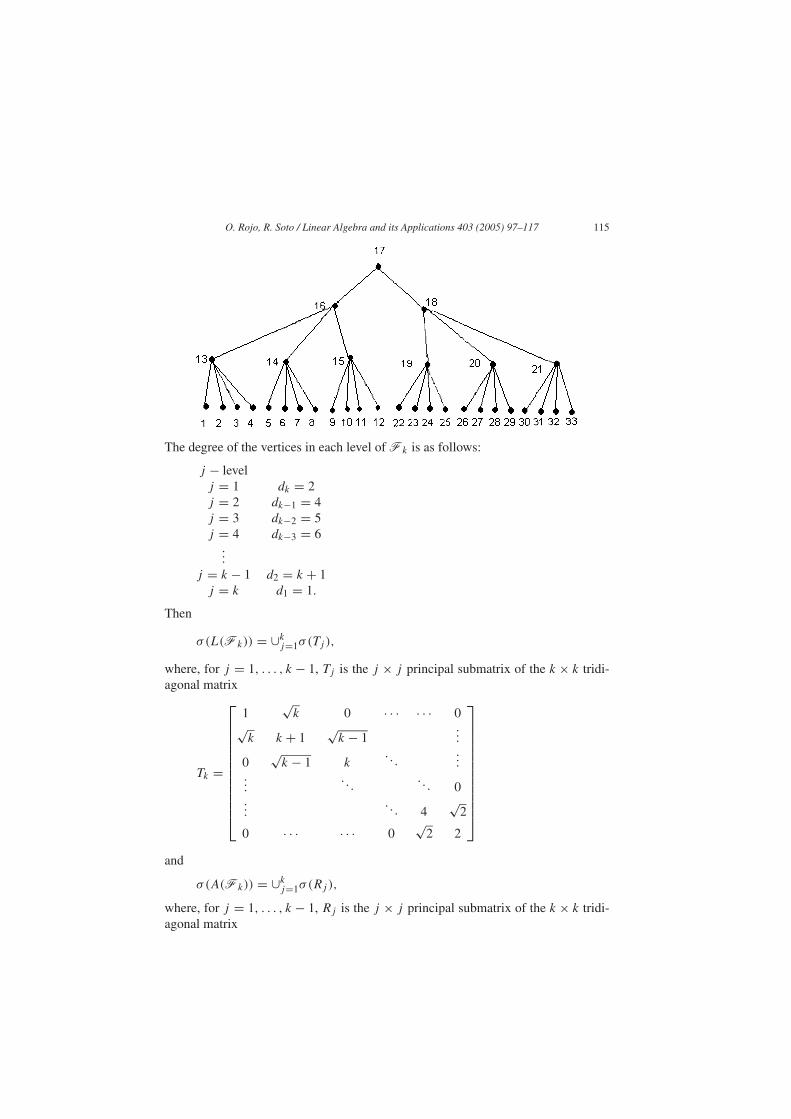
O. Rojo, R. Soto / Linear Algebra and its Applications 403 (2005) 97–117 115
The degree of the vertices in each level of Fk is as follows:
j − levelj = 1 dk = 2j = 2 dk−1 = 4j = 3 dk−2 = 5j = 4 dk−3 = 6
...
j = k − 1 d2 = k + 1j = k d1 = 1.
Then
σ(L(Fk)) = ∪kj=1σ(Tj ),
where, for j = 1, . . . , k − 1, Tj is the j × j principal submatrix of the k × k tridi-agonal matrix
Tk =
1√
k 0 · · · · · · 0√
k k + 1√
k − 1...
0√
k − 1 k. . .
......
. . .. . . 0
.... . . 4
√2
0 · · · · · · 0√
2 2
and
σ(A(Fk)) = ∪kj=1σ(Rj ),
where, for j = 1, . . . , k − 1, Rj is the j × j principal submatrix of the k × k tridi-agonal matrix

116 O. Rojo, R. Soto / Linear Algebra and its Applications 403 (2005) 97–117
Rk =
0√
k 0 · · · · · · 0√
k 0√
k − 1...
0√
k − 1. . .
. . ....
.... . .
. . .. . . 0
.... . . 0
√2
0 · · · · · · 0√
2 0
.
Example 7. For the tree F4 we have
T4 =
1 2 0 02 5
√3 0
0√
3 4√
20 0
√2 2
and the eigenvalues of L(F4) to four decimal places are
T1 : 1T2 : 0.1716 5.8284T3 : 0.0464 3.1794 6.7742T4 : 0 1.2363 3.8748 6.8890
The eigenvalues of the adjacency matrix A(F4) are the eigenvalues of the principalsubmatrices of
R4 =
0 2 0 02 0
√3 0
0√
3 0√
20 0
√2 0
and they are
R1 : 0R2 : −2 2R3 : −2.6458 0 2.6458R4 : −2.8284 −1 1 2.8284
Acknowledgment
The authors are grateful to the referee for valuable comments, which led to animproved version of the paper.

O. Rojo, R. Soto / Linear Algebra and its Applications 403 (2005) 97–117 117
References
[1] L.N. Trefethen, D. Bau III, Numerical Linear Algebra, Society for Industrial and Applied Mathemat-ics, 1997.
[2] M. Fiedler, Algebraic connectivity of graphs, Czechoslovak Math. J. 23 (1973) 298–305.[3] G.H. Golub, C.F. Van Loan, Matrix Computations, second ed., Johns Hopkins University Press, Bal-
timore, 1989.[4] R. Merris, Laplacian matrices of graphs: a survey, Linear Algebra Appl. 197–198 (1994) 143–176.[5] J.J. Molitierno, M. Neumann, B.L. Shader, Tight bounds on the algebraic connectivity of a balanced
binary tree, Electron. J. Linear Algebra 6 (2000) 62–71.[6] O. Rojo, The spectrum of the Laplacian matrix of a balanced binary tree, Linear Algebra Appl. 349
(2002) 203–219.[7] O. Rojo, M. Peña, A note on the integer eigenvalues of the Laplacian matrix of a balanced binary tree,
Linear Algebra Appl. 362 (2003) 293–300.
Copyright © 2022 FDOKUMEN


![Matrix floating[1]](https://static.fdokumen.com/doc/165x107/63234342078ed8e56c0ac6f9/matrix-floating1.jpg)