Aquat. Living Resour. 20, 77–84 (2007)c© EDP Sciences, IFREMER, IRD 2007DOI: 10.1051/alr:2007018www.edpsciences.org/alr

AquaticLivingResources

The spawning spatial structure of two co-occurring small pelagicfish off central southern Chile in 2005Claudio Castillo-Jordán1, Luis A. Cubillos1,a and Jorge Paramo2

1 Laboratorio de Evaluación de Poblaciones Marinas (EPOMAR), Departamento de Oceanografía, Universidad de Concepción, Casilla 160-C,Concepción, Chile

2 Grupo de Investigación Ciencia y Tecnología Pesquera Tropical (CITEPT), Universidad del Magdalena, Carrera 32, N◦ 22-08, Santa Marta,Colombia

Received 24 November 2006; Accepted 16 March 2007

Abstract – Anchovy and common sardine co-occur in the same reproductive and feeding habitat off central southernChile (33◦00′–41◦20′S), and have a similar reproductive strategy. Egg-survey data from one survey carried out duringthe austral winter in 2005 were used to analyze the spawning spatial structure of anchovy (Engraulis ringens) and com-mon sardine (Strangomera bentincki) through geostatistical techniques and generalized additive models. The spawningspatial structure of both species was characterized by a spatial autocorrelation intensity varying similarly with distancein all directions, ranging between 27.2 and 32.6 km for anchovy and common sardine, respectively. In average, egg den-sity of anchovy was higher than egg density of common sardine, with the bulk of the spawning for both species locatedin the southern sector of the study area (38◦S–40◦S). In this sector, both species showed an overlapped distribution, andegg densities were mainly associated to shallow and coastal zones, suggesting that coastal shape and bottom depth areimportant factors for the spawning of both species. In the south sector, the egg density of both species was positivelycorrelated, indicating that spatial structure of the spawning is not explained by a different strategy of space occupationamong anchovy and common sardine.

Key words: Spatial structure / Geostatistics / GAM modeling / Spawning areas / Pelagic fish eggs / Anchovy / Sardine

Résumé – Structure spatiale des pontes de deux petites espèces pélagiques, poissons coexistant au large descôtes du Chili (Centre-Sud) en 2005. L’anchois et la sardine commune fréquentent les mêmes zones de reproductionet d’alimentation au large du Chile (Centre-Sud, 33◦00′–41◦20′S), et ont des stratégies similaires de reproduction. Lesdonnées d’une campagne océanographique de récoltes des oeufs, qui s’est déroulée durant l’hiver austral de 2005, ontété utilisées pour analyser la structure spatiale des pontes de l’anchois (Engraulis ringens) et de la sardine (Strangomerabentincki), au moyen de techniques géostatistiques et de modèles additifs généralisés. La structure spatiale des deuxespèces était caractérisée par une intensité d’autocorrélation spatiale variant avec la distance et de façon similaire danstoutes les directions, s’étendant de 27,2 à 32,6 km respectivement, pour l’anchois et la sardine. En moyenne, la densitéen œufs d’anchois était plus élevée que celle de la sardine, avec une zone de forte densité pour les deux espèces, situéedans le secteur sud de la zone d’étude (38◦S–40◦S). Dans ce secteur, les distributions des deux espèces se recouvraient,et les densités en oeufs étaient associées principalement à des zones côtières et peu profondes, suggérant que la formede la côte et la profondeur sont des facteurs importants pour la reproduction des deux espèces. Dans le secteur sud, ladensité en œufs des deux espèces était positivement corrélée, indiquant que la structure spatiale des pontes n’est pasexpliquée par une stratégie différente de l’occupation de l’espace entre l’anchois et la sardine.

1 Introduction

In the central-south area off Chile (33◦00′S-41◦30′S),two commercially important small pelagic fish known as an-chovy (Engraulis ringens) and common sardine (Strangomerabentincki) are coexisting and inhabiting in the coastal zone ofa seasonal upwelling system (Cubillos et al. 1998; Cubilloset al. 2002). Anchovy and common sardine are caught by both

a Corresponding author: lucubillos@udec.cl

small-scale fishermen and industrial fleet of purse-seiners,with Talcahuano as the main port for landings. These speciesare caught together by fishermen because anchovy and com-mon sardine are co-occurring species and aggregated in mixedschools. Gerlotto et al. (2004) point out that common sar-dine and anchovy stocks are mixed and concentrated close tothe coast in several types of aggregations from small schoolsto dense layers, which cannot be differentiated acoustically.In addition, the biological characteristics are similar in terms

Article published by EDP Sciences and available at http://www.edpsciences.org/alr or http://dx.doi.org/10.1051/alr:2007018

78 C. Castillo-Jordán: Aquat. Living Resour. 20, 77–84 (2007)

of the spatial distribution, growth rate, natural mortality, agecomposition, reproduction time, spawning area, and recruit-ment time (Cubillos et al. 2001, 2002; Cubillos and Arcos2002).

According with Cubillos et al. (2001), the reproductivestrategy of these two species is to spawn at the end of southernwinter (August), when environmental conditions are character-ized by an alternation between northerly winds and southerlywinds. The northerly winds produce onshore transport andconvergence at the coast, favoring concentration and retentionof eggs and larvae at the coast, while southerly winds generatemoderate upwelling events favoring biological enrichment ofthe surface waters. This reproductive strategy of the species iscoherent with the triad hypothesis of Bakun (1996).

Although the reproductive strategy seems to be similar forboth species, the spatial structure in terms of the spatial corre-lation of egg densities, as well as the dependence of physicalvariables in the reproductive habitat over egg density could bedifferent for each species. Indeed, spatial structures and pat-terns can take several forms due to either exogenous or en-dogenous processes. Exogenous processes can induce spatialpatterns by factors independent of the variable of interest (e.g.physical gradients, transport, or the spatial configuration ofhabitats). Instead, endogenous ecological processes can deter-mine also a spatial structure, where the more relevant is eggpatchiness as an inherent property. In fact, eggs of a speciesare more likely to be spatially adjacent in a patchy fashionor exhibiting an “inherent” spatial autocorrelation because thespawning. This means that nearby values of egg density aremore likely to be similar than they would be by chance. Thegoal of this paper is to analyze the spawning spatial structureof the common sardine and anchovy, using information of oneegg survey carried out in winter 2005 in the central-south areaoff Chile (33◦00′S–41◦19′S). Geostatistical techniques are ap-plied to reveal the spatial autocorrelation of egg densities byexamining experimental variograms. The variogram range canbe thought of as an indicator of the average dimension of eggpatches as well as the average distance between egg patchesor clusters (see Petitgas 1993; Maravelias et al. 1996). In addi-tion, generalized additive models are used to analyze the influ-ence of sea surface temperature and the spatial configurationof the physical reproductive habitat. The results should be ofinterest for inferring and understanding differences in the ag-gregative strategies of the spawning of co-occurring species.

2 Material and methods

2.1 Study area and data

In order to determine the egg distribution and abundanceof anchovy and common sardine, a survey was carried outfrom August 21th to September 22th 2005, covering an areaof 32 523 km2. The study area was located in the central-south area off Chile (33◦00′S–41◦19′S), which represents themain spawning area for both species. According to Cubilloset al. (1999, 2001), spawning extends from July to Septem-ber, peaking between August and September for both anchovyand common sardine. In this way, a single survey is enoughto characterize the spawning process of the two species. The

Fig. 1. Study area of the egg survey (August 21–September 22, 2005),showing plankton stations (small dots) and positive stations with eggsfor anchovy (left) and common sardine (right). The bottom depth of100 m (inner) and 200 m (outer) is also shown along the coastal line.

study area was separated into three geographic zones, definedaccording with the orientation and shape of the coastal lineand the extension and distribution of the continental shelf (i.e.the 200 m bottom depth, Table 1, Fig. 1). The area between33◦00′S and 34◦20′S was considered an exploratory zone be-cause egg abundance practically have been not observed inthis zone previously (Castro et al. 1997; Castillo et al. 2002;Cubillos et al. 2005). In this zone transect lines were separatedby 20 nautical miles, with stations every 4 nautical miles alongeach transects. In the other two zones, the grid of plankton sta-tions were design to quantify egg densities of the species withtransect lines separated by 8 nautical miles and plankton sta-tions located 4 nautical miles apart. The central zone was allo-cated between 34◦46′S and 37◦10′S, while the south zone wasallocated between 37◦20′S and 41◦19′S (Fig. 1).

In each plankton station eggs were collected by verticalhauls with a CalVET net (25 cm diameter, 0.150 mm meshsize, Smith et al. 1985) from 70 m or close to the sea-bed fordepths lower than 70 m. Egg abundance was standardized tonumber of egg per 0.05 m2. In addition, in each plankton sta-tions sea surface temperature was recorded.

2.2 Geostatistics

Geostatistical techniques (Cressie 1993; Petitgas 1993)were used to describe the spatial structure of the egg density

C. Castillo-Jordán: Aquat. Living Resour. 20, 77–84 (2007) 79

Table 1. Description of the egg survey performed in the central-south spawning area of anchovy and common sardine off Chile in 2005.

Study area (33◦S–41◦19′S)North sector Central sector South sector

(33◦00′S–34◦20′S) (34◦46′S–37◦10′S) (37◦22′S–41◦19′S)Date 21 Sep.–22 Sep. 30 Aug.–15 Sep. 21 Aug.–31 Aug.Transect lines 4 21 32Number of stations 18 130 140Positive stations:

anchovy 7 (38.9%) 39 (30.0%) 63 (45.0%)common sardine 0 4 (3.1%) 36 (25.7%)

Total egg counts:anchovy 55 1815 4856

common sardine 0 10 1093Sea surface temperature (◦C) 13.4 (11.5–14.5) 12.3 (11.0–14.8) 11.7 (10.5–13.5)

of anchovy and common sardine, and to estimate the corre-lation range as an estimator of the average distance betweenegg patches as well as the mean egg density and its variance.Previously the coordinate system (latitude and longitude) wastransformed to nautical miles into Easting and Northing spatialcomponents by using UTM (Universal Transverse Mercator).The experimental variogram is defined as the variance of dif-ference between values that are h units apart and is a functionof variance and covariance, i.e.

γ̂(h) =1

2N(h)

N(h)∑i=1

[Z(xi) − Z(xi + h)]2 (1)

where h is a vector of distance and direction, and N(h) is thenumber of pairs of observations at distance h and given direc-tion. However, we also chose the robust (or stable) variogramestimator (Cressie and Hawkins 1980; Cressie 1993) since itpermitted a better definition for the variogram pattern for com-mon sardine:

2γ̂(h) =

(N(h)∑i=1|z(xi) − z(xi + h)|0.5

)4

(0.457 + 0.494

|N(h)|)

N(h)4· (2)

In order to explore and to detect whether the intensity of spatialautocorrelation vary according to direction (anisotropic pro-cess), experimental variograms were calculated for log trans-formed data in four directions (0◦, 45◦, 90◦ and 135◦). Therange and sill of these directional variograms were similarin both species (results not shown), reason for which omni-directional experimental variograms were computed for rawdata, this means including higher and zero densities. Asymp-totic functions such as the Spherical, Gaussian, and Exponen-tial models were fitted and selected according to the weightedleast-square minimization criterion of Cressie (1993). In thesefunctions, the nugget is the y-intercept, while the range and thesill are both determined by the upper inflection point where theline becomes flat. The x-coordinate of this inflexion point isthe range, while the y-coordinate is the sill. In addition, cross-validation (Isaaks and Srivastava 1989) was used to determinetwo kriging neighborhood parameters: the number of sectorsand the number of neighboring points used in the interpolationby kriging. The mean squared error of residuals was used to

select the best combination of the parameters (see Maraveliaset al. 1996). Ordinary point kriging was used to reproduce thestochastic processes across the region of interest to estimatethe egg density at any given locality within the study area. Weused the spatial module in S+ Spatial Stats software (Insight-ful Corporation) for exploring empirical variograms, and alsofor fitting models of variograms, while the EVA2 software (Pe-titgas and Prampart 1995; Petitgas and Lafont 1997) was usedfor variance estimation. The precision is given in terms of thecoefficient of variation (CV).

2.3 GAM modeling

To explore the dependence of egg density with envi-ronmental variables, we used Generalized Additive Models(GAM) with a quasipoisson error distribution and a log linkby using the “mgcv” library (v. 1.1-8) of Wood (2002, 2003)for the language and software R v. 2.0.2 (Ihaka and Gentle-man 1996; http://www.r-project.org). The general form of themodel was:

D = α + s(Long, Lat) + s(Depth) + s(SST) (3)

where α is the intercept, and s(•) represent a smooth func-tion (penalized regression splines), D is egg density (egg per0.05 m2), Long and Lat is the geographic longitude and lati-tude respectively; Depth is the bottom depth (m), and SST isthe sea surface temperature (◦C). We used the “mgcv” librarybecause it implements an automatic selection of the smoothingparameters associated with each smooth term on the basis ofgeneralized cross-validation (GCV). Crudely, cross-validationinvolves leaving one of the data-points out, fitting the modelto the remaining data, and then computing the squared differ-ence between those points. This procedure is repeated for alldata-points and for several amounts of smoothing, and hencethe smaller squared differences mean a better model. Also,one advantage of “mgcv” is the possibility of taking into ac-count the dependence on spatial location as an isotropic bi-variate function of longitude and latitude (Wood and Augustin2002). In fact, the correlation between Latitude and Longitudewas high (r = 0.884, n = 288), deserving this treatment. In-stead, the coefficients of correlation between Depth-Latitude(r = 0.207) and Depth-Longitude (r = 0.043) were lower, and

80 C. Castillo-Jordán: Aquat. Living Resour. 20, 77–84 (2007)

Fig. 2. Egg density of anchovy and common sardine in the study area,August-September 2005.

can be considered as an independent variable. In addition, SSTwas correlated better with Latitude (r = 0.534) and Longitude(r = 0.472) than with Depth (r = 0.185). First, Equation (3)was applied without temperature, and this model was namedas Model 1. Instead, when temperature was included the rela-tionship was named as Model 2.

3 Results

According with the incidence of positive stations, the bulkof the spawning of both species was more important in thesouth sector of the study area (Table 1, Fig. 1). Similar pat-tern was evident in terms of raw egg densities (Fig. 2). Indeed,the egg density of common sardine was practically null in thenorth and central sectors of the study area, except in some sta-tions in which egg counts were very low (Table 1, Fig. 2). Be-cause this is a limitation for the application of geostatisticaltechniques and GAM modeling, these techniques were appliedonly for the south sector for common sardine.

3.1 Spatial structural analysis and spawning patterns

For egg densities of anchovy a classical variogram wascomputed, while for the common sardine the robust exper-imental variogram was better. The directional variogramsshowed the same spatial autocorrelations in all directions (re-sults not showed), and according with the cross-validation,

the omni-directional spherical variogram was better for bothspecies (Fig. 3). The range of the variograms was satisfacto-rily determined in 14.7 and 17.6 nautical miles for anchovyand common sardine, respectively (27.2 and 32.6 km, respec-tively). The nugget is variability smaller than the samplingunit distance, as an effect not explained by spatial scale. Inthe case of anchovy, the nugget was null while for commonsardine the nugget was low (17% of the sill). The sill washigher for anchovy (= 14 634.56 egg per 0.05 m4) than for sar-dine (= 62.42 egg per 0.05 m4) because anchovy showed manysmall and few very large values inflating the variance.

According with the kriging, in the south sector of the studyarea, an important aggregation of anchovy and common sar-dine eggs was detected, with the bulk of the spawning dis-tributed from 38◦16′S to 40◦S for both species in the coastalsector (Figs. 4 and 5). In the north and central sectors, thespawning of anchovy revealed one centre of low egg densitieslocated between Valparaiso and San Antonio, and another onemore important within the Gulf of Arauco at 37◦05′S (Fig. 4).The geostatistical average egg density of anchovy for the en-tire study area was 32.8 eggs per 0.05 m2 (CV = 14.9%) whilefor the southern sector the average egg density of sardine was15.6 eggs per 0.05 m2 (CV = 6.04%).

3.2 GAM analysis

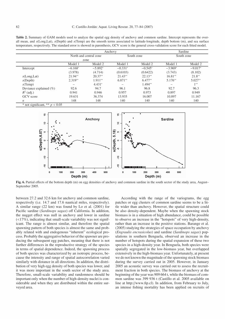
GAM modeling was carried out by separating two sectorsfor anchovy because of differences in egg densities, and onlythe south sector for common sardine. The results are summa-rized in Table 2. According with the general cross-validationscores (GCV), egg density of both species was better explainedby a bivariate function of Longitude and Latitude plus thebottom depth. Sea surface temperature was not significant foranchovy in the North-Central sector of the study area, and al-though significant effect was found in the south sector, its con-tribution to the overall fit was marginal. Similar results wereobserved in common sardine for the south sector (Table 2).

The effect of the bottom depth on the egg densities wasvery similar for both species (Fig. 6), the bulk of the spawn-ing tend to occur in waters lower than 75 m depth and peak-ing around 50 m depth of the sea bottom. In other words, thespawning of both species is restricted to the more coastal zoneof the study area.

The reproduction of the spatial distribution generated byGAM models was similar to the geostatistical results obtainedthrough kriging (results not shown). The spawning pattern ofanchovy had moderate egg density inside the Gulf of Arauco.Instead, in the south sector a similar spawning pattern was re-vealed for both species, with the bulk distributed between 38◦and 40◦S. It should be considered that both species showed ahigh co-occurrence of egg densities in the south sector, andalthough average egg density of common sardine was lowerthan the average anchovy egg density a good relationship be-tween log-transformed egg density values of both species wasfound in the south sector (r2 = 0.699, F = 321.9, p < 0.001,n = 140, Fig. 7).

C. Castillo-Jordán: Aquat. Living Resour. 20, 77–84 (2007) 81

Fig. 3. Omni-directional spherical model fitted to experimental variograms for total egg densities (eggs per 0.05 m2) of anchovy and commonsardine egg densities.

Fig. 4. Map of the surveyed area indicating the location of planktonstations and spatial distribution of anchovy eggs density (eggs per0.05 m2) as the reproduction of a spatially stochastic process by krig-ing.

4 Discussion

The main objective of this study was to detect differencesin the spatial structure in egg density of two co-occurring smallpelagic fish, which have a similar reproductive strategy in thecentral-south area off Chile (Cubillos et al. 2001). In the areabetween Valparaiso (33◦S) and Gulf of Arauco (37◦10′S), thespawning of common sardine was practically null. Instead,the bulk of the spawning of both species was important in the

Fig. 5. Map of the south surveyed area indicating the location ofplankton stations and spatial distribution of common sardine eggsdensity (eggs per 0.05 m2) as the reproduction of a spatially stochasticprocess by kriging, August–September 2005.

south sector of the study area (37◦22′S–41◦19′S). In the sur-vey sampling design, the inter-transect distance (North-Southdirection) was 8 nautical miles (14 km), while plankton sta-tions were 4 nautical miles (7.4 km) in the East-West direc-tion. Because the maximum range was 32.6 km for sardine(17.6 nautical miles), eggs collected more than 32.6 km apartshould be considered uncorrelated. In this way, inter-transectand inter-station distances were smaller than the patch size,allowing detecting, characterizing and quantifying the spatialpattern in the data. Therefore, the average egg density and vari-ance computed by conventional methods based on inferencemay be biased because that requires that observations are in-dependent.

According with the structural analysis, the range of thevariograms indicates that spatial autocorrelation fluctuates

82 C. Castillo-Jordán: Aquat. Living Resour. 20, 77–84 (2007)

Table 2. Summary of GAM models used to analyze the spatial egg density of anchovy and common sardine. Intercept represents the over-all mean, and s(Long,Lat), s(Depth) and s(Temp) are the smooth terms associated to latitude-longitude, depth bottom (m), and sea surfacetemperature, respectively. The standard error is showed in parenthesis, GCV score is the general cross-validation score for each fitted model.

Anchovy SardineNorth and central zone South zone South zone

zoneModel 1 Model 2 Model 1 Model 2 Model 1 Model 2

Intercept −6.168∗ −5.892∗ −0.331∗ −0.545∗ −3.969∗ −9.017∗

(3.978) (4.714) (0.6103) (0.6422) (3.743) (8.102)s(Long,Lat) 21.94∗∗ 20.37∗∗ 21.43∗∗ 22.13∗∗ 16.81∗∗ 21.8∗∗

s(Depth) 2.319∗∗ 1.911∗∗ 6.871∗∗ 6.477∗∗ 5.176∗∗ 5.027∗∗

s(Temp) − 4.431∗ − 1.494∗∗ − 1∗∗

Deviance explained (%) 92.6 94.7 96.1 96.8 92.7 96.3R2 (adj.) 0.941 0.946 0.957 0.973 0.897 0.949GCV score 19.631 36.374 13.935 16.007 10.897 11.167n 148 148 140 140 140 140* not significant, ** p < 0.05

Fig. 6. Partial effects of the bottom depth (m) on egg densities of anchovy and common sardine in the south sector of the study area, August–September 2005.

between 27.2 and 32.6 km for anchovy and common sardine,respectively (i.e. 14.7 and 17.6 nautical miles, respectively).A similar range (22 km) was found by Lo et al. (2001) forPacific sardine (Sardinops sagax) off California. In addition,the nugget effect was null in anchovy and lower in sardine(<17%), indicating that small-scale variability was not signif-icant. The range is almost similar, and therefore the spatialspawning pattern of both species is almost the same and prob-ably related with and endogenous “inherent” ecological pro-cess. Probably the aggregative behavior of the spawner are pro-ducing the subsequent egg patches, meaning that there is notfurther differences in the reproductive strategy of the speciesin terms of spatial dependence. Indeed, the spawning processof both species was characterized by an isotropic process, be-cause the intensity and range of spatial autocorrelation variedsimilarly with distance in all directions. In addition, the distri-bution of very high egg density of both species was lower, andit was more important in the south sector of the study area.Therefore, small-scale variability and randomness should beimportant only when the number of high-density nuclei is con-siderable and when they are distributed within the entire sur-veyed area.

According with the range of the variograms, the eggpatches or egg clusters of common sardine seems to be a lit-tle wider than anchovy. However, the spatial structure couldbe also density-dependent. Maybe when the spawning stockbiomass is in a situation of high abundance, could be possibleto observe an increase in the “hotspots” of very high-density,rather than an increase in the positive stations. Barange et al.(2005) studying the strategies of space occupation by anchovy(Engraulis encrasicolus) and sardine (Sardinops sagax) pop-ulations in southern Benguela, observed an increase in thenumber of hotspots during the spatial expansion of these twospecies in a high-density year. In Benguela, both species werespatially segregated in the low-biomass year, but overlappedextensively in the high-biomass year. Unfortunately, at presentwe do not known the magnitude of the spawning stock biomassduring the survey carried out in 2005. However, in January2005 an acoustic survey was carried out to assess the recruit-ment fraction in both species. The biomass of anchovy at thebeginning of the year was 909 664 t, while the biomass of com-mon sardine was 399 936 t (Castillo et al. 2005 available online at http://www.fip.cl). In addition, from February to July,an intense fishing mortality has been applied on recruits of

C. Castillo-Jordán: Aquat. Living Resour. 20, 77–84 (2007) 83

Fig. 7. Relationship between the common sardine and anchovy eggdensities (log-transformed values) in the south sector of the studyarea.

both species, particularly in the central sector of the study area.In 2005, the catch obtained during the first half of the yearwas 361 795 t of anchovy and 218 781 t of common sardine(SERNAPESCA 2006). This implies that the survival spawn-ing stock biomass in August could be lower for both species,and particularly for common sardine. Therefore, the low eggdensity of common sardine in the North-Central and Southsectors could be explained by a lower spawning stock biomass.In this way, we can conclude that the spawning of both specieswas not spatially segregated during a year in which the spawn-ing stock biomass was probably low.

According with GAM models, the best model to explainthe egg densities depend almost exclusively on geographic pre-dictors (longitude, latitude and bottom depth). Since egg den-sities depend exclusively on quantities that are not sensitivefor fish, the results could be not completely satisfactory froma biological point of view. In fact, often temperature is of bi-ological interest even if it is not the most important variablein model results. Nevertheless, Giannoulaki et al. (2006) ana-lyzed the effect of coastal topography on the spatial structureof anchovy and sardine in the eastern Mediterranean Sea; theysuggest that environmental spatial heterogeneity attributableto coastal topography affected the way fish schools were orga-nized into aggregations. Stratoudakis et al. (2003) used gener-alized additive model to explain sardine (Sardina pilchardus)egg distribution data. They used only spatial covariates suchas latitude, longitude, distance along the coastline, closest dis-tance to the coastline, and depth bottom.

In central southern Chile, the spatial reproductive strat-egy of both species seems to be similar, and also the spa-tial distribution of the spawning, which is dependent on thephysical characteristics of the spawning habitat. For instance,the bulk of the spawning is occurring in shallow waters andrestricted to the more coastal sector. The spatial differencesbetween the north, central, and south sectors of the study area

are associated with differences in the extension of the conti-nental shelf, the shape of the coastal line, the bottom depthdistribution, and also the presence of bays and protected zoneslike the Gulf of Arauco at 37◦05′S. These factors associatedwith some environmental variables such as wind regimes dur-ing the winter to spring transition (e.g. Cubillos et al. 2001)probably are more important for the spawning of both species,than physical variables as for example temperature, that canbe detected directly by spawner. In fact, the sea surface tem-perature during the survey was distributed homogeneously andfluctuating in a narrow range (11 and 13 ◦C, Table 1). This nar-row range of sea surface temperature is probably the optimumfor spawning, and to detect an important effect on egg densitiesa wide enough range of temperatures outside the biological op-timum are required for GAM modeling. In addition, probablythe river runoff and precipitation could be also important fac-tors for spawning, because these factors are affecting coastalsalinity during August to September in the study area (Castroand Hernández 2000; Castro et al. 2000; Quiñones and Montes2001).

According with the evidence showed in this paper, thecoastal shape and the bottom depth are important factors totake into account for the spawning distribution of both species.In the central sector, the continental shelf is wide and the threebays located there (Gulf of Arauco, “Bahía de Concepción”,and “Bahía Coliumo”) are acting as important spawning zones,probably through retention and concentration processes drivenfor winds regimes (Bakun 1996). In the southern sector, thecoastal shape is also acting as a big bay between 38◦20′ and40◦S. The overlapped distribution of the spawning in the southsector, as well as the correlation between eggs density of bothspecies, are indicating that the spatial structure of the spawn-ing is not explained by a different strategy of space occupationby anchovy and common sardine. Nevertheless, although morestudies are required to validate this statement our results canbe considered a first study for determine differences in the ag-gregative strategies of co-occurring species like anchovy andcommon sardine in central southern Chile.

Acknowledgements. We thank Nancy C.H. Lo, Andrés Uriarte,Leonardo R. Castro, and Luisa Espinosa for reviewing the results ofthis study. Thanks to two anonymous referees for useful suggestions.Thanks also go to the crew of the fishing boats “MARGARITA DELMAR”, “EBENEZER”, “AQUA LUNA” and “DON LEONEL”, aswell as the crew of the research vessel “KAY KAY” of the Univer-sidad de Concepción. Thank to the personnel participating on board,particularly Samuel Soto, Christian Valero, Rodrigo Veas, Elson Leal,Katty Riquelme, Sebastian Vasquez and Germán Vasquez. We want tothank to people of LOPEL (Universidad de Concepción), for collect-ing and processing plankton samples. This research was funded bythe “Fondo de Investigación Pesquera” (http://www.fip.cl), ResearchProject FIP N◦ 2005-02.

References

Bakun A., 1996, Patterns in the ocean: ocean processes and ma-rine population dynamics. University of California Sea Grant,San Diego, California, USA, and Centro de InvestigacionesBiológicas de Noroeste, La Paz, Baja California Sur, México.

84 C. Castillo-Jordán: Aquat. Living Resour. 20, 77–84 (2007)

Barange M., Coetzee J.C., Twatwa N.M., 2005, Strategies of spaceoccupation in anchovy and sardine in the southern Benguela: therole of stock size and intra-species competition. ICES J. Mar. Sci.62, 645–654.

Castillo J., Barbieri M.A., Espejo M., Saavedra A., Catasti V.,2002, Evaluación acústica de la biomasa, abundancia, distribu-ción espacial y caracterización de las agregaciones de anchovetay sardina común en el periodo de desove, invierno 2001. In:Evaluacion hidroacústica del stock desovante de anchoveta y sar-dina común, centro-sur, 2001. Inf. Téc. FIP–IT/2001-14, 241 p.(http://www.fip.cl)

Castillo J., Saavedra A., Gálvez P., 2005, Evaluación acústica de labiomasa, abundancia, distribución espacial y caracterización decardúmenes de anchoveta y sardina común durante el periodode reclutamiento. Zona Centro-Sur. Verano 2005. In: Evaluaciónhidroacústica del reclutamiento de anchoveta y sardina comúnentre V y X Regiones, 2004. Inf. Téc. FIP–IT/2004-05, 206 p.(http://www.fip.cl)

Castro L., Quiñones R., Arancibia H., Figueroa D., Roa R., SobarzoM., Retamal M., 1997, Areas de desove de anchoveta y sar-dina común en Chile central. Inf. Téc. FIP-IT/96-11, 114 p.(http://www.fip.cl)

Castro L.R., Hernández E.H., 2000, Early life stages survival of theanchoveta, Engraulis ringens, off central Chile during the 1995and 1996 winter spawning season. Trans. Am. Fish. Soc. 129,1107–1117.

Castro L.R., Salinas G.R., Hernández E.H., 2000, Environmental in-fluences on winter spawning of the anchoveta, Engraulis ringens,off Central Chile. Mar. Ecol. Prog. Ser. 197, 247–258.

Cressie N.A.C., Hawkins D.M., 1980, Robust estimation of the vari-ogram. I. J. Int. Assoc. Math. Geol. 12, 115–125.

Cressie N.A.C., 1993, Statistics for spatial data. John Wiley and Sons,New York.

Cubillos L., Canales M., Hernández A., Bucarey D., Vilugrón L.,Miranda L.. 1998, Poder de pesca, esfuerzo de pesca y cam-bios estacionales e interanuales en la abundancia relativa deStrangomera bentincki y Engraulis ringens en el área frente aTalcahuano, Chile (1990–1997). Invest. Mar. 26, 3–14.

Cubillos L., Canales M., Bucarey D., Rojas A., Alarcón R., 1999,Epoca reproductiva y talla media de primera madurez sexual deStrangomera bentincki y Engraulis ringens en la zona centro-surde Chile en el período 1993–1997. Invest. Mar. 27, 73–86.

Cubillos L.A., Arcos D.F., Canales M., Bucarey D., 2001, Seasonalgrowth of small pelagic fish off Talcahuano (37◦S–73◦W), Chile:a consequence of their reproductive strategy to seasonal up-welling? Aquat. Living Resour. 14, 115–124.

Cubillos L.A., Bucarey D.A., Canales M., 2002, Monthly abundanceestimation for common sardine Strangomera bentincki and an-chovy Engraulis ringens in the central-south Chile (34–40◦S).Fish. Res. 57, 117–130.

Cubillos L.A., Arcos D.F. 2002, Recruitment of common sardine(Strangomera bentincki) and anchovy (Engraulis ringens) in the1990s, and impact of the 1997–98 El Niño. Aquat. Living Resour.15, 87–94.

Cubillos L., Castro L., Oyarzún C. 2005, Evaluación del stock deso-vante de anchoveta y sardina común entre la V y X Regiones, año2004. Inf. Téc. FIP–IT/2004-03, 120 p. (http://www.fip.cl)

Gerlotto F., Castillo J., Saavedra A., Barbieri M.A., Espejo M., CotelP., 2004, Three-dimensional structure and avoidance behaviour ofanchovy and common sardine schools in central southern Chile.ICES J. Mar. Sci. 61, 1120–1126.

Giannoulaki M., Machias A., Koutsikopoulus, Somarakis S., 2006,The effect of coastal topography on the spatial structure of an-chovy and sardine. ICES J. Mar. Sci. 63, 650–662.

Ihaka R., Gentleman R., 1996, A language for data analysis andgraphics. J. Comput. Graph. Stat. 5, 299–314.

Isaaks E.H., Srivastava R.M. 1989, An introduction to applied geo-statistics. Oxford University Press, New York.

Lo N.C.H., Hunter J.R., Charter R., 2001, Use of a continuous eggsampler for ichthyoplankton surveys: application to the estima-tion of daily egg production of Pacific sardine (Sardinops sagax)off California. Fish. Bull. 99, 554–571.

Maravelias C., Reid D.G., Simmonds E.J., Haralabous J., 1996,Spatial analysis and mapping of acoustic survey data in the pres-ence of high local variability: geostatistical application to NorthSea herring (Clupea harengus). Can. J. Fish. Aquat. Sci. 53,1497–1505.

Petitgas P., 1993, Geostatistics for fish stock assessments: a reviewand an acoustic application. ICES J. Mar. Sci. 50, 285–298.

Petitgas P., 2001, Geoestatistics in fisheries survey design and stockassessment: models, variances and applications. Fish. Fish. 2,231–249.

Petitgas P., Prampart A., 1995, EVA: Estimation Variance: A geosta-tistical software for structure characterization and variance com-putation, Editions de l’Orstom, collection logORSTOM, Paris.

Petitgas P., Lafont T., 1997, EVA 2: Estimation Variance. Version 2:A geostatistical software on Windows 95 for the precision of fishstock assessment surveys. ICES CM-1997/Y:22.

Quiñones R.A., Montes R.M., 2001, Relationship between freshwaterinput to the coastal zone and the historical landings of the ben-thic/demersal fish Eleginops maclovinus in central-south Chile.Fish. Oceanogr. 10, 311–328

Rivoirard J., Simmonds J., Foote K.G., Fernandes P., Bez N., 2000,Geostatistics for Estimating Fish Abundance. Blackwell Science,London.

SERNAPESCA, 2006, Anuario estadístico de pesca, 2005. ServicioNacional de Pesca, Chile.

Smith P.E., Flerx W., Hewitt R.P., 1985, The CalCOFI vertical eggtow (CalVET) net. In: R. Lasker (ed.), An egg production methodfor estimating spawning biomass of pelagic fish: application tothe northern anchovy, Engraulis mordax. U.S. Dep. Commer.,NOAA Tech. Rep. NMFS 36, 27–32.

Stratoudakis Y., Bernal M., Borchers D.L., Borges M.F., 2003,Changes in the distribution of sardine eggs and larvae offPortugal, 1985-2000. Fish. Oceanogr. 12, 49–60.

Wood S.N., 2000, Modelling and smoothing parameter estimationwith multiple quadratic Penalties. J. R. Stat. Soc. B 62, 413–428.

Wood S.N., 2003, Thin-plate regression splines. J. R. Stat. Soc. B 65,95–114.

Wood S.N., Augustin, N.H., 2002, GAMs with integrated model se-lection using penalized regression splines and applications to en-vironmental modelling. Ecol. Model. 157, 157–177.