Seediscussions,stats,andauthorprofilesforthispublicationat:https://www.researchgate.net/publication/11353132

TheSpatialDimensionsofElectricallyCoupledNetworksofInterneuronsintheNeocortex

ArticleinTheJournalofNeuroscience:TheOfficialJournaloftheSocietyforNeuroscience·June2002

Source:PubMed

CITATIONS

176

READS

33

7authors,including:

YaelAmitai

Ben-GurionUniversityoftheNegev

45PUBLICATIONS3,664CITATIONS

SEEPROFILE

MichaelBeierlein

UniversityofTexasHealthScienceCenteratH…

27PUBLICATIONS2,823CITATIONS

SEEPROFILE

SaundraLPatrick

BrownUniversity

24PUBLICATIONS1,442CITATIONS

SEEPROFILE

DavidGolomb

Ben-GurionUniversityoftheNegev

76PUBLICATIONS2,981CITATIONS

SEEPROFILE

AllcontentfollowingthispagewasuploadedbySaundraLPatrickon04December2016.

Theuserhasrequestedenhancementofthedownloadedfile.Allin-textreferencesunderlinedinblueareaddedtotheoriginaldocument

andarelinkedtopublicationsonResearchGate,lettingyouaccessandreadthemimmediately.

The Spatial Dimensions of Electrically Coupled Networks ofInterneurons in the Neocortex

Yael Amitai,1,2 Jay R. Gibson,1 Michael Beierlein,1 Saundra L. Patrick,1 Alice M. Ho,1 Barry W. Connors,1and David Golomb2

1Department of Neuroscience, Brown University, Providence, Rhode Island 02912, and 2Department of Physiology andZlotowski Center for Neuroscience, Faculty of Health Sciences, Ben-Gurion University, Beer-Sheva 84105, Israel

Inhibitory interneurons of the neocortex are electrically coupled tocells of the same type through gap junctions. We studied thespatial organization of two types of interneurons in the rat somato-sensory cortex: fast-spiking (FS) parvalbumin-immunoreactive(PV�) cells, and low threshold-spiking (LTS) somatostatin-immunoreactive (SS�) cells. Paired recordings in layer 4 demon-strated that both the probability of coupling and the couplingcoefficient drop steeply with intersomatic distance, reaching zerobeyond 200 �m. The dendritic arbors of FS and LTS cells werereconstructed from electrophysiologically characterized, biocytin-filled cells; the two cell types had only minor differences in thenumber and span of their dendrites. However, there was a mark-edly higher density of PV� cells than SS� cells. PV� cells weredensest in layer 4, while SS� cell density peaked in the subgranu-lar layers. From these data we estimate that there is measurable

electrical coupling (directly or indirectly via intermediary cells)between each interneuron and 20–50 others. The large number ofelectrical synapses implies that each interneuron participates in alarge, continuous syncytium. To evaluate the functional signifi-cance of these findings, we examined several simple architecturesof coupled networks analytically. We present a mathematicalmethod to estimate the average summated coupling conductancethat each cell receives from all of its neighbors, and the averageleak conductance of individual cells, and we suggest that thesehave the same order of magnitude. These quantitative results haveimportant implications for the effects of electrical coupling on thedynamic behavior of interneuron networks.

Key words: FS cells; LTS cells; inhibitory interneurons; gapjunctions; dendritic fields; coupling coefficient; coupling con-ductance; network architecture

The circuitry of the neocortex has traditionally been representedby maps of neurons that are interconnected by axons and chem-ical synapses (Braitenberg, 1978; White, 1989). This is an impov-erished view, however, because there is now strong evidence thatelectrical synapses are also a frequent and important feature ofneocortical circuits. Electrical synapses are most prevalent be-tween inhibitory interneurons (Galarreta and Hestrin, 1999; Gib-son et al., 1999). The circuits defined by electrical synapses can behighly specific; among two common types of interneurons in theneocortex, the large majority of electrical synapses interconnectcells of the same type (Gibson et al., 1999). The importance ofelectrical synapses to the function of the neocortex is still poorlyunderstood, but recent studies suggest a role in neuronal synchro-nization and rhythm generation (Benardo, 1997; Beierlein et al.,2000; Galaretta and Hestrin, 2001; Deans et al., 2001).

Understanding what electrical synapses do in the neocortex,and precisely how they do it, will require quantitative informationabout the patterns of neural circuits defined by electrical connec-tions. Important issues include the incidence of connectivity, theorganization and the size of coupled assemblies of neurons, andthe strength of the electrical coupling each cell has with othercells. These kinds of data have been hard to come by. The

anatomical basis of electrical synapses is the gap junction (Ben-nett, 1977), a structure visible only with electron microscopy.Very few studies have described gap junctions between neurons inthe mammalian forebrain, and most of these have been betweencertain types of interneurons in either the neocortex (Sloper,1972) or hippocampus (Kosaka, 1983; Kosaka and Hama, 1985).Unlike chemical synapses in the cerebral cortex, gap junctionshave been seen most frequently at dendrodendritic and dendro-somatic sites (Sloper and Powell, 1978; Tamas et al., 2000; Sza-badics et al., 2001). Although this is very important information,it does not reveal the scale of electrical coupling at the level oflarger interneuronal circuits.

We have used data derived from dual recordings of electricallycoupled neurons in the rat somatosensory cortex, anatomicalreconstructions and immunohistochemistry for specific markersof GABAergic neurons, and theoretical analysis to study thespatial distribution of two coupled populations of interneurons inthe neocortex. Our goal has been to provide quantitative answersto the following questions: Do coupled neurons form small,restricted clusters or large, continuous networks? On average,how many neurons are coupled to each individual neuron? Whatare the effects of gap junctions on the biophysical properties of theneurons and the network? Our data suggest that GABAergicneurons of the neocortex form large electrically interconnectednetworks, where each neuron contacts tens of other neurons. Wealso show that the input conductance attributable to nonjunc-tional membrane and that attributable to the sum of electricalsynapses onto all other neurons have similar magnitudes; thisimplies that approximately one-half of the input conductancemeasured experimentally is contributed by gap junctions.

Received Dec. 4, 2001; revised Feb. 1, 2002; accepted Feb. 15, 2002.This research was supported by National Institutes of Health Grants NS25983 and

DA125000 (B.W.C.), United States—Israel Binational Science Foundation Grants9700043 (Y.A., B.W.C.) and 9800015 (D.G.), and Israel Science Foundation Grant59/98 (Y.A.). We thank E. Bienenstock, D. Hansel, and C. Meunier for helpfuldiscussions.

Correspondence should be addressed to Dr. Yael Amitai, Department of Physi-ology, Faculty of Health Sciences, Box 653, Ben-Gurion University, Beer-Sheva84105, Israel. E-mail: yaela@bgumail.bgu.ac.il.Copyright © 2002 Society for Neuroscience 0270-6474/02/224142-11$15.00/0

The Journal of Neuroscience, May 15, 2002, 22(10):4142–4152

MATERIALS AND METHODSSlice preparation and recording. Thalamocortical slices 400 �m thick wereobtained from Sprague–Dawley rats aged postnatal day 14 (P14) to P21,as described previously (Gibson et al., 1999). The slices were incubatedfor 1 hour and then placed in a submersion chamber at 32°C for record-ing. The bathing solution contained (in mM): 126 NaCl, 3 KCl, 1.25NaH2PO4 , 2 MgSO4 , 26 NaHCO3 , 10 dextrose, and 2 CaCl2 , saturatedwith 95% O2 /5% CO2. Micropipettes were filled with (in mM): 135K-gluconate, 4 KCl, 2 NaCl, 10 HEPES, 0.2–4 EGTA, 4 ATP-Mg, 0.3and GTP-Tris, 0.5–10 phosphocreatine-Tris, pH 7.25, 295 mOsm. Insome experiments, neurobiotin or biocytin (4 mg/ml) was added to thenormal filling solution. All recordings were made in current–clampmode, under infrared-differential interference contrast visualization. Allneurons were classified according to their firing pattern in response to aninjection of a square current pulse as either fast spiking (FS) cells orlow-threshold spiking (LTS) cells (details given in Gibson et al., 1999).When depolarized, FS cells fired with high frequencies of narrow actionpotentials, with little or no frequency adaptation. LTS cells had a ten-dency to fire on the rebound when depolarized from more negativemembrane potentials, their spikes were broader, and they exhibited clearfrequency adaptation. To characterize the electrical coupling betweentwo cells, a step current was injected into one cell and the voltageresponses of both cells were measured (see also Gibson et al., 1999). Thecoupling coefficient (CC) was defined as the ratio between the steady-state voltage deflection of the postjunctional cell and that of the prejunc-tional cell. Cells are defined as “electrically coupled” if the measured CCbetween them is �0.01, the smallest that can be reliably distinguishedabove the membrane voltage noise.

Histolog ical procedures. Slices that contained stained cells were fixed in4% paraformaldehyde in 0.1 M phosphate buffer, transferred to 30%sucrose, resectioned to 80 �m, and reacted with the avidin–biotin–peroxidase [avidin–biotin complex (ABC)] procedure (Vector Labora-tories, Burlingame, CA). For immunohistochemistry, Sprague–Dawleyrats aged P16–P18 were anesthetized with 30 mg/kg pentobarbital,perfused intracardially with 5 ml of heparinized saline followed by 4%paraformaldehyde in 0.1 M phosphate buffer, pH 5.4, for 25 min. Brainswere removed, hemisected, and placed in fixative for an additional 2 hrbefore changing to 0.1 M phosphate buffer. Subsequently, tissue wascryoprotected in 30% sucrose/0.1 M phosphate buffer, pH 7.4, overnight.The tissue was sliced at 60 �m along the thalamocortical plane (Agmonand Connors, 1991), which is approximately parallel to the barrel rows.Tissue was washed three times in PBS (0.1 M phosphate/0.15 M NaCl atpH 7.4) before incubation in 0.5% H2O2 for 1 hr. Slices were washedthree times in PBS followed by three more washes in Tris-buffered saline(TBS; 0.05 M Tris/0.15 NaCl, pH 7.4) for 10 min each. The slices wereincubated overnight at room temperature with shaking in primary anti-serum for either somatostatin (SS; Peninsula, San Carlos, CA) or parv-albumin (PV; Sigma, St. Louis, MO). Final concentrations of eachantiserum were 1:1000 and 1:400, respectively, including 10% normalgoat serum, 2% bovine serum albumin, 0.5% Triton X-100, and TBS (allpurchased from Sigma). On day 2, the tissue was washed three times inTBS and incubated 3 hr at room temperature in biotinylated anti-rabbitIgG (Vector Laboratories) using a 1:200 final dilution including 10%normal goat serum, 2% bovine serum albumin, 0.5% Triton X-100, andTBS. After several rinses, an ABC Elite kit (Vector Laboratories) wasused to visualize somatostatin or parvalbumin.

Morphometric analysis. Stained cells were digitally reconstructed at40� magnification with a Neurolucida system (MicroBrightField Inc.,Colchester, VT), and the dendritic branching patterns were evaluatedusing a standard Sholl analysis (Sholl, 1956). Sections reacted for PV orSS were viewed under the light microscope at 10� magnification andmapped with Neurolucida software in seven different, randomly selectedsections taken from three different animals. Stained cells were counted inat least 2-mm-wide vertical strips across all layers of the primary somato-sensory cortex. Background staining was sufficient to allow determinationof the borders of cortical laminas. In some cases, adjacent sectionswere stained for cytochrome oxydase to reveal layer 4 and the barrelstructures.

Cell density in thin sections was calculated with the Neurolucidasoftware. For additional analysis, the coordinates of cells in mappedsections were converted into ASCII files and analyzed using a routinewritten in Matlab. In this routine, cell density was calculated by dividingeach section into 30 � 50 �m rectangular bins, and a sliding average ofthe number of cells was performed in 4 � 4 such rectangles. To calculatethe volume density of the cells, we made the following measurements and

assumptions: (1) The maximal depth of focus (z-axis) was measured withNeurolucida and found to be �12 �m. (2) The collapse of the tissuealong the z-axis was estimated to be �60% (Benes and Lang, 2001); thus12 �m represents 30 �m of unfixed tissue thickness. (3) Because thesomata of many viewed cells in the thin plane of view are cut in themiddle, we added another 5 �m for each side of the section. Accordingly,the tissue thickness (z-axis) was additionally corrected to a value of 40�m for calculations of cell density by volume. We call this correctedmeasure the “effective thickness” of the tissue.

RESULTSMorphology of dendritic trees of FS andLTS interneuronsUltrastructural studies suggest that gap junctions form betweendendrites, or between dendrites and somata, of inhibitory neu-rons (Tamas et al., 2000; Szabadics et al., 2001). Thus, the poten-tial for such a junction exists wherever dendrosomatic membranesof two cells are in close proximity. We analyzed the spatial extentof the dendritic trees of FS and LTS interneurons. The dendrites ofeight FS cells and seven LTS cells that were well stained withbiocytin were fully reconstructed (Fig. 1). The dendritic trees ofboth types had variable profiles, and there was no clear correla-tion between the physiological type and any common morpholog-ical classification of dendritic pattern such as “bitufted” or “mul-tipolar.” Other studies of neocortical interneurons have alsoconcluded that the somatodendritic morphology of these cellsdoes not distinguish their subtype (Kawaguchi and Kubota, 1997;Bayraktar et al., 2000). Sholl analysis of the dendrites revealedsome quantitative differences between the two cell types (Fig.2A,B). The total proximal dendritic length (�200 �m from thesoma) was �17% larger for FS cells than for LTS cells (1690 �640 �m and 1440 � 890 �m, respectively), because FS cells hadmore primary dendrites and proximal branching (Fig. 1). How-ever, the dendrites of FS cells rarely extended beyond 400 �m,whereas some LTS cells possessed branches that extended �600�m. These longer dendrites were usually vertically oriented,ascended toward the pia, and account for the long tail in the LTSSholl histogram (Figs. 1, 2B) and the small deviation to the rightin the cumulative probability plot (Fig. 2C). For both cell types,�80–90% of their total dendritic length occurred within 200 �mfrom the soma (Fig. 2C). We conclude that the dendritic profilesof FS and LTS cells in layer 4 are similar in their general outline,and show only minor quantitative differences.

Figure 1. The soma-dendritic morphology of FS and LTS cells is rathervariable.

Amitai et al. • Size of Coupled Networks of Interneurons J. Neurosci., May 15, 2002, 22(10):4142–4152 4143

The spatial distribution of parvalbumin- andsomatostatin-immunoreactive cellsPrevious studies from our laboratory showed that FS cells weregenerally parvalbumin immunoreactive (PV�), while most LTScells were somatostatin immunoreactive (SS�) (Gibson et al.,1999). Studies from other laboratories have also concluded thatPV� and SS� cells correspond to two such specific and nonover-lapping populations of interneurons, distinguished by morphol-ogy and electrophysiology (Kubota et al., 1994; Gonchar andBurkhalter, 1997; Kawaguchi and Kubota, 1997). We used thesemolecular markers to analyze the spatial organization of the twoclasses of interneuron populations quantitatively. Sections of bar-rel cortex were cut in either the thalamocortical plane angle asused for our electrophysiology experiments (Agmon and Con-nors, 1991) or in the tangential plane parallel to the pia and thenprocessed for PV or SS immunoreactivity. Both immunostainingmethods stained only partial dendritic arbors. There were, how-ever, striking differences in the patterns of axonal immunostain-ing. Single SS� axons were seen coursing for hundreds of micronsthrough single sections, most often along the vertical dimension(Fig. 3A). There was an especially dense plexus of SS� axons inlayer 1. These features are consistent with the axonal arboriza-tion features of Martinotti cells, which have vertically projecting

axons that arborize in layer 1, and which are SS� (Kawaguchiand Kubota, 1997). In contrast, PV� axons could rarely be tracedfor any significant length. Instead, PV sections had numerousclear rings of stained boutons surrounding the somata of un-stained cells. These were especially prominent in layer 4 (Fig. 3B),and are consistent with the general conclusion that many PV�cells are basket cells (Hendry et al., 1989; Akil and Lewis, 1992).

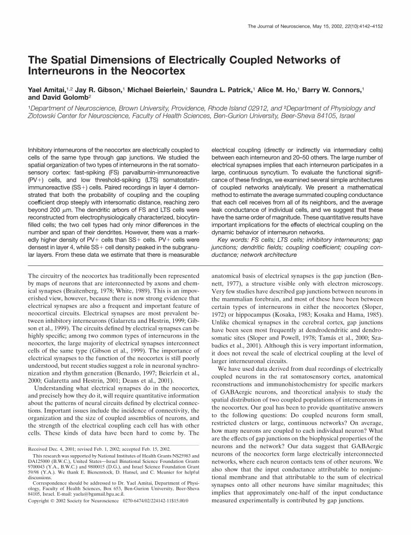
The average density of PV� cells across the entire corticalthickness was larger than that of SS� cells (92 � 9 vs 67 � 12cells/mm2, respectively). Because our estimated effective thick-ness of the sections is 40 �m (see Materials and Methods), wecalculated that the average neuron density by volume (�) was�2300 � 225 cells/mm3 for PV� cells and 1675 � 300 cells/mm3

for SS� cells.Both interneuron types were present in layers 2 through 6, but

they had very different distributions of density. The density ofPV� cells was especially high in layer 4, whereas SS� cells weremore concentrated in lower laminas (Fig. 4). Tangential sectionsthrough layer 4 revealed a higher density of PV� cells inside thebarrel borders (data not shown; Sanchez et al., 1992; McMullen etal., 1994). Autocorrelation of the radius vector of each cell againstall other cells in tangential sections through several layers did notreveal any anisotropy for both cell types (data not shown).

Figure 2. Sholl analysis of the inhibitory neurons from Figure 1 reveals more primary branches for FS cells (A) and a “tail” of longer branches in LTScells ( B). Comparing the cumulative length of the two cell types shows that for both, 80–90% of the dendrites occurred within 200 �m of the soma. FScells, closed circles; LTS cells, open squares.

Figure 3. Immunohistochemistry for somatostatin (A) and parvalbumin (B) in layer 4. Arrows in A point to a somatostatin-positive axon crossingupward. Arrows in B point to punctate parvalbumin-positive terminal staining around the somata of cells. Scale bars: A, 100 �m; B, 20 �m.

4144 J. Neurosci., May 15, 2002, 22(10):4142–4152 Amitai et al. • Size of Coupled Networks of Interneurons

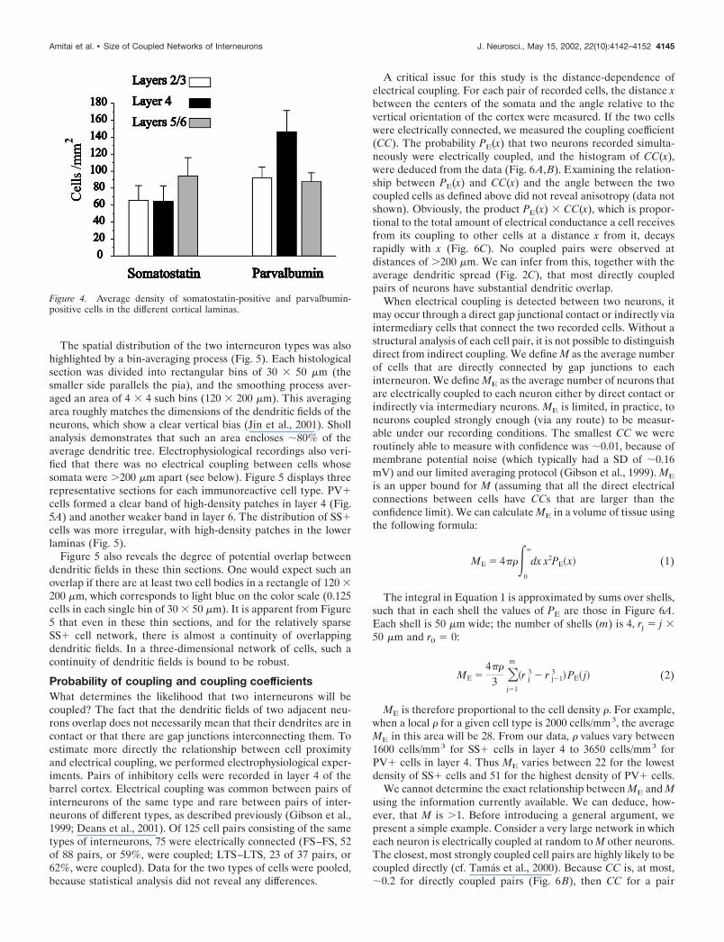
The spatial distribution of the two interneuron types was alsohighlighted by a bin-averaging process (Fig. 5). Each histologicalsection was divided into rectangular bins of 30 � 50 �m (thesmaller side parallels the pia), and the smoothing process aver-aged an area of 4 � 4 such bins (120 � 200 �m). This averagingarea roughly matches the dimensions of the dendritic fields of theneurons, which show a clear vertical bias (Jin et al., 2001). Shollanalysis demonstrates that such an area encloses �80% of theaverage dendritic tree. Electrophysiological recordings also veri-fied that there was no electrical coupling between cells whosesomata were �200 �m apart (see below). Figure 5 displays threerepresentative sections for each immunoreactive cell type. PV�cells formed a clear band of high-density patches in layer 4 (Fig.5A) and another weaker band in layer 6. The distribution of SS�cells was more irregular, with high-density patches in the lowerlaminas (Fig. 5).

Figure 5 also reveals the degree of potential overlap betweendendritic fields in these thin sections. One would expect such anoverlap if there are at least two cell bodies in a rectangle of 120 �200 �m, which corresponds to light blue on the color scale (0.125cells in each single bin of 30 � 50 �m). It is apparent from Figure5 that even in these thin sections, and for the relatively sparseSS� cell network, there is almost a continuity of overlappingdendritic fields. In a three-dimensional network of cells, such acontinuity of dendritic fields is bound to be robust.

Probability of coupling and coupling coefficientsWhat determines the likelihood that two interneurons will becoupled? The fact that the dendritic fields of two adjacent neu-rons overlap does not necessarily mean that their dendrites are incontact or that there are gap junctions interconnecting them. Toestimate more directly the relationship between cell proximityand electrical coupling, we performed electrophysiological exper-iments. Pairs of inhibitory cells were recorded in layer 4 of thebarrel cortex. Electrical coupling was common between pairs ofinterneurons of the same type and rare between pairs of inter-neurons of different types, as described previously (Gibson et al.,1999; Deans et al., 2001). Of 125 cell pairs consisting of the sametypes of interneurons, 75 were electrically connected (FS–FS, 52of 88 pairs, or 59%, were coupled; LTS–LTS, 23 of 37 pairs, or62%, were coupled). Data for the two types of cells were pooled,because statistical analysis did not reveal any differences.

A critical issue for this study is the distance-dependence ofelectrical coupling. For each pair of recorded cells, the distance xbetween the centers of the somata and the angle relative to thevertical orientation of the cortex were measured. If the two cellswere electrically connected, we measured the coupling coefficient(CC). The probability PE(x) that two neurons recorded simulta-neously were electrically coupled, and the histogram of CC(x),were deduced from the data (Fig. 6A,B). Examining the relation-ship between PE(x) and CC(x) and the angle between the twocoupled cells as defined above did not reveal anisotropy (data notshown). Obviously, the product PE(x) � CC(x), which is propor-tional to the total amount of electrical conductance a cell receivesfrom its coupling to other cells at a distance x from it, decaysrapidly with x (Fig. 6C). No coupled pairs were observed atdistances of �200 �m. We can infer from this, together with theaverage dendritic spread (Fig. 2C), that most directly coupledpairs of neurons have substantial dendritic overlap.

When electrical coupling is detected between two neurons, itmay occur through a direct gap junctional contact or indirectly viaintermediary cells that connect the two recorded cells. Without astructural analysis of each cell pair, it is not possible to distinguishdirect from indirect coupling. We define M as the average numberof cells that are directly connected by gap junctions to eachinterneuron. We define ME as the average number of neurons thatare electrically coupled to each neuron either by direct contact orindirectly via intermediary neurons. ME is limited, in practice, toneurons coupled strongly enough (via any route) to be measur-able under our recording conditions. The smallest CC we wereroutinely able to measure with confidence was �0.01, because ofmembrane potential noise (which typically had a SD of �0.16mV) and our limited averaging protocol (Gibson et al., 1999). ME

is an upper bound for M (assuming that all the direct electricalconnections between cells have CCs that are larger than theconfidence limit). We can calculate ME in a volume of tissue usingthe following formula:

ME � 4���0

�

dx x2PE�x (1)

The integral in Equation 1 is approximated by sums over shells,such that in each shell the values of PE are those in Figure 6A.Each shell is 50 �m wide; the number of shells (m) is 4, rj j �50 �m and r0 0:

ME �4��

3 �j1

m

�r j3 � r j�1

3 PE� j (2)

ME is therefore proportional to the cell density �. For example,when a local � for a given cell type is 2000 cells/mm3, the averageME in this area will be 28. From our data, � values vary between1600 cells/mm3 for SS� cells in layer 4 to 3650 cells/mm 3 forPV� cells in layer 4. Thus ME varies between 22 for the lowestdensity of SS� cells and 51 for the highest density of PV� cells.

We cannot determine the exact relationship between ME and Musing the information currently available. We can deduce, how-ever, that M is �1. Before introducing a general argument, wepresent a simple example. Consider a very large network in whicheach neuron is electrically coupled at random to M other neurons.The closest, most strongly coupled cell pairs are highly likely to becoupled directly (cf. Tamas et al., 2000). Because CC is, at most,�0.2 for directly coupled pairs (Fig. 6B), then CC for a pair

Figure 4. Average density of somatostatin-positive and parvalbumin-positive cells in the different cortical laminas.

Amitai et al. • Size of Coupled Networks of Interneurons J. Neurosci., May 15, 2002, 22(10):4142–4152 4145

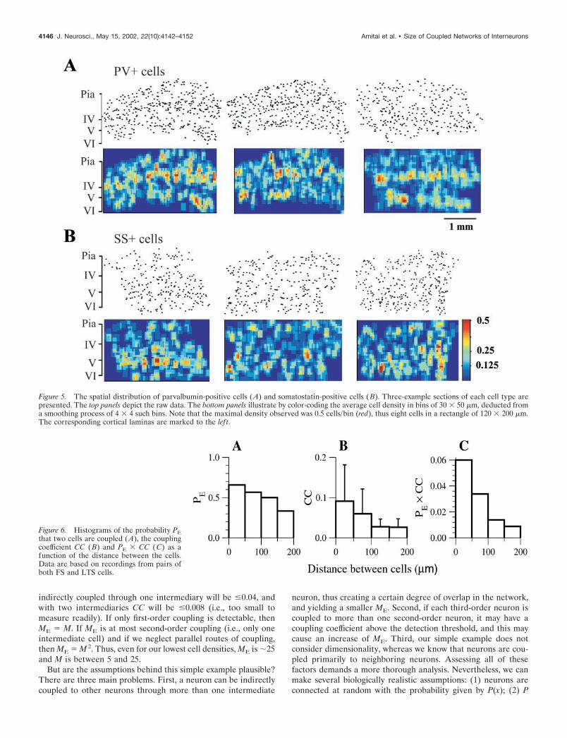
indirectly coupled through one intermediary will be �0.04, andwith two intermediaries CC will be �0.008 (i.e., too small tomeasure readily). If only first-order coupling is detectable, thenME M. If ME is at most second-order coupling (i.e., only oneintermediate cell) and if we neglect parallel routes of coupling,then ME M2. Thus, even for our lowest cell densities, ME is �25and M is between 5 and 25.

But are the assumptions behind this simple example plausible?There are three main problems. First, a neuron can be indirectlycoupled to other neurons through more than one intermediate

neuron, thus creating a certain degree of overlap in the network,and yielding a smaller ME. Second, if each third-order neuron iscoupled to more than one second-order neuron, it may have acoupling coefficient above the detection threshold, and this maycause an increase of ME. Third, our simple example does notconsider dimensionality, whereas we know that neurons are cou-pled primarily to neighboring neurons. Assessing all of thesefactors demands a more thorough analysis. Nevertheless, we canmake several biologically realistic assumptions: (1) neurons areconnected at random with the probability given by P(x); (2) P

Figure 5. The spatial distribution of parvalbumin-positive cells (A) and somatostatin-positive cells (B). Three-example sections of each cell type arepresented. The top panels depict the raw data. The bottom panels illustrate by color-coding the average cell density in bins of 30 � 50 �m, deducted froma smoothing process of 4 � 4 such bins. Note that the maximal density observed was 0.5 cells/bin (red), thus eight cells in a rectangle of 120 � 200 �m.The corresponding cortical laminas are marked to the lef t.

Figure 6. Histograms of the probability PEthat two cells are coupled (A), the couplingcoefficient CC (B) and PE � CC (C) as afunction of the distance between the cells.Data are based on recordings from pairs ofboth FS and LTS cells.

4146 J. Neurosci., May 15, 2002, 22(10):4142–4152 Amitai et al. • Size of Coupled Networks of Interneurons

does not depend on any other factor except x; and (3) the statisticsof the electrical connections are homogeneous. To obtain a moregeneral result, we need to use concepts borrowed from percola-tion theory. This theory describes how something (e.g., ioniccurrent) flows through the random interconnections of lattices(e.g., networks of neurons) (Stauffer and Aharony, 1992). Usingthe above assumptions and percolation theory, one can show thatif M � 1, each neuron is coupled (directly or indirectly) only to asmall number of other neurons, and ME is not much larger than1. Because our experimental results show that ME is of the orderof a few tens, M should be �1. If M � 1, the same theory tells usthat almost all of the neurons belong to one large connectednetwork, or syncytium, in which all cells are coupled to each otherthrough other cells that belong to the network (Erdos and Renyi,1960; Traub et al., 1999). This analysis cannot exclude cases inwhich electrical coupling exists only between neurons withinspatially restricted patches. However, assuming a uniform likeli-hood that dendrites of same-type interneurons will create elec-trical synapses when they are adjacent, the cellular distribution asrevealed by immunohistochemistry does not support such inho-mogeneity within the somatosensory area.

Models of electrically coupled networksThe density of electrical coupling within a cell network will haveimportant consequences for the estimated values of certain bio-physical properties. In particular, conductances attributable toelectrical coupling will add to membrane conductances, and sig-nificant errors can be made if network effects are not taken intoaccount. In the following analysis, we will estimate the contribu-tion of electrical coupling to the input conductances of each cellas measured experimentally. Two parameters in particular arelikely to be affected: gL, the intrinsic leak conductance of each cell(i.e., the leak conductance of the non-gap junctional membrane),and GE, the strength of each electrical connection between twoneurons. To estimate these values, one has to assume a model ofthe network architecture. We will first examine how these bio-physical parameters depend on the specific architecture of thenetwork, and then suggest a method to estimate them from datathat can be generated experimentally. All network architecture

models can be represented by the following steady-state equations(for i from 1 to N):

�gLVi � GE �j1

N

Jij�Vi � Vj � Ii � 0, (3)

where Vi is the voltage of the i th neuron and, at the neuronal reststate Vi 0, gL is the leak conductance, GE is the couplingconductance between any two cells, and Ii is the current injectedinto the i th neuron. For simplicity, we consider models withoutheterogeneity: all of the neurons have the same gL and all theexisting coupling strengths are GE. Because electrical synapsesare usually symmetrical (i.e., the coupling conductance from cellA to cell B is equal to the coupling conductance from cell B to cellA) (Galarreta and Hestrin, 2001), the matrix Jij is symmetric suchthat Jij Jji. Jij is 1 if electrical coupling exists between neuronsi and j, and is zero otherwise. We consider cases in which constantcurrent is injected to the neuron with an index i 0 only.Summing Equation 3 over all of the neurons, we obtain

gL �I0�

i

Vi(4)

Next we examine a few simple network architectures. We startwith a model that has only two cells and then show that theinfluence of the network should be considered by using morerealistic architectures.

The two-cell modelTraditionally, the coupling conductance between two cells, GE,has been calculated from the measured coupling coefficient, CC,assuming a two-cell model (Bennett, 1977). We consider here thesimple case where the two cells are identical. This architecture(Fig. 7A) includes two cells, each with an input conductance gL

(resistance RL 1/gL), which are coupled through a resistor RE

(conductance GE 1/RE). The cells have indices 0 and 1. Stepcurrent I0 is injected into cell 0. The coupling coefficient in thesteady state is CCi Vi/V0 (for i � 0). The conductance GE canbe estimated from the following relationship:

GE � gL

CC1

1 � CC1(5)

Figure 7. Architectures of network models. A, Two cells coupled by a gap junction with a conductance GE. B, A cell (0) coupled to M other cells. C,One-dimensional architecture. Each cell is coupled to M/2 cells on its lef t and M/2 cells on its right. Each coupling connection in B and C has aconductance GE gE/M. Cells in all architectures have a leak conductance gL (not specified in C).

Amitai et al. • Size of Coupled Networks of Interneurons J. Neurosci., May 15, 2002, 22(10):4142–4152 4147

For GE �� gL (and therefore V1 �� V0), Equations 4 and 5become: gL I0 /V0 , GE gL � CC1.

However, this model does not take into account the fact thateach cell may be coupled to many other cells. Obviously, the datawe described for networks of neocortical interneurons requiremore elaborate models.

One cell coupled to M other cellsIn this architecture (Fig. 7B), cell number 0 is electrically coupledto M other cells, which are not coupled to each other. It isconsiderably more realistic than the two-cell model, because weconcluded above that M is much greater than 1. The total cou-pling conductance on the 0th cell is gE M GE. The steady-statevoltages of cells in response to current injection into cell 0 aregiven by the following equations:

I0

V0� gL �

gL gE

gL � gE/M(6)

Vi �gE/M

gL � gE/MV0 ; i � 1. . .M (7)

From Equation 7, one can calculate gE/gL knowing Vi and V0:

gE/gL � M CCi/�1 � CCi (8)

For large M, these equations become: I0 /V0 gL � gE and Vi gEV0 /(M gL).

As we show below (see Appendix B), the sum i�0 CCi canbe calculated from experimental data and is useful for esti-mating network parameters. From Equation 8, this sum can becomputed by:

�i�0

CCi �gE/gL

1 � gE/�MgL(9)

The sum is approximately equal to gE/gL for large M or small gE,and we show below that under these conditions, one can estimatethis ratio experimentally.

What happens if we try to estimate gL (the nonjunctionalmembrane conductance) and gE (the total junctional conduc-tance) for one cell coupled to M other cells but use the traditionalapproach that assumes the simple two-cell model? The two-cellmodel makes the approximation gL I0 /V0. If we take intoaccount a large M, Equation 6 tells us that I0 /V0 gL � gE.Hence, our error is a factor of (gL � gE)/gL, and this error biasesthe calculation of both gL and gE upward. For example, if gL gE,the error is a factor of 2. Even if the coupling conductance GE

(between two cells) is relatively small, the value of the totalcoupling conductance gE M GE can be of the same order as theleak conductance of the cell, gL. Using the two-cell model cantherefore lead to unacceptably large errors.

Networks with one-dimensional architectureThe two architectures described above are too simplistic, but theydo demonstrate that network effects should be considered whenone estimates gL and gE. In practice, of course, we know that notall the neurons are directly coupled to the recorded neurons.Furthermore, as shown in Figure 6, the probability that two cellsare coupled depends strongly on the distance between them.Therefore, we next consider a model with spatially decayingconnectivity.

This architecture is one-dimensional, a long chain of neurons,

that stretches from �N/2 to N/2, where N �� M. Each neuron hasan index i and each is directly coupled to M other neurons that arearrayed symmetrically to either side. Thus, the cell at i 0 iscoupled to cells j �M/2 . . . 0 . . . M/2 (Fig. 7C). Cells near theedges are connected to a number of neurons that is smaller thanM. The network is studied for large N. The version of Equation 3for this system is

�gLVi �gE

M �j�M /2

j�0

M /2

�Vi � Vi�j � Ii � 0; �N/2 � i � N/2

(10)

The stimulus current Ii is I0 for i 0, and it is 0 otherwise. UsingFourier series, we obtain

Vi �I0

2��0

2�

dcos�i

gL �2gE

M �j1

M /2

�1 � cos� j�

(11)

We cannot evaluate the integral in Equation 11 exactly for M �2, and instead compute it numerically. An example is shown inFigure 8, where we use the parameters M 28 (the value derivedfrom a typical cell density of 2000 cells/mm3); M is close to ME,and gE gL. When current I0 is injected into the center cell, thevoltage Vi decreases gradually to cells i �14 and 14 (i.e., cells�M/2 and M/2) and then drops sharply at cells i �15 and 15,after which it decreases gradually again. These sharp jumps of Vi

occur because neuron number 14 (or M/2) is directly coupled tothe injected neuron (i 0), but neuron number 15 (or M/2 � 1)is only indirectly coupled to it. Interestingly, when gE and gL havesimilar values, the values of Vi for i that are just larger than M/2are not negligible at all. For example, for gE gL and M 28,V15 /V14 0.32. Yet, for this specific example, indirect connec-tions fall below the experimental confidence level.

The sum i�0 CCi, which is useful for calculating gE, can becalculated exactly in two limiting cases. In the limit of large M, weshow in Appendix A that

limM3�

�i�0

CCi �gE

gL(12)

Namely, (gL/gE) i�0 CCi 1 for M3 �. Similarly, we can showthat i�0 CCi gE/gL for gE/gL �� 1.

Figure 8. The coupling coefficient, CCi, as a function of the cell numberi for a one-dimensional architecture with M 28 and gE/gL 1. Thevalues were computed either by solving Equation 3 or by numericalintegration of Equation 11; the two results are equal. Note the jump inCCi between cells 14 and 15 (i M/2 and i M/2 � 1). The dashed linedenotes the confidence level of CC 0.01.

4148 J. Neurosci., May 15, 2002, 22(10):4142–4152 Amitai et al. • Size of Coupled Networks of Interneurons

What is the value of i�0 CCi in a parameter regime not closeto these limits? The dependence on connectivity, M, for threevalues of gE/gL (0.5, 1, and 2) is shown in Figure 9A. Figure 9Ademonstrates that Equation 12 holds for large M. Moreover, thedependence of i�0 CCi on M is weak, unless M is small (�10).Figure 9B demonstrates further that for a specific M in any of thearchitectures examined, the value of (gL/gE) i�0 CCi decreasesgradually and slowly from 1 as a function of gE/gL. The solid linerepresents the one-dimensional architecture and M 28, asexamined in the example above. Even for gE/gL 2, the value of(gL/gE) i�0 CCi is 0.95, demonstrating that the value of the sum i�0 CCi is close to gE/gL even beyond the two limiting casesdescribed above.

We also consider a two-dimensional model, in which neuronsare located on a two-dimensional lattice and are electricallyconnected if the distance between them is smaller than a certainvalue. The behavior of this model is found to be similar to thebehavior of the one-dimensional model, as represented by thedashed line in Figure 9B. This line is only slightly above the linefor the one-dimensional model with the same M. For comparison,we present also the dependence of (gL/gE) i�0 CCi for M 28 asa function of gE/gL for the architecture of one neuron coupled toM other neurons (Eq. 9). This line is only slightly below the linefor the one-dimensional model with the same M.

Together, the important result of this analysis is that the valueof (gL/gE) i�0 CCi depends only weakly on the model architec-ture. For all the architectures we examined, (gL/gE) i�0 CCi hasthe asymptotic value of 1 for large M or small gE/gL, and for gE �gL, the difference between one architecture and another is �5%.Therefore, we propose to use the sum i�0 CCi for estimatinggE/gL.

Estimating gL and gE from measurementsUnfortunately, we cannot develop a method for estimating GE(i,j) for a specific connection between two specific neurons, i and j,in the network. In many cases, however, the dynamic behavior ofneuronal networks can be described by knowing gE and gL (Chowand Kopell, 2000). We show above that the sum i�0 CCi can beused for estimating the ratio between gE and gL. Furthermore, wecan use the sum i Vi to estimate I0 /gL (Eq. 4). It is obviouslyimpractical to measure the sums i Vi and i�0 CCi directly inexperiments, because of the limited number of neurons that canbe recorded. Instead, we have developed a method for estimatingthese values, and therefore for estimating gE (the total conduc-tance of a cell from all of its electrical connections) and gL (theintrinsic leak conductance of a cell), by averaging over manyexperiments, and we present it in detail in Appendix B.

For a given set of dual intracellular measurements, the estima-tions for gE and gL depend only on the cell density �. As �increases, gL decreases and gE increases (Fig. 10). For a typical �of 2000 cells/mm3, gE contributes approximately one-half of themeasurable input conductance (gL 11 nS and gE 10 nS). Forthe extreme case of � close to 4000 cells/mm3, gE/gL is close to 2.In every reasonable scenario, the values of gE and gL are of thesame order of magnitude. The fact that the values of gL and gE aresimilar means that if the membrane conductance of the cell, gL, isestimated naively as I0 /V0 , as it generally is in systems of uncou-pled cells, the estimated value of gL would be approximately twicethe correct value.

What are the implications of these values on the values of GE?Although we cannot measure GE directly, we can estimate theorder of magnitude of its average value. Considering an averagevalue of � 2000 cells/mm3, we have estimated that gE 10 nSand M, the number of neurons that are directly coupled to eachneuron, is between 5 (�ME) and 28 (ME). Thus, for this celldensity, GE varies between 0.36 nS and 2 nS.

DISCUSSIONWe have investigated the spatial distribution of two coupledgroups of neocortical interneurons. From our morphological stud-ies we conclude that the somadendritic morphology of FS andLTS cells is similar, with �80% of the dendritic trees �200 �mfrom the soma. However, FS and LTS cells differ considerably intheir densities and laminar distribution. Electrophysiological re-cordings from same-type neuronal pairs demonstrated that the

Figure 9. Effects of network architectures on (gL/gE) i�0CCi. A, The dependence of (gL/gE) i�0 CCi at steady state onM for one-dimensional architecture and three values of gE/gL:0.5 (solid line), 1 (dotted line), and 2 (dashed line). B, Thedependence of (gL/gE) i�0 CCi at steady state on gE/gL forthree architectures: one-dimensional architecture (solid line),one cell coupled to M other cells (dotted line), and two-dimensional architecture (dashed line). M 28 for all thearchitectures. Calculations for the one-dimensional architec-ture were carried out as in Figure 8. Equation 9 was used forcalculating CC for the architecture with one cell coupled to Mother cells. In the two-dimensional architecture, cells arelocated on a two-dimensional grid, at positions x (i�, j�),where i and j are integers and � is the grid unit length.C ells at positions (i1 , j1 ) and (i2 , j2 ) are coupled if

��i1 � i2 2 � � j1 � j2 2 � 3. Calculations were performed bysolving Equation 3.

Figure 10. The dependence of gL (solid line) and gE (dashed line) on thecell density �, calculated using Equations B3 and B4, for the data obtainedexperimentally.

Amitai et al. • Size of Coupled Networks of Interneurons J. Neurosci., May 15, 2002, 22(10):4142–4152 4149

probability of electrical coupling and the coupling coefficientdeclined with the distance between somata. Electrical couplingnever occurred when the distance between somata was �200 �m.Our computations suggest that a single neuron is electricallycoupled to tens of other neurons, implying that each type ofinterneuron forms a highly interconnected network over largecortical areas.

Estimating parameters of electrical couplingThe strength of electrical coupling between two cells is easilycalculated when these cells are isolated (Bennett, 1977). For lackof better methods, the “two-cell model” has usually been used todetermine the electrical coupling strength between cell pairs evenin highly connected systems (Gibson et al., 1999; Galarreta andHestrin, 2001). However, this method can provide a good approx-imation only if the effects on the recorded cell pair of other,unrecorded, coupled cells are minimal, namely when gE is smallcompared with gL. Here we show that for the networks of neo-cortical interneurons, gE MGE is not small in comparison withgL; rather, the two have similar magnitudes. The two-cell modelcannot be used in these systems because it does not take intoaccount two important factors: (1) the increase of the effectiveleak conductance (I0 /V0 ) because of the current flow to otherneurons, and (2) the fact that electrical coupling between twocells can be mediated through other neurons.

We present here an approach for estimating the average mem-brane conductance, gL, and the average total electrical conduc-tance attributable to electrical junctions onto a single neuron, gE,based on a large number of measurements and on solving thevoltage profiles in several models. We estimate that the gL and gE

of inhibitory interneurons in the neocortex are of the same orderof magnitude (i.e., gap junctions contribute approximately one-half of the input conductance measured during electrophysiolog-ical experiments. The exact ratio between gL and gE depends onthe density of the cells within a coupled neuronal network.

A recent study of neocortical interneurons from connexin36(Cx36) knock-out (KO) mice demonstrated that, indeed, themean input resistance of cells in the KO is �30–40% higher thanthat of wild-type cells (Deans et al., 2001). This increase is not ashigh as our theoretical results predict, but it is also very likely thatthe KO cells achieve some partial compensation of membraneconductance during development. Nevertheless, this finding sup-ports our prediction that gap junctions provide a major contribu-tion to the total measured conductance of these cells.

The architecture of electrically coupled networks of neuronshas been studied mostly in noncortical tissues, such as the retina.There, the effect of gap junctions was examined using two-dimensional architectures in which each neuron is coupled only toits few nearest neighbors (hence M 4 for a rectangular grid)(Naka and Rushton, 1967; Gold, 1979; Poznanski and Umino,1997). Analysis reveals that when current is injected into a cellwithin such a nearest-neighbor architecture, the size of voltagedeflections in other cells decreases almost exponentially with thedistance from the injected cell. In contrast, each cell in our systemis coupled to tens of other cells, so models with large M are moreappropriate. In such models, voltage deflections decay onlyweakly over short distances, in agreement with our experimentaldata. Interestingly, a study of electrical coupling between neuronsin the inferior olive revealed spatial coupling patterns very similarto ours (Devor and Yarom, 2002): neurons in the olive are highlylikely to be coupled if their intersomatic distance is �100 �M, thedependence of PE and CC on distance is comparable with what

we find here, and the number of connected cells is estimated to bebetween 10 and 40. It will be interesting to perform similarinvestigations in other parts of the CNS to test the generality ofthese rules about the architecture of electrical networks.

Potential sources of biasOur calculations have several potential sources of bias. First, thecell density was calculated from random sections and correctedonly for shrinkage of the slice thickness. Our estimate is smallerthan the density of PV� cells in another study using stereometry(�7000 cells/mm3; Ren et al., 1992). However, the relative ratioof PV� neurons in that study is �54% of all GABAergic cells,which is much higher than most other estimates in rodent somato-sensory cortex (Gonchar and Burkhalter, 1997, Kawaguchi andKubota, 1997). It is also possible that the probability of coupling(Fig. 6A) was underestimated because some dendritic arbors weresevered by the slicing procedures. The signal-to-noise ratio pre-vents the detection of the least effective connections. All of thesetechnical limitations are likely to bias our results toward weakerelectrical coupling. Even so, our modeling results are robust toour experimental results and to a wide range of cell densities.

Another possible source of error arises from the relativelysmall electrophysiological sample from which the probability ofconnectivity was deduced. Nevertheless, the probability dataagree well with recent morphological data. Double-staining forCx36 reporter genes and specific markers of interneurons sug-gested that not all PV� and SS� interneurons express Cx36, andthe proportion of double-labeled cells was similar to the propor-tion of electrophysiologically coupled neighboring cells in thesample (Dean et al., 2001).

Our modeling work does not consider heterogeneities in gL,variations in the electrical coupling strength GE, and sparseconnectivity in which neurons are not necessarily coupled to eachother, even if they are adjacent. These factors could bias ourestimates of gE and gL. Qualitative estimation of the bias willrequire more theoretical work on models with relatively elaboratearchitectures. Preliminary modeling results with sparse and spa-tially decaying connectivity (data not shown) indicate that theeffects of sparseness on the estimated values of gE and gL aresmall.

Functional implicationsElectrical coupling is likely to affect both the properties of singlecells and the properties of cellular networks as a whole. Gapjunctions increase the effective leak conductance of neurons andthus decrease their passive time constants (Andreu et al., 2000).This may cause faster reaction times to stimulus-induced changesand may make firing times follow the membrane potential morefaithfully. The minimal current needed to initiate firing willincrease with electrical coupling as well, and the frequency-current dependence of a neuron will be shifted to the right, (i.e.,to larger current regimes) (Holt and Koch, 1997).

At the network level, it has been suggested that a population ofinhibitory neurons in vivo synchronizes its spikes and entrainspopulations of excitatory neurons via their inhibitory chemicalsynapses (Buzsaki et al., 1983). Data from brain slices do indeedconfirm that this scenario can occur under certain conditions(Whittington et al., 1995, Jefferys et al., 1996; Draguhn et al.,1998). Theoretical work, however, has shown that synchroniza-tion through inhibition has a fundamental limitation because ofthe joint effects of sparse connectivity and heterogeneity in thecellular intrinsic properties (Golomb and Hansel, 2000; Neltner et

4150 J. Neurosci., May 15, 2002, 22(10):4142–4152 Amitai et al. • Size of Coupled Networks of Interneurons

al., 2000; Golomb et al., 2001). Synchrony is destroyed by theheterogeneity of the network at weak inhibitory conductancesand because of sparseness at strong inhibitory conductances.There is, therefore, only a restricted window of conductancestrengths (if at all) in which network firing synchrony can beachieved by inhibition. Synchronization through electrical cou-pling is an alternative mechanism. Indeed, theoretical studieshave most commonly claimed that strong electrical coupling inneuronal systems tends to increase spike synchronization(Traub et al., 2001); if it is weak, other patterns of synchronymay emerge (Chow and Kopell, 2000). In local networks,electrical coupling is a much more robust mechanism for spikesynchronization than inhibitory connections (Golomb et al.,2001). Our study shows that the electrical coupling (gE) be-tween groups of interneurons is strong, and therefore electricalcoupling may play an important role in synchronizing the firingpatterns of interneurons.

Studies of LTS cells provide evidence for the spatial dimen-sions of coupled networks (Beierlein et al., 2000). When a net-work of LTS neurons is activated selectively with agonists, IPSPsbecome synchronized over distances of �400 �m. In connexin36knock-out mice, long-range synchrony is absent (Deans et al.,2001), implying that it is a coupling-dependent, collective net-work effect. These data are consistent with two of our conclu-sions: (1) the electrical coupling conductance gE is relativelystrong, and (2) interneurons form large, extensive electricallycoupled networks. The fact that synchronization of IPSPs (andprobably spikes) does not have a much larger correlation distancemay be a result of extensive sparseness and heterogeneity of thenetwork.

There may be other roles for large-scale, electrically connectednetworks of interneurons. In many cases, FS-type inhibitory neu-rons of the sensory neocortex have more broadly tuned receptivefields than regular-spiking neurons (Swadlow and Weyand, 1987;Simons and Carvell, 1989; Swadlow, 1989; Gibber et al., 2001);long-range electrical coupling among interneurons might accountfor this. Furthermore, the spread of activity through couplednetworks of interneurons could create a “surround inhibition”effect around focal areas of activation.

APPENDIX A: i�0 CCi for large MIn this Appendix, we prove that for the one-dimensionalarchitecture,

limM3�

�i�0

CCi � gE/gL . (A1)

We first note that, from Equation 4 and the definition of CCi,

I0

gL� �

i

Vi � V0�1 � �i�0

CCi. (A2)

Therefore, Equation A1 is correct if we can prove that

limM3�

V0 �I0

gL � gE. (A3)

We start by computing the sum in Equation 11 and obtaining

V0 �I0

2��0

2�

d1

gL � gE �gE

M�cos�M/2 � 1 �sin�M/2sin�

1 � cos� � .

(A4)

The first two terms in the square brackets are finite and go to zeroafter division by M. The third term diverges at 0. We need toshow that its contribution to the integral is as small as we wish,provided that M is large enough. To do this, we first see that thisterm divided by M is finite near 0:

sin�M/2sin�

M�1 � cos��� 1 � O�2. (A5)

This term reaches maximum at 0. For small values and largeM, the term behaves as 2 sin(M/2)/(M). We choose a value0 �� 2� such that the contributions to the integral (Eq. A5) fromthe ranges [0, 0] and [2� � 0 , 2�] are small. For the range[0 , 2� � 0], the term in Equation A5 is bounded:

� sin�M/2sin�

M�1 � cos����

1M�

sin�

1 � cos���

1M�

sin�0

1 � cos�0�.

(A6)

The second inequality is a result of the fact that the functionsin()/[1 � cos()] is monotonically decreasing in the interval (0,2�), and is antisymmetric around �. Hence, the contributionof the third term in the square brackets of Equation A4 can bemade arbitrarily small by choosing a large enough M, and Equa-tion A4 becomes Equation A3.

APPENDIX B: Estimating gL and gE

In this appendix, we present a method for estimating the sums i Vi and i�0 CCi by averaging over many experiments. Assum-ing homogeneous networks, we define PE(x) as the probabilitythat two cells at positions x1 and x2 x1 � x are electricallycoupled (in this appendix, x means a three-dimensional coordi-nate). The sum i Vi V0 � i�0 Vi, in response to a specificcurrent I0 is estimated to be

�V�0�pop � ��dxPE�xV�x, (B1)

where [V(0)]pop is the average of the membrane voltages over theentire neuronal population to which current is injected and � isthe cell density. By including the probability PE(x), we take intoaccount in the integral in Equation B1 only the voltage of neuronsthat show response to the current injected to neuron number “0.”Similarly, the sum i�0 CCi can be described by:

��dxPE�xCC�x. (B2)

The integrals in Equations B1 and B2 are approximated by sumsover shells, such that in each shell the values of PE and CC arethose given in Figure 6. The parameters gL and gE can be obtainedfrom the following equations:

I0/gL � �i

Vi � �V0�pop �4��

3 �j1

m

�rj3 � rj�1

3 PE� jV� j, (B3)

gE/gL � �i�0

CCi �4��

3 �j1

m

�rj3 � rj�1

3 PE� jCC� j. (B4)

REFERENCESAgmon A, Connors BW (1991) Thalamocortical responses of mouse

somatosensory (barrel) cortex in vitro. Neuroscience 41:365–379.

Amitai et al. • Size of Coupled Networks of Interneurons J. Neurosci., May 15, 2002, 22(10):4142–4152 4151

Akil M, Lewis DA (1992) Differential distribution of parvalbumin-immunoreactive pericellular clusters of terminal boutons in developingand adult monkey neocortex. Exp Neurol 115:239–249.

Andreu E, Fernandez E, Louis E, Ortega G, Sanchez-Andres JV (2000)Role of architecture in determining passive electrical properties in gapjunction-connected cells. Pflugers Arch-Eur J Physiol 439:789–797.

Bayraktar T, Welker E, Freund TF, Zilles K, Staiger JF (2000) Neuronsimmunoreactive for vasoactive intestinal polypeptide in the rat primarysomatosensory cortex: morphology and spatial relationship to barrel-related columns. J Comp Neurol 420:291–304.

Beierlein M, Gibson JR, Connors BW (2000) A network of electricallycoupled interneurons drives synchronized inhibition in neocortex. NatNeurosci 3:904–910.

Benardo LS (1997) Recruitment of GABAergic inhibition and synchro-nization of inhibitory interneurons in rat neocortex. J Neurophysiol77:3134–3144.

Benes FM, Lang N (2001) Two-dimensional versus three-dimensionalcell counting: a practical perspective. Trends Neurosci 24:11–17.

Bennett MVL (1977) The nervous system, part I. In: Handbook ofphysiology, section 1 (Brookhart JM, Mountcastle VB, eds), pp 357–416. Bethesda, MD: American Physiological Society.

Braitenberg V (1978) Cortical architectonics: general and areal. In: Ar-chitectonics of the cerebral cortex (Brazier MAB, Petche M, eds), pp443–465. New York: Raven.

Buzsaki G, Leung L, Vanderwolf CH (1983) Cellular bases of hip-pocampal EEG in the behaving rat. Brain Res Brain Res Rev6:139–171.

Chow CC, Kopell N (2000) Dynamics of spiking neurons with electricalcoupling. Neural Comput 12:1643–1678.

Deans MR, Gibson JR, Sellitto C, Connors BW, Paul DL (2001) Syn-chronous activity of inhibitory networks in neocortex requires electricalsynapses containing connexin36. Neuron 31:477–485.

Devor A, Yarom Y (2002) Electrotonic coupling in the inferior olivarynucleus revealed by simultaneous double patch recordings. J Neuro-physiol, in press.

Draguhn A, Traub RD, Schmitz D, Jefferys JGR (1998) Electrical cou-pling underlies high-frequency oscillations in the hippocampus in vitro.Nature 394:189–192.

Erdos P, Renyi A (1960) On the evolution of random graphs. Publ MathInst Hung Acad Sci 5:17–61.

Galarreta M, Hestrin S (1999) A network of fast-spiking cells in theneocortex connected by electrical synapses. Nature 402:72–75.

Galarreta M, Hestrin S (2001) Electrical synapses between GABA-releasing interneurons. Nat Rev Neurosci 2:425–433.

Gibber M, Chen B, Roerig B (2001) Direction selectivity of excitatoryand inhibitory neurons in ferret visual cortex. NeuroReport12:2293–2296.

Gibson JR, Beierlein M, Connors BW (1999) Two networks of electri-cally coupled inhibitory neurons in neocortex. Nature 402:75–79.

Gold GH (1979) Photoreceptor coupling in retina of the toad, Bufomarinus. II. Physiology. J Neurophysiol 42:311–328.

Golomb D, Hansel D (2000) The number of synaptic inputs and thesynchrony of large, sparse neuronal networks. Neural Comput12:1095–1139.

Golomb D, Hansel D, Mato G (2001) Mechanisms of synchrony ofneural activity in large networks. In: Handbook of biological physics,Vol 4: Neuro-informatics and neural modelling (Moss F, Gielen S, eds),pp 887–968. Amsterdam: Elsevier Science.

Gonchar Y, Burkhalter A (1997) Three distinct families of GABAergicneurons in rat visual cortex. Cereb Cortex 7:347–358.

Hendry SH, Jones EG, Emson PC, Lawson DE, Heizmann CW, Streit P(1989) Two classes of cortical GABA neurons defined by differentialcalcium binding protein immunoreactivities. Exp Brain Res76:467–472.

Holt GR, Koch C (1997) Shunting inhibition does not have a divisiveeffect on firing rate. Neural Comput 9:1001–1013.

Jefferys JGR, Traub RD, Whittington MA (1996) Neural networks forinduced “40 Hz” rhythms. Trends Neurosci 19:202–208.

Jin X, Mathers PH, Szabo G, Katarova Z, Agmon A (2001) Vertical biasin dendritic tress of non-pyramidal neocortical neurons expressingGAD67-GFP in vitro. Cereb Cortex 11:666–678.

Kawaguchi Y, Kubota Y (1997) GABAergic cell subtypes and theirsynaptic connections in rat frontal cortex. Cereb Cortex 7:476–486.

Kosaka T (1983) Gap junctions between nonpyramidal cell dendrites inthe rat hippocampus (CA1 and CA3 regions). Brain Res 277:347–351.

Kosaka T, Hama K (1985) Gap junctions between non-pyramidal celldendrites in the rat hippocampus (CA1 and CA3 regions): a combinedGolgi-electron microscopy study. J Comp Neurol 231:150–161.

Kubota Y, Hattori R, Yui Y (1994) Three distinct subpopulations ofGABAergic neurons in rat frontal agranular cortex. Brain Res649:159–73.

McMullen NT, Smelser CB, Rice FL (1994) Parvalbumin expressionreveals a vibrissa-related pattern in rabbit SI cortex. Brain Res660:225–231.

Naka KI, Rushton W (1967) The generation and spread of S-potentialsin fish (cyprinidae). J Physiol (Lond) 192:437–461.

Neltner L, Hansel D, Mato G, Meunier C (2000) Synchrony in hetero-geneous networks of spiking neurons. Neural Comput 12:1607–1641.

Poznanski RR, Umino O (1997) Syncytial integration by a network ofcoupled bipolar cells in the retina. Prog Neurobiol 53:273–291.

Ren JQ, Aika Y, Heizmann CW, Kosaka T (1992) Quantitative analysisof neurons and glial cells in the rat somatosensory cortex, with specialreference to GABAergic neurons and parvalbumin-containing neurons.Exp Brain Res 92:1–14.

Sanchez MP, Frassoni C, Alvarez-Bolado G, Spreafico R, Fairen A(1992) Distribution of calbindin and parvalbumin in the developingsomatosensory cortex and its primordium in the rat: an immunocyto-chemical study. J Neurocytol 21:717–736.

Sholl DA (1956) The organization of the cerebral cortex. London:Methuen.

Simons DJ, Carvell GE (1989) Thalamocortical response transformationin the rat vibrissa/barrel system. J Neurophysiol 61:311–330.

Sloper JJ (1972) Gap junctions between dendrites in the primate neo-cortex. Brain Res 44:641–646.

Sloper JJ, Powell TP (1978) Gap junctions between dendrites and so-mata of neurons in the primate sensori-motor cortex. Proc R Soc LondB Biol Sci 203:39–47.

Stauffer D, Aharony A (1992) Introduction to percolation theory, Ed 2.London: Taylor and Francis.

Swadlow HA (1989) Efferent neurons and suspected interneurons in S-1vibrissa cortex of the awake rabbit: receptive fields and axonal proper-ties. J Neurophysiol 62:288–308.

Swadlow HA, Weyand TG (1987) Corticogeniculate neurons, corticotec-tal neurons, and suspected interneurons in visual cortex of awakerabbits: receptive-field properties, axonal properties, and effects ofEEG arousal. J Neurophysiol 57:977–1001.

Szabadics J, Lorincz A, Tamas G (2001) and � frequency synchroni-zation by dendritic GABAergic synapses and gap junctions in a networkof cortical interneurons. J Neurosci 21:5824–5831.

Tamas G, Buhl EH, Lorincz A, Somogyi P (2000) Proximally targetedGABAergic synapses and gap junctions synchronize cortical interneu-rons. Nat Neurosci 3:366–371.

Traub RD, Schmitz D, Jefferys JGR, Draguhn A (1999) High-frequencypopulation oscillations are predicted to occur in hippocampal pyrami-dal neuronal networks interconnected by axoaxonal gap junctions.Neuroscience 92:407–426.

Traub RD, Kopell N, Bibbig A, Buhl EH, LeBeau FE, Whittington MA(2001) Gap junctions between interneuron dendrites can enhance syn-chrony of gamma oscillations in distributed networks. J Neurosci21:9478–9486.

White EL (1989) Cortical circuits: synaptic organization of the cerebralcortex: structure, function and theory. Boston: Birkhauser.

Whittington MA, Traub RD, Jefferys JGR (1995) Synchronized oscilla-tions in interneuron networks driven by metabotropic glutamate recep-tor activation. Nature 373:612–615.

4152 J. Neurosci., May 15, 2002, 22(10):4142–4152 Amitai et al. • Size of Coupled Networks of Interneurons