arX

iv:1

401.

1501

v1 [

astr

o-ph

.CO

] 7

Jan

201

4

Mon. Not. R. Astron. Soc. 000, ??–?? (xxxx) Printed 9 January 2014 (MN LATEX style file v2.2)

The SLUGGS Survey: Breaking degeneracies between dark

matter, anisotropy and the IMF using globular cluster

subpopulations in the giant elliptical NGC 5846

Nicola R. Napolitano1⋆, Vincenzo Pota2, Aaron J. Romanowsky3,

Duncan A. Forbes2, Jean P. Brodie4 and Caroline Foster5

1 INAF – Osservatorio Astronomico di Capodimonte, Salita Moiariello, 16, 80131 - Napoli, Italy2 Centre for Astrophysics & Supercomputing, Swinburne University, Hawthorn VIC 3122, Australia3 Department of Physics and Astronomy, San Jose State University, One Washington Square, San Jose, CA 95192, USA4 University of California Observatories, 1156 High Street, Santa Cruz, CA 95064, USA5 Australian Astronomical Observatory, PO Box 915, North Ryde, NSW 1670, Australia

Accepted Received

ABSTRACT

We study the mass and anisotropy distribution of the giant elliptical galaxy NGC 5846using stars, as well as the red and blue globular cluster (GC) subpopulations. We breakdegeneracies in the dynamical models by taking advantage of the different phase spacedistributions of the two GC subpopulations to unambiguously constrain the mass ofthe galaxy and the anisotropy of the GC system. Red GCs show the same spatialdistribution and behaviour as the starlight, whereas blue GCs have a shallower den-sity profile, a larger velocity dispersion and a lower kurtosis, all of which suggest adifferent orbital distribution. We use a dispersion–kurtosis Jeans analysis and findthat the solutions of separate analyses for the two GC subpopulations overlap in thehalo parameter space. The solution converges on a massive dark matter halo, consis-tent with expectations from ΛCDM and WMAP7 cosmology in terms of virial mass(logMDM ∼ 13.3M⊙) and concentration (cvir ∼ 8). This is the first such analysis thatsolves the dynamics of the different GC subpopulations in a self-consistent manner.Our method improves the uncertainties on the halo parameter determination by afactor of two and opens new avenues for the use of elliptical galaxy dynamics as testsof predictions from cosmological simulations. The implied stellar mass-to-light ratioderived from the dynamical modelling is fully consistent with a Salpeter initial massfunction (IMF) and rules out a bottom light IMF. The different GC subpopulationsshow markedly distinct orbital distributions at large radii, with red GCs having ananisotropy parameter β ∼ 0.4 outside ∼ 3Re (Re is the effective radius), and theblue GCs having β ∼ 0.15 at the same radii, while centrally (∼ 1Re) they are bothisotropic. We discuss the implications of our findings within the two–phase formationscenario for early-type galaxies.

Key words: dark matter – galaxies : kinematics and dynamics – galaxies : haloes –galaxies : haloes – galaxies : elliptical and lenticular, cD – galaxies: evolution.

1 INTRODUCTION

Early-type galaxies are key laboratories where the darkmatter (DM) paradigm can be tested. They are amongthe most massive stellar systems in the universe forwhich accurate kinematical measurements are available.

⋆ E-mail: napolita@na.astro.it

These include integrated long slit stellar kinematics (e.g.,Kronawitter et al. 2000; Gerhard et al. 2001; Jardel et al.2011; Salinas et al. 2012), integral field 3D kinematics(Cappellari et al. 2013a) and discrete kinematic tracerssuch as planetary nebulae (PNe, Romanowsky et al. 2003;Napolitano et al. 2009, N+09 hereafter; Napolitano et al.2011, N+11) and globular clusters (GCs, e.g., Cote et al.2003; Romanowsky et al. 2009; Schuberth et al. 2010;

2 Napolitano et al.

Richtler et al. 2011; Norris et al. 2012). The latter probe thegalaxy projected kinematics (Napolitano et al. 2001) out tolarge galactocentric distances (Peng et al. 2004a,b). Theseradii are comparable to those explored in the late 70s inspiral galaxies, in studies which resulted in the initial dis-covery of DM (Rubin et al. 1978; Bosma 1981). X-rays areoften used as viable mass probes, although the number ofsystems with the necessary undisturbed gas distributions islimited (e.g., Humphrey et al. 2006, 2012).

A growing body of evidence shows that many differ-ent stellar subsystems within galaxies share the same phasespace properties, i.e. starlight, red GCs (RGCs) and PNe(see e.g. Coccato et al. 2009 and Pota et al. 2013, P+13hereafter). Other tracers (e.g. the blue GCs, BGCs) areclearly decoupled, despite (presumably) sharing the samepotential. Indeed, it is thought that BGCs may trace thegalaxy halo component more closely than these other trac-ers (Brodie & Strader 2006; Forbes et al. 2012).

In general, these studies find good agreement betweenthe RGCs and the underlying starlight, a connection thatis corroborated by the consistency with other discrete stel-lar tracers like PNe (P+13), although notable exceptionsexist (Foster et al. 2011). If BGCs are instead governed bythe overall galaxy potential in a manner distinct from theRGCs, they act as an independent tracer of the potential tolarge galactocentric distances (up to >10 effective radii, Re).This provides strong constraints on the dark matter distribu-tion with radius. Thus, the combination of RGCs and BGCsoffers the opportunity to break the well-known degeneracybetween mass and orbital anisotropy that has so far plagueddynamical studies of early-type galaxies (Merrifield & Kent1990).

Earlier studies have claimed that hot stellar systems areextremely difficult to model by means of discrete dynami-cal tracers (Merritt & Hernquist 1991). However, it has nowbecome clear that, in the case of quasi-spherical systems,the combination of velocity maps from discrete tracers (e.g.GCs and/or PNe) and the kinematical information fromstarlight actually provides a powerful tool for constrain-ing the galaxy mass distribution (Napolitano et al. 2002;Romanowsky et al. 2009) as well as the orbital distribution(Saglia et al. 2000; N+09; de Lorenzi et al. 2009).

Notwithstanding their intrinsic robustness, these stud-ies have yet to solve two basic problems: 1) identifying theinitial mass function (IMF), and 2) breaking the DM haloparameter degeneracies.

The IMF is the prime source of uncertainty in deter-mining stellar masses as it can translate into variationsin the stellar mass-to-light ratio (M/L) of a factor of twoor more. Evidence for systematic variations of the IMFamong galaxies has been obtained by measuring the directeffect of the giant-to-dwarf star ratio on integrated galaxyspectra via spectral indices (e.g. Conroy & van Dokkum2012; Spiniello et al. 2012; Ferreras et al. 2013) and fromstudies that combine galaxy dynamics and lensing to in-fer the “gravitational” stellar mass-to-light ratio, (Υ⋆ e.g.,Thomas et al. 2011; Cappellari et al. 2012; Dutton et al.2013; Tortora et al. 2013). In order to quantify the IMFvariations, these spectroscopic and dynamical studies havemeasured the ratio of Υ⋆ to that of the Milky Way, ΥMW

(δIMF = Υ⋆/ΥMW), with the result that more massivegalaxies were found to have systematically larger δIMF (see

Tortora et al. 2013 for a review). However, the above dy-namical studies relied solely on data from the inner regionsof galaxies. Here, all assumed a fixed DM halo density dis-tribution (e.g., from collisionless simulations, Navarro et al.1996, NFW) and the total mass (e.g. from abundance match-ing studies, Moster et al. 2010) and the only free parametersinvolved was the stellar M/L. As the DM quantities need tobe tested against observations (e.g., more radially extendeddynamical studies such as the one we present here), the ar-gument in the dynamical studies carried out to date is thussomewhat circular. By contrast, kinematic tracers such asPNe or GCs, which extend out to large galactocentric radii,will allow a direct and self-consistent assessment of both theIMF and the DM halo in galaxies (see N+11).

The other problem is that the intrinsic/physical re-lationship between the various DM halo parameters, e.g.the concentration–virial mass (Humphrey et al. 2006) or thehalo density–scale radius (N+11) is well aligned with thetypical confidence contours of the modeled parameters. Thismakes the overall analysis highly degenerate. For this rea-son, a combined analysis of the different tracers (i.e., stars,RGCs and BGCs in our case) in a single galaxy may help tobreak the degeneracies in the typical halo parameter space.Modeled values for the different tracers may have confidencecontours that are tilted with respect to each other in haloparameter space and converge to a narrower common pa-rameter volume. This would significantly reduce the locus ofallowed halo solutions. It would also make early-type galax-ies (ETGs) a powerful cosmological testbed for separatingdifferent DM species (e.g. Cold from Warm) as they are ex-pected to occupy different areas of the parameter space (seee.g., Schneider et al. 2012). Simultaneous modelling of dif-ferent GC subpopulations has been attempted for a few casesand has so far yielded contradictory results (Schuberth et al.2010, 2012). The implication may be that the assumptionthat both GC subpopulations are in dynamical equilibriumis incorrect (Schuberth et al. 2010). Alternatively, due tothe inherent difficulties associated with cleanly separatingRGCs from BGCs (P+13), the BGC kinematics may havebeen poorly constrained.

Here we analyze stars plus RGC and BGC subpopula-tions of the giant elliptical galaxy NGC 5846 and performa self-consistent dynamical analysis in order to simultane-ously and self-consistently constrain the stellar M/L, thehalo parameters in the context of ΛCDM predictions, andthe orbital anisotropy of the galaxy. With the method out-lined above, we attempt to resolve typical degeneracies, inparticular that between halo mass and anisotropy.

NGC 5846 is the central and brightest galaxy in a group(Mahdavi et al. 2005) 23.1 Mpc away (Tonry et al. 20011).It is nearly spherical in shape with Hubble type E0 and iskinematically classified as a slow rotator (Emsellem et al.2011). These properties indicate that it is suitable for massmodelling under the assumption of spherical symmetry.

The GC system was studied using Hubble Space Tele-scope images (Forbes et al. 1997a; Chies-Santos et al. 2006).As in most massive galaxies, the GC system is clearly bi-modal in colour with BGC (metal-poor) and RGC (metal-rich) subpopulations as for most massive galaxies. Combin-

1 Distance modulus corrected by -0.16 as per Jensen et al. (2003).

Mass, anisotropy and IMF of NGC 5846 3

ing the HST with Subaru images, P+13 showed that theRGCs are more radially concentrated than the BGCs. Us-ing Keck spectroscopy of GCs, they measured little or norotation for the RGCs (in agreement with the starlight),and systematically higher velocity dispersion in the BGCsthan the RGCs.

Mass profile modelling of NGC 5846 has been per-formed previously in Kronawitter et al. (2000, K+00 here-after) and Cappellari et al. (2007, 2013b) who used the kine-matics of the galaxy starlight to probe the mass within ∼1effective radius. In order to probe larger galactocentric dis-tances, Saxton & Ferreras (2010) combined starlight kine-matics with PNe, Das et al. (2008) used X-rays and PNe,and Deason et al. (2012) used PNe.

The paper is organised as follows: In §2 we presentthe spatial distribution and kinematics of the GC systemfor both red and blue GC subpopulations. The dispersion–kurtosis procedure is presented in §3, while its results arederived in §4 for the RGCs and BGCs, separately in the firstinstance, and then jointly in order to find a single equilib-rium potential that can account for all observed kinematics.A discussion of the results and our conclusions can be foundin §6.

2 DATA

We analyse the GC dataset presented in P+13. These datawere acquired as part of the SAGES Legacy Unifying Globu-lars and GalaxiesS (SLUGGS) survey. The survey combineswide-field imaging with Keck/DEIMOS (Faber et al. 2003)multi-object spectroscopy of globular clusters and galaxystarlight for a sample of 25 nearby early-type galaxies2 .

For NGC 5846, HST/WFPC2 (Forbes et al. 1997a;Chies-Santos et al. 2006) and new Subaru gri photometry isavailable for the photometric pre-selection of GC candidates(see P+13 for details). The spectroscopic sample of P+13consists of 195 confirmed GCs collected over six DEIMOSmasks. As mentioned above, the GC system exhibits theclassical colour bimodality with a colour split between BGCsand RGCs around (g − i) = 0.95. For the time being, theseparation is based on the photometry only, although wewill also consider this separation from a dynamical point ofview.

2.1 Density profiles

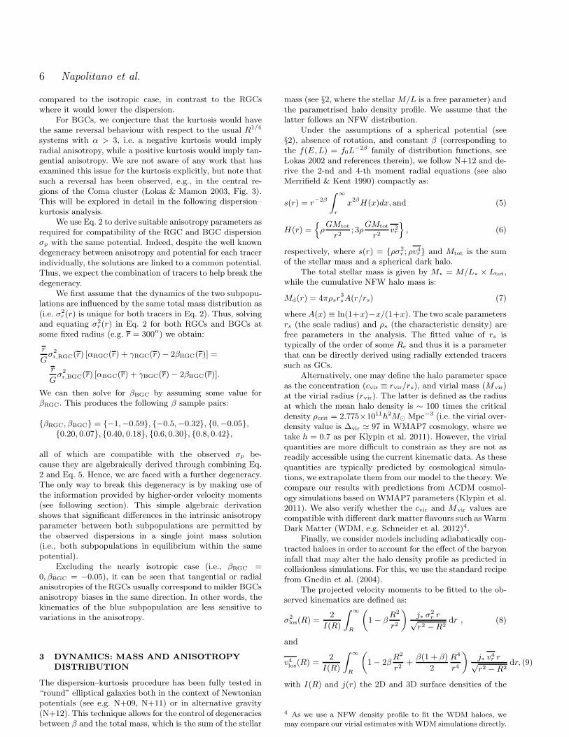
Fig. 1 shows the radial number density profiles(NGC/arcmin2) of the photometrically selected RGCsand BGCs together with the V−band galaxy surfacebrightness (SB) profile from K+00 adopted as the referencestarlight radial distribution. We show the Sersic (1963) fitto the stellar SB profile (n = 4.9, Re = 230′′ and µ0 = 14.3mag/arcsec−2) extrapolated over the whole radial range.The fit is vertically offset to match the RGC numberdensity data in the outskirts. As a result, the match withinR ∼ 1′ is not optimal. The RGC number density profile isdepleted with respect to the stellar SB profile in the inner

2 Further details of the survey are available in Brodie et al. (2014,in prep.) and at http://sluggs.ucolick.org

ç

ç

ç

ç

ç

ç

ç

ç

1 10

R @arcminD

1

10

NG

C@G

Cs

arcm

in-

2D

Figure 1. Sersic fit to the stellar surface brightness (SB, greenline) as compared to the RGC (red) and BGC (blue) surface den-sity profiles. The open and filled circles correspond to HST andSubaru data, respectively. The surface brightness has been arbi-trarily scaled to match the red NGC. It is evident that the RGCsclosely follow the stellar SB within the uncertainties, although thefit to the RGCs (red solid line) deviates slightly at large radii (seediscussion in the text). The Sersic fit to the BGCs number densityprofile is shown as a blue solid line. Using a different colour cut toseparate RGCs from BGCs (see §2.3) does not significantly affectthe slope of the density profiles as shown by the red and bluedashed lines (also arbitrarily scaled to match the normalisationof the respective solid lines).

regions due to GC cluster disruption. We assume Re = 81′′

as per Cappellari et al. (2006) and Deason et al. (2012)henceforth, which corresponds to 9.1 kpc at the distance ofNGC 5846. The RGCs closely follow the normalised stellarlight distribution outside of 1′. A Sersic fit to the RGCnumber density distribution yields n = 2.9, Re = 160′′ andNe = 3.3 GC arcsec−2.

The similarity between the radial RGC number densityand the stellar SB profiles indicates a close connection be-tween the RGCs and the overall stellar population as alsodiscussed in e.g. Forbes et al. (2012) and P+13. Remainingsmall deviations at large radii might be attributable to un-certainties on the GC background determination (see Eq.1 of P+13, here bg =0.13 arcmin−2). These minimal off-sets are insignificant compared to the model uncertainties.This motivates the use of the stellar SB profile to derive thede-projected stellar density profile for input into the Jeansequations, similar to the method employed for other discretedynamical tracers (e.g. PNe, N+09; N+11).

Since NGC 5846 is a non-rotating E1 galaxy(Coccato et al. 2009), we expect the deviation from spheri-cal symmetry to be less than 10% (Kronawitter et al. 2000;Binney & Tremaine 1987). Under the assumption of spher-ical symmetry, the deprojection of the observed SB is

4 Napolitano et al.

unique and can be derived as usual via the Abel integra-tion (Binney & Tremaine 1987):

j(r) =1

π

∫ r

0

dI

dr

dr√r2 + R2

, (1)

where r and R are the 3D and 2D radii, respectively, andI(R) is the interpolated SB in units of L⊙/arcsec2 . Eq. 1 issolved numerically. The same procedure is adopted to derivethe 3D distribution of the BGCs, this time by fitting theSersic profile to the BGC 2D distribution in Fig. 1 and thenapplying Eq. 1 to derive the 3D density.

We derive the total stellar luminosity by integrating theextrapolated SB profile and obtain Ltot = 9.8 × 1010L⊙,V .We then derive the total stellar mass by assuming a con-stant stellar M/L (Υ⋆in solar units), via the simple equa-tion Mstar = Υ⋆ × Ltot. The stellar density is given byρ⋆(r) = Υ⋆ × j(r). In particular, we fit Υ⋆ as a free parame-ter in the dynamical analysis and compare it with the samequantity derived from Stellar Population Synthesis (SPS)models (see §2.2) in order to compute the IMF mismatchparameter (δIMF).

The Sersic fit to the 2D density of the BGCs shownin Fig. 1 has an overall more diffuse profile than the oneof RGCs, i.e. Ne = 0.24 GC arcsec−2, n = 2.9 and Re =780′′. We have checked that the number density profile ofthe BGCs is not sensitive to the colour cut adopted in thephotometricly selected sample in P+13. As we shall see in§2.3, the kinematics of the two subpopulations suggest thatone can refine the colour selection of the two subpopulations,but this does not significantly impact the number densityslope, as shown by the dashed lines in Fig. 1, where we havetaken RGC from g − i > 1.0 and BGC from g − i < 0.85.Thus, we keep the BGC number density profile obtainedusing a colour separation at g−i = 0.95 in order to minimisethe uncertainties.

2.2 Mass-to-light ratio from SPS models

One key parameter we want to address in the dynamicalanalysis is the stellar M/L as derived from dynamical mod-els. This will allow us to evaluate the most likely IMF com-patible with the best fit dark matter halo and the observedkinematics. Here we derive the SPS based M/L based onliterature stellar parameters.

According to the analysis of absorption line indices pre-sented in Denicolo et al. (2005), stars in NGC 5846 areold (11.7 Gyr) and metal-rich ([Fe/H] = 0.19). Using thisinformation, we estimate a plausible stellar M/L usingthe Worthey (1994) models (i.e. the same as adopted byDenicolo et al. 2005) and obtain M/LV = 7.2 assuming aSalpeter (1955) IMF and solar (M/LV )⊙ = 4.83.

This central M/L estimate is slightly lower than thatadopted by SAURON in the I−band. Their estimate wasM/LI = 3.33 based on the SPS analysis within ∼ 1Re

(Cappellari et al. 2006, using a Kroupa 2001 IMF). ForV −I = 1.283, this corresponds to M/LV = 8.7 for a Salpeter(1955) IMF or M/LV = 5.4 for a Kroupa IMF.

The M/L has recently been revised to M/LR = 7.13 inATLAS3D (Cappellari et al. 2013b) using the Vazdekis et al.

3 from Hyperleda: http://leda.univ-lyon1.fr/.

50

150

250

350

v rm

s@k

ms-

1D

0 100 200 300 400 500R@arcsecD

-2

0

2

kurt

osis

0 100 200 300 400 500R@arcsecD

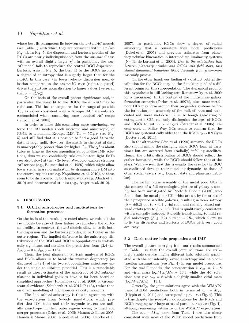
Figure 2. Dispersion and kurtosis profiles for the RGC (red sym-bols), BGC (blue symbols) and folded longslit stellar kinemat-

ics from K+00 (green stars). The left and right panels show theanalysis for a single colour separation at g − i = 0.95 and thedifferential colour cut presented in §2.3, respectively. For ease ofcomparison, light blue and red filled symbols in the right panelreplicate the original g − i = 0.95 cut separation from the leftpanel.

(2012) models and a Salpeter IMF, which also correspondsto M/LV = 8.6 (Salpeter IMF) or M/LV = 5.9 (KroupaIMF).

As our reference value, we have chosen the average ofall V -band estimates given above, i.e. 8.1±0.9Υ⊙(SalpeterIMF) or 5.1±0.6Υ⊙(Kroupa IMF) and 4.6±0.5Υ⊙(ChabrierIMF).

2.3 Kinematics

In Fig. 2 we show the velocity dispersion profile of the RGCsand BGCs separated according to P+13 using a colourthreshold g − i = 0.95, together with the long slit datafrom K+00 after averaging the positive and negative dataat a corresponding radius. We also show the excess kurtosisprofile (simply kurtosis henceforth) of the two subpopula-tions, which is a measure of the deviation from Gaussianityof the velocity distribution, and hence a proxy for orbitalanisotropy. For the stellar measurement, we convert the h4

parameter from K+00 according to the usual conversion for-mula κ ≃ 8

√6h4 (van der Marel & Franx 1993). For GCs

we use an unbiased kurtosis estimator (Joanes & Gill 1995,also see the Appendix for a discussion) tested on PN sam-ples (e.g., N+09). The GC velocity and velocity dispersionprofiles shown above are slightly different from the ones re-ported in P+13 because we used a different binning in orderto include more GCs in each spatial bin to derive reliablekurtosis estimates. The red and blue GC samples used forthe kurtosis estimate are smaller than samples used in otheranalyses (e.g. N+09 and N+11), although we ensure thateach radial bin contains at least 30 GCs. However, this re-quirement is slightly relaxed for the more stringent colourselections (see below) where radial bins contain >∼20 GCs.We have checked that there are no biases in the kurtosisestimates due to small number statistics using a suite of

Mass, anisotropy and IMF of NGC 5846 5

Monte Carlo simulations (see the Appendix). We find thatthe adopted definition reliably recovers the intrinsic kurtosisof simulated systems despite large statistical uncertainties.

As previously stressed in P+13, there is good agreementbetween the measured velocity dispersion and kurtosis ofthe innermost RGC and the stellar data. This confirms theworking assumption that RGCs are tracers of the underlyingstellar population, which we adopt hereafter.

In contrast, RGCs and BGCs have markedly differentdispersion profiles with the outermost data points differingby ∼ 30 km s−1 despite agreeing in the central regions. Asfor the kurtosis profiles, both GC subpopulations agree atall radii. However and unlike the density profiles (see §2.1),the kinematic measurements are more sensitive to the recip-rocal contamination between sub-populations as evidencedin figure 5 of P+13, wherein it is clear that the two subpop-ulations are too mixed around the chosen colour threshold.Thus, we explore the effects of an improved colour separationof the red and blue GC in order to reduce the probability ofcross-contamination. In particular, we investigate whethercross-contamination depends on radius as a result of rela-tive fractions (see Fig. 1) of RGCs and BGCs that dominateinside and outside R ∼ 250′′, respectively.

In Fig. 3 we show the GC colour distribution for tworadial bins. The bimodal GC colour distribution is fittedwith a double gaussian. We find that the relative fractions ofRGCs and BGCs vary with radii (also see e.g., Forbes et al.1998). In the inner radial bin (i.e. R < 250′′), the optimalcolour separation for minimal contamination of the RGCsample is g − i > 1.0, while the purest sample of BGCscorresponds to g − i < 0.8. Clean samples in the outer binare selected with g− i > 1.05 and g− i < 0.85 for the RGCsand BGCs, respectively.

The drawback of adopting this exclusive selection ap-proach is an obvious reduction in sample size with whichto compute the kinematics. Indeed, this differential colourselection yields a final sample of ∼ 140 GCs, a significantdecrease from the original 195. This approach is necessaryfor reliably delineating the behaviour of the two subpopu-lations in phase space as demonstrated in Fig. 2, where wecompute the kinematics using differential colour cuts. In thisfigure, the differences in the kinematics of the two subpop-ulations are enhanced thanks to the differential colour cut.The dispersion profile of the BGCs is systematically largerthan that of the RGCs by ∼ 40 km s−1. The kurtosis pro-files of the two subpopulations diverge beyond R ∼ 250′′

with RGCs reaching up to ∼ 1 and the BGCs plummetingto as low as ∼ −1. These differences are significant at the∼ 2σ level.

Whether this results from differences in the respectiveanisotropy distributions of the two subpopulations is notstraightforward and will be investigated as part of the dy-namical analysis presented in §3. We first present dynamicalarguments based on a simple algebraical approach and eval-uate the connection between the observed kinematics andpossible orbital distribution of the two GC subpopulationsin the next section.

0.4 0.6 0.8 1.0 1.2 1.4g-i

0

5

10

15

Cou

nts

R<250’’

0.4 0.6 0.8 1.0 1.2 1.4g-i

R>250’’

Figure 3. Colour separation of the RGCs and BGCs for inner(left) and outer (right) radial bins as labelled. The two subpop-ulations are separated using a double gaussian fit (black line).Individual components are shown in red and blue for the RGCsand BGCs, respectively. The relative fractions and mean coloursof the two subpopulations are different between the two radialbins as expected from their differing number density distributions(Fig. 1).

2.4 Effect of tracer density profiles on the

observed kinematics

As a prelude to the dynamical analysis to be presented in§3, we quantify the possible impact of the distinct numberdensity profiles (see §2.1) on the measured kinematics ofthe RGC and BGC. The radial component of the velocitydispersion is given by the radial Jeans equation:

v2circ(r) = σ2r(r) [α(r) + γ(r) − 2β(r)], (2)

where v2circ(r) = GM(r)/r, α ≡ −d ln j/d ln r, γ ≡−d ln σ2/d ln r and β = 1 − σ2

θ/σ2r , with σθ and σr the az-

imuthal and radial dispersion components in spherical coor-dinates, respectively. Assuming a power-law profile v2circ =V 20 r

−γ σ2 = σ20r

−γ , α, γ and β are constant with r and theprojected dispersion can be written as (Dekel et al. 2005):

σ2p(R) = A(α, γ)

(

(α + γ) − (α + γ − 1)β

(α + γ) − 2β

)

V 20 R−γ , (3)

where

A(α, γ) =1

(α + γ)

Γ[(α + γ − 1)/2]

Γ[(α + γ)/2]

Γ[α/2]

Γ[(α− 1)/2]. (4)

While we are clearly not in the simple power-law regime,the slope of the number density profiles mimics a power-law profile with changes of ±10% within the radial rangecovered by the kinematic data. Thus the use of Eq. 3 is areasonable approximation for the arguments below (see alsoDekel et al. 2005). The SB fit presented in §2.1 correspondsto αRGC ∼ 3.1 and αBGC ∼ 2 in the radial region whereboth GC subpopulations overlap. Hence, from Eq. 3 we havethat σp = σ0R

−γ . We can fit for γRGC and γBGC using theobserved data beyond Re. This yields σ0,RGC = 225 km s−1,γRGC ∼ 0.01, σ0,BGC = 285 km s−1 and γBGC ∼ 0.025.

For RGCs, α + γ > 3 implies that for β > 0 (radialanisotropy) the velocity dispersion decreases with both βand r, while for BGCs, α + γ < 3 implies that σp has alarger normalisation factor for β > 0, i.e., the presence ofradial anisotropy would enhance the dispersion of the BGCs

6 Napolitano et al.

compared to the isotropic case, in contrast to the RGCswhere it would lower the dispersion.

For BGCs, we conjecture that the kurtosis would havethe same reversal behaviour with respect to the usual R1/4

systems with α > 3, i.e. a negative kurtosis would implyradial anisotropy, while a positive kurtosis would imply tan-gential anisotropy. We are not aware of any work that hasexamined this issue for the kurtosis explicitly, but note thatsuch a reversal has been observed, e.g., in the central re-gions of the Coma cluster ( Lokas & Mamon 2003, Fig. 3).This will be explored in detail in the following dispersion–kurtosis analysis.

We use Eq. 2 to derive suitable anisotropy parameters asrequired for compatibility of the RGC and BGC dispersionσp with the same potential. Indeed, despite the well knowndegeneracy between anisotropy and potential for each tracerindividually, the solutions are linked to a common potential.Thus, we expect the combination of tracers to help break thedegeneracy.

We first assume that the dynamics of the two subpopu-lations are influenced by the same total mass distribution as(i.e. σ2

r(r) is unique for both tracers in Eq. 2). Thus, solvingand equating σ2

r(r) in Eq. 2 for both RGCs and BGCs atsome fixed radius (e.g. r = 300′′) we obtain:

r

Gσ2r,RGC(r) [αRGC(r) + γRGC(r) − 2βRGC(r)] =

r

Gσ2r,BGC(r) [αBGC(r) + γBGC(r) − 2βBGC(r)].

We can then solve for βBGC by assuming some value forβRGC. This produces the following β sample pairs:

{βRGC, βBGC} = {−1,−0.59}, {−0.5,−0.32}, {0,−0.05},{0.20, 0.07}, {0.40, 0.18}, {0.6, 0.30}, {0.8, 0.42},

all of which are compatible with the observed σp be-cause they are algebraically derived through combining Eq.2 and Eq. 5. Hence, we are faced with a further degeneracy.The only way to break this degeneracy is by making use ofthe information provided by higher-order velocity moments(see following section). This simple algebraic derivationshows that significant differences in the intrinsic anisotropyparameter between both subpopulations are permitted bythe observed dispersions in a single joint mass solution(i.e., both subpopulations in equilibrium within the samepotential).

Excluding the nearly isotropic case (i.e., βRGC =0, βBGC = −0.05), it can be seen that tangential or radialanisotropies of the RGCs usually correspond to milder BGCsanisotropy biases in the same direction. In other words, thekinematics of the blue subpopulation are less sensitive tovariations in the anisotropy.

3 DYNAMICS: MASS AND ANISOTROPY

DISTRIBUTION

The dispersion–kurtosis procedure has been fully tested in“round” elliptical galaxies both in the context of Newtonianpotentials (see e.g. N+09, N+11) or in alternative gravity(N+12). This technique allows for the control of degeneraciesbetween β and the total mass, which is the sum of the stellar

mass (see §2, where the stellar M/L is a free parameter) andthe parametrised halo density profile. We assume that thelatter follows an NFW distribution.

Under the assumptions of a spherical potential (see§2), absence of rotation, and constant β (corresponding tothe f(E,L) = f0L

−2β family of distribution functions, see Lokas 2002 and references therein), we follow N+12 and de-rive the 2-nd and 4-th moment radial equations (see alsoMerrifield & Kent 1990) compactly as:

s(r) = r−2β

∫

∞

r

x2βH(x)dx,and (5)

H(r) ={

ρGMtot

r2; 3ρ

GMtot

r2v2r

}

, (6)

respectively, where s(r) = {ρσ2r ; ρv4r} and Mtot is the sum

of the stellar mass and a spherical dark halo.The total stellar mass is given by M⋆ = M/L⋆ × Ltot,

while the cumulative NFW halo mass is:

Md(r) = 4πρsr3sA(r/rs) (7)

where A(x) ≡ ln(1+x)−x/(1+x). The two scale parametersrs (the scale radius) and ρs (the characteristic density) arefree parameters in the analysis. The fitted value of rs istypically of the order of some Re and thus it is a parameterthat can be directly derived using radially extended tracerssuch as GCs.

Alternatively, one may define the halo parameter spaceas the concentration (cvir ≡ rvir/rs), and virial mass (Mvir)at the virial radius (rvir). The latter is defined as the radiusat which the mean halo density is ∼ 100 times the criticaldensity ρcrit = 2.775×1011h2M⊙ Mpc−3 (i.e. the virial over-density value is ∆vir ≃ 97 in WMAP7 cosmology, where wetake h = 0.7 as per Klypin et al. 2011). However, the virialquantities are more difficult to constrain as they are not asreadily accessible using the current kinematic data. As thesequantities are typically predicted by cosmological simula-tions, we extrapolate them from our model to the theory. Wecompare our results with predictions from ΛCDM cosmol-ogy simulations based on WMAP7 parameters (Klypin et al.2011). We also verify whether the cvir and Mvir values arecompatible with different dark matter flavours such as WarmDark Matter (WDM, e.g. Schneider et al. 2012)4.

Finally, we consider models including adiabatically con-tracted haloes in order to account for the effect of the baryoninfall that may alter the halo density profile as predicted incollisionless simulations. For this, we use the standard recipefrom Gnedin et al. (2004).

The projected velocity moments to be fitted to the ob-served kinematics are defined as:

σ2los(R) =

2

I(R)

∫

∞

R

(

1 − βR2

r2

)

j∗ σ2r r√

r2 −R2dr , (8)

and

v4los(R) =2

I(R)

∫

∞

R

(

1 − 2βR2

r2+

β(1 + β)

2

R4

r4

)

j∗ v4r r√r2 −R2

dr, (9)

with I(R) and j(r) the 2D and 3D surface densities of the

4 As we use a NFW density profile to fit the WDM haloes, wemay compare our virial estimates with WDM simulations directly.

Mass, anisotropy and IMF of NGC 5846 7

tracer respectively. From these, we compute the projectedkurtosis as κ(r) = v4los/σ

4los.

Even though the equations listed above are valid forcases where β = const, we now generalise their applica-tion. To explore a wide range of anisotropy profiles in thedispersion–kurtosis dynamical analysis, we adopt the fol-lowing β(r) parametrisation introduced by Churazov et al.(2010):

β(r) =β2r

c + β1rca

rc + rca, (10)

which is characterised by two plateaus corresponding to β1

and β2 that set the asymptotic values for r → 0 and r → ∞,respectively. Over these radial ranges we confirm that ourassumption that β is constant still holds. Therefore, we mayuse only the kurtosis values measured at the low and highextremes of our radial range to constrain the anisotropy pa-rameters. In this case, the contribution from the c parameterthat determines the steepness of the transition from β1 toβ2 is marginal, while ra is the scale at which this transitionoccurs. For convenience, we fix β1 = 0 (as previously mea-sured by e.g. Cappellari et al. 2007) and ra = 200′′ as thisis the radius where the kurtosis shows a sudden rise towardpositive values (see Fig. 2). At this radius, it is likely thatthe RGC anisotropy changes significantly. We also try vary-ing ra and find that it does not have a significant effect onour results. For practical reasons and to reduce the numberof free parameters, we also fix the slope parameter to c = 6,as tests have shown that the current dataset cannot reliablyconstrain this parameter.

In the following sections, we model the observed disper-sion and kurtosis in order to derive the best fit parametersof our models, which include the stellar mass-to-light ratio,the dark halo parameters (rs and ρs) and the asymptoticanisotropy (β2). Our approach is designed to solve the mass-anisotropy degeneracy mainly in the outer regions in orderto have unbiased estimates of the halo parameters. We iter-atively solve Eqs. 2, 3, 5 and 6 and minimise χ2 as definedby

χ2 =

Ndata∑

i=1

[

λipobsi − pmod

i

δpobsi

]2

, (11)

where pobsi are the observed data points (σlos and κlos), pmodi

the model values, δpobsi the uncertainties on the observed val-ues, all of which are measured at radial position Ri. Whencombining the χ2 of the σlos and κlos to infer the model pa-rameters consistent with the separate GC tracers, we applya weight to each bin according to the penalisation factorλi ∼ 1/Ndata.

4 COMBINING RED AND BLUE GLOBULAR

CLUSTER DYNAMICS

The combination of multiple dynamical tracers is the bestway to break all degeneracies associated with dynamicalmodelling of hot systems. Because different GC subpopula-tions usually have decoupled kinematics that can be probedwith a single observational set-up, they constitute a naturaland powerful tool for degeneracy-free mass modelling.

4.1 Best-fit halo parameter determination

We have shown that the RGCs in NGC 5846 reliably tracethe kinematics of the galaxy stars. Hence, we combine theintegrated light data with those of the RGCs (surface densityand kinematics) into a single tracer family. The BGCs beinga second set of spatially and kinematically decoupled tracers.The final two datasets are of different quality in terms oftheir spatial sampling and error budget (Fig. 2). Therefore,we adopt the following approach to combine constraints fromRGCs and BGCs:

1) we model the innermost stellar dispersion and kur-tosis together with that of the RGC to obtain a full set ofstellar and halo parameters (Υ⋆, ρs, rs, β), where Υ⋆ is thedynamically derived stellar M/L. The high quality centralkinematic data (mainly long slit) constrain the central M/Land anisotropy more efficiently, while the extended RGCkinematics help constrain the halo parameters and largeradii anisotropy for RGCs.

2) Once Υ⋆ in the total potential is fixed by modellingthe integrated light and RGCs, we use the BGC dispersionand kurtosis independently to constrain the dark halo pa-rameters.

3) We find the system’s self-consistent halo model whereboth RGC and BGC halo solutions overlap. The confidenceintervals of the self-consistent halo model are obtained fromthe sum of both χ2 distributions with best fit parameterscorresponding to the minimum in combined χ2. Separatesolutions for other parameters (Υ⋆, β) are obtained for eachtracer set.

4) We perform the analysis assuming either a standardNFW or an adiabatically contracted NFW halo (noAC andAC, respectively), as well as either the isotropic case (i.e.β = 0) or a radial anisotropic profile β(r) as per Eq. 10 (isoand ani, respectively).

Best fit parameters for the various model combinationsdescribed in item 4 above are reported for the joint solu-tion of the RGCs and BGCs. Individual red and blue (items1 and 2 above) confidence contours of the halo parameters(ρs, rs) marginalised over other fitted parameters (Υ⋆, β)are shown in Fig. 4. Also plotted in black in the same figureare the combined (item 3 above) χ2 for the joint halo bestfit parameters, along with the expectation from cosmologicalsimulations in the ΛCDM and WMAP7 cosmology as perKlypin et al. (2011) with cvir − Mvir converted to ρs − rs.As direct predictions of these quantities within ΛCDM sim-ulations are not yet available, our derived expectations areobtained in a manner similar to that used for independentindirect inferences (e.g. Spitler et al. 2012, Eq. 3).

Fig. 5 shows the joint solutions for the various models.As we are interested in the joint solutions, we do not discussthe independent RGC and BGC solutions (red and blue con-tours in Fig. 4) further. There is no additional informationcontained in these solutions compared to the joint solutionsexcept for the fact that they are optimised for the individualtracer kinematics. Hence, they generally have lower χ2 thanthe combined best-fit and better reproduce the individualkinematic profiles than the joint models.

8 Napolitano et al.

0 25 50 75 100 125 150rs @arcsecD

0.000

0.002

0.004

0.006

Ρs@

Msu

npc-

3D

iso-noAC

0 25 50 75 100 125 150rs @arcsecD

iso-AC

0 25 50 75 100 125 150rs @arcsecD

anis-noAC

0 25 50 75 100 125 150rs @arcsecD

anis-AC

Figure 4. Confidence contours in the ρs − rs halo parameter space for the RGC (red curves) and BGC (blue curves) dynamics. Eachpanel reports a different model combination (see §4.2). Best-fit halo parameters are given with red and blue crosses respectively. Thecombined confidence contours for each model are plotted as black lines with the best fit values marked with a black crosses. The χ2 forthe best-fit combined solutions are given in Table 1. The filled area shows the expectation from cosmological simulations in the ΛCDMand WMAP7 cosmology as per Klypin et al. (2011) after converting (cvir −Mvir) to (ρs − rs).

Table 1. Summary of the best-fit multi-component model parameters. Typical uncertainties on the Υ⋆ , logM∗ and β parameter areof the order of 0.1Υ⊙,V 0.05 dex and ∼0.1, respectively. For the AC models, halo parameters are given pre-contraction, while fDM,Υ(Re), Υ(5Re) and Υ(Rvir) are given after contraction (Re = 81′′ = 9.1 kpc). The expected cvir from WMAP7 are indicated in squaredbrackets.

Model Υ⋆ logM∗ ρs/10−3 rs cvir log Mvir fDM(5Re) β(5Re) Υ(Re) Υ(5Re) Υ(Rvir) χ2/d.o.f.

(Υ⊙,V ) (M⊙) (M⊙/pc3) (kpc) (M⊙) RGC/BGC (Υ⊙,V ) (Υ⊙,V ) (Υ⊙,V ) (#par)

iso-noAC 8.2 11.90 1.5+0.4

−0.396+19

−207+6

−5[8] 13.33+0.30

−0.340.71+0.10

−0.130/0 11+2

−128+13

−8217 16/22(3)

iso-AC 7.0 11.84 1.6+0.3

−0.275

+15

−138+9

−4[8] 13.06

+0.25

−0.250.71

+0.09

−0.100/0 13

+1

−124

+8

−5105 18/22(3)

ani-noAC 8.0 11.89 1.9 +0.4

−0.281+4

−168+5

−4[8] 13.24+0.14

−0.280.71+0.05

−0.100.43/0.15 11+1

−128+6

−7178 12/18(4)

ani-AC 6.0 11.77 1.8 +0.2

−0.278+12

−118+9

−5[8] 13.16+0.19

−0.220.74+0.07

−0.080.4/0.2 13+1

−126+6

−5135 23/18(4)

4.2 Self-consistent models

We now closely inspect the best-fit models for RGCs andBGCs with a particular focus on the joint solutions thathave been obtained by combining their χ2 distributions asdescribed in the previous section.

4.2.1 Isotropic case: no-AC and AC models

Starting from the simple assumption of orbital isotropy (i.e.β = 0), Υ⋆ is allowed to vary from 4.5 to 9.5 Υ⊙,V , a rangethat encompasses the M/L predictions of both Chabrier anda super-Salpeter IMF.

For the iso-noAC case, χ2 in halo parameter space isminimised using Υ⋆= 8.2Υ⊙,V , which is consistent with aSalpeter IMF. The resulting individual confidence contoursfor the RGC and BGC models (Fig. 4) are stretched acrossthe parameter space, which illustrates the strong degen-eracy of the halo parameters. The situation is much im-proved for the iso-AC case where the confidence contours ofthe RGCs are more compact, and hence the degeneracy issomewhat alleviated. The best fit stellar M/L for iso-AC isΥ⋆= 7.0Υ⊙,V , which is close to the lowest limit allowed bystellar populations with a Salpeter IMF.

In both cases the confidence contours overlap and con-verge to a combined solution. The parameters that minimisethe χ2 are reported in Table 1. Overall, the halo parametersfor the two isotropic models are consistent with each other.

Even though the best fit iso-noAC model has a slightlylarger density (ρs) and concentration parameter (cvir), itis fully consistent (i.e. within the confidence area) with theiso-AC model.

In the left side of Fig. 5, the dispersion curve of theRGCs and BGCs predicted by the combined solutions tothe isotropic models are well fitted for both the iso-noACand AC cases. The former performs somewhat better forthe BGCs. On the other hand, the fit to the kurtosis is quitepoor outside ∼ 150′′ (i.e. ∼ 2Re) for both subpopulations. Inparticular, the modelled RGC kurtosis systematically under-predicts the observed one beyond R > 200′′, suggesting thepresence of radially biased orbits. In contrast, the modelledBGC kurtosis slightly overpredicts the measured one, pos-sibly indicating the presence of some level of anisotropy. Inthe central regions our working hypothesis is that the orbitsin the galaxy core are basically isotropic for both subpopu-lations.

Overall, the poor fit of the kurtosis profile at large radiidoes not seem to strongly affect the global significance ofthe final fit, which remains fairly good for both cases.

4.2.2 Anisotropic case: no-AC models

The introduction of the parametrised β(r) profile in Eq. 10allows a considerably better match of the model with theouter galaxy regions. The ani-noAC fit to the RGCs kine-matics has minimum χ2 = 9.6/12 for Υ⋆ = 8, which is fully

Mass, anisotropy and IMF of NGC 5846 9

RGC:iso-noAC

RGC:iso-AC

BGC:iso-noAC

BGC:iso-AC

KR-IMF

RGC:ani-AC

RGC:ani-noAC

BGC:ani-AC

BGC:ani-noAC

KR-IMF50

150

250

350

v rm

s@k

ms-

1D

-2

0

2

kurt

osis

0 100 200 300 400 500R@arcsecD

0.0

0.2

0.4

0.6

Β

0 100 200 300 400 500R@arcsecD

Figure 5. Joint best fit models of the dispersion (top), kurtosis (central) and anisotropy (bottom) profiles of RGC (red curves) and theBGC (blue curves). Symbols follow Fig. 2 and curve styles follow Fig. 4. The left panels show two isotropic models with noAC and AChaloes. The grey line is the forced solution for the RGC when converting to a Kroupa IMF with an AC halo (see §5). The right panelsshows the best fit red and blue anisotropic noAC and AC models as labeled. Also shown in grey is the best-fit AC halo with a KroupaIMF and orbital anisotropy.

compatible with a Salpeter IMF and is in line with thatfound in the isotropic case. The confidence contours of thehalo parameters for this solution (ani-noAC) are plotted inFig. 4. The joint solution is also shown and agrees nicelywith the WMAP7 prediction area.

The narrower range of halo parameter space for the ani-noAC versus the iso models is not a reflection of the relativeχ2 values that are, in fact, fairly similar, once normalised tothe number of degrees of freedom. Rather it is a result of theability of the former to better reproduce the overall data inFig. 5. The dispersion curves of the two models all match theobserved velocity dispersion profile of the RGCs, includingthe “bump” around R ∼ 180′′ found for the g − i = 0.95colour cut. We confirm that this bump is real despite beinghidden in the improved colour selection sample. Using fourbins with ∼ 22 RGCs, instead of the adopted 3 bins with∼ 28 RGCs, we also find a high dispersion of ∼ 250 km s−1

around R ∼ 180′′. Moreover, the kurtosis profiles of theRGCs match the observations at all radii including the twoplateaux in the anisotropy profile. In particular, as reportedin the lower panel of Fig. 5, the ani-noAC solution of RGCsshows a moderate (β ∼ 0.4) radial anisotropy corresponding

to the positive values of the kurtosis profile in the outermostregions.

The BGC kinematics are best fitted with β ∼ 0 in thecentral regions and mild radial anisotropy (β ∼ 0.15) out-side ra = 100′′. In this case, the ani-noAC is a remarkablybetter match to the observed dispersion and kurtosis thanthe iso model at all radii. It is interesting that the joint solu-tion robustly shows a difference in the orbital distributionsof the two subpopulations as mainly imprinted in the kurto-sis profiles. Indeed, the intricate combination of the densityand the velocity dispersion slopes (§2.4) conspire to producesignificantly different kurtosis profiles for similar asymptoticradial anisotropies. The dispersion–kurtosis analysis is suf-ficiently sensitive to highlight this difference.

4.2.3 Anisotropic case: AC models

We also fit the adiabatic contraction model for theanisotropic case. Similarly to the isotropic case, we obtaina drastic reduction of the confidence area in halo parame-ter space around the models. The converging solution usesΥ⋆ = 6Υ⊙,V , similar to the Kroupa IMF, and a halo model

10 Napolitano et al.

whose best fit parameters lie between the ani-noAC models(see Table 1) with which they are consistent within 1σ (seeFig. 4). In Fig. 5, the dispersion and kurtosis profiles of theRGCs are nearly indistinguishable from the ani-noAC casewith an overall slightly larger χ2. In particular, the ani-AC model fails to reproduce the central RGC dispersion–kurtosis. Also in Fig. 5, the best fit to the BGCs involvesa degree of anisotropy that is slightly larger than for thenoAC. In this case, the lower velocity dispersion normal-isation compared to the ani-noAC case (right-top panel)drives the kurtosis normalisation to larger values (we recall

that κ = v4p/σ4p).

On the basis of the overall poorer significance and, inparticular, the worse fit to the BGCs, the ani-AC may beruled out. This has consequences for the range of possibleΥ⋆, as values consistent with a Kroupa IMF are only ac-commodated when considering some standard AC recipe(Gnedin et al. 2004).

In order to make this conclusion more convincing, weforce the AC models (both isotropic and anisotropic) ofRGCs to a nominal Kroupa IMF, Υ⋆ = 5Υ⊙,V (see Fig.5) and still find that it is possible to find a good fit to thedata at large radii. However, the match to the central datais unacceptably poorer than for higher Υ⋆. The χ2 is abouttwice as large as the corresponding Salpeter-like IMF solu-tions, thus we can confidently rule out bottom light IMFs(see also below) at the > 2σ level. We do not explore strongerAC recipes (e.g., Blumenthal et al. 1986), which might allowlower stellar mass normalisation by dragging more DM intothe central regions (see e.g. Napolitano et al. 2010), as theseseem to be disfavoured by both simulations (e.g. Abadi et al.2010) and observational studies (e.g., Auger et al. 2010).

5 DISCUSSION

5.1 Orbital anisotropies and implications for

formation processes

On the basis of the results presented above, we rule out theiso models because of their failure to reproduce the kurto-sis profiles. In contrast, the ani models allow us to fit boththe dispersion and the kurtosis profiles, in particular in theouter regions. The implied difference in the anisotropy dis-tributions of the RGC and BGC subpopulations is statisti-cally significant and matches the predictions from §2.4 (i.e.βRGC = 0.4, βBGC = 0.18).

Thus, the joint dispersion–kurtosis analysis of RGCsand BGCs allows us to break the intrinsic degeneracy (asdiscussed in §2.4) of the two subpopulations anisotropy un-der the single equilibrium potential. This is a remarkableresult as direct estimates of the anisotropy of GC subpop-ulations in individual galaxies have so far been based onsimplified approaches (Romanowsky et al. 2009) or circum-stantial evidence (Schuberth et al. 2012; P+13), rather thanon direct modelling of higher-order velocity moments.

The final orbital anisotropy is thus in agreement withthe expectations from N-body simulations, which pre-dict that DM halos and their baryonic tracers are radi-ally anisotropic in their outer regions owing to infall andmerger processes (Dekel et al. 2005; Mamon & Lokas 2005;Hansen & Moore 2006; Nipoti et al. 2006; Onorbe et al.

2007). In particular, RGCs show a degree of radialanisotropy that is consistent with model predictions(Dekel et al. 2005) and previous estimates from plane-tary nebulae kinematics in intermediate luminosity systems(N+09, de Lorenzi et al. 2009). Due to the established link

between planetary nebulae and RGCs with field stars, this

shared dynamical behaviour likely descends from a common

assembly process.

On the other hand, our finding of a distinct orbital dis-tribution for the BGCs may be the “smoking gun” of a dif-ferent origin for this subpopulation. The dynamical proof ofthis hypothesis is still lacking (see Romanowsky et al. 2009for a discussion). In the context of the multi-phase galaxyformation scenario (Forbes et al. 1997b), blue, more metal-poor GCs may form around their progenitor systems beforethe formation and assembly of the bulk of stars and asso-ciated red, more metal-rich GCs. Although age-dating ofextragalactic GCs can only distinguish the ages of BGCsand RGCs to within ∼ 2 Gyrs (Strader et al. 2005), re-cent work on Milky Way GCs seems to confirm that theBGCs are systematically older than the RGCs by ∼ 0.8 Gyrs(Dotter et al. 2011).

In the alternative Cote et al. (1998) scenario, the RGCsalso should mimic the starlight, while BGCs form at earlytimes but are accreted from (radially) infalling satellites.Hence, the orbital distribution of BGCs should reflect theearlier formation, while the RGCs should follow that of thestars. We have seen that this is usually the case for the RGCas confirmed through their matching dynamics to those ofother stellar tracers (e.g. long slit data and planetary nebu-lae).

The earlier phase assembly of the metal poor GCs inthe context of a full cosmological picture of galaxy assem-bly has been investigated by Prieto & Gnedin (2008), whofound that the metal-poor GC orbits are set by the orbits oftheir progenitor satellite galaxies, resulting in near-isotropy(β ∼ ±0.2) out to ∼ 0.1 virial radii and radially biased out-ward orbits (out to β ∼ 0.5). This is qualitatively consistentwith a centrally isotropic β profile transitioning to mild ra-dial anisotropy (β ∼< 0.2) outside ∼ 2Re, which allows usto fit the dispersion and kurtosis of BGCs with very goodaccuracy.

5.2 Dark matter halo properties and IMF

The overall picture emerging from our results summarisedin Table 1 is that the overall joint solutions are strik-ingly stable despite having different halo solutions associ-ated with the considerably varied anisotropy and halo con-traction assumptions (see Fig. 4) in our model procedure.For the noAC models, the concentration is cvir = 7 − 8and virial mass log Mvir/M⊙ ∼ 13.3, while the AC solu-tions also give cvir = 8 with a slightly smaller virial mass〈log Mvir/M⊙〉 = 13.1.

Generally, the joint solutions agree with the WMAP7based ΛCDM predictions both in terms of cvir − Mvir

(Klypin et al. 2011) and corresponding ρs−rs (Fig. 4). Thisis true despite the separate halo solutions for the RGCs andBGCs ranging over large areas of parameter space (Fig. 4),although remaining within 1σ of the WMAP7 expectation.

The cvir − Mvir pairs from Table 1 are also nicelyconsistent with most of the WDM model predictions from

Mass, anisotropy and IMF of NGC 5846 11

Schneider et al. (2012, e.g., their Fig. 11). In this model,a concentration parameter of cvir ∼ 8 is expected at virialmasses log Mvir/M⊙ = 13.1−13.3 for m = 0.5−1 keV WDMparticles, while at the same masses cvir ∼ 7 is predicted form = 0.25 keV. Unfortunately, at the mass scales of mas-sive ellipticals, the WDM predictions do not differ from theΛCDM cvir −Mvir and it is not possible to disentangle thedifferent cosmologies. However, it is encouraging that thetight constraints on the halo parameters obtained using theRGC/BGC model combination in lower mass systems willallow discrimination of one DM flavour over the other.

As previously mentioned, the narrow distribution ofvirial parameters seems insensitive to the quite large changesof the anisotropy parameter, which varies from β = 0 toβ ∼ 0.4 (0.2) for the RGCs (BGCs, see Table 1). This is aninteresting feature emerging from our analysis and impliesthat for massive systems with fairly flat dispersion profiles,the constraints on the halo parameters are almost indepen-dent of the anisotropy assumption (see also the PN anal-ysis of NGC 4374 in N+11, their Table 2), and the over-all anisotropy can only be constrained through the highervelocity moments (i.e. the kurtosis in our case). The mainadvantage of using different tracers such as the two GC sub-populations is significantly reduced uncertainties in the mea-sured halo solutions as compared to those yielded by singleextended tracer (i.e. PNe) as in N+11. For instance, uncer-tainties in cvir are reduced by up to a factor of ∼ 4.

The assumption on halo contraction evidently affectsthe final stellar M/L inferred to fit the galaxy kinematics,especially in the inner regions. We find a mean 〈M/L〉 ∼6.5Υ⊙,V slightly lower than predicted by stellar popula-tion models using a Salpeter IMF for the AC models (see§1), that is ∼ 20% lower than that obtained for the noACcases (〈M/L〉 ∼ 8Υ⊙,V ), which is consistent with a SalpeterIMF. We also show that bottom-lighter IMFs (Chabrieror Kroupa IMF) are confidently ruled out, even when al-lowing for halo contraction. This is independent confirma-

tion of recent findings that stars in high mass galaxies form

with a bottom-heavier IMF (Conroy & van Dokkum 2012;Cappellari et al. 2012; Wegner et al. 2012; Tortora et al.2013; La Barbera et al. 2013). To our knowledge, this workis the first study using a radially extended dataset to con-strain the IMF along with an accurate determination of thehalo parameters.

The degeneracy between Υ⋆ and halo contraction is bro-ken thanks to the large radius baseline covered by the stellarand RGC data. The stellar data constrain the total masswithin ∼ Re, where the central DM contribution followsfrom the adopted Υ⋆ value. The DM profile at large radii(∼ 1–5 Re) differs depending on whether it is contractedor not, an ambivalence that is constrained by the RGCs.The BGC data further tighten the constraints on the haloparameters.

Although we have not directly explored DM halos withshallow central profiles (e.g. Donato et al. 2009), we canqualitatively infer that such halos would push more of thecentral mass into the stellar component, thus requiring asuper-Salpeter IMF.

Parametrizing IMF variations using the δIMF parameteras a measure the departure from the typical Milky Way IMF,we obtain δIMF = 1.8±0.2 for NGC 5846, which is consistentwith the typical values found in SDSS galaxies and other

0

100

200

300

400

v cir

c@k

ms-

1D

0

1

2

3

4

Mas

s�10

12@M

sunD

0 2 4 6 8 10R�Re

0.0

0.2

0.4

0.6

0.8

1.0

f DM

Figure 6. Summary of the galaxy mass distribution.Upper panel:

circular velocity of the stellar mass (green), dark mass (cyan)and total mass (black) for models shown in Fig. 5 with iden-tical curve styles. Middle panel: same as above for the stellarand total mass distribution. Lower panel: dark matter fraction(MDM/Mtot). Typical uncertainties are plotted for various radii

literature data at comparable stellar masses (Tortora et al.2013).

5.3 Comparison with other works

The giant elliptical NGC 5846 is a dark matter dominatedsystem with very high virial M/L (Υ(Rvir) > 100Υ⊙,V , seeTable 1). The circular velocity (vcirc) profiles of the modelsdiscussed herein exhibit the typical features of a massivedark matter halo (Fig. 6). For all models and after reachinga local minimum at ∼ Re, the vcirc increases around R > 3Re

before flattening out at the typical rs scale (i.e. 8 − 10 Re,see Table 1).

The total mass distributions of the various models are

12 Napolitano et al.

all nearly linearly increasing with radius as shown in themiddle panel of Fig. 6. In the same figure, the correspondingDM fractions (lower panel) are plotted. These show that theDM mass exceeds that of the stars (fDM > 0.5 by definition)at 1Re for the contracted models and ∼ 2Re for the noncontracted ones.

The DM fractions within 1Re are of order fDM ∼ 0.25for the normal DM solutions and fDM ∼ 0.4 for the con-tracted halo ones. This result is consistent with the typicalcentral DM fractions measured with large statistical sam-ple analyses from either galaxy dynamics and virial analysis(Tortora et al. 2009; Thomas et al. 2009; Napolitano et al.2010; Grillo 2010), or lensing studies (Auger et al. 2010;Tortora et al. 2010) using a Salpeter IMF.

In all cases presented in Fig. 6, typical uncertainties inderived dynamical quantities are plotted. As pointed out in§5.2, it is clear that all models are generally consistent withintypical uncertainties. This reflects the stability of the virialsolution against different assumptions of anisotropy that arecompatible with the observed kinematics.

The dynamical M/L within Re (Υ⋆ = 11−13, see Table1) is consistent with previous analyses from the ATLAS3D

project (Cappellari et al. 2013a), wherein a value of M/Lr =8.1 was found. Once converted to the V−band (see §2.2),this corresponds to M/LV ∼ 12.5. Our M/L estimate islower than K+00 (i.e. M/LB ∼ 11 at Re ), once the latteris converted to the V−band and corrected to a commondistance. This may be a consequence of their assumption ofa cored halo, which tends to show a flatter M/L(r) than thecuspy NFW profiles used in this work.

However, in the central region, our vcirc models are dom-inated by the stellar component that peaks around 0.5 Re

with ∼ 330 − 350km s−1. This is almost consistent with thefindings of ATLAS3D (361km s−1, Cappellari et al. 2013b),but lower than the K+00 model solution. This is shownin Fig. 7, where we see that we agree with K+00 outside1Re despite the smaller radial coverage of their star–onlymodel, which does not allow comparison of the results atlarge radii. The central discrepancies between this and theprevious two studies reflect the slightly larger stellar massnormalisation, compared to our estimate, that they both in-ferred (i.e. Υ⋆ ∼ 9.5 and Υ⋆ ∼ 9.2, respectively, for K+00and ATLAS3D at the same galactocentric distance and con-verted to V−band). This may be a consequence of the poorconstraints on the overall dark halo derived from their radi-ally confined kinematics.

The study of Deason et al. (2012) is the one moreclosely related to our work in terms of data and model ex-tent (see Fig. 7). Their analysis differs in that they do notfit the stellar component, but instead provide the solutionsfor both a Chabrier and a Salpeter IMF. In our analysis, weresolve this ambiguity by explicitly fitting for the IMFs andfind that a heavier stellar mass normalisation is favouredover Chabrier IMF.

Comparing our results to the Deason et al. (2012) so-lution with a Salpeter IMF, we only find agreement forfDM(5Re). This is a consequence of their smaller total stel-lar mass, which may be due to the limited radial extent oftheir selected surface brightness profile compared to thatused here.

In Fig. 7, the Deason et al. (2012) vcirc profile is steeperand higher than all other models within 2.5Re . This may

reflect their adoption of a constant slope to describe thetracer density profile that is not a good representation of thecentral galaxy regions. On larger scales, their vcirc also showsa steep decline that is significantly tilted with respect toour NFW model based profile. This implies a slightly lowertotal mass. For example, our total mass estimate (∼ 1.6 ×1012M⊙) is ∼ 30% larger than theirs at 5Re. Furthermore,the PNe dispersion profile is slightly lower at all radii (seee.g. P+13), which they model using an average anisotropy ofβ = 0.2. This value is lower than that of the RGCs presentedherein. Both of the above push their model toward lowervalues for the overall mass.

Finally, Fig. 7 also includes the X-ray model ofDas et al. (2008). Their circular velocity is consistent withthe central region estimates from dynamical studies, but itdiverges from 2Re onwards. It is possible that the disturbedX-ray structure in this system (Machacek et al. 2011) is notsuitable for equilibrium analysis.

6 CONCLUSIONS

We have presented the first self-consistent Jeans modelanalysis of red and blue GC subpopulations including adispersion–kurtosis analysis to break the degeneracies be-tween dark matter, anisotropy and IMF applied to the giantgalaxy NGC 5846.

The two GC subpopulations are accurately separatedusing their colour distribution and careful evaluation of theircolour mix as a function of radius. A conservative separationallows us to improve the kinematics of the RGCs and BGCs.These turn out to be decoupled, with the velocity dispersionprofile of the RGCs flattening to 210km s−1 outside 3Re

(Re = 81′′), and the velocity dispersion profile of the BGCsalso flattening, but being ∼ 40km s−1 larger than that of theRGCs. The kurtosis (κ) profiles of the two subpopulationsare fairly similar within R ≃ 3Re, where they both showκ ∼ −0.5, which is consistent with the outermost stellardata points from long slit spectroscopy. At larger radii theydiverge with RGCs increasing toward κ ∼ 1 and BGC gentlydecreasing toward κ ∼ −1. The kurtosis values for the twosubpopulations differ at the ∼ 2σ level at the largest radiusprobed.

We have modelled the kinematic data assuming astandard NFW profile, including the effect of adiabatic con-traction (Gnedin et al. 2004) and allowing the anisotropyparameter to vary with radius up to a constant value, afterconfirming that orbital isotropy, β = 0, in the centre (seealso Cappellari et al. 2007) provides a very good match tothe dispersion and kurtosis data for both RGCs and BGCs.The free parameters of our model are the dynamical stellarmass-to-light ratio (Υ⋆) the NFW density scale (ρs) andcharacteristic radius (rs), and the outer anisotropy value β.In particular, we allow the Υ⋆ to encompass a wide rangeof values in order to map the predictions of a number of(single slope) IMFs, from bottom light (e.g. Chabrier orKroupa IMF) to bottom heavy (e.g. Salpeter IMF).

Our main results are:

• Υ⋆ is 8.2Υ⊙,V for the isotropic case and 8Υ⊙,V for theradially varying anisotropy parameter β(r) (fully consistent

Mass, anisotropy and IMF of NGC 5846 13

Figure 7. Comparison with previous analyses. The GC fidu-cial model from this work (stars+GCs, orange curve) is com-pared with previous star–only inferences (K+00, red curve, andATLAS3D, red star), a PN model from Deason et al. (2012), andwith an X-ray model from Das et al. (2008). See text for a de-tailed discussion.

with a Salpeter IMF). Taking into account adiabatic con-traction, the stellar M/L is Υ⋆ ∼ 6 − 7Υ⊙,V , possibly sub-Salpeter. A Kroupa IMF is ruled out as it provides a muchpoorer fit to the central velocity dispersion values. If weuse the IMF mismatch parameter with respect to the MilkyWay, we obtain δIMF = 1.8, consistent with typical valuesobtained for massive ellipticals (see Tortora et al. 2013).

• We have performed a separate fit to the RGC and BGCkinematics (dispersion and kurtosis) and defined the jointsolution for the two subpopulations by combining the χ2

distributions. These self-consistent solutions show the exis-tence of a common halo compatible with the observed kine-matics. The two subpopulations, though, show a differentorbital distribution with the RGCs being more radially bi-ased in the outer regions than the BGCs. The full isotropicsolutions are generally less significant than the anisotropiccases.

In Table 1 we show the best–fit models obtained for thegalaxy. The overall halo parameters are rather stable, in-dependently of the anisotropy with either an average con-centration of cvir ∼ 8 and virial (stellar and dark) masslog Mvir ∼ 13.3 for the noAC models, or cvir ∼ 8 andlog Mvir ∼ 13.1 for the AC cases. The favoured solutionis the ani-noAC with anisotropy parameter for RGC ofβRGC ∼ 0.4 and for BGCs varying between βRGC ∼ 0.15at R > 3Re and isotropic at R ∼< 1.5Re. All parametersare fully compatible with ΛCDM expectations and WMAP7(e.g. from Klypin et al. 2011), but also with WDM simula-tions (e.g. Schneider et al. 2012), since ΛCDM and WDMare quite similar at these mass ranges.

• The difference in the orbital anisotropy between the twoGC subpopulations is statistically significant and suggests adifference in the red and blue GC formation mechanisms. Inparticular the milder anisotropy of the BGCs is compatiblewith the results of dark matter only N-body cosmologicalsimulations (Prieto & Gnedin 2008) following the assemblyin present day galaxies of these systems through mergers ofdwarf-like progenitors formed at high-redshift (z >∼3). Thelarger radial anisotropy found in RGCs, is instead consis-tent with expectations from simulations and model predic-tions (Dekel et al. 2005; Mamon & Lokas 2005) and arisefrom infall and merger processes. Previous estimates of plan-etary nebulae in intermediate luminosity systems (N+09,de Lorenzi et al. 2009) reinforce the emerging associationbetween the RGC subpopulations and the early-type galaxyunderlying stellar population (see e.g. Forbes et al. 2012).This decoupled orbital distribution of the two GC subpopu-lations is consistent with a two–phase assembly scenario ofearly-type systems (Forbes et al. 1997b; Cote et al. 1998).

All the above conclusions implicitly assume that the twoGC subpopulations are under equilibrium within a commonhalo. In systems where this condition is not satisfied, thismay be the primary reason for the failure to find commonsolutions between RGCs and BGCs (see e.g., NGC 1399,Schuberth et al. 2010).

There are two major novelties explored in this paperthat exploit the use of GCs to push beyond other tech-niques usually adopted for the extended dynamics of early-type galaxies (e.g. PNe, Peng et al. 2004a; Napolitano et al.2009, 2011, galaxy satellites, Prada et al. 2003).

The first is that GCs naturally provide two decoupledfamilies of tracers under a single observational set-up andconditions, which is necessary to break the mass–anisotropydegeneracy. The second is that the combination of RGCsand BGCs provides a very powerful improvement on thehalo parameter uncertainties. The converging solution of theRGCs and BGCs considerably reduces (up to a factor of two)the area of parameter space enclosing the best-fit solution tothe kinematics of the whole galaxy, including both the redand blue GCs. This makes GCs a most promising tool fortesting ΛCDM predictions with elliptical galaxy dynamics.The use of GCs has allowed us to confidently resolve most ofthe degeneracies involved and draw robust conclusions aboutthe dark halo properties, the IMF of the host galaxy, andthe anisotropy distribution of the two GC subpopulations.

In the future, we plan to extend this analysis to moresystems, and possibly to lower masses, in order to investi-gate whether or not the high precision in halo parametersderived using the RGC/BGC joint analysis can distinguishCold from Warm dark matter.

ACKNOWLEDGMENTS

We thank the anonymous referee for useful comments whichallowed us to improve the paper. DAF thanks the ARC forfinancial support from the grant DP130100388. This workwas supported by the National Science Foundation throughgrants AST-0909237 and AST-1211995. We thank Alis Dea-son for providing the mass profile of the galaxy in tabulatedform.

14 Napolitano et al.

APPENDIX A: TESTING THE KURTOSIS

ACCURACY USING MONTE CARLO

SIMULATIONS

As shown in §2.3, the stringent colour selection adopted toensure the cleanest sample separation produces low numberstatistics in each spatial bin. Bin sizes may be too smallto guarantee robust results even when using an unbiased

kurtosis definition (e.g. that of Joanes & Gill 1995):

κ =v4losσ4p

=n(n + 1)

(n− 1)(n− 2)(n− 3)

Σi(vi − v)4

σ4p

−3(n− 1)2

(n− 2)(n− 3)

where we adopt the following unbiased definition for σp:

σ2p =

Σi(vi − v)2

n− 1− σ2

meas,

with σmeas the individual velocity uncertainty (see P+13)and n the number of test particles. The problem with un-biased estimators of dispersion and kurtosis is addressedin Lokas & Mamon (2003), where Monte Carlo simulationswere used under the assumption of a Gaussian parent dis-tribution from which a given sample of objects is drawn inorder to define unbiased estimators. Here we want to usea different approach by testing the robustness of the esti-mators drawn from non-Gaussian distributions. Followingvan der Marel & Franx (1993), we assume symmetric (i.e.zero skewness) line-of-sight velocity distribution of the form

L(v) ∝ e−v2/2σ2

√2πσ

[1 + h4H4(v)], (A1)

where H4 is the fourth Gauss-Hermite polynomial and h4

is the corresponding coefficient. This coefficient is related tothe classical kurtosis κ ≃ 3 + 8

√6h4 (or simply 8

√6h4 for

the excess kurtosis adopted here, see §2.3). In Fig. A1 (top)we show L(v) for σ = 1 and three different κ = −0.3, 0, 0.3spanning the typical kurtosis values reported in Figs. 2 and5.

To evaluate the effect of the sample size on the kurto-sis estimates of the (intrinsic) line-of-sight distribution asabove, we have randomly drawn NGC = 25, 35, 45, 55 ra-dial velocities from the above L(v) over 200 Monte Carlorealisations of the same sample size. For each realisation, wecompute the mean and standard deviation of the kurtosisestimated using the unbiased definition as above.

The results are reported in Fig. A1 (bottom) for thethree L(v). The unbiased definition seems to work fairly welleven for small samples at the cost of larger statistical uncer-tainties. However, the uncertainties are consistent with theobserved uncertainties as defined in §2.3. For negative kur-tosis values, there is a significant bias toward more negativevalues, which is even more severe for larger samples. Takingthese discrepancies at face value, the negative kurtosis forthe BGCs might underestimate the true value that would bemore consistent with the model predictions of Fig. 5 (rightpanel).

The large statistical scatter of the kurtosis estimatesmight be a severe problem for our analysis relying on indi-vidual kurtosis profiles as derived in §2.3. Thus, we attemptto assess the robustness of the profile from the GC dataand the related error budget by performing a Jackknife re-sampling test, which consists of randomly drawing 3, 4 and 5objects per 20–25 GCs bin in turn and recomputing the kur-tosis before comparing the mean, 10th and 90th percentiles

-5 -4 -3 -2 -1 0 1 2 3 4 5v�Σ

0.0

0.1

0.2

0.3

0.4

0.5

prob

abili

ty

20 30 40 50 60NGC

-2

-1

0

1

2

kurt

osis

Figure A1. Monte Carlo simulations of kurtosis measurementsfor different normalised line-of-sight velocity distributions (up-per panel) corresponding to κ = −0.3, 0, 0.3 (purple, blue andblack, respectively). The mean and standard deviation of the kur-tosis estimates for different sample sizes and κ over 200 random

iterations are shown with same colours (lower panel). A smallhorizontal offset is adopted around the nominal NGC to improvethe readability of results.

with the original estimates over 100 realisations. We findthis Jackknife mean to be stable around the original valueswithin 0.03. The 10th/90th percentiles are always smallerby ∼ 70% than the standard uncertainties of the kurtosis.Based on these results, we conservatively choose to use thelarger error bars.

REFERENCES

Abadi, M. G., Navarro, J. F., Fardal, M., Babul, A., &Steinmetz, M. 2010, MNRAS, 407, 435

Amorisco, N. C., & Evans, N. W. 2012, MNRAS, 419, 184Auger M. W., Treu T., Bolton A. S., Gavazzi R., KoopmansL. V. E., Marshall P. J., Moustakas L. A., Burles S., 2010,ApJ, 724, 511

Binney, J., & Tremaine, S. 1987, ”Galaxy Dynamics”,Princeton, NJ, Princeton University Press, 1987

Blumenthal, G. R., Faber, S. M., Flores, R., & Primack,J. R. 1986, ApJ, 301, 27

Bosma, A. 1981, AJ, 86, 1825Brodie, J. P., & Strader, J. 2006, ARA&A, 44, 193Cappellari M., Bacon R., Bureau M., Damen M. C., DaviesR. L., de Zeeuw P. T., Emsellem E., Falcon-Barroso J.,

Mass, anisotropy and IMF of NGC 5846 15

Krajnovic D., Kuntschner H., McDermid R. M., PeletierR. F., Sarzi M., van den Bosch R. C. E., van de Ven G.,2006, MNRAS, 366, 1126

Cappellari M., Emsellem E., Bacon R., Bureau M., DaviesR. L., de Zeeuw P. T., Falcon-Barroso J., Krajnovic D.,Kuntschner H., McDermid R. M., Peletier R. F., Sarzi M.,van den Bosch R. C. E., van de Ven G., 2007, MNRAS,379, 418

Cappellari, M., McDermid, R. M., Alatalo, K., et al. 2012,Nature, 484, 485

Cappellari M., Scott N., Alatalo K., Blitz L., Bois M.,Bournaud F., Bureau M., Crocker A. F., Davies R. L.,Davis 2013, MNRAS, 432, 1709

Cappellari, M., McDermid, R. M., Alatalo, K., et al. 2013,MNRAS, 432, 1862

Chabrier, G. 2003, PASP, 115, 763Chies-Santos A. L., Pastoriza M. G., Santiago B. X., ForbesD. A., 2006, A&A, 455, 453

Churazov E., Tremaine S., Forman W., Gerhard O., DasP., Vikhlinin A., Jones C., Bohringer H., Gebhardt K.,2010, MNRAS, 404, 1165

Coccato L., Gerhard O., Arnaboldi M., Das P., DouglasN. G., Kuijken K., Merrifield M. R., Napolitano N. R., No-ordermeer E., Romanowsky A. J., Capaccioli M., CortesiA., de Lorenzi F., Freeman K. C., 2009, MNRAS, 394,1249

Conroy, C., & van Dokkum, P. G. 2012, ApJ, 760, 71Cote, P., Marzke, R. O., & West, M. J. 1998, ApJ, 501, 554Cote P., McLaughlin D. E., Cohen J. G., Blakeslee J. P.,2003, ApJ, 591, 850

Das P., Gerhard O., Coccato L., Churazov E., Forman W.,Finoguenov A., Bohringer H., Arnaboldi M., CapaccioliM., Cortesi A., de Lorenzi F., Douglas N. G., FreemanK. C., Kuijken K. a., 2008, Astronomische Nachrichten,329, 940

Deason, A. J., Belokurov, V., Evans, N. W., & McCarthy,I. G. 2012, ApJ, 748, 2

Dekel A., Stoehr F., Mamon G. A., Cox T. J., Novak G. S.,Primack J. R., 2005, Nature, 437, 707

de Lorenzi, F., Gerhard, O., Coccato, L., et al. 2009, MN-RAS, 395, 76

Denicolo, G., Terlevich, R., Terlevich, E., Forbes, D. A., &Terlevich, A. 2005, MNRAS, 358, 813

Donato, F., Gentile, G., Salucci, P., et al. 2009, MNRAS,397, 1169

Dotter, A., Sarajedini, A., & Anderson, J. 2011, ApJ, 738,74

Dutton, A. A., Maccio, A. V., Mendel, J. T., & Simard, L.2013, MNRAS, 432, 2496

Emsellem E., Cappellari M., Krajnovic D., Alatalo K.,Blitz L., Bois M., Bournaud F., Bureau M., Davies R. L.,Davis T. A., de Zeeuw P. T., 2011, MNRAS, 414, 888

Faber, S. M., Phillips, A. C., Kibrick, R. I., et al. 2003,Proc. SPIE, 4841, 1657

Ferreras, I., La Barbera, F., de la Rosa, I. G., et al. 2013,MNRAS, 429, L15

Forbes D. A., Brodie J. P., Huchra J., 1997, AJ, 113, 887Forbes, D. A., Brodie, J. P., & Grillmair, C. J. 1997, AJ,113, 1652

Forbes, D. A., Grillmair, C. J., Williger, G. M., Elson,R. A. W., & Brodie, J. P. 1998, MNRAS, 293, 325

Forbes D. A., Cortesi A., Pota V., Foster C., Romanowsky

A. J., Merrifield M. R., Brodie J. P., Strader J., CoccatoL., Napolitano N., 2012, MNRAS, 426, 975

Forbes D. A., Ponman T., O’Sullivan E., 2012, MNRAS,425, 66

Foster C., Spitler L. R., Romanowsky A. J., Forbes D. A.,Pota V., Bekki K., Strader J., Proctor R. N., Arnold J. A.,Brodie J. P., 2011, MNRAS, 415, 3393

Gerhard O., Kronawitter A., Saglia R. P., Bender R., 2001,AJ, 121, 1936

Gnedin O. Y., Kravtsov A. V., Klypin A. A., Nagai D.,2004, ApJ, 616, 16

Grillo C., 2010, ApJ, 722, 779Hansen, S. H., & Moore, B. 2006, New Astronomy, 11, 333Humphrey, P. J., Buote, D. A., Gastaldello, F., et al. 2006,ApJ, 646, 899

Humphrey, P. J., Buote, D. A., O’Sullivan, E., & Ponman,T. J. 2012, ApJ, 755, 166

Jardel J. R., Gebhardt K., Shen J., Fisher D. B., KormendyJ., Kinzler J., Lauer T. R., Richstone D., Gultekin K.,2011, ApJ, 739, 21

Jensen J. B., Tonry J. L., Barris B. J., Thompson R. I.,Liu M. C., Rieke M. J., Ajhar E. A., Blakeslee J. P., 2003,ApJ, 583, 712

Joanes D. N., Gill C. A., 1998, The Statistician, 47, 183Klypin, A. A., Trujillo-Gomez, S., & Primack, J. 2011, ApJ,740, 102

Kronawitter A., Saglia R. P., Gerhard O., Bender R., 2000,A&AS, 144, 53

Kroupa P., 2001, MNRAS, 322, 231Kuntschner H., Emsellem E., Bacon R., Cappellari M.,Davies R. L., de Zeeuw P. T., Falcon-Barroso J., KrajnovicD., McDermid R. M., Peletier R. F., Sarzi M., ShapiroK. L., van den Bosch R. C. E., van de Ven G., 2010, MN-RAS, 408, 97

La Barbera, F., Ferreras, I., Vazdekis, A., et al. 2013, MN-RAS, 1627

Lokas, E. L. 2002, MNRAS, 333, 697 Lokas, E. L., & Mamon, G. A. 2003, MNRAS, 343, 401Machacek, M. E., Jerius, D., Kraft, R., et al. 2011, ApJ,743, 15

Mahdavi A., Trentham N., Tully R. B., 2005, AJ, 130, 1502Mamon, G. A., & Lokas, E. L. 2005, MNRAS, 363, 705Merrifield, M. R., & Kent, S. M. 1990, AJ, 99, 1548Merritt D., Hernquist L., 1991, ApJ, 376, 439Moster, B. P., Somerville, R. S., Maulbetsch, C., et al. 2010,ApJ, 710, 903

Napolitano, N. R., Arnaboldi, M., Freeman, K. C., & Ca-paccioli, M., 2001, A&A, 377, 784

Napolitano N. R., Arnaboldi M., Capaccioli M., 2002,A&A, 383, 791

Napolitano N. R., Romanowsky A. J., Coccato L., Capacci-oli M., Douglas N. G., Noordermeer E., Gerhard O., Arn-aboldi M., de Lorenzi F., Kuijken K., Merrifield M. R.,O’Sullivan E., Cortesi A., Das P., Freeman K. C., 2009,MNRAS, 393, 329 (N+09)

Napolitano N. R., Romanowsky A. J., Tortora C., 2010,MNRAS, 405, 2351

Napolitano N. R., Romanowsky A. J., Capaccioli M., Dou-glas N. G., Arnaboldi M., Coccato L., Gerhard O., Kui-jken K., Merrifield M. R., Bamford S. P., Cortesi A., DasP., Freeman K. C., 2011, MNRAS, 411, 2035 (N+11)

Navarro, J. F., Frenk, C. S., & White, S. D. M. 1996, ApJ,

16 Napolitano et al.

462, 563Nipoti, C., Londrillo, P., & Ciotti, L. 2006, MNRAS, 370,681

Norris M. A., Gebhardt K., Sharples R. M., Faifer F. R.,Bridges T., Forbes D. A., Forte J. C., Zepf S. E., BeasleyM. A., Hanes D. A., Proctor R., Kannappan S. J., 2012,MNRAS, 421, 1485

Onorbe, J., Domınguez-Tenreiro, R., Saiz, A., & Serna, A.2007, MNRAS, 376, 39

Peng, E. W., Ford, H. C., & Freeman, K. C. 2004, ApJ,602, 685

Peng, E. W., Ford, H. C., & Freeman, K. C. 2004, ApJ,602, 705

Pota V., Forbes D. A., Romanowsky A. J., Brodie J. P.,Spitler L. R., Strader J., Foster C., Arnold J. A., BensonA., Blom C., Hargis J. R., Rhode K. L., Usher C., 2013,MNRAS, 428, 389

Prada, F., Vitvitska, M., Klypin, A., et al. 2003, ApJ, 598,260

Prieto, J. L., & Gnedin, O. Y. 2008, ApJ, 689, 919Richtler T., Salinas R., Misgeld I., Hilker M., Hau G. K. T.,Romanowsky A. J., Schuberth Y., Spolaor M., 2011,A&A, 531, A119

Romanowsky A. J., Douglas N. G., Arnaboldi M., KuijkenK., Merrifield M. R., Napolitano N. R., Capaccioli M.,Freeman K. C., 2003, Science, 301, 1696

Romanowsky A. J., Strader J., Spitler L. R., Johnson R.,Brodie J. P., Forbes D. A., Ponman T., 2009, AJ, 137,4956

Rubin, V. C., Thonnard, N., & Ford, W. K., Jr. 1978, ApJ,225, L107

Saglia R. P., Kronawitter A., Gerhard O., Bender R., 2000,AJ, 119, 153

Salinas R., Richtler T., Bassino L. P., Romanowsky A. J.,Schuberth Y., 2012, A&A, 538, A87

Salpeter E. E., 1955, ApJ, 121, 161Saxton C. J., Ferreras I., 2010, MNRAS, 405, 77Schneider A., Smith R. E., Maccio A. V., Moore B., 2012,MNRAS, 424, 684

Schuberth Y., Richtler T., Hilker M., Dirsch B., BassinoL. P., Romanowsky A. J., Infante L., 2010, A&A, 513,A52

Schuberth Y., Richtler T., Hilker M., Salinas R., Dirsch B.,Larsen S. S., 2012, A&A, 544, A115

Sersic, J. L. 1963, Boletin de la Asociacion Argentina deAstronomia La Plata Argentina, 6, 41

Spiniello, C., Trager, S. C., Koopmans, L. V. E., & Chen,Y. P. 2012, ApJ, 753, L32

Spitler, L. R., Romanowsky, A. J., Diemand, J., et al. 2012,MNRAS, 423, 2177

Strader, J., Brodie, J. P., Cenarro, A. J., Beasley, M. A.,& Forbes, D. A. 2005, AJ, 130, 1315

Tortora, C., Romanowsky, A. J., & Napolitano, N. R. 2013,ApJ, 765, 8

Thomas J., Saglia R. P., Bender R., Thomas D., GebhardtK., Magorrian J., Corsini E. M., Wegner G., 2009, ApJ,691, 770

Thomas, J., Saglia, R. P., Bender, R., et al. 2011, MNRAS,415, 545

Tonry J. L., Dressler A., Blakeslee J. P., Ajhar E. A.,Fletcher A. B., Luppino G. A., Metzger M. R., MooreC. B., 2001, ApJ, 546, 681

Tortora C., Napolitano N. R., Romanowsky A. J., Capac-cioli M., Covone G., 2009, MNRAS, 396, 1132

Tortora C., Napolitano N. R., Romanowsky A. J., JetzerP., 2010, ApJ, 721, L1

Tortora C., Romanowsky A. J., Napolitano N. R., 2013,ApJ, 765, 8

van der Marel, R. P., & Franx, M. 1993, ApJ, 407, 525Vazdekis, A., Ricciardelli, E., Cenarro, A. J., et al. 2012,MNRAS, 424, 157

Wegner, G. A., Corsini, E. M., Thomas, J., et al. 2012, AJ,144, 78

Worthey G., 1994, ApJS, 95, 107