The Skeptic's Guide to Physics - Jess Brewer's Home Web Site
298
The Skeptic’s Guide to Physics by Jess H. Brewer September 13, 2018
-
Upload
khangminh22 -
Category
Documents
-
view
0 -
download
0
Transcript of The Skeptic's Guide to Physics - Jess Brewer's Home Web Site
The Skeptic’s Guide to Physics
by Jess H. Brewer
September 13, 2018

2

CONTENTS i
Contents
Why Am I Doing This? xiii
1 Art and Science 1
2 Poetry of physics vs. “doing” Physics 5
2.1 Poetry as “Language Engineering” . . . . . . . . . . . . . . . . . . . . . . . . . . . 5
2.2 Understanding physics . . . . . . . . . . . . . . . . . . . . . . . . . . . . . . . . . . 6
2.3 “Doing Physics” . . . . . . . . . . . . . . . . . . . . . . . . . . . . . . . . . . . . . . 6
2.3.1 Politics . . . . . . . . . . . . . . . . . . . . . . . . . . . . . . . . . . . . . . . 7
2.3.2 Craftsmanship . . . . . . . . . . . . . . . . . . . . . . . . . . . . . . . . . . . 7
2.3.3 Teaching . . . . . . . . . . . . . . . . . . . . . . . . . . . . . . . . . . . . . . 8
2.3.4 Learning . . . . . . . . . . . . . . . . . . . . . . . . . . . . . . . . . . . . . . 8
3 Representations 11
3.1 Units & Dimensions . . . . . . . . . . . . . . . . . . . . . . . . . . . . . . . . . . . . 12
3.1.1 Time & Distance . . . . . . . . . . . . . . . . . . . . . . . . . . . . . . . . . 12
3.1.2 Choice of Units . . . . . . . . . . . . . . . . . . . . . . . . . . . . . . . . . . 13
3.1.3 Perception Through Models . . . . . . . . . . . . . . . . . . . . . . . . . . . 14
3.2 Number Systems . . . . . . . . . . . . . . . . . . . . . . . . . . . . . . . . . . . . . 15
3.3 Symbolic Conventions . . . . . . . . . . . . . . . . . . . . . . . . . . . . . . . . . . 15
3.4 Functions . . . . . . . . . . . . . . . . . . . . . . . . . . . . . . . . . . . . . . . . . 19
3.4.1 Formulae vs Graphs . . . . . . . . . . . . . . . . . . . . . . . . . . . . . . . 19
4 The Language of Math 21
4.1 Arithmetic . . . . . . . . . . . . . . . . . . . . . . . . . . . . . . . . . . . . . . . . . 21
4.2 Geometry . . . . . . . . . . . . . . . . . . . . . . . . . . . . . . . . . . . . . . . . . 22
4.2.1 Areas of Plane Figures . . . . . . . . . . . . . . . . . . . . . . . . . . . . . . 23
4.2.2 The Pythagorean Theorem: . . . . . . . . . . . . . . . . . . . . . . . . . . . 23
4.2.3 Solid Geometry . . . . . . . . . . . . . . . . . . . . . . . . . . . . . . . . . . 23
ii CONTENTS
4.3 Algebra 1 . . . . . . . . . . . . . . . . . . . . . . . . . . . . . . . . . . . . . . . . . 24
4.4 Trigonometry . . . . . . . . . . . . . . . . . . . . . . . . . . . . . . . . . . . . . . . 26
4.5 Algebra 2 . . . . . . . . . . . . . . . . . . . . . . . . . . . . . . . . . . . . . . . . . 26
4.6 Calculus . . . . . . . . . . . . . . . . . . . . . . . . . . . . . . . . . . . . . . . . . . 27
4.6.1 Rates of Change . . . . . . . . . . . . . . . . . . . . . . . . . . . . . . . . . 27
5 Measurement 29
5.1 Tolerance . . . . . . . . . . . . . . . . . . . . . . . . . . . . . . . . . . . . . . . . . 29
5.1.1 Sig Figs . . . . . . . . . . . . . . . . . . . . . . . . . . . . . . . . . . . . . . 30
5.1.2 Graphs &Error Bars . . . . . . . . . . . . . . . . . . . . . . . . . . . . . . . 30
5.1.3 Vector Tolerance . . . . . . . . . . . . . . . . . . . . . . . . . . . . . . . . . 30
5.2 Statistical Analysis . . . . . . . . . . . . . . . . . . . . . . . . . . . . . . . . . . . . 31
6 Falling Bodies 35
6.1 Galileo . . . . . . . . . . . . . . . . . . . . . . . . . . . . . . . . . . . . . . . . . . . 35
6.1.1 Harvard? . . . . . . . . . . . . . . . . . . . . . . . . . . . . . . . . . . . . . . 36
6.1.2 Weapons Research: Telescopes & Trajectories . . . . . . . . . . . . . . . . . 36
Constant Acceleration . . . . . . . . . . . . . . . . . . . . . . . . . . . . . . 36
Principles of Inertia and Superposition . . . . . . . . . . . . . . . . . . . . . 37
Calculating Trajectories . . . . . . . . . . . . . . . . . . . . . . . . . . . . . 38
6.2 The Scientific Method . . . . . . . . . . . . . . . . . . . . . . . . . . . . . . . . . . 40
6.3 The Perturbation Paradigm . . . . . . . . . . . . . . . . . . . . . . . . . . . . . . . 41
7 The Exponential Function 43
8 Vectors 49
9 Force vs. Mass 53
9.1 Inertia vs. Weight . . . . . . . . . . . . . . . . . . . . . . . . . . . . . . . . . . . . . 54
9.1.1 The Eotvos Experiment . . . . . . . . . . . . . . . . . . . . . . . . . . . . . 54
9.1.2 Momentum . . . . . . . . . . . . . . . . . . . . . . . . . . . . . . . . . . . 55
9.2 Newton’s Laws . . . . . . . . . . . . . . . . . . . . . . . . . . . . . . . . . . . . . . 55
9.3 What Force? . . . . . . . . . . . . . . . . . . . . . . . . . . . . . . . . . . . . . . . . 56
9.3.1 The Free Body Diagram . . . . . . . . . . . . . . . . . . . . . . . . . . . . . 56
Atwood’s Machine: . . . . . . . . . . . . . . . . . . . . . . . . . . . . . . . 57
10 Celestial Mechanics 61
10.1 Circular Motion . . . . . . . . . . . . . . . . . . . . . . . . . . . . . . . . . . . . . . 61

CONTENTS iii
10.1.1 Radians . . . . . . . . . . . . . . . . . . . . . . . . . . . . . . . . . . . . . . 61
10.1.2 Rate of Change of a Vector . . . . . . . . . . . . . . . . . . . . . . . . . . . 61
10.1.3 Centripetal Acceleration . . . . . . . . . . . . . . . . . . . . . . . . . . . . . 62
10.2 Kepler . . . . . . . . . . . . . . . . . . . . . . . . . . . . . . . . . . . . . . . . . . . 63
10.2.1 Empiricism . . . . . . . . . . . . . . . . . . . . . . . . . . . . . . . . . . . 63
10.2.2 Kepler’s Laws of Planet Motion . . . . . . . . . . . . . . . . . . . . . . . . . 64
10.3 Universal Gravitation . . . . . . . . . . . . . . . . . . . . . . . . . . . . . . . . . . . 64
10.3.1 Weighing the Earth . . . . . . . . . . . . . . . . . . . . . . . . . . . . . . . . 65
10.3.2 Orbital Mechanics . . . . . . . . . . . . . . . . . . . . . . . . . . . . . . . . 65
Orbital Speed . . . . . . . . . . . . . . . . . . . . . . . . . . . . . . . . . . . 65
Changing Orbits . . . . . . . . . . . . . . . . . . . . . . . . . . . . . . . . . 66
Periods of Orbits . . . . . . . . . . . . . . . . . . . . . . . . . . . . . . . . 66
10.4 Tides . . . . . . . . . . . . . . . . . . . . . . . . . . . . . . . . . . . . . . . . . . . . 66
11 The Emergence of Mechanics 69
11.1 Some Math Tricks . . . . . . . . . . . . . . . . . . . . . . . . . . . . . . . . . . . . . 69
11.1.1 Differentials . . . . . . . . . . . . . . . . . . . . . . . . . . . . . . . . . . . . 69
11.1.2 Antiderivatives . . . . . . . . . . . . . . . . . . . . . . . . . . . . . . . . . . 70
11.2 Impulse and Momentum . . . . . . . . . . . . . . . . . . . . . . . . . . . . . . . . . 71
11.2.1 Conservation of Momentum . . . . . . . . . . . . . . . . . . . . . . . . . . . 71
Example: Volkwagen-Cadillac Scattering . . . . . . . . . . . . . . . . . . . . 72
11.2.2 Centre of Mass Velocity . . . . . . . . . . . . . . . . . . . . . . . . . . . . . 73
11.3 Work and Energy . . . . . . . . . . . . . . . . . . . . . . . . . . . . . . . . . . . . . 74
11.3.1 Example: The Hill . . . . . . . . . . . . . . . . . . . . . . . . . . . . . . . . 75
11.3.2 Captain Hooke . . . . . . . . . . . . . . . . . . . . . . . . . . . . . . . . . . 76
Love as a Spring . . . . . . . . . . . . . . . . . . . . . . . . . . . . . . . . . 78
11.4 Potential Energy . . . . . . . . . . . . . . . . . . . . . . . . . . . . . . . . . . . . . 78
11.4.1 Conservative Forces . . . . . . . . . . . . . . . . . . . . . . . . . . . . . . . . 79
11.4.2 Friction . . . . . . . . . . . . . . . . . . . . . . . . . . . . . . . . . . . . . . 80
11.5 Torque & Angular Momentum . . . . . . . . . . . . . . . . . . . . . . . . . . . . . . 80
11.5.1 Central Forces . . . . . . . . . . . . . . . . . . . . . . . . . . . . . . . . . . . 81
The Figure Skater . . . . . . . . . . . . . . . . . . . . . . . . . . . . . . . . . 81
Kepler Again . . . . . . . . . . . . . . . . . . . . . . . . . . . . . . . . . . . 82
11.5.2 Rigid Bodies . . . . . . . . . . . . . . . . . . . . . . . . . . . . . . . . . . . . 82
A Moment of Inertia, Please! . . . . . . . . . . . . . . . . . . . . . . . . . . 82
11.5.3 Rotational Analogies . . . . . . . . . . . . . . . . . . . . . . . . . . . . . . . 83

iv CONTENTS
11.6 Statics . . . . . . . . . . . . . . . . . . . . . . . . . . . . . . . . . . . . . . . . . . . 83
11.7 Physics as Poetry . . . . . . . . . . . . . . . . . . . . . . . . . . . . . . . . . . . . . 84
12 Equations of Motion 85
12.1 “Solving” the Motion . . . . . . . . . . . . . . . . . . . . . . . . . . . . . . . . . . . 86
12.1.1 Timing is Everything! . . . . . . . . . . . . . . . . . . . . . . . . . . . . . . 86
12.1.2 Canonical Variables . . . . . . . . . . . . . . . . . . . . . . . . . . . . . . . 87
12.1.3 Differential Equations . . . . . . . . . . . . . . . . . . . . . . . . . . . . . . 87
12.1.4 Exponential Functions . . . . . . . . . . . . . . . . . . . . . . . . . . . . . . 88
Frequency = Imaginary Rate? . . . . . . . . . . . . . . . . . . . . . . . . . . 88
12.2 Mind Your p’s and q’s! . . . . . . . . . . . . . . . . . . . . . . . . . . . . . . . . 88
13 Simple Harmonic Motion 91
13.1 Periodic Behaviour . . . . . . . . . . . . . . . . . . . . . . . . . . . . . . . . . . . . 91
13.2 Sinusoidal Motion . . . . . . . . . . . . . . . . . . . . . . . . . . . . . . . . . . . . . 92
13.2.1 Projecting the Wheel . . . . . . . . . . . . . . . . . . . . . . . . . . . . . . . 92
13.3 Simple Harmonic Motion . . . . . . . . . . . . . . . . . . . . . . . . . . . . . . . . . 93
13.3.1 The Spring Pendulum . . . . . . . . . . . . . . . . . . . . . . . . . . . . . . 94
Imaginary Exponents . . . . . . . . . . . . . . . . . . . . . . . . . . . . . . . 95
13.4 Damped Harmonic Motion . . . . . . . . . . . . . . . . . . . . . . . . . . . . . . . . 96
13.4.1 Limiting Cases . . . . . . . . . . . . . . . . . . . . . . . . . . . . . . . . . . 96
13.5 Generalization of SHM . . . . . . . . . . . . . . . . . . . . . . . . . . . . . . . . . 97
13.6 The Universality of SHM . . . . . . . . . . . . . . . . . . . . . . . . . . . . . . . . 98
13.6.1 Equivalent Paradigms . . . . . . . . . . . . . . . . . . . . . . . . . . . . . . 98
13.7 Resonance . . . . . . . . . . . . . . . . . . . . . . . . . . . . . . . . . . . . . . . . . 98
14 Waves 101
14.1 Wave Phenomena . . . . . . . . . . . . . . . . . . . . . . . . . . . . . . . . . . . . . 101
14.1.1 Traveling Waves . . . . . . . . . . . . . . . . . . . . . . . . . . . . . . . . . . 102
14.1.2 Speed of Propagation . . . . . . . . . . . . . . . . . . . . . . . . . . . . . . . 102
14.2 The Wave Equation . . . . . . . . . . . . . . . . . . . . . . . . . . . . . . . . . . . . 103
14.3 Wavy Strings . . . . . . . . . . . . . . . . . . . . . . . . . . . . . . . . . . . . . . . 104
14.3.1 Polarization . . . . . . . . . . . . . . . . . . . . . . . . . . . . . . . . . . . . 105
14.4 Linear Superposition . . . . . . . . . . . . . . . . . . . . . . . . . . . . . . . . . . . 105
14.4.1 Standing Waves . . . . . . . . . . . . . . . . . . . . . . . . . . . . . . . . . . 105
14.4.2 Classical Quantization . . . . . . . . . . . . . . . . . . . . . . . . . . . . . . 106
14.5 Energy Density . . . . . . . . . . . . . . . . . . . . . . . . . . . . . . . . . . . . . . 107

CONTENTS v
14.6 Water Waves . . . . . . . . . . . . . . . . . . . . . . . . . . . . . . . . . . . . . . . 108
14.6.1 Phase vs. Group Velocity . . . . . . . . . . . . . . . . . . . . . . . . . . . . 108
14.7 Sound Waves . . . . . . . . . . . . . . . . . . . . . . . . . . . . . . . . . . . . . . . 109
14.8 Spherical Waves . . . . . . . . . . . . . . . . . . . . . . . . . . . . . . . . . . . . . . 111
14.9 Electromagnetic Waves . . . . . . . . . . . . . . . . . . . . . . . . . . . . . . . . . . 113
14.9.1 Polarization . . . . . . . . . . . . . . . . . . . . . . . . . . . . . . . . . . . . 113
14.9.2 The Electromagnetic Spectrum . . . . . . . . . . . . . . . . . . . . . . . . . 113
14.10Reflection . . . . . . . . . . . . . . . . . . . . . . . . . . . . . . . . . . . . . . . . . 114
14.11Refraction . . . . . . . . . . . . . . . . . . . . . . . . . . . . . . . . . . . . . . . . . 115
14.12Huygens’ Principle . . . . . . . . . . . . . . . . . . . . . . . . . . . . . . . . . . . . 118
14.13Interference . . . . . . . . . . . . . . . . . . . . . . . . . . . . . . . . . . . . . . . . 118
14.13.1 Interference in Time . . . . . . . . . . . . . . . . . . . . . . . . . . . . . . . 119
14.13.2 Interference in Space . . . . . . . . . . . . . . . . . . . . . . . . . . . . . . . 120
Phasors . . . . . . . . . . . . . . . . . . . . . . . . . . . . . . . . . . . . . . 121
15 Thermal Physics 127
15.1 Random Chance . . . . . . . . . . . . . . . . . . . . . . . . . . . . . . . . . . . . . . 128
15.2 Counting the Ways . . . . . . . . . . . . . . . . . . . . . . . . . . . . . . . . . . . . 128
15.2.1 Conditional Multiplicity . . . . . . . . . . . . . . . . . . . . . . . . . . . . . 128
The Binomial Distribution . . . . . . . . . . . . . . . . . . . . . . . . . . . . 129
15.2.2 Entropy . . . . . . . . . . . . . . . . . . . . . . . . . . . . . . . . . . . . . . 130
15.3 Statistical Mechanics . . . . . . . . . . . . . . . . . . . . . . . . . . . . . . . . . . . 131
15.3.1 Ensembles . . . . . . . . . . . . . . . . . . . . . . . . . . . . . . . . . . . . . 131
15.4 Temperature . . . . . . . . . . . . . . . . . . . . . . . . . . . . . . . . . . . . . . . . 132
15.4.1 The Most Probable . . . . . . . . . . . . . . . . . . . . . . . . . . . . . . . . 132
15.4.2 Criterion for Equilibrium . . . . . . . . . . . . . . . . . . . . . . . . . . . . . 133
Mathematical Derivation . . . . . . . . . . . . . . . . . . . . . . . . . . . . . 133
15.4.3 Thermal Equilibrium . . . . . . . . . . . . . . . . . . . . . . . . . . . . . . . 134
15.4.4 Inverse Temperature . . . . . . . . . . . . . . . . . . . . . . . . . . . . . . . 135
15.4.5 Units & Dimensions . . . . . . . . . . . . . . . . . . . . . . . . . . . . . . . 136
15.4.6 A Model System . . . . . . . . . . . . . . . . . . . . . . . . . . . . . . . . . 137
Negative Temperature . . . . . . . . . . . . . . . . . . . . . . . . . . . . . . 137
15.5 Time & Temperature . . . . . . . . . . . . . . . . . . . . . . . . . . . . . . . . . . . 138
15.6 Boltzmann’s Distribution . . . . . . . . . . . . . . . . . . . . . . . . . . . . . . . . . 139
15.6.1 The Isothermal Atmosphere . . . . . . . . . . . . . . . . . . . . . . . . . . . 140
15.6.2 How Big are Atoms? . . . . . . . . . . . . . . . . . . . . . . . . . . . . . . . 140

vi CONTENTS
15.7 Ideal Gases . . . . . . . . . . . . . . . . . . . . . . . . . . . . . . . . . . . . . . . . 141
15.8 Things I Left Out . . . . . . . . . . . . . . . . . . . . . . . . . . . . . . . . . . . . . 143
16 Weird Science 145
16.1 Maxwell’s Demon . . . . . . . . . . . . . . . . . . . . . . . . . . . . . . . . . . . . . 146
16.2 Action at a Distance . . . . . . . . . . . . . . . . . . . . . . . . . . . . . . . . . . . 147
17 Electromagnetism 149
17.1 “Direct” Force Laws . . . . . . . . . . . . . . . . . . . . . . . . . . . . . . . . . . . 149
17.1.1 The Electrostatic Force . . . . . . . . . . . . . . . . . . . . . . . . . . . . . 149
17.1.2 The Magnetic Force . . . . . . . . . . . . . . . . . . . . . . . . . . . . . . . 151
17.2 Fields . . . . . . . . . . . . . . . . . . . . . . . . . . . . . . . . . . . . . . . . . . . 152
17.2.1 The Electric Field . . . . . . . . . . . . . . . . . . . . . . . . . . . . . . . . 152
17.2.2 The Magnetic Field . . . . . . . . . . . . . . . . . . . . . . . . . . . . . . . 153
17.2.3 Superposition . . . . . . . . . . . . . . . . . . . . . . . . . . . . . . . . . . . 153
17.2.4 The Lorentz Force . . . . . . . . . . . . . . . . . . . . . . . . . . . . . . . . 153
17.2.5 “Field Lines” and Flux . . . . . . . . . . . . . . . . . . . . . . . . . . . . . 155
17.3 Potentials and Gradients . . . . . . . . . . . . . . . . . . . . . . . . . . . . . . . . 155
17.4 Units . . . . . . . . . . . . . . . . . . . . . . . . . . . . . . . . . . . . . . . . . . . 156
17.4.1 Electrical Units . . . . . . . . . . . . . . . . . . . . . . . . . . . . . . . . . . 156
Coulombs and Volts . . . . . . . . . . . . . . . . . . . . . . . . . . . . . . . 157
Electron Volts . . . . . . . . . . . . . . . . . . . . . . . . . . . . . . . . . . 157
Amperes . . . . . . . . . . . . . . . . . . . . . . . . . . . . . . . . . . . . . 157
The Coupling Constant . . . . . . . . . . . . . . . . . . . . . . . . . . . . . 158
17.4.2 Magnetic Units . . . . . . . . . . . . . . . . . . . . . . . . . . . . . . . . . . 158
Gauss vs. Tesla . . . . . . . . . . . . . . . . . . . . . . . . . . . . . . . . . . 158
17.5 Exercises . . . . . . . . . . . . . . . . . . . . . . . . . . . . . . . . . . . . . . . . . . 158
17.5.1 Rod of Charge . . . . . . . . . . . . . . . . . . . . . . . . . . . . . . . . . . . 158
17.5.2 Rod of Current . . . . . . . . . . . . . . . . . . . . . . . . . . . . . . . . . . 161
18 Gauss’ Law 163
18.1 The Point Source . . . . . . . . . . . . . . . . . . . . . . . . . . . . . . . . . . . . . 163
18.1.1 Gravity . . . . . . . . . . . . . . . . . . . . . . . . . . . . . . . . . . . . . . 165
The Spherical Shell . . . . . . . . . . . . . . . . . . . . . . . . . . . . . . . 166
18.1.2 The Uniform Sphere . . . . . . . . . . . . . . . . . . . . . . . . . . . . . . . 166
18.2 The Line Source . . . . . . . . . . . . . . . . . . . . . . . . . . . . . . . . . . . . . 167
18.3 The Plane Source . . . . . . . . . . . . . . . . . . . . . . . . . . . . . . . . . . . . 168

CONTENTS vii
19 Faraday’s Law 169
20.1 Handwaving Faraday . . . . . . . . . . . . . . . . . . . . . . . . . . . . . . . . . . . 169
20.1.1 Lenz’s Law . . . . . . . . . . . . . . . . . . . . . . . . . . . . . . . . . . . . 170
Reaction Force . . . . . . . . . . . . . . . . . . . . . . . . . . . . . . . . . . 170
20.1.2 Magic! . . . . . . . . . . . . . . . . . . . . . . . . . . . . . . . . . . . . . . . 170
20.2 The Hall Effect . . . . . . . . . . . . . . . . . . . . . . . . . . . . . . . . . . . . . . 170
21 Vector Calculus 173
21.1 Functions of Several Variables . . . . . . . . . . . . . . . . . . . . . . . . . . . . . . 173
21.1.1 Partial Derivatives . . . . . . . . . . . . . . . . . . . . . . . . . . . . . . . . 173
21.2 Operators . . . . . . . . . . . . . . . . . . . . . . . . . . . . . . . . . . . . . . . . . 173
21.2.1 The Gradient Operator . . . . . . . . . . . . . . . . . . . . . . . . . . . . 174
21.3 Gradients of Scalar Functions . . . . . . . . . . . . . . . . . . . . . . . . . . . . . 174
21.3.1 Gradients in 1 Dimension . . . . . . . . . . . . . . . . . . . . . . . . . . . 174
21.3.2 Gradients in 2 Dimensions . . . . . . . . . . . . . . . . . . . . . . . . . . . 174
21.3.3 Gradients in 3 Dimensions . . . . . . . . . . . . . . . . . . . . . . . . . . . 174
21.3.4 Gradients in N Dimensions . . . . . . . . . . . . . . . . . . . . . . . . . . 175
21.4 Divergence of a Field . . . . . . . . . . . . . . . . . . . . . . . . . . . . . . . . . 175
21.5 Curl of a Vector Field . . . . . . . . . . . . . . . . . . . . . . . . . . . . . . . . . . 176
21.6 Stokes’ Theorem . . . . . . . . . . . . . . . . . . . . . . . . . . . . . . . . . . . 177
21.7 The Laplacian Operator . . . . . . . . . . . . . . . . . . . . . . . . . . . . . . . . 177
21.8 Gauss’ Law . . . . . . . . . . . . . . . . . . . . . . . . . . . . . . . . . . . . . . . 177
21.9 Poisson and Laplace . . . . . . . . . . . . . . . . . . . . . . . . . . . . . . . . . . . 178
21.10Faraday Revisited . . . . . . . . . . . . . . . . . . . . . . . . . . . . . . . . . . . . . 178
21.10.1 Integral Form . . . . . . . . . . . . . . . . . . . . . . . . . . . . . . . . . . . 179
21.10.2Differential Form . . . . . . . . . . . . . . . . . . . . . . . . . . . . . . . . . 179
22 Ampere’s law 181
22.1 Integral Form . . . . . . . . . . . . . . . . . . . . . . . . . . . . . . . . . . . . . . . 181
22.2 Differential Form . . . . . . . . . . . . . . . . . . . . . . . . . . . . . . . . . . . . . 182
22.3 Displacement Current . . . . . . . . . . . . . . . . . . . . . . . . . . . . . . . . . . . 182
23 Maxwell’s Equations 185
23.1 Gauss’ Law . . . . . . . . . . . . . . . . . . . . . . . . . . . . . . . . . . . . . . . . 185
23.2 Faraday’s Law . . . . . . . . . . . . . . . . . . . . . . . . . . . . . . . . . . . . . . . 186
23.3 Ampere’s Law . . . . . . . . . . . . . . . . . . . . . . . . . . . . . . . . . . . . . . . 187
23.4 Maxwell’s Equations . . . . . . . . . . . . . . . . . . . . . . . . . . . . . . . . . . . 187
viii CONTENTS
23.5 The Wave Equation . . . . . . . . . . . . . . . . . . . . . . . . . . . . . . . . . . . . 188
24 A Short History of Atoms 191
24.1 Modern Atomism . . . . . . . . . . . . . . . . . . . . . . . . . . . . . . . . . . . . . 192
24.2 What are Atoms Made of? . . . . . . . . . . . . . . . . . . . . . . . . . . . . . . . . 192
24.2.1 Thomson’s Electron and e/m . . . . . . . . . . . . . . . . . . . . . . . . . . 192
24.2.2 Milliken’s Oil Drops and e . . . . . . . . . . . . . . . . . . . . . . . . . . . . 193
24.2.3 “Plum Puddings” vs. Rutherford . . . . . . . . . . . . . . . . . . . . . . . . 193
Scattering Cross Sections . . . . . . . . . . . . . . . . . . . . . . . . . . . . . 194
24.2.4 A Short, Bright Life for Atoms . . . . . . . . . . . . . . . . . . . . . . . . . 195
24.3 Timeline: “Modern” Physics . . . . . . . . . . . . . . . . . . . . . . . . . . . . . . . 196
24.4 Some Quotations . . . . . . . . . . . . . . . . . . . . . . . . . . . . . . . . . . . . . 198
24.5 SKIT: . . . . . . . . . . . . . . . . . . . . . . . . . . . . . . . . . . . . . . . . . . . 202
25 The Special Theory of Relativity 205
25.1 Galilean Transformations . . . . . . . . . . . . . . . . . . . . . . . . . . . . . . . . . 205
25.2 Lorentz Transformations . . . . . . . . . . . . . . . . . . . . . . . . . . . . . . . . . 206
25.3 Luminiferous Æther . . . . . . . . . . . . . . . . . . . . . . . . . . . . . . . . . . . . 207
25.3.1 The Speed of Light . . . . . . . . . . . . . . . . . . . . . . . . . . . . . . . . 207
25.3.2 Michelson-Morley Experiment . . . . . . . . . . . . . . . . . . . . . . . . . . 208
25.3.3 FitzGerald/Lorentz Æther Drag . . . . . . . . . . . . . . . . . . . . . . . . . 208
25.4 Einstein’s Simple Approach . . . . . . . . . . . . . . . . . . . . . . . . . . . . . . . 209
25.5 Simultaneous for Whom? . . . . . . . . . . . . . . . . . . . . . . . . . . . . . . . . . 209
25.6 Time Dilation . . . . . . . . . . . . . . . . . . . . . . . . . . . . . . . . . . . . . . . 210
25.6.1 The Twin Paradox . . . . . . . . . . . . . . . . . . . . . . . . . . . . . . . . 211
25.7 Einstein Contraction(?) . . . . . . . . . . . . . . . . . . . . . . . . . . . . . . . . . . 211
25.7.1 The Polevault Paradox . . . . . . . . . . . . . . . . . . . . . . . . . . . . . . 212
25.8 Relativistic Travel . . . . . . . . . . . . . . . . . . . . . . . . . . . . . . . . . . . . . 213
25.9 Natural Units . . . . . . . . . . . . . . . . . . . . . . . . . . . . . . . . . . . . . . . 216
25.10A Rotational Analogy . . . . . . . . . . . . . . . . . . . . . . . . . . . . . . . . . . 216
25.10.1Rotation in Two Dimensions . . . . . . . . . . . . . . . . . . . . . . . . . . . 216
25.10.2Rotating Space into Time . . . . . . . . . . . . . . . . . . . . . . . . . . . . 217
Proper Time and Lorentz Invariants . . . . . . . . . . . . . . . . . . . . . . 217
25.11Light Cones . . . . . . . . . . . . . . . . . . . . . . . . . . . . . . . . . . . . . . . . 218
25.12Tachyons . . . . . . . . . . . . . . . . . . . . . . . . . . . . . . . . . . . . . . . . . . 218
26 Relativistic Kinematics 219

CONTENTS ix
26.1 Momentum is Still Conserved! . . . . . . . . . . . . . . . . . . . . . . . . . . . . . . 219
26.1.1 Another Reason You Can’t Go as Fast as Light . . . . . . . . . . . . . . . . 221
26.2 Mass and Energy . . . . . . . . . . . . . . . . . . . . . . . . . . . . . . . . . . . . . 221
26.2.1 Conversion of Mass to Energy . . . . . . . . . . . . . . . . . . . . . . . . . . 222
Nuclear Fission . . . . . . . . . . . . . . . . . . . . . . . . . . . . . . . . . . 223
Potential Energy is Mass, Too! . . . . . . . . . . . . . . . . . . . . . . . . . . 225
Nuclear Fusion . . . . . . . . . . . . . . . . . . . . . . . . . . . . . . . . . . 225
Cold Fusion . . . . . . . . . . . . . . . . . . . . . . . . . . . . . . . . . . . . 226
26.2.2 Conversion of Energy into Mass . . . . . . . . . . . . . . . . . . . . . . . . . 227
26.3 Lorentz Invariants . . . . . . . . . . . . . . . . . . . . . . . . . . . . . . . . . . . . . 229
26.3.1 The Mass of Light . . . . . . . . . . . . . . . . . . . . . . . . . . . . . . . . 231
27 Radiation Hazards 233
27.1 What Hazards? . . . . . . . . . . . . . . . . . . . . . . . . . . . . . . . . . . . . . . 233
27.2 Why Worry, and When? . . . . . . . . . . . . . . . . . . . . . . . . . . . . . . . . . 235
27.2.1 Informed Consent vs. Public Policy . . . . . . . . . . . . . . . . . . . . . . . 236
27.2.2 Cost/Benefit Analyses . . . . . . . . . . . . . . . . . . . . . . . . . . . . . . 236
27.3 How Bad is How Much of What, and When? . . . . . . . . . . . . . . . . . . . . . . 237
27.3.1 Units . . . . . . . . . . . . . . . . . . . . . . . . . . . . . . . . . . . . . . . . 237
27.3.2 Effects . . . . . . . . . . . . . . . . . . . . . . . . . . . . . . . . . . . . . . . 238
27.4 Sources of Radiation . . . . . . . . . . . . . . . . . . . . . . . . . . . . . . . . . . . 239
27.5 The Bad Stuff: Ingested Radionuclides . . . . . . . . . . . . . . . . . . . . . . . . . 240
27.6 Protection . . . . . . . . . . . . . . . . . . . . . . . . . . . . . . . . . . . . . . . . . 241
27.7 Conclusions . . . . . . . . . . . . . . . . . . . . . . . . . . . . . . . . . . . . . . . . 241
28 Spin 243
28.1 Orbital Angular Momentum . . . . . . . . . . . . . . . . . . . . . . . . . . . . . . . 243
28.1.1 Back to Bohr . . . . . . . . . . . . . . . . . . . . . . . . . . . . . . . . . . . 243
28.1.2 Magnetic Interactions . . . . . . . . . . . . . . . . . . . . . . . . . . . . . . . 244
28.2 Intrinsic Spin . . . . . . . . . . . . . . . . . . . . . . . . . . . . . . . . . . . . . . . 244
28.3 Identical Particles: . . . . . . . . . . . . . . . . . . . . . . . . . . . . . . . . . . . . 245
28.3.1 Spin and Statistics . . . . . . . . . . . . . . . . . . . . . . . . . . . . . . . . 246
BOSONS . . . . . . . . . . . . . . . . . . . . . . . . . . . . . . . . . . . . . 246
FERMIONS . . . . . . . . . . . . . . . . . . . . . . . . . . . . . . . . . . . 246
28.4 Chemistry . . . . . . . . . . . . . . . . . . . . . . . . . . . . . . . . . . . . . . . . . 246
28.4.1 Chemical Reactions . . . . . . . . . . . . . . . . . . . . . . . . . . . . . . . . 247

x CONTENTS
29 Small Stuff 249
29.1 High Energy Physics . . . . . . . . . . . . . . . . . . . . . . . . . . . . . . . . . . . 249
29.1.1 QED . . . . . . . . . . . . . . . . . . . . . . . . . . . . . . . . . . . . . . . . 250
29.1.2 Plato’s Particles . . . . . . . . . . . . . . . . . . . . . . . . . . . . . . . . . . 251
29.1.3 The Go-Betweens . . . . . . . . . . . . . . . . . . . . . . . . . . . . . . . . . 251
The Perturbation Paradigm Stumbles . . . . . . . . . . . . . . . . . . . . . . 253
Weak Interactions . . . . . . . . . . . . . . . . . . . . . . . . . . . . . . . . . 254
29.1.4 The Zero-Body Problem . . . . . . . . . . . . . . . . . . . . . . . . . . . . . 255
29.1.5 The Seven(?) Forces . . . . . . . . . . . . . . . . . . . . . . . . . . . . . . . 256
29.1.6 Particle Detectors . . . . . . . . . . . . . . . . . . . . . . . . . . . . . . . . . 257
Scintillating! . . . . . . . . . . . . . . . . . . . . . . . . . . . . . . . . . . . . 257
Clouds, Bubbles and Wires . . . . . . . . . . . . . . . . . . . . . . . . . . . . 258
29.2 Why Do They Live So Long? . . . . . . . . . . . . . . . . . . . . . . . . . . . . . . 259
29.3 Particle Taxonomy . . . . . . . . . . . . . . . . . . . . . . . . . . . . . . . . . . . . 261
29.3.1 Leptons . . . . . . . . . . . . . . . . . . . . . . . . . . . . . . . . . . . . . . 261
29.3.2 Hadrons . . . . . . . . . . . . . . . . . . . . . . . . . . . . . . . . . . . . . . 261
29.3.3 Quarks . . . . . . . . . . . . . . . . . . . . . . . . . . . . . . . . . . . . . . . 264
Colour . . . . . . . . . . . . . . . . . . . . . . . . . . . . . . . . . . . . . . . 265
Why Quarks are Hidden . . . . . . . . . . . . . . . . . . . . . . . . . . . . . 266
29.4 More Quarks . . . . . . . . . . . . . . . . . . . . . . . . . . . . . . . . . . . . . . . 267
29.5 Where Will It End? . . . . . . . . . . . . . . . . . . . . . . . . . . . . . . . . . . . . 268
30 General Relativity & Cosmology 271
30.1 Astronomy . . . . . . . . . . . . . . . . . . . . . . . . . . . . . . . . . . . . . . . . 271
30.1.1 Tricks of the Trade . . . . . . . . . . . . . . . . . . . . . . . . . . . . . . . . 272
Parallax . . . . . . . . . . . . . . . . . . . . . . . . . . . . . . . . . . . . . . 272
Spectroscopy . . . . . . . . . . . . . . . . . . . . . . . . . . . . . . . . . . . 272
30.1.2 Astrophysics . . . . . . . . . . . . . . . . . . . . . . . . . . . . . . . . . . . 273
30.2 Bang! . . . . . . . . . . . . . . . . . . . . . . . . . . . . . . . . . . . . . . . . . . . 274
30.2.1 Crunch? . . . . . . . . . . . . . . . . . . . . . . . . . . . . . . . . . . . . . 274
30.3 Cosmology and Special Relativity . . . . . . . . . . . . . . . . . . . . . . . . . . . . 275
30.3.1 I am the Centre of the Universe! . . . . . . . . . . . . . . . . . . . . . . . . 275
30.4 Gravity . . . . . . . . . . . . . . . . . . . . . . . . . . . . . . . . . . . . . . . . . . 276
30.4.1 Einstein Again . . . . . . . . . . . . . . . . . . . . . . . . . . . . . . . . . . 276
The Correspondence Principle . . . . . . . . . . . . . . . . . . . . . . . . . 276
30.4.2 What is Straight? . . . . . . . . . . . . . . . . . . . . . . . . . . . . . . . . 276

CONTENTS xi
30.4.3 Warp Factors . . . . . . . . . . . . . . . . . . . . . . . . . . . . . . . . . . . 277
π as a Parameter . . . . . . . . . . . . . . . . . . . . . . . . . . . . . . . . . 278
Minkowski Space and Metrics . . . . . . . . . . . . . . . . . . . . . . . . . . 278
30.4.4 Supernovae and Neutron Stars . . . . . . . . . . . . . . . . . . . . . . . . . 278
30.4.5 Black Holes . . . . . . . . . . . . . . . . . . . . . . . . . . . . . . . . . . . . 279
Schwarzschild Black Holes . . . . . . . . . . . . . . . . . . . . . . . . . . . . 280
Kerr Black Holes . . . . . . . . . . . . . . . . . . . . . . . . . . . . . . . . . 280
Wormholes? . . . . . . . . . . . . . . . . . . . . . . . . . . . . . . . . . . . 281
Exploding Holes! . . . . . . . . . . . . . . . . . . . . . . . . . . . . . . . . . 281
Mutability . . . . . . . . . . . . . . . . . . . . . . . . . . . . . . . . . . . . 281
30.4.6 Gravitational Redshifts and Twisted Time . . . . . . . . . . . . . . . . . . . 282

xii CONTENTS
xiii
Why Am I Doing This?
Once upon a time I wrote a book to go withPhysics 340, a course for Arts students at theUniversity of British Columbia. After severalexperiments with existing textbooks, I decidedto start my own, based on the usual collection ofhandwritten lecture notes. My reasons did notinclude any conviction that I could do a betterjob than anyone else; rather that I hadn’t foundany text that set out to do quite the same thingthat I wanted to do, and I was too stubborn torevise my intentions to fit the literature. I havegotten worse with age.
What do I want to do? The impossible.Namely, to take you on a whirlwind tour ofPhysics from classical mechanics through mod-ern elementary particle physics, without anypatronizing appeals to faith in the experts. Iespecially want to avoid any hint of phraseslike, “scientific tests prove. . . ” that are em-ployed with such poisonous efficiency by mediamanipulators. I want to treat you like a savvygraduate student auditing a course outside yourspecialty, not like a woodenheaded ignoramuswho has no intellect to appeal to. In partic-ular, I believe that smart Arts people are assmart as (maybe smarter than!) smart Sciencepeople, and a good deal more eclectic on aver-age. So I will be addressing you as if you werein the Humanities, though you may just as wellbe a Nobel laureate chemist or a short-ordercook at a fast food restaurant. What do I carewhat you do for a living? I do want you to seePhysics the way I see it, not some edited-for-television version. A tall order? You bet. I’masking a lot? That’s what I’m here for.
Another point I ought to make clear immedi-
ately is that this is not a presentation “for peo-ple who hate math.” That would be like teach-ing a Mathematics course “for people who hatewords.” Anyone who hates a tool is sufferingfrom a neurosis; it may be sensible to hate oneor more of the ways the tool is used, but thetool itself is just a thing. I do propose to craftthis resource “for people who hate boredom.”
My idol, Richard Feynman, is reputed to havesaid, “Science is the belief in the ignorance ofexperts.” I love that phrase. It sums up thebare essence of the intellectual arrogance, thewillingness to believe in one’s own reasoning re-gardless of what “experts” say, that makes orig-inal science (and art) possible. In my opinion,it also makes democracy and justice possible;consider Stanley Milgram’s famous research onobedience. . . . But I digress. It is also true that,while experts may be ignorant, they are rarelystupid; and that a person who wants to trusthis or her own judgement above that of any au-thority has some obligation to hone said judge-ment to a razor edge. With arrogance comesresponsibility. So I am not just setting out toencourage people to disregard or denigrate ex-perts; merely to recognize their ignorance andto realize that we all have so much more igno-rance than knowledge that in that regard weare almost perfect equals.

xiv WHY AM I DOING THIS?
1
Chapter 1
Art and Science
There seems to be an ancient struggle in hu-man conceptual evolution between what mightbe called the yin and yang of epistemology (thestudy of learning and knowing): on the yin
(receptive, peaceful) side is what I would callknowledge of the Particular, or the primitive,intimate knowledge of an instant’s experienceof reality, without words or explanations or in-ternal dialogue. There are many names (iron-ically) for this form of knowing, some populartoday, such as “Being Here Now,” or “Surren-der to the Tao.” There is no denying that awise person seeks this form of knowledge. Theother, yang (creative, aggressive) side of know-ing I call knowledge of the Abstract, which is in-trinsically verbal — it is the passion for namingwhich sets humans apart (for better or worse)from other reasonably intelligent animals. Andit is the answer to “What’s in a name?” —namely, everything we know that can be com-municated about the thing named. This sidehas numerous hazards for us, but it is essen-tial for the existence of communication or theimprovement of “comprehension.”
Here is a tidy example of the distinction be-tween these two forms of knowing: supposeyou are walking in the woods and come upona tiny flower growing in the shade of a largetree; suppose you have never seen a flower likethis one before. On the one hand, your experi-ence of this particular flower can be deepened
and explored: smell the flower, study it fromall sides, touch it, lie down in the pine needlesand look up through the branches to get theflower’s viewpoint on things, etc. In all thisyou are best served by a lack of words and a re-ceptive spirit. On the other hand, you can tellby the structure of the stamen, etc., that thisis an orchid and probably (since it is on a redstem with no leaves) a specied of “coralroot” —perhaps a new variety of corallorhiza maculata.And so on. There is real satisfaction in findinga verbal “box” to put this experience in for clas-sification, categorization, filing and retrieval. Ifwe were dealing with a brightly coloured snake,rather than a flower, the practical value of theyang form of knowing would be more obvious.
Physics, like most philosophy, is devoted toknowledge of the Abstract. This is not to saythat physicists are disinterested in knowledgeof the Particular, either in their personal livesor in the laboratory; but I believe they agree al-most unanimously upon the yang principle asthe æsthetic basis for their work. All sciencesare not necessarily so devoted to Abstraction;a more empirical science will attach more sig-nificance to Particular information, and this isneither good nor bad — it is merely in æstheticdiscord with the “spirit” of Physics.
Such conflict can grow more acute at the ill-defined interface between “science” (æstheti-cally yang-based pursuits) and “art” (æsthet-ically yin-based pursuits), and this sometimesleads to unpleasant misunderstandings in which

2 CHAPTER 1. ART AND SCIENCE
an insecure scientist will label all artists as ig-norant buffoons or an insecure artist will lashout at all scientists as callous androids. (Bril-liant members of both species rarely need toelevate their own importance by downgradingothers.) From the silly coffee-room disputebetween “pure” and “applied” physicists overwhat constitutes valid or “legitimate” science tothe total alienation of a culture from the tech-nology on which it depends for survival, all suchconflicts are pitiful stupidity. To be human in-volves an integration of both ways of knowing,and neither a poet nor a physicist can performcompetently without this integration.
This interdependence is nowhere as obvious asin the tools used by physicists and poets. How,for instance, does either devise a means for ex-pressing a truly new idea? (For surely the goalof poetry is to say what has never before beensaid in quite the same way — i.e. to create anew idea/feeling for the reader/listener.) Oneseemingly logical answer is that there is no way;that language includes a finite number of ideasand images which can be expressed by a finitenumber of words or combinations of words, andthat this large but finite space of old ideas cannever be escaped through language. This no-tion is the source of the pessimistic aphorism“There’s nothing new under the sun.” It ispatently absurd, inasmuch as all languages wereonce nonexistent and were built up gradually— are still in the process of being created to-day, mostly by poets and their close relatives.This process is called Emergence by MichaelPolanyi, my favorite modern philosopher, whoused to be a physical chemist. As he carefullypoints out, the same is true of Physics, the po-etry of nature: new ideas are always Emergingas older ideas become familiar and “tacit.”
To return to the original question, how doesthis happen? What is the essential mechanismfor Emergence in both science and art? Theanswer, I believe, is that metaphor (and itsless ambitious ally, simile) is the vehicle for
all Emergence of ideas and feelings, whetherwe are explicitly aware of it or not. Half thedescriptive idioms in our language involve ex-plicitly metaphorical images (“leaf” through abook?) which vividly convey the desired ideaand at the same time add to the connotativerichness of the individual words; these imageswere originally created by poets (for my pur-poses a “poet” is defined as one who createsnew language through such images). Similarly,in Physics we speak of “isospin” as a particleproperty, even though it certainly has nothingto do with rotation in normal space, becausethis esoteric quantity seems to have transfor-mation properties analogous to those of angu-lar momentum. The metaphor is a little moreexplicit and a little less tangible to everyday ex-perience than “leafing,” but the same process isat work.
Thus today’s Physics rests, like today’s lan-guage, on a monumental pyramid of metaphorsand similes, leading back to our most primitivenotions of space and time and force, which areultimately indefinable. When I subtitled thisHyperReference “Physics as Poetry” I was be-ing most literal-minded!

3
Table 1.1 The Great False Dichotomy
KNOWLEDGE OF KNOWLEDGE OFvs.
THE PARTICULAR THE ABSTRACT
YIN ← THEME → YANG
the Receptive the Creative
Perceptual QUALITIES AnalyticalPrivate and ExtrovertIntimate ACTIVITIES ImpersonalWordless CommunicativeAccepting CataloguingWondering NamingIntuitive Logical
Calm ImpatientPeaceful EFFECTS Agressive
Integrated AlienatedMystical Egotistical
Vast but CircumscribedUnreliable POWERS but Reliable
& Inconsistent & Predictable
Aristotle Classical Plato, Galileo(details = essence) Protagonists (ideal = essence)
MODERNART & POLITICAL SCIENCE &MAGIC DIVISION TECHNOLOGY

4 CHAPTER 1. ART AND SCIENCE

2.1. POETRY AS “LANGUAGE ENGINEERING” 5
Chapter 2
Poetry of physics vs. “doing” Physics
2.1 Poetry as “Language Engi-neering”
Communication requires a consensus about lan-guage. We have dictionaries to help stabilizethat consensus; we have poets to help keep itevolving. I am not much of a poet, but I iden-tify with their part of the task: I use the dictio-nary words (making up “new” words like quarkhas always seemed a little on the tachy side tome; why break rules if they are fair?) but Isometimes try to decorate their meanings witha lot of connotations and allusions and specificdetails in a given context that are not in anydictionary and would be inappropriate in an-other context. This is a fun ego trip; it isalso necessary whenever one is trying to makea point that goes a little beyond where existinglanguage leaves off – which isn’t far from wherewe live daily.
Unlike most poets, however, I will do my bestto spoil the mystery of my private terminology:whenever I realize that I am using a word ina specific sense that transcends the dictionarymeaning and its colloquial connotations, I willtry to call attention to it and explain as muchas I can about the differences. Poets don’t dothis for a very good reason: part of the magic ofpoetry is its ambiguity. Not just random ambi-guity like dictionary words out of context, butcoherently ambiguous; a good poet is offendedby the question, “What exactly did you meanby that?” because all the possible meanings are
intended. Great poetry does not highlight onemeaning above all, but rather manipulates theinteractions between the several possible inter-pretations so that each enriches the others andall unite to form a whole greater than the sumof its parts. Unfortunately, the reader/listenercan only appreciate this subtlety after master-ing the nuances of the language in which thepoet writes or speaks. Those who have mas-tered the language of Physics do indeed relyupon the same sort of “coherent ambiguities”to get their points across, or else no one wouldbe able to discuss quantum mechanics at all(to give the prime example); this is why I havegiven the subtitle Physics as Poetry to this col-lection of HyperReferences. But at the begin-ning we are learning “science as a second lan-guage” and it is best to minimize ambiguitywhere possible.
The first and obvious example is the wordPHYSICS. If I mean the (hypothetical) orderlybehaviour of the (hypothetical) objective phys-ical universe, I will write “physics.” If I meanthe sociopolitical human activity, the consen-sual reality prescribed by a set of conventionalparadigms and accepted models about said uni-verse, I will write “Physics.” Unlike some de-constructionist sociologists, I believe the formerexists independently of the latter. Or at least Ihave a commitment to that æsthetic. . . .

6 CHAPTER 2. POETRY OF PHYSICS VS. “DOING” PHYSICS
2.2 Understanding physics
First let’s examine some of the assumptionswith which a physicist tries to comprehend theuniverse. The most important of these is theassumption that there is a universe. That is,that there is a real, substantial, external “phys-ical” reality1 which is the same for everyone,which we interact with directly and perceivedirectly through our senses, which are usuallyfairly trustworthy as far as they go. In otherwords, the opposite of Solipsism (look it up ifit’s unfamiliar; you should know your enemy).This could be wrong, of course, but if you arereally God in the universe of your own imagina-tion, why not imagine an objective, consistentuniverse with other people in it so we can geton with this? I did, heh heh.
Given that assumption, we physicists go onto postulate that the universe obeys the samerules in all places and at all times. Yes, yes,there are lots of speculations about changes inthe “laws of physics” as we know them now,such as Inflation in the Early Universe and allthat, but if that was how it happened and ifthere was a good reason for it then those arethe laws of physics; we just (once again) acceptthat what seem like laws today are just a localor temporary approximation or special case ofsomething more general and more subtle. Thishappens all the time (on a scale of decades orcenturies) in Physics.2 Whatever we observe,we have an unshakeable conviction that thereis a perfectly sensible reason for it. That doesnot mean that we know the reason, or ever will,or are even capable of understanding it, butwe try to.
These are the personality traits that make aphysicist. First was the æsthetic commitmentto the idea of a “real world.” Second is the urgeto understand why things behave the way they
1Boy, what a bunch of loaded terms! For now I will haveto fall back on the old standby, “You know what I mean. . . .”
2There, did you notice the distinction between physicsand Physics in that long sentence? Watch carefully!
do (or just are the way they are); this could belabelled curiosity, I suppose, but the physicist’strait is usually a bit more obsessive-compulsivethan connoted by that innocuous word. Thirdis the arrogance to assume that we can under-stand virtually anything. There are examplesof systems which can be proven to be intrinsi-cally unpredictable, but that doesn’t faze thephysicist; we are smugly satisfied with our un-derstanding of the unpredictability itself.
So how does this make us like poets? It’s hardto explain, but for both physicists and poetsthere’s a thrill in the moment of “Aha!” whenall the grotty little details finally come togetherin our presumptuous little heads and synthesizea sense that we “get it” at last.3 And for bothpoets and physicists, the most common vehiclefor this epiphany is the metaphor.
Therefore be not surprised when I haul out onebizarre image after another with great pride toshow yet another way of looking at angular mo-mentum, or waves, or Relativity. And remem-ber, you don’t have to be a good poet to lovepoetry. . . .
2.3 “Doing Physics”
There is more to this story, of course. Whetherfor some excellent, deep reason or just becauseof the practical benefits to society, professionalPhysicists are also almost always selected andtrained to enjoy “doing Physics.” You will hearthis phrase used frequently among Physicists.What does it mean? How do you “do” the un-derlying principles governing the behaviour ofthe universe? You don’t, of course; when weuse this phrase we are talking about capital-PPhysics, the human enterprise.
There are several aspects to “doing Physics.” Iwill list them in what is, for me, today, ascend-
3Whether we actually do “get it” accurately is not terri-bly important, as long as those other traits keep bringing usback to the real world to test our newfound understanding.

2.3. “DOING PHYSICS” 7
ing order of “enjoyability.” There is no reasonwhy anyone else should agree with this order,but I believe in full disclosure.
2.3.1 Politics
— explicitly sociopolitical activities usually in-volving distasteful compromises.
• Applying for grants: Mercifully,novices are spared the dirty work ofgrantsmanship for the first few years oftheir involvement with Physics.
• Getting papers published as dis-tinguished from writing papers, which(along with giving lectures) falls moreinto the “fun” category. If a novice writesa publishable paper there will usually besome mentor willing to do the dirty polit-ical work of getting it published (usuallyin return for co-authorship).
• Managing equipment: The ugly partof experimental science is bound up in thepolitics of getting money to buy equip-ment, organizing it and finding places toset it up, keep it running etc. so that thenovice experimenter can focus on actuallygetting the apparatus to work, which is(relatively speaking) the fun part.
• Managing people: Although the prac-tice of Physics has an intrinsically soli-tary aspect, many projects can only reachfruition when many people join in a com-mon effort; in these cases it is arguablethat the most important people involvedare those who provide leadership and or-ganization. Fortunately, in Physics suchpositions are rarely occupied by thosewho just like telling others what to do.Physics has room for an astonishing va-riety of personal styles, which makes ita rewarding field in which to be an ad-
ministrator, providing of course that oneenjoys people generally.
I am not a very enthusiastic manager, as youmay have surmised, but even in politics thereis room for real satisfaction. There can be quitea thrill in obtaining a few billion dollars for theconstruction of the world’s greatest acceleratoror managing a huge army of Ph.D. physicists toaccomplish a spectacularly ambitious task tak-ing hundreds of person-years of intense effort;however, like all forms of satisfaction related topower, these fade with familiarity and eventu-ally demand greater and greater achievementsto maintain the glamour. If you get aboardthis vehicle, be sure to plan carefully where youwant to get off.
2.3.2 Craftsmanship
— the fulfillment of the artisan.
• Tinkering with the apparatus: Be-fore experimental equipment or theoreti-cal models can be used to conduct a con-versation with Nature, they have to beworking properly. Achieving this stateis nontrivial. In fact it takes most ofthe effort; once the apparatus it workingand configured for the desired task, “get-ting the answer” can be just a matter of“turning the crank” and watching the re-sults pour out. But first you must get toknow the equipment intimately, and thereis only one way to do that: by using it.
• Problem-solving: This is an absolutelyessential aspect of “doing Physics” thatis often neglected by novices, with catas-trophic consequences. It is one thingto understand physics and quite anotherto be able to put that understanding towork. A good metaphor is the differencebetween a brilliant automotive mechanicand a great driver. It will help a lot if you

8 CHAPTER 2. POETRY OF PHYSICS VS. “DOING” PHYSICS
know how your car works, but winningthe Molson Indy takes something else.Driving experience will also help you bea better mechanic, and that’s an aspectof this metaphor I want to explore later.But for now I can’t emphasize stronglyenough that most of the hard work in aPhysics apprenticeship is in learning howto solve problems — and the only way tolearn that is by doing it — a lot of it.This puts most people off at first. I knowit did me.
• Engineering: Once you know how tosolve problems, you pick the ones youwant to solve and you learn how to putthe solutions to work in the real world.This is what I call Engineering, the art ofmaking Technology work. Lots of peoplewill be offended by the fact that I placedthis rather extensive field of endeavourso far toward the “not so enjoyable” endof my ordered list of Physics activities;they should not be. For one thing, thisis just a list of my personal tastes. Foranother, just because I don’t enjoy Engi-neering as much as (for instance) writingdoes not mean I don’t appreciate it; infact, some of the most satisfying work Ihave ever done would fall into this cate-gory. Just as the most enjoyable activ-ities can be made unpleasant by excess(writing a Ph.D. thesis is rarely a pleas-ant experience, but it is almost always asatisfying one), drudgery in the service ofan inspiring goal can leave very pleasantmemories.
Not surprisingly, I like an athletic metaphorfor Craftsmanship in Physics: competing in theWorld Championships may be the ultimate ex-perience for the athlete, but it represents a verytiny fraction of the athletic experience, mostof which consists of endless gruelling workoutsthat are rarely pleasant but always rewarding,
both in terms of the final goal and in terms ofhard-won accomplishment. There is only oneway to find out what you can do, and that’s bydoing it.
2.3.3 Teaching
— sharing your understanding.
• Lecturing: finding a really nice way toget across to others what I have just fig-ured out myself.
• Writing: same as lecturing except onegets more time to perfect one’s delivery.Here I include the electronic version(s) of“writing” as a natural extension of wordson paper; the Web also offers an oppor-tunity to use more tools similar to thoseone might employ in lectures, like soundand images.
I am not counting the “political” aspect ofprofessional teaching — organizing lectures,preparing and marking homework and exams,making judgements about other people’s per-formance and submitting those evaluations inthe form of marks. This has little to do withthe fun part of teaching except insofar as theone makes a place for the other to happen.
2.3.4 Learning
— the interface between Physics and physics.
• The glimpse of Nature: When youfinally finish fiddling with the apparatus(whether theoretical or experimental) andit seems to be working, it makes a sortof conduit through which a shy Naturecan reveal her secrets;4 such moments are
4If anyone is offended by my gender-specific reference toNature, tough. That’s the metaphor that works for me. IfI were a different gender myself, maybe I would prefer adifferent one.

2.3. “DOING PHYSICS” 9
rather rare, and too often occur when theexperimenter (or theorist) is dead tired,but one glimpse is usually all it takes tomake it all seem worthwhile.
• The epiphany: After you have assem-bled all you know about a new subjectand stirred the mix long enough, some-thing starts to congeal and the primal“Aha!” bursts through all the layers ofconfusion to enlighten you for a while.For me this almost always takes the formof a metaphor that lifts my comprehen-sion from the realm of Physics and plantsit in the Platonic ideal world of physics.(Or so it seems; but after all, Reality iswhat we make it. . . .)

10 CHAPTER 2. POETRY OF PHYSICS VS. “DOING” PHYSICS

11
Chapter 3
Representations
In Art and Science we pondered the distinctionbetween intuitive knowledge of the particularand analytical knowledge of the abstract. Theformer governs intimate personal experience —about which, however, nothing further can besaid without the latter, since all communicationrelies upon abstract symbolism of one form oranother. We can feel without symbols, but wecan’t talk.
Moreover, before two people can communicatethey must reach a consensus about the sym-bolic representation of reality they will employin their conversation. This is so obvious thatwe usually take it for granted, but few expe-riences are so unsettling as to meet someonewhose personal symbolic representation differsdrastically from consensual reality.
How was this consensus reached? How arbi-trary are symbolic conventions? Do they con-tinue to evolve? They never represent quitethe same things for different people; how dowe know if there is a reality “out there” tobe represented? These are questions that haveperplexed philosophers for thousands of years;we are not going to find final answers to themhere. But within the oversimplified context ofPhysics (the social enterprise, the human con-sensus of paradigmatic conventions, as opposedto physics, the actual workings of the universe)we may find some instructive lessons in the in-teractions between tradition, convention, con-sensus and analytical logic. This is the focus ofthe present Chapter.
Each word in a dictionary plays the same role inwriting or speech (or in “verbal” thought itself)as the hieroglyphic-looking symbols play in al-gebraic equations describing the latest ideas inPhysics. The big difference is . . . well, in truththere isn’t really a big difference. The smalldifferences are in compactness and in the de-gree to which ambiguity depends upon context.Obviously an algebraic symbol like t is rathercompact relative to a word composed of severalletters, like time. This allows storage of moreinformation in less space, which is practical butnot always pleasing.
As for ambiguity in context, words are designedto have a great deal of ambiguity until they areplaced in sentences, where the context partiallydictates which meaning is intended. But neverentirely. Part of the magic of poetry is its am-biguity; a good poet is offended by the ques-tion, “What exactly did you mean by that?”because all the possible meanings are intended.Great poetry does not highlight one meaningabove all, but rather manipulates the interac-tions between the several possible interpreta-tions so that each enriches the others and allunite to form a whole greater than the sum ofits parts. As a result, no one ever knows forcertain what another person is talking about;we merely learn to make good guesses.1
1This seems to be holding up progress in Artificial Intel-ligence (AI) research, where people trying to teach comput-ers to understand “natural language” (human speech) arestymied by the impossibility of reaching a unique logical in-terpretation of a typical sentence. Methinks they are trying

12 CHAPTER 3. REPRESENTATIONS
In Mathematics, some claim, every symbolmust be defined exhaustively and explicitlyprior to its use. I will not comment on thisclaim, but I will pounce on anyone who triesto extend it to Physics. A meticulous physicistwill try to provide an unambiguous definition ofevery unusual symbol introduced, but there aremany symbols that are used so often in Physicsto mean a certain thing that they have a well-known “default” meaning as long as they areused in a familiar context.
For instance, if F (t) is written on a blackboardin a Physics classroom, it is a good bet that Fstands for some force, t almost certainly rep-resents time, especially when appearing in thisform, and the parentheses () always denote thatF (whatever that is) is a function of t (what-ever it may be). This will be discussed furtherbelow and in later Chapters. The point is, al-gebraic notation follows a set of conventions,just like the grammar and syntax of verbal lan-guage, that defines the context in which eachsymbol is to be interpreted and thus provides alarge fraction of the meaning of a given expres-sion.
It is tempting to try to distinguish the dic-tionary from the Physics text by pointing outthat every word in the former is defined interms of the other words, so that the dictio-nary (plus the grammar of its language) forma perfectly closed, self-reference universe; whileall the symbols of Physics refer to entities in thereal world of physics. However, any such dis-tinction is purely æsthetic and has no rigourousbasis. Ordinary words are also meant to re-fer to things (i.e. personal experiences of re-ality) or at least to abstract classes of partic-ular experiences. If there is a noteworthy dif-ference, it consists of the potency of the æs-thetic commitment to the notion of an externalreality. “Natural” language can be applied aseffectively in the service of solipsism as materi-alism, but Physics was designed exclusively to
too hard.
describe a reality independent of human per-ception, “out there” and immutable, that ad-mits of analytical dissection and conforms toits own hidden laws with absolute consistency.The physicist’s task is to discover those lawsby ingenuity and patience, and to find ways ofexpressing them so that other humans can un-derstand them as well.
This may be a big mistake, of course. Theremay not be any external reality; physics may bejust the consensual symbolic representation ofPhysics and physicists; or there may not be anyphysicists other than myself, nor students in myclass nor readers of this text, other than in myvivid imagination. But who cares? Solipsismcannot be proven wrong, but it can be provenboring. And since Physics lies at the oppositeend of the æsthetic spectrum, no wonder it isso exciting!
3.1 Units & Dimensions
3.1.1 Time & Distance
Two of the most important concepts in Physicsare “length” and “time.” As is often the casewith the most important concepts, neither canbe defined except by example — e.g. “a meteris this long. . . .” or, “a second lasts from now. . . to now.” Both of these “definitions” com-pletely beg the question, if you consider care-fully what we are after; they merely define theunits in which we propose to measure distanceand time. Except for analogic reinforcementsthey do nothing at all to explain the “mean-ing” of the concepts “space” and “time.”
Modern science has replaced the standardplatinum-iridium reference meter (m) stickwith the indirect prescription, “. . . the dis-tance travelled by light in empty space duringa time of 1/299,792,458 of a second,” where asecond (s) is now defined as the time it takesa certain frequency of the light emitted by ce-

3.1. UNITS & DIMENSIONS 13
sium atoms to oscillate 9,192,631,770 times.2
This represents a significant improvement inas-much as we no longer have to resort to car-rying our meter stick to the International Bu-reau of Weights and Measures in Sevres, France(or to the U.S. National Bureau of Standardsin Boulder, Colorado) to make sure it is thesame length as the Standard Meter. We canjust build an apparatus to count oscillations ofcesium light and mark off how far light goes in30.663318988 or so oscillations [well, it’s easy ifyou have the right tools. . . .] and make our ownmeter stick independently, confident that it willcome out the same as the ones in France andColorado, because our atoms are guaranteed tobe just like theirs. We can even send signals toneighbors on Tau Ceti IV to tell them what sizeto make screwdrivers or crescent wrenches forexport to Earth, since there is overwhelming ev-idence that their atoms also behave exactly likeours. This is quite remarkable, and unprece-dented before the discovery of quantum physics;but unfortunately it does not make much dif-ference to the dilemma we face when we try todefine “distance.” Nature has kindly providedus with an unlimited supply of accurate me-ter sticks, but it is still just a name we give tosomething.
To learn the properties of that “something”which we call “distance” requires first that webelieve that there is truly a physical entity, withintrinsic properties independent of our percep-tions, to which we have given this name. This isextremely difficult to prove. Maybe not impos-sible, but I’ll leave that to the philosophers. Forthe physicist it is really a matter of æsthetics toenter into conversations with Nature as if therewere really a partner in such conversations. Inother words, I cannot tell you what “distance”is, but if you will allow me to assume that the
2This is only the latest in a long sequence of redefinitionsof the meter. Today’s version reflects our recognition ofthe speed of light as a universal constant. (Here is a trickquestion for you: if the speed of light were different in onetime and place from another, how could we tell?)
word refers to something “real,” I can tell youa great deal about its properties, until at somepoint you feel the partial satisfaction of inti-mate familiarity where perfect comprehensionis denied.
How do we begin to talk about time and space?The concepts are so fundamental to our lan-guage that all the words we might use to de-scribe them have them built in! So for the mo-ment we will have to give up and say, “Everyoneknows pretty much what we mean by time anddistance.” This is always where we have to be-gin. Physics is just like poetry in this respect:you start by accepting a “basis set” of images,without discussion; then you work those im-ages together to build new images, and after aperiod of refinement you find one day, mirac-ulously, that the new images you have createdcan be applied to the ideas you began with,giving a new insight into their meaning. This“bootstrap” principle is what makes thinkingprofitable.
Later on, then, when we have learned to ma-nipulate time and space more critically, we willacquire the means to break down the conceptsand take a closer look.
3.1.2 Choice of Units
All choices of units are completely arbitrary andare made strictly for the sake of convenience. Ifyou were a surveyor in 18th-Century England,you would consider the chain (66 feet by ourstandards) an extremely natural unit of length,and the meter would seem a completely ar-tificial and useless unit, because people wereshorter then and the yard (1 yard = 3600/3937of a meter) was a better approximation to anaverage person’s stride. Feet and hands wereeven better length units in those days; and ifyou hadn’t noticed, an inch is just about thelength of the middle bone in a small person’sindex finger.
If you couldn’t get your hands on a timepiece

14 CHAPTER 3. REPRESENTATIONS
with a second hand, the utility of secondswould seem limited to the (non-coincidental)fact that they are about the same as a restingheartbeat period. Years and days might seemless arbitrary to us, but we would have trou-ble convincing our friends on Tau Ceti IV.3 Re-member, our perspective in Physics is universal,and in that perspective all units are arbitrary.
We choose all our measurement conventionsfor convenience, often with monumental short-sightedness. The decimal number system is atypical example. At least when we realize thiswe can feel more forgiving of the clumsinessof many established systems of measurement.After all, a totally arbitrary decision is alwayswrong. (Or always right.)
Physicists are fond of devising “natural units”of measurement; but as always, what is con-sidered “natural” depends upon what is beingmeasured. Atomic physicists are understand-ably fond of the Angstrom (A), which equals10−10 m, which “just happens” to be roughlythe diameter of a hydrogen atom. Astronomersmeasure distances in light years, the distancelight travels in a year (365 × 24 × 60 × 60 ×2.99 × 108 = 9.43 × 10¹⁵ m), astronomicalunits (a.u.), which I think have something todo with the Earth’s orbit about the sun, or par-secs, which I seem to recall are related to sec-onds of arc at some distance. [I am not biasedor anything. . . .]
Astrophysicists and particle physicists tend touse units in which the velocity of light (a fun-damental constant) is dimensionless and hasmagnitude 1; then times and lengths are bothmeasured in the same units. People who livenear New York City have the same habit, oddly
3This is a recurring problem in science fiction novels: willour descendents on other planets use a “local” definition ofyears, [months,] days, hours and minutes or try to stick withan Earth calendar despite the fact that it would mean the lo-cal sun would come up at a different time every day? Worseyet, how will a far-flung Galactic Empire reckon dates, es-pecially considering the conditions imposed by Relativity?[The Star Trek solution is, of course, to ignore the laws ofphysics entirely.]
enough: if you ask them how far it is fromHartford to Boston, they will usually say, “Oh,about three hours.” This is perfectly sensibleinsofar as the velocity of turnpike travel in NewEngland is nearly a fundamental constant. Inmy own work at TRIUMF, I habitually mea-sure distances in nanoseconds (billionths ofseconds: 1 ns = 10−9 s), referring to the dis-tance (29.9 cm) covered in that time by a par-ticle moving at essentially the velocity of light.4
In general, physicists like to make all funda-mental constants dimensionless; this is indeedeconomical, as it reduces the number of unitsone must use, but it results in some odditiesfrom the practical point of view. A nuclearphysicist is content to measure distances in in-verse pion masses, but this is not apt to makea tailor very happy.
3.1.3 Perception Through Models
The upshot of all this is that you can’t trust anyunits to carry lasting significance; all is vanity.Each and every choice of units represents es-sentially a model of what is significant. Whatis vitally relevant to one observer may be triv-ial and ridiculous to another. Lest this seem adepressing appraisal, consider that the same istrue of all our means of perception, even includ-ing the physical sensing apparatus of our ownbodies: our eyes are sensitive to an incrediblytiny fraction of the spectrum of electromagneticradiation; what we miss is inconceivably vastcompared to what we detect. And yet we see alot, especially under the light of Sol, which atthe Earth’s surface happens to peak in just theregion of our eyes’ sensitivity. Our eyes are sim-ply a model of what is important locally, andwell adapted for the job.
The only understanding you can develop that
4Inasmuch as a ns is a roughly “person-sized” distanceunit, it could actually be used rather effectively in place offeet and meters, which would get rid of at least one arbitraryunit. Oh well.

3.3. SYMBOLIC CONVENTIONS 15
is independent of units has to do with how di-mensions can be combined, juxtaposed, etc. —their relationships with each other. The notionof a velocity as a ratio of distance to time is aconcept which will endure all vagaries of fash-ion in measurment. This is the sort of conceptthat we try to pick out of the confusion. This isthe sort of understanding for which the physi-cist searches.
3.2 Number Systems
We have seen that units of measurement and in-deed the very nature of the dimensions of mea-surement are arbitrary models of what is signif-icant, constructed for the practical convenienceof their users. If this causes you some frustra-tion or disappointment, you are not alone; moststudents of Physics initially approach the sub-ject in hope of finding, at last, some rigor andreliability in an increasingly insubstantial andmalleable reality. Sorry.
What most disillusioned Physics students donext is to seek refuge in mathematics. If phys-ical reality is subject to politics, at least therarefied abstract world of numbers is intrinsi-cally absolute.
Sorry again. Higher mathematics relies on purelogic, to be sure, but the representation used todescribe all the practically useful examples (e.g.“arithmetic”) is intrinsically arbitrary, basedonce again on rather simpleminded models ofwhat is significant in a practical sense. The dec-imal number system, based as it is upon a num-ber whose only virtue is that most people havethat number of fingers and thumbs, is a typicalexample. If we had only thought to distinguishbetween fingers and thumbs, using thumbs per-haps for “carrying,” we would be counting inoctal and be able to count up to twenty-fouron our hands. Better yet, if we assigned signif-icance to the order of which fingers we raised,as well as the number of fingers, we could count
in binary up to 31 on one hand, and up to 1023using both hands! However, we have alreadymade use of that information for other commu-nication purposes. . . .
Is mathematics then arbitrary? Of course not.We can easily understand the distinction be-tween the representation (which is arbitrary)and the content (which is not). Ten is still ten,regardless of which number system we use towrite it. Much more sophisticated notions canalso be expressed in many ways; in fact it maybe that we can only achieve a deep understand-ing of the concept by learning to express it inmany alternate “languages.”
The same is true of Physics.
3.3 Symbolic Conventions
In Physics we like to use a very compact no-tation for things we talk about a lot; this isæsthetically mandated by our commitment tomaking complicated things look [and maybeeven be] simpler. Ideally we would like to havea single character to represent each paradig-matic “thing” in our lexicon, but in practice wedon’t have enough characters5 and we have tore-use some of them in different contexts, justlike English!
In principle, any symbol can be used to repre-sent any quantity, or even a non-quantity (likean “operator”), as long as it is explicitly andcarefully defined. In practice, life is easier withsome “default” conventions for what varioussymbols should be assumed to mean unless oth-erwise specified. On the next pages are somethat I will be using a lot.6
5The wider availability of nice typesetting languages likeLATEX, in which this manuscript is being prepared, offers usthe opportunity to add new symbols like ℵ, and ♥, butthis won’t change the qualitative situation.
6(You will want to refer to these occasionally when tryingto guess what I am trying to say with formulae. Don’t worryif some are incomprehensible initially; for completeness, thelist includes lots of “advanced” stuff.)

16 CHAPTER 3. REPRESENTATIONS
Table 3.1 Roman symbols commonly used in Physics
ROMAN LETTERS:
A = an area; Ampere(s). a = acceleration; a general constant.
B = magnetic field. b = a general constant.
C = heat capacity; Coulomb(s). c = speed of light; a gen. constant.
D = a form of the electric field. d = differential operator; diameter.
E = energy ; electric field. e = 2.71828...; electron’s charge.
F = force; a general function. f = a fraction; a function as in f(x).
G = grav. constant; prefix Giga-. g = accel. of gravity at Earth’s surface.
H = magnetic field; Hamiltonian op. h = Planck’s constant; a height.
I = electric current. i =√−1 ; an index (subscript).
J = Joules; spin; angular momentum. j = a common integer index.
K = degrees Kelvin. k = an integer index; a gen. constant; kilo-.
L = angular momentum; length. l = an integer index; a length.
M = magnetization; mass; Mega-. m = metre(s); mass; an integer index.
N = Newton(s); a large number. n = a small number; prefix nano-.
O = “order of” symbol as in O(α). o = rarely used (looks like a 0).
P = probability; pressure; power. p = momentum; prefix pico-.
Q = electric charge. q = elec. charge; “canonical coordinate”.
R = radius; electrical resistance. r = radius.
S = entropy ; surface area. s = second(s); distance.
T = temperature. t = time.
U = potential energy; internal energy. u = an abstract variable; a velocity.
V = Volts; volume; potential energy. v = velocity.
W = work; weight. w = a small weight; a width.
X = an abstract function, as X(x). x = distance; any independent variable.
Y = an abstract function, as Y (y). y = an abstract dependent variable.
Z = atomic number; Z(z). z = an abstract dependent variable.

3.3. SYMBOLIC CONVENTIONS 17
Table 3.2 Greek symbols commonly used in Physics
GREEK LETTERS: (Capital Greek letters that look the same as Roman are omitted.)
α = fine structure constant; an angle.
β = v/c; an angle.
Γ = torque; a rate. γ = E/mc2; an angle.
∆ = “change in...”, as in ∆x. δ = an infinitesimal; same as ∆.
ǫ = an infinitesimal quantity.
E = “electromotive force”. ε = an energy.
ζ = a general parameter.
η = index of refraction.
Θ = an angle. θ = an angle (most common symbol).
ι = rarely used (looks like an i).
κ = arcane version of k.
Λ = a rate; a type of baryon. λ = wavelength; a rate.
µ = reduced mass; muon; prefix micro-.
ν = frequency in cycles/s (Hz); neutrino.
Ξ = a type of baryon. ξ = a general parameter.
Π = product operator. π = 3.14159. . . ; pion (a meson).
ρ = density per unit volume; resistivity.
Σ = summation operator. σ = cross section; area density; conductivity.
τ = a mean lifetime; tau lepton.
Υ = an elementary particle. υ = rarely used (looks like v).
Φ = a wave function; an angle. φ = an angle; a wave function.
χ = susceptibility.
Ψ = a wave function. ψ = a wave function.
ω = angular frequency (radians/s).

18 CHAPTER 3. REPRESENTATIONS
Table 3.3 Mathematical symbols commonly used in Physics
OPERATORS:
→ = “...approaches in the limit...” (as in ∆t → 0).
∂ = partial derivative operator (as in ∂F∂x
).
∇ = gradient operator (as in ∇φ = x∂φ∂x
+ y ∂φ∂y
+ z ∂φ∂z
).∫
= integral operator as in∫
y(x)dx
LOGICAL SYMBOLS: (Handy shorthand that I use a lot!)
.˙. = “Therefore...” ⇒ = “...implies...” ≡ = “...is defined to be...”
∃ = “there exists...” ∋ = “...such that...”
/ [a slash through any logical symbol] = negation; e.g. 6⇒ = “...does not imply...”

3.4. FUNCTIONS 19
3.4 Functions
Mathematics is often said to be the language ofPhysics. This is not the whole truth, but it ispart of the truth; one ubiquitous characteristicof Physics (the human activity), if not physics(the supposed methodology of nature), is theexpression of relationships between measurablequantities in terms of mathematical formulae.The advantages of such notation are that it isconcise, precise and “elegant,” and that it al-lows one to calculate quantitative predictionswhich can be compared with measured exper-imental results to test the validity of the de-scription.
The nearly-universal image used in such math-ematical descriptions of nature is the FUNC-TION, an abstract concept symbolized in theform y(x) [read “y of x”] which formally rep-resents mathematical shorthand for a recipe
whereby a value of the “dependent variable”y can be calculated for any given value of the“independent variable” x.
The explicit expression of such a recipe is al-ways in the form of an equation. For instance,the answer to the question, “What is y(x)?”may be “y = 2 + 5x2 − 3x3.” This tells ushow to get a numerical value of y to “go with”any value of x we might pick. For this reason,in Mathematics (the human activity) it is of-ten formally convenient to think of a functionas a mapping — i.e. a collection of pairs ofnumbers (x, y) with a concise prescription totell us how to find the y which goes with eachx. In this sense it is also easier to picture the“inverse function” x(y) which tells us how tofind a value of x corresponding to a given y.[There is not always a unique answer. Considery = x2.] On the other hand, whenever we go touse an explicit formula for y(x), it is essentialto think of it as a recipe — e.g. for the exampledescribed above, “Take the quantity inside theparentheses (whatever it is) and do the follow-ing arithmetic on it: first cube whatever-it-is
and multiply by 3; save that result and subtractit from the result you get when you multiply 5by the square of whatever-it-is; finally add 2 tothe difference and voila! you have the value ofy that goes with x = whatever-it-is.”
This is most easily understood by workingthrough a few examples, which we will doshortly.
3.4.1 Formulae vs Graphs
In Physics we often prefer the image of theGRAPH, because the easiest way to comparedata with a theoretical function in a holisticmanner is to plot both on a common graph.(The right hemisphere is best at holistic percep-tion, so we go right in through the visual cor-tex.) Fortunately, the issue of whether a graphor an equation is “better” is entirely subjective,because for every function there is a graph —although sometimes the interesting features areonly obvious when small regions are blown up,or when one or the other variable is plotted ona logarithmic scale, or suchlike.
Nevertheless, this process of translating be-tween left and right hemispheres has far-reaching significance to the practice of Physics.When we draw a graph, we cathect the patternrecognition skills of our visual cortex, a largeregion of the brain devoted mainly to formingconceptual models of the “meaning” of visualstimuli arriving through the optic nerve. Thisis the part that learned to tell the differencebetween a leaf fluttering in the breeze and thetip of a leopard’s tail flicking in anticipation; itperforms such pattern recognition without ourconscious intervention, and thus falls into the“intuitive” realm of mental functions. It is fan-tastically powerful, yet not entirely reliable (re-call the many sorts of “optical illusions” youhave seen).
The mere fact that many (not all) physicistslike to display their results in graphical formoffers a hint of our preferred procedure for hy-

20 CHAPTER 3. REPRESENTATIONS
Figure 3.1 A typical graph of y(x) [read “y asa function of x”].
pothesis formation (Karl Popper’s conjectures).Namely, the data are “massaged” [not the sameas “fudged” — massaging is strictly legitimateand all the steps are required to be explainedclearly] until they can be plotted on a graph ina form that “speaks for itself” — i.e. that ex-cites the strongest pattern-recognition circuit inthe part of our visual cortex that we use on sci-ence — namely, the straight line. Then the au-thor/speaker can enlist the collaboration of theaudience in forming the hypothesis that thereis a linear relationship between the two “mas-saged” variables.
For a simple example, imagine that a force Factually varies inversely with the square of dis-tance r: F (r) = k/r2 with k some appropriateconstant. A graph of measured values of F vs. rwill not be very informative to the eye except toshow that, yes, F sure gets smaller fast as r in-creases. But if the ingenious experimenter dis-covers by hook or by crook that a plot of F vs.
1/r2 (or 1/F vs. r2 or√
F vs. 1/r or. . . ) comesout looking like a straight line, you can be surethat the data will be presented in that form inthe ensuing talk or paper. The rigourous valid-ity of this technique may be questionable, butit works great.
You may have perceived analarmingly liberal use of algebra(or at least algebraic notation) inthis last section. I have “pulledno punches” here, showing the“proper” Physics notation for func-tions and derivatives right at the be-ginning, for several reasons. Firstis simple intellectual honesty: thisis the mathematical notation usedin Physics; why pretend other-wise? Eventually you want to beable to translate this notation intoyour own favourite representation(words, graphs, whatever) so whynot start getting used to it as soonas possible? Second, this is a sortof “implosion therapy” whereby Itreat any math phobias by satu-rating the fear response: once youknow it can’t get any worse, it startsgetting better. Be advised that wewill spend the next few chapters (offand on) getting used to algebraicrepresentations and their graphicalcounterparts.

4.1. ARITHMETIC 21
Chapter 4
The Language of Math
Soon we will tackle the problem of mea-surement, with all its pitfalls and practicaltricks. You may then sympathize with New-ton, who took such delight in retreating intothe Platonic ideal world of pure mathematics,where relationships between “variables” are notfraught with messy errors, but defined by sim-ple and elegant prescriptions. No matter thatwe are unable to measure these perfect rela-tionships directly; this is merely an unfortu-nate consequence of our imperfect instruments.(Hmmm. . . .) But first we need to describe thenotational conventions to be used in this bookfor the language of Mathematics, without whichPhysics would have remained mired in the richbut confusing ambiguities of natural language.Here is where we assemble the symbols intostructures that express (in some conventionalidiom) the relationships between the “things”the symbols represent.
Please do not feel insulted if the following re-view seems too elementary for someone at yourlevel. I have always found it soothing to reviewmaterial that I already know well, and am usu-ally surprised to discover how much I forgot insuch a short while. Also, I think you’ll find itpicks up a bit later on.
4.1 Arithmetic
We have already dwelt upon the formalism ofNumber Systems in a previous Chapter, wherewe reminded ourselves that just counting to ten
on paper involves a rather sophisticated andelaborate representational scheme that we alllearned as children and which is now tacit in ourthought processes until we go to the trouble todismantle it and consider possible alternatives.
Arithmetic is the basic algebra of Numbers andbuilds upon our tacit understanding of theirconventional representation. However, it wouldbe emphatically wrong to claim that, “Arith-metic is made up of Numbers, so there is noth-ing to Arithmetic but Numbers.” ObviouslyArithmetic treats a new level of understandingof the properties of (and the relationships be-tween) Numbers — something like the FrankLloyd Wright house that was not there in thebricks and mortar of which it is built. [Onecan argue that in fact the conceptual frameworkof Number Systems implicitly contains intima-tions of Arithmetic, but this is like arguing thatthe properties of atoms are implicit in the be-haviour of electrons; let’s leave that debate forlater.]
We learn Arithmetic at two levels: the actuallevel (“If I have two apples and I get three moreapples, then I have five apples, as long as noth-ing happens to the first two in the meantime.”)and the symbolic level (“2+3=5”). The for-mer level is of course both concrete (as in allthe examples) and profoundly abstract in thesense that one learns to understand that twoof anything added to three of the same sort ofthing will make five of them, independent ofwords or numerical symbols. The latter level is

22 CHAPTER 4. THE LANGUAGE OF MATH
more for communication (remember, we have toadopt and adapt to a notational convention inorder to express our ideas to each other) and fortechnology — i.e. for developing manipulativetricks to use on Numbers.
Skipping over the simple Arithmetic I assumewe all know tacitly, I will use long divisionas an example of the conventional technologyof Arithmetic.1 We all know (today) how todo long division. But can we explain how itworks? Suppose you were Cultural Attache toAlpha Centauri IV, where the local intelligentlife forms were interested in Earth Math andhad just mastered our ridiculous decimal nota-tion. They understand addition, subtraction,multiplication and division perfectly and havedeveloped the necessary skills in Earth-stylegimmicks (carrying, etc.) for the first three, butthey have no idea how we actually go about di-viding one multi-digit number by another. Tryto imagine how you would explain the long divi-sion trick. Probably by example, right? That’show most of us learn it. Our teacher worksout beaucoup examples on the blackboard andthen gives us beaucoup homework problems towork out ourselves, hopefully arrayed in a se-quence that sort of leads us through the processof induction (not a part of Logic, according toKarl Popper, but an important part of humanthinking nonetheless) to a bootstrap grasp onthe method. Nowhere, in most cases, does any-one give us a full rigourous derivation of the
1No doubt the useful lifetime of this example is only afew more years, since many students now learn to divideby punching the right buttons on a hand calculator, muchto the dismay of their aged instructors. I am not so upsetby this — one arithmetic manipulation technology is merelysupplanting another — except that “long division” is in prin-ciple completely understood by its user, whereas few peoplehave any idea what actually goes on inside an electroniccalculator. This dependence on mysterious and unfamil-iar technology may have unpleasant long-term psychologicalimpact, perhaps making us all more willing to accept thejudgements of authority figures without question. . . . Butin Mathematics, as long as you have once satisfied yourselfcompletely that some technology is indeed trustworthy andreliable, of course you should make use of it! (Do you knowthat your calculator always gives the right answers. . . ?)
method, yet we all have a deep confidence inits universality and reliability — which, I has-ten to add, I’m sure can be rigourously derivedif we take the trouble. Still, we are awfullytrusting. . . .
The point is, as Michael Polanyi has said, “Weknow more than we can tell.” The tacit knowl-edge of Arithmetic that you possess representsan enormous store of
• sophisticated abstract understanding
• arbitrary conventions of representationalnotation
• manipulative technology
that have already coloured your thought pro-cesses in ways that neither you nor anyone elsewill ever be able to fathom. We are all brain-washed by our Grammar school teachers!2 Thisbook, if it is of any use whatsoever, will have thesame sort of effect: it will “warp” your thinkingforever in ways that cannot be anticipated. Soif you are worried about being “contaminated”by Scientism (or whatever you choose to labelthe paradigms of the scientific community) thenstop reading immediately before it is too late!(While you’re at it, there are a few other activ-ities you will also have to give up. . . .)
4.2 Geometry
In Grammar school we also learn to recog-nize (and learn the grammar of) geometricalshapes. Thus the Right Hemisphere also getsearly training. Later on, in High School, we
2It occurs to me that Grammar school is called Gram-mar school because it is where we learn grammar — i.e. theconventional representations for things, ideas and the rela-tionships between them, whether in verbal language, writtenlanguage, mathematics, politics, science or social behaviour.These are usually called “rules” or even (when a particularlyheavy-handed emphasis is desired) “laws” of notation or ma-nipulation or behaviour. We also pick up a little technology,which in this context begins to look pretty innocuous!

4.2. GEOMETRY 23
get a bit more insight into the intrinsic proper-ties of Euclidean space (i.e. the “flat” kind wenormally seem to be occupying).
4.2.1 Areas of Plane Figures
• The area A of a square is the square ofthe length ℓ of any one of its 4 sides:A = ℓ 2. In fact the question of whichword “square” is named after which is asort of chicken vs. egg problem for whichthere is no logical resolution (even thoughthere may be an historically correct ety-mological answer).
• The area A of a rectangle (a bit more gen-eral) is the product of the length b of along side (“base”) and the length h of ashort side (“height”): A = bh.
• The area A of a triangle with base b andheight h (measured from the opposite ver-tex down perpendicular to the base) isA = 1
2bh. (This is easy to see for a right
triangle, which is obviously half a rectan-gle, sliced down the diagonal. You maywant to convice yourself that it is also truefor “any old triangle.”)
• The area A of a circle of radius r is givenby A = πr2 where π is a number, approx-imately 3.14159 [it takes an infinite num-ber of decimal digits to get it exactly; thisis because π is an irrational number3 —i.e. one which cannot be expressed as aratio of integers], defined in turn to be theratio of the circumference ℓ of a circle toits diameter d: π = ℓ/d or ℓ = πd.
Were you able to visualize all these simple plane(2-dimensional) shapes “in your head” without
3I do not know the proof that π is an irrational number,but I have been told by Mathematicians that it is, and Ihave never had any cause to question them. In principle,this is reprehensible (shame on me!) but I am not aware ofany practical consequences one way or the other; if anyoneknows one, please set me straight!
resort to actual drawings? If so, you may havea “knack” for geometry, if not Geometry. Ifit was confusing without the pictures, they areprovided in Fig. 4.1 with the appropriate labels.
Figure 4.1 A few plane geometrical shapes,with labels.
4.2.2 The Pythagorean Theorem:
The square of the length of the hy-potenuse of a right triangle is equal tothe sum of the squares of the lengthsof the two shorter sides.
I.e. for the Left Hemisphere we have
c2 = a2 + b2 (1)
where a, b and c are defined by the labelled pic-ture of a right triangle, shown in Fig. 4.2, whichcathects the Right Hemisphere and gets the twoworking together.
4.2.3 Solid Geometry
Most of us learned how to calculate the vol-umes of various solid or 3-dimensional objectseven before we were told that the name forthe system of conventions and “laws” govern-ing such topics was “Solid Geometry.” For in-stance, there is the cube, whose volume V is thecube (same chicken/egg problem again) of thelength ℓ of one of its 8 edges: V = ℓ 3. Similarly,a cylinder has a volume V equal to the prod-uct of its cross-sectional area A and its heighth perpendicular to the base: V = Ah. Notethat this works just as well for any shape ofthe cross-section — square, rectangle, triangle,circle or even some irregular oddball shape.
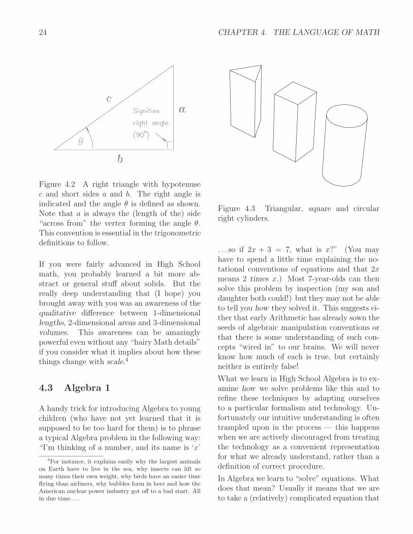
24 CHAPTER 4. THE LANGUAGE OF MATH
Figure 4.2 A right triangle with hypotenusec and short sides a and b. The right angle isindicated and the angle θ is defined as shown.Note that a is always the (length of the) side“across from” the vertex forming the angle θ.This convention is essential in the trigonometricdefinitions to follow.
If you were fairly advanced in High Schoolmath, you probably learned a bit more ab-stract or general stuff about solids. But thereally deep understanding that (I hope) youbrought away with you was an awareness of thequalitative difference between 1-dimensionallengths, 2-dimensional areas and 3-dimensionalvolumes. This awareness can be amazinglypowerful even without any “hairy Math details”if you consider what it implies about how thesethings change with scale.4
4.3 Algebra 1
A handy trick for introducing Algebra to youngchildren (who have not yet learned that it issupposed to be too hard for them) is to phrasea typical Algebra problem in the following way:“I’m thinking of a number, and its name is ‘x’
4For instance, it explains easily why the largest animalson Earth have to live in the sea, why insects can lift somany times their own weight, why birds have an easier timeflying than airliners, why bubbles form in beer and how theAmerican nuclear power industry got off to a bad start. Allin due time. . . .
Figure 4.3 Triangular, square and circularright cylinders.
. . . so if 2x + 3 = 7, what is x?” (You mayhave to spend a little time explaining the no-tational conventions of equations and that 2xmeans 2 times x.) Most 7-year-olds can thensolve this problem by inspection (my son anddaughter both could!) but they may not be ableto tell you how they solved it. This suggests ei-ther that early Arithmetic has already sown theseeds of algebraic manipulation conventions orthat there is some understanding of such con-cepts “wired in” to our brains. We will neverknow how much of each is true, but certainlyneither is entirely false!
What we learn in High School Algebra is to ex-amine how we solve problems like this and torefine these techniques by adapting ourselvesto a particular formalism and technology. Un-fortunately our intuitive understanding is oftentrampled upon in the process — this happenswhen we are actively discouraged from treatingthe technology as a convenient representationfor what we already understand, rather than adefinition of correct procedure.
In Algebra we learn to “solve” equations. Whatdoes that mean? Usually it means that we areto take a (relatively) complicated equation that
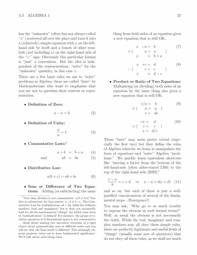
4.3. ALGEBRA 1 25
has the “unknown” (often but not always called“x”) scattered all over the place and turn it intoa (relatively) simple equation with x on the left-hand side by itself and a bunch of other sym-bols (not including x) on the right-hand side ofthe “=” sign. Obviously this particular formatis “just” a convention. But the idea is inde-pendent of the representation: “solve” for the“unknown” quantity, in this case x.
There are a few basic rules we use to “solve”problems in Algebra; these are called “laws” byMathematicians who want to emphasize thatyou are not to question their content or repre-sentation.
• Definition of Zero:
a − a = 0 (2)
• Definition of Unity:
a
a= 1 (3)
• Commutative Laws:5
a + b = b + a (4)
and ab = ba (5)
• Distributive Law:
a(b + c) = ab + bc (6)
• Sum or Difference of Two Equa-tions: Adding (or subtracting) the same
5Note that division is not commutative: a/b 6= b/a! Nei-ther is subtraction, for that matter: a−b 6= b−a. The Com-mutative Law for multiplication, ab = ba, holds for ordinarynumbers (real and imaginary) but it does not necessarilyhold for all the mathematical “things” for which some formof “multiplication” is defined! For instance, the group of ro-tation operators in 3-dimensional space is not commutative— think about making two successive rotations of a rigidobject about perpendicular axes in different order and youwill see that the final result is different! This seemingly ob-scure property turns out to have fundamental significance.We’ll talk about such things later.
thing from both sides of an equation givesa new equation that is still OK.
+ (x
x
−a =a =
=
bab + a
)(7)
− (x
x
+c =c =
=
dcd − c
)(8)
• Product or Ratio of Two Equations:Multiplying (or dividing) both sides of anequation by the same thing also gives anew equation that is still OK.
× (x/a =
a =x =
baab
)(9)
÷ (cx =c =x =
dc
d/c)
(10)
These “laws” may seem pretty trivial (espe-cially the first two) but they define the rulesof Algebra whereby we learn to manipulate theform of equations and “solve” Algebra “prob-lems.” We quickly learn equivalent shortcutslike “moving a factor from the bottom of theleft-hand-side [often abbreviated LHS] to thetop of the right-hand side [RHS]:”
x − a
b= c + d ⇒ x − a = b(c + d) (11)
and so on; but each of these is just a well-justified concatenation of several of the funda-mental steps. (Emergence!)
You may ask, “Why go to so much troubleto express the obvious in such formal terms?”Well, as usual the obvious is not necessarilythe truth. While the real, imaginary and com-plex numbers may all obey these simple rules,there are perfectly legitimate and useful fields of“things” (usually some sort of operators) thatdo not obey all these rules, as we shall see much

26 CHAPTER 4. THE LANGUAGE OF MATH
later in the course (probably). It is generally agood idea to know your own assumptions; wehaven’t the time to keep reexamining them con-stantly, so we try to state them as plainly as wecan and keep them around for reference “justin case. . . .”
4.4 Trigonometry
Trigonometry is a specialized branch of Geome-try in which we pay excruciatingly close atten-tion to the properties of triangles, in particu-lar right triangles. Referring to Fig. 4.2 again,we define the sine of the angle θ (abbreviatedsin θ) to be the ratio of the “far side” a to thehypotenuse c and the cosine of θ (abbreviatedcos θ) to be the ratio of the “near side” b to thehypoteneuse c:
sin θ ≡ a
ccos θ ≡ b
c(12)
The other trigonometric functions can easily bedefined in terms of the sin and cos:
tangent: tan θ ≡ a
b=
sin θ
cos θ
cotangent: cot θ ≡ b
a=
sin θ
cos θ=
1
tan θ
secant: sec θ ≡ c
b=
1
cos θ
cosecant: csc θ ≡ c
a=
1
sin θ
For the life of me, I can’t imagine why any-one invented the cotangent, the secant and thecosecant — as far as I can tell, they are totallysuperfluous baggage that just slows you downin any actual calculations. Forget them. [Ah-hhh. I have always wanted to say that! Ofcourse you are wise enough to take my advicewith a grain of salt, especially is you want toappear clever to Mathematicians. . . .]
The sine and cosine of θ are our trigonometricworkhorses. In no time at all, I will be wantingto think of them as functions — i.e. when yousee “cos θ” I will want you to say, “cosine oftheta” and think of it as cos(θ) the same wayyou think of y(x). Whether as simple ratios oras functions, they have several delightful prop-erties, the most important of which is obviousfrom the Pythagorean Theorem:6
cos2 θ + sin2 θ = 1 (13)
where the notation sin2 θ means the square ofsin θ — i.e. sin2 θ ≡ (sin θ) × (sin θ) — andsimilarly for cos θ. This convention is adoptedto avoid confusion, believe it or not. If we wrote“sin θ 2” it would be impossible to know for surewhether we meant sin(θ2) or (sin θ)2; we couldalways put parentheses in the right places toremove the ambiguity, but in this case thereis a convention instead. (People always haveconventions when they are tired of thinking!)
I will need other trigonometric identities lateron, but they can wait — why introduce mathuntil we need it? [I have made an obviousexception in this Chapter as a whole onlyto “jump start” your Mathematical language(re)training.]
4.5 Algebra 2
“I’m thinking of a number, and its name is ‘x’. . . ” So if
ax2 + bx + c = 0, (14)
what is x? Well, we can only say, “It depends.”Namely, it depends on the values of a, b and c,whatever they are. Let’s suppose the dimen-sions of all these “parameters” are mutuallyconsistent7 so that the equation makes sense.
6Surely you aren’t going to take my word for this! Con-vince yourself that this formula is really true!
7In Mathematics we never worry about such things; allour symbols represent pure numbers; but in Physics we usu-ally have to express the value of some physical quantity inunits which make sense and are consistent with the units ofother physical quantities symbolized in the same equation!

4.6. CALCULUS 27
Then “it can be shown” (a classic phrase ifthere ever was one!) that the “answer” is gen-erally8
x =−b ±
√b2 − 4ac
2a. (15)
This formula (and the preceding equation thatdefines what we mean by a, b and c) is knownas the Quadratic Theorem, so called because itoffers “the answer” to any quadratic equation(i.e. one containing powers of x up to and in-cluding x2). The power of such a general so-lution is prodigious. (Work out a few exam-ples!) It also introduces an interesting new wayof looking at the relationship between x andthe parameters a, b and c that determine itsvalue(s). Having x all by itself on one side of theequation and no x’s anywhere on the other sideis what we call a “solution” in Algebra. Let’smake a simpler version of this sort of equation:
“I’m thinking of a number, and its name is ‘y’. . . ” So if y = x2, what is y? The answer isagain, “It depends!” (In this case, upon thevalue of x.) And that leads us into a new sub-ject. . . .
4.6 Calculus
In a stylistic sense, Algebra starts to becomeCalculus when we write the preceding example,y = x2, in the form
y(x) = x2
which we read as “y of x equals x squared.”This is how we signal that we mean to thinkof y as a function of x, and right away we areleading into the terminology of Calculus. Recallthe final sections of the preceding Chapter.
However, Calculus really begins when we starttalking about the rate of change of y as x varies.
8The ± symbol means that both signs (+ and −) shouldrepresent legitimate answers.
4.6.1 Rates of Change
One thing that is easy to “read off a graph” ofy(x) is the slope of the curve at any given pointx. Now, if y(x) is quite “curved” at the point ofinterest, it may seem contradictory to speak ofits “slope,” a property of a straight line. How-ever, it is easy to see that as long as the curveis smooth it will always look like a straight lineunder sufficiently high magnification. This isillustrated in Fig. 4.4 for a typical y(x) by aprocess of successive magnifications.
Figure 4.4 A series of “zooms” on a segmentof the curve y(x) showing how the curved linebegins to look more and more like a straightline under higher and higher magnification.
We can also prescribe an algebraic method forcalculating the slope, as illustrated in Fig. 4.5:the definition of the “slope” is the ratio of theincrease in y to the increase in x on a van-ishingly small interval. That is, when x goesfrom its initial value x0 to a slightly larger valuex0+∆x, the curve carries y from its initial valuey0 = y(x0) to a new value y0+∆y = y(x0+∆x),and the slope of the curve at x = x0 is givenby ∆y/∆x for a vanishingly small ∆x. Whena small change like ∆x gets really small (i.e.small enough that the curve looks like a straight

28 CHAPTER 4. THE LANGUAGE OF MATH
Figure 4.5 A graph of the function y(x) show-ing how the average slope ∆y/∆x is obtainedon a finite interval of the curve. By takingsmaller and smaller intervals, one can eventu-ally obtain the slope at a point, dy/dx.
line on that interval, or “small enough to satisfywhatever criterion you want,” then we write itdifferently, as dx, a “differential” (vanishinglysmall) change in x. Then the exact definitionof the SLOPE of y with respect to x at someparticular value of x, written in conventionalMathematical language, is
dy
dx≡ lim
∆x→0
∆y
∆x≡ lim
∆x→0
y(x + ∆x) − y(x)
∆x(16)
This is best understood by an example: con-sider the simple function y(x) = x2. Then
y(x + ∆x) = (x + ∆x)2 = x2 + 2x∆x + (∆x)2
and y(x + ∆x) − y(x) = 2x∆x + (∆x)2.
Divide this by ∆x and we have
∆y
∆x= 2x + ∆x.
Now let ∆x shrink to zero, and all that remainsis
∆y
∆x−→∆x→0
dy
dx= 2x.
Thus the slope [or derivative, as mathemati-cians are wont to call it] of y(x) = x2 isdy/dx = 2x. That is, the slope increases lin-early with x. The slope of the slope — whichwe call9 the curvature, for obvious reasons —is then trivially d(dy/dx)/dx ≡ d2y/dx2 = 2,a constant. Make sure you can work this partout for yourself.
We have defined all these algebraic solutionsto the geometrical problem of finding the slopeof a curve on a graph in completely abstractterms — “x” and “y” indeed! What are x andy? Well, the whole idea is that they can be any-thing you want! The most common examplesin Physics are when x is the elapsed time, usu-ally written t, and y is the distance travelled,usually (alas) written x. Thus in an elementaryPhysics context the function you are apt to seeused most often is x(t), the position of someobject as a function of time. This particularfunction has some very well-known derivatives,namely dx/dt = v, the speed or (as long as themotion is in a straight line!) velocity of the ob-ject; and dv/dt ≡ d2x/dt2 = a, the accelerationof the object. Note that both v and a are them-selves (in general) functions of time: v(t) anda(t). This example so beautifully illustrates the“meaning” of the slope and curvature of a curveas first and second derivatives that many intro-ductory Calculus courses and virtually all intro-ductory Physics courses use it as the exampleto explain these Mathematical conventions. Ijust had to be different and start with some-thing a little more formal, because I think youwill find that the idea of one thing being a func-tion of another thing, and the associated ideasof graphs and slopes and curvatures, are handynotions worth putting to work far from theirtraditional realm of classical kinematics.
9This differs from the conventional mathematical defini-tion of curvature, κ ≡ dφ/ds, where φ is the tangential angleand s is the arc length, but I like mine better, because it’ssimple, intuitive and useful. (OK, I’m a Philistine. So shootme. ;-) Thanks to Mitchell Timin for pointing this out.

5.1. TOLERANCE 29
Chapter 5
Measurement
Earlier we discussed the tactical problems as-sociated with describing quantitative measure-ments, reminding ourselves that the tools weuse (numbers, dimensions, units) are almostperfectly arbitrary in isolation but embody afunctional or relational truth in the “grammar”of their use. Accepting these tools provision-ally, we turn now to the far messier problem ofactually performing measurements.
5.1 Tolerance
(Advertising Your Uncertainty)
Virtually all [I could follow the consensus andsay all, but I feel like hedging] “scientific” pro-cedures involve measurement of experimentalparameters such as distance, time, velocity,mass, energy, temperature, . . . etc. Virtuallyall measurements are subject to error; that is,they may be inaccurate (wrong) by some un-known amount due to effects ranging from er-rors in recording [“I said 3.32, not 3.23!”] tomiscalibrated instruments [“I thought these ticmarks were centimetres!”]. Such “systematicerrors” are embarrassing to the experimenter,as they imply poor technique, and are alwayshard to estimate; but we are honour-bound totry. An entirely different source of error thatconveys no negative connotations on the ex-perimenter is the fact that all measurementshave limited precision or “tolerance” — limited
by the “marks” on the generalized “ruler” usedfor measuring-by-comparison. (E.g., the dis-tance your measure with a micrometer is moreprecisely known than the distance you measurewith a cloth tape measure.)
Knowing this, most scientists and virtually allphysicists have an æsthetic about measured val-ues of things: they are never to be reportedwithout an explicit estimation of their uncer-tainty . That is, measurements must always bereported in the form
(VALUE ± UNCERTAINTY) UNITS
or equivalent notation (sometimes a shorthandversion), such as 3.1416(12) radians, meaning(3.1416 ± 0.0012) radians. [The (12) means theuncertainty in the last two digits is ± 12.] Thisshorthand form is convenient for long stringsof digits with only the last 1 or 2 digits uncer-tain, but the explicit form with the ± is morepleasing to the æsthetic mentioned above.
When, as in some elementary particle physicsexperiments lasting many years and costingmillions of dollars, a great deal of effort hasgone into measuring a single number, it is com-mon practice to make a clear distinction be-tween “statistical errors” (the precision of ourinstrumentation) and suspected “systematic er-rors” (mistakes). In most situations, however,both are lumped together or “added in quadra-ture” (the total uncertainty is the square root ofthe sum of the squares of the uncertainties dueto all the independent sources of error).1 It is
1More on this later. . . .

30 CHAPTER 5. MEASUREMENT
considered poor form to cavalierly overestimateone’s uncertainty to reduce the significance ofdeviations from expectations.
To write a measured value without its tolerance(uncertainty, “possible error,” etc.) is as badform as leaving out the units of the measure-ment. The significance of your measurement islost. To do this in the presence of physicists islike ordering Ripple with your meal at Maxim’s.Sadly, values are slipping throughout society,and otherwise respectable scientists can oftenbe heard to quote numbers without specifyinguncertainties. The best we can do is to be surewe do not contribute to this decay.
5.1.1 Sig Figs
In other disciplines (Chemistry and Engineer-ing especially) some people like to stick withthe explicit notational conventions describedabove but others are fond of the supposed econ-omy introduced by the so-called “significantfigures” (or “sig figs”) convention, in whichuncertainties are not explicitly expressed butare implicit in the last significant digit of thenumber written down. I have listened to somany long explanations of this convention in at-tempts to clarify its proper use and interpreta-tion for confused students that I prefer to adoptthe short form:
Forget “sig figs” in Physics.
Whenever you make a Physics measurement,express your result and its uncertainty in one ofthe explicit forms described earlier. The issueof how many significant digits to write down isthen one of common sense rather than conven-tion. It is silly to write down 0.123456±0.03,but it is not wrong.
One reason I encourage you to eschew “sigfigs” is that even silly-looking results like0.1234±0.0321 (why would anyone express anuncertainty to three significant digits?) actu-
ally make sense in special circumstances. Forinstance, if thousands of professors from allover the world spend half a billion dollars overtwenty years just to measure one really impor-tant property of elementary particles, you canhardly blame them for expressing the result aspainstakingly as possible. However, even thenit makes no sense to show more significant dig-its in the result than in its uncertainty; that’sjust common sense. So use yours.
5.1.2 Graphs &Error Bars
When plotting points on a graph, the uncer-tainty is included in the form of “error bars”which look like this:
“Bestestimate”
→
⊤|
⊙
|⊥
Region ofuncertainty: onestandard deviation (1σ) on either side⇒ 64% probability of“true” value beingwithin this region.
5.1.3 Vector Tolerance
Allow me to slip into something a little moreformal. . . .
Usually this topic would be called “Error Prop-agation in Functions of Several Variables” orsomething like that; I have used the term “vec-tor tolerance” because (a) the word “error” hasthese perjorative connotations for most peo-ple, whereas “tolerance” is usually considereda good thing;2 (b) when our final result is cal-culated in terms of several other quantities,each of which is uncertain by some amount,and when those uncertainties are independentof each other, we get a situation much liketrying to define the overall length of a vectorwith several independent perpendicular compo-nents. Each contribution to the overall uncer-tainty can be positive or negative, and on av-
2“Uncertainty” is somewhere in between.
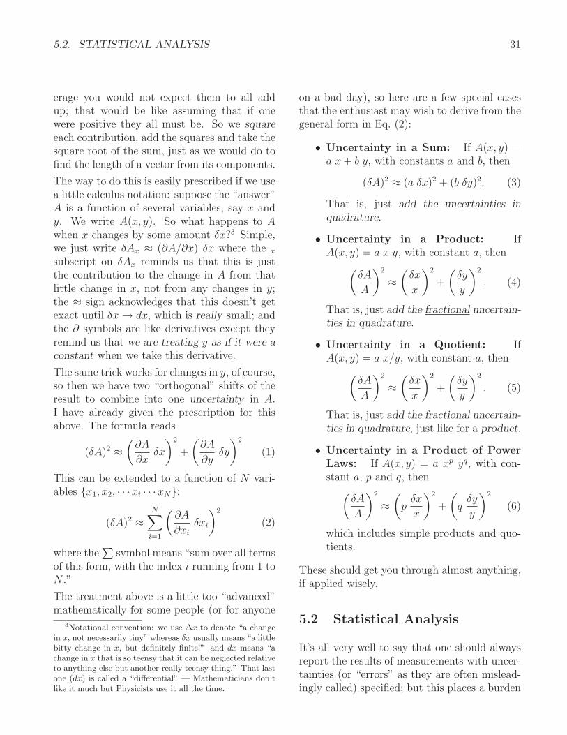
5.2. STATISTICAL ANALYSIS 31
erage you would not expect them to all addup; that would be like assuming that if onewere positive they all must be. So we squareeach contribution, add the squares and take thesquare root of the sum, just as we would do tofind the length of a vector from its components.
The way to do this is easily prescribed if we usea little calculus notation: suppose the “answer”A is a function of several variables, say x andy. We write A(x, y). So what happens to Awhen x changes by some amount δx?3 Simple,we just write δAx ≈ (∂A/∂x) δx where the x
subscript on δAx reminds us that this is justthe contribution to the change in A from thatlittle change in x, not from any changes in y;the ≈ sign acknowledges that this doesn’t getexact until δx → dx, which is really small; andthe ∂ symbols are like derivatives except theyremind us that we are treating y as if it were aconstant when we take this derivative.
The same trick works for changes in y, of course,so then we have two “orthogonal” shifts of theresult to combine into one uncertainty in A.I have already given the prescription for thisabove. The formula reads
(δA)2 ≈(
∂A
∂xδx
)2
+
(
∂A
∂yδy
)2
(1)
This can be extended to a function of N vari-ables x1, x2, · · ·xi · · ·xN:
(δA)2 ≈N
∑
i=1
(
∂A
∂xi
δxi
)2
(2)
where the∑
symbol means “sum over all termsof this form, with the index i running from 1 toN .”
The treatment above is a little too “advanced”mathematically for some people (or for anyone
3Notational convention: we use ∆x to denote “a changein x, not necessarily tiny” whereas δx usually means “a littlebitty change in x, but definitely finite!” and dx means “achange in x that is so teensy that it can be neglected relativeto anything else but another really teensy thing.” That lastone (dx) is called a “differential” — Mathematicians don’tlike it much but Physicists use it all the time.
on a bad day), so here are a few special casesthat the enthusiast may wish to derive from thegeneral form in Eq. (2):
• Uncertainty in a Sum: If A(x, y) =a x + b y, with constants a and b, then
(δA)2 ≈ (a δx)2 + (b δy)2. (3)
That is, just add the uncertainties inquadrature.
• Uncertainty in a Product: IfA(x, y) = a x y, with constant a, then
(
δA
A
)2
≈(
δx
x
)2
+
(
δy
y
)2
. (4)
That is, just add the fractional uncertain-ties in quadrature.
• Uncertainty in a Quotient: IfA(x, y) = a x/y, with constant a, then
(
δA
A
)2
≈(
δx
x
)2
+
(
δy
y
)2
. (5)
That is, just add the fractional uncertain-ties in quadrature, just like for a product.
• Uncertainty in a Product of PowerLaws: If A(x, y) = a xp yq, with con-stant a, p and q, then
(
δA
A
)2
≈(
pδx
x
)2
+
(
qδy
y
)2
(6)
which includes simple products and quo-tients.
These should get you through almost anything,if applied wisely.
5.2 Statistical Analysis
It’s all very well to say that one should alwaysreport the results of measurements with uncer-tainties (or “errors” as they are often mislead-ingly called) specified; but this places a burden

32 CHAPTER 5. MEASUREMENT
of judgement on the experimenter, who mustestimate uncertainties in a manner fraught withindividual idiosyncracies. Wouldn’t it be nice ifthere were a way to measure one’s uncertaintyin a rigourous fashion?
Well, there is. It is a little tedious and compli-cated, but easily understood: one must make alarge number of repeated measurements of thesame thing and analyze the “scatter” of the an-swers!
Suppose we are trying to determine the “true”value of the quantity x. (We usually refer tounspecified things as “x” in this business.) Itcould be your pulse rate or some other simplephysical observable.
We make N independent measurements xi (i =1, 2, 3, . . . , N) under as close to identical con-ditions as we can manage. Each measurment,we suspect, is not terribly precise; but we don’tknow just how imprecise. (It could be largelydue to some factor beyond our control; pulserates, for instance, fluctuate for many reasons.)
Now, the xi will “scatter” around the “true” xin a distribution that will put some xi smallerthan the true x and others larger. We assumethat whatever the cause of the scatter, it is basi-cally random — i.e. the exact value of one mea-surement xi+1 is not directly influenced by thevalue xi obtained on the previous measurement.(Actually, perfect randomness is not only hardto define, but rather difficult to arrange in prac-tice; it is sufficient that most fluctuations arerandom enough to justify the treatment beingdescribed here.) It is intuitively obvious (andcan even be rigorously proved in most cases)that our best estimate for the “true” x is the
average or mean value, x, given by:4
x ≡ 1
N
N∑
i=1
xi. (7)
But what is the uncertainty in x? Let’s call itσx.
How can we find σx mathematically from thedata? Well, if we assume that each indi-vidual measurement xi has the same single-measurement uncertainty σx, then the distribu-tion of xi should look like a “bell-shaped curve”or gaussian distribution:
Figure 5.1 A typical graph of D(x), the distri-bution of x, defined as the relative frequency ofoccurence of different values of x from succes-sive measurements. The “centre” of the distri-bution is at x, the average or mean of x. The“width” of the distribution is 2σ (one σ on ei-ther side of the mean.
Obviously, ∆xi ≡ xi−x is a measure of the “er-ror” in the ith measurement, but we cannot justfind the average of ∆xi, since by definition the
4The symbolN
X
i=1
represents an operator called “summa-
tion” — it means that the stuff to the right of the Σ,which will always have a subscript i in one or more places,is to be thought of as the “ith term” and all such termswith i values running from 1 to N are to be added together
to form the desired result. So, for instance,N
X
i=1
xi means
x1 + x2 + x3 + . . . + xN−1 + xN, or (to be more specific)if N = 3, just x1 + x2 + x3. This may seem a little ar-cane, but it is actually a very handy compact notation forthe rather common summation operation.
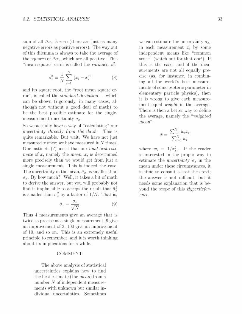
5.2. STATISTICAL ANALYSIS 33
sum of all ∆xi is zero (there are just as manynegative errors as positive errors). The way outof this dilemma is always to take the average ofthe squares of ∆xi, which are all positive. This“mean square” error is called the variance, s2
x:
s2x ≡ 1
N
N∑
i=1
(xi − x)2 (8)
and its square root, the “root mean square er-ror”, is called the standard deviation — whichcan be shown (rigorously, in many cases, al-though not without a good deal of math) tobe the best possible estimate for the single-measurement uncertainty σx.
So we actually have a way of “calculating” ouruncertainty directly from the data! This isquite remarkable. But wait. We have not justmeasured x once; we have measured it N times.Our instincts (?) insist that our final best esti-mate of x, namely the mean, x, is determinedmore precisely than we would get from just asingle measurement. This is indeed the case.The uncertainty in the mean, σx, is smaller thanσx. By how much? Well, it takes a bit of mathto derive the answer, but you will probably notfind it implausible to accept the result that σ2
x
is smaller than σ2x by a factor of 1/N . That is,
σx =σx√N
. (9)
Thus 4 measurements give an average that istwice as precise as a single measurement, 9 givean improvement of 3, 100 give an improvementof 10, and so on. This is an extremely usefulprinciple to remember, and it is worth thinkingabout its implications for a while.
COMMENT:
The above analysis of statisticaluncertainties explains how to findthe best estimate (the mean) from anumber N of independent measure-ments with unknown but similar in-dividual uncertainties. Sometimes
we can estimate the uncertainty σxi
in each measurement xi by someindependent means like “commonsense” (watch out for that one!). Ifthis is the case, and if the mea-surements are not all equally pre-cise (as, for instance, in combin-ing all the world’s best measure-ments of some esoteric parameter inelementary particle physics), thenit is wrong to give each measure-ment equal weight in the average.There is then a better way to definethe average, namely the “weightedmean”:
x =
∑Ni=1 wixi
∑Ni=1 wi
where wi ≡ 1/σ2xi
. If the readeris interested in the proper way toestimate the uncertainty σx in themean under these circumstances, itis time to consult a statistics text;the answer is not difficult, but itneeds some explanation that is be-yond the scope of this HyperRefer-
ence.

34 CHAPTER 5. MEASUREMENT

6.1. GALILEO 35
Chapter 6
Falling Bodies
Now that we have mastered all sorts of Algebraand Calculus skills, it is time to get on withNewtonian Mechanics, Gravitation, Cosmologyand all that, right?
Gee, I sure wish it were true.
Although (I hope you will agree) there are someinteresting historical and perceptual lessons tobe learned from Newton’s Mechanics, it is gen-erally rated as one of the more boring topics inPhysics;1 worse yet, we are not yet ready forNewton — “You have to creep before you cancrawl,” as it were. And in this business “creep-ing” is the business of Kinematics — the studyof motion per se.
Besides, before we go on to expound Newton’s“Laws” in their modern form we will need tohave a chapter on vectors, since forces are clas-sic examples of vectors — i.e. they have bothmagnitude and direction.2
1This is partly because everyone is so anxious to “get onto the good stuff” that they are predisposed to give a rathersuperficial treatment to Mechanics; and partly because mostbeginning Physics courses are expected to produce graduateswho can actually calculate tensions in wires, whether boxeswill slide off trucks and other practical things like that. For-tunately, I don’t care whether you can do that stuff or not,except for a few simple examples for the sake of illustrationand familiarization. This book may help you build a bridgein your back yard, but honestly I think there are much moreuseful study aids for developing such skills. What I am af-ter is just to get you familiar enough with the paradigms ofMechanics to allow bootstrapping on to the next stage.
2This is also true of distance, velocity and acceleration,which are the topics of this Chapter; but we have to startsomewhere.
6.1 Galileo
As I warned the reader in several places ear-lier, I am no historian. However, I do havemany traits in common with real Historians; inparticular, I like to construct theories of “whatprobably really happened” to fit my own inter-pretation of the historical “data.” Physicistsalso like this sort of revisionism, but I think weare mercifully more shameless and direct aboutit. [“Yeah, OK, I lied; but it was a good lie— doesn’t it make everything easier to under-stand?”] With this caveat, I will relate a bit ofBrewer’s History of Classical Mechanics.
Galileo Galilei (1564-1642) was a clever Ital-ian megalomaniac who took pleasure in pub-licly ridiculing his intellectual opponents andregarded the authorities as annoying buffoonsto be manipulated by any means available inorder to obtain funding for his pet projects. Hethus epitomized a fine tradition which continuesto this day. Galileo is widely credited with be-ing “the Father of Modern Science” because ofthe experimental æsthetics he championed3 andbecause of the impact of his major work, Two
New Sciences [mechanics and the strength ofmaterials], published in 1636. I am inclined tothink that his distinctive personality and stylehad just as much to do with his deserving thistitle; today these traits are still apt to improvethe bearer’s chances for distinction by various
3Often referred to as the “Scientific Method,” aboutwhich I will have more to say later on.

36 CHAPTER 6. FALLING BODIES
prizes and accolades.
6.1.1 Harvard?
Rather than reproduce the list of Galileo’s ad-ventures available in any textbook with even apretense of historical perspective, I will mentionone amusing claim that I heard somewhere:4
when Galileo got into trouble with the Churchover his heretical views5 he was offered a facultyposition at a new University in another coun-try where the Roman Church was not all thatpopular — the school in question was Harvard.6
6.1.2 Weapons Research: Telescopes &Trajectories
Ever the Modern Physicist, Galileo recognizedclearly that the big money and prestige werein military applications of science. In thosedays the new weapons technology was cannonsand how to aim them more accurately at tar-gets. His contributions to this art took twomain forms: the first was his invention of themagnifying telescope, with which it was possi-ble to identify targets at great range and as-sess the damage done to them by one’s can-nonballs. To be fair, I should point out thatthis invention was warmly received by seafar-ers and astronomers as well as generals; in fact,with it Galileo himself made famous and won-derful observations of the Moon, the “Galilean”moons (named after guess whom) of Jupiterand numerous other objects in our Solar Sys-tem, thereby initiating the modern pastime ofPlanetology that recently culminated in the
4You real Historians go check this out!5Actually they would probably have left him alone if he
hadn’t been so obnoxious about publicly rubbing their nosesin it.
6One imagines Galileo’s response was, “I’m not thatdesparate.” In those days Harvard had presumably not yetacquired much of a reputation. It is amusing to speculate onhow much more classic an example of the Modern Physicisthe would have made had Galileo accepted this offer of a NewWorld professorship.
fantastic close-up views of the outer planets andtheir satellites by Terran space probes. Onecan easily imagine how ridiculous the Church’sPtolemaic ergocentric model of the Heavensmust have seemed to Galileo after watchingso many other planets execute their orbits asclearly visible globes lit on the Sun side.7 Thereare two sides to every coin.
Galileo’s second contribution to the art of ar-tilliery was his formal explication of the be-haviour of falling bodies, of which cannonand musket balls were oft-mentioned examples.Galileo “showed”8 that the velocity of a fallingbody increases by equal increments in equaltimes (in the absence of friction), which is thedefinition of a state of constant acceleration.
Constant Acceleration
In terms of our newly-acquired left hemisphereskills, if we use y to designate height [say, abovesea level] and t to designate time, then the up-ward velocity vy [where the subscript tells usexplicitly that this is the upward velocity asopposed to the horizontal velocity which wouldprobably be written vx]
9 is given by
vy = vy0 − gt (1)
7The astronomical observations of Tycho Brahe and Jo-hannes Kepler empirically obliterated the Ptolemaic systemin favour of a correct heliocentric model of the Solar systemat about the same time as Galileo took on the Church inItaly; I am not certain how much interaction there was be-tween these apparently separate battles. More on this later.
8There is room for argument over whether he really“showed” this, both from a Popperian purist’s point of view[you can never verify a conjecture, only refute it] and fromthe point of view of the very æsthetic he helped to popularize— namely, that you shouldn’t “fudge” your results and thatother people should be able to reproduce them. It is, how-ever, certainly true that he made a very persuasive case forthe economy and utility of this confessed overidealization;and this is, after all, the true measure of any theory!
9Why not just call it v, if I am not going to be talkingabout any of the horizontal stuff? Well, this is a prettysimple equation, so I am going to “stack” it with lessonsin notation which will serve to make its meaning absolutelyunambiguous (subject to all these explanations) and to in-troduce fine points I will be needing shortly anyway.

6.1. GALILEO 37
where vy0 is the initial10 upward velocity (i.e.the upward velocity at t = 0), if any,11 and gis the downward12 acceleration of gravity, g ≈9.81 m/s2 on average at the Earth’s surface.13
Another way of writing the same equation isin terms of the derivative of the velocity withrespect to time,
ay ≡ dvy
dt≡ vy = −g, (2)
where I have introduced yet another notationalconvention used by Physicists: a little dotabove a symbol means the time derivative ofthat symbol — i.e. the rate of change (per unittime) of the quantity represented by that sym-bol.14 And since vy is itself the time derivative
10Note: generally any symbol with a subscript 0 (read“nought” as in x0 = “x nought”) designates an initial valueof the subscripted symbol — i.e. the value at t = 0. (Westop short of writing t0 for the initial time, in most cases,because we usually don’t need any further redundancy tomake the the description completely general.) Thus x maybe a variable, a function of time x(t), but its initial valuex0 ≡ x(0) is a constant, a parameter of its evolution in time.Since we will often talk about the final value of some variable(e.g. xf ) at time tf (at the end of some process), using thesubscript f to designate “final,” it is equally logical to usea subscript i for “initial,” so that the value of x(t) at t = 0would be written xi — this notation is perfectly synonymouswith the “nought” notation: x0 ≡ xi and the two may beused interchangably according to taste.
11Lots of people leave out the vy0in order to keep it sim-
pler, but of course that would be tantamount to assumingthat we were starting from rest, which ain’t necesarily so!Why oversimplify an already simple equation?
12Note that the conventional choice of “up” as being thepositive y direction forces us to put the acceleration of grav-ity into the equation with a minus sign, since it is in the“down” direction. Sometimes people try to make this looksimpler for beginners by defining down as the +y direction,but I like to get across as early as possible that a negativeacceleration simply means an acceleration in the directionopposite to the one we arbitrarily defined to be positive. Thesame is true of any quantity (e.g. the velocity or the posi-tion) that has a direction as well as a magnitude; this ideais vital to an understanding of vectors, which are coming upsoon!
13What?! How come I don’t give g to a huge number ofsignificant figures, with an uncertainty specified, as one issupposed to do for fundamental constants? Because g isneither fundamental nor constant! Far from it. More onthis later.
14I will soon need the analogous notation x ≡ d2x/dt2
to signify the second time derivative of x, so that ay ≡
of the height y [i.e. vy ≡ dy/dt ≡ y], if we likewe can write the original equation as
y = vy0 − gt. (3)
All these notational gymnastics have severalpurposes, one of which is to make you appreci-ate the simple clarity of the declaration, “Thevertical speed increases by equal increments inequal times,” as originally stated by Galileohimself. But I also want you to see how Physi-cists like to condense their notation until a verycompact equation “says it all.”
Principles of Inertia and Superposition
Galileo was actually the first to write down“Newton’s” celebrated First Law, in a formslightly different from Newton’s but just asgood:15
Galileo’s Principle of Inertia:
A body moving on a level surfacewill continue in the same directionat constant speed unless disturbed.
Note the term “body” employed in order to bedeliberately vague about what sort of entitiesthe Principle is meant to apply to. This term isretained in the language of modern Mechanics.It means, more or less, “a massive thing thathangs together.” Note also the other ringers,“level surface” and “unless disturbed.” Per-fectly level surfaces are mighty hard to comeby, but Galileo means, of course, a hypotheti-cal perfectly level surface. More serious is thevagueness of “unless disturbed.” This can eas-ily be used to make the argument circular: if
dvy/dt ≡ d2y/dt2 ≡ y. The “double-dot” form is the pre-ferred Physics notation for acceleration, mainly for reasonsof economy (it takes so few strokes to write).
15This is translated from the Italian by someone else; Ican’t vouch for the translation but I am confident that itgets the right idea across and I am not much interested inquibbles over the exact wording or what it might have meantabout Galileo’s “authentic originality.”

38 CHAPTER 6. FALLING BODIES
the body’s velocity changes direction or magni-tude, it is because it is “disturbed.” Well. . . .Newton invented a new concept to make “dis-turbance” a little more specific.
The other important insight Galileo saw fit toenshrine as a Principle was
Galileo’s Principle of Superposition:
If a body is subjected to two sep-arate influences, each producing acharacteristic type of motion, it re-sponds to each without modifyingits response to the other.
This, like the other Principle, seems transpar-ently obvious to Modern eyes,16 but without itone would never know how to start applyingGalileo’s simplified kinematics to the practicalproblem of trajectories. Again there is a littlesloppiness to the Principle that allows for coun-terexamples; no doubt Galileo had to rely reg-ularly on the most honest of all appeals: “Youknow what I mean.”
Calculating Trajectories
Applied to the case of trajectories close to theEarth’s surface,17 the equations governing con-stant horizontal velocity superimposed uponconstant downward acceleration take the form
x = 0 (4)
x = vx0 (constant) (5)
x = x0 + vx0 t (6)
and (7)
y = −g (8)
y = vy0 − g t (9)
y = y0 + vy0 t − 1
2g t2 (10)
16This may well be a good measure of the brilliance of aninsight.
17E.g., cannonballs! This sort of “techno doubletalk” isnot always used for obfuscation [I, for instance, am simplytrying to be general!] but Pentagon aides trying to be Gen-erals are very fond of it too.
where
x ≡ d2x
dt2≡ dvx
dt≡ vx ≡ ax, (11)
x ≡ dx
dt≡ vx, (12)
y ≡ d2y
dt2≡ dvy
dt≡ vy ≡ ay (13)
and y ≡ dy
dt≡ vy (14)
Hold it! Before you bolt for the door, takea moment to casually read through all thesehorrible-looking equations. I have made themlook long and hirsute on purpose, for two rea-sons: first, because this way they are in theirmost general form — i.e. we can be confidentthat these equations will correctly describe anytrajectory problem, but for any actual problemthe equations will usually simplify ; and second,because this is a sort of practical joke — ifyou look carefully you will see that the equa-tions are really pretty simple! All those “≡”symbols just mean, “. . . another way of puttingit, which amounts to exactly the same thing,is. . . .” That is, they just indicate equivalentnotations — or, in the language of linguistics,synonyms. So the latter batch of equations isjust reminding you of the convention Physi-cists use for writing time derivatives: “dot”and “double-dot” notation. The first batch ofequations tells you (in this notation) everythingthere is to know about the motion: the hori-zontal [x] motion is not under any acceleration[ax ≡ x = 0] so the horizontal velocity [vx ≡ x]is constant [x = vx0 ] and the distance trav-elled horizontally [x(t)] is just increasing lin-early with time t relative to its initial value x0
— i.e. x = x0+vx0t. The vertical motion differsonly in that it includes a constant downwardacceleration [ay ≡ y = −g] which adds a term[−gt] to y and another familiar term [−1
2gt2] to
y(t). Note that in every case the whole idea isto get the quantity on the left-hand side [lhs]of the equation equal to an explicit function oft on the right-hand side [rhs].

6.1. GALILEO 39
Let’s do a problem to illustrate how these equations work: Suppose we fire a cannon horizontallyfrom the top of a 19.62 m high bluff, imparting an initial velocity vx0 = 10 m/s to the cannonball.[By the definition of “horizontal,” vy0 = 0.] Where does the ball hit? [We neglect air friction andassume level (horizontal) ground at the bottom of the bluff.] For simplicity we can take x = 0 at
Figure 6.1 (a) Sketch of a trajectory problem in which the initial height [y0 = 19.62 m] and theinitial (horizontal) velocity [vx0 = 10 m/s] are given and we want to calculate the horizontal distance[xf ] at which the cannonball hits the ground [yf = 0]. (b) Corresponding plot of y(x), the trajectoryfollowed by the cannonball.
the muzzle of the cannon;18 similarly, we (naturally enough) take t = 0 to be the instant at whichthe ball leaves the muzzle of the cannon. Our general equations now “reduce” to a more particularset of equations for this specific example:
x = vx0 t and y = y0 − 1
2g t2
or, since vx0 = 10 m/s and y0 = 19.62 m,
x = (10m/s) t and y = (19.62m) − 1
2(9.81m/s2) t2
We now have a choice between working out the algebra in the first pair of equations or working outthe arithmetic in the second pair. The former is preferable partly because we don’t have to “juggleunits” while we work out the equations (a clumsy process which is usually neglected, leading toequations with numbers but no units, which in turn can lead to considerable confusion) and becausesolving for xf in terms of the two “parameters” y0 and vx0 [g is also a parameter, although we usuallytreat it as if it were a constant of Nature] gives an “answer” to any such problem with qualitativelysimilar conditions. Here’s the algebra:
x = vx0 t =⇒ t =x
vx0
which can be substituted for t in the second equation, giving
y = y0 − 1
2g
[
x
vx0
]2
.
18(This is typical — we always make as many simplifications as the arbitrariness of the notation allows!)
40 CHAPTER 6. FALLING BODIES
We are interested in the value of xf at the end of the trajectory — i.e. when yf = 0:
yf = 0 = y0 − 1
2g
[
xf
vx0
]2
=⇒ y0 =1
2g
x2f
v2x0
=⇒ 2y0
g=
x2f
v2x0
=⇒ 2y0 v2x0
g= x2
f =⇒ xf =
√
2y0 v2x0
g.
Now we “plug in” y0 = 19.62 m, vx0 = 10 m/s and g = 9.81 m/s2, giving
xf =
√
2 × 19.62m × [10m/s]2
9.81m/s2 =
√
2 × 2 × 9.81 × 100m3/s2
9.81m/s2 =√
400m2 = 20m.
And that’s the answer: xf = 20 m. Simple, huh?
6.2 The Scientific Method
One often hears that “the modern Scientific Method” can be traced back to Galileo, who firstprescribed the panacea of “Observe, Hypothesize, Experiment and Confirm.” This is completenonsense.19
First of all, people have been doing more or less the same thing since before the Dawn of RecordedHistory;20 Galileo just grabbed the headlines when there was first Good Press to get! He was ahero, true, in that he championed the arrogance of thinking for oneself against formidable oddsand outlined a procedure for doing it successfully (i.e. getting away with it) for which we all are inhis debt. But he could hardly claim a patent on the idea.
Second, Galileo’s Scientific Method, like his Mechanics, was an idealization of an imperfect ex-perimental reality. As discussed earlier, we cannot Observe without relying upon our repertoire
of models through which we interpret our sense data; the phrase, “Seeing is believing,” betraysa profound naivete if we consider carefully what we know about the retina, the optic nerve andthe visual cortex. We may Hypothesize freely, but only the most righteous scientists are actuallyhonest about when their hypotheses were formed — before or after the experiment!21 The one partof Galileo’s prescription that we truly took to heart was the exhortation to Experiment — i.e. togo directly to Nature with our questions about “what will happen if we. . . ?” Asking such questionsin a form that Nature will deign to answer unambiguously is a profound art indeed; a lifetime istoo short to learn it in. Finally, Galileo can be considered charmingly naive in his expectation thatExperimentation will be able to Confirm any Hypothesis. As Karl Popper has pointed out, there isno logical basis upon which any “general explanatory theory” can be proven correct by any finitenumber of experiments; the best we can hope for is a Conjecture which is “not yet Refuted” by theevidence, and this is impressive only if there is a lot of non-contradictory evidence!
19By now, you no longer need to be reminded that such comments are “in my humble opinion.”20Why not the Sunset of Recorded History, I sometimes wonder?21Newton, whom we often picture as the gardener who brought Galileo’s seeds to flower, is also famous for his arrogant
statement [a blatant lie], “Hypotheses non fingo,” or “I do not make conjectures.” (What a jerk!)

6.3. THE PERTURBATION PARADIGM 41
So the revised version of the “ScientificMethod” should read something like this:
1. Based on a lifetime of experience, form aHunch.
2. Using a trained analytical mind, refinethe Hunch into a well-posed Hypothesis.22
3. Think of a few Consequences of the Hy-pothesis that lead to Predictions that canbe tested by Experiment.23
4. Perform a Gedankenexperiment24 to visu-alize the results you should expect to getunder different circumstances.
5. Design a real Experiment, if possible, toproduce the most clear and unambiguousresults25 possible.
6. Descend to the level of grubby sociopoliti-coeconomic reality to seek funding, re-cruit personnel, fight battles for priority,coordinate with engineers, construct sev-eral versions of the apparatus (all but thelast of which do not work), tinker withbalky equipment, coax plausible resultsout of partially recorded data, argue withcollaborators about procedure and inter-pretation, etc., for as long as it takes toget the Experiment done [which may ex-ceed your lifespan in certain disciplines].
22This is not as easy as it sounds. Most Hunches do notsurvive close examination; they usually contain irreducibleinternal inconsistencies or self-contradictions that may, atbest, lead the Scientist back to a completely new Hunch.
23This is also harder than it sounds. Many Hypotheseshave no testable Consequences at all; most of the rest couldbe tested in principle but might require manipulation ofgalaxies or reenactments of the Big Bang to produce un-ambiguous experimental results.
24I.e., a “thought experiment.” This term was inventedby Albert Einstein, I believe, but the technique is as old asHumanity — this was the approved methodology of Aris-totelian science, and is still a great boon to research fundingagencies!
25I.e., those most commensurate with conventional mod-els and paradigms, either pro or con the Predictions of theHypothesis.
7. Publish a Result (or Results) — often de-termined by “consensus” [i.e. politics]among Collaborators — and let the Com-munity decide what it means.
8. Go back to Step 1, if you did not alreadydo so earlier.
Of course, these are the rules for a ProfessionalScientist; if you are content to remain an Am-ateur, the Scientific Method is a little simpler:
Think for yourself.
In all the above arguments, there is an im-plicit assumption that we usually do not dis-cuss: namely, that there is an “external” RealWorld independent of our perceptions and mod-els that behaves the way it does regardless ofour expectations or observations — that wecan, at least in spirit, set ourselves apart fromThe World as mere observers of its behaviour.Even in Classical Mechanics this is an obviousidealization, but perhaps a conscionable one.In Quantum Mechanics (as we shall see) thisbasic view of the Experimenter as Observer ischallenged at its roots! Nevertheless there arethings we can do which seem like Observationsand which we will have to use to “pull ourselvesup by the bootstraps” if we are to even graspwhat Quantum Mechanics has to tell us. So,for the time being, I encourage you to steepyourself in the traditional æsthetic of Exper-imental Science and try to be as “objective”and “non-interfering” as possible in making (orimagining) your Experimental Observations.
6.3 The Perturbation Paradigm
Galileo “demonstrated” the phenomenon ofconstant acceleration using a water clock and aball rolling down an inclined groove. In my ex-perience, even with modern equipment it is dif-

42 CHAPTER 6. FALLING BODIES
ficult to obtain decent data on this sort of phe-nomenon; and even these data are typically notconsistent with a true state of constant acceler-ation! There is no doubt that Galileo was quiteaware of these flaws in his description; he wasalso quite happy to consign them to the realmof the “non-ideal” — i.e. the deviations fromhis predictions were due to imperfections in theramp and the disturbance of the motion by thepresence of air. Galileo argued that the resultsof a falling-body experiment performed under-water would be a lot worse than those of hisexperiments in air, so that one merely neededto extrapolate to no medium at all (i.e. perfectvacuum) to obtain results in perfect agreementwith his predictions!
This overtly Platonic idealism was not new; butGalileo had hit upon a “good” approximation— one which actually did work better and bet-ter as the circumstances got closer and closer toa well-defined ideal case. The corrections couldbe regarded as negligible perturbations upon an“essentially correct” idealization, to be beateninto submission either by improvement of theapparatus or by laborious calculations.
Thus began what I call the “PerturbationParadigm” of Physics. This simple prescription— find a nice simple model that does “prettywell” and then “fix up” its inadequacies witha series of corrections or “perturbations” — isso powerful that we Physicists use it on almosteverything. The recent history of elementaryparticle physics gives a particularly poignantexample of how a problem that was seeminglyintractable by this perturbative method (andwhich promised for a while to lead us into gen-uinely new ways of thinking, which might havebeen nice for a change) was finally recast intoa form that allowed application of the Pertur-bation Paradigm after all. I will suppress theurge to tell you about it now. But just wait!

43
Chapter 7
The Exponential Function
Suppose the newspaper headlines read, “Thecost of living went up 10% this year.” Canwe translate this information into an equation?Let “V ” denote the value of a dollar, in termsof the “real goods” it can buy — whatevereconomists mean by that. Let the elapsed timet be measured in years (y). Then suppose thatV is a function of t, V (t), which function wewould like to know explicitly. Call now “t = 0”and let the initial value of the dollar (now) beV0, which we could take to be $1.00 if we dis-regard inflation at earlier times.1
Then our news item can be written
V (0) = V0 & V (1 y) = (1 − 0.1) V0 = 0.9 V0.
This formula can be rewritten in terms of thechanges in the dependent and independent vari-ables, ∆V = V (1 y) − V (0) and ∆t = 1 y:
∆V
∆t= −0.1 V0, (1)
where it is now to be understood that V ismeasured in “1998 dollars” and t is mea-sured in years. That is, the average time rate ofchange of V is proportional to the value of V atthe beginning of the time interval, and the con-stant of proportionality is −0.1 y−1. (By y−1
or “inverse years” we mean the per year rate ofchange.)
This is almost like a derivative. If only ∆t wereinfinitesimally small, it would be a derivative.
1Since our dollar will be worth less a year from now, weshould really call it deflation!
Since we’re just trying to describe the quali-tative behaviour, let’s make an approximation:assume that ∆t = 1 year is “close enough” to aninfinitesimal time interval, and that the aboveformula (1) for the inflation rate can be turnedinto an instantaneous rate of change:2
dV
dt= −0.1 V. (2)
This means that the dollar in your pocket rightnow will be worth only $0.99999996829 in onesecond.
Well, this is interesting, but we cannot go anyfurther with it until we ask a crucial question:“What will happen if this goes on?” That is,suppose we assume that equation (2) is not justa temporary situation, but represents a consis-tent and ubiquitous property of the functionV (t), the “real value” of your dollar bill as afunction of time.3
Applying the d/dt “operator” to both sides ofEq. (2) gives
d
dt
(
dV
dt
)
=d
dt(−0.1 V ) or
d2V
dt2= −0.1
dV
dt.
(3)But dV/dt is given by (2). If we substitute thatformula into the above equation (3), we get
d2V
dt2= (−0.1)2 V = 0.01 V. (4)
2The error introduced by this approximation is not veryserious.
3Banks, insurance companies, trade unions, and govern-ments all pretend that they don’t assume this, but theywould all go bankrupt if they didn’t assume it.
44 CHAPTER 7. THE EXPONENTIAL FUNCTION
That is, the rate of change of the rate of changeis always positive, or the (negative) rate ofchange is getting less negative all the time.4
In general, whenever we have a positive secondderivative of a function (as is the case here), thecurve is concave upwards. Similarly, if the sec-ond derivative were negative, the curve wouldbe concave downwards.
So by noting the initial value of V , which isformally written V0 but in this case equals$1.00, and by applying our understanding ofthe “graphical meaning” of the first derivative(slope) and the second derivative (curvature),we can visualize the function V (t) pretty well.It starts out with a maximum downward slopeand then starts to level off as time increas-es. This general trend continues indefinitely.Note that while the function always decreas-es, it never reaches zero. This is because, thecloser it gets to zero, the slower it decreases[see Eq. (2)]. This is a very “cute” feature thatmakes this function especially fun to imagineover long times.
We can also apply our analytical understandingto the formulas (2) and (4) for the derivatives:every time we take still another derivative, theresult is still proportional to V — the constantof proportionality just picks up another factorof (−0.1). This is a really neat feature of thisfunction, namely that we can write down all itsderivatives with almost no effort:
dV
dt= −0.1 V (5)
d2V
dt2= (−0.1)2 V = +0.01 V (6)
d3V
dt3= (−0.1)3 V = −0.001 V (7)
d4V
dt4= (−0.1)4 V = +0.0001V (8)
...dnV
dtn= (−0.1)n V for any n. (9)
4A politician trying to obfuscate the issue might say,“The rate of decrease is decreasing.”
This is a pretty nifty function. What is it?That is, can we write it down in terms of famil-iar things like t, t2, t3, and so on?
First, note that Eq. (9) can be written in theform
dnV
dtn= kn V, where k = −0.1 (10)
A simpler version would be where k = 1, giving
dnW
dtn= W, (11)
W (t) being the function satisfying this crite-rion. We should perhaps try figuring out thissimpler problem first, and then come back toV (t).
Let’s try expressing W (t), then, as a linear com-bination5 of such terms. For starters we will trya “third order polynomial” (i.e. we allow termsup to t3):
W (t) = a0 + a1t + a2t2 + a3t
3.
Then
dW
dt= a1 + 2a2t + 3a3t
2
follows by simple “differentiation” [a singleword for “taking the derivative”]. Now, thesetwo equations have similar-looking right-handsides, provided that we pretend not to noticethat term in t3 in the first one, and providedthe constants an obey the rule an−1 = nan [i.e.a0 = a1, a1 = 2a2 and a2 = 3a3]. But wecan’t really neglect that t3 term! To be sure,its “coefficient” a3 is smaller than any of therest, so if we had to neglect anything it mightbe the best choice; but we’re trying to be pre-cise, right? How precise? Well, precise enough.In that case, would we be precise enough if weadded a term a4t
4, preserving the rule aboutcoefficients [a3 = 4a4]? No? Then how abouta5t
5? And so on. No matter how precise an
5“Linear combination” means we multiply each term bya simple constant and add them up.

45
agreement with Eq. (11) we demand, we can al-ways take enough terms, using this procedure,to achieve the desired precision. Even if youdemand infinite precision, we just [just?] takean infinite number of terms:
W (t) =∞
∑
n=0
an tn, where an−1 = n an (12)
or an =an−1
n. (13)
Now, suppose we give W (t) the initial value 1.[If we want a different initial value we can justmultiply the whole series by that value, withoutaffecting Eq. (11).] Well, W (0) = 1 tells usthat a0 = 1. In that case, a1 = 1 also, anda2 = 1
2, and a3 = 1
2× 1
3, and a4 = 1
2× 1
3× 1
4,
and so on. If we define the factorial notation,
n! ≡ n×(n−1)×(n−2)× . . .×3×2×1 (14)
(read, “n factorial”) and define 0! ≡ 1, we canexpress our function W (t) very simply:
W (t) =∞
∑
n=0
tn
n!(15)
We could also write a more abstract version ofthis function in terms of a generalized variable“x”:
W (x) =∞
∑
n=0
xn
n!(16)
Let’s do this, and then define x ≡ k t and setV (t) = V0 W (x). Then, by the Chain Rule
for derivatives,6
dV
dt= V0
dW
dx
dx
dt(17)
and since ddt
(k t) = k, we have
dV
dt= k V0 W = k V. (18)
6The Chain Rule for derivatives says that if z is anexplicit function of y, z(y), and y is an explicit functionof x, y(x), then z is an implicit function of x and itsderivative with respect to x is given by
dz
dx=
dz
dy· dy
dx.
By repeating this we obtain Eq. (10). Thus
V (t) = V0 W (kt) = V0
∞∑
n=0
(kt)n
n!(19)
where k = −0.1 in the present case.
This is a nice description; we can always cal-culate the value of this function to any desireddegree of accuracy by including as many termsas we need until the change produced by addingthe next term is too small to worry us.7 But itis a little clumsy to keep writing down such anunwieldy formula every time you want to referto this function, especially if it is going to beas popular as we claim. After all, mathematicsis the art of precise abbreviation. So we giveW (x) [from Eq. (16)] a special name, the “ex-ponential” function, which we write as either8
exp(x) or ex. (20)
In FORTRAN it is represented as EXP(X). It isequal to the number
e = 2.71828182845904509 · · · (21)
raised to the xth power. In our case we havex ≡ −0.1 t, so that our “answer” is
V (t) = V0 e−0.1 t (22)
which is a lot easier to write down thanEq. (19).
Now, the choice of notation ex is not arbitrary.There are a lot of rules we know how to use ona number raised to a power. One is that
e−x ≡ 1
ex(23)
You can easily determine that this rule alsoworks for the definition in Eq. (16).
The “inverse” of this function (the power towhich one must raise e to obtain a specified
7This is exactly what a “scientific” hand calculator doeswhen you push the function key whose name will be revealedmomentarily.
8Now you know which key it is on a calculator.

46 CHAPTER 7. THE EXPONENTIAL FUNCTION
number) is called the “natural logarithm” or“ln” function. We write
if W = ex, then x = ln(W )
orx = ln(ex) (24)
A handy application of this definition is the rule
yx = ex ln(y) or yx = exp[x ln(y)]. (25)
Before we return to our original function, isthere anything more interesting about the “nat-ural logarithm” than that it is the inverse ofthe “exponential” function? And what is soall-fired special about e, the “base” of thenatural log? Well, it can easily be shown9 thatthe derivative of ln(x) is a very simple andfamiliar function:
d[ln(x)]
dx=
1
x. (26)
This is perhaps the most useful feature of ln(x),because it gives us a direct connection betweenthe exponential function and a function whosederivative is 1/x. [The handy and versatile
rule d(xr)dx
= rxr−1 is valid for any value of r,including r = 0, but it doesn’t help us withthis task. Why?] It also explains what is sospecial about the number e.
Summary: Exponential Functions
Our formula (22) for the real value of your dol-lar as a function of time is the only functionwhich will satisfy the differential equation (2)from which we started. The exponential func-tion is one of the most useful of all for solving awide variety of differential equations. For now,just remember this:
9Watch for this phrase! Whenever someone says “It caneasily be shown. . . ,” they mean, “This is possible to prove,but I haven’t got time; besides, I might want to assign it ashomework.”
Figure 7.1 The functions ex, e−x, ln(x) and 1/xplotted on the same graph over the range fromx = 0 to x = 4. Note that ln(0) is undefined.[There is no finite power to which we can raisee and get zero.] Similarly, 1/x is undefined atx = 0, while 1/(−x) = −1/x. Also, ln(1) = 0[because any number raised to the zeroth powerequals 1 — you can easily check this againstthe definitions] and ln(ξ) [where ξ any positivenumber less than 1] is negative. However, thereis no such thing as the natural logarithm of anynegative number.
Whenever you have dydx
= k y, youcan be sure that y(x) = y0 ekx
where y0 is the “initial value” of y[when x = 0]. Note that k can beeither positive or negative.
Finally, note the property of the second deriva-tive:
d2y
dx2= k2 y. (27)
We will see another equation almost like thiswhen we talk about Simple Harmonic Mo-
tion.

47
Mechanics Example: Damping
We should really work out at least one exampleapplying the exponential function to a real Me-chanics problem. The classic example is wherean object (mass m) is moving with an initialvelocity v0, starting from an initial positionx0, and experiences a frictional damping forceFd which is proportional to the velocity and(as always, for frictional forces) in the direc-tion opposite to the velocity: Fd = −κ v. Theequation of motion then reads a = −(κ/m) vor
d2x
dt2= −k
dx
dt(28)
where we have combined κ and m into theconstant k ≡ κ/m. This can also be writtenin the form
dv
dt= −k v
which should ring a bell! The solution (for thevelocity v) is
v(t) = v0 e−k t (29)
To obtain the solution for x(t), we switch backto the notation
dx
dt= v0 e−k t =⇒
∫ x
x0
dx = v0
∫ t
0
e−k t dt
and note that the function whose time deriva-tive is e−k t is − 1
ke−k t, giving
x − x0 = −v0
k
[
e−k t]t
0
where the [· · ·]t0 notation means that the ex-pression in the square brackets is to be “evalu-ated between 0 and t” — i.e. plug in the upperlimit (just t itself) for t in the expression andthen subtract the value of the expression withthe lower limit (0) substituted for t. In this casethe lower limit gives e−0 = e0 = 1 (anythingto the zeroth power gives one) so the result is
x(t) = x0 +v0
k
(
1 − e−k t)
(30)
The qualitative behaviour is plotted in Fig. 7.2.Note that x(t) approaches a fixed “asymp-totic” value xmax = x0 + v0/k as t → ∞. Thegeneric function (1 − e−k t) is another usefuladdition to your pattern-recognition repertoire.
Figure 7.2 Solution to the damping force equa-tion of motion, in which the frictional force isproportional to the velocity.

48 CHAPTER 7. THE EXPONENTIAL FUNCTION

49
Chapter 8
Vectors
A Generalization of“Orthogonality”
The definition of a vector as an entity with bothmagnitude and direction can be generalized ifwe realize that “direction” can be defined inmore dimensions than the usual 3 spatial di-rections, “up-down, left-right, and back-forth,”or even other dimensions excluding these three.The more general definition would read,
Definition: a vector quan-tity is one which has several in-dependent attributes which are allmeasured in the same units sothat “transformations” are possi-ble. (This last feature is only essen-tial when we want the advantagesof mathematical manipulation; itis not necessary for the concept ofmulti-dimensional entities.)
We can best illustrate this generalization withan example of a vector that has nothing to dowith 3-D space:
Example: the Cost of Living,~C, is in a sense a true vector quan-tity (although the Cost of Living in-dex may be properly thought of asa scalar, as we can show later).
To construct a simple version, the Cost of Liv-ing can be taken to include:
• C1 = housing (e.g., monthly rent);
• C2 = food (e.g., cost of a quart of milk);
• C3 = medical service (e.g., cost of a bot-tle of aspirin);
• C4 = entertainment (e.g., cost of amovie ticket);
• C5 = transportation (e.g., bus fare);
• C6 . . . C7 . . . etc. (a finite number of“components.”)
Thus we can write ~C as an ordered sequence ofnumbers representing the values of its respec-tive “components”:
~C = (C1, C2, C3, C4, C5, . . .) (1)
We would normally go on until we had a rea-sonably “complete” list – i.e., one with whichthe cost of any additional item we might imag-ine could be expressed in terms of the ones wehave already defined. The technical mathemat-ical term for this condition is that we have a“complete basis set” of components of the Costof Living.
Now, we can immediately see an “inefficiency”in the way ~C can been “composed:” As recentlyas 1975, it was estimated to take approximatelyone pound of gasoline to grow one pound offood in the U.S.A.; therefore the cost of foodand the cost of transportation are obviouslynot independent! Both are closely tied to the
50 CHAPTER 8. VECTORS
cost of oil. In fact, a large number of the com-ponents of the cost of living we observe are in-timately connected to the cost of oil (amongother things). On the other hand (before wejump to the fashionable conclusion that thesetwo components should be replaced by oil pricesalone), there is some measure of independencein the two components. How do we deal withthis quantitatively?
To reiterate the question more formally, how dowe quantitatively describe the extent to whichcertain components of a vector are superfluous(in the sense that they merely represent com-binations of the other components) vs. the ex-tent to which they are truly “independent?” Toanswer, it is convenient to revert to our oldstandby, the (graphable) analogy of the dis-tance vector in two dimensions.
Suppose we wanted to describe the position ofany point P in the “x − y plane.” We coulddraw the two axes “a” and “b” shown above.The position of an arbitrary point P is uniquelydetermined by its (a, b) coordinates, defined bythe prescription that to change a we move par-allel to the a-axis and to change b we moveparallel to the b-axis. This is a unique andquite legitimate way of specifying the positionof any point (in fact it is often used in crystal-lography where the orientation of certain crys-tal axes is determined by nature); yet there issomething vaguely troubling about this choiceof coordinate axes. What is it? Well, we havean intuitive sense of “up-down” and “sideways”as being perpendicular, so that if somethingmoves “up” (as we normally think of it), in theabove description the values of both a and b willchange. But isn’t our intuition just the resultof a well-entrenched convention? If we got usedto thinking of “up” as being in the “b” direc-tion shown, wouldn’t this cognitive dissonancedissolve?
No. In the first place, nature provides us withan unambiguous characterization of “down:” itis the direction in which things fall when re-
leased; the direction a string points when tiedto a plumb bob. “Sideways,” similarly, is thedirection defined by the surface of an undis-turbed liquid (as long as we neglect the cur-vature of the Earth’s surface). That is, grav-ity fixes our notions of “appropriate” geome-try. But is this in turn arbitrary (on nature’spart) or is there some good reason why “in-dependent” components of a vector should beperpendicular? And what exactly do we meanby “perpendicular,” anyway? Can we definethe concept in a way which might allow us togeneralize it to other kinds of vectors besidesspace vectors?
The answer is bound up in the way Euclidfound to express the geometrical properties ofthe world we live in; in particular, the “met-ric” of space – the way we define the magni-tude (length) of a vector. Suppose you takea ruler and turn it at many angles; your ideaof the length of the ruler is independent of itsorientation, right? Suppose you used the rulerto make off distances along two perpendicularaxes, stating that these were the horizontal andvertical components (x, y) of a distance vector.Then you use the usual “parallelogram rule” tolocate the tip of the vector, draw in a line fromthe origin to that point, and put an arrowheadon the line to indicate that you have a vector.Call it “~r”. You can use the same ruler, held atan angle, to measure the length r of the vector.Pythagoras gave us a formula for this length.It is
r =√
x2 + y2. (2)
This formula is the key to Euclidean geometry,and is the working definition of perpendicularaxes: x and y are perpendicular if and only ifEq. (2) holds. It does not hold for “a” and “b”described earlier!
You may feel that this “metric” is obvious andnecessary from first principles; it is not. If youtreat this formula as correct using the Earth’s

51
surface as the “x − y plane” you will get goodresults until you start measuring off distancesin the thousands of miles; then you will be’way off! Imagine for instance the perpendicu-lar lines formed by two longitudes at the NorthPole: these same “perpendicular” lines crossagain at the South Pole!
Well, of course, you say; that is because theEarth’s surface is not a plane; it is a sphere;it is curved. If we didn’t feign ignorance ofthat fact, if we did our calculations in threedimensions, we would always get the right an-swers. Unfortunately not. The space we live inis actually four-dimensional, and it is not flat,not “Euclidean,” in the neighborhood of largemasses. Einstein helped open our eyes to thisfact, and now we are stuck with a much morecognitively complex understanding.
But we have to start somewhere, and the spacewe live in from day to day in “pretty Eu-clidean,” and it is only in the violation of sen-sible approximations that modern physics isastounding, so we will pretend that only Eu-clidean vector spaces are important. (Do yousuppose there is a way to generalize our def-inition of “perpendicularity” to include non-Euclidean space as well?)
Finally returning to our original exam-ple, we would like to have ~C expressedin an “orthogonal, complete basis”, ~C =(C1, C2, C3, C4, C5, . . .), so that we can define
the magnitude of ~C by
C =| ~C |=√
C21 + C2
2 + C23 + . . . (3)
(“Orthogonal” and “normal” are just synonyms
for “perpendicular.”) We could call ~C the“Cost of Living Index” if we liked. There isa problem now. Our intuitive notion of “inde-pendent” components is tied up with the ideathat one component can change without affect-ing another; yet as soon as we attempt to bespecific about it, we find that we cannot evendefine a criterion for formal and exact indepen-
dence (orthogonality) without generating a newnotion: the idea of a magnitude as defined byEq. (3). Does this definition agree with out in-tuition, the way the “ruler” analogy did? Mostprobably we have no intuition about the “mag-nitude” of the “cost of living vector.” So wehave created a new concept – not an arbitraryconcept, but one which is guaranteed to havea large number of “neat” consequences, one wewill be able to do calculations with, make trans-formations of, and so on. In short, a “rich”concept.
There is another problem, though; while we caneasily test our space vectors with a ruler, thereis no unambiguous “ruler” for the “cost of livingindex.” Furthermore, we may make the approx-imation that the cost of tea bags is orthogonalto the cost of computer maintenance, but in so“messy” a business as economics we will neverbe able to prove this rigorously. There are toomany “hidden variables” influencing the resultsin ways we do not suspect. This is too bad, butwe can still live with the imperfections of anapproximate model if it serves us well.

52 CHAPTER 8. VECTORS

53
Chapter 9
Force vs. Mass
“If I have seen further than othermen, it is because I stood on theshoulders of giants.” - Isaac Newton
Isaac Newton (1642-1727) published his mas-terwork,Philosophiae Naturalis Principia Mathematica
(“Mathematical Principles of Natural Philoso-phy”) in 1687. In this tome he combined the in-dividually remarkable conceptual achievementsof calculus, vectors and an elegant expression ofthe simple relationship between force and in-ertia (which in effect gave definition to thoseentities for the first time) to produce an inte-grated description of the interactions betweenobjects and exactly how they produce differentkinds of motion. This was the true beginningof the science of dynamics, for it marked theadoption of the descriptive paradigms that arestill used universally to describe dynamics, evenafter Quantum Mechanics has exposed Newto-nian Mechanics as fundamentally inadequate.1
Newton, like most great thinkers, had a varietyof ludicrous foibles and was often a jerk in his
1Note that Quantum Mechanics does not “prove New-tonian Mechanics wrong;” it merely reveals its shortcom-ings and the limits of its straightforward applicability. Allparadigms have such shortcomings and limits, even Quan-tum Mechanics! Bridges did not fall down when QuantumMechanics was “discovered,” nor did engines or electromag-netic devices cease to function; we simply learned that New-tonian Mechanics and electromagnetic theory were approxi-mations to a more fundamentally accurate picture furnishedby Quantum Mechanics and Relativity, and where the ap-proximation was no longer adequate to give a qualitativelycorrect description of the actual behaviour of matter.
dealings with others. I will not attempt to doc-ument his personal life, though many have doneso [you can consult their work]; although it isinteresting and revealing, it doesn’t matter toour understanding of the conceptual edifice hebuilt in the Principia. Moreover, I will make noattempt to introduce concepts in the order thatNewton did, nor will I hesitate to use a moremodern notation or even an updated version ofa paradigm, with the rationale that (a) whatmatters most is getting the idea across clearly;and (b) we may have actually achieved a moreelegant, compact understanding than Newtonin the intervening centuries. This is one of theendearing (to me) traditions of Physics – andindeed of all genuine pursuit of truth2 – we trea-sure an æsthetic of searching for a better, moreelegant, more reliable, more accurate (with re-gard to predicting the results of experiments),truer model of the world and rooting out thedemonstrably wrong parts of existing models.A frightening number of people who claim toknow the Truth share no such æsthetic and infact are dedicated to suppressing such activi-ties when they threaten their most cherishedand unexamined Truths. Grrrr. . . .
Before we go on to expound Newton’s “Laws”in their modern form it is useful to examine the“self-evident” [oh, yeah?] concepts of force andmass and their relationship with that relativelyrigorously defined kinematic quantity, the ac-
2 I should say “truth” or otherwise indicate that I don’tmean there is some sort of ultimate Truth that we can dis-cover and then relax.

54 CHAPTER 9. FORCE VS. MASS
celeration.
9.1 Inertia vs. Weight
Prior to Newton, people who thought aboutsuch things observed that objects which hadlots of inertia [ı.e. were hard to get moving bypushing on them, even where a nearly friction-less horizontal motion was possible] were alsoinvariably heavy [ı.e. were pulled down towardthe centre of the Earth with great force]. Itwas therefore understandable for them to haveequated inertia with weight, the magnitude ofthe force of attraction to the Earth.3 Newtonwas among the first to suggest that inertia andweight were not necessarily the same thing, butthat in fact the Earth’s gravity just happenedto pull down on objects with a force propor-tional to their inertial factor or “mass” (m)which was actually defined in terms of theirresistance to horizontal acceleration by someforce other than gravity.
9.1.1 The Eotvos Experiment
Is there any way to test Newton’s conjecturethat “inertial mass” (the quantitative measureof an objects resistance to acceleration by anapplied force) is different from “gravitationalmass” (the factor determining the weight ofsaid object)? Certainly. But first we must makethe proposition more explicit:
• Inertial mass mI is an additive propertyof matter. That is, two identical objects,when combined, will have twice the iner-tial mass of either one by itself.4
3It is of course easy for us to see the error of such think-ing, because we are privy to Newton’s paradigms; this shouldnot delude us into scorning the efforts of the “giants” onwhose shoulders Newton stood to “see further than othermen.”
4This may seem absurdly self-evident, but in fact thereare physical properties that are not additive! So we want toexplicitly point out this assumption as a point of vulnera-
• When subjected to a given force ~F [a vec-tor quantity, since it certainly has bothmagnitude and direction], an object will
be accelerated in the direction of ~F at arate ~a which is inversely proportional5 toits inertial mass mI. Mathematically,
~a ∝~F
mI
. (1)
• Gravitational mass mG is also an additiveproperty of matter.
• The force of gravity ~W pulling an object“down” toward the centre of the Earth(ı.e. its weight) is proportional to itsgravitational mass mG. Let’s write theconstant of proportionality “g” so thatW = g mG (where W ≡ | ~W| is the mag-nitude of the weight, which is usually allwe need, knowing as we do which way is“down”) – or, in full vector notation,
~W = −g mG r (2)
(where r is the unit vector pointing fromthe centre of the Earth to the object inquestion).
The combination of the last two postulates iseasy to check using a simple balance. However,it is not so easy to separately check these twopropositions. See why? Fortunately, we don’thave to.
If we put together the two equations ~a ∝~F/mI and ~W = −g mG r, noting that, in the
case of the force of gravity itself, ~F ≡ ~W, weget
~a ∝ −r gmG
mI
(3)
bility of the model, in case it is found to break down lateron. This sort of “full disclosure” is characteristic of any en-terprise designed to get at the truth rather than to win anargument.
5This can be checked by applying a force to two identicalobjects stuck together and seeing if they accelerate exactlyhalf as fast as either one individually subjected to the sameforce.

9.2. NEWTON’S LAWS 55
– ı.e. the acceleration due to gravity is in the−r direction (towards the centre of the Earth),and is proportional to the ratio of the gravita-tional mass to the inertial mass. So. . . if thegravitational mass is proportional to the iner-tial mass, then all objects should experience thesame acceleration when falling due to the forceof gravity, at least in the absence of any otherforces like air friction. Wait! Isn’t this justwhat Galileo was always trying to tell us? Yep.But was he right?
Clearly the answer hangs on the proportional-ity of mG and mI. As we shall see, any nontriv-ial constant of proportionality can be absorbedinto the definition of the units of force; thus in-stead of ~a ∝ ~F/mI we can write ~a = ~F/mI
and the question becomes, “Are inertial massand gravitational mass the same thing?” Theexperimental test is of course to actually dropa variety of objects in an evacuated chamberwhere there truly is no air friction (nor, wehope, any other more subtle types of friction)and measure their accelerations as accuratelyas possible. This was done by Eotvos to an ad-vertised accuracy of 10−9 (one part per billion– often written 1 ppb) who found satisfactoryagreement with Galileo’s “law.”6 Henceforth Iwill therefore drop the G and I subscripts onmass and assume there is only one kind, mass,which I will write m.
9.1.2 Momentum
Rene Descartes and Christian Huygens to-gether introduced the concept of momentum asthe combination of an object’s weight with itsvelocity, developing a rather powerful scheme
6Recent re-measurements by Dicke et al. challengedEotvos’ ability to measure so accurately; they tentatively re-ported deviations from the expected results, suggesting thatthere might be an incredibly weak “fifth force” between theEarth and other matter that is different for protons thanfor neutrons. This was hot news for a while, but the ex-citement seems to have died down now, presumably due tonew measurements that once again agree with Galileo andEotvos.
for “before and after” analysis of isolated col-lisions and similar messy processes. I will beunfaithful to the historical sequence of concep-tual evolution in this case primarily because Iwant to introduce the “impulse and momentumconservation law” later on as an example of the“emergence” of new paradigms from a desireto invent shortcuts around tedious mathemati-cal calculations. Nevertheless, Newton actuallyformulated his Second Law in terms of momen-tum, so it would be too much of a distortion toomit at least a definition of momentum at thispoint, to wit:
~p ≡ m ~v (4)
I.e., the momentum of an object, a vector quan-tity which is almost always written ~p (mag-nitude |~p| ≡ p), is the product of the object’smass m and its vector velocity ~v.
9.2 Newton’s Laws
We are now ready to state Newton’s three“Laws” of motion, in Newton’s own words:
1. First Law: Every body con-tinues in its state of rest, orof uniform motion in a right[straight] line, unless it is com-pelled to change that state bya force impressed on it.
2. Second Law: The change inmotion [rate of change of mo-mentum with time] is propor-tional to the motive force im-pressed; and is made in thedirection of the right line inwhich that force is impressed.
3. Third Law: To every ac-tion there is always opposedan equal reaction; or, the mu-tual actions of two bodies arealways equal, and directed tocontrary parts.

56 CHAPTER 9. FORCE VS. MASS
Now, Newton’s language was fairly precise, butto our modern ears it sounds a bit stilted andnot very concise. We also imagine that, withthe benefit of several centuries of practice, wehave achieved a clearer understanding of theseLaws than Newton himself. Regardless of thevalidity of this conceit, we like to express theLaws in a more modern form with a little math-ematical notation thrown in:
1. First Law: A body’s veloc-ity ~v [which might be zero] willnever change unless and until aforce ~F acts on the body.
2. Second Law: The time rateof chage of the momentum of abody is equal to the force act-ing on the body. That is,
d~p
dt= ~F. (5)
3. Third Law: Whenever aforce ~FBA is applied to A byB, there is an equal and oppo-site reaction force ~FAB on Bdue to A. That is,
~FAB = −~FBA, (6)
where the subscript AB (forinstance) indicates the forcefrom A to B.
As long as the mass m is constant7 we have
d~p
dt=
d
dt(m~v) = m
d~v
dt= m~a
since the derivative of a constant times a vari-able is the constant times the derivative of thevariable. Then the Second Law takes themore familiar form,
~F = m~a. (7)7 Counterexamples are not as rare as you might think!
Consider for instance a rocket, which is constantly losingmass as the motor burns fuel. In such cases the originalform of the Second Law is essential.
This famous equation is often written in scalarform,
p ≡ dp
dt= F or F = m a
because ~p and ~F are always in the same direc-tion.
9.3 What Force?
The Third Law is a real ringer. It looks sotrivial, yet it warns us of a leading cause ofconfusion in mechanics problems: There are al-ways two forces for every interaction! When Aexerts a force ~FAB on B there is always an equaland opposite force ~FBA = −~FAB exerted backon A by B. The latter is arbitrarily designatedthe “reaction force,” but of course this is onlybecause we first started talking about the for-mer; both forces have equal intrinsic status. Soif you say, “The force between A and B is. . . .”I don’t know which force you are talking about!Never talk about “the force” unless you mean“the Force” from Star Wars. Always make upa sentence describing the action taking place:“The force exerted on [A] by [B] is. . . .”
9.3.1 The Free Body Diagram
A good way to keep track of this (and cathectthe right hemisphere in the process) is to drawwhat is universally known in Physics as a FreeBody Diagram [FBD]. When you need to ana-lyze the forces acting on a body [there are usu-ally more than one!] the first step is to decideupon the boundary of “the body” – ı.e. animaginary surface that separates “the body”from “the outside world” so that we can talkunambiguously about who is applying whichforce to whom. Having done this in our imag-ination, it is usually wise to actually draw alittle sketch of “the body” isolated from therest of the world; it needn’t be a good sketch,just a blob of approximately the right shape so

9.3. WHAT FORCE? 57
Figure 9.1 A man standing on the Earth (left)and his FBD (right). The man is pulled down-ward by the force of gravity W which is spreadout over all his individual atoms but can betreated as if it were concentrated at his cen-tre of gravity [CG] indicated on the diagramat about belt-buckle position. He is preventedfrom accelerating [falling] toward the centre ofthe Earth by the “normal force” N exerted up-wards by the ground against his feet. Theseare the only two forces we need to consider totreat the problem of his equilibrium – ı.e. thefact that he is not accelerating. The FBD onthe right is perhaps a rather extreme exampleof a “simplified sketch” but it does serve thepurpose, which is to show just the object inquestion and the forces acting on it from out-side.
we know what we are talking about. Then wedraw in each of the vector forces acting on thebody from other entities in the outside world;forces are always pictured as little arrows point-ing in the direction of application of the force.8
A rather trivial example is shown in Fig. 9.1.We call N a “normal” force because it is nor-mal (perpendicular) to the horizontal surfaceon which he stands; this terminology (and the
8If we mess up and draw the force in the opposite di-rection from its actual direction of application, we needn’tworry, as the mathematics will automatically deliver up a re-sult with a − sign as if to say, “This force is in the oppositedirection from the way you drew it, dummy!”
N symbol) will be extended to describe anyforce exerted by a frictionless surface [yes, Iknow, another idealization. . . ], which can onlybe perpendicular to that surface. Think aboutit.
Atwood’s Machine:
Figure 9.2 Atwood’s Machine – one object la-belled m1 is glued to a massless cart with mass-less wheels that roll without friction on a per-fectly horizontal surface. The cart is attachedto a massless, unstretchable string that runsover yet another massless, frictionless pulleyand is attached at the other end to a secondobject labelled m2 that is pulled downward bythe force of gravity. [You can see that a real ex-periment might involve a few corrections!] Atthe right are pictured the two separate FBD’sfor m1 and m2, showing all the external forcesacting on each. Here W1 is the weight of m1
and N is the normal force exerted on m1 by thehorizontal surface (through the cart) to keep itfrom falling. Since it does not fall, N must ex-actly balance W1. The only unbalanced forceon m1 is the tension T in the string, which ac-celerates it to the right. The tension in a stringis the same everywhere, so the same T pulls upon m2, partly counteracting its weight W2.
To illustrate the use of the FBD in nontriv-

58 CHAPTER 9. FORCE VS. MASS
ial mechanics problems we can imagine anotherseries of measurements9 with a simple deviceknown as Atwood’s Machine. The apparatus ispictured in Fig. 9.2.
It is easy to see that the two vertical forces(W1 and N) acting on m1 must cancel. Therest is less trivial. The weight of m2 is given byW2 = m2 g; thus for m1 and m2, respectively,we have the “equations of motion”
a1 =T
m1
(to the right)
and
a2 =m2 g − T
m2
(downward).
But we have here three unknowns (a1, a2 andT ) and only two equations. The rules of lin-ear algebra say that we need at least as manyequations as unknowns to find a solution! Oursalvation lies in recognition of the constraints ofthe system: Because the string does not stretchor go limp, both masses are constrained to moveexactly the same distance (though in differentdirections) and therefore both experience thesame magnitude of acceleration a. Thus ourthird equation is a1 = a2 = a and we can equatethe right sides of the two previous equations toget
T
m1
=m2 g − T
m2
which we multiply through by m1 m2 to get
m2 T = m1 m2 g − m1 T
or T [m1 + m2] = m1 m2 g
or T =m1 m2 g
m1 + m2
.
9Aha! another Gedankenexperiment ! But this time wecan actually imagine performing it in our basement – or ina teaching lab at the University (where in fact it is almostalways one of the required experiments in every first yearPhysics course). Of course, the actual experiment is be-set by numerous annoying imperfections that interfere withour cherished idealizations and require tedious and ingeniouscorrections. Even simple experiments are hard in real life!
Plugging this back into our first equation gives
a = gm2
m1 + m2
.
A quicker, simpler, more intuitive (and thusriskier) way of seeing this is to picture thepair of constrained masses as a unit. Let’s usethis approach to replace the distinction bew-teen gravitational and inertial mass, just to seehow it looks. The accelerating force is pro-vided by the weight W2 of m2 which is givenby W2 = g m2G
, where m2Gis the gravitational
mass of m2. However, this force must accelerateboth objects at the same rate because the stringconstrains both to move together (though indifferent directions). Thus the net inertia tobe overcome by W2 is the sum of the inertialmasses of m1 and m2, so the acceleration isgiven by
a =W2
m1I+ m2I
= gm2G
m1I+ m2I
ora
g=
m2G
m1I+ m2I
.
The latter form expresses the acceleration ex-plicity in units of g, the acceleration of gravity,which is often called “one gee.”
Suppose we have three identical objects, eachof which has the same inertial mass mI and thesame gravitational mass mG. [This can easilybe checked using a balance and a standard forcelike a spring.] Then we use two of them for m1
and m2, set the apparatus in motion and mea-sure the acceleration in “gees.” The result willbe a/g = mG/2mI. Next we put two of the ob-jects on the cart and leave the third hanging.This time we should get a/g = mG/3mI. Fi-nally we hand two and leave one on the cart,for a/g = 2mG/3mI. If the measured accelera-tions are actually in the ratios of 1
2: 1
3: 2
3then
it must be true that mG/mI is constant – ı.e.that mG is proportional to mI or that in factthey are really basically the same thing (in thiscase)! Unfortunately we have only confirmed

9.3. WHAT FORCE? 59
this for these three identical objects. In fact allwe have really demonstrated is that our originalpostulates are not trivially wrong. To go fur-ther we need to repeat the Eotvos experiment.

60 CHAPTER 9. FORCE VS. MASS

10.1. CIRCULAR MOTION 61
Chapter 10
Celestial Mechanics
One of the triumphs of Newton’s Mechanics wasthat he was able, using only his Laws of Mo-
tion and a postulated Universal Law of
Gravitation, to explain the empirical Laws
of Planetary Motion discovered by Jo-hannes Kepler. [Clearly there was a great dealmore respect for Law in those days than thereis now!] Although the phenomenology of orbits(circular, elliptical and hyperbolic) would ap-pear to be rather esoteric and applicable onlyto astronomy [and, today, astrogation], in factthe paradigm of uniform circular motion (i.e.motion in a circle at constant speed) is one ofthe most versatile in Physics. Let us begin,therefore, by deriving its essential and charac-teristic features.
10.1 Circular Motion
Although no real orbit is ever a perfect circle,those of the inner planets aren’t too far off andin any case it is a convenient idealization. Be-sides, we aren’t restricted to planetary orbitshere; the following derivation applies to anyform of uniform circular motion, from tetherballs on ropes to motorcycles on a circular trackto charged particles in a cyclotron.1
10.1.1 Radians
In Physics, angles are measured in radians.There is no such thing as a “degree,” al-though Physicists will sometimes grudginglyadmit that π is equivalent to 180. The angleθ shown in Fig. 10.1 is defined as the dimen-sionless ratio of the distance ℓ travelled alongthe circular arc to the radius r of the circle.There is a good reason for this. The trigono-metric functions cos(θ) ≡ x/r, sin(θ) ≡ y/r,tan(θ) ≡ y/x etc. are themselves defined as di-mensionless ratios and their argument (θ) oughtto be a dimensionless ratio (a “pure number”)too, so that these functions can be expressed aspower series in θ:
cos(θ) = 1 −θ2
2!+
θ4
4!· · ·
sin(θ) = θ −θ3
3!+
θ5
5!· · ·
Why would anyone want to do this? You’ll see,heh, heh. . . .
10.1.2 Rate of Change of a Vector
The derivative of a vector quantity ~A withrespect to some independent variable x (ofwhich it is a function) is defined in exactly the
1You could even imagine examples from “outsidePhysics,” in which the radius and speed were purelymetaphorical; but I can’t think of one. . . .

62 CHAPTER 10. CELESTIAL MECHANICS
Figure 10.1 [top] Definition of the angleθ ≡ ℓ/r. [bottom] Illustration of the trigono-metric functions cos(θ) ≡ x/r, sin(θ) ≡ y/r,tan(θ) ≡ y/x etc. describing the position of apoint B in circular motion about the centre atO.
same way as the derivative of a scalar function:
d~A
dx≡ lim
∆x→0
~A(x + ∆x) − ~A(x)
∆x(1)
There is, however, a dramatic difference be-tween scalar derivatives and vector derivatives:the latter can be nonzero even if the magni-tude A of the vector ~A remains constant. Thisis a consequence of the fact that vectors havetwo properties: magnitude and direction. Ifthe direction changes, the derivative is nonzero,even if the magnitude stays the same!
This is easily seen using a sketch in two dimen-sions:
Figure 10.2 Note that the notation ~A′
doesnot denote the derivative of ~A as it might in aMathematics text.
In the case on the left, the vector ~A′
is inthe same direction as ~A but has a differentlength. [The two vectors are drawn side by sidefor visual clarity; try to imagine that they areon top of one another.] The difference vector
∆~A ≡ ~A′ − ~A is parallel to both ~A and ~A
′.2
If we divide ∆~A by the change ∆x in the in-dependent variable (of which ~A is a function)and let ∆x → 0 then we find that the derivatived~A
dxis also ‖ ~A.
In the case on the right, the vector ~A′has the
same length (A) as ~A but is not in the same
direction. The difference ∆~A ≡ ~A′− ~A formed
by the “tip-to-tip” rule of vector subtraction isalso no longer in the same direction as ~A. Infact, it is useful to note that for these conditions(constant magnitude A), as the difference ∆~Abecomes infinitesimally small it also becomes
perpendicular to both ~A and ~A′.3 Thus the
rate of changed~A
dxof a vector ~A whose magni-
tude A is constant will always be perpendicular
to the vector itself :d~A
dx⊥ ~A if A is constant.
10.1.3 Centripetal Acceleration
From Fig. 10.3 we can see the relationship be-tween the change in position ∆~r and the change
2We write this ∆~A ‖ ~A ‖ ~A′
in standard notation.3We write this ∆~A ⊥ ~A in standard notation.
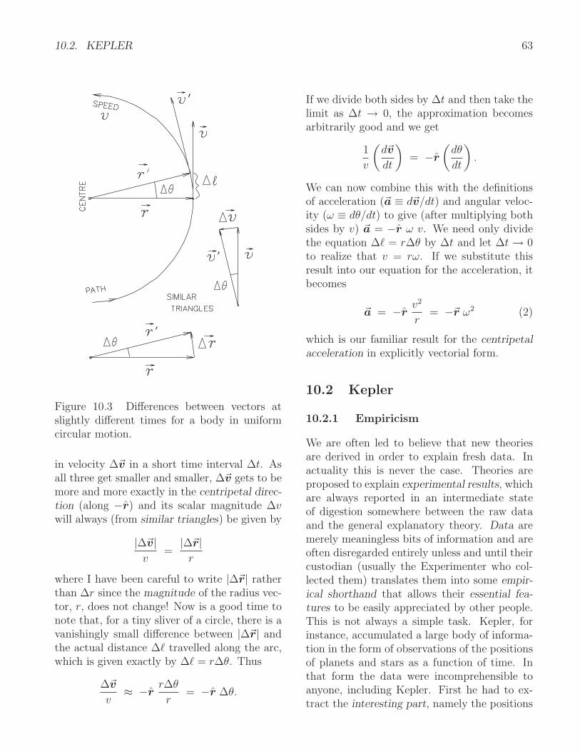
10.2. KEPLER 63
Figure 10.3 Differences between vectors atslightly different times for a body in uniformcircular motion.
in velocity ∆~v in a short time interval ∆t. Asall three get smaller and smaller, ∆~v gets to bemore and more exactly in the centripetal direc-tion (along −r) and its scalar magnitude ∆vwill always (from similar triangles) be given by
|∆~v|v
=|∆~r|
r
where I have been careful to write |∆~r| ratherthan ∆r since the magnitude of the radius vec-tor, r, does not change! Now is a good time tonote that, for a tiny sliver of a circle, there is avanishingly small difference between |∆~r| andthe actual distance ∆ℓ travelled along the arc,which is given exactly by ∆ℓ = r∆θ. Thus
∆~v
v≈ −r
r∆θ
r= −r ∆θ.
If we divide both sides by ∆t and then take thelimit as ∆t → 0, the approximation becomesarbitrarily good and we get
1
v
(
d~v
dt
)
= −r
(
dθ
dt
)
.
We can now combine this with the definitionsof acceleration (~a ≡ d~v/dt) and angular veloc-ity (ω ≡ dθ/dt) to give (after multiplying bothsides by v) ~a = −r ω v. We need only dividethe equation ∆ℓ = r∆θ by ∆t and let ∆t → 0to realize that v = rω. If we substitute thisresult into our equation for the acceleration, itbecomes
~a = −rv2
r= −~r ω2 (2)
which is our familiar result for the centripetalacceleration in explicitly vectorial form.
10.2 Kepler
10.2.1 Empiricism
We are often led to believe that new theoriesare derived in order to explain fresh data. Inactuality this is never the case. Theories areproposed to explain experimental results, whichare always reported in an intermediate stateof digestion somewhere between the raw dataand the general explanatory theory. Data aremerely meaningless bits of information and areoften disregarded entirely unless and until theircustodian (usually the Experimenter who col-lected them) translates them into some empir-ical shorthand that allows their essential fea-tures to be easily appreciated by other people.This is not always a simple task. Kepler, forinstance, accumulated a large body of informa-tion in the form of observations of the positionsof planets and stars as a function of time. Inthat form the data were incomprehensible toanyone, including Kepler. First he had to ex-tract the interesting part, namely the positions

64 CHAPTER 10. CELESTIAL MECHANICS
of the planets relative to the Sun, from rawdata complicated by the uninteresting effectsof the Earth’s rotation and its own annual triparound Sol, which required both a good modelof what was basically going on and a lot of dif-ficult calculations. Then, with these “reduced”data in hand, he had to draw pictures, plotdifferent combinations of the variables againsteach other, and generally mull over the data(presumably scratching his head and thinking,“Now what the hell does this mean?” or hiscontemporary equivalent) until he began to no-tice some interesting empirical generalizationsthat could be made about his results. Of courseI don’t know exactly how Kepler went aboutthis, but I do know the experience of turningnew data over and over in my mind and on pa-per until some consistent empirical relationshipbetween the variables “leaps out at me.” And Iam very impressed with the depth and delicacyof Kepler’s observations.
Note that the Empiricist4 has not explainedthe observed behaviour at this point, merelydescribed it.5 But a good description goes along way! One should never underestimate theimportance of this intermediate step in experi-mental science.
10.2.2 Kepler’s Laws of Planet Motion
1. Elliptical Orbits: Theorbits of the planets are6 el-
4(who may or may not be the same person as the Experi-mentalist and/or the Theoretician — these are just different“hats” that a Physicist may put on)
5Of course, as in Kepler’s case, the empirical descriptionis always in terms of some preselected model or paradigm;but the paradigm in question is generally a familiar andwidely accepted one, otherwise it is not very helpful incommunicating the results to others. Besides, the datathemselves are “collected” within the context of the Ex-perimenter’s paradigms and models about the world. The“simple” act of vision employs an enormous amount of “pro-cessing” in the visual cortex, as discussed earlier. . . .
6(neglecting perturbations from the other planets, as isassumed in all Kepler’s laws)
lipses7 with the Sun at one ofthe foci.
2. Constant Areal Veloc-
ity: The area swept out perunit time by a line joining theSun to the planet in questionis constant throughout the or-bit.8
3. Scaling of Periods: Thesquare of the period T ofthe orbit is proportional to thecube of the length of the semi-major axis (or, in the case of acircular orbit, the radius r) ofthe orbit:
T 2 ∝ r3
10.3 Universal Gravitation
By a process of logic that I will not attempt todescribe, Newton deduced that the force F be-tween two objects with masses m and M sep-arated by a distance r was given by
F =GmM
r2(3)
whereG = (6.67259±0.00085)×10−11 m3·kg−1·s−2 isthe Universal Gravitational Constant. Actu-ally, Newton didn’t know the value of G; heonly postulated that it was universal — i.e.
that it was the same constant of proportion-ality for every pair of masses in this universe.
7Note that a circle is just a special case of an ellipse inwhich the major and semimajor axes are both equal to theradius and both foci are at the centre of the circle.
8This feature, unlike the other two Laws, is true for any“central force” (a force attracting the body back toward thecentre, in this case the sun). The other two are only truefor inverse square laws, F ∝ 1/r2.

10.3. UNIVERSAL GRAVITATION 65
The actual determination of the value of G wasfirst done by Cavendish in an experiment to bedescribed below.
We should also express this equation in vec-tor form to emphasize that the force on eithermass acts in the direction of the other mass: if~F 12 denotes the force acting on mass m2 dueto its gravitational attraction by mass m1 then
~F 12 = − Gm1 m2
r212
r12 (4)
where r12 is a unit vector in the direction of~r12, the vector distance from m1 to m2, andr12 is the scalar magnitude of ~r12. Note thatthe reaction force ~F 21 on m1 due to m2 isobtained by interchanging the labels “1” and“2” which ensures that it is equal and oppositebecause ~r21 ≡ −~r12 by definition.
10.3.1 Weighing the Earth
Suppose you know your own mass m, deter-mined not from your weight but from experi-ments in which you are accelerated horizontallyby known forces. Then from your weight Wyou can calculate the mass of the Earth, ME,if only you know G, the universal gravitationalconstant, and RE, the radius of the Earth. Thetrouble is, you cannot use the same measure-ment (or any other combination of measure-ments of the weights of objects) to determineG. So how do we know G? If we can measureG then we can use our own weight-to-mass ra-tio (i.e. the acceleration of gravity, g) with theknown value of RE = 6.37×10⁶ m to determineME. How do we do it?
The trick is to measure the gravitational at-traction between two masses m1 and m2 thatare both known. This seems simple enoughin principle; the problem is that the attractiveforce between two “laboratory-sized” masses isincedibly tiny.9 Cavendish devised a clevermethod of measuring such tiny forces: He hung
9If the Earth attracts a 1 kg mass with a force of 9.81 N,
a “dumbbell” arrangement (two large spheri-cal masses on opposite ends of a bar) from theceiling by a long thin wire and let the systemcome completely to rest. Then he brought an-other large spherical mass up close to each ofthe end masses so that the gravitational attrac-tion acted to twist the wire. By careful tests onshorter sections of the same wire he was able todetermine the torsional spring constant of thewire and thus translate the angle of twist into atorque, which in turn he divided by the momentarm (half the length of the dumbbell) to obtainthe force of gravity F between the two labora-tory masses M1 and m2 for a given separation rbetween them. From this he determined G andfrom that, using
g =GME
R2E
(5)
he determined ME = 5.965 × 1024 kg for thefirst time. We now know G a bit better (seeabove) but it is a hard thing to measure accu-rately!
10.3.2 Orbital Mechanics
Let’s pretend for now that all orbits are simplecircles. In that case we can easily calculate theorbital radius r at which the centripetal forceof gravitational attraction F is just right toproduce the centripetal acceleration a requiredto maintain a steady circular orbit at a givenspeed v. For starters we will refer to a lightobject (like a communication satellite) in orbitabout the Earth.
Orbital Speed
The force and the acceleration are both cen-tripetal (i.e. back towards the centre of the
the gravitational force between two 1 kg masses separatedby RE would be smaller by a factor equal to the numberof kilograms in ME , which is a large number. Fortunatelythe smaller masses can be placed much closer together; thishelps quite a bit, but the force is still miniscule!

66 CHAPTER 10. CELESTIAL MECHANICS
Earth, so we can just talk about the magni-tudes of ~F and ~a:
F =GmME
r2and a =
v2
r.
but F = ma, so
GmME
r2=
mv2
r=⇒ GME
r= v2.
We can “solve” this equation for v in terms ofr,
v =
√
GME
r, (6)
or for r in terms of v:
r =GME
v2. (7)
You can try your hand with these equations.See if you can show that the orbital velocity atthe Earth’s surface (i.e. the speed required fora frictionless train moving through an Equato-rial tunnel to be in free fall all the way aroundthe Earth) is 7.905 km/s. For a more practicalexample, try calculating the radius and velocityof a geosynchronous satellite — i.e. a signal-relaying satellite in an Equatorial orbit with aperiod of exactly one day, so that it appears tostay at exactly the same place in the sky all thetime.10
Changing Orbits
The first thing you should notice about theabove equations is that satellites move slowerin higher orbits. This is slightly counterintu-itive in that they go slower when they have fur-ther to go to get all the way around, which has adramatic effect on the period (see below). How-ever, that’s the way it is. Consequently, if youare in a low orbit and you want to transfer intoa higher orbit, you eventually want to end upgoing slower. Nevertheless, the first thing you
10If you have a TV satellite dish, it is pointing at such asatellite; note that (if you live in the Northern Hemisphere)it is tipped toward the South. Why?
do to initiate such a change is to speed up! Seeif you can figure out why.11
Periods of Orbits
We can now explain (at least for circular orbits)Kepler’s Third Law. The period T of an orbitis the circumference 2πr divided by the speedof travel, v. Using the equation above for v interms of r gives
T =2πr
√
GME
r
=2π√GME
r32
or T 2 ∝ r3
as observed by Kepler. Newton explained why.
10.4 Tides
Here on the surface of the Earth, we have lit-tle occasion to notice that the force of gravitydrops off inversely as the square of the distancefrom the centre of the Earth.12 This is fortu-nate, since otherwise Galileo would not havebeen able to do his experiments demonstratingthe (approximate) constancy of the accelerationof gravity, g; moreover, scales and other mass-measuring technology based on uniform grav-ity would not work well enough for commerceof engineering to have evolved as it did. So we
11(The most intuitive explanation for this involves theconcepts of kinetic and potential energy, which we will watchemerge from Newton’s Mechanics in succeeding Chapters.
12Surely by now you have gotten skeptical of my repeateddeclarations that the mass of the Earth can be treated as ifit were all concentrated at the Earth’s centre of gravity (i.e.the centre of the Earth). What about all the bits right nextto us? They have a much smaller r2 and thus contribute farmore “pull” than those ‘way on the other side. Well, hangon to that skepticism! I’m not leading you astray (promise!)but a little later on I will be in a better position to useGauss’ Law to explain in a few quick steps why this works.You should only provisionally accept this notion until youhave seen a convincing argument with your own eyes.

10.4. TIDES 67
don’t notice any effects of the inverse squarelaw “here at home,” right? Well, let’s not behasty.
The Moon exerts an infinitesimal force on ev-ery bit of mass on Earth. At a distance ofRME = 380, 000 km, the Moon’s mass ofMM = 7.4 × 10²² kg generates a gravitationalacceleration of only gME = 3.42 × 10⁻⁵ m/s2;in other words, our gravitational attraction tothe Moon is 3.5 × 10⁻⁶ of our Earth weight.Moreover, the Moon’s gravitational accelera-tion changes by only −1.8× 10⁻¹³ m/s2 for ev-ery metre further away from the Moon we move— a really tiny gravitational gradient. Never-theless, the fact that the water in the oceanson the side of the Earth facing the Moon isattracted more and that on the side away fromthe Moon is attracted less leads to a slight bulgeof the water on both sides and a concomitantdip around the middle. As the Earth turns un-der these bulges and dips, we experience (nor-mally) two high tides and two low tides everyday.
The consequences of these tides are nontrivial,as we all know. Even though they are the re-sult of an incredibly small gravitational gra-dient, they represent enormous energies thathave been tapped for power generation in a fewplaces like the Bay of Fundy where resonance ef-fects generate huge movements of water. Moreimportantly in the long run (but of negligibleconcern in times of interest to humans) is thefact that the “friction” generated by these tidesis gradually sapping the kinetic energy of theEarth’s rotation and at the same time causingthe Moon to drift slowly further away from theEarth so that in a few billion years the Earthwill be “locked” as the Moon is now, with itsday the same length as a month (which willthen be twice as long as it is now) and the sameside always facing its partner. “Sic transit glo-
ria Mundi,” indeed! Let’s enjoy our spin whilewe can.
A less potent source of tidal forces (gravita-
tional gradients) on Earth is the Sun, with amass of about 3×1040 kg at a distance of about93 million miles or 1.5 × 10¹¹ m. You can cal-culate for yourself the Sun’s gravitational ac-celeration at the Earth: small but not entirelynegligible. The Sun’s gravitational gradient, onthe other hand, is truly miniscule; yet variousspecies of fish seem to have feeding patternslocked to the relative positions of the Sun andthe Moon, even at night when the more obvi-ous effects of the Sun are absent. The so-called“solunar tables” are an essential aid to the fa-natically determined fisherman! Yet, so far as Iknow, no one has any plausible explanation forhow a fish (or a bird or a shellfish, which alsoseem to know) can detect these minute forcegradients.
A more dramatic example of tidal forces is thegravitational field near a neutron star, whichhas a large enough gradient to dismember trav-ellers passing nearby even though their orbitstake them safely past.13 Near a small blackhole the tidal forces can literally rip the vac-uum apart into matter and antimatter, causingthe black hole to explode with unmatched vio-lence; this in fact limits how small black holescan be and still remain stable.14
13This motif has been used in several delightful sciencefiction stories, notably “Neutron Star” by Larry Niven. and? Egg ? by ? .
14Bill Unruh, of the UBC Physics Department, is one ofthe world’s leading experts on this subject.

68 CHAPTER 10. CELESTIAL MECHANICS

11.1. SOME MATH TRICKS 69
Chapter 11
The Emergence of Mechanics
What use are Newton’s “Laws” of Mechanics?Even a glib answer to that question can easilyfill a 1-year course, if you really want to know.My purpose here is merely to offer some hints ofhow people learned to apply Newton’s Laws todifferent types of Mechanics problems, began tonotice that they were repeating certain calcu-lations over and over in certain wide classes ofproblems, and eventually thought of cute short-cuts that then came to have a life of their own.That is, in the sense of Michael Polanyi’s The
Tacit Dimension, a number of new paradigmsemerged from the technology of practical appli-cation of Newton’s Mechanics.
The mathematical process of emergence gener-ally works like this: we take the Second Law
and transform it using a formal mathematicalidentity operation such as “Do the same thingto both sides of an equation and you get a newequation that is equally valid.” Then we thinkup names for the quantities on both sides ofthe new equation and presto! we have a newparadigm. I will show three important exam-ple of this process, not necessarily the way theyfirst were “discovered,” but in such a way asto illustrate how such things can be done. Butfirst we will need a few new mathematical tools.
11.1 Some Math Tricks
11.1.1 Differentials
We have learned that the symbols df anddx represent the coupled changes in f(x) andx, in the limit where the change in x (and conse-quently also the change in f) become infinites-imally small. We call these symbols the differ-entials of f and x and distinguish them from∆f and ∆x only in this sense: ∆f and ∆x canbe any size, but df and dx are always infinites-imal — i.e. small enough so that we can treatf(x) as a straight line over an interval only dxwide.
This does not change the interpretation of the
representationdf
dxfor the derivative of f(x)
with respect to x, but it allows us to think ofthese differentials df and dx as “normal” alge-braic symbols that can be manipulated in theusual fashion. For instance, we can write
df =
(
df
dx
)
dx
which looks rather trivial in this form. How-ever, suppose we give the derivative its ownname:
g(x) ≡ df
dx
Then the previous equation reads
df = g(x) dx or just df = g dx

70 CHAPTER 11. THE EMERGENCE OF MECHANICS
which can now be read as an expression of therelationship between the two differentials dfand dx. Hold that thought.
As an example, consider our familiar kinemat-ical quantities
a ≡ dv
dtand v ≡ dx
dt.
If we treat the differentials as simple algebraicsymbols, we can invert the latter definition andwrite
1
v=
dt
dx.
(Don’t worry too much about what this“means” for now.) Then we can multiply theleft side of the definition of a by 1/v and mul-tiply the right side by dt/dx and get an equallyvalid equation:
a
v=
dv
dt· dt
dx=
dv
dx
or, multiplying both sides by v dx,
a dx = v dv (1)
which is a good example of a mathematicalidentity, in this case involving the differentialsof distance and velocity. Hold that thought.
11.1.2 Antiderivatives
Suppose we have a function g(x) which we knowis the derivative [with respect to x] of someother function f(x), but we don’t know which— i.e. we know g(x) explicitly but we don’tknow [yet] what f(x) it is the derivative of. Wemay then ask the question, “What is the func-tion f(x) whose derivative [with respect to x]is g(x)?” Another way of putting this would beto ask, “What is the antiderivative of g(x)?”1
1This is a lot like knowing that 6 is some number n mul-tiplied by 2 and asking what n is. We figure this out byasking ourselves the question, “What do I have to multiplyby 2 to get 6?” Later on we learn to call this “division” andexpress the question in the form, “What is n = 6/2?” butwe might just as well call it “anti-multiplication” becausethat is how we solve it (unless it is too hard to do in ourheads and we have to resort to some complicated technologylike long division).
Another name for the antiderivative is the in-tegral, which is in fact the “official” version,but I like the former better because the namesuggests how we go about “solving” one.2
For a handy example consider g(x) =k x. Then the antiderivative [integral] of g(x)with respect to x is f(x) = 1
2k x2 + f0 [where
f0 is some constant] because the derivative[with respect to x] of x2 is 2x and the derivativeof any constant is zero. Since any combinationof constants is also a constant, it is equally validto make the arbitrary constant term of the sameform as the part which actually varies with x,viz. f(x) = 1
2k x2 + 1
2k x2
0. Thus f0 is thesame thing as 1
2k x2
0 and it is a matter of tastewhich you want to use.
Naturally we have a shorthand way of writingthis. The differential equation
df = g(x) dx
2Any introductory Calculus text will explain what anintegral “means” in terms of visual pictures that the righthemisphere can handle easily: whereas the derivative of f(x)is the slope of the curve, the integral of g(x) is the area un-der the curve. This helps to visualize the integral as thelimiting case of a summation: imagine the area under thecurve of g(x) from x0 to x being divided up into N rectan-gular columns of equal width ∆x = 1
N(x − x0) and height
g(xn), where xn = n ∆x is the position of the nth column.If N is a small number, then
PNn=1 g(xn) ∆x is a crude ap-
proximation to the area under the smooth curve; but as Ngets bigger, the columns get skinnier and the approxima-tion becomes more and more accurate and is eventually (asN → ∞) exact! This is the meaning of the integral sign:
Z x
x0
g(x) dx ≡ limN→∞
NX
n=1
g(xn) ∆x
where ∆x ≡ 1
N(x − x0) and xn = n ∆x.
Why do I put this nice graphical description in a footnote?Because we can understand most of the Physics applicationsof integrals by thinking of them as “antiderivatives” and be-cause when we go to solve an integral we almost always do itby asking the question, “What function is this the derivativeof?” which means thinking of integrals as antiderivatives.This is not a complete description of the mathematics, but itis sufficient for the purposes of this course. [See? We reallydo “deemphasize mathematics!”]

11.2. IMPULSE AND MOMENTUM 71
can be turned into the integral equation
f(x) =
∫ x
x0
g(x) dx (2)
which reads, “f(x) is the integral of g(x) withrespect to x from x0 to x.” We have used therule that the integral of the differential of f [orany other quantity] is just the quantity itself,3
in this case f :∫
df = f (3)
Our example then reads∫ x
x0
k x dx = k
∫ x
x0
x dx =1
2k x2 − 1
2k x2
0
where we have used the feature that any con-stant (like k) can be brought “outside the in-tegral” — i.e. to the left of the integral sign∫
.
Now let’s use these new tools to transform New-ton’s Second Law into something more com-fortable.
11.2 Impulse and Momentum
Multiplying a scalar times a vector is easy, itjust changes its dimensions and length — i.e.
it is transformed into a new kind of vector withnew units but which is still in the same direc-tion. For instance, when we multiply the vectorvelocity ~v by the scalar mass m we get the vec-tor momentum ~p ≡ m~v. Let’s play a littlegame with differentials and the Second Law:
~F =d~p
dt.
Multiplying both sides by dt and integratinggives
~F dt = d~p ⇒∫ t
t0
~F dt =
∫ ~p
~p0
d~p = ~p − ~p0.
(4)3This also holds for the integrals of differentials of vec-
tors.
The left hand side of the final equation is thetime integral of the net externally applied force~F . This quantity is encountered so often in Me-chanics problems [especially when ~F is known
to be an explicit function of time, ~F (t)] that wegive it a name:∫ t
t0
~F (t) dt ≡ impulse due to applied force ~F
(5)Our equation can then be read as a sentence:
“The impulse created by the net externalforce applied to a system is equal to the mo-mentum change of the system.”
11.2.1 Conservation of Momentum
The Impulse and Momentum law is cer-tainly a rather simple transformation of New-ton’s Second Law; in fact one may betempted to think of it as a trivial restatementof the same thing. However, it is much simplerto use in many circumstances. The most usefulapplication, surprisingly enough, is when thereis no external force applied to the system andtherefore no impulse and no change in momen-tum! In such cases the total momentum of thesystem does not change. We call this the Law
of Conservation of Momentum and use itmuch the same as Descartes and Huygens didin the days before Newton.4
Momentum conservation goes beyond Newton’sFirst Law, though it may appear to be thesame idea. Suppose our “system” [trick word,that!] consists not of one object but of several.Then the “net” [another one!] momentum ofthe system is the vector sum of the momentaof its components. This is where the power ofmomentum conservation becomes apparent. Aslong as there are no external forces, there can
4It should be remembered that Rene Descartes andChristian Huygens formulated the Law of Conservation
of Momentum before Newton’s work on Mechanics. Theyprobably deserve to be remembered as the First ModernConservationists!

72 CHAPTER 11. THE EMERGENCE OF MECHANICS
be as many forces as we like between the com-ponent parts of the system without having theslightest effect on their combined momentum.Thus, to take a macabre but traditional exam-ple, if we lob a hand grenade through the air,just after it explodes (before any of the frag-ments hit anything) all its pieces taken togetherstill have the same net momentum as before theexplosion.
The Law of Conservation of Momentum
is particularly important in analyzing the colli-sions of elementary particles. Since such colli-sions are the only means we have for performingexperiments on the forces between such parti-cles, you can bet that every particle physicist isvery happy to have such a powerful (and simple-to-use!) tool.
Example: Volkwagen-Cadillac Scattering
Let’s do a simple example in one dimension[thus avoiding the complications of adding andsubtracting vectors] based on an apocryphalbut possibly true story: A Texas Cadillacdealer once ran a TV ad showing a Cadil-lac running head-on into a parked Volkswa-gen Bug at 100 km/h. Needless to say, theBug was squashed flat. Figs. 11.1 and 11.2show a simplified sketch of this event, using the“before-and-after” technique with which ournew paradigm works best. Figure 11.1 showsan elastic collision, in which the cars bounce offeach other; Figure 11.2 shows a plastic collisionin which they stick together. For quantitativesimplicity we assume that the Cadillac has ex-actly twice the mass of the Bug (M = 2m).In both cases the net initial momentum of the“Caddy-Bug system” is MVi = 200m, whereI have omitted the “km/h” units of Vi, the ini-tial velocity of the Caddy. Therefore, since allthe forces act between the components of thesystem, the total momentum of the system isconserved and the net momentum after the col-lision must also be 200m.
Figure 11.1 Sketch of a perfectly elastic col-lision between a Cadillac initially moving at100 km/h and a parked Volkswagen Bug. Foran elastic collision, the magnitude of the rela-tive velocity between the two cars is the samebefore and after the collision. [The fact that thecars look “crunched” in the sketch reflects thefact that no actual collision between cars couldever be perfectly elastic; however, we will usethis limiting case for purposes of illustration.]
In the elastic collision, the final relative veloc-ity of the two cars must be the same as beforethe collision [this is one way of defining such acollision]. Thus if we assume (as on the draw-ing) that both cars move to the right after thecollision, with velocities Vf for the Caddy andvf for the Bug, then
vf − Vf = 100 or vf = Vf + 100.
Meanwhile the total momentum must be thesame as initially:
MVf + mvf = 200m or
2mVf + m(Vf + 100) = 200m
or 3mVf = 100m

11.2. IMPULSE AND MOMENTUM 73
Figure 11.2 A perfectly inelastic or plastic col-lision in which the cars stick together and moveas a unit after the collision.
giving the final velocities
Vf = 331
3km/h and vf = 133
1
3km/h.
In the plastic collision, the final system consistsof both cars stuck together and moving to theright at a common velocity vf . Again the totalmomentum must be the same as initially:
(M + m)vf = 200m or
3mvf = 200m or
vf = 662
3km/h.
Several features are worth noting: first, the fi-nal velocity of the Bug after the elastic colli-sion is actually faster than the Caddy was goingwhen it hit! If the Bug then runs into a brickwall, well. . . . For anyone unfortunate enoughto be inside one of the vehicles the severity ofthe consequences would be worst for the largestsudden change in the velocity of that vehicle— i.e. for the largest instantaneous acceler-ation of the passenger. This quantity is far
larger for both cars in the case of the elasticcollision. This is why “collapsibility” is an im-portant safety feature in modern automotivedesign. You want your car to be completelydemolished in a severe collision, with only thepassenger compartment left intact, in order tominimize the recoil velocity. This may be an-noyingly expensive, but it is nice to be aroundto enjoy the luxury of being annoyed!
Back to our story: The Cadillac dealer was,of course, trying to convince prospective VWbuyers that they would be a lot safer in aCadillac — which is undeniable, except inso-far as the Bug’s greater maneuverability andsmaller “cross-section” [the size of the “target”it presents to other vehicles] helps to avoid ac-cidents. However, the local VW dealer tookexception to the Cadillac dealer’s stated edito-rial opinion that Bugs should not be allowedon the road. To illustrate his point, he rana TV ad showing a Mack truck running intoa parked Cadillac at 100 km/h. The Cadillacwas quite satisfactorily squashed and the VWdealer suggested sarcastically that perhaps ev-eryone should be required by law to drive Macktrucks to enhance road safety. His point waswell taken.
11.2.2 Centre of Mass Velocity
If we calculate the total momentum of a com-posite system and then divide by the totalmass, we obtain the velocity of the system-as-a-whole, which we call the velocity of the centreof mass. If we imagine “running alongside” thesystem at this velocity we will be “in a refer-ence frame moving with the centre of mass,”where everything moves together and bouncesapart [or whatever] with a very satisfying sym-metry. Regardless of the internal forces of col-lisions, etc., the centre of mass [CM ] will bemotionless in this reference frame. This hasmany convenient features, especially for calcu-lations, and has the advantage that the inifinite

74 CHAPTER 11. THE EMERGENCE OF MECHANICS
number of other possible reference frames canall agree upon a common description in termsof the CM . Where exactly is the CM of a sys-tem? Well, wait a bit until we have definedtorques and rigid bodies, and then it will beeasy to show how to find the CM .
11.3 Work and Energy
We have seen how much fun it is to multiply theSecond Law by a scalar (dt) and integrate theresult. What if we try multiplying through bya vector? As we have seen in the chapter onVectors, there are two ways to do this: thescalar or “dot” product ~A · ~B, so named forthe symbol · between the two vectors, whichyields a scalar result, and the vector or “cross”product ~A × ~B, whose name also reflects theappearance of the symbol × between the twovectors, which yields a vector result. The for-mer is easier, so let’s try it first.
In anticipation of situations where the appliedforce ~F is an explicit function of the position5
~x — i.e. ~F (~x) — let’s try using a differentialchange in ~x as our multiplier:
~F · d~x = m~a · d~x
= md~v
dt· d~x
= md~v · d~x
dt
= md~v · ~v
= m~v · d~v
where we have used the definitions of ~a and ~v5In the section on Circular Motion we chose ~r to de-
note the vector position of a particle in a circular orbit, usingthe centre of the circle as the origin for the ~r vector. Herewe are switching to ~x to emphasize that the current descrip-tion works equally well for any type of motion, circular orotherwise. The two notations are interchangeable, but wetend to prefer ~x when we are talking mainly about rectilin-ear (straight-line) motion and ~r when we are referring ourcoordinates to some centre or axis.
with a little shifting about of the differentialdt and a reordering of the dot product [whichwe may always do] to get the right-hand side[RHS] of the equation in the desired form. Adelightful consequence of this form is that itallows us to convert the RHS into an explic-itly scalar form: ~v · d~v is zero if d~v ⊥ ~v —i.e. if the change in velocity is perpendicularto the velocity itself, so that the magnitude ofthe velocity does not change, only the direction.[Recall the case of circular motion!] If, on theother hand, d~v ‖ ~v, then the whole effect of d~vis to change the magnitude of ~v, not its direc-tion. Thus ~v · d~v is precisely a measure of thespeed v times the differential change in speed,dv:
~v · d~v = v dv (6)
so that our equation can now be written
~F · d~x = m v dv
and therefore
∫ ~x
~x0
~F · d~x = m
∫ v
v0
v dv = m
(
1
2v2 − 1
2v2
0
)
(7)(Recall the earlier discussion of an equivalentantiderivative.)
Just to establish the connection to the math-ematical identity a dx = v dv, we multiplythat equation through by m and get ma dx =mv dv. Now, in one dimension (no vectorsneeded) we know to set ma = F which givesus F dx = mv dv or, integrating both sides,
∫ x
x0
F dx =1
2mv2 − 1
2mv2
0
which is the same equation in one dimension.
OK, so what? Well, again this formula keptshowing up over and over when people set outto solve certain types of Mechanics problems,and again they finally decided to recast theLaw in this form, giving new names to theleft and right sides of the equation. We call

11.3. WORK AND ENERGY 75
~F ·d~x the work dW done by exerting a force~F through a distance d~x [work is something wedo] and we call 1
2mv2 the kinetic energy
T . [kinetic energy is an attribute of a movingmass] Let’s emphasize these definitions:
∫ ~x
~x0
~F · d~x ≡ ∆W , (8)
the work done by ~F (~x) over a path from ~x0
to ~x, and1
2mv2 ≡ T , (9)
the kinetic energy of mass m at speed v.
Our equation can then be read as a sentence:
“When a force acts on a body, the kineticenergy of the body changes by an amountequal to the work done by the force exertedthrough a distance.”
One nice thing about this “paradigm trans-formation” is that we have replaced a vectorequation ~F = m~a by a scalar equation∆W = ∆T . There are many situations inwhich the work done is easily calculated and thedirection of the final velocity is obvious; one canthen obtain the complete “final state” from the“initial state” in one quick step without hav-ing to go through the details of what happensin between. Another class of “before & after”problems solved!
11.3.1 Example: The Hill
Probably the most classic example of how theWork and Energy law can be used is thecase of a ball sliding6 down a frictionless hill,pictured schematically in Fig. 11.3. Now,Galileo was fond of this example and could havegiven us a calculation of the final speed of the
6 We could have the ball roll up and down the hill insteadof sliding, but that would involve rotational kinetic energy,and we’re not there yet.
Figure 11.3 Sketch of a ball sliding down africtionless hill. In position 1, the ball is atrest. It is then given an infinitesimal nudge andstarts to slide down the hill, passing position 2on the way. At the bottom of the hill [position3] it has its maximum speed v3 , which is thendissipated in sliding up the other side of thehill to position 4. Assuming that it stops ona slight slope at both ends, the ball will keepsliding back and forth forever.
ball for the case of a straight-line path (i.e. theinclined plane); but he would have thrown uphis hands at the picture shown in Fig. 11.3!Consider one spot on the downward slope, sayposition 2: the FBD of the ball is drawn in theexpanded view, showing the two forces ~N and~W acting on the mass m of the ball.7 Now,the ball does not jump off the surface or bur-row into it, so the motion is strictly tangentialto the hill at every point.8 Meanwhile, a fric-tionless surface cannot, by definition, exert anyforce parallel to the surface; this is why the nor-mal force ~N is called a “normal” force — itis always normal [perpendicular] to the surface.
7It is unfortunate that the conventional symbol for theweight, ~W , uses the same letter as the conventional sym-bol for the work, W . I will try to keep this straight byreferring to the weight always and only in its vector formand reserving the scalar W for the work. But this sort ofdifficulty is eventually inevitable.
8For now, I specifically exclude cases where the ball getsgoing so fast that it does get airborne at some places.

76 CHAPTER 11. THE EMERGENCE OF MECHANICS
So ~N ⊥ d~x which means that ~N ·d~x = 0 andthe normal force does no work! This is an im-portant general rule. Only the gravitationalforce ~W does any work on the mass m, andsince ~W = −m g y is a constant downwardvector [where we define the unit vector y as“up”], it is only the downward component ofd~x that produces any work at all. That is,~W · d~x = −m g dy, where dy is the compo-nent of d~x directed upward.9 That is, nomatter what angle the hill makes with the ver-tical at any position, at that position the workdone by gravity in raising the ball a differentialheight dy is given by dW = −m g dy [noticethat gravity does negative work going uphilland positive work going downhill] and the network done in raising the ball a total distance∆y is given by a rather easy integral:
∆W = −m g
∫
dy = −m g ∆y
where ∆y is the height that the ball is raised inthe process. By our Law, this must be equal tothe change in the kinetic energy T ≡ 1
2mv2 so
that1
2mv2 − 1
2mv2
0 = −m g ∆y. (10)
This formula governs both uphill slides, inwhich ∆y is positive and the ball slows down,and downhill slides in which ∆y is nega-tive and the ball speeds up. For the exam-ple shown in Fig. 11.3 we start at the top withv0 = v1 = 0 and slide down to position 3, drop-ping the height by an amount h in the process,so that the maximum speed (at position 3) isgiven by
1
2mv2
3 = mgh or v3 =√
2gh.
On the way up the other side the process ex-actly reverses itself [though the details may be
9Alas, another unfortunate juxtaposition of symbols! Weare using d~x to describe the differential vector positionchange and dy to describe the vertical component of d~x.Fortunately we have no cause to talk about the horizontalcomponent in this context, or we might wish we had usedd~r after all!
completely different!] in that the altitude onceagain increases and the velocity drops back tozero.
The most pleasant consequence of thisparadigm is that as long as the surface is trulyfrictionless, we never have to know any of thedetails about the descent to calculate the veloc-ity at the bottom! The ball can drop straightdown, it can slide up and down any number oflittle hills [as long as none of them are higherthan its original position] or it can even slidethrough a tunnel or “black box” whose inte-rior is hidden and unknown — and as long as Iguarantee a frictionless surface you can be con-fident that it will come out the other end atthe same speed as if it had just fallen the samevertical distance straight down. The directionof motion at the bottom will of course alwaysbe tangential to the surface.
For me it seems impossible to imagine the ballsliding up and down the hill without starting tothink in terms of kinetic energy being stored upsomehow and then automatically re-emergingfrom that storage as fresh kinetic energy. But Ihave already been indoctrinated into this wayof thinking, so it is hard to know if this is re-ally a compelling metaphor or just an extremelysuccessful one. You be the judge. I will forcemyself to hold off talking about potential en-ergy until I have covered the second prototypi-cal example of the interplay between work andenergy.
11.3.2 Captain Hooke
The spring embodies one of Physics’ premiereparadigms, the linear restoring force. Thatis, a force which disappears when the sys-tem in question is in its “equilibrium position”x0 [which we will define as the x = 0 posi-tion (x0 ≡ 0) to make the calculations easier]but increases as x moves away from equilib-rium, in such a way that the magnitude of theforce F is proportional to the displacement

11.3. WORK AND ENERGY 77
Figure 11.4 Sketch of a mass on a spring. Inthe leftmost frame the mass m is at rest and thespring is in its equilibrium position (i.e. neitherstretched nor compressed). [If gravity is pullingthe mass down, then in the equilibrium positionthe spring is stretched just enough to counter-act the force of gravity. The equilibrium posi-tion can still be taken to define the x = 0 posi-tion.] In the second frame, the spring has beengradually pulled down a distance xmax andthe mass is once again at rest. Then the massis released and accelerates upward under theinfluence of the spring until it reaches the equi-librium position again [third frame]. This time,however, it is moving at its maximum veloc-ity vmax as it crosses the centre position; assoon as it goes higher, it compresses the springand begins to be decelerated by a linear restor-ing force in the opposite direction. Eventually,when x = −xmax, all the kinetic energy hasbeen been stored back up in the compression ofthe spring and the mass is once again instanta-neously at rest [fourth frame]. It immediatelystarts moving downward again at maximum ac-celeration and heads back toward its startingpoint. In the absence of friction, this cycle willrepeat forever.
from equilibrium [F is linear in x] and the di-rection of F is such as to try to restore x tothe original position. The constant of propor-tionality is called the spring constant, alwayswritten k. Thus (using vector notation to ac-count for the directionality)
~F = −k ~x (11)
which is the mathematical expression of theconcept of a linear restoring force. This isknown as Hooke’s law. It is a lot more gen-eral than it looks, as we shall see later.
Keeping in mind that the ~F given above isthe force exerted by the spring against anyoneor anything trying to stretch or compress it.If you are that stretcher/compressor, the force
you exert is −~F . If you do work on the spring10
by stretching or compressing it11 by a differen-tial displacement d~x from equilibrium, thedifferential amount of work done is given by
dW = −~F · d~x = k ~x · d~x = k x dx
which we can integrate from x = 0 (the equi-librium position) to x (the final position) toget the net work W :
W = k
∫ x
0
x dx =1
2k x2 (12)
Once you let go, the spring will do the sameamount of work back against the only thingtrying to impede it — namely, the inertia ofthe mass m attached to it. This can be usedwith the Work and Energy Law to calculatethe speed vmax in the third frame of Fig. 11.4:since v0 = 0,
1
2m v2
max =1
2k x2
max or v2max =
k
mx2
max
10It is important to keep careful track of who is doing workon whom, especially in this case, because if you are carelessthe minus signs start jumping around and multiplying likecockroaches!
11It doesn’t matter which — if you stretch it out you haveto pull in the same direction as it moves, while if you com-press it you have to push in the direction of motion, so eitherway the force and the displacement are in the same directionand you do positive work on the spring.

78 CHAPTER 11. THE EMERGENCE OF MECHANICS
or vmax =
√
k
m|xmax|
where |xmax| denotes the absolute value ofxmax (i.e. its magnitude, always positive).Note that this is a relationship between themaximum values of v and x, which occurat different times during the process.
Love as a Spring
Few other paradigms in Physics are so easy totranslate into “normal life” terms as the lin-ear restoring force. As a whimsical example,consider an intimate relationship between twolovers. In this case x can represent “emotionaldistance” — a difficult thing to quantify but aneasy one to imagine. There is some equilibriumdistance x0 where at least one of the lovers ismost comfortable12 — this time, just to showhow it works, we will not choose x0 to be thezero position of x but leave it in the equationsexplicitly. When circumstances (usually work)force a greater emotional distance for a while,the lover experiences a sort of tension that pullshim or her back closer to the beloved. This isa perfect analogy to the linear restoring force:
F = −k (x − x0)
What few people seem to recognize is that this“force,” like any linear restoring force, is sym-metric: it works the same in both directions,too far apart and too close. When circum-stances permit a return to greater closeness,the lover rushes back to the beloved (figura-tively — we are talking about emotional dis-tance x here!) and very often “overshoots”the equilibrium position x0 to get temporarilycloser than is comfortable. The natural repul-sion that then occurs is no cause for dismay —you can’t really have an attraction without it —but some people seem surprised to discover that
12Sadly, x0 is not always the same for both partners inthe relationship; this is a leading cause of tension in suchcases. [Doesn’t this metaphor extend gracefully?]
the attraction that binds them to their beloveddoes not just keep acting no matter how closethey get; they are very upset that x can-not just keep getting closer and closer with-out limit.13 In later chapters I will have muchmore to say about the oscillatory pattern thatgets going [see Fig. 11.4] when the overshoot isallowed to occur without any friction to dissi-pate the energy stored in the stretched spring[a process known as damping ]. But first I reallymust pick up another essential paradigm thathas been begging to be introduced.
11.4 Potential Energy
Imagine yourself on skis, poised motionless atthe top of a snow-covered hill: one way or an-other, you are deeply aware of the potential ofthe hill to increase your speed. In Physics welike to think of this obvious capacity as the po-tential for gravity to increase your kinetic en-ergy. We can be quantitative about it by goingback to the bottom of the hill and recalling thelong trudge uphill that it took to get to thetop: this took a lot of work, and we know theformula for how much: in raising your eleva-tion by a height h you did an amount of workW = mgh “against gravity” [where m is yourmass, of course]. That work is now somehow“stored up” because if you slip over the edge itwill all come back to you in the form of kineticenergy! What could be more natural than tothink of that “stored up work” as gravitationalpotential energy
Vg = m g h (13)
which will all turn into kinetic energy if we al-low h to go back down to zero?14
13I suspect that such foolishness is merely an example ofsingle-valued logic [closer = better] obsessively misapplied,rather than some more insidious psychopathology. But Icould be wrong!
14The choice of a zero point for Vg is arbitrary, of course,just like our choice of where h = 0. This is not a problem if

11.4. POTENTIAL ENERGY 79
We can then picture a skier in a bowl-shapedvalley zipping down the slope to the bottom[Vg → T ] and then coasting back up to stopat the original height [T → Vg] and (after askillful flip-turn) heading back downhill again[Vg → T ]. In the absence of friction, this couldgo on forever: Vg → T → Vg → T → Vg →T → . . . .
The case of the spring is even more compelling,in its way: if you push in the spring a dis-tance x, you have done some work W =12k x2 “against the spring.” If you let go, this
work “comes back at you” and will acceleratea mass until all the stored energy has turnedinto kinetic energy. Again, it is irresistible tocall that “stored spring energy” the potentialenergy of the spring,
Vs =1
2k x2 (14)
and again the scenario after the spring is re-leased can be described as a perpetual cycle ofVs → T → Vs → T → Vs → T → . . . .
11.4.1 Conservative Forces
Physicists so love their Energy paradigm thatit has been elevated to a higher status than theoriginal Second Law from which it was de-rived! In orer to make this switch, of course,we had to invent a way of making the reversederivation — i.e. obtaining the vector force~F exerted “spontaneously” by the system inquestion from the scalar potential energy V ofthe system. Here’s how: in one dimensionwe can forget the vector stuff and just jugglethe differentials in dWme = Fme dx, wherethe Wme is the work I do in exerting a forceFme “against the system” through a distancedx. Assuming that all the work I do against thesystem is conserved by the system in the form ofits potential energy V , then dV = dWme. On
we allow negative potential energies [which we do!] since itis only the change in potential energy that appears in anyactual mechanics problem.
the other hand, the force F exerted by the sys-tem [e.g. the force exerted by the spring] is theequal and opposite reaction force to the forceI exert: F = −Fme. The law for conservativeforces in one dimension is then
F = −dV
dx(15)
That is, the force of (e.g.) the spring is minusthe rate of change of the potential energy withdistance.
In three dimensions this has a little more com-plicated form, since V (~x) could in principlevary with all three components of ~x: x, y andz. We can talk about the three componentsindependently,
Fx = −∂V
∂x, Fy = −∂V
∂yand Fz = −∂V
∂z
where the notation ∂ is used to indicate deriva-tives with respect to one variable of a functionof several variables [here V (x, y, z)] with theother variables held fixed. We call ∂V/∂x thepartial derivative of V with respect to x. Inthe same spirit that moved us to invent vec-tor notation in the first place [i.e. making thenotation more compact], we use the gradientoperator
~∇ ≡ x∂
∂x+ y
∂
∂y+ z
∂
∂z(16)
to express the three equations above in onecompact form:
~F = − ~∇V (17)
The gradient is easy to visualize in two di-mensions: suppose you are standing on a realhill. Since your height h ≡ z is actually pro-portional to your gravitational potential energyVg, it is perfectly consistent to view the actualhill as a graph of the function Vg(x, y) of East-West coordinate x and North-South coordi-nate y. In this picture, looking down on the

80 CHAPTER 11. THE EMERGENCE OF MECHANICS
hill from above, the direction of the gradient~∇Vg is uphill, and the magnitude of the gradi-ent is the slope of the hill at the position wherethe gradient is evaluated. The nice feature isthat ~∇Vg will automatically point “straightup the hill” — i.e. in the steepest direction.Thus −~∇Vg points “straight downhill” — i.e.
in the direction a marble will roll if it is releasedat that spot! There are lots of neat tricks wecan play with the gradient operator, but fornow I’ll leave it to digest.
11.4.2 Friction
What about not-so-conservative forces? Inthe real world a lot of energy gets dissipatedthrough what is loosely known as friction.Nowhere will you find an entirely satisfactorydefinition of precisely what friction is, so I won’tfeel guilty about using the cop-out and sayingthat it is the cause of all work that does not“get stored up as potential energy.” That is,when I do work against frictional forces, it willnot reappear as kinetic energy when I “let go.”
Where does it go? We have already startedgetting used to the notion that energy is con-served, so it is disturbing to find some workjust being lost. Well, relax. The energy dissi-pated by work against friction is still around inthe form of heat, which is something like dis-ordered potential and kinetic energy.15 We willtalk more about heat a few chapters later.
11.5 Torque & Angular Momen-tum
Finally we come to the formally trickiest trans-formation of the Second Law, the one involv-ing the vector product (or “cross product”) of~F with the distance ~r away from some ori-
15[Not quite, but you can visualize lots of little atomswiggling and jiggling seemingly at random — that’s heat,sort of.]
gin16 “O.” Here goes:
~r ×[
d~p
dt= ~F
]
gives ~r× d~p
dt= ~r× ~F
Now, the distributive law for derivatives appliesto cross products, so
d
dt[~r × ~p] =
d~r
dt× ~p + ~r × d~p
dt
but
d~r
dt≡ ~v and ~p ≡ m~v
sod~r
dt× ~p = m (~v × ~v) = 0
because the cross product of any vector withitself is zero.17 Therefore
d
dt[~r × ~p] = ~r × ~F .
If we define two new entities,
~r × ~p ≡ ~LO, (18)
the Angular Momentum about O
and~r × ~F ≡ ~τO, (19)
the Torque generated by ~F about O ,
then we can write the above result in the form
d~LO
dt= ~τO (20)
This equation looks remarkably similar to theSecond Law. In fact, it is the rotational ana-logue of the Second Law. It says that
16Note that everything we discuss in this case will be withreference to the chosen origin O, which may be chosen ar-bitrarily but must then be carefully remembered!
17Remember from the chapter on Vectors that only theperpendicular parts of two vectors contribute to the crossproduct. Any two parallel vectors have zero cross product.A vector crossed with itself is the simplest example.

11.5. TORQUE & ANGULAR MOMENTUM 81
“The rate of change of the angularmomentum of a body about the ori-gin O is equal to the torque gen-erated by forces acting about O.”
So what? Well, if we choose the origin cleverlythis “new” Law gives us some very nice gen-eralizations. Consider for instance an examplewhich occurs very often in physics: the centralforce.
11.5.1 Central Forces
Many [maybe even most] forces in nature are di-rected toward [or away from] some “source” ofthe force. An obvious example is Newton’s Uni-versal Law of Gravitation, but there are manyothers evident, especially in elementary parti-cle physics.18 We call these forces “central” be-cause if we regard the point toward [or awayfrom] which the force points as the centre (ororigin O) of our coordinate system, from whichthe position vector ~r is drawn, the cross prod-uct between ~r and ~F (which is along r) isalways zero. That is,
“A central force produces no torqueabout the centre; therefore the an-gular momentum about the centreremains constant under a centralforce.”
This is the famous Law of Conservation of
Angular Momentum. Note the limitationon its applicability.
The Figure Skater
Again, so what? Well, there are numerous ex-amples of central forces in which angular mo-mentum conservation is used to make sense of
18For instance, the electrostatic force between two pointcharges obeys exactly the same “inverse square law” as grav-itation, except with a much stronger constant of proportion-ality and the inclusion of both positive and negative charges.We will have lots more to do with that later on!
Figure 11.5 A contrived central-force problem.The ball swings around (without friction, ofcourse) on the end of a string fixed at the ori-gin O. The central force in the string cannotgenerate any torque about O, so the angularmomentum LO = mvr about O must re-main constant. As the string is pulled in slowly,the radius r gets shorter so the momentump = mv = mrω has to increase to compensate.
otherwise counterintuitive phenomena. For in-stance, consider the classic image of the figureskater doing a pirouette: she starts spinningwith hands and feet as far extended as possi-ble, then pulls them in as close to her body. Asa result, even though no torques were applied,she spins much faster. Why? I can’t draw agood figure skater, so I will resort to a cruderexample [shown in Fig. 11.5] that has the samequalitative features: imagine a ball (mass m)on the end of a string that emerges through ahole in an axle which is held rigidly fixed. Theball is swinging around in a circle in the end ofthe string. For an initial radius r and an ini-tial velocity v = rω, the initial momentum ismrω and the angular momentum about O isLO = mvr = mr2ω. Now suppose we pull inthe string until r′ = 1
2r. To keep the same
LO the momentum (and therefore the veloc-ity) must increase by a factor of 2, which meansthat the angular velocity ω ′ = 4ω since theball is now moving at twice the speed but hasonly half as far to go around the circumference

82 CHAPTER 11. THE EMERGENCE OF MECHANICS
of the circle. The period of the “orbit” has thusdecreased by a factor of four!
Returning to our more æsthetic example of thefigure skater, if she is able to pull in all her massa factor of 2 closer to her centre (on average)then she will spin 4 times more rapidly in thesense of revolutions per second or “Hertz” (Hz).
Kepler Again
A more formal example of the importance ofthe Law of Conservation of Angular Momen-tum under Central Forces is in its applicationto Celestial Mechanics, where the gravitationalattraction of the Sun is certainly a classic cen-tral force. If we always use the Sun as our ori-gin O, neglecting the influence of other planetsand moons, the orbits of the planets must obeyConservation of Angular Momentum about theSun. Suppose we draw a radius r from the Sunto the planet in question, as in Fig. 11.6. The
Figure 11.6 A diagram illustrating the arealvelocity of an orbit. A planet (mass m) orbitsthe Sun at a distance r. the shaded area isequal to 1
2r × r dθ in the limit of infinitesimal
intervals [i.e. as dθ → 0]. The areal velocity[rate at which this area is swept out] is thus12r2dθ/dt = 1
2r2ω.
rate at which this radius vector “sweeps outarea” as the planet moves is 1
2r2ω, whereas the
angular momentum about the Sun is mr2ω.The two quantities differ only by the constants12
and m; therefore Kepler’s empirical obser-
vation that the planetary orbits have constant“areal velocity” is equivalent to the requirementthat the angular momentum about the Sun bea conserved quantity.
11.5.2 Rigid Bodies
Despite the fact that all Earthly matter is com-posed mostly of empty space sprinkled lightlywith tiny bits of mass called atomic nuclei andeven tinier bits called electrons, the forces be-tween these bits are often so enormous thatthey hold the bits rigidly locked in a regulararray called a solid. Within certain limits thesearrays behave as if they were inseperable andperfectly rigid. It is therefore of some practicalimportance to develop a body of understandingof the behaviour of such rigid bodies under theinfluence of external forces. This is where theequations governing rotation come in.
A Moment of Inertia, Please!
Just as in the translational [straight-line mo-tion] part of Mechanics there is an inertial fac-tor m which determines how much p youget for a given v ≡ dx/dt ≡ x and how mucha ≡ dv/dt ≡ v ≡ d2x/dt2 ≡ x you get for agiven F ,19 so in rotational Mechanics there isan angular analogue of the inertial factor thatdetermines how much LO you get for a givenω ≡ θ and how much α ≡ ω you get for a givenτO. This angular inertial factor is called themoment of inertia about O [we must alwaysspecify the origin about which we are definingtorques and angular momentum] and is writtenIO with the prescription
IO =
∫
r2⊥ dm (21)
19 Here I have used the “dot notation” for time derivatives,defined in Ch. 6. This is merely a compact way of writingour favourite type of derivative — favourite because we con-sider knowing anything as a function of time as equivalent tocomplete knowledge of all its behaviour, since we can thenfind “everything else” by simply taking time derivatives.

11.6. STATICS 83
where the integral represents a summation overall little “bits” of mass dm [we call these “masselements”] which are distances r⊥ away froman axis through the point O. Here we discovera slight complication: r⊥ is measured fromthe axis, not from O itself. Thus a mass el-ement dm that is a long way from O butright on the axis will contribute nothing to IO.This continues to get more complicated untilwe have a complete description of RotationalMechanics with IO as a tensor of inertia andlots of other stuff I will never use again in thiscourse. I believe I will stop here and leave thefiner points of Rotational Mechanics for laterPhysics courses!
11.5.3 Rotational Analogies
It is, however, worth remembering that all thenow-familiar [?] paradigms and equations ofMechanics come in “rotational analogues:”
Linear AngularVersion Version Name
x θ angle
x ≡ v θ ≡ ω angular velocity
x ≡ v ≡ a θ ≡ ω ≡ αangularacceleration
m IOmoment ofinertia
p = m v LO = IOωangularmomentum
F τO torque
p = F LO = τO Second Law
T = 12mv2 T = 1
2IOω2 rotational kinetic
energy
dW = F dx dW = τdθ rotational work
F = −kx τ = −κθtorsional springlaw
Vs = 12k x2 Vs = 1
2κ θ2 torsional
potential energy
11.6 Statics
The enormous technology of Mechanical Engi-neering can be in some naıve sense be reducedto the two equations
~p = ~F and ~LO = ~τO.
Whole courses are taught on what amounts tothese two equations and the various tricks forsolving them in different types of situations.

84 CHAPTER 11. THE EMERGENCE OF MECHANICS
Fortunately, this isn’t one of them! Just togive a flavour, however, I will mention the basicproblem-solving technique of Statics, the sci-ence of things that are sitting still!20 That
means ~p = 0 and ~LO = 0 so that the rel-evant equations are now
∑
~F = 0 and∑
~τO = 0
where the∑
[summation] symbols emphasizethat there is never just one force or one torqueacting on a rigid body in equilibrium; if therewere, it (the force or torque) would be unbal-anced and acceleration would inevitably result!
To solve complex three-dimensional Staticsproblems it is often useful to back away fromour nice tidy vector formalism and explicitlywrite out the “equations of equilibrium” interms of the components of the forces along thex, y and z directions as well as the torquesabout the x, y and z axes [which meet at theorigin O]:
∑
Fx = 0∑
τx = 0 (22)∑
Fy = 0∑
τy = 0 (23)∑
Fz = 0∑
τz = 0 (24)
If you have some civil engineering to do, youcan work it out with these equations. Or hirean Engineer. I suggest the latter.
11.7 Physics as Poetry
This has been a long chapter; it needs somesummary remarks. All I have set out to dohere is to introduce the paradigms that emergedfrom Newton’s Second Law through mathe-matical identity transformations. This processof emergence seems almost miraculous some-times because by a simple [?] rearrangement
20This is pretty boring from a Physicist’s point of view,but even Physicists are grateful when bridges do not col-lapse.
of previously defined concepts we are able tocreate new meaning that wasn’t there before!This is one of the ways Physics bears a familyresemblance to Poetry and the other Arts. ThePoet also juxtaposes familiar images in a newway and creates meaning that no one has everseen before; this is the finest product of the hu-man mind and one of the greatest inspirationsto the human spirit.
In Physics, of course, the process is more slug-gish, because we insist on working out all theramifications of every new paradigm shift andevaluating its elegance and utility in some detailbefore we decide to “go with it.” This explainswhy it is so easy to describe just how the con-cepts introduced in this chapter emerged fromNewton’s Mechanics, but not so easy to tidilydescribe the consequences (or even the nature)of more recent paradigm shifts whose implica-tions are still being discovered. There is a lotof technical overhead to creativity in Physics.
A Physics paradigm shift is a profound alter-ation of the way Physicists see the world; butwhat do the rest of us care? It can be arguedthat such shifts have effects on our Reality evenif we choose to exclude Physics from our imme-diate awareness. Examples of this are plentifuleven in Classical Mechanics, but the first dra-matic social revolution that can be clearly seento have arisen largely from the practical con-sequences of breakthroughs in Physics was theIndustrial Revolution, the origins of which willbe discussed in the chapter on Thermal Physics.

85
Chapter 12
Equations of Motion
In the previous chapter we explored the pro-cess of emergence of new paradigms in Me-chanics, using various mathematical identitiesto transform Newton’s Second Law into newequations whose left- and right-hand sides weregiven names of their own, like impulse, mo-mentum, work, energy, torque and angular mo-mentum. Eighteenth-Century physicists thenlearned to manipulate these “new” concepts inways that greatly clarified the behaviour of ob-jects in the material universe. As a result,previously mysterious or counterintuitive phe-nomena began to make sense in terms of sim-ple, easy-to-use models, rather than long in-volved calculations. This is the essence of whatPhysics is all about. We work hard to maketodays’s difficult tasks easier, so that we willhave more free time and energy tomorrow towork hard to make tomorrow’s difficult taskseasier, so that. . . .
Meanwhile, these new words made their wayinto day-to-day language and introduced newparadigms into society, whose evolution in “TheAge of Reason” might have followed other pathswere it not for Newton’s work.1 The effectsof a more versatile and effective science of Me-chanics were also felt in blunt practical terms:combined with the new science of Thermody-
1Then again, maybe subtle sociological evolution had al-ready made these changes inevitable and Newton was justthe vehicle through which the emergent paradigms of theday infiltrated the world of science. Let’s do the Seven-teenth and Eighteenth Centuries over again without Newtonand see how it comes out!
namics (to be discussed in a later chapter), Me-chanics made possible an unprecedented growthof Mankind’s ability to push Nature aroundby brute force, a profitable enterprise (in theshort term) that led to the Industrial Revolu-tion. Suddenly people no longer had to acceptwhat Nature dealt, which enhanced their healthand wealth considerably — but in taking newcards they found they also had a new dealerwho was more merciless than Nature had everbeen: Greed.
Here arises a perennial question: are the evils of“technology abuse,” from pollution to exploita-tion to weapons of war, the “fault” of scien-tists who create the conceptual tools that maketechnology possible?2 My own opinion is thatwe scientists have a responsibility for our cre-ations in much the same way that parents havea responsibility for their children: we try to pro-vide a wholesome and enlightened atmospherein which they can grow and fulfill all their po-tential, offering our guidance and advice when-ever it will be accepted, and setting the bestexample we can; but in the end ideas are likepeople — they will determine their own des-tiny. The best scientists can do to guide theimpact of their ideas on society is to make surethe individual members of society have the op-portunity to learn about those ideas. Whether
2I presume that I do not need to point out the distinctionbetween Science and Technology. Even though politiciansseem to be fond of the word “scienceandtechnology,” I feelsure my readers are intelligent enough to find such a juxta-position humourous.

86 CHAPTER 12. EQUATIONS OF MOTION
anyone takes advantage of that opportunity ornot is out of our control. Whether irresponsibleor malign individuals make evil use of our ideasis also out of our control, though we can do ourbest to dissuade them.3
12.1 “Solving” the Motion
Getting back to the subject of Mechanics. . .
One of the reasons the paradigms in the previ-ous chapter emerged was that physicists werealways trying to “solve” certain types of “prob-lems” using Newton’s Second Law,4
F = m x
This equation can be written
x =1
mF (1)
to emphasize that it described a relationshipbetween the acceleration x, the inertial co-efficient m [usually constant] and the forceF . It is conventional to call an equation in thisform the “equation of motion” governing theproblem at hand. When F is constant [as for“local” gravity] the “solution” to the equationof motion is the well-known set of equationsgoverning constant acceleration, covered in thechapter on Falling Bodies. Things are notalways that simple, though.
Sometimes the problem is posed in such a waythat the force F is explicitly a function oftime, F (t). This is not hard to work with, atleast in principle, since the equation of motion(1) is then in the form
x =1
mF (t) (2)
3Some people feel that we should be prevented from hav-ing new ideas until those ideas have been “cleared” as in-nocuous. This would be hilarious if it weren’t so dangerous.
4Let’s limit our attention to one dimensional problemsfor the duration of this chapter, to keep things simple andavoid the necessity of using vector notation.
which can be straightforwardly integrated [as-suming one knows a function whose timederivative is F (t)] using the formal operation
v(t) ≡ x ≡∫ t
0
x dt =1
m
∫ t
0
F (t) dt (3)
— which, when multiplied on both sides by m,leads to the paradigm of Impulse and Momen-tum.
In other cases the problem may be posed insuch a way that the force F is explicitly afunction of position, F (x). Then the equationof motion has the form
x =1
mF (x) (4)
which can be converted without too much trou-ble [using the identity a dx = v dv ] into theparadigm of Work and Energy.
12.1.1 Timing is Everything!
If the equation of motion is the “question,”what constitutes an “answer”? Surely the mostconvenient thing to know about any given prob-lem is the explicit time dependence of the po-sition, x(t), because if we want the velocityv(t) ≡ x, all we have to do is take the first timederivative — which may not be entirely triv-ial but is usually much easier than integrating!And if we want the acceleration a(t) ≡ v ≡ x,all we have to do is take the time derivativeagain. Once you have found the acceleration,of course, you also know the net force on theobject, by Newton’s Second Law. A prob-lem of this sort is therefore considered “solved”when we have discovered the explicit functionx(t) that “satisfies” the equation of motion.
For example, suppose we know that
x(t) = x0 cos(ωt), (5)
where ω is some constant with units of radi-ans/unit time, so that ωt is an angle. The timederivative of this is the velocity
x ≡ v(t) = −ω x0 sin(ωt)

12.1. “SOLVING” THE MOTION 87
[look it up if needed] and the time derivative ofthat is the acceleration
x ≡ v ≡ a(t) = −ω2 x0 cos(ωt).
Note that the right-hand side of the last equa-tion is just −ω2 times our original formula forx(t), so we can also write
x = −ω2 x. (6)
Multiplying through both sides by the mass mof the object in motion gives
ma = F = −mω2 x,
which ought to look familiar to you: it is justHooke’s Law with a force constant k = mω2.Rearranging this a little gives
ω =√
k/m,
which may also look familiar. . . . More on thislater. Note, however, that we can very eas-ily deduce what is going on in this situation,including the type of force being applied, justfrom knowing x(t). That’s why we think of itas “the solution.”
12.1.2 Canonical Variables
Let’s write the equation of motion in a gener-alized form,
q =1
mF (7)
where I have used “q” as the “canonical coordi-nate” whose second derivative (q) is the “canon-ical acceleration.” Normally q will be the spa-tial position x [measured in units of lengthlike metres or feet], but you have already seenone case (rotational kinematics) in which “q” isthe angle θ [measured in radians], “m” is themoment of inertia IO and “F” is the torqueΓO; then a completely analogous set of equa-tions pertains. This turns out to be a quitecommon situation. Can we describe simply how
to go about formulating the equations of motionfor “systems” that might even be completelydifferent from the standard objects of ClassicalMechanics?
In general there can be any number of canoni-cal coordinates qi in a given “system” whosebehaviour we want to describe. As long as wehave an explicit formula for the potential en-ergy V in terms of one or more qi, we candefine the generalized force
Qi = −∂V
∂qi
(8)
If we then generalize the “inertial coefficient”m → µ, we can write out ith equation ofmotion in the form
qi =Qi
µ(9)
which in most cases will produce a valid andworkable solution. There is an even more gen-eral and elegant formulation of the canonicalequations of motion which we will discuss to-ward the end of this chapter.
I am not really sure how the term canonicalcame to be fashionable for referring to this ab-straction/generalization, but Physicists are allso fond of it by now that you are apt to hearthem using it in all their conversations to meansomething like archetypal: “It was the canon-ical Government coverup. . . ” or “This is acanonical cocktail party conversation. . . .”
12.1.3 Differential Equations
What we are doing when we “solve the equationof motion” is looking for a “solution” [in thesense defined above] to the differential equationdefined by Eq. (7). You may have heard hor-ror stories about the difficulty of “solving dif-ferential equations,” but it’s really no big deal;like long division, basically you can only use atrial-and-error method: does this function havethe right derivative? No? How about this one?

88 CHAPTER 12. EQUATIONS OF MOTION
And so on. Obviously, you can quickly learnto recognize certain functions by their deriva-tives; more complicated ones are harder, andit doesn’t take much to stump even a seasonedveteran. The point of all this is that “solv-ing differential equations” is a difficult and ar-cane art only if you want to be able to solveany differential equation; solving the few simpleones that occur over and over in physics is nomore tedious than remembering multiplicationtables. Some of the other commonly-occuringexamples have already been mentioned.
12.1.4 Exponential Functions
You have seen the procedure by which anew function, the exponential function q(t) =q0 exp(kt), was constructed from a power se-ries just to provide a solution to the differentialequation q = k q. (There are, of course, otherways of “inventing” this delightful function, butI like my story.) You may suspect that this sortof procedure will take place again and again, aswe seek compact notation for the functions that“solve” other important differential equations.Indeed it does! We have Legendre polynomi-als, various Bessel functions, spherical harmon-ics and many other “named functions” for justthis purpose. But — pleasant surprise! — wecan get by with just the ones we have so far foralmost all of Newtonian Mechanics, providedwe allow just one more little “extension” of theexponential function. . . .
Frequency = Imaginary Rate?
Suppose we have
q(t) = q0eλt.
It is easy to take the nth time derivative ofthis function — we just “pull out a factor λ” ntimes. For n = 2 we get q = λ2q0e
λt or just
q = λ2q. (10)
Now go back to the example “solution” inEq. (5), which turned out to be equivalent toHookes’s law [Eq. (6)]: x = −ω2 x, whereω =
√
k/m and k and m are the “spring con-stant” and the mass, respectively.
Equations (10) and (6) would be the same equa-tion if only we could let q ≡ x and λ2 = −ω2.Unfortunately, there is no real number whosesquare is negative. Too bad. It would be aw-fully nice if we could just re-use that familiarexponential function to solve mass-on-a-springproblems too. . . . If we just use a little imagi-nation, maybe we can find a λ whose square isnegative. This would require having a numberwhose square is −1, which takes so much imag-ination that we might as well call it i. If therewere such a number, then we could just write
λ = iω. (11)
That is, the rate λ in the exponential formulawould have to be an “imaginary” version of thefrequency ω in the oscillatory version, whichwould mean (if the solution is to be unique)that
eiωt = cos ωt.
It’s not.
Oh well, maybe later. . . .
12.2 Mind Your p’s and q’s!
Earlier we introduced the notion of canonicalcoordinates qi and the generalized forces Qi
defined by the partial derivatives of the poten-tial energy V with respect to qi. I promisedthen that I would describe a more general pre-scription later. Well, here it comes!
If we may assume that both the potential en-ergy V (qi, qi) and the kinetic energy T (qi, qi)are known as explicit functions of the canonicalcoordinates qi and the associated “canonicalvelocities” qi, then it is useful to define theLagrangian function
L(qi, qi) ≡ T (qi, qi) − V (qi, qi) (12)

12.2. MIND YOUR P ’S AND Q’S! 89
in terms of which we can then define the canon-ical momenta
pi ≡ ∂L∂qi
(13)
These canonical momenta are then guaranteedto “act like” the conventional momentum mxin all respects, though they may be somethingentirely different.
How do we obtain the equations of motion inthis new “all-canonical” formulation? Well,Hamilton’s Principle declares that the mo-tion of the system will follow the path qi(t)for which the “path integral” of L from initialtime t1 to final time t2,
I =
∫ t2
t1
L dt (14)
is an extremum [either a maximum or a mini-mum]. There is a very powerful branch of math-ematics called the calculus of variations thatallows this principle to be used5 to derive theLagrangian equations of motion,
pi =∂L∂qi
(15)
Because the “q” and “p” notation is alwaysused in advanced Classical Mechanics coursesto introduce the ideas of canonical equationsof motion, almost every Physicist attaches spe-cial meaning to the phrase, “Mind your p’sand q’s.” Now you know this bit of jargon andcan impress Physicist friends at cocktail par-ties. More importantly, you have an explicitprescription for determining the equations ofmotion of any system for which you are ableto formulate analogues of the potential energyV and the kinetic energy T .
There is one last twist to this canonical businessthat bears upon greater things to come. Thatis the procedure by which the description is re-cast in a form which depends explicitly uponqi and pi, rather than upon qi and qi. It
5Relax, we aren’t going to do it here.
turns out that if we define the Hamiltonianfunction
H(qi, pi) ≡∑
i
qi pi − L(qi, qi) (16)
then it is usually true that
H = T + V (17)
– that is, the Hamiltonian is equal to the totalenergy of the system! In this case the equationsof motion take the form
qi =∂H∂pi
and pi = −∂H∂qi
(18)
So what? Well, we aren’t going to crankout any examples, but the Lagrangian and/orHamiltonian formulations of Classical Mechan-ics are very elegant (and convenient!) gener-alizations that let us generate equations of mo-tion for problems in which they are by no meansself-evident. This is especially useful in solvingcomplicated problems involving the rotation ofrigid bodies or other problems where the mo-tion is partially constrained by some mecha-nism [usually an actual machine of some sort].It should also be useful to you, should you everdecide to apply the paradigms of Classical Me-chanics to some “totally inappropriate” phe-nomenon like economics or psychology. First,however, you must invent analogues of kineticenergy V and potential energy T and giveformulae for how they depend upon your canon-ical coordinates and velocities or momenta.
Note the dramatic paradigm shift from theforce and mass of Newton’s Second Law toa complete derivation in terms of energy in“modern” Classical Mechanics. It turns outthat this shift transfers smoothly into the not-so-classical realm of Quantum Mechanics,where the Hamiltonian H takes on a wholenew meaning.

90 CHAPTER 12. EQUATIONS OF MOTION

13.1. PERIODIC BEHAVIOUR 91
Chapter 13
Simple Harmonic Motion
In the previous chapter we found several newclasses of equations of motion. We now addone last paradigm to our repertoire — one sopowerful and ubiquitous in Physics that it de-serves a chapter all to itself.
13.1 Periodic Behaviour
Nature shows us many “systems” which re-turn periodically to the same initial state, pass-ing through the same sequence of intermediatestates every period. Life is so full of periodicexperiences, from night and day to the rise andfall of the tides to the phases of the moon to theannual cycle of the seasons, that we all comewell equipped with “common sense” tailored tothis paradigm.1 It has even been suggested thatthe concept of time itself is rooted in the cyclicphenomena of Nature.
In Physics, of course, we insist on narrowing thedefinition just enough to allow precision. Forinstance, many phenomena are cyclic without
1Many people are so taken with this paradigm that theyapply it to all experience. The I Ching, for instance, is saidto be based on the ancient equivalent of “tuning in” to the“vibrations” of Life and the World so that one’s awarenessresonates with the universe. By New Age reckoning, culti-vating such resonances is supposed to be the fast track toenlightenment. Actually, Physics relies very heavily on thesame paradigm and in fact supports the notion that manyapparently random phenomena are actually superpositionsof regular cycles; however, it offers little encouragement forexpecting “answers” to emerge effortlessly from such a tun-ing of one’s mind’s resonances. Too bad. But I’m gettingahead of myself here.
being periodic in the strict sense of the word.2
Here cyclic means that the same general pat-tern keeps repeating; periodic means that thesystem passes through the same “phase” at ex-actly the same time in every cycle and that allthe cycles are exactly the same length. Thusif we know all the details of one full cycle oftrue periodic behaviour, then we know the sub-sequent state of the system at all times, futureand past. Naturally, this is an idealization; butits utility is obvious.
Of course, there is an infinite variety of possibleperiodic cycles. Assuming that we can reducethe “state” of the system to a single variable“q” and its time derivatives, the graph of q(t)can have any shape as long as it repeats afterone full period. Fig. 13.1 illustrates a few ex-amples. In (a) and (b) the “displacement” ofq away from its “equilibrium” position [dashedline] is not symmetric, yet the phases repeat
2Examples of cyclic but not necessarily periodic phenom-ena are the mass extinctions of species on Earth that seemto have occurred roughly every 24 million years, the “seven-year cycle” of sunspot activity, the return of salmon to theriver of their origin and recurring droughts in Africa. Insome cases the basic reason for the cycle is understood andit is obvious why it only repeats approximately; in othercases we have no idea of the root cause; and in still othersthere is not even a consensus that the phenomenon is trulycyclic — as opposed to just a random fluctuation that justhappens to mimic cyclic behaviour over a short time. Ob-viously the resolution of these uncertainties demands “moredata,” i.e. watching to see if the cycle continues; with themass extinction “cycle,” this requires considerable patience.When “periodicity debates” rage on in the absence of ad-ditional data, it is usually a sign that the combatants havesome other axe to grind.

92 CHAPTER 13. SIMPLE HARMONIC MOTION
Figure 13.1 Some periodic functions.
every cycle. In (c) and (d) the cycle is symmet-ric with the same “amplitude” above and belowthe equilibrium axis, but at certain points theslope of the curve changes “discontinuously.”Only in (e) is the cycle everywhere smooth andsymmetric.
13.2 Sinusoidal Motion
There is one sort of periodic behaviour thatis mathematically the simplest possible kind.This is the “sinusoidal” motion shown inFig. 13.1(e), so called because one realizationis the sine function, sin(x). It is easiest to seethis by means of a crude mechanical example.
Figure 13.2 Projected motion of a point on therim of a wheel.
13.2.1 Projecting the Wheel
Imagine a rigid wheel rotating at constant an-gular velocity about a fixed central axle. A boltscrewed into the rim of the wheel executes uni-form circular motion about the centre of theaxle.3 For reference we scribe a line on thewheel from the centre straight out to the boltand call this line the radius vector. Imaginenow that we take this apparatus outside at highnoon and watch the motion of the shadow of thebolt on the ground. This is (naturally enough)called the projection of the circular motion ontothe horizontal axis. At some instant the radiusvector makes an angle θ = ωt+φ with the hor-
3Note the frequency with which we periodically recycleour paradigms!

13.3. SIMPLE HARMONIC MOTION 93
izontal, where ω is the angular frequency ofthe wheel (2π times the number of full revolu-tions per unit time) and φ is the initial angle(at t = 0) between the radius vector and thehorizontal.4 From a side view of the wheel wecan see that the distance x from the shadowof the central axle to the shadow of the bolt[i.e. the projected horizontal displacement ofthe bolt from the centre, where x = 0] will begiven by trigonometry on the indicated right-angle triangle:
cos(θ) ≡ x
r
⇒ x = r cos(θ) = r cos(ωt + φ) (1)
The resultant amplitude of the displacement asa function of time is shown in Fig. 13.3.
Figure 13.3 The cosine function.
The horizontal velocity vx of the projectedshadow of the bolt on the ground can also beobtained by trigonometry if we recall that thevector velocity ~v is always perpendicular tothe radius vector ~r. I will leave it as an exercisefor the reader to show that the result is
vx = − v sin(θ) = − r ω sin(ωt + φ) (2)
where v = rω is the constant speed of the boltin its circular motion around the axle. It also
4The inclusion of the “initial phase” φ makes this de-scription completely general.
follows (by the same sorts of arguments) thatthe horizontal acceleration ax of the bolt’sshadow is the projection onto the x directionof ~a, which we know is back toward the centreof the wheel — i.e. in the −x direction; itsvalue at time t is given by
ax = − a cos(θ) = − r ω2 cos(ωt + φ) (3)
where a =v2
r= rω2 is the magnitude of the
centripetal acceleration of the bolt.
13.3 Simple Harmonic Motion
The above mechanical example serves to intro-duce the idea of cos(θ) and sin(θ) as functionsin the sense to which we have (I hope) now be-come accustomed. In particular, if we realizethat (by definition) vx ≡ x and ax ≡ x, theformulae for vx(t) and ax(t) represent thederivatives of x(t):
x = r cos(ωt + φ) (4)
x = − r ω sin(ωt + φ) (5)
x = − r ω2 cos(ωt + φ) (6)
— which in turn tell us the derivatives of thesine and cosine functions:
d
dtcos(ωt + φ) = −ω sin(ωt + φ) (7)
d
dtsin(ωt + φ) = ω cos(ωt + φ) (8)
So if we want we can calculate the nth deriva-tive of a sine or cosine function almost as easilyas we did for our “old” friend the exponentialfunction. I will not go through the details thistime, but this feature again allows us to expressthese functions as series expansions:
exp(z) = 1 +z +12z2 + 1
3!z3 + 1
4!z4 + · · ·
cos(z) = 1 −12z2 + 1
4!z4 − · · ·
sin(z) = z − 13!z3 + · · ·
(9)

94 CHAPTER 13. SIMPLE HARMONIC MOTION
where I have shown the exponential functionalong with the sine and cosine for reasons thatwill soon be apparent.
It is definitely worth remembering the small
angle approximations
For θ ≪ 1, cos(θ) ≈ 1 − 12θ2
and sin(θ) ≈ θ.(10)
13.3.1 The Spring Pendulum
Another mecahnical example will serve to es-tablish the paradigm of Simple Harmonic
Motion (SHM) as a solution to a particulartype of equation of motion.5
Figure 13.4 Successive “snapshots” of a massbouncing up and down on a spring.
5Although we have become conditioned to expect suchmathematical formulations of relationships to be more re-moved from our intuitive understanding than easily visual-ized concrete examples like the projection of circular mo-tion, this is a case where the mathematics allows us to drawa sweeping conclusion about the detailed behaviour of anysystem that exhibits certain simple properties. Furthermore,these conditions are actually satisfied by an incredible vari-ety of real systems, from the atoms that make up any solidobject to the interpersonal “distance” in an intimate rela-tionship. Just wait!
As discussed in a previous chapter, the springembodies one of Physics’ premiere paradigms,the linear restoring force. That is, a force whichdisappears when the system in question is in its“equilibrium position” x0 [which we will defineas the x = 0 position (x0 ≡ 0) to make thecalculations easier] but increases as x movesaway from equilibrium, in such a way that themagnitude of the force F is proportional tothe displacement from equilibrium [F is linearin x] and the direction of F is such as totry to restore x to the original position. Theconstant of proportionality is called the springconstant, always written k. Thus F = −kxand the resultant equation of motion is
x = −(
k
m
)
x (11)
Note that the mass plays a role just as essentialas the linear restoring force in this paradigm.If m → 0 in this equation, then the accelera-tion becomes infinite and in principle the springwould just return instantaneously to its equilib-rium length and stay there!
In the leftmost frame of Fig. 13.4 the mass m isat rest and the spring is in its equilibrium posi-tion (i.e. neither stretched nor compressed) de-fined as x = 0. In the second frame, the springhas been gradually pulled down a distance xmax
and the mass is once again at rest. Then themass is released and accelerates upward underthe influence of the spring until it reaches theequilibrium position again [third frame]. Thistime, however, it is moving at its maximum ve-locity vmax as it crosses the centre position; assoon as it goes higher, it compresses the springand begins to be decelerated by a linear restor-ing force in the opposite direction. Eventually,when x = −xmax, all the kinetic energy hasbeen been stored back up in the compression ofthe spring and the mass is once again instanta-neously at rest [fourth frame]. It immediatelystarts moving downward again at maximum ac-celeration and heads back toward its starting

13.3. SIMPLE HARMONIC MOTION 95
point. In the absence of friction, this cycle willrepeat forever.
I now want to call your attention to the acutesimilarity between the above differential equa-tion and the one we solved for exponential de-cay:
x = −κx (12)
and, by extension,
x = κ2 x (13)
the solution to which equation of motion (i.e.the function which “satisfies” the differentialequation) was
x(t) = x0 e−κ t (14)
Now, if only we could equate κ2 with −k/m,these equations of motion (and therefore theirsolutions) would be exactly the same! Theproblem is, of course, that both k and m areintrinsically positive constants, so it is tough tofind a real constant κ which gives a negativenumber when squared.
Imaginary Exponents
Mathematics, of course, provides a simple so-lution to this problem: just have κ be animaginary number, say
κ ≡ i ω where i ≡√−1
and ω is a positive real constant. Let’s see ifthis trial solution “works” (i.e. take its secondderivative and see if we get back our equationof motion):
x(t) = x0 ei ω t (15)
x = i ω x0 ei ω t (16)
x = −ω2 x0 ei ω t (17)
or x = −ω2 x (18)
so ω ≡√
k
m(19)
OK, it works. But what does it describe? Forthis we go back to our series expansions for theexponential, sine and cosine functions and notethat if we let z ≡ iθ, the following mathemat-ical identity holds:6
ei θ = cos(θ) + i sin(θ) (20)
Thus, for the case at hand, if θ ≡ ω t [youprobably knew this was coming] then
x0 ei ω t = x0 cos(ωt) + i x0 sin(ωt)
— i.e. the formula for the projection of uni-form circular motion, with an imaginary part“tacked on.” (I have set the initial phase φ tozero just to keep things simple.) What doesthis mean?
I don’t know.
What! How can I say, “I don’t know,” aboutthe premiere paradigm of Mechanics? We’resupposed to know everything about Mechan-ics! Let me put it this way: we have happenedupon a nice tidy mathematical representationthat works — i.e. if we use certain rules to ma-nipulate the mathematics, it will faithfully givecorrect answers to our questions about how thisthing will behave. The rules, by the way, are asfollows:
Keep the imaginary componentsthrough all your calculations un-til the final “answer,” and thenthrow away any remaining imagi-nary parts of any actual measurablequantity.
The point is, there is a difference between un-derstanding how something works and knowingwhat it means. Meaning is something we put
6You may find this unremarkable, but I have never gottenover my astonishment that functions so ostensibly unrelatedas the exponential and the sinusoidal functions could be sointimately connected! And for once the mathematical oddityhas profound practical applications.

96 CHAPTER 13. SIMPLE HARMONIC MOTION
into our world by act of will, though not al-ways conscious will. How it works is there be-fore us and after we are gone. No one asks the“meaning” of a screwdriver or a carburetor ora copy machine; some of the conceptual toolsof Physics are in this class, though of coursethere is nothing to prevent anyone from puttingmeaning into them.7
13.4 Damped Harmonic Motion
Let’s take stock. In the previous chapter wefound that
x(t) = [constant] − v0
κe−κ t
satisfies the basic differential equation
x = −κx or a = −κv
defining damped motion (e.g. motion under theinfluence of a frictional force proportional tothe velocity). We now have a solution to theequation of motion defining SHM,
x = −ω2 x ⇒ x(t) = x0 ei ω t,
where
ω =
√
k
m
and I have set the initial phase φ to zero justto keep things simple. Can we put these to-gether to “solve” the more general (and realis-tic) problem of damped harmonic motion? Thedifferential equation would then read
x = −ω2 x − κ x (21)
which is beginning to look a little hard. Still,we can sort it out: the first term on the RHS
7I am reminded of a passage in one of Kurt Vonnegut’sbooks, perhaps Sirens of Titan, in which the story of cre-ation is told something like this: God creates the world; thenhe creates Man, who sits up, looks around and says, “What’sthe meaning of all this?” God answers, “What, there hasto be a meaning?” Man: “Of course.” God: “Well then, Ileave it to you to think of one.”
says that there is a linear restoring force and aninertial factor. The second term says that thereis a damping force proportional to the velocity.So the differential equation itself is not all thatfearsome. How can we “solve” it?
As always, by trial and error. Since we havefound the exponential function to be so useful,let’s try one here: Suppose that
x(t) = x0 eK t (22)
where x0 and K are unspecified constants.Now plug this into the differential equation andsee what we get:
x = K x0 eK t = K x
andx = K2 x0 eK t = K2 x
The whole thing then reads
K2 x = −ω2 x − κK x
which can be true “for all x” only if
K2 = −ω2 − κK or K2 + κK + ω2 = 0
which is in the standard form of a generalquadratic equation for K, to which there aretwo solutions:
K =−κ ±
√κ2 − 4ω2
2(23)
Either of the two solutions given by substitut-ing Eq. (23) into Eq. (22) will satisfy Eq. (21)describing damped SHM. In fact, generally anylinear combination of the two solutions will alsobe a solution. This can get complicated, but wehave found the answer to a rather broad ques-tion.
13.4.1 Limiting Cases
Let’s consider a couple of “limiting cases” ofsuch solutions. First, suppose that the linearrestoring force is extremely weak compared to

13.5. GENERALIZATION OF SHM 97
the “drag” force — i.e.8 κ ≫ ω =√
km
. Then√
κ2 − 4ω2 ≈ κ and the solutions are K ≈ 0[i.e. x ≈ constant, plausible only if x = 0]and K ≈ −κ, which gives the same sort ofdamped behaviour as if there were no restoringforce, which is what we expected.
Now consider the case where the linear restor-ing force is very strong and the “drag” force
extremely weak — i.e. κ ≪ ω =√
km
.
Then√
κ2 − 4ω2 ≈ 2 i ω and the solutionsare K ≈ −1
2κ ± i ω, or9
x(t) = x0 eK (24)
≈ x0 exp(±i ωt − γt) (25)
= x0 e±i ωt · e−γt (26)
where γ ≡ 12κ. We may then think of [i K] as
a complex frequency10 whose real part is ±ωand whose imaginary part is γ. What sortof situation does this describe? It describes aweakly damped harmonic motion in which theusual sinusoidal pattern damps away within an“envelope” whose shape is that of an exponen-tial decay. A typical case is shown in Fig. 13.5.
8The “≫” symbol means “. . . is much greater than. . . ”— there is an analogous “≪” symbol that means “. . . is muchless than. . . .”
9There is a general rule about exponents that says, “Anumber raised to the sum of two powers is equal to the prod-uct of the same number raised to each power separately,” or
ab+c = ab · ac.
10The word “complex” has, like “real” and “imaginary,”been ripped off by Mathematicians and given a very explicitmeaning that is not entirely compatible with its ordinarydictionary definition. While a complex number in Math-ematics may indeed be complex — i.e. complicated anddifficult to understand — it is defined only by virtue of itshaving both a real part and an imaginary part, such asz = a + i b, where a and b are both real. I hope thatmakes everything crystal clear. . . .
Figure 13.5 Weakly damped harmonic motion.The initial amplitude of x (whatever x is) isx0, the angular frequency is ω and the dampingrate is γ. The cosine-like oscillation, equivalentto the real part of x0 ei ω t, decays within theenvelope function x0 e−γ t.
13.5 Generalization of SHM
As for all the other types of equations of mo-tion, SHM need not have anything to do withmasses, springs or even Physics. Even withinPhysics, however, there are so many differentkinds of examples of SHM that we go out ofour way to generalize the results: using “q”to represent the “coordinate” whose displace-ment from the equilibrium “position” (alwaystaken as q = 0) engenders some sort of restor-ing “force” Q = −k q and “µ” to represent an“inertial factor” that plays the role of the mass,we have
q = −(
k
µ
)
q (27)
for which the solution is the real part of
q(t) = q0 ei ω t where ω =
√
k
µ(28)
When some form of “drag” acts on the system,we expect to see the qualitative behaviour pic-tured in Fig. 13.5 and described by Eqs. (22)and (23). Although one might expect virtuallyevery real example to have some sort of fric-tional damping term, in fact there are numer-ous physical examples with no damping what-

98 CHAPTER 13. SIMPLE HARMONIC MOTION
soever, mostly from the microscopic world ofsolids.
13.6 The Universality of SHM
If two systems satisfy the same equation of mo-tion, their behaviour is the same. Therefore themotion of the mass on the spring is in every re-spect identical to the horizontal component ofthe motion of the peg in the rotating wheel,even though these two systems are physicallyquite distinct. In fact, any system exhibitingboth a linear restoring “force” and aninertial factor analogous to mass will ex-hibit SHM.11 Moreover, since these argumentsmay be used equally well in reverse, the hori-zontal component of the force acting on the pegin the wheel must obey Fx = −kx, where kis an “effective spring constant.”
Why is SHM characteristic of such an enor-mous variety of phenomena? Because for suf-ficiently small displacements from equilibrium,every system with an equilibrium configurationsatisfies the first condition for SHM: the linearrestoring force. Here is the simple argument:a linear restoring force is equivalent to a po-tential energy of the form U(q) = 1
2k q2 —
i.e. a “quadratic minimum” of the potentialenergy at the equilibrium configuration q = 0.But if we “blow up” a graph of U(q) nearq = 0, every minimum looks quadratic un-der sufficient magnification! That means anysystem that has an equilibrium configurationalso has some analogue of a “potential energy”which is a minimum there; if it also has someform of inertia so that it tends to stay at rest (orin motion) until acted upon by the analogue of
11Examples are plentiful, especially in view of the fact thatany potential energy minimum is approximately quadraticfor small enough displacements from equilibrium. A primeexample from outside Mechanics is the electrical circuit, inwhich the charge Q on a capacitor plays the role of thedisplacement variable x and the inertial factor is providedby an inductance, which resists changes in the current I =dQ/dt.
a force, then it will automatically exhibit SHM
for small-amplitude displacements. This makesSHM an extremely powerful paradigm.
13.6.1 Equivalent Paradigms
We have established previously that a linear
restoring force F = −kx is completelyequivalent to a quadratic minimum in po-
tential energy U = 12kx2. We now find
that, with the inclusion of an inertial fac-
tor (usually just the mass m), either of thesephysical paradigms will guarantee the mathe-matical paradigm of SHM — i.e. the displace-ment x from equilibrium will satisfy the equa-tion of motion
x(t) = xmax cos(ωt + φ) (29)
where xmax is the amplitude of the oscilla-tion. Any x(t) of this form automatically sat-isfies the definitive equation of motion of SHM,namely
d2x
dt2= −ω2 x (30)
and vice versa — whenever x satisfies Eq. (30),the explicit time dependence of x will be givenby Eq. (29).
13.7 Resonance
No description of SHM would be complete with-out some discussion of the general phenomenonof resonance, which has many practical con-sequences that often seem very counterintu-itive.12 I will, however, overcome my zeal fordemonstrating the versatility of Mathematicsand stick to a simple qualitative description ofresonance. Just this once.
The basic idea is like this: suppose some systemexhibits all the requisite properties for SHM,
12It is, after all, one of the main purposes of this book todismantle your intuition and rebuild it with the faulty partsleft out and some shiny new paradigms added.

13.7. RESONANCE 99
Figure 13.6 Equivalent paradigms of SHM.
namely a linear restoring “force” Q = −k qand an inertial factor µ. Then if once set inmotion it will oscillate forever at its “resonantfrequency” ω =
√
kµ, unless of course there is
a “damping force” D = −κµq to dissipate theenergy stored in the oscillation. As long as the
damping is weak [κ ≪√
km
], any oscillations
will persist for many periods. Now suppose thesystem is initially at rest, in equilibrium, hohum. What does it take to “get it going?”
The hard way is to give it a great whack to start
it off with lots of kinetic energy, or a great tugto stretch the “spring” out until it has lots ofpotential energy, and then let nature take itscourse. The easy way is to give a tiny push tostart up a small oscillation, then wait exactlyone full period and give another tiny push toincrease the amplitude a little, and so on. Thisworks because the frequency ω is independentof the amplitude q0. So if we “drive” thesystem at its natural “resonant” frequency ω,no matter how small the individual “pushes”are, we will slowly build up an arbitrarily largeoscillation.13
Such resonances often have dramatic results.A vivid example is the famous movie of thecollapse of the Tacoma Narrows bridge, whichhad a torsional [twisting] resonance14 thatwas excited by a steady breeze blowing pastthe bridge. The engineer in charge antici-pated all the other more familiar resonances[of which there are many] and incorporated de-vices specifically designed to safely damp theiroscillations, but forgot this one. As a result,the bridge developed huge twisting oscillations[mistakes like this are usually painfully obviouswhen it is too late to correct them] and toreitself apart.
A less spectacular example is the trick of get-ting yourself going on a playground swing byleaning back and forth with arms and legs insynchrony with the natural frequency of oscil-lation of the swing [a sort of pendulum]. If yourkinesthetic memory is good enough you may re-call that it is important to have the “driving”push exactly π
2radians [a quarter cycle] “out of
phase” with your velocity — i.e. you pull whenyou reach the motionless position at the top of
13Of course, this assumes κ = 0. If damping occurs atthe same time, we must put at least as much energy in withour driving force as friction takes out through the dampingin order to build up the amplitude. Almost every system hassome limiting amplitude beyond which the restoring force isno longer linear and/or some sort of losses set in.
14(something like you get from a blade of grass held be-tween the thumbs to create a loud noise when you blow pastit)

100 CHAPTER 13. SIMPLE HARMONIC MOTION
your swing, if you want to achieve the maxi-mum result. This has an elegant mathematicalexplanation, but I promised. . . .

14.1. WAVE PHENOMENA 101
Chapter 14
Waves
In a purely mathematical approach to the phe-nomenology of waves, we might choose to startwith the Wave Equation, a differential equa-tion describing the qualitative features of wavepropagation in the same way that SHM is char-acterized by x = −ω2x. The advantage of suchan approach is that one gains confidence thatany phenomenon that can be shown to obeythe Wave Equation will automatically ex-hibit all the characteristic properties of wavemotion. This is a very economical way of look-ing at things.
Unfortunately, the phenomenology of wave mo-tion is not very familiar to most beginners —at least not in the mathematical form we willneed here; so in this instance I will adopt theapproach used in most first year Physics text-books for almost everything: I will start withthe answer (the simplest solution to the Wave
Equation) and explore its properties beforeproceeding to show that it is indeed a solutionof the Wave Equation — or, for that matter,before explaining what the Wave Equation
is.
14.1 Wave Phenomena
We can visualize a vivid example for the sakeof illustration: suppose the “amplitude” A isthe height of the water’s surface in the ocean(measured from A = 0 at “sea level”) and x isthe distance toward the East, in which direc-tion waves are moving across the ocean’s sur-
Figure 14.1 Two views of a wave.
face.1 Now imagine that we stand on a skinnypiling and watch what happens to the waterlevel on its sides as the wave passes: it goesup and down at a regular frequency, execut-ing SHM as a function of time. Next we standat a big picture window in the port side of asubmarine pointed East, partly submerged sothat the wave is at the same level as the win-dow; we take a flash photograph of the waveat a given instant and analyze the result: thewave looks instantaneously just like the graph
1Technically speaking, I couldn’t have picked a worse ex-ample, since water waves do not behave like our idealizedexample — a cork in the water does not move straight upand down as a wave passes, but rather in a vertical circle.Nevertheless I will use the example for illustration becauseit is the most familiar sort of easily visualized wave for mostpeople and you have to watch closely to notice the differenceanyway!

102 CHAPTER 14. WAVES
of SHM except the horizontal axis is distanceinstead of time. These two images are displayedin Fig. 14.1.
14.1.1 Traveling Waves
How do we represent this behaviour mathemat-ically? Well, A is a function of position ~r andtime t: A(~r, t). At any fixed position ~r, Aoscillates in time at a frequency ω. We can de-scribe this statement mathematically by sayingthat the entire time dependence of A is con-tained in [the real part of] a factor e−iωt (thatis, the amplitude at any fixed position obeysSHM ).2
The oscillation with respect to position ~r at anyinstant of time t is given by the analogous factor
ei~k·~r where ~k is the wave vector;3 it points inthe direction of propagation of the wave andhas a magnitude (called the “wavenumber”) kgiven by
k =2π
λ(1)
where λ is the wavelength. Note the analogybetween k and
ω =2π
T(2)
where T is the period of the oscillation in timeat a given point. You should think of λ as the“period in space.”
We may simplify the above description bychoosing our coordinate system so that the xaxis is in the direction of ~k, so that4 ~k · ~r =
2Note that e+iωt would have worked just as well, sincethe real part is the same as for e−iωt. The choice of signdoes matter, however, when we write down the combinedtime and space dependence in Eq. (4), which see.
3The name “wave vector” is both apt and inadequate —apt because the term vector explicitly reminds us that itsdirection defines the direction of propagation of the wave; in-adequate because the essential inverse relationship betweenk and the wavelength λ [see Eq. (1)] is not suggested bythe name. Too bad. It is at least a little more descriptivethan the name given to the magnitude k of ~k, namely the“wavenumber.”
4In general ~k ·~r = xkx +yky +zkz. If ~k = k ı then kx = kand ky = kz = 0, giving ~k · ~r = k x.
k x. Then the amplitude A no longer dependson y or z, only on x and t.
We are now ready to give a full description ofthe function describing this wave:
A(x, t) = A0 eikx · e−iωt
or, recalling the multiplicative property of theexponential function, ea · eb = e(a+b),
A(x, t) = A0 ei(kx−ωt). (3)
To achieve complete generality we can restorethe vector version:
A(x, t) = A0 ei(~k·~r−ωt) (4)
This is the preferred form for a general descrip-tion of a plane wave, but for present purposesthe scalar version (3) suffices. Using Eqs. (1)and (2) we can also write the plane wave func-tion in the form
A(x, t) = A0 exp
[
2πi
(
x
λ− t
T
)]
(5)
but you should strive to become completelycomfortable with k and ω — we will beseeing a lot of them in Physics!
14.1.2 Speed of Propagation
Neither of the images in Fig. 14.1 capturesthe most important qualitative feature of thewave: namely, that it propagates — i.e. movessteadily along in the direction of ~k. If we wereto let the snapshot in Fig. 14.1b become amovie, so that the time dependence could beseen vividly, what we would see would be thesame wave pattern sliding along the graph tothe right at a steady rate. What rate? Well,the answer is most easily given in simple qual-itative terms:
The wave has a distance λ (one wavelength)between “crests.” Every period T , one full

14.2. THE WAVE EQUATION 103
wavelength passes a fixed position. Thereforea given crest travels a distance λ in a time T sothe velocity of propagation of the wave is just
c =λ
Tor c =
ω
k(6)
where I have used c as the symbol for the propa-gation velocity even though this is a completelygeneral relationship between the frequency ω,the wave vector magnitude k and the propa-gation velocity c of any sort of wave, not justelectromagnetic waves (for which c has its mostfamiliar meaning, namely the speed of light).
This result can be obtained more easily by not-ing that A is a function only of the phase θ ofthe oscillation,
θ ≡ kx − ωt (7)
and that the criterion for “seeing the samewaveform” is θ = constant or dθ = 0. Ifwe take the differential of Eq. (7) and set itequal to zero, we get
dθ = k dx − ω dt = 0 or k dx = ω dt
ordx
dt=
ω
k.
But dx/dt = c, the propagation velocity of thewaveform. Thus we reproduce Eq. (6). Thistreatment also shows why we chose e−iωt forthe time dependence so that Eq. (7) would de-scribe the phase: if we used e+iωt then thephase would be θ ≡ kx + ωt which givesdx/dt = −c, — i.e. a waveform propagat-ing in the negative x direction (to the left asdrawn).
If we use the relationship (6) to write (kx −ωt) = k(x − ct), so that Eq. (4) becomes
A(x, t) = A0 eik(x−ct),
we can extend the above argument to wave-forms that are not of the ideal sinusoidal shapeshown in Fig. 14.1; in fact it is more vivid if
one imagines some special shape like (for in-stance) a pulse propagating down a string atvelocity c. As long as A(x, t) is a function onlyof x′ = x−ct, no matter what its shape, it willbe static in time when viewed by an observertraveling along with the wave5 at velocity c.This doesn’t require any elaborate derivation;x′ is just the position measured in such an ob-server’s reference frame!
14.2 The Wave Equation
This is a bogus “derivation” in that we startwith a solution to the Wave Equation andthen show what sort of differential equation itsatisfies. Of course, once we have the equationwe can work in the other direction, so this isnot so bad. . . .
Suppose we know that we have a travelingwave A(x, t) = A0 cos(kx − ωt).
At a fixed position (x = const) we see SHM
in time:(
∂2A
∂t2
)
x
= −ω2 A (8)
(Read: “The second partial derivative of A withrespect to time [i.e. the acceleration of A] withx held fixed is equal to −ω2 times A itself.”)I.e. we must have a linear restoring force.
Similarly, if we take a “snapshot” (hold t fixed)and look at the spatial variation of A, we findthe oscillatory behaviour analogous to SHM,
(
∂2A
∂x2
)
t
= − k2 A (9)
(Read: “The second partial derivative of A withrespect to position [i.e. the curvature of A] witht held fixed is equal to −k2 times A itself.”)
Thus
A = − 1
ω2
(
∂2A
∂t2
)
x
= − 1
k2
(
∂2A
∂x2
)
t
.
5Don’t try this with an electromagnetic wave! The ar-gument shown here is explicitly nonrelativistic, although amore mathematical proof reaches the same conclusion with-out such restrictions.

104 CHAPTER 14. WAVES
If we multiply both sides by −k2, we get
k2
ω2
(
∂2A
∂t2
)
x
=
(
∂2A
∂x2
)
t
.
But ω = ck sok2
ω2=
1
c2, giving the Wave
Equation:
∂2A
∂x2− 1
c2
∂2A
∂t2= 0 (10)
In words, the curvature of A is equal to 1/c2
times the acceleration of A at any (x, t) point(what we call an event in spacetime).
Whenever you see this differential equation gov-erning some quantity A, i.e. where the acceler-ation of A is proportional to its curvature, youknow that A(x, t) will exhibit wave motion!
14.3 Wavy Strings
θθ
µ
dF
x
y
d /2
d /2
θ
dm= d l
F
FFBD
Figure 14.2 A small segment of a taut string.
One system that exhibits wave motion is thetaut string. Picture a string with a uniformmass per unit length µ under tension F . Ig-noring any effects of gravity, the undisturbedstring will of course follow a straight line whichwe label the x axis. There are actually two wayswe can “perturb” the quiescent string: witha “longitudinal” compression/stretch displace-ment (basically a sound wave in the string) or
with a “transverse” displacement in a directionperpendicular to the x axis, which we will labelthe y direction.
The sketch in Fig. 14.2 shows a small string seg-ment of length dℓ and mass dm = µ dℓ whichmakes an average angle θ with respect to the xaxis. The angle actually changes from θ−dθ/2at the left end of the segment to θ+dθ/2 at theright end. For small displacements θ ≪ 1 [thelarge θ shown in the sketch is just for visualclarity] and we can use the small-angle ap-
proximations
dx = dℓ cos θ ≈ dℓ
dy = dℓ sin θ ≈ θ dℓ
dy
dx= tan θ ≈ θ (11)
Furthermore, for small θ the net force
dF = 2F sin(dθ/2) ≈ 2F (dθ/2) = F dθ (12)
acting on the string segment is essentially in they direction, so we can use Newton’s Second
Law on the segment at a fixed x location onthe string:
dF ≈ dm ay = y dm or
F dθ ≈ y µ dℓ or
(
∂2y
∂t2
)
x
≈ F dθ
µ dℓ≈ F
µ
(
dθ
dx
)
. (13)
Referring now back to Eq. (11) we can use θ ≈dy/dx to set
(
dθ
dx
)
≈(
∂2y
dx2
)
t
(14)
— i.e. the curvature of the string at time t.Plugging Eq. (14) back into Eq. (13) gives
(
∂2y
∂t2
)
x
− F
µ
(
∂2y
dx2
)
t
≈ 0 (15)

14.4. LINEAR SUPERPOSITION 105
which is the Wave Equation with
1
c2=
µ
For c =
√
F
µ. (16)
We may therefore jump right to the conclusionthat waves will propagate down a taut stringat this velocity.
14.3.1 Polarization
One nice feature of waves in a taut string is thatthey explicitly illustrate the phenomenon of po-larization: if we change our notation slightlyto label the string’s equilibrium direction (andtherefore the direction of propagation of a wavein the string) as z, then there are two orthog-onal choices of “transverse” direction: x ory. We can set the string “wiggling” in eithertransverse direction, which we call the two or-thogonal polarization directions.
Of course, one can choose an infinite numberof transverse polarization directions, but thesecorrespond to simple superpositions of x- andy-polarized waves with the same phase.
One can also superimpose x- and y-polarizedwaves of the same frequency and wavelengthbut with phases differing by ±π/2. This givesleft- and right-circularly polarized waves; Iwill leave the mathematical description of suchwaves (and the mulling over of its physicalmeaning) as an “exercise for the student. . . .”
14.4 Linear Superposition
The above derivation relied heavily on thesmall-angle approximations which arevalid only for small displacements of the stringfrom its equilibrium position (y = 0 for all x).This almost always true: the simple descrip-tion of a wave given here is only strictly validin the limit of small displacements from equilib-rium; for large displacements we usually pick up
“anharmonic” terms corresponding to nonlin-ear restoring forces. But as long as the restor-ing force stays linear we have an important con-sequence: several different waves can propagateindependently through the same medium. (E.g.
down the same string.) The displacement atany given time and place is just the linear sumof the displacements due to each of the simul-taneously propagating waves. This is knownas the principle of linear superposition,and it is essential to our understanding of wavephenomena.
In general the overall displacement A(x, t) re-sulting from the linear superposition of twowaves A1e
i(k1x−ω1t) and A2ei(k2x−ω2t) is given
by
A(x, t) = A1ei(k1x−ω1t) + A2e
i(k2x−ω2t). (17)
Let’s look at a few simple examples.
14.4.1 Standing Waves
Figure 14.3 Traveling vs. standing waves.
A particularly interesting example of superpo-sition is provided by the case where A1 = A2 =A0 , k1 = k2 = k and ω1 = −ω2 = ω. Thatis, two otherwise identical waves propagating in

106 CHAPTER 14. WAVES
opposite directions. The algebra is simple:
A(x, t) = A0
[
ei(kx−ωt) + ei(kx+ωt)]
= A0eikx
[
e−iωt + e+iωt]
= A0eikx[cos(ωt) − i sin(ωt)+ cos(ωt) + i sin(ωt)]
= 2A0 cos(ωt)eikx. (18)
The real part of this (which is all we everactually use) describes a sinusoidal waveformof wavelength λ = 2π/k whose amplitude2A0 cos(ωt) oscillates in time but which doesnot propagate in the x direction — i.e. thelower half of Fig. 14.3. Standing waves are verycommon, especially in situations where a travel-ing wave is reflected from a boundary, since thisautomatically creates a second wave of similaramplitude and wavelength propagating back inthe opposite direction — the very condition as-sumed at the beginning of this discussion.
14.4.2 Classical Quantization
None of the foregoing discussion allows us touniquely specify any wavelike solution to thewave equation, because nowhere have wegiven any boundary conditions forcing thewave to have any particular behaviour at anyparticular point. This is not a problem for thegeneral phenomenology discussed so far, but ifyou want to actually describe one particularwave you have to know this stuff.
Boundary conditions are probably easiest toillustrate with the system of a taut stringof length L with fixed ends, as shown inFig. 14.4.6 Fixing the ends forces the wavefunction A(x, t) to have nodes (positionswhere the amplitude is always zero) at those
6The Figure could also describe standing sound wavesin an organ pipe closed at both ends, or the electric fieldstrength in a resonant cavity, or the probability amplitudeof an electron confined to a one-dimensional “box” of lengthL.
Figure 14.4 The first three allowed standingwaves in a “closed box” (e.g. on a string withfixed ends).
positions. This immediately rules out travel-ing waves and restricts the simple sinusoidal“modes” to standing waves for which L isan integer number of half-wavelengths:7
λn =2L
n, n = 1, 2, 3, · · · (19)
Assuming that c = ω/k = λν = const, thefrequency ν [in cycles per second or Hertz(Hz)] of the nth mode is given by νn = c/λn or
νn = nc
2L, n = 1, 2, 3, · · · (20)
For a string of linear mass density µ undertension F we can use Eq. (16 to write whatone might frivolously describe as the guitar
tuner’s equation:
νn =n
2L
√
F
µ, n = 1, 2, 3, · · · (21)
Note that a given string of a given length Lunder a given tension F has in principle an in-finite number of modes (resonant frequencies);the guitarist can choose which modes to ex-cite by plucking the string at the position of anantinode (position of maximum amplitude) forthe desired mode(s). For the first few modesthese antinodes are at quite different places,
7Note that the nth mode has (n − 1) nodes in additionto the two at the ends.

14.5. ENERGY DENSITY 107
as evident from Fig. 14.4. As another “exer-cise for the student” try deducing the relation-ship between modes with a common antinode— these will all be excited as “harmonics” whenthe string is plucked at that position.
Exactly the same formulae apply to soundwaves in organ pipes if they are closed at bothends. An organ pipe open at one end must how-ever have an antinode at that end; this leadsto a slightly different scheme for enumeratingmodes, but one that you can easily deduce bya similar sequence of logic.
This sort of restriction of the allowed modes ofa system to a discrete set of values is knownas quantization. However, most people arenot accustomed to using that term to describemacroscopic classical systems like taut strings;we have a tendency to think of quantization assomething that only happens in quantum me-
chanics. In reality, quantization is an ubiqui-tous phenomenon wherever wave motion runsup against fixed boundary conditions.
14.5 Energy Density
Consider again our little element of string atposition x. We have shown that (for fixed x)the mass element will execute SHM as a func-tion of time t. Therefore there is an effectivelinear restoring force in the y directionacting on the mass element dm = µdx: dF =F dθ = F (∂2y/∂x2) dx. But for a simple trav-eling wave we have8 y(x, t) = y0 cos(kx−ωt) so(∂2y/∂x2) = −k2y, giving dF = − [k2 F dx] y.In other words, the effective spring constantfor an element of string dx long is κeff =k2 F dx where I have used the unconventionalnotation κ for the effective spring constant toavoid confusing it with the wavenumber k,which is something completely different. Ap-
8I have avoided complex exponentials here to avoid con-fusion when I get around to calculating the transverse speedof the string element, vy. The acceleration is the same asfor the complex version.
plying our knowledge of the potential energystored in a stretched spring, dU = 1
2κeff y2, we
have the elastic potential energy stored in thestring per unit length, dU/dx = 1
2k2 F y2 or,
plugging in y(x, t),
dU
dx=
1
2k2 F y2
0cos2(kx − ωt) (22)
— that is, the potential energy density is pro-portional to the amplitude squared.
What about kinetic energy? From SHM weexpect the energy to be shared between po-tential and kinetic energy as each mass ele-ment oscillates through its period. Well, thekinetic energy dK of our little element ofstring is just dK = 1
2dm v2
y. Again dm =µ dx and now we must evaluate vy. Work-ing from y(x, t) = y0 cos(kx − ωt) we havevy = −ω y0 sin(kx − ωt), from which we canwrite
dK
dx=
1
2µω2 y2
0sin2(kx − ωt). (23)
The total energy density is of course the sumof these two:
dE
dx=
dU
dx+
dK
dxor
dE
dx=
1
2y2
0
[
k2 F cos2 θ + µ ω2 sin2 θ]
where θ ≡ kx − ωt. Using c = ω/k =√
F/µ we can write this as
dE
dx=
1
2y2
0
[
µω2 cos2 θ + µω2 sin2 θ]
or
dE
dx=
1
2µω2 y2
0. (24)
You can use F k2 in place of µω2 if you like,since they are equal. [Exercise for the student.]
Note that the net energy density (potential pluskinetic) is constant in time and space for sucha uniform traveling wave. It just switches backand forth between potential and kinetic energy

108 CHAPTER 14. WAVES
twice every cycle. Since the average of eithercos2 θ or sin2 θ is 1/2, the energy density ison average shared equally between kinetic andpotential energy.
If we want to know the energy per unit time(power P ) transported past a certain point x bythe wave, we just multiply dE/dx by c = dx/dtto get
P ≡ dE
dt=
1
2µω2 c y2
0. (25)
Again, you can play around with the constants;instead of µω2 c you can use ω2
√Fµ and so
on.
Note that while the wave does not transportany mass down the string (all physical motionis transverse) it does transport energy. This isan ubiquitous property of waves, lucky for us!
14.6 Water Waves
Although all sorts of waves are ubiquitous inour lives,9 our most familiar “wave experiences”are probably with water waves, which are unfor-tunately one of the least simple types of waves.Therefore, although water waves are routinelyused for illustration, they are rarely discussed ingreat depth (heh, heh) in introductory Physicstexts. They do, however, serve to illustrate oneimportant feature of waves, namely that not allwaves obey the simple relationship c = ω/k fortheir propagation velocity c.
Let’s restrict ourselves to deep ocean waves,where the “restoring force” is simply gravity.(When a wave reaches shallow water, the bot-tom provides an immobile boundary that com-plicates matters severely, as anyone knows whohas ever watched surf breaking on a beach!)The motion of an “element” of water in sucha wave is not simply “up and down” as we pre-tended at the beginning of this chapter, but asuperposition of “up and down” with “back and
9Indeed, we are made of waves, as quantum mechanics
has taught us!
forth” in the direction of wave propagation. Acork floating on the surface of such a wave ex-ecutes circular motion, or so I am told. (It isactually quite difficult to confirm this assertionexperimentally since it requires a fixed refer-ence that is not moving with the water — ahard thing to arrange in practice without dis-turbing the wave itself.) More importantly, thepropagation velocity of such waves is higher forlonger wavelength.
14.6.1 Phase vs. Group Velocity
The precise relationship between angular fre-quency ω and wavenumber k for deep-waterwaves is
ω =
√
g k
2(26)
where g has its usual meaning. Such a func-tional relationship ω(k) between frequencyand wavenumber is known as the dispersion
relation for waves in the medium in question,for reasons that will be clear shortly.
If we have a simple traveling plane waveA(x, t) = A0 exp[i(kx − ωt)], with no begin-ning and no end, the rate of propagation of apoint of constant phase (known as the phase
velocity vph) is still given by Eq. (6):
vph ≡ ω
k(27)
However, by combining Eq. (27) with Eq. (26)we find that the phase velocity is higher forsmaller k (longer λ):
vph =
√
g
2k. (28)
Moreover, such a wave carries no information.It has been passing by forever and will continueto do so forever; it is the same amplitude every-where; and so on. Obviously our plane wave
is a bit of an oversimplification. If we want to

14.7. SOUND WAVES 109
send a signal with a wave, we have to turn iton and off in some pattern; we have to makewave pulses (or, anticipating the terminologyof quantum mechanics, “wave packets”).And when we do that with water waves, wenotice something odd: the wave packets prop-agate slower than the “wavelets” in them!
Figure 14.5 A wave packet moving at vg with“wavelets” moving through it at vph.
Such a packet is a superposition of waves withdifferent wavelengths; the k-dependence of vph
causes a phenomenon known as dispersion,in which waves of different wavelength, initiallymoving together in phase, will drift apart asthe packet propagates, making it “broader” inboth space and time. (Obviously such a dis-
persive medium is undesirable for the trans-mission of information!) But how do we deter-mine the effective speed of transmission of saidinformation — i.e. the propagation velocity ofthe packet itself, called the group velocity
vg?
Allow me to defer an explanation of the fol-lowing result until a later section. The generaldefinition of the group velocity (the speed oftransmission of information and/or energy in awave packet) is
vg ≡ ∂ω
∂k. (29)
For the particular case of deep-water waves,Eq. (29) combined with Eq. (26) gives
vg =1
2
√
g
2k. (30)
That is, the packet propagates at half the speedof the “wavelets” within it. This behaviour canactually be observed in the wake of a large ves-sel on the ocean, seen from high above (e.g.from an airliner).
Such exotic-seeming wave phenomena are ubiq-uitous in all dispersive media, which are any-thing but rare. However, in the following chap-ters we will restrict ourselves to waves propa-gating through simple non-dispersive media, forwhich the dispersion relation is just ω =c k with c constant, for which vph = vg = c.
14.7 Sound Waves
Figure 14.6 Cylindrical element of a compressiblemedium.
Picture a “snapshot” (holding time t fixed) of asmall cylindrical section of an elastic medium,shown in Fig. 14.6: the cross-sectional area isA and the length is dx. An excess pressureP (over and above the ambient pressure ex-isting in the medium at equilibrium) is exertedon the left side and a slightly different pressureP + dP on the right. The resulting volumeelement dV = Adx has a mass dm = ρ dV =ρAdx, where ρ is the mass density of themedium. If we choose the positive x directionto the right, the net force acting on dm in thex direction is dFx = PA−(P+dP )A = −AdP .
Now let s denote the displacement of particlesof the medium from their equilibrium positions.

110 CHAPTER 14. WAVES
(I didn’t use A here because I am using thatsymbol for the area. This may also differ be-tween one end of the cylindrical element and theother: s on the left vs. s + ds on the right.We assume the displacements to be in the x di-rection but very small compared to dx, whichis itself no great shakes.10
The fractional change in volume dV/V of thecylinder due to the difference between the dis-placements at the two ends is
dV
V=
(s + ds) A − s A
Adx=
ds
dx
=
(
∂s
∂x
)
t
(31)
where the rightmost expression reminds usexplicitly that this description is being con-structed around a “snapshot” with t held fixed.
Now, any elastic medium is by definition com-pressible but “fights back” when compressed(dV < 0) by exerting a pressure in the directionof increasing volume. The bulk modulus B isa constant characterizing how hard the mediumfights back — a sort of 3-dimensional analogueof the spring constant. It is defined by
P = −BdV
V. (32)
Combining Eqs. (31) and (32) gives
P = −B
(
∂s
∂x
)
t
(33)
so that the difference in pressure between thetwo ends is
dP =
(
∂P
∂x
)
t
dx = −B
(
∂2s
∂x2
)
t
dx. (34)
We now use∑
Fx = m ax on the mass ele-ment, giving
−AdP = AB
(
∂2s
∂x2
)
t
dx
10Note also that any of s, ds, P or dP can be either pos-itive or negative; we merely illustrate the math using anexample in which they are all positive.
= dm ax = ρAdx
(
∂2s
∂t2
)
x
(35)
where we have noted that the acceleration of allthe particles in the volume element (assumingds ≪ s) is just ax ≡ (∂2s/∂t2)x.
If we cancel Adx out of Eq. (35), dividethrough by B and collect terms, we get
(
∂2s
∂x2
)
t
− ρ
B
(
∂2s
∂t2
)
x
= 0 or
(
∂2s
∂x2
)
t
− 1
c2
(
∂2s
∂t2
)
x
= 0 (36)
which the acute reader will recognize as thewave equation in one dimension (x), pro-vided
c =
√
B
ρ(37)
is the velocity of propagation.
The fact that disturbances in an elastic mediumobey the wave equation guarantees that suchdisturbances will propagate as simple waveswith phase velocity c given by Eq. (37).
We have now progressed from the strictly one-dimensional propagation of a wave in a tautstring to the two-dimensional propagation ofwaves on the surface of water to the three-dimensional propagation of pressure waves inan elastic medium (i.e. sound waves); yet wehave continued to pretend that the only simpletype of traveling wave is a plane wave with con-stant ~k. This will never do; we will need to treatall sorts of wave phenomena, and although ingeneral we can treat most types of waves as lo-cal approximations to plane waves (in the sameway that we treat the Earth’s surface as a flatplane in most mechanics problems), it is impor-tant to recognize the most important featuresof at least one other common idealization —the spherical wave.

14.8. SPHERICAL WAVES 111
14.8 Spherical Waves
The utility of thinking of ~k as a “ray” be-comes even more obvious when we get awayfrom plane waves and start thinking of waveswith curved wavefronts. The simplest suchwave is the type that is emitted when a peb-ble is tossed into a still pool — an example ofthe “point source” that radiates waves isotrop-ically in all directions. The wavefronts are thencircles in two dimensions (the surface of thepool) or spheres in three dimensions (as forsound waves) separated by one wavelength λand heading outward from the source at thepropagation velocity c. In this case the “rays” kpoint along the radius vector r from the sourceat any position and we can once again writedown a rather simple formula for the “wavefunction” (displacement A as a function of po-sition) that depends only on the time t and thescalar distance r from the source.
A plausible first guess would be just A(x, t) =A0 ei(kr−ωt), but this cannot be right! Whynot? Because it violates energy conservation.The energy density stored in a wave is propor-tional to the square of its amplitude; in the trialsolution above, the amplitude of the outgoingspherical wavefront is constant as a function orr, but the area of that wavefront increases asr2. Thus the energy in the wavefront increasesas r2? I think not. We can get rid of this ef-fect by just dividing the amplitude by r (whichdivides the energy density by r2). Thus a trialsolution is
A(x, t) = A0
ei(kr−ωt)
r. (38)
which is, as usual, correct.11 The factor of1/r accounts for the conservation of energy in
11I should probably show you a few wrong guesses first,just to avoid giving the false impression that we always guessright the first time in Physics; but it would use up a lot ofspace for little purpose; and besides, “knowing the answer”is always the most powerful problem-solving technique!
the outgoing wave: since the spherical “wavefront” distributes the wave’s energy over a sur-face area 4πr2 and the flux of energy per unitarea through a spherical surface of radius r isproportional to the square of the wave ampli-tude at that radius, the integral of |f |2 over theentire sphere (i.e. the total outgoing power) isindependent of r, as it must be.
We won’t use this equation for anything rightnow, but it is interesting to know that itdoes accurately describe an outgoing12 spher-ical wave.
The perceptive reader will have noticed by nowthat Eq. (38) is not a solution to the wave
equation as represented in one dimension byEq. (10). That is hardly surprising, since thespherical wave solution is an intrinsically 3-dimensional beast; what happened to y and z?The correct vector form of the wave equation
is
∇2A − 1
c2
∂2A
∂t2= 0 (39)
where the Laplacian operator ∇2 can be ex-pressed in Cartesian13 coordinates (x, y, z) as14
∇2 =∂2
∂x2+
∂2
∂y2+
∂2
∂z2. (40)
12One can also have “incoming” spherical waves, for whichEq. (38) becomes
A(x, t) = A0
ei(kr+ωt)
r.
13The Laplacian operator can also be represented inother coordinate systems such as spherical (r, θ, φ) or cylin-drical (ρ, θ, z) coordinates, but I won’t get carried away here.
14The Laplacian operator can also be thought of as theinner (scalar or “dot”) product of the gradient operator~∇ with itself: ∇2 = ~∇ · ~∇, where
~∇ = ı∂
∂x+
∂
∂y+ k
∂
∂z
in Cartesian coordinates. This vector calculus stuff isreally elegant — you should check it out sometime — but itis usually regarded to be beyond the scope of an introductorypresentation like this.

112 CHAPTER 14. WAVES
With a little patient effort you can show thatEq. (38) does indeed satisfy Eq. (39), if youremember that r =
√
x2 + y2 + z2. Or youcan just take my word for it. . . .

14.9. ELECTROMAGNETIC WAVES 113
14.9 Electromagnetic Waves
We have some difficulty visualizing a wave consisting only of electric and magnetic fields. However,if we plot the strength of ~E along one axis and the strength of ~B along another (perpendicular)
axis, as in Fig. 14.7, then the direction of propagation k will be perpendicular to both ~E and ~B,as shown.
Figure 14.7 A linearly polarized electromagnetic wave. The electric and magnetic fields ~E and ~B aremutually perpendicular and both are perpendicular to the direction of propagation k (~k is the wavevector).
14.9.1 Polarization
The case shown in Fig. 14.7 is linearly polarized, which means simply that the ~E and ~B fields arein specific fixed directions. Of course, the directions of ~E and ~B could be interchanged, giving the“opposite” polarization. Polaroid sunglasses transmit the light waves with ~E vertical (which are
not reflected efficiently off horizontal surfaces) and absorb the light waves with ~E horizontal (whichare), thus reducing “glare” (reflected light from horizontal surfaces) without blocking out all light.
There is another possibility, namely that the two linear polarizations be superimposed so that boththe ~E and ~B vectors rotate around the direction of propagation k, remaining always perpendicularto k and to each other. This is known as circular polarization. It too comes in two versions, rightcircular polarization and left circular polarization, referring to the hand whose fingers curl in thedirection of the rotation if the thumb points along k.
14.9.2 The Electromagnetic Spectrum
We have special names for electromagnetic (EM) waves of different wavelengths and frequencies.15
We call EM waves with λ >∼ 1 m “radio waves,” which are subdivided into various ranges or “bands”like “short wave” (same thing as high frequency), VHF (very high frequency), UHF (ultra highfrequency) and so on.16 The dividing line between “radar” and “microwave” bands (for example)is determined by arbitrary convention, if at all, but the rule of thumb is that if the wavelengthfits inside a very small appliance it is “microwave.” Somewhere towards the short end of themicrowave spectrum is the beginning of “far infrared,” which of course becomes “near infrared”as the wavelength gets still shorter. The name “infrared” is meant to suggest frequencies belowthose of the red end of the visible light spectrum of EM waves, which extends (depending on the
15If the wavelength λ increases (so that the wavenumber k = 2π/λ decreases), then the frequency ω must decrease to match,since the ratio ω/k must always be equal to the same propagation velocity c.
16One can detect a history of proponents of different bands claiming ever higher (and therefore presumably “better”)frequency ranges. . . .

114 CHAPTER 14. WAVES
individual eye) from a wavelength of roughly 500 nm (5000 A) for red light through orange, yellow,green and blue to roughly 200 nm (2000 A) for violet light. Beyond that we lost sight of the shorterwavelengths (so to speak) and the next range is called “near ultraviolet,” the etymology of whichis obvious. Next comes “far ultraviolet” which fades into “soft x-rays” and in turn “hard x-rays”and finally “gamma rays” as the frequency increases and the wavelength gets shorter. Note all thedifferent kinds of “rays” that are all just other forms of light — i.e. EM waves — with differentwavelengths!
Figure 14.8 The electromagnetic spectrum. Note logarithmic wavelength and frequency scales.
14.10 Reflection
The simplest thing waves do is to reflect off flat surfaces. Since billiard balls do the same thingquite nicely, this is not a particularly distinctive behaviour of waves — which was probably one ofthe reasons why Newton was convinced that light consisted of particles.17 The reflection of waveslooks something like Fig. 14.9.
The incoming wave vector ~k makes the same angle with the surface (or, equivalently, with the
direction normal to the surface) as the outgoing wavevector ~k′:
θ = θ′ (41)
This is the most important property of reflection, and it can be stated in words thus:
The incident [incoming] angle is equal to the reflected [outgoing] angle.
17He was actually correct, but it is equally true that light consists of waves. If you are hoping that these apparentlycontradictory statements will be reconciled with common sense by the Chapter on Quantum Mechanics, you are in for adisappointment. Common sense will have to be beaten into submission by the utterly implausible facts.

14.11. REFRACTION 115
Figure 14.9 Reflection of a wave from a flat surface.
14.11 Refraction
Figure 14.10 Refraction of a wave at a boundary between two media where the propagation velocity (c)of the wave in the first medium is greater than that (c′) in the second medium. The diagram on the
left shows the wavefronts (“crests” of the waves) and the corresponding perpendicular wavevectors ~k
(incoming wave), ~k′(transmitted wave) and ~k” (reflected wave). The diagram on the right shows the
angles between the wavevectors and the normal to the interface.
When a wave crosses a boundary between two regions in which its velocity of propagation hasdifferent values, it “bends” toward the region with the slower propagation velocity. The followingmnemonic image can help you remember the qualitative sense of this phenomenon, which is knownas refraction: picture the wave front approaching the boundary as a yardstick moving throughsome fluid in a direction perpendicular to its length. If one end runs into a thicker fluid first, it will“drag” that end a little so that the trailing end gets ahead of it, changing the direction of motiongradually until the whole meter stick is in the thicker fluid where it will move more slowly.18
Conversely, if one end emerges first into a thinner fluid (where it can move faster) it will pick upspeed and the trailing end will fall behind. This picture also explains why there is no “bending” ifthe wave hits the interface normally (at right angles). The details are revealed mathematically (of
18Boy, is this ever Aristotelian!

116 CHAPTER 14. WAVES
Figure 14.11 Refraction of a wave at a boundary between two media where the propagation velocity (c)of the wave in the first medium is less than that (c′) in the second medium.
course) in Snell’s Law:19
sin(θ)
sin(θ′)=
c
c′(42)
where θ is the angle of incidence of the incoming wave (the angle that ~k makes with the normal to
the interface), θ′ is the angle that the refracted wavevector ~k′makes with the same normal, c is the
propagation velocity of the wave in the first medium and c′ is the propagation velocity of the wavein the second medium.
19Snell’s Law is normally expressed in terms of the index of refraction n in each medium:
n sin(θ) = n′ sin(θ′),
where (we now know) the index of refraction is the ratio of the speed of light in vacuum to the speed of light in themedium:
n ≡ c0
c.
The reason for inventing such a semicircular definition was that when Willebrord Snell discovered this empirical relationshipin 1621 he had no idea what n was, only that every medium had its own special value of n. (This is typical of anything thatgets the name “index.”) I see no pedagogical reason to even define the dumb thing.

14.11. REFRACTION 117
Another semi-obvious consequence of the factthat the “crests” of the waves remain contin-uous20 is that the wavelength gets shorter asthe wave enters the “thicker” medium or longeras it enters a “thinner” medium. Another wayof putting this is that the frequency stays thesame (and therefore so does the period T ) asthe wave crosses the boundary. Since c = λ/Tthis means that if the velocity decreases, so doesthe wavelength. One can follow this argumenta bit further to derive Snell’s Law from acombination of geometry and logic. I haven’tdone this, but you might want to. . . .
There is also always a reflected wave at any in-terface, though it may be weak. The reflectedwave is shown as dotted lines in Figs. 14.10 and14.11, where its wavevector is denoted ~k”. Thisphenomenon is familiar as a source of annoy-ance to anyone who has tried to watch tele-vision in a room with a sunny window facingthe TV screen. However, it does have someredeeming features, as can be deduced from athoughtful analysis of Eq. (42). For instance,if the wave is emerging from a “thick” mediuminto a “thin” medium as in Fig. 14.11 (like lightemerging from glass into air), then there is someincoming angle θc, called the critical angle,for which the refracted wave will actually beparallel to the interface — i.e. θ′ = π/2 (90).This implies sin(θ′) = 1 so that Snell’s Law
readssin(θc) =
c
c′(43)
which has a solution only if c′ > c — i.e.
for emergence into a “thinner” medium witha higher wave propagation velocity, as specifiedearlier.
What happens, qualitatively, is that as θ getslarger and larger (closer and closer to “graz-ing incidence”) the amplitude (strength) ofthe transmitted wave gets weaker and weaker,while the amplitude of the reflected wave getsstronger and stronger, until for incoming angles
20A “crest” doesn’t turn into a “trough” just because thepropagation velocity changes!
θ ≥ θc there is no transmitted wave and thewave is entirely reflected. This phenomenon isknown as total internal reflection andhas quite a few practical consequences.
Because of total internal reflection, a fish can-not see out of the water except for a lim-ited “cone” of vision overhead bounded bythe critical angle for water, which is aboutsin−1(1/1.33) or 49. Lest this lend recklessabandon to fishermen, it should be kept in mindthat the light “rays” which appear to come fromjust under 49 from the vertical are actuallycoming from just across the water’s surface,so the fish has a pretty good view of the sur-rounding environment — it just looks a bit dis-torted. To observe this phenomenon with yourown eyes, put on a good diving mask, carefullyslip into a still pool and hold your breath untilthe surface is perfectly calm again. Looking upat the surface, you will see the world from thefish’s perspective (except that the fish is prob-ably a good deal less anoxic) — inside a coneof about 49 from the vertical, you can see outof the water; but outside that cone, the surfaceforms a perfect mirror!
How total is total internal reflection? To-tal! If the surface has no scratches etc., thelight is perfectly reflected back into the densermedium. This is how “light pipes” work — lightput into one end of a long Lucite rod will fol-low the rod through bends and twists (as longas they are “gentle” so that the light never hitsthe surface at less than the critical angle) andemerge at the other end attenuated only bythe absorption in the Lucite itself. Even bet-ter transmission is achieved in fiber optics,where fine threads of special glass are preparedwith extremely low absorption for the wave-lengths of light that are used to send signalsdown them. A faint pulse of light sent into oneend of a fiber optic transmission line will emergemany kilometers down the line with nothing“leaking out” in between. (This feature is espe-cially attractive to those who don’t want their

118 CHAPTER 14. WAVES
conversations bugged, or so I am told.) Anotherapplication was invented by Lorne Whiteheadwhile he was a UBC Physics graduate student:by an ingenious trick he was able to make alarge-diameter hollow Light Pipe [trademark]which avoids even the small losses in the Lu-cite itself! Using this trick he is able to “pipe”large amounts of light from single (efficient)light sources [including rooftop solar collectors]into other areas [like the interiors of office build-ings] using strictly passive components that donot wear out. He founded a company calledTIR — see if you can guess what the acronymstand for!
14.12 Huygens’ Principle
At the beginning of this chapter we picturedonly plane waves, in which the wavefronts(“crests” of the waves) form long straight lines(or, in space, flat planes) moving along togetherin parallel (separated by one wavelength λ) ina common direction k. One good reason forsticking to this description for as long as possi-ble (and returning to it every chance we get) isthat it is so simple — we can write down an ex-plicit formula for the amplitude of a plane waveas a function of time and space whose qualita-tive features are readily apparent (with a littleeffort). Another good reason has to do with thefact that all waves look pretty much like planewaves when they are far from their origin.21 Wewill come back to this shortly. A final reasonfor our love of plane waves is that they are soeasily related to the idea of “rays.”
In geometrical optics it is convenient topicture the wavevector ~k as a “ray” of light(though we can adopt the same notion for anykind of wave) that propagates along a straightline like a billiard ball. In fact, the analogy be-tween ~k and the momentum ~p of a particle is
21This is sort of like the mathematical assertion that alllines look straight if we look at them through a powerfulenough microscope.
more than just a metaphor, as we shall see later.However, for now it will suffice to borrow thisimagery from Newton and company, who usedit very effectively in describing the corpusculartheory of light.22
However, near any localized source of wavesthe outgoing wavefronts are nothing like planewaves; if the dimensions of the source are smallcompared to the wavelength then the outgoingwaves look pretty much like spherical waves.For sources similar in size to λ, things can getvery complicated.
Christian Huygens (1629-1695) invented thefollowing gimmick for constructing actual wave-fronts from spherical waves:
Huygens’ Principle:
“All points on a wavefront can be consid-ered as point sources for the production ofspherical secondary wavelets. At a latertime, the new position of the wavefrontwill be the surface of tangency to thesesecondary wavelets.”
This may be seen to make some sense (try ityourself) but its profound importance to ourqualitative understanding of the behaviour oflight was really brought home by Fresnel (1788-1827), who used it to explain the phenomenonof diffraction, which we will discuss shortly.But first, let’s familiarize ourselves with thesimpler phenomena of interference.
14.13 Interference
To get more quantitative about this “additionof amplitudes,” we make the following assump-tion, which is crucial for the arguments to fol-low and is even valid for the most important
22“Corpuscles” are hypothetical particles of light that fol-low trajectories Newton called “rays,” thus starting a longtradition of naming every new form or radiation a “ray.”
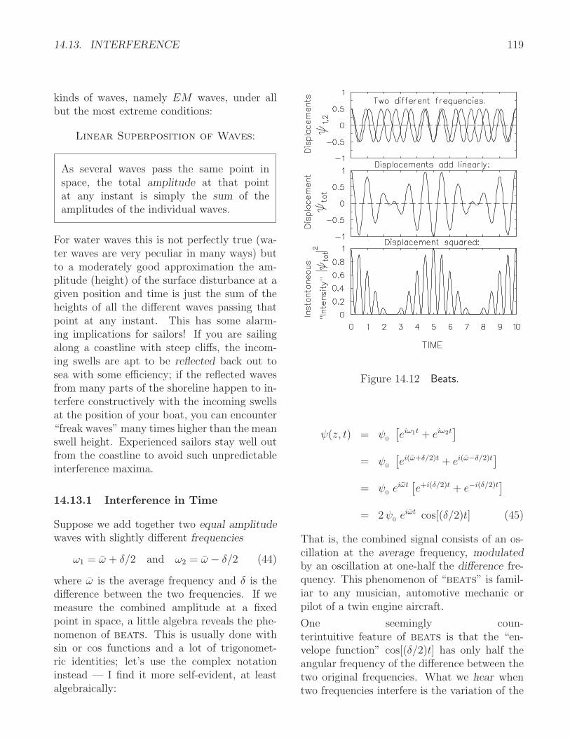
14.13. INTERFERENCE 119
kinds of waves, namely EM waves, under allbut the most extreme conditions:
Linear Superposition of Waves:
As several waves pass the same point inspace, the total amplitude at that pointat any instant is simply the sum of theamplitudes of the individual waves.
For water waves this is not perfectly true (wa-ter waves are very peculiar in many ways) butto a moderately good approximation the am-plitude (height) of the surface disturbance at agiven position and time is just the sum of theheights of all the different waves passing thatpoint at any instant. This has some alarm-ing implications for sailors! If you are sailingalong a coastline with steep cliffs, the incom-ing swells are apt to be reflected back out tosea with some efficiency; if the reflected wavesfrom many parts of the shoreline happen to in-terfere constructively with the incoming swellsat the position of your boat, you can encounter“freak waves” many times higher than the meanswell height. Experienced sailors stay well outfrom the coastline to avoid such unpredictableinterference maxima.
14.13.1 Interference in Time
Suppose we add together two equal amplitudewaves with slightly different frequencies
ω1 = ω + δ/2 and ω2 = ω − δ/2 (44)
where ω is the average frequency and δ is thedifference between the two frequencies. If wemeasure the combined amplitude at a fixedpoint in space, a little algebra reveals the phe-nomenon of beats. This is usually done withsin or cos functions and a lot of trigonomet-ric identities; let’s use the complex notationinstead — I find it more self-evident, at leastalgebraically:
Figure 14.12 Beats.
ψ(z, t) = ψ0
[
eiω1t + eiω2t]
= ψ0
[
ei(ω+δ/2)t + ei(ω−δ/2)t]
= ψ0 eiωt[
e+i(δ/2)t + e−i(δ/2)t]
= 2 ψ0 eiωt cos[(δ/2)t] (45)
That is, the combined signal consists of an os-cillation at the average frequency, modulatedby an oscillation at one-half the difference fre-quency. This phenomenon of “beats” is famil-iar to any musician, automotive mechanic orpilot of a twin engine aircraft.
One seemingly coun-terintuitive feature of beats is that the “en-velope function” cos[(δ/2)t] has only half theangular frequency of the difference between thetwo original frequencies. What we hear whentwo frequencies interfere is the variation of the

120 CHAPTER 14. WAVES
sound intensity with time; and the intensityis proportional to the square of the displace-ment.23 Squaring the envelope effectively dou-bles its frequency (see Fig. 14.12) and so the de-tected beat frequency is the full frequencydifference δ = ω1 − ω2.
This is a universal feature of waves and interfer-ence: the detected signal is the average inten-sity, which is proportional to the square of theamplitude of the displacement oscillations; andit is the displacements themselves that add lin-early to form the interference pattern. Be sureto keep this straight.
14.13.2 Interference in Space
Figure 14.13 A replica of Thomas Young’s orig-inal drawing (1803) showing the interference pat-tern created by two similar waves being emitted“in phase” (going up and down simultaneously)from two sources separated by a small distance.The arrows point along lines of constructive inter-ference (crests on top of crests and troughs under-neath troughs) and the dotted lines indicate “linesof nodes” where the crests and troughs cancel.
Suppose spherical waves emanate from twopoint sources oscillating in phase (one goes
23Actually the intensity is defined in terms of the averageof the square of the displacement over times long comparedwith the average frequency ω. This makes sense as long asthe beat frequency δ ≪ ω; but if ω1 and ω2 differ by anamount δ ∼ ω then it is hard to define what is meant by a“time average”. We will just duck this issue.
“up” at the same time as the other goes “up”)at the same frequency, so that the two wave-generators are like synchronized swimmers inwater ballet.24 Each will produce outgoingspherical waves that will interfere whereverthey meet.
The qualitative situation is pictured inFig.14.13, which shows a “snapshot” of two out-going spherical25 waves and the “rays” (~k direc-tions) along which their peaks and valleys (orcrests and troughs, whatever) coincide, givingconstructive interference. This diagram accom-panied an experimental observation by Youngof “interference fringes”” (a pattern of intensitymaxima and minima on a screen some distancefrom the two sources) that is generally regardedas the final proof of the wave nature of light.26
If we want to precisely locate the angles atwhich constructive interference occurs (“inter-ference maxima”) then it is most convenient to
think in terms of “rays” (~k vectors) as picturedin Fig. 14.14.
The mathematical criterion for constructive in-24This notion of being “in phase” or “out of phase” is
one of the most archetypal metaphors in Physics. It is socompelling that most Physicists incorporate it into theirthinking about virtually everything. A Physicist at a cock-tail party may be heard to say, “Yeah, we were 90 out ofphase on everything. Eventually we called it quits.” This isslightly more subtle than, “. . . we were 180 out of phase. . . ”meaning diametrically opposed, opposite, cancelling eachother, destructively interfering. To be “90 out of phase”means to be moving at top speed when the other is sittingstill (in SHM , this would mean to have all your energy inkinetic energy when the other has it all in potential energy)and vice versa. The ~E and ~B fields in a linearly polarizedEM wave are 90 out of phase, as are the “push” and the“swing” when a resonance is being driven (like pushing a kidon a swing) at maximum effect, so in the right circumstances“90 out of phase” can be productive. . . . Just remember,“in phase” at the point of interest means constructive inter-ference (maximum amplitude) and “180 out of phase” atthe point of interest means destructive interference (mini-mum amplitude — zero, in fact, if the two waves have equalamplitude).
25OK, they are circular waves, not spherical waves. Youtry drawing a picture of spherical waves!
26 Young’s classic experiment is in fact the archetype forall subsequent demonstrations of wave properties, as shallbe seen in the Chapter(s) on Quantum Mechanics.

14.13. INTERFERENCE 121
Figure 14.14 Diagram showing the condition forconstructive interference of two “rays” of thesame frequency and wavelength λ emitted inphase from two sources separated by a distance d.At angles for which the difference in path length∆ℓ is an integer number (m) of wavelengths, mλ,the two rays arrive at a distant detector in phaseso that their amplitudes add constructively, maxi-mizing the intensity. The case shown is for m = 1.
terference is simply a statement that the differ-ence in path length, ∆ℓ = d sin ϑm, for the two“rays” is an integer number m of wavelengthsλ, where the m subscript on ϑm is a reminderthat this will be a different angle for each valueof m:
d sin ϑm = m λ . (46)
(criterion for Constructive Interference)
Conversely, if the path length difference is ahalf-integer number of wavelengths, the twowaves will arrive at the distant detector exactlyout of phase and cancel each other out. Theangles at which this happens are given by
d sin ϑ destrm =
(
m +1
2
)
λ . (47)
(criterion for Destructive Interference)
Phasors
What happens when coherent light comesthrough more than two slits, all equally spaceda distance d apart, in a line parallel to the in-coming wave fronts? The same criterion (46)still holds for completely constructive interfer-ence (what we will now refer to as the princi-
pal maxima) but (47) is no longer a reliablecriterion for destructive interference: each suc-cessive slit’s contribution cancels out that of theadjacent slit, but if there are an odd number ofslits, there is still one left over and the com-bined amplitude is not zero.
Does this mean there are no angles where theintensity goes to zero? Not at all; but it isnot quite so simple to locate them. One wayof making this calculation easier to visualize(albeit in a rather abstract way) is with thegeometrical aid of phasors: A single wave
Figure 14.15 A single “phasor” of length ψ0
(the wave amplitude) precessing at a frequency ωin the complex plane.
can be expressed as ψ(x, t) = ψ0eiθ where
θ = kx − ωt + φ is the phase of the wave ata fixed position x at a given time t. (As usual,φ is the “initial” phase at x = 0 and t = 0.At this stage it is usually ignored; I just re-tained it one last time for completeness.) If wefocus our attention on one particular locationin space, this single wave’s “displacement” ψ atthat location can be represented geometricallyas a vector of length ψ0 (the wave amplitude) in

122 CHAPTER 14. WAVES
the complex plane called a “phasor” As timepasses, the “direction” of the phasor rotates atan angular frequency ω in that abstract plane.
There is not much advantage to this geomet-rical description for a single wave (except per-haps that it engages the right hemisphere of thebrain a little more than the algebraic expres-sion) but when one goes to “add together” twoor more waves with different phases, it helps alot! For example, two waves of equal amplitude
Figure 14.16 Two waves of equal amplitude ψ0
but different phases θ1 and θ2 are represented asphasors in the complex plane. Their vector sumhas the resultant amplitude ψ0 and the averagephase θ.
but different phases can be added together al-gebraically as in Eq. (45)
ψ = ψ0
[
eiθ1 + eiθ2]
= 2 ψ0 eiθ cos(δ/2)
= ψ0 eiθ (48)
where
ψ0 = 2 ψ0 cos(δ/2)
θ ≡ 12(θ1 + θ2)
δ ≡ θ2 − θ1 . (49)
That is, the combined amplitude ψ0 can be ob-tained by adding the phasors “tip-to-tail” like
ordinary vectors. Like the original components,the whole thing continues to precess in the com-plex plane at the common frequency ω.
We are now ready to use phasors to find theamplitude of an arbitrary number of waves ofarbitrary amplitudes and phases but a commonfrequency and wavelength interfering at a givenposition. This is illustrated in Fig. 14.17 for 5phasors. In practice, we rarely attempt such an
Figure 14.17 The net amplitude of a wave pro-duced by the interference of an arbitrary num-ber of other waves of the same frequency of arbi-trary amplitudes ψj and phases θj can in principlebe calculated geometrically by “tip-to-tail” vectoraddition of the individual phasors in the com-plex plane.
arbitrary calculation, since it cannot be simpli-fied algebraically.
Instead, we concentrate on simple combinationsof waves of equal amplitude with well definedphase differences, such as those produced by aregular array of parallel slits with an equal spac-ing between adjacent slits. Figure 14.18 showsan example using 6 identical slits with a spacingd = 100λ. The angular width of the interfer-ence pattern from such widely spaced slits isquite narrow, only 10 mrad (10−2 radians) be-tween principal maxima where all 6 rays are inphase. In between the principal maxima thereare 5 minima and 4 secondary maxima; this canbe generalized:

14.13. INTERFERENCE 123
The interference pattern for N equallyspaced slits exhibits (N − 1) minima and(N − 2) secondary maxima between eachpair of principal maxima.

124 CHAPTER 14. WAVES
Figure 14.18 The intensity pattern produced by the interference of coherent light passing throughsix parallel slits 100 wavelengths apart. Phasor diagrams are shown for selected angles. Notethat, while the phase angle difference δ between rays from adjacent slits is a monotonically increasingfunction of the angle ϑ (plotted horizontally) that the rays make with the “forward” direction, thelatter is a real geometrical angle in space while the former is a pure abstraction in “phase space”. Theexact relationship is δ/2π = (d/λ) sin ϑ ≈ (d/λ) ϑ for very small ϑ. Note the symmetry about the 3rd
minimum at ϑ ≈ 5 mrad. At ϑ ≈ 10 mrad the intensity is back up to the same value it had in the centralmaximum at ϑ = 0; this is called the first principal maximum. Then the whole pattern repeats. . . .
It may be conceptually helpful to show the geometrical explanation of the 6-slit interference patternin Fig. 14.18 in terms of phasor diagrams, but clearly the smooth curve shown there is not the resultof an infinte number of geometrical constructions. It comes from an algebraic formula that we canderive for an arbitrary angle ϑ and a corresponding phase difference δ = (2πd/λ) sin ϑ between raysfrom adjacent slits. The formula itself is obtained by analysis of a geometrical construction likethat illustrated in Fig. 14.19 for 7 slits, each of which contributes a wave of amplitude a, with aphase difference of δ between adjacent slits.

14.13. INTERFERENCE 125
Figure 14.19 Phasor diagram for calculat-ing the intensity pattern produced by the interfer-ence of coherent light passing through 7 parallel,equally spaced slits.
After adding all 7 equal-length phasors inFig. 14.19 “tip-to-tail”, we can draw a vectorfrom the starting point to the tip of the finalphasor. This vector has a length A (the netamplitude) and makes a chord of the circum-scribed circle, intercepting an angle
α = 2π − N δ , (50)
where in this case N = 7. The radius r of thecircumscribed circle is given by
a
2= r sin
(
δ
2
)
, (51)
as can be seen from the blowup in Fig. 14.20;this can be combined with the analogous
A
2= r sin
(α
2
)
(52)
to give the net amplitude
A = a
[
sin(
α2
)
sin(
δ2
)
]
. (53)
Figure 14.20 Blowup of one of the isoscelestriangles formed by a single phasor and two radiifrom the center of the circumscribed circle to thetip and tail of the phasor.
From Eq. (50) we know that α/2 = π − N δ/2,and in general sin(π − θ) = sin θ, so
A = a
[
sin(
N δ2
)
sin(
δ2
)
]
(54)
where
δ = 2π
(
d
λ
)
sin ϑ (55)
Although the drawing shows N = 7 phasors,this result is valid for an arbitrary number Nof equally spaced and evenly illuminated slits.

126 CHAPTER 14. WAVES

127
Chapter 15
Thermal Physics
NOTE.1
“A theory is the more impres-sive the greater the simplicity ofits premises, the more differentkinds of things it relates, and themore extended its area of applica-bility. Therefore the deep impres-sion that classical thermodynam-ics made upon me. It is the onlyphysical theory of universal contentwhich I am convinced will neverbe overthrown, within the frame-work of applicability of its basicconcepts.” — A. Einstein
“But although, as a matter of his-tory, statistical mechanics owes itsorigin to investigations in thermo-dynamics, it seems eminently wor-thy of an independent development,both on account of the eleganceand simplicity of its principles, andbecause it yields new results andplaces old truths in a new light indepartments quite outside of ther-modynamics.”
— J.W. Gibbs
We have seen how a few simple laws (in par-1I have “borrowed” the notation, general approach, basic
derivations and most of the quotations shown here from theexcellent textbook of the same name by Kittel & Kroemer,who therefore deserve all the credit (and none of the blame)for the abbreviated version displayed before you.
ticular Newton’s second law) can be com-bined with not-too-sophisticated mathematicsto solve a great variety of problems — prob-lems which eventually are perceived to fall intoa number of reasonably well-defined categoriesby virtue of the mathematical manipulationsappropriate to each — and that those distinctclasses of mathematical manipulations eventu-ally become familiar enough to acquire familiarnames of their own, such as “conservation ofimpulse and momentum” or “conservation ofwork and energy” or “conservation of torqueand angular momentum.” This emergence ofnew tacit paradigms was the great conceptualgift of the Newtonian revolution. But the mostprofound practical impact of the new scienceson society came in the form of the IndustrialRevolution, which was made possible only whenthe science of mechanics was combined withan understanding of how to extract usable me-chanical work from that most mysterious of allforms of energy, heat.
Historically, heat was recognized as a formof energy and temperature was understood interms of its qualitative properties long beforeanyone truly understood what either of theseterms actually meant in any rigorous micro-scopic model of matter. The link between New-ton’s mechanics and the thermodynamics ofJoule and Kelvin was forged by Boltzmann longafter steam power had changed the world, anda simple understanding of many of the finerpoints of Boltzmann’s statistical mechanics had

128 CHAPTER 15. THERMAL PHYSICS
to wait even longer until Quantum Mechan-ics provided a natural explanation for the req-uisite fact that the number of possible statesof any system, while huge, is not infinite, andthat small, simple systems are in fact restrictedto a countable number of discrete “stationarystates.” In this drama Albert Einstein was toplay a rather important role.
The following conceptual outline of StatisticalMechanics is designed to make the subject asclear as possible, not to be historically accurateor even fair. Having made this choice, how-ever, I hope to be able to display the essence ofthe most astonishing product of human Sciencewithout undue rigamarole, and perhaps to con-vey the wonder that arises from a deeper andmore fundamental understanding.
15.1 Random Chance
With so many miracles to choose from, wheredo I get off declaring Statistical Mechanics tobe “the most astonishing product of human Sci-ence?” This is of course a personal opinion, butit is one shared by many physicists — perhapseven a majority. The astonishment is a result ofthe incredible precision with which one can pre-dict the outcome of experiments on very com-plicated systems (the more complicated, themore precise!) based on the fundamental as-
sumption of statistical mechanics:
A system in thermal equilibrium isa priori equally likely to be found inany one of the fully-specified statesaccessible to it.
This seemingly trivial statement contains a cou-ple of ringers: the word “accessible” means, forinstance, that the total “internal” energy of thesystem — which is always written U — i.e. thesum of the kinetic and potential energies of allthe little particles and waves that make up thebig system — is fixed. There are many ways to
divide up that energy, giving more to one par-ticle and less to another, and the fundamen-
tal assumption says that they are all equallylikely; but in every case the energy must addup to the same U . This can obviously be veryconfusing, but fortunately we rarely attempt tocount up the possibilities on our fingers!
It is the assumption itself that is so amazing.How can anything but total ignorance resultfrom the assumption that we know nothing atall about the minute biases a real system mighthave for one state over another? More emphat-ically, how can such an outrageous assumptionlead to anything but wrong predictions? Itamounts to a pronouncement that Nature runsa perfectly honest casino, in which every possi-ble combination of the roll of the dice is actuallyequally likely! And yet every prediction derivedfrom this assumption has been demonstrated tobe accurate to the best precision our measure-ments can provide. And the consequences arenumerous indeed!
15.2 Counting the Ways
If we accept the fundamental assumption
at face value, then it is easy to calculate theprobability of finding the equilibrated system inany given fully specified state: if the state is notaccessible [e.g. if it takes more energy U thanwe have at our disposal] then the probabilityis zero; if it is accessible, then its probabilityis just 1
Ω, where Ω is the total number of
accessible states. The first step is therefore tocalculate Ω. In general this can get difficult,but we can choose a few simple examples toillustrate how the calculation goes.
15.2.1 Conditional Multiplicity
Suppose we have a jar full of pennies, say Npennies, all of which have had unique numberspainted on them so that they can be easily dis-

15.2. COUNTING THE WAYS 129
tinguished from each other. Now suppose weshake it thoroughly and dump it out on a niceflat table; each penny falls either “heads” or“tails” with equal a priori probability. Theprobability of penny #1 being “heads” is 1
2.
The probability of penny #1 being “heads” andpenny #2 being “tails” is 1
2× 1
2= 1
4. The prob-
ability of penny #1 being “heads” and penny#2 being “tails” and penny #3 being “tails” is12× 1
2× 1
2= 1
8. And so on. If the pennies are all
“statistically independent” (i.e. how one pennyfalls has no influence on the other pennies), theprobability of any specific arrangement of spe-cific pennies falling specific ways [what we calla fully specified state of the system] is
(
1
2
)N
=1
2N
where N is the total number of pennies.
Unfortunately, this is not what we want toknow. We don’t care which pennies fall whichway,2 only how many of each. This is whatwe call a partially specified or partially con-strained state of the system. What we reallywant to know is the number of ways we can getn heads and (N − n) tails.3
Suppose we specify that n pennies are “heads”and the remaining (N − n) are “tails.” Thenumber of ways we can do this is what we callΩ(n,N), the multiplicity function for the par-tially constrained state specified only by n and
2In the present case, we have a choice of whether totreat the pennies as “indistinguishable” or not. No twopennies are really indistinguishable, of course; even with-out our painted-on numbers, each one has unique scratcheson its surface and was crystallized from the molten statein a unique microscopic pattern. We could tell one fromanother; we just don’t care, for circumstantial reasons. Inquantum mechanics, however, you will encounter the con-cept of elementary particles [e.g. electrons] which are souncomplicated that they truly are indistinguishable [i.e.perfectly identical]; moreover, statistical mechanics pro-vides a means of actually testing to see whether they arereally absolutely indistinguishable or just very similar!
3It might be that we get to keep all the pennies that comeup heads, but for every penny that comes up tails we haveto chip in another penny of our own. In that case our profitwould be n − (N − n) = 2n − N cents.
N . Here’s how we calculate Ω(n,N): the num-ber of different ways we can rearrange all Ncoins is
N ! ≡ N · (N − 1) · (N − 2) · · · 3 · 2 · 1because we have N choices of which coin willbe first, then we have (N −1) choices of whichcoin will be second, then we have (N − 2)choices of which coin will be third, and so on.The total number of choices is the product ofthe numbers of choices at each step. However,we have overcounted by the number of differ-ent ways the heads can be rearranged amongthemselves, which by the same argument is n!,and by the number (N − n)! of ways the tailscan be rearranged among themselves. There-fore the total number of distinguishable com-binations that all give n heads and (N − n)tails is
Ω(n,N) =N !
n! · (N − n)!(1)
Another example would be a parking lot withN spaces in which n cars are parked. Thenumber of different ways we can label the spacesis N ! but the n occupied spaces can be rear-ranged amongst themselves n! different waysand the (N − n) empty spaces can be rear-ranged (N−n)! different ways without alteringthe partial constraint [namely, that only n ofthe spaces are filled].4 Then Eq. (1) describesthe number of different ways the cars can beparked without changing the total number ofparked cars.
The Binomial Distribution
To generalize, we talk about a system of Nparticles,5 each of which can only be in one
4If you were the parking lot owner and were charging $1per space [cheap!], your profit would be $n. I keep comingback to monetary examples — I guess cash is the socialanalogue of energy in this context.
5The term “particle” is [in this usage] meant to be asvague as possible, just like “system:” the particles are “re-ally simple things that are all very much alike” and thesystem is “a bunch of particles taken together.”

130 CHAPTER 15. THERMAL PHYSICS
of two possible single-particle states. A fullyspecified N -particle state of the system wouldhave the single-particle state of each individualparticle specified, and is not very interesting.The partially specified N -particle state withn of the particles in the first single-particlestate and the remaining (N − n) particles inthe other single-particle state can be realized inΩ(n,N) different ways, with Ω(n,N) givenby Eq. (1). Because there are only two pos-sible single-particle states, this case of Ω iscalled the binomial distribution. It is plotted6
in Fig. 15.1 for several values of N .
Note what happens to Ω(n,N) as N getsbigger: the peak value, which always occurs atnpeak = 1
2N , gets very large [in the plots it
is compensated by dividing by 2N , which isa big number for large N ] and the width ofthe distribution grows steadily narrower — i.e.
values of nN
far away from the peak get lessand less likely as N increases. The width isin fact the standard deviation7 of a hypotheti-cal random sample of n, and is proportionalto
√N . The fractional width (expressed as a
fraction of the total range of n, namely N) is
therefore proportional to√
NN
= 1√N
:
Fractional Width ∝ 1√N
(2)
which means that for really large N , likeN = 1020, the binomial distribution will getreally narrow, like a part in 1010, in terms ofthe fraction of the average.
6Actually what is plotted in Fig. 15.1 is the probabilityfunction
P(n) ≡ 1
2N· Ω(n, N) =
1
2N· N !
n! (N − n)!
vs. nN
, as explained in the caption. Otherwise it would bedifficult to put more than one plot on the same graph, asthe peak value of Ω(n, N) gets very large very fast as Nincreases!
7Recall your Physics Lab training on measurement!
Figure 15.1 The normalized binomial distribution for
several values of N . In order to put several cases on a
single graph, the horizontal axis shows n divided by its
maximum possible value N [giving the fraction of the
total range] and the binomial coefficient Ω(n,N) given
by Eq. (1) has been divided by the total number of pos-
sible fully specified N -particle states, 2N , to give the
“normalized” probability — i.e. if we add up the values
of Ω(n,N)/2N for all possible n from 0 to N , the
total probability must be 1. [This is eminently sensible;
the probability of n having some value is surely equal to
unity!]
15.2.2 Entropy
“If we wish to find in rational me-chanics an a priori foundation forthe principles of thermodynamics,we must seek mechanical definitionsof temperature and entropy.” —J.W. Gibbs
The function Ω(n,N) is called the multi-
plicity function for the partially specifiedsystem. If N and n get to be large numbers(which is usually the case when we are talkingabout things like the numbers of electrons ina crystal), Ω(n,N) can get really huge.8 Itis so huge, in fact, that it becomes very diffi-
8A good estimate of the size of N ! for large N is given

15.3. STATISTICAL MECHANICS 131
cult to cope with, and we do what one usuallydoes with ungainly huge numbers to make themmanageable: we take its logarithm. We definethe [natural] logarithm of Ω to be the en-
tropy σ:σ ≡ ln Ω (3)
Let’s say that again: the entropy σ is thenatural logarithm of the multiplicity func-
tion Ω — i.e. of the number of different wayswe can get the partially specified conditions inthis case defined by n.
Is this all there is to the most fearsome, themost arcane, the most incomprehensible quan-tity of thermodynamics? Yep. Sorry todisappoint. That’s it. Of course, we haven’tplayed around with σ yet to see what it mightbe good for — this can get very interesting —nor have I told this story in an historically ac-curate sequence; the concept of entropy pre-ceded this definition in terms of “statistical me-chanics” by many years, during which all ofits properties were elucidated and armies ofthermal physicists and engineers built the ma-chines that powered the Industrial Revolution.But understanding thermodynamics the old-fashioned way is hard! So we are taking theeasy route — sort of like riding a helicopter tothe top of Mt. Everest.
15.3 Statistical Mechanics
Before we go on, I need to move away from ourexamples of binomial distributions and cast thegeneral problem in terms more appropriate toMechanics. We can always go back and gener-alize the paradigm9 but I will develop it alongtraditional lines.
The owner of the parking lot described earlier
by Stirling’s approximation:
N ! ≈√
2πN · NN · e−N
9Count on it!
is only interested in the total number of carsparked because that number will determine hisor her profit. In Mechanics the “coin of therealm” is energy, which we have already saidis always written U in thermal physics. Theabstract problem in statistical mechanics
involves a complex system with many possiblestates, each of which has a certain total energyU . This energy may be in the form of the sumof the kinetic energies of all the atoms of a gasconfined in a box of a certain volume, or it maybe the sum of all the vibrational energies of acrystal; there is no end of variety in the physicalexamples. But we are always talking about therandom, disordered energy of the system, theso-called internal energy, when we talk aboutU .
Now, given a certain amount of internal en-ergy U , the number of different fully-specifiedstates of the system whose total internal en-ergy is U [our partial constraint] is the condi-tional multiplicity function Ω(U). Tak-ing the binomial distribution as our exampleagain, we could substitute crystal lattice sitesfor “parking places” and defects for “cars” [adefect could be an atom out of place, for in-stance]. If it takes an energy ε to createone defect, then the total internal energy storedin n defects would be U = n ε. Lots ofother examples can be imagined, but this onehas the energy U proportional to the numbern of defects, so that you can see how the U -dependence of Ω in this case is just like then-dependence of Ω before.
So what?
Well, things start to get interesting when youput two such systems in contact so that Ucan flow freely between them through randomstatistical fluctuations.
15.3.1 Ensembles
One of the more esoteric notions in statisti-
cal mechanics is the concept of an ensem-

132 CHAPTER 15. THERMAL PHYSICS
ble. This has nothing to do with music; it goesback to the original meaning of the French wordensemble, which is a collection or gathering ofthings — much more general and abstract thanthe small band of musicians we tend to visual-ize. Anyway, the Statistical Mechanical “en-
semble” is a collection of all the possible fullyspecified states of some system.
Of course, there are different kinds of ensem-
bles depending upon what global constraintsare in effect. For instance, the set of all possi-ble states of an isolated system S consistingof a fixed number N of “particles”10 with awell defined total energy U is called a micro-
canonical ensemble. This is what we havebeen discussing so far.
The set of all possible states of a system Sconsisting of a fixed number N of particlesbut in “thermal contact” with a much, muchlarger system R (called a “heat reservoir”)so that the energy U of S can flow in orout of R at random is called a canonical
ensemble.
And the set of all possible states of a systemS in contact with a reservoir R with whichit can exchange both energy (U) and particles(N) is called a grand canonical ensemble.
If the utility of these concepts is less than ob-vious to you, join the club. I won’t need to usethem to derive the good stuff below, but nowyou will be able to scoff at pedants that pretendyou can’t understand “Stat Mech” unless youknow what the various types of Ensembles are.
15.4 Temperature
“The general connection betweenenergy and temperature may onlybe established by probability con-siderations. [Two systems] are instatistical equilibrium when a trans-
10Remember, a “particle” is meant to be an abstract con-cept in this context!
fer of energy does not increase theprobability.”
— M. Planck
When we put two systems S1 and S2 (withN1 and N2 particles, respectively) into “ther-mal contact” so that the (constant) total energyU = U1 + U2 can redistribute itself randomlybetween S1 and S2, the combined systemS = S1 + S2 will, we postulate, obey the fun-
damental principle — it is equally likely tobe found in any one of its accessible states. Thenumber of accessible states of S (partially con-strained by the requirement that N1, N2 andU = U1 + U2 remain constant) is given by
Ω = Ω1(U1) × Ω2(U2) (4)
where Ω1 and Ω2 are the multiplicity
functions for S1 and S2 taken separately[both depend upon their internal energies U1
and U2] and the overall multiplicity function isthe product of the two individual multiplicityfunctions because the rearrangements withinone system are statistically independent of therearrangements within the other.11 Since theentropy is the log of the multiplicity andthe log of a product is the sum of the logs,Eq. (4) can also be written
σ = σ1(U1) + σ2(U2) (5)
— i.e. the entropy of the combined system isthe sum of the entropies of its two subsystems.
15.4.1 The Most Probable
So what? Well, here’s the thing: we know thatall accessible states of the system are a priori
equally likely; however, the number Ω of ac-cessible states will depend upon the division of
11If I flip my coin once and you flip your coin twice, thereare 21 = 2 ways my flip can go [h, t] and 22 = 4 waysyour 2 flips can go [HH, HT, TH, TT]; the total number ofways the combination of your flips and mine can go [hHH,hHT, hTH, hTT, tHH, tHT, tTH, tTT] is 2 × 4 = 8. Andso on.

15.4. TEMPERATURE 133
the total energy U between U1 and U2. More-over, for a certain value of U1 (and thereforeof U2 = U − U1), Ω will be a maximum —i.e. that value of U1 will make possible thelargest variety of equally likely random statesof the system and consequently we will be morelikely, on average, to find the system in stateswith that value of U1 than in other states12
with different values of U1.
This special value of U1 is called (reasonablyenough) the “most probable value” and is giventhe symbolic representation U1.
15.4.2 Criterion for Equilibrium
If our two systems are initially prepared sepa-rately with energies U1 and U2 other than themost probable, what will happen when we bringthem into contact so that U can flow betweenthem? The correct answer is, of course, “Ev-erything that possibly can happen.” But thereis a bigger variety of possibilities for certaingross distributions of energy than for others,and this makes those gross distributions morelikely than others. The overall entropy is thus ameasure of this likelihood. It seems inevitablethat one will eventually feel compelled to an-thropomorphize this behaviour and express itas follows:13
All random systems “like” varietyand will “seek” arrangements thatmaximize it.
In any case, the tendency of energy to flow fromone system to the other will not be governed byequalization of either energy or entropy them-selves, but by equalization of the rate of change
12Nothing precludes finding the system in states withother values of U1, of course. In fact we must do so some-times! Just less often.
13Perhaps the converse is actually true: human “wants”are actually manifestations of random processes whose vari-ety is greater in the direction of perceived desire. I find thisspeculation disturbing.
of entropy with energy, ∂σ∂U
. To see why, sup-pose (for now) that more energy always givesmore entropy. Then suppose that the entropyσ1 of system S1 depends only weakly on itsenergy U1, while the entropy σ2 of system S2
depends strongly on its energy U2. In mathe-matical terms, this reads
Suppose∂σ1
∂U1
<∂σ2
∂U2
Then removal of a small amount of energy dUfrom S1 will decrease its entropy σ1, butnot by as much as the addition of that same en-ergy dU to S2 will increase its entropy σ2.Thus the net entropy σ1 +σ2 will be increasedby the transfer of dU from S1 to S2. Thisargument is as convoluted as it sounds, but itcontains the irreducible essence of the definitionof temperature, so don’t let it slip by!
The converse also holds, so we can combine thisidea with our previous statements about thesystem’s “preference” for higher entropy andmake the following claim:
Energy U will flow spontaneously
from a system with smaller∂σ
∂Uto
a system with larger∂σ
∂U.
If the rate of increase of entropy with energy(
∂σ∂U
)
is the same for S1 and S2, then thecombined system will be “happy,” the energywill stay where it is (on average) and a state of“thermal equilibrium” will prevail.
Mathematical Derivation
Is there any way to derive a formal (mathemat-ical) criterion for the condition of thermal equi-librium, starting from a hypothetical knowledgeof Ω1 as a function of U1 and Ω2 as a functionof U2 = U − U1? Of course! Why else wouldI be doing this? The thing about a maximumof a function (or a minimum, for that matter;

134 CHAPTER 15. THERMAL PHYSICS
either type of extremum obeys the same rule) isthat the slope of the function must be zero atthe extremum. [Otherwise it would still havefurther up or down to go!] Since the slope isgiven by the derivative, this reads
Criterion for an extremum:∂Ω
∂U1
= 0
(6)In this case, since Ω = Ω1 · Ω2, the product
rule for derivatives gives
∂Ω
∂U1
=∂Ω1
∂U1
· Ω2 + Ω1 ·∂Ω2
∂U1
= 0 (7)
Now, Ω2 is a function of U2, not U1; but wecan get around that by using the chain rule,
∂Ω2
∂U1
=∂Ω2
∂U2
· ∂U2
∂U1
·
where U2 = U − U1 and U is a constant, so
∂U2
∂U1
= −1
We can therefore substitute −∂Ω2
∂U2
for∂Ω2
∂U1in Eq. (7):
∂Ω1
∂U1
· Ω2 − Ω1 ·∂Ω2
∂U2
= 0
or∂Ω1
∂U1
· Ω2 = Ω1 ·∂Ω2
∂U2
If we now divide both sides by the product Ω1 ·Ω2, we get
1
Ω1
· ∂Ω1
∂U1
=1
Ω2
· ∂Ω2
∂U2
. (8)
Now we need to recall the property of the nat-ural logarithm that was so endearing when wefirst encountered it: ln(x) is the functionwhose derivative is the inverse,
d
dxln(x) =
1
x
and, by the chain rule,
d
dxln(y) =
1
y· dy
dx
In this case “y” is Ω and “x” is U , so wehave
∂
∂Uln(Ω) =
1
Ω· ∂Ω
∂U
which means that Eq. (8) can be written
∂
∂U1
ln(Ω1) =∂
∂U2
ln(Ω2)
But the logarithm of the multiplicity func-
tion Ω is the definition of the entropy σ, sothe equation can be simplified further to read
∂σ1
∂U1
=∂σ2
∂U2
(9)
where of course we are assuming that all theother parameters (like N1 and N2) are heldconstant.
Note that we have recovered, by strict math-ematical methods, the same criterion dictatedby common sense earlier. The only advantageof the formal derivation is that it is rigourous,general and involves no questionable assump-tions.14
15.4.3 Thermal Equilibrium
Eq. (9) establishes the criterion for the most
probable configuration — i.e. the valueof U1 for which the combined systems havethe maximum total entropy, the maximum to-tal number of accessible states and the highestprobability. This also defines the condition ofthermal equilibrium between the two sys-tems — that is, if U1 = U1, any flow of energyfrom S1 to S2 or back will lower the number ofaccessible states and will therefore be less likely
14Or, at least, none that are readily apparent. . . .

15.4. TEMPERATURE 135
than the configuration15 with U1 = U1. There-fore if we leave the systems alone and come backlater, we will be most likely to find them in the“configuration” with U1 in system S1 and(U − U1) in system S2.
This seems like a pretty weak statement. Noth-ing certain, just a bias in favour of U1 overother possible values of U1 all the way fromzero to U . That is true. statistical me-
chanics has nothing whatever to say aboutwhat will happen, only about what is likely tohappen — and how likely! However, when thenumbers of particles involved become very large(and in Physics they do become very large), thefractional width of the binomial distribution[Eq. (2)] becomes very narrow, which translatesinto a probability distribution that is incredi-bly sharply peaked at U1. As long as energyconservation is not violated, there is nothingbut luck to prevent all the air molecules in thisroom from vacating the region around my headuntil I expire from asphyxiation. However, Itrust my luck in this. A quotation from Boltz-mann confirms that I am in distinguished com-pany:
“One should not imagine that twogases in a 0.1 liter container, ini-tially unmixed, will mix, then againafter a few days separate, then mixagain, and so forth. On the con-trary, one finds . . . that not untila time enormously long comparedto 101010
years will there be any no-ticeable unmixing of the gases. Onemay recognize that this is practi-cally equivalent to never. . . .”
— L. Boltzmann15Note the distinction between the words configuration
and state. The latter implies we specify everything aboutthe system — all the positions and velocities of all its par-ticles, etc. — whereas the former refers only to some grossoverall macroscopic specification like the total energy or howit is split up between two subsystems. A state is completelyspecified while a configuration is only partly specified.
15.4.4 Inverse Temperature
What do we expect to happen if the systemsare out of equilibrium? For instance, supposesystem S1 has an energy U1 < U1. Whatwill random chance “do” to the two systems?Well, a while later it would be more likely tofind system S1 with the energy U1 again.That is, energy would tend to “spontaneouslyflow” from system S2 into system S1 tomaximize the total entropy.16 Now stop andthink: is there any familiar, everyday propertyof physical objects that governs whether or notinternal energy (heat) will spontaneously flowfrom one to another? Of course! Every childwho has touched a hot stove knows that heatflows spontaneously from a hotter object [likea stove] to a cooler object [like a finger]. Weeven have a name for the quantitative measureof “hotness” — we call it temperature.
Going back to Eq. (9), we have a mathematicalexpression for the criterion for thermal equi-
librium, whose familiar everyday-life equiva-lent is to say that the two systems have thesame temperature. Therefore we have a com-pelling motivation to associate the quantity ∂σ
∂U
for a given system with the temperature ofthat system; then the equation reads the sameas our intuition. The only problem is that weexpect heat to flow from a system at high tem-perature to a system at low temperature; let’scheck to see what is predicted by the mathe-matics.17 Let’s suppose that for some initialvalue of U1 < U1 we have
∂σ1
∂U1
>∂σ2
∂U2
.
Then adding a little extra energy dU to S1
will increase σ1 by more than we decrease σ2
by subtracting the same dU from S2 [which
16This is the same as maximizing the probability, but fromnow on I want to use the terminology “maximizing the en-tropy.”
17We have already done this once, but it bears repeating!To avoid complete redundancy, this time we will reverse theorder of hot and cold.
136 CHAPTER 15. THERMAL PHYSICS
we must do, because the total energy is con-served]. So the total entropy will increase ifwe move a little energy from the system with asmaller ∂σ
∂Uto the system with a larger ∂σ
∂U.
The region of smaller ∂σ∂U
must therefore behotter and the region of larger ∂σ
∂Umust be
cooler. This is the opposite of what we expectof temperature, so we do the obvious: wedefine ∂σ
∂Uto be the inverse temperature
of a system:∂σ
∂U≡ 1
τ(10)
where (at last) τ is the temperature of thesystem in question. We can now express Eq. (9)in the form that agrees with our intuition:
Condition of thermal equilibrium:
τ1 = τ2 (11)
— i.e. if the temperatures of the two systemsare the same, then they will be in thermal equi-librium and everything will be most likely tostay pretty much as it is.
As you can see, temperature is not quitesuch a simple or obvious concept as we mayhave been led to believe! But now we have auniversal, rigorous and valid definition of tem-perature. Let’s see what use we can make ofit.
15.4.5 Units & Dimensions
I have borrowed from several authors the con-vention of expressing the entropy σ in ex-plicitly dimensionless form [the logarithm of apure number is another pure number]. By thesame token, the simple definition of tempera-
ture τ given by Eq. (10) automatically givesτ dimensions of energy, just like U . Thusτ can be measured in joules or ergs or othermore esoteric units like electron-volts; but weare accustomed to measuring temperature
in other, less “physical” units called degrees.What gives?
The story of how temperature units got in-vented is fascinating and sometimes hilarious;suffice it (for now) to say that these units wereinvented before anyone knew what temperaturereally was!18 There are two types of “degrees”in common use: Fahrenheit degrees19 and Cel-sius degrees (written C) which are moderatelysensible in that the interval between the freez-ing point of water (0C) and the boiling point ofwater (100C) is divided up into 100 equal “de-grees” [hence the alternate name “Centigrade”].However, in Physics there are only one kindof “degrees” in which we measure temperature:degrees absolute or “Kelvin”20 which are writ-ten just “K” without any symbol. One Kis the same size as one C, but the zero of theKelvin scale is at absolute zero, the coldest tem-perature possible, which is itself an interestingconcept. The freezing temperature of water isat 273.15 K, so to convert C into K you justadd 273.15 degrees. Temperature measured inK is always written T .
What relationship does τ bear to T? The lat-ter had been invented long before the develop-ment of Statistical Mechanics and the explana-tion of what temperature really was; but theseclumsy units never go away once people have
18 Well, to be fair, people had a pretty good workingknowledge of the properties of temperature; they just didn’thave a definition of temperature in terms of nuts-and-boltsmechanics, like Eq. (10).
19These silly units were invented by an instrument makercalled Fahrenheit [1686-1736] who was selling thermometersto meteorologists. He picked body temperature [a handyreference, constant to the precision of his measurements] forone “fiducial” point and for the other he picked the freezingpoint of saturated salt water, presumably from the NorthSea. Why not pure water? Well, he didn’t like negativetemperatures [neither do we, but he didn’t go far enough!]so he picked a temperature that was, for a meteorologist, ascold as was worth measuring. [Below that, presumably, itwas just “damn cold!”] Then he (sensibly) divided up theinterval between these two fiducials into 96 = 64 + 32 equal“degrees” [can you see why this is a pragmatic choice forthe number of divisions?] and voila! he had the Fahrenheittemperature scale, on which pure water freezes at 32F andboils at 212F. A good system to forget, if you can.
20Named after Thomson, Lord Kelvin [1852], a pioneer ofthermodynamics.

15.4. TEMPERATURE 137
gotten used to them. The two types of unitsmust, of course, differ by some constant con-version factor. The factor in this case is kB,Boltzmann’s constant:
τ ≡ kB T where
kB ≡ 1.38066 × 10⁻²³ J/K (12)
By the same token, the “conventional entropy”S defined by the relationship
1
T=
∂S
∂U(13)
must differ from our dimensionless version σby the same conversion factor:
S ≡ kB σ (14)
This equivalence completes the definition of themysterious entities of classical thermodynamicsin terms of the simple “mechanical” paradigmsof Statistical Mechanics. I will continue to useσ and τ here.
15.4.6 A Model System
Some of the more peculiar properties of temper-ature can be illustrated by a simple example:
Certain particles such as electrons have “spin12” which (it turns out) prevents their spins
from having any orientation in a magnetic field~B other than parallel to the field (“spin up”) orantiparallel to it (“spin down”). Because eachelectron has a magnetic moment ~µ (sort of likea tiny compass needle) lined up along its spin
direction, there is an energy ε = −~µ · ~B as-sociated with its orientation in the field.21 Fora “spin up” electron the energy is ε↑ = +µBand for a “spin down” electron the energy isε↓ = −µB.
21The rate of change of this energy with the angle betweenthe field and the compass needle is in fact the torque whichtries to align the compass in the Earth’s magnetic field, aneffect of considerable practical value.
Consider a system consisting of N electrons ina magnetic field and neglect all other interac-tions, so that the total energy U of the systemis given by
U = (N↑ − N↓) µB
where N↑ is the number of electrons with spinup and N↓ is the number of electrons with spindown. Since N↓ = N − N↑, this means
U = (2N↑ − N) µB or
N↑ =N
2+
U
2µB(15)
— that is, N↑ and U are basically the samething except for a couple of simple constants.As N↑ goes from 0 to N , U goes from−NµB to +NµB.
This system is another example of the bino-mial distribution whose multiplicity functionwas given by Eq. (1), with N↑ in place of n.This can be easily converted to Ω(U). Theentropy σ(U) is then just the logarithm ofΩ(U), as usual. The result is plotted in thetop frame of Fig. 15.2 as a function of energy.Note that the entropy has a maximum value forequal numbers of spins up and down — i.e. forzero energy. There must be some such peak inσ(U) whenever the energy is bounded above— i.e. whenever there is a maximum possibleenergy that can be stored in the system. Suchsituations do occur [this is a “real” example!]but they are rare; usually the system will holdas much energy as you want.
Negative Temperature
The “boundedness” of U and the consequent“peakedness” of σ(U) have some interestingconsequences: the slope of σ(U) [which, byEq. (10), defines the inverse temperature] de-creases steadily and smoothly over the entirerange of U from −NµB to +NµB, goingthrough zero at U = 0 and becoming negative

138 CHAPTER 15. THERMAL PHYSICS
Figure 15.2 Entropy, inverse temperature and temper-
ature of a system consisting of N = 32 spin- 12 particles
(with magnetic moments µ) in a magnetic field B.
for positive energies. This causes the tempera-ture itself to diverge toward +∞ as U → 0from the left and toward −∞ as U → 0from the right. Such discontinuous behaviouris disconcerting, but it is only the result of ourinsistence upon thinking of τ as “fundamen-tal” when in fact it is 1/τ that most sensiblydefines how systems behave. Unfortunately, itis too late to get thermometers calibrated in in-verse temperature and get used to thinking ofobjects with lower inverse temperature as be-ing hotter. So we have to live with some prettyodd properties of “temperature.”
Consider, for instance, the whole notion of neg-ative temperature, which is actually exhibitedby this system and can actually be preparedin the laboratory.22 What is the behaviour ofa system with a negative temperature? Ourphysical intuition, which in this case is trust-worthy, declares that one system is hotter thananother if, when the two are placed in thermalcontact, heat energy spontaneously flows out ofthe first into the second. I will leave it as an ex-ercise for the reader to decide which is most hot— infinite positive temperature or finite nega-tive temperature.
15.5 Time & Temperature
Let’s do the following Gedankenexperiment :Suppose I show you a movie of a swimmingpool full of waves and splashes; suddenly (in themovie) all the waves come together and squirta diver out of the pool. She flies gracefullythrough the air to land on the diving boardwhile the pool’s surface has miraculously re-turned to mirror smoothness. What is wrongwith this picture? Wait! Before you answer,you also get the following movie: A box full of100 black and 100 white marbles sits on a table;the marbles are arranged randomly. An anony-mous assistant picks up the box, closes the lid,shakes the box for a while, puts it down andopens the lid. All the white marbles are nowon the left side and all the black marbles are onthe right side. Why do you keep thinking thereis a problem? Try this: The same box, the sameassistant, the same story; except this time thereare only 4 marbles, two of each. Not so sure,hmmm? How about 2 marbles, one black andone white? Now we can’t tell a thing aboutwhether the movie is being shown forward orbackward, right? What is going on here?
Our concept of the “arrow of time” is some-how bound up with statistical mechanics and
22[by reversing the direction of the magnetic field beforethe spins have a chance to react]

15.6. BOLTZMANN’S DISTRIBUTION 139
is alarmingly fragile — we can lose our bear-ings completely just by confining our attentionto too small a system! As we will see later, the“fundamental” laws governing the microscopicinteractions of matter will be no help at all inclarifying this mystery.
15.6 Boltzmann’s Distribution
In defining the concept of temperature, we haveexamined the behaviour of systems in thermalcontact (i.e. able to exchange energy back andforth) when the total energy U is fixed. Inthe real world, however, it is not often that weknow the total energy of an arbitrary system;there is no “energometer” that we can stick intoa system and read off its energy! What weoften do know about a system it its tempera-ture. To find this out, all we have to do is sticka calibrated thermometer into the system andwait until equilibrium is established betweenthe thermometer and the system. Then we readits temperature off the thermometer. So whatcan we say about a small system23 S (likea single molecule) in thermal equilibrium witha large system (which we usually call a “heatreservoir” R) at temperature τ = kBT?
Well, the small system can be in any one ofa large number of fully-specified states. It isconvenient to be invent an abstract label for agiven fully-specified state so that we can talkabout its properties and probability. Let’s callsuch a state |α〉 where α is a “full label”— i.e. α includes all the information thereis about the state of S. It is like a completelist of which car is parked in which space, orexactly which coins came up heads or tails inwhich order, or whatever. For something simplelike a single particle’s spin, α may only specifywhether the spin is up or down. Now considersome particular fully-specified state |α〉 whose
23A “small system” can even be a “particle,” since bothterms are intentionally vague and abstract enough to meananything we want!
energy is εα. As long as R is very big and Sis very small, S can — and sometimes will —absorb from R the energy εα required to bein the state |α〉, no matter how large εα maybe. However, you might expect that states withreally big εα would be excited somewhat lessoften than states with small εα, because theextra energy has to come from R, and everytime we take energy out of R we decrease itsentropy and make the resultant configurationthat much less probable. You would be right.Can we be quantitative about this?
Well, the combined system S+R has a mul-tiplicity function Ω which is the product ofthe multiplicity function ΩS = 1 for S [whichequals 1 because we have already postulatedthat S is in a specific fully specified state |α〉]and the multiplicity function ΩR = eσ
R forR:
Ω = ΩS × ΩR = 1 × eσR
Moreover, the probability Pα of finding S instate |α〉 with energy εα will be proportionalto this net multiplicity:
Pα ∝ eσR
We must now take into account the effect onthis probability of removing the energy εα
from R to excite the state |α〉.The energy of the reservoir R before webrought S into contact with it was U . Wedon’t need to know the value of U , only thatit was a fixed starting point. The entropy of Rwas then σ
R(U). Once contact is made and
an energy εα has been “drained off” into S,the energy of R is (U − εα) and its entropyis σ
R(U − εα).
Because εα is so tiny compared to U , we cantreat it as a “differential” of U (like “dU”) andestimate the resultant change in σ
R[relative to
its old value σR(U)] in terms of the derivative
of σR
with respect to energy:
σR(U + dU) = σ
R(U) +
(
∂σR
∂U
)
· dU

140 CHAPTER 15. THERMAL PHYSICS
or in this case (with dU ≡ −εα)
σR(U − εα) = σ
R(U) −
(
∂σR
∂U
)
· εα
But this derivative is by definition the inverse
temperature of R:∂σ
R
∂U≡ 1
τ. Thus
σR(U − εα) = σ
R(U) − εα
τ
and thus the probability of finding S in thestate |α〉 obeys
Pα ∝ eσR
(U−εα) = exp[
σR(U) − εα
τ
]
or Pα ∝ eσR
(U) · exp(
−εα
τ
)
Since eσR
(U) is a constant independent of ei-ther εα or τ , that term will be the same forany state |α〉 so we may ignore it and writesimply
Pα ∝ exp(
−εα
τ
)
(16)
This is the famous Boltzmann factor thatdescribes exactly how to calculate the relativeprobabilities of different states |α〉 of a sys-tem in thermal contact with a heat reservoir attemperature τ . It is probably the single mostuseful rule of thumb in all of thermal physics.
15.6.1 The Isothermal Atmosphere
The gravitational potential energy of a gasmolecule of mass m at an altitude h abovesea level is given approximately by ε = mgh,where g = 9.81 m/s2. Here we neglect thedecrease of g with altitude, which is a goodapproximation over a few dozen miles. Nextwe pretend that the temperature of the atmo-sphere does not vary with altitude, which is un-true, but perhaps relative to 0 K it is not allthat silly, since the difference between the freez-ing (273.15 K) and boiling (373.15 K) pointsof water is less than 1/3 of their average. For
convenience we will assume that the whole at-mosphere has a temperature T = 300 K (aslightly warm “room temperature”).
In this approximation, the probability P(h) offinding a given molecule of mass m at heighth will drop off exponentially with h:
P(h) = P(0) exp
(
−mgh
τ
)
Thus the density of such molecules per unit vol-ume and the partial pressure pm of that speciesof molecule will drop off exponentially with al-titude h:
pm(h) = pm(0) exp
(
− h
h0
)
where h0 is the altitude at which the partialpressure has dropped to 1/e of its value pm(0)at sea level. We may call h0 the “mean heightof the atmosphere” for that species of molecule.A quick comparison and a bit of algebra showsthat
h0 =τ
mg
For oxygen molecules (the ones we usually careabout most) h0 ≈ 8 km. For helium atomsh0 ≈ 64 km and in fact He atoms rise to the“top” of the atmosphere and disappear into in-terplanetary space. This is one reason why wetry not to lose any helium from superconduct-ing magnets etc. — helium is a non-renewableresource!
15.6.2 How Big are Atoms?
Wait a minute! How did I calculate h0? I hadto know m for the different molecules, and thatrequires some knowledge of the sizes of atoms— information that has not yet been set forthin this book! In fact, empirical observationsabout how fast the pressure of the atmospheredoes drop off with altitude could give a prettygood idea of his big atoms are; this isn’t howit was done historically, but let’s give it a tryanyway:

15.7. IDEAL GASES 141
Suppose that, by climbing mountains and mea-suring the density of oxygen molecules (O2) as afunction of altitude, we have determined empir-ically that h0 for O2 is about 8,000 m. Then,according to this simple model, it must be truethat the mass m of an O2 molecule is about
m ≈ τ
h0 g=
300 × 1.38 × 10−23
8 × 103 × 9.81kg
or m ≈ 5.3 × 10⁻²⁶ kg
This is a mighty small mass!
Now to mix in just a pinch of actual history:Long ago, chemists discovered (again empiri-cally) that different pure substances combinedwith other pure substances in fixed ratios ofsmall integers times a certain characteristicmass (characteristic for each pure substance)called its molecular weight A. People hada pretty good idea even then that these puresubstances were made up of large numbers ofidentical units called “atoms,”24 but no one hadthe faintest idea how big atoms were — ex-cept of course that they must be pretty small,since we never could see any directly. The num-ber N0 of molecules in one molecular weightof a pure substance was (correctly) presumedto be the same, to explain why chemical reac-tions obeyed this rule. This number came to becalled a “mole” of the substance. For oxygen(O2), the molecular weight is roughly 32 gramsor 0.032 kg.
If we now combine this conventional definitionof a mole of O2 with our previous estimate ofthe mass of one O2 molecule, we can estimate
N0 ≈ 0.032
5.3 × 10⁻²⁶≈ 6 × 10²³
The exact number, obtained by quite differentmeans, is
N0 ≡ 6.02205 × 10²³ (17)
24I will cover the history of “Atomism” in a bit more detaillater on!
molecules per mole. This is known as Avo-
gadro’s number.
Turning the argument around, the mass of amolecule can be obtained from its molecularweight A as follows: One mole of any sub-stance is defined as a mass A × 1 gram, andcontains N0 molecules (or atoms, in the case ofmonatomic molecules) of the substance. Thushelium, with A = 4, weighs 4 gm (or 0.004 kg)per mole containing N0 atoms, so one He atomweighs (0.004/N0) kg or 6.6 × 10⁻²⁷ kg.
15.7 Ideal Gases
We have argued on an abstract basis that thestate of highest entropy (and hence the mostprobable state) for any complicated system isthe one whose macroscopic properties can beobtained in the largest possible number of dif-ferent ways; if the model systems we have con-sidered are any indication, a good rule of thumbfor how to do this is to let each “degree of free-dom” of the system contain (on average) anequal fraction of the total energy U . We canjustify this argument by treating that degreeof freedom as a “system” in its own right (al-most anything can be a “system”) and apply-ing Boltzmann’s logic to show that the proba-bility of that microsystem having an energy εwhile in thermal equilibrium at temperature τdecays exponentially as exp(−ε/τ). This im-plies a mean ε on the order of τ , if we don’tquibble over factors comparable to 1.
The Equipartition Theorem, which is morerigourously valid than the above hand-wavingwould suggest,25 specifies the factor to be ex-actly 1/2:
25If you want the details, here they are: Suppose that pi
is the canonical momentum characterizing the ith degreeof freedom of a system and that ε(pi) = bp2
i is the energyassociated with a given value of pi. Assume further thatpi can have a continuous distribution of values from −∞to +∞. Then the probability of pi having a given valueis proportional to exp(−bp2
i /τ) and therefore the average

142 CHAPTER 15. THERMAL PHYSICS
A system in thermal equilibriumwith a heat reservoir at temperatureτ will have a mean energy of 1
2τ
per degree of freedom.
In an ideal monatomic gas of N atoms attemperature τ each atom has three degreesof freedom: left–right (x), back–forth (y) andup–down (z). Thus the average internal energyof our monatomic ideal gas is
U =3
2N τ (18)
In spite of the simplicity of the above argu-ment26 this is a profound and useful result. Ittells us, for instance, that the energy U of anideal gas does not depend upon its pressure27
p! This is not strictly true, of course; inter-actions between the atoms of a gas make itspotential energy different when the atoms are(on average) close together or far apart. But formost gases at (human) room temperature and(Earth) atmospheric pressure, the ideal-gas ap-proximation is extremely accurate!
It also means that if we change the temperatureof a container of gas, the rate of change of the
energy associated with that degree of freedom is given by
〈ε(pi)〉 =
R +∞
−∞bp2
i e−bp2
i/τdpi
R +∞
−∞e−bp2
i/τdpi
These definite integrals have “well known” solutions:
Z +∞
−∞
x2e−ax2
dx =1
2
r
π
a3,
Z +∞
−∞
e−ax2
dx =
r
π
a,
where in this case a = b/τ and x = pi, giving
〈ε(pi)〉 =τ
2. QED
26We can, of course, make the explanation more elaborate,thus satisfying both the demands of rigourous logic and thePuritan conviction that nothing of real value can be obtainedwithout hard work. I will leave this as an exercise for otherinstructors.
27Unfortunately, we use the same notation (p) for bothmomentum and pressure. Worse yet, the notation for num-ber density (number of atoms per unit volume) is n. Sorry,I didn’t set up the conventions.
internal energy U with temperature, which isthe definition of the heat capacity
C ≡ ∂U
∂T, (19)
is extremely simple: since τ ≡ kBT and U =32Nτ , U = 3
2NkBT and so the heat capacity of
an ideal gas is constant:
C [ideal gas] =3
2N kB (20)
Now let’s examine our gas from a more mi-croscopic, “mechanical” point of view: pictureone atom bouncing around inside a cubical con-tainer which is a length L on a side. In the“ideal” approximation, atoms never hit eachother, but only bounce off the walls, so our con-sideration of a single atom should be indepen-dent of whether or not there are other atomsin there with it. Suppose the atom in questionhas a velocity ~v with components vx, vy andvz along the three axes of the cube.
Thinking only of the wall at the +x end ofthe box, our atom will bounce off this wall at arate 1/t where t is the time taken to travel adistance 2L (to the far wall and back again) ata speed vx: t = 2L/vx. We assume perfectlyelastic collisions — i.e. the magnitude of vx
does not change when the particle bounces, itjust changes sign. Each time our atom bouncesoff the wall in question, it imparts an impulseof 2mvx to that wall. The average impulse perunit time (force) exerted on said wall by saidatom is thus F1 = 2mvx/t or F1 = mv2
x/L.This force is (on average) spread out all over thewall, an area A = L2, so that the force perunit area (or pressure) due to that one particleis given by p1 = F1/A = mv2
x/L3. Since L3 =
V , the volume of the container, we can writep1 = mv2
x/V or
p1 V = m v2x
The average pressure p exerted by all Natoms together is just N times the mean value

15.8. THINGS I LEFT OUT 143
of p1: p = N〈p1〉, where the “〈· · ·〉” notationmeans the average of the quantity within theangle brackets. Thus
p V = N m 〈v2x〉 (21)
Now, the kinetic energy of our original atom isexplicitly given by
1
2mv2 =
1
2m(v2
x + v2y + v2
z)
since ~v is the vector velocity. We expect eachof the mean square velocity components 〈v2
x〉,〈v2
y〉 and 〈v2z〉 to average about the same in a
random gas, so each one has an average value of13
of their sum.28 Thus 〈v2x〉 = 〈v2
y〉 = 〈v2z〉 =
13〈v2〉 and the mean kinetic energy of a single
particle is U1 = 32m〈v2
x〉. The kinetic energyof all N atoms is just U = NU1, or
U =3
2N m 〈v2
x〉 (22)
But according to Eq. (18) we have U = 32Nτ ;
so we may write29
m 〈v2x〉 = τ (23)
Combining Eqs. (21) and (23), we obtain thefamous ideal gas law:
p V = N τ (24)
Despite the flimsiness of the foregoing argu-ments, the ideal gas law is a quantum me-chanically correct description of the interrela-tionship between the pressure p, the volumeV and the temperature τ ≡ kBT of an ideal
28We may say that the average kinetic energy “stored inthe x degree of freedom” of an atom is 1
2m〈v2
x〉.29This is equivalent to saying that the average energy
stored in the x degree of freedom of one atom [or, forthat matter, in any other degree of freedom] is 1
2τ —
which is just what we originally claimed in the equiparti-
tion theorem. We could have just jumped to this result,but I thought it might be illuminating to show an explicitargument for the equality of the mean energies stored inseveral different degrees of freedom.
gas of N particles, as long as the only wayto store energy in the gas is in the form of thekinetic energy of individual particles (usuallyatoms or molecules). Real gases can also storesome energy in the form of rotation or vibra-tion of larger molecules made of several atomsor in the form of potential energies of interac-tion (attraction or repulsion) between the par-ticles themselves. It is the latter interactionthat causes gases to spontaneously condense,below a certain boiling point Tb, into liquidsand, at a still lower temperature Tm (calledthe melting point), into solids. However, in thegaseous phase even carbon [vaporized diamond]will behave very much like an ideal gas at suf-ficiently high temperature and low pressure. Itis a pretty good Law!
15.8 Things I Left Out
As you can tell by the length of this chapter, Ifind it hard to stop talking about this wonderfulsubject. Thermal Physics is like an old but vi-brantly modern city with a long, fabulous andmeticulously preserved history: around everycorner there is a host of fascinating shops, the-atres, galleries and restaurants offering the lat-est goodies from a cosmopolitan state of the art,intermixed with libraries and museums thattell stories of heroic acts and world-changingevents. “Shop till you drop!” Still, I have tostop somewhere.
The foregoing has been a rather unusual intro-duction to Thermal Physics. I have completelyleft out the laws of thermodynamics —the traditional starting point for the subject— in favour of a strictly conceptual (thoughoften painfully formal, I know) explanation ofthe meaning of entropy and temperature, in theconviction that these notions can be general-ized to provide tools for quantitative analysisof random statistical processes in realms whereno one ever dreamed of applying the paradigmsof Physics. In my zeal to convey this conviction,
144 CHAPTER 15. THERMAL PHYSICS
I have also omitted any discussion of the pro-found practical applications of Thermodynam-ics, like engines and refrigerators. Worstof all, I have not told any stories of the bizarrespontaneous behaviour of large numbers of sim-ilar atoms under different conditions of temper-ature and pressure — the so-called equations
of state and phase diagrams of gases, liq-uids and solids, from Fermi gases to super-
fluids and superconductors. Part of thereason for this is that you need a bit moreintroduction to the phenomenology of Physics— quantum mechanics in particular — be-fore you can fully appreciate (or even, in somecases, describe) much of the above-mentionedbehaviour. All I can hope to have done in thisHyperReference is to have unlocked the door(and perhaps opened it a crack) to a worldof wonder and magic where analytical think-ing and mathematics play the role of spells andincantations. I urge you to continue this adven-ture beyond the limits (and end) of this Hyper-
Reference!

145
Chapter 16
Weird Science
The English word “weird” is self-descriptive, vi-olating for no apparent reason the grammaticalrule, “i before e except after c.” No doubtthere is some interesting etymological reasonfor this particular exception, but to students ofEnglish as a Second Language it must seem acompletely arbitrary booby-trap set for haplessvictims.
The numerous breakdowns of the “Laws ofPhysics” discovered in the early part of theTwentieth Century must have elicited similarreactions in students of Physics as a SecondLanguage [which is, of course, what we are alltrying to learn].
There is a story [which may even be historicallyaccurate, but for my purposes it doesn’t mat-ter] about a distinguished physicist around theend of the 19th Century who advised his brightstudent to go into some other more promisingfield [today it would be Computer Science orMicrobiology] because “Physics is just aboutwrapped up — all that remains is to tie upsome loose ends and work out a lot of engi-neering details.” Imagine the consternation ofthat student when, a decade or two later, it be-came clear that the basic classical “Laws” ofPhysics were all wrong and that the world be-haves essentially differently from our “commonsense” expectations! The success of ClassicalPhysics [before Relativity and Quantum Me-chanics] was just a lucky accident: in the worldwe perceive — naturally enough, a world of ob-jects of roughly our own size — the true qual-
itative behaviour of matter and energy is ob-scured by the enormous size of objects we canhandle and the miniscule speeds we can achievewith our own huge, puny bodies; in this anthro-pocentric limit [virtually infinite size relativeto atoms and virtually zero velocity relative tolight] Newton’s “Laws” turn out to be an excel-lent approximation to the truth, so we can stillmake good use of them. But they are wrong inan absolute qualitative sense. Of course, the“Laws” of Relativity and Quantum Mechan-ics are almost certainly wrong in an absolutequalitative sense, too. In fact, ever since their“discovery” (if that is the right word), their“truth” has been challenged continuously, oftenno more aggressively than by those who formu-lated them in the first place. Einstein in par-ticular was convinced that Quantum Mechanicswas merely a provisional calculational technol-ogy, that “God does not play dice.” And he wassurely right; sooner or later we are bound tofind where these new descriptions break down[e.g. in the description of gravity. . . ] and therewe will doubtless find the more “true” theoryof which they are merely limiting cases underrestricted conditions. [Ain’t it always the way?]But it is no criticism of any theory to predictthat it is ultimately wrong in an absolute sense;and in any case I am getting much too far aheadof myself here.

146 CHAPTER 16. WEIRD SCIENCE
16.1 Maxwell’s Demon
One hint that there is more to physics thanmeets the Classical eye can be obtained bythe following Gedankenexperiment credited toJ.C. Maxwell [whom we shall meet again soon]:
We know that a system prepared initially ina highly ordered state — i.e. one whose grossmacroscopic properties can only be achieved bya very small subset of all the possible fully spec-ified microscopic states (e.g. a box full of mar-bles with all the white ones on one side and allthe black ones on the other side) — is sure todrift toward more probable, less ordered (morerandom) states (e.g. all the marbles mixed up)as time goes on, if some “jiggling” is providedby the world around it. This intuitively obviousconclusion is translated by Physicists into theSecond Law of Thermodynamics, whichstates that entropy will always increase in anyspontaneous process involving a highly complexsystem.1 When examined critically, this conclu-sion can be seen to contain virtually everythingwe know about the “arrow of time” — i.e. theonly practical way to tell whether a movie ofsome process is being shown forward or back-ward. So it is a pretty basic idea.
Now suppose that we build a modern, micro-miniaturized robot2 that sits by a hole in a di-vider between the left and right sides of thebox of marbles and opens the door only forwhite marbles heading toward the right sideand for black marbles heading toward the leftside. This action can presumably take farless energy than the marbles’ kinetic energy;we simply substitute “will” (in this case, theprogrammer’s will as translated into action bythe robot) for “brute force” and avoid any“waste” of energy. Is it possible to reverse theSecond Law of Thermodynamics using a
1There are, of course, many other ways of stating theSecond Law, but this suffices for my purposes.
2Maxwell specified a “demon,” but as A.C. Clarke says,“Any sufficiently advanced technology is indistinguishablefrom magic,” so there is no practical difference.
“Maxwell’s Demon?”
The answer is not obvious. One can see whyby examining the analogous example of keep-ing one’s office or bedroom tidy: in this casea simple application of will should suffice tomaintain Order (keeping Entropy at bay) bysimply putting every article in its proper placeevery time the opportunity arises; however oneis apt to notice some dissipation of energy assuch good habits are put into practice. Withthe possible exception of a few “Saints of Or-der,” we all think of “tidying up” as work; andthe human machine is fuelled by a form of inter-nal combustion which entails a massive increaseof “global” entropy as food is consumed and di-gested. Therefore we may be able to suppressthe Second Law of Thermodynamics lo-cally (e.g. in our office or bedroom), but onlyat the expense of a far greater increase in theentropy of our surroundings.3
Can we, however, beat this “entropy back-lash” by building a much more efficient ma-chine into which we program our will? Can webuild a housekeeping robot that will keep ouroffice/bedroom tidy without consuming morethan a fraction of the energy it saves? Or, driv-ing the analogy back to the microscopic level,can we build a “Maxwell’s Demon” robot thatwill let only fast air molecules into our houseand let only slow ones out, so that the aver-age kinetic energy increases (i.e. the air warmsup) and we can stop paying our heating bill?One problem is the cost (in energy or entropyincrease) of building such a Demon-robot; butthis can be disregarded if the robot is so well-constructed that it never wears out, since anysuch system that gains on the Second Law
will eventually gain back any finite initial out-lay.4 If such a device is possible, then we can
3An awareness of such consequences is perhaps a firststep toward an enlightened form of “environmentalism.”
4Another lesson for the wise consumer: always considerthe long term energy-economics of a prospective appliancepurchase. For example, a fluorescent light takes as little as1/4 as much power as an incandescent bulb to generate the

16.2. ACTION AT A DISTANCE 147
make as many of them as we please and usethem to store up energy which we can use ineven our less efficient machines to push backthe tide of Entropy on all fronts. We can evenpicture self-replicating Maxwell’s Demons thatget sent out into the Universe to reverse theSecond Law everywhere — the ultimate Con-servationist scheme! Never mind whether thissounds like a good idea; could it work?
The answer is still not obvious. We will haveto come back to this question after we have aworking knowledge of Quantum Mechanics —and even then it will probably not be obvious,but at least we may be able to find an answer.
16.2 Action at a Distance
Another perplexing problem for turn-of-the-Century scientists was the issue of whether twoobjects had to “touch” in order to exert forceson each other. The car’s wheels touch the road,the crane lifts the concrete block by a cable at-tached to it and the arrow’s flight is slowed byair molecules rubbing against it; so how exactlyis the Earth’s gravitational force transmitted tothe cannonball?5
Physicists might have been willing to live withthe idea that “gravity is weird,” were it not for
same amount of light; on the other hand, turning the fluo-rescent light on and off may shorten its lifetime even moredramatically than for the equivalent incandescent bulb, andthe replacement fluorescent light costs far more (in energy)to make! So one should strive to use fluorescent light in ap-plications where the light stays on essentially all the time,but in on-and-off applications it is not so clear.
5This question has still not been answered in an intu-itively satisfactory way; the General Theory of Relativity[coming up!] nicely avoids the issue by making gravitationalacceleration equivalent to warped space-time — and thusreplies, “the question is meaningless.” Maybe all “forces”will eventually be shown to be false constructs, misleadingparadigms conjured up to satisfy foolish prejudices and ill-posed questions; it wouldn’t surprise me a bit. But for thetime being we still cling to the image of two “things” act-ing on each other and have managed to reconcile this image(sort of) with Quantum Mechanics and Relativity in all casesexcept Gravity, where even stretching the metaphor to thebreaking point has not sufficed. More on this later.
the fact that other types of forces also appearedto act “at a distance” without any strings at-tached (as it were) — namely, the electrical andmagnetic forces whose simplest properties hadbeen know for millenia but whose detailed be-haviour was only beginning to be understoodempirically in the late 19th Century. An am-ber rod rubbed with rabbit fur attracts or re-pels bits of lint or paper even when separatedby hard vacuum; a lodestone’s alignment willseek magnetic North wherever it is carried [animportant practical property!] except at theNorth Pole, where we seldom need to go. Howdoes the North Pole “touch” the magnetic com-pass needle? What is going on here? Howcan things act on each other without touching?Weird.
There are other examples of “weird science”that kept cropping up around the turn of theCentury; I will append some more to this Chap-ter as we go on, but for now it’s time to get onwith Electricity and Magnetism.

148 CHAPTER 16. WEIRD SCIENCE

17.1. “DIRECT” FORCE LAWS 149
Chapter 17
Electromagnetism
As suggested in the previous Chapter, Elec-tricity and Magnetism (or E&M, as they areknown in the trade) are “weird” phenomenabecause the palpable forces they generate onobjects seem to come from nowhere — noth-ing is “touching” the objects and yet they aremoved. The related fact that we are unable towilfully exert significant electrical or magneticforces directly on objects around us using anycombination of muscles or mechanical devicesremoves E&M still further from our personalsensory experience and thus makes them seem“weirder.” Even the most seasoned E&M vet-eran still experiences a sense of primitive won-der when a magnet on top of the table moves“by magic” under the influence of another mag-net underneath the table.
On the one hand, this makes E&M a fun sub-ject to study. On the other hand, it makesE&M hard to teach, because it will never make“common sense” like nuts-and-bolts Mechanics.C’est la vie. As our first foray into “Weird Sci-ence” it is only fitting that E&M should besomething we know is there but that we willjust have to get used to instead of ever hop-ing to rectify it with our common sense. It is,of course, “common sense” itself that is defec-tive. . . .
17.1 “Direct” Force Laws
There are two fundamental kinds of forces inE&M: the electrostatic force between two
charges and the magnetic force between twocurrents. Let’s start with the easy one.
17.1.1 The Electrostatic Force
First, what is a charge? We don’t know! Butthen, we don’t know what a mass is, either,except in terms of its behaviour: a mass resistsacceleration by forces and attracts other masseswith a gravitational force. The analogy is apt,in the sense that electrical charges exert forceson each other in almost exactly the same wayas masses do, except for two minor differences,which I will come to shortly. Recall Newton’sUniversal Law of Gravitation in its mostdemocratic form: the force ~F
G
12 acting on body#2 (mass m2) due to body #1 (mass m1) is
~FG
12 = −Gm1m2
r212
r12
where G is the Universal Gravitational Con-stant, r12 is the distance between the twomasses and r12 is the unit vector pointing from
#1 to #2. The electrostatic force ~FE
12 betweentwo charges q1 and q2 is of exactly the sameform:
~FE
12 = kEq1q2
r212
r12 (1)
where kE is some constant to make all the unitscome out right [allow me to sidestep this can ofworms for now!]. Simple, eh? This force law,also known as the Coulomb force,1 has al-
1The Coulomb force law, like the “coulomb” unit forelectric charge (to be discussed later), is named after a guy

150 CHAPTER 17. ELECTROMAGNETISM
Figure 17.1 Comparison of the gravitational force~F
G
12 on mass m2 due to mass m1 and the electro-
static (Coulomb) force ~FE
12 on electric charge q2
due to charge q1.
most the same qualitative earmarks as the forceof gravity: the force is “central” — i.e. it actsalong the line joining the centres of the charges— and drops off as the inverse square of the dis-tance between them; it is also proportional toeach of the charges involved. [We could thinkof mass as a sort of “gravitational charge” inthis context.]
So what are the “minor differences?” Well, thefirst one is in the sign. Both “coupling con-stants” (G and kE) are defined to be positive;therefore the − sign in the first equation tells
us that the gravitational force ~FG
12 on mass #2is in the opposite direction from the unit vec-tor r12 pointing form #1 to #2 — i.e. the forceis attractive, back toward the other body. Allmasses attract all other masses gravitationally;there are (so far as we know) no repulsive forcesin gravity. Another way of putting it wouldbe to say that “there are no negative masses.”By contrast, electric charges come in both pos-
called Coulomb; E&M units are littered with the names ofthe people who invented them or discovered related phe-nomena. Generally I find this sort of un-mnemonic namingscheme counterdidactic, but since we have no experientialreferents in E&M it’s as good a scheme as any.
itive (+) and negative (−) varieties; moreover,
Eq. (1) tells us that the electrical force ~FE
12 oncharge #2 is in the same direction as r12 as longas the product q1q2 is positive — i.e.
charges of like sign [both + or both −] repel
whereas unlike charges attract.
This means that a positive charge and a nega-tive charge of equal magnitude will get pulledtogether until their net charge is zero, where-upon they “neutralize” each other and ceaseinteracting with all other charges. To agood approximation, this is just what happens!Most macroscopic matter is electrically neutral,meaning that it has the positive and negativecharges pretty much piled on top of each other.2
The second “minor difference” between electri-cal and gravitational forces is in their magni-tudes. Of course, each depends on the sizeof the “coupling constant” [G for gravity vs.
kE for electrostatics] as well as the sizes of the“sources” [m1 and m2 for gravity vs. q1 and q2
for electrostatics] so any discussion of magni-tude has to be in reference to “typical” exam-ples. Let’s choose the heaviest stable elemen-tary particle that has both charge and mass:the proton, which constitutes the nucleus of ahydrogen atom.3 A proton has a positive chargeof
e = 1.60217733(49) × 10−19 C (coulomb) (2)
[Don’t worry about what a coulomb is just yet.]and a mass of
mp = 1.6726231(10) × 10−27 kg (3)2On a microscopic scale there are serious problems with
this picture. As the two charges get closer together, theforce grows bigger and bigger and the work required to pullthem apart grows without limit; in principle, according toClassical Electrodynamics, an infinite amount of work canbe performed by two opposite charges that are allowed to“fall into” each other, providing we can set up a tiny systemof levers and pulleys. Worse yet, the “self energy” of a sin-gle charge of vanishingly small size becomes infinite in theclassical limit. But I am getting ahead of myself again. . . .
3Now I am ’way ahead of myself; but we do need some-thing for an example here!

17.1. “DIRECT” FORCE LAWS 151
For any separation distance r, two protons at-tract each other (gravitationally) with a force
whose magnitude FG isG m2
p
kE e2 times the magni-tude FE of the (electrostatic) force with whichthey repel each other. This ratio has an as-tonishing value of 0.80915× 10−36 — the grav-itational attraction between the two protons isroughly a trillion trillion trillion times weakerthan the electrostatic repulsion. The electricalforce wins, hands down. However, in spite of itsphenomenal puniness, gravity can overcome allother forces if enough mass gets piled up in oneplace. This feature will be discussed at lengthlater on, but for now it is time to discuss thebasic magnetic force.
17.1.2 The Magnetic Force
As we shall see later, the “Laws” of E&M areso symmetric between electrical and magneticphenomena that most Physicists are extremelyfrustrated by the fact that no one has everbeen able to conclusively demonstrate the ex-istence (other than theoretical) of a “magneticcharge” (also known as a magnetic monopole ).If there were magnetic charges, the magneticforce equation would look just like the gravi-tational and electrostatic force laws above andthis part of the description would be nice andsimple. Alas, this is not the case. Static (con-stant in time) magnetic phenomena are gener-ated instead by the steady motion of electriccharges, represented by a current I (the chargepassing some fixed point per unit time) in some
direction ~ℓ. Usually (at least at the outset) wetalk about currents flowing in a conductor (e.g.a wire) through which the charges are free to
move with minimal resistance. Then ~ℓ is a vec-tor length pointing along the wire, or (if the
wire is curved) d~ℓ is an infinitesimal element ofthe wire at some point. We may then think interms of a “current element” Id~ℓ.
One such current element I1d~ℓ1 exerts a mag-
netic force d~FM
12 on a second current element
I2d~ℓ2 at a distance ~r12 (the vector from #1 to#2) given by
d~FM
12 = kMI1I2
r212
d~ℓ2 × (d~ℓ1 × r12) (4)
where kM is yet another unspecified constantto make all the units come out right [just wait!]and again r12 is the unit vector defining thedirection from #1 to #2.
Figure 17.2 The magnetic force d~FM
12 on current
element I2d~ℓ2 due to current element I1d~ℓ1.
This ugly equation (4) does give us some im-portant qualitative hints about the force be-tween two current-carrying wires: the force be-tween any two elements of wire drops off as theinverse square of the distance between them,just like the gravitational and electrostaticforces [although this isn’t much use in guessingthe force between real current-carrying wires,which don’t come in infinitesimal lengths] andthe force is in a direction perpendicular to bothwires. In fact, if we are patient we can seewhich way the magnetic forces will act be-tween two parallel wires: we can visualize adistance vector ~r from the first wire (#1) overto the second wire (#2); let it be perpendic-ular to both for convenience. The “right-
hand rule” will then tell us the direction of(d~ℓ1 × r12): if we “turn the screw” in the sense
of cranking through the angle from d~ℓ1 to r12),a right-handed screw [the conventional kind]
would move in the direction labelled d~B12 in

152 CHAPTER 17. ELECTROMAGNETISM
Fig. 17.2. This is the direction of (d~ℓ1 × r12).
Now if we crank d~ℓ2 into d~B12, the turn of thescrew will cause it to head back toward the firstwire! Simple, eh?
Seriously, no one is particularly enthused overthis equation! All anyone really retains fromthis intricate exercise is the following pair ofuseful rules:
1. Two parallel wires with electrical currentsflowing in the same direction will attracteach other.
2. Two parallel wires with electrical currentsflowing in opposite directions will repeleach other.
Nevertheless, electrical engineers and designersof electric motors and generators need to knowjust what sorts of forces are exerted by one com-plicated arrangement of current-carrying wireson another; moreover, once it had been discov-ered that moving charges create this weird sortof action-at-a-distance, no one wanted to justgive up in disgust and walk away from it. Whatcan we possibly do to make magnetic calcula-tions manageable? Better yet, is there any wayto make this seem more simple?
17.2 Fields
In Classical Mechanics we found several con-ceptual aids that not only made calculationseasier by skipping over inessential details butalso made it possible to carry around the bareessence of Mechanics in our heads in a smallnumber of compact “Laws.” This is generallyregarded as a good thing, although of coursewe pay a price for every entrenched paradigm— we may lose the ability (if we ever had it!)to “see things as they are” without filtering ourexperience through models. I will leave thatdebate to the philosophers, psychologists andmystics; it is true even in Physics, however, that
the more successful the paradigm the bigger theblind spot it creates for alternative descriptionsof the same phenomena. This bothers mostPhysicists, too, but there doesn’t seem to bea practical alternative; so we content ourselveswith maintaining an awareness of our own sys-tematic prejudices.
Perhaps the best example of this from thedays of “Classical” Physics [i.e. before Relativ-ity and Quantum Mechanics rained confusiondown on all of us] is the invention of the Elec-
tric and Magnetic Fields, written ~E and~B, respectively. The idea of fields is to breakdown the nasty problems described in the pre-vious Section into two easier parts:
1. First, calculate the field due to thesource charge or current.
2. Then calculate the force on a test chargeor current due to that field.
This also makes it a lot easier to organizeour calculations in cases where the sources arecomplicated arrays of charges and/or currents.Here’s how it works:
17.2.1 The Electric Field
The electric field ~E at any point in space isdefined to be the force per unit test charge dueto all the other charges in the universe. Thatis, there is probably no “test charge” q there toexperience any force, but if there were it wouldexperience a force
~F E = q ~E (5)
Note that since the force is a vector, ~E is avector field.
Since by definition ~E is there even if there isn’tany test charge present, it follows that there isan electric field at every point in space, all the

17.2. FIELDS 153
time! [It might be pretty close to zero, but it’sstill there!]4
Is the electric field real? No. Yes. Youdecide.5 This paradigm makes everything somuch easier that most Physicists can’t imaginethinking about E&M any other way. Does thisblind us to other possibilities? Undoubtedly.
A single isolated electric “source” charge Q[I am labelling it differently from my “test”charge q just to avoid confusion. Probably thatwon’t work.] generates a spherically symmetricelectric field
~E = kEQ
r2r (6)
at any point in space specified by the vectordistance ~r from Q to that point. That is, thefield ~E is radial [in the direction of the radiusvector] and has the same magnitude E at allpoints on an imaginary spherical surface a dis-tance r from Q.
It might be helpful to picture the accelerationof gravity as a similar vector field:
~g = −GME
r2r (7)
— i.e. ~g always points back toward the centreof the Earth (mass ME) and drops off as theinverse square of the distance r from the centreof the Earth.
17.2.2 The Magnetic Field
Any current element Id~ℓ contributes d~B to themagnetic field ~B at a given point in space:
d~B = kMI d~ℓ × r
r2(8)
where r is the unit vector in the direction of~r, the vector distance from the current element
4We often try to represent this graphically by drawing“lines of force” that show which way ~E points at variouspositions; unfortunately it is difficult to draw in ~E at allpoints in space. I will discuss this some more in a laterSection.
5Define “real.”
to the point in space where the magnetic fieldis being evaluated. Eq. (8) is known as theLaw of Biot and Savart. It is still notperfectly transparent, I’m sure you will agree,but it beats Eq. (4)!
Figure 17.3 The magnetic field d~B at position ~rdue to a current element Id~ℓ at the origin.
17.2.3 Superposition
While it may seem obvious, it bears sayingthat the electric fields due to several different“source” charges or the magnetic fields due toseveral different “source” current elements arejust added together (vectorially, of course) to
make the net ~E or ~B field. Horrible as it mightseem, this might in principle not be true —we might have to “add up” such fields in somehopelessly more complicated way. But it didn’tturn out that way in this universe. Lucky us!
17.2.4 The Lorentz Force
We can now put the second part of the pro-cedure [calculating the forces on a test chargedue to known fields] into a very compact formcombining both the electric and the magneticforces into one equation. If a particle withcharge q and mass m moves with velocity ~vin the combination of a uniform electric field ~Eand a uniform magnetic field ~B, the net forceacting on the particle is the Lorentz Force,

154 CHAPTER 17. ELECTROMAGNETISM
which can be written (in one set of units)
~F = q
(
~E +~v
c× ~B
)
, (9)
where (for now) we can think of c as just someconstant with units of velocity.
If ~E = 0 and ~v is perpendicular to ~B, theLorentz force is perpendicular to both ~B andthe momentum ~p = m~v. The force will deflectthe momentum sideways, changing its directionbut not its magnitude.6 As ~p changes direction,~F changes with it to remain ever perpendicularto the velocity — this is an automatic propertyof the cross product — and eventually the orbitof the particle closes back on itself to form acircle. In this way the magnetic field producesuniform circular motion with the plane ofthe circle perpendicular to both ~v and ~B.
Figure 17.4 Path of a charged particle with mo-mentum ~p in a uniform, static magnetic field ~Bperpendicular to ~p.
Using Newton’s Second Law and a generalknowledge of circular motion, one can derive aformula for the radius of the circle (r) in termsof the momentum of the particle (p = mv), its
6A force perpendicular to the motion does no work onthe particle and so does not change its kinetic energy orspeed — recall the general qualitative features of circular
motion under the influence of a central force.
charge (q) and the magnitude of the magneticfield (B). In “Gaussian units” (grams, centime-ters, Gauss) the formula reads7
r =pc
qB. (10)
It is also interesting to picture qualitativelywhat will happen to the particle if an electricfield ~E is then applied parallel to ~B: since ~Eaccelerates the charge in the direction of ~E,which is also the direction of ~B, and since ~Bonly produces a force when the particle movesperpendicular to ~B, in effect the “perpendicu-lar part of the motion” is unchanged (circularmotion) while the “parallel part” is unrestrictedacceleration. The path in space followed by theparticle will be a spiral with steadily increasing“pitch”:
Figure 17.5 Path of a charged particle in parallel~E and ~B fields.
7In “practical” units the formula reads
r [cm] =p [MeV/c]
0.3 B [kG] q [electron charges]
where cm are (as usual) centimeters, MeV/c are millions of“electron volts” divided by the speed of light (believe it ornot, a unit of momentum!) and kG (“kilogauss”) are thou-sands of Gauss. I only mention this now because I will useit later on and because it illustrates the madness of electro-magnetic units — see next Section!

17.3. POTENTIALS AND GRADIENTS 155
17.2.5 “Field Lines” and Flux
In Fig. 17.4 the uniform magnetic field is pic-tured as a forest of little parallel arrows of equallength, equally spaced. Something like this isalways necessary if we want to make a visualrepresentation of ~B, but it leaves a lot to bedesired. For instance, a uniform magnetic fieldhas the same magnitude and direction at ev-ery point in space, not just where the lines aredrawn. Moreover, as we have seen, the mag-netic force, if any, is never in the direction ofthe “lines of ~B” but rather perpendicular tothem, as shown in Fig. 17.4.
Nevertheless, the visual appeal of such a graph-ical representation in terms of “field lines” is socompelling that a whole description of E&Mhas been developed in terms of them. In thatdescription one speaks of “lines per unit area”as a measure of the strength of an electric ormagnetic field. The analogy is with hydro-dynamics, the flow of incompressible fluids, inwhich we may actually see “lines” of fluid flowif we drop packets of dye in the water.
In fluid dynamics there is actually “stuff” flow-ing, a transfer of mass that has momentum anddensity. In that context one naturally thinks ofthe flux of material through imaginary sur-faces perpendicular to the flow8 and indeed ~Bis sometimes referred to as the magnetic fluxper unit (perpendicular) area.
By the same token, if “lines” of ~B pass througha surface of area A normal (perpendicular) to~B, then we can (and do) talk about the mag-
netic flux Φ through the surface; Φ has unitsof magnetic field times area. If we want, we canturn this around and say that a magnetic fieldhas units of flux per unit area.
Even though we rarely take this “lines of ~B”
8For instance, the flux of a river past a fixed point mightbe measured in gallons per minute per square meter of areaperpendicular to the flow. A hydroelectric generator willintercept twice as many gallons per minute if it presentstwice as large an area to the flow. And so on.
business literally, it makes such a good imagethat we make constant use of it in handwav-ing arguments. Moreover, the concept of mag-
netic flux is well ensconced in modern E&Mterminology.
17.3 Potentials and Gradients
Recall from Mechanics that if we move a par-ticle a vector distance d~ℓ under the influence ofa force ~F , that force does dW = ~F ·d~ℓ worth ofwork on the particle — which appears as kineticenergy. Etc. If the force is due to the action ofan electric field ~E on a charge q, the work doneis dW = q ~E ·d~ℓ. This work gets “stored up” aspotential energy V as usual: dV = −dW . Justas we defined ~E as the force per unit charge,we now define the electric potential φ tobe the potential energy per unit charge, viz.
dV = q dφ where dφ = −~E · d~ℓ (11)
or, summing the contributions from all the in-finitesimal elements ~ℓ of a finite path throughspace in the presence of electric fields,9
φ ≡ −∫
~E · d~ℓ (12)
When multiplied by q, φ gives the potential en-ergy of the charge q in the electric field ~E.
Just as we quickly adapted our formulation ofMechanics to use energy (potential and ki-netic) as a starting point instead of force, inE&M we usually find it easier to start fromφ(~r) as a function of position (~r) and derive ~Ethe same way we did in Mechanics:
~E ≡ − ~∇φ (13)
9Note that, just as in the case of the mechanical poten-tial energy V , the zero of φ is chosen arbitrarily at somepoint in space; we are really only sensitive to differences inpotential. However, for a point charge it is conventional tochoose an infinitely distant position as the zero of the elec-trostatic potential, so that φ(r) for a point charge Q is thework required to bring a unit test charge up to a distance raway from Q, starting at infinite distance.

156 CHAPTER 17. ELECTROMAGNETISM
where, as before,10
~∇ ≡ x∂
∂x+ y
∂
∂y+ z
∂
∂z(14)
The most important example is, of course, theelectric potential due to a single “point charge”Q at the origin:
φ(~r) = kEQ
r(15)
Note that φ(r) → 0 as r → 0, as discussedin the previous footnote. This is a convenientconvention. I will leave it as an exercise for theenthusiastic reader to show that
~∇
(
1
r
)
= − r
r2.
Electric potential is most commonly measuredin volts (abbreviated V) after Count Volta, whomade the first useful batteries. We often speakof the “voltage” of a battery or an appliance.[The latter does not ordinarily have any electricpotential of its own, but it is designed to bepowered by a certain “voltage.” A light bulbwould be a typical case in point.] The volt isactually such a familiar unit that eletric fieldis usually measured in the derivative unit, voltsper meter (V/m). It really is time now to begindiscussing units — what are those constants kE
and kM , for instance? But first I have one lastremark about potentials.
The electrostatic potential φ is often referredto as the Scalar Potential, which immedi-ately suggests that there must be such a thingas a Vector Potential too. Just so. TheVector Potential ~A is used to calculate themagnetic field ~B but not quite as simply as weget ~E from ~∇φ. In this case we have to takethe “curl” of ~A to get ~B:
~B = ~∇ × ~A. (16)
Never mind this now, but we will get back to itlater.
10Remember the metaphor of ~∇φ as the “slope” of a “hill”whose height is given by φ(~r).
17.4 Units
When Physicists are working out problems “for-mally” (that is, trying to understand “howthings behave”) they are usually only concernedwith deriving a formula which describes the be-haviour, not so much with getting “numbers”out of the formula. This is why we can tolerateso much confusion in the details of the alternateelectromagnetic unit systems. We never actu-ally calculate any “answers” that an engineercould use to build devices with; we simply de-rive a formula for such calculations, preferablyin a form as free of specific units as possible,and leave the practical details up to the engi-neer (who may be us, later).
So I have left the unspecified “coupling con-stants” kE and kM undefined while we talkedabout the qualitative behaviour of electric andmagnetic fields. Now we finally have to assignsome units to all these weird quantities.
The history of units in E&M is a long horrorstory. It isn’t even very entertaining, at least tomy taste. Numerous textbooks provide excel-lent summaries of the different systems of unitsused in E&M [there are at least three!] buteven when one understands perfectly there isnot much satisfaction in it. Therefore I will pro-vide only enough information on E&M units todefine the unavoidable units one encounters ineveryday modern life and to allow me to go onto the next subject.
As long as electric and magnetic fields are notboth involved in the same problem, one canusually stick to familiar units expressed in areasonably clear fashion. Let’s discuss themone at a time.
17.4.1 Electrical Units
I will give the old-fashioned version of this saga,in which one picks either Volts or Coulombs
as the “fundamental” unit and derives the restfrom that. Today the Ampere [A] is actu-

17.4. UNITS 157
ally the most basic unit; it is defined to bethe current required to flow in both of two“very long” parallel wires 1 m apart in order togive a magnetic force per unit length of exactly2× 10−7 N/m acting on each wire. No, I’m notkidding. Then the Coulomb [C] is defined asthe electric charge that flows past any point in1 s when a steady current of 1 A is maintainedin a wire. I.e. we have 1 C = 1 A-s. Anyway,I will start with Coulombs because it is moremnemonic.
Coulombs and Volts
As indicated in Eq. (2), electric charge is usu-ally measured in coulombs (abbreviated C). Ifwe take this as a fundamental unit, we can an-alyze the definition of the volt (V) by referenceto Eq. (11): moving a charge of q = 1 C throughan electric potential difference ∆φ = 1 V pro-duces a potential energy difference of ∆V = 1 J.Therefore
a volt is a joule per coulomb.
If we prefer to think of the volt as a more fun-damental unit, we can turn this around and saythat
a coulomb is a joule per volt.
However, I think the former is a more comfort-able definition.
Electron Volts
We can also take advantage of the fact thatNature supplies electric charges in integer mul-tiples of a fixed quantity of charge11 to definesome more “natural” units. For instance, theelectric charge of an electron is −e [where eis the charge of a proton, defined in Eq. (2)].An electron volt (eV) is the kinetic energy
11This is what we mean when we say that charge is quan-tized.
gained by an electron [or any other particlewith the same size charge] when it is acceler-ated through a one volt (1 V) electric potential.Moving a charge of 1 C through a potential of1 V takes 1 J of work (and will produce 1 J ofkinetic energy), so we know immediately fromEq. (2) that
1 eV = 1.60217733(49) × 10−19 J (17)
This is not much energy if you are a toaster,but for an electron (which is an incredibly tinyparticle) it is enough to get it up to a veloc-ity of 419.3828 km/s, which is 0.14% of thespeed of light! Another way of looking at itis to recall that we can express temperature inenergy units using Boltzmann’s constant as aconversion factor. You can easily show for your-self that 1 eV is equivalent to a temperature of11,604 degrees Kelvin or about 11,331C. So inthe microscopic world of electrons the eV is apretty convenient (or “natural”) unit. But notin the world of toasters and light bulbs. So let’sget back to “conventional” units.
Amperes
Electric currents (the rate at which chargespass a fixed point in a wire, for instance) havedimensions of charge per unit time. If thecoulomb is our chosen unit for electric chargeand we retain our fondness for seconds as atime unit, then current must be measured incoulombs per second. We call these units am-
peres or Amps [abbreviated A] after a French-man named Ampere. Thus
1 A [ampere] ≡ 1 C/s [coulomb per second](18)
I have a problem with Amps. It makes aboutas much sense to give the coulomb per secondits own name as it would to make up a namefor meters per second. No one frets over thecomplexity of expressing speed in m/s or kphor whatever — in fact it serves as a good re-

158 CHAPTER 17. ELECTROMAGNETISM
minder that velocity is a rate of change of dis-tance with time — but for some reason we feelobliged to give C/s their own name. Ah well,it is probably because all this electrical stuff isso weird.12 Whatever the reason, we are stuckwith them now!
The Coupling Constant
We are now ready to define our electrical “cou-pling constant” kE. Referring to Eq.(15) wehave
φ [V ] = kEQ [C]
r [m]
which we can rearrange to read
kE =φ [V ] · r [m]
Q [C]
Thus kE must have dimensions of electric po-tential times distance per unit charge; we canpick units of V-m/C to stick with convention.This still doesn’t tell us the value of kE. Thismust be measured. The result is
kE = 8.98755 · · · × 109 V-m/C (19)
17.4.2 Magnetic Units
Gauss vs. Tesla
There are two “accepted” units for the mag-netic field ~B: gauss [abbreviated G] andtesla [abbreviated T]. Needless to say, bothare named after great E&M researchers. Theformer is handy when describing weak magneticfields — for instance, the Earth’s magnetic fieldis on the order of 1 G — but the unit that goesbest with our selected electrical units (becauseit is defined in terms of meters and coulombsand seconds) is the tesla. Fortunately theconversion factor is simple:
1 T ≡ 10,000 G.12And also, I suspect, because people were looking for a
good way to honour the great Physicist Ampere and all thebest units were already taken.
The tesla is also defined in terms of the we-
ber [W] (named after guess whom), a conven-tional unit of magnetic flux. The definition is
1 T ≡ 1 W/m2 or 1 W = 1 T × 1 m2
if you’re interested. So referring back to Eq. (8),we have
B [tesla] = kMI [A] dℓ[m]
(r[m])2
which we can rearrange to read
kM =B [tesla] (r [m])2
I [A] dℓ [m]
so that kM must have dimensions of magneticflux [Webers (W)] per unit current [Amp (A)]per unit length or units of W/A-m. Its value isagain determined by experiment:
kM ≡ µ0
4π= 10−7 W/A-m (20)
where µ0 is the permeability of free
space.
I will leave it as an exercise for the studentto plug these coupling constants back into theequations where they appear and show that ev-erything is, though weird, dimensionally con-sistent.
17.5 Exercises
17.5.1 Rod of Charge
As an exercise in the “brute force” integra-tion of Coulomb’s Law (unavoidable in manycases), here is one way to find the electric fielddue to a uniformly charged, skinny rod of finitelength L:
If the total charge Q is uniformly distributedalong the rod, then the charge per unit lengthis
λ =Q
L. (21)

17.5. EXERCISES 159
L
z
h
r θ
R
dE
dzλ=dq
dz
Figure 17.6 Electric field due to a uniformlycharged rod of finite length.
We want to evaluate the electric field ~E at anarbitrary “test point” in space. Such a pointcan be characterized completely by its perpen-dicular distance r from the rod and its distanceh up from the bottom end of the rod, measuredparallel to the rod, as shown. We choose tolook at the rod and the point in their commonplane.
Then we pick an arbitrarily position a distancez up from the bottom end of the rod, as shown.A small slice of the rod (width dz) at that po-sition contains a “charge element” dq = λ dzwhich contributes d~E to the electric field vec-tor ~E at the test point. Coulomb’s Law saysthat d~E points away from the charge element(assuming positive charge) and has a magni-tude
dE =kEλ dz
R2(22)
whereR =
√
r2 + (z − h)2 (23)
is the distance from the charge element to the
test point. In general d~E makes an angle θ withthe direction r perpendicular to the rod. If wedefine the z direction to be “up” parallel to therod, then we can separate d~E until its r and zcomponents:
dEr = dE cos θ (24)
dEz = −dE sin θ (25)
To integrate these equations we need to con-vert all variables to match the differential (overwhich we integrate). We could use Eq. (41) toexpress R in terms of z (where r and h are con-stants) and use
cos θ =r
R(26)
sin θ =(z − h)
R(27)
but this would leave us with integrals that can-not be solved by inspection.
If we want to solve this problem without refer-ence to external aids (like tables of integrals),it is better to convert into angles and trigono-metric functions as follows:
Equation (42) can be rewritten
1
R2=
cos2 θ
r2(28)
and sincez − h = r tan θ , (29)
giving
dz = r sec2 θ dθ =r dθ
cos2 θ, (30)

160 CHAPTER 17. ELECTROMAGNETISM
we can write Eq. (22) as
dE = kEλ
(
cos2 θ
r2
)(
r dθ
cos2 θ
)
=kEλ
rdθ (31)
and from that, Eqs. (24) and (25), respectively,as
dEr =kEλ
rcos θ dθ =
kEλ
rdu (32)
where u ≡ sin θ, and
dEz = −kEλ
rsin θ dθ =
kEλ
rdv (33)
where v ≡ cos θ.
Integrating these differentials is trivial; we areleft with just the differences between u (or v)at the limits of integration (the top and bottomof the rod):
Er =kEλ
r
[
(L − h)√
r2 + (L − h)2+
h√r2 + h2
]
(34)(note that u is negative at the bottom) and
Ez = kEλ
[
1√
r2 + (L − h)2− 1√
r2 + h2
]
(35)
These equations express a completely generalsolution to this problem.
Let’s check to see what these give for the fielddirectly out from the midpoint of the rod —i.e. for h = L/2:
Er =kEλ
r
[
L/2√
r2 + L2/4+
L/2√
r2 + L2/4
]
=kEλ
r
L√
r2 + L2/4(36)
and
Ez = kEλ
[
1√
r2 + L2/4− 1
√
r2 + L2/4
]
= 0 . (37)
Let’s also check to see what we get for Er (atthe midpoint) very far from the rod (r ≫ L):
Er−→r→∞
kEλL
r2=
kEQ
r2(38)
(i.e. Coulomb’s Law)√
and very close to the rod (r ≪ L):
Er−→r→0
2kEλ
r. (39)
The last result can be used as the field due toan infinitely long uniform line of charge. Butthere is a much easier way to obtain it. . . .

17.5. EXERCISES 161
17.5.2 Rod of Current
As an exercise in the “brute force” integrationof Law of Biot & Savart (unavoidable inmany cases), here is one way to find the mag-netic field due to a current I flowing in a skinnyrod of finite length L. (Of course the currentcannot just start at one end and stop at theother, but the field due to the rest of the cir-cuit can be added in separately.)
L
z
h
r θ
R
dz
I
B
Figure 17.7 Magnetic field due to a current-car-rying rod of finite length.
According to the Law of Biot & Savart,the current element I dz shown in the Figurecontributes
d~B =µ0
4πI dz
(
k × R
R2
)
(40)
to the magnetic field ~B at the “test point”
shown, where
R =√
r2 + (z − h)2 (41)
is the distance from the current element to thetest point, r is its perpendicular distance fromthe rod and h is its distance up from the bottomend of the rod, measured parallel to the rod.The “test point” is characterized completely byr and h.
We choose to look at the rod and the point intheir common plane. Thus the direction of ~Bcan be seen by inspection to be into the page.In fact ~B circulates around the rod in circularloops according to the Right Hand Rule.
To integrate equation (40) we need to con-vert all variables to match the differential (overwhich we integrate).
We could use Eq. (41) to express R in terms ofz (where r and h are constants) and use
cos θ =r
R(42)
sin θ =(z − h)
R(43)
but this would leave us with integrals that can-not be solved by inspection.
If we want to solve this problem without refer-ence to external aids (like tables of integrals),it is better to convert into angles and trigono-metric functions as follows:
Equation (42) can be rewritten
1
R2=
cos2 θ
r2(44)
and sincez − h = r tan θ , (45)

162 CHAPTER 17. ELECTROMAGNETISM
giving
dz = r sec2 θ dθ =r dθ
cos2 θ, (46)
we can write Eq. (40) as
dB =µ0I
4πcos θ
(
cos2 θ
r2
)(
r dθ
cos2 θ
)
=µ0I
4πrcos θdθ (47)
or
dB =µ0I
4πrdu (48)
where u ≡ sin θ.
Integrating this differential is trivial; we are leftwith just the difference between u at the limitsof integration (the top and bottom of the rod):
B =µ0I
4πr
[
(L − h)√
r2 + (L − h)2+
h√r2 + h2
]
(49)(note that u is negative at the bottom).
This equation expresses a completely generalsolution to this problem.
Let’s check to see what this gives for the fielddirectly out from the midpoint of the rod —i.e. for h = L/2:
B =µ0I
4πr
[
L/2√
r2 + L2/4+
L/2√
r2 + L2/4
]
=µ0I
4πr
L√
r2 + L2/4(50)
Let’s also check to see what we get (at the mid-point) very far from the rod (r ≫ L):
B −→r→∞
µ0I
4πr
L
r=
µ0IL
4πr2(51)
and very close to the rod (r ≪ L):
B −→r→0
µ0I
4πr
L
L/2=
µ0I
2πr. (52)
The last result can be used as the field due toan infinitely long current-carrying wire. Butthere is a much easier way to obtain it. . . .
Note that the general formula (49) (and theright-hand rule to determine directions) can be
used to find the net ~B from a circuit composedof any arrangement of straight wire segmentscarrying a current I, by the principle of super-position. Note also, however, that the result isa vector sum.

18.1. THE POINT SOURCE 163
Chapter 18
Gauss’ Law
If you go on in Physics you will learn allabout Gauss’ Law along with vector calcu-lus in your advanced course on Electricity
and Magnetism, where it is used to calculatethe electric field strength at various distancesfrom highly symmetric distributions of electriccharge. However, Gauss’ Law can be appliedto a huge variety of interesting situations hav-ing nothing to do with electricity except byanalogy. Moreover, the rigourous statement ofGauss’ Law in the mathematical language ofvector calculus is not the only way to expressthis handy concept, which is one of the few pow-erful modern mathematical tools which can beaccurately deduced from “common sense” andwhich really follows from a statement so simpleand obvious as to seem trivial and uninterest-ing, to wit:
(Colloquial form of Gauss’ Law)
“When something passes out of a region,it is no longer inside that region.”
How, you may ask, can such a dumb tautol-ogy teach us anything we don’t already know?The power of Gauss’ Law rests in its com-bination with our knowledge of geometry (e.g.the surface area A of a sphere of radius ris A = 4πr2) and our instinctive understand-ing of symmetry (e.g. there is no way for apoint of zero size to define a favoured direc-tion ). When we put these two skills togetherwith Gauss’ Law we are able to easily derive
some not-so-obvious quantitative properties ofmany commonly-occurring natural phenomena.
18.1 The Point Source
For example, consider a hypothetical “spher-ically symmetric” sprinkler head (perhapsmeant to uniformly irrigate the inside surfaceof a hollow spherical space colony): located atthe centre of the sphere, it “emits” (squirts out)dQ/dt gallons per second of water in all direc-tions equally, which is what we mean by “spher-ically symmetric” or “isotropic.”1 Here Q is the“amount of stuff” — in this case measured ingallons. Obviously (beware of that word, butit’s OK here), since water is conserved the to-tal flow of water is conserved: once a “steady-state” (equilibrated) flow has been established,the rate at which water is deposited on the wallsof the sphere is the same as the rate at whichwater is emitted from the sprinkler head at thecentre. That is, if we add up (integrate) the
“flux” ~J of water per second per square me-ter of surface area at the sphere wall over thewhole spherical surface, we must get dQ/dt.Mathematically, this is written
∫∫
S©~J · d~A =
dQ
dt(1)
1Note how our terminology of spherical coordinates stemsfrom terrestrial navigation (Tropics of Cancer, Capricorn,etc.). Since the 16th Century, our most familiar sphericalobject (next to the cannonball) has been the Earth.

164 CHAPTER 18. GAUSS’ LAW
where theRR
S© stands for an integral (sum ofelements) over a closed surface S. [This partis crucial, inasmuch as an open surface (like ahemisphere) does not account for all the fluxand cannot be used with Gauss’ Law]. Now,we must pay a little attention to the vector no-tation: the “flux” ~J always has a direction, likethe flux (current) of water flowing in a river orin this case the flux of water droplets passingthrough space.
Figure 18.1 An isotropic source.
Each droplet has a (vector) velocity, and thevelocity and the density of droplets combine toform the “flux” as described above. Not so triv-ial is the idea of a vector area element d~A, butthe sense of this is clear if we think of what hap-pens to the scalar flux (in gallons/sec) through
a hoop of wire of area d~A when we place itin a river: if the direction of the flow of theriver is perpendicular (“normal”) to the planeof the hoop, we get the maximum possible flux,namely the vector flux magnitude (the flow rateof the river) times the area of the hoop; if wereorient the hoop so that its area intercepts noflow (i.e. if the direction n “normal” to theplane of the hoop is perpendicular to the direc-tion of flow of the river) then we get zero fluxthrough the hoop. In general, the scalar rateof flow (here measured in gallons/sec) through
a “surface element” d~A whose “normal” direc-tion n is given by (~J · n)dA or just ~J ·d~A where
we have now defined the vector surface elementd~A ≡ ndA. This is pictured in Fig. 18.1 above.
Returning now to our sprinkler-head example,we have a Law [Eq. (1)] which is a mathematical(and therefore quantitative) statement of thecolloquial form, which in principle allows us tocalculate something. However, it is still of onlyacademic interest in general. Why? Becausethe integral described in Eq. (1) is so generalthat it may well be hopelessly difficult to solve,unless (!) there is something about the symme-try of the particular case under considerationthat makes it easy, or even “trivial.” Fortu-nately (though hardly by accident) in this casethere is — namely, the isotropic nature of thesprinkler head’s emission, plus the sphericallysymmetric (in fact, spherical) shape of the sur-face designated by “S” in Eq. (1). These twofeatures ensure that
1. the magnitude J = |~J | of the flux is thesame everywhere on the surface S; and
2. the direction of ~J is normal to the surfaceeverywhere it hits on S.
In this case, ~J · d~A = JdA and J is now aconstant which can be taken outside the inte-gral sign, leaving
J
∫∫
S©dA = Q
where Q is just a compact notation for dQ/dt.But
RR
S©dA is just the area of the sphere, 4πr2,where r is the radius of the sphere, so (1)becomes
4πr2J = Q
or
J(r) =Q
4πr2(2)
which states the general conclusion for anyspherically symmetric emission of a conservedquantity, namely

18.1. THE POINT SOURCE 165
The flux from an isotropic sourcepoints away from the centre andfalls off proportional to the inversesquare of the distance from thesource.
This holds in an amazing variety of situations.For instance, consider the “electric field lines”from a spherically symmetric electric chargedistribution as measured at some point a dis-tance r away from the centre. We visu-alize these electric field “lines” as streams ofsome mysterious “stuff” being “squirted out”by positive charges (or “sucked in” by negativecharges). The idea of an electric field line is ofcourse a pure construct; no one has ever seen orever will see a “line” of the electric field ~E, butif we think of the strength of ~E as the “numberof field lines per unit area perpendicular to ~E”and treat these “lines of force” as if they wereconserved in the same way as streams of water,we get a useful graphical picture as well as amodel which, when translated into mathemat-ics, gives correct answers. As suspicious as thismay sound, it is really all one can ask of a phys-ical model of something we cannot see. This isthe sense of all sketches showing electric fieldlines. For every little bit (“element”) of chargedq on one side of the symmetric distributionthere is an equal charge element exactly oppo-site (relative to the radius vector joining thecentre to the point at which we are evaluat-ing ~E); the “transverse” contributions of such
charge elements to ~E all cancel out, and so theonly possible direction for ~E to point is alongthe radius vector — i.e. as described above.An even simpler argument is that there is noway to pick a preferred direction (other thanthe radial direction) if the charge distributiontruly has spherical symmetry. This “symmetryargument” is implied in Fig. 18.1.
Now we must change our notation slightly fromthe general description of Eqs. (1) and (2) tothe specific example of electric charge and field.Inasmuch as one’s choice of a system of units
in electromagnetism is rather flexible, and sinceeach choice introduces a different set of con-stants of proportionality with odd units of theirown, I will merely state that “J turns into E,dQ/dt → q now stands for electric charge, andthere is a 1/ǫ0 in front of the dQ/dt ≡ q onthe right-hand side of Eq. (1)” to give us theelectrostatics version of (1):
∫∫
S©~E · d~A =
q
ǫ0
(3)
which, when applied to the isotropic charge dis-tribution, gives the result
E(r) =q
4πǫ0
· 1
r2(4)
The implication of Eq. (3) is then that, sincethe spherical shell contains the same amount ofcharge for all radii r > R, where R is thephysical radius of the charge distribution itself,it cannot matter how the charge is distributed(as long as it is spherically symmetric); to the
distant observer, the ~E field it produces willalways look just like the ~E field due to a pointcharge q at the centre; i.e. Eq. (4).
18.1.1 Gravity
Another example is gravity, which differs fromthe electrostatic force only in its relative weak-ness and the innocuous-looking fact that it onlycomes in one sign, namely attractive, whereasthe electric force can be either attractive (forunlike charges) or repulsive (for like charges).That is, “There are no negative masses.” Soall these equations hold equally well for gravity,except of course that we must again shuffle con-stants of proportionality around to make surewe are not setting apples equal to oranges. Inthis case we can use some symbol, say ~g, torepresent the force per unit mass at some posi-tion, as we did for ~E = force per unit charge,and talk about the “gravitational field” as if itwere really there, rather than being what would

166 CHAPTER 18. GAUSS’ LAW
be there (a force) if we placed a mass there.(Note that ~g will be measured in units of ac-celeration.) Then the role of “dQ/dt” in Eq. (1)is played by M , the total mass of the attract-ing body, and the constant of proportionality is4πG, where G is Newton’s Universal Gravita-tional Constant:
∫∫
S©~g · d~A = 4πGM (5)
and
g(r) =GM
r2(6)
for any spherically symmetric mass distributionof total mass M . Note that we have “derived”this fundamental relationship from argumentsabout symmetry, geometry and common sense,plus the weird notion that “lines” of gravita-tional force are “emitted” by masses and are“conserved” in the sense of streams of water— a pretty kinky idea, but evidently one withpowerful applications. Be sure you are satisfiedthat this is not a “circular argument;” we re-ally have derived Eq. (6) without using it in thedevelopment at all! Now, besides being sugges-tive of deeper knowledge, this trick can be usedto draw amusing conclusions about interestingphysical situations.
The Spherical Shell
For instance, suppose that one day we assembleall the matter in the Solar System and buildone gigantic spherical shell out of it. We ar-range its radius so that the force of gravity atits surface (standing on the outside) is “Earthnormal,” i.e. 9.81 N/kg or g = 9.81 m/s2. Thisis all simple so far, and Gauss’ Law tells usthat as long as we are outside of the sphericalshell enclosing the whole spherically symmet-ric mass distribution, the gravitational field wewill see is indistinguishable from that producedby the entire mass concentrated at a point atthe centre. The amazing prediction is that ifwe merely step inside the shell, there is still
spherical symmetry, but the spherical surfacetouching our new radius does not enclose anymass and therefore sees no gravitational field atall! This is actually correct: inside the spherewe are weightless, and travel opportunities toother parts of the shell (across the inside) be-come quite interesting. There are many moreexamples of entertaining properties of spheri-cally symmetric charge or mass distributions,all of which you can easily deduce from similararguments to dazzle your friends. Let us nowask, however, if any less symmetric situationscan also be treated easily with this technique.
18.1.2 The Uniform Sphere
Another familiar example of spherical symme-try is the uniformly dense solid sphere of mass(if we are interested in gravity) or the solidsphere of insulating material carrying a uniformcharge density ρ (if we want to do electrostat-ics). Let’s pick the latter, just for variety. Ifwe imagine a spherical “Gaussian surface” con-centric with the sphere, with a radius r lessthan the sphere’s radius R, the usual isotropicsymmetry argument gives
RR
S©~E · d~A = 4πr2E,where E is the (constant) radial electric fieldstrength at radius r < R. The net charge en-closed within the Gaussian surface is 4
3πr3 ρ,
giving 4πr2E = 1ǫ0
43πr3 ρ, or
E(r < R) =ρ
3ǫ0
r (7)
for the electric field inside such a uniform spher-ical charge density.
A similar linear relationship holds for the grav-itational field within a solid sphere of uniformmass density, of course, except in that case theforce on a “test mass” is always back towardthe centre of the sphere — i.e. a linear restor-ing force with all that implies. . . .

18.2. THE LINE SOURCE 167
18.2 The Line Source
A sphere, as we have seen, can be collapsed to apoint without affecting the external field; and apoint is essentially a “zero-dimensional object”— it has no properties that can help us to definea unique direction in space. The next higher-dimensional object would be one-dimensional,namely a line. What can we do with this?
In the spirit of the normal physics curriculum,we will now stick to the example of electrostat-ics, remembering that all the same argumentscan be used on gravity or indeed on other situ-ations not involving “force fields” at all. (Con-sider the sprinkler, or a source of “rays” oflight.) Suppose that we have an “infinite lineof charge,” i.e. a straight wire with a charge λper unit length. This is pictured in Fig. 18.2.
The same sort of symmetry arguments used inFig. 18.1 tell us that for every element of chargea distance d above position x on the wire,there is an equal element of charge an equal dis-tance d below position x, from which we canconclude that the “transverse” contributions tothe ~E field from the opposite charge elementscancel, leaving only the components pointingdirectly away from the wire; i.e. perpendicularto the wire. In what are referred to as “cylin-drical coordinates,” the perpendicular distancefrom the wire to our field point is called r,and the direction described above is the r di-rection. Thus ~E points in the r direction.(Indeed, if it wanted to point in another direc-tion, it would have to choose it arbitrarily, asthere is no other direction that can be defineduniquely by reference to the wire’s geometry!)
Given the direction of ~E and the “obvious”(but nevertheless correct) fact that it must havethe same strength in all directions (i.e. it mustbe independent of the “azimuthal angle” φ —another descriptive term borrowed from celes-tial navigation), we can guess at a shape for the
closed surface of Eq. (3) which will give us ~Eeither parallel to the surface (no contribution
to the outgoing flux) or normal to the surfaceand constant, which will let us take E outsidethe integral and just determine the total areaperpendicular to ~E: we choose a cylindricalshaped “pillbox” centred on the wire. No fluxescapes from the “end caps” because ~E is par-allel to the surface; ~E is constant in magnitudeover the curved outside surface and everywhereperpendicular (normal) to it. Thus
∫∫
S©~E · d~A = E
∫∫
S©dA = (E)(2πrL)
where 2πrL is the curved surface area of acylinder of radius r and height L.
Figure 18.2 An infinite, uniform line of charge.
The same surface, clipping off a length L ofwire, encloses a net charge q = λL. Pluggedinto (3), this gives
2πrLE =λL
ǫ0
or
E(r) =λ
2πǫ0
· 1
r(8)

168 CHAPTER 18. GAUSS’ LAW
which states the general conclusion for anycylindrically symmetric charge distribution,namely that
The electric field from a cylindri-cally symmetric charge distributionpoints away from the central lineand falls off proportional to the in-verse of the distance from the cen-tre.
This also holds in an amazing variety of situ-ations. Applications are left to the interestedstudent.
18.3 The Plane Source
Note the interesting trend: a zero-dimensionaldistribution (a point) produces a field thatdrops off as r−2, while a one-dimensional dis-tribution (a line) produces a field that drops offas r−1. We have to be tempted to see if a two-dimensional distribution (a plane) will give usa field that drops off as r0 — i.e. which doesnot drop off at all with the distance from theplane, but remains constant throughout space.This application of Gauss’ Law is a straight-forward analogy to the other two, and can beworked out easily by the reader. ;-)

20.1. HANDWAVING FARADAY 169
Chapter 19
Faraday’s Law
Like Gauss’ Law, Faraday’s Law is mostelegantly expressed using vector calculus,but Faraday’s Law can also be accurately(if informally) deduced from “common sense”combined with the Lorentz force:
~F = q(~E + ~v × ~B (1)
20.1 Handwaving Faraday
Figure 20.1 offers a hand-waving “derivation” ofFaraday’s Law from the Lorentz force:We start with the magnetic force ~F M on thecharges in a conducting bar that moves througha uniform magnetic field ~B at a speed ~v ⊥ ~B.A positive charge moving with the bar expe-riences an upward magnetic force and will tryto move to the top of the bar while negativecharges (e.g. electrons) will be forced down-ward until enough + charges pile up at the top(and − charges at the bottom) to create an elec-
tric field ~E whose force on a charge cancels ~F M .For a bar of length ℓ, the resulting voltage be-tween the ends is V = ℓE or V = ℓvB. But ℓvis the area swept out by the bar per unit time,ℓv = dA/dt.
Time to define magnetic flux ΦM :
ΦM ≡∫∫
~B · d~A (2)
is here the magnetic flux ΦM = BA passingthrough the closed loop of which an area A = ℓxbetween the bar and the edge of the magnetic
Figure 20.1 Sketch for “deriving” Faraday’s
law from the Lorentz force. Within thedashed line, a uniform magnetic field ~B pointsinto the page. Elsewhere there is no magneticfield. A metal bar moves to the right (perpen-dicular to its length), causing the positive chargesin the bar to experience an upward magnetic forceand negative charges (electrons) a downward one.Usually the positive charges can’t move, but inany case negative charges quickly “pile up” on thebottom end of the bar, leaving an excess positivecharge at the top end.
field region. The loop shown in black includesA and sticks out into a region where there is nomagnetic field. This loop may be made of phys-ical wires or it may only exist in our imagina-tion; either way, the flux through it is changingat a rate given by dΦM/dt = ℓvB. This is thesame as the voltage across the bar. Since noother voltages act, it is also the voltage around

170 CHAPTER 19. FARADAY’S LAW
the loop:
Eind = −dΦM
dt, (3)
— i.e. Faraday’s Law!
(What does that − sign signify?)
20.1.1 Lenz’s Law
Referring again to Fig. 20.1, if we imagine forthe moment that the black path actually is awire, then a current can flow around the loopdue to Eind. (We imagine the wire to have asmall resistance, to avoid confusing aspects ofsuperconductivity.) The current will flow clock-wise here, so as to reunite the + and − charges.This current makes its own magnetic field intothe page, and thus adds to the net flux throughthe loop in that direction, which was decreasingas the loop was pulled out of the field. So theinduced EMF “tries” to make a current flow tocounteract the change in flux.
This is Lenz’s Law.
Reaction Force
Lenz’ law predicts a current to the leftthrough the moving wire in the scenario shownin Fig. 20.2. The Lorentz force on that current-carrying wire is therefore fighing the motion.Work must be performed by the person pullingthe wire in the direction shown. That workgoes into the energy stored in the circulatingcurrent. This is a crude version of a dynamo.Hydroelectric dams use the same principle togenerate electrical power.
20.1.2 Magic!
We have “derived” Faraday’s law andLenz’s law for the particular scenario shownin Fig. 20.1. This may seem an artificial way ofexpressing what is obvious from the simple /scLorentz force law. What’s so amazing about asimple change of terminology? The “magic” of
Figure 20.2 Viewing Fig. 20.1 from the side, re-versing the direction of the magnetic field and re-placing the moving bar on the left with a slidingwire on the right that completes a loop, we cansee that for a constant magnetic field the mo-tion shown increases the flux through the loop, soLenz’ law predicts a clockwise current throughthe wire to “fight the change in flux”.
this Law is that it applies (and works!) equallyin situations that bear no resemblance to thisexample.
If there is no physical motion at all, but only achange in the strength of the magnetic field, westill get an induced EMF according to the sameequation. This accounts for the enormous im-pact of “electric power” on the modern world.
It also leads to our understanding of the natureof light itself, as shown by Maxwell.
20.2 The Hall Effect
In the Hall effect (discovered by Edwin Hallin 1879) the metal bar is at rest and the mag-netic field stays constant, but a current flowsthrough the conducting bar. If the currentis “up” as shown in Fig. 20.3, the result de-pends on whether the charge carriers are posi-tive or negative: if they are positively charged(like “holes” in a p-type semiconductor) thenthe motion of the actual individual charges is

20.2. THE HALL EFFECT 171
“up”, as shown in the top frame of Fig. 20.3.If the field is into the page, as shown, then theLorentz force on the positive charges is tothe right, and the positive charges “pile up”on the right side of the bar, leaving negativecharges behind on the left side. This accumu-lated charge separation eventually produces anelectric field big enough to counteract the mag-netic force on the moving charges, and gener-ates the Hall voltage, an electric potential dif-ference across the bar.
If the charge carriers are negatively charged(like electrons), then the upward current cor-responds to downward motion of the electrons;but the sign of the charge q also appears inEq. (1), so that the magnetic force is still to theright. Thus the negative carriers also “pile up”on the right side and the resulting Hall voltageis in the opposite direction.
The Hall effect it therefore an essential toolin determining the sign of the charge carriers inany conductor — which would be silly if theywere always electrons; but they aren’t!
Figure 20.3 Sketch for deriving the Hall ef-
fect from the Lorentz force. A uniformmagnetic field ~B points out of the page. A cur-rent I flows upward; this can be a current of pos-itive charge carriers moving upward (top drawing)or a current of negative charges (like electrons)movibng down (bottom drawing). In either case,the magnetic force on the carriers is to the right.Eventually the magnetic force will be cancelled bythe electric force due to charge accumulations onleft and right, creating a “Hall voltage” acrossthe conductor; but this voltage is in opposite di-rections for positive carriers and negative carriers.

172 CHAPTER 19. FARADAY’S LAW

21.2. OPERATORS 173
Chapter 21
Vector Calculus
So far I have conjured up somewhat bogus“derivations” of Gauss’ law and Faraday’s
law using the basic “force laws” for electricityand magnetism. I looked for a way to do thisfor Ampere’s law too, but found that, whileit is possible to derive Ampere’s law fromthe law of Biot and Savart, the deriva-tion involves very sophisticated mathematics;this sort of defeats the purpose, so I’ll justpull Ampere’s law out of a hat in the nextchapter and ask you to trust that it has beenfully checked out by experiment.1 But before Ican even state Ampere’s law in a simple andelegant form, I need some better notation —namely, that of vector calculus. If you aremathematically inclined you will surely enjoythe elegance and economy of vector notationwhen applied to calculus; if nothing else this isan æsthetic treat — read it just for fun!
21.1 Functions of Several Vari-ables
Suppose we go beyond f(x) and talk aboutF (x, y, z) — e.g. a function of the exact posi-tion in space. This is just an example, of course;the abstract idea of a function of several vari-ables can have “several” be as many as you likeand “variables” be anything you choose. An-other place where we encounter lots of functionsof “several” variables is in thermodynamics,
1 I hate doing this, but so far I haven’t been able to thinkof an alternative.
but for the time being we will focus our atten-tion on the three spatial variables x (left-right),y (back-forth) and z (up-down).
How can we tackle derivatives of this function?
21.1.1 Partial Derivatives
Well, we do the obvious: we say, “Hold all theother variables fixed except [for instance] x andthen treat F (x, y, z) as a function only of x,with y and z as fixed parameters.” Then weknow just how to define the derivative with re-spect to x. The short name for this derivativeis the partial derivative with respect to x,written symbolically
∂F
∂x
where the fact that there are other variablesbeing held fixed is implied by the use of thesymbol ∂ instead of just d.
Similarly for∂F
∂yand
∂F
∂z.
21.2 Operators
The foregoing description applies for any func-tion of (x, y, z); the concept of “taking partialderivatives” is independent of what function weare taking the derivatives of. It is thereforepractical to learn to think of
∂
∂xand
∂
∂yand
∂
∂y

174 CHAPTER 21. VECTOR CALCULUS
as operators that can be applied to any func-tion (like F ). Put the operator on the left of afunction, perform the operation and you get apartial derivative — a new function of (x, y, z).In general, such “operators” change one func-tion into another. Physics is loaded with oper-ators like these.
21.2.1 The Gradient Operator
The gradient operator is a vector operator,written ~∇ and called “grad” or “del.” It isdefined (in Cartesian coordinates x, y, z) as2
~∇ ≡ ı∂
∂x+
∂
∂y+ k
∂
∂z(1)
and can be applied directly to any scalar func-tion of (x, y, z) — say, φ(x, y, z) — to turn itinto a vector function,
~∇φ = ı∂φ
∂x+
∂φ
∂y+ k
∂φ
∂z.
21.3 Gradients of Scalar Func-tions
It is instructive to work up to this “one dimen-sion at a time.” For simplicity we will stick tousing φ as the symbol for the function of whichwe are taking derivatives.
21.3.1 Gradients in 1 Dimension
Let the dimension be x. Then we have no “ex-tra” variables to hold constant and the gradientof φ(x) is nothing but ıdφ
dx. We can illustrate the
“meaning” of ~∇φ by an example: let φ(x) bethe mass of an object times the acceleration ofgravity times the height h of a hill at horizon-tal position x. That is, φ(x) is the gravitational
2I am using the conventional notation for ı, , k as theunit vectors in the x, y, z directions, respectively.
potential energy of the object when it is at hor-izontal position x. Then
~∇φ = ıdφ
dx= ı
d
dx(mgh) = mg
(
dh
dx
)
ı.
Note that dhdx
is the slope of the hill and − ~∇φ isthe horizontal component of the net force (grav-ity plus the normal force from the hill’s surface)
on the object. That is, − ~∇φ is the downhillforce.
21.3.2 Gradients in 2 Dimensions
In the previous example we disregarded the factthat most hills extend in two horizontal direc-tions, say x = East and y = North. [If we stickto small distances we won’t notice the curva-ture of the Earth’s surface.] In this case thereare two components to the slope: the Eastwardslope ∂h
∂xand the Northward slope ∂h
∂y. The for-
mer is a measure of how steep the hill will seemif you head due East and the latter is a mea-sure of how steep it will seem if you head dueNorth. If you put these together to form a vec-tor “steepness” (gradient)
~∇h = ı∂h
∂x+
∂h
∂y
then the vector ~∇h points uphill — i.e. in thedirection of the steepest ascent. Moreover, thegravitational potential energy φ = mgh as be-fore [only now φ is a function of 2 variables,
φ(x, y)] so that − ~∇φ is once again the down-hill force on the object.
21.3.3 Gradients in 3 Dimensions
If the potential φ is a function of 3 variables,φ(x, y, z) [such as the three spatial coordinatesx, y and z — in which case we can write it alittle more compactly as φ(~r) where
~r ≡ xı + y + zk ,
21.4. DIVERGENCE OF A FIELD 175
the vector distance from the origin of our co-ordinate system to the point in space where φis being evaluated], then it is a little more dif-ficult to make up a “hill” analogy — try imag-ining a topographical map in the form of a 3-dimensional hologram where instead of lines ofconstant altitude the “equipotentials” are sur-faces of constant φ. (This is just what Physi-cists do picture!) Fortunately the math extendseasily to 3 dimensions (or any larger number, ifthat has any meaning in the context we choose).
In general, any time there is a potential energyfunction φ(~r) we can immediately write down
the force ~F associated with it as
~F ≡ − ~∇φ (2)
A perfectly analogous expression holds for theelectric field ~E [force per unit charge] in termsof the electrostatic potential φ [potential energyper unit charge]:3
~E ≡ − ~∇φ (3)
21.3.4 Gradients in N Dimensions
Although we won’t be needing to go beyond3 dimensions very often in Physics, you mightwant to borrow this metaphor for application inother realms of human endeavour where thereare more than 3 variables of which your scalarfield is a function. You could have φ be a mea-sure of happiness, for instance [though it is hardto take reliable measurements on such a sub-jective quantity]; then φ might be a function oflots of factors, such as x1 = freedom from vio-lence, x2 = freedom from hunger, x3 = freedomfrom poverty, x4 = freedom from oppression,and so on.4 Note that with an arbitrary num-
3I know, I know, I am using the φ symbol for two differentthings. Well, I said it was the preferred symbol for a scalarfield, so you shouldn’t be surprised to see it “recycled” manytimes. This won’t be the last!
4These are rotten examples, of course — the first practi-cal criterion for the variables of which any φ is a function isthat they should be linearly independent [i.e. orthogonal ]so that the dependence on one is not all mixed up with thedependence on another!
ber of variables we get away from thinking updifferent names for each one and just call theith variable “xi.”
Then we can define the gradient in N dimen-sions as
~∇φ = ı1∂φ
∂x1
+ ı2∂φ
∂x2
+ · · · + ıN∂φ
∂xN
or ~∇φ =N
∑
i=1
ıi∂φ
∂xi
where ıi is a unit vector in the xi direction.
21.4 Divergence of a Field
If we form the scalar (“dot”) product of ~∇ with
a vector function ~A(x, y, z) we get a scalar re-
sult called the divergence of ~A:
div~A ≡ ~∇ · ~A ≡ ∂Ax
∂x+
∂Ay
∂y+
∂Az
∂z(4)
This name is actually quite mnemonic: the di-
vergence of a vector field is a local measure ofits “outgoingness” — i.e. the extent to whichthere is more exiting an infinitesimal region ofspace than entering it. If the field is representedas “flux lines” of some indestructible “stuff”being emitted by “sources” and absorbed by“sinks,” then a nonzero divergence at somepoint means there must be a source or sink atthat position. That is to say,
“What leaves a region is no longer in it.”
For example, consider the divergence of thecurrent density ~J , which describes theflux of a conserved quantity such as elec-tric charge Q. (Mass, as in the current of ariver, would do just as well.)
To make this as easy as possible, let’s picture acubical volume element dV = dx dy dz. In gen-eral, ~J will (like any vector) have three compo-nents (Jx, Jy, Jz), each of which may be a func-tion of position (x, y, z). If we take the lower

176 CHAPTER 21. VECTOR CALCULUS
Figure 21.1 Flux into and out of a volume elementdV = dx dy dz.
left front corner of the cube to have coordinates(x, y, z) then the upper right back corner hascoordinates (x + dx, y + dy, z + dz). Let’s con-centrate first on Jz and how it depends on z.
It may not depend on z at all, of course. Inthis case, the amount of Q coming into the cubethrough the bottom surface (per unit time) willbe the same as the amount of Q going outthrough the top surface and there will be nonet gain or loss of Q in the volume — at leastnot due to Jz.
If Jz is bigger at the top, however, there willbe a net loss of Q within the volume dV dueto the “divergence” of Jz. Let’s see how much:the difference between Jz(z) at the bottom andJz(z + dz) at the top is, by definition, dJz =(
∂Jz
∂z
)
dz. The flux is over the same area at topand bottom, namely dx dy, so the total rate ofloss of Q due to the z-dependence of Jz is givenby
Qz = −dx dy
(
∂Jz
∂z
)
dz = −(
∂Jz
∂z
)
dx dy dz
or Q = −(
∂Jz
∂z
)
dV .
A perfectly analogous argument holds for the
x-dependence if Jx and the y-dependence of Jy,giving a total rate of change of Q
Q = −(
∂Jx
∂x+
∂Jy
∂y+
∂Jz
∂z
)
dV
or Q = − ~∇ · ~J dV
The total amount of Q in our volume elementdV at a given instant is just ρ dV , of course, sothe rate of change of the enclosed Q is just
Q = ρ dV
which means that we can write
∂ρ
∂tdV = − ~∇ · ~J dV
or, just cancelling out the common factor dVon both sides of the equation,
∂ρ
∂t= − ~∇ · ~J (5)
which is the compact and elegant “differentialform” of the Equation of Continuity.
This equation tells us that the “Q sourciness”of each point in space is given by the degreeto which flux “lines” of ~J tend to radiate awayfrom that point more than they converge to-ward that point — namely, the divergence
of ~J at the point in question. This esoteric-looking mathematical expression is, remember,just a formal way of expressing our originaldumb tautology!
21.5 Curl of a Vector Field
If we form the vector (“cross”) product of ~∇
with a vector function ~A(x, y, z) we get a vector
result called the curl of ~A:
curl ~A ≡ ~∇ × ~A ≡ ı
(
∂Az
∂y− ∂Ay
∂z
)
+
(
∂Ax
∂z− ∂Az
∂x
)

21.8. GAUSS’ LAW 177
+ k
(
∂Ay
∂x− ∂Ax
∂y
)
(6)
This is a lot harder to visualize than the di-
vergence, but not impossible. Suppose youare in a boat in a huge river (or Pass) wherethe current flows mainly in the x direction butwhere the speed of the current (flux of water)
varies with y. Then if we call the current ~J ,we have a nonzero value for the derivative ∂Jx
∂y,
which you will recognize as one of the terms inthe formula for ~∇× ~J . What does this imply?Well, if you are sitting in the boat, moving withthe current, it means the current on your portside moves faster — i.e. forward relative to theboat — and the current on your starboard sidemoves slower — i.e. backward relative to theboat — and this implies a circulation of thewater around the boat — i.e. a whirlpool! So~∇× ~J is a measure of the local “swirliness” ofthe current ~J , which means “curl” is not a badname after all!
21.6 Stokes’ Theorem
∮
C
~B · d~ℓ =
∫∫
A
( ~∇ × ~B) · d~S (7)
where the surface integral on the right is over asurface A bounded by the path C in the pathintegral on the left. This can be proven for-mally, but the proof is not trivial, so I am justgoing to state it and let you decide whether tolook up the proof to satisfy your skepticism.
21.7 The Laplacian Operator
If we form the scalar (“dot”) product of ~∇ withitself we get a scalar second derivative operatorcalled the Laplacian:
~∇ · ~∇ ≡ ∇2 ≡ ∂2
∂x2+
∂2
∂y2+
∂2
∂z2(8)
What does the ∇2 operator “mean?” Itis the three-dimensional generalization of theone-dimensional curvature operator d2/dx2.Consider the familiar one-dimensional functionh(x) where h is the height of a hill at horizon-tal position x. Then dh/dx is the slope of thehill and d2h/dx2 is its curvature (the rate ofchange of the slope with position). This prop-erty appears in every form of the wave equa-
tion. In three dimensions, a nice visualiza-tion is harder (there is no extra dimension “intowhich to curve”) but ∇2φ represents the equiv-alent property of a scalar function φ(x, y, z).
21.8 Gauss’ Law
The Equation of Continuity [see Eq. (5)]describes the conservation of “actual physicalstuff” entering or leaving an infinitesimal regionof space dV . For example, ~J may be the currentdensity (charge flow per unit time per unit areanormal to the direction of flow) in which case ρis the charge density (charge per unit volume);in that example the conserved “stuff” is electriccharge itself. Many other examples exist, suchas fluid dynamics (in which mass is the con-served stuff) or heat flow (in which energyis the conserved quantity). In Electromag-
netism, however, we deal not only with theconservation of charge but also with the conti-nuity of abstract vector fields like ~E and ~B. Inorder to visualize ~E, we have developed the no-tion of “electric field lines” that cannot be bro-ken except where they originate (from positivecharges) and terminate (on negative charges).[This description only holds for static electricfields; when things move or otherwise changewith time, things get a lot more complicated. . . and interesting!] Thus a positive charge isa “source of electric field lines” and a negativecharge is a “sink” — the charges themselvesstay put, but the lines of ~E diverge out of orinto them. You can probably see where this isheading.

178 CHAPTER 21. VECTOR CALCULUS
Gauss’ Law states that the net flux of electricfield “lines” out of a closed surface S is propor-tional to the net electric charge enclosed withinthat surface. The constant of proportionalitydepends on which system of units one is using;in SI units it is 1/ǫ. In mathematical short-hand, this reads
ǫ
∫∫
S©~E · d~A = Qencl .
Recalling our earlier discussion of diver-
gence, we can think of ~E as being a sort of fluxdensity of conserved “stuff” emitted by positiveelectric charges. Remember, in this case thecharges themselves do not go anywhere; theysimply emit (or absorb) the electric field “lines”which emerge from (or disappear into) the en-closed region. The rate of generation of this“stuff” is Qencl/ǫ. We can then apply Gauss’
Law to an infinitesimal volume element usingFig. 21.1 with ~D ≡ ǫ ~E in place of ~J .5 Exceptfor the “fudge factor” ǫ and the replacement ofQ by Qencl, the same arguments used to derivethe Equation of Continuity lead in thiscase to a formula relating the divergence of ~Dto the electric charge density ρ at any point inspace, namely
~∇ · ~D = ρ . (9)
This is the differential form of Gauss’ Law.
21.9 Poisson and Laplace
Even in its differential form, Gauss’ Law isa little tricky to solve analytically, since it isa vector differential equation. Generally wehave an easier time solving scalar differentialequations, even though they may involve higherorder partial derivatives. Fortunately, we can
5 Note how I cleverly slipped in the definition of the“electrical displacement” field ~D there. . . but I left outthe possibility of these fields existing inside an electricallypolarizable medium (like a dielectric) with polarization inwhich case we have ~D = ǫ~E = ǫ ~E + ~P .
convert the former into the latter: recall thatthe vector electric field can always be obtainedfrom the scalar electrostatic potential using
~E ≡ − ~∇φ .
Thus div~E ≡ ~∇ · ~E = − ~∇ · ~∇φ or
∇2φ = − 1
ǫρ . (10)
This relation is known as Poisson’s equa-
tion. Its simplified cousin, Laplace’s equa-
tion, applies in regions of space where thereare no free charges:
∇2φ = 0 . (11)
Each of these equations finds much use in realelectrostatics problems. Advanced students ofelectromagnetism learn many types of functionsthat satisfy Laplace’s equation, with dif-ferent symmetries; since a conductor is alwaysan equipotential (every point in a given con-ductor must have the same φ, otherwise therewould be an electric field in the conductor thatwould cause charges to move until they can-celled out the differences in φ), empty regionssurrounded by conductors of certain shapesmust have φ with a spatial dependence satis-fying those boundary conditions as well asLaplace’s equation. One can often writedown a complicated-looking formula for φ al-most by inspection, using this favourite methodof Physicists and Mathematicians, namely . . .knowing the answer.
21.10 Faraday Revisited
With these tools we can express Faraday’s
Law more elegantly.

21.10. FARADAY REVISITED 179
21.10.1 Integral Form
The induced voltage around a closed loop C canbe expressed as a line integral:
Eind =
∮
C
~E · d~ℓ
and the magnetic flux through that closed loopcan be expressed as a surface integral over anysurface A bounded by the loop C:
ΦM =
∫∫
A
~B · d~S
whose time derivative (all other things beingconstant) is given by
∂ΦM
∂t=
∫∫
A
∂ ~B
∂t· d~S
so we can write Faraday’s law in the form
∮
C
~E · d~ℓ = −∫∫
A
∂ ~B
∂t· d~S . (12)
21.10.2 Differential Form
Using Stokes’ theorem we can convertEq. (12) into its differential form:
~∇ × ~E = −∂ ~B
∂t, (13)
which relates the rate of change of the magneticfield to the “curliness” of the electric field atevery point in space. Cool!

180 CHAPTER 21. VECTOR CALCULUS

22.1. INTEGRAL FORM 181
Chapter 22
Ampere’s law
With vectur calculus firmly under ourbelts (?) we are now ready to tackle Ampere’s
law, right?
22.1 Integral Form
Figure 22.1 A wire carrying a current I passesthrough an arbitrary closed loop C, generating amagnetic field ~B in the region around the wire.At every point on C there is a path element d~ℓin the direction around the loop corresponding tothe direction the fingers of your right hand wouldpoint if you grabbed the wire with your thumbpointing along the current, and a magnetic field~B in some direction (not necessarily the same di-
rection as d~ℓ).
If at each step d~ℓ around the path C in Fig. 22.1we find the component of the magnetic field ~Bin the direction of d~ℓ, multiply the two, and addup all the results for the whole loop, we get the
integral form of Ampere’s law:
∮
C
~B · d~ℓ = µ0I (1)
where µ0 = 4π × 10−7
Webers/(Amp·m) [or Newtons/Amp2, or Hen-ries/m, or Tesla·m/Amp, or Volt·s/(Amp·m)] isthe permeability of free space.1
Figure 22.2 By symmetry, a wire carrying a cur-rent I generates a magnetic field ~B that formscircular loops centered on the wire at every radiusr.
In cases where the direction of ~B at every pointalong the path C is not known, this form ispretty useless for practical calculations. Butthe law of Biot & Savart tells us that thecontribution to ~B from each element of currentis always perpendicular to the current and pro-portional to the inverse square of the distance
1 What can I say? Electromagnetic units are weird!
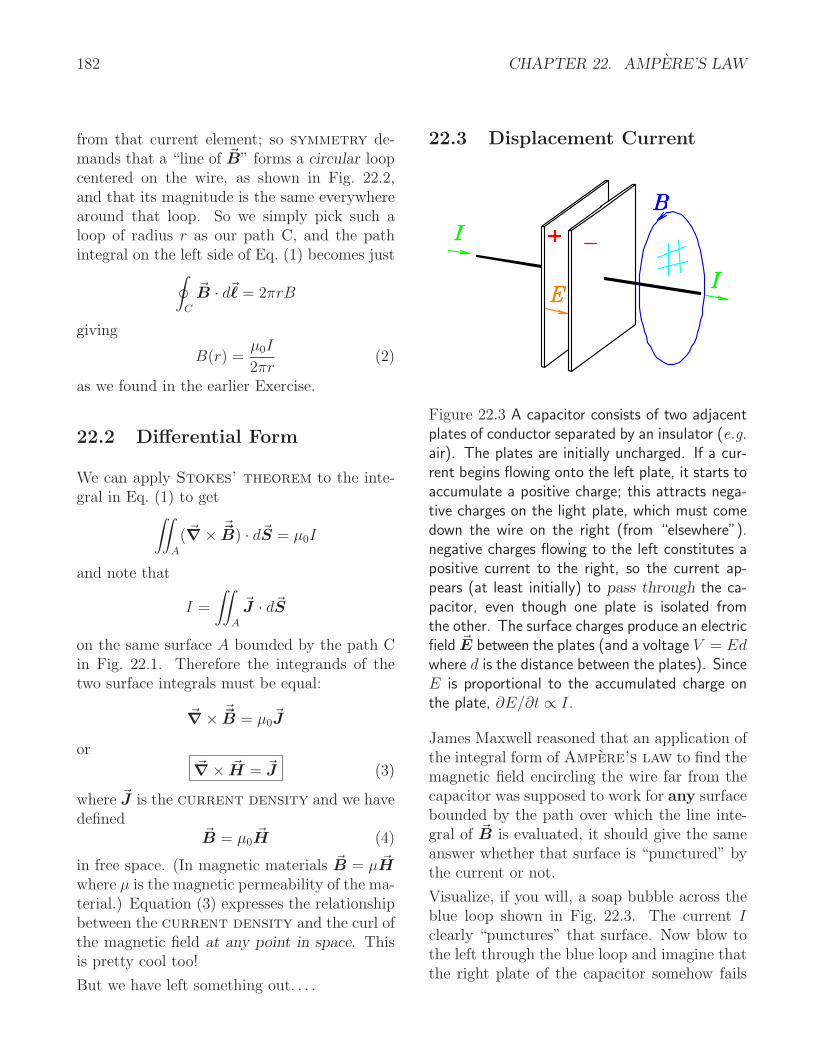
182 CHAPTER 22. AMPERE’S LAW
from that current element; so symmetry de-mands that a “line of ~B” forms a circular loopcentered on the wire, as shown in Fig. 22.2,and that its magnitude is the same everywherearound that loop. So we simply pick such aloop of radius r as our path C, and the pathintegral on the left side of Eq. (1) becomes just
∮
C
~B · d~ℓ = 2πrB
giving
B(r) =µ0I
2πr(2)
as we found in the earlier Exercise.
22.2 Differential Form
We can apply Stokes’ theorem to the inte-gral in Eq. (1) to get
∫∫
A
( ~∇ × ~~B) · d~S = µ0I
and note that
I =
∫∫
A
~J · d~S
on the same surface A bounded by the path Cin Fig. 22.1. Therefore the integrands of thetwo surface integrals must be equal:
~∇ × ~~B = µ0~J
or~∇ × ~H = ~J (3)
where ~J is the current density and we havedefined
~B = µ0~H (4)
in free space. (In magnetic materials ~B = µ ~Hwhere µ is the magnetic permeability of the ma-terial.) Equation (3) expresses the relationshipbetween the current density and the curl ofthe magnetic field at any point in space. Thisis pretty cool too!
But we have left something out. . . .
22.3 Displacement Current
Figure 22.3 A capacitor consists of two adjacentplates of conductor separated by an insulator (e.g.air). The plates are initially uncharged. If a cur-rent begins flowing onto the left plate, it starts toaccumulate a positive charge; this attracts nega-tive charges on the light plate, which must comedown the wire on the right (from “elsewhere”).negative charges flowing to the left constitutes apositive current to the right, so the current ap-pears (at least initially) to pass through the ca-pacitor, even though one plate is isolated fromthe other. The surface charges produce an electricfield ~E between the plates (and a voltage V = Edwhere d is the distance between the plates). SinceE is proportional to the accumulated charge onthe plate, ∂E/∂t ∝ I.
James Maxwell reasoned that an application ofthe integral form of Ampere’s law to find themagnetic field encircling the wire far from thecapacitor was supposed to work for any surfacebounded by the path over which the line inte-gral of ~B is evaluated, it should give the sameanswer whether that surface is “punctured” bythe current or not.
Visualize, if you will, a soap bubble across theblue loop shown in Fig. 22.3. The current Iclearly “punctures” that surface. Now blow tothe left through the blue loop and imagine thatthe right plate of the capacitor somehow fails

22.3. DISPLACEMENT CURRENT 183
to pop the resultant bubble, so that the surfacebounded by the blue loop now passes betweenthe capacitor plates, where there are no movingcharges. What gives?
Let’s review the electric field between two ca-pacitor plates: By Gauss’ law it’s constant farfrom the edges, points from the + plate to the− plate, and has a magnitude E = σ/ǫ0, whereσ = Q/A (the charge on one plate divided bythe area of the plate). Thus ǫ0E = D = Q/Aand taking the time derivative gives
A · ∂D
∂t=
∂Q
∂t≡ I.
But since ~D is constant over the area A andzero outside the capacitor, we can write this as
∫∫
A
∂ ~D
∂t· d~S = I.
That is, a changing electric field is equivalentto an actual current.
Maxwell called this surface integral of thechanging electric field a displacement cur-
rent after the name of ~D (the “electric dis-placement”). It turns out (with a little morerigorous derivation) to hold equally well for lesssimple geometries, giving us Maxwell’s ex-
tension of Ampere’s law,
∮
C
~H · d~ℓ =
∫∫
A
(
~J +∂ ~D
∂t
)
· d~S. (5)
which is equivalent to the differential version,
~∇ × ~H = ~J +∂ ~D
∂t(6)

184 CHAPTER 22. AMPERE’S LAW

23.1. GAUSS’ LAW 185
Chapter 23
Maxwell’s Equations
In 1860, while Americans were waging a bloodycivil war, a “thorough old Scotch laird” (thenonly 29) named James Clerk Maxwell was as-sembling the known laws of electromagnetisminto a compact and elegant form that was tolead, a year later, to the discovery that light isin fact a propagating disturbance in the elec-tromagnetic fields. That discovery was laterto overturn all the conceptual foundations ofclassical Physics and leave “common sense” inmuch the same condition as the United Statesafter the Civil War. It was hard times allaround, but exciting. . . .
23.1 Gauss’ Law
By now you are familiar with Gauss’ law inits integral form,
ǫ
∫∫
S© ~E · d~A = Qencl (1)
where Qencl is the electric charge enclosedwithin the closed surface S. Except for the“fudge factor” ǫ, which is just there to makethe units come out right, Gauss’ law is just asimple statement that electric field “lines” arecontinuous except when they start or stop onelectric charges. In the absence of “sources”(positive charges) or “sinks” (negative charges),electric field lines obey the simple rule, “Whatgoes in must come out.” This is what Gauss’
law says.
There is also a Gauss’ law for the magneticfield ~B; we can write it the same way,
(some constant)
∫∫
S© ~B · d~A = QMagn (2)
where in this case QMagn refers to the enclosedmagnetic charges, of which (so far) none haveever been found! So Gauss’ law for mag-
netism is usually written with a zero on theright-hand side of the equation, even though noone is very happy with this lack of symmetrybetween the electric and magnetic versions.
Figure 23.1 An infinitesimal volume of space.
Suppose now we apply Gauss’ law to a smallrectangular region of space where the z axis ischosen to be in the direction of the electric field,as shown in Fig. 23.1.1 The flux of electric field
1This Figure is very similar to the one used to derivethe equation of continuity, which in fact expresses thesame basic principles (conservation of some “stuff” producedlocally), although it is generally used for different purposes.

186 CHAPTER 23. MAXWELL’S EQUATIONS
into this volume at the bottom is Ez(z) dx dy.The flux out at the top is Ez(z + dz) dx dy; sothe net flux out is just [Ez(z+dz)−Ez(z)] dx dy.The definition of the derivative of E with re-spect to z gives us [Ez(z + dz) − Ez(z)] =(∂Ez/∂z) dz where the partial derivative is usedin acknowledgement of the possibility that Ez
may also vary with x and/or y. Gauss’ law
then reads ǫ(∂Ez/∂z) dx dy dz = Qencl. Whatis Qencl? Well, in such a small region there issome approximately constant charge density ρ(charge per unit volume) and the volume of thisregion is dV = dx dy dz, so Gauss’ law readsǫ(∂Ez/∂z) dV = ρ dV or just ǫ ∂Ez/∂z = ρ.If we now allow for the possibility of electric fluxentering and exiting through the other faces(i.e. ~E may also have x and/or y components),perfectly analogous arguments hold for thosecomponents, with the resultant “outflow-ness”given by
∂Ex
∂x+
∂Ey
∂y+
∂Ez
∂z= ~∇ · ~E ≡ div ~E
where the gradient operator ~∇ is shown in itscartesian representation (in rectangular coordi-nates x, y, z). It has completely equivalent rep-resentations in other coordinate systems suchas spherical (r, θ, φ) or cylindrical coordinates,but for illustration purposes the cartesian coor-dinates are simplest.
We are now ready to write Gauss’ law in itscompact differential form,
ǫ ~∇ · ~E = ρ (3)
and for the magnetic field, assuming no mag-netic charges (monopoles),
~∇ · ~B = 0 (4)
These are the first two of Maxwell’s equa-
tions.
23.2 Faraday’s Law
You should now be familiar with the long inte-gral mathematical form of Faraday’s Law ofmagnetic induction: in SI units,
∮
C~E · d~ℓ = − ∂
∂t
∫∫
S~B · d~S (5)
where the line integral of ~E around the closedloop C is (by definition) the induced EMFaround the loop and the right hand side refersto the rate of change of the magnetic fluxthrough the area S bounded by that closedloop.
Figure 23.2 Another infinitesimal volume ofspace.
To make this easy to visualize, let’s again drawan infinitesimal rectangular box with the z axisalong the direction of the magnetic field, whichcan be considered more or less uniform oversuch a small region. Then the flux through the“Faraday loop” is just Bz dx dy and the line in-tegral of the electric field is
Ex(y)dx+Ey(x+dx)dy−Ex(y+dy)dx−Ey(x)dy.
(Yes it is. Study the diagram!) Here, asbefore, Ey(x + dx) denotes the magnitude of
the y component of ~E along the front edgeof the box, and so on. As before, we notethat [Ey(x + dx) − Ey(x)] = (∂Ey/∂x) dx and

23.4. MAXWELL’S EQUATIONS 187
[Ex(y + dy) − Ex(y)] = (∂Ex/∂y) dy so thatFaraday’s law reads(
∂Ey
∂xdx
)
dy−(
∂Ex
∂ydy
)
dx = −(
∂Bz
∂t
)
dx dy
which reduces to the local relationship
(
∂Ey
∂x− ∂Ex
∂y
)
= −(
∂Bz
∂t
)
between the “swirlyness” of the spatial depen-dence of the electric field and the rate of changeof the magnetic field with time.
If you have studied the definition of the curl ofa vector field, you may recognize the left-handside of the last equation as the z component of
curl ~E ≡ ~∇ × ~E
≡ ı
(
∂Ez
∂y− ∂Ey
∂z
)
+
(
∂Ex
∂z− ∂Ez
∂x
)
+ k
(
∂Ey
∂x− ∂Ex
∂y
)
.
The x and y components of curl ~E are relatedto the corresponding components of ∂ ~B/∂t inexactly the same way, allowing us to writeFaraday’s law in a differential form whichdescribes part of the behaviour of electric andmagnetic fields at every point in space:
~∇ × ~E = −∂ ~B
∂t(6)
This says, in essence, that any change in themagnetic field with time induces an electricfield perpendicular to the changing magneticfield. Hold that thought.
23.3 Ampere’s Law
You are probably also adept at using the trickdeveloped by Henri Ampere for calculating the
magnetic field ( ~H ≡ ~B/µ) due to various sym-metrical arrangements of electric current (I).In its integral form and SI units, Ampere’s
law reads∮
C~H · d~ℓ = I +
∂
∂t
∫∫
S~D · d~S (7)
where Maxwell’s “displacement current”associated with a time-varying electric displace-ment ~D ≡ ǫ~E has been included. This equa-tion says (sort of), “The circulation of the mag-netic field around a closed loop is equal to aconstant times the total electric current link-ing that loop, except when there is a changingelectric field in the same region.”
As you know, this “Law” is used with vari-ous symmetry arguments to “finesse” the eval-uation of magnetic fields due to arrangementsof electric currents, much as Gauss’ law wasused to calculate electric fields due to differ-ent arrangements of electric charges. Skippingover the details, let me draw your attention tothe formal similarity to Faraday’s law andstate (this time without showing the derivation)that there is an analogous differential form ofAmpere’s law describing the behaviour of thefields at any point in space:
~∇ × ~H = ~J +∂ ~D
∂t(8)
If we ignore the current density ~J then thisequation says (sort of), “A changing electricfield generates a magnetic field at right an-gles to it,” which is rather reminiscent of whatFaraday’s law said.
Now we’re getting somewhere.
23.4 Maxwell’s Equations
In 1865, James Clerk Maxwell assembled allthe known “Laws” of E&M in their most com-pact, elegant (differential) form, shown here inSI units:

188 CHAPTER 23. MAXWELL’S EQUATIONS
Gauss’ Law for Electrostatics:
~∇ · ~D = ρ (9)
Gauss’ Law for Magnetostatics:
~∇ · ~B = 0 (10)
Faraday’s Law:
~∇ × ~E +∂ ~B
∂t= 0 (11)
Ampere’s Law:
~∇ × ~H − ∂ ~D
∂t= ~J (12)
These four basic equations are known collec-tively as Maxwell’s equations; they areconsidered by most Physicists to be a beauti-fully concise summary of E&M phenomenol-ogy.
Well, actually, a complete description of E&Malso requires two additional laws:
Equation of Continuity:
∂ρ
∂t= − ~∇ · ~J (13)
Lorentz Force:
~F = q(
~E + ~v × ~B)
. (14)
23.5 The Wave Equation
The two “Laws” of electrodynamics —Faraday’s Law and Ampere’s Law — canbe combined to produce a very important re-sult.
First let’s simplify matters by considering thebehaviour of electromagnetic fields in emptyspace, where
ρ = 0, ~J = 0, ~D = ǫ ~E and ~B = µ ~H .
Our two equations then read
~∇ × ~E = −∂ ~B
∂tand
~∇ × ~B
µ= ǫ
∂ ~E
∂t.
We can simplify further by assuming that theelectric field is in the y direction and the mag-netic field is in the z direction. In that case,
∂E
∂x= −∂B
∂tand
∂B
∂x= −ǫµ
∂E
∂t
where the second equation has been multipliedthrough by µ.
If we now take the derivative of the first equa-tion with respect to x and derivative of the sec-ond equation with respect to t, we get
∂2E
∂x2= − ∂2B
∂x∂tand
∂2B
∂t∂x= −ǫµ
∂2E
∂2t.
Since∂2B
∂x∂t=
∂2B
∂t∂x,
the combination of these two equations yields
∂2E
∂x2= ǫµ
∂2E
∂2t
which the discerning reader will recognize asthe one-dimensional Wave Equation for E,
∂2E
∂x2− 1
c2
∂2E
∂2t= 0 (15)
where the propagation velocity is
c =1√ǫµ
. (16)
You can easily show that there is an identicalequation for B.
A more general derivation yields the 3-dimensional version,
∇2 ~E =1
c2
∂2 ~E
∂t2or ¤
2 ~E = 0 . (17)
In either form, this equation expresses the factthat, since a changing electric field generates amagnetic field but that change in the magneticfield generates, in turn, an electric field, and soon, we can conclude that electromagnetic fields

23.5. THE WAVE EQUATION 189
will propagate spontaneously through regionsof total vacuum in the form of a wave of ~E and~B fields working with/against each other.
This startling conclusion (in 1865) led to therevision of all the “classical” paradigms ofPhysics, even such fundamental concepts asspace and time.

190 CHAPTER 23. MAXWELL’S EQUATIONS

191
Chapter 24
A Short History of Atoms
An accurate historical account of the develop-ment of Atomic Physics is probably the mosthopeless task in the History of Science disci-pline. The story began, almost certainly, beforethe dawn of recorded history. Written recordsfrom Western antiquity date from as early as450 BC, when the Greek Leucippus proposedthat all matter was composed of ατoµs, i.e.
miniscule indestructible subunits of which thereare only a few basic species. This view waspicked up by Leucippus’ student, Democritos ofAbdera, some 50 years later and popularized byEpicurus of Samos around 300 BC, who devel-oped the “Atomist” philosophical system thatwas epitomized by the Roman philosopher andpoet Titus Lucretius Carus in about 60 BC.
Meanwhile, in 335 BC Aristotle countered withthe proposition that matter was not grainy (aswould seem to be required by the Atomist view)but smoothly continuous and composed of fourbasic elements, also continuous: earth, air,
fire and water. This picture gained pop-ularity around 300 BC under Zeno of Cition,founder of the Stoics.
Thus the battle lines between a “bricks andmortar” view of matter and a “continuous”image of space, time and substance had beendrawn well before the birth of Jesus; it tookuntil the Twentieth Century to find the syn-thesis that allowed these two pictures (both ofwhich, incidentally, are correct) to coexist inpeace, though perhaps at the expense of whatonce passed for common sense.
Probably one key paradigm was Newton’s cal-
culus, which taught everyone to understandcontinuous mathematical behaviour in termsof discrete “differentials” whose intervalswere allowed to go to zero. Thus by the Nin-teenth Century all scientists and mathemati-cians were intimately familiar with this trickfor making the smooth look grainy and vice
versa. The psychological stage was set for a newphysical paradigm that reconciled Democritus’Atomism with Aristotle’s Elements.
There was also an enormous amount of workdone in the Middle Ages on determining ex-actly which ordinary household materials weretrue elements and which were combinationsof several elements — what we now call chem-
ical compounds. This was the work of untoldnumbers of Alchemists, most of whose workwas done in secret for fear of persecution bythose who considered such matters to be noneof Humanity’s business. Nevertheless, by theturn of the Nineteenth Century, a great manytrue elements had been correctly identifiedand some regularities had begun to appear.
The next difficulty with the History of AtomicPhysics is that a lot of it is Chemistry. Even af-ter Alchemy became respectable under the newname of Chemistry, a certain mutual disdainwas cherished between Physicists and Chemists— which unfortunately lives on to this day —and consequently the History of Atomism readsa little differently in the Chemistry textbooksfrom the Physics version. Both are equally le-

192 CHAPTER 24. A SHORT HISTORY OF ATOMS
gitimate, of course, but since History is sub-ject to politics and revisionism, one must al-ways read any account with a certain healthyskepticism.
I will therefore make no claim that my accountis fair, or even historically accurate; rather, mygoal will be to show how the ideas might havedeveloped in a perfectly logical sequence, us-ing the powerful optics of hindsight. If you arestimulated by this “fake history” to go learnfor yourself what really happened, then I willconsider my goal achieved.
24.1 Modern Atomism
Most Physicists (and all Chemists) will prob-ably agree that the crucial empirical obser-vations that set modern science on the trackof atoms (as we now know them) occurredaround the transition between the Eighteenthand Nineteenth Centuries when a number ofscientists including Antoine Laurent Lavoisier,Bryan and William Higgins, Joseph LouisProust, John Dalton and Joseph Louis Gay-Lussac1 discovered that certain chemical agentscombined in simple integer ratios of their“molecular weights” with other agents, aphenomenon most easily explained by assum-ing that these agents were the true chemical el-ements sought by the Alchemists2 and further-more that one molecular weight of any el-
ement contained the same number of atoms
of that element! This specific hypothesis iscredited to Lorenzo Romano Amadeo Avoga-rdo who in 1811 made a clear distinction be-tween atoms (irreducible chemical units) andmolecules, which are clumps of atoms. Forhis trouble he got Avogadro’s number N0
named after him. The actual number of atoms1As you might guess, the details of the history of these
discoveries also tend to vary with the nationality of the His-torian!
2The Alchemists were already pretty certain of many ofthese, of course; but they were accustomed to keeping theirmouths shut.
(or, for that matter, molecules) in one molec-
ular weight (or mole) of the correspondingelement is
N0 ≡ 6.02205 × 10²³molecules per mole. (1)
You may recognize this number from the Chap-ter on Thermal Physics, in particular theSection on the Kinetic Theory of Gases,the qualitative assumptions of which datedback as far as Robert Boyle, Robert Hooke andIsaac Newton himself in the late SeventeenthCentury. The work of Daniel Bernoulli in1738 foreshadowed the use of kinetic theory byJoseph Loschmidt in 1865 to make the first de-termination of the value of N0 from measure-ments of the actual behaviour of gases. Sta-
tistical Mechanics actually played a majorrole in the development of modern Atomic the-ory, but its role is often downplayed in historicalaccounts simply because its is harder to under-stand. I will probably do likewise — but atleast I admit it!
24.2 What are Atoms Made of?
By the end of the Nineteenth Century [I amleaving out a lot here!] most scientists were con-vinced that atoms were “real” (as opposed toa mere calculational aid or a handy mnemonicparadigm) and were looking for ways to deter-mine their true structure.
24.2.1 Thomson’s Electron and e/m
It was found that negatively charged particlescalled “cathode rays” could be coaxed out ofa hot metal filament by a large enough electricpotential and accelerated to hit a screen coveredwith phosphorescent material where they madea bright spot [the forerunner of today’s cathodray tubes or CRT’s], but until 1897 no one knewmuch about the properties of these particles. Inthat year Joseph John Thomson used magnetic

24.2. WHAT ARE ATOMS MADE OF? 193
deflection (the Lorentz force) to determinethe charge-to-mass ratio q/m of the cathoderays.3 He found an astonishingly large negativeratio: q/m = −1.76 × 10¹¹ coulombs/kg, in-dicating that the electron (as the “cathoderay” particle soon came to be known) must be avery light particle (mass me) with a very largeelectric charge (q = −e) where the “electroniccharge” e was thought until recently to be thequantum of electric charge — i.e. the irre-ducible minimum nonzero quantity of electriccharge, in integer multiples of which all largercharges must come.4
24.2.2 Milliken’s Oil Drops and e
Of course, this result revealed nothing about ei-ther e or me, just their ratio. But the abso-lute magnitude of e was determined ten yearslater by Robert A. Millikan, who watched tinydroplets of mineral oil through a microscope:the spherical oil drops, created with an ordi-nary atomizer (no pun intended), fell throughstill air in the Earth’s gravity at a terminalvelocity determined by their weight and thefrictional drag of the air, both of which canbe calculated from their radius. Now, everyonce in a while one of the drops would pick upa stray electron and become charged. If theexperiment was performed in a vertical elec-tric field of adjustable strength, the chargeddroplets could be made to “hover” by applyingjust the right voltage to overcome the force ofgravity. Then, knowing the electric field, Mil-likan was able to calculate the charge.5 The
3Such a device (for measuring the charge-to-mass ratioof electrically charged particles) is known as a magnetic
spectrometer. Thomson’s version was pretty crude bytoday’s standards, but this is still the most accurate methodfor measuring the q/m ratio of particles (and hence, if weknow their charge by some other means, their mass).
4This is really the original prototype example of a quan-
tized property. Many others were to follow, as we shallsee.
5Naturally, sometimes he got two or three electrons ona drop; but this was simple enough to take into account:sometimes he got a result of e, sometimes he got a result
result was e ≈ 1.6 × 10⁻¹⁹ C, which meantthat the mass of the electron must be reallysmall, namely me ≈ 9.1 × 10⁻³¹ kg.
24.2.3 “Plum Puddings” vs. Rutherford
The discovery of that the electron was suchan incredibly lightweight particle with such ahuge charge made it perfectly clear that anatom must be something like a “plum pud-ding” — a homogeneous, featureless matrix ofpositive charge (carrying most of the mass)with the electrons embedded in it like raisins.Otherwise the electrons were apt to be mov-ing, and this was unthinkable! If they were inmotion but stayed inside the atom, then theymust be continually changing direction. Thatmeans they must be accelerated, and by thattime everyone understood only too well that
accelerated charges radiate!
Specifically, an accelerated charge (especiallyone with such a large charge-to-mass ratio)must always radiate away energy in the formof electromagnetic waves — it is a sort of an-tenna — and so the normal quiescence of mat-ter “proves” that the electrons must be at restin their atoms; this can only be so if theyare “stuck” in a “plum pudding” of positivecharge.6
In about 1910 a new type of “radioactivity”was discovered: certain nuclei spontaneouslyemit “α rays” which were shown to have aq/m ratio nearly 4000 times smaller than elec-trons and where therefore much heavier par-ticles. Soon afterwards, Ernest Rutherford setout to demonstrate the correctness of the “plum
of 2e, sometimes he got a result of 3e, but he never got aresult of 1
2e, for instance, so it was clear which result was
the true charge quantum.6This is truly an unavoidable conclusion if we accept the
theory of classical electrodynamics at face value; it was notjust a misinterpretation. You may be sure that hordes ofPhysicists looked high and low for a way out of this andfound none.

194 CHAPTER 24. A SHORT HISTORY OF ATOMS
pudding” model of atoms by scattering theseα particles off gold atoms comprising a thingold foil.
The picture is analogous to firing cannon ballsat great slabs of gelatin in which are embeddedmany small marbles. The cannon balls will losea lot of energy going through the gelatin walls,but they certainly won’t change their directionof motion much.
To Rutherford’s astonishment, most of the αparticles passed right through the target foilwithout being deflected or losing much energy— indicating that what seemed to be “solid”metal was actually composed mainly of sheervacuum. Even more alarmingly, some of the αparticles bounced backward off the gold atoms— indicating that the mass of the gold atomwas almost all concentrated in a tiny hard ker-nel of positive charge some 10,000 to 100,000times smaller than the size of the atoms them-selves!
As Rutherford himself put it, “It is like firingshells at a piece of paper handkerchief and hav-ing them bounce back at you.”
Scattering Cross Sections
Inasmuch as we are going to discuss modernelementary particle physics later on, it isappropriate to stop for a moment and contem-plate Rutherford’s classic experiment, for theart of interpreting the distributions of scat-
tering angles when a beam of one typeof particle in a well-defined initial state isslammed into a target composed of other typesof particles is essentially the entire experimen-tal repertoire of the modern Particle Physicist.
Consider: the goal of the experimenter is tolearn more about the structure of particles thatare, individually, too small to be detected witha microscope. [If the particle is much smaller insize than the wavelength λ of the light used inthe microscope, the best it can do is scatter the
light into spherical outgoing wavefronts (Huy-
gens’ Principle), from which we can learnnothing about the shape of the particle itself.The approved terminology for this limitationis that the resolution of the microscope cannever be finer than the wavelength of the light ituses.] So how can we learn anything about theshape of the object particle? By scattering
other particles off it!
Imagine that there is an object hidden fromsight behind a thin piece of paper; you havea BB gun which you can use to bounce BBsoff the object. You get to to see which waythe BBs bounce, and if you have a more fancyapparatus you may get to measure their veloci-ties (momenta) before and after their collisionswith the object; moreover, if any bits fly off theobject as a result of a BB collision, you get tomeasure their directions and momenta as well.This is essentially the situation of the ParticlePhysicist. We may have a variety of particle
beams ranging from electrons to heavy nuclei,with energies ranging from a few eV to manyGeV (billions of eV) or even TeV (trillions ofeV) per particle — corresponding to peashoot-ers, BB guns, rifles, howitzers and rail guns —but the only way we can use them is to shoot“blind” at our target particles and study thescattering distribution.
You should try to imagine for yourself somequalitative phenomena you might look for totest various hypotheses about the target object— starting with Rutherford’s test for “plumpuddings” vs. hard-kernel atomic nuclei. Iwill not attempt to develop the arcane termi-nology of scattering theory here, but I will men-tion the basic paradigm: the thing one can mea-sure and describe most easily about a particleis the area it presents to an incoming beam;we call this the scattering cross section
and measure it in area units such as barns [onebarn ≡ (10−13 cm)2 or 10−30 m2)] — about thesize of an average nucleus.7
7This humourous name for the size of a target may have

24.2. WHAT ARE ATOMS MADE OF? 195
24.2.4 A Short, Bright Life for Atoms
A new picture of the atom thus emerged, inwhich all the positive charge and virtually allthe mass was concentrated in a tiny nucleus
at the centre of the atom and the light, nega-tively charged electrons orbited about it atrather large distances, much like the Earth andother planets about the Sun. This is a com-pelling and pretty image, and there is no prob-lem calculating the orbital velocities of the elec-trons in the attractive central force of the nu-cleus.
The problem is, the accelerations of said elec-trons are enormous, causing them to radiateaway their energy as electromagnetic waves(light) and spiral down into the nucleus. Thelifetime of such an atom must be less thanabout 1 ns (or 10−9 seconds), during which timethe atom gives off a bright pulse of light. Then,nothing.
This doesn’t quite fit the data. Atoms are ap-parently quite stable and we are still here totalk about it, so there must be something wrongwith this picture. Naturally, armies of Physi-cists went to work trying to find fault with thelogic of classical electrodynamics, but there wasno way out; the predictions were too simple tobe mistaken. Something was seriously wrong.
marked the start of a trend toward “cute” nomenclature inParticle Physics, which manifested itself later in strangeness,quarks and (most recently) truth and beauty as particleproperties — the latter pair now being retracted in favour oftop and bottom, which I regard as a failure of nerve and willon the part of Particle Physicists. But that is yet anotherstory. . . .

196 CHAPTER 24. A SHORT HISTORY OF ATOMS
24.3 Timeline: “Modern” Physics
450-300 BC Greek Atomists: Leucippus, Democritos, Epicurus . . .
335 BC Aristotle: continuous elements (earth, air, fire, water)
300 BC Zeno of Cition (founder of Stoics) popularizes Aristotelian view.
60 BC Titus Lucretius Carus of Rome epitomizes “Atomist” philosophy....
1879 Josef Stefan [expt] power emitted as blackbody radiation P = AσT 4
1884 Ludwig Boltzmann [theor] explains Stefan’s empirical law
1885 Johann Jakob Balmer [expt]empirical description of line spectra emitted by H atoms
1890 Johannes Robert Rydberg [expt]
1893 Wilhelm Wien [expt] blackbody spectrum displacement law:peak wavelength varies as T −1
1895 Wilhelm Conrad Roentgen [expt] discovers X-rays
1897 Joseph John Thomson [expt] measures boldmath q/m of the electron
1900 Max Planck [theor] derives correct blackbody radiation spectrum
1902 Philipp E.A. von Lenard [expt] measures photoelectric effect
1905 Albert Einstein [theor] explains photoelectric effect
1905 Albert Einstein [theor] publishes Special Theory of Relativity (STR)
1905 Albert Einstein [theor] explains Brownian motion (gives mass of atoms!)
1905 Ernest Rutherford [expt] performs first alpha-scattering experiments at McGill Univ.(Canada)
1907 Robert A. Milliken [expt] measures electron charge (now know both qe and me).
1912 William (H. & L.) Bragg [expt] shows that X-rays scatter off crystal lattices
1913 Hans Geiger & Ernest Marsden [expt] confirm Rutherford scattering results at Univ. ofManchester (U.K.)
1913 Niels Henrik David Bohr [theor] pictures H atom with quantized angular momentum

24.3. TIMELINE: “MODERN” PHYSICS 197
1916 Albert Einstein [theor] publishes General Theory of Relativity (GTR)
1916 Robert Andrews Milliken [expt] confirms photoelectric effect in detail
1922 Arthur Holly Compton [expt] scatters X-rays off electrons
1924 Louis Victor de Broglie [theor] hypothesizes “matter waves” with λ = h/p
1925 Wolfgang Pauli [theor] formulates his exclusion principle
1925 Max Born & Werner Heisenberg [theor] introduce quantum mechanics
1926 Erwin Schroedinger [theor] develops a nonrelativistic wave equation for quantum me-chanics
1927 Werner Heisenberg [theor] formulates his uncertainty principle
1928 Paul A.M. Dirac [theor] develops a relativistic wave equation for electronsand predicts antimatter...

198 CHAPTER 24. A SHORT HISTORY OF ATOMS
24.4 Some Quotations
Lord Rutherford, 1931:
“When we consider the life work of Faradayit is clear that his researches were guided andinspired by the strong belief that the variousforces of nature were inter-related and depen-dent on one another. It is not too much tosay that this philosophic conviction gave theimpulse and driving power in most of his re-searches and is the key to his extraordinary suc-cess in adding to knowledge.
“The more we study the work of Faraday withthe perspective of time, the more we are im-pressed by his unrivalled genius as an experi-menter and natural philosopher. When we con-sider the magnitude and extent of his discover-ies and their influence on the progress of scienceand industry, there is no honor too great to payto the memory of Michael Faraday — one of thegreatest scientific discoverers of all time.”
Maxwell:
“As I proceeded with the study of Faraday,I perceived that his method of conceivingthe phenomena was also a mathematical one,though not exhibited in the conventional formof mathematical symbols. I also found thatthese methods were capable of being expressedin the ordinary mathematical form, and thuscompared with those of the professed mathe-maticians.” — Treatise on Electricity and Mag-
netism, 1873
Faraday:
“When a mathematician engaged in investigat-ing physical actions and results has arrived athis conclusions, may they not be expressed incommon language as fully clearly and definitelyas in mathematical formulae? If so, would itnot be a great boon to such as I to expressthem so — translating them out of their hiero-glyphics that we also might work upon them byexperiment.” — letter to James Clerk Maxwell
Maxwell:
“I was aware that there was supposed to be adifference between Faraday’s way of conceivingphenomena and that of the mathematicians, sothat neither he nor they were satisfied with eachother’s language. I had also the conviction thatthis discrepancy did not arise from either partybeing wrong. I was first convinced of this by SirWilliam Thomson, to whose advice and assis-tance, as well as to his published papers, I owemost of what I have learned on the subject.” —Treatise on Electricity and Magnetism, 1873
Maxwell:
“. . . we have strong reason to conclude thatlight itself — including radiant heat, and otherradiations if any — is an electromagnetic dis-turbance in the form of waves propagatedthrough the electromagnetic field according toelectromagnetic laws.” — Dynamical Theory of
the Electromagnetic Field, 1864
Einstein:
“The greatest alteration in the axiomatic basisof physics — in our conception of the struc-ture of reality — since the foundation of the-oretical physics by Newton, originated in theresearches of Faraday and Maxwell on electro-magnetic phenomena.”
Boltzmann:
“Available energy is the main object at stake inthe struggle for existence and the evolution ofthe world.” [in D’A. W. Thompson, On Growth
and Form (Cambridge 1917).]
“The most ordinary things are to philosophya source of insoluble puzzles. With infiniteingenuity it constructs a concept of space ortime and then finds it absolutely impossiblethat there be objects in this space or that pro-cesses occur during this time . . . the source ofthis kind of logic lies in excessive confidence inthe so-called laws of thought.” [in B. McGuin-ness, Ludwig Boltzmann, Theoretical Physics
and Philosophical Problems, (Dordrecht, 1974)64.]
“To go straight to the deepest depth, I went for

24.4. SOME QUOTATIONS 199
Hegel; what unclear thoughtless flow of words Iwas to find there! My unlucky star led me fromHegel to Schopenhauer. . . . Even in Kant therewere many things that I could grasp so littlethat given his general acuity of mind I almostsuspected that he was pulling the reader’s legor was even an imposter.” [in D. Flamm. Stud.
Hist. Phil. Sci. 14 (1983) 257.]
“One should not imagine that two gases in a0.1 liter container, initially unmixed, will mix,then again after a few days separate, then mixagain, and so forth. On the contrary, one finds. . . that not until a time enormously long com-pared to 101010
years will there be any notice-able unmixing of the gases. One may recognizethat this is practically equivalent to never. . . .”
Einstein:
“A theory is the more impressive the greaterthe simplicity of its premises, the more differ-ent kinds of things it relates, and the more ex-tended its area of applicability. Therefore thedeep impression that classical thermodynamicsmade upon me. It is the only physical theoryof universal content which I am convinced willnever be overthrown, within the framework ofapplicability of its basic concepts.”
Planck:
“The general connection between energy andtemperature may only be established by proba-bility considerations. [Two systems] are in sta-tistical equilibrium when a transfer of energydoes not increase the probability.”
Thomson: [toast]
“To the electron: may it never be of any use!”
Niels Bohr:
“Evidence obtained under different experimen-tal conditions cannot be comprehended withina single picture, but must be regarded as com-plementary in the sense that only the totalityof the phenomena exhausts the possible infor-mation about the objects.”
“Notwithstanding the fundamental departure
from the ideas of the classical theories of me-chanics and electrodynamics involved in thesepostulates, it has been possible to trace a con-nection between the radiation emitted by theatom and the motion of the particles which ex-hibits a far-reaching analogy to that claimed bythe classical ideas of the origin of radiation.”
H.B.G. Casimir:
“Even Bohr, who concentrated more intenselyand had more staying power than any of us,looked for relaxation in crossword puzzles, insports, and in facetious discussions.”
Rutherford:
“Bohr’s different [from other Continental theo-rists] — he’s a football player!”
Pauli: [writing about his days as a student atMunich]
“I was not spared the shock which every physi-cist accustomed to the classical way of thinkingexperienced when he came to know Niels Bohr’sbasic postulate of quantum theory for the firsttime.”
Heisenberg:
“I learned optimism from Sommerfeld, mathe-matics at Gottingen, and physics from Bohr.”
Louis de Broglie:
“Two seemingly incompatible conceptions caneach represent an aspect of the truth. . . . Theymay serve in turn to represent the facts withoutever entering into direct conflict.” — Dialectica
“As in my conversations with my brother wealways arrived at the conclusion that in thecase of x-rays one had both waves and corpus-cles, thus suddenly — . . . it was certain in thecourse of summer 1923 — I got the idea thatone had to extend this duality to material parti-cles, especially to electrons. And I realised that,on the one hand, the Hamilton-Jacobi theorypointed somewhat in that direction, for it canbe applied to particles and, in addition, it repre-sents a geometrical optics; on the other hand,in quantum phenomena one obtains quantum

200 CHAPTER 24. A SHORT HISTORY OF ATOMS
numbers, which are rarely found in mechanicsbut occur very frequently in wave phenomenaand in all problems dealing with wave motion.”— from an interview in 1963
De Broglie described himself as “. . . havingmuch more the state of mind of a pure theoreti-cian than that of an experimenter or engineer,loving especially the general and philosophicalview. . . .”
“. . . the statistical theories hide a completelydetermined and ascertainable reality behindvariables which elude our experimental tech-niques.”
Einstein: [after reading Pauli’s article on rela-tivity]
“Whoever studies this mature and grandly con-ceived work might not believe that its author isa twenty-one year old man.”
Wolfgang Pauli:
“. . . a new phase of my scientific life began whenI first met Niels Bohr personally for the firsttime. During these meetings, Bohr asked mewhether I could come to Copenhagen for ayear.”
“The fact that the author thinks slowly is notserious, but the fact that he publishes fasterthan he thinks is inexcusable.”
“This paper is so bad it is not even wrong.” —Quoted in D. MacHale, Comic Sections (Dublin1993)
“I refuse to believe that God is a weak left-hander.”
Max Born:
“I am now convinced that theoretical physics isactual philosophy.” — Autobiography
“If God has made the world a perfect mecha-nism, He has at least conceded so much to ourimperfect intellect that in order to predict littleparts of it, we need not solve innumerable dif-ferential equations, but can use dice with fairsucess.” — Quoted in H.R. Pagels, The Cosmic
Code
“The difficulty involved in the proper and ad-equate means of describing changes in contin-uous deformable bodies is the method of dif-ferential equations. . . . They express math-ematically the physical concept of contiguousaction.” — Einstein’s Theory of Relativity
One of his research students described Born’sdays in Edinburgh: “When Born arrived in themorning he first used to make the round of hisresearch students, asking them whether theyhad any progress to report, and giving themadvice, sometimes presenting them with sheetsof elaborate calculations concerning their prob-lems which he had himself done the day before.. . . The rest of the morning was spent by Bornin delivering his lectures to undergraduate hon-ours students, attending to departmental busi-ness, and doing research work of his own. Mostof the latter, however, he used to carry out athome in the afternoons and evenings.”
(Born develops a nonrelativistic wave equa-tion for the electron in quantum mechan-ics.)
Erwin Rudolf Josef Alexander Schrodinger:[about his time at the Akademisches Gymna-sium in 1898]
“I was a good student in all subjects, lovedmathematics and physics, but also the strictlogic of the ancient grammars, hated only mem-orising incidental dates and facts. Of the Ger-man poets, I loved especially the dramatists,but hated the pedantic dissection of this work.”
“Especially in physics and mathematics,Schrodinger had a gift for understanding thatallowed him, without any homework, immedi-ately and directly to comprehend all the mate-rial during the class hours and to apply it. Af-ter the lecture . . . it was possible for [our pro-fessor] to call Schrodinger immediately to theblackboard and to set him problems, which hesolved with playful facility.” — from a student
in Schrdinger’s class at school
“A few days ago I read with great interest the

24.4. SOME QUOTATIONS 201
ingenious thesis of Louis de Broglie, which Ifinally got hold of. . . ” — letter to Einstein, 3
November 1925
“I have been intensely concerned these dayswith Louis de Broglie’s ingenious theory. It isextraordinarily exciting, but still has some verygrave difficulties.” — a different letter on 16
November 1925
“To each function of the position- andmomentum-coordinates in wave mechanicsthere may be related a matrix in such a waythat these matrices, in every case satisfy theformal calculation rules of Born and Heisen-berg. . . . The solution of the natural boundaryvalue problem of this differential equation inwave mechanics is completely equivalent to thesolution of Heisenberg’s algebraic problem.” —1926 paper
Werner Karl Heisenberg:
“To those of us who participated in the devel-opment of atomic theory, the five years follow-ing the Solvay Conference in Brussels in 1927looked so wonderful that we often spoke of themas the golden age of atomic physics. The greatobstacles that had occupied all our efforts inthe preceding years had been cleared out of theway; the gate to an entirely new field, the quan-tum mechanics of the atomic shells stood wideopen, and fresh fruits seemed ready for the pick-ing.”
“An expert is someone who knows some of theworst mistakes that can be made in his sub-ject, and how to avoid them.” — Physics and
Beyond (New York 1971)
Paul Adrien Maurice Dirac:
“I think that there is a moral to this story,namely that it is more important to havebeauty in one’s equations than to have themfit experiment. If Schroedinger had been moreconfident of his work, he could have publishedit some months earlier, and he could have pub-lished a more accurate equation. It seems thatif one is working from the point of view of get-
ting beauty in one’s equations, and if one hasreally a sound insight, one is on a sure line ofprogress. If there is not complete agreementbetween the results of one’s work and experi-ment, one should not allow oneself to be toodiscouraged, because the discrepancy may wellbe due to minor features that are not properlytaken into account and that will get cleared upwith further development of the theory.” — inScientific American, May 1963.
“Mathematics is the tool specially suited fordealing with abstract concepts of any kind andthere is no limit to its power in this field.” —Quoted in P.J. Davis and R. Hersh, The Math-
ematical Experience (Boston 1981)
“In science one tries to tell people, in such away as to be understood by everyone, some-thing that no one ever knew before. But inpoetry, it’s the exact opposite.” — Quoted inH. Eves, Mathematical Circles Adieu (Boston1977)
“I learned to distrust all physical concepts asthe basis for a theory. Instead one should putone’s trust in a mathematical scheme, even ifthe scheme does not appear at first sight to beconnected with physics. One should concen-trate on getting interesting mathematics.”
“Now when Heisenberg noticed that, he was re-ally scared.” — Quoted in D. MacHale, Comic
Sections (Dublin 1993)
“I consider that I understand an equation whenI can predict the properties of its solutions,without actually solving it.” — Quoted inF. Wilczek & B. Devine, Longing for the Har-
monies
“This result is too beautiful to be false.” —‘The evolution of the Physicist’s Picture of Na-ture’, Scientific American 208, 5 (1963)
202 CHAPTER 24. A SHORT HISTORY OF ATOMS
24.5 SKIT:
“The Dreams Stuff is Made Of”
Salviati: “That’s all very well and good, butthere is a problem. Actually there are severalproblems with Maxwell’s theory of electrody-namics and light. First off, the equations de-scribe a propagating electromagnetic wave, butthey don’t mention what it is propagating in,and for that reason they don’t specify what itis propagating relative to.”
Simplicio: “What does that matter?”
Salviati: “Simplicio, you idiot, if the wavepropagates past me at the velocity c predictedby Maxwell’s electrodynamics, but you aremoving relative to me at some large velocity,then the wave obviously can’t be moving pastyou at that same c. But the equations say itis!”
Simplicio: “So the equations must be wrong,right?”
Salviati: “No, the equations are right. Com-mon sense is wrong.”
Sagredo: “What?!”
Salviati: “Never mind, that’s Relativity. Wehave enough of a problem trying to makesense of the other unambiguous prediction ofMaxwell’s equations: that any time a charge isaccelerated, it radiates away energy in the formof electromagnetic waves.”
Sagredo: “So what’s the problem with that?Isn’t that how antennas make radio waves?”
Salviati: “Yes, but it’s also why any atom con-sisting of a negatively charged electron orbitingaround a heavy, positively charged nucleus willfall into it within about a billionth of a second.Too bad, you’re dead.”
Simplicio: “I still don’t see a problem. Obvi-ously atoms must not have that form.”
Salviati: “Obviously. Unfortunately, they dohave that form. Maybe we’d better visit Balmerand Rydberg, who are just starting to collectsome perplexing data on the light emitted byhot atoms. . . .”
England, 1885-1890:
Balmer and Rydberg: Conducting experimentswith a Bunsen burner and a nichrome wire onthe other side of the stage.
[Make up some dialogue.]
Outcome: argument about the empirical for-mulae describing the line spectra, leading to thegeneral idea that the light frequencies are dif-ferences between some maximum frequency andother frequencies that are smaller by factors of1/n2 where n is an integer.
Salviati: “Anyone who ever threw bits of stuffinto a campfire and noticed the different coloursproduced when different materials burns knowsthat atoms give off light when they are heatedenough. Analytical chemists know that onegood way to identify certain elements (espe-cially metals) is the flame test, in which youvapourize bits of your mystery sample in a Bun-sen burner and look at the pretty colours. Thequestion these guys were trying to answer was,How come those particular colours?
“So they set up spectrometers to find out howmuch light of different colours was in the atomicspectra, and to everyone’s amazement theyfound line spectra! That is, only certain verypure colours are emitted from a given element’satoms. This was completely mysterious and noone had the faintest idea what was going on,although Balmer, Ritz and Rydberg made upvery successful empirical formulas that couldaccurately predict the wavelengths of the lightemitted.
“The simplest atom, the hydrogen atom, wasthe first to be described with this empirical pre-cision, and soon it was to be the first to be un-

24.5. SKIT: 203
derstood in terms of a radical new theory.”
Sagredo: “Wait a minute. We know that ifwe heat up a wire it first gets red hot, thenorange, then yellow and finally white-hot. Howcan atoms give off the same colours regardlessof how hot you get them?”
Salviati: “An excellent question, Sagredo,and one which especially bothered the spec-troscopists, because a few years earlier thischaracteristic blackbody spectrum had been de-scribed in some detail. But that descriptionalso eluded explanation for two decades. Let’sgo to Germany and visit Stefan, Boltzmann andWien. . . .”
Simplicio: “This is pretty complicated. Are allthe new ideas that made up Quantum Mechan-ics this . . . obscure?”
Salviati: “No, Simplicio, the blackbody radi-ation part was the worst. Now let’s visit theCavendish Laboratory at Oxford in 1897 andsee what J.J. Thomson can tell us about elec-trons.”
Salviati: “Thomson has just built the first tele-vision set. The first cathode ray tube, anyway;there are no TV signals to receive, so I guessit’s an exaggeration to call it a TV set. But theprinciple is the same.”
Simplicio: “You mean cathode rays are elec-trons?”
Salviati: “Simplicio, sometimes you surpriseme! Yes, that’s exactly right.”
Sagredo: “So what’s the big deal?”
Salviati: “Ah, well, the trouble is, Thomson’selectrons turn out to have an electric chargeabout a thousand times bigger than they oughtto, given their mass. Actually Thomson onlyfound the ratio of their charge to their mass.It wasn’t until 1907 that Milliken measured theelectron’s charge directly by putting a single ex-tra electron on a tiny oil droplet and watchinghow it moved when he applied an electric field.But already in 1897 Thomson showed that elec-
trons carried a lot of charge and very little mass.The rest of the atom has most of the mass butonly the same amount of charge (only opposite)as all its electrons.”
Simplicio: “The nucleus, right?”
Salviati: “No, Simplicio, they didn’t knowabout the nucleus yet. People just assumedthe atom must be like a plum pudding, withthe positive charge all spread around with themass and the electrons stuck in it like raisins.”
Simplicio: “What a dumb idea! It only makessense to think of the electrons like planets or-biting the Sun.”
Sagredo: “Actually, Simplicio, it makes nosense at all.”
Simplicio: “What do you mean?”
Sagredo: “Look, Simplicio, remember Elec-trodynamics? Any accelerated charge radiatesaway energy as electromagnetic waves, right?So if an electron is in an orbit, it is constantlyaccelerated and it has to radiate away all itsenergy and fall into the nucleus. Has to. Lastsabout a billionth of a second, remember?”
Simplicio: “But atoms are stable!”
Salviati and Sagredo [in unison]: “Duh!”
Simplicio: “How is that possible?”
Salviati: “Now you’re beginning to see theproblem. Everyone knew it must have some-thing to do with Rydberg’s and Balmer’s weirdempirical rules about the quantization of fre-quencies of light emitted by atoms, but no onecould make any sense of it until 1913.
“But we’re getting ahead of ourselves. BeforeBohr could make his outrageous (and incorrect)hypothesis about hydrogen atoms, the way hadto be prepared by none other than Albert Ein-stein.”
Salviati: “In 1902 Philipp E.A. von Lenard dis-covered that you can’t excite electrons out of ametal using low frequency light, no matter howhigh you turn up the intensity. But if you useeven a little bit of higher frequency light, out

204 CHAPTER 24. A SHORT HISTORY OF ATOMS
pop lots of electrons. So it isn’t the power of theelectromagnetic radiation, it’s the frequency.”
Simplicio: “That doesn’t make any sense.”
Salviati: “Bingo. That’s where Albert comesin. He had a knack for showing simple rea-sons for inexplicable results; but you had to bewilling to trust logic more than common sense.In 1905, sitting at his desk in a Swiss patentoffice in Bern, he came up with three papersthat changed the world. One was on the Spe-cial Theory of Relativity, one was on Brownianmotion (that was his dissertation) and the thirdwas an explanation of Lenard’s photoelectric ef-fect.”
Simplicio: “I don’t see how it explains atomicspectra.”
Salviati: “Just remember that Eγ = hν =~ω (where ~ ≡ h/2π) and we’ll skip over toMontreal where Ernest Rutherford is bouncinga beam of Marie Curie’s alpha particles off goldatoms. . . .”

25.1. GALILEAN TRANSFORMATIONS 205
Chapter 25
The Special Theory of Relativity
Let’s briefly recapitulate the situation in 1865:Maxwell’s Equations, which correctly de-scribed all the phenomena of electromagnetismknown in the mid-19th Century (and thensome), predicted also that electromagneticfields should satisfy the wave equation —i.e., by virtue of a changing ~E creating ~Band vice versa, the electric and magnetic fieldswould be able to “play off each other” and prop-agate through space in the form of a wave withall the properties of light (or its manifestationsin shorter and longer wavelengths, which wealso term “light” when discussing electromag-netic waves in general). Fine, so far.
But there are some unsettling implications ofthis “final” explanation of light. First of all(and the focus of this Chapter) is the omis-sion of any reference to a medium that doesthe “wiggling” as the electromagnetic wave goesthrough it. Water waves propagate through wa-ter, sound waves through air, liquid or solid,plasma waves through plasmas, etc. This wasthe first time anyone had ever postulated awave that just propagated by itself throughempty vacuum (or “free space,” as it is oftencalled in this context). Moreover, the prop-agation velocity of light (or any electromag-netic wave) through the vacuum is given un-ambiguously by Maxwell’s equations to bec = 2.99792458×10⁸ m/s, regardless of the mo-tion of the observer.
25.1 Galilean Transformations
So what? Well, this innocuous looking claimhas some very perplexing logical consequenceswith regard to relative velocities, where wehave expectations that follow, seemingly, fromself-evident common sense. For instance, sup-pose the propagation velocity of ripples (waterwaves) in a calm lake is 0.5 m/s. If I am walk-ing along a dock at 1 m/s and I toss a pebblein the lake, the guy sitting at anchor in a boatwill see the ripples move by at 0.5 m/s but I willsee them dropping back relative to me! Thatis, I can “outrun” the waves. In mathemati-cal terms, if all the velocities are in the samedirection (say, along x), we just add relative ve-locities: if v is the velocity of the wave relativeto the water and u is my velocity relative to thewater, then v′, the velocity of the wave relativeto me, is given by v′ = v − u. This commonsense equation is known as the Galilean ve-
locity transformation — a big name for alittle idea, it would seem.
With a simple diagram, we can summarize thecommon-sense Galilean transformations
(named after Galileo, no Biblical reference):
First of all, it is self-evident that t′ = t, oth-erwise nothing would make any sense at all.1
Nevertheless, we include this explicitly. Simi-larly, if the relative motion of O′ with respectto O is only in the x direction, then y′ = y
1By now, this phrase should alert you to the likelihoodof error.

206 CHAPTER 25. THE SPECIAL THEORY OF RELATIVITY
Figure 25.1 Reference frames of a “stationary”observer O and an observer O′ moving in the xdirection at a velocity u relative to O. The coor-dinates and time of an event at A measured byobserver O are x, y, z, t whereas the coordinatesand time of the same event measured by O′ arex′, y′, z′, t′. An object at A moving at veloc-ity ~vA relative to observer O will be moving at adifferent velocity ~v′
A in the reference frame of O′.For convenience, we always assume that O and O′
coincide initially, so that everyone agrees aboutthe “origin:” when t = 0 and t′ = 0, x = x′,y = y′ and z = z′.
and z′ = z, which were true at t = t′ = 0,must remain true at all later times. In fact, theonly coordinates that differ between the two ob-servers are x and x′. After a time t, the distance(x′) from O′ to some object A is less than thedistance (x) from O to A by an amount ut, be-cause that is how much closer O′ has moved toA in the interim. Mathematically, x′ = x − ut.
The velocity ~vA of A in the reference frameof O also looks different when viewed from O′
— namely, we have to subtract the relative ve-locity of O′ with respect to O, which we havelabelled ~u. In this case we picked ~u along x,so that the vector subtraction ~v′
A = ~vA − ~u be-comes just v′
Ax= vAx − u while v′
Ay= vAy and
v′Az
= vAz . Let’s summarize all these “coordi-nate transformations:”
The Galilean transformations:
Coordinates:
x′ = x − ut (1)
y′ = y (2)
z′ = z (3)
t′ = t (4)
Velocities:
v′Ax
= vAx − u (5)
v′Ay
= vAy (6)
v′Az
= vAz (7)
This is all so simple and obvious that it is hardto focus one’s attention on it. We take all theseproperties for granted — and therein lies thedanger.
25.2 Lorentz Transformations
The problem is, it doesn’t work for light. With-out any stuff with respect to which to measurerelative velocity, one person’s vacuum looks ex-actly the same as another’s, even though theymay be moving past each other at enormous ve-locity! If so, then Maxwell’s equations tellboth observers that they should “see” the lightgo past them at c, even though one observermight be moving at 1
2c relative to the other!
The only way to make such a description self-consistent (not to say reasonable) is to allowlength and duration to be different for observersmoving relative to one another. That is, x′ andt′ must differ from x and t not only by additiveconstants but also by a multiplicative factor.
For æsthetic reasons I will reproduce here theequations that provide such coordinate trans-formations; the derivation will come later.
The ubiquitous factor γ is equal to 1 for
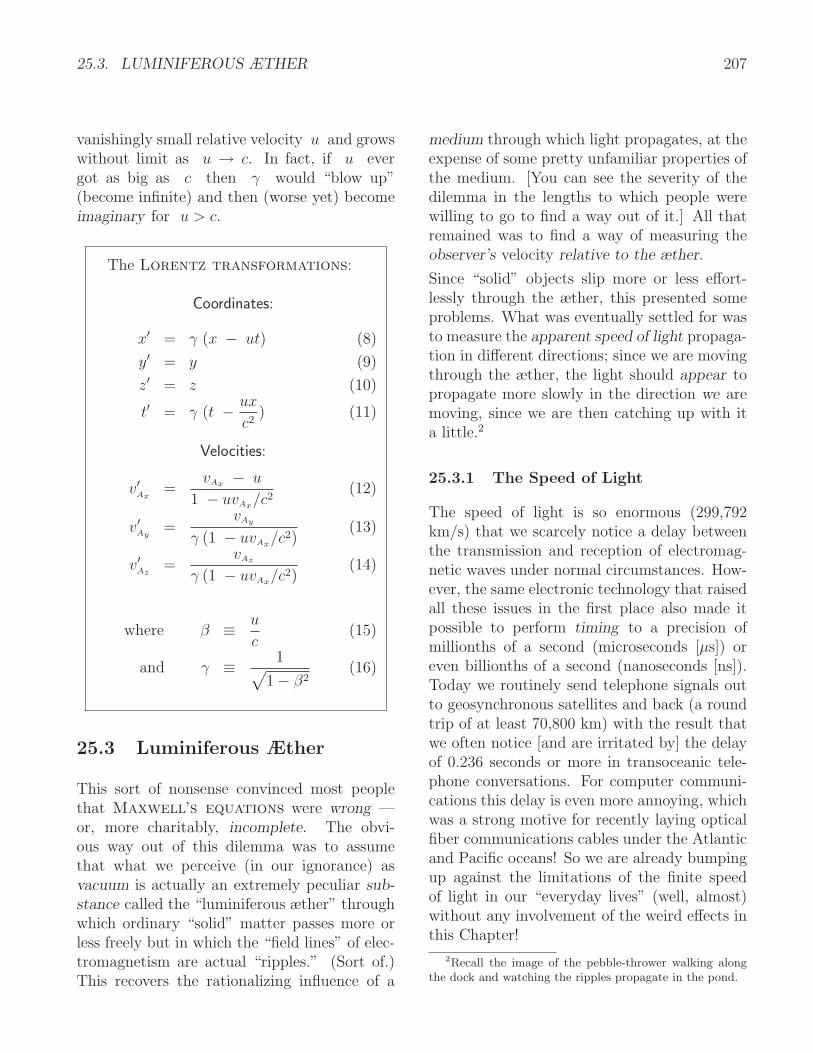
25.3. LUMINIFEROUS ÆTHER 207
vanishingly small relative velocity u and growswithout limit as u → c. In fact, if u evergot as big as c then γ would “blow up”(become infinite) and then (worse yet) becomeimaginary for u > c.
The Lorentz transformations:
Coordinates:
x′ = γ (x − ut) (8)
y′ = y (9)
z′ = z (10)
t′ = γ (t − ux
c2) (11)
Velocities:
v′Ax
=vAx − u
1 − uvAx/c2
(12)
v′Ay
=vAy
γ (1 − uvAx/c2)
(13)
v′Az
=vAz
γ (1 − uvAx/c2)
(14)
where β ≡ u
c(15)
and γ ≡ 1√
1 − β2(16)
25.3 Luminiferous Æther
This sort of nonsense convinced most peoplethat Maxwell’s equations were wrong —or, more charitably, incomplete. The obvi-ous way out of this dilemma was to assumethat what we perceive (in our ignorance) asvacuum is actually an extremely peculiar sub-stance called the “luminiferous æther” throughwhich ordinary “solid” matter passes more orless freely but in which the “field lines” of elec-tromagnetism are actual “ripples.” (Sort of.)This recovers the rationalizing influence of a
medium through which light propagates, at theexpense of some pretty unfamiliar properties ofthe medium. [You can see the severity of thedilemma in the lengths to which people werewilling to go to find a way out of it.] All thatremained was to find a way of measuring theobserver’s velocity relative to the æther.
Since “solid” objects slip more or less effort-lessly through the æther, this presented someproblems. What was eventually settled for wasto measure the apparent speed of light propaga-tion in different directions; since we are movingthrough the æther, the light should appear topropagate more slowly in the direction we aremoving, since we are then catching up with ita little.2
25.3.1 The Speed of Light
The speed of light is so enormous (299,792km/s) that we scarcely notice a delay betweenthe transmission and reception of electromag-netic waves under normal circumstances. How-ever, the same electronic technology that raisedall these issues in the first place also made itpossible to perform timing to a precision ofmillionths of a second (microseconds [µs]) oreven billionths of a second (nanoseconds [ns]).Today we routinely send telephone signals outto geosynchronous satellites and back (a roundtrip of at least 70,800 km) with the result thatwe often notice [and are irritated by] the delayof 0.236 seconds or more in transoceanic tele-phone conversations. For computer communi-cations this delay is even more annoying, whichwas a strong motive for recently laying opticalfiber communications cables under the Atlanticand Pacific oceans! So we are already bumpingup against the limitations of the finite speedof light in our “everyday lives” (well, almost)without any involvement of the weird effects inthis Chapter!
2Recall the image of the pebble-thrower walking alongthe dock and watching the ripples propagate in the pond.
208 CHAPTER 25. THE SPECIAL THEORY OF RELATIVITY
25.3.2 Michelson-Morley Experiment
The famous experiment of Albert AbrahamMichelson and Edward Williams Morley actu-ally involved an interferometer — a device thatmeasures how much out of phase two waves getwhen one travels a certain distance North andSouth while the other travels a different dis-tance East and West. Since one of these sig-nals may have to “swim upstream” and thendownstream against the æther flowing past theEarth, it will lose a little ground overall rel-ative to the one that just goes “across” andback, with the result that it gets out of phaseby a wavelength or two. There is no need toknow the exact phase difference, because onecan simply rotate the interferometer and watchas one gets behind the other and then vice
versa. When Michelson and Morley first usedthis ingenious device to measure the velocity ofthe Earth through the æther, they got an as-tonishing result: the Earth was at rest!
Did Michelson or Morley experience brief para-noid fantasies that the ergocentric doctrines ofthe Mediæval Church might have been rightafter all? Probably not, but we shall neverknow. Certainly they assumed they had madesome mistake, since their result implied thatthe Earth was, at least at that moment, at restwith respect to the Universe-spanning luminif-erous æther, and hence in some real sense atthe centre of the Universe. However, repeatingthe measurement gave the same result.
Fortunately, they knew they had only to waitsix months to try again, since at that time theEarth would be on the opposite side of the Sun,moving in the opposite direction relative to it(the Sun) at its orbital velocity, which should beeasily detected by their apparatus. This theydid, and obtained the same result. The Earthwas still at rest relative to the æther.
Now everyone was in a bind. If they insistedin positing an æther to dispell the absurditiesof propagation through a vacuum at a fixed ve-
locity, then they had to adopt the embarrassingview that the æther actually chose the Earth, ofall the heavenly bodies, to define its rest frame— and even followed it around in its acceleratedorbital path! This was too much.
25.3.3 FitzGerald/Lorentz Æther Drag
George Francis FitzGerald and H.A. Lorentz of-fered a solution of sorts: in drifting through theæther, “solid” bodies were not perfectly un-affected by it but in fact suffered a common“drag” in the direction of motion that causedall the yardsticks to be “squashed” in that di-rection, so that the apparatus seemed to beunaffected only because the apparatus and theyardstick and the experimenters’ eyeballs wereall contracted by exactly the same multiplica-tive factor! They showed by simple argumentsthat said factor was in fact γ = 1/
√
1 − β2
where β = u/c — i.e. exactly the factordefined earlier in the Lorentz transforma-
tions, so named after one of their originators!3
Their equations were right, but their explana-tion (though no more outlandish than what wenow believe to be correct) was wrong.
For one thing, these famous “Lorentz con-
tractions” of the lengths of meter or yard-sticks were not accompanied (in their model)by any change in the relative lengths of timeintervals — how could they be? Such an ideamakes no sense! But this leads to qualitativeinconsistencies in the descriptions of sequencesof events as described by different observers,which also makes no sense. Physics was cor-nered, with no way out.
Ernst Mach, who had a notorious distaste for“fake” paradigms (he believed that Physics hadno business talking about things that couldn’tbe experimented upon),4 proposed that Physicshad created its own dilemma by inventing a
3Poor FitzGerald gets less press these days, alas.4Mach would have had apoplexy over today’s quarks —
but that’s a story for a later Chapter!

25.5. SIMULTANEOUS FOR WHOM? 209
nonexistent “æther” in the first place, and wewould do well to forget it! He was right, in thiscase, but it took a less crusty and more opti-mistic genius to see how such a dismissal couldbe used to explain all the results at once.
25.4 Einstein’s Simple Approach
At this time, Albert Einstein was working as aclerk in the patent office in Zurich, a positionwhich afforded him lots of free time to toy withcrazy ideas. Aware of this dilemma, he sug-gested the following approach to the problem:since we have to give up some part of our com-mon sense, why not simply take both the ex-periments and Maxwell’s equations at facevalue and see what the consequences are? Nomatter how crazy the implications, at least wewill be able to remember our starting assump-tions without much effort. They are:
• The “Laws of Physics” are the same in oneinertial reference frame as in another, re-gardless of their relative motion.5
• All observers will inevitably measure thesame velocity of propagation for light intheir own reference frame, namely c.
These two postulates are the starting pointsfor Einstein’s celebrated Special Theory of
Relativity (STR), for which this Chapteris named.6 The adjective “Special” is theremainly to distinguish the STR from the General
5An inertial reference frame is one that is not accelerated— i.e. one that is at rest or moving at constant velocity.
6It is perhaps unfortunate that the theory was called“Relativity” when in fact it expresses the principle that the“Laws of Physics” are not relative; they are the same forall reference frames, moving or not! It is the transforma-tions between measurements by different observers in rela-tive motion that give weird results. When someone says,“Yeah, Einstein showed that everything is relative,” everyPhysicist within earshot winces. On the other hand, theSTR does explicitly rule out any absolute reference framewith respect to which all motion must be measured — thuselevating the negative result of the Michelson-Morley exper-
Theory of Relativity, which deals with gravityand accelerated reference frames, to be coveredlater.
25.5 Simultaneous for Whom?
The first denizen of common sense to fall victimto the STR was the “obvious” notion that if twophysical events occur at the same time in myreference frame, they must occur at the sametime in any reference frame. This is not trueunless they also occur at the same place. Let’ssee why.
Einstein was fond of performing imaginaryexperiments in his head — Gedankenexperi-
menten in German — because the resultantlaboratory was larger than anything he could fitinto the patent office and better equipped thaneven today’s funding agencies could afford. Un-fortunately, the laboratory of the imaginationalso affords the option of altering the Laws ofPhysics to suit one’s expectations, which meansthat only a person with a striking penchantfor honesty and introspection can work therewithout producing mostly fantasies. Einsteinwas such a person, as witnessed by the ironicfact that he used the Gedankenexperiment todismantle much of our common sense and re-place it with a stranger truth. Anyway, one ofhis devices was the laboratory aboard a fast-moving vehicle. He often spoke of trains, themost familiar form of transportation in Switzer-land to this day; I will translate this into theglass spaceship moving past a “stationary” ob-server [someone has to be designated “at rest,”although of course the choice is arbitrary].
In Fig. 25.2 both observers (O and O′) mustmeasure the same velocity (c) for the light fromthe flash bulb. The light propagates outwardsymmetrically in all directions (in particular,
iment to the status of a First Principle — and does implythat certain phenomena that we always thought were abso-lute, like simultaneity, are not! So the name “Relativity”does stimulate appropriate debate.

210 CHAPTER 25. THE SPECIAL THEORY OF RELATIVITY
Figure 25.2 A flash bulb is set off in the centre ofa glass spaceship (O′) at the instant it coincideswith a fixed observer O. As the spaceship movesby at velocity u relative to O, the light propa-gates toward the bow and stern of the ship at thesame speed c in both frames.
to the right and left) from the point where thebulb went off in either frame of reference. In theO′ frame, if the two detectors are equidistantfrom that point they will both detect the lightsimultaneously, but in the O frame the stern ofthe spaceship moves closer to the source of theflash while the bow moves away, so the sterndetector will detect the flash before the bowdetector!
This is not just an optical illusion or some mis-interpretation of the experimental results; thisis actually what happens! What is simultane-ous for O′ is not for O, and vice versa. Com-mon sense notwithstanding, simultaneity isrelative.
25.6 Time Dilation
Fig. 25.3 pictures a device used by R.P. Feyn-man, among others, to illustrate the phe-nomenon of time dilation: a clock aboarda fast-moving vessel (even a normal clock) ap-pears7 to run slower when observed from the
7The term “appears” may suggest some sort of illusion;this is not the case. The clock aboard the spaceship actuallydoes run slower in the Earth’s rest frame, and vice versa.
Figure 25.3 A “light clock” is constructed aboarda glass spaceship (reference frame O′) as follows:the “tick” of the clock is defined by one half thetime interval t′ required for the light from astrobe light to traverse the width of the ship (aheight h), bounce off a mirror and come back,a total distance of 2h. In the reference frameof a ground-based observer O (with respect towhom the ship is travelling at a velocity u), thelight is emitted a distance 2ut behind the placewhere it is detected a time 2t later. Since thelight has further to go in the O frame (a distanceℓ =
√h2 + u2t2), but it travels at c in both
frames, t must be longer than t′. This effect isknown as time dilation.
“rest frame” — the name we give to the ref-erence frame arbitrarily chosen to be at rest.Now, if we choose to regard the ship’s frameas “at rest” (as is the wont of those aboard)and the Earth as “moving,” a clock on Earthwill appear to be running slowly when observedfrom the ship! Who is right? The correct an-swer is “both,” in utter disregard for commonsense. This seems to create a logical paradox,which we will discuss momentarily. But firstlet’s go beyond the qualitative statement, “Theclock runs slower,” and ask how much slower.
For this we need only a little algebra and ge-

25.7. EINSTEIN CONTRACTION(?) 211
ometry; nevertheless, the derivation is perilous,so watch carefully. For O′, the time intervaldescribed in Fig. 25.3 is simply
t′ =h
cso that h = ct′
whereas for O the time interval is given by
t =ℓ
cwhere ℓ2 = h2 + u2t2
by the Pythagorean theorem. Expanding thelatter equation gives
t =
√h2 + u2t2
cor c2t2 = h2 + u2t2
which is not a solution yet because it does notrelate t to t′. We need to “plug in” h2 = c2t′2
from earlier, to get
c2t2 = c2t′2 + u2t2
or t2 = t′2 +u2
c2t2
or t2 (1 − β2) = t′2
where we have recalled the definition β ≡ u/c.In one last step we obtain
t =t′
√
1 − β2or t = γ t′
where γ is defined as before: γ ≡ 1/√
1 − β2.
This derivation is a little crude, but it showswhere γ comes from.
25.6.1 The Twin Paradox
Like most “paradoxes,” this one isn’t. But itsure looks like one at first glance. Suppose twoidentical twins part company at age twenty; thefirst twin hops aboard a spaceship of very ad-vanced design and heads out for the distantstars, eventually travelling at velocities veryclose to c, while the second twin stays home atrest. They give each other going-away presentsof identical watches guaranteed to keep perfect
time under all conditions. At the midpoint ofthe voyage, while coasting (and therefore in aninertial reference frame), the first twin looksback at Earth with a very powerful telescopeand observes the second twin’s wristwatch. Af-ter correcting for some truly illusory effects, heconcludes that the first twin’s watch is runningslower than his and that his twin on Earth mustbe aging more slowly as well. Meanwhile, thesecond twin, on Earth, is looking through histelescope at the first twin’s watch (aboard thespaceship) and concludes that the first twin issuffering the effects of time dilation and is con-sequently aging more slowly than him! Who isright? Both, at that moment.
Aha! But now we can bring the first twin homeafter his relativistic journey and compare ages.Certainly they can’t both be younger; this trulywould create a logical paradox that goes beyondthe mere violation of common sense!
What happens? The first twin, who went trav-elling, is in fact younger now than the twinwho stayed home. The paradox is resolved by ameticulous use of the Lorentz transforma-
tions, especially if we make use of the graphi-cal gimmick of the light cone, to be discussedlater.
25.7 Einstein Contraction(?)
We can obtain the concomitant effect ofLorentz contraction without too muchtrouble8 using the following Gedankenexperi-
8I haven’t shown all the false starts in which I got thewrong answer using what seemed like perfectly logical argu-ments. . . . Here’s a good one:
We can obtain the concomitant effect of Lorentz con-
traction in a sloppy way merely by referring back toFig. 25.2: let x be the distance between the flash bulband the forward detector, as measured by the observer O onthe ground, and let x′ be the same distance as measuredby the observer O′ aboard the spaceship. Assume that Ostretches out a tape measure from the place where the flashbulb is set off (say, by a toggle switch on the outer hull ofthe spaceship which gets hit by a stick held up by O as O′
flies by) to the position of the detector in the O frame at

212 CHAPTER 25. THE SPECIAL THEORY OF RELATIVITY
ment, which is so simple we don’t even needa Figure:
Suppose a spaceship gets a nice running startand whips by the Earth at a velocity u onthe way to Planet X, a distance x away asmeasured in the Earth’s reference frame, whichwe call O. [We assume that Planet X is atrest with respect to the Earth, so that thereare no complications due to their relative mo-tion.] If the spaceship just “coasts” the rest ofthe way at velocity u [this is what is meantby an inertial reference frame], then bydefinition the time required for the voyage ist = x/u. But this is the time as measured in theEarth’s reference frame, and we already knowabout time dilation, which says that the du-ration t′ of the trip as measured aboard theship (frame O′) is shorter than t by a factorof 1/γ: t′ = t/γ.
Let’s look at the whole trip from the point ofview of the observer O′ aboard the ship: sinceour choice of who is at rest and who is movingis perfectly arbitrary, we can choose to considerthe ship at rest and the Earth (and Planet X)to be hurtling past/toward the ship at velocityu. As measured in the ship’s reference frame,the distance from the Earth to Planet X is x′
and we must have u = x′/t′ by definition. Butwe also must have u = x/t in the other frame;and by symmetry they are both talking about
the instant of the flash. That way we don’t need to worryabout the position of the detector in the O frame when thelight pulse actually arrives there some time later; we are onlycomparing the length of the spaceship in one frame with thesame length in the other. [It may take a few passes of thespaceship to get this right; but hey, this is a Gedankenex-
periment, where resources are cheap!] Then the time lighttakes to traverse distance x′, according to O′, is t′ = x′/c,whereas the time t for the same process in the rest frameis t = x/c. Therefore, if (from time dilation) t is longerthan t′ by a factor γ, then x must also be longer thanx′ by the same factor if both observers are using the samec.
Simple, eh? Unfortunately, I got the wrong answer! Canyou figure out why?
the same u, so
x′
t′= u =
x
t
and since t = γt′ we must also have
x = γx′.
That is, the distance between fixed points, asmeasured by the space traveller, is shorter thanthat measured by stay-at-homes on Earth by afactor of 1/γ. This is because the Earth andPlanet X represent the moving system as mea-sured from the ship. This effect is known asLorentz contraction; it has nothing what-soever to do with “æther drag!” So one mightwonder why it isn’t called “Einstein contrac-tion,” since we calculated it the way Einsteinwould have.
Of course, the effect works both ways. Thelength of the spaceship, for instance, will beshorter as viewed from the Earth than it isaboard the spaceship itself, because in this casethe length in question is in the frame thatmoved with respect to the Earth. The senseof the contraction effect can be remembered bythis mnemonic:
Moving rulers are shorter. (17)
However, it is possible to conjure up situationsthat defy common sense and thus are often(wrongly) described as “paradoxes.”
25.7.1 The Polevault Paradox
I have a favourite Gedankenexperiment for il-lustrating the peculiarities of Lorentz con-
traction: picture a polevaulter standing be-side a 10 foot long barn with a 10 foot polevaultpole in her hands. Tape measures are broughtout and it is confirmed to everyone’s satisfac-tion that the pole is exactly the same length asthe barn. Got the picture? Now the barn door

25.8. RELATIVISTIC TRAVEL 213
is opened — no tricks — and our intrepid pol-evaulter walks back a few parsecs to begin herrun up.
Suppose we permit a certain amount of fantasyin this Gedankenexperiment and imagine thatSuperwoman, a very adept polevaulter, can runwith her pole at a velocity u = 0.6c. (Thusβ = 0.6 and γ = 1.25 — check it yourself!)This means that as she runs past a stationaryobserver her 10 foot pole turns into a 8 footpole due to Lorentz contraction. On theother hand, in her own reference frame she isstill carrying a 10 foot pole but the barn is nowonly 8 feet long. She runs into the barn andthe attendant (Superman) slams the barn doorbehind her.
From Superwoman’s point of view, the follow-ing sequence of events occurs: first the end ofher pole smashes through the end of the barn,and then9 (somewhat pointlessly, it seems) thebarn door slams behind her. A few nanosec-onds later she herself hits the end of the barnand the whole schmier explodes in a shower ofelementary particles — except for Superwomanand Superman, who are (thankfully) invulner-able.
Superman sees it differently. He has no trou-ble shutting the barn door behind Superwomanbefore her polevault pole hits the other end ofthe barn, so he has successfully performed hisassignment — to get Superwoman and her pol-evaulting skills hidden away inside the barn forthe two nanosecond period that the scout forthe Olympic Trials happens to be looking thisway. What happens after that is pretty muchthe same as described by Superwoman.
Imagine that you have been called in to medi-ate the ensuing argument. Who is right? Canyou counsel these two Superbeings out of a con-frontation that might devastate the surround-ing landscape? Or will this become the Parentof all Battles?
9It takes about 3.4 ns [nanoseconds, 10−9 s] to go 2 feetat a velocity of 0.6c.
Well, if they want to fight they will fight, ofcourse; but the least you can do is point outthat objectively there is nothing to fight about:they are both right! When you think aboutit you will see that they have both describedthe same events; it is only the sequence of theevents that they disagree on. And the sequenceof events is not necessarily the same for twoobservers in relative motion! It all comes backto the relativity of simultaneity and re-lated issues. For Superwoman the pole hits thewall before the door slams, while for Supermanthe door slams before the pole hits the wall.Both events occur for both observers, but thesequence is different.10
25.8 Relativistic Travel
Numerous misconceptions have been bred bylazy science fiction (SF) authors anxious tocircumvent the limitations imposed by theSTR. Let’s examine these limitations and askwhether in fact they restrict space-flight optionsas severely as SF fans have been led to believe.
The first and most familiar restriction is the fa-miliar statement, “You can’t ever go quite asfast as light.” Why is this? Well, considerthe behaviour of that ubiquitous scaling fac-tor γ as u → c (i.e., as β → 1): as βgets closer and closer to unity, (1 − β) getscloser and closer to zero, as does its square root,which means that γ “blows up” (becomes infi-nite) as u → c. Time dilation causes clocksaboard fast-moving spaceships to freeze com-pletely and Lorentz contraction causesthe length of the ship (in the direction of itsmotion) to squash to nothing, if u → c. [Asobserved by Earth-bound telescopes, of course.]Worse yet, if we could achieve a velocity greater
10If the door were at the far end of the barn (where thepole hits), there could be no such disagreement, since twoevents at the same place and the same time are for all in-tents and purposes part of the same event. It is only eventsseparated in space about which such differences of opinioncan arise.

214 CHAPTER 25. THE SPECIAL THEORY OF RELATIVITY
than c, time would not run backwards [orany of the other simplistic extrapolations tossedoff in mediocre SF ]; rather the time-dilation /Lorentz-contraction factor γ becomes imagi-nary — in other words, there is no such phys-ical solution to the Lorentz transforma-
tion equations! At least not for objects withmasses that are real in the mathematical sense.[I will deal with the hypothetical tachyons ina later section.] Another way of understandingwhy it is impossible to reach the speed of lightwill be evident when we begin to discuss Rel-
ativistic Kinematics in the next Chapter.
So there is no way to get from here to anotherstar 10 light years distant in less than ten years— as time is measured on Earth! However,contrary to popular misconceptions, this doesnot eliminate the option of relativistic travelto distant stars, because the so-called “subjec-tive time”11 aboard the spaceship is far shorter!This is because in the traveller’s reference framethe stars are moving and the distances betweenthem (in the direction of motion) shrink due toLorentz contraction.
It is quite interesting to examine these effectsquantitatively for the most comfortable form ofrelativistic travel: constant acceleration at 1g(9.81 m/s2) as measured in the spaceship’s restframe, allowing shipboard life to conform to theappearance of Earth-normal gravity. I will listtwo versions of the “range” of such a voyage(measured in the Earth’s rest frame) for dif-ferent “subjective” elapsed times (measured inthe ship’s rest frame) — one for arrival at rest[the only mode of travel that could be useful for“visiting” purposes], in which one must acceler-ate halfway and then decelerate the rest of theway, and one for a “flyby ,” in which you don’tbother to stop for a look [this could only appeal
11Time measured aboard the spaceship is no more “sub-jective” than time on Earth, of course; this terminology sug-gests that the experience of the traveller is somehow bogus,which is not the case. Time actually does travel more slowlyfor the moving observer and the distance between origin anddestination actually does get shorter.
to someone interested in setting a long-distancerecord].
The practical limit for an impulse drive con-verting mass carried along by ship into a colli-mated light beam with 100% efficiency is about10-12 years. Longer acceleration times requireuse of a “ram scoop” or similar device usingambient matter.
Now, what does this say about the real possibil-ities for relativistic travel? Without postulat-ing any “unPhysical” gimmicks — e.g. “warpdrives” or other inventions that contradict to-day’s version of the “Laws” of Physics — we caneasily compose SF stories in which humans (orothers) can travel all through our own Galaxywithout resorting to suspended animation12 orother hypothetical future technologies.13 Thereis only one catch: As Thomas Wolfe said, Youcan’t go home again. Or, more precisely, youcan go home but you won’t recognize the oldplace, because all those years it took light to getto your destination and back (that you cleverlydodged by taking advantage of Lorentz con-
traction) still passed normally for the folksback home, now thousands of years dead andgone.
So a wealthy misanthropic adventurer may de-cide to leave it all behind and go exploring, butno government will ever pay to build a recon-naissance vessel which will not return before thenext election. This implies that there may wellbe visitors from other stars, but they would bespecial sorts of characters with powerful curiosi-ties and not much interest in socializing. Andwe can forget about “scouts” from aggressiveraces bent on colonization, unless they take avery long view!
12The idea of suspended animation is a good one and I findit plausible that we may one day learn to use it safely; but itdoes not quite fall into the category of a simple extrapolationfrom known technology — yet.
13Except for the “ramscoop” technology and the requi-site shields against the thin wisp of ambient matter (pro-tons, electrons,. . . ) inhabiting interstellar space, which isconverted into high-energy radiation by virtue of our ship’srelative motion. Minor details.

25.8. RELATIVISTIC TRAVEL 215
Table 25.1 Distances covered (measured in Earth’s rest frame) by a spaceship accelerating at aconstant 1g (9.81 m/s2) in its own rest frame.
Elapsed Time Distance Travelled (Light Years)aboard ship (years) Arriving at Rest “Fly-by”
1 0.063 0.1282 0.98 2.763 2.70 9.074 5.52 26.35 10.26 73.26 18.14 200.77 31.14 547.38 52.6 1,4909 88 4,05010 146 11,01211 244 29,93612 402 81,37613 665 221,20014 1,096 601,30015 1,808 1,635,00016 2,981 4,443,00017 4,915 12,077,00018 8,103 32,830,00019 13,360 89,241,00020 22,000 243,000,00021 36,300 659,000,00022 59,900 1,792,000,00023 99,000 4,870,000,00024 163,000 13,200,000,00025 268,000 36,000,000,00026 442,000 98,000,000,00027 729,000 (present diam.28 1,200,000 of universe29 thought to be30 less than about
30,000,000,000)

216 CHAPTER 25. THE SPECIAL THEORY OF RELATIVITY
25.9 Natural Units
As I mentioned in the Chapter on Units and
Dimensions, in any context where the speedof travel is virtually (or, in this case, exactly)a constant, people automatically begin to ex-press distances in time units. [Q: “How far isis from New York to Boston?” A: “Oh, aboutthree hours.”] This is equivalent to defining thespeed of travel to be a dimensionless constantof magnitude 1. Relativistic Physics is no dif-ferent. Anyone who has to discuss relativisticphenomena at any length will usually slip into“natural units” where
c = 1
and distance and time are measured in the sameunits. You get to pick your favourite unit —seconds, meters, light years or (as we shall seelater) inverse masses! The list is endless. Thenβ is just “the velocity” measured in naturalunits and the calculations become much sim-pler. But you have to convert all your otherunits accordingly, and this can be interesting.It does take a little getting used to, but theexercise is illuminating.
25.10 A Rotational Analogy
If we compare the Lorentz transforma-
tions with the Galilean transforma-
tions, several striking qualitative features areapparent: the first is the multiplicative fac-tor γ which describes both time dilation
and Lorentz contraction; the second is thefact that time and space get mixed togetherby the Lorentz transformation — a blas-phemy in the paradigm of classical Physics.
The latter weirdness is going to be confusingno matter what we do; is there any way to atleast make it look familiar? What we need isan analogy with something that does “makesense” and is still intact. Fortunately there is
a precedent for a transformation that mixes co-ordinates, namely the rotation.
25.10.1 Rotation in Two Dimensions
Suppose we have a point A in a plane with per-pendicular x and y coordinate axes scribedon it, as pictured in Fig. 25.4.
Figure 25.4 A fixed point A can be located in aplane using either of two coordinate systems O(x, y) and O′ (x′, y′) that differ from each otherby a rotation of θ about the common origin(0, 0).
We can scribe a different pair of perpendicu-lar coordinate axes x′ and y′ on the sameplane surface using dashed lines by simply ro-tating the original coordinate axes by an angleθ about their common origin, the coordinatesof which are (0, 0) in either coordinate system.
Now suppose that we have the coordinates(xA, yA) of point A in the original coordinatesystem and we would like to transform thesecoordinates into the coordinates (x′
A, y′A) of
the same point in the new coordinate system.14
How do we do it? By trigonometry, of course.14This situation might arise if an architect suddenly dis-
covered that his new plaza had been drawn from coordinateslaid out by a surveyor who had aligned his transit to mag-netic North while standing next to a large industrial elec-tromagnet. The measurements are all OK but they have tobe converted to true latitude and longitude!

25.10. A ROTATIONAL ANALOGY 217
You can figure this out for yourself. The trans-formation is
x′ = x cos(θ) + y sin(θ) (18)
y′ = −x sin(θ) + y cos(θ) (19)
25.10.2 Rotating Space into Time
If we now look at just the x and t part of theLorentz transformation [leaving out they and z parts, which don’t do much anyway],we have
x′ = γ x − γβ ct (20)
ct′ = −γβ x + γ ct (21)
— i.e., the Lorentz transformation “sortof” rotates the space and time axes in “sortof” the same way as a normal rotation of x andy. I have used ct as the time axis to keepthe units explicitly the same; if we use “nat-ural units” (c = 1) then we can just drop cout of the equations completely and the anal-ogy becomes obvious. However, you should re-sist the temptation to think of the Lorentz
transformation as “just a rotation of spaceand time into each other.” If we “boost” theO′ frame by some large relative velocity in thenegative x direction and try to plot up x′ andct′ on the same graph as (x, ct) then we get aweird picture.
Proper Time and Lorentz Invariants
The most important important difference be-tween ordinary rotations and the Lorentz
transformations is that the former preservethe radius distance
r =√
x2 + y2 =√
x′2 + y′2 (22)
of point A from the origin, whereas the latterpreserve the proper time τ of an event:
cτ =√
c2t2 − x2 =√
c2t′2 − x′2 (23)
Figure 25.5 An attempt to draw (x′, ct′) coor-dinates on the same graph as the (x, ct) coordi-nates. The result is misleading because the spatialsurface on which it is drawn obeys Euclidean
geometry (the invariant length of an interval isthe square root of the sum of the squares of itstwo perpendicular components) whereas space-time obeys the Minkowski metric: the invari-ant “length” of a spacetime interval (the proper
time) is equal to c2t2 − x2, not c2t2 + x2). Youmay think of the Lorentz transformation
as a sort of rotation, but you can’t draw it as arotation, because you don’t have Minkowski pa-per!
The − sign in the latter is important!
In general, any quantity which we can define(like τ) that will have the same value in everyinertial reference frame, regardless of relativemotion, may be expected to become very pre-cious to our bruised sensibilities. The STR hasdismantled most of our common sense aboutwhich physical observables are reliable, univer-sal constants and which depend upon the ref-erence frame of the observer; if we can specifi-cally identify those properties of a quantity thatwill guarantee its invariance under Lorentz
transformations, then we can at least counton such quantities to remain reliably and di-rectly comparable for different observers. Suchquantities are known as Lorentz invariants.

218 CHAPTER 25. THE SPECIAL THEORY OF RELATIVITY
The criterion for Lorentz invariance is thatthe quantity in question be the scalar prod-uct of two 4-vectors, or any combination ofsuch scalar products. What do we mean by4-vectors? Space and time make the clas-sic example, but we can define a 4-vector tobe any 4-component quantity that transformslike spacetime. That is, aµ = a0, a1, a2, a3 —where a0 is the “timelike” component (like ct)and a1, a2, a3 are the three “spacelike” com-ponents (like x, y, z) — is a 4-vector if a “boost”of u in the x direction gives
a′0 = γ(a0 − βa1)
a′1 = γ(a1 − βa0)
a′2 = a2
a′3 = a3
just like for xµ = ct, x, y, z. The mostimportant example (other than xµ itself) ispµ = E, px, py, pz, the energy-momentum
4-vector, which we will encounter next.
25.11 Light Cones
If we picture Lorentz transformations asrotations of time and space into each other,we can make good use of a handy and simplegraphical gimmick: the “light cone.”
25.12 Tachyons

219
Chapter 26
Relativistic Kinematics
Since Mechanics is so intimately concerned with the relationships between mass, time and dis-tance, the weird properties of the time and space revealed by the STR may be expected to beaccompanied by some equally weird Mechanics at relativistic velocities. This is indeed the case.On the other hand, we can rely upon Einstein’s first postulate of the STR, namely that the “Lawsof Physics” are the same in one reference frame as in another. Thus most of our precious paradigmsof Mechanics (such as conservation laws) will still be reliable.
26.1 Momentum is Still Conserved!
For instance, momentum conservation must still hold, or else we would be able to tell onereference frame from another (in an absolute sense) by seeing which one got less than its shareof momentum in a collision. To pursue this example, we invoke momentum conservation in aglancing collision between two identical billiard balls, as pictured in Fig. 26.1:
[Get ready to keep track of a lot of subscripts and primes! If you want to avoid the tedium of payingclose attention to which quantity is measured in whose rest frame, skip to the formal derivation interms of Lorentz invariants and the 4-momentum. . . .]
Now, each of A and B is at rest in its own reference frame before the collision (A sees B approachingfrom the right at −u whereas B sees A approaching from the left at +u); after the collision, eachmeasures1 its own final velocity transverse (perpendicular) to the initial direction of motion of theother. Out of courtesy and in the spirit of scientific cooperation, each sends a message to the otherreporting this measurement. By symmetry, these messages must be identical:
v′A⊥
= vB⊥(1)
Using the same argument, each must report the same measurement for the transverse componentof the other’s velocity after the collision:
vA⊥= v′
B⊥(2)
1If the anthropomorphism of billiard balls bothers you, please imagine that these are very large “billiard balls” with cabinsoccupied by Physicists who make all these observations and calculations.

220 CHAPTER 26. RELATIVISTIC KINEMATICS
Figure 26.1 A glancing collision between two identical billiard balls of rest mass m, shown in the referenceframe of ball B. Ball A barely touches ball B as it passes at velocity u, imparting a miniscule transversevelocity vB⊥
(perpendicular to the initial velocity of A) to ball B and picking up its own transversevelocity vA⊥
in the process. Primed quantities (like v′A⊥
and v′B⊥
) are measured in A’s reference frame,whereas unprimed quantities (like vA‖
= u, vA⊥and vB⊥
) are measured in B’s reference frame.
Meanwhile, momentum conservation must still hold for the transverse components in eachframe:
In B (unprimed) frame m vB⊥= mA vA⊥
(3)
and in A (primed) frame m′B v′
B⊥= m v′
A⊥, (4)
where the masses of the billiard balls in their own rest frames are written as m but I have expresslyallowed for the possibility that a ball’s effective mass in the other ball’s frame may differ from itsrest mass. (It helps to know the answer.) Thus mA is the effective mass of A as seen from B’sreference frame and m′
B is the effective mass of B as seen from A’s reference frame.
We may now apply the Lorentz velocity transformation to the transverse velocity compo-nent of A:
v′A⊥
=vA⊥
γ(
1 − uvA‖/c2
) =
√
1 − β2 vA⊥
1 − u2/c2= γ vA⊥
(5)
Combining Eq. (1) with Eq. (3) gives m v′A⊥
= mA vA⊥which, combined with Eq. (5), gives
m γ vA⊥= mA vA⊥
or mA = γ m. Similarly, combining Eq. (2) with Eq. (4) gives m′B vA⊥
=m v′
A⊥= m γ vA⊥
or m′B = γ m.
We can express both results in a general form without any subscripts:
m′ = γ m (6)
The effective mass m′ of an object moving at a velocity u =βc is γ times its rest mass m (its mass measured in its ownrest frame).
That is, moving masses have more inertia!

26.2. MASS AND ENERGY 221
26.1.1 Another Reason You Can’t Go as Fast as Light
The preceding argument was not very rigourous, but it served to show the essential necessity forregarding the effective mass of an object as a relative quantity. Let’s see what happens as we tryto accelerate a mass to the velocity of light: at first it picks up speed just as we have been trainedto expect by Galileo.2 But as β becomes appreciable, we begin to see an interesting phenomenon:it gets harder to accelerate! (This is, after all, what we mean by “effective mass.”) As β → 1, themultiplicative “mass correction factor” γ → ∞ and eventually we can’t get any more speed out ofit, we just keep pumping energy into the effective mass. This immediately suggests a new way oflooking at mass and energy, to be developed in the following section.
But first let’s note an interesting side effect: the rate at which a constant accelerating force producesvelocity changes, as measured from a nonmoving reference frame, slows down by a factor 1/γ; butthe same factor governs the time dilation of the “speed” of the clock in the moving frame. So(as observed from a stationary frame) the change in velocity per tick of the clock in the movingframe is constant. This has no practical consequences that I know of, but it is sort of cute.
26.2 Mass and Energy
In the hand-waving spirit of the preceding section, let’s explore the consequences of Eq. (6). Thebinomial expansion of γ is
γ = (1 − β2)−12 = 1 + 1
2β2 − · · · (7)
For small β, we can take only the first two terms (later terms have still higher powers of β ≪ 1and can be neglected) to give the approximation
m′ ≈ (1 + 12β2) m or m′c2 ≈ mc2 + 1
2mu2 (8)
The last term on the right-hand side is what we ordinarily think of as the kinetic energy T . Sowe can write the equation (in the limit of small velocities) as
T = γ mc2 − mc2 (9)
It turns out that Eq. (9) is the exact formula for the kinetic energy at all velocities, despite the“handwaving” character of the derivation shown here.
We can stop right there, if we like; but the two terms on the right-hand side of Eq. (9) look sosimple and similar that it is hard to resist the urge to give them names and start thinking in termsof them.3 It is conventional to call γ mc2 the total relativistic energy and mc2 the rest
mass energy. What do these names mean? The suggestion is that there is an irreducible energyE0 = mc2 associated with any object of mass m, even when it is sitting still! When it speeds up, itstotal energy changes by a multiplicative factor γ; the difference between the total energy E = γ mc2
and E0 is the energy due to its motion, namely the kinetic energy T .2It had better! The behaviour of slow-moving objects did not undergo some sudden retroactive change the day Einstein
wrote down these equations!3This is, after all, the most ubiquitous instinct of Physicists and perhaps the main æsthetic foundation of Physics. It is
certainly what I mean by “Physics as Poetry!”

222 CHAPTER 26. RELATIVISTIC KINEMATICS
26.2.1 Conversion of Mass to Energy
Einstein’s association of the term mc2 with a rest mass energy E0 naturally led to a great dealof speculation about what might be done to convert mass into useable energy, since for a little massyou get a lot of energy! Let’s see just how much: in S.I. units 1 J ≡ 1 kg-m2/s2 so a 1 kg masshas a rest mass energy of (1 kg)×(2.9979 × 10⁸ m/s)2 = 8.9876 × 10¹⁶ J — i.e.,
1 kg ←→ 8.9876 × 10¹⁶ J (10)
which is a lot of joules. To get an idea how many, remember that one watt is a unit of powerequal to one joule per second, so a joule is the same thing as a watt-second. Therefore adevice converting one millionth of a gram (1 µg) of mass to energy every second would releaseapproximately 90 megawatts [millions of watts] of power!
Contrary to popular belief, the first conclusive demonstration of mass-energy conversion was ina controlled nuclear reactor. However, not long after came the more unpleasant manifestationof mass→energy conversion: the fission bomb. An unpleasant subject, but one about which itbehooves us to be knowledgeable. For this, we need a new energy unit, namely the kiloton [kt],referring to the energy released in the explosion of one thousand tons of TNT [trinitrotoluene], acommon chemical high explosive. The basic conversion factor is
1 kt ≡ a trillion calories = 4.186 × 10¹² J (11)
which, combined with Eq. (10), gives a rest-mass equivalent of
1 kt ←→ 4.658 × 10⁻⁵ kg (12)
That is, one kiloton’s worth of energy is released in the conversion of 0.04658 grams [46.58 mg]of mass. Thus a megaton [equivalent to one million tons of TNT or 103 kt] is released in theconversion of 46.58 grams of mass; and the largest thermonuclear device [bomb] ever detonated,about 50 megatons’ worth, converted some 2.329 kg of mass directly into raw energy.
Comment from Daniel Rosenblatt, 8 July 2003:
The largest thermonuclear bomb ever detonated was the Tsar Bomba. While its de-sign yield was 100 megatons, it was detonated without its 238U jacket, reducing itsactual yield to 50 megatons. This was because the engineers already knew how muchenergy the jacket would add to the explosion, and the fallout generated would havecontaminated thousands of square kilometres.
As a side note, the Tsar Bomba (as detonated) was the cleanest nucear weapon evertested, deriving only about 3% of its total energy from fission.4
4As implied by Daniel Rosenblatt’s comment, a large fraction of the energy released by a “fusion” bomb is actually generatedby fission of a 238U jacket around the true thermonuclear (fusion) core. While 238U does not spontaneously fission from theaddition of slow neutrons made in ordinary fission, and is thus immune to the chain reaction that takes place in 235U or239Pu, the fast neutrons from the fusion reaction will cause 238U to fission, releasing both energy and nasty radioisotopes.Why anyone would do it this way is beyond my understanding, since it generates so much more radioactive fallout that willeventually reach the country that launched the weapon in the first place. But this is not the only thing about nuclear warthat defies common sense! At any rate, we can see that the term “H bomb” is a misnomer in at least two different ways.

26.2. MASS AND ENERGY 223
Also, while there is no theoretical limit to the size of an H bomb, there is a practicalone. A 100 megaton bomb is almost useless militarily, and is also inefficient. Bombs ofthis size spend most of their energy re-re-re-pulverizing the target area. They do notscale up linearly (a bomb twice the size doesn’t destroy twice the area). The largestweapon in the US arsenal is the B53 at 9 megatons; the rest of the stockpile is in the100-475 Kt range.
Nuclear Fission
Where did the energy come from? What mass got converted? To answer this question we must lookat the processes involved on a sub-microscopic scale. First we must consider the natural tendencyfor oversized atomic nuclei to spontaneously split into smaller components.5 This process is knownas nuclear fission and is the energy source for all presently functioning nuclear reactors onEarth. [Also for so-called “atomic” bombs.]6
Figure 26.2 One case of the fission of 236U. The net mass of the initial neutron plus the 235U nucleusis 219,883 MeV/c2. The net mass of the fission products (two neutrons, a 95Mo nucleus and a 139Lanucleus) is 219,675 MeV/c2 — smaller because of the stronger binding of the Mo and La nuclei. The“missing mass” of 208 MeV/c2 goes into the kinetic energy of the fragments (mainly the neutrons),which of course adds up to 208 MeV.
The basic event in the most common variety of nuclear fission is the spontaneous splitting ofone 236U nucleus into (for example) 95Mo, 139La and two neutrons.7 [There are numerous otherpossible fission products. This is just one case.] The fraction of the total mass that gets converted
5I know I haven’t explained what I mean by a “nucleus” yet, or even an “atom;” but here I will suspend rigourous sequenceand “preview” this subject. The details are not important for this description.
6The name, “atomic bomb,” is a frightful misnomer; the atoms have nothing whatsoever to do with the process involvedin such horrible weapons of destruction, except insofar as their nuclei are the active ingredients. The correct name for the“atomic” bomb is the nuclear fission bomb.
7The notation used here is AEl, where the atomic weight A of an element is the total number of neutrons (unchargednucleons) and protons (positively charged nucleons) in the nucleus and El is the chemical symbol for the element in question.“Nucleon” is just a generic name for either protons or neutrons, which have about the same mass [the neutron is slightlyheavier] and the number of protons in a nucleus [called its atomic number Z] determines its net electrical charge, which inturn must be balanced by an equal number of negatively charged electrons in orbit about the nucleus to make up the atom.The atomic number Z therefore determines all the chemical properties of the atom and so defines which element it is. We

224 CHAPTER 26. RELATIVISTIC KINEMATICS
into kinetic energy is 208/219833 = 0.946×10⁻³ or about a tenth of a percent. The energy liberatedin the fission of one 236U nucleus produced in this way is 208 MeV or 0.333 × 10⁻¹⁰ J. That meansit takes 3 × 10¹⁰ such fissions to produce one joule of utilizable energy. Since there are 2.55 × 10²¹
such nuclei in one gram of pure 235U metal, 3 × 10¹⁰ isn’t such a large number!
What sort of control do we have over this process? To answer this question we must understand abit more about the details of the chain reaction whereby an appreciable number of such fissionstake place.
The 236U nucleus is formed by adding one neutron to a 235U nucleus, which is found in naturaluranium ore on Earth at a concentration of about 0.72% [the rest is almost all 238U]. Now, leftto its own devices (i.e., if we don’t drop any slow neutrons into it) a 235U nucleus will live for anaverage of 0.7038 billion years, eventually decaying spontaneously by α particle emission (not thefission reaction that produces more neutrons!) just like its brother isotope 238U, whose lifetime isonly about 6 times longer (4.468 billion years). If the lifetimes weren’t so long, there wouldn’t beany left on Earth to dig up — which might be regarded as a good thing overall, but we have to playthe hand we’re dealt. So an isolated 235U nucleus generally sits around doing nothing and mindingits own business; but when a slow neutron comes by (picture a ball bearing slowly rattling downthrough a peg board) it has a strong tendency to be captured by the 235U nucleus to form 236U, andthen the action starts. This is also a little tricky, because if the 236U nucleus gets a chance to settleinto its ground state (i.e., if all the jiggling and vibrating caused by absorption of a neutron has achance to die down) then it (the 236U nucleus) is also quite stable [mean lifetime = 23.42 millionyears] and also decays by α emission (no new neutrons). However, this is rarely the case; usuallythe excitations caused by absorbing that extra neutron are too much for the excited 236U nucleusand it fissions as described earlier, releasing several not-too-fast neutrons.
What follows depends upon the neighbourbood in which the fission occurs. If the original 235Unucleus is off by itself somewhere, the two neutrons just escape, rattle around until they lose enoughenergy to be captured by some less unstable nuclei, and the process ends. If the fission occurs rightnext to some other 235U nuclei, then the outcome depends (critically!) upon the moderation
[slowing down] of the neutrons: when they are emitted in the fission process, they are much toofast to be captured by other 235U nuclei and will just escape to bury themselves eventually in someinnocuous nuclei ensewhere. If, however, we run them through some moderator [slower-downer]such as graphite, heavy water (deuterium oxide, D2O) or, under extreme conditions of density andpressure, uranium metal itself, the neutrons will slow down by a sort of frictional drag until theyreach the right energy to be captured efficiently by other 235U nuclei. Then we get what is knownas a chain reaction. One neutron is captured by a 235U nucleus which splits up into fissionproducts including fast neutrons, which are moderated until they can be captured by other 235Unuclei, which then split up into fission products including fast neutrons, which are. . . .
The moderation of the neutrons generates a lot of heat in the moderator (it is a sort of friction,after all) which can be used in turn to boil water to run steam turbines to generate electricity. [Or
misused to make a large explosion.] A good fission reactor design (like the Canadian CANDU reactor)
could just specify Z in addition to A to know everything we need to know about the specific nucleus in question [which wecall an isotope], but names are more appealing than numbers [even to Physicists!] so we use the chemical symbol [e.g. U =Uranium, Mo = Molybdenum, La = Lanthanum, H = Hydrogen, He = Helium and Li = Lithium] as an abbreviation for thename of the element. Sometimes you will see Z as a subscript on the left of the chemical symbol, as in 238
92 U, but this is notthe only convention for isotopic notation and I see no reason to confuse matters any further. There — a micro-introductionto nuclear, atomic and chemical terminology!

26.2. MASS AND ENERGY 225
involves a moderator like heavy water (D2O) which boils away when the reactor core overheats,thus stopping the moderation and automatically shutting down the reactor. A bad design (like theSoviet or American reactors) uses moderator rods that are shoved into the core mechanicallyand can get stuck there if the core overheats, as happened at Three Mile Island and (much worse)at Chernobyl.8
Potential Energy is Mass, Too!
Where did the mass “go” in the reaction we just discussed? The answer is that the binding energy
of the 235U nucleus is substantially less negative than that of the final products.
Remember that the gravitational potential energy between two massive bodies is zero when theyare infinitely far apart and becomes more and more negative as they get closer together? [Lowergravitational potential energy for an object at a lower height?] Well, the strong nuclear force
that binds nuclei together has at least this much in common with gravity: it is attractive (atleast at intermediate range) and therefore produces a potential energy “well” into which theconstituents “fall” when we make up a nucleus.9
The other thing to realize is that potential energy counts in the evaluation of the total relativisticenergy of an object; and if the object is at rest, then its potential energy counts in the evaluationof its rest mass. As a result, we might expect the rest mass of a space ship to be slightly largerafter it leaves the Earth than it was on Earth, simply because it has left the “gravity well” of theEarth. This is the case! However, the mass change is imperceptibly small in this case.
Nuclear Fusion
Actually, a large nucleus is rarely heavier than the sum of its constituents. If you think aboutit, this is the equivalent of having a ball stored at the top of a potential energy hill.10 Once itmoves over the edge, the process is all downhill, resulting in liberation of kinetic energy. Theheaviest nuclei represent stored-up energy from “endothermic” (energy-absorbing) processes that
8There is an interesting history to the American [and presumably the Soviet] reactor design: the original version was built ona small scale to go into nuclear submarines, where it worked quite well (and was comparatively safe, considering the unlimitedsupply of coolant!). However, the successful submarine reactor design was simply scaled up to make the big land-based powerreactors, a thoroughly dumb and lazy manœuver by the power industry that has led to a long series of unnecessary troubles.If the world had standardized on the CANDU design, nuclear power would have a much better reputation today, except forthe irreducible (though undeserved) taint of psychological association with nuclear weapons, which has even prompted doctorsto change the name of NMR (nuclear magnetic resonance) imaging machines — probably the most harmless and beneficialdevices ever created by modern technology — to “MRI” (for Magnetic Resonance Imaging) just so their patients wouldn’t bespooked by the boogey-word “nuclear.”
9Note how extensively we rely on this gravitational metaphor! This is partly because we don’t know any more compellingpoetic technique and partly because it works so well — it is a “good” metaphor!
10If you think about it some more, you will realize that such a situation usually constitutes unstable equilibrium: thetiniest push will set the ball rolling downhill, never to return of its own accord. In this case (carrying the nice metaphor a littlefurther) there is actually a slight depression at the top of the hill, so that the ball can rest easy in metastable equilibrium:as long as it doesn’t get to rolling around too energetically [enough to roll up over the edge of the depression], the ball willstay where it is; but if we “tickle” it enough [in this case, by dropping in a neutron] it will bounce out and from there it isall downhill again. This picture works almost perfectly in developing your intuition about metastable nuclei, except for thepeculiar prediction of quantum mechanics that the ball can get through the “barrier” without ever having enough kineticenergy to make it up over the ridge! But that’s another story. . . .

226 CHAPTER 26. RELATIVISTIC KINEMATICS
took place in supernova explosions billions of years ago, and are in that sense correctly referredto as “supernova fossils.” Anything heavier than iron falls into this category!
Nuclei lighter than iron (57Fe), if they can be regarded as composed of lighter nuclei, are almostalways lighter than the sum of their constituents, simply because their binding energy is greater.The process of combining light nuclei to make heavier ones (up to iron) is called nuclear fusion,which also liberates kinetic energy. There are many, many varieties of nuclear fusion reactions,most of which are realized on a large scale in stars, whose main energy source is nuclear fusion. [Anice, romantic aspect of nuclear physics, for a change!] Our own Sun, for example, is one big fusionpower plant and has all the pleasant and unpleasant features of the putative man-made versions,such as radiation. . . .
Unfortunately, here on Earth we have not yet succeeded in controlling nuclear fusion well enoughto make a reactor that will generate more energy than it takes to run, though billions of dollarshave been (and will doubtless continue to be) spent in the attempt. So far all we have achievedwith notable success is the uncontrolled thermonuclear11 reaction [bomb] known as the “H bomb.”12
A nasty feature of thermonuclear bombs is that there doesn’t seem to be an upper limit on howbig one might make them. The only good thing about them (other than the questionable virtue of“deterrence”) is that they are not intrinsically as “dirty” (in terms of radioactive fallout) as fissionbombs, at least not “per kiloton.” However, most tactical “H bombs” are actually mainly fissiondevices triggered by a fusion core. This makes them quite dirty. Yuk. I have said rather more thanI like about this subject already.
Cold Fusion
“Wouldn’t it be nice,” most reasonable people would agree, “if there were a way to obtain energyfrom fusion of some innocuous nuclei like deuterium without the enormous temperatures of nuclearexplosions or the various ‘hot’ controlled fusion reactors on the drawing boards.” There certainlyis a way to get deuterium nuclei close enough together to fuse without high temperatures — in factI recently participated in an experiment that achieved D-D fusion at a temperature of 2.5 K: thisinvolves forming a molecule of two deuterons and one negative muon — an unstable elementaryparticle which is more or less like an electron except that its mass is 207 times bigger. The heavymuon pulls the deuterons so close together that they fuse. This works. Unfortunately it doesn’twork well enough to generate more energy than it took to make the muon in the first place! Theclosest anyone has come to “breakeven” using muons is more than a factor of ten too low in efficiency.Too bad. It is frustrating to come so close and then fail.
Perhaps because of this frustration, a few years ago some people deluded themselves into believingthat they had coaxed deuterons into fusing by regular electrochemical means in a palladium metalmatrix. Unfortunately this was bogus. Even more unfortunately, the fantasy remained so seductive
11We call such processes thermonuclear because the positively charged nuclei don’t “like” to get close enough to each otherfor the strong, short-range nuclear force to take over (they repell each other electrically), and to overcome this “Coulombbarrier” they are heated to such enormous temperatures that their kinetic energy is high enough to get them together andthen . . . bang! The heating is usually done by means of a small fission bomb, from what I understand.
12Once again, the popular terminology “H bomb” is completely misleading. The first thermonuclear bombs used a mixtureof deuterium (2H) and tritium (3H) — two isotopes of hydrogen — as the components that fused to form heavier products,hence the name; but modern thermonuclear bombs use (I think) deuterium and lithium, which can be combined chemicallyinto a solid form that is relatively easy to handle and not spontaneously radioactive.

26.2. MASS AND ENERGY 227
that a lot of otherwise respectable scientists were willing to compromise their integrity (probablyunconsciously – I hope) and generate supporting evidence from flawed experiments or muddy rea-soning. Consequently, many gullible people still believe in “cold fusion.” Who can blame them?If you can’t trust the experts, who can you trust? Maybe the popularity of the X-Files and othersigns of people losing their grip on reality can all be traced back to the betrayal of public trust inthe “cold fusion” debacle. Oh well. I did what I could.
26.2.2 Conversion of Energy into Mass
In a nuclear reactor, a spontaneous nuclear process results in a net decrease in the net massof all the particles involved. The “missing mass” appears as the kinetic energy of the reactionproducts, which is dissipated by what amounts to friction and generates heat that boils water; thesteam is used to spin turbines that run generators that send electrical power down the wires.
This leads to an obvious question: can we do the opposite? Can we take electrical power outof the wires, use it to raise the kinetic energy of some particles to enormous values, smack theparticles together and generate some extra mass? Yes! This is what a particle accelerator
like triumf13 does. Every such accelerator is a sort of “reactor in reverse,” taking electrical powerout of the grid and turning it into mass.
Such things happen naturally, too. Gamma rays of sufficient energy often convert into electron-positron pairs when they have a glancing collision with a heavy nucleus. This is pictured in Figs. 26.3and 26.4.
Figure 26.3 Electron-positron pair production by gamma rays (above) and by electrons (below). Thepositron (e+) is the antiparticle of the electron (e−) [to be explained in the Chapter on ElementaryParticle Physics]. The gamma ray (γ) must have an energy of at least 1.022 MeV [twice the rest massenergy of an electron] and the pair production must take place near a heavy nucleus (Z) which absorbsthe momentum of the γ.
13The acronym triumf stands for tri-university meson facility, in recognition of the three B.C. Universities that originallyfounded to project [there are now several more, but we don’t change the cute name] and the main product of the cyclotron.

228 CHAPTER 26. RELATIVISTIC KINEMATICS
There is a neat, compact way of representing such reactions by Feynman diagrams14 I will drawthem “left to right” but the convention is actually to draw them “down to up.” I don’t know why.
Figure 26.4 Feynman diagrams for pair production by a gamma ray (left) or an electron (right).These represent the processes in the preceding sketch.
The convention in Feynman diagrams is that antiparticle lines (e+, for instance) are drawn inthe “backward” sense as if they were propagating backward in time. This allows all “electron lines”to be unbroken, a graphical expression of the conservation of electrons.15 There are lotsmore elegant graphical features to Feynman diagrams, but I will wait until we discuss quantum
field theory in the Chapter on Elementary Particles to discuss them further.
The main point here is that the incoming particle(s) [γ or e−] must have at least 1.022 MeV of kineticenergy to create a positron and an electron, both of which have rest masses of 0.511 MeV/c2. Withan accelerator one can give the original projectile(s) more energy [there seems to be no limit on howmuch, except for mundane concerns about funding resources and real estate] and thus facilitiate thecreation of heavier particles. At triumf, for instance, we accelerate protons to 520 MeV [just overhalf their rest mass energy of 938 MeV], which is enough to create π mesons [mass = 139 MeV/c2]with reasonable efficiency; the high intensity16 of the triumf cyclotron qualifies it for the eliteclub of “meson factories,” so named because they “mass produce” π mesons (or pions) inunprecedented numbers.
Since heavier particles can in principle decay into lighter particles like gamma rays, neutrinos,antineutrinos, electrons and positrons, almost of these “manufactured” particles are unstable. Nev-ertheless, they hang around long enough to be studied and sometimes their very instability is whatmakes them interesting, if only because it precludes finding a cache of them in a more Naturalsetting.
I have gotten far beyond the terms of reference of this Chapter here, but I wanted to “preview”some of the phenomenology of Elementary Particle Physics while focussing your attention on the
14This is basically what won Feynman his Nobel Prize; these simple diagrams are rigourously equivalent to great hairycontour integrals that you would not really want to see! Thus Feynman brought the Right Hemisphere to bear on elementaryparticle physics. Without this simple tool I wonder how far we would have come by now. . . .
15Note that gamma particles [photons] are not conserved — they are always being created or destroyed!16The intensity of an accelerated particle beam can be measured in particles per unit time [triumf has about 1015 pro-
tons/sec] or, if the particles carry electric charge, in amperes of electrical current [triumf has about 140 µA (microamperes)].

26.3. LORENTZ INVARIANTS 229
Figure 26.5 Feynman diagram for production of a π+ meson by a collision between two protons (themost important interaction at triumf).
Figure 26.6 Feynman diagram for “associated production” of a K+ meson [mass = 494 MeV/c2
and “strangeness” S = +1] and a Σ+ hyperon [a type of baryon with mass = 1193 MeV/c2 andstrangeness S = −1] in a collision between a π+ and a proton (the pions produced at triumf don’thave enough energy to do this).
simple motive for building higher- and higher-energy accelerators:
The more kinetic energy is available, the more mass can be created. The heavier theparticle, the more options it is apt to have for other lighter particles to decay into, andthe more unstable it can be expected to be; hence the less likely we are to observe it inNature.17 And the heavier the particle, the more exotic its properties might be.
So far this simple strategy has paid off in many new discoveries; of course, it may not keep workingindefinitely. . . .
26.3 Lorentz Invariants
In the previous Chapter we encountered the notion of 4-vectors, the prototype of which is the space-
time vector, xµ ≡ ct, ~x ≡ x0, x1, x2, x3, where the “zeroth component” x0 is time multipliedby the speed of light (x0 ≡ ct) and the remaining three components are the three ordinary spatial
17The real surprises come when we find heavy particles that don’t decay into lighter ones [or at least not right away]; thisalways means some hitherto unsuspected conserved property like “strangeness” or “charm” — but now I really am gettingtoo far ahead!

230 CHAPTER 26. RELATIVISTIC KINEMATICS
Figure 26.7 Top: Feynman diagram for decay of a π+ meson [mass = 139 MeV/c2] into a positive muon
(µ+) [mass = 106.7 MeV/c2] and a [massless] muon neutrino (νµ). Bottom: Feynman diagram fordecay of a µ+ into a muon antineutrino (νµ), a positron (e+) and an electron neutrino (νe). These arethe reactions I use in almost all of my research.
coordinates. [The notation is new but the idea is the same.] In general a vector with Greek indices(like xµ) represents a 4-vector, while a vector with Roman indices (like xi) is an ordinary spatial3-vector. We could make up any old combination of a 3-vector and an arbitrary zeroth componentin the same units, but it would not be a genuine 4-vector unless it transforms like spacetime underLorentz transformations. That is, if we “boost” a 4-vector aµ by a velocity u = βc along thex1 axis, we must get (just like for xµ = ct, x, y, z)
a′0 = γ(a0 − βa1)
a′1 = γ(a1 − βa0)
a′2 = a2
a′3 = a3 .
It can be shown18 that the inner or scalar product of any two 4-vectors has the agreeableproperty of being a Lorentz invariant — i.e., it is unchanged by a Lorentz transformation
— i.e., it has the same value for all observers. This comes in very handy in the confusing world ofRelativity! We write the scalar product of two 4-vectors as follows:
aµbµ ≡
3∑
µ=0
aµbµ = a0b0 − ~a · ~b = a0b0 − (a1b1 + a2b2 + a3b3) (13)
where the first equivalence expresses the Einstein summation convention — we automaticallysum over repeated indices. Note the − sign! It is part of the definition of the “metric” of space
18Don’t you hate that phrase? Actually this one is pretty easy to work out; why don’t you do it for yourself?

26.3. LORENTZ INVARIANTS 231
and time, just like the Pythagorean theorem defines the “metric” of flat 3-space in Euclideangeometry.
Our first Lorentz invariant was the proper time τ of an event, which is just the square rootof the scalar product of the space-time 4-vector with itself :
cτ =√
xµxµ =√
c2t2 − ~x · ~x (14)
We now encounter our second 4-vector, the energy-momentum 4-vector:
pµ ≡ Ec, ~p ≡ E
c, px, py, pz (15)
where cp0 ≡ E = γmc2 is the total relativistic energy and ~p is the usual momentum 3-vectorof some object in whose kinematics we are interested. [Check for yourself that all the componentsof this vector have the same units, as required.] If we take the scalar product of pµ with itself, weget a new Lorentz invariant:
pµpµ ≡ E2
c2− ~p · ~p =
E2
c2− p2 (16)
where p2 ≡ ~p · ~p is the square of the magnitude of the ordinary 3-vector momentum.
It turns out19 that the constant value of this particular Lorentz invariant is just the c4 timesthe square of the rest mass of the object whose momentum we are scrutinizing: E2
c2− p2 = m2c2
or E2 − p2c2 = m2c4. As a result, we can write
E2 = p2c2 + m2c4 (17)
which is a very useful formula relating the energy E, the rest mass m and the momentum pof a relativistic body.
Although there are lots of other Lorentz invariants we can define by taking the scalar productsof 4-vectors, these two will suffice for my purposes; you may forget this derivation entirely if you sochoose, but I will need Eq. (17) for future reference.
26.3.1 The Mass of Light
Allow me to hearken momentarily back to Newton’s picture of light as particles.20 Actually thefollowing analysis pertains to any particles whose rest mass is zero. If m = 0 then Eq.(6) is absurd,except in the rather useless sense that we may let γ become infinite. On the other hand, Eq.(17)works fine if m = 0. Then we just have
E = pc (18)
— that is, the energy and momentum of a massless particle differ only by a factor of c, itsspeed of propagation. Although we cannot define γ because the massless particle always moves atc relative to any observer [this was, after all, one of the original postulates of the STR], we can talkabout its effective mass, which is the same as its kinetic energy divided by c2.
19Ouch! There’s another one.20This is also a preview of topics to come; as we shall see later, Newton was quite right! Light does come in well-defined
quanta known as photons, particles of zero rest mass that always propagate at the speed of you-know-what!

232 CHAPTER 26. RELATIVISTIC KINEMATICS
Thus, even though light has no rest mass (because it can never be at rest!), it does have aneffective mass which (it turns out) has all the properties one expects from mass — in particular,it has weight in a gravitational field [photons can “fall”] and exerts a gravitational attraction of itsown on other masses. The classic Gedankenexperiment on this topic is one in which the net massof a closed box with mirrored sides increases if it is filled with light bouncing back and forth off themirrors!
Is that weird, or what?

27.1. WHAT HAZARDS? 233
Chapter 27
Radiation Hazards
Few issues in our uncomfortably complicatedhigh-tech modern world are so muddled as thatof radiation hazards. The confusion stemspartly from the emotionally charged politicssurrounding any subject associated with theword “nuclear” — which in turn is the result ofthe brutalizing terror of nuclear war that has in-fected the psyches of several generations of ColdWar veterans — and partly from ignorance andmisunderstanding of what radiation does andhow it can be harmful — which in its own turnis the result of decades of gleeful indulgence inthe thrills of grade-B sci-fi horror films. More-over, most people seem quite content with theirfantasies and “good vs. evil” decision-makingstrategies, so don’t expect a deeper understand-ing to enhance your popularity! Nevertheless,knowledge is power and someone has to knowwhat’s going on, so it looks like you’re it. Letme tell you what I can.1
1Caveat! I encourage you to distrust everything I say(and everything anyone else says) on this subject until youhave seen (and believe) the data for yourself. Like mostpeople, I am not a scholar or even an expert in the field ofradiation hazards, just an amateur with strong convictionswhich will distort my presentation of the evidence; my onlyexcuse for subjecting you to my opinions is that everyoneelse seems to be so timid about expressing any ideas onthis subject that the only information you are likely to getelsewhere (without determined effort on your part) is evenmore politically motivated and less reliable than mine, whichI acquired through informal discussions with various peoplewho do have legitimate professional credentials.
27.1 What Hazards?
One thing we can all agree on is that radiationis bad for you, right? Well. . . . First we haveto be careful to define what we mean by “radi-ation.” Your fireplace radiates in the infrared(heat) and visible (light) parts of the electro-magnetic (EM) spectrum; these forms of ra-diation are certainly beneficial as long as theydon’t get out of control. On the other hand,visible light in the form of a high-power lasercan inflict damage, as can excessive heat oreven microwave EM radiation. On the shorter-wavelength side of the EM spectrum, ultravi-olet light can cause sunburn to the skin, whileX-rays penetrate deeper and can do the samesort of microscopic damage as the still shorter-wavelength gamma (γ) rays emitted by 60Co(cobalt) radioisotopes. Can we make generalstatements about all of these? Perhaps, “A lit-tle is good, but a lot is bad!” Sorry, nothingso simple. It is certainly true that we cannotmaintain health without both heat and light,and a certain amount of “near ultraviolet” maybe required for natural vitamin D productionin the skin, but we probably have no biologicalneed for microwave or radio frequency radia-tion; and all EM radiation from “far ultravio-let” upward in frequency (downward in wave-length) is exclusively and unambiguously badfor the individual.2
2Whether or not genetic mutations are beneficial for thehuman race as a whole is a difficult question both scientifi-cally and ethically; I will avoid trying to answer it.

234 CHAPTER 27. RADIATION HAZARDS
Why the big qualitative difference? What doultraviolet, X-rays and γ-rays do that visibleand infrared light don’t? At last, a questionto which there is a simple answer! They causeionization of atoms and molecules inside cells,leaving behind a variety of free radicals — typesof molecules that quickly react chemically withother nearby molecules. If the free radicals re-act with the DNA molecules in which are en-coded all the instructions to our cells for howto act and how to reproduce, some of these in-structions can get scrambled.
Surprisingly, this does not always happen. Thesimplest detectable damage to a DNA moleculeis a “single-strand break,” in which one of thestrands of the double helix is broken by a chem-ical reaction with a radical. It is a testimonyto the robustness of DNA that it is usually ableto repair its own single-strand breaks in a fewhours!3 If, however, the DNA molecule with asingle-strand break is subjected to further dam-age before it has a chance to “heal itself” thenit may sustain a “double-strand break” (twobreaks in the same strand), which it seems to befar less able to repair. Before we go on to dis-cuss the consequences of permanent DNA dam-age, it is important to note that the irreparabledamage usually takes place only after a largefraction of DNA molecules have already sus-tained temporary damage — and that the tem-porary damage is mostly repaired in a fairlyshort time. This explains why a given “dose”of radiation is less harmful when accumulatedover a long time than when delivered in thespace of a few hours.4
What sorts of bad things are liable to hap-
3Whether this is because of multiple redundancy or con-text programming I do not know, but it sure is an impressivefeat.
4I should add an extra caveat at this point: what I havesaid about single- and double-strand breaks and healingtimes is what I recall from sitting on the PhD committeeof a student working on pion radiotherapy about ten yearsago. I don’t imagine it has been substantially revised sincethen, but I am not absolutely sure. If you want a morereliable witness I will be glad to direct you to local experts.
pen when a DNA molecule sustains irreparabledamage, scrambling some part of the instruc-tion manual for the operation of the cell it in-habits?
• Cell Reproductive Death [most com-mon] — The cell containing the defec-tive DNA may be unable to reproduce it-self, so that although it may be able tofunction normally for its remaining natu-ral lifetime, when it dies a natural deathit will not have a new cell to replace it.Whether this causes a problem or not de-pends upon whether many other nearbycells have the same malady (one by itselfwill never be missed!) and upon the nat-ural lifetime of that type of cell — whichranges from a few days for hair follicles,skin and mucous membrane cells to “for-ever” for brain cells. Obviously, the lossof reproductive capacity is meaninglessfor a cell that never reproduces!
• Genetic Mutation [most subtle] — Ifthe cell in question happens to be a ga-mete destined for fusion with a memberof the opposite sex, the resulting individ-ual will have some scrambled instructionsin the construction manual and will prob-ably not grow up normally. In almostevery case this will be fatal to the fœ-tus, and in almost all the remaining casesit will be detrimental to the survival ofthe individual, although such mutationshave presumably played a role in evolu-tion to date. Note however that it isstrictly impossible for any individual’s ge-netic makeup to be retroactively alteredby radiation (like the Hulk or Spidermanor any number of cheap sci-fi horrors),as this would require the same accidentalscrambling to take place independently inevery DNA strand in the victim’s body!
For men, there are two types of geneticdamage: the sperm cells themselves have

27.2. WHY WORRY, AND WHEN? 235
an active lifetime of only a few days, af-ter which a new generation takes over;but the sperm-producing cells are neverreplaced and so can never repair damageto themselves. The latter applies also towomen: the female gametes (eggs) are allproduced early in life and, once damaged,cannot be repaired.
If the altered cell is “just any old cell”then usually the change is harmless — ei-ther the cell merely fails to do its part inthe body until it dies or else the affectedpart of the DNA is irrelevant to the func-tioning of that cell in the first place —but occasionally the change is related tocell division itself, and then there can bereal trouble.
• Cancer [most unpleasant] — Sometimes(very rarely) a damaged DNA moleculeinstructs a cell to mobilize all its resourcesand the resources of all its neighbours toreproduce as many copies of itself as pos-sible. The offspring preserve the man-date, and a chain reaction takes placethat “crashes the system.” This runawayreproductive zeal of a misguided cell iswhat we know as cancer, and it is theworst hazard of radiation exposure. Asfar as anyone knows, any exposure to ion-izing radiation increases one’s chances ofdeveloping cancer, and so we can unam-biguously say that ionizing radiation isbad for you.
Before we go on, it is interesting to note that allof the most potent therapies for treating can-cer involve either ionizing radiation or chemicalreactions that cause similar DNA damage; thestrategy for these “interventions” is always tocause such overwhelming DNA damage to thecancer cells that every single cancer cell suffers“cell reproductive death” as described above.Although there are various techniques for mak-ing the cancer cells more susceptible to the ra-
diation or harsh chemicals than normal cells,there are inevitably many casualties among thelatter. It is not unusual, for instance, to killoff (in the sense of “reproductive death”) asmany as 90% of the normal cells in the tissuessurrounding a tumour, relying upon the fantas-tic healing capacity of normal tissue to bounceback from this insult. Remember, the idea is tokill 100% (!) of the cancer cells.
It provides an important perspective to realizethat the radiation used to kill the cancer maydeliver a “dose” to healthy tissues that is morethan 10,000 times the maximum legal limit forenvironmental radiation exposure, and yet theincreased likelihood of developing another can-cer from the radiation therapy is regarded asa negligible risk relative to allowing the exist-ing cancer to progress unchecked. Whether ornot oncologists have optimized their treatmentstrategies is another charged issue which I willavoid, but it is clear that a large radiation dosedoes not necessarily “give you cancer” immedi-ately; rather it increases your chances of devel-oping cancer in the long run. By how much?And over how long a run? These are the quan-titative statistical questions that must be an-swered if one is to develop a rational schemefor evaluating radiation hazards.
27.2 Why Worry, and When?
Unfortunately much of our public policy todayseems to be based on the belief that if we couldonly eliminate the last vestiges of hazardousmaterials and dangerous practices from our so-ciety then none of us would ever get sick or die.This must be regarded as nonsense until med-ical science finds a way to halt or reverse thenatural aging process — which might not besuch a great idea.5
5Even if a sufficiently totalitarian regime could be insti-tuted to forcibly prevent the population from increasing ex-ponentially once immortality was commonplace, would sucha thing be beneficial? Would life seem as precious if it were

236 CHAPTER 27. RADIATION HAZARDS
If I were exposed to radiation that virtuallyguaranteed that I would develop cancer within200 years, but no sooner than 100 years, wouldI be wise to worry? What if it raised mychances of developing cancer within 20 years by2%? My chances of developing cancer within20 years are roughly 20% normally, now thatwe have eliminated most other mortal dangersexcept for heart disease. Most people wouldagree that I would be foolish to allow myself tobe exposed to enough radiation to increase mychances of developing cancer within 10 yearsby 10% (unless we mean 10% of 10%, in whichcase it is a rather small increase — one mustalways ask for precise explanations of statisti-cal statements!) and yet we all routinely chooseto engage in activities that are as least as haz-ardous, such as downhill skiing or motorcycleriding. Why do we reserve such terror for onesort of hazard when we so stoically accept oth-ers of far greater risk? Which is the healthierattitude?
27.2.1 Informed Consent vs. Public Pol-icy
One answer to this question is that thereare two entirely separate issues regarding life-threatening hazards: the first relates to per-
sonal choice, in which the individual has a rightto decide for him/herself how much risk is jus-tified for the sake of certain perceived benefits;the second relates to public policy, in which de-cisions may affect millions of people withouttheir knowledge or consent. It is not unethi-cal for me to choose to risk my life for what Iconceive to be worthwhile, or even for fun (aslong as I don’t expect anyone else to bear theconsequences); but it is unethical for me to sub-ject millions of other people to the same levelof risks without their consent.
not so annoyingly short? Again I shall bypass the thornyissues and play the hand I am dealt.
27.2.2 Cost/Benefit Analyses
Unfortunately, this does not necessarily makethe issues simpler. It does not help to con-clude that any global policy decision that in-creases the public risk at all is a priori wrong,because of unintended consequences and com-plex interconnections. A nuclear power plantin New York puts local residents at some riskfrom possible cancer due to possible radiationexposure from possible leaks due to probablebungling and/or inadequate engineering and/orsubstandard construction. On the other hand,a fossil fuel plant of the same size puts a dif-ferent population at risk from acid rain, ozonedepletion and the Greenhouse Effect. 6 Andno power plant at all increases the risk of pneu-monia in the area served during Winter brown-outs — probably the worst hazard of the threein the short term, but one to which millenniaof familiarity have hardened us!
The point is, every public policy decision cre-ates risks. Even a decrease in bus fare, if itaffects millions of people, will cause some peo-ple to die this year who would otherwise havelived longer. The questions must always be, “Isthis likely to do any good? How much good?Is it likely to do any harm? How much harm?What are the relative probabilities of good andharm? How many people are likely to sufferfrom the harm? How many people are likelyto benefit from the good?” And of course thetwo questions most popular with politicians,“Which people?” and “When?”
Time to duck the difficult issues again. I amsatisfied to point out the questions; I have nomore competence than the next person to offeranswers. Suffice it to say that any sensible pol-icy regarding radiation hazards, whether publicor personal, must take into account that each ofus is going to die, that our lifespan is frustrat-
6Also, surprisingly enough, from the radioactivity re-leased from fossil fuels in combustion, which is far greaterthan that released by a nuclear power plant in normal oper-ation.

27.3. HOW BAD IS HOW MUCH OF WHAT, AND WHEN? 237
ingly short no matter what we do, and that ourchances of dying of cancer (radiation-inducedor otherwise) are already rather high.7 So anystrategy dictated exclusively by absolute min-imization of our cancer risk is somewhat silly.Still, all other things being equal, less (ionizing)radiation is better!
27.3 How Bad is How Much ofWhat, and When?
Time to get quantitative. What kinds of radi-ation are there, how do we measure how muchwe get, and what effects can we expect from dif-ferent exposures to different parts of our bodiesover different times?
There are lots of kinds of radiation, from theEM spectrum we have already discussed toneutrons, alpha (α) particles, beta (β) “rays”(high-energy electrons) and γ-rays — all con-stant companions in our environment due tonatural or man-made radioisotopes — to theutterly harmless neutrinos coming from ourSun, to beams of high-energy protons, elec-trons, positrons, pions, muons etc., producedby accelerators like TRIUMF, to catastroph-ically destructive cosmic rays from which weare shielded by our atmosphere (except whenwe fly across country in an airliner) and so onad infinitum. Everyone is constantly exposedto most of these types of radiation, accumulat-ing an annual dose varying from a few hundredmR to several R. What are these units “R” andhow can we gauge what they mean in practicalterms? Time to get more technical.
27.3.1 Units
The basic unit of radiation dose used to be the“rad,” defined in terms of the energy deposited
7I have been assuming 30%, but that number could beout of date; I don’t think it makes much difference to myarguments.
by ionizing radiation per unit mass of exposedmatter (e.g. flesh or bone):
1 rad ≡ 100 erg/g
(g means gram here.) More recently, for somereason this nice mnemonic unit has been of-ficially supplanted by yet another “personalname SI unit” in honour of British physi-cist and radiation biologist Louis Harold Gray(1905-1965) — the “gray :”
1 gray ≡ 100 rad ≡ 1 J/kg.
Early work on radiation hazards was based onX-ray exposure8 and the units used were alwaysrœntgen (after the scientist by that name),which are about the same as rad for X-raysonly, and are virtually unused today. Later itwas found that even the rad was too simple; dif-ferent types of radiation (e.g. neutrons) werefound to be more (or less) destructive than X-rays for different types of tissues, so an empiri-cal “fudge factor” called the Relative BiologicalEffectiveness (RBE) was invented to accountfor these differences (averaged over all bodyparts, of course, which decreased its useful-ness). The RBEs of γ-rays, X-rays and β-rays(fast electrons) are all 1 by definition; thermalneutrons have an average RBE of 3; fast neu-trons (on average), protons and α-rays (4He nu-clei) all have RBEs of 10; and fast heavy ionshave an RBE of 20.9
A new unit was then constructed by combiningthe RBE with the dosage in rads, namely therem (rœntgen equivalent to man), defined by
rem ≡ RBE × rad.8I can remember sticking my feet into the fluoroscope at
the corner shoe store and looking at my foot bones insidemy new shoes; it was quite popular about 40 years ago.
9Actually, the RBE of neutrons varies tremendously fordifferent tissues and is a complicated function of the neutronenergy because of the energy-dependence of the neutron cap-ture cross-sections of different elements. Neutrons are verybad.

238 CHAPTER 27. RADIATION HAZARDS
The “R” in the preceding paragraph stands forrem and the “mR” for millirem — one thou-sandth of a rem.
Today the standard international unit for mea-suring “effective dosage” is the seivert, namedafter Rolf Sievert (1898-1966), a pioneeringSwedish radiation physicist. Converting be-tween rem and seivert is just like convertingbetween rad and gray :
1 seivert ≡ 100 rem.
Now that all mnemonic content has beendeleted from the names of the units associatedwith radiation dosage, you may expect thesenames to stick.10
27.3.2 Effects
All of these units are meaningless until one hassome idea of how bad one of them is for you.Here are some rules of thumb that may be offby factors of two from one case to the next:
• Instant Death: It takes a monumen-tal radiation dose to kill outright, typi-cally something like 5000 R (50 Grays)“whole-body” — i.e. half a million ergsof energy deposited in every gram of yourbody. This amount of energy wipes outyour central nervous system (CNS) imme-diately when delivered all at once. Need-less to say, only the military mind makesa strong distinction between this and thenext level down.
• Overnight Death: Approximately900 R (9 Grays) whole-body will accom-plish the same thing as 50 Grays but ittakes about a day.
10The purpose of SI units is evidently to make it as diffi-cult as possible for intelligent laypersons to understand what“experts” are talking about. I cannot imagine a more hu-miliating posthumous fate than to have countless genera-tions confused by some perfectly simple unit renamed the“brewer” in honour of my efforts to make some field moreunderstandable.
• Ugly Death: A somewhat lower dose,around 500 R (5 Grays) causes severe“radiation sickness” (i.e. nausea, hairloss, skin lesions, etc.) as the body’sshort-lived cells fail to provide new gen-erations to replace their normal mortal-ity (“cell reproductive death”). It is notthis trauma which usually kills, however,but the complications that arise from alack of resistance to infection, due in turnto the lack of new generations of whiteblood cells. If you survive the initial ra-diation sickness and avoid infection, youwill probably recover completely in theshort term; but you are very likely to de-velop cancer (especially leukemia) in lateryears (usually some 10-20 years later!)and your offspring, if any, will have a highprobability of genetic mutations.
• Sub-Acute Exposures: From a whole-body dose of around 100 R (1 Gray) de-livered in less than about a week, you areunlikely to notice any immediate severesymptoms. However, you are likely to de-velop leukemia in 10-30 years, and thereis a significant chance of genetic muta-tions in your offspring. A whole-body ex-posure of 5 R delivered over 1 year wasbelieved in 1970 to represent 1.8 “dou-bling doses” — i.e. it was thought tomultiply your odds of developing cancerby a factor of 2.8 if maintained year afteryear. At that time it was also the legal ex-posure limit for radiation workers in theU.S.A., set by the Atomic Energy Com-mission (AEC) there. Presumably quitea few people received this exposure for afew years, although it is unusual for morethan a small fraction of workers to receivethe maximum allowed exposure. For per-spective, it is noteworthy that a series ofspinal X-rays is apt to give an exposureof 1–4 R locally, and that an afternoonon Wreck Beach in midsummer often pro-

27.4. SOURCES OF RADIATION 239
duces a painful sunburn that represents10-20 R to the skin; the resultant burn isa bona fide radiation burn and is just asdangerous as any other kind! In fact, theoverwhelming majority of all radiation-induced cancer fatalities on Earth can beattributed directly to far ultraviolet fromour favourite nuclear fusion power plantin the sky: the Sun.
• Marginal Exposures: The average ex-posure from natural sources of radiationis on the order of 300 mR per year. Asof 1979 this was also the Canadian legallimit for public exposure from artificialsources. Whether an extra 300 mR makesa significant difference epidemiologicallyin the incidence of cancer depends almostentirely on what one considers significant;however, it is a fact that the statisticaldifference between populations that havereceived such an exposure “artificially”and those who have not is smaller thanthe statistical differences between popu-lations with different eating habits, wholive in different regions, who have differ-ent types of jobs, etc. This is partly be-cause of the wide variety in the amountand type of natural radiation exposure.
Before we go on to discuss sources of radia-tion, it is important to note that different or-gans or body parts have dramatically differentresistance to radiation. The hands, in particu-lar, are able to withstand radiation doses thatwould kill if the whole body were subjectedto them! The lens of the eye and the gonadsare considered to be the most vulnerable andshould be protected first.
27.4 Sources of Radiation
In 1972 a detailed survey was made of av-erage annual whole-body doses to the U.S.A.
population from various sources. Occupationaland miscellaneous artificial exposures averagedabout 1-2 mR/y (remember, some people gotenough to make up for the vast majority whogot none!); global fallout from nuclear testingmade up about 6 mR/y ; medical exposures (X-rays, radiotherapy, etc.) were good for nearly100 mR/y ; and natural background (see be-low) averaged about 120 mR/y. The numbershave not changed much in the intervening years.One must conclude that for the average personthere are only two significant sources of radia-tion exposure: medical and natural. Althoughthis begs the question of “extraordinary cases”who receive larger exposures in accidents suchas Chernobyl, it still helps to set perspectivesfor those examples.
Some medical and natural radiation sourcesare listed below. For medical examples I haveshown the mean dose per exposure. It is im-portant to note that these are only the eas-ily measured forms of radiation — X-rays andγ-rays — that penetrate flesh (and detectors!)easily. More insidious and difficult-to-measuretypes will be discussed in the next Section.
• Medical X-rays: Chest, radio-graphic: 45 mR. Chest, photofluoro-graphic: 504 mR. Spinal (per film):1265 mR. Dental (average): 1138 mR.11
• Cosmic Rays: Sea level: 30–40 mR/y.Colorado: 120 mR/y. At 40,000 ft:0.7 mR/h.12
• Natural Terrestrial Radionuclides:γ-radiation is fairly uniform in theU.S.A., ranging from 30 mR/y in Texas
11Note: medical X-rays are normally localized to the re-gion being imaged; they are not “whole-body” and thereforeare not as bad as they look. Still. . . .
12Note: that is per hour at a typical cruising altitude fora normal commercial jetliner; thus an average round-triptranscontinental flight yields a dose of 6-8 mR! The esti-mated average cosmic-ray dose for airline crew is 670 mR/y.Astronauts have it even worse.

240 CHAPTER 27. RADIATION HAZARDS
to 115 mR/y in South Dakota. Guesswhere the uranium deposits are!13
27.5 The Bad Stuff: IngestedRadionuclides
The information given above would seem to in-dicate that medical X-rays were the worst radi-ation hazard around, except for natural sourceswe can’t do much about. Unfortunately thisis a distortion based on the difficulty of mea-suring the most dangerous kind of radiation:α-emitting radionuclides (radioactive isotopes).Many heavy elements have isotopes which natu-rally fission into lighter elements plus a heliumnucleus, with the latter being emitted with asubstantial kinetic energy as an alpha “ray.”The range of most α particles is only a few cm inair and less than a mm in tissue, so the damagethey cause is localized. While this may be re-assuring when the isotopes are at arm’s length,it can be bad news if you have breathed theminto your lungs or swallowed them so that theycan collect in your bones, where they can do themost damage! Since there is such a wide varietyof radioactive elements with assorted chemicalproperties, it is wise to be aware of the specifichazards associated with each. I have neitherthe expertise nor the space to provide a com-prehensive survey here, but I can mention a fewof the most common culprits.
• Radon: All rock contains some amountof naturally occurring radium which grad-ually decays, releasing the chemically in-ert noble gas radon. Radon in turn is a ra-dioactive element which decays by emit-ting a rather low energy α particle that isquite difficult to detect since it has sucha short range it can’t penetrate the win-dow of a typical Geiger counter. Thus un-til recently there was little known about
13I don’t have the numbers for the Okanagen, but I believethey are even higher than for South Dakota.
radon in our environment, even though itis generally believed that Madame Curiedied from exposure to radon emitted bythe radium upon which she performed herfamous experiments. It is now felt bymany that radon is the most widespreadand dangerous of all radiation hazards,because it accumulates in the air of anybuilding made of rock, brick or concrete(especially those with closed circulationair conditioning!) and thence in the lungsof the people breathing that air. Lungsin fact make a superb filter for the ra-dioactive byproducts of radon, so thatone of the most effective radon detectionschemes is to measure the radioactivityof the people who live in high-radon en-vironments. In the lung tissue, the short-ranged α particles expend all their en-ergy where it does the most harm, rais-ing the incidence of lung disease and can-cer. Rocks from different regions have atremendous range of radium content, sothat a stone house may be perfectly safein one city and hazardous in another.14
• Potassium and Carbon: Radioiso-topes of potassium and carbon are con-tinually created in the atmosphere bycosmic ray bombardment; these isotopesbuild up to a constant level in all liv-ing tissues, only to decay away in a fewthousand years after death. This meansthat the most radioactive component inyour household is probably you!15 It alsoprovides a handy method of estimatingthe time since formerly living matter wasalive (14C and potassium-argon dating).
14I think Vancouver is just slightly on the hazardous side;but in the Okanagen, where there are concentrated uraniumore deposits, I might choose to live in a wooden house. How-ever, you should check out the latest data before you jumpto any conclusions.
15Married folks who sleep together pick up a few extramR/y from their spouses!

27.7. CONCLUSIONS 241
• Man-made Radionuclides: There aretoo many of these to make a comprehen-sive list here.16 The most famous is plu-tonium, 239Pu, the stuff of which fissionbombs are made. Plutonium is both adeadly chemical poison and a nasty ra-dioisotope. If a miniscule grain is caughtin your lungs or other tissues, it maynot do much damage to your body as awhole, but it exposes the tissue immedi-ately around it to a huge dose of radia-tion, drastically increasing the likelihoodof cancer in that tissue. Cancer is just asdeadly no matter where it begins, whichmakes the ingestion of radionuclides theworst possible sort of radiation hazard.
It is important to note that the food chainmay serve to concentrate “harmless” levels ofradionuclides in (e.g.) sea water to a levelwhich is worthy of our concern. Were it not forthis effect, and the fact that the waste prod-ucts of nuclear fission include a large varietyof radionuclides with various chemical proper-ties that naturally occurring isotopes do not ex-hibit, it would be a sensible strategy to disposeof radioactive waste by diluting it and spread-ing it far and wide in the oceans — since the netradioactivity of reactor fuel actually decreasesin the process of digging up the uranium, burn-ing it in a reactor and storing the spent fuelrods for 10 years until the short-lived isotopesdecay away. Because of the biological concen-tration effect, however, it is wiser to seek safelong-term containments for radioactive waste.
27.6 Protection
By far the best shielding against radioactiv-ity is Gauss’ Law: the intensity of a pointsource falls off as the square of its distance fromthe observer. All localized sources are labelled
16One may feel that there are simply too many, period!
with their activity at a given distance, for in-stance “10 mr/h at 1 m.” If one keeps at least10 m away from such a source, one will receiveless than 0.1 mR per hour, which is not wor-risome.17 Other safety measures include leadaprons, which are effective only for X-rays andγ-rays, and thick concrete shielding for neu-trons and high-energy charged particles (theseare much in evidence at TRIUMF).
27.7 Conclusions
Draw your own. Please.
Just try to keep in mind that neither extremeattitude (“There’s nothing to worry about.” vs
“The only acceptable risk is no risk at all.”)represents much of a commitment to the publicgood. Radiation hazards are subtle and com-plex, but the benefits of major sources of envi-ronmental radiation (e.g. medical X-rays) areimportant. They often save lives by endan-gering them; the deciding factor must involverelative probabilities and cost/benefit analyses,which may seem cold-blooded but are essentialif you really want to do as little harm and asmuch good as you can.
Remember, if you let someone else decide foryou, then you forfeit your right to righteous in-dignation if you later disapprove of their deci-sion.
17Needless to say, one should never touch a radioactivesource, because 1/r2 can be very large as r → 0.

242 CHAPTER 27. RADIATION HAZARDS
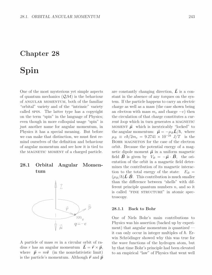
28.1. ORBITAL ANGULAR MOMENTUM 243
Chapter 28
Spin
One of the most mysterious yet simple aspectsof quantum mechanics (QM) is the behaviourof angular momentum, both of the familiar“orbital” variety and of the “intrinsic” varietycalled spin. The latter type has a copyrighton the term “spin” in the language of Physics;even though in more colloquial usage “spin” isjust another name for angular momentum, inPhysics it has a special meaning. But beforewe can make that distinction, we must first re-mind ourselves of the definition and behaviourof angular momentum and see how it is tied tothe magnetic moment of a charged particle.
28.1 Orbital Angular Momen-tum
A particle of mass m in a circular orbit of ra-dius r has an angular momentum ~L = ~r × ~p,where ~p = m~v (in the nonrelativistic limit)is the particle’s momentum. Although ~r and ~p
are constantly changing direction, ~L is a con-stant in the absence of any torques on the sys-tem. If the particle happens to carry an electriccharge as well as a mass (the case shown beingan electron with mass me and charge −e) thenthe circulation of that charge constitutes a cur-rent loop which in turn generates a magnetic
moment ~µ which is inextricably “locked” tothe angular momentum: ~µ = −µB
~L/~, whereµB ≡ e~/2me = 9.2741 × 10⁻²⁴ J/T is theBohr magneton for the case of the electronorbit. Because the potential energy of a mag-netic dipole moment ~µ in a uniform magneticfield ~B is given by VB = −~µ · ~B, the ori-entation of the orbit in a magnetic field deter-mines the contribution of its magnetic interac-tion to the total energy of the state: EB =(µB/~)~L· ~B. This contribution is much smallerthan the difference between “shells” with dif-ferent principle quantum numbers n, and so itis called “fine structure” in atomic spec-troscopy.
28.1.1 Back to Bohr
One of Niels Bohr’s main contributions toPhysics was his assertion (backed up by experi-ment) that angular momentum is quantized —it can only occur in integer multiples of ~. Er-win Schrodinger showed why this was true forthe wave functions of the hydrogen atom, butby that time Bohr’s principle had been elevatedto an empirical “law” of Physics that went well

244 CHAPTER 28. SPIN
beyond the realm of atoms. Schrodinger alsoshowed the peculiar nature of the quantiza-tion of ~L: first, its magnitude obeys |~L| =~√
ℓ(ℓ + 1) where ℓ can only have integer val-ues from zero to (n−1), n being the principle
quantum number for which En = −E/n2
in the case of hydrogen; second, its projectiononto the z axis obeys Lz = mℓ~ where mℓ cantake on only integer values from −ℓ to +ℓ.Note that Bohr’s original prescription for angu-lar momentum quantization (integer multiplesof ~) is actually applicable to the z component
of ~L — its projection onto the z quantizationaxis, which is chosen arbitrarily unless there isa magnetic field applied, in which case z is al-ways chosen along the field, ~B = Bz.
28.1.2 Magnetic Interactions
The reason mℓ is called the magnetic quan-
tum number (and the reason m is used forit, rather than some other letter) is that when
one imposes a magnetic field ~B on an atom,the energy levels En (determined only by n in
the absence of ~B) are “split” by the Zeeman
energy EB = µBmℓB due to the interactionpotential of the magnetic moment with the field(see above).
In 1925 Goudsmit and Uhlenbeck reportedthat, in addition to the “splittings” predictedby the quantization of the orbital angular mo-mentum eigenstates of the electrons in an ap-plied magnetic field, there were additional split-tings of roughly the same magnitude that couldonly be explained in terms of some “extra” an-gular momentum associated with the electronsthemselves. This was relevant to a previous re-sult that had mystified the community:
In 1922, Stern and Gerlach had done an experi-ment on various neutral atoms passing througha region of large magnetic field gradient, the ef-fect of which is to exert on the passing atoms anet force that is proportional to the componentof their angular momentum along the axis of
the gradient. This allowed Stern and Gerlachto experimentally verify that “spin 1” atoms(with ℓ = 1) did indeed have three and onlythree possible values of Lz = mℓ~: mℓ = +1, 0or −1; and similarly for other integer ℓ. How-ever, their experiments on neutral silver atomsrevealed two possible projections of the angularmomentum along the z axis, a range of optionsincompatible with the rules ℓ = 0, 1, · · · (n−1)and mℓ = −ℓ, · · · 0 · · · ℓ. The discoveries ofGoudsmit and Uhlenbeck suggested that theelectron itself might have an intrinsic angularmomentum that was (somehow) half as large asthe smallest allowable nonzero orbital angularmomentum — what we now call “spin 1
2.”
28.2 Intrinsic Spin
The following description is bogus. That it, thisis not “really” what intrinsic angular momen-tum is all about; but it is possible to under-stand it in “common sense” terms, so we canuse it as a mnemonic technique. Many QMconcepts are introduced via this sort of “cheat-ing” until students get comfortable enough withthem to define them rigourously. (The truthabout spin, like much of QM, can never bemade to seem sensible; it can only be gottenused to!) Imagine a big fuzzy ball of mass spin-ning about an axis. While you’re at it, imag-ine some electric charge sprinkled in, a certainamount of charge for every little bit of mass. (Ifyou like, you can think of a cloud of particles,each of which has the same charge-to-mass ra-tio, all orbiting about a common axis.) Eachlittle mass element contributes a bit of angularmomentum and a proportional bit of magneticmoment, so that ~L =
∑
~r × ~p (summed overall the mass elements) and, as for a single par-
ticle, ~µ =(constant)×~L. If the charge-to-massratio happens to be the same as for an electron,then (constant) = µB, the Bohr magneton.
Now imagine that, like a figure skater pulling
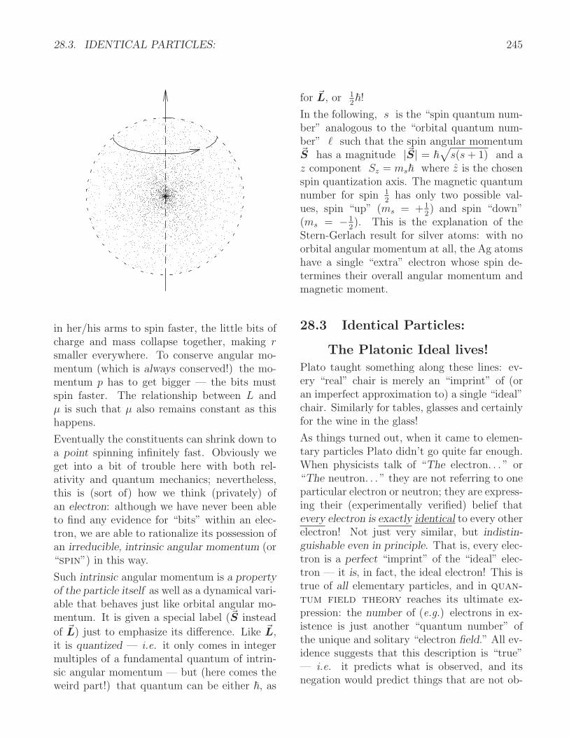
28.3. IDENTICAL PARTICLES: 245
in her/his arms to spin faster, the little bits ofcharge and mass collapse together, making rsmaller everywhere. To conserve angular mo-mentum (which is always conserved!) the mo-mentum p has to get bigger — the bits mustspin faster. The relationship between L andµ is such that µ also remains constant as thishappens.
Eventually the constituents can shrink down toa point spinning infinitely fast. Obviously weget into a bit of trouble here with both rel-ativity and quantum mechanics; nevertheless,this is (sort of) how we think (privately) ofan electron: although we have never been ableto find any evidence for “bits” within an elec-tron, we are able to rationalize its possession ofan irreducible, intrinsic angular momentum (or“spin”) in this way.
Such intrinsic angular momentum is a propertyof the particle itself as well as a dynamical vari-able that behaves just like orbital angular mo-mentum. It is given a special label (~S instead
of ~L) just to emphasize its difference. Like ~L,it is quantized — i.e. it only comes in integermultiples of a fundamental quantum of intrin-sic angular momentum — but (here comes theweird part!) that quantum can be either ~, as
for ~L, or 12~!
In the following, s is the “spin quantum num-ber” analogous to the “orbital quantum num-ber” ℓ such that the spin angular momentum~S has a magnitude |~S| = ~
√
s(s + 1) and az component Sz = ms~ where z is the chosenspin quantization axis. The magnetic quantumnumber for spin 1
2has only two possible val-
ues, spin “up” (ms = +12) and spin “down”
(ms = −12). This is the explanation of the
Stern-Gerlach result for silver atoms: with noorbital angular momentum at all, the Ag atomshave a single “extra” electron whose spin de-termines their overall angular momentum andmagnetic moment.
28.3 Identical Particles:
The Platonic Ideal lives!
Plato taught something along these lines: ev-ery “real” chair is merely an “imprint” of (oran imperfect approximation to) a single “ideal”chair. Similarly for tables, glasses and certainlyfor the wine in the glass!
As things turned out, when it came to elemen-tary particles Plato didn’t go quite far enough.When physicists talk of “The electron. . . ” or“The neutron. . . ” they are not referring to oneparticular electron or neutron; they are express-ing their (experimentally verified) belief thatevery electron is exactly identical to every otherelectron! Not just very similar, but indistin-guishable even in principle. That is, every elec-tron is a perfect “imprint” of the “ideal” elec-tron — it is, in fact, the ideal electron! This istrue of all elementary particles, and in quan-
tum field theory reaches its ultimate ex-pression: the number of (e.g.) electrons in ex-istence is just another “quantum number” ofthe unique and solitary “electron field.” All ev-idence suggests that this description is “true”— i.e. it predicts what is observed, and itsnegation would predict things that are not ob-
246 CHAPTER 28. SPIN
served.
28.3.1 Spin and Statistics
What are some of these predictions? Probablythe most unambiguous example is the dramaticeffect of the indistinguishable nature of the par-ticles on scattering probabilities. However, an-other example was historically more importantand is more obviously essential to the qualita-tive properties of our universe. This has to dowith atomic physics and the Pauli exclu-
sion principle for electrons. Said principlewas actually surmised from atomic physics datain the first place, and was later proved mathe-matically. We will simply state it.
BOSONS
All elementary particles with integer spin (s =0, 1, 2, 3, · · ·) are called bosons because theyobey Bose-Einstein statistics — namely,an unlimited number of identical bosons can bein exactly the same state. (Here “state” meansthat all properties are fully specified.) Exam-ples of bosons are photons, 4He atoms, pions,. . . .
FERMIONS
All elementary particles with half-integer spin(s = 1
2, 3
2, 5
2, · · ·) are called fermions be-
cause they obey Fermi-Dirac statistics —namely, no two identical fermions can be in ex-actly the same quantum state. (This rule in-cludes the Pauli exclusion principle, butit carries over into many other branches ofphysics.) Examples of fermions are electrons,protons, neutrons, muons, quarks, . . . .
The name fermion honours Enrico Fermi, who(with Paul A.M. Dirac) described the specialproperties of this type of particles.
28.4 Chemistry
and The Periodic Table
Let us consider the consequences of the Pauli
exclusion principle for the chemical prop-erties of atoms: for each allowed wave funtion(or “orbital”) of an electron in the Coulombpotential, fully specified by the quantum num-bers (n, ℓ,mℓ), there are two (and only two)possible spin states for the electron: spin “up”(ms = +1
2) and spin “down” (ms = −1
2). Since
the Pauli principle only excludes occupation ofexactly the same state by two electrons, thismeans that each orbital may be occupied by atmost two electrons; and if both electrons arepresent in that orbital, their spins are necessar-ily “paired” — equal and opposite in direction,thus perfectly cancelling each other and con-tributing nothing to the net angular momentumor magnetic moment.
Determining the chemical properties of the ele-ments thus becomes a simple matter of count-ing states: for each “shell” (n) we see how manydifferent orbitals there are with different val-ues of ℓ and mℓ and then multiply by two forthe two ms possibilities to get the total numberof electrons that will “fit” into that shell. Ofcourse, this simple picture contains some crudeapproximations that we must expect to breakdown before things get very complicated, andthey do. We assume, for example, that for apositive charge of +Ze on the nucleus, eachtime we “add another electron” it goes into thelowest available (unfilled) energy state and ef-fectively reduces the effective charge of the nu-cleus by one. That is, the first electron “sees” apositive charge of +Ze but the second electron“sees” a positive charge of +(Z − 1)e, and soon. This is not true, of course, for electrons inthe same n shell; they all pretty much see thesame apparent charge on the “core” of the atom(and see each others’ charges as well). One im-portant effect of such “screening” is that statesof higher ℓ (whose wavefunctions do not pene-

28.4. CHEMISTRY 247
trate as deeply into the core) “see” on averagea lower effective charge on the core and there-fore are slightly less bound (higher energy) thantheir low-ℓ neighbours. This provides the rulethat (up to a point) lower ℓ states are filled first.A collection of states with the same n and ℓ iscalled a “subshell.”
If we want to do this right for an arbitrarymany-electron atom, we have several very dif-ficult problems to solve: first, for large Z theinnermost electrons have kinetic energies com-parable to their rest mass energy; thus ournonrelativistic Schrodinger equation is inade-quate and one must resort to more advanceddescriptions. Second, the approximation thatone shell simply “screens” part of the nucleus’charge from the next shell is not that great,especially for wavefunctions that have a sig-nificant probability density near the nucleus;moreover, electrons in the same shell definitely“see” each other and are affected by that inter-action. One way of approaching this problemis to start with an initial guess based upon thisapproximation and then recalculate each elec-tron wavefunction including the effects of theother electrons in their wavefunctions; then goback and correct again with the new guess as astarting point. Eventually this “Hartree-Fock”method should converge on the actual wave-functions for all the electrons. . . . Finally, thecoupling of orbital and spin angular momen-tum contributions can follow several possiblescenarios, depending upon which couplings arethe strongest; the final result must always be asingle overall net angular momentum (and mag-netic moment) for the atom as a whole; but forlarge atoms it is very difficult to predict evenits magnitude; the only thing we can be sure ofis that if there are an even number of electrons,protons and neutrons making up the atom, itwill be a boson.
Having issued these caveats, we can go back toour “state counting”:
• For each “shell” characterized by an en-
ergy En (starting at n = 1, where n is theprinciple quantum number) we haven possible values of ℓ, ranging from ℓ = 0to ℓ = (n − 1).
• For each orbital quantum number ℓ,we have 2ℓ+1 possible values of the mag-
netic quantum number mℓ, rangingfrom mℓ = −ℓ to mℓ = +ℓ.
• For each orbital specified by (n, ℓ,mℓ),there are two possible values of ms: spinup (ms = +1
2) and spin down (ms = −1
2).
Thus there are a total of Nn =n−1∑
ℓ=0
2(2ℓ + 1)
possible fully-specified states for electrons inthe nth energy shell. For the first shell, N1 = 2;for the second shell, N2 = 8.
Since (at least for small n) it is a long way (inenergy) between shells, a “closed shell” is espe-cially stable — it “likes” neither to give up anelectron nor to acquire an extra one from an-other atom; it has “zero valence.” This meansan atom with N1 = 2 electrons [helium] isvery unreactive chemically, and so is one withN1 + N2 = 10 electrons [neon]. This goes onuntil the breakdown of our assumption that allthe electrons for one shell are filled in beforeany electrons from the next shell. This break-down comes at the n = 3, ℓ = 2 subshell. Then = 4, ℓ = 0 subshell is actually lower in energythan the n = 3, ℓ = 2 subshell and therefore fillsfirst, despite having a higher n. At this pointour simple qualitative rules fail and we mustrely on empirical information to further under-stand the chemical properties of the elements.
28.4.1 Chemical Reactions
Two atoms can “react” chemically in eitherof two ways. In the ionic reaction, one cangive up an electron (becoming a positive ionor cation [so called because it is attracted to anelectric cathode]) to the other, which becomes a

248 CHAPTER 28. SPIN
negative ion or anion [because it is attracted toan electric anode]; the two oppositely chargedions are then attracted to each other by theCoulomb interaction but do not have to stay to-gether — sort of like today’s high school dances.When the two atoms can’t decide which wouldrather be the donor or the receptor of elec-trons, they can form the ambiguous or cova-
lent bond, in which they share one or moreelectrons; in this case everyone stays electricallyneutral but no drifting away from one’s partneris allowed.
249
Chapter 29
Small Stuff
From Democritos through the Alchemists of the Middle Ages and Mendeleyev’s Periodic Table ofthe Elements all the way to modern Elementary Particle Physics, one of the first duties of“Natural Philosophers” has been to make up lists of all possible constituents of matter — preferably(for the sake of simplicity) including only the irreducible components.
This notion may well be obsolete in the literal physical sense, but the concept lives on; and it istempting (if misleading) to describe Elementary Particle Physics as the art of inventing the simplestpossible classification scheme for the “zoo” of known “elementary” particles.
Objects or entities can only be classified in terms of their properties. Thus the first task is to defineall the (known) intrinsic properties of matter as concisely as possible, invent ways of measuringhow much of each property a given particle has, and do the experiments. Of course, this is a highlyiterative process — after each round of experiments the theorists have to go back to their drawingboards and revise the Ultimate Classification Scheme — but the idea is still the same. My taskis now to summarize in one Chapter over half a century of progress along these lines. Naturally Iwill omit as many of the false starts and backtracks as possible, to make it look as if the presentscheme1 is correct and was obvious from the outset.
29.1 High Energy Physics
Before we begin to construct a classification scheme for the “elementary” particles, we need to havesome feeling for the phenomenology involved — and maybe even a bit of historical perspective.
In some sense High Energy Physics (the experimental discipline) began when the first cyclotroncapable of producing pions “artificially” was built by Ernest Orlando Lawrence at Berkeley in theearly 1940’s.2 However, high energy physics (the behaviour of Nature) began in the instant ofcreation of the Universe — and it will be a long time before we are able to study the interactions of
1Actually, to be honest, this is not the present scheme. It is the one I learned 30 years ago, beefed up with the tidbits I haveabsorbed since then. Nowadays people talk about the “Standard Model,” a more elegant presentation of the dog’s breakfastyou will get from this Chapter — but not, I think, really a different story. Some of the lower limits on the masses of as yetundiscovered particles will have doubled or tripled recently, so don’t take the numbers in the tables too seriously.
2Lawrence’s 184 inch Cyclotron, the biggest solid pole-tip magnet synchrocyclotron ever built, was originally conceived as agiant mass spectrometer for separating the isotopes of uranium for the first fission bomb; however, a far more efficient methodwas invented soon after it was built, and “the 184” went into service as a pion and muon producer. Many Ph.D. theses(including my own in 1972) were written on experiments performed at the 184 until it was dismantled in the 1980’s to

250 CHAPTER 29. SMALL STUFF
matter at the energies and densities of those first few femtoseconds.3 I will compromise by datinghigh energy physics (the modern human endeavour) from the hypothesis of Hideki Yukawa in1935 that the strong nuclear force must be mediated by the exchange of particles of intermediate[between electrons and protons] mass, which he therefore named “mesons” [as in mesozoic orMesopotamia(?)]. Where did he ever get such an idea?
29.1.1 QED
It began with the Feynman diagram first shown in the Chapter on relativistic kinematics.In Fig. 29.1 I show the Feynman diagrams for single and double photon exchange in Quantum
ElectroDynamics or QED, for which Richard P. Feynman shared a Nobel Prize. As before,I will draw Feynman diagrams “left to right” instead of the conventional “down to up.” Theidea of QED was (and is) that all electromagnetic interactions between charged particles can bedescribed in terms of the exchange of photons created by one particle and destroyed by another.The simplest case is the “first-order” diagram in Fig. 29.1, where two electrons exchange a singlephoton. The next (second-order) process is a factor of α2 less important, where α ≈ 1
137is the
fine structure constant (not a very mnemonic name any more), which is (sort of) the strengthof the QED “vertex” (the point where the photon begins or ends). Because each successive diagram(single photon exchange, double photon exchange, triple photon exchange, etc.) is a factor of about19,000 less important than the one before, QED is a perturbation theory that converges veryrapidly. That is, you can get a pretty accurate result with very few diagrams.
Figure 29.1 Feynman diagrams for electromagnetic electron-electron scattering in first order(left) and second order (right).
Each diagram, you see, is rigourously equivalent to a big messy integral which is definitely lessappealing to the Right Hemisphere; but the big integral can be evaluated to give the correct formulafor the interaction of the two electrons to that order in QED, properly taking into account all theramifications of quantum field theory. Which is. . . ? Let’s take another step back for better
make room for what was then the world’s most intense Synchrotron Light Source on the same site at what has been calledthe Lawrence Berkeley Laboratory (LBL) since the end of the 1960’s. [Before that it was called the Lawrence RadiationLaboratory (LRL); the name was changed to avoid association with the other LRL branch in Livermore (now known as LLL,the Lawrence Livermore Laboratory) where weapons research is conducted, and to expunge that fearsome word “Radiation.”Spineless politicians!]
3I refer, of course, to the “Big Bang” scenario, which is almost universally regarded as the best model of cosmogony [afancy word for Creation]. Perhaps I will get to say a few words about the Big Bang in a Chapter on general relativity.

29.1. HIGH ENERGY PHYSICS 251
perspective.
29.1.2 Plato’s Particles
When Quantum Mechanics was first developed, it was formulated in a nonrelativistic limit — i.e.,the particles involved were presumed not to have enough kinetic energy to create other particles.Because, if they did, then not only the quantum states of each particle, but the number of particlespresent, would have to be described by the theory. You can see that the combination of QuantumMechanics with Relativity makes relativistic quantum mechanics a rather more complicatedsort of problem.
Quantum mechanical equations were found for bosons (the Klein-Gordon equation) and forfermions (the Dirac equation) which obeyed the correct relativistic transformations, but nowthe wave functions [φ for bosons, ψ for fermions] could not be interpreted as simply as before— in terms of the probability amplitude for a single particle. Now they had to be interpreted asthe probability amplitude of the field of the corresponding particle, for which the number of suchparticles was merely a quantum number of the field.4
As a result, when a Particle Physicist speaks of “the electron,” (s)he is referring to the electronfield, an absolutely literal example of the Platonic Ideal, in which the disposition (and even thenumber) of actual individual electrons is merely a state of the electron [field]. An actual singleindividual particle in the laboratory is rarely the source of much information about the completeset of all its identical siblings.
A given Feynman diagram therefore represents one possible case of the numbers and types of parti-cles present in an interaction with a specified initial and final state. It is one possible manifestationof the fields.
29.1.3 The Go-Betweens
A common feature of all such Feynman diagrams is the virtual particle(s) being exchanged[created on one side and annihilated on the other] between the interacting particles. They are called“virtual” because they never manifest themselves directly outside the scattering region; of course,in most cases the same sorts of particles can be “knocked clear” of the collision by appropriatecombinations of momenta, but then the diagram has a different topology. For instance, in Fig. 29.2the right-hand diagram involves a simple rotation of the left-hand diagram by 90 and so it describesin some sense “the same physics” — but the process depicted, in which a positron and an electron“temporarily annihilate” into a photon and then that photon immediately converts into a new e+e−
pair, is nominally quite different from the electron-electron scattering in the left diagram. AnyQED adept would automatically think of both as being more or less the same thing.
How is it possible to create a particle “out of nothing” as pictured in these diagrams? Only byvirtue of the time-energy version of Heisenberg’s uncertainty principle, which says that you
4Just to give a hint of how this works, ψ is now composed of some complex exponential wave functions multiplied bycreation and annihilation operators that respectively increase and decrease the number of particles of that species by one.The creation and annihilation operators obey an algebra that corresponds to the statistical properties of the particle — e.g.,for fermions no two can be in the same state, etc. I will resist the temptation to show any of the equations, which are actuallyvery compact but (as one might expect) have an extremely high “interpretation density.”

252 CHAPTER 29. SMALL STUFF
Figure 29.2 Left: Feynman diagram for electron-electron scattering by single photon exchange.Right: “Crossing symmetry” diagram for electron-positron scattering in the “s-channel” byvirtual photon annihilation and pair production.
can “cheat” energy conservation by an uncertainty ∆E, but only for a short time ∆t such that
∆t ∆E ≥ ~
2(1)
The bigger the “cheat,” the shorter the time.
For photons, with no rest mass, a minimum of energy has to be “embezzled” from the “energybank” to create a virtual photon; as a result it can travel as far as it needs to find another chargedparticle to absorb [annihilate] it. A heavier particle, on the other hand, cannot live for long withouteither being reabsorbed by the emitting particle or finding a receiver to annihilate it; otherwise theuncertainty principle is violated. This brings us back to Yukawa.
Around Yukawa’s time every physicist knew that atomic nuclei were composed of nucleons (pro-tons and neutrons) confined to an extremely small volume. The problem with this picture is thatthe protons are all positively charged and the neutrons are (as the name suggests) neutral, so thatsuch a nucleus entails keeping positive charges very close to each other — something that coulomb
repulsion would rather they didn’t do! Therefore (reasoned Yukawa) there must be a “strong”attractive force between nucleons that was able to overpower the electrostatic repulsion.
But if the strong force were long-range like the electromagnetic force, then all nucleonseverywhere would “reach out to someone” and fall together into one gigantic nucleus! This appearsnot to be the case, luckily for us. Therefore (reasoned Yukawa) the strong force must be short-range.
Now, we have just finished describing what would make a force have a short range — namely, theexclusion principle: if the virtual quanta (particles) mediating the force are moderatelymassive [i.e., “mesons”] then they require a big “cheat” of energy conservation to be created in thefirst place, and must be annihilated again very soon to have existed at all. Yukawa compared theknown size of nuclei (about 10−15 m) with the uncertainty principle, assuming propagation atroughly the speed of light, and deduced that the mesons mediating the strong force must havea mass of about 130 MeV/c2.
A few years later, muons were discovered in high-energy cosmic rays,5 and the Physics worldwas quick to acclaim them as Yukawa’s mesons. Unfortunately, they were wrong; the muon is a
5Muons are the main component of cosmic rays that make it to the Earth’s surface — all the more strongly interacting

29.1. HIGH ENERGY PHYSICS 253
Figure 29.3 Left: Feynman diagram for proton-proton scattering by single pion exchange. Right:“Crossing symmetry” diagram for proton-antiproton scattering in the “s-channel” by virtualannihilation into a π0 followed by proton pair production. Note the similarity with the Feynmandiagrams for QED, where the pion’s role is played by a photon.
lepton, like the electron or the neutral neutrinos, which accounts for its penetration through theatmosphere (leptons do not interact strongly).6 This quickly became clear, and shortly thereafter thetrue “nuclear glue” meson, the pion, was discovered in very high-altitude cosmic ray experimentsand at the 184 inch Cyclotron in Berkeley. Then High Energy Physics began in earnest.
The Perturbation Paradigm Stumbles
It didn’t take long for the theory of strong interactions to run into problems. The essence ofthe difficulty lies in the very word “strong.” The strength of an interaction can be calibrated bythe magnitude of the dimensionless coupling constant applied at each vertex [wherever a virtualparticle is created or annihilated] in a Feynman diagram such as Fig. 29.1. As explained earlier,each such vertex in QED has a strength of α ≈ 1
137, which makes “higher order diagrams” rapidly
insignificant — great for calculating with a perturbation theory!
Unfortunately, the “strength” of a vertex in strong interactions is on the order of 1. This meansthat the single pion exchange diagram shown on the left in Fig. 29.3 or Fig. 29.4 is in principle nomore likely than the incomprehensible mess on the right in Fig. 29.4, involving manifold exchangesof pions and other mesons, as well as creation and annihilation of baryon-antibaryon pairs.7 Worseyet, this is only one example of the seemingly endless variety of possible diagrams one must inprinciple consider in order to make an accurate calculation of “simple” nucleon-nucleon scattering!
Of course, it wasn’t quite that bad. Handy “sum rules” were discovered that explained why singlepion exchange usually got you pretty close to the right answer, but in principle one had to make analmost infinitely difficult calculation in order to get the sort of precise predictions that PerturbationTheorists had come to expect from their experiences with QED. Moreover, there were conceptual
particles are absorbed or re-scattered in the atmosphere, which makes a pretty good shield. In fact, if you take a transcon-tinental trip at 30,000 feet altitude, you pick up about 50 mR of ionizing radiation from cosmic rays that are not absorbedbecause you are above most of the shield!
6In case you wondered, I am skipping over a lot of agonizing reevaluation and painstaking experiments that led to thediscoveries that justify using the “modern” names for all these particles; the muon was called a “mesotron” for years and isstill sometimes referred to as a “mu meson” in the USSR. But why sacrifice simplicity for mere historical accuracy?
7I haven’t bothered to label all the particles; see if you can find any violations of local conservation laws.

254 CHAPTER 29. SMALL STUFF
Figure 29.4 Left: Feynman diagram for single pion exchange. Right: A far more complicatedFeynman diagram that is in principle no less important!
nightmares to sweat out — if you look closely at Fig. 29.4, for instance, you will notice that a protoncan emit a pion [OK, there are pions inside protons] which can turn into a proton-antiproton pair[OK, there are protons inside pions. . . Wait a minute!] and so on. Like many nightmares, thisrevealed an unexplored avenue of understanding: in the 1960’s and 70’s, Geoffrey Chew and hisTheory group at Berkeley developed a non-perturbative theory of strong interactions that containedthe “bootstrap principle:” every hadron is made up of combinations of all the other hadrons(and itself). Although I never could understand Chew’s models, they represented a genuinely newparadigm that gained a good deal of purchase on the problem when suddenly the attention ofthe Particle Physics community was diverted by a revival of Perturbation Theory in the form ofa quark model, about which I will say more later; since then Chew’s approach has been sadlyneglected, which I suspect is a great loss to Physics. Still, if we can get answers more easily by“recycling an old paradigm,” the outcome is inevitable.
Weak Interactions
Skipping ahead to the 1980’s, the virtual quanta mediating the weak interaction (the forcenext weakest to the gravitational force) have only recently been identified directly in immenseexperiments at the biggest accelerators. These are the W± and Z0 “intermediate vector
bosons” whose masses are shown in Table 29.1.3. What can you conclude about the range of theweak interaction?
In a unification of the weak and electromagnetic interactions that won acclaim for numeroustheorists in the past two decades or so, the γ and the W and Z bosons have been shown tobe merely different aspects of the same “electroweak” force, despite their gross dissimilaritiesin mass and lifetime.8
8This theory now forms the core of what is known as “the standard model” of elementary particles — a name whichreveals a certain disaffection, since no one is particularly excited at the prospect of serving the Establishment prejudicesconnoted by a “standard model.” Particle Physicists, like most free thinkers, prefer the self-image of a romantic revolutionarychallenging established conventions and “standard models” everywhere. Not surprisingly, a great deal of experimental effortgoes into “tests of the Standard Model” which the experimenters openly hope will throw a monkey wrench into the works.
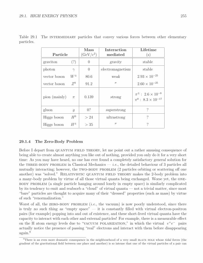
29.1. HIGH ENERGY PHYSICS 255
Table 29.1 The intermediary particles that convey various forces between other elementaryparticles.
Mass Interaction LifetimeParticle (GeV/c2) mediated (s)
graviton (?) 0 gravity stable
photon γ 0 electromagnetism stable
vector boson W± 80.6 weak 2.93 × 10⁻²⁵
vector boson Z0 91.2 ′′ 2.60 × 10⁻²⁵
pion (mainly) π 0.139 strongπ± : 2.6 × 10⁻⁸
π0 : 8.3 × 10⁻¹⁷
gluon g 0? superstrong ?
Higgs boson H0 > 24 ultrastrong ?
Higgs boson H± > 35 ′′ ?
29.1.4 The Zero-Body Problem
Before I depart from quantum field theory, let me point out a rather amusing consequence ofbeing able to create almost anything you like out of nothing, provided you only do it for a very shorttime: As you may have heard, no one has ever found a completely satisfactory general solution forthe three-body problem in Classical Mechanics — i.e., the detailed behaviour of 3 particles allmutually interacting; however, the two-body problem (2 particles orbiting or scattering off oneanother) was “solved.” Relativistic quantum field theory makes the 2-body problem intoa many-body problem by virtue of all those virtual quanta being exchanged. Worse yet, the one-
body problem (a single particle hanging around lonely in empty space) is similarly complicatedby its tendency to emit and reabsorb a “cloud” of virtual quanta — not a trivial matter, since most“bare” particles are thought to acquire many of their “dressed” properties (such as mass) by virtueof such “renormalization.”
Worst of all, the zero-body problem (i.e., the vacuum) is now poorly understood, since thereis truly no such thing as “empty space” — it is constantly filled with virtual electron-positronpairs (for example) popping into and out of existence, and these short-lived virtual quanta have thecapacity to interact with each other and external particles! For example, there is a measurable effecton the H atom energy levels due to “vacuum polarization,” in which the virtual e+e− pairsactually notice the presence of passing “real” electrons and interact with them before disappearingagain.9
9There is an even more dramatic consequence in the neighbourhood of a very small black hole whose tidal forces (thegradient of the gravitational field between one place and another) is so intense that one of the virtual particles of a pair can

256 CHAPTER 29. SMALL STUFF
Simple, eh?
29.1.5 The Seven(?) Forces
Although I have not yet defined what I mean by half the terms in Table 29.1.5, this is a convenientplace to summarize the known and hypothetical interactions of matter. It is conventional to group“superweak”10 together with the electroweak interaction (which “unifies” the weak and elec-
tromagnetic forces) and to put “superstrong” and “ultrastrong” in with the strong interactionso that you should not be surprised to hear that there are only three “official” forces — gravity,electroweak and strong. However, there is a certain amount of freedom in semantics here. . . .
Table 29.2 Interactions of the elementary particles. A “yes” means that the types of particleindicated at the left are directly coupled to the force above; “no” means the opposite; three asterisks(∗ ∗ ∗) means that the particle in question is the intermediary for that force.
Gravity Super- Weak Electro- Strong Super- Ultra-PARTICLE(s) weak magnetic strong strong
gravitons ∗ ∗ ∗
photons γ yes ? no ∗ ∗ ∗ no no no
neutrinos νe, νµ, ντ yes ? yes no no no no
leptons e, µ, τ yes ? yes yes no no no
mesons π,K, . . . yes ? yes yes yes no no
baryons p, n,Λ, . . . yes ? yes yes yes no no
neutral kaons K0, K0 yes yes yes yes yes no no
vector bosons W,Z yes ? ∗ ∗ ∗ yes no no no
quarks u, d, s, c, b, t yes ? yes yes no yes no
gluons g yes ∗ ∗ ∗
(hypothetical) T, V yes yes
Higgs bosons H yes ? ∗ ∗ ∗
Relative strength 10−40 ? 10−4 1137 1 10-100 > 1010?
fall into the black hole while the other is ejected and becomes a “real” particle — leading to intense radiation that can bedescribed as the explosive annihilation of the miniature black hole. This explains why there are no small black holes aroundany more, only big ones whose gravitational gradient is very gentle at the Schwartzschild radius. I will define these terms inthe Chapter on general relativity.
10The “superweak” force is a name coined to describe a really esoteric interaction which appears to affect only the decaysof strange neutral mesons (if it exists at all).

29.1. HIGH ENERGY PHYSICS 257
29.1.6 Particle Detectors
Turning back to the hardware of High Energy Physics (HEP), I should point out that it is not enoughto build accelerators capable of delivering enough energy to a collision to create more massive andmore exotic particles — one must also have some way to “see” those particles once they are created.This is in principle rather challenging, since they are all apt to be moving at near light speed andare certainly too small to detect with visible light; moreover, usually they don’t last very long —the heavier the particle, the larger the variety of lighter particles into which it might decay! Thisrule-of-thumb works quite well in general, so that exceptions (long-lived heavy particles) stand outrather dramatically; more on this later.
In practice it is surprisingly easy to “see” elementary particles, once you get used to a new way of“seeing.” The basis of all particle detectors is that charged particles cause ionization where theypass through matter.11 The ions they leave behind form a “track” that can be detected in severalways.
Scintillating!
The “workhorse” of experimental HEP is the scintillation counter. This simple device works asfollows: the ionization of certain types of molecules causes photochemical reactions that liberatevisible light called “scintillation” light.12 This light is conveyed through a clear liquid, plastic orcrystalline matrix, bouncing off polished exterior surfaces via total internal reflection until it reachesthe photocathode of a vacuum tube where the photons liberate electrons via the photoelectric
effect. These electrons are then accelerated by high voltages in the tube until they strike a “firstdynode” where each electron knocks loose about ten additional electrons which are acceleratedin turn to the “second dynode” where they in turn each knock loose another ten electrons each,and so on down a cascade of up to 18 dynodes. As a result, that one electron originally liberatedby the incoming photon can produce a pulse of 1018 electrons at the “anode” or the tube, whichis (mnemonically, for once) called a photomultiplier tube. These amazing devices have beenrefined over a period of nearly half a century until some have “quantum efficiencies” approaching100% (they can fairly reliably detect single photons) and (most importantly) generate electricalpulses a few ns (nanoseconds, billionths of a second) wide whose arrival at a bank of fast electronicsis correlated with the time the original ionizing particle hit the detector within a fraction of a ns.This means High Energy Physicists can routinely do timing with a resolution comparable to thelength of time it takes light to go 10 cm! Without this impressive timing capability it would bevery difficult to do any modern HEP experiments. Interestingly enough, this part of the technologyhas not improved significantly in several decades.
11Neutral particles either convert into charged particles (which do ionize the medium) or else are conspicuous in theirinvisibility!
12One example is old-fashioned “mothballs” — if you take a handful of mothballs into a very dark closet (you must get ridof all ambient light!) and wait for your eyes to adjust, you should be able to see tiny flashes of light every few seconds ascosmic ray muons zap the mothballs. There are many apocryphal stories about graduate students in closets with mothballsand manual counters in the early days of nuclear physics. . . .

258 CHAPTER 29. SMALL STUFF
Clouds, Bubbles and Wires
Although one can build arrays of scintillation counters that act like “pixels” in computer graphicsand can tell where particles go within an uncertainty of the size of the individual counters, this isvery expensive and not usually very precise. Moreover, it was not how the business of “tracking”elementary particles got started.
The earliest “position-sensitive detectors” took advantage of the tendency of liquid droplets toform (or “nucleate”) on ions when a gas (like air) is “supersaturated” with a vapour (like water oralcohol) that would like to precipitate but can’t quite make up its mind where to start. The result,once the process is finished, is a cloud of liquid droplets, hence the name “cloud chamber.” Butthis final state is not very useful. It is the situation just after a fast ionizing particle passes throughthe saturated gas that is interesting — the left-behind ions nucleate a trail of liquid droplets like astring of beads, and one can see (and/or take a picture of) that trail at that moment, to “see thetrack” of the particle. If it is passing through a magnetic field, the curvature of the track revealsits momentum and the density of the track reveals its charge and its speed, from which one learnsits mass and just about everything about it that can be measured directly. This device was usedfor many of the early cosmic ray experiments.
The trouble with cloud chambers is that they don’t have very fine resolution and the dropletsstart falling as soon as they form. Moreover, even a saturated gas has a rather low density, so ifone is looking for interactions of a beam particle with other nuclei the events are spread out overtoo large a volume to photograph efficiently. Another method still used today is to place a stack ofphotographic emulsions in the path of the beam and to examine the resulting tracks of silverparticles created by the ionizing particle. The problem with this technique is that the emulsion isnot reusable — one “takes an exposure” and then the emulsions must be dissected and painstakinglyexamined with a microscope. Too much work. What was really needed was a sort of “high densitycloud chamber” that “healed” soon after each track had been photographed.
The apocryphal story is that a HEP experimenter sat staring glumly into his beer glass one nightafter wishing for such a device, and noticed that the bubbles always seemed to form in the sameplaces. He sprinkled in a few grains of salt and, sure enough, the bubbles formed on the salt grains.“Eureka!” he cried, leaping up, “the bubbles form on ions!” And off he went to build the firstbubble chamber.13
The idea of the bubble chamber is that a liquid (usually liquid hydrogen) can be abruptlydecompressed, causing it to “want” to boil, but (like the supersaturated vapour) it can’t make upits mind where to start first.14 If the decompression is done just as ionizing particles pass throughthe liquid, the ions in their tracks will nucleate the first bubbles of vapour and a clear, sharp trackcan be seen and photographed; then the liquid is quickly recompressed, the bubbles go away, andthe chamber is ready for another “event.”
Such liquid hydrogen bubble chambers are still in use today, but they had their heyday back inthe 1950’s and 1960’s when higher energy accelerators introduced Particle Physicists to the “Hadron
13Probably this was a bar frequented by many HEP types, so such behaviour went unremarked.14If you have access to a microwave oven, you can observe this effect for yourself: take a cup of cold water and slowly
increase the cooking time (replacing it with new cold water each time) until it is just starting to boil as the timer runs out.Then do one more with a slightly decreased cooking time, take out the cup and drop in a few grains of sugar or salt — thedissolved gases will abruptly come out of solution around these “nucleation centres” to make a stream of bubbles for a shorttime.

29.2. WHY DO THEY LIVE SO LONG? 259
Zoo” of strongly-interacting particles. The most gratifying aspect of a bubble chamber picture isthat you can make a big copy of it and put it on your wall, where anyone can point to the differenttracks and say, “There goes a pion,” or, “This short gap here is a Lambda.” The picture appeals tothe all-important Visual Cortex, leading to such familiar phrases as, “Seeing is believing,” and, “Apicture is worth a thousand words.” [I won’t attack these comforting myths this time; I like bubblechamber pictures too!]
The trouble came when experimenters set out to measure the curvatures and densities of millions oftracks in bubble chamber pictures. This involves more than just patience; in the 1960’s an army of“scanners” was hired by the big HEP labs to filter hundreds of thousands of bubble chamber pictureslooking for certain topological configurations of tracks that were of interest to the experimenter;a lexicon of “vees” and “three-prongs” was built up and eventually these people could recognizeevents containing different types of elementary particles more efficiently than any Physicist — for,almost without exception, the scanners were nonscientists selected for their rare talents of patienceand pattern recognition. It was a fascinating sociological phenomenon, but it cost enormous sumsfor the salaries of these people and Physicists would always rather buy fancy equipment than createmere jobs. So, as electronics and computers grew in power and shrank in price, it was inevitable thatthe experiments pressing the limits of HEP technology would seek an “electronic bubble chamber”that could be read out, analyzed and tabulated all by computers.
The result was the wire chamber, which again uses the ionization caused by charged particlesbut this time detects the ion’s charges directly with sensitive electronics. There are many versionsof this technology, but almost all involve thousands of tiny wires strung through a target volumeat extremely precise positions and maintained at high voltage so that any ions formed will drifttoward one or more of the wires and form a pulse that can be read out at the ends of the wire andinterpreted. Such devices can “track” particles through huge volumes to a fraction of a mm andcan analyze hundreds or even thousands of events per second, with one “event” containing dozensor even hundreds of particle tracks.
Today’s large HEP experiments all involve scintillation counters, wire chamber arrays and othercomponents, each especially sensitive to one or another type of particles, and require on-line com-puters that must be built specially to handle the enormous flow of information;15 an ubiquitousfeature of really high energy particle physics is that there are enormous numbers of particles in the“final state” after two extremely high energy projectiles collide head-on. It is easy to see why thisis: the more energy you have, the more mass you can create. It also follows that the heavier theparticle, the more ways it has to decay, so the heaviest particles should have the shortest lifetimes.When this rule is not obeyed, we have cause to get suspicious.
29.2 Why Do They Live So Long?
If a heavy particle is free to decay into lighter particles, then why isn’t the universe filled withonly the lightest particles? Why, for instance, doesn’t an electron (mass 0.511 MeV/c2) decay intophotons (zero mass), with the excess mass appearing as kinetic energy? Well, to begin with, the
15For decades, HEP has “driven” the leading edge of supercomputer hardware and software development. Today’s computingenvironment is rapidly becoming more driven by the personal workstation, which is probably a more healthy arrangement,but it is certainly true that we would not have the computer technology we do without the demand created by HEP fromabout 1950 to about 1980.
260 CHAPTER 29. SMALL STUFF
electron has “spin 12” (i.e., an intrinsic angular momentum of 1
2~), while a photon has “spin 1”
(i.e., 1 ~). There is no way to combine several spin 1 objects to make a spin 12
object, so angular
momentum conservation forbids an electron to decay into photons. What else? Well, theelectron is charged, and the photons aren’t! So what? Well, electric charge Q is a conserved
quantity — not only is the total amount of charge in the universe constant, but the net chargein any reaction must also remain unchanged at every step.
OK, the electron is stable. But why can’t the proton decay into a positron (the antiparticle ofan electron), which has the same charge and the same spin as the proton? It could also give offtwo photons with opposite spins, satisfying all the criteria mentioned so far. Well, protons musthave some special property that we will call baryon number because only heavy particles like theproton have it. So far as we know, baryon number manifests itself only as a conserved quantity
in the interactions of elementary particles. We define the baryon number of a proton to be 1 andthat of electrons and photons to be zero. Baryon number is conserved just like electric charge, andthis accounts for the stability of protons: the proton is the lightest baryon, so there is nothing forit to decay into!
The next lightest baryon is the neutron, and it does indeed decay (slowly) into a proton, an electron(to compensate for the charge of the proton) and an electron antineutrino to compensate for theelectron number.16 Huh? What’s “electron number?” It’s yet another conserved quantity
that the weak interaction governing neutron decay has to keep account of. We know it exists onlybecause neutrons don’t decay into just a proton and an electron. The electron neutrino is a sortof chargeless, massless version of an electron that has almost no interaction with matter at all — atypical neutrino can pass through the Earth (and a lot more planets besides!) without much chanceof touching anything!
How about muons? Everyone says these are “sort of like heavy electrons,” so why can’t a muondecay into an electron and a photon?17 The muon does decay into an electron plus an electronantineutrino and a muon neutrino, but not into an electron and a photon. This is because themuon has another different conserved quantity called — you guessed it – muon number
which is a different flavour18 from electron number. Naturally, the muon neutrino hasmuon number too, and is therefore unmistakable for an electron neutrino. But only because itnever appears where an electron neutrino might.
Is all this perfectly clear? No? I don’t blame you. Just remember, whenever a particle refusesto decay into lighter particles for no apparent reason, it is presumed to be because of some newconserved quantity that one has and the others don’t. The assignment of names to theseephemeral quantities which Nature seems to hold in such reverence is pretty much arbitrary, sotheir “discoverers” get to think up names they think are mnemonic, allusive or just cute. There aresome examples that are a little embarrassing.
For instance, while discovering hordes of new short-lived heavy particles in the 1950’s, people ranacross a heavy, spinless, uncharged particle called the neutral kaon which decayed (as expected)
16It just barely makes it, mass-wise, which partly accounts for the slowness of the decay.17As a matter of fact, this is still an open question — experiments have recently pushed the upper limit on the “branching
ratio” for µ → eγ (i.e., the fraction of the time muons decay into electrons and photons) to less than one part in 1011 andmore experiments are underway, because several theories demand that such “flavour-violating” decays must exist at somelevel.
18No, I’m not kidding, the official name for the difference between muons and electrons (and, later on, tau leptons) is“lepton flavour.”

29.3. PARTICLE TAXONOMY 261
into lighter pions but very slowly, suggesting that kaons must have some new property which thestrong interaction (that should make kaons decay very rapidly into pions) could not “violate”but the weak interaction could. This new quantity, conserved in strong interactions but notnecessarily in weak interactions, was called “strangeness” for reasons that were obvious buthopelessly parochial. I hate this one, because it takes over a perfectly good English word that onemight want to use in the same sentence.19
It gets worse. But I have introduced far too many new particles and mentioned far too manyjargoney names without explaining what they are supposed to mean; I will come back to theliterary tastes of Particle Physicists after I have outlined some of the currently used classificationschemes.
29.3 Particle Taxonomy
The most efficient classification scheme is a succession of orthogonal binary dichotomies in which(if possible) roughly half the items to be classified go on each side of every successive distinction.These may be drawn as “Venn diagrams” in which a circle (representing everything) has a linedrawn through the middle.
The first distinction does not even come close to splitting up all the “elementary” particles intotwo equal groups, but at least it is unequivocal. This is the question of whether the particle isstrongly interacting or not. If it is affected by the strong interaction, it is called a hadron.If not, it is called a lepton. [Both of these have Greek roots. Look them up if you’re curious.]
29.3.1 Leptons
The leptons make a short list and are easy to classify by the three known “flavours” — e, µand τ . Each type experiences gravity, the electroweak interaction and apparently nothingelse.
29.3.2 Hadrons
The remaining strongly-interacting hadrons make a huge “zoo” of mostly short-lived particles ofalmost every shape and size. However, these too can be separated cleanly into two dichotomouscategories: the half-integer spin baryons (so named because they tend to be more heavy), whichare all fermions — i.e., each type obeys its own version of the Pauli exclusion principle —and the zero or integer spin mesons (so named because they tend to me medium heavy), whichare all bosons — i.e., you can put as many as you like in the same state at the same time. Wenow know lots of interesting things about the baryons and mesons, but the modern definitionsof these classes of hadrons are in terms of their spins.
Integer spin hadrons are bosons and are all called mesons; Half-integer spin hadrons are fermions;those which are not quarks are called baryons. All baryons have a “baryon number” B = 1; mesonshave none. The “hypercharge” Y of a particle is the sum of its baryon number and its strangeness:
19Kirk: “Boy, this particle sure looks strange.” Spock: “Not at all, Captain. If you look more closely, I believe you’ll findit’s charmed.”

262 CHAPTER 29. SMALL STUFF
Table 29.3 The leptons (particles with only weak and sometimes electromagnetic interactions).All leptons have spin J = 1
2~ and are therefore fermions. Each “generation” of lepton has its own
distinctive “flavour” (electron, muon, tau) and is governed by its own conserved “lepton number.”For each particle there corresponds an antiparticle of the same mass and spin but with oppositevalues of electric charge and lepton number of the corresponding flavour.
Mass Charge Lifetime PrinciplePARTICLE(s) (MeV/c2) Q/e (s) Decay Modes
electron e 0.511 −1 > 6 × 1029 none
e neutrino νe < 1.7 × 10⁻⁵ 0 ∞ none
muon µ 105.66 −1 2.2 × 10⁻⁶ µ− → e− + νe + νµ
µ+ → e+ + νe + νµ
µ neutrino νµ < 0.27 0 ∞ none
tau τ 1784 −1 3.03 × 10⁻¹³τ− → (µ, e)− + ν(µ,e) + ντ
τ− → (hadron)−
+ (neutrals) + ντ
τ neutrino ντ < 35 0 ∞ none
Y = B + S. Quarks all have B = 13
as well as fractional electric charge because it takes 3 tomake one baryon; otherwise they follow the same rules. For each particle (including quarks) therecorresponds an antiparticle of the same mass, spin, parity and isospin, but with opposite values ofelectric charge, strangeness, baryon number and hypercharge.
Generally speaking, all the heavy hadrons are very short-lived because the interaction governingtheir decay into lighter hadrons is, after all, strong. I have already mentioned a notable exceptionto this rule, namely the strange mesons, which take far longer than they should to decay intopions. In the 1950’s this led to the coining of the term strangeness to describe that strange(grrr. . . ) property of K mesons (for instance) that could not be “swept under the rug” by thestrong interaction. By checking to see what other particles could decay into kaons, and in thecompany of what else, a strangeness was assigned to each of the hadrons. Then a strange [Oops!Can’t use that!] — an odd [Ouch! That implies a parity quantum number] — a peculiar [Whew!]pattern began to manifest itself when the particles were grouped together according to the knownquantifiable properties of spin, charge, strangeness and mass.
The various hadrons are first separated into collections that all have the same spin, such as thescalar [zero spin] mesons or the vector [spin 1] mesons or the spin-1
2baryons or the spin-3
2
baryons. It is immediately evident that the masses of all the particles in any one of these groupsare roughly similar, whereas two different groups tend to have significantly different masses. Thisarouses some suspicion. Then we notice that, within these groups, the particles with the moststrangeness tend to be the heaviest.
Next we notice that if we plot the particles in a group on a graph of the two other quantifiableproperties — charge Q and strangeness S — they form arrangements that are remarkably similarin shape!20 The hexagonal arrangement with two particles at the centre appears in each of the
20The shapes are a little crooked in this representation. The hypercharge Y and isospin I (whose “projection” I3 along
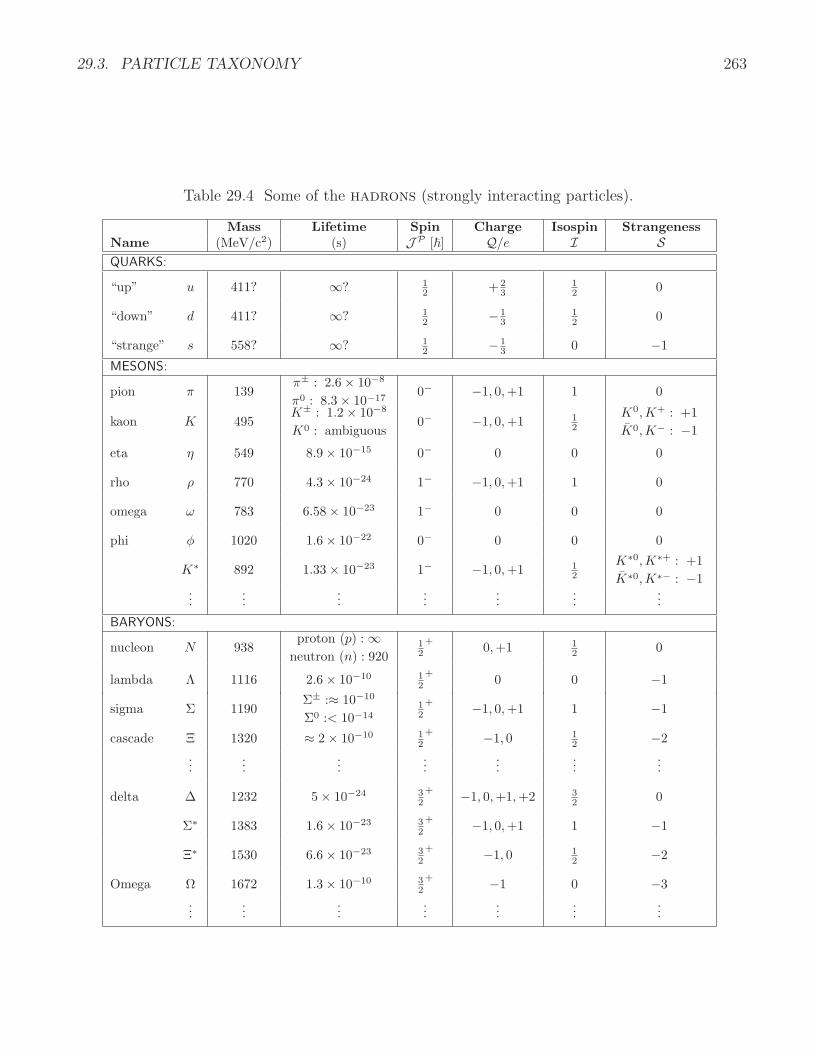
29.3. PARTICLE TAXONOMY 263
Table 29.4 Some of the hadrons (strongly interacting particles).
Mass Lifetime Spin Charge Isospin StrangenessName (MeV/c2) (s) J P [~] Q/e I SQUARKS:
“up” u 411? ∞? 12 + 2
312 0
“down” d 411? ∞? 12 − 1
312 0
“strange” s 558? ∞? 12 − 1
3 0 −1
MESONS:
pion π 139π± : 2.6 × 10⁻⁸
π0 : 8.3 × 10−170− −1, 0,+1 1 0
kaon K 495K± : 1.2 × 10⁻⁸
K0 : ambiguous0− −1, 0,+1 1
2
K0,K+ : +1
K0,K− : −1
eta η 549 8.9 × 10⁻¹⁵ 0− 0 0 0
rho ρ 770 4.3 × 10⁻²⁴ 1− −1, 0,+1 1 0
omega ω 783 6.58 × 10⁻²³ 1− 0 0 0
phi φ 1020 1.6 × 10⁻²² 0− 0 0 0
K∗ 892 1.33 × 10⁻²³ 1− −1, 0,+1 12
K∗0,K∗+ : +1
K∗0,K∗− : −1...
......
......
......
BARYONS:
nucleon N 938proton (p) : ∞
neutron (n) : 92012
+0,+1 1
2 0
lambda Λ 1116 2.6 × 10⁻¹⁰ 12
+0 0 −1
sigma Σ 1190Σ± :≈ 10−10
Σ0 :< 10−1412
+ −1, 0,+1 1 −1
cascade Ξ 1320 ≈ 2 × 10⁻¹⁰ 12
+ −1, 0 12 −2
......
......
......
...
delta ∆ 1232 5 × 10⁻²⁴ 32
+ −1, 0,+1,+2 32 0
Σ∗ 1383 1.6 × 10⁻²³ 32
+ −1, 0,+1 1 −1
Ξ∗ 1530 6.6 × 10⁻²³ 32
+ −1, 0 12 −2
Omega Ω 1672 1.3 × 10⁻¹⁰ 32
+ −1 0 −3
......
......
......
...

264 CHAPTER 29. SMALL STUFF
Figure 29.5 Murray Gell-Mann’s “Eightfold Way.” Left: the scalar mesons. Right: the spin-12
baryons. Note the striking similarity of the grouping when strangeness S is plotted againstcharge Q. The vector (spin 1) mesons form a group exactly like the scalar mesons on theleft, further reinforcing the pattern.
first three groupings listed above; Murray Gell-Mann decided that this must mean something
about the constituents of these particles, just as the regular groupings of elements in the periodic
table meant something about the constituents of atoms. Because of the number of particles in thepattern, because of his eclectic intellect and because he wanted to make up a catchy name for histheory that people would want to talk about just to sound savvy, Murray named this pattern theeightfold way after the spiritual/behavioural prescription in Buddhism. More cuteness.
29.3.3 Quarks
Fair enough, obviously these symmetries were trying to tell us something about the composition ofhadrons. What? Well, needless to say, Gell-Mann et al. did not immediately come up with a simplenuts-and-bolts assembly manual; instead, they developed an abstract mathematical descriptioncalled SU(3) analogous to the description of spin for electrons, SU(2). [If you’re interested, theacronym stands for Simple Unitary group of order 2 or 3.] I won’t attempt to elaborate, but youcan see why something like this was needed — as for the z component of spin, the projections ofthe three SU(3) operators along God-only-knows what axes in God-only-knows what dimensions21
cannot have a continuum of possible values but only a fixed number of discrete or quantized values.
God-only-knows what axis is the same as its charge Q, within a constant) were invented partly to make the diagrams of Y vs.
I3 nicely symmetric with the origin at the centre of each arrangement. I haven’t bothered.21Honest, we don’t have the faintest idea whether there is actually some space in which isospin actually refers to rotations
about some axis, we only know that isospin transforms that way. If there is such a space, none of its dimensions are ourfamiliar x, y or z directions. Very weird.

29.3. PARTICLE TAXONOMY 265
What is actually refers to is totally unknown. Or, more properly, it refers to just what it says; ifthat means nothing to us, well, that’s just because our empirical personal experience of the space ofSU(3) is so limited that we don’t relate to it very well. What do “normal” space and time actuallyrefer to?
Anyway, someone inevitably formulated a simpler instruction manual for assembling hadrons. Thiswas to give the requisite properties to three (there are more now, but hold off on that) really fun-damental component particles called “quarks.”22 All mesons are composed of a quark-antiquarkpair whereas baryons are composed of three quarks held together by a “superstrong” force me-diated by a new type of intermediary called “gluons” (g) [more cuteness, but who can argue. . . ].
Table 29.5 The known (or suspected) “generations” of quarks All quarks have a “baryon number”B = 1
3as well as fractional electric charge because it takes 3 to make one baryon. The “hypercharge”
Y of any particle is the sum of its baryon number and its strangeness: Y = B + S. For each quarkthere corresponds an antiquark of the same mass, spin, parity and isospin, but with opposite valuesof electric charge, strangeness, baryon number and hypercharge.
Mass Lifetime Spin Charge Isospin StrangenessName (MeV/c2) (s) J P [~] Q/e I S
“up” u 411? ∞? 12 + 2
312 0
“down” d 411? ∞? 12 − 1
312 0
“strange” s 558? ∞? 12 − 1
3 0 −1
“charm” c ≥ 1500? ∞? 12 + 2
3 0 0
“bottom” b ? ∞? 12 − 1
3 0 0
“top” t ? ∞? 12 + 2
3 0 0
cc J/ψ 3100 0.97 × 10⁻²⁰ 1− 0 0 0
......
......
......
...
Colour
The three original quarks are “up” (u), “down” (d) and of course “strange” (s). Each is a spin-12
fermion but it took some time to understand how three similar quarks could coexist in thesame state within a baryon. (The extension of the Pauli exclusion principle forbids this.)The resolution of this dilemma was to propose (and later believe) that each quark comes in threedifferent complementary “colours” (call them red, green and blue) that have to be combined tomake the composite particle (meson or baryon) colourless (white) just the way the three colourson a TV monitor must all be lit up at once to produce a white “pixel.” Of course, we have no
22See James Joyce’s Finnegan’s Wake for the origin of the term “quark” — it was originally a nonsense syllable, whichmakes it a pretty good choice for its present application. At least the commandeering of the word “quark” by Particle Physicsdid not inconvenience any users of the English language.

266 CHAPTER 29. SMALL STUFF
Figure 29.6 Upper left: the three lowest-mass quarks. Lower left: the corresponding antiquarks.Right: the spin-3
2baryons. The Ω− (strangeness −3) was predicted by a “quark content” analysis
and later found experimentally, convincing everyone that the SU(3) model was correct.
idea what colour is — it certainly has nothing whatsoever to do with the wavelengths of visiblelight! — but by now you should be comfortably disconnected from the world of empirical personalexperience, so the fact that the metaphor of colour gives us a handy way of getting right answersshould suffice.
Using this quark model with gluon exchange [gluons are colour changers, they convert a quarkfrom one colour to another when emitted or absorbed] in a fashion exactly analogous to QED,theorists are now able to accurately describe much of the structure of hadrons, thereby rescuingperturbation theory from the ashes of strong interactions, where it failed miserably.23 The newtheory inevitably became known as Quantum ChromoDynamics (or QCD) by analogy with QEDexcept with colour (Greek chromos) in place of electric charge.
Why Quarks are Hidden
If quarks are “real” particles and not just a cute mnemonic metaphor for some esoteric mathemat-ics,24 we ought to be able to “see” one in a bubble chamber or other device “watching” a highenergy scattering event. Unfortunately, this can never be. The reason is intriguing.
The “superstrong” force between quarks is transmitted by the exchange of gluons [a nice
23Unfortunately, the genuinely new paradigms that were springing up to deal with this crisis (e.g. Geoffrey Chew’s boot-
strap theory, in which each hadron is composed of small amounts of all the others [think about it!]) have been neglectedsince the development of QCD.
24Of course, energy is “just a cute mnemonic metaphor for some esoteric mathematics,” if we think back to ClassicalMechanics; but we have gotten so used to energy that we don’t think of it that way any more, whereas quarks arestill. . . well, weird.

29.4. MORE QUARKS 267
Figure 29.7 Left: QCD in first order — two quarks exchange a single gluon at close range. Right:if the two quarks get too far apart, the original gluon gets an chance to branch into several gluons,strengthening the attractive force.
descriptive name, for once!] which are massless, like photons, but have one trick up their sleevesthat photons don’t: they can “branch” (one gluon coupling to two gluons, and so on) if givenenough room. Thus, while the electromagnetic force drops off as 1/r2, the superstrong or QCDforce actually increases with increasing distance between the two quarks! Once the distance getsbig enough — as in a high-energy collision — the energy stored in the gluon field is so intense thatquark-antiquark pairs are created out of the vacuum between the quarks and the original quarkgrabs the new antiquark to become a meson, while the new quark takes the place of the old one inthe hadron that has collided.
Thus, try as we might, we can never create a free quark. We can never “see” these ubiquitousparticles that make up everything around us except leptons. This is very frustrating and for yearsled many Particle Physicists to insist that quarks were just figments of theorists’ imaginations. Butof course the paradigm works too well to be abandoned and the skeptics have by now pretty muchgiven up.
29.4 More Quarks
Elementary Particle Physics seemed to be “converging” at last on a simple description in termsof a manageable number of really elementary constituents until around 1964, when some roguessuggested that if there were 6 leptons (counting the neutrinos) then there ought to be 6 quarkstoo, Nature being endowed with frugality and æsthetics just like Mathematicians. Actually theargument may have been more convincing than that, but I didn’t understand it. This might nothave raised many eyebrows except that in 1974 two huge groups of Particle Physicists led by BurtonRichter and Samuel Ting simultaneously (or so close that no one could claim the other had stolenthe idea) discovered a new meson that was both very heavy (3100 MeV/c2) and extremely stable(0.97 × 10⁻²⁰ s). [Well, for a particle that heavy, 10−20 s is a long time!] This particle, which hasthe unique disadvantage of two names — J and ψ — because of the unusual circumstances of itsdiscovery and the enormous egos required for undertaking and directing such huge experiments, was

268 CHAPTER 29. SMALL STUFF
immediately recognized to be the manifestation of a new kind of quark, the c quark, which had yetanother weird property conserved by strong interactions. In an unsuccessful attempt to compensatefor the callousness with which useful words had been ripped off from the English language in thepast, the new property was named (groan) “charm.”
Now there is a whole new menagerie of charmed particles to complicate matters; and (skippingahead to today) another25 of the predicted 6 quarks has been found as well. It is the b quark, andwhat the “b” stands for makes an interesting story.
The final26 two quarks were originally posited to manifest two additional conserved properties calledtruth (t) and beauty (b). This, however, was too much even for the Particle Physics community.Whether we were finally exercising some restraint or had merely become embarrassed by newspaperheadlines reading, “CERN Physicists hunt for Naked Bottom,” or “Still no Truth in Quark Hunts,”shall never be known. It was, however, decided to retroactively change the names of the new quarks(and their corresponding properties) to “top” and “bottom” — which, you will note, have thesame first letter as the old names, so that the old publications written by Particle Physicists whoforbear to use the full names were still valid.
Now, personally, I think this was a mistake. No one is fooled by this attempt to pretend ParticlePhysicists are not crazy megalomaniacs, and now we have to try to remember the difference betweenup-down and top-bottom. Perhaps newly discovered particles should be submitted to a panelof English scholars for naming, but this would take some of the fun out of Particle Physics, and ifit isn’t fun then what is there to keep it going? Hmmm. . . .
29.5 Where Will It End?
Many people have been quick to point out that things don’t ever seem to get any better. First wehad the elements to explain, then nuclei; there was a pleasant time when the world consisted only ofphotons, electrons, neutrinos, protons, neutrons and pions — but we had to spoil it by looking moreclosely and making higher energy accelerators. Then the “hadron zoo” collapsed to three quarksand the gluon, and things were looking up again; but now there are six quarks (one of which, thet, still hasn’t been observed) and as many leptons, and at least 4 different intermediaries.
Is this just another round of simplification followed by more complexity at a deeper level? Possibly.It has been proposed that quarks and leptons may themselves be composite particles, and furtherthat every particle must have a “supersymmetric” (or “SUSY”) partner with the opposite sortof statistics — for each fermion there must be a supersymmetric boson, and vice versa.27 There isno shortage of new theories, nor is arrogance in short supply — one model called “superstrings”has been touted as a TOE (Theory Of Everything) by the New York Times (which loves to get into
25A Fermilab consortium has also announced a “body of evidence” for the sixth and heaviest quark, the t quark. MostPhysicists now are of the opinion that they are probably right, but the CERN LHC is still being built largely to make lots oft quarks to confirm its mass and other properties. Darn, I am getting ahead of myself again. Must be those pesky tachyons.
26There is now actual experimental evidence that there are only six quarks — or at least that any further quarks “genera-tions” are so massive as to have no observable consequences in any experiments we might perform on Earth. If you want toknow more about this story, ask a real Particle Physicist!
27The SUSY partner of the photon is the photino, the SUSY partner of the graviton is the gravitino, the SUSY partner ofthe W± boson is (I am not making this up!) the wino, and so on. This is not a joke, but no one knows if it is “real” either.That is, we do not yet know if Nature contains phenomena for which there is no other known explanation.
29.5. WHERE WILL IT END? 269
these debates).28 There is, however, a small practical problem.
All the Grand Unification Theories (or GUTs) predict wonderful simplifications at enormously highenergies on the scale of the first moments of the Big Bang — Cosmologists work closely with Parti-cle Physicists these days — but such energies cannot be achieved on Earth. Gigantic accelerators,like the LHC at CERN (in Switzerland and France29 or the ill-fated SSC (Superconducting Super-Collider) in the USA, cost billions of dollars and take up thousands of square kilometers of space.Particle Physicists hope they will find the next “round” of new structure at these energies, but thereare plausible theories that predict the next “interesting” break will come at stupendous energiesfar beyond those feasible on Earth.30 If this is true, experimental Particle Physics may not endforever [we may one day build a synchrotron in orbit about the Sun] but the present socioeconomicstructures will not be able to support further pushes toward higher energy. Particle Physics willthen be forced to go back and take longer, harder looks at the particles already observed, and the“Excelsior!” school of Particle Physics will be at an end.
Still, it’s been a great ride!
28My personal opinion is that such extravagant claims miss the point of Physics almost entirely. We know, for example,that the ordinary properties of solids are governed completely by QED, the most perfectly understood physical theory inthe history of Humanity, but we are still discovering unexpected qualitative behaviour of solids as we explore the seeminglyendless variety of ways that large numbers of simple units (like electrons) can interact collectively with other simple units (likephonons or positive ions). To understand the components out of which things are built is not the same as understanding thethings! So-called “naıve Reductionism” is alive and well in certain overly arrogant elementary particle Physicists. . . .
29The LHC is a big accelerator!30Let me tell you about my design for an accelerator in geosynchronous orbit. . . .

270 CHAPTER 29. SMALL STUFF

271
Chapter 30
General Relativity & Cosmology
As Elementary Particle Physicists direct their attention “down” toward the indescribably tiny, soCosmologists turn their gaze “upward” toward the unfathomably huge. Of course, these days bothare increasingly likely to be incarnate in the same individual — I’ll get to that later. As one whohas never looked through a telescope larger than I could carry, I am certain to give short shrift tothe magnificent observational science of astronomy, which provides cosmology (a theoreticaldiscipline) with all its data. But a summary of the former without good colour plates of star fieldsand nebulae would be a terrible waste anyway, so I hope I have motivated the curious to go out andread a good Astronomy book on their own. Moreover, I am so ignorant of General Relativity andmost of the fine points of Cosmology that I really have no business writing about either. ThereforeI must content myself with a justification in terms of my “unique point of view,” whereby I excusethe following distortions.
30.1 Astronomy
Having just declared my intention not to cover astronomy, here I start right in with it! Well, Iwant to make a few abstract generalizations about the subject. The first is a commentary on theidea of an observational science in a Quantum Mechanical millieu. Until recently, all astronomicalobservations were made by detecting light emitted by distant objects a long time ago. NowadaysAstronomers detect the full range of the electromagnetic spectrum, from long-wavelength radiowaves to gamma rays, as well as the odd neutrino,1 but the qualitative picture hasn’t changed: avirtual quantum is emitted at a distant source and absorbed here on Earth; by measuring the relativeintensity of such quanta arriving from different directions, we get a picture (literally) of the Universearound us. On the one hand, we cannot detect the photons without annihilating them; in this sensethe act of measurement interferes with the system being measured, as Quantum Mechanics hastaught us to expect. On the other hand, it is reasonable to expect that our interference is onlywith the photons themselves, not with their distant emitters; and in this sense the Astronomer isan awfully good approximation to the classical observer.
The next philosophical point is that the photons we detect on Earth may have been “in transit” for
1The Sudbury Neutrino Observatory (SNO), now under construction in a Canadian mine shaft, will revolutionize thistechnology; nevertheless, the best one can hope for is some rough estimate of the direction of the source of individual neutrinos.The pesky critters just don’t interact much! (Which is why they get here at all!)

272 CHAPTER 30. GENERAL RELATIVITY & COSMOLOGY
millions or even billions of years, depending upon how far away their source was when they wereemitted. Thus as we look outward to the distant galaxies we are also looking backward in time. Sortof. So if we see the same sort of spectrum (including, for instance, the ubiquitous hydrogen atomemission lines) from a star in another galaxy as we do from Sol, it means that the “Laws of Physics”are pretty much the same here and now as they were there and then. This gives a comforting senseof stability and permanence, even if our individual destinies are short and unknown.
In recent decades humans have developed the technical ability to go and have a closer look atother bodies in our own Solar System; this is absolutely delightful and has rekindled interest inAstronomy among the people who end up paying for it, better yet! However, it probably will cometo be known by a different name (e.g. planetology) simply because of the increased scope of theExperimenter’s capacity to interfere with the Observed. Ultimately, humans will again set foot onother worlds [as we did back in 1969 and the early 1970’s — doesn’t anyone remember?!] and carrythe Laboratory to the stars where whole new categories of information can be gathered. However,the sheer distance of other stars makes patience a virtue in such plans. . . .
30.1.1 Tricks of the Trade
Since Astronomers began to chart the heavens (probably before recorded history as we know it),they have been learning tricks for finding out more about the stars than would seem possible, giventheir limited experimental tools. I don’t know many of these, but I can point out a few of theimportant ones.
Parallax
When you watch a distant object out of the corner of your eye, you can keep it in view withoutturning your head even though you walk some distance at the same time, as long as you walk in astraight line. However, if the object is about the same distance away as the length of your walk,you will end up looking over your shoulder if you insist on keeping an eye on it. This is the essenceof parallax, the shift of the apparent direction of a source as the observer changes position —which might not seem to be much help to Astronomers, until you realize that the Earth movesquite some distance every year in its path about Sol. By carefully measuring the angular shift ina star’s position throughout a year, Astronomers can gauge its distance from the Earth out to animpressive range.
Spectroscopy
Meanwhile, looking at the spectrum of light from a star can tell us (a) how hot it is [recall theblackbody spectrum] and (b) what sort of atoms are in its “chromosphere” [the hot surface thatwe see]. Finally, the sheer brightness of the star (combined with a knowledge of its distance andtemperature) tells us how big it is.

30.1. ASTRONOMY 273
30.1.2 Astrophysics
Putting together lots of such information has allowed a large number of stars to be catalogued,with the result that certain combinations of brightness and spectral “signatures” can be generallyassigned to stars of a given age, size and character even before their distance is known empirically byparallax measurements. In this way a great deal has been learned about stellar evolution and(by inference) about the nuclear reactions in the cores of stars. This is the science of astrophysics,which differs from astronomy in that the latter seeks mainly to observe while the former seeks toexplain the stars.
Figure 30.1 A cartoon version of the Hertzsprung-Russell diagram showing the common cat-egories of stars arranged by their spectral class (colour) and brightness. Suns are plotted aspoints or circles. For a given galaxy or star cluster, the distribution of suns on this diagram characterizesthe age and evolution of the cluster.
Astrophysical theories of stellar evolution are wondrous detailed, which suggests that I omit further

274 CHAPTER 30. GENERAL RELATIVITY & COSMOLOGY
attempts to describe them here. It is important to note, however, that much of the edifice ofcosmology rests upon the internal consistency and predictive power of these theories.
30.2 Bang!
As spectroscopists began to study more and more distant stars, they noticed a peculiar effect: theDoppler effect for light from distant stars [apparent in the H atom line spectrum, for instance] wasnot randomly scattered between red and blue shifts, as might be expected for a Universe full ofstars “milling about.” Instead, Hubble discovered that the more distant the star, the bigger thered shift. That is, all the other stars are, on average, moving away from us; and the more distantthe star, the faster it is receding.
It was a relatively easy matter to estimate from Hubble’s constant how far away a star wouldhave to be in order to be receding from us at the speed of light; the answer was in the neighbourhoodof 10-20 billion light years. Since none can be moving any faster than the speed of light, this setsa crude limit on the size of the Universe.
Moreover, if this has been going on for 10-20 billion years, then all those stars and galaxies areshrapnel from an explosion 10-20 billion years ago that sent us all flying apart at velocities up tothe speed of light. This scenario is known as the Big Bang model of the origin (and subsequentevolution) of the Universe.
What a picture! In the moment of Creation, all the matter in the Universe was at a single point,after which [to use the refined understatement of Cosmologists] “it began to expand.” Initiallythe energy density was rather high, obviating all our notions about elementary particles, theheaviest of which looks like empty space by comparison. Only after the Universe had expanded andcooled by many, many orders of magnitude was it possible for the particles we know to “freeze out”and begin to go their separate ways.
Modern Cosmologists spend a great deal of their time worrying about the details of the “EarlyUniverse,” meaning the period from “t = 0” of the Big Bang until today’s elementary particlescondensed from the primal fireball. This explains (as promised) why there is often not muchseparation between cosmology and elementary particle physics — basically, the big wasonce small.
30.2.1 Crunch?
This raises the question: Will it be small again someday? Is the present trajectory of matter inthe Universe an “escape trajectory” so that the Universe will keep on expanding indefinitely, or isthere enough mass present to bind the Universe — slowing down the “shrapnel” by gravitationalattraction until it stops and begins to fall inexorably inwards. . . ?
To the best of my knowledge (which isn’t all that impressive), opinion is divided. No one has beenable to account for enough mass to keep the Universe “closed” (bound), so that it looks like a “Big
Crunch” is not in store for us. On the other hand, a careful analysis of the present distribution ofmatter in the Universe suggests (or so I am told) that a “wide open” Universe (forever expanding)is not compatible with its present homogeneity. In fact, the theorists would be happiest with a

30.3. COSMOLOGY AND SPECIAL RELATIVITY 275
perfect balance so that the Universe can’t quite make up its mind whether it is bound or not! [Thiswould appeal to anyone, but I think they actually have arguments why it must be so.] If this isthe case, we must be missing two things: (1) a lot of mass that doesn’t interact much and henceis known as dark matter composed of Weakly Interacting Massive Particles or wimps; (2) anyidea of the mechanism that ensures such incredibly “fine tuning” of the so-called cosmological
constant — if it were infinitesimally larger, the Universe would have collapsed back upon itselfin a matter of seconds, while a slightly smaller value would have us lost in empty space by now.
Am I out of my depth here, or what?
30.3 Cosmology and Special Relativity
So far I have been sweeping the worst confusion under the rug.
First off, when we talk about “the Universe today,” we mean “what we see today.” This isn’t quitefair, since the light we detect from distant objects was emitted a long time ago, maybe almost atthe beginning of time! We have no way of knowing, even in principle, what those objects have beenup to since then. Maybe they are all gone by now.
This creates a problem with energy conservation: since every star is in a different inertial referenceframe from every other, what is simultaneous for one is not for another; in that case, how does onetalk about energy conservation on a Cosmic scale? When do the books get balanced, according towhose perspective? I don’t know of any resolution for this confusion. Perhaps energy conservationis an obsolete concept on the large scale.
30.3.1 I am the Centre of the Universe!
On the other hand, the Big Bang picture does make it possible to resolve an old conflict be-tween Ergocentric and Heliocentric Cosmologies. All the “bits of shrapnel” were once in the sameplace and have been flying apart ever since; in the crude approximation that their trajectories arenon-interacting (i.e. disregarding the little deflections caused by gravitational attractions betweenneighbours), each one is perfectly justified in regarding itself as at rest while the others are all inmotion. If I am at rest now, then (in this approximation) I have been at rest all along, and am stillat the centre of the Universe where the Big Bang took place, whereas all you other bits are flyingoff to infinity.
Even if you insist upon a geometrical definition of the “centre of the Universe,” I am still at itscentre, for what can we possibly mean by the geometrical centre but the point equidistant from allthe most rapidly receding bits — namely, photons and other massless particles moving at the speedof light. Since these were all emitted initially from the same point where I was then, and all aremoving away in every direction at the same speed (guaranteed by the ST R), this is still the centre.
Of course, every other fragment is equally entitled to the same point of view — we are all at thecentre of the Universe, as viewed in our own reference frame!2
2Once again Physics comes around to the same conclusion that has been reached by Psychology.

276 CHAPTER 30. GENERAL RELATIVITY & COSMOLOGY
30.4 Gravity
Cosmology is intimately involved with gravity, about which we may have a lot of instincts butnot much accurate knowledge. Here’s where we finally get down to the hard part. The first trickis to understand the only interaction that really matters in today’s Universe: gravity. To do itright, of course, we must formulate a relativistic theory, since all those distant stars are movingaway from us at velocities approaching the speed of light. Enter Albert Einstein, again.
30.4.1 Einstein Again
Encouraged by his successes with Special Relativity and Quantum Mechanics, Albert tackled thethorny problem of General Relativity (the behaviour of Physics in accelerated reference frames)with his characteristic elan. The first difficulty was in distinguishing between truly acceleratedframes (like a compartment in a rocket) and frames that only seem to be accelerated (like whereyou are sitting). Consider: if you can’t look out the window, how do you know you are being pressedinto the seat of your chair by the Earth’s gravity, as opposed to being in a rocket somewhere ininterstellar space accelerating “up” at 9.81 m/s2? Well, yes, you walked into the room from outsideand sat down just a short while ago; but suppose you had lost your memory? How can you tell (byexperiment) which is the case?
The Correspondence Principle
Einstein, following his usual æsthetics of simplicity, assumed the “dilemma” was its own solution— namely, you can’t tell an accelerated reference frame from a reference frame in a gravitationalfield. This is known as the correspondence principle:
No experiment performed in a closed system can tell whether it is in an acceleratedreference frame or a reference frame in a gravitational field.
If you wake up in a closed box and you experience “weight” (as one normally does on Earth), thereis no way to be sure you are actually being attracted by gravity, as opposed to being in a spaceship(far from any stars or planets) which is accelerating at one “gee.” What’s more, if Einstein is right,no matter how clever you are you will not be able to measure any phenomenon from which you cantell the difference. The two cases are perfectly equivalent, hence the name of the Principle.3
So far this Principle agrees with experiments, which has led people to look for ways to makethe statement, “A gravitational field is the same thing as an accelerated reference frame,” soundreasonable. To make any progress along these lines we have to turn to an analysis of our notion of“acceleration” — i.e. of the nature of space and time, and therefore of geometry.
30.4.2 What is Straight?
If we want to do geometry, the first thing we need is a straightedge. Any straight line will do.What shall we use? Well, modern surveyors are mighty fond of lasers for the simple reason that
3You could open the door and look out, of course, but that would be cheating; besides, how do you know the view is notjust an excellent illusion?

30.4. GRAVITY 277
light travels in a straight line. (If light doesn’t, what does?!) At least in empty space this must betrue. So if we like we can define a “straight line” in 3-space (x, y, z) to be the path of a ray of light.We call this path a geodesic of space for an important reason that is best explained by analogy[like most topics in Relativity].
Consider air travel on Earth. Most intercontinental flights take routes called “great circles” whichmay go over the North Pole etc. This is because these are the shortest paths between two pointson the Earth, subject to the constraint that one must travel essentially in two dimensions along thesurface of the Earth. Such lines, the shortest distances between points subject to the constraintthat you must travel along a certain surface, are in general called geodesics, and now we begin tosee the connection.
Figure 30.2 “Great circle” routes on the Earth are geodesics of the Earth’s surface (a 2-D hyper-
surface embedded in 3-D space); geometrical figures drawn on this hypersurface do not obeyEuclidian geometry!
When we wander around the Earth’s surface like “bugs on a balloon,” we imagine that [neglectingthe odd bump here and there] we live in a 2-D space (North-South and East-West). In fact, weare simply restricted by practical considerations to a 2-D surface [within a few miles of altitude]“embedded” in a 3-D space. The analogous situation can arise for a 3-D hypersurface embeddedin a 4-D space-time continuum. Such a hypersurface contains the geodesics along which lighttravels.
30.4.3 Warp Factors
Before we go much further with the hard stuff, let’s see if there is any way to know whether we areconstrained to such a curved or “warped” [hyper]surface.
For the “bug on the balloon” there certainly is: simply check whether Euclidean geometry(trigonometry, etc.) works properly on figures in the “plane” of the Earth’s surface. As an ex-treme example, note that two “straight lines” which cross at one point on the Earth will cross againon the other side! Also note that one can make a “triangle” out of great circles in which all threeangles are 90! [Just make the length of each side equal to 1
4the circumference of the Earth.] And
so on.
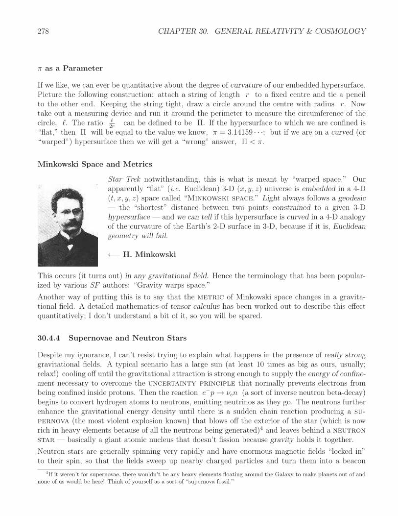
278 CHAPTER 30. GENERAL RELATIVITY & COSMOLOGY
π as a Parameter
If we like, we can ever be quantitative about the degree of curvature of our embedded hypersurface.Picture the following construction: attach a string of length r to a fixed centre and tie a pencilto the other end. Keeping the string tight, draw a circle around the centre with radius r. Nowtake out a measuring device and run it around the perimeter to measure the circumference of thecircle, ℓ. The ratio ℓ
2rcan be defined to be Π. If the hypersurface to which we are confined is
“flat,” then Π will be equal to the value we know, π = 3.14159 · · ·; but if we are on a curved (or“warped”) hypersurface then we will get a “wrong” answer, Π < π.
Minkowski Space and Metrics
Star Trek notwithstanding, this is what is meant by “warped space.” Ourapparently “flat” (i.e. Euclidean) 3-D (x, y, z) universe is embedded in a 4-D(t, x, y, z) space called “Minkowski space.” Light always follows a geodesic— the “shortest” distance between two points constrained to a given 3-Dhypersurface — and we can tell if this hypersurface is curved in a 4-D analogyof the curvature of the Earth’s 2-D surface in 3-D, because if it is, Euclideangeometry will fail.
←− H. Minkowski
This occurs (it turns out) in any gravitational field. Hence the terminology that has been popular-ized by various SF authors: “Gravity warps space.”
Another way of putting this is to say that the metric of Minkowski space changes in a gravita-tional field. A detailed mathematics of tensor calculus has been worked out to describe this effectquantitatively; I don’t understand a bit of it, so you will be spared.
30.4.4 Supernovae and Neutron Stars
Despite my ignorance, I can’t resist trying to explain what happens in the presence of really stronggravitational fields. A typical scenario has a large sun (at least 10 times as big as ours, usually;relax!) cooling off until the gravitational attraction is strong enough to supply the energy of confine-ment necessary to overcome the uncertainty principle that normally prevents electrons frombeing confined inside protons. Then the reaction e−p → νen (a sort of inverse neutron beta-decay)begins to convert hydrogen atoms to neutrons, emitting neutrinos as they go. The neutrons furtherenhance the gravitational energy density until there is a sudden chain reaction producing a su-
pernova (the most violent explosion known) that blows off the exterior of the star (which is nowrich in heavy elements because of all the neutrons being generated)4 and leaves behind a neutron
star — basically a giant atomic nucleus that doesn’t fission because gravity holds it together.
Neutron stars are generally spinning very rapidly and have enormous magnetic fields “locked in”to their spin, so that the fields sweep up nearby charged particles and turn them into a beacon
4If it weren’t for supernovae, there wouldn’t be any heavy elements floating around the Galaxy to make planets out of andnone of us would be here! Think of yourself as a sort of “supernova fossil.”

30.4. GRAVITY 279
emitting electromagnetic radiation synchronized with the spinning star. Such beacons are “seen”on Earth as regularly pulsing radio sources or “pulsars,” many of which are now known. Mostnebulae (the remnants of supernovae) contain neutron stars at their cores.
The phenomenology of neutron stars is itself a huge and fascinating subject about which I knowtoo little. Let’s both go look them up and read more about them!
30.4.5 Black Holes
If the neutron star is massive enough, then the gravitational force can grow strong enough even toovercome the hard-core repulsion between quarks and compress the neutrons themselves, making thegravitational force even stronger until no force can resist the gravitational collapse, at whichpoint the entire mass of the star compresses (theoretically) to a single point called the singularity.We can’t tell anything about the singularity for a simple reason: nothing that gets close to it canever get away again.
The easy, handwaving way to see why is as follows: at any distance from a massive object, any otherobject will be in orbit about it providing it executes circular motion at just the right speed. Asyou get closer, the orbital velocity gets higher. Now, for a sufficiently heavy object, there is someradius at which the nominal orbital velocity is the speed of light. From inside that radius, calledthe Schwarzschild radius (rS), not even light can escape but is inexorably drawn “down” intothe singularity. Thus all light (or anything else!) falling on such an object’s Schwarzschild radiuswill be perfectly absorbed, which accounts for the name, “black hole.”
We can easily estimate rS using a crude classical approximation: for a masss m in a circular orbitabout a mass M , F = ma gives GMm/r2 = mv2/r which reduces to GM/r = v2 or r = GM/v2. Ifv → c this becomes rS = GM/c2. This result is actually off by a factor of 2: the actual Schwarzschildradius is twice as large as predicted by this dumb derivation:
True rS = 2GM
c2.
I have tried to find a simple explanation for this extra factor of two, but failed. Simply using the“effective mass” γm in place of m makes no difference, for instance, because it appears on both sidesof the equation the same way. However, I don’t feel too bad, because apparently it took Einsteinabout seven years to get it right. [The time it took him to develop his General Theory of Relativity,which explains that extra factor properly.]
A more rigourous description is beyond me, but I can repeat what I’ve heard and list some of thephenomenology attributed to black holes, of which there are two types: the Schwatzschild
(non-rotating) black hole and the Kerr black hole, which spins. Presumably all real black holes areof the latter category, since virtually every star has some angular momentum, but there is probablya criterion for how fast it must spin to qualify as a Kerr black hole.

280 CHAPTER 30. GENERAL RELATIVITY & COSMOLOGY
Schwarzschild Black Holes
←− K. Schwarzschild
One of the interesting features of general relativity is that timeslows down as you approach the Schwarzschild radius of a black hole.Not to you, of course; your subjective experience of time is unaffected,but an outside observer would see your clock moving slower and slower(and turning redder and redder) as you fell into the black hole, until(paradoxically) you stopped completely (and were red-shifted out of sight)at rS. Your own experience would depend upon the mass of the blackhole. If it were big enough, the trip in free fall through rS would berather uneventful — you wouldn’t notice much of anything unusual, unlessof course you tried to get out again.
If, on the other hand, you approached a small black hole, the tidal forces [the gravitational gradient]would tear you apart before you even reached rS. This has some interesting consequences which Iwill discuss later.
The transformation between “outside” and “inside” coordinates has an interesting feature: while it isstrictly impossible for anything inside rS to come out, one can imagine extending the mathematicsof the relativistic transformation from outside to inside, at least formally. The result would be that“inside time” is in the opposite direction from “outside time.” This would mean that what we seeas matter falling inexorably into a black hole must “look” to the interior inhabitants (if any) like anexpansion of matter away from the singularity — a sort of Big Bang. Which raises an interestingquestion about our Big Bang: are we inside a black hole in someone else’s Universe? Hmm. . . .And are the black holes in our Universe time-reversed Big Bangs for the inhabitants (if any) oftheir interiors? Hmmmmmm. . . . Unfortunately, this sophistry is probably all wrong. If you want aproper, correct and comprehensible description of phenomena at the Schwarzschild radius, go talkto Bill Unruh!
Kerr Black Holes
Well, moving right along, I should repeat what I’ve heard about Kerr (spinning) black holes.The problem with Schwarzschild black holes is, of course, that exploring them is strictly aone-way trip; once you pass through their Schwarzschild radius, you are doomed to fall right on into the singularity.
Not so, apparently, with a Kerr black hole if it is spinning fast enough. Then the singularityis in a ring (sort of) and you can in principle plot a trajectory through the middle of the ring (orsomething like that) and come out the other side. Except that “the other side” may not have anyresemblance to where-when you went in on this side! This has already been used as a great gimmickfor SF stories involving time travel and other apparent logical paradoxes. I don’t understand it atall, and I doubt very much that anyone else does, but one can always postulate that someone will,someday, and use it for practical(?) purposes. After all, as Arthur C. Clarke says, “Any sufficientlyadvanced technology is indistinguishable from magic.”

30.4. GRAVITY 281
Wormholes?
←− John Archibald Wheeler
Another favourite gimmick of “hard SF” authors [those who try to make their stories consistentwith the known “Laws of Physics”] is the wormhole, a sort of “space warp” analogous to theblack hole but topologically more interesting. One can distort [e.g. fold] a 2-D surface (likea sheet of paper) embedded in a 3-D space until two apparently distant points are “actually”quite close together in the higher-dimensional continuum. Then a simple puncture across bothsides will provide a “shrt cut” and drastically change the connectedness [a formal term in themathematics of topology, believe it or not] of space. In a similar (?) fashion, one can imagine(?) a gravitational anomaly creating a “wormhole” making a “short cut” connection between twonominally distant regions of 3-D space. Great potential for space travel, right?
Sorry. John Archibald Wheeler, who has played a major role in the development of all this weirdGravitation stuff, proved a long time ago that wormholes always pinch off spontaneously beforeanything (even a signal propagating at the speed of light!) can get through them. Of course, thisfact doesn’t stop Star Trek Deep Space 9 from having a lot of fun with the idea anyway.
Exploding Holes!
Another feature of small black holes is that they are unstable. This was explained in some detailby Bill Unruh in the UBC Physics Department. The basic idea is that for a small black hole thetidal forces at the Schwarzschild radius are so enormous that they can tear apart the vacuum —that is, pull one of the partners in a “virtual pair” or “bubble” down into the black hole while theother escapes as radiation. The resultant energy loss is deducted from the mass of the black hole,making it still smaller. This is a runaway process that ends in a rather impressive explosion. Notto worry, all the small “primordial” black holes (made in the Big Bang) have by now decayed. Onthe other hand, a marginally larger primordial black hole might have taken until now to get downto a size where the radiation really starts taking off. . . .
Mutability
What conservation laws do black holes respect? Not many. Mass-energy, angular momentumand electric charge are the only properties of what falls in that remain properties of the black holeitself. That means that all other “conserved” properties of matter, like baryon number, are“mutable” in the final analysis.
One consequence is that protons might experience gravitational decay in which they collapse

282 CHAPTER 30. GENERAL RELATIVITY & COSMOLOGY
into a very tiny black hole, only to immediately explode into (probably) a positron and somegamma rays. The estimated lifetime of protons against such a fate is ∼ 1045 years, which is not tooworrisome.
Other consequences are more interesting, but only philosophically: the interior of a black hole [withwhich we can never communicate] may have entirely different properties — or even different “Lawsof Physics” — than what we drop into it. Wheeler has taken this idea much further than I canfollow, but it does make for interesting thinking. Good luck.
30.4.6 Gravitational Redshifts and Twisted Time
In addition to the “ordinary” redshifts of distant stars caused by the relativistic Doppler shift dueto the fact that they are actually receding from the observer on Earth, there is a graviational
redshift of the light from near a large mass M when observed from a position far from the source,even if the source and observer are at rest relative to one another. This is not too surprising if werecall that a gravitational field has to be indistinguishable from an accelerated reference frame, andan accelerated object cannot be at rest for long! But an easier way to see the result is to rememberthat a massless particle like a photon still has an effective mass m′ = E/c2 where (if I may borrowa hitherto undemonstrated result from quantum mechanics) E = hν for a photon. Here ν is thefrequency of the light and h = 6.626× 10⁻³⁴ J-s is Planck’s constant. Anyway, if the energy ofa photon far from M is E∞ = hν∞ (at r → ∞) then its effective mass there is m′
∞ = hν∞/c2 and asthe photon “falls” toward M it should pick up kinetic energy until at a finite distance r its energy isE = E∞ + GMm′/r where the new effective mass is m′ = E/c2. Thus E = E∞ + (GM/c2)E/r andif we collect the terms proportional to E we get E∞ = E(1 − r/r) where r ≡ GM/c2. Dividingthrough by h/cc gives the formula for the gravitational redshift,
ν∞ν
= 1 − rS
rwhere rS = 2
GM
c2.
(I have fudged in that extra factor of 2 that turns r into the correct Schwarzschild radius
rS). This derivation is completely bogus, of course, but it does indicate why there is a gravitationalredshift.
Given that any mechanism for generating electromagnetic waves constitutes a “clock” of sorts, thewaves emitted by such a device constitute a signal from it telling distant observers about the passageof time at the origin. (Think of each wave crest as a “tick” of the clock.) The very existence of agravitational redshift therefore implies that time passes slower for the clock that is closer tothe mass — a result that was referred to earlier without proof.