The Search for the Optimal Paper Helicopter

Erik Erhardt and Hantao Mai

December 4, 2002

Contents

1 Executive Summary 4

2 Problem Description 5

3 Screening Experiment 63.1 Data Generation . . . . . . . . . . . . . . . . . . . . . . . . . . . 63.2 Experimental Protocol . . . . . . . . . . . . . . . . . . . . . . . . 6

3.2.1 Blocking Considerations . . . . . . . . . . . . . . . . . . . 63.2.2 Tools . . . . . . . . . . . . . . . . . . . . . . . . . . . . . 73.2.3 Techniques . . . . . . . . . . . . . . . . . . . . . . . . . . 73.2.4 Factor Levels . . . . . . . . . . . . . . . . . . . . . . . . . 8

3.3 Collection of Data . . . . . . . . . . . . . . . . . . . . . . . . . . 83.4 Data Analysis . . . . . . . . . . . . . . . . . . . . . . . . . . . . . 9

3.4.1 Effects Analysis . . . . . . . . . . . . . . . . . . . . . . . . 93.4.2 Design Augmentation to Find Significant Factors . . . . . 10

4 Optimization 144.1 Path of Steepest Ascent . . . . . . . . . . . . . . . . . . . . . . . 14

4.1.1 Data Generation . . . . . . . . . . . . . . . . . . . . . . . 144.1.2 Testing for Curvature . . . . . . . . . . . . . . . . . . . . 144.1.3 Direction of Steepest Ascent . . . . . . . . . . . . . . . . 154.1.4 Pilot Study for Choosing Insignificant Factors . . . . . . . 154.1.5 Coordinates Along the Path of Steepest Ascent . . . . . . 17

4.2 Second-Order Response Surface . . . . . . . . . . . . . . . . . . . 174.2.1 Testing for Curvature . . . . . . . . . . . . . . . . . . . . 184.2.2 Fitting a Second-Order Response Surface Model . . . . . 194.2.3 Confirmatory Experiment . . . . . . . . . . . . . . . . . . 24

5 Conclusions 25

1

CONTENTS 2

A Appendix 26A.1 Aliasing Structure . . . . . . . . . . . . . . . . . . . . . . . . . . 26A.2 SAS Code for Screening Drop . . . . . . . . . . . . . . . . . . . . 27A.3 SAS Code for 22 Replicated Design . . . . . . . . . . . . . . . . . 28A.4 SAS Code for CCD Analysis . . . . . . . . . . . . . . . . . . . . . 29A.5 SAS Code for RSREG Procedure . . . . . . . . . . . . . . . . . . 30A.6 Matlab Commands for Computing Confidence Interval on the

Mean Response . . . . . . . . . . . . . . . . . . . . . . . . . . . . 32A.7 Initial Helicopter Pattern . . . . . . . . . . . . . . . . . . . . . . 33A.8 Optimal Helicopter Pattern . . . . . . . . . . . . . . . . . . . . . 34

B Bibliography 35

LIST OF FIGURES 3

List of Figures

1 Normal Quantile Plot . . . . . . . . . . . . . . . . . . . . . . . . 102 EFFECTS Plot . . . . . . . . . . . . . . . . . . . . . . . . . . . . 113 Residuals Plots . . . . . . . . . . . . . . . . . . . . . . . . . . . . 204 Response Surface . . . . . . . . . . . . . . . . . . . . . . . . . . . 225 90% Confidence Region for the Stationary Point . . . . . . . . . 236 Initial Helicopter Pattern . . . . . . . . . . . . . . . . . . . . . . 337 Optimal Helicopter Pattern . . . . . . . . . . . . . . . . . . . . . 34

List of Tables

1 Helicopter Factors . . . . . . . . . . . . . . . . . . . . . . . . . . 52 Factor Confounding Rules . . . . . . . . . . . . . . . . . . . . . . 63 Design Points for 28−4

IV Design Screening Experiment . . . . . . . 74 Factor levels in Coded and Natural Units . . . . . . . . . . . . . 95 Screening Drop Results . . . . . . . . . . . . . . . . . . . . . . . 96 EFFECTS Test Results . . . . . . . . . . . . . . . . . . . . . . . 117 LOUGHIN Permutation Test Results . . . . . . . . . . . . . . . . 128 Screening Experiment Center Points Results . . . . . . . . . . . . 129 22 Replicated Design Results . . . . . . . . . . . . . . . . . . . . 1510 Steepest Ascent Preparation Experiment 1 Results . . . . . . . . 1611 Steepest Ascent Preparation Experiment 2 Results . . . . . . . . 1612 Steepest Ascent Coordinates and Results in Natural Units . . . . 1713 CCD Levels in Coded and Natural Units . . . . . . . . . . . . . . 1814 CCD Experiment Results . . . . . . . . . . . . . . . . . . . . . . 1815 RSREG Parameter Estimates . . . . . . . . . . . . . . . . . . . . 1916 Lack-of-Fit Test . . . . . . . . . . . . . . . . . . . . . . . . . . . . 1917 RSREG Stationary Point . . . . . . . . . . . . . . . . . . . . . . 2118 Optimum Helicopter Factor Levels . . . . . . . . . . . . . . . . . 2119 Confirmatory Experiment Results . . . . . . . . . . . . . . . . . . 24

1 EXECUTIVE SUMMARY 4

1 Executive Summary

Response Surface Methodology (RSM) is a powerful method to parsimoniouslyexplore and optimize a process. In this paper we discuss the maximization ofthe flight time for a paper helicopter. Through the use of the statistical andmathematical techniques collected in RSM, we begin with an existing helicopterdesign and optimize the flight time.

To begin, we identify eight factors that potentially influence the flight time.We use an efficient screening experiment to select those vital few factors thathave a significant effect on the response. The four surviving factors determinethe paper weight and rotor configurations of our helicopter. This reduction infactors greatly simplifies our model.

Since the first-order model is appropriate in our initial experimental region,we use steepest ascent to move quickly to the ‘near optimum’ region. Curvatureis detected in only a few steps, forcing us to abandon this technique in favor ofa second-order model.

The analysis of this second-order model results in a stationary point whichis a point of maximum response within the experimental region. We constructa confidence interval for the mean response predicted by this stationary pointas well as a confidence region for the stationary point. By conducting theconfirmatory experiment, we find that the observed mean of the responses atthe stationary point is well within the 95% confidence interval of the meanresponse. This confirms the validity of our prediction.

Finally, we provide the pattern for the optimized helicopter in the Appendix.

2 PROBLEM DESCRIPTION 5

2 Problem Description

The goal of this project is to use response surface methodology (RSM) to max-imize the flight time of a paper helicopter. We employ experimental strategiesfor exploring the interest region in the independent variables, statistical model-ing to develop appropriate relationships between the response and the variables,and optimization methods to find the levels in the variables which maximize ourresponse (in our case, the flight time).

We begin our work by choosing a pattern for our helicopter. We decide touse the pattern provided by Prof. Petruccelli, given in Appendix A.7. This isan easy pattern to modify and replicate.

We then identify the many factors which may contribute to the flight timeof the helicopter. These factors are included in the Helicopter Factors Table onpage 5.

Table 1: Helicopter Factors

A=Rotor LengthB=Rotor WidthC=Body LengthD=Foot LengthE=Fold LengthF=Fold WidthG=Paper weightH=Direction of fold

We decided to retain all of these factors for experimentation. At the outset,it is better to have too many rather than too few factors.

In order to determine the vital few factors that contribute to flight time weperform a screening experiment using a 2k fractional factorial design with theinitial helicopter pattern as our center point.

It is likely that our initial helicopter pattern begins our experimentationfar from the region of optimum conditions. We expect at this stage that first-order approximation might be quite reasonable. We will test for curvature, butexpect it will not be significant. We will perform the steepest ascent procedureto move quickly to the ‘near optimum’ region. As we approach the region ofoptimum conditions, we expect that curvature will be more prevalent and thatthe interactions among the factors will cease to be negligible. At that pointwe will test for curvature. If curvature is found, we will fit a complete second-order model to locate the stationary point (we expect a maximum) and conductconfirmatory experiments. If we do not find a maximum, ridge analysis will beuseful to find a maximum within the experimental region.

3 SCREENING EXPERIMENT 6

3 Screening Experiment

3.1 Data Generation

In order to identify those factors important in keeping the helicopter aloft, wewill construct an efficient screening design. Our pattern has 8 factors. We desireto use a fractional factorial design that has at least resolution IV.

A resolution IV design has the advantage that no main effect is aliased withany other main effect or two-factor interaction. Even though two-factor inter-actions are aliased with each other, we expect this design will give us sufficientinformation on the significant main effects.

We use a 28−4IV design. This reduces significantly the number of runs while

retaining resolution IV. The Confounding Rules 1 for this design are given inFactor Confounding Rules Table on page 6 with the complete aliasing structurein Appendix A.1.

Table 2: Factor Confounding Rules

E=BCDF=ACDG=ABDH=ABC

These confounding rules define the experimental design points listed in theDesign Points for 28−4

IV Design Screening Experiment Table on page 7.

3.2 Experimental Protocol

3.2.1 Blocking Considerations

Before creating and dropping our helicopters we define conditions under whichblocking is a necessary consideration. For helicopter creation, considerationsinclude the paper stock, who marks the pattern on the paper, who cuts thepaper and who folds the paper. For helicopter dropping, considerations in-clude the conditions of the day (atmospheric pressure, temperature, dew point),conditions of the time (whether processes such as climate control are running,movement by people or other immediate events effecting air circulation), droplocation, who drops the helicopters, dropping method and who records the time.

We wish to resolve the blocking issues as much as possible caused by potentialnon-homogeneous conditions. We set up our experimental protocol to eliminateas many conditional factors as possible.

For the factors we can control, we are as consistent as possible. For example,Hantao plots the helicopter patterns on the paper and Erik cuts and folds them.

1 These confounding rules are the same as in [1] except the book switches G and H in theConfounding rules. We used SAS macro DESIGN2 to create the aliasing structure.

3 SCREENING EXPERIMENT 7

Table 3: Design Points for 28−4IV Design Screening Experiment

Obs BLOCK A B C D E F G H1 1 -1 -1 -1 -1 -1 -1 -1 -12 1 -1 -1 -1 1 1 1 1 -13 1 -1 -1 1 -1 1 1 -1 14 1 -1 -1 1 1 -1 -1 1 15 1 -1 1 -1 -1 1 -1 1 16 1 -1 1 -1 1 -1 1 -1 17 1 -1 1 1 -1 -1 1 1 -18 1 -1 1 1 1 1 -1 -1 -19 1 1 -1 -1 -1 -1 1 1 1

10 1 1 -1 -1 1 1 -1 -1 111 1 1 -1 1 -1 1 -1 1 -112 1 1 -1 1 1 -1 1 -1 -113 1 1 1 -1 -1 1 1 -1 -114 1 1 1 -1 1 -1 -1 1 -115 1 1 1 1 -1 -1 -1 -1 116 1 1 1 1 1 1 1 1 1

Hantao drops the helicopters while Erik records the time. We always dropthe helicopters from the second floor balcony in Fuller Laboratories at WPI.Hantao releases the helicopters while Erik times the drop with a stopwatchfrom the ground floor. If a helicopter experiences a disturbance during a drop,such as hitting a wall, or any other conditions which effects its performance, weredrop that helicopter. We limit ourselves to dropping only when the conditionsare observed to be homogeneous, though we have no way of measuring theseconditions.

By following these experimental protocols we can expect a relatively homo-geneous environment while conducting our experiment. Under that situation,block is no longer a necessary consideration.

3.2.2 Tools

In the process of manufacturing our helicopters, we use only those tools whichwill provide the most consistent results. For layout, we use a long ruler mea-suring centimeters along with a liquid ink pen for non-impressioning marking.For cutting, we always use the same paper cutter.

3.2.3 Techniques

While manufacturing of the helicopters we try to limit the error in each mea-suring, cutting and folding to no more than 0.1 centimeters. If we produce a

3 SCREENING EXPERIMENT 8

helicopter not meeting these standards, we do not use it and produce a replace-ment.

3.2.4 Factor Levels

Considerable attention is placed on the levels of each factor with variable screen-ing and process optimization as our goals. Choosing these levels on each factoris a vital decision and something we do not take lightly. We understand thatsloppy decisions in these early stages may lead to the inability to identify signif-icant factors and, at later stages, to inefficient process optimization. However,we also realize the difficulty in choosing ranges should not prohibit the use of ascreening design and region seeking methods.

In considering our design, there are some inherent constraints between fac-tors. One relationship is between fold width and rotor width. When the rotorwidth increases, the fold width does not increase proportionately with the totalwidth. So levels are chosen carefully in these two factors so that if they areindeed important, they are not judged to be insignificant in the analysis due topoorly chosen levels.

Another factor constraint is that the largest foot length does not exceed12 the smallest fold length. This provides the maximum availability for codedextremes in these two factors.

Also, two of our factors, G2 and H3 , are not continuous in their levels.In all other factors we attempt to provide an appropriate range with hope

to find the significant factors in the screening experiment.We start with a model approximately the size of the pattern given in Ap-

pendix A.7. To this model we assigned the natural units to coded values of 0.Then, by the above considerations we decide to choose the range which seemsappropriate to this helicopter pattern. Then we assign the values of the naturalunits at the high and low levels of the range to the coded values of -1 and +1.This can be seen in the Factor Level in Coded and Natural Units Table on page9.

3.3 Collection of Data

Based on the experimental protocol above, we cut and fold 16 helicopters inrandom order at the design points listed in the Design Points for 28−4

IV DesignScreening Experiment Table on page 7. We carefully transport them to FullerLaboratories to conduct our experiment. We drop the helicopters in randomorder recording the drop time of each. Our results for the Screening drop aregiven in the Screening Drop Results Table on page 9. Accompanying SAS Codefor the Screening Drop is included in Appendix A.2

2Since Paper weight is not a continuous factor, we confine ourselves to two levels. Light isfrom phone book whitepages and heavy is standard copy paper.

3Since Direction of fold is not a continuous factor, we confine ourselves to two levels.Against indicates the fold direction is opposite the direction of rotation. For example, if therotor on right side of the helicopter folds away from you, the fold on the right side will foldtoward you.

3 SCREENING EXPERIMENT 9

Table 4: Factor levels in Coded and Natural Units

Coded ValuesFactors -1 0 1 Range

A 5.5 8.5 11.5 6B 3 4 5 2C 1.5 3.5 5.5 4D 0 1.25 2.5 2.5E 5 8 11 6F 1.5 2 2.5 1G light (none) heavy (none)H against (none) with (none)

Table 5: Screening Drop Results

Obs Ord A B C D E F G H Time1 12 -1 -1 -1 -1 -1 -1 -1 -1 11.802 7 -1 -1 -1 1 1 1 1 -1 8.293 11 -1 -1 1 -1 1 1 -1 1 9.004 15 -1 -1 1 1 -1 -1 1 1 7.215 1 -1 1 -1 -1 1 -1 1 1 6.656 4 -1 1 -1 1 -1 1 -1 1 10.267 16 -1 1 1 -1 -1 1 1 -1 7.988 8 -1 1 1 1 1 -1 -1 -1 8.069 3 1 -1 -1 -1 -1 1 1 1 9.20

10 10 1 -1 -1 1 1 -1 -1 1 19.3511 9 1 -1 1 -1 1 -1 1 -1 12.0812 5 1 -1 1 1 -1 1 -1 -1 20.5013 6 1 1 -1 -1 1 1 -1 -1 13.5814 13 1 1 -1 1 -1 -1 1 -1 7.4715 14 1 1 1 -1 -1 -1 -1 1 9.7916 2 1 1 1 1 1 1 1 1 9.20

3.4 Data Analysis

3.4.1 Effects Analysis

After we collect our data, we check for significance in three ways. First we lookat the Normal Quantile Plot of the effects. These results are summarized in theNormal Quantile Plot on page 10.

Next we use SAS macro EFFECTS4 to compare the factor effect estimateswith the MOE and SMOE at the .95 confidence level. These results are sum-

4 EFFECTS is provided in the WPI SAS macro library.

3 SCREENING EXPERIMENT 10

Figure 1: Normal Quantile Plot

marized in the EFFECTS Plot on page 11 with the accompanying EFFECTSTest Results Table on page 11.

Lastly, we perform the LOUGHIN permutation test, at the .90 confidencelevel. These results are summarized in the LOUGHIN Permutation Test ResultsTable on page 12.

From each of these methods, no effect is found to be significant. So additionalcenter runs may be necessary.

3.4.2 Design Augmentation to Find Significant Factors

Because the above three methods did not provide significant factors, it is nec-essary to run some replicates at the center of the design to get an estimate ofpure error. To do this we run two sets of center points, each having three runs.One set at the high and the other set at the low level of the paper weight. Thiswill provide enough degrees of freedom to get an estimate of pure error. Weexpect the MOE and SMOE will decrease and we will be able to find significantfactors.

Because our center points are not at the actual continuous center, it is nec-essary to compute the MOE and SMOE values by hand. These equations aregiven as (1), (2) and (3).

MOE = SPE × tc−1,(1+L)/2 (1)

SMOE = SPE × tc−1,δ (2)

3 SCREENING EXPERIMENT 11

Figure 2: EFFECTS Plot

Table 6: EFFECTS Test Results

Effect Label Estimate MOE SMOEI12 A*B -2.2175 4.94516 10.0394I123 A*B*C -1.1375 4.94516 10.0394I1234 A*B*C*D 1.5625 4.94516 10.0394I124 A*B*D -4.2825 4.94516 10.0394I13 A*C 0.8400 4.94516 10.0394I134 A*C*D 0.7000 4.94516 10.0394I14 A*D 1.6850 4.94516 10.0394I23 B*C -0.3850 4.94516 10.0394I234 B*C*D 0.2500 4.94516 10.0394I24 B*D -2.0350 4.94516 10.0394I34 C*D 0.2475 4.94516 10.0394A A 3.9900 4.94516 10.0394B B -3.0550 4.94516 10.0394C C -0.3475 4.94516 10.0394D D 1.2825 4.94516 10.0394

SPE =

√√√√√√n1∑i=1

(Xi1 − X1)2 +n2∑i=1

(Xi2 − X2)2

(n1 − 1) + (n2 − 1)(3)

3 SCREENING EXPERIMENT 12

Table 7: LOUGHIN Permutation Test Results

Effect ID P Decision10.65125 0 1.0000 Reject

0.2475 12 1.0000 Reject0.25 123 1.0000 Reject

-0.3475 2 0.8723 Reject-0.385 23 1.0000 Reject

0.7 124 0.5433 Reject0.84 24 0.7849 Reject

-1.1375 234 0.6220 Reject1.2825 1 0.7417 Reject1.5625 1234 0.6849 Reject1.685 14 0.8017 Reject

-2.035 13 0.6985 Reject-2.2175 34 0.8004 Reject-3.055 3 0.4073 Reject

3.99 4 0.2216 Reject-4.2825 134 0.2835 Reject

Below we will set each factor to coded value zero, except G and H. For reasonsof parsimony, we will run H at only its low level. We expect the experiment willbe sufficient to identify the significant factors. The result of the center runs aregiven in the Screening Experiment Center Points Results on page 12.

Table 8: Screening Experiment Center Points Results

Obs Ord A B C D E F G H Time1 5 0 0 0 0 0 0 -1 -1 10.522 1 0 0 0 0 0 0 -1 -1 10.813 3 0 0 0 0 0 0 -1 -1 10.894 2 0 0 0 0 0 0 1 -1 15.915 4 0 0 0 0 0 0 1 -1 16.086 6 0 0 0 0 0 0 1 -1 13.88

By applying Equation (3) to these results, we obtain SPE = .8764. FromEquation (1), the MOE.05 = 2.4332 at the .05 significance level. By comparingthe MOE to the effect estimates, we conclude that the main effects A, B and Gare significant, while the others are not.

Hereafter, we will confine ourselves to the use of G at -1 (the light paper),since G has only two levels and it is clear that the response is much higher at itslow level. We will also confine ourselves to the low level in H since the response

3 SCREENING EXPERIMENT 13

tends to have better performance at this level.With the reduction of factors through lack of significance (C, D, E, F and

H) and confinement (G and H), we have only two factors to consider (A andB). Hereafter, we can use the full 22 factorial replicated design to start ouroptimization process.

4 OPTIMIZATION 14

4 Optimization

4.1 Path of Steepest Ascent

4.1.1 Data Generation

Since we have obtained the vital few factors responsible for keeping the heli-copter aloft, it is time to begin searching for optimum settings for those factors.By using the method of steepest ascent we can move parsimoniously to a regionin which the process is improved. This method uses sequential experimenta-tion along the path of steepest ascent so that we may expect the maximumincrease in response. The path is determined by fitting a first-order model us-ing an orthogonal design and moving in the direction of the regression coefficientestimates.

In our case we have only two factors, so it is not expensive to use a replicateddesign. We will use the reduction given in the previous section to define a full22 replicated design by confining the values of G and H to the low levels. Weuse the previously folded helicopters made from light paper (G = -1), modifyingany with fold direction (H) at the high level to the low level. This allows usto populate half our experiment with previously manufactured helicopters. Wefold eight new helicopters to complete the 22 design with four replicates, andan additional three for center runs.

These two blocks of helicopters, the old ones and new ones, have differentcharacteristics in the insignificant factors. However, the insignificant factors(C, D, E, F and H) have little effect on the response, therefore we should havecomparable performance from helicopters with the same levels in the significantfactors.

Our results from the 22 Design with four replicates for computing the pathof steepest ascent are given in the 22 Replicated Design Table on page 15. Ac-companying SAS Code for 22 Replicated Design is included in Appendix A.3.

4.1.2 Testing for Curvature

Since we include the 3 center runs in our experiment, we can check for curvatureof the surface being modeled.

The idea for the test for curvature is that if the surface is not curved, thenthe mean response at the center point is the same as the mean of the responsesat the factorial points. A measure of the mean of the responses at the factorialpoints is the sample mean of the responses at those points Y . A measure of themean response at the center point is the sample mean of the responses there,Y0. Thus, an estimate of the curvature is Y − Y0. If this estimate of curvatureis large relative to experimental error, there will be strong evidence that theresponse surface is curved.

In our case, the estimated standard error of Y − Y0 is

σ(Y − Y0) =

√S2

PE(1nf

+1nc

) =

√0.8464(

116

+13) = 0.5788 (4)

4 OPTIMIZATION 15

Table 9: 22 Replicated Design Results

Obs A B Time1 -1 -1 10.242 -1 -1 9.113 1 -1 16.524 1 -1 16.995 -1 1 10.206 -1 1 9.267 1 1 10.028 1 1 9.949 -1 -1 11.31

10 -1 -1 10.9411 1 -1 12.5812 1 -1 13.8613 -1 1 8.2014 -1 1 9.9215 1 1 9.9516 1 1 9.9317 0 0 11.6718 0 0 10.7419 0 0 9.83

For L = 0.95,

σ(Y − Y0)× tc−1,(1+L)/2 = 0.5788× 2.92 = 1.69 > |Y − Y0| = 0.4389 (5)

so there is insufficient evidence to conclude that there is surface curvature.Therefore, we can proceed in the path of steepest ascent.

4.1.3 Direction of Steepest Ascent

The fitted regression model is given by

y = 11.1163 + 1.2881a− 1.5081b (6)

The basis for computation of points along the path of steepest ascent arechosen to be 1 cm in factor A. This corresponds to 1

3 design units. As a result,the corresponding movement in design variable B is (−1.5081/1.2881)(1/3) =−0.39 in design units. The natural units for B is −0.39× 1 = −0.39cm.

4.1.4 Pilot Study for Choosing Insignificant Factors

Before conducting steepest ascent, we perform a pilot study in the insignificantfactors in an attempt to stabilize the helicopters. We know by experience that

4 OPTIMIZATION 16

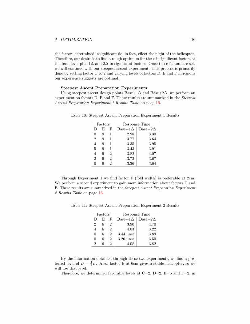
the factors determined insignificant do, in fact, effect the flight of the helicopter.Therefore, our desire is to find a rough optimum for these insignificant factors atthe base level plus 1∆ and 2∆ in significant factors. Once these factors are set,we will continue with our steepest ascent experiment. This process is primarilydone by setting factor C to 2 and varying levels of factors D, E and F in regionsour experience suggests are optimal.

Steepest Ascent Preparation ExperimentsUsing steepest ascent design points Base+1∆ and Base+2∆, we perform an

experiment on factors D, E and F. These results are summarized in the SteepestAscent Preparation Experiment 1 Results Table on page 16.

Table 10: Steepest Ascent Preparation Experiment 1 Results

Factors Response TimeD E F Base+1∆ Base+2∆0 9 1 2.98 3.302 9 1 3.77 3.644 9 1 3.35 3.955 9 1 3.43 3.914 9 2 3.82 4.072 9 2 3.72 3.670 9 2 3.36 3.64

Through Experiment 1 we find factor F (fold width) is preferable at 2cm.We perform a second experiment to gain more information about factors D andE. These results are summarized in the Steepest Ascent Preparation Experiment2 Results Table on page 16.

Table 11: Steepest Ascent Preparation Experiment 2 Results

Factors Response TimeD E F Base+1∆ Base+2∆2 6 2 3.90 4.704 6 2 4.03 3.220 6 2 3.44 unst 3.890 6 2 3.26 unst 3.502 6 2 4.08 3.82

By the information obtained through these two experiments, we find a pre-ferred level of D = 1

4E. Also, factor E at 6cm gives a stable helicopter, so wewill use that level.

Therefore, we determined favorable levels at C=2, D=2, E=6 and F=2, in

4 OPTIMIZATION 17

their natural units. As we follow the path of steepest ascent, we may find thatfactor F is large enough to wrap about the ‘tail’ of the helicopter. When thisis the case, we will confine ourselves to F= 2

3B, resulting in fold widths whichdivide the tail roughly into three equal parts.

4.1.5 Coordinates Along the Path of Steepest Ascent

We suspect five steps along the path of steepest ascent will bring us near theoptimum region followed by a deterioration in response. The coordinates alongthe Path of Steepest Ascent with the responses at those values are summarizedin the Steepest Ascent Coordinates and Results in Natural Units Table on page17. Six runs were made along the path, starting at the base. Eventually,severe deterioration in response occurred due to the fact that the first orderapproximation is no longer valid. In this case a reduction was experienced afterBase+3∆. Our further follow-up experiment will involve an experimental designcentered at Base+3∆.

Table 12: Steepest Ascent Coordinates and Results in Natural Units

Run A B ( F ) TimeBase 8.5 4.00 (2.0) 12.99∆ 1.0 -0.39Base + 1 ∆ 9.5 3.61 (2.0) 15.22Base + 2 ∆ 10.5 3.22 (2.0) 16.34Base + 3 ∆ 11.5 2.83 (1.5) 18.78 optimumBase + 4 ∆ 12.5 2.44 (1.5) 17.39Base + 5 ∆ 13.5 2.05 (1.2) 7.24

4.2 Second-Order Response Surface

In our exploration of the second-order response surface we want to use a designthat allows for estimation of interaction and quadratic terms. In our case, thedesign for this phase will be a spherical 22 Central Composite Design (CCD).The center runs allow for testing for curvature. If curvature is detected wewill abandon steepest ascent. The CCD is given in the CCD Levels in Codedand Natural Units Table on page 18. The results are summarized in the CCDExperiment Results Table on page 18. Accompanying SAS Code for the CCDanalysis is included in Appendix A.4.

Here, we assume the risk of performing unnecessary runs at the axial pointsin the case where curvature is not detected. However, in consideration of block-ing and estimations of quadratic terms, the axial points will be necessary ifcurvature is found.

4 OPTIMIZATION 18

Table 13: CCD Levels in Coded and Natural Units

Factor −√

2 -1 0 1√

2A 10.08 10.50 11.50 12.50 12.91B 2.28 2.44 2.83 3.22 3.38C 2.0 2.0 2.0 2.0 2.0D 1.5 1.5 1.5 1.5 1.5E 6.0 6.0 6.0 6.0 6.0F 1.5 1.5 1.5 2.0 2.0G light light light light lightH against against against against against

Table 14: CCD Experiment Results

Obs Ord A B Time1 7 -1 -1 13.652 3 1 -1 13.743 11 -1 1 15.484 5 1 1 13.535 9 0 0 17.386 2 0 0 16.357 1 0 0 16.418 10 1.414 0 12.519 4 -1.414 0 15.17

10 6 0 1.414 14.8611 8 0 -1.414 11.85

4.2.1 Testing for Curvature

Using Equations (4) and (5) we test for response curvature ‘near’ the optimalregion.

In our case, the estimated standard error of Y − Y0 is

σ(Y − Y0) =

√0.3342(

14

+13) = 0.4415 (7)

For L = 0.95,

σ(Y − Y0)× tc−1,(1+L)/2 = 0.4415× 2.92 = 1.289 < |Y − Y0| = 2.6133 (8)

so there is sufficient evidence to conclude that there is surface curvature. Thiscompletes our path of steepest ascent and we may proceed with second-ordermodeling.

4 OPTIMIZATION 19

4.2.2 Fitting a Second-Order Response Surface Model

Using the data given in the CCD Experiment Results Table on page 18, thecorresponding fitted second-order model is given by

y = 16.713− 0.702 a + 0.735 b− 1.311 a2 − 0.510 ab− 1.554 b2 (9)

In order to thoroughly check our model, the following three tests are per-formed. First, we will look at the significance in each of the model terms. Sec-ond, we perform a lack-of-fit test. Third, we verify our statistical assumptions.The complete output from the SAS RSREG Procedure is given in AppendixA.5.

T-test for Regression Coefficients From the RSREG Parameter EstimatesTable on page 19, we find all the factors except the interaction term to besignificant at the .05 level. This test gives us a very satisfactory result.

Table 15: RSREG Parameter Estimates

StandardParameter DF Estimate Error t Value Pr > |t|Intercept 1 16.713333 0.407813 40.98 0.0001a 1 -0.702726 0.249733 -2.81 0.0374b 1 0.734598 0.249733 2.94 0.0322a*a 1 -1.311042 0.297242 -4.41 0.0070b*a 1 -0.510000 0.353176 -1.44 0.2083b*b 1 -1.553542 0.297242 -5.23 0.0034

Lack-of-Fit Test The result from the lack-of-fit test is given in the Lack-of-FitTest Table on page 19. Because the P-value for this test statistic is verylarge, we accept the hypothesis that the model adequately describes thedata.

Table 16: Lack-of-Fit Test

Sum ofResidual DF Squares Mean Square F Value Pr > FLack of Fit 3 1.826200 0.608733 1.82 0.3737Pure Error 2 0.668467 0.334233Total Error 5 2.494666 0.498933

Residual Test Visual inspection of the Normal Quantile Plot for ResidualsPlot (right) on page 20 indicates that the Normal assumption for theerror is basically satisfied. By looking at the accompanying Residuals vs.

4 OPTIMIZATION 20

Figure 3: Residuals Plots

Predicted Value Plot (left), the constant variance is also basically satisfied.Further evidence is given by the Shapiro-Wilk test. The P-value for thistest is so large that we accept the Normal assumption.

Test Statistic Value p-valueShapiro-Wilk 0.959172 0.7613

Prediction of the Stationary PointUpon finishing the model checking, we now try to use our model to predict

the stationary point. The results from RSREG is given in the RSREG Station-ary Point Table on page 21. We are pleased the stationary point is a maximumin the experimental region.

By using the tools referred by [3], we construct and present to you with greatpleasure our Response Surface on page 22 and our 90% Confidence Region forthe Stationary Point on page 23.

The region shown in the 90% Confidence Region for the Stationary PointFigure on page 23 depicts the 90% confidence region for the stationary point.A true response surface maximum at any location inside the 90% confidenceregion could readily have produced the data that was observed. The quality ofthe confidence region depends a great deal on the nature of the design and thefit of the model to the data. Recall from Appendix A.5 that R2 is approximately92%, indicating a good fit.

It should be emphasized that a confidence region that is moderate in areais not necessarily bad news. A model that fits well yet generates a confidenceregion such as ours on the stationary point may imply flexibility in choosingthe optimum. We realize that in many RSM situations, estimation of optimum

4 OPTIMIZATION 21

conditions is very difficult. However, we should not get the feeling that RSMwill not produce important and interesting results about the process.

Table 17: RSREG Stationary Point

The RSREG ProcedureCanonical Analysis of Response Surface

CriticalFactor Value

a -0.324343b 0.289665

Predicted value at stationary point: 16.933689

EigenvectorsEigenvalues a b

-1.149933 0.845405 -0.534126-1.714651 0.534126 0.845405

Stationary point is a maximum.

The coded factors for the stationary point given in the RSREG StationaryPoint Table above for factors A and B convert to the natural values given inthe Optimum Helicopter Factor Levels Table on page 21. The pattern for ouroptimal helicopter is provided for your enjoyment in Appendix A.8.

Table 18: Optimum Helicopter Factor Levels

Factor Coded NaturalA -0.32 11.18B 0.29 2.94C x 2.0D x 2.0E x 6.0F x 1.5G light lightH against against

4 OPTIMIZATION 22

Response Surface Plot (Y) x1 - x2 plane

–2–1

01

2x1 –10

12

x2

4

6

8

10

12

14

16

Y

Figure 4: Response Surface

4 OPTIMIZATION 23

Confidence Region Plot (90.0%) x1 - x2 plane

–2

–1

0

1

2

x1

–2 –1 0 1 2x2

Figure 5: 90% Confidence Region for the Stationary Point

4 OPTIMIZATION 24

4.2.3 Confirmatory Experiment

Now that we have the setting for the optimal helicopter, we want to do a con-firmatory experiment to test the validity of this result. We manufacture sixhelicopters according to our optimal setting and record their dropping times.These results appear in the Confirmatory Experiment Results Table on page 24.

Table 19: Confirmatory Experiment Results

Obs Time1 15.542 16.403 19.674 19.415 18.556 17.29

This confirmatory experiment gives a mean response of 17.8100 with stan-dard deviation 1.6720. The 95% confidence interval on the mean response isgiven by [15.8314, 18.0360]. Our response falls within this interval, thus con-firming the validity of our response model. Accompanying Matlab commandsfor Computing Confidence Interval on the Mean Response are included in Ap-pendix 32.

5 CONCLUSIONS 25

5 Conclusions

There are several important items that have become apparent from this expe-rience with response surface methodology. The choice of experimental regionneeds to be made very carefully. Choice of range in the natural levels cannotbe taken lightly. This is particularly crucial in the phase of the analysis whenvariable screening is being done. The natural sequential nature of RSM allowsus to make intelligent choices of variable ranges after preliminary phases of thestudy have been analyzed. In our example, following variable screening, wewere careful to make good choices in the insignificant factors and well reasonedchoices of levels in the significant factors for the steepest ascent procedure. Af-ter steepest ascent was accomplished, our experience gave rise to easy choicesof variable levels to be used for a second-order analysis.

The goal of our experiment is to find optimum conditions in the helicopterfactors to maximize flight time. However, we are careful throughout the courseof our experimentation to keep in mind that estimated optimum conditions fromone experiment is only an estimate. The next experiment may well find the es-timated optimum conditions to be at a different set of coordinates. An exampleof this occurred in the screening experiment when a time of over 20 secondswas observed. This response was the greatest achieved, though the factor lev-els for this helicopter are far from the optimal. A comparable response wasnot seen again, neither by redropping the same helicopter, nor by the optimalhelicopter achieved through RSM. Furthermore, as uncontrollable noise factorschange from time to time, a computed set of optimum conditions may be afleeting concept. What is more important is for the analysis to reveal importantinformation about the process and information about the roles of the variables.The computation of a stationary point, a canonical analysis, or a ridge analy-sis may lead to important information about the process, and this in the longrun will often be more valuable than a single set of coordinates representing anestimate of optimum conditions.

A APPENDIX 26

A Appendix

A.1 Aliasing Structure

Factor Confounding Rules

E = BCDF = ACDG = ABDH = ABC

Aliasing Structure

I = ABCH = ABDG = ABEF = ACDF = ACEG = ADEH = AFGH = BCDE= BCFG = BDFH = BEGH = CDGH = CEFH = DEFG = ABCDEFGH

A = BCH = BDG = BEF = CDF = CEG = DEH = FGH = ABCDE = ABCFG= ABDFH = ABEGH = ACDGH = ACEFH = ADEFG = BCDEFGH

B = ACH = ADG = AEF = CDE = CFG = DFH = EGH = ABCDF = ABCEG= ABDEH = ABFGH = BCDGH = BCEFH = BDEFG = ACDEFGH

C = ABH = ADF = AEG = BDE = BFG = DGH = EFH = ABCDG = ABCEF= ACDEH = ACFGH = BCDFH = BCEGH = CDEFG = ABDEFGH

D = ABG = ACF = AEH = BCE = BFH = CGH = EFG = ABCDH = ABDEF= ACDEG = ADFGH = BCDFG = BDEGH = CDEFH = ABCEFGH

E = ABF = ACG = ADH = BCD = BGH = CFH = DFG = ABCEH = ABDEG= ACDEF = AEFGH = BCEFG = BDEFH = CDEGH = ABCDFGH

F = ABE = ACD = AGH = BCG = BDH = CEH = DEG = ABCFH = ABDFG= ACEFG = ADEFH = BCDEF = BEFGH = CDFGH = ABCDEGH

G = ABD = ACE = AFH = BCF = BEH = CDH = DEF = ABCGH = ABEFG= ACDFG = ADEGH = BCDEG = BDFGH = CEFGH = ABCDEFH

H = ABC = ADE = AFG = BDF = BEG = CDG = CEF = ABDGH = ABEFH= ACDFH = ACEGH = BCDEH = BCFGH = DEFGH = ABCDEFG

AB = CH = DG = EF = ACDE = ACFG = ADFH = AEGH = BCDF = BCEG= BDEH = BFGH = ABCDGH = ABCEFH = ABDEFG = CDEFGH

AC = BH = DF = EG = ABDE = ABFG = ADGH = AEFH = BCDG = BCEF= CDEH = CFGH = ABCDFH = ABCEGH = ACDEFG = BDEFGH

AD = BG = CF = EH = ABCE = ABFH = ACGH = AEFG = BCDH = BDEF= CDEG = DFGH = ABCDFG = ABDEGH = ACDEFH = BCEFGH

AE = BF = CG = DH = ABCD = ABGH = ACFH = ADFG = BCEH = BDEG= CDEF = EFGH = ABCEFG = ABDEFH = ACDEGH = BCDFGH

AF = BE = CD = GH = ABCG = ABDH = ACEH = ADEG = BCFH = BDFG= CEFG = DEFH = ABCDEF = ABEFGH = ACDFGH = BCDEGH

AG = BD = CE = FH = ABCF = ABEH = ACDH = ADEF = BCGH = BEFG= CDFG = DEGH = ABCDEG = ABDFGH = ACEFGH = BCDEFH

AH = BC = DE = FG = ABDF = ABEG = ACDG = ACEF = BDGH = BEFH= CDFH = CEGH = ABCDEH = ABCFGH = ADEFGH = BCDEFG

A APPENDIX 27

A.2 SAS Code for Screening Drop

data drop1;input obs order a b c d e f g h y;

ab=a*b;ac=a*c;ad=a*d;bc=b*c;bd=b*d;cd=c*d;bcd=b*c*d;acd=a*c*d;abd=a*b*d;abc=a*b*c;abcd=a*b*c*d;cards;

1 12 -1 -1 -1 -1 -1 -1 -1 -1 11.802 7 -1 -1 -1 1 1 1 1 -1 8.293 11 -1 -1 1 -1 1 1 -1 1 9.004 15 -1 -1 1 1 -1 -1 1 1 7.215 1 -1 1 -1 -1 1 -1 1 1 6.656 4 -1 1 -1 1 -1 1 -1 1 10.267 16 -1 1 1 -1 -1 1 1 -1 7.988 8 -1 1 1 1 1 -1 -1 -1 8.069 3 1 -1 -1 -1 -1 1 1 1 9.2010 10 1 -1 -1 1 1 -1 -1 1 19.3511 9 1 -1 1 -1 1 -1 1 -1 12.0812 5 1 -1 1 1 -1 1 -1 -1 20.5013 6 1 1 -1 -1 1 1 -1 -1 13.5814 13 1 1 -1 1 -1 -1 1 -1 7.4715 14 1 1 1 -1 -1 -1 -1 1 9.7916 2 1 1 1 1 1 1 1 1 9.20

;run;

A APPENDIX 28

A.3 SAS Code for 22 Replicated Design

data drop2;input obs a b y;

cards;1 -1 -1 10.242 -1 -1 9.113 1 -1 16.524 1 -1 16.995 -1 1 10.206 -1 1 9.267 1 1 10.028 1 1 9.949 -1 -1 11.3110 -1 -1 10.9411 1 -1 12.5812 1 -1 13.8613 -1 1 8.2014 -1 1 9.9215 1 1 9.9516 1 1 9.9317 0 0 11.6718 0 0 10.7419 0 0 9.83

;run;

A APPENDIX 29

A.4 SAS Code for CCD Analysis

data drop4;input obs ord a b y;if a=9 then a=sqrt(2);if a=-9 then a=-sqrt(2);if b=9 then b=sqrt(2);if b=-9 then b=-sqrt(2);

cards;1 7 -1 -1 13.652 3 1 -1 13.743 11 -1 1 15.484 5 1 1 13.535 9 0 0 17.386 2 0 0 16.357 1 0 0 16.418 10 9 0 12.519 4 -9 0 15.1710 6 0 9 14.8611 8 0 -9 11.85

;run;

proc rsreg data=drop4 out=drop4_out;model y=a b/nocode actual residual predict;

run;

A APPENDIX 30

A.5 SAS Code for RSREG Procedure

The RSREG Procedure

Response Surface for Variable y

Response Mean 14.630000Root MSE 0.706352R-Square 0.9167Coefficient of Variation 4.8281

Type I SumRegression DF of Squares R-Square F Value Pr > F

Linear 2 8.267663 0.2761 8.29 0.0259Quadratic 2 18.138871 0.6058 18.18 0.0051Crossproduct 1 1.040400 0.0347 2.09 0.2083Total Model 5 27.446934 0.9167 11.00 0.0099

Sum ofResidual DF Squares Mean Square F Value Pr > F

Lack of Fit 3 1.826200 0.608733 1.82 0.3737Pure Error 2 0.668467 0.334233Total Error 5 2.494666 0.498933

StandardParameter DF Estimate Error t Value Pr > |t|

Intercept 1 16.713333 0.407813 40.98 <.0001a 1 -0.702726 0.249733 -2.81 0.0374b 1 0.734598 0.249733 2.94 0.0322a*a 1 -1.311042 0.297242 -4.41 0.0070b*a 1 -0.510000 0.353176 -1.44 0.2083b*b 1 -1.553542 0.297242 -5.23 0.0034

Sum ofFactor DF Squares Mean Square F Value Pr > F

a 3 14.697326 4.899109 9.82 0.0155b 3 18.986602 6.328867 12.68 0.0090

The RSREG Procedure

A APPENDIX 31

Canonical Analysis of Response Surface

CriticalFactor Value

a -0.324343b 0.289665

Predicted value at stationary point: 16.933689

EigenvectorsEigenvalues a b

-1.149933 0.845405 -0.534126-1.714651 0.534126 0.845405

Stationary point is a maximum.

Studentized residual tests below show not enough evidenceto reject Normality assumption.

RT_y_1

N 11.0000 Sum Wgts 11.0000Mean 0.0552 Sum 0.6071Std Dev 1.4400 Variance 2.0735Skewness 0.6529 Kurtosis 1.3921USS 20.7689 CSS 20.7354CV 2609.1854 Std Mean 0.4342

100% Max 3.1777 99.0% 3.177775% Q3 0.7589 97.5% 3.177750% Med 0.1763 95.0% 3.177725% Q1 -0.6915 90.0% 1.20780% Min -2.2115 10.0% -1.5290

Range 5.3892 5.0% -2.2115Q3-Q1 1.4504 2.5% -2.2115Mode . 1.0% -2.2115

Test Statistic Value P-valueShapiro-Wilk 0.959172 0.7613Kolmogorov-Smirnov 0.130719 >.1500Cramer-von Mises 0.036858 >.2500Anderson-Darling 0.257465 >.2500

A APPENDIX 32

A.6 Matlab Commands for Computing Confidence Inter-val on the Mean Response

x1=[-1 1 -1 1 0 0 0 -sqrt(2) sqrt(2) 0 0]’x2=[-1 -1 1 1 0 0 0 0 0 -sqrt(2) sqrt(2)]’x=[ones(11,1) x1 x2 x1.*x1 x2.*x2 x1.*x2]mse=.4989x0=[1 -0.324343 0.289665 -0.324343^2 0.289665^2 -0.324343*0.289665]’y0= 16.933689t=2.5706lb=y0-t*sqrt(mse*(x0’*inv(x’*x)*x0))ub=y0+t*sqrt(mse*(x0’*inv(x’*x)*x0))

A APPENDIX 33

A.7 Initial Helicopter Pattern

Fold Fold

Rotor

Cut

Rotor

Body

Cut Cut

Fold Fold

4.5 cm 4.5 cm

10 cm

4.5 cm

9.5 cm

2.5 cm 2.5 cm

Figure 6: Initial Helicopter Pattern

A APPENDIX 34

A.8 Optimal Helicopter Pattern

f12cm

2cm

6cm

11.18cm

2.94cm 2.94cm

1.5cm1.5cm

r1 r2

f2 f3

Figure 7: Optimal Helicopter Pattern

B BIBLIOGRAPHY 35

B Bibliography

References

[1] Myers, Raymond H. and Montgomery, Douglas C., Response Sur-face Methodology, Process and Product Optimization Using De-signed Experiments, John Wiley & Sons, Inc., 1995.

[2] Petruccelli, J. D., Nandram, B. and Chen, M., Applied Statisticsfor Engineers and Scientists, Simon & Schuster, 1999.

[3] Del Castillo, Enrique and Cahya, Suntara. A Tool for Comput-ing Confidence Regions on the Stationary Point of a ResponseSurface, The American Statistician, November 2001, Vol. 55, No.4.